Embed Size (px)
Citation preview
IDENTIFICATION OF
HAZARDOUS MOTOR VEHICLE ACCIDENT SITES:
SOME BAYESIAN CONSIDERATIONS
A THESIS
SUBMI'rTED IN PARTIAL FULFILMENT
OF THE REQUIREMENTS FOR THE DEGREE
OF
DOCTOR OF PHILOSOPHY IN STATISTICS
IN THE
UNIVERSITY OF CANTERBURY
BY
PHILIP JOHN fiCHLUTER
University of Canterbury
1996
PHYSIC~ 15ClENCf;!! UflRArN
Abstract
Appropriate hazardous accident site identification and discrimination is a fundamen
tal difficulty that confronts traffic safety researchers. Readily employed Bayesian
methods can redress this difficulty and are the focus of this thesis.
Accident analysis, including hazardous site identification, invariably requires the
specification of some defined distributional function. However, several different dis
tributions have been proposed to model traffic accidents, and so the most suitable
model amongst these must be appropriately determined and selected.
Model selection should satisfactorily fulfill two requisite criteria; firstly, that the
best model is discriminated, and secondly, that this best distribution adequately
describes the data. To help satisfy these requirements we introduce the averaged
Bayes factor, a new method that determines the best model from likely candidate
distributions, and we propose a new Bayesian procedure that facilitates the quanti
tative assessment of model adequacy. In addition, a method quantifying the power
of detecting model inadequacy is presented.
With the specification of an appropriate accident distribution, procedures facili
tating hazardous site identification, ranking and selection are then proposed. These
procedures are accomplished using the hierarchical Bayesian method and three in
tuitive quantitative strategies. Especially useful is a variation of the posterior prob
ability that gives the probability each particular site is worst and by how much it is
worst. All proposed techniques are illustrated using previously published accident
data from 35 sites in Auckland, New Zealand.
1
Contents
1
2
Introduction
1.1 Background . - ...... 1.2 The Poisson assumption
1.3 Model selection I f .. •
1.3.1 Discrimination
1.3.2 Adequacy ... 1.4 Ranking and selection
1.5 Overview ........
Mathematical models and notation
2.1 Candidate distributions . . . . . .
2.2 N oninformative prior derivations .
2.2.1 M1 : Poisson ....... .
2.2.2 M2: Poisson/gamma .. .
2.2.3 M3 : mixture of two Poissons .
2.2.4 M4: geometric . . . . . . . . .
3 Model Discrimination
3.1 Preliminaries .....
3.1.1 Bayes factors
3.1.2 Training samples and partial likelihood methods .
3.2 Averaged Bayes factor . . . .
3.3 Bayesian information criterion
3.4 Numerical example . . . . . .
3.4.1 Averaged Bayes factor
ii
1
1
2
3
4
6
9
12
14
14
18
19
19
20
21
22
22
22
25
26
28
29
29
CONTENTS ... l1l
3.4.2 Bayes information criterion . . . . . . . . . . . . . . . . . . . 38
4 Model Adequacy and Power
4.1 Preliminaries . . . . . . . .
4.2 Adequacy measures and their assessment
4.3 Power of adequacy measures
4.4 Simulation approach . . . .
4.5 Numerical details ..... .
4.5.1 Posterior predictive distributions
4.5.2 Hold-out predictive distributions
4.5.3 Computational methods . . . .
4.5.4 Mean and variance adjustments
4.6 Numerical results . . . . . .
4.6.1 Adequacy of models
4.6.2 Power of detecting model inadequacy
4.6.3 The V 2 adequacy measure
5 Ranking and selection
5.1 Specification of an appropriate model
5.2 Hierarchical Baye,sian development .
5.3 Selection criteria .......... .
5.3.1 Posterior probability of selecting the worst site .
5.3.2 Predictive probability of future accident numbers
5.3.3 Expected number of future accidents
5.3.4 Appropriate use of selection criteria .
5.4 Hyperprior distributions and elicitation .
5.4.1 Informative hyperpriors ..
5.4.2 Noninformative hyperpriors
5.5 Numerical example .
5.5.1 Computation
5.5.2 Case I
5.5.3 Case II .
43
44
45
49
50
51
51
58
64
65
66
66
73
77
81
81
82
85
86
87
88
88
89
90
91
92
93
95
. 100
CONTENTS
6 Summary
6.1 Model discrimination
6.1.1 Averaged Bayes Factor
6.1.2 Application of the averaged Bayes factor
6.2 Mod"el adequacy and Power
6.2.1 Remarks . . . . . . .
6.2.2
6.2.3
Adequacy measures .
Application . . . .
6.3 Ranking and selection ..
6.3.1 Hierarchical model
6.3.2 Selection criteria .
6.4 General extensions . . . .
6.4.1
6.4.2
6.4.3
6.4.4
6.4.5
Averaged Bayes factor
Model adequacy . . . .
Bayesian hypothesis testing
Countermeasure evaluation.
Cost and loss . . . . . . . .
6.4.6 Hierarchical Bayesian modifications
6.5 Final remarks ................ .
Acknowledgements
References
Appendices
A Auckland data
B Bayes factor numerical results
C Tables of model adequacy and power calculations
lV
108
. 108
. 108
. 109
. 110
. 110
. 111
. 112
. 113
. 113
. 114
. 115
. 115
. 116
. 116
. 117
. 117
. 117
. 118
119
120
127
129
132
D Simulation hints and tables of predictive probability calculations 141
List of Tables
3.1 Guide-lines for interpreting Bji· . . . . . . . . . . . . . . . . . . . . . 23
3.2 Ranking frequencies of the four competing models at the 35 accident
sites using the averaged Bayes factor discrimination technique. . . . . 36
3.3 Site B data: averaged Bayes factors and associated posterior proba
bilities (Pi denotes P(Mi I re )) for the four competing models. . . . . 37
3.4 Ranking frequencies of the four competing models at the 35 accident
sites using the approximated BIC discrimination method. . . . . . . . 39
3.5 Site B data: approximated BIC Bayes factors and associated posterior
probabilities (Pi denotes P(Mi I m)) for the four competing models. 41
4.1 Frequency of model inadequacy (a= 0.05) at the 35 sites using three
'lY' measures stratified by the model's discrimination rank ( estab
Hshed using the averaged Bayes factor). . . . . . . . . . . . . . . . . . 69
4.2 Observed adequacy measures and associated critical values (a = 0.05)
of the four candidate models (listed according their averaged Bayes
factor rank) on the Site B data using the three discrepancy measures.
The symbols c i and d i denote log c~ ( Mj) and log d i ( Mj) values, re
spectively, for discrepancy measure i and modellVlj. . . . . . . . . . . 72
4.3 Power(%) for each candidate model, given Site B data, using the three
other candidate models and the binomial '13( n = 5, p = ~) model, each
considered separately, as the underlying distribution. The symbol Pf!i
denotes fJr(Mj, Mi)· . . . . . . . . . . . . . . . . . . . . . . . 77
5.1 Three hypothetically elicited scenarios from questions 1 and 2. 96
5.2 Posterior probabilities, Pi(v), for v = 1, 1.1 and 1.25. . . . . . . 96
5.3 Posterior means, E[A.i I reJ, for each prior information scenario. 99
v
LIST OF TABLES
5.4 Broadest boundary selection criteria estimates (min, max) for Site 1
assuming information scenario 2 and values of Pi( v ), i 2, ... , 35 and
v = 1,1.1,1.25, under the situation where the minima and maxima
Vl
of p1 ( v) are computed. . . . . . . . . . . . . . . . . . . . . . . . . . . 102
5.5 Tightened boundary selection criteria estimates (min, max) for site 1
assuming information scenario 2 and values of p;,(l), i = 2, ... , 35,
under the situation where the minima and maxima of p1 (1) are com-
puted .................................... 106
A.l Annual traffic accident counts for 35 intersection sites in Auckland,
Ne:w Zealand, and one hypothetical site labelled Site B ......... 128
B.1 Auckland data: averaged Bayes factors and associated posterior prob
abilities (Pi denotes P(Mi I w)) for the four competing models ..... 130
B.2 Auckland data: approximated BIO Bayes factors and associated pos
terior probabilities (Pi denotes P( Mi I w)) for the four competing
models. . ................................. 131
0.1 Logged di(M1 ) measures and associated critical values for the Pois
son model at the 35 accident sites using three separate discrepancy
measures (listed with averaged Bayes factor rank). The symbols ci
and di denote log c~(M1 ) and log di(M1 ), respectively. . ....... 133
0.2 Logged di(M1 ) measures and associated critical values for the Pois
son/gamma model at the 35 accident sites using three separate dis
crepancy measures (listed with averaged Bayes factor rank). The
symbols ci and di denote logc~(M1 ) and logdi(M1 ), respectively ... 134
0.3 Logged di(M1) measures and associated critical values for the mix
ture of two Poisson distributions model at the 35 accident sites using
three separate discrepancy measures (listed with averaged Bayes fac
tor rank). The symbols ci and di denote log~(M1 ) and logdi(M1),
respectively. . . . . . . . . . . . . . . . . . . . . . . . . . . . . . . . . 135
0.4 Logged di(M1) measures and associated critical values for the geomet
ric model at the 35 accident sites using three separate discrepancy
measures (listed with averaged Bayes factor rank). The symbols ci
and d i denote log c~ ( M1 ) and log d i ( M1 ), respectively. . . . . . . . . 136
LIST OF TABLES vn
C.5 Power(%) at a 0.05 to detect model inadequacy using each of the
three adequacy measures when the Poisson distribution was actually
generating the data. The symbol PJ11 denotes f:Jr(Mj, M1). . ..... 137
0.6 Power(%) at a= 0.05 to detect model inadequacy using each of the
three adequacy measures when the Poisson/gamma distribution was
actually generating the data. The symbol Pf12 denotes f:Jr(Mj,M2 ) • • 138
C.7 Power (%) at a 0.05 to detect model inadequacy using each of
the three adequacy measures when the mixture of two Poisson dis
tributions model was actually genera~ing the data. The symbol Pf13
der:totes f:Jr(Mj, M3). . .......................... 139
C.8 Power (%) at a = 0.05 to detect model inadequacy using each of
the three adequacy measures when the geometric model was actually
generating the data. The symbol Pf14 denotes f:Jr(Mj, M4 ). • .•••• 140
D.l Predictive probabilities, pdi(no), for information scenarios 1 and 2 ... 143
D.2 Predictive probabilities, pdi(n0 ), for information scenario 3 and using
the quasi-noninformative scenario. . . . . . . . . . . . . . . . . . . . 144
List of Figures
3.1 Averaged posterior probabilities P(Mi I a:), i = 1, 2, 3 and 4, derived
from the averaged Bayes factor and approximated BIC method over
the 35 accident sites. . . . . . . . . . . . . . . . . . . . . . . . . . . . 41
3.2 Posterior probabilities for the Poisson model at each of the 35 accident
sites and at Site B derived from the averaged Bayes factor (denoted
by' x ') and the approximated BIC method (denoted by 'o'). .· . . . . 42
4.1 Histogram of the log Df(M1 , M 1 ) adequacy measurement values eval
uated for Site 1 from a simulation of size N 10,000. The sym-
bols d1 and F1 are used to denote the log d1 (M1) value and the
log F' 1( d I 1, 1) distribution, respectively, while cl and c2 give the
corresponding critical values at a = 0.05. . . . . . . . . . . . . . . . . 67
4.2 Distributions of th~ three adequacy measures under the Poisson model
at Sites 10 and B, computed from simulations of size N 10, 000.
The symbols dr and Fr are used to denote log dr(M1 ) values and
log F r ( d 11, 1) distributions, respectively, while c, cl and c2 give the
corresponding critical values at a= 0.05. . . . . . . . . . . . . . . . . 68
4.3 The top graph presents the distribution of logF 1 (d j1,1) and as
sociated critical values for Site 1 data (dotted lines), together with
log F 1 ( d 11, 4) and corresponding power (solid line), while the bottom
graph gives the distribution of log F 1 ( d I 4, 4) and associated critical
values for Site 1 data (dotted lines), together with log F 1 ( d I 4, 1)
and power (solid line). . . . . . . . . . . . . . . . . . . . . . . . . . . 7 4
viii
LIST OF FIGURES
4.4 Power averaged over the 35 accident sites for each candidate model
using the three other candidate models, each considered separately,
as the underlying distribution. The symbol Dr denotes the power as
sociated with each fJJT measure for r = 1, 2, 3 and P( i I j) corresponds
IX
to Y(Mi, Mj)· .............................. 75
4.5 The p.d.f. 's of log F 2 ( d I j,j) and associated critical values using
Site B data for j = 1, 2, 3, 4 (dotted lines), together with the p.d.f.
of log F 2 ( d I j, B) and corresponding power when the data were gen
erated by the 11 ( 5, t) density (solid lines). The symbol P ( i I B) • "'2 cor!esponds to the graph presentmg P ( Mi, MB). . . . . . . . . . . . 78
4.6 Cumulative predictive distributions of Fi(Y lm), for the geometric
model (based on a drawn pi equalling the M.L.E.) and 11(5, t) densities
conditioned upon the Site B data. . . . . . . . . . . . . . . . . . . . . 79
5.1 Predictive probabilities of future accident numbers, pdi(n0 ), for all
35 sites under scenario 2 hyperprior information and the selection
window for two (Po, no) combinations. . . . . . . . . . . . . . . . . . 97
5.2 Posterior means for the 35 accident sites information scenario 2 (de
noted by 'x'), the degree of shrinkage from the xi/ni empirical acci- .
dent rate (denoted by '-') and the pooled accident mean, given by
~~1 xi/ ~{~1 ni = 1.78. . ........................ 100
5.3 A log-scaled plot of valid (a, b) combinations for elicited p-intervals
under scenario 2 hyperprior information. . ............... 104
5.4 The shaded region provides valid ( c, m) combinations associated with
information specified by the intervals 0.80 5 P(O $ a 2 $c) $ 0.95
and 0.5 S c S 1.5. . . . . . . . . . . . . . . . . . . . . . . . . . . . . . 105

Chapter 1
Introduction
1.1 Background
Internationally, Trinca et al. (1988) opine, at least half a million people are killed and
15 million are injured annually due to motor vehicle accidents. New Zealand, be
tween the years 1951-1992, officially recorded 23,548 road fatalities and 657,581 road
injury accidents for a population that expanded from 2.0 to 3.5 million (New Zealand
Land Transport Safety Authority, 1992). Clearly the subject of motor vehicle acci
dents is of immense social importance and demands thorough scientific investigation
by researchers in a variety of fields.
Correction of hazardous sites is one avenue available to traffic engineers in their
endeavour to reduce future accident numbers. Typical procedures for hazardous site
correction involves three basic tasks:
1. identification of hazardous locations;
2. diagnosis of the problems at identified locations and determination of potential
remedial treatments; and
3. appraisal of alternative treatments (to identify the most cost-effective) followed
1
Chapter 1. Introduction 2
by implementation of the best treatment if sufficiently cost-effective.
The first and most fundamental task of hazardous site identification is the primary
focus of the research described in this thesis.
Customarily, determination of those locations which appear unusually hazardous
is accomplished by comparing accident numbers, recorded over a common period, at
some collection of sites. Such comparisons and subsequent analytical investigations
have traditionally been made on the assumption that accident occurrence is governed
by the Poisson distribution.
1.2 The Poisson assumption
Gerlough and Schuhl (1955) were one of the first to formalise the use of the Poisson
distribution in the literature on traffic accident estimation and accident site compar
ison. Since this time a succession of authors, most prominently Haight (1967), have
continued in a similar vein and assumed Poisson accident occurrence in any theoret
ical development. However, until recently, there has been scant empirical research
specifically investigating and validating the appropriateness of this assumption.
While the Poisson model is appealing, in that only one parameter requires es
timation, it is also restrictive, in the sense that the theoretical dispersion index
(variance to mean ratio) must equal unity. To be consistent with this theoretical
constraint, accident data should yield empirical dispersion indices that are centred
around unity. Instances arise, however, where empirical dispersion indices are con
siderably discrepant from unity, thereby casting doubt upon the appropriateness of
the Poisson distribution.
Some of the dispute concerning the validity of the Poisson assumption has cen
tered on the data tabulated within Appendix A and analysed within this thesis.
Initially, Nicholson (1985), using an approximate test, suggested this data exhibited
more variation in the empirical dispersion index than could be expected from the
Poisson assumption. He concluded that the Poisson density may not always be ap
propriate. Later, Nicholson and Wong (1993) using these same data but an exact
combinatorial method, gleaned from Fisher (1950), recanted by concluding that the
Poisson distribution was generally suitable.
Other authors (Hutchinson and Mayne, 1977, Hauer 1978, Hauer, 1986, Hauer,
Chapter 1. Introduction 3
Ng and Lovell, 1988), using alternative accident data, have observed that the Poisson
distribution alone was not the most suitable model. This disenchantment with
the Poisson model has primarily stemmed from anecdotal evidence1 produced by a
variety of investigators describing that, in many instances, the empirical variance is
greater than the observed mean. Frequently, the associated empirical variance has
reportedly been appreciably greater than the observed mean.
Instead the negative binomial distribution, derived from a gamma mix of Pois
son parameters, has been favoured by many to account for the extra variability
frequently associated with traffic accident data. Given this genesis of the negative
binomial dia_tribution, we refer to it hereafter as the Poisson/ gamma density.
The uncertainty in the Poisson assumption for modelling accidents is not a recent
phenomenon. In 1898, Bortkiewicz (Johnson and Kotz, 1969) satisfactorily fitted
a Poisson distribution to the annual number of soldiers dying from mule kicks in
the Prussian Army Corps. However, two decades later, Greenwood and Yule (1920)
observed that the Poisson/ gamma distribution more closely fitted those data than
did 'the Poisson. But as these authors pointed out, closeness of fit is not proof
that the underlying hypothesis is correct. Nonetheless, a decision must be made as
to which probability generating function should be employed; a decision frequently
made in an intuitive but ad hoc unsophisticated way.
1.3 Model selection
Selection of an appropriate distribution from a collection of likely candidate mod
els requires the satisfactory fulfillment of two fundamental criteria; namely, which
among the group of candidates is best and is this best distribution adequate?
Goodness-of-fit tests and methods based on likelihood ratio criteria have tra
ditionally been used by frequentist statisticians to compare and choose between
competing models (see D'Agostino and Stephens, 1986, or Agresti, 1990, for exam
ple). Assuming that the model under consideration is true, goodness-of-fit tests are
based on calculating the tail area probability associated with a selected measure of
1 Anecdotal in the sense that scant statistical evidence has been furnished in the traffic literature either vindicating or admonishing the general applicability of the Poisson model.
Chapter 1. Introduction 4
discrepancy to assess whether evidence exists to determine if the model is incom
patible with the observed data. Three commonly employed discrepancy measures
are the chi-square, likelihood-ratio and Kolmogorov-Smirnov statistics. These fre
quentist methods, then, address both fundamental criteria simultaneously. However,
important companion power computations are frequently lacking and hence these
tests alone are of dubious value.
Current Bayesian model selection techniques do not simultaneously address the
two fundamental criteria. Instead, discrimination is initially made between the com
peting models followed by an assessment of the adequacy of the most likely model in
representing_ the data (Rubin, 1984, Gelman et al., 1995). Compared to the frequen
tist approach, some may consider this two stage Bayesian approach cumbersome or
inconvenient. We make no apology for the Bayesian approach as the inherent ad
vantages of this paradigm, we believe, outweigh the serious limitations contained
within the traditional frequentist methods. While it is not our endeavour, in this
· thesis, to formally survey and critique frequentist methods, it should nevertheless
be re-emphasised that these methods can not embody expert prior information into
their estimation framework and they rely upon tests of hypotheses to assess differ
ences between accident sites. In the accident analysis framework, these deficiencies
are quite unsatisfactory.
Section 1.3.1 introduces discrimination methodologies that facilitates identifica
tion of best models, while Section 1.3.2 introduces techniques allowing determination
of model adequacy. With the adoption of these techniques, the aforementioned un
certainty in the appropriateness of the Poisson density can be quantifiably assessed.
1.3.1 Discrimination
Discrimination between a group of competing models and determination of the best
model within the given group is commonly made, in the Bayesian framework, using
the Bayes factor; an excellent review and summary of Bayes factors is provided by
Kass and Raftery (1995).
When discriminating between a multiple of candidate models at a collection of
accident sites, it is unrealistic to expect that sufficient expert information will always
be available to specify proper prior distributions so that the standard Bayes factor
pair-wise model comparisons can be made. In these circumstances, the adoption
Chapter 1. Introduction 5
of noninformative priors would more appropriately reflect the quantity (or qual
ity) of expert information available to the analyst. However, appropriately defined
noninformative priors are invariably improper, in that they have infinite mass.
It is well documented that should improper noninformative priors be adopted
then ensuing Bayes factors are only defined up to an unspecified ratio ( 0 'Hagan,
1995, Berger and Pericchi, 1996), thereby negating their usefulness for selection pur
poses. However, the appeal of the Bayes factor has compelled a succession of authors
to develop strategies that enable its computation in the absence of prior informa
tion. Approximations to the Bayes factor, such as the Bayesian information criterion
(BIC) introduced by Schwarz (1978), or the implementation of conventional proper
prior distributions, despite the unavailability of prior information, have historically
been the most readily adopted methods. While the BIC technique is generally easy
to compute, this criterion contains several fundamental deficiencies, particularly for
selection based upon small sample numbers. Alternatively, specification of proper
prior distributions in the event where, at most, only vague prior information exists
is difficult to justify and not well suited for selection between multiple models of
varying or large dimension.
Recently, several techniques facilitating the use of improper noninformative priors
for Bayes factor derivations have been contributed to the literature. These tech
niques frequently rely on various forms of training samples and partial likelihood
methods. For instance, Smith and Spiegelhalter (1980) and later Spiegelhalter and
Smith (1982) use imaginary training samples; Aitkin (1991, 1992) uses the entire·
sample as a training sample and then uses the data again for determination of his
Bayes factor; O'Hagan (1995) uses a frac;tional part of the likelihood density, instead
of a training sample, to derive a Bayes factor; and, Berger and Pericchi (1996) take
averages of Bayes factors over all combination of minimal training samples.
These approaches have various weaknesses. Spiegelhalter and Smith remove the
arbitrary normalising constants by conducting an experiment based upon a mini
mal set of imagined data. The concept of a minimal experiment is not precisely
defined, leading to ambiguity over its definition and potentially· producing quite
discrepant results (see O'Hagan, 1995, and Aitkin, 1991, for more detailed discus
sion). It is Aitkin's repeated use of the entire sample, firstly as a training sample,
and secondly, in calculation of his posterior Bayes factor that is inconsistent with
Chapter 1. Introduction 6
traditional Bayesian logic and that introduces bias (see discussants to Aitkin, 1991,
and Berger and Pericchi, 1996). The fractional Bayes factor suggested by O'Hagan
certainly warrants further investigation. Difficulty currently exists with this method
in determining how large a fraction of the entire likelihood is required for accurate
and stable estimates, particularly when sample sizes are small. Berger and Pericchi's
intrinsic Bayes factor yields discrepant results for differing noninformative priors,
produces factors that depend on the type of averaging employed, and potentially
demands considerable numerical computation especially when there are numerous
. training samples or model comparisons.
In this thesis we present a new Bayesian technique, entitled the averaged Bayes
factor, that is free from these limitations. Upon implementation, the averaged Bayes
factor will enable practitioners to quantitatively and more accurately determine the
most appropriate generating functions from a group of competing functions in the
absence of prior information. One particular salient advantage of this technique,
apposite to traffic accident analysis, is that model discrimination can be based upon
a relatively small number of observations.
Once a best model has been discriminated from a group of competing densities, it
is important to determine whether this model is consistent with the observed data.
That is, in accordance with the second fundamental criterion, an assessment of the
model's adequacy in representing its data is required.
1.3.2 Adequacy
It is well recognised that statistically defined distributional functions are merely
convenient conceptual representations of observed phenomena and, apart from rare
situations, any model specification will never be correct. The purpose of model
selection, therefore, is to :find those distributional functions that best or most closely
represent the observed data and that are themselves consistent with this data.
Discrimination made from an incomplete list of candidate distributional functions
or by using data that are either insufficient or of poor quality may result in the best
models not representing their data adequately. To illustrate, suppose an entire
set of competing models poorly represent some data. Implementation of a Bayes
factor model discrimination strategy guarantees that the "best" distribution will be
determined. This best distribution will be genuinely superior to its competitors but,
Chapter 1. Introduction 7
nonetheless, will remain inadequate at describing the empirical data. Should this
inadequate distributional function nonetheless be employed for inferential purposes,
then resultant answers could be seriously in error.
Model discrimination using Bayes factors, or some variant, make no explicit
consideration of model adequacy. Indeed, when implemented, these discrimination
strategies advocate, without fail, superior models from a group of candidates, regard
less of their fit. Such Bayesian strategies, then, provide no assurance that selected
models adequately describe their data. Only model selection, combined with diag
nostics of model adequacy, will provide this assurance. Surprisingly, the topic of
model adeq'0acy does not appear to have received the attention it deserves in the
Bayesian framework, although Rubin (1984), Draper et al. (1993), Upadhyahy and
Smith (1993), and Gelman et al. (1995), amongst others, have all discussed the
subject.
Box (1980) persuasively argues that model validation should result from the as
sessment of that model's predictive distribution and not from its posterior distribu
tion of model parameters, particularly since prediction is the primary purpose of any
chosen model. Berger (1985) concurs with this belief and notes that Bayesians have
historically employed predictive distributions to validate assumptions. Based upon
the predictive distribution and using cross-validatory techniques, Gelfand, Dey and
Chang (1992) propose a set of adequacy measures (denoted here by 'lJr) to scrutinise
the ability of any model to mimic data. An addition to this list, using the full pre
dictive distribution, is the Kolmogorov-Smirnov discrepancy measure, suggested by
Upadhyahy and Smith (1993). Cross-validation essentially uses successive partitions
of the data for determining the predictive distributions under each selected model,
and then assesses adequacy by examining each model's performance in predicting the
associated hold-out samples, using various adequacy measures. The full predictive
method measures the discrepancy between the cumulative predictive distribution
and the empirical cumulative frequency distribution, in the Kolmogorov-Smirnov
fashion.
These adequacy measures, when evaluated on data for a given set of models,
provide no easily interpretable information pertaining to the compatibility between
models and the observed data. That is, the ']Jr adequacy measures, when numeri
cally computed, yield measurements that in the absence of a frame of reference, do
Chapter 1. Introduction 8
not suggest whether any particular model is adequate or not. We need to know what
sort of measurements could be expected if the model under consideration was indeed
the underlying generating function. A model's adequacy could then be accepted or
rejected by comparing the observed adequacy measure to its expected range. Clearly,
if the observed adequacy measure falls within its expected range then no reason exists
to dispute that model's adequacy; conversely, outlying observed adequacy measures
cast doubt on the adequacy of the model under investigation.
Advances in computing capacity and numerical techniques enable development
of the expected range to be viably ascertained through computer simulation. Com
puter simulation is a well established statistical tool, important and necessary for the
determination of many intractable statistical problems. For example, Markov chain
Monte Carlo (MCMC) approaches such as the Gibbs sampler (Gelfand and Smith,
1990), sampling-resampling techniques (Smith and Gelfand, 1992) and the Metropo
lis algorithm (Metropolis et al., 1953, Hastings, 1970, Muller, 1991) have enabled
statisticians to evaluate integrals rarely possible prior to the advent of this method.
Applications of sophisticated Bayesian analysis are now routinely undertaken on a
vast array of problems using these easily implemented simulation procedures.
In this thesis we propose a new method that facilitates the determination of a
frame of reference for any suitable adequacy measure, such as those delineated in
Gelfand, Dey and Chang (1992) and Upadhyahy and Smith (1993). Development of
the reference frame uses methods in cross-validation (Geisser and Eddy, 1979), pre
diction (Box, 1980) and simulation (such as Smith and Roberts, 1993). Once this
frame of reference has been derived, a quantitative assessment as to whether the
data were likely to have originated from the selected model can be made. Several
methods of assessment are described. Moreover, a natural extension of this ap
proach allows the quantitative computation of power, the probability that a model
is deemed inadequate when the data actually arise from some alternative model.
This measurement of power provides the strength of the adequacy measures abil
ity in detecting observations from alternative distributions. Equipped with these
techniques, the second fundamental model selection criterion can be readily and
appropriately addressed.
Upon specification of an appropriate accident distribution (one that satisfies
both fundamental criteria) analyses identifying the most hazardous locations can
Chapter 1. Introduction 9
then ensue.
1.4 Ranking and selection
Traffic accidents occur with such rarity that long observation periods (such as annual
intervals) are necessary to ensure that non-zero counts will be recorded. As an
immediate consequence, accident analysis typically deals with diminutive sample
sizes that yield estimated accident rates with large associated variance components.
Tests of hypothesis employed to detect statistical differences between accident sites,
then, have little power to discern such differences. This deficiency has impelled
traffic accident analysts to consider alternative methods.
As a matter of expediency, hazardous accident locations are frequently identified
using ordered lists. This can involve identifying some specified percentage of sites
with the highest empirical accident rate (defined to be the summed observed accident
count divided by the length of monitoring), but more commonly involves identifying
those locations where the empirical accident rate exceeds some specified threshold.
Whichever approach is adopted, it is common practise to prepare lists of accident
locations, ordered according to their empirical accident rate.
The ordered list is important as locations are generally selected by working down
the list until the allocated resources are exhausted for the detailed examination (that
is the diagnosis and identification of potential treatments) and, perhaps, subsequent
treatment of locati~ns. Different list orderings may well lead to a different set of
locations being examined in detail. An inappropriate ordering of locations, therefore,
could lead to a truly hazardous location not being examined and considered for
treatment.
Ordered lists constructed by ranking locations according to their empirical acci
dent rate, ignoring the variability associated with each estimate, do not ensure that
the worst location(s) will be identified. Moreover, selection based upon this rank
ing strategy provides no statement as to the probability that the worst location(s)
has been selected nor, equally importantly, by how much it is worst. Alteratively,
if one is comparing accident rates with threshold values then it is helpful to know
the probabilities of particular sites having underlying accident rates exceeding some
threshold. Although a particular site may have a high empirical accident rate, if its
Chapter 1. Introduction 10
period of observation is short compared to the other locations then this probability
may be relatively small and thus it would be inappropriate to expend resources on
(2), the diagnosis of problems and determination of potential remedial treatments
for such a site, or (3), the appraisal of alternative treatments followed by implemen
tation of the best treatment.
Bayesian methods have received increasing support from traffic researchers at
tempting to overcome these difficulties associated with the hazardous site iden
tification problem; several recent Bayesian and empirical Bayesian papers dealing
specifically with this problem ensue. Empirical Bayesian estimation procedures were
explored by_Hauer (1986) that enhanced the accuracy of empirical accident rate es
timators. Higle and Witkowski (1988) specify an upper limit,:\, on the 'acceptable'
underlying accident rate, and identified a site i as being hazardous when the prob
ability that the underlying accident rate exceeded :\ by a predetermined tolerance
level, D. Davies (1990) proposed a procedure for ranking a set of entities by con
sidering a ratio, p, between the underlying accident rate at each entity (target site)
and the pooled underlying accident rates of the remaining entities (reference sites).
For each target site a posterior distribution for p was derived and used to ascertain
a similarity measure a = Pr(p < 1 I data ). When the target site has a compara
tively large underlying accident rate, compared to the reference group, most of the
posterior mass for p exceeds 1. A small value of a, therefore, provided evidence that
the target site had a higher underlying accident rate than the reference sites and
formed the basis for selection.
Another form of the Bayesian approach, called the hierarchical Bayesian model,
has received some limited attention in the traffic accident literature. Christiansen,
Morris and Pendleton (1992) developed a hierarchical Bayesian Poisson regression
model for both the estimation and ranking of accident sites. Their site selection
criterion consisted of ranking, in descending order, the posterior accident rate es
timates for each site modified by factors such as: installation cost; future traffic
volume; and expected accident reduction if that site is modified. Sites were then
selected sequentially from the ordered list until an overall budget allocation was met.
A hierarchical Bayesian approach was also adopted by Ibrahim and Metcalfe (1993)
in their evaluation of mini-roundabouts as a road safety measure. Adoption of this
Chapter 1. Introduction 11
model enabled these authors to easily combine data from different sources and differ
ent time periods so that an assessment of the effect of replacing priority-controlled
junctions by mini-roundabouts could be made.
None of the above procedures deal with the problem of selecting a subset of
accident sites based on a probability assertion that the worst sites are selected.
Nor, perhaps more importantly, are any probability assertions made as to how much
worse one site is compared to another. While methods facilitating such probabilistic
assertions receive increasing attention in the literature (Gupta and Yang, 1985, Deely
and Gupta, 1988, Berger and Deely, 1988, Fong, 1992, Fong and Berger, 1993, Fong,
Chow and Albert, 1994), these techniques remain absent from current traffic accident
analysis practice.
It is a primary purpose of this thesis, therefore, to address these serious and
practically important inadequacies. In particular we describe the behaviour of three
strategies that can be used to accomplish the above goals. As will be demonstrated,
these selection criteria investigate different characteristics of the model and often
result in different site rankings. One procedure, founded upon predictive probabili
ties, will have selection demonstrated using a new and easily implemented graphical
technique.
Presented within each proposed selection criterion are two intuitively appealing
procedures suitable for selecting subsets of hazardous sites. Adoption of a particular
procedure depends on the practical requirement of the situation: should a subgroup
with fixed size r be desired, then the r most hazardous sites can be easily ascertained;
or should target safety levels be a primary focus, then selection of sites that exceed
designated hazardous threshold values can be made. Selection based on a fixed
subset size r will appeal to those with resource constraints while selection based upon
target safety levels will appeal to those wanting to avoid potentially (embarrassing'
levels of future accidents.
It is generally unrealistic to assume (de Finetti, 1974) that prior information
can be readily and reliably elicited for each individual site under investigation. We
believe, in practice, expert prior information pertaining to the characteristics of the
grouping of accident sites under investigation is both more readily available and reli
able. This appealing feature is embodied in our model by assuming exchangeability
amongst the underlying accident rates, which implies that these rates arise from
Chapter 1. Introduction 12
some common distribution. Based upon the exchangeability assumption, our pro
posed ranking and selection strategies parallel Bayesian considerations previously
made on the normal means problem; in particular, by Berger and Deely (1988) and
Fong and Berger (1993) to ANOVA models, by Fong (1992) to ANCOVA models,
and, by Fong, Chow and Albert (1994) on selecting the largest regression value.
Additionally, similar techniques have been employed to the binomial data problem
by Deely and Gupta (1988).
1.5 Overview
Before appropriate identification of hazardous sites can be undertalcen, at least in the
Bayesian framework, specification of a statistical accident model is required. This
thesis proposes and combines new techniques in model discrimination and model
adequacy which facilitate the determination of such a modeL Once the accident
model is determined, procedures facilitating hazardous site ranking and selection
will then be proffered.
Chapter 2 introduces four candidate accident models, derives their associated
noninformative priors and details the relevant notation. It is from these four candi
date models that model discrimination will be made, and this is the primary focus
of Chapter 3. Preliminary statistical techniques necessary for the derivation of the
averaged Bayes factor model discrimination method (such as the Bayes factor, train
ing samples and partial likelihood techniques), are described in Section 3.1. This
section also elucidates the problem encountered when employing improper nonin
formative priors to standard Bayes factor calculations. The averaged Bayes factor
is then described and statistically presented in Section 3.2. Next, the frequently
adopted approximation to the Bayesian information criterion (BIC) is briefly sum
marised and discussed in Section 3.3. Both discrimination techniques are employed
in Section 3.4, where discrimination between the four competing models (introduced
in Chapter 2) is conducted using previously published and discussed traffic accident
data for 35 intersection sites in Auckland, New Zealand. These accident data appear
in Table A.1 of Appendix A.
The adequacy of the discriminated models is the principle consideration of Chap
ter 4. Again, some preliminaries are required (defining posterior densities, posterior
Chapter 1. Introduction 13
predictive densities and hold-out predictive distributions) and these are found in Sec
tion 4.1. Three specific measures of model adequacy are introduced in Section 4.2
and procedures that facilitate their assessment and interpretation are given. The
next section follows with the theoretical and numerical development of power calcu
lations for these measures. A simulation technique that enables the determination
of model adequacy and associated power is then introduced in Section 4.4. All these
techniques are combined in Section 4.5 where adequacy analysis is conducted on the
four candidate distributions using the same Auckland data.
Section 5.1 of Chapter 5 begins with a synthesis of the analyses contained within
the precedio.g chapters and culminates with the identification of the most globally
suitable candidate model so that ranking and selection strategies can be formulated.
These ranking and selection strategies form the primary basis of Chapter 5. The
theoretical development uses a hierarchical Bayesian model, and this is presented
in Section 5.2. The proposed selection strategies are delineated in Section 5.3.
Discussions concerned with prior information distributional form, elicitation and
application to the model follow in Section 5.4. Numerical analyses using the accident
data housed in Table A.l ensue in Section 5.5. These analyses demonstrate aspects
of the model and selection criteria proposed.
In each of the Chapters 3-5, helpful computation suggestions appear and a de
scription of how the numerical calculations were undertaken for this thesis. Ap
pendices B, C and D house tabulations of the numerical results derived from the
implementation of the methods described in Chapters 3, 4 and 5, respectively.
Finally, Chapter 6 recapitulates the principle conclusions, discussions and pro
vides direction for further research.

Chapter 2
Mathematical models and notation
2.1 Candidate distributions
Traffic accident analysis, including the identification of hazardous locations and the
evaluation of treatment effectiveness, has traditionally been based on the assump
tion that observed accident occurrence can be adequately described by the Poisson
distribution. This general model panacea is not, however, without question, par
ticularly in those instances where the empirical dispersion index (variance to mean
ratio) is considerably discrepant from unity. Instead, to accommodate the empirical
over-dispersion commonly associated with traffic accident data, the Poisson/ gamma
distribution has been preferred by some investigators.
There are in fact a myriad of potential alternative densities. However, for the
purpose of this thesis, four candidate densities are considered: namely, the incum
bent Poisson distribution; the Poisson/ gamma distribution (or negative binomial
distribution, obtained from a gamma mix of Poisson parameters); the mixture of
two Poisson densities; and the hitherto unused geometric density.
The consideration of these statistical distributions implies that, for a given site
14
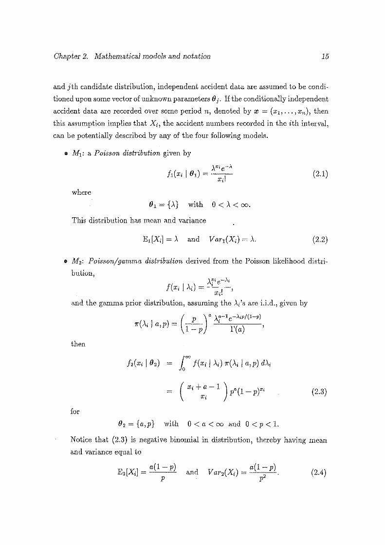
Chapter 2. Mathematical models and notation 15
and jth candidate distribution, independent accident data are assumed to be condi
tioned upon some vector of unknown parameters() j. If the conditionally independent
accident data are recorded over some period n, denoted by re = (xt, ... , xn), then
this assumption implies that Xi, the accident numbers recorded in the ith interval,
can be potentially described by any of the four following models.
• M1 : a Poisson distribution given by
(2.1)
where
() 1 = {A} with 0 < A < oo.
This distribution has mean and variance
(2.2)
• M2 : Poisson/gamma distribution derived from the Poisson likelihood distri
bution,
X .! l'
and the gamma prior distribution, assuming the A/s are i.i.d., given by
then
(2.3)
for
02 = {a,p} with 0 <a< oo and 0 < p < 1.
Notice that (2.3) is negative binomial in distribution, thereby having mean
and variance equal to
Chapter 2. Mathematical models and notation 16
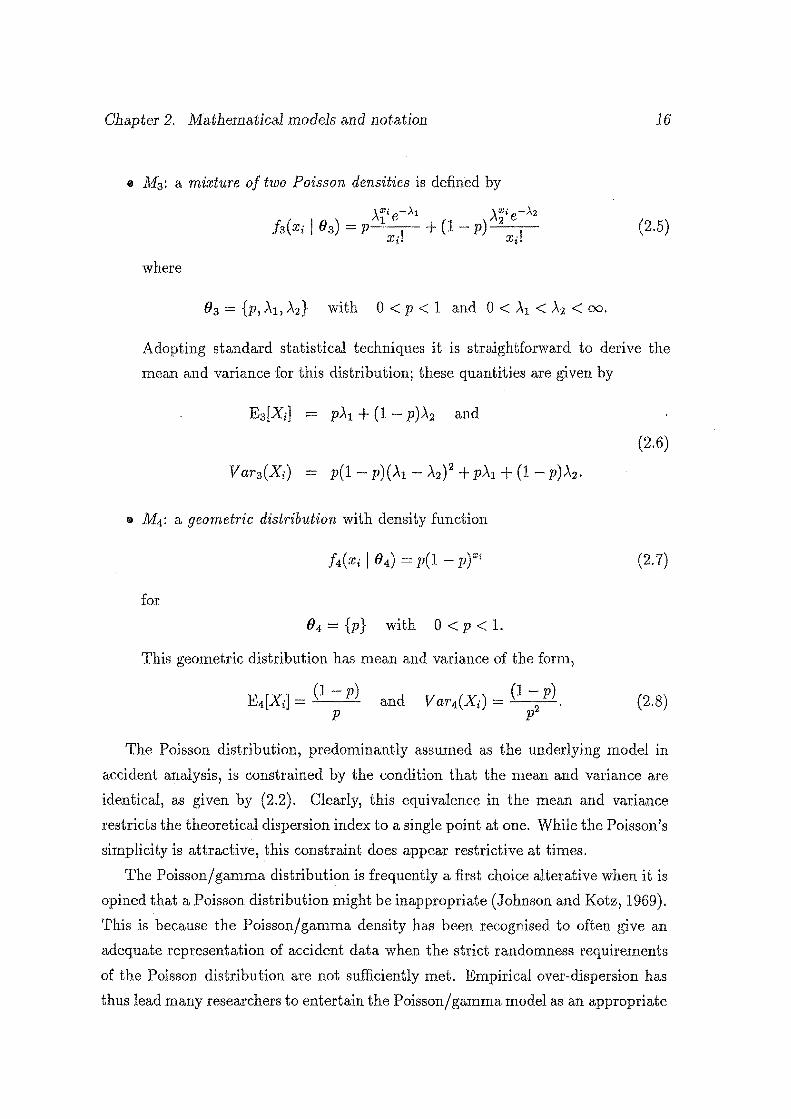
• M3 : a mixture of two Poisson densities is defined by
(2.5)
where
Adopting standard statistical techniques it is straightforward to derive the
mean and variance for this distribution; these quantities are given by
(2.6)
• M 4 : a geometric distribution with density function
(2.7)
for
84 = {p} with 0 < p < 1.
This geometric distribution has mean and variance of the form,
and (2.8)
The Poisson distribution, predominantly assumed as the underlying model in
accident analysis, is constrained by the condition that the mean and variance are
identical, as given by (2.2). Clearly, this equivalence in the mean and variance
restricts the theoretical dispersion index to a single point at one. While the Poisson's
simplicity is attractive, this constraint does appear restrictive at times.
The Poisson/ gamma distribution is frequently a first choice alterative when it is
opined that a Poisson distribution might be inappropriate (Johnson and Kotz, 1969).
This is because the Poisson/ gamma density has been recognised to often give an
adequate representation of accident data when the strict randomness requirements
of the Poisson distribution are not sufficiently met. Empirical over-dispersion has
thus lead many researchers to entertain the Poisson/ gamma model as an appropriate

Chapter 2. Mathematical models and notation 17
alternative distribution for measuring traffic accident data. As can be seen from
(2.4), this distribution has a variance greater than its mean, thereby allowing the
theoretical dispersion index to range on the (1, oo) interval.
Density functions based on mixtures of distributions have received some attention
in the statistical literature (Ashton, 1971, Everitt and Hand, 1981, Philippou, 1989).
Indeed this type of approach seems particularly pertinent to the investigation of
traffic accidents, as accidents frequently occur for more than one reason. A difficulty
exists in that data are rarely available for each conditional distribution separately.
Instead, data are generally available for the overall mixture of distributions and
thus the individual contribution by each conditional distribution can not easily be
ascertained. Moreover, the potential contributing factors for vehicle accidents are
numerous and diverse. Developing a mixture that allows for the separate effect of
each potentiality on the overall accident rate would lead to an extremely complex
model of little practical use. Instead, it was decided to consider broad categories
of factors, and allow each category to have a separate effect on the overall accident
rate.
Potential contributing factors are commonly considered to fall into three cate
gories:
1. driver factors (that is, psychological and physiological factors);
2. vehicle factors (such as visibility, lighting, and braking factors); and
3. environmental factors (such as road alignment, weather, and traffic flow fac
tors).
For this study, however, it was decided to not distinguish between the second and
third categories, and to consider a model mixing two Poisson densities. It is clear
from (2.6) that the theoretical dispersion index must also be greater than or equal
to one.
The geometric density is the fourth and final model considered. This density
represents, perhaps, an extreme model.choice that in practice would be infrequently
entertained. The geometric distribution, a special case of the negative binomial
distribution, is often referred to as a discrete waiting time distribution, in that
it represents how long (in terms of the number of vehicle passages) one has to
Chapter 2. Mathematical models and notation 18
wait for an accident to occur. Given the relationship between the geometric and
negative binomial distributions, it is evident that this distribution must also have
a theoretical dispersion index that ranges on the (1, oo) interval. Equation (2.8)
confirms this property.
From this specification of candidate models, it is apparent that certain nested
and nonnested relationships exist between these models. A model is nested within
another if the former is a special case of the latter. For example, suppose that M1
is geometric, with density ft(x I p) p (1- p)x, and M2 is negative binomial, with
· density function defined by h(x I a,p) ( a+:- 1 ) pa(l p)x; then it is easy
to see then· M1 is nested within M2 in the sense that we can write h(x I p) = f 2 (x I a = l,p). Nonnested models have no such relationship. Of the candidate
models considered here, M1 is nested within M3 , while M4 is nested within M2 ,
so that model discrimination must be made between combinations of nested and
nonnested models.
These four models can represent very different interpretations of accidents and
could result in quite different inferences if adopted.
2.2 N oninformative prior derivations
A widely used method for determining noninformative priors in a general setting
is that of Jeffreys (Berger, 1985). For a distributional function fi(w I Oi), where
()i (()ill ... , ()ih) is the vector of unknown parameters, this noninformative prior
results upon
(2.9)
where I(() i) is the ( h x h) expected Fisher information matrix and < det' represents
the determinant. Under commonly satisfied assumptions this information matrix
has element (j, k) equal to
Chapter 2. Mathematical models a.nd notation 19
2.2.1 M 1: Poisson
Adopting this strategy, it is easy to derive the Jeffreys noninformative prior for the
Poisson density (M1), which is given by
1l"f (lh) = Jx· In Section 3.4 we demonstrate that this improper noninformative prior yields a
proper marginal distribution for all Xi 2:: 0. This, in turn, implies that a noninfor
mative prior of this form gives a proper posterior for any such Xi·
2.2.2 M2: Poisson/gamma
Finding a suitable noninformative prior for the Poisson/gamma density (M2) is
somewhat more difficult. However, if the parameters of 1r!j ( 02) are taken as inde
pendent, so that 1r!j(02) h2,1(a) h2,2(p), and recalling that 0 < p < 1, then a
natural noninformative prior distributes p uniformly over the [0,1) interval so that
h2,2(p) U(O, 1).
If h2,1 (a) is now obtained using the method of Jeffreys then
::2 1ogfz(xi I a,p) = 1f;'(xi +a)- '1/J'(a)
where 1j;(z) = 8/8z1ogr(z) and 1};1(z) = 82/8z2logr(z) represent the digamma
and trigamma functions, respectively. Asymptotically, as z --+ oo, 1};'(z) can be
approximated by 1/z (equation 6.4.12 of Abramowitz and Stegun, 1965), so that
1 1 Xi+ a a
a(xi +a)'
Now the approximated expected Fisher information can be given by
Chapter 2. Mathematical models and notation 20
which, when expanded, equals
pa(1-p) [1 (a+1)(1 - )(a+1) (a+2)(a+1)(1 - )2 (a+1) l (a+1) + 1! p (a+2) + 2! p (a+3) + ... ·
Observe that under the same asymptotic conditions, the bracketed term can be
approximated by the binomial expansion (1- (1- p)t(a+l) so that
I( a) ~ pa(l- p) (1- (1- p))-(a+1) (a+ 1)
1 ex:
(a+ 1)"
The approximated Jeffreys noninformative prior for h2,1 (a) is then
1 h21(a) = VaTI ' a+1
and so an appropriate noninformative prior for the Poisson/ gamma density is given
by 1
Again, in Section 3.4 we demonstrate that a noninformative prior of this form ensures
a proper marginal distribution, and hence a proper posterior distribution, for all
Xi 2 0.
It could be suggested that a simple noninformative choice for h2 ,1 (a) would be
hz,t (a) 1. However, when hz,1 (a) = 1 is applied, the resultant posterior distri
bution is never proper for any Xi. Should h2,2(p) be derived using the method of
Jeffreys, then h2,2(p) ex: 1/p-J1 p. It is easy to verify that a prior of this form,
used in conjunction with the Jeffreys noninformative prior for h2,1(a), does not give
a proper posterior density for Xi = 0. Additionally, the "joint" Jeffreys prior derived
directly from (2.9) is complicated and of little practical use.
2.2.3 M3: mixture of two Poissons
A noninformative prior for the mixture of two Poisson densities (M3 ) is difficult
to derive from the approach of Jeffreys, as M3 is not from an exponential family.
If the parameters {p} and {.X1 ,A2 } of 1r£l(03 ) are treated as independent, so that
1r[j(Os) = h3 ,1(p)h3,.(>..1 , Az), and assuming the conditional relationship h3,.(At, .X2 ) =

Chapter 2. Mathematical models and notation 21
h3,2 (A1 I A2 ) h3,3 (A2), then an appropriate noninformative prior can be constructed
using the following rationale.
As before, a natural noninformative prior for p is uniform support over the [0, 1]
interval so that h3 ,1 (p) == U(O, 1). Now, A2 is a rate parameter from a Poisson distri
bution so, as seen in M1 , a sensible noninformative specification for this parameter
is h3,3 (A2) = ljJ):;. Lastly, conditional upon A2 and noting that 0 < A1 < A2 ,
a natural noninformative prior distributes A1 uniformly over the [0, A2) interval, so
that h3,2 (A1 I -\2) 1/A2 • When combined, this yields
1 A~/2
which results in a proper marginal (see Section 3.4) and hence a proper posterior
distribution for all Xi ~ 0.
It could be suggested that a simple noninformative choice for h3,2 (A1 I A2) would
be ha,2(-\1 I Az) 1, leading to 1r!j(Os) = 1/.J):;. However, if applied, it is easy to
verify that this noninformative prior results in a posterior distribution that is not
defined for any Xi.
2.2.4 M4: geometric
Finally, the noninformative prior for the geometric distribution (M4 ) using the
method of Jeffreys can easily be ascertained as
which results in a proper marginal (see Section 3.4) and hence a proper posterior
distribution for all Xi ~ 0.
Chapter 3
Model Discrimination
3.1 Preliminaries
3 .1.1 Bayes factors
Bayes factors have long been employed to discriminate between competing models;
see Kass and Raftery (1995) for a good review and list of references.
A Bayes factor can be derived as follows: suppose it is believed a priori that
any of .K statistical models M1 , • •. , M" could be usttd to describe a vector of data
re (x1, ... ,xn)i each model having some density /i(m I Oi)· The parameter vector
()i is unknown and has dimension hi for i = 1, ... , K respectively. Should 1ri(Oi)
represent the elicited prior distribution of the parameters for Mi then the Bayes
factor comparing Mj to Mi, denoted by Bji, is given by
(3.1)
where mi( re) is the marginal or predictive distribution of X under model Mi. Bayes
factors thus summarise the evidence provided by the data in favour of one statistical
model compared to its competitor.
22
Chapter 3. Model Discrimination 23
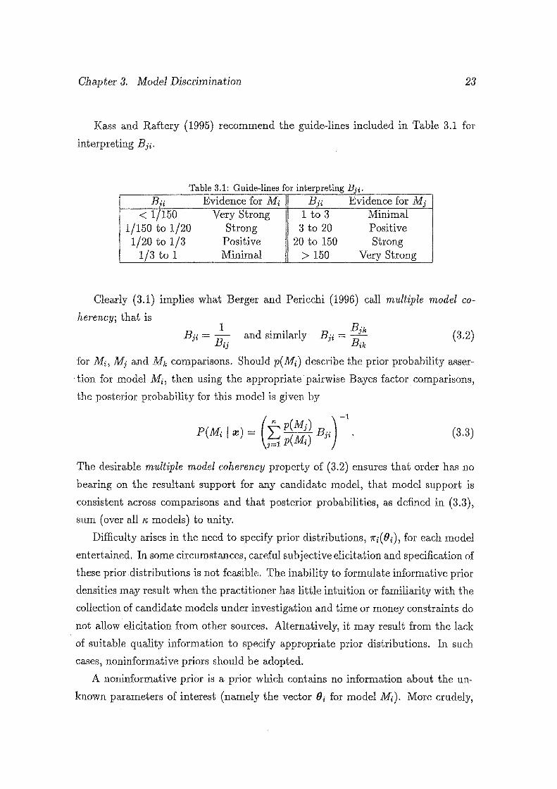
Kass and Raftery (1995) recommend the guide-lines included in Table 3.1 for
interpreting Bji·
Table 3.1: Guide-lines for interpreting Bji.
Bji Evidence for Mi Bji Evidence for Mj
< 1/150 Very Strong 1 to 3 Minimal 1/150 to 1/20 Strong 3 to 20 Positive 1/20 to 1/3 Positive 20 to 150 Strong
1/3 to 1 Minimal > 150 Very Strong
Clearly (3.1) implies what Berger and Pericchi (1996) call multiple model co-
herency; that is 1 Bjk
Bji =- and similarly Bji Bij Bik
(3.2)
for Mi, Mj and Mk comparisons. Should p(Mi) describe the prior probability asser-
tion for model Mi, then using the appropriate pairwise Bayes factor comparisons,
the posterior probability for this model is given by
(3.3)
The desirable multiple model coherency property of (3.2) ensures that order has no
bearing on the resultant support for any candidate model, that model support is
consistent across comparisons and that posterior probabilities, as defined in (3.3),
sum (over all "' models) to unity.
Difficulty arises in the need to specify prior distributions, 7q(8i), for each model
entertained. In some circumstances, careful subjective elicitation and specification of
these prior distributions is not feasible. The inability to formulate informative prior
densities may result when the practitioner has. little intuition or familiarity with the
collection of candidate models under investigation and time or money constraints do
not allow elicitation from other sources. Alternatively, it may result from the lack
of suitable quality information to specify appropriate prior distributions. In such
cases, noninformative priors should be adopted.
A noninformative prior is a prior which contains no information about the un
known parameters of interest (namely the vector (}i for model Mi)· More crudely,
Chapter 3. Model Discrimination 24
it is a prior which "favours" no possible value of (Ji over any others. Even with
the availability of informative prior information, noninformative priors are often
employed to offer an automated or objective Bayesian analysis.
Noninformative priors (denoted by 1rf ( 8i)) are frequently improper, in that they
have infinite mass, and are typically written as
where hi(8i) is some function on (Ji· For example, the uniform prior is often expressed
as 1r[V ( 8i) <X 1.
Formally, we can write
where Ci is treated as some unspecified normalising constant. Ensuing Bayesian
analysis involving a single model results in a posterior distribution for the unknown
parameter (Ji of the form
(3.4)
Ci J fi ( iV I (J i) hi ( (J i) d(J i .
Notice that the unspecified normalising constants Ci in (3.4) cancel out. Elimination
of these constants implies that if J fi( re I 8i) hi( (Ji) d(Ji is proper (i.e. has finite mass)
then the posterior density (3.4) is also proper, despite Ci being unspecified.
When dealing with more than a single model, as in (3.1), the resultant Bayes
factors are typically defined up to
B?f = mf(ro) = Cj f fi(iV I 8j) hj(Bj) d(Jj Jt mf(ro) Ci J fi(ro I 8i) hi(8i) d(Ji
(3.5)
where mf'(ro) = J fi(ro I 8i)7rf(8i)d8i is the marginal distribution for model i based
on a noninformative prior. Equation (3.5) depends on the unspecified Cj/Ci ratio and
hence is unsatisfactory for selection purposes.
Various attempts at addressing and eliminating this unspecified Cj / Ci ratio inher
ent within (3.5) have been propounded, including several techniques using training
samples and partial likelihood methods. These training samples and partial likeli
hood methods have considerable appeal and form the basis for the derivation of the
averaged Bayes factor.
Chapter 3. Model Discrimination 25
3.1.2 Training samples and partial likelihood Inethods
It may be possible to use a part of the data within a given model to compute a proper
posterior distribution using a noninformative prior. This proper posterior can then
be adopted as a prior density so that Bayes factors can be derived from the remaining
data. A sample used for the development of the prior posterior distribution is called
a training sample. Thus a training sample is a special subset of the given data
that allows the specification of a proper posterior distribution free from unspecified
normalising constant multipliers. Such posteriors used as prior distributions ensure
·that subsequent Bayes factor derivations can be usefully employed for discrimination
purposes, despite the absence of prior information.
Suppose that m(l) is some subset of the data and m(l') denotes those observed
data outside this subset, so that m = { m ( l), m ( !')} = ( x1 , .•. , Xn). For example,
m(l) = { Xt, .•. , xi} and :u(l') = { Xi+h ••. , Xn} represents one such partition of the
n data points. Now :u(l), the training sample, can be used to convert the improper
noninformative prior 'lf'f ( 0 i) to a proper posterior 'lf'f ( 0 i I :u (l)) for model Mi, by
noting
fi( m(l) I oi) 'lf'r ( Oi) mf'(m(l))
where, again, Ci is an unspecified normalising constant and
(3.6)
(3.7)
is the marginal density of the training sample under Mi. Observe that Ci cancels
out in (3.6). Using the remainder of the data, denoted by m(l'), the Bayes factor is
given by
(3.8)
which is free from the unwanted ratio of unspecified normalising constants, as de
sired.
Training samples should be large enough so that 'lf'[V(Oi I m(l)) is proper for all
candidate models (that is 0 < 'lf'[V(Oi I :u(l)) <co fori= 1, ... , 1'0) yet they should
Chapter 3. Model Discrimination 26
be as small as possible so that most of the data can be used in calculations for the
weighted likelihood ratio of models Mj to Mi in (3.8). For 1r{"(Oi I w(l)) to be proper
for all"' candidate models, then m{"(w(l)), i 1, ... ,, given by (3.7) must also be
proper. These notions are formalised by the following definition given by Berger
and Pericchi (1996).
Definition. A training sample, w(l), is called proper if 0 < mf(w(l)) < oo for
all Mi, and minimal if it is proper and no subset is proper.
Typically, for a particular data set ro, there are many varied minimal training
sample partitions. The Bayes factor defined by (3.8) is clearly dependent on the
particular minimal training sample selected and hence adoption of different training
samples will result in different Bayes factors. It is this fact that we now exploit with
the introduction of the averaged Bayes factor.
3.2 Averaged Bayes factor
The Bayes factor BJ[ ( l) defined in (3.8) depends on the particular minimal training
sample chosen. To eliminate this dependency, and increase stability, the averaged
Bayes factor is introduced as follows.
Let XT = { ro(1), ro(2), ... , ro(L)} denote the set of all minimal training samples,
w(l). The principle idea is to take an average of the posterior densities 1r{"(Oi I w(l)),
given in (3.6), over all L combinations of minimal training samples w(l) E XT for
each model under investigation. Associated averaged distributions are subsequently
used as the prior distribution in (3.1), so that a pseudo-marginal distribution can
be ascertained for each respective model under comparison. Derivation of the aver
aged Bayes factor naturally ensues with the pairwise comparisons of these pseudo
marginal distributions.
Mathematically, we define the pseudo-marginal distribution of X under model
Mi as
(3.9)
Chapter 3. Model Discrimination 27
thus the averaged Bayes factor, Bfl, for model comparison Mj to Mi, is given by
A mf(ro) Bji = -N( )'
mi ro (3.10)
From this derivation of the averaged Bayes factor it is clear that the following
properties hold.
Properties
1. The formulation of the averaged Bayes factor ensures that the ratio of unspec
ified constants in (3.5) is eliminated.
2. The pseudo-marginal distribution mf'(ro ), given by (3.9), can be independently
computed for each of the K, candidate models. This is important and compu
tationally advantageous, because once mf' ( ro) is numerically ascertained any
pairwise comparison involving Mi can then be. conducted. Some averaging
techniques do not enjoy this property.
3. The important multiple model coherency property of (3.2) is preserved. This
is due to (3.10) being composed from the ratio of independently computed
mf' ( m) distributions for pairwise model comparisons.
4. The averaged Bayes factor is a fully automated criterion, in that it only re
quires standard noninformative priors for its computation. Moreover, due to
the averaging process in (3.9), it is relatively insensitive to the particular non
informative prior density used, so that reference priors, Jeffreys priors or other
appropriately derived noninformative priors can be adopted without substan
tially affecting the resultant Bayes factor. Not all noninformative Bayes factor
methods are able to make this assurance.
5. Selection using (3.10) can be made for nested or nonnested models, and for
multiple model comparisons.
6. Stability of resultant factors and independence from particular training data is
assured by the averaging of 1r[V ( 9 i I ro ( l)) over all L minimal training samples
m(l) E Xy. This is because any unusual training sample will contribute only
a small fraction (in fact 1/ L) of the prior information used for the derivation
of the marginal density mf' ( ro ).
Chapter 3. Model Discrimination 28
This averaged Bayes factor method, therefore, appears to have somedistinct advan
tages over current noninformative variants of the Bayes factor.
To contrast the averaged Bayes factor, we use the most commonly adopted
Bayesian discrimination method, the Bayesian information criterion. This approach
is the topic of the next section.
3.3 Bayesian information criterion
The most conventionally employed "Bayesian" model selection technique is that of
the renowned Bayesian information criterion (BIC) introduced by Schwarz (1978).
For conditionally independent data this criterion has been modified by various au
thors (such as Raftery, 1993, and Raftery, 1995) so that the Bayes factor given in
(3.1) can be approximated by
Bf!. = IJ(w I ~j) n-(hj-hi)/2
Jt /i(w I Bi) (3.11)
where fii is the vector of maximum likelihood estimates (MLE) under Mi and, as
before, hi is the dimension of the parameter vector Bi. The model selection crite
rion (3.11) is typically reported as 2loge Bj~, which has parallels with the standard
likelihood ratio test statistic for testing Mi against Mj (Raftery, 1995).
The asymptotic principles and simplifications used to derive the BIC criterion
and its approximations are satisfactory when dealing with large samples. Subse
quent examination has revealed that serious biases can manifest themselves when
these criteria are applied to samples of small size (O'Hagan, 1995, Berger and Per
icchi, 1996). Indeed, the asymptotically constant term that is ignored in the devel
opment of (3.11) can dominate the Bayes factor under such circumstances. As this
term can be either arbitrarily large or small, the BIC criterion can systematically
bias the results in favour of either the simpler or the more complicated model under
comparison. Moreover, this bias can be quite substantial.
Accident data are generally available at individual sites for a small number of
years. This suggests that the BIC criterion, and other methods based upon similar
asymptotic principles and approximations, may contain serious systematic bias, ren
dering them unsuitable for model selection purposes in much of the accident analysis
framework.
Chapter 3. Model Discrimination 29
The BIC criterion is further hampered by the fact that informative prior infor
mation pertaining to the unknown parameters of interest cannot be embodied within
the model, something that strictly Bayesian methods should facilitate.
3.4 Numerical example
Model discrimination between the four candidate models introduced in Section 2.1 is
now undertaken. Discrimination is conducted separately at each of the 35 traffic ac
cident intersection sites included in Table A.l of Appendix A and at the hypothetical
Site B. In all instances it is assumed that insufficient resources are available to con
struct informative prior densities, necessitating the embodiment of noninformative
priors. For convenience, those noninformative priors delineated within Section 2.2
will be employed.
Discrimination is initially conducted using the averaged Bayes factor and then,
for comparison, this discrimination is repeated using the approximated BIC method.
3.4.1 Averaged Bayes factor
The derivation of the marginal distributions, as defined in (3.7), based upon a train
ing sample of just a single observation, re(l) = {xj}, is easily undertaken for the four
candidate models.
Marginal distribution: mf(re(l))
Recall from ( 3, 7) that
then for M1 , the Poisson distribution,

Chapter 3. Model Discrimination 30
and recognising the form of the gamma distribution, providing x; 1/2 > 0, then
f(Xj + 1/2) 100 _\(IDj+l/2)-le-..\d\ mf ( w( l)) = 1\
x;! 0 r(x; + 1/2)
r(xj + 1/2) r(x; + 1)
which is proper for all x; ~ 0.
Marginal distribution: mf(re(l))
For M2 , the- Poisson/ gamma density, the marginal is defined by
mf(ro(l)) = r foo ( Xj +a -1) pa(l- pyvi ~ da dp. lo lo Xj a+ 1
Recognising the form of the beta distribution, providing a+ 1 > 0 and x; + 1 > 0,
henceintegrating with respect top and then with respect to a gives
mf(re(l)) = j= ( x;+a-1) 1 f(a+1)f(x;+l) X
Jo Xj va+T f(Xj +a+ 2)
r r(x; +a 2) p(a+l)-1(1 p)<xi+l)-1dp da lo r(a + 1) r(x; + 1)
roo a ~
lo (x; +a) (x; +a+ 1)
l :; [2 :.ctan(l/ y'x; - 1) - 1r]( ,!x; - 1 + (x; + 1) [1r 2arctan(1/vfX7)] /y'Xj
which is proper for all x; ~ 0.
Marginal distribution: mf ( w ( l))
For M3 , the mixture of two Poisson densities,
for Xj = 0 for Xj 1
for Xj ~ 2,
(3.12)

Chapter 3. Model Discrimination 31
(term 1)
,\~i e-A2 1
J J /(1- p) .I 3/2 dp d,\1 d,\2 XJ• ,\2
(term 2).
Consider initially term 1. Integrating with respect to p and then with respect to ..\2
(recalling that 0 < A1 < ..\2 < oo) gives
Recognising the form of the gamma distribution, providing Xj + 1/2 > 0, then
r(xj + 1/2) r(xj + 1)
which is proper for all Xj 2:: 0. Now consider term 2. Integrating with respect top
and then ,\1 gives
Again recognising the form of the gamma distribution, providing Xj + 1/2 > 0, then
which is also proper for all x j 0. Combining both terms 1 and 2 yields,
N( (l)) = 3 f(Xj + 1/2) m3 re 2 r(xj + 1) .
Chapter 3. Model Discrimination 32
Marginal distribution: mf(re(l))
Lastly, for M4 , the geometric density,
mf (re(l)) lol 1 p(l - p y;j vr=P dp
0 p -p
1 -
Xj 1/2
which is proper for all Xj ~ 0.
Minimal training sample
A minimal training sample thus consists of a single observation, re(l) = {x3}, pro
vided that x3 ~ 0. This condition on Xj is clearly satisfied for our accident data.
For this numerical example it is also apparent that XT, the set of all minimal
training samples, has n members so that L = n.
Pseudo-marginal distribution: mf ( re)
The pseudo-marginal distribution mf(m), as defined in (3.9), can be expressed in
closed form. Its derivation can be found using the following rationale.
mf"("') = j J,C.i: I o,) [~ t, .. j"(o, I ro(l))l dB,
~ j h(re I 81) 1rf(01 I re(l)) d01 + ... + ~ j h(re I 01) 1rf(01 I re(n)) d01
after expanding the summation and noting L n. Now considering the jth term,
then
f ft(re(j) I 81) 1r1(01) d01
h(xj I 81) 1r1(81) mf(re(j))
)..WJ-1f2e-;..
I'(xj + 1/2)
Chapter 3. Model Discrimination 33
which is clearly recognisable as having the form of a gamma density. Under the
aforementioned assumption of conditionally independent data, which implies
n
fk(m I lh) = IT!k(xi I Ok) i=l
for any given Mk, then
where S l:i=t Xi· Exploiting the form of the gamma density, providing that
S + Xj + 1/2 > 0 (which is always true for accident counts), this intergal can be
rewritten as
which integrates out to
[ n 1 l f(S Xj + 1/2) g Xi! f(xj + 1/2) (n + 1)S+xi+1/2'
Now, summing over then terms gives
-N( ) 1 [rrn 1 l ~ f(S + Xj + 1/2) ( 1)-S-rc·-1/2 m1 m = - - 1 L..i n + J •
n i=l Xi. j=l f(xj + 1/2)
Pseudo-marginal distribution: mf ( m)
Numerical integration is necessary for the computation of mf(m), although only n
one-dimensional integrations over a are required as the integration over p can be
done in closed form.
The posterior distribution based upon the jth training sample is
where m2(m(j)) is given by (3.12). The jth term of the pseudo-marginal distribution
is thus

Chapter 3. Model Discrimination 34
I_JJ[fi(xi+a-1)pa(l-p)UJ•] 1. (Xj+a-1)pa(1 p)UJi dadp n i=1 Xi m2 (ro(J )) Xj va+f
C (X> [rr ( Xi+ a- 1 )] 1 ( Xj +a 1 ) r0
1 p(n+l)a(l- p)S+xj dp da.
. lo i=1 Xi va+f Xj Jo
where C = [nm2(ro(j)))-1 • Recognising the form of the beta distribution, providing
(n + 1)a + 1 > 0 and S + Xj + 1 > 0, this integration equals
C roo [rr ( Xi+~ 1 )] ( Xj t a- 1 ) B(S + Xj t 1, (n t l)a + 1) X
lo i=1 x, Xj va+f
11 p((n+l)a+l)-1(1 _ p)(S+xj+l)-1 · dpda,
o B(S+xjt1,(ntl)a+1) where B(x,y) is the beta function with relation B(x,y) = r(x) r(y)jr(x + y).
Integrating with respect to p yields
C roo [rr ( Xi t ~ 1 )] ( Xj t a- 1 ) B(S t Xj t 1, (n t 1)a t 1) da. Jo i=l X~ Xj va+f
Lastly, replacing C and summing over the n terms gives
1 n 1 m~(ro) -2: N( ('))X
n j=l m2 ro J
roo [rr ( Xi + ~ - 1 )] ( Xj t ~ lo i=l x, x3
Pseudo-marginal distribution: mf ( ro)
1 ) B ( S + x j + 1, ( n + 1) a + 1) da. va+T
The term mf ( ro) can not be readily simplified so the solution must be achieved
through three-dimepsional numerical integration.
Pseudo-marginal distribution: mf ( ro)
Using a similar rationale to that used for the derivation of mf ( ro), the pseudo
marginal distribution can be written in closed form for M4 . This is done by noting
the posterior distribution based upon the jth training sample is
Chapter 3. Model Discrimination
and so the jth term of the pseudo-marginal is given by
~ j h(re I 84) .1ff(B4 I re(j)) d84
~ 11 [il p(1- Pt'] (xi+ 1/2)(1- p)xj-l/2dp
= (Xj + 1/2) {1
pn(l _ p)S+xJ-1f2dp. n Jo
35
Recognising the form of the beta density, providing n + 1 > 0 and S + Xj + 1/2 > 0,
this integral can be rewritten as
(xr+ 1/2)
11 p(n+I)-1(1 _ p)(S+xi+I/2)-1
B(S + Xj + 1/2,n + 1) B(S . 112 1) dp n o + x3 + ,n +
(xi+ 1/ 2) B(S + Xj + 1/2, n + 1). n
Summation over n such terms gives 1 n
mf (re) = -~)xi+ 1/2) B(S Xj + 1/2, n + 1). n J=1
Computation
When both 1rf(Oi I re(l)) and mf(re) can be expressed in closed algebraic form
then computation is straightforward. However, in general some form of numerical
integration is usually required. Typically, it seems, the posterior distribution con
ditioned on the training sample, 1r['l ( 0 i I re (l)), can be expressed in some closed
algebraic form and it is inevitably the pseudo-marginal density mf ( re) that requires
numerical integration. Fortunately there ·are a plethora of suitable techniques that
can be readily implemented.
Numerous methods exist for computing either 1r['l ( 0 i I re( l)) or mf ( re). In partic
ular, standard quadrature integration can be usefully employed for low dimensional
integration, and for integrations of higher dimension, Monte Carlo integration and
the Metropolis algorithm are advantageous; see Kass and Raftery (1995), Smith
and Gelfand (1992), Smith and Roberts (1993), Muller (1991), Berger and Pede
chi (1996) and Gelfand, and Dey and Chang (1992) for discussion on this.
For the particular numerical example contained within this thesis, integration
was conducted on m!j ( re) over a using the trapezoidal rule, while the Metropolis
algorithm (Muller, 1991) was used for the determination of mf(m).
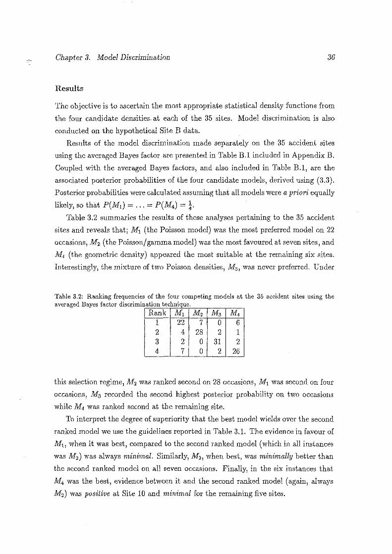
Chapter 3. Model Discrimination 36
Results
The objective is to ascertain the most appropriate statistical density functions from
the four candidate densities at each of the 35 sites. Model discrimination is also
conducted on the hypothetical Site B data.
Results of the model discrimination made separately on the 35 accident sites
using the averaged Bayes factor are presented in Table B.1 included in Appendix B.
Coupled with the averaged Bayes factors, and also included in Table B.1, are the
associated posterior probabilities of the four candidate models, derived using (3.3).
Posterior probabilities were calculated assuming that all models were a priori equally
likely, so that P(Mt) = . . . P(M4) = i· Table 3.2 summaries the results of these analyses pertaining to the 35 accident
sites and reveals that; M1 (the Poisson model) was the most preferred model on 22
occasions, M 2 (the Poisson/ gamma model) was the most favoured at seven sites, and
M4 (the geometric .density) appeared the most suitable at the remaining six sites.
Interestingly, the mixture of two Poisson densities, M3 , was never preferred. Under
Table 3.2: Ranking frequencies of the four competing models at the 35 accident sites using the averaged Bayes factor discrimination technique.
Rank M1 M2 M3 M4 1 22 7 0 6 2 4 28 2 1 3 2 0 31 2 4 7 0 2 26
this selection regime, M 2 was ranked second on 28 occasions, M1 was second on four
occasions, M3 recorded the second highest posterior probability on two occasions
while M4 was ranked second at the remaining site.
To interpret the degree of superiority that the best model wields over the second
ranked model we use the guidelines reported in Table 3.1. The evidence in favour of
M1, when it was best, compared to the second ranked model (which in all instances
was M2 ) was always minimal. Similarly, M2, when best, was minimally better than
the second ranked model on all seven occasions. Finally, in the six instances that
M4 was the best, evidence between it and the second ranked model (again, always
M2) was positive at Site 10 and minimal for the remaining five sites.
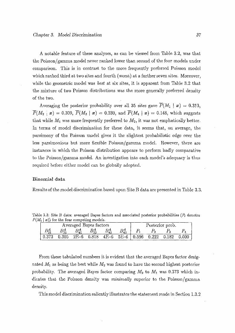
Chapter 3. Model Discrimination 37
A notable feature of these analyses, as can be viewed from Table 3.2, was that
the Poisson/ gamma model never ranked lower than second of the four models under
comparison. This is in contrast to the more frequently preferred Poisson model
which ranked third at two sites and fourth (worst) at a further seven sites. Moreover,
while the geometric model was best at six sites, it is apparent from Table 3.2 that
the mixture of two Poisson distributions was the more generally preferred density
of the two.
Averaging the posterior probability over all 35 sites gave P(M1 I x) = 0.313,
P(Mz I :v) = 0.309, P(M3 I :v) = 0.230, and P(M4 I :v) = 0.148, which suggests
that while ¥ 1 was more frequently preferred to M2 , it was not emphatically better.
In terms of model discrimination for these data, it seems that, on average, the
parsimony of the Poisson model gives it the slightest probabilistic edge over the
less parsimonious but more flexible Poisson/gamma model. However, there are
instances in which the Poisson distribution appears to perform badly comparative
to the Poisson/ gamma model. An investigation into each model's adequacy is thus
required before either model can be globally adopted.
Binomial data
Results of the model discrimination based upon Site B data are presented in Table 3.3.
Table 3.3: Site B data: averaged Bayes factors and associated posterior probabilities (P;, denotes P(Mi Ire)) for the four competing models.
Averaged Bayes factors Posterior prob. B~ Bfi Bfr B~ Bfz Bfs pl p2 p3 p4
0.373 0.305 2E-6 0.818 4E-6 5E-6 0.596 0.222 0.182 0.000
From these tabulated numbers it is evident that the averaged Bayes factor desig
nated M 1 as being the best while M 2 was found to have the second highest posterior
probability. The averaged Bayes factor comparing M2 to M 1 was 0.373 which in
dicates that the Poisson density was minimally superior to the Poisson/ gamma
density.
This model discrimination saliently illustrates the statement made in Section 1.3.2
Chapter 3. Model Discrimination 38
whereby Bayes factor strategies advocate superior models from the group under in
vestigation, regardless of their fit. Had we not known that the data were binomial,
and made no consideration of the adequacy of the Poisson model, we would have
blithely proceeded with this discriminated model in subsequent analyses. Poten
tially, quite erroneous conclusions could have thus been drawn.
3.4.2 Bayes information criterion
For comparison, the approximation of the Bayes information criterion (3.11) was
also applied on the same data to discriminate between the four competing models.
Computation
While maximum likelihood estimates (MLE) for the Poisson and geometric distri
butions are easily derived, estimates for the Poisson/ gamma and mixture of Poisson
distributions are not.
Maximum likelihood estimators for the Poisson/ gamma model, which in effect
gives rise to the negative binomial distribution, were obtained on solution of equa
tions (30) and (31.1) on page 132 of Johnson and Katz (1969), such that: (X)
aP =X and log(l + P) I)xf3-l + j 1t1 Fj j=l
where Fj = l:~j fi = proportion of ru which are greater than or equal to j and
j3 (1- fi)fp. Instances arise, however, when the MLE does not exist (due to the data being
under-dispersed) in which case parameters were calculated assuming that the sample
variance was c larger than the sample mean, where c is some small number (in this
case lE-10). This implies that p xf(x +c) and a= xpf(l- p). The maximum likelihood estimates for the mixture of two Poisson densities are
also not explicitly solvable for the parameters of interest, necessitating the use of
iterative techniques. Everitt and Hand (1981) derive such a system of equations
with
Chapter 3. Model Discrimination 39
where
F(i I Xj) =Pi Pi( X I ~i) P(x I p,.\)
for A= (~b ~2) and p = (pl,pz). Note here that p2 1-p1. Given initial values for
~ and p, these equations can be used to form the basis for this iterative estimation
algorithm. Unfortunately a deficiency of this iterative technique, common with
many such algorithms, is that different initial values may lead to widely different
final estimates. All resultant estimates were thus verified using the Newton-Raphson
algorithm and checks on the value of the likelihood function.
Results
Table B.2 contained in Appendix B houses the results from implementation of (3.11).
Associated posterior probabilities, derived using (3.3), are also included in this table.
Again, these posterior probabilities were calculated assuming a priori that each
model was equally likely.
Perusal of these calculations, which have been summarised in Table 3.4, reveal
that M1 was best at 26 sites (up four from the number designated by the averaged
Bayes factor), M 2 was best at two sites (down five), M4 was best at seven sites (up
one), while M3 was never superior (as before).
Table 3.4: Ranking frequencies of the four competing models at the 35 accident sites using the approximated BIC discrimination method.
Rank M1 Mz M3 M4 1 26 2 0 7 2 3 25 0 7 3 3 8 16 8 4 3 0 19 13
Although infrequently the best model, M 2 was ranked second on 25 occasions,
M1 was second on three occasions, while M4 was ranked second at the remaining
seven sites. Notably, M3 was never selected within the top two of the four models
studied for any site. Again using the discrimination strengths of Table 3.1, evidence
in favour of lvft, when it was best, compared to the second ranked model was in 15
instances positive and on a further eleven occasions minimal. Mz was minimally
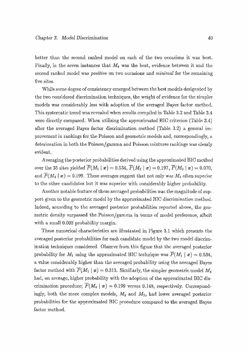
Chapter 3. Model Discrimination 40
better than the second ranked model on each of the two occasions it was best.
Finally, in the seven instances that M4 was the best, evidence between it and the
second ranked model was positive on two occasions and minimal for the remaining
five sites.
While some degree of consistency emerged between the best models designated by
the two considered discrimination techniques, the weight of evidence for the simpler
models was considerably less with adoption of the averaged Bayes factor method.
This systematic trend was revealed when results compiled in Table 3.2 and Table 3.4
were directly compared. When utilising the approximated BIC criterion (Table 3.4)
after the av:eraged Bayes factor discrimination method (Table 3.2) a general im
provement in rankings for the Poisson and geometric models and, correspondingly, a
deterioration in both the Poisson/ gamma and Poisson mixtures rankings was clearly
evident.
Averaging the posterior probabilities derived using the approximated BIC method
. over the 35 sites yielded P(M1 I re) = 0.534, P(M2 I re) 0.197, P(M3 Ire) = 0.070,
and P(l\14 Ire) = 0.199. These averages suggest that not only was M1 often superior
to the other candidates but it was superior with considerably higher probability.
Another notable feature of these averaged probabilities was the magnitude of sup
port given to the geometric model by the approximated BIC discrimination method.
Indeed, according to the averaged posterior probabilities reported above, the geo
metric density surpassed the Poisson/ gamma in terms of model preference, albeit
with a small 0.002 probability margin.
These numerical characteristics are illustrated in Figure 3.1 which presents the
averaged posterior probabilities for each candidate model by the two model discrim
ination techniques considered. Observe from this figure that the averaged posterior
probability for M1 using the approximated BIC technique was P(M1 I re) 0.534,
a value considerably higher than the averaged probability using the averaged Bayes
factor method with P(M1 l re) 0.313. Similiarly, the simpler geometric model M4
had, on average, higher probability with the adoption of the approximated BIC dis
crimination procedure; P(M4 I re) = 0.199 versus 0.148, respectively. Correspond
ingly, both the more complex models, M2 and M3 , had lower averaged posterior
probabilities for the approximated BIC procedure compared to the averaged Bayes
factor method.
Chapter 3. Model Discrimination 41
Figure 3.1: Averaged posterior probabilities P(Mi I (IJ), i = 1, 2, 3 and 4, derived from the averaged Bayes factor and approximated BIG method over the 35 accident sites.
0.6..-------.------,-------,------.-----,
0.45
0.15
~~ averaged Bayes factor
1m:mm approximated BIG method
......... o~~~= .... = .... ~·-~~=·=···=····~·-~~~~--U~==~
M4 M1 M2 M3 Models
The increased support for the Poisson model by the approximated BIC method,
compared to the averaged Bayes factor, is illustrated for each individual site in
Figure 3.2. In this figure, the extent of the increased support for the Poisson model
by the approximated BIC method has been depicted by the dotted lines. This figure
quite dramatically demonstrates the previously described inherent failing of the BIC
approach, in this case favouring the simpler model when the sample size was small.
Binomial data
Increased support by the BIC method for the simplier model was also evident when
the hypothetical data were analysed, as can be seen in Table 3.5. Calculations
Table 3.5: Site B data: approximated BIG Bayes factors and associated posterior probabilities (Pi denotes P( Mi I ro)) for the four competing models.
approximated BIC Bayes factors Posterior prob. Bfl B%1 Bfl Bffz Bfz Bf3 pl Pz Ps p4
0.224 0.010 2E-6 0.044 7E-6 2E-4 0.811 0.181 0.008 0.000
based on the hypothetical data revealed that M1 was best and that M 2 was, again,
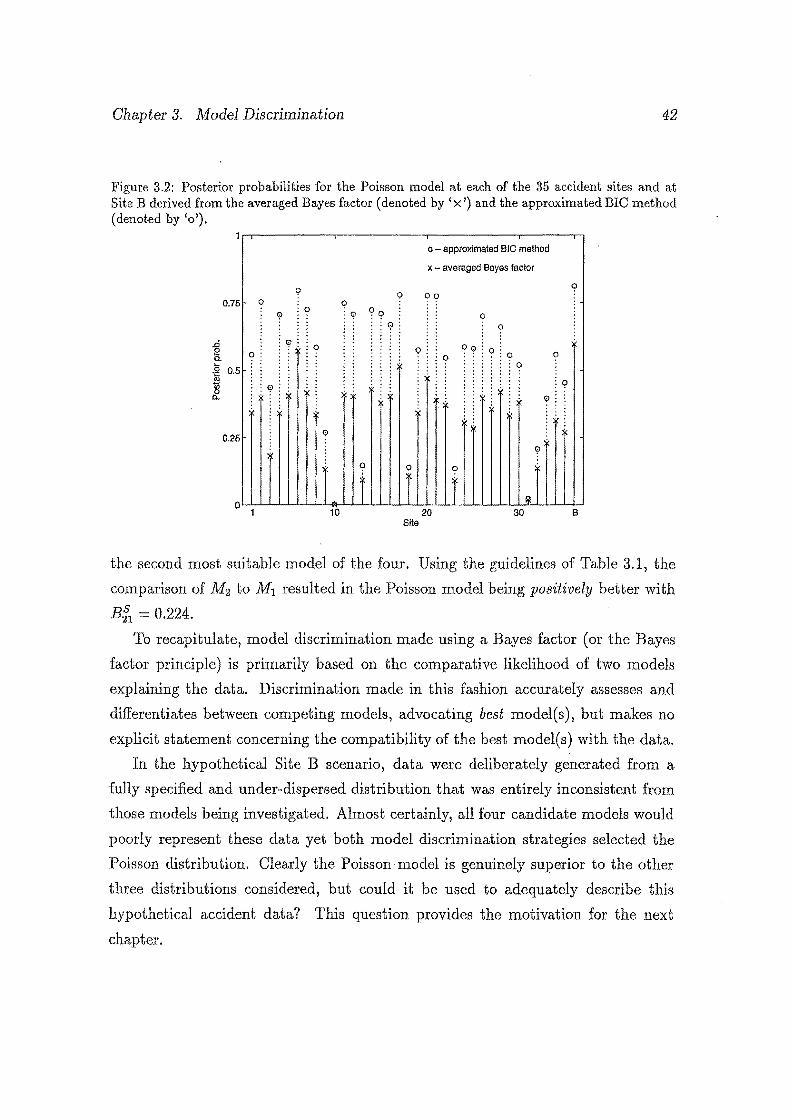
Chapter 3. Model Discrimination 42
Figure 3.2: Posterior probabilities for the Poisson model at each of the 35 accident sites and at Site B derived from the averaged Bayes factor (denoted by 'X') and the approximated BIC method (denoted by 'o').
o - approximated BIC method
x- averaged Bayes factor
the second most suitable model of the four. Using the guidelines of Table 3.1, the
comparison of M2 to M1 resulted in the Poisson model being positively better with
B~1 = 0.224.
To recapitulate, model discrimination made using a Bayes factor (or the Bayes
factor principle) is primarily based on the comparative likelihood of two models
explaining the data. Discrimination made in this fashion accurately assesses and
differentiates between competing models, advocating best model(s), but makes no
explicit statement concerning the compatibility of the best model(s) with the data.
In the hypothetical Site B scenario, data were deliberately generated from a
fully specified and under-dispersed distribution that was entirely inconsistent from
those models being investigated. Almost certainly, all four candidate models would
poorly represent these data yet both model discrimination strategies selected the
Poisson distribution. Clearly the Poisson model is genuinely superior to the other
three distributions considered, but could it be used to adequately describe this
hypothetical accident data? This question provides the motivation for the next
chapter.
Chapter 4
Model Adequacy and Power
The proposed averaged Bayes factor technique discriminates by simply comparing
models. Having differentiated between a group of models using such a technique, it
may be tempting to simply choose a particular Mj because it performed <<the best"
for the given data amongst the K competing models. However, model selection made
in this fashion ignores the important question of: "Is Mj consistent enough with the
observed data for us to confidently use such a model?". Only further examination
of the preferred model can suitably answer this question.
In this chapter we assume that the analyst, through some appropriate means,
has discriminated and identified what they consider to be the best density Mj. The
analyst, wanting to answer the important question and confirm the applicability of
Mj, must then test its compatibility with the observed data. That is, the analyst
must ascertain whether the empirical data are likely to have originated from this
chosen model. If the observed data had little chance of arising from Mj then its
appropriateness must be seriously questioned, as such a model is unlikely to provide
accurate or useful information for ensuing inferences.
43
Chapter 4. Model Adequacy and Power 44
4.1 Preliminaries
Suppose that the distributional function Mj is discriminated from a pool of candidate
densities M1 , ... , MK to best represent some conditionally independent vector of data
re (x1, ... , xn)· Selection of model Mj implies Xi is assumed to be distributed
by fi (Xi I 0 j) hence the data are conditional upon some hrdimensional vector of
unknown parameters e j.
Posterior distribution
If 7rj(Oj) represents some informative or noninformative (dropping the superscript
N) prior distribution for Oj, then, as we have seen in (3.4), the posterior distribution
of (} i is given by the hj-dimensional integral
( 4.1)
where n
fi(m I Oj) =IT fi(xi I Oj)· i=l
Posterior predictive distribution
Using a similar rationale to Gelman et al. (1995), we define the random variable Y
as the replicated data that could have been observed, or, in the predictive sense, as
the data we would see over the next n years if the circumstances that produced m
over the last n years were repeated with the same model and underlying accident
rate 0. Specifically, y is a replication just like re.
The predictive distribution corresponding to Mj for the vector of unobserved
random variables, Y, denoted by !J(y I m), can then be given by
(4.2)
As the data are assumed to be conditionally independent, ( 4.2) can be simplified to
( 4.3)
Gelman et al. (1995), and we hereafter, refer to (4.3) as the posterior predictive
distribution. This nomenclature arises naturally by noting that the prediction vector
Chapter 4. Model Adequacy and Power 45
of future observables y is condition on (} j which is distributed by the posterior
distribution 7rj(Bj I ru).
The cumulative distribution function of fJ(y I ru) under the hypothesised model
Mj is denoted by Fj(Y I ru ).
Hold-out predictive distribution
Cross-validation works on the principle that successive observations Xi, i = 1, ... , n,
are singly held out of a sample thereby allowing the remaining n - 1 observations
ID(i) = (x1, ... , Xi-1, Xi+l, ••. , Xn) to determine a hold-out predictive density denoted
by fJ(xi j ID(i))· Cross-validation calculations then ensue by employing various mea
sures to assess the likelihood of each Xi originating from fJ(xi I ID(i))·
The hold-out predictive density is defined by
(4.4)
for a particular selected model Mj when the data are assumed to be conditionally
independent. The mean and variance of this predictive density (4.4) are denoted by
flj(i) = EJ(Xi I ID(i)] and aJ(i) varj(Xi I ID(i)), respectively.
4.2 Adequacy measures and their assessment
The strategy is to assess, under some assumed model Mj, the ability of distributions
(4.3) in forecasting and (4.4) in representing the observed data which have been held
out of the sample. This assessment can be accomplished using various adequacy
measures.
Three measures offered by Gelfand, Dey and Chang (1992) and Upadhyahy and
Smith (1993) are conducive to the simulation approach suggested within this thesis.
Other measures exist or could be constructed but, for brevity, only these three
choices of model adequacy will be reported.
1. Let fJJ1(Mj) Ei,1(xi- fli(i))
2/a](i)' the summed squared standardised resid
ual for each held out observation Xi assuming model Mj.
2. Let fJJ2(Mj) = Tii=l fi(xi I ID(i)), the product of the predictive likelihoods for
each held out observation Xi assuming model Mj.
Chapter 4. Model Adequacy and Power 46
3. Let tJJ3 (Mj) = supt I Fn(t)- Fj(t I re) I, the Kolmogorov-Smirnov measure
ment of discrepancy under model Mj, where Fn(t) is the empirical cumulative
frequency distribution given by
Fn(t) = number of Xi's .:::.; t n .
For a data sequence re = (x1 , ... , xn) and discriminated model Mj, answers to
the question "is this identified model adequate?'' can be achieved using adequacy
measures t])r ( Mj).
While tJJ1 , :JJ2 and :!J3 are all complicated functions of the data they possess
two important properties: they have intuitive appeal and are readily computed.
The :!J1 statistic measures the standardised squared deviations from the mean (sim
ilar to summed squared residuals and chi-squared goodness-of-fit statistics) in a
fashion similar to the PRESS statistic recommended by Allen (1971); tJJ 2 repre
sents the product of predictive probabilities, a statistic introduced by Geisser and
Eddy (1979); while '1J3 measures the compatibility between the empirical data and
its associated predictive distribution under some model. These are standard and
frequently employed goodness-of-fit measures.
To make any quantitative judgement based on the observed adequacy measure
ment, the statistical distribution of that adequacy measure when the assumed model
Mj is true is required. This statistical distribution provides the frame of reference
or, more simply, the type of tJJr values that can be expected under Mj. Once ascer
tained, the observed adequacy measurement can be compared to the distribution of
measures expected under Mj so that an assessment of the assumed model's adequacy
can be made.
If the observed adequacy measurement falls in the tails of its associated distribu
tion of expected adequacy measures, then the likelihood of the observed adequacy
measurement originating from that distribution is small. This, in turn, implies that
it is unlikely that the empirical data giving rise to this observed adequacy measure
ment could have originated from the assumed model. Alternatively, if the observed
adequacy measurement was embodied within the anticipated range of its associated
distribution of expected measures, then no evidence exists to question the origin of
the observed adequacy measurement. This, in turn, implies that there is no reason
to doubt the validity of the assumed model.
Chapter 4. Model Adequacy and Power 47
Before these ideas can be statistically expressed, some additional notation is
required. The observed adequacy measurement based upon some measure fJJT(MJ),
observed data ro and assumed model Mj, is denoted by d'~'(Mj)· Let Di(Mh Mk)
represent the value derived from applying the fJJT(Mj) adequacy measure to some
data vector y i which or gina ted (as discussed later) from some underlying model Mk.
The distribution of D'[(Mh Mk) values is denoted by :F'~'(d I j, k), and the symbol
D'~'(Mj, Mk) is used to denote a random variable from :Fr(d I j, k).
For any observed adequacy measurement d r ( Mj) we are interested in determining
its expected statistical distribution when Mj is true; that is, we seek :Fr(d I j,j), the
distribution_ of Dr(M;,Mi) values. Once this distribution has been derived, critical
values can be ascertained and compared with the observed adequacy measurement
d r ( Mj). For any specified a level, critical values c~ ( Mi) are defined by
(4.5)
or
{
P (Dr(M;,Mi):; c~;2 (Mi)):; ~ and
P (D'~'(M;,Mi) 2: cJ-a;2(Mi)):; ~ (4.6)
depending on the one-sided or two-sided nature of the rejection regions, respectively.
Should the investigation into M/s adequacy be made using a one-sided rejection
region, then ( 4. 7) defines the appropriate decision rule once critical values c[_o: ( Mj)
have been ascertained from :F'~'(d I j,j).
Reject the adequacy of Mj iff d'~'(Mj) 2: c[_a(Mj),
otherwise accept the adequacy of Mj. (4.7)
If d'~'(Mj) > c[_a(Mi) then, using conventional statistical logic, d'~'(Mj) is deemed
unlikely to have arisen from :Fr ( d I j, j), at level a. Moreover, this implies that the
likelihood of the observed data originated from selected model Mj is small thereby
questioning this model's adequacy.
Similarly, should the examination of M/s adequacy be conducted using two-sided
rejection regions, then ( 4.8) defines the appropriate decision rule.
Chapter 4. Model Adequacy and Power 48
{
dr(Mj) ~ c~I2 (Mj) Reject the adequacy of Mj iff or
. dr(Mj) ~ c[_a12(Mj),
(4.8)
otherwise accept the adequacy of Mj.
Again, c~12(Mj) and c[_a12(Mj) are critical values derived from :Fr(d I j,j).
The approach of ( 4. 7) and ( 4.8) implies that if the predictive distribution of the
assumed underlying model is able to accurately mimic the observed data, then we
anticipate that the observed adequacy measures dr(Mj) would be contained within
those regions given high probability by :Fr(d I j,j). However, models yielding pre
dictive distributions that fail to reproduce data similar to that observed would result
in observed adequacy measures d r ( Mj) lying on the extremities of the associated
Dr(Mj, Mj) distributions. Consequently, a model Mj is deemed to be inadequate for
measure rJf at the a significance level if dr(Mj) is rejected by either (4.7) or (4.8),
which ever is the appropriate decision rule. The pre-specified a value is simply the
usual significance level.
For the situation described herein, adequacy measure distributions :F 1 ( d I j, j)
and :F 2 (d I j,j) are both assumed to have two-sided rejection regions. This arises
since alternative densities exist that generate data re such that values of d 1(Mj) and
d 2 ( Mj) are generally both lower or higher than can be expected when Mj is actually
true. This implies that both low and high d 1 (Mj) and d 2 ( Mj) values are indicative
of an alternative rather than the incumbent selected model. Appropriate model
adequacy discrimination thereby requires the specification of two-sided rejection
regions as given by (4.6) and (4.8).
However, for the tJJ3 Kolmogorov-Smirnov adequacy measure, it is unknown
whether reasonable alternative probability distributions exist that generate data
re such that the values of the d3 (Mj) statistic are generally lower than. can be
expected from :F 3(d I j,j). An alternative distribution of this type would have
to generate data with frequency closer to the assumed predictive distribution than
could be expected to be generated from that predictive distribution itself. Apart
from deterministic distributions, it seems that such distributions would, in practice,
rarely exist and therefore the one-sided rejection regions, defined by ( 4.5) and ( 4. 7),
Chapter 4. Model Adequacy and Power 49
appear entirely appropriate.
The one-sided and two-sided nature of the rejection regions for these adequacy
measures will be discussed further in Section 4.5.
4.3 Power of adequacy measures
The power of an adequacy test is defined to be the probability that the selected
model Mi is deemed inadequate when re, in actuality, arose from some alternative
density function. Calculations of power are useful for determining the sensitivity of
a particular. f})r measure in identifying data. that are not consistent with the assumed
underlying model.
Statistically, the power of the adequacy measure f})r under model Mj when the
alternative Mk is actually the underlying generating function, is defined for the
one-sided test by
(4.9)
and for two-sided test by
( 4.10)
For this calculation to be conceptually meaningful, the alternative density function
Mk must be generally consistent or adequate with the accident data commonly
observed. It makes no intuitive sense to estimate the probability that a. particular
distribution will be found to be inadequate, conditional upon some alternative model
Mk that itself is entirely inconsistent with the observed empirical data.. Power
estimates should be based upon those alternative distributions that are themselves
generally adequate or that are likely to be compatible with the data..
To carry out our proposed assessment of adequacy for some particular model M3,
appropriate-distributions for both ;=r(d I j,j) and ;=r(d I j, k) must be determined,
at least to the extent that calculations of (4.5), (4.6), (4.9) and (4.10) are possible.
This will be accomplished in the next section using Monte Carlo simulation.
Chapter 4. Model Adequacy and Power 5.0
4.4 Simulation approach
Through simulation the practitioner is empowered with a method that quantitatively
measures whether observed adequacy measurements are consistent with the selected
model.
Conditional upon a set of observed data w ( x1, ••. , xn), a selected model Mj
and some measure of adequacy '})r, our recommended simulation scheme takes the
following course.
1. Evaluate the observed adequacy measurement value dr(Mj).
2. Generate N observations of replicated data {y1 , ••. , YN }, each Yi being an
n vector generated from the posterior predictive distribution fi (y I w).
3. For theN values of Yi compute associated Di(Mj, Mj) values.
4. Compile an ordered list of Di(Mj,Mj) values, forming fr(d I j,j), and hence
obtaining critical values ~(MJ)·
5. Determine model M/s adequacy using either (4.7) or (4.8), whichever is ap
propriate.
Suppose, using some measure '})r, that the power of finding Mj inadequate when
the data arose from model Mk is now required. That is, it is necessary to estimate
pr(Mj, Mk)· Estimates of power can be determined in a similar fashion to the
simulation scheme presented above. The manner in which this can be done now
follows.
Having previously performed Steps 1-5 above, f3r(Mj, Mk) can be estimated
(using either (4.9) or (4.10), whichever is appropriate) by repeating Step 2 except
replacing fJ (y I w) with fk (y I w). Application of the posterior predictive dis
tribution fk(Y I w) ensures that the generated N observations of replicated data
will be acquired from Mk. Next, Step 3 should also be repeated except that now
Di(Mj, Mk) will be computed as the N values of replicated data were acquired
from Mk and not Mj. Finally, an estimate of power can be attained by counting
Q the number of instances Di(MJ, Mk) < c[_a(MJ), for a one-sided adequacy test,
or c~12 (MJ) < Di(MJ,Mk) < c[_a12(MJ), for a two-sided adequacy test, and then
assigning f3r(Mj,Mk) = 1- QjN.
Chapter 4. Model Adequacy and Power 51
Upon first impression it may appear that this suggested technique uses the ob
served data twice, namely in Steps 1 and 2, something contrary to the traditional
Bayesian logic. Certainly, dr(Mj) can only be constructed using the observed data
so it is the use of f;(y I w) and fk(Y I w) that may appear questionable. We opine,
however, that the employment of these posterior predictive distributions conditioned
upon the observed data w is perfectly reasonable. Our justification for this stance
is based on the following rationale.
The primary objective in determining model adequacy is to ascertain whether
the best members contained within the family of parameters for a model under in
vestigation .can adequately describe the data. That is, model assessment should
be made by examining the compatibility between the empirical observations and
the specification of the model which is most consistent with those observed data.
From a Bayesian perspective, our best understanding of future observations is de
rived from the predictive distribution (Box, 1980, Berger, 1985, Rubin, 1984). This
implies that it is both coherent and sensible to employ the predictive distribution
conditioned upon the observed data for the determination of adequacy distributions,
critical values, adequacy interpretations and power estimates, as proposed in this
chapter. Furthermore, data have been used in this fashion previously (Upadhyahy
and Smith, 1993, Gelman et al., 1995).
4.5 Numerical details
The objective is to examine the adequacy of those models deemed as being the best,
identified using the averaged Bayes factor in Section 3.4. In particular, the global
adequacy of the Poisson and Poisson/ gamma models needs investigation. Before this
can be undertaken, mathematical details of the posterior predictive distribution and
the hold-out predictive distribution for the four candidate models requires attention.
4.5.1 Posterior predictive distributions
The posterior predictive distributions are used to generate the replicate data. Recall
that these replicate data are, in essence, predictive data that we would see over the
next n years if the circumstances were unchanged from the last n years when w were
observed.
Chapter 4. Model Adequacy and Power 52
The complicated nature of the posterior predictive distributions defined by ( 4.3)
makes it difficult to directly acquire replicate data from these densities. Instead,
simulation is required to generate such data.. Fortunately, this technique can easily
be accommodated into the simulation scheme developed in the preceding section.
In Step 2 of Section 4.4, we required the generation of N observations of replicated
data {y1 , •.• , YN }, each Yi being ann vector generated from the posterior predictive
distribution fi(y I ::v). Using the method of Gelman et al. (1995), this can be easily
accomplished by initially drawing N values of 9 j from the posterior distribution
7rj(9j I ::v), given by (4.1). We denote these drawn 9j values by 9~ fori 1, ... ,N.
Once drawn-, we then generate one Yi vector from the predictive distribution for each
simulated 9~. The predictive distribution is given by fJ(y I 9~, ::v) = fi(y I 9~) when
the data are assumed to be conditionally independent. Acquisition of conditionally
independent data from fj(Y I 9~) is easily achieved as this predictive distribution is
fully specified. This technique thus provides the N observations of replicate data
generated from fi(y I ::v) required by our simulation scheme.
However, before the proposed simulation scheme can be implemented, we need to
the specify the posterior distributions ( 4.1) for the four models under investigation
and verify that they are defined. These posterior distributions are now considered.
Posterior distribution: 1r1 ( 81 I ::v)
The posterior distribution for M1 has denominator given by
where, as before, S 2:~1 Xi. Recognising the form of the gamma distribution,
providing n > 0 and S + 1/2 > 0, this integral can be rewritten by
which simplifies to
Chapter 4. Model Adequacy and Power
and so the posterior distribution can be expressed by the gamma density
S+l/2 1f' (0 I m) = n . ,X(S+l/2)-1e-n>.
1 1 r(s + 1/2) ·
which is proper for Xi ~ 0 and n ~ 1.
Posterior distribution: 1f'2( 82 I m)
The marginal distribution of m for M2 can be expressed by
53
(4.11)
foo [fr ( Xi+ a- 1 )] 1 {1 pna(1 - Pl dp da. lo i=1 Xi va+J lo
Recognising the form of the beta distribution, providing na + 1 > 0 and S + 1 > 0,
this integral can be rewritten as
{00 [ft ( Xi -1- a- 1 )] B(S -1- 1, na
lo i=l Xi .Ja+l 1)
11 p(na+l)-1(1 _ p)(S+l)-1 · dpda
o B( S + 1, na + 1)
which simplifies to
rX) [ft ( Xi+ a- 1 )] B(S + 1, na + 1) da. lo i=l Xi va+J
Therefore, the posterior distribution for M2 requires one-dimensional integration
over a, and can be expressed by
( 4.12)
It is straight forward to prove that (4.12) gives a defined and proper integral
over a and p for all Xi ~ O, y ~ 0 and n ~ l. To show this, it is sufficient to prove
that the denominator is defined and bounded away from 0 and oo.
Let R denote the denominator of (4.12). After expansion, note that
R = C {00 I1i=1 [(xi a-1)((xi-1)+a-l) ... (O+a 1)] da lo [((S + 1) + na)(S + na) ... (1 + na)](a l)nva+ 1
Chapter 4. Model Adequacy and Power 54
< C rx; (xmax- 1 + a)8
da lo (a+1)8+3/2
reo ( Xmax - 1 + a) S 1 d - C Jo a+1 (a+1)3/2 a
where c r(S + 1) [ITf:::l Xi!r1 and Xmax = max(xt, ... 'Xn)· Now, for any Xmax 2:: 0 and a> 0, it can be observed that (xmax 1 + a)/(a 1) (xmax + 1). Hence
C roo (Xmax -1 + a)S 1 d < C roo (Xmax + 1)8
da lo a+1 (a+1)3/2 a lo (a+1)3/2
s roo 1 - C (xmax + 1) Jo (a+ 1)3/ 2 da
and thus R < oo. A similar approach can be exploited to establish a minimum
bound for R that is bounded above O, by noting that
R > C reo 1 da. - lo ((S + 1) na)8 +312
These finite and non-zero bounds ensure that 1r2( 02 I :v) is proper for Xi 2:: 0 and
n2::1.
Posterior distribution: 1fa( ()3 I :v)
The posterior distribution for M 3 can not easily be simplified from
( 4.13)
where 0 < p < 1 and 0 < ,\1 < >.2 < oo. Despite this, it is relatively easy to verify
that this distribution is proper for all Xi 2:: 0 and n 2:: 1 over p, ,\1 and ,\2 •
Again, to prove that this distribution is proper, it is sufficient to show that
the denominator is defined and bounded away from 0 and oo. Let R denote the
denominator of (4.13). After expansion, it is clear that
R = [il :,,] E j j j p"(l p)' A; A;e-f'•e-'\~;2 dp d.\1 d.\2
Chapter 4. Model Adequacy and Power 55
where a, b, c, d, f and g are all integer constants greater than or equal to 0 and fulfill
the conditional relationship (for any n ;::: 1): iff= 0 ::::} c 0 and g > 0; while, if
g 0::::} d = 0 and f > 0. Considering any one term, say Ri, in the summation for
R, then
Ri = Ct fooo 1>.2 _x~_x;-3/2e-f>'1e-n>.2 11 pa(l p)b dp d.Xt d.X2
where C1 = [fif=1 Xi!]-1
. Recognising the form of the beta distribution and integrat
ing with respect to p gives
c roo r>-2.\c.\d-3/2 -!>11 -g.\2 rv(a+l)-1(1-p)(b+l)-1 d d.X d.X Ri = 2 Jo lo 1 2 e e lo B(a + 1, b 1) p 1 2
c2 100 1).2 .\j'.\g-3/2e-f>-1e-n>-2 d.\1 d.\2
where C2 = C1 B(a + 1, b + 1). We now explore Ri for all variable potentialities.
For f 0
Using the conditional relationship f = 0 ::::} c 0 and g > 0, and recognising the
form of the gamma distribution, then
Ri C2 1oo _x;-312 e -o.\2 1"2 1 d.X1 d.X2
C r( d + 1/2) {00 gd+l/
2 .X (d+l/2)-1 -g>.2 d.\ 2 gd+l/2 lo r(d+l/2) 2 e 2
- B(a l,b+l)r(:d!1~{2) [ilx~!] which is defined.
For g 0
Using the conditional relationship g = 0::::} d = 0 and f > 0, reversing the order of
integration and recognising the form of the gamma distribution, then
Ri C2 roo .\~e-f-'1 roo X2312 d.\2 d.\1 lo 1>.1
Chapter 4. Model Adequacy a.nd Power 56
2 0 r(c + 1/2) roo r+l/2 .\(c+l/2)-1 -1>.1 d.\ 2 jc+l/2 lo r(c + 1/2) 1 e 1
r( c + 1/2) [ n 1 l - 2 B (a + 1, b + 1) jc+l/2 }] xd
which is defined.
For both f > 0 and g > 0
Recognising the form of the gamma distribution, Ri can be rewritten as
~ 02 koo A~-3/2e-g>..z 1)..2 .\~e-1>.1 d.\1 d.\2
0 roo .\d-3/2 -gA2r(c + 1) r)..2 r+1 .\(c+l)-1 -f>,l d.\ d.\ 2 Jo 2 e fc+l lo r( c + 1) 1 e 1 2
and noting from Mood, Graybill and Boes (1986), page 114, that
1x Ar r-1 (.\x)j
--ur-le->..u du::::: 1- I.: e->..x-.,-0 r(r) j=O J.
( 4.14)
then upon reparameterisation and substitution, the integration becomes
( 4.15)
a - '(d+l/2)-1 -(g+J)>..z d' -a - \ (d+3/2)-1 -(g+f).A2 d' -f lloo j2loo s 11 Az e A2 3 21 A2 e A2 •••
. 0 . 0
where 0 3 ::::: 0 2 r(c 1)/ r+l. For d ;?: 1 it is evident that each integral term in
( 4.15) can be recognised as being gamma in form and are thus all defined. However,
for d 0, this result is not so transparent. We now examine this specific case.
Chapter 4. Model Adequacy and Power 57
After assigning d = 0 in ( 4.15), the integrals beyond the second term are clearly
recognisable as being distributed in a gamma fashion and are therefore proper. It is
the first two integral terms that require further specific consideration. Combining
these two terms, ignoring the constant 03 and integrating by parts yields
roo [e-g>..2 e-(u+/)>.2] 00 Jo )...;3/2[e-o>-2_e-(u+f)>-2]d)...2 = -2 vx;
0
+
(4.16)
2fooo ;.:;1/2 [-ge-u>-2 + (g + f)e-(B+f)>.2) d)...z,
The second _term in ( 4.16) is, once more, clearly recognisable as being a combination
of two proper gamma densities, and so it remains to verify that the first term is
bounded away from oo.
When Az -+ oo, it is clear that
so, in this limit, the first term of ( 4.16) equals zero. As A2 -+ 0, it is useful to expand
the exponential terms, viz
to explicitly understand what happens in this limit. Upon expansion,
e-u>-2 6-(u+ 1)>.2
vx;-A 1/2 g 3/2 g 5/2
[ 1 2 3 l A - g A2 + 2! )...2 - 3f A2 + . . . -
[_1 __ ( + j))...l/2 + (g + j)Z A _ (g + !)3
A 5/2 + l A g 2 21 s;2 31 2 ...
= 0.
This implies that when d = 0, the first term of ( 4.16) is 0 while the second term
is some defined value from a gamma density. Summing over Ri ensures that R is
bounded away from 0 and oo and thus 1r3 ( 03 I m) is proper for Xi ;::: 0 and n ;::: 1.
Chapter 4. Model Adequacy and Power 58
Posterior distribution: 1r 4 ( (} 4 I re)
Lastly, the posterior for the geometric density can be derived and written in closed
form, as follows. The marginal distribution of re for M 4 is given by
j j4(re I 04) 1r4(04) d04 = 11
[gp(l- pyi] p}=pdp
fol pn-1(1 _ p)S-1/2dp.
Recognising the form of the beta distribution, providing n > 0 and S + 1/2 > 0,
and rewriting the expression gives
{1 pn-1(1 _ p)(S+l/2)-1 B(S + 1/2, n) Jo B(S + 1/2, n) dp,
which integrates to
B(S + 1/2, n)
so that
(4.17)
This posterior distribution is clearly recognisable as being beta in distribution and
is proper for all Xi 2': 0 and n > 1.
4.5.2 HoldMout predictive distributions
The primary goal of hold-out prediction is to assess how well those observations
which are singly omitted from the observed phenomena are forecasted by the pre
dictive model conditioned on the remaining data. Clearly, such techniques are only
applicable for n 2': 2.
Similar to the posterior distributions derived in the preceding section, the cross
validatory hold-out predictive distributions for M1 and M4 can be expressed in closed
form while densities Mz and M3 require numerical integration.
Predictive distribution: ft(xi I :.V(i))
It is evident from ( 4.11) that the M1 hold-out posterior density is given by
(n- l)S(i)+l/2 _\(S(i)+l/2)-1e-(n-1),\ r(s(i) + 1/2)
Chapter 4. Model Adequacy and Power 59
where S(i) == L:-j::::l,#i Xj. From ( 4.4) it is apparent that the hold-out predictive can
be derived by noting
roo )..Xie-,\ (n- 1)S(i)+l/2 )..(S(i)+l/2)-le-(n-1),\d).. fl(Xi I ro) :::::: lo Xj! r(S(i) + 1/2)
(n 1)S<;)+l/2 /oo ,>..(Sci)+x;+l/2)-le-n,\d)...
xi! r(s(i) + 1/2) lo
Recognising the gamma distribution, providing s(i) Xi + 1/2 > 0 and n > 0, this
expression can be rewritten as
(n- 1)s<i)+t/2 r(Sc·) + x· + 1/2) ioo ns(i)+x;+l/2 ( I ) . ~ ~ ).. sci)+a:;+l 2 -1e-n>..d).. Xi! f(S(i) + 1/2) n 8<i)+x;+l/2 o f(S(i) +Xi+ 1/2)
and upon integration equals
which is negative binomial in distribution. This hold-out predictive density is, there
fore, proper providing Xi 2:: 0 and s(i.) 2:: 0 for any n 2:: 2. Exploiting the negative
binomial form, it is straightforward to derive
Itt( i)
2 0" 1( i)
Predictive distribution: fz(xi I X(i))
_ sci>+ 1/2 n-1
and
(4.19)
From ( 4.12), it is clear that computation of 1r2(62 I X(i)) requires one-dimensional
numerical integration over a with
where
R == II Xj a laoo L n ( + 0 '=l,#i Xj
1 )] B(S(i)+l,(n-l)a+l) da.
Va+1
Chapter 4. Model Adequacy and Power 60
Hence, this hold-out predictive density has the form
h(xi I ID(i)) = (4.20)
~t.>O(xi+a-1)[ IT (xj+a-l)]B(Sci)+xi+l,na l)da R lo Xi ._1 ...... Xj 'a+f J- ,J-rt V u, I J.
which is proper for si > 0 and n 2:: 2.
Recalling (2.4), then the mean for this hold-out predictive density can be found
by noting
- Rl rXJ [ fr ( Xj + ~ - 1 )] B(S(i) + 2, (n- l)a)--==a =X lo .
1 ...... x3 J= ,J-r~
Rl roo [ fi ( Xj + ~ - 1 )] B(S(i) + 2, (n- l)a) --=a= da lo .
1 ...... x3 J= .J-rt
since the parameters in the beta distribution for the integral over p are both positive.
Using a similar strategy to that described in the previous section, it is straightfor
ward to show that this mean is defined for n 2:: 2.
Unfortunately, this property does not hold for the variance. Noting from (2.4)
that
then the second moment for this hold-out predictive density can be expressed by
E2[Xf I ID(i)] =
Rl foo[ IT (xj+~-l)]B(S(i)+2,a(n-l)-l)vi-rrda +
lo ._1 ·-~-· x3 a+ 1 J- ,J-r-Z
Chapter 4. Model Adequacy and Power 61
(4.21)
1 looo [ n ( x ·+a- 1 )] a2 R
II 3 , B(S(i) + 3, a(n- 1)- 1) ya+1 da
o ._1 ·...~-· X2 a+ 1 J- ,Jr~
and this does not exist for a::::; 1/(n- 1). Consequently, this implies o-~(i) does not
exist for a::::; 1/(n- 1).
Predictive distribution: fs( Xi I OO(i))
It is evident that the hold-out predictive distribution for the mixture of two Poisson
distributions can be expressed by
\ Xj -Azl ql\2 e X
·' J'
( 4.22)
where q = 1 p. Additionally, using the results presented for (4.13), which are
paralleled here, it is clear that both the numerator and denominator of ( 4.22) are
proper for all Xi ~ 0 and n ~ 2.
Recalling from (2.6) that the mean of a mixture of two Poisson distributions is
E3 [Xi] = pA1 + (1- p)A2, then this predictive distribution has mean given by
[ pA XJ e->.1 qXci e->.2]
J J J I1j,l,if'j 1
.1 + 2 .r fr• dp dA1 dA2 x3 . x3 . .\2
To verify whether this expression yields a defined mean only the numerator requires
specific consideration as, from above, it is clear that the denominator is always
defined and bounded away from 0 and oo for Xi ~ 0 and n ~ 2. After expansion,
the numerator has one term that takes the form
[
n AXj ->.1]1 j j ju p)A2 II p 1 ~' 312 dpdA1dA2
j=l,#i XJ. A2
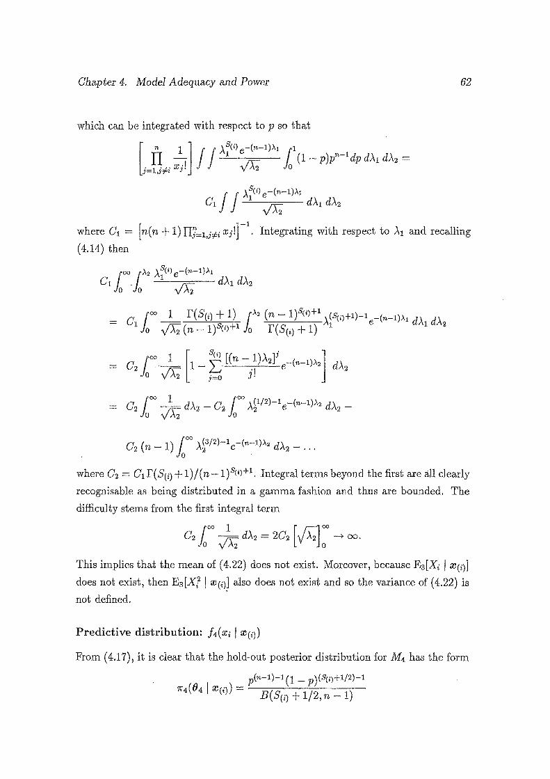
Chapter 4. Model Adequacy and Power 62
which can be integrated with respect to p so that
J J A:(i) e-(n-1).\1
o1 VA; dA1 dA2
where 01 = [n(n + 1) Tij=l,#i Xj!r1. Integrating with respect to At and recalling
(4.14) then
02 ( n 1) loco )..~3/2)-1 e-(n-1).\2 d)..2 - ...
where 02 = 01 r( S(i) 1) I ( n -l)s(i)+l, Integral terms beyond the first are all clearly
recognisable as being distributed in a gamma fashion and thus are bounded. The
difficulty stems from the first integral term
02 fooo )x; d)..2 = 202 [ ~] ~ -+ 00.
This implies that the mean of (4.22) does not exist. Moreover, because E3 [Xi I X(i)]
does not exist, then E3[Xfl X(i)) also does not exist and so the variance of (4.22) is
not defined.
Predictive distribution: h(xi I X(i))
From ( 4.17), it is clear that the hold-out posterior distribution for M4 has the form
p(n-1)-1(1 _ p)(S(i)+l/2)-1
?r4 (64 I X(i)) = B(S(i) + 1/2, n 1)
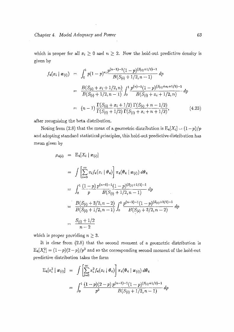
Chapter 4. Model Adequacy and Power 63
which is proper for all Xi ~ 0 and n 2. Now the hold-out predictive density is
given by
= B(S(i) +Xi+ 1/2, n) flp(n)-1(1- p)(Su)+x;+l/2)-1 d
B(S(i) 1/2, n- 1) Jo B(S(i) +Xi+ 1/2, n) p
= (n 1) r(S(i) +Xi+ 1/2) r(S(i) + n- 1/2) f(S(i) + 1/2) f(S(i) Xi+ n + 1/2)'
( 4.23)
after recogn-ising the beta distribution.
Noting from (2.8) that the mean of a geometric distribution is E4[Xi] = (1 p)jp
and adopting standard statistical principles, this hold-out predictive distribution has
mean given by
j [~ Xi}4(xi l84)]1r4(84 I X(i)) d04
lal (1 _ p) p(n-1)-1(1 _ p)(S(i)+l/2)-1
..:......___;_ --::::--;-:::-'---"-;'-----;- dp o p B(S(i)+1/2,n-1)
B(S(i) + 3/2, n _ 2) {1 p(n-2)__:1(1 _ p)(s(i)+3/2)-1 dp
B(S(i) + 1/2, n - 1) lo B(S(i) + 3/2, n- 2)
sci>+ 1/2 n-2
which is proper providing n ~ 3.
It is clear from (2.8) that the second moment of a geometric distribution is
E4[X1] = (1 p)(2 p)jp2 and so the corresponding second moment of the hold-out
predictive distribution takes the form
E4[xll X(i)] = j [~xff4(xi l84)]1r4(84l re(i)) d84
{
0
1 (1 p)(2 _ p) p(n-1)-1(1 p)(S(i)+l/2)-1
Jo p2 B(S(i) + 1/2, n- 1) dp
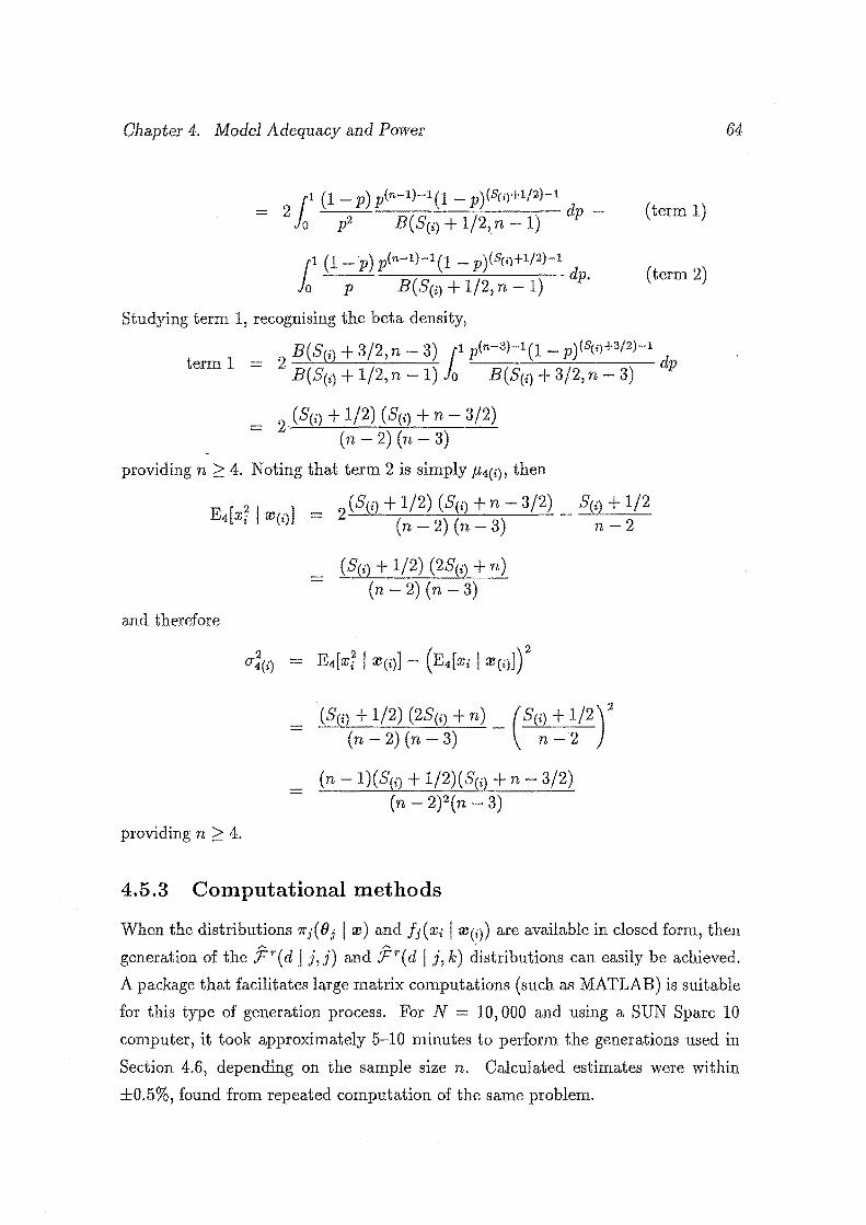
Chapter 4. Model Adequacy and Power
11 (1 _ p) p(n-1)-1(1 _ p)(S(i)+l/2)-1
2 dp-o p2 B(S(i) + 1/2,n 1)
(term 1)
{1 (1 _ ·p) p(n-1)-1(1 _ p)(S(i)+l/2)-1
Jo p B(S(i) + 1/2, n- 1) dp. (term 2)
Studying term 1, recognising the beta density,
2 B(S(i) + 3/2, n- 3) lol p(n-3)-1(1- p)(s(i)+3/2)-1 dp
term 1 = B(S(i) + 1/2, n- 1) o B(S(i) + 3/2, n 3)
n- 3/2) 3)
providing n 2 4. Noting that term 2 is simply ~t4(i), then
n- 3/2) 3)
and therefore
sci) + 1/2 n-2
(S(i) + 1/2) (2S(i) + n) _ (S(i) + 1/2)2
(n 2) (n- 3) n 2
(n -l)(S(i) 1/2)(S(i) + n- 3/2) (n 2)2(n- 3)
providing n 4.
4.5.3 Computational methods
64
When the distributions 'lf'j(Oj Ire) and ]j(xi I ID(i)) are available in closed form, then
generation of the J"r(d J j,j) and !ftr(d I j, k) distributions can easily be achieved.
A package that facilitates large matrix computations (such as MATLAB) is suitable
for this type of generation process. For N = 10,000 and using a SUN Spare 10
computer, it took approximately 5-10 minutes to perform the generations used in
Section 4.6, depending on the sample size n. Calculated estimates were within
±0.5%, found from repeated computation of the same problem.
Chapter 4. Model Adequacy and Power 65
When neither 7rj(8j I ::v) nor fi(xi I ::V(i)) are available in closed form, then nu~
merical approximations are necessary. While conceptually the process of obtaining
the adequacy distributions remains straightforward, the disadvantage is that con
siderably more computer resources are required. Specifically, the difficulty arises
when multiple determinations of fj(Xi I ::V(i)), f.lj(i) and o}(i) are required over i for
each of the N generated samples. It might be tempting to approximate the hold~out
predictive density function by fi(xi I ::v), reducing the numerical integral evalua
tions. However, Gelfand, Dey and Chang (1992) claim that this should be avoided,
as fi(xi I ::v) may be quite different from fi(xi I ::V(i)), even when Xi's are assumed
to be conditionally independent.
In this thesis, acquisition of (}~ values from 7rj(8j I ::v) was easily made using
the sample-resample method of Smith and Gelfand (1992). For the determination
of integrals relating to h(xi I ::V(i)), the trapezoidal rule was readily and accu
rately applied, while the sample-mean Monte Carlo method (Rubinstein, 1981) was
adopted to approximate fa(xi I ::V(i)), P,3 (i), rr5(i) and related integrations. This
sample-mean Monte Carlo integration technique allows an approximation to the de
sired 3-dimensional integrals to be computed within a feasible time frame, provided
a facility exists where large matrix manipulations can easily be handled (such as
in MATLAB). The parameter space bound used when adopting the sample-mean
Monte Carlo method was 0 < ,\1 < ,\2 < 100. In the accident analysis context, it is
considered unlikely that driver factors or vehicle and environmental factors would
have an annual underlying accident rate exceeding ten, so it could be construed that
the upper bound of 100 on the ,\2 parameter space is conservative.
Simulations of size N = 2, 500 were used when these integral approximation
methods were employed in Section 4.6. Computations occupied a SUN Spare 10
computer for approximately 1-3 hours, depending on the sample size n. Calculated
estimates were almost invariably within ±2%, again found from repeated calculation
of the same problem.
4.5.4 Mean and variance adjustments
From the mathematical details provided in Section 4.5.2, it was evident that the
hold-out predictive distribution h(xi I ::V(i)) has mean and variance that tends to
infinity for unbounded .-\2 while h(xi I ::V(i)) has an undefined variance when a S
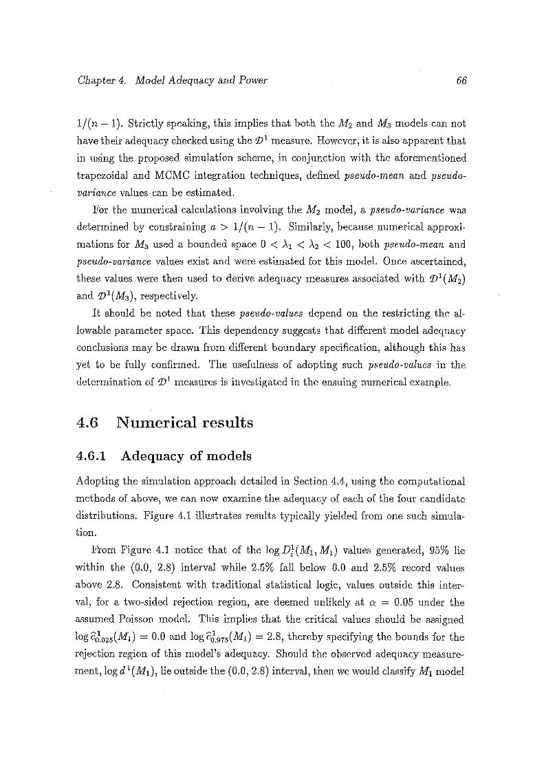
Chapter 4. Model Adequacy and Power 66
1/(n -1). Strictly speaking, this implies that both the M 2 and M3 models can not
have their adequacy checked using the :JJ1 measure. However, it is also apparent that
in using the proposed simulation scheme, in conjunction with the aforementioned
trapezoidal and MCMC integration techniques, defined pseudo-mean and pseudo
variance values can be estimated.
For the numerical calculations involving the M2 model, a pseudo-variance was
determined by constraining a > 1/(n- 1). Similarly, because numerical approxi
mations for M3 used a bounded space 0 < ..\1 < ..\2 < 100, both pseudo-mean and
pseudo-variance values exist and were estimated for this model. Once ascertained,
these values_ were then used to derive adequacy measures associated with :JJ1 (M2)
and :JJ1(M3), respectively.
It should be noted that these pseudo-values depend on the restricting the al
lowable parameter space. This dependency suggests that different model adequacy
conclusions may be drawn from different boundary specification, although this has
yet to be fully confirmed. The usefulness of adopting such pseudo-values in the
determination of :!J1 measures is investigated in the ensuing numerical example.
4.6 Numerical results
4.6.1 Adequacy of models
Adopting the simulation approach detailed in Section 4.4, using the computational
methods of above, we can now examine the adequacy of each of the four candidate
distributions. Figure 4.1 illustrates results typically yielded from one such simula
tion.
From Figure 4.1 notice that of the log D}(M1 , M 1) values generated, 95% lie
within the (0.0, 2.8) interval while 2.5% fall below 0.0 and 2.5% record values
above 2.8. Consistent with traditional statistical logic, values outside this inter
val, for a two-sided rejection region, are deemed unlikely at a = 0.05 under the
assumed Poisson model. This implies that the critical values should be assigned
log cl_025 (MI) = 0.0 and log cl,975(M1) = 2.8, thereby specifying the bounds for the
rejection region of this model's adequacy. Should the observed adequacy measure
ment, log d1(M1 ), lie outside the (0.0, 2.8) interval, then we would classify M1 model
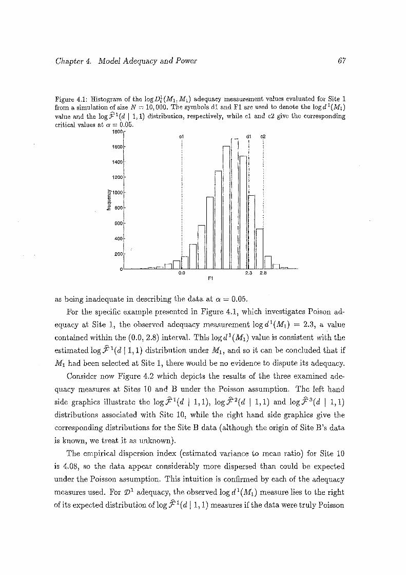
Chapter 4. Model Adequacy and Power 67
Figure 4.1: Histogram of the logDf(M1, M1) adequacy measurement values evaluated for Site 1 from a simulation of size N = 10,000. The symbols dl and F1 are used to denote the log d 1(M1) value and the log f 1 ( d I 1, 1) distribution, respectively, while c1 and c2 give the corresponding critical values at a = 0.05.
1800 c2
1600
1400
1200
(;'1000 c: Ql ::> 0"
& 800
600
400
200
0 2.3 2.8
F1
as being inadequate in describing the data at a= 0.05.
For the specific example presented in Figure 4.1, which investigates Poison ad
equacy at Site 1, the observed adequacy measurement log d 1(M1) = 2.3, a value
contained within the (0.0, 2.8) interval. This logd 1(M1) value is consistent with the
estimatedlogF 1(d 11,1) distribution under M1 , and so it can be concluded that if
M1 had been selected at Site 1, there would be no evidence to dispute its adequacy.
Consider now Figure 4.2 which depicts the results of the three examined ade
quacy measures at Sites 10 and B under the Poisson assumption. The left hand
side graphics illustrate the logF1 (d I 1, 1), logF 2(d I 1, 1) and logF 3 (d I 1, 1)
distributions associated with Site 10, while the right hand side graphics give the
corresponding distributions for the Site B data (although the origin of Site B 's data
is known, we treat it as unknown).
The empirical dispersion index (estimated variance to mean ratio) for Site 10
is 4.08, so the data appear considerably more dispersed than could be expected
under the Poisson assumption. This intuition is confirmed by each of the adequacy
measures used. For IJJ1 adequacy, the observed log d 1 ( M1 ) measure lies to the right
of its expected distribution of log F 1 ( d 11, 1) measures if the data were truly Poisson
Chapter 4. Model Adequacy and Power 68
Figure 4.2: Distributions of the three adequacy measures under the Poisson model at Sites 10 and B, computed from simulatio~ of size N 10,000. The symbols dr and Fr are used to denote logdr(M1) values and log.Fr(d 11,1) distributions, respectively, while c, cl and c2 give the corresponding critical values at a = 0.05.
cJ c? d1 d1
....; ....; "0 "0 0.0.5 0.0.5
0 1.8 3.4 4.3
0 1.4 2.3 3.6
Site 10: F1 SlteB: F1 0.15 d2 0.15
....; 0.1 ....; 0.1 -q -q c.
0.0.05 0.05
0 -39.8 -32.9
0 -46.3 -33.0
Site 10: F2 Site B: F2
....; ...: ~0.5 ~0.5
0 0 -1.7 -1.8
Site 10: F3 Site B: F3
distributed. Similarly, log d 2(M1 ) lies to the left and log d3 (M1 ) to the right of their
associated expected distributions under the Poisson assumption. Using any of these
measures, we would deem M1 (Poisson) as being inadequate at describing Site 10
data at a = 0.05.
Site B recorded an empirical dispersion index of 0.21 which, in this instance, sug
gested that the data were more under-dispersed than anticipated from the Poisson
assumption. This suggestion is substantiated by each of the three adequacy mea
sures rejecting the Poisson assumption at a = 0.05. For this scenario, log d1(Mt)
and log d2(M1 ) values lie on the opposite side of their associated expected distribu
tions to that when Site 10 was investigated, while log d3(M1 ) again lies to the right.
This diagrammatically verifies the two-sided nature of the :D1 and :D2 adequacy
measure test and the one-sided nature of :D3 •
Tables C.l-0.4 included in Appendix C summarise the adequacy analyses under
taken on each of the four candidate models at the 35 accident sites using adequacy
measures vr, r l, 2, 3. In practice, it is envisaged that only those models gener
ally discriminated as best, and thus with the potential of being selected, will have
their adequacy checked. However, for the purpose of illustration and investigation
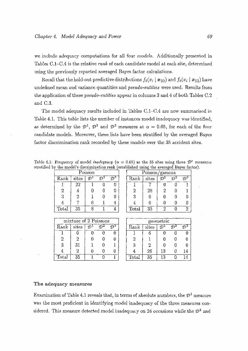
Chapter 4. Model Adequacy and Power 69
we include adequacy computations for all four models. Additionally presented in
Tables C.1-C.4 is the relative rank of each candidate model at each site, determined
using the previously reported averaged Bayes factor calculations.
Recall that the hold-out predictive distributions h(xi I ID(i)) and h(xi I ill(i)) have
undefined mean and variance quantities and pseudo-entities were used. Results from
the application of these pseudo-entities appear in columns 3 and 4 of both Tables C.2
and C.3.
The model adequacy results included in Tables C.l-0.4 are now summarised in
Table 4.1. This table lists the number of instances model inadequacy was identified,
as determil}ed by the 'D1, 'D2 and 'D3 measures at a = 0.05, for each of the four
candidate models. Moreover, these lists have been stratified by the averaged Bayes
factor discrimination rank recorded by these models over the 35 accident sites.
Table 4.1: Frequency of model inadequacy (a = 0.05) at the 35 sites using three 'Dr measures stratified by the model's discrimination rank (established using the averaged Bayes factor).
Poisson Poisson/ gamma Rank sites 'Dl 'D2 'D3 Rank sites 'Dl 'D2 'D3
1 22 1 0 0 1 7 0 0 1 2 4 0 0 0 2 28 2 0 1 3 2 1 0 0 3 0 0 0 0 4 7 6 1 4 4 0 0 0 0
Total 35 8 1 4 Total 35 2 0 2
mixture of 2 Poissons geometric Rank sites 'Dl 'D'}, 'D0 Rank sites 'Dl 'D2 'D3
1 0 0 0 0 1 6 0 0 0 2 2 0 0 0 2 1 0 0 0 3 31 1 0 1 3 2 0 0 0 4 2 0 0 0 4 26 13 0 14
Total 35 1 0 1 Total 35 13 0 14
The adequacy measures
Examination of Table 4.1 reveals that, in terms of absolute numbers, the 'D1 measure
was the most proficient in identifying model inadequacy of the three measures con
sidered. This measure detected model inadequacy ori 24 occasions while the 'D2 and
Chapter 4. Model Adequacy and Power 70
'D 3 identified inadequacy in one and 21 instances, respectively. However, aside from
Poisson model adequacy considerations, the 'D3 measure was seen to identify model
inadequacy with a similar degree of proficiency as that demonstrated by the 'D 1
measure. By comparison, the 'D 2 measure discerned model inadequacy infrequently
and with the least success.
This phenomenon featured most prominently in Table 4.1 when geometric ad
equacy was considered. While both the 'D1 and 'D3 measures consistently rejected
the adequacy of the geometric model (in 37% and 40%, respectively, of the 35 in
stances considered), the 'D 2 adequacy measure was unable to demonstrate once that
this model was incompatible with the data. This result can be explained by a de
ficiency inherent in this measure, as a measure of goodness-of-fit, for this type of
data; further explanation will follow in Section 4.6.3.
The consistency between adequacy measures in determining model inadequacy
can be assessed by referring to Tables 0.1-0.4. It is evident from perusal of these
tables that the instance where model inadequacy was identified by the 'D 2 measure,
both the 'D1 and 'D3 measures also demonstrated inadequacy. Moreover, model
inadequacy was identified by the 'D3 measure on 21 occasions, and of these 17 (81 %) were also identified by the 'D1 measure.
These results demonstrated that model inadequacy was identified with some
degree of consistency between the three examined adequacy measures, particularly
between the 'D1 and 'D3 measures. However, as these measures investigate different
characteristics of the assumed model, some differences in the identification of model
inadequacy naturally existed.
Model performance
A distinguishing feature of Table 4.1 was the relatively high number of sites at
which the Poisson model was found to be inadequate. Based upon the 'D1 ade
quacy measurement calculations,· model inconsistency with the empirical data was
demonstrated at eight (23%) sites. Identification of Poisson inadequacy was not as
frequent with the adoption of the 'D 2 and 'D3 measures; with one (3%) and four sites
(11%), respectively, meeting the rejection criterion.
Another noteworthy feature of this investigation was the identification of M1
model inadequacy by the 'D1 measure at Site 6, a site where the Poisson model had
Chapter 4. Model Adequacy and Power 71
previously been discriminated as being the best model. Examination of the data
at Site 6 revealed a high degree of under-dispersion, with the estimated dispersion
index equalling 0.453. Not surprisingly, none of the considered candidate models
were adjudged as adequately describing this under-dispersed data by this measure.
Sites modelled by the Poisson/ gamma model were identified as being inadequate
in only two (6%) instances by both the '1J 1 and '1J3 measures. The ability of the
Poisson/ gamma to model over-dispersion thus ensured that it was identified as being
adequate with considerably greater frequency than the Poisson model.
One unanticipated result occurred at Site 9 (see Tables C.l-0.4). At this site,
the Poisson/ gamma model was ranked as being the best, yet according to the '1J3
measure, this model was inadequate. The Poisson model, ranked fourth, was also
deemed to be inadequate. Examination of the data revealed over-dispersion (with
an estimated dispersion index equalling 1. 75), thus it was not surprising that the
Poisson model was inconsistent with this empirical data. However, both the mixture
. of two Poissons (ranked second) and geometric (ranked third) models were adjudged
as being adequate. It seems, therefore, that the Occam's razor1 (Starfield, Smith and
Bleloch, 1990, Jefferys and Berger, 1992) inherently contained within the averaged
Bayes factor technique favoured model parsimony over data consistency for those
accidents recorded at Site 9.
Evidence indicating inadequacy of the mixture of two Poisson densities model
was relatively rare. Indeed, both the '1J1 and V3 measures designated only one site
ofthe 35 as being inadequate, the under-dispersed Site 6. In this instance, model
M3 was ranked third by the averaged Bayes factor, the position this model generally
held, and thus this inadequacy is of no great consequence.
On each of the nine occasions that the geometric model rose above the fourth
rank, it was never found to be inadequate by any of the three adequacy measures
implemented. Nonetheless, the general applicability of this model must be treated
with suspicion as it recorded the fourth and worst rank on 26 (74%) occasions and
was demonstrated to be inadequate at 13 (37%) and 14 (40%) sites by the V 1 and
V 3 adequacy measures, respectively.
1 Named after a fourteenth century English philosopher William of Occam (or Ockham) who propounded a heuristic in Latin "Non sunt multiplicanda entia praeter necessitatem". Translated literally, this means "Things should not be multiplied without good reason", but in the context of model discrimination it means that if two models explain data equally well, the simpler should be preferred.
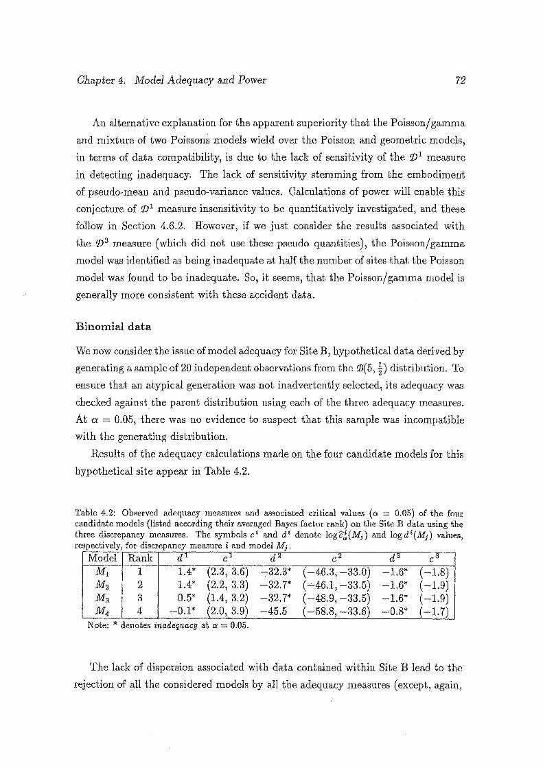
Chapter 4. Model Adequacy a.nd Power 72
An alternative explanation for the apparent superiority that the Poisson/ gamma
and mixture of two Poissons models wield over the Poisson and geometric models,
in terms of data compatibility, is due to the lack of sensitivity of the tJJ 1 measure
in detecting inadequacy. The lack of sensitivity stemming from the embodiment
of pseudo-mean and pseudo-variance values. Calculations of power will enable this
conjecture of tJJ1 measure insensitivity to be quantitatively investigated, and these
follow in Section 4.6.2. However, if we just consider the results associated with
the tJJ 3 measure (which did not use these pseudo quantities), the Poisson/gamma
model was identified as being .inadequate at half the number of sites that the Poisson
model was found to be inadequate. So, it seems, that the Poisson/gamma model is
generally more consistent with these accident data.
Binomial data
We now consider the issue of model adequacy for Site B, hypothetical data derived by
generating a sample of 20 independent observations from the 'B(5, k) distribution. To
ensure that an atypical generation was not inadvertently selected, its adequacy was
checked against the parent distribution using each of the three adequacy measures.
At a 0.05, there was no evidence to suspect that this sample was incompatible
with the generating distribution.
Results of the adequacy calculations made on the four candidate models for this
hypothetical site appear in Table 4.2.
Table 4.2: Observed adequacy measures and associated critical values (a = 0.05) of the four candidate models (listed according their averaged Bayes factor rank) on the Site B data using the three discrepancy measures. The symbols ci and di denote logc~(MJ) and logdi(MJ) values, respectively, for discrepancy measure i and model Mj.
Model Rank dl cl d2 c2 d3 c3
Mt 1 1.4* (2.3, 3.6) ~32.3* ( -46.3, -33.0) -1.6* ( -1.8) M2 2 1.4* (2.2, 3.3) -32.7* ( -'-46.1, -33.5) -1.6* (-1.9) M3 3 0.5* (1.4, 3.2) -32.7* ( -48.9, -33.5) -1.6* ( -1.9) M4 4 -0.1* (2.0, 3.9) -45.5 ( -58.8, -33.6) -0.8* ( -1.7)
Note: * denotes inadequacy at a= 0.05.
The lack of dispersion associated with data contained within Site B lead to the
rejection of all the considered models by all the adequacy measures (except, again,
Chapter 4. Model Adequacy and Power 73
when using the '1J 2 adequacy measure on the M4 geometric model). This result is
certainly reassuring as we were privileged in knowing that the data actually arose
from an under-dispersed binomial distribution.
Analysis of this site, coupled with the results obtained from investigation of
Site 6 data, forcefully demonstrates the need for adequacy considerations to be
made before discriminated models are employed for analysis. At both Sites 6 and B
the Poisson density was assessed as being the most preferred model, yet further
exploration revealed that this model was, in actuality, quite inconsistent from the
data it was suppose to represent. Bayesian model selection techniques make no
explicit statement of the discriminated model's goodness-of-fit with the empirical
data.
4.6.2 · . Power of detecting model inadequacy
It was evident from the preceding section that the ability of identifying model in
adequacy was not the same for each of the measures considered. Moreover, as the
data collection periods were of widely different lengths, it could be surmised that the
ability of any given '!Jr measure in detecting model inadequacy might vary across
sites. This motivated an investigation into detecting the power of finding model
inadequacy when the model was indeed false.
An assessment of power was achieved by investigating the likelihood that a par
ticular selected model was deemed inadequate when an alternative model, itself
generally compatible with the observed data w, was taken as the actual underlying
distribution. All assessments of power made within this thesis were based upon
a= 0.05.
Figure 4.3 illustrates a typical simulation scenario computing P1 (M1 , M4 ), the
power of identifying Poisson model inadequacy when the underlying distribution was
geometric (top graph), and P1(M4 , M1 ), the power of identifying geometric model
inadequacy when the underlying distribution was Poisson (bottom graph). Both
these illustrated power computations were derived using adequacy measure 'IJ1 on
Site 1 data. The shaded region gives the region of rejection based on a= 0.05 and
hence power. For these scenarios, if the data were truly generated by the geometric
distribution, we would reject the Poisson assumption 71% of the time; while, if the
underlying function was Poisson, then in 56% of instances the geometric adequacy
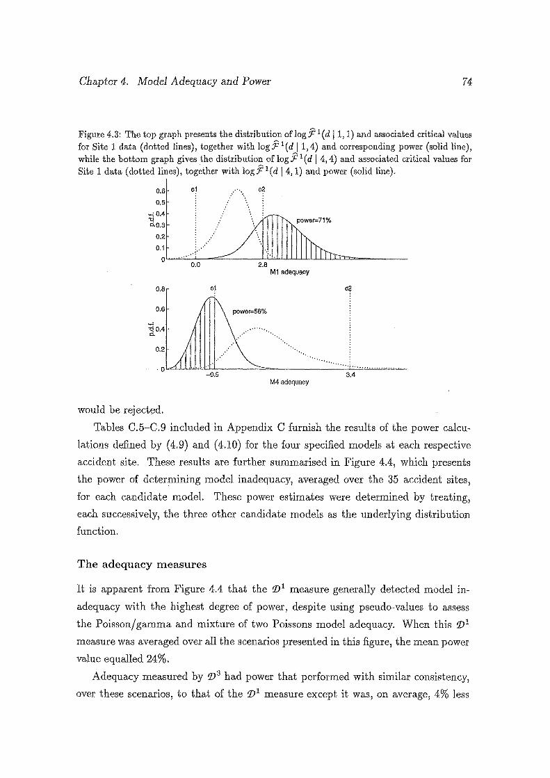
Chapter 4. Model Adequacy and Power 74
Figure 4.3: The top graph presents the distribution of log !F 1(d jl, 1) and associated critical values for Site 1 data (dotted lines), together with log!F 1 (d j1,4) and corresponding power (solid line), while the bottom graph gives the distribution oflog!F 1(d 14,4) and associated critical values for Site 1 data (dotted lines), tog~ther with log!F 1(d j4, 1) and power (solid line).
0.6
0.5
....; 0.4 '"q 0..0,3
0.2
c1 ... c2
. . power=71%
O.i .... :····· 0~~~--~------~~~~LW~~~===-------
0.0
0.8 o1
0.6
~0.4 c..
0.2
·0 -0.5
would be rejected.
2.8 M1 adequacy
'•,
M4 adequacy
... .... ····· .. ········ '"" ..
3.4
Tables C.5-C.9 included in Appendix C furnish the results of the power calcu
lations defined by (4.9) and (4.10) for the four specified models at each respective
accident site. These results are further summarised in Figure 4.4, which presents
the power of determining model inadequacy, averaged over the 35 accident sites,
for each candidate model. These power estimates were determined by treating,
each successively, the three other candidate models as the underlying distribution
function.
The adequacy measures
It is apparent from Figure 4.4 that the tJJ1 measure generally detected model in
adequacy with the highest degree of power, despite using pseudo-values to assess
the Poisson/ gamma and mixture of two Poissons model adequacy. When this '1) 1
measure was averaged over all the scenarios presented in this figure, the mean power
value equalled 24%.
Adequacy measured by tJJ3 had power that performed with similar consistency,
over these scenarios, to that of the '1J1 measure except it was, on average, 4% less
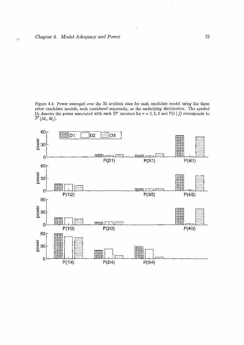
Chapter 4. Model Adequacy and Power 75
Figure 4.4: Power averaged over the 35 accident sites for each candidate model using the three other candidate models, each considered separately, as the underlying distribution. The symbol Dr denotes the power associated with each tjy measure for r = 1, 2, 3 and P(i I j) corresponds to
.... Q)
(M;,Mj)·
60
~ 30 c.
o~.----------------~~~=w~~---U~u=~~~--~~~~~~-
P(211}
.... Q)
60
~30 c.
P(311) P(411)
o~~~U-~~~------------------~~-L~--L---~~~=W--J_
P(112) P(312) P(412) 60
.... Q)
~30 c.
OL--U~W-~L-~--~~~~U-~------------------~~~=L~J_
.... Q)
60
~30 0..
P{113)
P(114)
P(213) P(413)
P(214) P(314)
Chapter 4. Model Adequacy and Power 76
powerful.
Consistency, however, was lacking from the rJJ 2 measures. In one averaged power
comparison presented in Figure 4.4, the rJJ 2 measure had power that out performed
that associated with either rJJ 1 or rJJ3 measures and on a further eight occasions,
its averaged power was only slightly below the most powerful measure. In contrast,
the remaining three comparisons revealed that rJJ 2 identified model inadequacy with
exceptionally poor power (frequently 0% or thereabouts). The rJJ1 and rJJ3 measures,
by comparison, detected model inadequacy for these comparisons with considerable
success. This feature resulted in the averaged power across all scenarios for the rJJ 2
equalling 13%, some 11% below that recorded by the qj1 measure.
It is evident that in the three instances the rJJ 2 measure performed poorly, each
measured geometric model inadequacy. The reasoning behind this apparent pecu
liarity is explained in Section 4.6.3.
Model performance
The power of detecting model inadequacy for each of the entertained candidate
models, using data known to have arisen from some other underlying alternative
distribution, is now examined.
From the bar-graph depiction in Figure 4.4 it is clear that when data were gen
erated from the geometric model and Poisson adequacy was monitored (denoted by
P(l I 4) in this figure), all three measures rejected the applicability of the Poisson
model with high power ( F:::J 60%). Almost equally powerful was the rejection, by the
rJJ 1 and rJJ3 measures, of geometric adequacy when the underlying distribution was
Poisson (represented by P ( 4 11) in Figure 4.4). In fact, both the rJJ 1 and rJJ3 mea
sures detected geometric inadequacy with high degrees of power for data generated
from all three alternative candidate models entertained: Poisson; Poisson/ gamma;
and the mixture of two Poissons (represented by P(4 11), P(41 2), and P(41 3) in
Figure 4.4, respectively).
None of the reported measures yielded power of any substance when investigating
Poisson/ gamma or mixture of two Poisson inadequacy from Poisson, Poisson/ gamma
and the mixture of two Poissons underlying models. In these scenarios the resultant
power .was typically around 5%, the a level. Poisson model inadequacy under either
the Poisson/gamma (given by P(1 I 2)) or the mixture of two Poissons (given by
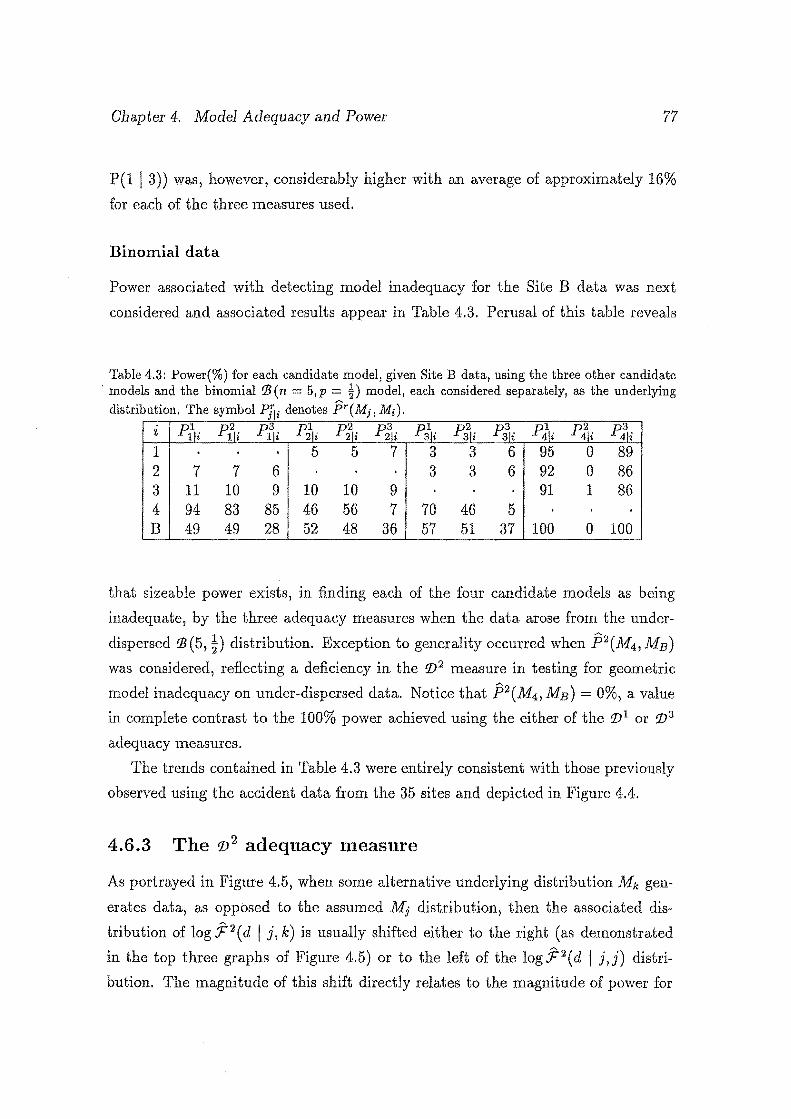
Chapter 4. Model Adequacy and Power 77
P(1 I 3)) was, however, considerably higher with an average of approximately 16%
for each of the three measures used.
Binomial data
Power associated with detecting model inadequacy for the Site B data was next
considered and associated results appear in Table 4.3. Perusal of this table reveals
Table 4.3: Power(%) for each candidate model, given Site B data, using the three other candidate · models and the binomial tJ3(n = 5,p = ~)model, each considered separately, as the underlying
distribution. The symbol PJ11 denotes f'r(MJ, Mi)·
z Plli p~i Pfli p21li p~i Plli PJ-Ii Pffli P3\: PJii p~i Pfli
1 . 5 5 7 3 3 6 95 0 89 2 7 7 6 3 3 6 92 0 86 3 11 10 9 10 10 9 . 91 1 86 4 94 83 85 46 56 7 70 46 5 B 49 49 28 52 48 36 57 51 37 100 0 100
that sizeable power exists, in finding each of the four candidate models as being
inadequate, by the three adequacy measures when the data arose from the under
dispersed tJ3(5, ~)distribution. Exception to generality occurred when P2(M4 ,MB)
was considered, reflecting a deficiency in the tJJ 2 measure in testing for geometric
model inadequacy on under-dispersed data. Notice that P2 (M4 ,MB) = 0%, a value
in complete contrast to the 100% power achieved using the either of the tJJ1 or tJJ 3
adequacy measures.
The trends contained in Table 4.3 were entirely consistent with those previously
observed using the accident data from the 35 sites and depicted in Figure 4.4.
4.6.3 The ']) 2 adequacy measure
As portrayed in Figure 4.5, when some alternative underlying distribution Mk gen
erates data, as opposed to the assumed Mj distribution, then the associated dis
tribution of log J' 2 ( d I j, k) is usually shifted either to the right (as demonstrated
in the top three graphs of Figure 4.5) or to the left of the log F 2 ( d I j, j) distri
bution. The magnitude of this shift directly relates to the magnitude of power for
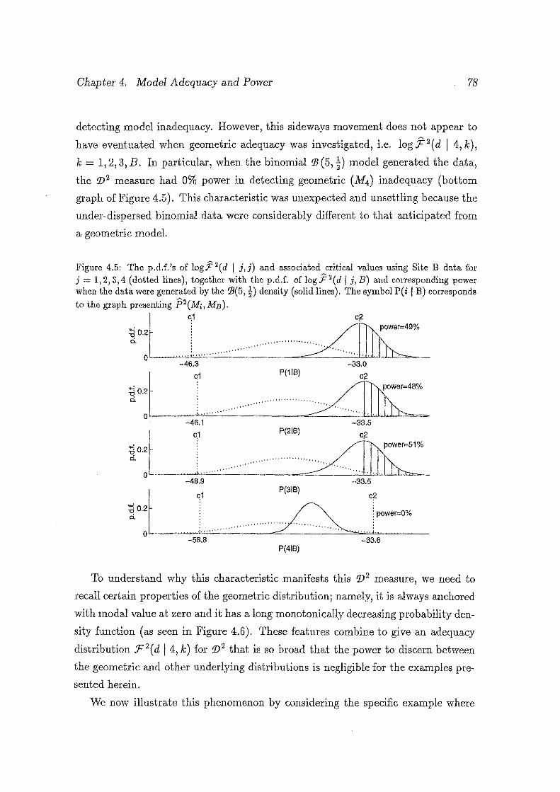
Chapter 4. Model Adequacy and Power 78
detecting model inadequacy. However, this sideways movement does not appear to
have eventuated when geometric adequacy was investigated, i.e. log F 2(d I 4, k),
k = 1,2,3,B. In particular, when the binomial ~(5, t) model generated the data,
the tJJ 2 measure had 0% power in detecting geometric ( M4 ) inadequacy (bottom
graph of Figure 4.5). This characteristic was unexpected and unsettling because the
under-dispersed binomial data were considerably different to that anticipated from
a geometric model.
Figure 4.5: The p.d.f.'s of logF 2(d I j,j) and associated critical values using Site B data for j = 1,2,3,4 (dotted lines), together with the p.d.f. oflogF 2(d I j,B) and corresponding power when the data were generated by the ~(5, ~)density (solid lines). The symbol P(i I B) corresponds to the graph presenting P2(Mi, MB)·
~,:l .... I ........... ·························~% -46.3 -33.0
~ 0 :l.__~~,..,..J'-'-' .. -'-. ·-· ._ ... _. ·_· ·_· ·_··_·· ·_· ._ .. _· ._ .. _P_I'._'"_I""'·LJJJh::::::::.· .. _. ·_· ·_· _· ·_· .. _. ·_· ·_,o?c..:." ,_,_,. "'-'J...po...t..w..J-er-<=:::::.48=o/c""'"-o
-46.1 -33.5
~ O:l'----~~"""'1"'-' .. _:_:.··-"-···_··_··_··_··_···_··_··_··_"_P(_'_'"_J~="=="·_ .. _··_··_···_··_··_ .. ...:.J.~:...:..··~ ....... J....po.J...w...Le...J:r=:::.51~o/c-o -48.9 -33.5
~ 0 :~......l_~~ .. ,_, .. '""'f:.:..· ":.,_"_ .. _· ._ .. _ .. ·_· ·_· ._ .. _ ... _ .. -==~:::..P_('_'"_.~ .. _ .. _· ._ .. _ .. _·. _ ... _. ~";..:.." ""''""'J'"""~o~w~e-r=_oo_Yo_ -58.8 -33.6
P(41B)
To understand why this characteristic manifests this tJJ 2 measure, we need to
recall certain properties of the geometric distribution; namely, it is always anchored
with modal value at zero and it has a long monotonically decreasing probability den
sity function (as seen in Figure 4.6). These features combine to give an adequacy
distribution :F 2 ( d I 4, k) for tJJ 2 that is so broad that the power to discern between
the geometric and other underlying distributions is negligible for the examples pre
sented herein.
We now illustrate this phenomenon by considering the specific example where
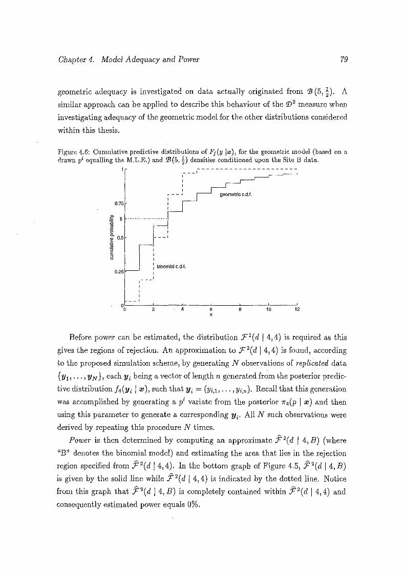
Chapter 4. Model Adequacy and Power 79
geometric adequacy is investigated on data actually originated from :B (5, ~). A
similar approach can be applied to describe this behaviour of the tJJ 2 measure when
investigating adequacy of the geometric model for the other distributions considered
within this thesis.
Figure 4.6: Cumulative predictive distributions of Fj (y Ire), for the geometric model (based on a drawn pi equalling the M.L.E.) and :B(5, t) densities conditioned upon the Site B data.
0.76
1 I
I
--_I I I I I
r---..>
: binomial c.d.f. I I
2 4 6 X
8 10 12
Before power can be estimated, the distribution :F 2 ( d I 4, 4) is required as this
gives the regions of rejection. An approximation to :F 2 (d j4,4) is found, according
to the proposed simulation scheme, by generating N observations of replicated data
{Yu ... , YN }, each Yi being a vector of length n generated from the posterior predic
tive distribution f4(Yi I ro ), such that Yi = (Yi,l, ... , Yi,n)· Recall that this generation
was accomplished by generating a pi variate from the posterior 7r4(p I ro) and then
using this parameter to generate a corresponding Yi· All N such observations were
derived by repeating this procedure N times.
Power is then determined by computing an approximate f 2(d I 4,B) (where
"B" denotes the binomial model) and estimating the area that lies in the rejection
region specified from F 2 (d 14,4). In the bottom graph of Figure 4.5, J 2 (d I4,B)
is given by the solid line while F2(d I 4,4) is indicated by the dotted line. Notice
from this graph that f 2(d I4,B) is completely contained within J 2(d 14,4) and
consequently estimated power equals 0%.
Chapter 4. Model Adequacy and Power 80
We now show that a model (denoted by B) which generates replicate data Yi
of length n that is geometric from model M4 (specified by pi) except for the first
data point Yi,1 , which is generated from :B (5, !), yields an adequacy distribution
F 2(d j4,B) generally contained within F 2(d j4,4). Because this F 2(d I4,B) has
only one binomial value in each n vector of Yi and is generally contained within
F 2(d I 4,4), it follows that F 2 (d I 4,B) composed of entirely binomial data must
also be contained within F 2 (d 14,4).
We take, for convenience, Yi,l as being the binomial or geometric generated data
corresponding toMB and M4, respectively, (although any term of then vector could
have been chosen).
Suppose that all replicated data are acquired using the inverse generating method2
(Pidd, 1986) derived from some common randomly generated ('u" vector, u = ( Ui,1, ..• , Ui,n), then the following relationships hold. If ti denotes the value where
the c. d. f.'s for both the geometric (specified by pi) and binomial predictive densities
·· intersect (see Figure 4.6) then, from the adoption of the inverse generating method,
Ui,l > ti implies the generated geometric data point is greater than or equal to the
generated binomial data point. Because of the monotonically decreasing probability
density function associated with the geometric model, this implies, in general, that
Dl(M4, M4) Dt(M4, MtJ) and thus the right hand tail of F 2(d j4, B) is shifted to
the left of f: 2 ( d I 4, 4). Similarly, when Ui,l :::; ti, then the generated geometric data
point is smaller than or equal to the generated binomial data point. This implies,
in general, that D[(M4 , M4);::: Dt(M4,MfJ) and so the left hand tail of F2(d 14, B) is shifted to the right of F2
( d I 4, 4).
These features combine to give a distribution F 2 (d I 4, B) generally contained
within F2(d !4,4). Because B has only one binomial data point in each Yi and has
corresponding adequacy distribution contained within F2(d I 4,4), it follows that
replicate data generated entirely from the binomial distribution would also yield an
adequacy distribution contained within f: 2 ( d I 4, 4).
2Briefly this technique can be described as follows. Suppose F(x), a known c.d.f., is randomly assigned a value u, a random variable uniformly distributed on the [0, 1] interval, then any value of u may be transformed into a value x by inverting the c.d.f. and solving for x. Algebraically, if
u:::: F(x) = iw f(t) dt . then a:= G(u),
where G(u) is the inverse cumulative function.
Chapter 5
Ranking and selection
5.1 Specification of an appropriate model
It was evident, from Table 4.1, that of the four candidate models investigated over
the 35 intersection accident sites, the mixture of two Poisson densities was generally
the most adequate at a = 0.05. It was also apparent that this model was demon
strated as having slightly fewer identifications of model inadequacy to that of the
Poisson/ gamma model. Comparative to the mixture of two Poisson densities and
Poisson/ gamma models, in terms of model adequacy, the Poisson model performed
considerably worse and the geometric worse still.
Model adequacy does not and should not imply model selection (U padhyahy
and Smith, 1993). Appealing to Occam's razor, it is disadvantageous and inefficient
to select overly cumbersomes models containing structural or variable redundancies
when more parsimonious models exist that are equally compatible with the data.
Adequacy calculations make no consideration of model parsimony. This notion was
borne out with the most adequate mixture of two Poisson densities model receiv
ing little support from the averaged Bayes factor model discrimination technique.
81
Chapter 5. Ranking and selection 82
Although the most adequate model, the mixture of two Poisson densities lack of par
simony, relative to the three alternative candidate models investigated, suggested
that this model could be improved upon.
In contrast, simplicity is a strength of the geometric model. In those situations
with considerably dispersed data, this model ably and adequately represented the
empirical data, unlike the Poisson modeL In most situations, however, the geometric
model received little model discrimination favour from the averaged Bayes factor
and, as previously observed from Table 4.1, was frequently inadequate.
The averaged Bayes factor favoured the Poisson model more frequently than the
Poisson/gamma model, although, at a number of sites the Poisson model did worse,
often considerably. As observed in Section 3.4, this phenomenon resulted in the
averaged posterior probability over all 35 sites being virtually indistinguishable for
both Poisson and Poisson/gamma models with P(M1 I :v) = 0.313 and P(M2 I :v) = 0.309.
The parsimonious strength possessed by the Poisson model, in having only one
model parameter, was also its weakness at times, as the Poisson model had diffi
culty in accommodating over-dispersed data. The consequence of this deficiency,
as portrayed in Table 4.1, was that at 23% of the sites (using the qj- measure) the
Poisson model could not adequately represent the empirical data. By comparison,
the slightly more complicated but flexible Poisson/ gamma model, which recorded
inadequacy at only 6% of the sites, demonstrated that it more appropriately handled
those over-dispersed scenarios.
On the basis of these results, it appeared that the Poisson/ gamma model was
more suitable in representing traffic accidents than the Poisson model; at least for the
data presented in Table A.l. We thus conduct hazardous site ranking and selection
with the embodiment of the Poisson/ gamma statistical model.
5.2 Hierarchical Bayesian development
The objective is to select the site, or sites, that are most hazardous. As the determi
nation of such hazardous sites requires the simultaneous investigation and compari
son of accident sites, new notation must be defined to accommodate this situation,
which follows.
Chapter 5. Ranking and selection 83
Let Xib Xi2, .•. , Xin; represent the observed accident counts measured for a period
ni at the ith accident site for i = 1, 2, ... , f{. Furthermore, let x = ( x1 , x2, ... , x K),
where Xi L;j:,1 Xij, denote the vector of summed observations from the ]{ sites.
Suppose also that the ]{ accident sites are independent.
Adopting the model recommendations drawn in Section 5.1, we presume that
the observed data Xij, at each site, can be described by the Poisson distribution
and that each accident site has underlying accident rate Ai, with Ai > 0. Noting
the distribution of a sum of independent Poisson distributed random variables is
itself a Poisson random variable with parameter equal to the sum of the individual
parameters., then the distribution describing the summed accidents, Xi, for each site
conditional on Ai is given by
(5.1)
fori= 1,2, ... ,K and Ai > 0.
The Bayesian method specifies that these Ai 's, A = ( .\1 , .\2 , .•• , AK), are a real
isation from some common prior distribution 7r(A), and the hierarchical Bayesian
approach seeks to place a second stage subjective prior on the parameters of 1r(A).
From the investigations of Chapters 3 and 4, and summary contained in Sec
tion 5.1, it is evident that prior information is suitably modelled by assuming that
the Ai 's are a random sample from some conjugate gamma distribution. To facilitate
the elicitation of prior information, the gamma distribution is reparametrised from
that adopted in Section 2.1 with
(5.2)
for fJ > 0 and '17 > 0, where
ba g(y I a, b)= r(a) Ya-le-by
is the notation for the gamma distribution for a > 0 a.nd b > 0. The prior distribu
tion on A can then be written as
(5.3)
where K
1f(A I {J,q) =II 1f(Ai I {3,q), i=l
Chapter 5. Ranking and selection 84
which assures the underlying important quantities -\1 , .•• , AK are exchangeable. We
remark that the assumption of exchangeability is important in modelling prior opin
ion about these quantities and that the representation above is but one of many
forms which assure exchangeability.
The particular form of 1r( Ai I (3, "7) given by (5.2) facilitates the elicitation of
prior information about (3 and "7 due to the mean and variance relationships
(5.4)
The hierarchical structure then consists of placing prior distribution h((3, "1 ),
called the 'hyperprior density', on the unknown hyperparameters. It will be con
venient to determine h(f3, "7) by adopting the conditional relationship between the
hyperparameters (3 and "1 of the form
h((3,,) = h2("71 (3) hl(/3). (5.5)
Hyperprior density h1 ((3) will be taken as a member of the gamma family,
g(fJ I a, b), .and the hyperprior density over "1 is defined by
m(3 (m + 1) c 0 < "7 ~ cf (3
h2(, I /3) (5.6)
(m + 1)("7f3)m+l c/(3 < "1·
The values of the parameters for ht(f3) and h2 ("1 I (3) depend upon what prior
information is available and are discussed in more detail in Section 5.4.
Using the notation and assumptions of above, the distribution of Xi given the
hyperparameters (3 and "1 can be expressed by
f(xi I (3, "1) = fooo f(xi I Ai) 7r{Ai I /3, "1) dAi
(1/"1 )f31'~~ni; [oo A {x;+.B/TJ)-1 e->.;(n;+l/TJ) d,\. r((3fry)xillo t ~
and exploiting the gamma distribution providing Xi+ (3/ry > 0 and ni 1/'f/ > 0,
which is assured because (3 > 0 and "1 > 0, then
(lf"l).el71ni1 r(xi + /3/"7) j(xijf3,'f/) = r({J/'f/)Xi! (ni+1/Tf)x;+.8/7J
(5.7)
Chapter 5. Ranking and selection 85
in which
n6 (y I a, b) = ( y + ~- 1 ) ab(l - a)Y
denotes the negative binomial distribution for a > 0 and b > 0. As the data are
assumed to be conditionally independent
K
f(w I fJ,ry) = Ilf(xi I fJ,ry) (5.8) i=l
so the full marginal distribution of the data can be expressed by
(5.9)
Using Bayes theorem and (5.7), it is easy to see that
(5.10)
- g () .. i I Xi + ~, ni + .!_) T/ rJ
and it follows that the distribution of A conditional on w, (3 and 77 is given by ·
K
?r(A I w, fJ, ry) = Ilg(,\i I Xi i=l
fJ 1 -,ni + -). T/ 77
The posterior distribution of A given the data w can then be expressed as
(5.11)
(5.12)
It will be the case that the precise form of this posterior will not be required
since decisions about which accident site, or subset of accident sites, that should
be selected are based on easily computed expectations taken with respect to this
posterior distribution.
5.3 Selection criteria
In this thesis we propose three new criteria for determining which accident site is
worst, using: the posterior probabilityj the predictive probability; and the posterior
mean. Within each criterion there exist two intuitively appealing approaches that
select hazardous sites from the collection under investigation, namely:
Chapter 5. Ranking and selection 86
1. Stipulate a number of sites, r, to be deemed hazardous, for r <I<. Upon ap
plication of the appropriate selection criterion, find the subgroup that contains
the r most hazardous sites.
2. After specifying levels which are considered dangerous for the practical sit
uation and appropriate selection criteria, select those sites that exceed the
designated threshold values.
Strategy (1) regulates selection numbers but ignores accident hazard potential for
those sites not selected. This approach would appeal to those who diagnose prob
lems, identify potential countermeasures, and select appropriate remedial treat
ments, but have constrained resources thereby restricting their investigation into
a maximum of r sites over a given time. Stratagem (2) ensures selection of sites
deemed hazardous at some critical level, but leaves variable the number of sites that
may be selected. Should policy decree, say, that sites having at least 50% chance
of exceeding 5 accidents per year must require investigation, then strategy (2) is
clearly the more appropriate selection approach.
As suggested, implementation of a specific selection criterion depends upon the
requirements of the practitioner for the given situation; each criterion is now de
scribed below.
5.3.1 Posterior probability of selecting the worst site
The first criterion we propose is the posterior probability that the underlying acci
dent rate of one site is larger than the underlying accident rates of the remaining
sites by a positive multiple 'v'. Mathematically, let
Pi(v) P()..i > AjV for all i =/:-jIm) (5.13)
where v E [0, oo]. When v = 1, Pi(v) is simply the posterior probability that >.1 is
the largest; hence 2:~1 Pi(1) = 1. For v > 1 the posterior probability represents an
expression of just how much worse one accident site is compared to all the others.
Note that this calculation is required for each of the K sites within the group.
Selection is made by either: (1) selecting the r largest Pi(v) values, i = 1, ... ,K, for a particular v; or (2) obtained by taking the smallest subgroup of sites with
summed Pi ( v) values that exceeds some threshold value, say P*, for i = 1, ... , K
Chapter 5. Ranking and selection 87
and v. Should no one accident site, or subgroup of sites, differ sufficiently from
the remaining accident sites for v > 1, then the practitioner may reconsider their
parameter specifications either by decreasing the v margin or by lowering the prob
ability requirement. Note, for v f: 1 it is no longer the case that I:~1 Pi( v) equals
unity.
Invoking (5.1) - (5.8), the formula which allows numerical calculation of the
Pi( v )'s is seen to be
Pi(v) f 7r( .:\ I X) d.\ JA;(v)
(5.14)
f(ro I (3,1]) h((3 ) d d(3 f(ro) ' 11 11
where Ai(v) = {.:\: Ai > AjV for all j f: i}, Si =Xi ((3/rJ), r'i = ni + (1/rJ), and 'q' represents the cumulative density function ( c.d.f.) of the gamma distribution. Thus
to compute Pi( v ), for each site, we simply have to evaluate a 3-dimensional integral,
provided an 1ncomplete gamma function is available.
5.3.2 Predictive probability of future accident numbers
Suppose that the random variable 1i denotes the number of accidents in the next
period at site i. The second selection criterion we propose is based on the Bayesian
predictive probability of 1i and is defined as
(5.15)
for pre-specified n0 , such that no E z+. The variable n0 represents, to the prac
titioner, an important future accident number, and the probability computation
indicates the site's likelihood of having at least n0 accidents in the next time period.
Selection is made by either: (1) selecting the r largest pdi(no) values, i =
1, ... , K, for a particular n0 ; or (2) by taking those sites, for i = 1, ... , K, with
pdi(no) greater than some threshold value, say P0 , at a specified n0 • For a particu
lar n0 > O, no accident site may realise a predictive probability greater than some
threshold value P0 • In this instance the experimenter may reconsider the n0 level or
reduce the probability requirement P0 •
Chapter 5. Ranking and selection 88
Using (5.1) - (5.8), and noting that
P(Yi 2:: no I w) = j P(Yi 2:: no I A, w) 7r( A I w) dA
then the formula required to calculate these predictive probabilities, for n0 2:: 1, is
given by
roo roo [ no-1 l f(w l/3,7]) pdi(no) = Jo Jo 1- 2: n6(y I Si,ri) · f( ) h(,8,1])d,Bd17
0 0 y:=O W (5.16)
where Si (1 + 7]ni)/(1 + 17 rJni), and r'i = Xi + (,B /17 ). Here the computation
requires evaluation of only a 2-dimensional integraL For n0 = 0, the predictive
probability the next period has at least 0 accidents, pdi(O) = 1.
5.3.3 Expected number of future accidents
The third and final criterion for comparing accident sites uses the average accident
rate given the observed data, commonly referred to as the posterior mean, and is
derived as follows:
E[,\i I w] = Jooo Ai 7r(Ai I w) d,\i·
The posterior mean is a point estimate of the underlying accident rate. This mean
also usefully provides the expected accident numbers over the long term. For in
stance, suppose E[,\i I w] = 3.1, then in 10 years 31 accidents are expected at site i.
Selection is made by either: (1) selecting the r largest E[,\i I w] values, i =
1, ... , I<; or (2) through determining which sites have E[,\i I w] values that exceed
some threshold value, say h, for i:::::: 1, ... , K.
Again employing (5.1) (5.8), we can write
which is an easily calculated 2-dimensional numerical integral.
5.3.4 Appropriate use of selection criteria
Proposed in this thesis are three selection criteria, namely Pi( v ), pdi(no) and E[Ai I w];
their appropriate use is governed by the practical situation and requirements of the
practitioner. Should the practitioner's objective be to reduce accident numbers in
Chapter 5. Ranking and selection 89
the next immediate time period then selection based upon the predictive probability
pdi(no) criterion is most appropriate. Calculations of pdi(no) specifically concentrate
on the probability of future accident numbers in the next period, hence are clearly
applicable when short term goals are to be achieved. If, however, selection decisions
are to be made for the long term then either the Pi( v) or E[Ai I ro] criteria are suit
able. While calculations involving E[ Ai I ro] are computationally easier than Pi ( v), the posterior probability allows more flexibility with the specification of a distance
measure 'v' and provides more intuitive probabilistic answers.
The criteria above contrast markedly to the situation where a conventional test
of hypothesis is undertaken in an attempt to determine whether fluctuations be
tween accident sites are due to chance or some underlying difference. Hypothesis
tests of this nature often yield statistically inconclusive results. Hence, the practi-
. tioner has no statement as to which site, or subset of sites, is worst nor is there any
assertion about the magnitude of difference between sites. Our criteria suggested
above address these. deficiencies and give the practitioner intuitively appealing pro
cedures upon which appropriate decisions specific to their practical situation can be
made. The analyses contained within Section 5.5 on the accident data presented in
Table A.l will indicate how our criteria compare and are computed.
5.4 Hyperprior distributions and elicitation
The situation arises where practitioners consider that they have sufficient infor
mation to specify precise values for (3 and 77 in 1r ( ,\ I (3, 77) defined by ( 5.11); for
example, see Hauer (1986). Specific forms of the prior distribution for the unknown
parameters ,\ are thus derived. Alternatively, some assume that each Ai is generated
by a unique 'prior' distribution with unknown parameters f3i and 77i, an approach
generally referred to as the naive empirical Bayesian model. Past history is fre
quently used to estimate these unknown parameters. Both of the above approaches
are generally quite unrealistic for reasons expounded in Deely and Lindley (1981)
and Deely and Gupta (1988). A more realistic approach utilises the notion of ex
changeability amongst the Ai's, a technique detailed in Berger (1985) and Deely and
Gupta (1988). Our approach is to exploit this notion of exchangeability and use
elicitation to construct informative hyperprior distributions. It may be that such
Chapter 5. Ranking and selection 90
prior information is not available for this elicitation procedure to be effective so that
a noninformative hyperprior distribution is more appropriate. We discuss both of
these situations below.
5.4.1 Informative hyperpriors
There are essentially two phases in constructing informative hyperprior densities that
model the type of prior information we envisage is available from the practitioner.
The first, part 1, requires elicitation from the practitioner of their prior knowledge
about the accident sites as a group. The second, part 2, requires the adoption of
hyperprior distributions that adequately describe the elicited information.
For part 1, we will use the response to the following questions:
1. Where do you expect the average of the Ai 's to be?
That is, can you specify an interval, ( s1 , t 1), where you believe that the average
underlying accident rate for the group of sites will lie within?
2. How variable do you consider the Ai 's to be?
That is, can you specify an interval, ( s2 , t 2 ), where you believe all the under
lying accident rates for the group of sites will lie within?
It should be emphasised that these questions address quite different aspects of the
uncertainty about f3 and 'f/· The first question elicits the practitioner's belief as
to the location of the mean underlying accident rate amongst the group so that a
distribution on f3 can be ascertained. The second question gleans practitioner belief
about the bounds for the group of underlying accident rates and thus provides
information about the prior variance Tff3. Clearly this implies s2 :::; s1 and t2 ~ h. For part 2 we need to determine the parameters of the hyperprior density, as
given in (5.6). Answers elicited from question 1 enable the determination of h1((3),
here taken as a member of the gamma distribution with mean equated to the mid
point of the interval ( s1, t1 ) and variance [ ( t1- s1 ) / 4] 2 . This choice of h1 ((3) provides
a rich form capable of describing a wide variety of circumstances.
Answers to question 2 permits specification of the parameters for h2 (rt j (3).
Using the solicited information an appropriate distribution on J 2 (see (5.4) ), the
conditional variance of Ai given f3 and ry, can be initially obtained. Since the elicited
Chapter 5. Ranking and selection 91
information expresses a bound, c, on a 2 , we take this to imply a flat distribution
on the interval (O,c). However the possibility that the variance could exceed this
value is permitted and is modelled with a distribution that decays exponentially
to 0. This distribution, used previously in Deely and Zimmer (1988), is called the
'shoe' distribution and is given by
m (m + 1) c 0 < a 2 :s:; c
(m + 1)(a2)m+1 c < a-2
where c = [(t2 - s2 )/4)2 and m is chosen so that P(O < a 2 ::::; c) describes the
confidence of the practitioner. Observe that P(O < o-2 ::::; c) m/(m + 1), so
an estimate of m is easily attained. Transforming this distribution on o-2, using
'fl = o-2/ /3, the distribution of h2 (q I /3) as given in (5.6) is readily obtained.
We notice that the responses elicited from questions 1 and 2 could be modelled in
other ways besides the one described above. In this thesis, for comparison purposes,
we consider one other interpretation; namely, where the responses to questions 1
and 2 provide merely bounds on the hyperparameters. This approach we label
Case II, while the first discussed hyperprior specification we term Case I.
5.4.2 Noninformative hyperpriors
When the practitioner has insufficient information to adequately respond to ques
tions 1 and 2 it is appropriate to use noninformative hyperpriors for h(/3, 'fl ). The
manner this is done depends upon ensuring that the posterior distribution is a proper
pdf. The simplest form for the noninformative case, that is h(/3, q) = 1, does not
yield a proper posterior. A proper posterior distribution results, however, when a
quasi-noninformative uniform distribution is adopted. As the name suggests, the
quasi-noninformative uniform distribution simply implies that each hyperparame
ter is distributed uniformly over a very large support. The upper bounds of these
uniform densities are large but finite, ensuring that a proper posterior distribution
results. This hyperprior distribution has support so large that simulation procedures
can not discriminate between it and a uniform distribution on a larger bounded sup
port.
Chapter 5. Ranking a.nd selection 92
It could be suggested that a noninformative hyperprior should be deduced using
a method such as Jeffreys (Section 2.2). Here, this approach leads to complicated
expressions of little practical use.
Another alternative noninformative hyperprior assumes that 'I] "' UJ( a, b), where
Uj(a, b) is the inverse gamma distribution with density bae-b/1Jf"la+lr(a) and pa
rameters a > 0 and b > 0, and f3 is assigned some constant value (see Gelfand
and Smith (1990) for example). Noninformity results by taking a and b to be very
small, perhaps 0. In the noninformative setting, assignment of hyperparameter f3 is frequently inconvenient or impossible thereby reducing the flexibility and general
applicability of this hyperprior.
It might also be suggested that reparameterising with f1, = f3 and 0'2 = 'l]/3, then
adopting the location and scale invariance technique described in Berger (1985) so
that h(Jl,, 0'2) = 1/ 0'2 , could be used. This approach, in this instance, does not yield
a proper posterior for all m.
It will be shown in Section 5.5 that our quasi-noninformative uniform distribution
is a reasonable choice for the noninformative case.
5.5 Numerical example
In Section 5.5.2 we consider analyses, designated by Case I, where responses gleaned
from questions 1 and 2 are interpreted so that unique members of the gamma and
family (5.6) are determined respectively for h1 (f3) and h2( 1] I {3). For comparison
purposes three different sets of hypothetical answers to questions 1 and 2 are applied,
mimicking varying strengths of prior belief potentially held by the practitioner, in
addition to the quasi-noninformative hyperprior distribution. For each of these
scenarios the three selection criteria advocated in Section 5.3 are then computed.
In Section 5.5.3 we interpret the second hypothetical set of answers to questions 1
and 2 in such a way as to merely put bounds on the hyperparameters; these calcu
lations we denote by Case II. When the broadest interpretation of this information
is considered the results obtained from each of the three selection criteria are so
diverse that they are of little practical use. However, as will be seen in the latter
of Section 5.5.3, the inclusion of additional information compensates for this and
yields selection criteria results that are useful.
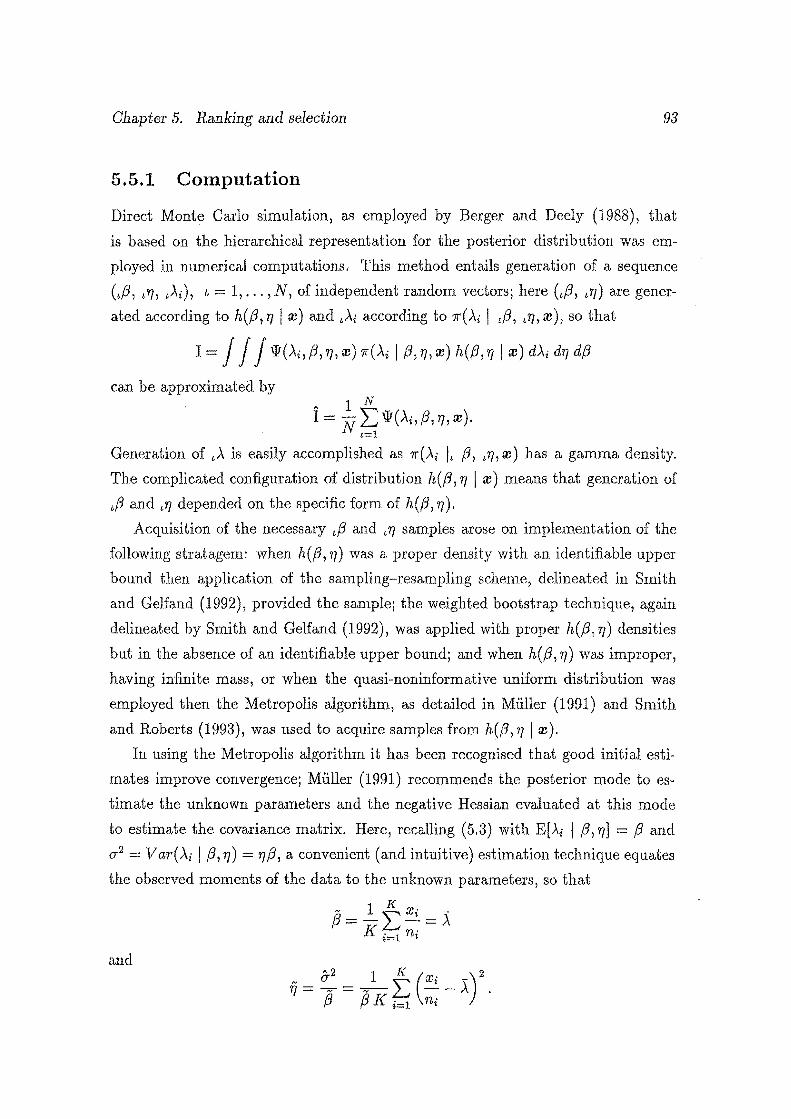
Chapter 5. Ranking and selection 93
5.5.1 Computation
Direct Monte Carlo simulation, as employed by Berger and Deely (1988), that
is based on the hierarchical representation for the posterior distribution was em
ployed in numerical computations. This method entails generation of a sequence
(d3, .'r}, .-Xi), "= 1, ... ,N, of independent random vectors; here (.{3, .n) are gener
ated according to h(fJ,rJ I x) and .-Xi according to 7r(Ai I .{J, .n,x), so that
l= j j jw(.XhfJ,rJ,X)1r(AijfJ,rJ,x)h(fJ,rJix)d.XidrJdfJ
can be approximated by A 1 N
I = N L lJ! ( Ai' fJ' 1]) X). •=1
Generation of .-X is easily accomplished as 7r(Ai 1. fJ, .1], x) has a gamma density.
The complicated configuration of distribution h(fJ, 1] I ro) means that generation of
.fJ and •17 depended on the specific form of h(fJ, rJ). Acquisition of the necessary .{J and •fJ samples arose on implementation of the
following stratagem: when h(fJ, 1]) was a proper density with an identifiable upper
bound then application of the sampling-resampling scheme, delineated in Smith
and Gelfand (1992), provided the sample; the weighted bootstrap technique, again
delineated by Smith and Gelfand (1992), was applied with proper h(fJ, rJ) densities
but in the absence of an identifiable upper bound; and when h(fJ, 1]) was improper,
having infinite mass, or when the quasi-noninformative uniform distribution was
employed then the Metropolis algorithm, as detailed in Miiller (1991) and Smith
and Roberts (1993), was used to acquire samples from h(fJ, 1] I ID ).
In using the Metropolis algorithm it has been recognised that good initial esti
mates improve convergence; Miiller (1991) recommends the posterior mode to es
timate the unknown parameters and the negative Hessian evaluated at this mode
to estimate the covariance matrix. Here, recalling (5.3) with E[.Xi I fJ, rJ] = fJ and
u2 = V ar( Ai I fJ, 1]) = 1] fJ, a convenient (and intuitive) estimation technique equates
the observed moments of the data to the unknown parameters, so that
and
~ 1 ~Xi -fJ=-,t_;-=A
I< i=I ni
Chapter 5. Ranking and selection 94
The covariance matrix E has several components, all of which require estimation,
namely; the variance of (J, u$, the variance of 'TJ ,u;, and p the covariance between
fJ and 7], so
[ &$ p&-{3&77 ]·
.E= p&-{3&77 a-;
Convenient estimates can be obtained by randomly partitioning sites into J sub
groups each of size I<j, j = 1, ... , J, then estimating ~j and fjj by
and
K· ~ 1 ~ jXi -fJJ = - L.t - = AJ
I<j i=I jni
N &J 1 ~ ( 3xi _ ) 2
'f/j = -:::;-- = -N L.t - - Aj fJj {Jj I<j i=l jni
for j = 1, ... , J. Here jXi denotes the number of accidents in subgroup j for site i
and jni is the monitoring length of that site. Variance and covariance estimates over
the subgroups can be found, in the usual way, via
2 1 ~N N 2 a-{3 = J1 ~(fJj- fJ) ' J=l
A2 1 ~(N N)2 0'7] = -- L.t 'f/j- 'TJ
J 1 j=l
and J N N
A '£j=l(fJj- fJ)(fjj- fj)
p = Jr,f=l ({Jj - ~) 2 L,f=l ( fjj - f7) 2 •
Repeating the partitioning and averaging estimates may improve the accuracy of
the initial parameters.
If the incomplete gamma function is unavailable for the computation of Pi(v), then Bowman and Shenton (1988) describe at least three convenient methods in
which this form of (j (>-.i/v I Sj, rj) can be numerically computed: expanding the
exponential (which converges rapidly if Ai/v is small); the Stieltjies continued frac
tion approach; and, the continued fraction of Schlomilch. Moreover, gamma dis
tributed random variates can readily be generated from an algorithm detailed in
Fishman (1973) and the 'shoe' variates drawn using the inverse transformation
method, as described in Pidd (1986). These methods have been briefly summarised
in Appendix D and Section 4.6.3, respectively.
Chapter 5. Ranking and selection 95
Direct Monte Carlo calculations in each instance, using SAS programming lan
guage, were executed using N = 10,000. SAS was chosen due to its ability in
determining incomplete gamma functions, its random gamma variate generator and
SAS has other applicable statistical routines. The standard error of these calcula
tions was in the proximity of ±0.001, found from multiple recalculations of identical
problems and through standard estimation techniques. This degree of accuracy is
probably beyond that required by any traffic researcher and N = 1, 000 could result
in more efficient but slightly less reliable estimates.
5.5.2 Case I
We imagine that three sets of responses have been elicited from questions 1 and 2,
and are now tabulated in columns 2 and 3 of Table 5.1. As indicated in the discussion
pertaining to hyperpriors, we use this information to determine the parameters of
the .gamma density by the formulae
a b
and
a member of the shoe distribution by the formula
and m is determined by expressing a level of confidence in the practitioner's answer
to question 2. This calculation follows easily by observing that P(O < a2 :::; c)
mf(m + 1), the left hand side of the equation being the degree of confidence in the
practitioner's statement about an upper bound on the variance. Note that h2 (ry I fJ)
is obtained from (5.6) using the values c and m ascertained above. The results of
these computations are contained in columns 4-7 of Table 5.1.
Our first presented criterion for selecting accident sites uses the posterior proba
bility quantity, Pi( v ). Based upon three arbitrarily selected v values, v = 1, 1.1 and
1.25, the results of this calculation for each of the 35 accident sites are contained
in Table 5.2. It is apparent from perusal of Table 5.2 that only the first three sites
have any sizeable value for Pi ( v). This feature is, perhaps, intuitively implied by the
observed data as the observed accident rates for the first three sites are considerably
greater than the majority that remain. While intuition suggests that a site with a
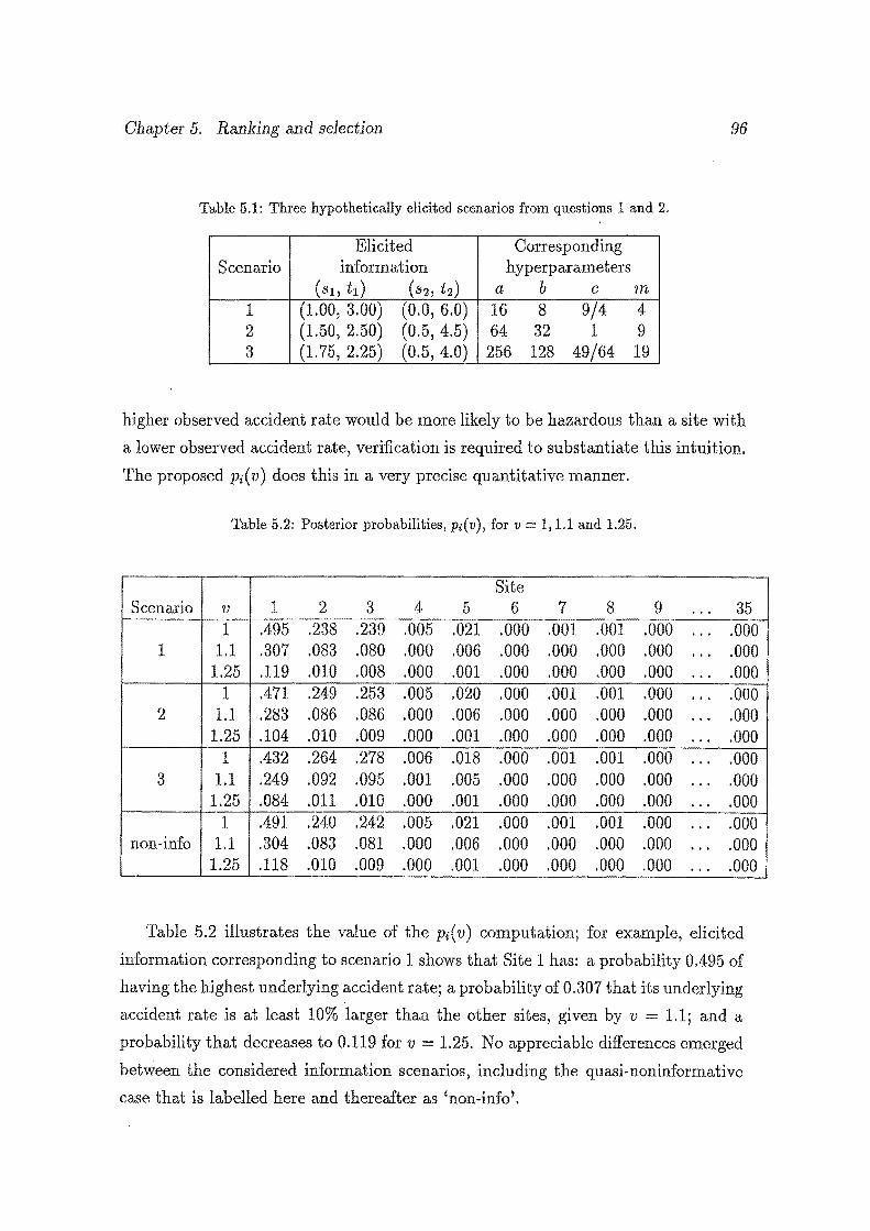
Chapter 5. Ranking and selection 96
Table 5.1: Three hypothetically elicited scenarios from questions 1 and 2.
Elicited Corresponding Scenario information hyperparameters
( Sl, t1) (s2, t2) a b c m 1 (1.00, 3.00) (0.0, 6.0) 16 8 9/4 4 2 (1.50, 2.50) (0.5, 4.5) 64 32 1 9 3 (1.75, 2.25) (0.5, 4.0) 256 128 49/64 19
higher observed accident rate would be more likely to be hazardous than a site with
a lower observed accident rate, verification is required to substantiate this intuition.
The proposed Pi( v) does this in a very precise quantitative manner.
Table 5.2: Posterior probabilities, Pi(v), for v = 1,1.1 and 1.25.
Site Scenario v 1 2 3 4 5 6 7 8 9 ... 35
1 .495 .238 .239 .005 .021 .000 .001 . 001 .000 ... .000 1 1.1 .307 .083 .080 .000 .006 .000 .000 . 000 .000 ... .000
1.25 .119 .010 .008 .000 .001 .000 .000 . 000 .000 ... .000 1 .471 .249 .253 .005 .020 .000 .001 . 001 .000 ... .000
2 1.1 .283 .086 .086 .000 .006 .000 .000 .000 . 000 ... .000 1.25 .104 .010 . 009 .000 .001 .000 .000 .000 .000 ... .000
1 .432 .264 .278 .006 .018 .000 .001 . 001 .000 ... .000 3 1.1 .249 .092 .095 .001 .005 .000 .000 .000 . 000 ... .000
1.25 .084 .011 .010 .000 .001 .000 .000 .000 . 000 ... .000 1 .491 .240 . 242 .005 .021 .000 .001 .001 .000 ... .000
non-info 1.1 .304 .083 .081 .000 .006 .000 .000 . 000 .000 ... .000 1.25 .118 .010 .009 .000 .001 .000 .000 . 000 .000 ... .000
Table 5.2 illustrates the value of the Pi( v) computation; for example, elicited
information corresponding to scenario 1 shows that Site 1 has: a probability 0.495 of
having the highest underlying accident rate; a probability of 0.307 that its underlying
accident rate is at least 10% larger than the other sites, given by v = 1.1; and a
probability that decreases to 0.119 for v = 1.25. No appreciable differences emerged
between the considered information scenarios, including the quasi-noninformative
case that is labelled here and thereafter as 'non-info'.
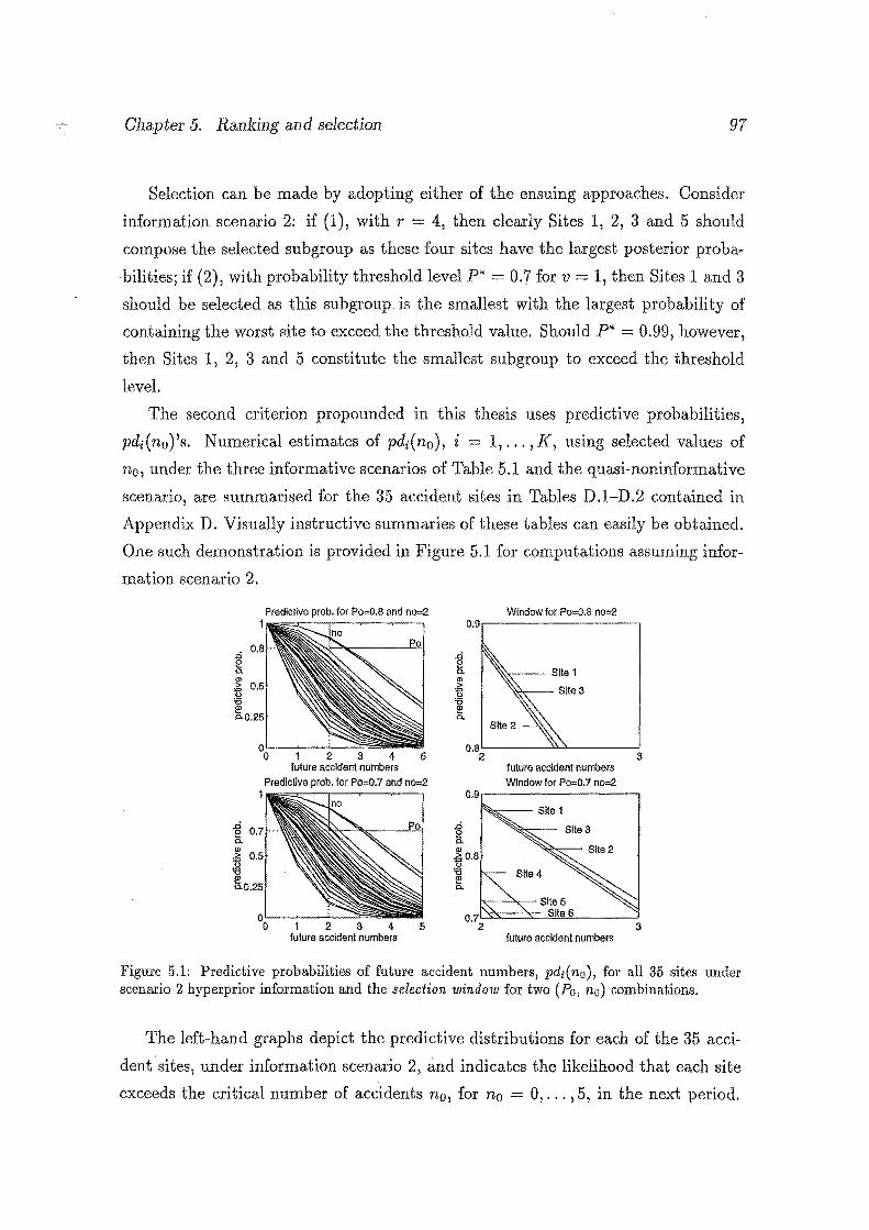
Chapter 5. Ranking and selection 97
Selection can be made by adopting either of the ensuing approaches. Consider
information scenario 2: if (1), with r :=: 4, then clearly Sites 1, 2, 3 and 5 should
compose the selected subgroup as these four sites have the largest posterior proba
bilities; if (2), with probability threshold level P*::::: 0.7 for v = 1, then Sites 1 and 3
should be selected as this subgroup is the smallest with the largest probability of
containing the worst site to exceed the threshold value. Should P* 0.99, however,
then Sites 1, 2, 3 and 5 constitute the smallest subgroup to exceed the threshold
level.
The second criterion propounded in this thesis uses predictive probabilities,
pdi(no)'s. Numerical estimates of pdi(n0 ), i 1, ... , I<, using selected values of
n0 , under the three informative scenarios of Table 5.1 and the quasi-noninformative
scenario, are summarised for the 35 accident sites in Tables D.1-D.2 contained in
Appendix D. Visually instructive summaries of these tables can easily be obtained.
One such demonstration is provided in Figure 5.1 for computations assuming infor
mation scenario 2.
~ 0. <I>
1
·~ 0.5 '6 ~ o.0.25
Predictive prob. for Po=0.8 and n0=2
0o 1 2 3 4 5 future accident numbers
Predictive prob. for Po=0.7 and n0=2 1
Window for Po=O.a no=2 0.9r-----------,
3 future accident numbers Window for Po=0.7 no=2
0.9
.ci e c.
~0.8 ,Q
"" ~ 0.
Site5 Site a
3 future accident numbers
Figure 5.1: Predictive probabilities of future accident numbers, pdi(n0 ), for all 35 sites under scenario 2 hyperprior information and the selection window for two (Po, no) combinations.
The left-hand graphs depict the predictive distributions for each of the 35 acci
dent sites, under information scenario 2, and indicates the likelihood that each site
exceeds the critical number of accidents n0 , for n0 = 0, ... , 5, in the next period.
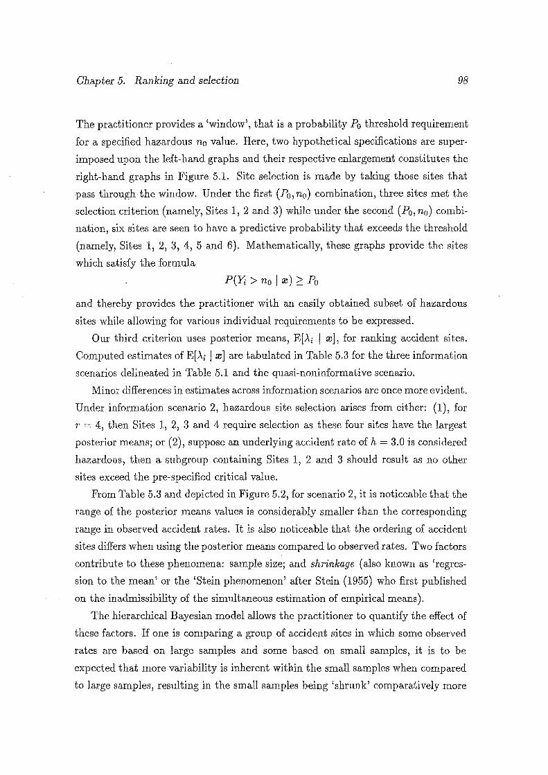
Chapter 5. Ranking and selection 98
The practitioner provides a 'window', that is a probability Po threshold requirement
for a specified hazardous no value. Here, two hypothetical specifications are super
imposed upon the left-hand graphs and their respective enlargement constitutes the
right-hand graphs in Figure 5.1. Site selection is made by taking those sites that
pass through the window. Under the first (Po, n0 ) combination, three sites met the
selection criterion (namely, Sites 1, 2 and 3) while under the second (Po, n0 ) combi
nation, six sites are seen to have a predictive probability that exceeds the threshold
(namely, Sites 1, 2, 3, 4, 5 and 6). Mathematically, these graphs provide the sites
which satisfy the formula
P(Yi > no I x) ;:::: Po
and thereby provides the practitioner with an easily obtained subset of hazardous
sites while allowing for various individual requirements to be expressed.
Our third criterion uses posterior means, E[Ai I re], for ranking accident sites.
Computed estimates of E[.:\i I x] are tabulated in Table 5.3 for the three information
scenarios delineated in Table 5.1 and the quasi-noninformative scenario.
Minor differences in estimates across information scenarios are once more evident.
Under information scenario 2, hazardous site selection arises from either: (1), for
r = 4, then Sites 1, 2, 3 and 4 require selection as these four sites have the largest
posterior means; or (2), suppose an underlying accident rate of h = 3.0 is considered
hazardous, then a subgroup containing Sites 1, 2 and 3 should result as no other
sites exceed the pre-specified critical value.
From Table 5.3 and depicted in Figure 5.2, for scenario 2, it is noticeable that the
range of the posterior means values is considerably smaller than the corresponding
range in observed accident rates. It is also noticeable that the ordering of accident
sites differs when using the posterior means compared to observed rates. Two factors
contribute to these phenomena: sample size; and shrinkage (also known as 'regres
sion to the mean' or the 'Stein phenomenon' after Stein (1955) who first published
on the inadmissibility of the simultaneous estimation of empirical means).
The hierarchical Bayesian model allows the practitioner to quantify the effect of
these factors. If one is comparing a group of accident sites in which some observed
rates are based on large samples and some based on small samples, it is to be
expected that more variability is inherent within the small samples when compared
to large samples, resulting in the small samples being 'shrunk' comparatively more
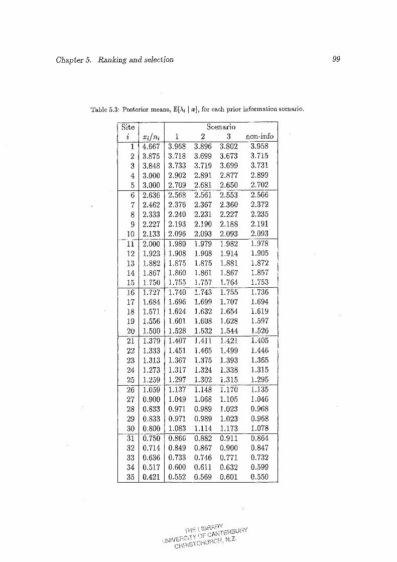
Chapter 5. Ranking and selection 99
Table 5.3: Posterior means, E[.\i I reJ, for each prior information scenario.
Site Scenario z x£/ni 1 2 3 non-info 1 4.667 3.968 3.896 3.802 3.958 2 3.875 3.718 3.699 3.673 3.715 3 3.848 3.733 3.719 3.699 3.731 4 3.000 2.902 2.891 2.877 2.899 5 3.000 2.709 2.681 2.650 2.702 6 2.636 2.568 2.561 2.553 2.566 7 2.462 2.376 2.367 2.360 2.372 8 2.333 2.240 2.231 2.227 2.235 9 2.227 2.193 2.190 2.188 2.191
10 2.133 2.096 2.093 2.093 2.093 11 2.000 1.980 1.979 1.982 1.978 12 1.923 1.908 1.908 1.914 1.905 13 1.882 1.875 1.875 1.881 1.872 14 1.867 1.860 1.861 1.867 1.857 15 1.750 1.755 1.757 1.764 1.753 16 1.727 1.740 1.743 1.755 1.736 17 1.684 1.696 1.699 1.707 1.694 18 1.571 1.624 1.632 1.654 1.619 19 1.556 1.601 1.608 1.628 1.597 20 1.500 1.528 1.532 1.544 1.526 21 1.379 1.407 1.411 1.421 1.405 22 1.333 1.451 1.465 1.499 1.446 23 1.313 1.367 1.375 1.393 1.365 24 1.273 . 1.317 1.324 1.338 1.315 25 1.259 1.297 1.302 1.315 1.295 26 1.059 1.137 1.148 1.170 1.135 27 0.900 1.049 1.068 1.105 1.046 28 0.833 0.971 0.989 1.023 0.968 29 0.833 0.971 0.989 1.023 0.968 30 0.800 1.083 1.114 1.173 1.078 31 0.750 0.866 0.882 0.911 0.864 32 0.714 0.849 0.867 0.900 0.847 33 0.636 0.733 0.746 0.771 0.732 34 0.517 0.600 0.611 0.632 0.599 35 0.421 0.552 0.569 0.601 0.550
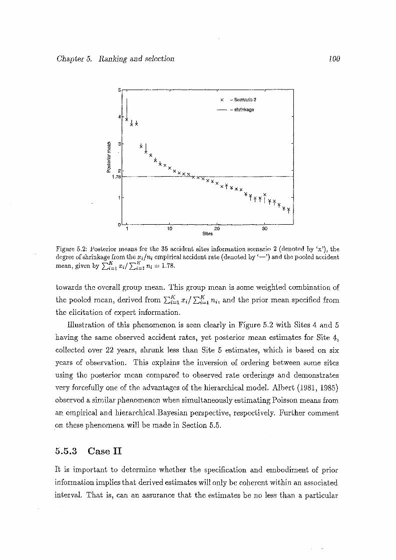
Chapter 5. Ranking and selection
6rr--------~----------.-----------,-----,
x - Scenario 2
- -shrinkage
0~--------~----------~----------~----~ 10 20
Sites 30
100
Figure 5.2: Posterior means for the 35 accident sites information scenario 2 (denoted by 'x'), the degree of shrinkage from the x;/ni empirical accident rate (denoted by'-') and the pooled accident mean, given by 2:~1 x;/2:{~1 ni = 1.78.
towards the overall group mean. This group mean is some weighted combination of
the pooled mean, derived from 2:~1 xd 2:~1 ni, and the prior mean specified from
the elicitation of expert information.
Illustration of this phenomenon is seen clearly in Figure 5.2 with Sites 4 and 5
having the same observed accident rates, yet posterior mean estimq.tes for Site 4,
collected over 22 years, shrunk less than Site 5 estimates, which is based on six
years of observation. This explains the inversion of ordering between some sites
using the posterior mean compared to observed rate orderings and demonstrates
very forcefully one of the advantages of the hierarchical model. Albert (1981, 1985)
observed a similar phenomenon when simultaneously estimating Poisson means from
an empirical and hierarchicaLBayesian perspective, respectively. Further comment
on these phenomena will be made in Section 5.5.
5.5.3 Case II
It is important to determine whether the specification and embodiment of prior
information implies that derived estimates will only be coherent within an associated
interval. That is, can an assurance that the estimates be no less than a particular
Chapter 5. Ranking and selection 101
value or greater than another value for specific prior information be made? The
desire to specify bounds arises naturally due to insufficient time, money or resources
to elicit specific enough information to draw the assumptions used to specify the
hyperprior distributions given by Case I or result from experts who are unable to
elaborate further on the population of interest.
So, in this situation, we are interested in providing .another interpretation to
the answers elicited to questions 1 and 2. We demonstrate that if the broadest
interpretation of the elicited information is taken then boundaries associated with
any estimate are so widely divergent that the elicited information is of negligible
practical use. However, the elicited responses can be interpreted in a variety of ways
in order to 'tighten up' the most general interpretation. Here we consider a method,
involving some minor additional elicitation, where sensible results can be achieved
while still allowing the practitioner considerable flexibility. That is, we provide one
method of relaxing the rigid interpretation of questions 1 and 2 presented in Case I
so that sensible boundaries around any estimates can be attained.
Broadest interpretation
In Case I, the mean of (3 was assigned the value ajb = (t1 + st)/2. This is now
relaxed to simply say that ajb can be anywhere on the (s1 , t1) interval. Moreover, the
variance for (3 was previously equated to a/b2 [(t1-s1)/4]2, but this is now relaxed
so that ajb2 is simply constrained between 0 and its largest possible value, obtained
by equally dividing the mass and positioning each half on the boundary points s1
and t1 respectively. Remembering that h1((3) rv g(f31 a, b), then algebraically:
a ~ [b(tl
2- St)l 2
====? a ~ 0 and
(5.18)
(5.19)
Now consider the h2(rt I (3) specifications. In Case I, the uniform upper bound be
fore exponential decline on the variability of the Ai's was equated to c = [(t2 -s2)/4]2
and m found on solution to P(O ~ a 2 .::;: c) = mf(m+ 1), representing the confidence
in or of the practitioner. Suppose now that c can range between the smallest pos
sible variance, equal to 0, and the largest possible variance, again found by placing
half the mass on each boundary point s2 and t2 respectively. Furthermore, assume
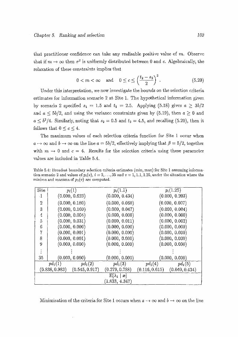
Chapter 5. Ranking and selection 102
that practitioner confidence can take any realisable positive value of m. Observe
that if m-+ oo then a 2 is uniformly distributed between 0 and c. Algebraically, the
relaxation of these constraints implies that
0 < m < oo and 0 < c < (tz- 82)
2
• - - 2 (5.20)
Under this interpretation, we now investigate the bounds on the selection criteria
estimates for information scenario 2 at Site 1. The hypothetical information given
by scenario 2 specified s1 1.5 and t 1 = 2.5. Applying (5.18) gives a ;:::: 3b/2
and a :::; 5b/2, and using the variance constraints given by (5.19), then a ;:::: 0 and
a b2 /4. Similarly, noting that s2 = 0.5 and t 2 = 4.5, and recalling (5.20), then it
follows that 0 :::; c :::; 4.
The maximum values of each selection criteria function for Site 1 occur when
a-+ oo and b-+ oo on the line a= 5b/2, effectively implying that {3 = 5/2, together
with m -+ 0 and c = 4. Results for the selection criteria using these parameter
values are included in Table 5.4.
Table 5.4: Broadest boundary selection criteria estimates (min, max) for Site 1 assuming information scenario 2 and values of p;(v), i = 2, ... , 35 and v = 1, 1.1, 1.25, under the situation where the minima and maxima of Pl ( v) are computed.
Site Pi(l) Pi(l.l) Pi(1.25) 1 (0.000, 0.623) (0.000, 0.434) (0.000, 0.203)
2 (0.000, 0.180) (0.000, 0.060) (0.000, 0.007) 3 (0.000, 0.160) (0.000, 0.047) (0.000, 0.004) 4 (0.000, 0.004) (0.000, 0.000) (0.000, 0.000) 5 (0.000, 0.031) (0.000, 0.011) (0.000, 0.002) 6 (0.000, 0.000) (0.000, 0.000) (0.000, 0.000) 7 (0.000, 0.001) (0.000, 0.000) (0.000, 0.000) 8 (0.000, 0.001) (0.000, 0.000) (0.000, 0.000) 9 (0.000, 0.000) (0.000, 0.000) (0.000, 0.000)
35 (0.000, 0.000) (0.000, 0.000) (0.000, 0.000) pdl(1) pdl(2) pdl(3) pd1(4) pd1(5)
(0.838, 0.983) (0.545, 0.917) (0.279, 0. 788) (0.116, 0.615) (0.040, 0.434) E[A1 I w]
(1.833, 4.347)
Minimisation of the criteria for Site 1 occurs when a -+ oo and b -+ oo on the line
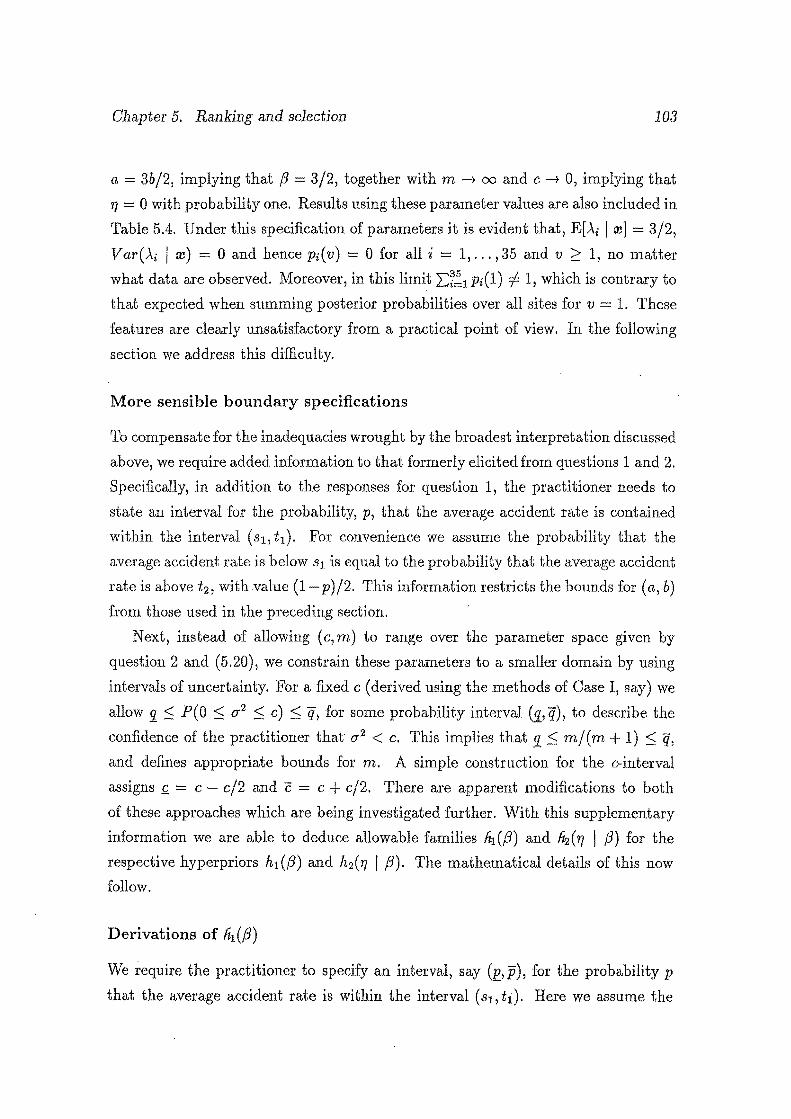
Chapter 5. Ranking and selection 103
a = 3b/2, implying that (:J 3/2, together with m ~ oo and c ~ O, implying that
17 = 0 with probability one. Results using these parameter values are also included in
Table 5.4. Under this specification of parameters it is evident that, E[.\ I mJ = 3/2,
Var(>.i I m) = 0 and hence Pi(v) = 0 for all i = 1, ... ,35 and v ;:::: 1, no matter
what data are observed. Moreover, in this limit 2:7!1 Pi(l) 1, which is contrary to
that expected when summing posterior probabilities over all sites for v = 1. These
features are clearly unsatisfactory from a practical point of view. In the following
section we address this difficulty.
More sensible boundary specifications
To compensate for the inadequacies wrought by the broadest interpretation discussed
above, we require added information to that formerly elicited from questions 1 and 2.
Specifically, in addition to the responses for question 1, the practitioner needs to
state an interval for the probability, p, that the average accident rate is contained
within the interval (s1, t1). For convenience we assume the probability that the
average accident rate is below s1 is equal to the probability that the average accident
rate is above t 2 , with value (1 p)/2. This information restricts the bounds for (a, b) from those used in the preceding section.
Next, instead of allowing ( c, m) to range over the parameter space given by
question 2 and (5.20), we constrain these parameters to a smaller domain by using
intervals of uncertainty. For a fixed c (derived using the methods of Case I, say) we
allow 9_ :::;; P(O S u2 S c) :::;; q, for some probability interval (g_, q), to describe the
confidence of the practitioner that u2 < c. This implies that 9_:::;; m/(m + 1) :::;; q, and defines appropriate bounds for m. A simple construction for the c-interval
assigns Q = c - c/2 and c = c + c/2. There are apparent modifications to both
of these approaches which are being investigated further. With this supplementary
information we are able to deduce allowable families /i1 ((:J) and liz ("' I (:J) for the
respective hyperpriors h1 ((:J) and h2 ( 17 I (:J). The mathematical details of this now
follow.
Derivations of /i1 ((3)
We require the practitioner to specify an interval, say (p,p), for the probability p
that the average accident rate is within the interval (s1 , t1). Here we assume the
Chapter 5. Ranking and selection 104
probability that this average is below s1 is equal to the probability it is above t 1
with value (1 - p)/2. These constraints result in the ft1((3) distribution, g((3 I a, b), having parameters a and b that must lie on the solid curve indicated in Figure 5.3.
Figure 5.3: A log-scaled plot of valid (a, b) combinations for elicited p-intervals under scenario 2 hyperprior information.
Some selected interval values for (E., p) appear in Figure 5.3; for example if
(E.= 0.5, p 0.75) then the (a, b) parameters consistent with this information lie
on the solid curve between (4.1, 2.1) and (11.4, 6.1). Also depicted in this figure
are the boundaries corresponding to information scenario 2 which stipulated that
(s1 = 1.5, t1 = 2.5) and hence implied a;::: 3b/2 and a ~ 5bf2. From Figure 5.3 it is
evident that any specified E. above 0.333 is coherent with the response provided to
question 1. It is also clear that there exist potential instances where the intervals
expressed for p and the values elicited for (s1 , t1) are inconsistent. The exact value
where p is no longer coherent was not explicitly found as it was not relevant to the
example.
Derivations of fi;, ( 'f/ I (3)
Initially we determine a family on the distribution for o-2 and then use the transfor
mation 0'2 = 17f3 to deduce a family of allowable hyperpriors for h2('f/ I (3).
In Case I, elicitation of question 2 and our interpretation of that information
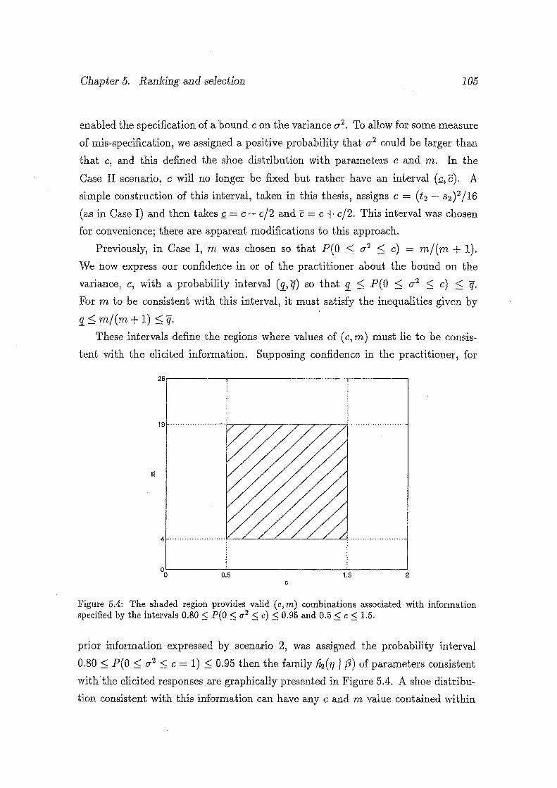
Chapter 5. Ranking and selection 105
enabled the specification of a bound c on the variance a 2• To allow for some measure
of mis-specification, we assigned a positive probability that a2 could be larger than
that c, and this defined the shoe distribution with parameters c and m. In the
Case II scenario, c will no longer be fixed but rather have an interval (£,c). A
simple construction of this interval, taken in this thesis, assigns c (t2 - s2)2/16
(as in Case I) and then takes £ = c- c/2 and c = c + c/2. This interval was chosen
for convenience; there are apparent modifications to this approach.
Previously, in Case I, m was chosen so that P(O :=_; a 2 :::; c) = m/(m + 1).
We now express our confidence in or of the practitioner about the bound on the
variance, c, with a probability interval (:L.;q) so that :1. :=_; P(O :=_; a2 :::; c) :::; q. For m to be consistent with this interval, it must satisfy the inequalities given by
:1. mf(m + 1) < q. These intervals define the regions where values of ( c, m) must lie to be consis
tent with the elicited information. Supposing confidence in the practitioner, for
25.--------,,---------------~~---------.
19 , .................. ..
E
0.5 1.5 2 c
Figure 5.4: The shaded region provides valid (c, m) combinations associated with information specified by the intervals 0.80 ::=; P(O,:::; o-2 ::=;c) ::=; 0.95 and 0.5 ::=; c ::=; 1.5.
prior information expressed by scenario 2, was assigned the probability interval
0.80 :::; P(O :=_; a2 :=_; c = 1) S 0.95 then the family ~('r/ I fJ) of parameters consistent
with the elicited responses are graphically presented in Figure 5.4. A shoe distribu
tion consistent with this information can have any c and m value contained within
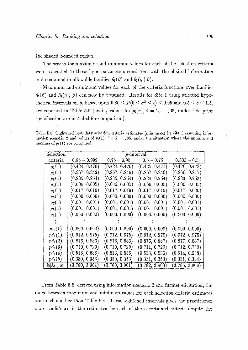
Chapter 5. Ranking and selection 106
the shaded bounded region.
The search for maximum and minimum values for each of the selection criteria
were restricted to those hyperparameters consistent with the elicited information
and contained in allowable families fi1 (fJ) and ~ ('I] I fJ). · Maximum and minimum values for each of the criteria functions over families
fi1(fJ) and /i;,('fJ I fJ) can now be obtained. Results for Site 1 using selected hypo
thetical intervals on p, based upon 0.80 P(O ~ 0'2 ~c) ~ 0.95 and 0.5 ~ c < 1.5,
are reported in Table 5.5 (again, values for Pi( v ), i = 2, ... , 35, under this prior
specification are included for comparison).
Table 5.5: Tightened boundary selection criteria estimates (min, max) for site 1 assuming information scenario 2 and values of Pi(1), i = 2, ... , 35, under the situation where the minima and maxima of Pl (1) are computed.
Selection p-interval criteria 0.95 0.999 0.75- 0.95 0.5-0.75 0.333 0.5 P1(1) (0.424, 0.470) (0.424, 0.4 70) (0.425, 0.471) (0.426, 0.473) P2(l) (0.267, 0.249) (0.267, 0.249) (0.267, 0.249) (0.266, 0.247) P3(1) (0.285, 0.254) (0.285, 0.254) (0.284, 0.254) (0.283, 0.253) P4(1) (0.006, 0.005) (0.006, 0.005) (0.006, 0.005) (0.006, 0.005) Ps(l) (0.017, 0.019) (0.017' 0.019) (0.017, 0.019) (0.017, 0.020) P6(1) (0.000, 0.000) (0.000, 0.000) (0.000, 0.000) (0.000, 0.000) P7(1) (0.001, 0.001) (0.001, 0.001) (0.001, 0.001) (0.001, 0.001) Ps(l) (0.001, 0.001) (0.001, 0.001) (0.001, 0.001) (0.001, 0.001) pg(l) (0.000, 0.000) (0.000, 0.000) (0.000, 0.000) (0.000, 0.000)
. P35(1) (0.000, 0.000) (0.000, 0.000) (0.000, 0.000) (0.000, 0.000) pdl (1) (0.972, 0.975) (0.972, 0.975) (0.972, 0.975) (0.972, 0.975) pdl (2) (0.876, 0.886) (0.876, 0.886) (0.876, 0.887) (0.877, 0.887) pd1(3) (0.710, 0.729) (0.710, 0.729) (0.711, 0. 729) (0.712, 0.730) pdl ( 4) (0.513, 0.536) (0.513, 0.536) (0.513, 0.536) (0.514, 0.538) pd1(5) (0.330, 0.353) (0.330, 0.353) (0.331, 0.353) (0.331, 0.354)
E(,\1 I re] (3. 780, 3.901) (3.780, 3.901) (3. 782, 3.903) (3.785, 3.906)
From Table 5.5, derived using information scenario 2 and further elicitation, the
range between maximum and minimum values for each selection criteria estimates
are much smaller than Table 5.4. These tightened intervals gives the practitioner
more confidence in the estimates for each of the ascertained criteria despite the

Chapter 5. Ranking and selection 107
uncertainty inherent within the elicited information, and illustrates the value of
extra information from responses to questions 1 and 2.
Chapter 6
Summary
We now recapitulate both the proposed techniques and the main findings from
the application of these techniques to the Auckland data.
6.1 Model discrimination
6.1.1 Averaged Bayes Factor
When selecting between a multiple of mathematical models (each having a vector
of unknown parameters) at a collection of sites, it is unlikely that sufficient expert
subjective knowledge will always be available to create proper prior distributions
so that standard informative Bayesian analyses can proceed. In these instances,
utilisation of noninformative priors provides a realistic and feasible tool for analysts
to discriminate between models in the Bayesian framework. Implementation of such
priors have traditionally has been fraught with difficulties due to the arbitrary nature
of the multiplicative constant. Adoption of training samples provides a method of
resolution, thereby facilitating a powerful noninformative Bayesian selection mech-. am sm.
In this thesis we introduced the averaged Bayes factor. This technique assures co
herent pairwise model comparisons and facilitates posterior probability derivations
108
Chapter 6. Summary 109
useful for simultaneous model discrimination and selection. The averaged Bayes
factor method also produces quantitative, computationally straightforward and in
terpretable answers. Moreover, due to the averaging process, this method provides
stable answers that are independent from particular training samples. Not all these
properties are shared by existing noninformative Bayesian methods. Additionally,
the averaged Bayes factor facilitates selection between competing models whether
nested, nonnested or some combination. The latter is achieved only with consid
erable effort in the non-Bayesian framework, particularly with such small sample
numbers.
We have demonstrated that in the traffic accident analysis context, model selec
tion using the BIC criterion favours, often quite substantially, the simpler models
when compared to the averaged Bayes factor approach. This failing was clearly illus
trated by the Poisson model (M1 ), and to a lesser extent the geometric model (M4),
having considerably more support under the approximated BIC selection method
than under the corresponding comparisons using averaged Bayes factors. The de
ficiency of the BIC method is due to its asymptotic development whereby a term
is justifiably ignored as the sample size tends to infinity. Unfortunately, when the
sample size is relatively small, this. ignored term can impact significantly on the
resultant Bayes factor and its omission creates a substantial systematic bias. Typ
ically, traffic accident analysis deals with small sample sizes, thereby introducing
potentially serious bias into the BIC selection procedure or its approximations.
From the properties given in Section 3.2 and on the basis of the numerical ex
ample, it seems that the averaged Bayes factor method has wider applicability than
many of its competitors.
6.1.2 Application of the averaged Bayes factor
Applying the averaged Bayes factor on the Auckland data included in Table A.l
we demonstrated that the Poisson model was the most frequently favoured of those
considered. Also apparent was the consistency in the favourability of the Pois
son/ gamma model; this model never having a discrimination rank below two of
the four models considered over the 35 accident sites. This consistency accounted
for the averaged posterior probabilities for both the Poisson and Poisson/ gamma
models being almost identical with P(M1 I m) = 0.313 and P(M2 I m) = 0.309.
Chapter 6. Summary 110
Without model adequacy considerations, the weight of support, at this stage,
would probably favour the Poisson model. The appeal of its simplicity coupled with
its discrimination ranking and P(M1 I w) probability superiority over the other
models would suggest that accident analysis should precede with the adoption of
this model.
Similarly, without verification of the Poisson model's adequacy, it would have un
doubtedly been selected as the most appropriate to best represent the hypothetical,
binomial generated, Site B data. This discrimination on data deliberately chosen to
be discordant from all the candidate models forcefully demonstrates the inadequacies
of the Bayes factor approach if used alone for model selection purposes.
6.2 Model adequacy and Power
6.2.1 Remarks
It is clear that model selection and model adequacy are interrelated but neither im
plies the other. We believe, therefore, that upon selection it is important to directly
investigate the likelihood of observed data originating from the chosen model. If
data and their associated selected model are irreconcilable then it is unlikely that
any ensuing inferences based on this inadequate model will be accurate or useful.
In such circumstances it may be appropriate to extend the set of candidate models
available for model selection or re-examine the data. If, however, the inadequate
model is utilised then considerable care must be taken over the interpretation of any
results.
Model adequacy does not imply model selection as frequently many different
models, of varying degrees of complexity and dimension, exist or can be constructed
that are consistent with some data under analysis. Highly sophisticated or overly
specified models are infrequently the most parsimonious and rarely appropriate.
Good model selection techniques, such as the Bayes factor approach, discriminate
between competing models based on their complexity and comparative likelihood.
We thus concur with Upadhyahy and Smith (1993) and do not advocate adequacy as
a method for model selection, instead we view model adequacy as a method providing
guidance as to whether a particular discriminated model seems compatible with the
Chapter 6. Summary 111
observed data.
In this thesis we describe an intuitive method that enables both model adequacy
and its associated power to be quantifiably and sensibly ascertained, using methods
in cross-validation, prediction and simulation. The proposed simulation scheme
delineated within allows the construction of pictorial representations of these entities
to be easily undertaken thereby allowing a fuller understanding of the relationship
between data and selected models to be derived.
We believe that it is important for model adequacy to be recognised and ad
dressed once mathematical representations of the data have been selected. If ade
quacy is ignored, how can any researcher have confidence in their ensuing analyses
and inferences?
6.2.2 Adequacy measures
Model adequacy was conducted using three separate 'lY measures. Generally, the
most powerful and robust of these considered measures wq,s rJJ1 , the chi-square mea
sure. The applicability of this measure depends, however, on the availability of the
mean and variance of the hold-out predictive distribution. In their absence, pseudo
values allowed the adoption of the rJJ1 measure. Results from this rJJ 1 adaptation
performed satisfactorily and with reasonable power for the examples demonstrated
within this thesis. However, the general applicability and suitability of this measure
estimated using these contrived pseudo-entities certainly requires further investiga
tion. Nonetheless, based upon the results contained in this thesis, we recommend
'1J 1 as the most suitable measurement of discrepancy although further confirmation
using a greater breadth of distributions, adequacy measures and data is required.
Adequacy measured by '1J3 was invariably less powerful than corresponding '1J1
measures. However, the '1J3 measure is attractive in the sense that it was unrestricted
by the indefinite mean and variance quantities that compromised the '1J1 measure.
This adequacy measure, therefore, is a suitable and appropriate companion to the
'1J1 measure.
It was surprising to find that the rJJ 2 measures were widely inconsistent in their
power. As a consequence of the extremely poor power frequently associated with
the rJJ 2 measure under certain conditions, we can not recommend '1J 2 as a useful
global adequacy measure.
Chapter 6. Summary 112
6.2.3 Application
It was clearly demonstrated that the 'best' model, in the discriminatory sense, is not
necessarily adequate. All the considered measures resoundingly rejected the appli
cability of the Poisson model on the hypothetical accident Site B. In was evident the
Poisson model was patently deficient in modelling the under-dispersion associated
with this site. Ensuing analyses using this best model would almost certainly result
in erroneous or misleading conclusions.
When examining the 35 accident sites collectively, the inconsistent global ad
equacy of the Poisson model comparative to the Poisson/ gamma model became
apparent. Using the powerful :D1 adequacy measure, at eight sites (23%) the Pois
son model was deemed inadequate at a = 0.05 while the Poisson/gamma model
recorded two (6%) such inadequacies. The model inadequacy frequency that was
associated with the Poisson density casts serious doubt on its global applicability,
especially since the Poisson/ gamma model performs so comparatively well. This
result may appear quite discrepant or contrary from that anticipated after the dis
criminatory success of the Poisson model. However, an explanation for this result
can be provided using the following reasoning.
To understand this phenomenon we first need to revisit the averaged Bayes factor
results. The natural embodiment of Occam's razor within the Bayes factor calcu
lations ensures that the Poisson model is always favoured over the Poisson/gamma
model (which has larger dimensionality) when the data have empirical dispersion
index close to one. Despite this, the Poisson/ gamma is usually only minimally
worse than the Poisson model on these occasions. However, in the presence of over
dispersed data, the favourability of the Poisson model falls away relatively quickly
and the preference of the Poisson/ gamma model is revealed. In these instances the
Poisson frequently slipped to the fourth and worst rank, and was typically very
strongly worse than the Poisson/gamma model. Consequently, as a model, the Pois
son model is quite extreme, in the sense that: when it is best, it is good; but when
it is worst, it is terrible! By comparison, the Poisson/ gamma model is far more
circumspect and accommodating.
With the simultaneous ranking and selection between hazardous accident sites,
it thus appears that the Poisson/ gamma more appropriately accommodates the
diversity inherent within accident data. Further research conducted on accident
Chapter 6. Summary 113
data sets from alternative sources is required before this recommendation can be
offered with more certainty.
6.3 Ranking and selection
The analyses of Section 5.5 illustrates quite forcefully the advantages and salient
features of the hierarchical model and corresponding selection criteria proposed in
this thesis. These ideas are explained below.
6.3.1 Hierarchical model
Among the basic facts that motivate this analytical technique is that in many multi
variate estimation problems, such as those encompassed in vehicle accident studies,
the 'standard' maximum likelihood estimates employed are inadmissible, there is
no facility to incorporate the often abundant subjective information concerning the
accidents sites, and standard tests of hypothesis invariably provide unsatisfactory
non-significant results due to large associated standard errors. These deficiencies
can be surmounted by embracing a hierarchical Bayesian paradigm.
A distinguishing trait of the hierarchical model, then, is its ability to quantita
tively, accurately and easily discriminate between sites that commonly have small
and variable accident count periods. In particular, the model naturally discrim
inates between sites (without any special considerations) when observed accident
rates from q sites, q ~ J{, are equal while the period of monitoring is in fact dif
ferent. For example from Table 5.3 it can be seen that the observed accident rate
for both Sites 4 and 5 is 3.0, however, when using a noninformative hyperprior and
v 1, it can be seen from Table 5.2 that the posterior probability that Site 5 is
worst is 4.2 times more likely than Site 4. This discrepancy in posterior probabilities
is due to the differing length of observation periods; here Site 4 had data recorded
over 22 years while Site 5 was recorded over six years.
When adopting the noninformative hyperprior and v 1, the posterior proba-
bility of obtaining the worst accident rate equalled 0.973 for the subgroup composed
of Sites 1, 2 and 3. Instead, if r = 4, then the best subset contains Sites 1, 2,
3 and 5 with an associated posterior probability of 0.994. On this basis, should
reconstruction of Sites 1, 2, 3 and 5 be undertaken then the probability that the
Chapter 6. Summary 114
worst accident site remains unselected is 0.006. Notice that Site 4 is not selected
here although it has the same observed accident rate as Site 5 (which is selected).
The hierarchical model provides a natural mechanism whereby prior information
can be elicited and incorporated in the analysis. The hypothetical answers we used
in Section 5.5 illustrate the way in which the practical information can be useful in
the analysis. The model itself shows how this information is to be used. This type
of decision making has not been available to practising engineers in other kinds of
analyses.
6.3.2 Selection criteria
The three selection criteria suggested in this thesis have been shown to offer a
variety of useful information when applied to the data in Table A.l. The various
characteristics of these criteria indicate when they should be appropriately employed.
Using the Pi( v) allows the practitioner the ability to determine which site has the
highest underlying accident rate and by how much. The pdi(no) criterion, on the
other hand, offers a different but equally valid method of selecting hazardous sites
based upon the number of accidents in the next period. Finally, the third criterion,
that of the mean underlying accident rate of a site, offers other insights into ranking
sites for remedial treatment.
Generally the three criteria do agree in their ranking but there are some minor
differences .. For example, when using the pdi(no) criterion for Sites 20, 21 and 22
then: for n0 1, Sites 20 and 21 are preferred over Site 22; for no 2, 3 and 4,
Site 20 is preferred over Site 22 which in turn is preferred over Site 21; and for
n0 = 5, Site 22 is preferred over both Sites 20 and 21 (although not reported here,
the latter is also true for n0 > 5). Similarly, under all considered hyperprior scenarios
E[.As I m] < E(.-\4 I m] while Ps(v) > P4(v). Other differences are evident but remain
mmor.
Case I results were quite insensitive to the four quite disparate hypothetical
information scenarios employed. The robustness of the estimates gives confidence
in both the model employed and the data themselves. Furthermore, meaningful
estimator boundaries were achieved, as demonstrated by Case II analyses, with
the elicitation of additi<;mal information to question 1. These boundaries give the
practitioner a grasp of the potential variation a~sociated with the selection criteria
Chapter 6. Summary 115
estimates, and a confidence band in which estimators are most likely to be found.
The current focus on identifying the worst locations is based on the premise
that once a location has been identified, diagnosis of the problems and potential
treatments will be straightforward (that is the deficiencies and remedies will be ob
vious to an experienced accident investigator). It was from this perspective that
selection was introduced and demonstrated in this thesis. Consideration should be
given to the identification of best locations (those locations with the lowest under
lying accident rates) as examination of these sites and comparison with worst sites
may well assist identification of differences in the two types of locations and suggest
appropriate treatments for the worst locations (to make them more like the best
locations). Ranking and selection of the best locations can be easily attained using
any of the selection criteria suggested within this thesis simply through the reversal
of the inequality sign in (5.13), (5.15) and all subsequent respective equations.
6.4 General extensions
6.4.1 Averaged Bayes factor
As previously alluded to, model discrimination in the traffic accident analysis frame
work typically deals with small sample sizes. Such diminutive samples allow individ
ual observations to have a substantial influence on the averaged Bayes factor, or any
Bayes factor variant for that matter. A diagnostic, such as that proposed by Pettit
and Young (1990), can easily be developed to detect an observation which is most
influential on the averaged Bayes factor. This diagnostic would provide more insight
into both the data (so that seemingly peculiar observations could be identified and
verified from their source or record) and the models under comparison.
There are a plethora of model discrimination techniques available, of which the
averaged Bayes factor is but one. However, the desirable properties and intuitive
derivation associated with this technique (Section 3.2) suggests that its applicability
should be further investigated on a more diverse array of problems, such as providing
regression diagnostics.
Chapter 6. Summary 116
6.4.2 Model adequacy
Although not explicitly considered here, model adequacy can be further extended to
determine whether elicited and modelled informative prior densities combined with
some assumed (or selected) likelihood function are consistent with the observed
phenomena m. Adequacy calculations of this type could usefully assess and validate
the reliability of any prior information.
We note that the full Bayesian paradigm has not been applied to the proposed
model adequacy stratagem. That is, in accordance with the Bayesian philosophy,
the uncertainty about the adequacy of a model should ideally be described by a
probability distribution. This area is open for further development.
6.4.3 Bayesian hypothesis testing
Although this is generally not the definitive objective of a traffic engineer, there
may be instances where testing the equivalence of unknown accident rates between
sites is necessary. An alternative model for significance testing within a Bayesian
framework, initiated by Jeffreys (1967) and continued by Deely and Gupta (1988),
can be applied to test H0 : A1 A2 = ... = AK. Mathematical details now follow.
Recall that the prior distribution (5.2) has mean and variance E[Ai I (:J, '17] f3 and Var(Ai I /3, 'I])= 'I](:J, see (5.4), so by incorporating a prior probability 'Y that
Ho is true it is straightforward to develop a significance test. That is, a value 'Y is
assigned so that P(Ho is true) P('l] = 0) = 'Y· The posterior probability of H0 is
found by computing
I* = [1 + 1 -I f( x) l-1 1 f(x I 0)
where f(x) and f(re I (:J,'I]) are given by (5.9) and (5.8) respectively, thus
f(re I 0) = fooo f(x I /3,0) h(/3,0) dfJ
where x '£f==1 Xi/ k. Each Pi( v) should be multiplied by (1 'Y*) to obtain the
posterior probability that Ai is largest since Pi ( v) is conditional upon H0 being false;
which implies 'I] > 0.
Chapter 6. Summary 117
6.4.4 Countermeasure evaluation
The evaluation of accident countermeasures and the identification and ranking of
hazardous locations can be reduced to a before and after study. That is, one is inter
ested in ascertaining whether some treatment is effective in reducing the underlying
accident rate for a given site. Although not specifically considered in this thesis, it
follows directly that the hierarchical Bayesian framework can easily be applied to
this situation. Treating the series of accidents before and after the accident site re
construction separately, placing prior distributions and combining with the observed
. accident frequencies, the posterior distribution can be constructed. The selection
criteria can then be utilised to evaluate the effectiveness of the reconstruction on
reducing the underlying accident rate.
6.4.5 Cost and loss
Implicated in the selection criteria and ensuing selection strategies has been the
notion of equivalence between accident sites in terms of cost, C, of intervention and
potential for accident reduction. Although not detailed here, these selection ideas
can be extented to situations where this equivalence no longer exists, so that Ci # C3
for sites i and j respectively.
The posterior probability selection criteria suggested in this thesis inherently
incorporates an analogue of the "O-K" loss function (see Berger, 1985, for example).
Loss is zero if a correct decision is made (selection of a hazardous site or omission
of a non-hazardous site), and K if an incorrect decision made (selection of a non
hazardous site or omission of a hazardous site). Selection based upon the proposed
Pi( v) probabilities ensures the minimised expected loss. This loss function can be
extended to situations where actions at different sites incur different losses.
6.4.6 Hierarchical Bayesian modifications
There are various modifications of the hierarchical model that might be explored.
Firstly, a general linear model as considered in Christiansen, Morris and Pendle
ton (1992) may give some improved accuracy. For example, the replacement of fJ in
(5.2) by Yilfll Yizflz + ... + Yiqflq where Yil, Yiz, .. . , Yiq are known 'regressors' for
i = 1, ... , k and f3 = ({11 , {12, ••• , {lq) is a vector of unknown 'regression' coefficients
Chapter 6. Summary 118
with hyperprior h1((3). This model would incorporate various descriptions of changes
in Ai as well as the naive Bayesian model in which each Ai is assumed independent
with a known gamma distribution but with possibly different parameters.
Another possible extension of the hierarchical Bayesian model involves the notion
of partial exchangeability (de Finetti, 1974, Diaconis 1988, Lad 1996), particularly
relevant when J( is large. This thesis has concentrated on the situation where I<
is moderately small and homogeneous, assuming all I< sites are exchangeable. In
some instances exchangeability amongst an entire group of sites may not be realistic,
instead exchangeability may be tenable only within subgroups and from subgroup
to subgroup exchangeability may only exist in their means. This fact may not be
recognisable until after observing the data, however the hierarchical Bayesian model
should be enriched to allow this possibility of partial exchangeability.
6.5 Final remarks
If one is to properly understand traffic accidents, more must be learnt about their
behaviour; and that if one expects to control traffic accident occurrence efficiently
and provide suitable means for control, one must be able to uniformly estimate
and predict traffic accident patterns. Only when efficient statistical methods are
implemented will traffic management arrive at rules of action that best address
accident reduction, and minimise the enormous cost to society. It is hoped that
the statistical techniques presented in this thesis make some advancement in that
direction.

Acknowledgements
I wish to express my sincere appreciation to my supervisor, Prof. John Deely,
for his guidance in the undertaking of this thesis. Working with him on this project
has been an invaluable experience for me.
I would also like to thank Dr. Alan Nicholson of the Engineering Department
of the University of Canterbury for access to the data and for his insights into the
realm of accident estimation. Additionally I thank Dr. Murray Smith, Dr. Frank
Lad, Dr. Andrew Hill and Dr. Andrea Piesse for their professional assistance. I also
extend my gratitude to friends and family for their encouragement and succour. In
particular, I am greatly indebted to Ms. Brigitte Wells for her patience, support and
understanding given to me over the course of this thesis.
This research was supported, in part, by a Transit New Zealand Scholarship and
a University of Canterbury Doctoral Scholarship.
119
References
Abramowitz, M. and Stegun, LA. (1965). Handbook of Mathematical Functions.
New York: Dover.
Auckland City Council (1996). Personal correspondence.
Agresti, A. (1990). Categorical Data Analysis. New York: Wiley.
Aitken, M. (1991). Posterior Bayes factors (with discussion). Journal of the Royal
Statistical Society (Series B), 53, 111-142.
Aitken, M. (1992). Evidence and the posterior Bayes factor. The Mathematical
Scientist, 17, 15-25.
Albert, J.H. (1981). Simultaneous estimation of Poisson means. Journal of Multi
variate Analysis, 11, 400-417.
Albert, J.H. (1985). Simultaneous estimation of Poisson means under exchangeable
and independence models. Journal of Statistical Computation and Simulation,
23, 1-14.
Allen, D.M. (1971). The prediction sum of squares as a criterion for selecting predic
tion variables. Technical Report No. 23. Department of Statistics: University
of Kentucky.
Ashton, W.D. (1971). Distribution for gaps in road traffic. Journal of the Institute
of Mathematics and its Applications, 7, 37-46.
120
REFERENCES 121
Berger, J.O. (1985). Statistical Decision Theory and Bayesian Analysis (2nd edn.).
New York: Springer-Verlag.
Berger, J.O. and Deely, J.J. (1988). A Bayesian approach to ranking and selection of
related means with alternatives to AOV methodology. Journal of the American
Statistical Association, 83, 364-373.
Berger, J.O. and Pericchi, L.R. (1996). The intrinsic Bayes factor for model se
lection and prediction. Journal of the American Statistical Association, 91,
109-122.
Bowman, K.O. and Shenton, L.R. (1988). Properties of Estimators for the Gamma
Distribution. New York: Marcel Dekker.
Box, G. (1980). Sampling and Bayes' inference in scientific modelling and robust
ness. Journal of the Royal Statistical Society (Series A), 143, 382-430.
Christiansen, C.L., Morris, C.N. and Pendleton, O.J. (1992). A hierarchical Poisson
model, with beta adjustments for traffic accident analyses. Technical Report
No. 103. University of 'I'exas at Austin: Center for Statistical Sciences.
D'Agostino, R.B. and Stephens, M.A. (1986). Goodness-of-Fit Techniques. New
York: Marcel Dekker.
Davies, J.K.W. (1990). A Bayesian analysis of some accident data. The Statisti
cian, 39, 11-17.
Deely, J.J. and Gupta, S.S. (1988). Hierarchical Bayesian selection procedures for
the best binomial population. Technical Report No. 88-21 C. Purdue Univer
sity: Center for Statistical Decision Sciences and Department of Statistics.
Deely, J.J. and Lindley, D.V. (1981). Bayes empirical Bayes. Journal of the Amer
ican Statistical Association, 76, 833-841.
Deely, J.J. and Zimmer, W.J. (1988). Choosing a quality supplier- a Bayesian ap
proach. Bayesian Statistics III ( J.M. Bernardo, M.H. DeGroot, D.V. Lindley
and A.F.M. Smith, eds.), Oxford: University Press, 585-592.
REFERENCES 122
de Finetti, B. (1974). Theory of Probability (trans. A. Machi and A.F.M. Smith).
New York: Wiley.
Diaconis, P. (1988). Recent progress on de Finetti's notion of exchangeability.
Bayesian Statistics III ( J.M. Bernardo, M.H. DeGroot, D.V. Lindley and
A.F.M. Smith, eds.), Oxford: University Press, 111-125.
Draper, D., Hodges, J.S., Mallows, C.L. and Pregibon, D. (1993). Exchangeability
and data analysis. Journal of the Royal Statistical Society1 Series A, 156, 9-37.
Everitt, B.S. and Hand, D.J. (1981). Finite Mixtures of Distributions. London:
Chapman and Hall.
Fisher, R.A. (1950). The significance of deviations from expectation in a Poisson
series. Biometrics, 6(1), 17-24.
Fishman, G.S. (1973). Concepts and Methods in Discrete Event Digital Simulation.
New York: Wiley.
Fong, D.K.H. (1992). Ranking and estimation of related means in the presence of
a covariate- a Bayesian approach. Journal of the American Statistical Asso
ciation, 87, 1128-1136.
Fong, D.K.H. and Berger, J.O. (1993). Ranking, estimation and hypothesis testing
in unbalanced two-way additive models- a Bayesian approach. Statistics and
Decisions, 11, 1-24.
Fong, D.K.H., Chow, M. and Albert, J.H. (1994). Selecting the normal population
with the best regression value - a Bayesian approach. Journal of Statistical
Planning and Inference, 40, 97-111.
Gelman, A., Carlin, J.B., Stern, H.S., and Rubin, D.B. (1995). Bayesian Data
Analysis. London: Chapman & Hall.
Gerlough, D.L. and Schuhl, A. (1955). Poisson and Traffic. Connecticut: Columbia
University Press.
Greenwood, M. and Yule, G.U. (1920). An enquiry into the nature of frequency
distributions representative of multiple happenings, with particular reference
REFERENCES 123
to the occurrence of multiple attacks of disease or repeated accidents. Journal
of the Royal Statistical Society, 83, 255-279.
Geisser, S. and Eddy, W.F. (1979). A predictive approach to model selection. Jour
nal of the American Statistical Association, 7 4, 153-160.
Gelfand, A.E., Dey, D.K. and Chang, H. (1992). Model determination using predic
tive distributions with implementation via sampling-based methods. Bayesian
Statistics 4 (J.M. Bernardo, J.O. Berger, A.P. Dawid and A.F.M. Smith, eds.),
Oxford: University Press, 147-167.
Gelfand, A.E. and Smith, A.F.M. (1990). Sampling-based approaches to calculat
ing marginal densities. Journal of the American Statistical Association, 85,
398-409.
Gupta, S.S. and Yang, H.M. (1985). Bayes-P* subset selection procedures for the
best population. Journal of Statistical Planning and Inference, 12, 213-233.
Haight, F.A. (1967). Handbook of the Poisson Distribution. New York: Wiley.
Hastings, W.K. (1970). Monte Carlo sampling methods using Markov chains and
their application. Biometrika, 57, 97-109.
Hauer, E. (1978). Traffic conflict surveys: some study design considerations. TRRL
Supplementary Report No. 352.
Hauer, E. (1986). On the estimation of the expected number of accidents. Accident
Analysis and Prevention, 18, 1-12.
Hauer, E., Ng, J.C.N. and Lovell, J. (1988). Estimation of safety at signalized
intersections. Transportation Research Record 1185. TRB, National Research
Council, Washington, D.C., 48-61.
Higle, J.L. and Witkowski, J.M. (1988). Bayesian identification of hazardous loca
tions (with discussions). Transportation Research Record, 1185, 24-36.
Hutchinson, T.P. and Mayne, A.J. (1977). The year-to-year variability in the num
ber of road accidents. Traffic Engineering and Control, 18, 432-433.
REFERENCES 124
Ibrahim, K.B. and Metcalfe, A.V. (1993). Bayesian overview for evaluation of mini
roundabouts as a road safety measure. The Statistician, 42, 525-540.
Jefferys, W.H. and Berger, J.O. (1992). Ockham's razor and Bayesian analysis.
American Scientist, January-February, 64-72.
Jeffreys, H. (1967). Theory of Probability (3rd edn.). London: Oxford University
Press.
Johnson, N.L. and Kotz, S. (1969). Discrete Distributions. New York: Wiley.
Kass, R.E. and Raftery, A.E. (1995). ~Bayes factors. Journal of the American Sta
tistical Association, 90, 773-795.
Lad, F. (1996). Operational Subjective Statistical Methods: a mathematical, philo
sophical1 and historical introduction. New York: Wiley.
Metropolis, N., Rosenbluth, A.W., Rosenbluth, M.N. and Teller, A.H. (1953).
Equation of state calculations by fast computing machines. The Journal of
Chemical Physics, 21, 1087-1092.
Mood, A.M. Graybill, F.A. and Boes, D.C. (1986). Introduction to the Theory of
Statistics (3rd edn. ). Singapore: McGraw-Hill.
Muller, P. (1991). A generic approach to posterior integration and Gibbs sampling.
Technical Report No. 91-09. Department of Statistics: Purdue University.
New Zealand Land Transport Safety Authority (1992). Motor Accidents in New Zealand.
Wellington: New Zealand Land Transport Safety Authority.
Nicholson, A.J. (1985). The variability of accident counts. Accident Analysis and
Prevention, 17, 47-56.
Nicholson, A.J. and Wong, Y.D. (1993). Are accidents Poisson-distributed? A
· statistical test. Accident Analysis and Prevention, 25, 91-97.
O'Hagan, A. (1995). Fractional Bayes factors for model comparison (with discus
sion). Journal of the Royal Statistical Society (Series B), 57, 99-138.
REFERENCES 125
Pettit, 1.1. and Young, K.D.S. (1990). Measuring the effect of observations on
Bayes factors. Biometrika, 77, 455-466.
Philippou, P. (1989). Mixtures of distributions by the Poisson distribution of order
k. Biometrical Journal, 31, 67-74.
Pidd, M. (1986). Computer Simulation in Management Science. Chichester: Wiley.
Raftery, A.E. (1993). Approximate Bayes factors and accounting for model uncer
tainty in generalized linear models. Technical Report No. 255. Department of
Statistics: University of Washington.
Raftery, A.E. (1995). Bayesian model selection in social research. Sociological Method
ology 1995(P.V. Marsden, ed.), Cambridge: Blackwells (to be published).
Rubin, D. (1984)~ Bayesianly justifiable and relevant frequency calculations for the
applied statistician. The Annals of Statistics, 12, 1151--1172.
Rubinstein, R.Y. (1981). Simulation and the Monte Carlo Method. New York: Wi
ley.
Schwarz, G. (1978). Estimating the dimension of a modeL Annals of Statistics, 6,
461-464.
Smith, A.F.M. and Gelfand, A.E. (1992). Bayesian statistics without tears: a
sampling-resampling perspective. The American Statistician, 46, 84-88.
Smith, A.F.M. and Roberts, G.O. (1993). Bayesian computation via the Gibbs
sampler and related Markov chain Monte Carlo methods. Journal of the Royal
Statistical Society (Series B), 55, 3-23.
Smith, A.F.M. and Spiegelhalter, D.J. (1980). Bayes factors and choice criteria for
linear models. Journal of the Royal Statistical Society (Series B), 42, 213-220.
Spiegelhalter, D.J. and Smith, A.F.M. (1982). Bayes factors for linear and log-linear
models with vague prior information. Journal of the Royal Statistical Society
(Series B), 36, 111-147.
Starfield, A.M., Smith, K.A. and Bleloch, A.L. (1990). How To Model It: problem
solving for the computer age. New York: McGraw-Hill.

REFERENCES 126
Stein, C. (1955). Inadmissibility of the usual estimator for the mean of a multi
variate normal distribution. In Proceedings of the Third Berkeley Symposium.
Berkeley: University of California Press, 197-206.
Trinca, G.W., Johnston, I.R., Campbell, B.J., Haight, F.A., Knight, P.R., Mackay,
G.M., McLean, A.J. and Petrucelli, E. (1988). Reducing Traffic Injury: A
Global Challenge. Melbourne: Royal Australasian College of Surgeons.
Upadhyahy, S.K. and Smith, A.F.M. (1993). A Bayesian approach to model com
parison in reliability via predictive simulation. Technical Report No. 93-18.
Department of Mathematics: Imperial College of Science, Technology and
Medicine.
Appendix A
Auckland· data
To illustrate the strategies introduced in this thesis we use data obtained from
35 traffic intersection sites in Auckland city,_ along with information about changes
in intersection layout or form of control. The most recent series were taken such that
no series bridged a change in intersection layout or control. These data have been
previously reported in published literature by Nicholson (1985) and are included in
Table A.l below. The series duration ranged from five to 33 years inclusively, with
a 16 year median.
In addition, for illustrative purposes, we include some hypothetical accident data
generated from a binomiall3(n = 5,p !) model. This particular binomial spec
ification, with E[x] = 5/2 and Var(x) ~ 5/4, was deliberately chosen so that gen
erated data would have an empirical mean resembling the more hazardous sites in
Table A.1 while having considerably less variability. Although numerically conve
nient, this particular binomial parameter specification has little contextual meaning
as "n" usually corresponds the number of trials and ''p" represents the probability
of an event. The annual traffic count entering each of these 35 sites has been esti
mated to be in the vicinity of eleven million (Auckland City Council, 1996) thence
the probability of an accident is extremely small.
The hypothetical accident site will be referred to as Site B.
127
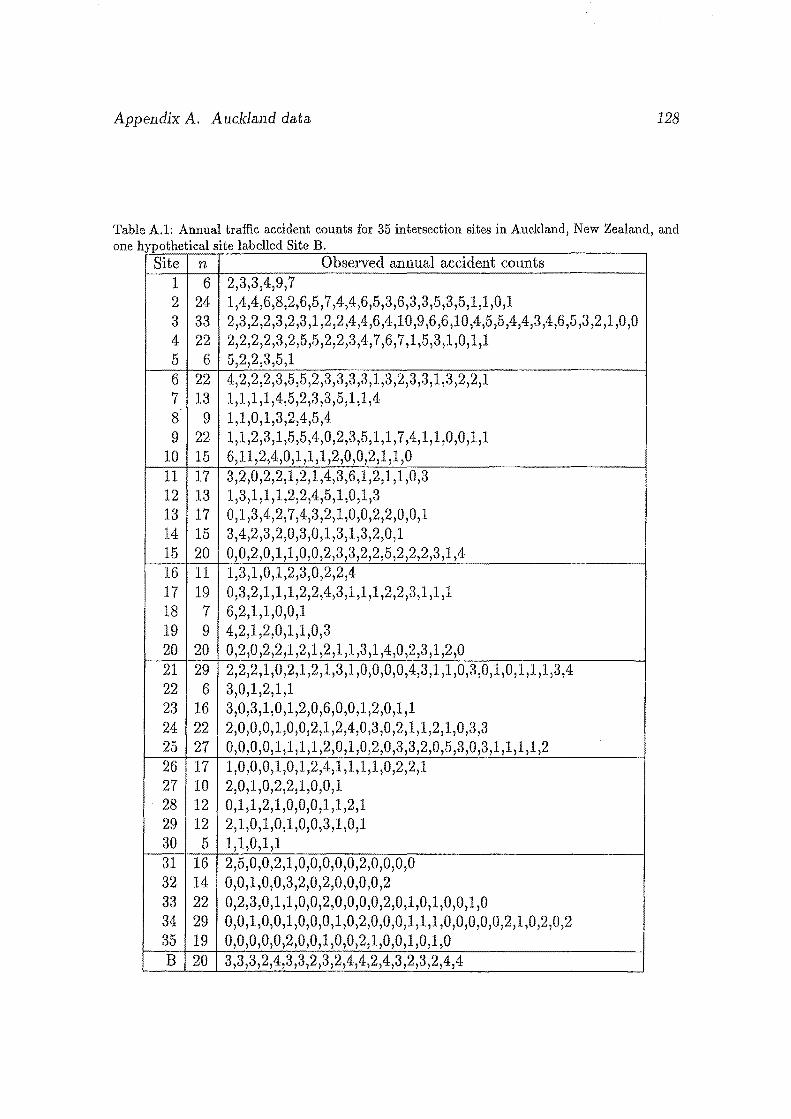
Appendix A. Auckland data 128
Table A.l: Annual traffic accident counts for 35 intersection sites in Auckland, New Zealand, and one hypothetical site labelled Site B.
Site n Observed annual accident counts 1 6 2,3,3,4,9,7 2 24 1,4,4,6,8,2,6,5,7,4,4,6,5,3,6,3,3,5,3,5,1,1,0,1 3 33 2,3,2,2,3,2,3,1,2,2,4,4,6,4,10,9,6,6,10,4,5,5,4,4,3,4,6,5,3,2,1,0,0 4 22 2,2,2,2,3,2,5,5,2,2,3,4,7,6,7,1,5,3,1,0,1,1 5 6 5,2,2,3,5,1 6 22 4,2,2,2,3,5,5,2,3,3,3,3,1,3,2,3,3,1,3,2,2,1 7 13 1,1,1,1,4,5,2,3,3,5,1,1,4 8 9 1,1,0,1,3,2,4,5,4 9 22 1,1,2,3,1,5,5,4,0,2,3,5,1,1,7,4,1,1,0,0,1,1
10 15 6,11,2,4,0,1,1,1,2,0,0,2,1,1,0 11 17 3,2,0,2,2,1,2,1,4,3,6,1,2,1,1,0,3 12 13 1,3,1,1,1,2,2,4,5,1,0,1,3 13 17 0,1,3,4,2,7,4,3,2,1,0,0,2,2,0,0,1 14 15 3,4,2,3,2,0,3,0,1,3,1,3,2,0,1 15 20 0,0,2,0,1,1,0,0,2,3,3,2,2,5,2,2,2,3,1,4 16 11 1,3,1,0,1,2,3,0,2,2,4 17 19 0,3,2,1,1,1,2,2,4,3,1,1,1,2,2,3,1,1,1 18 7 6,2,1,1,0,0,1 19 9 4,2,1,2,0,1,1,0,3 20 20 0,2,0,2,2,1,2,1,2,1,1,3,1,4,0,2,3,1,2,0 21 29 2,2,2,1,0,2,1,2,1,3,1,0,0,0,0,4,3,1,1,0,3,0,1,0,1,1,1,3,4 22 6 3,0,1,2,1,1 23 16 3,0,3,1,0,1,2,0,6,0,0,1,2,0,1,1 24 22 2,0,0,0,1,0,0,2,1,2,4,0,3,0,2,1,1,2,1,0,3,3 25 27 0,0,0,0,1,1,1,1,2,0,1,0,2,0,3,3,2,0,5,3,0,3,1,1,1,1,2 26 17 1,0,0,0,1,0,1,2,4,1,1,1,1,0,2,2,1 27 10 2,0,1,0,2,2,1,0,0,1 28 12 0,1,1,2,1,0,0,0,1,1,2,1 29 12 2,1,0,1,0,1,0,0,3,1,0,1 30 5 1,1,0,1,1 31 16 2,5,0,0,2,1,0,0,0,0,0,2,0,0,0,0 32 14 0,0,1,0,0,3,2,0,2,0,0,0,0,2 33 22 0,2,3,0,1,1,0,0,2,0,0,0,0,2,0,1,0,1,0,0,1,0 34 29 0,0,1,0,0,1,0,0,0,1,0,2,0,0,0,1,1,1,0,0,0,0,0,2,1,0,2,0,2 35 19 0,0,0,0,0,2,0,0,1,0,0,2,1,0,0,1,0,1,0 B 20 3,3,3,2,4,3,3,2,3,2,4,4,2,4,3,2,3,2,4,4
Appendix B
Bayes factor numerical results
129
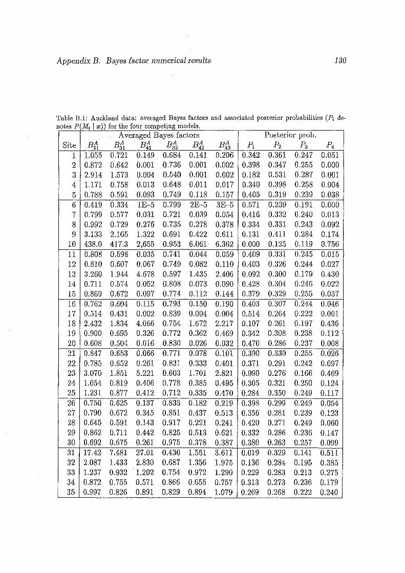
Appendix B. Bayes factor numerical results 130
Table B.l: Auckland data: averaged Bayes factors and associated posterior probabilities (Pi de-notes P(Mi I :v)) for the four competing models.
Averaged Bayes factors tl Posterior prob. Site Bf.r Bft Bfi B~ B~ B P1 P2 P3 P4
1 1.055 0.721 0.149 0.684 0.141 0.206 0.342 0.361 0.247 0.051 2 0.872 0.642 0.001 0.736 0.001 . 0.002 0.398 0.347 0.255 0.000 3 2.914 1.573 0.004 0.540 0.001 0.002 0.182 0.531 0.287 0.001 4 1.171 0.758 0.013 0.648 0.011 0.017 0.340 0.398 0.258 0.004 5 0.788 0.591 0.093 0.749 0.118 0.157 0.405 0.319 0.239 0.038 6 0.419 0.334 1E-5 0.799 2E-5 3E-5 0.571 0.239 0.191 0.000 7 0.799 0.577 0.031 0.721 0.039 0.054 0.416 0.332 0.240 0.013 8 0.992 0.729 0.276 0.735 0.278 0.378 0.334 0.331 0.243 0.092 9 3.133 2.165 1.322 0.691 0.422 0.611 0.131 0.411 0.284 0.174
10 438.0 417.3 . 2,655 0.953 6.061· 6.362 0.000 0.125 0.119 0.756 11 0.808 0.598 0.035 0.741 0.044 0.059 0.409 0.331 0.245 0.015 12 0.810 0.607 0.067 0.749 0.082 0.110 0.403 0.326 0.244 0.027 13 3.260 1.944 4.678 0.597 1.435 2.406 0.092 0.300 0.179 0.430 14 0.711 0.574 0.052 0.808 0.073 0.090 0.428 0.304 0.246 0.022 15 0.869 0.672 0.097 0.774 0.112 0.144 0.379 0.329 0.255 0.037 16 0.762 0.604 0.115 0.793 0.150 0.190 0.403 0.307 0.244 0.046 17 0.514 0.431 0.002 0.839 0.004 0.004 0.514 0.264 0.222 0.001 18 2.432 1.834 4.066 0.754 1.672 2.217 0.107 0.261 0.197 0.436 19 0.900 0.695 0.326 0.772 0.362 0.469 0.342 0.308 0.238 0.112 20 0.608 0.504 0.016 0.830 0.026 0.032 0.470 0.286 0.237 0.008 21 0.847 0.653 0.066 0.771 0.078 0.101 0.390 0.330 0.255 0.026 22 0.785 0.652 0.261 0.831 0.333 0.401 0.371 0.291 0.242 0.097 23 3.070 1.851 5.221 0.603 1.701 2.821 0.090 0.276 0.166 0.469 24 1.054 0.819 0.406 0.778 0.385 0.495 0.305 0.321 0.250 0.124 25 1.231 0.877 0.412 0.712 0.335 0.470 0.284 0.350 0.249 0.117 26 0.750 0.625 0.137 0.833 0.182 0.219 0.398 0.299 0.249 0.054 27 0.790 0.672 0.345 0.851 0.437 0.513 0.356 0.281 0.239 0.123 28 0.645 0.591 0.143 0.917 0.221 0.241 0.420 0.271 0.249 0.060 29 0.862 0.711 0.442 0.825 0.513 0.621 0.332 0.286 0.236 0.147 30 0.692 0.675 0.261 0.975 0.378 0.387 0.380 0.263 0.257 0.099 31 17.42 7.481 27.01 0.430 1.551 3.611 0.019 0.329 0.141 0.511 32 2.087 1.433 2.830 0.687 1.356 1.975 0.136 0.284 0.195 0.385 33 1.237 0.932 1.202 0.754 0.972 1.290 0.229 0.283 0.213 0.275 34 0.872 0.755 0.571 0.866 0.655 0.757 0.313 0.273 0.236 0.179 35 0.997 0.826 0.891 0.829 0.894 1.079 0.269 0.268 0.222 0.240
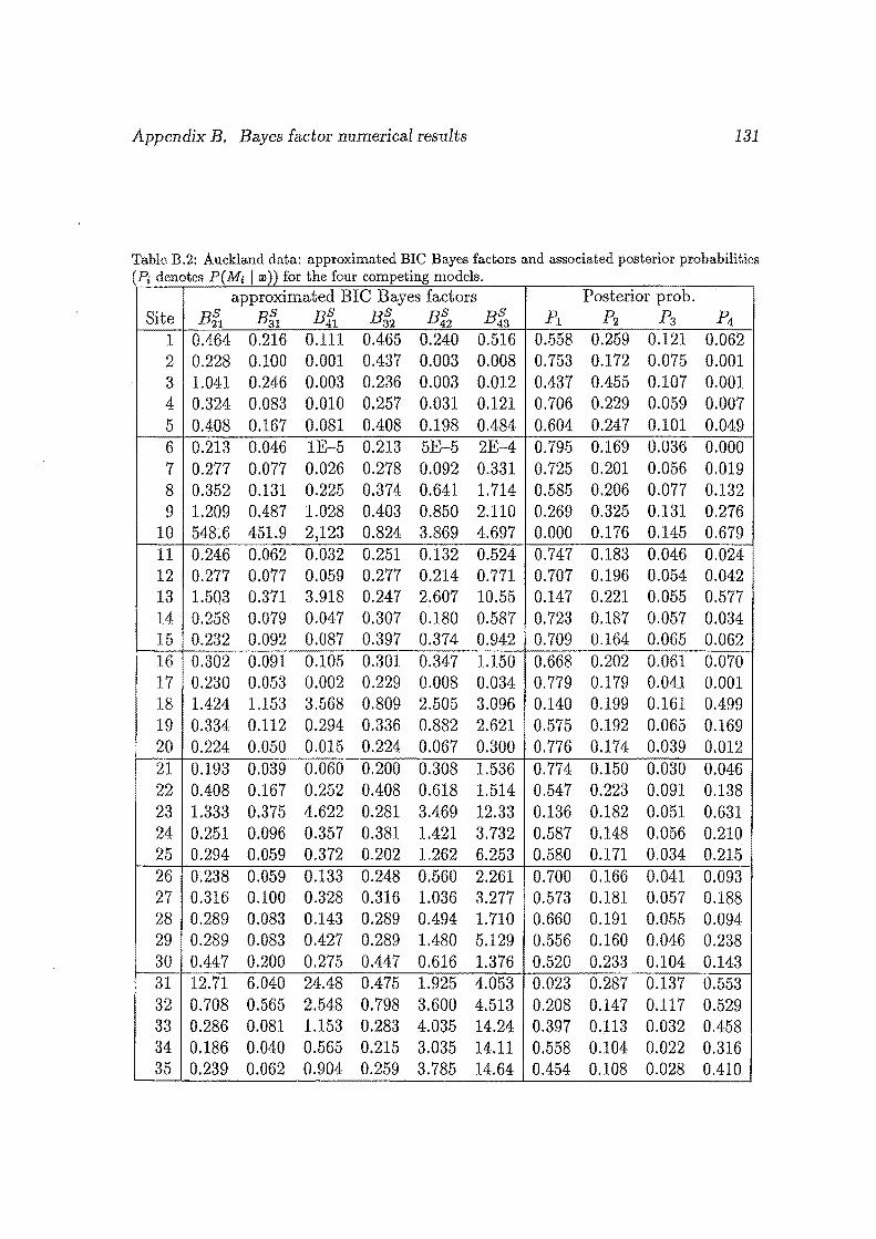
Appendix B. Bayes factOl' numerical results 131
Table B.2: Auckland data: approximated BIC Bayes factors and associated posterior probabilities (Pi denotes P(Mi I m)) for the four competing models.
approximated BIC Bayes factors Posterior prob. Site Bf1 Bff1 Bf1 Bff2 B~ Bf3 pl p2 p3 p4
1 0.464 0.216 0.111 0.465 0.240 0.516 0.558 0.259 0.121 0.062 2 0.228 0.100 0.001 0.437 0.003 0.008 0.753 0.172 0.075 0.001 3 1.041 0.246 0.003 0.236 0.003 0.012 0.437 0.455 0.107 0.001 4 0.324 0.083 0.010 0.257 0.031 0.121 0.706 0.229 0.059 0.007 5 0.408 0.167 0.081 0.408 0.198 0.484 0.604 0.247 0.101 0.049 6 0.213 0.046 1E-5 0.213 5E-5 2E-4 0.795 0.169 0.036 0.000 7 0.277 0.077 0.026 0.278 0.092 0.331 0.725 0.201 0.056 0.019 8 0.352 0.131 0.225 0.374 0.641 1.714 0.585 0.206 0.077 0.132 9 1.209 0.487 1.028 0.403 0.850 2.110 0.269 0.325 0.131 0.276
10 548.6 451.9 2,123 0.824 3.869 4.697 0.000 0.176 0.145 0.679 11 0.246 0.062 0.032 0.251 0.132 0.524 0.747 0.183 0.046 0.024 12 0.277 0.077 0.059 0.277 0.214 0.771 0.707 0.196 0.054 0.042 13 1.503 0.371 3.918 0.247 2.607 10.55 0.147 0.221 0.055 0.577 14 0.258 0.079 0.047 0.307 0.180 0.587 0.723 0.187 0.057 0.034 15 0.232 0.092 0.087 0.397 0.374 0.942 0.709 0.164 0.065 0.062 16 0.302 0.091 0.105 0.301 0.347 1.150 0.668 0.202 0.061 0.070 17 0.230 0.053 0.002 0.229 0.008 0.034 0.779 0.179 0.041 0.001 18 1.424 1.153 3.568 0.809 2.505 3.096 0.140 0.199 0.161 0.499 19 0.334 0.112 0.294 0.336 0.882 2.621 0.575 0.192 0.065 0.169 20 0.224 0.050 0.015 0.224 0.067 0.300 0.776 0.174 0.039 0.012 21 0.193 0.039 0.060 0.200 0.308 1.536 0.774 0.150 0.030 0.046 22 0.408 0.167 0.252 0.408 0.618 1.514 0.547 0.223 0.091 0.138 23 1.333 0.375 4.622 0.281 3.469 12.33 0.136 0.182 0.051 0.631 24 0.251 0.096 0.357 0.381 1.421 3.732 0.587 0.148 0.056 0.210 25 0.294 0.059 0.372 0.202 1.262 6.253 0.580 0.171 0.034 0.215 26 0.238 0.059 0.133 0.248 0.560 2.261 0.700 0.166 0.041 0.093 27 0.316 0.100 0.328 0.316 1.036 3.277 0.573 0.181 0.057 0.188 28 0.289 0.083 0.143 0.289 0.494 1.710 0.660 0.191 0.055 0.094 29 0.289 0.083 0.427 0.289 1.480 5.129 0.556 0.160 0.046 0.238 30 0.447 0.200 0.275 0.447 0.616 1.376 0.520 0.233 0.104 0.143 31 12.71 6.040 24.48 0.475 1.925 4.053 0.023 0.287 0.137 0.553 32 0.708 0.565 2.548 0.798 3.600 4.513 0.208 0.147 0.117 0.529 33 0.286 0.081 1.153 0.283 4.035 14.24 0.397 0.113 0.032 0.458 34 0.186 0.040 0.565 0.215 3.035 14.11 0.558 0.104 0.022 0.316 35 0.239 0.062 0.904 0.259 3.785 14.64 0.454 0.108 0.028 0.410
Appendix C
Tables of model adequacy and
power calculations
132
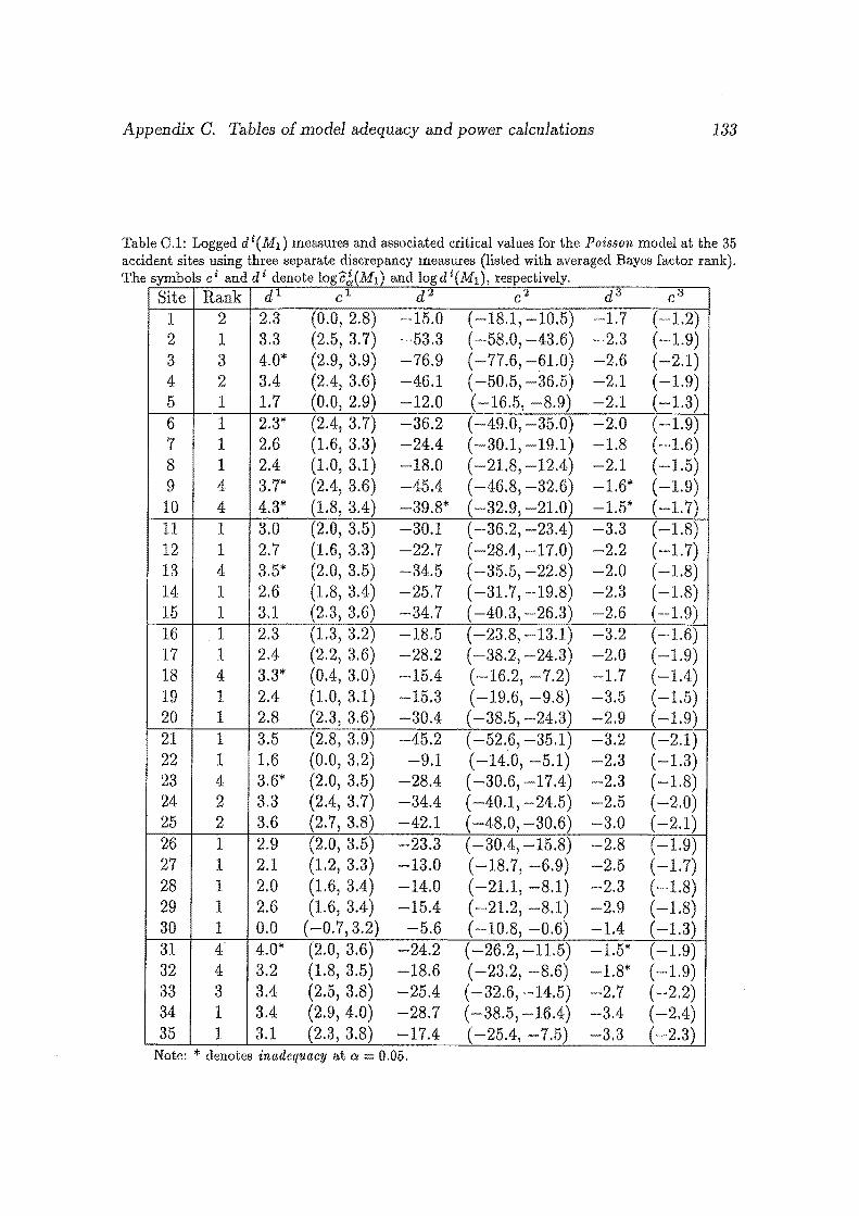
Appendix C. Tables of model adequacy and power calculations 133
Table 0.1: Logged di(M1) measures and associated critical values for the Poisson model at the 35 accident sites using three separate discrepancy measures (listed with averaged Bayes factor rank).
e symbols ci and di denote logc~(Ml) and logdi(M1), respectively. Th
~R~nk dl cl d2 c2 d3 ca
2.3 (0.0, 2.8) -15.0 ( -18.1, -10.5) -1.7 ( -1.2) 2 1 3.3 (2.5, 3.7) -53.3 ( -58.0, -43.6) -2.3 ( -1.9) 3 3 4.0* (2.9, 3.9) -76.9 ( -77.6, -61.0) -2.6 ( -2.1) 4 2 3.4 (2.4, 3.6) -46.1 ( -50.5, -36.5) -2.1 (-1.9) 5 1 1.7 (0.0, 2.9) -12.0 ( -16.5, -8.9) -2.1 ( -1.3) 6 1 2.3* (2.4, 3.7) -36.2 ( -49.0, -35.0) -2.0 (-1.9) 7 1 2.6 (1.6, 3.3) -24.4 ( -30.1, -19.1) -1.8 ( -1.6) 8 1 2.4 (1.0, 3.1) -18.0 ( -21.8, -12.4) -2.1 ( -1.5) 9 4 3.7* (2.4, 3.6) -45.4 ( -46.8, -32.6) -1.6* ( -1.9)
10 4 4.3* (1.8, 3.4) -39.8* ( -32.9, -21.0) -1.5* ( -1.7) 11 1 3.0 (2.0, 3.5) -30.1 ( -36.2, -23.4) -3.3 ( -1.8) 12 1 2.7 (1.6, 3.3) -22.7 (-28.4,-17.0) -2.2 ( -1.7) 13 4 3.5* (2.0, 3.5) -34.5 ( -35.5, -22.8) -2.0 (-1.8) 14 1 2.6 (1.8, 3.4) -25.7 ( -31.7, -19.8) -2.3 ( -1.8) 15 1 3.1 (2.3, 3.6) -34.7 ( -40.3, -26.3) -2.6 ( -1.9) 16 1 2.3 (1.3, 3.2) -18.5 ( -23.8, -13.1) -3.2 ( -1.6) 17 1 2.4 (2.2, 3.6) -28.2 ( -38.2, -24.3) -2.0 (-1.9) 18 4 3.3* (0.4, 3.0) -15.4 (-16.2, -7.2) .7 (-1.4) 19 1 2.4 (1.0, 3.1) -15.3 ( -19.6, -9.8) -3.5 ( -1.5) 20 1 2.8 (2.3, 3.6) -30.4 ( -38.5, -24.3) -2.9 ( -1.9) 21 1 3.5 (2.8, 3.9) -45.2 ( -52 .. 6, -35.1) -3.2 ( -2.1) 22 1 1.6 (0.0, 3.2) -9.1 (-14.0, -5.1) -2.3 ( -1.3) 23 4 3.6* (2.0, 3.5) -28.4 ( -30.6, -17.4) -2.3 (-1.8) 24 2 3.3 (2.4, 3.7) -34.4 ( -40.1, -24.5) -2.5 ( -2.0) 25 2 3.6 (2.7, 3.8) -42.1 ( -48.0, -30.6) -3.0 ( -2.1) 26 1 2.9 (2.0, 3.5) -23.3 ( -30.4, 15.8) -2.8 ( -1.9) 27 1 2.1 (1.2, 3.3) -13.0 ( -18.7, -6.9) -2.5 ( -1.7) 28 1 2.0 (1.6, 3.4) -14.0 ( -21.1, 1) -2.3 ( -1.8) 29 1 2.6 (1.6, 3.4) -15.4 ( -21.2, -8.1) -2.9 ( -1.8) 30 1 0.0 (-0.7, 3.2) -5.6 ( -10.8, -0.6) -1.4 ( -1.3) 31 4 4.0* (2.0, 3.6) -24.2 ( -26.2, ·11.5) -1.5* ( -1.9) 32 4 3.2 (1.8, 3.5) -18.6 ( -23.2, -8.6) -1.8* ( -1.9) 33 3 3.4 (2.5, 3.8) -25.4 ( -32.6, -14.5) -2.7 ( -2.2) 34 1 3.4 (2.9, 4.0) -28.7 ( -38.5, -16.4) -3.4 ( -2.4) 35 1 3.1 (2.3, 3.8) -17.4 ( -25.4, -7.5) -3.3 ( -2.3)
Note: * denotes inadequacy at a 0.05.
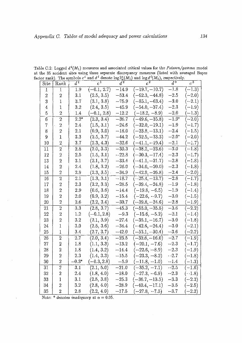
Appendix G. Tables of model adequacy and power calculations 134
Table C.2: Logged di(M1) measures and associated critical values for the Poisson/gamma model at the 35 accident sites using three separate discrepancy measures (listed with averaged Bayes factor rank) The symbols ci and d 1 denote logc'(M1) and logdi(M1), respectively. ct
Site Rank dl cl d2 cz d3 c3
1 1 1.9 (-0.1, 2.7) -14.9 ( -19.7,-10.7) -1.8 ( -1.3) 2 2 3.1 (2.5, 3.5) -53.4 ( -62.3, -44.8) -2.5 ( -2.0) 3 1 3.7 (3.1, 3.8) -75.9 ( -85.1, -63.4) -3.0 (-2.1) 4 1 3.2 (2.4, 3.5) -45.9 ( -54.0, -37.4) -2.3 (-1.9) 5 2 1.4 ( -0.1, 2.8) -12.2 ( -18.2, -8.9) -2.0 ( -1.3) 6 2 2.2* (2.3, 3.4) -36.7 ( -49.6, -35.8) -1.9* ( -2.0) 7 2 2.4 (1.5, 3.1) -24.6 (-32.0, -19.1) -1.9 ( -1.7) 8 2 2.1 (0.9, 3.0) 18.0 ( -23.8, -13.1) -2.4 ( -1.5) 9 1 3.3 (2.5, 3.7) -44.2 ( -52.5, -33.3) -2.0* ( -2.0)
10 2 3.7 (2.3, 4.3) -32.6 ( -41.1, -19.4) -2.1 ( -1.7) 11 2 2.8 (2.0, 3.3) -30.3 ( -38.2,-23.6) -3.0 ( -1.8) 12 2 2.5 (1.5, 3.1) -22.8 (-30.3,-17.4) -2.3 ( -1.7) 13 2 3.1 (2.1, 3.7) -33.4 ( -41.1, -21.7) -2.8 ( -1.8) 14 2 2.4 (1.8, 3.2) -26.0 ( -34.0, -20.0) -2.3 ( -1.8) 15 2 2.9 (2.3, 3.5) . -34.9 ( -42.9, -26.8) -2.4 ( -2.0) 16 2 2.1 (1.3, 3.1) -18.7 (-25.4, -13.7) -2.8 ( ~1.7) 17 2 2.3 (2.2, 3.3) -28.5 ( -39.4, -24.8) -1.9 ( -1.8) 18 2 2.9 (0.6, 3.6) -14.4 ( -19.8, -6.5) -1.9 ( -1.4) 19 2 2.0 (0.9, 3.2) -15.4 ( -22.6, -9.7) -3.0 ( -1.5) 20 2 2.6 (2.2, 3.4) -30.7 ( -39.8, -24.6) -2.8 ( -1.9) 21 2 3.3 (2.8, 3. 7) -45.3 ( -55.0, -35.5) -3.6 ( -2.2) 22 2 1.2 ( -0.1, 2.8) -9.3 ( -15.6, -5.2) -2.1 (-1.4) 23 2 3.2 (2.1, 3.9) -27.4 ( -35.1, -16.7) -3.0 (-1.8) 24 1 3.0 (2.5, 3.6) -34.4 ( -42.6, -24.4) -3.0 ( -2.1) 25 1 3.4 (2.7, 3.7) -42.0 ( -53.1, -30.4) -3.6 ( -2.2) 26 2 2.7 (2.0, 3.4) -23.5 ( -32.6,-16.0) -2.7 (-1.9) 27 2 1.8 (1.1, 3.3) -13.2 ( -20.1, -7.6) -2.3 ( -1.7) 28 2 1.8 (1.4, 3.2) -14.4 ( -22.6, -8.9) -2.3 ( -1.9) 29 2 2.3 (1.4, 3.3) -15.5 ( -23.3, -8.2) -2.7 ( -1.8) 30 2 -0.3* ( -0.3, 2.8) -5.9 ( -11.8, -1.0) -1.4 ( -1.3) 31 2 3.1 (2.1, 5.0) -21.0 ( -35.2, -7.1) -2.5 ( -1.6) 32 2 2.4 (1.8, 4.0) -18.0 ( -27.3, -6.9) -2.3 ( -1.8) 33 1 3.1 (2.5, 3.8) -25.3 ( -36.7, -13.5) -3.3 ( -2.2) 34 2 3.2 (2.8, 4.0) -28.9 ( -40.4, -17.1) -3.5 ( -2.5) 35 2 2.8 (2.2, 4.0) -17.5 ( -27.8, -7.5) -3.7 ( -2.2)
Note: * denotes inadequacy at a; = 0.05.
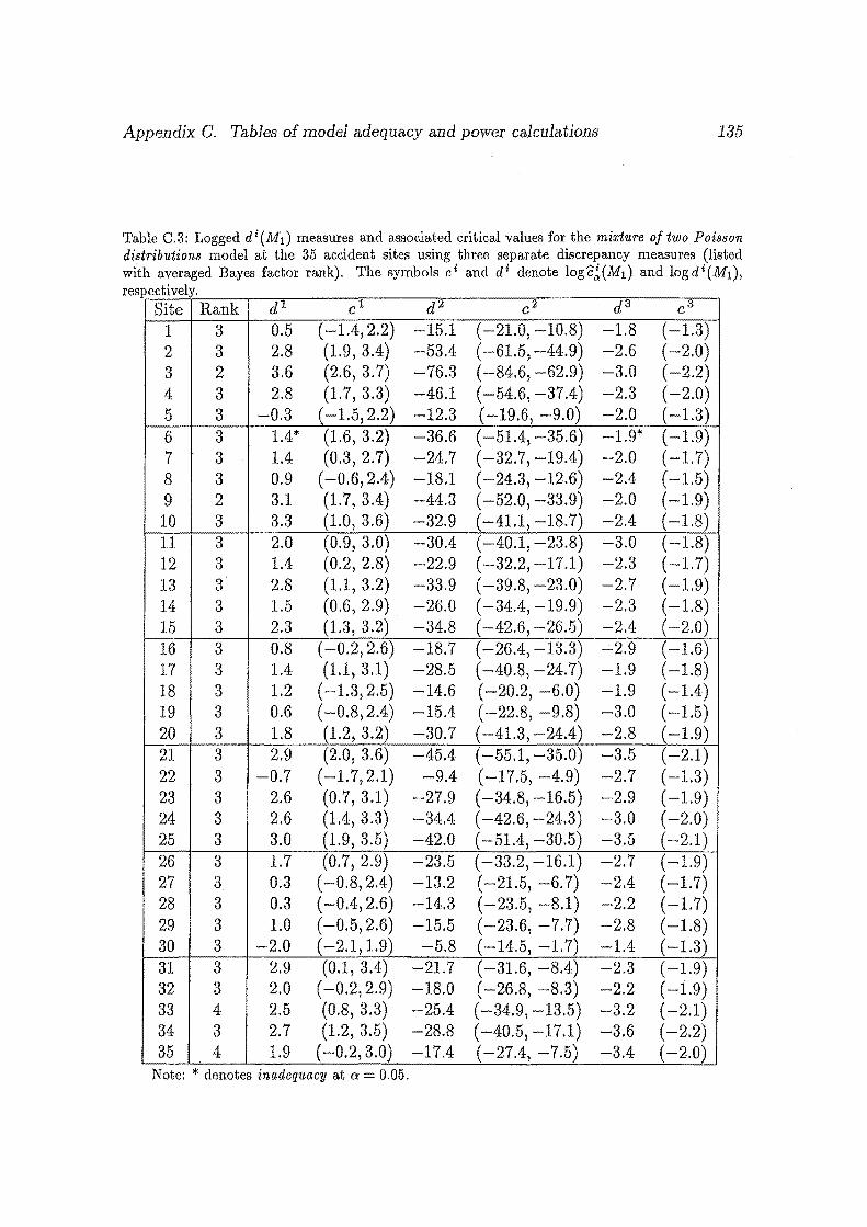
Appendix C. Tables of model adequacy and power calculations 135
Table C.3: Logged di(Ml) measures and associated critical values for the mixture of two Poisson distributions model at the 35 accident sites using three separate discrepancy measures (listed with averaged Bayes factor rank). The symbols c' and di denote logc~(M1) and logdi(M1), res t' l pee 1ve .
Site Rank dl cl d2 c2 d3 c3
1 3 0.5 ( -1.4, 2.2) -15.1 ( -21.0, -10.8) -1.8 ( -1.3) 2 3 2.8 (1.9, 3.4) -53.4 ( -61.5, -44.9) -2.6 ( -2.0) 3 2 3.6 (2.6, 3. 7) -76.3 ( -84.6, -62.9) -3.0 ( -2.2) 4 3 2.8 (1.7, 3.3) -46.1 ( -54.6, -37.4) -2.3 ( -2.0) 5 3 -0.3 ( -1.5, 2.2) -12.3 ( -19.6, -9.0) -2.0 (-1.3) 6 3 1.4* (1.6, 3.2) -36.6 ( -51.4, -35.6) -1.9* ( -1.9) 7 3 1.4 (0.3, 2.7) -24.7 (-32.7, -19.4) -2.0 ( -1.7) 8 3 0.9 ( -0.6, 2.4) -18.1 ( -24.3, -12.6) -2.4 ( -1.5) 9 2 3.1 (1.7, 3.4) -44.3 (-52.0, -33.9) -2.0 ( -1.9)
10 3 3.3 (1.0, 3.6) -32.9 (-41.1, -18.7) -2.4 ( -1.8) 11 3 2.0 (0.9, 3.0) -30.4 ( -40.1, -23.8) -3.0 ( -1.8) 12 3 1.4 (0.2, 2.8) -22.9 ( -32.2, -17.1) -2.3 ( -1.7) 13 3 2.8 (1.1, 3.2) -33.9 ( -39.8, -23.0) -2.7 (-1.9) 14 3 1.5 (0.6, 2.9) -26.0 ( -34.4, -19.9) -2.3 ( -1.8) 15 3 2.3 (1.3, 3.2) -34.8 ( -42.6, -26.5) -2.4 ( -2.0) 16 3 0.8 ( -0.2, 2.6) -18.7 (-26.4, -13.3) -2.9 ( -1.6) 17 3 1.4 (1.1, 3.1) -28.5 ( -40.8, -24.7) -1.9 ( -1.8) 18 3 1.2 ( -1.3, 2.5) -14.6 ( -20.2, -6.0) -1.9 (-1.4) 19 3 0.6 (-0.8,2.4) -15.4 ( -22.8, -9.8) -3.0 ( -1.5) 20 3 1.8 (1.2, 3.2) -30.7 ( -41.3, -24.4) -2.8 (-1.9) 21 3 2.9 (2.0, 3.6) -45.4 ( -55.1, -35.0) -3.5 (-2.1) 22 3 -0.7 (-1.7,2.1) -9.4 ( -17.5, -4.9) -2.7 ( -1.3) 23 3 2.6 (0.7, 3.1) -27.9 ( -34.8, -16.5) -2.9 (-1.9) 24 3 2.6 (1.4, 3.3) -34.4 (-42.6, -24.3) -3.0 ( -2.0) 25 3 3.0 (1.9, 3.5) -42.0 ( -51.4, -30.5) -3.5 ( -2.1) 26 3 1.7 (0.7, 2.9) -23.5 ( -33.2, -16.1) -2.7 ( -1.9) 27 3 0.3 ( -0.8, 2.4) -13.2 ( -21.5, -6. 7) -2.4 ( -1. 7) 28 3 0.3 ( -0.4, 2.6) -14.3 ( -23.5, -8.1) -2.2 ( -1.7) 29 3 1.0 ( -0.5, 2.6) -15.5 ( -23.6, -7.7) -2.8 ( -1.8) 30 3 -2.0 (-2.1, 1.9) -5.8 ( -14.5, ·1.7) -1.4 (-1.3) 31 3 2.9 (0.1, 3.4) -21.7 ( -31.6, -8.4) -2.3 ( -1.9) 32 3 2.0 ( -0.2, 2.9) -18.0 ( -26.8, -8.3) -2.2 ( -1.9) 33 4 2.5 (0.8, 3.3) -25.4 ( -34.9, -13.5) -3.2 ( -2.1) 34 3 2.7 (1.2, 3.5) -28.8 (-40.5,-17.1) -3.6 ( -2.2) 35 4 1.9 ( -0.2, 3.0) -17.4 (-27.4, -7.5) -3.4 ( -2.0)
Note: * denotes inadequacy at a= 0.05.
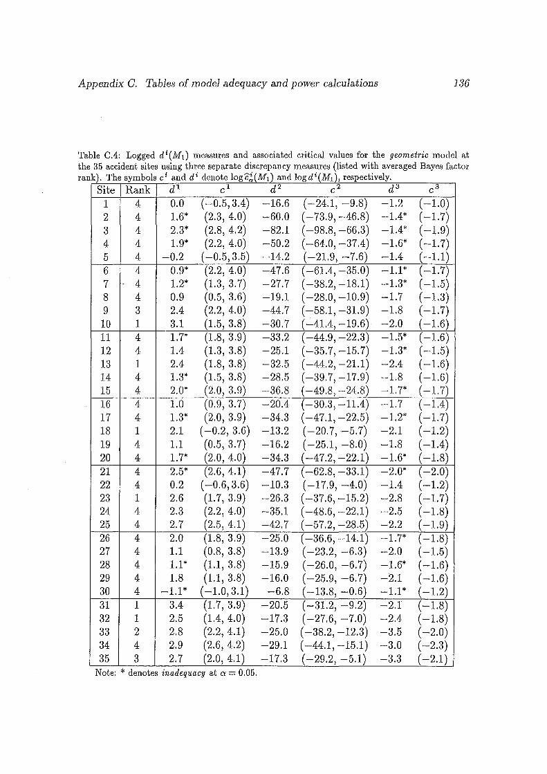
Appendix G. Tables of model adequacy and power calculations 136
Table C.4: Logged di(M1 ) measures and associated critical values for the geometric model at the 35 accident sites using three separate discrepancy measures (listed with averaged Bayes factor rank). The symbols ci and di denote logc~(Ml) and logdi(Ml), respectively.
Site Rank dl cl d2 c2 d3 c3
1 4 0.0 ( -0.5, 3.4) -16.6 ( -24.1, -9.8) -1.2 ( -1.0) 2 4 1.6* (2.3, 4.0) -60.0 ( -73.9, -46.8) -1.4* ( -1.7) 3 4 2.3* (2.8, 4.2) -82.1 ( -98.8, -66.3) -1.4* (-1.9) 4 4 1.9* (2.2, 4.0) -50.2 ( -64.0, -37.4) -1.6* ( -1.7) 5 4 -0.2 (-0.5, 3.5) -14.2 (-21.9, -7.6) -1.4 ( -1.1) 6 4 0.9* (2.2, 4.0) -47.6 ( -61.4, -35.0) -1.1* ( -1.7) 7 4 1.2* (1.3, 3. 7) -27.7 ( -38.2, -18.1) -1.3* (-1.5) 8 4 0.9 (0.5, 3.6) -19.1 ( -28.0, -10.9) -1.7 (-1.3) 9 3 2.4 (2.2, 4.0) -44.7 ( -58.1, -31.9) -1.8 ( -1.7)
10 1 3.1 (1.5, 3.8) -30.7 ( ...:._41.4, -19.6) -2.0 ( -1.6) 11 4 1.7* (1.8, 3.9) -33.2 ( -44.9, -22.3) -1.5* (-1.6) 12 4 1.4 (1.3, 3.8) -25.1 ( -35.7, -15.7) -1.3* (-1.5) 13 1 2.4 (1.8, 3.8) -32.5 ( -44.2, -21.1) -2.4 ( -1.6) 14 4 1.3* (1.5, 3.8) -28.5 ( -39.7, -17.9) -1.8 ( -1.6) 15 4 2.0* (2.0, 3.9) -36.8 ( -49.8, -24.8) -1.7* ( -1.7) 16 4 1.0 (0.9, 3.7) -20.4 ( -30.3, -11.4) -1.7 ( -1.4) 17 4 1.3* (2.0, 3.9) -34.3 ( -47.1, -22.5) -1.2* ( -1.7) 18 1 2.1 (-0.2, 3.6) -13.2 ( -20.7, -5.7) -2.1 (-1.2) 19 4 1.1 (0.5, 3. 7) -16.2 ( -25.1, -8.0) -1.8 ( -1.4) 20 4 1.7* (2.0, 4.0) -34.3 ( -47.2, -22.1) -1.6* ( -1.8) 21 4 2.5* (2.6, 4.1) -47.7 ( -62.8, -33.1) -2.0* ( -2.0) 22 4 0.2 (-0.6, 3.6) -10.3 ( -17.9, -4.0) -1.4 ( -1.2) 23 1 2.6 (1.7, 3.9) -26.3 ( -37.6, -15.2) -2.8 ( -1.7) 24 4 2.3 (2.2, 4.0) -35.1 ( -48.6, -22.1) -2.5 ( -1.8) 25 4 2.7 (2.5, 4.1) -42.7 ( -57.2, -28.5) -2.2 ( -1.9) 26 4 2.0 (1.8, 3.9) -25.0 ( -36.6, -14.1) -1.7* ( -1.8) 27 4 1.1 (0.8, 3.8) -13.9 ( -23.2, -6.3) -2.0 (-1.5) 28 4 1.1 * (1.1, 3.8) -15.9 ( -26.0, -6.7) -1.6* ( -1.6) 29 4 1.8 (1.1, 3.8) -16.0 ( -25.9, -6. 7) -2.1 ( -1.6) 30 4 -1.1* (-1.0,3.1) -6.8 ( -13.8, -0.6) -1.1* ( -1.2) 31 1 3.4 (1.7, 3.9) -20.5 ( -31.2, -9.2) -2.1 ( -1.8) 32 1 2.5 (1.4, 4.0) -17.3 ( -27.6, -7.0) -2.4 (-1.8) 33 2 2.8 (2.2, 4.1) -25.0 ( -38.2, -12.3) -3.5 ( -2.0) 34 4 2.9 (2.6, 4.2) -29.1 ( -44.1, -15.1) -3.0 ( -2.3) 35 3 2.7 (2.0, 4.1) -17.3 ( -29.2, -5.1) -3.3 (-2.1)
Note: * denotes inadequacy at a= 0.05.
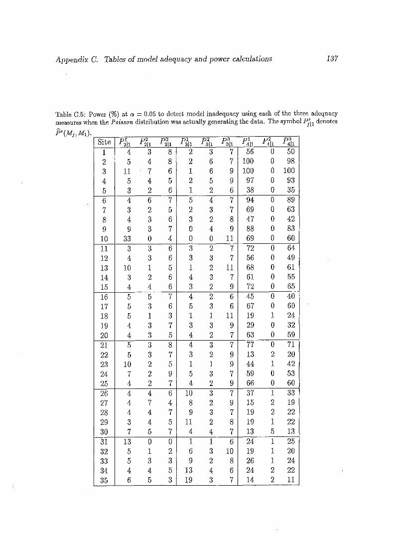
Appendix C. Tables of model adequacy and power calculations 137
Table C.5: Power (%) at a = 0.05 to detect model inadequacy using each of the three adequacy measures when the Poisson distribution was actually generating the data. The symbol P!'11 denotes ~ J.
pr(Mj,Ml)· Site Pih Pi11 p~l Pih Pi11 p~l PJ11 Pf11 p~l
1 4 3 8 2 3 7 56 0 50
2 5 4 8 2 6 7 100 0 98
3 11 7 6 1 6 9 100 0 100
4 5 4 5 2 5 9 97 0 93
5 3 2 6 1 2 6 38 0 35
6 4 6 7 5 4 7 94 0 89
7 3 2 5 2 3 7 69 0 63
8 4 3 6 3 2 8 47 0 42
9 9 3 7 0 4 9 88 0 83
10 33 0 4 0 0 11 69 0 60
11 3 3 6 3 2 7 72 0 64 12 4 3 6 3 3 7 56 0 49
13 10 1 5 1 2 11 68 0 61
14 3 2 6 4 3 7 61 0 55 15 4 4 6 3 2 9 72 0 65
16 5 5 7 4 2 6 45 0 40
17 5 3 6 5 3 6 67 0 60
18 5 1 3 1 1 11 19 1 24
19 4 3 7 3 3 9 29 0 32
20 4 3 5 4 2 7 63 0 59
21 5 3 8 4 3 7 77 0 71 22 5 3 7 3 2 9 13 2 20 23 10 2 5 1 1 9 44 1 42
24 7 2 9 5 3 7 59 0 53 25 4 2 7 4 2 9 66 0 60
26 4 4 6 10 3 7 37 1 33 27 4 7 4 8 2 9 15 2 19 28 4 4 7 9 3 7 19 2 22
29 3 4 5 11 2 8 19 1 22 30 7 5 7 4 4 7 13 5 13
31 13 0 0 1 1 6 24 1 25 32 5 1 2 6 3 10 19 1 20 33 5 3 3 9 2 8 26 1 24 34 4 4 5 13 4 6 24 2 22 35 6 5 3 19 3 7 14 2 11
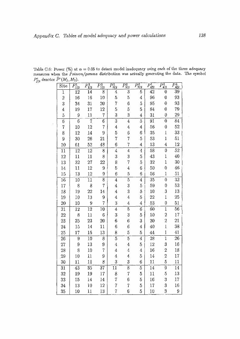
Appendix C. Tables of model adequacy and power calculations 138
Table C.6: Power (%) at a ::::: 0.05 to detect model inadequacy using each of the three adequacy measures when the Poisson/gamma distribution was actually generating the data. The symbol PJ12 denotes pr (Mj, M2).
Site Pf12 Pf12 Pf!2 PJ12 P(f12 PlJ2 ·p1,2 Pl12 Pt12 1 12 14 8 4 3 5 42 0 39 2 16 16 10 5 5 4 96 0 93 3 34 31 20 7 6 5 95 0 93 4 19 17 12 5 5 5 84 0 79 5 9 11 7 3 3 4 31 0 29 6 6 7. 6 3 4 5 91 0 84 7 10 12 7 4 4 4 56 0 52 8 12 14 9 5 6 6 35 1 33 9 30 26 21 7 7 5 53 1 51
10 61 52 48 6 7 4 13 4 12 11 12 12 8 4 4 4 58 0 52 12 11 11 8 3 3 5 43 1 40 13 32 27 22 8 7 5 32 1 30 14 11 12 9 5 4 6 50 0 46 15 13 12 9 6 5 6 56 1 51 16 10 11 8 4 5 4 35 0 32 17 8 8 7 4 3 5 59 0 53 18 19 22 14 4 3 5 10 3 13 19 10 13 9 4 4 5 22 1 25 20 10 9 7 3 4 4 53 0 51 21 12 12 10 4 5 6 60 1 56 22 8 11 6 3 3 5 10 2 17 23 25 23 20 6 6 3 20 2 21 24 15 14 11 6 6 4 40 1 38 25 17 15 13 8 5 5 44 1 41 26 9 10 8 5 5 4 28 1 26 27 9 13 9 4 4 5 12 3 16 28 8 10 7 4 4 4 16 2 18 29 10 11 9 4 4 5 14 2 17 30 11 11 8 3 3 6 11 5 11 31 43 35 37 11 8 5 14 9 14 32 19 19 17 8 7 5 11 5 13 33 15 14 14 7 6 5 16 3 17 34 13 10 12 7 7 5 17 3 16 35 10 11 13 7 6 5 10 3 9
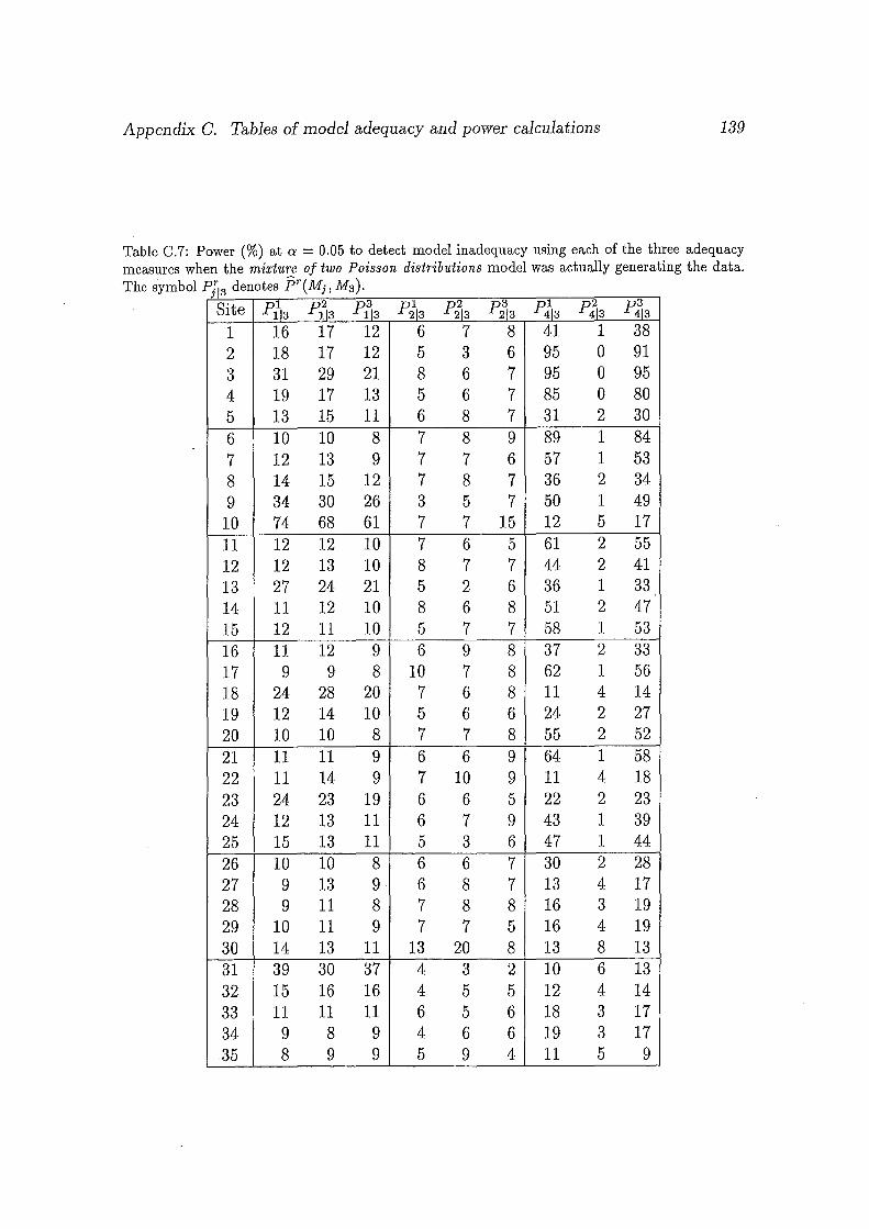
Appendix C. Tables of model adequacy and power calculations 139
Table C.7: Power (%) at a = 0.05 to detect model inadequacy using each of the three adequacy measures when the mixture of two Poisson distributions model was actually generating the data. The symbol PJ13 denotes fir(Mj, Ma).
Site Pfl3 Pfi3 Pl!3 p21!3 P{l3 p~3 PJI3 Pfl3 P1J3
1 16 17 12 6 7 8 41 1 38 2 18 17 12 5 3 6 95 0 91 3 31 29 21 8 6 7 95 0 95 4 19 17 13 5 6 7 85 0 80 5 13 15 11 6 8 7 31 2 30 6 10 10 8 7 8 9 89 1 84 7 12 13 9 7 7 6 57 1 53 8 14 15 12 7 8 7 36 2 34 9 34 30 26 3 5 7 50 1 49
10 74 68 61 7 7 15 12 5 17 11 12 12 10 7 6 5 61 2 55 12 12 13 10 8 7 7 44 2 41 13 27 24 21 5 2 6 36 1 33 14 11 12 10 8 6 8 51 2 47 15 12 11 10 5 7 7 58 1 53 16 11 12 9 6 9 8 37 2 33 17 9 9 8 10 7 8 62 1 56 18 24 28 20 7 6 8 11 4 14 19 12 14 10 5 6 6 24 2 27 20 10 10 8 7 7 8 55 2 52 21 11 11 9 6 6 9 64 1 58 22 11 14 9 7 10 9 11 4 18 23 24 23 19 6 6 5 22 2 23 24 12 13 11 6 7 9 43 1 39 25 15 13 11 5 3 6 47 1 44 26 10 10 8 6 6 7 30 2 28 27 9 13 9 6 8 7 13 4 17 28 9 11 8 7 8 8 16 3 19 29 10 11 9 7 7 5 16 4 19 30 14 13 11 13 20 8 13 8 13 31 39 30 37 4 3 2 10 6 13 32 15 16 16 4 5 5 12 4 14 33 11 11 11 6 5 6 18 3 17 34 9 8 9 4 6 6 19 3 17 35 8 9 9 5 9 4 11 5 9
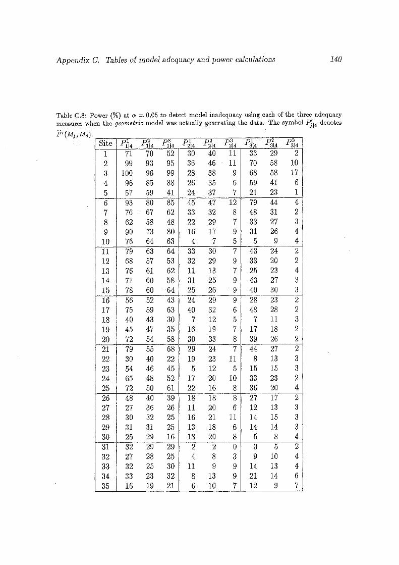
Appendix C. Tables of model adequacy and power calculations 140
Table C.8: Power (%) at a 0.05 to detect model inadequacy using each of the three adequacy measures when the geometric model was actually generating the data. The symbol PJ14 denotes
J3r(MJ,M4) .
PJ-14 Pil4 Site P{,4 Pfl4 Pft4 PJ-14 Pfft4 PS4 p~4 1 71 70 52 30 40 11 33 29 2 2 99 93 95 36 46 11 70 58 10 3 100 96 99 28 38 9 68 58 17 4 96 85 88 26 35 6 59 41 6 5 57 59 41 24 37 7 21 23 1 6 93 80 85 45 47 12 79 44 4 7 76 67 62 33 32 8 48 31 2 8 62 58 48 22 29 7 33 27 3 9 90 73 80 16 17 9 31 26 4
10 76 64 63 4 7 5 5 9 4 11 79 63 64 33 30 7 43 24 2 12 68 57 53 32 29 9 33 20 2 13 76 61 62 11 13 7 25 23 4 14 71 60 58 31 25 9 43 27 3 15 78 60 64 25 26 ' 9 40 30 3 16 56 52 43 24 29 9 28 23 2 17 75 59 63 40 32 6 48 28 2 18 40 43 30 7 12 5 7 11 3 19 45 47 35 16 19 7 17 18 2 20 72 54 58 30 33 8 39 26 2 21 79 55 68 29 24 7 44 27 2 22 30 40 22 19 23 11 8 13 3 23 54 46 45 5 12 5 15 15 3 24 65 48 52 17 20 10 33 23 2 25 72 50 61 22 16 8 36 20 4 26 48 40 39 18 18 8 27 17 2 27 27 36 26 11 20 6 12 13 3 28 30 32 25 16 21 11 14 15 3 29 31 31 25 13 18 6 14 14 3 30 25 29 16 13 20 8 5 8 4 31 32 29 29 2 2 0 3 5 2 32 27 28 25 4 8 3 9 10 4 33 32 25 30 11 9 9 14 13 4 34 33 23 32 8 13 9 21 14 6 35 16 19 21 6 10 7 12 9 7
Appendix D
Simulation hints and tables of
predictive probability calculations
The uniform, 'shoe' and exponential distributions were easily generated by the
inverse transformation method, as described in Pidd (1986) and briefly summarised
in Section 4.6.3.
Gamma distributed variants can readily be generated from an algorithm detailed
in Fishman (1973), and briefly described as follows. Suppose that X is from a gamma
distribution, g(a, b), and k = [a] where the quantity [a] denotes the largest integer
in a. Fishman considered X to be the sum of k + 1 independent gamma variants, all
with scale parameter b, but the first k of which have unit shape parameter and the
k + 1th having shape parameter y =a- [a]. If Y and Z are independent variants
from Be(1, 1 -1) (the beta density) and g(1, 1), which is the £(1) (the exponential
density), respectively. Then W = (1/b)YZ is a variate with g(a, b).
Generations from both Be(/, 1 -1) and £(1) distributions are straightforward;
y = Ut(O, 1)1/Y Ut(O, 1)1/-r + U2 [0, 1)1/(l--y)
and
Z -log(U[O, 1])
141
Appendix D. Simulation hints and tables of predictive probability calculations 142
provided Ul[O, 1]lh + U2[0, 1]11(1-"'1) ~ 1, where Ui[O, 1) is a random variate from the
uniform [0, 1) distribution, U(O, 1).
For the posterior probabilities numerical calculations of the cumulative gamma
distribution required determination. The cumulative two parameter gamma density
can be rewritten as
G(x I a, b) fox g(u I a, b) du for a> 0, b > 0
rx b(bu )a-1 -bu
lo r(a) e du
- rta) labx ta-1e-t dt.
Bowman and Shenton (1988) describe at least three methods in which this form
of G( x I a, b) can be numerically computed; expanding the exponential, the Stieltjies
continued fraction approach and the continued fraction of Schlomilch. The latter of
these approaches is most readily adopted for these calculations, where
1 {x a-1 -t d e-xxa ( 1 X 2x 3x r(a)lo t e t= r(a) a-x+ a-x+1+ a-x+2+ a-x+3+ ... )
for x > 0 and a > 0. ·The gamma function was calculated via the asymptotic
formula, such that
ln r(x) 1 1 1 1
r::::J (x- 2)lnx- x + 2 1n 2?r + 12x- 360x3 + 1 1 1 691
1260x5 - 1680x7 + 1188x9 - 360360x11 + · · · (D.1)
which converges rapidly achieving any desired level of accuracy when x is large. If
however x is small then implementation of the recurrence formula
r(x) - r(x + m) - ( ) ( ) for m = 1, 2, ... x x+1 ... x+m-1
ensures that equation (D.1) converges rapidly for any x. The specified accuracy
level was assigned to be ± 0.00001, which ordinarily could be reached in summing
ten terms of the continued fraction.
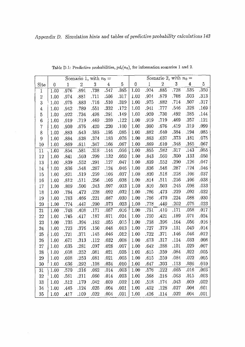
Appendix D. Simulation hints and tables of predictive probability calculations 143
Table D.l: Predictive probabilities, pdi(no), for information scenarios 1 and 2.
Scenario 1, with n0 = Scenario 2, with no=
Site 0 1 2 3 4 5 0 1 2 3 4 5
1 1.00 .976 .891 .738 .547 .365 1.00 .974 .885 .728 .535 .350
2 1.00 .974 .881 .711 .506 .317 1.00 .974 .879 .708 .503 .313
3 1.00 .975 .883 .716 .510 .319 1.00 .975 .882 .714 .507 .317
4 1.00 .942 .780 .551 .332 .172 1.00 .941 .777 .546 .328 .169
5 1.00 .922 .734 .498 .291 .149 1.00 .920 .730 .492 .285 .144
6 1.00 .919 .719 .469 .259 .122 1.00 .919 .719 .469 .257 .121
7 1.00 .900 .676 .420 .220 .100 1.00 .900 .676 .419 .219 .099
8 1.00 .883 .643 .385 .195 .085 1.00 .882 .640 .384 .194 .085
9 1.00 .884 .638 .374 .183 .076 1.00 .883 .637 .373 .181 .075
10 1.00 .869 .611 .347 .166 .067 1.00 .869 .610 .348 .165 .067
11 1.00 .854 .581 .318 .144 .056 1.00 .855 .582 .317 .143 .055 12 1.00 .841 .560 .299 .132 .050 1.00 .843 .560 .300 .133 .050 13 1.00 .839 .552 .291 .127 .047 1.00 .839 .552 .290 .126 .047
14 1.00 .836 .548 .287 .124 .046 1.00 .836 .548 .287 .124 .046 15 1.00 .821 .519 .259 .106 .037 1.00 .820 .518 .258 .106 .037 16 1.00 .812 .511 .256 .106 .038 1.00 .814 .511 .256 .106 ;038
17 1.00 .809 .500 .243 .097 .033 1.00 .810 .503 .245 .098 .033 18 1.00 .784 .472 .228 .092 .032 1.00 .786 .473 .229 .092 .032
19 1.00 .783 .466 .221 .087 .030 1.00 .786 .470 .224 .088 .030 20 1.00 .774 .447 .200 .073 .023 1.00 .778 .449 .202 .075 .023
21 1.00 .748 .408 .171 .057 .016 1.00 .751 .410 .171 .058 .017 22 1.00 .745 .417 .187 .071 .024 1.00 .750 .421 .189 .071 .024 23 1.00 .735 .394 .162 .055 .015 1.00 .738 .396 .164 .056 .016 24 1.00 .723 .376 .150 .048 .013 1.00 .727 .379 .151 .049 .014 25 1.00 .721 .371 .145 .046 .012 1.00 .722 .371 .146 .046 .012 26 1.00 .671 .313 .112 .032 .008 1.00 .673 .317 .114 .033 .008 27 1.00 .635 .281 .097 .028 .007 1.00 .642 .288 .101 .029 .007 28 1.00 .608 .252 .081 .021 .005 1.00 .615 .259 .084 .022 .005 29 1.00 .608 .253 .081 .021 .005 1.00 .615 .259 .084 .022 .005 30 1.00 .636 .292 .108 .034 .010 1.00 .647 .303 .113 .036 .010 31 1.00 .570 .216 .062 .014 .003 1.00 .576 .222 .065 .016 .003 32 1.00 .561 .211 .060 .014 .003 1.00 .568 .216 .063 .015 .003 33 1.00 .512 .170 .042 .009 .002 1.00 .518 .174 .043 .009 .002 34 1.00 .445 .124 .025 .004 .001 1.00 .452 .128 .027 .004 .001 35 1.00 .417 .109 .022 .004 .001 1.00 .426 .114 .022 .004 .001
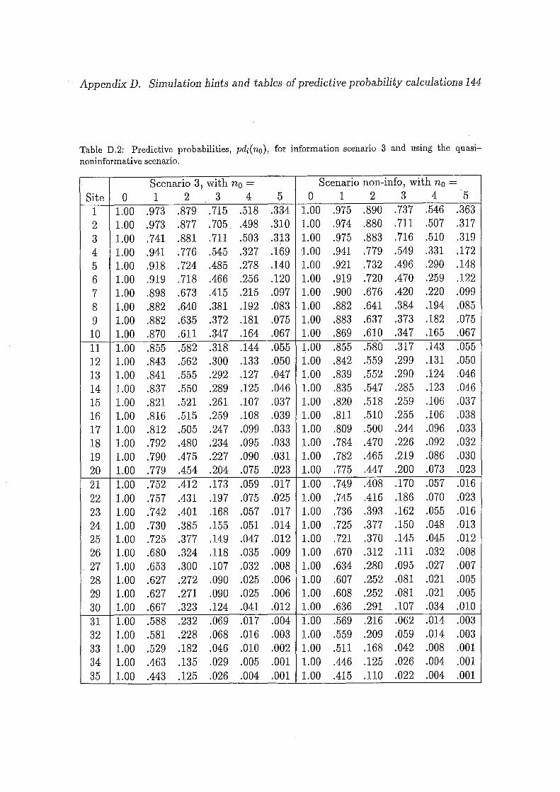
Appendix D. Simulation hints and tables of predictive probability calculations 144
Table D.2: Predictive probabilities, pdi(no), for information scenario 3 and using the quasinoninformative scenario.
Scenario 3, with no = Scenario non-info, with n0 = Site 0 1 2 3 4 5 0 1 2 3 4 5
1 1.00 .973 .879 .715 .518 .334 1.00 .975 .890 .737 .546 .363
2 1.00 .973 .877 .705 .498 .310 1.00 .974 .880 .711 .507 .317
3 1.00 .741 .881 .711 .503 .313 1.00 .975 .883 .716 .510 .319
4 1.00 .941 .776 .545 .327 .169 1.00 .941 .779 .549 .331 .172
5 1.00 .918 .724 .485 .278 .140 1.00 .921 .732 .496 .290 .148
6 1.00 .919 .718 .466 .256 .120 1.00 .919 .720 .470 .259 .122
7 1.00 .898 .673 .415 .215 .097 1.00 .900 .676 .420 .220 .099
8 1.00 .882 .640 .381 .192 .083 1.00 .882 .641 .384 .194 .085
9 1.00 .882 .635 .372 .181 .075 1.00 .883 .637 .373 .182 .075
10 1.00 .870 .611 .347 .164 .067 1.00 .869 .610 .347 .165 .067
11 1.00 .855 .582 .318 .144 .055 1.00 .855 .580 .317 .143 .055
12 1.00 .843 .562 .300 .133 .050 1.00 .842 .559 .299 .131 .050
13 1.00 .841 .555 .292 .127 .047 1.00 .839 .552 .290 .124 .046
14 1.00 .837 .550 .289 .125 .046 1.00 .835 .547 .285 .123 .046
15 1.00 .821 .521 .261 .107 .037 1.00 .820 .518 .259 .106 .037
16 1.00 .816 .515 .259 .108 .039 1.00 .811 .510 .255 .106 .038
17 1.00 .812 .505 .247 .099 .033 1.00 .809 .500 .244 .096 .033 18 1.00 .792 .480 .234 .095 .033 1.00 .784 .470 .226 .092 .032
19 1.00 .790 .475 .227 .090 .031 1.00 .782 .465 .219 .086 .030 20 1.00 .779 .454 .204 .075 .023 1.00 .775 .447 .200 .073 .023
21 1.00 .752 .412 .173 .059 .017 1.00 .749 .408 .170 .057 .016
22 1.00 .757 .431 .197 .075 .025 1.00 .745 .416 .186 .070 .023
23 1.00 .742 .401 .168 .057 .017 1.00 .736 .393 .162 .055 .016 24 1.00 .730 .385 .155 .051 .014 1.00 .725 .377 .150 .048 .013 25 1.00 .725 .377 .149 .047 .012 1.00 .721 .370 .145 .045 .012 26 1.00 .680 .324 .118 .035 .009 1.00 .670 .312 .111 .032 .008 27 1.00 .653 .300 .107 .032 .008 1.00 .634 .280 .095 .027 .007 28 1.00 .627 .272 .090 .025 .006 1.00 .607 .252 .081 .021 .005 29 1.00 .627 .271 .090 .025 .006 1.00 .608 .252 .081 .021 .005 30 1.00 .667 .323 .124 .041 .012 1.00 .636 .291 .107 .034 .010
31 1.00 .588 .232 .069 .017 .004 1.00 .569 .216 .062 .014 .003 32 1.00 .581 .228 .068 .016 .003 1.00 .559 .209 .059 .014 .003 33 1.00 .529 .182 .046 .010 .002 1.00 .511 .168 .042 .008 .001 34 1.00 .463 .135 .029 .005 .001 1.00 .446 .125 .026 .004 .001 35 1.00 .443 .125 .026 .004 .001 1.00 .415 .110 .022 .004 .001