Embed Size (px)
Citation preview
I 1 i i U i ' T f i QUARTERLY REPORT
LANOSAT fl INVESTIGATION PROGRAMME
No. 28230
Ix
REPORT NO. 568 till ^MARCH 19771
PHYSICS AND ENGINEERING LABORATORY
DSIR
NEW ZEALAND
QUARTERLY REPORT
LANf>SAT f. I INVESTIGATION PROGRAMME
No. 28230
REPORT NO. 568 MARCH 1977
Priricipa L rnvestigabor:
I")i Murvyn C. Probine (Programme No. 28230)
Co- Cjn - i i iiors :
i 1 Richard P. Suggate
!i,.if>l (J. McGreevy
i F. Stirling
(Programme No. 2823A)
(Programme No. 2823B)
(Programme No. 2823C)
CONTENTS
PART I DEVELOPMENT OF REMOTE SENSING TECHNOLOGY IN
NEW ZEALAND "
PART II SEISMOTECTONIC, STRUCTURAL, VOLCANOLOGIC AND
GEOMORPHIC STUDY OF NEW ZEALAND
PART III INDIGENOUS FOREST ASSESSMENT
PART IV MAPPING LAND USE AND ENVIRONMENTAL STUDIES IN
NEW ZEALAND ' . .
PART V NEW ZEALAND FOREST SERVICE LANDSAT PROJECTS
PART VI VEGETATION MAP AND LANDFORM MAP OF AUPOURI
PENINSULA, NORTHLAND
PART VII GEOGRAPHICAL APPLICATIONS OF LANDSAT MAPPING

FOREWORD
i'hia is the penultimate report of the present contract.It is lihetrsfrore pleasing to see the increasing maturity of theprogramme showing through in the number of studies that arecomplete, or almost complete. Furthermore, it is pleasing tonote that the number of active participants, and institutions,is continuing to increase as the potential of the technologybecomes better known, and more widely appreciated.
However, the programme has not been without its problems.To the best of our knowledge no imagery has been acquired overNew Zealand since the end of May 1976. During the 1976/77 NewZealand summer there was an unusually extensive and continuouscloud cover which, in many cases, coincided with the times ofsatellite passes. Failure to acquire imagery, for this reason,has been disappointing for many reasons; but it has beenparticularly damaging in two specific areas:
1. A major wheat survey to be undertaken for the .Department of Agriculture has produced nosatellite results in spite of intensive "groundtruth" preparations.
2. We have so far not obtained complete satellitecoverage of the country, and we therefore lackthe images to complete the mapping programme.
I understand that heavy demand for imagery, coupled with thefailure of one "on board" recorder, is making it difficult forNASA to provide further imagery over this country. However, inthe short time remaining before the completion of this contract,I would urge that further effort be made to provide as muchimagery -as climatic conditions will allow. A suggestion for morereliable selection of "cloud free" conditions is made on page 72of the report.
The organisation of this presentation follows the patternof past reports. Investigations aimed at developing thetechnology of remote sensing are detailed in Part I; andinvestigations relating to specific-applications by user groupsare detailed in Parts II to VII.
In Part I there is a very full report by the PEL RemoteSensing Group on the effect of the atmosphere on spectralsigpa-tUres. Dr Michael Duggin of the CSIRO, Australia, was a
• colialxirartor in this programme. There are also significant newresults ori an image rectification method suitable for smallcomputers, and work on ship detection using LANDSAT imagery (which,ISO fap as we know, breaks completely new ground), Applications alsodesctfibe^ Include forest inventory studies, snow field assessment,initial Work on crop stress analysis, and new work on applicationsof tidal es-tuary investigations. -
In Parts II to IV the continuing programmes of theCo-investigators are outlined; and, in addition, Parts V toVII contain descriptions of specific new programmes which havedeveloped out of the main programme. These include, in Part V,forest service investigations on windthrow in forests,classification of forest types, mapping of snow areas, and firedamage monitoring in forests; in Part VI the use of imagery formapping vegetation and landform is described by the Ministry ofWorks and Development; and, finally, in Part VII ProfessorRoss Gochrane describes further work by his department onapplications to land use studies.
Interest in off-shore monitoring from satellites has beenstimulated by both Dr Ellis's visit to NASA late last year, andby the New Zealand Prime Minister's recent announcement that thiscountry will declare a 200 mile economic management zone aroundour shores later this year.
The increasing interest in the LANDSAT series of satellites,and the growing realisation of the potential of the SEASAT series,is bringing the decision closer on whether we should, or shouldnot, piarchase the facilities for "real time" local reception ofsatellite imagery.
Once again it is a pleasure to record our thanks to our NASAcolleagues for continued help and co-operation. In the face of allof the help we have received so far, it is somewhat embarrassing tohave to request further assistance. however, additional imagery tofill the gap in coverage from May 1976 to March 1977, is a verypressing need. In defence of this further request, I can onlyplead that it would be a pity to terminate the contract withincomplete coverage of the country and point to the fact (as isrevealed in this report) that imagery acquired so far is beingused to good effect by the New Zealand team.
Dr Mervyn C. ProbinePrincipal Investigator
and .
Assistant Director-General, DSIR
21 March 1977 :
PART I
".:LOPHI OF REMOTE SENSING TECHNOLOGY
IN NEW ZEALAND
Invest i;j i < Ion _No . : 28230
incipnI invest!gator: Dr Mervyn C. Probine
Agency: Physics and Engineering LaboratoryDepartment of Scientific and
Industrial Research
Address: Private BagLower HuttNew Zealand
Wellington 666-919
Author•; : Dr P.J. EllisDr M.J. McDonnellDr I.L. ThomasMr A.D. Fowler
Dr A.J. Lewis
Dr M.J. Duggin
Mr N. Ching
(Research Visitor -Louisiana, U.S.A.)
(Division of MineralPhysics, CSIRO,Australia)
(New Zealand ForestService)
Mr C.T. Nankivell (Technical Trainee)
Remote ; Lng Section Report No.: - RS 77/2
CONTENTS
PAGE
1. INTRODUCTION 1
2. TECHNIQUES 2
2.1, Photographic Processing 2
2.2 Aircraft Programme 2
2.3 Atmospheric Work 4
2.3.1 Introduction 4
2.3.2 Objectives 4
2.3.3 Radiometer Calibration 5
2.3.4 Global and Solar Irradiance 6
2.3.5 Derived and Predicted Values of SolarIrrcidiance 9
2.3.6 Comparison of Beam Transmittance Measure- :ments in Southern and Northern Hemisphere 10
2.3.7 Summary and Conclusions 10
2.4 IBM CCT Processing 21
2.4.1 CCT Reformatting 21
2.4.2 CCT Data on a Nationwide Computer Network 21
•'2.5 CCT Processing on the HP 2100 22
2.5.1 Rectification of LANDSAT Subimages , 22
2,6 Cartographic Reflector 27
2.1 "PEACESAT" 27
2,ii Laboratory Upgrading 27
3. A&C£>MPLISHMENTS, IMMEDIATE OBJECTIVES AND SIGNIFICANT28
3.1. Image Rectification Results 28
3.2- Ship Detection from LANDSAT 31

II
CONTENTS (Cntd)
PAGE
3.3 Kaingaroa State Forest interpretation 41
3.4 Use of LANDSAT MSS Data in Snow Field Assessment 43
3.5 How Critical are Soil Type/Crop Stress etc.Influences in Differentiating Wheat TypesUsing MSS Sensing? 57
3.6 Monitoring Suspended Sediment and SiltationChanges in a Tidal Basin Using LANDSAT MSS Data 63
4. PUBLICATIONS , 71
4.1 P.E.L. Reports 71
4.2 Newsletter 71
5. PROBLEMS 72
5.1 LANDSAT 2 Coverage of New Zealand 72
5.2 Data Products 72
5.3 CCT Line Length Variations 72
6. ACKNOWLEDGEMENTS 73
lp INTRODUCTION
By arrangement with NASA, the publication of this report hasbeen delayed by three months to cover the New Zealand summer period,which is normally the most favourable period for satellite andaircraft data acquisition. During this time, a major project forthe remote sensing section was to have been an attempt to survey thecereal crops of mid-Canterbury from LANDSAT imagery. To this end,ground truth surveys of Leeston, Southbridge and Darfield areaswere made., covering, over four hundred fields witjh information ofcrop type, variety, soil conditions and treatment.
Unfortunately, no images of any part of New Zealand have beenacquired, to our knowledge, since 31 May 1976. The problem seemsto have been largely caused by a year of exceptionally high cloudcover, which on many occasions was synchronised with the satelliteoverpasses. The high rainfall resulted in very good cereal crop,which was harvested at least a month later than normal. The onlyimagery acquired before harvest was a multispectral aircraftsurvey (Section 2.2). .
Most of the topics in this report are therefore related toLANDSAT imagery acquired before May 1976. It is now planned toconduct a retrospective ground truth survey of the extended testareas, to correlate with LANDSAT images taken in August and October1975. Resulting from a visit to the EROS Data Centre (PJE),a variety of enhanced images of the October scene are available,processed by the "Image 100" interactive analyser. Some preliminarywork with these images is discussed in Section 3.5 (ILT).
Other projects, such as the Eyrewell windthrow analysis,continue from work described in the previous reports. -The tendencyis for the "user" group to take over the interpretative phase ofthese projects, and the report on Eyrewell is to be found in thecontribution from the New Zealand Forest Service (Part V).
Technique development at P.E.L. continues with emphasis on CCTprocessing. Programs are now available to users on one of thenational networks (Section 2.4 ILT), and a complete package ofgeometric correction programs is being completed using the P.E.L.in-house facility (Section 2.5 MMcD). A scanning microdensitometershould be completed very shortly to enable aircraft imagery to bedigitised and processed by computer.
The Water and Soil Division of the Ministry of Works andDevelopment has appointed a full-time co-ordinator for its remotesensing activities, Douglas Hicks, whose contribution appears inpart VI. A close liaison has already been established with theP.E.L. a eel: ion, and we look forward to a continuing and fruitfulcollaboration. The main contributor from the Department of Landsand Survey, Douglas McK. Scott, has returned to Scotland, and wewelcome Bojj Child, who is now the co-ordinator for that Department.
New Zealand has a long coastline and an extensive offshoreregion. Doth of these are becoming increasing subjects of study.The Pauataxhanui inlet survey (Section 3.6) is one of a series ofintensive ahudies of estuarine areas being conducted or planned.
Interest in offshore monitoring from satellites has recently beenstimulated by discussions with NASA personnel in Washington,Goddard Space Flight Centre and Pasadena (PJE). (PEL OverseasVisit Report Mo. 72.) As a result, the P.E.L. group decided tosee if the resolution of LANDSAT images permitted objects such asships to be detected, using CCT data. The success of thisexperiment is detailed in Section 3.2 (MMcD and AJL).
It is becoming increasingly evident that future use of"operational" satellite imagery in New Zealand will depend on theready availability and frequency of the data, and this in turnimplies "real time" reception from a local satellite receivingstation. The total lack of LANDSAT II imagery over the last yearhas served to emphasise the situation, although this absence of datacan be used to make a case against the use of satellites, and infavour of a "reliable" in-house system based on aircraft. For thisreason we feel that every effort should be made to improve the flowof data from LANDSAT, if its cost-effectiveness is to be demonstratedin this country, and the case for direct reception is to beconvincingly made.
To try to alleviate this problem, some suggestions concerningcloud-cover criteria and satellite scheduling are made in Section5.1.
2. TECHNIQUES ,
2.1 Photographic Processing
Methods described in previous reports continue to be used toprovide imagery for Co-investigators and other user groups. Muchof this work involves the colour compositing of 70 mm LANDSATproducts in the colour additive viewer. With the advent of the newlaser generated 1:1,000,000 scale transparencies from EROS, therearises the problem of producing colour composites from these improvedproducts. The necessity for such composites will be reduced when theremote sensing section commissions a "colorwrite" machine, capableof producing colour composites directly from CCTs. However, whereCCTs are not available, colour composites may still have to be madefrom photographic products, and methods of doing this are beinginvestigated.
.2.2 Aircraft Programme
Over •hhe past reporting period effort has been directed atcommencing a single crop (wheat) inventory of the Canterbury Plainsarea between the Waimakariri and Rakaia Rivers. It was hoped tomount joint ground truth/aircraft underflying with the satellitecoverage predicted for the later stages of the growing cycle (latesouthern spring) and the late maturation phase of the cycle (mid-southern summer). Unfortunately the wet weather, whilst leading tounusually wwll developed crop stands, has also prevented any satellitecoverage of: 'the area and has also cancelled the scheduled springflying programme.
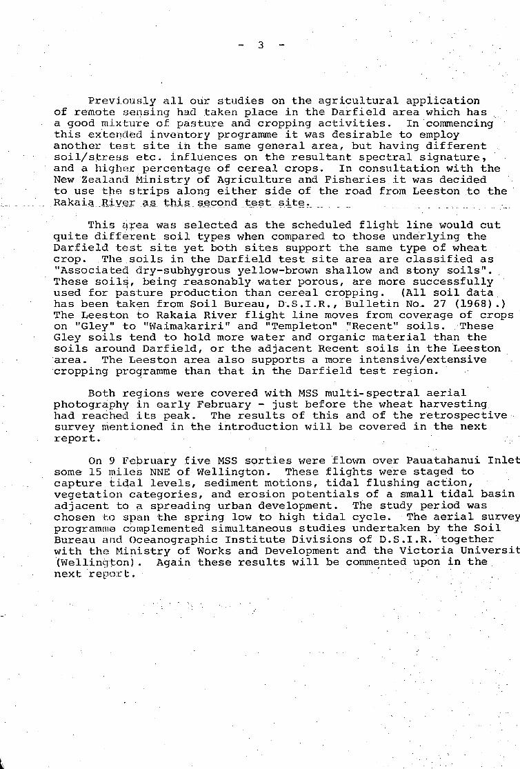
Previously all our studies on the agricultural applicationof remote sensing had taken place in the Darfield area which hasa good mixture of pasture and cropping activities. In commencingthis extended inventory programme it was desirable to employanother test site in the same general area, but having differentsoil/stress etc. influences on the resultant spectral signature,and a higher percentage of cereal crops. In consultation with theNew Zealand Ministry of Agriculture and Fisheries it was decidedto use the strips along either side of the road from Leeston to the.Rakaia.. .River as this, second test site.
This area was selected as the scheduled flight line would cutquite different soil types when compared to those underlying theDarfield test site yet both sites support the same type of wheatcrop. The soils in the Darfield test site area are classified as"Associated dry-subhygrous yellow-brown shallow and stony soils".These soils, being reasonably water porous, are more successfullyused for pasture production than cereal cropping. (All soil datahas been taken from Soil Bureau, D.S.1.R., Bulletin No. 27 (1968).)The Leeston to Rakaia River flight line moves from coverage of cropson "Gley" to "Waimakariri" and "Templeton" "Recent" soils. TheseGley soils tend to hold more water and organic material than thesoils around Darfield, or the adjacent Recent soils in the Leestonarea. The Leeston area also supports a more intensive/extensivecropping programme than that in the Darfield test region.
Both regions were covered with MSS multi-spectral aerialphotography in early February - just before the wheat harvestinghad reached its peak. The results of this and of the retrospectivesurvey mentioned in the introduction will be covered in the nextreport. .
On 9 February five MSS sorties were flown over Pauatahanui Inletsome 15 miles NNE of Wellington. These flights were staged tocapture tidal levels, sediment motions, tidal flushing action^vegetation categories, and erosion potentials of a small tidal basinadjacent to a spreading urban development. The study period waschosen to span the spring low to high tidal cycle. The aerial surveyprogramme complemented simultaneous studies undertaken by the SoilBureau and Oceanographic Institute Divisions of D.S.I.R. togetherwith the Ministry of Works and Development and the Victoria Universit(Wellington). Again these results will be commented upon in thenext report* / .
2.3 Atmospheric Work
2.3.1 Introduction - - - -
Studies are being conducted in New Zealand and Australia, onthe atmosphere and its effect on spectral signatures in the LANDSATbandpasses. The project is a joint one with Minerals ResearchDivision, CSIRO, Australia. In this reporting period, however, wediscuss only the measurements made with New Zealand equipment attest sites in both countries. A brief introduction to this workis to be found in the First Quarterly Report (NTIS-N76-20606).The methods outlined are described here in more detail, withresults of measurements made over a two year period.
This Section covers the calibration of the radiometer used tomake ground based measurements of global and solar irradiance. Thelaboratory calibration, combined with solar irradiance data, takenover several hours on a clear day, enables the spectral irradianceof the Sun at the top of the atmosphere to be determined.Comparison of these values for each LANDSAT bandpass with valuesderived from published data, serves as a check of the validity ofall these measurements, and the techniques involved.
In this report, only the solar irradiance data, measured witha collimated detection viewing the Sun directly, is considered.Derived parameters include the atmospheric extinction coefficientand beam transmission, and data from Australian and New Zealandtest sites is compared with similarly derived data from theNorthern Hemisphere.
213.2 Objectives
The objectives of this ongoing programme can be summarised.
(a) To calibrate the LANDSAT radiometer in the irradiance mode,in the laboratory using a standard lamp, and to use theinstrument to determine the solar spectral irradiances inthe LANDSAT bandpass at the top of the atmosphere.Comparison can then be made with published values.
(b) To record global and solar irradiance data over a periodof years at test sites in Australia and New Zealand, andhence to establish the typical values and short and longterm fluctuations.
(c) To compare measured quantities such as beam transmittancewith similar quantities measured by observers in the NorthernHemisphere.
(d) To apply the recorded atmospheric data to the correctiono.l: M3S band imagery.
'2*3,3 Radiometer Calibration
2.3.3.1 Sgectral_Resgonse_of_Instrument
An "ideal" LANDSAT radiometer would have a uniform responseto incide>rit power within each of the MSS defined bandpasses of100 nm and 300 nm width, and zero response to all other wavelengthsIn practice, the limitations of filter manufacture and the spectraldependence of detector responsivity will combine to produce_an^overall "instrument response" which is not ideal. This means that,in general, the instrument output reading will depend on thespectral distribution of the incident radiation, as well as on itsabsolute value within the passbahd.
An expression for instrument output is easily derived. Wedefine S(X) as the incident power density per unit bandwidth atthe radiometer, from a spectrally varying source at wavelength X.
AR(X) is the instrument response per unit bandwidth at wave-length X, with R(X) as the peak normalised response function andA as a constant gain factor.
In a narrow band AX, centered on X, the instrument output isgiven by:
V (AX) = A S(X) R(X) AX
Over all wavelengths, the instrument output is therefore:
V = A f°° S(X) R(X) dX 2.3.1O .• - ' . . - ..:/ . ' - '
Thus the output recorded by the radiometer depends upon the productof S(X) and R(X), which must both be known if the output is to bemeaningful in absolute terms.
It is convenient here to define three quantities. The"effective irradiance" is defined as the incident power densitywhich contributes to the instrument output reading, that is,within the actual bandpass of the radiometer.
The "equivalent square bandwidth" is the width of a "squarebandpass" response function which is equal in area to the areaunder the actual peak normalised response curve.
The "square MSS bandpass" is a response of unity within the100 nm or 300 nm passbands and zero at all other wavelengths.
A common practice is to assume a "square MSS bandpass", andto interpret all incident power from spectrally varying sources interms of this "square" response. This gives rise to errors if the"unknown" source has a different spectral distribution to thatwhich has been used to calibrate the instrument. This arisesdirectly from equation 2.3.1, since a change in S(X) will producea different response, depending on whether R(X) is "square" or"actual".

The output errors illustrated in this report (Table 2.3.1)are small compared to those which can occur in radiometricmeasurements of terrestrial targets, which generally have morerapidly varying spectral radiance within the MSS bandpass. Thisleads one to question the accuracy of absolute radiance data,particularly when comparing results from different radiometers.
2.3.3.2 LabgratgrY_Caiibration_of_Instrument
All the measurements described in this report were made witha LANDSAT radiometer manufactured by Gamma Scientific.
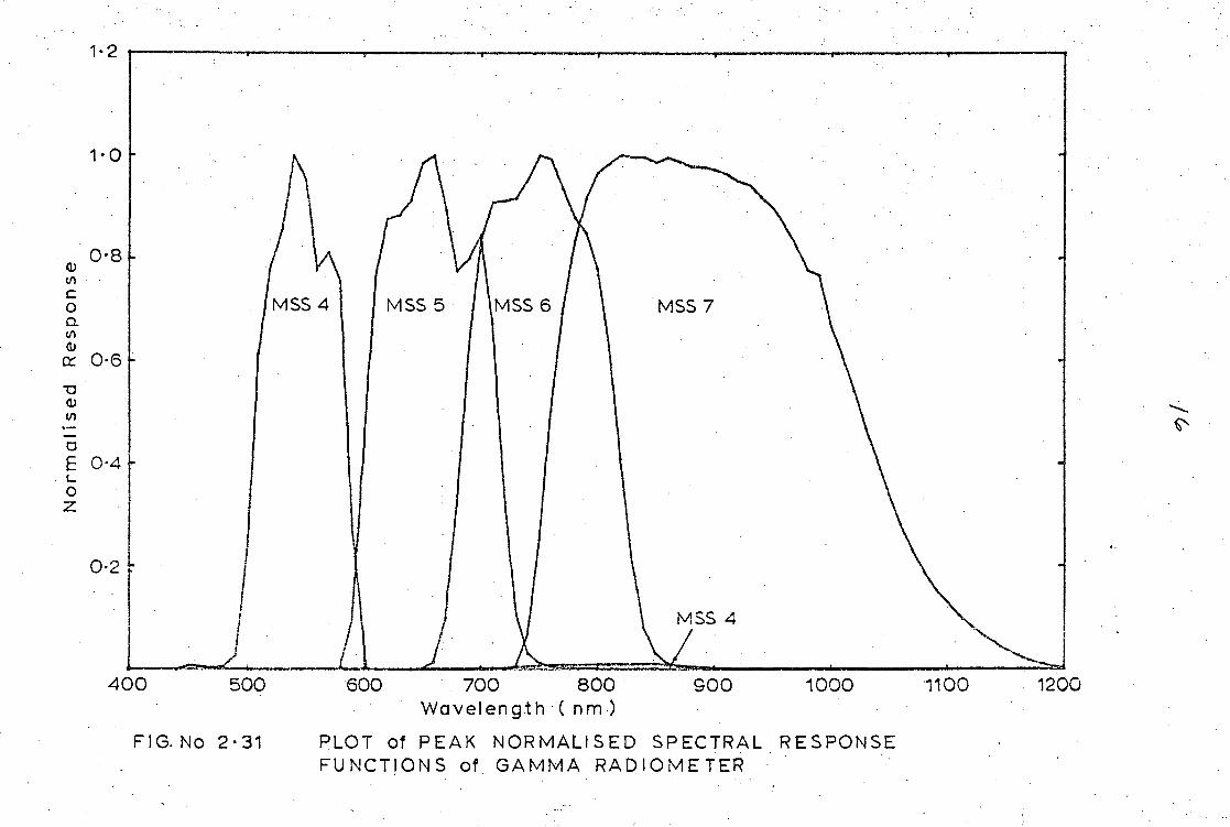
The wavelength response of each MSS band was first determinedin the PEL Photometry Section, using a quartz iodine source, doubleprism mo no chroma tor and calibration thermopile. Plots of the peaknormalised response functions are shown in Figure 2.3.1. Theresults indicate that a spectral "leak" exists on the long waveside of MSS band 4, and the energy contribution due to this leakamounts to 5.8% of the scale reading when viewing a standard lamp.
The instrument was then calibrated in the irradiance mode,that is, using the cosine receptor, against a standard lamp witha known spectral distribution of output power. The lamp itselfwas checked for total irradiance against an NPL sub-standard source,and found to be within 0.5% of its rated value.
The results are shown in Table 2.3.1. The column labelled (2)shows the irradiance at the radiometer entrance aperture within the"square MSS bandpasses", and not necessarily contributing to theinstrument reading.
2.3.4 Global and Solar Irradiance
2.3.4.1 Atmospheric_Model_and_Derivation_gf _Parameters
The nomenclature used in papers on atmospheric work varieswidely between authors. In an attempt to come closer to a"standard" terminology, we have adopted the definitions ofThekaekara (1972) for irradiance (E) and for zenith angle (Z) .
The global (spectral) irradiance on a horizontal surfacea ground level is given by:
E,_(A) = E (A) cos Z exp (-a(A)m) + ECVV(A) ---- 2.3.2v.i O
E (A) =' solar spectral irradiance per unit bandwidthat the top of the atmosphere
Z = solar zenith angle
a (A).. . = atmospheric extinction coefficient at wave-length A
m = airmass - defined as the ratio of total numberof attenuating particles in the observer's line
of sight, to the total number ofattenuating particles in the verticalcolumn ,
£„ Y(X) = global irradiance per unit bandwidth dueto radiation emanating from the sky.
Equation 2.3.2 is based on a simplified "flat Earth" modelwhich takes no account of the Earth's curvature/ and assumes ahomogeneous" ~l"ayere"d" a ~ t m o ~ s p h e r e \ ~ ~ *• ~
The quantity E_(X) is the global irradiance per unit band-width at the wavelength X. We can define the quantities E/ » (AX),and a(AX)> as the irradiance and extinction coefficient withina specified bandwidth AX.
Global irradiance E_(AX) is measured directly with a radio-meter having a bandwidth response AX, and a horizontal Lambertianreceiving surface (cosine receptor) .
Solar irradiance E (AX), is defined as the irradiance, inbandwidth AX, originating directly from the Sun, together withcontributions along the Sun/detector path, and falling on adetector surface which is normal to the Sun's rays. We find thatE (AX) is most easily measured with a tracking radiometer andcollimating tube which admits radiation from the Sun's disc andhas a limiting field of view of not more than 3°.
Solar irradiance is described by a simpler expression thanequation 2.3.2, since E is removed and the cosine term nolonger applies.
E (AX) = E (AX) exp (-a (AX) m) .... 2.3.3o O . . - / •
If E^fAX) is measured for a number of different zenith anglesthat is, at different times of the day, it is possible to deducethe value of a and the instrument reading which corresponds toEQ(AX) ,
This assumes that airmass m is a known function of solarzenith angle Z. For values of Z which do not exceed a specifiedlimit: ,
rn = sec Z .... 2.3.4
The 1.1.M.1,ting values of Z are considered in the next section. Theassumption is also made that the Solar constant and atmospherictransmiaaion do not change during the period of the measurements.
We have chosen to insert the measured values of ES(AX) intoa computer program which finds the least squares fit of expression2.3.3 to these values. The zenith angle is computed from the timeand date of: measurement, Sun declination and observer's latitude.

Equally/ by taking logarithms of 2.3.3, we have:
Ln E (AX) = Ln E (AX) - a (AX) ms o • 2.3.5
The values of Ln ES(AX) can be plotted against m(== sec Z) , anda straight line fit gives a (slope), and E, from the intercept onthe irradiance axis.
This method of deriving a and Eo is well known, and is usedby a number of authors (Shaw et al. 1973, Rogers 1974). Indeed,it is the basis of the "Smithsonian long method" of determiningthe Solar constant (Johnson 1954) .
2.3.4.2 The_Effect_of_Lar2e_Zenith_An2les
The range of zenith angles which are considered to satisfyequation 2.3.4 varies widely with author:
Limiting range of Z = 0° - 62° (Thekaekara 1972)
= 0° - 80° (Shaw et al . 1973)11 = 0° - 60° (Rogers 1974)11 . = 0° " 70° (Johnson 1954)
A more accurate expression for m at large zenith angles is givenby the empirical relation due to Bemporad:
m = sec Z - 0.001867 (sec Z-l) - 0.002875 (sec Z-l) -
0.0008083 (sec Z-l)3
2
2.3.6
The atmospheric transmission factor along the line of sightis given by:
T „ = exp (- a (AX) m) 2.3.7
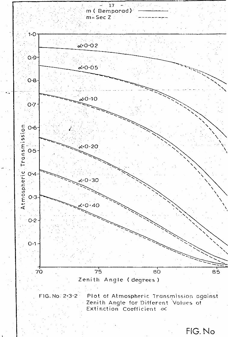
Generally, it is the error in TS, caused by an error inestimating m, which is of interest, and this error is also afunction of the extinction coefficient. Figure 2.3.2 is a plotof T3 against m for various values of a (AX), m is calculatedfrom 2,11, 4 and from 2.3.6. It can be seen that for all valuesof extinction coefficient, TS differs by < 0.5% at a zenith angleof 75° .Car the two. calculations of m. ,
Shaw et al. (1973) and Rogers (1974) make irradiance measurementsout to /.en 1th angles 84.2° (m = 10) and 81.7° (m = 7) respectively.The difficulty of making accurate measurements at these large zenithangles caii be appreciated when it is realised that the airmasschanges from 7 to 10 for a Sun angle change of only 2.5°,corresponding to a time change of ten minutes. .
Because of the necessity for stability of atmospheric trans-mission during the determination of EQ and a, we have avoided the
ends of the day, and limited our measurements to a period ofsix hours centered on Solar noon, and to values of airmass notexceeding four.
2.3.4.3 R§sults_of_Measurements_at_Test_Sites
For accurate measurement of the solar spectral irradianceat the top of the atmosphere (EO(AX)), the criterion of stable_aJtmosphe,r.ic_ t r ansmis s ion_.over_ tne_.me.a.s.ur,ement_ per.io.d..has proved j~_to be difficult to realise in practice. Of the test sites atWellington, Pauatahanui, Wainuiomata, Darfield arid Menindee, onlyat Wellington, and at the Australian test site at Menindee, NewSouth Wales, have results of sufficient accuracy been obtained.
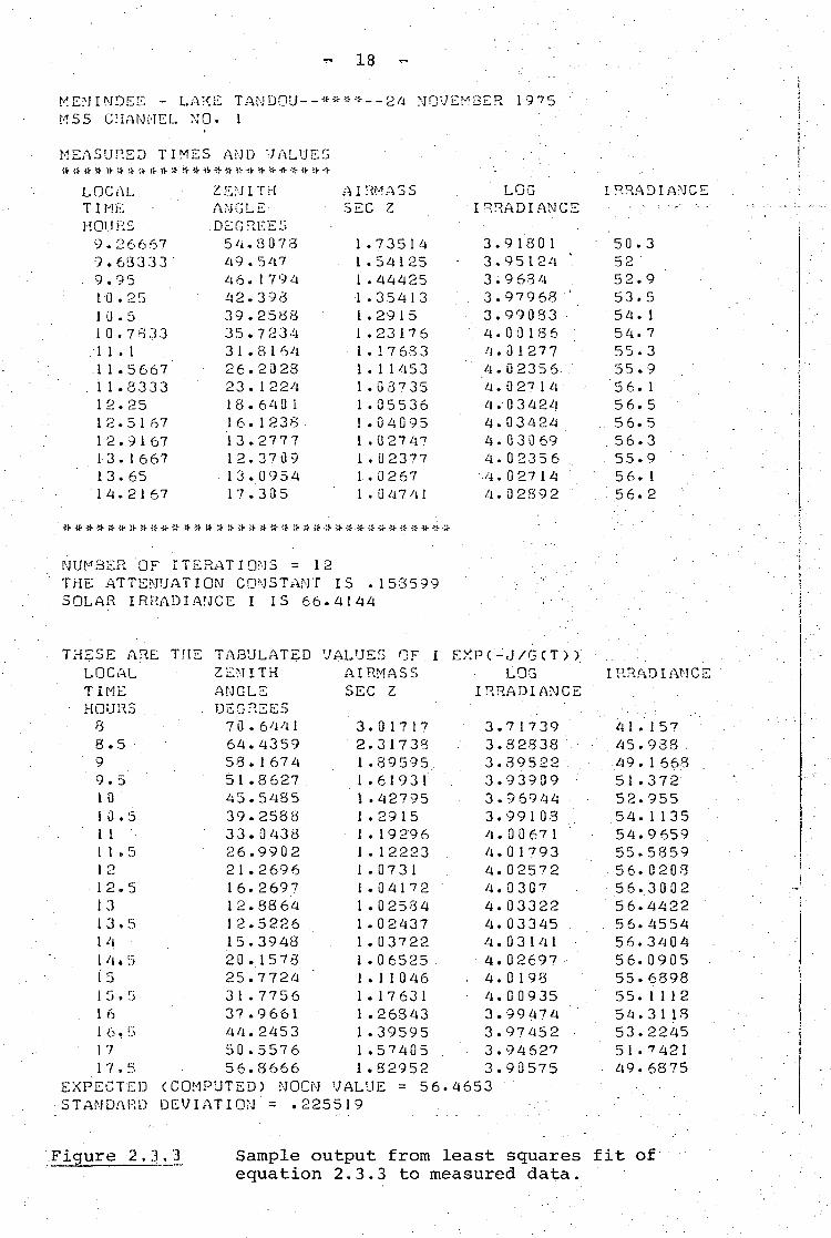
Global and solar irradiance measurements have been made atabout twenty minute intervals over a six hour period centered onsolar noon. A sample of the computer output from the least squaresfit program is shown in Figure 2.3.3.
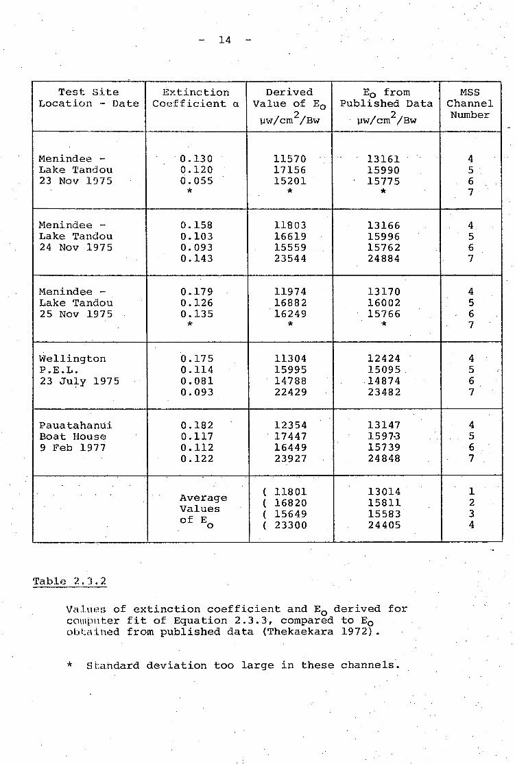
For all test sites, each set of measurements has beensubjected to the least squares fit program. Because atmosphericfluctuations increase the standard deviation and reduce theconfidence in the derived values Eo and a, only five data setshave been selected for the estimation of Eo. These all havestandard deviations of less than 0.7. The derived values of Eoshown in Table 2.3.2 are the result of applying the laboratorycalibration to the computer radiometer reading for Eo.
All the solar irradiance values given in Table 2.3.2 are for"effective irradiance" as defined in Section 2.3.3.1.
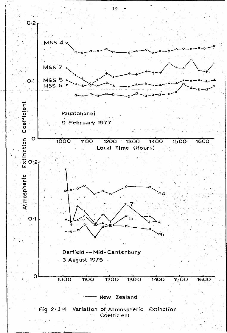
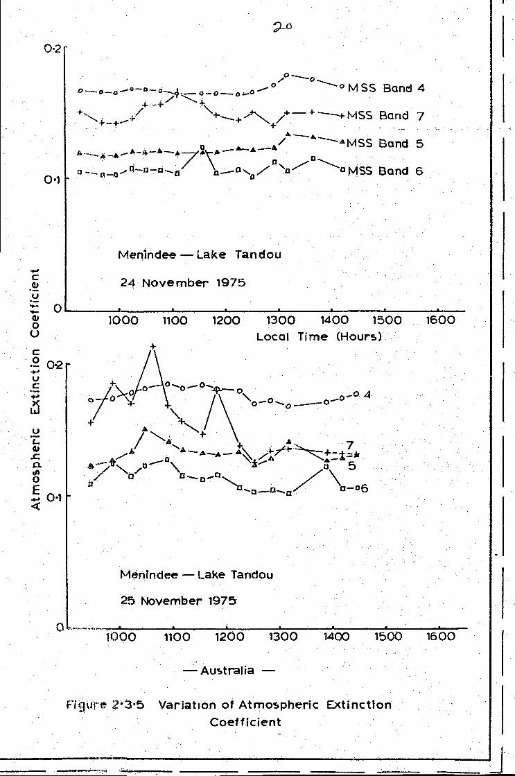
Once calibrated, the radiometer can be used to measure theshort term variations in extinction coefficient using equation2.3.3 and the known values of Eo. Figures 2.3.4 and 2.3.5 areplots of diurnal variations of extinction coefficient in NewZealand and Australia.
2*3.5 Derived and Predicted Values of Solar Irradianceat the Top of the Atmosphere
Before a comparison of solar irradiance EO(AX), as derivedfrom our measurements, can be made with EO(AX) predicted from thepublished data (Thekaekara 1972), it is necessary to correct thepublished figures for annual variations due to the Earth's ellipticorbit.
The I'larth/Sun distance at any time of the year can be computedto sufficient accuracy, and as a fraction of the mean value, by aniterative procedure involving a simple form of Kepler's equation:
E - e sin E > 2ir (t - T) .2.3.8
and :?://rmean = 1 ~ e cos E .... 2.3.9
- 10 -
E = eccentric anomaly
e = orbit eccentricity
(t ~ T) = time after perihelion in years
The ratio of irradiance Eo at time (t - T) to the meanvalue is calculated by:
EQ = EQ (mean) {} ---- 2.3.10
The maximum variations occur at the perihelion (Solarconstant •- 1399 W/m2) and at the aphelion (Solar constant =1309 W/m2) in accordance with the values cited by Thekaekara(1972).
Column 4 in Table 2.3.2 gives the "effective irradiance"at the top of the atmosphere, corrected for orbit ellipticity,and calculated from the published data.
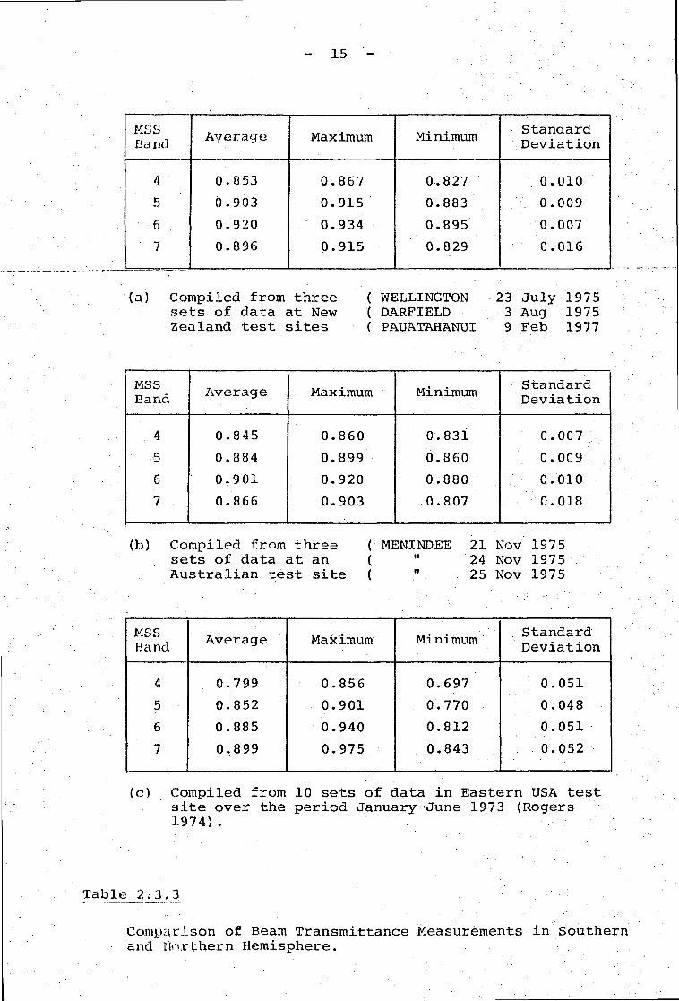
2.3.6 Comparison of Beam Transmittance Measurementsin Southern and Northern Hemisphere
Beam transmittance Tg is defined here as the transmissionthrough a vertical column of the atmosphere.
Thus TB = exp (.-• a (AX))
Rogers (1974) gives average, maximum and minimum values of TBderived from 10 sets of field measurements in the Eastern U.S.A.and these are reproduced in Table 2.3.3 (c). Table 2.3.3 (a)gives the same parameters for three sets of New Zealand data,and 2.3.3 (b) shows three sets of Australian data.
2.3.7 Summary and Conclusions
2.3.7.1 §§diometer_Calibration
In this report, we have endeavoured to point out some ofthe problems involved in calibrating a radiometer, and in definingthat calibration, either in the irradiance or radiance mode.Discrepancies between the "actual" spectral response of theinstrument and the "calibration bandpass", often assumed to besquare aiiet of nominal width, can give rise to errors in measuringthe irrcidlance of a source of unknown spectral distribution, orthe radlance of target of unknown spectral distribution.
We have described a calibration procedure in which the spectralresponse Of the instrument in each MSS band is carefully measuredand the response function is then multiplied by the calibrationsource function, to give a curve whose area is proportional to

11 -
the instrument reading. In this way, the instrument is calibratedfor the "effective'1 irradiance incident upon the detector.
The laboratory calibration has been checked by the iterativefitting of a simple atmospheric model to measurements taken overfive days in New Zealand and Australia. This fitting procedureautomatically derives the Solar irradiance at the top of theatmosphere, within the instrument bandwidth, and in terms of theinstrument scale reading.
The average of these five sets of derived values convertedinto yw/cm^/Bw using the laboratory calibration, have then beencompared with values calculated from the published figures ofextra-terrestrial Solar spectral irradiance.
Our measurements give extra-terrestrial irradiances whichdiffer from the published figures by the following amounts(expressed as a percentage):
MSS band 4: - 9.4% MSS band 5: .+ 6.4%
MSS band 6: + 0.4% MSS band 7: - 4.6%
In view of the large number of variables involved in thesemeasurements, we feel that these discrepancies are smaller thanmight have been expected. However, we consider that furtherinvestigations should be made to identify the differences,particularly the "cross over" between bands 4 and 5. .
Part of the problem is to be found in the variability of theatmosphere over the test sites, leading to a large standarddeviation between the data and the fitted curve. This points tothe necessity for making more "clear day" measurements, and is anargument in favour of setting up a recording radiometer which track;the Sun and provides near continuous data during the day,
2.3.7-2 Atmosgheric_Extinetion
The results of atmospheric extinction measurements, illustratein Figures 2.3.4 and 2.3.5, show clearly the greater opacity of theatmosphere in MSS band 4, due mainly to Rayleigh scattering. MSSband 7, however, contains a broad based water vapour absorptionband, centered at about 930 nm, and this results in a consistentlyhigher extinction coefficient in this band. The short termfiuctucitions are also greater in band 7, probably due to themovement of water vapour "cells" near the ground.
The .Large fluctuations in band 7, and the high extinctioncoefficients for the Menindee test site were slightly puzzling,since tlrLa test site in Western New South Wales is in a semi-desertarea. The measurements, however, were made in extremely hotconditions on the bank of an irrigation canal, and this couldaccount for a high atmospheric water vapour content in the immediatvicinity "of the instrument.
- 12 -
2.3.7*3 Com£arison_of_Beam_Transmittance_in_Two_Hemisgheres
Comparison of the results of Rogers (1974) with the NewZealand and Australian figures shows some significant features. *The average transmittances in the visible and first I/R bands arehigher for the New Zealand and Australian test sites compared tothose for the Eastern U.S.A. test site.
Rogers' results show a consistent increase in atmospherictransmittance from MSS 4 to MSS 7. Our results indicate that MSS-7is more severely affected by atmospheric water vapour.
2.3.7.4 Future_Work
We believe that measurements should continue at selectedtest sites, and that effect of variables such as atmosphericpressure, humidity, and instrument stability with temperatureshould be more fully investigated.
The objectives (d) in section 2.3.2 remain to be achieved aspart of our ongoing programme.
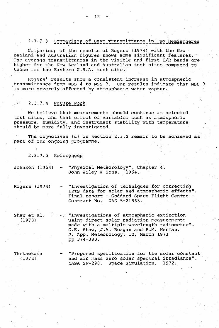
2.3.7.5 References
Johnson (1954) "Physical Meteorology", Chapter 4,John Wiley & Sons. 1954.
Rogers (1974) "Investigation of techniques for correctingERTS data for solar and atmospheric effects",Final report - Goddard Space Flight Centre -Contract No. NAS 5-21863.
Shaw et al,(1973)
"Investigations of atmospheric extinctionusing direct solar radiation measurementsmade with a multiple wavelength radiometer".G.E. Shaw, J.A. Reagan and B.M. Herman.J. App. Meteorology, 12, March 1973pp 374-380.
Thekaekura(197-;.)
"Proposed specification for the solar constantand air mass zero solar spectral irradiance".NASA SP-298. Space Simulation. 1972.

- 13 -
. So
urc
e
SI
II
II
It
S2
ii
ti
H
InstrumentRead ing
mV
20.6
37.8
57.3
85.1
EquivalentSquare
Bandwidthhm
72.8
104.5
124.4
264.6
(1)
EffectiveIrradiance
at Instrument2
yw/cm /Bw
366.1
984.9
1487.1
3539.3
12815
15570
15342
24221
(2)
Irradiancein "Square"MSS Bands
2yw/cm /Bw
503.5
912.5
1194.3
4075.1
17701
15150
12373
24912
Ratiod')/7(2)
0.727
1.079
1.245
0.869
0.724
1.028
1.240
0.972
MS£CH.NO.
4
5
6
7
4
5
6
7
Notes; 1-Source Si: Standard Lamp No. 178A at 2854° K
2-Source S2: Mean Solar Irradiance at top of Atmosphere
3-"Effective Irradiance", "Irradiance in Square MSS Bands"are defined in Section 2.3.3.1.
Table 2.3.1
Response of radiometer to a standard lamp, and calculatedvalues of mean solar irradiance, within the actualinstrument bandpasses, and the nominal "Square" MSS Bands,
- 14 -
Test siteLocation - Date
Menindee -Lake Tandou23 Nov 1975
Menindee -Lake Tanclou24 Nov 1975
Menindee -Lake Tandou25 Nov 1975
WellingtonP.E.L.23 July 1975
PauatahanuiBoat House9 Feb 1977
ExtinctionCoefficient a
0.1300.1200.055*
0.1580.1030.0930.143
0.1790.1260.135*
0.1750.1140.0810.093
0.1820.1170.1120.122
AverageValuesof EQ
DerivedValue of E0
oyw/cm /Bw
115701715615201*
11803166191555923544
119741688216249*
11304159951478822429
12354174471644923927
( 11801( 16820( 15649( 23300
E0 fromPublished Data
2yw/cm /Bw
131611599015775*
13166159961576224884
131701600215766*
12424150951487423482
131471597-31573924848
13014158111558324405
MSSChannelNumber
4567
4567
4567
4567
4567
1234
Table 2.3.2
Values of extinction coefficient and EQ derived forcomputer fit of Equation 2.3.3, compared to Eoobtained from published data (Thekaekara 1972).
Standard deviation too large in these channels.
- 15 -
MSSBand
4
5
6
7
Average
0.053
0.903
0.920
0.896
Maximum
0.867
0.915
0.934
0.915
Minimum
0.827
0.883
0.895
0.829
StandardDeviation
o.oio0.009
0.007
0.016
(a) Compiled from threesets of data at NewZealand test sites
( WELLINGTON( DARFIELD( PAUATAHANUI
23 July 19753 Aug 19759 Feb 1977
MSSBand
4
_ 5
6
7
Average
0.845
0.884
0.901
0.866
Maximum
0.860
0.899
0.920
0.903
Minimum
0.831
0.860
0.880
0.807
StandardDeviation
0.007
0.009
0.010
0.018
(b) Compiled from threesets of data at anAustralian test site
( MENINDEE(( "
21 Nov 197524 Nov 197525 Nov 1975
MSSBand
4
5
6
7
Average
0.799
0.852
0.885
0.899
Maximum
0.856
0.901
0.940
0.975
Minimum
0.697
0.770
0.812
0.843
StandardDeviation
0.051
0.048
0.051
0.052
(c) Compiled from 10 sets of data in Eastern USA testsite over the period January-June 1973 (Rogers1974) .
Table 2,3,3
Comparison of Beam Transmittance Measurements in Southernand No.rbhern Hemisphere.
400 500
FIG. No 2-31
600 700 800Wavelength ( nm )
PLOT of PEAK NORMALISEDFUNCTIONS of GAMMA RAD
900
SPECTRALOMETER
1000
RESPONSE
1100 1200
.. ::. . I : . . ' - " ' 17
m ( Bemporad); m = Sec Z
75 80
Zen i th Ang le (degrees)
85
FIG.No. 2-3-2 Plot of Atmospheric Transmission againstZenith Angle for Different Values ofExtinct ion Coeff ic ient ex:
FIG. No
18
MEMIMDEE - LAKE T AHDOU --** »*- -24 NOVEMBER 1.9 5MSS CHANNEL NO. 1
MEASURED TIMES AND VALUES-.V J.t # * it * It * it it !t ?
LOCAL.TIMEHOURS '9.266679.68333 '9.9510.2510.510 .7333
.1 1.11 1 .566711 .33331 2.2512.51 6712.91 6713. 166713.6514.21 67
(• » It -.t -it «• -it >.t * * -* *t it it
ZENITHANGLE.DEGREES54.807849. 54746. 179442.39339.258835.723431.816426.202823.122418. 640 116. 123813.277712.370913. 095417.305
AIRMASSSEC Z
1.735141 .541 251 .444251 .3541 3I .29151 .231761 . 176331 . 1 14531 .037351 .055361 .040951 .027471 . 023771 . 02671 . 04741
. LOGIRRADIANC
91301951249 63 4979689903300186
4.012774.02356
0271403424034240 3 0 6902356027 14
IRRADIANCE
50.5252.53.54.54.55.55.56.56.56.56,55.56.
4.02392 56. 2
*#***» -:t J * # * «• :(• s- -* it a * * * # it * •* *•* * * * ft -it :- it -x-
NUM3ER 'OF ITERATIOMS = 12THE ATTEMUATIOM CONSTANT IS .153599SOLAR IRRADIANCE I IS 66.4144
THESE ARELOCALTIMEHOURS38.599.51 010.51 11 1 . 51212.51313,51414.5151 5 . 51 61 6. i51717.5
EXPECTEDSTANDARD
TH TABULATED VALUES OF . I EXPC-J/GCT))ZENITH AIRMASS LOGANGLE SEC Z IRRADIANCEDEGREES . ' .70.64.53.51 .45.39.33.26.21 .16.12.1 2.15.20 .25.31 .37 .
44.50.56.
644143591 6748627 .5485258304389902269626978864522639481573772477569661245355768666
3.2.1 .1 .1 .1 .1 .1 .1 .1 .1 .1 .1 .1 .1 .1 .1 .1 .1 .1 .
017173173389595,61931 .4279529151929612223073104172025840243703722065251 10461763126343395955740532952
3.3.3.3.3.3.4.4.4.4.4.4.4.4.
. 4.4.3.3.3.3.
717398283839522 ' ..939099694499103006710 179302572030-7033220334503141026970 1980093599474 "97452 -9452790575
I U R A D I A M C E
41 .45.49.51 .52.54.54.55.56.56.56.56.56.56.55.55.54.53.51 •
157938 .1 6633729551 1359659585902033002442245543404090563981 1 1 231 1322457421
49.6875(COMPUTED) MOON VALUE = 56.DEVIATION = .225519
4653
:Figure 2.3. 3^ Sample output from least squares fit ofequation 2.3.3 to measured data.
-19 -
0-2
O-1
ooO
co•«-•uc•+*XU
JU
'L-o>JCa.inOE
MSS 4—- °~-o-
'O o-
MSS 7"\.
. MSS 5 AMSS 6 o
/V-/\ /4- +_ ^-Jr~-Jc-•* 4"—*-
O1
o
'•{J-—«
Rauatahanui
9 February 1977
1OOO 110O 12OO 13OO 14OO 15OO 16OOLocal Time (Hours)
Darfreld — Mid-Canterbury
3 August 1975
tOOO 11OO 12OO 130 O 14OO 15OO 16OO
New Zealand
Fig 2*3'4 Variation of Atmospheric ExtinctionCoefficient
\)'<L
O-1
-Mc •
£ o
o — o-o-*—0
•
*\f^-/
a- ' * x-Q-n
°— -— .•~o^,.__o-o— o^o--oX °^-°MSSBand4
i. <^ ^^^** «L
X-*--^+/*\ /•— + +MSS Band 7
n __Jl_A^A/'~~"*k"^AMSS Band 5 " •
-a— p n— -a\QX NDxX^ °MSS Band 6
Menjndee — Lake Tandou
24 November 1975
a
g 1000uc
uc•»•»
Q.
O
£ o-i
O
o^X/°
' Ay:/v°
B • a - • ft •
110O 12OO 13OO MOO 15OO 16OOLocal Time (Hours)
•f
'\\^-\o-^ o-*.\^—\ + \^•A \ A- -7--^- t - i-iLV-'0\, X\"^. — n^n/- 0-06u Q
Menindee — Lake Tandou
25 November 1975
10OO 11OO 12OO 1300 1400 15OO 16OO
Australia —
2'3-5 Variation of Atmospheric ExtinctionCoefficient

- 21 -
2-4 IBM CGT Processing : .
2* 4.1 CCT He formatting V / ,-.'•:-. : '.''.-•
pl;iring this reporting period considerable attention hasbeen directed at optimising the Job Control Language and filemanagement routines used in taking the four strip EROS tape andproducing a five file reformatted product (one calibration datafile and ifour single band whole scene files). Further work hasalso improved the PL/I reformattingprocedures. Rres.ent. tests . .indicate that a four fold reduction in IBM 370/168 CPU time hasresulted from this optimisation and restructuring exercise.Once difficulties in sharing storage space, for the 31 M bytewhole scene on non-dedicated disk packs, with other users havebeen overcome production runs will commence.
2.4.2 CCT Data on a Nationwide Computer Network
Using the New Zealand Government Ministry of Works and . .Development IBM 370/168, being available to users on a timeshared terminal system throughout New Zealand, some basicprograms have been made available to investigators during thereporting period. All CCT data files are stored under the"alias" system in Wellington and, currently, may be accessedin the batch mode through TSO. Programs that will furnish Bitor EBCDIC dumps, complete CCT decode and 47 level coded pictureprint outs are available. These programs are all written totallyin machine independent language - here PL/1. Card decks forthese programs'; are available through the P.E'.L. Remote SensingSection as is a report describing the program packages. •. ~

- 22 -
2.5 CCT Processing on the HP 2100
The main achievement during this reporting period has beenthe development of a computer program'package to perform a fullgeometric rectification of a LANDSAT subimage. The proceduresadopted in these programs are explained in section 2.5.1.A number of corrected images have been prepared/ using a 10 yardsampling interval and these are to be sent to Optronics to bewritten out on their colorwrite machine. These images should beready for our final report in June. The development of thegeometric correction program has allowed time sequential imageryto be produced by subtracting spatially registered but timeseparated LANDSAT scenes. A time sequential image of the Eyrewellforest area is also being sent to Optronics. Production of suchimages will be much simpler when we have our own photowrite machine.
Multispectral aircraft negatives of our Darfield test areahave been scanned at Massey University on their Optronics Photoscanmachine. Unfortunately we were not able to accurately registerthe different image bands as they were scanned. Consequently thenegatives have been geometrically corrected in the computer so thatthey are now in register with each other, with the standard NewZealand UTM inch to the mile map series, and with corrected LANDSATsubimages of the same area. This should prove a considerableadvantage in analysing the aircraft negatives.
2.5.1 Rectification of LANDSAT Subimages
The image rectification system developed for use on our HP 2100computer is based on the system developed by Van Wie and Stein et al(1975, 1976) but differs from it in certain key respects. Thesedifferences will be made clear as the rectification system isdiscussed step by step.
The reason for developing our own rectification system ismainly financial. The Goddard system would involve us in too muchexpenditure for computer time on a large computer. However, we haveavailable ciri HP 2100 minicomputer for which we are not charged. TheGoddard system will rectify whole LANDSAT scenes in the UTM projection.Our system will rectify a LANDSAT subimage on the HP 2100 in anydesired mapping projection. The size of the input subimage dependson the extent of the rotation required. This is due to the limitedcore storage available. For example a small input image(e.g. 12U x 128 pixels) can be fully rotated, whereas a large inputimage can only be rotated by a small amount.
There are many sources of geometric errors in LANDSAT imagery.Many of. lilies errors need to be treated differently. The error sourceswill be discussed briefly here. For a more detailed discussion referto Van Wie et al (1975, 1976). Band to band misregistration hasalready been corrected in the CCT's. The pixels inserted by NASA tocompensate for line length variations cause an error on average of28.5 m. These can be removed when the CCT's are reformatted. Theeffect of the sensor delay during sampling, and the earth's rotationcause each row to be offset from the preceding one. This iscompensated for by adding a correction term to each column when an

- 23 -
image co-ordinate (row, column) is calculated. Variations in themirror velocity profile catuse an error in the column co-ordinatealong'each.row which is approximately described by a sine errorfunction. The sine error function is zero at the end of each rowand goes through one cycle along each row. The amplitude of thesine error function is known to be about 7 pixels.
The Goddard approach is to explicitly correct the inputLANDSAT image for the effects of sensor delay, the earth's ,rotation and the mirror velocity profile to give a corrected input-image T-he--next step-is- to- deduce~a-suitable-mapping, function from.the UTM map projection to the corrected input image. Let theco-ordinates for the input image, the corrected input image andthe map be (R,C), (U,V) and (X,Y) respectively. .The Goddard systemhas available an affine transformation or a polynomial mappingfunction. For the polynomial mapping function, which is the moreaccurate, coefficients C-^ and D^ are required for the generalmapping described by
2 2 3/-I _ i _ /^ v -i_ r* v - t - f " * v - t - f * w J./"1 v _i_ /"• ' Y _i_— C + C , X " r l _ ~ X + C - , A -rt,, A X T L . _ i T C,- A +O 1 2 3 4 5 6
2 2 3C V V I <~* W JL. C* V i .^ A X + Cg AX + Ug X -t- . . . .
V = D + D, X + D0 Y + D0 X2 + D. XY + Dc Y
2 + Dc X3 +
O 1 2 3 4 D b
o 7 -3 ,D., X Y + DQ XY + DQ Y + ....
/ Q . y . , ..
The desired order of polynomial is chosen according to the mappingaccuracy required. Next the C^ and D^ are computed by means of aleast squares fit to a number of known ground control points (GCP's)The polynomial mapping function is intended to correct for allerrors which have not been explicitly compensated for. These arecaused by satellite height and altitude variations, the earth'scurvature and the tangential nature of the UTM projection itself.This last error is part of what Van Wie ejt aJL call perspectivedistortion. It is correctable if all the points in the originalLANDSAT image are at the same height (e.g. sea level). However,points at different heights will be offset along rows because LANDSAhas a central perspective instead of the orthogonal perspective ofa UTM .map projection. This error is not correctable, although it ispossible to correct the image for a single chosen height (e.g. sealevel). This correction can be achieved by adjusting each GCP by anamount which depends on its altitude and distance from the satellitetrack through the centre of the image. This correction appears tohave bean neglected by Van Wie et al. If a GCP is taken on top ofa mountcVtn it could cause an error of several pixels.
Our approach is somewhat different. We have noted that theeffect ol: the earth's curvature and the perspective distortion (fora given height) along rows both have the form of a sine error functiThus, ttieae errors can be included in the correction for the mirrorvelocity profile by adjusting the sine amplitude to an optimumvalue. This optimum value can be simply found by plotting the meanabsolute GCP error against sine amplitude, and choosing the amplituc
- 24 -
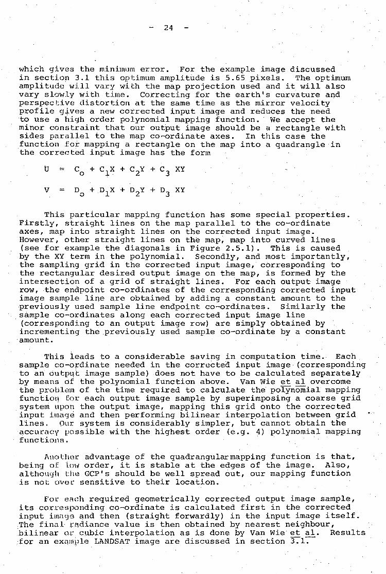
which gives the minimum error. For the example image discussedin section 3.1 this optimum amplitude is 5.65 pixels. The optimumamplitude will vary wibh the map projection used and it will alsovary slowly with time. Correcting for the earth's curvature andperspective distortion at the same time as the mirror velocityprofile gives a new corrected input image and reduces the needto use a high order polynomial mapping function. We accept theminor constraint that our output image should be a rectangle withsides parallel to the map co-ordinate axes. In this case thefunction for mapping a rectangle on the map into a quadrangle inthe corrected input image has the form
U = CQ + C-j^X + C2Y + C3 XY _ ~ •
V = D + D,X + D-Y + D_ XYO -L £. J
This particular mapping function has some special properties.Firstly, straight lines on the map parallel to the co-ordinateaxes, map into straight lines on the corrected input image.However, other straight lines on the map, map into curved lines(see for example the diagonals in Figure 2.5.1). This is causedby the XY term in the polynomial. Secondly, and most importantly,the sampling grid in the corrected input image, corresponding tothe rectangular desired output image on the map, is formed by the .intersection of a grid of straight lines. For each output imagerow, the endpoint co-ordinates of the corresponding corrected inputimage sample line are obtained by adding a constant amount to thepreviously used sample line endpoint co-ordinates. Similarly thesample co-ordinates along each corrected input image line(corresponding to an output image row) are simply obtained byincrementing the previously used sample co-ordinate by a constantamount.
This leads to a considerable saving in computation time. Eachsample co-ordinate needed in the corrected input image Ccorrespendingto an output image sample) does not have to be calculated separatelyby means of the polynomial function above. Van Wie et al overcomethe problem of the time required to calculate the polynomial mappingfunction for each output image sample by superimposing a coarse gridsystem upon the output image, mapping this grid onto the correctedinput image and then performing bilinear interpolation between gridlines. Our system is considerably simpler, but cannot obtain theaccuracy passible with the highest order (e.g. 4) polynomial mappingfunctions.
Another advantage of the quadrangularmapping function is that,being oi: Low order, it is stable at the edges of the image. Also,although the GCP's should be well spread out, our mapping functionis not over sensitive to their location.
For each required geometrically corrected output image sample,its corresponding.co-ordinate is calculated first in the correctedinput image and then (straight forwardly) in the input image itself.The final radiance value is then obtained by nearest neighbour,bilinear or cubic interpolation as is done by Van Wie e_t aj . Resultsfor an example LANDSAT image are discussed in section 3.1.
- 25
REFERENCES
Van Wie, P. and Stein, M. (1976). "A LANDSAT digitalimage rectification system". Report X-931-76-101,Goddard Space Flight Centre, Greenbelt, Maryland.
Van Wie, P., • Stein, M., Puccinelli, E. and Fields, B.(1975) . "LANDSAT digital image rectificationsystem - preliminary documentation", InformationExtraction Division, Goddard Space Flight Centre.

- 26 -
\\
(a)
(b)
Figure, 2.5.1 Example mapping of a rectangle on amap (a) into a quadrangle in thecorrected input image (b).
- 27 -
2•6 Car tag raphia Reflee tor . . . .
The 4 ft diameter diverging reflector continues to be setup at the P.E.L. Auroral Station (45.04°S, 169.69°E) for everypredicted LANDSA.!' 2 overpass for which cloud cover conditionsare favourable. To date, due to the lack of sustained clearweather periods and satellite scheduling priorities, no imageryhas been apparently recorded.
it is planned to design, build and install a plane reflectorsystem at: the above: station during the next reporting period. ~The increase in orbital cross track drift control, combined withour orbital prediction programme shortly coming into use, willenable tji.is system improvement to be made. An increase in reflectedpower density and uniformity will result from this upgrading.
i • . ' - •2.7 "PEACESAT" .
The link has not been used over the last reporting perioddue principally to Peter Ellis making a visit to GSFC and otheragencies in the U.S. With the commencement of the SouthernHemisphere's academic year we look forward to further exchangeswith our South Pacific colleagues. :
2 i 8 Laboratory Upgrading
With the increasing interest being shown in remote sensingby outside agencies it has become necessary to provide more spaceand better facilities for users to work alongside the P.E,L. group.The analysis and darkroom areas are being redesigned to allowusers to operate interpretative equipment independent of darkroomoperations. These areas are scheduled to progress towards "cleanroom" status. - , •

- 28 -
3. ACCOMPLISHMENTS, IMMEDIATE OBJECTIVES AND SIGNIFICANT RESULTS
3.1 Image Rectification Results
The package of computer programs for geometrically correctingLANDSAT subiinages, which was described in section 2.5, has beentested on LANDSAT II scene 2334-21123. Preliminary results arepresented in this section.
Nineteen points suitable for use as ground control points(GCP's) were chosen by inspection of the LANDSAT scene. Thesepoints were the centres of small lakes and forest road intersections,and mainly sharp water-land interfaces. A number of shaded computerlineprinter outputs were then obtained which included each GCP.New Zealand standard inch to the mile (1:63360) UTM maps were thenobtained which also included each GCP. The co-ordinates of each GCPin the LANDSAT image and the map were then determined by examining,for each GCP, the appropriate shaded printout and map together. Toobtain reasonable accuracy (i.e. +0.5 pixel in the image row andcolumn co-ordinates and + 20 yards in the map co-ordinates) it ismost important that the printout and map should be examined together.Our experience is that the best type of GCP is a land-water interfacewith the land forming an acute angled peninsula.
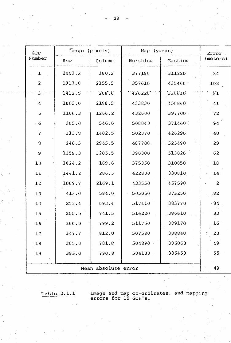
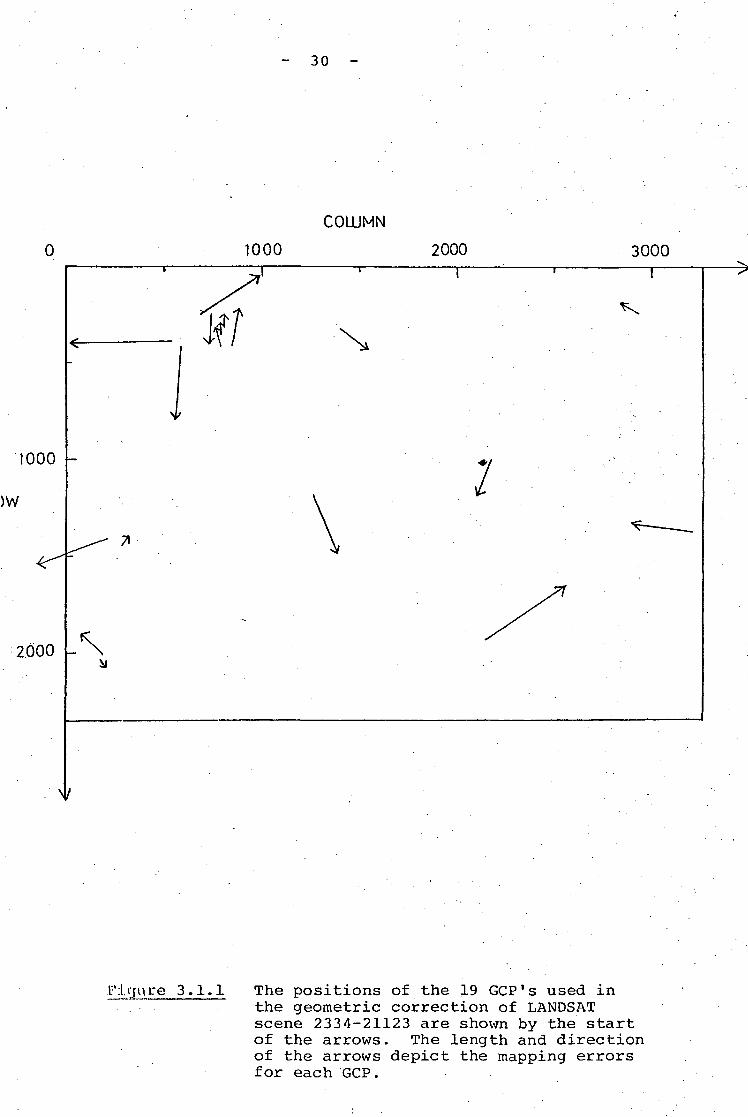
In Table 3.1.1 the image co-ordinates and the map co-ordinatesare given for the nineteen GCP's. It should be noted that the imagecolumns given have not been corrected for the pixels inserted byNASA to correct for line length variations. Also shown in Table 3.1.1in meters for each GCP is the distance between the result of mappingthe GCP in map co-ordinates to the image, and the GCP measured in.image co-ordinates. The distribution of the GCP's and the directionand size of the errors is shown in Figure 3.1.1. All possiblecorrections were included in the mapping function. The correctionsfor the altitude variation of the GCP's and the pixels inserted tocorrect for line length variations seemed to have little effect.This was perhaps because their effects were small compared to themean absolute error of 49 m.
Many suitable GCP's were available in this image, as there arefor most: New Zealand scenes so long as there is not too much cloudcover. More images need to be processed, and the processed imagesneed to be compared to maps before the mapping accuracy of this methodcan be fully evaluated. However, initial tests indicate the accuracyis sufficient for our purposes.
- 29 -
GCPNumber
1
2
3
4
5
6
7
8
9
10
11
12
13
14
15
16
17
18
19
Image (pixels)
Rov;
2001.2
1917,0
1412.5
1003.0
1166.3
385.0
313.8
240.5
1359.3
2024.2
1441.2
1009.7
413.0
253.4
255.5
300.0
347.7
385.0
393.0
Column
180.2
2155.5
208". 0
2188.5
1266.2
546.0
1402.5
2945.5
3205.5
169.6
286.3
2169.1
584.0
693.4
741.5
799.2
812.0
781.8
790.8
Map (yards)
Northing
377180
357610
"426220"
433830
432600
508040
502370
487700
390300
375350
422800
433550
505050
517110
516220
511750
507580
504890
504100
Easting
311220
435460
326610
458860
397700
371460
426290
.523490
513020
310050
330810
457590
373250
383770
386610
389170
388840
386060
386450
Mean absolute error
Error(meters)
34
102
81
41
72
94
40
29
62
18
14
2
82
84
33
16
: 23
49
55
49
Table 3.1.1 Image and map co-ordinates, and mappingerrors for 19 GCP's.
- 30 -
0
COLUMN
1000 2000 3000—I—
1000
)W7
2000
F:i.qure 3.1.1 The positions of the 19 GCP's used inthe geometric correction of LANDSATscene 2334-21123 are shown by the startof the arrows. The length and directionof the arrows depict the mapping errorsfor each GCP.
-31 -
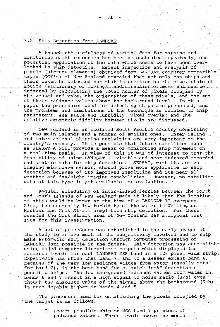
3.2 Ship Detection from LMfDSAT .
Although the usefulness of LANDSAT data for mapping andmonitoring earth resources has been demonstrated repeatedly, onepotential! application of the data which seems to have been over-looked is ship detection. Recent inspection and analysis ofpixels (picture elements) obtained from LANDSAT computer compatibletapes (CCT's) of New Zealand revealed that not only can ships andtheir wakea be detected but that information on the size, state of.motion—(-S-ta-tionary- or moving.) , and-direction^-of -mov.emen.t can.be..--...._.inferred by calculating the total number of pixels occupied bythe vessel and wake, the orientation of these pixels, and the sumof their radiance values above the background level. In thispaper the procedures used for detecting ships are presented, andthe problems and limitations of the technique as related to shipparameters, sea state and turbidity, pixel overlap and therelative geometric fidelity between pixels are discussed.
New Zealand is an isolated South Pacific country consistingof two main islands and a number of smaller ones. Inter-islandand international shipping activities are very important to thecountry's economy. It is possible that future satellites suchas SEASAT-A will provide a means of monitoring ship movement ona real-time basis. In view of this it was of interest to test thefeasibility of using LANDSAT II visible and near-infrared recorded ,radiometric data for ship detection. SEASAT, with its activeimaging microwave sensor, should prove more applicable to shipdetection because of its improved resolution and its near all-weather and day/night imaging capabilities. However, no satellitedata of this type is yet available for evaluation.
Regular scheduling of inter-island ferries between the Northand South Islands of New Zealand made it likely that the locationof ships would be known at the time of a LANDSAT II overpass.Also, the generally low turbidity of the water in WellingtonHarbour and Cook Strait simplifies ship detection. For thesereasons the Cook Strait area of New Zealand was a logical testsite for this investigation.
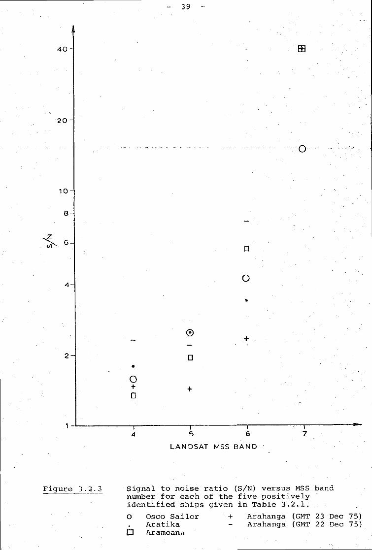
A get of procedures was established in the early stages ofthe study to remove much of the subjectivity involved and to helpmake automatic ship detection through computer processing ofLANDSAT data possible in the future. Ship detection was accomplishe<using coded computer lineprinter outputs which displayed theradiance levels for each LANDSAT MSS band in a 128 pixel wide strip.Experience has shown that band 7, and to a lesser extent band 6,because of: the very low radiance Values from water (usually zerofor band 7), is the best band for a "quick look" detection ofpossible ships. The low background radiance values from water inbands 6 and 7 result in a high signal to noise ratio (S/N) even ;though the absolute value of the signal above the background (S-N)is considerably higher in bands 4 and 5.
The procedure used for establishing the pixels occupied bythe target is as follows: .
I Iiocate possible ship on MSS band 7 printout ofradiance values. Three levels above the modal
- 32 -
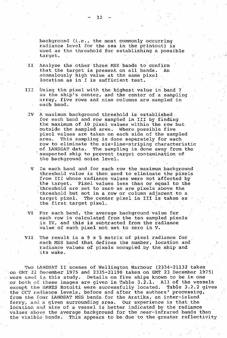
background (i.e., the most commonly occurringrcidiance level for the sea in the printout) isused as the threshold for establishing a possibletarget. -" - •
II Analyse the other three MSS bands to confirmthat the target is present on all bands. Ananomalously high value at the same pixellocation as in I is sufficient test. '
III Using the pixel with the highest value in band 7as the ship's center, and the center of a samplingarray, five rows and nine columns are sampled ineach band.
IV A maximum background threshold is establishedfor each band and row sampled in III by findingthe maximum of 10 pixel values within the row butoutside the sampled area. Where possible fivepixel values are taken on each side of the sampledarea. This sampling is done separately for eachrow to eliminate the six-line-striping characteristicof LANDSAT data. The sampling is done away from thesuspected ship to prevent target contamination ofthe background noise level.
V In each band and for each row the maximum backgroundthreshold value is then used to eliminate the pixelsfrom III whose radiance values were not affected bythe target. Pixel values less than or equal to thethreshold are set to zero as are pixels above thethreshold but not in a row or column adjacent to atarget pixel. The center pixel in III is taken asthe first target pixel.
VI For each band, the average background value foreach row is calculated from the ten sampled pixelsin IV, and this is subtracted from the radiancevalue of each pixel not set to zero in V.
VII The result is a 9 x 5 matrix of pixel radiance foreach MSS band that defines the number, location andradiance values of pixels occupied by the ship andits wake.
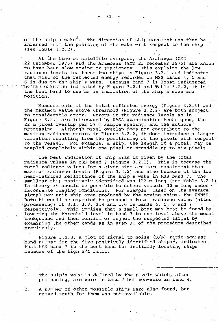
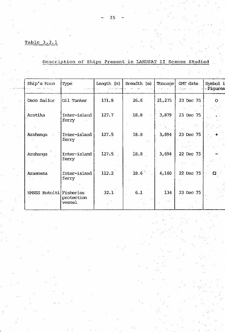
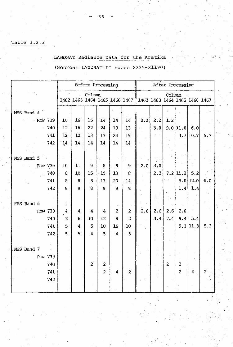
Two LANDSAT II scenes of Wellington Harbour (2334-21132 takenon GMT 22 December 1975 and 2335-21190 taken on GMT 23 December 1975)were used in this study. Details on five ships known to be in oneor both oL- these images are given in Table 3.2.1. All of the vesselsexcept the HMNZS Rotoiti were successfully located. Table 3.2.2 givesthe CCT radiance levels, before and after the authors' processing,from the four LANDSAT MSS bands for the Aratika, an inter-islandferry, and a given surrounding area. Our experience is that thelocation and size of a vessel is better indicated by the radiancevalues above the average background for the near-infrared bands thanthe visible bands. This appears to be due to the greater reflectivity
- 33 -
of the ship's wake". The direction of ship movement can then beinferred from the position of the wake with respect to the ship(see Table 3.2.2) .
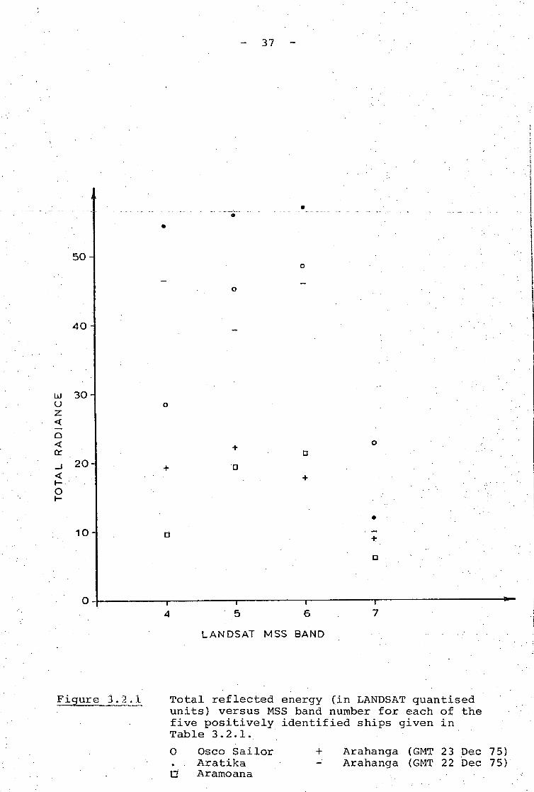
At the time of satellite overpass, the Arahanga (GMT22 December 1975) and the Aramoana (GMT 23 December 1975) are knownto have been slow moving or stationary. This explains the lowradiance levels for these two ships in Figure 3.2.1 and indicatesthat mosb of: the reflected energy recorded in MSS bands 4, 5 and6 is due to the ship's wake. Because band 7 is least influenced"by~~ the wake, as indicate~d~ by Figure•~~3~.2~.~1 and Table ~3~. 2--2v ~it isthe best band to use as an indication of the ship's size andposition^
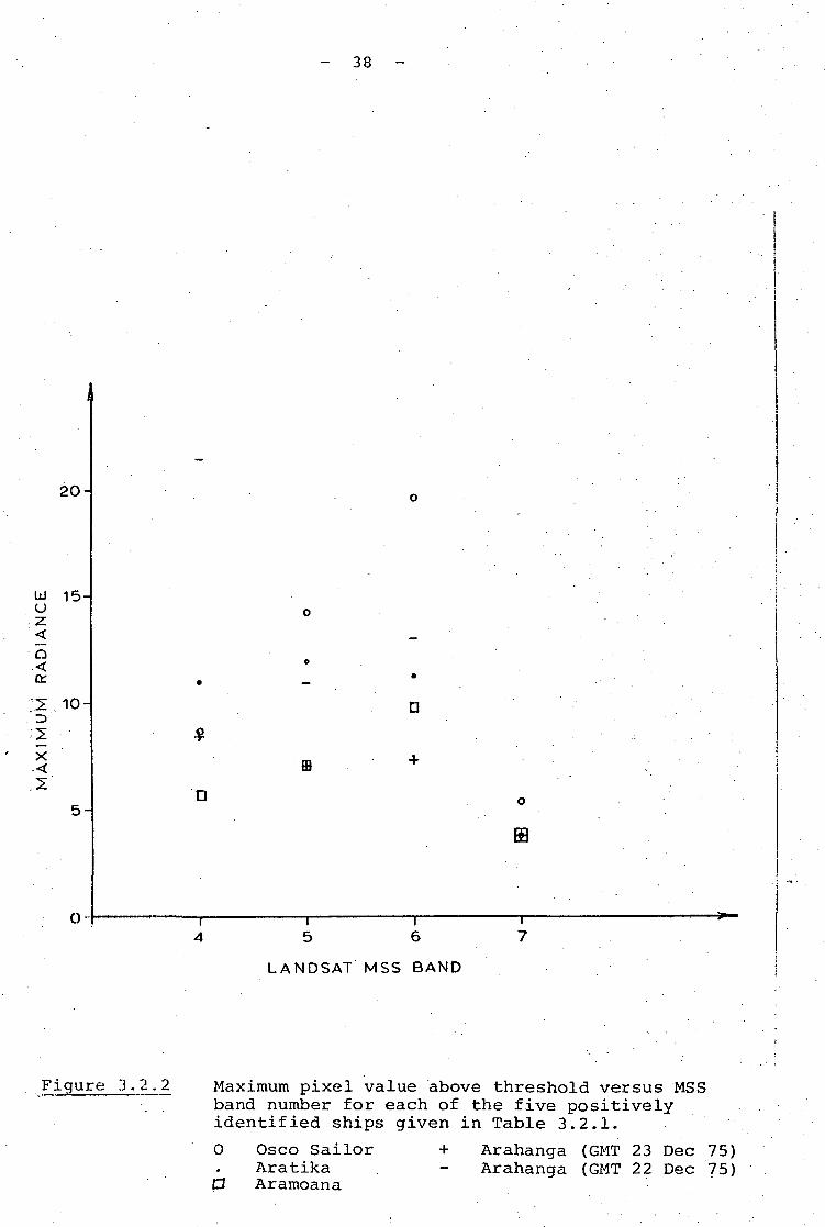
Measurements of the total reflected energy (Figure 3.2.1) andthe maximum value above threshold (Figure 3.2.2) are both subjectto considerable error. Errors'in the radiance levels as inFigure 3.2.1 are introduced by NASA quantisation techniques, the22 m pixel overlap per 57 m sample spacing, and the authors'processing. Although pixel overlap does not contribute to themaximum radiance errors in Figure 3.2.2, it does introduce a largervariation resulting from the positioning of the pixels with respectto the vessel. For example, a ship, the length of a pixel, may besampled completely within one pixel or straddle up to six pixels.
The best indication of ship size is given by the totalradiance values in MSS band 7 (Figure 3.2.1). This is because thetotal radiance values for a given size are more consistent thanmaximum radiance levels (Figure 3.2.2) and also because of the lownear-infrared reflectance of the ship's wake in MSS band 7. Thesmallest ship positively identified was 112; m long (see Table 3.2.1)In theory it should be possible to detect vessels 30 m long underfavourable imaging conditions. For example, based on the averagesignal per unit ship area produced by the moving ships, the HMNZSRotoiti would be expected to produce a total radiance value (afterprocessing) of 3.1, 3.3, 3.4 and 1.0 in bands 4, 5, 6 and 7respectively. This implies that a small boat may best be found bylowering the threshold level in band 7 to one level above the modalbackground and then confirm or reject the suspected target byexamining the other bands as in step II of the procedure describedpreviously.
Figure 3.2.3, a plot of signal to noise (S/N) ratio againstband number for the five positively identified ships2, indicatesthat MSS band 7 is the best band for initially locating shipsbecause of the high S/N ratio.
1. The wtrLp's wake is defined by the pixels which, afterprocessing, are zero in band 7 but non-zero in band 4,
2. A number of other possible ships were also found, buttruth for them was not available.

- 34 -
A number of problems were encountered in trying to detectships. For example, the contribution of turbidity to radiancevariations in the sea needs to be of low spatial frequency. Alsothe 22 in pixel overlap along rows needs to be taken into accountin determining the most likely position for the vessel, as do theextra pixels NASA have inserted to compensate for variations inscan line length.
Anomalies were found in the data which we were unable toadequately explain. For example one pixel in the Tasman Sea inband 7 had a radiance value of 63. This is the maximum possiblevalue in band 7 and is at least fifteen times greater than themaximum band 7 radiance for any ship studied. The pixel wassurrounded by pixels of value 0. No anomalous radiance value wasfound nearby in either band 4 or 5 but a high value was found inband 6 which was, however, offset by two pixels along a row. Theonly plausible, but unlikely, explanation suggested was that thehigh values were caused by reflections from another satellitepassing beneath LANDSAT II with the offset between bands beingcaused by the slightly different sampling times for bands 6 and 7,
Figure 3.2.4 is a coded computer printout of MSS band 7showing the Aratika approaching the entrance to Tory Channel inthe Marlborough Sounds.
- 35 -
Table 3.2.1
Description of Ships Present in LANDSAT II Scenes Studied
Ship's Name
Osco Sailor
Aratika
Arahanga
Arahanga
Aramoana
HMNZS Roboiti
Type
Oil Tanker
Inter-islandferry
Inter-islandferry
Inter-islandferry
Inter-islandferry
Fisheriesprotectionvessel
Length (m)
171.8
127.7
127.5
127.5
112.2
32.1
Breadth (m)
26.6
18.8
18.8
18.8
18.6 '
6.1
Tonnage
21,275
3,879
3,894
3,894
4,160
134
GMT date
23 Dec 75
23 Dec 75
23 Dec 75
22 Dec 75
22 Dec 75
23 Dec 75
Symbol i- Figures
O
; . « •
+
' -
Q
- 36 -
Table 3.2.2
LANDSAT Radiance Data for the Aratika
(Source: LANDSAT II scene 2335-21190)
MSS Band 4
Row 739
740
741
742
MSS Band 5
Bow 739
740
741
742
MSS Band 6
Itow 739
740
741
742
MSS Band 7
ttaw 739
740
741
742
Before Processing
Column1462 1463 1464 1465 1466 1467
16
12
12
14
10
8
8
8
4
2
5
5
16
16
12
14
11
10
8
9
4
6
4
5
15
22
13
14
9
15
8
8
4
10
5
4
2
14
24
17
14
8
19
13
9
4
12
10
5
2
2
14
19
24
14
8
13
20
9
2
8
16
4
4
14
13
19
14
9
8
14
8
2
2
10
5
2
After Processing
Column1462 1463 1464 1465 1466 1467
2.2
2.0
2,6
2.2
3.0
3.0
2.2
2.6
3.4
1.2
9.0
7.2i •
2.6
7.4
2
11.0
3.7
11.2
5.0
1.4
2.6
9.4
5.3
2
2
6.0
10.7
5.2
12.0
1.4
5.4
11.3
4
5.7
6.0
5.3
2
- 37 -
50-
40-
ui 3OCJz:<Q
20-
o
10-
-rA 5 6
LANDSAT MSS BAND
T"
7
Figure 3.2 .1 Total reflected energy (in LANDSAT quantisedunits) versus MSS band number for each of thefive positively identified ships given inTable 3.2.1.
O Osco SailorAratika
L3 Aramoana
Arahanga (GMT 23 Dec 75)Arahanga (GMT 22 Dec 75)
20-
UJ 15-Uz<Q
o:
;X, 10
X
2
5-
0-
- 38 -
n
nr7
—r4
T~5
T~6
LANDSAT MSS BAND
Figure 3.2.2 Maximum pixel value above threshold versus MSSband number for each of the five positivelyidentified ships given in Table 3.2.1.
0 Osco SailorAratika
0 Aramoana
+ Arahanga (GMT 23 Dec 75)Arahanga (GMT 22 Dec 75)
- 39 -
40-
2O-
10-
8
O
CO6- n
4-o
2-
i „.
D•
O
D
~r4
T"5
T"6
T"7
LANDSAT MSS BAND
Figure 3.2.3 Signal to noise ratio (S/N) versus MSS bandnumber for each of the five positivelyidentified ships given in Table 3.2.1.
O Osco SailorAratika
D Aramoana
Arahanga (GMT 23 Dec 75)Arahanga (GMT 22 Dec 75)

- 40 -
C i-
- =c >l- =J •!(
^7 il
- ^2 |]- ^3 -i- ^t J- ^j i
Cj '- ^ •»- ^3 -j— -^3 l- -t i!- -o !•. « . - a 1}— ^3 !J|
: - {~ ^3 t,- CM!,- =3 1
•-> '
- S I
- =3 i
I ^ j- -T3 .;- =5 •'•
— ^J !- ^i r- ^ r
: ?. ,1c/ r- cr i?
- C! r;- cr :<~ =3 r- 3 r- =3 t- ^ i
- =7 '- C! t- C! <- =? f— C* '- cr <- cr r- Cf f
- c, ;- cr ."• Z.J -i
- C! -
- S :: ^ ;- "3 •- CT .- 53 (J- cr f- ~ :- 0 <- c, vr- 0 <li- CJ.<:- =? N- C! <- f <- t- .— P*" 1
- K i
~ '!- '— t^f- \
~" I*"*"1 V_. ^ .- ,-' <- "'r \- f ,
:£-. «•• ,- f- .
—C ccc r-,-I -C,c irC rjC K,,r A »i -..f. Cr ar ct.,.r f--.r •<:_r tr• -cjr tr .r. rv ir= T- .r o^ a
f ~K3 iT
• •r'.
j rv.i — ...I C .r or f£. .f t-~r -£. .r ifr C!r ff.r a. ••
' C .\ o- .,V OC.
v u-\ =3..
x rv *
v c.- cr,.- <z:
- if
- l\ r
- c.'; 'J .- «:.— f^. .r- sC „
D i/~..2 Cl.J^ F* .; rv, t
: cT cr .?• oc..r r-.'• -f. .3- tr..r nl- ror rv i[• •—
3~ Ot LT .<: «:!" I--.». '.c;K tr''. *-f«• f*'.«• rv
(
ii
"
.
- « x
ff tC_J<f.^~
~- '
- x •c.
12. ICJa >(S I
u t- C; <
ll <
^T. «Ll- C
:x
\^ |'.L
rC.-,•b
UH
US
GU
XA
C,-.,.. - -
CA
p. ,-;i f- ik
y— •
-* Ar
•vJ/
. : -«v a f-j a <£ c iX a -.i Ijf~ <3— vC
ir LV.31 U.J «t I
J- C (_ ;r i^ c: i_• y- iP -•* '_: a •r x.' c.
c^
x "£.H C ;X ^ .D *~ •x; ex
~ r^-
- *•
•
\,L r\ <,- — •
DC c <x ^ •X !Z <C (^ •C CJ <X aci: c; <i. C «r «? •x c; ;x "-. •JL. X1 C- >—'?. X. (a x '^ =i".«1 .
«
;J -C •X _' -c, *-
- r- i
...3- Lfi X. Ir _ I- U. -3- ITi: vC| r
fe vC ••
a r-^ lx •- e »L e: -t o-& f~- .i; cri; Ar ••
•»
Ji!t: a: :V f^ -
S*. f*»- 1f ' '
" -1 ;L J- 1
1_ £2 i- Ah . *\ *
/
>•-
s .1
E= c-- * I3 i<: :3 IT <
- r- i
•*
17/ v
»
*te».-ld&
v
-c >
c r- <
^
\ •
n
•
' (e a- <
- r- i
»
>
(
(
ttSKWH
^1^uJflUIJB^
worn
4inMCOana*
n**m
=> ~- iv rv.' (— r^-
>
•
.
•• •
•..vv
- rv.X IT\ (\c <?
^- t- •-
/\
.
v rv.1 '- r- r
*
*
*
-
*
/ *•
:V
'
- +ft c: >
f . {• l
? IT -v rv. f^ ^ r
'
•
.
*• A.
• A .
' a: ic c cy o 'n o <J <3 C. I
t
c r~ «v rv.1 t- P~ r
4
»
•
•
1
1 ft
•t- +t «• -r c <r cc ia c <r. 0 <
i .
v rv r- r- i
N
*
» . .t- ..~ rvx r-_; <i3s U.3- X- U.
\'
3 ^~sT1. ff.
'"• r-
•• i
c t°~-L tr <X X ;j- tr S- ix iL *" !i i
:»V r^ft ff i- r- l
.
«
.
•.
k
"
'
*
•*-*
% «~ ^
— *"™ -
" 1
x >£- •x c 'x C <L.. e -x -^ '£ <t <' " ,
3 ITf ff 1-M
*
ft
P\
-y •>• V
F /^J <i
T. XS •—O —Ja — :v -:c r-«/" [>/"-
^ r-
*,
ii
gi
x Ix* ^X Xx Lx3fj C7*
- r-
• ,
vI ' •
t
jmH
H0
4«H
TO
•^w
•J* " ^^ V iTt vpV
am^«^
~*"
t
2 as cE acX OE
S .-3" Cf
•
j
;
Ii
i
•
;
j
1j
• I
1
it
' t
!
!
i1
i!
v=»i•— iB-lrx '^"*• .
Figure '3.2. 4 Coded computer printout of MSS band 1showing the Aratika approaching theentrance to Tory Channel (GMT 23 Dec 75)LANDSAT scene 2335-21190.
- 41 -
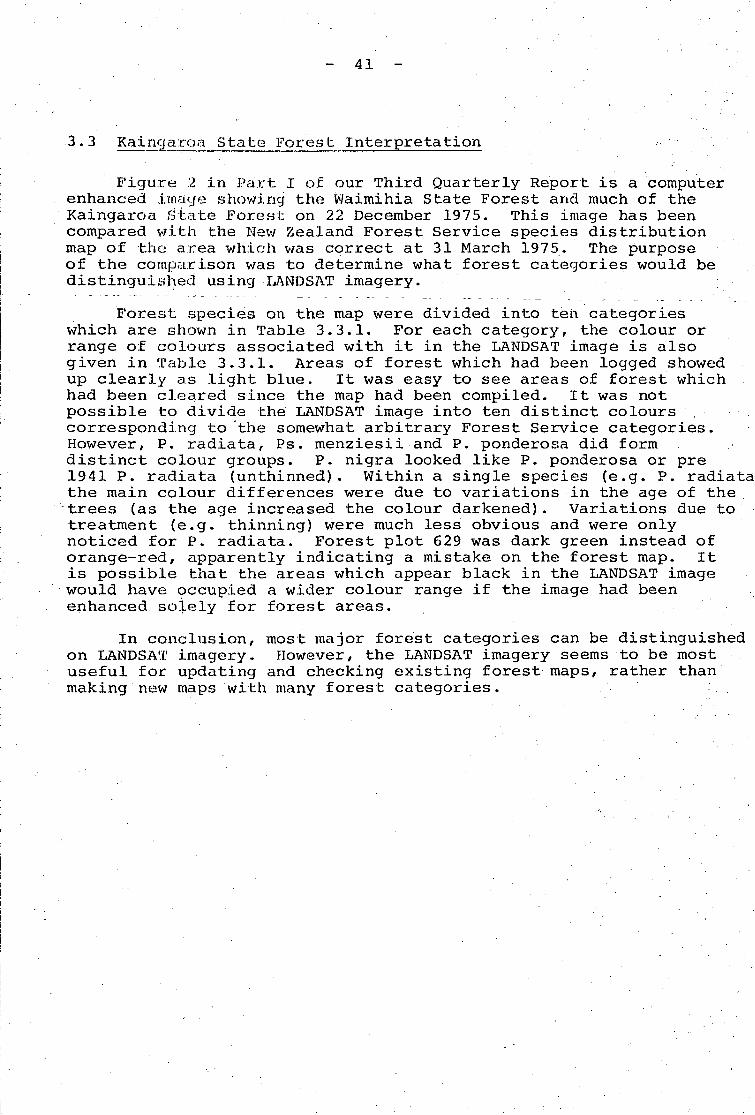
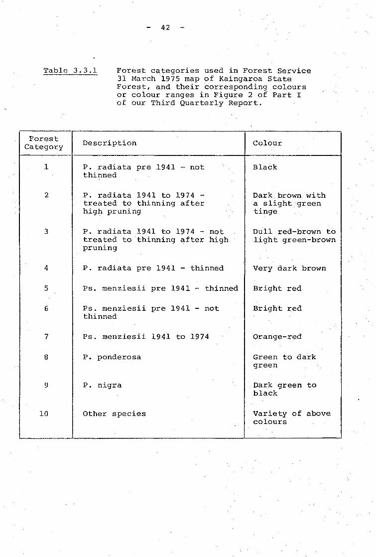
3.3 Kaingaroa State Forest Interpretation
Figure 2 in Part I of our Third Quarterly Report is a computerenhanced image showing the Waimihia State Forest and much of theKaingaroa .State Forest; on 22 December 1975. This image has beencompared with the New Zealand Forest Service species distributionmap of the area which was correct at 31 March 1975. The purposeof the comparison v/as to determine what forest categories would bedistinguished using LANDSAT imagery.
Forest species on the map were divided into ten categorieswhich are shown in Table 3.3.1. For each category, the colour orrange of colours associated with it in the LANDSAT image is alsogiven in Table 3.3.1. Areas of forest which had been logged showedup clearly as light blue. It was easy to see areas of forest whichhad been cleared since the map had been compiled. It was notpossible to divide the LANDSAT image into ten distinct colourscorresponding to 'the somewhat arbitrary Forest Service categories.However, P. radiata, Ps. menziesii and P. ponderosa did formdistinct colour groups. P. nigra looked like P. ponderosa or pre1941 P. radiata (unthinned). Within a single species (e.g. P. radiatathe main colour differences were due to variations in the age of thetrees (as the age increased the colour darkened). Variations due totreatment (e.g. thinning) were much less obvious and were onlynoticed for P. radiata. Forest plot 629 was dark green instead oforange-red, apparently indicating a mistake on the forest map. Itis possible that the areas which appear black in the LANDSAT imagewould have occupied a wider colour range if the image had beenenhanced soiely for forest areas.
In conclusion, most major forest categories can be distinguishedon LANDSAT imagery. However, the LANDSAT imagery seems to be mostuseful for updating and checking existing forest maps, rather thanmaking new maps with many forest categories.
- 42 -
Table 3.3.1 Forest categories used in Forest Service31 March 1975 map of Kaingaroa StateForest, and their corresponding coloursor colour ranges in Figure 2 of Part Iof our Third Quarterly Report.
ForestCategory
4
5
6
7
8
10
Description
P. radiata pre 1941thinned
- not
P. radiata 1941 to 1974 - •treated to thinning afterhigh pruning
P. radiata 1941 to 1974 - nottreated to thinning after highpruning
P. radiata pre 1941 - thinned
Ps. menziesii pre 1941 - thinned
Ps. menziesii pre 1941 - notthinned
Ps. menziesii 1941 to 1974
P. ponderosa
P. nigra
Other species
Colour
Black
Dark brown witha slight greentinge
Dull red-brown tolight green-brown
Very dark brown
Bright red
Bright red
Orange-red
Green to darkgreen
Dark green toblack
Variety of abovecolours
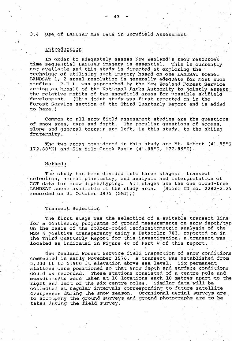
- 43 -
3 . 4 Use of LANDSAT MSS Data in Snowfield Assessment
In order to adequately assess New Zealand's snow resourcestime sequential LANDSAT imagery is essential. This is currentlynot available and this study is directed at exploring thetechnique of utilising such imagery based on one LANDSAT scene.LANDSAT 1, 2 area! resolution is generally adequate for most suchstudies. P.E.L. was approached by the New Zealand Forest Serviceacting 011 behalf of the National Parks .Authority, .'to.. jointly assess;the relative merits of two snowfield areas for possible skifielddevelopment. (This joint study was first reported on in theForest Service section of the Third Quarterly Report and is addedto here . )
Common to all snow field assessment studies are the questionsof snow area, type and depth. The peculiar questions of access,slope and general terrain are left, in this study, to the skiingfraternity.
The two areas considered in this study are Mt. Robert (41.85°S172.80°E) and Six Mile Creek Basin (41.88°S, 172.85°E).
Methods
The study has been divided into three stages: transectselection, aereal planimetry, and analysis and interpretation ofCCT data for snow depth/typing. All stages use the one cloud-freeLANDSAT scene available of the study area. .{Scene ID no. 2282-2125recorded on 31 October 1975 (GMT) i)
Transect_Se lection
The first stage was the selection of a suitable transect linefor a continuing programme of ground measurements on snow depth/ typOn the basis of the colour-coded isodensitometric analysis of theMSS 4 positive transparency using a Datacolor 703, reported on inthe Third Quarterly Report for this investigation, a transect waslocated as indicated in Figure 4c of Part V of this report.
Mew Zealand Forest Service field inspection of snow conditionscommenced in early November 1976. A transect was established from5,200 ft to 5,900 ft elevation above sea level. Six permanentstations \vere positioned so that snow depth and surface conditionscould be recorded. These stations consisted of a centre pole andmeasurements were taken at 10 locations each 10 metres apart to theright and left of the six centre poles. Similar data will becollected at regular intervals corresponding to future satelliteoverpasses during the snow season. Occasional aerial surveys areto accompany the ground surveys and ground photographs are to betaken during the field survey.
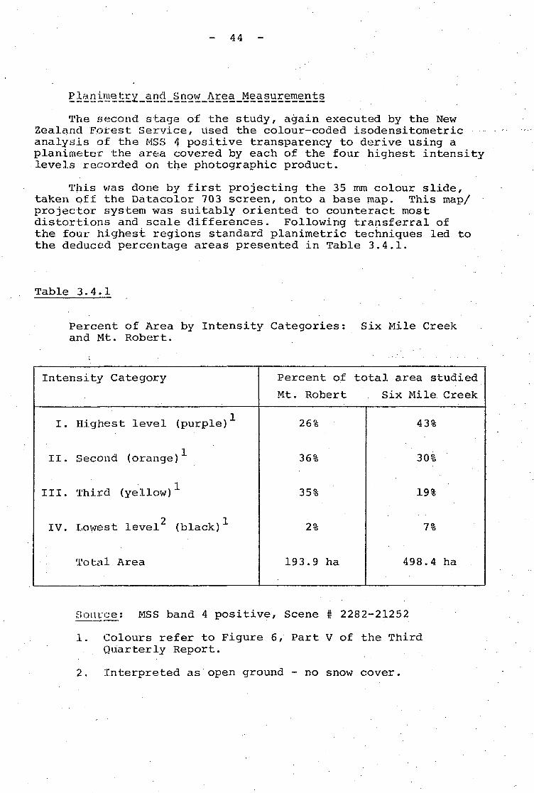
- 44 -
The second stage of the study, again executed by the NewZealand Forest Service, used the colour-coded isodensitometricanalysis of the MSS 4 positive transparency to derive using aplanimeter the area covered by each of the four highest intensitylevels recorded on the photographic product.
This was done by first projecting the 35 mm colour slide,taken off the Datacolor 703 screen, onto a base map. This map/projector system was suitably oriented to counteract mostdistortions and scale differences. Following transferral ofthe four highest regions standard planimetric techniques led tothe deduced percentage areas presented in Table 3.4.1.
Table 3.4.1
Percent of Area by Intensity Categories: Six Mile Creekand Mt. Robert.
Intensity Category
I. Highest level (purple)
II. Second (orange)
III. Third (yellow)1
IV. Lowest level (black)
Total Area
Percent of total area studied
Mt. Robert Six Mile Creek
26%
36%
35%
2%
193.9 ha
43%
30%
19%
7%
498.4 ha
£oiu;£e: MSS band 4 positive, Scene # 2282-21252
1. Colours refer to Figure 6, Part V of the ThirdQuarterly Report.
2. Interpreted as open ground - no snow cover.
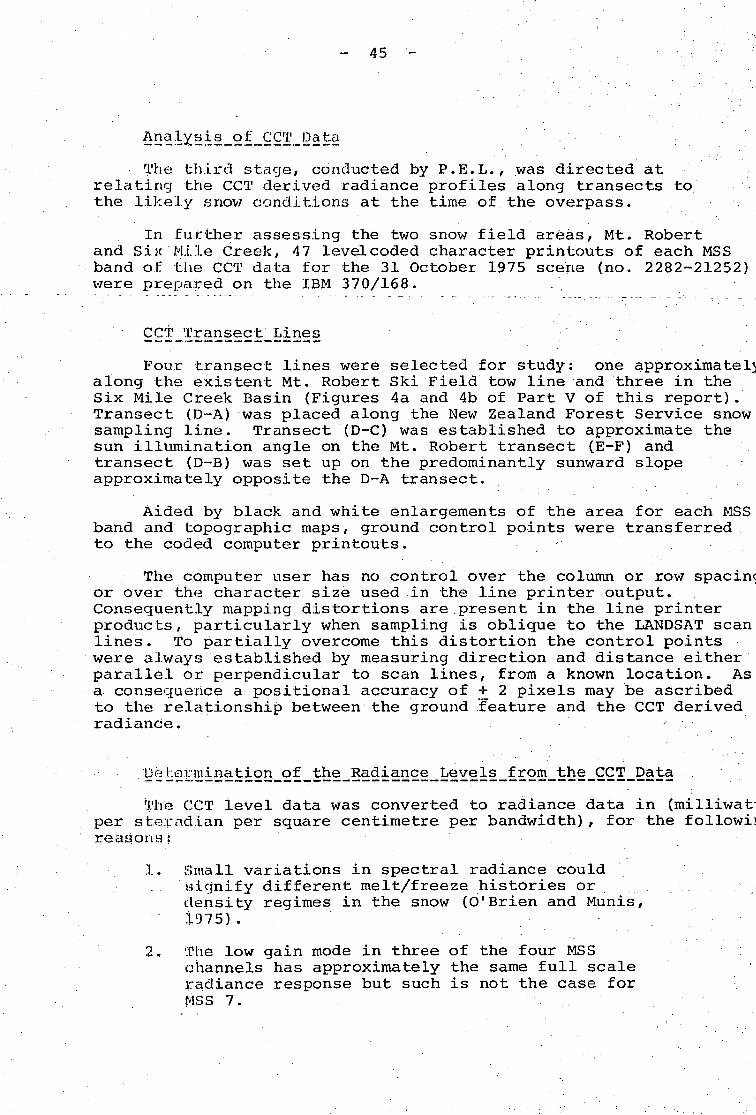
- 45 -
The third stcige, conducted by P.E.L., was directed atrelating the CCT derived radiance profiles along transects tothe likely snow conditions at the time of the overpass.
In further assessing the two snow field areas, Mt. Robertand Six Mile Creek, 47 level coded character printouts of each MSSband of the CCT data for the 31 October 1975 scene (no. 2282-21252)were prepared on the IBM 370/168. .,
Four transect lines were selected for study: one approximatelyalong the existent Mt. Robert Ski Field tow line and three in theSix Mile Creek Basin (Figures 4a and 4b of Part V of this report).Transect (D~A) was placed along the New Zealand Forest Service snowsampling line. Transect (D-C) was established to approximate thesun illumination angle on the Mt. Robert transect (E-F) andtransect (D-B) was set up on the predominantly sunward slopeapproximately opposite the D-A transect.
Aided by black and white enlargements of the area for each MSSband and topographic maps, ground control points were transferredto the coded computer printouts.
The computer user has no control over the column or row spacincor over the character size used in the line printer output.Consequently mapping distortions are present in the line printerproducts, particularly when sampling is oblique to the LANDSAT scanlines. To partially overcome this distortion the control pointswere always established by measuring direction and distance eitherparallel or perpendicular to scan lines, from a known location. Asa consequence a positional accuracy of + 2 pixels may be ascribedto the relationship between the ground feature and the CCT derivedradiance.
The CCT level data was converted to radiance data in (milliwatlper steradian per square centimetre per bandwidth), for the followiireasons s
.1. Small variations in spectral radiance could .Signify different melt/freeze histories ordensity regimes in the snow (O'Brien and Munis,1975).
2, The low gain mode in three of the four MSS :channels has approximately the same full scaleradiance response but such is not the case forM S S 7 . ' - . . . '
- 46 -
3. The CCT data for MSS 4, 5, 6 is decompressed(range 0-127) whereas, the MSS 7 data is in thelinear mode (range 0-63) .
The bandwidths of MSS 4, 5, 6 are all nominally the sameat 100 nm but that for MSS 7 is nominally 300 nm. This latterMSS band spans a number of water vapour absorption bands in theatmosphere, whose contribution is largely uncertain. Consequentlythe radiance is expressed in "bandwidth" terms rather than in"nanometer" terms.
The pixel radiance values were plotted together with thetopographic elevation profile and presented in Figures 3.4.1, 2,3 and 4. (The uncertainties in the four MSS band radiances are+ 0.03 (mw ster"1 cnT2 bandwidth"1) for MSS 4, + 0.02 for MSS 5,+0.02 for MSS 6 and +0.09 for MSS 7.)
Criteria_f or _Boundary__Se lection
The next step was the determination of the snow regionboundaries along each transect. Obviously in regions where thesnow cover is sparse the uncovered terrain will contribute to thefinal recorded radiance levels for each pixel.
Realising that snow will always increase the recorded radianceover that of the basic ground terrain leads to the two majorcriteria for selecting a boundary between terrain and snow andthen between types of snow.
The first criterion involves plotting the frequency ofoccurrence, in selected radiance intervals for each MSS band, andnoting natural groupings of radiance "blocks" at the greaterradiance end of the scale. For this study data from all fourtransects were used in these plots so that this "radiance block"classification criterion would be uniform between the Mt. Robertand Six Mile Creek Basin. The plots are presented in Figure 3.4.5.
The second criterion relies on all bands responding tochanging terrain/snow or snow/snow boundaries by all recordingincreased or decreased radiances together. This "radiance gradient"classification criterion was used to check the suggestions advancedby the "radiance block" selection process. (This selection orderwas uaecl to avoid any possible analyst bias in boundary selection.)
As f\ final check the selected boundaries were marked on theFigures .1.4.1, 2, 3 and 4, and the topographic elevation noted. Inthe "conUcol" basin, which spanned a range of sun illuminationangles bul: had essentially the same climatic regime, a similaraltitude v\fcmld be expected for each boundary.
Upon inspection then of Figure 3.4.5 the "radiance block"-selections were performed for each band and then checked using the"radiance gradient" criterion for each of the transects. The

- 47 -
selected boundaries were-then marked by vertical bars on thetransect plots (Figures 3.4.1, 2, 3 and 4).
It rapidly became evident that the "radiance gradient"criterion was a far more sensitive aid to boundary selectionthan "radiance blocking". For this reason extra boundaries tothose indicated solely by "radiance blocking" were marked onFigure 3.4.1, 2 and 3. (Another could have been appropriate ontransect E-F but the increased radiance values were not maintainedand the ground topography changed character at the suggested"boundary fa round" 5,00~0ft elevation) /)" "It "was also "apparent "that"MSS 7 "radiance block" values often did not reinforce the boundarypositions indicated by the other bands. Its role in "radiancegradient" determination was equal to that of other bands.
The topographic elevations, and the applicable variations,were now read from the plots (Figures 3.4.1, 2, 3 and 4) and theresults are presented in table 3.4.2.
Table 3.4.2
Topographic elevation (in feet), and variation of variousground cover/snow and snow/snow boundaries-'- extractedfrom the radiance transect plots of Figures 3.4.1,2,3 and 4.
Transect
Ground/snow
Snow/ snow
Snow/ show
D-A
4850 + 50
A
5300 + 50
A
-
5500 +50
B
D-B
f00 - 2°0°0
A
5200 --2QO
A
5650 W
A
Overloadobscuresextraregions
D-C
4600 + 50
A
4900 + 150
A
5300 + 50
A
Overloadobscuresextraregion
E-F
4650 +50
A ' '
(4900 + 50
A .,; •/possible only ashistory againstit)
.- :
1, These anow/snow boundaries labelled A would seem to indicateless clerise/drier history snow at higher elevations. Thoselabelled n could mark denser/wetter history snow at higherelevations.
- 48 -
Several light aircraft overpasses were made with hand heldoblique colour photographs being taken during September andOctober 1976. The photographs taken on 29 October 1976 (Figure3.4.6) have been used to aid the analysis of LANDSAT CCT(31 October 1975) data. The time-lag of approximately one yearis partially reconciled by inspection of New Zealand MeteorologicalService climatic data for September and October of 1975 and 1976.Monthly summaries of temperature and precipitation for the LakeRotoiti station (located between the two basins) indicate thatthere was little difference between the two years. Monthly meantemperature differences were less than 1°C and monthly precipitationdifferences were less than 4 mm. Snowfall for Lake Rotoiti stationalso indicates similar conditions prevailed at the time of theoverpass to that shown in Figure 3.4.6. One week prior to eachoverpass fresh snow fell to the same elevation (2,500 ft). Sunelevation and azimuth angles differ between the overpass and theoverflight due to the different times. The sun elevation andazimuth was 44° and 65° respectively for the LANDSAT overpass and60° and 21° for the aircraft flight.
Field data and hand-held photographs were also acquired byone of the authors (AJL) during November 1976.
The primary objective of this study, to compare snow conditionsin the two basins, has been accomplished using LANDSAT data. Thereis little question that the two basins exhibited great differencesin the percentage of snow covered area (see Table 3.4.1) and thelower elevation of 100% snow cover when transects of MSS radiancevalues from the Six Mile Creek (Figure 3.4.3) and Mt. Robert(Figure 3.4.4) are compared. Upon inspection of these figures,it is noted that the Six Mile Creek Basin transect (D-C) hassimilar radiance values below 4,600 ft; slightly higher valuesbetween 4,600 and 5,000 ft; and much higher radiance values above5/000 ft than the Mt. Robert Basin transect (E-F) . It is thereforeconcluded that the differences in radiance levels indicate a greaterarea.l snow cover in Six Mile Creek Basin, with the effect of lowerradiance values from vegetation/snow regions contributing to thesample within the pixels in the Mt. Robert area. A comparison ofthe two visible bands (MSS 4 and 5) for the two basins demonstratesthis di (iterance. Over 50% of the transect in Six Mile Creek Basinhas radUinee values higher than the maximum radiance values in theMt. Robert Basin. Confirmation of this conclusion is substantiatedby the colour oblique photography (Figure 3.4.6) taken of the twobasins at different times but, as mentioned previously, with similarsnow conditions.
The LANDSAT data can be divided into different radiance/topographic categories that show similarity between transects(Table 3.4.2). Although a correlation of these numerical categorieswith natural conditions of snow is deemed possible, confirmationrequires simultaneous field and satellite cover.
- 49 -
Several general observations have been made from the data -'that should help future interpretation of MSS radiance valuesfrom snow covered areas. The most important of these is the -•.•'effect of local slope angles and orientation, on the radiance "/• .from the snow. The effect of orientation with respect to the sunis evident in a comparison of transects D-A (Figure 3.4.1), asouth-facing slope directed away from the sun, and D-B (Figure3.4.2), a north-facing slope directed towards the sun. Higherradiance values and even overloading in three bands was recordedfor the sun facing slope. From aircraft photographs taken inSeptember 1976 of the Six Mile Creek Basin, local hot spots fromsolar reflection appear at several locations along transect D-C.Overloading of the MSS 5 sensor well below the crest suggeststhat a similar phenomenon has occurred on the satellite overpass,i.e. strong solar reflection from a local slope facet resultingin a hot spot.
The areal extent of a snow field together with the snow/vegetation boundary is easily gleaned from the LANDSAT MSS dataand requires little data manipulation. However, further informationmay be deduced from the natural breaks that occur in the MSS data.Although not confirmed, in this case, by corroborative ground datathe breaks suggest variations in snow type, depth, history or somecombination of the three did exist at the satellite overpass time.
The general increase in radiance values in the. three Six MileCreek Basin transects strongly suggests that the snow is fresher anddrier as the elevation increases. This relationship of snow radianceand the condition and/or moisture content of snow was reported byO'Brien and Munis (1975). Along with the natural breaks in thedata, this has been used with apparent success to categorise andclassify these snow transects into four regions (Table 3.4.1). Thetwo higher levels are interpreted to be potentially skiable snowand the two lower levels are probably non-skiable with the lowestradiance region being below the snow line.
Reference
O'Brien II.W. and Munis R.H. "Operational applicationsof satellite snowcover observations" published byNASA Report SP-391, p 345, (1975).
50 -
FIGURE CAPTIONS
Figure 3.4.1 The variation in MSS radiance along the D-Atransect together with the ground topographyprofile. Suggested snow region,boundariesmarked by vertical bars.
Figure 3.4.2 As for Figure 3.4.1 for transect D-B,Overload regions shown as O-O-0-0.
Figure 3.4.3 As for Figure 3.4.2 for transect D-C.
Figure 3.4.4 As for Figure 3.4.1 for transect E-F.
Figure 3.4.5 The differential and cumulative frequency ofradiance occurrence for each of the MSS bands.(This plot includes the data from all fourtransects D-A, D-B, D-C, E-F.)
Figure 3.4.6 Oblique aerial photographs taken on29 October 1976. Mt. Robert in the topphotograph and Six Mile Creek in the bottomphotograph.

- 51 • •-NOI1VA313
ooT«D
OOO(0
Oou>m
oowo
oo00IT
OoV•o
oooV
•*r>
T*n
Cn•HfM
Cvl
n
H ifl >0 Ni/i (/> t/i to ^ui t/i </> ui "•s: x 2 2 H
on
«c\»
1PIM
• ro
Ol
CM
oC\J
CO <0 C3
6Hi
6NT
6C\l
6o6
MIPIMpuoq UJD j-~ • c— i- MOI ) 30 N V I Q Vii • SSW •
•
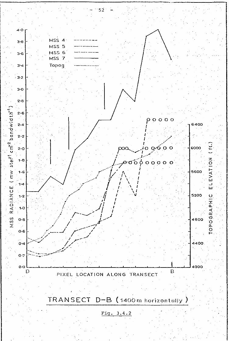
- 52 -
4-0
MSS 4
MSS 5
MSS 6
MSS 7
Topog
...y&-C5'b 6 O O O O O"
-»64OO
• 6OOO
O
- 5600
- 520O
- 48OO
u
Q.
<or
Q0.OI-
- 440O
4OOO
PIXEL LOCATION ALONG TRANSECTB
TRANSECT D-B ( l40Om horizonluljy )
Fig. 3.4.2
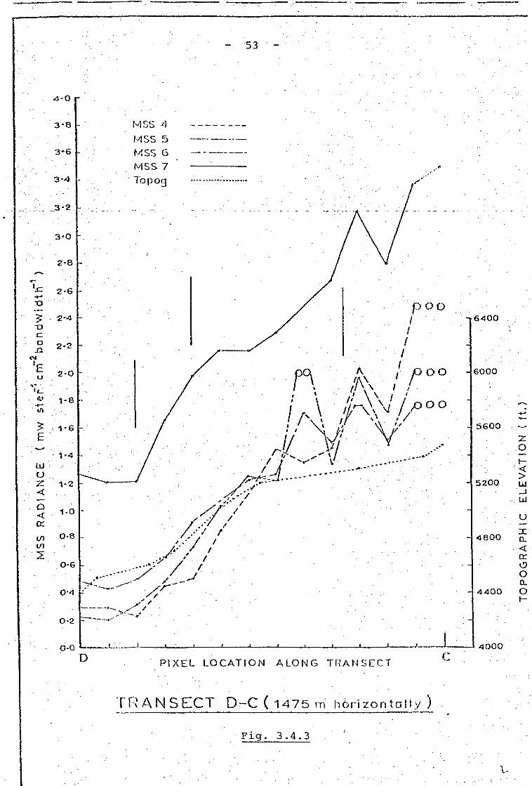
- 53 -
4-O
D PIXEL LOCATION ALONG T R A N S E C T
TRANSECT D-C ( 1475 m hbrizontal ly )
Fig. 3 .4 .3
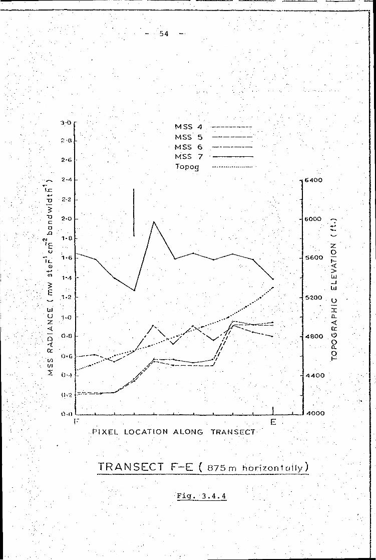
- 54 -
3.-O
?.*a
••«-» 2-4
.? 2"2
•D ?.0
OJQ
™E 1,. orr n-6It.
c>
1-4
LU
2:
Q
cc
'0uiT
.0.8
O-6
O-l} 1 L.
F
M:5
MSS 6
7
6-5OO
6000
2O
S60O ~
U
UI
5200
48OO
DCD.
CC
OCLOj-
4400
4OOO
PIXEL LOCATION ALONG TRANSECT
TRANSECT F-E ( 875m horizontally)
Fig. 3 . 4 . 4

.Fig. 3.. 4.5
0-0
Rrequencv of rad iance occu r rence t ransects .A-D, B-D , C-D .E-F for MSS 4,5,6,7..;. ,, . :•. , :.
cumula t ive f requency
MSS 4R A D I A N C E (mw stef1 cm"2- bandwidtrT1 ;

Figure 3. \._6_ Oblique aerial photographs taken on 29 OctoberL976. Mt. Robert in the top photograph andSix Mile Creek in the bottom photograph.
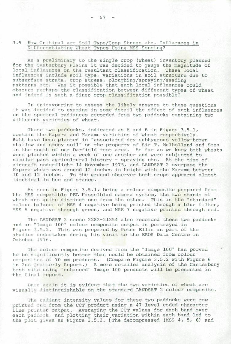
- 57 -
3.5 ngw^C^t^Lbi^ccil are Soil Type/Crop Stress etc. Influences inDifforentiating "wheat Types Using MSS Sensing?
A:> a preliminary to the single crop (wheat) inventory plannedfor the Canterbury Plains it was decided to gauge the magnitude oflocal inL: I nonces on the resultant classification. These localinfluences include soil type, variations in soil structure due tosubsurface strata, crop stress, ploughing/sprayiny/seedingpatterns -:>tc. Was it possible that such local influences couldobscure perhaps the classification between different types of wheatand indeed i.s such a finer crop classification ponsible?
In endeavouring to assess the likely answers to these questionsit was decided to examine in some detail the effect of such influenceson the spectral radiances recorded from two paddocks containing twodifferent varieties of wheat.
These two paddocks, indicated as A and B in Figure 3.5.1,contain the Kapara and Karamu varieties of wheat respectively.Both have been planted in "associated dry subhygrous yellow-brownshallow and stony soil" on the property of Sir T. Mulholland and Sonsin the south of our Darfield test area. As far as we know both wheatswere planted within a week of one another and were subjected tosimilar past agricultural history - spraying etc. At the time ofaircraft underflight 14 November 1975, and LANDSAT 2 overpass theKapara wheat was around 12 inches in height with the Karamu between10 and 12 inches. To the ground observer both crops appeared almostidentical in hue and stance.
As seen in Figure 3.5.1, being a colour composite prepared fromthe MSS compatible PEL Hasselblad camera system, the two stands ofwheat are quite distinct one from the other. This is the "standard"colour balance of MSS 4 negative being printed through a blue filter,MSS 5 negative through green, and MSS 7 negative printed through red.
The LAHDSAT 2 scene 2282-21254 also recorded these two paddocksand an "Image 100" colour composite output is portrayed inFigure 3. "5. 2. This was prepared by Peter Ellis as part of thestudies nn-lortaken during his visit to the EROS Data Centre inOctober .!.'.»7 6.
T'u ' colour composite derived from the "Image 100" has provedto be M i ' j i i l ficantly better than could be obtained from colourcomponi. I.M i oE 70 mm products. (Compare Figure 3.5.2 with Figure 6in 2iul (pi it.-lierly Report.) A more detailed analysis of the Canterburybest: Bite using "enhanced" Image 100 products will be presented inthe C h i i l report.
(••n in .1 |,iin it is evident that the two varieties of wheat arev i s u i l l \ 'li itinguishable on the standard LANDSAT 2 colour composite.
Tli.' i 1'li.ant intensity values for these two paddocks were rowprinted mil: from the CCT product using a 47 level coded characterline priii I.or output. Averaging the CCT values for each band overeach padilo.'k, and plotting their variation within each band led tothe plot •.liven as Figure 3.5.3. (The decompressed (MSS 4, 5, 6) and
- 58 -
linear (M.S.S 7) CGT data were related to the calibrated maximumradiances fur the MSS system ("LANDSAT" Users Handbook) in orderto derive l h > : plot.f-.--.fi "radiances per channel bandwidth"^ Thislatter Vru.iation, apparently evident in the aircraft scene, wouldseem to h-v./e resulted from underlying structure in the alluvialstrata:; <)/;' the soi..1 together with farming, ploughing and seedingpractices. Some evidence too of crop stress would seem to beevident, from both CCT and aircraft products, near the northernand southern paddock boundaries. The variation in the CCT radianceover each paddock is indicated by the relevant "error bars" inFigure 3.5.3.
From this figure it is noted that the Kapara wheat exhibitsa marginally higher spectral radiance in MSS 4 and 5 than theKaramu wheat with the roles being markedly reversed in MSS 6 and 7.It is further noted that local influences could have greater effectin crop variety classification in MSS 4 and 5 than in MSS 6 and 7.
Three conclusions, then, emerge from this study:
1. It is apparently possible to classify between somevarieties of the wheat crop provided adequate groundtruth information is applied to the recorded spectralradiance set.
2. Adequate ground truth for a test area pilot studyshould include: crop type and variety, date ofplanting, fertiliser/spraying history, soil typeand moisture stress patterns together with grazinghistory.
3. The role of MSS 6 and 7 in the complete visual andcomputerised classification procedure for wheatshould be further investigated.

- 59 -
FIOURE CAPTIONS
Figure 3 . 'j. 1. A colour composite of part of the Darfieldtest area showing the Kapara wheat paddockas A and the Karamu wheat paddock as B.
MSS 4 -ve
MSS 5 -ve
MSS 7 -ve
printed through blue
printed through green
printed through red
Figure 3.5.2 An Image 100 colour composite of the partof scene 2282-21254 showing the Kapara/Karamuplots.
Figure 3.5.3 A comparison of target radiance (in terms ofmw cm"^ ster" per MSS channel bandwidth) asa function of MSS band for Kapara and Karamuwheat. The data for the two wheats areplotted horizontally offset one from theother. (From scene 2282-21254.)

Figure J I A colour composite of part of the Darfield testarea showing the Kapara wheat paddock as A andthe Karamu wheat paddock as B.
MSS 4 -ve printed through blueMSS 5 -ve printed through greenMSS 7 -ve printed through red

Figure 'J, I'), 2 An Image 100 colour composite of the part ofscene 2282-21254 showing the Kapara/Karamuplots.

2-4-
2'2-
- 62 -
Fig. 3.5.3
Scene 1DJ|=: ;!282-21 254
Date : 31 Oct.,,1975
Kapara Wheat ( paddock C5)
O Karamu Wheat (paddock C6)
0
2-0-
1-8-
1-6-
1-4-
x:. •1 1
XIi
ccaJC
1-2W (/)U Q
a
o:1-0-
0-8-
<ijct
ClO oa- ,o'( 'M,... p
0-6-
O-4
0-2-
o-o- ! i
BAND No.
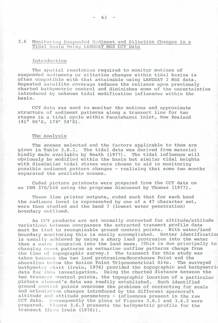
- 63 -
3.6 Monihori -ti'-'j _S\i ' i . ••!• ' •'' >'• "iimcnt and Siltation Changes in aZLfl2JLI IH in Us irnj f.Al(D.'J/\T MSS CCT Data
Iritrt id i to tion
The spat; Lai resolution required to monitor motions ofsuspended sediments or siltation changes within tidal basins isoften compatible with that attainable using LANDSAT 2 MSS data.Repeated satellite coverage reduces the reliance upon previouslycharted bathymetrie control and diminishes some of the uncertaintiesintroduced by unknown tidal modification influences within thebasin.
CCT data was used to monitor the motions and approximatestructure of sediment patterns along a transect line for twostages in a tidal cycle within Pauatahanui Inlet, New Zealand(41° 06'S, 174° 54'E).
The Analysis
The scenes selected and the factors applicable to them aregiven in Table 3.6.1. The tidal data was derived from materialkindly made available by Heath (1977). The tidal influence willobviously bo modified within the basin but similar tidal heightswith dissimilar tidal states were chosen to aid in monitoringpossible sediment pattern changes - realising that some two monthsseparated the available scenes.
Coded picbure printouts were prepared from the CCT data onan IBM 370/168 using the programs discussed by Thomas (1977).
These line printer outputs, coded such that for each bandthe radiance level is represented by one of a 47 character set,were then studied and the band 7 (lowest water penetration)boundary outlined.
As CCT products are not normally corrected for altitude/attitudevariations between overpasses the extracted transect profile datamust be tied to recognisable ground control points. With water/landboundary monitoring this is easily accomplished. Better identificatioiis usually achieved by using a sharp land protrusion into the waterthan a w-il'M Incursion into the land mass. (This is due principally tochanging i - i ' M - k patterns as estuarine outflow patterns change fromthe tiiu» oi: topographic survey.) The transect for this study wastaken tu'.l • M the two land protrusions Moor ehouse Point and theshoreline 11 • Iow the Ration Point Trigonometrical Site. The surveyedba thyme t.t \' < hirt (Irwin, 1976) provided the topographic and bathymetricdata foi: I hi > investigation. Using the charted distance between thetwo trami set control points, the topographic location of a particularpicture t» i »Mii"iit' s data was readily established. Such identifiedground control points overcome the problems of correcting for scaleand oricul.it i<m changes introduced by the different spacecraftaltitude and attitude parameters - influences present in the rawCCT data. jquently the plots of Figures 3.6.1 and 3.6.2 wereprepared. I'hiure 3.6.3 presents the bathymetric profile for thetransect (£L,».I Irwin (1976)).
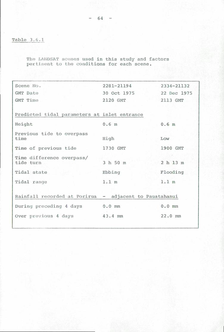
- 64 -
Table 3. (>. I
Tin.-' fiANDSAT scenes used in this study and factorspertinent to ttie conditions for each scene.
Scene tin.
GMT Dat-.»
GMT Time
2281-21194
30 Oct 1975
2120 GMT
Predicted tidal parameters at inlet entrance
Height 0.6 m
Previous tide to overpasstime High
Time of previous tide 1730 GMT
Time difference overpass/tide turn 3 h 50 m
Tidal sbate Ebbing
Tidal range 1.1 m
2334-21132
22 Dec 1975
2113 GMT
0.6 m
Low
1900 GMT
2 h 13 m
Flooding
1.1 m
Rainfall recorded at Porirua - adjacent to Pauatahanui
During preceding 4 days 0.0 mm 0.0 mm
Over previous 4 days 43.4 mm 22.0 mm
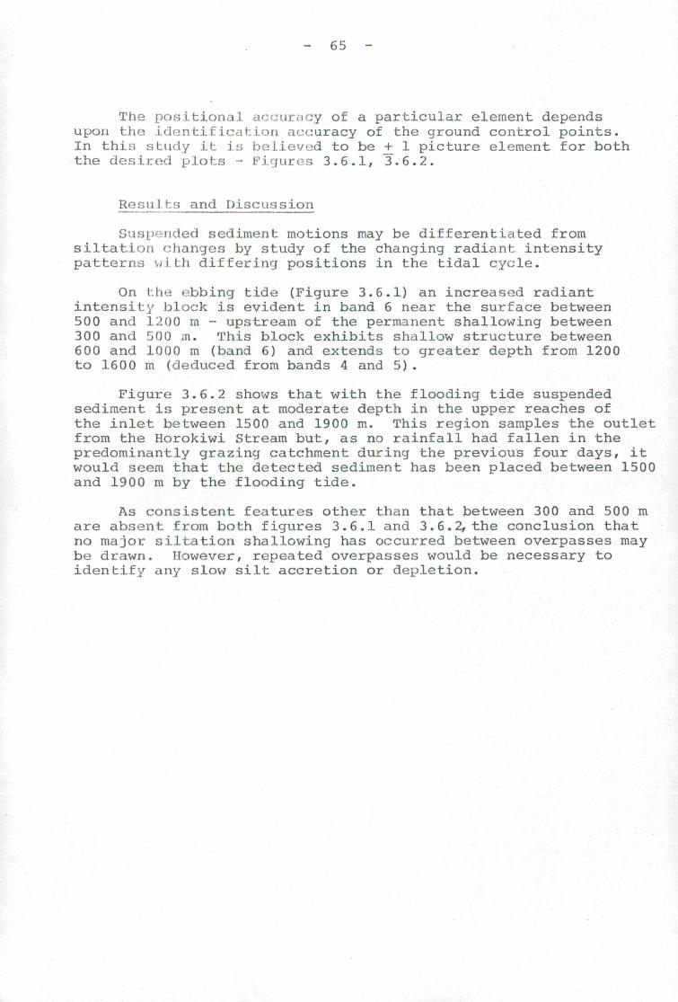
- 65 -
The positional accuracy of a particular element dependsupon the identification accuracy of the ground control points.In this stud/ it iy believed to be 4^ 1 picture element for boththe desired plots Figures 3.6.1, ~3.6.2.
Re.r; 11 I i i and Disc as s ion
Suspended sedimenb motions may be differentiated fromsiltation changes by study of the changing radiant:, intensitypatterns with differing positions in the tidal cycle.
On t-.he ebbing tide (Figure 3.6.1) an increased radiantintensity block is evident in band 6 near the surface between500 and 1200 rn - upstream of the permanent shallowing between300 and 500 m. This block exhibits shallow structure between600 and 1000 m (band 6) and extends to greater depth from 1200to 1600 m (deduced from bands 4 and 5).
Figure 3.6.2 shows that with the flooding tide suspendedsediment is present at moderate depth in the upper reaches ofthe inlet between 1500 and 1900 m. This region samples the outletfrom the Horokiwi Stream but, as no rainfall had fallen in thepredominantly grazing catchment during the previous four days, itwould seem that the detected sediment has been placed between 1500and 1900 m by the flooding tide.
As consistent features other than that between 300 and 500 mare absent from both figures 3.6.1 and 3.6.2, the conclusion thatno major siltation shallowing has occurred between overpasses maybe drawn. However, repeated overpasses would be necessary toidentify any slow silt accretion or depletion.
- 66 -
REFERENCES
Heath R. (1977) Private Communication. DSIR OceanographicInstitute, New Zealand.
Irv/.in J. (1976) "Pauatahanui Inlet Bathymetry 1:5,000"DSIR Oceanographic Institute Chart No. '17, NewZealand.
Thoiti.it; I.L. (1977) "Basic programs for accessing andutilising LANDSAT MSS CCT data using the PL/1 languageon an IBM 370/168 computer". DSIR Physics andEngineering Laboratory Report No. 566.
- 67 -
FIGURE CAPTIONS
F i.cjure 3.6.1 Radiant intensity variations along thetransect line for scene 2281-21194.
Figure. 3.6.2 Radiant intensity variations along thetransect line for scene 2334-21132.
Figure 3.6.3 Bathymetry profile along the transectline from Irwin (1976).
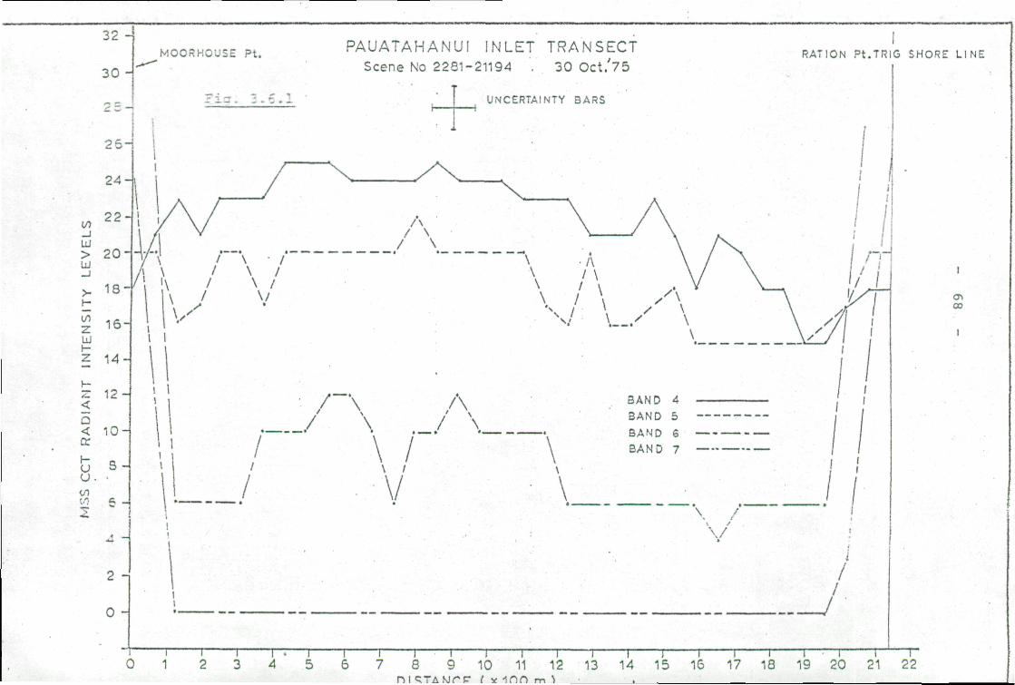
32 -
30 -
2 s- -
26-
2*4 ~~
c/, 22~UJ> 20UJ_i>. 18-K-
| 16-UJi-z 14-
H-Z 12-<D< 10-tt
t 5-<J. -VIt/5 A -
A —
2 -
0 _
C
|
MOCRHGUSE Pt. PAUATAHANUI INLET TRANSECT R A T ] O N pt.TR
!•*** Scene No 2281-21194 . 30 Oct/75T
i_. ;. UNCERTAINTY BARS
H"1 Ii •
A % X\ I/ ^v Ii / Xr
1 / / ^ ^ \ ^
Vy v ' \/\ :/V\Jfi' . I /
1 1 '! . / \ A SAND
/ \ /N I/ \ / \ BAND 5 i
1 ' • / \ -/ \ BAND .
/ \ \ BAND 7 1 1\ i \ ! I
1 / \l \ 1 11 . _/ V \ / /
! : \/
! :1 I
| /
/'
i I I • I I I 1 ' ! 1 1 1 1 1 1 1 ' i i -• • 1) 1 2 3 4 5 6 8 9 10 11 12 13 14 15 16 17 18 19 20 21
n i «;TA M ^ r ^ v - i n n m ^
G SHORE L INE
•
1
00
1
i
r22
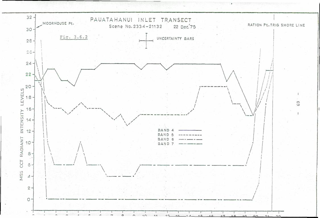
32 •
30-
28 -
26-
94 -
22 -
_i
UJ
>. 16-i—
CT
R
AD
IAN
T
INT
EN
Sl
5*
00 O
l\i
.N
l~,.
' 1
1
l i
U
10^ 4 _
2
2-
o-
PAUATAHANUI INLET TRANSECTMOORHOUSE Pt. RATinvi P+ r
^ Scene No. 2334-21132 22 D.ec.75 P t 'T
Fiq. 2 . 6 . 2 UNCFRTAINTY BARS
Ii
'
\
^i
1
_
' / \X \ / \ I /^-^ ,-\ j1 \ \ / / /
\v xx\s / X -N \ I// '
\'' 1 Ii • iBA N D A
SAND <=>BAND 5 ,
i BAND 6 j
\ A S A N D 7 /
A . . // \ /
.1 /* i • //. • •* " /
iRIG SHORE LINE
CTl
l
:
i i i i • i •• i ; i i — i 1 r i 1 1 1 i i — ' 1 —

R A T I O N P x .SHORE LIN
Ul
uiI/)
UJ
2
o_iUJCD
Z 3-J—
Q.UJQ
i ~ C w S E ?* i
o
1
2DD 400 600 300 1000 1200 1400 1600 1800 2000 2200ICO SCO BOO 700 900 1100 1300 1 &00 1700 1300 2100
DISTANCE f rom MOOREHOUSE .POINT (m)
Fig. 3 .6 .3
P A U A T A H A N U ! INLET T R A N S E C T
Bathymetry Prof i le( f r o m Oceangraphic Inst.chart 47; 1976)
- 71 -
4. PUBLICATIONS
4 •
P.J. Kills "Overseas Visit to NASA and the EROSData Center, U.S.A., October/November1976". P.E.L. Overseas Visit ReportNo. 72, November 1976.
M.J. McDonnell "Computer programs for processing LANDSATimagery on an HP 2100 computer: Part III"P.E.L. Report No. 567, March 1977.
I.L. Thomas "Basic programs for accessing andutilising LANDSAT MSS CCT data using thePL/1 language on an IBM 370/168 computer".P.E.L. Report No. 566, March 1977.
4.2 Newsletter
One copy of the "Remote Sensing Newsletter" was circulatedin late 1976. Its main purpose was to furnish the predictedLANDSAT 2 overpass dates in time for planning co-ordinated fieldprogrammes over the coming year through New Zealand.
- 72 -
5 .
5.1 LA I n . r 2 Coverage of New Zealand
'•"• kii'r./i i-.-lqo no scenes have been recorded over New Zealandsince IJ. May [.')/(< d-,. spite the best efforts of NASA staff to takeadvant i i of cloud cover/priority slots to support our investigations.Of the i'« icenes so far recorded by LANDSAT 2 seventeen wererecorded i.a response to a special request for coverage between14 and .1.7 February 1976 whether cloud was present or not.
The fiict that tape recorder limitations and higher prioritycovera'je requirements in other areas has reduced that coverageobtainable over New Zealand would seem to be less of a constraintthan this country's high incidence of cloud cover.
Aii Mow Zealand is a relatively small country with markedlydiverse agricultural/forestry geologic etc. patterns occurringwell within the scope of one LANDSAT image, we should like tosuggest a reappraisal of our initial scheduling request of cloudcover tolerance of 30%. Scenes with greater than 30% cloud coverhave been used to extract data useful to New Zealand investigations(e.g. West Coast lineament study contained in Third QuarterlyReport) .
It is rare for New Zealand to be wholly cloud covered andconsequently we speculate as to the possibility of some coveragebeing scheduled for New Zealand between the bounds of the predictedcloud fronts rather than the complete orbital track being essentiallycloud free, as would be required by our earlier request of a 30%cloud tolerance.
An inspection of cloud cover imagery received by the NewZealand Meteorological Service from the NOAA spacecraft wouldindicate that this would be a more fruitful approach than thatinitially employed.
We would welcome NASA comment on this problem area.
5.2 1 1 1 1 i Products
photographic products were received during the reportingperiod. COT products have been received from both LANDSAT 2 aspart of investigation no. 2823, and from LANDSAT 1 being purchasedin !:5up|'"t I. of such studies. Currently, at 28 February 1977, wehold I ! lANDSAT 2 CCT sets, of the agreed 22 sets, with a further10 LAND9AT 2 CCT sets on order.
5.3 ivr i.i.ne Length Variations
M IM perhaps worth pointing out that in the CCT's we haverecvM i the first two registration fill characters at the end ofeach i i ' K i Line are not (X^ FF ) but some random number. Also thelast two to four pixels for each band in each scan line are zero.The nuiiilx'i of non-zero pixels in a given scan line thus varies withthe band number, even though according to the end of line calibrationdata, th . in line length is the same for each band. This seems tobe in con!,adiction to the 1976 LANDSAT Data Users Handbook and needsclari ficai i • >n.

- 73 -
6• ACKNOWLEDGEMENTS
One author: (P.J. Ellis) would like to thank the staff ofNASA in Washington and Goddard, and the USGS at Sioux Falls,for their great hospitality during a recent visit, and for theopportunity to use the "Image 100" interactive analysingsystem.

PART II
SEISMOTECTONIC, STRUCTURAL, VOLCANOLOGIC AND
GEOMORPHIC STUDY OF NEW ZEALAND
Investigation No 2823 A
Co-Investiga tor: Dr Richard P. Suggate
Agency: N.Z. Geological Survey
Address: Department of Scientific andIndustrial Research
P.O. Box 30-368Lower HuttNew Zealand
Telephone No.: Wellington 699-059
Author: Mr P. Oliver

LANDSAT II PROGRESS REPORT
LAND'iAT imagery of selected areas has been examined forgeological features. A covering of vegetation masks the lithologybut lineam-ents related to faulting, and large scale lithologicstructures, were observed. In all cases linear features were foundto be clearly visible on black and white positive transparenciesof MSS bands 6 and 7.
1. NORTH CANTERBURY-SOUTH MARLBOROUGH AREA
Cloud-free images (E-2192-21265) of this area were examined.Figure 1 shows the lineaments on these images. Many of the majorlineaments correspond to known faults which are predominantlyorientated in a north-east to south-west direction. A secondaryset of lineaments is orientated in an approximately north to southdirection.
Along the eastern margin of the Southern Alps there is a highdensity of parallel minor linear features. These are predominantlysub-parallel to the major faults, but are also locally parallel tothe known strike of the Torlesse sandstone and siltstone beds mappedby Gregg (1964). In the area west of Hawarden the lineaments curvearound to strike north. This is consistent with the strike of thebeds in this area, which have been mapped in detail by Bradshaw(1972), and indicates that these parallel sets of minor lineamentsare related to bedding structures rather than faults.
The area covered by the parallel sets of minor lineaments alsocorresponds to a low relief topography giving this area a geo-morpholoojically distinct erosion pattern easily distinguished fromthat to the west that forms the Southern Alps. On the basis oftheir textural appearance on the LANDSAT images, the rocks of theCavendish Hills and Okuku Range appear to be similar to the Jurassicrocks of the Lowry Peaks Range.
Minor lithologic lineaments were not observed in the SouthernAlps as these had a covering of winter snow. The west part of thisarea is also covered by summer-time LANDSAT II image (E-2409-21293)in which minor lineaments were observed (Third Quarterly Report,No. 553, Sept. 1976). The summer images of the Southern Alps werenot only predominantly snow free but, because of a higher sun angle,also shoH-M major lithologic units' as dark and light bands. In thewinter imi i^s (E-2192-21265) the low sun angle did not favour visualrecogni t i'.'..i of lithologic units. The low sun angle also resulted inlong shadows that obscured many of the features observed, in thelarger v-ilLeys, in the summer images. This shadowing effect was,however, of direct benefit in the recognition of the sets of parallelminor lin-vtments observed on images E-2192-21265. Thus where therewas low relief topography the long shadows caused by a low sun angleaccentuated the erosional features that were predominantly controlledby litholo<jy.
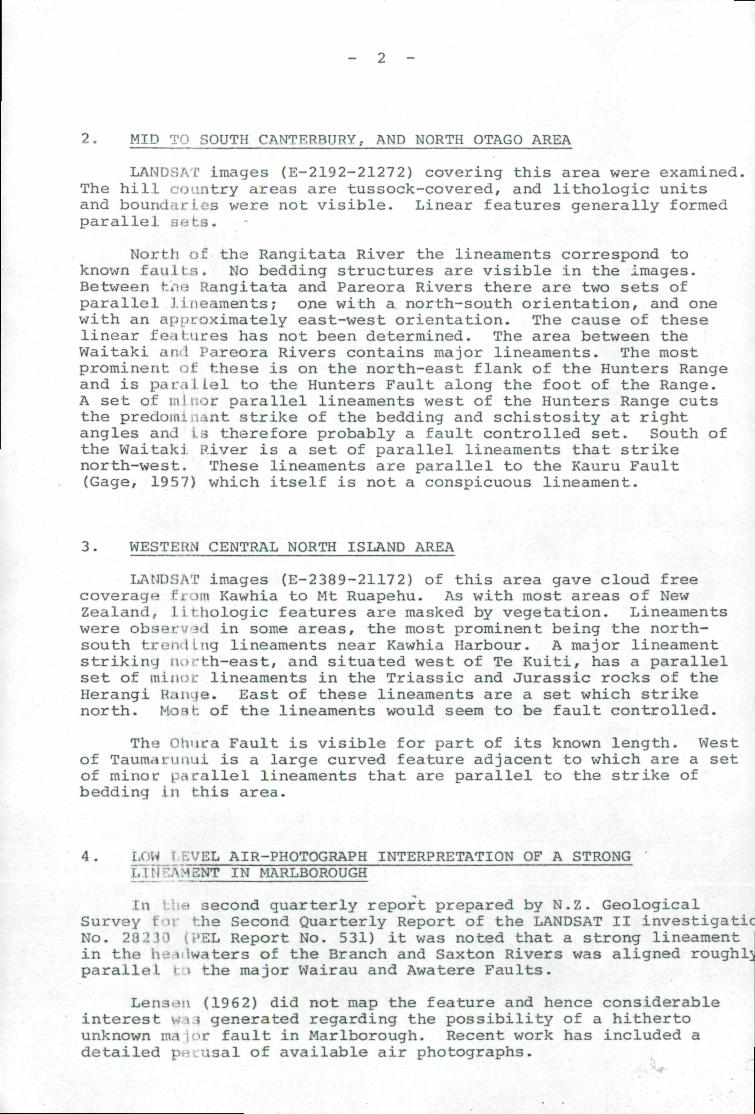
2. MID TO SOUTH CANTERBURY. AND NORTH OTAGQ AREA
LANDS At1 images (E-2192-21272) covering this area were examined,The hill country areas are tussock-covered, and lithologic unitsand boundaries were not visible. Linear features generally formedparallel sets.
North of the Rangitata River the lineaments correspond toknown faults. No bedding structures are visible in the images.Between hi'io Rangitata and Pareora Rivers there are two sets ofparallel lineaments; one with a north-south orientation, and onewith an approximately east-west orientation. The cause of theselinear features has not been determined. The area between theWaitaki ami Pareora Rivers contains major lineaments. The mostprominent of these is on the north-east flank of the Hunters Rangeand is pai.Mll.el to the Hunters Fault along the foot of the Range.A set of minor parallel lineaments west of the Hunters Range cutsthe predomiaant strike of the bedding and schistosity at rightangles and Ls therefore probably a fault controlled set. South ofthe Waitaki River is a set of parallel lineaments that strikenorth-west. These lineaments are parallel to the Kauru Fault(Gage, 1957) which itself is not a conspicuous lineament.
3. WESTEKM CENTRAL NORTH ISLAND AREA
LAUDSAT images (E-2389-21172) of this area gave cloud freecoverage Fr-.Mu Kawhia to Mt Ruapehu. As with most areas of NewZealand, L i tihologic features are masked by vegetation. Lineamentswere observed in some areas, the most prominent being the north-south tren.li.ng lineaments near Kawhia Harbour. A major lineamentstriking u.>rth-east, and situated west of Te Kuiti, has a parallelset of minor lineaments in the Triassic and Jurassic rocks of theHerangi Han.je. East of these lineaments are a set which strikenorth. Moah of the lineaments would seem to be fault controlled.
The Oh'ira Fault is visible for part of its known length. Westof Taumaruuui is a large curved feature adjacent to which are a setof minor parallel lineaments that are parallel to the strike ofbedding .in this area.
4 . Wl £VEL AIR-PHOTOGRAPH INTERPRETATION OF A STRONGLI ti LAMENT IN MARLBOROUGH
In - second quarterly report prepared by N.Z. GeologicalSurvey f-ir the Second Quarterly Report of the LANDSAT II investigaticNo. 28230 (i'EL Report No. 531) it was noted that a strong lineamentin the Iv.j i;lwaters of the Branch and Saxton Rivers was aligned roughlyparallel ' » the major Wairau and Awatere Faults.
Leri3>-.m (1962) did not map the feature and hence considerableinterest wi? generated regarding the possibility of a hithertounknown ma ;;T fault in Marlborough. Recent work has included adetailed p<:.;.;sal of available air photographs.
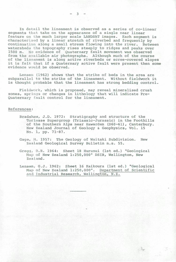
In detail the lineament is observed as a series of co-linearsegments that; take on the appearance of a single near linearfeature on the much larger scale LANDSAT images. Each segment ischaracter i.3eel by a linear stretch of riverbed and frequently bycontinuation along a small stream flowing into the river. Betweenwatersheds the topography rises steeply to ridges and peaks over1500 m. Ho evidence of Quaternary fault movement was observedfrom the available air photographs. Although much of the courseof the liii'.?riii\ent is along active riverbeds or scree-covered slopesit is fell-, that if a Quaternary active fault were present then someevidence would be observed.
Lensen (1962) shows that the strike of beds in the area aresubparallel to the strike of the lineament. Without fieldwork itis thought probable that the lineament has strong bedding control.
FieLdwork, which is proposed, may reveal mineralised crushzones, springs or changes in lithology that will indicate Pre-Quaternary Omit control for the lineament.
References;
Bradshaw, J.D. 1972: Stratigraphy and structure of theTorlesse Supergroup (Triassic-Jurassic) in the Foothillsof the Southern Alps near Hawarden (S60-61), Canterbury.New Zealand Journal of Geology & Geophysics, Vol. 15No. 1, pp. 71-87.
Gage, M. 1957: The Geology of Waitaki Subdivision. NewZealand Geological Survey Bulletin n.s. 55.
Gregq, D.R. 1964: Sheet 18 Hurunui (1st ed.) "GeologicalMap of New Zealand 1:250,000" DSIR, Wellington, NewZeal and.
Lensen, G.J. 1962: Sheet 16 Kaikoura (1st ed.) "GeologicalMap of New Zealand 1:250,000". Department of Scientificand Industrial Research, Wellington, N.Z.
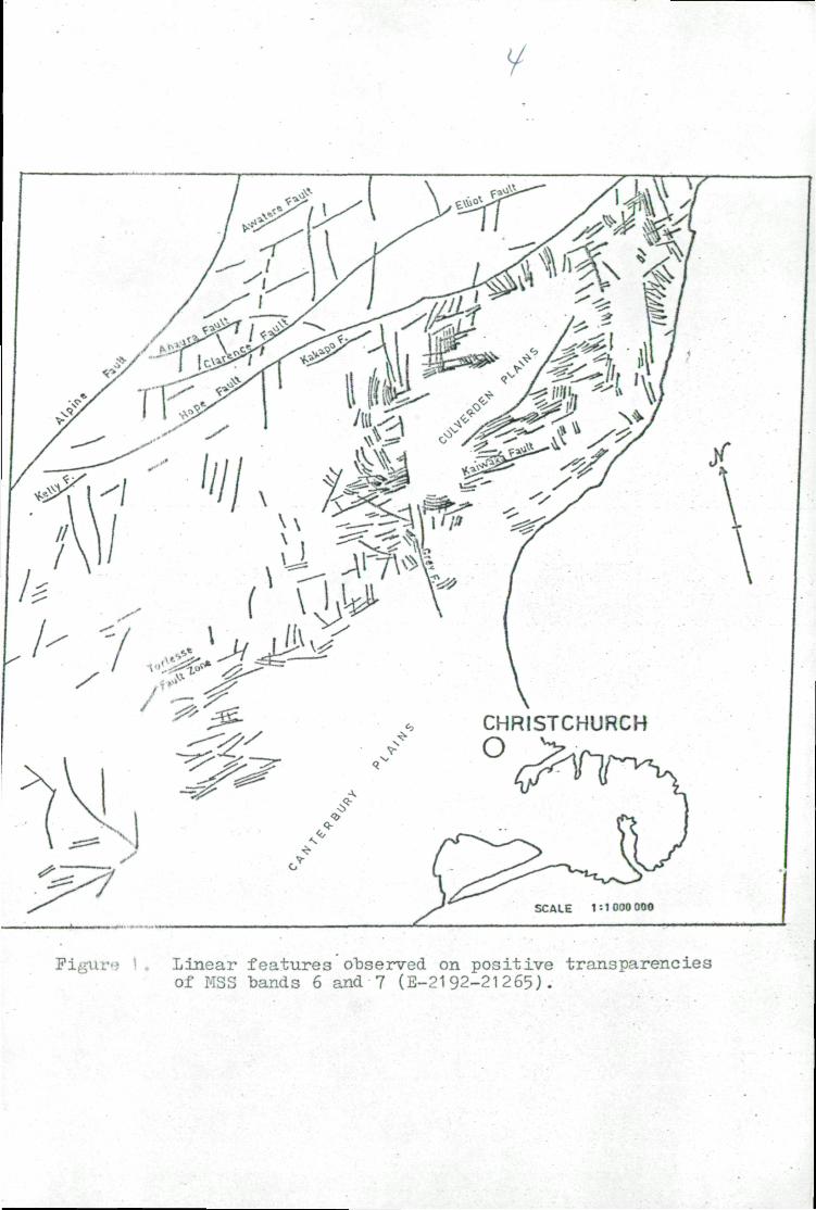
CHRISTCHURCHO
Figure ' . Lijaear features observed on positive transparenciesof MSS bands 6 and 7 (E-2192-21265).
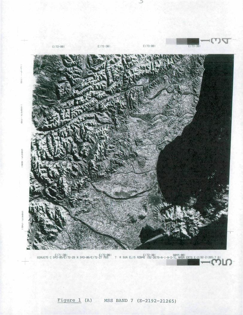
EI72-80I E172-36I E173-80!'CD NT
EI7I-30I E172-00I EI72-30I S044-00I02HUG75 C S43-05/EI72-29 N S13-06/EI72-27 HSS 7 R SUN EL15 RZ046 J92-2679-N-1-N-D-IL NRSfl ERTS E-2I92-2I265-7 <a\
Figure 1 (A) MSS BAND 7 (E-2192-21265)
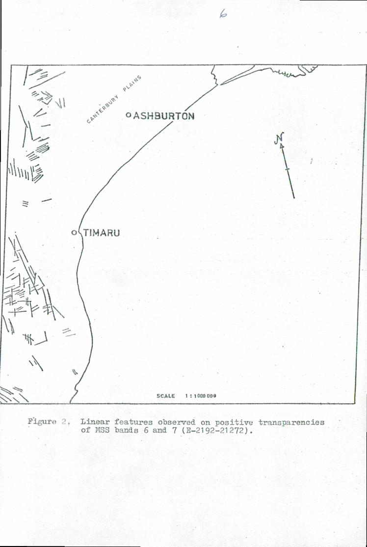
Ti.
QASH3URTON
SCALE 1 : 1000 000
Figure 2. Linear features observed on positive transparenciesof MSS bands 6 and 7 (E-2192-21272).

<LTJU
HH EI7l-30\02RUG75 C S44-30/EI7I-57 N S44-3I/EI7I -51 MSS 7 R SUN ELK RZ046 I92-2679-N-I-N-D-IL NRSR ERTS E-2I92-2I272-7 01
'COG
Figure 2 (A) MSS BAND 7 (E-2192-21272)
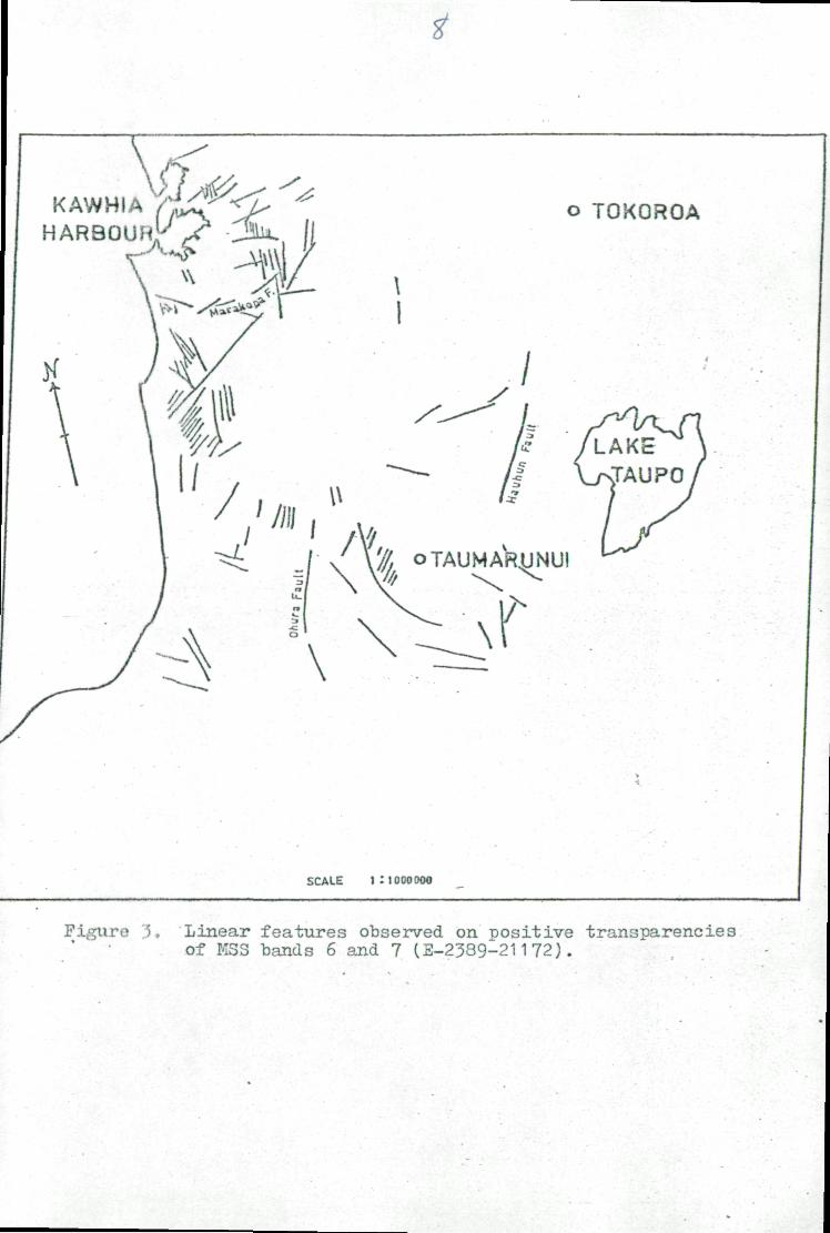
KAWHIAHARBOUR^
o TOKOROA
-
OTAUMARIJNU!
\ f
SCALE I I IOOOOOO
-'
Figure 5, Linear features observed on nositive transparenciesof KSS bands 6 and 7 CE-2339-21172}.
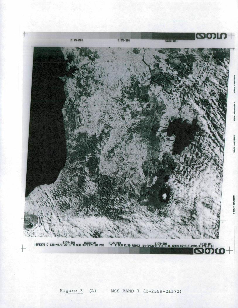
Figure 3 (A) MSS BAND 7 (E-2389-21172)

PART 111
INDIGENOUS FOREST ASSESSMENT
Investigation No.: 2823 B
Co-Investigator: Mr Michael G. McGreevy
Agency: Forest Research Institute
Address: Private BagRotoruaNew Zealand
Telephone No.: Rotorua 82-179
Author: Mr Michael G. McGreevy

INDIGENOUS FOREST ASSESSMENT
To achieve the original objective of assessing New Zealand'sindigenous forest resource using multi-stage sampling in conjunctionwith LANDSAT cover of New Zealand's forest resource, it was hopedthat seasonal variation in the spectral signatures of major foresttypes would help to define them on the imagery. Insufficient imageryhas been received to allow a seasonal comparison. Any variationwhich is due to the date of the imagery must be included as part ofthe variation within the individual type's spectral signature.
A second problem, varying solar elevation among images, hasmade visual comparisons of signatures on more than one image nearlyimpossible. Possible solutions to this problem would be to use rawdigital tapes in defining signatures, using digital tapes which arecorrected for differences in solar elevation, or to treat each imageas a separate entity and define a signature only in terms of thatimage. Due to delays in obtaining and processing digital imagery,we adopted the latter approach in initial interpretation. Usingvisual interpretation of colour composites we have been able todistinguish the following classes: beech and beech complexes,hardwoods, and scrub. These of course can be distinguished fromagricultural and urban areas.
It is desirable to define as many forest types as possible inthe initial stage of sampling. To determine if other types can bedefined on digital imagery, we have photographed 11 areas of indigenousforest on flat (less than 5 degrees) topography in colour andpanchromatic negative films'. The areas are indicated on image ERTSE-2334-21123-4 and the type definition which they represent are givenin Table 1. If no positive results are found in this test theinventory will proceed using the types identified previously inconjunction with available LANDSAT imagery.
ASSESSMENT OF DOTHISTROMA PINI IN PINUS RADIATA
Initial investigations showed no positive correlation betweenradiance measurements from LANDSAT and disease levels in various
stands. To ensure that this lack of correlation is not due tovarying topography, stand age, and silvicultural treatment in thesestands, stands which are of the same age, have had the samesilviculhutal treatments, and are on slopes of less than 10 degreeshave been identified on LANDSAT imagery. Digital information fromimage ERT3 E-2281-21185 is being compared with visual assessmentmade approximately 1 month prior to the image. The mean and varianceof the i uiiance levels on these stands are presently being derived.The correlation analysis betv/een these levels and the disease levelshould be completed during the next reporting period.
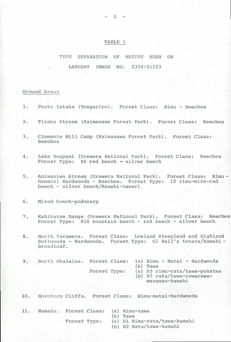
TABLE 1
TYPE SEPARATION OF NATIVE BUSH ON
LANDSAT IMAGE NO. 2334-21123
Ground Areas
1. Poutu Intake (Tongariro). Forest Class: Rimu - Beeches
2. Tiraka Stream (Kaimanawa Forest Park). Forest Class: Beeches
3. Clements Mill Camp (Kaimanawa Forest Park). Forest Class:Beeches
4. Lake Ruapani (Urewera National Park). Forest Class: BeechesForest Type: K6 red beech — silver beech
5. Aniwaniwa Stream (Urewera National Park). Forest Class: Rimu -General Hardwoods - Beeches. Forest Type: 12 rimu-miro-redbeech - silver beech/Kamahi-tawari
6. Mixed beech-podocarp
7. Kahikatea Range (Urewera National Park). Forest Class: BeechesForest Type: K10 mountain beech - red beech - silver beech
8. North Tarawera. Forest Class: Lowland Steepland and HighlandSoJ:t..woods - Hardwoods. Forest Type: Gl Hall's totara/kamahi-broadLeaf.
9. North Okataina. Forest Class: (a) Rimu - Matai - Hardwoods(b) Tawa
Forest Type: (a) D3 rimu-rata/tawa-pukatea(b) N7 rata/tawa-rewarewa-
mangeao-kamahi
10. Horohoro Cliffs. Forest Class: Rimu-matai-hardwoods
11. Mamaku. Forest Class: (a) Rimu-tawa(b) Tawa
Forest Type: (a) Dl Rimu-rata/tawa-kamahi(b) N2 Rata/tawa-kamahi
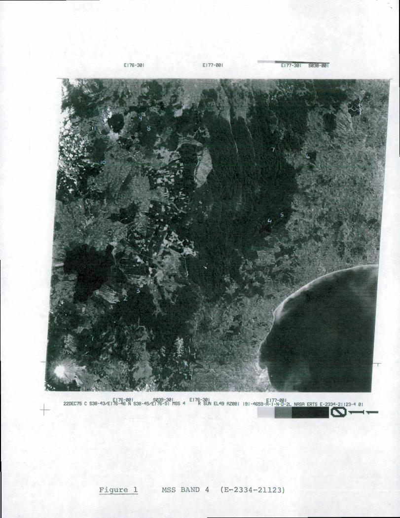
El 76-301 El 77-801 EI77-30I S038-00I
I S039-30I EI76-30I22DEC75 C S38-43/EI S38-45/EI76-5I flSS " R SUN EL49 RZ08I 191-4659-R-l-N-D-2L NRSfl ERTS E-233"-2l I23-* 01
Figure 1 MSS BAND 4 (E-2334-21123;

PART IV
MAPPING LAND USE AND ENVIRONMENTAL
STUDIES IN NEW ZEALAND
Investigation No 2823C
Co-Investigator: Mr Ian F. Stirling
Agency: Department of Lands and Survey
Address: Private BagWellingtonNew Zealand
Telephone No.: Wellington 735-022
Extension 286
Author: R.C. Child

CONTENTS
Page No,
Title Page
Consents Page
List of Illustrations
Introduction 1
Land Use Investigations 2
Topographical Mapping 2
Distribution of Imagery 3
Reflector Programme 4
Remote Sensing Workshop 4
Other Activities 4
Conclusion 4
LIST OF ILLUSTRATIONS
Figure 1 Sample of ICAO 1:500,000 scale map
Figure 2 New maps
Figure 3 Planning studies in New Zealand
Figure 4 Sample extract of compilation for KingCountry Land Use Study

1. INTRODUCTION
1.1 Ovor the period since the third quarterly report ourDepartment's activity has undergone changes. The most significantand disruptive at this time has been the return to Scotland of theauthor of the previous reports, Mr Douglas McK. Scott. Hisvaluable co-ordination and knowledge will be missed by the NewZealand x'emote sensing team, especially by the present author.Consequently sometime has been taken up with consolidating andreassessing our activity.
1.2 Previous interest and minor involvement with LANDSAT imageryas a possible source of information in the resource mapping fieldby this author as Divisional Cartographer, Planning and InventoryDivision of Cartographic Branch, has led to his appointment as areplacement to Doug Scott.
1.3 The Department of Lands and Survey has continued itsinvestigation and use of LANDSAT imagery in the environment andland use study field. The eventual aim being to reduce theexpensive and long acquisition times usually involved in studiesof this nature with the subsequent increase in output.
1.4 There is a slow but growing awareness and interest to use thepotentials of multi spectral imagery in the land planning fieldwhich is itself becoming a more active discipline.
1.5 As has been mentioned in previous reports, the opportunitiesfor applying some of the benefits of LANDSAT imagery has coincidedwith several major changes in our national mapping programme.
1.5.1 Recently we have given a critical reappraisal of ourresource mapping programme. We have initiated changes aimed atmeeting basic requirements of planners, that resource data iscollected and presented visually in as short a time as possible.Previously our maps were based on productive/unproductive,developed/undeveloped interpretive information. It was foundthat this form became out of date and of limited use for planningpurposes but there was a need for a Land Use map that showed an'as is1 situation. A pilot study has been initiated in Northland(north of Auckland) at a scale of 1:100,000 with topics that includeGeology, Soils, Land Use, Land Tenure, Vegetation and Wildlife.The general specifications have also been adopted for a combinedDepartments study of the King Country area in the North Island.It is Emm the 'ground truth' information compiled for the Land Usemap ol: this study that investigation into the potential use ofLANDSAT imagery for this purpose has been conducted. Areas offuture i. -source study are the McKenzie Basin, Stewart Island, anextension of the King Country study and Northland.
1.5.2 The recent change to metrics involved the calculationof a now map projection and grid and the remapping of the basicmap serial of New Zealand at 1:50,000. This mapping incorporatesinform.iLi.ou from new source material. Also involved is theproduction of a new 1:250,000 based on the 1:50,000 sheetlines.It is in t.he production of this 1:250,000 series that LANDSATimagery .is proving to be increasingly useful.

Page Intentionally Left Blank

is now compared for hydrographic selection and generalisation,topographic shape, vegetation cover etc. The use of a variationin the composition of the colour in the composites andexperimentation with colour isodensitometer images is beinginvestigated. Evaluation will be made with the eventual aimbeing to produce, if possible, primary source material fromLANDSAT.
The use of imagery for relief shading purposes continuesas indicated in previous reports. The 'overview1 presentationoffered by these images has no alternative equivalent. For smallscale map hill shading reductions of large scale material becameexpensive and numerous.
A serious limiting factor experienced in the use of LANDSATimages for this scale of mapping is the discontinuous coverageof New Zealand.
2.2.2 1:500,000 scale mapping
The 1:500,000 scale ICAO maps covering New Zealand in 4overlapping sheets that utilised LANDSAT imagery for comparativepurposes has now been printed.
2.2.3 1:1,000,000 scale mapping
The production of a new edition of this map is now in progress.Source material will be checked against available LANDSAT imagesto assess the contribution possibilities of this more recent data.A suggested mosaiced image of New Zealand is hampered by the non-availability of total cover but methods of producing such an imageare being investigated for eventual publication.
2.2.4 Offshore Islands
As indicated in our initial proposal we hoped that LANDSATimagery would facilitate our mapping of numerous offshore islandsespecially their orientation and position in relation to the mainisland?. Cuvier Island has been mapped from aerial photography butorient 11 i <~<\\ is hampered by the fact that there is only oneco-ordln tl eel triangulation point on the island. Orientation couldbe achieved from LANDSAT imagery especially if control points couldbe marked by reflectors.
2 . 2 . ') Antarctic Mapping
Om: Department has had recent discussions with R.H. Lyddon,Chief, i • -iraphic Division, U.S. Geological Survey on the subjectof map'.iiu'i activity in Antarctica. It was agreed generally thatco-oi • ! ' • • H -d mapping in the Ross Sea, Victoria Land area would beinveu-;• i |.Ot?d and undertaken utilising LANDSAT imagery. This activityis out.'? i'L.: our contractual agreement but is reported for interestedparti •
2 . 3 Diti) l.bution of Imagery
Intei. >st in our 'Quick look1 prints produced for LANDSAT IIimagery rv:'.r;lved in New Zealand has led to the requirement for usersfor a set i.c prints for LANDSAT I images. Although much of our

LANDSAT I imagery was not of a high quality 'Quick look1 printsets as well as being distributed to contributors and investigatorsof the IrnHf/ery are made available throughout New Zealand in twelvemain centres for public viewing.
2 . 4 Reflector Programme
The coincidence of our reflector programme and the particularlcloudy summer in New Zealand has suggested to sortie that thisreflector has great possibilities as a rain making machine! Oneach overpass until recently there has been too much cloud coverto expect satisfactory results. We are optimistic enough of goodresults to be considering modified reflectors in other parts ofthe country where mapping requirements suggest marked control.
2 . 5 Remote Sensing Workshop
As a follow up to last year's introductory workshop, a furtherinformal gathering of Department personnel:
Mr W. Robertson Director of PlanningMr D. Francis Director of MappingMr P. Sadler Chief CartographerMr R. Child Divisional Cartographer
Remote Sensing
and guest Professor A. Lewis, Louisiana State University discussedfuture resource planning activity and the contribution remote sensi:could give. Also discussed was a future workshop for planners toindicate the availability of remote sensing data and facilities andto promote the use of LANDSAT imagery.
2.6 Other Activities
Transparencies produced by P.E.L. have been investigated incomparison with prints for interpretation and plotting purposesand the transparency has been found to reveal more detail. We havefound that the use of transparencies in photogrammetric instrumentshas produced promising results.
2 . 7 Ciinu lusion
investigations have reached several stages. The initialaims h;wu been pursued and in most cases are yielding better resultthan w *•>«••>* considered possible at the early stages of research. Thihas Itj'l tx more intensive effort being applied. The objective isto recicMt conclusions for these original objectives this year andto then view supplementary requirements that have been initiated.This h-is become and is still growing into a field of research thathas yet: to show its full potential.
My thanks to the P.E.L. team whose co-operation and liaisonhave mad'? "\yr taking over from Doug Scott much easier than it wouldotherwise have been and who manage to co-ordinate the varied andexpanding -spheres of interest in remote sensing in New Zealand.
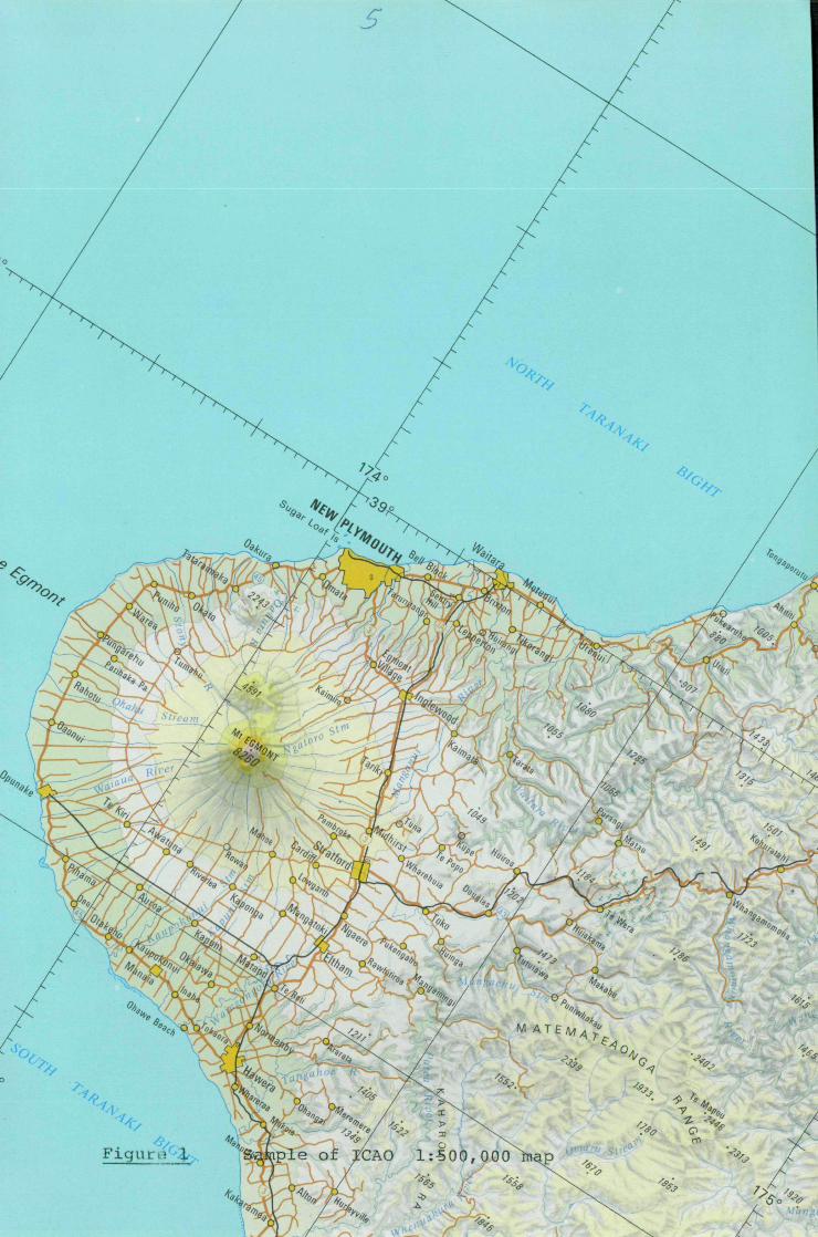
vo<
'&} 'ft
•'<*
<+&,
Figutrir^-..
^
*6*»„
*
iple of /CAO 1:500
/ K* o-k.%°\.-
%M A T E / W x , ^
M0
^ %
^ <\, ^
,000 inap\ f-S.
% \,L ^ s . \
r*
%:
^%
iV >^— T "# /
^ ^ /G> Arn \/•^ r/
'4^A

L,F I G , 2, p, 1
DEPARTMENT OF LANDS AND SURVEY
NEW MAPS
BACKGllOUND
Accelerating environmental and social changes have accentuated the need for reliabletopographic maps, providing an inventory of the country's physical features, and haveincreased the requirement for up-to-date cadastral maps, presenting a positivei den tifi cation of all land parcels and their legal status.
Sncli maps used in conjunction form a basis for the planning and administration ofhousing, commercial and industrial development, provision of public and social services,protection of the environment, maintenance of law, defence, and the other administrationsof government and local authorities in the modem society.
The existing basic topographical map series at one inch to one mile (NZMS 1) wascommenced in 1936. Coverage of the North and South Islands was completed in 1976.This series has served the country well over the 40-year period and will continue to meetneeds in some areas for several years. However, the specifications of this series nolonger fully satisfy the requirements of many users. In addition, the intensification ofland use and development and provision of services has created a demand forcomprehensive map coverage on scales larger than those at present produced.
Nationwide coverage (except for south-west Fiordland)of the basic cadastral mappingseries at one inch to one mile (NZMS 177) was accomplished in 1968. Deficiencies arecontained in many sheets which were merely reproduced from much earlier maps, and thisseries no longer provides an adequate base for recording legal boundary changes or forprinting reproduction. For convenience, the scale and sheet layout of this series mustbe changed to agree with changes made to the new basic topographical map layout.Also, as with topographical maps, the requirements of land administration and planninghave created a demand for cadastral map coverage on scales larger than those at presentproduced.
On I January 1973 the Department inaugurated a one-colour survey plan system andintroduced metric units for the execution and presentation of all surveys affecting landtitle. Mote recently, a single projection and a single grid that allow for the accuratepresentation of the whole country on a uniform system were devised. A furtherdevul'ipiiittit has been the introduction of new cadastral record sheets on transparentfoil. 'I'liia will facilitate the efficient and economic compilation of basic cadastral maps.K - - J H M - I H I H . M I of urban cadastral maps will be by way of plan prints.
It In opportune with the implementation of these innovations to reconsider all aspectsof map production with a view to improving scales, layouts, and specifications of basicmapping \\\ order to meet the requirements of map users.
NKW PROJECTION AND GRID
\\ »v projection is confonnal but is otherwise unlike any other projection used forl > i . ipping. Scale variation is within ± 0.024%, considerably less than that of any
oth •< 'ion previously used for New Zealand.
Tlu» lie i grid, to be known as the New Zealand Map Grid, provides the sheetlines forthe n -»v l..< tie map series. The true origin (Lat 41"S: Long 173'E) is assigned arbitrarycooiitmn'Md sufficiently large to render all coordinates positive, or east and north, of a"fal * • • in". In a metre coordinate system sufficiently extensive to cover the wholeco.iniry in i northing must reach seven integral figures. In the scheme now adopted thecoiuilin t ' r > s have seven integral figures in all cases. To avoid confusion, the coordinateshave l i u - i i i. iimbered so that eastings are always less than 5 000 000 metres and thenorthing . </;iys greater. The grid is oriented so that the north-south axis of coordinatesis tang-»if. ••» the 173°E meridian at the true origin.
The P1 •• •< Zealand Map Grid, and the layout of the new basic 1:50 000 topographicaland cada-" M 'nap series are illustrated in Fig. 1.

F I G , 2, P, 2
THE NSW SERIES
To implement the programme of new mapping the Department is to produce thefollowing new map series.
NZMS 260 NEW ZEALAND TOPOGRAPHICAL MAP 1:50 000
This new netit»rf of 324 sheets will supersede the present NZMS 1 series. It is to bebased entirely on new photogranunetric mapping plotted at a scale of 1:25 000 fromup-to-date aerial photography. (Refer to NZMS 270 Topoplot Map at 1:25 000.)Production will be by progressive expansion in selected areas of the country. Sheetformat is to be 40 km x 30 km. Contours are to be shown at 20-metre vertical intervalsand this subst;uUial upgrading of relief presentation will greatly facilitate planning,utilisation. 8ci>*(ilific. and development activities. Map detail is to be "bled" off thetop and right wlges of the sheets to facilitate continuity of information on to adjoiningsheets. Many other improvements on the NZMS 1 series have also been introduced.Drawing has commenced on the first NZMS 260 sheets.
NZMS 261 NEW ZEALAND CADASTRAL MAP 1:50 000This new series has the same basic sheet layout as NZMS 260 and will supersede
the present NZMS 177 series. Production of the new maps is well advanced with manysheets already published and most others in some stage of preparation. The seriesshould be complete at an early date. Production will economically utilise material fromexisting maps and from larger scale record maps. The new maps present a uniform andup-to-date record of boundaries.
NZMS 262 NEW ZEALAND TOPOGRAPHICAL MAP 1:250 000
This series will supersede the 26 sheet NZMS 18 1:250 000 series. Each of the 18sheets will have a format of 200 km x 150 km with sheet lines based on the NZMG. Asmetric contours covering a wide area will not be available for some time, and because ofdifficulty in interpolation of metric contours from existing material, this series is to bepublished initially without contours. However, relief will still be adequately representedby spot heights ;md improved relief shading. These maps will meet an increasing demandby government, local authorities,and the public for up-to-date, comprehensive informationat this scale.
The sheet layout for NZMS 262 is illustrated in Fig. 3
EXISTING SERIES AVAILABILITY
Until maps in ;in entire region are superseded by the new series previously described,all existing map sieries will be maintained by revision and reprint to ensure that up-to-dateinformation rBcnaiiiH readily available.
NZMS 269 NEW ZEALAND TOPOGRAPHICAL MAP 1:10 000
This will be 3J» entirely new series, initiated to provide larger scale mapping ofmajor built up areas and their environs, and in other areas if required. Sheet lines willbe those of the 1: 10 000 Cadastral Record Maps, each sheet covering an area5 km x 7.5 km. .Specifications are yet to be prepared but it is possible that this serieswill consist of oithophoto (true-to-scale photo) maps, overlaid with 5-metre verticalinterval con loom utniluced by photogrammetric methods.
NZMS 270 NEW ;;,«: \LAND TOPOPLOT MAP 1:25 000
These slu-M -UM plotted at 1:25 000 by photogrammetric methods as a base for thepreparation of < i u i MZMS 280 1:50 000 series. Sheetlines are a subdivision of the1:50 000 she^t UI IH-J and have a map coverage of 20 km x 15 km. The maps will not bepublished in i^ihrnr but are available ia plan print form, initially as unchecked plots,then, after Jiwl-J i^'.king, as NZMS 270 maps. In final form contours will be availableseparately i'nm > u \ - » r detail and vice versa, if required, for ease of interpretation.Photogrammrttry is «,» be produced on a progressive basis and various areas of NewZealand will be oo\ "ind systematically on a priority basis. See Fig. 2 for NZMS 270sheetlines and n inn i— dng.
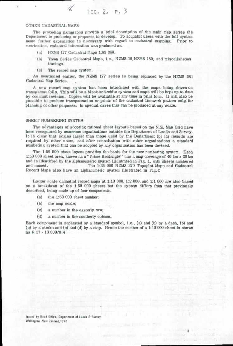
F I G , 2, P, 3
OTHER CADASTRAL MAPSThe preceding paragraphs provide a brief description of the main map series the
Department is producing ot proposes to develop. To acquaint users with the full systemsom« f i i rUiwr explanation is necessary with regard to cadastral mapping. Prior tomeirieaticu. cadastral information was produced as:
' • > riZMS 177 Cadastral Maps 1:63 360.(li) Town Sttries Cadastral Maps, i.e., NZMS 16, NZMS 189, and miscellaneous
tracings.
((.•) The record map system.As mentioned earlier, the NZMS 177 series is being replaced by the NZMS 281
Cadastral Map Series.
A new record map system has been introduced with the maps being drawn ontransparent foils. This will be a black-and-white system and maps will be kept up to dateby conviiaiit revision. Copies will be available at any time in print form. It will also bepossible to produce transparencies or prints of the cadastral linework pattern only, forplanning or other purposes. In special cases this can be produced at any scale.
SHEET NUMBERING SYSTEMThe advantages of adopting rational sheet layouts based on the N.Z. Map Grid have
been recognised by numerous organisations outside the Department of Lands and Survey.It is clear that scales larger than those used by the Department for its records arerequired by other users, and after consultation with other organisations a standardnumbering system that can be adopted by any organisation has been devised.
The I:f50 000 sheet layout provides the basis for the new numbering system. Each1:50 000 sheet area, known as a "Prime Rectangle" has a map coverage of 40 km x 30 kmand is identified by the alphanumeric system illustrated in Fig. 1, with sheets numberedand named. The 1:25 000 NZMS 270 Toppplot Maps and CadastralRecord Maps also have an alphanumeric system illustrated in Fig. 2
Larger scale cadastral record maps at 1:10 000, 1:2 000, and 1:1 000 are also basedon a breakdown of the 1:50 000 sheets but the system differs from that previouslydescribed, being made up of four components:
(a) the 1:50 000 sheet number;(b) the map scale;
(c) a number in the easterly row;(d) a number in the southerly column.
Each component is separated by a standard symbol, i.e., (a) and (b) by a dash, (b) and(c) by a f»trok« and (c) and (d) by a stop. Hence the number of a 1:10 000 sheet is shownas !t :fl - lit 000/8.4
Issutd by il*i| Offic«, D»partm»nt of Landi 6 Survey.Wellington, .N«» ,'j|l»nd,1978
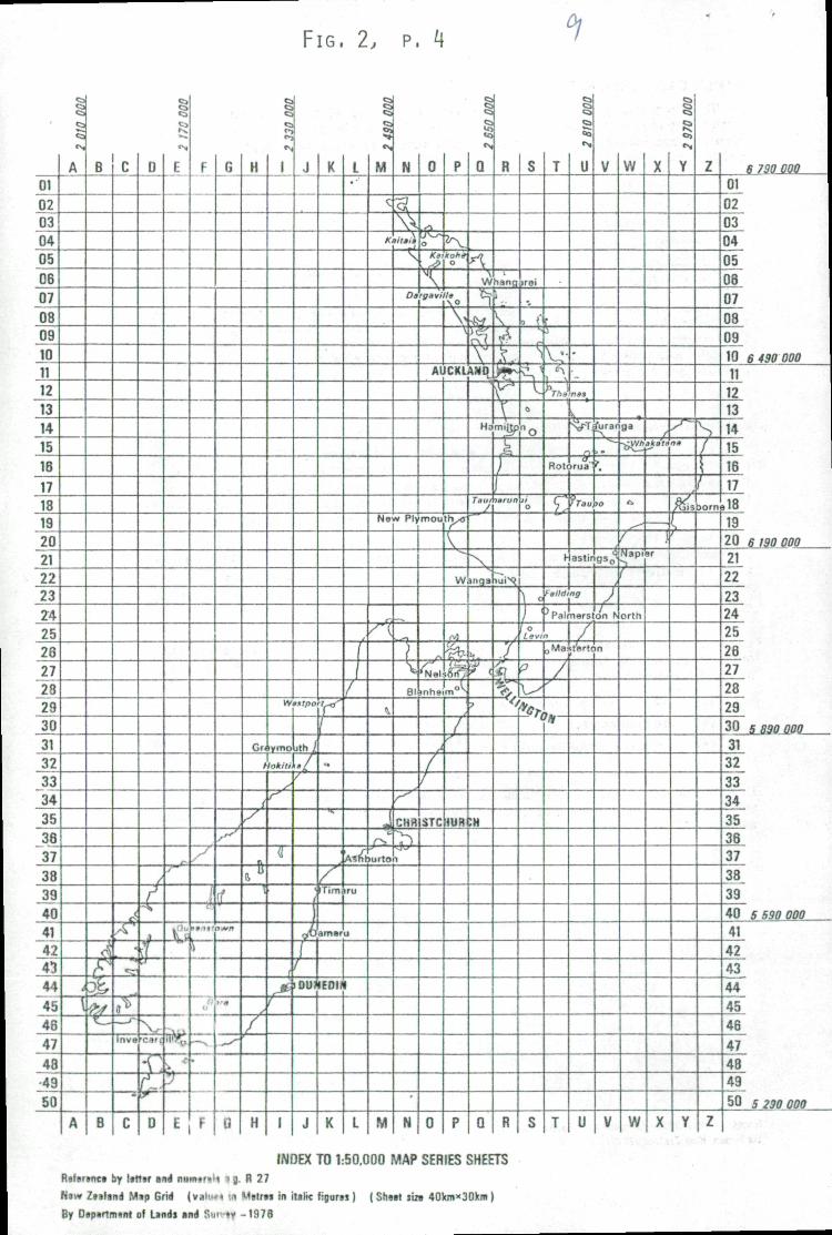
FIG, 2, P,
•
01020304050607080910111213141516
1718192021222324252627282930313233343538373839404142434445484748-4950
<ir>t,
«N
A
]
A
B
3EP£
^
B
C
•i
A '
2— r
Trwe
c
0
.z~5»
ft
^
x\_rC*n
EPL»•"
D
1Sj«N
E
/
@
**t.:'
E
F
.J
1.|
• • ,«•
1
"" *N
F
G
y"'
rf
n-*^
>-*
~'~
Q
H
Gr
1
§«N
1 J
Wtstpo1
/mouth /
Hokitikt/
1
7
51
/
/
H
/r'
tt
<
,*
1
: •
1
/
OUI
J
K
p
|
..
/'Tim
amur
fni.
K
L• •'
|
/
A<!nt
ru
U
L
$«Ni
M
^
K
He
/'\
\
\£
rs
urto
M
n
sitM
r>
\
Da
H Ply
3sBl
?"
ZHR
•>
H
0
,r?;'--'i0
Ka,-?vjr
•gavi
P
>v-TO/-*
O
to\°
V1
AUCKL
mou
4jal
^nha
jj
//
STC
0
B
iw
rtfr&;.3j
s
/
UIR
P
1
a«N
Q
n' A
W
5•S\«iq
HE
Taut
~\
ntja
1*3y c
7
H
Q
R
i -in-
\3£>£mijjp
k
2ta run
Ji
.
2EE
Vy
R
S
irei
.
3 f
^d_ ^I
Q
"o
II0
\ d
) |o
ievi
(3
v i»^
s
T
1
5•h*.
Rot
£
(
rt/W
3 Pal
,
3Ma
/^
5 ,,'#
T
1
1«>•
U
-
nffs
-
VT
Vrua
^7-aiy
astir
"S
Tiers
V
furan~\
"^-_
f
JO
gs0^
2on K
7;t'artc
U
n
V
w
8*
-j^V/i
1 ,
r-'/
Napi5
orth
W
X
/aka't»
\%r
K
11«N
Y
~7*n«
fa*(
Y
Z
s/Iborn
Z
« 750 Wff01
020304050607080910 649000011
121314151617
,181920 6190000212223242526272829
30 589000031
323334353637383940 5 590 00041
4243444546474849
50 5290000
INDEX TO 1:50.000 MAP SERIES SHEETSRifennc* by l*tt»r and numtrci .j R 27
Now Ztilsnd Map Grid (v.« i i - -« •! Mvtrts in italic figuni) ( Sh«et sin 40kmx30km )
By Dsptdmint of Lands and ' ' • '< • •* -1976

FIG, 2 , P , 5MAP NUMBERING SYSTEM
1:50 000
This sheet isNZMS 270 R27B(1 : 25 000 scale)
Sheet size 20X15 km
1 2 3 4 5 6 7 8
1.1
1.2
1.3
1.4
2.1
2.2
2.3
2.4
3.1
3.2
3.3
3.4
4.1
4.2
4.3
4.4
5.1
5.2
5.3
5.4
6.1
6.2
6.3
6.4
7.1
7.2
7.3
7.4
8.1
8.3
8.4
This sheet isR27-10 000/8.2
(1 :10 000 scale)
Sheet size 5 X 7.5 km
(8X4 sheets in each1 : 50 000 prime rectangle)
1: 2000 scale
(Sire IX 1.5 km
flO X 20 sheetsin Mi:h \ : 50000piim*» lectangle)
1 : '".HO scale
(Siza 0 t> X 0.75 km80 X 40 sheets
in e«ch I : 50 000prints i <>i:t!ingl«)
This sheet isR27-2000/39.18
This sheet isR27-1000/80.40
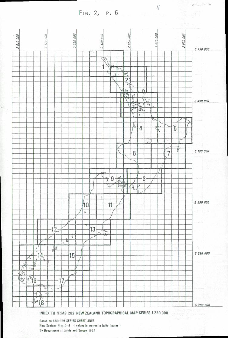
FIG, 2, P, 6
1 i
4-\
:y
2l_5
5
790 000
6 490 000
-5
£
6 6 190 000
/vj
2
^L
10 11
1?
? -4 U
"18
H8
15
-!7;
5 890 000
S 590 000
5 230 000
INDEX TO N 'MS 262 NEW ZEALAND TOPOGRAPHICAL MAP SERIES 1:250 000
Based on l.S'l •.•>".» SERIES SHEET LINES
Naw Zealand "' > <<r id ( values in metres in italic figures )
By Department i ijuds and Survey 1976
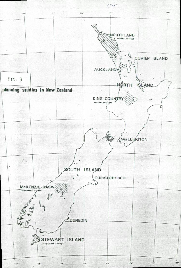
NORTHLANDunder action
CUVIER ISLAND
AUCKLAND
N$RTH ISLV
planning studies in New Zealand
KING COUNJRYunder actions—
V\£ELLIMGTON
- a
UTH ISLA
CHRISTCHURCH
:±1DUNEDIN
STEWART ISLAND
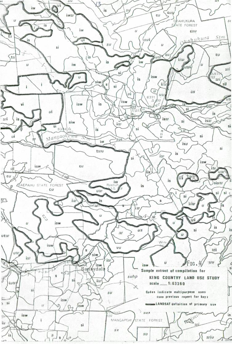
Ul
Sample extract of compilation for
suhp KING COUNTRY LAND USE STUDY
scale 1:63360
Codas i n d i c a t e mult ipurpose uses( s e e p rev ious report for k«y >
LANDSAT definition of primary use
WANGAPEHt/STATE
TV iu
PART V
NEV/ ZEALAND FOREST SERVICE
LANDSAT PROJECTS
Address: New Zealand Forest Service«• Private BagWellington
Telephone Ho.: Wellington 721-569
NZFS Co-ordinator ..Mr Neville Ching
Authors: Mr N. Ching
Mr B. Lean
Mr R. Dale
(NZFS, Wellington)
(NZFS, Christchurch)
(NZFS, Auckland)

CONTENTS
Paqe
Title Page
Contents Page 1
Figure Captions 2
1. Canterbury Windthrow - B. Lean 3
2. Classification of Forest Types inthe King Country - R. Dale
3. Mapping of Snow Areas on theSt. Arnaud Mountain Range 6
4. Hanmer Fire Damage Monitoring 6'
FIGURE CAPTIONS
Figure 1 Ground truth map of Eyrewell State Forestapplicable to scene no. 2282-21254.
Figure 2 Relation between the colour coded LANDSAT compositeof scene 2282-21254 and panchromatic aerial imageryof various regions in Eyrewell State Forest. (Forinterpretation Key see text.)
Figure 3 Eyrewell Forest windthrow interpretation obtainedfrom LANDSAT scene no. 2282-21254.
Figure 4 Location of transect lines for the St. ArnaudMt. Robert snow cover study
(a) Transect line for CCT radiance comparisonson Mt. Robert
(b) CCT radiance transect lines at the head ofSix Mile Creek Basin on the St. ArnaudRange.
(c) Ground sampling transect line.
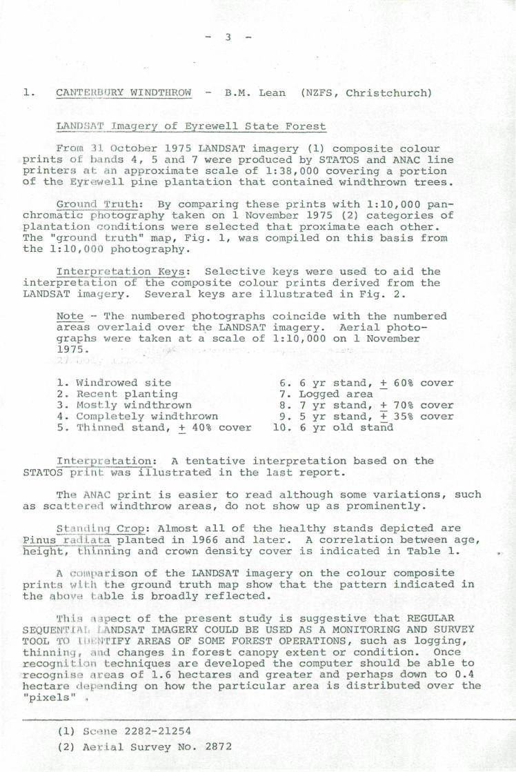
- 3 -
1. CANTERBURY WINDTHROW - B.M. Lean (NZFS, Christchurch)
LANf)/]AT Imagery of Eyrewell State Forest
From 31 October 1975 LANDSAT imagery (1) composite colourprints of hands 4, 5 and 7 were produced by STATOS and ANAC lineprinters at an approximate scale of 1:38,000 covering a portionof the Eyr.-iwell pine plantation that contained wind thrown trees.
Ground Truth; By comparing these prints with 1:10,000 pan-chromatic photography taken on 1 November 1975 (2) categories ofplantation conditions were selected that proximate each other.The "ground truth" map, Fig. 1, was compiled on this basis fromthe 1:10,000 photography.
.j rotation Keys: Selective keys were used to aid theinterpretation of the composite colour prints derived from theLANDSAT imagery. Several keys are illustrated in Fig. 2.
Note - The numbered photographs coincide with the numberedareas overlaid over the LANDSAT imagery. Aerial photo-graphs were taken at a scale of 1:10,000 on 1 November1975.
1. Windrowed site 6. 6 yr stand, ^f 60% cover2. Recent planting 7. Logged area3. Mostly wind thrown 8. 7 yr stand, +_ 70% cover4. Completely windthrown 9. 5 yr stand, j^ 35% cover5. Thinned stand, +_ 40% cover 10. 6 yr old stand
Interpra tation: A tentative interpretation based on theSTATOS prinT. was illustrated in the last report.
The ANAC print is easier to read although some variations, suchas scattered windthrow areas, do not show up as prominently.
f> i i i i iuj Crop: Almost all of the healthy stands depicted arePinus r a J .1. a t.a planted in 1966 and later. A correlation between age,height, thinning and crown density cover is indicated in Table 1.
A '• ••'''! • irison of the LANDSAT imagery on the colour compositeprints wll.h the ground truth map show that the pattern indicated inthe abovH t able is broadly reflected.
This i .?pact of the present study is suggestive that REGULARSEQUENT! vNDSAT IMAGERY COULD BE USED AS A MONITORING AND SURVEYTOOL TO I . PIFY AREAS OF SOME FOREST OPERATIONS, such as logging,thinni.iv.), and changes in forest canopy extent or condition. Oncerecognition techniques are developed the computer should be able torecogriis ' areas of 1.6 hectares and greater and perhaps down to 0.4hectare du^. 'tiding on how the particular area is distributed over the"pixels" .
(1) Some 2282-21254
(2) Aerial Survey No. 2872
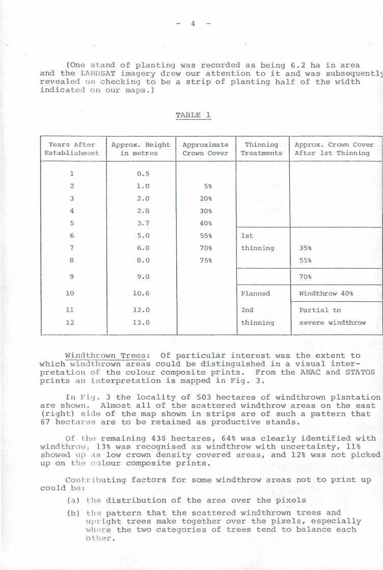
(One stand of planting was recorded as being 6.2 ha in areaand the LANnSAT imagery drew our attention to it and was subsequentlyrevealed on checking to be a strip of planting half of the widthindicated on our maps.)
TABLE 1
Years AfterEstablishment
1
2
3
4
5
6
7
8
9
10
11
12
Approx. Heightin metres
0.5
1.0
2.0
2.8
3.7
5.0
6.0
8.0
9.0
10.6
12.0
13.0
ApproximateCrown Cover
5%
20%
30%
40%
55%
70%
75%
ThinningTreatments
1st
thinning
Planned
2nd
thinning
Approx. Crown CoverAfter 1st Thinning
35%
55%
70%
Windthrow 40%
Partial to
severe wind throw
Windbhrown Trees: Of particular interest was the extent towhich windthrown areas could be distinguished in a visual inter-pretation of. the colour composite prints. From the ANAC and STATOSprints an interpretation is mapped in Fig. 3.
In FLcj. 3 the locality of 503 hectares of windthrown plantationare shown. Almost all of the scattered windthrow areas on the east(right) side of the map shown in strips are of such a pattern that67 hectares are to be retained as productive stands.
Of I lui remaining 43S hectares, 64% was clearly identified withwindthrv.iv/, 13% was recognised as windthrow with uncertainty, 11%showed up .^s low crown density covered areas, and 12% was not pickedup on th<* r: i.lour composite prints.
Contributing factors for some windthrow areas not to print upcould be;
(a) the distribution of the area over the pixels
(b) th ; pattern that the scattered windthrown trees andupright trees make together over the pixels, especially\vl>. >re the two categories of trees tend to balance eachof

Generally, stands covered with windthrown material show updistinctively on the colour composite prints, but where standingtrees and land surface areas become mixed with the windthrowntrees then it shows up on the prints with varying success.
Summary
The co Lour composite prints produced by the ANAC line printerare easier to interpret. The expanding crown coverage of the youngtree crop was reflected and some forest operations snowed up.Significant areas of windthrown trees were recognised and mixedareas of windthrown and standing trees were partially indicated.
Remarks
An improvement in the computer classification and subsequentprints (colour or computer printout) is needed.
The wind-throw classification of the pixels is affected bythree scene object variables:
1. windthrown material
2. standing trees
3. visible land surfaces.
Familiarisation with the apparent radiances of the subjectmatters in Llie various LANDSAT bands should help, and (if feasible)perhaps "proportion estimation" of chosen signatures in selectedLANDSAT v/civebands by the computer would refine classification.
If completely windthrown areas and areas of varying density ofwindthrow could be emphasised on the colour composite prints orcomputer printouts then this should help interpretation and checking

2. CLASSIFICATION OF FOREST TYPES IN THE KING COUNTRY -Mr R"'"fiale (NZFS, Auckland)
The [,/UJDSAT photographic data (Fig. 4 - colour diapositivesoff the isodensitometer and 1:63,360 enlargements of Fig. 3, whichboth appeared in the Third Quarterly Report) have been of littleuse for this land use study. The reason for this is the resolutionof the imagery for forest typing and forest descriptions must begreater than that available. The only use made of the photographswas in identification of clearfelling and conversion areas,particularly for private forests in the absence of up to datelarge scale aerial photography. The 1:63,360 enlargements, althoughused, were of poor definition but the information was gained by thehelp of two photos similar in scale to Fig. 3 of the Third Report.
Unfortunately the tight deadlines imposed for the completionof the land use study and the sheer volume of work involved has notenabled a closer study of the applications of LANDSAT in foresttyping for this form of study.
3. MAPPING OF SNOW AREAS ON THE ST. ARNAUD MOUNTAIN RANGE
A transect has been set out on the ground and measurementsare being made to coincide with the satellite overpass - weatherpermitting.
The transect was located on a south facing slope. This sitewas chosen as it appeared to be the most likely location for aski field.
The transect's centre line was marked out with a series ofpegs - approximately 100 ft apart. Depth readings are made alongthe centre line and at a distance 100 ft either side of the centreline.
This la indicated between locations on Fig. 4c which showsthe centre line and a line 100 ft either side where the outer readincare made.
SfcciEf at P.E.L. are utilising coded computer print out data toplot olum ? .»'j in four band MSS radiant intensity along the fourtransect 1 lues shown in Fig. 4 (A-D, C-D, B-D, E-F) . The scene undeistudy h M • using CCT data is the same as that studied usingphotographic techniques and shown in Figs. 5b and 6 of the ThirdQuarterly I' ?port - scene no. 2282-21252. A progress report on thisstudy in :[lven in Part I of this quarterly report.
4 . HANiMKU FIRE DAMAGE MONITORING
As outlined in the Third Quarterly Report it was planned to usemultispectml imagery to monitor any changes in vigour within thefoliage ot ! he Hanmer State Forest damaged by fire on 22/23 March 19'Bad weather Uas acted against acquisition of all the desired satelliaircraft co•- ->rage but one flight, on 4 February 1977, has been possi:The results -.ire currently being studied.

Port EYREWELL STATE FOREST
GROUND TRUTH
PLANTATION COVER
] Over 65% crown cover
1 65 - 35% » »
I | 35 -20% » "
| | Less than 20% » »
| [ Windthrow (sc'td =scattered)
| | Logged
[ | 1975 planting
[ J Site prepared partiallyScate I: 38000
Prepared by N.Z.F.S. (Chch.)
Figure 1 Ground truth map of Eyrewell State Forestapplicable to scene no. 2282-21254.
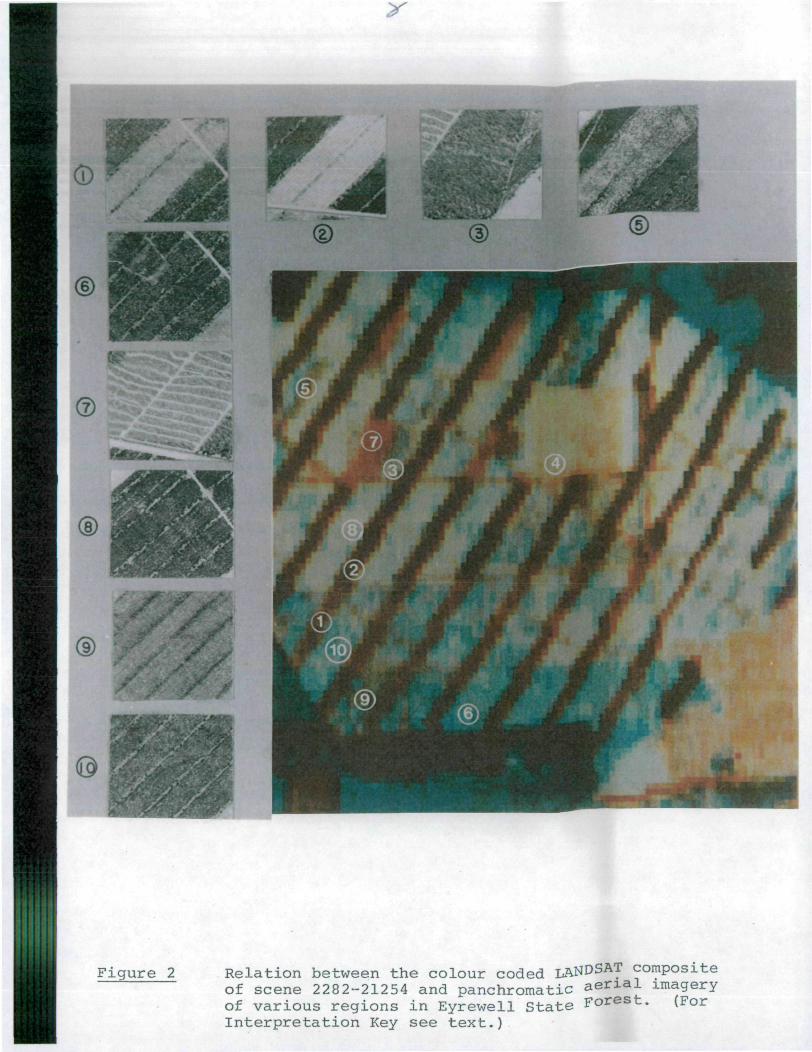
>._
Figure 2 Relation between the colour coded LANDSAT compositeof scene 2282-21254 and panchromatic ae imageryof various regions in Eyrewell State F°r<
Interpretation Key see text.)
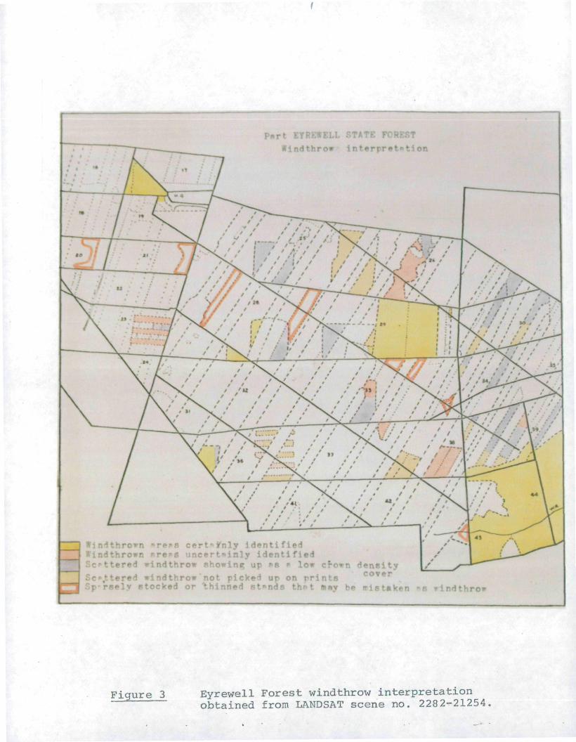
P*rt >
1
/nly i denti fed
rindthrow showing up »s » lor isity
row not pick- -its OTe
•
Figure 3 Eyrewell Forest windthrow interpretationobtained from LANDSAT scene no. 2282-21254
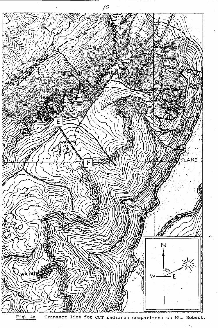
Fig. 4a Transect line for CCT radiance comparisons on Mt. Robert.
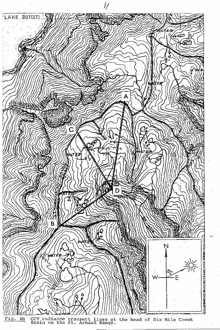
.'-.LAKE' ..RQTOITL:
•Fig. 4b CCT.rcidiance transect lines at the head of Six Mile CreekBasin on the St. Arnaud Range.
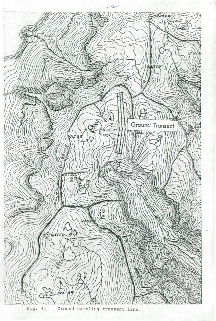
j Ground TransectIT
mm.Ground sampling transect line

PART VI
VEGETATION MAP AND LANDFORM MAP OF
AUPOURI PENINSULA, NORTHLAND
Agency: Ministry of Works and DevelopmentWater and Soil Division
Address: P.O. Box 12-041Wellington NorthNew Zealand
Telephone No ._: We 11 ington 729-929
Extension 596
Author: Mr Douglas L. Hicks

FIGURE CAPTIONS
Figure 1 Vegetation map of Aupouri Peninsula, Northland,
Figure 2 Landform map of Aupouri Peninsula, Northland.
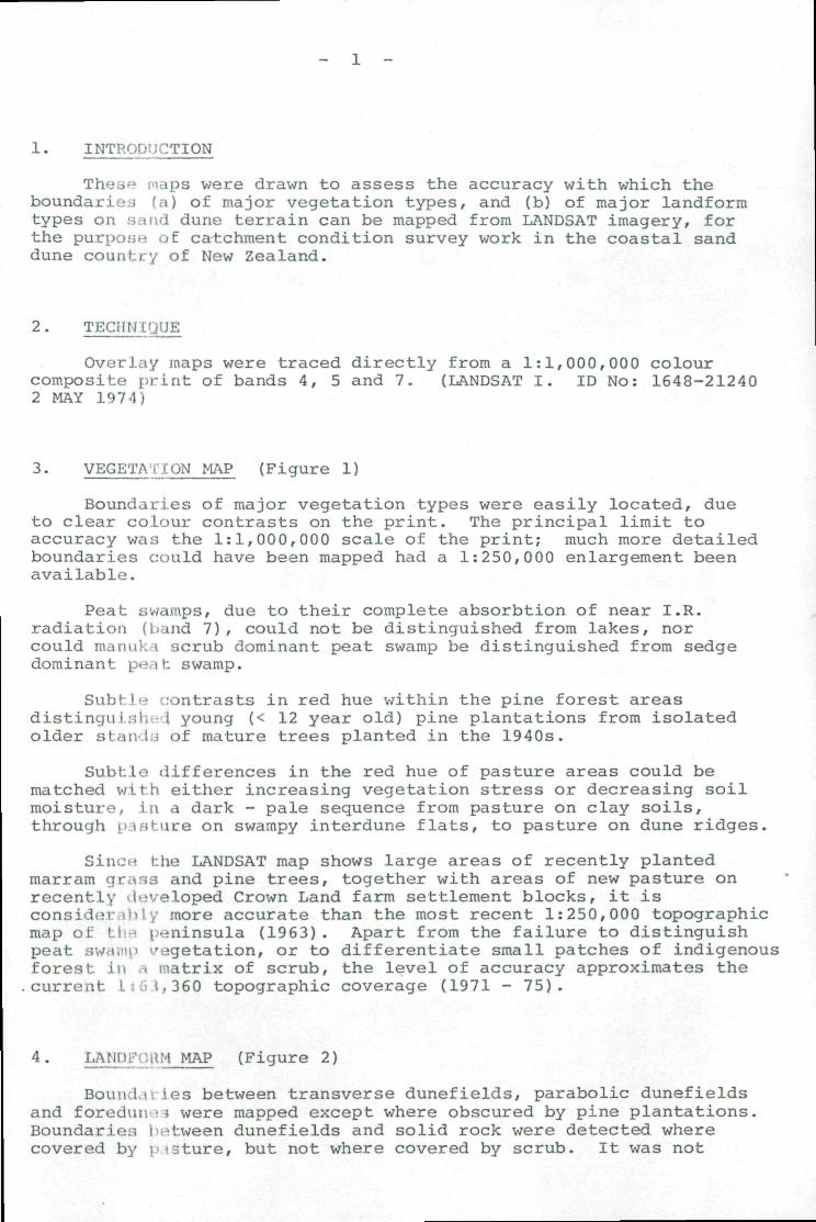
1. INTRODUCTION
Th-- . ips were drawn to assess the accuracy with which theboundarif-';. fa) of major vegetation types, and (b) of major landformtypes on s;-md dune terrain can be mapped from LANDSAT imagery, forthe purport: r, £ catchment condition survey work in the coastal sanddune country of New Zealand.
2. TECHNIQUE
Overlay maps were traced directly from a 1:1,000,000 colourcomposite print of bands 4, 5 and 7. (LANDSAT I. ID No: 1648-212402 MAY 1974)
3. VEGETATION MAP (Figure 1)
Boundaries of major vegetation types were easily located, dueto clear colour contrasts on the print. The principal limit toaccuracy was the 1:1,000,000 scale of the print; much more detailedboundaries could have been mapped had a 1:250,000 enlargement beenavailable.
Peat swamps, due to their complete absorbtion of near I.R.radiation (band 7), could not be distinguished from lakes, norcould manuka scrub dominant peat swamp be distinguished from sedgedominant peat swamp.
Subtle contrasts in red hue within the pine forest areasdistinguish 1 young (< 12 year old) pine plantations from isolatedolder statv.ld of mature trees planted in the 1940s.
Subtle differences in the red hue of pasture areas could bematched with either increasing vegetation stress or decreasing soilmoisture, in a dark - pale sequence from pasture on clay soils,through i>.t?«ture on swampy interdune flats, to pasture on dune ridges.
Sine*- the LANDSAT map shows large areas of recently plantedmarram grass and pine trees, together with areas of new pasture onrecently developed Crown Land farm settlement blocks, it isconsider ii) I y more accurate than the most recent 1:250,000 topographicmap of t!•••' v-reninsula (1963) . Apart from the failure to distinguishpeat swd.'H' vegetation, or to differentiate small patches of indigenousforest it. . matrix of scrub, the level of accuracy approximates thecurrent l : > - i , 3 6 0 topographic coverage (1971 - 75).
4. LANii-' -'-I MAP (Figure 2)
Bound.i -. ies between transverse dunefields, parabolic dunefieldsand foredun^> were mapped except where obscured by pine plantations.Boundaries between dunefields and solid rock were detected wherecovered by pasture, but not where covered by scrub. It was not
possible to detect boundaries between parabolic dunes of differentages (three parabolic dunefields are present), or between foredunesof different ages (two foredune belts are present). In some places,a known correspondence between a scrub-pasture boundary and ageomorphi.c boundary enabled the latter to be mapped, even thoughthere was no obvious change in terrain.
Clear dune ridge patterns were visible in all three types ofdunefield, and could have been mapped had a 1:250,000 enlargementbeen available.
The accuracy of the LANDSAT map, in detecting major landformboundaries, is not as great as either the 1961 1:250,000 NewZealand Geological Survey map, nor the author's unpublished1:50,000 '/• morphological map. This is due to the failure of theLANDSAT image to detect changes in drainage patterns, dune shapesand soil types, which are crucial for delineating dunefields ofdifferent ages.
5. CONCLUSIONS
LANDSAT imagery enables accurate mapping of all the vegetationtypes shown on the 1:250,000 and 1:63,360 topographic coverage ofthe Aupouri Peninsula, with the exception of peat swamp vegetation.The detail and accuracy of the map exceeds that of 1:250,000 coverageand approaches that of 1:63,360 coverage.
LANDSAT imagery can differentiate pine plantations on sandcountry into at least two age classes. It can also differentiatepasture on the basis of stress induced by soil moisture variations,from wet inter-dune hollows to dry ridges.
LANDSAT imagery is unsuitable for geomorphological mapping insand dune country, since while it can detect major differences interrain (e«g. dune ridge patterns), it cannot detect less obviousvariations in dune characteristics, such as soil type. It doeshave some geomorphological application, as a means of mapping duneridge patterns, and as a means of detecting long term change in theposition and vegetation cover of active dunes.
It is unlikely that LANDSAT imagery, in its present form, canbe used for initial catchment condition survey work in sand dunecountry on the New Zealand coastline. This is due to its inabilityto detect subtle parameters of dune conditions, e.g. variations insoil type, and individual erosion scars. However, should subsequentre-survey be required, to establish catchment trend, comparativeLANDSAT i< s-jery for the two survey dates would enable assessment ofchanges in position and vegetation cover of active dunes. It wouldalso en.ibU; assessment of changes in vegetation and land use onstable c'hni'.-i country. In both cases, field checks would be necessaryto obtain wore detailed information about the changes depicted bythe imagery.

I I Q u
V * q a I a.1 i' an I lq.p aT M u a o U r l l g . n i n t u . L o . . I H>r In larva. ,
H -T ( J t T Ti,,x r-cn <jj r\ [ ro tn i a r\ eLS a U X yfm g a.
I. Ba,e SC.nl i.n« |V^M
0 M C PI t Iv v vvlff. I la.hr-a.rn V7r-ck.(t |axUnor«t I
a D. P! t f- I /\ A AJ3. Tine r Lar»lo(.L»on» I -*
-. O
. Ott
s Ly- S.,
6.
"?. laevL Jtuo-mp* and
I I-
Figur. • 1 Vegetation map of Aupouri Peninsula, Northland

riouira
!..» and T arm I la.a CM r\u.pau.ci fa n>r»»u.Leu p l\l or I n Lgr» oL
LJ^xujn From Ltxr»cl.^a.L i X m ac q a. loC-8'2.1
Sc*L I : 1,000,000.
I.
•C. I r-
U»TLxtt
U'oir»»i/«.rs4. U'u.nas mmEZZI
. Ki<^a.r ' I OOOl lcLiri n in aL I - - I
3. r
Iv . f~ o r e. c*
s..
7. FU^j^tL J,U i IL countr uf '
on saLi'oL roc.1
s S S-t
O. I «,rrouce«L secnJL ola
I
Figur- '. Landform map of Aupouri Peninsula, Northland.

PART VII
GE< HICAL APPLICATION IN LANDSAT MAPPING:
n; AND ENVIRONMENTAL STUDIES USING SATELLITE
!*Y, ELECTRONICALLY ENHANCED IMAGERY, AND
COMPUTER PROCESSING TECHNIQUES
Investigator: Professor G. Ross Cochrane
Agency: Department of GeographyUniversity of Auckland
Address: Private BagAucklandNEW ZEALAND
Telephone No. Auckland 74-740
Author: G. Ross Cochrane
1• INTRODUCTION
The Department of Geography of the University of Aucklandis continuing its analysis of a range of LANDSAT single bandand coloiu composite imagery made available by P.E.L. The useof facilities for image interpretation at P.E.L. remote sensingunit is gratefully acknowledged.
Major interest is focussed upon:
1. Lariduse mapping
2. Vegetation classification
3. Pasture change and seasonal productivity
4. Hydrology
5. Geologic-geomorphic mapping
6. Coastal processes
2• TECHNIQUES
2.1 Photographic Interpretation
Standard photo interpretation techniques are being used onselected LANDSAT single band and colour composites at 1:1,000,000and larger scales and on Photowrite enlargements of bands 4, 5and 7 of -in area of central North Island. Substage sampling hasused large scale aerial photos and maps supported by some fieldchecking.
2.2 Enhanced Processes
Thi-'St! have included optical enhancement with a colour additiveviewer and electronic enhancement (density slicing and colourenhancement) of selected areas on various bands to provideaddit.i <MM L detail for comparison with photo images.
2.3 < 'er Processes
'fintout maps of selected areas showing radiance valueshave i n provided by P.E.L. for comparative mapping analyses.
3. AIM i, i CATION OF LANDSAT DATA
The .hi [lowing specific investigations have been carried outby the aui.hor and graduate students of the Department of Geographyat the University of Auckland. Some of these are a continuation
of stud lea recorded in P.E.L., DSIR September 1976 QuarterlyReport, m lu>rs are new investigations.
1. /.nalysis of suspended sediment patterns in thei 11 rth of Thames.
2. f.ake Taupo suspended sediment study: apreliminary report.
3. ' gional and seasonal patterns of sediments.in New Zealand coastal waters.
4. Coastal geomorphology. Analysis of sand dunes,Aotea Harbour, west coast North Island.
5. Applications of LANDSAT imagery for mappingregional geology -
(a) Marlborough(b) Rotorua-Taupo
6. Comparative evaluation of enlarged Photowritebands 4, 5, and 7 for landuse and land covermapping.
7. Thematic mapping: Large scale mapping of vegetationfrom a LANDSAT-II image of East Taupo.
8. Thematic mapping: Landuse mapping of the AupouriPeninsula, Northland from LANDSAT.
9. Thematic mapping: Vegetation mapping in Westland,South Island, from LANDSAT colour composites.
10. Thematic mapping: Usefulness of LANDSAT data formonitoring range conditions in Marlborough.
4- DISCUSSION
Ac; full detailed statements of each of these investigationswill Inj i resented in the next quarterly report some generalobservations only will be outlined here.
5. ->L PROCESSING
In i I lition to using photo interpretation and enhancementtechni > ju>'H in these analyses, increasing emphasis has been placed 01evaluM i ii i detailed large scale sample patterns of selected areasusing iter printout data from LANDSAT CCTs. Generally, thegreatl, In Teased detail and larger scales of computer printout dathave fac1 I Ltated detailed mapping in such diverse investigationsas lake B iiments; stream plumes; ocean currents and thermalfronts; ^hic forest types by species and age; pasture andlucerne; rub types; and categories of natural vegetation.
6. COLOUR COMPOSITES
These investigation;? using LANDSAT colour composite imagery,even at scales of 1:1,000,000 have demonstrated that landuse andland cover delta can ba obtained efficiently over large areas.Many equivalent Category II land cover classes to those outlinedby Anderson »j t al. 1976 (U.S.G.S. Prof. Paper 364) have beenrecognised in widely diverse areas of New Zealand. Such imageryis even more valuable at enlarged scales especially for rapidlyand efficiently updating information with a high degree ofaccuracy.
Unfortunately, because of the heavy demands placed upon P.E.L,in providing user-services we have not been able to have as muchcolour composite enlargement imagery as we would like in order tocarry out a wider range of comparative evaluation.
Investigation have also indicated that ready availability ofcolour composite positive transparencies would provide a moreuseful tool for land cover and landuse mapping than either thestandard colour composite positive prints or enlargements.
Our surveys suggest that the use of colour composite imageryis a relatively inexpensive technique that is highly flexible inapplication.
In addition to its value for mapping of agricultural landusethe utility of LANDSAT colour composite imagery enlargements formapping vegetation is very encouraging. Many major plantassociations can be recognised by their distinctive tonalsignatures. Equal success has been achieved in studies fromLANDSAT colour composites of Westland, Volcanic Plateau andNorthland.
7. DENSITY SLICING AND COLOUR ENHANCEMENT
These techniques have facilitated geomorphic studies greatlyincreasing Hio ability to detect (a) some differences in sanddune geotnorphology and (b) to identify linears in the Marlboroughregion and In the Volcanic Plateau. The use of sequential imageryhas been -••'M-loyed in the Marlborough area but not in the Taupoarea as to iH:o only one image has been available. Seasonaldifferences in vegetation often help demark lineaments.
A. >;MH:\". of techniques have been employed in our suspendedsediment iiMlyses as was reported in the 1976 September QuarterlyReport. Tb • ••• analytical procedures have been employed in newareas incl't^uf studies of sedimentation in Lake Taupo, New Zealand'slargest ! ater lake.


