Hardware Scheduling and Placement in Operating Systems

for Reconfigurable SoC

Yuan-Hsiu Chen

A Thesis Submitted toInstitute of Computer Science and Information Engineering

College of EngineeringNational Chung Cheng University

for the Degree ofMaster

inComputer Science and Information Engineering

2005

Abstract

Existing operating systems can manage the execution of software tasks, however

the manipulation of hardware tasks is very limited. The major goal of this research is

to design and implement an embedded operating system that manages both software

and hardware tasks in the same framework. In this research, we will demonstrate

how to add the management of hardware tasks to a traditional operating system.

To manage hardware tasks, some issues need to be solved, three of which are as

follows. The first one is the dynamic scheduling of hardware tasks. A good schedul-

ing method for the dynamically reconfigurable architecture will not only help us to

improve execution efficiency, but also reduce power consumption. The second issue

is allocation. Dynamic partial reconfiguration usually results in many fragmented

spaces. To fully utilize the platform resources, efficiently managing the remaining

space is necessary. The last issue is how to place a hardware task in a reconfigurable

logic space. Finding the best fit space can reduce the free space wasted and let more

tasks to be placed at the same time in a reconfigurable platform.

Keywords: Dynamic Reconfigurable SoC, FPGA, Scheduling, Placement

Contents

1 Introduction 6

1.1 Background . . . . . . . . . . . . . . . . . . . . . . . . . . . . . . . . . . . . . . . . . 7

1.2 Motivation and Purpose . . . . . . . . . . . . . . . . . . . . . . . . . . . . . . . . . . 8

1.3 The Target . . . . . . . . . . . . . . . . . . . . . . . . . . . . . . . . . . . . . . . . . 10

1.4 Our approach . . . . . . . . . . . . . . . . . . . . . . . . . . . . . . . . . . . . . . . . 11

2 Previous work 15

2.1 Scheduling Methods . . . . . . . . . . . . . . . . . . . . . . . . . . . . . . . . . . . . 16

2.2 Allocation and Placement Methods . . . . . . . . . . . . . . . . . . . . . . . . . . . . 19

3 Hardware Task Scheduling in FPGA 22

3.1 Introduction . . . . . . . . . . . . . . . . . . . . . . . . . . . . . . . . . . . . . . . . . 22

3.2 Task Modeling . . . . . . . . . . . . . . . . . . . . . . . . . . . . . . . . . . . . . . . 23

3.3 Hardware Scheduling Without Deadline . . . . . . . . . . . . . . . . . . . . . . . . . 23

3.4 Hardware Scheduling With Deadline . . . . . . . . . . . . . . . . . . . . . . . . . . . 24

4 Placement Methodology for Hardware Task 27

4.1 Introduction . . . . . . . . . . . . . . . . . . . . . . . . . . . . . . . . . . . . . . . . . 27

1

4.2 Task Classification . . . . . . . . . . . . . . . . . . . . . . . . . . . . . . . . . . . . . 29

4.3 Recording Placement Information . . . . . . . . . . . . . . . . . . . . . . . . . . . . . 31

4.4 Placement Method . . . . . . . . . . . . . . . . . . . . . . . . . . . . . . . . . . . . . 33

4.5 Example . . . . . . . . . . . . . . . . . . . . . . . . . . . . . . . . . . . . . . . . . . . 36

5 EXPERIMENT RESULTS 43

5.1 Experiment with Random Data . . . . . . . . . . . . . . . . . . . . . . . . . . . . . . 43

5.2 Experiment with Real Data . . . . . . . . . . . . . . . . . . . . . . . . . . . . . . . . 48

6 CONCLUSIONS 50

2

List of Figures

1.1 The configurable logic for hardware tasks. . . . . . . . . . . . . . . . . . . . . . . . . 11

1.2 The architecture of an operating system for reconfigurable systems. . . . . . . . . . . 12

1.3 A Placement Example. . . . . . . . . . . . . . . . . . . . . . . . . . . . . . . . . . . . 14

3.1 Scheduling methodology without deadline (SRPT). . . . . . . . . . . . . . . . . . . . 24

3.2 Comparing the SRPT and LLF Scheduling Methodologies. . . . . . . . . . . . . . . . 26

4.1 The overall architecture of FPGA with configurable logic blocks . . . . . . . . . . . . 28

4.2 The difference between our method and stuffing. . . . . . . . . . . . . . . . . . . . . 29

4.3 Structure of space list and task list. . . . . . . . . . . . . . . . . . . . . . . . . . . . . 31

4.4 The example of tasks in FPGA to illustrate space list and task list. . . . . . . . . . . 32

4.5 Placement steps. . . . . . . . . . . . . . . . . . . . . . . . . . . . . . . . . . . . . . . 33

4.6 Example of Conflict. . . . . . . . . . . . . . . . . . . . . . . . . . . . . . . . . . . . . 34

4.7 Example of two type tasks place into free space. . . . . . . . . . . . . . . . . . . . . 35

4.8 Example of Placement: Total task information. . . . . . . . . . . . . . . . . . . . . . 37

4.9 Example of Placement: (a). . . . . . . . . . . . . . . . . . . . . . . . . . . . . . . . . 38

4.10 Example of Placement: (b). . . . . . . . . . . . . . . . . . . . . . . . . . . . . . . . . 38

4.11 Example of Placement: (c). . . . . . . . . . . . . . . . . . . . . . . . . . . . . . . . . 39

3

4.12 Example of Placement: (d). . . . . . . . . . . . . . . . . . . . . . . . . . . . . . . . . 39

4.13 Example of Placement: (e). . . . . . . . . . . . . . . . . . . . . . . . . . . . . . . . . 40

4.14 Example of Placement: (f). . . . . . . . . . . . . . . . . . . . . . . . . . . . . . . . . 40

4.15 Example of Placement: (g). . . . . . . . . . . . . . . . . . . . . . . . . . . . . . . . . 41

4.16 Example of Placement: (h). . . . . . . . . . . . . . . . . . . . . . . . . . . . . . . . . 41

4.17 Example of Placement: Final information of two list. . . . . . . . . . . . . . . . . . . 42

5.1 The placement example with ratio 4:1. . . . . . . . . . . . . . . . . . . . . . . . . . . 45

5.2 The fragmentation with ratio 1:4. . . . . . . . . . . . . . . . . . . . . . . . . . . . . . 46

5.3 Result of our method and stuffing. . . . . . . . . . . . . . . . . . . . . . . . . . . . . 47

4

List of Tables

4.1 Finding the Best Classification Ratio. . . . . . . . . . . . . . . . . . . . . . . . 30

5.1 Experimental Results and Comparison . . . . . . . . . . . . . . . . . . . . . . . . . . 44

5.2 The Attributes of Six Real Tasks. . . . . . . . . . . . . . . . . . . . . . . . . . . 48

5.3 Three Case with 50 Real Tasks. . . . . . . . . . . . . . . . . . . . . . . . . . . . 48

5.4 Experimental Results and Comparison with Real Tasks . . . . . . . . . . . . . . . . 49

5

Chapter 1

Introduction

Nowadays, a hand-held product can provide a variety of applications such as digital

video, 3D games, MP3 player, and so on. ASICs can be used to make these appli-

cations feasible. However, it may be costly and highly complex, because if someone

wants to add a new application in the near future, one must add an ASIC into the

platform and modify the entire circuit. Furthermore, it is highly probable that the

ASICs will not all run at the same time, because users may require only some of

the applications simultaneously. In general, applications implemented using ASICs

will increase the time to market and the design and production costs. An alternative

method is letting a microprocessor to accomplish all of these applications. Although

when adding a new application this will become simpler than using ASICs completely,

but it perhaps cannot provide the required performance. Hence, some hardware imple-

mentations are required. The characteristic of dynamically reconfigurable platforms

6

such as those using FPGA are between ASIC and microprocessor. FPGAs can be

configured at run-time according to the dynamically required applications, so they

are more flexible than ASICs. FPGAs are also faster than microprocessors in task

execution. Therefore, dynamically reconfigurable platforms perhaps are gradually

being used more and more extensively. Specifically in partially reconfigurable plat-

forms, one can change the configuration of some CLBs (Configurable Logic Blocks)

while other CLBs are still running. However partial reconfiguration is more complex.

We must manage the FPGA space and know when and where the hardware tasks

are to be placed. Controlling partially reconfigurable platforms is quite similar to

virtual memory management in operating systems. In this work, our objective is to

implement an embedded operating system to manage both the hardware and software

tasks simultaneously.

1.1 Background

Generally, EDA tools are used to setup and configure dynamic partially recon-

figurable platforms. The FPGA chips are configured through the JTAG interface.

However in this work, we would like to dynamically control all the resources in a

dynamic partially reconfigurable platform. To achieve this objective, a controller

must to be designed into the platform, which must be small and fast. A possible

tool that can be used instead of the conventional FPGA synthesis tools is the Xil-

inx JBits, which is a set of Java classes providing an API into the Xilinx Virtex II

7

FPGA family bitstream. However, the proposed controller is not only responsible for

configuration as that in JBits, but also the management of the logic resources. The

jobs that a controller must perform include hardware task scheduling, space alloca-

tion, and task placement are all. In the future, many products will make use of the

reconfigurable embedded systems, such as wearable computing and mobile systems.

Therefore, we intend to create an efficient controller to manage the resources of re-

configurable platforms. This controller will be done in the content of an operating

system for reconfigurable systems.

1.2 Motivation and Purpose

Since a dynamically reconfigurable platform usually consists of a microprocessor and

FPGA, a hardware-software co-design methodology is required. Existing operating

systems already have the capability to manage software processes running on a micro-

processor. If we extend an existing operating system, we can avoid the time to design

the software related functions for memory management, inter-process communica-

tion, and process scheduling. We also believe that hardware-software co-scheduling

and communication are also easier to design when extending an existing operating

system. Uniformly treating all system tasks, including both hardware and software

tasks, would be beneficial for hardware-software co-scheduling. Because hardware

and software tasks may have data dependency resulting in process sequencing. If

one of them waits for the other for a long time due to data dependency, the whole

8

system will be very inefficient. Hence, we can let an operating system to coordinate

their execution sequence so as to avoid complex asynchronous control and obtain the

best efficiency. According to the dependency mentioned before, the data between

hardware and software will need to be communicated.

Our implementation of the proposed operating system will provide channels be-

tween the FPGA and the processor to allow communication. The operating system

will also provide a configuration channel to convey configuration data.

The proposed operating system will eventually support the ability for switching

between hardware and software tasks. The most suitable hardware-software switch

time is determined by the operating system which will check the workloads at both

the FPGA and the processor or check the task urgency. Furthermore, it also desirable

that hardware tasks can be preempted, just like software task preemption. To satisfy

real time requirements hardware preemption is also needed. However, preemption will

result in the problem of configuration overhead. If the frequency of preemption is high,

high power consumption could be another side effect. The decision on preemption

will be implemented into the operating system.

Perhaps many people still do not know why one must use an operating system.

Besides the above-mentioned advantages about hardware-software co-design, below

are some reasons why we decided to implement an operating system for reconfigurable

systems.

• increases portability: A reconfigurable system can be easily ported to another

9

platform, by modifying only the architecture related part in an operating system

for reconfigurable system, without the need to start from scratch.

• shorten time to market: When a new product resembles a previous one, we can

reuse some modules in the operating system to reduce the design time. Similar

to the increase in portability, we also need to only modify certain parts of a

system.

• easy partitioning: If the architecture has both FPGA and CPU, and the oper-

ating system supports hardware and software task switching, then a software

task running on the CPU, can be switched and dispatched to run on the FPGA

by the operating system for improved performance. Operating systems can be

made to perform dynamic partitioning easily and efficiently.

1.3 The Target

The target platform on which we will conduct our experiments is the Xilinx ML310,

which has a VirtexII Pro XC2VP30-FF896 chip with two PowerPC405 cores, 256MB

DDR RAM, a 512MB CompactFlash card, and a 10/100 MB/s ethernet interface. The

XC2VP30-FF896 chip has 3680 CLBs, and it is a partial dynamically reconfigurable

chip. The FPGA configurable space is considered to be a set of columns, where a

column spans the height of a chip and the set of columns spread across the width of

the chip. Fig. 1.1 shows the overall architecture of the FPGA chip. The right side

10

rectangle in Fig. 1.1 shows the structure of a basic unit of configuration. The left side

in Fig. 1.1 is the example of placement, there are two tasks A and B on FPGA, the

task A occupies one column and the task B occupies two. In this platform, the basic

placement unit of configuration is one column of CLBs. Hence, the configuration in

this chip is just a one dimensional problem, which means that we need only know

how wide a task is to place it into the chip. Thus, the space allocation is easier than

the two dimensional placement.

CLB

CLB

CLB

CLB

CLB

CLB

CLB

CLB

TaskA

TaskB

Figure 1.1: The configurable logic for hardware tasks.

1.4 Our approach

In the design of an operating system for reconfigurable systems, the focus here will

be on the hardware task scheduling, placement, and space allocation. The criteria

11

for finding solutions to the above research issues include the usage of reconfigurable

resources such as the utilization of the FPGA space, real time performance for tasks,

power consumption and so on. Fig. 1.2 illustrates the prototype of an operating sys-

tem for reconfigurable systems. The left side of Fig. 1.2 depicts the original existing

software task management. The right side shows the hardware counterpart for man-

aging the FPGA resources. The details of the scheduler, placer, and allocator will be

described later. The loader component in Fig. 1.2 is in charge of the configuration. It

transports the configuration data to the FPGA. Communicator is a bridge between

the processor and the FPGA. Signals and messages transfer through this interface.

Finally, the arrow between software scheduler and hardware scheduler represents the

process of co-scheduling.

Scheduler

OSS H

Scheduler

Placer

Allocator

MMU

FPGA

Communicator

.

.

.Loader

Figure 1.2: The architecture of an operating system for reconfigurable systems.

12

In the following, we introduce the proposed method of scheduling, placement, and

allocation. We choose the Shortest Remaining Processing Time (SRPT) [1] or Least

laxity First (LLF) [3] to decide the scheduling priority. The task having the shorter

remaining time or least laxity will have a higher priority. The system will thus choose

the task with the shortest remaining time or least laxity in the ready queue to process

first. For the placement and allocation methods, we can refer to Fig. 1.3. In Fig. 1.3,

there are two coordinate axes representing the width of FPGA in terms of columns

and time in cycle. Basically, the proposed placer in this thesis will separate the arrived

tasks into two types. One of them has longer processing times but use lesser space,

and the other one have shorter processing times but use more space. For example,

tasks 1 and 3 in Fig. 1.3 are of type A, and tasks 2, 4, and 5 are of type B. Graphically,

tasks of type A are more flat and lying-down, while tasks of type B are more thin

and standing. The placer places the two types of tasks towards the two ends of the

width axis, that is, on one end tasks of low SUR type are placed and on the other

end tasks of type high SUR are placed. We adopt this classification method so as to

reduce the amount of space wasted, because it reduces the amount of fragmentation.

Details of the placement algorithm will be given in Chapter 4.

13

(width)column

cycle (time)

T1

T3

T2

T5

T4

Figure 1.3: A Placement Example.

14

Chapter 2

Previous work

The major issues related to the design and implementation of an operating sys-

tem for reconfigurable systems including task scheduling, allocation, and placement.

These issues are intimately related, because we must think about not only execution

sequence, but also the space in the reconfigurable logic device to reduce reconfigura-

tion overhead. Scheduling methods can be classified as static scheduling and dynamic

scheduling. Allocation and placement can be 1 dimensional or 2 dimensional prob-

lems of management in the FPGA space. An overview of previous work related to

these methodologies will be described in this Chapter.

Section 2.1 gives a review on some approaches for hardware task scheduling. Sec-

tion 2.2 surveys different approaches of placement and allocation.

15

2.1 Scheduling Methods

There are many similarities between the scheduling of hardware and software tasks.

For example irrespective of hardware or software, the scheduler needs some a-priori

information about tasks such as task priority, execution time, task size, deadline, and

so on. Hence, some methods for software task scheduling could also be implemented

for hardware task scheduling.

Scheduling methods can be classified into static scheduling and dynamic schedul-

ing, according to the time of scheduling the ready tasks. Static scheduler is used

before the execution of an application. For an application with statically known data

dependencies, task arrival time, and execution time, static scheduling can be used.

However, it is impossible to anticipate the behavior of all tasks before execution in a

dynamically reconfigurable system implementation, so we must schedule the tasks dy-

namically at run time. Though dynamic scheduling will achieve the better execution

sequence than static scheduling when some information could not know at run time,

but it will spend more time than static scheduling to decide the processing sequence

at run time.

Most schedulers are based on task priority. For example, in list scheduling [4], there

is a list of ready tasks, sorted by their priorities. If there are multiple ready tasks

ready, the scheduler will select a task with the highest priority to run. The difference

among these schedulers is the method for calculating the task priority. There are

16

some algorithms to compute the priority as follows.

• Static Scheduling

– As Soon As Possible (ASAP) and As Late As Possible (ALAP): These two

algorithms are static, which means the priority is calculated before schedul-

ing. If we know the before and after processing sequence and task depen-

dence before scheduling, ASAP will let task as soon as possible to be placed

into FPGA and not violates the processing sequence. ALAP will place the

task into FPGA as late as possible and obeys the sequence.

• Dynamic Scheduling

– First In First Out (FIFO): Tasks in queue will be sorted by their arrival

time. The earliest arriving task is at the head of the queue. The FIFO

scheduler selects tasks from the queue head.

– Shortest Job First (SJF): This algorithm sorts the queue according to the

execution time of the tasks. The head of the queue is a task with the shortest

execution time.

– Earliest Deadline First (EDF): The scheduler sorts tasks by their deadline.

A task with the earliest deadline is executed first.

– Shortest Remaining Processing Time (SRPT): This method supports task

preemption. The scheduler sorts the queue in ascending order of the remain-

ing execution time of tasks.

17

A new metric used to compute priority was proposed in [4]. This metric combines

ALAP and dynamic ASAP to compute task priority dynamically [4]. Unlike static

ASAP computes the priority before scheduling, the dynamic ASAP computes priority

at run time. When a task is scheduled, all dynamic ASAP values will be recalculated.

The ALAP time does not change at run time during dynamic scheduling, but dynamic

ASAP can realize the situation at run time to choose a better execution sequence. In

[8], the dynamic scheduling algorithm is based on the event windows and the active set

information. The scheduling algorithm of event windows is based on the task type and

task priority. Task priority is used to decide execution sequence. A task type means

this task would use which type circuit of dynamic reconfigurable logic. In the next

section, we will describe the configuration type along with the dynamic reconfigurable

logic. For minimizing the reconfiguration overhead a specific scheduling is supported

in [10]. It selects an existing run-time/design-time scheduling methodology called

Task Concurrency Management (TCM) [18] since it results in only a small run-time

penalty as most of the computation is done at design time. Although the TCM

can reduce power consumption, but it is not aware of the reconfiguration overhead.

Hence, there are three modules [10] that update the output of the TCM scheduler at

run-time.

18

2.2 Allocation and Placement Methods

In this section will introduce some management methods for the FPGA logic space

such as space allocation and task placement. These methods are intimately related

to the dynamic reconfigurable device, and they attempt to obtain better utilization

of these reconfigurable spaces.

Two well known online algorithms for the 1D problem are first fit (FF) and best

fit (BF). BF results in less fragments, but FF is much faster than BF algorithm.

We will introduce some methodologies about the FPGA area utilization next. The

reconfigurable logic could be partition into many blocks with different sizes [14]. All

of these blocks have fixed length in the vertical dimension, so block size is only

related to width. Because the sizes of blocks are different, the placer can select the

most suitable size of block for a task. Choosing the best fit block size result in

a smaller fragmentation. In [8], the FPGA space was divided into many Dynamic

Reconfigurable Logics (DRL), and each DRL will be classified into different type. If

a task ready to execute and find there is DRL has the same type, this task could

execute immediately without reconfiguring DRL. There are two event windows to

record execution and configuration events. If new tasks become ready for execution,

new task events are generated and inserted in execution event windows. When the

suitable DRL type for a task can be found in the FPGA, the event of this task will

be inserted in the execution event window. If all the DRL types are not suitable for

19

a new task, an event will be inserted in the reconfiguration event window. Scheduler

will select one event from reconfiguration event window and start to reconfigure the

DRL when execution event window is empty. This methodology tends to decrease the

member of reconfigurations for reducing the overall reconfiguration overhead, because

the DRL will not be reconfigured if there exists events in the execution event window

that use the same DRL type continually.

Two techniques to implement scheduling and placement called Horizon and Stuff-

ing are proposed in [14]. In the horizon technique two lists used, the scheduling

horizon list and the reservation list. The scheduling horizon list is a set of intervals,

an interval is written as [X,Y]@T, where [X,Y] denotes the width from X to Y in one

dimension and T is the last release time. The reservation list stores all tasks which

are scheduled but not yet executed. When a new task arrives, the scheduler will find

a suitable width from scheduling horizon list for this task. The stuffing technique

also uses two lists, but the free space list replaces the scheduling horizon list in the

horizon technique. The free space list is a set of intervals [X,Y] that denote currently

unused resource rectangles with height H. X and Y means the left end and right end

position in FPGA, is just the task width. H means the execution time of this task. If

a task arrives, it will find a space from the free space list. Though a free space width

may fit the task width, yet we should check whether this task conflicts with other

tasks which are in the reservation list during execution time. The main difference

between Horizon and Stuffing is that Stuffing could use the FPGA space efficiency.

20

Because Stuffing would find suitable slices from task ready time, but Horizon finds

the suitable slices from the time that these slices never be used after. When using

Horizon even though these slices from the free time to next using time have enough

time to process this task, this interval time would not be used.

21

Chapter 3

Hardware Task Scheduling in

FPGA

3.1 Introduction

This Chapter will give a detailed description on the hardware scheduler. We

propose two scheduling methodologies in this work as follows. For tasks without

deadlines we use the Shortest Remaining Processing Time (SRPT) methodology for

task scheduling. For tasks with deadlines we change the method to decide priority

for hardware tasks, that is, we use the Least Laxity First (LLF) algorithm.

22

3.2 Task Modeling

The hardware to be configured on an FPGA is modeled as a set of hardware

tasks, where each task t has a set of attributes including arrival time A(t), execution

time E(t), deadline D(t), and area C(t) (in terms of the number of FPGA columns

required). These numbers can be obtained by synthesizing a hardware function using

a synthesis tool such as Synplify or XST.

3.3 Hardware Scheduling Without Deadline

How to decide the priority for a task is the key decision in any scheduling method.

Suppose we have only information about execution time E(t) and task size (C(t))

at the time of scheduling. Task size is related to placement, so this information will

not be used for scheduling. The SRPT is a very suitable method when we know only

the execution time about tasks. SRPT [1] is an optimal algorithm for minimizing

mean response time and it has also been analyzed that the common misconception

of unfairness in SRPT to large tasks is unfounded.

The priority for each task is defined by their remaining processing time. The

task which needs the least execution time will be assigned the highest priority. In

the scheduling method there is a queue to place hardware tasks that are ready for

execution. Every ready task must go through the scheduler before it is put in the

ready queue. The scheduler will insert the tasks into the ready queue according to

23

their priorities. Hence, the task in the front part of the queue will be scheduled first.

For the example in Fig. 3.1, there is a queue and with four scheduled tasks. The four

tasks in the queue have their individual execution times, the scheduler will determine

their priorities as follows. The order of their priorities from high to low is A, B, C,

and D. In Fig. 3.1, the execution time of the next ready task E is 15, it will be inserted

between task C and task D.

GTask

Exe. time10

FTask

Exe. time20

ETask

Exe. time15

…..

Queue

A 5

B 8

C 14

D 20

Taskexecution

time

Placement

Schedule

A 5

B 8

C 14

D 20

Add taskE 15

Figure 3.1: Scheduling methodology without deadline (SRPT).

3.4 Hardware Scheduling With Deadline

If we have information about task deadline, maybe we could use this to get better

performance. Because, when one task misses its deadline, it would affect other tasks

that are waiting for the task. If we reduce the amount of deadline misses, we could

24

make the application performance more efficient.

For scheduling real-time hardware tasks with deadlines, we can use either EDF

or LLF. However, because hardware tasks are non-preemptive and truly parallel, we

decided to use LLF, which degrades a little more gracefully under overload than EDF,

extends relatively well to scheduling multiple processors, which are similar to parallel

hardware tasks, and approaches the schedulability of EDF for non-preemptive tasks.

Now we will describe the LLF methodology. In LLF, the priority of a task t

is assigned as given in Equation 3.1, where D(t) is task deadline, E(t) is the task

execution time, now is the current time, and P (t) is the priority. Intuitively, the

priority is the slack time for a task.

P (t) = D(t)− E(t)− now (3.1)

A LLF example is shown in Fig. 3.2. There are three ready tasks A, B, and C

with execution time 10, 5, and 15, and deadline 25, 30, and 20 respectively. If we

suppose the current time of them are the same, the priorities of A, B, and C are 15,

25, and 5. Hence, the order in ready queue are C, A, and B. Using the LLF all of

these three tasks can complete execution before their deadlines.

During scheduling we have not considered the task size and the FPGA space size,

hence some tasks may miss their deadlines if there is not enough space for these tasks.

The placement methodology will be described in Chapter 4.

25

Task A

Exec. 10Deadline 25

Task B

Exec. 5Deadline 30

Task C

Exec. 15Deadline 20

Schedule

C

A

B

LLF

Head

P = 5

P = 15

P = 25

Figure 3.2: Comparing the SRPT and LLF Scheduling Methodologies.

26

Chapter 4

Placement Methodology for

Hardware Task

4.1 Introduction

The XC2VP30 chip we use to experiment has 80 rows and 46 columns. In

Chapter 1 we have discussed that the smallest placement unit is one column of CLBs.

Hence there will be 46 columns for hardware task placement. Fig. 4.1 illustrates the

architecture of FPGA with configurable logic blocks, the column of CLBs with gray

background is the smallest placement unit. Hence, we need to know how wide a task

is but need not to know how high the task occupies. If we only consider the FPGA

space for placement, it is a one dimensional problem. In order to more effectively

utilize FPGA space, we also consider the task execution time. Hence, in out method

27

the hardware task placement is a two dimensional problem.

IOB

IOB

IOB

IOB

CLB CLBCLB CLB CLBCLB

CLB CLBCLB CLB CLBCLB

CLB CLBCLB CLB CLBCLB

CLB CLBCLB CLB CLBCLB

CLB CLBCLB CLB CLBCLB

CLB CLBCLB CLB CLBCLB

CLB CLBCLB CLB CLBCLB

CLB CLBCLB CLB CLBCLB

BUS

MACROS

BUS

MACROS

Figure 4.1: The overall architecture of FPGA with configurable logic blocks

The main difference between our classified stuffing and the original stuffing method

[11] is the classification of hardware tasks. In our method, we classify all hardware

tasks into two types and the placement location of these two types of tasks are

different, while in the stuffing method there is no such distinction. An example

is shown in Fig. 4.2. Suppose tasks A, B, and C are already placed as shown in

Fig. 4.2 and the placements are the same in our method and in stuffing. Next, task D

is to be placed, however the location it is placed will be different in out method and

in stuffing. In stuffing, it is placed adjacent to task C in the center columns of the

FPGA space. In contrast, in our method task D will be placed from the rightmost

columns. As a consequence, in our method tasks E and F can be placed earlier than

that in stuffing, resulting in a shorter schedule. Finally, the fragmentation in our

28

ClassifiedStuffing

Stuffing

Time(cycle)

Column151413121110987654321

A

B

C

D

EF

1 2 3 4 5 6 7 8 9 10111213141516171819202122232425262728 29 30

1 2 3 4 5 6 7 8 9 10111213141516171819202122232425262728 29 30

Column151413121110987654321

A

C

B

D

EF

Time(cycle)

Figure 4.2: The difference between our method and stuffing.

classified stuffing will also be lesser than that in stuffing because the space is used

more compactly.

4.2 Task Classification

For a task t, we call the ratio C(t)/E(t) the Space Utilization Rate (SUR) of t.

Given a set of hardware tasks, they are classified into two types, namely high SUR

tasks with SUR(t) > 1 and low SUR tasks with SUR(t) ≤ 1. The classification of a

task determines where it will be placed in the FPGA as follows. High SUR tasks are

placed starting from the leftmost available columns of the FPGA space, while low

29

Table 4.1: Finding the Best Classification Ratio.SR\ CR 1:4 1:3 1:1 3:2 3:1 4:1 5:1

4:1 TF 667 667 667 665 654 638 640TT 192.1 192.1 192.1 192.1 191.6 191.1 191.1

1:1 TF 471 471 435 441 461 456 459TT 172.7 172.7 171.4 171.9 172.8 172.6 172.7

1:4 TF 427 429 431 435 435 440 443TT 162.3 162.6 162.6 162.7 162.7 162.8 163

SR: set ratio, CR: Classification ratio

SUR tasks are placed starting from the rightmost available columns. This choice of

segregating the tasks and their placement is to reduce the conflicts between the high

and low SUR tasks. A conflict often results in unused FPGA space, which in turn

increases the total execution time. Because the classification scheme does not take

the number of tasks of each type into account, one may wonder if this classification

will not gain much when there is an imbalance between the number of high and low

SUR tasks. However, after through experiments, we found the best results (least

fragmentation, shortest execution time) are always obtained when we divide the task

set considering only their SUR values.

To support our choice of task classification using SUR value and not considering

the number of tasks of each type, we performed several experiments by using different

classification ratio (CR) for a task set. The results are tabulated in Table 4.1, where

we can observe that the best results are usually obtained when the classification ratio

is the same as the set ratio, that is, the threshold for classification can depend only

on the SUR values.

30

4.3 Recording Placement Information

In our placement methodology we need two lists, space list for recording the free

space, and a task list for recording the task location in FPGA after placement naming.

Besides these two lists each task has four attributes, namely width, execution time,

arrival time, and deadline.

space list

task list

Freetime

Leftend

Rightend

Freetime

Leftend .......

Space 1 Space 2

Starttime

Leftend

Rightend

Exe.time

Starttime .......

Task 1 Task 2

Figure 4.3: Structure of space list and task list.

Fig. 4.3 illustrates the structure of space list and task list. For every free space in

the space list we will record three information which are release time for columns of

CLBs, the leftmost and rightmost columns in FPGA of this free space. When placer

places a task into FPGA, task list will store four information about this task. First

is the starting time of task executing on FPGA, following are leftmost column and

rightmost column in FPGA that task occupies. The final information is execution

time of this task. Space list could supply information for placer to find a fit free space

for task, and task list could let placer detect whether there is any conflict among

the tasks. How to find a fit space from space list and how to detect conflicts will be

31

explained in Section 4.4. Now we will explain how to store information into space list

and task list.

FPGAWidth

(Column) Task A

Task B

1

10

Time (cycle)1 2 5 103 4 6 7 8 9 1511 12 13 14

2

3

4

5

6

7

8

9

0 1 8 8 1 10 …..Space list

Space 1 Space 2

0 9 10 8 …..Task list

Task A

Add Task B

0 9 10 8 0 1 6 5 …..Task list

Task A Task B

0 7 8 5 1 8 8 1 10 …..Space list

Space 1 Space 2 Space 3

Figure 4.4: The example of tasks in FPGA to illustrate space list and task list.

In Fig. 4.4 we assume that the FPGA has 10 columns of CLBs. First, the placer

dispatches task A to the FPGA, the task list will store [0,9,10,8] for this task and

space list will change from one free space [0,1,10] to two free spaces [0,1,8,8,1,10].

Next, task B will be placed, the task list adds [0,1,6,5] after [0,9,10,8] and the space

list will change a lot after placement. The first is that the free space [0,1,8] will

change into [0,7,8]. Second, a new free space [5,1,8] must be inserted between [0,7,8]

32

Task with highestpriority

Recognize task

Stand

Find fit space

Flat

Decide placementlocation

Conflictchecking

Place into thisspace

Modify spacelist

No

Yes

Figure 4.5: Placement steps.

and [8,1,10], because free spaces in space list are sorted by their release time, so it

will not be added to the end of the queue.

4.4 Placement Method

For different types of tasks we will provide different placement methods. In Section

4.2 we have explained how to recognize task type, now we will give a detailed descrip-

tion of the placement method for these two types in this section. Fig. 4.5 illustrates

33

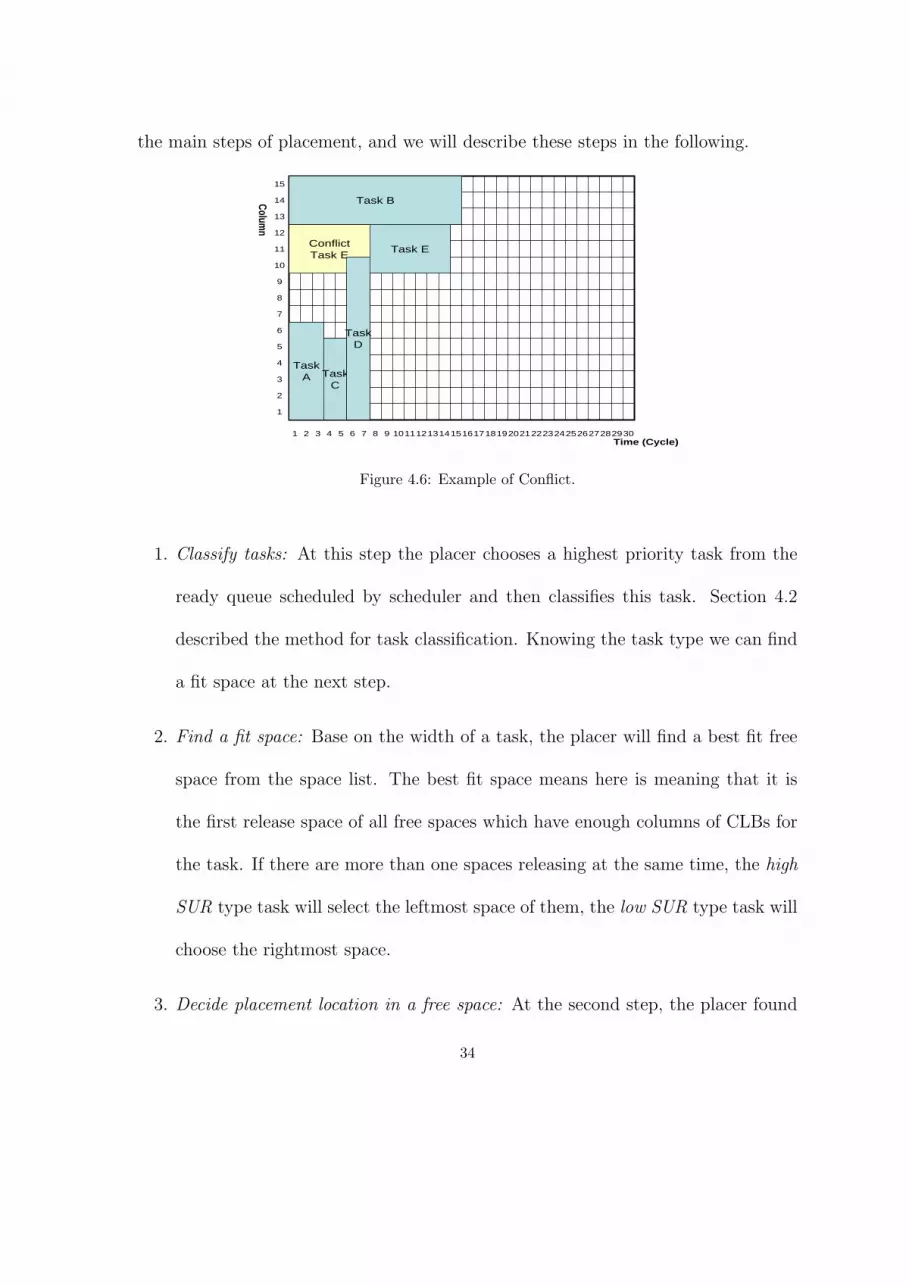
the main steps of placement, and we will describe these steps in the following.

1 2 3 4 5 6 7 8 9 101112131415161718192021222324252627282930

ConflictTask E

Task B

TaskA Task

C

TaskD

Task E

1

2

3

4

6

5

7

8

15

14

13

12

11

10

9

Time (Cycle)

Column

Figure 4.6: Example of Conflict.

1. Classify tasks: At this step the placer chooses a highest priority task from the

ready queue scheduled by scheduler and then classifies this task. Section 4.2

described the method for task classification. Knowing the task type we can find

a fit space at the next step.

2. Find a fit space: Base on the width of a task, the placer will find a best fit free

space from the space list. The best fit space means here is meaning that it is

the first release space of all free spaces which have enough columns of CLBs for

the task. If there are more than one spaces releasing at the same time, the high

SUR type task will select the leftmost space of them, the low SUR type task will

choose the rightmost space.

3. Decide placement location in a free space: At the second step, the placer found

34

a best fit space for a task, but this space maybe wider than that required by the

task. In this case, according to the task type we determine which columns of

CLBs of the best fit space will be used. For example, in Fig. 4.7 task A is high

3

4

5

6

7

8

9

10

11

12

13

14

Cycle

Column

Task A

7

2

High SUR

Task B 3

9

10

11121314151617Column

Low SUR

E

C

C

E

Cycle

Figure 4.7: Example of two type tasks place into free space.

SUR type and B is low SUR type. When the placer finds a fit space for task A

from column 3 to column 14, task A will be placed from column 3 to column 9.

If there is a free space from column 10 to column 17 for task B, it will be placed

from column 17 to column 15. Because the high SUR type task will be placed

from the leftmost column and low SUR type will be placed from the rightmost

column.

4. Conflict checking conflict: At this step we already know where a task is placed,

35

but we need to check if any task has been placed into the same columns during

execution time of this task. Fig. 4.6 is a conflict example. The first time the

placer will find the space of column 7 to column 12 and it decides to place at

column 10 to column 12. However, the placer has already decided to place task

D from column 1 to column 10 at the 6th cycle, hence task E will conflict with

task D. If a conflict exists, we must choose another fit space for this task by

going back to Step(2). In Fig. 4.6 the placer will choose a new free space from

column 1 to column 12 at the 8th cycle for placing task E.

5. Modify space list: After a task is placed into a best fit space, not only the

information of this fit space need to be modified, but also some other free spaces

in the space list may be influenced. The example of this step will be given in

Section 4.5.

4.5 Example

In this section we will use figures to illustrate a placement example. In this

example there are eight tasks as shown in Fig. 4.8. One thing we must notice is that

the space list always has one free space at the beginning, that is [1,1,15]. The other

thing we need to explain in our example is how to modify the space list. For example

in Fig. 4.10, before task B has been placed there are two free spaces [1,10,15] and

[4,1,15]. After placing task B as in Fig. 4.11 the space [1,10,15] will be modified to

36

Task Arrival time (cycle)

Width(Column)

Exec. Time (cycle))

A 0 9 3

B 0 2 14

C 1 7 2

D 1 10 5

E 2 3 16

F 4 12 3

G 4 8 4

H 5 2 11

Space List Task List

1 1,1,15 null

Figure 4.8: Example of Placement: Total task information.

[1,10,13], the space [4,1,15] will be [4,1,13], and the new space [15,1,15] will be added.

Thus it can be seen that placing a task will affect some free spaces, and all free spaces

in the space list are sorted by their release time. Below are the detailed illustration of

placement, where we could follow the step to understand our placement methodology.

37

Space List Task List

151413121110987654321

1 2 3 4 5 6 7 8 9 101112131415161718192021222324252627282930

Column

Time (cycle)

A

1 1,1,15 null

Figure 4.9: Example of Placement: (a).

Space List Task List

1 1,1,9,31 1,10,15

2 4,1,15

151413121110987654321

1 2 3 4 5 6 7 8 9 101112131415161718192021222324252627282930

Column

Time (cycle)

A

B

Figure 4.10: Example of Placement: (b).

38

Space List Task List

1 1,10,13

2 4,1,13

3 15,1,15

1 1,1,9,3

2 1,14,15,14

151413121110987654321

1 2 3 4 5 6 7 8 9 101112131415161718192021222324252627282930

Column

Time (cycle)

A

B

C

Figure 4.11: Example of Placement: (c).

Space List Task List

1 1,10,13

2 4,8,13

3 6,1,13

4 15,1,15

1 1,1,9,3

2 1,14,15,14

3 4,1,7,2

151413121110987654321

1 2 3 4 5 6 7 8 9 101112131415161718192021222324252627282930

Column

Time (cycle)

A

B

CD

Figure 4.12: Example of Placement: (d).

39

Space List Task List1 1,10,13

2 4,8,13

3 6,11,13

4 11,1,13

5 15,1,15

1 1,1,9,3

2 1,14,15,14

3 4,1,7,2

4 6,1,10,5

151413121110987654321

1 2 3 4 5 6 7 8 9 101112131415161718192021222324252627282930

Column

Time (cycle)

A

B

CD

E

Figure 4.13: Example of Placement: (e).

Space List Task List1 1,10,13

2 4,8,10

3 11,1,10

4 15,14,15

5 20,1,15

1 1,1,9,3

2 1,14,15,14

3 4,1,7,2

4 4,11,13,16

5 6,1,10,5

151413121110987654321

1 2 3 4 5 6 7 8 9 101112131415161718192021222324252627282930

Column

Time (cycle)

A

B

CD

E

F

Figure 4.14: Example of Placement: (f).

40

Space List Task List1 1,10,13

2 4,8,10

3 11,1,10

4 15,14,15

5 20,13,15

6 23,1,15

1 1,1,9,3

2 1,14,15,14

3 4,1,7,2

4 4,11,13,16

5 6,1,10,5

6 20,1,12,3

151413121110987654321

1 2 3 4 5 6 7 8 9 101112131415161718192021222324252627282930

Column

Time (cycle)

A

B

CD

E

F

G

Figure 4.15: Example of Placement: (g).

Space List Task List1 1,10,13

2 4,8,10

3 11,9,10

4 15,1,10

5 15,14,15

6 20,13,15

7 23,1,15

1 1,1,9,3

2 1,14,15,14

3 4,1,7,2

4 4,11,13,16

5 6,1,10,5

6 11,1,8,4

7 20,1,12,3

151413121110987654321

1 2 3 4 5 6 7 8 9 101112131415161718192021222324252627282930

Column

Time (cycle)

A

B

CD

E

F

G

H

Figure 4.16: Example of Placement: (h).

41

Space List Task List

1 1,10,13

2 4,8,10

3 11,9,10

4 15,1,10

6 23,1,13

7 26,1,15

5 20,13,13

1 1,1,9,3

2 1,14,15,14

3 4,1,7,2

4 4,11,13,16

5 6,1,10,5

6 11,1,8,4

7 15,14,15,11

8 20,1,12,3

Figure 4.17: Example of Placement: Final information of two list.

42

Chapter 5

EXPERIMENT RESULTS

5.1 Experiment with Random Data

To evaluate the advantages of the classified stuffing method compared with the

original stuffing technique [11], we experimented with 150 sets of randomly generated

hardware tasks, fifty of which had 50 tasks, fifty of which had 200 tasks, and the

other fifty had 500 tasks. The input task sets were also characterized by different set

ratios, where the set ratio of a task set is defined as |S>1| : |S≤1|, where S>1 = {t |

SUR(t) > 1}, S≤1 = {t | SUR(t) ≤ 1} so as to find out the kind of task sets for

which our classified stuffing works better than stuffing. We experimented with three

sets of tasks with set ratios 4:1, 1:1, and 1:4. The experiments were conducted on a

P4 1.6 GHz PC with 512 MB RAM.

In the two-dimensional area of FPGA space versus execution time as illustrated in

43

Table 5.1: Experimental Results and Comparison

Task Set Classified Stuffing S&P Time(S) Original Stuffing (reduction) (ms)

|S| SR TC TF TT AF TR TF TT AF TR

4:1 1,711 505 105 4.8 3 477 104 4.6 3 3(−5.5%) (−1%) (−4.2%)

1:1 1,707 405 100 4 5 380 99 3.8 4 250 (−6.2%) (−1%) (−5%)

1:4 1550 418 93 4.5 2 392 92 4.3 2 2(−6.2%) (−1%) (−4.4%)

4:1 6,780 1237 381 3.25 3 1119 376 2.97 3 13(−9.5%) (−1.3%) (−8.6%)

1:1 6,478 887 350 2.53 1 760 344 2.21 1 20200 (−14.3%) (−1.7%) (−12.6%)

1:4 6,133 823 330 2.49 0 739 326 2.27 0 27(−10.2%) (−1.2%) (−8.8%)

4:1 17,145 2246 922 2.43 5 2007 911 2.20 5 47(−10.6%) (−1.2%) (−9.5%)

1:1 16,080 1619 842 1.92 9 1242 825 1.50 9 77500 (−23.3%) (−2.0%) (−21.9%)

1:4 15,077 1341 782 1.71 5 1185 775 1.53 5 98(−11.6%) (−0.9%) (−10.5%)

SR: set ratio, TC: total column-cycles, TF : total fragmentation, TT : total time,

AF : average fragmentation (TF/TT ), TR: #tasks rejected, S&P: Scheduling and Placement

SR = |S>1| : |S≤1|, S>1 = {t | SUR(t) > 1}|, S≤1 = |{t | SUR(t) ≤ 1} called Set Ratio

Fig. 4.2 each unit of placement is a column-cycle, where the space unit is a column

and the time unit is a cycle. Table 5.1 shows the results of applying our method and

the stuffing method to the same set of tasks, where the total column-cycles is the

amount of column-cycles used by all tasks, the total fragmentation is the number of

column-cycle not utilized, the total time is the total number of cycles for executing

all tasks, the average fragmentation is the quotient of total fragmentation by total

time, and the number of rejected tasks is the number of tasks whose deadlines could

not be satisfied. For each task set, the data in Table 5.1 are the overall averages of

44

1 2 3 4 5 6 7 8 9 101112131415161718192021222324252627282930

Colum

n

Time (cycle)

151413121110987654321

A

B

C DE

F

GH

Figure 5.1: The placement example with ratio 4:1.

the results obtained from experimenting with 50 different sets of randomly generated

tasks.

From Table 5.1, we can observe that for both the methods and for all the sets of

tasks the set ratio of 1:4 results in a shorter schedule and more compact placement

as evidenced by the smaller fragmentation, which means that it is desirable to have

hardware tasks synthesized into tasks with low SUR. The intuition here is that a

greater number of high SUR tasks would require wider FPGA spaces resulting in

larger fragmentation and thus longer schedules. Fig. 5.1 depicts is an example of a

task set with set ratio as 4:1, where we observe that there exists more tasks which

occupy wider spaces of FPGA than other set ratios. Because the width of FPGA is

fixed, when a wide task is placed there will remain limited spaces which are hard to

45

1 2 3 4 5 6 7 8 9 101112131415161718192021222324252627282930

Colum

n

Time (cycle)

151413121110987654321

C

G

A

D

F

B

E

Figure 5.2: The fragmentation with ratio 1:4.

utilize unless there is a narrow task like task B in Fig. 5.1. The light grey area from

1th cycle to 20th cycle in the Fig. 5.1 is the fragmentation. Fig. 5.2 shows a task set

with set ratio as 1:4. It is easier to utilize the remaining space after placing some

narrow tasks. There will exist more space that can be utilized when the set ratio is

1:4.

From Table 5.1, we can observe that for all the cases our method performs better

than stuffing in terms of both lesser amount of fragmentation and lesser number of

cycles. The total fragmentation is reduced by 5.5% to 23.3% and the total execution

time is reduced by 0.9% to 2.0%. The reduction becomes more prominent in the case

with set ratio 1:1 because there is an increased interference between the placements

of the low SUR tasks and the high SUR tasks resulting in a larger fragmentation

46

Figure 5.3: Result of our method and stuffing.

and longer schedules in the original stuffing method. These kinds of interferences are

diminished in classified stuffing. Comparing the task sets with different cardinalities,

namely 50, 200 and 500, one can observe that the larger the task set is the better

is the performance of our method. This shows that our method scales better than

stuffing to more complex reconfigurable hardware systems. Fig. 5.3 gives the total

fragmentation results with different set ratios and amount of tasks.

As far as the performance of the scheduler and placer is concerned, the time taken

by the classified stuffing method and the original stuffing method are almost the

same. This is because the added classification technique does not also expend any

significant amount of time, while it does improve the FPGA space utilization and

total task execution time.

47

Table 5.2: The Attributes of Six Real Tasks.Huffman Lossless Lossless MPEG4

Attribute \ Task Type DES 3-DES JPEG JPEG JPEG EncoderDecoder Decoder Encoder

Columns 1 3 4 13 10 12Execution time 7 8 4 3 1 2(10−8 second)

SUR 0.14 0.38 1 4.33 10 6

Table 5.3: Three Case with 50 Real Tasks.Huffman Lossless Lossless MPEG4

Task Type DES 3-DES JPEG JPEG JPEG EncoderDecoder Decoder Encoder

SR \ SUR 0.14 0.38 1 4.33 10 6Case 1 14:11 4 9 15 10 5 7Case 2 1:1 13 7 5 4 9 12Case 3 3:2 11 3 16 5 5 10

5.2 Experiment with Real Data

We use six types of real tasks to experiment in this section. Table 5.2 shows

the six types of tasks and their required columns and execution time when they

are configured on an FPGA. There are fifty tasks to schedule and placement. The

columns and execution times of tasks are fixed, the arrival time and deadline will

be randomly generated for each task. We experiment with three cases where the

numbers of each kind of tasks are different as shown in Table 5.3. Table 5.4 shows

the results of applying our method and the stuffing method to these three cases.

The total fragmentation is reduced by 1.5% to 7.4% and the total execution time is

reduced by 0% to 1.8%.

48

Table 5.4: Experimental Results and Comparison with Real TasksTask Set Classified Stuffing S&P Time

(S) Original Stuffing (reduction) (ms)Case TC TF TT AF TR TF TT AF TR

1,092 298 66 4.5 0 276 65 4.2 0 21 (−7.4%) (−1.5%) (−6.7%)

873 334 57 5.9 0 329 57 5.8 0 32 (−1.5%) (0%) (−1.7%)

890 291 56 5.2 0 279 55 5.1 0 23 (−4.1%) (−1.8%) (−1.9%)

49

Chapter 6

CONCLUSIONS

An improved classified stuffing technique proposed in this work showed signifi-

cant benefits in both a shorter schedule and a more compact placement. This was

demonstrated through a large number of task sets. The current method focuses only

on hardware task scheduling. In the future we plan to investigate hardware-software

task co-scheduling.

50

Bibliography

[1] N. Bansal and M. Harchol-Balter. Analysis of SRPT scheduling: investigating unfairness. In

Proc. of the ACM SIGMETRICS International Conference on Measurement and Modeling of

Computer Systems, pages 279-290. ACM Press, 2001.

[2] J.S. Jean, K. Tomko, V. Yavagal, J. Shah, , and R. Cook. Dynamic reconfiguration to support

concurrent applications. IEEE Transactions on Computers, 48(6):591–602, June 1999.

[3] J. Leung. A new algorithm for scheduling periodic, real-time tasks. algorithmica, 4:209-219.

1989.

[4] B. Mei, P. Schaumont, and S. Vernalde. A hardware-software partitioning and scheduling

algorithm for dynamically reconfigurable embedded systems. In Proc. of the 11th ProRISC

Workshop on Circuits, Systems and Signal Processing Veldhoven, November 2000.

[5] J.-Y. Mignolet, S. Vernalde, D. Verkest, and R. Lauwereins. Enabling hardware-software multi-

tasking on a reconfigurable computing platform for networked portable multimedia appliances.

In Proc. of the International Conference on Engineering of Reconfigurable Systems and Algo-

rithms (ERSA), pages 116-122, 2002.

[6] J. Noguera and R. M. Badia. A hw/sw partitioning algorithm for dynamically reconfigurable

51

architectures. In Proc. of the Design Automation and Test, Europe (DATE), pages 729-734,

2001.

[7] J. Noguera and R. M. Badia. Dynamic run-time hw/sw scheduling techniques for reconfigurable

architectures. In Proc. of the 17th International Conference on Hardware Software Codesign

(CODES), pages 205-210, May 2002.

[8] J. Noguera and R. M. Badia. System-level power-performance trade-offs in task scheduling

for dynamically reconfigurable architectures. In Proc. of the 2003 International Conference

on Compilers, Architectures and Synthesis for Embedded Systems, ACM Press, pages 73-83,

October 2003.

[9] V. Nollet, P. Coene, D. Verkest, S. Vernalde, and R. Lauwereins. Designing an operating

system for a heterogeneous reconfigurable SoC. In Proc. of the 17th International Symposium

on Parallel and Distributed Processing, pages 174, April 2003.

[10] J. Resano, D. Mozos, D. Verkest, F. Catthoor, and S. Vernalde. Specific scheduling support to

minimize the reconfiguration overhead of dynamically reconfigurable hardware. In Proc. of the

41st Annual Design Automation Conference, pages 119-124, San Diego, California, USA, June

2004.

[11] C. Steiger, H. Walder, and M. Platzner. Operating systems for reconfigurable embedded plat-

forms: Online scheduling of real-time tasks. IEEE Transactions on Computers, 53(11):1392–

1407, November 2004.

[12] H. Walder and M. Platzner. Non-preemptive multitasking on FPGAs: Task placement and

footprint transform. In Proc. of the International Conference on Engineering of Reconfigurable

Systems and Algorithms (ERSA), pages 24-30, 2002.

52

[13] H. Walder and M. Platzner. Reconfigurable hardware operating systems: From design concepts

to realizations. In Proc. of the 3rd International Conference on Engineering of Reconfigurable

Systems and Architectures (ERSA’03), pages 284-287, Las Vegas (NV), USA, June 2002.

[14] H. Walder and M. Platzner. Online scheduling for block-partitioned reconfigurable devices.

In Proc. of the Design Automation and Test, Europe (DATE) Volume 1, pages 10290-10295,

March 2003.

[15] H. Walder and M. Platzner. Reconfigurable hardware OS prototype. In Swiss Federal Institute

of Technology Zurich (ETH), Computer Engineering and Networks Laboratory, TIK Report Nr.

168 Zurich, Switzerland, pages 8, April 2003.

[16] G. Wigley and D. Kearney. The development of an operating system for reconfigurable com-

puting. In Proc. of the IEEE Symposium on Field-Programmable Custom Computing Machines

(FCCM’01), April 2001.

[17] G. Wigley and D. Kearney. Research issues in operating systems for reconfigurable computing.

In Proc. of the 2nd International Conference on Engineering of Reconfigurable Systems and

Algorithms (ERSA’02), pages 10-16, June 2002.

[18] P. Yang, C. Wong, P. Marchal, F. Catthoor, D. Desmet, D. Verkest, and R. Lauwereins. Energy-

aware runtime scheduling for embedded-multiprocessors SoCs. IEEE Journal on Design and

Test of Computers, pages 46–58, 2001.

53