Embed Size (px)
Citation preview
Identitat visual aplicada a la papereria bàsica Identitat visual aplicada a les portades de publicacions, d’anuncis i de cartells
Identitat visual aplicada a elements publicitaris de gran format
Portades publicacions. D1
Anuncis. D1
Opis. D2 Cartells. D1Banderola. D2
Identificació bàsicaEl conjunt de signes que identifiquenla UAB i que componen la marca són:el símbol, l’acrònim, el logotip i els colorscorporatius. Els tres primers s’utilitzengairebé en la totalitat dels suports comun conjunt identificador de la UAB.Per adaptar el conjunt a les diversesproporcions dels diferents suportsde comunicació, s’han previst diversessolucions d’aplicació de la marca.Totes aquestes possibilitats alternativesnormalitzades fan que la marca tinguiuna major versatilitat i proporcionena l’usuari una gran flexibilitat en el momentde la seva correcta aplicació. Sempreque sigui possible, es reproduirà elconjunt logotip-acrònim en els colorscorporatius.
Aplicacions de la marca
Versió en una tinta Versió en color Versió en negatiu
Acompanyaments. Exemples
Acompanyaments de primer nivell Acompanyaments de primer i de segon nivell
Marca UAB Ús de la pastillaPer a les aplicacions a les portadesde publicacions i als diferents elementspublicitaris de la Universitat Autònomade Barcelona, s’ha dissenyat una versióde la marca en negatiu, dintre d’unapastilla negra, amb la intenció decrear una àrea de reserva de la marcaper poder aplicar-la amb més llibertat,independentment del color o de la imatgede fons del suport, protegint-la.L’aplicació de la pastilla és flexiblei es pot aplicar a dalt o a baix depenentde les necessitats del dissenyador.
10x
A4
A5 100x210
148x148
210x100
700x500
950x500
D1 i D2S’ha creat un codi per normalitzarl’aplicació correcta de la marca ambpastilla (D1 i D2). El D1 s’aplica a lespeces de comunicació de la UAB de midamés petita i la seva unitat bàsicade mesura (x) equival a 5 mm. El codid’aplicació de la marca D2 s’aplica,sobretot, als elements publicitaris decomunicació externa de gran format comopis, tanques publicitàries, banderoles,etc. La seva unitat bàsica de mesura(x) equival a 5 cm.
A4 revista
1/4 pàgina diari
1/2 plana revista
Faldó diari
10x
Paper de carta
Paper de cartaFormat 297x210 mm (A4)Paper tipus offset reciclat blanc de 100 gLogotip UAB en colorTipografia cos/interlineat):Acompanyaments: Helvetica Neue 75 i 55 cos 8/10Adreça: Helvetica Neue 55 cos 7/9Registre mercantil: Helvetica Neue 55 cos 5/7Mateixa normativa per a la targeta gran i el saluda.
SobreFormat 115x225 mmPaper tipus offset reciclat blancLogotip UAB en colorTipografia (cos/interlineat):Acompanyaments: Helvetica Neue 75 i 55 cos 8/10Adreça: Helvetica Neue 55 cos 7/9Mateixa normativa per a sobres format A5 i A4 apaïsat.
TargetaFormat 55x80 mmPaper tipus offset reciclat blanc 300 g mínimLogotip UAB en colorTipografia (cos/interlineat):Acompanyaments i nom: Helvetica Neue 75 i 55 cos 7/9Nom i cognoms: Helvetica Neue 75 i 55 cos 7/9Adreça: Helvetica Neue 55 cos 6/8
Targeta
Edifici X · Campus de la UAB · 08193 Bellaterra(Cerdanyola del Vallès) · Barcelona · SpainTel. +34 93 581 22 99 · Fax +34 93 581 33 [email protected] · www.uab.cat
Acompanyament de primer nivellAcompanyament de segon nivell
Nom i cognomsCàrrec
5 55
7,5
A4
= 5 mmD1
= 5 cmD2
Opis
10x
10x
7xGabinet del Rectorat
Vicerectorat d’OrdenacióAcadèmica
Facultat de MedicinaDiplomatura de Fisioteràpia
Unitat de Treball CampusServeis a la Comunitat Universitària
Facultat de Ciènciesde la Comunicació
Comunicació Audiovisual
Unitat d’Infraestructuresi Manteniment
Direcció d’ArquitecturaColor del textEl color dels textos de tota la papereria serà el negre, exceptea les targetes de visita on el nom i els cognoms de la personaaniran en el color corporatiu Pantone 1605 C.
10
Mesures en mil·límetres
20
7,5
10x
10x
25 10 9515 15
Edifici X · Campus de la UAB · 08193 Bellaterra(Cerdanyola del Vallès) · Barcelona · SpainTel. +34 93 581 22 99 · Fax +34 93 581 33 [email protected] · www.uab.cat
Acompanyament de primer nivellAcompanyament de segon nivell
10
Sobre
25 1015
10
10Acompanyament de primer nivellAcompanyament de segon nivell
Edifici X · Campus de la UAB08193 Bellaterra (Cerdanyola del Vallès)Barcelona · Spain
24x
A3
16x
2x
3x
Departament de Matematiques
Tesi Doctoral:
Group representations, algebraic dynamics
and torsion theories
Dirigida per: Candidat:
Prof. DOLORS HERBERA ESPINAL SIMONE VIRILI
Curs Academic 2013–2014

Memoria presentada per aaspirar al grau de doctor
en Matematiques

Certifico que la present Memoria ha estatrealitzada per en Simone Virili,
sota la direccio de laDra. Dolors Herbera Espinal.
Bellaterra, Juliol 2014
Firmat: Dra. Dolors Herbera Espinal

Acknowledgements
First of all, I want to give my sincere acknowledgement to my advisor Dolors Herbera for herguidance, encouragement and trust: she gave me time, freedom and several suggestions thathelped me to carry out this project.
I am grateful to the Departament de Matematiques, in particular to Pere Ara, Ferran Cedoand Wolfgang Pitsch, for sharing their knowledge and for having contributed to this work withcomments, ideas and corrections.Part of this work was carried out during two short visits to the BIREP group in Bielefeld andto the Department of Mathematics of the University of Vienna: I want to thank respectivelyHenning Krause and Goulnara Arzhantseva for giving me these opportunities.
It is a pleasure to thank all the collaborators that played a part in the development of thisproject. In particular I want to express my gratitude to Dikran Dikranjan, Anna GiordanoBruno and Luigi Salce for teaching me about algebraic entropy and for the last six years ofmathematical collaboration. I want also to thank Peter Vamos for discussing with me about hisold and new ideas.
My special thanks go to my family and friends, both in Italy and in Catalonia. I’m particu-larly grateful to Matteo for his support when this adventure started four years ago. Finally, mygreatest acknowledgement goes to Gerard, for his friendship, love and patience.

Introduction
Length functions. In mathematics, it is frequent to introduce real valued functions, whichmay attain infinity, to measure some finiteness properties of the objects we are dealing with(e.g., dimension of vector spaces, rank, composition length, logarithm of the cardinality). In1968, Northcott and Reufel observed the underlying common properties of some particularlywell-behaved invariants and axiomatized the abstract notion of length function. Indeed, givenan Abelian category C, a function
L : ObpCq Ñ Rě0 Y t8u
is a length function provided it satisfies the following properties:
(LF.1) L is additive, that is, LpY2q “ LpY1q ` LpY3q for any short exact sequence 0 Ñ Y1 Ñ
Y2 Ñ Y3 Ñ 0 in C;
(LF.2) L is upper continuous, that is, LpY q “ suptLpYαq : α P Λu for any object Y in C andany directed system S “ tYα : α P Λu of sub-objects of Y such that
ř
Λ Yα “ Y .
One of the goals of this thesis is to answer (at least partially) to the following questionregarding the extension of length functions to modules over crossed products:
Question 0.1. Let R be a ring, let G be a monoid and fix a crossed product R˚G. Is it possibleto find a map
tlength functions on R-Modu ÝÑ tlength functions on R˚G-Modu
L ÞÝÑ LR˚G
satisfying the formula LpMq “ LR˚GpR˚GbRMq for any left R-module M?
Extension to polynomial rings. There is a classical way to answer Question 0.1 in thepositive when G “ N is the monoid of natural numbers and R˚G “ RrNs “ RrXs is the ring ofpolynomials in one variable over R.
Indeed, let A be a left Noetherian ring with a distinguished central element X P A. There isan important length function of the category of left A-modules called the multiplicity of X (seefor example [79, Chapter 7]). Given a finitely generated left A-module AF , the multiplicity ofX in F is defined as
mult`pX,F q “
#
`pF {φXpF qq ´ `pKerpφXqq if `pF {φXpF qq ă 8;
8 otherwise;(0.0.1)
where ` is the composition length and φX : F Ñ F is the endomorphism of F induced by leftmultiplication by X. Given an arbitrary left A-module AM , one lets
mult`pX,Mq “ suptmult`pX,F q : F ďM fin. gen.u .
i

ii Introduction
This classical notion of multiplicity was used by Vamos as a model to construct an L-multplicityof X based on a given length function L of A-Mod (see [98, Chapter 5]), just substituting ` inthe above definition by an arbitrary length function L.
Let A “ RrXs be a polynomial ring over a left Noetherian ring R, and let L : R-Mod ÑRě0Yt8u be a length function. One can extend trivially L to A-Mod (just forgetting the actionof X) and then take the L-multiplicity multL of the element X P A, which is formally definedas in (0.0.1). This defines a map
mult : tlength functions on R-Modu ÝÑ tlength functions on RrXs-Modu
L ÞÝÑ multL .
The values of L can be recovered via the formula
LpMq “ multLpRrXs bRMq ,
that holds for any left R-module M . This procedure of extending length functions from thecategory of modules over a given ring to the modules over its ring of polynomials is useful inmany situations but it has the disadvantage that it just works in the Noetherian case.
In the recent paper [93], Salce, Vamos and the author studied the problem of the extensionof a given length function on a category of modules R-Mod to a length function of (suitablesubcategories of) RrXs-Mod, without any hypothesis on the base ring. The key idea is tosee a left RrXs-module RrXsM as a pair pRM,φXq of a left R-module and a distinguishedendomorphism, given by left multiplication by X. This allows us to see left RrXs-modules asdiscrete-time dynamical systems. Then, under suitable hypotheses, we can attach a dynamicalinvariant to pRM,φXq, called algebraic L-entropy (see below for more details). Surprisinglyenough, it turns out that the values of the algebraic L-entropy and of the L-multiplicity of a leftRrXs-module coincide whenever these values are both defined.
A dynamical approach. Let us say something more about the dynamical aspects of this work.Indeed, given a set M and a self-map φ : M ÑM , one can consider the discrete-time dynamicalsystem pM,φq, whose evolution law is
NˆM ÑM such that pn, xq ÞÑ φnpxq .
Depending on the possible structures on pM,φq – for example when φ is a continuous self-mapof a topological space M , or φ is an endomorphism of a module M – there exist various notionsof entropy, which, roughly speaking, provide a tool to measure the “disorder”, “growth rate” or“mixing” of the evolution of the system.
In 1965, Adler, Konheim and McAndrew introduced the topological entropy, which is aninvariant of dynamical systems pM,φq, where M is a compact space and φ is a continuousself-map. This concept was successively modified and generalized by Bowen, Hood and others.
Turning to the algebraic side, in the final part of the paper where the topological entropywas introduced, Adler et al. suggested a notion of entropy for a given endomorphism φ : GÑ Gof a discrete torsion Abelian group G:
entpφq “ sup
"
limnÑ8
log |F ` φpF q ` . . .` φn´1pF q|
n: F ď G, log |F | ă 8
*
.
In 1974, Weiss studied the basic properties of entp´q, also connecting it with the topologicalentropy of endomorphisms of profinite Abelian groups via the Pontryagin-Van Kampen dual-ity. The turning point in the study of this notion of entropy came in 2009, when Dikranjan,Goldsmith, Salce and Zanardo proved the main properties of entp´q.
iii
Another important step to make a notion of entropy available to module-theorists, is dueto Salce and Zanardo [94]. Given a ring R and a suitable invariant i : R-Mod Ñ Rě0 Y t8u,Salce and Zanardo defined a notion of entropy entipφq for a given endomorphism φ of a left R-module, substituting by the invariant i the logarithm of the cardinality used to define entp´q forendomorphisms of torsion Abelian groups. In the autor’s master thesis [99], it was proved thatif the invariant i is a length function satisfying suitable conditions then the resulting entropyis a length function. This result was published in the joint paper with Salce and Vamos [93],which also includes the connection with multiplicity we mentioned before.
At this point one should notice that the dynamical systems pM,φq described above are justactions of the monoid N on the set M by iterations of φ, that is, morphisms from N to themonoid of self-maps of M . But, of course, there is nothing special about N; in fact, given anymonoid Γ, one can study dynamical systems pM,λq where λ is a map that associates to anyγ P Γ an endomorphism λγ : M Ñ M (in the previous case λn “ φn for all n P N). In thisdirection, it is worth noting that Ornstein and Weiss [81] extended the main results about thetopological entropy of a self-map to the topological entropy of the action of an amenable group.
In this thesis we construct a general machinery to associate a notion of entropy to this kindof dynamical systems pM,λq. Most of the existing notions of entropy can be viewed as particularcases of this general framework.
A general scheme for entropies. To define our entropy function we need essentially fouringredients:
– a commutative semigroup pS,`q;
– a map v : S Ñ Rě0;
– a monoid Γ that acts on S via a homomorphism λ : Γ Ñ AutpS, vq;
– an averaging sequence s “ tFn : n P Nu of non-empty finite subsets of Γ.
We call the pair pS, vq a pre-normed semigroup and we define the s-entropy of the action λ as
hpλ, sq “ sup
$
&
%
lim supnPN
v´
ř
gPFnλgpxq
¯
|Fn|: x P S
,
.
-
.
When Γ “ N one usually takes s to be the sequence of intervals Fn “ t0, . . . , n´ 1u. When Γ isan amenable group (see Section 4.2), the most natural choice for the averaging sequence s seemsto be that of a Følner sequence.
We encode the above scheme in a category l.RepΓpSemivq of left representations of Γ onpre-normed semigroups and this yields a general notion of entropy
hp´, sq : l.RepΓpSemivq Ñ Rě0 Y t8u .
Given a category C, an entropy function CÑ Rě0 Y t8u is defined via a functor
F : CÑ l.RepΓpSemivq ,
letting the entropy of Y P ObpCq be hpF pY q, sq.The philosophical point is that, whenever one has a notion of entropy in a given category,
there is “usually” a functorial way to construct a “pre-normed semigroup”, a monoid Γ and a
iv Introduction
suitable Γ-action such that the entropy in the category of representations of Γ on pre-normedsemigroups equals the original entropy. It turns out that most of the usual notions of entropy canbe defined this way. For example, the topological entropy con be defined via a semigroup of opencovers, while the algebraic entropy entp´q can be defined via a semigroup of finite subgroups.
The idea that all the notions of entropy in mathematics should be considered as differentinstances of a unique underlying concept is due to Dikran Dikranjan and he started working onit, at least, from 2006. In 2008, we started collaborating on a common project. During the yearsthese ideas continued growing and we could include more and more examples in our generalscheme. Some of this work, for actions of the monoid N, will be included in the forthcomingpaper [30] by Dikranjan and Giordano Bruno (see also the recent survey paper [29]).
The algebraic L-entropy. We can now come to our partial answer to Question 0.1. Givena crossed product R˚G of a ring R with a countable amenable group G, and given a lengthfunction L : R-Mod Ñ Rě0 Y t8u, for any left R˚G-modules R˚GM we consider the semigroup
FinLpMq “ tRK ď RM : LpKq ă 8u ,
with the sum of submodules. We endow FinLpMq with the pre-norm
vL : FinLpMq Ñ Rě0 Y t8u such that vLpKq “ LpKq .
There is a natural left action λ : GÑ AutpFinLpMqq given by left multiplication. Given a Følnersequence s of G, we can consider the s-entropy of the action λ in the category of pre-normedsemigroups. With this procedure we construct an invariant
entL : R˚G-Mod Ñ Rě0 Y t8u .
It turns out that entL is not well-behaved on the entire category R˚G-Mod, so we definelFinLpR˚Gq to be the subclass of R˚G-Mod consisting of all left R˚G-modules R˚GM suchthat LpKq ă 8, for any finitely generated R-submodule K of M . For example, lFinLpR˚Gqcontains all the left R˚G-modules R˚GM such that LpMq ă 8. Furthermore, a consequence ofthe continuity of L on directed colimits of submodules is that, given a left R-module RK suchthat LpKq ă 8, the left R˚G-module R˚GbR K is in lFinLpR˚Gq.We prove the following
Theorem 8.18. Given a ring R and a countable amenable group G, fix a crossed product R˚Gand a discrete (i.e. the finite values of L form a subset of Rě0 which is order-isomorphic to N)length function L : R-Mod Ñ Rě0 Y t8u which is compatible with R˚G (see Definition 8.2).Then, the invariant
entL : lFinLpR˚Gq Ñ Rě0 Y t8u
satisfies the following properties:
(1) entL is upper continuous;
(2) entLpR˚GbR Kq “ LpKq for any L-finite left R-module K;
(3) entLpNq ą 0 for any non-trivial R˚G-submodule N ď R˚GbR K;
(4) entL is additive.
v
In particular, entL is a length function of lFinLpR˚Gq.
Thus, using entropy, we show that when G is an amenable group there are “many” lengthfunctions of R-Mod which can be extended to a “large” subcategory of R˚G-Mod. Let us alsoremark that, even for R “ Z and L “ log2 | ´ |, Elek [36] proved that it is not always possibleto find a length function of the category RrGs-Mod which takes a finite value on the module
RrGsRrGs, if G is not amenable. This shows that the answer to Question 0.1 is negative ingeneral.
In order to understand how to apply Theorem 8.18, it is important to know when there are“enough” length functions in R-Mod that satisfy the hypotheses of the theorem. Starting withan easy example, if R is a field then all the length functions are multiples of the dimension ofvector spaces. All such functions can be used to construct a well-behaved notion of entropy.
More generally, when R is a ring with left Gabriel dimension (e.g., a left Noetherian ring, seeChapter 2), we can prove a complete structure theorem for all the length functions of R-Mod, interms of the Gabriel spectrum of R-Mod (i.e., the set of isomorphism classes of indecomposableinjective modules). For this we re-prove, partially using different methods, and slightly generalizean old result of Vamos [98]. For the proof of this theorem we make use of some torsion-theoreticmethods.Using the structure of length functions, we can deduce the existence of many length functions ofR-Mod that satisfy the hypotheses of Theorem 8.18 independently on the choice of the crossedproduct R˚G, when R has left Gabriel dimension.
Three motivating problems. The interest in having a well-behaved invariant, like entL, forcategories of modules over crossed products comes from some classical conjectures that we arenow going to describe.
– (Linear) Surjunctivity Conjecture. A map is surjunctive if it is non-injective or surjective. LetA be a finite set and equip AG “
ś
gPGA with the product of the discrete topologies on each
copy of A. There is a canonical left action of G on AG defined by
gxphq “ xpg´1hq for all g, h P G and x P AG .
A long standing open problem by Gottschalk [52] is that of determining whether or not anycontinuous and G-equivariant map φ : AG Ñ AG is surjunctive, we refer to this problem asthe Surjunctivity Conjecture.An analogous problem is as follows. Let K be a field, let V be a finite dimensional K-vectorspace, endow V G with the product of the discrete topologies and consider the canonical left G-action on V G. It is asked whether any G-equivariant continuous and K-linear map V G Ñ V G
is surjunctive, we refer to this problem as the L-Surjunctivity Conjecture.
– Stable Finiteness Conjecture. A ring R is directly finite if xy “ 1 implies yx “ 1 for allx, y P R. Furthermore, R is stably finite if the ring of kˆ k matrices MatkpRq is directly finitefor all k P N`. A long-standing open problem due to Kaplansky [64] is to determine whetherthe group ring KrGs is stably finite for any field K, we refer to this problem as the StableFiniteness Conjecture. Notice that, MatkpKrGsq – EndKrGspKrGskq, so an equivalent way tostate the Stable Finiteness Conjecture is to say that any surjective endomorphism of a freeleft KrGs-module of finite rank is injective.
– Zero-Divisors Conjecture. Another conjecture of Kaplasky (see [84] and [83]) affirms thatKrGs is a domain for any torsion free group G and any field K. We refer to this conjecture asthe Zero-Divisors Conjecture.
vi Introduction
All the above conjectures are open in general. In 1999, Gromov [53] defined sofic groups (seeDefinition 9.5) and proved a very general version of the Surjunctivity Conjecture (see also [105])for this class of groups. Gromov’s result also implies the L-Surjunctivity Conjecture for soficgroups (see also [13]).
The Stable Finiteness Conjecture was known in full generality for fields of characteristic 0,while there was no progress in the positive characteristic case until 2002, when Ara, O’Mearaand Perera [5] proved that any crossed product K˚G of a division ring K with an amenablegroup G is stably finite, and used this result to deduce the Stable Finiteness Conjecture for theclass of residually amenable groups. Short after, Elek and Szabo [38] verified the conjecture forG a sofic group (see also [13] and [6] for alternative proofs).
Applications of entropy. Let us remark that the Surjuctivity Conjecture was classicallyknown to hold for amenable groups: the usual proof in this particular case was an applicationof the topological entropy studied by Orstein and Weiss. This fact suggested that the notion ofalgebraic entropy should be applicable to the amenable case of the Stable Finiteness Conjecture.In fact, an application of Theorem 8.18 is the following:
Theorem 10.6. Let R be a left Noetherian ring, let G be a countable amenable group and letR˚G be a crossed product. Let RK be a finitely generated left R-module, let R˚GM “ R˚GbRK,and let R˚GN ď R˚GM . Then, any surjective endomorphism of left R˚G-modules φ : N Ñ N isinjective.In particular, EndR˚GpNq is directly finite.
The hypothesis that G is amenable in the above theorem is essential. In fact, already fornon-commutative free groups the above theorem fails (see Example 10.9).
A different application of the algebraic entropy is to problems related to the Zero-DivisorsConjecture. In fact, in [22] Chung and Thom used the topological entropy to study some casesof the Zero-Divisors Conjecture. We can generalize and complete their results as follows:
Theorem 10.10. Let K be a division ring and let G be a countably infinite amenable group.For any fixed crossed product K˚G, the following are equivalent:
(1) K˚G is a left and right Ore domain;
(2) K˚G is a domain;
(3) entdimpK˚GMq “ 0, for every proper quotient M of K˚G;
(4) Impentdimq “ NY t8u.
In other words, the algebraic entropy detects the zero-divisors in K˚G. As an immediateconsequence of the above theorem, we obtain that, in the above hypotheses, K˚G is a domain ifand only if it admits a flat embedding in a division ring.
A point-free approach in the sofic case. After viewing that in the amenable case we couldgeneralize the known results about the Stable Finiteness Conjecture to crossed products, wetried to obtain a similar result for sofic groups. As we said, in this generality there is no hopeto prove a result like Theorem 8.18 and so we need to find different tools to tackle the problem.Let us describe our strategy.
Let G be a group, let R be a ring and fix a crossed product R˚G. Let K be a finitelygenerated left R-module, let R˚GM “ R˚G bR K and consider an endomorphism of left R˚G-modules φ : M Ñ M . It is well-known that the poset LpMq of R-submodules of M (ordered
vii
by inclusion) is a lattice with very good properties. Consider the natural left action (by leftmultiplication) of G on LpMq. The first important observation is that, at this level of latticesof R-submodules, there is essentially no difference between RrGs and general crossed products(since the difference between the two construction is just in some units of R which leave invariantthe R-submodules). Furthermore, φ induces a G-equivariant semi-lattice homomorphism
Φ : LpMq Ñ LpMq such that ΦpHq “ φpHq .
The second key-observation is that φ is injective (resp., surjective) if and only if Φ has the sameproperty. Thus, using this construction we can translate our original problem in terms of some“well-behaved” lattices with a G-action and semi-lattice G-equivariant endomorphisms on them.
The surprising thing is to realize that, when proving the L-Surjunctivity Conjecture, one isactually working with the same kind of group actions on lattices as for the Stable FinitenessConjecture. Let us be more precise: consider a left R-module N , take the product NG endowedwith the product of the discrete topologies and the usual left G-action, and consider a G-equivariant continuous endomorphism ψ : NG Ñ NG. If N is Artinian, one can show thatthe poset N pNGq of closed submodules of NG, ordered by reverse inclusion, is a lattice withmany common features with a lattice of submodules of a discrete module. There is a naturalright action of G on N pNGq, induced by the left G-action on NG. Furthermore, ψ induces aG-equivariant semi-lattice homomorphism
Ψ : N pNGq Ñ N pNGq such that ΨpHq “ ψ´1pHq .
It turns out that ψ is injective (resp., surjective) if and only if Ψ is surjective (resp., injective).Thus, with this construction we can translate (a general form of) the L-Surjunctivity Conjecturein terms of lattices with a G-action and G-equivariant semi-lattice endomorphisms on them,exactly as we did for the Stable Finiteness Conjecture.
After these observations it was clear that the Stable Finiteness Conjecture and the L-Surjunctivity Conjecture should be treated as expressions in different languages of the sameproblem. In Chapter 2 we study the category of qframes, which are lattices with propertiesanalogous to the lattices LpR˚GMq and N pNGq described above. Then, in Chapter 11, we provea general theorem (see Theorem 11.5) for a G-equivariant endormorphism of left representationson qframes, where G is a sofic group. The proof is quite technical and uses the machinery oftorsion and localization to reduce the problem to semi-Artinian qframes.
As a consequence, we obtain the following general version of the L-Surjunctivity Conjecturefor sofic groups:
Theorem 11.8 Let R be a ring, let G be a sofic group and let RN be an Artinian left R-module.Then any continuous and G-equivariant endomorphism φ : NG Ñ NG is surjunctive.
Notice that the above theorem generalizes in different directions the main results of [15] and[14]. Furthermore, we prove a general version of the Stable Finiteness Conjecture in the soficcase, extending results of [38] and [5]:
Theorem 11.11 Let R be a ring, let G be a sofic group, fix a crossed product R˚G, let NR bea finitely generated right R-module and let M “ R˚GbN . Then,
(1) if NR is Noetherian, then any surjective R˚G-linear endomorphism of M is injective;
(2) if NR has Krull dimension, then EndR˚GpMq is stably finite.
viii Introduction
Another use of torsion theories: model approximations. In the last part of the thesiswe study a problem of a different nature, the connection with the rest of the thesis comes fromthe methods we use. In fact, the formalism of torsion theories and localization of Grothendieckcategories, that is used directly or indirectly in all our main results, is applied in Chapter12 to clarify and generalize some recent results of Chacholski, Neeman, Pitsch, and Schererabout model approximations of the category of unbounded chain complexes over a Grothendieckcategory.
Let us start with some background for the problem. Model categories were introduced inthe late sixties by Quillen [89]. A model category pM,W,B, Cq is a bicomplete category Mwith three distinguished classes of morphisms, called respectively weak equivalences, fibrationsand cofibrations, satisfying some axioms (see Definition 12.2). An important property of modelcategories is that one can invert weak equivalences, obtaining a new category, called the homotopycategory.
The concept of model approximation was introduced by Chacholski and Scherer [21] with theaim of constructing homotopy limits and colimits in arbitrary model categories. The advantageof model approximations is that it is easier in general to prove that a given category has a modelapproximation than defining a model structure on it. On the other hand, model approximationsallow to construct derived functors and to define the homotopy category. Consider a categoryC with a distinguished class of morphisms WC and a model category pM,W,B, Cq. A modelapproximation of pC,WCq by pM,W,B, Cq is a pair of adjoint functors
l : C //oo M : r
such that l sends the elements of WC to elements of W and other technical conditions (for detailssee Definition 12.13).
Chacholski, Pitsch, and Scherer [19] introduced a useful model approximation for the categoryof unbounded complexes ChpRq over a ring R, whose homotopy category is the usual derivedcategory DpRq. This construction encodes in a pair of adjoint functors the classical ideas toconstruct injective resolutions of unbounded complexes. The aim of the successive paper [18] ofthe same three authors together with Neeman, is to modify the construction of [19] in order toobtain a “model approximation for relative homological algebra”.
Let us be more specific about the meaning of relative homological algebra in this context.Consider a Grothendieck category C, roughly speaking, an injective class is a suitable class Iof objects of C that is meant to represent a “different choice” for the injective objects in thecategory (see Definition 12.30). Chacholski, Pitsch, and Scherer [20] studied the injective classesof the category of modules Mod-R over a commutative ring R, classifying all the injective classesof injective objects.
Given a Grothendieck category C and an injective class of injective objects I, one saysthat a morphism of unbounded complexes φ‚ : M‚ Ñ N‚ is an I-quasi-isomorphism providedHomCpφ
‚, Iq is a quasi-isomorphism of complexes of Abelian groups for all I P I. The followingquestions naturally arise:
Question 0.2. In the above notation, denote by WI the class of I-quasi-isomorphisms, then
(1) is it possible to find a model approximation for pChpCq,WIq? If so, what does the homotopycategory of such approximation look like?
(2) Is it possible (in analogy with [19]) to give an adjunction that encodes an inductive construc-tion of the relative injective resolutions of unbounded complexes?
ix
Chacholski, Neeman, Pitsch, and Scherer [18] partially answer the above questions in casethe category C is the category of modules over a commutative Noetherian ring R. They showedthat the above questions have a positive answer if R has finite Krull dimension. On the otherhand, if the Krull dimension of R is not finite, there always exists an injective class of injectivesI for which part (2) of the question has a negative answer.
In Chapter 12, we try to tackle the above questions in the general setting of Grothendieckcategories. Our key observation is that there is a bijective correspondence between injectiveclasses of injectives and hereditary torsion theories induced by the following correspondence:
τ “ pT ,Fq � // Iτ “ tinjective objects in Fu .
The bijection with hereditary torsion theories allows us to generalize the classification of theinjective classes of injective object. We can now answer part (1) of Question 0.2 in full generality.First of all, recall that it is possible to associate to any hereditary torsion theory τ a localizationof the category C, which is encoded in the following pair of adjoint functors:
CQτ // C{T ,Sτ
oo
where C{T is a Grothendieck category, which is called the localization of C at τ . One extends thefunctors Qτ and Sτ to the categories ChpCq and ChpC{T q (just applying them degree-wise), thisgives rise to an adjunction. Abusing notation, we use the same symbols for these new functors.Then, one proves that a morphism of complexes φ‚ in ChpCq is an Iτ -quasi-isomorphism if andonly if Qτ pφ
‚q is a quasi-isomorphism in ChpC{T q. Furthermore, if we endow ChpC{T q withthe canonical injective model structure, there is a model approximation
Qτ : pChpCq,WIτ q//oo ChpC{T q : Sτ .
The homotopy category associated with this model approximation has a very concrete form: itis precisely the derived category DpC{T q, see Theorem 12.50.
The answer to part (2) of Question 0.2 is more delicate. First of all, one needs to understandwhat fails in the construction of [18]: the quotient category C{T may fail to be pAb.4˚q-k forall k P N (see Definition 12.26), even if C is a very nice category (say a category of modulesover a commutative Noetherian ring). This, a fortiori trivial, observation is sufficient to explainwhy one cannot always construct inductively the relative injective resolutions of unboundedcomplexes. In fact, there is no reason for an object X‚ in the homotopy category DpC{T qof pChpCq,WIτ q for being isomorphic to the homotopy limit of its truncations if C{T is notpAb.4˚q-k for any k P N. Going back to the original question, we can partially answer as follows:one can always find a model approximation of pChpCq,WIτ q by towers of model categories ofhalf-bounded complexes over C{T provided C{T is pAb.4˚q-k for some k P N.
Structure of the thesisThe thesis is organized in twelve chapters divided in five parts.
Part I encompasses the first three chapters and consists mainly of background material. Somesections contain basic results and are included with the intention to fix notations and to makethe results of this thesis available to readers with diverse backgrounds. In general, we tend toomit the proofs for the most widely known results (giving instead references to the literature),while we include the proofs when we think that their arguments are particularly important for
x Introduction
the comprehension or when the proofs available in the literature are not satisfactory for somereason.
In Chapter 1 we provide the necessary background in general category theory with emphasison Abelian and Grothendieck categories. Furthermore, we recall the machinery of torsion the-ories and localization of Gabriel categories, stating the Gabriel-Popescu Theorem and some ofits consequences.
In Chapter 2 we introduce the category of quasi-frame and we study the basic constructionsin this category. Two useful tools in this context are the Krull and the Gabriel dimension ofquasi-frames. Using the fact that the poset of sub-objects of a given object in a Grothendieckcategory is a quasi-frame, we re-obtain the classical notions of Krull and Gabriel dimension forsuch objects. We also introduce and study a relative version of the Gabriel dimension.
In Chapter 3 we provide the necessary background in topological groups and modules. Inparticular, in the first half of the chapter, after some preliminaries, we state the Pontryagin-VanKampen Duality Theorem and the Fourier Inversion Theorem. In the second half of the chapterwe give a complete proof of particular case of the Mulcer Duality Theorem between discrete andstrictly linearly compact modules.
Part II is devoted to the study of entropy in a categorical setting, this part contains Chapters4, 5 and 6.
In Chapter 4 we introduce the category of pre-normed semigroups and the category of leftΓ-representations of a monoid Γ over a given category. Then, we introduce and study an entropyfunction in the category of left Γ-representations over the category of normed-semigroups. Inthe second part of the chapter we concentrate on the case when Γ is an amenable group.
Chapter 5 consist of a series of examples of classical invariants that can be obtained functo-rially using the entropy of pre-normed semigroups.
In Chapter 6 we prove a Bridge Theorem (generalizing a result of Peters) that connects thetopological entropy on locally compact Abelian groups to the algebraic entropy on the dual,using the results of Chapter 3.
Part III is devoted to the study of length functions and to apply the machinery of entropyto extend length functions to crossed products. It consists of Chapters 7 and 8.
In Chapter 7 we prove a general structure theorem for length functions of Grothendieckcategories with Gabriel dimension, this generalizes a result of Vamos. Given a ring R and agroup G, we use the structure of length functions over R-Mod to give a precise criterion for alength function L : R-Mod Ñ Rě0Yt8u to be “compatible” with a given crossed products R˚G(length functions compatible with R˚G are, roughly speaking, the functions that one may hopeto extend to R˚G-Mod).
In Chapter 8 we define the algebraic L-entropy of a left R˚G-module M , where R is a generalring and G is a countable amenable group. The entire chapter is devoted to the proof of themain properties of entropy. In particular the proof of the additivity of the entropy function takesmore than one third of the chapter.
In Part IV we apply the theory developed in the three previous parts of the thesis to someclassical conjectures in group representations. This part encompasses Chapters 9, Chapter 10and 11.
In Chapter 9 we state the conjectures we are interested in, that is, the Surjunctivity Con-jecture, the L-Surjunctivity Conjecture, the Stable Finiteness Conjecture and the Zero-DivisorsConjecture. In order to state properly the (L-)Surjunctivity Conjecture we briefly recall somebasics about cellular automata. We use the Muller Duality Theorem to prove some relationsamong the conjectures.

xi
In Chapter 10 we concentrate on the amenable case of the above conjectures. In particular,we show how to use topological entropy to prove the surjunctivity conjecture for amenable groupsand we use the algebraic L-entropy to study (general versions of) the Stable Finiteness and theZero-Divisors Conjectures.
In Chapter 11 we concentrate on the sofic case of the L-Surjunctivity and of the StableFiniteness Conjectures. In particular, we reduce both conjectures to a more general statementabout endomorphisms of quasi-frames. This allows us to extend the known results on bothconjectures.
Finally, Part V is devoted to the study of model approximations for relative homologicalalgebra. In particular, we apply the machinery introduced in Chapters 1 and 2 to generalize andreinterpret some recent results of Chacholski, Neeman, Pitsch, and Scherer.
We conclude this introduction with the following “dependence graph” among the variouschapters of the thesis:
1
&&MMMMMMM
yyssssss4
xxqqqqqqq
2
��::::::::::::::::::::::xxqqqqqq
%%KKKKKK 5
&&MMMMMMM
�� ��;;;;;;;;;3oo
yyssssss
�����������
12 7
&&MMMMMMM 6
8��
9
�����������xxqqqqqq
10
11
xii Introduction
Contents
Introduction i
I Background material 1
1 Categories and modules: an outline 3
1.1 Categories and functors . . . . . . . . . . . . . . . . . . . . . . . . . . . . . . . . 3
1.1.1 Preliminar definition and basic examples . . . . . . . . . . . . . . . . . . . 3
1.1.2 Universal constructions . . . . . . . . . . . . . . . . . . . . . . . . . . . . 7
1.1.3 (Pre)Additive and Abelian categories . . . . . . . . . . . . . . . . . . . . . 11
1.1.4 Subobjects and quotients . . . . . . . . . . . . . . . . . . . . . . . . . . . 15
1.1.5 Grothendieck categories . . . . . . . . . . . . . . . . . . . . . . . . . . . . 17
1.1.6 Injective and projective objects . . . . . . . . . . . . . . . . . . . . . . . . 19
1.1.7 Categories of modules . . . . . . . . . . . . . . . . . . . . . . . . . . . . . 20
1.2 Homological algebra . . . . . . . . . . . . . . . . . . . . . . . . . . . . . . . . . . 22
1.2.1 Cohomology . . . . . . . . . . . . . . . . . . . . . . . . . . . . . . . . . . . 22
1.2.2 Injective resolutions and classical derived functors . . . . . . . . . . . . . 24
1.3 Torsion theories and localization . . . . . . . . . . . . . . . . . . . . . . . . . . . 26
1.3.1 Torsion theories . . . . . . . . . . . . . . . . . . . . . . . . . . . . . . . . . 26
1.3.2 Localization . . . . . . . . . . . . . . . . . . . . . . . . . . . . . . . . . . . 29
1.3.3 The Gabriel-Popescu Theorem and its consequences . . . . . . . . . . . . 31
2 Lattice Theory 35
2.1 The category of Quasi-frames . . . . . . . . . . . . . . . . . . . . . . . . . . . . . 35
2.1.1 Lattices . . . . . . . . . . . . . . . . . . . . . . . . . . . . . . . . . . . . . 35
2.1.2 Constructions in QFrame . . . . . . . . . . . . . . . . . . . . . . . . . . . 37
2.1.3 Composition length . . . . . . . . . . . . . . . . . . . . . . . . . . . . . . 40
2.1.4 Socle series . . . . . . . . . . . . . . . . . . . . . . . . . . . . . . . . . . . 42
2.2 Krull and Gabriel dimension . . . . . . . . . . . . . . . . . . . . . . . . . . . . . . 43
2.2.1 Krull and Gabriel dimension . . . . . . . . . . . . . . . . . . . . . . . . . 43
2.2.2 Torsion and localization . . . . . . . . . . . . . . . . . . . . . . . . . . . . 47
2.2.3 Gabriel categories and Gabriel spectrum . . . . . . . . . . . . . . . . . . . 49
2.2.4 Relative Gabriel dimension in Grothendieck categories . . . . . . . . . . . 54
2.2.5 Locally Noetherian Grothendieck categories . . . . . . . . . . . . . . . . . 56
3 Duality 59
3.1 Pontryagin-Van Kampen Duality . . . . . . . . . . . . . . . . . . . . . . . . . . . 59
3.1.1 Topological spaces, measures and integration . . . . . . . . . . . . . . . . 59
xiii
xiv CONTENTS
3.1.2 Topological groups and Haar measure . . . . . . . . . . . . . . . . . . . . 64
3.1.3 The duality theorem . . . . . . . . . . . . . . . . . . . . . . . . . . . . . . 69
3.2 Muller’s Duality . . . . . . . . . . . . . . . . . . . . . . . . . . . . . . . . . . . . 71
3.2.1 Generalities on topological rings and modules . . . . . . . . . . . . . . . . 71
3.2.2 (Strictly) Linearly compact modules . . . . . . . . . . . . . . . . . . . . . 72
3.2.3 The duality theorem . . . . . . . . . . . . . . . . . . . . . . . . . . . . . . 73
II A general scheme for entropies 77
4 Entropy on semigroups 79
4.1 Entropy for pre-normed semigroups . . . . . . . . . . . . . . . . . . . . . . . . . . 79
4.1.1 Pre-normed semigroups and representations . . . . . . . . . . . . . . . . . 79
4.1.2 Entropy of representations on pre-normed semigroups . . . . . . . . . . . 80
4.1.3 Bernoulli representations . . . . . . . . . . . . . . . . . . . . . . . . . . . 84
4.2 Representation of amenable groups . . . . . . . . . . . . . . . . . . . . . . . . . . 85
4.2.1 Quasi-tilings . . . . . . . . . . . . . . . . . . . . . . . . . . . . . . . . . . 89
4.2.2 Non-negative real functions on finite subsets of an amenable group . . . . 93
4.2.3 Consequences of the convergence of defining limits . . . . . . . . . . . . . 95
5 Lifting entropy along functors 97
5.1 Statical and dynamical growth of groups . . . . . . . . . . . . . . . . . . . . . . . 98
5.2 Mean topological dimension . . . . . . . . . . . . . . . . . . . . . . . . . . . . . . 101
5.3 Uniform spaces and their entropies . . . . . . . . . . . . . . . . . . . . . . . . . . 102
5.3.1 Entropy in uniform spaces . . . . . . . . . . . . . . . . . . . . . . . . . . . 104
5.3.2 Topological entropy . . . . . . . . . . . . . . . . . . . . . . . . . . . . . . 106
5.3.3 Topological entropy on LC groups . . . . . . . . . . . . . . . . . . . . . . 107
5.4 Algebraic entropies . . . . . . . . . . . . . . . . . . . . . . . . . . . . . . . . . . . 109
5.4.1 Peters’ entropy . . . . . . . . . . . . . . . . . . . . . . . . . . . . . . . . . 109
5.4.2 Algebraic L-entropy . . . . . . . . . . . . . . . . . . . . . . . . . . . . . . 109
6 The Bridge Theorem 111
6.1 Pre-normed semigroups of positive-definite functions . . . . . . . . . . . . . . . . 112
6.2 Proofs . . . . . . . . . . . . . . . . . . . . . . . . . . . . . . . . . . . . . . . . . . 113
6.2.1 Proof of Proposition 6.5 . . . . . . . . . . . . . . . . . . . . . . . . . . . . 113
6.2.2 Proof of Proposition 6.6 . . . . . . . . . . . . . . . . . . . . . . . . . . . . 116
III Length functions 119
7 Length functions in Grothendieck categories 121
7.1 A Structure Theorem for length functions . . . . . . . . . . . . . . . . . . . . . . 121
7.1.1 Length functions . . . . . . . . . . . . . . . . . . . . . . . . . . . . . . . . 121
7.1.2 Operations on length functions . . . . . . . . . . . . . . . . . . . . . . . . 123
7.1.3 The classification in the semi-Artinian case . . . . . . . . . . . . . . . . . 126
7.1.4 The main structure theorem . . . . . . . . . . . . . . . . . . . . . . . . . . 128
7.2 Length functions compatible with self-equivalences . . . . . . . . . . . . . . . . . 131
7.2.1 Orbit-decomposition of the Gabriel spectrum . . . . . . . . . . . . . . . . 132
7.2.2 A complete characterization in Gabriel categories . . . . . . . . . . . . . . 134
CONTENTS xv
7.2.3 Examples . . . . . . . . . . . . . . . . . . . . . . . . . . . . . . . . . . . . 135
8 Algebraic L-entropy 137
8.1 Algebraic L-entropy for amenable group actions . . . . . . . . . . . . . . . . . . . 137
8.1.1 Crossed products . . . . . . . . . . . . . . . . . . . . . . . . . . . . . . . . 137
8.1.2 The action of G on monoids of submodules . . . . . . . . . . . . . . . . . 138
8.1.3 Definition of the L-entropy . . . . . . . . . . . . . . . . . . . . . . . . . . 142
8.1.4 Basic properties . . . . . . . . . . . . . . . . . . . . . . . . . . . . . . . . 143
8.2 The algebraic entropy is a length function . . . . . . . . . . . . . . . . . . . . . . 144
8.2.1 The algebraic entropy is upper continuous . . . . . . . . . . . . . . . . . . 144
8.2.2 Values on (sub)shifts . . . . . . . . . . . . . . . . . . . . . . . . . . . . . . 145
8.2.3 The Addition Theorem . . . . . . . . . . . . . . . . . . . . . . . . . . . . 147
IV Surjunctivity, Stable Finiteness and Zero-Divisors 153
9 Description of the conjectures and known results 155
9.1 Cellular Automata . . . . . . . . . . . . . . . . . . . . . . . . . . . . . . . . . . . 155
9.1.1 Linear cellular automata . . . . . . . . . . . . . . . . . . . . . . . . . . . . 157
9.2 Endormophisms of modules . . . . . . . . . . . . . . . . . . . . . . . . . . . . . . 158
9.2.1 The Stable Finiteness Conjecture . . . . . . . . . . . . . . . . . . . . . . . 159
9.2.2 The Zero-Divisors Conjecture . . . . . . . . . . . . . . . . . . . . . . . . . 160
9.3 Relations among the conjectures . . . . . . . . . . . . . . . . . . . . . . . . . . . 161
9.3.1 Duality . . . . . . . . . . . . . . . . . . . . . . . . . . . . . . . . . . . . . 161
9.3.2 Zero-divisors and pre-injectivity . . . . . . . . . . . . . . . . . . . . . . . . 162
10 The amenable case 165
10.1 Surjunctivity . . . . . . . . . . . . . . . . . . . . . . . . . . . . . . . . . . . . . . 165
10.2 Stable finiteness . . . . . . . . . . . . . . . . . . . . . . . . . . . . . . . . . . . . . 168
10.3 Zero-Divisors . . . . . . . . . . . . . . . . . . . . . . . . . . . . . . . . . . . . . . 170
11 The sofic case 173
11.1 Main Theorems . . . . . . . . . . . . . . . . . . . . . . . . . . . . . . . . . . . . . 173
11.1.1 The 1-dimensional case . . . . . . . . . . . . . . . . . . . . . . . . . . . . 173
11.1.2 Higher dimensions . . . . . . . . . . . . . . . . . . . . . . . . . . . . . . . 177
11.2 Applications . . . . . . . . . . . . . . . . . . . . . . . . . . . . . . . . . . . . . . . 178
11.2.1 L-Surjunctivity . . . . . . . . . . . . . . . . . . . . . . . . . . . . . . . . . 178
11.2.2 Stable finiteness of crossed products . . . . . . . . . . . . . . . . . . . . . 180
V Relative Homological Algebra 183
12 Model approximations 185
12.1 Model categories and derived functors . . . . . . . . . . . . . . . . . . . . . . . . 185
12.1.1 The homotopy category . . . . . . . . . . . . . . . . . . . . . . . . . . . . 187
12.1.2 Derived functors . . . . . . . . . . . . . . . . . . . . . . . . . . . . . . . . 188
12.1.3 Model approximation . . . . . . . . . . . . . . . . . . . . . . . . . . . . . 189
12.1.4 Towers of models . . . . . . . . . . . . . . . . . . . . . . . . . . . . . . . . 191
12.2 Local cohomology . . . . . . . . . . . . . . . . . . . . . . . . . . . . . . . . . . . . 191
xvi CONTENTS
12.2.1 Exactness of products in the localization . . . . . . . . . . . . . . . . . . . 19612.3 Injective classes . . . . . . . . . . . . . . . . . . . . . . . . . . . . . . . . . . . . . 198
12.3.1 Examples . . . . . . . . . . . . . . . . . . . . . . . . . . . . . . . . . . . . 19812.3.2 Injective classes vs torsion theories . . . . . . . . . . . . . . . . . . . . . . 19912.3.3 Module categories . . . . . . . . . . . . . . . . . . . . . . . . . . . . . . . 201
12.4 Model approximations for relative homological algebra . . . . . . . . . . . . . . . 20212.4.1 A relative injective model approximation . . . . . . . . . . . . . . . . . . 20212.4.2 Approximations via towers of models . . . . . . . . . . . . . . . . . . . . . 20312.4.3 Approximation of (Ab.4˚)-k categories . . . . . . . . . . . . . . . . . . . . 204
Part I
Background material
1

Chapter 1
Categories and modules: an outline
In Chapter 1 we present the categorical concepts needed in the thesis. We include basic def-initions and examples about general category theory and then we specialize to Abelian andGrothendieck categories. We also include some general facts about module theory and homo-logical algebra. The chapter culminates with a discussion of the Gabriel-Popescu Theorem andsome of its consequences.The theory of localization of Abelian categories goes back to Gabriel’s thesis [44] but we use herea slightly different approach, analogous to the treatment of localization in [96] for categories ofmodules: we first construct localizations in Grothendieck categories with enough injectives, weuse these results to localize categories of modules (that clearly have enough injectives) and wededuce the Gabriel-Popescu Theorem which states that any Grothendieck category is a local-ization of a category of modules. As a byproduct, one obtains that any Grothendieck categoryhas enough injectives and so we can localize any such category.
1.1 Categories and functors
1.1.1 Preliminar definition and basic examples
A category is an algebraic structure consisting of “objects” that are linked by “arrows” with twobasic properties: the ability to compose the arrows associatively and the existence of an identityarrow for each object.
Definition 1.1. A category C consists of the following three data:
– a class of objects ObpCq;
– a set of morphisms HomCpA,Bq, for every ordered pair of objects pA,Bq of C;
– a composition law
HomCpA,Bq ˆHompB,Cq ÝÑ HomCpA,Cq
pφ, ψq ÞÝÑ ψ ˝ φ
for every ordered triple pA,B,Cq of objects of C.
To underline the fact that a morphism φ belongs to HomCpA,Bq, we also write φ : AÑ B. Themorphisms from one object to itself are called endomorphisms, we let EndCpAq “ HomCpA,Aq.The above data are subject to the following axioms:
3
4 Categories and modules: an outline
(Cat.1) given φ1 : AÑ B, φ2 : B Ñ C and φ3 : C Ñ D, we have pφ3 ˝ φ2q ˝ φ1 “ φ3 ˝ pφ2 ˝ φ1q;
(Cat.2) for all A P ObpCq, there exists a morphism idA P EndCpAq, called identity, such thatidA ˝ φ “ φ and ψ ˝ idA “ ψ for all B P ObpCq, φ : B Ñ A and ψ : AÑ B.
Sometimes we denote composition of morphisms in a category by juxtaposition, omitting thesymbol “˝”.
Definition 1.2. Let C be a category and let A, B P ObpCq. A morphism φ P HomCpA,Bq is anisomorphism if there exists ψ P HomCpB,Aq such that ψφ “ idA and φψ “ idB. An isomorphismφ : X Ñ X is said to be an automorphism of X. The set of automorphisms of X is denoted byAutCpXq.
If φ P HomCpA,Bq is an isomorphism, there exists a unique ψ P HomCpB,Aq such thatψφ “ idA and φψ “ idB. We denote such ψ by φ´1 and we call it the inverse of φ.
Example 1.3. Let C be a category, we denote by Cop the opposite category of C, that is, thecategory such that ObpCopq “ ObpCq and HomCoppA,Bq “ HomCpB,Aq for every A,B P ObpCopq.
Example 1.4. A semi-group is a pair pG, ¨q with G a set and where ¨ : GˆGÑ G is a binaryassociative operation (that is, pf ¨ gq ¨ h “ f ¨ pg ¨ hq for all f , g and h P G). If there is a unitelement e P G (that is, e ¨ g “ g ¨ e “ g for all g P G) then we say that the triple pG, ¨, eq is amonoid. In a monoid (or semi-group) we usually denote by ¨ the operation and we denote by ethe identity element. If the operation is commutative then it is denoted by ` and the identityelement is denoted by 0.Any monoid G can be considered as a category CG with a single object ‚ and such that EndCGp‚q “
G. Any category with one object is of this form.More generally, in a given category C, EndCpAq, with the operation induced by composition ofmorphisms and idA as unit element, is a monoid for all A P ObpCq.
Example 1.5. We denote by Set the category of sets. The class of objects of Set is the class ofall sets and the set of morphisms between two sets is the family of all functions between them.Composition and identity are as expected.
Example 1.6. We denote by Top the category of topological spaces. The class of objects ofTop is the class of all topological spaces pT, τq, where T is a set and τ is a topology, that is acollection of subsets of T such that:
– H and T P τ ;
– arbitrary unions of elements of τ belong to τ ;
– finite intersections of elements of τ belong to τ .
The elements of τ are called open sets, while the elements of the form T zA, with A P τ , arecalled closed sets. A morphism φ : pT1, τ1q Ñ pT2, τ2q in Top is a continuous map, that is, a mapφ : T1 Ñ T2 such that φ´1pAq P τ1 for all A P τ2. Composition and identities are as expected.
Example 1.7. Let I be a set. A binary relation “ď” on I is a preorder if it is transitive (i.e.,if i ď j and j ď k, then i ď k, for all i, j, k P I), and reflexive (i.e., i ď i for all i P I). If ď isa preorder on I, then the pair pI,ďq is said to be a preordered set. If ď is also antisymmetric(i.e., if i ď j and j ď i, then i “ j, for all i, j P I) then it is a partial order and pI,ďq is apartially ordered set (or a poset). Furthermore, pI,ďq is a totally ordered set if it is a poset
1.1 Categories and functors 5
such that, for all a, b P I, either a ď b or b ď a.Given a preordered set pI,ďq, one can define a category CatpI,ďq whose objects are the elementsof I and, for all i, j P I,
HomCatpI,ďqpi, jq “
#
t‚u if i ď j;
H otherwise.
In particular, given any set J , the discrete order on J is a relation defined as follows: i ď jif and only if i “ j. Of course this is a preorder. We call the category CatpJ,ďq the discretecategory over J .
Example 1.8. Let I be a set and let Ci be a category, for all i P I. The product categoryś
iPI Ci is defined as follows:
– Obpś
iPI Ciq “ś
iPI ObpCiq, where theś
iPI on the right hand side represents the cartesianproduct of classes;
– Homś
iPI CippCiqiPI , pC
1iqiPIq “
ś
iPI HomCipCi, C1iq, for all pCiqiPI , pC
1iqiPI P Obp
ś
iPI Ciq;
– composition is defined component-wise, using the composition laws in each Ci.
Definition 1.9. Given two categories C1 and C2, a functor F : C1 Ñ C2 is a (generalized)function that
(Func.1) associates to any object A in C1 an object F pAq in C2;
(Func.2) associates to each morphism φ : X Ñ Y P C1 a morphism F pfq : F pY q Ñ F pXq P C2.Furthermore, F pidAq “ idF pAq, for all A P ObpC1q and F pψ ˝ φq “ F pψq ˝ F pφq, forany pair of morphisms φ : X Ñ Y and ψ : Y Ñ Z.
Let C be a category, the obvious functor idC : C Ñ C such that F pXq “ X and F pφq “ φ,for any object X P ObpCq and any morphism φ : X Ñ Y in C, is said to be the identity functor.Notice also that, given three categories C1, C2 and C3, and functors F : C1 Ñ C2, G : C2 Ñ C3,there is a well defined composition G ˝ F : C1 Ñ C3.
Example 1.10. Let C be a category. Any fixed object A P ObpCq determines two functors
HomCpA,´q : CÑ Set and HomCp´, Aq : Cop Ñ Set .
The functor HomCpA,´q maps an object B P ObpCq to the set HomCpA,Bq and a morphismφ : B Ñ C to the map
HomCpA, φq : HomCpA,Bq Ñ HomCpA,Cq such that ψ ÞÑ φ ˝ ψ .
The functor HomCp´, Aq is defined similarly.
Example 1.11. Given two semi-groups pG1, ¨q and pG2, ¨q, a map φ : G1 Ñ G2 is a homomor-phism (resp., a anti-homomorphism) if φpg ¨hq “ φpgq ¨φphq (resp., φpg ¨hq “ φphq ¨φpgq), for allg and h P G1. If G1 and G2 are monoids, then φ is a homomorphism of monoids (resp., anti-homomorphism of monoids) if it is a homomorphism of semi-groups (resp., anti-homomorphismof semi-groups) and φpeq “ e. If φ : G1 Ñ G2 is a homomorphism of monoids, one can seethat it induces a functor Fφ : CG1 Ñ CG2 in the obvious way, similarly a anti-homomorphismψ : G1 Ñ G2 corresponds to a functor Hψ : pCG1q
op Ñ CG2. All the functors among one-objectcategories have this form.

6 Categories and modules: an outline
Example 1.12. The category of semi-groups Semi (resp., the category of monoids Mon), isthe category whose class of objects ObpSemiq (resp., ObpMonq) is the class of all semi-groups(resp., monoids) and morphisms are semi-group (resp., monoid) homomorphisms with the usualcomposition of maps.
Example 1.13. A group is a monoid in which any element has an inverse. A group is Abelianif its operation is commutative. A homomorphism of (Abelian) groups is a semigroup homomor-phism. We denote by Group (resp., Ab) the category of all (Abelian) groups and homomorphismsof groups among them.Notice that, given a category C and an object X P ObpCq, the set AutCpXq with the operationinduced by composition is a group.
Definition 1.14. A subcategory C1 of a category C is a category such that ObpC1q is a subclassof ObpCq, HomC1pA,Bq is a subset of HomCpA,Bq for any pair of objects A,B P ObpC1q andsuch that composition and identity morphisms in C1 and in C coincide.
One can see that Mon is a subcategory of Semi, which is a subcategory of Set. In general, ifC1 is a subcategory of C, then there is an inclusion functor F : C1 Ñ C.
Definition 1.15. Let F : C1 Ñ C2 be a functor between two categories. For any pair of objectsA and B P ObpC1q there is a map
HomC1pA,Bq ÝÑ HomC2pF pAq, F pBqq such that φ ÞÝÑ F pφq .
If the above map is surjective for any pair of objects of C1, one says that the functor F is full,while if all such maps are injective one says that F is faithful. A functor which is both full andfaithful is said to be fully faithful.
An example of faithful functor is the inclusion of a subcategory C1 in a bigger category C.Notice that the inclusions of Ab in Group and of Group in Mon are full functors, while theinclusion of Mon in Semi is not full.
Definition 1.16. Let C be a category and let C1 be a subcategory. If the inclusion F : C1 Ñ C isfull, we say that C1 is a full subcategory of C.
Given a category C, in order to specify a full subcategory C1 of C, it is enough to specifyObpC1q.
Definition 1.17. Let C1 and C2 be two categories and let F , F 1 : C1 Ñ C2 be two functors.A natural transformation ν : F ñ F 1 between F and F 1 is obtained taking for all C P C1 amorphism νC : F pCq Ñ F 1pCq such that the following squares commute
F pCq
νC��
F pφq // F pDq
νD��
F 1pCqF 1pφq
// F 1pDq
for all D P ObpC1q and φ P HomC1pC,Dq. We say that ν is a natural isomorphism provided allthe νC are isomorphisms.
1.1 Categories and functors 7
Example 1.18. A category I is said to be small if its morphisms (and consequently its objects)form a set (not a proper class). Given a small category I and a category C one can definethe functor category FuncpI,Cq as follows. The objects of FuncpI,Cq are the functors from Ito C, while the morphisms between two functors F, F 1 : I Ñ C are the natural transformationsF ñ F 1. Composition and identities are as expected.
Definition 1.19. Let C1 and C2 be two categories.
– An adjunction pF,Gq between C1 and C2 is a pair of functors F : C2 Ñ C1 and G : C1 Ñ
C2, such that the functor HomC2p´, Gp´qq : C2 ˆ C1 Ñ Set is naturally isomorphic toHomC1pF p´q,´q : C2 ˆ C1 Ñ Set. In case pF,Gq is an adjunction, we say that F is leftadjoint to G and that G is right adjoint to F .
– A functor G : C1 Ñ C2 is an equivalence of categories if there exists a functor F : C2 Ñ C1 suchthat FG and GF are naturally isomorphic to the identity functors idC1 and idC2 respectively.
– An equivalence between Cop1 and C2 is said to be a duality.
The proof of the following lemma is straightforward and so it is left to the reader.
Lemma 1.20. Let C be a category, let I be a set and let I be the discrete category over I. Then,there is an equivalence of categories FuncpI ,Cq –
ś
I C.
Lemma 1.21. [96, Proposition 9.1, Ch. IV] Let C1 and C2 be two categories and let F : C2 Ñ C1
be a functor. If G, G1 : C1 Ñ C2 are both right adjoints to F , then there is a natural isomorphismν : Gñ G1.
Thanks to the above lemma, adjoints are uniquely determined up to natural isomorphism,so we can speak about “the” right (or left) adjoint to a given functor
Lemma 1.22. [70, Theorem 1, Sec. 8, Ch. IV] Let C1, C2 and C3 be categories and let pF,Gq andpH,Kq be two adjunctions between C1 and C2, and C2 and C3 respectively. Then, the compositionof the two adjunctions pF ˝H,G ˝Kq is an adjunction between C1 and C3.
Let I, J be small categories and consider a functor F : I Ñ J . Given a category C, there isan induced functor
F˚ : FuncpJ,Cq Ñ FuncpI,Cq ,
defined by composition.
Definition 1.23. Let I, J be small categories, let C be a category and consider a functorF : I Ñ J . Then,
– the left adjoint F : : FuncpI, Cq Ñ FuncpJ,Cq to F˚ is the left Kan extension of F (if it exists);
– the right adjoint F ; : FuncpI, Cq Ñ FuncpJ,Cq to F˚ is the right Kan extension of F (if itexists).
1.1.2 Universal constructions
Let C be a category. In this subsection we briefly recall some constructions in C that are definedby “universal properties”.
Definition 1.24. Let C be a category. An object C P ObpCq is said to be initial (resp., terminal)if, for all A P ObpCq there exists a unique morphism φ : C Ñ A (resp., ψ : AÑ C).
8 Categories and modules: an outline
Lemma 1.25. Let C be a category and let C and D be two initial (resp., terminal) objects inC. Then, there is a unique isomorphism φ : C Ñ D.
Proof. By definition of initial object, there is a unique morphism φ : C Ñ D and a uniquemorphism ψ : D Ñ C, furthermore the unique endomorphism of C is idC and the uniqueendomorphism of D is idD. It follows that φ ˝ ψ “ idD and ψ ˝ φ “ idC , that is, ψ “ φ´1 isthe inverse of φ, which is the unique isomorphism going from C to D. Analogous considerationshold for terminal objects.
A universal property is a condition imposing that a given object is the initial or final objectin a suitable category. As we proved, this automatically ensures that an object satisfying sucha property (if it exists) is unique up to unique isomorphism.
Definition 1.26. Let I be a small category and let F : I Ñ C be a functor; for all i P ObpIq wedenote by Ci the object F piq. The colimit of F is a pair plim
ÝÑF, pεiqiPObpIqq with lim
ÝÑF P ObpCq
and εi P HomCpCi, limÝÑF q, for all i P ObpIq, such that εj ˝ F pφq “ εi, for any φ P HomIpi, jq,and which satisfies the following universal property:
(˚) for any pair pC, pφiqiPObpIqq with C P ObpCq and φi P HomCpCi, Cq, for all i P ObpIq, suchthat φj ˝ F pφq “ φi, for any φ P HomIpi, jq, there exists a unique morphism Φ : lim
ÝÑF Ñ C
such that φi “ Φ ˝ εi for all i P ObpIq.
Dually, consider a small category I and a functor F : Iop Ñ C. A pair plimÐÝ
F, pπiqiPObpIqq withlimÐÝ
F P ObpCq and πi P HomCplimÐÝF,Ciq is a limit of F if, when viewed in Cop, this pair is acolimit of the opposite functor F op : I Ñ Cop.
Notice that, given a category C, a small category I and a functor F : I Ñ C, one can definea category whose objects are pairs pL, pπi : LÑ F piqqiPObpIqq, with L P ObpCq, such that, givena morphism φ : iÑ j in I, F pφqπi “ πj . A morphism between two given objects pL, pφiqiPObpIqq
and pL1, pφ1iqiPObpIqq is a morphism Φ P HomCpL,L1q such that φ1iΦ “ φi for all i P ObpIq. A
colimit of F is an initial object of this category.
By the universal property, if a (co)limit exists, then it is uniquely determined up to a uniqueisomorphism, so there is no ambiguity in the notations lim
ÝÑF and lim
ÐÝF .
Definition 1.27. Let pI,ďq be a preordered set and let C be a category. A direct systemtCi, φj,i : i ď j P Iu consists of
– a family tCi : i P Iu of objects of C;
– a family tφj,i : Ci Ñ Cj : i ď ju of morphisms such that φk,jφj,i “ φk,i, whenever i ď j ď k.
An inverse system is defined dually.
Notice that, to specify a direct system tCi, φj,i : i ď j P Iu is equivalent to define a functorF : CatpI,ďq Ñ C, dually, an inverse system tDi, ψi,j : i ď j P Iu corresponds to a functorG : CatpI,ďqop Ñ C. In this case we also use the following notation
limÝÑ
F “ limÝÑiPI
Ci and limÐÝ
G “ limÐÝiPI
Di .
Definition 1.28. A category C is complete (resp., cocomplete) if for every small category Iand every functor F : Iop Ñ C (resp., F : I Ñ C), F has a limit (resp., a colimit).
1.1 Categories and functors 9
Lemma 1.29. [70, Corollary, Sec. 3, Ch. V] Let C be a complete (resp., cocomplete) categoryand let I be a small category. Then, FuncpI,Cq is a complete (resp., cocomplete) category.
Example 1.30. Let I be a set and let A “ pAiqiPI be a family of objects of C indexed by I. Aproduct of A is a pair p
ś
A, pπiqiPIq, whereś
A P ObpCq and πi P HomCpś
A, Aiq for all i P I,which satisfies the following universal property:
(˚) for any pair pP, pφiqiPIq, with P P ObpCq and φi P HomCpP,Aiq for all i P I, there exists aunique morphism Φ : P Ñ
ś
A such that φi “ πi ˝ Φ for all i P I.
Dually, the coproduct of A is a pair pÀ
A, pεiqiPIq, withÀ
A P ObpCq and εi P HomCpAi,À
Aqfor all i P I, which is a product of A in Cop.(Co)Products correspond to (co)limits of functors from the discrete category over the set I tothe category C.
Example 1.31. Let X, Y and Z P ObpCq, and consider two morphisms φ : Z Ñ X andφ1 : Z Ñ Y . A push out (also denoted by PO) of φ and φ1 is a triple pP, α : X Ñ P, α1 : Y Ñ P q,where αφ “ α1φ1, that satisfies the following universal property:
(˚) for any triple pQ, f : X Ñ Q, f 1 : Y Ñ Qq, where f 1φ “ φ1f , there exists a unique morphismΦ : P Ñ Q such that Φα1 “ f 1 and Φα “ f .
Dually, given two morphisms ψ : X Ñ Z and ψ1 : Y Ñ Z. A pull back (also denoted by PB) ofψ and ψ1 is a triple pP, β : P Ñ X,β : P Ñ Y q, where ψβ “ ψ1β1 which is a PO in Cop.PBs and POs are respectively limits and colimit of functors from t‚ Ð ‚ Ñ ‚u to C.
Definition 1.32. A non-empty category I is said to be filtered if
– given i and j P ObpIq there exists k P ObpIq such that HomIpi, kq ‰ H ‰ HomIpj, kq;
– given i, j P ObpIq and two arrows φ, ψ P HomIpi, jq there exist k P ObpIq and ξ P HomIpj, kqsuch that ξ ˝ φ “ ξ ˝ ψ.
Example 1.33. A preordered set pI,ďq is said to be directed(resp., downward directed) if forall i, j P I there exists k P I such that i ď k and j ď k (resp., i ě k and j ě k).Consider the category CatpI,ďq defined in Example 1.7. Notice that CatpI,ďq is filtered if andonly if pI,ďq is directed.
Definition 1.34. Let C be a category, let I be a small category and let F : I Ñ C (resp.,G : Iop Ñ C) be a functor. If I is filtered, a colimit of F (resp., a limit of G) is said be a filteredcolimit (resp., a filtered limit).
Definition 1.35. Let C and D be two categories, let F : C Ñ D be a functor. We say thatF commutes with limits (or preserves limits) if, for any small category I and any functorG : Iop Ñ C that has a limit in C, the composition FG : Iop Ñ D also has a limit and there isan isomorphism
limÐÝpFGq Ñ F plim
ÐÝGq
that is compatible with the natural maps of limits. Functors that commute with colimits (orpreserve colimits) are defined dually.Similarly, if F : Cop Ñ D is a functor, we say that F sends limits to colimits if, for any smallcategory I and any functor G : Iop Ñ C that has a limit in C, the composition FG : I Ñ D hasa colimit and there is an isomorphism
limÝÑpFGq Ñ F plim
ÐÝGq

10 Categories and modules: an outline
that is compatible with the natural maps of limits and colimits. Functors that send colimits tolimits are defined dually.Restricting the class of possible small categories I, standard variations are possible. For examplewe say that F : CÑ D commutes with (finite, countable) products, if for any discrete categoryI over a (finite, countable) set and any functor G : Iop Ñ C that has a product in C, thecomposition FG : Iop Ñ D also has a product and there is an isomorphism lim
ÐÝpFGq Ñ F plim
ÐÝGq
that is compatible with the natural maps of products.
Lemma 1.36. [70, Theorem 1, Sec. 4, Ch. V] Let C be a category and let C P ObpCq. Then, thefunctor HomCpC,´q : CÑ Set commutes with limits, while the functor HomCp´, Cq : Cop Ñ Setsends colimits to limits.
Lemma 1.37. [70, Theorem 1, Sec. 5, Ch. V] Let C, D be two categories and let F : CÑ D bea functor. If F is a right adjoint then it preserves limits, while, if it is a left adjoint, it preservescolimits.
Let I be a small category, let C be a category and suppose that any functor F : I Ñ C hasa colimit. One can define a functor
limÝÑ
: FuncpI,Cq Ñ C
that associates to any functor F P ObpFuncpI,Cqq its colimit limÝÑ
F . Indeed, let F and F 1 PObpFuncpI,Cqq, denote by plim
ÝÑF, pεiqiPObpIqq and plim
ÝÑF 1, pε1iqiPObpIqq the colimits of F and F 1
respectively, and take a natural transformation ν P HomFuncpI,CqpF, F1q. Then, for all i P ObpIq,
there is a map φi “ ε1i ˝ νi : F piq Ñ limÝÑ
F 1. By the universal property of the colimit, there is aunique morphism lim
ÝÑν : limÝÑ
F Ñ limÝÑ
F 1, such that ε1i ˝ νi “ limÝÑ
ν ˝ εi for all i P ObpIq.
Analogously, if any functor F : FuncpIop,Cq Ñ C has a limit, one can show that there is afunctor
limÐÝ
: FuncpIop,Cq Ñ C .
With similar considerations (see also Lemma 1.20), given a set I and a category C which has acoproduct (resp., product) for any I-indexed set of objects, one can define the coproduct functorÀ
:ś
I CÑ C (the product functorś
:ś
I CÑ C).
Lemma 1.38. [96, Proposition 8.8, Ch. IV] Let C be a complete category and let I, J be twosmall categories. Let F : I ˆ J Ñ C be a functor and notice that it induces two functors
F : I Ñ FuncpJ,Cq and F : J Ñ FuncpI,Cq .
Then, limÝÑplimÝÑ
F q “ limÝÑ
F “ limÝÑplimÝÑ
F q.
Of course, the above lemma admits a dual formulation showing that “limits commute withlimits”.
Using the notions of limits and colimits one can give formulas to construct the left and rightKan extensions of a functor. Using these formulas one proves the following
Lemma 1.39. [65, Theorem 2.3.3] Let I, J be small categories, let F : I Ñ J be a functor andlet C be a category. Then,
(1) if C has all colimits then F : exists. Furthermore, if F is fully faithful, then F : is fullyfaithful and there is a natural equivalence of functors F˚F
: – idFuncpJ,Cq;
1.1 Categories and functors 11
(2) if C has all limits then F ; exists. Furthermore, if F is fully faithful, then F ; is fully faithfuland there is a natural equivalence of functors F˚F
; – idFuncpJ,Cq;
In the last part of this subsection we discuss the notions of kernel and cokernel.
Definition 1.40. Let C be a category. An object C P ObpCq is a zero-object if it is both initialand terminal.
If a zero-object exists, all the zero-objects in C are isomorphic, so one can speak aboutthe zero-object of C, which is usually denoted by 0. For any A P ObpCq we denote by ζ0,A
(resp., ζA,0) the unique element of HomCpA, 0q (resp., HomCp0, Aq). The morphisms of the formζB,A “ ζB,0 ˝ ζ0,A P HomCpA,Bq are called zero-morphisms. If we do not need to specify A andB we just write 0 for ζB,A.
Definition 1.41. Let C be a category with a zero-object and let φ : A Ñ B be a morphism inC. A kernel of φ is a pair pKerpφq, kq with Kerpφq P ObpCq and k P HomCpKerpφq, Aq such thatkφ “ 0, which satisfies the following universal property
(˚) for any pair pK, k1q with K P ObpCq and k1 P HomCpK,Aq such that k1φ “ 0, there exists aunique morphism ψ : K Ñ Kerpφq such that kψ “ k1.
Dually, a pair pCoKerpφq, cq with CoKerpφq P ObpCq and c P HomCpB,CoKerpφqq, is a cokernelof φ if it defines a kernel of φ in Cop.
1.1.3 (Pre)Additive and Abelian categories
Definition 1.42. A category C is pre-additive if it satisfies the following two axioms:
(Add.1) it has a zero-object;
(Add.2) given A, B P ObpCq, there is a map ` : HomCpA,Bq ˆ HomCpA,Bq Ñ HomCpA,Bqsuch that pHomCpA,Bq,`q is an Abelian group and
– pψ1 ` ψ2qφ “ ψ1φ ` ψ2φ, for all A, B, C P ObpCq, φ P HomCpA,Bq and ψ1,ψ2 P HomCpB,Cq;
– φ1pψ1 ` ψ2q “ φ1ψ1 ` φ1 ` ψ2, for all B, C, D P ObpCq, ψ1, ψ2 P HomCpB,Cq andφ1 P HomCpC,Dq.
A pre-additive category is additive if it satisfies the following axiom:
(Add.3) all finite products and coproducts exist.
Example 1.43. The category Ab is additive. In fact, the zero-object in Ab is the trivial Abeliangroup, while the additive structure on HomAbpA,Bq, for any two Abelian groups A and B, isgiven by point-wise addition. Furthermore, given a set I and Abelian groups Ai, for all i P I,one defines
ź
I
Ai “ tpxiqiPI : xi P Aiu andà
I
Ai “ tpxiqiPI Pź
I
Ai : |i P I : xi ‰ 0| ă 8u .
For all i, j P I, let δji : Ai Ñ Aj be a group homomorphism such that δji pxq “ x if i “ j and
δji pxq “ 0 otherwise. For all j P I, there are canonical group homomorphisms
πj :ź
I
Ai Ñ Aj and εj : Aj Ñà
I
Ai ,
12 Categories and modules: an outline
such that πjppxiqiPIq “ xj and εjpxq “ pδijpxqqiPI . One can show that pś
I Ai, pπiqiPIq andpÀ
I Ai, pεiqiPIq are respectively the product and the coproduct of the family tAi : i P Iu. So Abhas not only finite products and coproducts, but it has a product and a coproduct for any set ofobjects.
Definition 1.44. Given two pre-additive categories C and C1, a functor F : CÑ C1 is additiveif, given A and B P ObpCq, the canonical map
HomCpA,Bq Ñ HomC1pF pAq, F pBqq
is a homomorphism of Abelian groups.
Proposition 1.45. [70, Proposition 4, Sec. 2, Ch. VIII] Let C1 and C2 be additive categoriesand let F : C1 Ñ C2 be a functor. Then, the following are equivalent:
(1) F is additive;
(2) F commutes with finite coproducts.
Example 1.46. Given a pre-additive category C, we usually consider the functors HomCpX,´qand HomCp´, Xq, as functors C Ñ Ab and Cop Ñ Ab, respectively. Considering these functorswith target the category of Abelian groups, it is not difficult to show that they are both additive.
Example 1.47. A ring is a quintuple pR, ¨,`, 1, 0q such that pR, ¨, 1q is a monoid, that we callthe multiplicative structure of R, and pR,`, 0q is an Abelian group, that we call the additivestructure of R. Furthermore, one supposes that the multiplicative and the additive structures arecompatible, that is:
pr ` sq ¨ t “ pr ¨ tq ` ps ¨ tq and t ¨ pr ` sq “ pt ¨ rq ` pt ¨ sq ,
for all r, s and t P R. A ring is commutative if ¨ is a commutative operation.Given two rings pR, ¨,`, 1, 0q and pR1, ¨1,`1, 11, 01q, a map φ : R Ñ R1 is a ring homomorphismif it is a homomorphism of monoids with respect to the addivite and multiplicative structuresof R and R1. We denote by Ring the category of all rings with ring homomorphisms. It is notdifficult to show that Ring is an additive category.For a given ring R, the one-object category CR described in Example 1.4 is naturally a pre-additive category with the addition induced by the operation “`” in R. Furthermore, given aring homomorphism φ : RÑ R1, it naturally induces an additive functor between CR and CR1.
Lemma 1.48. [70, Theorem 3, Sec. 1, Ch. IV] Let C1 and C2 be two pre-additive categoriesand let pF,Gq be an adjunction between them. Then, F is an additive functor if and only if Gis an additive functor. Furthermore, in this case the natural maps
νA,B : HomC2pB,GpAqq Ñ HomC1pF pBq, Aq
are isomorphisms of Abelian groups for all A P C1 and B P C2.
Corollary 1.49. Let C1 and C2 be additive categories and let F : C1 Ñ C2 be a functor. If Fhas a right or a left adjoint, then F is additive.
Proof. By Lemma 1.37, a left adjoint functor preserves colimits and, in particular, it commuteswith binary coproducts. So, if F is a left adjoint, it is additive by Proposition 1.45. On the otherhand, if F has a left adjoint G, then G is additive and thus F is additive by Lemma 1.48.
1.1 Categories and functors 13
In a preadditive category one can show that finite products and finite coproducts coincide.The following lemma can be proved using [96, Proposition 3.2, Ch. IV].
Lemma 1.50. Let C be a preadditive category and let tCi : i P Iu be a finite family of ob-jects. Given a product p
ś
iPI Ci, pπiqiPIq there exist morphisms ε1j : Cj Ñś
iPI Ci such thatpś
iPI Ci, pε1iqiPIq is a coproduct. Dually, given a coproduct p
À
iPI Ci, pεiqiPIq there exist mor-phisms π1j :
À
iPI Ci Ñ Cj such that pÀ
iPI Ci, pπ1iqiPIq is a product.
In particular, tCi : i P Iu has a product if and only if it has a coproduct and, in this case,
ź
iPI
Ci –à
iPI
Ci .
Definition 1.51. Let C be an additive category. Given a morphism φ : A Ñ B in C, theimage Impφq (resp., the coimage CoImpφq) of φ is Impφq “ KerpCoKerpφqq (resp., CoImpφq “CoKerpKerpφqq). We say that the additive category C is Abelian if and only if
(Ab.1) every morphism of C has a kernel and a cokernel;
(Ab.2) for every morphism φ : A Ñ B in C, the canonical morphism from Impφq to CoImpφqis an isomorphism, that is, the unique map φ making the following diagram commute(which exists by the universal properties of kernels and cokernels) is an isomorphism:
Kerpφq // A //
φ
��
CoImpφq
φ��
CoKerpφq Boo Impφq .oo
(1.1.1)
Example 1.52. The category Ab is an Abelian category. We have seen in Example 1.43 thatAb is additive. Furthermore, given a morphism φ : A Ñ B, Kerpφq is the subgroup tx P A :φpxq “ 0u with the natural inclusion in A, while CoKerpφq is the quotient B{tφpxq : x P Au,with the natural projection B Ñ B{tφpxq : x P Au.
Definition 1.53. Let C be a category, let A, B and X P ObpCq and fix three morphisms φ, ψ PHomCpA,Bq and χ P HomCpX,Aq. Then,
– χ separates φ and ψ if φ ‰ ψ implies φχ ‰ ψχ;
– χ is an epimorphism if it separates any pair of morphisms in HomCpA,Bq, for all B P ObpCq;
– χ is a monomorphism if it is an epimorphism in Cop.
The following lemma is an immediate consequence of the definitions:
Lemma 1.54. Let C be a category, let A, B, C P ObpCq and consider two morphisms φ : AÑ Band ψ : B Ñ C. The following statements hold true:
(1) if ψφ is a monomorphism, then φ is a monomorphism;
(2) if ψφ is an epimorphism, then ψ is an epimorphism.
Example 1.55. In the category Set (resp., Semi, Mon), monomorphisms are precisely injectivemaps (resp., injective homomorphisms), epimorphisms are surjective maps (resp., surjectivehomomorphisms) and the isomorphisms are bijective maps (resp., bijective homomorphisms).
14 Categories and modules: an outline
The following lemma will be useful later on
Lemma 1.56. Let C be a category and let φ : X Ñ Y be a morphism in C. A morphismk1 : K Ñ X is a kernel of φ if and only if it is a monomorphism such that:
(˚) for any pair pH,hq with H P ObpCq and h P HomCpH,Xq such that hφ “ 0, there exists amorphism ψ : H Ñ K such that k1ψ “ h.
Proof. Let k : Kerpφq Ñ X be a kernel of φ. It is clear that k satisfies (˚), let us show that k is amonomorphism. Indeed, given an object Z P ObpCq and morphisms ψ1, ψ2 P HomCpZ,Kerpφqqsuch that kψ1 “ kψ2, since φpkψ1q “ 0 “ φpkψ2q and using the definition of kernel, there existsa unique morphism ψ : Z Ñ Kerpφq such that kψ “ kψ1 “ kψ2, that is ψ1 “ ψ “ ψ2.On the other hand, let k1 : K Ñ X be a monomorphism that satisfies (˚). Let Z P ObpCq andlet ψ : Z Ñ X be such that φψ “ 0. By (˚), there exists a morphism ψ1 : Z Ñ K such thatk1ψ1 “ ψ, while such ψ1 is unique by the fact that k1 is a monomorphism.
Notice that an isomorphism is both an epimorphism and a monomorphism. One can findexamples where the converse does not hold true. On the other hand, in Abelian categories wecan prove the following:
Lemma 1.57. [96, Propositions 2.3 and 4.1] Let C be an Abelian category and let φ : AÑ B bea morphism. Then,
(1) φ is a monormophism if and only if Kerpφq “ 0;
(2) φ is an epimorphism if and only if CoKerpφq “ 0;
(3) φ is an isomorphism if and only if it is both mono and epi.
Definition 1.58. Let C be an Abelian category.
– A sequence C1 d1ÝÑ C2 d2
ÝÑ . . .dn´1
ÝÑ Cn of morphisms in C is exact in Ci (for i “ 2, 3, . . . , n´1)if the canonical morphism Impφi´1q Ñ Ci is a kernel for φi; it is exact if it is exact in Ci forall i “ 2, . . . , n´ 1;
– a short exact sequence is an exact sequence of the form 0 Ñ AÑ B Ñ C Ñ 0.
Proposition 1.59. [70, Lemma 5, Sec. 4, Ch. V] Let C be an Abelian category and considerthe following commutative diagram
A1 //
f��
B1 //
g
��
C 1 //
h��
0
0 // A // B // C
If the above diagram has exact rows, then there is an exact sequence
Kerpfq Ñ Kerpgq Ñ Kerphq Ñ CoKerpfq Ñ CoKerpgq Ñ CoKerphq .
Moreover, if A1 Ñ B1 is a monomorphism, then so is Kerpfq Ñ Kerpgq, and if B Ñ C is anepimorphism, then so is CoKerpgq Ñ CoKerphq.
Definition 1.60. Let F : CÑ C1 be an additive functor between two Abelian categories. We saythat F is
1.1 Categories and functors 15
– left exact if 0 Ñ F pAq Ñ F pBq Ñ F pCq is an exact sequence for any short exact sequence0 Ñ AÑ B Ñ C Ñ 0 in C;
– right exact if F pAq Ñ F pBq Ñ F pCq Ñ 0 is an exact sequence for any short exact sequence0 Ñ AÑ B Ñ C Ñ 0 in C;
– exact if 0 Ñ F pAq Ñ F pBq Ñ F pCq Ñ 0 is a short exact sequence for any short exactsequence 0 Ñ AÑ B Ñ C Ñ 0 in C.
Notice that F is exact if and only if it is both left and right exact.
Example 1.61. Given an Abelian category C and C P ObpCq, the Hom-functors HomCpC,´q :C Ñ Ab and HomCp´, Cq : Cop Ñ Ab (see Example 1.46) are both left exact (use the universalproperties of kernels and cokernels).
The following proposition can be proved using that (co)kernels are particular (co)limits.
Proposition 1.62. [96, Proposition 8.6, Ch. IV] Let C, C1 be Abelian categories and let F :CÑ C1 be an additive functor. Then,
(1) F is left exact if and only if F commutes with finite limits if and only if F preserves kernels;
(2) F is right exact if and only if F commutes with finite colimits if and only if F preservescokernels.
The following corollary follows from Proposition 1.62 and Lemma 1.37.
Corollary 1.63. Let C and C1 be Abelian categories. If F : CÑ C1 is a left (resp., right) adjointfunctor, then F is right (resp., left) exact.
1.1.4 Subobjects and quotients
Definition 1.64. Let A, B and B1 be objects in a category C. Two monomorphisms φ : B Ñ Aand φ1 : B1 Ñ A are equivalent if there exists an isomorphism ψ : B Ñ B1 such that φ “ φ1ψ. Anequivalence class of monomorphisms with target A is, by definition, a subobject of A. Quotientobjects are defined dually as equivalence classes of epimorphisms.A subobject of a quotient object (or, equivalently, a quotient of a subobject) is said to be asegment.
With a little abuse, we say that some representing monomorphism φ : B Ñ A is a subobject,if there is no need to specify the morphism φ we just write B ď A. There is a partial orderrelation between subobjects, in fact, given two subobjects φ : B Ñ A and φ1 : B1 Ñ A, B ď B1
if there is a morphism ψ : B Ñ B1 such that φ “ φ1ψ. It easily follows that, if B ď B1 andB1 ď B, then they represent the same subobject.
Notice that if C has a zero-object 0 P ObpCq, then 0 ď X for all X P ObpCq.
Example 1.65. In the category Group any monomorphism into a group G is equivalent to theinclusion of a subgroup in G, while any epimorphism is equivalent to the canonical projectionfrom G onto the quotient over a normal subgroup.Similar descriptions hold in Ab.
16 Categories and modules: an outline
Definition 1.66. Let C be an Abelian category and let A P ObpCq. A subobject B ď A is a directsummand of A if there exists a subobject C ď A such that the canonical morphism B ‘ C Ñ Ais an isomorphism.Furthermore, a non-zero object X P ObpCq is indecomposable if its only direct summands are 0and X.
By definition, a direct summand is a sub-object and, by Lemma 1.50, it is also a quotientobject.
Definition 1.67. A category C is said to be well-powered if for any object X there is a set (asopposed to a proper class) of (equivalence classes of) subobjects. We denote by LpXq the posetof subobjects of X, with the partial order relation ď.
For an example of an Abelian category which is not well-powered see [78, Corollary C.3.3].
Let C be an Abelian category and let φ be a morphism in C. Using Lemma 1.54 one can showthat the kernel of φ is a monomorphism, while its cokernel is an epimorphism. By the universalproperty of kernels (resp., cokernels), any other kernel (resp., cokernel) of φ represents the samesubobject (resp., quotient object) of A. Thus, there is no ambiguity in writing Kerpφq ď A. Forany subobject A1 ď A, we denote by A{A1 the quotient object represented by the cokernel ofthe monomorphism A1 Ñ A.
A consequence of the axiom (Ab.2) is the following
Lemma 1.68. Let C be an Abelian category and let φ : A Ñ B be a morphism. Then,A{Kerpφq – Impφq.
Given an object A, a subobject ε : C Ñ A and a morphism φ : AÑ B, the restriction of φ toC is the composition φæC “ φ ˝ ε : C Ñ B. The image of φæC is denoted by φpCq, in particular,Impφq “ φpAq. By definition of the image, there is an induced morphism C Ñ φpCq, such thatthe composition C Ñ φpCq Ñ B is exactly φæC . Abusing notation we denote also this secondmorphism by φæC . On the other hand, given a sub-object ε : D Ñ B, there is a sub-objectφ´1pDq Ñ A defined by the following pullback diagram:
φ´1pDq //
��PB
D
ε
��A
φ// B
Definition 1.69. Let C be an Abelian category. Given an endomorphism φ : AÑ A, a sub-objectC of A is φ-invariant if φpCq ď C.
Definition 1.70. Let pL,ďq be a poset and let F Ď L be a subset. An upper bound (resp., lowerbound) for F is an element x P L such that x ě f (resp., x ď f) for all f P F . The least upperbound or join (resp., greatest lower bound or meet) of F is the minimum (resp., maximum) ofthe set of all the upper (resp., lower) bounds of F . Least upper bounds and greatest lower boundsmay not exist but, if they do, we denote them respectively by
Ž
F andŹ
F or, by f1 _ ¨ ¨ ¨ _ fkand f1 ^ ¨ ¨ ¨ ^ fk if F “ tf1, . . . , fku is finite.A poset is a lattice if any of its finite subsets has a least upper bound and a greatest lowerbound. Furthermore, a lattice is complete if it has joins and meets for any of its subsets (finiteor infinite).Given two lattices pL,ďq, pL1,ďq and a map φ : LÑ L1,
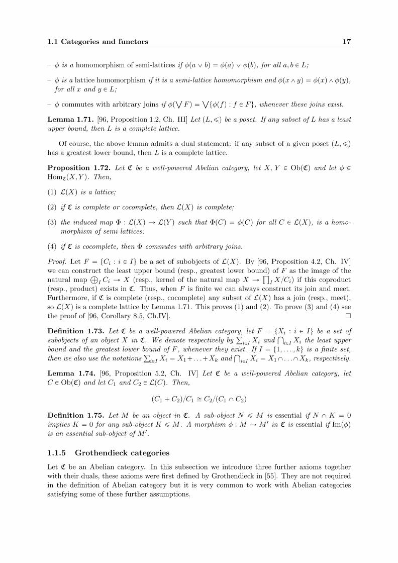
1.1 Categories and functors 17
– φ is a homomorphism of semi-lattices if φpa_ bq “ φpaq _ φpbq, for all a, b P L;
– φ is a lattice homomorphism if it is a semi-lattice homomorphism and φpx^yq “ φpxq^φpyq,for all x and y P L;
– φ commutes with arbitrary joins if φpŽ
F q “Ž
tφpfq : f P F u, whenever these joins exist.
Lemma 1.71. [96, Proposition 1.2, Ch. III] Let pL,ďq be a poset. If any subset of L has a leastupper bound, then L is a complete lattice.
Of course, the above lemma admits a dual statement: if any subset of a given poset pL,ďqhas a greatest lower bound, then L is a complete lattice.
Proposition 1.72. Let C be a well-powered Abelian category, let X, Y P ObpCq and let φ PHomCpX,Y q. Then,
(1) LpXq is a lattice;
(2) if C is complete or cocomplete, then LpXq is complete;
(3) the induced map Φ : LpXq Ñ LpY q such that ΦpCq “ φpCq for all C P LpXq, is a homo-morphism of semi-lattices;
(4) if C is cocomplete, then Φ commutes with arbitrary joins.
Proof. Let F “ tCi : i P Iu be a set of subobjects of LpXq. By [96, Proposition 4.2, Ch. IV]we can construct the least upper bound (resp., greatest lower bound) of F as the image of thenatural map
À
I Ci Ñ X (resp., kernel of the natural map X Ñś
I X{Ci) if this coproduct(resp., product) exists in C. Thus, when F is finite we can always construct its join and meet.Furthermore, if C is complete (resp., cocomplete) any subset of LpXq has a join (resp., meet),so LpXq is a complete lattice by Lemma 1.71. This proves (1) and (2). To prove (3) and (4) seethe proof of [96, Corollary 8.5, Ch.IV].
Definition 1.73. Let C be a well-powered Abelian category, let F “ tXi : i P Iu be a set ofsubobjects of an object X in C. We denote respectively by
ř
iPI Xi andŞ
iPI Xi the least upperbound and the greatest lower bound of F , whenever they exist. If I “ t1, . . . , ku is a finite set,then we also use the notations
ř
iPI Xi “ X1`. . .`Xk andŞ
iPI Xi “ X1X. . .XXk, respectively.
Lemma 1.74. [96, Proposition 5.2, Ch. IV] Let C be a well-powered Abelian category, letC P ObpCq and let C1 and C2 P LpCq. Then,
pC1 ` C2q{C1 – C2{pC1 X C2q
Definition 1.75. Let M be an object in C. A sub-object N ď M is essential if N X K “ 0implies K “ 0 for any sub-object K ď M . A morphism φ : M Ñ M 1 in C is essential if Impφqis an essential sub-object of M 1.
1.1.5 Grothendieck categories
Let C be an Abelian category. In this subsection we introduce three further axioms togetherwith their duals, these axioms were first defined by Grothendieck in [55]. They are not requiredin the definition of Abelian category but it is very common to work with Abelian categoriessatisfying some of these further assumptions.
18 Categories and modules: an outline
(Ab.3) For every set tAi : i P Iu of objects of C, the coproductÀ
iPI Ai exists in C.
(Ab.3˚) For every set tAi : i P Iu of objects of C, the productś
Ai exists in C.
We have seen in Example 1.43 that Ab satisfies both (Ab.3) and (Ab.3˚).
Lemma 1.76. [96, Corollary 8.3, Ch. IV] Let C be an Abelian category. Then, C satisfies (Ab.3)(resp., (Ab.3˚)) if and only if C is cocomplete (resp., complete).
(Ab.4) C satisfies (Ab.3), and the coproduct of a family of monomorphisms is a monomorphism.
(Ab.4˚) C satisfies (Ab.3˚), and the product of a family of epimorphisms is an epimorphism.
Lemma 1.77. Let C be an (Ab.3) Abelian category, then C is (Ab.4) if and only if, for any setI, the functor
À
I :ś
I CÑ C is exact. Dually, an (Ab.3˚) category C is (Ab.4˚) if and only ifś
I :ś
I CÑ C is exact, for any set I.
Proof. Let I be a set, by the dual of [96, Proposition 3.1, Ch. IV],À
I :ś
I CÑ C preservesepimorphisms, that is, it sends cokernels to cokernels. By Proposition 1.62 this means that
À
I
is right exact, while (Ab.4) is equivalent to say thatÀ
I sends kernels to kernels, that is, it isleft exact.
(Ab.5) C satisfies (Ab.3), and filtered colimits of exact sequences are exact.
(Ab.5˚) C satisfies (Ab.3˚), and filtered limits of exact sequences are exact.
Proposition 1.78. [96, Proposition 1.1, Ch. V] Let C be a cocomplete Abelian category. Thenthe following are equivalent:
(1) C satisfies (Ab.5);
(2) given M P ObpCq, K ďM and a directed system tNi : i P Iu Ď LpMq,˜
ÿ
I
Ni
¸
XK “ÿ
I
pNi XKq ;
(3) given a morphism φ : M ÑM 1 and a directed system tNi : i P Iu Ď LpMq,
φ´1
˜
ÿ
I
Ni
¸
“ÿ
I
φ´1pNiq .
Definition 1.79. Let C be a category. A subclass G of ObpCq generates C if every pair of distinctmorphisms f, g P HomCpA,Bq there exists X P G and χ P HomCpX,Aq that separates φ and ψ.If G “ tGu consists of a single object, we say that G is a generator of C. The definitions ofcogenerating class and cogenerator are dual.
Lemma 1.80. [96, Proposition 6.6, Ch. IV] Let C be an Abelian category with a generator, thenC is well-powered.
Definition 1.81. A Grothendieck category is an (Ab.5) Abelian category with a generator.
1.1 Categories and functors 19
1.1.6 Injective and projective objects
Definition 1.82. Let C be an Abelian category. An object X P ObpCq is injective (resp.,projective) if the functor HomCp´, Xq : Cop Ñ Ab (resp., HomCpX,´q : CÑ Ab) is exact.
Notice that an object X is injective in C if and only if it is projective in Cop. In the followinglemma we give equivalent characterizations of injective and projective objects. The proof givenin [96, Proposition 6.1, Ch. I] can be easily adapted to our general context.
Lemma 1.83. Let C be an Abelian category and let X P ObpCq. The following are equivalent:
(1) X is an injective object;
(2) HomCpφ,Xq : HomCpB,Xq Ñ HomCpA,Xq is surjective for any monomorphism φ : AÑ Bin C;
(3) given a monomorphism φ : AÑ B in C and a morphism ψ : AÑ X, there exists a morphismψ : B Ñ X making the following diagram commutative:
0 // Aφ //
ψ��
B
ψ~~X
Dual characterizations hold for projective objects.
The following corollary is a direct consequence of Lemma 1.36.
Corollary 1.84. Let C be an Abelian category and let tCi : i P Iu be a set of objects. Then,
(1)À
I Ci is injective if and only if Ci is injective for all i P I;
(2)ś
I Ci is projective if and only if Ci is projective for all i P I.
Lemma 1.85. [96, Proposition 1.4, Ch. X] Let C be a category, let D be an Abelian subcategory,denote by F : DÑ C the inclusion functor and suppose that F has an exact left adjoint G : CÑD. Then, an object E P ObpDq is injective in D if and only if F pEq is injective in C.
Definition 1.86. Let C be an Abelian category. We say that C has enough injectives if, for anyX P ObpCq, there exists an injective object E and a monomorphism X Ñ E.
When a category has enough injectives, it is interesting to know if there exists a “minimal”injective object containing a given object as a subobject:
Definition 1.87. Let C be an Abelian category and let X P ObpCq. An injective envelope of Xis an object E P ObpCq together with an essential monomorphism X Ñ E.
Lemma 1.88. [96, Proposition 2.3, Ch. V] Let C be an Abelian category, let X P ObpCq andlet α : X Ñ E, α1 : X Ñ E1 be two injective envelopes of X. Then, there is an isomorphismφ : E Ñ E1 such that α1 “ φα. In particular, an injective envelope is unique up to isomorphism.
Given an Abelian category C and an object X P ObpCq, we denote by EpXq the injectiveenvelope of X, whenever it exists.
Lemma 1.89. [96, Proposition 2.5, Ch. V] Let C be a Grothendieck category. The following areequivalent:
(1) C has enough injectives;
(2) any object of C has an injective envelope.
20 Categories and modules: an outline
1.1.7 Categories of modules
Definition 1.90. Let I be a small pre-additive category and let C be a pre-additive category.The additive functor category AddpI,Cq is the full sub-category of FuncpI,Cq whose objects areall the additive functors I Ñ C.
Proposition 1.91. Let C be an Abelian category and let I be a small category. Then,
(1) FuncpI,Cq is Abelian;
(2) if I is preadditive, then AddpI,Cq is an Abelian subcategory of FuncpI,Cq;
(3) if C is complete (resp., cocomplete), then AddpI,Cq is complete (resp., cocomplete).
Proof. Part (1) is [96, Propositions 7.1, Ch. IV], while part (2) is [96, Proposition 7.2, Ch. IV].Finally, the proof of part (3) is completely analogous to the proof of [96, Proposition 8.7, Ch.IV] (see the comment after Proposition 8.8 on p. 102 of [96]).
The following proposition is known under the name of Yoneda Lemma, it is important as itgives a family of projective generators for AddpI,Cq.
Proposition 1.92. [96, Proposition 7.3 and Corollary 7.5, Ch. IV] Let C be an Abelian categoryand let I be a small preadditive category. For all A P ObpIq let hA “ HomIpA,´q : I Ñ Ab andhA “ HomIp´, Aq : Iop Ñ Ab. Then, there are natural isomorphisms:
HomAddpI,CqphA, T q – T pAq and HomAddpIop,CqphB, Sq – SpBq ,
for all A, B P ObpIq, T P AddpI,Cq and S P AddpIop,Cq. The category I is equivalent to thefull subcategory of AddpI,Cq (resp., of AddpIop,Cq) whose objects are of the form hB (resp.,hB), with B P ObpCq. Finally, the sets phBqBPObpIq and phBqBPObpIq are families of projectivegenerators respectively for AddpI,Cq and AddpIop,Cq.
Let I, J be small preadditive categories, consider an additive functor F : I Ñ J and let Cbe a Grothendieck category. Then, there is an induced functor
resF : AddpJ,Cq Ñ AddpI,Cq ,
defined by composition (which is the restriction of the functor F˚ : FuncpJ,Cq Ñ FuncpI,Cq usedin Definition 1.23). In the following lemma we prove the existence of what is usually called the“additive Kan extension along F”, anyway in this context we prefer a different terminology, seeDefinition 1.94; for a proof of Lemma 1.93 and more details on this construction we refer to [75,Section 6].
Lemma 1.93. Let I, J be small preadditive categories, let C be a Grothendieck category andconsider an additive functor F : I Ñ J . Then, ??F : AddpJ,Cq Ñ AddpI,Cq is exact and it hasa left adjoint.
Definition 1.94. Let I, J be small preadditive categories, let C be a Grothendieck categoryand consider an additive functor F : I Ñ J . The functor resF : AddpJ,Cq Ñ AddpI,Cqdefined by composition with F is called the scalar restriction along F while its left adjoint extF :AddpJ,Cq Ñ AddpI,Cq is called the scalar extension along F .
In what follows we specialize to categories of modules.
1.1 Categories and functors 21
Definition 1.95. Let R be a ring and let CR be the pre additive category defined in Example 1.47,an additive functor F : CR Ñ Ab (resp., G : CopR Ñ Ab) is said to be a left R-module (resp., rightR-module). The category of left (resp., right) R-modules AddpCR,Abq (resp., AddpCopR ,Abq) isusually denoted by R-Mod (resp., Mod-R).
The following corollary can be deduced from Proposition 1.91, anyway the usual way to proveit is to explicitly construct kernels, cokernels, products and coproducts in categories of modules.
Corollary 1.96. Let R be a ring, then Mod-R and R-Mod are complete and cocomplete Abeliancategories.
Consider a left R-module F : CR Ñ Ab and let M “ F p‚q. We generally adopt the compactnotation RM , instead of F : CR Ñ Ab, where the action of F on the morphisms of CR is encodedin the following “scalar multiplication”:
RˆM ÑM pr,mq ÞÑ rm “ pF prqqpmq ,
that satisfies the following properties:
(Mod.1) rpm` nq “ rm` rn;
(Mod.2) pr ` sqm “ rm` sm;
(Mod.3) prsqm “ rpsmq;
(Mod.4) 1m “ m;
for all m, n P M and r, s P R. Notice that, given two left R-modules RM and RM1, a homo-
morphism of Abelian groups φ : M Ñ M 1 is a morphism in the category of left R-modules ifand only if φprmq “ rφpmq.Given a left R-module RM , a submodule (that is, a subobject in the category R-Mod) is a sub-group N ďM such that rn P N for all r P R and n P N .Given a left R-module RM and a submodule N ď M , the quotient module (that is, a quotientobject in the category R-Mod) RpM{Nq is the quotient group M{N with the following scalarmultiplication
RˆM{N ÑM{N such that pr,mNq ÞÑ prmqN .
Analogous definitions hold in Mod-R.
We denote by RR (resp., RR) the Abelian group underlying R with left (resp., right) R-module structure coming from the multiplication in R. This module corresponds to the functorh‚ (resp., h‚) described by the Yoneda Lemma and it is a projective generator for R-Mod (resp.,Mod-R). The submodules of RR are the left ideals of R, while the submodules of RR are theright ideals of R.
Theorem 1.97. Let R be a ring, then both R-Mod and Mod-R are complete and cocompleteGrothendieck categories with enough injectives and a projective generator.
Proof. By Corollary 1.96, both R-Mod and Mod-R are complete and cocomplete Abelian cat-egories generated respectively by RR and RR, furthermore one can verify the axiom (Ab.5) byhand. The fact that they have enough injectives is proved, for example, in [96, Proposition 9.3,Ch. I].
22 Categories and modules: an outline
Let R and S be two rings and let φ : R Ñ S be a ring homomorphism. As we said, this isthe same as taking an additive functor Fφ : CR Ñ CS between the two one-object categories CRand CS . Abusing notation, we denote resFφ by resφ
resφ : S-Mod ÝÑ R-Mod
pM : CS Ñ Abq ÞÝÑ pM ˝ Fφ : CR Ñ Abq
The left adjoint extφ to resφ, that is, the scalar extension along Fφ, is usually constructed as atensor product in this context, that is, extφ – ´bR RRS (see [75, Section 6]).
Definition 1.98. Let R and S be two rings. A ring homomorphism φ : R Ñ S is left (resp.,right) flat if extφ : R-Mod Ñ S-Mod (resp., extφ : Mod-RÑ Mod-S) is an exact functor.
Example 1.99. Let D be a ring and recall that an element x P D is a zero-divisor if there existsa non-zero element y P D such that xy “ 0. An element which is not a zero-divisor is said to beregular, if any non-zero element of D is regular then D is said to be a domain.Given a domain D, we let Σ “ tx P D : x is regularu “ Dzt0u and we say that D is a left Oredomain if it is a domain and DxXDy ‰ t0u for all x, y P Dzt0u (notice for example that anycommutative domain is left Ore).Given a left Ore domain we define the left field of fractions of D as follows: first we say that twoelements ps, dq, ps1, d1q P ΣˆD are equivalent, in symbols ps, dq „ ps1, d1q, if there exist a, b P Dsuch that as “ bs1 P Σ and ad “ bd1. We denote by rs, ds the equivalence class of ps, dq and welet Σ´1D “ ΣˆD{ „ be the set of these equivalence classes. The set Σ´1D is a skew field whenendowed with the following operations, for all ps1, d1q, ps2, d2q P ΣˆD:
rs1, d1s ¨ rs2, d2s “ ras1, bd2s and rs1, d1s ` rs2, d2s “ ru, cd1 ` dd2s ,
where ad1 “ bs2 P Σ and u “ cs1 “ ds2 P Σ. There is a canonical injective ring homomorphismε : D Ñ Σ´1D, this induces a scalar restriction resε : Σ´1D-Mod Ñ D-Mod, and a scalarextension extε : D-Mod Ñ Σ´1D-Mod. One can show that the scalar extension is exact in thisparticular case so that ε : D Ñ Σ´1D is a flat endomorphism of rings (see for example [96,Proposition 3.5, Ch. II]).
1.2 Homological algebra
1.2.1 Cohomology
In this subsection we recall some basic definitions and constructions inside the category of cochaincomplexes over a given Abelian category.
Definition 1.100. Let C be a an Abelian category and consider a sequence of objects and mor-phisms
X‚ : ¨ ¨ ¨ ÝÑ Xi´1 di´1
ÝÑ Xi diÝÑ Xi`1 ÝÑ ¨ ¨ ¨
We say that X‚ is a cochain complex if didi´1 “ 0, for all i P Z. A cochain complex X‚ is exactin Xi if Impdi´1q “ Kerpdiq. The cochain complex X‚ is exact (or acyclic) if it is exact in Xi
for all i P Z.
Definition 1.101. Given an Abelian category C and two cochain complexes C‚ and D‚, amorphism of cochain complexes φ‚ : C‚ Ñ D‚ is a sequence of morphisms φi : Ci Ñ Di such
1.2 Homological algebra 23
that the following diagram commutes:
C‚
φ‚
��
¨ ¨ ¨ // Ci´1di´1C //
φi´1
��
CidiC //
φi
��
Ci`1di`1C //
φi`1
��
¨ ¨ ¨
D‚ ¨ ¨ ¨ // Di´1di´1D // Di
diD // Di`1di`1D // ¨ ¨ ¨
that is, di´1D φi´1 “ φidi´1
C , for all i P Z.
Notice that the degree-wise composition of two composable morphisms of cochain complexesis a morphism of cochain complexes.
Definition 1.102. Given an Abelian category C we denote by ChpCq the category of cochaincomplexes and morphisms of cochain complexes. For all n P Z, we denote by ChěnpCq (resp.,ChąnpCq, ChďnpCq, ChănpCq) the full subcategory of ChpCq whose objects are all the cochaincomplexes C‚ such that Ci “ 0 for all i ă n (resp., i ď n, i ą n, i ě n).
The category ChpCq of cochain complexes is an Abelian category whose zero-object is thecomplex whose i-th component is the zero-object of C, for all i P Z. The sum on the homo-morphism sets is defined degree-wise exploiting the addition in the homomorphism groups in C.Similarly, one can construct degree-wise products, coproducts, kernels and cokernels.Furthermore, one can show that ChěnpCq, ChąnpCq, ChďnpCq and ChănpCq are Abelian sub-categories of ChpCq for all n P Z.
Definition 1.103. Given an Abelian category C and a cochain complex X‚, we denote by Xěn PObpChěnpCqq the n-th truncation of X‚, that is
Xěn : ¨ ¨ ¨ // 0 // 0 // CoKerpdn´1q // Xn`1 // Xn`2 // ¨ ¨ ¨ .
Similarly, given a homomorphism of cochain complexes φ‚ : X‚ Ñ Y ‚, we denote by φěn :Xěn Ñ Y ěn the obvious induced morphism. This allows to define the n-th truncation functor:
ChpCq Ñ ChěnpCq .
One can prove that the n-th truncation functor is the right adjoint to the inclusion functorChěnpCq Ñ ChpCq.
Lemma 1.104. Let C and D be two Abelian categories and let F : CÑ D be a functor. ApplyingF degree-wise we obtain a functor F ‚ : ChpCq Ñ ChpDq. If we suppose also that F is exact,then F ‚ is exact and
HnpF ‚pX‚qq – F pHnpX‚qq ,
for any cochain complex X‚ over C. Furthermore, if pF,Gq is an adjoint pair between Abeliancategories, then pF ‚, G‚q is an adjunction between the respective categories of complexes.
Proof. The first part follows using that exact functors preserve kernels and cokernels, and definedusing these constructions. The second part follows by [70, Theorem 1, Sec. 8, Ch. 1].
In the above settings we will usually abuse notation and denote F ‚ simply by F .
24 Categories and modules: an outline
Definition 1.105. Let C be an Abelian category and let n P Z. The n-th cohomology functor
Hn : ChpCq Ñ C
is defined as follows. Given a cochain comples X‚, HnpX‚q “ Kerpdnq{Impdn´1q, while, given amorphism φ‚ : X‚ Ñ Y ‚ of cochain complexes, Hnpφ‚q : HnpX‚q Ñ HnpY ‚q is the map inducedby φn.A morphism φ‚ : X‚ Ñ Y ‚ in ChpCq is said to be a quasi-isomorphism if Hnpφ‚q is an isomor-phism for all n P Z.
Notice that a cochain complex X‚ is exact if and only if HnpX‚q “ 0 for all n P Z. Inparticular, a complex is exact if and only if it is quasi-isomorphic to the zero-complex.
Definition 1.106. Given an Abelian category C and a morphism φ‚ : X‚ Ñ Y ‚ in ChpCq, themapping cone conepφ‚q is a cochain complex whose n-th component is Xn`1 ‘ Y n and whosedifferentials are represented in matrix form as follows:
ˆ
dn`1X 0φn dnY
˙
: Xn`1 ‘ Y n // Xn`1 ‘ Y n .
The following lemma shows that the construction of the mapping cone provides a differentway to look at quasi-isomorphisms: these are exactly the homomorphisms whose cone is exact.
Lemma 1.107. [104, Corollary 1.5.4] Let C be an Abelian category and let φ‚ : X‚ Ñ Y ‚ be amorphism in ChpCq. Then,
(1) φ‚ is a quasi-isomorphism;
(2) Hnpφ‚q is an isomorphism for all n P Z;
(3) conepφ‚q is an exact complex.
We conclude the section with the following fundamental lemma.
Lemma 1.108. [104, Corollary 1.3.1] Let C be an Abelian category and let 0 Ñ X‚ Ñ Y ‚ ÑZ‚ Ñ 0 be a short exact sequence in ChpCq. Then, there is an exact sequence:
. . .Ñ HnpX‚q Ñ HnpY ‚q Ñ HnpZ‚q Ñ Hn`1pX‚q Ñ Hn`1pY ‚q Ñ Hn`1pZ‚q Ñ . . .
1.2.2 Injective resolutions and classical derived functors
In this section we recall some basic results about injective resolutions and derived functors. Letus start defining injective resolutions of objects in Abelian categories:
Definition 1.109. Let C be an Abelian category and let X P ObpCq. Identify X with an objectin ChpCq whose components are all 0 but its 0-th component which is X. Then, an injectiveresolution of X is a quasi-isomorphism λ : X Ñ E‚ where E‚ P ObpChě0pCqq, and En isinjective for all n P Z.
The following lemma establishes the existence of injective resolutions and the so-called “Com-parison Theorem”.
Lemma 1.110. [104, Lemma 2.3.6 and Theorem 2.3.7] Let C be an Abelian category with enoughinjectives and let φ : X Ñ Y be a morphism in C. Then,
1.2 Homological algebra 25
(1) X has an injective resolution;
(2) given two injective resolutions λ1 : X Ñ E‚1 and λ2 : Y Ñ E‚2 , there is a homomorphism ofcomplexes Φ‚ : E‚1 Ñ E‚2 such that λ2φ “ Φ0λ1.
Using injective resolutions we can define right derived functors:
Definition 1.111. Let C and D be Abelian categories with enough injectives, let F : CÑ D bea functor and let n P N. The n-th right derived functor RnF pφq : C Ñ D of F is defined asfollows:
– choose for any object X P ObpCq an injective resolution X Ñ E‚pXq;
– given X P ObpCq, let RnF pXq “ HnpF pE‚pXqqq;
– given a morphism φ : X Ñ Y in C, take a morphism Φ‚ : E‚pXq Ñ E‚pY q as in Lemma1.110 and let RnF pφq “ HnpΦ‚q : RnF pXq Ñ RnF pY q.
In the following proposition we collect the main general properties of derived functors neededin the thesis. For a proof see [104, Sections 2.4 and 2.5]
Proposition 1.112. Let C and D be Abelian categories with enough injectives and let F : CÑ Dbe a functor. Then, for all n P N,
(1) RnF is a well-defined functor and it does not depend on the choice of resolutions;
(2) if F is left exact, then R0F is naturally isomorphic to F ;
(3) if F is left exact and if E P ObpCq is injective, then RnF pEq “ 0 for all n ą 0;
(4) F is an exact functor if and only if RnF is the 0-functor for all n ą 0;
(5) given a short exact sequence 0 Ñ X Ñ Y Ñ Z Ñ 0 in C, there is a long exact sequence
0 Ñ R0F pXq Ñ R0F pY q Ñ R0F pZq Ñ R1F pXq Ñ . . .
. . .Ñ RnF pZq Ñ Rn`1F pXq Ñ Rn`1F pY q Ñ Rn`1F pZq . . .
Let C be an Abelian category with enough injectives. After identifying a given object X P
ObpCq with a cochain complex concentrated in degree 0, by Lemma 1.110 we can find a boundedbelow complex of injectives which is quasi-isomorphic to X. We can generalize this fact asfollows:
Lemma 1.113. [65, Lemma 13.2.1] Let C be an Abelian category with enough injectives andlet n P Z. Then any complex X‚ P ObpChěnpCqq is quasi isomorphic to a complex Y ‚ PObpChěnpCqq such that Y m is injective for all m P Z.
Given two complexes X‚ and Y ‚ with differentials denoted respectively by d‚X and d‚Y ,HompX‚, Y ‚q is a cochain complex of Abelian groups whose n-th component is
HompX‚, Y ‚qn “ź
iPZHomCpX
i, Y n`iq ,
and whose n-th differential is the following group homomorphism:
dn : HompX‚, Y ‚qn Ñ HompX‚, Y ‚qn`1 pφiqiPZ ÞÑ pφi`1diX ` p´1qn`1dn`iY φiqiPZ .
26 Categories and modules: an outline
Definition 1.114. Given an Abelian category C, a cochain complex E‚ is said to be dg-injectiveif En is an injective object for all n P Z and if the complex HompX‚, E‚q is exact, for any exactcochain complex X‚.
Example 1.115. Bounded complexes of injectives are dg-injective, while unbounded complexesof injectives may be non-dg-injective (see for example [65, Lemma 13.2.4]).
1.3 Torsion theories and localization
1.3.1 Torsion theories
Definition 1.116. Let C be a Grothendieck category and let A Ď ObpCq be a subclass. A is aSerre class if, given a short exact sequence
0 Ñ AÑ B Ñ C Ñ 0 ,
B belongs to A if and only if both B and C belong to A. Furthermore, A is a hereditary torsionclass (or localizing class) if it is a Serre class and it is closed under taking arbitrary coproducts.
Let us recall also the following definition.
Definition 1.117. Let C be a Grothendieck category, let X P ObpCq, let κ be an ordinal and letXα be a subobject of X for all α ă κ. The family tXα : α ă κu is a continuous chain provided:
– X0 “ 0 and Xα ď Xα ` 1 for all α ă κ;
– if λ ă κ is a limit ordinal, then Xλ “ř
αăλXα.
If tXα : α ă σu is a continuous chain of subobjects of a given X P ObpCq, we denoteř
αăσXα
also byŤ
αăσXα.
Lemma 1.118. Let C be a Grothendieck category and let D Ď ObpCq be closed under takingsubobjects and quotients. Then, the class T of all the D-filtrated objects, that is, all the X P
ObpCq admitting a continuous chain tXα : α ă κu of subobjects such that Xα`1{Xα P D for allα ă κ and
Ť
αăκXα “ X, is a hereditary torsion subclass of C.
Proof. Let Y ď X P C.If X P T , we can find a continuous chain tXα : α ă λu such that
Ť
αăλXα “ X and Xα`1{Xα P
D for all α ă λ. This implies (by the closure properties of D) that tXα X Y : α ă λu andtpXα ` Y q{Y : α ă λu are continuous chains with successive quotients belonging to D. Thus, Yand X{Y P T .On the other hand, if Y and X{Y P T , that is, there exist continuous chains tYα : α ă λ1u andtXα{Y : α ă λ2u such that
Ť
αăλ1Yα “ Y ,
Ť
αăλ2Xα{Y “ X{Y and with successive quotients
in D, then tYα : α ă λ1u Y tXα : α ă λ2u is a continuous chain with successive quotients in Dand whose union is X.So far, this proves that T is a Serre class; we need to verify that T is closed under takingcoproducts. Let tXi : i P Iu be a family of objects in T and suppose that, for all i P I, tXi,α :α ă λiu is a continuous chain with successive quotients in D and such that
Ť
αăλiXi,α “ Xi.
Chose a total order ď on I, and fix the lexicographic order on I “ tpi, αq : i P I, α ă λiu. Forall pi, αq P I we let X˚i,α “
À
jăiXj ‘Xi,α. Clearly, tX˚i,α : pi, αq P Iu is a continuous chain withsuccessive quotients in D and whose union equals
À
I Xi.
1.3 Torsion theories and localization 27
Lemma 1.119. Let C be a Grotheindieck category and let T be a hereditary torsion class. Forall X P ObpCq, let
TpXq “ÿ
tT ď X : T P T u .
Then,
(1) TpXq “ X if and only if X P T ;
(2) TpTpXqq “ TpXq and TpX{TpXqq “ 0, for all X P ObpCq.
Proof. (1) and the first part of (2) are easy consequences of the closure properties of T . For thesecond half of part (2), let X P ObpCq and consider a subobject Y ď X{TpXq such that Y P T .Then, there is a short exact sequence 0 Ñ TpXq Ñ π´1pY q Ñ Y Ñ 0, where π : X Ñ X{TpXqis the canonical projection. Since T is a Serre class, π´1pY q P T and so π´1pY q ď TpXq,showing that Y “ 0.
Given a subclass A of objects of C, we define the following two classes
AK “ tX P C : HomCpA,Xq “ 0 , @A P Au and KA “ tX P C : HomCpX,Aq “ 0 , @A P Au ,
which are called respectively right and left orthogonal class to A.
Corollary 1.120. Let C be a Grotheindieck category and consider a subclass T Ď ObpCq that isclosed under taking subobjects. The following are equivalent:
(1) T is a hereditary torsion class;
(2) T “ KpT Kq.
Proof. (1)ñ(2). It is easy to see that T Ď KpT Kq. On the other hand, let X P KpT Kq and defineTpXq as in Lemma 1.119. Then, we have a short exact sequence
0 Ñ TpXq Ñ X Ñ X{TpXq Ñ 0 .
Notice that X{TpXq P T K (use the fact that the image of an object in T is again in T ), sothe canonical morphism X Ñ X{TpXq is the zero-morphism, that is, X{TpXq “ 0, that is,X “ TpXq P T .
(2)ñ(1). Suppose that T “ KpT Kq and let 0 Ñ X Ñ Y Ñ Z Ñ 0 be a short exact sequence. IfY P T , then X P T by hypothesis. Furthermore, given M P T K and a morphism φ : Z ÑM , thecomposition Y Ñ Z Ñ M has to be 0, thus φ “ 0 and so Z P KpT Kq “ T . On the other hand,if X, Z P T , M P T K and ψ : Y Ñ M , then the composition X Ñ Y Ñ M is trivial and so, byexactness, there exists a unique morphism ψ1 : Z Ñ M such that ψ1π “ ψ, where π : Y Ñ Zis the canonical epimorphism. Since the unique morphism Z Ñ M is the zero-morphism, weobtain that ψ “ 0, so Y P KpT Kq “ T . Thus, T is a Serre class. The fact that T is closed undercoproducts follows by Lemma 1.36.
Definition 1.121. A hereditary torsion theory τ in C is a pair of classes pT ,Fq such that
– T is a hereditary torsion class;
– pT qK “ F and KpFq “ T .
28 Categories and modules: an outline
We call T and F respectively the class of the τ -torsion and of the τ -torsion free objects. Sinceall the torsion theories in the sequel are hereditary, we just say “torsion theory”, “torsion class”and “torsion free class” to mean respectively “hereditary torsion theory”, “hereditary torsionclass” and “hereditary torsion free class”.
Example 1.122. (1) Let C be a Grothendieck category. The pairs p0,Cq and pC, 0q are torsiontheories. We call them respectively the trivial and the improper torsion theory.
(2) Let G be an Abelian group; an element g P G is torsion if there exists a positive integer nsuch that ng “ 0. The group G is torsion if any of its elements is torsion, while it is torsionfree if its unique torsion element is 0. The class T of all torsion Abelian groups is a torsionclass in Ab, while the class F of the torsion free Abelian groups is a torsion free class. Inparticular, pT ,Fq is a torsion theory.
(3) A generalization of part (2) is as follows: let D be a left Ore domain and denote by Σthe set of the regular elements of D. Then T “ tM P ObpD-Modq : @m P M, Ds PΣ, such that sm “ 0u is a torsion class. The orthogonal of T is F “ T K “ tM P
ObpD-Modq : @m PM, s P Σ, sm ‰ 0u.Generalizing further, if we have two rings R, S, a flat ring homomorphism φ : R Ñ S anda torsion theory pT ,Fq P S-Mod, then we can define a torsion theory pTφ,Fφq in R-Modletting Tφ “ tM P ObpR-Modq : extφpMq P T u.
(4) Let C be a Grothendieck category. Given an injective object E in C, one can define a torsiontheory τ “ pT ,Fq, with T “ KtEu and F “ T K; such τ is said to be the torsion theorycogenerated by E. Similarly, given a class E of injective objects, and letting T 1 “ KtEu andF 1 “ pT 1qK, τ 1 “ pT 1,F 1q is said to be the torsion theory cogenerated by E.
Lemma 1.123. Let C be a Grotheindieck category, let τ “ pT ,Fq be a torsion theory and letφ : X1 Ñ X2 be a morphism in C. Let Tτ pXiq “
ř
tT ď Xi : T P T u (i “ 1, 2), then,φpTτ pX1qq ď Tτ pX2q.
Proof. Notice that φpTτ pX1qq “ φpř
tT ď X1 : T P T uq “ř
tφpT q ď X1 : T P T u (seeProposition 1.72). Furthermore, since T is a Serre class, tφpT q ď X1 : T P T u Ď tT ď X2 : T PT u.
Thanks to Lemma 1.123, we can define a functor C Ñ T , that turns out to be the rightadjoint to the inclusion T Ñ C:
Definition 1.124. Let C be a Grotheindieck category and let τ “ pT ,Fq be a torsion theory.The τ -torsion functor Tτ : CÑ T is defined as follows:
– Tτ pXq “ř
tT ď X : T P T u, for any object X P ObpCq;
– Tτ pφq : Tτ pXq Ñ Tτ pY q is the restriction of φ : X Ñ Y , for any morphism φ in C.
Lemma 1.125. Let C be a Grotheindieck category and let τ “ pT ,Fq be a torsion theory. Then,
(1) Tτ pXq “ 0 if and only if X P F . In particular, there is a short exact sequence 0 Ñ T ÑX Ñ F Ñ 0 with T P T and F P F , for all X P ObpCq;
(2) Tτ is right adjoint to the inclusion T Ñ C;
Proof. For part (1) see the first half of the proof of Corollary 1.120. For part (2) notice that,for all T P T and X P ObpCq, HomCpT,Xq – HomCpT,Tτ pXqq “ HomT pT,Tτ pXqq, where theisomorphism comes from the fact that T is closed under taking quotients, so φpT q ď Tτ pXq forall φ P HomCpT,Xq.
1.3 Torsion theories and localization 29
1.3.2 Localization
In this subsection we show how the concept of torsion theory is related to that of localization.Most of the material in this subsection is adapted from Gabriel’s thesis [44].
Definition 1.126. Let C be a Grothendieck category. A localization of C is a pair of adjointfunctors pQ : C Ñ D,S : D Ñ Cq, where S is fully faithful, Q is exact and D is an Abeliancategory. In this situation, D is said to be a quotient category, Q is a quotient functor and Sis a section functor. The composition L “ S ˝Q : CÑ C is said to be the localization functor.
Let us remark that, in other contexts, one may find definitions of localization of an Abeliancategory that do not require that the quotient functor is exact. Anyway, some of the conceptsof localization commonly used in algebra are particular cases of the above definition, as thefollowing example shows.
Example 1.127. Let D be an Ore domain and let Σ be the set of regular elements of D. As wesaid in Example 1.99, the canonical ring homomorphism ε : D Ñ Σ´1D, induces an adjunctionpresε, extεq. Furthermore, resε is fully faithful and extε is exact, thus we can think to extε asa quotient functor, to resε as a section functor and to Σ´1D-Mod as a quotient category ofD-Mod.
Lemma 1.128. [66, Lemma 2.2] Let C be a Grothendieck category, let pQ,Sq be a localizationof C and denote by L “ S ˝Q : C Ñ C the localization functor. For all X P ObpCq there is anatural isomorphism LpXq – LpLpXqq.
One can encounter different definitions of localization in other contexts, see for example [90].Let us explain the connection between localizations and torsion theories. Indeed, starting witha localization pQ : CÑ D,S : DÑ Cq and letting L “ S ˝Q,
KerpLq “ tX P C : LpXq “ 0u “ tX P C : QpXq “ 0u “ KerpQq
is a torsion class (use the exactness of Q and the fact that it is a left adjoint). Hence, thelocalization pQ,Sq induces a torsion theory pKerpQq,KerpQqKq.
On the other hand, one can construct a localization out of a torsion theory. In this sectionwe describe this localization in case our Grothendieck category C has enough injectives. ByTheorem 1.97, this allows us to localize any category of modules.
Definition 1.129. Let C be a Grothendieck category with enough injectives. An object X P
ObpCq is τ -local provided EpXq and EpXq{X P F . The localization of C at τ is the full sub-category C{T of C of the τ -local objects. The inclusion Sτ : C{T Ñ C is called the τ -sectionfunctor.
Lemma 1.130. Let C be a Grothendieck category with enough injectives, let τ “ pT ,Fq be atorsion theory and let X, X 1, X2 P F . Then,
(1) the object Lτ pXq “ π´1pTτ pEpXq{Xqq, where π : EpXq Ñ EpXq{X is the canonical pro-jection, is τ -local;
(2) given a morphism φ : X Ñ X 1, there exists a unique morphism Lτ pφq : Lτ pXq Ñ Lτ pX1q
such that the following square commutes
Xφ //
��
X 1
��Lτ pXq
Lτ pφq// Lτ pX1q ;
30 Categories and modules: an outline
(3) given two morpshims φ : X Ñ X 1 and φ1 : X 1 Ñ X2, then Lτ pφ1 ˝ φq “ Lτ pφ
1q ˝ Lτ pφq.
Proof. (1) Notice that X ď Lτ pXq ď EpXq, thus EpLτ pXqq “ EpXq P F . Furthermore,
EpLτ pXqq
Lτ pXq“
EpXq
Lτ pXq–
EpXq{X
Lτ pXq{X–
EpXq{X
Tτ pEpXq{XqP F .
(2) Let φ1 : X Ñ EpX 1q be the composition of φ and X 1 Ñ EpX 1q. Since X Ñ EpXq is a
monomorphism we can extend φ1 to a morphism φ : EpXq Ñ EpX 1q. We claim that φpLτ pXqq ďLτ pX
1q. In fact, φpLτ pXqq{X1 is a quotient of φpLτ pXqq{pX
1 X φpX 1qq – Lτ pXq{φ´1pX 1q “
Lτ pXq{X P T , and so φpLτ pXqq{X1 P T . Thus, we can define Lτ pφq : Lτ pXq Ñ Lτ pX
1q as therestriction of φ.It remains to show the uniqueness of Lτ pφq. Indeed, let ψ : Lτ pXq Ñ Lτ pX
1q be a morphismsuch that ψæX “ φ1. Then, pLτ pφq ´ ψqpXq “ 0 and so Lτ pφq ´ ψ can be decomposed asLτ pφq ´ ψ “ gf , with f : Lτ pXq Ñ Lτ pXq{X the canonical projection and g : Lτ pXq{X Ñ
Lτ pX1q. By definition Lτ pXq{X P T , while Lτ pX
1q P F , thus g “ 0 and Lτ pφq ´ ψ “ 0f “ 0,showing that ψ “ Lτ pφq.
(3) follows by the uniqueness proved in part (2).
The above lemma allows us to define a localization functor Lτ : CÑ C:
Definition 1.131. Let C be a Grothendieck category with enough injectives and let τ “ pT ,Fqbe a torsion theory. The τ -localization functor Lτ : CÑ C is defined as follows:
– Lτ pXq “ π´1pTτ pEpXq{Xqq, where π : EpXq Ñ EpXq{X is the canonical projection, for allX P F ;
– Lτ pXq “ Lτ pX{Tτ pXqq, for all X P ObpCq;
– given a morphism φ : X Ñ X 1 in C, Lτ pφq : Lτ pXq Ñ Lτ pX1q is the unique morphism that
makes the following square commute
X{Tτ pXqφ //
��
X 1{Tτ pX1q
��Lτ pXq
Lτ pφq // Lτ pX1q.
Furthermore, we let Qτ : C Ñ C{T be the unique functor such that Lτ “ SτQτ . Qτ is calledτ -quotient functor. We say that τ is exact if Lτ is an exact functor.
Theorem 1.132. Let C be a complete Grothendieck category with enough injectives and letτ “ pT ,Fq be a torsion theory on C. Then,
(1) Qτ is left adjoint to Sτ ;
(2) C{T is a complete Grothendieck category;
(3) Qτ is an exact functor that commutes with coproducts;
(4) an object E P C{T is injective if and only if Sτ pEq is injective in C.
1.3 Torsion theories and localization 31
Proof. (1) We have to prove that there is a natural isomorphism
HomC{T pQτ pXq, Y q – HomCpX,Sτ pY qq ,
for all X P ObpCq and Y P C{T . Since Sτ is fully faithfull, this is the same as proving anatural isomorphism HomCpLτ pXq, Y q – HomCpX,Y q (with X, Y P ObpCq and Y τ -local). Letα : X Ñ Lτ pXq be the canonical morphism and notice that α induces a map
α˚ : HomCpLτ pXq, Y q–Ñ HomCpX,Y q α˚pφq “ φ ˝ α .
When X P F , α˚ is an isomorphism by Lemma 1.130(2), while the general case follows noticingthat there is a natural isomorphism HomCpX,Y q – HomCpX{Tτ pXq, Y q.
(2) By [96, Propositions 1.2 and 1.3, Ch. X] and part (1), we obtain that kernels exist in C{Tand that it is enough to show that Qτ sends kernels to kernels. We show this in two steps:
– First of all we prove that, given monomorphism φ : X Ñ Y in C, Qτ pφq : Qτ pXq Ñ Qτ pY q isa monomorphism in C{T . It is sufficient to show that Lτ pφq is a monomorphism in C. We canassume without loss of generality that X, Y P F (otherwise substitute them by X{Tτ pXq andY {Tτ pY q respectively, and notice that the induced morphism X{Tτ pXq Ñ Y {Tτ pY q is againa monomorphism). In this case, 0 “ Kerpφq “ KerpLτ pφqqXX and thus KerpLτ pφqq “ 0 sinceX is essential in Lτ pXq.
– Consider now a morphism φ : X Ñ Y in C, let k : K Ñ X be a kernel of φ and let us showthat Qτ pkq : Qτ pKq Ñ Qτ pXq is a kernel of Qτ pφq in C{T . We suppose without any lossin generality that X, Y P F (in fact, letting φ : X{Tτ pXq Ñ Y {Tτ pY q be the induced map,Kerpφq “ Kerpφq{Tτ pKerpφqq and so Qτ pKerpφqq “ Qτ pKerpφqq). Let Z P C{T , let ψ : Z ÑQτ pXq be a morphism such that Qτ pφqψ “ 0 and let Z “ Sτ pZq, ψ “ Sτ pψq : Z Ñ Lτ pXq,so that Lτ pφqψ “ 0. Consider the restriction ψ1 : ψ´1pXq Ñ X; since ψ1φ “ 0, there exists amorphism f : ψ´1pXq Ñ K such that kf “ ψ1. Notice that Z{ψ´1pXq “ ψpZq{pψpZqXXq “pZ `Xq{X ď Lτ pXq{X P T and so, Lτ pψ
´1pXqq “ Lτ pZq “ Z. Hence, Qτ pfq : Z Ñ Qτ pKqis such that Qτ pkqQτ pfq “ Qτ pψq “ ψ. We conclude by Lemma 1.56 that Qτ pKq is a kernelfor Qτ pφq.
(3) Qτ is exact since it is a left adjoint (thus right exact) and it preserves kernels. The fact thatit preserves coproducts follows by Lemma 1.37.
(4) This follows by Lemma 1.85.
1.3.3 The Gabriel-Popescu Theorem and its consequences
The following theorem, usually known as the “Gabriel-Popescu Theorem”, was first proved in[88].
Theorem 1.133. [96, Theorem 4.1, Ch. X] Let C be a Grothendieck category, let G be agenerator of C, let R “ EndCpGq and denote by T : C Ñ Mod-R the functor T “ HomCpG,´qwhere, for any object X P C, the right R-module structure on T pXq is given by the followingmap
HomCpG,Xq ˆ EndCpGq Ñ HomCpG,Xq such that pφ, ρq ÞÑ φ ˝ ρ .
Then,
(1) T is fully faithful;
32 Categories and modules: an outline
(2) if we denote by τ “ pT ,Fq the torsion theory cogenerated by
E “ tEpT pXq ‘ EpT pXqq{T pXqq : X P ObpCqu ,
(see Example 1.122 (4)) then the composition CTÝÑ Mod-R
QτÝÑ pMod-Rq{T is a natural
equivalence of categories.
The following corollaries are direct consequences of the above theorem and Theorem 1.132.
Corollary 1.134. Let C be a Grothendieck category, then
(1) C is complete;
(2) C has enough injective objects.
Corollary 1.135. Let C be a Grothendieck category and let τ “ pT ,Fq be a torsion theory onC. Consider a family tXi : i P Iu Ď C{T , then
ź
iPI
Xi – Qτ
˜
ź
iPI
Sτ pXiq
¸
.
Proof. Being a right adjoint, Sτ commutes with limits, thus Sτ pś
iPI Xiq –ś
iPI Sτ pXiq. ApplyQτ to conclude.
Corollary 1.136. Let C be a Grothendieck category and let τ “ pT ,Fq be a torsion theory inC. Then τ is cogenerated by an injective object E.
Proof. Take a generator G of C and let E be the product of all the injective envelopes of theτ -torsion free quotients of G. Then, T coincides with KtEu and F “ T K is the class of all theobjects that embed in some product of copies of E.
The proof of Corollary 1.136 shows that the torsion theories in a Grothendieck category Cform a set, not a proper class (in fact, one can bound the cardinality of this set by the cardinalityof the power set of the family of quotients of a chosen generator G of C).
Definition 1.137. Let C be a Grothendieck category. We denote by TorspCq the poset of all thetorsion theories on C, ordered as follows: given τ “ pT ,Fq and τ 1 “ pT 1,F 1q P TorspCq,
τ 1 ĺ τ if and only if T 1 Ď T if and only if F Ď F 1 .
When τ 1 ĺ τ , we say that τ is a generalization of τ 1, while τ 1 is a specialization of τ .
Corollary 1.138. Let C be a Grothendieck category and let τ “ pT ,Fq be a torsion theory.Then, F is closed under taking injective envelopes.
The notion of stable torsion theory was introduced by Gabriel in [48], see also [82] and [7].
Definition 1.139. Let C be a Grothendieck category. A torsion theory τ “ pT ,Fq on C is stableif T is closed under taking injective envelopes. Furthermore, C is stable if any τ P TorspCq isstable.
Corollary 1.140. Let C be a Grothendieck category and let τ “ pT ,Fq be a torsion theory onC. The following statements are equivalent
1.3 Torsion theories and localization 33
(1) τ is stable;
(2) given E P ObpCq is an injective object, then E – Tτ pEq ‘ E{Tτ pEq.
Proof. (1)ñ(2). Identify Tτ pEq and its injective envelope with subobjects of E, so that Tτ pEq ďEpTτ pEqq ď E. Since EpTτ pEqq is τ -torsion, EpTτ pEqq ď Tτ pEq. Thus, Tτ pEq “ EpTτ pEqq.Having proved that Tτ pEq is injective, the desired decomposition follows.
(2)ñ(1). Let X P T and let E be an injective envelope of X. Then, E “ Tτ pEq ‘ E{Tτ pEqand so we can identify E{Tτ pEq with a sub-object of E. Since X is an essential sub-object ofE and X X E{Tτ pEq “ 0, E{Tτ pEq “ 0.
34 Categories and modules: an outline
Chapter 2
Lattice Theory
In Chapter 2 we introduce the category QFrame of quasi frames. In QFrame we study somelattice-theoretic notions that are usually introduced in module theory, such as the compositionlength, the uniform dimension and the socle series.In the second part of the chapter we study the basic properties of two cardinal invariants ofqframes: Krull dimension and Gabriel dimension. Using these notions we can define torsion andlocalization in the category QFrame.Given a Grothendieck category C and a torsion theory τ in C, there is a notion of τ -Gabrieldimension for the objects of C. We show that this notion can be defined using the Gabrieldimension of quasi frames and we deduce its basic properties.
2.1 The category of Quasi-frames
2.1.1 Lattices
Let pL,ďq be a lattice. Given two elements x and y P L, the segment between x and y is
rx, ys “ ts P L : x ď s ď yu .
We also let px, ys “ rx, ysztxu, rx, yq “ rx, ysztyu and px, yq “ rx, ysztx, yu. Notice that rx, ys isa lattice with the order induced by L.
Definition 2.1. Let pL,ďq be a lattice. Then,
– pL,ďq is bounded if it has a maximum (usually denoted by 1) and a minimum (usually denotedby 0);
– pL,ďq is modular if, for all a, b and c P L with a ď c,
a_ pb^ cq “ pa_ bq ^ c ;
– pL,ďq is distributive if, for all a, b and c P L,
a_ pb^ cq “ pa_ bq ^ pa_ cq and a^ pb_ cq “ pa^ bq _ pa^ cq ;
– pL,ďq is upper-continuous if it is complete and, for any directed subset txi : i P Iu of L (or,equivalently, for any chain in L) and any x P L,
x^ł
iPI
xi “ł
iPI
px^ xiq ;
35
36 Lattice Theory
– given a P L, an element c is a pseudo-complement for a if it is maximal with respect to theproperty that a^ c “ 0. pL,ďq is pseudo-complemented if, for any choice of x ď y in L, anyelement a P rx, ys has a pseudo-complement in rx, ys, that is, an element c P rx, ys maximalwith respect to the property that a^ c “ x;
– pL,ďq is a frame if it is complete and, for any subset txi : i P Iu of L and any x P L,
x^ł
iPI
xi “ł
iPI
px^ xiq .
Notice that a complete lattice always has a minimumŽ
H “ 0 and a maximumŹ
H “ 1.
Example 2.2. (1) The family of closed sets ClosedpX, τq of a topological spaces pX, τq, orderedby reverse inclusion, is a frame. In fact, given a set tCi : i P Iu of closed sets,
Ž
Ci “Ş
Ci P ClosedpX, τq, whileŹ
Ci “Ť
iPI Ci, where for any subset E Ď X we denote byE “
Ş
tC : E Ď C P ClosedpX, τqu the closure of E in X;
(2) a total order pL,ďq is a frame, in fact, given x P L and tyi : i P Iu Ď L, we have two cases
x^ł
iPI
yi “
#
x if x ďŽ
iPI yi;Ž
iPI yi if x ěŽ
iPI yi.
In both cases, there exists (at least) an element j P I such that x ď yj, soŽ
iPIpx ^ yiq “Ž
i‰jpx^ yiq _ x ě x “ x^Ž
iPI yi;
(3) given a Grothendieck category C and an object M P ObpCq, LpMq is an upper-continuousmodular lattice. Indeed, it is a complete lattice by Lemma 1.72, since any Grothendieckcategory is well-powered, and it is upper-continuous by Proposition 1.78, for modularity seefor example [96, Proposition 5.3, Ch. IV]).
We collect in the following lemma some observations on the notions introduced in Definition2.1, for a proof see Sections 2, 3 and 4 of Chapter III in [96].
Lemma 2.3. Let pL,ďq be a lattice. Then,
(1) if L is distributive, then it is also modular;
(2) if L is upper-continuous and modular, then it is pseudo-complemented;
(3) L is complete if and only if any subset F of L has a meet. Furthermore, if L is completethen it is bounded;
(4) if L is a frame, then it is distributive, upper continuous, bounded, complete and pseudo-complemented.
Definition 2.4. Let pL1,ďq and pL2,ďq be two lattices and consider a map φ : L1 Ñ L2. Then,φ preserves segments if rφpaq, φpbqs “ φpra, bsq, for all a ď b P L1.
Example 2.5. Let C be a Grothendieck category and let φ : X Ñ Y be a morphism in C. Then,the map
Φ : LpXq Ñ LpY q such that ΦpCq “ φpCq ,
induced by φ is a semi-lattice homomorphism that commutes with arbitrary joins and preservessegments. Indeed, Φ is a semi-lattice homomorphism that commutes with arbitrary joins by
2.1 The category of Quasi-frames 37
Proposition 1.72 and the fact that any Grothendieck category is complete. To show that Φ sendssegments to segments, let K1 ď K2 P LpXq and consider K P rΦpK1q,ΦpK2qs. Then,
K “ Φpφ´1pKqq “ Φpφ´1pKq X φ´1pφpK2qqq
“ Φpφ´1pKq X pK2 `Kerpφqqq “ Φppφ´1pKq XK2q `Kerpφqq
“ Φpφ´1pKq XK2q ` ΦpKerpφqq “ Φpφ´1pKq XK2q ,
where in the first line we used that K ď Impφq, while in the second line we used the modularityof LpXq. Since φ´1pKq XK2 P rK1,K2s we proved that Φ sends segments to segments.
Lemma 2.6. Let pL1,ďq and pL2,ďq be two lattices and consider a map φ : L1 Ñ L2. Then,
(1) if L1 has a minimum element 0 and φ commutes with arbitrary joins, then φp0q is a minimumin L2;
(2) if L1 and L2 are bounded and φ preserves segments, then φ is surjective if and only if itsimage contains 0 and 1.
Proof. Remember that 0 “Ž
H and so, since φ commutes with arbitrary joins, φp0q “Ž
H inL2. This proves (1). Part (2) easily follows from the definitions.
Definition 2.7. A quasi-frame (or qframe) is an upper-continuous modular lattice. A mapbetween two quasi-frames is a homomorphism of quasi-frames if it is a homomorphism of semi-lattices that preserves segments and commutes with arbitrary joins.We denote by QFrame the category of quasi-frames and homomorphisms of quasi-frames.
Notice that, given a qframe pL,ďq and two elements a ď b P L, the segment ra, bs is again aqframe, even if the inclusion ra, bs Ñ L is not a homomorphism of qframes.
2.1.2 Constructions in QFrame
Let us introduce some terminology and some useful constructions in the category of qframes.
Definition 2.8. Let φ : L1 Ñ L2 be a homomorphism of qframes. The element Kerpφq “Ž
φpxq“0 x P L1 is called the kernel of φ. We say that φ is algebraic provided the restrictionφ : rKerpφq, 1s Ñ L2 of φ to rKerpφq, 1s is injective.
Notice that an algebraic homomorphism of qframes is injective if and only if its kernel is 0.
Example 2.9. Let C be a Grothendieck category and let φ : X Ñ Y be a morphism in C. Then,the morphism Φ : LpXq Ñ LpY q such that ΦpKq “ φpKq, for all K P LpXq, is algebraic. Indeed,notice that KerpΦq “ Kerpφq and that, given K1, K2 P rKerpφq, 1s such that ΦpK1q “ ΦpK2q, weget K1 “ K1 `Kerpφq “ φ´1pφpK1qq “ φ´1pφpK2qq “ K2 `Kerpφq “ K2.
Definition 2.10. Let pL,ďq be a qframe, let I be a set and let F “ txi : i P Iu be a subset of Lsuch that xi ‰ 0 for all i P I. We say that F is a join-independent family if, for any i P I,
¨
˝
ł
jPIztiu
xj
˛
‚^ xi “ 0 .
Furthermore, we say that F is a basis for L if it is join-independent andŽ
iPI xi “ 1. Theuniform dimension u.dimpLq of L is
u.dimpLq “ supt|F | : F a finite join independent family in Lu .
If u.dimpLq “ 1, L is said to be a uniform qframe.
38 Lattice Theory
Lemma 2.11. Let pL,ďq be a qframe, let x P L and let tyi : i P Iu be a basis of L. If x ‰ 0,there exists a finite subset of I such that x^
Ž
iPF xi ‰ 0.
Proof. Notice that 0 ‰ x “ x ^Ž
tŽ
iPF yi : F Ď I finiteu “Ž
tx ^Ž
iPF yi : F Ď I finiteu, sofor at least one finite subset F of I, x^
Ž
iPF xi ‰ 0
Definition 2.12. Let I be a set and, for all i P I, let pLi,ďq be a qframe. We construct theproduct of this family as follows:
ź
iPI
Li “ tx “ pxiqI : xi P Li , for all i P Iu
with the partial order relation defined by
p x ď y q ðñ p xi ď yi , for all i P I q .
One can prove thatś
iPI Li is again a qframe. Furthermore, for any subset J Ď I thecanonical surjective map
πJ :ź
iPI
Li Ñź
jPJ
Lj ,
defined by πJppxiqIq “ pxjqJ , and the canonical injective map
εJ :ź
jPJ
Lj Ñź
iPI
Li ,
defined by εJppxjqJq “ pyiqiPI , with yi “ xi if i P J , while xi “ 0 for all i P IzJ , are homomor-phisms of qframes.
Definition 2.13. Let pL,ďq be a qframe. A congruence on pL,ďq is a subset R Ď LˆL whichsatisfies the following properties:
(Cong.1) R is an equivalence relation;
(Cong.2) for all a, b and c P L, pa, bq implies pa_ c, b_ cq;
(Cong.3) for all a, b and c P L, pa, bq implies pa^ c, b^ cq.
When R is a congruence, we write a „ b to denote that pa, bq P R. Furthermore, if R satisfiesthe following condition (Cong.4), then R is said to be a strong congruence:
(Cong.4) for all a P L the equivalence class ras has a maximum.
Lemma 2.14. Let pL,ďq be a qframe and let R be a strong congruence on L. Let L{R be theset of equivalence classes in L and endow it with the following binary relation:
p ras ĺ rbs q ðñ p Da1 P ras and b1 P rbs such that a1 ď b1 q .
Then ĺ is a partial order, and pL{R,ĺq is a qframe. Furthermore, the canonical map π : LÑL{R such that x ÞÑ rxs is a surjective homomorphism of qframes which commutes with finitemeets.
2.1 The category of Quasi-frames 39
Proof. ĺ is a partial order. It is clear that ĺ is well-defined and reflexive. Let a, b P L besuch that ras ĺ rbs and rbs ĺ ras, let us show that ras “ rbs. Indeed, by definition there existsa1, a2 P ras and b1, b2 P rbs such that a1 ď b1 and b2 ď a2. Thus, a „ a1 “ a1 ^ b1 „ a1 ^ b2 „a2 ^ b2 “ b2 „ b, that is, ras “ rbs, proving that R is symmetric. Let us now verify transitivity,that is, given ras ĺ rbs ĺ rcs P L{R, ras ĺ rcs. To do so, take a1 P ras, b1 and b2 P rbs, andc1 P rcs such that a1 ď b1 and b2 ď c1. It is then clear that a1 ď b1 _ b2 ď b1 _ c1, and also thatc1 “ c1 _ b2 „ c1 _ b1, thus ras ĺ rcs as desired.Lattice structure. Let a and b P L and let us show that ra ^ bs is a greatest lower bound forras and rbs in L{R. Indeed, it is clear that ra^ bs is ĺ of both ras and rbs. Furthermore, givenc P L such that rcs ĺ ras and rcs ĺ rbs, there exist ca, cb P rcs, such that ca ď a and cb ď b.Thus, rcs “ rca ^ cbs ĺ ra ^ bs, showing that ra ^ bs is a greatest lower bound. One can showanalogously that ra_ bs is a least upper bound for ras and rbs.Modularity. Let a, b and c P L and suppose ras ĺ rcs. Choose a1 P ras and c1 P rcs such thata1 ď c1, then, by the modularity of L, a1 _ pb^ c1q “ pa1 _ bq ^ c1 and so
ras _ prbs ^ rcsq “ ra1s _ prbs ^ rc1sq “ pra1s _ rbsq ^ rc1s “ pras _ rbsq ^ rcs .
Completeness. Consider a family F “ trxis : i P Iu in L{R, we claim that rŽ
iPI xis is a leastupper bound for F . In fact, it is clear that r
Ž
iPI xis ľ rxjs for all j P I. Furthermore, givenc P L such that rcs ľ rxis for all i P I, we can choose x1i P rxis such that x1i ď c for all i P I,where c “
Ž
rcs. Letting xi “Ž
rxis, c “ c ^ x1i „ c ^ xi and so xi ď c, for all i P I. Thus,rcs “ rcs ľ r
Ž
iPI xis “ rŽ
iPI xis.pL{R,ĺq is a qframe. We have just to verify upper continuity. Let trxis : i P Iu be a directedfamily in L{R and let xi “
Ž
rxis, for all i P I. The set txi : i P Iu is directed and so, for allx P L, x^
Ž
iPI xi “Ž
iPIpx^ xiq. Thus, by our description of the lattice operations,
rxs ^ł
iPI
rxis “ rxs ^ł
iPI
rxis “ł
iPI
prxs ^ rxisq “ł
iPI
prxs ^ rxisq .
π is a surjective homomorphism of qframes that commutes with finite meets. It is all clear fromthe description of the lattice operation in L{R a part the fact that π preserves segments. So takex ď y P L and consider rzs P rrxs, ryss. Let x1 P rxs and z1 P rzs be such that x1 ď z1. Clearly,x ď z1_x P rzs, in fact, x „ x1 implies z1_x „ z1_x1 “ z1. Furthermore, y ě pz1_xq^y P rzs, infact, given z2 P rzs and y1 P rys such that z2 ď y1, we obtain pz1_xq^ y „ z2^ y „ z2^ y1 “ z2.Thus, pz1 _ xq ^ y P rx, ys and πppz1 _ xq ^ yq “ rzs.
Definition 2.15. A qframe pL,ďq is compact if, for any subset S Ď L such thatŽ
S “ 1, thereexists a finite subset F Ď S such that
Ž
F “ 1.
Lemma 2.16. Let pL,ďq be a qframe, let x P L and let tyi : i P Iu be a family such thatŽ
yi “ 1. If r0, xs is compact, there exists a finite subset F of I such that x ďŽ
iPF yi.
Proof. Notice that x “ x ^Ž
iPItŽ
iPG yi : G Ď I finiteu “Ž
tx ^Ž
iPG yi : G Ď I finiteu.By compactness, there exists a finite subset K of the set of finite subsets of I such that x “Ž
tx^Ž
iPG yi : G P Ku. Taking F “Ť
GPK G we get
x “ł
#
x^ł
iPG
yi : G P K
+
ď x^ł
iPF
yi ď x .
Thus, x “ x^Ž
iPF yi, which means exactly that x ďŽ
iPF yi.
40 Lattice Theory
2.1.3 Composition length
Definition 2.17. Let pL,ďq be a qframe. Given a finite chain
σ : x0 ď x1 ď ¨ ¨ ¨ ď xn
of elements of L, we say that the length `pσq of σ is the number of strict inequalities in the chain.A second chain σ1 : y0 ď y1 ď ¨ ¨ ¨ ď ym is a refinement of σ if tx0, x1, . . . , xnu Ď ty0, y1, . . . , ymu.
The following lemma is known as Artin-Schreier’s Refinement Theorem.
Lemma 2.18. [96, Proposition 3.1, Ch. III] Let pL,ďq be a qframe, let a ď b P L and let
σ1 : a “ x0 ď x1 ď ¨ ¨ ¨ ď xn “ b and σ2 : a “ y0 ď y1 ď ¨ ¨ ¨ ď ym “ b .
Then, there exists a series σ : a “ z0 ď z1 ď ¨ ¨ ¨ ď zt “ b that refines both σ1 and σ2.
Definition 2.19. Let pL,ďq be a qframe. The length of L is
`pLq “ supt`pσq : σ a finite chain of elements of Lu P NY t8u .
If `pLq ă 8 we say that L is a qframe of finite length.
For any element x P L we use the notation `pxq to denote the length of the segment r0, xs.In the following lemmas we describe some properties of this numerical invariant.
A qframe pL,ďq is said to be trivial if it has just one element. In what follows, by non-trivialqframe we mean a qframe which contains at least two elements. Furthermore, pL,ďq is said tobe an atom (or to be simple) if it has two elements.
Remark 2.20. A qframe pL,ďq is trivial if and only if `pLq “ 0, while it is an atom if and onlyif `pLq “ 1.
Definition 2.21. Let pL,ďq be a qframe and consider a finite chain
σ : 0 “ x0 ď x1 ď ¨ ¨ ¨ ď xn “ 1
If all the segments rxi, xi`1s, with i “ 0, . . . , n´1, are simple, then we say that σ is a compositionseries.
Using Lemma 2.18, it is not difficult to deduce the following lemma, which is usually knownas Jordan-Holder Theorem.
Lemma 2.22. Let pL,ďq be a qframe of finite length. Then,
(1) any finite chain in L can be refined to a composition series;
(2) any two composition series in L have the same length;
(3) `pLq “ n if and only if there exists a composition series of length n in L.
Definition 2.23. A qframe pL,ďq is
– Noetherian if any ascending chain x1 ď x2 ď ¨ ¨ ¨ ď xn ď . . . stabilizes at some point;
– Artinian if any descending chain x1 ě x2 ě ¨ ¨ ¨ ě xn ě . . . stabilizes at some point.
2.1 The category of Quasi-frames 41
Using Lemma 2.22, one can prove that `pLq ă 8 if and only if L is both Noetherian andArtinian (see also Lemma 2.35).
Lemma 2.24. Let pL,ďq be a qframe. Then, L is Noetherian if and only if r0, xs is compactfor all x P L.
Proof. Suppose that L is Noetherian, let x P L and consider a subset S Ď r0, xs such thatŽ
S “ x. Consider an ascending chain in L defined inductively as follows:
– let F0 “ H and let x0 “ 0;
– given n P N for which Fn has already been defined, we have two possibilities. IfŽ
Fn “ Sthen we let Fn`1 “ Fn, otherwise there exists a finite subset Fn`1 of S that contains Fn andsuch that
Ž
Fn ăŽ
Fn`1. We let xn`1 “Ž
Fn`1.
Now, the sequence x0 ď x1 ď ¨ ¨ ¨ ď xn ď . . . is an infinite ascending sequence so that thereexists n P N such that xn “ xn for all n ě n. In particular, x “
Ž
Fn, where Fn is a finitesubset of S, proving that r0, xs is compact.On the other hand, suppose that r0, xs is compact for all x P L and consider an ascending chain
x0 ď x1 ď . . . ď xn ď . . .
Let x “Ž
iPN xi and notice that, by compactness, there exists a finite subset F Ď N such thatx “
Ž
fPF xf . Letting n “ maxtF u, xm “ xn for all m ě n.
Lemma 2.25. [26, Lemma 3.2] Let pL,ďq be a qframe of finite length and let x, y P L. Then,
`px_ yq ` `px^ yq “ `pxq ` `pyq .
Lemma 2.26. Let φ : L1 Ñ L2 be a homomorphism of qframes:
(1) if φ is injective, then `pL1q ď `pL2q;
(2) if φ is surjective, then `pL2q ď `pL1q.
Proof. (1) Let σ : x1 ď x2 ď ¨ ¨ ¨ ď xn be a chain in L1, then φpσq : φpx1q ď φpx2q ď ¨ ¨ ¨ ď φpxnqis a chain in L2. Furthermore, if xi ‰ xj , then φpxiq ‰ φpxjq by injectivity. Thus, `pφpσqq “ `pσqand so `pL1q ď `pL2q.
(2) Let σ : x1 ď x2 ď ¨ ¨ ¨ ď xn be a chain in L2. Since φ is surjective, there exist y1, . . . , yn P L1
such that φpyiq “ xi for all i “ 1, . . . , n. Clearly, σ1 : y1 ď py1 _ y2q ď ¨ ¨ ¨ ď py1 _ y2 _ . . ._ ynqand, for all i “ 1, . . . , n, φpy1 _ . . ._ yiq “ φpy1q _ . . ._ φpyiq “ x1 _ . . ._ xi “ xi. If xi ‰ xi`1,then y1 _ . . ._ yi ‰ y1 _ . . ._ yi _ yi`1 and so `pσq ď `pσ1q. Thus, `pL2q ď `pL1q.
Corollary 2.27. Let I be a set. For all i P I, let pLi,ďq be a non-trivial qframe and letL “
ś
I Li. Then,
`pLq “
#
ř
iPI `pLiq if I is finite;
8 otherwise.
Proof. If `pLiq “ 8 for some i P I there is nothing to prove, so we suppose that `pLiq is finitefor all i P I. Let εi : Li Ñ L be the canonical inclusion and let 1i “
Ž
εpLiq, for all i P I. Noticethat εipLiq “ r0, 1is, so `pLiq “ `p1iq, and L “ r0,
Ž
iPI 1is, so `pLq “ `pŽ
iPI 1iq.When I is finite, the proof follows by Lemma 2.25 and the fact that, 1i ^
Ž
j‰i 1j “ 0.If I is not finite, then for any finite subset J Ď I, we have `p
ś
J Ljq “ř
J `pLjq ě |J | by thefirst part of the proof. Furthermore, `p
ś
I Liq ě `pś
J Ljq, by Lemma 2.26 applied to the mapsπJ :
ś
I Li Ñś
J Lj . Thus, ` pś
I Liq ě supt|J | : J Ď I finiteu “ 8.
42 Lattice Theory
Lemma 2.28. Let pL,ďq be a qframe of finite length, let pL1,ďq be a qframe, and let φ : LÑ L1
be a homomorphism of qframes. Then φ is injective if and only if it is surjective, if and only if`pLq “ `pφpLqq.
Proof. Let us start proving that φ is injective if and only if `pLq “ `pφpLqq. Indeed, supposethat `pLq “ `pφpLqq and let x, y P L be such that φpxq “ φpyq. If, looking for a contradictionx ‰ y, then either x ă x_y or y ă x_y. Without loss of generality, we suppose that x ă x_y.Take the chain 0 ď x ă x_ y ď 1 between 0 and 1 and refine it to a composition chain
σ : 0 ď ¨ ¨ ¨ ď x ă ¨ ¨ ¨ ă x_ y ă ¨ ¨ ¨ ď 1 ,
thus `pσq “ `pLq (see Lemma 2.22). The image via a homomorphism of qframes of a compositionchain is a (eventually shorter) composition chain in the image. Thus, `pφpσqq “ `pφpLqq “ `pLq “`pσq, in particular, φpxq ‰ φpx_ yq “ φpxq _ φpyq, which contradicts the fact that φpxq “ φpyq.For the converse it is enough to verify that the image of a composition chain via an injectivehomomorphism is a composition chain in the image with the same length.Let us now verify that φ is surjective if and only if `pLq “ `pφpLqq. Indeed, if φ is not surjective,that is
Ž
φpLq ‰ 1, consider a composition chain σ : 0 “ x0 ď x1 ď . . . ď xn “Ž
φpLq inr0,
Ž
φpLqs. We can define a longer chain σ1 : 0 “ x0 ď x1 ď . . . ď xn ă 1 in L. Hence,`pφpLqq “ `pσq ă `pσ1q ď `pLq. The converse is trivial since L “ φpLq clearly implies that`pLq “ `pφpLqq.
2.1.4 Socle series
Definition 2.29. Let pL,ďq be a qframe. The socle spLq of L is the join of all the atoms in L.For all x P L, we let spxq “ spr0, xsq.
Lemma 2.30. Let pL,ďq be a qframe and let I be a set. Then,
(1) spxq ď x and spx1q ď spx2q, for all x P L and x1 ď x2 P L;
(2) spŽ
iPI xiq “Ž
iPI spxiq, where xi P L for all i P I;
(3) spŹ
iPI xiq “Ź
iPI spxiq, where xi P L for all i P I;
(4) if φ : LÑ L1 is a homomorphism of qframes, then φpspLqq ď spL1q.
Proof. Parts (1), (2) and (3) follow by the properties described in [26, page 47]. For part (4),notice that φpspLqq “ φp
Ž
tx P L : r0, xs is an atomu “Ž
tφpxq : r0, xs is an atomu ďŽ
ty PL1 : r0, ys is an atomu (use the fact that φ takes intervals to intervals).
Thanks to part (4) of Lemma 2.30, we can give the following
Definition 2.31. Let pL,ďq be a qframe and let SocpLq “ r0, spLqs. Furthermore, given ahomomorphism φ : L Ñ L1 of qframes, we denote by Socpφq : SocpLq Ñ SocpL1q the restrictionof φ. This defines a covariant functor Soc : QFrame Ñ QFrame.
Definition 2.32. Let pL,ďq be a qframe and let x P L. We say that x is completely meetirreducible if, given a family tyiuiPI Ď rx, 1s such that
Ź
yi “ x, there exists i P I such thatyi “ x.
Lemma 2.33. Let pL,ďq be a qframe and let x P L. Then, x is completely meet irreducible ifand only if the lattice rx, 1s is uniform and its socle is an atom.
2.2 Krull and Gabriel dimension 43
Proof. Suppose first that x is completely meet irreducible. To show that rx, 1s is uniform considerany two elements y1, y2 P px, 1s such that y1 ^ y2 “ x. Then either y1 “ x or y2 “ x, so thefamily ty1, y2u is not join-independent. If Socprx, 1sq ‰ txu, then Socprx, 1sq is an atom byuniformity. On the other hand, if looking for a contradiction Socprx, 1sq “ txu, then for ally P px, 1q, px, yq is not empty (otherwise rx, ys is an atom) and so we can inductively constructa transfinite sequence as follows:
– y1 “ 1;
– if α is an ordinal for which yα is already constructed, yα`1 is an element in px, yαq;
– if λ is a limit ordinal for which yα is constructed for all α ă λ, and px,Ź
αăλ yαq ‰ H, wechoose yλ P px,
Ź
αăλ yαq, otherwise we stop.
Of course, there exists a limit ordinal λ for which x “Ź
αăλ yα, so we obtain a sequence tyαuαăλsuch that
Ź
αăλ yα “ x but x ‰ yα for all α ă λ, which is a contradiction.
On the other hand, suppose that rx, 1s is uniform and that Socprx, 1sq “ rx, ss is an atom,and choose a family tyiuiPI Ď rx, 1s such that
Ź
iPI yi “ x. If, looking for a contradiction,yi ‰ x for all i P I, then yi ^ s ‰ x by uniformity and, since rx, ss is an atom, s ď yi. Thus,x “
Ź
iPI yi ě s^Ź
iPI yi “Ź
iPIps^ yiq “ s, which is a contradiction.
We can iterate the procedure that defines the socle as follows:
Definition 2.34. Let pL,ďq be qframe. Then,
– s0pLq “ spLq;
– for any ordinal α, sα`1pLq “ sprsαpLq, 1sq;
– for any limit ordinal α, sλpLq “Ž
αăλ sαpLq.
L is semi-Artinian if sτ pLq “ 1 for some ordinal τ .
It is not difficult to show that the uniform dimension of a semi-Artinian qframe is the lengthof its socle.
Lemma 2.35. [26, Theorem 5.2 and Proposition 5.3] Let pL,ďq be a qframe. Then,
(1) L is semi-Artinian if and only if r0, xs and rx, 1s are semi-Artinian for all x P L;
(2) L is semi-Artinian and Noetherian if and only if `pLq ă 8.
2.2 Krull and Gabriel dimension
2.2.1 Krull and Gabriel dimension
Definition 2.36. Let pL,ďq be a qframe. The Krull dimension K.dimpLq of L is defined asfollows:
– K.dimpLq “ ´1 if and only if L is trivial;
– if α is an ordinal and we already defined what it means to have Krull dimension β for anyordinal β ă α, K.dimpLq “ α if and only if K.dimpLq ‰ β for all β ă α and, for anydescending chain
x1 ě x2 ě x3 ě . . . ě xn ě . . .
in L, there exists n P N` such that K.dimprxn, xn`1sq “ βn for all n ě n and βn ă α.
44 Lattice Theory
If K.dimpLq ‰ α for any ordinal α we set K.dimpLq “ 8.
Notice that the qframes with 0 Krull dimension are precisely the Artinian qframes.
Definition 2.37. A subclass X Ď ObpQFrameq is a Serre class if it is closed under isomorphismsand, given L P ObpQFrameq and x ď y ď z P L, rx, ys, ry, zs P X if and only if rx, zs P X .
The class of all lattices with Krull dimension ď α for some ordinal α is a Serre class (see [26,Proposition 13.5]).
Lemma 2.38. Let pL1,ďq and pL2,ďq be qframes. If K.dimpL1q exists and if there exists asurjective homomorphism of qframes φ : L1 Ñ L2, then K.dimpL1q ě K.dimpL2q.
Proof. Let us proceed by induction on K.dimpL1q “ α. If α “ ´1, then clearly also K.dimpL2q “
´1. Suppose now that α ą ´1 and that we already proved our result for all β ă α. IfK.dimpL2q ă K.dimpL1q there is nothing to prove, so suppose that K.dimpL2q ă K.dimpL1q andlet us show that K.dimpL2q “ K.dimpL1q. Indeed, consider a descending chain in L2
x0 ě x1 ě ¨ ¨ ¨ ě xn ě . . .
By the surjectivity of φ, we can choose yi P L1 so that φpyiq “ xi, for all i P N, let alsoy1i “
Ž
jěi yj . It is not difficult to see that
y10 ě y11 ě ¨ ¨ ¨ ě y1n ě . . .
and that φpy1iq “Ž
jěi φpyjq “ xi. By definition of Krull dimension, there exists n P N` such thatK.dimpry1n, y
1n`1sq “ βn for all n ě n and βn ă α. By inductive hypothesis, K.dimprxn, xn`1sq ď
K.dimpry1n, y1n`1sq “ βn, showing that K.dimpL2q ď α, and so, K.dimpL2q “ α.
Definition 2.39. Let pL,ďq be a qframe. We define the Gabriel dimension G.dimpLq of L bytransfinite induction:
– G.dimpLq “ 0 if and only if L is trivial. A qframe S is 0-simple (or just simple) if it is anatom;
– let α be an ordinal for which we already know what it means to have Gabriel dimension β, for allβ ď α. A qframe S is α-simple if, for all 0 ‰ a P S, G.dimpr0, asq ę α and G.dimpra, 1sq ď α;
– let σ be an ordinal for which we already know what it means to have Gabriel dimension β, forall β ă σ. Then, G.dimpLq “ σ if G.dimpLq ć σ and, for all 1 ‰ a P L, there exists b ą asuch that ra, bs is β-simple for some ordinal β ă σ.
If G.dimpLq ‰ α for any ordinal α we set G.dimpLq “ 8.
Notice that the qframes with Gabriel dimension equal to 1 are precisely the semi-Artinianqframes. Also the class of all qframes with Gabriel dimension ď α for some ordinal α is a Serreclass (see part (1) of Lemma 2.42). For any ordinal α, G.dimpSq “ α ` 1, for any α-simpleqframe S.
Lemma 2.40. Let α be an ordinal and let pL,ďq be an α-simple qframe. Any non-trivial sub-qframe of L is α-simple.
2.2 Krull and Gabriel dimension 45
Proof. We proceed by transfinite induction on α. If α “ 0, then L is an atom and there isno non-trivial sub-qframe but L itself. Let α ą 0 and choose 0 ‰ b ď a P L. By definition,G.dimpr0, bsq ę α so, to prove that r0, as is α-simple, it is enough to show that G.dimprb, asq ď α.If G.dimprb, asq ă α there is nothing to prove, so let us consider the case when G.dimprb, asq ă α.Let a1 P pb, as, choose a pseudo-complement c of a in ra1, 1s and let d P rc, 1s be such that rc, ds isβ-simple for some β ă α. Let b1 “ d^ a, then ra1, b1s is non-trivial by the maximality includedin the definition of pseudo-complement, furthermore, by modularity, ra1, b1s is isomorphic torc, b1 _ cs, which is a sub-qframe of rc, ds. By inductive hypothesis, ra1, b1s is β-simple. Thisproves that G.dimprb, asq “ α, as desired.
Theorem 2.41. Let pL,ďq be a qframe. The following statements hold true:
(1) L has Krull dimension if and only if any segment of L has finite uniform dimension and Lhas Gabriel dimension;
(2) if L has Krull dimension, then K.dimpLq ď G.dimpLq ď K.dimpLq ` 1;
(3) if L is Noetherian, then there exists a finite chain 0 “ x0 ď x1 ď ¨ ¨ ¨ ď xn “ 1 such thatrxi´1, xis is αi-simple for some ordinal αi, for all i “ 1, . . . , n. Furthermore, L has Krulldimension and G.dimpLq “ K.dimpLq ` 1.
Proof. For (1), see Exercise (116) in [80] (an argument to solve that exercise can be found in[51]). For parts (2) and (3) see respectively [26, Theorem 13.9] and (statement and proof of)[26, Theorem 13.10].
In the following lemmas we collect some properties of Gabriel dimension. Their proof isinspired by the treatment in [80] but we prefer to give complete proofs also here.
Lemma 2.42. Let L be a qframe with Gabriel dimension. The following statements hold true:
(1) if a ď b P L, then G.dimpra, bsq ď G.dimpLq;
(2) if a P L, then G.dimpLq “ maxtG.dimpr0, asq,G.dimpra, 1squ;
(3) given a subset F Ď L such thatŽ
F “ 1, G.dimpLq “ suptG.dimpr0, xsq : x P Fu.
(4) if L is not trivial, then G.dimpLq “ suptG.dimpra, bsq : ra, bs β-simple for some βu;
(5) G.dimpLq ď β ` 1, where β “ suptG.dimprx, 1sq : x ‰ 0u.
Proof. Let G.dimpLq “ α.
(1) We proceed by transfinite induction on α. If α “ 0, there is nothing to prove, as well aswhen α ą 0 and G.dimpra, bsq ă α. Consider the case when α ą 0 and G.dimpra, bsq ă α. Leta1 P ra, bq and let us find b1 P pa1, bs such that ra1, b1s is β-simple for some β ă α. Indeed, weconsider a pseudo-complement c of b in ra1, 1s and we let d P rc, 1s be such that rc, ds is β-simplefor some β ă α. Let b1 “ d ^ b. By modularity, ra1, b1s – rc, pd ^ bq _ cs, which is an initialsegment in rc, ds. By Lemma 2.40, ra1, b1s is β-simple.
(2) Let β1 “ G.dimpr0, asq and β2 “ G.dimpra, 1sq. By part (1), α ě maxtβ1, β2u. Let us showthat α ď maxtβ1, β2u, that is, given 1 ‰ b P L we need to find c P pb, 1s such that rb, cs isγ-simple for some γ ă maxtβ1, β2u. Indeed, given 1 ‰ b P L, we distinguish two cases. If a ď b,then b P ra, 1s and so there is c P pb, 1s such that rb, cs is γ-simple for some γ ă β2. If a ę b,then there is c P ra ^ b, as such that rb ^ a, cs is γ-simple for some γ ă β1 and, by modularity,rb, b_ cs – ra^ b, cs.
46 Lattice Theory
(3) Let suptG.dimpr0, xsq : x P Fu “ β. Given 1 ‰ a P L, we have to show that there existsb P ra, 1s such that ra, bs is γ-simple for some γ ă β. By hypothesis, there exists x P F such thatx ę a. Thus, x ‰ x^ a P r0, xs and so there exists b1 P rx^ a, xs such that rx^ a, b1s is γ-simplefor some γ ă G.dimpr0, xsq ď β. Let b “ b1 _ a; by modularity ra, bs – rx^ a, b1s is γ-simple asdesired.
(4) Consider a continuous chain in L defined as follows:
– x0 “ 0;
– if σ “ τ ` 1 is a successor ordinal, then xσ “ 1 if xτ “ 1, while xσ is an element ě xτ suchthat rxσ, xτ s is β-simple for some β;
– xσ “Ž
τăσ xτ if σ is a limit ordinal.
Since we supposed that L has Gabriel dimension, then the above definition is correct and thereexists an ordinal σ such that xσ “ 1. Let us prove our statement by induction on σ. Ifσ “ 1, there is nothing to prove. Furthermore, if σ “ τ ` 1, then by part (2), G.dimpLq “maxtG.dimpr0, xτ sq,G.dimprxτ , xσsq and we can conclude by inductive hypothesis. If σ is alimit ordinal, one concludes similarly using part (3).
(5) It is enough to prove the statement for γ-simple lattices for all ordinals γ and then apply part(4). So, let γ be an ordinal and let L be γ-simple lattice. Then, G.dimpLq “ γ`1 and we shouldprove that suptG.dimprx, 1sq : x ‰ 0u ě γ. If, looking for a contradiction, suptG.dimprx, 1sq :x ‰ 0u “ β ă γ, then just by definition, L is β-simple, that is a contradiction.
Corollary 2.43. Let pL,ďq be a qframe and let α be an ordinal. Then, G.dimpLq ď α if andonly if, for any element x ‰ 1, there exists y ą x such that G.dimprx, ysq ď α.
Proof. Let x0 “ 0, for any ordinal γ let xγ`1 “ 1 if xγ “ 1, otherwise we let xγ`1 be anelement ą xγ such that G.dimprxγ , xγ`1sq ď α. Furthermore, for any limit ordinal λ we letxλ “
Ž
γăλ xγ . Let us prove by transfinite induction that G.dimpr0, xγsq ď α for all γ, thiswill conclude the proof since there exists γ such that xγ “ 1. Our claim is clear when γ “ 0.Furthermore, if γ “ β` 1 and G.dimpr0, xβsq ď α, then by Lemma 2.42 (2), G.dimpr0, xγsq ď α.If γ is a limit ordinal and G.dimpr0, xβsq ď α for all β ă γ, one concludes by Lemma 2.42 (3).
Lemma 2.44. Let pL,ďq be a qframe with Gabriel dimension, let pL1,ďq be a qframe and letφ : LÑ L1 be a surjective morphism of qframes. Then, G.dimpL1q ď G.dimpLq.
Proof. Let us proceed by transfinite induction on G.dimpLq.If G.dimpLq “ 0, then L is a trivial as well as L1, so there is nothing to prove.Suppose now that G.dimpLq “ α ą 0 and that we have already verified our claim for all β ă α.Let first α “ γ ` 1 be a successor ordinal and let L be γ-simple. Then, for all 0 ‰ a P L,G.dimpra, 1sq ď γ and so, by inductive hypothesis, G.dimpφpra, 1sqq ď γ. By Lemma 2.42 (5),G.dimpφpLqq ď γ ` 1 “ α.Let now x1 P L1, consider the set S “ tx P L : φpxq “ x1u and let x “
Ž
S, so that φpxq “Ž
xPS φpxq “ x1. Let also y ě x be such that rx, ys is β-simple for some β ă α and lety1 “ φpyq P L1. Then, y1 ě x1, furthermore y1 ‰ x1 (since y1 “ x1 would imply that y P S, thatis, y “ x, which is a contradiction). By the first part of the proof, G.dimprx1, y1sq ď β ` 1 ď α.To conclude apply Corollary 2.43.

2.2 Krull and Gabriel dimension 47
2.2.2 Torsion and localization
Definition 2.45. Let pL,ďq be a qframe, and let α be an ordinal. We define the α-torsion partof L as
tαpLq “ł
tx P L : G.dimpr0, xsq ď αu .
For any given a P L, we let tαpaq “ tαpr0, asq.
Lemma 2.46. Let pL,ďq be a qframe, let a, b P L and let α be an ordinal. Then,
(1) tαpaq “ a^ tαp1q;
(2) tαpa_ bq ď tαpaq _ b, provided a^ b “ 0;
(3) tαpa_ bq “ tαpaq _ tαpbq, provided a^ b “ 0;
In particular, tαpŽ
iPI xiq “Ž
iPI tαpxiq for any join-independent set txi : i P Iu in L.
Proof. (1) By definition, tαpaq ď a^ tαp1q. On the other hand, by upper continuity,
a^ł
tx P L : G.dimpr0, xsq ď αu “ł
ta^ x P L : G.dimpr0, xsq ď αu
“ł
tx P r0, as : G.dimpr0, xsq ď αu “ tαpaq .
This works since the family tx P L : G.dimpr0, xsq ď αu is directed by part (2) of Lemma 2.42.
(2) Let x P r0, a_bs be such that G.dimpr0, xsq ď α, then x_b P r0, a_bs and G.dimprb, x_bsq “G.dimprb^ x, xsq ď G.dimpr0, xsq ď α. This shows (˚) below:
tαpa_ bq “ł
tx P r0, a_ bs : G.dimpr0, xsq ď αu
p˚q
ďł
tx_ b P r0, a_ bs : G.dimprb, x_ bsq ď αu
“ł
tx P rb, a_ bs : G.dimprb, xsq ď αu
p˚˚q“
ł
tx_ b : x P r0, as and G.dimpr0, xsq ď αu
p ˚˚˚q“ b_
ł
tx : x P r0, as and G.dimpr0, xsq ď αu “ b_ tαpaq ,
where (˚˚) holds since te map x ÞÑ x_ b is an isomorphism between r0, as and rb, b_ as (use thefact that a^ b “ 0), and in
`
˚
˚˚
˘
we used upper-continuity.
(3) It is clear that tαpbq _ tαpaq ď tαpa_ bq. Using twice part (2) and the modularity of L,
tαpbq _ tαpaq ď tαpa_ bq ď ptαpaq _ bq ^ ptαpbq _ aq “ tαpaq _ pb^ ptαpbq _ aqq
“ tαpaq _ ppb^ aq _ tαpbqq “ tαpaq _ tαpbq .
where the last equality holds since a^ b “ 0.
For the last part of the statement, notice that
ł
iPI
xi “ł
FĎI finite
˜
ł
iPF
xi
¸
.
48 Lattice Theory
Thus, using upper-continuity and part (3) of the lemma,
tα
˜
ł
iPI
xi
¸
“ tαp1q ^ł
FĎI finite
˜
ł
iPF
xi
¸
“ł
FĎI finite
˜
tαp1q ^ł
iPF
xi
¸
“ł
FĎI finite
˜
ł
iPF
tαpxiq
¸
“ł
iPI
tαpxiq .
Lemma 2.47. Let L be a qframe, let x P L and let tys : s P Su Ď L. Suppose that
(1) r0, yss – r0, yts for all s, t P S;
(2) r0, yss is Noetherian for some (hence all) s P S;
(3) tys : s P Su is a basis for L.
Then, G.dimpr0, xsq is a successor ordinal.
Proof. A consequence of Theorem 2.41 (3) is that, for all s P S, tα`1pysq ‰ tαpysq for justfinitely many ordinals α (the same α’s for all s P S). Furthermore,
Ž
sPS tαpysq “ tαp1q for allα, by the above lemma. Thus, tα`1p1q ‰ tαp1q for finitely many ordinals α. Notice also thattαpxq “ tαp1q^x for all α, thus tα`1pxq ‰ tαpxq implies tα`1p1q ‰ tαp1q and so, tα`1pxq ‰ tαpxqfor finitely many ordinals α. Hence, G.dimpr0, xsq “ suptα` 1 : tα`1pxq ‰ tαpxqu “ maxtα` 1 :tα`1pxq ‰ tαpxqu is a successor ordinal.
Proposition 2.48. Let pL,ďq be a qframe and let α be an ordinal. Then,
(1) x P r0, tαp1qs if and only if G.dimpr0, xsq ď α;
(2) given a qframe pL1,ďq and a homomorphism of qframes φ : LÑ L1, φptαpLqq ď tαpL1q.
Proof. (1) By part (3) of Lemma 2.42, G.dimpr0, tαp1qsq ď α and so, by part (1) of the samelemma, G.dimpr0, xsq ď G.dimpr0, tαp1qsq ď α for all x P r0, tαp1qs. On the other hand, ifG.dimpr0, xsq ď α, then x ď tαp1q by construction.
(2) is an application of part (1) and Lemma 2.44.
Definition 2.49. Let α be an ordinal. Given a qframe pL,ďq, we let TαpLq “ r0, tαp1qs, while,given a homomorphism of qframes φ : LÑ L1, we let tαpφq : TαpLq Ñ TαpL
1q be the restrictionof φ. This defines a covariant functor Tα : QFrame Ñ QFrame that we call α-torsion functor.
Definition 2.50. Let pL,ďq be a qframe, let α be an ordinal and define the following relationbetween two elements x and y in L:
px „α yq if and only if pG.dimprx^ y, x_ ysq ď αq
Lemma 2.51. Let pL,ďq be a qframe and let α be an ordinal, then „α is a strong congruenceon L.
2.2 Krull and Gabriel dimension 49
Proof. The fact that „α is a congruence follows by Lemma 2.42 (2) and [4, Proposition 2.4].Furthermore, given x P L, let us show that
Ž
rxs P rxs. In fact,
G.dim
¨
˝
»
–x,ł
yPrxs
y
fi
fl
˛
‚“ G.dim
¨
˝
»
–x,ł
yPrxs
x_ y
fi
fl
˛
‚“ suptG.dimprx, x_ ysq : y P rxsu ď α ,
by Lemma 2.42 (3). Thus, „α is a strong congruence.
We denote by QαpLq the quotient of L over „α and by πα : L Ñ QαpLq the canonicalsurjective homomorphism.
Proposition 2.52. Let pL,ďq and pL1,ďq be qframes, let φ : L Ñ L1 be a homomorphism ofqframes, and let α be an ordinal.
(1) If x „α y in L, then φpxq „α φpyq in L1;
(2) G.dimpQαpTα`1pLqqq ď 1, that is, QαpTα`1pLqq is semi-Artinian for any ordinal α.
Proof. (1) By Lemma 2.44, G.dimprx ^ y, x _ ysq ě G.dimpφprx ^ y, x _ ysqq “ G.dimprφpx ^yq, φpxq_φpyqsq. Furthermore, φpxq^φpyq ě φpx^yq and so G.dimprφpxq^φpyq, φpxq_φpyqsq ďG.dimrφpx^ yq, φpxq _ φpyqs ď α, by Lemma 2.42 (1).
(2) Let S “ ra, bs be an α-simple segment of Tα`1pLq. Then, παpSq is an atom since a is not α-equivalent to b (as G.dimpSq “ α`1) and b is α-equivalent to any c P pa, bs (as G.dimprc, bsq ď α).If QαpTα`1pLqq “ 0 there is nothing to prove, otherwise choose an element x P Tα`1pLqsuch that παptα`1p1qq ‰ παpxq P QαpTα`1pLqq and let x “
Ž
rxs P Tα`1pLq. Notice thatG.dimprx, tα`1p1qsq “ α ` 1 (otherwise rxs “ rtα`1p1qs). By definition of Gabriel dimension,there exists y P Tα`1pLq such that rx, ys is β-simple for some β ă α ` 1 and, since y R rxs,we have β “ α. By the previous discussion, rπαpxq, παpyqs is 0-simple. One can conclude byCorollary 2.43.
Definition 2.53. Let α be an ordinal. Given a qframe pL,ďq, we let QαpLq “ L{„α, while,given a homomorphism of qframes φ : L Ñ L1, we let Qαpφq : QαpLq Ñ QαpL
1q be the inducedhomomorphism. This defines a functor Qα : QFrame Ñ QFrame that we call α-localizationfunctor.
It is not difficult to show that Qα is compatible with the composition of morphisms, so thatthe above definition is correct.
2.2.3 Gabriel categories and Gabriel spectrum
Definition 2.54. Let C be a Grothendieck category. The Gabriel filtration of C is a transfinitechain t0u “ C0 Ď C1 Ď ¨ ¨ ¨ Ď Cα Ď . . . of torsion classes defined as follows:
– C0 “ t0u;
– suppose that α is an ordinal for which Cα has already been defined, an object C P C is said tobe α-cocritical if C 1 R Cα and C{C 1 P Cα, for any non-trivial sub-object C 1 ď C;
– suppose that σ is an ordinal for which Cβ has already been defined, for all β ă σ. Then, Cσ isthe smallest torsion class containing Cβ and all the β-cocritical objects, for all β ă σ.
A Grothendieck category C is said to be a Gabriel category if C “Ť
α Cα.
50 Lattice Theory
As one may expect, there is a relation between Gabriel categories and the Gabriel dimensionfor qframes. See Proposition 2.68 for a connection between these two concepts.
Let C be a Gabriel category and let τ “ pT ,Fq be a torsion theory. One can show that C{Tis a Gabriel category as well (showing by induction that Qτ pCαq Ď pC{T qα for all α).
For any ordinal α, we let τα “ pCα,CKαq; in what follows, we write α-torsion (resp., torsion free,
local,...) instead of τα-torsion (resp., torsion free, local,...). Furthermore, we let Tα : C Ñ Cα,Sα : C{Cα Ñ C and Qα : C Ñ C{Cα be respectively the α-torsion, the α-section and the α-quotient functors. Abusing notation, we use the same symbols for the functors Tα : Cα`1 Ñ Cαand Qα : Cα`1 Ñ Cα`1{Cα, induced by restriction.
Definition 2.55. Let C be a Grothendieck category, an object X P ObpCq is simple if its qframeof subobjects LpXq is an atom. Furthermore, X is said to be cocritical if it is α-cocritical forsome α.
Lemma 2.56. Let C be a Gabriel category, let X P ObpCq and consider an ordinal α. Then,
(1) X P Cα`1 if and only if there exists an ordinal σ and a continuous chain 0 “ N0 ď N1 ď
¨ ¨ ¨ ď Nσ “ X, such that Ni`1{Ni is either α-cocritical or α-torsion for every i ă σ.
(2) if α is a limit ordinal, then X P Cλ if and only if X “ř
αăλ TαpXq.
Proof. (1) Let A be the class of all objects which are union of a chain as in the statement. Sinceevery hereditary torsion class is closed under taking direct limits and extension, we obtain theinclusion A Ď Cα`1. On the other hand, Cα`1 is minimal between the hereditary torsion classeswhich contain Cα and the α-cocritical objects, thus the converse inclusion follows by the factthat A is a torsion class (apply Lemma 1.118 to the class Cα Y tα-cocritical objectsu).
(2) Notice that, since α is a limit ordinal, Cα is the smallest torsion class that contains all thetorsion classes Cβ with β ă α. Let D “ tX P C : X “
ř
βăα TβpXqu, we have to show thatCα “ D. Indeed, given X P D, we have an epimorphism
À
βăα TβpXq Ñ X, and so, since Cαis closed under quotients and coproducts, X P Cα. Thus, D Ď Cα. On the other hand, it is notdifficult to show that D is a torsion class and that it contains Cα, for all α ă λ. By minimality,Cλ Ď D.
Corollary 2.57. Let C be a Gabriel category and let 0 ‰ X P ObpCq. Then, X has a cocriticalsubobject.
Proof. Let α be the smallest ordinal such that X P Cα, we proceed by induction on α. If α “ 1,then by Lemma 2.56 (1), X has a simple subobject (as being 0-torsion means being trivial, whilebeing 0-cocritical means being simple). Similarly, if α “ β ` 1, then there exists an ordinal σand a continuous chain 0 “ X0 ď X1 ď ¨ ¨ ¨ ď Xσ “ X, such that Xi`1{Xi is either β-cocriticalor β-torsion for every i ă σ. Let i the smallest ordinal for which Xi is not trivial. If Xi is β-critical then we are done, while if Xi is β-torsion, then we can conclude by inductive hypothesis.Finally, if α is a limit ordinal, then X “
Ť
βăα TβpXq, by Lemma 2.56 (1). Thus there existssome β ă α for which 0 ‰ TβpXq ď X and, by the inductive hypothesis, TβpXq has a cocriticalsubobject.
Lemma 2.58. Let C be a Gabriel category, let C P C be an object and let α be an ordinal. Thefollowing are equivalent:
(1) C is α-cocritical;
(2) C is α-torsion free and QαpCq is simple;
2.2 Krull and Gabriel dimension 51
(3) there exists a simple object S P C{Cα such that C embeds in SαpSq.
Proof. (1)ñ(2). If C is α-cocritical, then it is α-torsion free by definition. Let 0 ‰ X ď QαpCq,then 0 ‰ SαpXq ď LαpCq. Since C is essential in LαpCq, then C X SαpXq ‰ 0. This induces ashort exact sequence
0 Ñ SαpXq X C Ñ C Ñ C{pSαpXq X Cq Ñ 0 ,
with C{pSαpXqXCq P Cα. Applying Qα, we obtain a short exact sequence 0 Ñ X Ñ QαpCq Ñ0 Ñ 0, showing that X “ QαpCq, that is therefore simple.
(2)ñ(3). Since C is α-torsion free, it embeds in LαpCq “ SαpQαpCqq.
(3)ñ(1). SαpSq is α-torsion free, so C is α-torsion free. Furthermore, let 0 ‰ X ď C, then0 ‰ QαpXq ď QαpCq ď S and, since S is simple, QαpXq “ QαpCq “ S. Thus, QαpX{Cq “QαpXq{QαpCq “ 0, that is, X{C P Cα.
Corollary 2.59. Let C be a Gabriel category. Then, Cα`1{Cα is semi-Artinian for all α ăG.dimpCq.
Proof. Let 0 ‰ X P Cα`1{Cα and consider SαpXq P Cα`1. By Corollary 2.57, there exists acocritical subobject C ď SαpXq. Since SαpXq is α-torsion free by construction, C is α-cocriticaland so QαpCq is simple in Cα`1{Cα by Lemma 2.58. By the exactness of Qα, QαpCq ď X.Thus, we proved that any object in Cα`1{Cα has a simple subobject.
Proposition 2.60. Let C be a Gabriel category and let E and E1 P C be injective objects. Thefollowing statements hold true:
(1) E is indecomposable if and only if there exists a cocritical object C such that E – EpCq;
(2) if E and E1 are indecomposables and cogenerate the same torsion theory, then E – E1.
Proof. (1) Suppose E “ EpCq, where C is α-cocritical for some ordinal α and let E1, E2 ď Ebe two subobjects such that E “ E1 ‘ E2 with E1 ‰ 0. Then E1 X C ‰ 0 and C{pC X E1q
embeds in E2. Since E2 is α-torsion free and C{pC XE1q is α-torsion, C{pC XE1q “ 0, that is,C ď E1. Thus, E2 X C “ 0, which implies that E2 “ 0.On the other hand, suppose 0 ‰ E is indecomposable. Since C is a Gabriel category, there existsa cocritical subobject C ď E (see Corollary 2.57). Since E is indecomposable, E “ EpCq.
(2) Let τ “ pT ,Fq and τ 1 “ pT 1,F 1q be the torsion theories cogenerated by E and E1 respectivelyand suppose τ “ τ 1. By part (1), there exists an ordinal α and an α-cocritical object C such thatE “ EpCq. Thus, E is α-torsion free and so Cα Ď T “ T 1. Furthermore, C ď E P F “ F 1 andso HomCpC,E
1q ‰ 0. Let φ : C Ñ E1 be a non-trivial morphism and notice that it is necessarilya monomorphism, in fact, if 0 ‰ Kerpφq ď C then φpCq – C{Kerpφq P Cα Ď T 1, that contradictsthe fact that φpCq ď E1 P F 1. Thus, C – φpCq and so E1 – EpφpCqq – EpCq “ E.
Remark 2.61. Let C be a stable Gabriel category and let E be an indecomposable injective object.By Proposition 2.60, there is an ordinal α and an α-cocritical object C such that E – EpCq.By construction C P Cα`1zCα and, by stability, EpCq P Cα`1. This shows that, in stable Gabrielcategories, any indecomposable injective object belongs to Cα`1zCα for some α.
Definition 2.62. Let C be a Grothendieck category. A torsion theory τ “ pT ,Fq that can becogenerated by the injective envelope of a cocritical object is said to be prime.The α-Gabriel spectrum SpαpCq is the family of isomorphism classes of injective envelopes ofα-cocritical objects. The Gabriel spectrum SppCq of C is the family of isomorphism classes ofindecomposable injective objects in C.
52 Lattice Theory
With this terminology, Proposition 2.60 translates as follows.
Corollary 2.63. Let C be a Gabriel category. Then the following map
SppCq // tprime torsion theoriesu
E � // pKE, pKEqKq
is a bijection. Furthermore, SppCq “Ť
α SpαpCq.
Using the above corollary, we usually identify the set of prime torsion theories with theGabriel spectrum. In particular, we write π P SppCq (or π P SpαpCq) to mean that π is a primetorsion theory. Furthermore, we let Epπq be a representative of the isomorphism class of theindecomposable injectives which cogenerate π.
Theorem 2.64. Let C be a Gabriel category and let E P ObpCq be an injective object. For allπ P SppCq there exists a set Iπ such that
E – E
˜
à
πPSppCq
EpπqpIπq
¸
.
Furthermore, the set of pairs tpπ, |Iπ|q : π P SppCqu uniquely determines E up to isomorphism.
The proof of the above theorem uses a general machinery that we are not interested to treathere. Thus, we give just a sketch of the proof, pointing to the literature for details.
Proof. Let CSpec be the spectral category of C defined as follows:
– the objects of CSpec are exactly the injective objects of C;
– given two objects E1, E2 of CSpec, the morphisms are defined as follows:
HomCSpecpE1, E2q “ limÝÑ
HomCpE,E2q , E essential subobject of E1.
There is a canonical left exact functor P : CÑ CSpec taking an object to its injective envelope.It is useful to notice that, given two objects X and Y P C we have that
P pXq – P pY q (in CSpec) ðñ EpXq – EpY q (in C) . (2.2.1)
For more details on this construction we refer to [96, Sec. 6 and 7, Ch. V]. By Corollary 2.57,every non-trivial object in C has a cocritical subobject. By [96, Proposition 7.3, Ch. V], thisimplies that CSpec is a discrete (i.e., any object of CSpec is a coproduct of simple objects) spectralcategory. In particular, given an injective object E P C, P pEq decomposes in CSpec as the directsum of indecomposable (i.e., simple) objects. Furthermore, it is not difficult to see that anobject P pCq is simple in CSpec if and only if EpCq is indecomposable in C. We obtain in CSpecthe following decomposition
P pEq “à
πPSppCq
P pEpπqqpIπq .
Thus, we get the desired decomposition E “ E´
À
πPSppCqEpπqpIπq
¯
. For the uniqueness state-
ment it is enough to apply Theorem 1 of [102] in the category CSpec.

2.2 Krull and Gabriel dimension 53
Lemma 2.65. Let C be a Gabriel category, let π, π1 P SppCq and consider the following condi-tions (see Definition 1.137):
(1) π ĺ π1;
(2) HomCpEpπ1q, Epπqq ‰ 0.
Then, (1) implies (2). If π is stable, also the converse holds.
Proof. By definition, π ĺ π1 if and only if any π1-torsion free object is π-torsion free. In this case,Epπ1q is π-torsion free, thus HomCpEpπ
1q, Epπqq ‰ 0. On the other hand, if HomCpEpπ1q, Epπqq ‰
0 and π is stable, then Epπ1q is not π-torsion, thus it is π-torsion free (see Lemma 1.140) and soπ ĺ π1.
Definition 2.66. Let C be a Grothendieck category. Given a subset S Ď SppCq, we say that Sis generalization closed (resp., specialization closed) if it contains all the prime torsion theoriesthat are generalizations (resp., specializations) of its members.
Theorem 2.67. Let C be a Gabriel category and let τ “ pT ,Fq be a torsion theory. Define thefollowing subsets of SppCq:
– Spτq “ tπ P SppCq : Tτ pEpπqq ‰ 0u;
– Gpτq “ tπ P SppCq : Tτ pEpπqq “ 0u.
Then, SpτqYGpτq “ SppCq and this is a disjoint union. Furthermore, given τ 1 P TorspCq, τ “ τ 1
if and only if Gpτq “ Gpτ 1q if and only if Spτq “ Spτ 1q.If C is stable, then Spτq and Gpτq are respectively specialization and generalization closed. Fur-thermore, any specialization (resp., generalization) closed subset of SppCq is of the form Spτq(resp., Gpτq) for some τ P TorspCq and Sp´q (resp., Gp´q) induces a bijection between TorspCqand the set of specialization (resp., generalization) closed subsets of SppCq.
Proof. Let τ and τ 1 be two torsion theories such that Gpτq “ Gpτ 1q. Given X P F , thereexist sets Iπ, for all π P Gpτq such that EpXq – Ep
À
πPGpτqEpπqpIπqq (see Theorem 2.64).
Since Gpτq “ Gpτ 1q, EpXq is τ 1-torsion free, showing that F Ď F 1. One proves similarlythat F 1 Ď F , so F “ F 1, that is, τ “ τ 1. Analogously, notice that Spτq “ Spτ 1q impliesGpτq “ SppCqzSpτq “ SppCqzSpτ 1q “ Gpτ 1q and so τ “ τ 1 for the first part of the proof.Assume now that C is stable and let π ĺ π1 P SppCq, that is, HomCpEpπ
1q, Epπqq ‰ 0 (see Lemma2.65). If Tτ pEpπ
1qq ‰ 0, then Epπ1q P T (by stability), thus any proper quotient of Epπ1q isτ -torsion. Hence, Tτ pEpπqq ‰ 0. We proved that Spτq is specialization closed, the fact thatGpτq is generalization closed follows from the fact that it is the complement of Spτq.Finally, let G be a generalization closed subset of SppCq and let
T “ KtEpπq : π P Gu , F “ T K and τ “ pT ,Fq .
Then pSppCqzGq Y G “ SppCq “ Spτq Y Gpτq and it is easy to see that G Ď Gpτq. Letπ1 P SppCqzG. If, looking for a contradiction, Epπ1q R T , then there exists π P G such thatHomCpEpπ
1q, Epπqq ‰ 0. By Lemma 2.65 π1 is a generalization of π and so π1 P G, which is acontradiction. Hence, SppCqzG Ď Spτq and so Spτq “ SppCqzG and Gpτq “ G.
54 Lattice Theory
2.2.4 Relative Gabriel dimension in Grothendieck categories
Proposition 2.68. Let C be a Grothendieck category and let α be an ordinal. Then, Cα “ tX P
ObpCq : G.dimpLpXqq ď αu.
Proof. The case α “ 0 being clear, we prove the statement by induction on α. Suppose that,for all β ă α
Cβ “ tX P ObpCq : G.dimpLpXqq ď βu .
By injective hypothesis, an object X is β-cocritical for some β ă α if and only if LpXq is aβ-simple qframe. Let D “ tX P ObpCq : G.dimpLpXqq ď αu and let us show that Cα “ D.Indeed, Cα Ď D since D is a torsion class (see Lemma 2.42) that contains Cβ and the β-cocriticalobjects, for all β ă α. On the other hand, let X P D and consider TαpXq. If, looking for acontradiction, TαpXq ‰ X, then there exists Z P pTαpXq, Xs such that G.dimprTαpXq, Zsq ă α.We obtain a short exact sequence
0 Ñ TαpXq Ñ Z Ñ Z{TαpXq Ñ 0 .
Since Cα is a Serre class, Z P Cα, so Z ď TαpXq, that is a contradiction. Thus, D Ď Cα.
The concept of Gabriel dimension in Grothendieck categories was introduced in [44] (underthe name of “Krull dimension”) and systematically studied in [51] and in many other papersand books after that. We introduce here a relative version of this invariant.
Definition 2.69. Let C be a Gabriel category, let τ “ pT ,Fq be a torsion theory and let X P Cbe an object. We define respectively the τ -Gabriel dimension of C and the τ -Gabriel dimensionof X as follows
G.dimτ pCq “ mintα : C{T “ pC{T qαu and G.dimτ pXq “ mintα : Qτ pXq P pC{T qαu .
When τ “ p0,Cq is the trivial torsion theory, the τ -Gabriel dimension is called Gabriel dimensionand we denote it respectively by G.dimpCq and G.dimpXq.
Let C be a Gabriel category, let τ “ pT ,Fq be a torsion theory and let X P ObpCq. Noticethat, by Proposition 2.68, G.dimτ pXq “ G.dimpLpQτ pXqqq.
Given an objectX in a Grothendieck category C, we say thatX is Noetherian (resp., Artinian,semi-Artinian), provided LpXq is a qframe with the same property. Recall that a Grothendieckcategory D is said to be semi-Artinian if D “ D1, that is, any of its objects is semi-Artinian,equivalently, every object in D has a simple sub-object.
Lemma 2.70. Let C be a Grothendieck category and let τ “ pT ,Fq be a torsion theory. Then:
(1) G.dimτ pCq “ suptG.dimτ pXq : X P Cu;
(2) if Y ď X P C, then G.dimτ pXq “ maxtG.dimτ pY q,G.dimτ pX{Y qu;
(3) if tXi : i P Iu is a family of objects in C, then G.dimτ pÀ
I Xiq “ supI G.dimτ pXiq;
(4) if N P C is a Noetherian object, then Qτ pNq is Noetherian and G.dimτ pNq is a successorordinal. Furthermore, there exists a finite series 0 “ Y0 ă Y1 ă ¨ ¨ ¨ ă Yk “ N such thatYi{Yi´1 is cocritical for all i “ 1, . . . , k.

2.2 Krull and Gabriel dimension 55
Proof. (1) is trivial.
(2) By the exactness of Qτ , LpQτ pY qq equals the segment r0,Qτ pY qs in LpQτ pXqq, whileLpQτ pX{Y qq equals the segment rQτ pY q, 1s in LpQτ pXqq. Thus,
G.dimτ pXq “ G.dimpLpQτ pXqqq
“ maxtG.dimpr0,Qτ pY qsq,G.dimprQτ pY q, 1squ “ maxtG.dimτ pY q,G.dimτ pX{Y qu ,
where the second equality follows by Lemma 2.42 (2).
(3) Since Qτ commutes with coproducts, Qτ pÀ
I Xiq “À
I Qτ pXiq. Thus, we have a familyF “ tQτ pXiq : i P Iu Ď LpQτ p
À
I Xiqq such thatŽ
F “ 1. By Lemma 2.42 (3),
G.dimτ
˜
à
I
Xi
¸
“ G.dim
˜
L
˜
Qτ
˜
à
I
Xi
¸¸¸
“ supI
G.dimpr0,Qτ pXiqsq “ supI
G.dimτ pQτ pXiqq .
(4) Use Proposition 2.41 (3).
Definition 2.71. Let C be a Grothendieck category, let τ “ pT ,Fq P TorspCq, let C1 “ C{Tand consider a torsion theory τ 1 “ pT 1,F 1q P TorspC1q. The following class of objects of C is atorsion class:
Tτ˝τ 1 “ tX P C : Qτ pXq P T 1u .
We denote by τ ˝ τ 1 the torsion theory whose torsion class is Tτ˝τ 1.
Notice that, just by definition, the quotient functors relative to τ , τ 1 and τ ˝ τ 1 fit in thefollowing commutative diagram:
C
Qτ˝τ 1
44Qτ // C{T
Qτ 1 // C{Tτ˝τ 1 – C1{T 1 .
Lemma 2.72. Let C be a Gabriel category, let τ “ pT ,Fq P TorspCq, let C1 “ C{T , denote by ταthe torsion theory in C1 whose torsion class is pC1qα (the α-th member of the Gabriel filtrationof C1), and let X P C. Then:
(1) G.dimτ pXq “ α` 1 if and only if G.dimτ˝ταpXq “ 1;
(2) G.dimτ˝ταpXq “ 0 implies that G.dimτ pXq ď α.
Proof. (1) G.dimτ pXq “ G.dimpQτ pXqq “ α ` 1 if and only if Qτ pXq P pC1qα`1zpC
1qα, that is,G.dimτ˝ταpXq “ G.dimpQταpQτ pXqqq “ 1.
(2) G.dimτ˝ταpXq “ 0 if and only if Qτ˝ταpXq “ 0, that is, Qτ pXq P KerpQταq “ pC1qα.Equivalently, G.dimτ pXq “ G.dimpQτ pXqq ď α.
Lemma 2.73. Let C be a stable Gabriel category, let τ P TorspCq and let π “ pT ,Fq andπ1 “ pT 1,F 1q be two distinct prime torsion theories. If G.dimτ pEpπqq “ G.dimτ pEpπ
1qq ą ´1,then HomCpEpπq, Epπ
1qq “ 0.
56 Lattice Theory
Proof. By Remark 2.61, G.dimτ pEpπqq “ G.dimτ pEpπ1qq “ β ` 1 for some ordinal β ě ´1.
Denote by τβ P TorspC{T q the torsion theory whose torsion class is pC{T qβ. Then, by Lemma2.72, G.dimτ˝τβ pEpπqq “ G.dimτ˝τβ pEpπ
1qq “ 1 and, by stability, both Epπq and Epπ1q areτ ˝ τβ-torsion free, so τ ˝ τβ-local, thus
HomCpEpπq, Epπ1qq “ HomCpLpτ˝τβEpπqq,Lτ˝τβ pEpπ
1qqq – HomC{Tτ˝τβ pEpπq, Epπ1qq ,
so there is no loss in generality if we assume that τ is the trivial torsion theory and β “ 0. Supposenow that HomCpEpπq, Epπ
1qq ‰ 0, that is, Epπq is not π1-torsion, thus, by stability, Epπq is π1-torsion free. Now, since we are assuming G.dimpEpπqq “ 1, there exists a simple object S P Csuch that Epπq – EpSq and HomCpS,Epπ
1qq ‰ 0. By the simplicity of S and the fact that Epπ1qis indecomposable we obtain that Epπ1q – EpSq – Epπq, which is a contradiction.
Corollary 2.74. Let C be a stable Gabriel category, let τ “ pT ,Fq P TorspCq and let π ‰ π1 PSppCq. If Epπq, Epπ1q R T and HomCpEpπq, Epπ
1qq ‰ 0, then G.dimτ pEpπqq ą G.dimτ pEpπ1qq.
Proof. Looking for a contradiction, suppose that G.dimτ pEpπqq ď G.dimτ pEpπ1qq. By Theorem
1.132, Qτ pEpπqq is an indecomposable injective object in C{T , thus, by Remark 2.61 there existsan ordinal α such that G.dimτ pEpπqq “ α` 1. Let
– C1 “ C{T , τ1 “ pT1,F1q P TorspC1q, where T1 “ pC1qα, τ1 “ τ ˝ τ1 P TorspCq, E1 “ Qτ1pEpπqqand E11 “ Qτ1pEpπ
1qq;
– C2 “ C1{T1, τ2 “ pT2,F2q P TorspC2q, where T2 “KtE11u and τ2 “ τ ˝ τ2 P TorspCq;
– C3 “ C2{T2.
Both Epπq and Epπ1q are τ1-local and so HomC2pE1, E11q – HomCpEpπq, Epπ
1qq ‰ 0. Thismeans that E1 is not τ2-torsion, thus both G.dimτ2pEpπqq and G.dimτ2pEpπ
1qq are strictly biggerthan 0. On the other hand, G.dimτ2pEpπqq ď G.dimτ1pEpπqq “ 1 (see Lemma 2.72), whileG.dimτ2pEpπ
1qq “ 1 (since, given a cocritical sub-object C of Epπ1q, Lτ2pCq is simple). Thiscontradicts the conclusion of Lemma 2.73.
2.2.5 Locally Noetherian Grothendieck categories
Definition 2.75. A Grothendieck category C is locally Noetherian if it has a set of Noethe-rian generators. Equivalently, any object in C is the direct union of the directed family of itsNoetherian subobjects.
Corollary 2.76. Any locally Noetherian Grothendieck category C is a Gabriel category. More-over, if G is a set of Noetherian generators for C, G.dimpCq “ G.dimp
À
Gq.
Proof. Let G be a set of Noetherian generators of C. By Lemma 2.70 (4), each G P G has Gabrieldimension. By Lemma 2.70 (3),
À
G has Gabriel dimension and so, by Lemma 2.70 (2) anyquotient of
À
G has a smaller Gabriel dimension. Thus, by Lemma 2.70 (1), G.dimpCq existsand it coincides with G.dimp
À
Gq.
In the following proposition and corollary we collect some results about locally Noetheriancategories:
Proposition 2.77. [96, Proposition 4.3 and Corollary 4.4, Ch. V] Let C be a Grothendieckcategory. Then, C is locally Noetherian if and only if directed colimits of injective objects areinjective.
2.2 Krull and Gabriel dimension 57
By the above proposition, Theorem 2.64 has the following form in locally Noetherian cate-gories.
Corollary 2.78. Let C be a locally Noetherian Grothendieck category and let E P ObpCq be aninjective object. For all π P SppCq there exists a set Iπ such that
E –à
πPSppCq
EpπqpIπq .
Furthermore, the set of pairs tpπ, |Iπ|q : π P SppCqu uniquely determines E up to isomorphism.
A ring R is left (resp., right) Noetherian if RR (resp., RR) is a Noetherian object in R-Mod(resp., Mod-R). Furthermore, a ring is Noetherian if it is both left and right Noetherian. ByCorollary 2.76, G.dimpR-Modq “ G.dimpRRq for any left Noetherian ring R.
In the last part of this subsection we specify some of the above results in the case whenC “ R-Mod is the category of modules over a commutative Noetherian ring. This particularcase will be used in Chapter 12 to re-obtain the main results of [20], [18] and [19], from ourgeneral theory.
Lemma 2.79. [96, Proposition 4.5, Ch. VII] Let R be a commutative Noetherian ring. Then,R-Mod is a stable Gabriel category.
Definition 2.80. Let R be a ring. The product of two two-sided ideals a, b Ď R is ab “ tab :a P a, b P bu. A two-sided ideal p Ď R is prime if, given two two-sided ideals a, b such thatab Ď p, either a Ď p or b Ď p. The spectrum SpecpRq of R is the poset of all the prime idealsin R (ordered by inclusion). Given p, q P SpecpRq, if p Ď q we say that p is a generalization ofq and that q is a specialization of p.
Lemma 2.81. Let R be a commutative Noetherian ring, then there is a bijection
SpecpRq Ñ SppR-Modq , p ÞÑ EpR{pq .
Furthermore, given p, q P SpecpRq and denoting by πppq and πpqq the prime torsion theoriescogenerated by EpR{pq and EpR{qq respectively,
pp Ď qq ðñ pπpqq ĺ πppqq .
Proof. The fact that this map is well-defined and bijective is [72, Proposition 3.1]. Further-more, if p ď q, then there is an epimorphism R{p Ñ R{q and this can be used to show thatHomRpEpR{pq, EpR{qqq ‰ 0. By Lemma 2.65, this shows that πpqq ĺ πppq. On the other hand,if πpqq ĺ πppq, then EpR{pq is not πpqq-torsion and so, by stability, it is πpqq-torsion free. Inparticular, HomRpR{p, EpR{qqq ‰ 0. Consider a non-trivial morphism φ : R{p Ñ EpR{qq andconsider the restriction φ1 : R{p Ñ φpR{pq. Since RR is a projective generator, there is a non-trivial morphism ψ : RÑ φpR{pq that extends to a morphism ψ : RÑ R{p such that φ1ψ “ ψ.Then, p Ď Kerpφq by construction and Kerpφq Ď q by [72, Lemma 3.2]. Thus, p Ď q.

58 Lattice Theory
Chapter 3
Duality
The aim of Chapter 3 is to illustrate two classical duality theorems, taking also the occasion torecall all the background needed to state and apply these theorems. Indeed, in the first partof the chapter we recall some basics about topological groups and harmonic analysis in locallycompact groups. After that, we recall the Pontryagin-Van Kampen Duality Theorem for locallycompact Abelian groups and the Fourier Inversion Theorem.In the second part of the chapter we recall some facts about (strictly) linearly compact modulesand we give a complete proof of the Muller Duality Theorem between discrete and strictlylinearly compact modules in a particular case.
3.1 Pontryagin-Van Kampen Duality
3.1.1 Topological spaces, measures and integration
In Example 1.6 we defined a topological space pX, τq to be a set X with a distinguished familyτ of open subsets that satisfies suitable closure properties. An easy example for a topologicalspace is given by the discrete spaces, that are the topological spaces in which any subspaces isopen.
Definition 3.1. Let pX, τq be a topological space. A set B of open subsets of X is a base of τif any non-empty open set is a union of elements of B.
In a discrete topological space pX, τq the set ttxu : x P Xu is a base for the topology.In general, given a topological space pX, τq, it is possible to give a “local characterization” of τ ,that is, we can describe τ via the collection of “filters of neighborhoods” of the points.
Definition 3.2. Let pI,ďq be a poset and let F Ď I be a subset. Then, F is a filter if thefollowing conditions hold:
– F is downward directed;
– for all x P F and y P I, if x ď y, then y P F .
Any downward directed set is said to be base of filter. Furthermore, given a base of filter B anda filter F , we say that B is a base for F if F “ tx P I : Db P B s.t. b ď xu.
Definition 3.3. Let pX, τq be a topological space. Then,
59
60 Duality
– given a point x P X, a neighborhood of x is a set V that contains an open A such thatx P A Ď V . We denote by VXpxq, or just Vpxq if X is clear from the context, the setof neighborhoods of x. Given a subset S Ď X, a neighborhood of S is a set V that is aneighborhood of each element of S.
– X is a Hausdorff space if, given x ‰ y P X, there exist V P Vpxq and U P Vpyq such thatU X V “ H.
Notice that a base completely determines the topology of a space. Furthermore, given atopological space pX, τq and a point x P X, the family of neighborhoods Vpxq is a filter in theposet of subsets of X (ordered by inclusion). The knowledge of these filters, for any point of X,completely determines the topology, in fact, a subset is open if and only if it is a neighborhoodof each of its points. These observations can be used to prove the following elementary lemma.
Lemma 3.4. Let pX, τq and pY, τ 1q be topological spaces and let φ : X Ñ Y be a map. Then thefollowing are equivalent
(1) φ is continuous;
(2) given a base B1 of τ 1, φ´1pB1q is open for all B1 P B1;
(3) for all x P X, given a base C of VY pφpxqq, φ´1pUq P Vpxq for all U P C.
Definition 3.5. Let pX, τq be a topological space. Then,
– a pre-base of τ is a set B of open sets such that the set of finite intersections of members ofB is is a base of τ ;
– given x P X, a pre-base of neighborhoods of x is a family B of neighborhoods of x such thatthe set of finite intersections of members of B is a base of the filter Vpxq.
The following corollary is a direct consequence of Lemma 3.4.
Corollary 3.6. Let pX, τq and pY, τ 1q be topological spaces and let φ : X Ñ Y be a map. Thenthe following are equivalent
(1) φ is continuous;
(2) given a pre-base B1 of τ 1, φ´1pB1q is open, for all B1 P B1;
(3) given x P X and a pre-bae Bφpxq of Vpφpxqq, φ´1pUq P Vpxq, for all U P Bφpxq.
Definition 3.7. Let pX, τq be a topological space and let Y Ď X be a subset:
– the induced topology on Y is defined by declaring open all the subsets of the form AXY , withA open in X. We sometimes denote this topology by τæY ;
– Y is compact if for any family of open sets tAi : i P Iu such that Y ĎŤ
iPI Ai there exists afinite subset F Ď I such that Y Ď
Ť
iPF Ai.
The space X is locally compact if any of its elements has a compact neighborhood.
Compare the definition of compact space with Definition 2.15. Notice also that, given atopological space pX, τq and a subspace pY, τæY q, the inclusion Y Ñ X is a monomorphism inthe category of topological spaces. Not any subobject in this category is of this form.
3.1 Pontryagin-Van Kampen Duality 61
Definition 3.8. Let X be a set, and let F “ tCi : i P Iu be a family of subsets of X. Then Fhas the finite intersection property if, for any finite subset F Ď I,
Ş
iPF Ci ‰ H.
Lemma 3.9. [87, Theorem 4, Ch. 2] Let pX, τq be a topological space. Then the following areequivalent:
(1) X is compact;
(2) any family of open subsets of X with the finite intersection property has non-empty inter-section;
Definition 3.10. Let pX, τq and pY, τ 1q be topological spaces and let φ : X Ñ Y be a map. Wesay that φ is open (resp., closed, proper), provided for any open (resp., closed, compact) subsetA Ď X, φpAq has the same property. Furthermore, φ is a homeomorphism if it is bijective,continuous and open.
Notice that homeomorphisms are the isomorphisms in the category of topological spaces.
Theorem 3.11. Let pX, τq and pY, τq be topological spaces and let φ : X Ñ Y be a continuousmap. Then,
(1) if X is compact (resp., locally compact), then so is any of its closed subsets;
(2) if Y is Hausdorff, then any of its compact subsets is closed;
(3) if X is compact and Y is Hausdorff, then φ is proper.
In particular, if X is compact, Y is Hausdorff and φ is surjective, then φ is open.
Proof. For parts (1), (2) and (3) see respectively B), C) and D) in [87, Section 13, Ch. 2]. Forthe last part, consider an open subset A Ď X, then XzA is closed and so, by part (1), compact.By part (3), φpXzAq is compact and so, by part (2), it is closed. By the surjectivity of φ,φpXzAq “ Y zφpAq, showing that φpAq is open.
Definition 3.12. Let I be a set and let pXi, τiq be topological spaces, for all i P I. The productpś
iPI Xi, τq of these topological spaces is a topological space defined as follows:
– as a setś
iPI Xi “ tpxiqiPI : xi P Xiu. For all j P I, there are surjections πj :ś
iPI Xi Ñ Xj
such that πjppxiqiPIq “ xj;
– a pre-base of τ is given by tπ´1j pAq : j P I, A P τju.
The topology τ is called the product topology.
Notice that, by definition, the maps πj in the above definition are continuous and open.Furthermore, pp
ś
iPI Xi, τq, pπjqjPIq is a product in the category of topological spaces.The following classical result is usually known as Tychonoff’s Theorem.
Theorem 3.13. [87, Theorem 5, Ch. 2] Let I be a set and let pXi, τiq be a topological space forall i P I. Then, the product
ś
iPI Xi is compact if and only if Xi is compact for all i P I.
In the second part of this subsection we introduce some basic definition about measures andLebesgue integration.
Definition 3.14. Let X be a set. A family Σ of subsets of X is a σ-algebra if
62 Duality
– Σ is not empty;
– Σ is closed under complementation, that is, XzA P Σ for all A P Σ;
– Σ is closed under countable unions.
If pX, τq is a topological space, the Borel sets are the sets belonging to the smallest σ-algebracontaining all the open sets.
Definition 3.15. Let pX, τq be a topological space and let Σ be the σ-algebra of the Borel sets.A Borel measure on X is a function m : Σ Ñ Rě0 Y t8u such that
– mpHq “ 0;
– mpŤ
nPNBnq “ř
nPNBn, if Bn P Σ and Bn XBm “ H, for all n ‰ m P N.
Furthermore, a Borel measure m : Σ Ñ Rě0 Y t8u is regular if
– it is outer regular, that is, mpEq “ inftmpUq : E Ď U, U openu, for all E P Σ;
– it is inner regular, that is, mpAq “ suptmpKq : K Ď A, K compactu, for all A P τ .
Definition 3.16. Let pX, τq be a topological space and let φ : X Ñ R and ψ : X Ñ C be maps.Then,
– φ is (Borel) measurable if tx P X : φpxq ą au is a Borel set, for all a P R;
– ψ is (Borel) measurable if its real and imaginary parts are measurable;
– ψ is positive if it is real-valued and φpxq ě 0 (in R), for all x P X;
– the support supppψq of ψ is defined as the closure of the set of points on which ψ is ‰ 0, thatis
supppψq “ tx P X : ψpxq ‰ 0u Ď X .
Recall that a continuous complex-valued function is always measurable.
Let X be a set, let φ, ψ : X Ñ C be maps and let λ P C. We use the following notations
– λφ : X Ñ C is the map such that x ÞÑ λ ¨ φpxq;
– φ ¨ ψ : X Ñ C is the map such that x ÞÑ φpxq ¨ ψpxq;
– φ` ψ : X Ñ C is the map such that x ÞÑ φpxq ` ψpxq;
– |φ| : X Ñ C is the map such that x ÞÑ |φpxq| (the norm of φpxq, see Example 3.25).
Let C be a subset of X and define the characteristic function χC : X Ñ C of C as
χCpxq “
#
1 if x P C;
0 otherwise.
Definition 3.17. Let pX, τq be a topological space, let m be a Borel measure on X and letφ : X Ñ C be a measurable function. Then,
– a measurable partition of X is a family tA1, . . . , Aku of Borel subsets of X, such thatŤki“1Ai “
X and Ai XAj “ H for all i ‰ j ď k;
3.1 Pontryagin-Van Kampen Duality 63
– if φ is positive, the Lebesgue integralş
X φpxq dmpxq (or simplyş
X φdm) is
sup
#
kÿ
i“1
pinftφpxq : x P AiumpAiqq : tA1, . . . , Aku is a measurable partition of X
+
.
We say that φ is integrable providedş
X φdm ă 8
– if φpXq Ď R, then one defines two maps φ` : X Ñ Rě0 and φ´ : X Ñ Rě0 such that, for allx P X:
φ`pxq “ maxt0, φpxqu and φ´pxq “ ´mint0, φpxqu .
If both φ` and φ´ are integrable, then φ is said to be integrable and one defines the Lebesgueintegral as
ş
X φdm “ş
X φ`dm´
ş
X φ´ dm;
– in the general case, one can define two functions φ1, φ2 : X Ñ R such that φpxq “ φ1pxq `iφ2pxq, for all x P X. If both φ1 and φ2 are integrable, then φ is said to be integrable and onedefines the Lebesgue integral as
ş
X φdm “ş
X φ1 dm` iş
X φ2 dm.
Let pX, τq be a topological space, let m be a Borel measure and let φ : X Ñ C be a map.Then, φ is integrable if and only if
ş
X |φ| dm ă 8. In this case, given a Borel subset E of X,the function φ ¨ χE is still integrable and we let
ż
Eφdm “
ż
Xφ ¨ χE dm .
The following bounds for the integral follow directly from the definitions
inftφpxq : x P EumpEq ď
ż
Eφdm ď suptφpxq : x P EumpEq . (3.1.1)
We conclude this subsection with some general properties of Lebesgue integration. A proofof parts (1), (2) and (3) of the following lemma can be found in [42, Propositions 2.21, 2.22 and2.23], part (4) is a consequence of [42, Proposition 2.13], while an argument to prove part (5) isgiven in [92, Appendix E8].
Lemma 3.18. Let pX, τq be a topological space, and let m be a Borel measure. Let φ, ψ : X Ñ Cbe integrable maps and let a, b P C. Then
(1)ş
X aφ` bψ dm “ aş
X φdm` bş
X ψ dm;
(2) |ş
X φdm| ďş
X |φ| dm;
(3)ş
E φdm “ş
E ψ dm for any Borel subset E Ď X, if and only ifş
X |φ ´ ψ| dm “ 0, if andonly if the set tx P X : φpxq ‰ ψpxqu is contained in a set of measure zero;
(4) if both φ and ψ are positive and φpxq ď ψpxq for all x P X, thenş
X φdm ďş
X ψ dm;
(5) there exists a sequence of compact subsets C1 Ď C2 Ď . . . Ď Cn Ď . . . Ď X such thatş
X |φ´ φ ¨ χCn | dm ă 1{n, for all n P N`.
64 Duality
3.1.2 Topological groups and Haar measure
Definition 3.19. Let G be a group. A topology τ on G is a group topology if the map
f : GˆGÑ G such that fpx, yq “ xy´1 ,
is continuous, where G ˆ G carries the product topology. A topological group is a pair pG, τqof a group G and a group topology τ on G. We denote by TopGr the category whose objectsare the topological groups and the morphisms are the continuous group homomorphisms. GivenpG, τq, pG1, τ 1q P ObpTopGrq, we let HomTopGrpG,Hq “ CHompG,Hq. An isomorphism in thecategory TopGr, that is, a map which is both an isomorphism of groups and a homeomorphism,is said to be a topological isomorphism.A topological group pG, τq is Hausdorff (resp., compact, locally compact), if it has the sameproperties as a topological space. Analogously, pG, τq is Abelian if G is Abelian as a group. Byan LC group (resp., LCA group) we mean a locally compact Hausdorff (Abelian) group. Wedenote by LcGr and LcaGr the full subcategory of TopGr, whose objects are the LC and LCAgroups respectively.
Let pG, ¨q be a group, let U, V Ď G and let x P G. We use the following notation
– xU “ txu : u P Uu;
– Ux “ tux : u P Uu;
– U´1 “ tu´1 : u P Uu;
– UV “ tuv : u P U and v P V u.
Let pG, τq be a topological group and let x P G. Notice that, just by definition, the morphisms
G // G G // G G // G
g � // xg g � // gx g � // x´1gx
(3.1.2)
are homeomorphisms. In particular, if Vpeq is the family of neighborhoods of e in G, Vpxq “txV : V P Vpequ “ tV x : V P Vpequ.
Lemma 3.20. [34, Theorem 2.1.1] Let G be a group and let Vpeq be the filter of all neighborhoodsof e in some group topology τ on G. Then:
(1) for every U P Vpeq there exists V P Vpeq with V V Ď U ;
(2) for every U P Vpeq there exists V P Vpeq with V ´1 Ď U ;
(3) for every U P Vpeq and for every x P G there exists V P Vpeq with xV x´1 Ď U .
Conversely, if V is a filter on G satisfying (1), (2) and (3), then there exists a unique grouptopology τ on G such that V coincides with the filter of all τ -neighborhoods of e in G.
A consequence of the above lemma is that, to specify a group topology on a given group,one has just to specify a pre-base of the neighborhoods of a point. Another consequence is thefollowing:
Corollary 3.21. Let pG, τq and pG1, τ 1q be topological groups and let φ : G Ñ G1 be a map.Then, φ is continuous if and only if φ´1pNq P VGpeq, for all N in a given pre-base VG1peq of theneighborhoods of e in G1.
3.1 Pontryagin-Van Kampen Duality 65
Lemma 3.22. Let pG, τq be a topological group. Then, G is Hausdorff (resp., discrete) if andonly if teu is closed (resp., open).
Proof. If teu is open, then any point is open in G by (3.1.2) and, since arbitrary unions of opensare open, any subset of G is open; the converse is trivial. On the other hand, teu is closed if andonly if all the points are closed, if and only if G is Hausdorff by [58, Theorem 4.8].
Let pG, τq be a group and let S be a subset. There is a useful way to describe the closure Sof S in G:
Lemma 3.23. Let pG, τq be a topological group, let B be a base of neighborhoods of e in G andlet S be a subset. Then,
S “č
V PBSV “
č
V PBV S .
Proof. Given x P G, x R S “Ş
SĎC closedC if and only if there exists a closed set containingS such that x R C, if and only if there exists a neighborhood N of x such that N X S “ H
(take for example N “ GzC). Equivalently, there exists U P B such that UxX S “ H, that is,x R SU´1 Ě
Ş
V PB SV .
Let pG, τq be a group and let H be a subgroup. One can show that the closure H is still asubgroup of G, and it is normal if H is normal. When not otherwise specified, we will assumethat H carries the topology induced by G. Furthermore, if H is normal, then there is a naturalgroup topology induced on the quotient group G{H. Indeed, letting π : GÑ G{H be the naturalprojection, the open subsets of G{H are exactly the images of the open sets in G. Notice that,by definition, the projection π is open and continuous.
Proposition 3.24. Let pG, τq be a topological group and let H ď G be a subgroup. Then,
(1) if H is open, then it is closed;
(2) if H is normal, then it is closed if and only if G{H is Hausdorff;
(3) if H is normal, then it is open if and only if G{H is discrete;
(4) if H is normal and closed, and G is Hausdorff, then G is compact (resp., locally compact)if and only if both H and G{H have the same property.
Proof. (1) If H is open, then GzH “Ť
gPGzH Hg and each Hg is open in G. Thus, GzH is openin G.
(2) GzH is open if and only if πpGzHq “ pG{Hqzteu is open, if and only if teu is closed in G{H.Conclude using Lemma 3.22.
(3) H is open if and only if πpHq “ teu is open in G{H. Conclude using Lemma 3.22.
(4) See [58, Theorem 5.2].
Example 3.25. (1) The additive group pR,`q is a topological LCA group when endowed withthe usual euclidean topology, that is, the unique topology having ttx P R : |x| ă 1{nu : n PN`u as a base of neighborhoods of 0;
(2) given x “ a ` ib P C (with a, b P R) we let |x| “?a2 ` b2 be the norm of x. The
euclidean topology on pC,`q has a base of neighborhoods of 0 consisting of sets of the formtx P C : |x| ă 1{nu, with n ranging in N`. With this topology, the additive group C is atopological LCA group;
66 Duality
(3) consider the subset S “ tx P C : |x| “ 1u. Then, pS, ¨q is a group, that is an LCA group withthe topology induced by C. Consider R with the topology described in (1); then Z is a closedsubgroup and we can take the quotient T “ R{Z. The map
TÑ S such that x ÞÑ e2πix
is a topological isomorphism.
Given a family tpGi, τiq : i P Iu of topological groups, the product groupś
I Gi endowedwith the product topology is again a topological group. This construction gives us products inthe categories TopGr, LcGr and LcaGr.
Definition 3.26. Let pG, τq be a topological group and let Σ be the σ-algebra of Borel subsetsof G. A left Haar measure on G is a regular Borel measure µ : Σ Ñ Rě0 Y t8u such thatµpxEq “ µpEq for all E P Σ and x P G and such that µpCq ă 8 for any compact subset C Ď G.
Of course, one can define similarly right Haar measures. The two concepts coincide onAbelian groups.
Example 3.27. Let G be a group endowed with the discrete topology, so that any subset of G isa Borel subset, while the compact subsets are precisely the finite ones. Then, a left Haar measureon G is given by µpEq “ |E| if E is a finite subset, µpEq “ 8 otherwise. Given φ : GÑ C onecan verify that
ş
G φdµ “ suptř
gPF φpgq : F Ď G finiteu.
In general it is not possible to prove the existence of a left Haar measure on a given topologicalgroup G, but this is possible under suitable hypotheses. The following theorem is proved in [58,Section 15].
Theorem 3.28. Let pG, τq be an LC group. Then, there exists a left Haar measure µ : Σ Ñ
Rě0 Y t8u on the Borel subsets of G. Furthermore, if µ1 is another left Haar measure, thenthere exists λ P R such that λµpEq “ µ1pEq for all E P Σ.
Given a topological group pG, τq and a function φ : GÑ C we define
φa : GÑ C such that φapxq “ φpaxq .
A consequence of the left invariance and of the “uniqueness” of the left Haar measure is thefollowing
Corollary 3.29. Let pG, τq be an LC group, let µ be a fixed left Haar measure, let φ : G Ñ Cbe an integrable function and let a P G. Then, φa is integrable and
ş
G φdµ “ş
G φa dµ.
In the following lemma we introduce the modulus, that is a group homomorphism
∆ : AutpGq Ñ R`
that tells us how to compute the measure of the image of a Borel set under a topologicalautomorphism.
Lemma 3.30. [58, (15.26) pag. 208] Let pG, τq be an LC group and let µ be a fixed Haarmeasure on G. Letting R` denote the multiplicative group of positive reals, there exists a grouphomomorphism
∆ : AutpGq Ñ R`, such that µpαEq “ ∆pαqµpEq
for every topological automorphism α of G and every Borel subset E of G.
3.1 Pontryagin-Van Kampen Duality 67
Let us recall the following useful relation which allows to compute the integral of the com-position of an integrable function with an automorphism (see again [58, (15.26) p. 208] for aproof).
Corollary 3.31. Let pG, τq be a LC group and let µ be a fixed Haar measure on G. If φ : GÑ Cis integrable and α P AutpGq is a topological automorphism, then
ż
Gφ ˝ α´1 dµ “ ∆pαq
ż
Gφdµ .
Definition 3.32. Let pG, τq be an LC group and let µ : Σ Ñ Rě0 Y t8u be a Haar measure onG. Given an integrable function φ : GÑ C, the L1-norm of φ is
||φ||1 “
ż
G|φ| dµ .
A canonical example for an absolutely integrable function is given by the functions withcompact support.
Lemma 3.33. [58, Theorem 12.7] Let pG, τq be an LC group, let µ be a fixed Haar measure onG and let φ, ψ : GÑ C be two positive, integrable functions. Then, ||φ` ψ||1 ď ||φ||1 ` ||ψ||1.
The following lemma is an easy consequence of the definition, we state it just because wewill need this precise statement.
Lemma 3.34. Let pG, τq be an LC group, let µ be a fixed Haar measure on G and let φ,ψ : GÑ C be two positive, absolutely integrable functions. Then, ||φ´ ψ||1 ě ||φ||1 ´ ||ψ||1.
Proof. Since φ and ψ are positive, then |φ´ ψ|pxq ě pφ´ ψqpxq “ p|φ| ´ |ψ|qpxq, for all x P G.Now apply Lemma 3.18 (4).
In the setting of Definition 3.32, given two integrable functions φ, ψ : GÑ C, we say that φis equivalent to ψ if ||φ´ ψ||1 “ 0. By part (3) of Lemma 3.18, this is an equivalence relation.
Definition 3.35. Let pG, τq be an LC group and let µ : Σ Ñ Rě0 Y t8u be a Haar measure onG. We let L1pGq be the set of equivalence classes of integrable functions on G. Furthermore, welet L1pGq` Ď L1pGq be the family of equivalence classes that contain at least a positive function.
By Lemma 3.18 (3), given two equivalent integrable functions φ and ψ,ş
E φdµ “ş
E ψ dµfor any Borel subset E and ||φ||1 “ ||ψ||1, for any choice of a Haar measure µ on G. By writingφ P L1pGq, we mean that φ is a representative of an equivalence class of integrable functions.Furthermore, when working with an equivalence class in φ P L1pGq`, we generally choose apositive representative. By the previous observations, the value of integrals and of the L1-normdoes not depend on the specific choice of the representative.
Until now we could work with general LC groups. From now on we will assume commuta-tivity, so we will work on LCA groups. Therefore we pass to the additive notation.
Definition 3.36. Let G be an LCA group, let µ be a fixed Haar measure on G and let φ, ψ PL1pGq. The convolution of φ and ψ is
φ ˚ ψ : GÑ C , φ ˚ ψpxq “
ż
Gφpgqψpx´ gqdµ .
68 Duality
In the following lemma we recall some properties of convolutions; the proof of parts (1), (2)and (3) can be found in [92, Sections 1.1.6 and 1.1.7], while the proof of (4) follows as in [92,Section 1.1.6 (e)] using positivity.
Lemma 3.37. Let G be an LCA group, let µ be a fixed Haar measure on G and let φ, φ1,ψ P L1pGq. Then
(1) φ ˚ ψ P L1pGq;
(2) pφ` φ1q ˚ ψ “ φ ˚ ψ ` φ1 ˚ ψ and φ ˚ ψ “ ψ ˚ φ;
(3) if φ and ψ have compact supports, then supppφ ˚ ψq Ď supppφq ` supppψq;
(4) if φ and ψ P L1pGq`, then ||φ ˚ ψ||1 “ ||φ||1||ψ||1.
In the following remark we show how convolution acts with respect to translation.
Remark 3.38. [58, Remark 20.11] Let G be an LCA group, let φ, ψ P L1pGq and let g, x P G.Then
pφ ˚ ψqgpxq “ pφ ˚ ψqpx` gq “ pφg ˚ ψqpxq “ pφ ˚ ψgqpxq .
Definition 3.39. Let G be an LCA group. A function φ : GÑ C is said to be positive-definiteif, for any positive integer n and any choice of x1, . . . , xn P G and c1, . . . , cn P C, the followingcondition holds true:
nÿ
i,j“1
cicjφpxi ´ xjq P Rě0 , (3.1.3)
where c is the complex conjugate of c P C.
Let us start with some basic fact about positive-definite functions, whose proof follows by[92, page 18] and [41, Corollary 3.21 and Proposition 3.35].
Lemma 3.40. Let G be an LCA group and let φ : GÑ C be a positive-definite function. Then,
(1) φp´xq “ φpxq, for all x P G;
(2) |φpxq| ď φp0q, for all x P G. In particular, if φ is positive then φpGq Ď r0, φp0qspĎ Rq andso φp0q is a maximum;
(3) there exists a continuous function ψ : G Ñ C such that tx P G : φpxq ‰ ψpxqu is containedin a set of Haar measure 0.
In principle it is not easy to figure out what the condition of being positive-definite means;the following lemma allows one to produce a positive-definite function from a square integrablefunction and so also to obtain some natural examples.
Lemma 3.41. [92, Section 1.4.2] Let G be an LCA group, let µ be a fixed Haar measure, letφ : GÑ C be such that
ş
|φ|2 dµ ă 8 and let rφ : GÑ C be the function such that rφpxq “ φp´xq.
Then, φ ˚ rφ is positive-definite.
As a consequence of the above lemma, we get the following
Example 3.42. Let G be an LCA group. Whenever C “ ´C is a symmetric neighborhood of 0 inG with compact closure, the above lemma shows that the convolution χC ˚χC is positive-definite.
3.1 Pontryagin-Van Kampen Duality 69
In the following lemma we study some properties of functions of the form χC ˚ χC .
Lemma 3.43. Let G be an LCA group, let α : G Ñ G be a topological automorphism and letC Ď G be a Borel subset. Then,
(1) χαC “ χC ˝ α´1;
(2) χαC ˚ χαC “ ∆pαqpχC ˚ χCq ˝ α´1;
(3) ||pχC ˚ χCq ˝ α´1||1 “ ∆pαqµpCq2.
Proof. Let µ be a fixed Haar measure.
(1) follows from the definition of characteristic function.
(2) Let x P G and define two maps φ, ψ : G Ñ C such that φpgq “ χCpα´1pgqqχCpα
´1px ´ gqqand ψpgq “ χCpgqχCpα
´1pxq ´ gq, for all g P G. Notice that φ “ ψ ˝ α´1, so by Corollary 3.31,
ppχC ˝ α´1q ˚ pχC ˝ α
´1qqpxq “
ż
Gφdµ “ ∆pαq
ż
Gψ dµ “ ∆pαqpχC ˚ χCqpα
´1pxqq .
(3) By parts (1) and (2), ||pχC ˚χCq˝α´1||1 “ ||χαC ˚χαC ||1{∆pαq. Furthermore, χαC P L
1pGq`,thus by Lemmas 3.37 and 3.30, ||χαC ˚ χαC ||1 “ ||χαC ||
21 “ µpαCq2 “ ∆pαq2µpCq2.
Definition 3.44. Let G be an LCA group. We denote by PpGq the family of equivalence classesof positive-definite functions GÑ C (where two positive-definite functions are equivalent if theydiffer on a set of measure 0). Furthermore, we let P1pGq “ PpGq X L1pGq and P1pGq` “PpGq X L1pGq`.
Lemma 3.41 can be used to construct positive-definite functions with prescribed support:
Lemma 3.45. In the above notation, let U be a compact neighborhood of 0. Then, there existsa non-trivial φ P P1pGq` such that supppφq Ď U .
Proof. Let V Ď U be a compact neighborhood of 0 such that V ´ V Ď U and let V 1 be an openneighborhood of 0 contained in V . Notice that t0u and GzV 1 are two closed and disjoint subsetsof G. Thus there exists a continuous function
f : GÑ r0, 1s such that fp0q “ 1 and fpxq “ 0 @x P GzV 1 ,
by the Uryssohn Lemma (see for example [87, page 67]). In particular, supppfq Ď V 1 Ď V andsuppp rfq Ď ´V (where rfpxq “ fp´xq as in Lemma 3.41). We let φ “ f ˚ rf . By Lemma 3.37,supppφq Ď V ´V Ď U and φ P L1pGq, while it is easily verified that φ is non-trivial and positive.The conclusion follows by Lemma 3.41.
3.1.3 The duality theorem
Definition 3.46. Let G be an LCA group and let G˚ “ CHompG,Tq be the additive groupof continuous homomorphisms from G to T. The compact-open topology on G˚ is defined bytaking as a base of neighborhoods of 0 the sets of the form
WpC,Uq “ tγ P G˚ : γpCq Ď Uu
with C a compact neighborhood of 0 in G and U an neighborhood of 0 in T. Furthermore, given acontinuous homomorphism of LCA groups φ : GÑ H, we define φ˚ : H˚ Ñ G˚ by the followingformula
φ˚pγq “ γ ˝ φ ,
for all γ P H˚.
70 Duality
Lemma 3.47. [34, Lemma 3.1.1 and Exercise 2.10.2(c)] Let G, H be LCA groups and letφ : GÑ H be a continuous homomorphism. Then,
(1) G˚ is an LCA group;
(2) φ˚ is a continuous homomorphism;
(3) G is compact (resp., discrete) if and only if G˚ is discrete (resp., compact).
By the above lemma, the correspondence described in Definition 3.46 gives us a functorp´q˚ : LcaGrop Ñ LcaGr. The Pontryagin-Van Kampen Duality states that p´q˚ is adjointto itself and, furthermore, that it induces a duality, in other words the functor p´q˚˚ (that is,the composition of the functor p´q˚ with itself) is naturally equivalent to the identity functor.Furthermore, by Lemma 3.47 (3), this restricts to a duality between the category of discrete andthe category of compact Hausdorff Abelian groups.
Theorem 3.48. [34, Theorem 3.2.7] Define, for all G P ObpLcaGrq the evaluation map ωG :GÑ G˚˚ by x ÞÑ ωGpxq, where
ωGpxq : G˚ Ñ T is such that ωGpxqpγq “ γpxq .
Then, ω : idLcaGr ñ p´q˚˚ is a natural isomorphism of functors.
Using the Prontryagin-Van Kampen duality one can give the following useful characterizationof positive-definite functions, which can be found in [92, p. 19]. This result is usually calledBochner’s Theorem.
Theorem 3.49. Let G be an LCA group. A continuous function φ : GÑ C is positive-definiteif and only if there exists a (necessarily unique) regular measure m on G˚ such that mpG˚q ă 8and
φpxq “
ż
G˚ωGpxq dm , for all x P G .
We conclude this section recalling the notion of Fourier transform.
Definition 3.50. Let G be an LCA group and let µ be a fixed Haar measure. Given φ P L1pGq,the Fourier transform of φ is defined as
pφ : G˚ Ñ C such that pφpγq “
ż
Gφpxqγp´xq dµ , @γ P G˚ .
In the following lemma we describe the behavior of the Fourier transform with respect toconvolution and composition with an automorphism.
Lemma 3.51. Let G be an LCA group and let µ be a fixed Haar measure. Let φ, ψ P P1pGq`
and let α P AutpGq be a topological automorphism. Then,
(1) {φ ˝ α´1 “ ∆pαqpφ ˝ α˚;
(2) zφ ˚ ψ “ pφ ¨ pψ.

3.2 Muller’s Duality 71
Proof. For the proof of (1) one can proceed as in the following computation:
{φ ˝ α´1pγq “
ż
Gφpα´1pxqqγp´xqdµ “ ∆pαq
ż
Gφpxqγpαp´xqqdµ
“ ∆pαq
ż
Gφpxqα˚pγqp´xqdµ “ ∆pαqpφpα˚pγqq ,
where the appearance of ∆pαq at the end of the first line is due to Corollary 3.31. Part (2)follows by [92, Section 1.2.4, Part (b)].
The following theorem is known as Fourier Inversion Theorem.
Theorem 3.52. Let G be an LCA group, let µ be a fixed Haar measure and let φ P L1pGq be acontinuous function.
(1) If φ is positive-definite, then pφ P L1pG˚q`.
(2) If pφ P L1pG˚q, then φpxq “p
pφp´xq, for all x P G.
Proof. Part (1) follows by the first part (a) of [92, Theorem on p. 22] and [41, Corollary (4.23)].For the proof of part (2) we refer to [41, Page 102].
3.2 Muller’s Duality
3.2.1 Generalities on topological rings and modules
Definition 3.53. A topological ring is a pair pR, τq, where R is a ring and τ is a group topologyon the Abelian group pR,`q and such that the function
RˆRÑ R such that pr, sq ÞÑ rs
is continuous when RˆR is endowed with the product topology. Given a topological ring pR, τq,a topological right R-module is a pair pMR, σq where MR is a right R-module and σ is a grouptopology on the Abelian group M , such that the function
M ˆRÑM such that pm, rq ÞÑ mr
is continuous when M ˆR is endowed with the product topology of τ and σ.Analogous definitions hold for left R-modules.
In what follows we generally work with discrete rings (that is, topological rings endowed withthe discrete topology) and topological left or right modules over them. As for topological groups,given a topological ring R and topological rightR-modules pM, τq and pN, τ 1q, pM, τq is Hausdorffif and only if t0u is closed. Furthermore, a homomorphism of right R-modules φ : M Ñ N iscontinuous if and only if φ´1pV q is a neighborhood of 0 in M for any neighborhood V of 0 in N .If M 1
R ďM is a submodule, we consider on M 1R and on pM{M 1qR the group topologies induced
by τ . When endowed with these topologies, M 1R and pM{M 1qR are topological modules.
Definition 3.54. Let R be a discrete ring and let pMR, τq be a topological right R-module. ThenpM, τq is linearly topologized if there is a (pre-)base of neighborhoods of 0 consisting of opensubmodules.
We denote by LT-R the category of linearly topologized Hausdorff right R-modules and con-tinuous homomorphisms of right R-modules. We denote by CHomRpM1,M2q the group of allthe continuous homomorphisms from M1 to M2.

72 Duality
Let R be a discrete ring and let MR be a right R-module. Notice that the discrete topologyon M is linear because a pre-base for this topology is t0u. In the following example we describetwo classes of modules whose only possible linear Hausdorff topology is the discrete one.
Example 3.55. Let R be a discrete ring and let pMR, τq be a linearly topologized Hausdorffright R-module. If either MR is Artinian or if it is uniform and it has simple socle, then τ isthe discrete topology. Indeed, let B be a base of Vp0q consisting of open submodules. Since M isHausdorff, then t0u “
Ş
V PB V “ t0u. If MR is uniform and it has simple socle, the element 0 ofthe qframe LpMq is completely meet irreducible (see Lemma 2.33), and so t0u P B. On the otherhand, if looking for a contradiction M is Artinian and t0u R B, then choose arbitrarily V1 P Band, for all n P N`, let Vn`1 P B be such that Vn ą Vn`1 (it exists since Vn ‰ 0,
Ş
B “ t0uand B is closed under taking intersections). Then, tVnunPN` is an infinite descending sequenceof submodules, contradicting the Artinianity of M .
3.2.2 (Strictly) Linearly compact modules
Definition 3.56. Let R be a discrete ring and let pMR, τq be a linearly topologized Hausdorffright R-module. A (open, closed) linear variety is a subset of M of the form x`N where x PMand N is a (open, closed) submodule. Then,
– pM, τq is linearly compact if any family of open linear varieties with the finite intersectionproperty has non-empty intersection;
– pM, τq is strictly linearly compact if it is linearly compact and any surjective continuoushomomorphism φ : M ÑM 1, with pM 1, τ 1q P ObpLT-Rq, is open.
We denote by SLC-R the full subcategory of LT-R whose objects are the strictly linearly compactmodules.
Compare the above definition with the characterization of compactness given in Lemma 3.9.In particular, in a compact space any family of open neighborhoods of the points with the finiteintersection property is supposed to have non-empty intersection. In a linearly compact modulethis is supposed to happen just for families of open linear varieties. The definition of strict linearcompactness is justified by the parallel with the last part of Theorem 3.11.
Lemma 3.57. Let R be a discrete ring, let pMR, τq be a linearly topologized Hausdorff rightR-module, let n be a positive integer and let xi ` Vi be an open variety for any i “ 1, . . . , n. IfŞni“1 xi ` Vi ‰ H, then there exists y PM such that
Şni“1 xi ` Vi “ y `
Şni“1 Vi.
Proof. Let us prove the result for n “ 2, the general case follows by induction. Choose arbitrarilyy “ x1`v1 “ x2`v2 P px1`V1qXpx2`V2q and let us show that px1`V1qXpx2`V2q “ y`pV1XV2q.We show first that px1` V1q X px2` V2q Ď y` pV1X V2q. Indeed, given z “ x1`w1 “ x2`w2 P
px1 ` V1q X px2 ` V2q, w1 ´ w2 “ x2 ´ x1 “ v1 ´ v2 and so, v1 ´ w1 “ v2 ´ w2 P V1 X V2. Thusy “ x1 ` v1 “ x1 `w1 ´w1 ` v1 “ z ` v1 ´w1, showing that z “ y ´ pv1 ´w1q P y ` pV1 X V2q.On the other hand, given w P V1XV2, y`w “ x1`pv1`wq “ x2`pv2`wq P px1`V1qXpx2`V2q.This show that px1 ` V1q X px2 ` V2q Ě y ` pV1 X V2q.
In the following lemma we work out the definition of strictly linearly compact module in thediscrete case.
Lemma 3.58. [103, Theorem 28.14] Let R be a discrete ring and let pMR, τq be a discrete rightR-module. Then, M is Artinian if and only if it is strictly linearly compact.
3.2 Muller’s Duality 73
Recall that a topological Abelian group pM, τq is complete if it is complete in the uniformstructure on M , defined by saying that a subset of M ˆM is an entourage if and only if itcontains the set tpx, yq : x´ y P Uu for some U P Vp0q (we refer to Section 5.3 for more detailsabout uniform spaces and completeness in this context).For a linearly topologized Hausdorff right R-module pMR, τq there is another characterizationfor completeness. Indeed, given a linear base B for τ , completeness of M is equivalent to affirmthat there is a topological isomorphism (i.e., isomorphism of right R-modules which is also ahomeomorphism)
M Ñ limÐÝV PB
M{V
where the limit is endowed with the subset topology induced by the product of the discretetopologies in
ś
V PBM{V .
The proof of the following properties can be found in [103, Chapter VII].
Proposition 3.59. Let R be a discrete ring and let pMR, τq be a linearly topologized Hausdorffright R-module. Then,
(1) M is (strictly) linearly compact if and only if both N and M{N are (strictly) linearly compact(with respect to the induced topologies), for any closed N ďM .
(2) If M is the product of a family tpNi, τiq : i P Iu, then M is (strictly) linearly compact if andonly if Ni is (strictly) linearly compact for all i P I;
(3) M is (strictly) linearly compact if and only if M is complete and M{Bi is (strictly) linearlycompact discrete, where B “ tBi : i P Iu is a linear base for M .
If R is a field, by part (3) of the above proposition and Lemma 3.58, a linearly topologizedHausdorff R-vector space is linearly compact if and only if it is strictly linearly compact, if andonly if it is complete and it has a base of neighborhoods consisting of vector subspaces of finitecodimension.
We will need also the following fact, which can be found again in [103, Chapter VII]:
Lemma 3.60. Let R be a discrete ring and let pM1, τ1q, pM2, τ2q P ObpLT-Rq. If M1 is (strictly)linearly compact and φ : M1 ÑM2 is a continuous morphism, then φpM1q is (strictly) linearlycompact.
3.2.3 The duality theorem
We start fixing the setting that we will keep all along this subsection.
(Dual.1) R is a ring that is linearly compact as a right R-module endowed with the discretetopology;
(Dual.2) KR is a minimal injective cogenerator, that is, KR is the injective envelope of thecoproduct of a family of representatives of the simple right R-modules. We assume KR
is Artinian;
(Dual.3) we denote by A the endomorphism ring of KR.
Example 3.61. The above setting for duality occurs, for example, when R is a (skew) field ora commutative local complete Noetherian ring (see [71]).
74 Duality
Notice that K has a natural left A-module structure induced by the following map:
AˆK Ñ K such that αk “ αpkq ,
for all k P K and α P HomRpK,Kq “ A.
Lemma 3.62. [76, Lemma 4] In the setting (Dual.1, 2, 3), the left A-module AK is an injectivecogenerator of A-Mod.
Let AN be a left A-module and define a linearly topologized right R-module N˚ as follows.As an Abelian group N˚ “ HomApN,Kq, the R-module structure is induced by
N˚ ˆRÑ N˚ such that pφrqpnq “ pφpnqqr ,
for all n P N , φ P N˚ and r P R. Furthermore, we consider on N˚ the so-called finite topology,that is, the unique linear topology that has a base of neighborhoods of 0 composed by thesubmodules of the form
WpF q “ tf P N˚ : fpxq “ 0 , @x P F u for a finite subset F Ď N .
Lemma 3.63. In the setting (Dual.1, 2, 3), let AN be a left A-module. Then, pN˚qR is astrictly linearly compact right R-module.
Proof. First of all, notice that pN˚qR is Hausdorff since AK is a cogenerator by Lemma 3.62.Furthermore, let F “ tf1, . . . , fnu be a finite subset of N . It is not difficult to verify that themap
pN˚{WpF qqR Ñ KF such that ν `WpF q ÞÑ pνpf1q, . . . , νpfnqq ,
is an injective homomorphism. Thus, pN˚{WpF qqR embeds in the Artinian module KF , and itis therefore Artinian.
For any finite subset F Ď N , let ΦF : N˚ Ñ N˚{WpF q be the natural projection. Letalso XR “
ś
FĎN finiteN˚{WpF q, let πF : X Ñ N˚{WpF q be the natural projection and let
Φ : N˚ Ñ X be the unique morphism such that πFΦ “ ΦF for any finite subset F Ď N . Noticethat KerpΦq “
Ş
F KerpΦF q “Ş
F WpF q “ t0u since N˚ is Hausdorff.Endow X with the product topology, that is, a pre-base of neighborhoods of 0 is given by
tπ´1F pt0uq : F Ď N finiteu. By Proposition 3.59 (2), this topology makes X into a strictly
linearly compact right R-module. Let us verify that
(a) Φ is continuous;
(b) A ď N˚ is open if and only if ΦpAq “ A1 X ΦpN˚q with A1 ď X open;
(c) ΦpN˚q is closed in X;
then N˚ is topologically isomorphic to the closed submodule ΦpN˚q of X and so it is strictlylinearly compact by Proposition 3.59 (1).(a) Use that Φ´1pπ´1
F pt0uqq “ Φ´1F pt0uq “WpF q is open in N˚.
(b) Notice that ΦpWpF qq “ ΦpΦ´1pπ´1F pt0uqqq “ ΦpN˚q X π´1
F pt0uq. Given an open submoduleA ď N˚, there exists a finite subset F Ď N such that WpF q Ď A. It follows that A1 “ΦpAq`π´1
F pt0uq ď X is open and that ΦpAq “ ΦpAq`ΦpWpF qq “ ΦpAq`pπ´1F pt0uqXΦpN˚qq “
A1 X ΦpN˚q.(c) Consider the closure
ΦpN˚q “č
FĎN finite
ΦpN˚q ` π´1F pt0uq ,
3.2 Muller’s Duality 75
so f P ΦpN˚q if and only if, for any finite F Ď N there exists gF P N˚ such that f ´ ΦpgF q P
π´1F pt0uq, that is, πF pfq “ ΦF pgF q. Define an element g P N˚ as follows
g : N Ñ K such that gpnq “ gtnupnq .
One can show that g is a homomorphism of left A-modules and that f “ Φpgq P ΦpN˚q. Thus,ΦpN˚q “ ΦpN˚q.
Let AN and AN1 be two left A-modules and let ψ : N Ñ N 1 be a morphism of left A-modules.
We defineψ˚ : pN 1q˚ Ñ N˚ such that ψ˚pgq “ g ˝ ψ ,
for all g P pN 1q˚.
Lemma 3.64. In the setting (Dual.1, 2, 3), let AN and AN1 be two left A-modules and let
ψ : N Ñ N 1 be a homomorphism of left A-modules. Then, ψ˚ : pN 1q˚ Ñ N˚ is continuous.
Proof. Let F be a finite subset of N and denote by WN pF q the basic neighborhood of 0 in N˚
corresponding to F . Then,pψ˚q´1pWN pF qq “WN 1pψpF qq ,
where WN 1pψpF qq denotes the basic neighborhood of 0 in pN 1q˚ corresponding to ψpF q, and itis therefore open.
Given a strictly linearly compact right R-module pMR, τq, we let ApM˚q be a discrete left
A-module such that M˚ “ CHomRpM,Kq as an Abelian group, and the action of A is definedby
AˆM˚ ÑM˚ such that pα, φq ÞÑ α ˝ φ ,
for all φ P M˚ and α P A “ EndRpKq. Furthermore, given another strictly linearly compactright R-module pM 1, τ 1q and a continuous homomorphism φ : M Ñ M 1 we define the followinghomomorphism of left A-modules:
φ˚ : pM 1q˚ ÑM˚ such that pφ˚pfqqpxq “ fpφpxqq ,
for all x PM and f P pM 1q˚.
Notice that we have defined two functors
p´q˚ : pSLC-Rqop Ñ A-Mod and p´q˚ : pA-Modqop Ñ SLC-R . (3.2.1)
In the following theorem we verify that these functors are a duality.
Theorem 3.65. Let R be a ring, let KR be a minimal injective cogenerator and let A “
EndRpKq. Suppose that R is linearly compact discrete and that KR is Artinian. Then, theabove functors (3.2.1) define a duality between A-Mod and SLC-R.
Proof. We define two natural isomorphisms
ω : idA-Mod ñ p´q˚˚ and ω : idSLC-R ñ p´q˚˚ .
Indeed, let pM, τq P ObpSLC-Rq, N P ObpA-Modq and define the evaluation maps
ωM : M ÑM˚˚ ωN : N Ñ N˚˚
x ÞÑ ωM pxq y ÞÑ ωN pyq ,
76 Duality
where ωM pxqpfq “ fpxq for all f P M˚ and ωN pyqpgq “ gpyq for all g P N˚. It is easily seenthat these maps are homomorphisms of modules and that ωM is continuous. Furthermore, it isnot difficult to check that both ωM and ωN are injective, using the fact that KR and AK areinjective cogenerators in Mod-R and A-Mod respectively (see Lemma 3.62). Let us prove that
(a) ωM is surjective;
(b) ωN is surjective.
Notice that part (b) is sufficient to show that ω : idA-Mod ñ p´q˚˚ is a natural isomorphism.Furthermore, if part (a) holds, then by definition of strictly linearly compact, ωN is also open.Thus, ωN is a topological isomorphism and so also ω : idSLC-R ñ p´q˚˚ is a natural isomorphism.It remains to verify (a) and (b).
(b) Let ν : N˚ Ñ K be a continuous homomorphism, that is, there exists a finite subsetF “ tf1, . . . , fnu Ď N such that WpF q Ď Kerpνq. In particular, there is an induced morphismof discrete modules
ν : N˚{WpF q Ñ K .
Notice that WpF q “Şni“1 Wptfiuq and that N˚{Wptfiuq embeds in K for all i “ 1, . . . , n. Thus,
there is an embedding ε : N˚{WpF q Ñ Kn and ν factors through it (by injectivity), that is,there exists a map ν : Kn Ñ K such that the following diagram commutes:
N˚{WpF q ν //
ε%%KKKKKKKKKK
Kn
ν
OO
By Lemma 1.36, HomRpKn,Kq “ pEndRpKqq
n “ An. Thus, there exist a1, . . . , an P A suchthat νppkiqi“1,...,nq “
řni“1 aiki, for all pkiqi“1,...,n P K
n. This means that, given x P N˚,
νpxq “ νpx`WpF qq “ νεpx`WpF qq
“
nÿ
i“1
aixpfiq “ x
˜
nÿ
i“1
aifi
¸
.
Thus, letting y “řni“1 aifi P N , ν “ ωN pyq.
(a) Suppose, looking for a contradiction, that ωM : M Ñ M˚˚ is not surjective. Then, thereexists ξ PM˚˚zωM pMq. Since KR is a cogenerator, there exists a morphism φ : M˚˚ Ñ K suchthat φpξq ‰ 0 and φpωM pMqq “ 0. Now, φ P M˚˚˚ and by part (b) there is f P M˚ such thatωM˚pfq “ φ. Notice that, for all x PM
fpxq “ ωM pxqpfq “ ωM˚pfqpωM pxqq “ φpωM pxqq “ 0 ,
that is, f “ 0. This implies that φ “ 0, which contradicts the fact that φpξq ‰ 0.
The setting of the above theorem is a particular situation of a more general setting where aduality theorem can be proved, see [77]. Notice also that the results in [77] have been generalizedin various directions (see for example the bibliography of [74]). On the other hand, the particularstatement above is powerful enough for our needs and it has the advantage that it is not necessaryto define “canonical choices” of topologies as in [77].
Remark 3.66. Theorem 3.65 can be used to recover Sections 4 and 5 in [37]. In particular,the weak exactness of the duality functors described in [37, Section 5] can be improved to realexactness.
Part II
A general scheme for entropies
77

Chapter 4
Entropy on semigroups
In this chapter we introduce the category of commutative pre-normed semigroups and its non-full subcategory of normed semigroups. After that, we define the categories of left and rightrepresentations of a given monoid Γ on a category. Finally, we introduce a notion of entropyfor representations on commutative pre-normed semigroups and we study some of its basicproperties, with particular emphasis on the case when Γ is an amenable group.
4.1 Entropy for pre-normed semigroups
4.1.1 Pre-normed semigroups and representations
Definition 4.1. Let S “ pS, ¨q be a semigroup. A pre-norm on S is a non-negative real-valuedmap v : S ÝÑ Rě0. A norm on S is a sub-additive pre-norm v, that is, vpx ¨yq ď vpxq`vpyq forall x, y P S. If v is a pre-norm (resp., a norm) on S, we say that the pair pS, vq is a pre-normed(resp., normed) semigroup. Furthermore, given two pre-normed semigroups pS, vq and pS1, v1q,a semigroup homomorphism φ : S Ñ S1 is said to be contractive if v1pφpxqq ď vpxq for all x P S.
For example, consider a qframe pL,ďq. Then, the operation _ : L ˆ L Ñ L makes pL,_qinto a semigroup. If we consider the function ` : LÑ Rě0Yt8u, such that `pxq “ `pr0, xsq, thenpL, `q is a normed semigroup. Furthermore, any homomorphism of qframes φ : L Ñ L1 inducesa contractive homomorphism pL, `q Ñ pL1, `q.
Definition 4.2. Let Semiv be the category of commutative pre-normed semigroups, whose ob-jects are all commutative pre-normed semigroups, and with morphisms all the semigroup homo-morphisms. We denote by Semi˚v the non-full subcategory of Semiv whose objects are normedsemigroups and where all the morphisms are supposed to be contractive.
Definition 4.3. Let C be a category and let pΓ, ¨q be a monoid. The category l.RepΓpCq ofleft Γ-representations (resp., right Γ-representations) on C is the functor category FuncpCΓ,Cq(resp., FuncpCopΓ ,Cq), where CΓ is the one-object category defined in Example 1.4.
In the notation of the above definition,
– the objects of l.RepΓpCq are monoid homomorphisms α : Γ Ñ EndCpMq, for some M P ObpCq;
– a morphism φ : pα : Γ Ñ EndCpMqq Ñ pα1 : Γ Ñ EndCpM1qq is a morphism φ : M ÑM 1 in C
79
80 Entropy on semigroups
such that the following squares commute for all g P Γ:
Mφ //
αpgq��
M 1
α1pgq��
Mφ //M 1
Thus, a left Γ-representation is essentially a dynamical system on the “space” M and “time”indexed by Γ. When we want to underline this dynamical point of view we use the notationαüM (or pα,ΓqüM if we want to specify Γ) for α : Γ Ñ EndCpMq. Similar observations holdfor r.RepΓpCq, using anti-homomorphisms of monoids.
If the image of a left Γ-representation α is contained in AutCpMq, we say that α is invertible.Notice that if Γ is a group, any left Γ-representation is necessarily invertible.
Example 4.4. Let pN,`q be the cyclic monoid of natural numbers, let R be a ring and considerthe category R-Mod of left R-modules. A left N-representation on R-Mod is exactly the sameas a left RrXs-module. In fact, it is a classical point of view (see for example [63, Section 12]or [9, Chapter 7]) that of considering a left RrXs-module RrXsM as a left R-module RM with adistinguished R-linear endomorphism φ : M ÑM , which represents the action of X. So, RrXsMcan be viewed as the left N-representation αφ ü M , where αφpnq “ φn for all n P N.
The above example can be generalized as follows:
Example 4.5. Let pΓ, ¨q be a monoid and let R be a ring. The monoid ring RrΓs is defined asfollows. For all g P Γ we take a symbol g, then the elements of RrΓs are formal sums of the form
ÿ
gPΓ
rgg ,
with rg “ 0 for all but a finite number of indices. The sum of two elements is defined component-wise, that is, p
ř
gPΓ rggq ` př
gPG sggq “ř
gPΓprg ` sgqg, while multiplication is given by
˜
ÿ
gPΓ
rgg
¸˜
ÿ
gPΓ
sgg
¸
“ÿ
gPΓ
¨
˝
ÿ
hk“g
shrk
˛
‚g .
Notice that in particular g ¨ h “ gh. Clearly, RrNs “ RrXs. Analogously, the ring of Laurent
polynomials is defined as RrZs “ RrX˘1s, one can find the notations RrX1, . . . , Xks “ RrNksand RrX˘1
1 , . . . , X˘1k s “ RrZks. As in the previous example one can show that the category
l.RepΓpR-Modq is equivalent to RrΓs-Mod.
4.1.2 Entropy of representations on pre-normed semigroups
Let Γ be a monoid, let pS, vq be a commutative pre-normed semigroup and let pα,Γq ü S be aleft Γ-representation. Let also FpΓq be the family of finite subsets of Γ. For all F P FpΓq andx P S, the F -th α-trajectory of x is the following element of S:
TF pα, xq “ź
fPF
αpfqpxq . (4.1.1)
Definition 4.6. Let pI,ďq be a directed poset and let X be a set:
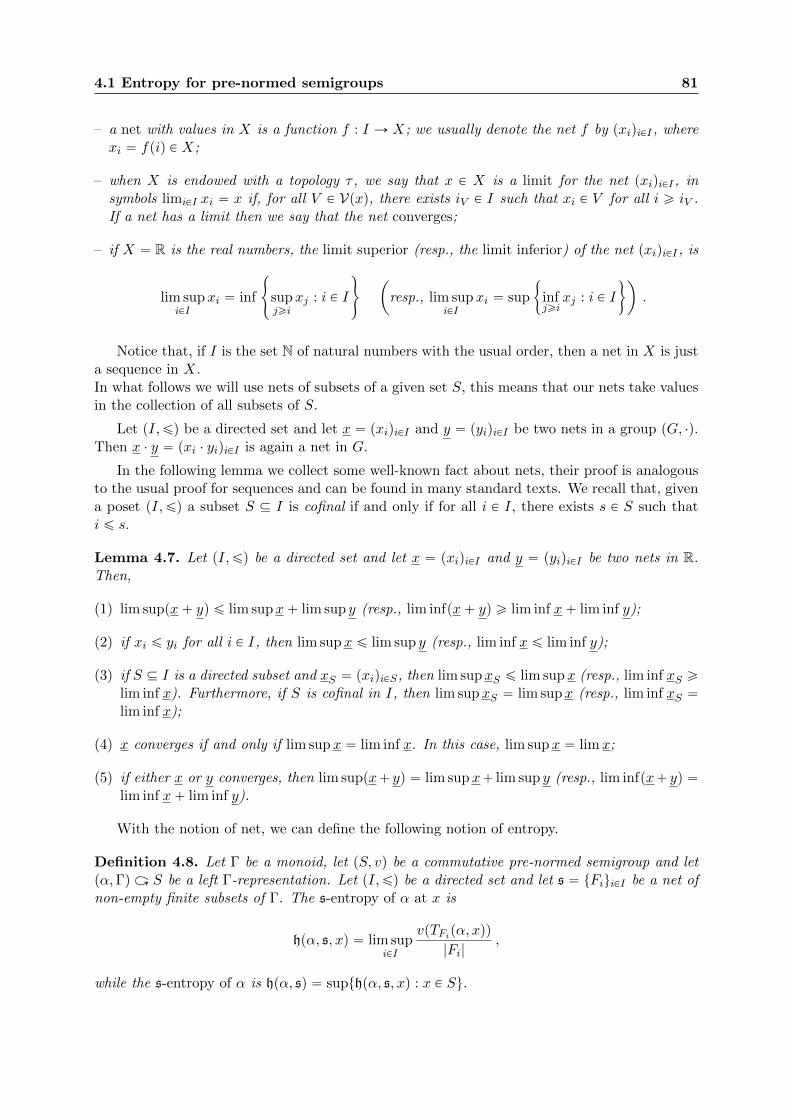
4.1 Entropy for pre-normed semigroups 81
– a net with values in X is a function f : I Ñ X; we usually denote the net f by pxiqiPI , wherexi “ fpiq P X;
– when X is endowed with a topology τ , we say that x P X is a limit for the net pxiqiPI , insymbols limiPI xi “ x if, for all V P Vpxq, there exists iV P I such that xi P V for all i ě iV .If a net has a limit then we say that the net converges;
– if X “ R is the real numbers, the limit superior (resp., the limit inferior) of the net pxiqiPI , is
lim supiPI
xi “ inf
#
supjěi
xj : i P I
+
ˆ
resp., lim supiPI
xi “ sup
"
infjěi
xj : i P I
*˙
.
Notice that, if I is the set N of natural numbers with the usual order, then a net in X is justa sequence in X.In what follows we will use nets of subsets of a given set S, this means that our nets take valuesin the collection of all subsets of S.
Let pI,ďq be a directed set and let x “ pxiqiPI and y “ pyiqiPI be two nets in a group pG, ¨q.Then x ¨ y “ pxi ¨ yiqiPI is again a net in G.
In the following lemma we collect some well-known fact about nets, their proof is analogousto the usual proof for sequences and can be found in many standard texts. We recall that, givena poset pI,ďq a subset S Ď I is cofinal if and only if for all i P I, there exists s P S such thati ď s.
Lemma 4.7. Let pI,ďq be a directed set and let x “ pxiqiPI and y “ pyiqiPI be two nets in R.Then,
(1) lim suppx` yq ď lim supx` lim sup y (resp., lim infpx` yq ě lim inf x` lim inf y);
(2) if xi ď yi for all i P I, then lim supx ď lim sup y (resp., lim inf x ď lim inf y);
(3) if S Ď I is a directed subset and xS “ pxiqiPS, then lim supxS ď lim supx (resp., lim inf xS ělim inf x). Furthermore, if S is cofinal in I, then lim supxS “ lim supx (resp., lim inf xS “lim inf x);
(4) x converges if and only if lim supx “ lim inf x. In this case, lim supx “ limx;
(5) if either x or y converges, then lim suppx` yq “ lim supx` lim sup y (resp., lim infpx` yq “lim inf x` lim inf y).
With the notion of net, we can define the following notion of entropy.
Definition 4.8. Let Γ be a monoid, let pS, vq be a commutative pre-normed semigroup and letpα,Γq ü S be a left Γ-representation. Let pI,ďq be a directed set and let s “ tFiuiPI be a net ofnon-empty finite subsets of Γ. The s-entropy of α at x is
hpα, s, xq “ lim supiPI
vpTFipα, xqq
|Fi|,
while the s-entropy of α is hpα, sq “ supthpα, s, xq : x P Su.
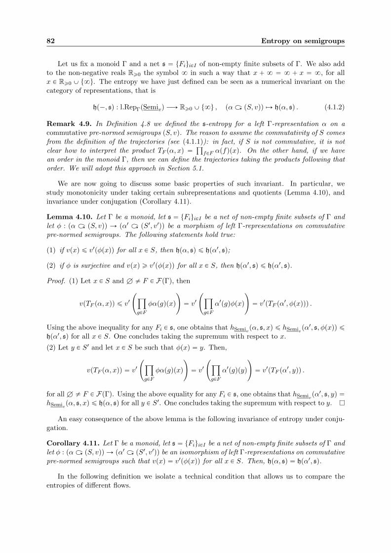
82 Entropy on semigroups
Let us fix a monoid Γ and a net s “ tFiuiPI of non-empty finite subsets of Γ. We also addto the non-negative reals Rě0 the symbol 8 in such a way that x ` 8 “ 8 ` x “ 8, for allx P Rě0 Y t8u. The entropy we have just defined can be seen as a numerical invariant on thecategory of representations, that is
hp´, sq : l.RepΓpSemivq ÝÑ Rě0 Y t8u , pα ü pS, vqq ÞÑ hpα, sq . (4.1.2)
Remark 4.9. In Definition 4.8 we defined the s-entropy for a left Γ-representation α on acommutative pre-normed semigroups pS, vq. The reason to assume the commutativity of S comesfrom the definition of the trajectories (see (4.1.1)): in fact, if S is not commutative, it is notclear how to interpret the product TF pα, xq “
ś
fPF αpfqpxq. On the other hand, if we havean order in the monoid Γ, then we can define the trajectories taking the products following thatorder. We will adopt this approach in Section 5.1.
We are now going to discuss some basic properties of such invariant. In particular, westudy monotonicity under taking certain subrepresentations and quotients (Lemma 4.10), andinvariance under conjugation (Corollary 4.11).
Lemma 4.10. Let Γ be a monoid, let s “ tFiuiPI be a net of non-empty finite subsets of Γ andlet φ : pα ü pS, vqq Ñ pα1 ü pS1, v1qq be a morphism of left Γ-representations on commutativepre-normed semigroups. The following statements hold true:
(1) if vpxq ď v1pφpxqq for all x P S, then hpα, sq ď hpα1, sq;
(2) if φ is surjective and vpxq ě v1pφpxqq for all x P S, then hpα1, sq ď hpα1, sq.
Proof. (1) Let x P S and H ‰ F P FpΓq, then
vpTF pα, xqq ď v1
˜
ź
gPF
φαpgqpxq
¸
“ v1
˜
ź
gPF
α1pgqφpxq
¸
“ v1pTF pα1, φpxqqq .
Using the above inequality for any Fi P s, one obtains that hSemivpα, s, xq ď hSemivpα1, s, φpxqq ď
hpα1, sq for all x P S. One concludes taking the supremum with respect to x.
(2) Let y P S1 and let x P S be such that φpxq “ y. Then,
vpTF pα, xqq “ v1
˜
ź
gPF
φαpgqpxq
¸
“ v1
˜
ź
gPF
α1pgqpyq
¸
“ v1pTF pα1, yqq .
for all H ‰ F P FpΓq. Using the above equality for any Fi P s, one obtains that hSemivpα1, s, yq “
hSemivpα, s, xq ď hpα, sq for all y P S1. One concludes taking the supremum with respect to y.
An easy consequence of the above lemma is the following invariance of entropy under conju-gation.
Corollary 4.11. Let Γ be a monoid, let s “ tFiuiPI be a net of non-empty finite subsets of Γ andlet φ : pα ü pS, vqq Ñ pα1 ü pS1, v1qq be an isomorphism of left Γ-representations on commutativepre-normed semigroups such that vpxq “ v1pφpxqq for all x P S. Then, hpα, sq “ hpα1, sq.
In the following definition we isolate a technical condition that allows us to compare theentropies of different flows.
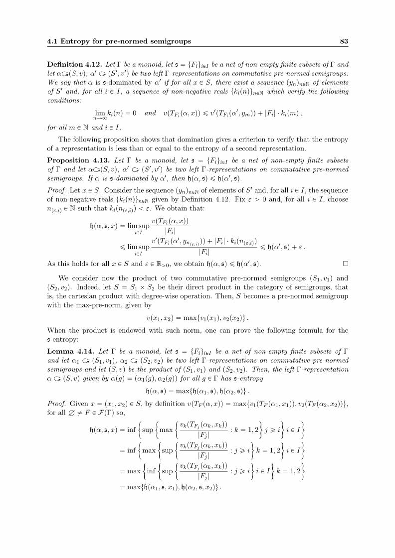
4.1 Entropy for pre-normed semigroups 83
Definition 4.12. Let Γ be a monoid, let s “ tFiuiPI be a net of non-empty finite subsets of Γ andlet αüpS, vq, α1 ü pS1, v1q be two left Γ-representations on commutative pre-normed semigroups.We say that α is s-dominated by α1 if for all x P S, there exist a sequence pynqnPN of elementsof S1 and, for all i P I, a sequence of non-negative reals tkipnqunPN which verify the followingconditions:
limnÑ8
kipnq “ 0 and vpTFipα, xqq ď v1pTFipα1, ymqq ` |Fi| ¨ kipmq ,
for all m P N and i P I.
The following proposition shows that domination gives a criterion to verify that the entropyof a representation is less than or equal to the entropy of a second representation.
Proposition 4.13. Let Γ be a monoid, let s “ tFiuiPI be a net of non-empty finite subsetsof Γ and let αüpS, vq, α1 ü pS1, v1q be two left Γ-representations on commutative pre-normedsemigroups. If α is s-dominated by α1, then hpα, sq ď hpα1, sq.
Proof. Let x P S. Consider the sequence pynqnPN of elements of S1 and, for all i P I, the sequenceof non-negative reals tkipnqunPN given by Definition 4.12. Fix ε ą 0 and, for all i P I, choosenpε,iq P N such that kipnpε,iqq ă ε. We obtain that:
hpα, s, xq “ lim supiPI
vpTFipα, xqq
|Fi|
ď lim supiPI
v1pTFipα1, ynpε,iqqq ` |Fi| ¨ kipnpε,iqq
|Fi|ď hpα1, sq ` ε .
As this holds for all x P S and ε P Rą0, we obtain hpα, sq ď hpα1, sq.
We consider now the product of two commutative pre-normed semigroups pS1, v1q andpS2, v2q. Indeed, let S “ S1 ˆ S2 be their direct product in the category of semigroups, thatis, the cartesian product with degree-wise operation. Then, S becomes a pre-normed semigroupwith the max-pre-norm, given by
vpx1, x2q “ maxtv1px1q, v2px2qu .
When the product is endowed with such norm, one can prove the following formula for thes-entropy:
Lemma 4.14. Let Γ be a monoid, let s “ tFiuiPI be a net of non-empty finite subsets of Γand let α1 ü pS1, v1q, α2 ü pS2, v2q be two left Γ-representations on commutative pre-normedsemigroups and let pS, vq be the product of pS1, v1q and pS2, v2q. Then, the left Γ-representationα ü pS, vq given by αpgq “ pα1pgq, α2pgqq for all g P Γ has s-entropy
hpα, sq “ maxthpα1, sq, hpα2, squ .
Proof. Given x “ px1, x2q P S, by definition vpTF pα, xqq “ maxtv1pTF pα1, x1qq, v2pTF pα2, x2qqu,for all H ‰ F P FpΓq so,
hpα, s, xq “ inf
"
sup
"
max
"
vkpTFj pαk, xkqq
|Fj |: k “ 1, 2
*
j ě i
*
i P I
*
“ inf
"
max
"
sup
"
vkpTFj pαk, xkqq
|Fj |: j ě i
*
k “ 1, 2
*
i P I
*
“ max
"
inf
"
sup
"
vkpTFj pαk, xkqq
|Fj |: j ě i
*
i P I
*
k “ 1, 2
*
“ maxthpα1, s, x1q, hpα2, s, x2qu .

84 Entropy on semigroups
Taking suprema with x1 P S1 and x2 P S2 we obtain the result.
Let us consider also the coproduct of two commutative pre-normed semigroups pS1, v1q andpS2, v2q. Indeed, we let S “ S1‘S2 be their coproduct in the category of semigroups, that coin-cides again with the cartesian product. S becomes a pre-normed semigroup with the followingpre-norm
v‘px1, x2q “ v1px1q ` v2px2q .
When S is endowed with such norm, one can prove one inequality of a weak “addition formula”for the s-entropy. The converse inequality is also true in many concrete situations (see Lemma4.40) but it cannot be proved in full generality (see for example Walters’ book [100, p. 176]):
Lemma 4.15. Let Γ be a monoid, let s “ tFiuiPI be a net of non-empty finite subsets of Γand let α1 ü pS1, v1q, α2 ü pS2, v2q be two left Γ-representations on commutative pre-normedsemigroups. Then, letting S “ S1 ‘ S2, the left Γ-representation α ü pS, v‘q given by αpgq “pα1pgq, α2pgqq for all g P Γ has s-entropy
hpα, sq ď hpα1, sq ` hpα2, sq .
Proof. Let x “ px1, x2q P S and i P I, then by definition vpTFipα, xqq “ v1pTFipα1, x1qq `
v2pTFipα2, x2qq. Dividing by |Fi| and taking the lim sup with i varying in I we obtain
hpα, s, xq “ lim supiPI
ˆ
v1pTFipα1, x1qq ` v2pTFipα2, x2qq
|Fi|
˙
ď hpα1, s, x1q ` hpα2, s, x2q .
Taking the supremum with x1 and x2 varying in S1 and S2 respectively, the thesis follows.
4.1.3 Bernoulli representations
Let Γ be a group, let S be a commutative monoid and let v be a pre-norm on S such thatvp1q “ 0. For all g P Γ let Sg “ S and consider the monoid M “
À
gPΓ Sg, which becomes apre-normed monoid with the pre-norm
v‘pxq “ÿ
gPΓ
vpxgq for any x “ pxgqgPΓ PM .
We can naturally define a map:
BS : Γ Ñ AutpMq , BSphqpxgqgPΓ “ pxh´1gqgPΓ ,
for all h P Γ and x “ pxgqgPΓ PM . Notice that, the following relation holds
BSph1qpBSph2qpxqq “ pxh´12 h´1
1 gqgPΓ “ BSph1h2qpxq ñ BSph1qBSph2q “ BSph1h2q ,
so BS is a left Γ-representation. If one prefers to work with right representations, one can simi-larly define B1
Sphqpxgqg “ pxhgqg. We call pBS ,Γq ü pM, v‘q the Bernoulli left Γ-representationover S.
Lemma 4.16. Let pS, vq be a commutative pre-normed monoid, let Γ a group and let BS ü
pM,v‘q be the Bernoulli left Γ-representation. Then, for any net s “ tFiuiPI of non-empty finitesubsets of Γ:
hpBS , sq ě suptvpxq : x P Su .
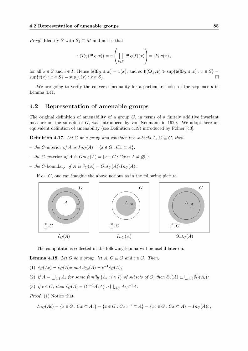
4.2 Representation of amenable groups 85
Proof. Identify S with S1 ĎM and notice that
vpTFipBS , xqq “ v
¨
˝
ź
fPFi
BSpfqpxq
˛
‚“ |Fi|vpxq ,
for all x P S and i P I. Hence hpBS , s, xq “ vpxq, and so hpBS , sq ě supthpBS , s, xq : x P Su “suptvpxq : x P Su “ suptvpxq : x P Su.
We are going to verify the converse inequality for a particular choice of the sequence s inLemma 4.41.
4.2 Representation of amenable groups
The original definition of amenability of a group G, in terms of a finitely additive invariantmeasure on the subsets of G, was introduced by von Neumann in 1929. We adopt here anequivalent definition of amenability (see Definition 4.19) introduced by Følner [43].
Definition 4.17. Let G be a group and consider two subsets A, C Ď G, then
– the C-interior of A is InCpAq “ tx P G : Cx Ď Au;
– the C-exterior of A is OutCpAq “ tx P G : CxXA ‰ Hu;
– the C-boundary of A is BCpAq “ OutCpAqzInCpAq.
If e P C, one can imagine the above notions as in the following picture
A x.
e. C
G
BCpAq
x.
e. C
A
G
InCpAq
A x.
e. C
G
OutCpAq
The computations collected in the following lemma will be useful later on.
Lemma 4.18. Let G be a group, let A, C Ď G and c P G. Then,
(1) BCpAcq “ BCpAqc and BCcpAq “ c´1BCpAq;
(2) if A “Ť
iPI Ai for some family tAi : i P Iu of subsets of G, then BCpAq ĎŤ
iPi BCpAiq;
(3) if e P C, then BCpAq “ pC´1AzAq Y
Ť
cPC Azc´1A.
Proof. (1) Notice that
InCpAcq “ tx P G : Cx Ď Acu “ tx P G : Cxc´1 Ď Au “ txc P G : Cx Ď Au “ InCpAqc ,
86 Entropy on semigroups
and that
OutCpAcq “ tx P G : CxXAc ‰ Hu “ tx P G : Cxc´1 XA ‰ Hu
“ txc P G : CxXA ‰ Hu “ OutCpAqc .
Thus, BCpAcq “ OutCpAcqzInCpAcq “ OutCpAqczInCpAqc “ pOutCpAqzInCpAqqc “ BCpAqc.The proof of the second claim is analogous.
(2) Notice that
InCpAq “ tx P G : Cx Ď Au Ě tx P G : Cx Ď Ai for some i P Iu
“ď
iPI
tx P G : Cx Ď Aiu “ď
iPI
InCpAiq ,
and that
OutCpAq “ tx P G : CxXA ‰ Hu “ tx P G : CxXAi ‰ H for some i P Iu
“ď
iPI
tx P G : CxXAi ‰ Hu “ď
iPI
OutCpAiq .
Thus, BCpAq ĎŤ
iPI OutCpAiqzŤ
iPI InCpAq ĎŤ
iPI BCpAiq.
(3) Since e P C, InCpAq Ď A Ď OutCpAq. Furthermore,
OutCpAqzA “ tx P GzA : Dc P C s.t. cx P Au “ tx P GzA : Dc P C s.t. x P c´1Au “ C´1AzA
and
AzInCpAq “ tx P A : Dc P C s.t. cx R Au “ tx P A : Dc P C s.t. x R c´1Au “ď
cPC
Azc´1A .
Thus, BCpAq “ OutCpAqzInCpAq “ pOutCpAqzAq Y pAzInCpAqq “ pC´1AzAq Y
Ť
cPC Azc´1A.
Definition 4.19. A group G is amenable if and only if there exists a directed set pI,ďq and anet tFi : i P Iu of non-empty finite subsets of G such that, for any C P FpGq,
limI
|BCpFiq|
|Fi|“ 0 . (4.2.1)
Any such net is called a Følner net.
In the following lemma we collect some closure properties of the class of amenable groups.
Lemma 4.20. [16, Propositions 4.5.1, 4.5.4, 4.5.5 and 4.5.10] Let G be a group and let H ď G.Then,
(1) if G is amenable, then H is amenable;
(2) if H is normal, then G is amenable if and only if both H and G{H are amenable;
(3) if G is the directed colimit of a directed system of amenable groups, then G is amenable.
Let X be a set and let A, B Ď X. The symmetric difference is the following subset of X:
A∆B “ pAzBq Y pBzAq
4.2 Representation of amenable groups 87
Lemma 4.21. Let G be an amenable group and let s “ tFiuiPI be a net of non-empty finitesubsets of G. Then, the following are equivalent
(1) limI |Fi∆gFi|{|Fi| “ 0 for all g P G;
(2) limI |Fi∆CFi|{|Fi| “ 0 for all non-empty C P FpGq;
(3) s is a Følner net.
Proof. (1)ñ(2). Let C “ tg1, . . . , gnu P FpGq. Then, for all i P I, Fi∆CFi ĎŤnk“1pFi∆gkFiq.
Thus, limI |Fi∆CFi|{|Fi| ďřnk“1 limI |Fi∆gkFi|{|Fi| “ 0.
(2)ñ(1) is trivial.
(2)ñ(3). First of all, notice that if limI |Fi∆KFi|{|Fi| “ 0 for some K P FpGq, then in particularlimI |FizKFi|{|Fi| “ 0 and limI |KFizFi|{|Fi| “ 0. Let C P FpGq, by Lemma 4.18 (1) we cansuppose that e P C. Furthermore, by Lemma 4.18 (3), |BCpFiq| ď |C
´1FizFi| Yř
cPC |Fizc´1Fi|
and so, limI |BCpFiq|{|Fi| ď limI |C´1AzA|{|Fi| Y
ř
cPC limI |Fizc´1Fi|{|Fi| “ 0.
(3)ñ(1). Let g P G and let C “ te, g´1u. Then, OutCpFiq “ gFiYFi while InCpFiq “ gFiXFi.Thus, BCpFiq “ Fi∆gFi and so limi |Fi∆gFi|{|Fi| “ limI |BCpFiq|{|Fi| “ 0.
Lemma 4.22. Let G be an amenable group, let F P FpGq be non-empty and let tFiuiPI be aFølner net. Then, the following are Følner sequences:
(1) tFiF uiPI ;
(2) tFi Y F uiPI ;
(3) tFiuiPJ with J Ď I a cofinal subset.
Proof. (1) Let C P FpGq, then using Lemma 4.18
limI
|BCpFiF q|
|FiF |ď lim
I
|F ||BCpFiq|
|Fi|“ |F | lim
I
|BCpFiq|
|Fi|“ 0 ,
proving (1).
(2) Let C P FpGq. Using again Lemma 4.18
limI
|BCpFi Y F q|
|Fi Y F |ď lim
I
|BCpF q| ` |BCpFiq|
|Fi|“ lim
I
|BCpF q|
|Fi|` lim
I
|BCpFiq|
|Fi|“ 0 ,
proving (2).
(3) is trivial.
Corollary 4.23. Let G be an infinite amenable group and let tFiuiPI be a Følner net. Then,limiPI |Fi| “ 8.
Proof. We may suppose, without loss of generality, that e P Fi for all i P I. Indeed, setF 1i “ Fi Y teu, this gives a Følner net by Lemma 4.22 and clearly limiPI |Fi| “ 8 if and only iflimiPI |F
1i | “ 8.
If there exists an element g P G and i P I such that g R Fj for all j ě i, then let C “ te, g´1u
and notice that g P BCpFjq for all j ě i. Thus,
0 “ limiPI|BCpFjq|{|Fj | ě lim
iPI1{|Fj | .
88 Entropy on semigroups
This may happen only if limiPI |Fi| “ 8.On the other hand, if for all g P G and for all i P I there exists j ě i such that g P Fj , then
choose an infinite family tgn : n P Nu in G, let Sn “ ti P I : gn P Fiu Ď I for all n P N and letSn “
Şnk“0 Sk. By construction, S0 is cofinal in I. If all the Sn are cofinal in I, in particular
they are not empty and, given s P Sn, |Fs| ě |tg1, . . . , gnu| “ n and so limiPI |Fs| “ 8. On theother hand, if there exists a minimum n P N such that Sn is not cofinal in I, it means that Sn´1
is cofinal in I and that there exists s P Sn´1 such that gn R Ft for all t ě s. By the first part ofthe proof, limiPI |Fi| “ limiPSn´1
|Fi| “ 8.
In the last part of the subsection we concentrate on countable amenable groups.
Remark 4.24. If G is countable, then also FpGq is countable. Thus, given a net s “ tFiuiPI inFpGq, there is a countable subset J of I such that J is order-isomorphic to N and sJ “ tFiuiPJis cofinal in s. By Lemma 4.22 (3), sJ is Følner. This allows to always take I “ N and justspeak about Følner sequences in countable groups.
Definition 4.25. Given a group G and a Følner sequence s “ tFn : n P Nu, we say that s is aFølner exhaustion if
– e P F0 and Fn Ď Fn`1 for all n P N;
–Ť
nPN Fn “ G.
Example 4.26. Every finite group is amenable. Furthermore, taking G “ Zk, one can constructexplicitly a Følner exhaustion tFn : n P Nu as follows:
Fn “
#
kÿ
i“1
λiei : λi P Z such thatkÿ
i“1
|λi| ď n
+
where tei : i “ 1, . . . , nu are the canonical generators of G.
Lemma 4.27. Let G be a countably infinite amenable group and let tFnunPN be a Følner sequencein G. Then there exists an increasing sequence tNpnqunPN of natural numbers and a Følnerexhaustion tSnunPN of G such that
(1) FNpnq Ď Sn for all n P N;
(2) limnPN|FNpnq|
|Sn|“ 1.
Proof. Since G is countable we can enumerate its elements, that is, G “ tgi : i P Nu, we supposethat g0 “ e. For all n P N let An “ tg0, . . . , gnu, notice that teu Ď A0 Ď ¨ ¨ ¨ Ď An Ď . . . andŤ
nPNAn “ G. Let also tεnunPN be a sequence in Rě0 which converges to 0. Put Np0q “ 0,S0 “ F0YA0 and let Sn`1 “ SnYAn`1YFNpn`1q, where Npn`1q ě Npnq is chosen inductivelyto satisfy
|BAn`1pSn`1q|{|Sn`1| ă εn`1 and|An`1 Y Sn|
|FNpn`1q|ă εn`1
this can be done since tFiYpSnYAnquiPN is a Følner sequence by Lemma 4.22 and limnÑ8 |Fn| “8 by Corollary 4.23. Now, let C P FpGq, by construction there exists n such that C Ď An forall n ě n, thus
limN
|BCpSnq|
|Sn|ď lim
něn
|BAnpSnq|
|Sn|ď lim
něnεn “ 0 ,
4.2 Representation of amenable groups 89
showing that tSnunPN is a Følner exhaustion. Furthermore, part (1) of the statement is clear,while part (2) can be shown as in the following computation:
1 “ limnPN
|FNpnq|
|FNpnq|ě lim
nPN
|FNpnq|
|Sn|“ lim
nPN
|FNpnq|
|Sn|` limně1
|An Y Sn´1|
|FNpnq|
“ limně1
|FNpnq| ` |An Y Sn´1|
|Sn|ě lim
nPN
|Sn|
|Sn|“ 1 .
4.2.1 Quasi-tilings
In what follows, we recall some terminology and results due to Ornstein and Weiss [81] (seealso [62], [67] and [101]). All the proofs and statements of this subsection are adapted from theoriginal papers with some slight changes to make them fit into our context.
Definition 4.28. Let G be a group, let A P FpGq, let ε P p0, 1q, α P p0, 1s and δ P r0, 1q, let Ibe a finite set and consider A “ tAiuiPI Ď FpGq. The family A is
– ε-disjoint if there is a family tBiuiPI Ď FpGq such that
- Bi Ď Ai and |Bi| ą p1´ εq|Ai|, for all i P I;
- Bi XBj “ H, whenever i ‰ j P I;
– a α-cover of A if |AX pŤ
iPI Aiq| ě α|A|;
– a δ-even cover of A if
- Ai Ď A, for all i P I;
- there exists M ą 0 such thatř
iPI χAipxq ďM for all x P A, andř
iPI |Ai| ě p1´ δq|A|M .
Remark 4.29. Let G be a group, let A P FpGq, let δ P p0, 1q, let I be a finite set and considerA “ tAiuiPI Ď FpGq. If A is an δ-even cover, then A is an p1´ δq-cover. In fact,
ˇ
ˇ
ˇ
ˇ
ˇ
AX
˜
ď
iPI
Ai
¸ˇ
ˇ
ˇ
ˇ
ˇ
p˚q“
ˇ
ˇ
ˇ
ˇ
ˇ
ď
iPI
Ai
ˇ
ˇ
ˇ
ˇ
ˇ
p˚˚q
ě1
M
ÿ
iPI
|Ai|p ˚˚˚qě
1
Mp1´ δqM |A| “ p1´ δq|A| ,
where p˚q holds since Ai Ď A for all i P I, p˚˚q is a consequence of the fact that each x P A canbelong to at most M elements of A and
`
˚
˚˚
˘
follows by the second condition in the definition ofδ-even cover.
Definition 4.30. Let G be a group, let A P FpGq, let ε P p0, 1q, let I be a finite set and considerA “ tAiuiPI Ď FpGq. The family A is an ε-quasi-tiling of A if there exists a family of tilingcenters tCiuiPI Ď FpGq such that
– CiAi Ď A and tcAi : c P Ciu forms an ε-disjoint family, for all i P I;
– CiAi X CjAj “ H, if i ‰ j P I;
– tCiAi : i P Iu forms an p1´ εq-cover of A.
90 Entropy on semigroups
It is a deep result, due to Ornstein and Weiss, that whenever G is a countable amenable groupand tFnunPN is a Følner exhaustion, for any (small enough) ε ą 0, one can find a nice family ofsubsets of G that ε-quasi-tiles Fn for all (big enough) n P N. In the rest of this subsection weare going to prove the following theorem.
Theorem 4.31. Let G be a countably infinite amenable group, let tFnunPN and tF 1nunPN berespectively a Følner sequence and a Følner exhaustion for G. Then, for all ε P p0, 1{4q andn P N, there exist n1, . . . , nk P N such that n ď n1 ď ¨ ¨ ¨ ď nk and tFn1 , . . . , Fnku ε-quasi-tilesF 1m, for all big enough m.
Before proceeding to the proof, we need a series of technical lemmas.
Lemma 4.32. Let G be a group, let C and A P FpGq, let ε P p0, 1q and let c P G. If |BCpAq| ăε|A|, then |BCpAcq| ă ε|Ac|.
Proof. By Lemma 4.18, BCpAcq “ BCpAqc and so |BCpAcq| “ |BCpAq|. Similarly, |A| “ |Ac|.
Lemma 4.33. Let G be a group, let I be a finite set, let A “ tAiuiPI Ď FpGq, let A “Ť
A, letC P FpGq and let ε, δ P p0, 1q.
(1) If A is ε{2-disjoint, thenř
iPI |Ai| ď p1` εq|A|;
(2) If A is ε{2-disjoint and |BCpAiq| ď δ|Ai| for all i P I, then BCpAq ď δp1` εq|A|.
Proof. (1) By definition of ε{2-disjointedness, there exists a family tBiuiPI Ď FpGq such thatBi Ď Ai, |Bi| ą p1´ ε{2q|Ai| and Bi XBj “ H, for all i ‰ j P I. Then,
|A| ě
ˇ
ˇ
ˇ
ˇ
ˇ
ď
iPI
Bi
ˇ
ˇ
ˇ
ˇ
ˇ
“ÿ
iPI
|Bi| ě p1´ ε{2qÿ
iPI
|Ai| .
One concludes noticing that p1´ ε{2q´1 ď 1` ε.
(2) By Lemma 4.18, BCpAq ĎŤ
iPi BCpAiq, so
|BCpAq| ď
ˇ
ˇ
ˇ
ˇ
ˇ
ď
iPI
BCpAiq
ˇ
ˇ
ˇ
ˇ
ˇ
ďÿ
iPI
|BCpAiq|p˚q
ď δÿ
iPI
|Ai|p˚˚q
ď δp1` εq|A| ,
where p˚q holds since |BCpAiq| ď δ|Ai| for all i P I, while p˚˚q is true by part (1).
Lemma 4.34. Let G be a group, let A and S be two finite subsets of G containing e, letH “ InSS´1pAq and let ε P p0, 1q. If |BSS´1pAq| ď p1 ´ εq|A|, then tSgugPH is an ε-even coverof A.
Proof. Let M “ |S|, we have to prove thatř
gPH χSgpxq ď M , for all x P A (which is true noelement of A can belong to more that |S| translates of S) and that
ř
gPH |Sg| ě ε|A|M . Thefact that |BSS´1pAq| ď p1´ εq|A| implies that |H| ě ε|A| and so
ř
gPH |Sg| ě ε|A|M .
Lemma 4.35. Let G be a group, let A P FpGq and let ε, δ P p0, 1q. If A is a δ-even cover of A,then there is a subset B Ď A such that
(1) B is ε-disjoint;
(2) it εp1´ δq-covers A;
4.2 Representation of amenable groups 91
(3) given B P B, |Ť
BzB| ă εp1´ δq|A|.
Furthermore, if (1), (2) and (3) hold for some set B, then for all B P B,
1´ εp1´ δq ě|Az
Ť
B||A|
ą 1´ εp1´ δq ´ |B|{|A| .
Proof. Let B be a maximal ε-disjoint subfamily of A. Suppose, looking for a contradiction, thatB is not an εp1´ δq-cover of A (that is, |
Ť
B| ă εp1´ δq|A|) and consider the following claim:
p˚q there exists B P A such that |B Xď
B| ă ε|B|.
Let us verify p˚q. Assume, looking for a contradiction, that p˚q does not hold and consider thefollowing observations:
a) by our initial absurd hypothesis, |Ť
B| ă εp1´ δq|A|;
b) by the negation of (˚),ř
BPA |B XŤ
B| ě εř
BPA |B|;
c) by the definition of δ-even cover, there exists M ą 0 such thatř
BPA |B| ě p1´ δq|A|M ;
d) by the definition of δ-even cover, given x PŤ
BpĎ Aq, there exist at most M differentmembers B P A such that x P B. Thus,
ř
BPA |B XŤ
B| ďM |Ť
B|.
Combining b) and c),ř
BPA |B XŤ
B| ě εp1´ δq|A|M , while, combining a) and d),ř
BPA |B XŤ
B| ă εp1 ´ δq|A|M , that is a contradiction. Thus, (˚) is verified. Now, consider B P A suchthat |BX
Ť
B| ă ε|B| and notice that B R B and that BYtBu is still ε-disjoint. This contradictsthe maximality of B.Thus, B satisfies properties (1) and (2) in the statement. Take now B P B and notice that, if|Ť
BzB| ě εp1 ´ δq|A|, then B1 “ BztBu is again a subset of A satisfying (1) and (2). Thus,removing a finite number of elements from B, we can find a subset of A that satisfies (1), (2)and (3).For the last part of the statement, notice that the bound |Az
Ť
B| {|A| ď 1 ´ εp1 ´ δq comesdirectly from condition (2), while the other bound can be computed as follows. Take B P B,then
|AzŤ
B||A|
“ 1´|Ť
BzB| ` |B||A|
ą 1´ εp1´ δq ´|B|
|A|
We can finally prove the main result of this section:
Proof of Theorem 4.31. Fix ε P p0, 1{4q and n P N, and choose k P N` and δ ą 0 such that
´
1´ε
2
¯kă ε and 6kδ ă
ε
2.
Notice that the second condition, together with the choice of ε, implies δ ă 1{48. Since tFnunPNis a Følner exhaustion, we can choose n ď n1 ď n2 ď . . . ď nk P N such that
|BFniF´1nipFni`1q|
|Fni`1 |ă δ and
|Fni |
|Fni`1 |ă δ (4.2.2)
92 Entropy on semigroups
Furthermore, since tF 1nunPN is a Følner sequence, for any big enough m P N,
|BFnkF´1nkpF 1mq|
|F 1m|ă δ and
|Fnk |
|F 1m|ă δ . (4.2.3)
Fix a positive integer m as above; we construct by downward induction a family tC1, . . . , Ckuwith the following properties: letting Ak “ F 1m and Aj´1 “ AjzFnjCj for all j “ 2, . . . , k, andletting Ki “ FniF
´1ni for all i “ 1, . . . , k,
(ai) tFnic : c P Ciu is ε-disjoint;
(bi) tFnic : c P Ciu is an εp1´ 6iδq-cover of Ai;
(ci) 1´ εp1´ δq ě |AizFniCi| {|Ai| ą 1´ εp1´ δq ´ δ, |BKipAiq|{|Ai| ă δ and |Fni |{|Ai| ă δ.
Notice that, once we found such families, FniCi “ AizAi´1 and so FniCi X FnjCj “ H if i ‰ j.Furthermore,
|AkzŤ
FniCi|
|Ak|“|A1zFn1C1|
|Ak|“|A1zFn1C1|
|A1|
|A1|
|A2|. . .|Ak´1|
|Ak|
ď p1´ εp1´ 6kδqqp1´ εp1´ 6k´1δqq . . . p1´ εp1´ δqq ă p1´ ε{2qk ă ε .
Thus, tFn1 , . . . , Fnku ε-quasi-tiles Ak “ F 1m with tiling centers tC1, . . . , Cku and the proof isconcluded.
Case i “ k. Let Ak “ F 1m and let Kk “ FnkF´1nk
; with this notation, (4.2.3) reads as
|BKkpAkq|
|Ak|ă δ and
|Fnk |
|Ak|ă δ ,
notice that these are the two last conditions in (ck). Consider Hk “ InKkpAkq, then tFnkhuhPHkis a δ-even cover of Ak, by Lemma 4.34. Thus, by Lemma 4.35, there exists Ck Ď Hk thatsatisfies (ak), (bk) and (ck).
Case i ă k. Suppose we have already constructed Ck, . . . , Ci`1 with the desired properties.Then,
|BKipAiq|
|Ai|ď|BKi`1pAi`1q|
|Ai|` |Ci`1|
BKipFni`1q
|Ai|
ăδ
|Ai`1zFni`1Ci`1|p|Ai`1| ` |Fni`1 ||Ci`1|q (ci`1) and (4.2.2)
ăδ|Ai`1|
|Ai`1zFni`1Ci`1|
ˆ
1`1
1´ ε
˙
(ai`1)
ăδ
1´ εp1´ δq ´ δ
ˆ
1`1
1´ ε
˙
(ci`1)
ă 6δ ε ă 1{4 and δ ă 1{48,
where the first inequality follows since BKipAiq Ď BKi`1pAi`1qYŤ
cPCi`1BKipFni`1qc (use Lemma
4.18). Furthermore, using again (4.2.2), (ci`1) and the initial bounds for ε and δ,
|Fni |
|Ai|“
|Fni |
|Fni`1 |
|Fni`1 |
|Ai`1|
|Ai`1|
|Ai|ă
δ2
1´ εp1´ δq ´ δă δ .
This shows the second part of (ci). Now, if we let Hi “ InKipAiq, then tFnihuhPHi is a 6δ-evencover of Ai, by Lemma 4.34. Thus, by Lemma 4.35, there exists Ci Ď Hi that satisfies (ai), (bi)and (ci).
4.2 Representation of amenable groups 93
4.2.2 Non-negative real functions on finite subsets of an amenable group
In this subsection we recall some results and terminology about non-negative invariants for thefinite subsets of G, that is, functions f : FpGq Ñ Rě0.
Definition 4.36. Let G be a group and let f : FpGq Ñ Rě0. We say that f is
– monotone if fpAq ď fpA1q, for all A Ď A1 P FpGq;
– sub-additive if fpAYA1q ď fpAq ` fpA1q, for all A, A1 P FpGq;
– (left) G-equivariant if fpgAq “ fpAq, for all A P FpGq and g P G.
Notice that, given a group G and a G-equivariant function f : FpGq Ñ Rě0, fptguq “ fpteuq,for all g P G. Thus, if f is also sub-additive, then fpAq ď
ř
gPA fptguq “ |A|fpteuq, for allA P FpGq. Notice that a consequence of this is that, given a net s “ tFiuiPI of non-empty finitesubsets of G, then
lim supiPI
fpFiq
|Fi|ď lim sup
iPI
|Fi|fpteuq
|Fi|“ fpteuq .
In particular, any such limit superior is finite.
The following corollary is a consequence of Theorem 4.31. It is important to underline thatthe choice of the n1, . . . , nk in the statement does not depend on the function f , but we canreally find a family tn1, . . . , nku, which works for all f at the same time.
Corollary 4.37. Let G be a countably infinite amenable group and let tFnunPN, tF 1nunPN berespectively a Følner exhaustion and a Følner sequence in G. Then, for any ε P p0, 1{4q andn P N there exist integers n1, . . . , nk such that n ď n1 ď ¨ ¨ ¨ ď nk and, for any sub-additive andG-equivariant f : FpGq Ñ R
lim supnÑ8
fpF 1nq
|F 1n|ďMε`
1
1´ εmax1ďiďk
fpFniq
|Fni |,
where M “ fpteuq.
Proof. Let ε P p0, 1{4q and n P N. By Theorem 4.31, there exist positive integers n1, . . . , nk suchthat n ď n1 ď ¨ ¨ ¨ ď nk and tFn1 , . . . , Fnku ε-quasi-tiles F 1n, for all big enough n P N. We letCn1 , . . . , C
nk be the tiling centers for F 1n. Thus, when n is big enough,
F 1n Ěkď
i“1
Cni Fni and
ˇ
ˇ
ˇ
ˇ
ˇ
kď
i“1
Cni Fni
ˇ
ˇ
ˇ
ˇ
ˇ
ě max
#
p1´ εq|F 1n| , p1´ εqkÿ
i“1
|Cni ||Fni |
+
.
Letting f : FpGq Ñ Rě0 be a sub-additive and G-invariant function,
fpF 1nq
|F 1n|ď
f´
F 1nzŤki“1C
ni Fni
¯
|Fn|`
f´
Ťki“1C
ni Fni
¯
|F 1n|ďM
ˇ
ˇ
ˇF 1nz
Ťki“1C
ni Fni
ˇ
ˇ
ˇ
|F 1n|`
f´
Ťki“1C
ni Fni
¯
ˇ
ˇ
ˇ
Ťki“1C
ni Fni
ˇ
ˇ
ˇ
ďMε`
řki“1 |C
ni |fpFniq
p1´ εqřki“1 |C
ni ||Fni |
ďMε`1
1´ εmax1ďiďk
fpFniq
|Fni |,
where M “ fpteuq, as desired.
94 Entropy on semigroups
The following result, generally known as “Ornstein-Weiss Lemma”, is proved in [81] for asuitable class of locally compact amenable groups (a direct proof, along the same lines, in thediscrete case can be found in [101], while a nice alternative argument, based on ideas of Gromov,is given in [67]).
Proposition 4.38. Let G be a countably infinite amenable group and consider a monotone, sub-additive and G-equivariant function f : FpGq Ñ Rě0. Then, for any Følner sequence tFnunPN,the sequence pfpFnq{|Fn|qnPN converges and the value of the limit limnPN fpFnq{|Fn| is the samefor any choice of the Følner sequence.
Proof. Let f : FpGq Ñ Rě0 be a monotone, sub-additive and G-equivariant function, and letM “ fpteuq. Choose also a Følner exhaustion tFnunPN and a Følner sequence tF 1nunPN in G. ByCorollary 4.37, for all ε P p0, 1{4q and n P N there exist k P N and n ď n1 ă ¨ ¨ ¨ ă nk P N suchthat
lim supnPN
fpF 1nq
|F 1n|ďMε`
1
1´ εmax1ďiďk
fpFniq
|Fni |ďMε`
1
1´ εsupnďn
fpFniq
|Fni |
Since this holds for all ε P p0, 1{4q and n P N, we get lim supnPNfpF 1nq|F 1n|
ď lim supnPNfpFnq|Fn|
. Let
now tNpnqu be an increasing sequence of natural numbers such that limnPN fpFNpnqq{|FNpnq| “lim infnPN fpFnq{|Fn|. Then, by the first part of the proof,
lim supnPN
fpFnq{|Fn| ď limnPN
fpFNpnqq{|FNpnq| “ lim infnPN
fpFnq{|Fn| ,
thus tfpFnq{|Fn|u converges to a limit λ. Using the same kind of argument one shows that, forany Følner exhaustion tSnunPN, limnPN fpSnq{|Sn| “ λ. Using Lemma 4.27, choose an increasingsequence tNpnqunPN of natural numbers and a Følner exhaustion tSnunPN of G such that F 1Npnq Ď
Sn for all n P N and limnPN|F 1Npnq
|
|Sn|“ 1. Notice that
λ ě lim supnPN
fpF 1Npnqq
|F 1Npnq|ě lim inf
nPN
fpF 1Npnqq
|F 1Npnq|“ lim inf
nPN
fpF 1Npnqq ` fpSnzF1Npnqq
|Sn|ě lim
fpSnq
|Sn|“ λ .
The Ornstein-Weiss Lemma immediately implies the following convergence result for theentropy of left representations on normed semigroups. Notice that there exists a generalization ofthe above result to cancelable amenable semigroups (see [17]), using such stronger version of theOrnstein-Weiss Lemma one would obtain more general results about s-entropies. Furthermore,Krieger’s proof (see [67]) of the Ornstein-Weiss Lemma holds for Følner nets in general, thiswould allow to extend the following corollary to amenable groups of any cardinality.
As usual, we are tacitly assuming Hypothesis (˚).
Corollary 4.39. Let pM,vq be a normed semigroup, let Γ be a countably infinite amenable groupand let α ü M be a left Γ-representation. For any given Følner sequence s “ tFnunPN of Γ, thelim sup defining the s-entropy of α converges and its limit does not depend on the choice of theparticular Følner sequence, provided the following conditions hold:
(1) vpxq, vpyq ď vpxyq for all x and y PM ;
(2) vpαgpxqq “ vpxq for all x PM and g P Γ.
4.2 Representation of amenable groups 95
Proof. One has just to show that, for all x P M , the following function satisfies the hypothesisof the Ornstein-Weiss Lemma:
fx : FpΓq Ñ Rě0 Y t8u such that fxpF q “ vpTF pα, xqq .
Now, fx is sub-additive by the sub-additivity of the norm, it is monotone by hypothesis (1) andit is left Γ-equivariant by hypothesis (2).
4.2.3 Consequences of the convergence of defining limits
The convergence of defining limits has many nice consequences, in this subsection we showtwo of them: the additivity of s-entropy on the coproduct of two representations and a precisecomputation of the entropy of some Bernoulli flows.
Lemma 4.40. Let Γ be a countably infinite amenable group and let s be a Følner sequence.Consider two left Γ-representations α1 ü pS1, v1q and α2 ü pS2, v2q on normed semigroupsand let S “ S1 ‘ S2 and α ü pS, v‘q be such that αpgq “ pα1pgq, α2pgqq for all g P Γ. Ifvipsq, viptq ď vipstq for all s, t P Si (with i “ 1, 2) and vipαipgqpsqq “ vipsq for all s P Si (withi “ 1, 2) and g P Γ, then
hpα, sq “ hpα1, sq ` hpα2, sq .
Proof. The proof is the same of Lemma 4.15, using the fact that the limit of the sum of twoconverging sequences is the sum of the limits of the two sequences.
Lemma 4.41. Let pK, vq be a normed monoid such that
(1) vpxq, vpyq ď vpxyq for all x, y P K;
(2) there exists an element k P K such that suptvpxq : x P Ku “ vpkq.
Given a countably infinite amenable group Γ and a Følner sequence s “ tFnunPN, the s-entropyof the Bernoulli Γ-flow is hpBK , sq “suptvpxq : x P Ku.
Proof. For all g P Γ let pKg, vgq “ pK, vq and let M “À
gPΓKg. Endow M with the coproduct
norm v‘ of the norms vg. For any F P FpΓq let kF PM be such that kF “ pkF,gqgPΓ, where
kF,g “
#
k if g P F ;
e otherwise.
These elements have the following useful properties:
(a) by definition, v‘pkF q “ |F | suptvpxq : x P Ku, for all F P FpΓq. Furthermore, sincekF “
ś
fPF ktfu and by our hypotheses (1) and (2), it follows that v‘pαgpkF qαhpkF qq “
|gF YhF | suptvpxq : x P Ku, for all F P FpΓq and g, h P Γ. More generally v‘pTF 1pα, kF qq “|F 1F | suptvpxq : x P Ku, for all F and F 1 P FpΓq;
(b) given x “ pxgqgPΓ P M , let F “ tg P Γ : xg ‰ eu and notice that v‘pxq ď v‘pkF q, by thechoice of k. Applying again our hypotheses, it follows that v‘pTF pα, xqq ď v‘pTF pα, kF qq.
96 Entropy on semigroups
The above property (b) shows that hpα, sq “ supFPFpΓq hpα, s, kF q. Now, using the Følnercondition, we obtain
limnÑ8
|FnF |
|Fn|ď lim
nÑ8
|Fn YŤ
fPF BF pFnqf |
|Fn|ď 1` lim
nÑ8
ÿ
fPF
|BF pFnqf |
|Fn|“ 1 . (4.2.4)
Thus, also applying the above property (a),
hpBK , s, kF q “ lim supiPI
|FiF | suptvpxq : x P Ku
|Fi|ď lim
iPI
|FiF |
|Fi|suptvpxq : x P Ku
p˚q“ suptvpxq : x P Ku ,
where (˚) follows by (4.2.4). The converse inequality follows by Lemma 8.21.
Chapter 5
Lifting entropy along functors
In this chapter we show how to lift along a functor the general notion of entropy defined inChapter 4 for representations on normed semigroups. This allows us to define many classicalinvariants that we will describe.
Definition 5.1. Let C be a category, let Γ be a monoid and let s be a net of non-empty finitesubsets of Γ. Given a functor F : CÑ l.RepΓpSemivq and an object X P ObpCq, we define
hF pX, sq “ hpF pXq, sq .
The generality of the above definition will be needed in some concrete situations, neverthelessit is sometimes useful to lift entropies along a functor F : C Ñ l.RepΓpSemivq which “factorsthrough” the category l.RepΓpSemi˚vq. This means that, if F pXq “ pα : Γ Ñ AutSemivpS, vqq for agiven X P ObpCq, then v is a norm (not just a pre-norm) and αg is contractive for all g P Γ (whenG is a group, this implies that αg´1 is contractive as well, so we have the stronger condition thatvpαgpxqq “ vpxq, for all x P S). Furthermore, given a morphism φ : X Ñ Y in C, the image F pφqis a morphism of representations which is induced by a contractive homomorphism of normedsemigroups:
Definition 5.2. Let C be a category and let F 1 : C Ñ l.RepΓpSemivq be a functor. We saythat F 1 factors through l.RepΓpSemi˚vq if there exists a functor F : CÑ l.RepΓpSemi˚vq such thatF 1 “ E ˝ F , where E : l.RepΓpSemi˚vq Ñ l.RepΓpSemivq is the inclusion functor.
Notice that in practice it is the same to give a functor F : C Ñ l.RepΓpSemi˚vq or a functorF 1 : C Ñ l.RepΓpSemivq that factors through l.RepΓpSemi˚vq. In what follows we will also writehF pX, sq with X P ObpCq to mean hE˝F pX, sq.
Corollary 5.3. Let C be a category, let Γ be a group, let s be a net of non-empty finite subsetsof Γ and let F : CÑ l.RepΓpSemi˚vq be a functor. Given two objects X and Y in C,
(1) if X – Y , then hF pX, sq “ hF pX, sq;
(2) if F sends monomorphisms to monomorphisms and X ď Y , then hF pX, sq ď hF pY, sq;
(3) if F sends epimorphisms to epimorphisms and X is a quotient object of Y , then hF pX, sq ďhF pY, sq;
(4) if F commutes with products, then hF pX ˆ Y, sq “ maxthF pX, sq, hF pY, squ;
97
98 Lifting entropy along functors
(5) if F commutes with coproducts, then hF pX ‘ Y, sq ď hF pX, sq ` hF pY, sq. Furthermore, ifG is a countably infinite amenable group and s is a Følner sequence, then hF pX ˆ Y, sq “hF pX, sq ` hF pY, sq.
We remark that, in the notation of the above corollary, F does not commute with coproductsin most of the concrete cases that we will study. Anyway, the strategy to prove the analog ofpart (5) above is to show that F pX ‘ Y q is s-dominated by F pXq ‘ F pY q, even if they are notisomorphic representations.
5.1 Statical and dynamical growth of groups
Definition 5.4. A digraph G is a pair pV,Eq, where V is a set of vertices and E Ď V ˆ V isa set of ordered pairs of vertices, called edges. Furthermore, G is a labeled digraph if we fix amap E Ñ B, from the set of edges to a set of labelings B. If we need to make explicit that theset of labelings is B we say that G is a B-labeled digraph.
One can construct a category of B-labeled digraphs for a fixed set of labelings B. For doingso we need to introduce the notion of morphism of labeled digraphs:
Definition 5.5. Let B be a set of labelings and consider two B-labeled digraphs G1 “ pV1, E1q
and G2 “ pV2, E2q. Let also φ1 : E1 Ñ B and φ2 : E2 Ñ B be the maps which define the labeling.A morphism of labeled digraphs α : G1 Ñ G2 is a map α : V1 Ñ V2 such that
(1) pv, v1q P E1 implies that pαpvq, αpv1qq P E2, for all v, v1 P V1;
(2) φ1pv, v1q “ φ2pαpvq, αpv
1qq, for all pv, v1q P E1.
By definition, a digraph G consists of a set of vertices connected by directed edges. Thissimple structure is enough for introducing a concept of distance and a family of neighborhoodsof any vertex of G:
Definition 5.6. Let G “ pV,Eq be a digraph. Given v, v1 P V , a (finite) directed path from v tov1 is a sequence of edges pv0, v1q, pv1, v2q, . . . , pvn´1, vnq P E such that v0 “ v and vn “ v1. Thepath distance (or just distance) in G is a function d : V ˆ V Ñ N Y t8u such that dpv, v1q “tnumber of edges in a minimal directed path between v and v1u if some directed path connectingv and v1 exists; dpv, v1q “ 8 otherwise. For all v P V and n P N we let NG
n pvq “ tv1 P V :dpv, v1q ď nu be the n-th neighborhood of v in G. If G is clear from the context we also denoteNGn pvq by Nnpvq.
Since the B-labeled digraphs for a fixed set B form a category, we can safely speak aboutisomorphic B-labeled digraphs or about labeled sub-digraphs. In particular, given a B-labeleddigraph G “ pV,Eq, with a little abuse of terminology we consider Nnpvq (for all v P V andn P N) as a labeled sub-digraph of G, where pv1, v2q is an edge in Nnpvq (for v1, v2 P Nnpvq) ifand only if pv1, v2q P E.
Our main example for a labeled digraph will be the following:
Definition 5.7. Let G be a finitely generated group and let B be a finite symmetric set ofgenerators. The Cayley digraph of G with respect to B is a B-labeled digraph GpG,Bq “ pV,Eqsuch that the set of vertices V coincides with G and there is a directed edge pg, gbq for all g P Gand b P B; such edge is labeled by b.The distance between two vertices in GpG,Bq is denoted by dBp´,´q. For all g P G and n P N
5.1 Statical and dynamical growth of groups 99
we denote by NnpB, gq the n-th neighborhood of g in GpG,Bq. In order to simplify notation, weusually denote NnpB, eq simply by NnpBq. The B-length of an element x P G is `Bpxq “ dBpe, xq,so that NnpBq “ tx P G : `Bpxq ď nu.
Example 5.8. Let G “ Zk “ Ze1 ˆ ¨ ¨ ¨ ˆZek for some positive integer k. The canonical choiceof generators is to take B “ t´e1, . . . ,´ek, 0, e1, . . . , eku. Then,
NnpBq “
#
kÿ
i“1
λiei : λi P Z such thatkÿ
i“1
|λi| ď n
+
.
Definition 5.9. Let β, β1 : N Ñ R be two functions, then β1 weakly dominates β if there areconstants h and k P N such that βpnq ď hβ1phn ` kq ` k, for all x P N. In symbols, β ĺ β1.We also say that β and β1 are weakly equivalent if they weakly dominate one another; weakequivalence is an equivalence relation that we denote by β „ β1.A given map β : NÑ N has
– polynomial growth if β „ f , where f : NÑ R is such that fpnq “ nk for some k P N`;
– exponential growth if β „ g, where g : NÑ R is such that gpnq “ hn for some real h ą 1;
– intermediate growth if it is not of polynomial nor exponential growth and there exist f, g : NÑN such that f ĺ β ĺ g, with f of polynomial growth and g of exponential growth.
With all these definitions at hand, we can recall the notion of “growth rate of a group”.
Definition 5.10. Let G be a finitely generated group and denote by CpGq be the family of thefinite subsets of G containing e. For all B P CpGq, the growth function γB of G relative to B isdefined by
γB : NÑ N γBpnq “ |NnpB˚q| ,
where B˚ “ B Y B´1 and NnpBq is the n-th neighborhood of e in the Cayley digraph of thesubgroup xBy of G generated by B.
Lemma 5.11. Let G be a group and let B, B1 P CpGq.
(1) If xB1y Ď xBy, then γB1 ĺ γB. In particular, γB1 „ γB provided xB1y “ xBy;
(2) If xBy is infinite, then γB has at least polynomial and at most exponential growth.
Proof. (1) Since xBy Ď xB1y “Ť
nPNNnpB1q, there exists k P N such that B Ď NkpB
1q. Then,for all n P N, NnpBq Ď Nn`kpB
1q, which implies that
γBpnq “ |NnpBq| ď |Nn`kpB1q| “ γB1pn` kq ,
showing that γB ĺ γB1 . A similar argument gives γB1 ĺ γB in case xB1y “ xBy.
(2) It is enough to prove that n ď γBpnq ď |B|n, for all n P N. The upper bound comes by the
definition of NnpB˚q, which is the set of all words of length ď n in the alphabet B˚ (recall that
B is assumed to contain e). For the lower bound suppose, looking for a contradiction, that thereexists a smallest n P N such that γBpnq ă n (such n is necessarily ą 1 as γB takes values ě 1).By the minimality of n and the monotonicity of γB, we get
n´ 1 ď γBpn´ 1q ď γBpnq ď n´ 1 .
This implies that NnpB˚q “ Nn´1pB
˚q “ xBy, which contradicts our assumption of xBy beinginfinite.
100 Lifting entropy along functors
Definition 5.12. Let G be a group. Then,
(1) G has polynomial growth if γB has at most polynomial growth for all B P CpGq;
(2) G is of exponential growth if there exists B P CpGq such that γB has exponential growth;
(3) G is of intermediate growth otherwise.
Furthermore, we say that M has subexponential growth if it has either polynomial or interme-diate growth.
The following lemma is a useful tool to find examples of amenable groups.
Lemma 5.13. Let G be a finitely generated group of subexponential growth. Fixed a finitesymmetric set e P B of generators, tNnpBq : n P Nu is a Følner exhaustion for G.
Proof. First of all, let us show that, for all k P N, limN γBpn ` kq{γBpnq “ 1. Indeed, supposelooking for a contradiction that there exists ε ą 0 such that γBpn ` kq ą p1 ` εqγBpnq. Then,γBpnkq ą p1 ` εqn|B| showing that γB weakly dominates the map n ÞÑ p1 ` εqn|B| which hasexponential growth, a contradiction.
Let now g P G “Ť
nPNNnpBq and let k be the minimal positive integer such that g P NkpBq.Then,
limN
|NnpBqgzNnpBq|
|NnpBq|ď lim
N
|Nn`kpBqzNnpBq|
|NnpBq|“ lim
N
|Nn`kpBq|
|NnpBq|´ lim
N
|NnpBq|
|NnpBq|“ 1´ 1 “ 0 ,
by the first part of the proof. One should also verify that limN |NnpBqzNnpBqg|{|NnpBq| “ 0.This follows by what we proved, observing that |NnpBqzNnpBqg| “ |NnpBqg
´1zNnpBq|.
Definition 5.14. The growth rate of the group G with respect to a set B P CpGq is γpG,Bq “lim supnÑ8 log γBpnq{n. We let also γpGq “ suptγpG,Bq : B P CpGqu.
Observe that γpGq ą 0 if and only if G has exponential growth.
In the last part of the section we establish a connection between γp´q and the entropy ofpre-normed semigroups. We omit the proof of the following easy lemma.
Lemma 5.15. Let G be a group, endow CpGq with the following operation
¨ : CpGq ˆ CpGq Ñ CpGq such that pB1, B2q ÞÑ B1B2 .
Let also vpBq “ log |B| for all B P CpGq. Then, pCpGq, ¨, vq is a normed monoid.Furthermore, any group homomorphism φ : G1 Ñ G2 induces a homomorphism of monoids
Φ : CpG1q Ñ CpG2q such that B ÞÑ φpBq .
Let now G be a group and consider the trivial N-representation
αG : NÑ EndpCpGqq such that αGpnq “ idCpGq .
Let also s “ tFnunPN be the sequence of finite subsets of N such that
Fn “ t0, 1, . . . , nu .
5.2 Mean topological dimension 101
Notice that CpGq is not a commutative semigroup in general. According to Remark 4.9, we canstill define the s-entropy of αG with respect to a fixed order in N. We just choose the usual one(even if, for the trivial action any order would give the same result).
Notice that TFnpαG, Bq “ NnpBq, and so vpTFnpαG, Bqq “ logpγBpnqq, for all B P CpGq andfor all n P N. Thus,
γpGq “ supthpαG, s, Bq : B P Su “ hpαG, sq .
One can interpret the above equation as saying that γpGq is the entropy of a dynamicalsystem whose evolution law is given by the identity; it seems legit to call γpGq the staticalgrowth rate of G. If one substitutes the trivial N-representation on CpGq by some other, say theleft N-representation αpG,φq : N Ñ EndpCpGqq such that αpG,φqpnqpBq “ φnpBq (for all n P Nand B P CpGq) for some endomorphism φ : GÑ G, one obtains what we can call the dynamicalgrowth rate of G with respect to φ:
γφpGq “ supthpαpG,φq, s, Bq : B P Su “ hpαpG,φq, sq .
We refer to [29] and its reference list for an account of classical and recent results on boththe statical and the dynamical growth rates. We remark that in [29] one can also find a briefdiscussion of what happens reversing the order on N.
5.2 Mean topological dimension
In this section we recall the definition of the mean topological dimension, given by Gromov [54](see also [68] and [24]), showing that this invariant can be recovered using our general schemefor entropies.
Definition 5.16. Let pX, τq be a topological space. Then,
– an open cover of X is a family U “ pUiqiPI of open subsets of X, such thatŤ
iPI Ui “ X. Wedenote by covpXq the family of finite open covers of X;
– given U , V P covpXq and a continuous self-map φ : X Ñ X, we let
U _ V “ tU X V : U P U , V P Vu and φ´1pUq “ tφ´1U : U P Uu ;
– given U , V P covpXq, U is a refinement of V, in symbols U ĺ V provided for all U P U thereexists V P V such that U Ď V .
Notice that U _ V is a refinement of both U and V, furthermore a cover W refines both Uand V if and only if it refines U _ V.
Lemma 5.17. Let pX, τq, pY, τ 1q be topological spaces. Then, pcovpXq,_q is a commutativemonoid. Furthermore, given a continuous map φ : X Ñ Y the following map is a monoidhomomorphism:
Φ : covpY q Ñ covpXq such that ΦpUq “ φ´1pUq .
Proof. Let U , V P covpXq, then U _V is an open cover of X, in fact the intersection of two opensets is open and
X “ X XX “ď
UPUU X
ď
V PVV “
ď
V PV
˜
ď
UPUU X V
¸
“ď
V PV
ď
UPUpU X V q “
ď
WPU_VW .
Furthermore, the associativity of _ follows by the associativity of the intersection and the unit incovpXq is the open cover tXu. Finally, it is an easy exercise to show that Φ is a homomorphismof monoids.
102 Lifting entropy along functors
Definition 5.18. Let pX, τq be a topological space and let U “ pUiqiPI P covpXq. Then,
– given x P X, the local order of U at x is ordpU , xq “ |tj P J : x P Uju| ` 1;
– the global order of U is ordpUq “ maxtordpU , xq : x P Xu;
– the topological dimension of U is
DpUq “ mintordpVq : V is a finite open cover of X such that V ĺ Uu .
Lemma 5.19. Let pX, τq, pY, τ 1q be topological spaces. Then, pcovpXq, Dq is a normed monoid.Furthermore, given a continuous map φ : X Ñ Y , the induced map Φ : covpY q Ñ covpXq is acontracting monoid homomorphism.
Proof. The first part follows by [24, Lemma 2.5]. On the other hand, choose V P ordpXq suchthat U ĺ V and DpUq “ ordpVq. Given x P X such that ordpΦpVqq “ ordpΦpVq, xq,
DpΦpUqq ď ordpΦpVqq “ ordpΦpVq, xq ď ordpV, φpxqq ď ordpVq “ DpUq .
Definition 5.20. Let pX, τq be a topological space, let Γ be a monoid and let α ü X be a leftΓ-representation. For any finite open cover U of X, and F P FpΓq we let
Uα,F “ł
fPF
α´1f pUq .
Given a net s “ tFiuiPI of non-empty finite subsets of Γ, the topological s-mean dimension of αwith respect to U is
ηpα, s,Uq “ lim supiPI
DpUα,Fiq|Fi|
.
The topological s-mean dimension of α is ηpα, sq “ suptηpα, s,Uq : U a finite open coveru.
Proposition 5.21. Define a functor F : r.RepΓpTopq Ñ l.RepΓpSemi˚vq such that
(1) if α ü X P Obpr.RepΓpTopqq and αpgq “ φ : X Ñ X, then F pαqpgq “ Φ : covpXq Ñ covpXqis such that ΦpVq “ φ´1pVq;
(2) for any morphism φ : α1 Ñ α2 of right Γ-representations, F pφq is defined as in Lemma 5.19.
Then, ηpα, sq “ hF pα, sq. Furthermore, if G is an amenable group and s is a Følner sequence,then ηpα, sq converges, that is, ηpα, sq “ limnPNDpUα,Fnq{|Fn|.
5.3 Uniform spaces and their entropies
Let X be a set, given two subsets U and V Ď X ˆX we consider the following operations:
– U´1 “ tpy, xq : px, yq P Uu, the inverse of U ;
– U ˝ V “ tpx, yq P X ˆX : Dz P X, px, zq P U and pz, yq P V u, the composition of U and V ;
– Upxq “ ty P X : px, yq P Uu, the U -neighborhood of x.
5.3 Uniform spaces and their entropies 103
Definition 5.22. Let X be a set. A uniform structure on X is a set U of subsets of X ˆ X,whose elements are called entourages and satisfy the following axioms:
(U1) if U P U, then U contains the diagonal ∆ “ tpx, xq : x P Xu;
(U2) if U P U, V Ď X ˆX and U Ď V , then V P U;
(U3) if U , V P U, then U X V P U;
(U4) if U P U, then there exists V P U such that V ˝ V Ď U ;
(U5) if U P U, then U´1 P U.
A pair pX,Uq is said to be a uniform space. Given two uniform spaces pX,Uq, pY,Vq, a mapφ : X Ñ Y is uniformly continuous if for every entourage V P V there exists an entourage U P Usuch that for every px1, x2q P U , pφpx1q, φpx2qq P V .
The class of uniform spaces together with uniformly continuous maps form a category. Thereis a canonical functor from this category to the category of topological spaces that is describedin the following lemma, whose proof follows from the definitions.
Lemma 5.23. Let pX,Uq, pY,Vq be uniform spaces and let φ : X Ñ Y be a uniformly continuousmap. The family tUpxq : U P U, x P Xu is a pre-base for a topology on X that we denote by τU.Furthermore, φ is continuous when we endow X and Y with the topologies τU and τV respectively.
Definition 5.24. Let pX,Uq be a uniform space, let pI,ďq be a directed set and let pxiqiPI be anet in X. Then,
– pxiqiPI is a Cauchy net if, for every entourage V P U there exists k such that for all i, j ě k,pxi, xjq P V ;
– pxiqiPI is a convergent net if it converges with respect to the topology τU induced by U.
Furthermore, pX,Uq is complete if any Cauchy net is a convergent net.
Definition 5.25. Let pX,Uq be a uniform space. To any entourage U P U, one associates abasic uniform cover
CpUq “ tUpxq : x P Xu .
A cover A of X is said to be uniform if there exists U P U such that CpUq ĺ A.
The proof of the following lemma is an easy exercise.
Lemma 5.26. Let pX,Uq be a uniform space. If A and B are uniform covers and φ : X Ñ Xis a uniformly continuous map, then both A_ B and φ´1pAq are uniform covers.
Our main example of uniform space are the topological groups:
Example 5.27. Let pG, τq be a topological group. There are two canonical uniform structureson G:
– an entourage for the right uniformity is a subset U of GˆG that contains tpm,nq : mn´1 P Nufor some N P VGpeq;
– an entourage for the left uniformity is a subset U of GˆG that contains tpm,nq : m´1n P Nufor some N P VGpeq.
104 Lifting entropy along functors
Of course these two uniform structures coincide if M is Abelian. Furthermore, the topologyinduced by these two uniformities is the original topology τ .
Another important example of uniform space is described in the following proposition.
Proposition 5.28. [40, Section 8] Let pX, τq be a Hausdorff compact topological space. The setUτ of all the neighborhoods of the diagonal ∆ Ď X ˆ X is the unique uniform structure on Xthat induces the topology τ . Furthermore, a continuous map X Ñ X is automatically uniformlycontinuous with respect to this uniform structure.
5.3.1 Entropy in uniform spaces
Let Γ be a monoid, let pX,Uq be a uniform space and consider a left Γ-representation α : Γ ÑAutpX,Uq. In this subsection we describe three different ways to define a notion of entropy forα; two of them, via separated and spanning sets, are classical and based on ideas of Bowen [10],the third is based on ideas described in [33] and generalizes the original definition of topologicalentropy introduced in [1].
Definition 5.29. Let pX,Uq be a uniform space, let K Ď X be a compact subset (with respectto τU), let U P U, let Γ be a monoid and let F P FpΓq. Given a left Γ-representation α : Γ ÑAutpX,Uq,
– a subset S Ď X is said to pF,Uq-span K with respect to α, if for every k P K there is x P Ssuch that pαgpkq, αgpxqq P U for all g P F . We set
rF pU,K,αq “ mint|S| : S pF,Uq-spans K with respect to αu ;
– a subset S Ď X is said to be pF,Uq-separated with respect to α, if for each pair of distinctpoints x, y P S there exists g P F such that pαgpxq, αgpyqq R U . We set
sF pU,K,αq “ maxt|S| : S Ď K and F is pF,Uq-separated with respect to αu ;
– if A is a uniform cover of X, let NpK,Aq “ mint|B| : B ĺ Au. We set
cF pU,K, αq “ N
˜
K,ł
gPF
α´1g pCpUqq
¸
.
The quantities rF pU,K,αq, sF pU,K, αq and cF pU,K,αq are well defined (and finite) as K iscompact.
Lemma 5.30. Let pX,Uq be a uniform space, let Γ be a monoid and consider a left Γ-representationα : Γ Ñ AutpX,Uq. If U P U, K is a compact subset of X and F P FpΓq, then
(1) σF pU,K,αq ď σF pW,K,αq, with σ “ s, r, c, provided W P U and W Ď U ;
(2) sF pU,K,αq ď cF pW,K,αq, for each W P U with W´1 ˝W Ď U ;
(3) cF pU,K, αq ď rF pW,K,αq, for each W P U with W´1 Ď U ;
(4) rF pU,K,αq ď sF pU,K,αq.

5.3 Uniform spaces and their entropies 105
Proof. (1) is a consequence of the definitions.
(2) By part (1), we only need to prove that K contains no pF,W´1 ˝ W q-separated subsetswith respect to α of size ą cF pW,K,αq. Indeed, suppose there is a subset S Ď K such that|S| ą cF pW,K,αq. By definition, we can find two distinct elements x1, x2 P S and, for all g P F ,an element yg P X such that
x1, x2 Pč
gPF
α´1g pW pygqq P
ł
gPF
α´1g pCpW qq .
Thus, pαgpx1q, αgpx2qq PW´1 ˝W , for all g P F , proving that S is not pF,W´1 ˝W q-separated
with respect to α.
(3) Let E Ď K be a finite subset that pF,W q-spans K with respect to α. By definition, givenk P K, there exists x P E such that pαgpkq, αgpxqq PW for all g P F , that is,
k P α´1g pW
´1 pαgpxqqq Ď α´1g pU pαgpxqqq ,
for all g P F . For all x P E, let Bx “Ş
gPF α´1g pUpαgpxqqq, so that B “ tBx : x P Eu covers
K, |B| “ |E| and B ĺŽ
gPF α´1g pCpUqq. Thus, by the definition of cF pU,K, αq, we have that
cF pU,K, αq ď |E|.
(4) follows by the fact that a maximal pF,Uq-separated subset of K with respect to α, pF,Uq-spans K with respect to α.
Definition 5.31. Let pX,Uq be a uniform space, let K Ď X be a compact subset, let U P Uand let s “ tFi : i P Iu be a net of non-empty finite subsets of a monoid Γ. Given a leftΓ-representation α : Γ Ñ AutpX,Uq, we define
σspU,K,αq “ lim supiPI
log σFi pU,K,αq
|Fi|,
where σ stands for r, s or c.
The following lemma follows easily by Lemma 5.30.
Lemma 5.32. Let pX,Uq be a uniform space, let Γ be a monoid, fix a net s of non-empty finitesubsets of Γ and consider a left Γ-representation α : Γ Ñ AutpX,Uq. If U P U and K is acompact subset of X, then
(1) sspU,K,αq ď cspW,K,αq, for each W P U with W´1 ˝W Ď U ;
(2) cspU,K, αq ď rspW,K,αq, for each W P U with W´1 Ď U ;
(3) rspU,K,αq ď sspU,K,αq.
We conclude this subsection showing that the three approaches for defining the entropy of arepresentation on a uniform space are just different ways to introduce the same invariant:
Theorem 5.33. Let pX,Uq be a uniform space, let Γ be a monoid, fix a net s of non-emptyfinite subsets of Γ and consider a left Γ-representation α : Γ Ñ AutpX,Uq. Given a compactsubset K of X and letting
hσpK,α, sq “ suptσspU,K, αq : U P Uu
where σ stands for r, s or c, hrpK,α, sq “ hspK,α, sq “ hcpK,α, sq.
106 Lifting entropy along functors
Proof. We will prove the following inequalities:
hspK,α, sqp˚q
ď hcpK,α, sqp˚˚q
ď hrpK,α, sqp˚˚˚ qď hspK,α, sq .
Indeed, given U P U, by the axiom (U4), there exists V P U such that V ˝ V Ď U , furthermore,by the axioms (U3) and (U5), W “ V ´1 X V P U. It follows that W´1 ˝W Ď U and so, byLemma 5.32 (1), sspU,K,αq ď cspW,K,αq ď hcpK,α, sq. This proves (˚) by the arbitrariness ofU . The proof of (˚˚) follows similarly using the axiom (U5) and Lemma 5.32 (2). Finally,
`
˚˚
˚
˘
is a direct application of Lemma 5.32 (3).
By the above theorem one can give the following definition.
Definition 5.34. Let pX,Uq be a uniform space, let Γ be a monoid, let α : Γ Ñ AutpX,Uq be aleft Γ-flow and let s be a net of non-empty finite subsets of Γ. The uniform s-entropy of α is
hUpα, sq :“ supKhrpK,α, sq “ sup
KhspK,α, sq “ sup
KhcpK,α, sq
In general, the uniform s-entropy cannot be defined functorially via the semigroup s-entropy.One can generalize the notion of semigroup s-entropy considering the category of semigroupswith suitable families of pre-norms and not just pre-normed semigroups, this is done in [32].Anyway, we will see in the following subsections that the uniform s-entropy can be defined usingthe formalism of the semigroup entropy in case pX,Uq is compact and Hausdorff or when X isan LC group and U is its canonical (left or right) uniformity.
5.3.2 Topological entropy
The following definition generalizes the topological entropy defined in [1].
Definition 5.35. Let pX, τq be a compact Hausdorff topological space, let Γ be a monoid, letα ü pX, τq be a left Γ-representation and fix a net s “ tFi : i P Iu of non-empty finite subsetsof G. Given an open cover A of X one lets
NpAq “ mint|B| : B ĺ Au .
The topological s-entropy of α is defined as follows
hT pα, sq “ sup thT pA, α, sq : A open cover of Xu ,
where
hT pA, α, sq “ lim supiPI
log´
N´
Ž
gPFiα´1g A
¯¯
|Fi|.
Using Theorem 5.33 we obtain the following
Corollary 5.36. Let pX, τq be a compact Hausdorff space and denote by U the unique uniformstructure on X compatible with τ . Given a monoid Γ, a net s “ tFi : i P Iu of non-empty finitesubsets of Γ and a left Γ-representation α ü pX, τq,
hT pα, sq “ hUpα, sq .

5.3 Uniform spaces and their entropies 107
Proof. For all U P U, one can find an open refinement AU of CpUq (just take, for all x P X,an open neighborhood of x contained in Upxq). Furthermore, for any open cover A of X, thereexists UA P U such that CpUAq ĺ A (see, for instance, [40, Exercise 8.1.H]). Notice that, directlyfrom the definitions,
hT pA, α, sq ď cspUA, X, αq and cspU,X, αq ď hT pAU , α, sq .
Also using the fact that cspU,C, αq ď cspU,X, αq for any compact subset C Ď X, one easilyobtains that hT pα, sq “ hUpα, sq.
Let CompTop be the category of compact Hausdorff topological spaces and continuous maps,and define a functor
F : CompTop Ñ Semiv
such that F pX, τq “ pcovpXq, Np´qq for any compact Hausdorff space pX, τq and that actscontravariantly on maps analogously to Lemma 5.17. Given a monoid Γ, F induces a functorpF : r.RepΓpCompTopq Ñ l.RepΓpSemivq. It is now easy to see that hT p´, sq “ hF˚p´, sq for anynet s of non-empty finite subsets of Γ.
5.3.3 Topological entropy on LC groups
Definition 5.37. Let G be an LC group and denote by CpGq the set of compact neighborhoodsof e in G (this notation is compatible with the one used in Section 5.1. In fact, the elementsof CpGq are just finite subsets containing e, provided the group G is discrete). Let also Γ be amonoid and let α : Γ Ñ EndpGq be a left Γ- representation. Given K P CpGq and F P FpΓq, let
CF pα,Kq “č
gPF
α´1g K .
Given a net s “ tFi : i P Iu of non-empty elements of FpΓq, we let
kpK,α, sq “ lim supiPI
´ logpµpCFipα,Kqq
|Fi|.
Finally, let kpα, sq “ sup tkpK,α, sq : K P CpGqu.
Proposition 5.38. In the notation of the above definition, kpα, sq coincides with the uniforms-entropy hUpα, sq of α, where U is the canonical right uniformity on G, provided supiPI |Fi| “ 8.
Proof. We start proving that hUpα, sq ď kpα, sq. Fix arbitrarily a compact subset C Ď G andan entourage U P U, we are going to show that
sspU,C, αq ď kpα, sq . (5.3.1)
By the arbitrariness of C and U , this would imply hUpα, sq ď kpα, sq. So, let us verify (5.3.1).Take two compact neighborhoods of e, K and H P CpGq, with the following properties:
(N1) tpx, yq : xy´1 P Ku Ď U ;
(N2) H´1H Ď K and HH Ď K.
108 Lifting entropy along functors
Now consider the cover txH : x P Cu of C and, using compactness, extract a finite sub-covertxH : x P C 1u, for some finite subset C 1 Ď C. Then N “
Ť
xPC1 xK is a compact neighborhoodof C and µpNq is finite and not 0. Notice that, for any given c P C there exists xc P C
1 suchthat c Ď xcH and so, a direct consequence of (N2) is that
cH Ď xcHH Ď xcK Ď N . (5.3.2)
For all i P I, let Ei be a maximal pFi, Uq-separated subset of C with respect to α (that is,|Ei| “ sFipU,C, αq); by construction, the following conditions are verified:
ď
ePEi
eCFipα,Hqp˚q
Ď N , eCFipα,Hq X fCFipα,Hqp˚˚q“ H , @e ‰ f P Ei ,
where (˚) holds by (5.3.2). To verify (˚˚), notice that, since Ei is pFi, Uq-separated, thereexists g1 P Fi such that pαg1peq, αg1pfqq R U , which implies that αg1pef
´1q R K, thus ef´1 RŞ
gPFiα´1g pKq. By (N1), ef´1 R
Ş
gPFiα´1g pH
´1Hq “ CFipα,Hq´1CFipα,Hq, which clearly
implies (˚˚). We obtain that,
µpNq ě µ
˜
ď
ePEi
eCFipα,Hq
¸
“ÿ
ePEi
µpeCFipα,Hqq “ sFipU,C, αqµpCFipα,Hqq .
Hence, logpsFipU,C, αqq ď ´ logpµpCFipα,Hqqq ` logpµpNqq for all i P I, which, dividing by |Fi|and passing to the lim sup implies (5.3.1), as desired.
On the other hand, let K P CpGq be a compact neighborhood of 1 and for all i P I, choosea minimal subset Ei of M that pFi, Uq-spans K, where U “ tpx, yq : xy´1 P Ku P U. It followsdirectly from the definitions that K Ď
Ť
ePEieCFipα,Kq for all i P I, thus
rFipU,K,αqµpCFipα,Kqq ěÿ
ePEi
µpeCFipα,Kqq ě µ
˜
ď
ePEi
eCFipα,Kq
¸
ě µpKq ą 0 .
Hence, ´ logpµpCFipα,Kqqq ď logprFipU,K,αqq ´ logpµpKqq for all i P I, which, dividing by |Fi|and passing to the lim sup implies hUpα, sq ě rspU,K,αq ě kpK,α, sq. By the arbitrariness ofK P CpGq, one gets hUpα, sq ě kpα, sq, concluding the proof.
Definition 5.39. Let G be an LC group, let Γ be a monoid, let α : Γ Ñ EndpGq be a left Γ-representation and let s be a net of non-empty finite subsets of Γ. The common value kpα, sq “hUpα, sq is called topological entropy and denoted by hT pα, sq.
One can take as a partial justification for the above terminology the fact that hT pα, sqreally coincides with the topological entropy of α when G is compact (as shown in the previoussubsection). We conclude this subsection showing how to recover hT pα, sq from our generalscheme for defining entropies, in case α is an invertible representation.
Definition 5.40. Let G be an LC group and fix an Haar measure µ on G. The topologicalpre-normed semigroup associated to G is
CT pGq “ pCpGq,X, vT q ,
where the operation is just intersection and, for all K P CpGq
vT pKq “
#
´ logpµpKqq if µpKq ď 1;
0 otherwise.
5.4 Algebraic entropies 109
Let G be an LC group, let Γ be a monoid and let α : Γ Ñ AutpGq be an invertible rightrepresentation. Fix an Haar measure µ on G such that µpKq “ 1 for a given K P CpMq. Noticethat vT pKq “ 0 if K contains K, while vT pKq ą 0 if K is contained in K. There is an inducedleft Γ-representation αT : Γ Ñ AutSemivpCT pGqq such that αT pgqpKq “ α´1
g pKq. With thisnotation, we have the following equalities:
CF pα,Kq “ TF pαT ,Kq , kpK,α, sq “ hpαT , s,Kq
Thus, hT pα, sq “ kpα, sq “ hpαT , sq.
5.4 Algebraic entropies
5.4.1 Peters’ entropy
In this subsection we introduce our candidate for being the “dual” of the topological s-entropyon LCA groups, that is, Peters’ algebraic s-entropy. This is analogous to the entropies studiedfor Z-representations in [85] and [86].
Definition 5.41. Let G be an LCA group, let Γ be a monoid and let α : Γ Ñ EndpGq be a leftΓ- representation. Given K P CpGq and F P FpΓq, let
TF pα,Kq “ÿ
gPF
αgpKq .
Given a net s “ tFi : i P Iu of non-empty elements of FpΓq, we let
hApK,α, sq “ lim supiPI
logpµpTFipα,Kqq
|Fi|.
Peters’ algebraic s-entropy of α is hApα, sq “ sup thApK,α, sq : K P CpGqu.
Let G be an LCA group and fix an Haar measure µ on the Borel subsets of G; the algebraicpre-normed semigroup associated to G is CApGq “ pCpGq,`, vAq, such that K `K 1 “ tx ` x1 :x P K and x1 P K 1u for all K and K 1 P CpMq and the pre-norm is defined by
vApKq “
#
logpµpKqq if µpKq ě 1;
0 otherwise.
Given a left Γ-flow α ü G, there is an induced left Γ-representation
αA : GÑ EndpCApMqq αApgqpKq “ αgpKq for all g P G, k P K .
Thus, hApα, sq “ hpαA, sq.
5.4.2 Algebraic L-entropy
Definition 5.42. Let C be an Abelian category and let L : ObpCq Ñ Rě Y t8u be an invariantof C (i.e., Lp0q “ 0 and LpMq “ LpNq whenever M – N). The invariant i is called sub-additiveif the following conditions hold:
(Inv.1) LpN1 `N2q ď LpN1q ` LpN2q for all subobjects N1, N2 of M ;
110 Lifting entropy along functors
(Inv.2) LpM{Nq ď LpMq for every subobjects N of M .
For all M P ObpCq, let FinLpMq “ tN P LpMq : ipNq ă 8u.
The following definition of algebraic entropy is a generalization of the entropy defined in [94]:
Definition 5.43. Let C be an Abelian category and let L : ObpCq Ñ RěYt8u be a sub-additiveinvariant. Let M P ObpCq, let Γ be a monoid and let α : Γ Ñ EndCpMq be a left Γ-representation.For any F P FpΓq and K P FinLpMq we let
TF pα,Kq “ÿ
fPF
αf pKq .
Given a net s “ tFiuiPI of non-empty finite subsets of Γ, the algebraic s-entropy of α with respectto K is entLpα, s,Kq “ lim supiPI LpTFipα,Kqq{|Fi|. Furthermore, the algebraic s-entropy of αis entLpα, sq “ suptentLpα, s,Kq : K P FinLpMqu.
Let C be an Abelian category and let L be a sub-additive invariant of C. Notice that, givenM P ObpCq, FinLpMq is a sub-monoid of pLpMq,`q. Define a norm on FinLpMq setting
vLpHq “ LpHq
for any H P FinLpMq. For any morphism φ : M Ñ N in C, there is an induced morphism
FinLpφq : FinLpMq Ñ FinLpNq such that FinLpφqpHq “ φpHq .
Moreover the norm vL makes the morphism FinLpφq contractive by the property (Inv.2) ofthe invariant. Therefore, the assignments M Ñ FinLpMq and φ Ñ FinLpφq define a functorF : C Ñ Semi˚v . Given a monoid Γ, F induces a functor pF : l.RepΓpCq Ñ l.RepΓpSemi˚vq. Letnow s be a net of non-empty finite subsets of Γ and let α P Obpl.ReppCqq, one can show easilythat entLpα, sq “ h
pFpα, sq.
Chapter 6
The Bridge Theorem
Let Γ be a monoid, let s be a net of non-empty finite subsets of Γ, let C and D be two categoriesand let
F1 : CÑ l.RepΓpSemivq and F2 : DÑ l.RepΓpSemivq
be functors. If there exists a functor G : CÑ D such that F2 ˝G “ F1, then by definition
hF1pX, sq “ hF2pGpXq, sq (6.0.1)
for all X P ObpCq. Of course, it may happen that we can find a functor G : C Ñ D such that(6.0.1) holds but not necessarily F2 ˝ G “ F1. The expression “bridge theorem” was coined byLuigi Salce to indicate any theorem claiming the existence of a functor G : C Ñ D (which is abridge between hF1p´, sq and hF2p´, sq) such that (6.0.1) holds for all X P C. There are manyexamples of bridge theorems, this chapter is devoted to the proof of the Bridge Theorem betweenPeters’ algebraic entropy and topological entropy on LCA groups. In this case the functor G isthe Pontryagin-Van Kampen duality functor.
The statement of the following theorem (when Γ “ Z, I “ N and Fn “ t0, . . . , n ´ 1u forall n P N) is due to Justin Peters [85] and r86s. Anyway the proof given in [86] contains manymisprints and, in some cases, some of the arguments are so obscure that we had to find differentproofs for some lemmas. On the other hand, the machinery of semi-group entropies clarifies theideas of Peters and allows for a clean proof of the following Bridge Theorem.
Theorem 6.1. Let G be an LCA group, let Γ be a monoid, let s “ tFiuiPI be a net of non-emptyfinite subsets of Γ and let α : Γ Ñ AutpGq be an invertible left representation. Then,
hApα, sq “ hT pα˚, sq ,
where α˚ : Γ Ñ AutpG˚q is the right Γ-representation induced by the Pontryagin-Van Kampenduality, that is, α˚pgqpγq “ γ ˝ αpgq : GÑ T, for all γ P G˚ and g P G.
In what follows, we fix the notation of the above theorem. Furthermore, as we explained inthe previous sections, one can consider the induced G-flows αA ü CApGq and α˚T ü CT pG˚q inorder to define the algebraic s-entropy of α and the topological s-entropy of α˚ respectively.As the net s remains unchanged throughout this chapter, we omit to specify it. In particular, wesay that a Γ-representation dominates another Γ-representation to mean that it s-dominates itand we use the notations hApαq and hT pα
˚q, instead of hApα, sq and hT pα˚, sq. In this notation,
the Bridge Theorem consists in proving that
hApαq “ hT pα˚q .
111
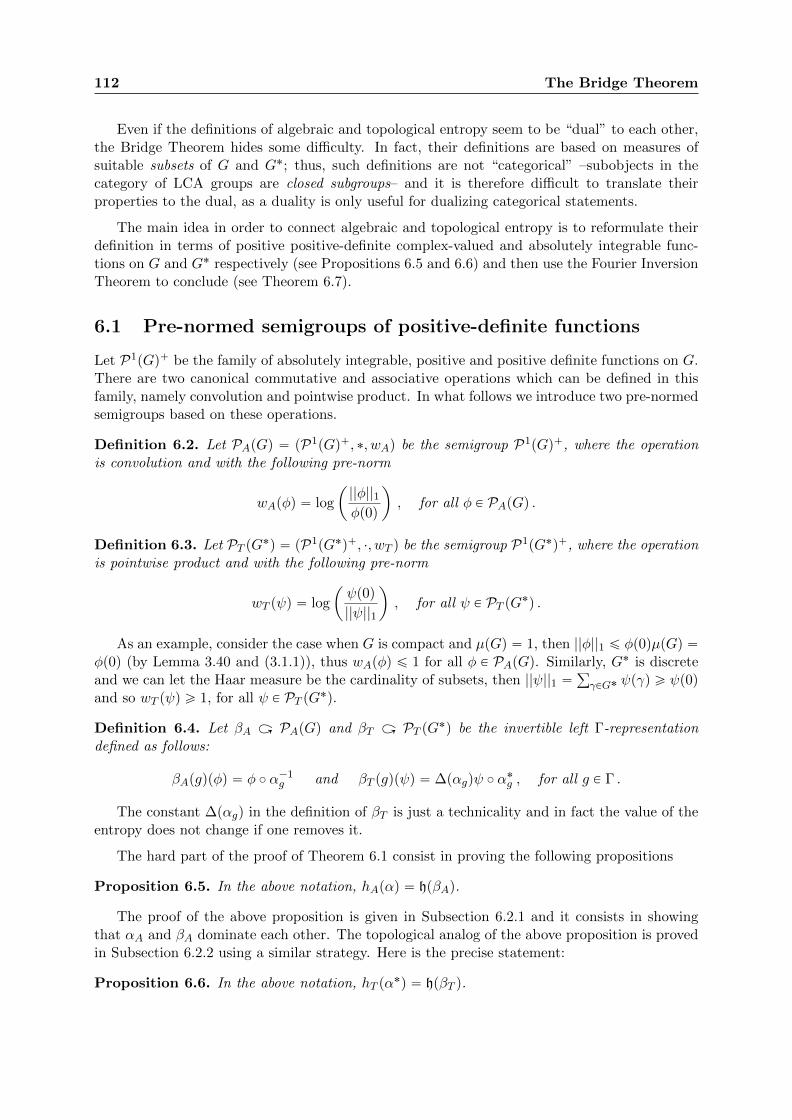
112 The Bridge Theorem
Even if the definitions of algebraic and topological entropy seem to be “dual” to each other,the Bridge Theorem hides some difficulty. In fact, their definitions are based on measures ofsuitable subsets of G and G˚; thus, such definitions are not “categorical” –subobjects in thecategory of LCA groups are closed subgroups– and it is therefore difficult to translate theirproperties to the dual, as a duality is only useful for dualizing categorical statements.
The main idea in order to connect algebraic and topological entropy is to reformulate theirdefinition in terms of positive positive-definite complex-valued and absolutely integrable func-tions on G and G˚ respectively (see Propositions 6.5 and 6.6) and then use the Fourier InversionTheorem to conclude (see Theorem 6.7).
6.1 Pre-normed semigroups of positive-definite functions
Let P1pGq` be the family of absolutely integrable, positive and positive definite functions on G.There are two canonical commutative and associative operations which can be defined in thisfamily, namely convolution and pointwise product. In what follows we introduce two pre-normedsemigroups based on these operations.
Definition 6.2. Let PApGq “ pP1pGq`, ˚, wAq be the semigroup P1pGq`, where the operationis convolution and with the following pre-norm
wApφq “ log
ˆ
||φ||1φp0q
˙
, for all φ P PApGq .
Definition 6.3. Let PT pG˚q “ pP1pG˚q`, ¨, wT q be the semigroup P1pG˚q`, where the operationis pointwise product and with the following pre-norm
wT pψq “ log
ˆ
ψp0q
||ψ||1
˙
, for all ψ P PT pG˚q .
As an example, consider the case when G is compact and µpGq “ 1, then ||φ||1 ď φp0qµpGq “φp0q (by Lemma 3.40 and (3.1.1)), thus wApφq ď 1 for all φ P PApGq. Similarly, G˚ is discreteand we can let the Haar measure be the cardinality of subsets, then ||ψ||1 “
ř
γPG˚ ψpγq ě ψp0qand so wT pψq ě 1, for all ψ P PT pG˚q.
Definition 6.4. Let βA ü PApGq and βT ü PT pG˚q be the invertible left Γ-representationdefined as follows:
βApgqpφq “ φ ˝ α´1g and βT pgqpψq “ ∆pαgqψ ˝ α
˚g , for all g P Γ .
The constant ∆pαgq in the definition of βT is just a technicality and in fact the value of theentropy does not change if one removes it.
The hard part of the proof of Theorem 6.1 consist in proving the following propositions
Proposition 6.5. In the above notation, hApαq “ hpβAq.
The proof of the above proposition is given in Subsection 6.2.1 and it consists in showingthat αA and βA dominate each other. The topological analog of the above proposition is provedin Subsection 6.2.2 using a similar strategy. Here is the precise statement:
Proposition 6.6. In the above notation, hT pα˚q “ hpβT q.
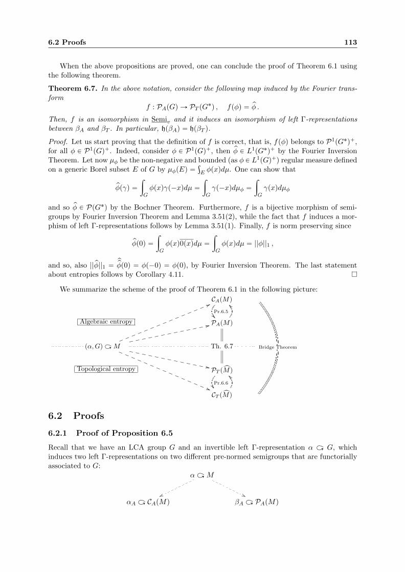
6.2 Proofs 113
When the above propositions are proved, one can conclude the proof of Theorem 6.1 usingthe following theorem.
Theorem 6.7. In the above notation, consider the following map induced by the Fourier trans-form
f : PApGq Ñ PT pG˚q , fpφq “ pφ .
Then, f is an isomorphism in Semiv and it induces an isomorphism of left Γ-representationsbetween βA and βT . In particular, hpβAq “ hpβT q.
Proof. Let us start proving that the definition of f is correct, that is, fpφq belongs to P1pG˚q`,for all φ P P1pGq`. Indeed, consider φ P P1pGq`, then pφ P L1pG˚q` by the Fourier InversionTheorem. Let now µφ be the non-negative and bounded (as φ P L1pGq`) regular measure definedon a generic Borel subset E of G by µφpEq “
ş
E φpxqdµ. One can show that
pφpγq “
ż
Gφpxqγp´xqdµ “
ż
Gγp´xqdµφ “
ż
Gγpxqdµφ
and so pφ P PpG˚q by the Bochner Theorem. Furthermore, f is a bijective morphism of semi-groups by Fourier Inversion Theorem and Lemma 3.51(2), while the fact that f induces a mor-phism of left Γ-representations follows by Lemma 3.51(1). Finally, f is norm preserving since
pφp0q “
ż
Gφpxq0pxqdµ “
ż
Gφpxqdµ “ ||φ||1 ,
and so, also ||pφ||1 “p
pφp0q “ φp´0q “ φp0q, by Fourier Inversion Theorem. The last statementabout entropies follows by Corollary 4.11.
We summarize the scheme of the proof of Theorem 6.1 in the following picture:
CApMq
Pr.6.5��
Bridge Theorem
Algebraic entropy PApMq
^^
pα,Gq ü M
66lllllllllllllll
22fffffffffffff
,,XXXXXXXXXXXXX
((RRRRRRRRRRRRRRRTh. 6.7
Topological entropy PT pxMq
Pr.6.6��CT pxMq
^^
6.2 Proofs
6.2.1 Proof of Proposition 6.5
Recall that we have an LCA group G and an invertible left Γ-representation α ü G, whichinduces two left Γ-representations on two different pre-normed semigroups that are functoriallyassociated to G:
α ü M
ww ''αA ü CApMq βA ü PApMq
114 The Bridge Theorem
We have to show that the entropy of the two induced representations is the same. We startproving that αA is dominated by βA. Roughly speaking this says that the way in which α actson compact neighborhoods is controlled by the action on positive-definite complex functions.This, by Proposition 4.13, implies the inequality “ď” in Proposition 6.5.
Lemma 6.8. In the above notation, βA dominates αA.
Proof. Let C P CApGq and F P FpΓq; for all n P N we construct φn P PApGq and εn P R` suchthat
vApTF pαA, Cqq ď wApTF pβA, φnqq ` 2|F | log pεnq and limnÑ8
εn “ 1 . (6.2.1)
Indeed, let D1 be an open neighborhood of 0 contained in C; by the compactness of C thereexist x1, . . . , xh P G such that C Ď px1 `D1q Y ¨ ¨ ¨ Y pxh `D1q “ D. One can verify that D isan open neighborhood of 0 in G with compact closure. For all K Ď G and n P N`, let
Kpnq “ tk1 ` . . .` kn : k1, . . . , kn P Ku .
We let
εn “µ`
Dpn`1q˘
µ`
Dpnq˘ and φn “ χDpnq ˚ χDpnq ;
thus, to conclude we have just to verify (6.2.1). In particular, the fact that limnÑ8 εn “ 1follows by [39, Corollary 1.2] and so we have just to compute the value of wApTF pβA, φnqq.For all x P TF
`
αA, Dp2q˘
there exist xf and x1f P αApfqpDp2qq for all f P F such that x “
ř
fPF pxf ` x1f q and so, letting ∆pαF q “
ś
fPF ∆pαpfqq,
TF pβA, φn`1q pxq “ TF pβA, φn`1qx p0q “æ
fPF
pβA pfq pφn`1qqxf`x1fp0q
“ ∆ pαF qæ
fPF
´
χαApfqpDpn`1qq
¯
xf˚
´
χαApfqpDpn`1qq
¯
x1f
p0q (6.2.2)
ě ∆ pαF qæ
fPF
´
χαApfqpDpnqq ˚ χαApfqpDpnqq
¯
p0q “ TF pβA, φnq p0q ;
where the first line follows by Remark 3.38, the equality in the second line comes from Lemma3.43 and Remark 3.38, and the inequality in the third line follows since pχαApfqpDpn`1qqqy ě
χαApfqpDpnqq, for all y P αApfqpCq. Using (6.2.2) and (3.1.1) we get
||TF pβA, φn`1q||1 ě
ż
TF pαA,Dp2qqTF pβA, φn`1qpxqdµ ě µpTF pαA, D
p2qqq ¨ TF pβA, φnqp0q .
Furthermore, by Lemmas 3.37(4) and 3.43,
||TF pβA, φnq||1 “ź
fPF
||βApfqpφnq||1 “ ∆pαF qµpCpnqq2|F | .
Putting together all the above estimates, one can conclude as follows:
vApTF pαA, Cqq ď logµpTF pαA, Dp2qqq ď log
ˆ
||TF pβA, φnq||1TF pβA, φnqp0q
˙
`
ˆ
log||TF pβA, φn`1q||1
||TF pβA, φnq||1
˙
“ wApTF pβA, φnqq ` 2|F | log
˜
∆pαF qµpDpn`1qq
∆pαF qµpDpnqq
¸
“ wApTF pβA, φnqq ` 2|F | logpεnq .
6.2 Proofs 115
We can now conclude the proof of Proposition 6.5 showing the converse inequality.
Lemma 6.9. In the above notation, αA dominates βA.
Proof. Let φ P PApGq and F P FpΓq; for all n P N` we construct a ψn P PApGq with compactsupport such that
wApTF pβA, φqq ď wApTF pβA, ψnqq ` 2|F | logp1` 1{nq . (6.2.3)
After that we let Dn “ supppψnq P CApGq and we verify that wApTF pβA, ψnqq ď vApTF pαA, Dnqq,so that
wApTF pβA, φqq ď vApTF pαA, Dnqq ` 2|F | logp1` 1{nq , (6.2.4)
concluding the proof. Let us start with our program: we define φ1 “ 1||φ||1
φ. Notice that
||φ1||1 “ 1 and
wApTF pαA, φ1qq “ log
ˆ
||TF pβA, φ1q||1
TF pβA, φ1qp0q
˙
“ log
˜
||φ||´|F |1 ¨ ||TF pβA, φq||1
||φ||´|F |1 ¨ TF pβA, φqp0q
¸
“ wApTF pβA, φqq .
Now let ψ “ φ1 ˚φ1 and notice that ψ P PApGq (φ1 “ rφ1 by Lemma 3.40, now apply Lemma 3.41)and ||ψ||1 “ 1. Furthermore,
TF pβA, ψqp0q “
ż
GTF pβA, φ
1qpxq ¨ TF pβA, φ1qp´xqdµ ď TF pβA, φ
1qp0q ¨ ||TF pβA, φ1q||1
and, by Lemma 3.37(4), ||TF pβA, ψq||1 “ ||TF pβA, φ1q||21, thus
wApTF pβA, ψqq ě log
ˆ
||TF pβA, φ1q||21
TF pβA, φ1qp0q||TF pβA, φ1q||1
˙
“ wApTF pβA, φ1qq “ wApTF pβA, φqq .
For all n P N there exists a compact symmetric neighborhood Cn P CApGq such that φn “ φ1 ¨χCnsatisfies ||φ1´φn||1 ă 1{p2nq. We let ψn “ φn ˚φn P PApGq (φn “ Ăφn and so one can use Lemma3.41). Furthermore, using Lemma 3.37 and the fact that ||φn||1 ď ||φ
1||1 “ 1, we get
1´ ||ψn||1 “ ||ψ||1 ´ ||ψn||3.34ď ||ψ ´ ψn||1 ď ||ψ ´ φ
1 ˚ φn||1 ` ||φ1 ˚ φn ´ ψn||1 (6.2.5)
ď ||φ1||1||φ1 ´ φn||1 ` ||φn||1||φ
1 ´ φn||1ď2||φ1 ´ φn||1 ă 1{n .
Notice also that ||TF pβA, ψq||1 “ś
fPF ||βApfqpψq||1 “ ∆pαF q||φ1||2|F |1 “ ∆pαF q by Lemma 3.37
and (3.31). Similarly, ||TF pβA, ψnq||1 “ ∆pαF q||ψn|||F |1 . Furthermore, by construction φn ď φ1,
thus ψn ď ψ and, more generally, βApgqpψnq ď βApgqpψq for all g P Γ and so TF pβA, ψnqp0q ďTF pβA, ψqp0q. Putting together all the above computations, we can verify (6.2.3):
wApTF pβA, φqq ď wApTF pβA, ψqq “ log
ˆ
||TF pβA, ψnq||1TF pβA, ψqp0q
¨||TF pβA, ψq||1||TF pβA, ψnq||1
˙
ď wApTF pβA, ψnqq ` log
˜
∆pαF q||ψ|||F |1
∆pαF q
¸
(6.2.5)ď wApTF pβA, ψnqq ` |F | log p1` 1{nq
116 The Bridge Theorem
As we said, to conclude we have just to verify that wApTF pβA, ψnqq ď vApTF pαA, Dnqq, whereDn “ supppψnq P CApGq. Indeed, let χ “ χTF pαn,Dnq and notice that, by Lemma 3.37,supppTF pβA, ψnqq Ď TF pβA, Dnq. Thus,
pχ ˚ TF pβA, ψnqqp0q “
ż
Gχpxq ¨ TF pβA, ψnqp´xqdµ
“
ż
GTF pβA, ψnqpxqdµ “ ||TF pβA, ψnq||1 .
The conclusion now follows by Lemma 3.40 and (3.1.1) as in the following computation
0 “ logppχ ˚ TF pβA, ψnqqp0qq ´ logp||TF pβA, ψnq||1
“ log
ˆż
Gχpxq ¨ TF pβA, ψnqp´xqdµ
˙
´ log p||TF pβA, ψnq||1q
“ log
˜
ż
TF pαA,DnqTF pβA, ψnqp´xqdµ
¸
´ log p||TF pβA, ψnq||1q
ď logpµpTF pαA, Dnqq ¨ TF pβA, ψnqp0qq ´ log p||TF pβA, ψnq||1q
“ vApTF pαA, Dnqq ´ wApTF pβA, ψnqq .
6.2.2 Proof of Proposition 6.6
Let us rapidly recall the situation. We have an LCA groupG˚ and invertible right Γ-representationα˚ ü G˚, which induces two left Γ-representations on two different pre-normed semigroups thatare functorially associated to G˚:
α˚ ü G˚
ww ((αT ü CT pG˚q βT ü PT pG˚q
We have to show that the entropy of the two representations is the same. We divide the proofin two lemmas. We start proving that αT dominates βT . Roughly speaking this says that theway in which α˚ acts on positive-definte complex functions on G˚ is controlled by the actionon compact neighborhoods. This implies the inequality “ď” in Proposition 6.6, by Proposition4.13.
Lemma 6.10. In the above notation, αT dominates βT .
Proof. Let us consider F P s and φ P PT pG˚q. We will show that, for all n P N`, there exists acompact neighborhood Vn such that
wT pTF pβT , φqq ď vT pTF pαT , Vnqq ` |F | logppn` 1q{nq . (6.2.6)
In fact, letting εn “ nφp0q{pn` 1q, any compact neighborhood Vn P CT pGq contained in
V pφ, nq “!
f P xM : φpfq ě εn
)
,
will work. To see this, one can verify that αT pgqpVnq Ď V pβT pgqpφq, nq and so
βT pgqpφq ě εn ¨ χαT pgqpVnq , @ g P Γ .
6.2 Proofs 117
In particular, TF pβT , φq “ś
gPF βT pgqpφq ěś
gPF εn ¨ χαT pgqpVnq “ ε|F |n ¨ χTF pαT ,Vnq, where the
last equality just follows noticing that the pointwise product of characteristic functions is thecharacteristic function of the intersection. We obtain that
ε´|F |n ¨ ||TF pβT , φq||1 ě ||TF pβT , χVnq||1 “ µpTF pαT , Vnqq .
Taking logarithms one can derive (6.2.6).
We can now conclude the proof of Proposition 6.6 showing the converse inequality.
Lemma 6.11. In the above notation, βT dominates αT .
Proof. Given U P CT pG˚q, we can find a function φ P PT pG˚q such that φp0q “ 1 and supppφq ĎU , by Lemma 3.45. By Lemma 3.40, φp0q “ 1 is a maximum for φ, thus φ ď χU . Similarly,βT pgqpφq ď βT pgqpχU q for all g P Γ.For all F P s we obtain the following inequality ||TF pβT , φq||1 ď ||TF pβT , χU q||1 “ µpTF pαT , Uqq.To conclude notice that TF pβT , φqp0q “ φp0q|F | “ 1 and so wT pTF pβT , φqq ě vT pTF pαT , Uqq.
118 The Bridge Theorem
Part III
Length functions
119

Chapter 7
Length functions in Grothendieckcategories
7.1 A Structure Theorem for length functions
7.1.1 Length functions
In any category C it is possible to define real-valued invariants in order to measure variousfiniteness properties of the objects. In general, we call invariant of C, any map i : ObpCq ÑRě0 Y t8u such that ipXq “ ipX 1q whenever X and X 1 are isomorphic objects in C.
If we make some stronger assumption on the structure of the category C, we can refine ourdefinition of invariant in order to obtain a more treatable notion. Indeed, suppose that C is anAbelian category. In this setting it seems natural to ask that, given a short exact sequence
0 Ñ X1 Ñ X2 Ñ X3 Ñ 0 (7.1.1)
in C, ipX2q “ ipX1q ` ipX3q. In this case, we say that i is additive on the sequence (7.1.1). If iis additive on all the short exact sequences of C and ip0q “ 0, then we say that i is an additiveinvariant (or additive function).In the following lemma we collect some useful properties of additive functions.
Lemma 7.1. Let C be an Abelian category and let i : ObpCq Ñ Rě0 Y t8u be an additivefunction. Then,
(1) ipXq ě ipY q for every segment Y of X P ObpCq;
(2) ipX1`X2q` ipX1XX2q “ ipX1q` ipX2q for every pair of sub-objects X1, X2 of X P ObpCq;
(3)ř
jodd ipXjq “ř
jeven ipXjq for every exact sequence 0 Ñ X1 Ñ X2 Ñ ¨ ¨ ¨ Ñ Xn Ñ 0 in C.
A natural assumption in the context of Grothendieck categories is the upper continuity ofinvariants: given an object X P C and a directed set S “ tXα : α P Λu of sub-objects of X suchthat
ř
ΛXα “ X, we say that i is continuous on S if
ipXq “ suptipXαq : α P Λu . (7.1.2)
If i is continuous on all the directed systems of subobjects of the objects of C, we say that i isupper continuous. Obviously, upper continuity can be defined in arbitrary Abelian categorieseven if it seems more meaningful when all directed colimits exist and are exact.
121
122 Length functions in Grothendieck categories
Definition 7.2. Let C be an Abelian category. An additive and upper continuous invarianti : ObpCq Ñ Rě0 Y t8u is said to be a length function.
In what follows we generally denote length functions by the symbol L.
Definition 7.3. Let C be a Grothendieck category. An object X P ObpCq is finitely generated(resp., Noetherian) if and only if its qframe of subobjects LpXq is compact (resp., Noetherian).Furthermore, a category C is locally finitely generated (resp,. locally Noetherian) if there existsa set F of generators of C such that each G P F is finitely generated (resp,. Noetherian).
Given a ring R, the category R-Mod is locally finitely generated (here RR is a finitelygenerated generator), while R-Mod is locally Noetherian if and only if R is a Noetherian ring.
The usual definition of length function is given in module categories, which are in particularlocally finitely generated Grothendieck categories. In this special setting, the usual definition ofupper continuity is different (see part (3) of the following proposition). We now show that weare not defining a new notion of upper continuity but just generalizing this concept to arbitraryGrothendieck categories (similar observations, with analogous proofs, were already present in[98] for module categories).
Proposition 7.4. Let C be a Grothendieck category and L : C Ñ Rě0 Y t8u be an additivefunction. Consider the following statements:
(1) L is a length function;
(2) given an object M P ObpCq, an ordinal κ and a continuous chain tMα : α ă κu of sub-objectsof M such that M “
ř
αăκMα, LpMq “ suptLpMαq : α ă κu;
(3) for every object M P ObpCq, LpMq “ suptLpF q : F finitely generated sub-object of Mu.
Then (1)ô(2) and (2)ð(3). If C is locally finitely generated, then the above statements are allequivalent.
Proof. (1)ñ(2) is trivial since continuous chains are directed posets. On the other hand, considera directed poset pI,ďq and a direct system tMi : i P Iu of sub-objects of M . If I is finite thenI has a maximum, so there is nothing to prove. On the other hand, if I is an infinite set, oneshows as in the proof of [47, Lemma 1.2.10], that pI,ďq is the union of a continuous well-orderedchain of directed subsets, each of which has strictly smaller cardinality than I. One concludesby transfinite induction that (2)ñ(1).Assume now (3) and consider a continuous chain as in part (2). For every finitely generatedsub-object F of X, there exists α ă κ such that F ďMα and so we obtain that
LpMq “ suptLpF q : F f.g. sub-object of Mu ď suptLpMαq : α ă κu ď LpMq .
To conclude, notice that if C is locally finitely generated, then any object is the direct union ofthe direct system of its finitely generated sub-objects. In this situation, (1) implies (3).
The notion of length function on a Grothendieck category is quite formal, this is why it seemsuseful to stop for a while and describe some concrete examples of length functions.
Example 7.5. The logarithm of the cardinality log |´| : Z-Mod Ñ Rě0Yt8u, where log |G| “ 8whenever G is not finite, is a length function.
7.1 A Structure Theorem for length functions 123
Example 7.6. Given a skew field K, the dimension dim : ObpK-Modq Ñ Rě0Yt8u is a lengthfunction. More generally, given a left Ore domain D, the rank of a left D-module DM is definedas rkpDMq “ dimpΣ´1D bDMq. This gives a length function rk : ObpD-Modq Ñ Rě0 Y t8u.
Example 7.7. Let C be a Grothendieck category. Then, the composition length ` : ObpCq ÑRě0 Y t8u, defined by `pMq “ `pLpMqq, is a length function.
Other examples can be obtained lifting a known length function along a localization functor asshown in Section 7.1.2. Another strategy to produce new examples is that of “linearly combining”some known length functions:
Definition 7.8. (1) Given a length function L of C and λ P Rě0Yt8u, we consider the function
λL : ObpCq Ñ Rě0 Y t8u such that λLpMq “ λ ¨ pLpMqq , @M P ObpCq ,
with the convention that 8 ¨ 0 “ 0 ¨ 8 “ 0;
(2) given a set I and additive functions Li of C for all i P I, we consider the function
ÿ
iPI
Li : ObpCq Ñ Rě0 Y t8u such thatÿ
iPI
LipMq “ sup
#
ÿ
iPF
LipMq : F Ď I finite
+
,
for all M P ObpCq.
It is an exercise to prove that the sum of length functions and the multiplication of a lengthfunction by a constant are again length functions.
7.1.2 Operations on length functions
Let C be a Grothendieck category and let τ “ pT ,Fq be a torsion theory on C. In this sectionwe are going to show how the length functions of C are related with the ones of T and C{T .
Proposition 7.9. In the above notation, there is a bijective correspondence
f : tlength functions L of C with T Ď KerpLqu//tlength functions of C{T u : goo .
Proof. The maps f and g are defined in Lemmas 7.10 and 7.11 respectively. It follows by thedefinitions that they are inverse each other.
Lemma 7.10. If Lτ : ObpC{T q Ñ Rě0 Y t8u is a length function, then there exists a uniquelength function L : ObpCq Ñ Rě0 Y t8u such that LpMq “ Lτ pQτ pMqq for all M P ObpCq.Furthermore, T Ď KerpLq. We set gpLτ q “ L.
Proof. Existence follows by the fact that Qτ is an exact functor that preserves colimits. Unique-ness is clear and the last statement comes from the fact that T “ KerpQτ q.
Lemma 7.11. If L : ObpCq Ñ Rě0Yt8u is a length function such that T Ď KerpLq, then thereexists a unique length function Lτ : ObpC{T q Ñ Rě0 Y t8u such that LpMq “ Lτ pQτ pMqq forall M P ObpCq. We set fpLq “ Lτ .

124 Length functions in Grothendieck categories
Proof. For all M P ObpCq, there is an exact sequence of the form 0 Ñ T1 ÑM Ñ SτQτ pMq ÑT2 Ñ 0, with T1, T2 P T . As by hypothesis L is trivial on τ -torsion objects, we obtain byadditivity that LpMq “ LpSτQτ pMqq. Using this simple observation, we can define
Lτ pNq “ LpSτ pNqq, for all N P ObpC{T q ,
and verify that LpMq “ LpSτQτ pMqq “ Lτ pQτ pMqq as desired. The uniqueness statementfollows by the fact that the functor Qτ is essentially surjective. It remains to verify that Lτ is alength function. Indeed, let 0 Ñ N ÑM ÑM{N Ñ 0 be a short exact sequence in C{T . Thisinduces an exact sequence 0 Ñ Sτ pNq Ñ Sτ pMq Ñ Sτ pM{Nq Ñ T Ñ 0, with T P T . Hence,Lτ pMq “ LpSτ pMqq “ LpSτ pNqq ` LpSτ pM{Nqq ` 0 “ Lτ pNq ` Lτ pM{Nq. The proof that Lis upper continuous follows by a similar argument and transfinite induction.
In the first part of this subsection we described how to transfer length functions along theadjoint pair Qτ : C Õ C{T : Sτ ; now we turn our attention to the adjunction Tτ : C Õ T : inc.In particular, whenever L is a length function on C, one can define its restriction to T asLæT : T Ñ Rě0 Y t8u, such that LæT pMq “ LpMq for all M P C, and prove that it is a lengthfunction. Notice that this can be applied to any full abelian subcategory T of C, not only tohereditary torsion classes.
On the other hand, if we start with a length function L on T , we want to find a canonicalway to extend it to the bigger category C. In [98] (see also [97]) Peter Vamos introduced atechnique to extend length functions which works in a more general setting. Indeed, let T bea Serre subclass of C and consider a length function L on T . We start defining an invariant(which is not supposed to have any good property but that of being useful for our constructions)L˚ : ObpCq Ñ Rě0 Y t8u as follows:
L˚pXq “
#
LpXq if X P T ;
0 otherwise.(7.1.3)
Given an object M P ObpCq and a series σ : 0 “ N0 Ď N1 Ď ¨ ¨ ¨ Ď Nn “M of M , we let
pLpσq “ÿ
iďn
L˚pNi{Ni´1q .
Definition 7.12. In the above notation, the Vamos extension pL : ObpCq Ñ Rě0 Y t8u of L toC is the function defined by pLpXq “ suptpLpσq : σ ranging over all the finite series of Xu.
In the next proposition we verify that pL satisfies the axioms of a length function.
Proposition 7.13. Let T be a Serre subclass of a Grothendieck category C. If L : T Ñ Rě0Yt8u
is a length function, then pL : ObpCq Ñ Rě0 Y t8u is a length function. Furthermore, if L1 :ObpCq Ñ Rě0 Y t8u is any additive function extending L, then L1pMq ď LpMq for all M P C.
Proof. We start by proving additivity. Let 0 // Aι // B
π // C // 0 be a short exactsequence in C. Consider two series
σA : 0 Ď A0 Ď ¨ ¨ ¨ Ď An “ A , σC : 0 Ď C0 Ď ¨ ¨ ¨ Ď Cm “ C .
For all i “ 0, . . . ,m, let Bi “ π´1pCiq, this defines a series of B
σB : 0 Ď ιpA0q Ď ¨ ¨ ¨ Ď ιpAnq Ď B0 Ď ¨ ¨ ¨ Ď Bm “ B .
7.1 A Structure Theorem for length functions 125
Clearly, pLpσBq “ pLpσAq ` pLpσCq, proving that pLpBq ě pLpAq ` pLpCq. On the other hand, givena series σB : 0 Ď B0 Ď ¨ ¨ ¨ Ď Bn “ B, we let, for all i “ 1, . . . , n, Ai “ ι´1pBiq and Ci “ πpBiq.This defines two series
σA : 0 Ď A0 Ď ¨ ¨ ¨ Ď An “ A , σC : 0 Ď C0 Ď ¨ ¨ ¨ Ď Cn “ C .
Furthermore, there are short exact sequences 0 Ñ Ai{Ai´1 Ñ Bi{Bi´1 Ñ Ci{Ci´1 Ñ 0. Usingthe additivity of L˚ on T and the closure properties of T , pLpσAq ` pLpσCq ě pLpσBq, whichimplies that pLpBq ď pLpAq ` pLpCq. It remains to prove upper continuity. Indeed, let M P Cand consider a directed set tMα : α P Λu of sub-objects such that
ř
ΛMα “ M . By additivity,pLpMq ě supΛ
pLpMαq. On the other hand, given a series σ : 0 “ N0 Ĺ N1 Ĺ ¨ ¨ ¨ Ĺ Nn “M , weprove by induction on n P N` that pLpσq ď supΛ
pLpMαq. We distinguish two cases:
(1) if pLpσq “ 8, then there exists a non-negative integer m ă n such that Nm`1{Nm P T andLpNm`1{Nmq “ 8. Notice also that Nm`1{Nm “
ř
ΛppMα XNm`1q `Nmq{Nm and so,
supΛ
pLpMαq ě supΛ
pL
ˆ
pMα XNm`1q `Nm
Nm
˙
“ supΛL
ˆ
pMα XNm`1q `Nm
Nm
˙
“ LpNm`1{Nmq “ 8 ,
where the first inequality comes by additivity of pL and the following equalities come by thefact that pL coincides with L on T .
(2) Suppose now that pLpσq ă 8. If n “ 1, then either pLpσq “ 0 and there is nothing to prove,or 0 ă pLpσq “ L˚pMq, but in this case M P T and the thesis follows by the fact that L is alength function on T . On the other hand, if n ą 1, let
σ1 : 0 “ N0 Ĺ N1 Ĺ ¨ ¨ ¨ Ĺ Nn´1 , and σ2 : 0 Ĺ Nn{Nn´1 ,
and notice that pLpσq “ pLpσ1q ` pLpσ2q. Furthermore, Nn´1 “ř
ΛpNn´1 X Mαq and
Nn{Nn´1 “ř
ΛpMα ` Nn´1q{Nn´1. By inductive hypothesis pLpσ1q ď supΛpLpNn´1 XMαq
and pLpσ2q ď supΛpLppMα `Nn´1q{Nn´1q. Hence,
pLpσq “ pLpσ1q ` pLpσ2q ď supΛ
pLpNn´1 XMαq ` supΛ
pLppMα `Nn´1q{Nn´1q “ supΛ
pLpMαq ,
where the last equality comes from the additivity of pL and the fact that the sum of supremaof two convergent nets is the supremum of the sum of the two nets.
We conclude this section proving that Vamos extension and lifting of length functions via alocalization functor preserve linear combinations.
Lemma 7.14. Let T be a Serre subclass of a Grothendieck category C, let Λ be a set and chooseλpαq P Rě0 Y t8u for all α P Λ.
(1) Given length functions Lα : T Ñ Rě0 Y t8u for all α P Λ and letting L “ř
Λ λpαqLα,pL “
ř
Λ λpαqxLα.
(2) If T is closed under direct limits, Lα : ObpC{T q Ñ Rě0 Y t8u are length functions for allα P Λ and L “
ř
Λ λpαqLα, then gpLq “ř
Λ λpαqgpLαq, where g is defined in Lemma 7.10.
126 Length functions in Grothendieck categories
Proof. (1) By the minimality of Vamos extension proved in Proposition 7.13, pL ďř
Λ λpαqxLα.
On the other hand, if M P ObpCq and pLpMq “ 8, then 8 “ pLpMq ďř
Λ λpαqxLαpMq and there
is nothing to prove. It remains to show that, if pLpMq ă 8, then pLpMq ěř
Λ λpαqxLαpMq. The
case |Λ| ă 8 is essentially an application of Lemma 2.18. Suppose now that Λ is not finiteand let LF “
ř
αPF λpαqLα for every non-empty finite subset F Ď Λ; by definition LpMq “
suptLF pMq : F Ď Λ finiteu. By the first part of the proof, xLF “ř
αPF λpαqxLα, so we have only
to prove that pLpMq ě suptxLF pMq : F Ď Λ finiteu for all M P ObpCq. This follows noticing thatxLF pσq ď pLpσq for any finite F Ď Λ and any series σ of M .
(2) follows by definition of the map g.
7.1.3 The classification in the semi-Artinian case
All along this subsection we denote by C a semi-Artinian Grothendieck category, that is, aGabriel category whose Gabriel dimension is 1. Notice that this is equivalent to say that anyobject in C is the union of its socle series. The main result of this subsection is to give a structuretheorem for all the length functions in C.
Lemma 7.15. Let C be a semi-Artinian Grothendieck category and let L,L1 : C Ñ Rě0 Y t8u
be two length functions. Then L “ L1 if and only if their values on simple objects are the same.
Proof. One implication is trivial, so suppose that L and L1 coincide on simple objects. Consideran object M P C and write it as the union of a continuous chain
0 “ N0 ď N1 ď ¨ ¨ ¨ ď Nα ď ¨ ¨ ¨ ďď
α
Nα “M ,
such that Ni`1{Ni is a simple object for all i (this can be done since M is the union of its socleseries). By hypothesis LpNi`1{Niq “ L1pNi`1{Niq for all i. The conclusion follows by transfiniteinduction using additivity and upper continuity.
Definition 7.16. Let C be a semi-Artinian Grothendieck category and let π “ pT ,Fq P SppCq.We let `π : ObpCq Ñ Rě0 Y t8u be the length function such that
`πpMq “ `pQπpMqq such that @M P ObpCq .
That is, `π is the lifting of the composition length ` : ObpC{T q Ñ Rě0Yt8u along the localizationfunctor Qπ : C Ñ C{T . The functions of the form `π with π P SppCq are called atomic lengthfunction.
Lemma 7.17. Let C be a semi-Artinian Grothendieck category, let π “ pT ,Fq P SppCq, let Cpπqbe the socle of Epπq (which is a simple object) and let C be a simple object. Then,
`πpCq “
#
1 if C – Cpπq;
`πpCq “ 0 otherwise.
Proof. By definition of `π, it is clear that `πpCq “ 1 if and only if C R T and that `πpCq “ 0otherwise. So let us prove that C R T if and only if C – Cpπq. Indeed, if there is anisomorphism C Ñ Cpπq one takes the composition with the inclusion Cpπq Ñ Epπq to getHomCpC,Epπqq ‰ 0, so C R T . On the other hand, suppose HomCpC,Epπqq ‰ 0, thenHomCpC,Cpπqq “ HomCpC,SocpEpπqqq ‰ 0 and, since any non-trivial morphism between twosimple objects is an isomorphism, C – Cpπq.
7.1 A Structure Theorem for length functions 127
In the following theorem we prove that any length function in C is a linear combination ofatomic length functions.
Theorem 7.18. Let C be a semi-Artinian Grothendieck category and let L : ObpCq Ñ Rě0Yt8u
be a length function. Then,
L “ÿ
πPSppCq
λpπq ¨ `π ,
where λpπq “ LpCpπqq, with Cpπq “ SocpEpπqq for all π P SppCq. Furthermore, the constantsλpπq are uniquely determined by L.
Proof. Let L1 “ř
πPSppCq λpπq ¨ `π; we already mentioned that a linear combination of length
functions is a length function, so L1 is a length function. By Lemma 7.17, `πpCpπ1qq “ 0 for all
π1 ‰ π, so L1pCpπqq “ λpπq`πpCpπqq “ LpCpπqq for all π P SppCq, which shows that L “ L1, byLemma 7.15. The proof of the uniqueness statement is analogous.
Using the uniqueness of the above decomposition, we can unambiguously give the followingdefinition:
Definition 7.19. Let C be a semi-Artinian Grothendieck category and let L : ObpCq Ñ Rě0 Y
t8u be a length function. The support of L is SupppLq “ tπ P SppCq : λpπq ‰ 0u.
As an immediate consequences of the above theorem we obtain the following corollaries.
Corollary 7.20. Let C be a semi-Artinian Grothendieck category such that |SupppCq| “ 1.Then, any length function L : ObpCq Ñ Rě0 Y t8u is a multiple of the composition length.
Corollary 7.21. Let D be a left Ore domain and denote by T Ď D-Mod the class of torsion leftD-modules. The following are equivalent for a non-trivial length function L : ObpD-Modq ÑRě0 Y t8u:
(1) T Ď KerpLq;
(2) there exists α P Rě0 Y t8u such that L “ α ¨ rk (see Example 7.6).
Furthermore, if LpDq ă 8 then the above equivalent conditions hold and α “ LpDq in (2).
Proof. The implication (2)ñ(1) is trivial, in fact Kerprkq “ T . Let us prove that (1)ñ(2). ByTheorem 7.9, L is the lifting of a length function on D-Mod{T – Q-Mod, where Q is the skewfield of left fractions of D. Clearly, Q-Mod satisfies the hypotheses of the above corollary, thusthere exists α P Rě0 Y t8u such that L “ gpα ¨ dimQq “ α ¨ gpdimQq “ α ¨ rk.For the last statement, we suppose LpDq ă 8 and we verify (1). Let M be a torsion leftD-module. Using upper continuity and additivity we can prove that LpMq “ 0 if and only ifLpDxq “ 0 for all x P M . Thus, let x P M be a non-trivial element and consider the followingexact sequences
0 Ñ AnnDpxq Ñ D Ñ DxÑ 0 and 0 Ñ D Ñ AnnDpxq ,
where the second sequence exists as AnnDpxq is a non-trivial left ideal of D (as M is torsion)and D is a domain. This shows that LpDq “ LpDxq ` LpAnnDpxqq ě LpDxq ` LpDq; thusLpDxq ď LpDq ´ LpDq “ 0. Finally, LpDq “ α ¨ rkpDq “ α.
128 Length functions in Grothendieck categories
7.1.4 The main structure theorem
The main result of this subsection is to show that, analogously to the semi-Artinian case, anylength function on a Gabriel category C can be written as a linear combination of atomic lengthfunctions. We start defining atomic length functions in this context.
Definition 7.22. Let C be a Gabriel category, let α ă G.dimpCq and let Cα`1 “ Cα`1{Cα. Then,Cα`1 is semi-Artinian and so, given π “ pT ,Fq P SppCα`1q “ SpαpCq, the length function`π : ObpCα`1q Ñ Rě0 Y t8u is defined, as in the previous subsection, to be the lifting of thecomposition length in Cα`1{T . Using Lemma 7.10 we can uniquely lift `π to a length functionon Cα`1 such that Cα Ď Kerp`πq and then, using Vamos extension, we extend it to a lengthfunction of C. Abusing notation, we denote this new function again by `π : ObpCq Ñ Rě0Yt8u.The functions of the form `π with π P SppCq are called atomic length function.
Notice that, by definition, given π P SpαpCq, Cα Ď Kerp`πq.
Definition 7.23. Let C be a Gabriel category and let L : ObpCq Ñ Rě0 Y t8u be a lengthfunction. An object M P ObpCq is L-finite if LpMq ă 8, we let FinpLq be the Serre class ofall the L-finite objects. Furthermore, we denote by FinpLq the minimal torsion class containingFinpLq.
Definition 7.24. Let C be a Gabriel category and let L : ObpCq Ñ Rě0 Y t8u be a lengthfunction. The finite component Lfin of L is the Vamos extension to C of the restriction of L toFinpLq, that is Lfin “ {LæFinpLq : ObpCq Ñ Rě0 Y t8u.The infinite component L8 of L is defined by
L8pMq “
#
0 if M P FinpLq;
8 otherwise.
We remark that the finite component Lfin can very well assume infinite values (if Lfin isnon-trivial, just take M such that LfinpMq ‰ 0, so Lfinp
À
NMq “ 8); anyway its name isjustified by the fact that Lfin is, by definition, determined by the finite values of L.
Lemma 7.25. Let C be a Gabriel category and let L : ObpCq Ñ Rě0Yt8u be a length function.Then, both the finite and the infinite component of L are length functions.
Proof. The fact that Lfin is a legnth function follows by Proposition 7.13. On the other hand,given a short exact sequence 0 Ñ N Ñ M Ñ M{N Ñ 0, M P FinpLq if and only if Nand M{N P FinpLq. Similarly, given an object M P C and a directed system of sub-objectstNi : i P Iu such that
ř
iPI Ni “ M , M P FinpLq if and only if Ni P FinpLq for all i P I. Thus,also L8 is a length function.
Notice that L “ Lfin`L8. This decomposition of L allows us to reduce the problem of findinga presentation of L as linear combination of atomic length functions to the same problem forL8 and Lfin.
Definition 7.26. Let C be a Gabriel category and let L : ObpCq Ñ Rě0 Y t8u be a lengthfunction. For all α ă G.dimpCq we let τLα “ pT L
α ,FLα q be the torsion theory in Cα`1{Cα such
that T Lα “ tQαpMq : M P FinpLqu. The infinite support of L is the following subset of the
spectrum
Supp8pLq “ď
αăκ
Supp8α pLq , where Supp8α pLq “ tπ P SpαpCq : Cpπq P FLα u .
7.1 A Structure Theorem for length functions 129
Notice that in Cα`1{Cα, T Lα “
Ş
πPSupp8αKerp`πq, to show this use the correspondences
described in Theorem 2.67 and the fact that torsion free classes are closed under taking injectiveenvelopes.
Proposition 7.27. Let C be a Gabriel category and let L : ObpCq Ñ Rě0 Y t8u be a lengthfunction. Then, L8 “
ř
πPSupp8pLq8 ¨ `π.
Proof. Let L1 “ř
πPSupp8pLq8 ¨ `π. Both L8 and L1 take values in t0,8u, thus they coincide if
and only if KerpL8q “ KerpL1q:
KerpL8q “ FinpLq “č
αăκ
tM P C : QαTα`1pMq P T Lα u “
č
πPSupp8pLq
Kerp`πq “ KerpL1q .
We can now turn our attention to the decomposition of Lfin.
Lemma 7.28. Let C be a Gabriel category and let L : ObpCq Ñ Rě0Yt8u be a length function.Then, there exists a unique family tLpαq : ObpCα`1q Ñ Rě0 Y t8u : α ă G.dimpCqu of lengthfunctions such that
(1) Lfin “ř
αăG.dimpCq Lα, where Lα : ObpCq Ñ Rě0 Y t8u is the Vamos extension of Lpαq;
(2) Cα Ď KerpLpαqq, for all α ă G.dimpCq.
Proof. For all α ď G.dimpCq we consider the Serre classes FinpαqpLq “ FinpLq X Cα and FinpLq.We start defining inductively length functions Lpαq : Finpα`1qpLq Ñ Rě0Yt8u, and their Vamosextensions Lα : FinpLq Ñ Rě0 Y t8u, for all α ă G.dimpCq:
– Lp0qpMq “ LpMq, for all M P Finp1qpLq;
– LpαqpMq “ LpMq ´ř
βăα LβpMq, for all M P Finpα`1qpLq and α ă G.dimpCq.
It is not difficult to verify by transfinite induction that all the Lpαq and Lα are length functions.Let us verify the following claims by induction on G.dimpCq:
(1’) LpMq “ř
αăG.dimpCq LαpMq, for all M P FinpLq;
(2’) FinpαqpLq Ď KerpLpαqq, for all α ă G.dimpCq.
If G.dimpCq “ 1 (i.e., C is semi-Artinian), then LpMq “ Lp0qpMq “ L0pMq for all M P
Finp1qpLq “ FinpLq, proving (1’), while (2’) is trivial since Finp0qpLq “ t0u.Suppose now that G.dimpCq is a limit ordinal. If M P FinpαqpLq for some α ă G.dimpCq, thenby inductive hypothesis, LpMq “
ř
βăα LβpMq and so LpαqpMq “ LpMq ´
ř
βăα LβpMq “ 0,
proving (2’). Furthermore, given M P FinpLq, we can write M “Ť
βăG.dimpCqpTβpMqq (seeLemma 2.56). Then,
LpMq “ supβăG.dimpCq
LpTβpMqq “ supβăG.dimpCq
$
&
%
ÿ
αďβ
LαpTβpMqq
,
.
-
“ supβăG.dimpCq
$
&
%
ÿ
αăG.dimpCq
LαpTβpMqq
,
.
-
“ÿ
αăG.dimpCq
LαpMq ,
130 Length functions in Grothendieck categories
where the first equality follows by the upper continuity of L, the second one follows by part(1’) of the inductive hypothesis (TβpMq P Cβ and G.dimpCβq “ β ă G.dimpCq), the third onefollows by the, already established, claim (2’), and the last equality uses the upper continuity ofř
αăG.dimpCq Lα.
Finally, if G.dimpCq “ κ`1 is a successor ordinal, andM P FinpκqpLq, then LpMq “ř
αăκ LαpMq
by inductive hypothesis and so LpκqpMq “ LpMq´ř
αăκ LαpMq “ 0, proving (2’). Furthermore,
for any M P FinpLq,
ÿ
αďκ
LαpMq “ÿ
αăκ
LαpMq ` LκpMqp˚q“
ÿ
αăκ
LαpMq ` LpMq ´ÿ
αăκ
LαpMq “ LpMq ,
where p˚q comes by the fact that Cκ`1 “ C so Finpκ`1qpLq “ FinpLq and Lκ “ Lpκq. Thus, also(1’) is established.
For any α ă G.dimpCq we define the length functions Lpαq : Cα`1 Ñ Rě0 Y t8u and Lα :
CÑ Rě0Yt8u, as the Vamos extensions of Lpαq and Lα respectively. We can extend the aboveclaims (1’) and (2’) to these new functions as follows. First of all, LfinpMq “
ř
αăG.dimpCq LαpMqby (1’) and the fact that Vamos extension preserves linear combinations. Furthermore, for allα ă G.dimpCq and M P Cα, LpαqpMq “ 0 by the construction of Vamos extension and since, by
(2’), Lpαq vanishes on all the factors belonging FinpαqpCq of any series of M . This shows thatCα Ď KerpLpαqq.
The proof of the uniqueness can be obtained by transfinite induction on G.dimpCq.
By the above lemma, we have uniquely determined length functions Lpαq : ObpCα`1q Ñ
Rě0Yt8u for all α ă G.dimpCq, such that Lpαq is trivial on Cα. Thus, there exist unique lengthfunctions
Lα : ObpCα`1{Cαq Ñ Rě0 Y t8u (7.1.4)
such that LpαqpMq “ LαpQαpMqq for all M P ObpCα`1q, by Lemma 7.11. Notice also that allthe categories of the form Cα`1{Cα are semi-artinian and so we have a well defined notion ofsupport for the functions Lα.
Definition 7.29. Let C be a Gabriel category and let L : ObpCq Ñ Rě0 Y t8u be a lengthfunction. The finite support of L is the following subset of SppCq:
SuppfinpLq “ď
αăκ
SupppLαq .
With the above notion of support we can finally decompose Lfin as linear combination ofatomic length functions.
Proposition 7.30. Let C be a Gabriel category and let L : ObpCq Ñ Rě0 Y t8u be a lengthfunction. Then, there is a unique choice of constants λpπq P Rą0 so that
Lfin “ÿ
πPSuppfinpLq
λpπq ¨ `π .
Proof. For all α ă G.dimpCq, we have a uniquely determined decomposition
Lα “ÿ
πPSupppLαq
λpπq`π
7.2 Length functions compatible with self-equivalences 131
in Cα`1{Cα, by Theorem 7.18. Furthermore, by Lemma 7.14, this decomposition can be liftedto a decomposition in Cα`1 and then extended to a decomposition in C, obtaining that
Lα “ÿ
πPSupppLαq
λpπq`π , for all α ă κ .
The desired decomposition now follows by Lemma 7.28.
We conclude this section summarizing the main results on decomposition of length functionsin Gabriel categories in the following theorem. We remark that this statement is analogous tothe “Main Decomposition Theorem” in [98]
Theorem 7.31. Let C be a Gabriel category and L : ObpCq Ñ Rě0 Y t8u a length function.Then, there is a unique way to choose constants λpπq P Rą0, for all π P SuppfinpLq such that
L “ Lfin ` L8 “ÿ
πPSuppfinpLq
λpπq ¨ `π `ÿ
πPSupp8pLq
8 ¨ `π .
7.2 Length functions compatible with self-equivalences
Let C be a Grothendieck category and recall that a functor F : C Ñ C is an equivalence ofcategories if and only if
(Eq. 1) F is essentially surjective, i.e., for all X P ObpCq, there exists Y P ObpCq such thatF pXq – Y ;
(Eq. 2) F is fully faithful.
A consequence of this characterization of self-equivalences is that any such functor preservesall the structures defined by universal properties, in particular, it commutes with direct andinverse limits and it preserves exactness of sequences. Furthermore, it commutes with injectiveenvelopes and it preserves lattices of subobjects.
Let now L : ObpCq Ñ Rě0 Y t8u be a length function and fix a self-equivalence F : CÑ C.It is easily seen that LF : ObpCq Ñ Rě0 Y t8u such that LF pMq “ LpF pMqq for all M P ObpCqis a length function. In what follows we are going to study to what extent LF can differ fromL. The following example shows that L and LF may be very different.
Example 7.32. Consider a field K and consider the category KˆK-Mod – K-ModˆK-Mod.This category is semi-Artinian and it has a self-equivalence F : KˆK-Mod Ñ KˆK-Mod suchthat pM,Nq ÞÑ pN,Mq and pφ, ψq ÞÑ pψ, φq. If we take L to be the length function such thatLppM,Nqq “ dimKpMq, then clearly LF ppM, 0qq “ 0 ‰ dimpMq “ LppM, 0qq, provided M ‰ 0.
Definition 7.33. Given a Grothendieck category C and a self-equivalence F : CÑ C, we say thata length function L : ObpCq Ñ Rě0 Y t8u is compatible with F provided LF pMq “ LpF pMqq “LpMq for all M P ObpCq.
In this section we exploit the classification of length functions in Gabriel categories to find anecessary and sufficient condition on a length function to be compatible with a self-equivalence.Our motivation for studying compatibility of length functions with self-equivalences is the fol-lowing. Given a ring R and a ring automorphism φ : RÑ R, we obtain a restriction of scalars
Fφ : R-Mod Ñ R-Mod . (7.2.1)
Notice that Fφ is a self-equivalence since clearly Fφ ˝ Fφ´1 – idR-Mod – Fφ´1 ˝ Fφ. We areinterested in finding length functions L such that LpFφpMqq “ LpMq.
132 Length functions in Grothendieck categories
7.2.1 Orbit-decomposition of the Gabriel spectrum
We start with a technical result. Let A be a subclass of C, we denote by rA the class of all theobjects of C which are isomorphic to some object in A.
Lemma 7.34. Let C be a Grothendieck category, let F : C Ñ C a self-equivalence and letτ “ pT ,Fq be a torsion theory. The following are equivalent:
(1) ČF pT q “ T ;
(2) ČF pFq “ F ;
(3) given X P ObpCq, X is τ -local if and only if FX is τ -local;
(4) FLτ “ LτF .
Proof. The equivalence between (1) and (2) follows since HomCpA,Bq – HomCpF pAq, F pBqq,for all A, B P ObpCq and by the fact that F “ T K and T “ KF .
(2)ñ(3). Given a τ -local X P ObpCq, one can consider the following exact sequence
0 Ñ Tτ pFXq Ñ FX Ñ LτFX Ñ T Ñ 0 ,
where T – Tτ pEpFXq{FXq P T . Since F is an equivalence, it is exact and it commuteswith injective envelopes, so T – Tτ pF pEpXq{Xqq which is trivial by the fact that X is τ -local(implying that EpXq{X P F) and (2).
(3)ñ(1). It follows by the fact that the τ -torsion objects are exactly the objects not admittingnon-trivial morphisms to a τ -local object.
(1)&(3)ñ(4). Let X P ObpCq and consider the following exact sequence
0 Ñ Tτ pXq Ñ X Ñ Lτ pXq Ñ T Ñ 0 ,
where T P T . Applying QτF to the above sequence, using the exactness of such functor and(1), one gets QτF pXq – QτFLτ pXq. Now, applying Sτ and using (3) we obtain LτF pXq –LτFLτ pXq “ FLτ pXq.
(4)ñ(3). Let X P ObpCq. Then, X is τ -local if and only if X – Lτ pXq, if and only if FX –
FLτ pXq. Thus, using (4), FX – LτF pXq, which is equivalent to say that FX is τ -local.
In the following lemma we show that the equivalence F : CÑ C induces a bijection of Sp0pCqonto itself. This fact is then applied in Proposition 7.36 to show that F induces bijections ofSpαpCq onto itself, for all α ă G.dimpCq.
Lemma 7.35. Let C be a Gabriel category. For any simple object S, the object F pSq is againsimple. Furthermore, if we define a function
f0 : Sp0pCq Ñ Sp0pCq
mapping π P Sp0pCq to the isomorphism class of F pEpπqq in Sp0pCq, then f0 is well-defined andbijective.
Proof. The fact that F sends simples to simples follows by the fact that an equivalence preservesthe lattice of sub-objects of a given object. For the second part of the statement, just noticethat, given two simple objects S1 and S2, S1 – S2 is equivalent to F pS1q – F pS2q and so, sinceany simple object is isomorphic to the socle of precisely one indecomposable injective, we aredone.
7.2 Length functions compatible with self-equivalences 133
Proposition 7.36. Let C be a Gabriel category and F : CÑ C a self-equivalence. Then,
(1α) ČF pCαq “ Cα;
(2α) the functor Fα : C{Cα Ñ C{Cα defined by the composition Fα “ QαFSα is an equivalence;
for all 0 ď α ă G.dimpCq. In particular, via the identification SpαpCq “ SppCα`1{Cαq “Sp0pC{Cαq, each Fα induces a bijection
fα : SpαpCq Ñ SpαpCq ,
defined as in Lemma 7.35.
Proof. We prove simultaneously (1α) and (2α) by transfinite induction on α.In case α “ 0, then (10) just says that F pt0uq “ t0u, so it is trivially verified, while (20) is trueas F0 is just F .Suppose now that (1α) and (2α) are verified for some 0 ď α ă G.dimpCq. Notice that Cα`1{Cαcan be identified with pC{Cαq1, that is, the smallest hereditary torsion subclass of C{Cα containingall the simple objects. Since Fα is an equivalence, it sends hereditary torsion classes to hereditarytorsion classes. Thus, the isomorphism closure of FαpCα`1{Cαq is exactly Cα`1{Cα, as by Lemma7.35 the image under an equivalence of a class containing all the simples, contains all the simples.Given X P ObpCq, we have the following equivalences:
pX P Cα`1q ô pX :“ QαpXq P Cα`1{Cαq ô pDY P Cα`1{Cα : FαpY q – Xq
ô pDY P Cα`1 : FαQαpY q – Xq ,
where the second equivalence follows by (1α). Now, to prove (1α`1) we have to show that thelast of the above conditions is equivalent to pDY P Cα`1 : F pY q – Xq. The implication pDY P
Cα`1 : F pY q – Xq ñ pDY P Cα`1 : FαQαpY q – Xq is trivial, as QαF pY q – QαFSαQαpY q “FαQαpY q. For the converse implication, assume that there exists Y P Cα`1 such that FαQαpY q –QαpXq. We have the following diagram with exact rows:
0 // T1// F pY 1q // SαQαF pY
1q
–
��
// T2// 0
0 // T3// X // SαQαX // T4
// 0
where Y 1 “ SαQαpY q and T1, T2, T3, T4 P Cα. Using (2α), one obtains Cα “ ČF pCαq Ď ČF pCα`1q,
so the first line of the diagram says that SαQαF pY1q P ČF pCα`1q, the isomorphism then shows
that SαQαX P ČF pCα`1q. One concludes by the second line that X P ČF pCα`1q, proving (1α`1).In order to show (2α`1) one has to show that Fα`1 is essentially surjective and fully faithful.The former is verified as follows: take X P C{Cα`1, let X “ Sα`1X, choose Y P C such thatF pY q – X and let Y “ Qα`1Y , one concludes that
Fα`1pY q “ Qα`1FSα`1Qα`1pY qp˚q
– Qα`1Sα`1Qα`1F pY q – Qα`1F pY q – X ,
where p˚q is given by Lemma 7.34 (4) (using that we already verified (1α`1), which correspondsto part (1) of that lemma). To verify full faithfulness take X,Y P C{Cα`1, then
HomC{Cα`1pX,Y q – HomCpSα`1X,Sα`1Y q – HomCpFSα`1X,FSα`1Y q
– HomC{Cα`1pFα`1X,Fα`1Y q ,
134 Length functions in Grothendieck categories
where the last isomorphism follows as, by Lemma 7.34 (3), FSα`1X and FSα`1Y are bothpα` 1q-local.Finally, let λ ă G.dimpCq be a limit ordinal and assume (1α), (2α) for all α ă λ. Then, (1λ)
trivially follows recalling that Cλ is the smallest hereditary torsion class containing Cα “ ČF pCαq
for all α ă λ and the same description can be given for ČF pCλq. Furthermore, (2λ) follows by(1λ) and Lemma 7.34 exactly as in the successor case.
Motivated by the above proposition, we can give the following:
Definition 7.37. Given a Gabriel category C, a self-equivalence F : C Ñ C and a point π PSpαpCq Ď SppCq in the Gabriel spectrum, we let
OF pπq “ tfnα pπq : n P Zu
be the F -orbit of π, where fα : SpαpCq Ñ SpαpCq is the bijective map described in Proposition7.36.
It is clear that each point of the spectrum belongs to a unique F -orbit. In particular, theF -orbits induce a partition of the Gabriel spectrum.
7.2.2 A complete characterization in Gabriel categories
In the present subsection we use the orbit decomposition of the Gabriel spectrum and theclassification of length functions in Gabriel categories in order to give a sufficient and necessarycondition for a length function to be compatible with a given self-equivalence. The main resultof this section is the following
Theorem 7.38. Let C be a Gabriel category, F : C Ñ C be a self-equivalence and L : C ÑRě0Y t8u be a length function. Then, F and L are compatible if and only if, for all π P SppCq,
(1) if π P Supp8pLq then OF pπq Ď Supp8pLq;
(2) if π P SuppfinpLq, then
(2.a) OF pπq Ď SuppfinpLq;
(2.b) λpπ1q “ λpπq, for all π1 P OF pπq.
Let us recall our decomposition of L : ObpCq Ñ Rě0 Y t8u obtained in Section 7.1.4. Thefirst thing we did was to define a torsion theory τ “ pT ,Fq, where T “ FinpLq is the smallesthereditary torsion class containing FinpLq. This allowed us to write L a sum of its finite andinfinite components:
L “ Lfin ` L8 ,
where L8 assumes the value 0 on T and 8 elsewhere, while Lfin is the Vamos extension of therestriction of L to T .Similarly we can define a torsion theory τF “ pT F ,FF q with T F “ FinpLF q. This induces adecomposition
LF “ LfinF ` L8F .
Theorem 7.38 will follow showing that τ “ τF (or, equivalently, L8 “ L8F ) and Lfin “ LfinF . Inthe setting of Theorem 7.38, we denote by fα the self-bijection of SpαpCq induced by F .
Lemma 7.39. In the above notation, the following are equivalent:
7.2 Length functions compatible with self-equivalences 135
(1) τ “ τF , that is, L8 “ L8F ;
(2) π P Supp8pLq implies OF pπq Ď Supp8pLq, for all π P SppCq.
Proof. Let α ă G.dimpCq and choose π P SpαpCq. Then, π P Supp8α pLF q if and only ifL8F pSαpCpπqqq “ 8 (where Cpπq “ SocpEpπqq in Cα`1{Cα), if and only if L8pFSαpCpπqqq “ 8,if and only if fαpπq P Supp8α pLq. Thus,
Supp8α pLF q “ fαpSupp8α pLqq .
By this equality it is clear that Supp8α pLF q “ Supp8α pLq if and only if Supp8α pLq “ fαpSupp8α pLqq,which is equivalent to affirm that Supp8α pLq is fα and f´1
α -invariant. This happens for allα ă G.dimpCq if and only if (2) is verified.
We can now concentrate on showing that Lfin “ LfinF is equivalent to condition (2) inTheorem 7.38:
Lemma 7.40. In the above notation, the following are equivalent:
(1) Lfin “ LfinF ;
(2) if π P SuppfinpLq, then
(2.a) OF pπq Ď SuppfinpLq;
(2.b) λpπ1q “ λpπq, for all π1 P OF pπq.
Proof. For all α ă G.dimpCq, let
Lα, pLF qα : ObpCα`1{Cαq Ñ Rě0 Y t8u
be the functions described in (7.1.4) relative to L and LF respectively. Using Lemma 7.34,one can follow the steps of the construction of Lα in the proof of Lemma 7.28 and showthat pLF qαpMq “ LαpF pMqq for all M P Cα`1. Thus pLF qαpMq “ LαpFαpMqq for all M P
ObpCα`1{Cαq (where as usual Fα “ QαFSα). By the structure of length functions in Gabriel
categories, Lfin “ LfinF if and only if Lα “ pLF qα for all α ă G.dimpCq. Let α ă G.dimpCq,π P SpαpCq and let Cpπq “ SocpEpπqq in Cα`1{Cα. Then,
pLF qαpCpπqq “ LαpFαpCpπqqq “ LαpCpfαpπqqq .
Thus, Suppfinα pLq “ fαpSuppfinα pLF qq and so Suppfinα pLq “ Suppfinα pLF q if and only if Suppfinα pLqis fα and f´1
α -invariant, which is condition (2.a) in the statement. Furthermore, given π PSuppfinα pLq, the constant associated to π in the decomposition of L is LαpCpπqq, while theconstant associated to π in the decomposition of LF is LαpCpfαpπqqq. Thus the two functionscoincide if and only if Lα is constant on the simple objects belonging to the same orbit underfα, that is, condition (2.b) in the statement.
7.2.3 Examples
Let K be a division ring and consider the category K-Mod of left K-modules. SppK-Modqconsist of a single point, thus Theorem 7.38 says that any length function is compatible withany self-equivalence of K-Mod. On the other hand, we already proved in Corollary 7.20 thatthe length functions on K-Mod are just multiples of the composition length (which in this caseis just the dimension over K) so this is not a very deep result.
136 Length functions in Grothendieck categories
The previous example can be generalized as follows. Let C be a Gabriel category and considerthe composition length ` : ObpCq Ñ Rě0 Y t8u. Then, Finp`q “ C1 and so Supp8p`q “SppC{C1q “
Ť
αě1 SpαpCq, while Suppfinp`q “ SppC1q “ Sp0pCq. Clearly both the finite and theinfinite spectrum are invariant under any family of self-bijections tfα : SpαpCq Ñ SpαpCq : α ăG.dimpCqu. Furthermore, the constants associated to each π P Suppfinp`q in the decompositionof ` as linear combination of atomic functions are all 1. Thus, Theorem 7.38 can be applied toshow that ` is compatible with any self-equivalence of C.
A further generalization of the above example can be achieved as follows. Let C be a Gabrielcategory, for any α ă G.dimpCq we define a length function
`α : ObpCq Ñ Rě0 Y t8u such that `αpMq “ `pQαpMqq ,
where ` is the composition length in C{Cα`1. One can show that Suppfinp`αq “ SpαpCq andSupp8p`αq “ SppC{Cα`1q “
Ť
βąα SpβpCq, furthermore
`α “ÿ
πPSpαpCq
`π `ÿ
πPSppC{Cα`1q
8 ¨ `π .
Theorem 7.38 implies that `α (and any of its multiples) is compatible with any self-equivalenceof C.
Chapter 8
Algebraic L-entropy
8.1 Algebraic L-entropy for amenable group actions
8.1.1 Crossed products
Given a ring R and a group G, we constructed in Example 4.5 the group ring RrGs. In thissubsection we introduce the concept of crossed product R˚G, which is a generalization of RrGs.For more details on this kind of construction we refer to [84].
Definition 8.1. Let R be a ring and let G be a group. A crossed product R˚G of R with G isa ring constructed as follows: as a set, R˚G is the collection of all the formal sums of the form
ÿ
gPG
rgg ,
with rg P R and rg “ 0 for all but finite g P G, and where each g is a symbol uniquely assignedto a g P G. Sum in R˚G is defined component-wise exploiting the addition in R:
˜
ÿ
gPG
rgg
¸
`
˜
ÿ
gPG
sgg
¸
“ÿ
gPG
prg ` sgqg .
To define a product in R˚G, one takes two maps σ : G Ñ AutRingpRq and ρ : G ˆ G Ñ UpRq,(where UpRq is the group of units of R); we denote the image of r via the automorphism σpgqby rσpgq, for all g P G and r P R. We impose the following axioms on the maps σ and ρ, for allr P R and g1, g2, g3 P G:
(Cross.1) ρpg1, g2qρpg1g2, g3q “ ρpg2, g3qσpg1qρpg1, g2g3q;
(Cross.2) rσpg2qσpg1q “ ρpg1, g2qrσpg1g2qρpg1, g2q
´1;
(Cross.3) ρpg1, 1q “ ρp1, g1q “ 1 and σpeq “ 1.
The product in R˚G is defined by the rule prgqpshq “ rsσpgqρpg, hqgh, together with bilinearity,that is
˜
ÿ
gPG
rgg
¸˜
ÿ
gPG
sgg
¸
“ÿ
gPG
¨
˝
ÿ
h1h2“g
rh1sσph1qh2
ρph1, h2q
˛
‚g .
137
138 Algebraic L-entropy
The axioms (Cross.1) and (Cross.2), are the exact conditions to make multiplication in R˚Gassociative and unitary, while (Cross.3) is telling us that 1R˚G “ e. Of course the definition ofR˚G does not depend only on R and G, as the choices of σ and ρ are fundamental for definingthe product. Anyway one avoids a notation like RrG, ρ, σs and uses the more compact (thoughimprecise) R˚G. Of course, the easiest example of crossed product is the group ring RrGs, whichcorresponds to trivial maps σ and ρ.
Notice that there is a canonical injective ring homomorphism
RÑ R˚G r ÞÑ re .
In view of this embedding we identify R with a subring of R˚G. Notice also that the homomor-phism RÑ R˚G induces a scalar restriction functor
R˚G-Mod Ñ R-Mod , such that R˚GM ÞÑ RM .
and a scalar extension functor
R-Mod Ñ R˚G-Mod , such that RM ÞÑ R˚GbRM .
On the other hand, in general there is no natural map G Ñ R˚G which is compatible withthe operations. Anyway, the obvious assignment g ÞÑ g respects the operations modulo someunits of R. As described in (7.2.1), for all g P G there is a self-equivalence of the categoryR-Mod, induced by the ring automorphism σpgq
Fσpgq : R-Mod Ñ R-Mod .
Definition 8.2. Let R be a ring, let G be a group and let R˚G be a given crossed product.A length function L : R-Mod Ñ Rě0 Y t8u is said to be compatible with R˚G provided L iscompatible with the self-equivalence Fσpgq, for all g P G.
Notice that, given a ring R such that R-Mod has Gabriel dimension, the length functions `αof R-Mod described in Subsection 7.2.3 are compatible with any crossed product R˚G for anygroup G.
8.1.2 The action of G on monoids of submodules
LetR be a ring, letG be a group and fix a crossed productR˚G. In this subsection we functoriallyassociate to a left module over R˚G a left G-representation on a suitable submonoid of its monoidof submodules, this will allow us to define a notion of algebraic entropy in R˚G-Mod, lifting thesemigroup entropy along this functor.
Given a leftR˚G-module R˚GM , we denote by pLRpMq,`, 0q the monoid of leftR-submodulesof M . We let also
λ : GÑ AutpLRpMqq such that λpgq “ λg ,
where λgpKq “ gK for all K P LRpMq. For any subset F Ď G and any K P LRpMq, the F -thλ-trajectory of K is
TF pλ,Kq “ÿ
gPF
λgpKq “ÿ
gPF
gK .
Notice that TF pR˚G,Kq P LRpMq. The (full) λ-trajectory of K is the R˚G-submodule of Mgenerated by K, that is,
TGpλ,Kq “ÿ
gPG
λgpKq “ÿ
gPG
gK “ R˚G ¨K .
8.1 Algebraic L-entropy for amenable group actions 139
Lemma 8.3. Let R be a ring, let G be a group, fix a crossed product R˚G and let R˚GM bea left R˚G-module. Then R˚GM is finitely generated as a left R˚G-module if and only if thereexists a finitely generated R-submodule K P LRpMq such that M “ TGpλ,Kq.
Proof. If R˚GM is finitely generated as a left R˚G-module then choose a finite set of generatorsx1, . . . , xn, so that, M “ R˚Gx1 ` ¨ ¨ ¨ `R˚Gxn “ TGpλ, x1R` ¨ ¨ ¨ ` xnRq. On the other hand,if M “ TGpλ,Kq with K finitely generated, than any finite set of generators of K generates Mas R˚G-module.
Lemma 8.4. Let R be a ring, let G be a group, fix a crossed product R˚G and let R˚GM be aleft R˚G-module. Given a R˚G-submodule R˚GN ď M and a subset F Ď G, there is a shortexact sequence of left R-modules
0 Ñ TF pλ,Kq XN Ñ TF pλ,Kq Ñ TF pλ, pK `Nq{Nq Ñ 0 .
Proof. The non-trivial maps in (8.4) are induced by the embedding N ÑM and by the projec-tion M Ñ M{N . One can verify that the resulting sequence is exact noticing that TF pλ, pK `
Nq{Nq “ pTF pλ,Kq `Nq{N , in fact, g1pk1 `Nq ` ¨ ¨ ¨ ` gnpkn `Nq “ pg1
k1 ` ¨ ¨ ¨ ` gnknq `Nfor all k P N`, k1, . . . , kn P K and g1, . . . , gn P F .
Thanks to the following lemma, we can define the announced functor (see Definition 8.6)
R˚G-Mod Ñ l.RepGpSemi˚vq .
Lemma 8.5. Let R be a ring, let G be a group, let R˚G be a fixed crossed product and letL : ObpR-Modq Ñ Rě0Yt8u be a length function compatible with R˚G. Let also R˚GM, R˚GNbe left R˚G-modules and let φ : M Ñ N be a homomorphism of left R˚G-modules. Then
(1) pFinLpMq,`, vLq is a normed monoid, where FinLpMq “ tK P LRpMq : LpKq ă 8u, andvLpKq “ LpKq for all K P FinLpMq;
(2) letting λgpKq “ gK “ tg ¨k : k P Ku for all g P G and K P FinLpMq, gives a homomorphismof groups
λ : GÑ AutpFinLpMqq, λpgq “ λg : FinLpMq Ñ FinLpMq ,
where AutpFinLpMqq denotes here the automorphism group of FinLpMq as a normed monoid;
(3) there is an induced contracting homomorphism of valued monoids FinLpφq : FinLpMq ÑFinLpNq such that FinLpφqpKq “ φpKq for all K P FinLpMq. Furthermore, λgFinLpφq “FinLpφqλg, for all g P G.
Proof. (1) By the additivity of L, FinLpMq is a sub-monoid of LRpMq. The fact that vL is anorm can be proved as follows: let K1, K2 P FinLpMq, then K1 `K2 is a quotient of K1 ‘K2,so LpK1q ` LpK2q “ LpK1 ‘K2q ě LpK1 `K2q.
(2) First of all one should verify that λgpKq is an R-submodule of M . Indeed, given r P R and
k P K, rpgkq “ prgqk “ pgrσpg´1qqk “ gprσpg
´1qkq P gK “ λgpKq. It is easy to see that each λgrespects the operation and the unit of our monoid. Furthermore,
λgλhpKq “ pg ¨ hqK “ pρpg, hqghqK “ ghρpg, hqσppghq´1qK “ ghK “ λghpKq .
To conclude, it remains to show that vLpλgpKqq ď vLpKq for any given g P G and K P FinLpMq.This follows from our assumption that L is compatible with Fσpgq, in fact, λgpKq – FσpgqpKqand so vLpλgpKqq “ vLpKq.
140 Algebraic L-entropy
(3) It is clear the FinLpφq is a monoid homomorphism. To show that is is contractive use theadditivity of L and the fact that φ is in particular a homomorphism of left R-modules. Now,given K P FinLpMq and g P G,
λgpFinLpφqpKqq “ tgφpkq : k P Ku “ tφpgkq : k P Ku “ FinLpφqpλgpKqq ,
where the second equality holds since φ is a homomorphism of left R˚G-modules.
Definition 8.6. Let R be a ring, let G be a group, let R˚G be a crossed product and letL : ObpR-Modq Ñ Rě0 Y t8u be a length function compatible with R˚G. We define a functor
FinL : R˚G-Mod Ñ l.RepGpSemi˚vq
that sends a left R˚G-module R˚GM to λ : G Ñ AutpFinLpMqq and a homomorphism φ of leftR˚G-modules to FinLpφq (see Lemma 8.5).
In many cases, the monoid FinLpMq carries redundant information for our needs, for thisreason it is usually useful to reduce to the smaller monoid consisting of the finitely generatedmodules in FinLpMq. The following lemma, which is an immediate consequence of the uppercontinuity and of the discreteness of L, allows for such reduction. Before that, we need to recallthe following definition:
Definition 8.7. Let R be a ring and let L : ObpR-Modq Ñ Rě0Yt8u be a length function. Wesay that L is discrete if the set of finite values of L is isomorphic to N as an ordered set.
Given a subset S of Rě0 that is order isomorphic (with the order induced by R) to N, then
– inftS1u P S1 for all S1 Ď S;
– suptS1u P S1 for any bounded above S1 Ď S.
Lemma 8.8. Let R be a ring, let G be a group, fix a crossed product R˚G and let R˚GM bea left R˚G-module. Given a discrete length function L : ObpR-Modq Ñ Rě0 Y t8u compatiblewith R˚G and given K P FinLpMq, there exists a finitely generated K 1 P FinLpMq such thatLpK 1q “ LpKq.
Proof. By the upper continuity of L, LpKq “ suptLpHq : RH ď K fin. gen.u. By the discrete-ness of L, the bounded set tLpHq : RH ď K fin. gen.u has a maximum and so one can take anyfinitely generated RK
1 ď K that realizes this maximum.
We need to introduce a last tool on the monoid of submodules LRpMq, that is, a closureoperator. Indeed, we consider the torsion class KerpLq of all left R-modules K such that LpKq “0. The torsion functor relative to this class was denoted in [93] by zL : R-Mod Ñ KerpLq, where,given K P R-Mod,
zLpKq “ tx P K | LpRxq “ 0u ;
zLpKq is called the L-singular submodule of K. If zLpKq “ K (or, equivalently, LpKq “ 0)we say that M is L-singular. There is a standard technique to associate a closure operator toany given torsion class (see [96]). In particular, given K P LpMq, we let π : M Ñ M{K be thenatural projection and we define
KL˚ “ π´1pzLpM{Kqq
to be the L-purification of K in M . An element K P LpMq is said to be L-pure if KL˚ “ K,while, if K ď K 1 P LpMq, we say that N is L-essential in K 1 if LpK 1{Kq “ 0, that is, ifK ď K 1 ď KL˚. With this terminology we can reformulate Lemma 8.8 as follows:
8.1 Algebraic L-entropy for amenable group actions 141
Corollary 8.9. In the notation of Lemma 8.8, any K P FinLpMq has an L-essential finitelygenerated submodule.
We collect in the following lemma some useful properties of L-purifications, which follow bythe fact that p´qL˚ is a closure operator associated to a torsion theory (see for example [96]).We give a complete proof for the sake of completeness.
Lemma 8.10. Let R be a ring, let L : ObpR-Modq Ñ Rě0Yt8u be a length function, let M bea left R-module and consider two submodules K1 and K2 P LpMq. Then,
(1) ppK1qL˚qL˚ “ pK1qL˚;
(2)
ˆ
K1 `K2
K1
˙
L˚
“pK1 `K2qL˚
K1;
(3) pK1qL˚ ` pK2qL˚ ď pK1 `K2qL˚ and ppK1qL˚ `K2qL˚ “ pK1 `K2qL˚;
(4) LppK1 `K2q{pK11 `K
12qq “ 0 whenever K 1
1 ď K1 ď pK11qL˚ and K 1
2 ď K2 ď pK12qL˚.
Proof. (1) It is clear thatK1 ď pK1qL˚ ď ppK1qL˚qL˚, furthermore pK1qL˚{K1, ppK1qL˚qL˚{pK1qL˚
belong to KerpLq. The following short exact sequence
0 Ñ pK1qL˚{K1 Ñ ppK1qL˚qL˚{K1 Ñ ppK1qL˚qL˚{pK1qL˚ Ñ 0
shows that ppK1qL˚qL˚{K1 P KerpLq and so ppK1qL˚qL˚ ď pK1qL˚.
(2) Consider the following commutative diagram
Mπ1
{{wwwwwwwwwπ2
&&NNNNNNNNNNN
M{K1π3 //M{pK1 `K2q
where π1, π2 and π3 denote the natural projections. Then
ˆ
K1 `K2
K1
˙
L˚
“ π´13
ˆ
zL
ˆ
M
K1 `K2
˙˙
“ π1
ˆ
π´12
ˆ
zL
ˆ
M
K1 `K2
˙˙˙
“pK1 `K2qL˚
K1
(3) Notice that K1, K2 ď K1`K2, hence pK1qL˚, pK2qL˚ ď pK1`K2qL˚, showing that pK1qL˚`
pK2qL˚ ď pK1 ` K2qL˚. Furthermore, the inclusion pK1qL˚ ` K2 ď pK1 ` K2qL˚ proves thatppK1qL˚ ` K2qL˚ ď ppK1 ` K2qL˚qL˚ “ pK1 ` K2qL˚. For the converse inclusion one can usethat K1 `K2 ď pK1qL˚ `K2 and so pK1 `K2qL˚ ď ppK1qL˚ `K2qL˚.
(4) By hypothesis, K 11 ď K1 ď pK
11qL˚ and K 1
2 ď K2 ď pK12qL˚. Thus,
K1 `K2
K 11 `K
12
ďpK 1
1qL˚ ` pK12qL˚
K 11 `K
12
ďpK 1
1 `K12qL˚
K 11 `K
12
P KerpLq .

142 Algebraic L-entropy
8.1.3 Definition of the L-entropy
Let us start this subsection with the definition of L-entropy.
Definition 8.11. Let R be a ring, let G be a countably infinite amenable group, let R˚G be acrossed product, choose a Følner sequence s “ tFnunPN and let L : ObpR-Modq Ñ Rě0 Y t8u
be a discrete length function compatible with R˚G. Let also R˚GM be a left R˚G-module anddenote by λ : G Ñ FinLpMq the left G-representation induced by the left R˚G-structure of M .For all K P FinLpMq, the algebraic L-entropy of R˚GM at K is
entLpλ,Kq “ limnPN
LpTFnpλ,Kqq
|Fn|.
The algebraic L-entropy of R˚GM is entLpMq “ suptentLpλ,Kq : K P FinLpMqu.
Notice that the algebraic L-entropy is exactly the lifting of the semigroup entropy h alongthe functor
FinL : R˚G-Mod Ñ l.RepGpSemi˚vq
described in Subsection 8.1.2. In fact, the limit that defines entL exists by Corollary 4.39 (sincethe monoid FinLpMq satisfies conditions (1) and (2) in that corollary by Lemma 8.5). Similarly,the definition of entL does not depend on the choice of the Følner sequence s, as any suchsequence gives rise to the same invariant.
Let us remark that, if R is a (skew) field and if we choose L to be the dimension of leftvector spaces over R, then L is discrete and compatible with any crossed product R˚G; moregenerally, this happens for all the functions `α described in Subsection 7.2.3. On the other hand,if R˚G “ RrGs, then the compatibility condition is trivially satisfied by any length function Land one just needs to assume discreteness.
It turns out that the L-entropy is not well-behaved on the whole category R˚G-Mod but juston a suitable class of left R˚G-modules with “enough” L-finite submodules:
Definition 8.12. Let R be a ring and let M be a left R-module. We say that M is locallyL-finite if FinLpMq contains all the finitely generated submodules of M . We denote by lFinpLqthe class of all the locally L-finite left R-modules. Furthermore, given a group G and a crossedproduct R˚G, we denote by lFinLpR˚Gq the class of all the left R˚G-modules R˚GM such that
RM P lFinpLq.
Notice that lFinpLq is closed under taking direct limits, quotients and submodules but notin general under extensions (see [93] for a counter-example).
In general, we will consider entL as an invariant on the class of locally L-finite R˚G-modulesand not on the whole class ObpR˚G-Modq:
entL : lFinLpR˚Gq Ñ Rě0 Y t8u .
Remark 8.13. We defined the algebraic L-entropy for left R˚G-modules in case G is countable.Anyway, standard variations of the above arguments using Følner nets, allow one to define asimilar invariant in case G is not countable.
8.1 Algebraic L-entropy for amenable group actions 143
8.1.4 Basic properties
In this subsection we study the basic properties of the algebraic L-entropy. For simplicity wefix all along this subsection a ring R, a countably infinite amenable group G, a crossed productR˚G and a discrete length function L : ObpR-Modq Ñ Rě0 Y t8u compatible with R˚G. Wealso let R˚GM be a locally L-finite left R˚G-module and we denote by λ : G Ñ FinLpMq theleft G-representation induced by the left R˚G-structure of M .
Example 8.14. If LpRMq ă 8, then entLpR˚GMq “ 0. In fact, if RK ď M is any L-finiteR-submodule of M , then by definition entLpλ,Kq ď limnÑ8 LpMq{|Fn| ď limnÑ8 LpMq{n “ 0(for the second inequality use the fact that, as G is infinite we can take a Følner sequence suchthat Fn ň Fn`1 for all n P N, thus |Fn| ě n).
The following result allows us to redefine the algebraic entropy in terms of finitely generatedsubmodules.
Proposition 8.15. Let K P FinLpMq and H ď K be an L-essential submodule. Then
(1) entLpλ,Hq “ entLpλ,Kq;
(2) entLpR˚GMq “ suptentLpλ,Kq : K finitely generatedu.
Proof. (1) By definition of L-essential submodule, K{H P KerpLq. Furthermore, for all g P G,λgpKq{λgpHq – FσpgqpK{Hq so, as by hypothesis L is compatible with Fσpgq, also λgpKq{λgpHq PKerpLq. In particular, λgpHq is L-essential in λgpKq for all g P G. By Lemma 8.10(4) and theadditivity of L,
LpTFnpλ,Kqq “ LpTFnpλ,Hqq ,
for all n P N, where tFnunPN is a Følner sequence. Therefore, entLpλ,Kq “ entLpλ,Hq.
(2) The “ď” inequality comes directly from the definition of entropy. On the other hand, byLemma 8.8 any L-finite submodule K of M has an L-essential finitely generated submodule Hand by part (1) entLpλ,Kq “ entLpλ,Hq, which easily yields our claim.
The definition of entropy in terms of finitely generated submodules given in Proposition 8.15allows us to prove many important properties. In the following lemma we show that the entropyis monotone under taking submodules and quotients.
Lemma 8.16. Let N ďM be an R˚G-submodule. Then
(1) entLpR˚GMq ě entLpR˚GNq;
(2) entLpR˚GMq ě entLpR˚GpM{Nqq.
Proof. Denote respectively by λ1 : G Ñ FinLpNq and λ : G Ñ FinLpM{Nq the left G-representation induced by the left R˚G-structure of N and M{N respectively.
(1) It is enough to notice that, whenever K ď N is an L-finite submodule of N , it is also anL-finite submodule of M and entLpλ
1,Kq “ entLpλ,Kq ď entLpR˚GMq.
(2) Given a finitely generated submodule K ď M{N , there exists a finitely generated (thusL-finite) submodule K ď M such that pK `Nq{N – K. Given a Følner sequence tFnunPN, byLemma 8.4,
TFnpλ, Kq “ pTFnpλ,Kq `Nq{N and so LpTFnpλ, Kqq ď LpTFnpλ,Kqq for all n P N .
Dividing by |Fn| and taking the limit with nÑ8 we get entLpλ, Kq ď entLpλ,Kq ď entLpR˚GMq.This ends the proof by Proposition 8.15.
144 Algebraic L-entropy
The above lemma has a converse in some particular situation:
Lemma 8.17. Let N ďM be an R˚G-submodule. Then,
(1) entLpR˚GMq “ entLpR˚GNq, provided LpM{Nq “ 0;
(2) entLpR˚GMq “ entLpR˚GpM{Nqq, provided LpNq “ 0.
Proof. One inequality of both statements follows by Lemma 8.16, thus we have just to verifythe other one. We denote respectively by λ1 : G Ñ FinLpNq and λ : G Ñ FinLpM{Nq the leftG-representation induced by the left R˚G-structure of N and M{N respectively.Part (1) follows by Proposition 8.15, noticing that, whenever K ďM is an L-finite submodule,then K X N is L-essential in K, thus, entLpλ,Kq “ entLpλ,K X Nq “ entLpλ
1,K X Nq ďentLpR˚GNqFor part (2), let K P FinLpMq and consider the short exact sequence described in Lemma8.4, which shows that LpTFnpλ,Kqq “ LpTFnpλ, Kqq ` LpTFnpλ,Kq XNq “ LpTFnpλ, Kqq. Theconclusion follows.
8.2 The algebraic entropy is a length function
In the present section we are going to prove the following
Theorem 8.18. Let R be a ring, let G be a countably infinite amenable group, fix a crossedproduct R˚G and let L : ObpR-Modq Ñ Rě0Yt8u be a discrete length function compatible withR˚G. Then the invariant entL : lFinLpR˚Gq Ñ Rě0 Y t8u satisfies the following properties:
(1) entL is upper continuous;
(2) entLpR˚GbR Kq “ LpKq for any L-finite left R-module K;
(3) entLpNq ą 0 for any non-trivial R˚G-submodule N ď R˚GbR K;
(4) entL is additive.
In particular, entL is a length function on lFinLpR˚Gq.
Part (1) will be verified in Subsection 8.2.1, parts (2) and (3) will be proved in Subsection8.2.2 and part (4) will be the main result of Subsection 8.2.3. All along this section we will keepthe notation of Theorem 8.18.
8.2.1 The algebraic entropy is upper continuous
In this subsection we are going to show that the algebraic L-entropy is an upper continuousinvariant. We start with the following lemma that deals with the case when M is generated (asR˚G-module) by an L-finite R-submodule K, that is, M “ TGpλ,Kq. In such situation one doesnot need to take a supremum to compute entropy.
Lemma 8.19. Let M be a left R˚G-module such that M “ TGpλ,Kq for some K P FinLpMq,then
entLpMq “ entLpλ,Kq .
8.2 The algebraic entropy is a length function 145
Proof. Given a finitely generated R-submodule H of M , we can find a finite subset e P F Ď Gsuch that H Ď TF pλ,Kq. This shows that entLpλ,Hq ď entLpλ, TF pλ,Kqq. Now notice that,using the Følner condition,
limnÑ8
|FnF |
|Fn|ď lim
nÑ8
|Fn YŤ
fPF BF pFnqf |
|Fn|ď 1` lim
nÑ8
ÿ
fPF
|BF pFnqf |
|Fn|“ 1 .
On the other hand, |FnF |{|Fn| ě 1 so limnÑ8 |FnF |{|Fn| “ 1. We obtain that
entLpλ, TF pλ,Kqq “ limnÑ8
TFnpλ, TF pλ,Kqq
|Fn|“ lim
nÑ8
TFnF pλ,Kq
|Fn|¨|Fn|
|FnF |“ entLpλ,Kq ,
where the last equality comes from the fact that tFnF unPN is a Følner sequence by Lemma4.22 and since the definition of entL does not depend on the choice of a particular Følnersequence. Thus, entLpλ,Hq ď entLpλ,Kq for any finitely generated H P LpMq; one concludesusing Proposition 8.15.
The upper continuity of entL can now be verified easily using the above lemma and Propo-sition 8.15:
Corollary 8.20. entL : lFinLpR˚Gq Ñ Rě0 Y t8u is an upper continuous invariant.
Proof. The fact that entL is an invariant can be derived by the definition and the fact that L isan invariant. Now, let M P lFinLpR˚Gq, then by Proposition 8.15 and Lemmas 8.19 and 8.3 weget
entLpR˚GMq “ suptentLpλ,Kq : K finitely generated R-submodule of Mu
“ suptentLpR˚GpTGpλ,Kqq : K finitely generated R-submodule of Mu
“ suptentLpR˚GNq : N finitely generated R˚G-submodule of Mu .
8.2.2 Values on (sub)shifts
The present subsection is devoted to compute the values of the algebraic entropy on the R˚G-modules of the form M “ R˚G bR K, for some left R-module K, and their R˚G-submodules.Indeed, fix a left R-module K and let M “ R˚GbRK. As a left R-module there is a direct sumdecomposition RM –
À
gPG gK, so that one can uniquely represent a generic element x PM inthe form x “
ř
gPG gxg, where xg P K for all g P G and xh “ 0 for almost all h P G. Notice that
hpÿ
gPG
gxgq “ÿ
gPG
h gxg “ÿ
gPG
hgρph, gqσpgq´1xg “
ÿ
gPG
g ρph, h´1gqσph´1gq´1
xh´1g .
We denote the action of G on FinLpMq by
β : GÑ AutpFinLpMqq, where βpgq “ βg .
The choice of the greek letter β to represent this action comes from the Bernulli actions whichare defined in ergodic theory and can be viewed as dual to the actions described here. Weremark that the left action β : G Ñ FinLpMq is not isomorphic in general to the left BernoulliG-representation B : GÑ
À
G FinLpKq described in Subsection 4.1.3, even if we will show thatthese two representations have the same entropy.
146 Algebraic L-entropy
Notice that β has the following properties, where F is a subset of G:
TF pβ, gKq “à
hPF
hgK and TGpβ, gKq “M . (8.2.1)
In the following example we compute the algebraic entropy of Bernoulli shifts.
Example 8.21. In the above notation, suppose LpKq ă 8. By Lemma 8.19 and (8.2.1),we obtain that entLpR˚GMq “ entLpβ,Kq. Furthermore, again by (8.2.1), LpTF pβ,Kqq{|F | “LpKq, for all F P FpGq. Therefore, entLpMq “ LpKq.
The computation in the above example shows that the entropy of M “ R˚G bR K is 0 ifand only if LpKq “ 0, if and only if LpMq “ 0. Our next goal is to show that, if R˚GN is asubmodule of R˚GM , then entLpR˚GNq “ 0 if and only if LpRNq “ 0. This will be proved inProposition 8.23 but first we need to recall some useful terminology and results from [12].
Let E and F be subsets of G. A subset N Ď G is an pE,F q-net if it satisfies the followingconditions:
– the subsets pgEqgPN are pairwise disjoint, that is, gE X g1E “ H for all g ‰ g1 P N ;
– G “Ť
gPN gF .
It is proved in [12, Lemma 2.2] that, for any subset E of a group G, one can always find anpE,EE´1q-net. The following lemma is a variation of [12, Lemma 4.3].
Lemma 8.22. Let tFnunPN be a Følner sequence of G, let E Ď F Ď G be finite subsets with e P Fand let N be an pE,F q-net. Then there exist 0 ă α ď 1 and n0 P N such that |FnXN | ě α ¨ |Fn|,for all n ą n0.
Proof. For each n P N, let F`Fn “ OutF pFnq X N and notice that F`Fn zpFn X N q Ď BF pFnq.Furthermore, since Fn is covered by the sets gF , g P F`Fn , we have |Fn| ď |F ||F
`Fn |. Let now
α1 “ 1{|F |, thus
α1|Fn| ´ |Fn XN | ď |F`Fn | ´ |Fn XN | ď |F`Fn zpFn XN q| ď |BF pFnq| .
Let 0 ă α2 ă α1; by the Følner condition, there exists n0 P N such that |BF pFnq|{|Fn| ď α2 for alln ą n0. Thus, letting α “ α1´α2, one has 0 ă α ď 1 and |FnXN | ě α1|Fn| ´ BF pFnq ě α|Fn|,for all n ą n0.
Proposition 8.23. Let K be an L-finite left R-module and let R˚GN be a submodule of R˚GM .Then,
entLpR˚GNq “ 0 if and only if LpRNq “ 0 .
Proof. Suppose LpRNq ‰ 0, then there exists x P N such that LpRxq ‰ 0. Let E be the setof all elements h P G such that, writing x “
ř
gPG gxg, the component xh is not 0. We fix an
pE,EE´1q-net N . Notice that, given f1 ‰ f2 P N , then βf1pRxq X βf2pRxq “ 0. Thus, byLemma 8.22 we can find n0 P N and 0 ă α ď 1 such that
LpTFnpβ,Rxqq ě LpTFnXN pβ,Rxqq “ |Fn XN |LpRxq ě α|Fn|LpRxq
for all n ą n0. In particular, entLpR˚GNq ě entLpβ,Rxq ě αLpRxq ‰ 0.
8.2 The algebraic entropy is a length function 147
8.2.3 The Addition Theorem
In the present subsection we complete the proof of Theorem 8.18 verifying a very strong propertyof the algebraic entropy, that is, its additivity on lFinLpR˚Gq. In particular, we have to verifythat, given a locally L-finite left R˚G-module M , and an R˚G-submodule N ďM ,
entLpR˚GMq “ entLpR˚GNq ` entLpR˚GpM{Nqq . (8.2.2)
We fix all along this subsection the following notations for the actions induced by the R˚G-module structures:
λ : GÑ AutpFinLpMqq λ1 : GÑ AutpFinLpNqq λ : GÑ AutpFinLpM{Nqq
g ÞÑ λg g ÞÑ λ1g “ λgæFinLpNq g ÞÑ λg
We start proving the inequality “ě” of (8.2.2).
Lemma 8.24. entL pR˚GMq ě entL pR˚GNq ` entL pR˚GpM{Nqq .
Proof. Let K1 ď N and K2 ďM{N be finitely generated R-submodules. Fix a finitely generatedsubmodule K ďM such that pK `Nq{N “ K2 and K XN Ě K1. Given a finite subset F Ď G,by Lemma 8.4 there is a short exact sequence
0 Ñ TF pλ,Kq XN Ñ TF pλ,Kq Ñ TF pλ,K2q Ñ 0 .
Noticing that TF pλ1,K1q Ď TF pλ,KqXN , we get LpTF pλ,Kqq ě LpTF pλ
1,K1qq`LpTF pλ,K2qq.Applying this inequality to the sets belonging to a Følner sequence tFnunPN, yields
entLpR˚GMq ě entLpλ,Kq ě entLpλ1,K1q ` entLpλ,K2q .
The result follows by the arbitrariness of the choice of K1 and K2.
The first step in proving the converse inequality is to show that we can reduce the problemto the case when both M and N are finitely generated R˚G-modules. This goal is obtained inthe following corollary (which is just a reformulation of Corollary 4.37), and the subsequent twolemmas.
Corollary 8.25. Let tFnunPN be a Følner exhaustion of G. Then, for any ε P p0, 1{4q andn P N there exist n1, . . . , nk P N with n ď n1 ď ¨ ¨ ¨ ď nk such that, given an L-finite submoduleK ďM ,
entLpλ,Kq ď ε ¨ LpKq `1
1´ ε¨ max
1ďiďk
LpTFni pλ,Kqq
|Fni |.
Proof. This is a straightforward application of Corollary 4.37. In fact, the function fK : FpGq ÑRě0 such that fKpF q “ LpTF pλ,Kqq satisfies the hypotheses of such corollary for any L-finiteR-submodule K of M , by Lemma 8.5. Furthermore, limnÑ8 fKpFnq{|Fn| “ entLpλ,Kq by thedefinition of entropy.
Lemma 8.26. Consider a sequence N0 ď N1 ď ¨ ¨ ¨ ď Nt ď ¨ ¨ ¨ ď M of R˚G-submodulesof M such that N “
Ť
tPNNt and let λt : G Ñ AutpFinLpM{Ntqq be the actions induced onthe quotients. Then, given an L-finite submodule K ď M and letting K “ pK ` Nq{N andKt “ pK `Ntq{Nt for all t P N,
entLpλ, Kq “ inftPN
entLpλt, Ktq .
148 Algebraic L-entropy
Proof. The inequality “ď” follows by Lemma 8.16. On the other hand, for all ε ą 0 there existsnε P N such that
LpTFnpλ, Kqq
|Fn|ď entLpλ, Kq ` ε , for all n ě nε . (8.2.3)
By Corollary 8.25, for any given ε1 P p0, 1{4q, there exist n1, . . . , nk P N such that nε ď n1 ď
¨ ¨ ¨ ď nk and
entLpλt, Ktq ď ε1 ¨ LpKtq `1
1´ ε1¨ max
1ďiďk
LpTFni pλt, Ktqq
|Fni |(8.2.4)
holds for all t P N. Now, for all i P t1, . . . , ku, the set tLpTFni pλt, Ktqq : t P Nu is a set of values ofL, all smaller than or equal to the finite value LpTFipλ,Kqq. Since we supposed L to be discrete,this set has a minimum, say LpTFni pλti , Ktiqq. Let s “ max1ďiďk ti and notice that
LpTFni pλs, Ksqq “ LpTFni pλ, Kqq , for all i “ 1, . . . , k.
(This follows by the additivity of L and the fact that LppN X pTFni pλ,Kq ` Nsqq{Nsq “ 0, asthis module is the union of modules of the form pNt X pTFni pλ,Kq `Nsqq{Ns with t ě s, whichare L-singular by the choice of s).Using the above computations, we get
inftPN
entLpλt, Ktq ď entLpλs, Ksq ď ε1 ¨ LpKsq `1
1´ ε1¨ max
1ďiďk
LpTFni pλs, Ksqq
|Fni |
“ ε1 ¨ LpKsq `1
1´ ε1¨ max
1ďiďk
LpTFni pλ, Kqq
|Fni |
ď ε1 ¨ LpKq `1
1´ ε1¨ pentLpλ, Kq ` εq .
Letting ε1 tend to 0 we obtain that inftPN entLpλt,Kq ď entLpλ, Kq ` ε. As this holds for allε ą 0, the conclusion follows.
As we announced, we can now prove the following reduction to the case when R˚GN and
R˚GM are finitely generated.
Lemma 8.27. If (8.2.2) holds whenever R˚GN and R˚GM are finitely generated, then it holdsin general.
Proof. We already proved the inequality “ě” in (8.2.2) always holds, thus we concentrate juston the converse inequality. Indeed, given a finitely generated submodule R˚GK of R˚GM weclaim that
entLpR˚GKq “ entLpR˚GpK XNqq ` entLpR˚GppK `Nq{Nqq . (8.2.5)
Notice that, if we prove the above claim, we can easily conclude using upper continuity as follows:
entLpR˚GMq “ suptentLpR˚GKq : K ďM f.g.u
“ suptentLpR˚GpK XNqq ` entLpR˚GpK `Nq{Nq : K ďM f.g.u
ď suptentLpR˚GpK XNqq : K ďM f.g.u ` suptentLpR˚GpK `Nq{Nq : K ďM f.g.u
“ entLpR˚GNq ` entLpR˚GpM{Nqq .
It remains to verify claim (8.2.5). Indeed, choose a finitely generated R-submodule H of K, suchthat K “ TGpλ,Hq. Notice also that KXN “
Ť
nPN TGpλ, TNnpBqpλ,HqXNq. For all n P N, we
8.2 The algebraic entropy is a length function 149
let Hn be an L-essential, finitely generated R-submodule of TNnpBqpλ,Hq XN . By Proposition8.15, we obtain that
entLpR˚GpN XKqq “ supnPN
entLpλ, TNnpBqpλ,Hq XNq “ supnPN
entLpλ,Hnq .
We let K 1 “Ť
nPN TGpλ,Hnq. Notice that K 1 is L-essential in K X N (in fact, pK X Nq{K 1 isthe union of modules of the form ppTNnpBqpλ,Hq XNq `K
1q{K 1 and each of these modules is aquotient of an L-singular module of the form pTNnpBqpλ,Hq XNq{TGpλ,Hnq). By Lemma 8.17and Proposition 8.15 we obtain that
entLpR˚GpK XNqq “ entLpR˚GK1q
“ limnÑ8
entLpR˚GTGpλ,Hnqq
“ supnPN
entLpR˚GTGpλ,Hnqq .
Similarly, one derives by Lemma 8.26 that
entLpR˚GpK{pK XNqq “ entLpR˚GpK{K1qq
“ limnÑ8
entLpR˚GpK{TGpλ,Hnqqq
“ infnPN
entLpR˚GpK{TGpλ,Hnqqq .
By hypothesis, entLpR˚GTGpλ,Hnqq ` entLpR˚GpK{TGpλ,Hnqqq “ entLpR˚GKq for all n P N.Putting together all these computations we obtain:
entLpR˚GKq “ limnÑ8
pentLpR˚GTGpλ,Hnqq ` entLpR˚GpK{TGpλ,Hnqqqq
“ limnÑ8
entLpR˚GTGpλ,Hnqq ` limnÑ8
entLpR˚GpK{TGpλ,Hnqqq
“ entLpR˚GpK XNqq ` entLpR˚GpK{pK XNqq ,
which verifies (8.2.5), concluding the proof.
Finally, we have all the instruments to conclude the proof of the additivity of entL. Thecomputations in the proof of the following lemma are freely inspired to the proof of the Abramov-Rokhlin Formula given in [101]. The context (and even the statements) in that paper is quitedifferent but the ideas contained there can be perfectly adapted to our needs.
Lemma 8.28. entL pR˚GMq ď entL pR˚GNq ` entL pR˚GpM{Nqq .
Proof. By Lemma 8.27, we can suppose that both M and N are finitely generated R˚G-modules.In particular, there exists a finitely generated R-submodule K 1 ď N and a finitely generatedR-submodule K2 ďM{N such that N “ TGpλ
1,K 1q and M{N “ TGpλ, K2q. Since K2 is finitelygenerated, there exists a finitely generated R-submodule K2 of M , such that pK2 ` Nq{N “
K2. We let K “ K 1 ` K2 and we notice that M “ TGpλ,Kq. Finally, we let K1 be an L-essential finitely generated submodule of K X N containing K 1. Notice that, by Lemma 8.19we obtain that entLpR˚GMq “ entLpλ,Kq, entLpR˚GNq “ entLpλ
1,K X Nq “ entLpλ1,K1q and
entLpR˚GpM{Nqq “ entLpλ, K2q.Let ε P p0, 1{4q and fix a Følner exhaustion tFnunPN. By the existence of the limits defining
the algebraic L-entropies, we can find n P N such that, for all n ą nˇ
ˇ
ˇ
ˇ
LpTFnpλ,Kqq
|Fn|´ entLpMq
ˇ
ˇ
ˇ
ˇ
ă ε ,
ˇ
ˇ
ˇ
ˇ
LpTFnpλ1,K1qq
|Fn|´ entLpNq
ˇ
ˇ
ˇ
ˇ
ă ε , (8.2.6)
150 Algebraic L-entropy
ˇ
ˇ
ˇ
ˇ
LpTFnpλ, K2qq
|Fn|´ entLpM{Nq
ˇ
ˇ
ˇ
ˇ
ă ε .
For all m P N,
LpTFmpλ,Kqq
|Fm|“LpTFmpλ
1,K1qq
|Fm|`LpTFmpλ,Kq{TFmpλ
1,K1qq
|Fm|
and so, for all m ě n,
entLpMq ăLpTFmpλ,Kqq
|Fm|` ε “
LpTFmpλ1,K1qq
|Fm|`LpTFmpλ,Kq{TFmpλ
1,K1qq
|Fm|` ε (8.2.7)
ă entLpNq `LpTFmpλ,Kq{TFmpλ
1,K1qq
|Fm|` 2ε .
In the remaining part of the proof we are going to show that there exists a positive integer ksuch that
LpTFmpλ,Kq{TFmpλ1,K1qq
|Fm|ď
1
1´ εentLpR˚GpM{Nqq ` ε
ˆ
LpKqpk ` 1q `1
1´ ε
˙
, (8.2.8)
for all big enough m P N. Applying (8.2.8) to (8.2.7), one gets
entLpMq ă entLpNq `1
1´ εentLpM{Nq ` ε
ˆ
LpKqpk ` 1q `1
1´ ε
˙
` 2ε
which, as it holds for all ε P p0, 1{4q, gives the desired inequality. Thus, to conclude we have toverify (8.2.8).
Since tFnu is a Følner exhaustion, N “Ť
nPN TFnpλ1,K1q and so, for any L-finite submodule
H ďM , we can use the upper continuity of L to obtain that
LpH XNq “ limnÑ8
LpH X TFnpλ1,K1qq .
By additivity, this implies that LppH`Nq{Nq “ limnÑ8 LppH`TFnpλ1,K1qq{TFnpλ
1,K1qq and,by the discreteness of L, this limit is the minimum of the values. By Theorem 4.31, there existn ă n1 ă ¨ ¨ ¨ ă nk P N such that tFn1 , . . . , Fnku ε-quasi-tiles Fm for all m ě n. Applying theabove argument with H “ TFni pλ,Kq (for all i “ 1, . . . , k), we can find n P N such that
L
ˆ
TFni pλ,Kq ` TFnpλ1,K1q
TFnpλ1,K1q
˙
“ L
ˆ
TFni pλ,Kq `N
N
˙
(8.2.9)
for all n ě n and all i “ 1, . . . , k. From now on we suppose m to be a positive integer such that
m ě maxtn, nu and |BFnpFmq|{|Fm| ď ε , (8.2.10)
where the second condition can be assumed since tFnunPN is Følner. Since tFn1 , . . . , Fnku ε-quasi-tiles Fm, we can choose tiling centers C1, . . . , Ck, obtaining the following inequalities
|Fm| ě
ˇ
ˇ
ˇ
ˇ
ˇ
kď
i“1
CiFni
ˇ
ˇ
ˇ
ˇ
ˇ
ě max
#
p1´ εq|Fm| , p1´ εqkÿ
i“1
|Ci||Fni |
+
, (8.2.11)

8.2 The algebraic entropy is a length function 151
which imply that
LpTFmzŤki“1 CiFni
pλ,Kqq
|Fm|ď|Fmz
Ťki“1CiFni |
|Fm|LpKq “
¨
˝1´
ˇ
ˇ
ˇ
Ťki“1CiFni
ˇ
ˇ
ˇ
|Fm|
˛
‚LpKq ď εLpKq .
Applying this computation and using again (8.2.11), one gets:
LpTFmpλ,Kq{TFmpλ1,K1qq
|Fm|ď
1
|Ťki“1CiFni |
L
˜
TŤki“1 CiFni
pλ,Kq ` TFmpλ1,K1q
TFmpλ1,K1q
¸
` εLpKq
ďp1´ εq´1
řki“1 |Ci||Fni |
kÿ
i“1
L
ˆ
TCiFni pλ,Kq ` TFmpλ1,K1q
TFmpλ1,K1q
˙
` εLpKq .
(8.2.12)
Now, let ti “ p|Ci||Fni |q{řkj“1 |Cj ||Fnj | and notice that ti P p0, 1q and
řki“1 ti “ 1. Then
1řkj“1 |Cj ||Fnj |
kÿ
i“1
L
ˆ
TCiFni pλ,Kq ` TFmpλ1,K1q
TFmpλ1,K1q
˙
(8.2.13)
“
kÿ
i“1
ti|Ci||Fni |
L
ˆ
TCiFni pλ,Kq ` TFmpλ1,K1q
TFmpλ1,K1q
˙
.
Since e P Fni , Ci Ď Fm Ď InFnpFmq Y BFnpFmq for all i “ 1, . . . , k and so
1
|Ci||Fni |L
ˆ
TCiFni pλ,Kq ` TFmpλ1,K1q
TFmpλ1,K1q
˙
ď1
|Ci||Fni |
ÿ
cPCi
L
ˆ
TcFni pλ,Kq ` TFmpλ1,K1q
TFmpλ1,K1q
˙
ď1
|Ci||Fni |
¨
˚
˝
ÿ
cPCiXInFnpFmq
L
ˆ
TFni pλ,Kq ` Tc´1Fmpλ1,K1q
Tc´1Fmpλ1,K1q
˙
` |BFnpFmq|LpKq
˛
‹
‚
(8.2.14)
ď1
|Fni |L
˜
TFni pλ,Kq ` TFnpλ1,K1q
TFnpλ1,K1q
¸
`|BFnpFmq|LpKq
|Ci||Fni |
“1
|Fni |L
ˆ
TFni pλ,Kq `N
N
˙
`|BFnpFmq|LpKq
|Ci||Fni |
where the first inequality in the last line comes from the fact that (by definition of InFnpFmq),Fn Ď c´1Fm for all c P Ci X InFnpFmq; the last equality is an application of (8.2.9)).
152 Algebraic L-entropy
Let us assemble together the above computations:
LpTFmpλ,Kq{TFmpλ1,K1qq
|Fm|
(8.2.12)ď
p1´ εq´1
řki“1 |Ci||Fni |
kÿ
i“1
L
ˆ
TCiFni pλ,Kqq ` TFmpλ1,K1qq
TFmpλ1,K1q
˙
` εLpKq
(8.2.13)ď
1
1´ ε
kÿ
i“1
ti|Ci||Fni |
L
ˆ
TCiFni pλ,Kq ` TFmpλ1,K1q
TFmpλ1,K1q
˙
` εLpKq
(8.2.14)ď
1
1´ ε
kÿ
i“1
ti|Fni |
L
ˆ
TFni pλ,Kq `N
N
˙
`
kÿ
i“1
ti1´ ε
|BFnpFmq|LpKq
|Ci||Fni |` εLpKq
ď
kÿ
i“1
ti1´ ε
TFni pλ, K2q
|Fni |`
1
1´ ε
kÿ
i“1
|BFnpFmq|LpKqřki“1 |Ci||Fni |
` εLpKq
(8.2.11),(8.2.10),(8.2.6)ď
1
1´ εpentLpR˚GpM{Nqq ` εq ` εLpKqpk ` 1q
“1
1´ εentLpR˚GpM{Nqq ` ε
ˆ
LpKqpk ` 1q `1
1´ ε
˙
.
Part IV
Surjunctivity, Stable Finitenessand Zero-Divisors
153

Chapter 9
Description of the conjectures andknown results
Recall that a concrete category is a pair pC, F : C Ñ Setq, where C is a category and F is afaithful functor. In a concrete category one says that a morphism φ is injective (resp., surjective,bijective) if so is the map F pφq. An object X of C is said to be hopfian (resp., cohopfian) if anysurjective (resp., injective) endomorphism of X is bijective. Such notion is usually introducedin categories of (Abelian) groups, rings, modules, or topological spaces.
In this chapter we describe some classical conjectures related with the concepts of (co)Hopficity,also underlying the relations among them and explaining some of the main known results.
9.1 Cellular Automata
In this section we introduce some basic definitions and facts about cellular automata. For moredetails we refer to [16].
Definition 9.1. Let X be a set and let G be a group. We consider the product XG of |G|-manycopies of X, endowed with the product topology of the discrete topologies on each copy of G. Weconsider the elements of XG as functions x : GÑ X, so that for any subset F of G, there is awell-defined restriction xæF : F Ñ X. Consider the following left G-representation on XG
λ : GÑ AutToppXGq λpgq “ λg
such that pλgpxqqphq “ xpg´1hq, for all g, h P G. A cellular automaton is a map φ : XG Ñ XG
such that there exists a finite subset W Ď G and a map τ : XW Ñ X such that
φpxqpgq “ τpλ´1g pxqæW q .
The map τ is called a local defining map and W is a defying window for φ. The set X is saidto be the alphabet of our automaton.
Let us give the following easier characterization of those maps φ : XG Ñ XG that are cellularautomata. This characterization, due to Ceccherini-Silberstein and Coornaert, is a generalizationof the classical Curtis-Hedlund Theorem.
Lemma 9.2. Let X be a set and let G be a group. Consider the uniformity on XG whoseentourages of the diagonal are of the form:
UF “ tpx, yq P XG ˆXG : xæF “ yæF u ,
155

156 Description of the conjectures and known results
where F runs over all the finite subsets of G. Then, a map φ : XG Ñ XG is a cellular automatonif and only if φ is uniformly continuous and λgφ “ φλg, for all g P G.
Proof. Suppose first that φ is a cellular automaton, let W be a defining window and let τ :XW Ñ X be a local defining map. Then, for any finite subset F of G,
φ´1pUF q “ tpx, yq P XG ˆXG : φpxqæF “ φpyqæF u
“ tpx, yq P XG ˆXG : φpxqpfq “ φpyqpfq, @f P F u
“ tpx, yq P XG ˆXG : τpλ´1f pxqæW q “ τpλ´1
f pyqæW q, @f P F u
Ě tpx, yq P XG ˆXG : xæfW “ yæfW , @f P F u “ UFW .
Let g P G and x P XG, then
λgpφpxqqphq “ φpxqpg´1hq “ τpλ´1g´1h
pxqæW q “ τpλ´1h pλgpxqqæW q “ φpλgpxqqphq ,
for all h P G. This proves that λgφ “ φλg for all g P G.
On the other hand, suppose that φ is uniformly continuous and λgφ “ φλg, for all g P G.Choose a finite subset W Ď G such that φ´1pUteuq Ě UW , notice that W exists by uniform
continuity. By the choice of W , whenever we have two elements x, y P XG such that xæW “ yæW ,φpxqpeq “ φpyqpeq, thus we can unambiguously define a map τ : XW Ñ X, where τpx : W Ñ
Xq “ φpx : GÑW qpeq, where x is any element of XG such that xæW “ x. Now, given g P G,
φpxqpgq “ λg´1φpxqpeq “ φpλg´1pxqqpeq “ τpλ´1g pxqæW q ,
so τ is a defining map and W is a defining window for φ.
A map is surjunctive if it is non-injecitve or surjective. By the above lemma, one can seethat, given a set X and a group G, all the automata φ : XG Ñ XG are surjunctive if and onlyif pλ,Gq ü XG is co-Hopfian in the category of right G-representations on Top.
The following long standing conjecture was stated by Gottschalk [52] in 1973:
Conjecture 9.3. Let X be a finite set and let G be a group. Then, any cellular automatonφ : XG Ñ XG is surjunctive.
We refer to Conjecture 9.3 as the Surjunctivity Conjecture. This classical problem, which isopen in general, has been known for a long time to have a positive solution whenever G is anamenable group. It was just in 1999 when Gromov [53] came out with a general theorem solvingthe problem in the positive for the large class of sofic groups (see also [105]). In what follows werecall the definition of this class of groups.
Let V be a nonempty finite set and denote by SV the symmetric group on V . Given twopermutations σ1 and σ2 P SV we let
dV pσ1, σ2q “|tv P V : σ1pvq ‰ σ2pvqu|
|V |,
be the normalized Hamming distance between σ1 and σ2.
Definition 9.4. Let G be a group, let K Ď G be a subset and let ε ě 0. Given a finite set V , aleft pK, εq-quasi representation of G on V is a map ϕ : GÑ SV such that:
9.1 Cellular Automata 157
(QA.1) ϕpeq “ idV ;
(QA.2) for all k1 and k2 P K, dV pϕpk1k2q, ϕpk1qϕpk2qq ď ε;
(QA.3) for all k1 ‰ k2 P K, dV pϕpk1q, ϕpk2qq ě 1´ ε.
Whenever we have a left quasi representation ϕ : G Ñ SV we adopt the following notation.Given two subsets V 1 Ď V and G1 Ď G, we let G1V 1 “ tϕgpvq : g P G1, v P V 1u. In case V 1 “ tvuis a singleton set we let G1v “ G1tvu. Similarly, if G1 “ tgu is a singleton, gV 1 “ tguV 1.Furthermore, gv “ ϕgpvq for all v P V and g P G1.
Notice that a left pG, 0q-quasi representation is just a left G-representation on Set.
For finitely generated groups, the following definition of sofic group is equivalent to thedefinition given in [105] and [53] (see [11]).
Definition 9.5. A group G is sofic if, for any finite subset K Ď G and for any positive constantε, there exists a finite set V and a left pK, εq-quasi representation of G on V .
9.1.1 Linear cellular automata
One can define particular classes of cellular automata requiring the existence of a defining mapwith specific properties. In this subsection we consider automata defined by continuous linearmaps:
Definition 9.6. Let G be a group, let R be a topological ring, let X be a topological left R-moduleand consider a cellular automaton φ : XG Ñ XG. We say that φ is a linear cellular automatonif there is a defining window W and a local defining map τ : XW Ñ X that is a continuoushomomorphism of left R-modules (where XW is endowed with the product topology).
One defines analogously linear cellular automata starting with topological right R-modules.
Lemma 9.7. Let G be a group, let R be a topological ring, let X be a topological left R-moduleand consider a map φ : XG Ñ XG. Endow XG with the product topology and consider thefollowing statements:
(1) φ is a linear cellular automaton;
(2) φ is a continuous and λgφ “ φλg, for all g P G.
Then, (1)ñ(2). If N is discrete, then also (2)ñ(1).
Proof. (1)ñ(2). Let W Ď G be a defining window and let α : XW Ñ X be the associatedlocal defining map. For any subset G1 Ď G we let πG1 : XG Ñ XG1 be the canonical projectionπpxq “ xæG1 . Recall that a typical basic neighborhood of 0 for the product topology on XG isof the form π´1
G1 pAq for some finite subset G1 Ď G and some open neighborhood A of 0 in XG1 .
For any open neighborhood A of 0 in X, φ´1pπ´1tgupAqq “ π´1
gW pτ´1pAqq is an open neighbor-
hood in XG. This is enough to show that φ is continuous since tπ´1tgupAq : g P Gu is a prebase of
the topology. The fact that λgφ “ φλg, for all g P G is true for any cellular automaton.
(2)ñ(1). When X is discrete this follows by Lemma 9.2.
158 Description of the conjectures and known results
A consequence of Lemma 9.7 is that, in the notation of the lemma, if pλ,Gq ü XG is co-Hopfian in the category of left G-representations on topological left R-modules, then any linearcellular automaton φ : XG Ñ XG is surjunctive.
The following conjecture is analogous to the Surjunctivity Conjecture for a particular classof linear cellular automata.
Conjecture 9.8. Let K be a field, let V be a finite dimensional K-vector space and let G be agroup. Then, any linear cellular automaton φ : V G Ñ V G is surjunctive.
The above conjecture, to which we refer as the Linear Surjunctivity Conjecture was statedby Ceccherini-Silberstein and Coornaert (see [16]) and has a positive solution for fields of char-acteristic 0. Furthermore, Gromov’s general surjunctivity theorem in [53] (see also [13]) showsthat the L-Surjunctivity Conjecture holds for the class of sofic groups. Again, the general caseis unknown.
9.2 Endormophisms of modules
Let us start with the following example:
Example 9.9. Let R be a ring and let M be a Noetherian left R-module. Then, M is Hopfian.Indeed, given a surjective morphism φ : M ÑM , consider the following sequence of submodules:
Kerpφq ď Kerpφ2q ď ¨ ¨ ¨ ď Kerpφnq ď . . .
By noetherianity there exists n P N` such that Kerpφnq “ Kerpφnq, for all n ě n. By thefollowing sequence of isomorphisms induced by φ, we obtain that φ is a monomorphism and soit is injective:
Kerpφq –Kerpφ2q
Kerpφq– ¨ ¨ ¨ –
Kerpφn`1q
Kerpφnq“ 0 .
Let us consider also the following definition related to hopficity.
Definition 9.10. A ring R is directly finite if xy “ 1 implies yx “ 1 for all x, y P R. Further-more, R is stably finite if the ring MatkpRq of k ˆ k square matrices with coefficients in R, isdirectly finite for all k P N`.
The connection with hopficity is given in the following lemma.
Lemma 9.11. Let R be a ring, let RM be a left R-module and consider the following statements:
(1) M is hopfian;
(2) EndRpMq is directly finite.
In general, (1) implies (2). Furthermore, if M is projective, then (1) and (2) are equivalent.
Proof. (1)ñ(2). Let φ, ψ P EndRpMq be such that φψ “ id, which implies that φ is surjective.By the hopficity of M we obtain that φ is an automorphism, that is, φψ “ ψφ “ id.
(2)ñ(1) assuming thatM is projective. Let φ : M ÑM be a surjective endomorphism. Considerthe following diagram in which the dotted arrow is given by the projectivity of M
M aa
Dψ
φ //M // 0
M
id
OO
Thus, φ has a right inverse which, by (2), is also a left inverse.
9.2 Endormophisms of modules 159
Lemma 9.12. Let R be a ring, let RM and RN be left R-modules; suppose that RM is hopfianand RN is a direct summand of RM . Then RN is hopfian as well.In particular, R is stably finite (if and) only if any finitely generated projective left R-module ishopfian.
Proof. Let RN1 ď M be a complement for N , that is M – N ‘ N 1 and let φ : N Ñ N be a
surjective endomorphism. Let Φ : M Ñ M be such that Φpn, n1q “ pφpnq, n1q, for all n P Nand n1 P N 1. Clearly Φ is surjective and KerpΦq “ Kerpφq ‘ t0u. Now, KerpΦq is trivial by thehopficity of M and so also Kerpφq “ 0 concluding the proof.
By the above lemma the class of Hopfian modules is closed by taking direct summands. Onthe other hand, in general the class of Hopfian modules is not closed under taking finite directsums, not even over the ring Z, for a classical (counter)example see [25, Example 3]. Similarly,the class of Hopfian modules is not closed under taking submodules. In order to obtain a classwith better closure properties, Anna Giordano Bruno and the author used in [46] the concept ofhereditarily hopfian Abelian group, that is, an Abelian group all of whose subgroups are Hopfian.We remark that prof. Brendan Goldsmith let us know that this concept is well-known to experts,even if it seems not to appear in the literature before [46].
Example 9.13. The additive group of ring of p-adic integers Jp is Hopfian but not hereditarilyHopfian.In fact, any Z-linear endomorphism of pJp,`q is also Jp-linear, so EndZpJpq is canonicallyisomorphic, as a ring, to the commutative ring EndJppJpq – Jp. This shows that JpJp is directlyfinite (since EndJppJpq is commutative) and so JpJp is Hopfian, being a projective Jp-module(alternatively one can argue directly that JpJp is a Noetherian Jp-module). Thus, also ZJp isHopfian.On the other hand, ZJp has infinite torsion-free rank, that is, there is a subgroup G ď Jp of theform G – ZpNq which is clearly not Hopfian. Hence, ZJp is not hereditarily hopfian.
Generalizing from the case of Abelian groups we get the following definition:
Definition 9.14. Given a ring R, we say that a left R-module M is hereditarily Hopfian if andonly if all of its submodules are Hopfian.
9.2.1 The Stable Finiteness Conjecture
A long-standing open question about directly finite rings is the following conjecture due toKaplansky [64]
Conjecture 9.15. For any field K and any group G, the group ring KrGs is stably finite.
In case the field K is commutative and has characteristic 0, then the problem was solved inthe positive by Kaplansky. There was no progress in the positive characteristic case until 2002,when Ara, O’Meara and Perera [5] proved that a group algebra DrGs is stably finite wheneverG is residually amenable and D is any division ring. This last result was generalized by Elekand Szabo [38] (see also [13] and [6] for alternative proofs), who proved the following
Theorem 9.16. For any division ring K and any sofic group G, the group ring KrGs is stablyfinite.
160 Description of the conjectures and known results
A straightforward consequence of the above theorem is that MatnpKrGsq is stably finite forany division ring K and any sofic group G. Now, by the Artin-Wedderburn Theorem, givena semisimple Artinian ring R, there exist positive integers k, n1, . . . , nk P N` and divisionrings K1, . . . ,Kk such that R – Matn1pK1q ˆ ¨ ¨ ¨ ˆ MatnkpKkq. This implies that, RrGs –Matn1pK1rGsq ˆ ¨ ¨ ¨ ˆ MatnkpKkrGsq, thus a consequence of the above theorem is that RrGsis stably finite whenever R is semisimple Artinian and G sofic. This result can be furthergeneralized as follows:
Remark 9.17. [Ferran Cedo, private communication (2012)] If R is a ring with left Krulldimension, then RrGs is stably finite. First of all, notice that, if I is a nilpotent ideal of R,then IrGs “ RrGsI is a nilpotent ideal of RrGs and so one can reduce the problem modulonilpotent ideals. Now, by [73, Corollary 6.3.8], the prime radical N of R is nilpotent and N “
P1 X ¨ ¨ ¨ X Pm, where P1, . . . , Pm are minimal prime ideals. Thus, by [73, Proposition 6.3.5],R{N is a semiprime Goldie ring and so, by [73, Theorem 2.3.6] R{N has a classical semisimpleArtinian ring of quotients S. In particular, pR{NqrGs embeds in SrGs and it is therefore stablyfinite.
Both the proof of the residually amenable case due to Ara, O’Meara and Perera, and theproof of the sofic case due to Elek and Szabo, consist in finding a suitable embedding of KrGsin a ring which is known to be stably finite. Such methods are really effective but, as far as weknow, cannot be used to obtain information on the modules over KrGs. It seems natural to askthe following question related to Conjecture 9.15:
Question 9.1. Let R be a ring, let G be a group, let R˚G be a crossed product and let M be afinitely generated left R-module. Under what conditions is R˚GbRM Hopfian (or hereditarily)Hopfian?
In particular, Theorem 9.16 proves the Hopficity of R˚G bR R in the very particular casewhen R is a field, R˚G “ RrGs and G is sofic. Furthermore, in [5] one can find a proof of thefact that any crossed product D˚G of a division ring D and an amenable group G, is stablyfinite.
We will generalize both these results in Chapters 10 and 11.
9.2.2 The Zero-Divisors Conjecture
Let us introduce another classical conjecture due to Kaplansky about group rings:
Conjecture 9.18. Let K be a field and G be a torsion-free group. Then KrGs is a domain.
Some cases of the above conjecture are known to be true but the conjecture is fairly openin general (for a classical reference on this conjecture see for example [83]). In most of theknown cases, the strategy for the proof is to find an immersion of KrGs in some division ring.This is clearly sufficient but, in principle, it is a stronger property. To the best of the author’sknowledge, the following question remains open:
Question 9.2. Is it true that KrGs is a domain if and only if KrGs is a subring of a divisionring?
The above question is known to have positive answer if G is amenable (see [69, Example8.16]).
9.3 Relations among the conjectures 161
9.3 Relations among the conjectures
9.3.1 Duality
In the introduction of [38], it is observed that the Surjunctivity Conjecture implies the StableFiniteness Conjecture, in case K is a finite field. Roughly speaking, the idea is to consider Kas an Abelian group, view pKrGsqk as a dense subgroup of the compact group pKkqpGq and toextend maps by continuity.Let us give a different argument. In brief, consider the finite field K as a finite discrete Abeliangroup; then, applying Pontryagin-Van Kampen’s duality to a G-equivariant endomorphism φ ofthe discrete group pKkqpGq (with the left G-action) we get a continuous G-equivariant endomor-phism pφ of the compact group pKkqG (with the right G-action) endowed with the product of thediscrete topologies, and viceversa.Thus, Pontryagin-Van Kampen’s duality induces an anti-isomorphism
pEndl.RepGpLcaGrqppKkqpGqqqop – Endr.RepGpLcaGrqppKkqGq
between the ring of G-equivariant K-endomorphisms of pKkqpGq and the ring of G-equivariantcontinuous K-endomorphisms of pKkqG. Ceccherini-Silberstein and Coornaert [13] give a differ-ent argument that shows that the same ring anti-isomorphism holds for arbitrary fields (theycompose their map with the usual anti-involution on MatkpKrGsq to make it an actual ringisomorphism). This proves that the L-Surjunctivity Conjecture is equivalent to the StableFiniteness Conjecture.
In this subsection we apply the Mulcer Duality Theorem, proved in Chapter 3, to relate ques-tions regarding linear cellular automata to questions regarding modules. This process culminatesin Corollary 9.22, which is a generalization of the above anti-isomorphism.
Given a ring R and a group G, by Lemmas 3.58 and 9.7, and Proposition 3.59, a linearcellular automaton whose alphabet is a discrete Artinian right R-module is exactly a morphismin r.RepGpSLC-Rq. In particular, the following corollary applies to show that such linear cellularautomata have the so-called closed image property.
Corollary 9.19. Let G be a group and let R be a ring. Let λ1 : G Ñ AutSLC-RpN1q andλ2 : G Ñ AutSLC-RpN2q be two right representations of G on strongly linearly compact rightR-modules. Given a morphism of representations φ : N1 Ñ N2, the image φpN1q is closed andinvariant under the action of G on N2.
Proof. Apply Lemma 3.60.
The following corollary of Theorem 3.65 provides a “bridge” between automata and homo-morphisms of left ArGs-modules.
Corollary 9.20. Let G be a group and consider the setting described in (Dual.1, 2, 3). Theduality described in Theorem 3.65 induces a duality between ArGs-Mod and r.RepGpSLC-Rq.
Proof. It is enough to notice that a left action ρ : G Ñ AutApMq of G on a left A-module Mcorresponds to a right action ρ˚ : GÑ AutSLC-RpM
˚q of G on the dual module M˚ (just lettingρ˚pgq “ pρpgqq˚ for all g P G) and that a right action λ : GÑ AutSLC-RpNq on a strongly linearlycompact right R-module N (notice that G acts via topological automorphisms) corresponds toa left action λ˚ : G Ñ AutApN
˚q of G on N˚. Applying Theorem 3.65 one obtains a dualitybetween r.RepGpSLC-Rq and l.RepGpMod-Aq; to conclude just remember that l.RepGpA-Modqis equivalent to ArGs-Mod.
162 Description of the conjectures and known results
The following corollary generalizes [16, Theorem 8.12.1]
Corollary 9.21. Let G be a group, let R be a ring and let N be a strictly linearly compact rightR-module. Let X ď NG be a closed G-invariant submodule. Then, any bijective G-equivariantcontinuous homomorphism φ : X Ñ X has a continuous and G-equivariant inverse.Furthermore, in the setting described in (Dual.1, 2, 3) and letting H “ Kn for some positiveinteger n, any injective linear cellular automaton φ : HG Ñ HG has a left inverse that is a linearcellular automaton.
Proof. By Proposition 3.59, X is strictly linearly compact, so φ is a topological automorphismand thus its inverse ψ : X Ñ X is automatically a topological automorphism. The fact that ψis G-equivariant can be deduced from the fact that it is the inverse of a G-equivariant map.
For the second part, since H is strictly linearly compact discrete, an endomorphism of HG isG-equivariant and continuous if and only if it is a linear cellular automaton. Furthermore, thedual of HG is ArGsn that is a projective left ArGs-module, so HG is an injective object inthe category r.RepGpSLC-Rq. Now, an injective linear cellular automaton φ : HG Ñ HG is amonomorphism and so it has a left inverse ψ : HG Ñ HG in r.RepGpSLC-Rq. By the previousdiscussion, ψ is a linear cellular automaton.
The following corollary improves [13, Theorem 1.3].
Corollary 9.22. Let G be a group and consider the setting described in (Dual.1, 2, 3). Given aright G-representation λ : G Ñ AutSLC-RpNq on a strictly linearly compact right R-module N ,let M be the left ArGs-module which is dual to λ ü N . Then there is an anti-isomorphism ofrings
pEndr.RepGpSLC-RqpNqqop // EndArGspMq
φ � // φ˚ .
In particular, Endr.RepGpSLC-RqppKnqGq is anti-isomorphic to MatnpArGsq for any positive integer
n. Hence, ArGs is stably finite if and only if any linear cellular automaton φ : pKnqG Ñ pKnqG
is surjunctive, for any positive integer n.
Proof. The first statement is an easy consequence of duality. The fact that Endr.RepGpSLC-RqpKnq
is anti-isomorphic to MatkpArGsq follows noticing that the dual of pKnqG is exactly ArGsn andthat EndArGspArGs
nq – MatnpArGsq. The last statement follows by the previous one recall-
ing that linear cellular automata pKnqG Ñ pKnqG are exactly the continuous G-equivariantendomorphisms of pKnqG and using the second part of Corollary 9.21.
9.3.2 Zero-divisors and pre-injectivity
The following lemma will allow us to translate the Zero-Divisors Conjecture in the language oflinear cellular automata. Before that, consider a group G and the setting described (Dual.1, 2,3), take a strictly linearly compact right R-module N and let G ü NG be the usual right actionof G. Then, the dual of this right G-representation is the left ArGs-module ArGs bA N
˚.
Lemma 9.23. Let G be a group and consider the setting described in (Dual.1, 2, 3). Let Nbe a strictly linearly compact right R-module and let M “ N˚ be its dual. The following areequivalent:
(1) any non-trivial endomorphism ArGs bAM Ñ ArGs bAM of left ArGs-modules is injective;

9.3 Relations among the conjectures 163
(2) any non-trivial linear cellular automaton NG Ñ NG is surjective.
Proof. Let φ : NG Ñ NG be a linear cellular automaton. We have already noticed that φ is amorphism in r.RepGpSLC-Rq , let us show that φ is an epimorphism in this category if and onlyif it is surjective. Surjective implies epimorphism in any concrete category so let us suppose thatφ is an epimorphism. By Lemma 3.60, Impφq is closed in NG and it is clearly G-invariant. Weobtain the following sequence in r.RepGpSLC-Rq:
NG φ // NG π // NG{Impφq
where πφ “ 0 but, since we supposed that φ is an epimorphism, π “ 0, that is, Impφq “ NG.
By the above discussion, condition (2) holds if and only if any linear cellular automatonNG Ñ NG is an epimorphism in r.RepGpSLC-Rq, thus, by duality, any endomorphism ArGs bAM Ñ ArGs bAM in ArGs-Mod is a monomorphism, which is equivalent to condition (1) in thestatement.
We conclude this subsection combining the above result with a result of Ceccherini-Silbersteinand Coornaert, for which we need the following
Definition 9.24. Let R be a ring, let N be right R-module, let G be a group and let φ :NG Ñ NG be a linear cellular automaton. Then, φ is pre-injective if and only if the restrictionφ : N pGq Ñ N pGq is injective.
Proposition 9.25. Let K be a field and let G be a group. The following are equivalent:
(1) KrGs is a domain;
(2) any non-trivial linear cellular automaton KG Ñ KG is pre-injective;
(3) any non-trivial linear cellular automaton KG Ñ KG is surjective.
Proof. The equivalence between (1) and (3) is a consequence of Lemma 9.23, while the equiva-lence between condition (1) and condition (2) is [16, Corollary 8.16.12]
The above proposition extends [16, Corollary 8.16.13] to non-amenable groups.
164 Description of the conjectures and known results
Chapter 10
The amenable case
10.1 Surjunctivity
Let X be a finite set and let G be an amenable group. The classical way to prove that any givencellular automaton φ : XG Ñ XG is surjunctive is via topological entropy. In this section weexplain in detail this approach. First of all we need to give a formula to compute the entropy ofleft G-representations induced on the closed G-invariant subsets Y of XG. Given an open coverB of XG we let
BY “ tB X Y : B P Bu .
Notice that BY is an open cover of Y .
Lemma 10.1. Let X be a finite set, let G be a group and let Y Ď XG be a G-invariant (withrespect to the usual left G-representation pλ,Gq ü XG) closed subset. For any finite subsetF Ď G, let πF : XG Ñ XF be the restriction map and let A “ tπ´1
teupxq : x P Xu. Then,
(1) let C “ tC1, . . . , Cnu be a finite open cover of Y , where Ci “ π´1Fipxiq X Y for some finite
subset Fi Ď G and xi P XFi, for all i “ 1, . . . , n. Then, C has a refinement of the form
pŽ
gPF λ´1g AqY for some finite subset F Ď G.
(2) given an open cover B of Y , there is a finite subset e P F Ď G such that pŽ
gPF λ´1g AqY ĺ B;
(3) NppŽ
gPF λ´1g AqY q “ |πF pY q| for any F Ď G.
Proof. (1) Let F “Ťni“1 Fi and notice that p
Ž
gPF λ´1g AqY is a partition. Furthermore, each Ci
is a finite union of elements of pŽ
gPF λ´1g AqY and any element of p
Ž
gPF λ´1g AqY is contained in
some Ci (sinceŤni“1Ci “ Y “
Ť
pŽ
gPF λ´1g AqY and since p
Ž
gPF λ´1g AqY is a partition). Thus,
pŽ
gPF λ´1g AqY ĺ C.
(2) First of all, we extract a finite sub-cover B1 of B. Let B1 “ tB1, . . . , Bnu, then each Bi isa union of sets of the form
Ş
gPF λ´1g π´1
Fipxq X Y with F Ď G finite and x P XF . Let C be the
family of all such sets and let C1 be a finite sub-cover of C, which exists by compactness. Noticethat C1 ĺ C ĺ B1 ĺ B and that C1 has a refinement of the desired form by part (1).
(3) Let A1, A2 P pŽ
gPF λ´1g AqY . By definition, there exist xi P πF pY q such that Ai “ π´1
F pxiqX
Y (for i “ 1, 2) and so A1 “ A2 if and only if x1 “ x2. Thus, the sets in pŽ
gPF λ´1g AqY are in
bijection with the elements of πF pY q.
The above technical lemma allows us to prove the following useful formula.
165
166 The amenable case
Proposition 10.2. Let X be a finite set, let G be a countably infinite amenable group and lets “ tFnunPN be Følner sequence for G. Given a closed G-invariant subset Y Ď XG with theinduced G-action pλæY , Gq ü Y ,
hT pλæY , sq “ limnPN
log |πFnpY q|
|Fn|.
In particular, hT pλæY , sq ď log |X| and hT pλ, sq “ log |X|.
Proof. Notice that, given two open covers B1, B2 of Y , if B1 ĺ B2, then NpB1q ě NpB2q andŽ
gPF λ´1g B1 ĺ
Ž
gPF λ´1g B1 for any finite subset F Ď G. This shows that hT pB1, λæY , sq ě
hT pB2, λæY , sq whenever B1 ĺ B2.
By the above discussion and Lemma 10.1 (2)
hT pλæY , sq “ sup
$
&
%
hT
¨
˝
˜
ł
gPF
λ´1g A
¸
Y
, λæY , s
˛
‚: F Ď G finite
,
.
-
.
Consider now a finite subset F Ď G and notice that
hT
¨
˝
˜
ł
gPF
λ´1g A
¸
Y
, λæY , s
˛
‚“ limnPN
logN´´
Ž
gPFnFλ´1g A
¯
Y
¯
|FnF |
|FnF |
|Fn|
p˚q“ lim
nPN
logN´´
Ž
gPFnFλ´1g A
¯
Y
¯
|FnF |
p˚˚q“ hT pAY , λæY , sq
where p˚q is true since limnPN |FnF |{|Fn| “ 1 (this can be proved as in the proof of Lemma8.19), while p˚˚q follows from the fact that FnF is a Følner sequence (see Lemma 4.22) and thetopological entropy does not depend on the choice of the Følner sequence.
The above computation proves that hT pλæY , sq “ hT pAY , λæY , sq, thus by Lemma 10.1 (3)
hT pλæY , sq “ limnPN
log |πFnpY q|
|Fn|.
The last statements follow since log |πFnpY q| ď log |XFn | “ |Fn| log |X|, for all n P N.
For our application to surjunctivity we need also to show that the inequality hT pλæY , sq ďlog |X| in the above proposition is strict whenever the inclusion Y Ď XG is proper. For that weneed to apply the formalism of pE,F q-nets (see Subsection 8.2.2).
Lemma 10.3. Let G be a group, let E, K Ď G be finite subsets, let F “ EE´1 and let N Ď Gbe an pE,F q-net. Then,
K Ďď
gPNXInEpKqgF Y BF pKqF .
In particular, |N X InEpKq|{|K| ě 1{|F | ´ |BF pKq|{|K|.
Proof. By the definition of pE,F q-net, the translates of F cover G, so
K Ďď
NXOutF pKqgF .
10.1 Surjunctivity 167
Furthermore, pN X OutF pKqqzpN X InEpKqq Ď OutF pKqzInF pKq “ BF pKq. Putting togetherthese observations we obtain:
Kzď
gPNXInEpKqgF Ď
ď
gPNXOutF pKqgF z
ď
gPNXInEpKqgF
Ďď
gPpNXOutF pKqqzpNXInEpKqqgF Ď BF pKqF .
This shows that |K| ´ |Ť
gPNXInEpKq gF | “ |K| ´ |N X InEpKq||F | ď |BF pKq||F |.
Using the above technical lemma we can give some concrete computation of topologicalentropy.
Proposition 10.4. Let X be a finite set, let G be a countably infinite amenable group and lets “ tFnunPN be Følner exhaustion for G. Given a closed G-invariant proper subset Y Ĺ XG
with the induced G-action pλæY , Gq ü Y , hT pλæY , sq ň log |X|.
Proof. We verified in Proposition 10.2 that
hT pλæY , sq “ limnPN
log |πFnpY q|
|Fn|ď log |X| ,
so we have to show that the above inequality is strict. Since Y Ĺ XG, there exists n P N suchthat πFnpY q ‰ XFn for all n ě n, thus, log |πFnpY q| ď |Fn| log |X|´1 for all n ě n. Let E “ Fn,let F “ EE´1 and let N be an pE,F q-net. Then, for all n ě n, let Fn “ Fnz
Ť
gPNXInEpFnq gE,so
πFnpY q Ďź
gPNXInEpFnqπgEpY q ˆX
Fn .
Using Lemma 10.3, |N X InEpFnq|{|Fn| ě 1{|F | ´ |BF pFnq|{|Fn| and so, for all n ě n,
log |πFnpY q|
|Fn|ď|N X InEpFnq| log |πEpY q| ` p|Fn| ´ |N X InEpFnq||E|q log |X|
|Fn|
ď|N X InEpFnq| logp|XE | ´ 1q ` p|Fn| ´ |N X InEpFnq||E|q log |X|
|Fn|
“ log |X| ´|N X InEpFnq|
|Fn|log
ˆ
|XE |
|XE | ´ 1
˙
ď log |X| ´
ˆ
1
|F |´|BF pFnq|
|Fn|
˙
log
ˆ
|XE |
|XE | ´ 1
˙
By the above computation and the Følner condition,
limnPN
log |πFnpY q|
|Fn|“ lim
něn
log |πFnpY q|
|Fn|ď lim
něn
ˆ
log |X| ´
ˆ
1
|F |´|BF pFnq|
|Fn|
˙
log
ˆ
|XE |
|XE | ´ 1
˙˙
“ log |X| ´1
|F |log
ˆ
|XE |
|XE | ´ 1
˙
ă log |X| ,
as desired.
We are now ready for the announced result:
168 The amenable case
Theorem 10.5. Let X be a finite set, let G be a countably infinite amenable group and letφ : XG Ñ XG be a cellular automaton. Then, φ is surjunctive.
Proof. Suppose that φ is injective and let us prove that φ is surjective. Notice that φpXGq “ Y isa closed and φ induces an homeomorphism between XG and Y (see Theorem 3.11); furthermore,Y is a G-invariant subset of XG. Let s “ tFnunPN be Følner sequence for G, then hT pλæY , sq “hT pλ, sq since λæY ü Y and λ ü XG are isomorphic representations. By Proposition 10.4 thisimplies that Y “ XG, that is, φ is surjective.
10.2 Stable finiteness
In this section we use the theory of algebraic entropy to prove that a large class of left R˚G-modules is hereditarily Hopfian, in case R is left Noetherian and G is amenable. We remarkthat this is a very strong version of Kaplasky’s Stable Finiteness Conjecture in the amenablecase, which can be re-obtained as a corollary.
Theorem 10.6. Let R be a left Noetherian ring, G a countably infinite amenable group andlet R˚G be a fixed crossed product. Then, for any finitely generated left R-module RK, the leftR˚G-module R˚GbR K is hereditarily Hopfian.In particular, EndR˚GpMq is stably finite for any submodule R˚GM ď R˚GbR K.
The proof of the above theorem makes use of the full force of the localization techniquesintroduced in Chapters 1 and 2. Such heavy machinery hides in some sense the idea behindthe proof; this is the reason for which we prefer to give first the proof of the following moreelementary statement, whose proof is far more transparent.
Lemma 10.7. Let K be a division ring, let G be a countably infinite amenable group and fixa crossed product K˚G. For all n P N`, pK˚Gqn “ K˚G b Kn is a hereditarily hopfian leftK˚G-module.
Proof. Let n P N` and choose K˚G-submodules N ď M ď pK˚Gqn such that there exists ashort exact sequence
0 Ñ N ÑM ÑM Ñ 0 ,
we have to show that N “ 0. The length function dim : K-Mod Ñ Rě0Yt8u is compatible withany crossed product, so we can consider the dim-entropy of left K˚G-modules. In particular, wehave that entdimpMq “ entdimpMq ` entdimpNq and
0 ď entdimpNq ď entdimpMq ď entdimpK˚GbKnq “ n .
Thus, entdimpNq “ 0. By Proposition 8.23, this implies that dimpNq “ 0, that is, N “ 0.
The same argument of the above proof can be used to prove Theorem 10.6, modulo thefundamental tool of Gabriel dimension:
Proof of Theorem 10.6. Consider a left R˚G-submodule M ď R˚G bR K and a short exactsequence of left R˚G-modules
0 Ñ Kerpφq ÑMφÝÑM Ñ 0 .
In order to go further with the proof we need to show that, as a left R-module, the Gabrieldimension of Kerpφq is a successor ordinal whenever it is not ´1 (i.e., whenever Kerpφq ‰ 0).This follows by the following
10.2 Stable finiteness 169
Lemma 10.8. In the hypotheses of Theorem 10.6, G.dimpRNq is a successor ordinal forany non-trivial R-submodule N ď R˚GbR K.
Proof. A consequence of Lemma 2.70 (4) is that Tα`1pKq{TαpKq ‰ 0 for just finitelymany ordinals α. Notice that TαpR˚G bR Kq – R˚G bR TαpKq, as left R-modules, forany ordinal α. Thus, Tα`1pR˚G bR Kq{TαpR˚G bR Kq ‰ 0 for finitely many ordinals.Notice also that TαpNq “ TαpR˚GbR Kq XN for all α, thus,
Tα`1pNq
TαpNq“
Tα`1pR˚GbR Kq XN
TαpR˚GbR Kq XN–
–pTα`1pR˚GbR Kq XNq `TαpR˚GbR Kq
TαpR˚GbR Kqď
Tα`1pR˚GbR Kq
TαpR˚GbR Kq
is different from zero for finitely many ordinals α. Thus,
G.dimpNq “ suptα` 1 : Tα`1pNq{TαpNq ‰ 0u “ maxtα` 1 : Tα`1pNq{TαpNq ‰ 0u
is clearly a successor ordinal.
Now, suppose that Kerpφq ‰ 0 and let G.dimpKerpφqq “ α` 1. We want to show that
φæTα`1pMq : Tα`1pMq Ñ Tα`1pMq
is surjective. Indeed, if there is x P Tα`1pMqzφpTα`1pMqq, it means that there exists y PMzTα`1pMq such that φpyq “ x (by the surjectivity of φ). This is to say that there is a shortexact sequence
0 Ñ Kerpφq XR˚Gy Ñ R˚Gy Ñ R˚GxÑ 0 ,
with G.dimpRpR˚Gyqq ŋ α ` 1 ě maxtG.dimpRpKerpφq X R˚Gyqq,G.dimpRpR˚Gxqqu, whichcontradicts Lemma 2.70 (2). Thus, we have a short exact sequence of left R˚G-modules
0 Ñ Kerpφq Ñ Tα`1pMq Ñ Tα`1pMq Ñ 0 .
Consider the length function `α : R-Mod Ñ Rě0 Y t8u described in Subsection 7.2.3 and recallthat Kerp`αq is exactly the class of all left R-modules with Gabriel dimension ď α. Furthermore,Tα`1pKq is a Noetherian module, thus, QαpTα`1pKqq is a Noetherian object in a semi-Artiniancategory, that is, an object with finite composition length, for this reason `αpTα`1pKqq “`pQαpTα`1pKqqq ă 8. Using the computations of Example 8.21 and the Addition Theorem, weget
ent`αpTα`1pR˚GbKqqq “ ent`αpR˚GbTα`1pKqqq “ `αpTα`1pKqq ă 8
andent`αpTα`1pMqq “ ent`αpTα`1pMqq ` ent`αpKerpφqq .
Hence, ent`αpKerpφqq “ 0 which, by Proposition 8.23, is equivalent to say that Kerpφq Ď Kerp`αq,contradicting the fact that G.dimpKerpφqq “ α` 1.
In the above proof we made use of the Addition Theorem for the algebraic entropy, whichis quite a deep result. We want to underline that if one is only interested in the second partof the statement, that is, stable finiteness of endomorphism rings, then it is sufficient to usethe weaker additivity of the algebraic entropy on direct sums, which can be verified as an easyexercise independently from the Addition Theorem.
170 The amenable case
Example 10.9. Let G be a free group of rank ě 2 and let K a field. It is well-known that KrGsis not left (nor right) Noetherian so we can find a left ideal KrGsI ď KrGs which is not finitelygenerated. Furthermore, by [23, Corollary 7.11.8], KrGs is a free ideal ring, so I is free. Thismeans that I is isomorphic to a coproduct of the form KrGspNq which is obviously not Hopfian.
10.3 Zero-Divisors
In this section we provide an alternative argument to answer Question 9.2 for amenable groups (inthe more general setting of crossed products) and we translate the amenable case of Conjecture9.18 into an equivalent statement about algebraic entropy. This approach is inspired to the workof Nhan-Phu Chung and Andreas Thom [22]. Indeed, we can prove the following
Theorem 10.10. Let K be a division ring and let G be a countably infinite amenable group.For any fixed crossed product K˚G, the following are equivalent:
(1) K˚G is a left Ore domain;
(2) K˚G is a domain;
(3) entdimpK˚GMq “ 0, for every proper quotient M of K˚G;
(4) Impentdimq “ NY t8u.
Before proving the above theorem we need to establish the following relation between theOre property and the existence of a suitable length function.
Proposition 10.11. A domain D is left Ore if and only if there exists a length functionL : ObpD-Modq Ñ Rě0 Y t8u such that LpDq “ 1.
Proof. If D is left Ore, then D is a flat subring of a division ring K. Then there is an exactfunctor K bD ´ : D-Mod Ñ K-Mod which commutes with direct limits. Thus, we can definethe desired length function L simply letting LpDMq “ dimKpKbDMq.On the other hand, suppose that there is a length function L : ObpD-Modq Ñ Rě0 Y t8u suchthat LpDq “ 1 and choose x, y P Dzt0u. Since D is a domain, both Dx and Dy contain(and are contained in) a copy of D, thus LpDxq “ LpDyq “ 1. If, looking for a contradiction,DxXDy “ t0u, then
1 “ LpDq ě LpDx`Dyq “ LpDx‘Dyq “ LpDxq ` LpDyq “ 2,
which is a contradiction.
It is a classical result that any left Noetherian domain is left Ore (see for example [73,Theorem 1.15 in Chapter 2.1]). By the above proposition we can generalize this result as follows:
Corollary 10.12. A domain with left Gabriel dimension is necessarily left Ore.
Proof. Let D be a domain with left Gabriel dimension. First of all we verify that G.dimpDDq isnot a limit ordinal. Indeed, if G.dimpDDq “ λ is a limit ordinal, then D “
Ť
αăλ TαpDq. Thismeans that, for any non-zero x P D, there exists α ă λ such that Dx P TαpDq. Choose a non-zero x P D, as D is a domain, there is a copy of D inside Dx. Thus, G.dimpDq ď G.dimpDxq ď αfor some α ă λ, a contradiction.If G.dimpDDq “ α` 1 for some ordinal α, then we can consider the length function
`α : ObpD-Modq Ñ Rě0 Y t8u , `αpMq “ `pQαpMqq .

10.3 Zero-Divisors 171
To conclude one has to show that `αpDq “ 1, that is, QαpDq is a simple object. Since Cα`1{Cαis semi-Artinian, there is a simple subobject S of QαpDq. Then SαpSq is a sub-module ofSαQαpDq. Identify SαpSq, SαQαpDq and D with submodules of EpDq, since D is essential inEpDq, there is 0 ‰ x such that x P SαpSq XD, but then SαpSq contains an isomorphic copy ofD. Thus QαSαpSq “ S contains an isomorphic copy of QαpDq, which is therefore simple.
We can finally prove our result:
Proof of Theorem 10.10. (1)ñ(2) is trivial while (2)ñ(1) follows by Proposition 10.11 and thefact that the algebraic dim-entropy is a length function on K˚G-Mod such that entdimpK˚GK˚Gq “1.
(2)ñ(3). Consider a short exact sequence 0 Ñ K˚GI Ñ K˚GK˚G Ñ K˚GM Ñ 0, withI ‰ 0. Choose 0 ‰ x P I, then K˚Gx – K˚G, and so entdimpK˚GMq “ entdimpK˚GK˚Gq ´entdimpK˚GIq ď 1´ 1 “ 0.
(3)ñ(4). Let us show first that for any finitely generate left K˚G-module K˚GF , entdimpK˚GF q PN. In fact, choose a finite set of generators x1, . . . , xn for F and, letting F0 “ 0 and Fi “K˚Gx1 ` ¨ ¨ ¨ ` K˚Gxi for all i “ 1, . . . , n, consider the filtration 0 Ď F1 Ď F2 Ď ¨ ¨ ¨ Ď Fn “ F .By additivity,
entdimpF q “nÿ
i“1
entdimpFi{Fi´1q .
All the modules F1{F0, . . . , Fn{Fn´1 are cyclics (i.e. quotients of K˚G), thus entdimpFi{Fi´1q P
t0, 1u by hypothesis. Hence, entdimpF q P N. To conclude one argues by upper continuity thatthe algebraic dim-entropy of an arbitrary left K˚G-module is the supremum of a subset of N,thus it belongs to NY t8u.(4)ñ(2). Let x P K˚G and consider the short exact sequence
0 Ñ I Ñ K˚GÑ K˚GxÑ 0
where I “ ty P K˚G : yx “ 0u. Suppose that x is a zero-divisor, that is, I ‰ 0 or, equivalently,dimpKIq ‰ 0. By Proposition 8.23, entdimpIq ą 0 and, by our assumption, entLpIq ě 1. Hence,using additivity, entdimpK˚Gxq “ 0. Again by Proposition 8.23, this implies dimpK˚Gxq “ 0and consequently K˚Gx “ 0, that is, x “ 0. Thus, the unique zero-divisor in K˚G is 0.
172 The amenable case
Chapter 11
The sofic case
In this chapter we describe a “point-free strategy” to solve the sofic case of both the L-Surjunctivity and of the Stabel Finiteness Conjectures. In particular, we will prove the followingtheorems.
Theorem 11.8 Let R be a ring, let G be a sofic group and let RN be an Artinian left R-module.Then, any linear cellular automaton φ : NG Ñ NG is surjunctive.
Notice that the above theorem generalizes in different directions the main results of [15] and[14]. Furthermore, the following general version of the Stable Finiteness Conjecture for soficgroups, generalizes results of [38] and [5]:
Theorem 11.11 Let R be a ring, let G be a sofic group, fix a crossed product R˚G, let NR bea finitely generated right R-module and let MR˚G “ N bR R˚G.
(1) If NR is Noetherian, then any surjective homomorphism φ : M ÑM is injective;
(2) if NR has Krull dimension, then EndR˚GpMq is stably finite.
The chapter is organized as follows: first we prove some general results for qframes in Section11.1, then in Section 11.2 we deduce from these results the proof of the above theorems.
11.1 Main Theorems
11.1.1 The 1-dimensional case
I’ve learnt the arguments used in the proof of the following lemma while reading [38, proof ofProposition 4.4] and [105, proof of Lemma 3.1]. Also Lemma 11.2 is inspired by the argumentused by Weiss to show surjunctivity of sofic groups.
Lemma 11.1. Let G be a group, let K be a finite symmetric subset of G and let H “ KK.Choose n P Ně2, let ε be a positive constant such that ε ă 1
2n|H|2, let V be a finite set, let
ϕ : GÑ SV be an pH, εq-quasi-action of G on V and define the following set:
V “ tv P V : hv ‰ h1v and ph1h2qv “ h1ph2vq, for all h ‰ h1 P H, h1, h2 P Hu .
Then, the following statements hold true:
(1) |V | ě p1´ 1{nq|V |;
(2) there is a subset W Ď V such that Kv XKw “ H for all v ‰ w PW and |W | ě |V |{2|H|.
173
174 The sofic case
Proof. (1) A given v P V belongs to V if and only if it satisfies the following two conditions:
(a) ϕh1pvq ‰ ϕh2pvq for all h1 ‰ h2 P H;
(b) ϕh1h2pvq “ ϕh1pϕh2pvqq for all h1, h2 P H.
There are less than |H|2 equations in (a) and each of these equations can fail for at most ε|V |elements v in V . Similarly, there are |H|2 equations in (b) and each of these equations can failfor at most ε|V | elements v P V . Thus, the cardinality of V is at least
|V | ´ p|H|2ε|V | ` |H|2ε|V |q ě |V |p1´ 2|H|2εq ě |V |p1´ 1{nq .
(2) Let W be a maximal subset of V with the property that Kv XKw “ H for all v ‰ w PW .We claim that HW contains V . In fact, if there is v P V such that v R HW , this means that, forall w P W , Kv XKw “ H, contradicting the maximality of W . Thus, |V | ď |WH| ď |W ||H|.To conclude, use that 2|V | ě |V | by part (1) and the choice of n.
Lemma 11.2. In the same setting of Lemma 11.1, let pL1,ďq and pL2,ďq be two qframes offinite length and consider a homomorphism of qframes Φ : L1 Ñ L2. Let l P Ně1 and supposethat
(1) there is distinguished family of elements txv : v P KV u such that
(1.1)Ž
KV xv “ 1 ;
(1.2) `pxvq “ l, for all v P KV ;
(2) ` pŽ
vPKw Φpxvqq ď |K|l ´ 1, for all w P V .
Then, `pImpΦqq ď´
1´ 12|H|l
¯
|V |l.
Proof. Choose a W Ď V as in part (2) of Lemma 11.1. By Lemma 2.25,
`pΦpL1qq “ `
˜
ł
vPKV
Φpxvq
¸
ď `
¨
˝
ł
vPKV zKW
Φpxvq
˛
‚` `
˜
ł
vPKW
Φpxvq
¸
.
Furthermore,
`
˜
ł
vPKW
Φpxvq
¸
ďÿ
wPW
`
˜
ł
vPKw
Φpxvq
¸
ď |W |p|K|l ´ 1q .
By the choice of W , |KV zKW | “ |KV | ´ř
wPW |Kw| “ |KV | ´ |W ||K| and, by Lemma 2.26,
`´
Ž
vPKV zKW Φpxvq¯
ď `´
Ž
vPKV zKW xv
¯
, thus
`
¨
˝
ł
vPKV zKW
xv
˛
‚ďÿ
vPKV zKW
`pxvq “ |KV zKW |l “ p|KV | ´ |W ||K|ql ď p|V | ´ |W ||K|ql ,
Putting together all these data, we get
`pΦpL1qq ď |W |p|K|l ´ 1q ` p|V | ´ |W ||K|ql “ ´|W | ` |V |l ď
ˆ
1´1
2|H|l
˙
|V |l .
11.1 Main Theorems 175
Theorem 11.3. Let M be a qframe, let G be a sofic group, let ρ : G Ñ AutpMq be a rightaction of G on M (we let ρpgq “ ρg for all g P G) and let φ : M Ñ M be a G-equivarianthomomorphism of qframes, that is, ρgφ “ φρg, for all g P G. Choose an element y P M suchthat
(a) `pyq “ l ă 8;
(b) the family tyg : g P Gu is join-independent, where yg “ ρgpyq for all g P G;
(c) there exists a finite symmetric subset F Ď G such that φpyq ďŽ
gPF yg and e P F .
Fix an F as in (c) and let K be a finite symmetric subset of G containing F . Then, the followingconditions are mutually exclusive:
(1) y ďŽ
gPK φpygq;
(2) `´
Ž
gPK φpygq¯
ď |K|l ´ 1.
Proof. Assume, looking for a contradiction, that both (1) and (2) are verified. We start byconstructing some objects to which we want to apply Lemmas 11.1 and 11.2.
First we construct the objects mentioned in Lemma 11.1. Choose a positive integer n ě 2|H|l,letH “ KK, let ε be a positive constant such that ε ă 1
2n|H|2, let V be a finite set, let ϕ : GÑ SV
be an pH, εq-quasi-action of G on V and define
V “ tv P V : hv ‰ h1v and ph1h2qv “ h1ph2vq, for all h ‰ h1 P H, h1, h2 P Hu .
Secondly, we construct the objects mentioned in Lemma 11.2. For a subset G1 Ď G, we usethe notation yG1 “
Ž
gPG1 yg and, for all v P V , we let QG1
v be a qframe isomorphic to r0, yG1s.
For all v P V , we identify both Qev “ Qteuv and QKv with sub-qframes of QHv in such a way that
there is an isomorphism of qframes
qv : QHv ÝÑ r0, yHs ,
such that qvpQevq “ r0, ys and qvpQ
Kv q “ r0, yKs. For all v P V , the map σv : Hv Ñ H such that
σvphvq “ h is well defined and bijective. So, given v P V and w P Hv we let
qwv : QHw ÝÑr0, yHσvpwqs
be the composition qwv “ ρσvpwqqw. Let us introduce the following notation for all G1 Ď G:
QG1
“ź
vPV
QG1
v , @G1 Ď G .
For all v P V , we denote by ιG1
v : QG1
v Ñ QG1
the canonical inclusion in the product. Consider,for all v P V , the following homomorphism of qframes:
Ψv : QH ÝÑ r0, yHHs such that pawqwPV ÞÑł
wPHvXV
qwv pawq
Given a, b P QH , let
a „ b ðñ Ψvpaq “ Ψvpbq @v P V .
176 The sofic case
This defines a strong congruence on QH and, by restriction, on QK . Let L1 “ QK{„ andL2 “ QH{„ and let π1 : QK Ñ L1 and π2 : QH Ñ L2 be the canonical projections. For allv P ¯V , let Φv : QKv Ñ QHv be the unique map such that qvΦvpxq “ φpqvpxqq, for all x P QKv . Welet Φ : QK Ñ QH be the product of these maps, that is, ΦpxvqvPV “ pΦvpxvqqvPV . Given twoelements a „ b P QK , Φpaq „ Φpbq. In fact, for all v P V ,
ΨvΦpaq “ł
wPHvXV
ρσvpwqqwΦwpawq “ł
wPHvXV
ρσvpwqφqwpawq “ φ
˜
ł
wPHvXV
qwv pawq
¸
“ φ
˜
ł
wPHvXV
qwv pbwq
¸
“ . . . “ ΨvΦpbq .
Let Φ : L1 Ñ L2 be the unique map such that Φπ1 “ π2Φ. One verifies that Φ is a morphism ofqframes.
Now that the setting is constructed we need to verify that the hypotheses (1) and (2) ofLemma 11.2 are satisfied. For all v P V and k P K we let xvk “ ιKv pq
´1v pykqq. Let us show that
xvk „ xv1
k1 if and only if kv “ kv1. Indeed, given v, v1 P V and k, k1 P K such that xvk „ xv1
k1 , noticethat
Ψvpxvkq “ yk and Ψvpx
v1
k1q “ ρσvpv1qyk1
if v1 P Hv, otherwise it is 0. Thus, σvpv1qk1 “ k, that is, v1 “ σvpv
1qv “ pk1q´1kv, so k1v1 “ kv(here we are using that v, v1 P V ). Hence, given w “ kv P KV , we can define xw “ π1px
vkq
without any ambiguity. ClearlyŽ
vPKV xv “ 1, let us show that the family txv : v P KV u Ď L1
is join-independent. Indeed, given k1v1 P KV ,
xk1v1 ^ł
k1v1‰kvPKV
xkv “ π1
¨
˝xv1
k1 ^ł
k1v1‰kwPKV
xvk
˛
‚“ π1p0q “ 0 ,
where the first equality comes from the definition of the xw and the properties of π1 (see Lemma2.14), while the second equality holds since the family txvk : kv P KV u Ď QK is join-independent.
Furthermore, for all w P V :
`
˜
ł
vPKw
Φpxvq
¸
“ `
˜
ł
vPKw
Φπ1pQKv q
¸
“ `
˜
ł
vPKw
π2ΦvpQKv q
¸
ď `
˜
ł
vPKw
ΦpQKv q
¸
ď `pφpr0, yKsqq ď |K|l ´ 1 .
In the last part of the proof we obtain the contradiction we were looking for. Indeed, we claimthat the restriction of π2 to Qe is injective and that π2pQ
eq Ď ΦpL1q. In fact, let a “ pavqvPV andb “ pbvqvPV P Q
e and suppose that π2paq “ π2pbq, that is, a „ b. For all v P V and w P Hv X V ,by construction, qwv pawq, q
wv pbwq ď yσvpwq. So, using modularity and the independence of the
family tyg : g P Gu,
qvpavq “ qvpavq _ 0 “ hvpavq _
¨
˝
ł
v‰wPHvXV
qwv pawq ^ y
˛
‚“ y ^
¨
˝qvpavq _ł
v‰wPHvXV
qwv pawq
˛
‚
“ y ^Ψvpaq “ y ^Ψvpbq “ . . . “ qvpbvq ,
11.1 Main Theorems 177
that is, av “ bv, for all v P V . Our second claim follows by construction and the hypothesis (1).Also recalling the estimate for |V | given in Lemma 11.1, the two claims we just verified implythat
`pImpΦqq ě `pπ2pQpeqqq “ `pQpeqq “ |V |l ě
ˆ
1´1
n
˙
|V |l .
Furthermore, by Lemma 11.2, `pImpΦqq ă´
1´ 12|H|l
¯
|V |l. Thus, n ă 2|H|l, which is a contra-
diction.
11.1.2 Higher dimensions
Lemma 11.4. Let pM,ďq be a qframe, let G be a group, let ρ : GÑ AutpMq be a right actionof G on M and consider an algebraic G-equivariant homomorphism of qframes φ : M Ñ M .Suppose that there exists an element y P M such that r0, ys is finitely generated and such that,letting yg “ ρgpyq for all g P G, the family tyg : g P Gu is a basis for M . Then,
(1) φ is surjective if and only if there exists a finite subset K Ď G such that y ďŽ
gPK φpygq;
(2) φ is not injective if and only if there exist a finite subset K Ď G and 0 ‰ x ďŽ
gPK yg suchthat φpxq “ 0.
Proof. (1) Suppose that φ is surjective, thenŽ
gPG φpygq “ φp1q “ 1. By Lemma 2.16, onecan find a finite subset K Ď G such that y ď
Ž
gPG φpygq . On the other hand, if there existsK Ď G such that y ď
Ž
gPK φpygq, then yh ďŽ
gPKh´1 φpygq ď φp1q for all h P G. Thus,1 “
Ž
hPG yh ď φp1q and so φ is surjective.
(2) By the algebraicity of φ, if φ is not injective, there is a non-trivial element x1 P Kerpφq.By Lemma 2.11, there exists a finite subset K Ď G such that x1 ^
Ž
gPK yg ‰ 0, so thatx “ x1 ^
Ž
gPK yg is the element we were looking for. The converse is trivial.
Theorem 11.5. Let pM,ďq be a qframe, let G be a sofic group, let ρ : GÑ AutpMq be a rightaction of G on M and consider a surjective algebraic G-equivariant homomorphism of qframesφ : M Ñ M . For a given element y P M such that r0, ys is compact, consider the followingconditions:
(a˚) r0, ys is Noetherian;
(a˚1) K.dimpr0, ysq exists and there is a homomorphism of qframes ψ : M Ñ M such thatφψ “ id;
(b˚) letting yg “ ρgpyq for all g P G, the family tyg : g P Gu is a basis for M .
If (b˚) and either (a˚) or (a1˚) hold, then φ is injective.
Proof. Suppose, looking for a contradiction, that φ is not injective. Suppose that (b˚) is verified,so by Lemma 11.4, there exists a finite subset K of G such that
(1˚) y ďŽ
gPK φpygq;
(2˚) there exists 0 ‰ x ďŽ
gPK yg such that φpxq “ 0.
Furthermore, since r0, ys is compact, also r0, φpyqs is compact and so there exists a finite subsetF Ď G such that
178 The sofic case
(3˚) φpyq ďŽ
gPF yg.
In case (a˚) is verified, by Lemma 2.47 there exists an ordinal α such that G.dimpr0,Kerpφqsq “α` 1. On the other hand, if (a’˚) is verified, we let α be any ordinal such that tαpxq ‰ tα`1pxq.In both cases, let M “ QαpTα`1pMqq and denote by π : Tα`1pMq Ñ M the canonical projection.We let x “ πptα`1pxqq and y “ πptα`1pyqq. There is an induced right action of G on M , ρ : GÑAutpMq, where ρg “ QαpTα`1pρgqq for all g P G. Of course, the map φ “ QαpTα`1pφqq : M Ñ Mis G-equivariant. One can prove that ρgpyq “ πptα`1pygqq, for all g P G, and so, whenever (b˚) isverified, the family tyg : g P Gu, where yg “ ρgpyq, is a basis of M (it is clear that
Ž
yg “ 1, tosee that this family is join-independent use that the canonical projection commutes with joinsand finite meets by Lemma 2.14).
Suppose that (a˚) is verified. By Proposition 2.52 (2), r0, ys is semi-Artinian and, by(a˚), it is also Noetherian. Thus, `pyq “ l ă 8. Notice that, by (3˚), φpyq ď
Ž
gPF ygand, by (1˚), tα`1pyq P r0,
Ž
gPK φpygqs, thus there exists z ďŽ
gPK yg such that φpzq “tα`1pyq. By the algebraicity of φ and Lemma 2.42 (2), G.dimpr0, zsq “ maxtG.dimpr0,Kerpφq ^zsq,G.dimpr0, tα`1pyqsqu “ α ` 1, thus z P r0,
Ž
gPK tα`1pygqs. Applying π, we obtain an ele-
ment πpzq P r0,Ž
gPK ygs such that φpπpzqq “ πpφpzqq “ y. Thus, y ďŽ
gPK φpygq. By the
choice of α, Kerpφq ‰ 0 and so, by Lemma 2.11, there exists a finite subset F 1 Ď G such thatKerpφq ^
Ž
gPF 1 yg ‰ 0. Let K 1 be a finite symmetric subset of G which contains both F 1 andK, then
y ďł
gPK1
φpygq and `
¨
˝
ł
gPK1
φpygq
˛
‚ď |K 1|l ´ 1 ,
by the above discussion and Lemma 2.28. These two conditions cannot happen for the same K 1
by Theorem 11.3, so we get a contradiction.
Suppose now that (a1˚) is verified. We define ψ “ QαpTα`1pψqq : M Ñ M , so that φψ “ id.Consider the socle SocpMq “ r0, spMqs and notice that spMq “
Ž
gPG spr0, ygsq. Since r0, ysis semi-Artinian and it has Krull dimension, then it is Artinian, thus, it has a socle of finitelength: let l “ `pspyqq. By the choice of α, x ‰ 0 and spxq “ x ^ spMq ‰ 0, since, beingM semi-Artinian, spMq is essential in M . Since SocpMq is fully invariant (see Lemma 2.30(4)), φæSocpMqψæSocpMq “ idSocpMq. The family tspygq : g P Gu is clearly join-independent.
Furthermore, using the fact that r0, spyqs is compact (since it has finite length), also r0, φpspyqqsand r0, ψpspyqqs are compact, so there exists a finite subset F 1 Ď G such that φpspyqq, ψpspyqq ďŽ
gPF 1 spygq. Let K 1 Ď G be a finite symmetric subset that contains both F 1 and K, then
spyq “ φpψpspyqqq ď φ
¨
˝
ł
gPK1
spygq
˛
‚ďł
gPK1
φpspygqq and `
¨
˝
ł
gPK1
φpspygqq
˛
‚ď |K 1|l ´ 1 ,
by Lemma 2.28 and the fact that φpspxqq “ 0. This is a contradiction by Theorem 11.3.
11.2 Applications
11.2.1 L-Surjunctivity
In this subsection we use the general results we proved for qframes in the first half of the chapterto deduce a surjunctivity theorem for a suitable family of linear cellular automaton. Let us startdefining a natural qframe associated with strictly linearly compact modules.
11.2 Applications 179
Definition 11.6. Let R be a discrete ring and let M be a linearly topologized left R-module.We let pN pMq,ďq be the poset of submodules of M , ordered by reverse inclusion.
Lemma 11.7. Let R be a discrete ring, let M and N be strictly linearly compact left R-modulesand let φ : M Ñ N be a continuous homomorphism of left R-modules. Then, N pMq and N pNqare qframes and the map
Φ : N pNq Ñ N pMq such that ΦpCq “ φ´1pCq
is a homomorphism of qframes. Furthermore, if φ is injective then Φ is surjective and algebraic,and, under these hypotheses, Φ is injective if and only if φ is surjective.
Proof. It is easy to check that N pMq and N pNq are complete lattices (in fact, the maximumof N pMq is 0, while its minimum is M ; furthermore the meet of two closed submodules is theclosure of their sum, while the join of a family (finite or infinite) of closed submodules is theirintersection). To show that N pMq is modular take A, B, C P N pMq such that A ď C (thatis, C Ď A). Using, the modularity of the lattice of all submodules LpMq of M with the usualorder, one gets C ` pB XAq “ pC `Bq XA, thus
C ` pB XAq “ pC `Bq XA “ pC `Bq XA ,
which is the modular law in N pMq. The fact that N pMq and N pNq are upper continuous isproved for example in [103, Theorem 28.20].
The map Φ is well-defined by the continuity of φ, that ensures that φ´1pCq P N pMq, for allC P N pNq. Since φ´1 commutes with arbitrary intersections, Φ commutes with arbitrary joins.Let now C1 ď C2 P N pNq and let us show that ΦprC1, C2sq “ rΦpC1q,ΦpC2qs. Indeed, givenC P rΦpC1q,ΦpC2qs, φ
´1pC2q Ď C Ď φ´1pC1q, so that C2 X φpMq Ď φpCq Ď C1 X φpMq. Thus,
C “ ΦpφpCqq “ ΦpφpCq ` pC2 X φpMqqq
“ ΦppφpCq ` C2q X φpMqq “ ΦpφpCq ` C2q ,
where in the first line we used that C contains the kernel of φ, while in the second line weapplied the modular law. Since φpCq ` C2 P rC1, C2s, Φ sends segments to segments and so it isa morphism of qframes.
Suppose now that φ is injective. To show that Φ is surjective notice that, by the injectivity of φ,Φpr0, 1sq “ r0,Φp1qs “ r0,Kerpφqs “ N pMq. It remains to show that Φ is algebraic: it is enoughto notice that KerpΦq “ φpMq and that, given C1, C2 P rφpMq, 1s such that ΦpC1q “ ΦpC2q,then
C1 “ C1 X φpMq “ φpφ´1pC1qq “ φpφ´1pC2qq “ C2 X φpMq “ C2 .
Finally, since Φ is algebraic, Φ is injective if and only if KerpΦq “ 0, that is, φpMq “M , whichis equivalent to say that φ is surjective.
Theorem 11.8. Let R be a ring, let G be a sofic group and let RN be an Artinian left R-module.Then, any linear cellular automaton φ : NG Ñ NG is surjunctive.
Proof. Suppose that φ : NG Ñ NG is an injective linear cellular automaton and let us provethat it is surjective.
By Lemmas 3.58 and 3.59 (2), NG is strictly linearly compact so, by Lemma 11.7, N pNGq is aqframe. Furthermore, the map
ρ : GÑ AutpN pNGqq ρpgq “ ρg ,
180 The sofic case
such that ρgpKq “ λ´1g pKq, for all K P N pNGq and g P G, is a right action and the map
Φ : N pNGq Ñ N pNGq ΦpKq “ φ´1pKq ,
for all K P N pNGq, is a G-equivariant surjective algebraic homomorphism of qframes.
Let y “ π´1e pt0uq, where πe : NG Ñ N e is the usual projection, notice that r0, ys – N pNq is a
Noetherian lattice and let yg “ ρgpyq, for all g P G. It is clear that tyg : g P Gu is a basis forN pNGq.
By the above discussion, hypotheses (a˚) and (b˚) of Theorem 11.5 are satisfied and so Φ isinjective. By Lemma 11.7, φ is surjective.
11.2.2 Stable finiteness of crossed products
Lemma 11.9. Let R be a ring, let MR and NR be right R-modules and let φ : M Ñ N be ahomomorphism of right R-modules. Then, pLpMq,ďq and pLpNq,ďq are qframes and the map
Φ : LpMq Ñ LpNq such that ΦpKq “ φpKq
is a homomorphism of qframes. Furthermore, if φ is surjective, then Φ is surjective and algebraic,and, in this case, Φ is injective if and only if φ is injective.
Proof. In any given Grothendieck category, the posets of sub-objects are qframes (the maximumof LpMq is M , while its minimum is 0, furthermore, join and meet are given by sum and inter-section respectively). By Proposition 1.72, Φ is a semi-lattice homomorphism which commuteswith arbitrary joins. To show that Φ sends segments to segments, let K1 ď K2 P LpMq andconsider K P rΦpK1q,ΦpK2qs. Then,
K “ Φpφ´1Kq “ Φpφ´1K X φ´1φpK2qq
“ Φpφ´1K X pK2 `Kerpφqqq “ Φppφ´1K XK2q `Kerpφqq
“ Φpφ´1K XK2q ` ΦpKerpφqq “ Φpφ´1K XK2q ,
where in the first line we used that K is contained in the image of φ, while in the second line weused the modularity of LpMq. Since φ´1pKq XK2 P rK1,K2s we proved that Φ sends segmentsto segments, thus it is a morphism of qframes.
Suppose now that φ is surjective. Then, Φ is surjective as Φp1q “ φpMq “ N , which is themaximum of LpNq. To show that Φ is algebraic, notice that KerpΦq “ Kerpφq and that, givenK1, K2 P rKerpφq, 1s such that ΦpK1q “ ΦpK2q, we get
K1 “ K1 `Kerpφq “ φ´1pφpK1qq “ φ´1pφpK2qq “ K2 `Kerpφq “ K2 .
Finally, notice that φ is injective if and only if Kerpφq “ KerpΦq “ 0, which happen, by thealgebraicity of Φ, if and only if Φ is injective.
Lemma 11.10. Let R be a ring, let G be a group, fix a crossed product R˚G, let MR˚G bea right R˚G-module and let φ : MR˚G Ñ MR˚G be an endomorphism of right R˚G-modules.Letting LRpMq denote the qframe of R-submodules of M , the following map
ρ : GÑ AutpLRpMqq ρ ÞÑ ρg : LRpMq Ñ LRpMq ,
where ρgpKq “ Kg, for all g P G and K P LRpMq is a right G-representation. Furthermore, theendomorphism of qframes
Φ : LRpMq Ñ LRpMq such that ΦpKq “ φpKq
is G-equivariant.
11.2 Applications 181
Proof. Let N P LRpMq, r P R and g P G. Then, ρgpNqr “ Ngr “ Nrσpgqg Ď Ng and soρgpNq P LRpMq. Let now tNi : i P Iu a family of elements in LRpMq, then
ρg
˜
ÿ
iPI
Ni
¸
“
˜
ÿ
iPI
Ni
¸
g “ÿ
iPI
pNigq “ÿ
iPI
ρgpNiq
so ρg is a semi-lattice homomorphism which commutes with arbitrary joins. Furthermore, giveng, h P G and N P LRpMq,
ρgpρhpNqq “ ρgpNhq “ Nhg “ Nτph, gqhg “ Nhg “ ρhgpNq ,
where the fourth equality holds since τph, gq P UpRq. In particular, ρgρg´1 “ ρg´1ρg “ idLRpMqso, given a segment rN1, N2s in LRpMq and N P rρgpN1q, ρgpN2qs, then N “ ρgpρg´1Nq andρg´1N P rN1, N2s. Thus we proved that each ρg is a homomorphism of qframes and that ρ is aright G-representation.
Finally, let us show that ρgΦ “ Φρg. Indeed, given N P LRpMq,
ρgΦpNq “ φpNqg “ φpNgq “ ΦpρgpNqq ,
where the third equality holds since φ is a homomorphism of left R˚G-modules.
Theorem 11.11. Let R be a ring, let G be a sofic group, fix a crossed product R˚G, let NR bea finitely generated right R-module and let M “ N bR˚G . Then,
(1) if NR is Noetherian, then any surjective R˚G-linear endomorphism of M is injective;
(2) if NR has Krull dimension, then EndR˚GpMq is stably finite.
Proof. The proof is an application of Theorem 11.5 and consists in translating the statement ina problem about qframes using the above lemmas.
Suppose first (1) and let φ : M Ñ M be a surjective endomorphism of right R˚G-modules.Consider the qframe LRpMq of all the right R-submodules of M (which is described in Lemma11.9), with the right G-action described in Lemma 11.10. By the same lemma, φ induces aG-equivariant surjective algebraic homomorphism of qframes Φ : LRpMq Ñ LRpMq.Let y “ N b e P LRpMq, and notice that conditions (a˚) and (b˚) in Theorem 11.5 are verifiedfor this choice of y. Thus, by the theorem, Φ is injective and this is equivalent to say that φ isinjective by Lemma 11.9.
The proof of part (2) is analogous.
182 The sofic case
Part V
Relative Homological Algebra
183

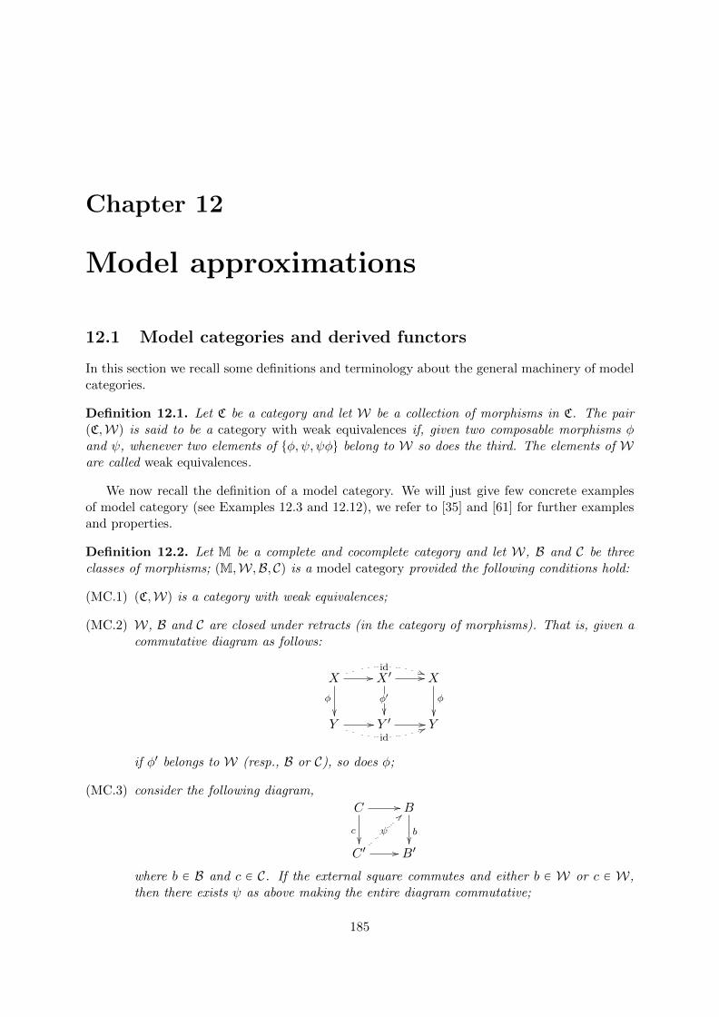
Chapter 12
Model approximations
12.1 Model categories and derived functors
In this section we recall some definitions and terminology about the general machinery of modelcategories.
Definition 12.1. Let C be a category and let W be a collection of morphisms in C. The pairpC,Wq is said to be a category with weak equivalences if, given two composable morphisms φand ψ, whenever two elements of tφ, ψ, ψφu belong to W so does the third. The elements of Ware called weak equivalences.
We now recall the definition of a model category. We will just give few concrete examplesof model category (see Examples 12.3 and 12.12), we refer to [35] and [61] for further examplesand properties.
Definition 12.2. Let M be a complete and cocomplete category and let W, B and C be threeclasses of morphisms; pM,W,B, Cq is a model category provided the following conditions hold:
(MC.1) pC,Wq is a category with weak equivalences;
(MC.2) W, B and C are closed under retracts (in the category of morphisms). That is, given acommutative diagram as follows:
Xid ))//
φ
��
X 1 //
φ1
��
X
φ
��Y //
id55Y 1 // Y
if φ1 belongs to W (resp., B or C), so does φ;
(MC.3) consider the following diagram,
C //
c��
B
b��
C 1
ψ
>>
// B1
where b P B and c P C. If the external square commutes and either b P W or c P W,then there exists ψ as above making the entire diagram commutative;
185
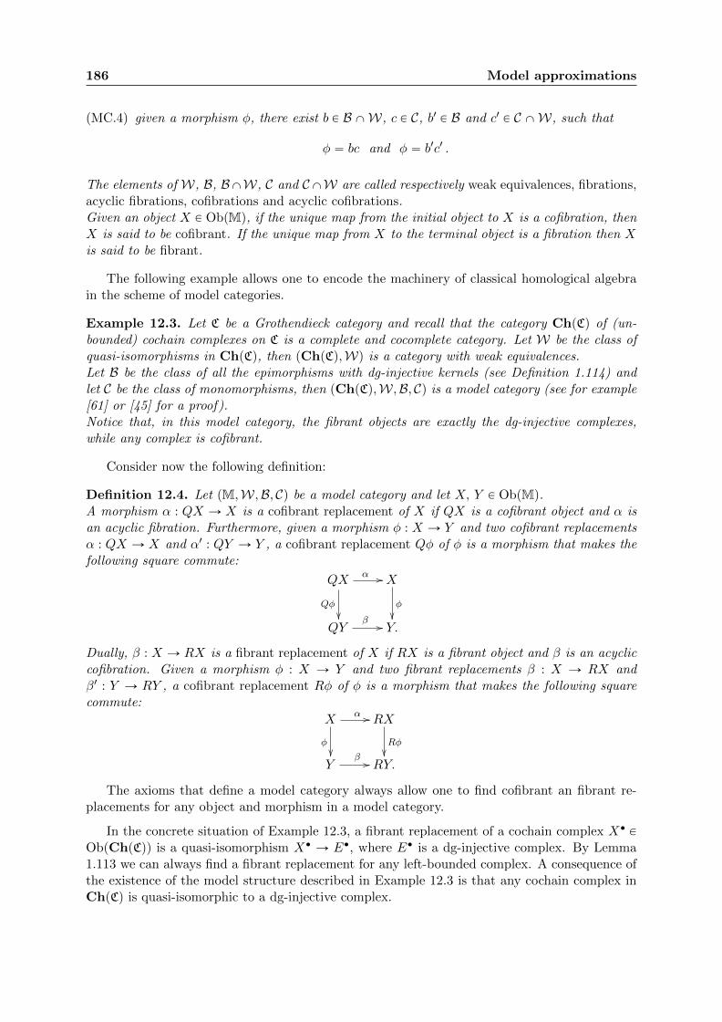
186 Model approximations
(MC.4) given a morphism φ, there exist b P B XW, c P C, b1 P B and c1 P C XW, such that
φ “ bc and φ “ b1c1 .
The elements of W, B, BXW, C and CXW are called respectively weak equivalences, fibrations,acyclic fibrations, cofibrations and acyclic cofibrations.Given an object X P ObpMq, if the unique map from the initial object to X is a cofibration, thenX is said to be cofibrant. If the unique map from X to the terminal object is a fibration then Xis said to be fibrant.
The following example allows one to encode the machinery of classical homological algebrain the scheme of model categories.
Example 12.3. Let C be a Grothendieck category and recall that the category ChpCq of (un-bounded) cochain complexes on C is a complete and cocomplete category. Let W be the class ofquasi-isomorphisms in ChpCq, then pChpCq,Wq is a category with weak equivalences.Let B be the class of all the epimorphisms with dg-injective kernels (see Definition 1.114) andlet C be the class of monomorphisms, then pChpCq,W,B, Cq is a model category (see for example[61] or [45] for a proof).Notice that, in this model category, the fibrant objects are exactly the dg-injective complexes,while any complex is cofibrant.
Consider now the following definition:
Definition 12.4. Let pM,W,B, Cq be a model category and let X, Y P ObpMq.A morphism α : QX Ñ X is a cofibrant replacement of X if QX is a cofibrant object and α isan acyclic fibration. Furthermore, given a morphism φ : X Ñ Y and two cofibrant replacementsα : QX Ñ X and α1 : QY Ñ Y , a cofibrant replacement Qφ of φ is a morphism that makes thefollowing square commute:
QXα //
Qφ
��
X
φ
��QY
β // Y.
Dually, β : X Ñ RX is a fibrant replacement of X if RX is a fibrant object and β is an acycliccofibration. Given a morphism φ : X Ñ Y and two fibrant replacements β : X Ñ RX andβ1 : Y Ñ RY , a cofibrant replacement Rφ of φ is a morphism that makes the following squarecommute:
Xα //
φ��
RX
Rφ��
Yβ // RY.
The axioms that define a model category always allow one to find cofibrant an fibrant re-placements for any object and morphism in a model category.
In the concrete situation of Example 12.3, a fibrant replacement of a cochain complex X‚ PObpChpCqq is a quasi-isomorphism X‚ Ñ E‚, where E‚ is a dg-injective complex. By Lemma1.113 we can always find a fibrant replacement for any left-bounded complex. A consequence ofthe existence of the model structure described in Example 12.3 is that any cochain complex inChpCq is quasi-isomorphic to a dg-injective complex.
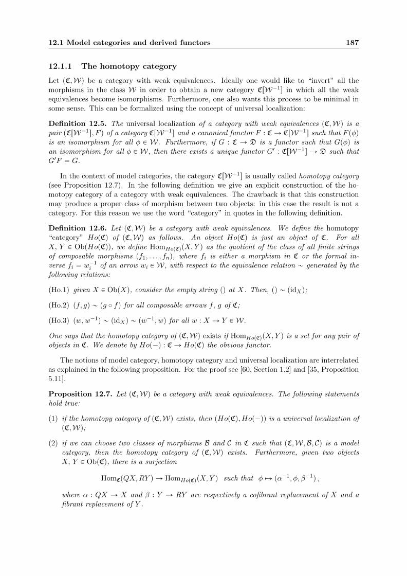
12.1 Model categories and derived functors 187
12.1.1 The homotopy category
Let pC,Wq be a category with weak equivalences. Ideally one would like to “invert” all themorphisms in the class W in order to obtain a new category CrW´1s in which all the weakequivalences become isomorphisms. Furthermore, one also wants this process to be minimal insome sense. This can be formalized using the concept of universal localization:
Definition 12.5. The universal localization of a category with weak equivalences pC,Wq is apair pCrW´1s, F q of a category CrW´1s and a canonical functor F : CÑ CrW´1s such that F pφqis an isomorphism for all φ P W. Furthermore, if G : C Ñ D is a functor such that Gpφq isan isomorphism for all φ P W, then there exists a unique functor G1 : CrW´1s Ñ D such thatG1F “ G.
In the context of model categories, the category CrW´1s is usually called homotopy category(see Proposition 12.7). In the following definition we give an explicit construction of the ho-motopy category of a category with weak equivalences. The drawback is that this constructionmay produce a proper class of morphism between two objects: in this case the result is not acategory. For this reason we use the word “category” in quotes in the following definition.
Definition 12.6. Let pC,Wq be a category with weak equivalences. We define the homotopy“category” HopCq of pC,Wq as follows. An object HopCq is just an object of C. For allX, Y P ObpHopCqq, we define HomHopCqpX,Y q as the quotient of the class of all finite stringsof composable morphisms pf1, . . . , fnq, where fi is either a morphism in C or the formal in-verse fi “ w´1
i of an arrow wi PW, with respect to the equivalence relation „ generated by thefollowing relations:
(Ho.1) given X P ObpXq, consider the empty string pq at X. Then, pq „ pidXq;
(Ho.2) pf, gq „ pg ˝ fq for all composable arrows f, g of C;
(Ho.3) pw,w´1q „ pidXq „ pw´1, wq for all w : X Ñ Y PW.
One says that the homotopy category of pC,Wq exists if HomHopCqpX,Y q is a set for any pair ofobjects in C. We denote by Hop´q : CÑ HopCq the obvious functor.
The notions of model category, homotopy category and universal localization are interrelatedas explained in the following proposition. For the proof see [60, Section 1.2] and [35, Proposition5.11].
Proposition 12.7. Let pC,Wq be a category with weak equivalences. The following statementshold true:
(1) if the homotopy category of pC,Wq exists, then pHopCq, Hop´qq is a universal localization ofpC,Wq;
(2) if we can choose two classes of morphisms B and C in C such that pC,W,B, Cq is a modelcategory, then the homotopy category of pC,Wq exists. Furthermore, given two objectsX, Y P ObpCq, there is a surjection
HomCpQX,RY q Ñ HomHopCqpX,Y q such that φ ÞÑ pα´1, φ, β´1q ,
where α : QX Ñ X and β : Y Ñ RY are respectively a cofibrant replacement of X and afibrant replacement of Y .
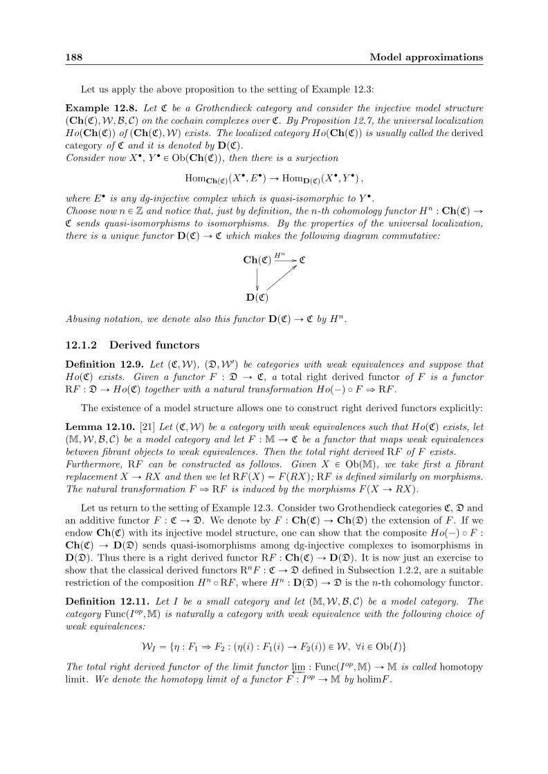
188 Model approximations
Let us apply the above proposition to the setting of Example 12.3:
Example 12.8. Let C be a Grothendieck category and consider the injective model structurepChpCq,W,B, Cq on the cochain complexes over C. By Proposition 12.7, the universal localizationHopChpCqq of pChpCq,Wq exists. The localized category HopChpCqq is usually called the derivedcategory of C and it is denoted by DpCq.Consider now X‚, Y ‚ P ObpChpCqq, then there is a surjection
HomChpCqpX‚, E‚q Ñ HomDpCqpX
‚, Y ‚q ,
where E‚ is any dg-injective complex which is quasi-isomorphic to Y ‚.Choose now n P Z and notice that, just by definition, the n-th cohomology functor Hn : ChpCq ÑC sends quasi-isomorphisms to isomorphisms. By the properties of the universal localization,there is a unique functor DpCq Ñ C which makes the following diagram commutative:
ChpCq
��
Hn// C
DpCq
<<zzzzzzzzz
Abusing notation, we denote also this functor DpCq Ñ C by Hn.
12.1.2 Derived functors
Definition 12.9. Let pC,Wq, pD,W 1q be categories with weak equivalences and suppose thatHopCq exists. Given a functor F : D Ñ C, a total right derived functor of F is a functorRF : DÑ HopCq together with a natural transformation Hop´q ˝ F ñ RF .
The existence of a model structure allows one to construct right derived functors explicitly:
Lemma 12.10. [21] Let pC,Wq be a category with weak equivalences such that HopCq exists, letpM,W,B, Cq be a model category and let F : M Ñ C be a functor that maps weak equivalencesbetween fibrant objects to weak equivalences. Then the total right derived RF of F exists.Furthermore, RF can be constructed as follows. Given X P ObpMq, we take first a fibrantreplacement X Ñ RX and then we let RF pXq “ F pRXq; RF is defined similarly on morphisms.The natural transformation F ñ RF is induced by the morphisms F pX Ñ RXq.
Let us return to the setting of Example 12.3. Consider two Grothendieck categories C, D andan additive functor F : C Ñ D. We denote by F : ChpCq Ñ ChpDq the extension of F . If weendow ChpCq with its injective model structure, one can show that the composite Hop´q ˝ F :ChpCq Ñ DpDq sends quasi-isomorphisms among dg-injective complexes to isomorphisms inDpDq. Thus there is a right derived functor RF : ChpCq Ñ DpDq. It is now just an exercise toshow that the classical derived functors RnF : CÑ D defined in Subsection 1.2.2, are a suitablerestriction of the composition Hn ˝RF , where Hn : DpDq Ñ D is the n-th cohomology functor.
Definition 12.11. Let I be a small category and let pM,W,B, Cq be a model category. Thecategory FuncpIop,Mq is naturally a category with weak equivalence with the following choice ofweak equivalences:
WI “ tη : F1 ñ F2 : pηpiq : F1piq Ñ F2piqq PW, @i P ObpIqu
The total right derived functor of the limit functor limÐÝ
: FuncpIop,Mq Ñ M is called homotopylimit. We denote the homotopy limit of a functor F : Iop ÑM by holimF .
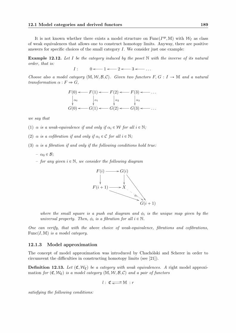
12.1 Model categories and derived functors 189
It is not known whether there exists a model structure on FuncpIop,Mq with WI as classof weak equivalences that allows one to construct homotopy limits. Anyway, there are positiveanswers for specific choices of the small category I. We consider just one example:
Example 12.12. Let I be the category induced by the poset N with the inverse of its naturalorder, that is:
I : 0 1oo 2oo 3oo . . .oo
Choose also a model category pM,W,B, Cq. Given two functors F, G : I Ñ M and a naturaltransformation α : F ñ G,
F p0q
α0
��
F p1q
α1
��
oo F p2q
α2
��
oo F p3q
α3
��
oo . . .oo
Gp0q Gp1qoo Gp2qoo Gp3qoo . . .oo
we say that
(1) α is a weak-equivalence if and only if αi PW for all i P N;
(2) α is a cofibration if and only if αi P C for all i P N;
(3) α is a fibration if and only if the following conditions hold true:
– α0 P B;
– for any given i P N, we consider the following diagram
F piq //
��
Gpiq
��
��77777777777777777
F pi` 1q //
**TTTTTTTTTTTTTTTT X
φi$$
Gpi` 1q
where the small square is a push out diagram and φi is the unique map given by theuniversal property. Then, φi is a fibration for all i P N.
One can verify, that with the above choice of weak-equivalence, fibrations and cofibrations,FuncpI,Mq is a model category.
12.1.3 Model approximation
The concept of model approximation was introduced by Chacholski and Scherer in order tocircumvent the difficulties in constructing homotopy limits (see [21]).
Definition 12.13. Let pC,WCq be a category with weak equivalences. A right model approxi-mation for pC,WCq is a model category pM,W,B, Cq and a pair of functors
l : C //oo M : r
satisfying the following conditions:
190 Model approximations
(MA.1) l is left adjoint to r;
(MA.2) if φ PWC, then lpφq PW;
(MA.3) if ψ is a weak equivalence between fibrant objects in M, then rpψq PWC;
(MA.4) if lpXq Ñ Y is a weak equivalence in M with X fibrant, the adjoint morphism X Ñ rpY qis in WC.
Given two categories with weak equivalences pC1,W1q and pC2,W2q, one can find conditionsunder which a model approximation of pC2,W2q gives automatically a model approximation ofpC1,W1q:
Lemma 12.14. Let pC1,W1q and pC2,W2q be categories with weak equivalences and let
l : C1//oo C2 : r
be an adjunction such that:
(1) φ PW1 implies lφ PW2;
(2) ψ PW2 implies rψ PW1;
(3) if a morphism lpCq Ñ D is in W2, then the adjoint morphism C Ñ rpDq is in W1.
If pM,W,B, Cq is a model category and l1 : C2 Ô M : r1 is a model approximation, then
L : C1//oo M : R
is a model approximation, where L “ l1 ˝ l and R “ r ˝ r1.
Proof. We have to verify conditions (MA.1)-(MA.4):
(MA.1) is [70, Theorem 1, Sec. 8, Ch. 1].
(MA.2) If φ P W1, then lφ P W2 by our hypothesis (1). Apply the definition of model approxi-mation to obtain that Lpφq “ l1plpφqq is a weak equivalence in M.
(MA.3) If ψ is a weak equivalence between fibrant objects in M, then r1pψq P W2, by thedefinition of model approximation. Apply (2) to obtain that Rψ “ rpr1pψqq PW1.
(MA.4) Let X P M be fibrant, let Y P C1 and let X Ñ LpY q be a weak equivalence in M.The adjoint (under the adjunction pl1, r1q) morphism r1pXq Ñ lpY q belongs to W2, by thedefinition of model approximation. Using (3), the adjoint (under the adjunction pl, rq) morphismrpr1pXqq Ñ Y belongs to W1.
The above lemma provides a motivation for the following
Definition 12.15. Let pC1,W1q and pC2,W2q be two categories with weak equivalences. Anadjunction l : C1 Ô C2 : r is said to be compatible with weak equivalences if conditions (1), (2)and (3) in Lemma 12.14 are satisfied.
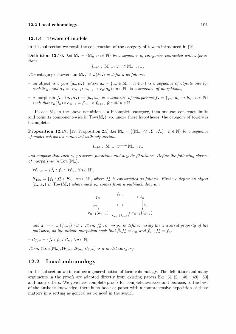
12.2 Local cohomology 191
12.1.4 Towers of models
In this subsection we recall the construction of the category of towers introduced in [19].
Definition 12.16. Let M‚ “ tMn : n P Nu be a sequence of categories connected with adjunc-tions
ln`1 : Mn`1//oo Mn : rn .
The category of towers on M‚, TowpM‚q is defined as follows:
– an object is a pair pa‚, α‚q, where a‚ “ tan P Mn : n P Nu is a sequence of objects one foreach Mn, and α‚ “ tαn`1 : an`1 Ñ rnpanq : n P Nu is a sequence of morphisms;
– a morphism f‚ : pa‚, α‚q Ñ pb‚, β‚q is a sequence of morphisms f‚ “ tfn : an Ñ bn : n P Nusuch that rnpfnq ˝ αn`1 “ βn`1 ˝ fn`1, for all n P N.
If each Mn in the above definition is a bicomplete category, then one can construct limitsand colimits component-wise in TowpM‚q, so, under these hypotheses, the category of towers isbicomplete.
Proposition 12.17. [19, Proposition 2.3] Let M‚ “ tpMn,Wn,Bn, Cnq : n P Nu be a sequenceof model categories connected with adjunctions
ln`1 : Mn`1//oo Mn : rn
and suppose that each rn preserves fibrations and acyclic fibrations. Define the following classesof morphisms in TowpM‚q:
– WTow “ tf‚ : fn PWn , @n P Nu;
– BTow “ tf‚ : f˚n P Bn , @n P Nu, where f˚n is constructed as follows. First we define an objectpp‚, π‚q in TowpM‚q where each pn comes from a pull-back diagram
pn
P.B.βn��
fn´1 // bn
βn��
rn´1pan´1qrn´1pfn´1q
// rn´1pbn´1q
and πn “ rn´1pfn´1q ˝ βn. Then, f˚n : an Ñ pn is defined, using the universal property of thepull-back, as the unique morphism such that βnf
˚n “ αn and fn´1f
˚n “ fn.
– CTow “ tf‚ : fn P Cn , @n P Nu
Then, pTowpM‚q,WTow,BTow, CTowq is a model category.
12.2 Local cohomology
In this subsection we introduce a general notion of local cohomology. The definitions and manyarguments in the proofs are adapted directly from existing papers like [3], [2], [48], [49], [50]and many others. We give here complete proofs for completeness sake and because, to the bestof the author’s knowledge, there is no book or paper with a comprehensive exposition of thesematters in a setting as general as we need in the sequel.
192 Model approximations
Definition 12.18. Let C be a Grothendieck category and let τ “ pT ,Fq P TorspCq. The n-th τ -local cohomology Γnτ : C Ñ T is the n-th right derived functor of the τ -torsion functorTτ : CÑ T .
It is difficult to study the properties of local cohomology in full generality, so we need toimpose one or more of the following hypotheses on the ambient category C in almost all of ourresults:
(Hyp.1) C is stable (see Definition 1.139).
(Hyp.2) C is locally Noetherian (see Definition 2.75).
(Hyp.3) all the prime torsion theories on C are exact (see Definition 1.131).
Example 12.19. Let C “ R-Mod be the category of left R-modules over a ring R. When Csatisfies (Hyp.1), (Hyp.2) and (Hyp.3), R is said to be left effective. Examples of left effectiverings include:
(1) commutative Noetherian rings;
(2) left Noetherian Azumaya algebras, see [50, page 173];
(3) prime hereditary Noetherian quasi-local rings which are bounded orders in their classicalrings of fractions, see [50, Example 2.3].
Lemma 12.20. Let C be a Grothendieck category, let τ “ pT ,Fq P TorspCq be stable and letX P ObpCq. Then,
(1) Γnτ pXq “ 0 for all n ą 0, provided X is τ -torsion;
(2) there is a natural isomorphism Γnτ pXq – Γnτ pX{Tτ pXqq, for all n ą 0;
(3) there is a natural isomorphism Γn`1τ pXq – Γnτ pEpXq{Xq, for all n ą 0;
(4) if X is τ -torsion free, then Γ1τ pXq – Tτ pEpXq{Xq.
(5) there is a natural isomorphism Γn`1τ pXq – RLnτ pXq, for all n ą 0;
(6) if X is τ -torsion free, then Γ1τ pXq – Lτ pXq{X.
Proof. (1) Let us consider an injective resolution λ : X Ñ E‚ inductively as follows:
– En “ 0 and dn “ 0 for all n ă 0;
– E0 “ EpXq and λ is the canonical embedding of X in its injective envelope;
– E1 “ EpCoKerpλqq and d0 “ ε0 ˝ π0 where π0 : E0 Ñ CoKerpλq is the canonical projectionand ε0 is the canonical embedding of CoKerpλq in its injective envelope;
– for all n ě 1 we let En`1 “ EpCoKerpdn´1qq and dn “ εn ˝ πn where πn : En Ñ CoKerpdn´1q
is the canonical projection and εn is the canonical embedding of CoKerpdn´1q in its injectiveenvelope.
12.2 Local cohomology 193
It is an exercise to show that λ : X Ñ E‚ is an injective resolution (this is well-known, forexample one can use the dual argument of the proof of [104, Lemma 2.2.5]). Using the fact thatτ is stable, we obtain that EnpXq is τ -torsion for all n P N and so E‚pXq “ Tτ pE
‚pXqq is anexact complex in all degrees but, eventually, in the 0-th degree.
(2) Consider the short exact sequence 0 Ñ Tτ pXq Ñ X Ñ X{Tτ pXq Ñ 0. This gives a longexact sequence in cohomology
0 Ñ Γ0τ pTτ pXqq Ñ Γ0
τ pXq Ñ Γ0τ pX{Tτ pXqq Ñ
Ñ Γ1τ pTτ pXqq Ñ Γ1
τ pXq Ñ Γ1τ pX{Tτ pXqq Ñ Γ2
τ pTτ pXqq Ñ ¨ ¨ ¨ ,
which implies the desired isomorphism as, by part (1), we have that Γnτ pTτ pXqq “ 0, for alln ą 0.
(3)–(4) Consider the short exact sequence 0 Ñ X Ñ EpXq Ñ EpXq{X Ñ 0. This gives a longexact sequence in cohomology
0 Ñ Tτ pXq Ñ Tτ pEpXqq Ñ Tτ pEpXq{Xq Ñ Γ1τ pXq Ñ Γ1
τ pEpXqq Ñ
Γ1τ pEpXq{Xq Ñ Γ2
τ pXq Ñ Γ2τ pEpXqq Ñ Γ2
τ pEpXq{Xq Ñ Γ3τ pXq Ñ Γ3
τ pEpXqq Ñ . . .
which implies the isomorphism in (3) as, Γnτ pEpXqq “ 0 for all n ą 0, being EpXq is injective.If X P F , then EpXq P F by stability and so Tτ pEpXqq “ 0, proving (4).
(5)–(6) Fix an injective resolution X Ñ E‚. By Lemma 1.140, En – Tτ pEnq ‘ En{Tτ pE
nq forall n P N. Consider the complex Tτ pE
‚q and the quotient complex E‚{Tτ pE‚q, which are both
complexes of injective objects. Notice that there is a short exact sequence in ChpCq
0 Ñ Tτ pE‚q Ñ E‚ Ñ E‚{Tτ pE
‚q Ñ 0 .
The cohomologies of the complex Tτ pE‚q are exactly the τ -local cohomologies of M , while the
cohomologies of E‚ are all trivial but, eventually, the 0-th cohomology. Furthermore, En{Tτ pEnq
is τ -torsion free and injective, so it is τ -local; in particular, Lτ pEnq – En{Tτ pE
nq for alln P N. We obtain an isomorphism of complexes E‚{Tτ pE
‚q – Lτ pE‚q, which shows that the
cohomologies of the complex E‚{Tτ pE‚q give exactly the right derived functors of the localization
functor L. Thus, we have a long exact sequence
0 Ñ Tτ pXq Ñ X Ñ Lτ pXq Ñ Γ1τ pXq Ñ 0 Ñ R1Lτ pXq Ñ
Ñ Γ2τ pXq Ñ 0 Ñ R2Lτ pXq Ñ Γ3
τ pXq Ñ 0 Ñ R3Lτ pXq Ñ ¨ ¨ ¨ ,
which gives the desired isomorphisms.
An immediate consequence of parts (5) and (6) of the above proposition is the following
Corollary 12.21. Let C be a Grothendieck category, let τ P TorspCq be stable and exact, and letX P C. Then,
Γnτ pXq “ 0 @n ą 1 .
If X is τ -local, then also Γ0τ pXq “ Γ1
τ pXq “ 0.
Corollary 12.22. Let C be a Grothendieck category and let τ2 ĺ τ1 P TorspCq be stable. Then,
pΓiτ1pXq “ 0 , @0 ď i ď nq ñ pΓiτ2pXq “ 0 , @0 ď i ď nq
for all X P ObpCq and n P N.
194 Model approximations
Proof. We prove our statement by induction on n P N.If n “ 0, the result is clear as 0 “ Γ0
τ1pXq – Tτ1pXq Ě Tτ2pXq – Γ0τ2pXq.
If n ě 1 and suppose the result holds for any smaller integer. Consider the following isomor-phisms:
(a) Γ0τ1pXq – Γ0
τ2pXq “ 0, as in the case n “ 0, in particular X is both τ1 and τ2-torsion free;
(b) Γ1τ pXq – Γ0
τ pEpXq{Xq for τ P tτ1, τ2u, by (a) and Lemma 12.20(4).
(c) Γkτ pXq – Γk´1τ pEpXq{Xq for all 1 ă k ď n and τ P tτ1, τ2u, by Lemma 12.20(3).
By (b) and (c), we have that Γiτ1pEpXq{Xq “ 0 for all 0 ď i ď n ´ 1 and so, by inductivehypothesis, Γiτ2pEpXq{Xq “ 0 for all 0 ď i ď n ´ 1. Applying again (b) and (c), Γiτ2pXq “ 0for all 1 ď i ď n. Hence, adding (a), Γiτ2pXq “ 0 for all 0 ď i ď n which is what we wanted toprove.
Given a Noetherian object N in C, recall that N is automatically a compact object, thatis, the functor HomCpN,´q commutes with direct limits (see for example [96, Proposition 3.4,Ch. V]). More explicitly, given a directed set Λ and a direct system pXα, φβ,αqΛ in C, we have anatural isomorphism
limÝÑαPΛ
HomCpN,Xαq – HomC
˜
N, limÝÑαPΛ
Xα
¸
. (12.2.1)
Proposition 12.23. Let C be a Grothendieck category satisfying (Hyp.2) and let τ P TorspCq.Then,
(1) given two objects X and M P ObpCq, we have a natural isomorphism
HomCpX,TτMq – limÝÑY
HomCpX{Y,Mq ,
with Y ranging in the family of sub-objects of X such that X{Y P T (ordered by reverseinclusion);
(2) all the τ -local cohomology functors commute with direct limits.
Proof. (1) Let Y be a sub-object of X such that X{Y P T . For any morphism φ : X{Y Ñ M ,φpX{Y q ď Tτ pMq ď M and so HomCpX{Y,Tτ pMqq – HomCpX{Y,Mq. Furthermore, there isan injective map
´ ˝pY : HomCpX{Y,Tτ pMqqp– HomCpX{Y,Mqq ÝÑ HomCpX,Tτ pMqq (12.2.2)
where pY : X Ñ X{Y is the canonical projection. By the universal property of the direct limit,there is a unique map Φ, making the following diagrams commutative, whenever Y1 ď Y2 ď Xand X{Y1 P T :
HomCpX{Y1,Mq
))
´˝pY1
HomCpX,Tτ pMqq lim
ÝÑYHomCpX{Y,Mq .D! Φoo
HomCpX{Y2,Mq
OO
´˝pY2
>> 44
12.2 Local cohomology 195
Now, Φ is injective by the injectivity of the maps described in (12.2.2) and the commutativityof the above diagram; furthermore, one can show that Φ is surjective as follows: an element φ PHomCpX,Tτ pMqq belongs to the image of Φ if and only if there exists Y ď X such that X{Y P Tand there is a morphism ψ : X{Y Ñ M such that φ “ ψpY . Given φ P HomCpX,Tτ pMqq, weeasily get that φpXq P T and so, letting Y “ Kerpφq, we have that X{Y P T . Furthermore,there is an induced (mono)morphism ψ : X{Y Ñ Tτ pXq such that φ “ ψpY , as desired.
(2) According to [56, Proposition 3.6.2], it suffices to verify that
(a) R0Tτ – Tτ commutes with direct limits;
(b) limÝÑΛ
Eα is Tτ -acyclic (i.e., Γnτ plimÝÑΛEαq “ 0 for all n ą 0) for any directed system pEα, φβ,αqΛ
of injective objects.
Let pMα, φβ,αqΛ be a directed system in C, over a directed set Λ. We have to verify thatTτ plimÝÑΛ
Mαq – limÝÑΛ
Tτ pMαq. For this we show that there is a natural equivalence of functorsHomCp´,Tτ plimÝÑΛ
Mαqq – HomCp´, limÝÑΛTτ pMαqq, which implies (a) by the Yoneda Lemma.
For all X P C there is a natural isomorphism
HomCpX,Tτ plimÝÑΛ
Mαqq – HomplimÝÑN
N,Tτ plimÝÑΛ
Mαqq ,
with N ranging in the family of Noetherian sub-objects of X, so
HomCpX,Tτ plimÝÑΛ
Mαqq – limÐÝN
HompN,Tτ plimÝÑΛ
Mαqq
This allows us to assume that X is itself Noetherian. In this case:
HomCpX,Tτ plimÝÑΛ
Mαqq – limÝÑY
HompX{Y, limÝÑΛ
Mαq with X{Y P T , by (1)
– limÝÑY
limÝÑΛ
HompX{Y,Mαq by (12.2.1)
– limÝÑΛ
limÝÑY
HompX{Y,Mαq
– HompX, limÝÑΛ
Tτ pMαqq .
Part (b) follows by Proposition 2.78 (1), and the fact that injective objects are F -acyclic for anyleft exact functor F .
Lemma 12.24. Let C be a Grothendieck category satisfying (Hyp.1) and (Hyp.2), let π P SppCq,let τ “ pT ,Fq P TorspCq and let C be a cocritical object such that EpCq – Epπq.If ´1 ă G.dimτ pCq ă 8, then G.dimτ pLπpCq{Cq ă G.dimτ pCq.
Proof. By hypothesis G.dimτ pCq ą ´1. Furthermore, if G.dimτ pCq “ n ` 1 for some n P N,we can denote by τn P TorspC{T q the torsion theory whose torsion class is pC{T qn. Then,G.dimτ˝τnpCq “ 0. Thus, there is no loss of generality in assuming that G.dimτ pCq “ 0 (other-wise substitute τ by τ ˝ τn and then use part (2) of Lemma 2.72).Assuming that G.dimτ pCq “ 0, we have to show that LπpCq{C P T . Let E be an injectiveobject that cogenerates τ . By Proposition 2.78, there exist a set I, a family of prime torsiontheories tπi “ pTi,Fiq : i P Iu Ď SppCq and a family of non-trivial cardinals tαi : i P Iu such thatE –
À
iPI Epπiqpαiq, thus T “
Ş
iPI Ti and so we reduced to prove that
HomCpLπpCq{C,Epπiqq “ 0 , (12.2.3)
196 Model approximations
for all i P I. Let i P I, if πi “ π, then LπpCq{C – TπpEpπq{Cq is πi-torsion by construction,so (12.2.3) follows. On the other hand, if πi ‰ π, suppose looking for a contradiction, thatHomCpLπpCq{C,Epπiqq ‰ 0 which implies HomCpLπpCq, Epπiqq ‰ 0 which, by the injectivity ofEpπiq, implies HomCpEpπq, Epπiqq ‰ 0. By Corollary 2.74, 0 “ G.dimτ pEpπqq ą G.dimτ pEpπiqq,equivalently, Epπiq P T , that is HomCpEpπiq, Eq “ 0, which is clearly a contradiction.
The following theorem is an improved version of [50, Proposition 2.4].
Theorem 12.25. Let C be a Grothendieck category satisfying (Hyp.1), (Hyp.2) and (Hyp.3),let τ P TorspCq and let X P ObpCq. Then, Γnτ pXq ‰ 0 implies G.dimτ pXq ` 2 ě n.
Proof. By (Hyp.3), X is the direct union of its Noetherian sub-objects. By Proposition 12.23,the vanishing of τ -local cohomologies on Noetherian objects implies their vanishing on X. Thuswe can suppose X to be Noetherian. By Lemma 2.70 (4), there exist sub-objects 0 “ Y0 ď
Y1 ď ¨ ¨ ¨ ď Yk “ X such that Yi{Yi´1 is cocritical for all i “ 1, . . . , k. One can verify byinduction on k that the vanishing of the τ -local cohomology functors on all the factors of theform Yi{Yi´1 implies their vanishing on X. Thus we may suppose X to be cocritical, in particularEpXq – Epπq for some π P SppCq.
If G.dimτ pXq is not finite, then there is nothing to prove, therefore we suppose G.dimτ pXq “d ă 8 and we proceed by induction on d. If d “ ´1, then Γnτ pXq “ 0 for all n ą 0, byLemma 12.20 (1). Thus, Γnτ pXq ‰ 0 implies n “ 0 ď G.dimτ pXq ` 2 “ ´1 ` 2 “ 1. If d ą ´1,consider the following long exact sequence:
0 Ñ Γ0τ pXq Ñ Γ0
τ pLπpXqq Ñ Γ0τ pLπpXq{Xq Ñ Γ1
τ pXq Ñ Γ1τ pLπpXqq Ñ
Ñ Γ1τ pLπpXq{Xq Ñ ¨ ¨ ¨ Ñ Γnτ pXq Ñ Γnτ pLπpXqq Ñ Γnτ pLπpXq{Xq Ñ Γn`1
τ pXq Ñ . . .
Notice that Γ0τ pXq “ Γ0
τ pLπpXqq “ 0, since we supposed that d ą ´1 and so, by stability, X is τ -torsion free. Furthermore, using (Hyp.3) and Corollary 12.21, one can show that ΓnπpLπpXqq “ 0for all n P N. Using again that X (and so Epπq) is τ -torsion free, we get τ ĺ π and so we canapply Corollary 12.22 to show that Γnτ pLπpXqq “ 0 for all n ą 0. One obtains the followingisomorphisms:
Γnτ pXq “ Γn´1τ pLπpXq{Xq , @n ě 1 .
By Lemma 12.24, G.dimτ pLπpXq{Xq ă d and so we can apply our inductive hypothesis toshow that Γnτ pLπpXq{Xq “ 0 for all n ą G.dimτ pLπpXq{Xq ` 2. Thus, if Γnτ pXq ‰ 0 forsome n ą 0, then Γn´1
τ pLπpXq{Xq ‰ 0 and so n ´ 1 ď G.dimτ pLπpXq{Xq ` 2, that is, n ďG.dimτ pLπpXq{Xq ` 3 ď G.dimτ pXq ` 2.
12.2.1 Exactness of products in the localization
In the definition of Grothendieck category one assumes direct limits to be exact but no assump-tion is required on the exactness of products. We will see in the last part of this paper thatknowing that a Grothendieck category has “almost exact products” has very nice consequenceson its derived category. In the following definition we precise the meaning of “almost exactproducts”:
Definition 12.26. Let C be a Grothendieck category. For a non-negative integer n, C is said tosatisfy the axiom (Ab.4˚)-k if, for any set I and any collection of objects tXiuiPI ,
ź
iPI
pnqXi “ 0 @n ą k ,
whereśpnqiPIp´q is the n-th derived functor of the product
ś
: CI Ñ C.
12.2 Local cohomology 197
Notice that condition (Ab.4˚)-0 is exactly (Ab.4˚) (see Subsection 1.1.5).In general, there is no reason for a Grothendieck category to be (Ab.4˚)-k for any k. Anyway,
categories of modules are (Ab.4˚) and, by the Gabriel-Popescu Theorem, any Grothendieckcategory is a quotient category of a category of modules. Thus, it seems natural to ask forsufficient conditions on a torsion theory τ “ pT ,Fq in an (Ab.4˚) Grothendieck category C thatensure that the quotient category C{T is (Ab.4˚)-k for some k P N. We give two such conditionsin the following lemma, a deeper criterion is given in Theorem 12.28.
Lemma 12.27. Let C be an (Ab.4˚) Grothendieck category, let τ “ pT ,Fq P TorspCq andsuppose one of the following conditions holds:
(1) T is closed under taking products (in this case τ is said to be a TTF);
(2) τ is exact.
Then, the quotient category C{T is still (Ab.4˚).
Proof. Let I be a set and for each i P I consider objects Ai, Bi and Ci P C{T such that
0 Ñ Ai Ñ Bi Ñ Ci Ñ 0 is exact in C{T .
Hence, for all i P I, one obtains exact sequences 0 Ñ Sτ pAiq Ñ Sτ pBiq Ñ Sτ pCiq Ñ Ti Ñ 0 inC, where Ti P T . Using the (Ab.4˚) property in C we get an exact sequence
0 Ñź
iPI
Sτ pAiq Ñź
iPI
Sτ pBiq Ñź
iPI
Sτ pCiq Ñź
iPI
Ti Ñ 0 .
If τ is a TTF, thenś
iPI Ti is τ -torsion and so we can apply Qτ to the above exact sequenceobtaining the following short exact sequence
0 Ñź
iPI
Ai Ñź
iPI
Bi Ñź
iPI
Ci Ñ Qτ pź
iPI
Tiq “ 0 ,
by Corollary 1.135 and the exactness of Qτ . On the other hand, if Sτ is exact, we get Ti “ 0for all i P I above and so again one can easily conclude.
Theorem 12.28. Let C be an (Ab.4˚) Grothendieck category which satisfies hypotheses (Hyp.1),(Hyp.2) and (Hyp.3), and let τ P TorspCq. If G.dimpC{T q “ k ă 8, then C{T is (Ab.4˚)-k ` 1.
Proof. Let tXiuiPI be a family of objects in C{T . For all i P I, choose an injective resolution0 Ñ Sτ pXiq Ñ E‚i of Sτ pXiq in C. Since Qτ is exact and sends injective objects to injectiveobjects, the complex Qτ pE
‚i q provides an injective resolution for Xi. Thus, for all n ą k ` 1,
ź
iPI
pnqXi “ Hn
˜
ź
iPI
Qτ pE‚i q
¸
“ Hn
˜
Qτ
˜
ź
iPI
Lτ pE‚i q
¸¸
by Corollary 1.135
“ Qτ
˜
Hn
˜
ź
iPI
Lτ pE‚i q
¸¸
exact funct. commute with cohom.
“ Qτ
˜
ź
iPI
Hn pLτ pE‚i qq
¸
“ Qτ
˜
ź
iPI
RLnτ pE‚i q
¸
exact funct. commute with cohom.
“ Qτ
˜
ź
iPI
Γn`1τ pE‚i q
¸
“ 0 Lemma 12.20 and Theorem 12.25.
198 Model approximations
Corollary 12.29. Let C be an (Ab.4˚) Grothendieck category which satisfies hypotheses (Hyp.1),(Hyp.2) and (Hyp.3). If G.dimpCq “ k ă 8, then C{T is (Ab.4˚)-k ` 1 for all τ “ pT ,Fq PTorspCq.
12.3 Injective classes
Let C be a Grothendieck category and let I be a class of objects of C. Slightly generalizing thesetting of [20], we say that a morphism φ : X Ñ Y in C is an I-monomorphism if
HomCpφ,Kq : HomCpY,Kq Ñ HomCpX,Kq
is an epimorphism of Abelian groups for every K P I. We say that C has enough I-injectives ifevery object X admits an I-monomorphism X Ñ K for some K P I.
Definition 12.30. [20] A subclass I of a Grothendieck category C is an injective class (of C) ifit is closed under products and direct summands, and C has enough I-injectives.
Lemma 12.31. Let I be an injective class of a Grothendieck category C. An object X of Cbelongs to I if and only if HomCp´, Xq sends all I-monomorphisms to epimorphisms of Abeliangroups.
Proof. Suppose that HomCp´, Xq sends I-monomorphisms to surjective morphisms. By defi-nition of injective class, there is an I-monomorphism ϕ : X Ñ E for some E P I. Hence,HomCpϕ,Xq : HomCpE,Xq Ñ HomCpX,Xq is surjective and so X is a direct summand of E.Thus, X belongs to I. The converse is trivial.
Definition 12.32. Let C be a Grothendieck category and let I be an injective class. I is aninjective class of injectives provided any object in I is an injective object. We denote by InjpCqthe poset of all the injective classes of injectives in C, where, given I and I 1 P InjpCq
I ĺ I 1 if and only if I Ď I 1 .
12.3.1 Examples
Before proceeding further we give some examples of injective classes (not necessarily of injec-tives).
Example 12.33. Let C be a Grothendieck category. Then
(1) I “ 0 is an injective class. In this case every morphism is an I-monomorphism;
(2) I “ C is an injective class. In this case, a morphism is an I-monomorphism if and only ifit has a left inverse (it is a splitting monomorphism);
(3) the class I of all injective objects is an injective class. With this choice, I-monomorphismsare the usual monomorphisms.
Part (3) of the above example can be generalized as follows:
Lemma 12.34. Let C be a Grothendieck category and let φ : X Ñ Y be a morphism in C. Then,φ is a monomorphism if and only if HomCpφ,Eq is an epimorphism of Abelian groups for anyinjective object E of C.In particular, given an injective class I of C, every I-monomorphism is in particular a monomor-phism if and only if I contains the class of injectives.
12.3 Injective classes 199
Proof. If φ is a monomorphism, it is clear that HomCpφ,Eq is an epimorphism for any injectiveobject E. On the other hand, suppose that HomCpφ,Eq is an epimorphism for any injectiveobject E of C. Let ψ : Z Ñ X be a morphism such that φψ “ 0, and let us verify that ψ “ 0.We can suppose that ψ is a monomorphism, in fact, otherwise we can substitute ψ with theinduced morphism ψ : Z{Kerpψq Ñ X. Thus, let E “ EpZq and notice that HomCpψ,Eq andHomCpφ,Eq are both epimorphisms and so HomCpψ,Eq ˝ HomCpφ,Eq is an epimorphism, butHomCpψ,Eq ˝ HomCpφ,Eq “ HomCpφ ˝ ψ,Eq “ 0. Thus, HomCpZ,Eq “ 0 which is to say thatZ “ 0, as desired.For the last statement, notice that if I contains all the injective objects then, by the first part,any I-monomorphism has to be a monomorphism. On the other hand, suppose that any I-monomorphism is a monomorphism. This means in particular that any given injective objectE is such that HomCp´, Eq sends I-monomorphism to epimorphisms. By Lemma 12.31, thismeans that E P I.
Example 12.35. Let C be a Grothendieck category and let τ “ pT ,Fq P TorspCq, then F is aninjective class. In fact, F is closed under taking products and direct summands. Furthermore,given an object X and F P F , apply the functor HomCp´, F q to the exact sequence 0 Ñ Tτ pXq ÑX Ñ X{Tτ pXq Ñ 0, to obtain the following exact sequence of Abelian groups:
HomCpX{Tτ pXq, F q Ñ HomCpX,F q Ñ HomCpTτ pXq, F q .
Since HomCpTτ pXq, F q “ 0, the canonical projection X Ñ X{Tτ pXq is an F-monomorphismof X into an element of F .
Example 12.36. Let R be a ring and let I ď R be a two-sided ideal. We claim that the class
I “ tM P R-Mod : IM “ 0u
is an injective class in R-Mod. In fact, I is closed under products and direct summands. Further-more, given a left R-module M , we can always consider the canonical projection p : M ÑM{IM ,where M{IM P I. We have to show that p is an I-monomorphism. Let N P I and letφ : M Ñ N be a morphism. Given x P IM , there exists y P M and i P I such that iy “ x andso, φpxq “ φpiyq “ iφpyq “ 0 as IN “ 0. Thus, φ factors through p as desired.
We remark that an injective class does not need to satisfy any reasonable closure propertybut closure under products and direct summands (that are assumed in the definition). In fact, anexample of an injective class that is closed nor under subobjects or infinite direct sums is givenby the class of all injective objects (at least in the non-locally Noetherian case). An injectiveclass that is not closed under extensions is described in Example 12.36. For further exampleswe refer to [20].
12.3.2 Injective classes vs torsion theories
Definition 12.37. Let C be a Grothendieck category and let τ “ pT ,Fq P TorspCq. We definethe following subclass of C:
Iτ “ tinjective objects in Fu .
It is possible to give quite an explicit characterization of those morphisms that are Iτ -monomorphism:
Lemma 12.38. Let C be a Grothendieck category, let τ “ pT ,Fq P TorspCq and let φ : X Ñ Ybe a morphism in C. The following are equivalent:
200 Model approximations
(1) φ is an Iτ -monomorphism;
(2) HomCpφ,Eq is an epimorphism for any injective object E which cogenerates τ ;
(3) Kerpφq is τ -torsion;
(4) Qτ pφq is a monomorphism.
Proof. The implication (1)ñ(2) is trivial since an injective object which cogenerates τ necessarilybelongs to Iτ . Let us prove the implication (2)ñ(3). Choose an injective cogenerator E for τand apply the functor HomCp´, Eq to the exact sequence 0 Ñ Kerpφq Ñ X Ñ Y obtaining thefollowing exact sequence of Abelian groups
HomCpY,Eq Ñ HomCpX,Eq Ñ HomCpKerpφq, Eq Ñ 0 .
If HomCpφ,Eq is an epimorphism then HomCpKerpφq, Eq “ 0 that is, Kerpφq is τ -torsion. Theequivalence (3)ô(4) follows by the exactness of Qτ and the fact that KerpQτ q “ T . It remainsonly to prove that (3)ñ(1). Indeed, given K P Iτ we can obtain as before an exact sequenceHomCpY,Kq Ñ HomCpX,Kq Ñ HomCpKerpφq,Kq. Since K is τ -torsion free and Kerpφq isτ -torsion, HomCpKerpφq,Kq “ 0, as desired.
Lemma 12.39. Let C be a Grothendieck category and let τ “ pT ,Fq P TorspCq. Then, Iτ PInjpCq.
Proof. Iτ is the intersection of F with the class EC of all the injective objects in C. The closureproperties of F and EC imply that Iτ is closed under products and direct summands. It remainsto show that C has enough Iτ -injectives. Indeed, let X be an object of C and let φ : X Ñ
EpX{Tτ pXqq be the composition of the canonical morphisms X Ñ X{Tτ pXq and X{Tτ pXq ÑEpX{Tτ pXqq. Clearly EpX{Tτ pXqq P Iτ and, furthermore, the kernel of φ is precisely Tτ pXq.By Lemma 12.38, φ is an Iτ -monomorphism.
Let C be a Grothendieck category. By the above lemma, we can associate an injective classof injectives to any given torsion theory. Let now I P InjpCq and define
FI “ tsub-objects of the elements of Iu .
Lemma 12.40. Let C be a Grothendieck category and let I P InjpCq. Then, FI is a torsion freeclass.
Proof. Closure under taking sub-objects, products and injective envelopes easily follow by con-struction and the closure hypotheses on I. It remains to prove that FI is closed under takingextensions. Let X be an object in C and let Y ď X be a sub-object such that both Y andX{Y P FI . By construction, there exist I1 and I2 P I such that Y ď I1 and X{Y ď I2.Let φ1 : X Ñ I1 be a morphism extending the canonical inclusion Y Ñ I1 (whose existenceis ensured by the injectivity of I1) and let φ2 : X Ñ I2 be the composition of the canonicalprojection X Ñ X{Y with the inclusion X{Y Ñ I2. Define φ “ φ1 ‘ φ2 : X Ñ I1 ‘ I2. Then,Kerpφq “ Kerpφ1q XKerpφ2q “ 0 and so X is a sub-object of I1 ‘ I2 P I.
Definition 12.41. Let C be a Grothendieck category and let I P InjpCq. We define τI to be theunique torsion theory on C whose torsion free class is FI .
We are now ready to prove the main result of this subsection:
12.3 Injective classes 201
Theorem 12.42. Let C be a Grothendieck category. Then the map τ ÞÑ Iτ is an order-reversingbijection between TorspCq and InjpCq. The inverse bijection is given by the correspondence I ÞÑτI .
Proof. Let τ “ pT ,Fq P TorspCq we want to prove that FIτ “ F . The inclusion FIτ Ď F istrivial, while, given F P F and an injective cogenerator E for τ , there exists a set S such thatF ď ES P Iτ and so F P FIτ .
On the other hand, let I P InjpCq and τI “ pF , T q. We want to prove that IτI “ I. Theinclusion I Ď IτI is trivial, while, given I P IτI , by definition I P F “ FI and so I is an injectivesub-object, and so a summand, of an element of I, thus I P I.
The above theorem together with Theorem 2.67 gives the following
Corollary 12.43. Let C be a Grothendieck category satisfying (Hyp.1). There are bijections
tGen. closed subsets of SppCqu // InjpCqoo //tSpec. closed subsets of SppCquoo
GpτIq I�oo � // SpτIq
12.3.3 Module categories
In this subsection we specialize our results about injective classes to categories of modules,re-obtaining as corollaries the main results of [20].
Definition 12.44. [27, 20] Let R be a ring. A non-empty set A of left ideal of R is said to bea torsion free set (or, saturated set) if the following conditions hold:
(NS.1) A is closed under arbitrary intersections;
(NS.2) for all x P R and I P A, pI : xq “ tr P R : rx P Iu P A;
(NS.3) if a proper left ideal J ă R has the property that, for all x P RzJ , there is I P A, suchthat pJ : xq Ď I, then J P A.
Let us recall the following fact from [27].
Lemma 12.45. [27, Corollary 2.3.14] Let R be a ring. There is a bijective correspondencebetween TorspR-Modq and the family of torsion free sets of ideals of R.
The following corollary, which is a consequence of Lemma 12.45 and Theorem 12.42, is ageneralization of [20, Theorem 3.7].
Corollary 12.46. Let R be a ring. There is a bijective correspondence between InjpR-Modq andthe family of torsion free sets of ideals of R.
The following corollary is a consequence of the above lemma and Corollary 12.43.
Corollary 12.47. [20, Corollary 3.9] Let R be a commutative Noetherian ring. There is abijective correspondence between InjpR-Modq and the family generalization closed sets of primeideals of R.
202 Model approximations
12.4 Model approximations for relative homological algebra
12.4.1 A relative injective model approximation
Let C be a Grothendieck category and let τ “ pT ,Fq P TorspCq. We extend the τ -quotient andthe τ -section functors to categories of complexes applying them compont-wise:
Qτ : ChpCq //oo ChpC{T q : Sτ . (12.4.1)
We use the same symbols for these new functors, it is an exercise to show that they are adjoint.
Definition 12.48. Let C be a Grothendieck category and let I P InjpCq. A morphism φ‚ ofcochain complexes is an I-quasi-isomorphism provided HomCpφ
‚,Kq is a quasi-isomorphism ofcomplexes of Abelian groups for all K P I.Given τ “ pT ,Fq P TorspCq, we define the following class of morphisms in ChpCq
Wτ “ tφ‚ : Hnpconepφ‚qq P T , @n P Zu .
Recall that the mapping cone construction commutes with any additive functor (this can beeasily verified by hand). This is used repeatedly in the following lemma.
Lemma 12.49. Let C be a Grothendieck category, let τ “ pT ,Fq P TorspCq and denote by Wbe the class of quasi-isomorphisms in ChpC{T q. The following are equivalent for a morphismφ‚ in ChpCq:
(1) φ‚ PWτ ;
(2) Qτ pφ‚q PW;
(3) φ‚ is an Iτ -quasi-isomorphism.
Furthermore, pChpCq,Wτ q is a category with weak equivalences.
Proof. Since Qτ is exact, Hn and Qτ commute. Thus, for all n P N:
Qτ pHnpconepφ‚qqq – HnpconepQτ pφ
‚qqq .
This proves the equivalence between (1) and (2).
For the equivalence between (1) and (3), notice that HomCpφ‚,Kq is a quasi-isomorphism for all
K P Iτ if and only if, for all n P Z and K P Iτ ,
0 “ HnpconepHomCpφ‚,Kqqq – HnpHomCpconepφ‚q,Kqq – HomCpH
npconepφ‚qq,Kq .
Thus, HomCpφ‚,Kq is a quasi-isomorphism for all K P Iτ if and only if Hnpconepφ‚qq P KpIτ q “
T , for all n P Z.
The following theorem answers part (1) of Question 0.2 in full generality:
Theorem 12.50. Let C be a Grothendieck category and let τ “ pT ,Fq P TorspCq. Consider thecategory with weak equivalences pChpCq,Wτ q and the injective model category pChpC{T q,W,B, Cqdefined as in Example 12.3. Then, the adjunction
Qτ : pChpCq,Wτ q//oo pChpC{T q,W,B, Cq : Sτ
is a model approximation. Furthermore, the homotopy category relative to this model approxi-mation is naturally isomorphic to the unbounded derived category DpC{T q.Proof. We have to verify conditions (MA.1)–(MA.4). Condition (MA.1) just states that pQτ ,Sτ qis an adjunction, while (MA.2), (MA.3) and (MA.4) are consequences of Lemma 12.49. The state-ment about the homotopy category follows by the explicit construction given in Proposition 5.5of [21] and the fact that Qτ is essentially surjective.
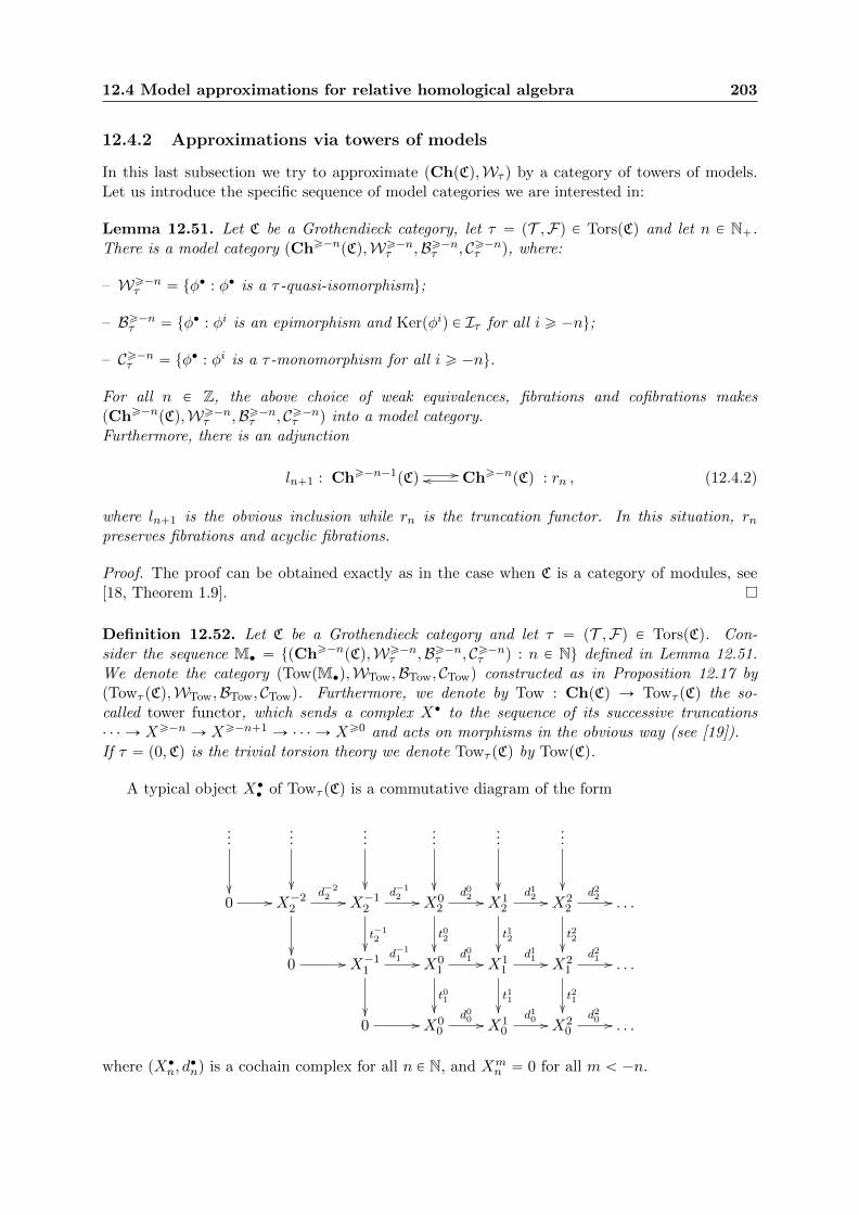
12.4 Model approximations for relative homological algebra 203
12.4.2 Approximations via towers of models
In this last subsection we try to approximate pChpCq,Wτ q by a category of towers of models.Let us introduce the specific sequence of model categories we are interested in:
Lemma 12.51. Let C be a Grothendieck category, let τ “ pT ,Fq P TorspCq and let n P N`.There is a model category pChě´npCq,Wě´n
τ ,Bě´nτ , Cě´nτ q, where:
– Wě´nτ “ tφ‚ : φ‚ is a τ -quasi-isomorphismu;
– Bě´nτ “ tφ‚ : φi is an epimorphism and Kerpφiq P Iτ for all i ě ´nu;
– Cě´nτ “ tφ‚ : φi is a τ -monomorphism for all i ě ´nu.
For all n P Z, the above choice of weak equivalences, fibrations and cofibrations makespChě´npCq,Wě´n
τ ,Bě´nτ , Cě´nτ q into a model category.Furthermore, there is an adjunction
ln`1 : Chě´n´1pCq //oo Chě´npCq : rn , (12.4.2)
where ln`1 is the obvious inclusion while rn is the truncation functor. In this situation, rnpreserves fibrations and acyclic fibrations.
Proof. The proof can be obtained exactly as in the case when C is a category of modules, see[18, Theorem 1.9].
Definition 12.52. Let C be a Grothendieck category and let τ “ pT ,Fq P TorspCq. Con-sider the sequence M‚ “ tpChě´npCq,Wě´n
τ ,Bě´nτ , Cě´nτ q : n P Nu defined in Lemma 12.51.We denote the category pTowpM‚q,WTow,BTow, CTowq constructed as in Proposition 12.17 bypTowτ pCq,WTow,BTow, CTowq. Furthermore, we denote by Tow : ChpCq Ñ Towτ pCq the so-called tower functor, which sends a complex X‚ to the sequence of its successive truncations¨ ¨ ¨ Ñ Xě´n Ñ Xě´n`1 Ñ ¨ ¨ ¨ Ñ Xě0 and acts on morphisms in the obvious way (see [19]).If τ “ p0,Cq is the trivial torsion theory we denote Towτ pCq by TowpCq.
A typical object X‚‚ of Towτ pCq is a commutative diagram of the form
...
��
...
��
...
��
...
��
...
��
...
��0 // X´2
2
��
d´22 // X´1
2
t´12��
d´12 // X0
2
t02��
d02 // X12
t12��
d12 // X22
t22��
d22 // . . .
0 // X´11
��
d´11 // X0
1
t01��
d01 // X11
t11��
d11 // X21
t21��
d21 // . . .
0 // X00
d00 // X10
d10 // X20
d20 // . . .
where pX‚n, d‚nq is a cochain complex for all n P N, and Xm
n “ 0 for all m ă ´n.
204 Model approximations
12.4.3 Approximation of (Ab.4˚)-k categories
Let C be a Grothendieck category and let τ “ pT ,Fq P TorspCq. The category Towτ pCq can beseen as a full subcategory of the category FuncpN,ChpCqq of functors N Ñ ChpCq and so wecan restrict the usual limit functor to obtain a functor lim : Towτ pCq Ñ ChpCq.
In [19] and [18] the authors show that when C is a category of modules over a commutativeNoetherian ring of finite Krull dimension,
Tow : pChpCq,Wτ q//oo pTowτ pCq,WTow,BTow, CTowq : lim , (12.4.3)
is a model approximation for all τ P TorspCq. On the other hand, if the Krull dimension is notfinite, one can always find counterexamples. In what follows we try to better understand thiskind of construction when C is a general Grothendieck category. First of all, notice that whenwe construct the homotopy category DpC{T q inverting the weak equivalences in pChpCq,Wτ q
we are really doing two things at the same time:
(1) localize complexes over C to complexes over C{T ;
(2) pass from a category of complexes over C{T to its derived category.
Our strategy is to separate the two operations in two different “steps”, where each “step”corresponds to a pair of adjoint functors. The composition of these adjunctions is our candidatefor a model approximation, as we will see in Theorem 12.54.
When C is an (Ab.4˚) Grothendieck category, let X‚ P ObpChpCqq and consider the sequenceof truncations ¨ ¨ ¨ Ñ Xě´2 Ñ Xě´1 Ñ Xě0. By Example 12.12 we can construct holimXě´i.One can prove as in [8, Application 2.4] that there is a quasi-isomorphism
X‚ÝÑholimXě´i . (12.4.4)
This formula is useful as it allows to reduce many questions to half-bounded complexes. On theother hand, for (12.4.4) to hold, it is sufficient that the ambient category is (Ab.4˚)-k for somefinite k:
Theorem 12.53. [59, Theorem 1.3] Let C be a Grothendieck and assume that C satisfies (Ab.4˚)-k for some positive integer k. Then, for every X‚ P ObpChpCqq, there is a quasi-isomorphismX‚ÝÑholimXě´i.
We are now ready to prove our main result.
Theorem 12.54. Let C be a Grothendieck category and let τ “ pT ,Fq P TorspCq be a torsiontheory such that C{T is (Ab.4˚)-k for some positive integer k. Then, the composition of thefollowing adjunctions
pChpCq,Wτ qQτ //ooSτ
pChpC{T q,WqTow //oolim
pTowpC{T q,WTow,BTow, CTowq
is a model approximation.
Proof. By Lemma 12.14, it is enough to show that pQτ ,Sτ q is compatible with weak equivalences(and this follows by Lemma 12.49) and that pTow, limq is a model approximation. The proofthat pTow, limq is a model approximation is given in [19] for categories of modules. One canfollow that proof almost without changes, using Theorem 12.53 (that applies here since C{T is(Ab.4˚)-k) instead of Application 2.4 in [8].
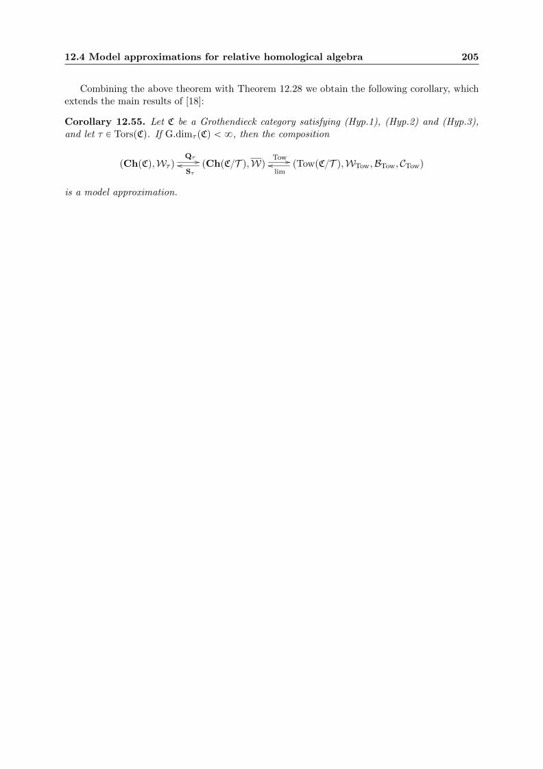
12.4 Model approximations for relative homological algebra 205
Combining the above theorem with Theorem 12.28 we obtain the following corollary, whichextends the main results of [18]:
Corollary 12.55. Let C be a Grothendieck category satisfying (Hyp.1), (Hyp.2) and (Hyp.3),and let τ P TorspCq. If G.dimτ pCq ă 8, then the composition
pChpCq,Wτ qQτ //ooSτ
pChpC{T q,WqTow //oolim
pTowpC{T q,WTow,BTow, CTowq
is a model approximation.

206 Model approximations
Bibliography
[1] R. L. Adler, A. G. Konheim, and M. H. McAndrew, Topological entropy, Trans. Amer.Math. Soc. 114 (1965), 309–319. MR 0175106 (30 #5291)
[2] Toma Albu and Constantin Nastasescu, Some aspects of non-noetherian local cohomology,Commun. Algebra 8 (1980), 1539–1560 (English).
[3] , Local cohomology and torsion theory I, Rev. Roumaine Math. Pures Appl. 26(1981), no. 1, 3–14. MR 616016 (84b:13012)
[4] Toma Albu and Patrick F. Smith, Localization of modular lattices, Krull dimension, andthe Hopkins-Levitzki theorem. I, Math. Proc. Cambridge Philos. Soc. 120 (1996), no. 1,87–101. MR 1373350 (96k:06014)
[5] Pere Ara, Kevin C. O’Meara, and Francesc Perera, Stable finiteness of group rings inarbitrary characteristic, Adv. Math. 170 (2002), no. 2, 224–238. MR 1932330 (2003j:16035)
[6] Goulnara Arzhantseva and Liviu Paunescu, Linear sofic groups and algebras, http://
arxiv.org/abs/1212.6780, 12 2012.
[7] John A. Beachy, Stable torsion radicals over FBN rings, J. Pure Appl. Algebra 24 (1982),no. 3, 235–244. MR 656845 (84b:16001)
[8] Marcel Bokstedt and Amnon Neeman, Homotopy limits in triangulated categories, Com-positio Math. 86 (1993), no. 2, 209–234. MR 1214458 (94f:18008)
[9] Nicolas Bourbaki, Algebra II. Chapters 4–7, Elements of Mathematics (Berlin), Springer-Verlag, Berlin, 2003, Translated from the 1981 French edition by P. M. Cohn and J.Howie, Reprint of the 1990 English edition [Springer, Berlin; MR1080964 (91h:00003)].MR 1994218
[10] Rufus Bowen, Entropy for group endomorphisms and homogeneous spaces, Trans. Amer.Math. Soc. 153 (1971), 401–414. MR 0274707 (43 #469)
[11] V. Capraro and M. Lupini, Introduction to Sofic and Hyperlinear groups and Connes’embedding conjecture, ArXiv e-prints (2013).
[12] Tullio Ceccherini-Silberstein and Michel Coornaert, The Garden of Eden theorem for linearcellular automata, Ergodic Theory Dynam. Systems 26 (2006), no. 1, 53–68. MR 2201937(2007a:37017)
[13] , Injective linear cellular automata and sofic groups, Israel J. Math. 161 (2007),1–15. MR 2350153 (2010c:37021)
207

208 BIBLIOGRAPHY
[14] , Linear cellular automata over modules of finite length and stable finiteness ofgroup rings, J. Algebra 317 (2007), no. 2, 743–758. MR 2362939 (2009a:16046)
[15] , On the surjunctivity of Artinian linear cellular automata over residually finitegroups, Geometric group theory, Trends Math., Birkhauser, Basel, 2007, pp. 37–44. MR2395787 (2009e:68071)
[16] , Cellular automata and groups, Springer Monographs in Mathematics, Springer-Verlag, Berlin, 2010. MR 2683112 (2011j:37002)
[17] Tullio Ceccherini-Silberstein, Fabrice Krieger, and Michel Coornaert, An analogue ofFekete’s lemma for subadditive functions on cancellative amenable semigroups, http:
//arxiv.org/abs/1209.6179, 2012.
[18] Wojciech Chacholski, Amnon Neeman, Wolfgang Pitsch, and Jerome Scherer, Relativeinjective resolutions via truncations, part II.
[19] Wojciech Chacholski, Wolfgang Pitsch, and Jerome Scherer, Relative injective resolutionsvia truncations, part I.
[20] , Injective classes of modules, Journal of Algebra and Its Applications 12 (2013),no. 4, 1250188, 13. MR 3037263
[21] Wojciech Chacholski and Jerome Scherer, Homotopy theory of diagrams, Mem. Amer.Math. Soc. 155 (2002), no. 736, x+90. MR 1879153 (2002k:55026)
[22] Nhan-Phu Chung and Andreas Thom, Some remarks on the entropy for algebraic actionsof amenable groups, http://arxiv.org/abs/1302.5813, 2013.
[23] P. M. Cohn, Free ideal rings and localization in general rings, New Mathematical Mono-graphs, vol. 3, Cambridge University Press, Cambridge, 2006. MR 2246388 (2007k:16020)
[24] Michel Coornaert and Fabrice Krieger, Mean topological dimension for actions of discreteamenable groups, Discrete Contin. Dyn. Syst. 13 (2005), no. 3, 779–793 (English).
[25] A. L. S. Corner, Three examples of hopficity in torsion-free abelian groups, Acta Math.Acad. Sci. Hungar. 16 (1965), 303–310. MR 0183776 (32 #1253)
[26] Grigore Calugareanu, Lattice concepts of module theory, Dordrecht: Kluwer AcademicPublishers, 2000 (English).
[27] John Dauns and Yiqiang Zhou, Classes of modules, Boca Raton, FL: Chapman &Hall/CRC, 2006 (English).
[28] Dikran Dikranjan and Anna Giordano Bruno, Entropy on abelian groups, in preparationhttp://arxiv.org/abs/1007.0533, 2010.
[29] Dikran Dikranjan and Anna Giordano Bruno, Discrete dynamical systems in group theory,Proceedings of the Conference “Advances in Group Theory and Applicazions 2011” PortoCesareo, 2013.
[30] , A uniform approach to chaos, preprint, 2013.
BIBLIOGRAPHY 209
[31] Dikran Dikranjan, Brendan Goldsmith, Luigi Salce, and Paolo Zanardo, Algebraic entropyfor abelian groups, Trans. Amer. Math. Soc. 361 (2009), no. 7, 3401–3434. MR 2491886(2012b:37043)
[32] Dikran Dikranjan and Hans-Peter Kunzi, Uniform entropy vs topological entropy, work inprogress (9 pages), 2014.
[33] Dikran Dikranjan, Manuel Sanchis, and Simone Virili, New and old facts about entropy inuniform spaces and topological groups, Topology Appl. 159 (2012), no. 7, 1916–1942. MR2904082
[34] Dikran N. Dikranjan, Ivan R. Prodanov, and Luchezar N. Stoyanov, Topological groups,Monographs and Textbooks in Pure and Applied Mathematics, vol. 130, Marcel Dekker,Inc., New York, 1990, Characters, dualities and minimal group topologies. MR 1015288(91e:22001)
[35] William G. Dwyer and Jan Spalinski, Homotopy theories and model categories, Hand-book of algebraic topology, North-Holland, Amsterdam, 1995, pp. 73–126. MR 1361887(96h:55014)
[36] Gabor Elek, The Euler characteristic of discrete groups and Yuzvinskii’s entropy additionformula, Bull. London Math. Soc. 31 (1999), no. 6, 661–664. MR 1711022 (2000f:37017)
[37] , The rank of finitely generated modules over group algebras, Proc. Amer. Math.Soc. 131 (2003), no. 11, 3477–3485 (electronic). MR 1991759 (2004i:43003)
[38] Gabor Elek and Endre Szabo, Sofic groups and direct finiteness, J. Algebra 280 (2004),no. 2, 426–434. MR 2089244 (2005d:16041)
[39] W. R. Emerson and F. P. Greenleaf, Asymptotic behavior of products Cp “ C ` ¨ ¨ ¨ `C inlocally compact abelian groups, Trans. Amer. Math. Soc. 145 (1969), 171–204. MR 0249535(40 #2780)
[40] Ryszard Engelking, General topology, second ed., Sigma Series in Pure Mathematics, vol. 6,Heldermann Verlag, Berlin, 1989, Translated from the Polish by the author. MR 1039321(91c:54001)
[41] Gerald B. Folland, A course in abstract harmonic analysis, Studies in Advanced Mathe-matics, CRC Press, Boca Raton, FL, 1995. MR 1397028 (98c:43001)
[42] , Real analysis, second ed., Pure and Applied Mathematics (New York), JohnWiley & Sons, Inc., New York, 1999, Modern techniques and their applications, A Wiley-Interscience Publication. MR 1681462 (2000c:00001)
[43] Erling Følner, On groups with full Banach mean value, Math. Scand. 3 (1955), 243–254(English).
[44] Pierre Gabriel, Des categories abeliennes, Bull. Soc. Math. France 90 (1962), 323–448.MR 0232821 (38 #1144)
[45] James Gillespie, Kaplansky classes and derived categories, Math. Z. 257 (2007), no. 4,811–843. MR 2342555 (2009e:55030)
210 BIBLIOGRAPHY
[46] Anna Giordano Bruno and Simone Virili, String numbers of abelian groups, J. AlgebraAppl. 11 (2012), no. 4, 1250161, 30. MR 2959431
[47] Rudiger Gobel and Jan Trlifaj, Approximations and endomorphism algebras of modules.Volume 2, extended ed., de Gruyter Expositions in Mathematics, vol. 41, Walter deGruyter GmbH & Co. KG, Berlin, 2012, Predictions. MR 2985654
[48] Jonathan S. Golan, Localization of noncommutative rings, Marcel Dekker Inc., New York,1975, Pure and Applied Mathematics, No. 30. MR 0366961 (51 #3207)
[49] , Torsion theories, Pitman Monographs and Surveys in Pure and Applied Math-ematics, vol. 29, Longman Scientific & Technical, Harlow, 1986 (English). MR 880019(88c:16034)
[50] Jonathan S. Golan and Jacques Raynaud, Derived functors of the torsion functor andlocal cohomology of noncommutative rings, J. Austral. Math. Soc. Ser. A 35 (1983), no. 2,162–177. MR 704422 (84g:16025)
[51] Robert Gordon and J. Chris Robson, The Gabriel dimension of a module, J. Algebra 29(1974), 459–473. MR 0369425 (51 #5658)
[52] Walter Gottschalk, Some general dynamical notions, Recent advances in topological dy-namics (Proc. Conf. Topological Dynamics, Yale Univ., New Haven, Conn., 1972; in honorof Gustav Arnold Hedlund), Springer, Berlin, 1973, pp. 120–125. Lecture Notes in Math.,Vol. 318. MR 0407821 (53 #11591)
[53] M. Gromov, Endomorphisms of symbolic algebraic varieties, J. Eur. Math. Soc. (JEMS) 1(1999), no. 2, 109–197. MR 1694588 (2000f:14003)
[54] Misha Gromov, Topological invariants of dynamical systems and spaces of holomorphicmaps. I, Math. Phys. Anal. Geom. 2 (1999), no. 4, 323–415 (English).
[55] A. Grothendieck, Sur quelques points d’algebre homologique, Tohoku Math. J. (2) 9 (1957),119–221 (French).
[56] Alexander Grothendieck, Sur quelques points d’algebre homologique, Tohoku Math. J. (2)9 (1957), 119–221. MR 0102537 (21 #1328)
[57] Edwin Hewitt and Kenneth A. Ross, Abstract harmonic analysis. Vol. II: Structure andanalysis for compact groups. Analysis on locally compact Abelian groups, Die Grundlehrender mathematischen Wissenschaften, Band 152, Springer-Verlag, New York, 1970. MR0262773 (41 #7378)
[58] , Abstract harmonic analysis. Vol. I, second ed., Grundlehren der MathematischenWissenschaften [Fundamental Principles of Mathematical Sciences], vol. 115, Springer-Verlag, Berlin, 1979, Structure of topological groups, integration theory, group represen-tations. MR 551496 (81k:43001)
[59] Amit Hogadi and Chenyang Xu, Products, homotopy limits and applications, http://
arxiv.org/abs/0902.4016 (2009), (13 pages).
[60] Mark Hovey, Model categories, Providence, RI: American Mathematical Society, 1999(English).
BIBLIOGRAPHY 211
[61] Mark Hovey, Cotorsion pairs, model category structures, and representation theory, Math.Z. 241 (2002), no. 3, 553–592. MR 1938704 (2003m:55027)
[62] Wen Huang, Xiangdong Ye, and Guohua Zhang, Local entropy theory for a countablediscrete amenable group action, J. Funct. Anal. 261 (2011), no. 4, 1028–1082. MR 2803841
[63] Irving Kaplansky, Infinite abelian groups, Revised edition, The University of MichiganPress, Ann Arbor, Mich., 1969. MR 0233887 (38 #2208)
[64] , Fields and rings, Chicago Lectures in Mathematics, University of Chicago Press,Chicago, IL, 1995, Reprint of the second (1972) edition. MR 1324341 (96a:12001)
[65] Masaki Kashiwara and Pierre Schapira, Categories and sheaves, Grundlehren der Math-ematischen Wissenschaften [Fundamental Principles of Mathematical Sciences], vol. 332,Springer-Verlag, Berlin, 2006. MR 2182076 (2006k:18001)
[66] Henning Krause, A note on cohomological localization, arXiv:0611101, 2006.
[67] Fabrice Krieger, Le lemme d’Ornstein-Weiss d’apres Gromov, Dynamics, ergodic theory,and geometry, Math. Sci. Res. Inst. Publ., vol. 54, Cambridge Univ. Press, Cambridge,2007, pp. 99–111. MR 2369443 (2009f:43001)
[68] Elon Lindenstrauss and Benjamin Weiss, Mean topological dimension., Isr. J. Math. 115(2000), 1–24 (English).
[69] Wolfgang Luck, L2-invariants: theory and applications to geometry and K-theory, Ergeb-nisse der Mathematik und ihrer Grenzgebiete. 3. Folge. A Series of Modern Surveysin Mathematics [Results in Mathematics and Related Areas. 3rd Series. A Series ofModern Surveys in Mathematics], vol. 44, Springer-Verlag, Berlin, 2002. MR 1926649(2003m:58033)
[70] Saunders Mac Lane, Categories for the working mathematician, second ed., Graduate Textsin Mathematics, vol. 5, Springer-Verlag, New York, 1998. MR 1712872 (2001j:18001)
[71] I. G. Macdonald, Duality over complete local rings, Topology 1 (1962), 213–235. MR0151491 (27 #1476)
[72] Eben Matlis, Injective modules over Noetherian rings, Pacific J. Math. 8 (1958), 511–528.MR 0099360 (20 #5800)
[73] J. C. McConnell and J. C. Robson, Noncommutative Noetherian rings, revised ed., Grad-uate Studies in Mathematics, vol. 30, American Mathematical Society, Providence, RI,2001, With the cooperation of L. W. Small. MR 1811901 (2001i:16039)
[74] Claudia Menini, Orsatti’s contribution to module theory, Abelian groups, module theory,and topology (Padua, 1997), Lecture Notes in Pure and Appl. Math., vol. 201, Dekker,New York, 1998, pp. 9–18. MR 1651152 (2000a:01028)
[75] Barry Mitchell, Rings with several objects, Advances in Math. 8 (1972), 1–161. MR 0294454(45 #3524)
[76] Bruno J. Muller, Linear compactness and Morita duality, J. Algebra 16 (1970), 60–66.MR 0263875 (41 #8474)
212 BIBLIOGRAPHY
[77] , Duality theory for linearly topologized modules, Math. Z. 119 (1971), 63–74. MR0279143 (43 #4869)
[78] Amnon Neeman, Triangulated categories, Princeton, NJ: Princeton University Press, 2001(English).
[79] D. G. Northcott, Lessons on rings, modules and multiplicities. Reprint of the 1968 hardbacked., Cambridge: Cambridge University Press, 2008 (English).
[80] Constantin Nastasescu and Freddy van Oystaeyen, Dimensions of ring theory, Mathemat-ics and its Applications, 36. Dordrecht etc.: D. Reidel Publishing Company, a member ofthe Kluwer Academic Publishers Group. XI, 360 p.;(1987)., 1987.
[81] Donald S. Ornstein and Benjamin Weiss, Entropy and isomorphism theorems for actionsof amenable groups, J. Analyse Math. 48 (1987), 1–141. MR 910005 (88j:28014)
[82] Zoltan Papp, On stable noetherian rings, Trans. Amer. Math. Soc. 213 (1975), 107–114.MR 0393120 (52 #13930)
[83] Donald S. Passman, The algebraic structure of group rings, Robert E. Krieger PublishingCo. Inc., Melbourne, FL, 1985, Reprint of the 1977 original. MR 798076 (86j:16001)
[84] , Infinite crossed products, Pure and Applied Mathematics, vol. 135, AcademicPress Inc., Boston, MA, 1989. MR 979094 (90g:16002)
[85] Justin Peters, Entropy on discrete abelian groups, Adv. in Math. 33 (1979), no. 1, 1–13.MR 540634 (80i:28037)
[86] , Entropy of automorphisms on L.C.A. groups, Pacific J. Math. 96 (1981), no. 2,475–488. MR 637984 (83e:54038)
[87] L. S. Pontryagin, Topological groups, Translated from the second Russian edition by ArlenBrown, Gordon and Breach Science Publishers, Inc., New York-London-Paris, 1966. MR0201557 (34 #1439)
[88] N. Popescu and P. Gabriel, Caracterisation des categories abeliennes avec generateurs etlimites inductives exactes, C. R. Acad. Sci., Paris 258 (1964), 4188–4190 (French).
[89] Daniel G. Quillen, Homotopical algebra, Lecture Notes in Mathematics, No. 43, Springer-Verlag, Berlin, 1967. MR 0223432 (36 #6480)
[90] Andrew Ranicki (ed.), Non-commutative localization in algebra and topology, LondonMathematical Society Lecture Note Series, vol. 330, Cambridge, Cambridge UniversityPress, 2006. MR 2222649 (2007f:55002)
[91] Jan-Erik Roos, Derived functors of inverse limits revisited, J. Lond. Math. Soc., II. Ser.73 (2006), no. 1, 65–83 (English).
[92] Walter Rudin, Fourier analysis on groups, Wiley Classics Library, John Wiley & SonsInc., New York, 1990, Reprint of the 1962 original, A Wiley-Interscience Publication. MR1038803 (91b:43002)
[93] Luigi Salce, Peter Vamos, and Simone Virili, Length functions, multiplicities and algebraicentropy, Forum Math. 25 (2013), 255–282 (English).
BIBLIOGRAPHY 213
[94] Luigi Salce and Paolo Zanardo, A general notion of algebraic entropy and the rank-entropy,Forum Math. 21 (2009), no. 4, 579–599. MR 2541474 (2011b:16020)
[95] N. Spaltenstein, Resolutions of unbounded complexes, Compos. Math. 65 (1988), no. 2,121–154 (English).
[96] Bo Stenstrom, Rings and modules of quotients, Lecture Notes in Mathematics, Vol. 237,Springer-Verlag, Berlin, 1971. MR 0325663 (48 #4010)
[97] Peter Vamos, Additive functions and duality over Noetherian rings, Quart. J. Math. OxfordSer. (2) 19 (1968), 43–55. MR 0223434 (36 #6482)
[98] , Length functions on modules, Ph.D. thesis, University of Sheffield, 1968.
[99] Simone Virili, Algebraic i-entropies, Master Thesis, 2010.
[100] Peter Walters, An introduction to ergodic theory, Graduate Texts in Mathematics, vol. 79,Springer-Verlag, New York, 1982. MR 648108 (84e:28017)
[101] Thomas Ward and Qing Zhang, The Abramov-Rokhlin entropy addition formula foramenable group actions, Monatsh. Math. 114 (1992), no. 3-4, 317–329. MR 1203977(93m:28023)
[102] R. B. Warfield, Jr., Decompositions of injective modules, Pacific J. Math. 31 (1969), 263–276. MR 0249467 (40 #2712)
[103] Seth Warner, Topological rings, North-Holland Mathematics Studies, vol. 178, North-Holland Publishing Co., Amsterdam, 1993. MR 1240057 (95a:16058)
[104] Charles A. Weibel, An introduction to homological algebra, Cambridge Studies in Ad-vanced Mathematics, vol. 38, Cambridge University Press, Cambridge, 1994. MR 1269324(95f:18001)
[105] Benjamin Weiss, Sofic groups and dynamical systems, Sankhya Ser. A 62 (2000),no. 3, 350–359, Ergodic theory and harmonic analysis (Mumbai, 1999). MR 1803462(2001j:37022)

214 BIBLIOGRAPHY
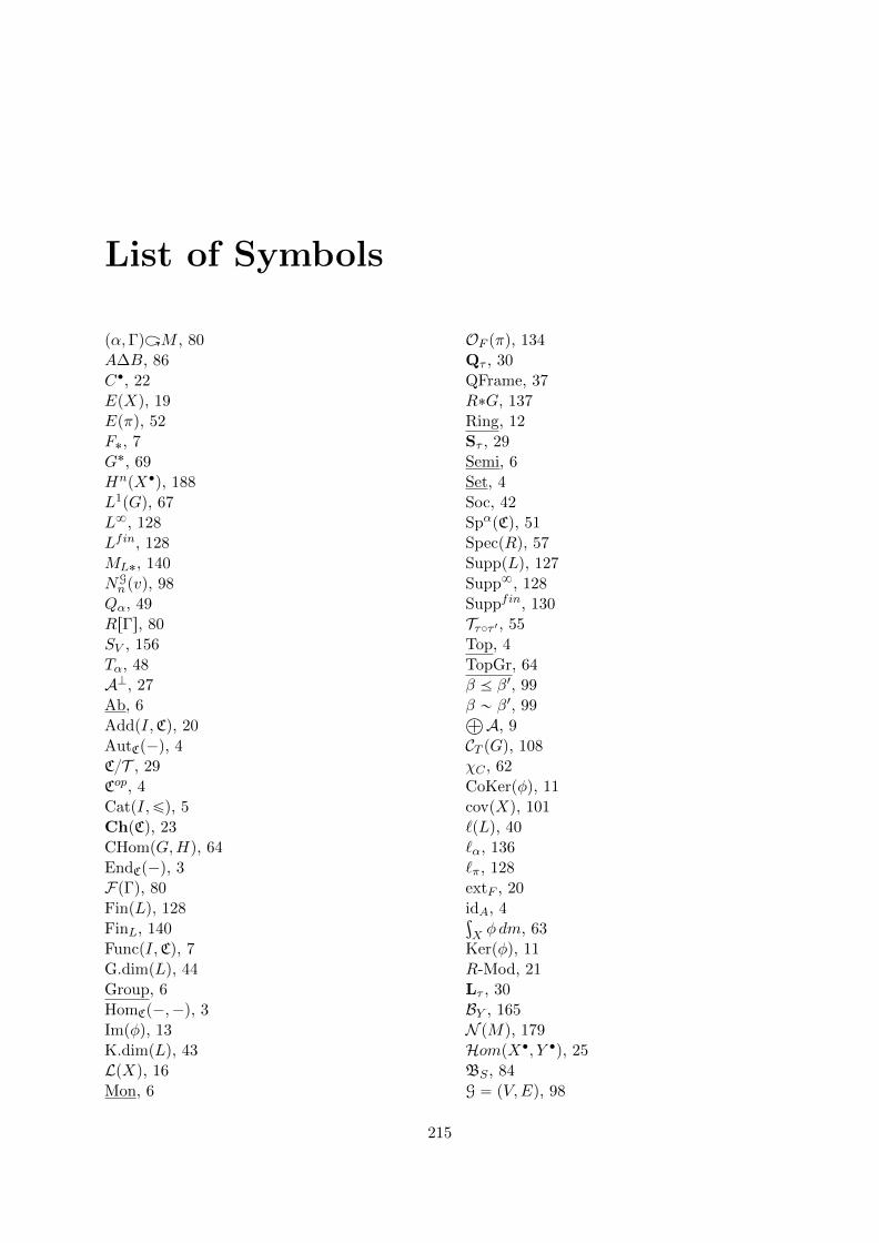
List of Symbols
pα,ΓqüM , 80
A∆B, 86
C‚, 22
EpXq, 19
Epπq, 52
F˚, 7
G˚, 69
HnpX‚q, 188
L1pGq, 67
L8, 128
Lfin, 128
ML˚, 140
NGn pvq, 98
Qα, 49
RrΓs, 80
SV , 156
Tα, 48
AK, 27
Ab, 6
AddpI,Cq, 20
AutCp´q, 4
C{T , 29
Cop, 4
CatpI,ďq, 5
ChpCq, 23
CHompG,Hq, 64
EndCp´q, 3
FpΓq, 80
FinpLq, 128
FinL, 140
FuncpI,Cq, 7
G.dimpLq, 44
Group, 6
HomCp´,´q, 3
Impφq, 13
K.dimpLq, 43
LpXq, 16
Mon, 6
OF pπq, 134
Qτ , 30
QFrame, 37
R˚G, 137
Ring, 12
Sτ , 29
Semi, 6
Set, 4
Soc, 42
SpαpCq, 51
SpecpRq, 57
SupppLq, 127
Supp8, 128
Suppfin, 130
Tτ˝τ 1 , 55
Top, 4
TopGr, 64
β ĺ β1, 99
β „ β1, 99À
A, 9
CT pGq, 108
χC , 62
CoKerpφq, 11
covpXq, 101
`pLq, 40
`α, 136
`π, 128
extF , 20
idA, 4ş
X φdm, 63
Kerpφq, 11
R-Mod, 21
Lτ , 30
BY , 165
N pMq, 179
HompX‚, Y ‚q, 25
BS , 84
G “ pV,Eq, 98
215
Mod-R, 21ord, 102FinpLq, 128φ ˚ ψ, 67ś
A, 9resF , 20τ 1 ĺ τ , 32τ “ pT ,Fq, 27Tτ , 28TorspCq, 32u.dimpLq, 37Semiv, 79Semi˚v , 79limÝÑ
F , 8
limÐÝ
F , 8
pφ, 70
ζA,B, 11
dV pσ1, σ2q, 156
fα, 133
spLq, 42
tαpLq, 47
zLpMq, 140KA, 27
(x,y), 35
(x,y], 35
[x,y), 35
[x,y], 35
216
Index
F -orbit, 134I-monomorphism, 198α-cover, 89α-torsion part, 47δ-cover
even, 89s-dominated, 83s-entropy, 81σ-algebra, 61ε-disjoint family, 89pA, 132
adjunction, 7compatible with weak equivalences, 190
alphabet, 155anti-homomorphism
of monoids, 5of semigroups, 5
atomic length function, 128automorphism, 4
base of a topology, 59basis, 37Borel
measurable, 62measure, 62
regular, 62sets, 62
category, 3Abelian, 13additive, 11cocomplete, 8complete, 8concrete, 155discrete, 5filtered, 9functor, 7
additive, 20
Grothendieck, 18
locally finitely generated, 122
locally Noetherian, 122
model, 185
of Abelian groups, 6
of groups, 6
of monoids, 6
of rings, 12
of semigroups, 6
opposite, 4
pre-additive, 11
product, 5
small, 7
well-powered, 16
with enough injectives, 19
with weak equivalences, 185
cellular automaton, 155
linear, 157
pre-injective, 163
class
hereditary
torsion, 26
injective, 198
localizing, 26
orthogonal, 27
Serre, 26
closure, 36
cochain complex, 22
acyclic, 22
dg-injective, 26
exact, 22
morphism of, 22
cofibration, 186
cofinal subset, 81
colimit
filtered, 9
compact space, 60
completely meet irreducible, 42
217
composition series, 40congruence, 38Conjecture
L-Surjunctivity, 158Stable Finiteness, 159Surjunctivity, 156Zero-Divisors, 160
continuous chain, 26continuous map, 4convergent net, 81convolution, 67coproduct, 9cover
basic, 103crossed product, 137
defining window, 155derived category, 188direct summand, 16directed path, 98discrete order, 5discrete space, 59duality, 7
epimorphism, 13equivalence of categories, 7
Følnernet, 88sequence, 88
fibration, 186filter, 59filter base, 59finite intersection property, 61flat homomorphism of rings, 22Fourier transform, 70frame, 36function
G-equivariant, 93characteristic, 62integrable, 63monotone, 93sub-additive, 93
functor, 5additive, 12adjoint, 7commutes with (co)limits, 9exact, 15faithful, 6
full, 6identity, 5left exact, 15localization, 30quotient, 30right exact, 15section, 29sends (co)limits to (co)limits, 9torsion, 28truncation, 23
Gabrielcategory, 49dimension, 44filtration, 49spectrum, 51
generalization closed subset, 53generator, 18group, 6
Abelian, 6amenable, 86LC, 64LCA, 64sofic, 157topological, 64
group topology, 64
Haar measure, 66Hamming distance, 156Hausdorff space, 60hereditary torsion theory, 27homeomorphism, 61homomorphism
contractive, 79of groups, 6of lattices, 17of monoids, 5of rings, 12of semi-groups, 5preserving segments, 36
homotopy category, 187Hopfian
hereditarily, 159
idealprime, 57
identity, 4image, 13injective envelope, 19
218
invariant, 121additive, 121upper continuous, 121
isomorphism, 4
join-independent family, 37
Krull dimension, 43
labeled digraph, 98lattice, 16
bounded, 35complete, 16distributive, 35modular, 35pseudo-complemented, 36upper-continuous, 35
left field of fractions, 22left uniformity, 103length function, 122
atomic, 126compatible with R˚G, 138compatible with a self-equivalence, 131finite component of, 128infinite component of, 128
length of a qframe, 40limit, 8
co-, 8filtered, 9
linear variety, 72local defining map, 155
mapclosed, 61open, 61proper, 61
module, 21linearly compact, 72strictly linearly compact, 72topological, 71
monoid, 4monomorphism, 13morphism
essential, 17inverse, 4restriction, 16separating, 13zero, 11
natural
isomorphism, 6transformation, 6
neighborhoodof a vertex, 98
net, 81Cauchy, 103convergent, 103
norm, 79
objectL-finite, 128cofibrant, 186cohopfian, 155fibrant, 186finitely generated, 122hopfian, 155indecomposable, 16initial, 7injective, 19invariant, 16local, 29projective, 19quotient, 15simple, 50sub-, 15
essential, 17terminal, 7torsion, 28torsion free, 28zero, 7
open cover, 101basic, 103
ordertotal, 4
order (of an open cover), 102
partially ordred set, 4pre-base of a topology, 60pre-norm, 79pre-normed semigroup
topological, 108preordered set, 4product, 9product of topological spaces, 61pseudo-complement, 36pull back, 9push out, 9
quasi-action, 156
219
quasi-frame, 37compact, 39homomorphism of, 37
algebraic, 37product of, 38uniform, 37
quotient module, 21
rank, 123refinement, 40regular element, 22replacement
cofibrant, 186fibrant, 186
representationBernoulli, 84
right uniformity, 103ring, 12
commutative, 12directly finite, 158monoid, 80stably finite, 158topological, 71
saturated set of ideals, 201scalar
extension, 20restriction, 20
segment, 15, 35semi-group, 4semi-lattice
homomorphism of, 17semigroup
normed, 79pre-normed, 79
sequenceshort exact, 14
setclosed, 4directed, 9open, 4
socle, 42specialization closed subset, 53
spectrum of a ring, 57subcategory, 6
full, 6submodule, 21support
finite, 130infinite, 128
support (of a length function), 127surjunctive map, 156system
direct, 8inverse, 8
topologicaldimension, 102space, 4
topologycompact-open, 69finite, 74induced, 60
torsion free set of ideals, 201torsion theory
cogenerated by an object, 28exact, 30generalization of a, 32improper, 28prime, 51specialization of a, 32trivial, 28
uniform s-entropy, 106uniform dimension, 37uniform space, 103
complete, 103uniformly continuous map, 103universal property, 8
Vamos extension, 124
weak domination of functions, 99weak equivalence of functions, 99
zero-divisor, 22
220


