Embed Size (px)
Citation preview
Algebraic Calculi
for
Separation Logic
Dissertation zur Erlangung des Grades eines
Doktors der Naturwissenschaften (Dr. rer. nat)an der Fakultät für Angewandte Informatik
der Universität Augsburg
vorgelegt von
Han Hing Dang
2014

Gutachter:
Erstgutachter: Prof. Dr. Bernhard MöllerZweitgutachter: Prof. Dr. Bernhard Bauer
Tag der mündlichen Prüfung:
09. Dezember 2014
Love is not �nding someone to live with.
It's �nding someone you can't live without.
Rafael Ortiz
To my �ancée Olga

CONTENTS
Contents
Preamble 1
1 Introduction 51.1 Motivation . . . . . . . . . . . . . . . . . . . . . . . . . . . . . . . . . 51.2 Separation Logic . . . . . . . . . . . . . . . . . . . . . . . . . . . . . . 71.3 Algebras for Pointer Structures . . . . . . . . . . . . . . . . . . . . . . 91.4 Contributions and Organisation . . . . . . . . . . . . . . . . . . . . . . 10
2 Separation Logic � An Overview 122.1 A Storage Model and Spatial Assertions . . . . . . . . . . . . . . . . . 122.2 Program Constructs for Resource Manipulation . . . . . . . . . . . . . 162.3 The Frame Rule . . . . . . . . . . . . . . . . . . . . . . . . . . . . . . 20
3 Algebraic Spatial Assertions 233.1 A Denotational Model for Assertions . . . . . . . . . . . . . . . . . . . 23
3.1.1 Related Work: BI Algebras . . . . . . . . . . . . . . . . . . . . 313.2 Characterising Behaviour Abstractly . . . . . . . . . . . . . . . . . . . 32
3.2.1 Intuitionistic Assertions . . . . . . . . . . . . . . . . . . . . . . 333.2.2 Resource Independence . . . . . . . . . . . . . . . . . . . . . . 363.2.3 Preciseness . . . . . . . . . . . . . . . . . . . . . . . . . . . . . 403.2.4 Full Allocation . . . . . . . . . . . . . . . . . . . . . . . . . . . 423.2.5 Supported Assertions . . . . . . . . . . . . . . . . . . . . . . . 44
3.3 Relationship to Separation Algebras . . . . . . . . . . . . . . . . . . . 51
4 Relational Separation 574.1 Interpreting Commands Relationally . . . . . . . . . . . . . . . . . . . 574.2 On Partial and Total Correctness . . . . . . . . . . . . . . . . . . . . . 614.3 Abstracting Modularity . . . . . . . . . . . . . . . . . . . . . . . . . . 67
4.3.1 A Pointfree Frame Property . . . . . . . . . . . . . . . . . . . . 724.3.2 Resource Preservation . . . . . . . . . . . . . . . . . . . . . . . 76
CONTENTS
4.3.3 A Calculational Proof of the Frame Rule . . . . . . . . . . . . . 784.3.4 Related Algebraic Approaches . . . . . . . . . . . . . . . . . . . 81
4.4 Applications to Concurrency . . . . . . . . . . . . . . . . . . . . . . . 854.4.1 Relations and Concurrent Separation Logic . . . . . . . . . . . 854.4.2 Disjoint Concurrency . . . . . . . . . . . . . . . . . . . . . . . . 944.4.3 Concurrent Kleene Algebras . . . . . . . . . . . . . . . . . . . . 98
4.5 Pointfree Dynamic Frames . . . . . . . . . . . . . . . . . . . . . . . . . 1094.5.1 Abstracting Dynamic Frames . . . . . . . . . . . . . . . . . . . 1104.5.2 Locality and Frame Accumulation . . . . . . . . . . . . . . . . 116
5 Transitive Separation Logic 1235.1 The Algebraic Foundation . . . . . . . . . . . . . . . . . . . . . . . . . 1235.2 A Stronger Notion of Separation . . . . . . . . . . . . . . . . . . . . . 1275.3 An Algebra of Linked Structures . . . . . . . . . . . . . . . . . . . . . 1325.4 Structural Properties of Linked Structures . . . . . . . . . . . . . . . . 1345.5 Assertions and Program Commands . . . . . . . . . . . . . . . . . . . 1395.6 Inference Rules . . . . . . . . . . . . . . . . . . . . . . . . . . . . . . . 143
5.6.1 Selector Assignments . . . . . . . . . . . . . . . . . . . . . . . . 1435.6.2 Frame Rules . . . . . . . . . . . . . . . . . . . . . . . . . . . . 144
5.7 Veri�cation Examples . . . . . . . . . . . . . . . . . . . . . . . . . . . 1485.7.1 List Reversal . . . . . . . . . . . . . . . . . . . . . . . . . . . . 1485.7.2 Tree Rotation . . . . . . . . . . . . . . . . . . . . . . . . . . . . 150
5.8 A Treatment of Overlaid Data Structures . . . . . . . . . . . . . . . . 154
6 Conclusion 1616.1 Summary . . . . . . . . . . . . . . . . . . . . . . . . . . . . . . . . . . 1616.2 Future Work . . . . . . . . . . . . . . . . . . . . . . . . . . . . . . . . 162
A Deferred Proofs and Properties 165A.1 Deferred Proofs . . . . . . . . . . . . . . . . . . . . . . . . . . . . . . . 165A.2 Further Properties of the Assertion Calculus . . . . . . . . . . . . . . . 178A.3 Deferred Figures . . . . . . . . . . . . . . . . . . . . . . . . . . . . . . 184
Bibliography 185
List of Figures 199
Index 200
Curriculum Vitae 203
1
Preamble
Übersicht
Ein bedeutendes Forschungsthema für die moderne Softwaretechnik ist die Entwick-lung von formalen Methoden, die Korrektheit von Computerprogrammen bzgl. ihrerSpezi�kation sicherstellen. Diverse Verfahren wurden innerhalb der letzten Jahrzehnteentwickelt, speziell im Fachgebiet der logischen Methoden. Eine der ein�ussreichstenund bekanntesten Methodiken aus diesem Bereich ist die Separationslogik. Sie hatsich aus der Hoare-Logik entwickelt, um speziell die Beweisführung auf Programmenmit einer Vielzahl an Referenzen auf dynamisch reservierten Speicher zu vereinfachen.Durch spezielle Mechanismen erlaubt sie einfache Formeln zur Charakterisierung derFormen und Strukturen von Datentypen. Insbesondere hat sich diese Logik durchdie Möglichkeit einer kompositionellen Konstruktion von Korrektheitsbeweisen alsskalierbar erwiesen, speziell für komplexeren Programmcode. Während der letztenJahre wurde eine Vielzahl von Ausprägungen in diesem Forschungsbereich geschaf-fen, die sich von Anwendungen für Nebenläu�gkeit bis hin zur Mechanisierung undprogrammgestützten Veri�kation von imperativen und objektorientierten Program-men erstrecken.
Jede dieser anwendungsspezi�sch entwickelten Separationslogiken erweitert den ur-sprünglichen Kern, der skalierbare Beweisführung ermöglicht, um eine spezielle Se-mantik und syntaktische Ausdrücke. Jedoch sind die meisten dieser Kalküle sehr kom-plex und nicht weitreichend anwendbar oder sie verwenden allgemeingültige Abstrak-tionen, die schwer zu verstehen sind und nur mühsam von Nicht-Experten gehand-habt werden können. Im Vergleich dazu bieten algebraische Techniken einen ba-lancierten Mittelweg für beide Probleme. Einerseits sind sie ausreichend abstraktund allgemein um Verhalten zu erfassen und darzustellen. Andererseits vereinfachensie Beweise durch einfache und (un)gleichungsbasierte Formeln, die Herleitungen vonnicht-trivialen Konsequenzen und Eigenschaften ermöglichen. Das Ziel der vorliegen-den Dissertation besteht aus der Entwicklung von algebraischen Kalkülen für eineuniforme Darstellung und Abstraktion von Verhalten in Separationslogiken. Dies er-
Preamble
möglicht im Speziellen generelle Resultate einer Theorie auf eine andere zu übertragen.Darüber hinaus können durch die Verwendungen einfacher Formeln, auch auf abstrak-ter Ebene, Programmwerkzeuge zur Unterstützung und Steuerung der Entwicklungweiterer Theorien verwendet werden.
2
Abstract
A major research topic for the discipline of software engineering is the developmentof formal methods that ensure correctness of computer programs w.r.t. their speci�-cations. Various approaches have been developed over the last decades, especially inthe �eld of logical methods. One of the most in�uential and popular methodologiesin this area is separation logic. It has evolved from Hoare logic as a treatment thatfacilitates reasoning about programs that massively work with references to dynami-cally allocated storage. Due to special mechanisms it allows simple formulas for thecharacterisation of shapes and structures of data types. Moreover, it has proven to bescalable by enabling a compositional construction of correctness proofs in particularfor large program code. During the last years various developments in this researcharea have been established ranging from applications within concurrency to mechani-sation and tool-supported veri�cation of imperative and object-oriented programs.
Each application-speci�c separation logic introduces special syntax and semantics ontop of the original core that enables scalable reasoning. However, most of the calculiare very complex and not widely applicable, or they involve general abstractions thatare di�cult to understand and handle for non-experts. By contrast, algebraic tech-niques provide a balanced compromise for both problems. On the one hand they areabstract and general enough to capture and represent behaviour in a concise and sim-ple way. On the other hand they facilitate reasoning by formulas in an (in)equationalstyle that allow derivations of non-trivial consequences and properties. The aim ofthe present thesis is to develop algebraic calculi for a uniform representation and ab-straction of behaviour in separation logics. This yields in particular the possibility oftransferring general results between various separation logical theories. Moreover, dueto simple formulas expressed within �rst-order logic they also enable at the abstractlevel a tool support for developing further theories.
3
Preamble
Acknowledgement
First of all, I am most grateful to my supervisor Prof. Dr. Bernhard Möller for givingme the possibility to write a doctoral thesis. Without his support, motivation andencouragements during the years I would never have �nished this work. Moreover, Iwant to thank Prof. Dr. Bernhard Bauer for reviewing this thesis.
I am also very grateful to Dr. Peter Höfner who has already supported me at the timewhen I �nished my diploma thesis. His never ending variety of ideas in discussionsalways impressed me and enormously in�uenced my thinking in developing solutionsfor research-related problems.
Moreover, I would like to thank my colleagues Dr. Markus Endres, Roland Glück, Dr.Alfons Huhn, Prof. Dr. Werner Kieÿling, Dominik Köppl, Dr. Martin Müller, PatrickRoocks and Florian Wenzel for an enjoyable atmosphere during the past years at theUniversität Augsburg and in particular Andreas Zelend and Alba vom Wolfschlag forenjoyable conversations. I also thank Dr. Georg Struth for fruitful discussions andall reviewers of the RAMiCS, MPC conferences, the ATE, PAAR workshops and ofthe JLAP, JLAMP and SCP journals for helpful and inspiring comments.
For �nancial support I thank Prof. Dr. Bernhard Möller for providing me withteaching assistant jobs during my �rst years. I would also like to thank Prof. Dr.Werner Kieÿling and Prof. Dr. Dirk Hachenberger for bridging fundings with furtherteaching assistant jobs. Moreover, I gratefully acknowledge the German researchfoundation (DFG) for funding a position and especially many thanks to Prof. Dr.Bernhard Möller and Dr. Peter Höfner for their e�orts in writing all of the proposalsover the last years. Finally, I am grateful to Sir Tony Hoare for the cooperation withinthe DFG-project AlgSep.
Also I am most grateful to my family for any support during the last years. In par-ticular, many thanks to my brothers Chi Tai and Han Kie for the endless discussionsabout any computer science related topics and my sister Anna for always giving meadvice in any matter. Moreover, I am deeply grateful to my �ancée Olga for alwayssupporting me in any decisions I made and being there for me whenever I neededsomeone in my life.
Finally, many thanks to my friends and all people who supported me during the pastyears.
4
Chapter 1
Introduction
Separation Logic was developed to facilitate reasoning about shared mutable datastructures in a Hoare logic style. It comes with suitable operations and spatial predi-cates that ensure for frequently used data structures central correctness properties asthe absence of sharing resources. There exists also a variety of algebraic approachesthat re�ect central concepts for the treatment of such data structures. In this sectionwe provide some historical background on separation logic and algebraic approachesfor pointer structures. Moreover, we give a short overview on recent developmentsand conclude by summarising the structure and contributions of this thesis.
1.1 Motivation
Many formal methods have been developed during the past decades to ensure cor-rectness of programs that heavily work with pointers, i.e., references to resources of aprogram. This has been proven to be a di�cult and tedious task, especially with log-ical calculi by Hoare and Dijkstra in their original forms [Hoa69, Dij76]. A reason forthis is that these treatments do not provide adequate and general enough constructsfor dealing with complex data structures. The problem therefore is that certain prop-erties or invariants have to be de�ned in a fashion that is di�cult to understand andread. This in turn makes the lengthy correctness proofs less reliable and the wholeapproach usable only for experts, i.e., the minority of users.
Hence, Reynolds, O'Hearn and others introduced an extension of such calculi, called
Introduction
separation logic [Rey02], that provides operators to facilitate the task of specifyingthe mentioned properties and invariants of data structures. The speciality of thislogic is a connective, called separating conjunction, that ensures disjointness of setsof resources. This has the advantage that the resources of the disjoint sets cannotbe aliases of each other. In combination with recursively de�ned predicates it allowsrelatively simple characterisations of shared mutable data structures such as singlyand doubly-linked lists or tree structures. In addition to that the logic also validatesa special inference rule called the frame rule, which allows under certain assumptionslocal and modular reasoning about programs by focusing on relevant parts of the statespace. This makes the approach more scalable and hence also applicable for tacklinglarge programs by compositionally verifying procedures on smaller parts of storageand then obtaining a global proof of the program by reassembling the proofs of theparts.
Nowadays there exists a lot of research around separation logic, resulting in a mul-titude of logical calculi (see e.g., [Par10]) for particular applications ranging frominformation hiding [ORY09] to concurrency reasoning [O'H07] and rely/guarantee set-tings [VP07]. All of these treatments include the basic concepts of separation. More-over, a variety of theorem proving tools on a decidable fragment of separation logic hasbeen developed for automating the logic and veri�cation tasks [BCO06, JP08, Tue08].A general disadvantage of most approaches is that each calculus and correspondingtheorem prover has to be developed anew, although their foundations and cores arethe same. This development is cumbersome, expensive and time-consuming. In par-ticular, the knowledge of experts is often required for introducing special behaviourin the setting. This can be facilitated by the abstraction from irrelevant details andconcentrating on the foundations that establish the advantages and characteristics ofseparation logic.
Algebraic techniques have proved to be adequate for the abstraction of logical cal-culi. The abstract and calculational proofs enable formal reasoning using simple(in)equational laws as known from school algebra. Such laws can be used to describethe main core of all separation logic-based calculi and moreover enable the derivationof general and commonly used properties and inference rules. We develop such ab-stract and general algebraic calculi where one can compositionally enrich the basicsetting with additional axioms that include special behaviour of various forms of sep-aration logic calculi. Thus, the algebraic setting represents a compact and uniformrepresentation of such. We provide, in particular, abstract and general formulationsfor the assertion language of separation logic which denote frequently reused parts.Moreover we characterise in a relational and pointfree style the local behaviour thatestablishes modularity of that approach, also in a concurrent environment. Moreover,due to abstractness we can relate the core of separation logic also to the theory ofdynamic frames that is basically inspired by the concepts of separation. Using the
6
1.2 Separation Logic
established formalisations we develop an extension to separation logic that furtherfacilitates reasoning within graph structures by introducing several new operators.
A �nal advantage that comes with an algebraic treatment is that the obtained lawscan directly be fed into existing fully automated theorem proving systems as done e.g.,in [HS07, HS08, DH08]. This allows a tool-supported and tool-guided developmentof various separation-logical calculi without any need to construct proof systems forevery special problem domain. In particular, this approach makes use of the stepwiseevolving power of general-purpose theorem provers.
1.2 Separation Logic
The central concepts and ideas to keep resources of a program distinct appeared �rst inBurstall's work [Bur72] in 1972. According to [Rey09] these represented the �rst stepstowards separation logic. A sound instance of that logic was introduced independentlyin 1999 by the authors Ishtiaq and O'Hearn in [IO01] and Reynolds in [Rey00]. In theirworks an intuitionistic version of the logic was developed that provides assertions witha monotonicity property in the following sense: if an assertion holds for some parts ofthe dynamically allocatable storage then it is also valid for any larger storage. The keyconcept of both approaches was a �spatial conjunction� on assertions for expressingseparation between memory regions. Concretely, for arbitrary assertions p and q theirseparating conjunction p ∗ q asserts that p and q both hold, but each for a separatepart of the storage.
In [IO01], Ishtiaq and O'Hearn also developed a variant within classical logic which ismore expressive than the intuitionistic version. More concretely, their work does notincorporate the mentioned monotonicity property. In particular the starting point fortheir assertion language was another theoretical foundation called the logic of bunchedimplications, abbreviated by BI [OP99, Pym02]. This early approach was developedby O'Hearn and Pym and represented a logical proof system that also included theideas for an abstract treatment of resources. In [OP99] a Kripke semantics for currentseparation logic assertions was provided that described the intuition for the separatingconjunction and its adjoint, the separating implication alias the magic wand operation.
Building on this semantic foundation O'Hearn and others continued to develop an-other important ingredient of separation logic, called the frame rule [ORY01]. Thatspecial inference rule includes the concepts of separation and allows, in some circum-stances, local reasoning about changing storage without a�ecting disjoint portions.This expresses the main power of separation logic as correctness proofs become scal-able. A semantic foundation for this inference rule has been established in [YO02]yielding a denotational model for separation logic. Finally, the basic version of the
7
Introduction
logic was presented in [Rey02] and extended by Reynolds with a command languagethat allows altering separate ranges and includes pointer arithmetic.
Starting from this, the logic had an immense in�uence on formal methods for reasoningabout program correctness. In [Yan01, Yan07], an algorithm that is frequently usedfor garbage collectors is treated within separation logical approaches. The algorithmis called the Schorr-Waite graph marking and has the advantage that it only requiresan extra bit per node to identify marked nodes [SW67]. A variant of separation logicthat presents a correctness of a copying garbage collector can be found in [TSBR08].Moreover, separation logic has been extended with proof rules that are suitable forinformation hiding in [ORY09]. As another application for the logic it has beenadapted to object-orientation [PB05] coping with JAVA-like classes and procedureswhile maintaining modularity.
Further research considers separation logic and concurrency. First ideas to this havebeen developed in [O'H07] by O'Hearn, resulting in concurrent separation logic. Itwas used as a formal method to reasoning about concurrent programs that massivelyinvolve pointers. A semantics to this approach that proved soundness of that logichas been introduced by Brookes [Bro07]. A further proof that validates soundness byan operational semantics was developed in [Vaf11]. A concrete veri�cation of a non-blocking stack in a concurrent setting that used the special proof rules of concurrentseparation logic can be found in [PBO07]. There also exists another approach toverifying concurrent algorithms by so-called rely/guarantee techniques [CJ00, VP07].This setting facilitates reasoning about interference by providing adequate proof rulesand conditions under which assertions remain stable under certain interference, i.e.,guarantee some behaviour. For this there exist also variants of separation logic thatinclude the concept of permissions [BCY06].
Moreover, also at the data structure level there exists a variety of treatments yield-ing more suitable operators for reasoning about sharing [WBO08, HV13]. A modalextension to verify data-parallel pointer programs has been considered [Nis06]. Fur-thermore, a separation logic that copes with low-level programs has been intro-duced [TKN07]. Moreover, for automating the veri�cation of program propertiesa multitude of extensions has been considered [CS10], also incorporating aspects ofconcurrency or enabling machine-supported veri�cation, e.g., in tools like Small-foot [BCO06] which is implemented on a decidable fragment of separation logic[BCO05], or the Verifast program veri�er [JP08]. In addition to this also higher-order logic theorem proving tools such as Isabelle/HOL have been combined withseparation logic [Tue08]. Further research on automation considered shape analy-sis methodologies [YLB+08, CDOY09b] that in particular allowed the extraction ofspeci�cations and preconditions by the source code of a hardware driver and systemcode [CDOY09a].
8
1.3 Algebras for Pointer Structures
A more theoretical view to extract the core behaviour of separation logical calculiwas provided in various other works. A �rst comprehensive and useful abstractionis currently being explored in [DYBG+13] which provides a formal foundation andadditional ingredients to obtain several separation logical calculi. Similar generalisedapproaches to this that are used to capture a wide range of models of separation logicwas developed in the treatment of local actions and abstract separation logic [COY07].Moreover, relationships to other frameworks such as the theory of dynamic frameshas been discussed, since that approach was developed to tackle similar problems asseparation logic does [SJP09].
1.3 Algebras for Pointer Structures
Early approaches on an algebraic treatment of pointer structures have been inves-tigated from 1990 on by Möller [Möl92, Möl93a, Möl93b]. An algebraic foundationfor pointer structures was introduced that already allowed the characterisation offrequently required properties like the absence of cycles or disjointness of the setof reachable nodes from a designated root node. The latter property correspondsclosely to the central concept of separation logic assertions that guarantee by separat-ing conjunction spatial disjointness of sets of resources. This allowed a calculationalveri�cation of algorithms on lists like their concatenation or reversal [Möl97]. Fur-ther investigations on this problem �eld led to observation on more complex datastructures as trees, forests and particularly cyclic lists [Möl99a] yielding concepts todescribe updates on pointer structures along speci�ed links and the characterisationof sharing patterns and their exclusion.
Building on this algebraic approach, Ehm developed in 2003 a formal treatment ofpointer structures called pointer Kleene algebra based on the algebraic structure ofKleene algebras [Ehm03, Ehm04]. These structures come with a special operationfor �nite iteration called the Kleene star and were introduced to model the theoryof regular events. They have been extensively studied by Conway [Con71] in 1971,resulting in various axiomatisations of Kleene algebras based on quantales, which area special case of idempotent semirings. In the case of pointer structures iteration isused to abstractly model reachability along arbitrarily many links. The approach ofEhm also includes elements of the theory of L-fuzzy relations, i.e., Goguen categories(e.g., [Win07]) to introduce labels on links and operations to extend the de�nitionsof reachability on such abstract structures. Moreover, it has been shown that thealgebraic treatment also allowed a derivational approach for obtaining correctnesspreserving functional de�nitions of pointer algorithms [Ehm01]. The reverse directionfor a veri�cation purpose in sense of Hoare logics has also been sketched in [Ehm03].
There are algebraic approaches for the propositional fragment of Hoare logics [Koz00,
9
Introduction
MS06a] and the wp-calculus of Dijkstra [MS06b] that also consider Kleene algebrasand quantales. In particular, they have been used in various applications ranging fromconcurrency control [Coh94, HMSW09a, HMSW09b] to program analysis [KP00] andsemantics [MHS06]. The algebraic approach achieved several goals. The view becamemore abstract, which led to a considerable reduction of detail and hence allowedsimpler and more concise proofs. On some occasions also additional precision wasgained. Furthermore, the algebraic abstraction places the considered theories into amore general context and therefore allows re-use of a large body of existing results.
The used algebraic structures, i.e., Kleene algebras and idempotent semirings, areformulated in pure �rst-order logic. This further enables the use of o�-the-shelf au-tomated theorem provers for verifying properties at the more abstract level [HS07,HSS08]. A lot of feasibility and case studies have been investigated during the re-cent years [Str07, Höf08], particularly for the case of pointer Kleene algebra [DM11].Moreover, various theorem proving systems that can be found within the TPTP Li-brary [SS98] have been evaluated with the mentioned algebraic structures. As oneresult of this, Prover9 [McC05] turned out to be the most adequate system forautomating these tasks [DH08]. Most of the input �les can be found at the webpage [Höf] for the interested reader. However, the case of quantales is slightly di�er-ent as it comes with axioms not expressive within �rst-order logic. An encoding ofan axiomatisation and some automated proofs of basic properties within higher-orderlogic can be found in [DH12] with less promising results with nowadays standardsystems. Newer approaches on this topic use semi-automated proof assistants likeIsabelle/HOL [AS12, ASW13b] or Coq [BP12]. An extensive amount of proofsusing Isabelle/HOL can be found in [ASW13a].
1.4 Contributions and Organisation
The contribution of this thesis consists of three parts. We developed an abstractionof the spatial assertion of separation logic based on quantales. For this we de�ned aset-based variant of the separating conjunction that enabled simple algebraic proofsof main properties. Moreover, by the abstraction to quantales this further allowedpointfree inequational characterisations of assertion classes. The abstract develop-ments also allow the transfer of the gained results to other separation logical theories.As the second main contribution we developed a relational calculus to model the ef-fects and behaviour of separation logic that guarantee its modularity and scalability inprogram proofs. This allowed further formulations for other separation logical calculiin a sequential and also concurrent setting. The last contribution that we present isan algebraic extension of separation logic for a more suitable treatment of pointer orlinked object structures. This approach signi�cantly allows simple correctness proofs
10
1.4 Contributions and Organisation
of algorithms on linked data structures that split into one part guaranteeing preser-vation of structural invariants and another preserving functional correctness.
The thesis is organised as follows:
Chapter 2 gives an overview of separation logic in its classical form. First, we providea standard storage model and main concepts of the assertion language. Moreover,we present the programming layer of the logic itself and introduce de�nitions thatestablish modularity within that approach.
In Chapter 3 we continue with a denotational model for the assertions of separationlogic based on sets of states. We further abstract this structure to general quantaleswhich allows the exclusion of irrelevant details of separation logic assertions. As our�rst contribution we provide completely pointfree characterisations of well-known andfrequently used assertion classes. This yields fully algebraic and abstract proofs ofcentral properties in a calculational style.
The second contribution of this thesis can be found in Chapter 4. There, we pro-vide a relational calculus extended to cope with separation. In particular, we giveformulations to include the fault-avoiding triple de�nition of separation logic into thepointfree setting and developed characterisations of central properties and de�nitionsto establish soundness of the frame rule. Finally, we give a concise and algebraicproof of that inference rule and extended the formulations to incorporate also con-currency proof rules. As a �nal step for this chapter we provide relationships of therelational treatment to other similar approaches as, e.g., concurrent Kleene algebrasin the case of concurrency and the dynamic frames theory as another approach thatinvolves framing.
Chapter 5 represents the third contribution of this thesis and gives an extension toseparation logic at its data structure level. In this chapter we replace the resourcesof separation logic by elements of a modal Kleene algebra that abstractly capturepointer or linked structures. By this we give de�nitions of operations and predicatesthat allow simple proofs of preservation of tree-like structures. Moreover, we presentas case studies for that approach correctness proofs of algorithms for lists, trees andin particular threaded trees that involve both data structures.
Finally, Chapter 6 provides a summary of this thesis and gives some open questionsfor future work.
In the Appendix one can �nd all deferred proofs and properties for the interestedreaders.
11
Separation Logic � A Short Overview
Chapter 2
Separation Logic
� A Short Overview
In this chapter we give basic de�nitions of the standard approach of separation logicthat was introduced in [Rey02]. We provide a standard storage model on which theseparation logical assertions are evaluated. Moreover, we give all standard de�nitionsof the spatial assertions and present some simple examples to demonstrate the mainconcepts for establishing correctness of frequently used data structures. As anotherimportant concept we give operational semantics for the program commands of thatlogic and provide formulations that entail scalability of the whole approach.
2.1 A Storage Model and Spatial Assertions
As already mentioned, separation logic is an extension of Hoare logic and, besidesreasoning about explicitly named program variables, it comes with additional newconnectives for a �exible treatment of dynamically allocated storage. For this exten-sion, a program state in separation logic consists of a store and a heap component.In contrast, plain Hoare logic states only involve a store, since just values of usedprogram variables have to be remembered. In the remainder we consistently write sfor stores and h for heaps.
For a formal model of the underlying storage we �rst provide some de�nitions. Inthe standard approach one de�nes values and addresses as integers, stores and heaps
12
2.1 A Storage Model and Spatial Assertions
as partial functions from variables or addresses to values and states as pairs of storesand heaps:
Values = ZZ ,
{nil} ∪ Addresses ⊆ Values ,
Stores = V ; Values ,
Heaps =⋃
A
(A; Values) , (A ⊆ Addresses, A �nite)
States = Stores ×Heaps ,
where V denotes the set of program variables, ∪ is with disjoint union on sets andM ; N means the set of partial functions between arbitrary sets M and N . Theconstant nil is handled as an improper reference like null in the imperative program-ming language C . By the above de�nition, nil is not an address and hence heaps donot assign values to nil , which is a natural requirement. The domain of a relationmodelling a partial function R is de�ned by
dom(R) =df {x : ∃ y : (x, y) ∈ R} .
More concretely, the domain of a store dom(s) denotes all variables currently used bya program while dom(h) is the set of all allocated addresses on a heap h .
As in [Möl93b] and for later de�nitions of program commands we also need an updateoperator to model changes in stores and heaps. Let f1 and f2 be partial functions.Then we de�ne
f1 | f2 =df f1 ∪ {(x, y) : (x, y) ∈ f2 ∧ x 6∈ dom(f1)} . (2.1)
By this, f1 updates the partial function f2 with all possible pairs (x, y) of f1 in sucha way that f1 | f2 is again a partial function. The domain of the right argument of∪ is disjoint from that of f1 . In particular, f1 | f2 can be seen as an extension of f1
to dom(f1) ∪ dom(f2) . We abbreviate an update {(x, y)} | f on a single variable oraddress by omitting the set-braces and write (x, y) | f instead.
Now, expressions in separation logic are de�ned to be independent of the heap andhence only need the store component of a given state for their evaluation. This entailsthat their evaluation will not have any side e�ects. As in Hoare logic, they simplydenote values or Boolean conditions. Syntactically, we distinguish exp-expressionswhich are arithmetical expressions over variables and values and bexp-expressionswhich are Boolean expressions, i.e., comparisons and true, false :
var ::= x | y | z | ...exp ::= 0 | 1 | 2 | ... | var | exp ± exp | ...bexp ::= true | false | exp = exp | exp < exp | ...
13
Separation Logic � A Short Overview
Assuming that all free variables of an expression e are contained in dom(s) , thesemantics es of an expression e w.r.t. a store s is straightforward. For example,∀ z ∈ Values : zs = z, trues = true or falses = false .
As a next step, we de�ne syntax and semantics of separation logic assertions. Theyextend the Hoare logic ones with additional constructs to make assumptions aboutthe heap component of a state. Their syntax is de�ned by
assert ::= bexp | ¬ assert | assert ∨ assert | ∀ var . assert |emp | exp 7→ exp | assert ∗ assert | assert −∗ assert .
The assertions in the upper row are known from predicate logic while the ones belowcan be used to express spatial properties about the heap. In the following we use theletters p, q and r for assertions. Note, the standard ones above can be supplementedby the logical connectives ∧ , → and ∃ that are de�ned, as usual, by p ∧ q =df
¬ (¬ p ∨ ¬ q), p→ q =df ¬ p ∨ q and ∃ v : p =df ¬∀ v : ¬ p .The semantics of assertions is given by a relation s, h |= p of satisfaction. Informally,s, h |= p holds i� the state (s, h) satis�es the assertion p . The semantics is de�nedinductively as follows (cf. [Rey09]):
s, h |= b ⇔df bs = true
s, h |= ¬p ⇔df s, h 6|= ps, h |= p ∨ q ⇔df s, h |= p or s, h |= qs, h |= ∀ v : p ⇔df ∀x ∈ ZZ : (v, x) | s, h |= ps, h |= emp ⇔df h = ∅s, h |= e1 7→ e2 ⇔df h = {( es1 , es2 )}s, h |= p ∗ q ⇔df ∃h1, h2 ∈ Heaps : dom(h1) ∩ dom(h2) = ∅ and
h = h1 ∪ h2 and s, h1 |= p and s, h2 |= qs, h |= p−∗ q ⇔df ∀h′ ∈ Heaps : (dom(h′) ∩ dom(h) = ∅ and s, h′ |= p)
implies s, h′ ∪ h |= q .
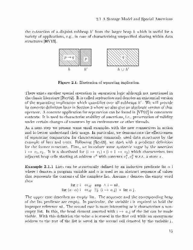
Here, b is a bexp-expression and e1, e2 are exp-expressions. As mentioned, the �rstfour clauses do not consider the heap and are well known (e.g. [Hoa69]). The remain-ing lines express the meaning of the new constructs: emp ensures that the heap h isempty and hence contains no addressable cells. The assertion e1 7→ e2 characterisesthe heap of a state to contain exactly one cell at the address es1 with value es2 . Forbuilding up more complex heaps, the operator of separating conjunction ∗ is intro-duced. It can conversely also be interpreted as a connective that ensures propertieson disjoint regions of the underlying heap. Finally, a state (s, h) satis�es the separat-ing implication p−∗ q if h ensures that whenever it is extended with a disjoint heaph′ with (s, h) |= p , the combined heap h ∪ h′ needs to satisfy (s, h ∪ h′) |= q . Anillustration of this can be found in Figure 2.1. This allows under some circumstances
14
2.1 A Storage Model and Spatial Assertions
the extraction of a disjoint subheap h′ from the larger heap h which is useful for avariety of applications, e.g., in case of characterising unspeci�ed sharing within datastructures [HV13].
p −∗ q
h
p
h′
q
h ∪ h′
Figure 2.1: Illustration of separating implication.
There exists another special operation in separation logic although not mentioned inthe classic literature [Rey02]. It is called septraction and denotes an existential versionof the separating implication which quanti�es over all subheaps h′ . We will provideits concrete de�nition later in Section 3 where we also give an algebraic version of thatoperator. A concrete application for septraction can be found in [VP07] in concurrentcontexts. It is used to characterise stability of assertions, i.e., preservation of validityunder certain changes of resources by an environment or other threads.
As a next step we present some small examples with the new connectives in actionand to better understand their usage. In particular, we demonstrate the e�ectivenessof separating conjunction for characterising commonly used data structures by theexample of lists and trees. Following [Rey09], we start with a predicate de�nitionfor the former structure. First, we introduce some syntactic sugar by the assertioni 7→ v1, v2 . It is a shorthand for (i 7→ v1) ∗ (i + 1 7→ v2) which characterises twoadjacent heap cells starting at address vs with contents vs1 , v
s2 w.r.t. a store s .
Example 2.1.1 Lists can be structurally de�ned by an inductive predicate list α i
where i denotes a program variable and α is used as an abstract sequence of valuesthat represents the contents of the complete list. Assume ε denotes the empty wordthen
list ε i ⇔df emp ∧ i = nil ,list (a · α) i ⇔df ∃ j. (i 7→ a, j) ∗ list α j .
The upper case describes an empty list. The sequence and the corresponding heapof the list predicate are empty. In particular, the variable i is required to hold theimproper reference nil . The second case is more interesting as it characterises a non-empty list. In this, the head element asserted with i 7→ a, j of the list can be madevisible. With this de�nition the value a is stored in the �rst cell while an anonymousaddress to the rest of the list is saved in the second cell denoted by the variable j .
15
Separation Logic � A Short Overview
Such addresses are generally realised in separation logic by existentially quanti�edvariables in formulas. Note, that separating conjunction in this case implies that i
and j can not hold the same address, i.e., they are not aliases. Moreover, one caneasily use the following formula for sequences α, β
list α i ∗ list β j
to characterise two disjoint lists on the heap. By the usage of separating conjunctionand the recursive de�nition of the predicate list one can show that both lists can notshare some of their allocated heap cells. ut
Example 2.1.2 Another example is given by the following de�nition that charac-terises the shape of a tree data structure. For representing the values of the data�elds in a tree so-called S-expressions [Rey09] are used which we will not elaboratehere. Conceptually the recursive de�nition of tree predicates is similar to that of lists:
tree a i ⇔df emp ∧ i = a ,tree (τ0 · τ1) i ⇔df ∃ i0, i1. i 7→ i0, i1 ∗ (tree τ0 i0) ∗ (tree τ1 i1) .
The base case is represented by an empty heap where the data value of the treeis kept in the variable i . Compared to lists, the above base case in the de�nitionof trees implies that at least some value a , not necessarily nil, is contained in anytree. The recursive case is similar as above for lists where tree τi ii represent the leftand right subtrees of the larger tree. Again, it can be seen that by the assertiontree τ0 i0 ∗ tree τ1 i1 one can characterise two disjoint trees on the heap that do notshare any cells. Both trees occupy di�erent portions of storage. ut
2.2 Program Constructs for Resource Manipulation
We now introduce the program constructs associated with the original approach ofseparation logic [Rey02]. Like in the assertion part, additional program constructsare introduced for changing the dynamically allocated resources. Syntactically, theprogram commands are given by
comm ::= var := exp | skip | comm ; comm| if bexp then comm else comm | while bexp do comm| newvar var in comm | newvar var := exp in comm| var := cons (exp, . . . , exp)| var := [exp] | [exp] := exp| dispose exp .
16
2.2 Program Constructs for Resource Manipulation
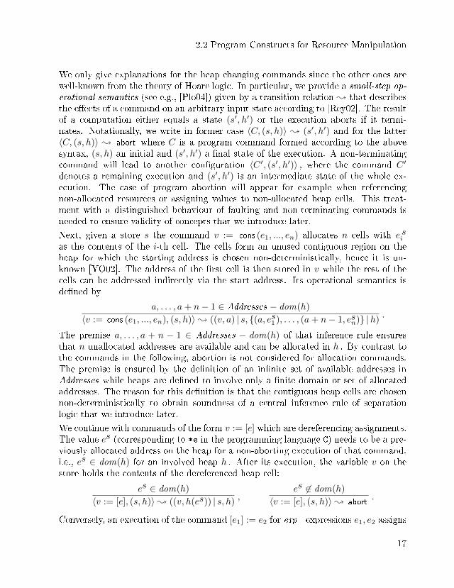
We only give explanations for the heap changing commands since the other ones arewell-known from the theory of Hoare logic. In particular, we provide a small-step op-erational semantics (see e.g., [Plo04]) given by a transition relation ; that describesthe e�ects of a command on an arbitrary input state according to [Rey02]. The resultof a computation either equals a state (s′, h′) or the execution aborts if it termi-nates. Notationally, we write in former case 〈C, (s, h)〉 ; (s′, h′) and for the latter〈C, (s, h)〉 ; abort where C is a program command formed according to the abovesyntax, (s, h) an initial and (s′, h′) a �nal state of the execution. A non-terminatingcommand will lead to another con�guration 〈C ′, (s′, h′)〉 , where the command C ′
denotes a remaining execution and (s′, h′) is an intermediate state of the whole ex-ecution. The case of program abortion will appear for example when referencingnon-allocated resources or assigning values to non-allocated heap cells. This treat-ment with a distinguished behaviour of faulting and non-terminating commands isneeded to ensure validity of concepts that we introduce later.
Next, given a store s the command v := cons (e1, ..., en) allocates n cells with e sias the contents of the i-th cell. The cells form an unused contiguous region on theheap for which the starting address is chosen non-deterministically, hence it is un-known [YO02]. The address of the �rst cell is then stored in v while the rest of thecells can be addressed indirectly via the start address. Its operational semantics isde�ned by
a, . . . , a+ n− 1 ∈ Addresses − dom(h)
〈v := cons (e1, ..., en), (s, h)〉; ((v, a) | s, {(a, es1 ), . . . , (a+ n− 1, esn)} |h).
The premise a, . . . , a + n − 1 ∈ Addresses − dom(h) of that inference rule ensuresthat n unallocated addresses are available and can be allocated in h . By contrast tothe commands in the following, abortion is not considered for allocation commands.The premise is ensured by the de�nition of an in�nite set of available addresses inAddresses while heaps are de�ned to involve only a �nite domain or set of allocatedaddresses. The reason for this de�nition is that the contiguous heap cells are chosennon-deterministically to obtain soundness of a central inference rule of separationlogic that we introduce later.
We continue with commands of the form v := [e] which are dereferencing assignments.The value es (corresponding to *e in the programming language C) needs to be a pre-viously allocated address on the heap for a non-aborting execution of that command,i.e., es ∈ dom(h) for an involved heap h . After its execution, the variable v on thestore holds the contents of the dereferenced heap cell:
es ∈ dom(h)
〈v := [e], (s, h)〉; ((v, h(es)) | s, h),
es 6∈ dom(h)
〈v := [e], (s, h)〉; abort.
Conversely, an execution of the command [e1] := e2 for exp - expressions e1, e2 assigns
17
Separation Logic � A Short Overview
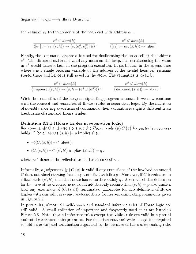
the value of e2 to the contents of the heap cell with address e1 :
es ∈ dom(h)
〈[e1] := e2, (s, h)〉; (s, (es1 , es2 ) |h)
,es 6∈ dom(h)
〈[e1] := e2, (s, h)〉; abort.
Finally, the command dispose e is used for deallocating the heap cell at the addresses . The disposed cell is not valid any more on the heap, i.e., dereferencing the valuein es would cause a fault in the program execution. In particular, in the special casewhere e is a single program variable v , the address of the invalid heap cell remainsstored there and hence is still saved in the store. The semantics is given by
es ∈ dom(h)
〈 dispose e, (s, h)〉; (s, h− (es, h(es))),
es 6∈ dom(h)
〈 dispose e, (s, h)〉; abort.
With the semantics of the heap-manipulating program commands we now continuewith the concept and semantics of Hoare triples in separation logic. By the inclusionof possibly aborting executions of commands, their semantics is slightly di�erent fromtreatments of standard Hoare triples.
De�nition 2.2.1 (Hoare triples in separation logic)For commands C and assertions p, q the Hoare triple {p}C {q} for partial correctnessholds i� for all states (s, h) |= p implies that
� ¬(〈C, (s, h)〉;∗ abort ) ,
� 〈C, (s, h)〉;∗ (s′, h′) implies (s′, h′) |= q ,
where ;∗ denotes the re�exive transitive closure of ; .
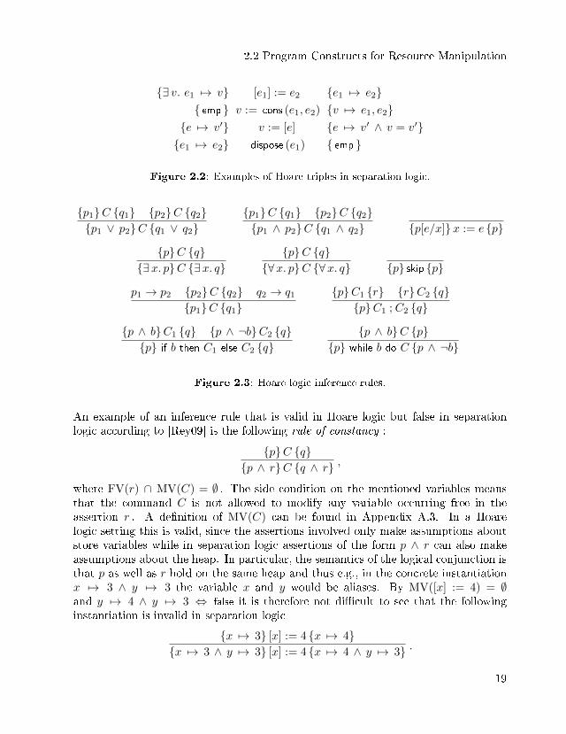
Informally, a judgement {p}C {q} is valid if any executions of the involved commandC does not abort starting from any state that satis�es p . Moreover, if C terminates ina �nal state (s′, h′) then that state has to further satisfy q . A variant of this de�nitionfor the case of total correctness would additionally require that (s, h) |= p also impliesthat any execution of 〈C, (s, h)〉 terminates. Examples for this de�nition of Hoaretriples with can valid pre- and postconditions for heap-manipulating commands givenin Figure 2.2.
In particular, almost all well-known and standard inference rules of Hoare logic arestill valid. A small collection of important and frequently used rules are listed inFigure 2.3. Note, that all inference rules except the while - rule are valid in a partialand total correctness interpretation. For the latter case and while - loops it is requiredto add an additional termination argument to the premise of the corresponding rule.
18
2.2 Program Constructs for Resource Manipulation
{∃ v. e1 7→ v} [e1] := e2 {e1 7→ e2}{ emp } v := cons (e1, e2) {v 7→ e1, e2}
{e 7→ v′} v := [e] {e 7→ v′ ∧ v = v′}{e1 7→ e2} dispose (e1) { emp }
Figure 2.2: Examples of Hoare triples in separation logic.
{p1}C {q1} {p2}C {q2}{p1 ∨ p2}C {q1 ∨ q2}
{p1}C {q1} {p2}C {q2}{p1 ∧ p2}C {q1 ∧ q2} {p[e/x]}x := e {p}
{p}C {q}{∃x. p}C {∃x. q}
{p}C {q}{∀x. p}C {∀x. q} {p} skip {p}
p1 → p2 {p2}C {q2} q2 → q1
{p1}C {q1}{p}C1 {r} {r}C2 {q}{p}C1 ; C2 {q}
{p ∧ b}C1 {q} {p ∧ ¬b}C2 {q}{p} if b then C1 else C2 {q}
{p ∧ b}C {p}{p} while b do C {p ∧ ¬b}
Figure 2.3: Hoare logic inference rules.
An example of an inference rule that is valid in Hoare logic but false in separationlogic according to [Rey09] is the following rule of constancy :
{p}C {q}{p ∧ r}C {q ∧ r} ,
where FV(r) ∩ MV(C) = ∅ . The side condition on the mentioned variables meansthat the command C is not allowed to modify any variable occurring free in theassertion r . A de�nition of MV(C) can be found in Appendix A.3. In a Hoarelogic setting this is valid, since the assertions involved only make assumptions aboutstore variables while in separation logic assertions of the form p ∧ r can also makeassumptions about the heap. In particular, the semantics of the logical conjunction isthat p as well as r hold on the same heap and thus e.g., in the concrete instantiationx 7→ 3 ∧ y 7→ 3 the variable x and y would be aliases. By MV([x] := 4) = ∅and y 7→ 4 ∧ y 7→ 3 ⇔ false it is therefore not di�cult to see that the followinginstantiation is invalid in separation logic
{x 7→ 3} [x] := 4 {x 7→ 4}{x 7→ 3 ∧ y 7→ 3} [x] := 4 {x 7→ 4 ∧ y 7→ 3} .
19
Separation Logic � A Short Overview
To overcome this issue in separation logic O'Hearn and others replaced the Booleanconjunction in this rule with the separating conjunction ∗ . This resulted in a powerfuland central inference rule that enabled modular and local reasoning about parts of aprogram which can be further embedded into a larger context under a mild restrictionon the set of involved variables. This basically re�ects the power of separation logicand explains it impact on program veri�cation. We will take a closer look at thatinference rule in the next section.
2.3 The Frame Rule
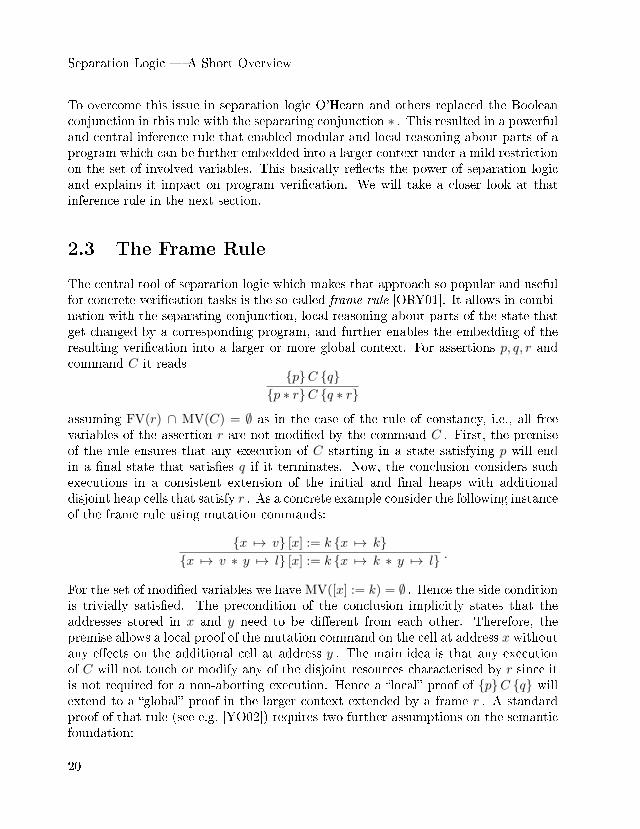
The central tool of separation logic which makes that approach so popular and usefulfor concrete veri�cation tasks is the so-called frame rule [ORY01]. It allows in combi-nation with the separating conjunction, local reasoning about parts of the state thatget changed by a corresponding program, and further enables the embedding of theresulting veri�cation into a larger or more global context. For assertions p, q, r andcommand C it reads
{p}C {q}{p ∗ r}C {q ∗ r}
assuming FV(r) ∩ MV(C) = ∅ as in the case of the rule of constancy, i.e., all freevariables of the assertion r are not modi�ed by the command C . First, the premiseof the rule ensures that any execution of C starting in a state satisfying p will endin a �nal state that satis�es q if it terminates. Now, the conclusion considers suchexecutions in a consistent extension of the initial and �nal heaps with additionaldisjoint heap cells that satisfy r . As a concrete example consider the following instanceof the frame rule using mutation commands:
{x 7→ v} [x] := k {x 7→ k}{x 7→ v ∗ y 7→ l} [x] := k {x 7→ k ∗ y 7→ l} .
For the set of modi�ed variables we have MV([x] := k) = ∅ . Hence the side conditionis trivially satis�ed. The precondition of the conclusion implicitly states that theaddresses stored in x and y need to be di�erent from each other. Therefore, thepremise allows a local proof of the mutation command on the cell at address x withoutany e�ects on the additional cell at address y . The main idea is that any executionof C will not touch or modify any of the disjoint resources characterised by r since itis not required for a non-aborting execution. Hence a �local� proof of {p}C {q} willextend to a �global� proof in the larger context extended by a frame r . A standardproof of that rule (see e.g. [YO02]) requires two further assumptions on the semanticfoundation:
20
2.3 The Frame Rule
safety monotonicity: If a command C does not abort when starting an executionfrom a state (s, h) , then C can also successfully run on states with a larger heapcomponent, i.e., (s, h′) with h ⊆ h′ . This is formally expressed as
¬(〈C, (s, h)〉;∗ abort ) ⇒ ¬(〈C, (s, h′)〉;∗ abort ) .
frame property: Every execution of a command C can be tracked back to anexecution of C running on states with possibly smaller heaps. By this, untouchedallocated resources that do not a�ect any execution of C can be omitted. This readsformally for heaps h0, h1 with dom(h0) ∩ dom(h1) = ∅ as
(¬(〈C, (s, h0)〉;∗ abort ) ∧ 〈C, (s, h0 ∪ h1)〉;∗ (s′, h′) ) ⇒∃h′0 : 〈C, (s, h0)〉;∗ (s′, h′0) ∧ h′ = h′0 ∪ h1 ∧ dom(h′0) ∩ dom(h1) = ∅ .
For establishing validity of the frame rule there also exists another approach [Vaf11]that uses a notion of con�guration safety that inductively ensures non-aborting exe-cutions in terms of the operational semantics w.r.t. the steps a command can execute.By this, validity of Hoare triples is given if a command can safely execute all of itssteps. We will consider for this thesis only the above de�ned properties and providefully algebraic and pointfree characterisations of them that will consequently enablean abstract and generalised proof of the frame rule.
21

Chapter 3
Algebraic Spatial Assertions
An abstract and algebraic treatment of the assertion part of separation logic is pre-sented, in particular of separating conjunction. For an adequate abstraction we startwith an embedding of assertions into a set-based model that allows a treatment ina calculational style. In particular, we describe a translation of the spatial opera-tors into that setting. This concrete model is further abstracted into the algebraicstructure of so-called quantales in which assertions are represented as elements of thealgebra. Using this algebra, di�erent behaviours of special classes of assertions arecharacterised in a pointfree fashion by simple (in)equations. Moreover, this entailsabstract and simple proofs of properties which can be checked and largely automatedusing general theorem proving systems. Another advantage of the algebraic viewis that it yields new insights on separation logic by the application of the obtainedresults to a wide range of concrete models.
3.1 A Denotational Model for Assertions
A common methodology for providing a denotational model for logical assertions isgiven by an embedding of the satisfaction-based semantics for single states into anequivalent set-based and therefore pointfree setting. By this, every assertion will beassociated with the set of all states that satisfy the corresponding assertion. We basi-cally follow the approach of [DHM09, DHM10]. Concretely, for an arbitrary assertionp formed using the syntax given in Section 2.1 we de�ne its set-based semantics as
[[ p ]] =df {(s, h) : s, h |= p} .
Algebraic Spatial Assertions
Clearly, by this de�nition all well-known Boolean connectives on assertions directlycoincide with corresponding set-based operations where | denotes the update operationon partial functions de�ned in Equation (2.1) and represents set complementationw.r.t. the carrier set States, i.e., for a set of states X we have X = States −X . Oneinductively obtains the following equations for the standard logic connectives,
[[¬ p ]] = {(s, h) : s, h 6|= p} = [[ p ]] ,
[[ p ∨ q ]] = [[ p ]] ∪ [[ q ]] ,
[[ p ∧ q ]] = [[ p ]] ∩ [[ q ]] , [[ p→ q ]] = [[ p ]] ∪ [[ q ]] ,
[[ ∀ v : p ]] = {(s, h) : ∀x ∈ Z : (v, x) | s, h |= p }=
⋂x∈Z{(s, h) : ((v, x) | s, h) ∈ [[ p ]] } ,
[[ ∃ v : p ]] = [[ ∀ v : ¬ p ]] = {(s, h) : ∃x ∈ Z. (v, x) | s, h |= p }=
⋃x∈Z{(s, h) : ((v, x) | s, h) ∈ [[ p ]] } .
As particular cases, [[ true ]] = States and [[ false ]] = ∅ . Similarly, set-based variantsfor the assertion emp that characterises the empty heap and e1 7→ e2 that denotes asingle cell heap can be given by
[[ emp ]] = {(s, h) : h = ∅} and [[ e1 7→ e2 ]] ={
(s, h) : h ={(es1 , e
s2
)}}.
For an adequate reformulation of separating conjunction ∗ on sets of states expressingheap disjointness we obtain
[[ p ∗ q ]] = [[ p ]] ·∪ [[ q ]] ,
where for sets P,Q ∈ P(States) we de�ne
P ·∪ Q =df {(s, h ∪ h′) : (s, h) ∈ P, (s, h′) ∈ Q, dom(h) ∩ dom(h′) = ∅} .
Assuming that the considered states involve the same stores and address-disjointheaps, this operator exactly renders the semantics of separating conjunction in aset-based fashion. Generally, this construction yields an algebraic embedding of sep-aration logic assertions into an abstract calculus by viewing the constructed sets ofstates as elements of a speci�c structure that we discuss in the following. A centralrequirement for this task involves the inclusion of algebraic counterparts of all theabove set-based operations. Especially due to the usage of possible in�nite intersec-tions and unions it turned out that an appropriate algebraic structure for this purposeare quantales which have been introduced in [Mul86, Ros90].
De�nition 3.1.1 (Quantale)
24
3.1 A Denotational Model for Assertions
(a) A quantale is a structure (S,≤, · , 1) such that
� (S,≤) is a complete lattice where, for T ⊆ S, the element⊔T denotes the
supremum of T anddT its in�mum,
� (S, · , 1) is a monoid,
� multiplication distributes over arbitrary suprema, i.e., for a ∈ S and T ⊆ S ,
a · (⊔T ) =⊔{a · b : b ∈ T} and (
⊔T ) · a =
⊔{b · a : b ∈ T} . (3.1)
The least and greatest element of a quantale w.r.t. ≤ are denoted by 0 and >,resp. Binary in�ma and suprema of two elements a, b ∈ S are denoted by a u band a+ b, resp. We assume that u binds tighter than + .
(b) A quantale is called commutative i� a · b = b · a for all a, b ∈ S .
(c) A quantale is called Boolean i� its underlying lattice is distributive, i.e., for alla, b, c ∈ S
a u (b+ c) = a u b+ a u c and a+ b u c = (a+ b) u (a+ c) ,
and is complemented. Complementation will be denoted by . Moreover, thegreatest element > is de�ned by 0 .
Note that by this de�nition + and u are commutative, associative and idempotent.The former operator has the unit 0 and annihilator > while conversely u has > asits unit and 0 as its annihilator. The natural order ≤ satis�es a ≤ b ⇔ a+ b = b ⇔a u b = a for arbitrary elements a, b ∈ S .Furthermore in a quantale one can derive that the least element satis�es
⊔ ∅ = 0 .Due to Equation (3.1) this immediately implies that · is strict in both arguments, i.e.,we have 0 · a = 0 = a · 0 for all a ∈ S and hence 0 is an annihilator.
The following equivalences are valid in quantales and will facilitate inequational rea-soning in proofs provided in later sections:
a+ b ≤ c ⇔ a ≤ c ∧ b ≤ c and a ≤ b u c ⇔ a ≤ b ∧ a ≤ c . (3.2)
In the case of Boolean quantales we have
a u b ≤ c ⇔ a ≤ b→ c . (shu)
where b → c =df b + c . This property is called shunting and entails in particular,a u b ≤ 0 ⇔ b ≤ a .
25
Algebraic Spatial Assertions
For easier readability we suppose that multiplication · binds tighter than u and + .
The assumption that (S,≤) is a complete lattice guarantees the existence of in�nitesuprema and in�ma as required for a complete algebraic treatment of separation logicassertions. We can now conclude the following result.
Theorem 3.1.2 The structure AS =df (P(States), ⊆ , ·∪ , [[ emp ]]) is a commutativeand Boolean quantale with P +Q = P ∪Q .
Proof. First, it is not di�cult to see that (P(States), ⊆ ) forms a complete and dis-tributive lattice where
⊔and
dcoincide with
⋃and
⋂, respectively. Moreover,
that ·∪ is associative, commutative and has [[ emp ]] as its unit follows from the de�ni-tions and pointwise lifting. Hence, (P(States), ·∪ , [[ emp ]]) represents a commutativemonoid. The distributivity laws of separating conjunction can also be lifted to theset-based setting and extended in AS to arbitrary unions. Finally, Boolean comple-ments in AS can be obtained using set-complementation . utBy Theorem 3.1.2 it is obvious that [[ true ]] coincides with > and [[ false ]] with 0 .Binary intersections and unions are abstracted to u and + , respectively. As alreadymentioned a concrete instance of the in�nite distributivity laws in Equation (3.1) canbe found in logical formulas involving existential quanti�cations like p ∗ (∃ v. q) ⇔∃ v. p ∗ q and its symmetric variant for arbitrary assertions p, q and variable v 6∈FV(p) .
In the case of arbitrary in�ma, only validity of inequational variants of distributivitylaws can be obtained, i.e., for an abstract quantale (S,≤, · , 1) and subset T ⊆ S wehave
(lT ) · b ≤
l{a · b : a ∈ T} and a · (
lT ) ≤
l{a · b : b ∈ T} . (3.3)
Special cases or instances of these abstract laws w.r.t. AS are given in separation logice.g., by
(p ∧ q) ∗ r ⇒ (p ∗ r) ∧ (q ∗ r) and (∀x. p) ∗ q ⇒ ∀x. p ∗ q .
A further useful property of quantales is that by the above inequational distributivitylaws, multiplication is isotone in both arguments, i.e., for elements a, b, c, d : a ≤b ∧ c ≤ d ⇒ a · b ≤ c · d . This can be translated into separation logic for adequateassertions p, q, r, s to the valid inference rule
p ⇒ r q ⇒ s
p ∗ q ⇒ r ∗ s .
More laws and examples can be found in [Dan09]. Next, we derive an algebraiccharacterisation for the remaining separation logic operations. First, we start with a
26
3.1 A Denotational Model for Assertions
treatment of the separating implication. Its logic-based application is given in [Rey02,Rey09] by instantiations of so-called currying and decurrying inference rules. Forarbitrary assertions p, q, r separating implication and separating conjunction satisfythe following interplay:
p ∗ q ⇒ r
p ⇒ (q−∗ r) (currying)p ⇒ (q−∗ r)p ∗ q ⇒ r
(decurrying) .
From an algebraic viewpoint these laws are very similar to the Galois equivalencescharacterising residuals in quantales [Bir67, Lam68]. Such elements represent thegreatest solutions x w.r.t. the order ≤ of the inequation a · x ≤ b for arbitraryelements a, b of a quantale.
De�nition 3.1.3 (Residuals)
(a) In any quantale, the right residual a\b exists and is characterised by the Galoisconnection
x ≤ a\b ⇔df a · x ≤ b . (3.4)
a\b as the greatest solution of the inequation a · x ≤ b denotes a pseudo-inverseto multiplication.
(b) Symmetrically, the left residual b/a can be de�ned by
x ≤ b/a ⇔df x · a ≤ b . (3.5)
In the case of a commutative quantale both residuals coincide, i.e., a\b = b/a .
Note that in quantales residuals do always exist by the assumption of a completeunderlying lattice that guarantees the existence of arbitrary suprema. In the concretequantale AS, we will provide a proof that algebraic residuals coincide conceptually inthe set-based setting with separating implication which reads
[[ p −∗ q ]] = {(s, h) : ∀h′ ∈ Heaps : ( dom(h) ∩ dom(h′) = ∅ ∧ (s, h′) ∈ [[ p ]])
⇒ (s, h ∪ h′) ∈ [[ q ]]} .
Residuals have been researched for already several decades and hence a large amountof general results can be immediately applied to the concrete quantale AS and thusbecome consequences in separation logic. For notational bene�t we use in the followingthe same symbols for residuals in AS and abstract quantales.
Lemma 3.1.4 In AS, [[ p−∗ q ]] = [[ p ]]\[[ q ]] = [[ q ]]/[[ p ]] .
27
Algebraic Spatial Assertions
Proof. By set theory and de�nition of ·∪ , we have
(s, h) ∈ [[ p−∗ q ]]⇔ ∀h′ : (dom(h) ∩ dom(h′) = ∅ ∧ (s, h′) ∈ [[ p ]] ⇒ (s, h ∪ h′) ∈ [[ q ]])⇔ {(s, h ∪ h′) : dom(h) ∩ dom(h′) = ∅ ∧ (s, h′) ∈ [[ p ]]} ⊆ [[ q ]]⇔ {(s, h)} ·∪ [[ p ]] ⊆ [[ q ]]
and therefore, for arbitrary set R of states,
R ⊆ [[ p−∗ q ]]⇔ ∀ (s, h) ∈ R : (s, h) ∈ [[ p−∗ q ]]⇔ ∀ (s, h) ∈ R : {(s, h)} ·∪ [[ p ]] ⊆ [[ q ]]⇔ R ·∪ [[ p ]] ⊆ [[ q ]] .
Hence, by de�nition of right residuals, [[ p−∗ q ]] = [[ p ]]\[[ q ]] . The second equationfollows immediately since ·∪ in AS commutes (cf. Theorem 3.1.2). utA similar result was stated in [IO01]. There it was mentioned that the assertional partof separation logic is an instance of an abstract approach called the logic of bunchedimplications [OP99]. We will elaborate on this in Section 3.1.1.
In our setting, by Lemma 3.1.4 the currying and decurrying inference rules becometheorems in the assertion quantale AS , and hence also all well-known laws about −∗are now theorems of the standard theory of residuals (e.g. [BJ72]). As an example afrequently used inference rule in separation logic is
q ∗ (q−∗ p) ⇒ p
which describes the general behaviour of separating implication that whenever a heapsatisfying q gets combined with a disjoint for which q−∗ p holds then the whole heapwill satisfy p . Abstractly, we can show, as a direct consequence of the de�nition ofresiduals, that for arbitrary elements a, b ∈ S the inequality b · (b\a) ≤ a holds.
Lemma 3.1.5 b · (b\a) ≤ a and symmetrically (a/b) · b ≤ a is valid.
Proof. By De�nition 3.1.3 we infer b · (b\a) ≤ a ⇔ b\a ≤ b\a ⇔ true . utNow, setting a = [[ p ]] and b = [[ q ]] one obtains validity of the inequation in AS andhence also soundness of the above inference rule in separation logic.
For later calculational proofs we list a couple of helpful properties. Right residualsare anti-disjunctive in their �rst argument and conjunctive in their second one, i.e.,for a set T ⊆ S of quantale S
y\(lT ) =
l{y\x : x ∈ T} and (
⊔T )\x =
l{y\x : y ∈ T} .
28
3.1 A Denotational Model for Assertions
In the semantics of separation logic this entails as an example validity of the logicalequivalence p−∗ (∀ v. q) ⇔ ∀ v. p−∗ q where v 6∈ FV(p) . Abstractly, the above lawsimmediately imply for arbitrary elements z the following consequence
x ≤ y ⇒ z\x ≤ z\y ∧ y\z ≤ x\z .
Another law involves e.g., a further characterisation of > by y\> = > = 0\x . Manyof these laws are proved algebraically in [Dan09] and have also been automated.
As a last ingredient and for completeness reasons we include into AS another oper-ator that is closely related to separating implication. It is called septraction in theseparation logic literature e.g. in [VP07] and is de�ned as follows.
De�nition 3.1.6 (Septraction)For assertions p, q septraction is de�ned by p −� q ⇔df ¬( p −∗ (¬q)) .
The intuition of this operator can be given by the following lemma. We provide itspointwise meaning using the carrier set States.
Lemma 3.1.7 s, h |= p −� q ⇔ ∃ h : h ⊆ h ∧ s, h− h |= p ∧ s, h |= q .
The proof of Lemma 3.1.7 is deferred to Appendix A. Informally, if a heap h satis�esp −� q , then it can be extended with a heap that satis�es p so that q holds for theresulting one. Equivalently, one can also quantify over the existence of a remainingdisjoint heap satisfying p . In contrast to separating implication it comes with angelicbehaviour since it only quanti�es existentially over the remaining heap portion wherep holds while in the case of the implicational version its condition needs to be ful�lledby all heaps. Due to this one often refers to septraction as the existential separatingimplication.
Using the above de�nitions we can analogously derive a set-based version of sep-traction in AS . Interestingly, its logical pointfree de�nition directly coincides in ASwith so-called detachment operators [Bir67] that also do exist in arbitrary Booleanquantales. As in the case of residuals we notationally also use the same symbol fordetachments in AS and arbitrary Boolean quantales.
De�nition 3.1.8 (Detachments)In a Boolean quantale, the left detachment can be de�ned based on the left residualfor elements a, b by
acb =df a\b .
Symmetrically the right detachment is de�ned by abb =df a/b . If the underlyingquantale is commutative acb = bba .
29
Algebraic Spatial Assertions
Therefore, in the quantale AS one obtains by Theorem 3.1.2
[[ p −� q ]] = [[¬(p−∗(¬q)) ]] = [[ p ]]\[[ q ]] = [[ p ]] c [[ q ]] .
As in the case of residuals and separating implication, a large amount of alreadyknown laws for detachments immediately applies to the assertion quantale AS andthus to the assertional part of separation logic.
Detachments are isotone in both arguments. Moreover, from the characterising Galoisconnection of residuals one obtains by de Morgan's laws the exchange properties
abb ≤ x ⇔ x · b ≤ a and acb ≤ x ⇔ a · x ≤ b . (exc)
Another important consequence are the Dedekind rules [JT51]
a u b · c ≤ (abc u b) · c and a u b · c ≤ b · (bca u c) . (Ded)
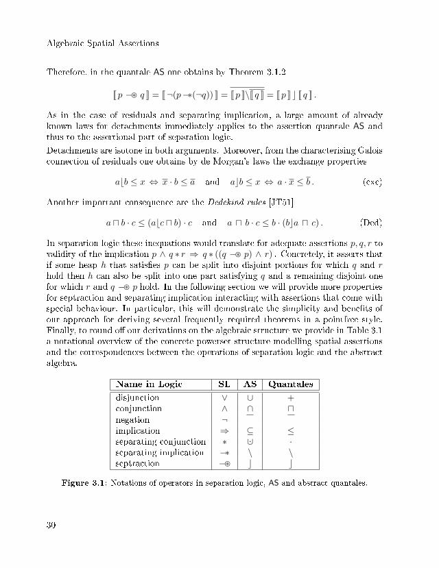
In separation logic these inequations would translate for adequate assertions p, q, r tovalidity of the implication p ∧ q ∗ r ⇒ q ∗ ((q −� p) ∧ r) . Concretely, it asserts thatif some heap h that satis�es p can be split into disjoint portions for which q and rhold then h can also be split into one part satisfying q and a remaining disjoint onefor which r and q −� p hold. In the following section we will provide more propertiesfor septraction and separating implication interacting with assertions that come withspecial behaviour. In particular, this will demonstrate the simplicity and bene�ts ofour approach for deriving several frequently required theorems in a pointfree style.Finally, to round o� our derivations on the algebraic structure we provide in Table 3.1a notational overview of the concrete powerset structure modelling spatial assertionsand the correspondences between the operations of separation logic and the abstractalgebra.
Name in Logic SL AS Quantales
disjunction ∨ ∪ +conjunction ∧ ∩ unegation ¬implication ⇒ ⊆ ≤separating conjunction ∗ ·∪ ·separating implication −∗ \ \septraction −� c c
Figure 3.1: Notations of operators in separation logic, AS and abstract quantales.
30
3.1 A Denotational Model for Assertions
3.1.1 Related Work: BI Algebras
Abstract and algebraic structures for the spatial assertions of separation logic havealso been investigated in earlier approaches. Originally, in 1999 O'Hearn and Pymdeveloped a logical approach called the logic of bunched implications (BI) [OP99]. Itintroduced the general ideas of the structure of today's separation-logical assertions.The standard interpretations depending on the carrier set States was considered as anmodel of a Boolean variant of BI [IO01]. In contrast to classical logical approaches,BI comes with two di�erent conjunction and implication operations, i.e., concretelythey coincide in separation logic with ∧ , ∗ and → ,−∗ . The spatial operations ∗ ,−∗are also called multiplicative connectives while the remaining ones are named additivein the literature. Algebraic presentations of BI use as a starting base the structure ofa Heyting algebra (S,≤) , i.e., a lattice containing a greatest and least element w.r.t.≤ and binary meets denoted by a u b that are residuated. They represent a loweradjoint and have a corresponding upper adjoint→ that is characterised by the Galoisconnection
a u b ≤ c ⇔ a ≤ b→ c .
Note that in any Boolean algebra this condition is always satis�ed and stated in thepresent quantale-based approach as shunting (cf. (shu)). More interestingly, in addi-tion to the assumed Heyting algebra one requires a further residuated commutativemonoid structure denoted by (S, ∗, emp) that similarly to the above satis�es
a ∗ b ≤ c ⇔ a ≤ b−∗ c .
Its purpose is to abstractly model the substructural part of separation logic given byseparating conjunction. Concretely ∗ does not satisfy the weakening and contractionrules
a ∗ b ≤ a and a ≤ a ∗ a (3.6)
in contrast to u , since otherwise both operations would coincide (cf. [OP99]). In sum,the full algebraic structure is called a BI algebra. Since separation logic in its earlydevelopments was provided as an intuitionistic logic [Rey00] and Heyting algebrasmodel propositional versions of such logics, an adequate abstraction [Pym02, POY04]is found by these algebras. An approach to propositional versions of classical logics,e.g., separation logic in its nowadays version [Rey02] requires the extension of BI to aBoolean algebra by replacing the underlying Heyting algebra by a Boolean one. Thatapproach is called a Boolean BI algebra and it di�ers from the algebraic treatmentbased on commutative Boolean quantales in not requiring the following structuralassumptions:
� an underlying complete lattice involving in�nite meets and joins,
31
Algebraic Spatial Assertions
� the associated in�nite (semi)distributivity laws w.r.t. ∗ .
Due to the characterisation of ∗ as a lower adjoint in the above Galois connectionthe second property would be immediately implied if arbitrary (in�nite) meets andjoins are available (e.g. [EKMS92, Möl99b]). Further considerations of Boolean BIalgebras extended to complete lattices can be found in [BBTS05, BBTS07]. In par-ticular, similar powerset constructions as presented in Section 3.1 are discussed andprovided in those papers within a categorical setting called BI hyperdoctrines. Morecategory theory related approaches involving in�nite distributivity laws are discussedin [Pym02, POY04, Bie04] where especially topological representations are consideredthat also involve complete BI algebras.
The presented approach will stay within an algebraic treatment. Its main focus com-prises, in addition to its abstract character, the further possibility of calculating alarge set of theorems in fully pointfree way especially in combination with algebraiccharacterisations of special behaviour of certain assertion classes [Rey09] which arepresented in the subsequent section. Due to the simple representations and largely�rst-order logic formulated (in)equations that setting also comes with the advantageto easily generate mechanised and (semi)automated proofs. This in turn guaranteesmore safety and con�dence in the correctness of the presented derivations.
Finally, we also remark that, based on the logic of BI, abstract resource semanticsand interpretations in a Kripke-style have been already derived in [Pym02]. Thesemodel-theoretic considerations entailed a pointwise de�nition of the separating im-plication that corresponds in a particular case to the de�nition based on the carrierset States [IO01]. Hence Lemma 3.1.4 expresses exactly the expected equalities byinterpreting separating implication as residuals within Boolean quantales.
3.2 Characterising Behaviour Abstractly
With the developed foundation of the previous section we can now move one stepfurther and consider the algebraic approach for characterising di�erent classes of as-sertions in separation logic as presented in [Rey02, Rey09]. Motivated by the factthat certain consequences of such classes can be described in a pointfree fashion, thequestion arises whether it is possible to obtain a completely algebraic treatment of theassertion classes. As an example so-called pure assertions characterise on states (s, h)only conditions that do not involve the heap component, i.e., exclusively propertiesabout store variables are expressed. This implies e.g., that logical and separatingconjunction coincide for pure assertions P,Q , i.e.,
P ∗Q ⇔ P ∧ Q .
32
3.2 Characterising Behaviour Abstractly
By results of the previous section it is an easy task to abstract this law to arbitraryquantales. In what follows, investigations are presented for the most common as-sertion classes to �nd suitable algebraic abstractions that enable the derivation ofproperties at the propositional level of separation logic as above. This immediatelyfacilitates assertional reasoning, especially in the case of purely �rst-order logicalcharacterisations that enable automation or at least mechanised proofs.
3.2.1 Intuitionistic Assertions
We start by considering the class of intuitionistic assertions. They re�ect the in-tuitionistic behaviour of assertions in the early developments of [Rey00]. In moreabstract settings as in the logic of BI, the intuitionistic behaviour is called Kripkemonotonicity and assumed for Kripke interpretations that abstract heaps to the se-mantics of possible worlds [POY04]. In the concrete setting of States the behaviour isgiven in [IO01] as a monotonicity condition and can be described in the sense that in-tuitionistic assertions do not characterise the domain of a heap or the set of allocatedheap cells exactly. Hence, an imprecision is introduced due to some additional set ofanonymous cells that may reside on the heap. This can happen in the case when e.g.,pointer references to some prior allocated storage are lost.
Following [Rey09], an assertion p is called intuitionistic i�
∀ s ∈ Stores, ∀h, h′ ∈ Heaps : (h ⊆ h′ ∧ s, h |= p ) ⇒ s, h′ |= p . (3.7)
Intuitively, if a heap h that satis�es an intuitionistic assertion p then any larger heap,i.e., extended by arbitrary cells, still satis�es p . It turned out that this particularclosure condition can be characterised within the quantale AS in a pointfree style.
Theorem 3.2.1 In AS an element [[ p ]] is intuitionistic i� it satis�es
[[ p ]] ·∪ [[ true ]] ⊆ [[ p ]] .
Proof. By de�nition of true, set theory, using for (⇒ ) h′′ = h′−h and for (⇐ ) thatdom(h) ∩ dom(h′′) = ∅ ∧ h′ = h ∪ h′′ ⇒ h′′ = h′ − h, a logic step, de�nition of ∗ ,
∀ s, h, h′ : (h ⊆ h′ ∧ s, h |= p) ⇒ s, h′ |= p⇔ ∀ s, h, h′ : (h ⊆ h′ ∧ s, h |= p ∧ s, (h′ − h) |= true ) ⇒ s, h′ |= p⇔ ∀ s, h, h′ : ( s, h |= p ∧ s, (h′ − h) |= true ∧ dom(h) ∩ dom(h′ − h) = ∅
∧ h′ = h ∪ (h′ − h) ) ⇒ s, h′ |= p⇔ ∀ s, h, h′ : ( ∃h′′ : s, h |= p ∧ s, h′′ |= true ∧ dom(h) ∩ dom(h′′) = ∅
∧h′ = h ∪ h′′ ) ⇒ s, h′ |= p
33
Algebraic Spatial Assertions
⇔ ∀ s, h′ : (∃h, h′′ : s, h |= p ∧ s, h′′ |= true ∧ dom(h) ∩ dom(h′′) = ∅∧h ∪ h′′ = h′ ) ⇒ s, h′ |= p
⇔ ∀ s, h′ : s, h′ |= p ∗ true ⇒ s, h′ |= p .
Now, the claim follows from the translation of assertions into AS given in Section 3.1.ut
Thus, Theorem 3.2.1 yields the following de�nition by the abstraction of its result toarbitrary Boolean quantales.
De�nition 3.2.2In an arbitrary Boolean quantale S an element a is called intuitionistic i� it satis�es
a · > ≤ a .
Note that this inequation can be strengthened to an equation since its converse holdsfor arbitrary Boolean quantales by neutrality of 1 and the fact that multiplication isisotone. Hence, > is characterised as a neutral element w.r.t. multiplication on the setof intuitionistic elements. Clearly, > is intuitionistic. In the case of separation logic,> coincides with true as a unit for separating conjunction ∗ . This result is stated asa consequence e.g. in [IO01]. Abstractly, elements of the form a · > are also calledin the literature vectors or ideals. Those elements are well known, and therefore onecan easily transfer many properties (e.g. [SS93, Mad06]) to this particular applicationdomain without any additional e�ort. We list some of them to show again the advan-tages of the algebraic approach and start by some intuitive closure properties whichcan also be found in [Rey02].
Lemma 3.2.3 Consider a commutative Boolean quantale S, intuitionistic elementsa, ai ∈ S with i ∈ IN and an arbitrary element b ∈ S. Then the following composedelements are also intuitionistic:
(a) a · b , hence also a · > ,
(b) b\a , hence also >\a ,
(c)d{ai : i ∈ IN} ,
(d)⊔{ai : i ∈ IN} .
Proof. The proof of part (a) is immediate from commutativity of · and the assump-tion. For part (b) we have (b\a) · > ≤ b\a ⇔ b · (b\a) · > ≤ a by De�nition 3.1.3and the claim follows from b · (b\a) ≤ a by Lemma 3.1.5 and the assumption that ais intuitionistic. The remaining parts follow from Equation (3.3), Equation (3.1) andthe assumptions. utNote, that weaker assumptions in Lemma 3.2.3 can be used than e.g. providedin [Rey02]. We continue by particular laws that describe the interaction of · andu involving intuitionistic assertions.
34
3.2 Characterising Behaviour Abstractly
Lemma 3.2.4 Consider a commutative Boolean quantale S, intuitionistic elementsa, a′ ∈ S and arbitrary elements b, c ∈ S . Then
(a) (a u b) · c ≤ a u b · c ,
(b) (a u b) · > ≤ a ,
(c) a · b ≤ a u b ·> ,
(d) a · a′ ≤ a u a′ .
Proof. To show (a) we calculate (a u b) · c ≤ a · c u b · c ≤ a · > u b · c ≤ a u b · c .Setting c = > in (a) the inequation of (b) follows from isotony of u . For a proof of(c) we know a · b ≤ a · > ≤ a and a · b ≤ > · b = b · > by isotony and commutativityof · . Again, Equation (3.2) shows the claim. Trivially (d) follows from (c) settingb = a′, applying the de�nition of intuitionistic elements and using isotony of u . utNote that part (b) implies by isotony of multiplication the weakening rule for ∗ of BIalgebras (cf. Equation (3.6)), i.e., a ∗ b ≤ a assuming a is intuitionistic. Moreover, itis not di�cult to see that the reverse inequations of the above given laws can not beobtained for the quantale AS considering translations of adequate separation logicalassertions. In particular, part (d) above only validates an inequation on intuitionisticelements characterising the interplay of multiplication and meet, or concretely separa-tion and logical conjunction, respectively. A counterexample for the opposite directionin that case is easily constructed with a = a′ = [[x 7→ 1 ∗ true ]] = [[x 7→ 1 ]] ·∪ [[ true ]] .Obviously a and a′ are both intuitionistic. Hence the de�nitions (cf. Section 2.1)immediately imply that a ∩ a′ = a 6= ∅ and a ·∪ a′ = [[x 7→ 1 ]] ·∪ [[ true ]] ·∪ [[x 7→1 ]] ·∪ [[ true ]] = ∅ since ·∪ is commutative and [[x 7→ 1 ]] ·∪ [[x 7→ 1 ]] = ∅ .This further implies that even for intuitionistic elements, the contraction law a ≤ a ·adoes not hold. We show in the subsequent section that a strengthening of the interplaygiven in part (d) to an equation can be guaranteed for assertions whose validity isindependent of the underlying heap component within arbitrary states.
Finally, we remark that similar abstract characterisations as given in De�nition 3.2.2can also be found in [BBTS05, BBTS07] within a higher-order and also abstractsetting of separation logic, called BI-hyperdoctrines. Intuitionistic assertions q canbe found there under the de�nition of monotone assertions w.r.t. heaps h of states(s, h) ∈ States. A pointfree characterisation is given by a quanti�cation over arbitraryassertions p in ∀ p. p ∗ q → q . This closely correlates to our compact characterisationby interpreting p, q as elements of a commutative Boolean quantale and → as itsassociated natural order ≤ . Then one can easily conclude
(∀ p. p · q ≤ q ) ⇔ q · > ≤ q ,
where ⇒ follows by commutativity of · and setting p = > and the reverse direction⇐ directly holds by isotony of multiplication.
35
Algebraic Spatial Assertions
3.2.2 Resource Independence
In this section special attention is paid to a particular class of assertions for whichthe behaviour can simply be described by not making any assumptions about theheap component of states, i.e., assertions that are valid for arbitrary heaps. Con-crete instances within separation logic are given by any bexp - expression (cf. Sec-tion 2.1) like false, true or e = e′ which coincide with assertions of usual Hoare logicapproaches [Hoa69]. Originally, in the separation logic literature such assertions ap-peared in [IO01, Rey02] under the notion of pure assertions . They are syntacticallydescribed there as assertions that do not contain emp and 7→ (w.r.t. the syntax givenin Section 2.1). An exclusion of the spatial operations ∗ and −∗ making assumptionsabout the underlying heaps in formulas is not required since these operations willcollapse with logical conjunction and implication, respectively. A complete algebraicproof of this fact will be provided later.
Another application of pure assertions can be found in [PS11, PS12]. The setting inthose papers considers an extended carrier set where each state is equipped with a mapfor modelling permission to access certain �elds of objects. Separating conjunction isde�ned there to split permission maps while only allowing states with equal stores andheaps. An abstraction of pure assertions to an algebraic setting will also incorporatesuch particular models.
For establishing an algebraic characterisation of pure assertions we turn back to thestandard setting based on the carrier set States . First we provide a common de�nitionof pure assertions given by the following formula
p is pure ⇔df (∀ s ∈ Stores : ∀h, h′ ∈ Heaps : s, h |= p ⇔ s, h′ |= p ) . (3.8)
First, we immediately infer from the above de�nition that if p holds for any stateat all then especially s, ∅ |= p holds. Trivially, then p is also satis�ed by any heaplarger than the empty one. Both facts will be used to derive a pointfree characterisa-tion of pure assertions. Following the ideas introduced in [DHM09, DHM11] we cancharacterise pure assertions in the quantale AS follows.
Theorem 3.2.5 In AS an element [[ p ]] is pure i� it satis�es
[[ p ]] = ([[ p ]] ∩ [[ emp ]]) ·∪ [[ true ]] .
Proof. The following logical formula is a pointwise version of the above equationfollowing Section 3.1.
∀ s ∈ Stores, ∀h ∈ Heaps : ( s, h |= p ⇔ s, h |= (p ∧ emp ) ∗ true ) . (3.9)
36
3.2 Characterising Behaviour Abstractly
We show that it is equivalent to the de�nition given in (3.8). For better readabilitywe omit the universal quanti�cation over stores in the remainder. First, we simplifys, h |= (p ∧ emp ) ∗ true . Using the de�nitions of Section 2.1, we get for arbitraryh ∈ Heaps
s, h |= ( p ∧ emp ) ∗ true
⇔ ∃h1, h2 ∈ Heaps : dom(h1) ∩ dom(h2) = ∅ ∧ h = h1 ∪ h2
∧ s, h1 |= p ∧ s, h1 |= emp ∧ s, h2 |= true
⇔ ∃h1, h2 ∈ Heaps : dom(h1) ∩ dom(h2) = ∅ ∧ h = h1 ∪ h2
∧ s, h1 |= p ∧ h1 = ∅⇔ ∃h2 ∈ Heaps : h = h2 ∧ s, ∅ |= p⇔ s, ∅ |= p .
Now, Equation (3.8) implies
∀h, h′ ∈ Heaps : ( s, h |= p ⇔ s, h′ |= p )⇒ ∀h ∈ Heaps : ( s, h |= p ⇔ s, ∅ |= p )⇔ ∀h ∈ Heaps : ( s, h |= p ⇔ s, h |= (p ∧ emp ) ∗ true ) .
For the converse direction, we conclude for arbitrary s, h, h′ using Equation (3.9) andthe above result twice that s, h |= p ⇔ s, ∅ |= p ⇔ s, h′ |= p . utHence, any pure assertion p also satis�es the logical formula p ⇔ (p ∧ emp ) ∗ true
which includes the above mentioned facts that the empty heap and any extension of italso satisfy it. Moreover, the characterisation of Theorem 3.2.5 immediately enablesa lifting to the abstracter level of arbitrary Boolean quantales yielding the followingresult.
De�nition 3.2.6In an arbitrary Boolean quantale S an element a is called pure i� it satis�es
a = (a u 1) · > .
This equation characterises pure elements as �xed points of the function f(a) =(a u 1) · > . Since f is built from isotone operations it is also isotone. Now, by theassumptions of an underlying complete lattice, the Knaster-Tarski theorem [Tar55]immediately implies that the set of pure elements is also a complete lattice. By thein�nite distributivity laws and the assumption of a Boolean quantale, we get for anyset of pure elements X that also
⊔X and
dX is pure.
As a next step we can use De�nition 3.2.6 to give further characterisations of pureelements in arbitrary commutative and Boolean quantales. We list some of them inthe following.
37
Algebraic Spatial Assertions
Lemma 3.2.7 In any commutative Boolean quantale, an element a is pure i� one ofthe following equivalent properties is satis�ed.
(a) a · > ≤ a and a · > ≤ a ,
(b) a · > ≤ a and a u b · c ≤ (a u b) · (a u c) for all b, c ∈ S ,
(c) (a u b) · c = a u b · c for all b, c ∈ S .
A proof can be found in Appendix A.
The advantages of these characterisations are that part (a) also holds in the setting ofnon-commutative quantales as it provides a simple characterisation of pureness thatimmediately reveals that pure elements and their complements are also intuitionistic.We summarise
Corollary 3.2.8 Every pure element of a Boolean quantale is also intuitionistic.
In particular, in any Boolean quantale 0 = > and therefore we can conclude that
Corollary 3.2.9 > and 0 are the greatest and smallest pure elements, respectively.
Part (b) of Lemma 3.2.7 states that in addition to being intuitionistic, pure elementsalso entail an inequational distributivity property. An upper bound of the intersectionof an arbitrary product with a pure element a is obtained by multiplying the possiblesmaller intersections of a with the arguments of the product. Finally, part (c) isstated as a property of pure elements in [Rey02] which is now fully algebraicallyderived in the abstract setting. By setting b = > and c = 1 it is not di�cult to seethat De�nition 3.2.6 is a special case of it. Note that since the underlying quantale iscommutative, it is also possible to use the dual of part (c), namely b · (auc) = a u b ·cas a characterisation of pure assertions.
We note that a similar result for a pointfree characterisation of pure assertions has alsobeen derived in [BBTS05, BBTS07]. The characterisation is given within a higher-order logic setting in category theory. It semantically corresponds very much to whatis presented in part (c).
Another characterisation for pure elements involves detachments, i.e., in concreteseparation logic the septraction operator.
Lemma 3.2.10 In a commutative Boolean quantale, the distributivity law a u b · c ≤(a u b) · (a u c) is equivalent to ab> ≤ a and >ca ≤ a .
38
3.2 Characterising Behaviour Abstractly
A proof of this lemma is deferred to Appendix A. The element >ca can be interpretedin AS as the ⊆ - downward closure of a w.r.t. the heap component of states, i.e., byremoving parts of the allocated resources in the heap, the respective state will remainin a.
To conclude the paragraph concerning pure elements we list a few properties whichcan be easily proved completely in our algebraic approach.
Corollary 3.2.11 Pure elements form a Boolean lattice, i.e., they are closed under+ , u and . Moreover the lattice is complete.
The following lemma shows that in the complete lattice of pure elements meet andjoin coincide with composition and sum, respectively.
Lemma 3.2.12 Consider a commutative Boolean quantale S, pure elements a, a′ ∈ Sand arbitrary elements b, c ∈ S. Then
(a) a · b = a u b · > ,
(b) a · a′ = a u a′ , in particular a · a = a and a · a = 0 .
Proof. For a proof of part (a) we calculate, using Lemma 3.2.7(c), a u b · > =a u > · b = (a u >) · b = a · b . To show part (b), we use again Lemma 3.2.7(c) andneutrality of 1 w.r.t. multiplication and obtain a · a′ = a u a′ · 1 = a u a′. utMany further properties, in particular, for the interaction of pure assertions withresiduals and detachments, can be found in Appendix A.2. It is possible to obtainsimilar connections for separating implication and septraction interacting with pureassertions like in Lemma 3.2.7(c) where the case for separating conjunction is stated.
We conclude this section with a consideration of pure elements from an algebraicviewpoint. There exists a relationship of pure elements and particular ones that canbe found below 1 w.r.t. ≤ . In the concrete assertion quantale AS, such elementscoincide with sets that characterise states involving empty heaps. Generally, theseelements are called tests [MB85, Koz97] and come with special behaviour which wesum up in the following de�nition.
De�nition 3.2.13 (Tests)We de�ne a test in a quantale S as an element t ≤ 1 that has a complement ¬t relativeto 1 , i.e., t + ¬t = 1 and t · ¬t = 0 = t · ¬t . The set of all tests of S is denoted bytest(S) . It is closed under + and · , where the former coincides with t and the lattercorresponds to u . Moreover, it forms a Boolean algebra with 0 and 1 as its least andgreatest elements.
39
Algebraic Spatial Assertions
Note that in any Boolean quantale the element a u 1 for each a is a test where¬(a u 1) = a u 1 holds for its relative complement. In particular, every elementbelow 1 is a test. Now, consider the characterising equation a = (a u 1) · > of pureelements. It exactly renders the relationship of pure elements and test elements inthat there exists for each a a corresponding test a u 1 . Clearly, the same holds forthe complements. In AS such sets of states involve empty heaps and contain exactlyall information and assumed conditions on the store variables of a pure assertion.Conversely, for each test t ≤ 1 there exists also a pure element given by t · > (cf.Lemma A.2.1 in the Appendix). Note that in any Boolean quantale the complementssatisfy t · > = (t u 1) · > (e.g. [DM01a]).
3.2.3 Preciseness
The previously discussed assertion classes come with the behaviour that assertions aresatis�ed on some heap and unspeci�ed extensions of it, i.e., they are given in an intu-itionistic fashion. However, concrete veri�cation tasks in separation logic frequentlyrequire the ability to point out a unique part of the heap. Examples can be found inapplications that provide particular frameworks for reasoning about information hid-ing [ORY09] or that establish special proof rules allowing unspeci�ed sharing withingraph structures [HV13].
The concept of precise assertions has turned out to be adequate for such reasoningtasks [Rey09]. These assertions ensure the existence of a unique subheap which isrelevant to their predicate. A pointwise de�nition for precise assertions is given bythe formula
∀ s, h, h1, h2 : (s, h1 |= p ∧ s, h2 |= p ∧ h1 ⊆ h ∧ h2 ⊆ h) ⇒ h1 = h2 .
By this there exists for all states (s, h) at most one subheap h′ of h which alreadycontains the allocated resources that p requires, i.e., for which we have (s, h′) |= p .Concrete examples in separation logic are emp , the single cell assertion i 7→ j forprogram variables i, j and the recursive list predicate list α i of Example 2.1.1 whereα denotes a sequence of values.
Since we are again mainly interested in deriving pointfree formulas for arbitraryBoolean quantales that abstractly re�ect the behaviour of this assertion class, wefollow a result given in [ORY09]. It is stated there that the above de�nition forprecise assertions is equivalent to the logical formula
(p ∧ q) ∗ (p ∧ r) ⇔ p ∗ (q ∧ r) ,
where p is precise and q, r are arbitrary assertions. The formula states that separatingconjunction distributes of over logical conjunction for precise assertions p . Note that
40
3.2 Characterising Behaviour Abstractly
the ⇐ - direction is always valid due to logical weakening and thus can be dropped.Applying the previous results on interpreting formulas of separation logic in AS wecan immediately state the following theorem.
Theorem 3.2.14 In AS an element [[ p ]] is precise i� it satis�es, for all [[ q ]] and [[ r ]],
([[ p ]] ·∪ [[ q ]]) ∩ ([[ p ]] ·∪ [[ r ]]) ⊆ [[ p ]] ·∪ ([[ q ]] ∩ [[ r ]]) .
Hence, for arbitrary Boolean quantales we can algebraically characterise precise as-sertions as follows.
De�nition 3.2.15In an arbitrary Boolean quantale S an element a is called precise i� for all b, c ∈ S
a · b u a · c ≤ a · (b u c) .
Obviously, the above inequation can again be strengthened in quantales to an equationby isotony of u and · . In that form it is also called determinacy known from relationalgebras (e.g., [DM01a]). The above de�nition algebraically characterises precisenessby distributivity of multiplication over binary in�ma. A similar characterisation forpreciseness within a higher-order logic approach to separation logic can also be foundin [BBTS05, BBTS07].
Depending on the used model and application it is also possible to extend De�ni-tion 3.2.15 for completeness issues to distributivity over arbitrary non-empty in�malike e.g. in [COY07, RG08], i.e.,
X 6= ∅ ⇒l{a · x : x ∈ X} ≤ a ·
lX .
In [COY07] the above characterisation involving arbitrary in�ma is used to abstractlycharacterise the structure of programs. These are modelled by functions or moreconcretely state transformers that output strongest postconditions represented as setsof states w.r.t. a given input state satisfying a considered precondition.
For our purposes one can replace the characterisation of Theorem 3.2.14 in AS with amore general one involving arbitrary intersections if required. In the case of separationlogic assertions, a concrete instance of such distributivity law can then be found inthe formula
∀x. (p ∗ q) ⇔ p ∗ (∀x. q)assuming p is precise and variable x does not occur free in p (cf. [Rey09]).
Since for most purposes the case for binary in�ma su�ces, we stay with the abovede�nition. In particular, this has the advantage that reasoning about preciseness
41
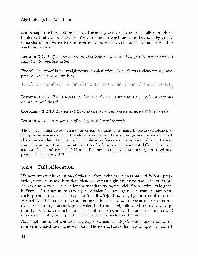
Algebraic Spatial Assertions
can be supported by �rst-order logic theorem proving systems which allow proofs tobe derived fully automatically. We continue our algebraic considerations by givingsome closure properties for this assertion class which can be proved completely in thealgebraic setting.
Lemma 3.2.16 If a and a′ are precise then so is a · a′, i.e., precise assertions areclosed under multiplication.
Proof. The proof is by straightforward calculation. For arbitrary elements b, c andprecise elements a, a′, we have
(a · a′) · b u (a · a′) · c = a · (a′ · b) u a · (a′ · c) ≤ a · (a′ · b u a′ · c) ≤ a · a′ · (b u c) .ut
Lemma 3.2.17 If a is precise and a′ ≤ a then a′ is precise, i.e., precise assertionsare downward closed.
Corollary 3.2.18 For an arbitrary assertion b and precise a, also a u b is precise.
Lemma 3.2.19 a is precise i� a · b ≤ a · b for arbitrary b .
The latter lemma gives a characterisation of preciseness using Boolean complements.For precise elements it is therefore possible to state some general behaviour thatcharacterises the interaction of multiplication (separating conjunction) and Booleancomplementation (logical negation). Proofs of above results are not di�cult to obtainand can be found e.g., in [DM01a]. Further useful properties are again listed andproved in Appendix A.2.
3.2.4 Full Allocation
We now turn to the question of whether there exist assertions that satisfy both prop-erties, preciseness and intuitionisticness. At �rst sight trying to �nd such assertionsdoes not seem to be sensible for the standard storage model of separation logic givenin Section 2.1, since an assertion p that holds for any larger heap cannot unambigu-ously point out an exact heap portion [Rey09]. However, by the use of the toolMace4 [McC05] an abstract counter model to this fact was discovered. A reinterpre-tation of it in separation logic revealed that completely allocated heaps, i.e., heapsthat do not allow any further allocation of resources are at the same time precise andintuitionistic. Algebraic proofs for this will be provided in the sequel.
Note that this is not contradicting any statement in [Rey09] where allocation of re-sources is de�ned there to never abort. The idea to this is that according to Section 2.1
42
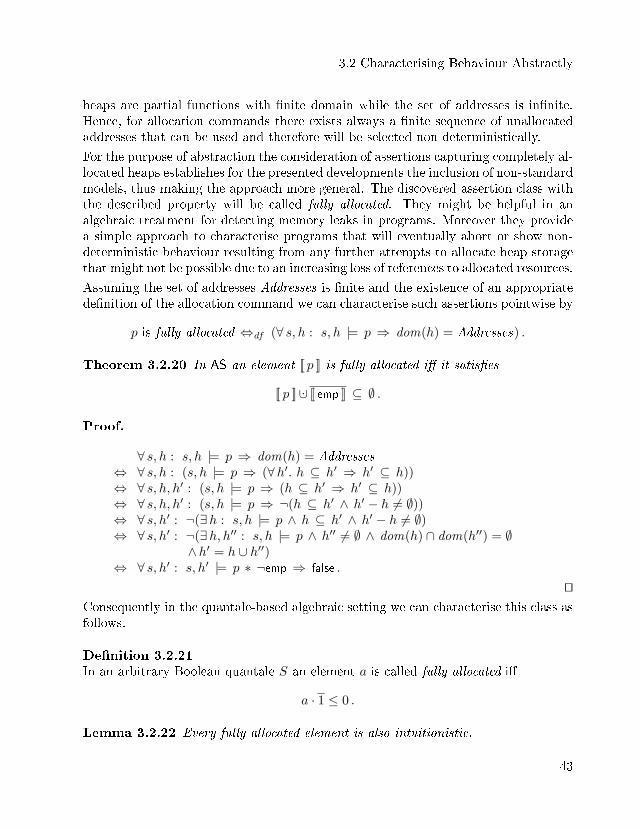
3.2 Characterising Behaviour Abstractly
heaps are partial functions with �nite domain while the set of addresses is in�nite.Hence, for allocation commands there exists always a �nite sequence of unallocatedaddresses that can be used and therefore will be selected non-deterministically.
For the purpose of abstraction the consideration of assertions capturing completely al-located heaps establishes for the presented developments the inclusion of non-standardmodels, thus making the approach more general. The discovered assertion class withthe described property will be called fully allocated. They might be helpful in analgebraic treatment for detecting memory leaks in programs. Moreover they providea simple approach to characterise programs that will eventually abort or show non-deterministic behaviour resulting from any further attempts to allocate heap storagethat might not be possible due to an increasing loss of references to allocated resources.
Assuming the set of addresses Addresses is �nite and the existence of an appropriatede�nition of the allocation command we can characterise such assertions pointwise by
p is fully allocated ⇔df (∀ s, h : s, h |= p ⇒ dom(h) = Addresses) .
Theorem 3.2.20 In AS an element [[ p ]] is fully allocated i� it satis�es
[[ p ]] ·∪ [[ emp ]] ⊆ ∅ .
Proof.
∀ s, h : s, h |= p ⇒ dom(h) = Addresses⇔ ∀ s, h : (s, h |= p ⇒ (∀h′. h ⊆ h′ ⇒ h′ ⊆ h))⇔ ∀ s, h, h′ : (s, h |= p ⇒ (h ⊆ h′ ⇒ h′ ⊆ h))⇔ ∀ s, h, h′ : (s, h |= p ⇒ ¬(h ⊆ h′ ∧ h′ − h 6= ∅))⇔ ∀ s, h′ : ¬(∃h : s, h |= p ∧ h ⊆ h′ ∧ h′ − h 6= ∅)⇔ ∀ s, h′ : ¬(∃h, h′′ : s, h |= p ∧ h′′ 6= ∅ ∧ dom(h) ∩ dom(h′′) = ∅
∧h′ = h ∪ h′′)⇔ ∀ s, h′ : s, h′ |= p ∗ ¬emp ⇒ false .
utConsequently in the quantale-based algebraic setting we can characterise this class asfollows.
De�nition 3.2.21In an arbitrary Boolean quantale S an element a is called fully allocated i�
a · 1 ≤ 0 .
Lemma 3.2.22 Every fully allocated element is also intuitionistic.
43
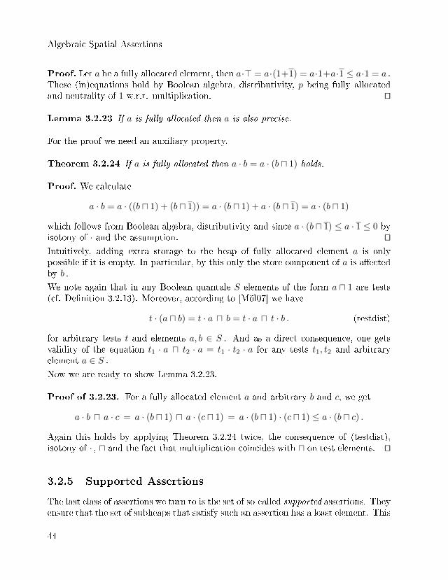
Algebraic Spatial Assertions
Proof. Let a be a fully allocated element, then a·> = a·(1+1) = a·1+a·1 ≤ a·1 = a .These (in)equations hold by Boolean algebra, distributivity, p being fully allocatedand neutrality of 1 w.r.t. multiplication. ut
Lemma 3.2.23 If a is fully allocated then a is also precise.
For the proof we need an auxiliary property.
Theorem 3.2.24 If a is fully allocated then a · b = a · (b u 1) holds.
Proof. We calculate
a · b = a · ((b u 1) + (b u 1)) = a · (b u 1) + a · (b u 1) = a · (b u 1)
which follows from Boolean algebra, distributivity and since a · (b u 1) ≤ a · 1 ≤ 0 byisotony of · and the assumption. utIntuitively, adding extra storage to the heap of fully allocated element a is onlypossible if it is empty. In particular, by this only the store component of a is a�ectedby b .
We note again that in any Boolean quantale S elements of the form a u 1 are tests(cf. De�nition 3.2.13). Moreover, according to [Möl07] we have
t · (a u b) = t · a u b = t · a u t · b . (testdist)
for arbitrary tests t and elements a, b ∈ S . And as a direct consequence, one getsvalidity of the equation t1 · a u t2 · a = t1 · t2 · a for any tests t1, t2 and arbitraryelement a ∈ S .Now we are ready to show Lemma 3.2.23.
Proof of 3.2.23. For a fully allocated element a and arbitrary b and c, we get
a · b u a · c = a · (b u 1) u a · (c u 1) = a · (b u 1) · (c u 1) ≤ a · (b u c) .
Again this holds by applying Theorem 3.2.24 twice, the consequence of (testdist),isotony of · , u and the fact that multiplication coincides with u on test elements. ut
3.2.5 Supported Assertions
The last class of assertions we turn to is the set of so-called supported assertions. Theyensure that the set of subheaps that satisfy such an assertion has a least element. This
44
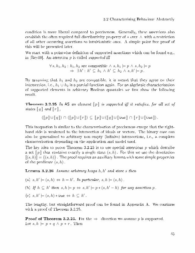
3.2 Characterising Behaviour Abstractly
condition is more liberal compared to preciseness. Generally, these assertions alsoestablish the often required full distributivity property of ∗ over ∧ with a restrictionof all other occurring assertions to intuitionistic ones. A simple point-free proof ofthis will be presented later.
We start with a pointwise de�nition of supported assertions which can be found e.g.,in [Rey09]. An assertion p is called supported i�
∀ s, h1, h2 : h1, h2 are compatible ∧ s, h1 |= p ∧ s, h2 |= p⇒ ∃h′ : h′ ⊆ h1 ∧ h′ ⊆ h2 ∧ s, h′ |= p .
By assuming that h1 and h2 are compatible, it is meant that they agree on theirintersection, i.e., h1 ∪ h2 is a partial function again. For an algebraic characterisationof supported elements in arbitrary Boolean quantales we �rst show the followingresult.
Theorem 3.2.25 In AS an element [[ p ]] is supported i� it satis�es, for all set ofstates [[ q ]] and [[ r ]] ,
([[ p ]] ·∪ [[ q ]]) ∩ ([[ p ]] ·∪ [[ r ]]) ⊆ [[ p ]] ·∪ ([[ q ]] ·∪ [[ true ]] ∩ [[ r ]] ·∪ [[ true ]]) .
This inequation is similar to the characterisation of preciseness except that the right-hand side is weakened to the intersection of ideals or vectors. The binary case canalso be generalised to arbitrary non-empty (in�nite) intersections, i.e., a completecharacterisation depending on the application and model used.
The key idea to prove Theorem 3.2.25 is to use special assertions p which describea set [[ p ]] that contains exactly a single state (s, h) . For this we use the denotation[[(s, h)]] = {(s, h)} . The proof requires an auxiliary lemma with some simple propertiesof the predicate (s, h) .
Lemma 3.2.26 Assume arbitrary heaps h, h′ and store s then
(a) s, h′ |= (s, h) ⇔ h = h′. In particular, s, h |= (s, h) .
(b) If h ⊆ h′ then s, h |= p ⇔ s, h′ |= p ∗ (s, h′ − h) for any assertion p .
(c) s, h′ |= (s, h) ∗ true ⇔ h ⊆ h′ .
The lengthy, but straightforward proof can be found in Appendix A. We continuewith a proof of Theorem 3.2.25.
Proof of Theorem 3.2.25. For the ⇒ - direction we assume p is supported.Let s, h |= p ∗ q ∧ p ∗ r . Then
45
Algebraic Spatial Assertions
s, h |= p ∗ q ∧ p ∗ r⇔ {[ de�nition of ∗ ]}∃h1, h2 : h1 ⊆ h ∧ h2 ⊆ h ∧ s, h1 |= p ∧ s, h− h1 |= q
∧ s, h2 |= p ∧ s, h− h2 |= r
⇒ {[ p supported, h1 ∪ h2 ⊆ h is a function ]}∃h1, h2, h
′ : s, h′ |= p ∧ h′ ⊆ h1 ⊆ h ∧ h′ ⊆ h2 ⊆ h∧ s, h− h1 |= q ∧ s, h− h2 |= r
⇒ {[ h− h1 ⊆ h− h′, s, h1 − h′ |= true, analogously h2 ]}∃h′ : s, h′ |= p ∧ s, h− h′ |= q ∗ true ∧ s, h− h′ |= r ∗ true
⇔ {[ de�nition of ∗ ]}s, h |= p ∗ (q ∗ true ∧ r ∗ true) .
For the other direction we assume, for arbitrary assertions q, r and states (s, h) that
s, h |= p ∗ q ∧ p ∗ r ⇒ s, h |= p ∗ (q ∗ true ∧ r ∗ true) (3.10)
as well as s, h1 |= p and s, h2 |= p for arbitrary heaps h1, h2 with h1∪h2 is a function.From this we calculate
s, h1 |= p ∧ s, h2 |= p
⇔ {[ h1 ⊆ h1 ∪ h2 and h2 ⊆ h1 ∪ h2 and Lemma 3.2.26(b) ]}s, h1 ∪ h2 |= p ∗ (s, (h1 ∪ h2)− h1) ∧ s, h1 ∪ h2 |= p ∗ (s, (h1 ∪ h2)− h2)
⇒ {[ Assumption (3.10) ]}s, h1 ∪ h2 |= p ∗
((s, (h1 ∪ h2)− h1) ∗ true ∧ (s, (h1 ∪ h2)− h2) ∗ true
)
⇔ {[ de�nition of ∗ ]}∃h′ : h′ ⊆ h1 ∪ h2 ∧ s, h′ |= p ∧
s, (h1 ∪ h2)− h′ |= (s, (h1 ∪ h2)− h1) ∗ true ∧ (s, (h1 ∪ h2)− h2) ∗ true⇔ {[ de�nition of ∧ ]}∃h′ : h′ ⊆ h1 ∪ h2 ∧ s, h′ |= p
∧ s, (h1 ∪ h2)− h′ |= (s, (h1 ∪ h2)− h1) ∗ true∧ s, (h1 ∪ h2)− h′ |= (s, (h1 ∪ h2)− h2) ∗ true
⇔ {[ Lemma 3.2.26(c) (twice) ]}∃h′ : h′ ⊆ h1 ∪ h2 ∧ s, h′ |= p ∧ (h1 ∪ h2)− h1 ⊆ (h1 ∪ h2)− h′
∧ (h1 ∪ h2)− h2 ⊆ (h1 ∪ h2)− h′⇔ {[ by h′ ⊆ h1 ∪ h2 ∧ (h1 ∪ h2)− hi ⊆ (h1 ∪ h2)− h′ ⇒ h′ ⊆ hi ]}∃h′ : h′ ⊆ h1 ∪ h2 ∧ s, h′ |= p ∧ h′ ⊆ h1 ∧ h′ ⊆ h2
⇔ {[ logic step ]}∃h′ : s, h′ |= p ∧ h′ ⊆ h1 ∧ h′ ⊆ h2 .
ut
46
3.2 Characterising Behaviour Abstractly
As for the assertion classes before, this characterisation can be lifted to the abstractlevel of quantales.
De�nition 3.2.27In a Boolean quantale S an element a is supported i� it satis�es for arbitrary b,c
a · b u a · c ≤ a · (b · > u c · >) .
Following this characterisation of supported assertions we can now abstractly derivevarious useful properties as direct consequences in a completely algebraic fashion.
Lemma 3.2.28 If a is supported and b, c are intuitionistic then
a · b u a · c ≤ a · (b u c) .
Proof. Immediately from the de�nitions. utAgain this result describes the common usage of supported assertions. They areless strict than precise ones and at the same time enable the frequently requireddistributivity law.
Lemma 3.2.29 If a is pure then it is also supported. In particular, 0 and > aresupported.
Proof. By Lemma 3.2.12(a) twice, associativity, commutativity, idempotence of u ,isotony and Lemma 3.2.12(a) again,
a · b u a · c = (a u b · >) u (a u c · >)= a u (b · > u c · >)≤ a u (b · > u c · >) · >= a · (b · > u c · >) .
utFor pure assertions a least subheap is identi�ed with the empty heap and hence it isclear that they are also supported.
Lemma 3.2.30 a is precise implies a is supported.
Proof. By the de�nition of precise elements and isotony we infer
a · b u a · c ≤ a · (b u c) ≤ a · (b · > u c · >) .
ut
47
Algebraic Spatial Assertions
Lemma 3.2.31 Supported elements are closed under · .
Proof. Assume supported elements a and a′ then
a · a′ · b u a · a′ · c ≤ a · (a′ · b · > u a′ · c · >)≤ a · a′ · (b · > · > u c · > · >)≤ a · a′ · (b · > u c · >) .
ut
Corollary 3.2.32 If a is supported and b is precise or pure then a · b is supported.
Lemma 3.2.33 a · > is supported implies that also a is supported.
Proof. Assuming a is supported, we infer from isotony, commutativity and >·> = >a · b u a · c ≤ a · > · (b · > u c · >) ≤ a · (> · b · > u > · c · >) = a · (b · > u c · >) .
utIn summary, we can conclude that
Corollary 3.2.34 a is supported i� a · > is supported.
Next we continue with a so-called precising operation (e.g. in [Rey08]) introducedby Yang. Is used to clarify the concrete relationships of precise assertions with theones being at the same time supported and intuitionistic. The operation is de�ned inseparation logic by the mapping Pr(p) =df p ∧ ¬(p ∗ ¬ emp ) . Intuitively, it removesall non-empty resources of states that are not required for satisfying an assertion p .Since Pr(_) is already given in a pointfree form we can immediately abstract it to thesetting of commutative Boolean quantales S by
Pr(a) = a u a · 1for an element a ∈ S . In the sequel we will require additional assumptions for man-aging algebraic proofs of properties for this mapping. The assumptions characterisespeci�c behaviour of the carrier set States but are still general and natural for rea-soning about resources.
We begin with a special property for the emptiness assertion emp . It reads in sep-aration logic ¬emp ∗ ¬emp ⇒ ¬emp and intuitively states that each heap that canbe split into at least two non-empty subheaps still remains non-empty. For arbitraryBoolean quantales this abstracts to
1 · 1 ≤ 1 (nonemp)
and does not generally hold. As a consequence of this we summarise
48
3.2 Characterising Behaviour Abstractly
Lemma 3.2.35 1 · > = 1 and 1 ≤ 1 · 1 .
Proof. First, by Boolean algebra, distributivity, neutrality and (nonemp)
1 · > = 1 · (1 + 1) = 1 · 1 + 1 · 1 = 1 .
The second inequation follows from shunting. utHence, assuming (nonemp) also 1 turns into an intuitionistic element. In the liter-
ature, the element 1 · 1 has also been used in the context of temporal logics [VK98,Höf09] and is called there step . Although it is interpreted by progress in time, resultsof these works are abstractly provided within an algebraic approach and hence canbe transferred and reinterpreted into a separation logical setting.
We continue with pointfree proofs of properties related to Pr(_) which can also befound in [Rey08].
Lemma 3.2.36 Pr(1 + a) = 1 . In particular, Pr(>) = 1 .
Proof. By de�nition of Pr(_), Boolean algebra and distributivity
Pr(1 + a) = (1 + a) u (1 + a) · 1 = (1 + a) u 1 · 1 + a · 1= (1 + a) u (1 u a · 1) = (1 u a · 1) + (a u 1 u a · 1)
= 1 u a · 1 .
Clearly, Pr(1 + a) ≤ 1 . For the other direction we calculate using Lemma 3.2.35 that
1 = 1 u 1 = 1 u > · 1 ≤ 1 u a · 1 . ut
Lemma 3.2.37 If a is precise then Pr(a) = a .
Proof. Setting b = 1 in Lemma 3.2.19 one obtains a · 1 ≤ a . This is equivalent to
a ≤ a · 1 and hence Pr(a) = a u a · 1 = a . ut
Lemma 3.2.38 If a is precise then Pr(a · >) = a .
Proof. Lemma 3.2.35 simpli�es a · > u a · > · 1 = a · > u a · 1 . By Boolean algebra
we infer a · > u a · 1 = (a+ a · 1) u a · 1 = a u a · 1 ≤ a . Lemma 3.2.19 implies the
converse a = a u a · > ≤ a · > u a · 1 . utThis means that the precising operation does not modify precise elements. More-over, note that by Lemma 3.2.30 and Corollary 3.2.34 elements of the form a · > areintuitionistic and supported for a precise a. Hence Pr(_) turns supported and intu-itionistic elements built from precise ones back into that original form. In [Rey08]
49
Algebraic Spatial Assertions
it is shown in separation logic that the logical mapping (_) ∗ true conversely has thesame behaviour on assertions Pr(p) if p is intuitionistic and supported.
Unfortunately an algebraic proof of this fact requires again an additional assumptionfor a property of supported assertions that can not be generally derived in arbitraryBoolean quantales from De�nition 3.2.27. A reason for this is that the abstractionto quantales also includes concrete algebras besides AS that come with di�erent be-haviour excluding such speci�c properties. It is therefore necessary to restrict thesetting to a subset of algebras to manage the required properties.
The concrete property is formulated in [Rey08] by a result that states that the def-inition for supported assertions p is equivalent to assuming that for arbitrary s, h :whenever {h′ : h′ ⊆ h, (s, h′) |= p} 6= ∅ then it has a least element. The inclusionof this behaviour within the algebraic approach requires that supported elements aadditionally satisfy
a ≤ (a u a · 1) · > . (suppleast)
Intuitively this means in separation logic that heap cells characterised by Pr(p) arecontained in any heap of states characterised by supported assertions p . In theconcrete model, it also represents the least heap that satis�es p . To see this we giveEquation (suppleast) in a pointwise form for arbitrary s, h
s, h |= p ⇒ ∃h1 : h1 ⊆ h ∧ s, h1 |= p ∧(∀h′ : h′ ⊆ h1 ∧ s, h′ |= p ⇒ h1 − h′ = ∅ ) .
Instead of assuming (suppleast) in addition to De�nition 3.2.27, another possibilitywould be to use an equivalent characterisation for supported elements that involvesPr(_) and implies (suppleast).
Lemma 3.2.39 a is supported and satis�es (suppleast) i� a · b u a · c ≤ Pr(a) · (b ·> u c · >) .
Proof. The ⇒ - direction follows from isotony, assumptions and > · (b · > u c · >) ≤> · b · > u > · c · > = b · > u c · > . For the reverse implication we infer by Pr(a) ≤ athat a is supported and setting b = c = 1 yields (suppleast). utThis means in particular that under the assumption of (suppleast) the original al-gebraic de�nition of supported elements is equivalent to the new one involving theprecising operation. Finally, we conclude
Lemma 3.2.40 Pr(a) · > = a when a satis�es (suppleast) and is intuitionistic.
Proof. By isotony and a is intuitionistic, we have Pr(a) · > ≤ a · > ≤ a . Moreover,the other inequation follows from (suppleast). ut
50
3.3 Relationship to Separation Algebras
As future work on this topic, it would be interesting to investigate the algebraic cal-culus whether there exists a more suitable axiomatisation that represents an adequateabstraction of supported assertions, especially for the case of quantales similar to AS .Lemma 3.2.39 can be used as a starting point but unfortunately is not suitable forobtaining simple and concise derivations of properties. There still exist properties forwhich it is not known if they can be shown from that characterisation. This could bedue to the lack of laws for characterising an interplay of multiplication and complemen-tation or due to undecidability results on propositional separation logic [BK10]. Theconclusions of latter approach are formalised within the context of proof systems forBI logics. Corresponding algebras are closely related to the algebraic approach basedon quantales (cf. Section 3.1.1). There might also be some relationships to [BV14].An extension of Boolean BI algebras is introduced there that allows the characteri-sation of basic and frequently required properties within the algebra which was notpossible using the former approach.
Example properties which we were not able to infer are closure of the characterisationin Lemma 3.2.39 under multiplication like in Lemma 3.2.31, where it is shown underthe assumption of De�nition 3.2.27. Furthermore, it is not known if Lemma 3.2.39implies in arbitrary commutative Boolean quantales that Pr(a) is precise assumingthat a is supported as stated in [Rey08]. Only a stronger result stating that Pr(a) issupported can be immediately inferred.
3.3 Relationship to Separation Algebras
We showed that a large part of the assertions and their behaviour in separationlogic can be lifted to a point-free and algebraic setting that allowed simple proofs ofnon-trivial properties in a calculational style due to the abstraction from irrelevantdetails. The obtained (in)equations of the previous sections generally re�ect theabstract behaviour of the speci�c assertion classes without depending on structuralproperties of the concrete considered model. Hence the characterisations can also beused for other separation logics.
Another approach that abstracts from the concrete de�nition of states as pairs ofstores and heaps has been taken by Calgagno and others in [COY07]. In their work,states are seen as arbitrary resources of a program which themselves come with analgebraic structure. They form elements of a so-called separation algebra or resourcealgebra. Assertions are given like in AS using a powerset structure, i.e., as sets ofstates.
In the following, we give a de�nition and concrete examples of such algebras. More-over, we relate the standard store and heap model of Section 2.1 with such structures
51
Algebraic Spatial Assertions
and explain how the results on pointfree algebraic characterisations for assertions canbe interpreted for resource algebras.
De�nition 3.3.1 (Separation algebra [COY07])A separation algebra is a cancellative and partial commutative monoid that we denoteby (Σ, • , u) . Elements of the algebra are called states or resources and denoted byσ, τ, . . . ∈ Σ . Due to partiality two terms are de�ned to be equal i� both are de�nedand equal or both terms are unde�ned. This induces a combinability relation # de�nedby
σ0 # σ1 ⇔df σ0 • σ1 is de�ned
and a substate relation given for σ0, σ1 ∈ Σ by
σ0 � σ1 ⇔df ∃σ2. σ0 • σ2 = σ1 .
By writing σ • τ for states σ, τ we will implicitly assume σ # τ in the sequel if it isnot explicitly stated. The empty state u is the unit of the partial binary operator •which satis�es cancellativity in the sense that σ1 • τ = σ2 • τ ⇒ σ1 = σ2 for arbitrarystates σ1, σ2, τ .
Next we provide some concrete examples for separation algebras to get an idea forapplications of those structures.
Example 3.3.2
a) A standard example is given by the set of heaps represented as partial func-tions. The corresponding separation algebra is denoted by (Heaps, ∪ , ∅) wherecombinability for heaps h0, h1 is de�ned by
h0 #h1 ⇔ dom(h0) ∩ dom(h1) = ∅ .
Clearly, ∪ is used in this context as the disjoint union of partial functions as inthe standard carrier set States. For the purpose of abstraction one can deviateto arbitrary sets of addresses and values instead of using the instances Addressesand Values of Section 2.1.
b) Another simple model is the algebra (States, ∗S , {(∅, ∅)}) where
(s0, h0) ∗S (s1, h1) =df (s0 ∪ s1, h0 ∪ h1) .
By this de�nition, the involved stores are also treated like heaps, i.e.,
(s0, h0) # (s1, h1) ⇔ dom(s0) ∩ dom(s1) = ∅ ∧ dom(h0) ∩ dom(h1) = ∅ .
52
3.3 Relationship to Separation Algebras
The e�ect of this combinability relation is that using a lifted version of ∗S toassertions, store variable de�nitions are only kept locally. Hence assignments tovariables are not globally visible. In sum, states in this model can only be uni�edi� the domains of partial functions modelling stores and heaps are disjoint.
ut
Example 3.3.3 (Permission Algebras)More interestingly, heaps as partial functions can also be extended to carry for eachof their cells an additional value that signalises if reading and/or writing to that cellis permitted [Boy03, BCOP05]. Applications for such algebras can be found e.g.,in approaches involving concurrency [Vaf11]. Permissions allow heaps to overlap onsome of their addresses, i.e., sharing parts of their resources. The values modellingpermission form an algebraic structure called permission algebra, given by a partialcommutative semigroup (P, ? ) . For this separation algebra heaps are de�ned aspartial functions A; (V × P ) that map a set of addresses A to pairs consisting of avalue of V and an element of a permission algebra P . Combinability is given by
h0 #h1 ⇔ h0(a) ? h1(a) is de�ned for all a ∈ dom(h0) ∩ dom(h1)
where ? is lifted to V × P by
(v0, p0) ? (v1, p1) =df
{(v0, p0 ? p1) v0 = v1 ∧ p0 ? p1 is de�nedunde�ned otherwise.
Hence all overlapping addresses of the considered heaps need to agree on the valuesin V and have combinable permissions in P . In sum, the combinator ∪? for heapsh0, h1 is de�ned by
(h0 ∪? h1)(a) =df
h0(a) a ∈ dom(h0)− dom(h1)h1(a) a ∈ dom(h1)− dom(h0)h0(a) ? h1(a) otherwise.
The basic idea is that shared heap cells that might belong to di�erent threads of aprogram should not be changed arbitrarily to exclude inconsistencies and thereforenon-deterministic program behaviour. Depending on the permission values involvedeither read and write access or only read access is granted to certain threads. For abetter intuition we provide some prominent examples of permission algebras that canbe found the literature.
Fractional permissions [Boy03] are rational values v in the interval (0, 1] . They areinterpreted as follows: If v = 1 , full permission to read and write a particular cell isgiven while any value< 1 , only grants read access. Concretely, one has v0?v1 = v0+v1
53
Algebraic Spatial Assertions
and clearly this is only de�ned i� v0 +v1 ≤ 1 . The advantage of this approach is thatfull permission to each cell can be split in�nitely often for transferring read accessesto arbitrarily many threads.
Counting permissions [BCOP05] are used to keep track of the set of threads thatmaintain read permission to a resource. In this setting each allocated resource keepsthe value v = 0 at the beginning which grants total permission. Now, read access istransferred to a thread which receives the value −1 while v gets increased by 1 andthus v denotes the number of read permissions that has been split o�. Summarised,counting permissions are elements of Z and for integers i, j the combination i?j = i+jis de�ned i� either i < 0 ∧ j < 0 or when one of the values is ≥ 0 then also i+ j ≥ 0 .Intuitively for each resource there exists only one positive permission and it is notpossible that more read permissions have been transferred than tracked in the positiveone. ut
More examples of separation and permission algebras can be found in [COY07]. Gen-erally, this formalism captures a variety of interesting models. An exploration of theconcrete relationships to the quantale-based treatment of separation logic assertionswould immediately extend the application range of that approach.
First, it can be seen that the standard model used in separation logic that used store-heaps pairs as states is not listed in the examples above. Instead, one either missesthe store component or it is treated in the same way as the heap, i.e., it is split intodisjoint parts (cf. Example 3.3.2). In fact, if we would de�ne the ·∪ of Section 3.1 onstates by
(s, h) ·∪ (s′, h′) =df (s, h ∪ h) ⇔ s = s′ ∧ dom(h) ∩ dom(h′) = ∅
that model would not form a separation algebra according to De�nition 3.3.1 since·∪ would not have a unit element in States. It is possible to �nd a unit for a subsetof states by a restriction to a �xed store s in S(s) =df {(s, h) : h ∈ Heaps}. Theunit w.r.t. ·∪ would then be (s, ∅) . Hence, by the only consideration of states withequal stores in ·∪ an asymmetry in the treatment of resources within a separationalgebra is introduced. Such a resource model would correspond to a so-called multi-unit separation algebra as de�ned in [DHA09]. Such algebras come with the sameaxioms as in De�nition 3.3.1 with the di�erence that there exists a set of units Usatisfying ∀σ ∈ Σ : ∃ui ∈ U : ui • σ = σ . Hence the standard model on the carrierset States can be seen as the union of single-unit separation algebras as providedin De�nition 3.3.1. Each of these individual single-unit separation algebras can bedistinguished by its store s .
Following [DHA09] there exists a possibility to get the standard model into the formof single-unit separation algebra. This is abstractly provided by the de�nition of a
54
3.3 Relationship to Separation Algebras
lifting operator for multi-unit separation algebras. Its basic idea is to remove all unitelements and replace them by a new distinct element that will represent the unit ofthe resulting separation algebra. Concretely, in the particular case of store and heappairs, we do this by restructuring the carrier set States. We de�ne a particular set toinclude all units while all other states become singleton sets and further rede�ne ·∪on these elements. Concretely, we de�ne the lifted setting by
LStates =df {{(s, h)} : (s, h) ∈ States, h 6= ∅} ,empL =df {(s, ∅) : s ∈ Stores}
and additionally set for p, q ∈ LStates ∪ {empL}
p ·t q =df {(s, h ∪ h′) : (s, h) ∈ p ∧ (s, h′) ∈ q} , wherep # q ⇔ ∃ (s, h) ∈ p , (s′, h′) ∈ q : dom(h) ∩ dom(h′) = ∅ ∧ s = s′ .
It is not di�cult to verify that p ·t empL = p = empL ·t p for arbitrary p ∈ LStates ∪{empL} . In the case of p 6= empL the resulting set is again a singleton set and otherwiseequals empL . Moreover, ·t remains commutative, associative and clearly satis�escancellativity. Hence, the structure (StatesL ∪ {empL}, ·t , empL) forms a separationalgebra and thus can be used within treatments that use this form of abstraction.
Now, for modelling assertions using separation algebras one can use a straightforwardlifting to sets of elements, like in Section 3.1. This is done in the powerset modelgiven in [COY07]. Assuming a separation algebra (Σ, •, u) , the carrier set is given byP(Σ) and one de�nes for P,Q ∈ P(Σ)
P ∗Q =df {σ • τ : σ # τ, σ ∈ P, τ ∈ Q} ,emp =df {u} .
By similar argumentations as given in the proof of Theorem 3.1.2, (P(Σ), ⊆ , ∗, emp )also forms a Boolean commutative quantale. Moreover, due to the abstract behaviourof the pointfree characterisations, the results on the assertion classes can simply beapplied for this particular model and thus for separation algebras.
For obtaining corresponding pointwise formulas interpreted on abstract resource al-gebras, one can identify occurrences of states (s, h) and single heaps h with adequateelements of an underlying separation algebra (Σ, • , u) . A formulation of precisenesscan be found e.g., in [COY07].
55

Chapter 4
Relational Separation
An algebra for the program part of separation logic is developed based on the cal-culus of relations. For this we extend the relational structure with a connective toadequately model separation that in particular allows a further reuse of abstract de-rived results on the assertion part. Moreover relational interpretations of programcommands and formulations of abstract behaviour are provided. This enables point-free soundness proofs of the frame rule in a calculational and concise way. Moreover,we give further general formulations and relationships to approaches that involve con-currency like concurrent separation logic and concurrent Kleene algebras. Finally, wederive by the use of the relational structure compositional and pointfree abstractionsfor the framework of dynamic frames.
4.1 Interpreting Commands Relationally
As a starting point for setting up a calculus based on relations for separation logic webegin with deriving a relational interpretation of all commands from the small-stepoperational semantics given in Section 2.2. For managing this, one obtains from thesemantics the general e�ects of each execution of a single command starting from anarbitrary con�guration by relating any adequate input state with some altered outputone. We generally follow the approach of [DHM11] to model program commands asrelations between states and provide interpretations for the case of a partial and totalcorrectness setting as in [DGM+14]. Clearly, since the latter additionally requiresthat termination needs to be ensured, the concrete treatment of such commands
Relational Separation
di�ers from the partial correctness one. Moreover, note that the basic assumptionsfor establishing validity of the frame rule distinguish non-termination from programabortion which results from prohibited memory access (cf. Section 2.3). Hence foran abstract treatment it is also required to include the additional state abort in thepartial correctness case while it is not needed for a treatment in a total correctnesssetting since program abortion and non-termination are identi�ed and interpreted asthe empty relation ∅ there.
De�nition 4.1.1 (Relational commands)A command in a total correctness setting is a relation
C ∈ TCmds =df P(States × States) .
In the case of partial correctness it is given by
C ∈ PCmds =df P((States × (States ∪ { abort })) ∪ {( abort , abort )})
where abort 6∈ States represents a distinct state.
Note that commands in PCmds that start from abort will remain in that state. Bythis there can not exist a transition to some state (s, h) starting from an erroneousone, i.e., the program will get stuck whenever a memory error occurs in the programexecution. Both settings yield a denotational model for the commands of separationlogic by inductively assigning a formal semantics, i.e., a relation [[C ]] ∈ PCmds or[[C ]] ∈ TCmds, to every syntactic command C formed by the grammar comm givenin Section 2.2. As a particular case one de�nes [[ skip ]] =df I where I denotes the iden-tity relation de�ned by σ I σ′ ⇔ σ = σ′ for σ, σ′ ∈ States ∪ { abort } . Moreover, forthe remaining commands we additionally specify all required correctness conditionslike e.g., all values of free occurring variables being de�ned within the domains of thestores involved or that only allocated heap cells are accessible. In the Appendix A.3,a de�nition of the functions FV(C), the set of free variables and MV(C), the set ofmodi�ed variables w.r.t. a command C is provided. In the case of (Boolean) expres-sions we assume that a corresponding function FV is prede�ned. The interpretationsfor the commands that are not heap-dependent can be found in Figure 4.1.
For a more compact notation, we abbreviate the semantic de�nition by the use of aconvention similar to that of the re�nement calculus provided e.g. in [BvW98]. Arelation R will be de�ned by a formula F linking input states (s, h) with output ones(s′, h′) , i.e., we de�ne that R = F abbreviates the clause (s, h)R (s′, h′) ⇔df F .As a particular case, it is required for the denotational model that we also assign toBoolean expressions b a relational semantics to manage the de�nition of the com-mands involving if - conditionals and while - loops. We view them abstractly as as-sertion commands assume b that only output the unchanged input state that satis�es
58
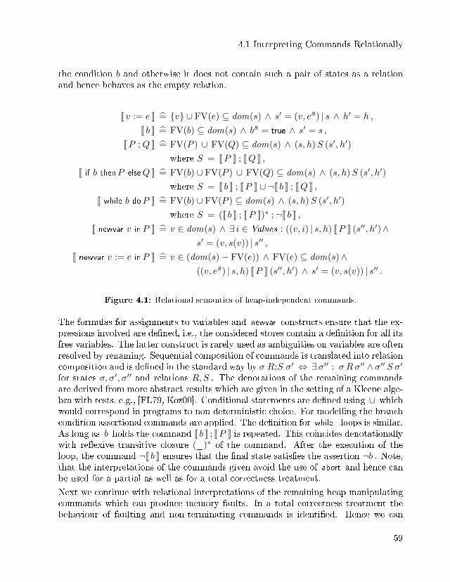
4.1 Interpreting Commands Relationally
the condition b and otherwise it does not contain such a pair of states as a relationand hence behaves as the empty relation.
[[ v := e ]] = {v} ∪ FV(e) ⊆ dom(s) ∧ s′ = (v, es) | s ∧ h′ = h ,
[[ b ]] = FV(b) ⊆ dom(s) ∧ bs = true ∧ s′ = s ,
[[P ;Q ]] = FV(P ) ∪ FV(Q) ⊆ dom(s) ∧ (s, h)S (s′, h′)
where S = [[P ]] ; [[Q ]] ,
[[ if b thenP elseQ ]] = FV(b) ∪ FV(P ) ∪ FV(Q) ⊆ dom(s) ∧ (s, h)S (s′, h′)
where S = [[ b ]] ; [[P ]] ∪ ¬[[ b ]] ; [[Q ]] ,
[[ while b doP ]] = FV(b) ∪ FV(P ) ⊆ dom(s) ∧ (s, h)S (s′, h′)
where S = ([[ b ]] ; [[P ]])∗ ; ¬[[ b ]] ,
[[ newvar v inP ]] = v ∈ dom(s) ∧ ∃ i ∈ Values : ((v, i) | s, h) [[P ]] (s′′, h′)∧s′ = (v, s(v)) | s′′ ,
[[ newvar v := e inP ]] = v ∈ (dom(s)− FV(e)) ∧ FV(e) ⊆ dom(s)∧((v, es) | s, h) [[P ]] (s′′, h′) ∧ s′ = (v, s(v)) | s′′ .
Figure 4.1: Relational semantics of heap-independent commands.
The formulas for assignments to variables and newvar constructs ensure that the ex-pressions involved are de�ned, i.e., the considered stores contain a de�nition for all itsfree variables. The latter construct is rarely used as ambiguities on variables are oftenresolved by renaming. Sequential composition of commands is translated into relationcomposition and is de�ned in the standard way by σ R;S σ′ ⇔ ∃σ′′ : σ Rσ′′ ∧ σ′′ S σ′for states σ, σ′, σ′′ and relations R,S . The denotations of the remaining commandsare derived from more abstract results which are given in the setting of a Kleene alge-bra with tests, e.g., [FL79, Koz00]. Conditional statements are de�ned using ∪ whichwould correspond in programs to non-deterministic choice. For modelling the branchcondition assertional commands are applied. The de�nition for while - loops is similar.As long as b holds the command [[ b ]] ; [[P ]] is repeated. This coincides denotationallywith re�exive transitive closure (_)∗ of the command. After the execution of theloop, the command ¬[[ b ]] ensures that the �nal state satis�es the assertion ¬b . Note,that the interpretations of the commands given avoid the use of abort and hence canbe used for a partial as well as for a total correctness treatment.
Next we continue with relational interpretations of the remaining heap manipulatingcommands which can produce memory faults. In a total correctness treatment thebehaviour of faulting and non-terminating commands is identi�ed. Hence we can
59
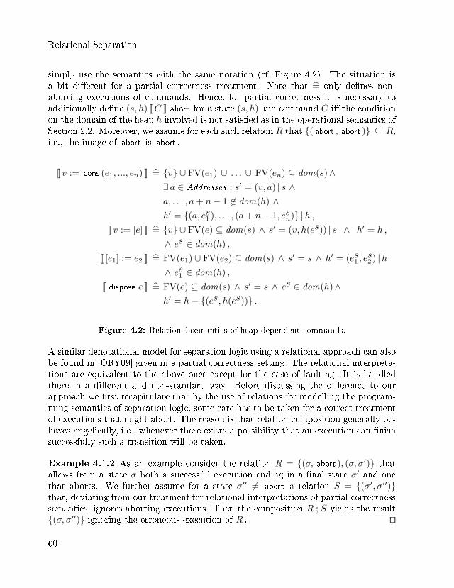
Relational Separation
simply use the semantics with the same notation (cf. Figure 4.2). The situation isa bit di�erent for a partial correctness treatment. Note that = only de�nes non-aborting executions of commands. Hence, for partial correctness it is necessary toadditionally de�ne (s, h) [[C ]] abort for a state (s, h) and command C i� the conditionon the domain of the heap h involved is not satis�ed as in the operational semantics ofSection 2.2. Moreover, we assume for each such relation R that {( abort , abort )} ⊆ R,i.e., the image of abort is abort .
[[ v := cons (e1, ..., en) ]] = {v} ∪ FV(e1) ∪ . . . ∪ FV(en) ⊆ dom(s)∧∃ a ∈ Addresses : s′ = (v, a) | s ∧a, . . . , a+ n− 1 6∈ dom(h) ∧h′ = {(a, es1 ), . . . , (a+ n− 1, esn)} |h ,
[[ v := [e] ]] = {v} ∪ FV(e) ⊆ dom(s) ∧ s′ = (v, h(es)) | s ∧ h′ = h ,
∧ es ∈ dom(h) ,
[[ [e1] := e2 ]] = FV(e1) ∪ FV(e2) ⊆ dom(s) ∧ s′ = s ∧ h′ = (es1 , es2 ) |h
∧ es1 ∈ dom(h) ,
[[ dispose e ]] = FV(e) ⊆ dom(s) ∧ s′ = s ∧ es ∈ dom(h)∧h′ = h− {(es, h(es))} .
Figure 4.2: Relational semantics of heap-dependent commands.
A similar denotational model for separation logic using a relational approach can alsobe found in [ORY09] given in a partial correctness setting. The relational interpreta-tions are equivalent to the above ones except for the case of faulting. It is handledthere in a di�erent and non-standard way. Before discussing the di�erence to ourapproach we �rst recapitulate that by the use of relations for modelling the program-ming semantics of separation logic, some care has to be taken for a correct treatmentof executions that might abort. The reason is that relation composition generally be-haves angelically, i.e., whenever there exists a possibility that an execution can �nishsuccessfully such a transition will be taken.
Example 4.1.2 As an example consider the relation R = {(σ, abort ), (σ, σ′)} thatallows from a state σ both a successful execution ending in a �nal state σ′ and onethat aborts. We further assume for a state σ′′ 6= abort a relation S = {(σ′, σ′′)}that, deviating from our treatment for relational interpretations of partial correctnesssemantics, ignores aborting executions. Then the composition R ; S yields the result{(σ, σ′′)} ignoring the erroneous execution of R . ut
60
4.2 On Partial and Total Correctness
Generally, to obtain validity of the frame rule the converse behaviour is requiredin separation logic, i.e., considering Example 4.1.2, only the aborting execution ofR should remain in the composed relation R ; S . Now a treatment of abort withrelational composition leads in [ORY09] to a setting that involves non-standard andmore complex de�nitions for sequential composition of programs and within a properde�nition for loops. The relational calculus we use in the following rather takes adi�erent direction. For managing faulting executions we assume additional structureon the commands involved so that relation composition and re�exive transitive closureas well as all general well-known results of these operations can be reused.
Another treatment that deals with the possibility of program faults is provided bythe approach of demonic relational semantics that can be found e.g. in [Ngu91,BvdW93, DBS+95, DMN97]. As can be imagined from its name that approach usesnon-deterministic choice of programs in a demonic fashion, i.e., whenever the pro-gram has the possibility of faulting then it will go wrong. A more abstract andalgebraic treatment for that structures can be found in [DMT06] in terms of idempo-tent semirings and Kleene algebras. Semirings are a special case of quantales where nounderlying complete lattice is assumed. A total correctness view is taken in that workin the following sense: a state σ only belongs to the domain of a command relationi� no execution starting from σ may lead to an error. Hence, using this semantics itis not needed to include abort into the carrier set of states. But relation compositionoperators within that approach become in a demonic treatment more complex, sinceone has to use the demonic variants of the usual (angelic) operators of union andsequential composition.
An alternative would be to use monotonic predicate transformers [Pre09]. However,this would step outside the current relational framework and the aim for a simplealgebraic calculus.
We will see in the following that in the provided algebraic treatment a distinguishingof partial and total correctness will not be essential. The reason for this is that inthe abstract treatment of commands all involved properties will be given within aso-called fault-avoiding behaviour [YO02].
4.2 On Partial and Total Correctness
All subsequent results are formalised abstractly in terms of arbitrary separation al-gebras. The relationships of the standard model based on the carrier set States to(multi-unit) separation algebras denoted by (Σ, •, U) where U is a set of units. Theirstructure is provided at the end of Section 3.3. By this, all abstractions and resultsthat we introduce in the sequel are applicable for the concrete resource model w.r.t.
61
Relational Separation
the carrier set States . Since the set of single-unit separation algebras is a strict sub-set of the set of multi-unit ones, we give all de�nitions in the following on the latteralgebras.
We start with all basic de�nitions and notations for the used relational structure. Acommand now essentially is a relation R ⊆ Σ×Σ , except for the treatment of faults.Clearly, all well-known operations including sequential composition ; , given by
R ; S =df {(σ1, σ2) : ∃σ3 : (σ1, σ3) ∈ R ∧ (σ3, σ2) ∈ S}and re�exive transitive closure (_)∗ are available, assuming a separation algebra(Σ, • , U) with σi ∈ Σ . We introduce a distinct element σ⊥ 6∈ Σ that abstractlymodels program abortion in the relational structure for partial correctness which isgiven by
(P(Σ× (Σ ∪ {σ⊥}) ∪ {(σ⊥, σ⊥)}, ⊆ , ; , I)
while for total correctness it is given by the simpler structure (P(Σ×Σ), ⊆ , ; , I) . Con-crete examples of that structures are (PCmds, ⊆ , ; , I) and (TCmds, ⊆ , ; , I) applyingthe structural transformations de�ned in Section 3.3. Both abstract structures formBoolean quantales with identity relations I w.r.t. their corresponding carrier set, i.e.,I = {(σ, σ) : σ ∈ Σ} in the total correctness case and I = {(σ, σ) : σ ∈ Σ ∪ {σ⊥}} inthe other case. The greatest element > of each structure coincides with the universalrelation, again w.r.t. the underlying carrier set.
We continue with modelling Hoare triples {p}C {q} of separation logic (cf. De�ni-tion 2.2.1) using the relation-based denotation. For this we follow a standard algebraicapproach given in [Koz00]. There, Hoare logic is algebraically modelled using moreabstract structures like semirings or quantales. The role of the pre- and postcondi-tions p and q are played in that approach by tests (cf. De�nition 3.2.13), i.e., in theconcrete relational quantales elements that coincide with subsets of the identity re-lation. Note that on tests relation composition ; and binary intersection ∩ coincide.Tests are also given by relations of the form
[[ p ]] = {(σ, σ) | σ ∈ [[ p ]] } (4.1)
for arbitrary set of states [[ p ]] as de�ned in Section 3.1. This immediately yields adirect embedding of elements of the assertion quantale AS as tests into a relationalquantale. By this we can directly reuse all results of the previous section also forthe relational structure. It is clear that the above subidentities and sets of states arein one - to - one correspondence. The set [[ p ]] can be retrieved from [[ p ]] by [[ p ]] =
dom([[ p ]]) . We will write pC in the following for a command C to denote dom(C) ,i.e., its domain in a relational subidentity structure. It is characterised pointfree bythe universal property (e.g. [DMS06])
pR ⊆ p ⇔ R ⊆ p ;R , (reldom)
62
4.2 On Partial and Total Correctness
where p ranges over the set of tests. The locality property p(R ; pS) ⊆ p(R ; S), whichis independent of the above equivalence, is satis�ed for the concrete case of relations.It states that the domain of a composed relation R ; S depends only on the domainof S , but not on S itself. Symmetrically, one can also de�ne the codomain operationRq for relations R . In what follows we will write [[ p ]] to denote to the correspondingsubidentity instead of a set of states. A related approach on relational interpretationsfor assertions can be found in [TBY12]. Their approach di�ers to the present one inusing n - ary relations with applications in information hiding. For our purposes wedo not require such a lift.
As a next step, we turn to a relation-algebraic characterisation of Hoare triples inseparation logic beginning with partial correctness behaviour. Note that according toDe�nition 2.2.1 the semantics of these triples is di�erent from that of standard Hoarelogic approaches. An additional assumption is required to guarantee that none of theexecutions of a considered command aborts from any state satisfying the involved pre-condition. The idea behind this is that the semantics is treated as resource-sensitiveto obtain proper triples and in particular validity of the frame rule. As an example,one cannot obtain for the triple { emp } v := [e] { ? } a valid postcondition expressiblewith the syntax of the assertion language given in Section 2.1. Moreover, this meansthat the Hoare triples in separation logic are de�ned to be fault-avoiding.
We now continue to extend a prior and well-known algebraic approach for proposi-tional Hoare logic triples with this particular behaviour so that program abortion isalso considered. For this we implicitly assume for notational abbreviation an arbitrarytranslation of syntactical commands and assertions to relations and tests respectively.A denotational semantics of Hoare triples {p}C {q} in a partial correctness settingfor standard Hoare logic (e.g. [Koz02]) can be given for relations by
p ; C ⊆ C ; q ⇔ p ; C ; ¬q ⊆ ∅ ⇔ p ; C = p ; C ; q (4.2)
where p, q are suitable subidentities. The formula involving test negation can bedi�cult to use for our purposes since there we have only general laws for the interplayof concrete assertions of the form p ∗ q and logical negation. The �rst formulacompared to the last one allows inequational reasoning which is often easier to handle.Hence we will mainly use the �rst version as an adequate formulation in calculations.
For an extension of the approach to incorporate faulting executions of programs westart by de�ning a special test ⊥ =df {(σ⊥, σ⊥)} as in [DGM+14]. It is used in thesequel for pointfree formulations of conditions involving program abortion.
De�nition 4.2.1A relation C respects ⊥ i� ⊥ ; C = ⊥ .
This law states that ⊥ is a left annihilator on the set of ⊥ - respecting relations. In
63
Relational Separation
a pointwise form this corresponds to relations C satisfying σ⊥ C σ ⇒ σ = σ⊥ . Notethat for the tests p arising in Section 4.1 we have p ∩ ⊥ = ∅ . This allows a relationalcharacterisation of heap-dependent commands. Concrete examples are the mutation,dereferencing and disposal commands of Section 2.2. Clearly, the identity relationalso respects ⊥ .
Lemma 4.2.2 σ⊥ - respecting relations are closed under ∪, ; and Kleene star ∗ .
The proof is an easy calculation using the well-known star induction law R;S ⊆ R ⇒R;S∗ ⊆ R for any relations R,S (e.g., [Con71]). This guarantees that aborting exe-cutions will not be ruled out by union or composition of abort respecting commands.For characterising the above mentioned safety condition that ensures the absence ofaborting executions we de�ne that a state σ is safe w.r.t. a relation C i� ¬(σ C σ⊥ )holds. In a pointfree fashion, this can be formalised by p(C ; ⊥) ⊆ ∅ or equivalentlyp ;p(C ;⊥) ⊆ ∅ for arbitrary tests p . Intuitively, p includes at most the states where Cwill not abort if it starts from them. For a more compact and intuitive representationwe now introduce special modal operators that re�ect behaviour more concisely (cf.e.g. [MS06a]). We give de�nitions for our concrete relation-based setting although itis not di�cult to lift all subsequent results and handle them more abstractly withinmodal Kleene algebras.
De�nition 4.2.3 (Forward diamond and box)For an arbitrary relation C and test p we de�ne
|C〉 p =dfp(C ; p) and |C] p =df ¬|C〉¬p = ¬p(C ; ¬p) .
The forward diamond |C〉 p denotes the test that represents all initial states fromwhich p can be reached within one execution step of C while the forward box |C] pdually describes a demonic variant where p must be reached within every single C -step.
With the help of these de�nitions we can immediately infer
p ; p(C ;⊥) ⊆ 0 ⇔ p ⊆ ¬p(C ;⊥) ⇔ p ⊆ ¬p(C ; ¬(¬⊥)) ⇔ p ⊆ |C]¬⊥ .
Hence we can give a pointfree characterisation of the set of safe states using themodal box operator. For better readability we introduce for a test p the abbreviationp =df p ; ¬⊥ . This corresponds to the abort - free part of p . As a particular case we
get I = ¬⊥ .
De�nition 4.2.4For a relation C we de�ne safe (C) =df |C] I = ¬p(C ;⊥) . By this we characterise allsafe states of a relation C. We call a test p safe for C i� p ⊆ safe (C) .
64
4.2 On Partial and Total Correctness
As an immediate consequence of this we give the following lemma.
Lemma 4.2.5 For any relations C,D we have safe (C ∪ D) = safe (C) ∩ safe (D) .
Moreover, if D respects ⊥ then safe (C ;D) = safe (C) ; safe (C ; I ;D) . Hence, safe (C ;D) = safe (C) ; safe (C ;D) .
Proof. The �rst claim follows since box operations are antidisjunctive in the �rstargument. For the second we calculate
safe (C ;D) = ¬p(C ;D ;⊥)
= ¬(p(C ; I ;D ;⊥) ∪ p(C ;⊥ ;D ;⊥))
= ¬p(C ; I ;D ;⊥) ∩ ¬p(C ;⊥ ;D ;⊥)
= safe (C ; I ;D) ∩ ¬p(C ;⊥ ;⊥)
= safe (C ; I ;D) ; safe (C)
using the de�nition, distributivity of p_ , De Morgan and idempotence of tests, andthat ; and ∩ coincide on tests. utAs discussed at the end of Section 4.1, this again re�ects a demonic treatment ofabort respecting relations. Note that the test |C〉 I as an angelic variant would notbe adequate to characterise safe states since it only represents the set of all initialstates for which there exists a non-faulting execution of C . To see this, considerExample 4.1.2 involving the relation C = {(σ, σ⊥), (σ, σ′)}. Clearly, we have (σ, σ) ∈|C〉 I , but still σ can lead to program abortion. However, the box operator is exactlywhat we need in this case. It rules out σ by only including only all initial states ofthe execution paths of C that can not abort.
Finally, we can now discuss some candidates for a relational characterisation of Hoaretriples in separation logic. For the forward box and the backward diamond operationde�ned by 〈C|p =df (p ; C)q there exists a relationship given by the Galois connection
p ⊆ |C] q ⇔ 〈C| p ⊆ q . (4.3)
As a particular case, we get p ⊆ |C] I is equivalent to 〈C| p ⊆ I . Note thatequivalently to (4.2) we can also use 〈C| p ⊆ q involving the backward diamondoperation for a relational treatment of Hoare triples (e.g. [MS06a]) that are not re-source sensitive. Hence, by the characterisation of binary in�ma we immediatelyinfer 〈C| p ⊆ q ∧ 〈C| p ⊆ I ⇔ 〈C| p ⊆ q . This form is still not fully adequatefor our purposes due to the asymmetry by just excluding ⊥ in the postcondition q .One problem with this form is that will particularly falsify validity of the Hoare logicwhile - inference rule. Thus, we de�ne
65
Relational Separation
De�nition 4.2.6 (Partial correctness with abortion)A partial correctness Hoare triple in separation logic is relationally given by
{p}C {q} ⇔df 〈C| p ⊆ q
⇔ p ; C ⊆ C ; q .
Another possibility for De�nition 4.2.6 would be to use 〈C| p ⊆ q ∧ q ⊆ I whichimplies the above condition and therefore is stronger. We will stay with the abovede�nition since it is more compact and simpler to use. Moreover, it structurallycoincides with the original form of relational Hoare triples ignoring program abortion.Therefore we can immediately instantiate existing proofs (e.g. [MS06a]) without anyfurther need for recalculations and state the following result.
Theorem 4.2.7 All partial correctness inference rules of propositional Hoare logicremain valid under the partial correctness interpretation of Hoare triples respectingprogram abortion.
Note that the proof can be lifted to the more abstract setting of a modal Kleenealgebras as in [DGM+14]. Hence we can again get (semi)automated and calculationalsoundness proofs of the Hoare logic proof rules by the use of theorem proving systems.Another advantage of the encoding of the Hoare triples in De�nition 4.2.6 is that italso implies that the involved precondition p only characterises safe states.
Lemma 4.2.8 {p}C {q} implies p is safe for C .
Proof. By (4.3), isotony of box in its second argument, and de�nition of safe (_) :
〈C| p ⊆ q ⇔ p ⊆ |C] q ⇒ p ⊆ |C] I ⇔ p ⊆ safe (C) .
utAs a last result we state that the de�nitions provided in Section 4.1 in fact satisfyDe�nition 4.2.6 and hence can be used for a relational treatment for Hoare triples ofseparation logic.
Lemma 4.2.9 The relational denotations [[_]] for commands and assertions in Sec-tion 4.1 satis�es the partial correctness interpretation of Hoare triples respecting pro-gram abortion, i.e., {p}C {q} ⇔ [[ p ]] ; [[C ]] ⊆ [[C ]] ; [[ q ]] .
Proof. By de�nition of the interpretations [[ p ]] and [[ q ]] we can conclude that
[[ p ]] = [[ p ]] ; ¬⊥ = [[ p ]]
66
4.3 Abstracting Modularity
since [[ p ]] ∩ ⊥ ⊆ ∅ and ∩ coincides with ; on tests. utNext we turn to the case of total correctness. We recapitulate the semantics in thisapproach: A state σ only belongs to the domain of a relation i� there exists an ex-ecution starting from σ that does not abort and terminates in some �nal state τ .Hence, program abortion and non-termination are identi�ed and coincide denotation-ally with divergence, i.e., the empty relation ∅ . Therefore we need to state for totalcorrectness Hoare triples that the precondition p ensures termination of a commandC by assuming relationally p ⊆ pC .
De�nition 4.2.10 (Total correctness)We de�ne a total correctness Hoare triple in separation logic by
[ p ]C [ q ] ⇔df 〈C| p ⊆ q ∧ p ⊆ pC
⇔ p ; C ⊆ C ; q ∧ p ⊆ pC .
Theorem 4.2.11 All total correctness inference rules of standard Hoare logic remainvalid under the total correctness interpretation of Hoare triples.
Proof. It is only required to show closure of the termination condition p ⊆ pC foreach rule. As an example we prove that condition for the sequential compositionrule {p}C {r} ∧ {r}D {q} ⇒ {p}C ;D {q} . By p being a test, property of domain,{p}C {r} and isotony of domain, {r}D {q} and isotony of domain, and locality ofdomain:
p ⊆ pC ⇒ p ⊆ p;pC ⇔ p ⊆ p(p;C) ⇒ p ⊆ p(C ;r) ⇒ p ⊆ p(C ;pD) ⇔ p ⊆ p(C ;D) .
Proofs for the remaining inference rules can easily be calculated and automated withinthe abstract setting of modal Kleene algebras. utNote, that the while - inference rule needs an extra termination argument. An ade-quate condition is expressed relationally by (b ; C)∗ ⊆ (b ; C)∗ ; ¬b which states thateach loop of C that starts in a state for which b holds will eventually end in a statewhere b is false after �nitely many C - steps.
It can be seen that beside the well-known Hoare logic inference rules a pointfreevalidity proof of the central frame rule of separation logic is still missing. In thesubsequent section we provide a relational treatment of that inference rule and givepointfree abstractions of properties for establishing it.
4.3 Abstracting Modularity
The frame rule (cf. Section 2.3) allows veri�cation tasks to be performed locally onthe required set of resources of a program. The main advantage is that program
67
Relational Separation
proofs become scalable and easier to read and understand. Conversely it allows theembedding of procedure veri�cations into larger contexts for obtaining global proofs.This behaviour is established by assuming validity of two crucial properties, called theframe property and safety monotonicity. We recapitulate that, intuitively, commandsthat satisfy the former property include program executions that may run on a pos-sibly smaller set of resources. The program can be tracked back to a minimal set ofresources that guarantees that it will not abort. Moreover, the latter property statesthat when at least the required allocated resources are available then the consideredcommand can also be executed from any larger states with additional non-relevantresources without aborting.
The objective of this section is to derive relation-algebraic counterparts for the men-tioned conditions. This would allow a simpler and abstract soundness proof of theframe rule in a calculational style. We start with some fundamental de�nitions thatyield a relational variant of the separating conjunction. For this we follow the treat-ment of [DHM11, DM12a] and introduce an extension of the relational structurefrom the previous section so that an independent treatment of arbitrary partitions ofstates is possible. For the purpose of abstraction we give all de�nitions in the sequelon arbitrary separation algebras capturing all models of Section 3.3. We will use thenotation of the more generalised multi-unit separation algebras (Σ, • , U) and referto them in the following just by the term �separation algebra�. Moreover, dependingon a total or partial correctness treatment we will use Σ or the extended carrier setΣ⊥ =df Σ ∪ {σ⊥} . For an appropriate treatment of state splittings within Σ⊥ weneed to extend the separation algebra operation • to also capture σ⊥ by
σ • τ = σ⊥ ⇔df σ = σ⊥ ∨ τ = σ⊥ , (abortext)
i.e., each state denoting program abortion yields again σ⊥ in the join. Hence, wealways have for any state σ that σ⊥ # σ .
De�nition 4.3.1 (Split and Join)Assume a separation algebra (Σ, • , U) where U denotes a set of units. The splitrelation � ⊆ Σ× (Σ× Σ) , respectively Σ⊥ × (Σ⊥ × Σ⊥) , is given by
σ� (σ1, σ2) ⇔df σ1 #σ2 ∧ σ = σ1 • σ2 .
The join relation � is the converse of split, i.e.,
(σ1, σ2)� σ ⇔df σ1 #σ2 ∧ σ = σ1 • σ2 .
We introduce a special symmetric symbol for it, rather than writing �˘ where _denotes the converse, to ease reading.
68
4.3 Abstracting Modularity
The general idea with this de�nition is to enable calculations on state partitions byextending the setting from relations between states to state pairs.
De�nition 4.3.2 (Pairs of relations)Union, inclusion and composition of pairs of relations are de�ned componentwise. TheCartesian product R × S ⊆ (Σ× Σ)× (Σ× Σ) , respectively R × S ⊆ (Σ⊥ × Σ⊥)×(Σ⊥×Σ⊥) , of two appropriate relations R,S ⊆ Σ×Σ , respectively R,S ⊆ Σ⊥×Σ⊥ ,is de�ned by
(σ1, σ2) (R× S) (τ1, τ2) ⇔df σ1Rτ1 ∧ σ2 S τ2 .
We assume in the sequel that ; binds tighter than ∩ and × while ∩ binds tighterthan × . It is clear that id =df I × I is the identity of composition on pairs while>×> is the largest pair relation where > denotes the universal relation.
De�nition 4.3.3Tests in the set of product relations are again sub-identities; as before they are idem-potent and commute under ; . The Cartesian product of tests is a test again. However,there are other tests, such as the combinability check # ⊆ (Σ×Σ)× (Σ×Σ) , respec-tively (Σ⊥ × Σ⊥)× (Σ⊥ × Σ⊥) , on pairs of states, given by:
(σ1, σ2) # (τ1, τ2) ⇔df σ1 #σ2 ∧ σ1 = τ1 ∧ σ2 = τ2 .
This relation acts as a �lter since only combinable pairs of states pass it while allother pairs are not considered.
Lemma 4.3.4 We have # = �;� ∩ id and hence # ⊆�;� . Moreover # ;� = �and symmetrically � ; # = � . Finally, � ;� = I.
It is well known that × and ; satisfy an equational exchange law:
(R1 ×R2) ; (S1 × S2) = (R1 ; S1)× (R2 ; S2) . (×/;)
Next we lift the operation • and the relation # on states to the setting of relations.
De�nition 4.3.5The ∗ - composition R∗S of relations R,S ⊆ Σ×Σ , respectively Σ⊥×Σ⊥ , is de�nedby the formula
R ∗ S =df � ; (R× S) ;� .
Intuitively by this de�nition, the relation σ (R ∗ S) τ holds i� σ can be split asσ = σ1 • σ2 with combinable partitions σ1, σ2 on which R and S can act and produce
69
Relational Separation
results τ1, τ2 that are again combinable and yield τ = τ1 • τ2. For a concrete exampleconsider the separation algebra (States, ·∪ , emp) . We can interpret the semantics ofthe split relation w.r.t. that carrier set as follows: a state (s, h) can be split intostates (s, h1) and (s, h2) with h = h1 ·∪h2 i� dom(h1) ∩ dom(h2) = ∅ . Clearly, wecan also embed the operation ·∪ into a lifted version on tests, for that we also write
·∪ , by P ·∪ Q =df P ·∪Q for P,Q ⊆ States and as de�ned in (4.1). Assumingthe separation algebra States, the product p ·∪ q of tests p, q would coincide with� ; (p× q) ;� .
In particular, we remark that De�nition 4.3.5 re�ects angelic behaviour in the sensethat, whenever σ1 and σ2 are not combinable or disjoint, R and S are prevented fromstarting, since these states are eliminated by the de�nition. The same happens if σ1
and σ2 are combinable but R and S produce non-combinable output states τ1 and τ2 .
We will see in the following that the relations of the form R ∗ S can be either usedto characterise the structure and behaviour of programs or can be conceptually inter-preted as a parallel execution of programs within a concurrent setting. The formercase will be discussed in the subsequent section. For now we continue by some con-sequences of De�nition 4.3.5.
First, by de�nition of separation algebras the partial operator • is associative andcommutative. Hence, the lifted operation ∗ is also associative and commutative.Moreover, it has the test e =df {(u, u) : u ∈ U} as its unit. For tests p, q the∗ - composition p ∗ q is a test again, irrespective of the underlying separation algebra.
Lemma 4.3.6 I is idempotent w.r.t. ∗ , i.e., I ∗ I = I.
Proof. We calculate, using the de�nitions and Lemma 4.3.4,
I ∗ I = � ; (I × I) ;� = � ; id ;� = � ;� = I.
utFor a partial correctness treatment we can immediately infer the following lemmafrom (abortext).
Lemma 4.3.7
(a) ¬⊥ ;� = � ; (¬⊥ × ¬⊥) ,
(b) ⊥ ;� = � ; (⊥× I) ∪ � ; (I ×⊥) ,
(c) ⊥ = C ∗ ⊥ for arbitrary relations C .
70
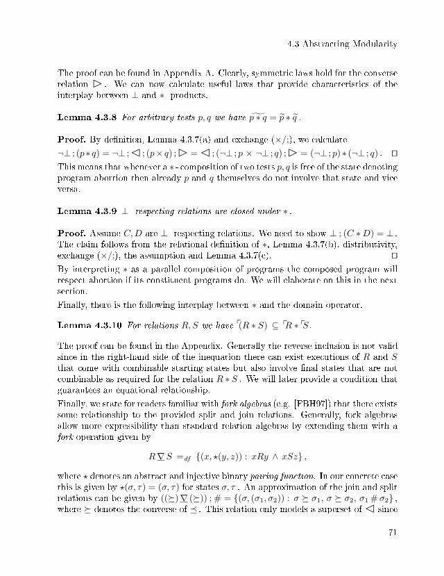
4.3 Abstracting Modularity
The proof can be found in Appendix A. Clearly, symmetric laws hold for the converserelation � . We can now calculate useful laws that provide characteristics of theinterplay between ⊥ and ∗ - products.
Lemma 4.3.8 For arbitrary tests p, q we have p ∗ q = p ∗ q .
Proof. By de�nition, Lemma 4.3.7(a) and exchange (×/;), we calculate¬⊥ ; (p ∗ q) = ¬⊥ ;� ; (p× q) ;� = � ; (¬⊥ ; p × ¬⊥ ; q) ;� = (¬⊥ ; p) ∗ (¬⊥ ; q) . utThis means that whenever a ∗ - composition of two tests p, q is free of the state denotingprogram abortion then already p and q themselves do not involve that state and viceversa.
Lemma 4.3.9 ⊥ - respecting relations are closed under ∗ .
Proof. Assume C,D are ⊥ - respecting relations. We need to show ⊥ ; (C ∗D) = ⊥ .The claim follows from the relational de�nition of ∗, Lemma 4.3.7(b), distributivity,exchange (×/;), the assumption and Lemma 4.3.7(c). utBy interpreting ∗ as a parallel composition of programs the composed program willrespect abortion if its constituent programs do. We will elaborate on this in the nextsection.
Finally, there is the following interplay between ∗ and the domain operator.
Lemma 4.3.10 For relations R,S we have p(R ∗ S) ⊆ pR ∗ pS.
The proof can be found in the Appendix. Generally the reverse inclusion is not validsince in the right-hand side of the inequation there can exist executions of R and Sthat come with combinable starting states but also involve �nal states that are notcombinable as required for the relation R ∗ S . We will later provide a condition thatguarantees an equational relationship.
Finally, we state for readers familiar with fork algebras (e.g. [FBH97]) that there existssome relationship to the provided split and join relations. Generally, fork algebrasallow more expressibility than standard relation algebras by extending them with afork operation given by
R∇S =df {(x, ?(y, z)) : xRy ∧ xSz} ,
where ? denotes an abstract and injective binary pairing function. In our concrete casethis is given by ?(σ, τ) = (σ, τ) for states σ, τ . An approximation of the join and splitrelations can be given by ((�)∇ (�)) ; # = {(σ, (σ1, σ2)) : σ � σ1, σ � σ2, σ1 #σ2} ,where � denotes the converse of � . This relation only models a superset of � since
71
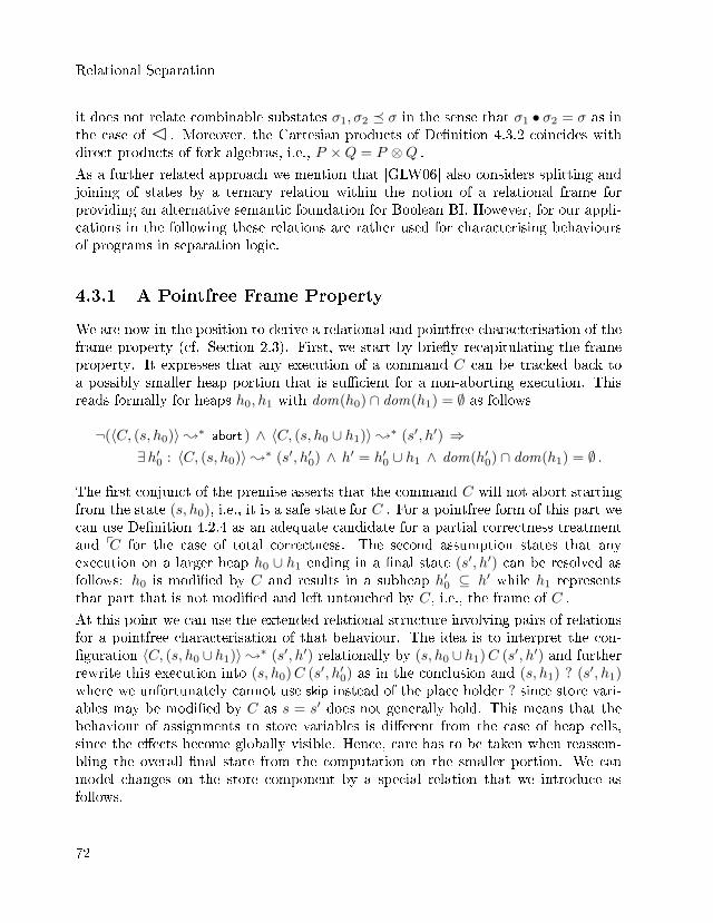
Relational Separation
it does not relate combinable substates σ1, σ2 � σ in the sense that σ1 • σ2 = σ as inthe case of � . Moreover, the Cartesian products of De�nition 4.3.2 coincides withdirect products of fork algebras, i.e., P ×Q = P ⊗Q .
As a further related approach we mention that [GLW06] also considers splitting andjoining of states by a ternary relation within the notion of a relational frame forproviding an alternative semantic foundation for Boolean BI. However, for our appli-cations in the following these relations are rather used for characterising behavioursof programs in separation logic.
4.3.1 A Pointfree Frame Property
We are now in the position to derive a relational and pointfree characterisation of theframe property (cf. Section 2.3). First, we start by brie�y recapitulating the frameproperty. It expresses that any execution of a command C can be tracked back toa possibly smaller heap portion that is su�cient for a non-aborting execution. Thisreads formally for heaps h0, h1 with dom(h0) ∩ dom(h1) = ∅ as follows
¬(〈C, (s, h0)〉;∗ abort ) ∧ 〈C, (s, h0 ∪ h1)〉;∗ (s′, h′) ⇒∃h′0 : 〈C, (s, h0)〉;∗ (s′, h′0) ∧ h′ = h′0 ∪ h1 ∧ dom(h′0) ∩ dom(h1) = ∅ .
The �rst conjunct of the premise asserts that the command C will not abort startingfrom the state (s, h0), i.e., it is a safe state for C . For a pointfree form of this part wecan use De�nition 4.2.4 as an adequate candidate for a partial correctness treatmentand pC for the case of total correctness. The second assumption states that anyexecution on a larger heap h0 ∪ h1 ending in a �nal state (s′, h′) can be resolved asfollows: h0 is modi�ed by C and results in a subheap h′0 ⊆ h′ while h1 representsthat part that is not modi�ed and left untouched by C, i.e., the frame of C .
At this point we can use the extended relational structure involving pairs of relationsfor a pointfree characterisation of that behaviour. The idea is to interpret the con-�guration 〈C, (s, h0 ∪ h1)〉;∗ (s′, h′) relationally by (s, h0 ∪ h1)C (s′, h′) and furtherrewrite this execution into (s, h0)C (s′, h′0) as in the conclusion and (s, h1) ? (s′, h1)where we unfortunately cannot use skip instead of the place holder ? since store vari-ables may be modi�ed by C as s = s′ does not generally hold. This means that thebehaviour of assignments to store variables is di�erent from the case of heap cells,since the e�ects become globally visible. Hence, care has to be taken when reassem-bling the overall �nal state from the computation on the smaller portion. We canmodel changes on the store component by a special relation that we introduce asfollows.
72
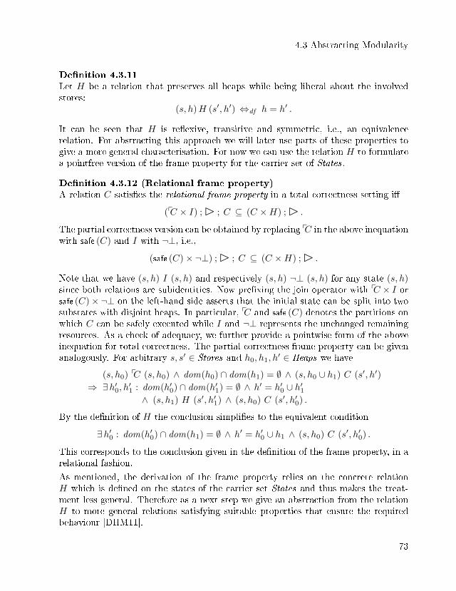
4.3 Abstracting Modularity
De�nition 4.3.11Let H be a relation that preserves all heaps while being liberal about the involvedstores:
(s, h)H (s′, h′) ⇔df h = h′ .
It can be seen that H is re�exive, transitive and symmetric, i.e., an equivalencerelation. For abstracting this approach we will later use parts of these properties togive a more general characterisation. For now we can use the relation H to formulatea pointfree version of the frame property for the carrier set of States.
De�nition 4.3.12 (Relational frame property)A relation C satis�es the relational frame property in a total correctness setting i�
(pC × I) ;� ; C ⊆ (C ×H) ;� .
The partial correctness version can be obtained by replacing pC in the above inequationwith safe (C) and I with ¬⊥, i.e.,
(safe (C)× ¬⊥) ;� ; C ⊆ (C ×H) ;� .
Note that we have (s, h) I (s, h) and respectively (s, h) ¬⊥ (s, h) for any state (s, h)since both relations are subidentities. Now pre�xing the join operator with pC × I orsafe (C)׬⊥ on the left-hand side asserts that the initial state can be split into twosubstates with disjoint heaps. In particular, pC and safe (C) denotes the partitions onwhich C can be safely executed while I and ¬⊥ represents the unchanged remainingresources. As a check of adequacy, we further provide a pointwise form of the aboveinequation for total correctness. The partial correctness frame property can be givenanalogously. For arbitrary s, s′ ∈ Stores and h0, h1, h
′ ∈ Heaps we have
(s, h0) pC (s, h0) ∧ dom(h0) ∩ dom(h1) = ∅ ∧ (s, h0 ∪ h1) C (s′, h′)⇒ ∃h′0, h′1 : dom(h′0) ∩ dom(h′1) = ∅ ∧ h′ = h′0 ∪ h′1
∧ (s, h1) H (s′, h′1) ∧ (s, h0) C (s′, h′0) .
By the de�nition of H the conclusion simpli�es to the equivalent condition
∃h′0 : dom(h′0) ∩ dom(h1) = ∅ ∧ h′ = h′0 ∪ h1 ∧ (s, h0) C (s′, h′0) .
This corresponds to the conclusion given in the de�nition of the frame property, in arelational fashion.
As mentioned, the derivation of the frame property relies on the concrete relationH which is de�ned on the states of the carrier set States and thus makes the treat-ment less general. Therefore as a next step we give an abstraction from the relationH to more general relations satisfying suitable properties that ensure the requiredbehaviour [DHM11].
73
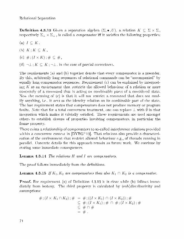
Relational Separation
De�nition 4.3.13 Given a separation algebra (Σ, • , U), a relation K ⊆ Σ × Σ ,respectively Σ⊥ ×Σ⊥ , is called a compensator i� it satis�es the following properties:
(a) I ⊆ K ,
(b) K ;K ⊆ K ,
(c) # ; (I ×K) ; # ⊆ # ,
(d) ¬⊥ ;K ⊆ K ; ¬⊥ , in the case of partial correctness.
The requirements (a) and (b) together denote that every compensator is a preorder.By this, arbitrarily long sequences of relational commands can be �accompanied� byequally long compensator sequences. Requirement (c) can be explained by interpret-ing K as an environment that restricts the allowed behaviour of a relation or moreconcretely of a command that is acting on combinable parts of a considered state.Now the meaning of (c) is that it will not restrict a command that does not mod-ify anything, i.e., it acts as the identity relation on its combinable part of the state.The last requirement states that compensators does not produce memory or programfaults. Note that for a total correctness treatment, one can replace ⊥ with ∅ in thatinequation which makes it trivially satis�ed. These requirements are used amongstothers to establish closure of properties involving compensators, in particular theframe property.
There exists a relationship of compensators to so-called interference relations providedwithin a concurrent context in [DYBG+13]. That relations also provide a characteri-sation of the environment that restrict allowed behaviour e.g., of threads running inparallel. Concrete details for this approach remain as future work. We continue bystating some immediate consequences.
Lemma 4.3.14 The relations H and I are compensators.
The proof follows immediately from the de�nitions.
Lemma 4.3.15 If K1,K2 are compensators then also K1 ∩ K2 is a compensator.
Proof. For requirement (a) of De�nition 4.3.13 it is clear while (b) follows imme-diately from isotony. The third property is calculated by (sub)distributivity andassumptions:
# ; (I × K1 ∩K2) ; # = # ; ((I ×K1) ∩ (I ×K2)) ; #⊆ # ; (I ×K1) ; # ∩ # ; (I ×K2) ; #⊆ # ∩ #= # .
74
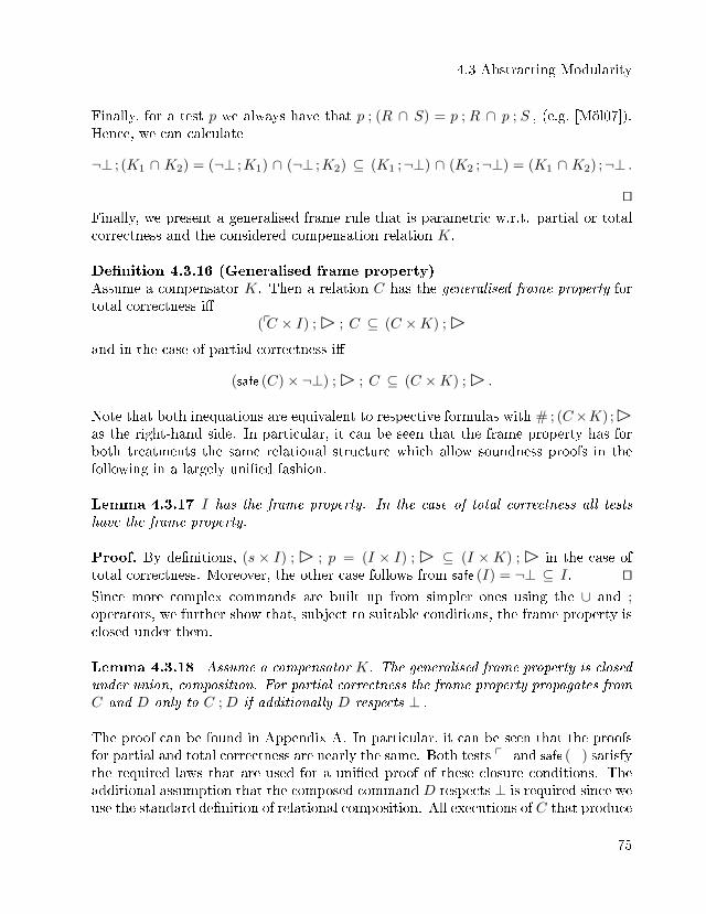
4.3 Abstracting Modularity
Finally, for a test p we always have that p ; (R ∩ S) = p ; R ∩ p ; S , (e.g. [Möl07]).Hence, we can calculate
¬⊥ ; (K1 ∩ K2) = (¬⊥ ;K1) ∩ (¬⊥ ;K2) ⊆ (K1 ;¬⊥) ∩ (K2 ;¬⊥) = (K1 ∩ K2) ;¬⊥ .
utFinally, we present a generalised frame rule that is parametric w.r.t. partial or totalcorrectness and the considered compensation relation K.
De�nition 4.3.16 (Generalised frame property)Assume a compensator K. Then a relation C has the generalised frame property fortotal correctness i�
(pC × I) ;� ; C ⊆ (C ×K) ;�
and in the case of partial correctness i�
(safe (C)× ¬⊥) ;� ; C ⊆ (C ×K) ;� .
Note that both inequations are equivalent to respective formulas with # ; (C×K) ;�as the right-hand side. In particular, it can be seen that the frame property has forboth treatments the same relational structure which allow soundness proofs in thefollowing in a largely uni�ed fashion.
Lemma 4.3.17 I has the frame property. In the case of total correctness all testshave the frame property.
Proof. By de�nitions, (s × I) ; � ; p = (I × I) ; � ⊆ (I ×K) ; � in the case oftotal correctness. Moreover, the other case follows from safe (I) = ¬⊥ ⊆ I. utSince more complex commands are built up from simpler ones using the ∪ and ;operators, we further show that, subject to suitable conditions, the frame property isclosed under them.
Lemma 4.3.18 Assume a compensator K. The generalised frame property is closedunder union, composition. For partial correctness the frame property propagates fromC and D only to C ;D if additionally D respects ⊥ .
The proof can be found in Appendix A. In particular, it can be seen that the proofsfor partial and total correctness are nearly the same. Both tests p_ and safe (_) satisfythe required laws that are used for a uni�ed proof of these closure conditions. Theadditional assumption that the composed command D respects ⊥ is required since weuse the standard de�nition of relational composition. All executions of C that produce
75
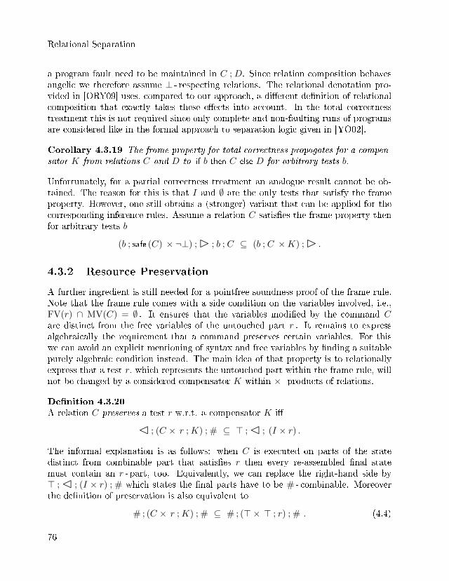
Relational Separation
a program fault need to be maintained in C ;D. Since relation composition behavesangelic we therefore assume ⊥ - respecting relations. The relational denotation pro-vided in [ORY09] uses, compared to our approach, a di�erent de�nition of relationalcomposition that exactly takes these e�ects into account. In the total correctnesstreatment this is not required since only complete and non-faulting runs of programsare considered like in the formal approach to separation logic given in [YO02].
Corollary 4.3.19 The frame property for total correctness propagates for a compen-sator K from relations C and D to if b then C else D for arbitrary tests b.
Unfortunately, for a partial correctness treatment an analogue result cannot be ob-tained. The reason for this is that I and ∅ are the only tests that satisfy the frameproperty. However, one still obtains a (stronger) variant that can be applied for thecorresponding inference rules. Assume a relation C satis�es the frame property thenfor arbitrary tests b
(b ; safe (C) × ¬⊥) ;� ; b ; C ⊆ (b ; C ×K) ;� .
4.3.2 Resource Preservation
A further ingredient is still needed for a pointfree soundness proof of the frame rule.Note that the frame rule comes with a side condition on the variables involved, i.e.,FV(r) ∩ MV(C) = ∅ . It ensures that the variables modi�ed by the command Care distinct from the free variables of the untouched part r . It remains to expressalgebraically the requirement that a command preserves certain variables. For thiswe can avoid an explicit mentioning of syntax and free variables by �nding a suitablepurely algebraic condition instead. The main idea of that property is to relationallyexpress that a test r, which represents the untouched part within the frame rule, willnot be changed by a considered compensator K within × - products of relations.
De�nition 4.3.20A relation C preserves a test r w.r.t. a compensator K i�
� ; (C × r ;K) ; # ⊆ > ;� ; (I × r) .
The informal explanation is as follows: when C is executed on parts of the statedistinct from combinable part that satis�es r then every re-assembled �nal statemust contain an r - part, too. Equivalently, we can replace the right-hand side by> ;� ; (I × r) ; # which states the �nal parts have to be # - combinable. Moreoverthe de�nition of preservation is also equivalent to
# ; (C × r ;K) ; # ⊆ # ; (>× > ; r) ; # . (4.4)
76
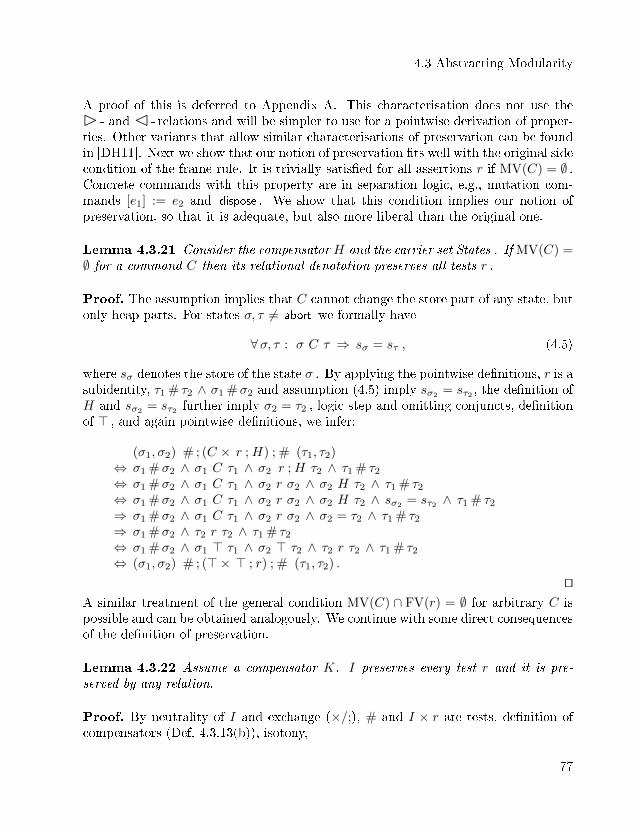
4.3 Abstracting Modularity
A proof of this is deferred to Appendix A. This characterisation does not use the� - and � - relations and will be simpler to use for a pointwise derivation of proper-ties. Other variants that allow similar characterisations of preservation can be foundin [DH11]. Next we show that our notion of preservation �ts well with the original sidecondition of the frame rule. It is trivially satis�ed for all assertions r if MV(C) = ∅ .Concrete commands with this property are in separation logic, e.g., mutation com-mands [e1] := e2 and dispose . We show that this condition implies our notion ofpreservation, so that it is adequate, but also more liberal than the original one.
Lemma 4.3.21 Consider the compensator H and the carrier set States . If MV(C) =∅ for a command C then its relational denotation preserves all tests r .
Proof. The assumption implies that C cannot change the store part of any state, butonly heap parts. For states σ, τ 6= abort we formally have
∀σ, τ : σ C τ ⇒ sσ = sτ , (4.5)
where sσ denotes the store of the state σ . By applying the pointwise de�nitions, r is asubidentity, τ1 # τ2 ∧ σ1 #σ2 and assumption (4.5) imply sσ2 = sτ2 , the de�nition ofH and sσ2 = sτ2 further imply σ2 = τ2 , logic step and omitting conjuncts, de�nitionof > , and again pointwise de�nitions, we infer:
(σ1, σ2) # ; (C × r ;H) ; # (τ1, τ2)⇔ σ1 #σ2 ∧ σ1 C τ1 ∧ σ2 r ;H τ2 ∧ τ1 # τ2⇔ σ1 #σ2 ∧ σ1 C τ1 ∧ σ2 r σ2 ∧ σ2 H τ2 ∧ τ1 # τ2⇔ σ1 #σ2 ∧ σ1 C τ1 ∧ σ2 r σ2 ∧ σ2 H τ2 ∧ sσ2
= sτ2 ∧ τ1 # τ2⇒ σ1 #σ2 ∧ σ1 C τ1 ∧ σ2 r σ2 ∧ σ2 = τ2 ∧ τ1 # τ2⇒ σ1 #σ2 ∧ τ2 r τ2 ∧ τ1 # τ2⇔ σ1 #σ2 ∧ σ1 > τ1 ∧ σ2 > τ2 ∧ τ2 r τ2 ∧ τ1 # τ2⇔ (σ1, σ2) # ; (>× > ; r) ; # (τ1, τ2) .
utA similar treatment of the general condition MV(C) ∩ FV(r) = ∅ for arbitrary C ispossible and can be obtained analogously. We continue with some direct consequencesof the de�nition of preservation.
Lemma 4.3.22 Assume a compensator K. I preserves every test r and it is pre-served by any relation.
Proof. By neutrality of I and exchange (×/;), # and I × r are tests, de�nition ofcompensators (Def. 4.3.13(b)), isotony,
77
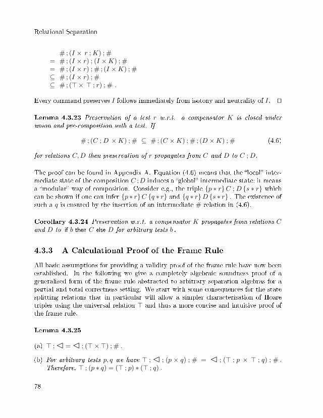
Relational Separation
# ; (I × r ;K) ; #= # ; (I × r) ; (I ×K) ; #= # ; (I × r) ; # ; (I ×K) ; #⊆ # ; (I × r) ; #⊆ # ; (>× > ; r) ; # .
Every command preserves I follows immediately from isotony and neutrality of I. ut
Lemma 4.3.23 Preservation of a test r w.r.t. a compensator K is closed underunion and pre-composition with a test. If
# ; (C ;D ×K) ; # ⊆ # ; (C ×K) ; # ; (D ×K) ; # (4.6)
for relations C,D then preservation of r propagates from C and D to C ;D.
The proof can be found in Appendix A. Equation (4.6) means that the �local� inter-mediate state of the composition C ;D induces a �global� intermediate state; it meansa �modular� way of composition. Consider e.g., the triple {p ∗ r}C ;D {s ∗ r} whichcan be shown if one can infer {p ∗ r}C {q ∗ r} and {q ∗ r}D {s ∗ r} . The existence ofsuch a q is ensured by the insertion of an intermediate # relation in (4.6).
Corollary 4.3.24 Preservation w.r.t. a compensator K propagates from relations Cand D to if b then C else D for arbitrary tests b .
4.3.3 A Calculational Proof of the Frame Rule
All basic assumptions for providing a validity proof of the frame rule have now beenestablished. In the following we give a completely algebraic soundness proof of ageneralised form of the frame rule abstracted to arbitrary separation algebras for apartial and total correctness setting. We start with some consequences for the statesplitting relations that in particular will allow a simpler characterisation of Hoaretriples using the universal relation > and thus a more concise and intuitive proof ofthe frame rule.
Lemma 4.3.25
(a) > ;� = � ; (>×>) ; # .
(b) For arbitrary tests p, q we have > ; � ; (p × q) ; # = � ; (> ; p × > ; q) ; # .Therefore, > ; (p ∗ q) = (> ; p) ∗ (> ; q) .
78
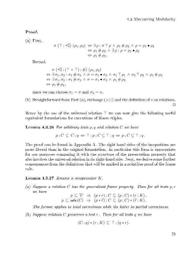
4.3 Abstracting Modularity
Proof.
(a) First,σ (> ;�) (ρ1, ρ2) ⇔ ∃ ρ : σ> ρ ∧ ρ1 # ρ2 ∧ ρ = ρ1 • ρ2
⇔ ρ1 # ρ2 ∧ ∃ ρ : ρ = ρ1 • ρ2
⇔ ρ1 # ρ2 .
Second,
σ (� ; (>×>) ; #) (ρ1, ρ2)⇔ ∃σ1, σ2 : σ1 #σ2 ∧ σ = σ1 • σ2 ∧ σ1> ρ1 ∧ σ2> ρ2 ∧ ρ1 # ρ2
⇔ ∃σ1, σ2 : σ1 #σ2 ∧ σ = σ1 • σ2 ∧ ρ1 # ρ2
⇔ ρ1 # ρ2 ,
since we can choose σ1 = σ and σ2 = u .
(b) Straightforward from Part (a), exchange (×/;) and the de�nition of ∗ on relations.ut
Hence by the use of the universal relation > we can now give the following usefulequivalent formulations for executions of Hoare triples.
Lemma 4.3.26 For arbitrary tests p, q and relation C we have
p ; C ⊆ C ; q ⇔ > ; p ; C ⊆ > ; q ⇔ p ; C ⊆ > ; q .
The proof can be found in Appendix A. The right-hand sides of the inequations aremore liberal than in the original formulation. In particular this form is appropriatefor our purposes comparing it with the structure of the preservation property thatalso involves the universal relation in its right-hand side. Next, we derive some furtherconsequences from the de�nitions that will be applied in a pointfree proof of the framerule.
Lemma 4.3.27 Assume a compensator K.
(a) Suppose a relation C has the generalised frame property. Then for all tests p, rwe have
p ⊆ pC ⇒ (p ∗ r) ; C ⊆ (p ; C) ∗ (r ;K) ,p ⊆ safe (C) ⇒ (p ∗ r) ; C ⊆ (p ; C) ∗ (r ;K) .
The former applies to total correctness while the latter to partial correctness.
(b) Suppose relation C preserves a test r . Then for all tests q we have
(C ; q) ∗ (r ;K) ⊆ > ; (q ∗ r) .
79
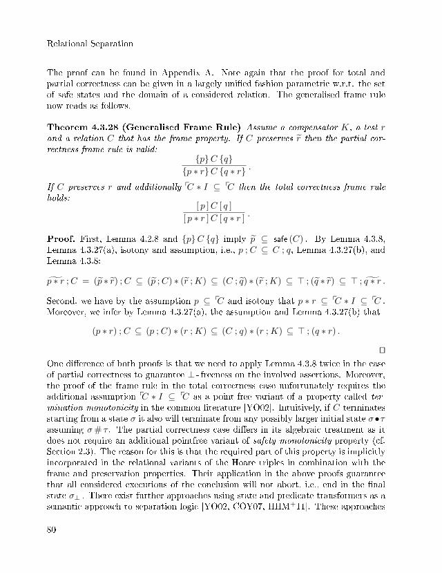
Relational Separation
The proof can be found in Appendix A. Note again that the proof for total andpartial correctness can be given in a largely uni�ed fashion parametric w.r.t. the setof safe states and the domain of a considered relation. The generalised frame rulenow reads as follows.
Theorem 4.3.28 (Generalised Frame Rule) Assume a compensator K, a test rand a relation C that has the frame property. If C preserves r then the partial cor-rectness frame rule is valid:
{p}C {q}{p ∗ r}C {q ∗ r} .
If C preserves r and additionally pC ∗ I ⊆ pC then the total correctness frame ruleholds:
[ p ]C [ q ]
[ p ∗ r ]C [ q ∗ r ].
Proof. First, Lemma 4.2.8 and {p}C {q} imply p ⊆ safe (C) . By Lemma 4.3.8,Lemma 4.3.27(a), isotony and assumption, i.e., p ; C ⊆ C ; q, Lemma 4.3.27(b), andLemma 4.3.8:
p ∗ r ;C = (p ∗ r) ;C ⊆ (p ;C) ∗ (r ;K) ⊆ (C ; q) ∗ (r ;K) ⊆ > ; (q ∗ r) ⊆ > ; q ∗ r .
Second, we have by the assumption p ⊆ pC and isotony that p ∗ r ⊆ pC ∗ I ⊆ pC .Moreover, we infer by Lemma 4.3.27(a), the assumption and Lemma 4.3.27(b) that
(p ∗ r) ; C ⊆ (p ; C) ∗ (r ;K) ⊆ (C ; q) ∗ (r ;K) ⊆ > ; (q ∗ r) .
utOne di�erence of both proofs is that we need to apply Lemma 4.3.8 twice in the caseof partial correctness to guarantee ⊥ - freeness on the involved assertions. Moreover,the proof of the frame rule in the total correctness case unfortunately requires theadditional assumption pC ∗ I ⊆ pC as a point-free variant of a property called ter-mination monotonicity in the common literature [YO02]. Intuitively, if C terminatesstarting from a state σ it also will terminate from any possibly larger initial state σ•τassuming σ# τ . The partial correctness case di�ers in its algebraic treatment as itdoes not require an additional pointfree variant of safety monotonicity property (cf.Section 2.3). The reason for this is that the required part of this property is implicitlyincorporated in the relational variants of the Hoare triples in combination with theframe and preservation properties. Their application in the above proofs guaranteethat all considered executions of the conclusion will not abort, i.e., end in the �nalstate σ⊥ . There exist further approaches using state and predicate transformers as asemantic approach to separation logic [YO02, COY07, HHM+11]. These approaches
80
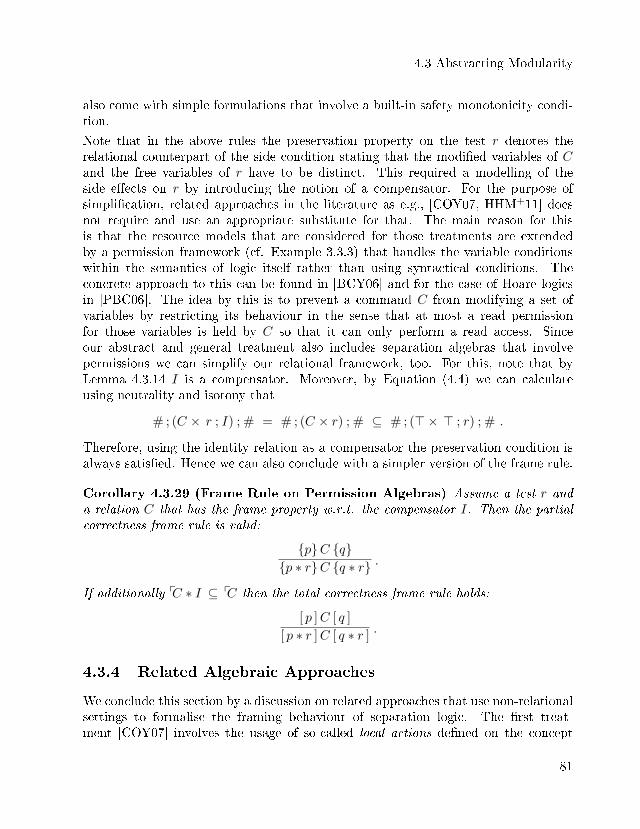
4.3 Abstracting Modularity
also come with simple formulations that involve a built-in safety monotonicity condi-tion.
Note that in the above rules the preservation property on the test r denotes therelational counterpart of the side condition stating that the modi�ed variables of Cand the free variables of r have to be distinct. This required a modelling of theside e�ects on r by introducing the notion of a compensator. For the purpose ofsimpli�cation, related approaches in the literature as e.g., [COY07, HHM+11] doesnot require and use an appropriate substitute for that. The main reason for thisis that the resource models that are considered for those treatments are extendedby a permission framework (cf. Example 3.3.3) that handles the variable conditionswithin the semantics of logic itself rather than using syntactical conditions. Theconcrete approach to this can be found in [BCY06] and for the case of Hoare logicsin [PBC06]. The idea by this is to prevent a command C from modifying a set ofvariables by restricting its behaviour in the sense that at most a read permissionfor those variables is held by C so that it can only perform a read access. Sinceour abstract and general treatment also includes separation algebras that involvepermissions we can simplify our relational framework, too. For this, note that byLemma 4.3.14 I is a compensator. Moreover, by Equation (4.4) we can calculateusing neutrality and isotony that
# ; (C × r ; I) ; # = # ; (C × r) ; # ⊆ # ; (>× > ; r) ; # .
Therefore, using the identity relation as a compensator the preservation condition isalways satis�ed. Hence we can also conclude with a simpler version of the frame rule.
Corollary 4.3.29 (Frame Rule on Permission Algebras) Assume a test r anda relation C that has the frame property w.r.t. the compensator I. Then the partialcorrectness frame rule is valid:
{p}C {q}{p ∗ r}C {q ∗ r} .
If additionally pC ∗ I ⊆ pC then the total correctness frame rule holds:
[ p ]C [ q ]
[ p ∗ r ]C [ q ∗ r ].
4.3.4 Related Algebraic Approaches
We conclude this section by a discussion on related approaches that use non-relationalsettings to formalise the framing behaviour of separation logic. The �rst treat-ment [COY07] involves the usage of so-called local actions de�ned on the concept
81
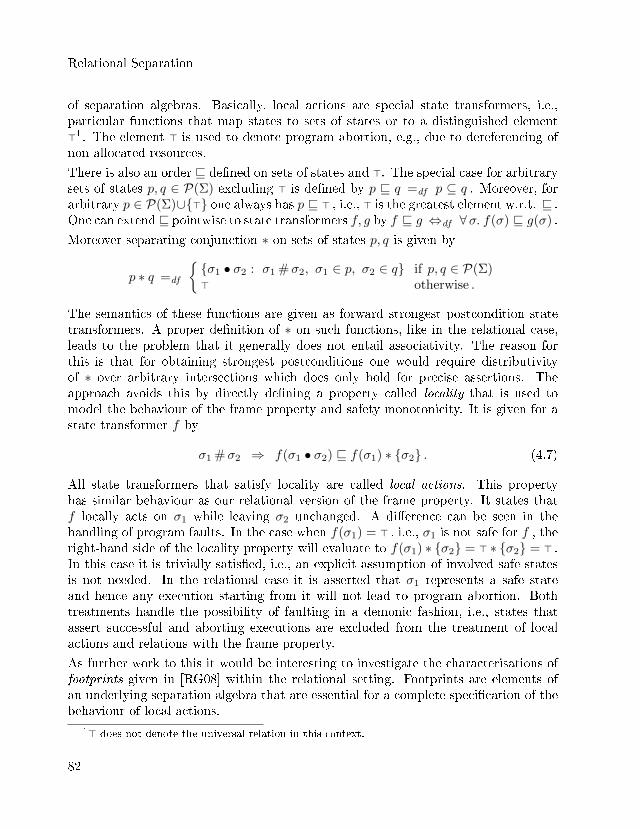
Relational Separation
of separation algebras. Basically, local actions are special state transformers, i.e.,particular functions that map states to sets of states or to a distinguished element>1. The element > is used to denote program abortion, e.g., due to dereferencing ofnon-allocated resources.
There is also an order v de�ned on sets of states and >. The special case for arbitrarysets of states p, q ∈ P(Σ) excluding > is de�ned by p v q =df p ⊆ q . Moreover, forarbitrary p ∈ P(Σ)∪{>} one always has p v > , i.e., > is the greatest element w.r.t. v .One can extendv pointwise to state transformers f, g by f v g ⇔df ∀σ. f(σ) v g(σ) .
Moreover separating conjunction ∗ on sets of states p, q is given by
p ∗ q =df
{{σ1 • σ2 : σ1 #σ2, σ1 ∈ p, σ2 ∈ q} if p, q ∈ P(Σ)> otherwise .
The semantics of these functions are given as forward strongest postcondition statetransformers. A proper de�nition of ∗ on such functions, like in the relational case,leads to the problem that it generally does not entail associativity. The reason forthis is that for obtaining strongest postconditions one would require distributivityof ∗ over arbitrary intersections which does only hold for precise assertions. Theapproach avoids this by directly de�ning a property called locality that is used tomodel the behaviour of the frame property and safety monotonicity. It is given for astate transformer f by
σ1 #σ2 ⇒ f(σ1 • σ2) v f(σ1) ∗ {σ2} . (4.7)
All state transformers that satisfy locality are called local actions. This propertyhas similar behaviour as our relational version of the frame property. It states thatf locally acts on σ1 while leaving σ2 unchanged. A di�erence can be seen in thehandling of program faults. In the case when f(σ1) = > , i.e., σ1 is not safe for f , theright-hand side of the locality property will evaluate to f(σ1) ∗ {σ2} = > ∗ {σ2} = > .In this case it is trivially satis�ed, i.e., an explicit assumption of involved safe statesis not needed. In the relational case it is asserted that σ1 represents a safe stateand hence any execution starting from it will not lead to program abortion. Bothtreatments handle the possibility of faulting in a demonic fashion, i.e., states thatassert successful and aborting executions are excluded from the treatment of localactions and relations with the frame property.
As further work to this it would be interesting to investigate the characterisations offootprints given in [RG08] within the relational setting. Footprints are elements ofan underlying separation algebra that are essential for a complete speci�cation of thebehaviour of local actions.
1> does not denote the universal relation in this context.
82
4.3 Abstracting Modularity
Another approach [HHM+11] involves a more meaningful structure given by so-calledmonotone predicate transformers, i.e., functions of type P(Σ) → P(Σ) . Di�erentlyfrom the approach of local actions, the semantics are dually provided as backwardweakest precondition predicate transformers. This yields a de�nition of separatingconjunction directly on such functions as in the case of relations:
(F1 ∗ F2)(Y ) =df
⋃{F1(Y1) ∗ F2(Y2) : Y1 ∗ Y2 ⊆ Y } ,(F1 ; F2)(Y ) =df F1(F2(Y )) ,
Id (Y ) =df Y.
Note that ∗ is used in the �rst equation on sets of states on the right-hand side andin an overloaded form on functions on the left-hand side. A locality property forpredicate transformer F is given for a set of states P by
F (P ) =⋃{F (X) ∗R : X ∗R = P} . (4.8)
The set X describes the set of safe states for the function F while R denotes again theuntouched set of substates w.r.t. P . Note that predicate transformers entail moreexpressiveness than state transformers. Interestingly, it has been shown in [HHM+11]that Equation (4.8) is equivalent to the more compact form:
F ∗ Id = F .
This means in particular that each execution of the program F can be replaced byone that only operates on the necessary and possible smaller part of the state whilethe rest of it remains unchanged (abstractly denoted by the function Id). It wouldbe interesting to obtain a similar characterisation in the relational model. In thefollowing, we derive some formulations and relationships to the semantics of the aboveformula by the use of the relational setting. Hence, we denote by the operator ∗ inwhat follows its relational version.
First remember that e as de�ned before Lemma 4.3.6 is the unit of ∗ and e ⊆ I . Thuswe can immediately conclude:
Lemma 4.3.30 For arbitrary relation C we have C ⊆ C ∗ I.
Proof. By isotony, we infer C = C ∗ e ⊆ C ∗ I . utThe other inclusion, i.e., C ∗ I ⊆ C , does not generally hold. For this we need anadditional assumption about C . This inequation can be derived from a stronger formof test preservation given in De�nition 4.3.20:
� ; (C × r) ; # ⊆ C ;� ; (I × r) . (4.9)
83
Relational Separation
The semantics of this inequation in a total correctness treatment is as follows: whenC is executed on a part of the state such that the remainder of the state satis�esr one can also run C on the complete state and still obtains an r - part in the �nalstate. A partial correctness interpretation would not exclude initial unsafe states,i.e., aborting executions. Note that one obtains from Equation (4.9) by isotony thespecialisation of De�nition 4.3.20 to K = I. Conceptually, Equation (4.9) assumesthe existence of local executions of C leaving state portions of r unchanged. Therelational frame property conversely talks about the structure of C in that it can bedivided into subexecutions. Finally, we summarise:
Lemma 4.3.31 C ∗ I ⊆ C i�s Equation (4.9) holds for all tests r .
The proof can be found in Appendix A. It can be seen that there are some proof-theoretic relationships between our relational de�nitions for proving soundness ofthe frame rule and the concept of the locality condition C ∗ I ⊆ C . However, forthat particular domain it does not seem very realistic to relate locality to that formof test preservation. By using the compensator I , one implicitly assumes that theunderlying separation algebras handle the involved side conditions of the frame rules,e.g., by permission equipped variables. In that case the preservation property shouldalways be satis�ed since it is used as an abstraction of the property that a commandC does not modify the free variables of an assertion r .
Finally, we compare the structure of the relational proofs with the corresponding onesin [HHM+11]. First, note that predicate transformers are ordered with the reversedpointwise inclusion order, i.e., F v G ⇔ ∀X : F (X) ⊇ G(X) . It was shown thatthe frame rule is equivalent to the inequation
(F ∗G) ;H v (F ;H) ∗G
for adequate predicate transformers F,G,H using a generalised characterisation ofHoare triples. This inequation, also called the small exchange law, was previouslyintroduced within the approach of concurrenct Kleene algebras [HMSW11]. We willelaborate on this algebraic structure later in Section 4.4.3.
In the relational setting, that inequation is not generally valid using the standardsubset order on relations. However, as can be seen in Lemma 4.3.27 a structurallysimilar variant has been established with the pointfree version of the frame property.By choosing the compensator K = I this yields for tests p, r and a relation C withthe frame property:
p ⊆ pC ⇒ (p ∗ r) ; C ⊆ (p ; C) ∗ r ,p ⊆ safe (C) ⇒ (p ∗ r) ; C ⊆ (p ; C) ∗ r .
84
4.4 Applications to Concurrency
Although the test p is restricted in the premise of the implications, the relationalproofs of the frame rule become as simple as the one for the predicate transformer ap-proach in [HHM+11]. As a further remark, the approach of [HHM+11] requires specialfunctions for the semantics of Hoare triples. They are called best predicate transform-ers and are used as an adequate substitute for assertions. Intuitively, these functionssimulate the allocation of resources that are characterised by pre- and postconditions.In the relational calculus, assertions can simply be handled with the subalgebra oftests. Another advantage of the relational approach is that ∗ distributes over arbi-trary suprema while this is not the case for predicate transformers. By monotonicityone can only obtain a super-distributivity law for that treatment.
4.4 Applications to Concurrency
In De�nition 4.3.5 we provided a general operation ∗ on arbitrary relations that, de-pending on the underlying separation algebra, captures as a special case the semanticsof the separating conjunction. This extended operation allowed relational formula-tions that characterised the behaviour and structure of separation logical commands ina sequential setting. As already mentioned, one can also interpret general ∗ - productsC ∗ D of relations C,D as their parallel execution on # - related parts of resources.This will be the main topic of this section. We start by presenting some centralconcepts and proof rules of concurrent separation logic (CSL) [Bro07, O'H07]. CSLhas proved to be an e�ective methodology for scalable reasoning about concurrency.Moreover, we provide relational abstractions of this and pointfree validity proofs asin [DM12a, DM14]. As a next step we derive several relationships to other approachesthat also involve algebraic semantics by modelling concurrent composition as separa-tion of programs. This yields, besides further concrete applications for the presentedrelational abstractions, also new insights for future considerations about relations andconcurrency reasoning.
4.4.1 Relations and Concurrent Separation Logic
We start this section with concrete de�nitions of the semantics of CSL and brie�yexplain the concepts of the concurrency extension of separation logic. After thisrelational denotations and formulations will be provided to model e�ects of separatingresources within concurrent programs. These yield a fully pointfree proof of a centralinference rule in CSL that we introduce in the sequel.
CSL is an extension of its sequential version with additional concepts and proofrules for reasoning about pointer manipulating programs in a concurrent environ-
85
Relational Separation
ment [O'H07]. A soundness proof of this logic in a partial correctness treatment isprovided in [Bro07] that uses a trace-based denotation with interleaving semantics.Starting from this approach we derive in the sequel relational abstractions of this.We begin by introducing extended separation logic triples in proof rules of CSL thatcome with an additional construct for controlling access to shared resources in a con-current environment. It is called the resource context and is denoted by Γ. It isused to safeguard identi�ers or program variables that belong to a critical resource rwith a corresponding invariant. Such resources can usually be accessed concurrentlyand therefore require some care to avoid non-deterministic behaviour. Contexts areappended to formulas involving separation logic triples, i.e.,
Γ ` {p}C {q} .
Programs C that use resources of Γ need to maintain the invariants involved afterexecution. As a concrete example of such a resource one can think of a shared queue,implemented as a list. The invariant can be given by list α i (cf. Example 2.1.1) andthe protected variable by i . The ghost variable α is not protected by Γ since it is notvisible within the program itself. Now any execution accessing the list by a dequeueor enqueue of elements needs to maintain the linking structure of the list.
Generally, soundness of the proof rules in CSL require that resource invariants areprecise assertions. Another soundness proof that comes with a weaker requirementcan be found in [Vaf11]. We will not go into any further details on resource contextssince intuition su�ces to grasp the central ingredient of CSL, namely the concurrencyrule, which allows a parallel composition of programs:
Γ ` {p1}C {q1} Γ ` {p2}D {q2}Γ ` {p1 ∗ p2 }C ‖ D { q1 ∗ q2} (concrule)
where pi, qi are separation logic assertions and C,D denote commands. There areadditional side conditions for this proof rule on the variables involved: FV(p1, q1) ∩MV(D) = FV(p2, q2) ∩MV(C) = ∅ , and that FV(C) ∩MV(D) and FV(D) ∩MV(C)need to be subsets of the identi�ers protected by the resource context Γ . The formerside condition is similar as in the frame rule and requires that assertion variablesof the untouched resources should not be modi�ed. The latter condition assertsthat modi�ed variables occurring free in a parallel program must be used inside acritical region, i.e., protected by the resource context. Otherwise races can occur,i.e., simultaneous accesses of parallel running programs to the same resources. Suchraces may induce uncontrolled behaviour and therefore need to be excluded. Theconcurrency rule informally allows, under the described circumstances, to composeprograms in parallel, each of them running on ∗ - separated regions of storage.
86
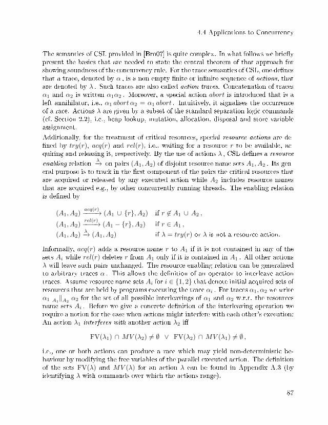
4.4 Applications to Concurrency
The semantics of CSL provided in [Bro07] is quite complex. In what follows we brie�ypresent the basics that are needed to state the central theorem of that approach forshowing soundness of the concurrency rule. For the trace semantics of CSL, one de�nesthat a trace, denoted by α , is a non-empty �nite or in�nite sequence of actions, thatare denoted by λ . Such traces are also called action traces. Concatenation of tracesα1 and α2 is written α1α2 . Moreover, a special action abort is introduced that is aleft annihilator, i.e., α1 abort α2 = α1 abort . Intuitively, it signalises the occurrenceof a race. Actions λ are given by a subset of the standard separation logic commands(cf. Section 2.2), i.e., heap lookup, mutation, allocation, disposal and store variableassignment.
Additionally, for the treatment of critical resources, special resource actions are de-�ned by try(r), acq(r) and rel(r), i.e., waiting for a resource r to be available, ac-quiring and releasing it, respectively. By the use of actions λ , CSL de�nes a resource
enabling relationλ−→ on pairs (A1, A2) of disjoint resource name sets A1, A2 . Its gen-
eral purpose is to track in the �rst component of the pairs the critical resources thatare acquired or released by any executed action while A2 includes resource namesthat are acquired e.g., by other concurrently running threads. The enabling relationis de�ned by
(A1, A2)acq(r)−−−−→ (A1 ∪ {r}, A2) if r 6∈ A1 ∪ A2 ,
(A1, A2)rel(r)−−−−→ (A1 − {r}, A2) if r ∈ A1 ,
(A1, A2)λ−→ (A1, A2) if λ = try(r) or λ is not a resource action.
Informally, acq(r) adds a resource name r to A1 if it is not contained in any of thesets Ai while rel(r) deletes r from A1 only if it is contained in A1 . All other actionsλ will leave such pairs unchanged. The resource enabling relation can be generalisedto arbitrary traces α . This allows the de�nition of an operator to interleave actiontraces. Assume resource name sets Ai for i ∈ {1, 2} that denote initial acquired sets ofresources that are held by programs executing the trace αi . For traces α1, α2 we writeα1 ‖A1 A2
α2 for the set of all possible interleavings of α1 and α2 w.r.t. the resourcesname sets Ai . Before we give a concrete de�nition of the interleaving operation werequire a notion for the case when actions might interfere with each other's execution:An action λ1 interferes with another action λ2 i�
FV(λ1) ∩ MV (λ2) 6= ∅ ∨ FV(λ2) ∩ MV (λ1) 6= ∅ ,
i.e., one or both actions can produce a race which may yield non-deterministic be-haviour by modifying the free variables of the parallel executed action. The de�nitionof the sets FV(λ) and MV (λ) for an action λ can be found in Appendix A.3 (byidentifying λ with commands over which the actions range).
87
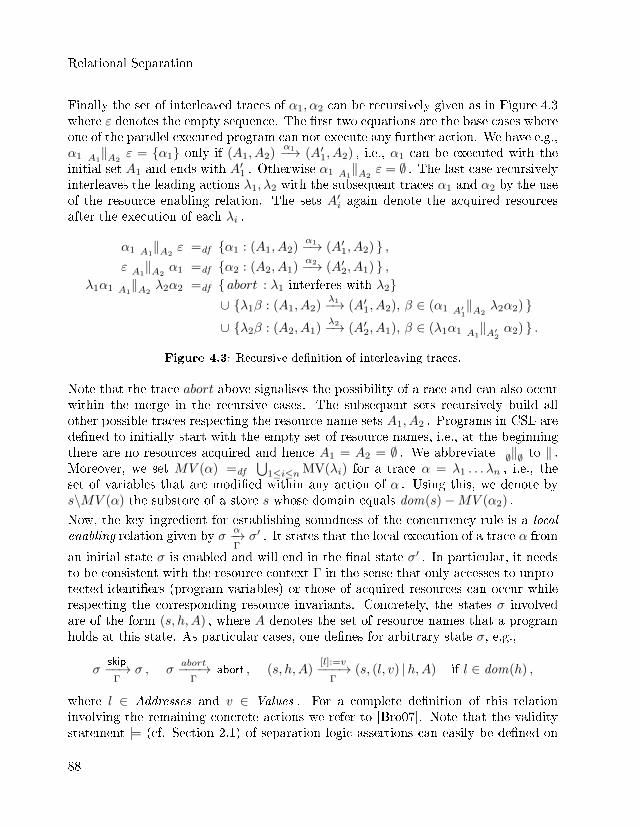
Relational Separation
Finally the set of interleaved traces of α1, α2 can be recursively given as in Figure 4.3where ε denotes the empty sequence. The �rst two equations are the base cases whereone of the parallel executed program can not execute any further action. We have e.g.,α1 ‖A1 A2
ε = {α1} only if (A1, A2)α1−→ (A′1, A2) , i.e., α1 can be executed with the
initial set A1 and ends with A′1 . Otherwise α1 ‖A1 A2ε = ∅ . The last case recursively
interleaves the leading actions λ1, λ2 with the subsequent traces α1 and α2 by the useof the resource enabling relation. The sets A′i again denote the acquired resourcesafter the execution of each λi .
α1 ‖A1 A2ε =df {α1 : (A1, A2)
α1−→ (A′1, A2) } ,ε ‖A1 A2
α1 =df {α2 : (A2, A1)α2−→ (A′2, A1) } ,
λ1α1 ‖A1 A2λ2α2 =df { abort : λ1 interferes with λ2}
∪ {λ1β : (A1, A2)λ1−→ (A′1, A2), β ∈ (α1 ‖A′
1 A2λ2α2) }
∪ {λ2β : (A2, A1)λ2−→ (A′2, A1), β ∈ (λ1α1 ‖A1 A′
2α2) } .
Figure 4.3: Recursive de�nition of interleaving traces.
Note that the trace abort above signalises the possibility of a race and can also occurwithin the merge in the recursive cases. The subsequent sets recursively build allother possible traces respecting the resource name sets A1, A2 . Programs in CSL arede�ned to initially start with the empty set of resource names, i.e., at the beginningthere are no resources acquired and hence A1 = A2 = ∅ . We abbreviate ‖∅ ∅ to ‖ .Moreover, we set MV (α) =df
⋃1≤i≤n MV(λi) for a trace α = λ1 . . . λn , i.e., the
set of variables that are modi�ed within any action of α . Using this, we denote bys\MV (α) the substore of a store s whose domain equals dom(s)−MV (α2) .
Now, the key ingredient for establishing soundness of the concurrency rule is a localenabling relation given by σ
α−→Γσ′ . It states that the local execution of a trace α from
an initial state σ is enabled and will end in the �nal state σ′ . In particular, it needsto be consistent with the resource context Γ in the sense that only accesses to unpro-tected identi�ers (program variables) or those of acquired resources can occur whilerespecting the corresponding resource invariants. Concretely, the states σ involvedare of the form (s, h,A) , where A denotes the set of resource names that a programholds at this state. As particular cases, one de�nes for arbitrary state σ, e.g.,
σskip−−→Γ
σ , σabort−−−→
Γabort , (s, h,A)
[l]:=v−−−→Γ
(s, (l, v) |h,A) if l ∈ dom(h) ,
where l ∈ Addresses and v ∈ Values . For a complete de�nition of this relationinvolving the remaining concrete actions we refer to [Bro07]. Note that the validitystatement |= (cf. Section 2.1) of separation logic assertions can easily be de�ned on
88
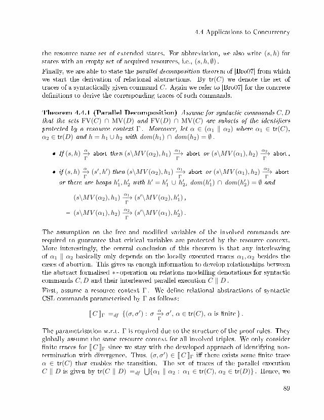
4.4 Applications to Concurrency
the resource name set of extended states. For abbreviation, we also write (s, h) forstates with an empty set of acquired resources, i.e., (s, h, ∅) .Finally, we are able to state the parallel decomposition theorem of [Bro07] from whichwe start the derivation of relational abstractions. By tr(C) we denote the set oftraces of a syntactically given command C. Again we refer to [Bro07] for the concretede�nitions to derive the corresponding traces of such commands.
Theorem 4.4.1 (Parallel Decomposition) Assume for syntactic commands C,Dthat the sets FV(C) ∩ MV(D) and FV(D) ∩ MV(C) are subsets of the identi�ersprotected by a resource context Γ . Moreover, let α ∈ (α1 ‖ α2) where α1 ∈ tr(C),α2 ∈ tr(D) and h = h1 ∪ h2 with dom(h1) ∩ dom(h2) = ∅ .
� If (s, h)α−→Γ
abort then (s\MV (α2), h1)α1−→Γ
abort or (s\MV (α1), h2)α2−→Γ
abort ,
� if (s, h)α−→Γ
(s′, h′) then (s\MV (α2), h1)α1−→Γ
abort or (s\MV (α1), h2)α2−→Γ
abort
or there are heaps h′1, h′2 with h′ = h′1 ∪ h′2, dom(h′1) ∩ dom(h′2) = ∅ and
� (s\MV (α2), h1)α1−→Γ
(s′\MV (α2), h′1) ,
� (s\MV (α1), h2)α2−→Γ
(s′\MV (α1), h′2) .
The assumption on the free and modi�ed variables of the involved commands arerequired to guarantee that critical variables are protected by the resource context.More interestingly, the central conclusion of this theorem is that any interleavingof α1 ‖ α2 basically only depends on the locally executed traces α1, α2 besides thecases of abortion. This gives us enough information to develop relationships betweenthe abstract formalised ∗ - operation on relations modelling denotations for syntacticcommands C,D and their interleaved parallel execution C ‖ D .
First, assume a resource context Γ . We de�ne relational abstractions of syntacticCSL commands parameterised by Γ as follows:
[[C ]]Γ =df {(σ, σ′) : σα−→Γσ′, α ∈ tr(C), α is �nite } .
The parametrisation w.r.t. Γ is required due to the structure of the proof rules. Theyglobally assume the same resource context for all involved triples. We only consider�nite traces for [[C ]]Γ since we stay with the developed approach of identifying non-termination with divergence. Thus, (σ, σ′) ∈ [[C ]]Γ i� there exists some �nite traceα ∈ tr(C) that enables the transition. The set of traces of the parallel executionC ‖ D is given by tr(C ‖ D) =df
⋃{α1 ‖ α2 : α1 ∈ tr(C), α2 ∈ tr(D)} . Hence, we
89
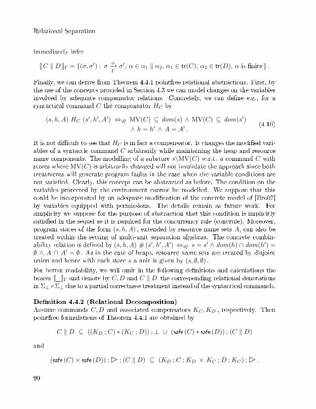
Relational Separation
immediately infer
[[C ‖ D ]]Γ = {(σ, σ′) : σα−→Γσ′, α ∈ α1 ‖ α2, α1 ∈ tr(C), α2 ∈ tr(D), α is �nite } .
Finally, we can derive from Theorem 4.4.1 pointfree relational abstractions. First, bythe use of the concepts provided in Section 4.3 we can model changes on the variablesinvolved by adequate compensator relations. Concretely, we can de�ne e.g., for asyntactical command C the compensator HC by
(s, h,A) HC (s′, h′, A′) ⇔df MV(C) ⊆ dom(s) ∧ MV(C) ⊆ dom(s′)
∧ h = h′ ∧ A = A′ .(4.10)
It is not di�cult to see that HC is in fact a compensator. It changes the modi�ed vari-ables of a syntactic command C arbitrarily while maintaining the heap and resourcename components. The modelling of a substore s\MV(C) w.r.t. a command C withstores where MV(C) is arbitrarily changed will not invalidate the approach since bothtreatments will generate program faults in the case when the variable conditions arenot satis�ed. Clearly, this concept can be abstracted as before. The condition on thevariables protected by the environment cannot be modelled. We suppose that thiscould be incorporated by an adequate modi�cation of the concrete model of [Bro07]by variables equipped with permissions. The details remain as future work. Forsimplicity we suppose for the purpose of abstraction that this condition is implicitlysatis�ed in the sequel as it is required for the concurrency rule (concrule). Moreover,program states of the form (s, h,A) , extended by resource name sets A, can also betreated within the setting of multi-unit separation algebras. The concrete combin-ability relation is de�ned by (s, h,A) # (s′, h′, A′) ⇔df s = s′ ∧ dom(h) ∩ dom(h′) =∅ ∧ A ∩ A′ = ∅ . As in the case of heaps, resource name sets are treated by disjointunion and hence with each store s a unit is given by (s, ∅, ∅) .For better readability, we will omit in the following de�nitions and calculations thebraces [[_]]Γ and denote by C,D and C ‖ D the corresponding relational denotationsin Σ⊥×Σ⊥ due to a partial correctness treatment instead of the syntactical commands.
De�nition 4.4.2 (Relational Decomposition)Assume commands C,D and associated compensators KC ,KD , respectively. Thenpointfree formulations of Theorem 4.4.1 are obtained by
C ‖ D ⊆ ((KD ; C) ∗ (KC ;D)) ;⊥ ∪ (safe (C) ∗ safe (D)) ; (C ‖ D)
and
(safe (C)× safe (D)) ;� ; (C ‖ D) ⊆ (KD ; C ;KD × KC ;D ;KC) ;� .
90
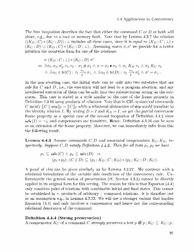
4.4 Applications to Concurrency
The �rst inequation describes the fact that either the command C or D or both willabort, e.g., due to a race or memory fault. Note that by Lemma 4.3.7 the relation((KD ; C) ∗ (KC ; D)) ; ⊥ includes all these cases, since it is equal to (KD ; C ; ⊥) ∗(KC ; D) ∪ (KD ; C) ∗ (KC ; D ; ⊥) . Assuming states σ, σ′ we provide for a betterintuition the pointwise form for one of the relations:
σ (KD ; C ;⊥) ∗ (KC ;D) σ′
⇔ ∃σ1, σ2, σ′2, τ1, τ2 : σ1 #σ2 ∧ σ = σ1 • σ2 ∧ σ1 KD τ1 ∧ σ2 KC τ2
∧ ∃α1 ∈ tr(C) : τ1α1−→Γ
σ⊥ ∧ ∃α2 ∈ tr(D) : τ2α2−→Γ
σ′2 ∧ σ′ = σ⊥ .
In the non-aborting case, the initial state can be split into two substates that aresafe for C and D , i.e., the execution will not lead to a program abortion, and anyinterleaved execution of them can be split into two subexecutions acting on the sub-states. This case is stated in a style similar to the case of the frame property inDe�nition 4.3.16 using products of relations. Note that in CSL syntactical commandsC satisfy [[C ‖ skip ]]Γ = [[C ]]Γ while a relational abstraction of skip would translate tothe identity relation I. By setting D = I and KD = I, we get the partial correctnessframe property as a special case of the second inequation of De�nition 4.4.2 sincesafe (I) = ¬⊥ and compensators are transitive. Hence, De�nition 4.3.16 can be seenas an extension of the frame property. Moreover, we can immediately infer from thisthe following result.
Lemma 4.4.3 Assume commands C,D and associated compensators KC ,KD, re-spectively. Suppose C,D satisfy De�nition 4.4.2. Then for all tests p1, p2 we have
p1 ⊆ safe (C) ∧ p2 ⊆ safe (D) ⇒(p1 ∗ p2) ; (C ‖ D) ⊆ (p1 ;KD ; C ;KD) ∗ (p2 ;KC ;D ;KC) .
A proof of this can be given similarly as for Lemma 4.3.27. We continue with arelational formulation of the variable side conditions of the concurrency rule. Un-fortunately the general notion of preservation (cf. Section 4.3.2) cannot be directlyapplied in its original form for this setting. The reason for this is that Equation (4.4)only considers pairs of relations with combinable initial and �nal states. This cannotbe established in ∗ - products of arbitrary ; - composed relations. It is therefore putas an assumption e.g., in Lemma 4.3.23. We will use a stronger variant that impliesEquation (4.4) and only involves a compensator and hence not the correspondingrelational denotation of the command.
De�nition 4.4.4 (Strong preservation)A compensator KC of a command C strongly preserves a test p i� p ;KC ⊆ KC ; p .
91
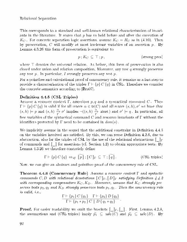
Relational Separation
This corresponds to a standard and well-known relational characterisation of invari-ants in the literature. It states that p has to hold before and after the execution ofKC . For concrete separation logic assertions, assume KC = HC as in (4.10). Thenby preservation, C will modify at most irrelevant variables of an assertion p . ByLemma 4.3.26 this form of preservation is equivalent to
p ;KC ⊆ > ; p , (strong pres)
where > denotes the universal relation. As before, this form of preservation is alsoclosed under union and relation composition. Moreover, any test q strongly preservesany test p . In particular, I strongly preserves any test p .
For a pointfree and calculational proof of concurrency rule, it remains as a last step toprovide a characterisation of the triples Γ ` {p}C {q} in CSL. Therefore we considerthe concrete semantics according to [Bro07].
De�nition 4.4.5 (CSL Triples)Assume a resource context Γ, assertions p, q and a syntactical command C . ThenΓ ` {p}C {q} is valid if for all traces α ∈ tr(C) and all states (s, h), σ′ we have that(s, h) |= p and (s, h)
α−→Γσ′ implies ¬((s, h)
α−→Γ
abort ) and σ′ |= q . In particular, all
free variables of the syntactical command C and resource invariants of Γ without theidenti�ers protected by Γ need to be contained in dom(s) .
We implicitly assume in the sequel that the additional constraint in De�nition 4.4.5on the variables involved are satis�ed. By this, we can reuse De�nition 4.2.6, due toabstraction, also for the triples of CSL by the use of the relational abstractions [[_]]Γof commands and [[_]] for assertions (cf. Section 4.2) to obtain appropriate tests. ByLemma 4.3.26 we therefore concretely de�ne
Γ ` {p}C {q} ⇔df [[ p ]] ; [[C ]]Γ ⊆ > ; [[ q ]] . (CSL triples)
Now, we can give an abstract and pointfree proof of the concurrency rule of CSL.
Theorem 4.4.6 (Concurrency Rule) Assume a resource context Γ and syntacticcommands C,D with relational denotations [[C ]]Γ, [[D ]]Γ satisfying De�nition 4.4.2with corresponding compensators KC ,KD . Moreover, assume that KC strongly pre-serves tests p2, q2 and KD strongly preserves tests p1, q1 . Then the concurrency ruleis valid, i.e.,
Γ ` {p1}C {q1} Γ ` {p2}D {q2}Γ ` {p1 ∗ p2 }C ‖ D { q1 ∗ q2} .
Proof. For easier readability we omit the brackets [[_]]Γ, [[_]] . First, Lemma 4.2.8,the assumptions and (CSL triples) imply p1 ⊆ safe (C) and p2 ⊆ safe (D) . By
92
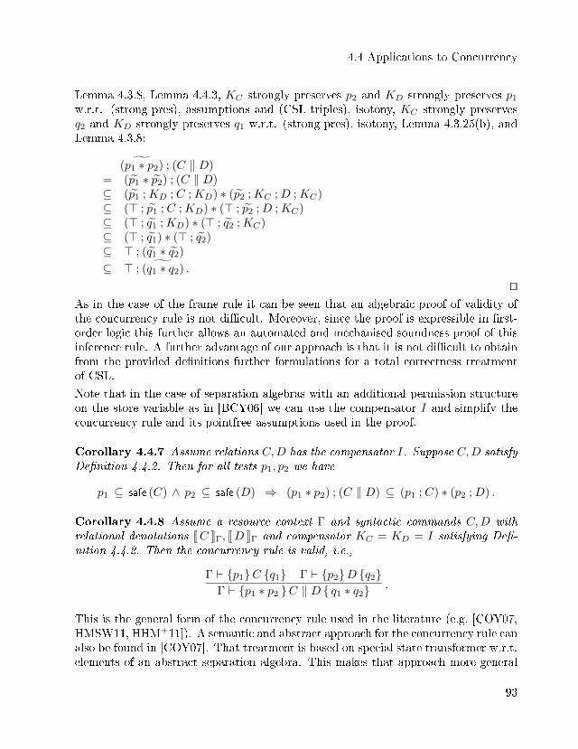
4.4 Applications to Concurrency
Lemma 4.3.8, Lemma 4.4.3, KC strongly preserves p2 and KD strongly preserves p1
w.r.t. (strong pres), assumptions and (CSL triples), isotony, KC strongly preservesq2 and KD strongly preserves q1 w.r.t. (strong pres), isotony, Lemma 4.3.25(b), andLemma 4.3.8:
˜(p1 ∗ p2) ; (C ‖ D)= (p1 ∗ p2) ; (C ‖ D)⊆ (p1 ;KD ; C ;KD) ∗ (p2 ;KC ;D ;KC)⊆ (> ; p1 ; C ;KD) ∗ (> ; p2 ;D ;KC)⊆ (> ; q1 ;KD) ∗ (> ; q2 ;KC)⊆ (> ; q1) ∗ (> ; q2)⊆ > ; (q1 ∗ q2)
⊆ > ; ˜(q1 ∗ q2) .
utAs in the case of the frame rule it can be seen that an algebraic proof of validity ofthe concurrency rule is not di�cult. Moreover, since the proof is expressible in �rst-order logic this further allows an automated and mechanised soundness proof of thisinference rule. A further advantage of our approach is that it is not di�cult to obtainfrom the provided de�nitions further formulations for a total correctness treatmentof CSL.
Note that in the case of separation algebras with an additional permission structureon the store variable as in [BCY06] we can use the compensator I and simplify theconcurrency rule and its pointfree assumptions used in the proof.
Corollary 4.4.7 Assume relations C,D has the compensator I. Suppose C,D satisfyDe�nition 4.4.2. Then for all tests p1, p2 we have
p1 ⊆ safe (C) ∧ p2 ⊆ safe (D) ⇒ (p1 ∗ p2) ; (C ‖ D) ⊆ (p1 ; C) ∗ (p2 ;D) .
Corollary 4.4.8 Assume a resource context Γ and syntactic commands C,D withrelational denotations [[C ]]Γ, [[D ]]Γ and compensator KC = KD = I satisfying De�-nition 4.4.2. Then the concurrency rule is valid, i.e.,
Γ ` {p1}C {q1} Γ ` {p2}D {q2}Γ ` {p1 ∗ p2 }C ‖ D { q1 ∗ q2} .
This is the general form of the concurrency rule used in the literature (e.g. [COY07,HMSW11, HHM+11]). A semantic and abstract approach for the concurrency rule canalso be found in [COY07]. That treatment is based on special state transformer w.r.t.elements of an abstract separation algebra. This makes that approach more general
93
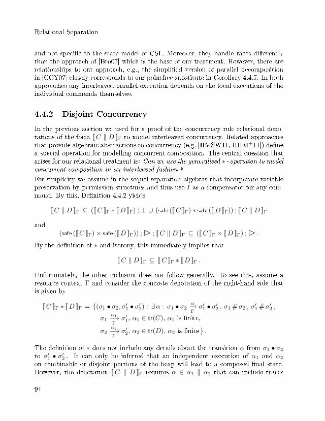
Relational Separation
and not speci�c to the state model of CSL. Moreover, they handle races di�erentlythan the approach of [Bro07] which is the base of our treatment. However, there arerelationships to our approach, e.g., the simpli�ed version of parallel decompositionin [COY07] closely corresponds to our pointfree substitute in Corollary 4.4.7. In bothapproaches any interleaved parallel execution depends on the local executions of theindividual commands themselves.
4.4.2 Disjoint Concurrency
In the previous section we used for a proof of the concurrency rule relational deno-tations of the form [[C ‖ D ]]Γ to model interleaved concurrency. Related approachesthat provide algebraic abstractions to concurrency (e.g. [HMSW11, HHM+11]) de�nea special operation for modelling concurrent composition. The central question thatarises for our relational treatment is: Can we use the generalised ∗ - operation to modelconcurrent composition in an interleaved fashion ?
For simplicity we assume in the sequel separation algebras that incorporate variablepreservation by permission structures and thus use I as a compensator for any com-mand. By this, De�nition 4.4.2 yields
[[C ‖ D ]]Γ ⊆ ([[C ]]Γ ∗ [[D ]]Γ) ;⊥ ∪ (safe ([[C ]]Γ) ∗ safe ([[D ]]Γ)) ; [[C ‖ D ]]Γ
and(safe ([[C ]]Γ)× safe ([[D ]]Γ)) ;� ; [[C ‖ D ]]Γ ⊆ ([[C ]]Γ × [[D ]]Γ) ;� .
By the de�nition of ∗ and isotony, this immediately implies that
[[C ‖ D ]]Γ ⊆ [[C ]]Γ ∗ [[D ]]Γ .
Unfortunately, the other inclusion does not follow generally. To see this, assume aresource context Γ and consider the concrete denotation of the right-hand side thatis given by
[[C ]]Γ ∗ [[D ]]Γ = {(σ1 • σ2, σ′1 • σ′2) : ∃α : σ1 • σ2
α−→Γσ′1 • σ′2 , σ1 #σ2 , σ
′1 #σ′2 ,
σ1α1−→Γ
σ′1, α1 ∈ tr(C), α1 is �nite,
σ2α2−→Γ
σ′2, α2 ∈ tr(D), α2 is �nite } .
The de�nition of ∗ does not include any details about the transition α from σ1 • σ2
to σ′1 • σ′2 . It can only be inferred that an independent execution of α1 and α2
on combinable or disjoint portions of the heap will lead to a composed �nal state.However, the denotation [[C ‖ D ]]Γ requires α ∈ α1 ‖ α2 that can include traces
94
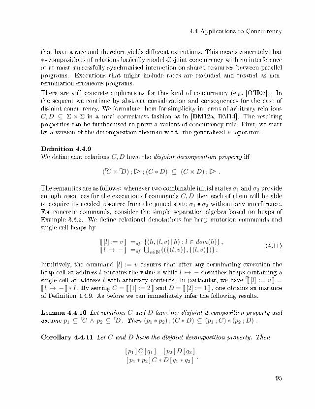
4.4 Applications to Concurrency
that have a race and therefore yields di�erent executions. This means concretely that∗ - compositions of relations basically model disjoint concurrency with no interferenceor at most successfully synchronised interaction on shared resources between parallelprograms. Executions that might include races are excluded and treated as non-termination erroneous programs.
There are still concrete applications for this kind of concurrency (e.g. [O'H07]). Inthe sequent we continue by abstract consideration and consequences for the case ofdisjoint concurrency. We formulate them for simplicity in terms of arbitrary relationsC,D ⊆ Σ × Σ in a total correctness fashion as in [DM12a, DM14]. The resultingproperties can be further used to prove a variant of concurrency rule. First, we startby a version of the decomposition theorem w.r.t. the generalised ∗ - operator.
De�nition 4.4.9We de�ne that relations C,D have the disjoint decomposition property i�
(pC × pD) ;� ; (C ∗D) ⊆ (C ×D) ;� .
The semantics are as follows: whenever two combinable initial states σ1 and σ2 provideenough resources for the execution of commands C,D then each of them will be ableto acquire its needed resource from the joined state σ1 • σ2 without any interference.For concrete commands, consider the simple separation algebra based on heaps ofExample 3.3.2. We de�ne relational denotations for heap mutation commands andsingle cell heaps by
[[ [l] := v ]] =df {(h, (l, v) |h) : l ∈ dom(h)} ,[[ l 7→ − ]] =df
⋃v∈IN{({(l, v)}, {(l, v)})} . (4.11)
Intuitively, the command [l] := v ensures that after any terminating execution theheap cell at address l contains the value v while l 7→ − describes heaps containing asingle cell at address l with arbitrary contents. In particular, we have p[[ [l] := v ]] =[[ l 7→ − ]] ∗ I. By setting C = [[ [1] := 2 ]] and D = [[ [2] := 1 ]] , one obtains an instanceof De�nition 4.4.9. As before we can immediately infer the following results.
Lemma 4.4.10 Let relations C and D have the disjoint decomposition property andassume p1 ⊆ pC ∧ p2 ⊆ pD . Then (p1 ∗ p2) ; (C ∗D) ⊆ (p1 ; C) ∗ (p2 ;D) .
Corollary 4.4.11 Let C and D have the disjoint decomposition property. Then
[ p1 ]C [ q1 ] [ p2 ]D [ q2 ]
[ p1 ∗ p2 ]C ∗D [ q1 ∗ q2 ].
95
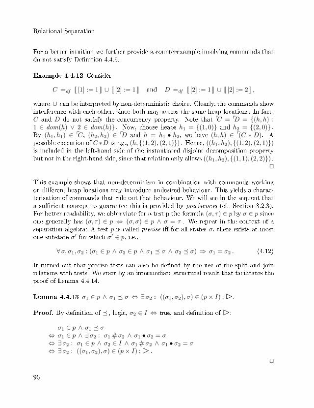
Relational Separation
For a better intuition we further provide a counterexample involving commands thatdo not satisfy De�nition 4.4.9.
Example 4.4.12 Consider
C =df [[ [1] := 1 ]] ∪ [[ [2] := 1 ]] and D =df [[ [2] := 1 ]] ∪ [[ [2] := 2 ]] ,
where ∪ can be interpreted by non-deterministic choice. Clearly, the commands showinterference with each other, since both may access the same heap locations. In fact,C and D do not satisfy the concurrency property. Note that pC = pD = {(h, h) :1 ∈ dom(h) ∨ 2 ∈ dom(h)} . Now, choose heaps h1 = {(1, 0)} and h2 = {(2, 0)} .By (h1, h1) ∈ pC, (h2, h2) ∈ pD and h = h1 • h2, we have (h, h) ∈ p(C ∗ D). Apossible execution of C ∗D is e.g., (h, {(1, 2), (2, 1)}) . Hence, ((h1, h2), {(1, 2), (2, 1)})is included in the left-hand side of the instantiated disjoint decomposition propertybut not in the right-hand side, since that relation only allows ((h1, h2), {(1, 1), (2, 2)}) .
ut
This example shows that non-determinism in combination with commands workingon di�erent heap locations may introduce undesired behaviour. This yields a charac-terisation of commands that rule out that behaviour. We will see in the sequent thata su�cient concept to guarantee this is provided by preciseness (cf. Section 3.2.3).For better readability, we abbreviate for a test p the formula (σ, τ) ∈ p by σ ∈ p sinceone generally has (σ, τ) ∈ p ⇔ (σ, σ) ∈ p ∧ σ = τ . We repeat in the context of aseparation algebra: A test p is called precise i� for all states σ, there exists at mostone substate σ′ for which σ′ ∈ p, i.e.,
∀σ, σ1, σ2 : (σ1 ∈ p ∧ σ2 ∈ p ∧ σ1 � σ ∧ σ2 � σ) ⇒ σ1 = σ2 . (4.12)
It turned out that precise tests can also be de�ned by the use of the split and joinrelations with tests. We start by an intermediate structural result that facilitates theproof of Lemma 4.4.14.
Lemma 4.4.13 σ1 ∈ p ∧ σ1 � σ ⇔ ∃σ2 : ((σ1, σ2), σ) ∈ (p× I) ;�.
Proof. By de�nition of � , logic, σ2 ∈ I ⇔ true, and de�nition of �:
σ1 ∈ p ∧ σ1 � σ⇔ σ1 ∈ p ∧ ∃σ2 : σ1 #σ2 ∧ σ1 • σ2 = σ⇔ ∃σ2 : σ1 ∈ p ∧ σ2 ∈ I ∧ σ1 #σ2 ∧ σ1 • σ2 = σ⇔ ∃σ2 : ((σ1, σ2), σ) ∈ (p× I) ;� .
ut
96
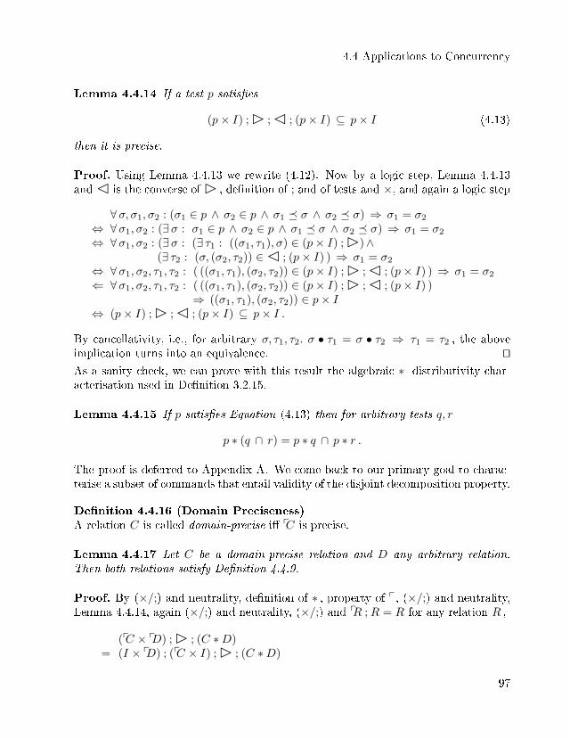
4.4 Applications to Concurrency
Lemma 4.4.14 If a test p satis�es
(p× I) ;� ;� ; (p× I) ⊆ p× I (4.13)
then it is precise.
Proof. Using Lemma 4.4.13 we rewrite (4.12). Now by a logic step, Lemma 4.4.13and� is the converse of� , de�nition of ; and of tests and ×, and again a logic step
∀σ, σ1, σ2 : (σ1 ∈ p ∧ σ2 ∈ p ∧ σ1 � σ ∧ σ2 � σ) ⇒ σ1 = σ2
⇔ ∀σ1, σ2 : (∃σ : σ1 ∈ p ∧ σ2 ∈ p ∧ σ1 � σ ∧ σ2 � σ) ⇒ σ1 = σ2
⇔ ∀σ1, σ2 : (∃σ : (∃ τ1 : ((σ1, τ1), σ) ∈ (p× I) ;�)∧(∃ τ2 : (σ, (σ2, τ2)) ∈� ; (p× I) ) ⇒ σ1 = σ2
⇔ ∀σ1, σ2, τ1, τ2 : ( ((σ1, τ1), (σ2, τ2)) ∈ (p× I) ;� ;� ; (p× I) ) ⇒ σ1 = σ2
⇐ ∀σ1, σ2, τ1, τ2 : ( ((σ1, τ1), (σ2, τ2)) ∈ (p× I) ;� ;� ; (p× I) )⇒ ((σ1, τ1), (σ2, τ2)) ∈ p× I
⇔ (p× I) ;� ;� ; (p× I) ⊆ p× I .
By cancellativity, i.e., for arbitrary σ, τ1, τ2. σ • τ1 = σ • τ2 ⇒ τ1 = τ2 , the aboveimplication turns into an equivalence. utAs a sanity check, we can prove with this result the algebraic ∗ - distributivity char-acterisation used in De�nition 3.2.15.
Lemma 4.4.15 If p satis�es Equation (4.13) then for arbitrary tests q, r
p ∗ (q ∩ r) = p ∗ q ∩ p ∗ r .
The proof is deferred to Appendix A. We come back to our primary goal to charac-terise a subset of commands that entail validity of the disjoint decomposition property.
De�nition 4.4.16 (Domain Preciseness)A relation C is called domain-precise i� pC is precise.
Lemma 4.4.17 Let C be a domain-precise relation and D any arbitrary relation.Then both relations satisfy De�nition 4.4.9.
Proof. By (×/;) and neutrality, de�nition of ∗ , property of p, (×/;) and neutrality,Lemma 4.4.14, again (×/;) and neutrality, (×/;) and pR ;R = R for any relation R ,
(pC × pD) ;� ; (C ∗D)= (I × pD) ; (pC × I) ;� ; (C ∗D)
97
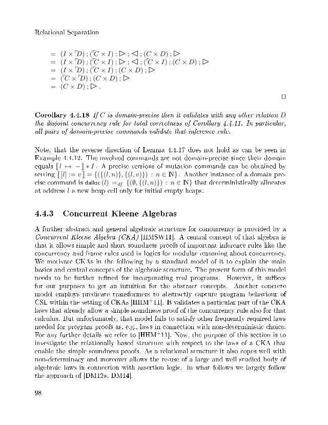
Relational Separation
= (I × pD) ; (pC × I) ;� ;� ; (C ×D) ;�= (I × pD) ; (pC × I) ;� ;� ; (pC × I) ; (C ×D) ;�= (I × pD) ; (pC × I) ; (C ×D) ;�= (pC × pD) ; (C ×D) ;�= (C ×D) ;� .
ut
Corollary 4.4.18 If C is domain-precise then it validates with any other relation Dthe disjoint concurrency rule for total correctness of Corollary 4.4.11. In particular,all pairs of domain-precise commands validate that inference rule.
Note, that the reverse direction of Lemma 4.4.17 does not hold as can be seen inExample 4.4.12. The involved commands are not domain-precise since their domainequals [[ l 7→ − ]] ∗ I . A precise versions of mutation commands can be obtained bysetting [[ [l] := v ]] = {({(l, n)}, {(l, v)}) : n ∈ IN} . Another instance of a domain pre-cise command is dalloc (l) =df {(∅, {(l, n)}) : n ∈ IN} that deterministically allocatesat address l a new heap cell only for initial empty heaps.
4.4.3 Concurrent Kleene Algebras
A further abstract and general algebraic structure for concurrency is provided by aConcurrent Kleene Algebra (CKA) [HMSW11]. A central concept of that algebra isthat it allows simple and short soundness proofs of important inference rules like theconcurrency and frame rules used in logics for modular reasoning about concurrency.We motivate CKAs in the following by a standard model of it to explain the mainbasics and central concepts of the algebraic structure. The present form of this modelneeds to be further re�ned for incorporating real programs. However, it su�cesfor our purposes to get an intuition for the abstract concepts. Another concretemodel employs predicate transformers to abstractly capture program behaviour ofCSL within the setting of CKAs [HHM+11]. It validates a particular part of the CKAlaws that already allow a simple soundness proof of the concurrency rule also for thatcalculus. But unfortunately, that model fails to satisfy other frequently required lawsneeded for program proofs as, e.g., laws in connection with non-deterministic choice.For any further details we refer to [HHM+11]. Now, the purpose of this section is toinvestigate the relationally based structure with respect to the laws of a CKA thatenable the simple soundness proofs. As a relational structure it also copes well withnon-determinacy and moreover allows the re-use of a large and well studied body ofalgebraic laws in connection with assertion logic. In what follows we largely followthe approach of [DM12a, DM14].
98
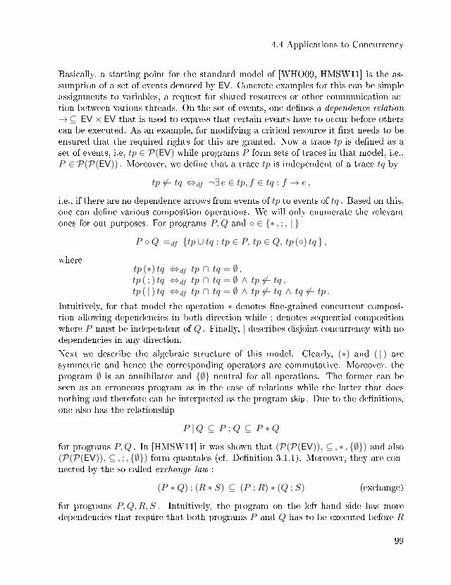
4.4 Applications to Concurrency
Basically, a starting point for the standard model of [WHO09, HMSW11] is the as-sumption of a set of events denoted by EV. Concrete examples for this can be simpleassignments to variables, a request for shared resources or other communication ac-tion between various threads. On the set of events, one de�nes a dependence relation→⊆ EV× EV that is used to express that certain events have to occur before otherscan be executed. As an example, for modifying a critical resource it �rst needs to beensured that the required rights for this are granted. Now a trace tp is de�ned as aset of events, i.e, tp ∈ P(EV) while programs P form sets of traces in that model, i.e.,P ∈ P(P(EV)) . Moreover, we de�ne that a trace tp is independent of a trace tq by
tp 6← tq ⇔df ¬∃ e ∈ tp, f ∈ tq : f → e ,
i.e., if there are no dependence arrows from events of tp to events of tq . Based on this,one can de�ne various composition operations. We will only enumerate the relevantones for out purposes. For programs P,Q and ◦ ∈ {∗ , ; , | }
P ◦Q =df {tp ∪ tq : tp ∈ P, tp ∈ Q, tp (◦) tq } ,
wheretp (∗) tq ⇔df tp ∩ tq = ∅ ,tp ( ; ) tq ⇔df tp ∩ tq = ∅ ∧ tp 6← tq ,tp ( | ) tq ⇔df tp ∩ tq = ∅ ∧ tp 6← tq ∧ tq 6← tp .
Intuitively, for that model the operation ∗ denotes �ne-grained concurrent composi-tion allowing dependencies in both direction while ; denotes sequential compositionwhere P must be independent of Q . Finally, | describes disjoint concurrency with nodependencies in any direction.
Next we describe the algebraic structure of this model. Clearly, (∗) and ( | ) aresymmetric and hence the corresponding operators are commutative. Moreover, theprogram ∅ is an annihilator and {∅} neutral for all operations. The former can beseen as an erroneous program as in the case of relations while the latter that doesnothing and therefore can be interpreted as the program skip . Due to the de�nitions,one also has the relationship
P |Q ⊆ P ;Q ⊆ P ∗Q
for programs P,Q . In [HMSW11] it was shown that (P(P(EV)), ⊆ , ∗ , {∅}) and also(P(P(EV)), ⊆ , ; , {∅}) form quantales (cf. De�nition 3.1.1). Moreover, they are con-nected by the so-called exchange law :
(P ∗Q) ; (R ∗ S) ⊆ (P ;R) ∗ (Q ; S) (exchange)
for programs P,Q,R, S . Intuitively, the program on the left-hand side has moredependencies that require that both programs P and Q has to be executed before R
99
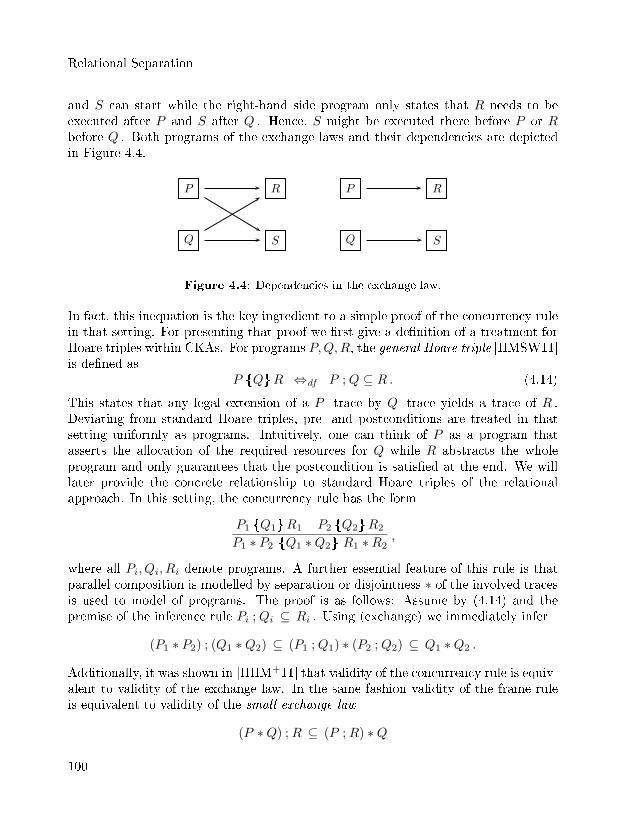
Relational Separation
and S can start while the right-hand side program only states that R needs to beexecuted after P and S after Q . Hence, S might be executed there before P or Rbefore Q . Both programs of the exchange laws and their dependencies are depictedin Figure 4.4.
Q
P
S
R
Q
P
S
R
Figure 4.4: Dependencies in the exchange law.
In fact, this inequation is the key ingredient to a simple proof of the concurrency rulein that setting. For presenting that proof we �rst give a de�nition of a treatment forHoare triples within CKAs. For programs P,Q,R, the general Hoare triple [HMSW11]is de�ned as
P {Q}R ⇔df P ;Q ⊆ R . (4.14)
This states that any legal extension of a P - trace by Q - trace yields a trace of R .Deviating from standard Hoare triples, pre- and postconditions are treated in thatsetting uniformly as programs. Intuitively, one can think of P as a program thatasserts the allocation of the required resources for Q while R abstracts the wholeprogram and only guarantees that the postcondition is satis�ed at the end. We willlater provide the concrete relationship to standard Hoare triples of the relationalapproach. In this setting, the concurrency rule has the form
P1 {Q1}R1 P2 {Q2}R2
P1 ∗ P2 {Q1 ∗Q2} R1 ∗R2,
where all Pi, Qi, Ri denote programs. A further essential feature of this rule is thatparallel composition is modelled by separation or disjointness ∗ of the involved tracesis used to model of programs. The proof is as follows: Assume by (4.14) and thepremise of the inference rule Pi ;Qi ⊆ Ri . Using (exchange) we immediately infer
(P1 ∗ P2) ; (Q1 ∗Q2) ⊆ (P1 ;Q1) ∗ (P2 ;Q2) ⊆ Q1 ∗Q2 .
Additionally, it was shown in [HHM+11] that validity of the concurrency rule is equiv-alent to validity of the exchange law. In the same fashion validity of the frame ruleis equivalent to validity of the small exchange law
(P ∗Q) ;R ⊆ (P ;R) ∗Q
100
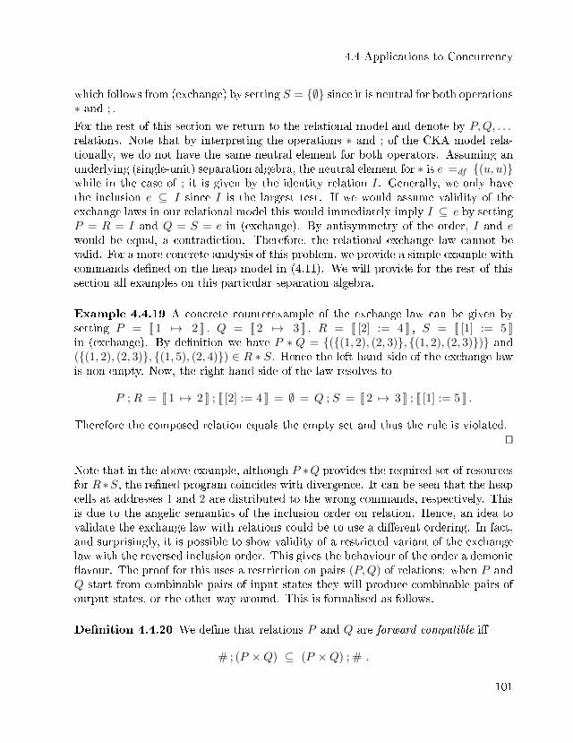
4.4 Applications to Concurrency
which follows from (exchange) by setting S = {∅} since it is neutral for both operations∗ and ; .
For the rest of this section we return to the relational model and denote by P,Q, . . .relations. Note that by interpreting the operations ∗ and ; of the CKA model rela-tionally, we do not have the same neutral element for both operators. Assuming anunderlying (single-unit) separation algebra, the neutral element for ∗ is e =df {(u, u)}while in the case of ; it is given by the identity relation I. Generally, we only havethe inclusion e ⊆ I since I is the largest test. If we would assume validity of theexchange laws in our relational model this would immediately imply I ⊆ e by settingP = R = I and Q = S = e in (exchange). By antisymmetry of the order, I and ewould be equal, a contradiction. Therefore, the relational exchange law cannot bevalid. For a more concrete analysis of this problem, we provide a simple example withcommands de�ned on the heap model in (4.11). We will provide for the rest of thissection all examples on this particular separation algebra.
Example 4.4.19 A concrete counterexample of the exchange law can be given bysetting P = [[ 1 7→ 2 ]] , Q = [[ 2 7→ 3 ]] , R = [[ [2] := 4 ]] , S = [[ [1] := 5 ]]in (exchange). By de�nition we have P ∗ Q = {({(1, 2), (2, 3)}, {(1, 2), (2, 3)})} and({(1, 2), (2, 3)}, {(1, 5), (2, 4)}) ∈ R ∗ S. Hence the left-hand side of the exchange lawis non-empty. Now, the right-hand side of the law resolves to
P ;R = [[ 1 7→ 2 ]] ; [[ [2] := 4 ]] = ∅ = Q ; S = [[ 2 7→ 3 ]] ; [[ [1] := 5 ]] .
Therefore the composed relation equals the empty set and thus the rule is violated.ut
Note that in the above example, although P ∗Q provides the required set of resourcesfor R∗S, the re�ned program coincides with divergence. It can be seen that the heapcells at addresses 1 and 2 are distributed to the wrong commands, respectively. Thisis due to the angelic semantics of the inclusion order on relation. Hence, an idea tovalidate the exchange law with relations could be to use a di�erent ordering. In fact,and surprisingly, it is possible to show validity of a restricted variant of the exchangelaw with the reversed inclusion order. This gives the behaviour of the order a demonic�avour. The proof for this uses a restriction on pairs (P,Q) of relations: when P andQ start from combinable pairs of input states they will produce combinable pairs ofoutput states, or the other way around. This is formalised as follows.
De�nition 4.4.20 We de�ne that relations P and Q are forward compatible i�
# ; (P ×Q) ⊆ (P ×Q) ; # .
101
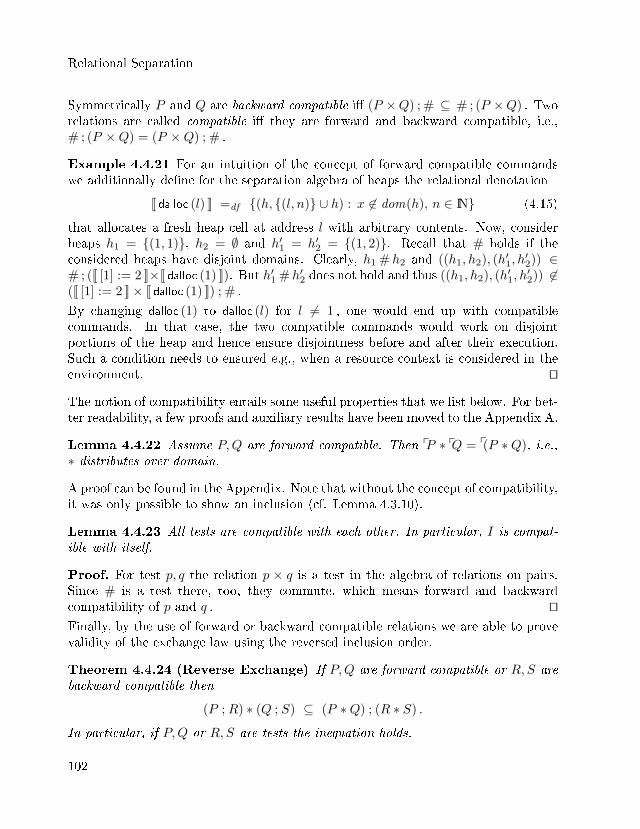
Relational Separation
Symmetrically P and Q are backward compatible i� (P ×Q) ; # ⊆ # ; (P ×Q) . Tworelations are called compatible i� they are forward and backward compatible, i.e.,# ; (P ×Q) = (P ×Q) ; # .
Example 4.4.21 For an intuition of the concept of forward compatible commandswe additionally de�ne for the separation algebra of heaps the relational denotation
[[ dalloc (l) ]] =df {(h, {(l, n)} ∪ h) : x 6∈ dom(h), n ∈ IN} (4.15)
that allocates a fresh heap cell at address l with arbitrary contents. Now, considerheaps h1 = {(1, 1)}, h2 = ∅ and h′1 = h′2 = {(1, 2)}. Recall that # holds if theconsidered heaps have disjoint domains. Clearly, h1 #h2 and ((h1, h2), (h′1, h
′2)) ∈
# ; ([[ [1] := 2 ]]×[[ dalloc (1) ]]). But h′1 #h′2 does not hold and thus ((h1, h2), (h′1, h′2)) 6∈
([[ [1] := 2 ]]× [[ dalloc (1) ]]) ; # .
By changing dalloc (1) to dalloc (l) for l 6= 1 , one would end up with compatiblecommands. In that case, the two compatible commands would work on disjointportions of the heap and hence ensure disjointness before and after their execution.Such a condition needs to ensured e.g., when a resource context is considered in theenvironment. ut
The notion of compatibility entails some useful properties that we list below. For bet-ter readability, a few proofs and auxiliary results have been moved to the Appendix A.
Lemma 4.4.22 Assume P,Q are forward compatible. Then pP ∗ pQ = p(P ∗Q), i.e.,∗ distributes over domain.
A proof can be found in the Appendix. Note that without the concept of compatibility,it was only possible to show an inclusion (cf. Lemma 4.3.10).
Lemma 4.4.23 All tests are compatible with each other. In particular, I is compat-ible with itself.
Proof. For test p, q the relation p × q is a test in the algebra of relations on pairs.Since # is a test there, too, they commute, which means forward and backwardcompatibility of p and q . utFinally, by the use of forward or backward compatible relations we are able to provevalidity of the exchange law using the reversed inclusion order.
Theorem 4.4.24 (Reverse Exchange) If P,Q are forward compatible or R,S arebackward compatible then
(P ;R) ∗ (Q ; S) ⊆ (P ∗Q) ; (R ∗ S) .
In particular, if P,Q or R,S are tests the inequation holds.
102
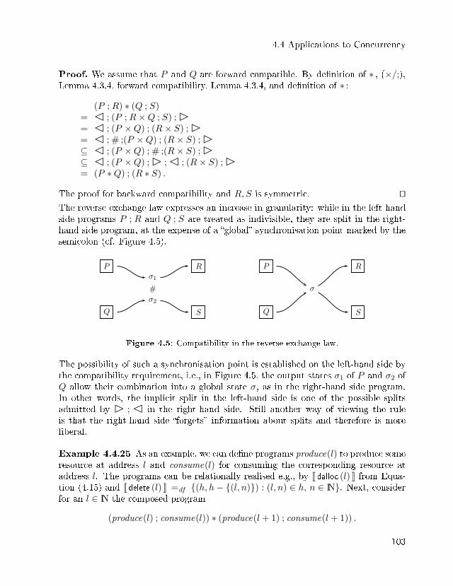
4.4 Applications to Concurrency
Proof. We assume that P and Q are forward compatible. By de�nition of ∗ , (×/;),Lemma 4.3.4, forward compatibility, Lemma 4.3.4, and de�nition of ∗ :
(P ;R) ∗ (Q ; S)= � ; (P ;R×Q ; S) ;�= � ; (P ×Q) ; (R× S) ;�= � ; # ;(P ×Q) ; (R× S) ;�⊆ � ; (P ×Q) ; # ;(R× S) ;�⊆ � ; (P ×Q) ;� ;� ; (R× S) ;�= (P ∗Q) ; (R ∗ S) .
The proof for backward compatibility and R,S is symmetric. utThe reverse exchange law expresses an increase in granularity: while in the left-handside programs P ; R and Q ; S are treated as indivisible, they are split in the right-hand side program, at the expense of a �global� synchronisation point marked by thesemicolon (cf. Figure 4.5).
P
Q
R
S
σ1
σ2
#
P
Q
R
S
σ
Figure 4.5: Compatibility in the reverse exchange law.
The possibility of such a synchronisation point is established on the left-hand side bythe compatibility requirement, i.e., in Figure 4.5, the output states σ1 of P and σ2 ofQ allow their combination into a global state σ, as in the right-hand side program.In other words, the implicit split in the left-hand side is one of the possible splitsadmitted by � ; � in the right-hand side. Still another way of viewing the ruleis that the right-hand side �forgets� information about splits and therefore is moreliberal.
Example 4.4.25 As an example, we can de�ne programs produce(l) to produce someresource at address l and consume(l) for consuming the corresponding resource ataddress l. The programs can be relationally realised e.g., by [[ dalloc (l) ]] from Equa-tion (4.15) and [[ delete (l) ]] =df {(h, h− {(l, n)}) : (l, n) ∈ h, n ∈ IN}. Next, considerfor an l ∈ IN the composed program
(produce(l) ; consume(l)) ∗ (produce(l + 1) ; consume(l + 1)) .
103
Relational Separation
In this program, each producer and its corresponding consumer are treated together asan indivisible program. Since the producers and consumers work on disjoint resources,they are compatible and we can use the reverse exchange law to reorder the programabove into
(produce(l) ∗ produce(l + 1)) ; (consume(l) ∗ consume(l + 1)) .
This version represents a program where all resource allocations need to be executedconcurrently before any of the resources can be consumed. The synchronisation pointdenoted by ; re�ects an intermediate state that includes the produced resources atthe addresses l and l + 1 . ut
As a further step we connect the de�nition of generalised Hoare triples (4.14) that ad-mit programs as assertions with a well-known one for Hoare logic (cf. Equation (4.2)),i.e., p ; Q ⊆ Q ; r for any relation Q and tests p, r . The major di�erence of bothde�nitions is that the former approach does not impose any structural restriction onthe denotations for modelling pre- and postconditions.
As shown in Lemma 4.3.26, we have the relationship
p ;Q ⊆ Q ; r ⇔ > ; p ;Q ⊆ > ; r ⇔ (>; p){Q} (>; r) .
This allows in particular to immediately translate results for standard Hoare triplesinto ones for general triples. The composition > ; p maps a test p to a more generalrelation that makes no assumption about its initial starting states, i.e., any executionfrom an arbitrary state will end up in one contained in p . Trivially, the symmetricrelation p ;> makes no restriction on �nal states or its codomain.
Unfortunately, the modi�ed exchange law introduces an inconsistency, since the orderfor the proved exchange rule is reversed in contrast to the order of the relationalinterpretation for general Hoare triples. However, one can obtain some further resultsby this, which from a theoretical point of view might help for future considerationsabout the exchange law and relational models.
As a �rst approach we note that for a relational treatment of faulting within a sep-aration logic, we added in the total correctness approach to the semantics of Hoaretriples (cf. De�nition 4.2.10) an enabledness condition p ⊆ pQ as additional conjunct.We will see that reversing this condition, i.e., stating pQ ⊆ p entails a soundness proofof a variant of the concurrency rule using the reverse exchange law. The conditionstates that Q enforces the precondition p in that all of its initial states need to satisfyp . With this we de�ne for tests p, r and relation Q
{p}Q{r} ⇔df p ;Q ⊆ Q ; r ∧ pQ ⊆ p . (4.16)
This yields some useful properties and conditions. The following observation is trivial,but useful for our �rst variant of the concurrency rule.
104
4.4 Applications to Concurrency
Lemma 4.4.26 {p ; q}Q{r} ⇔ {p} q ;Q{r} ∧ pQ ⊆ p .
Proof. By de�nition and associativity we immediately infer (p ; q) ; Q ⊆ Q ; r ⇔p ; (q ;Q) ⊆ Q ; r . Moreover, pQ ⊆ p ; q ⊆ p and pQ = p(pQ ;Q) ⊆ p(q ;Q) ⊆ p . utThis lemma specialises in a number of ways. Since tests are idempotent we obtain bysetting q = p that
Corollary 4.4.27 {p}Q{r} ⇔ {p} p ;Q{r} ∧ pQ ⊆ p .
The relation p ;Q can be viewed as an execution that �rst asserts the precondition pbefore executing Q . Next, we may set p = I = [[ true ]] in Lemma 4.4.26 to get
Corollary 4.4.28 {q}Q{r} ⇔ {true} q ;Q{r} .
Note that the condition pQ ⊆ p of the involved triples is equivalent to the formulaQ ⊆ p ;Q . This can be further strengthened to an equation, i.e., Q = p ;Q . Hence,we can conclude
Theorem 4.4.29 For tests p1, p2, r1, r2 and relations Q1, Q2 we have
{p1}Q1 {r1} {p2}Q2 {r2}
{true}Q1 ∗Q2 { r1 ∗ r2}.
Proof. By [[ true ]] = I , {pi}Qi {ri} implies Qi ⊆ pi ;Qi , by {pi}Qi {ri}, and reverseexchange law (Lemma 4.4.24) with tests r1 and r2 :
I ;(Q1∗Q2) = Q1∗Q2 ⊆ (p1 ;Q1)∗(p2 ;Q2) ⊆ (Q1 ;r1)∗(Q2 ;r2) ⊆ (Q1∗Q2);(r1∗r2) .
utNote that compatibility of the commands Qi is not needed for instantiating the re-verse exchange law. Hence, the compatibility requirement is not a restriction for thisapplication. In particular, Theorem 4.4.29 states that these inference rules are veryliberal w.r.t. the involved preconditions, also in combination with disjoint concurrentcompositions. The requirement by this is that all executions of each relation Qi haveto be enabled by the precondition. We can bring this inference rule into a form closerto the original and more common version:
Corollary 4.4.30 Theorem 4.4.29 is equivalent to
{p1}Q1 {r1} {p2}Q2 {r2}
{p1 ∗ p2}Q1 ∗Q2 { r1 ∗ r2}.
105
Relational Separation
Proof. By the second proof step above, reverse exchange and p1 ∗ p2 ⊆ I we have
Q1 ∗Q2 ⊆ (p1 ;Q1) ∗ (p2 ;Q2) ⊆ (p1 ∗ p2) ; (Q1 ∗Q2) ⊆ Q1 ∗Q2 .
Hence Q1 ∗Q2 = (p1 ∗ p2) ; (Q1 ∗Q2) , so that Corollary 4.4.28 shows the claim. utThe following result provides together with Theorem 4.4.29 the analogue of the equiv-alence between the exchange law and the concurrency rule as shown in [HHM+11] alsofor the relation-based treatment.
Lemma 4.4.31 Validity of Theorem 4.4.29 implies a special case of the reverse ex-change law: for arbitrary commands Pi and tests ri ,
(P1 ; r1) ∗ (P2 ; r2) ⊆ (P1 ∗ P2) ; (r1 ∗ r2) .
The proof can be found in Appendix A.
We remark that the de�nition of the triples provided in Equation (4.16) unfortunatelydoes not validate unrestricted strengthening of the precondition p as it has to includeat least the domain of the relation Q . Therefore, we continue with another possi-bility to interpret the reversed order of the exchange law that allows the mentionedweakening or strengthening of proof rules. The idea is to link that law with a dualde�nition of triples w.r.t. one of standard Hoare triples. By this we will again seethat the concurrency and frame rules for those triples can easily be derived using thereverse exchange law. First, we give a de�nition of [Hoa11].
De�nition 4.4.32For relations P,Q,R we de�ne Plotkin triples by
〈P,Q〉 → R ⇔df R ⊆ P ;Q
and dual partial correctness triples by
P [Q]R ⇔df P ⊆ Q ;R .
Note that in comparison with generalised Hoare triples the ; - composed relation is onright-hand side of the inclusion order. Intuitively, the former characterises a set ofpossible �nal states satisfying the postcondition R after execution of Q from initialstates of the precondition P . For this one can think of labelled transition systems,where Q represents some sequence of actions that possibly leads from a con�gurationor state in P to some �nal con�guration of R . The semantics of such triples is ratherangelic since it states only that such a transition may exists. The notation is inspiredby Plotkin's structural operational semantics [Plo04] in which 〈s, C〉 → t means thatevaluation of term C starting in state s may lead to a term t .
106
4.4 Applications to Concurrency
The dual partial correctness triples describe possible starting states of P that end inR after some execution of Q. According to [Hoa11], dual partial correctness triplescan, e.g., be used as a method for the generation of test cases. Assuming that Rrepresents erroneous �nal states of Q , then P characterises some conditions that willlead to such error situations. Plotkin triples can be used for a dual application.
Using again the relationship of Lemma 4.3.26 the dual partial correctness triplestransform for tests p, q into
(p ;>) [Q] (q ;>) ⇔ p ;> ⊆ Q ; (q ;>) ⇔ p ⊆ (Q ; q) ;> ⇔ p ⊆ p(Q ; q)
and, symmetrically, Plotkin triples transform into
〈> ; p ,Q〉 → > ; q ⇔ > ; q ⊆ (> ; p) ;Q ⇔ q ⊆ > ; (p ;Q) ⇔ q ⊆ (p ;Q)q ,
where _q denotes the symmetric codomain operator. We concentrate on dual partialcorrectness triples and use the abbreviation
p [[Q]] q ⇔df (p ;>) [Q] (q ;>) ⇔ p ⊆ p(Q ; q) . (4.17)
The dual results can be similarly calculated for Plotkin triples. Since the order withinthese triple de�nitions works in the same direction as in the reverse exchange laws wecan immediately state the following result.
Lemma 4.4.33 The concurrency rule for dual partial correctness or Plotkin triplesholds i� the reverse exchange law holds.
A proof for this lemma can be derived dually to the proof of [HHM+11] stating thatthe exchange law is equivalent to the concurrency rule involving general Hoare triples.Unfortunately, in our setting the reverse exchange law does only hold conditionallyw.r.t. the assumption of compatible pairs of relations. In contrast to the approach thatused the triple de�nition of Equation (4.16), the compatibility assumption is requiredfor a soundness proof of the concurrency rule involving the triples of Equation (4.17).
Theorem 4.4.34 If Q1, Q2 are forward compatible then the concurrency rule for dualpartial correctness triples holds, i.e., for tests p1, p2, q1, q2
p1 [[Q1]] q1 p2 [[Q2]] q2
p1 ∗ p2 [[Q1 ∗Q2]] q1 ∗ q2.
Again this is also valid when Q1 and Q2 are backward compatible and Plotkin insteadof dual partial correctness triples are used.
107
Relational Separation
Proof. By assumption we have p1 ⊆ p(Q1;q1) , p2 ⊆ p(Q2;q2) and the restricted variantof the reverse exchange law. Hence, by isotony and Lemma 4.4.22 we calculate
p1 ∗ p2 ⊆ p(Q1 ; q1) ∗ p(Q2 ; q2) = p((Q1 ; q1) ∗ (Q2 ; q2)) ⊆ p((Q1 ∗Q2) ; (q1 ∗ q2)) .
utNote that an advantage of this relational treatment is that it allows the simple usageof tests for modelling pre- and postconditions while the standard model of CKAs onlyhas a trivial test algebra consisting of the elements ∅ and {∅} .As a further result, it was shown in [HHM+11] that using general Hoare triples, theframe rule is equivalent to the small exchange law, i.e., (P ∗Q) ;R ⊆ (P ;R) ∗Q forprograms P,Q,R . This form could be obtained from the exchange law if ∗ and ; wouldhave the same unit. This is not the case for relations since we generally only have onein equation (cf. Lemma 4.3.30). If we would assume similar as in [HHM+11] relationssatisfying the compact characterisation of Lemma 4.3.31 we can also conclude
Corollary 4.4.35 If Q ∗ I = Q and Q is forward compatible with I then the framerule for dual partial correctness triples holds, i.e., for tests p, q, r
p [[Q]] q
p ∗ r [[Q]] q ∗ r .
(A dual result again holds for Plotkin triples).
The behaviour of the triples of De�nition 4.4.32 is called �dual� on purpose, sincethe calculations given above are symmetric to the algebraic approach of [HHM+11].Both provided inference rules have the restriction that compatible pairs of involvedrelations are needed. The reason for this is that, by Lemma 4.3.4 only # ⊆ � ;�is valid. The restriction could be excluded if I × I ⊆ � ; � could be established.In particular, this would yield non-restricted validity of the reverse exchange law.However this requires an arti�cial extension of the split and join relations to totalones, i.e., � ;� needs to include an extra state as a result for non-combinable pairsof states. This can be done by enriching the underlying separation algebra by a freshstate σ and using a new combinator ◦ , instead of • , de�ned by
σ ◦ τ = σ ⇔df ¬ σ# τ
and σ ◦ τ = σ • τ in any other case. The extended carrier set can then be givenby Σ =df Σ ∪ {σ } . For theoretical considerations we can construct by this arelational model that allows a connection to the algebraic structure of a locality bi-monoid [HHM+11]. Its general purpose is to connect behaviour of CSL with thestructure of a CKA.
108
4.5 Pointfree Dynamic Frames
De�nition 4.4.36A locality bimonoid is de�ned by (S,≤, ∗, 1∗, ; , 1;) where (S,≤) is partially ordered andthe operations ∗ , ; are monotone w.r.t. the carrier set S. Moreover, (S, ∗, 1∗) needsto form a commutative monoid and (S, ; , 1;) a monoid. Additionally, the structurehas to satisfy the exchange law and 1; ∗ 1; = 1; .
By the use of the extended split and join relations, we can interpret≤ as the reverse setinclusion order ⊇ since the reverse exchange law holds unconditionally. In summary,using Lemma 4.3.6, we have the following result.
Lemma 4.4.37 (P(Σ × Σ ), ⊇ , ∗ , e, ; , I) forms a locality bimonoid.
These considerations are rather of theoretical interest. Note that by reversing theset inclusion order turns t and u into ∩ and ∪ . By using the test subalgebraas algebraic counterpart to model logical assertions the interpretation of the notionof a test becomes unnatural. The reason for this is that p ∧ q will be identi�ed,unusually, with p t q and p ∨ q with p u q . From an algebraic viewpoint thesemodi�cations entail simpli�cations, since no additional constraints are required tovalidate the reverse exchange law. However, by considering the extra failure-state σ one deviates from the usual angelic semantics of relations.
4.5 Pointfree Dynamic Frames
In this section we present another application for the derived algebraic abstractions ofthe principles and concepts of separation logic. Besides allowing compact reasoningabout shared mutable data structures it also represents by its frame rule an adequatesolution to the frame problem [MH69]. Concretely, the frame problem asks for amethodology that allows specifying which resources of a program can be changed andwhich ones are left unchanged without naming them explicitly. Such a methodologyshould additionally guarantee modularity and hence scalability in speci�cation andcorrectness proofs of programs. A further popular approach to the frame problem isthe theory of dynamic frames [Kas11] that provides the mentioned modularity whilestill being expressive enough to handle a variety of concrete programs. There existfurther variations of the theory that address the automation of program veri�cation(e.g., [SJP09, Lei10, GGN11]).
Now, the main goal of the following considerations is to develop algebraic abstractionsfor the theory of dynamic frames similar as we have provided for separation logic. Inparticular, by including the former approach into the extended relational structure,a more general treatment of resources within separation algebras (cf. Section 3.3) is
109
Relational Separation
possible. Moreover, pointfree characterisations of central properties will allow simpleproofs of crucial concepts in a calculational style. Generally, the provided relationalcalculus for separation logic further extends towards a unifying approach includingalso the theory of dynamic frames. In what follows we basically follow [Dan14].
4.5.1 Abstracting Dynamic Frames
The basic setting for resource states in the theory of dynamic frames are �nitemappings from an in�nite set of locations Loc to an in�nite set of values Val thatcomprises at least integers and Booleans. This closely corresponds to the (single-unit) separation algebra based on simple heaps (cf. Example 3.3.2 a) ). Hence,we have a concrete instance of a separation algebra for which we formally writeDFSA =df (Loc ; Val, ∪ , ∅) where ∪ denotes union of location-disjoint functions, ∅the completely unde�ned function and σ # τ ⇔ dom(σ) ∩ dom(τ) = ∅ . We writedom(σ) for a mapping or state σ to denote its domain or more concretely all of itsallocated locations, i.e., a subset of Loc . Moreover, we use DFSA as an abbreviationfor the dynamic frames separation algebra and de�ne the substate σ
∣∣Xthat restricts
the domain of the state σ to a set of locations X.
Lemma 4.5.1 For a state τ assume dom(τ) = X. Then for arbitrary σ we have(σ • τ)
∣∣X
= τ .
We concentrate for this section only on single-unit separation algebras as we do notrequire multi-unit ones. It is not a di�cult task to extend the treatment to sepa-ration algebras involving multi-units. As a next step, we provide abstractions forthe concrete dynamic frames resource setting and manage several central propertiesof the approach within the abstraction to separation algebras. For this we requireadditional assumptions given in [DHA09] and basically follow the approach of thatwork. A separation algebra (Σ, • , u) satis�es disjointness i� for all σ, τ
σ • σ = τ ⇒ σ = τ (4.18)
and it satis�es cross-split i� for arbitrary states σi with i ∈ {1, 2, 3, 4}
σ1 • σ2 = σ3 • σ4 ⇒ ∃σ13, σ14, σ23, σ24 : σ1 = σ13 • σ14 ∧ σ2 = σ23 • σ24
∧ σ3 = σ13 • σ23 ∧ σ4 = σ14 • σ24 .(4.19)
Disjointness in the presence of cancellativity implies that the only element that canbe combined with itself is the neutral element u , i.e.,
σ#σ ⇒ σ = u . (4.20)
110
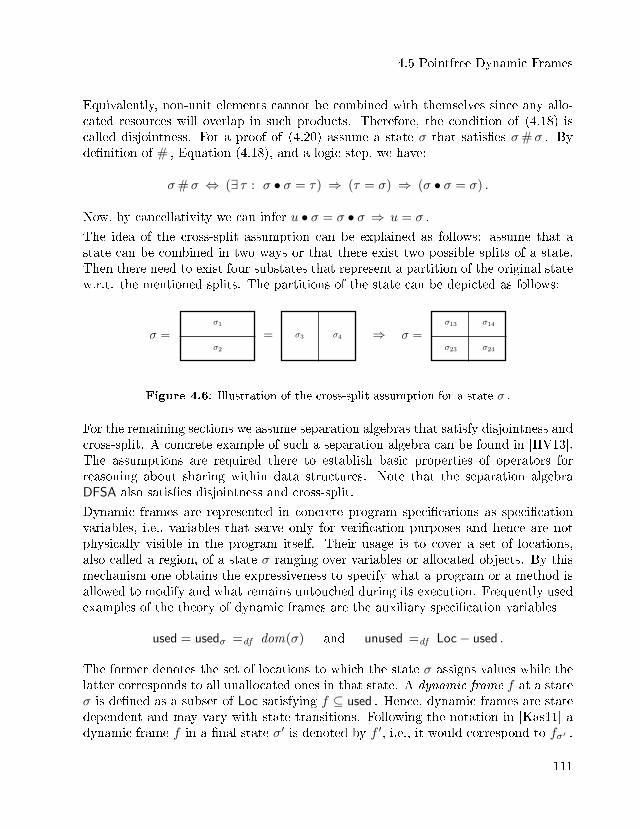
4.5 Pointfree Dynamic Frames
Equivalently, non-unit elements cannot be combined with themselves since any allo-cated resources will overlap in such products. Therefore, the condition of (4.18) iscalled disjointness. For a proof of (4.20) assume a state σ that satis�es σ#σ . Byde�nition of # , Equation (4.18), and a logic step, we have:
σ#σ ⇔ (∃ τ : σ • σ = τ) ⇒ (τ = σ) ⇒ (σ • σ = σ) .
Now, by cancellativity we can infer u • σ = σ • σ ⇒ u = σ .
The idea of the cross-split assumption can be explained as follows: assume that astate can be combined in two ways or that there exist two possible splits of a state.Then there need to exist four substates that represent a partition of the original statew.r.t. the mentioned splits. The partitions of the state can be depicted as follows:
σ =σ1
σ2
= σ3 σ4 ⇒ σ =σ23
σ13
σ24
σ14
Figure 4.6: Illustration of the cross-split assumption for a state σ .
For the remaining sections we assume separation algebras that satisfy disjointness andcross-split. A concrete example of such a separation algebra can be found in [HV13].The assumptions are required there to establish basic properties of operators forreasoning about sharing within data structures. Note that the separation algebraDFSA also satis�es disjointness and cross-split.
Dynamic frames are represented in concrete program speci�cations as speci�cationvariables, i.e., variables that serve only for veri�cation purposes and hence are notphysically visible in the program itself. Their usage is to cover a set of locations,also called a region, of a state σ ranging over variables or allocated objects. By thismechanism one obtains the expressiveness to specify what a program or a method isallowed to modify and what remains untouched during its execution. Frequently usedexamples of the theory of dynamic frames are the auxiliary speci�cation variables
used = usedσ =df dom(σ) and unused =df Loc− used .
The former denotes the set of locations to which the state σ assigns values while thelatter corresponds to all unallocated ones in that state. A dynamic frame f at a stateσ is de�ned as a subset of Loc satisfying f ⊆ used . Hence, dynamic frames are statedependent and may vary with state transitions. Following the notation in [Kas11] adynamic frame f in a �nal state σ′ is denoted by f ′, i.e., it would correspond to fσ′ .
111
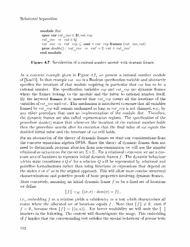
Relational Separation
module Ratspec var rat_inv ∈ IB, rat, reprat_inv ⇒ rat ∈ Qrat_inv ⇒ rat_rep ⊆ used ∧ rat_rep frames (rat_inv, rat)proc double() : rat_inv ⇒ rat′ = 2 · rat ∧ rat_inv′end module
Figure 4.7: Speci�cation of a rational number module with dynamic frames.
As a concrete example given in Figure 4.7, we present a rational number moduleof [Kas11]. In that example rat_inv is a Boolean speci�cation variable and abstractlyspeci�es the invariant of that module requiring in particular that rat has to be arational number. The speci�cation variables rep and rat_rep are dynamic frameswhere the former belongs to the module and the latter to rational number itself.By the keyword frames it is asserted that rat_rep covers all the locations of thevariables of rat_inv and rat . This mechanism is introduced to ensure that all variablesframed by rat_rep will remain unchanged as long as rat_rep is not changed, e.g., byany other procedure that uses an implementation of the module Rat. Therefore,the dynamic frames are also called representation regions. The speci�cation of theprocedure double() states that whenever the invariant of the rational number holdsthen the procedure asserts after its execution that the �nal value of rat equals thedoubled initial value and the invariant of rat still holds.
For an abstraction of the theory of dynamic frames we start our considerations fromthe concrete separation algebra DFSA. Since the theory of dynamic frames does notneed to distinguish program abortion from non-termination we will use the simplerrelational structures on the carrier set Σ×Σ . For a relational treatment we use a con-stant sets of locations to represent initial dynamic frames f . The dynamic behaviourwithin state transitions σQσ′ for a relation Q will be represented by relational andpointfree formalisations rather than using functions or expressions that depend onthe states σ or σ′ as in the original approach. This will allow more concise structuralcharacterisations and pointfree proofs of basic properties involving dynamic frames.
More concretely, assuming an initial dynamic frame f to be a �xed set of locationswe de�ne
[[ f ]] =df {(σ, σ) : dom(σ) = f} ,
i.e., embedding f as a relation yields a subidentity or a test which characterises allstates where the allocated set of locations equals f . Note that [[ f ]] 6= ∅ , even iff = ∅ , because then [[ f ]] = {(u, u)} . For better readability we will omit the [[_]]brackets in the following. The context will disambiguate the usage. This embeddingof f implies that the corresponding test satis�es the special behaviour of precise tests
112
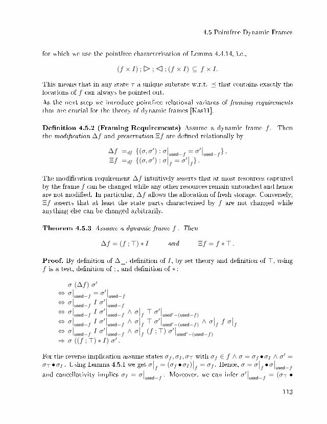
4.5 Pointfree Dynamic Frames
for which we use the pointfree characterisation of Lemma 4.4.14, i.e.,
(f × I) ;� ;� ; (f × I) ⊆ f × I.
This means that in any state τ a unique substate w.r.t. � that contains exactly thelocations of f can always be pointed out.
As the next step we introduce pointfree relational variants of framing requirementsthat are crucial for the theory of dynamic frames [Kas11].
De�nition 4.5.2 (Framing Requirements) Assume a dynamic frame f . Thenthe modi�cation ∆f and preservation Ξf are de�ned relationally by
∆f =df {(σ, σ′) : σ∣∣used−f = σ′
∣∣used−f} ,
Ξf =df {(σ, σ′) : σ∣∣f
= σ′∣∣f} .
The modi�cation requirement ∆f intuitively asserts that at most resources capturedby the frame f can be changed while any other resources remain untouched and henceare not modi�ed. In particular, ∆f allows the allocation of fresh storage. Conversely,Ξf asserts that at least the state parts characterised by f are not changed whileanything else can be changed arbitrarily.
Theorem 4.5.3 Assume a dynamic frame f . Then
∆f = (f ;>) ∗ I and Ξf = f ∗ > .
Proof. By de�nition of ∆_, de�nition of I, by set theory and de�nition of >, usingf is a test, de�nition of ; , and de�nition of ∗ :
σ (∆f) σ′
⇔ σ∣∣used−f = σ′
∣∣used−f
⇔ σ∣∣used−f I σ
′∣∣used−f
⇔ σ∣∣used−f I σ
′∣∣used−f ∧ σ
∣∣f> σ′
∣∣used′−(used−f)
⇔ σ∣∣used−f I σ
′∣∣used−f ∧ σ
∣∣f> σ′
∣∣used′−(used−f)
∧ σ∣∣ff σ∣∣f
⇔ σ∣∣used−f I σ
′∣∣used−f ∧ σ
∣∣f
(f ;>) σ′∣∣used′−(used−f)
⇒ σ ((f ;>) ∗ I) σ′ .
For the reverse implication assume states σf , σI , σ> with σf ∈ f ∧ σ = σf •σI ∧ σ′ =σ> •σI . Using Lemma 4.5.1 we get σ
∣∣f
= (σf •σI)∣∣f
= σf . Hence, σ = σ∣∣f•σ∣∣used−f
and cancellativity implies σI = σ∣∣used−f . Moreover, we can infer σ′
∣∣used−f = (σ> •
113
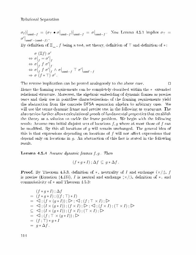
Relational Separation
σI)∣∣used−f = (σ> • σ
∣∣used−f )
∣∣used−f = σ
∣∣used−f . Now Lemma 4.5.1 implies σ> =
σ′∣∣used′−(used−f)
.
By de�nition of Ξ_ , f being a test, set theory, de�nition of > and de�nition of ∗ :
σ (Ξf) σ′
⇔ σ∣∣f
= σ′∣∣f
⇔ σ∣∣ff σ′
∣∣f
⇔ σ∣∣ff σ′
∣∣f∧ σ
∣∣used−f > σ′
∣∣used′−f
⇒ σ (f ∗ >) σ′ .
The reverse implication can be proved analogously to the above case. utHence the framing requirements can be completely described within the ∗ - extendedrelational structure. Moreover, the algebraic embedding of dynamic frames as precisetests and their use in pointfree characterisations of the framing requirements yieldthe abstraction from the concrete DFSA separation algebra to arbitrary ones. Wewill use the terms dynamic frame and precise test in the following as synonyms. Theabstraction further allows calculational proofs of fundamental properties that establishthe theory as a solution to tackle the frame problem. We begin with the followingresult: Assume two initial disjoint sets of locations f, g where at most those of f canbe modi�ed. By this all locations of g will remain unchanged. The general idea ofthis is that expressions depending on locations of f will not a�ect expressions thatdepend only on locations in g. An abstraction of this fact is stated in the followingresult.
Lemma 4.5.4 Assume dynamic frames f, g . Then
(f ∗ g ∗ I) ; ∆f ⊆ g ∗∆f .
Proof. By Theorem 4.5.3, de�nition of ∗ , neutrality of I and exchange (×/;), fis precise (Equation (4.13)), I is neutral and exchange (×/;), de�nition of ∗ , andcommutativity of ∗ and Theorem 4.5.3:
(f ∗ g ∗ I) ; ∆f= (f ∗ g ∗ I) ; ((f ;>) ∗ I)= � ; (f × (g ∗ I)) ;� ;� ; (f ;> × I) ;�= � ; (I × (g ∗ I)) ; (f × I) ;� ;� ; (f × I) ; (>× I) ;�⊆ � ; (I × (g ∗ I)) ; (f × I) ; (>× I) ;�= � ; (f ;> × (g ∗ I)) ;�= (f ;>) ∗ g ∗ I= g ∗∆f .
114
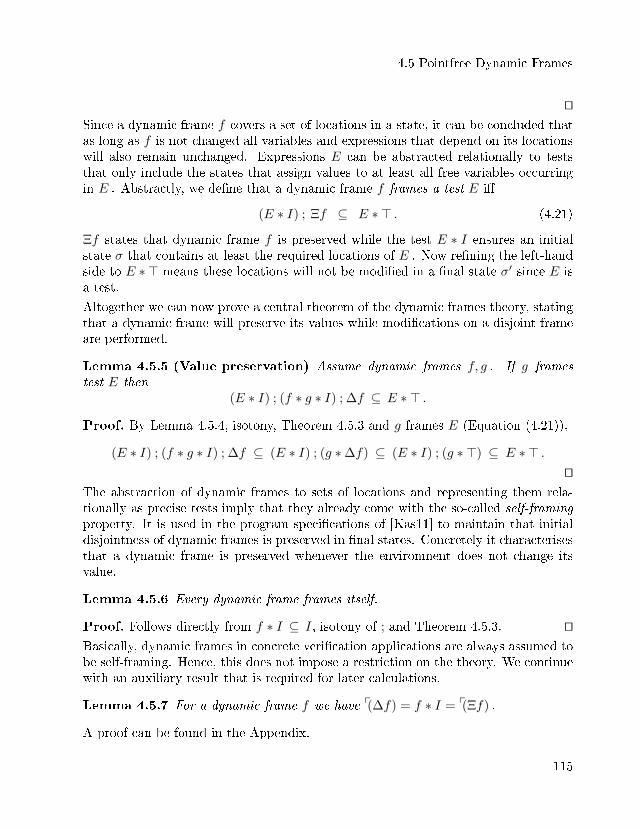
4.5 Pointfree Dynamic Frames
utSince a dynamic frame f covers a set of locations in a state, it can be concluded thatas long as f is not changed all variables and expressions that depend on its locationswill also remain unchanged. Expressions E can be abstracted relationally to teststhat only include the states that assign values to at least all free variables occurringin E . Abstractly, we de�ne that a dynamic frame f frames a test E i�
(E ∗ I) ; Ξf ⊆ E ∗ > . (4.21)
Ξf states that dynamic frame f is preserved while the test E ∗ I ensures an initialstate σ that contains at least the required locations of E . Now re�ning the left-handside to E ∗ > means these locations will not be modi�ed in a �nal state σ′ since E isa test.
Altogether we can now prove a central theorem of the dynamic frames theory, statingthat a dynamic frame will preserve its values while modi�cations on a disjoint frameare performed.
Lemma 4.5.5 (Value preservation) Assume dynamic frames f, g . If g framestest E then
(E ∗ I) ; (f ∗ g ∗ I) ; ∆f ⊆ E ∗ > .
Proof. By Lemma 4.5.4, isotony, Theorem 4.5.3 and g frames E (Equation (4.21)),
(E ∗ I) ; (f ∗ g ∗ I) ; ∆f ⊆ (E ∗ I) ; (g ∗∆f) ⊆ (E ∗ I) ; (g ∗ >) ⊆ E ∗ > .ut
The abstraction of dynamic frames to sets of locations and representing them rela-tionally as precise tests imply that they already come with the so-called self-framingproperty. It is used in the program speci�cations of [Kas11] to maintain that initialdisjointness of dynamic frames is preserved in �nal states. Concretely it characterisesthat a dynamic frame is preserved whenever the environment does not change itsvalue.
Lemma 4.5.6 Every dynamic frame frames itself.
Proof. Follows directly from f ∗ I ⊆ I, isotony of ; and Theorem 4.5.3. utBasically, dynamic frames in concrete veri�cation applications are always assumed tobe self-framing. Hence, this does not impose a restriction on the theory. We continuewith an auxiliary result that is required for later calculations.
Lemma 4.5.7 For a dynamic frame f we have p(∆f) = f ∗ I = p(Ξf) .
A proof can be found in the Appendix.
115
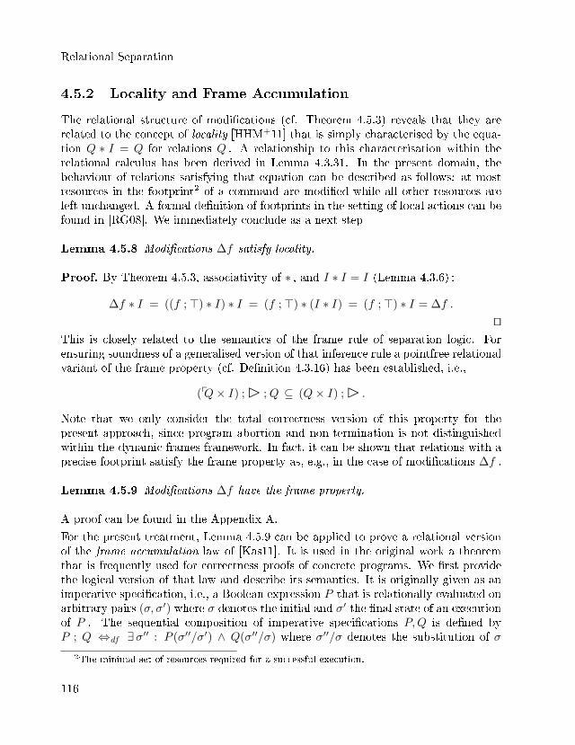
Relational Separation
4.5.2 Locality and Frame Accumulation
The relational structure of modi�cations (cf. Theorem 4.5.3) reveals that they arerelated to the concept of locality [HHM+11] that is simply characterised by the equa-tion Q ∗ I = Q for relations Q . A relationship to this characterisation within therelational calculus has been derived in Lemma 4.3.31. In the present domain, thebehaviour of relations satisfying that equation can be described as follows: at mostresources in the footprint2 of a command are modi�ed while all other resources areleft unchanged. A formal de�nition of footprints in the setting of local actions can befound in [RG08]. We immediately conclude as a next step
Lemma 4.5.8 Modi�cations ∆f satisfy locality.
Proof. By Theorem 4.5.3, associativity of ∗ , and I ∗ I = I (Lemma 4.3.6) :
∆f ∗ I = ((f ;>) ∗ I) ∗ I = (f ;>) ∗ (I ∗ I) = (f ;>) ∗ I = ∆f .
utThis is closely related to the semantics of the frame rule of separation logic. Forensuring soundness of a generalised version of that inference rule a pointfree relationalvariant of the frame property (cf. De�nition 4.3.16) has been established, i.e.,
(pQ× I) ;� ;Q ⊆ (Q× I) ;� .
Note that we only consider the total correctness version of this property for thepresent approach, since program abortion and non-termination is not distinguishedwithin the dynamic frames framework. In fact, it can be shown that relations with aprecise footprint satisfy the frame property as, e.g., in the case of modi�cations ∆f .
Lemma 4.5.9 Modi�cations ∆f have the frame property.
A proof can be found in the Appendix A.
For the present treatment, Lemma 4.5.9 can be applied to prove a relational versionof the frame accumulation law of [Kas11]. It is used in the original work a theoremthat is frequently used for correctness proofs of concrete programs. We �rst providethe logical version of that law and describe its semantics. It is originally given as animperative speci�cation, i.e., a Boolean expression P that is relationally evaluated onarbitrary pairs (σ, σ′) where σ denotes the initial and σ′ the �nal state of an executionof P . The sequential composition of imperative speci�cations P,Q is de�ned byP ; Q ⇔df ∃σ′′ : P (σ′′/σ′) ∧ Q(σ′′/σ) where σ′′/σ denotes the substitution of σ
2The minimal set of resources required for a successful execution.
116
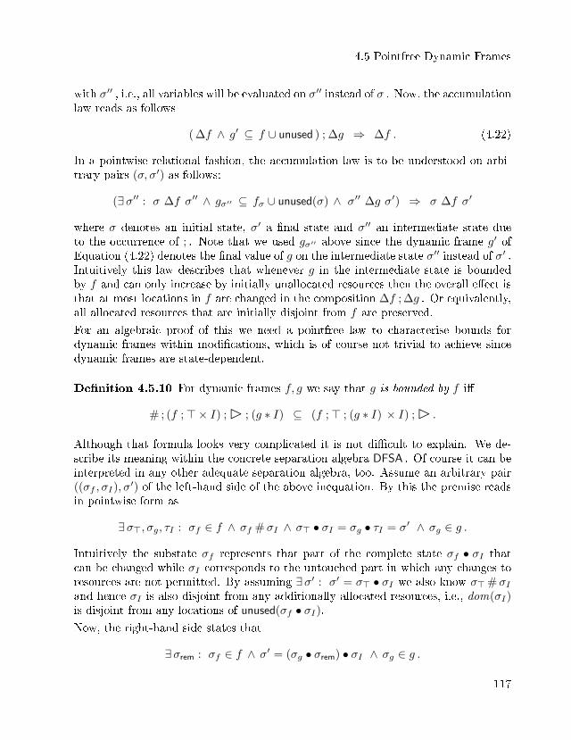
4.5 Pointfree Dynamic Frames
with σ′′ , i.e., all variables will be evaluated on σ′′ instead of σ . Now, the accumulationlaw reads as follows
( ∆f ∧ g′ ⊆ f ∪ unused ) ; ∆g ⇒ ∆f . (4.22)
In a pointwise relational fashion, the accumulation law is to be understood on arbi-trary pairs (σ, σ′) as follows:
(∃σ′′ : σ ∆f σ′′ ∧ gσ′′ ⊆ fσ ∪ unused(σ) ∧ σ′′ ∆g σ′) ⇒ σ ∆f σ′
where σ denotes an initial state, σ′ a �nal state and σ′′ an intermediate state dueto the occurrence of ; . Note that we used gσ′′ above since the dynamic frame g′ ofEquation (4.22) denotes the �nal value of g on the intermediate state σ′′ instead of σ′ .Intuitively this law describes that whenever g in the intermediate state is boundedby f and can only increase by initially unallocated resources then the overall e�ect isthat at most locations in f are changed in the composition ∆f ; ∆g . Or equivalently,all allocated resources that are initially disjoint from f are preserved.
For an algebraic proof of this we need a pointfree law to characterise bounds fordynamic frames within modi�cations, which is of course not trivial to achieve sincedynamic frames are state-dependent.
De�nition 4.5.10 For dynamic frames f, g we say that g is bounded by f i�
# ; (f ;>× I) ;� ; (g ∗ I) ⊆ (f ;> ; (g ∗ I) × I) ;� .
Although that formula looks very complicated it is not di�cult to explain. We de-scribe its meaning within the concrete separation algebra DFSA . Of course it can beinterpreted in any other adequate separation algebra, too. Assume an arbitrary pair((σf , σI), σ
′) of the left-hand side of the above inequation. By this the premise readsin pointwise form as
∃σ>, σg, τI : σf ∈ f ∧ σf #σI ∧ σ> • σI = σg • τI = σ′ ∧ σg ∈ g .
Intuitively the substate σf represents that part of the complete state σf • σI thatcan be changed while σI corresponds to the untouched part in which any changes toresources are not permitted. By assuming ∃σ′ : σ′ = σ> • σI we also know σ>#σIand hence σI is also disjoint from any additionally allocated resources, i.e., dom(σI)is disjoint from any locations of unused(σf • σI).Now, the right-hand side states that
∃σrem : σf ∈ f ∧ σ′ = (σg • σrem) • σI ∧ σg ∈ g .
117
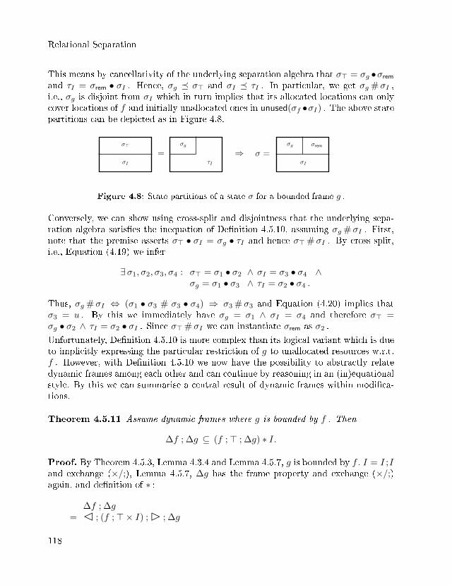
Relational Separation
This means by cancellativity of the underlying separation algebra that σ> = σg •σremand τI = σrem • σI . Hence, σg � σ> and σI � τI . In particular, we get σg #σI ,i.e., σg is disjoint from σI which in turn implies that its allocated locations can onlycover locations of f and initially unallocated ones in unused(σf •σI) . The above statepartitions can be depicted as in Figure 4.8.
σ =σ⊤
σI
=σg
τI
⇒ σ =σI
σg σrem
Figure 4.8: State partitions of a state σ for a bounded frame g .
Conversely, we can show using cross-split and disjointness that the underlying sepa-ration algebra satis�es the inequation of De�nition 4.5.10, assuming σg #σI . First,note that the premise asserts σ> • σI = σg • τI and hence σ>#σI . By cross-split,i.e., Equation (4.19) we infer
∃σ1, σ2, σ3, σ4 : σ> = σ1 • σ2 ∧ σI = σ3 • σ4 ∧σg = σ1 • σ3 ∧ τI = σ2 • σ4 .
Thus, σg #σI ⇔ (σ1 • σ3 # σ3 • σ4) ⇒ σ3 #σ3 and Equation (4.20) implies thatσ3 = u . By this we immediately have σg = σ1 ∧ σI = σ4 and therefore σ> =σg • σ2 ∧ τI = σ2 • σI . Since σ>#σI we can instantiate σrem as σ2 .
Unfortunately, De�nition 4.5.10 is more complex than its logical variant which is dueto implicitly expressing the particular restriction of g to unallocated resources w.r.t.f . However, with De�nition 4.5.10 we now have the possibility to abstractly relatedynamic frames among each other and can continue by reasoning in an (in)equationalstyle. By this we can summarise a central result of dynamic frames within modi�ca-tions.
Theorem 4.5.11 Assume dynamic frames where g is bounded by f . Then
∆f ; ∆g ⊆ (f ;> ; ∆g) ∗ I.
Proof. By Theorem 4.5.3, Lemma 4.3.4 and Lemma 4.5.7, g is bounded by f , I = I ;Iand exchange (×/;), Lemma 4.5.7, ∆g has the frame property and exchange (×/;)again, and de�nition of ∗ :
∆f ; ∆g= � ; (f ;>× I) ;� ; ∆g
118
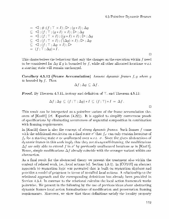
4.5 Pointfree Dynamic Frames
= � ; # ;(f ;> × I) ;� ; (g ∗ I) ; ∆g⊆ � ; (f ;> ; (g ∗ I) × I) ;� ; ∆g= � ; (f ;> × I) ; ((g ∗ I)× I) ;� ; ∆g
⊆ � ; (f ;> × I) ; (p(∆g)× I) ;� ; ∆g⊆ � ; (f ;> ; ∆g × I) ;�= (f ;> ; ∆g) ∗ I .
utThis characterises the behaviour that only the changes on the execution within f needto be considered for ∆g if g is bounded by f , while all other allocated locations w.r.ta starting state will remain unchanged.
Corollary 4.5.12 (Frame Accumulation) Assume dynamic frames f, g where gis bounded by f . Then
∆f ; ∆g ⊆ ∆f .
Proof. By Theorem 4.5.11, isotony and de�nition of >, and Theorem 4.5.11:
∆f ; ∆g ⊆ (f ;> ; ∆g) ∗ I ⊆ (f ;>) ∗ I = ∆f .
utThis result can be interpreted as a pointfree variant of the frame accumulation the-orem of [Kas11] (cf. Equation (4.22)). It is applied to simplify correctness proofsof speci�cations by eliminating occurrences of sequential composition in combinationwith framing requirements.
In [Kas11] there is also the concept of strong dynamic frames. Such frames f comewith the additional restriction on a �nal state σ′ that fσ′ can only contain locations offσ for a starting state σ or unallocated ones w.r.t. σ . Since the given abstractions ofdynamic frames in this work imply that they are always self-framing, the modi�cations∆f are only able to extend f in σ′ by previously unallocated locations as in [Kas11].Hence, simple modi�cations ∆f already coincide with the stronger variant within ourabstraction.
As a �nal result for the abstracted theory we present the treatment also within thecontext of related work, i.e., local actions (cf. Section 4.3.4). In [COY07] an abstractapproach to separation logic was presented that is built on separation algebras andprovides a model of programs in terms of so-called local actions. A relationship to therelational approach and the corresponding de�nitions has already been provided inSection 4.3.4. In contrast to the relational calculus the local action framework workspointwise. We present in the following by the use of previous ideas about abstractingdynamic frames local action formalisations of modi�cation and preservation framingrequirements. Moreover, we show that these de�nitions satisfy the locality property
119
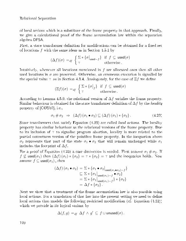
Relational Separation
of local actions which is a substitute of the frame property in that approach. Finally,we give a calculational proof of the frame accumulation law within the separationalgebra DFSA.
First, a state transformer de�nition for modi�cations can be obtained for a �xed setof locations f with the same ideas as in Section 4.5.1 by
(∆f)(σ) =df
{Σ ∗ {σ
∣∣used−f} if f ⊆ used(σ)
> otherwise .
Intuitively, whenever all locations mentioned in f are allocated ones then all otherused locations in σ are preserved. Otherwise, an erroneous execution is signalled bythe special value > as in Section 4.3.4. Analogously, for the case of Ξf we de�ne
(Ξf)(σ) =df
{Σ ∗ {σ
∣∣f} if f ⊆ used(σ)
> otherwise .
According to Lemma 4.5.9, the relational version of ∆f satis�es the frame property.Similar behaviour is obtained for the state transformer de�nition of ∆f by the localityproperty of [COY07], i.e.,
σ1 #σ2 ⇒ (∆f) (σ1 • σ2) v (∆f) (σ1) ∗ {σ2} . (4.23)
State transformers that satisfy Equation (4.23) are called local actions. The localityproperty has similar behaviour as the relational versions of the frame property. Dueto its inclusion of > to signalise program abortion, locality is more related to thepartial correctness version of the pointfree frame property. In the inequation aboveσ2 represents that part of the state σ1 • σ2 that will remain unchanged while σ1
includes the footprint of ∆f .
For a proof of Equation (4.23) a case distinction is needed. First assume σ1 #σ2. Iff 6⊆ used(σ1) then (∆f) (σ1) ∗ {σ2} = > ∗ {σ2} = > and the inequation holds. Nowassume f ⊆ used(σ1) , then
(∆f) (σ1 • σ2) = Σ ∗ {σ1 • σ2
∣∣used(σ1•σ2)−f}
v Σ ∗ {σ1
∣∣used(σ1)−f • σ2}
= Σ ∗ {σ1
∣∣used(σ1)−f} ∗ {σ2}
= ∆f ∗ {σ2} .Next we show that a treatment of the frame accumulation law is also possible usinglocal actions. For a translation of that law into the present setting we need to de�nelocal actions that models the following restricted modi�cation (cf. Equation (4.22))which we provide in its logical variant by
∆(f, g) =df ∆f ∧ g′ ⊆ f ∪ unused(σ) .
120
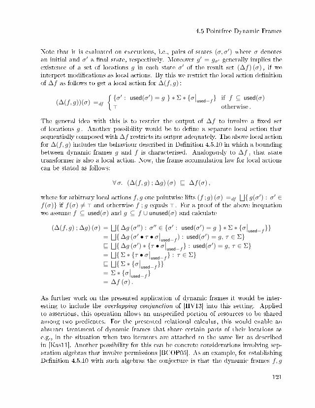
4.5 Pointfree Dynamic Frames
Note that it is evaluated on executions, i.e., pairs of states (σ, σ′) where σ denotesan initial and σ′ a �nal state, respectively. Moreover g′ = gσ′ generally implies theexistence of a set of locations g in each state σ′ of the result set (∆f) (σ) , if weinterpret modi�cations as local actions. By this we restrict the local action de�nitionof ∆f as follows to get a local action for ∆(f, g) :
(∆(f, g))(σ) =df
{ {σ′ : used(σ′) = g } ∗ Σ ∗ {σ∣∣used−f} if f ⊆ used(σ)
> otherwise .
The general idea with this is to restrict the output of ∆f to involve a �xed setof locations g . Another possibility would be to de�ne a separate local action thatsequentially composed with ∆f restricts its output adequately. The above local actionfor ∆(f, g) includes the behaviour described in De�nition 4.5.10 in which a boundingbetween dynamic frames g and f is characterised. Analogously to ∆f , that statetransformer is also a local action. Now, the frame accumulation law for local actionscan be stated as follows:
∀σ. (∆(f, g) ; ∆g) (σ) v ∆f(σ) ,
where for arbitrary local actions f, g one pointwise lifts (f ;g) (σ) =df
⊔{ g(σ′) : σ′ ∈f(σ)} if f(σ) 6= > and otherwise f ; g equals > . For a proof of the above inequationwe assume f ⊆ used(σ) and g ⊆ f ∪ unused(σ) and calculate
(∆(f, g) ; ∆g) (σ) =⊔{∆g (σ′′) : σ′′ ∈ {σ′ : used(σ′) = g } ∗ Σ ∗ {σ
∣∣used−f}}
=⊔{∆g (σ′ • τ • σ
∣∣used−f ) : used(σ′) = g, τ ∈ Σ}
v ⊔{∆g (σ′) ∗ {τ • σ∣∣used−f} : used(σ′) = g, τ ∈ Σ}
=⊔{Σ ∗ {τ • σ
∣∣used−f} : τ ∈ Σ}
v ⊔{Σ ∗ {σ∣∣used−f}}
= Σ ∗ {σ∣∣used−f}
= ∆f (σ) .
As further work on the presented application of dynamic frames it would be inter-esting to include the overlapping conjunction of [HV13] into this setting. Appliedto assertions, this operation allows an unspeci�ed portion of resources to be sharedamong two predicates. For the presented relational calculus, this would enable anabstract treatment of dynamic frames that share certain parts of their locations ase.g., in the situation when two iterators are attached to the same list as describedin [Kas11]. Another possibility for this can be concrete considerations involving sep-aration algebras that involve permissions [BCOP05]. As an example, for establishingDe�nition 4.5.10 with such algebras the conjecture is that the dynamic frames f, g
121
Relational Separation
would have to hold full permission to each of its captured resources. Moreover, therelationships to concrete approaches [DYDG+10, PS11, JB12] and their integrationinto this framework have to be investigated.
122
Chapter 5
Transitive Separation Logic
Separation logic has been developed to allow more �exible reasoning about heap por-tions or, more concretely, about linked object/record structures than Hoare logic. Inthis chapter we give an algebraic extension of separation logic at the data structurelevel. We de�ne new operations that, in addition to guaranteeing heap separation,make assumptions about the linking structure. Phenomena to be treated comprisereachability analysis, (absence of) sharing, cycle detection and preservation of sub-structures under destructive assignments. We demonstrate the practicality of thisapproach with examples of in-place list-reversal, tree rotation and threaded trees.
5.1 The Algebraic Foundation
We start with a brief example to motivate the following developments. As discussedbefore, the central connective of separation logic is the separating conjunction p ∗ qof assertions p, q . It guarantees that the addresses of the resources mentioned by pand q are disjoint. In simple settings where none of the resources of p depend onthose of q and vice versa, any simple assignment to resources of p does not yield anychanges of that in q . By this, one gets a compositional approach to reasoning aboutprograms. However, the situation becomes more complex when dependencies betweenthe set of resources exist. For a concrete example consider Figure 5.1. Clearly, fromthe variables x and y two singly linked lists can be accessed. Now, let p mention thestarting addresses of the list records with contents 1, . . . , 5 and q those of the records
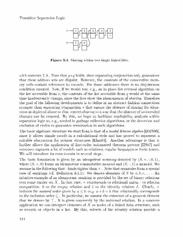
Transitive Separation Logic
x 1 2 3 4 5
◦
y 7 8
Figure 5.1: Sharing within two singly linked lists.
with contents 7, 8 . Note that p∗q holds, since separating conjunction only guaranteesthat these address sets are disjoint. However, the contents of the consecutive mem-ory cells contain references to records. For those addresses there is no disjointnesscondition ensured. Now, if we would run, e.g., an in-place list reversal algorithm onthe list accessible from x, the contents of the list accessible from y would at the sametime inadvertently change, since the lists show the phenomenon of sharing. Thereforethe goal of the following developments is to de�ne in an abstract fashion connectivesstronger than separating conjunction ∗ that ensure the absence of sharing for situa-tions as depicted above or that restrict sharing in a way that the absence of unintendedchanges can be ensured. By this, we hope to facilitate reachability analysis withinseparation logic as, e.g., needed in garbage collection algorithms, or the detection andexclusion of cycles to guarantee termination in such algorithms.
The basic algebraic structure we start from is that of a modal Kleene algebra [DMS06],since it allows simple proofs in a calculational style and has proved to represent asuitable abstraction for pointer structures [Ehm04]. Another advantage is that itfurther allows the application of �rst-order automated theorem provers [HS07] andmoreover captures a lot of models such as relations, regular languages or �nite traces.We will introduce its constituents in several steps.
The basic foundation is given by an idempotent semiring denoted by (S,+, ·, 0, 1) ,where (S,+, 0) forms an idempotent commutative monoid and (S, · , 1) a monoid. Weassume in the following that · binds tighter than + . Note that quantales form a specialcase of semirings (cf. De�nition 3.1.1). We denote elements of S by a, b, c, . . . . Anintuitive example of an idempotent semiring is provided by the set of binary relationsover some carrier set X . In that case, + corresponds to relational union, · to relationcomposition, 0 to the empty relation and 1 to the identity relation I. Clearly, +induces the natural order given by a ≤ b ⇔df a+ b = b that relationally correspondsto the inclusion order ⊆ . In particular, we assume the existence of a greatest elementthat we denote by > . It is given concretely by the universal relation. In a concreteapplication we can interpret elements of X as nodes of a linked data structure, suchas records or objects in a list. By this, subsets of the identity relation provide a
124
5.1 The Algebraic Foundation
uniform and adequate algebraic representation for sets of nodes of X . In generalsemirings, this approach is mimicked by sub-identity elements p ≤ 1 , called tests(cf. De�nition 3.2.13). We recapitulate that each of these elements is requested tohave a complement relative to 1 , i.e., an element ¬p that satis�es p + ¬p = 1 andp · ¬p = 0 = ¬p · p .With tests, the abstract product p · a can be used to restrict an element a to linksthat start in nodes of p while, symmetrically, a · p restricts a to links ending in nodesof p . Following [DMS06], these products can be used to axiomatise algebraic variantsof domain and codomain operators denoted by p_ and _q , respectively. Abstractly,for an arbitrary element a and test p they are given by the axioms
a ≤ pa · a , p(p · a) ≤ p , p(a · b) = p(a · pb) ,a ≤ a · aq , (a · p)q ≤ p , (a · b)q = (aq · b)q .
These imply fundamental properties such as additivity and isotony, among others (cf.e.g [DMS06]). Note that we used the same symbol as in the concrete relational caseof (reldom) in Section 4.2 since the abstract operations in fact characterise in therelational case sub-identities which are in one-to-one correspondence with the usualdomain and codomain. In particular, it can be shown that the �rst two axioms ofdomain are equivalent to an abstract form of (reldom).
Built on these notions we also recapitulate the backward diamond operation (cf. Sec-tion 4.2) in an more abstract form. It plays a central role for our reachability analysesand is de�ned by 〈a|p =df (p · a)q . Since this is an abstract version of the diamondoperator from modal logic, an idempotent semiring with it is called modal. Con-cretely, the backward diamond 〈a|p calculates all immediate successor nodes under a ,starting from the set of nodes p , i.e., all nodes that are reachable within one a - step,aka the image of p under a . This operation distributes through union and is strictand isotone in both arguments.
Finally, to calculate reachability via arbitrarily many links or a - steps, we extend thealgebraic structure to a modal Kleene algebra [Koz94] by an iteration operator ∗ . Itcan be axiomatised by the following unfold and induction laws:
1 + x · x∗ ≤ x∗ , x · y + z ≤ y ⇒ x∗ · z ≤ y ,1 + x∗ · x ≤ x∗ , y · x+ z ≤ y ⇒ z · x∗ ≤ y .
This implies that a∗ is the least �xed-point µf of f(x) = 1 + a · x . By this we de�nethe reachability function as follows:
reach(p, a) =df 〈a∗|p .Among other properties, reach distributes through + in its �rst argument and isisotone in both arguments. Moreover we have p ≤ reach(p, a) and the induction rule
125
Transitive Separation Logic
p ≤ q ∧ 〈a|q ≤ q ⇒ reach(p, a) ≤ q . Further properties within a fuzzy relationalgebra approach can be found in [Ehm03].
For the present chapter we basically follow the approach of [DM12b, DM13]. Thelast ingredient that we introduce for an adequate treatment of pointer structures is aspecial element within the algebra that represents the improper reference nil or null .Relationally, we can express it as the singleton relation 2 =df {(O,O)} , where O isa distinguished element of the set of nodes. Such singleton sub-identity relations canabstractly be de�ned as atomic tests p .
De�nition 5.1.1A test p is called atomic i� p 6= 0 and q ≤ p ⇒ q = 0 ∨ q = p for arbitrary tests q .In particular, we assume 2 to be an atomic test.
Using 2 we also characterise the subset of elements that have no links emanating fromthe pseudo-reference 2 to any other address 6= 2 . This is a natural requirement, sincethe general purpose of 2 is to denote a terminator reference. We refer to this propertyas properness.
De�nition 5.1.2An element a is called proper i� 2 · a ≤ 2 .
Note that by properness 2 ·a is a test. We summarise some more consequences of thisde�nition.
Lemma 5.1.3 a1, a2 are proper i� a1 + a2 is proper.
Proof. Follows immediately from distributivity and the suprema split in (3.2). ut
Lemma 5.1.4 For an element a with 2 · pa = 0 the following properties hold:
1. a is proper , 2. 2 · a = 0 , 3. a = ¬2 · a .
Proof. For 1 and 2 we calculate 2 ·a = 2 ·pa ·a = 0 ·a = 0 ≤ 2 by domain axioms andassumption. Finally, for 3 we have a = 1 · a = (2 + ¬2) · a = 2 · a + ¬2 · a = ¬2 · aby neutrality, 2 being a test, distributivity and 2. ut
Lemma 5.1.5 If a is proper then reach(2, a) = 2 .
Proof. First, we always have 2 ≤ reach(2, a) . The other inequation reach(2, a) ≤ 2
is implied by 〈a|2 ≤ 2 using the reach induction rule. This is shown as follows:(2 · a)q ≤ 2q = 2 by assumption and 2 being a test. ut
126
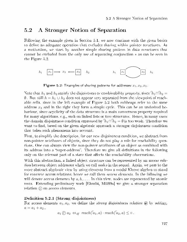
5.2 A Stronger Notion of Separation
5.2 A Stronger Notion of Separation
Following the example given in Section 5.1, we now continue with the given basicsto de�ne an adequate operation that excludes sharing within pointer structures. Asa motivation, we start by another simple sharing pattern in data structures thatcannot be excluded from the only use of separating conjunction ∗ as can be seen inthe Figure 5.2.
h1 x3x1 x2 h2 h1 x1 x2 h2
Figure 5.2: Examples of sharing patterns for addresses x1, x2, x3 .
Note that h1 and h2 satisfy the disjointness or combinability property, since ph1∩ph2 =∅ . But still h = h1 ∪ h2 does not appear very separated from the viewpoint of reach-able cells, since in the left example of Figure 5.2 both subheaps refer to the sameaddress x3 and in the right they form a simple cycle. This can be an undesired be-haviour, since acyclicity of the data structure is a main correctness property requiredfor many algorithms, e.g., such on linked lists or tree structures. Hence, in many casesthe domain disjointness condition expressed by ph1∩ph2 = ∅ is too weak. Therefore wewant to �nd, based on the given algebraic approach a stronger disjointness conditionthat takes such phenomena into account.
First, to simplify the description, for our new disjointness condition, we abstract fromnon-pointer attributes of objects, since they do not play a role for reachability ques-tions. One can always view the non-pointer attributes of an object as combined withits address into a �super-address�. Therefore we give all de�nitions in the followingonly on the relevant part of a state that a�ects the reachability observations.
With this abstraction, a linked object structure can be represented by an access rela-tion between object addresses which we call nodes in the sequel. Again, we pass to themore abstract algebraic view by using elements from a modal Kleene algebra to standfor concrete access relations; hence we call them access elements. In the following wewill denote access elements by a, b, . . . . In this view, nodes are represented by atomictests. Extending preliminary work [Ehm04, Möl99a] we give a stronger separationrelation ©# on access elements.
De�nition 5.2.1 (Strong disjointness)For access elements a1, a2, we de�ne the strong disjointness relation ©# by setting,a = a1 + a2 ,
a1©# a2 ⇔df reach(pa1, a) · reach(pa2, a) ≤ 2 .
127
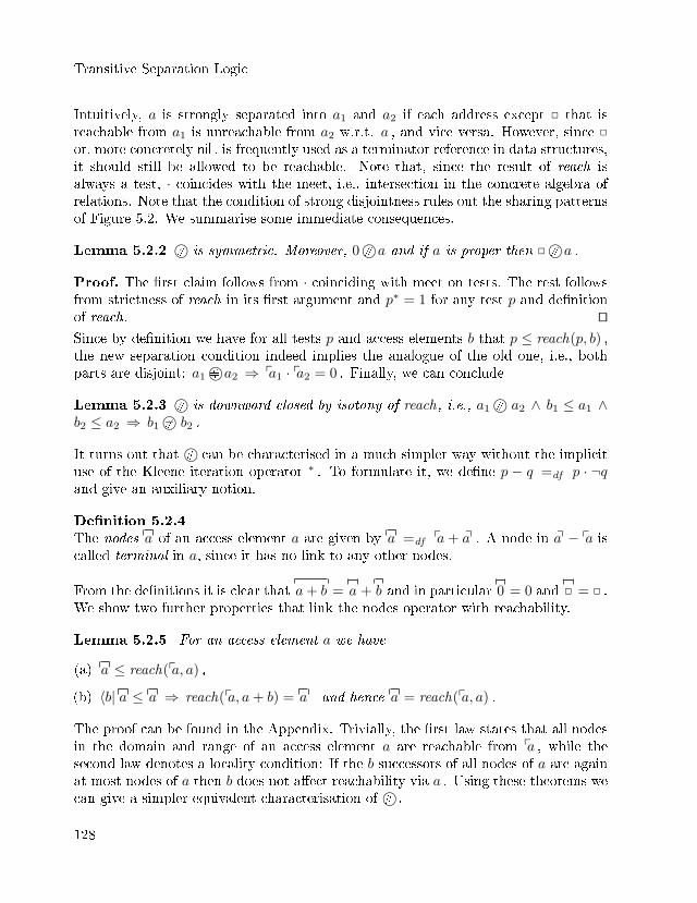
Transitive Separation Logic
Intuitively, a is strongly separated into a1 and a2 if each address except 2 that isreachable from a1 is unreachable from a2 w.r.t. a , and vice versa. However, since 2
or, more concretely nil , is frequently used as a terminator reference in data structures,it should still be allowed to be reachable. Note that, since the result of reach isalways a test, · coincides with the meet, i.e., intersection in the concrete algebra ofrelations. Note that the condition of strong disjointness rules out the sharing patternsof Figure 5.2. We summarise some immediate consequences.
Lemma 5.2.2 ©# is symmetric. Moreover, 0©# a and if a is proper then 2©# a .
Proof. The �rst claim follows from · coinciding with meet on tests. The rest followsfrom strictness of reach in its �rst argument and p∗ = 1 for any test p and de�nitionof reach. utSince by de�nition we have for all tests p and access elements b that p ≤ reach(p, b) ,the new separation condition indeed implies the analogue of the old one, i.e., bothparts are disjoint: a1©# a2 ⇒ pa1 · pa2 = 0 . Finally, we can conclude
Lemma 5.2.3 ©# is downward closed by isotony of reach, i.e., a1©# a2 ∧ b1 ≤ a1 ∧b2 ≤ a2 ⇒ b1©# b2 .
It turns out that ©# can be characterised in a much simpler way without the implicituse of the Kleene iteration operator ∗ . To formulate it, we de�ne p − q =df p · ¬qand give an auxiliary notion.
De�nition 5.2.4The nodes a of an access element a are given by a =df pa+ aq . A node in aq − pa iscalled terminal in a, since it has no link to any other nodes.
From the de�nitions it is clear that a+ b = a + b and in particular 0 = 0 and 2 = 2 .We show two further properties that link the nodes operator with reachability.
Lemma 5.2.5 For an access element a we have
(a) a ≤ reach(pa, a) ,
(b) 〈b| a ≤ a ⇒ reach(pa, a+ b) = a and hence a = reach(pa, a) .
The proof can be found in the Appendix. Trivially, the �rst law states that all nodesin the domain and range of an access element a are reachable from pa , while thesecond law denotes a locality condition: If the b successors of all nodes of a are againat most nodes of a then b does not a�ect reachability via a . Using these theorems wecan give a simpler equivalent characterisation of ©# .
128
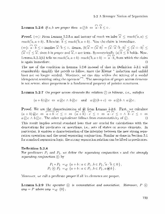
5.2 A Stronger Notion of Separation
Lemma 5.2.6 If a, b are proper then a©# b ⇔ a · b ≤ 2 .
Proof. (⇒): From Lemma 5.2.5.a and isotony of reach we infer a ≤ reach(pa, a) ≤reach(pa, a+ b) . Likewise, b ≤ reach(pb, a+ b) . Now the claim is immediate.
(⇐): a · b ≤ 2 implies a ·pb ≤ 2. Hence, 〈b| a = (a ·b)q = (a · a ·pb · b)q ≤ (a ·2 · b)q ≤(a ·2)q ≤ a , since b is proper and a,2 are tests. Symmetrically 〈a| b ≤ b holds. Now,
Lemma 5.2.5(b) tells us reach(pa, a+ b) · reach(pb, a+ b) = a · b , from which the claimis again immediate. utThe use of the condition in Lemma 5.2.6 instead of that in De�nition 5.2.1 willconsiderably simplify the proofs to follow, since the Kleene ∗ induction and unfoldlaws are no longer needed. Moreover, we can stay within the setting of a modalidempotent semiring using the operator . The assumption of proper access elementsis not severe, since properness is a fundamental property of pointer structures.
Lemma 5.2.7 On proper access elements the relation ©# is bilinear, i.e., satis�es
(a+ b)©# c ⇔ a©# c ∧ b©# c and a©# (b+ c) ⇔ a©# b ∧ a©# c .
Proof. We use the characterisation of ©# from Lemma 5.2.6. First, we calculate
(a + b)©# c ⇔ a+ b · c ≤ 2 ⇔ (a + b) · c ≤ 2 ⇔ a · c ≤ 2 ∧ b · c ≤ 2 ⇔a©# c ∧ b©# c . The other equivalence follows from commutativity of ©# . utThis result implies several standard laws that are crucial for calculations with thedenotations for predicates or assertions, i.e., sets of states or access elements. Inparticular, it enables a characterisation of the interplay between the new strong sepa-ration operation and the usual separating conjunction. Similar as done in Section 3.1for standard separation logic, the strong separation relation can be lifted to predicates.
De�nition 5.2.8For predicates P1 and P2, we de�ne the separating conjunction ∗ and the stronglyseparating conjunction ©∗ by
P1 ∗ P2 =df {a+ b : a ∈ P1 , b ∈ P2 , pa · pb ≤ 0 } ,P1 ©∗ P2 =df {a+ b : a ∈ P1 , b ∈ P2 , a©# b } .
Moreover, we call a predicate proper if all its elements are proper.
Lemma 5.2.9 The operator ©∗ is commutative and associative. Moreover, P ©∗emp = P where emp =df {0} .
129
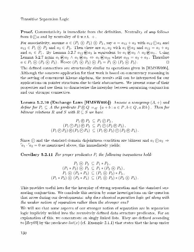
Transitive Separation Logic
Proof. Commutativity is immediate from the de�nition. Neutrality of emp followsfrom 0©# a and by neutrality of 0 w.r.t. + .
For associativity, assume a ∈ (P1 ©∗ P2) ©∗ P3 , say a = a12 + a3 with a12©# a3 anda12 ∈ P1 ©∗ P2 and a3 ∈ P3. Then there are a1, a2 with a1©# a2 and a12 = a1 + a2
and ai ∈ Pi . By Lemma 5.2.7 a12©# a3 is equivalent to a1©# a3 ∧ a2©# a3 . UsingLemma 5.2.7 again a1©# a2 ∧ a1©# a3 ⇔ a1©# a23 where a23 = a2 + a3 . Thereforea ∈ P1 ©∗ (P2 ©∗ P3) . Hence (P1 ©∗ P2)©∗ P3 = P1 ©∗ (P2 ©∗ P3) . utThe de�ned connectives are structurally similar to operations given in [HMSW09b].Although the concrete application for that work is based on concurrency reasoning inthe setting of concurrent Kleene algebras, the results still can be interpreted for ourapplications on pointer structures due to their abstractness. We present some of theirproperties and use them to characterise the interplay between separating conjunctionand our stronger connective.
Lemma 5.2.10 (Exchange Laws [HMSW09b]) Assume a semigroup (A,+) andde�ne for Pi ⊆ A the predicate P ©R Q =df {a+ b : a ∈ P , b ∈ Q , aR b } . Then forbilinear relations R and S with R ⊆ S we have
P1©R P2 ⊆ P1©S P2 ,(P1©S P2)©R P3 ⊆ P1©S (P2©R P3) ,
(P1©S P2)©R (P3©S P4) ⊆ (P1©R P3)©S (P2©R P4) .
Since ©# and the standard domain disjointness condition are bilinear and a1©# a2 ⇒pa1 · pa2 = 0 as mentioned above, this immediately yields:
Corollary 5.2.11 For proper predicates Pi the following inequations hold:
P1 ©∗ P2 ⊆ P1 ∗ P2 ,(P1 ∗ P2)©∗ P3 ⊆ P1 ∗ (P2 ©∗ P3) ,P1 ©∗ (P2 ∗ P3) ⊆ (P1 ©∗ P2) ∗ P3 ,
(P1 ∗ P2)©∗ (P3 ∗ P4) ⊆ (P1 ©∗ P3) ∗ (P2 ©∗ P4) .
This provides useful laws for the interplay of strong separation and the standard sep-arating conjunction. We conclude this section by some investigations on the questionthat arose during our developments: why does classical separation logic get along withthe weaker notion of separation rather than the stronger one?
We will see that some aspects of our stronger notion of separation are in separationlogic implicitly welded into the recursively de�ned data structure predicates. For anexplanation of this, we concentrate on singly linked lists. They are de�ned accordingto [Rey09] by the predicate list(x) (cf. Example 2.1.1) that states that the heap under
130
5.2 A Stronger Notion of Separation
consideration consists of the cells of a singly linked list with starting address x . Itsvalidity in a heap h is de�ned by the following clauses:
h |= list(nil) ⇔df h = ∅ ,x 6= nil ⇒ (h |= list(x) ⇔df ∃ y : h |= [x 7→ y] ∗ list(y)) .
For simplicity, we omit the store component that records as in the de�nition of Ex-ample 2.1.1 the values of the program variables. Hence h has to be an empty heapwhen x = nil , and a heap with at least one cell at its beginning when x 6= nil , namely[x 7→ y] .
First, note that using©∗ instead of ∗ in the de�nition above would not work, becausethe heaps used are obviously not strongly separate, since their cells are connected byforward pointers to their successor cells. In the next section we introduce an approachto present such a connection within our algebra. For a more concrete description ofthe relationship of strong separation and the usual separation condition we de�ne theconcept of closedness.
De�nition 5.2.12An access element a is called closed i� aq ≤ pa+ 2 .
In a closed element a there exist no dangling references. As an example, the abovelists within heaps are closed as they are terminated by the value nil which abstractlycorresponds to the element 2 . We summarise a few consequences of De�nition 5.2.12.
Lemma 5.2.13 If a1 and a2 are closed then a1 + a2 is also closed.
Proof. Immediate from distributivity of domain and codomain. ut
Lemma 5.2.14 An access element a is closed i� aq − pa ≤ 2 .
Proof. As tests form a Boolean subalgebra we conclude aq − pa ≤ 2 ⇔ aq · ¬pa ≤2 ⇔ aq ≤ pa+ 2 . ut
Lemma 5.2.15 For proper and closed a1, a2 with pa1 · pa2 = 0 we have a1©# a2 .
Proof. By distributivity and order theory we know
a1 · a2 ≤ 2 ⇔ pa1 · pa2 ≤ 2 ∧ pa1 · a2q ≤ 2 ∧ a1q · pa2 ≤ 2 ∧ a1q · a2q ≤ 2 .
The �rst conjunct holds by the assumption and isotony. Note that properness implies2 · pai ≤ 2 . Hence for the second and analogously for the third conjunct we calculate
131
Transitive Separation Logic
pa1 · a2q ≤ pa1 · (pa2 + 2) = pa1 · pa2 + pa1 · 2 ≤ 2 . The last one reduces by distributivityand the assumptions to 2 · 2 ≤ 2 which is trivial, since 2 is a test. utDomain-disjointness of access elements is ensured by the standard separating con-junction. It can be shown, by induction on the structure of the list predicate, that allaccess elements characterised by its analogue are closed, so that the lemma applies.This is why for a large part of separation logic the standard disjointness propertysu�ces.
5.3 An Algebra of Linked Structures
According to [Sim06], generally recursive predicate de�nitions, such as the list predi-cate, are semantically not well de�ned in the classical form of separation logic. For-mally, their de�nitions require the inclusion of �xpoint operators and additional syn-tactic sugar. This often makes the used assertions more complicated as e.g., by ex-pressing reachability via anonymous addresses stored in existentially quanti�ed vari-ables, formulas often become very complex. To overcome this de�ciency we provideoperators and predicates that implicitly include such additional information, i.e., nec-essary correctness properties like the exclusion of sharing and reachability.
In what follows we extend our algebra following precursor work in [Ehm04, Ehm03,Möl99a, Möl92] and give some de�nitions to describe the shape of linked object struc-tures, in particular of tree-like ones. We start by a characterisation of acyclicity.
De�nition 5.3.1An access element a is called acyclic i� for all atomic tests p 6= 2 we have p·〈a+|p = 0 ,where a+ =df a · a∗ .
For a concrete example of this de�nition, one can think of an access relation a whereeach entry (x, y) in a+ denotes the existence of a path from address x to y withina . Atomicity is needed to represent a single node; the de�nition would not work forarbitrary sets of nodes. The element 2 is excluded, since it is used as a terminatorreference and no structural properties are needed for it. A simpler characterisationcan be given as follows.
Lemma 5.3.2 a is acyclic i� for all atomic tests p 6= 2 we have p · a+ · p = 0 .
Proof. p · 〈a+|p = 0 ⇔ (p · a+)q · p = 0 ⇔ (p · a+ · p)q = 0 ⇔ p · a+ · p = 0 sincecodomain is strict. utNext, since certain access operations are deterministic, we need an algebraic charac-terisation of determinacy. We borrow it from [DM01a]:
132
5.3 An Algebra of Linked Structures
De�nition 5.3.3An access element a is deterministic i� ∀ p : 〈a||a〉p ≤ p , where the dual diamond isabstractly de�ned by |a〉p =df
p(a · p) .
A further relational characterisation of determinacy of an access relation a is given bya · a ≤ 1 , where ˘ is the converse operator. Since in our basic algebraic structure ofsemirings no general converse operation is available, we have to express the respectiveproperties in another way. We have chosen to use the well established notion of modaloperators. This way our algebra works also for other structures than relations. Theroles of the expressions a and a are now played by 〈a| and |a〉, respectively.
Lemma 5.3.4 If a is deterministic and pa is an atom then also aq is an atom.
A proof can be found in Appendix A. Interestingly, that proof does not presupposethat the set of all tests is an atomic lattice. Now we de�ne our model of linked objectstructures.
De�nition 5.3.5 (Linked structures)We assume a �nite set L of selector names and a modal Kleene algebra S.
� A linked structure is a family a = (al)l∈L of proper and deterministic accesselements al ∈ S . This re�ects that access along each particular selector isdeterministic. The overall access element associated with a is then Σl∈L al ,by slight abuse of notation again denoted by a ; the context will disambiguate.The set of all linked structures over L is denoted by SL . Since 2 is proper anddeterministic we will also view it as an element of SL although it does not haveany selectors.
� A linked structure a is a forest i� a is acyclic and injective, i.e., has maximalin-degree 1 except possibly for 2 . Algebraically this is expressed by the dual ofthe formula for determinacy, namely
∀ p : |a′〉〈a′|p ≤ p , where a′ =df a · ¬2 .
Moreover, we de�ne for forests a
roots(a) =df (pa− aq) + 2 · pa .
By properness and since 2 is atomic, the term 2 · pa equals 2 when 2 ≤ a and is0 otherwise.
133
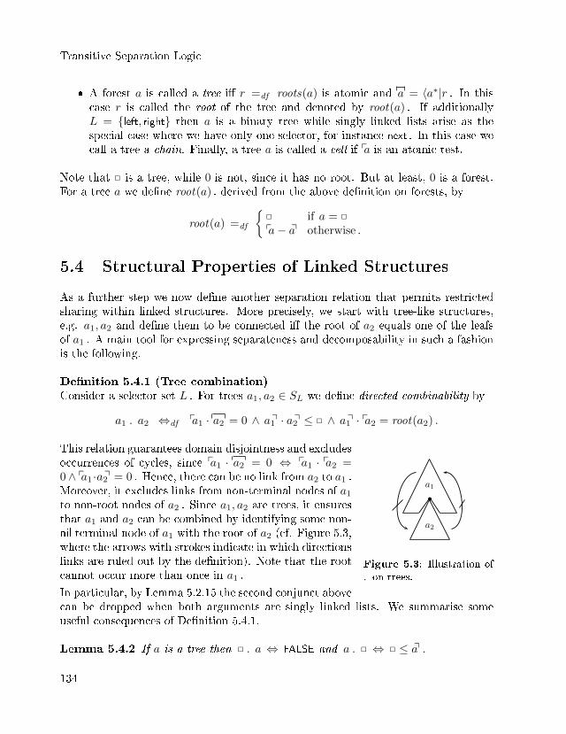
Transitive Separation Logic
� A forest a is called a tree i� r =df roots(a) is atomic and a = 〈a∗|r . In thiscase r is called the root of the tree and denoted by root(a) . If additionallyL = {left, right} then a is a binary tree while singly linked lists arise as thespecial case where we have only one selector, for instance next . In this case wecall a tree a chain. Finally, a tree a is called a cell if pa is an atomic test.
Note that 2 is a tree, while 0 is not, since it has no root. But at least, 0 is a forest.For a tree a we de�ne root(a) , derived from the above de�nition on forests, by
root(a) =df
{2 if a = 2
pa− aq otherwise .
5.4 Structural Properties of Linked Structures
As a further step we now de�ne another separation relation that permits restrictedsharing within linked structures. More precisely, we start with tree-like structures,e.g. a1, a2 and de�ne them to be connected i� the root of a2 equals one of the leafsof a1 . A main tool for expressing separateness and decomposability in such a fashionis the following.
De�nition 5.4.1 (Tree combination)Consider a selector set L . For trees a1, a2 ∈ SL we de�ne directed combinability by
a1 . a2 ⇔df pa1 · a2 = 0 ∧ a1q · a2q ≤ 2 ∧ a1q · pa2 = root(a2) .
•a1
a2
Figure 5.3: Illustration of. on trees.
This relation guarantees domain disjointness and excludesoccurrences of cycles, since pa1 · a2 = 0 ⇔ pa1 · pa2 =0 ∧ pa1 ·a2q = 0 . Hence, there can be no link from a2 to a1 .Moreover, it excludes links from non-terminal nodes of a1
to non-root nodes of a2 . Since a1, a2 are trees, it ensuresthat a1 and a2 can be combined by identifying some non-nil terminal node of a1 with the root of a2 (cf. Figure 5.3,where the arrows with strokes indicate in which directionslinks are ruled out by the de�nition). Note that the rootcannot occur more than once in a1 .
In particular, by Lemma 5.2.15 the second conjunct abovecan be dropped when both arguments are singly linked lists. We summarise someuseful consequences of De�nition 5.4.1.
Lemma 5.4.2 If a is a tree then 2 . a ⇔ FALSE and a . 2 ⇔ 2 ≤ aq .
134
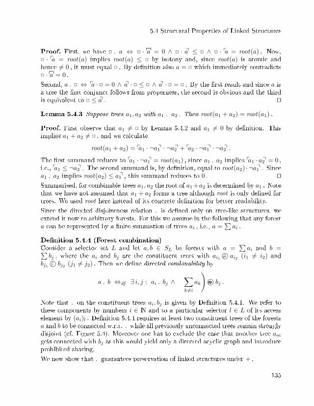
5.4 Structural Properties of Linked Structures
Proof. First, we have 2 . a ⇔ 2 · a = 0 ∧ 2 · aq ≤ 2 ∧ 2 · pa = root(a) . Now,2 · pa = root(a) implies root(a) ≤ 2 by isotony and, since root(a) is atomic andhence 6= 0 , it must equal 2 . By de�nition also a = 2 which immediately contradicts2 · a = 0 .
Second, a . 2 ⇔ pa · 2 = 0 ∧ aq · 2 ≤ 2 ∧ aq · 2 = 2 . By the �rst result and since a isa tree the �rst conjunct follows from properness, the second is obvious and the thirdis equivalent to 2 ≤ aq . ut
Lemma 5.4.3 Suppose trees a1, a2 with a1 . a2 . Then root(a1 + a2) = root(a1) .
Proof. First observe that a1 6= 2 by Lemma 5.4.2 and a1 6= 0 by de�nition. Thisimplies a1 + a2 6= 2 , and we calculate
root(a1 + a2) = pa1 · ¬a1q · ¬a2q + pa2 · ¬a1q · ¬a2q .
The �rst summand reduces to pa1 · ¬a1q = root(a1) , since a1 . a2 implies pa1 · a2q = 0 ,i.e., pa1 ≤ ¬a2q . The second summand is, by de�nition, equal to root(a2) ·¬a1q . Sincea1 . a2 implies root(a2) ≤ a1q , this summand reduces to 0 . utSummarised, for combinable trees a1, a2 the root of a1 +a2 is determined by a1 . Notethat we have not assumed that a1 + a2 forms a tree although root is only de�ned fortrees. We used root here instead of its concrete de�nition for better readability.
Since the directed disjointness relation . is de�ned only on tree-like structures, weextend it now to arbitrary forests. For this we assume in the following that any foresta can be represented by a �nite summation of trees ai , i.e., a =
∑ai .
De�nition 5.4.4 (Forest combination)Consider a selector set L and let a, b ∈ SL be forests with a =
∑ai and b =∑
bj , where the ai and bj are the constituent trees with ai1©# ai2 (i1 6= i2) andbj1©# bj2 (j1 6= j2) . Then we de�ne directed combinability by
a . b ⇔df ∃ i, j : ai . bj ∧(∑
k 6=iak
)©# bj .
Note that . on the constituent trees ai, bj is given by De�nition 5.4.1. We refer tothese components by numbers i ∈ IN and to a particular selector l ∈ L of its accesselement by (ai)l . De�nition 5.4.4 requires at least two constituent trees of the forestsa and b to be connected w.r.t. . while all previously unconnected trees remain stronglydisjoint (cf. Figure 5.4). Moreover one has to exclude the case that another tree amgets connected with bj as this would yield only a directed acyclic graph and introduceprohibited sharing.
We now show that . guarantees preservation of linked structures under + .
135
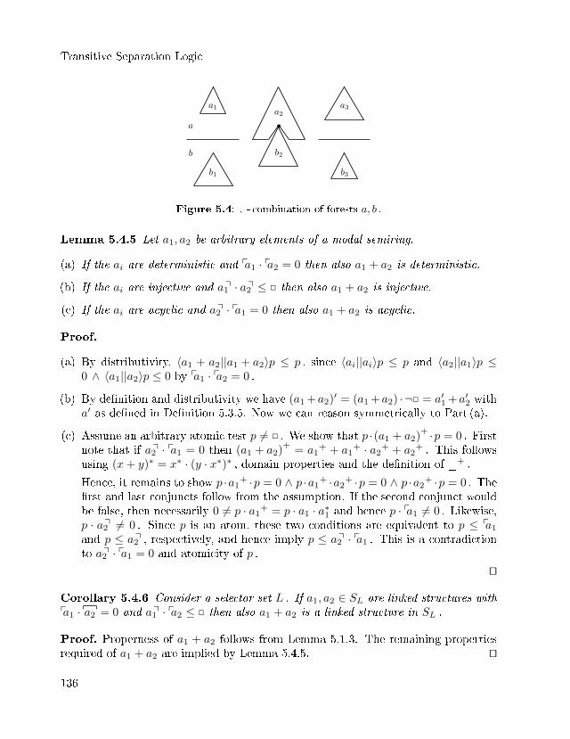
Transitive Separation Logic
•a2
b2
a1
b1
a
a3
b3
b
Figure 5.4: . - combination of forests a, b .
Lemma 5.4.5 Let a1, a2 be arbitrary elements of a modal semiring.
(a) If the ai are deterministic and pa1 · pa2 = 0 then also a1 + a2 is deterministic.
(b) If the ai are injective and a1q · a2q ≤ 2 then also a1 + a2 is injective.
(c) If the ai are acyclic and a2q · pa1 = 0 then also a1 + a2 is acyclic.
Proof.
(a) By distributivity, 〈a1 + a2||a1 + a2〉p ≤ p , since 〈ai||ai〉p ≤ p and 〈a2||a1〉p ≤0 ∧ 〈a1||a2〉p ≤ 0 by pa1 · pa2 = 0 .
(b) By de�nition and distributivity we have (a1 +a2)′ = (a1 +a2) · ¬2 = a′1 +a′2 witha′ as de�ned in De�nition 5.3.5. Now we can reason symmetrically to Part (a).
(c) Assume an arbitrary atomic test p 6= 2 . We show that p ·(a1 + a2)+ ·p = 0 . First
note that if a2q · pa1 = 0 then (a1 + a2)+
= a1+ + a1
+ · a2+ + a2
+ . This followsusing (x+ y)∗ = x∗ · (y · x∗)∗ , domain properties and the de�nition of _+ .
Hence, it remains to show p ·a1+ ·p = 0 ∧ p ·a1
+ ·a2+ ·p = 0 ∧ p ·a2
+ ·p = 0 . The�rst and last conjuncts follow from the assumption. If the second conjunct wouldbe false, then necessarily 0 6= p · a1
+ = p · a1 · a∗1 and hence p · pa1 6= 0 . Likewise,p · a2q 6= 0 . Since p is an atom, these two conditions are equivalent to p ≤ pa1
and p ≤ a2q , respectively, and hence imply p ≤ a2q · pa1 . This is a contradictionto a2q · pa1 = 0 and atomicity of p .
ut
Corollary 5.4.6 Consider a selector set L . If a1, a2 ∈ SL are linked structures withpa1 · a2 = 0 and a1q · pa2 ≤ 2 then also a1 + a2 is a linked structure in SL .
Proof. Properness of a1 + a2 follows from Lemma 5.1.3. The remaining propertiesrequired of a1 + a2 are implied by Lemma 5.4.5. ut
136
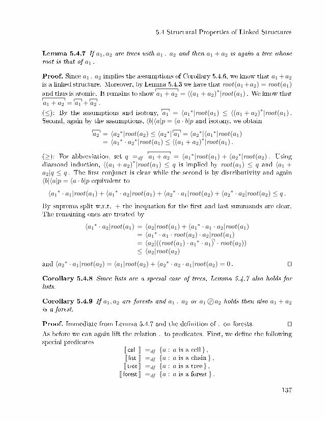
5.4 Structural Properties of Linked Structures
Lemma 5.4.7 If a1, a2 are trees with a1 . a2 and then a1 + a2 is again a tree whoseroot is that of a1 .
Proof. Since a1 .a2 implies the assumptions of Corollary 5.4.6, we know that a1 +a2
is a linked structure. Moreover, by Lemma 5.4.3 we have that root(a1 +a2) = root(a1)
and thus is atomic. It remains to show a1 + a2 = 〈(a1 + a2)∗|root(a1) . We know that
a1 + a2 = a1 + a2 .
(≤): By the assumptions and isotony, a1 = 〈a1∗|root(a1) ≤ 〈(a1 + a2)
∗|root(a1) .Second, again by the assumptions, 〈b|〈a|p = 〈a · b|p and isotony, we obtain
a2 = 〈a2∗|root(a2) ≤ 〈a2
∗| a1 = 〈a2∗|〈a1
∗|root(a1)= 〈a1
∗ · a2∗|root(a1) ≤ 〈(a1 + a2)
∗|root(a1) .
(≥): For abbreviation, set q =df a1 + a2 = 〈a1∗|root(a1) + 〈a2
∗|root(a2) . Usingdiamond induction, 〈(a1 + a2)
∗|root(a1) ≤ q is implied by root(a1) ≤ q and 〈a1 +a2|q ≤ q . The �rst conjunct is clear while the second is by distributivity and again〈b|〈a|p = 〈a · b|p equivalent to〈a1∗ · a1|root(a1) + 〈a1
∗ · a2|root(a1) + 〈a2∗ · a1|root(a2) + 〈a2
∗ · a2|root(a2) ≤ q .By suprema split w.r.t. + the inequation for the �rst and last summands are clear.The remaining ones are treated by
〈a1∗ · a2|root(a1) = 〈a2|root(a1) + 〈a1
∗ · a1 · a2|root(a1)= 〈a1
∗ · a1 · root(a2) · a2|root(a1)
= 〈a2|((root(a1) · a1∗ · a1)q · root(a2))
≤ 〈a2|root(a2)
and 〈a2∗ · a1|root(a2) = 〈a1|root(a2) + 〈a2
∗ · a2 · a1|root(a2) = 0 . ut
Corollary 5.4.8 Since lists are a special case of trees, Lemma 5.4.7 also holds forlists.
Corollary 5.4.9 If a1, a2 are forests and a1 . a2 or a1©# a2 holds then also a1 + a2
is a forest.
Proof. Immediate from Lemma 5.4.7 and the de�nition of . on forests. utAs before we can again lift the relation . to predicates. First, we de�ne the followingspecial predicates
[[ cell ]] =df {a : a is a cell } ,[[ list ]] =df {a : a is a chain } ,[[ tree ]] =df {a : a is a tree } ,
[[ forest ]] =df {a : a is a forest } .
137
Transitive Separation Logic
Clearly, [[ cell ]] ∩ Snext ⊆ [[ list ]] ⊆ [[ tree ]] ⊆ [[ forest ]] and [[ cell ]] ⊆ [[ tree ]] . Notethat we used the subset [[ cell ]] ∩ Snext since by de�nition no restriction on the set ofselectors L is mentioned.
De�nition 5.4.10 (Directed combination)For a selector set L and P,Q ⊆ forest ∩ SL we de�ne directed combinability ©. by
P ©. Q =df { a1 + a2 : a1 ∈ P, a2 ∈ Q, a1 . a2 } .
To avoid excessive notation, in the sequel we tacitly assume that all predicates involvedin our formulas are restricted to the same set of selectors as in this de�nition. Thisde�nition allows, conversely, also talking about decomposability: If a ∈ P1©. P2
then a can be split into two disjoint parts a1, a2 such that a1 . a2 holds. For betterreadability we omit the braces [[_]] in what follows.
Lemma 5.4.11 forest©. forest ⊆ forest , tree©. tree ⊆ tree and list ©. list ⊆ list . Asparticular cases we have cell ©. list ⊆ list , tree©. cell ⊆ tree and cell ©. tree ⊆ tree .
Lemma 5.4.12 Let P,Q,R ⊆ tree then
P ©. (Q©. R) ⊆ (P ©. Q)©. R ,P ©. (Q©. R) ⊆ (P ©∗ R) ∗Q ,
(P ©. Q)©∗ R ⊆ P ©. (Q©∗ R) ,P ©∗ (Q©. R) ⊆ (P ©∗ Q)©. R .
Proof. We start with the �rst two laws. Assume a1 ∈ P , a2 ∈ Q, a3 ∈ R anda1 . (a2 + a3) and a2 . a3 . By Lemma 5.4.2 we know a1, a2 6= 2 . Moreover, byLemma 5.4.7 a2 + a3 is a tree with root(a2 + a3) = root(a2) . Now, a1 . (a2 + a3)implies a1q · pa2 + a1q · pa3 = pa2 − a2q . Multiplying this equation by pa2 and using thata2.a3 implies pa3 ·pa2 = 0 we obtain a1q ·pa2 = pa2−a2q = root(a2) . Hence, a1q ·pa3 = 0 ,since root(a2) is atomic. By this we can immediately derive from distributivity andthe de�nitions that a1 . a2 ∧ (a1 + a2) . a3 and a1©# a3 ∧ p(a1 + a3) · pa2 ≤ 0 , whichshows the �rst two laws.
For the third law, assume a1 . a2 and (a1 + a2)©# a3 which is equivalent to a1©# a3 ∧a2©# a3 . Note, that a2 + a3 is a forest. Hence by De�nition 5.4.4 the claim isimmediate.
Finally, the last inequation follows directly from bilinearity of ©# and the de�nitionof . on forests. ut
138
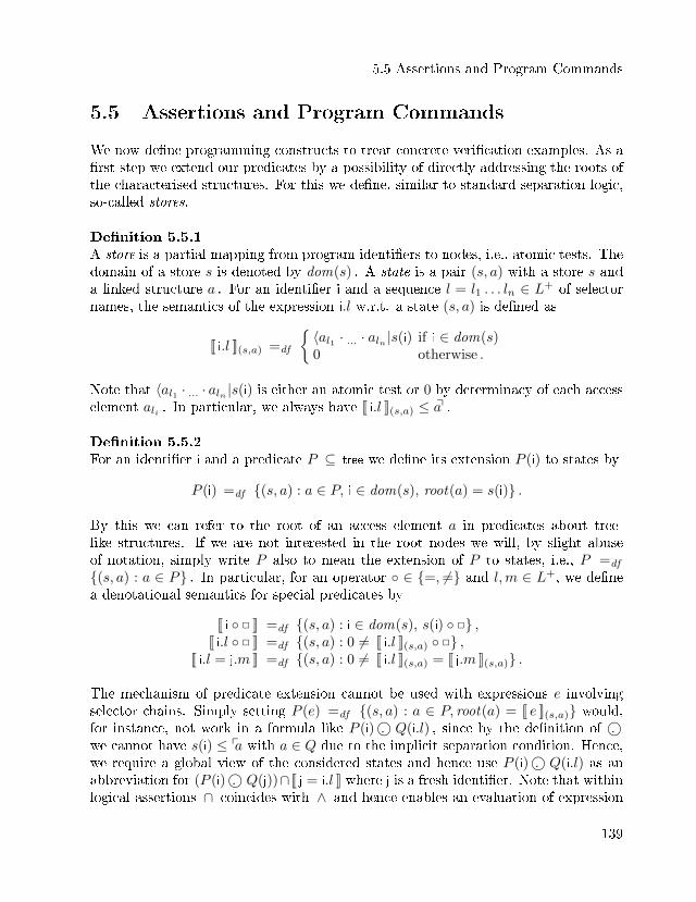
5.5 Assertions and Program Commands
5.5 Assertions and Program Commands
We now de�ne programming constructs to treat concrete veri�cation examples. As a�rst step we extend our predicates by a possibility of directly addressing the roots ofthe characterised structures. For this we de�ne, similar to standard separation logic,so-called stores.
De�nition 5.5.1A store is a partial mapping from program identi�ers to nodes, i.e., atomic tests. Thedomain of a store s is denoted by dom(s) . A state is a pair (s, a) with a store s anda linked structure a . For an identi�er i and a sequence l = l1 . . . ln ∈ L+ of selectornames, the semantics of the expression i.l w.r.t. a state (s, a) is de�ned as
[[ i.l ]](s,a) =df
{〈al1 · ... · aln |s(i) if i ∈ dom(s)0 otherwise .
Note that 〈al1 · ... · aln |s(i) is either an atomic test or 0 by determinacy of each accesselement ali . In particular, we always have [[ i.l ]](s,a) ≤ aq .
De�nition 5.5.2For an identi�er i and a predicate P ⊆ tree we de�ne its extension P (i) to states by
P (i) =df {(s, a) : a ∈ P, i ∈ dom(s), root(a) = s(i)} .
By this we can refer to the root of an access element a in predicates about tree-like structures. If we are not interested in the root nodes we will, by slight abuseof notation, simply write P also to mean the extension of P to states, i.e., P =df
{(s, a) : a ∈ P} . In particular, for an operator ◦ ∈ {=, 6=} and l,m ∈ L+, we de�nea denotational semantics for special predicates by
[[ i ◦ 2 ]] =df {(s, a) : i ∈ dom(s), s(i) ◦ 2} ,[[ i.l ◦ 2 ]] =df {(s, a) : 0 6= [[ i.l ]](s,a) ◦ 2} ,
[[ i.l = j.m ]] =df {(s, a) : 0 6= [[ i.l ]](s,a) = [[ j.m ]](s,a)} .
The mechanism of predicate extension cannot be used with expressions e involvingselector chains. Simply setting P (e) =df {(s, a) : a ∈ P, root(a) = [[ e ]](s,a)} would,for instance, not work in a formula like P (i)©. Q(i.l) , since by the de�nition of ©.we cannot have s(i) ≤ pa with a ∈ Q due to the implicit separation condition. Hence,we require a global view of the considered states and hence use P (i)©. Q(i.l) as anabbreviation for (P (i)©. Q(j))∩ [[ j = i.l ]] where j is a fresh identi�er. Note that withinlogical assertions ∩ coincides with ∧ and hence enables an evaluation of expression
139
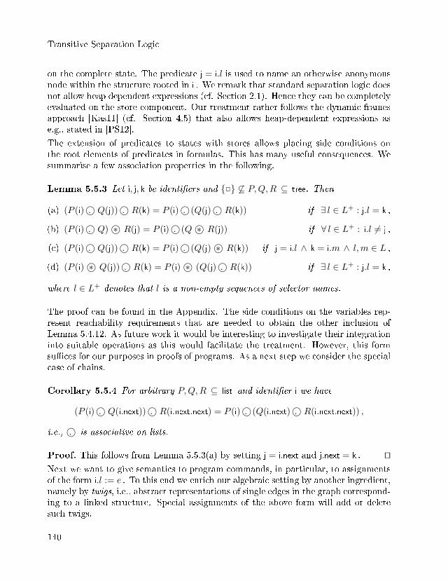
Transitive Separation Logic
on the complete state. The predicate j = i.l is used to name an otherwise anonymousnode within the structure rooted in i . We remark that standard separation logic doesnot allow heap dependent expressions (cf. Section 2.1). Hence they can be completelyevaluated on the store component. Our treatment rather follows the dynamic framesapproach [Kas11] (cf. Section 4.5) that also allows heap-dependent expressions ase.g., stated in [PS12].
The extension of predicates to states with stores allows placing side conditions onthe root elements of predicates in formulas. This has many useful consequences. Wesummarise a few association properties in the following.
Lemma 5.5.3 Let i, j, k be identi�ers and {2} 6⊆ P,Q,R ⊆ tree. Then
(a) (P (i)©. Q(j))©. R(k) = P (i)©. (Q(j)©. R(k)) if ∃ l ∈ L+ : j.l = k ,
(b) (P (i)©. Q)©∗ R(j) = P (i)©. (Q©∗ R(j)) if ∀ l ∈ L+ : i.l 6= j ,
(c) (P (i)©. Q(j))©. R(k) = P (i)©. (Q(j)©∗ R(k)) if j = i.l ∧ k = i.m ∧ l,m ∈ L ,
(d) (P (i)©∗ Q(j))©. R(k) = P (i)©∗ (Q(j)©. R(k)) if ∃ l ∈ L+ : j.l = k ,
where l ∈ L+ denotes that l is a non-empty sequences of selector names.
The proof can be found in the Appendix. The side conditions on the variables rep-resent reachability requirements that are needed to obtain the other inclusion ofLemma 5.4.12. As future work it would be interesting to investigate their integrationinto suitable operations as this would facilitate the treatment. However, this formsu�ces for our purposes in proofs of programs. As a next step we consider the specialcase of chains.
Corollary 5.5.4 For arbitrary P,Q,R ⊆ list and identi�er i we have
(P (i)©. Q(i.next))©. R(i.next.next) = P (i)©. (Q(i.next)©. R(i.next.next)) ,
i.e., ©. is associative on lists.
Proof. This follows from Lemma 5.5.3(a) by setting j = i.next and j.next = k . utNext we want to give semantics to program commands, in particular, to assignmentsof the form i.l := e . To this end we enrich our algebraic setting by another ingredient,namely by twigs, i.e., abstract representations of single edges in the graph correspond-ing to a linked structure. Special assignments of the above form will add or deletesuch twigs.
140
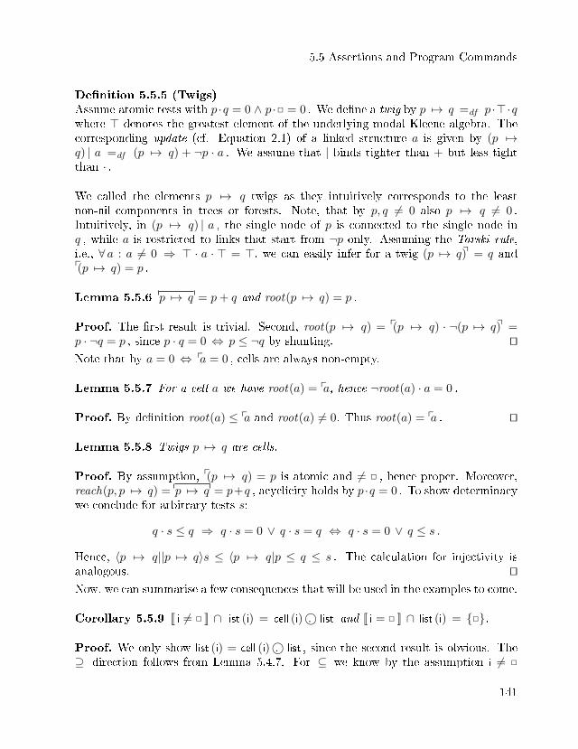
5.5 Assertions and Program Commands
De�nition 5.5.5 (Twigs)Assume atomic tests with p ·q = 0 ∧ p ·2 = 0 . We de�ne a twig by p 7→ q =df p ·>·qwhere > denotes the greatest element of the underlying modal Kleene algebra. Thecorresponding update (cf. Equation 2.1) of a linked structure a is given by (p 7→q) | a =df (p 7→ q) + ¬p · a . We assume that | binds tighter than + but less tightthan · .
We called the elements p 7→ q twigs as they intuitively corresponds to the leastnon-nil components in trees or forests. Note, that by p, q 6= 0 also p 7→ q 6= 0 .Intuitively, in (p 7→ q) | a , the single node of p is connected to the single node inq , while a is restricted to links that start from ¬p only. Assuming the Tarski rule,i.e., ∀ a : a 6= 0 ⇒ > · a · > = >, we can easily infer for a twig (p 7→ q)q = q andp(p 7→ q) = p .
Lemma 5.5.6 p 7→ q = p+ q and root(p 7→ q) = p .
Proof. The �rst result is trivial. Second, root(p 7→ q) = p(p 7→ q) · ¬(p 7→ q)q =p · ¬q = p , since p · q = 0 ⇔ p ≤ ¬q by shunting. utNote that by a = 0 ⇔ pa = 0 , cells are always non-empty.
Lemma 5.5.7 For a cell a we have root(a) = pa, hence ¬root(a) · a = 0 .
Proof. By de�nition root(a) ≤ pa and root(a) 6= 0. Thus root(a) = pa . ut
Lemma 5.5.8 Twigs p 7→ q are cells.
Proof. By assumption, p(p 7→ q) = p is atomic and 6= 2 , hence proper. Moreover,reach(p, p 7→ q) = p 7→ q = p+q , acyclicity holds by p ·q = 0 . To show determinacywe conclude for arbitrary tests s:
q · s ≤ q ⇒ q · s = 0 ∨ q · s = q ⇔ q · s = 0 ∨ q ≤ s .
Hence, 〈p 7→ q||p 7→ q〉s ≤ 〈p 7→ q|p ≤ q ≤ s . The calculation for injectivity isanalogous. utNow, we can summarise a few consequences that will be used in the examples to come.
Corollary 5.5.9 [[ i 6= 2 ]] ∩ list (i) = cell (i)©. list and [[ i = 2 ]] ∩ list (i) = {2}.
Proof. We only show list (i) = cell (i)©. list , since the second result is obvious. The⊇ - direction follows from Lemma 5.4.7. For ⊆ we know by the assumption i 6= 2
141
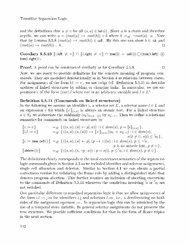
Transitive Separation Logic
and the de�nitions that a 6= 2 for all (s, a) ∈ list (i) . Since a is a chain and thereforeacyclic, we can write a = (root(a) 7→ root(b)) + b where b =df ¬root(a) · a . Notethat by Lemma 5.5.8 (root(a) 7→ root(b)) ∈ cell . By this one can show b ∈ list and(root(a) 7→ root(b)) . b . ut
Corollary 5.5.10 [[ i.left 6= 2 ]] ∩ [[ i.right 6= 2 ]] ∩ tree(i) = cell (i)©. (tree(i.left) ©∗tree(i.right)) .
Proof. A proof can be constructed similarly as for Corollary 5.5.9. utNow, we are ready to provide de�nitions for the concrete meaning of program com-mands. They are modelled denotationally as in Section 4 as relations between states.For assignments of the form i.l := e , we use twigs (cf. De�nition 5.5.5) to describeupdates of linked structures by adding or changing links. In particular, we use ex-pressions e of the form 〈var〉.l where var is an arbitrary variable and l ∈ L+ .
De�nition 5.5.11 (Commands on linked structures)In the following we assume an identi�er i , a selector set L , a selector name l ∈ L andan expression e for which [[ e ]](s,a) is always an atomic test. For a linked structurea ∈ SL we abbreviate the subfamily (ak)k∈L−{l} by aL−l . Then we de�ne a relationalsemantics for commands on linked structures by
[[ i := e ]] =df { ((s, a), (s[i← p], a)) : i ∈ dom(s), p = [[e]](s,a) } ,[[ i.l := e ]] =df { ((s, a), (s, (s(i) 7→ [[ e ]](s,a))|al + aL−l) : i ∈ dom(s),
s(i) 6= 2, s(i) ≤ pal } ,[[ i := new cell () ]] =df { ((s, a), (s[i← p], (p 7→ 2)|a) : i ∈ dom(s), p ≤ ¬pa ,
p is an atomic test, p 6= 2 } ,[[ delete (i) ]] =df { ((s, a), (s,¬p · a)) : p = s(i), p ≤ pa, i ∈ dom(s), p 6= 2 } .
The de�nitions closely corresponds to the total correctness semantics of the separationlogic commands given in Section 2.2 as we included identi�er and selector assignments,single cell allocation and deletion. Similar to Section 4.1 we can obtain a partialcorrectness version for validating the frame rule by adding a distinguished state thatdenotes program abortion. This further requires an inclusion of aborting executionsto the commands of De�nition 5.5.11 whenever the conditions involving pa or pal arenot satis�ed.
One particular di�erence to standard separation logic is that we allow assignments ofthe form i.l := j.m for identi�ers i, j and selectors l,m , i.e., a dereferencing on bothsides of the assignment operator := . In separation logic this can be mimicked by theuse of a temporal store variable. In general selector assignments do not preserve thetree structure. We provide su�cient conditions for that in the form of Hoare triplesin the next section.
142
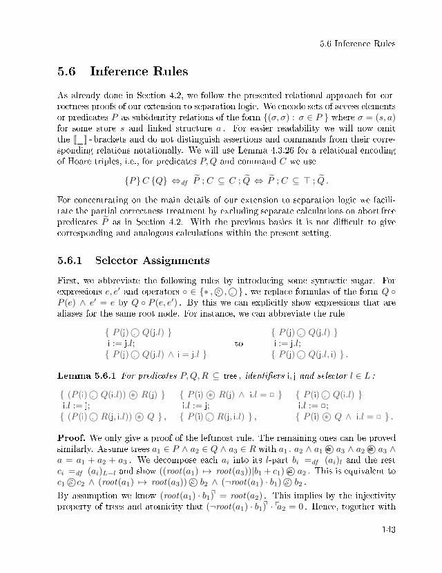
5.6 Inference Rules
5.6 Inference Rules
As already done in Section 4.2, we follow the presented relational approach for cor-rectness proofs of our extension to separation logic. We encode sets of access elementsor predicates P as subidentity relations of the form {(σ, σ) : σ ∈ P } where σ = (s, a)for some store s and linked structure a . For easier readability we will now omitthe [[_]] - brackets and do not distinguish assertions and commands from their corre-sponding relations notationally. We will use Lemma 4.3.26 for a relational encodingof Hoare triples, i.e., for predicates P,Q and command C we use
{P}C {Q} ⇔df P ; C ⊆ C ; Q ⇔ P ; C ⊆ > ; Q .
For concentrating on the main details of our extension to separation logic we facili-tate the partial correctness treatment by excluding separate calculations on abort freepredicates P as in Section 4.2. With the previous basics it is not di�cult to givecorresponding and analogous calculations within the present setting.
5.6.1 Selector Assignments
First, we abbreviate the following rules by introducing some syntactic sugar. Forexpressions e, e′ and operators ◦ ∈ {∗ ,©# ,©. } , we replace formulas of the form Q ◦P (e) ∧ e′ = e by Q ◦ P (e, e′) . By this we can explicitly show expressions that arealiases for the same root node. For instance, we can abbreviate the rule
{ P (j)©. Q(j.l) }i := j.l;{ P (j)©. Q(j.l) ∧ i = j.l }
to{ P (j)©. Q(j.l) }i := j.l;{ P (j)©. Q(j.l, i) } .
Lemma 5.6.1 For predicates P,Q,R ⊆ tree , identi�ers i, j and selector l ∈ L :
{ (P (i)©. Q(i.l))©∗ R(j) }i.l := j;{ (P (i)©. R(j, i.l))©∗ Q } ,
{ P (i)©∗ R(j) ∧ i.l = 2 }i.l := j;{ P (i)©. R(j, i.l) } ,
{ P (i)©. Q(i.l) }i.l := 2;{ P (i)©∗ Q ∧ i.l = 2 } .
Proof. We only give a proof of the leftmost rule. The remaining ones can be provedsimilarly. Assume trees a1 ∈ P ∧ a2 ∈ Q ∧ a3 ∈ R with a1 .a2 ∧ a1©# a3 ∧ a2©# a3 ∧a = a1 + a2 + a3 . We decompose each ai into its l-part bi =df (ai)l and the restci =df (ai)L−l and show ((root(a1) 7→ root(a3))|b1 + c1)©# a2 . This is equivalent toc1©# c2 ∧ (root(a1) 7→ root(a3))©# b2 ∧ (¬root(a1) · b1)©# b2 .
By assumption we know (root(a1) · b1)q = root(a2) . This implies by the injectivityproperty of trees and atomicity that (¬root(a1) · b1)q · pa2 = 0 . Hence, together with
143
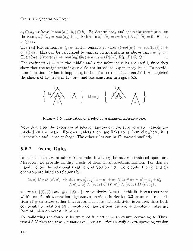
Transitive Separation Logic
a1©. a2 we have (¬root(a1) · b1)©# b2 . By determinacy and again the assumption onthe roots, a1q · pa2 = root(a2) is equivalent to b1q · pa2 = root(a2) ∧ c1q · pa2 = 0 . Hence,c1©# c2 .
The rest follows from a1©. a2 and it remains to show ((root(a1) 7→ root(a3))|b1 +c1)©. a3 . This can be calculated by similar considerations as above using a1©# a3 .Therefore, ((root(a1) 7→ root(a3))|b1) + aL−l ∈ (P (i)©. R(j, i.l))©∗ Q . utThe conjuncts i.l = 2 in the middle and right inference rules are useful, since theyshow that the assignments involved do not introduce any memory leaks. To providemore intuition of what is happening in the leftmost rule of Lemma 5.6.1, we depictedthe shapes of the trees in the pre- and postcondition in Figure 5.5.
{••i
a
i.l j •}
i.l := j
{••i
j
a
•}
Figure 5.5: Illustration of a selector assignment inference rule.
Note that after the execution of selector assignment the subtree a still resides un-touched on the heap. However, unless there are links to it from elsewhere, it isinaccessible and hence garbage. The other rules can be illustrated similarly.
5.6.2 Frame Rules
As a next step we introduce frame rules involving the newly introduced operators.Moreover, we provide validity proofs of them in an algebraic fashion. For this wemainly follow the relational treatment of Section 4.3. Concretely, the ©∗ and ©.operators are lifted to relations by
(s, a) C ◦D (s′, a′) ⇔ ∃ a1, a2, a′1, a′2 : a = a1 + a2 ∧ a1 # a2 ∧ a′ = a′1 + a′2
∧ a′1 # a′2 ∧ (s, a1) C (s′, a′1) ∧ (s, a2) D (s′, a′2) ,
where ◦ ∈ {©∗ ,©. } and # ∈ {©# , . } , respectively. Note that this �ts into a treatmentwithin multi-unit separation algebras as provided in Section 3.3 by adequate de�ni-tions of # on states rather than access elements. Cancellativity is ensured since bothcombinability relations ©# , . involve domain disjointness and + denotes an abstractform of union on access elements.
For validating the frame rules we need in particular to ensure according to Theo-rem 4.3.28 that the new commands on access relations satisfy a corresponding version
144
5.6 Inference Rules
of the frame property (cf. De�nition 4.3.16) which we can use with the compensatorH (cf. De�nition 4.3.11) , i.e.,
(safe (C)× ¬⊥) ;� ; C ⊆ (C ×H) ;� .
Lemma 5.6.2 All commands of De�nition 5.5.11 have the frame property w.r.t. ©# .
Proof. The cases for allocation and deletion are not di�cult. For simple variableassignments, only the store component is modi�ed and the argumentation is the sameas in our treatment for standard separation logic. Therefore we now concentrate onthe selector assignment i.l := e for commands C . For the reader's bene�t we repeatits non-aborting relational semantics:
{ ((s, a), (s, (s(i) 7→ [[ e ]](s,a))|al + aL−l) : i ∈ dom(s) , s(i) 6= 2 , s(i) ≤ pal } .First assume a non-aborting execution ((s, a), (s, a′l + aL−l)) of C where a′l =df
(s(i) 7→ [[ e ]](s,a))|al , [[ e ]](s,a) is atomic and the above conditions are satis�ed. More-over we assume access elements with a = ap + ar and ap©# ar where for a store s wehave that (s, ap) is safe for C . By this, there exists a transition ((s, ap), (s, bp)) of Cwhere bp =df (s(i) 7→ [[ e ]](s,ap))|(ap)l + (ap)L−l with s(i) ≤ p(ap)l .
First, we show bp©# ar . By bilinearity of ©# we have
bp©# ar ⇔ (s(i) 7→ [[ e ]](s,ap))|(ap)l ©# ar ∧ (ap)L−l ©# ar .
The second conjunct follows by downward closedness of ©# from the assumption
ap©# ar . The �rst conjunct is by Lemma 5.5.6 equivalent to (s(i) + [[ e ]](s,ap)) · ar ≤2 ∧ (¬s(i) · (ap)l) · ar ≤ 2 . Again the latter conjunct follows from downward closed-ness of ap©# ar . For the former conjunct we �rst calculate s(i) · ar ≤ pap · ar ≤ 0by ap©# ar . By De�nition 5.5.1 we infer by isotony that [[ e ]](s,ap) ≤ [[ e ]](s,a) . Since[[ e ]](s,a) is atomic both tests are equal. Hence, by the assumptions and ap©# ar we
conclude that [[ e ]](s,ap) · ar ≤ 2 .
Finally, we need to show a′l + aL−l = bp + ar . Since pap · par ≤ 0 and s(i) ≤ pap wehave (s(i) 7→ [[ e ]](s,ap))|(ap)l + (ar)l = (s(i) 7→ [[ e ]](s,ap))|al = (s(i) 7→ [[ e ]](s,a))|al .Moreover, aL−l = (ap)L−l + (ar)L−l and the claim follows. ut
Corollary 5.6.3 The ©∗ - frame rule, i.e.,
{P}C {Q}{P ©∗ R}C {Q©∗ R}
is valid for all predicates R and commands C that do not modify or reference anyidenti�er occurring in R.
145
Transitive Separation Logic
As a next step we give frame rules involving the operator ©. . The usage of thisoperation requires the inclusion of predicates that characterise forests or tree-likestructures as its combinability relation . involves the de�nition of root . For simplicitywe stay with tree structures as the rule is only required in later veri�cation examplesfor trees. However, the frame rule can also be extended to forests like the symmetricinference rule we provide afterwards. By restricting ourselves to trees we only need arestricted version of frame property, i.e.,
(tree ; safe (C) × tree ; ¬⊥) ;� ; C ⊆ (C ×H) ;� .
We call it the tree - frame property w.r.t. . . By this we conclude:
Lemma 5.6.4 Any command C of De�nition 5.5.11 has the tree - frame propertyw.r.t. . .
Proof. The proof is similar as for Lemma 5.6.2. As before we consider only the caseof selector assignments and assume a non-aborting execution ((s, a), (s, a′l + aL−l)) ofC where a′l =df (s(i) 7→ [[ e ]](s,a))|al with [[ e ]](s,a) is atomic, i ∈ dom(s) , s(i) 6= 2
and s(i) ≤ pal . Moreover we assume trees ap, ar with a = ap + ar and ap . arwhere for a store s we have that (s, ap) is safe for C . By this, there exists a transition((s, ap), (s, bp)) of C where bp =df (s(i) 7→ [[ e ]](s,ap))|(ap)l+(ap)L−l with s(i) ≤ p(ap)land atomic test [[ e ]](s,ap) .
By this, ap . ar implies s(i) · ar ≤ 0 ∧ [[ e ]](s,ap) · arq ≤ 2 ∧ [[ e ]](s,ap) · par ≤ root(ar) .
In particular, we calculate root(ar) = apq · par ≤ apq = (ap)lq + (ap)L−lq and since byassumption s(i) ≤ p(ap)l and s(i)·root(ar) ≤ 0 we can infer root(ar) ≤ (¬s(i) · (ap)l)q+(ap)L−lq . With these assumptions it is not di�cult to calculate bp . ar. Moreover therest of the claim follows by similar argumentations as in the proof of Lemma 5.6.3. utIntuitively, the calculated inequation root(ar) ≤ (¬s(i) · (ap)l)q + (ap)L−lq describesthat the root of the tree ar either remains unmodi�ed in (ap)l or is reachable viaanother selector 6= l anyway. This describes in particular the local behaviour of theselector assignments.
Corollary 5.6.5 Assume predicates P,R ⊆ tree . The ©. - frame rule, i.e.,
{P}C {Q}{P ©. R}C {Q©. R}
is valid for all predicates Q and commands C that do not modify any expressionoccurring in R and reference at most the roots of the trees in R .
146
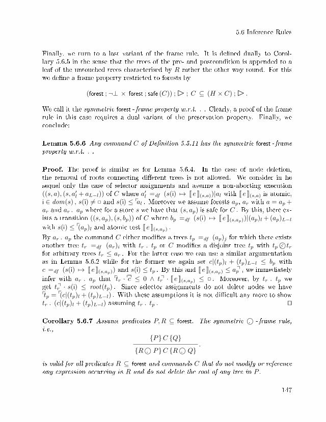
5.6 Inference Rules
Finally, we turn to a last variant of the frame rule. It is de�ned dually to Corol-lary 5.6.5 in the sense that the trees of the pre- and postcondition is appended to aleaf of the untouched trees characterised by R rather the other way round. For thiswe de�ne a frame property restricted to forests by
(forest ; ¬⊥ × forest ; safe (C)) ;� ; C ⊆ (H × C) ;� .
We call it the symmetric forest - frame property w.r.t. . . Clearly, a proof of the framerule in this case requires a dual variant of the preservation property. Finally, weconclude:
Lemma 5.6.6 Any command C of De�nition 5.5.11 has the symmetric forest - frameproperty w.r.t. . .
Proof. The proof is similar as for Lemma 5.6.4. In the case of node deletion,the removal of roots connecting di�erent trees is not allowed. We consider in hesequel only the case of selector assignments and assume a non-aborting execution((s, a), (s, a′l + aL−l)) of C where a′l =df (s(i) 7→ [[ e ]](s,a))|al with [[ e ]](s,a) is atomic,i ∈ dom(s) , s(i) 6= 2 and s(i) ≤ pal . Moreover we assume forests ap, ar with a = ap +ar and ar . ap where for a store s we have that (s, ap) is safe for C . By this, there ex-ists a transition ((s, ap), (s, bp)) of C where bp =df (s(i) 7→ [[ e ]](s,ap))|(ap)l + (ap)L−lwith s(i) ≤ p(ap)l and atomic test [[ e ]](s,ap) .
By ar . ap the command C either modi�es a trees tp =df (ap)j for which there existsanother tree tr =df (ar)i with tr . tp or C modi�es a disjoint tree tp with tp©# trfor arbitrary trees tr ≤ ar . For the latter case we can use a similar argumentationas in Lemma 5.6.2 while for the former we again set c|(tp)l + (tp)L−l ≤ bp withc =df (s(i) 7→ [[ e ]](s,ap)) and s(i) ≤ tp . By this and [[ e ]](s,ap) ≤ apq , we immediately
infer with ar . ap that ptr · c ≤ 0 ∧ trq · [[ e ]](s,ap) ≤ 2 . Moreover, by tr . tp weget trq · s(i) ≤ root(tp) . Since selector assignments do not delete nodes we haveptp = p(c|(tp)l + (tp)L−l) . With these assumptions it is not di�cult any more to showtr . (c|(tp)l + (tp)L−l) assuming tr . tp . ut
Corollary 5.6.7 Assume predicates P,R ⊆ forest. The symmetric ©. - frame rule,i.e.,
{P}C {Q}{R©. P}C {R©. Q}
.
is valid for all predicates R ⊆ forest and commands C that do not modify or referenceany expression occurring in R and do not delete the root of any tree in P .
147
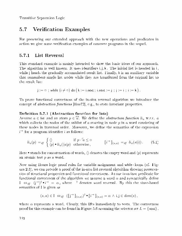
Transitive Separation Logic
5.7 Veri�cation Examples
For presenting our extended approach with the new operations and predicates inaction we give some veri�cation examples of concrete programs in the sequel.
5.7.1 List Reversal
This standard example is mainly intended to show the basic ideas of our approach.The algorithm is well known. It uses identi�ers i, j, k . The initial list is headed in i ,while j heads the gradually accumulated result list. Finally, k is an auxiliary variablethat remembers single list nodes while they are transferred from the original list tothe result list:
j := 2 ; while (i 6= 2) do(k := i.next ; i.next := j ; j := i ; i := k
).
To prove functional correctness of the in-situ reversal algorithm we introduce theconcept of abstraction functions [Hoa72], e.g., to state invariant properties.
De�nition 5.7.1 (Abstraction function for lists)Assume a ∈ list and an atom p ∈ a . We de�ne the abstraction function lia w.r.t. awhich collects the nodes of the sublist of a starting in node p in a word consisting ofthese nodes in traversal order. Moreover, we de�ne the semantics of the expressioni→ for a program identi�er i as follows:
lia(p) =df
{〈〉 if p · pa ≤ 2
〈p〉 • lia(〈a|p) otherwise ,[[ i→ ]](s,a) =df lia(s(i)) . (5.1)
Here • stands for concatenation of words, 〈〉 denotes the empty word and 〈p〉 representsan atomic test p as a word.
Now using Hoare logic proof rules for variable assignment and while - loops (cf. Fig-ure 2.3), we can provide a proof of the in-situ list reversal algorithm showing preserva-tion of structural properties and functional correctness. As our invariant predicate forfunctional correctness of the algorithm we assume a word α and syntactically de�neI ⇔df (j→)† • i→ = α , where _† denotes word reversal. By this the state-basedsemantics of I is given as
(s, a) ∈ I ⇔df ([[ j→ ]](s,a))† • [[ i→ ]](s,a) = α ∧ i, j ∈ dom(s) ,
where α represents a word. Clearly, this lifts immediately to tests. The correctnessproof for this example can be found in Figure 5.6 assuming the selector set L = {next} .
148
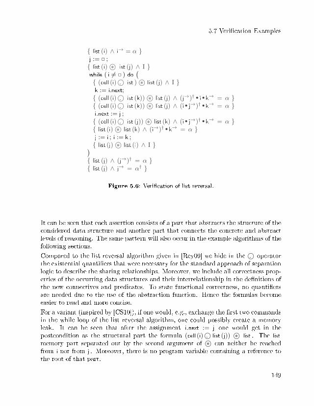
5.7 Veri�cation Examples
{ list (i) ∧ i→ = α }j := 2 ;{ list (i)©∗ list (j) ∧ I }while ( i 6= 2 ) do
(
{ (cell (i)©. list )©∗ list (j) ∧ I }k := i.next;{ (cell (i)©. list (k))©∗ list (j) ∧ (j→)† • i • k→ = α }{ (cell (i)©. list (k))©∗ list (j) ∧ (i • j→)† • k→ = α }i.next := j ;{ (cell (i)©. list (j))©∗ list (k) ∧ (i • j→)† • k→ = α }{ list (i)©∗ list (k) ∧ (i→)† • k→ = α }j := i ; i := k ;{ list (j)©∗ list (i) ∧ I })
{ list (j) ∧ (j→)† = α }{ list (j) ∧ j→ = α† }
Figure 5.6: Veri�cation of list reversal.
It can be seen that each assertion consists of a part that abstracts the structure of theconsidered data structure and another part that connects the concrete and abstractlevels of reasoning. The same pattern will also occur in the example algorithms of thefollowing sections.
Compared to the list reversal algorithm given in [Rey09] we hide in the ©. operatorthe existential quanti�ers that were necessary for the standard approach of separationlogic to describe the sharing relationships. Moreover, we include all correctness prop-erties of the occurring data structures and their interrelationship in the de�nitions ofthe new connectives and predicates. To state functional correctness, no quanti�ersare needed due to the use of the abstraction function. Hence the formulas becomeeasier to read and more concise.
For a variant (inspired by [CS10]), if one would, e.g., exchange the �rst two commandsin the while loop of the list reversal algorithm, one could possibly create a memoryleak. It can be seen that after the assignment i.next := j one would get in thepostcondition as the structural part the formula (cell (i)©. list (j)) ©∗ list . The list
memory part separated out by the second argument of ©∗ can neither be reachedfrom i nor from j . Moreover, there is no program variable containing a reference tothe root of that part.
149
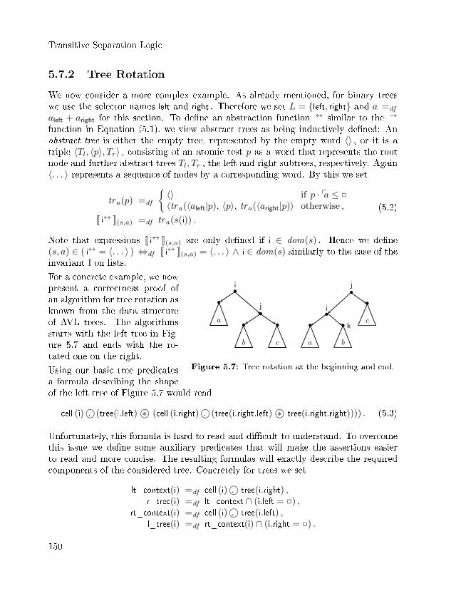
Transitive Separation Logic
5.7.2 Tree Rotation
We now consider a more complex example. As already mentioned, for binary treeswe use the selector names left and right . Therefore we set L = {left, right} and a =df
aleft + aright for this section. To de�ne an abstraction function ↔ similar to the →
function in Equation (5.1), we view abstract trees as being inductively de�ned: Anabstract tree is either the empty tree, represented by the empty word 〈〉 , or it is atriple 〈Tl, 〈p〉, Tr〉 , consisting of an atomic test p as a word that represents the rootnode and further abstract trees Tl, Tr , the left and right subtrees, respectively. Again〈. . . 〉 represents a sequence of nodes by a corresponding word. By this we set
tra(p) =df
{〈〉 if p · pa ≤ 2
〈tra(〈aleft|p), 〈p〉, tra(〈aright|p)〉 otherwise ,
[[ i↔ ]](s,a) =df tra(s(i)) .
(5.2)
Note that expressions [[ i↔ ]](s,a) are only de�ned if i ∈ dom(s) . Hence we de�ne(s, a) ∈ ( i↔ = 〈. . . 〉 ) ⇔df [[ i↔ ]](s,a) = 〈. . . 〉 ∧ i ∈ dom(s) similarly to the case of theinvariant I on lists.
a
•
i•
b
••j
c
••i
a b
j•
• c
•
• k
Figure 5.7: Tree rotation at the beginning and end.
For a concrete example, we nowpresent a correctness proof ofan algorithm for tree rotation asknown from the data structureof AVL trees. The algorithmsstarts with the left tree in Fig-ure 5.7 and ends with the ro-tated one on the right.
Using our basic tree predicatesa formula describing the shapeof the left tree of Figure 5.7 would read
cell (i)©. (tree(i.left)©∗ (cell (i.right)©. (tree(i.right.left)©∗ tree(i.right.right)))) . (5.3)
Unfortunately, this formula is hard to read and di�cult to understand. To overcomethis issue we de�ne some auxiliary predicates that will make the assertions easierto read and more concise. The resulting formulas will exactly describe the requiredcomponents of the considered tree. Concretely for trees we set
lt_context(i) =df cell (i)©. tree(i.right) ,r_tree(i) =df lt_context ∩ (i.left = 2) ,
rt_context(i) =df cell (i)©. tree(i.left) ,l_tree(i) =df rt_context(i) ∩ (i.right = 2) .
150
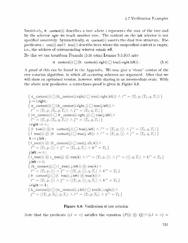
5.7 Veri�cation Examples
Intuitively, lt_context(i) describes a tree where i represents the root of the tree andby the selector right we reach another tree. The context on the left selector is notspeci�ed concretely. Symmetrically, rt_context(i) asserts the dual tree structure. Thepredicates r_tree(i) and l_tree(i) describe trees where the unspeci�ed context is empty,i.e., the address of corresponding selector equals nil .
By this we can transform Formula (5.3) using Lemma 5.5.3(c) into
rt_context(i)©. (lt_context(i.right)©. tree(i.right.left)) . (5.4)
A proof of this can be found in the Appendix. We now give a �clean� version of thetree rotation algorithm, in which all occurring subtrees are separated. After that wewill show an optimised version, however, with sharing in an intermediate state. Withthe above new predicates, a correctness proof is given in Figure 5.8.
{ rt_context(i)©. (lt_context(i.right)©. tree(i.right.left)) ∧ i↔ = 〈Tl, p, 〈Tk, q, Tr〉〉 }j := i.right ;{ rt_context(i)©. (lt_context(i.right, j)©. tree(j.left))∧i↔ = 〈Tl, p, 〈Tk, q, Tr〉〉 ∧ j↔ = 〈Tk, q, Tr〉 }{ (rt_context(i)©. lt_context(i.right, j))©. tree(j.left)∧i↔ = 〈Tl, p, 〈Tk, q, Tr〉〉 ∧ j↔ = 〈Tk, q, Tr〉 }i.right := 2 ;{ (l_tree(i)©∗ lt_context(j))©. tree(j.left) ∧ i↔ = 〈Tl, p, 〈〉〉 ∧ j↔ = 〈Tk, q, Tr〉 }{ l_tree(i)©∗ (lt_context(j)©. tree(j.left)) ∧ i↔ = 〈Tl, p, 〈〉〉 ∧ j↔ = 〈Tk, q, Tr〉 }k := j.left ;{ l_tree(i)©∗ (lt_context(j)©. tree(j.left, k))∧i↔ = 〈Tl, p, 〈〉〉 ∧ j↔ = 〈Tk, q, Tr〉 ∧ k↔ = Tk }j.left := 2 ;{ l_tree(i)©∗ r_tree(j)©∗ tree(k) ∧ i↔ = 〈Tl, p, 〈〉〉 ∧ j↔ = 〈〈〉, q, Tr〉 ∧ k↔ = Tk }j.left := i ;{ (lt_context(j)©. l_tree(i, j.left))©∗ tree(k)∧i↔ = 〈Tl, p, 〈〉〉 ∧ j↔ = 〈〈Tl, p, 〈〉〉, q, Tr〉 ∧ k↔ = Tk }{ lt_context(j)©. (l_tree(i, j.left)©∗ tree(k))∧i↔ = 〈Tl, p, 〈〉〉 ∧ j↔ = 〈〈Tl, p, 〈〉〉, q, Tr〉 ∧ k↔ = Tk }i.right := k ;{ lt_context(j)©. (rt_context(i, j.left)©. tree(k, i.right))∧j↔ = 〈〈Tl, p, Tk〉, q, Tr〉 ∧ i↔ = 〈Tl, p, Tk〉 ∧ k↔ = Tk }
Figure 5.8: Veri�cation of tree rotation.
Note that the predicate (i.l = 2) satis�es the equation (P (i) ©∗ Q) ∩ (i.l = 2) =
151
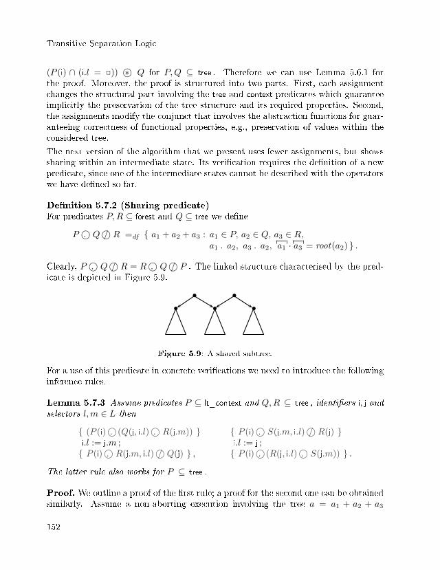
Transitive Separation Logic
(P (i) ∩ (i.l = 2)) ©∗ Q for P,Q ⊆ tree . Therefore we can use Lemma 5.6.1 forthe proof. Moreover, the proof is structured into two parts. First, each assignmentchanges the structural part involving the tree and context predicates which guaranteeimplicitly the preservation of the tree structure and its required properties. Second,the assignments modify the conjunct that involves the abstraction functions for guar-anteeing correctness of functional properties, e.g., preservation of values within theconsidered tree.
The next version of the algorithm that we present uses fewer assignments, but showssharing within an intermediate state. Its veri�cation requires the de�nition of a newpredicate, since one of the intermediate states cannot be described with the operatorswe have de�ned so far.
De�nition 5.7.2 (Sharing predicate)For predicates P,R ⊆ forest and Q ⊆ tree we de�ne
P ©. Q©/ R =df { a1 + a2 + a3 : a1 ∈ P, a2 ∈ Q, a3 ∈ R,a1 . a2, a3 . a2, a1 · a3 = root(a2) } .
Clearly, P ©. Q©/ R = R©. Q©/ P . The linked structure characterised by the pred-icate is depicted in Figure 5.9.
••
••
•
Figure 5.9: A shared subtree.
For a use of this predicate in concrete veri�cations we need to introduce the followinginference rules.
Lemma 5.7.3 Assume predicates P ⊆ lt_context and Q,R ⊆ tree , identi�ers i, j andselectors l,m ∈ L then
{ (P (i)©. (Q(j, i.l)©. R(j.m)) }i.l := j.m ;{ P (i)©. R(j.m, i.l)©/ Q(j) } ,
{ P (i)©. S(j.m, i.l)©/ R(j) }i.l := j ;{ P (i)©. (R(j, i.l)©. S(j.m)) } .
The latter rule also works for P ⊆ tree .
Proof. We outline a proof of the �rst rule; a proof for the second one can be obtainedsimilarly. Assume a non-aborting execution involving the tree a = a1 + a2 + a3
152
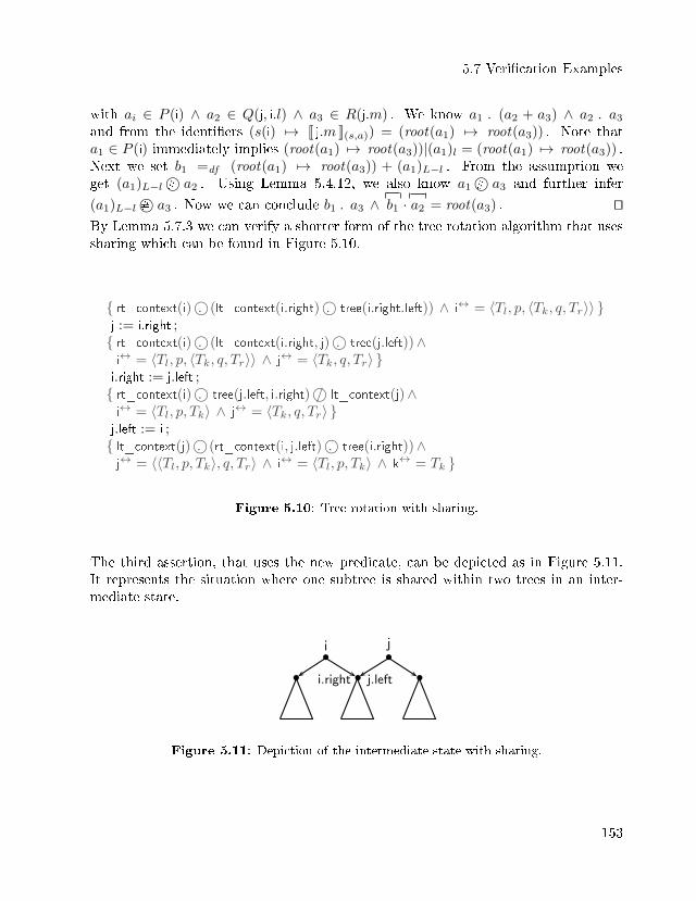
5.7 Veri�cation Examples
with ai ∈ P (i) ∧ a2 ∈ Q(j, i.l) ∧ a3 ∈ R(j.m) . We know a1 . (a2 + a3) ∧ a2 . a3
and from the identi�ers (s(i) 7→ [[ j.m ]](s,a)) = (root(a1) 7→ root(a3)) . Note thata1 ∈ P (i) immediately implies (root(a1) 7→ root(a3))|(a1)l = (root(a1) 7→ root(a3)) .Next we set b1 =df (root(a1) 7→ root(a3)) + (a1)L−l . From the assumption weget (a1)L−l©# a2 . Using Lemma 5.4.12, we also know a1©# a3 and further infer
(a1)L−l©# a3 . Now we can conclude b1 . a3 ∧ b1 · a2 = root(a3) . utBy Lemma 5.7.3 we can verify a shorter form of the tree rotation algorithm that usessharing which can be found in Figure 5.10.
{ rt_context(i)©. (lt_context(i.right)©. tree(i.right.left)) ∧ i↔ = 〈Tl, p, 〈Tk, q, Tr〉〉 }j := i.right ;{ rt_context(i)©. (lt_context(i.right, j)©. tree(j.left))∧i↔ = 〈Tl, p, 〈Tk, q, Tr〉〉 ∧ j↔ = 〈Tk, q, Tr〉 }i.right := j.left ;{ rt_context(i)©. tree(j.left, i.right)©/ lt_context(j)∧i↔ = 〈Tl, p, Tk〉 ∧ j↔ = 〈Tk, q, Tr〉 }j.left := i ;{ lt_context(j)©. (rt_context(i, j.left)©. tree(i.right))∧j↔ = 〈〈Tl, p, Tk〉, q, Tr〉 ∧ i↔ = 〈Tl, p, Tk〉 ∧ k↔ = Tk }
Figure 5.10: Tree rotation with sharing.
The third assertion, that uses the new predicate, can be depicted as in Figure 5.11.It represents the situation where one subtree is shared within two trees in an inter-mediate state.
•
i••i.right j.left
•j
•
Figure 5.11: Depiction of the intermediate state with sharing.
153
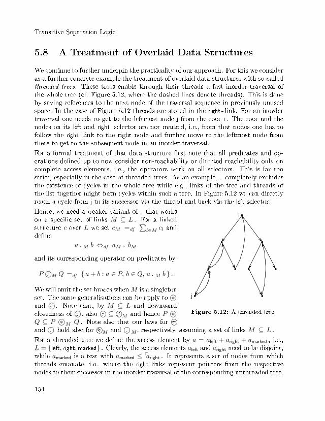
Transitive Separation Logic
5.8 A Treatment of Overlaid Data Structures
We continue to further underpin the practicality of our approach. For this we consideras a further concrete example the treatment of overlaid data structures with so-calledthreaded trees. These trees enable through their threads a fast inorder traversal ofthe whole tree (cf. Figure 5.12, where the dashed lines denote threads). This is doneby saving references to the next node of the traversal sequence in previously unusedspace. In the case of Figure 5.12 threads are stored in the right - link. For an inordertraversal one needs to get to the leftmost node j from the root i . The root and thenodes on its left and right - selector are not marked, i.e., from that nodes one has tofollow the right - link to the right node and further move to the leftmost node fromthere to get to the subsequent node in an inorder traversal.
For a formal treatment of that data structure �rst note that all predicates and op-erations de�ned up to now consider non-reachability or directed reachability only oncomplete access elements, i.e., the operators work on all selectors. This is far toostrict, especially in the case of threaded trees. As an example, . completely excludesthe existence of cycles in the whole tree while e.g., links of the tree and threads ofthe list together might form cycles within such a tree. In Figure 5.12 we can directlyreach a cycle from j to its successor via the thread and back via the left selector.
•i
• •
• • • •
•j •
Figure 5.12: A threaded tree.
Hence, we need a weaker variant of . that workson a speci�c set of links M ⊆ L . For a linkedstructure c over L we set cM =df
∑l∈M cl and
de�ne
a .M b ⇔df aM . bM
and its corresponding operator on predicates by
P ©.M Q =df { a+ b : a ∈ P, b ∈ Q, a .M b } .
We will omit the set braces whenM is a singletonset. The same generalisations can be apply to©∗and ©# . Note that, by M ⊆ L and downwardclosedness of ©# , also ©# ⊆ ©#M and hence P ©∗Q ⊆ P ©∗ M Q . Note also that our laws for ©#and ©. hold also for ©#M and ©. M , respectively, assuming a set of links M ⊆ L .
For a threaded tree we de�ne the access element by a = aleft + aright + amarked , i.e.,L = {left, right,marked} . Clearly, the access elements aleft and aright need to be disjoint,while amarked is a test with amarked ≤ paright . It represents a set of nodes from whichthreads emanate, i.e., where the right links represent pointers from the respectivenodes to their successor in the inorder traversal of the corresponding unthreaded tree.
154
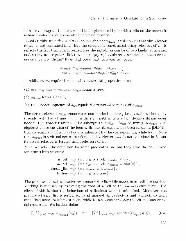
5.8 A Treatment of Overlaid Data Structures
In a �real� program this test would be implemented by marking bits on the nodes; itis here treated as an access element for uniformity.
Based on this, we de�ne a virtual access element athread ; this means that the selectorthread is not contained in L, but the element is constructed using selectors of L. Itre�ects the fact that in a threaded tree the right-links can be of two kinds: at markednodes they are �regular� links to non-empty right subtrees, whereas at non-markednodes they are �thread� links that point back to ancestor nodes:
athread =df amarked · aright + aRLm ,aRLm =df (¬amarked · aright) · a∗left · ¬paleft .
In addition, we require the following structural properties of a :
(a) aLR =df aleft + ¬amarked · aright forms a tree,
(b) athread forms a chain,
(c) the inorder sequence of aLR equals the traversal sequence of athread .
The access element aRLm connects a non-marked node x , i.e., a node without anythreads, with the leftmost node in the right subtree of x which denotes its successornode in the inorder traversal. The subexpression a∗left · ¬paleft occurring in aRLm is analgebraic representation of the loop while paleft do aleft . It has been shown in [DM01b]that determinacy of a loop body is inherited by the corresponding while loop. Notethat athread is a virtual access relation, i.e., its selector thread is not contained in L , butits access relation is formed using selectors of L .
Next, we relax the de�nition for some predicates, so that they take the new linkedstructures into account:
u_cell =df {a : aLR is a cell, amarked ≤ 0 } ,m_cell =df {a : aLR is a cell, amarked = root(a) } ,
thread_list =df {a : athread is a chain } ,lr_tree =df {a : aLR is a tree } .
The predicate u_cell characterises unmarked cells while nodes in m_cell are marked.Marking is realised by assigning the root of a cell to the marked component. Thee�ect of this is that the behaviour of a Boolean value is mimicked. Moreover, thepredicate thread_list is restricted to all marked right selectors and connections fromunmarked nodes to left-most nodes while lr_tree considers only the left and unmarkedright selectors. We further de�ne
[[ j→ ]](s,a) =df liathread(s(j)) and [[ i; ]](s,a) =df inorder(traLR(s(i))) , (5.5)
155
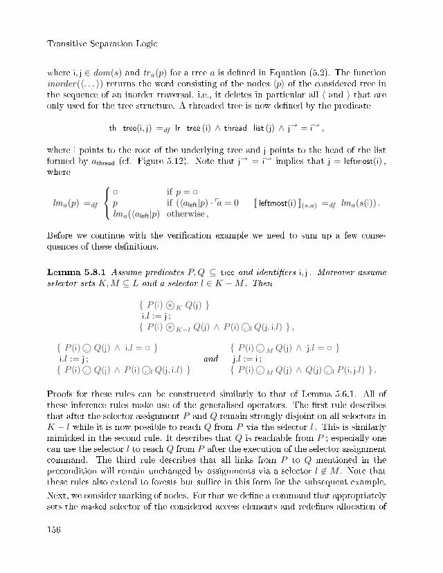
Transitive Separation Logic
where i, j ∈ dom(s) and tra(p) for a tree a is de�ned in Equation (5.2). The functioninorder(〈. . . 〉) returns the word consisting of the nodes 〈p〉 of the considered tree inthe sequence of an inorder traversal, i.e., it deletes in particular all 〈 and 〉 that areonly used for the tree structure. A threaded tree is now de�ned by the predicate
th_tree(i, j) =df lr_tree (i) ∧ thread_list (j) ∧ j→ = i; ,
where i points to the root of the underlying tree and j points to the head of the listformed by athread (cf. Figure 5.12). Note that j→ = i; implies that j = leftmost(i) ,where
lma(p) =df
2 if p = 2
p if (〈aleft|p) · pa = 0lma(〈aleft|p) otherwise ,
[[ leftmost(i) ]](s,a) =df lma(s(i)) .
Before we continue with the veri�cation example we need to sum up a few conse-quences of these de�nitions.
Lemma 5.8.1 Assume predicates P,Q ⊆ tree and identi�ers i, j . Moreover assumeselector sets K,M ⊆ L and a selector l ∈ K −M . Then
{ P (i)©∗ K Q(j) }i.l := j ;{ P (i)©∗ K−l Q(j) ∧ P (i)©. lQ(j, i.l) } ,
{ P (i)©. Q(j) ∧ i.l = 2 }i.l := j ;{ P (i)©. Q(j) ∧ P (i)©. lQ(j, i.l) }
and{ P (i)©. M Q(j) ∧ j.l = 2 }j.l := i ;{ P (i)©. M Q(j) ∧ Q(j)©. l P (i, j.l) } .
Proofs for these rules can be constructed similarly to that of Lemma 5.6.1. All ofthese inference rules make use of the generalised operators. The �rst rule describesthat after the selector assignment P and Q remain strongly disjoint on all selectors inK − l while it is now possible to reach Q from P via the selector l . This is similarlymimicked in the second rule. It describes that Q is reachable from P ; especially onecan use the selector l to reach Q from P after the execution of the selector assignmentcommand. The third rule describes that all links from P to Q mentioned in theprecondition will remain unchanged by assignments via a selector l 6∈ M . Note thatthese rules also extend to forests but su�ce in this form for the subsequent example.
Next, we consider marking of nodes. For that we de�ne a command that appropriatelysets the marked selector of the considered access elements and rede�nes allocation of
156
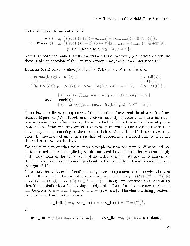
5.8 A Treatment of Overlaid Data Structures
nodes to ignore the marked selector:
mark(i) =df { ((s, a), (s, (s(i) + amarked) + aL−marked)) : i ∈ dom(s) } ,i := new cell () =df { ((s, a), (s[i← p], (p 7→ 2)|aL−marked + amarked) : i ∈ dom(s) ,
p is an atomic test, p ≤ ¬pa , p 6= 2 } .Note that both commands satisfy the frame rules of Section 5.6.2. Before we can usethem in the veri�cation of the concrete example we give further inference rules.
Lemma 5.8.2 Assume identi�ers i, j, k with i, k 6= 2 and a word α then
{ th_tree(i, j)©∗ u_cell (k) }j.left := k ;{ (lr_tree (i)©. LR u_cell (k)) ∧ thread_list (j) ∧ k • j→ = i; } ,
{ u_cell (k) }mark(k) ;{ m_cell (k) } ,
and{ (u_cell (k)©. right thread_list (j, k.right)) ∧ k • j→ = α }mark(k) ;{ (m_cell (k)©. thread thread_list (j, k.right)) ∧ k→ = α } .
These laws are direct consequences of the de�nition of mark and the abstraction func-tions in Equation (5.5). Proofs can be given similarly as before. The �rst inferencerule expresses that after making the unmarked cell in k the left subtree of j , theinorder list of the resulting overall tree now starts with k and continues with thatheaded by j . The meaning of the second rule is obvious. The third rule states thatafter the execution of mark the right - link of k represents a thread link, so that thethread list is now headed by k .
We can now give another veri�cation example to view the new predicates and op-erators in action. For simplicity, we do not treat balancing so that we can simplyadd a new node as the left subtree of the leftmost node. We assume a non-emptythreaded tree with root in i and j 6= i heading the thread list. Then we can reason asin Figure 5.13.
Note that the abstraction functions on i , j are independent of the newly allocatedcell k . Hence, as in the case of tree rotation we can infer e.g., (P ∩ (j→ = i;)) ©∗u_cell (k) = (P ©∗ u_cell (k)) ∩ (j→ = i;) . Finally, we conclude this section bysketching a similar idea for treating doubly-linked lists. An adequate access elementcan be given by a = anext + aprev with L = {next, prev} . The characterising predicatefor this data structure then reads
dl_list(i, j) =df next_list (i) ∧ prev_list (j) ∧ i→ = (←j)†,
where
next_list =df {a : anext is a chain } , prev_list =df {a : aprev is a chain } .
157
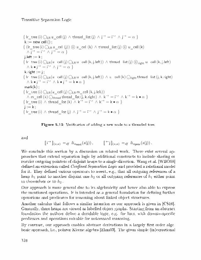
Transitive Separation Logic
{ lr_tree (i)©. LR u_cell (j) ∧ thread_list (j) ∧ j→ = i; ∧ j→ = α }k := new cell () ;{ (lr_tree (i)©. LR u_cell (j))©∗ u_cell (k) ∧ thread_list (j)©∗ u_cell (k)∧ j→ = i; ∧ j→ = α }
j.left := k ;{ lr_tree (i)©. LR(u_cell (j)©. LR u_cell (k, j.left)) ∧ thread_list (j)©∗ right u_cell (k, j.left)∧ k • j→ = i; ∧ j→ = α }
k.right := j ;{ lr_tree (i)©. LR(u_cell (j)©. LR u_cell (k, j.left)) ∧ u_cell (k)©. right thread_list (j, k.right)∧ k • j→ = i; ∧ k • j→ = k • α }
mark(k) ;{ lr_tree (i)©. LR(u_cell (j)©. LR m_cell (k, j.left))∧ m_cell (k)©. thread thread_list (j, k.right) ∧ k→ = i; ∧ k→ = k • α }{ lr_tree (i) ∧ thread_list (k) ∧ k→ = i; ∧ k→ = k • α }j := k ;{ lr_tree (i) ∧ thread_list (j) ∧ j→ = i; ∧ j→ = k • α }
Figure 5.13: Veri�cation of adding a new node to a threaded tree.
and[[ i→ ]](s,a) =df lianext(s(j)) , [[←j ]](s,a) =df liaprev(s(j)) .
We conclude this section by a discussion on related work. There exist several ap-proaches that extend separation logic by additional constructs to include sharing orrestrict outgoing pointers of disjoint heaps to a single direction. Wang et al. [WBO08]de�ned an extension called Con�ned Separation Logic and provided a relational modelfor it. They de�ned various operators to assert, e.g., that all outgoing references of aheap h1 point to another disjoint one h2 or all outgoing references of h1 either pointto themselves or to h2 .
Our approach is more general due to its algebraicity and hence also able to expressthe mentioned operations. It is intended as a general foundation for de�ning furtheroperations and predicates for reasoning about linked object structures.
Another calculus that follows a similar intention as our approach is given in [CS10].Generally, there heaps are viewed as labelled object graphs. Starting from an abstractfoundation the authors de�ne a decidable logic, e.g. for lists, with domain-speci�cpredicates and operations suitable for automated reasoning.
By contrast, our approach enables abstract derivations in a largely �rst-order alge-braic approach, i.e., pointer Kleene algebra [Ehm03]. The given simple (in)equational
158
5.8 A Treatment of Overlaid Data Structures
laws allow a direct usage of automated theorem proving systems as Prover9 [McC05]or any other systems through the TPTP Library [SS98] at the level of the under-lying resource algebra [HS08]. This supports and helpfully guides the developmentof domain speci�c predicates and operations. The assertions we have presented aresimple and still suitable for expressing shapes of linked structures without the needof any arithmetic as in [CS10]. Part of such assertions can be automatically veri�edusing Smallfoot [BCO05].
A novel approach to sharing in data structures can be found in [HV13]. This ap-proach can be directly used with arbitrary separation logics and introduces, di�eringfrom our approach, an operation called overlapping conjunction. This operator incontrast to the separating conjunction allows unspeci�ed overlapping of the resourcescharacterised by predicates. It enables impressive reasoning about sharing in combi-nation with the separating implication. However, the formulas involved unfortunatelybecome very complex and di�cult to understand. We hope that the approach of thepresent thesis can also capture complex examples like the garbage collecting algorithmgiven in [HV13] with easier and more concise formulas.
159

Chapter 6
Conclusion
A variety of algebraic calculi for separation logic has been presented. They rangefrom an algebra for the extended assertion language of separation logic to a rela-tional approach that allowed formulations of the modular behaviour of the involvedcommands. By this we further developed general and simple approaches to provethe frame and concurrency rules. In particular, we also established relationships toother similar sequential and concurrent approaches. In this chapter we summarisethe results and give some open questions for future research.
6.1 Summary
We have developed an abstraction and algebraic calculus for separation logic asser-tions. The considered denotational model for the abstractions is based on simplesets of states and allowed a further abstraction to the structure of a quantale. Bythis, pointfree characterisations of assertion classes with particular behaviour havebeen developed that yield simple proofs of central properties used in concrete veri�-cation tasks. This captures, in particular, pure, intuitionistic, precise and supportedassertions.
A further relation-based algebraic calculus for commands was introduced that allowedby simple embedding of the algebraic treatment of assertions a reuse of previouslygained results. The calculus is enriched by an extra operation on arbitrary relationsto model the separating conjunction of separation logic. The de�nitions allowed again
Conclusion
pointfree versions of central properties, i.e., safety monotonicity and the frame prop-erty, that are used for a concise soundness proof of the frame rule. This developmentalso entailed formulations for the preservation of resources as variables, which is han-dled in separation logic by meta variable side conditions. In addition to this we havepresented some further applications with relationships to concurrency and anotherapproach that also copes well with framing called the dynamic frames theory. Moreconcretely, formulations in the context of concurrent separation logic and concurrentKleene algebras have been derived.
Finally, as the last contribution of this work we developed from the formal and alge-braic foundation a transitive separation logic that introduced operations more suitablefor reasoning about reachability within linked object structures. For this we enrichedthe underlying resource algebra in terms of a modal Kleene algebra or more concretelya modal semiring that enabled an abstract characterisation of linked structures. Bythis we were able to de�ne more specialised operators, in particular for the completeexclusion of sharing within such structures and further restricting the involved links inone direction. Moreover, we presented the treatment in action by a standard exampleon lists and also more complex examples on trees and overlaid data structures likethreaded trees which involves lists and trees.
6.2 Future Work
We presented in this thesis several algebraic calculi and approaches for an abstractand general treatment of behaviours and e�ects of separation logics. In particular,the developed formalisations yield simple frameworks for the derivation of non-trivialproperties and operations that allowed a more adequate and facilitated description ofdata representations and the structure of resources. However, there are still limita-tions and open problems that deserve consideration.
As mentioned at the end of Section 3.2.5 the precising operation for supported as-sertions can be lifted to the abstract setting of quantales. A lot of properties can beproved from the given abstraction in a simple and concise fashion. Unfortunately, itwas required to adjust the algebra by axioms for the derivation of some consequenceswith the given characterisation. This poses the question whether the provided for-malisations are in this form adequate enough or if there exist another characterisationand axioms that allow a fully algebraic treatment of that assertion class. A startingpoint for these investigations can be [BV14]. In that work an extension of the relatedalgebraic approach of Boolean BI algebras is introduced that further allows the in-clusion of basic and frequently used properties of separation or resource algebras thatwas not possible with the former approach. As further investigations on this one canconsider algebraic treatments of non-discussed assertion classes as e.g., strictly exact
162
6.2 Future Work
assertions [Rey08].
In Section 4.4.2 we discussed the generalised version of separating conjunction tocharacterise concurrent non-interfering programs. The relational de�nition of separa-tion includes the extension to pairs of relations by Cartesian products that allows anindependent treatment of programs on individual parts of states. We suppose thatan extension of the de�nition of separation at this point may enable a more preciseand adequate treatment of races like in [COY07] within the relational notation. Onewould require a de�nition on pairs of commands that also includes possible interac-tions of the parallel executed programs. In particular, this might entail an equationalrelationship in [[C ‖ D ]]Γ ⊆ [[C ]]Γ ∗ [[D ]]Γ and thus possibly give a relational modelof concurrent Kleene algebras by verifying soundness of the exchange law (cf. Sec-tion 4.4.3).
Further treatments and extended approaches for the dynamic frames theory need tobe compared to our relational abstractions. This yields in particular more applicationsfor the theory and again abstractions that conversely help to guide the development offurther separation logics. We summarise a few approaches that �t into this research as,e.g., [DYDG+10] where the notion of concurrent abstract predicates is introduced thatincludes abstractions for reasoning about shared portions of storage within concurrentcontexts. Relationships to this theory would immediately relate the dynamic framestreatment also to the topic of concurrency. As similar approach is taken by �ctionalseparation logic [JB12] that de�nes on top of separation logic a meta-theory thatallows modular reasoning about data types that include sharing. Moreover it wouldbe interesting to investigate the relationships to our extension to transitive separationlogic in Chapter 5. A further research direction that deserves attention concentrateson the relationships of implicit dynamic frames, i.e., a variation to the original theorythat captures aspects of automation, to separation logic [PS11]. These results mighthelp to design and develop further investigations on relational formulations for thetheory of Section 4.5.
Finally, a general intention of the present work was to relate the earlier approach ofpointer Kleene algebra with concepts of separation logic which resulted in transitiveseparation logic. In particular, we obtained more suitable operators for reasoningabout structural data structures and their sharing relationships. As future work, itwill be interesting to explore more complex object structures and verify challenginggarbage collecting algorithms. For this standard examples in the literature are theSchorr-Waite graph marking algorithm [SW67] and further adaptations for the treat-ment of concurrent garbage collection algorithms. A derivational approach to thisis given in [PPS10] while �rst formulations towards this topic within pointer Kleenealgebra can be found in [Dan12].
163

Appendix A
Deferred Proofs and Properties
A.1 Deferred Proofs
Proof of Lemma 3.1.7. By Lemma 3.1.4 we have [[ p−∗ q ]] = [[ p ]]\[[ q ]] . Now it iseasy to see that
s, h |= p −� q
⇔ {[ de�nition of −� ]}s, h |= ¬(p−∗(¬q))
⇔ {[ de�nition of −∗ ]}¬(∀h′ : ((dom(h′) ∩ dom(h) = ∅, s, h′ |= p) ⇒ s, h′ ∪ h |= ¬q))
⇔ {[ logic: ¬ over ∀ ]}∃h′ : ¬((dom(h′) ∩ dom(h) = ∅, s, h′ |= p) ⇒ s, h′ ∪ h |= ¬q)
⇔ {[ logic: ¬(A ⇒ B) ⇔ (A ∧ ¬B) ]}∃h′ : dom(h′) ∩ dom(h) = ∅ ∧ s, h′ |= p ∧ s, h′ ∪ h 6|= ¬q
⇔ {[ logic ]}∃h′ : dom(h′) ∩ dom(h) = ∅ ∧ s, h′ |= p ∧ s, h′ ∪ h |= q
⇔ {[ setting for (⇒) h =df h′ ∪ h and for (⇐) h′ =df h− h ]}∃ h : h ⊆ h ∧ s, h− h |= p ∧ s, h |= q .
ut
Deferred Proofs and Properties
Proof of Lemma 3.2.7.
(a) The claim follows immediately from Lemma 3.2.10, (exc) and part (b).
(b) We �rst show that a = (a u 1) · > follows from both inequations. By neutralityof > and 1 w.r.t. u and · resp., assumption and isotony, we get
a = a u > = a u 1 · > ≤ (a u 1) · (a u >) ≤ (a u 1) · > .
Moreover, by isotony and assumption (au 1) · > ≤ a · > ≤ a . Next we show thata = (a u 1) · > implies a · > ≤ a and a · > ≤ a which, by part (a), implies theclaim. For the �rst inequation we calculate by assumption, > · > = > and theassumption again: a · > = (a u 1) · > · > = (a u 1) · > = a . For the secondinequation, we note that in a Boolean quantale the law t · > = (t u 1) · > holdsfor all subidentities t (t ≤ 1) (e.g. [DM01a]). From this we get
a · > = (a u 1) · > · > = (a u 1) · > · > = (a u 1) · > = (a u 1) · > = a .
(c) We show the equivalence of (au b) · c = a u b · c with part (b). First we prove the⇐ - direction and split the proof showing each inequation separately. Assumingthe distributivity property of part (b) we show ≥ by
a u b · c ≤ (a u b) · (a u c) ≤ (a u b) · c .
For the ≤ - direction we know (a u b) · c ≤ a · c ≤ a · > ≤ a which follows fromisotony and the assumption a · > ≤ a . Now, with (a u b) · c ≤ b · c we canimmediately conclude (a u b) · c ≤ a u b · c .Next we give a proof for the ⇒ - direction and assume (au b) · c = a u b · c holds.First, a · > = (a u a) · > = a u a · > ≤ a. Furthermore, we calculate
a u b · c = a u a u b · c = a u (a u b) · c = a u c · (a u b) = (a u b) · (a u c)
which follows from idempotence of u , assumption, commutativity of · and againassumption and commutativity. ut
Proof of Lemma 3.2.10. (⇐): Using Equation (Ded), isotony and the assumption,we get
a u b · c ≤ (abc u b) · c ≤ (ab> u b) · c ≤ (a u b) · c
166
A.1 Deferred Proofs
and the symmetric formula a u b · c ≤ b · (a u c) for arbitrary elements a, b, c . Now,the claim follows using idempotence of u , isotony and the above derived inequationsin
a u b · c = a u a u b · c ≤ a u (a u b) · c ≤ (a u b) · (a u c) .(⇒): By setting b = a and c = > in the distributivity law, we obtain a u a · > ≤(aua) ·(au>) = 0 ·a = 0 and hence, by (shu) a ·> ≤ a. This is equivalent to ab> ≤ ausing (exc). ut
Proof of Lemma 3.2.26.
(a) Since [[(s, h)]] is a singleton set, this is obvious.
(b) By de�nition of ∗, Part (a), h ⊆ h′ ∧ h ⊆ h′ implies h′ − h = h′ − h ⇔ h = h,and set theory:
s, h′ |= p ∗ (s, h′ − h)
⇔ ∃ h : h ⊆ h′ ∧ s, h |= p ∧ s, h′ − h |= (s, h′ − h)
⇔ ∃ h : h ⊆ h′ ∧ s, h |= p ∧ h′ − h = h′ − h⇔ ∃ h : h ⊆ h′ ∧ s, h |= p ∧ h = h⇔ s, h |= p .
(c) By de�nition of ∗ , s, h′ − h |= true is true, Part (1), and set theory:
s, h′ |= (s, h) ∗ true⇔ ∃ h : h ⊆ h′ ∧ s, h |= (s, h) ∧ s, h′ − h |= true
⇔ ∃ h : h ⊆ h′ ∧ s, h |= (s, h)
⇔ ∃ h : h ⊆ h′ ∧ h = h⇔ h ⊆ h′ .
ut
Proof of Lemma 4.3.4. For the �rst claim we calculate as follows.
(σ1, σ2) # (τ1, τ2)
⇔ {[ De�nition 4.3.3 ]}σ1 #σ2 ∧ σ1 = τ1 ∧ σ2 = τ2
⇔ {[ logic ]}σ1 #σ2 ∧ τ1 # τ2 ∧ σ1 = τ1 ∧ σ2 = τ2
167
Deferred Proofs and Properties
⇔ {[ De�nition 3.3.1 ]}σ1 #σ2 ∧ ∃σ : σ1 • σ2 = σ ∧ τ1 # τ2 ∧ ∃ τ : τ1 • τ2 = τ ∧ σ1 = τ1 ∧ σ2 = τ2
⇔ {[ σ1 = τ1 ∧ σ2 = τ2 implies σ = τ ]}∃σ : σ1 #σ2 ∧ σ1 • σ2 = σ ∧ τ1 • τ2 = σ ∧ τ1 # τ2 ∧ σ1 = τ1 ∧ σ2 = τ2
⇔ {[ logic ]}∃σ : (σ1, σ2) � σ ∧ σ� (τ1, τ2) ∧ σ1 = τ1 ∧ σ2 = τ2
⇔ {[ de�nition of ; ]}(σ1, σ2) (� ;�) (τ1, τ2) ∧ σ1 = τ1 ∧ σ2 = τ2
⇔ {[ de�nition of id ]}(σ1, σ2) (� ;� ∩ id) (τ1, τ2)
The remaining claims are immediate from the de�nitions. ut
Proof of Lemma 4.3.7. For Part (a) we have by (abortext) for arbitrary statesσ, τ :
¬(σ • τ = σ⊥) ⇔ ¬(σ = σ⊥) ∧ ¬(τ = σ⊥) .
Hence, for arbitrary states σ, τ, ρ we reason as follows
ρ (¬⊥ ;�) (σ, τ) ⇔ ¬(ρ = σ⊥) ∧ ρ � (σ, τ)⇔ ¬(ρ = σ⊥) ∧ ρ = σ • τ ∧ σ # τ⇔ ¬(σ • τ = σ⊥) ∧ ρ = σ • τ ∧ σ # τ⇔ ¬(σ = σ⊥) ∧ ¬(τ = σ⊥) ∧ ρ = σ • τ ∧ σ # τ⇔ ρ � ; (¬⊥ × ¬⊥) (σ, τ)
by the de�nitions and the above equivalence. Part (b) and (c) immediately followsfrom (abortext). ut
Proof of Lemma 4.3.10. For arbitrary σ we have
σ p(R ∗ S) σ
⇔ {[ De�nition 4.3.5 and de�nition of domain ]}∃σ1, σ2, τ1, τ2 . σ1 #σ2 ∧ σ = σ1 • σ2 ∧ τ1 # τ2 ∧ σ1 R τ1 ∧ σ2 S τ2
⇒ {[ omitting conjunct τ1 # τ2 and shifting quanti�cation over τ1, τ2 ]}∃σ1, σ2 . σ1 #σ2 ∧ σ = σ1 • σ2 ∧ ∃ τ1, τ2 . σ1 R τ1 ∧ σ2 S τ2
⇔ {[ de�nition of domain ]}∃σ1, σ2 . σ1 #σ2 ∧ σ = σ1 • σ2 ∧ σ1 pR σ1 ∧ σ2 pS σ2
⇔ {[ De�nition 4.3.5 ]}σ (pR ∗ pS) σ .
168
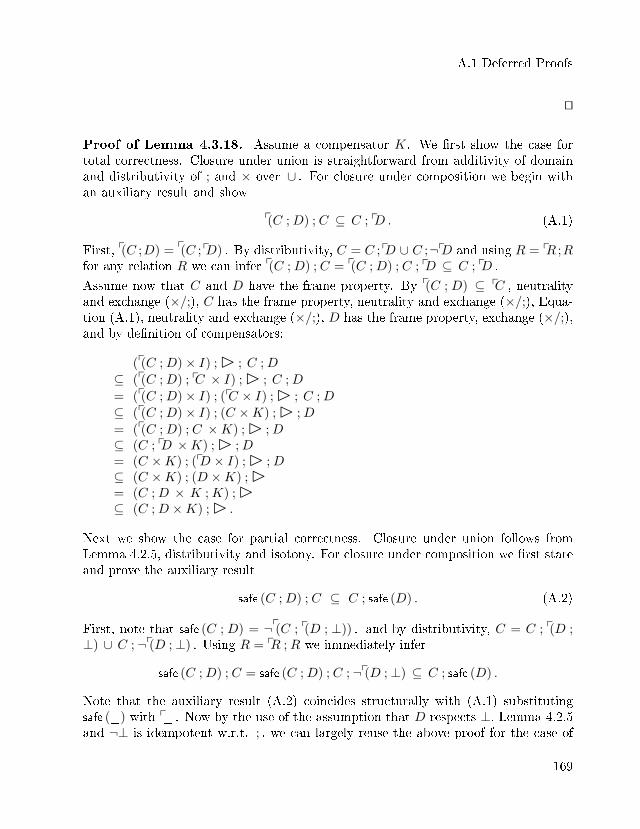
A.1 Deferred Proofs
ut
Proof of Lemma 4.3.18. Assume a compensator K. We �rst show the case fortotal correctness. Closure under union is straightforward from additivity of domainand distributivity of ; and × over ∪ . For closure under composition we begin withan auxiliary result and show
p(C ;D) ; C ⊆ C ; pD . (A.1)
First, p(C ;D) = p(C ;pD) . By distributivity, C = C ;pD ∪ C ;¬pD and using R = pR ;Rfor any relation R we can infer p(C ;D) ; C = p(C ;D) ; C ; pD ⊆ C ; pD .
Assume now that C and D have the frame property. By p(C ; D) ⊆ pC , neutralityand exchange (×/;), C has the frame property, neutrality and exchange (×/;), Equa-tion (A.1), neutrality and exchange (×/;), D has the frame property, exchange (×/;),and by de�nition of compensators:
(p(C ;D)× I) ;� ; C ;D
⊆ (p(C ;D) ; pC × I) ;� ; C ;D
= (p(C ;D)× I) ; (pC × I) ;� ; C ;D
⊆ (p(C ;D)× I) ; (C ×K) ;� ;D
= (p(C ;D) ; C ×K) ;� ;D⊆ (C ; pD ×K) ;� ;D= (C ×K) ; (pD × I) ;� ;D⊆ (C ×K) ; (D ×K) ;�= (C ;D × K ;K) ;�⊆ (C ;D ×K) ;� .
Next we show the case for partial correctness. Closure under union follows fromLemma 4.2.5, distributivity and isotony. For closure under composition we �rst stateand prove the auxiliary result
safe (C ;D) ; C ⊆ C ; safe (D) . (A.2)
First, note that safe (C ; D) = ¬p(C ; p(D ; ⊥)) . and by distributivity, C = C ; p(D ;⊥) ∪ C ; ¬p(D ;⊥) . Using R = pR ;R we immediately infer
safe (C ;D) ; C = safe (C ;D) ; C ; ¬p(D ;⊥) ⊆ C ; safe (D) .
Note that the auxiliary result (A.2) coincides structurally with (A.1) substitutingsafe (_) with p_ . Now by the use of the assumption that D respects ⊥, Lemma 4.2.5and ¬⊥ is idempotent w.r.t. ; , we can largely reuse the above proof for the case of
169
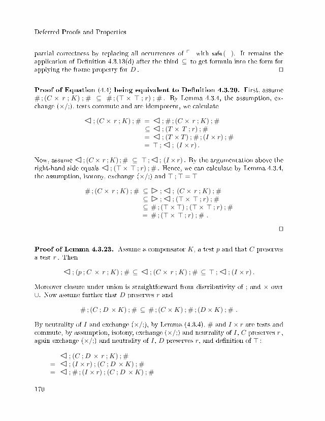
Deferred Proofs and Properties
partial correctness by replacing all occurrences of p_ with safe (_). It remains theapplication of De�nition 4.3.13(d) after the third ⊆ to get formula into the form forapplying the frame property for D . ut
Proof of Equation (4.4) being equivalent to De�nition 4.3.20. First, assume# ; (C × r ; K) ; # ⊆ # ; (> × > ; r) ; # . By Lemma 4.3.4, the assumption, ex-change (×/;), tests commute and are idempotent, we calculate
� ; (C × r ;K) ; # = � ; # ; (C × r ;K) ; #⊆ � ; (T × T ; r) ; #= � ; (T × T ) ; # ; (I × r) ; #= > ;� ; (I × r) .
Now, assume� ; (C× r ;K) ; # ⊆ > ;� ; (I × r) . By the argumentation above theright-hand side equals � ; (>× > ; r) ; # . Hence, we can calculate by Lemma 4.3.4,the assumption, isotony, exchange (×/;) and > ;> = >
# ; (C × r ;K) ; # ⊆ � ;� ; (C × r ;K) ; #⊆ � ;� ; (>× > ; r) ; #⊆ # ; (>×>) ; (>× > ; r) ; #= # ; (>× > ; r) ; # .
ut
Proof of Lemma 4.3.23. Assume a compensator K, a test p and that C preservesa test r . Then
� ; (p ; C × r ;K) ; # ⊆ � ; (C × r ;K) ; # ⊆ > ;� ; (I × r) .
Moreover closure under union is straightforward from distributivity of ; and × over∪. Now assume further that D preserves r and
# ; (C ;D ×K) ; # ⊆ # ; (C ×K) ; # ; (D ×K) ; # .
By neutrality of I and exchange (×/;), by Lemma (4.3.4), # and I × r are tests andcommute, by assumption, isotony, exchange (×/;) and neutrality of I, C preserves r ,again exchange (×/;) and neutrality of I, D preserves r, and de�nition of > :
� ; (C ;D × r ;K) ; #= � ; (I × r) ; (C ;D ×K) ; #= � ; # ; (I × r) ; (C ;D ×K) ; #
170
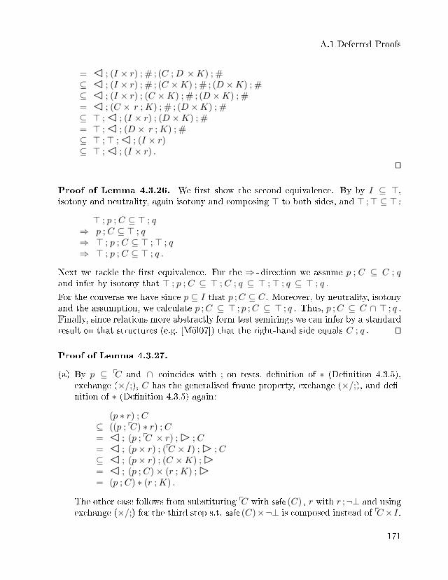
A.1 Deferred Proofs
= � ; (I × r) ; # ; (C ;D ×K) ; #⊆ � ; (I × r) ; # ; (C ×K) ; # ; (D ×K) ; #⊆ � ; (I × r) ; (C ×K) ; # ; (D ×K) ; #= � ; (C × r ;K) ; # ; (D ×K) ; #⊆ > ;� ; (I × r) ; (D ×K) ; #= > ;� ; (D × r ;K) ; #⊆ > ;> ;� ; (I × r)⊆ > ;� ; (I × r) .
ut
Proof of Lemma 4.3.26. We �rst show the second equivalence. By by I ⊆ >,isotony and neutrality, again isotony and composing > to both sides, and > ;> ⊆ > :
> ; p ; C ⊆ > ; q⇒ p ; C ⊆ > ; q⇒ > ; p ; C ⊆ > ;> ; q⇒ > ; p ; C ⊆ > ; q .
Next we tackle the �rst equivalence. For the ⇒ - direction we assume p ; C ⊆ C ; qand infer by isotony that > ; p ; C ⊆ > ; C ; q ⊆ > ;> ; q ⊆ > ; q .
For the converse we have since p ⊆ I that p ;C ⊆ C. Moreover, by neutrality, isotonyand the assumption, we calculate p ;C ⊆ > ; p ;C ⊆ > ; q . Thus, p ;C ⊆ C ∩ > ; q .Finally, since relations more abstractly form test semirings we can infer by a standardresult on that structures (e.g. [Möl07]) that the right-hand side equals C ; q . ut
Proof of Lemma 4.3.27.
(a) By p ⊆ pC and ∩ coincides with ; on tests, de�nition of ∗ (De�nition 4.3.5),exchange (×/;), C has the generalised frame property, exchange (×/;), and de�-nition of ∗ (De�nition 4.3.5) again:
(p ∗ r) ; C⊆ ((p ; pC) ∗ r) ; C= � ; (p ; pC × r) ;� ; C= � ; (p× r) ; (pC × I) ;� ; C⊆ � ; (p× r) ; (C ×K) ;�= � ; (p ; C)× (r ;K) ;�= (p ; C) ∗ (r ;K) .
The other case follows from substituting pC with safe (C) , r with r ;¬⊥ and usingexchange (×/;) for the third step s.t. safe (C)׬⊥ is composed instead of pC× I.
171
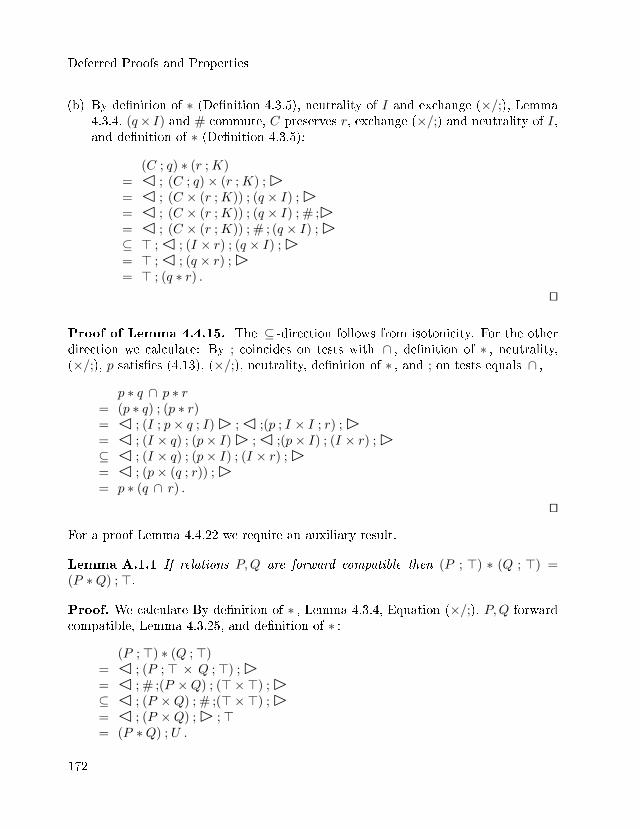
Deferred Proofs and Properties
(b) By de�nition of ∗ (De�nition 4.3.5), neutrality of I and exchange (×/;), Lemma4.3.4, (q× I) and # commute, C preserves r, exchange (×/;) and neutrality of I,and de�nition of ∗ (De�nition 4.3.5):
(C ; q) ∗ (r ;K)= � ; (C ; q)× (r ;K) ;�= � ; (C × (r ;K)) ; (q × I) ;�= � ; (C × (r ;K)) ; (q × I) ; # ;�= � ; (C × (r ;K)) ; # ; (q × I) ;�⊆ > ;� ; (I × r) ; (q × I) ;�= > ;� ; (q × r) ;�= > ; (q ∗ r) .
ut
Proof of Lemma 4.4.15. The ⊆ -direction follows from isotonicity. For the otherdirection we calculate: By ; coincides on tests with ∩ , de�nition of ∗ , neutrality,(×/;), p satis�es (4.13), (×/;), neutrality, de�nition of ∗ , and ; on tests equals ∩ ,
p ∗ q ∩ p ∗ r= (p ∗ q) ; (p ∗ r)= � ; (I ; p× q ; I)� ;� ;(p ; I × I ; r) ;�= � ; (I × q) ; (p× I)� ;� ;(p× I) ; (I × r) ;�⊆ � ; (I × q) ; (p× I) ; (I × r) ;�= � ; (p× (q ; r)) ;�= p ∗ (q ∩ r) .
ut
For a proof Lemma 4.4.22 we require an auxiliary result.
Lemma A.1.1 If relations P,Q are forward compatible then (P ; >) ∗ (Q ; >) =(P ∗Q) ;>.
Proof. We calculate By de�nition of ∗ , Lemma 4.3.4, Equation (×/;), P,Q forwardcompatible, Lemma 4.3.25, and de�nition of ∗ :
(P ;>) ∗ (Q ;>)= � ; (P ;> × Q ;>) ;�= � ; # ;(P ×Q) ; (>×>) ;�⊆ � ; (P ×Q) ; # ;(>×>) ;�= � ; (P ×Q) ;� ;>= (P ∗Q) ; U .
172
A.1 Deferred Proofs
The reverse inequation follows similarly from # ⊆ id . utFinally we are able to prove Lemma 4.4.22.
Proof of Lemma 4.4.22. First note that pP = P ; > ∩ I. The same holds for Q.By this we calculate
pP ∗ pQ = (P ;> ∩ I) ∗ (Q ;> ∩ I) ⊆ (P ;>) ∗ (Q ;>) = (P ∗Q) ;> .
Moreover pP ∗ pQ ⊆ I, since both are tests. Hence we can conclude pP ∗ pQ ⊆(P ∗Q) ; U ∩ I = p(P ∗Q) . The reverse inclusion was shown in Lemma 4.3.10. ut
The combinability check # is a test on pairs of relations. Hence, it induces someuseful closure properties that we list in the following.
Corollary A.1.2 If P,Q are forward compatible and R ⊆ P then also R,Q are for-ward compatible. This result also holds for backward compatibility, hence compatibilityis downward closed, too.
Proof. We show the following more general result: Let C,D,E be relations on pairsof states such that C is a test. If C is an invariant of D, i.e., C ; D ⊆ D ; C, andE ⊆ D then C is also an invariant of E. For this we calculate
C ; E = C ; (D ∩ E) = C ;D ∩ C ; E ⊆ D ; C ∩ C ; E =D ∩ C ; E ; C ⊆ C ; E ; C ⊆ E ; C .
The fourth step follows, since C is a test. A proof can, e.g., be found in [Möl07]. Nowthe main claim follows by setting C = #, D = P ×Q and E = R×Q . utNote that this proof extends to arbitrary test semirings.
Corollary A.1.3 If P is forward/backward compatible with Q and R then it is alsoforward/backward compatible with Q ∪R .
Proof. We show the case of forward compatibility:
# ; (P × (Q ∪R)) = # ; ((P ×Q) ∪ (P ×R)) = # ; (P ×Q) ∪ # ; (P ×R) ⊆(P ×Q) ; # ∪ (P ×R) ; # = ((P ×Q) ∪ (P ×R)) ; # = (P × (Q ∪R)) ; # .
ut
Corollary A.1.4
a) Let P,Q and R,S be forward compatible. Then also P ;R and Q ;S are forwardcompatible. Again the same holds for backward compatibility.
173
Deferred Proofs and Properties
b) If P and Q are forward/backward compatible then so are Pn and Qn for alln ∈ IN, where the n-th power of a command means n-fold sequential compositionof the command with itself. Hence also Pn ∗Qn ⊆ (P ∗Q)n .
Proof.
a) # ; (P ;R × Q ; S) = # ; (P ×Q) ; (R× S) ⊆ (P ×Q) ; # ;(R× S) ⊆(P ×Q) ; (R× S) ; # = (P ;R×Q ; S) ; # .
b) Straightforward induction on n using Part a) and the reverse exchange law. ut
Proof of Lemma 4.4.31. We set Qi = Pi ; ri and pi = pQi in Theorem 4.4.29. Thisvalidates the premise of the rule, since {pQi}Qi {ri} ⇔ pQi ;Qi ⊆ Qi ; ri ∧ pQi ⊆pQi ⇔ Qi ⊆ Qi ;ri and Qi ;ri = (Pi ;ri) ;ri = Pi ;ri = Qi . Hence, by the conclusionof the rule we get
(pQ1 ∗ pQ2) ; (Q1 ∗Q2) ⊆ (Q1 ∗Q2) ; (r1 ∗ r2) . (A.3)
Next we calculate: By de�nitions of Qi , property of domain, by Lemma 4.3.10, by(A.3), de�nitions of Qi , and by ri ⊆ I :
(P1 ; r1) ∗ (P2 ; r2) = Q1 ∗Q2 = p(Q1 ∗Q2) ; (Q1 ∗Q2) ⊆ (pQ1 ∗ pQ2) ; (Q1 ∗Q2) ⊆(Q1 ∗Q2) ; (r1 ∗ r2) = ((P1 ; r1) ∗ (P2 ; r2)) ; (r1 ∗ r2) ⊆ (P1 ∗ P2) ; (r1 ∗ r2) .
ut
Nest, we recapitulate Equation (4.9):
� ; (C × r) ; # ⊆ C ;� ; (I × r)
and say that C s-preserves a test r i� this condition is satis�ed. We list a few usefulproperties in connection with these notions.
Lemma A.1.5
(a) I s-preserves I.
(b) For any relation C and test r we have � ; (C × r) ; # ⊆ (C ∗ I) ;� ; (I × r) .
(c) If C s-preserves a test r then C ∗ r ⊆ C ; (I ∗ r) . In particular, I ∗ I ⊆ I . Henceif C s-preserves any test r then C ∗ I ⊆ C .
Proof.
174
A.1 Deferred Proofs
(a) The claim follows immediately by setting C = I = r in Equation (4.9).
(b) We calculate: By Equation (×/;), neutrality, I× r and # are tests and commute,Lemma 4.3.4, de�nition of ∗ ,
� ; (C × r) ; #= � ; (C × I) ; (I × r) ; #= � ; (C × I) ; # ; (I × r)⊆ � ; (C × I) ;� ;� ; (I × r)= (C ∗ I) ;� ; (I × r) .
(c) The �rst claim is immediate from the de�nition of locality by right-composingboth sides of the inclusion with � , isotony and the de�nition of ∗ . Hence thesecond claim is trivial by isotony. The third claim follows by setting r = I andusing I ∗ I = I .
utWe can now give the
Proof of Lemma 4.3.31. The direction (⇒) is just Lemma A.1.5(c). For (⇐) weobtain by Lemma A.1.5(b) and the assumption, for arbitrary test r ,
� ; (C × r) ; # ⊆ (C ∗ I) ;� ; (I × r) ⊆ C ;� ; (I × r) .
ut
Corollary A.1.6 C ∗ I ⊆ C ⇔ � ; (C × I) ; # ⊆ C ;� .
Proof. The direction (⇐ ) follows from composing both sides with� . For the otherdirection we immediately get by de�nition and isotony� ; (Q× I) ;� ;� ⊆ Q ;� ,since C ∗ I ⊆ C . Now the claim follows from Lemma 4.3.4 using # ⊆� ;� . ut
Proof of Lemma 4.5.7. By Theorem 4.5.3 and de�nition of ∗ , f is a test, I = I ; Iand Equation (×/;), Lemma 4.4.23, Lemma 4.3.4, Theorem 4.5.3, and de�nition of ∗ ,
∆f = � ; (f ;>× I) ;�= � ; (f ; f ;>× I) ;�= � ; (f × I) ; (f ;>× I) ;�= � ; (f × I) ; # ;(f ;>× I) ;�⊆ � ; (f × I) ;� ;� ; (f ;>× I) ;�= (f ∗ I) ; ∆f .
175
Deferred Proofs and Properties
Hence, by (reldom) we have p(∆f) ⊆ f ∗ I . For the converse we calculate f ∗ I =p(f ∗ I) ⊆ p((f ;>) ∗ I) = p(∆f) . Analogous calculations show the result for Ξf . ut
Proof of Lemma 4.5.9.
σ1p(∆f) σ1 ∧ σ1 • σ2 ∆f σ′
⇔ {[ Lemma 4.5.8 and Lemma 4.5.7 ]}σ1 f ∗ I σ1 ∧ σ1 • σ2 ∆f ∗ I σ′
⇔ {[ de�nition of ∗ ]}∃σf , σI , τ1, τ2, τ ′1. σ1 = σf • σI ∧ σf ∈ f ∧ σ1 • σ2 = τ1 • τ2∧ τ1 ∆f τ ′1 ∧ σ′ = τ ′1 • τ2
⇔ {[ Theorem 4.5.3 ]}∃σf , σI , τ1, τ2, τ ′1, τf , τ ′f , τI . σ1 = σf • σI ∧ σf ∈ f ∧σ1 • σ2 = τ1 • τ2 ∧ τ1 = τf • τI ∧ τ ′1 = τ ′f • τI ∧ τf ∈ f ∧σ′ = τ ′1 • τ2
⇒ {[ Equation (4.13) implies σf = τf , logic ]}∃σf , σI , τ1, τ2, τ ′f , τI . σ1 = σf • σI ∧ σf ∈ f ∧σ1 • σ2 = τ1 • τ2 ∧ τ1 = σf • τI ∧ σ′ = τ ′f • τI • τ2
⇒ {[ cancellativity implies σI • σ2 = τI • τ2, logic ]}∃σf , σI , τ ′f . σ1 = σf • σI ∧ σf ∈ f ∧ σ′ = (τ ′f • σI) • σ2
⇔ {[ de�nition of ; , ∗ and Theorem 4.5.3 ]}∃σ′1. σ1 ∆f σ′1 ∧ σ′ = σ′1 • σ2 .
ut
Proof of Lemma 5.2.5.
(a) First, pa ≤ reach(pa, a) by the reach induction rule from Section 5.1. Second, bya domain property, aq = (pa · a)q = 〈a|pa ≤ reach(pa, a) .
(b) For (≤) we know by diamond star induction that reach(pa, a + b) ≤ a ⇐ pa ≤a ∧ 〈(a + b)| a ≤ a . pa ≤ a holds by de�nition of , while 〈(a + b)| a ≤ aresolves by diamond distributivity to 〈a| a ≤ a ∧ 〈b| a ≤ a . Finally, the
claim holds by (a ·a)q ≤ aq and the assumption. The direction (≥) follows fromPart a, a ≤ a+ b and isotony of reach .
ut
Proof of Lemma 5.3.4. We �rst show the auxiliary result
p ≤ aq ∧ |a〉p = 0 ⇒ p = 0 . (A.4)
176
A.1 Deferred Proofs
We have, by the de�nition of diamond, full strictness of domain and since ¬aq is thegreatest right annihilator, |a〉p = 0 ⇔ p(a · p) = 0 ⇔ a · p = 0 ⇔ p ≤ ¬aq . Sinceby assumption p ≤ aq, we get p ≤ aq · ¬aq = 0 .
Now we continue with the proof of Lemma 5.3.4. Suppose aq = 0 . Then by fullstrictness also a = 0 and hence pa = 0, contradicting atomicity of pa . Hence aq 6= 0 .
Now assume p ≤ aq ∧ p 6= 0 . By Equation A.4 we have 0 6= |a〉p = p(a ·p) ≤ pa . Hence,atomicity of pa implies |a〉p = pa . Now, by de�nition of codomain and determinacy ofa ,
aq = 〈a|pa = 〈a||a〉p ≤ p ,so that altogether we have p = aq , which, by the assumptions and the de�nition ofatomicity, shows the claim. ut
Proof of Lemma 5.5.3. Assume a1 ∈ P (i) ∧ a2 ∈ Q(j) ∧ a3 ∈ R(k) and assumeai 6= 2 .
(a): We only show the ⊆ - direction, since ⊇ was already shown in Lemma 5.4.12.By the de�nitions it remains to show that (a1 + a2) . a3 ∧ a1 . a2 implies a1 . (a2 +a3) ∧ a2 . a3 . The assumption (a1 + a2) . a3 resolves to
pa1 ·a3 ≤ 0 ∧ pa2 ·a3 ≤ 0 ∧ a1q ·a3q ≤ 2 ∧ a2q ·a3q ≤ 2 ∧ a1q ·pa3+a2q ·pa3 = root(a3) . (∗)
The last conjunct implies a2q · pa3 ≤ root(a3) . Moreover, note that the side conditionof (a) implies root(a3) ≤ a2 . Hence, root(a3) = root(a3) · pa3 ≤ a2 ·pa3 = pa2 · pa3 +a2q · pa3 = a2q · pa3 and therefore root(a3) = a2q · pa3 . This shows a2 . a3, which furtherby Lemma 5.4.3 implies root(a2 + a3) = root(a2) and a1q · pa3 ≤ root(a3) . From thiswe obtain by (∗), since root(a3) 6= 2 is an atom and a1q · a2q ≤ 2 by a1 . a2 , thata1q · pa3 = 0 as well. Hence, again by a1 . a2, we obtain root(a2) = a1q · pa2 + a1q · pa3 ,which establishes a1 . (a2 + a3) .
(b): The ⊆ - direction was again shown in Lemma 5.4.12. Now assume a1 . (a2 + a3)and a2©# a3 . The side condition implies a1 ·root(a3) ≤ 0 which in turn impliesa1q · pa3 ≤ ¬root(a3) . Therefore a1 . a3 does not hold and consequently a1 . a2 anda1©# a3 need to be true by the de�nition of . for forests.
(c): We assume (a1 + a2) . a3 ∧ a1 . a2 and show a1 . (a2 + a3) ∧ a2©# a3 . As for (a),(a1+a2).a3 implies a1q ·pa3+a2q ·pa3 = root(a3) . We calculate a2q ·pa3 ≤ a2q ·root(a3) =a2q ·a1 ·root(a3) = a2q ·a1q ·root(a3) ≤ 2·pa3 ≤ 0 by assumptions and the side condition.Hence, a2 . a3 and a1q · pa3 = root(a3) which by the assumption (a1 + a2) . a3 furtherimplies a1 . a3 . Next, the reverse direction is shown by root(ai) ≤ a1 ⇒ ¬(a1©# ai) ,which in turn implies by a1 . (a2 + a3) and De�nition 5.4.4 that a1 . ai for i = 2, 3 .Now, using assumption a2 .a3 we immediately get (a1 +a2).a3 from De�nition 5.4.4again.
177
Deferred Proofs and Properties
(d): Again ⊇ was proved in Lemma 5.4.12 while ⊆ holds, since the side conditionimplies root(a3) ≤ a2 and hence a1 . a3 can not hold by a1©# a2 . Therefore byde�nition we can only have a1©# a3 ∧ a2 . a3 . Now the claim follows from bilinearityof ©# . ut
Proof of Equation (5.3) ⇔ Equation (5.4).
cell (i)©. (tree(i.left)©∗ (cell (i.right)©. (tree(i.right.left)©∗ tree(i.right.right))))
= {[ Lemma 5.5.3 (c) ]}(cell (i)©. tree(i.left))©. (cell (i.right)©. (tree(i.right.left)©∗ tree(i.right.right)))
= {[ de�nition of rt_context ]}rt_context(i)©. (cell (i.right)©. (tree(i.right.left)©∗ tree(i.right.right)))
= {[ commutativity of ©∗ ]}rt_context(i)©. (cell (i.right)©. (tree(i.right.right)©∗ tree(i.right.left)))
= {[ Lemma 5.5.3 (c) ]}rt_context(i)©. ((cell (i.right)©. tree(i.right.right))©. tree(i.right.left))
= {[ de�nition of lt_context ]}rt_context(i)©. (lt_context(i.right)©. tree(i.right.left))
The same calculation can be done for the �nal state of Figure 5.7, i.e., the equation
cell (j)©. ((cell (i, j.left)©. (tree(i.left)©∗ tree(k, i.right)))©∗ tree(j.right))
equals the following
lt_context(j)©. (rt_context(i, j.left)©. tree(k, i.right)) .
ut
A.2 Further Properties of the Assertion Calculus
We provide some theorems that characterise in particular the interplay of pure andprecise assertions in combination with residuals and detachment operators. By thiswe also demonstrate simple algebraic proofs of non-trivial properties characterisingbehaviour of assertions in separation logic.
Lemma A.2.1 If t is a test then the element t · > is pure.
178
A.2 Further Properties of the Assertion Calculus
Proof. We use the characterisation of De�nition 3.2.6 and calculate (t · > u 1) · > =t · (> u 1) · > = t · > which follows immediately from the equation (testdist). utWe now investigate the interplay between pure assertions and algebraic residuals.
Corollary A.2.2 For arbitrary elements a, b, c we have a u (b\c) ≤ (a u b)\c .
Proof. By De�nition 3.1.3, isotony and Lemma 3.1.5,
a u (b\c) ≤ (a u b)\c ⇔ (a u b) · (a u (b\c)) ≤ c⇐ b · (b\c) ≤ c⇐ c ≤ c⇔ true .
ut
Lemma A.2.3 If a is pure then for arbitrary b, c the following (in)equations hold:
(a u b)\(a u c) = (a u b)\c , (A.5)
a u (b\c) ≤ b\(a u c) , (A.6)
a u (b\c) = a u (b\(a u c)) , (A.7)
a u (b\c) = a u ((a u b)\c) , (A.8)
a u (b\c) = a u ((a u b)\(a u c)) , (A.9)
a u ((a u b)\(a u c)) ≤ b\(a u c) . (A.10)
Proof. For a proof of (A.5) we use the proof principle of indirect equality, i.e.,
x = y ⇔ (∀ z : z ≤ x ⇔ z ≤ y) .
The ⇒ - direction is obvious while for the converse we can instantiate z to x and yand hence by antisymmetry of ≤ the claim holds. Next we continue with the mainproof. By de�nition, Lemma 3.2.7(c), shunting, distributivity, a + a = >, shunting,Lemma 3.2.7(c), and de�nition:
∀x : x ≤ (a u b)\(a u c)⇔ ∀x : (a u b) · x ≤ a u c⇔ ∀x : a u b · x ≤ a u c⇔ ∀x : b · x ≤ a+ (a u c)⇔ ∀x : b · x ≤ (a+ a) u (a+ c)⇔ ∀x : a u b · x ≤ c⇔ ∀x : (a u b) · x ≤ c⇔ ∀x : x ≤ (a u b)\c .
179
Deferred Proofs and Properties
Now we give a proof of Part (A.6). By de�nition of residuals, Lemma 3.2.7(c),Lemma 3.1.5 and isotony,
a u (b\c) ≤ b\(a u c) ⇔ b · (a u (b\c)) ≤ a u c ⇔ a u (b · (b\c)) ≤ a u c ⇔ true .
The ≤ - direction of (A.7) follows immediately from (A.6) by multiplying both sidewith au and using idempotence of u . The ≥ - direction can be shown as follows: Byidempotence and isotony of u , de�nition of resdiduals, Lemma 3.2.7(c), Lemma 3.1.5,and isotony,
a u (b\(a u c)) ≤ a u (b\c)⇔ a u (b\(a u c)) ≤ b\c⇔ b · (a u (b\(a u c))) ≤ c⇔ a u (b · (b\(a u c))) ≤ c⇔ true .
Next, the ≤-direction of (A.8) follows immediately by Corollary A.2.2. By idempo-tence and isotony of u , de�nition of residuals, Lemma 3.2.7(c), and Lemma 3.1.5:
a u ((a u b)\c) ≤ a u (b\c)⇔ a u ((a u b)\c) ≤ b\c⇔ b · (a u ((a u b)\c)) ≤ c⇔ (a u b) · ((a u b)\c) ≤ c⇔ true .
Finally (A.9) follows immediately from (A.8) and (A.5) and Equation (A.10) holdsby (A.9) and (A.6). utThese laws provided frequently used theorems characterising the interplay betweenpure elements and residuals. It can be seen that all of them can be calculated in asimple and purely algebraic fashion. We now turn to detachments interacting withpure elements. This yields analogous import and export laws for detachments as inthe case of pure elements interacting with multiplication or more concretely separatingconjunction in Lemma 3.2.7(c).
Lemma A.2.4 Assume a is pure and b, c arbitrarily. Then (auc)c(aub) = cc(aub) .
Proof. The ≤ - direction follow immediately from isotony of c in its �rst argument.The other direction can be shown as follows: By (exc), de�nition of c , Booleanalgebra, shunting, Lemma 3.2.7(c), Lemma A.2.3 (A.7) and (A.9), Lemma 3.2.7(c),shunting, Boolean algebra, commutativity of · and Lemma 3.1.5,
180
A.2 Further Properties of the Assertion Calculus
cc(a u b) ≤ (a u c)c(a u b)⇔ c · (a u c)c(a u b) ≤ a u b⇔ c · ((a u c)\a u b) ≤ a u b⇔ c · ((a u c)\a u b) ≤ a+ b
⇔ a u (c · ((a u c)\a u b)) ≤ b⇔ c · (a u ((a u c)\a u b)) ≤ b⇔ c · (a u (c\a u b)) ≤ b⇔ a u (c · (c\a u b)) ≤ b⇔ c · (c\a u b) ≤ a+ b
⇔ c · (c\a u b) ≤ a u b⇔ true .
ut
Lemma A.2.5 For arbitrary b, c and pure a the inequation (a u c)c(a u b) ≤ 0 isvalid. Therefore also (a u c)c(a u b) ≤ 0 .
Proof. By (exc), Boolean algebra, Lemma 3.2.7(c), and isotony:
(a u b)b(a u c) ≤ 0
⇔ > · (a u c) ≤ a u b⇔ > · (a u c) ≤ a+ b
⇔ a u > · c ≤ a+ b⇔ true .
ut
Lemma A.2.6 For arbitrary b, c and pure a we have (a u c)cb = cc(a u b) .
Proof. By Boolean algebra, distributivity of c , Lemma A.2.5, and Lemma A.2.4:
(a u c)cb= (a u c)c((a u b) + (a u b))= ((a u c)c(a u b)) + ((a u c)c(a u b))= (a u c)c(a u b)= cc(a u b) .
ut
Lemma A.2.7 For arbitrary b, c and pure a we have a u (ccb) = cc(a u b) .
Proof. We �rst show the ≥ - direction: By (exc), Boolean algebra, distributivity,supremum splitting and isotony, isotony of · and de�nition of c , commutativity,Lemma 3.2.7(a) and Lemma 3.1.5,
181
Deferred Proofs and Properties
cc(a u b) ≤ a u (ccb)⇔ c · a u (ccb) ≤ a u b⇔ c · (a+ ccb) ≤ a+ b
⇔ (c · a) + (c · ccb) ≤ a+ b
⇐ c · a ≤ a ∧ c · ccb ≤ b⇐ > · a ≤ a ∧ c · (c\b) ≤ b⇔ true .
For the other direction we calculate: By shunting, (exc), Boolean algebra, superdis-tributivity, Lemma 3.1.5, Boolean algebra,
a u (ccb) ≤ cc(a u b)⇔ ccb ≤ cc(a u b) + a
⇔ c · cc(a u b) + a ≤ b⇔ c · ((c\a u b) u a) ≤ b⇐ c · (c\a u b) u c · a ≤ b⇐ a u b u c · a ≤ b⇔ (a u c · a) + (b u c · a) ≤ b .
Now, since a is pure, we infer a u c · a ≤ a u > · a ≤ a u a ≤ 0 and claim followsfrom isotony. ut
Corollary A.2.8 For arbitrary b, c and pure a,
a u ccb = cc(a u b) = (a u c)cb = (a u c)c(a u b) .
As a next step we give some further useful properties of precise assertions whichfacilitates calculating with them.
Lemma A.2.9 If b, c are precise and a is pure, then (a u b) + (a u c) is precise.
Proof. We assume arbitrary elements d, e ∈ S . By distributivity, Lemma 3.2.7(c)and Corollary 3.2.11, distributivity, aua = 0 , idempotence of u , b and c are precise,Lemma 3.2.7(c) and Corollary 3.2.11, and distributivity:
((a u b) + (a u c)) · d u ((a u b) + (a u c)) · e= ((a u b) · d+ (a u c) · d) u ((a u b) · e+ (a u c) · e)= (a u (b · d) + a u (c · d)) u (a u (b · e) + a u (c · e))= a u (b · d) u a u (b · e) + a u (c · d) u a u (b · e) +
a u (b · d) u a u (c · e) + a u (c · d) u a u (c · e)
182
A.2 Further Properties of the Assertion Calculus
= a u (b · d) u (b · e) + a u (c · d) u (c · e)= a u (b · (d u e)) + a u (c · (d u e))= ((a u b) · (d u e)) + ((a u c) · (d u e))= ((a u b) + (a u c)) · (d u e) .
ut
Lemma A.2.10 If a is precise then (a u b) · c u a · d = (a u b) · (c u d) for arbitraryelements b, c, d .
Proof. First, we calculate by isotony, Boolean algebra, and a is precise,
(a u b) · (c u d) u a · d ≤ a · (c u d) u a · d = a · ((c u d) u d) = 0 . (∗)
We prove the equation by showing each inequation separately. The ≤ - direction canbe shown as follows: By Boolean algebra, distributivity, by (∗), and isotony:
(a u b) · c u a · d= (((a u b) · (c u d)) + ((a u b) · (c u d))) u a · d= (((a u b) · (c u d) u a · d) + ((a u b) · (c u d) u a · d)= ((a u b) · (c u d)) u (a · d)≤ (a u b) · (c u d) .
The converse inequation follows by isotony, i.e., (aub) ·(cud) ≤ (aub) ·c u (aub) ·d ≤(a u b) · c u a · d . ut
Corollary A.2.11 If a or a′ is precise, then (au b) ·a′ u a · (a′ u c) = (au b) · (a′ u c)for all b, c .
This law characterises an interplay between · and u w.r.t. precise elements in thesense that only the subheaps that �t together, i.e., a and a u b, respectively a′ anda′ u c, remain within the intersection on the left-hand side of the above equation.
183
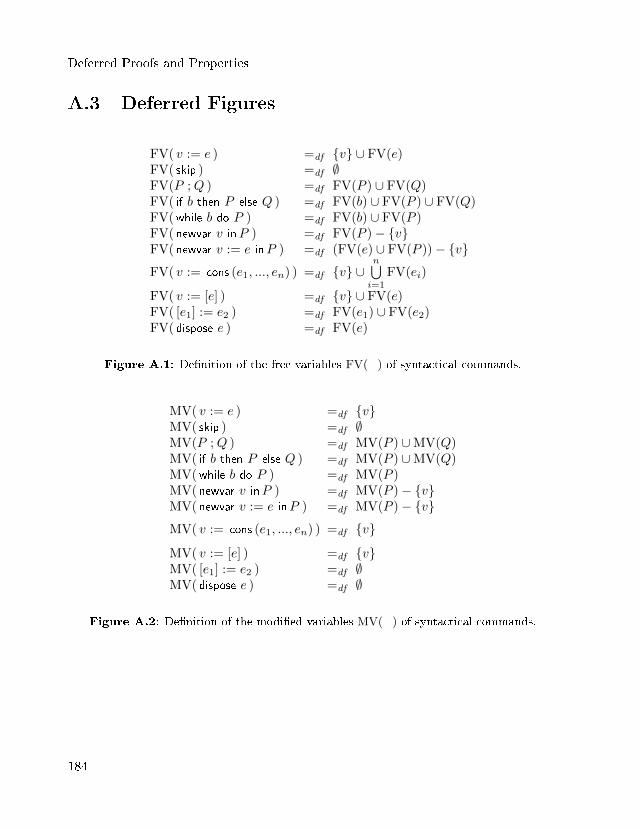
Deferred Proofs and Properties
A.3 Deferred Figures
FV( v := e ) =df {v} ∪ FV(e)FV( skip ) =df ∅FV(P ;Q ) =df FV(P ) ∪ FV(Q)FV( if b then P else Q ) =df FV(b) ∪ FV(P ) ∪ FV(Q)FV(while b do P ) =df FV(b) ∪ FV(P )FV( newvar v inP ) =df FV(P )− {v}FV( newvar v := e inP ) =df (FV(e) ∪ FV(P ))− {v}FV( v := cons (e1, ..., en) ) =df {v} ∪
n⋃i=1
FV(ei)
FV( v := [e] ) =df {v} ∪ FV(e)FV( [e1] := e2 ) =df FV(e1) ∪ FV(e2)FV( dispose e ) =df FV(e)
Figure A.1: De�nition of the free variables FV(_) of syntactical commands.
MV( v := e ) =df {v}MV( skip ) =df ∅MV(P ;Q ) =df MV(P ) ∪MV(Q)MV( if b then P else Q ) =df MV(P ) ∪MV(Q)MV(while b do P ) =df MV(P )MV( newvar v inP ) =df MV(P )− {v}MV( newvar v := e inP ) =df MV(P )− {v}MV( v := cons (e1, ..., en) ) =df {v}MV( v := [e] ) =df {v}MV( [e1] := e2 ) =df ∅MV( dispose e ) =df ∅
Figure A.2: De�nition of the modi�ed variables MV(_) of syntactical commands.
184
Bibliography
[AS12] A. Armstrong and G. Struth, Automated Reasoning in Higher-OrderRegular Algebra, Relational and Algebraic Methods in Computer Science(W. Kahl and T. G. Gri�n, eds.), Lecture Notes in Computer Science,vol. 7560, Springer-Verlag, 2012, pp. 66�81.
[ASW13a] A. Armstrong, G. Struth, and T. Weber, Kleene Algebra, Archive ofFormal Proofs, 2013.
[ASW13b] , Program Analysis and Veri�cation Based on Kleene Algebrain Isabelle/HOL, Interactive Theorem Proving (S. Blazy, C. Paulin-Mohring, and D. Pichardie, eds.), Lecture Notes in Computer Science,vol. 7998, Springer-Verlag, 2013, pp. 197�212.
[BBTS05] B. Biering, L. Birkedal, and N. Torp-Smith, BI Hyperdoctrines andHigher-Order Separation Logic, Proccedings of 14th European Sympo-sium on Programming (ESOP 2005) (S. Sagiv, ed.), Lecture Notes inComputer Science, vol. 3444, Springer-Verlag, 2005, pp. 233�247.
[BBTS07] , BI-hyperdoctrines, Higher-order Separation Logic, and Abstrac-tion, ACM Transactions on Programming Languages and Systems 29(2007), no. 5, 24.
[BCO05] J. Berdine, C. Calcagno, and P. O'Hearn, A Decidable Fragment of Sep-aration Logic, FSTTCS 2004: Foundations of Software Technology andTheoretical Computer Science 3328 (2005), 110�117.
[BCO06] J. Berdine, C. Calcagno, and P. W. O'Hearn, Smallfoot: Modular Au-tomatic Assertion Checking with Separation Logic, Formal Methods forComponents and Objects (FMCO2005) (F. de Boer, M. M. Bonsangue,S. Graf, and W. de Roever, eds.), Lecture Notes in Computer Science,vol. 4111, Springer-Verlag, 2006, pp. 115�137.
BIBLIOGRAPHY
[BCOP05] R. Bornat, C. Calcagno, P. O'Hearn, and M. Parkinson, Permission Ac-counting in Separation Logic, Proceedings of the 32nd ACM SIGPLAN-SIGACT symposium on Principles of programming languages, Principlesof Programming Languages POPL'05, ACM Press, 2005, pp. 259�270.
[BCY06] R. Bornat, C. Calcagno, and H. Yang, Variables As Resource in Sep-aration Logic, Electronic Notes on Theoretical Computer Science 155(2006), 247�276.
[BD02] M. Broy and E. Denert, Software Pioneers: Contributions to SoftwareEngineering, Springer-Verlag, 2002.
[Bie04] B. Biering, On the Logic of Bunched Implications and its Relation toSeparation Logic, Master's thesis, University of Copenhagen, 2004.
[Bir67] G. Birkho�, Lattice Theory, 3rd ed., American Mathematical Society,1967.
[BJ72] T. S. Blyth and M. F. Janowitz, Residuation Theory, Pergamon Press,1972.
[BK10] J. Brotherston and M. Kanovich, Undecidability of Propositional Sepa-ration Logic and Its Neighbours, Proceedings of the 2010 25th AnnualIEEE Symposium on Logic in Computer Science, LICS '10, IEEE Com-puter Society, 2010, pp. 130�139.
[Boy03] J. Boyland, Checking Interference with Fractional Permissions, Proceed-ings of the 10th International Conference on Static Analysis, SAS'03,Springer-Verlag, 2003, pp. 55�72.
[BP12] T. Braibant and D. Pous, Deciding Kleene Algebras in Coq, LogicalMethods in Computer Science 8 (2012), no. 1, 1�42.
[Bro07] S. Brookes, A Semantics for Concurrent Separation Logic, TheoreticalComputer Science 375 (2007), 227�270.
[Bur72] R. M. Burstall, Some Techniques for Proving Correctness of Programswhich Alter Data Structures, Machine Intelligence 7 (1972), 23�50.
[BV14] J. Brotherston and J. Villard, Parametric Completeness for SeparationTheories, Proceedings of the 41st ACM SIGPLAN-SIGACT Symposiumon Principles of Programming Languages, POPL '14, ACM Press, 2014,pp. 453�464.
186
BIBLIOGRAPHY
[BvdW93] R. C. Backhouse and J. van der Woude, Demonic Operators and Mono-type Factors, Mathematical Structures in Computer Science 3 (1993),no. 4, 417�433.
[BvW98] R.-J. Back and J. von Wright, Re�nement Calculus: A Systematic In-troduction, Graduate Texts in Computer Science, Springer-Verlag, 1998.
[CDOY09a] C. Calcagno, D. Distefano, P. O'Hearn, and H. Yang, CompositionalShape Analysis by Means of Bi-abduction, ACM SIGPLAN Notices 44(2009), no. 1, 289�300.
[CDOY09b] , Space Invading Systems Code, Logic-Based Program Synthesisand Transformation (M. Hanus, ed.), Springer-Verlag, 2009, pp. 1�3.
[CJ00] P. Collette and C. B. Jones, Enhancing the Tractability ofRely/Guarantee Speci�cations in the Development of Interfering Oper-ations, Proof, Language and Interaction (G. Plotkin, C. Stirling, andM. Tofte, eds.), MIT Press, 2000, pp. 277�307.
[Coh94] E. Cohen, Using Kleene Algebra to Reason about Concurrency Control,Tech. report, Telcordia, 1994.
[Con71] J. H. Conway, Regular Algebra and Finite Machines, Chapman & Hall,1971.
[COY07] C. Calcagno, P. W. O'Hearn, and H. Yang, Local Action and AbstractSeparation Logic, Proceedings of the 22nd Symposium on Logic in Com-puter Science, IEEE Computer Society Press, 2007, pp. 366�378.
[CS10] Y. Chen and J.-W. Sanders, Abstraction of Object Graphs in ProgramVeri�cation, Proc. of 10th Intl. Conference on Mathematics of ProgramConstruction (C. Bolduc, J. Desharnais, and B. Ktari, eds.), LectureNotes in Computer Science, vol. 6120, Springer-Verlag, 2010, pp. 80�99.
[Dan09] H.-H. Dang, Algebraic Aspects of Separation Logic, Tech. Report 2009-1,Institut für Informatik, Universität Augsburg, 2009.
[Dan12] , On the Algebraic Derivation of Garbage Collec-tors, Relational and Algebraic Methods in Computer Sci-ence � PhD Programme at RAMiCS 13 (W. Kahl andT. G. Gri�n, eds.), Technical Report, Faculty of Com-puter Science and Technology, University of Cambridge, 2012,http://www.cl.cam.ac.uk/conference/ramics13/Dang_alggarcol.pdf.
187
BIBLIOGRAPHY
[Dan14] , Abstract Dynamic Frames, Relational and Algebraic Methodsin Computer Science (RAMiCS 14) (P. Höfner, P. Jipsen, W. Kahl,and M. E. Müller, eds.), Lecture Notes in Computer Science, vol. 8428,Springer-Verlag, 2014, pp. 157�172.
[DBS+95] J. Desharnais, N. Belkhiter, S. B. M. Sghaier, F. Tchier, A. Jaoua,A. Mili, and N. Zaguia, Embedding a Demonic Semilattice in a RelationalAlgebra, Theoretical Computer Science 149 (1995), no. 2, 333�360.
[DGM+14] H.-H. Dang, R. Glück, B. Möller, P. Roocks, and A. Zelend, ExploringModal Worlds, Journal of Logic and Algebraic Programming 83 (2014),135�153.
[DH08] H.-H. Dang and P. Höfner, First-Order Theorem Prover Evaluationw.r.t. Relation- and Kleene Algebra, Relations and Kleene Algebrain Computer Science � PhD Programme at RelMiCS 10/AKA05(R. Berghammer, B. Möller, and G. Struth, eds.), Technical Report, no.2008-04, Institut für Informatik, Universität Augsburg, 2008, pp. 48�52.
[DH11] , Variable Side Conditions and Greatest Relations in AlgebraicSeparation Logic, Proceedings of the 12th international conference onRelational and Algebraic Methods in Computer Science (H. de Swart,ed.), Lecture Notes in Computer Science, vol. 6663, Springer-Verlag,2011, pp. 125�140.
[DH12] , Automated Higher-order Reasoning about Quantales, PAAR-2010: Proceedings of the 2nd Workshop on Practical As-pects of Automated Reasoning (R. A. Schmidt, S. Schulz,and B. Konev, eds.), EPiC Series, vol. 9, EasyChair, 2012,http://www.easychair.org/publications/?page=515428679, pp. 40�51.
[DHA09] R. Dockins, A. Hobor, and A. W. Appel, A Fresh Look at Separation Al-gebras and Share Accounting, Proceedings of the 7th Asian Symposiumon Programming Languages and Systems, APLAS '09, Springer-Verlag,2009, pp. 161�177.
[DHM09] H.-H. Dang, P. Höfner, and B. Möller, Towards Algebraic SeparationLogic, Relations and Kleene Algebra in Computer Science (R. Bergham-mer, A. Jaoua, and B. Möller, eds.), Lecture Notes in Computer Science,vol. 5827, Springer-Verlag, 2009, pp. 59�72.
[DHM10] , Algebraic Separation Logic, Tech. Report 2010-06, Institute ofComputer Science, University of Augsburg, 2010.
188
BIBLIOGRAPHY
[DHM11] , Algebraic Separation Logic, Journal of Logic and Algebraic Pro-gramming 80 (2011), no. 6, 221�247.
[Dij76] E. W. Dijkstra, A Discipline of Programming, Prentice Hall, 1976.
[DM01a] J. Desharnais and B. Möller, Characterizing Determinacy in Kleene Al-gebra, Information Sciences 139 (2001), 253�273.
[DM01b] , Characterizing Determinacy in Kleene Algebra (revised ver-sion), Tech. Report 2001-03, Institute of Computer Science, Universityof Augsburg, April 2001.
[DM11] H.-H. Dang and B. Möller, Simplifying Pointer Kleene Algebra, Proceed-ings of the First Workshop on Automated Theory Engineering, Wrocaw,Poland (P. Höfner, A. McIver, and G. Struth, eds.), CEUR WorkshopProceedings, vol. 760, CEUR-WS.org, 2011, pp. 20�29.
[DM12a] , Reverse Exchange for Concurrency and Local Reasoning, Math-ematics of Program Construction (J. Gibbons and P. Nogueira, eds.),Lecture Notes in Computer Science, vol. 7342, Springer-Verlag, 2012,pp. 177�197.
[DM12b] , Transitive Separation Logic, 13th International Conference onRelational and Algebraic Methods in Computer Science (RAMiCS 13)(W. Kahl and T. G. Gri�n, eds.), Lecture Notes in Computer Science,vol. 7560, Springer-Verlag, 2012, pp. 1�16.
[DM13] , Extended Transitive Separation Logic, Tech. Report 2013-07,Institut für Informatik, Universität Augsburg, 2013.
[DM14] , Concurrency and Local Reasoning under Reverse Exchange, Sci-ence of Computer Programming 85, Part B (2014), 204�223, SpecialIssue on Mathematics of Program Construction 2012.
[DMN97] J. Desharnais, A. Mili, and T. T. Nguyen, Re�nement and DemonicSemantics, Relational Methods in Computer Science (C. Brink, W. Kahl,and G. Schmidt, eds.), Springer-Verlag, 1997, pp. 166�183.
[DMS06] J. Desharnais, B. Möller, and G. Struth, Kleene Algebra with Domain,ACM Transactions on Computational Logic 7 (2006), no. 4, 798�833.
[DMT06] J. Desharnais, B. Möller, and F. Tchier, Kleene Under a Modal DemonicStar, Journal of Logic and Algebraic Programming 66 (2006), 127�160.
189
BIBLIOGRAPHY
[DYBG+13] T. Dinsdale-Young, L. Birkedal, P. Gardner, M. Parkinson, and H. Yang,Views: Compositional Reasoning for Concurrent Programs, Proceedingsof the 40th annual ACM SIGPLAN-SIGACT symposium on Principlesof programming languages, POPL '13, ACM Press, 2013, pp. 287�300.
[DYDG+10] T. Dinsdale-Young, M. Dodds, P. Gardner, M. Parkinson, andV. Vafeiadis, Concurrent Abstract Predicates, ECOOP 2010 � Object-Oriented Programming, 24th European Conference, Maribor, Slovenia,June 21-25, 2010. Proceedings (T. D'Hondt, ed.), Lecture Notes in Com-puter Science, vol. 6183, Springer-Verlag, 2010, pp. 504�528.
[Ehm01] T. Ehm, Transformational Construction of Correct Pointer Algorithms,Perspectives of System Informatics (D. Bjørner, M. Broy, and A. V.Zamulin, eds.), Lecture Notes in Computer Science, vol. 2244, Springer-Verlag, 2001, pp. 116�130.
[Ehm03] , The Kleene Algebra of Nested Pointer Structures: Theory andApplications, Ph.D. thesis, Universität Augsburg, 2003.
[Ehm04] , Pointer Kleene Algebra, RelMiCS/AKA 2003 (R. Berghammer,B. Möller, and G. Struth, eds.), Lecture Notes in Computer Science, vol.3051, Springer-Verlag, 2004, pp. 99�111.
[EKMS92] M. Erne, J. Koslowski, A. Melton, and G. E. Strecker, A Primer onGalois Connections, York Academy of Science, 1992.
[FBH97] M. F. Frias, G. Baum, and A. M. Haeberer, Fork Algebras in Algebra,Logic and Computer Science, Fundam. Inform. 32 (1997), no. 1, 1�25.
[FL79] M. J. Fischer and R. E. Ladner, Propositional Dynamic Logic of RegularPrograms, Journal of Computer and System Sciences 18 (1979), no. 2,194�211.
[GGN11] D. Garbervetsky, D. Gorín, and A. Neisen, Enforcing Structural Invari-ants using Dynamic Frames, Proceedings of the 17th Intl Conferenceon Tools and Algorithms for the Construction and Analysis of Systems,TACAS'11/ETAPS'11, Springer-Verlag, 2011, pp. 65�80.
[GLW06] D. Galmiche and D. Larchey-Wendling, Expressivity Properties ofBoolean BI Through Relational Models, Proceedings of the 26th Interna-tional Conference on Foundations of Software Technology and Theoreti-cal Computer Science, FSTTCS'06, Springer-Verlag, 2006, pp. 357�368.
190
BIBLIOGRAPHY
[HHM+11] C. A. R. Hoare, A. Hussain, B. Möller, P. W. O'Hearn, R. L. Petersen,and G. Struth, On Locality and the Exchange Law for Concurrent Pro-cesses, CONCUR 2011 (J. P. Katoen and B. König, eds.), Lecture Notesin Computer Science, vol. 6901, Springer-Verlag, 2011, pp. 250�264.
[HMSW09a] C. A. R. Hoare, B. Möller, G. Struth, and I. Wehrman, ConcurrentKleene Algebra, CONCUR 09 � Concurrency Theory (M. Bravetti andG. Zavattaro, eds.), Lecture Notes in Computer Science, vol. 5710,Springer-Verlag, 2009, pp. 399�414.
[HMSW09b] , Foundations of Concurrent Kleene Algebra, Relations andKleene Algebra in Computer Science (R. Berghammer, A. Jaoua, andB. Möller, eds.), Lecture Notes in Computer Science, vol. 5827, Springer-Verlag, 2009, pp. 166�186.
[HMSW11] C. A. R. Hoare, B. Möller, G. Struth, and I. Wehrman, ConcurrentKleene Algebra and its Foundations, Journal of Logic and AlgebraicProgramming 80 (2011), no. 6, 266�296.
[Hoa69] C. A. R. Hoare, An Axiomatic Basis for Computer Programming, Com-munications of the ACM 12 (1969), no. 10, 576�580, Reprint in [BD02].
[Hoa72] , Proofs of Correctness of Data Representations, Acta Informat-ica 1 (1972), 271�281.
[Hoa11] , An Algebra for Program Designs, Notes on Summer School inSoftware Engineering and Veri�cation in Moscow, 2011.
[Höf] P. Höfner, Database for Automated Proofs of Kleene Algabra,http://www.dcs.shef.ac.uk/∼georg/ka (accessed December 17,2014).
[Höf08] , Automated reasoning for hybrid systems � Two case studies,Relations and Kleene Algebra in Computer Science (R. Berghammer,B. Möller, and G. Struth, eds.), Lecture Notes in Computer Science,vol. 4988, Springer-Verlag, 2008, pp. 191�205.
[Höf09] , Algebraic Calculi for Hybrid Systems, Ph.D. thesis, UniversitätAugsburg, 2009.
[HS07] P. Höfner and G. Struth, Automated Reasoning in Kleene Algebra, Au-tomated Deduction � CADE-21 (F. Pfenning, ed.), Lecture Notes inArti�cial Intelligence, vol. 4603, Springer-Verlag, 2007, pp. 279�294.
191
BIBLIOGRAPHY
[HS08] , Can Re�nement be Automated?, Re�ne 2007 (E. Boiten, J. Der-rick, and G. Smith, eds.), Electronic Notes on Theoretical ComputerScience, vol. 201, Elsevier Science Publishers Ltd., 2008, pp. 197�222.
[HSS08] P. Höfner, G. Struth, and G. Sutcli�e, Automated Veri�cation of Re�ne-ment Laws, Annals of Mathematics and Arti�cial Intelligence, SpecialIssue on First-order Theorem Proving 1 (2008), 35�62.
[HV13] A. Hobor and J. Villard, The Rami�cations of Sharing in Data Struc-tures, Proceedings of the 40th Annual ACM SIGPLAN-SIGACT Sym-posium on Principles of Programming Languages (R. Giacobazzi andR. Cousot, eds.), POPL, ACM Press, 2013, pp. 523�536.
[IO01] S. Ishtiaq and P. W. O'Hearn, BI as an Assertion Language for MutableData Structures, ACM SIGPLAN Notices 36 (2001), no. 3, 14�26.
[JB12] J. B. Jensen and L. Birkedal, Fictional Separation Logic, Proceedings ofthe 21st European Conference on Programming Languages and Systems,ESOP'12, Springer-Verlag, 2012, pp. 377�396.
[JP08] B. Jacobs and F. Piessens, The VeriFast Program Veri�er, Tech. ReportCW-520, Department of Computer Science, Katholieke Universiteit Leu-ven, Belgium, 2008.
[JT51] B. Jónsson and A. Tarski, Boolean Algebras with Operators, Part I,American Journal of Mathematics 73 (1951), 891�939.
[Kas11] I. T. Kassios, The Dynamic Frames Theory, Formal Aspects of Com-puting 23 (2011), no. 3, 267�289.
[Koz94] D. Kozen, A Completeness Theorem for Kleene Algebras and the Algebraof Regular Events, Information and Computation 110 (1994), no. 2, 366�390.
[Koz97] , Kleene Algebra with Tests, ACM Transactions on ProgrammingLanguages and Systems 19 (1997), no. 3, 427�443.
[Koz00] , On Hoare Logic and Kleene Algebra with Tests, ACM Transac-tions on Computational Logic 1 (2000), no. 1, 60�76.
[Koz02] , On Hoare Logic, Kleene Algebra, and Types, In the Scope ofLogic, Methodology, and Philosophy of Science: Volume One of the 11thInt. Congress Logic, Methodology and Philosophy of Science, Cracow,August 1999 (P. Gärdenfors, J Wole«ski, and K. Kijania-Placek, eds.),
192
BIBLIOGRAPHY
Studies in Epistemology, Logic, Methodology, and Philosophy of Science,vol. 315, Kluwer Academic Publishers, 2002, pp. 119�133.
[KP00] D. Kozen and M.-C. Patron, Certi�cation of Compiler Optimizations us-ing Kleene Algebra with Tests, Proceedings of the 1st International Con-ference on Computational Logic (CL2000) (J. Lloyd, V. Dahl, U. Fur-bach, M. Kerber, K.-K. Lau, C. Palamidessi, L. Moniz Pereira, Y. Sagiv,and P. J. Stuckey, eds.), Lecture Notes in Computer Science, vol. 1861,Springer-Verlag, 2000, pp. 568�582.
[Lam68] J. Lambek, Deductive Systems and Categories I. Syntactic Calculus andResiduated Categories, Mathematical Systems Theory 2 (1968), no. 4,287�318.
[Lei10] K. Rustan M. Leino, Dafny: An Automatic Program Veri�er for Func-tional Correctness, Proceedings of the 16th Intl. Conf. on Logic for Pro-gramming, Arti�cial Intelligence, and Reasoning, Springer-Verlag, 2010,pp. 348�370.
[Mad06] R. Maddux, Relation Algebras, Studies in Logic and the Foundations ofMathematics, vol. 150, Elsevier Science Publishers Ltd., 2006.
[MB85] E. Manes and D. Benson, The Inverse Semigroup of a Sum-OrderedSemiring, Semigroup Forum 31 (1985), 129�152.
[McC05] W. McCune, Prover9 and Mace4, http://www.cs.unm.edu/∼mccune/prover9, 2005.
[MH69] J. McCarthy and P. J. Hayes, Some Philosophical Problems from theStandpoint of Arti�cial Intelligence, Machine Intelligence 4 (B. Meltzerand D. Michie, eds.), Edinburgh University Press, 1969, pp. 463�502.
[MHS06] B. Möller, P. Höfner, and G. Struth, Quantales and Temporal Log-ics, Algebraic Methodology and Software Technology (M. Johnson andV. Vene, eds.), Lecture Notes in Computer Science, vol. 4019, Springer-Verlag, 2006, pp. 263�277.
[Möl92] B. Möller, Some Applications of Pointer Algebra, Programming andMathematical Method (M. Broy, ed.), NATO ASI Series, Series F: Com-puter and Systems Sciences, no. 88, Springer-Verlag, 1992, pp. 123�155.
[Möl93a] , Derivation of Graph and Pointer Algorithms, Springer-Verlag,1993.
193
BIBLIOGRAPHY
[Möl93b] , Towards Pointer Algebra, Science of Computer Programming21 (1993), no. 1, 57�90.
[Möl97] , Calculating with Pointer Structures, Proceedings of the IFIPTC2/WG 2.1 International Workshop on Algorithmic Languages andCalculi, Chapman & Hall, 1997, pp. 24�48.
[Möl99a] , Calculating with Acyclic and Cyclic Lists, Information Sciences119 (1999), no. 3-4, 135�154.
[Möl99b] , Calculational System Design, Nato Science Series, Series F:Computer and System Sciences, vol. 173, ch. Algebraic Structures forProgram Calculation, pp. 25�97, IOS Press, 1999.
[Möl07] , Kleene Getting Lazy, Science of Computer Programming 65(2007), 195�214.
[MS06a] B. Möller and G. Struth, Algebras of Modal Operators and Partial Cor-rectness, Theoretical Computer Science 351 (2006), no. 2, 221�239.
[MS06b] , wp Is wlp, Relational Methods in Computer Science (W. Mac-Caull, M. Winter, and I. Düntsch, eds.), Lecture Notes in ComputerScience, vol. 3929, Springer-Verlag, 2006, pp. 200�211.
[Mul86] C. Mulvey, &, Rendiconti del Circolo Matematico di Palermo 12 (1986),no. 2, 99�104.
[Ngu91] T. T. Nguyen, A Relational Model of Nondeterministic Programs, Inter-national Journal on Foundations of Computer Science 2 (1991), 101�131.
[Nis06] S. Nishimura, Reasoning About Data-Parallel Pointer Programs ina Modal Extension of separation logic, Algebraic Methodology andSoftware Technology, 11th International Conference (M. Johnson andV. Vene, eds.), Lecture Notes in Computer Science, vol. 4019, Springer-Verlag, 2006, pp. 293�307.
[O'H07] P. W. O'Hearn, Resources, Concurrency, and Local Reasoning, Theoret-ical Computer Science 375 (2007), no. 1�3, 271�307.
[OP99] P. W. O'Hearn and D. J. Pym, The Logic of Bunched Implications,Bulletin of Symbolic Logic 5 (1999), no. 2, 215�244.
[ORY01] P. W. O'Hearn, J. C. Reynolds, and H. Yang, Local Reasoning aboutPrograms that Alter Data Structures, CSL '01: Proceedings of the 15th
194
BIBLIOGRAPHY
International Workshop on Computer Science Logic (L. Fribourg, ed.),Lecture Notes in Computer Science, vol. 2142, Springer-Verlag, 2001,pp. 1�19.
[ORY09] , Separation and Information Hiding, ACM Transactions on Pro-gramming Languages and Systems 31 (2009), no. 3, 1�50.
[Par10] M. Parkinson, The Next 700 Separation Logics, Veri�ed Software: The-ories, Tools, Experiments (G. T. Leavens, P. W. O'Hearn, and S. K. Ra-jamani, eds.), Lecture Notes in Computer Science, vol. 6217, Springer-Verlag, 2010, pp. 169�182.
[PB05] M. Parkinson and G. Bierman, Separation Logic and Abstraction, Pro-ceedings of the 32Nd ACM SIGPLAN-SIGACT Symposium on Princi-ples of Programming Languages, POPL '05, ACM Press, 2005, pp. 247�258.
[PBC06] M. Parkinson, R. Bornat, and C. Calcagno, Variables as Resource inHoare Logics, Proceedings of the Twenty-First Annual IEEE Symposiumon Logic in Computer Science (LICS 2006), IEEE Computer SocietyPress, 2006, pp. 137�146.
[PBO07] M. Parkinson, R. Bornat, and P. O'Hearn, Modular Veri�cation of aNon-blocking Stack, Proceedings of the 34th Annual ACM SIGPLAN-SIGACT Symposium on Principles of Programming Languages, POPL'07, ACM Press, 2007, pp. 297�302.
[Plo04] G. D. Plotkin, A Structural Approach to Operational Semantics, Journalof Logic and Algebraic Programming 60�61 (2004), 17�139.
[POY04] D. J. Pym, P. W. O'Hearn, and H. Yang, Possible Worlds and Resources:The Semantics of BI, Theoretical Computer Science 315 (2004), no. 1,257�305.
[PPS10] D. Pavlovic, P. Pepper, and D. R. Smith, Formal Derivation of Con-current Garbage Collectors, Mathematics of Program Construction(C. Bolduc, J. Desharnais, and B. Ktari, eds.), Lecture Notes in Com-puter Science, vol. 6120, Springer-Verlag, 2010, pp. 353�376.
[Pre09] V. Preoteasa, Frame Rule for Mutually Recursive Procedures Manipulat-ing Pointers, Theoretical Computer Science 410 (2009), no. 42, 4216�4233.
195
BIBLIOGRAPHY
[PS11] M. Parkinson and A. J. Summers, The Relationship Between Separa-tion Logic and Implicit Dynamic Frames, Proceedings of the 20th Eu-ropean Conference on Programming Languages and Systems: Part ofthe Joint European Conferences on Theory and Practice of Software,ESOP'11/ETAPS'11, Springer-Verlag, 2011, pp. 439�458.
[PS12] , The Relationship Between Separation Logic and Implicit Dy-namic Frames, Logical Methods in Computer Science 8 (2012), no. 3,1�54.
[Pym02] D. J. Pym, The Semantics and Proof Theory of the Logic ofBunched Implications, Applied Logic Series, no. 26, Kluwer Aca-demic Publishers, 2002, Errata and remarks (Pym 2008) main-tained at http://homepages.abdn.ac.uk/d.j.pym/pages/BI-monograph-errata.pdf.
[Rey00] J. C. Reynolds, Intuitionistic Reasoning about Shared Mutable DataStructure, Millennial Perspectives in Computer Science (J. Davies,B. Roscoe, and J. Woodcock, eds.), Palgrave, 2000, pp. 303�321.
[Rey02] , Separation Logic: A Logic for Shared Mutable Data Structures,LICS '02: Proceedings of the 17th Annual IEEE Symposium on Logicin Computer Science, IEEE Computer Society, 2002, pp. 55�74.
[Rey08] , Lecture Notes for the First Phd Fall School on Logics and Se-mantics of state, 2008, http://www.cs.cmu.edu/∼jcr/copenhagen08.pdf.
[Rey09] , An Introduction to Separation Logic, In Engineering Methodsand Tools for Software Safety and Security (M. Broy, ed.), IOS Press,2009, pp. 285�310.
[RG08] M. Raza and P. Gardner, Footprints in Local Reasoning, Foundationsof Software Science and Computational Structures (R. Amadio, ed.),Lecture Notes in Computer Science, vol. 4962, Springer-Verlag, 2008,pp. 201�215.
[Ros90] K. I. Rosenthal, Quantales and their Applications, Pitman ResearchNotes in Mathematics Series, vol. 234, Longman Scienti�c & Technical,1990.
[Sim06] E.-J. Sims, Extending Separation Logic with Fixpoints and PostponedSubstitution, Theoretical Computer Science 351 (2006), no. 2, 258�275.
196
BIBLIOGRAPHY
[SJP09] J. Smans, B. Jacobs, and F. Piessens, Implicit Dynamic Frames: Com-bining Dynamic Frames and Separation Logic, Proc of the 23rd Euro-pean Conf. on ECOOP, Genoa, Springer-Verlag, 2009, pp. 148�172.
[SS93] G. Schmidt and T. Ströhlein, Relations and Graphs: Discrete Mathe-matics for Computer Scientists, Springer-Verlag, 1993.
[SS98] G. Sutcli�e and C.B. Suttner, The TPTP Problem Library: CNF releasev1.2.1, Journal of Automated Reasoning 21 (1998), no. 2, 177�203.
[Str07] G. Struth, Reasoning Automatically about Termination and Re�nement,6th International Workshop on First-Order Theorem Proving (S. Ranise,ed.), vol. Technical Report ULCS-07-018, Department of Computer Sci-ence, University of Liverpool, 2007, pp. 36�51.
[SW67] H. Schorr and W. M. Waite, An E�cient Machine-independent Proce-dure for Garbage Collection in Various List Structures, Communicationsof the ACM 10 (1967), no. 8, 501�506.
[Tar55] A. Tarski, A Lattice-theoretical Fixpoint Theorem and its Applications,Paci�c Journal of Mathematics 5 (1955), no. 2, 285�309.
[TBY12] J. Thamsborg, L. Birkedal, and H. Yang, Two for the Price of One: Lift-ing Separation Logic Assertions, Logical Methods in Computer Science8 (2012), no. 3:22, 1�31.
[TKN07] H. Tuch, G. Klein, and M. Norrish, Types, Bytes, and Separation logic,POPL '07: Proceedings of the 34th Annual ACM SIGPLAN-SIGACTSymposium on Principles of Programming Languages, ACM Press, 2007,pp. 97�108.
[TSBR08] N. Torp-Smith, L. Birkedal, and J. C. Reynolds, Local Reasoning abouta Copying Garbage Collector, ACM Transactions on Programming Lan-guages and Systems 30 (2008), no. 4, 24:1�24:58.
[Tue08] T. Tuerk, A Separation Logic Framework in HOL, Tech. Report 2008-1-Ait Mohamed, Department of Electrical Computer Engineering, Con-cordia University, 2008.
[Vaf11] V. Vafeiadis, Concurrent Separation Logic and Operational Semantics,Electronic Notes on Theoretical Computer Science 276 (2011), 335�351.
[VK98] B. Von Karger, Temporal Algebra, Mathematical Structures in ComputerScience 8 (1998), no. 3, 277�320.
197
BIBLIOGRAPHY
[VP07] V. Vafeiadis and M. J. Parkinson, A Marriage of Rely/Guarantee andSeparation logic, CONCUR 2007 - Concurrency Theory, 18th Inter-national Conference, Lecture Notes in Computer Science, vol. 4703,Springer-Verlag, 2007, pp. 256�271.
[WBO08] S. Wang, L.-S. Barbosa, and J.-N. Oliveira, A Relational Model for Con-�ned Separation Logic, Proc. of the 2nd IFIP/IEEE Intl. Symposium onTheoretical Aspects of Software Engineering, TASE '08, IEEE ComputerSociety Press, 2008, pp. 263�270.
[WHO09] I. Wehrman, C. A. R. Hoare, and P. W. O'Hearn, Graphical Models ofSeparation Logic, Information Processing Letters 109 (2009), no. 17,1001�1004.
[Win07] M. Winter, Goguen Categories: A Categorical Approach to L-fuzzy Re-lations, 1st ed., Springer Publishing Company, Incorporated, 2007.
[Yan01] H. Yang, An Example of Local Reasoning in BI Pointer Logic: TheSchorr-Waite Graph Marking Algorithm, SPACE 2001: Informal pro-ceedings of Workshop on Semantics, Program Analysis and Comput-ing Environments for Memory Management (F. Henglein, J. Hughes,H. Makholm, and H. Niss, eds.), 2001, pp. 41�68.
[Yan07] , Relational Separation Logic, Theoretical Computer Science 375(2007), no. 1�3, 308�334.
[YLB+08] H. Yang, O. Lee, J. Berdine, C. Calcagno, B. Cook, D. Distefano, andP. O'Hearn, Scalable Shape Analysis for Systems Code, Computer AidedVeri�cation, 20th International Conference (A. Gupta and S. Malik,eds.), Lecture Notes in Computer Science, vol. 5123, Springer-Verlag,2008, pp. 385�398.
[YO02] H. Yang and P. W. O'Hearn, A Semantic Basis for Local Reasoning,Foundations of Software Science and Computation Structures, Proceed-ings FOSSACS 2002 (M. Nielsen and U. Engberg, eds.), Lecture Notesin Computer Science, vol. 2303, Springer-Verlag, 2002, pp. 402�416.
198
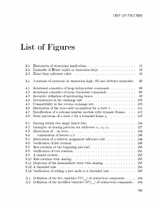
LIST OF FIGURES
List of Figures
2.1 Illustration of separating implication. . . . . . . . . . . . . . . . . . . . 152.2 Examples of Hoare triples in separation logic. . . . . . . . . . . . . . . 192.3 Hoare logic inference rules. . . . . . . . . . . . . . . . . . . . . . . . . 19
3.1 Notations of operators in separation logic, AS and abstract quantales. 30
4.1 Relational semantics of heap-independent commands. . . . . . . . . . . 594.2 Relational semantics of heap-dependent commands. . . . . . . . . . . . 604.3 Recursive de�nition of interleaving traces. . . . . . . . . . . . . . . . . 884.4 Dependencies in the exchange law. . . . . . . . . . . . . . . . . . . . . 1004.5 Compatibility in the reverse exchange law. . . . . . . . . . . . . . . . . 1034.6 Illustration of the cross-split assumption for a state σ . . . . . . . . . . 1114.7 Speci�cation of a rational number module with dynamic frames. . . . 1124.8 State partitions of a state σ for a bounded frame g . . . . . . . . . . . 118
5.1 Sharing within two singly linked lists. . . . . . . . . . . . . . . . . . . 1245.2 Examples of sharing patterns for addresses x1, x2, x3 . . . . . . . . . . 1275.3 Illustration of . on trees. . . . . . . . . . . . . . . . . . . . . . . . . . . 1345.4 . - combination of forests a, b . . . . . . . . . . . . . . . . . . . . . . . . 1365.5 Illustration of a selector assignment inference rule. . . . . . . . . . . . 1445.6 Veri�cation of list reversal. . . . . . . . . . . . . . . . . . . . . . . . . 1495.7 Tree rotation at the beginning and end. . . . . . . . . . . . . . . . . . 1505.8 Veri�cation of tree rotation. . . . . . . . . . . . . . . . . . . . . . . . . 1515.9 A shared subtree. . . . . . . . . . . . . . . . . . . . . . . . . . . . . . . 1525.10 Tree rotation with sharing. . . . . . . . . . . . . . . . . . . . . . . . . 1535.11 Depiction of the intermediate state with sharing. . . . . . . . . . . . . 1535.12 A threaded tree. . . . . . . . . . . . . . . . . . . . . . . . . . . . . . . 1545.13 Veri�cation of adding a new node to a threaded tree. . . . . . . . . . . 158
A.1 De�nition of the free variables FV(_) of syntactical commands. . . . . 184A.2 De�nition of the modi�ed variables MV(_) of syntactical commands. . 184
199

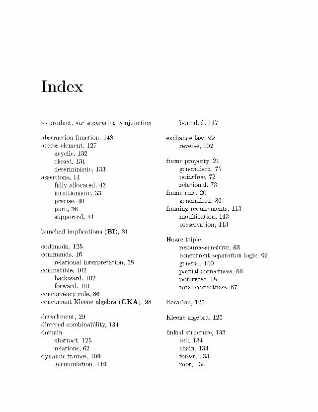
Index
∗ - product, see separating conjunction
abstraction function, 148access element, 127
acyclic, 132closed, 131deterministic, 133
assertions, 14fully allocated, 43intuitionistic, 33precise, 40pure, 36supported, 44
bunched implications (BI), 31
codomain, 125commands, 16
relational interpretation, 58compatible, 102
backward, 102forward, 101
concurrency rule, 86concurrent Kleene algebra (CKA), 98
detachment, 29directed combinability, 134domain
abstract, 125relations, 62
dynamic frames, 109accumulation, 119
bounded, 117
exchange law, 99reverse, 102
frame property, 21generalised, 75pointfree, 72relational, 73
frame rule, 20generalised, 80
framing requirements, 113modi�cation, 113preservation, 113
Hoare tripleresource-sensitive, 63concurrent separation logic, 92general, 100partial correctness, 66pointwise, 18total correctness, 67
iteration, 125
Kleene algebra, 125
linked structure, 133cell, 134chain, 134forest, 133root, 134
tree, 134local actions, 81, 82locality, 116
bimonoid, 109
modal operatorsabstract, 125relations, 64
operational semantics, 17
parallel decomposition, 89pointfree, 90
permission algebra, 53counting permissions, 54fractional permissions, 53
predicate transformer, 83locality, 83
preservation, 76strong, 91
properness, 126
quantale, 24
relationangelic behaviour, 60Cartesian product, 69compensator, 74demonic behaviour, 65domain-precise, 97join, 68split, 68
residual, 27resource context, 86respect program abortion, 63
safe states, 64safety monotonicity, 21selector, 133separating conjunction, 14
AS, 24
separating implication, 14AS, 27
separation algebra, 51separation logic, 12
concurrent, 85transitive, 123
septraction, 29strong disjointness, 127
termination monotonicity, 80tests, 39
atomic, 126pairs, 69
threaded trees, 154twig, 141
update, 141
Curriculum Vitae
Han Hing Dang
Personal Data
Date of birth February 19, 1984Citizenship German
Education
since May 2009 Doctorate, University of Augsburg, GermanyMarch 2009 Diploma in Computer Science (major) and
in Mathematics (minor)October 2004 � March 2009 Study of Computer Science
July 2004 Abitur
Academic Positions
since October 2010 Researcher, University of Augsburg, GermanyMay 2009 � September 2010 Research Assistant, University of Augsburg, Germany


