Embed Size (px)
Citation preview

Robert Lazarsfeld
Positivity in AlgebraicGeometry, I.
Classical Setting: Line Bundles and Linear Series
November 10, 2003
Springer
Berlin Heidelberg NewYorkHong Kong LondonMilan Paris Tokyo


To Lee Yen, Sarah and John


Preface
The object of this book is to give a contemporary account of a body of work incomplex algebraic geometry loosely centered around the theme of positivity.
Our focus lies on a number of questions that grew up with the field duringthe period 1950–1975. The sheaf–theoretic methods which revolutionized alge-braic geometry in the fifties — notably the seminal work of Kodaira, Serre andGrothendieck — brought into relief the special importance of ample divisors.By the mid sixties a very satisfying theory of positivity for line bundles waslargely complete, and first steps were taken to extend the picture to bundles ofhigher rank. In a related direction, work of Zariski and others led to a greatlydeepened understanding of the behavior of linear series on algebraic varieties.At the border with topology the classical theorems of Lefschetz were under-stood from new points of view, and extended in surprising ways. Hartshorne’sbook [252] and the survey articles in the Arcata proceedings [257] give a goodpicture of the state of affairs as of the mid seventies.
The years since then have seen continued interest and activity in thesematters. Work initiated during the earlier period has matured and found newapplications. More importantly, the flowering of higher dimensional geometryhas led to fresh perspectives and — especially in connection with vanishingtheorems — vast improvements in technology. It seems fair to say that thecurrent understanding of phenomena surrounding positivity goes fundamen-tally beyond what it was thirty years ago. However many of these new ideashave remained scattered in the literature, and others up to now have not beenworked out in a systematic fashion. The time seemed ripe to pull togethersome of these developments, and the present volumes represent an attempt todo so.
The book is divided into three parts. The first, which occupies Volume I,focuses on line bundles and linear series. In the second volume, Part Two parttakes up positivity for vector bundles of higher ranks. Part Three deals withideas and methods coming from higher dimensional geometry, in the form of

VIII
multiplier ideals. A brief introduction appears at the beginning of each of theparts.
I have attempted to aim the presentation at non-specialists. Not conceivingof this work as a text, I haven’t started from a clearly defined set of prereq-uisites. But the subject is relatively non-technical in nature, and familiaritywith the canonical texts [256] and [224] (combined with occasional faith andeffort) is more than sufficient for the bulk of the material. In places — forexample, Chapter 4 on vanishing theorems — our exposition is if anythingmore elementary than the standard presentations.
I expect that many readers will want to access this material in short seg-ments rather than sequentially, and I have tried to make the presentation asfriendly as possible for browsing. At least a third of the book is devoted to con-crete examples, applications and pointers to further developments. The moresubstantial of these are often collected together into separate sections. Oth-ers appear as Examples or Remarks (typically distinguished by the presenceand absence respectively of indications of proof). Sources and attributions aregenerally indicated in the body of the text: these references are supplementedby brief sections of Notes at the end of each chapter.
We work throughout with algebraic varieties defined over the complexnumbers. Since substantial parts of the book involve applications of vanish-ing theorems, hypotheses of characteristic zero are often essential. However Ihave attempted to flag those foundational discussions that extend with onlyminor changes to varieties defined over algebraically closed fields of arbitrarycharacteristic. By the same token we often make assumptions of projectivitywhen in reality properness would do. Again I try to provide hints or referencesfor the more general facts.
Although we use the Hodge decomposition and the Hard Lefschetz theo-rem on several occasions, we say almost nothing about the Hodge-theoreticconsequences of positivity. Happily these are treated in several sources, mostrecently in the beautiful book [553], [552] of Voisin. Similarly, the reader willfind relatively little here about the complex analytic side of the story. For thiswe refer to Demailly’s notes [110] or his forthcoming book [104].
Concerning matters of organization, each chapter is divided into severalsections, many of which are further partitioned into subsections. A reference toSection 3.1 points to the first section of Chapter 3, while Section 3.1.B refers tothe second subsection therein. Statements are numbered consecutively withineach section: so for example Theorem 3.1.17 indicates a result from Section3.1 (which, as it happens, appears in 3.1.B). As an aid to the reader, eachof the two volumes reproduces the table of contents of the other. The indexand list of references cover both volumes. Large parts of Volume I can beread without access to Volume II, but Volume II makes frequent reference toVolume I.

IX
Acknowledgements. I am grateful to the National Science Foundation, theGuggenheim Foundation and the University of Michigan for support duringthe preparation of these volumes.
I have benefited from comments and suggestions from many students andcolleagues, including: T. Bauer, G. Bini, F. Bogomolov, A. Bravo, H. Bren-ner, A. Chen, D. Cutkosky, M. De Cataldo, T. De Fernex, J.-P. Demailly,I. Dolgachev, L. Ein, G. Farkas, R. Friedman, T. Garrity, A. Gibney, C. Ha-con, R. Hartshorne, S. Helmke, M. Hochster, J. Howald, C Huneke, P. Jahnke,Y. Kawamata, D. Keeler, M. Kim, F. Knudsen, A. Kuronya, J. M. Landsberg,M. Mustata, T. Nevins, H. Pinkham, M. Popa, I. Radloff, M. Reid, M. Roth,J. Sidman, A. Sommese, T. Stafford, I. Swanson, T. Szemberg, B. Teissier,Z. Teitler, D. Varolin, E. Viehweg, J. Winkelmann, A. Wolfe and Q. Zhang.
This project has profited from collaborations with a number of co-authors,including Jean-Pierre Demailly, Mark Green and Karen E. Smith. Joint workmany years ago with Bill Fulton has helped to shape the content and presen-tation of Chapter 3 and Part Two. I likewise owe a large mathematical debtto Lawrence Ein: I either learned from him or worked out together with hima significant amount of the material in Part Three, and our collaboration hashad an influence in many other places as well.
I am grateful to several individuals that made particularly valuable con-tributions to the preparation of these volumes. Janos Kollar convinced me tostart the book, and Bill Fulton insisted (on several occasions) that I finishit. Besides their encouragement, they contributed detailed suggestions fromcareful readings of drafts of several chapters. I also received copious commentson different parts of a preliminary draft from Jun-Muk Hwang, Steve Kleimanand Karen Smith. Olivier Debarre read through the draft in its entirety, andprovided a vast number of corrections and improvements.
Like many first-time authors, I couldn’t have imagined when I began writ-ing how long and consuming this undertaking would become. I’d like to takethis opportunity to express my profound appreciation to the colleagues, friendsand family members that offered support, encouragement and patience alongthe way.
December, 2003 Robert Lazarsfeld


Contents
Notation and Conventions . . . . . . . . . . . . . . . . . . . . . . . . . . . . . . . . . . . . . 1
Part One: Ample Line Bundles and Linear Series
Introduction to Part One . . . . . . . . . . . . . . . . . . . . . . . . . . . . . . . . . . . . . . 5
1 Ample and Nef Line Bundles . . . . . . . . . . . . . . . . . . . . . . . . . . . . . . 71.1 Preliminaries: Divisors, Line Bundles and Linear Series . . . . . . . 7
1.1.A Divisors and Line Bundles . . . . . . . . . . . . . . . . . . . . . . . . . . 81.1.B Linear Series . . . . . . . . . . . . . . . . . . . . . . . . . . . . . . . . . . . . . . 121.1.C Intersection Numbers and Numerical Equivalence . . . . . . 151.1.D Riemann-Roch . . . . . . . . . . . . . . . . . . . . . . . . . . . . . . . . . . . . 20
1.2 The Classical Theory . . . . . . . . . . . . . . . . . . . . . . . . . . . . . . . . . . . . 241.2.A Cohomological Properties . . . . . . . . . . . . . . . . . . . . . . . . . . 251.2.B Numerical Properties . . . . . . . . . . . . . . . . . . . . . . . . . . . . . . 331.2.C Metric Characterizations of Amplitude . . . . . . . . . . . . . . . 39
1.3 Q-Divisors and R-Divisors . . . . . . . . . . . . . . . . . . . . . . . . . . . . . . . . 441.3.A Definitions for Q-divisors . . . . . . . . . . . . . . . . . . . . . . . . . . . 441.3.B R-Divisors and Their Amplitude . . . . . . . . . . . . . . . . . . . . 47
1.4 Nef Line Bundles and Divisors . . . . . . . . . . . . . . . . . . . . . . . . . . . . 501.4.A Definitions and Formal Properties . . . . . . . . . . . . . . . . . . . 501.4.B Kleiman’s Theorem . . . . . . . . . . . . . . . . . . . . . . . . . . . . . . . . 521.4.C Cones . . . . . . . . . . . . . . . . . . . . . . . . . . . . . . . . . . . . . . . . . . . . 581.4.D Fujita’s Vanishing Theorem . . . . . . . . . . . . . . . . . . . . . . . . . 65
1.5 Examples and Complements . . . . . . . . . . . . . . . . . . . . . . . . . . . . . . 691.5.A Ruled Surfaces . . . . . . . . . . . . . . . . . . . . . . . . . . . . . . . . . . . . 701.5.B Products of Curves . . . . . . . . . . . . . . . . . . . . . . . . . . . . . . . . 721.5.C Abelian Varieties . . . . . . . . . . . . . . . . . . . . . . . . . . . . . . . . . . 781.5.D Other Varieties . . . . . . . . . . . . . . . . . . . . . . . . . . . . . . . . . . . . 791.5.E Local Structure of the Nef Cone . . . . . . . . . . . . . . . . . . . . . 81

XII Contents
1.5.F The Cone Theorem . . . . . . . . . . . . . . . . . . . . . . . . . . . . . . . . 851.6 Inequalities . . . . . . . . . . . . . . . . . . . . . . . . . . . . . . . . . . . . . . . . . . . . . 87
1.6.A Global Results . . . . . . . . . . . . . . . . . . . . . . . . . . . . . . . . . . . . 871.6.B Mixed Multiplicities . . . . . . . . . . . . . . . . . . . . . . . . . . . . . . . 90
1.7 Amplitude for a Mapping . . . . . . . . . . . . . . . . . . . . . . . . . . . . . . . . . 931.8 Castelnuovo-Mumford Regularity . . . . . . . . . . . . . . . . . . . . . . . . . . 98
1.8.A Definitions, Formal Properties, and Variants . . . . . . . . . . 981.8.B Regularity and Complexity . . . . . . . . . . . . . . . . . . . . . . . . . 1061.8.C Regularity Bounds . . . . . . . . . . . . . . . . . . . . . . . . . . . . . . . . . 1091.8.D Syzygies of Algebraic Varieties . . . . . . . . . . . . . . . . . . . . . . 114
Notes . . . . . . . . . . . . . . . . . . . . . . . . . . . . . . . . . . . . . . . . . . . . . . . . . . . . . . . 118
2 Linear Series . . . . . . . . . . . . . . . . . . . . . . . . . . . . . . . . . . . . . . . . . . . . . . 1212.1 Asymptotic Theory . . . . . . . . . . . . . . . . . . . . . . . . . . . . . . . . . . . . . . 121
2.1.A Basic Definitions . . . . . . . . . . . . . . . . . . . . . . . . . . . . . . . . . . 1222.1.B Semiample Line Bundles . . . . . . . . . . . . . . . . . . . . . . . . . . . 1282.1.C Iitaka Fibration . . . . . . . . . . . . . . . . . . . . . . . . . . . . . . . . . . . 132
2.2 Big Line Bundles and Divisors . . . . . . . . . . . . . . . . . . . . . . . . . . . . 1382.2.A Basic Properties of Big Divisors . . . . . . . . . . . . . . . . . . . . . 1392.2.B Pseudoeffective and Big Cones . . . . . . . . . . . . . . . . . . . . . . 1452.2.C Volume of a Big Divisor . . . . . . . . . . . . . . . . . . . . . . . . . . . . 148
2.3 Examples and Complements . . . . . . . . . . . . . . . . . . . . . . . . . . . . . . 1572.3.A Zariski’s Construction . . . . . . . . . . . . . . . . . . . . . . . . . . . . . . 1572.3.B Cutkosky’s Construction . . . . . . . . . . . . . . . . . . . . . . . . . . . 1582.3.C Base Loci of Nef and Big Linear Series . . . . . . . . . . . . . . . 1632.3.D The Theorem of Campana and Peternell . . . . . . . . . . . . . 1652.3.E Zariski Decompositions . . . . . . . . . . . . . . . . . . . . . . . . . . . . . 167
2.4 Graded Linear Series and Families of Ideals . . . . . . . . . . . . . . . . . 1712.4.A Graded Linear Series . . . . . . . . . . . . . . . . . . . . . . . . . . . . . . 1712.4.B Graded Families of Ideals . . . . . . . . . . . . . . . . . . . . . . . . . . . 175
Notes . . . . . . . . . . . . . . . . . . . . . . . . . . . . . . . . . . . . . . . . . . . . . . . . . . . . . . . 182
3 Geometric Consequences of Positivity . . . . . . . . . . . . . . . . . . . . . 1833.1 The Lefschetz Theorems . . . . . . . . . . . . . . . . . . . . . . . . . . . . . . . . . . 183
3.1.A Topology of Affine Varieties . . . . . . . . . . . . . . . . . . . . . . . . 1843.1.B The Theorem on Hyperplane Sections . . . . . . . . . . . . . . . . 1903.1.C Hard Lefschetz Theorem . . . . . . . . . . . . . . . . . . . . . . . . . . . 197
3.2 Projective Subvarieties of Small Codimension . . . . . . . . . . . . . . . 1993.2.A Barth’s Theorem . . . . . . . . . . . . . . . . . . . . . . . . . . . . . . . . . . 1993.2.B Hartshorne’s Conjectures . . . . . . . . . . . . . . . . . . . . . . . . . . . 202
3.3 Connectedness Theorems . . . . . . . . . . . . . . . . . . . . . . . . . . . . . . . . . 2053.3.A Bertini Theorems . . . . . . . . . . . . . . . . . . . . . . . . . . . . . . . . . . 2053.3.B Theorem of Fulton and Hansen . . . . . . . . . . . . . . . . . . . . . . 2083.3.C Grothendieck’s Connectedness Theorem . . . . . . . . . . . . . . 210
3.4 Applications of the Fulton-Hansen Theorem . . . . . . . . . . . . . . . . 212

Contents XIII
3.4.A Singularities of Mappings . . . . . . . . . . . . . . . . . . . . . . . . . . . 2123.4.B Zak’s Theorems . . . . . . . . . . . . . . . . . . . . . . . . . . . . . . . . . . . 2173.4.C Zariski’s Problem . . . . . . . . . . . . . . . . . . . . . . . . . . . . . . . . . . 225
3.5 Variants and Extensions . . . . . . . . . . . . . . . . . . . . . . . . . . . . . . . . . . 2283.5.A Connectedness Theorems for Homogeneous Varieties . . . 2293.5.B Higher Connectivity for Maps to Projective Space . . . . . 231
Notes . . . . . . . . . . . . . . . . . . . . . . . . . . . . . . . . . . . . . . . . . . . . . . . . . . . . . . . 235
4 Local Positivity . . . . . . . . . . . . . . . . . . . . . . . . . . . . . . . . . . . . . . . . . . . . 2374.1 Seshadri Constants . . . . . . . . . . . . . . . . . . . . . . . . . . . . . . . . . . . . . . 2374.2 Lower Bounds . . . . . . . . . . . . . . . . . . . . . . . . . . . . . . . . . . . . . . . . . . . 245
4.2.A Background and Statements . . . . . . . . . . . . . . . . . . . . . . . . 2464.2.B Multiplicities of Divisors in Families . . . . . . . . . . . . . . . . . 2504.2.C Proof of Theorem 5.2.5 . . . . . . . . . . . . . . . . . . . . . . . . . . . . . 254
4.3 Abelian Varieties . . . . . . . . . . . . . . . . . . . . . . . . . . . . . . . . . . . . . . . . 2584.3.A Period lengths and Seshadri constants . . . . . . . . . . . . . . . . 2584.3.B Proof of Theorem 5.3.6 . . . . . . . . . . . . . . . . . . . . . . . . . . . . . 2644.3.C Complements . . . . . . . . . . . . . . . . . . . . . . . . . . . . . . . . . . . . . 267
4.4 Local Positivity Along an Ideal Sheaf . . . . . . . . . . . . . . . . . . . . . . 2694.4.A Definition and Formal Properties of the s-Invariant . . . . 2704.4.B Complexity Bounds . . . . . . . . . . . . . . . . . . . . . . . . . . . . . . . . 274
Notes . . . . . . . . . . . . . . . . . . . . . . . . . . . . . . . . . . . . . . . . . . . . . . . . . . . . . . . 278
Appendices
A Projective Bundles . . . . . . . . . . . . . . . . . . . . . . . . . . . . . . . . . . . . . . . . 279
B Cohomology and Complexes . . . . . . . . . . . . . . . . . . . . . . . . . . . . . . . 281B.1 Cohomology . . . . . . . . . . . . . . . . . . . . . . . . . . . . . . . . . . . . . . . . . . . . 281B.2 Complexes . . . . . . . . . . . . . . . . . . . . . . . . . . . . . . . . . . . . . . . . . . . . . . 283
References . . . . . . . . . . . . . . . . . . . . . . . . . . . . . . . . . . . . . . . . . . . . . . . . . . . . . 289
Index . . . . . . . . . . . . . . . . . . . . . . . . . . . . . . . . . . . . . . . . . . . . . . . . . . . . . . . . . . 315


Contents of Volume II
Notation and Conventions II–1
Part Two: Positivity for Vector Bundles
Introduction to Part Two II–5
6 Ample and Nef Vector Bundles II–76.1 Classical Theory II–7
6.1.A Definition and First Properties II–86.1.B Cohomological Properties II–116.1.C Criteria for Amplitude II–156.1.D Metric Approaches to Positivity of Vector Bundles II–18
6.2 Q-Twisted and Nef Bundles II–206.2.A Twists by Q-Divisors II–206.2.B Nef Bundles II–23
6.3 Examples and Constructions II–266.3.A Normal and Tangent Bundles II–276.3.B Ample Cotangent Bundles and Hyperbolicity II–356.3.C Picard Bundles II–436.3.D The Bundle Associated to a Branched Covering II–466.3.E Direct Images of Canonical Bundles II–506.3.F Some Constructions of Positive Vector Bundles II–53
6.4 Ample Vector Bundles on Curves II–566.4.A Review of Semistability II–566.4.B Semistability and Amplitude II–59
Notes II–63
7 Geometric Properties of Ample Bundles II–657.1 Topology II–65
7.1.A Sommese’s Theorem II–65

XVI Contents of Volume II
7.1.B Theorem of Bloch and Gieseker II–687.1.C A Barth-type Theorem for Branched Coverings II–71
7.2 Degeneracy Loci II–747.2.A Statements and First Examples II–747.2.B Proof of Connectedness of Degeneracy Loci II–787.2.C Some Applications II–827.2.D Variants and Extensions II–87
7.3 Vanishing Theorems II–897.3.A Vanishing Theorems of Griffiths and Le Potier II–897.3.B Generalizations II–95
Notes II–98
8 Numerical Properties of Ample Bundles II–1018.1 Preliminaries from Intersection Theory II–101
8.1.A Chern Classes for Q-Twisted Bundles II–1028.1.B Cone Classes II–1048.1.C Cone Classes for Q-Twists II–110
8.2 Positivity Theorems II–1118.2.A Positivity of Chern Classes II–1118.2.B Positivity of Cone Classes II–114
8.3 Positive Polynomials for Ample Bundles II–1178.4 Some Applications II–124
8.4.A Positivity of Intersection Products II–1258.4.B Non-Emptiness of Degeneracy Loci II–1278.4.C Singularities of Hypersurfaces Along a Curve II–129
Notes II–133
Part Three: Multiplier Ideals and Their Applications
Introduction to Part Three II–137
9 Multiplier Ideal Sheaves II–1399.1 Preliminaries II–140
9.1.A Q-Divisors. II–1409.1.B Normal Crossing Divisors and Log Resolutions. II–1429.1.C The Kawamata-Viehweg Vanishing Theorem II–147
9.2 Definition and First Properties II–1519.2.A Definition of Multiplier Ideals. II–1529.2.B First Properties II–158
9.3 Examples and Complements II–1629.3.A Multiplier Ideals and Multiplicity II–1629.3.B Invariants Arising From Multiplier Ideals II–1649.3.C Monomial Ideals II–1709.3.D Analytic Construction of Multiplier Ideals II–176

Contents of Volume II XVII
9.3.E Adjoint Ideals II–1789.3.F Multiplier and Jacobian Ideals II–1819.3.G Multiplier Ideals on Singular Varieties II–182
9.4 Vanishing Theorems for Multiplier Ideals II–1859.4.A Local Vanishing for Multiplier Ideals II–1869.4.B The Nadel Vanishing Theorem II–1889.4.C Vanishing on Singular Varieties II–1919.4.D Nadel’s Theorem in the Analytic Setting II–1929.4.E Non-Vanishing and Global Generation II–193
9.5 Geometric Properties of Multiplier Ideals II–1959.5.A Restrictions of Multiplier Ideals II–1959.5.B Subadditivity II–2019.5.C The Summation Theorem II–2049.5.D Multiplier Ideals in Families II–2099.5.E Coverings II–212
9.6 Skoda’s Theorem II–2169.6.A Integral Closure of Ideals II–2179.6.B Skoda’s Theorem: Statements II–2229.6.C Skoda’s Theorem: Proofs II–2269.6.D Variants II–229
Notes II–231
10 Some Applications of Multiplier Ideals II–23310.1 Singularities II–233
10.1.A Singularities of Projective Hypersurfaces II–23310.1.B Singularities of Theta Divisors II–23510.1.C A Criterion for Separation of Jets of Adjoint Series II–238
10.2 Matsusaka’s Theorem II–23910.3 Nakamaye’s Theorem on Base Loci II–24510.4 Global Generation of Adjoint Linear Series II–250
10.4.A Fujita Conjecture and Angehrn-Siu Theorem II–25110.4.B Loci of Log-Canonical Singularities II–25310.4.C Proof of the Theorem of Angehrn and Siu II–257
10.5 The Effective Nullstellensatz II–260
11 Asymptotic Constructions II–26711.1 Construction of Asymptotic Multiplier Ideals II–268
11.1.A Complete Linear Series II–26811.1.B Graded Systems of Ideals and Linear Series II–274
11.2 Properties of Asymptotic Multiplier Ideals II–28011.2.A Local Statements II–28011.2.B Global Results II–28311.2.C Multiplicativity of Plurigenera II–290
11.3 Growth of Graded Families and Symbolic Powers II–29111.4 Fujita’s Approximation Theorem II–297

XVIII Contents of Volume II
11.4.A Statement and First Consequences II–29711.4.B Proof of Fujita’s Theorem II–30311.4.C The Dual of the Pseudoeffective Cone II–304
11.5 Siu’s Theorem on Plurigenera II–310Notes II–319
References II–321
Index II–347

Notation and Conventions
For the most part we follow generally accepted notation, as in [256]. We dohowever adopt a few specific conventions:
• We work throughout over the complex numbers C.
• A scheme is an algebraic scheme of finite type over C. A variety is areduced and irreducible scheme. We deal exclusively with closed points ofschemes.
• If X is a variety, a modification of X is a projective birational mappingµ : X ′ −→ X.
• Given an irreducible variety X, we say that a property holds at a generalpoint of X if it holds for all points in the complement of a proper algebraicsubset. A property holds at a very general point if it is satisfied off theunion of countably many proper subvarieties.
• Let f : X −→ Y be a morphism of varieties or schemes, and a ⊆ OYan ideal sheaf on Y . We sometimes denote by f−1a ⊆ OX the ideal sheafa·OX on X determined by a. While strictly speaking this conflicts with thenotation for the sheaf-theoretic pullback of a, we trust that no confusionwill result.
• If E is a vector bundle on a scheme X, P(E) denotes the projective bundleof one-dimensional quotients of E. On a few occasions we will want to workwith the bundle of one-dimensional subspaces of E: this is denoted Psub(E).Thus
Psub(E) = P(E∗).
A brief review of basic facts concerning projective bundles appears in Ap-pendix A.
• Given a vector space or vector bundle E, SkE denotes the kth symmetricpower of E, and Sym(E) = ⊕Sk(E) is the full symmetric algebra on E.
• Let X1, X2 be varieties or schemes. Without specific comment we write
1

2 Contents of Volume II
pr1 : X1 ×X2 −→ X1 , pr2 : X1 ×X2 −→ X2
for the two projections of X1 ×X2 onto its factors. When other notationfor the projections seems preferable, we introduce it explicitly.
• Given a real-valued function f : N −→ R defined on the natural numbers,we say that f(m) = O(mk) if
lim supm→∞
|f(m)|mk
< ∞.

Part One
Ample Line Bundles and Linear Series


5
Introduction to Part One
Linear series have long stood at the center of algebraic geometry. Systemsof divisors were employed classically to study and define invariants of pro-jective varieties, and it was recognized that varieties share many propertieswith their hyperplane sections. The classical picture was greatly clarified bythe revolutionary new ideas that entered the field starting in the 1950’s. Tobegin with, Serre’s great paper [489], along with the work of Kodaira (e.g.[325]), brought into focus the importance of amplitude for line bundles. Bythe mid 1960’s a very beautiful theory was in place, showing that one couldrecognize positivity geometrically, cohomologically or numerically. During thesame years, Zariski and others began to investigate the more complicated be-havior of linear series defined by line bundles that may not be ample. Thisled to particularly profound insights in the case of surfaces [572]. In yet an-other direction, the classical theorems of Lefschetz comparing the topology ofa variety with that of a hyperplane section were understood from new pointsof view, and developed in surprising ways in [234] and [24].
The present Part One is devoted to this body of work and its develop-ments. Our aim is to give a systematic presentation, from a contemporaryviewpoint, of the circle of ideas surrounding linear series and ample divisorson a projective variety.
We start in Chapter 1 with the basic theory of positivity for line bundles.In keeping with the current outlook, Q- and R-divisors and the notion ofnefness play a central role, and the concrete geometry of nef and ample conesis given some emphasis. The chapter concludes with a section on Castelnuovo-Mumford regularity, a topic which we consider to merit inclusion in the canonof positivity.
Chapter 2 deals with linear series, our focus being the asymptotic geometryof linear systems determined by divisors that may not be ample. A numericalcriterion due to Siu [496], giving a condition to guarantee that the difference oftwo nef divisors be big, plays an important role. We also present here severalconcrete examples of the sort of interesting and challenging behavior that suchlinear series can display.
In Chapter 3 we turn to the theorems of Lefschetz and Bertini and theirsubsequent developments by Barth, Fulton-Hansen and others. Here the sur-prising geometric properties of projective subvarieties of small codimensioncome into relief. The Lefschetz hyperplane theorem is applied in Chapter ??to prove the classical vanishing theorems of Kodaira and Nakano. Chapter?? also contains the vanishing theorem for big and nef divisors discovered byKawamata and Viehweg, as well as one of the generic vanishing theorems from[217].
Finally, Chapter 4 takes up the theory of local positivity. This is a topicthat has emerged only recently, starting with ideas of Demailly for quantifyinghow much of the positivity of a line bundle can be localized at a given point

6
of a variety. Although some of the results are not yet definitive, the picture issurprisingly rich and structured.
Writing about linear series seems to lead unavoidably to conflict betweenthe additive notation of divisors and the multiplicative language of line bun-dles. Our policy is to avoid explicitly mixing the two. However on many occa-sions we adopt the compromise of speaking about divisors while using notationsuggestive of bundles. We discuss this convention — as well as some of thesecondary issues it raises — at the end of Section 1.1.A.

1
Ample and Nef Line Bundles
This chapter contains the basic theory of positivity for line bundles and divi-sors on a projective algebraic variety.
After some preliminaries in Section 1.1 on divisors and linear series, wepresent in Section 1.2 the classical theory of ample line bundles. The basicconclusion is that positivity can be recognized geometrically, cohomologicallyor numerically. Section 1.3 develops the formalism of Q- and R-divisors, whichis applied in Section 1.4 to study limits of ample bundles. These so-called nefdivisors are central to the modern view of the subject, and Section 1.4 containsthe core of the general theory. Most of the remaining material is more concretein flavor. Section 1.5 is devoted to examples of ample cones and to furtherinformation about their structure, while Section 1.6 focuses on inequalities ofHodge type. After a brief review of the definitions and basic facts surroundingamplitude for a mapping, we conclude in Section 1.8 with an introduction toCastelnuovo-Mumford regularity.
We recall that according to our conventions we deal unless otherwise statedwith complex algebraic varieties and schemes, and with closed points on them.However as we go along we will point out that much of this material remainsvalid for varieties defined over algebraically closed fields of arbitrary charac-teristic.
1.1 Preliminaries: Divisors, Line Bundles and LinearSeries
In this section we collect some facts and notation that will be used frequentlyin the sequel. We start in Section 1.1.A by recalling some constructions in-volving divisors and line bundles, and turn in the second subsection to linearseries. Section 1.1.C deals with intersection numbers and numerical equiv-alence, and we conclude in 1.1.D by discussing asymptotic formulations ofthe Riemann-Roch theorem. As a practical matter we assume that much of

8 Chapter 1. Ample and Nef Line Bundles
this material is familiar to the reader.1 However we felt it would be useful toinclude a brief summary in order to fix ideas.
1.1.A Divisors and Line Bundles
We start with a quick review of the definitions and facts concerning Cartierdivisors, following [256, p. 140ff], [411, Chapters 9 and 10] and [317]. We takeup first the very familiar case of reduced and irreducible varieties, and thenpass to more general schemes.
Consider then an irreducible complex variety X, and denote by MX =C(X) the (constant) sheaf of rational functions on X. It contains the structuresheaf OX as a subsheaf, and so there is an inclusion O∗X ⊆M∗X of sheaves ofmultiplicative abelian groups.
Definition 1.1.1. (Cartier divisors). A Cartier divisor on X is a globalsection of the quotient sheaf M∗X/O∗X . We denote by Div(X) the group of allsuch, so that
Div(X) = Γ(X,M∗X/O∗X
). ut
Concretely, then, a divisor D ∈ Div(X) is represented by data
(Ui, fi)
con-sisting of an open covering Ui of X together with elements fi ∈ Γ
(Ui,M
∗X
),
having the property that on Uij = Ui ∩ Uj one can write
fi = gijfj for some gij ∈ Γ(Uij ,O∗X
). (1.1)
The function fi is called a local equation for D at any point x ∈ Ui. Two suchcollections determine the same Cartier divisor if there is a common refinementVk of the open coverings on which they are defined so that they are givenby data
(Vk, fk)
and
(Vk, f ′k)
with
fk = hkf′k on Vk for some hk ∈ Γ
(Vk,O∗X
).
The group operation on Div(X) is always written additively: if D,D′ ∈Div(X) are represented respectively by data
(Ui, fi)
and
(Ui, f ′i)
, then
D+D′ is given by
(Ui, fif ′i)
. The support of a divisor D =
(Ui, fi)
is theset of points x ∈ X at which a local equation of D at x is not a unit in OxX.D is effective if fi ∈ Γ
(Ui,OX
)is regular on Ui: this is written D < 0.
Suppose now that X is a possibly non-reduced algebraic scheme. Then thesame definition works except that one has to be more careful about what onemeans by MX , which now becomes the sheaf of total quotient rings of OX .2 As1 For the novice, we give some suggestions and pointers to the literature.2 Grothendieck speaks of the sheaf of “meromorphic functions” on X (cf. [233,
20.1]). However since we are working with complex varieties this seems potentiallyconfusing, and we prefer to follow the terminology of [256].

1.1 Preliminaries: Divisors, Line Bundles and Linear Series 9
explained in [411, Chapter 9] there is a unique sheaf MX on X characterizedby the property that if U = Spec(A) is an affine open subset of X, then
Γ(U,MX
)= Γ
(U,OX
)tot
= Atot
is the total ring of fractions of A, i.e. the localization of A at the set of nonzero-divisors.3 Similarly, on the stalk level there is an isomorphism MX,x =(OX,x
)tot
. As before one has an inclusion O∗X ⊆M∗X of multiplicative groupsof units, and Definition 1.1.1 — as well as the discussion following it — remainsvalid without change.
Convention 1.1.2. (Divisors). In Parts One and Two of this work weadopt the convention that when we speak of a “divisor” we always mean aCartier divisor. (In Part Three it will be preferable to think instead of Weildivisors.) ut
One should view Cartier divisors as “cohomological” objects, but one canalso define “homological” analogues:
Definition 1.1.3. (Cycles and Weil divisors). Let X be a variety orscheme of pure dimension n. A k-cycle on X is a Z-linear combination ofirreducible subvarieties of dimension k. The group of all such is written Zk(X).A Weil divisor on X is an (n − 1)-cycle, i.e. a formal sum of codimensionone subvarieties with integer coefficients. We often use WDiv(X) in place ofZn−1(X) to denote the group of Weil divisors. ut
Remark 1.1.4. (Cycle map for Cartier divisors). There is a cycle map
Div(X) −→WDiv(X) , D 7→ [D] =∑
ordV (D) · [V ]
where ordV (D) is the order of D along a codimension one subvariety. Ingeneral this homomorphism is neither injective nor surjective, although it isone-to-one when X is a normal variety and an isomorphism when X is non-singular. (See [186, Chapter 2.1] for details and further information.) ut
A global section f ∈ Γ(X,M∗X
)determines in the evident manner a divisor
D = div(f) ∈ Div(X).
As usual, a divisor of this form is called principal and the subgroup of all suchis Princ(X) ⊆ Div(X). Two divisors D1, D2 are linearly equivalent, writtenD1 ≡lin D2, if D1 −D2 is principal.
Let D be a divisor on X. Given a morphism f : Y −→ X, one would liketo define a divisor f∗D on Y by pulling back the local equations for D. Thefollowing condition is sufficient to guarantee that this is meaningful:3 See [317] for a discussion of how one should define MX on arbitrary open subsets.

10 Chapter 1. Ample and Nef Line Bundles
Let V ⊆ Y be any associated subvariety of Y , i.e. the subvariety de-fined by an associated prime of OY in the sense of primary decompo-sition. Then f(V ) should not be contained in the support of D.
If Y is reduced the requirement is just that no component of Y map into thesupport of D.
A similar condition allows one to define the divisor of a section of a linebundle L on X. Specifically, let s ∈ Γ
(X,L
)be a global section of L. Assume
that s does not vanish on any associated subvariety of X — for example,if X is reduced, this just means that s shouldn’t vanish identically on anycomponent of X. Then a local equation of s determines in the natural way adivisor div(s) ∈ Div(X). We leave it to the reader to formulate the analogouscondition under which a “rational section” s ∈ Γ
(X,L⊗OX MX
)gives rise a
divisor.A Cartier divisor D ∈ Div(X) determines a line bundle OX(D) on X,
leading to a canonical homomorphism:
Div(X) −→ Pic(X) , D 7→ OX(D) (1.2)
of abelian groups, where Pic(X) denotes as usual the Picard group of isomor-phism classes of line bundles on X. Concretely, if D is given by data
(Ui, fi)
as above, then one can build OX(D) by using the gij in (1.1) as transitionfunctions. More abstractly, one can view (the isomorphism class of) OX(D)as the image of D under the connecting homomorphism
Div(X) = Γ(X,M∗X/O∗X
)−→ H1
(X,O∗X
)= Pic(X)
determined by the exact sequence 0 −→ O∗X −→ M∗X −→ M∗X/O∗X −→ 0 ofsheaves on X. Evidently
OX(D1) ∼= OX(D2) ⇐⇒ D1 ≡lin D2.
If D is effective then OX(D) carries a global section s = sD ∈ Γ(X,OX(D)
)with div(s) = D. In general OX(D) has a rational section with the analogousproperty.
The question of whether every line bundle comes from a divisor is moredelicate. On the positive side:
Example 1.1.5. (Line bundles from divisors). There are a couple ofnatural hypotheses to guarantee that every line bundle arises from a divisor.
(i). If X is reduced and irreducible, or merely reduced, then the homomor-phism in (1.2) is surjective.
(ii). If X is projective then the same statement holds even if it is non-reduced.
(If X is reduced and irreducible then any line bundle L has a rational sections, and one can take D = div(s). For the second statement — which is due to

1.1 Preliminaries: Divisors, Line Bundles and Linear Series 11
Nakai [429] — one can use the theorem of Cartan-Grothendieck-Serre (Theo-rem 1.2.6) to reduce to the case in which L is globally generated (Definition1.1.10). But then one can find a section s ∈ Γ
(X,L
)that does not vanish on
any of the associated subvarieties of X, in which case D = div(s) gives therequired divisor.) ut
On the other hand, there is also
Example 1.1.6. (Kleiman’s example). Following [319] and [487] we con-struct a non-projective non-reduced scheme X on which the mapping (1.2)is not surjective.4 Start by taking Y to be Hironaka’s example of a smoothnon-projective threefold containing two disjoint smooth rational curves A andB with A+B ≡num 0 as described in [256, Appendix B, Example 3.4.1]. Nowfix points a ∈ A, b ∈ B and introduce nilpotents at a and b to produce anon-reduced scheme X containing Y . Note that X has depth zero at a andb, so these points must be disjoint from the support of every Cartier divisoron X. Observe also that Pic(X) −→ Pic(Y ) is an isomorphism thanks to thefact that ker
(O∗X −→ O∗Y
)is supported on a finite set, and so has vanishing
H1 and H2.We claim that there exists a line bundle L on X with the property that∫
A
c1(L) > 0. (*)
In fact, it follows from Hironaka’s construction that one can find a line bundleon Y satisfying the analogous inequality, and by what have said above thisbundle extends to X. Suppose now that L = OX(D) for some divisor D onX. Decompose the corresponding Weil divisor as a sum [D] =
∑mi[Di] of
prime divisors with mi 6= 0. None of the Di can pass through a or b, so eachDi is Cartier and
D =∑
miDi
as Cartier divisors on X. Now(Di ·A
)≥ 0 and
(Di ·B
)≥ 0 since each of the
Di — avoiding as they do the points a and b — meet A and B properly. Onthe other hand, it follows from (*) that there is at least one index i such that(miDi ·A
)> 0: in particular mi > 0 and
(Di ·A
)> 0. But
(Di ·B
)= −
(Di ·A
)since B ≡num −A and therefore
(Di · B
)< 0, a contradiction. (As Schroer
observes, the analogous but slightly simpler example appearing in [252, I.1.3]is erroneous.) ut
Later on, the canonical bundle of a smooth variety will play a particularlyimportant role:
Notation 1.1.7. (Canonical bundle and divisor). Let X be a non-singular complete variety of dimension n. We denote by ωX = ΩnX thecanonical line bundle on X, and by KX any canonical divisor on X. ThusOX(KX) = ωX . ut4 We will use here the basic facts of intersection theory recalled later in this section.

12 Chapter 1. Ample and Nef Line Bundles
Finally, a word about terminology. There is inevitably a certain amountof tension between the additive language of divisors and the multiplicativeformalism of line bundles. Our convention is always to work additively withdivisors and multiplicatively with line bundles. However on many occasionsit is natural or customary to stay in additive mode when nonetheless one hasline bundles in mind. In these circumstances we will speak of divisors but usenotation suggestive of bundles, as for instance in the following statement ofthe Kodaira vanishing theorem:
Let L be an ample divisor on a smooth projective variety X of dimen-sion n. Then Hi
(X,OX(KX + L)
)= 0 for every i > 0.
(The mathematics here appears in Chapter ??.) While for the most part thisconvention seems to work well, it occasionally leads us to make extraneousprojectivity or integrality hypotheses in order to be able to invoke Example1.1.5. Specifically, we will repeatedly work with the Neron-Severi group N1(X)of X and the corresponding real vector space N1(X)R = N1(X) ⊗R. Hereadditive notation seems essential, so we are led to view N1(X) as the groupof divisors modulo numerical equivalence (Definition 1.1.15). On the otherhand, functorial properties are most easily established by passing to Pic(X).For this to work smoothly one wants to know that every line bundle comesfrom a divisor, and this is typically guaranteed by simply assuming that Xis either a variety or a projective scheme. We try to flag this artifice when itoccurs.
1.1.B Linear Series
We next review some basic facts and definitions concerning linear series. Forfurther information the reader can consult [252, Chapter I.2], [256, ChapterII, Sections 6, 7] and [224, Chapter 1.4].
Let X be a variety (or scheme), L a line bundle on X, and V ⊆ H0(X,L
)a non-zero subspace of finite dimension. We denote by |V | = Psub(V ) theprojective space of one-dimensional subspaces of V . When X is a completevariety, |V | is identified with the linear series of divisors of sections of V inthe sense of [256, Chapter II, §7], and in general we refer to |V | as a linearseries.5 Taking V = H0
(X,L
)— assuming this space is finite dimensional,
as will be the case for instance if X is complete — yields the complete linearseries |L|. Given a divisor D, we also write |D | for the complete linear seriesassociated to OX(D).
Evaluation of sections in V gives rise to a morphism5 Observe that on a non-integral scheme it may happen that not every element of|V | determines a divisor, since there may exist s ∈ V for which div(s) is notdefined. In this case calling |V | a linear series is slightly unconventional. Howeverwe trust that no confusion will result.

1.1 Preliminaries: Divisors, Line Bundles and Linear Series 13
evalV : V ⊗C OX −→ L
of vector bundles on X.
Definition 1.1.8. (Base locus and base ideal). The base ideal of |V |,written
b(|V |
)= b
(X, |V |
)⊆ OX
is the image of the map V ⊗CL∗ −→ OX determined by evalV . The base locus
Bs(|V |)⊆ X
of |V | is the closed subset of X cut out by the base ideal b(|V |
). When we
wish to emphasize the scheme structure on Bs(|V |)
determined by b(|V |) wewill refer to Bs
(|V |)
as the base scheme of |V |. When V = H0(X,L
)or
V = H0(X,OX(D)
)are finite dimensional, we write respectively b
(|L|)
andb(|D |
)for the base-ideals in question. ut
Very concretely, then, Bs(|V |
)is the set of points at which all the sections
in V vanish, and b(|V |
)is the ideal sheaf spanned by these sections.
Example 1.1.9. (Inclusions). Assuming for the moment that X is pro-jective (or complete), fix a Cartier divisor D on X. Then for any integersm, ` ≥ 1, one has an inclusion
b(|`D|) · b
(|mD|) ⊆ b
(|(`+m)D|
).
(Use the natural homomorphism
H0(X,OX(`D)
)⊗H0
(X,OX(mD)
)−→ H0
(X,OX(`mD)
)determined by multiplication of sections.) ut
The easiest linear series with which to deal are those for which the base-locus is empty.
Definition 1.1.10. (Free linear series). One says that |V | is free, orbasepoint-free, if its base-locus is empty, i.e. if b
(|V |)
= OX . A divisor D orline bundle L is free if the corresponding complete linear series is so. In thecase of line bundles one says synonymously that L is generated by its globalsections or globally generated. ut
In other words, |V | is free if and only if for each point x ∈ X one can find asection s = sx ∈ V such that s(x) 6= 0.
Assume now (in order to avoid trivialities) that dimV ≥ 2, and set B =Bs(|V |). Then |V | determines a morphism
φ = φ|V | : X −B −→ P(V)

14 Chapter 1. Ample and Nef Line Bundles
from the complement of the base-locus in X to the projective space of one-dimensional quotients of V . Given x ∈ X, φ(x) is the hyperplane in V con-sisting of those sections vanishing at x. If one chooses a basis s0, . . . , sr ∈ V ,this amounts to saying that φ is given in homogeneous coordinates by the(somewhat abusive!) expression
φ(x) = [s0(x), . . . , sr(x)] ∈ Pr.
When X is an irreducible variety it is sometimes useful to ignore the base-locus, and view φ|V | as a rational mapping φ : X 99K P(V ). If |V | is free thenφ|V | : X −→ P(V ) is a globally defined morphism.
At least when B = ∅ these constructions can be reversed, so that a mor-phism to projective space gives rise to a linear series. Specifically, supposegiven a morphism
φ : X −→ P = P(V )
from X to the projective space of one dimensional quotients of a vector spaceV , and assume that φ(X) does not lie on any hyperplanes. Then pullback ofsections via φ realizes V = H0
(P,OP(1)
)as subspace of H0
(X,φ∗OP(1)
),
and |V | is a free linear series on X. Moreover φ is identified with the corre-sponding morphism φ|V |.
Example 1.1.11. If X is a non-singular variety and B ⊆ X has codimension≥ 2, then a similar construction works starting with a morphism
φ : X −B −→ P = P(V ).
(In fact, φ∗OP(1) extends uniquely to a line bundle L on X — correspondingto the divisor obtained by taking the closure of the pullback of a hyperplane— and φ∗ realizes V as a subspace of H0
(X,L
), with Bs
(|V |)⊆ B.) ut
Example 1.1.12. (Projection). Suppose that W ⊆ V is a subspace (sayof dimension ≥ 2). Then Bs
(|V |)⊆ Bs
(|W |
), so that φ|V | and φ|W | are
both defined on X − Bs(|W |). Viewed as morphisms on this set one has therelation φ|W | = π φ|V |, where
π : P(V )−P(V/W ) −→ P(W )
is linear projection centered along the subspace P(V/W ) ⊆ P(V ). Note thatif |W | — and hence also |V | — is free, and if X is complete, then π|X isfinite (since it is affine and proper). So in this case, the two morphisms
φ|V | : X −→ P(V ) , φ|W | : X −→ P(W )
differ by a finite projection of φ|V |(X). ut

1.1 Preliminaries: Divisors, Line Bundles and Linear Series 15
1.1.C Intersection Numbers and Numerical Equivalence
This subsection reviews briefly some definitions and facts from intersectiontheory.
Intersection numbers. Let X be a complete irreducible complex variety.Given Cartier divisors D1, . . . , Dk ∈ Div(X) together with an irreducible sub-variety V ⊆ X of dimension k, the intersection number(
D1 · . . . ·Dk · V)∈ Z (1.3)
can be defined in various ways. To begin with, of course, the quantity inquestion arises as a special case of the theory in [186]. However intersectionproducts of divisors against subvarieties do not require the full strength ofthat technology: a relatively elementary direct approach based on numeri-cal polynomials was developed in the sixties by Snapper [504] and Kleiman[314]. Extensions and modern presentations of the Snapper-Kleiman theoryappear in [335, VI.2], [100, Chapter 1.2] and [20, Chapter 1]. We prefer tominimize foundational discussions by working topologically, referring to [186]for additional properties as needed.6 Some suggestions for the novice appearin Remark 1.1.13
Specifically, in the above situation each of the line bundles OX(Di) has aChern class
c1(OX(Di)
)∈ H2
(X; Z
),
the cohomology group in question being ordinary singular cohomology of Xwith its classical topology. The cup product of these classes is then an element
c1(OX(D1)
)· . . . · c1
(OX(Dk)
)∈ H2k
(X; Z
):
here and elsewhere we write α ·β or simply αβ for the cup product of elementsα, β ∈ H∗
(X; Z
). Denoting by [V ] ∈ H2k
(X; Z
)the fundamental class of V ,
cap product leads finally to an integer(c1(OX(D1)
)· . . . · c1
(OX(Dk)
))∩ [V ] ∈ H0
(X; Z
)= Z (1.4)
which of course is nothing but the quantity appearing in (1.3). We generallyuse one of the notations(
D1 · . . . ·Dk · V)
,
∫V
D1 · . . . ·Dk
6 The essential foundational savings materialize when we deal with higher codimen-sion intersection theory — e.g. Chern classes of vector bundles — in Part Twoof this book. Working topologically allows one to bypass potential complicationsinvolved in specifying groups to receive the classes in question. It then seemednatural to use topologically-based intersection theory throughout.

16 Chapter 1. Ample and Nef Line Bundles
(or a small variant thereof) for the intersection product in question. By lin-earity one can replace V by an arbitrary k-cycle, and evidently this productdepends only on the linear equivalence class of the Di. If D1 = . . . = Dk = Dwe write
(Dk ·V
)and when V = X is irreducible of dimension n and we often
use the abbreviation(D1 · . . . ·Dn
)∈ Z. Intersection numbers involving line
bundles in place of divisors are of course defined analogously.Similar constructions work when X or V are possibly non-reduced com-
plete complex schemes provided only that V has pure dimension k. The homol-ogy and cohomology groups of X are those of the underlying Hausdorff space:in other words, H∗
(X; Z
)and H∗
(X; Z
)do not see the scheme structure of
X. However one introduces the cycle [V ] of V , viz. the algebraic k-cycle
[V ] =∑Vi
(lengthOViOV
)· [Vi]
on X, where Vi are the irreducible components of V (with their reducedscheme structures), and OVi is the local ring of V along Vi. By linearity weget a corresponding class [V ] =
∑ (lengthOViOV
)· [Vi] ∈ H2k
(X; Z
). Then
the cap product appearing in (1.4) defines the intersection number
(D1 · . . . ·Dk · [V ]
)=∫
[V ]
D1 · . . . ·Dk ∈ Z.
Somewhat abusively we often continue to write simply(D1 · . . . ·Dk ·V
)∈ Z, it
being understood that one has to take into account any multiple componentsof V . If V has pure dimension d and k ≤ d then we define
(D1 · . . . ·Dk · [V ]
)=def
(c1(OX(D1)
)· . . . · c1
(OX(Dk)
))∩ [V ]
∈ H2d−2k
(X; Z
). (1.5)
These intersection classes are compatible with the constructions in [186] andthey satisfy the usual formal properties, as in [186, Chapter 2].7 For instanceif X has pure dimension n and D is an effective Cartier divisor on X, thenwe may view D as a subscheme of X and
c1(OX(D)
)∩ [X] = [D] ∈ H2(n−1)
(X; Z
)(1.6)
([186, Chapter 2.5]). The same formula holds even if D is not effective providedthat one interprets the right-hand side as the homology class of the Weil7 More precisely, the constructions of [186, Chapter 2] yield a class(
c1(OX(D1)
)· . . . · c1
(OX(Dk)
))∩ [V ] ∈ Ad−k(X)
in the Chow group which maps to the class in (1.5) under the cycle mapAd−k(X) −→ H2(d−k)
(X; Z
).

1.1 Preliminaries: Divisors, Line Bundles and Linear Series 17
divisor determined by D (Example 1.1.3). Similarly, if V is an irreduciblevariety, then
c1(OX(D)
)∩ [V ] = c1
(OX(D) |V
)∩ [V ] = [D],
where D ∈ Div(V ) is a divisor on V with OV (D) = OX(D) |V . This induc-tively leads to the important fact that the intersection class
(D1 · . . . ·Dk · [V ]
)in (1.5) is represented by an algebraic (d − k)-cycle on X. In fact it is evenrepresented by a (d− k)-cycle on Supp(D1) ∩ . . . ∩ Supp(Dk) ∩ V .
Remark 1.1.13. (Advice for the novice). The use of topological defini-tions as our “official” foundation for intersection theory might not be the mostaccessible approach for a novice. So we say here a few words about what weactually require, and where one can learn it. In the present volume, all oneneeds for the most part is to be able to define the intersection number(
D1 · . . . ·Dn
)=∫X
D1 · . . . ·Dn ∈ Z
of n Cartier divisors D1, . . . , Dn on an n-dimensional irreducible projective(or complete) variety X. The most important features of this product (whichin fact characterize it in the projective case) are:
(i). The integer(D1 · . . . ·Dn
)is symmetric and multilinear as a function of
its arguments;(ii).
(D1 · . . . ·Dn
)depends only on the linear equivalence classes of the Di ;
(iii). If D1, . . . , Dn are effective divisors that meet transversely at smoothpoints of X, then(
D1 · . . . ·Dn
)= #
D1 ∩ . . . ∩Dn .
Given an irreducible subvariety V ⊆ X of dimension k, the intersection num-ber (
D1 · . . . ·Dk · V ) ∈ Z (*)
is then defined by replacing each divisor Di with a linearly equivalent divisorD′i whose support does not contain V , and intersecting the restrictions of theD′i on V .8 It is also important to know that if Dn is reduced, irreducibleand effective, then one can compute (D1 · . . . ·Dn) by taking V = Dn in (*).The intersection product satisfies the projection formula: if f : Y −→ X is agenerically finite surjective proper map, then∫
Y
f∗D1 · . . . · f∗Dn =(
deg f)·∫X
D1 · . . . ·Dn.
By linearity, one can replace V in (*) by an arbitrary k-cycle, and the analo-gous constructions when X or V carries a possibly non-reduced scheme struc-ture are handled as above by passing to cycles.8 This is independent of the choice of D′i thanks to (ii).

18 Chapter 1. Ample and Nef Line Bundles
The case dimX = 2 is treated very clearly in Chapter 5, Section 1 of[256], and this is certainly the place for a beginner to start. The extensionto higher dimensions might to some extent be taken on faith. Alternatively,as noted above the theory is developed in detail via the method of Snapperand Kleiman in [335, Chapter 6.2], [100, Chapter 1.2] or [20, Chapter 1].In this approach the crucial Theorem 1.1.24 is established along the way todefining intersection products. A more elementary presentation appears in[491, Chapter 4] provided that one is willing to grant 1.1.24. ut
Numerical equivalence. We continue to assume that X is a complete alge-braic scheme over C. Of the various natural equivalence relations defined onDiv(X), we will generally deal with the weakest:
Definition 1.1.14. (Numerical equivalence). Two Cartier divisors
D1 , D2 ∈ Div(X)
are numerically equivalent, written D1 ≡num D2, if(D1 · C
)=(D2 · C
)for every irreducible curve C ⊆ X,
or equivalently if (D1 · γ) = (D2 · γ) for all one-cycles γ on X. Numericalequivalence of line bundles is defined in the analogous manner. A divisoror line bundle is numerically trivial if it is numerically equivalent to zero,and Num(X) ⊆ Div(X) is the subgroup consisting of all numerically trivialdivisors. ut
Definition 1.1.15. (Neron-Severi group). The Neron-Severi group of Xis the group
N1(X) = Div(X)/Num(X),
of numerical equivalence classes of divisors on X. ut
The first basic fact is that this group is finitely generated:
Proposition 1.1.16. (Theorem of the base). The Neron-Severi groupN1(X) is a free abelian group of finite rank.
Definition 1.1.17. (Picard number). The rank of N1(X) is called thePicard number of X, written ρ(X). ut
Proof of Proposition 1.1.16. A divisor D on X determines a cohomology class
[D]hom = c1(OX(D)) ∈ H2(X; Z
),
and if [D]hom = 0 then evidently D is numerically trivial. Therefore the groupHom(X) of cohomologically trivial Cartier divisors is a subgroup of Num(X).It follows that N1(X) is a quotient of a subgroup of H2
(X; Z
), and in par-
ticular is finitely generated. It is torsion-free by construction. ut

1.1 Preliminaries: Divisors, Line Bundles and Linear Series 19
The next point is that intersection numbers respect numerical equivalence:
Lemma 1.1.18. Let X be a complete variety or scheme, and let
D1, . . . , Dk, D′1, . . . , D
′k ∈ Div(X)
be Cartier divisors on X. If Di ≡num D′i for each i, then(D1 ·D2 · . . . ·Dk · [V ]
)=(D′1 ·D′2 · . . . ·D′k · [V ]
)for every subscheme V ⊆ X of pure dimension k.
The Lemma allows one to discuss intersection numbers among numericalequivalence classes:
Definition 1.1.19. (Intersection of numerical equivalence classes).Given classes δ1, . . . , δk ∈ N1(X), we denote by∫
[V ]
δ1 · . . . · δk or(δ1 · . . . · δk · [V ]
)the intersection number of any representatives of the classes in question. ut
Proof of Lemma 1.1.18. We assert first that if E ≡num 0 is a numericallytrivial Cartier divisor on X, then
(E ·D2 · . . . ·Dk · [V ]
)= 0 for any Cartier
divisors D2, . . . , Dk. In fact, c1(OX(D2)
)·. . .·c1
(OX(Dk)
)∩ [V ] is represented
by a one-cycle γ on X, and so(E · D2 · . . . · Dk · [V ]
)= (E · γ) = 0 by
definition of numerical equivalence. This shows that(D1 ·D2 · . . . ·Dk · [V ]
)=(
D′1 ·D2 · . . . ·Dk · [V ])
provided that D1 ≡num D′1, and the Lemma followsby induction on k. ut
Remark 1.1.20. (Characterization of numerically trivial line bun-dles). A useful characterization of numerically trivial line bundles is es-tablished in Kleiman’s expose [46, XIII, Theorem 4.6] in SGA6. Specifically,consider a line bundle L on a complete scheme X. Then L is numericallytrivial if and only if there is an integer m 6= 0 such that L⊗m ∈ Pic0(X), i.e.such that L⊗m is a deformation of the trivial line bundle. We sketch a proofin Section 1.4.D in the projective case based on a vanishing theorem of Fujitaand Grothendieck’s Quot schemes. (We also give there a fuller explanationof the statement.) ut
Remark 1.1.21. (Lefschetz (1,1)-theorem). When X is a non-singularprojective variety, Hodge theory gives an alternate description of N1(X). Set
H2(X; Z
)t.f.
= H2(X; Z
)/ ( torsion ) .
It follows from the result quoted in the previous remark that if D is a nu-merically trivial divisor then [D]hom ∈ H2
(X; Z
)is a torsion class. Therefore

20 Chapter 1. Ample and Nef Line Bundles
N1(X) embeds into H2(X; Z
)t.f.
. On the other hand, the Lefschetz (1, 1)-theorem asserts that a class α ∈ H2
(X; Z
)is algebraic if and only if α has
type (1, 1) under the Hodge decomposition of H2(X; C
)(cf. [224, Chapter 1,
§2]). Therefore
N1(X) = H2(X; Z
)t.f.∩ H1,1
(X; C
). ut
Finally we say a word about functoriality. Let f : Y −→ X be a morphismof complete varieties or projective schemes. If α ∈ Pic(X) is a class mappingto zero in N1(X), then it follows from the projection formula that f∗(α) isnumerically trivial on Y . Therefore the pullback mapping on Picard groupsdetermines thanks to Example 1.1.5 a functorial induced homomorphism f∗ :N1(X) −→ N1(Y ).
Remark 1.1.22. (Non-projective schemes). As indicated at the endof Section 1.1.A, the integrality and projectivity hypotheses in the previousparagraph arise only in order to use the functorial properties of line bundlesto discuss divisors. To have a theory that runs smoothly for possibly non-projective schemes, it would be better — as in [314] — to take N1(X) to bethe additive group of numerical equivalence classes of line bundles: we leavethis modification to the interested reader. As explained above we prefer tostick with the classical language of divisors. ut
1.1.D Riemann-Roch
We will often have occasion to draw on asymptotic forms of the Riemann-Roch theorem, and we give a first formulation here. More detailed treatmentsappear in [335, VI.2], [100, Chapter 1.2], and [20, Chapter 1], to which we willrefer for proofs.
We start with a definition:
Definition 1.1.23. (Rank and cycle of a coherent sheaf). Let X be anirreducible variety (or scheme) of dimension n, and F a coherent sheaf on X.The rank rank(F) of F is the length of the stalk of F at the generic point ofX. If X is reduced, then
rank(F) = dimC(X) F ⊗C(X).
If X is reducible (but still of dimension n), then one defines similarly the rankof F along any n-dimensional irreducible component V of X: rankV (F) =lengthOvFv, where Fv is the stalk of F at the generic point v of V . The cycleof F is the n-cycle
Zn(F) =∑V
rankV (F) · [V ],
the sum being taken over all n-dimensional components of X. ut

1.1 Preliminaries: Divisors, Line Bundles and Linear Series 21
One then has
Theorem 1.1.24. (Asymptotic Riemann-Roch, I). Let X be an irre-ducible projective variety of dimension n, and let D be a divisor on X. Thenthe Euler characteristic χ
(X,OX(mD)
)is a polynomial of degree ≤ n in m,
with
χ(X,OX(mD)
)=
(Dn)
n!mn + O(mn−1). (1.7)
More generally, for any coherent sheaf F on X:
χ(X,F ⊗OX(mD)
)= rank(F) ·
(Dn)
n!·mn + O(mn−1). (1.8)
Corollary 1.1.25. In the setting of the Theorem, if Hi(X,F ⊗OX(mD)
)=
0 for i > 0 and mÀ 0 then
h0(X,F ⊗OX(mD)
)= rank(F) ·
(Dn)
n!mn + O(mn−1) (1.9)
for large m. More generally, (1.9) holds provided that
hi(X,F ⊗OX(mD)
)= O(mn−1)
for i > 0. utRemark 1.1.26. (Reducible schemes). The formula (1.7) remains valid ifX is a possibly reducible complete scheme of pure dimension n provided asusual that we interpret
(Dn)
as the intersection number∫
[X]Dn. The same
is true of (1.8) provided that the first term on the right is replaced by(∫Zn(F)
Dn)· m
n
n!.
With the analogous modifications, the Corollary likewise extends to possiblyreducible complete schemes. ut
We do not prove Theorem 1.1.24 here. The result is established in a rela-tively elementary fashion via the approach of Snapper-Kleiman in [335, Corol-lary VI.2.14] (see also [20, Chapter 1]). Debarre [100, Theorem 1.5] gives avery accessible account of the main case F = OX . However one can quicklyobtain 1.1.24 and 1.1.26 as special cases of powerful general results: see thenext Example.
Example 1.1.27. (Theorem 1.1.24 via Hirzebruch-Riemann-Roch).Theorem 1.1.24 and the extension in 1.1.26 yield easily to heavier machinery.In fact, if X is a non-singular variety then the Euler characteristic in questionis computed by the Hirzebruch-Riemann-Roch theorem:
χ(X,F ⊗OX(mD)
)=∫X
ch(F ⊗OX(mD)) · Td(X).

22 Chapter 1. Ample and Nef Line Bundles
Viewing ch(F ⊗OX(mD)) as a polyomial in m, one has
ch(F ⊗OX(mD)) = ch(F) · ch(OX(mD)
)= rank(F) ·
c1(OX(D)
)nn!
mn + lower degree terms,
which gives (1.8) in this case. On an arbitrary complete scheme one can in-voke similarly the general Riemann-Roch theorem for singular varieties [186,Corollary 18.3.11 and Example 18.3.6].9 ut
Finally we record two additional results for later reference. The first assertsthat Euler characteristics are multiplicative under etale covers:
Proposition 1.1.28. (Etale multiplicativity of Euler characteristics).Let f : Y −→ X be a finite etale covering of complete schemes, and let F beany coherent sheaf on X. Then
χ(Y , f∗F
)= deg (Y −→ X) · χ
(X , F
)This follows for example from the Riemann-Roch theorem and [186, Example18.3.9]. An elementary direct approach — communicated by Kleiman — isoutlined in Example 1.1.30.
Example 1.1.29. The Riemann-Hurwitz formula for branched coverings ofcurves shows that Proposition 1.1.28 fails in general if f is not etale. ut
Example 1.1.30. (Kleiman’s proof of Proposition 1.1.28). We sketch aproof of 1.1.28 when X is projective. Set d = deg(f). Arguing as in Example1.4.42 one reduces to the case where X is an integral variety and F = OX ,and by induction on dimension one can assume that the result is known for allsheaves supported on a proper subset ofX. Since f is finite one has χ(Y,OY ) =χ(X, f∗OY ), so the issue is to show that
χ(X, f∗OY ) = d · χ(X,OX). (*)
For this, choose an ample divisor H on X. Then for pÀ 0 one can constructexact sequences
0 −→ OX(−pH)d −→ f∗OY −→ G1 −→ 0
0 −→ OX(−pH)d −→ OdX −→ G2 −→ 0,(**)
where G1, G2 are supported on proper subsets of X. Now suppose one knewthat 1.1.28 held for F = f∗OY , i.e. suppose that one knows
χ(Y, f∗f∗OY ) = d · χ(X, f∗OY ). (***)
9 Note however that the term τX,n(F) is missing from the last displayed formulain [186, 18.3.6].

1.1 Preliminaries: Divisors, Line Bundles and Linear Series 23
Since we can assume that 1.1.28 holds for G1 and G2, the exact sequences (**)will then yield (*). So it remains to prove (***).
To this end, consider the fibre square
Wg //
g
Y
f
Y
f// X
where W = Y ×X Y . Since f is etale, W splits as the disjoint union of a copyof Y and another scheme W ′ etale of degree d − 1 over Y . So by inductionon d, we can assume that χ(W,OW ) = χ(Y, g∗OW ) = d · χ(Y,OY ). On theother hand, f∗f∗OY = g∗g
∗OY = g∗OW since f is flat ([256, III.9.3]), andthen (***) follows. ut
The second result, allowing one to produce very singular divisors, will beuseful in Chapters 4 and 10.
Proposition 1.1.31. (Constructing singular divisors). Let X be an ir-reducible projective (or complete) variety of dimension n, and let D be adivisor on X with the property that hi
(X,OX(mD)
)= O(mn−1) for i > 0.
Fix a positive rational number α with
0 < αn <(Dn).
Then when m À 0 there exists for any smooth point x ∈ X a divisor E =Ex ∈ |mD | with
multx(E) ≥ m · α. (1.10)
Here multx(E) denotes as usual the multiplicity of the divisor E at x, i.e. theorder of vanishing at x of a local equation for E. The proof will show thatthere is one large value of m that works simultaneously at all smooth pointsx ∈ X.
Proof. Producing a divisor with prescribed multiplicity at a given point in-volves solving the system of linear equations determined by the vanishingof an appropriate number of partial derivatives of a defining equation. Toprove the Proposition we simply observe that under the stated assumptionsthere are more variables than equations. Specifically, the number of sectionsof OX(mD) is estimated by 1.1.25:
h0(X,OX(mD)
)=
(Dn)
n!mn + O(mn−1).
On the other hand, it is at most(n+ c− 1
n
)=
cn
n!+ O(cn−1)

24 Chapter 1. Ample and Nef Line Bundles
conditions for a section of OX(mD) to vanish to order ≥ c at a smooth pointx ∈ X. Taking m À 0 and suitable m · α < c < m ·
(Dn)1/n, we get the
required divisor. ut
Remark 1.1.32. (Other ground fields). The discussion in this sectiongoes through with only minor changes if X is an algebraic variety schemedefined over an algebraically closed field of any characteristic. (In subsection1.1.C one would use the algebraic definition of intersection numbers, and adifferent argument is required to prove that N1(X) has finite rank: see [314,Chapter IV]). ut
1.2 The Classical Theory
Given a divisor D on a projective variety X, what should it mean for D to bepositive? The most appealing idea from an intuitive point of view is to ask thatD be a hyperplane section under some projective embedding of X — one saysthen that D is very ample. However this turns out to be rather difficult to workwith technically: already on curves it can be quite subtle to decide whether ornot a given divisor is very ample. It is found to be much more convenient tofocus instead on the condition that some positive multiple of D is very ample— in this case D is ample. This definition leads to a very satisfying theory,which was largely worked out in the fifties and early sixties. The fundamen-tal conclusion is that on a projective variety, amplitude can be characterizedgeometrically (which we take as the definition), cohomologically (theorem ofCartan-Serre-Grothendieck) or numerically (Nakai-Moishezon-Kleiman crite-rion).
This section is devoted to an overview of the classical theory of ampleline bundles. One of our purposes is to set down the basic facts in a formconvenient for later reference. The cohomological material in particular iscovered (in greater generality and detail) in Hartshorne’s text [256], to whichwe will refer where convenient. Chapter I of Hartshorne’s earlier book [252]contains a nice exposition of the theory, and in several places we have drawnon his discussion quite closely.
We begin with the basic definition.
Definition 1.2.1. (Ample and very ample line bundles and divisorson a complete scheme). Let X be a complete scheme, and L a line bundleon X.
(i). L is very ample if there exists a closed embedding X ⊆ P of X intosome projective space P = PN such that
L = OX(1) =def OPN (1) | X.

1.2 The Classical Theory 25
(ii). L is ample if L⊗m is very ample for some m > 0.
A Cartier divisor D on X is ample or very ample if the corresponding linebundle OX(D) is so. ut
Remark 1.2.2. (Amplitude). We will interchangably use “ampleness” and“amplitude” to describe the property of being ample. We feel that the eupho-nious quality of the latter term compensates for the fact that it may not becompletely standard in the present context. (Confusion with other meaningsof amplitude seems very unlikely.) ut
Example 1.2.3. (Ample line bundle on curves). If X is an irreduciblecurve, and L is a line bundle on X, then L is ample if and only if deg(L) >0. ut
Example 1.2.4. (Varieties with Pic = Z). If X is a projective variety withPic(X) = Z, then any non-zero effective divisor on X is ample. (Use 1.2.6(iv).)This applies, for instance, whenX is a projective space or a Grassmannian. ut
Example 1.2.5. (Intersection products). If D1, . . . , Dn are ample divisorson an n-dimensional projective variety X, then
(D1 · . . . · Dn
)> 0. (One
can assume that each Di is very ample, and then the inequality reduces toExample 1.2.3.) ut
1.2.A Cohomological Properties
The first basic fact is that amplitude can be detected cohomologically:
Theorem 1.2.6. (Cartan-Serre-Grothendieck Theorem). Let L be aline bundle on a complete scheme X. The following are equivalent:
(i). L is ample.
(ii). Given any coherent sheaf F on X, there exists a positive integer m1 =m1(F) having the property that
Hi(X,F ⊗ L⊗m
)= 0 for all i > 0 , m ≥ m1(F).
(iii). Given any coherent sheaf F on X, there exists a positive integer m2 =m2(F) such that F ⊗ L⊗m is generated by its global sections for allm ≥ m2(F).
(iv). There is a positive integer m3 > 0 such that L⊗m is very ample forevery m ≥ m3.
Remark 1.2.7. (Serre vanishing). The conclusion in (ii) is often referredto as Serre’s vanishing theorem. ut
Outline of Proof of Theorem 1.2.6. (i) ⇒ (ii). We assume to begin with thatL is very ample, defining an embedding of X into some projective space P.

26 Chapter 1. Ample and Nef Line Bundles
In this case, extending F by zero to a coherent sheaf on P, we are reducedto the vanishing of Hi
(P,F(m)
)for m À 0, which is the content of [256,
Theorem III.5.2]. In general, when L is merely ample, fix m0 such that L⊗m0
is very ample. Then apply the case already treated to each of the sheavesF ,F ⊗ L, . . . ,F ⊗ L⊗m0−1.(ii) ⇒ (iii). Fix a point x ∈ X, and denote by mx ⊂ OX the maximal idealsheaf of x. By (ii) there is an integer m2(F , x) such that
H1(X,mx · F ⊗ L⊗m
)= 0 for m ≥ m2(F , x).
It then follows from the exact sequence
0 −→ mx · F −→ F −→ F / mx · F −→ 0
upon twisting by L⊗m and taking cohomology that F ⊗L⊗m is globally gen-erated in a neighborhood of x for every m ≥ m2(F , x). By quasi-compactnesswe can then choose a single natural number m2(F) that works for all x ∈ X.(iii) ⇒ (iv). It follows first of all from (iii) that there exists a positive integerp1 such that L⊗m is globally generated for all m ≥ p1. Denote by
φm : X −→ PH0(X,L⊗m
)the corresponding map to projective space. We need to show that we canarrange for φm to be an embedding by taking mÀ 0, for which it is sufficientto prove that φm is one-to-one and unramified ([256, II.7.3]). To this end,consider the set
Um =y ∈ X
∣∣ L⊗m ⊗my is globally generated.
This is an open set (Example 1.2.9), and Um ⊂ Um+p for p ≥ p1 thanks to thefact that L⊗p is generated by its global sections. Given any point x ∈ X wecan find by (iii) an integer m2(x) such that x ∈ Um for all m ≥ m2(x), andtherefore X = ∪Um. By quasicompactness there is a single integer m3 ≥ p1
such that L⊗m ⊗ mx is generated by its global sections for every x ∈ Xwhenever m ≥ m3. But the global generation of L⊗m ⊗ mx implies thatφm(x) 6= φm(x′) for all x′ 6= x, and that φm is unramified at x. Thus φm isan embedding for all m ≥ m3, as required.(iv) ⇒ (i): Definitional. ut
Remark 1.2.8. (Amplitude on non-complete schemes). One can alsodiscuss ample line bundles on possibly non-complete schemes. In this moregeneral setting, property (iii) from 1.2.6 is taken as the definition of amplitude.
ut
Example 1.2.9. Let B be a globally generated line bundle on a completevariety or scheme X. Then

1.2 The Classical Theory 27
U =def
y ∈ X | B ⊗my is globally generated
is an open subset ofX. (SinceB is globally generated, it suffices by Nakayama’sLemma to prove the openness of the set
V =def
y ∈ X | H0
(X,B
)−→ B ⊗OX/m2
y is surjective .
But this follows from the existence of a coherent sheaf P on X, whose fibreat y is canonically P(y) = B ⊗OX/m2
y, together with a map u : H0(X,B
)⊗
OX −→ P which fibre by fibre is given by evaluation of sections. In fact ifu(y) is surjective at one point y then it is surjective in a neighborhood of yby the coherence of coker(u). As for P, it is the sheaf P = P 2
X(B) of secondorder principal parts of B: starting with the ideal sheaf I∆ of the diagonal onX ×X one takes
P 2X(B) = pr2,∗
(pr∗1B ⊗ (OX×X/I2
∆)).
See [233, Chapter 16] for details on these sheaves.) ut
Example 1.2.10. (Sums of divisors). Let D and E be (Cartier) divisorson a projective scheme X. If D is ample, then so too is mD+E for all mÀ 0.In fact, mD + E is very ample if m À 0. (For the second assertion choosepositive integers m1,m2 such that mD is very ample for m ≥ m1 and mD+Eis free when m ≥ m2. Then mD +E is very ample once m ≥ m1 +m2.) ut
Example 1.2.11. (Ample line bundles on a product). If L and Mare ample line bundles on projective schemes X and Y respectively, thenpr∗1L⊗ pr∗2M is ample on X × Y . ut
Remark 1.2.12. (Matsusaka’s theorem). According to Theorem 1.2.6,if L is an ample line bundle on a projective variety X then there is an integerm(L) such that L⊗m is very ample for m ≥ m(L). However the proof ofthe theorem fails to give any concrete information about the value of thisinteger. So it is interesting to ask what geometric information m(L) dependson, and whether one can give effective estimates. A theorem of Matsusaka [387]and Kollar-Matsusaka [338] states that if X is a smooth projective varietyof dimension n, then one can find m(L) depending only on the intersectionnumbers
∫c1(L)n and
∫c1(L)n−1c1(X). Siu [496] used the theory of multiplier
ideals to give an effective statement, which was subsequently improved andclarified by Demailly [110]. A proof of the theorem of Kollar-Matsusaka viathe approach of Siu-Demailly appears in Section 10.2. An example due toKollar, showing that in general one cannot take m(L) independent of L, ispresented in Example 1.5.7. ut
Proposition 1.2.13. (Finite pullbacks, I). Let f : Y −→ X be a finitemapping of complete schemes, and L an ample line bundle on X. Then f∗Lis an ample line bundle on Y . In particular, if Y ⊆ X is a subscheme of X,then the restriction L | Y of L to Y is ample.

28 Chapter 1. Ample and Nef Line Bundles
Remark 1.2.14. See Corollary 1.2.28 for a partial converse. ut
Proof of Proposition 1.2.13. Let F be a coherent sheaf on Y . Then f∗(F ⊗
f∗L⊗m)
= f∗F ⊗L⊗m by the projection formula, and Rjf∗(F ⊗ f∗L⊗m
)= 0
for j > 0 thanks to the finiteness of f . Therefore
Hi(Y,F ⊗ f∗L⊗m
)= Hi
(X, f∗F ⊗ L⊗m
)for all i, and the statement then follows from the characterization (ii) ofamplitude in Theorem 1.2.6. ut
Corollary 1.2.15. (Globally generated line bundles). Suppose that L isglobally generated, and let
φ = φ|L| : X −→ P = PH0(X,L
)be the resulting map to projective space defined by the complete linear system|L|. Then L is ample if and only if φ is a finite mapping, or equivalently ifand only if ∫
C
c1(L) > 0
for every irreducible curve C ⊆ X.
Proof. The preceding Proposition shows that if φ is finite, then L is ample. Inthis case evidently
∫Cc1(L) > 0 for every irreducible curve C ⊆ X. Conversely,
if φ is not finite then there is a subvariety Z ⊆ X of positive dimension whichis contracted by φ to a point. Since L = φ∗OP(1), we see that L restricts to atrivial line bundle on Z. In particular, L | Z is not ample, and so thanks againto the previous Proposition, neither is L. Moreover if C ⊆ Z is any irreduciblecurve, then
∫Cc1(L) = 0. ut
The next result allows one in practice to restrict attention to reduced andirreducible varieties.
Proposition 1.2.16. Let X be a complete scheme, and L a line bundle onX.
(i). L is ample on X if and only if Lred is ample on Xred.
(ii). L is ample on X if and only if the restriction of L to each irreduciblecomponent of X is ample.
Proof. In each case the “only if” statement is a consequence the previousProposition. So for (i) we need to show that if Lred is ample on Xred, thenL itself is already ample. To this end we again use characterization (ii) ofTheorem 1.2.6. Fix a coherent sheaf F on X, and let N be the nilradical ofOX , so that N r = 0 for some r. Consider the filtration

1.2 The Classical Theory 29
F ⊃ N · F ⊃ N 2 · F ⊃ · · · ⊃ N r · F = 0.
The quotients N iF/N i+1F are coherent OXred -modules, and therefore
Hj(X, (N iF/N i+1F)⊗ L⊗m
)= 0 for j > 0 and mÀ 0
thanks to the amplitude of L | Xred. Twisting the exact sequences
0 −→ N i+1F −→ N iF −→ N iF/N i+1F −→ 0
by L⊗m and taking cohomology, we then find by decreasing induction on ithat
Hj(X,N iF ⊗ L⊗m
)= 0 for j > 0 and mÀ 0.
When i = 0 this gives the vanishings required for 1.2.6(ii). The proof of(ii) is similar. Specifically, supposing as we may that X is reduced, let X =X1 ∪ · · · ∪Xr be its decomposition into irreducible components, and assumethat L | Xi is ample for every i. Fix a coherent sheaf F on X, let I be theideal sheaf of X1 in X, and consider the exact sequence
0 −→ I · F −→ F −→ F / I · F −→ 0. (*)
The outer terms of (*) are supported on X2∪· · ·∪Xr and X1 respectively. Soby induction on the number of irreducible components, we may assume that
Hj(X, IF ⊗ L⊗m
)= Hj
(X, (F/IF)⊗ L⊗m
)= 0
for j > 0 and m À 0. It then follows from (*) that Hj(X,F ⊗ L⊗m
)= 0
when j > 0 and mÀ 0, as required. ut
A theorem of Grothendieck [232, III.4.7.1] shows that — in an extremelystrong sense — amplitude is an open condition in families.
Theorem 1.2.17. (Amplitude in families). Let f : X −→ T be a propermorphism of schemes, and L a line bundle on X. Given t ∈ T , write
Xt = f−1(t) , Lt = L | Xt.
Assume that L0 is ample on X0 for some point 0 ∈ T . Then there is an openneighborhood U of 0 in T such that Lt is ample on Xt for all t ∈ U .
Observe that we do not assume that f is flat.
Proof of Theorem 1.2.17. We follow a proof given by Kollar and Mori [340,Proposition 1.41]. The statement being local on T , we suppose that T =Spec(A) is affine.
We assert to begin with that for any coherent sheaf F on X, there is apositive integer m(F , L) such that

30 Chapter 1. Ample and Nef Line Bundles
Rif∗(F ⊗ L⊗m
)= 0 in a neighborhood Um ⊆ T of 0 (*)
for all i ≥ 1 and m ≥ m(F , L). In fact, this is certainly true for large i — e.g.i > dimX0 — and we proceed by decreasing induction on i. Assuming thenthat (*) is known for given i ≥ 2 and all F , we need to show that it holds alsofor i− 1.
To this end, consider the maximal ideal m0 ⊂ A of 0 in T , and choosegenerators u1, . . . , up ∈ m0. This gives rise to a presentation
A⊕pu−→ A −→ A/m0 −→ 0
of A/m0, where u(a1, . . . , ap) =∑aiui. Pulling back by f and tensoring by
F we arrive at an exact diagram:
0 // ker(f∗u⊗ 1) // OpX ⊗F
((PPPPPPf∗u⊗1 // F // F ⊗OX0
// 0
im(f∗u⊗ 1)
88qqqqqqq
''NNNNNN
0
66mmmmmmmmm 0 .
By the induction hypothesis applied to the kernel sheaf:
Rif∗(
ker(f∗u⊗ 1)⊗ L⊗m)
= 0 near 0
for m À 0. Furthermore, since L0 is ample, the higher direct images of F ⊗OX0 ⊗L⊗m — which are just the cohomology groups on X0 of the sheaves inquestion — vanish when m is large. It then follows upon tensoring by L⊗m
and chasing through the above diagram that the map
Ri−1f∗(F ⊗ L⊗m)⊗OT OpT
1⊗u // Ri−1f∗(F ⊗ L⊗m)
on direct images is surjective in a neighborhood U ′m of 0 for m À 0. On theother hand, by construction 1⊗u factors through the inclusion m0 ·Ri−1f∗(F⊗L⊗m) ⊂ Ri−1f∗(F ⊗ L⊗m). In other words, if m is sufficiently large, then
Ri−1f∗(F ⊗ L⊗m) = m0 ·Ri−1f∗(F ⊗ L⊗m)
in a neighborhood of 0. But by Nakayama’s Lemma, this implies thatRi−1f∗(F ⊗ L⊗m) = 0 near 0, as required. Thus we have verified (*).
We assert next that the canonical mapping
ρm : f∗f∗L⊗m −→ L⊗m
is surjective along Xt for all t in a neighboorhood U ′′m of 0 provided that m issufficiently large. To see this, apply (*) to the ideal sheaf IX0/X of X0 in X.One finds that

1.2 The Classical Theory 31
f∗(L⊗m) −→ f∗(L⊗m ⊗OX0) = H0(X0, L
⊗m0
)(**)
is surjective when m À 0. But all sufficiently large powers of the ampleline bundle L0 are globally generated. So composing (**) with the evaluationH0(X0, L
⊗m0
)⊗ OX0 −→ L⊗m0 , it follows that ρm is surjective along X0 for
mÀ 0. By the coherence of coker ρm, ρm is also surjective along Xt for t near0, as claimed.
Shrinking T we can suppose that ρm is globally surjective for some fixedlarge integer m. Now f∗(L⊗m) is itself globally generated since T is affine.Choosing finitely many sections generating f∗(L⊗m) and pulling back to X,we arrive at a surjective homomorphism f∗Or+1
T ³ L⊗m of sheaves on X.This defines a mapping
φ : X −→ P(Or+1T ) = Pr × T
over T . The amplitude of L0 implies that φ is finite on X0, and hence φt =φ|Xt : Xt −→ Pr is likewise finite for t in a neighborhood of 0. Thus L⊗mt =φ∗tOPr (1) is indeed ample. ut
Remark 1.2.18. Observe for later reference that the final step of the proofjust completed shows that there is a neighborhood U = Um of 0 in T suchthat the mapping
φ : XU =def f−1(U) −→ Pr × U
over U determined by L⊗m is finite. ut
We close this discussion by presenting some useful applications of Serrevanishing.
Example 1.2.19. (Asymptotic Riemann-Roch, II). Let D be an ampleCartier divisor on an irreducible projective variety X of dimension n. Then
h0(X,OX(mD)
)=
(Dn)n!·mn +O(mn−1).
More generally, if F is any coherent sheaf on X then
h0(X,F ⊗OX(mD)
)= rank(F)
(Dn)n!·mn +O(mn−1).
(This follows immediately from Theorem 1.1.24 by virtue of the vanishing
Hi(X,F ⊗OX(mD)
)= 0
for i > 0 and mÀ 0. In fact, in the case at hand the dimensions in questionare given for m À 0 by polynomials with the indicated leading terms.) Thisextends to reducible or non-reduced schemes X as in Remark 1.1.26; we leavethe statement to the reader. ut

32 Chapter 1. Ample and Nef Line Bundles
Example 1.2.20. (Upper bounds on h0). If E is any divisor on anirreducible projective variety X of dimension n, then there is a constant C > 0such that
h0(X,OX(mE)
)≤ Cmn for all m.
(Fix an ample divisor D on X. Then aD − E is effective for some a À 0,and consequently h0
(X,OX(mE)
)≤ h0
(X,OX(maD)
). The assertion then
follows from Example 1.2.19.) See Example 1.2.33 for a generalization. utExample 1.2.21. (Resolutions of a sheaf). Let X be a projective variety,and D an ample divisor on X. Then any coherent sheaf F on X admits a(possibly non-terminating) resolution of the form
. . . −→ ⊕OX(−p1D) −→ ⊕OX(−p0D) −→ F −→ 0
for suitable integers 0¿ p0 ¿ p1 ¿ . . . . (Choose p0 À 0 so that F⊗OX(p0D)is globally generated. Fixing a collection of generating sections determines asurjective map ⊕OX −→ F ⊗OX(p0D). Twisting by OX(−p0D) then givesrise to a surjection ⊕OX(−p0D) −→ F , and one continues by applying thesame argument to the kernel of this map.) Even though they may be infinite,one can sometimes use such resolutions to reduce cohomological questionsabout coherent sheaves to the case of line bundles. The next Example providesan illustration. utExample 1.2.22. (Surjectivity of multiplication maps). Let X be aprojective variety or scheme, and let D and E be ample Cartier divisors onX. Then there is a positive integer m0 = m0(D,E) such that the naturalmaps
H0(X,OX(aD)
)⊗H0
(X,OX(bE)
)−→ H0
(X,OX(aD + bE)
)are surjective whenever a, b ≥ m0. More generally, for any coherent sheavesF ,G on X, there is an integer m1 = m1(D,E,F ,G) such that
H0(X , F ⊗OX(aD)
)⊗H0
(X , G ⊗OX(bE)
)−→
H0(X , F ⊗ G ⊗OX(aD + bE))
)is surjective for a, b ≥ m1. (For the first statement consider on X × X theexact sequence
0 −→ I∆ −→ OX×X −→ O∆ −→ 0, (*)
∆ ⊂ X ×X being the diagonal. Writing (aD, bE) for the divisor pr∗1(aD) +pr∗2(bE) on X ×X, the displayed sequence (*) shows that it suffices to verifythat
H1(X ×X, I∆
((aD, bE)
))= 0 (**)
for a, b ≥ m0. To this end, apply 1.2.21 to the ample divisor (D,E) to con-struct a resolution

1.2 The Classical Theory 33
. . .→ ⊕OX×X((−p1D,−p1E)
)−→ ⊕OX×X
((−p0D,−p0E)
)−→ I∆ → 0.
By Proposition B.1.1 from Appendix B, it is enough for (**) to produce aninteger m0 such that
Hi(X ×X , OX×X
(((a− pi−1)D, (b− pi−1)E
) )= 0
whenever i > 0 and a, b ≥ m0. But this is non-trivial only when i ≤ dimX×X,and the cohomology group in question is computed by the Kunneth formula.So the existence of the required integer m0 follows immediately from Serrevanishing. The second statement is similar, except that one works with I∆ ⊗pr∗1(F)⊗pr∗2(G) in place of I∆, observing that (*) remains exact after tensoringthrough by pr∗1(F) ⊗ pr∗2(G) thanks to flatness. Alternatively, one could useFujita’s Vanishing Theorem 1.4.35 to bypass 1.2.21.) ut
1.2.B Numerical Properties
A second very fundamental fact is that amplitude is characterized numerically:
Theorem 1.2.23. (Nakai-Moishezon-Kleiman criterion). Let L be aline bundle on a projective scheme X. Then L is ample if and only if∫
V
c1(L)dim(V ) > 0 (1.11)
for every positive-dimensional irreducible subvariety V ⊆ X (including theirreducible components of X).
Kleiman’s paper [313] contains an illuminating discussion of the historyof this basic result. In brief, it was originally established by Nakai [427] forsmooth surfaces. Moishezon [400] proof of 1.2.23 for non-singular varieties ofhigher dimension, and suggested in [401] a definition of intersection numberswhich led to its validity on singular varieties as well. Nakai [428] subsequentlyextended the statement to arbitrary projective algebraic schemes, and finallyKleiman [314, Chapter III] treated the case of arbitrary complete schemes.The (now standard) proof we will give is due to Kleiman. In spite of thecollaborative nature of Theorem 1.2.23, we will generally refer to it in theinterests of brevity simply as Nakai’s criterion.
Before giving the proof we mention two important consequences. First, itfollows from the Theorem that the amplitude of a divisor depends only on itsnumerical equivalence class:
Corollary 1.2.24. (Numerical nature of amplitude). If D1, D2 ∈ Div(X)are numerically equivalent Cartier divisors on a projective variety or schemeX, then D1 is ample if and only if D2 is. ut
In particular it makes sense to discuss the amplitude of a class δ ∈ N1(X):

34 Chapter 1. Ample and Nef Line Bundles
Definition 1.2.25. (Ample classes). A numerical equivalence class δ ∈N1(X) is ample if it is the class of an ample divisor. Ample (algebraic) classesin H2
(X,Z
)or H2
(X,Q
)are defined in the same way. ut
Example 1.2.26. (Varieties with Picard number = 1). If X is a pro-jective variety having Picard number ρ(X) = 1, then any non-zero effectivedivisor on X is ample. This extends Example 1.2.4, and applies for exampleto a very general abelian variety having a polarization of fixed type. ut
Remark 1.2.27. The structure of the cone of all ample classes on a fixedprojective variety is discussed further in Section 1.4. Several examples areworked out in Section 1.5. ut
The second corollary shows that amplitude can be tested after pulling backby a finite surjective morphism:
Corollary 1.2.28. (Finite pullbacks, II). Let f : Y −→ X be a finite andsurjective mapping of projective schemes, and let L be a line bundle on X. Iff∗L is ample on Y , then L is ample on X.
Proof. Let V ⊆ X be an irreducible variety. Since f is surjective, there is anirreducible variety W ⊆ Y mapping (finitely) onto V : starting with f−1(V ),one constructs W by taking irreducible components and cutting down bygeneral hyperplanes. Then by the projection formula:∫
W
c1(f∗L)dimW = deg(W −→ V ) ·∫V
c1(L)dimV
so the assertion follows from the Theorem. ut
We now turn to the very interesting proof of the Nakai-Moishezon-Kleimancriterion. The argument will lead to several other results as well.
Proof of Theorem 1.2.23. Suppose first that L is ample. Then L⊗m is veryample for some mÀ 0, and
mdimV ·∫V
(c1(L)
)dimV =∫V
(c1(L⊗m)
)dimV
is the degree of V in the corresponding projective embedding of X. Con-sequently, this integral is strictly positive. (Alternatively, one could invokeExample 1.2.5.)
Conversely, assuming the positivity of the intersection numbers appearingin the Theorem, we prove that L is ample. By Proposition 1.2.16 we arefree to suppose that X is reduced and irreducible. The result being clear ifdimX = 1, we put n = dimX and assume inductively that the Theorem isknown for all schemes of dimension ≤ n− 1. It is convenient at this point toswitch to additive notation, so write L = OX(D) for some divisor D on X.

1.2 The Classical Theory 35
We assert first that
H0(X,OX(mD)
)6= 0 for mÀ 0.
In fact, asymptotic Riemann-Roch (Theorem 1.1.24) gives to begin with that
χ(X,OX(mD)
)= mn (Dn)
n!+ O(mn−1), (*)
and (Dn) =∫Xc1(L)n > 0 by assumption. Now write D ≡lin A − B as
a difference of very ample effective divisors A and B (using e.g. Example1.2.10). We have two exact sequences:
0 // OX(mD −B) ·A // OX((m+ 1)D) // OA((m+ 1)D) // 0
0 // OX(mD −B) ·B // OX(mD) // OB(mD) // 0.
By induction, OA(D) and OB(D) are ample. Consequently the higher coho-mology of each of the two sheaves on the right vanishes when m À 0. So wefind that if mÀ 0, then
Hi(X,OX(mD)
)= Hi
(X,OX(mD −B)
)= Hi
(X,OX((m+ 1)D)
)for i ≥ 2. In other words, if i ≥ 2 then the dimensions hi
(X,OX(mD)
)are
eventually constant. Therefore
χ(X,OX(mD)
)= h0
(X,OX(mD)
)− h1
(X,OX(mD)
)+ C
for some constant C and mÀ 0. So it follows from (*) that H0(X,OX(mD)
)is non-vanishing when m is sufficiently large, as asserted. Since D is ampleif and only if mD is, there is no loss in generality in replacing D by mD.Therefore we henceforth suppose that D is effective.
We next show that OX(mD) is generated by its global sections if mÀ 0.As D is assumed to be effective this is evidently true away from Supp(D),so the issue is to show that no point of D is a base point of the linear series|OX(mD)|. Consider to this end the exact sequence
0 −→ OX((m− 1)D
) ·D−→ OX(mD) −→ OD(mD) −→ 0. (*)
As before, OD(D) is ample by induction. Consequently OD(mD) is globallygenerated and H1
(X,OD(mD)
)= 0 for m À 0. It then follows first of all
from (*) that the natural homomorphism
H1(X,OX
((m− 1)D
))−→ H1
(X,OX
(mD
))(**)
is surjective for every m À 0. The spaces in question being finite dimen-sional, the maps in (**) must actually be isomorphisms for sufficiently largem. Therefore the restriction mappings

36 Chapter 1. Ample and Nef Line Bundles
H0(X,OX(mD)
)−→ H0
(X,OD(mD)
)are surjective for mÀ 0. But since OD(mD) is globally generated, it followsthat no point of Supp(D) is a base-point of |mD|, as required.
Finally, the amplitude of OX(mD) — and hence also of OX(D) — nowfollows from Corollary 1.2.15 since by assumption
(mD · C
)> 0 for every
irreducible curve C ⊆ X. ut
Remark 1.2.29. (Nakai’s criterion on proper schemes). The statementof Theorem 1.2.23 remains true for any complete scheme X, without assumingat the outset that X is projective. The projectivity hypothesis was used in theprevious proof to write the given divisor D as a difference of two very ampledivisors, but with a little more care one can modify this step to work on anycomplete X. See [314, Chapter III] or [252, p. 31] for details. ut
We conclude this subsection with several other applications of the line ofreasoning that led to the Nakai criterion.
Example 1.2.30. (Divisors with ample normal bundle). We outlinea result due to Hartshorne [252, III.4.2] concerning divisors having amplenormal bundles. Let X be a projective variety, and let D ⊂ X be an effectiveCartier divisor on X whose normal bundle OD(D) is ample. Then:
(i). For mÀ 0, OX(mD) is globally generated.(ii). For mÀ 0, the restriction
H0(X,OX(mD)
)−→ H0
(D,OD(mD)
)is surjecive.
(iii). There is a proper birational morphism
f : X −→ X
from X to a projective variety X such that f is an isomorphism in aneighborhood of D, and D =def f(D) is an ample effective divisor on X.
(For (i) and (ii), argue as in the proof of Theorem 1.2.23. For (iii) assumethat m is sufficiently large so that (i) and (ii) hold, and in addition OD(mD)is very ample. Then take X to be the image of the Stein factorization of themapping
φ : X −→ P = PH0(X,OX(mD)
),
defined by |OX(mD |, with f : X −→ X the evident morphism. By (ii) andthe assumption on OD(mD), f is finite over a neighborhood of f(D). Thensince f∗OX = OX it follows that f maps a neighborhood of D isomorphicallyto its image in the variety X. In particular, f is birational.) ut

1.2 The Classical Theory 37
Example 1.2.31. (Irreducible curves of positive self-intersection ona surface). Let X be a smooth projective surface, and let C ⊆ X be anirreducible curve with
(C2)> 0. Then OX(mC) is free for mÀ 0. ut
Example 1.2.32. (Further characterizations of amplitude). Kleiman[314, Chapter 3, §1] gives some additional characterizations of amplitude. LetD be a Cartier divisor on a projective algebraic scheme X. Then D is ampleif and only if it satisfies either of the following properties:
(i). For every irreducible subvariety V ⊆ X of positive dimension, there isa positive integer m = m(V ), together with a non-zero section 0 6= s =sV ∈ H0
(V,OV (mD)
), such that s vanishes at some point of V .
(ii). For every irreducible subvariety V ⊆ X of positive dimension,
χ(V,OV (mD)
)→∞ as m→∞.
(It is enough to prove this when X is reduced and irreducible. Suppose that(i) holds. Taking first V = X and replacing D by a multiple, we can assumethat D is effective. By induction on dimension OD(D) is ample, and so by1.2.30 (i) OX(mD) is free for mÀ 0. But the hypothesis implies that OX(D)is non-trivial on every curve, and hence Corollary 1.2.15 applies. Supposing(ii) holds, one can again assume inductively that OE(D) is ample for everyeffective divisor E on X. Then the proof of Theorem 1.2.23 goes through withlittle change, except that one uses (ii) rather than Riemann-Roch to controlχ(X,OX(mD)), while in order to apply 1.2.15 one notes that (ii) implies thatOX(D) restricts to an ample bundle on every irreducible curve in X.) ut
The next example shows that on a scheme of dimension n, dimensions ofcohomology groups can grow at most like a polynomial of degree n:
Example 1.2.33. (Growth of cohomology). Let X be a projective schemeof dimension n and D a divisor on X. If F is any coherent sheaf on X then
hi(X,F(mD)
)= O(mn)
for every i. (Write D = A−B as the difference of very ample divisors havingthe property that neither A nor B contain any of the subvarieties of X definedby the associated primes of F . Then the two sequences
0 // F(mD −B
) ·A // F((m+ 1)D
)// F ⊗OA
((m+ 1)D
)// 0
0 // F(mD −B
) ·B // F(mD
)// F ⊗OB
(mD
)// 0.
are exact. By induction on dimension one finds that∣∣ hi(X,F((m+ 1)D))− hi
(X,F(mD)
) ∣∣ = O(mn−1),
and the assertion follows.) ut

38 Chapter 1. Ample and Nef Line Bundles
Example 1.2.34. In the setting of 1.2.33, it can easily happen that thehigher cohomology groups have maximal growth. For instance, if X is smoothand −D is ample, then hn
(X,OX(mD)
)= h0
(X,OX(KX −mD)
)by Serre
duality, and the latter group grows like mn. For a more interesting example,let X be the blowing-up Blp(P2) of P2 at a point, with exceptional divisorE. Then h1
(X,OX(mE)
)=(m2
)has quadratic growth. ut
Example 1.2.35. (Growth of cohomology of pullbacks). Let
µ : X ′ −→ X
be a surjective and generically finite mapping of projective varieties or schemesof dimension n. Fix a divisor D on X and put D′ = µ∗D. Then for every i ≥ 0
hi(X ′,OX′(mD′)
)= hi
(X, (µ∗OX′)⊗OX(mD)
)+O(mn−1).
(This follows from the Leray spectral sequence and Example 1.2.33 in viewof the fact that the higher direct images Rjµ∗OX′ (j > 0) are supported onproper subschemes of X.) utExample 1.2.36. (Higher cohomology of nef divisors, I). Kollar [335,V.2.15] shows that one can adapt the proof of Nakai’s Criterion to establishthe following
Theorem. Let X be a projective scheme of dimension n, and D adivisor on X having the property that(
DdimV · V)≥ 0 for all irreducible subvarieties V ⊆ X.
Thenhi(X,OX(mD)
)= O(mn−1) for i ≥ 1. (1.12)
We outline Kollar’s argument here. As we will see in Section 1.4, the hypothesison D is equivalent to the assumption that it be nef. A stronger statement isestablished in Theorem 1.4.40 using a vanishing theorem of Fujita.
(i). Arguing as in the proof of 1.2.23, one shows by induction on dimensionthat ∣∣hi(X,OX((m+ 1)D
))− hi
(X,OX
(mD
)) ∣∣ = O(mn−2)
provided that i ≥ 2. This yields (1.12) for i ≥ 2.(ii). Combining (i) with Asymptotic Riemann-Roch (Theorem 1.1.24), it fol-
lows that
h0(X,OX
(mD
))− h1
(X,OX
(mD
))=
(Dn)
n!·mn + O(mn−1).
If h0(X,OX(mD)
)= 0 for all m > 0, then the left hand side is non-
positive. But since by assumption(Dn)≥ 0, this forces
(Dn)
= 0 andwe get the required estimate on h1
(X,OX(mD)
).

1.2 The Classical Theory 39
(iii). In view of (ii), we can assume that H0(X,OX(m0D)
)6= 0 for some
m0 > 0. Fix E ∈ |m0D| and consider the exact sequence
0 −→ OX((m−m0)D
)−→ OX
(mD
)−→ OE
(mD
)−→ 0.
Applying the induction hypothesis to E we find that
h1(X,OX
(mD
))− h1
(X,OX
((m−m0)D
))≤ h1
(E,OE(mD)
)= O(mn−2),
and the case i = 1 of (1.12) follows. ut
Remark 1.2.37. (Complete schemes). With a little more care, one canshow that 1.2.33 and 1.2.36 remain valid for arbitrary complete schemes. See[100, Proposition 1.31]. ut
Remark 1.2.38. (Other ground fields). Except for Matsusaka’s theorem(Example 1.2.12) all of the results and arguments appearing so far in thissection remain valid without change for varieties defined over an algebraicallyclosed field of arbitrary characteristic. ut
1.2.C Metric Characterizations of Amplitude
The final basic result we recall here is that when X is smooth — and so may beconsidered as a complex manifold — amplitude can be detected analytically.The discussion will be rather brief, and we refer for instance to [557] or [224,Chapter 1, Sections 1, 2, and 4], for background and details.
We start with some remarks on positivity of differential forms. Let X bea complex manifold. For x ∈ X, write TxXR for the tangent space to the un-derlying C∞ real manifold, and let J : TxXR −→ TxXR be the endomorphismdetermined by the complex structure on X, so that J2 = −Id. Given a C∞2-form ω on X, we denote by ω(v, w) = ωx(v, w) ∈ R the result of evaluatingω on a pair of real tangent vectors v, w ∈ TxXR.
Definition 1.2.39. (Positive, (1,1) and Kahler forms). The 2-form ωhas type (1, 1) if
ωx(Jv, Jw) = ωx(v, w)
for every v, w ∈ TxXR and every x ∈ X. A (1, 1)-form is positive if
ωx(v, Jv) > 0
for every x ∈ X and all non-zero tangent vectors 0 6= v ∈ TxXR. A Kahlerform is a closed positive (1, 1)-form, i.e. a positive form ω of type (1, 1) suchthat dω = 0. ut

40 Chapter 1. Ample and Nef Line Bundles
Example 1.2.40. (Local description). Let z1, . . . , zn be local holomorphiccoordinates on the complex manifold X. A two-form ω is of type (1, 1) if andonly if it can be written locally as
ω = i2
∑hαβ dzα ∧ dzβ ,
where(hαβ
)is a Hermitian matrix of C-valued C∞ functions on X. It is
positive if and only if(hαβ
)is positive definite at each point x ∈ X. ut
Example 1.2.41. (Hermitian metrics). Let H be a Hermitian metric onX, given by Hermitian formsHx( , ) on TxXR varying smoothly with x ∈ X.10
Then the negative imaginary part
ω = −ImH
of H is a (1, 1)-form on X, and if H is positive definite then ω is positive.Conversely a positive (1, 1)-form ω determines a positive definite Hermitianmetric by the rule
Hx(v, w) = ωx(v, Jw)− iωx(v, w). ut
Fix a Kahler form ω on X. Let ∆ be the unit disk, with complex coordinatez = x + iy, and suppose that µ : ∆ −→ X is a holomorphic mapping. Thenµ∗ω is likewise positive of type (1, 1), and hence
µ∗ω = φ(x, y) · dx ∧ dy
where φ(x, y) is a positive C∞ function on ∆. Therefore if C ⊆ X is a one-dimensional complex submanifold, then
∫Cω > 0 (provided that the integral
is finite). Similarly, for any complex submanifold V ⊆ X, the integrand com-puting
∫VωdimV is everywhere positive. So it is suggestive to think of a posi-
tive (1, 1)-form as one satisfying “pointwise” inequalities of Nakai-Moishezon-Kleiman type.
Example 1.2.42. (Fubini-Study form on Pn, I). Complex projectivespace Pn carries a very beautiful SU(n+1)-invariant Kahler form ωFS. Follow-ing [16, Appendix 3], we construct it by first building an SU(n+ 1)-invariantHermitian metric HFS on Pn. The Fubini-Study form ωFS will then arise asthe negative imaginary part ωFS = −ImHFS of this Fubini-Study metric.
Consider the standard Hermitian inner product 〈v, w〉 = tv · w on V =Cn+1. Set V 0 = V − 0 and denote by
ρ : V 0 −→ Pn = Psub(V )
the canonical map. Define to begin with a Hermitian metric H ′ on V 0 byassociating to x ∈ V 0 the Hermitian inner product10 Our convention is that Hx should be complex linear in the first argument and
conjugate linear in the second.

1.2 The Classical Theory 41
H ′x(v, w) =⟨v|x| ,
w|x|⟩
for v , w ∈ TxV0 = V
and |x| =√〈x, x〉. The metric H ′ is constructed so as to be invariant under
the natural C∗-action on V 0. Now ρ∗TPn is canonically a quotient of TV 0,and so H ′ induces in the usual manner a C∗-invariant metric on ρ∗TPN ,which then descends to a Hermitian metric HFS on TPn.
More explicitly, writeWx ⊆ V for theH ′x-orthogonal complement to C·x ⊆V , and let πx : V −→Wx be orthogonal projection:
πx(v) = v − 〈x, v〉〈x, x〉 · x.
Then Wx is identified with Tρ(x)Pn and πx with dρx, and
Hρ(x)
(dρxv, dρxw
)FS
= H ′x(πxv, πxw)
=〈v, w〉〈x, x〉 − 〈v, x〉〈x,w〉
〈x, x〉2.
If we take the usual affine local coordinates z1, . . . , zn on Pn — correspondingto x = (1, z1, . . . , zn) ∈ V 0 — then one finds11 that
ωFS =def −ImHFS
=locallyi
2·( ∑ dzα ∧ dzα
1 +∑|zα|2
−(∑
zαdzα)∧(∑
zαdzα)(
1 +∑|zα|2
)2 ).
By construction HFS is invariant under the natural SU(n+ 1)-action on Pn,and hence so too is ωFS.
We next verify that ωFS is indeed a Kahler form. The positivity of ωFS
follows using Example 1.2.41 from the fact that HFS is positive definite. Al-ternatively, since ωFS is SU(n + 1)-invariant it is enough to prove positivityat any one point p ∈ Pn, and when p = [1, 0, . . . , 0] this is clear from the localdescription. Following [419, Lemma 5.20], SU(n+ 1)-invariance also leads toa quick proof that ωFS is closed. In fact, given p ∈ Pn choose an elementγ ∈ SU(n + 1) such that γ(p) = p while dγp = −Id. Then for any threetangent vectors u, v, w ∈ TpPn one has
dωFS(u, v, w) = γ∗(dωFS)(u, v, w) = dωFS(−u,−v − w),
i.e. dωFS = 0. ut11 It may be useful to consider here an n-dimensional vector space W = Cn, with
its standard Hermitian product 〈u, v〉 = tu · v. Then as w varies over W theexpressions
ηw(u, v) = −Im(〈u, v〉
), η′w(u, v) = −Im
(〈u,w〉〈w, v〉
)define (1, 1)-forms η and η′ on W which in terms of standard linear coordinatesw1, . . . , wn on W are given by η = i
2·∑dwα ∧ dwα and η′ = i
2·(∑
wαdwα)∧(∑
wαdwα).

42 Chapter 1. Ample and Nef Line Bundles
Example 1.2.43. (Fubini-Study form on Pn, II). Another approach tothe Fubini-Study form involves the Hopf map. Keeping the notation of theprevious example, consider the unit sphere
Cn+1 ⊇ S2n+1 = S
with respect to the standard inner product 〈 , 〉, with
p : S −→ Pn
the Hopf mapping. Denote by ωstd the standard symplectic form on Cn+1, i.e.
ωstd =∑
dxα ∧ dyα,
where zα = xα+ iyα are the usual complex coordinates on Cn+1. Then ωFS ischaracterized as the unique symplectic form on Pn having the property that
p∗ωFS = ωstd | S.
(This follows from the construction in the previous Example.) ut
Suppose now given a holomorphic line bundle L onX on which a Hermitianmetric h has been fixed. We write | |h for the corresponding length functionon the fibres of L. The Hermitian line bundle (L, h) determines a curvatureform
Θ(L, h) ∈ C∞(X,Λ1,1T ∗XR) :
this is a closed (1, 1)-form on X having the property that i2πΘ(L, h) represents
c1(L). If s ∈ Γ (U,L) is a non-vanishing local holomorphic section of L, thenfor instance one can define Θ(L, h) locally by the formula
Θ = −∂∂ log |s|2h ,
this being independent of the choice of s.The analytic approach to positivity is to ask that the form i
2πΘ(L, h)representing c1(L) be positive:
Definition 1.2.44. (Positive line bundles). The line bundle L is positive(in the sense of Kodaira) if it carries a Hermitian metric h such that i
2πΘ(L, h)is a Kahler form. ut
Example 1.2.45. (Fubini-Study metric on the hyperplane bundle).The hyperplane bundle OPn(1) on Pn carries a Hermitian metric h whosecurvature form is a multiple of the Fubini-Study form ωFS (Example 1.2.42).In fact, the standard Hermitian product 〈v, w〉 = tv · w on V = Cn+1 givesrise to a Hermitian metric on the trivial bundle VPn on Pn = Psub(V ). ThenOPn(−1) inherits a metric as a sub-bundle of VPn , which in turn determinesa metric h on OPn(1). Very explicitly, write [x] ∈ Pn for point corresponding

1.2 The Classical Theory 43
to a vector x ∈ V − 0 and consider a section s ∈ V ∗ = H0(Pn,OPn(1)
).
Then h is determined by the rule
∣∣s( [x])∣∣2h
=|s(x)|2〈x, x〉 ,
where the numerator on the right is the squared modulus of the result ofevaluating the linear functional s on the vector x.
If we work with the usual affine coordinates z = (z1, . . . , zn) correspondingto the point x = (1, z1, . . . , zn) ∈ V and take s ∈ V ∗ to be the functional givenby projection onto the zeroth coordinate, then∣∣s( [x]
)∣∣2h
=1
1 +∑|zα|2
.
An explicit calculation [224, p.30] shows that
i2πΘ(OPn(1), h) =locally − i
2π · ∂∂ log( 1
1 +∑|zα|2
)=
i
2π·( ∑ dzα ∧ dzα
1 +∑|zα|2
−(∑
zαdzα)∧(∑
zαdzα)(
1 +∑|zα|2
)2 )= 1
π · ωFS.
In particular, OPn(1) is positive in the sense of Kodaira. ut
The beautiful fact is that if L is a positive line bundle on a compact Kahlermanifold X, then X is algebraic and L is ample:
Theorem. (Kodaira embedding theorem). Let X be a compact Kahlermanifold, and L a holomorphic line bundle on X. Then L is positive if andonly if there is a holomorphic embedding
φ : X → P
of X into some projective space such that φ∗OP(1) = L⊗m for some m > 0.
One direction is elementary: if such an embedding exists, then the pullbackof the standard Fubini-Study metric on OP(1) determines a positive metricon L⊗m and hence also on L. Conversely, if one assumes that X is alreadya projective variety — in which case it follows by the GAGA theorems thatL is an algebraic line bundle — then the amplitude of a positive line bundleis a consequence of the Nakai Criterion. Indeed, i
2πΘ(L, h) represents c1(L),and as we have noted the positivity of this form implies the positivity of theintersection numbers appearing in 1.2.23.12
12 Recall ([224, p. 32]) that if V is singular, one computes∫Vc1(L)dimV by integrat-
ing the appropriate power of i2πΘ(L, h) over the smooth locus of V .

44 Chapter 1. Ample and Nef Line Bundles
The deeper assertion is that as soon as L is a positive line bundle ona compact Kahler manifold, some power of L has enough sections to definea projective embedding of X. This is traditionally proved by establishingfor positive line bundles an analogue of the sort of vanishings appearing inTheorem 1.2.6. We refer to [224, Chapter 2, §4] for details.
1.3 Q-Divisors and R-Divisors
For questions of positivity, it is very useful to be able to discuss small per-turbations of a given divisor class. The natural way to do so is through theformalism of Q- and R- divisors, which we develop in this section. As anapplication, we establish that amplitude is an open condition on numericalequivalence classes.
1.3.A Definitions for Q-divisors
As one would expect, a Q-divisor is simply a Q-linear combination of integralCartier divisors:
Definition 1.3.1. (Q-divisors). Let X be an algebraic variety or scheme.A Q-divisor on X is an element of the Q-vector space
DivQ(X) =def Div(X)⊗Z Q.
We represent a Q-divisor D ∈ DivQ(X) as a finite sum
D =∑
ci ·Ai, (1.13)
where ci ∈ Q and Ai ∈ Div(X). By clearing denominators we can also writeD = cA for a single rational number c and integral divisor A, and if c 6= 0then cA = 0 if and only if A is a torsion element of Div(X). A Q-divisor D isintegral if it lies in the image of the natural map Div(X) −→ DivQ(X). TheQ-divisor D is effective if it is of the form D =
∑ciAi with ci ≥ 0 and Ai
effective. ut
Definition 1.3.2. (Supports). Let D ∈ DivQ(X) be a Q-divisor. A codi-mension one subset E ⊆ X supports D, or is a support of D if D admits arepresentation (1.13) in which the union of the supports of the Ai is containedin E. ut
Since the expression (1.13) may not be unique, E is not canonically deter-mined. But this does not cause any problems.
All the usual operations and properties of Cartier divisors extend naturallyto this setting simply by tensoring with Q:

1.3 Q-Divisors and R-Divisors 45
Definition 1.3.3. (Equivalences and operations on Q-divisors). As-sume henceforth that X is complete.
(i). Given a subvariety or subscheme V ⊆ X of pure dimension k, a Q-valuedintersection product
DivQ(X)× . . .×DivQ(X) −→ Q(D1, . . . , Dk
)7→∫
[V ]
D1 · . . . ·Dk =(D1 · . . . ·Dk · [V ]
)is defined via extension of scalars from the analogous product on Div(X).
(ii). Two Q-divisors D1, D2 ∈ DivQ(X) are numerically equivalent, written
D1 ≡num D2
(or D1 ≡num,Q D2 when confusion seems possible) if(D1 · C
)=(D2 · C
)for every curve C ⊆ X. We denote by N1(X)Q the resulting finite di-mensional Q-vector space of numerical equivalence classes of Q-divisors.
(iii). Two Q-divisors D1, D2 ∈ DivQ(X) are linearly equivalent, written
D1 ≡lin,Q D2 (or simply D1 ≡lin D2)
if there is an integer r such that rD1 and rD2 are integral and linearlyequivalent in the usual sense, i.e. if r
(D1−D2
)is the image of a principal
divisor in Div(X).
(iv). If f : Y −→ X is a morphism such that the image of every associ-ated subvariety of Y meets a support of D ∈ DivQ(X) properly, thenf∗D ∈ DivQ(Y ) is defined by extension of scalars from the correspondingpullback on integral divisors (this being independent of the representa-tion of D in (1.13)).
(v). If f : Y −→ X is an arbitrary morphism of complete varieties or pro-jective schemes, extension of scalars gives rise to a functorial inducedhomomorphism f∗ : N1(X)Q −→ N1(Y )Q compatible with the divisor-level pullback defined in (iv). ut
Remark 1.3.4. More concretely, these operations and equivalences are de-termined from those on integral divisors by writing D =
∑ciAi — or, after
clearing denominators, D = cA — and expanding by linearity. So for instanceD ≡num,Q 0 if and only if
∑ci(Ai ·C) = 0 for every curve C ⊆ X. Note also
that there is an isomorphism
N1(X)Q = N1(X)⊗Z Q. ut

46 Chapter 1. Ample and Nef Line Bundles
Remark 1.3.5. It can happen that two integral divisors in distinct linearequivalence classes become linearly equivalent in the sense of (iii) when con-sidered as Q-divisors. For this reason one has to be careful when dealing withQ-linear equivalence. For the most part we will work with numerical equiva-lence, where this problem does not arise. ut
Continue to assume that X is complete. The definition of ampleness forQ-divisors likewise presents no problems:
Definition 1.3.6. (Amplitude for Q-divisors). A Q-divisor
D ∈ DivQ(X)
is ample if any one of the following three equivalent conditions is satisfied:
(i). D is of the form D =∑ciAi where ci > 0 is a positive rational number
and Ai is an ample Cartier divisor.
(ii). There is a positive integer r > 0 such that r ·D is integral and ample.
(iii). D satisfies the statement of Nakai’s criterion, i.e.(DdimV · V
)> 0
for every irreducible subvariety V ⊆ X of positive dimension. ut
(The equivalence of (i) – (iii) is immediate.) As before, amplitude is preservedby numerical equivalence, and we speak of ample classes in N1(X)Q.
As an illustration, we prove that amplitude is an open condition undersmall perturbations of a divisor:
Proposition 1.3.7. Let X be a projective variety, H an ample Q-divisor onX, and E an arbitrary Q-divisor. Then H + εE is ample for all sufficientlysmall rational numbers 0 ≤ |ε| ¿ 1. More generally, given finitely many Q-divisors E1, . . . , Er on X,
H + ε1E1 + . . .+ εrEr
is ample for all sufficiently small rational numbers 0 ≤ |εi| ¿ 1.
Proof. Clearing denominators, we may assume that H and each Ei areintegral. By taking m À 0 we can arrange for each of the 2r divisorsmH ± E1, . . . ,mH ± Er to be ample (Example 1.2.10). Now provided that|εi| ¿ 1 we can write any divisor of the form
H + ε1E2 + . . .+ εrEr
as a positive Q-linear combination of H and some of the Q-divisors H± 1mEi.
But a positive linear combination of ample Q-divisors is ample. ut

1.3 Q-Divisors and R-Divisors 47
Remark 1.3.8. (Weil Q-divisors). As in Example 1.1.3, write WDiv(X)for the additive group of Weil divisors on an irreducible variety X. The groupof Weil Q-divisors is defined to be
WDivQ(X) =def WDiv(X)⊗Z Q.
So a Weil Q-divisor is just a Q-linear combination of codimension one subva-rieties. As before, there is a cycle class map [ ] : DivQ(X) −→WDivQ(X).
Now assume that X is normal. Then the cycle mapping is injective, andin this case one can identify DivQ(X) with a subgroup of WDivQ(X). Thisprovides a convenient and concrete way of manipulating Cartier Q-divisors ona normal variety. A Weil Q-divisor E ∈WDivQ(X) is said to be Q-Cartier ifit lies in DivQ(X). Thus all the operations and equivalence relations definedin Definition 1.3.3 make sense for Q-Cartier Weil Q-divisors provided that Xis normal. (However we do not attempt to pass to Weil divisors when X failsto be normal.) ut
Example 1.3.9. To illustrate the preceding remark, consider the quadriccone X ⊂ P3 with vertex O, and let E ⊂ X be a ruling of X, i.e. a linethrough O (Figure 1.1). Viewed as a Weil divisor, E is not Cartier. But if A
E
X
O
Figure 1.1. Ruling of quadric cone
is the Cartier divisor obtained by intersecting X with the hyperplane in P3
tangent to X along E, then A = 2 ·E. Thus E is Q-Cartier, and in particularwe can compute its self-intersection:(
E · E)
=(
12A ·
12A)
= 14 · 2 = 1
2 . ut
1.3.B R-Divisors and Their Amplitude
The definition of R-divisors proceeds in an exactly analogous fashion. Thusone defines the real vector space
DivR(X) = Div(X)⊗R

48 Chapter 1. Ample and Nef Line Bundles
of R-divisors on X. Supposing X is complete there is an associated R-valuedintersection theory, giving rise in particular to the notion of numerical equiva-lence. Very concretely, an R-divisor is represented by a finite sum D =
∑ciAi
where ci ∈ R and Ai ∈ Div(X). D is numerically trivial if and only if∑ci(Ai ·C
)= 0 for every curve C ⊆ X. The resulting vector space of equiva-
lence classes is denoted by N1(X)R. We say that D is effective if D =∑ciAi
with ci ≥ 0 and Ai effective. pullbacks and supports of R-divisors are likewisedefined as before.
Example 1.3.10. One has an isomorphism
N1(X)R = N1(X)⊗Z R.
(Use the fact — to be established shortly in the proof of Proposition 1.3.13 —that a numerically trivial R-divisor is an R-linear combination of numericallytrivial integral divisors.) ut
For ampleness of R-divisors, however, the situation is slightly more subtle(Remark 1.3.12). We take as our definition the analogue of (i) in 1.3.6:
Definition 1.3.11. (Amplitude for R-divisors). Assume that X is com-plete. An R-divisor D on X is ample if it can be expressed as a finite sum
D =∑
ciAi
where ci > 0 is a positive real number and Ai is an ample Cartier divisor. ut
Observe that a finite positive R-linear combination of ample R-divisors istherefore ample.
Remark 1.3.12. (Nakai inequalities for R-divisors). If D is an ampleR-divisor then certainly (
DdimV · V)> 0 (*)
for every irreducible V ⊆ X of positive dimension. However now it is nolonger clear that these inequalities characterize amplitude. For instance, ifD =
∑ciAi with ci > 0 and Ai integral and ample, then(
DdimV · V)≥(∑
ci)dimV
thanks to the fact that the intersection product on integral Cartier divisors isZ-valued. In particular, for fixed ample D the intersection numbers in (*) arebounded away from zero. On the other hand, one could imagine the existenceof an R-divisor D satisfying (*) but for which the intersection numbers inquestion cluster towards 0 as V varies over all subvarieties of a given dimen-sion. Surprisingly enough, however, these difficulties don’t actually occur: atheorem of Campana and Peternell [68] states that the Nakai inequalities (*)do in fact imply that an R-divisor D on a projective variety is ample. Thisappears as Theorem 2.3.18 below. However we prefer to develop the generaltheory without appealing to this result. ut

1.3 Q-Divisors and R-Divisors 49
As before, amplitude depends only on numerical equivalence classes:
Proposition 1.3.13. (Ample classes for R-divisors). The amplitude ofan R-divisor depends only upon its numerical equivalence class.
Proof. It is sufficient to show that if D and B are R-divisors, with D ampleand B ≡num 0, then D + B is again ample. To this end, observe first that Bis an R-linear combination of numerically trivial integral divisors. Indeed, thecondition that an R-divisor
B =∑
riBi ( ri ∈ R , Bi ∈ Div(X) )
be numerically trivial is given by finitely many integer linear equations onthe ri, determined by integrating over a set of generators of the subgroup ofH2
(X,Z
)spanned by algebraic 1-cycles on X. The assertion then follows from
the fact that any real solution to these equations is an R-linear combinationof integral ones.
We are now reduced to showing that if A and B are integral divisors, withA ample and B ≡num 0, then A+ rB is ample for any r ∈ R. If r is rationalwe already know this. In general, we can fix rational numbers r1 < r < r2,plus a real number t ∈ [0, 1] such that r = tr1 + (1− t)r2. Then
A+ rB = t(A+ r1B
)+ (1− t)
(A+ r2B),
which exhibits A+rB as a positive R-linear combination of ample Q-divisors.ut
Example 1.3.14. (Openness of amplitude for R-divisors). The state-ment of Proposition 1.3.7 remains valid for R-divisors. In other words:
Let X be a projective variety and H an ample R-divisor on X. Givenfinitely many R-divisors E1, . . . , Er, the R-divisor
H + ε1E1 + . . .+ εrEr
is ample for all sufficiently small real numbers 0 ≤ |εi| ¿ 1.
(When H and each Ei are rational this follows from the proof of Proposition1.3.7, and one reduces the general case to this one. To begin with, since eachEj is a finite R-linear combination of integral divisors, there is no loss ofgenerality in assuming at the outset that all of the Ej are integral. Now writeH =
∑ciAi with ci > 0 and Ai ample and integral, and fix a rational number
0 < c < c1. Then
H +∑
εjEj =(cA1 +
∑εjEj
)+(c1 − c
)A1 +
∑i≥2
ciAi.
The first term on the right is governed by the case already treated, and theremaining summands are ample.) ut

50 Chapter 1. Ample and Nef Line Bundles
Example 1.3.15. If X is projective, then the finite dimensional vector spaceN1(X)R is spanned by the classes of ample divisors on X. (Use 1.3.14.) ut
Remark 1.3.16. (More general ground fields). This discussion in thissection again goes through with only minor changes if X is a projective schemeover an arbitrary algebraically closed ground field. (In the proof of 1.3.13one would replace H2
(X; Z) with the group N1(X) of numerical equivalence
classes of curves (Definition 1.4.25).) ut
1.4 Nef Line Bundles and Divisors
We have seen that if X is a projective variety, then a class δ ∈ N1(X)Q isample if and only if it satisfies the Nakai inequalities:∫
V
δdimV > 0 for all irreducible V ⊆ X with dimV > 0.
This suggests that limits of ample classes should be characterized by thecorresponding weak inequalities∫
V
δdimV ≥ 0 for all V ⊆ X. (*)
It is a basic and remarkable fact (Kleiman’s Theorem) that it suffices to test(*) when V is a curve. For this reason, it turns out to be very profitable towork systematically with such limits of ample classes. From the contemporaryviewpoint these so-called nef divisors lie at the heart of the theory of positivityfor line bundles.
We start in Section 1.4.A with the definition and basic properties. Themost important material appears in Section 1.4.B, which contains Kleiman’stheorem and its consequences. It is reinterpreted in the following subsection,where we introduce the ample and nef cones. Finally we discuss in Section1.4.D an extremely useful vanishing theorem due to Fujita.
1.4.A Definitions and Formal Properties
We begin with the definition.
Definition 1.4.1. (Nef line bundles and divisors). Let X be a completevariety or scheme. A line bundle L on X is numerically effective or nef if∫
C
c1(L) ≥ 0
for every irreducible curve C ⊆ X. Similarly, a Cartier divisor D on X (withZ, Q or R coefficients) is nef if

1.4 Nef Line Bundles and Divisors 51(D · C
)≥ 0
for all irreducible curves C ⊂ X. ut
The definition evidently only depends on the numerical equivalence class of Lor D, and so one has a notion of nef classes in N1(X), N1(X)Q and N1(X)R.Note that any ample class is nef, as is the sum of two nef classes.
Remark 1.4.2. The terminology “nef”, although now standard, did not comeinto use until the mid 1980’s: it was introduced by Reid.13 The concept previ-ously appeared in the literature under various different names. For example,in his paper [572] Zariski speaks of “arithmetically effective” divisors. Kleimanused “numerically effective” in [314]. In that paper, a divisor satisfying theconclusion of Theorem 1.4.9 was called “pseudoample”. ut
Remark 1.4.3. (Chow’s Lemma). In dealing with nefness, one can oftenuse Chow’s Lemma to reduce statements about complete varieties or schemesto the projective case. Specifically, suppose that X is a complete variety (orscheme). Then there exists a projective variety (or scheme) X ′, together with asurjective morphism f : X ′ −→ X which is an isomorphsm over a dense opensubset of X. In the relative setting, an analogous statement holds startingfrom a proper morphism X −→ T . See [256, Exercise II.4.10] for details. ut
The formal properties of nefness are fairly immediate:
Example 1.4.4. (Formal properties of nefness). Let X be a completevariety or scheme, and L a line bundle on X.
(i). Let f : Y −→ X be a proper mapping. If L is nef, then f∗(L) is a nefline bundle on Y . In particular, restrictions of nef bundles to subschemesremain nef.
(ii). In the situation of (i), if f is surjective and f∗(L) is nef on Y , then Litself is nef.
(iii). L is nef if and only if Lred is nef on Xred.
(iv). L is nef if and only if its restriction to each irreducible component of Xis nef.
(For (ii) one needs to check that if f : Y −→ X is a surjective morphism of(possibly non-projective) complete varieties, and if C ⊂ X is an irreduciblecurve, then there is a curve C ′ ⊂ Y mapping onto C. To this end, one can useChow’s lemma to reduce to the case when Y is projective, where the assertionis clear. See [314, Chapter I, §4, Lemma 1].) ut
Example 1.4.5. Let X be a complete variety (or scheme) and L a globallygenerated line bundle on X. Then L is nef. ut13 Reid was motivated by the fact that nef is also an abbreviation for “numerically
eventually free”.

52 Chapter 1. Ample and Nef Line Bundles
Example 1.4.6. (Divisors with nef normal bundle). Let X be a com-plete variety, and D ⊆ X an effective divisor on X. If the normal bundleND/X = OD(D) to D in X is nef, then D itself is a nef divisor. In particular,if X is a surface and C ⊆ X is an irreducible curve with (C2) ≥ 0, then C isnef. (This generalizes the previous example.) utExample 1.4.7. (Nefness on homogeneous varieties). Let X be a com-plete variety, and suppose that a connected algebraic group G acts transitivelyon X. Then any effective divisor D on X is nef. This applies for instance to ar-bitrary flag manifolds and abelian varieties. (Fix an irreducible curve C ⊂ X.Then the translate gD of D by a general element g ∈ G meets C properly.Moreover, gD ≡num D since G is connected. Therefore(
D · C)
=(gD · C
)≥ 0,
and hence D is nef.) utRemark 1.4.8. (Metric characterizations of nefness). Let X be a com-plex projective manifold, and L a line bundle on X. In the spirit of Section1.2.C, it is natural to ask whether one can recognize the nefness of L met-rically. If L carries a Hermitian metric h such that the corresponding Chernform c1(L) = i
2πΘ(L, h) is non-negative, then certainly L is nef. Howeverthere are examples [116, Example 1.7] of nef bundles that do not admit suchmetrics.
On the other hand, one can in effect use Corollary 1.4.10 below to reduceto the case of positive bundles. Specifically, fix a Kahler form ω on X. ThenL is nef if and only if for every ε > 0 there exists a Hermitian metric hε on Lsuch that
i2π Θ(L, hε) > −ε · ω
in the sense that i2πΘ(L, hε) + ε ω is a Kahler form. This also gives a way
of defining nefness on arbitrary compact Kahler manifolds (which might notcontain any curves). We refer to [116, §1.A] for details, and to [110, §6] for asurvey. ut
1.4.B Kleiman’s Theorem
The fundamental result concerning nef divisors is due to Kleiman:
Theorem 1.4.9. (Kleiman’s Theorem). Let X be a complete variety (orscheme). If D is a nef R-divisor on X, then(
Dk · V)≥ 0
for every irreducible subvariety V ⊆ X of dimension k. Similarly,∫V
c1(L)dimV ≥ 0
for any nef line bundle L on X.

1.4 Nef Line Bundles and Divisors 53
Before giving the proof, we present several applications and corollaries.The essential content of Kleiman’s theorem is to characterize nef divisors
as being limits of ample ones. The next statement gives a first illustration ofthis principle; another formulation appears in Theorem 1.4.23.
Corollary 1.4.10. Let X be a projective variety or scheme, and D a nefR-divisor on X. If H is any ample R-divisor on X, then
D + ε ·H
is ample for every ε > 0. Conversely, if D and H are any two divisors suchthat D + εH is ample for all sufficiently small ε > 0, then D is nef.
Proof. If D + εH is ample for ε > 0, then(D · C
)+ ε(H · C
)=((D + εH) · C
)> 0
for every irreducible curve C. Letting ε → 0 it follows that (D · C) ≥ 0, andhence that D is nef.
Assume conversely that D is nef and H is ample. Replacing εH by H, itsuffices to show that D+H is ample. To this end, the main point is to verifythat D+H satisfies the Nakai-type inequalities appearing in Definition 1.3.6(iii). Provided that D+H is (numerically equivalent to) a rational divisor, thiswill establish that it is ample; the general case will follow by an approximationargument.
So fix an irreducible subvariety V ⊆ X of dimension k > 0. Then
((D +H)k · V
)=
k∑s=0
(k
s
)(Hs ·Dk−s · V
). (*)
Since H is a positive R-linear combination of integral ample divisors, theintersection (Hs ·V ) is represented by an effective real (k−s)-cycle. ApplyingKleiman’s theorem to each of the components of this cycle, it follows that(Hs ·Dk−s ·V ) ≥ 0. Thus each of the terms in (*) is non-negative, and the lastintersection number (Hk ·V ) is strictly positive. Therefore
((D+H)k ·V
)> 0
for every V , and in particular if D +H is rational then it is ample.It remains to prove that D+H is ample even when it is irrational. To this
end, choose ample divisors H1, . . . ,Hr whose classes span N1(X)R. By theopen nature of amplitude (Example 1.3.14), the R-divisor
H(ε1, . . . , εr) = H − ε1H1 − . . . εrHr
remains ample for all 0 ≤ εi ¿ 1. But the classes of these divisors fill up anopen14 subset of N1(X)R, and consequently there exist 0 < εi ¿ 1 such that14 Openness refers here to the usual topology on the finite dimensional real vector
space N1(X)R.

54 Chapter 1. Ample and Nef Line Bundles
D′ = D + H(ε1, . . . , εr) represents a rational class in N1(X)R. The case ofthe Corollary already treated shows that D′ is ample. Consequently so too is
D +H = D′ + ε1H1 + . . .+ εrHr,
as required. ut
The Corollary in turn gives rise to a test for amplitude involving onlyintersections with curves:
Corollary 1.4.11. Let X be a projective variety or scheme, and H an ampleR-divisor on X. Fix an R-divisor D on X. Then D is ample if and only ifthere exists a positive number ε > 0 such that(
D · C)(
H · C) ≥ ε (1.14)
for every irreducible curve C ⊂ X.
In other words, the amplitude of a divisor D is characterized by the require-ment that the degree of any curve C with respect to D be uniformly boundedbelow in terms of the degree C with respect to a known ample divisor. (SeeExample 1.5.3 for a concrete illustration of how this can fail.)
Proof of Corollary 1.4.11. The inequality (1.14) is equivalent to the conditionthat D − εH be nef. So assuming (1.14) holds, it follows from the previousCorollary 1.4.10 that
D =(D − εH
)+ εH
is ample. Conversely, if D is ample then D − εH is even ample for 0 ≤ ε¿ 1(Example 1.3.14). ut
Example 1.4.12. If H1 and H2 are ample divisors on a projective varietyX, then there are positive rational numbers M,m > 0 such that
m ·(H1 · C
)≤(H2 · C
)≤ M ·
(H1 · C
)for every irreducible curve C ⊂ X. (Choose M and m so that M · H1 − H2
and H2 −m ·H1 are both ample.) ut
Another application is Seshadri’s criterion for amplitude. Aside from itsintrinsic interest, this result forms the basis for our discussion of local pos-itivity in Chapter 4. As a matter of notation, given an irreducible curve C,multxC denotes the multiplicity of C at a point x ∈ C.
Theorem 1.4.13. (Seshadri’s Criterion). Let X be a projective varietyand D a divisor on X. Then D is ample if and only if there exists a positivenumber ε > 0 such that (
D · C)
multxC≥ ε (1.15)
for every point x ∈ X and every irreducible curve C ⊆ X passing through x.

1.4 Nef Line Bundles and Divisors 55
In other words we ask that the degree of every curve be uniformly boundedbelow in terms of its singularities.
Proof of Theorem 1.4.13. We first show that (1.15) holds when D is ample.To this end note that if Ex is an effective divisor which passes through xand meets an irreducible curve C properly, then the local intersection numberi(Ex, C;x) of Ex and C at x is bounded below by multxC. In particular,(
Ex · C)≥ multxC.
But if D is ample, so that mD is very ample for some mÀ 0, then for every xand C one can find an effective divisor Ex ≡lin mD with the stated properties.Therefore (D · C) ≥ 1
mmultxC for all x and C.Conversely, suppose that (1.15) holds for some ε > 0. Arguing by induction
on n = dimX, we can assume that OV (D) is ample for every irreducibleproper subvariety V ⊂ X. In particular,
(DdimV · V
)> 0 for every proper
V ⊂ X of positive dimension. By Nakai’s criterion, it therefore suffices toshow that (Dn) > 0.
To this end, fix any smooth point x ∈ X, and consider the blowing-up
µ : X ′ = Blx(X) −→ X
of X at x, with exceptional divisor E = µ−1(x). We claim that the R-divisor
µ∗D − ε · E
is nef on X ′. Granting this, Theorem 1.4.9 implies:(Dn)X− εn =
((µ∗D − ε · E
)n)X′
≥ 0
(where we indicate with a subscript the variety on which intersection numbersare being computed). Therefore (Dn) > 0, as required. For the nefness of(µ∗D − ε · E
), fix an irreducible curve C ′ ⊂ X ′ not contained in E and set
C = µ(C ′), so that C ′ is the proper transform of C. Then(C ′ · E
)= multxC
thanks to [186, p. 79] (see Lemma 4.1.10). On the other hand,(C ′ · µ∗D
)X′
=(C ·D
)X
by the projection formula. So the hypothesis (1.15) implies that((µ∗D − ε ·
E) · C ′)≥ 0. Since OE(E) is a negative line bundle on the projective space
E the same inequality certainly holds if C ′ ⊂ E. Therefore(µ∗D− εE
)is nef
and the proof is complete. ut

56 Chapter 1. Ample and Nef Line Bundles
As a final application, we prove a result about the variation of nefness infamilies:
Proposition 1.4.14. (Nefness in families). Let f : X −→ T be a surjectiveproper morphism of varieties, and let L be a line bundle on X. For t ∈ T put
Xt = f−1(t) , Lt = L | Xt.
If L0 is nef for some given 0 ∈ T , then there is a countable union B ⊂ T ofproper subvarieties of T , not containing 0, such that Lt is nef for all t ∈ T−B.
Proof. First, we can assume by Chow’s Lemma that f is projective. Next, afterpossibly shrinking T , we can write L = OX(D) where D is a Cartier divisoron X whose support does not contain any of the fibres Xt. Fix also a Cartierdivisor A on X such that At = A|Xt is ample for all t. According to Corollary1.4.10, Dt is nef if and only if Dt + 1
mAt is ample for every positive integerm > 0. By assumption this holds when t = 0, and it follows from Theorem1.2.17 that the locus on T where Dt + 1
mAt fails to be ample is contained ina proper subvariety Bm ⊂ T not containing 0. Then take B = ∪Bm. ut
Remark 1.4.15. It seems to be unknown whether one actually needs a count-able union of subvarieties in 1.4.14. ut
We now turn to the proof of Kleiman’s Theorem.
Proof of Theorem 1.4.9. One can assume that X is irreducible and reduced,and by Chow’s Lemma one can assume in addition that X is projective. Weproceed by induction on n = dimX, the assertion being evident if X is acurve. We therefore suppose that
(Dk · V ) ≥ 0 for all irreducible V ⊂ X of dimension ≤ n− 1 , (*)
and the issue is to show that (Dn) ≥ 0. Until further notice we suppose thatD is a Q-divisor: the argument reducing the general case to this one appearsat the end of the proof.
Fix an ample divisor H on X, and consider for t ∈ R the self-intersectionnumber
P (t) =def
(D + tH
)n ∈ R.
Expanding out the right hand side, we can view P (t) as a polynomial in t,and we are required to verify that P (0) ≥ 0. Aiming for a contradiction, weassume to the contrary that P (0) < 0.
Note first that if k < n, then(Dk ·Hn−k) ≥ 0. (**)
In fact, H being ample, Hn−k is represented by an effective rational k-cycle.So (**) follows by applying the induction hypothesis (*) to the components

1.4 Nef Line Bundles and Divisors 57
of this cycle. In particular, for k < n the coefficient of tn−k in P (t) is non-negative. Since by assumption P (0) < 0, it follows that P (t) has a single realroot t0 > 0.
We claim next that for any rational number t > t0, the Q-divisor D+ tHis ample. To verify this, it is equivalent to check that((
D + tH)k · V ) > 0
for every irreducible V ⊆ X of dimension k. When V = X this follows fromthe fact that P (t) > P (t0) = 0. If V ( X one expands out the intersectionnumber in question as a polynomial in t. As in (*) and (**) all the coefficientsare non-negative, while the leading coefficient
(Hk · V
)is strictly positive.
The claim is established.Now write P (t) = Q(t) +R(t), where
Q(t) =(D ·(D + tH
)n−1)
R(t) =(tH ·
(D + tH
)n−1).
If t > t0 then (D+tH) is ample, and hence(D·(D+tH)n−1
)is the intersection
of a nef divisor with an effective 1-cycle. Therefore Q(t) ≥ 0 for all rationalt > t0, and consequently Q(t0) ≥ 0 by continuity. On the other hand, thanksto (**) all the coefficients of R(t) are non-negative, and the highest one (Hn)is strictly positive. Therefore R(t0) > 0. But then P (t0) > 0, a contradiction.Thus we have proven the theorem in case D is rational.
It remains only to check that the Theorem holds when D is an arbitrarynef R-divisor. To this end, choose ample divisors H1, . . . ,Hr whose classesspan N1(X)R. Then ε1H1 + . . .+ εrHr is ample for all εi > 0. In particular,
D(ε1, . . . , εr) = D + ε1H1 + . . .+ εrHr,
being the sum of a nef and an ample R-divisor, is (evidently) nef. But theclasses of these divisors fill up an open subset in N1(X)R, and therefore wecan find arbitrarily small 0 < εi ¿ 1 such that D(ε1, . . . , εr) is (numericallyequivalent to) a rational divisor. For such divisors, the case of the Theoremalready treated shows that(
D(ε1, . . . , εr)k · V)≥ 0
for all irreducible V of dimension k. Letting the εi → 0, it follows that (Dk ·V ) ≥ 0. ut
Example 1.4.16. (Intersection products of nef classes). Let
δ1, . . . , δn ∈ N1(X)R

58 Chapter 1. Ample and Nef Line Bundles
be nef classes on a complete variety or scheme X. Then∫X
δ1 · . . . · δn ≥ 0.
(By Chow’s Lemma, one can assume that X is projective. Then using Corol-lary 1.4.10 one can perturb the δi slightly so that they become ample classes.But in this case the assertion is clear.) ut
Remark 1.4.17. Let X be a projective variety and L a line bundle on X. Byanalogy with Kleiman’s Theorem, one might be tempted to wonder whetherthe strict positivity of the degrees
∫Cc1(L) of L of on every curve C ⊆ X
implies that∫Vc1(L)dimV > 0 for every V ⊆ X. However this is not the case.
A counter-example due to Mumford is outlined in Example 1.5.2 below. utExample 1.4.18. (Minimal surfaces). Let X be a smooth projective sur-face of non-negative Kodaira dimension, i.e. with the property that |mKX | 6=∅ for some m > 0. Then X is minimal — in other words, it contains no smoothrational curves having self-intersection (−1) — if and only if the canonical di-visor KX is nef. (Fix D ∈ |mKX |, and write D =
∑aiCi with ai > 0 and Ci
irreducible. If C ⊆ X is an irreducible curve with(KX ·C
)< 0, then evidently
C must appear as one of the Ci, say C = C1. Then(a1C · C
)≤(D · C
)< 0,
and it follows from the adjunction formula that C is a (−1)-curve.) utRemark 1.4.19. (Higher dimensional minimal varieties). The previousexample points to a notion of minimality for varieties of higher dimension. Anon-singular projective variety is minimal if its canonical divisor KX is nef.More generally, a minimal variety is a normal projective variety, having onlycanonical singularities, with KX nef.15 Kawamata, Shokurov, Reid and othershave shown that minimal varieties share many of the excellent properties ofminimal surfaces (cf. [299] or [340] for an overview). By analogy with the caseof surfaces, it is natural to ask whether every smooth projective variety —say of general type, to fix ideas — is birationally equivalent to a minimalvariety. Mori [406] proved that this is so in dimension three, but in arbitrarydimensions the question remains open as of this writing. However the minimalmodel program of trying to construct such models has led to many importantdevelopments. We again refer to [340] or [100] for a survey. Section 1.5.Fdescribes some related work. ut
1.4.C Cones
The meaning of Theorem 1.4.9 is clarified by introducing some natural and im-portant cones in the Neron-Severi space N1(X)R and its dual. This viewpointwas pioneered by Kleiman in [314, Chapter 4].15 See [475], [336], [340] or [100] for the relevant definitions. One of the requirements
is that KX exists as a Q-Cartier divisor, so that the intersection products(KX ·C
)defining nefness make sense.

1.4 Nef Line Bundles and Divisors 59
Let X be a complete complex variety or scheme. We start by defining thenef and ample cones. As a matter of teminology, if V is a finite dimensionalreal vector space, by a cone in V we understand a set K ⊆ V stable undermultiplication by positive scalars.16
Definition 1.4.20. (Ample and Nef cones). The ample cone
Amp(X) ⊂ N1(X)R
of X is the convex cone of all ample R-divisor classes on X. The nef cone
Nef(X) ⊂ N1(X)R
is the convex cone of all nef R-divisor classes. ut
It follows from the definitions that one could equivalently define Amp(X) tobe the convex cone in N1(X)R spanned by the classes of all ample integral(or rational) divisors, i.e. the convex hull of all positive real multiples of suchclasses.
Remark 1.4.21. As soon as ρ(X) = dimN1(X)R ≥ 3 the structure of thesecones can become quite complicated. For example, they may or may not bepolyhedral. Several concrete examples are worked out in the next section. ut
Remark 1.4.22. (Visualization). It is sometimes convenient to representa cone by drawing its intersection with a hyperplane not passing through theorigin. For example, the pentagonal cone shown in Figure 1.2 would be drawnas a pentagon in the plane. ut
Figure 1.2. Representing cones
16 In order that the ample classes form a cone in N1(X)R, we do not require thatcones contain the origin.

60 Chapter 1. Ample and Nef Line Bundles
We view N1(X)R as a finite dimensional vector space with its standardEuclidean topology. This allows one in particular to discuss closures and in-teriors of sets of numerical equivalence classes of R-divisors.
At least in the projective case, Kleiman’s Theorem is equivalent to thefact that the nef cone is the closure of the ample cone.
Theorem 1.4.23. (Kleiman, [314]). Let X be any projective variety orscheme.
(i). The nef cone is the closure of the ample cone:
Nef(X) = Amp(X).
(ii). The ample cone is the interior of the nef cone:
Amp(X) = int(
Nef(X)).
Proof. It is evident that the nef cone is closed, and it follows from Example1.3.14 that Amp(X) is open. This gives the inclusions
Amp(X) ⊆ Nef(X) and Amp(X) ⊆ int(Nef(X)
).
The remaining two inclusions
Nef(X) ⊆ Amp(X) and int(Nef(X)
)⊆ Amp(X) (*)
are consequences of Corollary 1.4.10. In fact let H be an ample divisor on X.If D is any nef R-divisor then 1.4.10 shows that D+εH is ample for all ε > 0.Therefore D is a limit of ample divisors, establishing the first inclusion in (*).For the second, observe that if the class of D lies in the interior of Nef(X),then D − εH remains nef for 0 < ε¿ 1. Consequently
D =(D − εH
)+ εH
is ample thanks again to Corollary 1.4.10. ut
Remark 1.4.24. (Non-projective complete varieties). Kleiman [314]shows that 1.4.23 (ii) holds on a possibly non-projective complete variety Xassuming only that the Zariski topology on X is generated by the complementsof effective Cartier divisors: this is automatic, for instance, if X is smooth orQ-factorial. In this setting, Nef(X) has non-empty interior if and only if X isacually projective. ut
Another perspective is provided by introducing the vector space of curvesdual to N1(X)R:

1.4 Nef Line Bundles and Divisors 61
Definition 1.4.25. (Numerical equivalence classes of curves). LetX be a complete variety. We denote by Z1(X)R the R-vector space of realone-cycles on X, consisting of all finite R-linear combinations of irreduciblecurves on X. An element γ ∈ Z1(X)R is thus a formal sum
γ =∑
ai · Ci
where ai ∈ R and Ci ⊂ X is an irreducible curve. Two one-cycles γ1, γ2 ∈Z1(X)R are numerically equivalent if(
D · γ1
)=(D · γ2
)for every D ∈ DivR(X). The corresponding vector space of numerical equiva-lence classes of one-cycles is written N1(X)R. Thus by construction one hasa perfect pairing
N1(X)R ×N1(X)R −→ R , (δ, γ) 7→(δ · γ
)∈ R.
In particular,N1(X)R is a finite dimensional real vector space on which we putthe standard Euclidean topology. (Of course one defines numerical equivalenceof integral and rational one-cycles similarly.) ut
The relevant cones in N1(X)R are those spanned by effective curves:
Definition 1.4.26. (Cone of curves). Let X be a complete variety. Thecone of curves
NE(X) ⊆ N1(X)R
is the cone spanned by the classes of all effective one-cycles on X. Concretely,
NE(X) =∑
ai[Ci] | Ci ⊂ X an irreducible curve, ai ≥ 0.
Its closureNE(X) ⊆ N1(X)R
is the closed cone of curves on X. ut
The notation NE(X) seems to have been introduced by Mori in his fun-damental paper [404]. The abbreviation is suggested by the observation — tobe established momentarily — that NE(X) is dual to the cone of numericallyeffective divisors. utRemark 1.4.27. An example where NE(X) is not itself closed is given in1.5.1. ut
A basic fact is that NE(X) and Nef(X) are dual:
Proposition 1.4.28. In the situation of Definition 1.4.26, NE(X) is theclosed cone dual to Nef(X), i.e.
NE(X) =γ ∈ N1(X)R |
(δ · γ
)≥ 0 for all δ ∈ Nef(X)
.

62 Chapter 1. Ample and Nef Line Bundles
Proof. This is a consequence of the theory of duality for cones. Specifically,suppose that K ⊆ V is a closed convex cone in a finite dimensional real vectorspace. Recall that the dual of K is defined to be the cone in V ∗ given by
K∗ =φ ∈ V ∗ | φ(x) ≥ 0 ∀ x ∈ K
.
The duality theorem for cones (cf. [29, p.162]) states that under the naturalidentification of V ∗∗ with V , one has K∗∗ = K. In the situation at hand,take V = N1(X)R and K = NE(X). Then Nef(X) = NE(X)∗ by definition.Consequently NE(X) = Nef(X)∗, which is the assertion of the Proposition.
ut
Continue to assume that X is complete, and fix a divisor D ∈ DivR(X),not numerically trivial. We denote by
φD : N1(X)R −→ R
the linear functional determined by intersection with D, and we set
D⊥ = γ ∈ N1(X)R |(D · γ
)= 0
D>0 =
γ ∈ N1(X)R |
(D · γ
)> 0
.
Thus D⊥ = kerφD is a hyperplane and D>0 an open halfspace in N1(X)R.One defines D≥0 , D≤0 , D<0 ⊂ N1(X)R similarly.
Theorem 1.4.29. (Amplitude via cones). Let X be a projective variety(or scheme), and let D be an R-divisor on X. Then D is ample if and only if
NE(X)− 0 ⊆ D>0.
Equivalently, choose any norm ‖ ‖ on N1(X)R, and denote by
S = γ ∈ N1(X)R | ‖γ‖ = 1
the “unit sphere” of classes in N1(X)R of length 1. Then D is ample if andonly if (
NE(X) ∩ S)⊆(D>0 ∩ S
). (1.16)
The Theorem is illustrated in Figure 1.3: D is ample if and only if the closedcone NE(X) (except the origin) lies entirely in the positive halfspace de-termined by D. The result is sometimes known as Kleiman’s criterion foramplitude.
Proof of Theorem 1.4.29. We assume that (1.16) holds, and show that D isample. To this end, consider the linear functional φD : N1(X)R −→ R deter-mined by intersection with D. Then φD(γ) > 0 for all γ ∈
(NE(X) ∩ S
). But
NE(X) ∩ S is compact, and therefore φD is bounded away from zero on thisset. In other words, there exists a positive real number ε > 0 such that

1.4 Nef Line Bundles and Divisors 63
D ⊥
D >0
NE(X)___
Figure 1.3. Test for amplitude via the cone of curves
φD(γ) ≥ ε for all γ ∈ NE(X) ∩ S.
Thus (D · C
)≥ ε · ‖C‖ (*)
for every irreducible curve C ⊆ X. On the other hand, choose ample divisorsH1, . . . ,Hr on X whose classes form a basis of N1(X)R. Then ‖ ‖ is equivalentto the “taxicab” norm
‖γ‖taxi =∑|(Hi · γ
)|.
Setting H =∑Hi it therefore follows from (*) that for suitable ε′ > 0:(
D · C)≥ ε′ ·
(H · C
)for every irreducible curve C ⊆ X. But then the amplitude of D is a con-sequence of Corollary 1.4.11. We leave the converse to the reader (cf. [335,Proposition II.4.8]). ut
Example 1.4.30. Let X be a projective variety. Then the closed cone ofcurves NE(X) ⊂ N1(X)R does not contain any infinite straight lines. In otherwords, if γ ∈ N1(X)R is a class such that both γ,−γ ∈ NE(X), then γ = 0. ut
Example 1.4.31. (Finiteness of integral classes of bounded degree).Let X be a projective variety, and H an ample divisor on X. Denote byN1(X) = N1(X)Z the group of numerical equivalence classes of integral one-cycles, and put
NE(X)Z = NE(X) ∩N1(X)Z.
Then for any positive number M > 0, the setγ ∈ NE(X)Z |
(H · γ
)≤M

64 Chapter 1. Ample and Nef Line Bundles
is finite. (One can choose ample R-divisors H1, . . . , Hr forming a basis ofN1(X)R such that H =
∑Hi. If γ ∈ NE(X)Z, then(
H · γ)
=∑(
Hi · γ)
=∑∣∣(Hi · γ
)∣∣is the norm ‖γ‖taxi of γ in the “taxi-cab” norm determined by the Hi. Sothe set in question is contained in the sphere of radius M with respect tothis norm. Being compact, this sphere contains only finitely many integerpoints.) ut
Definition 1.4.32. (Extremal rays). Let K ⊆ V be a closed convex conein a finite dimensional real vector space. An extremal ray r ⊆ K is a one-dimensional subcone having the property that if v + w ∈ r for some vectorsv, w ∈ K, then necessarily v, w ∈ r. ut
An extremal ray is contained in the boundary of K.
Example 1.4.33. (Curves on a surface). If X is a smooth projectivesurface, then a one-cycle is the same thing as a divisor. Hence N1(X)R =N1(X)R, and in particular the various cones we have defined all live in thesame finite dimensional vector space.
(i). One has the inclusionNef(X) ⊆ NE(X),
with equality if and only if(C2)≥ 0 for every irreducible curve C ⊂ X.
(ii). If C ⊂ X is an irreducible curve with(C2)≤ 0, then NE(X) is spanned
by [C] and the subcone
NE(X)C≥0 =def C≥0 ∩ NE(X).
(iii). In the situation of (ii), [C] lies on the boundary of NE(X). If in addition(C2)< 0 then [C] spans an extremal ray in that cone.
The conclusion of (iii) when(C2)< 0 is illustrated in Figure 1.4 (drawn
according to the convention of Remark 1.4.22). (It is evident that Amp(X) ⊆NE(X), and the inclusion in (i) follows by passing to closures. For (ii), observethat if C ′ ⊂ X is any effective curve not containing C as a component, then(C ·C ′
)≥ 0. If
(C2)< 0, then [C] does not lie in NE(X)C≥0, and the second
assertion of (iii) follows.) Kollar analyzes the cone of curves on an algebraicsurface in more detail in [335, II.4]. ut
Remark 1.4.34. (Positive characteristics). The material so far in thissection goes through for varieties defined over an algebraically closed field ofarbitrary characteristic. ut

1.4 Nef Line Bundles and Divisors 65
[ C ]
C ≥ 0
NE(X)___
C ⊥
Figure 1.4. Curve of negative self-intersection on a surface
1.4.D Fujita’s Vanishing Theorem
We now discuss a theorem of Fujita [173] showing that Serre-type vanishingscan be made to operate uniformly with respect to twists by nef divisors.Fujita’s result is very useful in applications. The proof will call on vanishingtheorems for big and nef line bundles to be established in Section ??, so froma strictly logical point of view Fujita’s statement is somewhat out of sequencehere.17 We felt however that an early presentation is justified by the insightit provides.
Here is Fujita’s theorem:
Theorem 1.4.35. (Fujita’s vanishing theorem). Let X be a complex pro-jective scheme and let H be an ample (integral) divisor on X. Given anycoherent sheaf F on X, there exists an integer m(F , H) such that
Hi(X,F ⊗OX(mH +D)
)= 0 for all i > 0 , m ≥ m(F , H),
and any nef divisor D on X.
The essential point here is that the integer m(F ,H) is independent of the nefdivisor D.
Proof of Theorem 1.4.35. Arguing as in the proof of Proposition 1.2.16, itsuffices to prove the Theorem under the additional assumption that X is17 Needless to say, the proof of vanishing in ?? does not draw on Fujita’s result. The
interested reader can go directly to Chapter ?? after skimming Sections 2.1.A,2.2.A, and 3.1.

66 Chapter 1. Ample and Nef Line Bundles
irreducible and reduced. Moreover by induction on dimX, one can assumethat the Theorem is known for all sheaves F supported on a proper subschemeof X. To streamline the discussion, we will henceforth say that the theoremholds for a given coherent sheaf G if the statement is true when F = G.
We claim next that it is enough to exhibit any one integer a ∈ Z suchthat the Theorem holds for OX(aH). In fact, according to Example 1.2.21 anarbitrary coherent sheaf F admits a (possibly infinite) resolution by bundlesof the form ⊕OX(−pH). Using Proposition B.1.1 and Remark B.1.2 fromAppendix B this reduces one to proving the stated vanishing for finitely manysuch bundles. On the other hand, if the Theorem holds for OX(aH) for anyone integer a, then it follows formally (by suitably adjusting m(F ,H)) thatit holds for any finite collection of the line bundles OX(bH).
Let µ : X ′ −→ X be a resolution of singularities, and consider the torsion-free sheaf
KX = µ∗OX′(KX′)
where KX′ is a canonical divisor on X ′.18 If a À 0 there is an injectivehomomorphism
u : KX −→ OX(aH)
of coherent sheaves on X, deduced from a non-zero section of OX′(µ∗(aH)−
KX′). The cokernel of u is supported on a proper subscheme of X, so one can
assume that the Theorem holds for coker(u). Therefore it is enough to showthat the theorem holds for F = KX , for this then implies the statement forOX(aH).
Finally, take F = KX . Here Example ?? applies, but we recall the ar-gument. The vanishing theorem of Grauert-Riemenschneider (Theorem ??)guarantees that
Rjµ∗OX′(KX′) = 0 for j > 0.
Therefore
Hi(X , KX ⊗OX(aH +D)
)= Hi
(X ′ , OX′
(KX′ + µ∗(aH +D)
) )(*)
for all i. On the other hand, if a > 0 then µ∗(aH +D) is a nef divisor on X ′
whose top self-intersection number is positive (i.e. it is “big” in the sense of2.2.1: see 2.2.16). But then the group on the right in (*) vanishes thanks toTheorem ??. ut
Remark 1.4.36. (Positive characteristics). Fujita uses an argument withthe Frobenius to show that the Theorem also holds over algebraically closedground fields of positive characteristic. ut
We next indicate some applications of Fujita’s result. The first shows thatthe set of all numerically trivial line bundles on a projective variety forms abounded family.18 This is the Grauert-Riemenschneider canonical sheaf on X: see Example ??.

1.4 Nef Line Bundles and Divisors 67
Proposition 1.4.37. (Boundedness of numerically trivial line bun-dles). Let X be a projective variety or scheme. Then there is a scheme T (offinite type!) together with a line bundle L on X × T having the property thatany numerically trivial line bundle L on X arises as the restriction
Lt = L |Xt for some t ∈ T,
where Xt = X × t.
Proof of Proposition 1.4.37. Fix a very ample line bundle OX(1) on X. Sinceany numerically trivial line bundle is nef, 1.4.35 shows that there exists aninteger m0 À 0 such that
Hi(X,L⊗OX(m0 − i)
)= 0 for i > 0
and every numerically trivial bundle L. By an elementary result of Mumford— appearing as Theorem 1.8.3 below — this implies first that
AL =def L⊗OX(m0)
is globally generated. Theorem 1.8.3 also gives Hi(X,L⊗OX(m)
)= 0 for
i > 0 and m ≥ m0, so that
h0(X,L⊗OX(m)
)= χ
(X,L⊗OX(m)
)= χ
(X,OX(m)
)for m ≥ m0 and every numerically trivial L: in the second equality we areusing Riemann-Roch to know that twisting by L does not affect the Eulercharacteristic. In particular, all the bundles AL have the same Hilbert poly-nomial, and they can each be written as a quotient of the trivial bundle ONX forN = χ
(X,OX(m0)
). But Grothendieck’s theory of Quot schemes implies that
the set of all quotients ofONX having fixed Hilbert polynomial are parametrizedby a scheme H of finite type, and there exists moreover a universal quotientsheaf ONX×H ³ F flat over H. (See [275, Chapter 2.2] for a nice account ofGrothendieck’s theory.) We then obtain T as the open subscheme of H con-sisting of points t ∈ H for which Ft is locally free on X = Xt (cf. [275, Lemma2.18]). ut
Proposition 1.4.37 has as a consequence the characterization of numericallytrivial bundles mentioned in Remark 1.1.20, at least for projective schemes:
Corollary 1.4.38. (Characterization of numerically trivial line bun-dles). Let X be a projective variety or scheme, and L a line bundle on X.Then L is numerically trivial if and only if there is an integer m > 0 suchthat L⊗m is a deformation of the trivial line bundle.

68 Chapter 1. Ample and Nef Line Bundles
Keeping notation as in 1.4.37, the conclusion means that there exists an ir-reducible scheme T , points 0, 1 ∈ T , and a line bundle L on X × T , suchthat
L1 = L⊗m and L0 = OX .
The proof will show that one could even take T to be a smooth connectedcurve.
Proof of Corollary 1.4.38. If L⊗m is a deformation of OX then evidently L isnumerically trivial. Conversely, according to the previous result all numericallytrivial line bundles fall into finitely many irreducible families. Therefore theremust be two distinct integers p 6= q such that L⊗p and L⊗q lie in the samefamily. But then L⊗(p−q) is a deformation of the trivial bundle. The statementimmediately before the Proof follows from the fact that any two points on anirreducible variety can be joined by a map from a smooth irreducible curve tothe variety (Example 3.3.5). ut
Remark 1.4.39. It is established in [46] that the Corollary continues to holdif X is complete but possibly non-projective. ut
We conclude with a result that strengthens the statement of Example1.2.36. It shows that the growth of the cohomology of a nef line bundle isbounded in terms of the degree of the cohomology:
Theorem 1.4.40. (Higher cohomology of nef divisors, II). Let X be aprojective variety or scheme of dimension n, and D a nef divisor on X. Thenfor any coherent sheaf F on X:
hi(X,F(mD)
)= O(mn−i). (1.17)
Proof. We may suppose by induction that the statement is known for allschemes of dimension ≤ n−1. Thanks to Fujita’s theorem, there exists a veryample divisor H having the property that Hi
(X,F(mD +H)
)= 0 for i > 0
and every m ≥ 0. Assuming as we may that H doesn’t contain any of thesubvarieties of X defined by the associated primes of F , we have the exactsequence
0 −→ F(mD) ·H−→ F(mD +H) −→ F(mD +H)⊗OH −→ 0.
Therefore when i ≥ 1:
hi(X,F(mD)
)≤ hi−1
(H,F(mD +H)⊗OH
)= O(m(n−1)−(i−1))
as required. ut
Combining the Theorem with 1.1.25 one has:

1.5 Examples and Complements 69
Corollary 1.4.41. (Asymptotic Riemann-Roch, III). Let X be an irre-ducible projective variety or scheme of dimension n, and let D be a nef divisoron X. Then
h0(X,OX(mD)
)=
(Dn)
n!·mn + O(mn−1).
More generally,
h0(X,F ⊗OX(mD)
)= rank(F) ·
(Dn)
n!·mn + O(mn−1) (1.18)
for any coherent sheaf F on X. ut
Example 1.4.42. Kollar [335, VI.2.15] shows that in the situation of Theo-rem 1.4.40 one can prove a slightly weaker statement without using Fujita’svanishing theorem. Specifically, with X, F and D as in 1.4.40 he establishesthe bound:
hi(X,F ⊗OX(mD)
)= O(mn−1) for i ≥ 1. (1.19)
In particular, one can avoid Fujita’s result for Corollary 1.4.41. (When F =OX , Kollar’s argument was outlined in Example 1.2.36. In general, arguing asin Proposition 1.2.16, one first reduces to the case in which X is reduced andirreducible. If rank(F) = 0 then F is supported on a proper subscheme, sothe statement follows by induction on dimension. Assuming rank(F) = r > 0fix a very ample divisor H. Then F(pH) is globally generated for p À 0, sothere is an injective homomorphism u : OrX(−pH) −→ F whose cokernel issupported on a proper subscheme of X. Then (1.19) for the given sheaf F isimplied by the analogous assertion for the line bundle OX(−pH). This in turnfollows from the previously treated case of OX by choosing a general divisorA ∈ |pH | and arguing by induction on dimension from the exact sequence
0 −→ OX(−A) −→ OX −→ OA −→ 0.
We refer to [335, VI.2.15] for details.) ut
1.5 Examples and Complements
This section gives some concrete examples of ample and nef cones, andpresents some further information about their structure. We begin with ruledsurfaces in Section 1.5.A. The product of a curve with itself is discussed in1.5.B, where in particular we present an interesting theorem of Kouvidakis.Abelian varieties are treated in Section 1.5.C, while 1.5.D contains telegraphicsummaries of some other situations where ample cones have been studied. Sec-tion 1.5.E is concerned with results of Campana and Peternell describing the

70 Chapter 1. Ample and Nef Line Bundles
local structure of the nef cone. We conclude in 1.5.F with a brief summary(without proofs) of Mori’s cone theorem. We warn the reader that the presentsection assumes a somewhat broader background than has been required upto now.
1.5.A Ruled Surfaces
As a first example, we work out the nef and effective cones for ruled surfaces.At one point we draw on some facts concerning semistability that are discussedand established later in §6.4. The reader may consult [256, Chapter V, §2] or[100, Chapter 1.9] for a somewhat different perspective.
Let E be a smooth projective curve of genus g, let U be a vector bundleon E of rank two, and set X = P(U) with
π : X = P(U) −→ E
the bundle projection. For ease of computation we assume that U has evendegree. After twisting by a suitable divisor, we can then suppose without lossof generality that degU = 0.
Recall that N1(X)R is generated by the two classes
ξ = c1(OP(U)(1)
)and f = [F ],
where F is a fibre of π. The intersection form on X is determined by(ξ2)
= degU = 0 ,(ξ · f
)= 1 ,
(f2)
= 0.
In particular,(
(af + bξ)2)
= 2ab. If we represent the class (af + bξ) bythe point (a, b) in the f -ξ plane, it follows that the nef cone Nef(X) must liewithin the first quadrant a, b ≥ 0. Moreover the fibre F is evidently nef (e.g.by Example 1.4.6). Therefore the non-negative “f -axis” forms one of the twoboundaries of Nef(X). Equivalently, f lies on the boundary of NE(X).
The second ray bounding Nef(X) depends on the geometry of U . Specifi-cally, there are two possibilities:Case I: U is unstable. By definition, a rank two bundle U of degree 0 isunstable if it has a line bundle quotient A of negative degree a = deg(A) < 0.Assuming such a quotient exists,
C = P(A) ⊂ P(U) = X
is an effective curve in the class af + ξ. One has(C2)
= 2a < 0, and it followsfrom Example 1.4.33 that the ray spanned by [C] bounds NE(X). ThereforeNef(X) is bounded by the dual ray generated by (−af + ξ). The situation isillustrated in Figure 1.5.Case II: U is semistable. By definition, a bundle of degree 0 is semistableif it does not admit any quotients of negative degree. It is a basic fact that if

1.5 Examples and Complements 71
f
ξ
Nef Divisors
Effective Curves
f
ξ
Closed Cone of Effective Curves Nef Cone
=
Case I : U unstable Case II: U semistable
Figure 1.5. Neron@Neron-Severi group of a ruled surface
U is semistable then so too are all the symmetric powers SmU of U (Corollary6.4.14). In the present situation this implies that if A is a line bundle of degreea such that H0
(E,SmU ⊗A
)6= 0, then a ≥ 0. Now suppose that C ⊂ X is
an effective curve. Then C arises as a section of OP(U)(m) ⊗ π∗A for someinteger m ≥ 0 and some line bundle A on E. On the other hand,
H0(P(U),OP(U)(m)⊗ π∗A
)= H0
(E,SmU ⊗A
),
so by what we have just said a = degA ≥ 0. In other words, the class (af+mξ)of C lies in the first quadrant. So in this case Nef(X) = NE(X) and the conesin question fill up the first quadrant of the f -ξ plane.
Example 1.5.1. (Ruled surfaces where NE(X) is not closed). In thesetting of Case II, it is interesting to ask whether whether the “positive ξ-axis” R+ · ξ actually lies in the cone NE(X) of effective curves, or merely inits closure. In other words, we ask whether there exists an irreducible curveC ⊂ X with [C] = mξ for some m ≥ 1. The presence of such a curve isequivalent to the existence of a line bundle A of degree 0 on E such thatH0(E,SmU ⊗A
)6= 0, which implies that SmU is semistable but not strictly
stable. Using a theorem of Narasimhan and Seshadri [436] describing stablebundles in terms of unitary representations of the fundamental group π1(E),Hartshorne checks in [252, I.10.5 ] that if E has genus g(E) ≥ 2 then thereexist bundles U of degree 0 on E having the property that
H0(E,SmU ⊗A
)= 0 for all m ≥ 1 (1.20)
whenever degA ≤ 0: in fact this holds for a “sufficiently general” semistablebundle U . Thus there is no effective curve C on the resulting surfaceX = P(U)with class [C] = mξ, and therefore the positive ξ-axis does not itself lie in thecone of effective curves. This example is due to Mumford. ut

72 Chapter 1. Ample and Nef Line Bundles
Example 1.5.2. (Non-ample bundle which is positive on all curves).Mumford observed that the phenomenon just described also yields an exampleof a surface X which carries a line bundle L such that
∫Cc1(L) > 0 for every
irreducible curve C ⊆ X on X, but where L fails to be ample. In fact, letU be a bundle satisfying the condition in (1.20) and take X = P(U) andL = OP(U)(1). This shows that it is not enough to check intersections withcurves in Nakai’s criterion. By the same token it gives an example where thelinear functional φξ determined by intersection with ξ is positive on the coneof curves NE(X) for a non-ample bundle ξ, explaining why one passes to theclosed cone NE(X) in Theorem 1.4.29. utExample 1.5.3. The line bundle L = OP(U)(1) constructed in Example 1.5.1is nef but not ample. It is instructive to see explicitly how the condition inCorollary 1.4.11 fails for L (as of course it must). In fact, a theorem of Segre,Nagata and Ghione (Examples 7.2.13, 7.2.14) implies that for every m thereis a line bundle Am on E of degree ≤ g such that H0
(E,SmU ⊗Am
)6= 0. As
above, this gives rise to a curve Cm ⊂ X with∫Cm
c1(L) = degAm bounded.For the reference ample class H one can take for instance H = ξ + f . Thenone sees that the intersection numbers
(Cm ·H
)go to infinity with m, and so
limm→∞
∫Cm
c1(L)(Cm ·H
) = 0. ut
1.5.B Products of Curves
Our next examples involve products of curves, and we start by establishingnotation. Denote by E a smooth irreducible complex projective curve of genusg = g(E). We set
X = E × E,with projections pr1 , pr2 : X −→ E. Fixing a point P ∈ E, consider inN1(X)R the three classes
f1 = [ P × E ] , f2 = [ E × P ] , δ = [ ∆ ],
where ∆ ⊂ E ×E is the diagonal (Figure 1.6). Provided that g(E) ≥ 1 theseclasses are independent, and if E has general moduli then it is known thatthey span N1(X)R. Intersections among them are governed by the formulae:(
δ · f1
)=(δ · f2
)=(f1 · f2
)= 1,(
(f1)2)
=((f2)2
)= 0,(
δ2)
= 2− 2g.
Elliptic curves. Assume that g(E) = 1. Then X = E × E is an abeliansurface, and one has:

1.5 Examples and Complements 73
f2
δ
E
E
f1
P
P
Figure 1.6. Cartesian product of curve
Lemma 1.5.4. Any effective curve on X is nef, and consequently
NE(X) = Nef(X).
A class α ∈ N1(X)R is nef if and only if(α2)≥ 0 ,
(α · h
)≥ 0
for some ample class h. In particular, if
α = x · f1 + y · f2 + z · δ,
then α is nef if and only if
xy + xz + yz ≥ 0x+ y + z ≥ 0
(*)
If we identify x·f1+y ·f2+z ·δ in the natural way withthe point (x, y, z) ∈ R3, then the equations (*) definea circular cone K ⊂ R3. When ρ(X) = 3 — whichas we have noted is the case for a sufficiently generalelliptic curve E — it is precisely the nef cone, i.e. K =Nef(X). In general, K is the intersection of Nef(X)with a linear subspace of N1(X)R. In either event, theProposition shows that Nef(X) is not polyhedral. (Seealso Example 1.5.6 and Proposition 1.5.17.) Kollaranalyzes this example in more detail in [335, ChapterII, Exercise 4.16].
Proof of Lemma 1.5.4. The first statement is a special case of Example 1.4.7.A standard and elementary argument with Riemann-Roch (cf. [256, V.1.8 ])shows that if D is an integral divisor on X such that
(D2)> 0 and
(D ·H
)> 0

74 Chapter 1. Ample and Nef Line Bundles
for some ample H, then for m À 0 mD is linearly equivalent to an effectivedivisor. The second statement follows, and one deduces (*) by taking h =f1 + f2 + δ. ut
Remark 1.5.5. (Irrational polyhedral cones). One can use this exampleto construct a projective variety V with ρ(V ) = 2 for which Nef(V ) ⊆ R2 isan irrational polyhedron: see Example 4.4.17. ut
Remark 1.5.6. (Arbitrary abelian surfaces). An analogous statementholds on an arbitrary abelian surface X. Specifically, NE(X) = Nef(X) andα ∈ N1(X)R is nef if and only if
(α2)≥ 0 and
(α · h
)≥ 0 for some ample
class h. Moreover if ρ(X) = r then in suitable linear coordinates x1, . . . , xron N1(X)R, Nef(X) is the cone given by
x21 − x2
2 − . . .− x2r ≥ 0 , x1 ≥ 0.
(Note that in any event r ≤ 4.) Abelian varieties of arbitrary dimension arediscussed below. utExample 1.5.7. (An example of Kollar). If D is an ample divisor ona variety Y , then by definition there is a positive integer m(D) such thatOY (mD) is very ample when m ≥ m(D). We reproduce from [133, Example3.7] Kollar’s example of a surface Y on which the integer m(D) is not boundedindependently of D. (By contrast, if Y is a smooth curve of genus g then onecan take m(D) = 2g + 1.) Keeping notation as above, start with the productX = E × E of an elliptic curve with itself, and for each integer n ≥ 2, formthe divisor
An = n · F1 + (n2 − n+ 1) · F2 − (n− 1) ·∆,F1, F2 being fibres of the two projections pr1,pr2 : X −→ E. One has
(An ·
An)
= 2 and(An · (F1 + F2)
)= n2 − 2n + 3 > 0. It follows from 1.5.4 that
An is ample.Now set R = F1 + F2, let B ∈ |2R | be a smooth divisor, and take for Y
the double cover f : Y −→ X of X branched along B (see Proposition ?? forthe construction of such coverings). Let Dn = f∗An. Then Dn is ample, andwe claim that the natural inclusion
H0(X,OX(nAn)
)−→ H0
(Y,OY (nDn)
)(*)
is an isomorphism. It follows that n · Dn cannot be very ample, and hencethat m
(Dn
)> n. For the claim, observe that f∗OY = OX ⊕ OX(−R), and
thereforef∗(OY (nDn)
)= OX(nAn)⊕OX(nAn −R).
So to verify that (*) is bijective, it suffices to prove that
H0(X,OX(nAn −R)
)= 0.
But this follows from the computation that(
(n ·An −R)2)< 0. ut

1.5 Examples and Complements 75
Curves of higher genus. Suppose now that g = g(E) ≥ 2. In this case theample cone of X = E × E is already quite subtle, and not fully understoodin general. Here we will give a few computations emphasizing the interplaybetween amplitude on X and the classical geometry of E. Some related resultsappear in Section 4.3.A.
Following [555], it is convenient to make a change of variables and replaceδ by the class
δ′ = δ − (f1 + f2).
This brings the intersection product into the simpler form(δ′ · f1
)=(δ′ · f2
)= 0 ,
(δ′ · δ′) = −2g.
Given a positive real number t > 0, we focus particularly on understandingwhen the class
et = t(f1 + f2)− δ′
is nef.19 Since (f1 +f2) is ample, et becomes ample for tÀ 0. For the purposeof the present discussion set
t(E) = inft > 0 | et is nef
. (1.21)
As(et · et
)= 2t2 − 2g, we find that in any event t(E) ≥ √g.
An interesting result of Kouvidakis [341] shows that for many classes ofcurves, the invariant t(E) reflects in a quite precise way the existence of specialdivisors on E. As a matter of terminology, we say that a branched covering
π : E −→ P1
is simple if π has only simple ramification (locally given by z 7→ z2), and if notwo ramification points in E lie over the same point of P1. Writing B ⊂ P1
for the branch locus of π, this condition guarantees that π1(P1 −B) acts viamonodromy as the full symmetric group on a general fibre π−1(y) (cf. [48,Lemma 1.3]).
Theorem 1.5.8. (Theorem of Kouvidakis). Assume that E admits a sim-ple branched covering
π : E −→ P1
of degree d ≤ [√g ] + 1. Then t(E) = g
d−1 .
Corollary 1.5.9. If E is a very general curve of genus g, then
√g ≤ t(E) ≤ g
[√g ].
19 This amounts to determining part of the ample cone of the symmetric productS2E: see Example 1.5.14.

76 Chapter 1. Ample and Nef Line Bundles
The assumption on E means that the conclusion holds for all curves parame-terized by the complement of a countable union of proper subvarieties of themoduli space Mg.
Remark 1.5.10. It is natural to conjecture that t(E) =√g for very general
E of sufficiently large genus. When g is a perfect square, this follows fromthe Corollary. Ciliberto and Kouvidakis [82] have shown that the statementis implied by a conjecture of Nagata (Remark 4.1.14) provided that g ≥10. When E is a general curve of genus 3 it follows from computations ofKouvidakis [341] and Bauer and Szemberg [35] that t(E) = 9
5 . utRemark 1.5.11. If E is a very general curve of large genus, Kollar askswhether the diagonal ∆ ⊆ E × E is the only irreducible curve of negativeself-intersection. ut
Proof of Corollary 1.5.9. By the Riemann Existence Theorem, there exists acurve E0 of genus g admitting a simple covering π : E0 −→ P1 of degreed = [
√g] + 1. The Theorem shows that
t(E0) =g
[√g ].
The Corollary then follows by letting E0 vary in a complete family of curvesof genus g, and applying Proposition 1.4.14 to the corresponding family ofproducts. ut
For the Theorem the essential observation is the following
Lemma 1.5.12. Assume that there exists a reduced irreducible curve
C0 ⊂ E × E
with [C0] = es = s(f1 + f2)− δ′ for some s ≤ √g. Then et is nef if and onlyif t ≥ g
s , and consequently t(E) = gs .
Proof. This could be deduced from Example 1.4.33 (ii), but it is simplest toargue directly. Suppose then that t ≥ g
s . One has(et ·C0
)= 2st−2g ≥ 0, so it
remains to show that if C1 ⊂ E×E is any irreducible curve distinct from C0,then
(et · C1) ≥ 0. The intersection product on E × E being non-degenerate,
we can write[C1] = x1f1 + x2f2 − yδ′ + α
where α ∈ N1(X)R is a class orthogonal to f1, f2 and δ′. By intersecting withf2 and f1, we find that x1, x2 ≥ 0. Moreover
(C1 · C0
)≥ 0 since C0 and C1
meet properly, which yields
s(x1 + x2)− 2gy ≥ 0. (*)
But(C1 · et
)= t(x1 + x2) − 2gy, and the two inequalities in the hypothesis
of the Lemma imply that t ≥ s. Therefore (*) shows that(C1 · et
)≥ 0, as
required. ut

1.5 Examples and Complements 77
Proof of Theorem 1.5.8. Thanks to the Lemma, it suffices to produce an irre-ducible reduced curve C = Cf ⊂ E×E having class (d− 1)(f1 + f2)− δ′, andthese exist very naturally. Specifically, consider in E × E the fibre product
E × E ⊃ E ×P1 E =
(x, y) | π(x) = π(y).
This contains the diagonal ∆E as a component, and we take C to be theresidual divisor: set theoretically, C is the closure of the set of all pairs (x, y) ∈E × E with x 6= y such that π(x) = π(y). Thus
[C] = d(f1 + f2)− δ= (d− 1)(f1 + f2)− δ′.
Moreover C is clearly reduced (being generically so), and it is irreduciblethanks to the fact that the monodromy of f is the full symmetric group. ut
Example 1.5.13. (Characterization of hyperelliptic curves). It followsfrom Theorem 1.5.8 that if E is hyperelliptic, then t(E) = g. In fact, thischaracterizes hyperelliptic curves: if E is non-hyperelliptic, then
t(E) ≤ g − 1.
This strengthens and optimizes a result of Taraffa [520], who showed that
t(E) ≤ 2√g2 − g ≈ 2g
for any curve E of genus g. (The main point is to check that any non-hyperelliptic curve E carries a simple covering π : E −→ P1 of degree g(cf. [48, Lemma 1.4]). Then, as in the proof of (1.5.8), let C = Cπ be thecurve residual to ∆E in E ×P1 E ⊂ E × E. The class of C is given by[C] = (g−1)(f1+f2)−δ′, and C is irreducible since f is simple. But
(C2)≥ 0,
and consequently C is nef.) ut
Example 1.5.14. (Symmetric products). Following [341] let Y = S2Ebe the second symmetric product of E, so that there is a natural double coverp : X = E×E −→ S2E = Y . This gives rise to an inclusion p∗ : N1(Y )R −→N1(X)R realizing the Neron-Severi space of Y as a subspace in that of X.The classes
f = f1 + f2 and δ′
lie in N1(Y )R, and when E has general moduli they span it. The invariantt(E) determines one of the rays bounding the intersection
Nef(Y ) ∩(R · δ′ + R · f
)of Nef(Y ) with the subspace spanned by δ′ and f . The other bounding rayis generated by gf + δ′. In other words, (sf + δ′) ∈ N1(Y )R is nef iff s ≥ g.

78 Chapter 1. Ample and Nef Line Bundles
(The class gf + δ′ in question is the pullback of the theta divisor ΘE of theJacobian of E under the Abel-Jacobi map u : S2E −→ Jac(E). Hence gf + δ′
is nef, and as f is ample so too is (sf + δ′) when s ≥ g. On the other hand,δ = [∆] is effective and(
(sf + δ′) · (δ))
=((sf + δ′) · (δ′ + f)
)= 2s− 2g.
Consequently (sf + δ′) is not nef when s < g.) ut
Remark 1.5.15. (Higher dimensional symmetric product). Let E bea general curve of even genus g = 2k. Using deep results of Voisin from [551],Pacienza [452] works out the nef cone of the symmetric product Y = SkE.Since ρ(Y ) = 2, the cone in question is determined as above by two slopes: inthe case at hand, Pacienza shows that they are rational. ut
Example 1.5.16. (Vojta’s divisor). Fix real numbers r, s > 0 and let
a1 = a1(r) =√
(g + s)r , a2 = a2(r) =
√(g + s)r
.
Put vr = a1f1 + a2f2 + δ′, so that(vr · vr
)= 2s. If
r >(g + s)(g − 1)
s,
then vr is nef. (See [555, Proposition 1.5].) This divisor – or more precisely theheight function it determines – plays an important role in Vojta’s proof of theMordell conjecture (i.e. Faltings’ Theorem). See [352] for a nice overview. ut
1.5.C Abelian Varieties
In this subsection, following [68], we describe the ample and nef cones of anabelian variety of arbitrary dimension.
Let X be an abelian variety of dimension n, and let H be a fixed ampledivisor on X. The essential point is the following, which generalizes Lemma1.5.4.
Proposition 1.5.17. An arbitrary R-divisor D on X is ample if and only if(Dk ·Hn−k) > 0 (1.22)
for all 0 ≤ k ≤ n, and D is nef if and only if(Dk ·Hn−k) ≥ 0 for all k.
Sketch of Proof. If D is ample or nef, then the stated inequalities follow fromExamples 1.2.5 and 1.4.16. Conversely, we show that if D is an integral divisorsatisfying (1.22), then D is ample: as there are only finitely many inequalities

1.5 Examples and Complements 79
involved, the corresponding statement for R-divisors follows. To this end,consider the polynomial P (t) = PD(t) ∈ Z[t] defined in the usual way by theexpression
PD(t) =( (D + t ·H
)n ).
The given inequalities imply that P (t) > 0 for every real number t ≥ 0. Soit is enough to show that if D is not ample, then PD(t) has a non-negativereal root t0 ≥ 0. But this follows from the theory of the index of a line bundleon an abelian variety ([413, pp. 154-155]). In brief, write X = V/Λ as thequotient of an n-dimensional complex vector space modulo a lattice, and lethD, hH be the Hermitian forms on V determined by D and H. To say that Dfails to be ample means that hD is not positive definite. On the other hand,hD + t · hH is positive definite for tÀ 0. Hence there exists t0 ≥ 0 such thathD + t0 · hH is indefinite. But then PD(t0) = 0. (See [353, p. 79] for a moredetailed account.) ut
Corollary 1.5.18. If δ ∈ N1(X)R is a nef class which is not ample, then(δn)
= 0.
Proof. If δ is nef but not ample, then the Proposition implies that(δk · hn−k
)= 0 for some k ∈ [1, n],
h being a fixed ample class. But the Hodge-type inequalities in Corollary 1.6.3show that (
δk · hn−k)n≥(δn)k·(hn)n−k
.
Since both terms on the right are non-negative, the assertion follows. ut
Remark 1.5.19. (Examples of hypersurfaces of large degree bound-ing the nef cone). Corollary 1.5.18 gives rise to explicit examples wherethe nef cone is locally bounded by polynomial hypersurfaces of large degree:see [68, Example 2.6]. General results of Campana-Peternell about this nefboundary appear in Section 1.5.E. ut
Remark 1.5.20. Bauer [31] shows that the nef cone Nef(X) of an abelianvariety is rational polyhedral if and only if X is isogeneous to a productof abelian varieties of mutually distinct isogeny types, each having Picardnumber one. ut
1.5.D Other Varieties
We survey here a few other examples of varieties whose ample cones have beenstudied in the literature. Our synopses are very brief: relevant definitions anddetails can be found in the cited references.

80 Chapter 1. Ample and Nef Line Bundles
Blow-ups of P2. Let X be the blowing up of the projective plane at ten ormore very general points. Denote by ei ∈ N1(X) the classes of the exceptionaldivisors, and let ` be the pullback to X of the hyperplane class on P2. Wemay fix 0 < ε¿ 1 such that h =def `− ε ·
∑ei is an ample class.
It is known that one can find (−1)-curves of arbitrarily high degree onX (see [256, Ex. V.4.15]). In other words, there exists a sequence Ci ⊆ X ofsmooth rational curves, with(
Ci · Ci)
= −1 and(Ci · h
)→∞ with i.
By 1.4.32, each [Ci] generates an extremal ray in NE(X). On the other hand,letKX denote as usual a canonical divisor onX. Then
(Ci·KX
)= −1 does not
grow with i. This means that the rays R+ · [Ci] generated by the Ci cluster inN1(X)R towards the plane K⊥X defined by the vanishing of KX . The situation— which is an illustrative instance of Mori’s Cone Theorem (Theorem 1.5.33)— is illustrated schematically in Figure 1.7. It is conjectured that NE(X) iscircular on the region (KX)>0 — i.e. that NE(X)∩ (KX)>0 consists of classesof non-negative self-intersection — but this is not known. (The cone of curvesof X is governed by a conjecture of Hirschowitz [265]. See [393] for an accountof some recent work on this question using classical methods, and Remark4.1.23 for an analogue in symplectic geometry.)
KX⊥
NE(X)__
(KX)<0
Figure 1.7. Cone of curves on blow-up of P2.
K3 surfaces. Kovacs [342] has obtained very precise information about thecone of curves of a K3 surface X. He shows for example that if ρ(X) ≥ 3,then either X does not contain any curves of negative self-intersection, or elseNE(X) is spanned by the classes of smooth rational curves on X. He deducesas a corollary that either NE(X) is circular, or else has no circular part at all.
Holomorphic symplectic fourfolds. Hassett and Tschinkel [259] have stud-ied the ample cone on holomorphic symplectic varieties of dimension four.

1.5 Examples and Complements 81
They formulate a conjecture giving a Hodge-theoretic description of this cone(at least in important cases), and they present some evidence for this con-jecture. Huybrechts [273] [274] establishes some related results on the Kahlercone of hyper-Kahler manifolds.
Mg,n. A very basic question, going back to Mumford, is to describe the am-ple cone of the Deligne-Mumford compactification Mg,n of the moduli spaceparameterizing n-pointed curves of genus g. The case of g = 0 is already veryinteresting and subtle: the variety M0,n has a rich combinatorial structure,and has been the focus of considerable attention (cf. [301], [283]). Fultonconjectured that the closed cone of curves NE(M0,n) is generated by certainnatural one-dimensional boundary strata in M0,n. This has been verified forn ≤ 6 by Farkas and Gibney [163] following earlier work of Farber and Keel.Gibney, Keel and Morrison [199] show that the truth of Fulton’s conjecturefor all n would in fact lead to a description of the ample cone of Mg,n inall genera. Fulton conjectured analogously that the closed cone Eff(M0,n) ofpseudoeffective divisors (Definition 2.2.25) should be generated by boundarydivisors, but counterexamples were given by Keel and by Vermeire [541]. Thispseudoeffective cone has been studied for small n by Hassett and Tschinkel[260]. ut
1.5.E Local Structure of the Nef Cone
We present here an interesting theorem of Campana and Peternell [68] describ-ing the local structure of the nef cone at a general point. It depends on theirresult — which we prove later as Theorem 2.3.18 — that the Nakai-Moishezoninequalities characterize the amplitude of real divisor classes.
We start by introducing some notation and terminology intended tostreamline the discussion. Let X be an irreducible projective variety or schemeof dimension n and V ⊆ X a subvariety. Then intersection with V determinesa real homogeneous polynomial on N1(X)R:
ϕV : N1(X)R −→ R , ϕV (ξ) =∫V
ξdimV .
Thus degϕV = dimV , and ϕV is given by an integer polynomial with respectto the natural integral structure on N1(X)R. By Kleiman’s Theorem 1.4.9,all the ϕV are non-negative on Nef(X).
Definition 1.5.21. (Null cone). The null cone NV ⊆ N1(X)R determinedby V is the zero-locus of ϕV :
NV =ξ ∈ N1(X)R | ϕV (ξ) = 0
. ut
Note that ϕV and NV depend only on the homology class of V . Consequentlyas V varies over all subvarieties of X, only countably many distinct functionsand cones occur.

82 Chapter 1. Ample and Nef Line Bundles
Example 1.5.22. When X is a smooth surface, NX is the familiar quadraticcone of classes of self-intersection zero. ut
Example 1.5.23. If X is the blow-up of Pn at k points, then in suitablecoordinates NX is the Fermat-type hypersurface defined by the equation
xn = yn1 + . . .+ ynk . ut
Example 1.5.24. (Singularities of the null cone). Let f : X −→ Ybe a surjective morphism of irreducible projective varieties or schemes withdimX = n and dimY = d. Then ϕX vanishes with multiplicity n − d alongthe image of f∗ : N1(Y )R −→ N1(X)R. (Given ξ = f∗η, consider ϕX(ξ + h)for any ample h ∈ N1(X)R.) This result is due to Wisniewski [563]: see thatpaper or [335, Exercise III.1.9] for some applications. ut
Remark 1.5.25. (Calabi-Yau threefolds). Wilson [561], [562] uses a deepand careful analysis of the null cone NX — especially its arithmetic properties— to prove some interesting results about the geometry of a Calabi-Yau three-fold X. For example, he proves that if ρ(X) > 19, then X is a resolution ofsingularities of a “Calabi-Yau model” (i.e. a Calabi-Yau threefold which mayhave mild singularities) of smaller Picard number. Wilson also shows thatthe ample cones of Calabi-Yau threefolds are invariant under deformations ifand only if none of the manifolds in question contains a smooth elliptic ruledsurface. ut
Definition 1.5.26. (Nef boundary). The nef boundary BX ⊆ N1(X)R ofX is the boundary of the nef cone:
BX = ∂Nef(X).
It is topologized as a subset of the Euclidean space N1(X)R. ut
Example 1.5.27. We may restate Corollary 1.5.18 as asserting that if X isan abelian variety then BX ⊆ NX , i.e. its nef boundary lies on the null coneof X. ut
The results of Campana and Peternell are summarized in the next twostatements:
Theorem 1.5.28. Given any point ξ ∈ BX on the nef boundary, there is asubvariety V ⊆ X such that ϕV (ξ) = 0.
In other words, any point in the nef boundary actually lies on one of the nullcones NV ⊆ N1(X)R. The possibility that V = X is of course not excluded.
Because there are only countably many such cones, at most points the nefboundary BX must then look locally like one of them:
Theorem 1.5.29. There is an open dense set CP(X) ⊆ BX with the prop-erty that for every point ξ ∈ CP(X), there is an open neighborhood U = U(ξ)

1.5 Examples and Complements 83
Nef(X)
Figure 1.8. Null cones bounding Nef(X).
of ξ in N1(X)R, together with a subvariety V ⊆ X of X (depending on ξ ),such that
BX ∩ U(ξ) = NV ∩ U(ξ).
In other words, BX is cut out in U(ξ) by the polynomial ϕV .
The conclusion of the Theorem is illustrated schematically in Figure 1.8, whichshows (with the convention of Remark 1.4.22) null cones bounding Nef(X).Note however that in general there may be infinitely many cones NV requiredto fill out the nef boundary in Theorem 1.5.28, leading to clustering phenom-ena not shown in the picture.
Remark 1.5.30. The proof of 1.5.29 will show that we can take
dϕV (ξ) 6= 0 for ξ ∈ CP(X).
It follows that NV is smooth at ξ, and moreover that we can choose U(ξ) sothat ϕV < 0 on U(ξ)− Nef(X). In other words, U(ξ) ∩ Nef(X) is defined onU(ξ) by the inequality ϕV ≥ 0. ut
Example 1.5.31. If ξ ∈ CP(X), and if NV is the corresponding null cone asin 1.5.30, then the dual hypersurface
NV ∗ ⊆ N1(X)∗R = N1(X)R
of hyperplanes tangent toNV bounds NE(X) in a neighborhood of the tangentplane to NV at ξ. ut
Remark 1.5.32. (Numerical characterization of the Kahler cone).Demailly and Paun [115] have recently established the striking result that ananalogue of Theorem 1.5.28 remains true on any compact Kahler manifold.Given such a manifold X one considers the cone Kahler(X) of all Kahler

84 Chapter 1. Ample and Nef Line Bundles
classes in H1,1(X,R
)(Definition 1.2.39). The main result of [115] is that
Kahler(X) is a connected component of the set of all classes α ∈ H1,1(X,R
)such that ∫
V
αdimV > 0 (*)
for every irreducible analytic subvariety V ⊆ X of positive dimension. It fol-lows for instance that if X contains no proper subvarieties, then the Kahlercone of X is a connected component of the set of classes with positive self-intersection. When X is projective, Demailly and Paun prove moreover thatKahler(X) actually coincides with the set of classes satisfying (*). Theseresults of course imply 1.5.28 (at least on smooth varieties), but in factthey are stronger since in general N1(X)R might span a proper subspaceof H1,1
(X,R
). ut
Proof of Theorem 1.5.28. This is a restatement of the Nakai criterion for R-divisors (Theorem 2.3.18). In fact, if ξ ∈ BX then certainly ϕV (ξ) ≥ 0 for allV ⊆ X. But if ϕV (ξ) > 0 for every V then the result in question implies thatξ ∈ Amp(X). ut
Proof of Theorem 1.5.29. Given a subvariety V ⊆ X, let
OV =ξ1 ∈ BX | some neighborhood of ξ1 in BX lies in NV
,
and putO =
⋃V⊆X
OV .
Clearly O is open, and we claim that it is dense in BX . For in the contrary casewe would find a point z ∈ BX having a compact neighborhood K in BX suchthat
(K−NV
)is dense in K for every V . Since there are only countably many
distinct NV as V varies over all subvarieties of X, Baire’s theorem implies that⋂V
(K −NV
)= K −
⋃V
NV
is dense, hence non-empty. But by Theorem 1.5.28 K ⊆⋃V NV , a contradic-
tion.Now let P ⊆ BX denote the set of all points satisfying the conclusion of
the Theorem. Again P is open by construction, so the issue is to show thatit is dense. To this end, fix any point ξ1 ∈ O and a subvariety V ⊆ X ofminimal dimension such that ξ1 ∈ OV . Choose also a very ample divisor H onX meeting V properly, and let h ∈ N1(X)R denote its numerical equivalenceclass. Then ξ1 6∈ O(V ∩H) thanks to the minimality of V . Therefore ξ1 is a limitof points ξ ∈ OV such that∫
V
(ξdimV−1 · h
)> 0. (*)

1.5 Examples and Complements 85
We will show that if ξ ∈ OV is any point satisfying (*), then ξ ∈ P . Thisimplies the required density of P , and will complete the proof.
So fix such a point ξ. We claim first that dϕV (ξ) 6= 0, and hence that NVis non-singular near ξ. In fact,(
dimV)·∫V
(ξdimV−1 · h
)= lim
t→0
1t·∫V
(ξ + t · h
)dimV
is the directional derivative of ϕV at ξ in the direction h, which is non-vanishing by (*). We now argue that if U(ξ) is a small convex neighborhoodof ξ in N1(X)R, then
BX ∩ U(ξ) = NV ∩ U(ξ). (**)
This will show that ξ ∈ P , as required. For (**), the point roughly speakingis that BX ∩ U(ξ) — being a piece of the boundary of a closed convex setwith non-empty interior — is a topological manifold, and since BX ∩ U(ξ) ⊆NV ∩ U(ξ) for sufficiently small U(ξ), the sets in question must coincide. Inmore detail, let L ⊆ N1(X)R be the embedded affine tangent space to NV atξ, and let
π : N1(X)R −→ L
be an affine linear projection. Thus π restricts to an isomorphism NV −→ Lin a neighborhood of ξ. On the other hand, since BX is the boundary of aclosed convex set, the image under π of a convex neighborhood of ξ in BX isa convex neighborhood of π(ξ) in L. But BX ∩U(ξ) ⊆ NV by construction, sothis implies that BX ∩U(ξ) contains an open neighborhood of ξ in NV . Afterpossibly shrinking U(ξ), (**) follows. ut
1.5.F The Cone Theorem
Let X be a smooth complex projective variety, and KX a canonical divisoron X. In his seminal paper [404], Mori proved that the closed cone of curvesNE(X) has a surprisingly simple structure on the subset of N1(X)R of classeshaving negative intersection with KX . He showed moreover this has importantstructural implications for X. We briefly summarize here some of these results,and state some simple consequences, but we don’t give proofs. Chapter 1 ofthe book [340] contains an excellent introduction to this circle of ideas, andfull proofs appear in Chapters 1 and 3 of that book. See also [100] for anaccount aimed at novices, and [386] for a very detailed exposition in the spiritof [340].
As above, let X be a smooth projective variety. Given any divisor D onX write
NE(X)D≥0 = NE(X) ∩ D≥0
for the subset of NE(X) lying in the non-negative half-space determined byD. Mori [404] first of all proved

86 Chapter 1. Ample and Nef Line Bundles
Theorem 1.5.33. (Cone Theorem). Assume that dimX = n and that KX
fails to be nef.
(i). There are countably many rational curves Ci ⊆ X, with
0 ≤ −(Ci ·KX
)≤ n+ 1,
which together with NE(X)KX≥0 generate NE(X), i.e.
NE(X) = NE(X)KX≥0 +∑i
R+ · [Ci].
(ii). Fix an ample divisor H. Then given any ε > 0, there are only finitelymany of these curves — say C1, . . . , Ct — whose classes lie in the region(KX + ε ·H)≤0. Therefore
NE(X) = NE(X)(KX+εH)≥0 +t∑i=1
R+ · [Ci].
The Theorem was illustrated in the example of P2 blown up at ten or morepoints: see Figure 1.7.
Example 1.5.34. (Fano Varieties). Let X be a Fano variety, i.e. a smoothprojective variety such that −KX is ample. Then NE(X) ⊆ N1(X)R is a finiterational polytope, spanned by the classes of rational curves. (Apply statement(ii) of the Cone Theorem.) utExample 1.5.35. (Adjoint bundles). LetX be a smooth projective varietyof dimension n, and H any ample integer divisor on X. Then KX + (n+ 1)His nef, and KX + (n+ 2)H is ample. More generally, if D is any ample divisorsuch that (
D · C)≥ n+ 1 (respectively
(D · C
)≥ n+ 2)
for every irreducible curve C ⊆ X, then KX +D is nef (respectively KX +Dis ample). (This follows from the inequalities on the intersection numbers(Ci·KX
)appearing in statement (i) and the fact that the intersection numbers(
Ci ·H)
are positive integers.) See Example 1.8.23 and Section 10.4.A for someremarks on the interest in statements of this sort. ut
Mori proved Theorem 1.5.33 via his “bend and break” method. This inturn has found a multitude of other applications, for example to the circle ofideas involving rational connectedness. We refer to Kollar’s book [335] for anextensive survey of some of these developments. An alternative cohomolog-ical approach to the Cone Theorem — which works also on mildly singularvarieties, but does not recognize the curves Ci as rational — was developedby Kawamata and Shokurov following ideas of Reid ([290], [493], [476]). Weagain refer to [340, Chapter 3] for details.

1.6 Inequalities 87
The rational curves Ci appearing in the Cone Theorem generate extremalrays of NE(X) in the sense of Definition 1.4.32. Mori showed that if dimX = 3,and if r is an extremal ray in NE(X)(K+εH)≤0, then there is a mapping
contr : X −→ X
which contracts every curve whose class lies in r. This was extended to smoothprojective varieties of all dimensions, as well as to varieties with mild sin-gularities, by Kawamata and Shokurov again following ideas of Reid. Thiscontraction theorem is of great importance, because it opens the door to thepossibility of constructing minimal models for varieties of arbitrary dimen-sion. Specifically, given a projective variety X whose canonical bundle is notnef, these results guarantee that X carries an extremal curve which contractsunder the corresponding morphism contr : X −→ X. Then one would liketo repeat the process starting on X. Unfortunately, this naive idea runs intoproblems coming from the singularities of X. However this minimal modelprogram has led to many important developments in recent years. Besides thebook [340] of Kollar and Mori, the reader can consult [299], [100] or [386] foran account of some of this work.
1.6 Inequalities
In recent years, generalizations and analogues of the classical Hodge indexinequality have arisen in several contexts, starting with work of Khovanskiiand Teissier (cf. [307], [522], [523], [387], [379], [110]). This section is devotedto a presentation of some of this material. We start with some inequalitiesof Hodge-type among the intersection numbers of nef divisors on a completevariety, and then discuss briefly some related results of Teissier for the mixedmultiplicities of m-primary ideals.
1.6.A Global Results
The basic global result is a generalization of the Hodge Index Theorem onsurfaces. The statement was known (at least by experts) to follow from in-equalities of Khovanskii, Matsusaka and Teissier (Example 1.6.4); it achievedwide circulation in Demailly’s paper [108]. The direct argument we give wassuggested by Ein and Fulton.
Theorem 1.6.1. (Generalized inequality of Hodge type). Let X be anirreducible complete variety (or scheme) of dimension n, and let
δ1, . . . , δn ∈ N1(X)R
be nef classes. Then(δ1 · . . . · δn
)n≥(
(δ1)n)· . . . ·
((δn)n
). (1.23)

88 Chapter 1. Ample and Nef Line Bundles
Proof. We can assume first of all that X is reduced since in general its cyclesatisfies [X] = a · [Xred] for some a > 0. By Chow’s lemma (Remark 1.4.3),we can suppose also that X is projective. In this case, it suffices to prove theTheorem under the additional assumption that the δi are ample. In fact, ifthe stated inequality holds for δi ∈ Amp(X), then by continuity it holds alsofor δi ∈ Nef(X) = Amp(X) (Theorem 1.4.23).
We now argue by induction on n = dimX. If X is a smooth projectivesurface, then the stated inequality is a version of the Hodge Index Theorem(cf. [256], Ex. V.1.9). As in the previous paragraph, once one knows (1.23) forample classes, it follows also for nef ones. This being said, if X is singular, onededuces (1.23) by passing to a resolution. We assume henceforth that n ≥ 3,and that (1.23) is already known on all irreducible varieties of dimension n−1.
We next claim that given any ample classes
β1, . . . , βn−1, h ∈ N1(X)R,
one has the inequality(β1 · . . . · βn−1 · h
)n−1
≥(
(β1)n−1 · h)· . . . ·
((βn−1)n−1 · h
). (1.24)
In fact, it suffices by continuity to prove this when h and the βi are rationalample classes. So we may assume that they are represented by very ampledivisors B1, . . . Bn−1 and H on X, and the issue is to verify the inequality(
B1 · . . . ·Bn−1 ·H)n−1
≥(
(B1)n−1 ·H)· . . . ·
((Bn−1)n−1 ·H
).
We suppose that H is an irreducible projective scheme of dimension n − 1,and that each Bi meets H properly. Denoting by Bi the restriction of Bi toH, the inequality in question is term by term equivalent to the relation(
B1 · . . . ·Bn−1
)n−1
≥(
(B1)n−1)· . . . ·
((Bn−1)n−1
)of intersection numbers on H. But this follows by applying the inductionhypothesis to H.
We now show that the desired inequality (1.23) follows formally from(1.24). So let
δ1, . . . , δn ∈ N1(X)R
be n ample classes on X.20 Fix some index j ∈ [1, n] and apply (1.24) withh = δj and β1, . . . , βn−1 the remaining δi. One finds:(
δ1 · . . . · δn)n−1
≥∏i6=j
(δn−1i · δj
).
20 The amplitude of the δi guarantees that all of the intersection numbers appearingin the computations that follow are positive. Therefore we can cancel and takeroots without further thought.

1.6 Inequalities 89
Taking the product over j, this yields:(δ1 · . . . · δn
)n(n−1)
≥∏j
∏i6=j
(δn−1i · δj
). (1.25)
But now apply (1.24) with h = β1 = . . . = βn−2 = δi and βn−1 = δj to find:(δn−1i · δj
)n−1
≥(δni
)n−2(δi · δn−1
j
).
Therefore:∏j
∏i 6=j
(δn−1i · δj
)n−1
≥∏j
∏i6=j
(δni
)n−2
·(δi · δn−1
j
)
=
(∏i
(δni
)(n−1)(n−2))∏
j
∏i6=j
(δj · δn−1
i
) .
The second term on the right cancels against the left-hand side, and taking(n− 2)nd roots one arrives at:∏
j
∏i 6=j
(δn−1i · δj
)≥∏i
(δni
)(n−1)
.
The inequality (1.6.1) now follows by plugging this into (1.25) and taking(n− 1)st roots. ut
We now record some variants and special cases. To begin with, one hasthe following:
Variant 1.6.2. Let X be an irreducible complete variety or scheme of di-mension n, and fix an integer 0 ≤ p ≤ n. Let
α1, . . . , αp, β1, . . . , βn−p ∈ N1(X)R
be nef classes. Then(α1 · . . . · αp · β1 · . . . · βn−p
)p≥(αp1 · β1 · . . . · βn−p
)· . . . ·
(αpp · β1 · . . . · βn−p
). (1.26)
Indication of proof. Following the argument leading to the inequality (1.24)in the proof of the Theorem, one applies 1.6.1 to the complete intersectionB1 ∩ . . . ∩Bn−p of suitable very ample divisors on X. ut
The case of two classes is particularly useful:

90 Chapter 1. Ample and Nef Line Bundles
Corollary 1.6.3. (Inequalities for two classes). Let X be an irreduciblecomplete variety or scheme of dimension n, and let α, β ∈ N1(X)R be nefclasses on X. Then the following inequalities are satisfied:
(i). For any integers 0 ≤ q ≤ p ≤ n:(αq · βn−q
)p≥(αp · βn−p
)q·(βn)p−q
. (1.27)
(ii). For any 0 ≤ i ≤ n:(αi · βn−i
)n≥(αn)i·(βn)n−i
. (1.28)
(iii). ( (α+ β
)n )1/n
≥( (αn) )1/n
+( (βn) )1/n
. (1.29)
Proof. For (i), take α1 = . . . = αq = α and αq+1 = . . . = αp = β1 = . . . =βn−p = β in Variant 1.6.2. Statement (ii) is the special case q = i and p = nof (i). For (iii) expand out (α+ β)n, apply (ii), and take nth roots. ut
Example 1.6.4. (Inequalities of Khovanskii and Teissier). In the situ-ation of 1.6.3, put si =
(αi · βn−i
). Then for all 1 ≤ i ≤ n− 1:
s2i ≥ si−1 · si+1.
In other words, the function i 7→ log si is concave. (Apply 1.6.2 with p = 2,α1 = α, α2 = β, β1 = . . . = βi−1 = α and βi = . . . = βn−p = β. ) See[335, VI.2.15.8] for some applications due to Matsusaka. The papers [229]and [451] of Gromov and Okounkov have some interesting ideas on concavitystatements of this sort. Okounkov also establishes an inequality [451, (3.6)]closely related to (1.29). ut
Remark 1.6.5. (Positive characteristics). The material in this sectionremains valid for varieties defined over an algebraically closed field of arbitrarycharacteristic. ut
1.6.B Mixed Multiplicities
We now sketch some local analogues originating with Teissier. Let X be avariety or scheme of pure dimension n, and let x ∈ X be a (closed) point withmaximal ideal m ⊆ OX . We suppose given k ≤ n ideal sheaves
a1, . . . , ak ⊆ OX with Supp(OX/ai) = x,

1.6 Inequalities 91
i.e. we assume that the ai are m-primary. Fix also non-negative integersd1, . . . , dk with
∑di = n. Then one can define the mixed multiplicity
e(a
[d1]1 ; a
[d2]2 ; . . . ; a
[dk]k
)∈ N
of the ai, for instance by the property that the lengths
lengthOX(OX/at11 · . . . · a
tkk
)are given for ti À 0 by a polynomial of the form∑
d1+...+dk=n
n!d1! · . . . · dk!
e(a
[d1]1 ; a
[d2]2 ; . . . ; a
[dk]k
)· td1
1 . . . · tdkk
+(
lower degree terms).
So for example e(a[n]) = e(a) is the classic Samuel multiplicity of a (viewedas an ideal in the local ring O = OX,x). When X is affine, and one takes di“general” elements fi,1, . . . , fi,di ∈ ai,21 then e
(a
[d1]1 ; a
[d2]2 ; . . . ; a
[dk]k
)com-
putes the intersection multiplicity at x of the corresponding divisors. Moregeometrically, let
µ : X ′ −→ X
be a proper birational map which dominates the blow-up of each ai, so thatai ·OX′ = OX′(−fi) for some effective Cartier divisor fi on X ′ which contractsto x. Then
e(a
[d1]1 ; a
[d2]2 ; . . . ; a
[dk]k
)= (−1) ·
((−f1)d1 · . . . · (−fk)dk
).
Note that by allowing repetitions, it is enough to study the multiplicitiese(a1 ; . . . ; an) associated to n (possibly non-distinct) ideals a1, . . . , an ⊆ OX .We refer to [521], [522], [523], [473], [478], [322] and [323] for fuller accountsand further developments.
Example 1.6.6. (Samuel multiplicity of a product). Given m-primaryideals a, b ⊆ OX as above, the Samuel multiplicity e(ab) of their product hasthe expression
e(ab)
=n∑i=0
(n
i
)e(a[i] ; b[n−i])
in terms of the mixed multiplicities of a and b. (This follows immediately fromthe definition.) ut
Teissier [521], [522] and Rees-Sharp [473] proved some inequalities amongthese mixed multiplicities that one can view as local analogues of the globalstatements appearing in the previous subsection.21 For instance, one can take general C-linear combinations of a system of generators
of the ideal in question: see Definition 9.2.27.

92 Chapter 1. Ample and Nef Line Bundles
Theorem 1.6.7. (Inequalities for mixed multiplicities). Fix x ∈ X asabove.
(i). For any m-primary ideals a1, . . . , an ⊆ OX , one has
e(a1 ; . . . ; an)n ≤ e(a1) · . . . · e(an).
(ii). Given m-primary ideals a, b ⊆ OX , and any integers 0 ≤ q ≤ p ≤ n:
e(a[q] ; b[n−q])p ≤ e
(a[p] ; b[n−p])q · e(b)p−q.
(iii). With a, b ⊆ OX as in (ii), and 0 ≤ i ≤ n:
e(a[i] ; b[n−i])n ≤ e
(a)i · e(b)n−i.
(iv). In the situation of (iii), set mi = e(a[i] ; b[n−i]). Then for 1 ≤ i ≤ n−1:
m2i ≤ mi−1 ·mi+1.
Remark 1.6.8. (Reversal of inequalities). Note that in comparison to theglobal statements, the direction of the inequalities here is reversed. This maybe explained by noting that the global results finally come down to the factthat the intersection form has signature (1,−1) on a two-dimensional space ofample classes on a surface. One can view the local inequalities, on the otherhand, as ultimately springing from the negativity of the intersection form onthe space spanned by the exceptional curves in a birational map of surfaces.Of course, the classical Hodge index theorem is at work in both cases. ut
Example 1.6.9. (An inequality of Teissier). Given m-primary idealsa, b ⊆ OX as in the Theorem, the Samuel multiplicities of a, b and ab satisfythe inequality
e(ab)1/n ≤ e
(a)1/n + e
(b)1/n
. ut
Example 1.6.10. Teissier gives the following nice example in [522, ExampleA]. Consider polynomials f1, . . . , fn ∈ C[z1, . . . , zn] defining a finite map f :Cn −→ Cn, and let g1, . . . , gn−1 be general elements in the ideal generated bythe fi. Assume that f1, . . . , fn all vanish at the origin, so that f(0) = 0. The gicut out a curve Γ ⊆ Cn which is typically singular at 0. But the multiplicityof Γ at 0 is bounded by the degree of f :
mult0(Γ ) ≤(
deg f)1− 1
n .
(Take a = (z1, . . . , zn), b = (f1, . . . , fn), and i = 1 in (iii).) One can replacethe polynomials in question by convergent power series. ut

1.7 Amplitude for a Mapping 93
Remark 1.6.11. It will follow from the proof that the inequalities in theTheorem hold for m-primary ideals a1, . . . , an ⊆ O in any Noetherian n-dimensional local ring (O,m) having infinite residue field. ut
Sketch of Proof of Theorem 1.6.7. We focus on (i). When n = 2 the assertionis that e(a; b)2 ≤ e(a) · e(b): this was established by Teissier [521] for normalsurfaces and by Rees and Sharp [473], Theorem 2.2, for m-primary ideals inany local Noetherian ring (O,m) of dimension two.22 As in the cited papers,we proceed by induction on n = dimX. Specifically, Teissier ([521], p. 306)shows23 that if f ∈ an is sufficiently general, and if one denotes by
Y = div(f) ⊆ X
the hypersurface cut out by f and by ai ⊆ OY the ideals determined by theai, then
eX(a1 ; . . . ; an
)= eY
(a1 ; . . . ; an−1
)(*)
where we are using subscripts to indicate the scheme on which the multiplic-ities are computed. By induction, one finds that
eX(a1 ; . . . ; an
)n−1 = eY(a1 ; . . . ; an−1
)n−1
≤ eY (a1) · . . . · eY (an−1)
= eX(a
[n−1]1 ; an
)· . . . · eX
(a
[n−1]n−1 ; an
),
where in the last line we have used (*) again to express the multiplicity of aion Y as a mixed multiplicity on X. The resulting inequality
e(a1 ; . . . ; an
)n−1 ≤ e(a
[n−1]1 ; an
)· . . . · e
(a
[n−1]n−1 ; an
)of mixed multiplicities on X is the analogue of equation (1.24) in the proof ofTheorem 1.6.1, and as in that argument the inequality appearing in (i) nowfollows formally. ut
1.7 Amplitude for a Mapping
In this section we outline the basic facts concerning amplitude relative to amapping. We follow the conventions of Grothendieck in [231], which differslightly from those adopted by Hartshorne in [256].
22 In the geometric setting, the idea roughly speaking is to resolve the singularities ofthe blow-up of ab, and to use the fact that the intersection form on the exceptionalfibre is negative.
23 Teissier proves this assuming only that the residue field of (O,m) is infinite.

94 Chapter 1. Ample and Nef Line Bundles
By way of preparation, consider a proper mapping f : X −→ T of schemes,and a coherent sheaf F on X. Then f∗F is a coherent sheaf on T , and so onecan form the T -scheme
P(F) =def ProjOT(Sym(f∗F)
)−→ T
whose fibre over a given point t ∈ T is the projective space of one-dimensionalquotients of the fibre f∗(F)⊗C(t). This is the analogue in the relative settingof the projective space of sections of a sheaf on a fixed complete variety.Moreover there is a natural mapping f∗f∗F −→ F whose surjectivity is theanalogue of the global generation of F in the absolute situation.
These remarks motivate
Definition 1.7.1. (Amplitude for a map). Let f : X −→ T be a propermapping of algebraic varieties or schemes, and let L be a line bundle on X.
(i). L is very ample relative to f , or f -very ample if the canonical map
ρ : f∗f∗L −→ L
is surjective and defines an embedding:
X j //
f @@@@@@@@ P(f∗L)
xxxxxxxxx
T
of schemes over T .(ii). L is ample relative to f , or f -ample if L⊗m is f -very ample for some
m > 0.
A Cartier divisor D on X is very ample ample for f if the corresponding linebundle is so, and f -amplitude for Cartier Q-divisors is defined by clearingdenominators. ut
Example 1.7.2. If E is a vector bundle on a scheme T , then the Serre linebundle OP(E)(1) on X = P(E) is ample for the natural mapping π : P(E) −→T . ut
We start by recording several useful observations.
Remark 1.7.3. (Amplitude is local on the base). Observe that bothproperties in 1.7.1 are local on T . In other words, either condition holds forf : X −→ T if and only it holds for each of the restrictions fi : Xi =f−1(Ui) −→ Ui of f to the inverse images of the members of an open coveringUi of T . ut

1.7 Amplitude for a Mapping 95
Remark 1.7.4. (Equivalent condition for f-very ample). The conditionin Definition 1.7.1 (i) is equivalent to the existence of a coherent sheaf F onT , plus an embedding i : X → P(F) over T , such that L = OP(F)(1) |X.In fact, such an embedding gives rise to a surjection τ : f∗F −→ L, whichdetermines a homomorphism σ : F −→ f∗L together with a factorization
f∗F τ // //
f∗σ $$HHHHHHHHH L
f∗f∗L
ρ
<<zzzzzzzzz
of τ . It follows in the first place that ρ is surjective. Moreover the givenembedding i is realized as the composition of the morphism j : X −→ P(f∗L)arising from ρ with a linear projection(
P(f∗L)−P(cokerσ))−→ P(F)
of T -schemes. This shows that j is an embedding. (See [231, II.4.4.4] for de-tails.)
It follows in particular that if T is affine — so that f∗L is globally gen-erated — then L is very ample for f if and only if there is an embeddingj : X → PN × T such that L = j∗OPN×T (1). This is taken as the definitionof very ample relative to a mapping in [256]. utRemark 1.7.5. The condition in 1.7.1 (ii) does not appear as the definitionof f -amplitude in [231], but it is equivalent to that definition by virtue of [231,II.4.6.11]. ut
An analogue of Theorem 1.2.6 holds in the present setting:
Theorem 1.7.6. Let f : X −→ T be a proper morphism of schemes, and La line bundle on X. Then the following are equivalent:
(i). L is ample for f .
(ii). Given any coherent sheaf F on X, there exists a positive integer m1 =m1(F) such that
Rif∗(F ⊗ L⊗m
)= 0 for all i > 0 , m ≥ m1(F).
(iii). Given any coherent sheaf F on X, there is a positive integer m2 =m2(F) such that the canonical mapping
f∗f∗(F ⊗ L⊗m
)−→ F ⊗ L⊗m
is surjective whenever m ≥ m2.
(iv). There is a positive integer m3 > 0 such that L⊗m is f-very ample forevery m ≥ m3.

96 Chapter 1. Ample and Nef Line Bundles
References for Proof. As in the proof of Theorem 1.2.6, for (i) =⇒ (ii) onereduces first to the case in which L is very ample for f . The assertion beinglocal on T one can suppose that T is affine, and then [256, III.5.2] applies.Note that if T is affine, then the condition in (iii) is equivalent to askingthat F ⊗ L⊗m be globally generated. This being said, (ii) ⇔ (iii) follows (atleast when f is projective) from [256, III.5.3], and under the same hypothesis(iii) ⇒ (iv) is a consequence of [256, II.7.6]. For an arbitrary proper mappingf , and the remaining implications, consult [231, II.4.6.8, II.4.6.11] and [232,III.2.6]. ut
Example 1.7.7. Suppose given a diagram:
Yµ //
g@@@@@@@ X
f~~~~~~~~~
T
of schemes over T , with µ finite. If L is an f -ample line bundle on X, thenµ∗L is ample relative to g. ut
The following useful result allows one in practice to reduce to the absolutesetting:
Theorem 1.7.8. (Fibre-wise amplitude). Let f : X −→ T be a propermorphism of schemes, let L be a line bundle on X, and for t ∈ T set
Xt = f−1(t) , Lt = L | Xt.
Then L is ample for f if and only if Lt is ample on Xt for every t ∈ T .
Proof. If L is ample for f , then the previous Example 1.7.7 shows that eachof the restrictions Lt is ample on Xt. Conversely, suppose that Lt is amplefor every t ∈ T . As noted in Remark 1.2.18, the proof of Theorem 1.2.17shows that every point t ∈ T has a neighborhood U with the property thatL|f−1(U) = φ∗
(OP×T (1)
)for a finite mapping XU = f−1(U) −→ Pr × U
of schemes over U . Recalling that f -amplitude is local on T , it follows fromExample 1.7.7 that L is indeed ample with respect to f . ut
Corollary 1.7.9. (Nakai’s criterion for a mapping). In the setting ofthe previous Theorem, a Q-divisor D on X is ample with respect to f if andonly if
(DdimV · V
)> 0 for every irreducible subvariety V ⊂ X of positive
dimension which maps to a point in T . ut
The next result summarizes the connection between relative and globalamplitude.
Proposition 1.7.10. Consider a morphism

1.7 Amplitude for a Mapping 97
f : X −→ T
of projective schemes. Let L be a line bundle on X, and let A be an ampleline bundle on T . Then L is f-ample if and only if L⊗ f∗
(A⊗m
)is an ample
line bundle on X for all mÀ 0.
Proof. Assume that L is f -ample. Replacing L by a high power, we can sup-pose that f∗f∗L −→ L is surjective. Since A is ample, f∗(L)⊗A⊗p is globallygenerated if p is sufficiently large. Therefore its pullback f∗f∗(L)⊗ f∗A⊗p islikewise generated by its global sections, and choosing generators gives rise toa morphism
φ : X −→ P× T
of schemes over T with the property that L⊗ f∗(A⊗p) = φ∗pr∗1OP(1). More-over φ is finite since it is evidently so on each fibre of f . Therefore
L⊗ f∗(A⊗p+1) = φ∗(pr∗1OP(1)⊗ pr∗2A
)is the pullback of an ample line bundle under a finite map, and consequentlyis ample. The converse follows from 1.7.8. ut
Finally, we say a few words about nefness for a mapping. Here one takesthe analogue of 1.7.8 as the definition:
Definition 1.7.11. (Nefness relative to a mapping). Given a propermorphism f : X −→ T as above, a line bundle L on X is nef relative tof if the restriction Lt = L |Xt of L to each fibre is nef, or equivalently if(c1(L) · C
)≥ 0 for every curve C ⊆ X mapping to a point under T . ut
Note that the analogue of Proposition 1.7.10 need not be true.
Example 1.7.12. The following example is taken from [340, Example 1.46].Let X = E×E be the product of an elliptic curve with itself and f : X −→ Ethe first projection. Let D = E × point and denote by ∆ ⊆ E × E thediagonal. Then D −∆ is f -nef. However for any divisor A on E the divisor
D −∆+ f∗(A)
has self-intersection −2, and hence cannot be nef. ut
Remark 1.7.13. (Fujita vanishing for a mapping). In his paper [304],Keeler extends Fujita’s vanshing theorem 1.4.35 to the relative setting. ut
Remark 1.7.14. (Other ground fields). Everything in this section goesthrough to varieties defined over an algebraically closed field of arbitrary char-acteristic. ut

98 Chapter 1. Ample and Nef Line Bundles
1.8 Castelnuovo-Mumford Regularity
The Cartan-Serre-Grothendieck theorems imply that all the cohomologicalsubtleties that may be associated to a coherent sheaf F on a projective spaceP disappear after twisting by a sufficiently high multiple of the hyperplaneline bundle. Specifically, for mÀ 0:
• the higher cohomology groups of F(m) vanish;
• F(m) is generated by its global sections;
• the maps H0(P,F(m))⊗H0(P,OP(k)) −→ H0(P,F(m+ k)) are surjec-tive for every k > 0.
Castelnuovo-Mumford regularity gives a quantitative measure of how muchone has to twist in order that these properties take effect. It then governs thealgebraic complexity of a coherent sheaf, and for this reason has been the focusof considerable recent activity. As we shall see, regularity is also well-adaptedto arguments involving vanishing theorems.
In the first subsection, we give the definition and basic properties, anddescribe some variants. The complexity-theoretic meaning is indicated in thesecond, and in the third we survey without proof several results giving boundson regularity. Section 1.8.D gives a brief overview — also without proof — ofa circle of ideas surrounding syzygies of algebraic varieties.
1.8.A Definitions, Formal Properties, and Variants
Fix a complex vector space V of dimension r+1, and denote by P = P(V ) thecorresponding r-dimensional projective space. We start with the definition ofm-regularity of a coherent sheaf on P.
Definition 1.8.1. (Castelnuovo-Mumford regularity of a coherentsheaf). Let F be a coherent sheaf on the projective space P, and let m be aninteger. One says that F is m-regular in the sense of Castelnuovo-Mumford if
Hi(P,F(m− i)
)= 0 for all i > 0.
As long as the context is clear, we usually speak simply of an m-regular sheaf.
Example 1.8.2. (i). The line bundle OP(a) is (−a)-regular.
(ii). The ideal sheaf IL ⊆ OP of a linear subspace L ⊆ P is 1-regular.
(iii). If X ⊆ P is a hypersurface of degree d, then its structure sheaf OX —viewed via extension by zero as a coherent sheaf on P — is (d − 1)-regular. ut
While the formal definition may seem rather non-intuitive, a result ofMumford gives a first indication of the fact that Castelnuovo-Mumford regu-larity measures the point at which cohomological complexities vanish.

1.8 Castelnuovo-Mumford Regularity 99
Theorem 1.8.3. (Mumford’s Theorem, I). Let F be an m-regular sheafon P. Then for every k ≥ 0:
(i). F(m+ k) is generated by its global sections.
(ii). The natural maps
H0(P,F(m)) ⊗ H0(P,OP(k)) −→ H0(P,F(m+ k))
are surjective.
(iii). F is (m+ k)-regular.
Proof. Since F(m+ `) is in any event globally generated for `À 0 (Theorem1.2.6), the surjectivities in (ii) imply that F(m) itself must already be gen-erated by its global sections. The same is then true of F(m + k) wheneverk ≥ 0. Hence we need only prove (ii) and (iii), and thanks to (iii) it sufficesto treat the case k = 1.
For this we consider the canonical Koszul complex of bundles on P = P(V )(see Appendix B.2). Denote by VP = V ⊗C OP the trivial vector bundle onP with fibre V . Starting with the surjective bundle map
VP(−1) = V ⊗OP(−1) −→ OP,
form the exact sequence
0 −→ Λr+1VP(−r − 1) −→ . . . −→ Λ2VP(−2) −→ VP(−1) −→ OP −→ 0.(K•)
Twisting through by F(m+ 1) yields an exact complex
. . . −→ Λ3VP ⊗F(m− 2) −→ Λ2VP ⊗F(m− 1) −→ VP ⊗F(m)−→ F(m+ 1) −→ 0. (*)
The m-regularity of F implies that Hi(P, Λi+1VP ⊗F(m− i)
)= 0, and it
follows by chasing through (*) that the map
H0(P,F(m)
)⊗H0
(P,OP(1)
)= H0
(P, VP ⊗F(m)
)→ H0
(P,F(m+ 1)
)is surjective. This proves (ii). For (iii) one twists (K•) by F(m) and arguessimilarly. ut
Theorem 1.8.3 is equivalent to a variant involving globally generated ampleline bundles on any projective variety. Since we frequently use it in this form,we give the relevant definition and statement explicitly:
Definition 1.8.4. (Regularity with respect to a globally generatedample line bundle). Let X be a projective variety and B an ample linebundle on X which is generated by its global sections. A coherent sheaf F onX is m-regular with respect to B if
Hi(X,F ⊗B⊗(m−i)) = 0 for i > 0. ut

100 Chapter 1. Ample and Nef Line Bundles
Then 1.8.3 becomes:
Theorem 1.8.5. (Mumford’s Theorem, II). Let F be an m-regular sheafon X with respect to B. Then for every k ≥ 0:
(i). F ⊗B⊗(m+k) is generated by its global sections.
(ii). The natural maps
H0(X,F ⊗B⊗m
)⊗H0
(X,B⊗k
)−→ H0
(X,F ⊗B⊗(m+k)
)are surjective.
(iii). F is (m+ k)-regular with respect to B.
Proof. One repeats the proof of Theorem 1.8.3 with OP(1) replaced by Band V replaced by H0
(X,B
). Alternatively, one can apply 1.8.3 to the direct
image of F under the finite map X −→ P determined by B. ut
For most purposes, dealing with sheaves on projective space involves littleloss in generality. This is therefore the context in which we shall work —unless stated otherwise — for the remainder of this section.
A number of additional concrete examples are worked out in the next sub-section. Here we continue by presenting some formal properties of regularity.
Example 1.8.6. (Extensions). An extension of two m-regular sheaves onthe projective space P is itself m-regular. ut
Example 1.8.7. Suppose that a coherent sheaf F on P is resolved by a longexact sequence
. . . −→ F2 −→ F1 −→ F0 −→ F −→ 0
of coherent sheaves on P. If Fi is (m+ i)-regular for every i ≥ 0, then F is m-regular. Moreover, in this case the mapping H0
(P,F0(m)
)−→ H0
(P,F(m)
)is surjective. ut
A partial converse of Example 1.8.7 provides a useful characterization ofm-regularity.
Proposition 1.8.8. (Linear resolutions). Let F be a coherent sheaf onthe projective space P. Then F is m-regular if and only if F is resolved by along exact sequence
. . . −→ ⊕OP(−m− 2) −→ ⊕OP(−m− 1) −→ ⊕OP(−m) −→ F −→ 0(1.30)
whose terms are direct sums of the indicated line bundles.
Proof. Given a long exact sequence (1.30), the m-regularity of F follows fromExample 1.8.7 (or equivalently by reading off the vanishings Hi
(P,F(m −

1.8 Castelnuovo-Mumford Regularity 101
i))
= 0 for i > 0). Conversely, supposing that F is m-regular, we constructthe resolution (1.30) step by step. To this end, recall first from Proposition1.8.3 (i) that F(m) is globally generated. Setting W = H0
(P,F(m)
), one
therefore has a surjective sheaf homomorphism e : WP⊗OP(−m) −→ F . LetF1 = ker e:
0 −→ F1 −→WP ⊗OP(−m) −→ F −→ 0. (*)
We will show momentarily that F1 is (m + 1)-regular. Granting this, take abasis of sections generating F1(m+ 1) and construct an exact sequence
W ′P ⊗OP(−m− 1) −→WP ⊗OP(−m) −→ F −→ 0.
Then continue until one arrives finally at (1.30). As for the (m+ 1)-regularityof F1, it is almost immediate. In fact, by construction the homomorphismH0(P,WP
)−→ H0
(P,F(m)
)determined by (*) is surjective, and there-
fore H1(P,F1(m)
)= 0. On the other hand, it follows from (*) and the m-
regularity of F that
Hi+1(P,F1
((m+ 1)− (i+ 1)
))= Hi+1 (P,F1(m− i))= Hi (P,F(m− i))= 0
for i > 0. Therefore F1 is (m+ 1)-regular, as required. ut
We next use Proposition 1.8.8 to show that at least for vector bundles,regularity has pleasant tensorial properties.
Proposition 1.8.9. (Regularity of tensor products). Let F be a coher-ent sheaf on P, and let E be a locally free sheaf on P. If F is m-regular andE is `-regular, then E ⊗F is (`+m)-regular.
Corollary 1.8.10. (Wedge and symmetric products). If E is an m-regular locally free sheaf, then the p-fold tensor power T pE is (pm)-regular.In particular, ΛpE and SpE are likewise (pm)-regular. ut
Proof of Proposition 1.8.9. Starting with the resolution (1.30) of F appearingin Proposition 1.8.8, tensor through by E to obtain a complex
. . . −→ ⊕E(−m− 2) −→ ⊕E(−m− 1) −→ ⊕E(−m) −→ E ⊗F −→ 0.
Since tensoring by a locally free sheaf preserves exactness, this sequence is infact exact. But E(−m− i) is (`+m+ i)-regular thanks to the `-regularity ofE, and so the (`+m)-regularity of E ⊗F follows from Example 1.8.7. ut
Remark 1.8.11. This proof shows that it suffices for Proposition 1.8.9 toassume that at every point of P either E or F is locally free. ut

102 Chapter 1. Ample and Nef Line Bundles
Example 1.8.12. It seems unlikely that the conclusion of Proposition 1.8.9will hold in general if both of the sheaves in question fail to be locally freealong a set of dimension ≥ 2. However no actual counter-examples seem to beknown. utExample 1.8.13. In the situation of Proposition 1.8.9, the natural map
H0(P,F(m)
)⊗H0
(P, E(`)
)−→ H0
(P,F ⊗ E(m+ `)
)is surjective. utRemark 1.8.14. (Regularity in positive characteristics). Everythingwe have said so far except Corollary 1.8.10 goes through without change forvarieties defined over an algebraically closed field of arbitrary characteristic.(In positive characteristics, the symmetric and alternating products appearingin 1.8.10 may no longer be direct summands of the tensor product.) utExample 1.8.15. (Green’s theorem). Let W ⊆ H0
(P,OP(d)
)be a sub-
space of codimension c giving a free linear series. Then the map
sk : W ⊗H0(P,OP(k)
)−→ H0
(P,OP(d+ k)
).
determined by multiplication of polynomials is surjective for k ≥ c. In otherwords, any homogeneous polynomial of degree ≥ d+c lies in the ideal spannedby W . (Let Md be the vector bundle on P = P(V ) arising as the kernel ofthe evaluation map on forms of degree d:
0 −→Md −→ SdV ⊗OP −→ OP(d) −→ 0.
Then Md is 1-regular, and so ΛkMd is k-regular thanks to 1.8.10. On the otherhand, W determines an analogous bundle MW :
0 −→MW −→W ⊗OP −→ OP(d) −→ 0,
and the two bundles in question sit in a sequence 0 −→ MW −→ Md −→OcP −→ 0. One then uses the Eagon-Northcott complex (EN1) from AppendixB to show that MW is (c + 1)-regular, which implies that sk is surjective assoon as k ≥ c.) This result and its generalizations have interesting applicationsto infinitesimal computations in Hodge theory: see [211], [212] or [73, Chapter7]. utRemark 1.8.16. (Warning on generalized regularity). Owing to thefact that a globally generated ample line bundle B on a projective varietyX need not itself be (−1)-regular, one should not expect Propositions 1.8.8and 1.8.9 or Corollary 1.8.10 to extend to the setting of Definition 1.8.4. Forexample, F = OX has a (trivial) linear resolution, but it is not in general0-regular. However Arapura and Keeler [13, Corollary 3.2] observe that ifR = max1, regB(OX), then F ⊗B⊗m has an “R-linear” resolution. ut
It is often useful to know the best possible regularity of a sheaf:

1.8 Castelnuovo-Mumford Regularity 103
Definition 1.8.17. (Regularity of a sheaf). The Castelnuovo-Mumfordregularity reg(F) of a coherent sheaf F on P is the least integer m for whichF is m-regular (or −∞ if F is supported on a finite set, and hence m-regularfor all m¿ 0). ut
We conclude this subsection by discussing some variants.
Example 1.8.18. (Regularity with respect to a vector bundle). LetX be an irreducible projective variety of dimension n, and let U be a vectorbundle on X having the property that for every point x ∈ X, there is a sectionof U whose zero locus is a finite set containing x. (Example: U = B⊕ · · · ⊕B(n times), where B is a globally generated ample line bundle on X.) If F is acoherent sheaf on X such that
Hi(X,ΛiU∗ ⊗F
)= 0 for i > 0,
then F is globally generated. (Let s ∈ Γ (X,U) be a section vanishing on afinite subscheme Z ⊂ X. Form the Koszul complex K• determined by theresulting map U∗ −→ OX and suppose for the moment that K• is exact(which will be the case e.g. if X is smooth and rankU = dimX) and that Fis locally free. Tensoring through by F , the given vanishings imply that therestriction map
H0(X,F
)−→ H0
(X,F ⊗OZ
)is surjective, and hence that F is globally generated at every point of Z.Thanks to Proposition B.1.1 in Appendix B the same argument works evenif K• is not exact or F is not locally free, since in any event K• ⊗F is exactoff the finite set Z.) ut
Example 1.8.19. (Global generation on Grassmannians). Let G =G(k,m) be the Grassmannian of k-dimensional quotients of an m-dimensionalvector space, and denote by Q the tautological rank k quotient bundle on G.Suppose that F is a coherent sheaf on G satisfying the condition that forevery i > 0,
Hi(G, Λi1Q∗ ⊗ · · · ⊗ Λim−kQ∗ ⊗F
)= 0 whenever i1 + · · ·+ im−k = i.
Then F is globally generated. (Given any point x ∈ G, the (m−k)-fold directsum V = Q⊕· · ·⊕Q has a section vanishing precisely at x.) This result is dueto M. Kim [308], who used it to study branched coverings of Grassmannians.(See Sections 6.3.D and 7.1.C). ut
Remark 1.8.20. (Regularity on Grassmannians). A general theory ofregularity on Grassmannians has been developed and studied by Chipalkatti[80]. ut
Remark 1.8.21. (Regularity on abelian varieties). Pareschi and Popahave introduced some very interesting notions of regularity on an abelianvariety X with respect to an arbitrary ample line bundle L on X [457], [456].

104 Chapter 1. Ample and Nef Line Bundles
For example, let F be a coherent sheaf on X, and assume that F satisfies thevanishing:
Hi(X,F ⊗ L−1 ⊗ P
)= 0 for all i > 0 and P ∈ Pic0(X).
It is established in [457] that then F is globally generated. This generalizes auseful lemma of Kempf. Pareschi and Popa establish similar statements underweaker hypotheses, and use them to prove several of striking results about thegeometry of abelian varieties and their subvarieties, as well as the equationsdefining their projective embeddings. ut
Just as regularity can be valuable for proving that a sheaf is globallygenerated, it is also useful for establishing that certain line bundles are veryample:
Example 1.8.22. (Criterion for very ample bundles). Let X be anirreducible projective variety of dimension n, and B an ample line bundlewhich is generated by its global sections. One has then the following
Proposition. Let N be a line bundle on X which is 0-regular withrespect to B in the sense of Definition 1.8.4. Then N⊗B is very ample.
(It is enough to show that the sheaf N ⊗ B ⊗ mx is globally generated forany point x ∈ X, mx being the maximal ideal of x. As in Example 1.8.18 thisin turn will follow if we show that given any x ∈ X, there is a finite schemeZ = Z(x) containing x such that N ⊗B ⊗ IZ is 0-regular with respect to B,for this implies the 0-regularity of N ⊗B⊗mx. Having fixed x ∈ X, take Z tobe the zero-scheme cut out by n general sections of B which vanish at x. As inExample 1.8.18, form the resulting Koszul complex and twist by B ⊗N : onereads off the required 0-regularity of B ⊗N ⊗ IZ from the vanishings givingthe 0-regularity of N .) ut
The next example shows that Kodaira-type vanishing theorems are well-suited to regularity statements.
Example 1.8.23. (Adjoint bundles). Let X be a smooth complex pro-jective variety of dimension n and let D be an ample divisor on X. As usualdenote by KX a canonical divisor on X, and let P be an arbitrary nef divisoron X. There has been a great deal of interest recently in adjoint-type bundlesof the form
Lk = OX(KX + kD + P ).
One can view these as the analogues of line bundles of large degree on curves(see Section 10.4.A). Under various hypotheses on D, divisors of this shapehave also been extensively studied by Sommese and his school (see [44]), aswell as by Fujita (see [175]).
Assume now that D is free (and ample). Then the divisor Lk aboveis free when k ≥ n + 1 and very ample when k ≥ n + 2. (The Kodaira

1.8 Castelnuovo-Mumford Regularity 105
vanishing theorem ?? asserts that if A is any ample divisor on X, thenHi(X,OX(KX +A)
)= 0 for i > 0. One uses this as input to Theorem
1.8.5 and Example 1.8.22.) These results for Lk are elementary special casesof a celebrated conjecture of Fujita, which asserts that the same statementsshould hold — at least when P = 0 — assuming only that D is ample. Fu-jita’s conjecture is discussed in more detail in Section 10.4. See also Theorem1.8.60. ut
We conclude by outlining a relative notion of regularity.
Example 1.8.24. (Regularity with respect to a mapping). Let f :X −→ Y be a proper surjective mapping of varieties (or schemes). We supposegiven a line bundle A on X which satisfies:
(a). A is ample for f ;(b). The canonical mapping f∗f∗A −→ A is surjective.
For example, condition (b) holds if A is globally generated. If Y is normal andX is the normalized blowing-up of a sheaf of ideals a ⊆ OY , with exceptionaldivisor E ⊆ OX , then (a) and (b) hold with A = OX(−E). (For (b), use thata ⊆ f∗OX(−E).)
Given a coherent sheaf F on X, we define F to be m-regular with respectto A and f if
Rif∗(F ⊗A⊗(m−i)) = 0 for i > 0.
Then the natural analogue of Theorem 1.8.3 holds in this setting. Specifically,assume that F is m-regular with respect to A and f . Then for every k ≥ 0:
(i). The homomorphism
f∗f∗(F ⊗A⊗(m+k)
)−→ F ⊗A⊗(m+k)
is surjective;(ii). The map
f∗(F ⊗A⊗m
)⊗ f∗
(A⊗k
)−→ f∗
(F ⊗A⊗(m+k)
)is surjective;
(iii). F is (m+ k)-regular with respect to A and f .
(The statement being local on Y one can assume that Y is affine. Then thereexists a finite dimensional vector space V ⊆ H0
(Y, f∗A
)of sections which
generate f∗A, giving rise to a surjective bundle map VY = V ⊗OY −→ f∗A.Pulling back and composing with f∗f∗A −→ A, one arrives at a surjectivemap VX −→ A of bundles on X, and now one argues as in the proof ofTheorem 1.8.3. Namely, form the corresponding Koszul complex and twist byF ⊗A⊗m:

106 Chapter 1. Ample and Nef Line Bundles
. . . −→ Λ2VX ⊗F ⊗A⊗(m−1) −→ VX ⊗F ⊗A⊗m −→ F ⊗A⊗(m+1) −→ 0.
Chasing through the complex and using the hypothesis of m-regularity, onefinds that the map VY ⊗ f∗
(F ⊗ A⊗m
)−→ f∗
(F ⊗ A⊗(m+1)
)is surjective.
But this factors through
f∗A⊗ f∗(F ⊗A⊗m
)−→ f∗
(F ⊗A⊗(m+1)
),
and (ii) follows. The proof of (iii) is similar, while for (i) one uses (ii) plusthe fact that f∗f∗
(F ⊗A⊗(m+k)
)−→ F ⊗A⊗(m+k) is surjective for k À 0 by
virtue of the f -amplitude of A.) ut
Example 1.8.25. (Regularity on a projective bundle). Let X be avariety or scheme, and E a vector bundle on X, with projectivization π :P(E) −→ X. A coherent sheaf F on P(E) is m-regular with respect to π if
Riπ∗(F ⊗OP(E)(m− i)
)= 0
for i > 0. If this condition holds, then:
(i). π∗π∗(F ⊗OP(E)(m)
)surjects onto F ⊗OP(E)(m);
(ii). The mapping
π∗(F ⊗OP(E)(m)
)⊗ π∗OP(E)(k) −→ π∗
(F ⊗OP(E)(m+ k)
)is surjective for k ≥ 0; and
(iii). F is (m+ 1)-regular for π.
(This follows from the previous example with A = OP(E)(1).) ut
1.8.B Regularity and Complexity
We now present some results suggesting that the regularity of a sheaf governsthe complexity24 of the algebraic objects associated to it.
Continuing to work on the projective space P = P(V ), denote by S =Sym(V ) the homogeneous coordinate ring of P, so that S is a polynomial ringin r + 1 variables. Fix a coherent sheaf F on P, and let
F =⊕k
H0(P,F(k)
)be the corresponding graded S-module. We assume for simplicity that
H0(P,F(k)
)= 0 for all k ¿ 0,
24 We stress that we are using the term “complexity” in a non-technical sense.

1.8 Castelnuovo-Mumford Regularity 107
so that F is finitely generated.25
Like any finitely generated S-module, F admits a minimal graded freeresolution E•:
0 −→ Er+1 −→ . . . −→ E1 −→ E0 −→ F −→ 0. (1.31)
Here each Ep is a free graded S-module:
Ep =⊕i
S(−ap,i),
and minimality means that the maps of E• are given by matrices of homoge-neous polynomials containing no non-zero constants as entries. The integersap,i ∈ Z specifying the degrees of the generators of Ep are uniquely determinedby F and hence F . Set
ap = ap(F) = maxiap,i,
so that ap is the largest degree of a generator of the pth module of syzygies of F .Algorithms for computing with homogeneous polynomials typically proceeddegree by degree, so the integers a0, . . . , ar+1 in effect serve as a measure ofthe algebraic complexity of F or the underlying sheaf F .
From the present point of view, the basic meaning of regularity is that itis equivalent to an upper bound on all of the ap.
Theorem 1.8.26. (Regularity and syzygies). The sheaf F is m-regularif and only if each of the integers ap = ap(F) satisfies the inequality
ap ≤ p+m. (1.32)
So knowing the regularity of a coherent sheaf is the same thing as havingbounds on the degrees of generators of all the modules of syzygies of thecorresponding module.
Example 1.8.27. (Complete intersections). Let X ⊆ P be the completeintersection of hypersurfaces of degrees d1, . . . , de, and let IX be the idealsheaf of X. Then the Koszul resolution of the homogeneous ideal IX of Xshows that
reg(IX) = (d1 + · · ·+ de − e+ 1).
In this example, the regularity is governed by the highest module of syzygiesof IX rather than by the degrees of its generators. ut25 This is equivalent to the assumption that none of the associated primes of F have
zero-dimensional support. If this condition is not satisfied, then one should workinstead with a truncation F≥k0 = ⊕k≥k0H
0(P,F(k)
)of F .

108 Chapter 1. Ample and Nef Line Bundles
Indication of Proof of Theorem 1.8.26. The argument parallels the proof ofProposition 1.8.8. If F admits a resolution satisfying the degree bound (1.32),then sheafifying yields a resolution of F to which Example 1.8.7 applies. As-sume conversely that F is m-regular. Then it follows from statement (ii) ofMumford’s Theorem that all the generators of F occur in degrees ≤ m. Choos-ing generators then gives rise to an exact sequence of S-modules
0 −→ F1 −→ ⊕S(−a0,i) −→ F −→ 0
with all a0,i ≤ m. The sheafification of F1 is (m + 1)-regular, and hence allgenerators of F1 occur in degrees ≤ (m + 1). Continuing the process step bystep leads to the required resolution. ut
A particularly interesting case occurs when F is the ideal sheaf of a sub-variety (or subscheme) of projective space:
Definition 1.8.28. (Regularity of a projective subvariety). We say thata subvariety (or subscheme) X ⊆ P is m-regular if its ideal sheaf IX is. Theregularity of X is the regularity reg(IX) of its ideal. ut
Thus if X is m-regular, then its saturated homogeneous ideal
IX = ⊕H0(P, IX(k)
)is generated by forms of degrees ≤ m and the pth syzygies among these gen-erators appear in degrees ≤ m+ p. In the next subsection we will discuss theproblem of bounding the regularity of X in terms of geometric data. Section1.8.D centers around some more subtle invariants associated to syzygies.
We conclude this subsection with some examples. The first shows that inchecking the regularity of a subvariety, some of the vanishings in the definitionare automatic:
Example 1.8.29. If X ⊆ P has dimension n, then (for m > 0) X is m-regularif and only if Hi
(P, IX(m− i)
)= 0 for 1 ≤ i ≤ n+ 1. ut
Example 1.8.30. (Regularity of finite sets). Suppose that X ⊆ P is afinite subset consisting of d distinct (reduced) points. Then X is d-regular, andif the points of X are collinear then X is not (d − 1)-regular. The analogousstatement holds if X is a finite scheme of length d. utExample 1.8.31. (Regularity of some monomial curves). Suppose thatC ⊂ Pr is a smooth rational curve, embedded by a possibly incomplete linearseries. Then (for m > 0) C is m-regular if and only if hypersurfaces of degreem− 1 cut out a complete linear series on C, i.e. the map
H0(P,OP(m− 1)) −→ H0(C,OC(m− 1))
is surjective. If C is the image of the embedding
P1 → P3 , [s, t] 7→ [sd, sd−1t, std−1, td],
then C is (d− 1)-regular but not (d− 2)-regular. ut

1.8 Castelnuovo-Mumford Regularity 109
Example 1.8.32. (Regularity of a disjoint union). Let X,Y ⊂ P bedisjoint subvarieties or subschemes. If X is m-regular and Y is `-regular, thenX ∪ Y is (m + `)-regular. (Use Remark 1.8.11.) Sidman proves some relatedresults for homogeneous ideals in [494]. ut
Remark 1.8.33. (Algebraic pathology). Castelnuovo-Mumford regularitydoes not behave very well with respect to natural algebraic operations, butexamples are hard to come by. For example, given a homogeneous ideal I ⊆ S,Ravi [472] raised the question whether reg(
√I) ≤ reg(I).26 However counter-
examples were only recently given, by Chardin and D’Cruz [76]. This paperalso gives an example where the regularity of an ideal increases after removingsome positive dimensional embedded components. In general, the absence ofsystematic techniques for constructing examples is one of the biggest lacunaein the current state of the theory. ut
Remark 1.8.34. (Work of Bayer and Stillman). Bayer and Stillman[37] establish a more precise connection between regularity and complexity.Namely, suppose that I ⊆ S is the saturated homogeneous ideal of a schemeX ⊆ P. Most computational algorithms in algebraic geometry are based onchoosing coordinates on P, and working with Grobner bases. Bayer and Still-man show that the regularity reg(X) of X is equal to the largest degree of agenerator of the initial ideal in(I) of I with respect to the reverse-lex orderon generic coordinates. In other words, the regularity of X is already detectedas soon as one computes Grobner bases. In the same paper the authors give acomputationally efficient method of calculating the regularity of an ideal. ut
1.8.C Regularity Bounds
The results of the previous section point to the interest in finding upperbounds on the regularity of a projective scheme X ⊆ P in terms of geometricdata. Here we survey without proof some of the main results in this direction.While the picture is not yet complete a rather fascinating dichotomy emerges,as emphasized in the influential survey [36] of Bayer and Mumford. On the onehand for arbitrary schemes X — for which essentially best-possible boundsare known — the regularity can grow doubly exponentially as a function ofthe input parameters. On the other hand, the situation for “nice” varieties isvery different: in particular, the regularity of non-singular varieties is knownor expected to grow linearly in terms of geometric invariants. (The situationfor reduced but possibly singular varieties remains somewhat unclear.)
Gotzmann’s bound. The earliest results bounded regularity in terms ofHilbert polynomials. Given a projective scheme X ⊆ P, with ideal sheafI = IX ⊆ OP, write26 Concerning the meaning of regularity for an arbitrary homogeneous ideal, see the
comments following Example 1.8.38.

110 Chapter 1. Ample and Nef Line Bundles
Q(k) = χ(X,OX(k)
)for the Hilbert polynomial of X. In the course of his construction of Grothen-dieck’s Hilbert schemes, Mumford [411] bounded the regularity of X in termsof Q.27 Although one could render the statements effective, Mumford’s ar-guments were not intended to give sharp estimates. Brodmann has extendedMumford’s boundedness theorem in various ways (see [63, Chapters 16 - 17]and the references therein).
Using a different approach, Gotzmann [205] subsequently found the opti-mal statement in this direction:
Theorem 1.8.35. (Gotzmann’s regularity theorem). There are uniqueintegers
a1 ≥ a2 ≥ · · · ≥ as ≥ 0
such that Q(k) can be expressed in the form
Q(k) =(k + a1
a1
)+(k + a2 − 1
a2
)+ · · ·+
(k + as − (s− 1)
as
),
and then I is s-regular. ut
We refer to [213], [215, §3] and [65] for discussion, proofs and generalizations.
Example 1.8.36. (One-dimensional schemes). Suppose that X ⊆ Pr isa one-dimensional scheme of degree d and arithmetic genus p = 1−χ
(X,OX
),
so thatQ(k) = dk + (1− p).
Then the Gotzmann representation is obtained by taking
s =(d
2
)+ (1− p)
a1 = · · · = ad = 1, ad+1 = · · · = as = 0.
In particular X is((d2
)+ 1 − p
)-regular. One can contrast this statement
with the Castelnuovo-type bound from [235] for reduced irreducible curves: ifX ⊆ Pr is a non-degenerate curve of degree d, then X is (d + 2 − r)-regular(see 1.8.46). ut
Bounds from defining equations. As Bayer remarks, in an actual compu-tation — where a scheme is described by explicit equations — the degrees ofgenerators of an ideal will be known or bounded from the given input data.So it is very natural to look for regularity bounds in terms of these degrees.
We start with a definition:27 In fact, Mumford introduced Definition 1.8.1 and proved Theorem 1.8.3 in order
to establish the boundedness of the family of all projective subschemes havinggiven Hilbert polynomial.

1.8 Castelnuovo-Mumford Regularity 111
Definition 1.8.37. (Generating degree of an ideal). The generatingdegree d(I) of an ideal sheaf I ⊆ OP is the least integer d such that I(d) isgenerated by its global sections. Similarly, if
J ⊆ S = C[T0, . . . , Tr]
is a homogeneous ideal, the generating degree d(J) of J is the largest degreeof a minimal generator of J . ut
Note that if I ⊆ S is the saturated homogeneous ideal determined by an idealsheaf I ⊆ OP, then d(I) ≥ d(I).
Example 1.8.38. (Generating degree of a smooth variety). Let X ⊆Pr be a smooth variety of dimension n, and write IX for the ideal sheaf of Xin Pr. Then
d(IX) ≤ deg(X),
i.e. X is cut out scheme-theoretically by hypersurfaces of degree ≤ deg(X).(Let Λ ⊆ Pr be a linear space of dimension r − n− 1 disjoint from X. Thenthe cone CΛ(X) over X centered on Λ is a hypersurface of degree d = deg(X)passing through X. As Λ varies, these hypersurfaces generate IX(d).) Thisresult is due to Mumford: see [414] for details. ut
The first bounds are most naturally stated for homogeneous ideals. Onecan develop the general theory in this context (cf. [36] or [144]), but for presentpurposes it is simplest to recall that a homogeneous ideal I ⊆ S is m-regularif I is saturated in degrees ≥ m and if the corresponding ideal sheaf I ism-regular. Bayer and Mumford [36, Proposition 3.8] give a very elementaryproof of an essentially doubly exponential bound:
Theorem 1.8.39. (Bound for arbitrary ideals). If I ⊆ C[T0, . . . , Tr] isany homogeneous ideal, then
reg(I) ≤(2d(I)
)r!. ut
They also observe [36, Theorem 3.7] that work of Giusti and Galligo leads to
the stronger bound reg(I) ≤(2d(I)
)2r−1
.Quite surprisingly, the shape of these statements cannot be avoided: there
are examples of ideals whose regularity actually grows doubly exponentiallyin the generating degree. Indeed, Bayer and Stillman [38] show that a con-struction used by Mayr and Meyer leads to the remarkable fact:
Set r = 10n and fix an integer d ≥ 3. Then there exists an idealI ⊆ C[T0, . . . , Tr] with d(I) = d+ 2 and
reg(I) ≥ (d)2n−1.

112 Chapter 1. Ample and Nef Line Bundles
Note that by introducing a new variable and working on Pr+1 one can thenget ideal sheaves whose regularity satisfies the analogous bounds. We remarkthat the example of Mayr-Meyer-Bayer-Stillman is rather combinatorial innature: it would be interesting to have also more geometric constructions.
By contrast, for the ideals of non-singular varieties the picture is com-pletely different. Specifically, a result of Bertram, Ein and the author from[49] leads to a linear inequality in the generating degree:
Theorem 1.8.40. (Linear bound for smooth ideals). Let X ⊂ Pr be asmooth irreducible complex projective variety of dimension n and codimensione = r − n, and set d = d(I). Then
Hi(Pr, IX(k)
)= 0 for i ≥ 1 and k ≥ e · d− r.
In particular, X is (ed− e+ 1)-regular.
The proof — which is a very quick application of vanishing theorems — ap-pears in Section ?? below. A more algebraic approach has recently been givenby Chardin and Ulrich [77].
Example 1.8.41. The bound in the Theorem is achieved by the complete in-tersection of e hypersurfaces of degree d, so the statement is the best possible.In fact, these are the only borderline cases (Example 1.8.43). ut
Example 1.8.42. (Criterion for projective normality). As in Theorem1.8.40, suppose that X ⊆ Pr is a smooth subvariety of dimension n andcodimension e which is cut out by hypersurfaces of degree d. If ed ≤ r + 1then X is projectively normal, and if ed ≤ r then X is projectively Cohen-Macaulay. These inequalities apply for instance to n-folds X ⊆ P2n+1 orX ⊆ P2n which are cut out by quadrics. ut
Example 1.8.43. (Borderline cases of regularity bound). In the situ-ation of Theorem 1.8.40, X fails to be (ed− e)-regular if and only if it is thetransversal complete intersection of e hypersurfaces of degree d. So we may saythat complete intersections have the worst regularity among all smooth vari-eties cut out by hypersurfaces of given degrees. (The vanishings in Theorem1.8.40 show that if X fails to be (ed− e)-regular, then necessarily
Hn+1(Pr, IX(ed− e− n− 1)
)= Hn
(X,OX(ed− r − 1)
)6= 0,
or equivalently H0(X,ωX ⊗OX(r + 1− ed)
)6= 0. Assuming for simplicity
thatX has dimension≥ 1, choose e general hypersurfacesD1, . . . , De of degreed passing through X, so that
D1 ∩ · · · ∩De = X ∪X ′.
But X ∩X ′ is an effective divisor on X representing the line bundle
OX(de)⊗ det(N∗X/P) = ω−1X (ed− r − 1).

1.8 Castelnuovo-Mumford Regularity 113
It follows that X∩X ′ = ∅, and since X∪X ′ is in any event connected (e.g. byTheorem 3.3.3), we conclude that X = D1 ∩ · · · ∩De. See [49] for details.) ut
Remark 1.8.44. (Generators of different degrees). The result estab-lished in [49] takes into account generators of different degrees. Specifically,suppose that X ⊂ Pr is a non-singular variety of codimension e cut outscheme-theoretically by hypersurfaces of degrees d1 ≥ d2 ≥ · · · ≥ dm. Then
Hi(Pr, IaX(k)
)= 0 for i > 0 and k ≥ ad1 + d2 + · · ·+ de − r,
and in particular X is (d1 + · · · + de − e + 1)-regular. Again this regularitystatement is sharp (exactly) for complete intersections. ut
Remark 1.8.45. (Regularity of singular subvarieties). It would be veryinteresting to know to what extent these results remain valid for reduced (butpossibly singular) varieties X ⊆ P. One can use multiplier ideals to constructsheaves J ⊆ IX that have the expected regularity, but J may differ from IXalong the singular locus of X. See Example 10.1.5 for further discussion. ut
Castelnuovo-type bounds. Consider a subvariety X ⊆ P with ideal sheafIX . For i ≥ 2 (and k ≥ 0) there is an isomorphism
Hi(P, IX(k)
)= Hi−1
(X,OX(k)
).
Therefore these groups depend only on the line bundle on X defining the em-bedding, and in practice they can often be handled relatively easily. Thusthe essential point for regularity bounds is usually to control the groupsH1(P, IX(k)
), which measure the failure of hypersurfaces of degree k to cut
out a complete linear series on X. This leads to a connection with some clas-sical results of Castelnuovo.
Specifically, let C ⊆ Pr be a smooth irreducible curve of degree d whichdoesn’t lie in any hyperplanes. Castelnuovo proved that hypersurfaces of de-grees ≥ d− 2 cut out a complete linear series on C. By the argument leadingup to his celebrated bound on the genus of a space curve, this implies that Cis (d− 1)-regular. The optimal statement along these lines was established byGruson, Peskine and the author in [235]:
Theorem 1.8.46. (Regularity for curves). Let C ⊆ Pr be an irreducible(but possibly singular) reduced curve of degree d. Assume that C is non-degenerate, i.e. that it doesn’t lie in any hyperplanes. Then C is (d+ 2− r)-regular.
Example 1.8.31 exhibits some borderline examples in P3. The paper [235] alsotreats the case of possibly reducible curves.
The natural extrapolation of 1.8.46 to varieties of higher dimension occuredto several mathematicians at the time of [235].

114 Chapter 1. Ample and Nef Line Bundles
Conjecture 1.8.47. (Castelnuovo-type regularity conjecture). Con-sider a smooth non-degenerate subvariety X ⊆ Pr of dimension n and degreed. Then X is (d+ n+ 1− r)-regular.
This has been established for surfaces by Pinkham and the author in [464] and[360], and for threefolds by Ran in [470]. We refer to [346] for a nice surveyand some extensions. Eisenbud and Goto conjecture in [145] that the boundshould hold for any reduced and irreducible non-degenerate variety. For someevidence in this direction see the papers [458], [120] of Peeva-Sturmfels andDerksen-Sidman.
Example 1.8.48. (Mumford’s bound). Suppose that X ⊆ Pr is a smoothsubvariety of degree d. Then X is
((n + 1)(d − 1) + 1
)-regular. (By taking a
generic projection, one reduces to the case r = 2n + 1 and e = n + 1. Thenuse the fact that X is scheme-theoretically cut out by hypersurfaces of degreed (Example 1.8.38) and apply 1.8.40.) ut
Asymptotic regularity of powers of an ideal. It is a basic principle incommutative algebra that the powers of an ideal often exhibit better behaviorthan the ideal itself. Recently it has become clear that this holds in particularfor Castelnuovo-Mumford regularity.
Specifically, the regularity of powers of an ideal is studied in several pa-pers ([49], [516], [198], [74], [88], [326], [87], [494]). Asymptotically the picturebecomes very clean. Most notably, Cutkosky, Herzog and Trung [88], andindependently Kodiyalam [326] prove the appealing result:
Theorem 1.8.49. Let I ⊂ C[T0, . . . , Tr] be an arbitrary homogeneous ideal.Then
limk→∞
reg(Ik)k
= limk→∞
d(Ik)k
≤ d(I),
where as above d(J) is the generating degree of a homogeneous ideal J . ut
These authors also show that the limit in question is an integer. The essentialpoint is to exploit the finite generation of certain Rees rings. Analogous resultsfor ideal sheaves — deduced from Fujita’s vanishing theorem — were given in[87], and are reproduced in Section 4.4.
1.8.D Syzygies of Algebraic Varieties
There are are a number of natural settings — particularly involving embed-dings defined by complete linear series — where the regularity of a varietycarries only coarse geometric information (cf. Example 1.8.52). In his pioneer-ing paper [210], Green observed that in such cases it is interesting to studymore delicate algebraic invariants, involving syzygies. This circle of ideas hasgenerated considerable work in recent years, and we present here a quickoverview — entirely without proof — of some of the highlights. Eisenbud’s

1.8 Castelnuovo-Mumford Regularity 115
forthcoming book [143] contains a detailed introduction from a more algebraicperspective.
Let X be an irreducible projective variety, and L a very ample line bundleon X defining an embedding
φL : X → P = PH0(X,L
).
Consider the graded ring RL = R(X,L) = ⊕H0(X,L⊗m
)determined by
L (Definition 2.1.16), and write S = SymH0(X,L
)for the homogeneous
coordinate ring of P. Viewed as an S-module,RL admits as in (1.31) a minimalgraded free resolution E•:
... // ⊕S(−a2,j) // ⊕S(−a1,j) //S
⊕⊕S(−a0,j)
// RL // 0.
E2 E1 E0
Here the first summand in E0 corresponds to the degree zero generator ofRL given by the constant function 1, and a0,j ≥ 2 for every j thanks tothe fact that φL defines a linearly normal embedding. Similarly, a moment’sthought reveals that ai,j ≥ i + 1 for all i ≥ 1 and every j. Observe that φLdefines a projectively normal embedding of X if and only if E0 = S, i.e. thesummands ⊕S(−a0,j) are not actually present. In this case, the remainder ofE• determines a resolution of the homogeneous ideal IX/P of X in P.
We ask when the first p terms in E• are as simple as possible:
Definition 1.8.50. (Property (Np)). The embedding line bundle L satisfiesProperty (Np) if E0 = S, and
ai,j = i+ 1 for all j
whenever 1 ≤ i ≤ p. A divisor D satisfies (Np) if (Np) holds for the corre-sponding line bundle OX(D). ut
Thus, very concretely:

116 Chapter 1. Ample and Nef Line Bundles
(N0) holds for L ⇐⇒ φL defines a projectively normal embedding;
(N1) holds for L ⇐⇒(N0) is satisfied, and the homogeneous idealI = IX/P of X in P is generated by quadrics;
(N2) holds for L ⇐⇒
(N1) is satisfied, and the first module of syzy-gies among quadratic generators Qα ∈ I isspanned by relations of the form∑
LαQα = 0,
where the Lα are linear forms;
and so on. Properties (N0) and (N1) were studied by Mumford [414], whocalled them “normal generation” and “normal presentation” respectively. Thepresent terminology was introduced by Green and the author in [216].
Example 1.8.51. (Rational and elliptic normal curves). A rationalnormal cubic C ⊆ P3 satisfies (N2). An elliptic normal curve E ⊆ P3 ofdegree 4 satisfies (N1) but not (N2). (C is defined by the maximal minors ofa 2× 3 matrix of linear forms, and so admits an Eagon-Northcott resolution(EN0) from Appendix B. Similarly, E is the complete intersection of twoquadrics.) ut
Example 1.8.52. (Regularity of curves of large degree). Let X be asmooth curve of genus g ≥ 1, and let L be a line bundle of degree d ≥ 2g+ 1.Then L defines an embedding X ⊆ Pd−g in which X is 3-regular but not 2-regular. This uniform behavior of Castelnouvo-Mumford regularity contrastswith a number of interesting results and questions relating the syzygies to thegeometry of X and L: see 1.8.53, 1.8.54 and 1.8.58. ut
Curves. Consider to begin with a non-singular projective curve X of genusg, and a line bundle L on X. A classical result of Castelnuovo, Mattuck [388]and Mumford [414] states that if degL ≥ 2g+1 then L is normally generated,while Fujita [169] and St. Donat [480] showed that if degL ≥ 2g + 2 thenL is normally presented. Green [210] proved that these are special cases of ageneral result for higher syzygies:
Theorem 1.8.53. (Syzygies of curves of large degree). Assume thatdegL ≥ 2g + 1 + p. Then (Np) holds for L.
The crucial point for the proof is to interpret syzygies via Koszul cohomology.A quick formulation using vector bundles appears in [361].
Remark 1.8.54. (Borderline cases). The inequality in 1.8.53 is best pos-sible. In fact, it is established in [219] that if L is a line bundle of degree2g + p, then (Np) fails for L if and only if either X is hyperelliptic or X hasa (p+ 2)-secant p-plane in the embedding defined by L. ut

1.8 Castelnuovo-Mumford Regularity 117
The most interesting statements concern canonical curves, where L =OX(KK) is the canonical bundle. Here there are again two classical results:Noether’s theorem that KX defines a projectively normal embedding if Xis non-hyperelliptic, and Petri’s theorem that the homogeneous ideal of acanonical curve X ⊆ Pg−1 is generated by quadrics unless X is trigonal or asmooth plane quintic (cf. [14, Chapter III, §2, §3]). Green realized that thisshould generalize to higher syzygies via the Clifford index:
Definition 1.8.55. (Clifford index). Let A be a line bundle on a smoothcurve X. The Clifford index of A is
Cliff(A) = deg(A)− 2r(A),
where as usual r(A) = h0(X,A
)− 1. The Clifford index of X itself is
Cliff(X) = min
Cliff(A) | h0(X,A
)≥ 2 , h1
(X,A
)≥ 2.
. ut
Thus Clifford’s theorem states that Cliff(X) ≥ 0, with equality if and onlyif X is hyperelliptic. Similarly, Cliff(X) = 1 if and only if X is trigonal or asmooth plane quintic. If X is a general curve of genus g, then
Cliff(X) =[g − 1
2
].
The natural extension of the theorems of Noether and Petri is containedin a celebrated conjecture of Green:
Conjecture 1.8.56. (Green’s conjecture on canonical curves). TheClifford index Cliff(X) is equal to the least integer p for which Property (Np)fails for the canonical divisor KX .
One direction is elementary: it was established by Green and the author in[210, Appendix] that if Cliff(X) = e, then (Ne) fails. What seems very difficultis to start with a syzygy and produce a line bundle. The first non-classicalcase p = 2 was treated by Schreyer [486] and Voisin [550].
The most significant progress to date on Green’s conjecture is due to Voisin[551], [554], who proves that it holds for general curves:
Theorem 1.8.57. (Voisin’s theorem on canonical curves). If X is ageneral curve of genus g, then Green’s conjecture holds for X.
At least in the case of even genus, the idea is to study curves lying on asuitably generic K3 surface: it was established in [359] that such curves areBrill-Noether general, so this is a natural place to look. By a number of deepcalculations], Voisin is able to establish a vanishing on the surface that implies1.8.57. Cases of 1.8.57 had been obtained previously by Teixiodor.
Remark 1.8.58. (Further conjectures for curves). Green and the authorproposed in [216] a more general conjecture. Specifically, suppose that L is avery ample line bundle with

118 Chapter 1. Ample and Nef Line Bundles
degL ≥ 2g + 1 + p− 2 · h1(X,L
)− Cliff(X).
Then (Np) should hold for L unless φL embeds X with a (p+2)-secant p-plane.The case p = 0 is treated in [216]. In another direction, one can consider thefull resolution of a curve X of large degree. Conjecture 3.7 of [216] assertsthat its grading depends (in a precise way) only on the gonality of X. Thishas recently been established for general curves of large gonality by Aproduand Voisin [11] using the ideas of Voisin from [551]. ut
Abelian varieties. Embeddings of abelian varieties were also considered clas-sically from an algebraic perspective. Let X be an abelian variety of dimensiong, and let L be an ample line bundle on X. It is a classical theorem of Lef-schetz that L⊗m is very ample provided that m ≥ 3, and Mumford, Koizumi[327] and Sekiguchi [488] proved that L⊗m is normally generated in this case.Mumford [414] and Kempf [306] proved that if ≥ 4, then X is cut out byquadrics under the embedding defined by L⊗m. The author remarked thatthese statements admit a natural extrapolation to higher syzygies, and theresulting conjecture was established by Pareschi [455]:
Theorem 1.8.59. (Pareschi’s theorem). Property (Np) holds for L⊗m assoon as m ≥ p+ 3.
Pareschi’s theorem has been systematized and extended by Pareschi and Popathrough their work on regularity for abelian varieties ([457], [456]).
Varieties of arbitrary dimension. Inspired by Fujita’s conjectures (Section10.4.A), Mukai observed that one can rephrase Green’s Theorem 1.8.53 asasserting that if A is an ample divisor on a curve C then D = KC + (p +3)A satisfies (Np). Given an arbitrary smooth variety X of dimension n, heremarked that it is then natural to wonder whether D = KX + (n+ p+ 2)Asatisfies (Np). At the moment this seems completely out of reach: even Fujita’sconjecture that the divisor in question is very ample when p = 0 remains verymuch open as of this writing.
However the situation becomes much simpler if one works with very ampleinstead of merely ample divisors. Specifically, Ein and the author [134] usedvanishing theorems for vector bundles to establish:
Theorem 1.8.60. (Syzygies of “hyper-adjoint” divisors). Let X be asmooth projective variety of dimension n, let B be a very ample divisor on X,and let P be any nef divisor. Then
D = KX + (n+ 1 + p)B + P
satisfies Property (Np).
When p = 0 the assertion is that KX +(n+1)B defines a projectively normalembedding of X: a simple proof appears in Example ??. (Note that if X = Pn,

1.8 Castelnuovo-Mumford Regularity 119
p = 0, and B is a hyperplane divisor then D is trivial, so the statement needsto be properly interpreted. However in all other cases the divisor in questionis actually very ample.) Syzygies of surfaces have been studied by Gallego andPurnaprajna [196], [195].
Notes
The material in Sections 1.1 – 1.4 is for the most part classical, although thecontemporary outlook puts greater emphasis on nef bundles and Q-divisorsthan earlier perspectives. Chapter 1 of Hartshorne’s notes [252] remains anexcellent source for the basic theory of ample and nef divisors. We have alsodrawn on [335, Chapter VI] and [340, Chapter 1.5], as well as Debarre’s pre-sentation [100]. Theorem 1.4.40 (at least for locally free sheaves on smoothvarieties) appears in [110].
As stated in the text, our approach to the Hodge-type inequalities in The-orem 1.6.1 was suggested by Fulton and Ein (see [183, p. 120]).
The essential facts about Castelnuovo–Mumford regularity are present orimplicit in [411] and [414]. Examples 1.8.18, 1.8.22 and 1.8.24 are generalizedfolklore, while Proposition 1.8.9 was noted by the author some years ago inresponse to a question from Ein. Special cases of Mumford’s Theorem 1.8.5have been rediscovered repeatedly in the literature in connection with vanish-ing theorems.


2
Linear Series
This chapter presents some of the basic facts and examples concerning linearseries on a projective variety X. The theme is to use the theory developed inthe previous chapter to study the complete linear series |mD | associated to adivisor D on X which may not be ample or nef.
After giving the basic definitions, we focus in Section 2.1 on the asymptoticbehavior of |mD | as m→∞. The heart of the Chapter appears in the secondsection, where we study big divisors. These are the birational analogues ofample line bundles, and they play a central role in many parts of this book.Section 2.3 is devoted to examples and complements: in particular we giveseveral concrete examples of the sort of challenging (i.e. interesting!) behaviorthat can occur for big linear series. Finally we discuss in Section 2.4 a formal-ism for extending some of these ideas to the setting of possibly incompletelinear series, as well as an algebraic construction that yields local models ofseveral global phenomena associated to linear series.
We recall that according to Convention 1.1.2, the term divisor withoutfurther adjectives always means a Cartier divisor.
2.1 Asymptotic Theory
Let L be a line bundle on a projective variety X. We investigate in this sectionthe asymptotic behavior of the linear series |L⊗m | as m→∞. The basic fact,due to Iitaka and Ueno, is that up to birational equivalence they define anessentially unique rational mapping φ : X 99K Y , and L is close to trivial (ina suitable sense) along the fibres of φ.
The first subsection is devoted to definitions and examples. In the secondwe construct the fibration φ in the important case when some power of L isglobally generated. The general Iitaka fibration appears in the third subsec-tion.

122 Chapter 2. Linear Series
Throughout this section X denotes unless otherwise stated an irreduciblecomplex projective variety.
2.1.A Basic Definitions
This subsection is devoted to some basic definitions and examples concerninglinear series.
We start with the semigroup associated to a line bundle or divisor.
Definition 2.1.1. (Semigroup and exponent of a line bundle). Let Lbe a line bundle on the irreducible projective variety X. The semigroup of Lconsists of those non-negative powers of L that have a non-zero section:
N(L) = N(X,L) =m ≥ 0 | H0
(X,L⊗m
)6= 0.
(In particular, N(L) = (0) if H0(X,L⊗m
)= 0 for all m > 0.) Assuming
N(L) 6= (0), all sufficiently large elements of N(X,L) are multiples of a largestsingle natural number e = e(L) ≥ 1, which we may call the exponent of L,and all sufficiently large multiples of e(L) appear in N(X,L).1 The semi-group N(X,D) and exponent e = e(D) of a Cartier divisor D are definedanalogously, or equivalently by passing to L = OX(D). ut
Example 2.1.2. Let T be a projective variety of dimension d ≥ 1 that carriesa non-trivial torsion line bundle η, having order e in Pic(T ). Let Y be anyprojective variety of dimension k, and B a very ample line bundle on Y . Set
X = Y × T , L = pr∗1(B)⊗ pr∗2(η).
Then e(L) = e and N(L) = Ne. Note that in this example L⊗m is globallygenerated if m ∈ N(L), whereas by definition H0
(X,L⊗m
)= 0 otherwise. ut
Given m ∈ N(X,L), consider the rational mapping
φm = φ|L⊗m | : X 99K PH0(X,L⊗m
)associated to the complete linear series |L⊗m |. We denote by
Ym = φm(X) ⊆ PH0(X,L⊗m
)the closure of its image, i.e. the image of the closure of the graph of φm. Oneof our objects will be to understand the asymptotic birational behavior ofthese mappings as m→∞.
Definition 2.1.3. (Iitaka dimension). Assume that X is normal. Thenthe Iitaka dimension of L is defined to be1 The exponent e is the g.c.d. of all the elements of N(L).

2.1 Asymptotic Theory 123
κ(L) = κ(X,L) = maxm∈N(L)
dimφm(X)
,
provided that N(L) 6= (0). If H0(X,L⊗m
)= 0 for all m > 0, one puts
κ(X,L) = −∞. If X is non-normal, pass to its normalization ν : X ′ −→ Xand set
κ(X,L) = κ(X ′, ν∗L).
Finally, for a Cartier divisor D one takes κ(X,D) = κ(X,OX(D)).2 ut
Thus either κ(X,L) = −∞, or else
0 ≤ κ(X,L) ≤ dimX.
Example 2.1.4. For the pair (X,L) considered in Example 2.1.2, κ(X,L) =dimY = k. ut
Example 2.1.5. (Kodaira dimension). Let X be a smooth projective vari-ety, and KX a canonical divisor on X. Then κ(X) = κ(X,KX) is the Kodairadimension of X: it is the most basic birational invariant of a variety. The Ko-daira dimension of a singular variety is defined to be the Kodaira dimensionof any smooth model. ut
Example 2.1.6. (Kodaira dimension of singular varieties). If X issmooth, then OX(KX) = ωX is the dualizing line bundle on X. Howeverwhen X is singular, it may happen that the dualizing sheaf ωX exists asa line bundle on X, but κ(X,ωX) > κ(X). (This occurs for instance whenX ⊆ P3 is the cone over a smooth plane curve of large degree.) The impactof singularities on Kodaira dimension and other birational invariants plays animportant role in the minimal model program. Reid’s survey [475] gives a niceintroduction to this circle of ideas. ut
Example 2.1.7. (Iitaka dimensions of restrictions). The Iitaka dimen-sion of a line bundle can vary unpredictably under restriction to subvarieties.For example let X = BlP (P2) be the blowing up of P2 at a point, and denoteby E and H respectively the exceptional divisor and the pull-back of a hyper-plane divisor. Then OX(H) and OX(H +E) have maximal Iitaka dimension,but their restrictions to E have Iitaka dimensions 0 and −∞ respectively. So inthese cases the Iitaka dimension drops upon restriction. On the other hand, letX = P1×P1 and take L = pr∗1OP1(−1)⊗pr∗2OP1(1), so that κ(X,L) = −∞.If Y = point × P1 then κ(Y, L |Y ) = 1, so that here Iitaka dimension hasincreased upon restriction. ut
Example 2.1.8. (Non-normal varieties). Linear series on a non-normalvariety may behave quite differently than their pull-backs to the normalizationν : X ′ −→ X. As a simple example, let X be a nodal plane cubic curve, andlet2 The Iitaka dimension of a line bundle L or divisor D is sometimes also called theL- or D- dimension of X.

124 Chapter 2. Linear Series
L ∈ Pic0(X) ∼= Gm
be a non-torsion line bundle of degree zero. Then H0(X,L⊗m
)= 0 for all
m > 0. On the other hand,
X ′ = P1 , L′ = ν∗L = OP1 ,
and so h0(X,L′ ⊗m
)= 1 for every m > 0. By taking products as in Example
2.1.2, one can construct analogous examples with H0(X,L⊗m
)= 0 for all m >
0, and κ(X ′, L′) arbitrarily large. So if one did not pass to the normalizationin Definition 2.1.3 one would not obtain a birationally invariant theory. utExample 2.1.9. (Iitaka dimension and deformations). The Iitaka di-mension of a line bundle L is not invariant under deformations of L. Forexample, if L ∈ Pic0(X), then κ(X,L) = 0 if L is trivial or torsion, butκ(X,L) = −∞ otherwise. Taking products as in (2.1.2) yields similar ex-amples where κ can be arbitrarily large. Other examples (on a variablefamily of varieties) appear in 2.2.13. On the other hand we will see in thenext section (Corollary 2.2.8) that bundles L with maximal Iitaka dimensionκ(X,L) = dimX are recognized from their numerical equivalence classes, sothat the Iitaka dimension is constant under deformations of L (on a fixedvariety) in this case. utExample 2.1.10. (Powers achieving the Iitaka dimension). Assumethat X is normal. If κ(X,L) = κ, then dimφm(X) = κ for all sufficiently largem ∈ N(X,L). (Replacing L by L⊗e one can suppose that L has exponente(L) = 1, so there exists a positive integer p0 such that H0
(X,L⊗p
)6= 0 for
all p ≥ p0. Fix some k such that dimφk(X) = κ. Multiplying by a non-zerosection in H0
(X,L⊗p
)determines for every p ≥ p0 an embedding
H0(X,L⊗k
)⊆ H0
(X,L⊗k+p
). (*)
This in turn gives rise to a factorization φk = νp φk+p, where
νp : PH0(X,L⊗k+p
)99K PH0
(X,L⊗k
)is the rational mapping arising from the linear projection associated to (*)(Example 1.1.12). Therefore dimYk+p ≥ dimYk = κ, and the reverse inequal-ity holds by definition.) ut
We will frequently need to deal with morphisms f : X −→ Y having theproperty that H0
(Y, L
)= H0
(X, f∗L
)for every line bundle L on Y . The
next definition expresses a natural condition for this.
Definition 2.1.11. (Algebraic fibre space). An algebraic fibre space is asurjective projective mapping f : X −→ Y of reduced and irreducible varietiessuch that f∗OX = OY .3 ut3 Mori [405, p. 272] requires in addition that X and Y be non-singular and projec-
tive, but the present definition is more convenient for our purposes.

2.1 Asymptotic Theory 125
Note that given any projective surjective morphism g : V −→W of irreduciblevarieties, the Stein factorization [256, III.11.5] expresses g as a composition
Va−→W ′
b−→W,
where a is an algebraic fibre space and b is finite. So g itself is a fibre spaceif and only if the finite part of its Stein factorization is trivial. In particular,all the fibres of a fibre space f as above are connected. Conversely, if Y isnormal then any projective surjective morphism f : X −→ Y with connectedfibres is a fibre space (see [256, Proof of Corollary 11.4]). By the same token,if f : X −→ Y is an algebraic fibre space with X normal, and if µ : X ′ −→ Xis a birational mapping, then the composition f µ : X ′ −→ Y is again a fibrespace.
Example 2.1.12. (Fibre spaces and function fields). Let f : X −→ Ybe a projective surjective morphism of normal varieties, and
C(Y ) ⊆ C(X)
the corresponding finitely generated extension of function fields. Then f is afibre space if and only if C(Y ) is algebraically closed in C(X). This allowsone to attach a meaning to algebraic fibre spaces in the birational category:one would ask that a dominant rational mapping X 99K Y of normal varietiesinduce an algebraically closed extension of function fields. (Suppose first thatC(Y ) is not algebraically closed in C(X). Considered as a rational mapping,f then factors as a composition
Xu99K Y ′ v99K Y,
where Y ′ is generically finite of degree ≥ 2 over Y . Replacing Y ′ and X bysuitable birational modifications — which, by the normality of X, doesn’taffect the fibre space hypothesis — one can suppose that u and v are in factmorphisms. But then f cannot be a fibre space, or else all the fibres of vwould be connected. Conversely, if C(Y ) is algebraically closed in C(X), thenthe finite part of Stein factorization of f must be trivial (Y being normal),whence f is a fibre space.) utLemma 2.1.13. (Pull-backs via a fibre space). Let f : X −→ Y be analgebraic fibre space, and let L be a line bundle on Y . Then
H0(X, f∗L⊗m
)= H0
(Y,L⊗m
)for all m ≥ 0.
In particular, κ(Y,L) = κ(X, f∗L).
Proof. Quite generally, H0(X, f∗L⊗m
)= H0
(Y, f∗(f∗L⊗m)
). But
f∗(f∗L⊗m
)= f∗OX ⊗ L⊗m
thanks to the projection formula, and f∗OX = OY since f is a fibre space. ut

126 Chapter 2. Linear Series
Example 2.1.14. (Injectivity of Picard groups). Let X and Y be irre-ducible projective varieties, and f : X −→ Y an algebraic fibre space. Thenthe induced homomorphism
f∗ : Pic(Y ) −→ Pic(X)
is injective. (In fact, suppose that B is a line bundle on Y such thatf∗B ∼= OX . Then H0
(Y,B
)= H0
(X, f∗B
)6= 0 thanks to 2.1.13, and simi-
larly H0(Y,B∗
)= H0
(X, f∗B∗
)6= 0. Therefore B = OY .) ut
Example 2.1.15. (Normality of fibre spaces). Let f : X −→ Y be analgebraic fibre space. If X is normal, then Y is also normal. (Let ν : Y ′ −→ Ybe the normalization of Y . Then f factors through ν, and as f is a fibre spacethis forces ν to be an isomorphism.) ut
We close this subsection by introducing two further constructions. Thefirst is an important algebra associated to a line bundle or divisor.
Definition 2.1.16. (Section ring associated to a line bundle). Givena line bundle L on a projective variety X, the graded ring or section ringassociated to L is the graded C-algebra
R(L) = R(X,L) =⊕m≥0
H0(X,L⊗m
).
The graded ring R(D) = R(X,D) associated to a Cartier divisor D is definedsimilarly. ut
Example 2.1.17. If X = Pn and L = OPn(1), then R(L) = C[T0, . . . , Tn] isthe homogeneous coordinate ring of Pn. ut
The geometric properties of L are greatly influenced by whether or notR(L) is finitely generated. We therefore propose:
Definition 2.1.18. (Finitely generated line bundles and divisors). Aline bundle L on a projective variety X is finitely generated if its section ringR(X,L) is a finitely generated C-algebra. A divisor D is finitely generated ifOX(D) is so. ut
Several examples where finite generation fails appear in Section 2.3. Examples2.1.29, 2.1.30 and Theorem 2.3.15 give some consequences and criteria forfinite generation.
Passing to additive notation, we discuss next the stable base-locus of adivisor. Suppose then that X is an irreducible projective variety and thatD is a (Cartier) divisor on X with κ(X,D) ≥ 0. Given m ≥ 1 we considerthe set-theoretic base locus Bs
(|mD|
)of |mD |, with the convention that
Bs(|mD|
)= X if |mD | = ∅.

2.1 Asymptotic Theory 127
Definition 2.1.19. (Stable base locus). The stable base locus of D is thealgebraic set
B(D)
=⋂m≥1
Bs(|mD|
). (2.1)
We emphasize that the stable base locus is defined only as a closed subset ofX: we do not wish to view the right side of (2.1) as being an intersection ofschemes. (See Example 2.1.24.) ut
The terminology stems from the fact that the base loci Bs(|mD|
)actually
stabilize to B(D)
for sufficiently large and divisible m:
Proposition 2.1.20. The stable base locus B(D)
is the unique minimalelement of the family of algebraic sets
Bs(|mD|
) m≥1
. (2.2)
Moreover there exists an integer m0 such that
B(D)
= Bs(|km0D|
)for all k ≥ 1.
Proof. Given any natural numbers m, ` ≥ 1, there is a set-theoretic inclusion
Bs(|`mD|
)⊆ Bs
(|mD|
)(*)
thanks to the reverse inclusion b(|mD|)` ⊆ b
(|m`D|) on base ideals (Exam-
ple 1.1.9). This implies right away that the family of closed sets appearing in(2.2) does indeed have a unique minimal element, which by definition mustthen coincide with B
(D). In fact, the existence of at least one minimal el-
ement follows from the descending chain condition on Zariski-closed subsetsof X. On the other hand, if Bs
(|pD|
)and Bs
(|qD|
)are each minimal, then
thanks to (*) they both coincide with Bs(|pqD|
). The second assertion of the
Proposition follows similarly from (*). ut
Remark 2.1.21. (Realizing the stable base locus). It is not in generalpossible to take m0 = 1 in the last statement of the Proposition. To beginwith, if e(D) = e > 1 then by definition Bs
(|mD|
)= X unless e|m. Therefore
B(D)
= Bs(|mD|
)only if e|m. However even when e(D) = 1 it can happen
that B(D)6= Bs
(|mD|
)for arbitrarily large values of m. For instance in
Example 2.3.4 we construct a divisor D on a surface having the property that|mD | is free if m is even, while Bs
(|mD|
)is a curve when m is odd. In this
case B(D)
= ∅, so here again it does not happen that B(D)
= Bs(|mD|
)for all sufficiently large m. (In fact, the divisor D in this example is even bigand nef in the sense of Section 2.2.) utExample 2.1.22. (Multiples). For any Cartier divisor D with κ(X,D) ≥ 0one has
B(pD)
= B(D)
for all p ≥ 1.
(This follows from the last statement of 2.1.20.) ut

128 Chapter 2. Linear Series
Remark 2.1.23. (Q-divisors). The previous Example leads to a naturaldefinition of B
(D)
for an arbitrary Q-divisor D: choose p so that pD isintegral, and put B
(D)
= B(pD). ut
Example 2.1.24. (Scheme structures). Recall that Bs(|mD|
)carries a
natural scheme structure determined by the base-ideal b(|mD |
)⊆ OX (Defi-
nition 1.1.8). However considered as schemes, these base loci may be distincteven when their underlying sets coincide. For a simple example, take X to bethe blow-up of P2 at a point, denote by E and H respectively the exceptionaldivisor and the pull-back of a line, and set D = H + E. Then
b(|mD |
)= OX(−mE),
i.e. the scheme-theoretic base locus is the mth-order neighborhood mE of E. Amore subtle example appears in 2.3.5: here the base scheme of |mD | consistsof a curve occuring “with multiplicity one” together with an embedded pointthat varies aperiodically with m. ut
2.1.B Semiample Line Bundles
We now turn to the problem of understanding the asymptotic behavior of themappings φk determined by |L⊗k | for large k ∈ N(X,L). This subsectionfocuses on the important case when some power of L is free: here all theessential ideas occur in a particularly transparent setting. We also discussfiniteness properties of the section rings of such bundles.
We start with some definitions.
Definition 2.1.25. (Semiample bundles and divisors). A line bundleL on a complete scheme is semiample if L⊗m is globally generated for somem > 0. A divisor D is semiample if the corresponding line bundle is so. ut
Fixing a semiample line bundle L, for the purposes of this discussion we denoteby M(X,L) ⊆ N(X,L) the sub-semigroup
M(X,L) =m ∈ N | L⊗m is free
.
We write f = f(L) for the “exponent” of M(X,L), i.e. the largest naturalnumber such that every element of M(X,L) is a multiple of f (so that inparticular L⊗kf is free for k À 0). Note that it can happen that f(L) > 1even when κ(X,L) = dimX and N(X,L) = N: see Example 2.3.4 below.
Given m ∈ M(X,L), write as above Ym = φm(X) for the image of themorphism
φm = φ|L⊗m| : X −→ Ym ⊆ P = PH0(X,L⊗m
)determined by the complete linear series |L⊗m |. By a slight abuse of notation,we view φm as a mapping from X to Ym rather than to P. Keeping thisconvention in mind, one has:

2.1 Asymptotic Theory 129
Theorem 2.1.26. (Semiample fibrations). Let X be a normal projectivevariety, and let L be a semiample bundle on X. Then there is an algebraicfibre space
φ : X −→ Y
having the property that for any sufficiently large integer k ∈M(X,L):
Yk = Y and φk = φ.
Furthermore there is an ample line bundle A on Y such that f∗A = L⊗f ,where f = f(L) is the exponent of M(X,L).
In other words, for m À 0 the mappings φm stabilize to define a fibre spacestructure on X (essentially characterized by the fact that L⊗f is trivial on thefibres). Observe that Lemma 2.1.13 implies that H0
(X,L⊗kf
)= H0
(Y,A⊗k
)for all k ≥ 0, while it follows from Example 2.1.15 that Y is normal.
We start by making some observations that will be important in the proofof the Theorem. So consider as above a normal projective variety X and a linebundle L on X such that L⊗m is globally generated for some fixed integer m >0. Then SkH0
(X,L⊗m
)determines a free subseries of |L⊗km |, corresponding
to the kth Veronese re-embedding of Ym. This Veronese embedding of Ym inturn arises as a projection of the morphism determined by the complete linearseries |L⊗km | (Example 1.1.12). In other words φm factors as a compositionφm = νk φkm:
X
φm
φkm
""EEEEEEEE
Ykm
νk||zzzzzzzz
Ym
where νk : Ykm −→ Ym is a finite mapping (again by 1.1.12). Note alsothat Ym carries a very ample line bundle Am — viz. the restriction of thehyperplane bundle on P = PH0
(X,L⊗m
)— such that φ∗mAm = L⊗m and
H0(X,L⊗m
)= H0
(Ym, Am
).
The essential observation is now the following:
Lemma 2.1.27. In the situation of the Theorem, fix any m ∈M(X,L). Thenfor all sufficiently large integers k À 0, the composition
Xφkm // Ykm
νk // Ym
gives the Stein factorization of φm, i.e. φkm is an algebraic fibre space. Inparticular Ykm and φkm are independent of k for k À 0.

130 Chapter 2. Linear Series
Proof. Let Xψ // V
µ // Ym be the Stein factorization of φm, so that ψis a fibre space, V is normal, and µ is finite. Denote by Am the ample bundleon Ym which pulls back to L⊗m on X. Since µ is finite, B =def µ
∗Am is anample line bundle on V . Therefore B⊗k is very ample on V for all k À 0. Onthe other hand,
ψ∗B⊗k = L⊗km and H0(X,L⊗km
)= H0
(V,B⊗k
)thanks to Lemma 2.1.13. But this means that V is the image of X under themorphism φ|kmL| : X −→ PH0
(X,L⊗km
), i.e. that Ykm = V and φkm = ψ
for k À 0. ut
We now turn to the
Proof of Theorem 2.1.26. In order to lighten notation we assume (as we mayby replacing L by L⊗f ) that f = f(L) = 1, so that every sufficiently largepower of L is free. Now fix relatively prime positive integers p and q such thatφp and φq satisfy the conclusion of Lemma 2.1.27. In other words, assumethat Ykp = Yp and φkp = φp for all k ≥ 1, and similarly for Yq and φq. Thenin the first place Yp = Ypq = Yq and φp = φpq = φq: write φ : X −→ Y for theresulting fibre space.
We next produce a line bundle A on Y which pulls back to L = L⊗f . Infact, Y carries very ample bundles Ap and Aq such that φ∗Ap = L⊗p andφ∗Aq = L⊗q. But since p and q are relatively prime, we can write 1 = rp+ sqfor suitable r, s ∈ Z, and it suffices to take
A = A⊗rp ⊗A⊗sq .
Now φ∗ : Pic(Y ) −→ Pic(X) is injective thanks to the fact that φ is a fibrespace (Example 2.1.14). Therefore Ap = A⊗p and Aq = A⊗q, and in particularA is ample.
It remains to show that Ym = Y and φm = φ for all mÀ 0. To this end, fixpositive integers c, d ≥ 1. Then the product ScH0
(Y,A⊗p
)⊗ SdH0
(Y,A⊗q
)determines a free linear subseries of
H0(Y,A⊗(cp+dq)
)= H0
(X,L⊗(cp+dq)
).
As in the discussion preceding Lemma 2.1.27, it follows that φ factors as thecomposition of φcp+dq with a finite map. Since φ is a fibre space, this impliesthat φ = φcp+dq. But any sufficiently large integer m is of the form cp + qd,and the Theorem follows. ut
Theorem 2.1.26 leads to some important finite generation properties ofsemiample bundles.

2.1 Asymptotic Theory 131
Example 2.1.28. (Surjectivity of multiplication maps). Let L be aline bundle on a normal projective variety X which is generated by its globalsections. Then there exists an integer m0 = m0(L) such that the mappings
H0(X,L⊗a
)⊗H0
(X,L⊗b
)−→ H0
(X,L⊗(a+b)
)determined by multiplication are surjective whenever a, b ≥ m0. More gener-ally, for any coherent sheaf F on X
H0(X,F ⊗ L⊗a
)⊗H0
(X,L⊗b
)−→ H0
(X,F ⊗ L⊗(a+b)
)is onto for a, b À 0. (Use the fibre space φ : X −→ Y associated to L toreduce to the case 1.2.22 of ample bundles. For the second statement, observethat H0
(Y, φ∗F ⊗A⊗a
)= H0
(X,F ⊗ φ∗(A⊗a)
).) ut
Example 2.1.29. (Finite generation of semiample bundles). The pre-vious example implies a basic theorem of Zariski:
Theorem. Let L be a semiample line bundle on a normal projectivevariety X. Then L is finitely generated (Definition 2.1.18 ), i.e. thesection ring R(X,L) of L is finitely generated as a C-algebra.
(Supposing that L⊗k is free, 2.1.28 implies that the Veronese subalgebraR(X,L)(k) is finitely generated. Applying 2.1.28 taking F in turn to be eachof the sheaves L,L⊗2, . . . , L⊗k−1 yields the finite generation of R(X,L) itself.)With a little more care one can prove that the Theorem holds for a semiamplebundle on any complete scheme: see for instance [20, Theorem 9.14]. There isalso an analogous statement – likewise due to Zariski – for the multi-gradedring defined by several semiample bundles. ut
Example 2.1.30. (Section rings of finitely generated line bundles).As a partial converse to the previous example, consider a finitely generated
line bundle L (Definition 2.1.18) on a normal projective variety X. Then thereexist a natural number p > 0, a projective birational map ν : X+ −→ X withX+ normal, and an effective divisor N+ on X+ such that
L+ =def ν∗(L⊗p)⊗OX+(−N+)
is globally generated, and
R(X,L)(p) = R(X+, L+).
In other words, after passing to a Veronese subring, any finitely generatedsection ring becomes the section ring of a semiample bundle on a modificationof the given variety. (Let R = R(X,L) be the graded ring of L. Since R isfinitely generated we may fix an integer p À 0 so that Rp generates theVeronese subring R(p) ([61, Chapter III, Proposition 1.2]), i.e. so that

132 Chapter 2. Linear Series
SymmH0(X,L⊗p
)−→ H0
(X,L⊗mp
)is surjective for all m ≥ 0. Writing bk ⊆ OX for the base-ideal of |L⊗k |, itfollows that bmp = bmp for all m ≥ 0. Let ν : X+ −→ X be the normalization ofthe blow-up ofX along bp, with exceptional divisorN+. Then L+ = ν∗(L⊗p)⊗OX+(−N+) is free. Moreover ν∗OX+(−mN+) = bmp is the integral closure ofbmp (Definition 9.6.2), and hence
ν∗((L+)⊗m
)= L⊗mp ⊗ bmp
thanks to the projection formula. Keeping in mind that bmp = bmp ⊆ bmp , onefinds:
H0(X+, (L+)⊗m
)= H0
(X, ν∗
((L+)⊗m
))= H0
(X,L⊗mp ⊗ bmp
)= H0
(X,L⊗mp
),
as required.) ut
Remark 2.1.31. (Theorem of Zariski-Fujita). In his fundamental paper[572], Zariski proved a surprising fact about linear series having finite baseloci:
Theorem. Let L be a line bundle on a projective variety X with theproperty that the base locus Bs
(|L|)
is a finite set. Then L is semi-ample, i.e. L⊗m is free for some m > 0.
Fujita [172] generalized this by showing that the same conclusion holds assum-ing that L restricts to an ample line bundle on the base-locus Bs
(|L|). We
refer to [20, Theorem 9.17] for a very simple proof of Zariksi’s theorem, basedon an extension of 2.1.28 to the multi-graded ring defined by several linearseries. See [128] for a clean formulation of the proof of Fujita’s theorem. Keel[302], [303] studies some strengthenings of these facts that hold for varietiesdefined over the algebraic closure of a finite field. ut
2.1.C Iitaka Fibration
We now give the asymptotic analysis of the rational mappings
φk = φ|L⊗k| : X 99K Yk ⊆ P = PH0(X,L⊗k
)in the general setting. As above, we ignore the ambient projective space P andview φk as a rational mapping to Yk. The main result is a birational analogueof Theorem 2.1.26:

2.1 Asymptotic Theory 133
Theorem 2.1.32. (Iitaka fibrations). Let X be a normal projective vari-ety, and L a line bundle on X such that κ(X,L) > 0. Then for all sufficientlylarge k ∈ N(X,L), the rational mappings φk : X 99K Yk are birationallyequivalent to a fixed algebraic fibre space
φ∞ : X∞ −→ Y∞
of normal varieties, and the restriction of L to a very general fibre of φ∞ hasIitaka dimension = 0. More specifically, there exists for large k ∈ N(X,L) acommutative diagram
X
φk
X∞
u∞oo
φ∞
Yk Y∞νk
oo_ _ _ _ _
of rational maps and morphisms, where the horizontal maps are birationaland u∞ is a morphism. One has dimY∞ = κ(X,L). Moreover, if we setL∞ = u∗∞L, and take F ⊆ X∞ to be a very general fibre of φ∞, then
κ(F,L∞ |F
)= 0. (2.3)
More precisely, the assertion is that the last displayed formula holds for thefibres of φ∞ over all points in the complement of the union of countably manyproper subvarieties of Y∞.
Definition 2.1.33. (Iitaka fibration associated to a line bundle). Inthe setting of the Theorem, φ∞ : X∞ −→ Y∞ is the Iitaka fibration associatedto L. It is unique up to birational equivalence. The Iitaka fibration of a divisorD is defined by passing to OX(D). ut
Remark 2.1.34. Conversely, if λ : X 99K W is a rational fibre space ofnormal varieties (in the sense of Example 2.1.12), and if the restriction of Lto a very general fibre F of λ has Iitaka dimension zero, i.e. κ(F,L|F ) = 0,then λ factors through the Iitaka fibration of L. (See [405, §1].) ut
Definition 2.1.35. (Iitaka fibration of a variety). The Iitaka fibration ofan irreducible variety X is by definition the Iitaka fibration associated to thecanonical bundle on any non-singular model of X. A very general fibre F ofthe Iitaka fibration satisfies κ(F ) = 0 (cf. [405, §2]). ut
Example 2.1.36. (Subvarieties of abelian varieties). Let X ⊆ A be ann-dimensional irreducible subvariety of an abelian variety, and denote by Gthe Grassmannian of n-dimensional subspaces of the tangent space T0A. Thenthe Gauss mapping determines a rational map
γ : X 99K Y = γ(X) ⊆ G,

134 Chapter 2. Linear Series
which can be identified with the Iitaka fibration of X. (This is a result ofUeno-Kawamata-Kollar: see [405, (3.10)].) ut
The proof of Theorem 2.1.32 is straight-forward but a bit messy: the ideais simply to follow the outline of the argument establishing the correspondingstatement for free fibrations. Mori presents a quicker approach from a morealgebraic point of view in [405].
Proof of Theorem 2.1.32. Fix any m ∈ N(X,L) such that dimYm = κ(X,L).Step 1. We first argue that if k À 0 then all the mappings φkm : X 99K Ykm arebirationally equivalent to a fixed algebraic fibre space ψ(m) : X(m) −→ Y(m)
of normal varieties.In fact, let um : X(m) −→ X be a resolution of indeterminacies of φm, i.e.
a birational morphism with
u∗m |L⊗m | = |Mm |+ Fm,
where Mm is a globally generated line bundle on the normal variety X(m), Fmis the fixed divisor of |u∗mL⊗m |, and
ψm : X(m) −→ Ym ⊆ PH0(X(m),Mm
)= PH0
(X,L⊗m
)is the morphism defined by |Mm |. The situation is summarized by the toptriangle of the following commutative diagram:
X
φm
X(m)
umoo
ψkm
ψm
Ym Y ′kmλk
oo
Consider now the morphism ψkm : X(m) −→ Y ′km defined by |M⊗km |. Then, as
indicated in the diagram, ψm factors as the composition X(m)ψkm−→ Y ′km
λk−→Ym with λk finite. It follows from Theorem 2.1.26 that for k À 0 the ψkmstabilize to a fixed fibre space ψ(m) : X(m) −→ Y(m). On the other hand,|M⊗km | defines a linear subseries of |u∗mL⊗km |, and hence also of |L⊗km |. AsX(m) is birational to X we can view ψ(m) as a rational mapping from X toY(m), and then we get a factorization
X(m) ∼ X
ψ(m)
φkm
%%JJ
JJ
J
Ykm
µkyyt tt
tt
Y(m)

2.1 Asymptotic Theory 135
with µk generically finite. But C(Y(m)) is algebraically closed in C(X) (Ex-ample 2.1.12), and hence µk is birational. So φkm coincides birationally withψ(m) : X(m) −→ Y(m), as asserted.
Step 2. The fibre spaces X(m) −→ Y(m) just constructed are all birationallyisomorphic, and the next step is to choose a common model.
Specifically, replacing L by L⊗e we may assume first of all that L hasexponent e(L) = 1. Fix then two large relatively prime integers p and q suchthat dimYp = dimYq = κ(X,L) (Example 2.1.10). With notation as in Step 1there exists by construction an integer mÀ 0 such that Y(p) and Y(q) are theimages of X(p) and X(q) under the morphisms defined by the complete linear
series |M⊗(pm−1)p | and |M⊗(qm−1)
q | respectively. Fix next a normal variety X∞together with birational morphisms
vp : X∞ −→ X(p) , vq : X∞ −→ X(q)
such that up vp = uq vq. Write u∞ : X∞ −→ X for the resulting bira-tional morphism determined by up and uq. Now consider on X∞ the globallygenerated line bundle
Mp,q = v∗pM⊗(pm−1)p ⊗ v∗qM
⊗(qm−1)q .
Denote by Y∞ the normalization of the image of X∞ under the morphismdefined by the complete linear series |Mp,q |, and by φ∞ : X∞ −→ Y∞ thecorresponding mapping. Then Y∞ maps finitely to the Segre embedding ofthe product Y(p) × Y(q), and so one has morphisms wp : Y∞ −→ Y(p) andwq : Y∞ −→ Y(q) sitting in the commutative diagram:
X(p)
ψ(p)
X∞vpoo
φ∞
vq // X(q)
ψ(q)
Y(p) Y∞wp
oowq
// Y(q)
Then dimY∞ = κ(X,L), and therefore wp and wq are generically finite; sincethey factor the algebraic fibre spaces ψ(p) vp and ψ(q) vq, they are actu-ally birational. By the same token, φ∞ is an algebraic fibre space since thecomposition wp φ∞ is. Note that by construction Y∞ carries an ample andglobally generated line bundle Ap,q such that φ∗∞Ap,q = Mp,q (viz. the pull-back of the hyperplane line bundle defining the appropriate Segre embeddingof Y(p) × Y(q)).
Now fix positive integers c, d ≥ 1. Then one has
H0(X∞,Mp,q
)⊆ H0
(X∞, u
∗pM⊗(cpm−1)p ⊗ u∗qM⊗(dqm−1)
q
)⊆ H0
(X∞, u
∗∞L⊗(cpm+dqm)
),

136 Chapter 2. Linear Series
the first inclusion being defined via multiplication by a fixed section ofu∗pM
⊗(c−1)pm−1
p ⊗ u∗qM⊗(d−1)qm−1
q . This gives rise in the usual way to a fac-torization
X∞u∞ //
φ∞
X
φcpm+dqm
Y∞ Ycpm+dqmµcpm+dqmoo_ _ _ _ _ _
with µcpm+dqm generically finite. It follows as before from Example 2.1.12 thatµcpm+dqm must be birational, and since every k À 0 is of the form cpm+dqm,taking νk = µ−1
k gives the diagram appearing in the statement of the Theorem.
Step 3. It remains to show that a very general fibre F of φ∞ has L-dimensionzero.
Set L∞ = u∗∞L. Since evidently κ(F,L∞|F ) ≥ 0, the issue is to establishthe reverse inequality. To this end, fix a very general point y ∈ Y∞, and let
F = Fy = φ−1∞ (y) ⊆ X∞.
We can assume that νk is defined and regular at y for every k À 0, and thatu∞(F ) is not contained in the locus of indeterminacy of any of the φk.4 Thenφk u∞ maps F to a point, and this means that the restriction morphism
ρk : H0(X∞, L
⊗k∞)−→ H0
(F,L⊗k∞ |F
)has rank one for every k À 0. We will show that in fact ρk is surjective forevery k À 0.
Fix next a very ample line bundle B on Y∞. We assert that there is a largepositive integer m0 > 0 such that
H0(X∞, L
⊗m0∞ ⊗ φ∗∞(B∗)
)6= 0 (2.4)
Granting this for the time being, we get for fixed k and any r > 0 a diagram:
H0(X∞, L
⊗k∞ ⊗ φ∗∞B⊗r
) //
βk,r
H0(X∞, L
⊗(k+rm0)∞
)ρk+rm0
H0(F,(L⊗k∞ ⊗ φ∗∞B⊗r
)|F) // H0
(F,L
⊗(k+rm0)∞ |F
)4 We are imposing here countably many open conditions on y, explaining why we
require y to be very general.

2.1 Asymptotic Theory 137
the vertical maps arising via restriction to F . Now for general F = Fy thehomomorphism βk,r on the left is identified with the map
H0(Y∞, φ∞,∗
(L⊗k∞
)⊗B⊗r
)−→
(φ∞,∗
(L⊗k∞
)⊗B⊗r
)⊗C(y)
obtained by evaluating sections of the indicated direct image sheaf at the pointy ∈ Y ; here C(y) = OyY∞/my is the residue field of Y∞ at y. But since B isample, for fixed k the sheaf φ∞,∗
(L⊗k∞
)⊗B⊗r is globally generated for r À 0.
Therefore βk,r is surjective for fixed k and r À 0. On the other hand, we’veseen that ρk+rm0 has rank one. It follows from the diagram that rankβk,r = 1,and therefore
dimH0(F,(L⊗k∞ ⊗ φ∗∞B⊗r
)|F)
= 1.
But since φ∗∞B is trivial along F , this implies that
h0(F,L⊗k∞ |F
)= 1,
as required.It remains only to verify the non-vanishing (2.4). Recall that Y∞ carries
an ample and globally generated line bundle A = Ap,q pulling back to Mp,q
on X∞. Then A⊗m1 ⊗ B∗ has a non-zero section for some m1 À 0. On theother hand, M⊗m1
p,q is by construction a subsheaf of L⊗(pm+qm)m1∞ , and (2.4)
follows. ut
We conclude with an alternative characterization of the Iitaka dimensionof a line bundle.
Corollary 2.1.37. Let L be a line bundle on an irreducible normal projectivevariety X, and set κ = κ(X,L). Then there are constants a,A > 0 such that
a ·mκ ≤ h0(X,L⊗m
)≤ A ·mκ
for all sufficiently large m ∈ N(X,L). ut
Remark 2.1.38. It seems to be unknown whether or not
lim infm∈N(L)
h0(X,L⊗m
)mκ
= lim supm∈N(L)
h0(X,L⊗m
)mκ
.
However when κ(X,L) = dimX — i.e. when L is big (Definition 2.2.1) —then in fact lim h0(X,L⊗m)
mdimX exists: see Example 11.4.7. ut
Sketch of Proof of Corollary 2.1.37. The assertion is invariant under replac-ing X by a birational modification, so we may assume that φ : X −→ Y is theIitaka fibration associated to L.5 By resolving singularities, we may suppose5 I.e. we take X = X∞, Y = Y∞ and L = L∞.

138 Chapter 2. Linear Series
also that X is non-singular. It follows from equation (2.4) in the proof of The-orem 2.1.32 that there is a large positive integer m0 together with an amplebundle B on Y such that Lm0 ⊗ φ∗B∗ has a non-zero section. This impliesthat
h0(X,L⊗(`·m0)
)≥ h0
(Y,B⊗`
)=
`κ
κ!
∫Y
c1(B)κ + o(`κ).
This gives a lower bound on h0(X,L⊗m
)of the appropriate shape for all
sufficiently divisible m ∈ N(L), and we leave it to the reader to extend thebound to all m ∈ N(L).
For the reverse inequality we will suppose for simplicity that H0(X,L
)6=
0, so that N(X,L) = N: then take D to be an effective divisor on X withOX(D) = L. Now decompose D as a sum
D = Dvert +Dhoriz,
where Dvert consists of those components of D which map via φ to a propersubvariety of Y , while every component of Dhoriz maps onto Y . Thus everyfibre F of φ meets Dhoriz but the general fibre is disjoint from Dvert. We assertthat
H0(X,OX(mDvert)
)= H0
(X,OX(mD)
)for all m ≥ 0. (*)
Grant this for the moment. We can find an ample divisor H on Y such thatDvert 4 φ∗H, and then by (*):
h0(X,OX(mD)
)= h0
(X,OX(mDvert
)) ≤ h0
(Y,OY (mH)
).
The required upper bound follows as before from asymptotic Riemann-Rochon Y . As for (*), it is equivalent to show that every section of OX(mD)contains mDhoriz as a base-divisor. But if this fails, then
h0(F,OF (mD)
)= h0
(F,OF (mDhoriz)
)≥ 2
for a general fibre F of φ, and this contradicts the fact (Theorem 2.1.32) thatκ(F,L |F ) = 0 for a very general fibre F . ut
2.2 Big Line Bundles and Divisors
In this section we study a particularly important class of line bundles, namelythose of maximal Iitaka dimension. The basic facts are presented in the firstsubsection, where the development centers around a numerical criterion dueto Siu for the difference of two nef divisors to be big. We discuss the big andpseudo-effective cones in Section 2.2.B. Finally, in the third subsection wedefine and study the volume of a big divisor.
Throughout this section, X continues to denote unless otherwise stated anirreducible projective variety of dimension n.

2.2 Big Line Bundles and Divisors 139
2.2.A Basic Properties of Big Divisors
Definition 2.2.1. (Big). A line bundle L on the irreducible projective varietyX is big if κ(X,L) = dimX. A Cartier divisor D on X is big if OX(D) isso. ut
In view of the Iitaka fibration theorem, when X is normal it is equivalent toask that the mapping φm : X 99K PH0
(X,L⊗m
)defined by L⊗m be birational
onto its image for some m > 0.6
Example 2.2.2. (Varieties of general type). A smooth projective varietyX is (by definition) of general type if and only if its canonical bundle OX(KX)is big. ut
Recall that the Iitaka dimension of a divisor on a variety X is computed bypassing to the normalization of X. We start by observing that in the presentsituation this is unnecessary.
Lemma 2.2.3. Assume that X is a projective variety of dimension n. Adivisor D on X is big if and only if there is a constant C > 0 such that
h0(X,OX(mD)
)≥ C ·mn (2.5)
for all sufficiently large m ∈ N(X,D).
Proof. If X is normal, this follows from the definition and Theorem 2.1.32.In general, let ν : X ′ −→ X be the normalization of X, and put D′ = ν∗D.We will show that D′ has maximal Iitaka dimension on X ′ if and only if (2.5)holds on X. Using the projection formula, one has
h0(X ′,OX′(mD′)
)= h0
(X, ν∗OX′ ⊗OX(mD)
)for all m. On the other hand, there is an exact sequence
0 −→ OX −→ ν∗OX′ −→ η −→ 0
of sheaves on X where η is supported on a scheme of dimension ≤ n − 1.Therefore
h0(X,OX(mD)
)≤ h0
(X, ν∗OX′ ⊗OX(mD)
)≤ h0
(X,OX(mD)
)+ h0
(X, η ⊗OX(mD)
).
But h0(X, η ⊗OX(mD)
)= O(mn−1) since η is supported on a proper sub-
scheme (Example 1.2.33). It follows that h0(X,OX(mD)
)grows like mn if
and only if h0(X ′,OX′(mD′)
)does. ut
6 This also follows directly from Corollary 2.2.7 below.

140 Chapter 2. Linear Series
Example 2.2.4. (Blow-ups of projective space). The blow-up of pro-jective space at a finite set of points provides some interesting examples. LetS ⊆ Pn be a finite set, viewed as a reduced scheme, and let
µ : X = BlS(Pn) −→ Pn
be the blowing up of Pn along S. Denote by E and H respectively the excep-tional divisor and the pull-back of a hyperplane class, and put D = dH − rE.One has
µ∗OX(mD) = OPn(md)⊗ Imr,I = IS/P being the ideal sheaf of S in Pn, and therefore H0
(X,OX(mD)
)is
identified with the space of hypersurfaces of degree md that vanish to order≥ mr at each point of S. Assume that #S = s. Then D is big provided thatdn > s · rn. On the other hand, it is quite possible that D fails to be nef: forexample, if d < 2r then the proper transform of a line through two points inS has negative intersection with D. utRemark 2.2.5. (Hyperplane sections). Note that we deal with bignessonly for line bundles on an irreducible projective vartiety. On the other hand,it is sometimes convenient to be able to work inductively with hyperplanesections. Although with a little more care one could avoid this, it is useful torecall that if X is an irreducible projective variety of dimension ≥ 2, and ifH is a very ample divisor on X which is general in its linear series, then H isitself irreducible and reduced. In fact, being a general hyperplane section of areduced scheme, H is reduced (cf. [166, Corollary 3.4.9] or [281, ***]), and itis irreducible by Theorem 3.3.1. ut
The first essential result is due to Kodaira.
Proposition 2.2.6. (Kodaira’s lemma). Let D be a big Cartier divisorand F an arbitrary effective Cartier divisor on X. Then
H0(X,OX(mD − F )
)6= 0
for all sufficiently large m ∈ N(X,D).
Proof. Suppose that dimX = n, and consider the exact sequence
0 −→ OX(mD − F ) −→ OX(mD) −→ OF (mD) −→ 0.
Since D is big, there is a constant c > 0 such that h0(X,OX(mD)
)≥ c ·mn
for sufficiently large m ∈ N(X,D). On the other hand, F being a scheme ofdimension n − 1, h0
(F,OF (mD)
)grows at most like mn−1 (Example 1.2.20
or 1.2.33). Therefore
h0(X,OX(mD)
)> h0
(F,OF (mD)
)for large m ∈ N(X,D), and the assertion follows from the displayed sequence.
ut

2.2 Big Line Bundles and Divisors 141
Kodaira’s Lemma has several important consequences. First, it leads to auseful characterization of big divisors:
Corollary 2.2.7. (Characterization of big divisors). Let D be a divisoron an irreducible projective variety X. Then the following are equivalent:
(i) D is big.
(ii). For any ample integer divisor A on X, there exists a positive integerm > 0 and an effective divisor N on X such that mD ≡lin A+N .
(iii). Same as in (ii) for some ample divisor A.
(iv). There exists an ample divisor A, a positive integer m > 0 and an effec-tive divisor N such that mD ≡num A+N .
Proof. Assuming thatD is big, take r À 0 so that rA ≡lin Hr and (r+1)A ≡lin
Hr+1 are both effective. Apply 2.2.6 with F = Hr+1 to find a positive integerm and an effective divisor N ′ with:
mD ≡lin Hr+1 +N ′ ≡lin A+(Hr +N ′
).
Taking N = Hr +N ′ gives (ii). The implications (ii) =⇒ (iii) =⇒ (iv) beingtrivial, we assume (iv) and deduce (i). If mD ≡num A + N , then mD −N isnumerically equivalent to an ample divisor, and hence ample. So after possiblypassing to an even larger multiple of D we can assume that mD ≡lin H +N ′,where H is very ample and N ′ is effective. But then κ(X,D) ≥ κ(X,H) =dimX, so D is big. ut
Corollary 2.2.8. (Numerical nature of bigness). The bigness of a divi-sor D depends only on its numerical equivalence class.
Proof. This follows from statement (iv) in the previous Corollary. ut
Example 2.2.9. (Cohomological characterization of big divisors). LetD be a big divisor on a projective variety X. Then D is big if and only if thefollowing holds:
For any coherent sheaf F on X, there exists a positive integer m =m(F) such that F ⊗ OX(mD) is generically globally generated, i.e.such that the natural map
H0(X,F ⊗OX(mD)
)⊗C OX −→ F ⊗OX(mD)
is generically surjective.
(Combine 2.2.7 (ii) with the theorem of Cartan-Serre-Grothendieck.) Thisstatement is given by Mori in [405]. ut
Concerning the exponent of a big divisor, one finds:

142 Chapter 2. Linear Series
Corollary 2.2.10. (Exponent of big divisors). If D is big then e(D) = 1,i.e. every sufficiently large multiple of D is effective.
Proof. Given D, choose a very ample divisor H on X such that H−D ≡lin H1
is effective. By Corollary 2.2.7 there is an integer m ∈ N(X,D) such thatmD ≡lin H +N for some effective divisor N . Then
(m− 1)D ≡lin (H −D) +N ≡lin H1 +N
is also effective. In other words, the two consecutive integers m and m − 1both lie in the semi-group N(X,D) of D, and hence e(D) = 1. ut
Finally, Kodaira’s Lemma implies that the restriction of a big line bundleto a “sufficiently general” subvariety remains big:
Corollary 2.2.11. (Restrictions of big divisors). Let L be a big linebundle on a projective variety X. There is a proper Zariski closed subset V ⊆X having the property that if Y ⊆ X is any subvariety of X not contained inV then the restriction LY = L | Y of L to Y is a big line bundle on Y . Inparticular, if H is a general member of a very ample linear series, then LHis big.
Proof. Say L = OX(D), and using Corollary 2.2.7 write mD ≡lin H + Nwhere N is effective and H is very ample. Take V to be the support of N .If Y 6⊆ V , then the restriction mDY of mD to Y is again the sum of a veryample and an effective divisor, and hence is big. ut
Example 2.2.12. One should not expect that an arbitrary restriction of abig divisor is big. For instance let X = BlPP2 be the blowing up of the planeat a point P , and let E and H denote respectively the exceptional divisor andthe pull-back of a line. Then OX(H + E) is big, but OE(H +E) = OP1(−1)is not. ut
Example 2.2.13. (Variational pathologies). It is possible to have a fam-ily of line bundles Lt on varieties Xt, parameterized say by a curve T , suchthat κ(Xt, Lt) = −∞ for general t ∈ T , but with L0 big for some special point0 ∈ T . For example, starting with a finite set S ⊂ P2 of points in the plane,consider as in 2.2.4 the blow-up
XS = BlS(P2) −→ P2
of P2 along S, and put DS = 2HS −ES . By taking S to be a large number ofsufficiently general points, one can assume that there are no curves of degree2m in P2 having multiplicity ≥ m at each of the points of S. This means that
H0(XS ,OXS (mDS)
)= 0 for all m > 0.

2.2 Big Line Bundles and Divisors 143
On the other hand, if the points of S are collinear, then DS −HS is effective,and hence DS is big. The family (Xt, Lt) is obtained by letting S vary in asuitable one-parameter family St. Note however that on a fixed variety bignessis invariant under deformation thanks to Corollary 2.2.8. ut
Note that an integral divisor A is big if and only if every (or equivalentlysome) positive multiple of A is big. This leads to a natural notion of bignessfor a Q-divisor:
Definition 2.2.14. (Big Q-divisors). A Q-divisor D is big if there is apositive integer m > 0 such that mD is integral and big. ut
As in 2.2.8, bigness is a numerical property of Q-divisors. In the next sub-section we extend the definition to R-divisors and discuss the correspondingcone in N1(X)R.
We now come to a basic result of Siu [496] giving a numerical conditionfor a difference of nef divisors to be big.
Theorem 2.2.15. (Numerical criterion for bigness). Let X be a projec-tive variety of dimension n, and let D and E be nef Q-divisors on X. Assumethat (
Dn)> n ·
(Dn−1 ·E). (2.6)
Then D − E is big.
Proof. By continuity the hypothesis (2.6) continues to hold if we fix an ampledivisor H and replace D and E respectively by D + εH and E + εH for0 < ε ¿ 1. Therefore we may suppose that both D and E are ample. Then,since (2.6) is preserved under multiplying D and E by a large integer, we may— and do — assume also that D and E are integral and very ample.
Fix now an integer m > 0, and choose m general divisors E1, . . . , Em ∈ |E |linearly equivalent to E. Then
OX(m(D − E)
) ∼= OX(mD −
m∑i=1
Ei),
so H0(X,OX(m(D − E))
) ∼= H0(X,OX(mD −
∑Ei))
is identified with thegroup of sections of OX(mD) vanishing on each Ei. This in turn may beanalyzed via the exact sequence
0 −→ H0(X,OX
(mD −
∑Ei))−→ H0
(X,OX
(mD
))−→
m⊕i=1
H0(Ei,OEi(mD)
). (2.7)
Using asymptotic Riemann-Roch (Example 1.2.19) on X and each Ei wededuce that

144 Chapter 2. Linear Series
h0(X,OX
(m(D − E)
))≥ h0
(X,mD
)−
m∑i=1
h0(Ei,OEi(mD)
)=
(Dn)
n!mn −
m∑i=1
(Dn−1 · Ei
)(n− 1)!
mn−1 +O(mn−1)
=
(Dn)
n!mn − n
(Dn−1 · E
)n!
mn +O(mn−1).
In particular, the hypothesis (2.6) implies that h0(X,OX
(m(D − E)
))grows
like a positive multiple of mn, and the Theorem follows. ut
As a first consequence, one obtains an important characterization of big-ness for nef divisors.
Theorem 2.2.16. (Bigness of nef divisors). Let D be a nef divisor onan irreducible projective variety X of dimension n. Then D is big if and onlyif its top self-intersection is strictly positive, i.e.
(Dn)> 0.
Proof. Suppose to begin with that(Dn)> 0. Then the hypothesis of Theorem
2.2.15 is satisfied with E = 0, and hence D is big. Conversely, suppose thatD is nef and big. Then mD ≡lin H +N for some very ample H and effectiveN , and suitable m > 0 (2.2.7). But
(Dn−1 · N
)≥ 0 by Kleiman’s Theorem
1.4.9, and therefore
m ·(Dn)
=((H +N) ·Dn−1)
≥(H ·Dn−1
).
In light of Corollary 2.2.11 we may assume moreover that the restriction D | His a big and nef divisor on H. So by induction (Dn−1 ·H
)> 0, and the required
inequality(Dn)> 0 follows. ut
Remark 2.2.17. (Alternative approach to Theorem 2.2.16). The cri-terion for the bigness of nef divisors alternatively follows from asymptoticRiemann-Roch in the form of Corollary 1.4.41 (see also 1.4.42). ut
Example 2.2.18. (Big line bundles with negative numerics). Oneshould keep in mind that absent nefness, the intersection numbers associatedto a big line bundle can be very negative. For example, let X be a smoothsurface containing a (−1)-curve E and let A be a very ample divisor on X.Then D` = A+ `E is big for all ` ≥ 0 but
(D` ·D`
)¿ 0 for large `. ut
Example 2.2.19. (Alternative characterization of big and nef divi-sors). Let D be a divisor on an irreducible projective variety X. Then D isnef and big if and only if there is an effective divisor N such that D − 1
kN isample for all k À 0. (Assume that D is big and nef. Then there is a positive in-teger m, an effective divisor N , and an ample divisor A with mD ≡num A+N .Thus for k > m:

2.2 Big Line Bundles and Divisors 145
kD ≡num
((k −m)D +A
)+ N,
and the term in parentheses, being the sum of a nef and an ample divisor, isample.) ut
Remark 2.2.20. (Holomorphic Morse inequalities). One can view The-orem 2.2.15 as a special case of more general inequalities on the cohomologyof a difference of nef divisors. Specifically, let X be a projective variety ofdimension n, and let D and E be nef divisors on X, and put F = D − E.Then for any integer q ∈ [0, n] one has the two inequalities:
hq(X,OX(mF )
)≤ mn
(Dn−q · Eq
)(n− q)!q! + O(mn−1)
q∑i=0
(−1)q−i hi(X,OX(mF )
)≤ mn
n!
q∑i=0
(−1)q−i(n
i
)(Dn−i · Ei
)+O(mn−1).
Theorem 2.2.15 follows from the case q = 1 of the second. These were originallyestablished analytically by Demailly [110, §12] using his holomorphic Morseinequalities [105]. Angelini [10] later gave a simple algebraic proof along thelines of the argument leading to 2.2.15. (Demailly and Angelini assume thatX is smooth but using 1.2.35 one can reduce to this case by passing to aresolution of singularities.) ut
2.2.B Pseudoeffective and Big Cones
In this subsection we rephrase 2.2.7 to characterize the cone of all big divisors.As before X is an irreducible projective variety of dimension n.
We start by extending the definitions to R-divisors.
Definition 2.2.21. (Big R-divisors). An R-divisor D ∈ DivR(X) is big ifit can be written in the form
D =∑
ai ·Di
where each Di is a big integral divisor and ai is a positive real number. ut
This is justified by the observation that if D1 and D2 are big Q-divisors, thenso too is a1D1 + a2D2 for any positive rational numbers a1, a2.
The formal properties established in the previous subsection extend to thepresent setting:
Proposition 2.2.22. (Formal properties of big R-divisors). Let D andD′ be R-divisors on X.
(i). If D ≡num D′, then D is big if and only if D′ is big.

146 Chapter 2. Linear Series
(ii). D is big if and only if D ≡num A+N where A is an ample and N is aneffective R-divisor.
Sketch of Proof. For (i) argue as in the proof of Proposition 1.3.13. Turningto (ii), it follows immediately from 2.2.7 (iv) that a big R-divisor has anexpression of the indicated sort. For the converse one reduces to showing thatif B and N are integral divisors, with B big and N effective, then B + sNis big for any real number s > 0. If s ∈ Q this follows again from 2.2.7. Ingeneral, choose positive rational numbers s1 < s < s2 and t ∈ [0, 1] such thats = ts1 + (1− t)s2. Then
B + sN = t(B + s1N) + (1− t)
(B + s2N
)exhibits B + sN as a positive linear combination of big Q-divisors. ut
Example 2.2.23. (Big and nef R-divisors). Let D be a nef and big Rdivisor. Then there is an effective R-divisor N such that D− 1
kN is an ampleR-divisor for every sufficiently large k ∈ N. (Compare Example 2.2.19.) ut
Corollary 2.2.24. Let D ∈ DivR(X) be a big R-divisor, and let E1, . . . , Et ∈DivR(X) be arbitrary R-divisors. Then
D + ε1E1 + . . .+ εtEt
remains big for all sufficiently small real numbers 0 ≤ |εi| ¿ 1.
Proof. This follows from statement (ii) of the previous Proposition thanks tothe open nature of amplitude (Example 1.3.14). ut
Note that in view of 2.2.22 (i) it makes sense to talk about a big R-divisorclass. We can then define some additional cones in N1(X)R.
Definition 2.2.25. (Big and pseudoeffective cones). The big cone
Big(X) ⊆ N1(X)R
is the convex cone of all big R-divisor classes on X. The pseudoeffective cone
Eff(X) ⊆ N1(X)R
is the closure of the convex cone spanned by the classes of all effective R-divisors. A divisor D ∈ DivR(X) is pseudoeffective if its class lies in thepseudoeffective cone.7 ut
One then has7 The term “pseudoeffective” (regrettably) seems to be standard: cf. [110], [434],
[19].

2.2 Big Line Bundles and Divisors 147
Theorem 2.2.26. The big cone is the interior of the pseudoeffective coneand the pseudoeffective cone is the closure of the big cone:
Big(X) = int(
Eff(X))
, Eff(X) = Big(X).
Proof. The pseudoeffective cone is closed by definition, the big cone is openby 2.2.24, and Big(X) ⊆ Eff(X) thanks to 2.2.22 (ii). It remains to establishthe inclusions
Eff(X) ⊆ Big(X) , int(
Eff(X))⊆ Big(X).
We focus on the first of these. Given η ∈ Eff(X), one can write η as thelimit η = limk ηk of the classes of effective divisors. Fixing an ample classα ∈ N1(X)R one has
η = limk→∞
(ηk + 1
kα).
Each of the classes ηk + 1kα is big thanks to 2.2.22 (ii), so η is a limit of big
classes. ut
Remark 2.2.27. (Pseudoeffective divisors on a surface). On a smoothprojective surface X, where we may identify curves with divisors, the pseu-doeffective cone coincides with the closed cone of curves NE(X) (Definition1.4.26). In particular, it follows from Proposition 1.4.28 that a divisor D on asmooth projective surface X is pseudoeffective if and only if
(D ·H
)≥ 0 for
every nef divisor H on X. utRemark 2.2.28. (Dual of the pseudoeffective cone). We saw in Section1.4.C that the nef cone Nef(X) of a projective variety X is dual to the closedcone NE(X) ⊆ N1(X)R of effective curves on X. In the same spirit, it isnatural to ask what cone in N1(X)R is dual to Eff(X). This has only recentlybeen determined, by Boucksom, Demailly, Paun and Peternell [?]. Roughlyspeaking, they show that the dual of the pseudoeffective cone is spannedby “mobile” curves, i.e. classes of curves arising as complete intersections ofample divisors on a modification of X. The precise statement and proof of thetheorem of BDPP appears in Section 11.4.C. utRemark 2.2.29. (Fujita’s rationality conjecture). Let X be a smoothprojective variety whose canonical bundle is not big, and let L be an ampledivisor on X. Fujita [176], [178] conjectures that the quantity
a(X,L) = inft > 0 | (KX + tL) is effective
is always rational. This is the analogue for the effective cone of the rationalitytheorem of Kawamata and Shokurov (cf. [340, Chapter 3.4]). The invarianta(X,L) plays an important role in work of Manin, Tschinkel and others con-cerning the number of points of bounded height on varieties for which −KX
is effective (cf. [168]). Tschinkel’s survey [528] gives a very nice overview ofFujita’s program and its arithmetic significance. ut

148 Chapter 2. Linear Series
Finally, although being effective is not characterized numerically, it is use-ful to have a notion of an effective numerical equivalence class.
Definition 2.2.30. (Effective class). A class e ∈ N1(X)Q or e ∈ N1(X)R
is effective if e is represented by an effective divisor with the indicated coeffi-cients. ut
2.2.C Volume of a Big Divisor
We turn now to an interesting invariant of a big divisor D that measures theasymptotic growth of the linear series |mD | for mÀ 0:
Definition 2.2.31. (Volume of a line bundle). Let X be an irreducibleprojective variety of dimension n, and let L be a line bundle on X. Thevolume8 of L is defined to be the non-negative real number
vol(L) = volX(L) = lim supm→∞
h0(X,L⊗m
)mn/n!
. (2.8)
The volume vol(D) = volX(D) of a Cartier divisor D is defined similarly, orby passing to OX(D). ut
Note that vol(L) > 0 if and only if L is big. If L is nef, then it follows fromasymptotic Riemann-Roch (Corollary 1.4.41) that
vol(L) =∫X
c1(L)n (2.9)
is the top self-intersection of L.9 We will show later that in general there isan analogous interpretation in terms of “moving self-intersection numbers”,and that moreover the lim sup in (2.8) is actually a limit: see Remark 2.2.50and Section 11.4.
Example 2.2.32. (Volume on a blow-up of projective space). In thesituation of 2.2.4, let X = BlS(Pn) be the blowing up of Pn at s = #S points,and put D = dH − rE. Then vol(D) ≥ dn − s · rn.
Example 2.2.33. (Volume of difference of nef divisors, I). It followsfrom the proof of Theorem 2.2.15 that if D and E are nef, then
vol(D − E
)≥(Dn)− n
(Dn−1 · E
). ut
8 This was called the “degree” of the graded linear series ⊕H0(X,OX(mL)
)in
[139], but the present terminology is more natural and seems to be becomingstandard.
9 When X is smooth and L is ample this integral computes (up to constants) thevolume of X in the metric determined by a Kahler form representing c1(L): hencethe term “volume”.

2.2 Big Line Bundles and Divisors 149
Remark 2.2.34. (Irrational volumes). The volume of a big line bundlecan be an irrational number: see Section 2.3.B. ut
The next result summarizes the first formal properties of this invariant.
Proposition 2.2.35. (Properties of the volume). Let D be a big divisoron an irreducible projective variety X of dimension n.
(i). For a fixed natural number a > 0,
vol( aD ) = an vol(D ).
(ii). Fix any divisor N on X, and any ε > 0. Then there exists an integerp0 = p0(N, ε) such that
1pn
∣∣vol(pD −N
)− vol
(pD)∣∣ < ε
for every p > p0.
Remark 2.2.36. One can view the second statement as hinting at the con-tinuity properties of the volume. A stronger result along these lines appearsbelow as Theorem 2.2.44.
We start with two Lemmas:
Lemma 2.2.37. Let L be a big line bundle and A a very ample divisor onX. If E,E′ ∈ |A | are very general divisors, then
volE(L | E) = volE′(L | E′).
Proof. In fact, for every m > 0 there exists by semi-continuity a Zariski-opendense subset Um ⊆ |A| such that
h0(E,L⊗m | E
)= h0
(E′, L⊗m | E′
)for every E,E′ ∈ Um. ut
Lemma 2.2.38. Let D be any divisor on X, and a ∈ N a fixed positiveinteger. Then
lim supm
h0(X,OX(mD)
)mn / n!
= lim supk
h0(X,OX(akD)
)(ak)n / n!
. (2.10)
Proof. If κ(X,D) < n = dimX then both sides vanish, so we suppose that Dis big. Given r ∈ N, put
vr = lim supk
h0(X,OX
((ak + r)D
))(ak + r)n / n!
,
so that the assertion to be established is that vol(D) = v0. For any fixednatural number r0 ∈ N the definition of vol(D) implies that

150 Chapter 2. Linear Series
vol(D) = maxvr0+1, . . . , vr0+a
.
So it is enough to produce any r0 > 0 for which we can show that
v0 = vr for all r ∈ [r0 + 1, r0 + a].
To this end, fix r0 À 0 so that h0(X,OX(rD)
)6= 0 for r ≥ r0. Then
choose q À 0 such that qa− (r0 + a) ≥ r0. For r ∈ [r0 + 1, r0 + a] we can thenfix divisors
Dr ∈ |rD | , D′r ∈ |(qa− r)D |.These in turn give rise to inclusions
OX(kaD
)⊆ OX
((ka+ r)D
)⊆ OX
((k + q)aD
)for every k ∈ N and r ∈ [r0 + 1, r0 + a]. Hence
h0(X,OX
(kaD
))≤ h0
(X,OX
((ka+ r)D
))≤ h0
(X,OX
((k + q)aD
)).
(*)But
lim supk
h0(X,OX
((ka+ r)D
))(ka)n / n!
= lim supk
h0(X,OX
((ka+ r)D
))(ka+ r)n / n!
(multiply on the left by (ka)n
(ka+r)n ), and similarly lim supkh0(X,OX((k+q)aD)
(ka)n / n! =v0. Therefore (*) implies that v0 = vr for r ∈ [r0 + 1, r0 + a], as required. ut
Proof of Proposition 2.2.35. The first statement follows immediately fromLemma 2.2.38, which yields
vol(aD) = lim supk
h0(X,OX(akD)
)kn / n!
= an lim supk
h0(X,OX(akD)
)(ak)n / n!
= an vol(D).
For (ii) we start with some reductions. Write N ≡lin A−B as the differenceof two effective divisors. Since D is big we can write rD−B ≡lin B1 for someeffective divisor B1 and suitable integer r > 0, so that
pD −N ≡lin (p+ r)D −(A+B1
).
Moreover by (i),
limp→∞
vol((p+ r)D
)pn
= limp→∞
vol(pD)pn
= vol(D).
Thus we can assume without loss of generality that N is effective. If N ′ is asecond effective divisor, then evidently

2.2 Big Line Bundles and Divisors 151
vol(pD − (N +N ′)
)≤ vol
(pD −N
)≤ vol
(pD).
So it is enough to prove the statement for N +N ′ in place of N . In particular,by taking N ′ to be a sufficiently large multiple of an ample divisor we arereduced to the case in which N is very ample.
Assuming that N is very ample (and in particular effective), the argumentused in the proof of Theorem 2.2.15, together with Lemma 2.2.37, shows thatif E ∈ |N | is very general then
h0(X , OX
(m(pD −N)
) )≥
h0(X , OX
(mpD)
) )− m · h0
(E , OE
(mpD
) ).
This implies that
volX(pD −N) ≥ volX(pD)− n · volE(pDE), (*)
where DE = D|E is the restriction of D to E. But by (i),
volE(pDE) = pn−1 volE(DE).
Statement (ii) follows upon dividing through by pn in (*). ut
Remark 2.2.39. (Volume of a Q-divisor). When D is a Q-divisor, onecan define the volume vol(D) of D as in (2.8), taking the lim sup over those mfor which mD is integral. However it is perhaps quicker to choose some a ∈ Nfor which aD is integral, and then set vol(D) = 1
an vol(aD). It follows from2.2.35 (i) that this is independent of the choice of a. ut
Example 2.2.40. (Volume of a finitely generated divisor). Let D bea finitely generated divisor (Definition 2.1.18) on a normal projective varietyX. Then vol(D) is rational. (Using Example 2.1.30 this reduces to the case ofsemiample divisors, where (2.9) applies.) ut
Using Fujita’s vanishing theorem (Section 1.4.D), we next deduce from2.2.35 that the volume of a line bundle depends only upon its numericalequivalence class:
Proposition 2.2.41 (Numerical nature of volume). If D , D′ are nu-merically equivalent divisors on X, then
vol(D)
= vol(D′).
In particular, it makes sense to talk of the volume vol(ξ) of a class ξ ∈N1(X)Q.
For 2.2.41, the essential point is the following:

152 Chapter 2. Linear Series
Lemma 2.2.42. There exists a fixed divisor N having the property that
H0(X,OX(N + P )
)6= 0
for every numerically trivial divisor P . In particular, if P0 is any numericallytrivial divisor then for every m ∈ Z, N ± mP0 is linearly equivalent to aneffective divisor.
Proof. Fix a very ample divisorB onX. Fujita’s vanishing theorem guaranteesthat if F is a sufficiently large multiple of B, then Hi
(X,OX(F +A)
)= 0 for
i > 0 and every nef divisor A. In particular, this applies to A = P + (n− i)B,where as always n = dimX. It follows by Castelnuovo-Mumford regularity(Theorem 1.8.5) that F +P + nB is globally generated for every numericallytrivial P . In particular, it suffices to take N = F + nB. ut
Proof of Proposition 2.2.41. We can assume that D and D′ are big, and theissue is to show that vol(D) = vol(D + P ) for any numerically trivial divisorP . To this end, fix any integer p > 0, and take N as in the preceding Lemma.Then H0
(X,OX(N − pP )
)6= 0: choosing a non-zero section in this group
gives rise for every m ≥ 0 to an inclusion
OX(m(p(D + P )−N
) )→ OX
(m(pD)
).
Therefore vol(p(D + P )−N
)≤ vol
(pD)
= pn vol(D). On the other hand,
1pn vol
(p(D + P )−N
)→ vol
(D + P
)as p→∞ thanks to 2.2.35 (ii). We conclude that vol(D + P ) ≤ vol(D). Thereverse inequality follows upon replacing P by −P and D by D + P . ut
The volume of a divisor is also a birational invariant.
Proposition 2.2.43. (Birational invariance of volume, I). Let
ν : X ′ −→ X
be a birational projective mapping of irreducible varieties of dimension n.Given an integral or Q-divisor D on X, put D′ = ν∗D. Then
volX′(D′) = volX(D).
Proof. This follows from Example 1.2.35, but it is more elementary to arguedirectly. It suffices to treat the case of integral D, and then by the projectionformula one has:
H0(X ′,OX′(mD′)
)= H0
(X, ν∗
(OX′(mD′)
))= H0
(X, (ν∗OX′)⊗OX(mD)
).

2.2 Big Line Bundles and Divisors 153
To analyze the sheaf ν∗OX′ we proceed as in the proof of Proposition 2.2.3.Specifically, since ν is birational there is an exact sequence
0 −→ OX −→ ν∗OX′ −→ η −→ 0,
where η is supported on a scheme of dimension ≤ n − 1. By what we saidabove, this leads to the inequalities
h0(X,OX(mD)
)≤ h0
(X ′,OX′(mD′)
)= h0
(X,OX(mD)
)+ h0
(X, η ⊗OX(mD)
)= h0
(X,OX(mD)
)+ O(mn−1),
and the assertion follows. ut
Finally, we study the continuity properties of the volume.
Theorem 2.2.44. (Continuity of volume). Let X be an irreducible pro-jective variety of dimension n, and fix any norm ‖ ‖ on N1(X)R inducing theusual topology on that finite dimensional vector space. Then there is a positiveconstant C > 0 such that∣∣ vol
(ξ)− vol
(ξ′) ∣∣ ≤ C ·
(max
(‖ξ‖ , ‖ξ′‖
))n−1
· ‖ ξ − ξ′ ‖ (2.11)
for any two classes ξ, ξ′ ∈ N1(X)Q.
Corollary 2.2.45. (Volume of real classes). The function ξ 7→ vol(ξ) onN1(X)Q extends uniquely to a continuous function
vol : N1(X)R −→ R.
Proof of Corollary 2.2.45. Equation (2.11) guarantees that if we choose a se-quence ξi ∈ N1(X)Q converging to a given real class ξ ∈ N1(X)R, thenlimi→∞ vol(ξi) exists and is independent of the choice of ξi. ut
Example 2.2.46. (Volume on blow-up of projective space). We workout the volume function in a simple case. Let X = BlP (Pn) be the blowingup of Pn at a point P , and denote by e, h ∈ N1(X)R = R2 respectively theclasses of the exceptional divisor E and the pullback H of a hyperplane. Thenef cone of X is generated by h and h − e. In the sector of the plane theyspan, the volume is given by
vol(x · h − y · e) =(
(x · h − y · e)n)
= xn − yn.
On the other hand, when k, ` ≥ 0 the linear series |kH + `E| contains `E asa fixed component. So in the region spanned by h and e — which correspondsto effective divisors which are not nef — the volume is given by
vol(x · h− y · e) =(
(x · h)n)
= xn.
Elsewhere the volume is zero. The situation is illustrated in Figure 2.1, whichshows the volume vol(xh− y e) as a function of (x, y) ∈ R2. ut

154 Chapter 2. Linear Series
xn
xn - ynh
- e
0
Figure 2.1. Volume on blow-up of projective space
Proof of Theorem 2.2.44. Since both sides of (2.11) are homogeneous of de-gree n in (ξ, ξ′), we are free to prove the inequality after replacing the givenclasses by a common large multiple. Having said this, fix very ample divisorsA1, . . . , Ar on X whose classes form a basis of N1(X)Q. It is enough to provethat (2.11) holds for divisors
D = a1 ·A1 + . . .+ ar ·ArD′ = a′1 ·A1 + . . .+ a′r ·Ar,
with ai, a′i ∈ Z. It will be convenient to work with the norm given by ‖D‖ =
max|ai|. We will assume to begin with that ai − a′i = bi ≥ 0, so write
D′ = D −B with B =∑
bi ·Ai < 0.
Let Ej ∈ |Aj | be a very general divisor, so that in particular Ej meetseach Ai properly. We claim that
vol(D −B) ≥ vol(D) − n ·r∑j=1
bj · volEj (Dj), (2.12)
where Dj = D|Ej is the restriction of D to Ej . In fact, it suffices by inductionto prove this in the special case B = b1A1, where we argue as in the proof of2.2.15. Specifically, given mÀ 0, choose mb1 very general divisors Fα ∈ |A1 |and consider the exact sequence
0 −→ OX(mD −mb1A1
)−→ OX
(mD
)−→
mb1⊕α=1
OFα(mD
).
Using Lemma 2.2.37, the dimension of H0 of each of the terms on the rightis approximated by volE1(D1) · mn−1
(n−1)! , and the assertion follows.

2.2 Big Line Bundles and Divisors 155
Now let D+ =∑|ai| ·Ai be the divisor obtained by making all the coeffi-
cients of D non-negative, and let D+j = D+ | Ej . Then D+
j −Dj is effective,so
volEj (Dj) ≤ volEj (D+j ).
On the other hand, D+j is nef, and consequently
volEj (D+j ) =
( ( ∑|ai| ·Ai
)n−1 ·Aj)
≤ Cj ·(
max |ai| )n−1
= Cj ·(‖D‖
)n−1
for a suitable constant Cj > 0 depending on j and the divisors Ai. So takingC = 2rn ·maxCj , and noting that
∑bi ≤ r maxbj = r ‖B‖, (2.12) leads
to the bound
vol(D)− vol
(D −B
)≤ C
2·(‖D‖
)n−1 · ‖B‖. (2.13)
Now consider the general case D′ = D+E−F where E and F are effectiveintegral linear combinations of the Ai, with no non-zero “coordinates” incommon. Then (2.13) gives
vol(D) − vol(D − F ) ≤ C
2·(‖D‖
)n−1 · ‖F‖
vol(D + E − F ) − vol((D + E − F )− E
)≤ C
2·(‖D + E − F‖
)n−1 · ‖E‖.
Observing that max(‖E‖, ‖F‖
)= ‖E−F‖, the triangle inequality then yields
| vol(D)− vol
(D + E − F
)|
≤ C ·(
max(‖D‖ , ‖D + E − F‖
) )n−1
· ‖E − F‖,
as required. ut
Example 2.2.47. (Volume of difference of nef divisors, II). Let ξ, η ∈Nef(X)R be real nef classes on an n-dimensional projective variety X. Then
vol(ξ − η) ≥(ξn)− n ·
(ξn−1 · η
).
(For rational classes this follows by homogeneity from Example 2.2.33, andfor R-divisors one argues by continuity.) ut
Example 2.2.48. (Volume increases in effective directions). If ξ ∈N1(X)R is big and e ∈ N1(X)R is effective, then
vol(ξ) ≤ vol(ξ + e).

156 Chapter 2. Linear Series
(If ξ and e are rational this is clear from the fact that vol(D+E) ≥ vol(D) forintegral divisors D and E with E effective. The statement follows in general byperturbing the classes in question and invoking the continuity of volume.) utExample 2.2.49. (Birational invariance of volume, II). Let
ν : X ′ −→ X
be a birational projective mapping of irreducible varieties. Then
volX(ξ) = volX′(ν∗ξ)
for any class ξ ∈ N1(X)R. (By continuity this follows from Proposition2.2.43.) utRemark 2.2.50. (Further properties of the volume). In Section 11.4we prove a result of Fujita to the effect that the volume of a big line bundleon X can be approximated arbitrarily closely by that of a nef Q-divisor ona modification of X. This in turn will allow us to deduce several additionalfacts about this invariant:
• The lim sup in (2.8) is actually a limit.• The volume of a big divisor can be interpreted geometrically in terms of
“moving self-intersection numbers”, generalizing (2.9).• The volume function satisfies the log-concavity relation
vol(ξ + ξ′
)1/n ≥ vol(ξ)1/n + vol
(ξ′)1/n
for any two big classes ξ, ξ′ ∈ N1(X)R, generalizing the Hodge-type in-equality 1.6.3 (iii) for nef classes. ut
Remark 2.2.51. (Volume on toric varieties). It is established in [138]that if X is a smooth projective toric variety, then Eff(X) is a polyhedral cone,and carries a decomposition into finitely many closed polyhedral subcones onwhich volX is given by a polynomial of degree n = dimX. The piecewisepolynomial nature of volX in the toric setting is illustrated by Example 2.2.46.
utRemark 2.2.52. (Nature of volume function). Bauer, Kuronya andSzemberg [34] have used Zariski decompositions (Section 2.3.E) to study thevolume function when X is a smooth projective surface. They show thatin this case Big(X)R admits a decomposition into locally polyhedral cham-bers on which vol(ξ) is a quadratic polynomial function of ξ. On the otherhand, they also exhibit a threefold X for which vol(ξ) is not piecewise poly-nomial (although it is locally analytic in this example). It remains a veryinteresting open question to say something about the nature of the functionvolX : N1(X)R −→ R in general. The natural expectation here is that thereexists a “big” open set U ⊆ N1(X)R such that volX is real analytic on eachconnected component of U : one could hope that U is actually dense, but thismight run into trouble with clustering phenomena. ut

2.3 Examples and Complements 157
Remark 2.2.53. (Volume on a Kahler manifold). Boucksom [59] definesand studies the volume of a big class α ∈ H1,1(X,R) on an arbitrary Kahlermanifold X. Among other things, he proves that the continuity of volumeremains true in this setting as well. ut
2.3 Examples and Complements
This section is devoted to some concrete examples and further results concern-ing the phenomena that can occur for linear series. We start by explaining twomethods for exhibiting interesting examples, one originating with Zariski andthe other a very powerful construction introduced and exploited by Cutkosky.We then discuss the base loci of big and nef linear series, and present a cri-terion for the corresponding graded ring to be finitely generated. Next, as anapplication of the numerical criterion 2.2.15 for bigness, we prove a theoremof Campana and Peternell to the effect that the Nakai inequalities charac-terize ample R-divisor classes. Finally, we discuss Zariski decompositions onsurfaces.
2.3.A Zariski’s Construction
Zariski observed that one could use the geometry of algebraic curves to pro-duce examples of linear series on surfaces with various sorts of noteworthybehavior. In order to illustrate the method, we reproduce from [572] an ex-ample of a big and nef divisor D on a surface X with the property that thegraded ring R(D) = ⊕H0
(X,OX(mD)
)is not finitely generated. Mumford’s
paper [417] gives a very nice account of the history of Zariski’s example and itsrelation with Hilbert’s fourteenth problem. See also 2.3.3 for another exampleand Section 2.3.C for some related general results.
Start with a smooth cubic curve C0 ⊂ P2, and denote by ` the hyperplaneclass on P2. Choose twelve general points P1, . . . , P12 ∈ C0 in such a way thatthe line bundle
OC0
(P1 + . . .+ P12 − 4`
)=def η ∈ Pic0(C0)
is a non-torsion class. Now take
µ : X = BlP1,...,P12P2 −→ P2
to be the blowing up of P2 at the chosen points, with exceptional divisorE =
∑12i=1Ei (Ei being the component over Pi). Write H = µ∗` for the
pull-back of the hyperplane class on P2, and let C ∈ |3H − E | be the propertransform of C0: thus C ∼= C0. We consider the divisor
D = 4H − E.

158 Chapter 2. Linear Series
Note that D ≡lin H+C, and consequently D is big. Observing that OC(D) =η∗ is nef, and that D − C is free, one sees that D is also nef.
We assert that for every m ≥ 1 the linear series |mD | contains C in itsbase-locus, whereas |mD − C | is free. This easily implies that R(D) cannotbe finitely generated: in fact, finite generation requires that the multiplicityof a base-curve in |mD | must go to infinity with m. (See Section 2.3.C).
The fact that C ⊆ Bs |mD | is clear, since OC(mD) = η⊗−m has nosections. On the other hand mD−C ≡lin (m− 1)D+H, and using the exactsequence
0 −→ OX((m− 1)D +H − C) ·C−→ OX((m− 1)D +H)−→ OC((m− 1)D +H) −→ 0
one shows by induction on m that mD−C is free. (Observe that the term onthe right is a line bundle of degree three on the elliptic curve C, hence free.)
Example 2.3.1. (A generalization). As Mumford [417] points out, a sim-ilar construction works in a more general setting. Start with an algebraicsurface X and a curve C ⊆ X such that
(C2)< 0 and such that moreover the
map Pic(X) −→ Pic(C) is injective. (As above, examples arise by blowing upsufficiently many general points on a smooth curve sitting on a surface havingPicard number one.) Fix a very ample divisor A on X and put:
a =(C ·A
), −b =
(C · C
), D = bA+ aC.
As before D is nef and big, and C appears in the base-locus of |mD | for everym ≥ 1. On the other hand, it follows using Fujita’s vanishing theorem 1.4.35and Castelnuovo-Mumford regularity 1.8.5 that there is a fixed integer p0 > 0such that mD − p0C is free for all mÀ 0. ut
2.3.B Cutkosky’s Construction
Cutkosky starts with a direct sum of line bundles on a base variety V andthen passes to the corresponding projective bundle. The philosophy is thatone can exploit in this manner the geometry of the various cones sitting insidethe Neron-Severi space N1(V )R.
Specifically, let V be an irreducible projective variety, say of dimensiondimV = v, and fix integral (Cartier) divisors A0, A1, . . . , Ar on V . Put
E = OV (A0)⊕ . . .⊕OV (Ar),
so that E is a vector bundle of rank r+ 1 on V . The examples arise by taking
X = P(E) and L = OP(E)(1).
Thus X is an irreducible projective variety of dimension n = v+r. Cutkosky’sidea is that judicious choices of the Ai lead to interesting behavior of the linearseries associated to L.

2.3 Examples and Complements 159
Lemma 2.3.2. Let X = P(E) be the variety just introduced, and for simplic-
ity of notation write OX(k) to denote the bundle OP(E)(k) on X.
(i). One has
H0(X,OX(k)
)=
⊕a0+...+ar=k
H0(V,OV
(a0A0 + . . .+ arAr
)).
(ii). OX(1) is ample if and only if each of the divisors Ai is ample on V .
(iii). OX(1) is nef if and only if each of the Ai is a nef divisor on V .
(iv). OX(1) is big if only only if some non-negative Z-linear combination ofthe Ai is a big divisor on V .
(v). Given m ∈ N, OX(m) is free if and only if mAi moves in a free linearseries on V for each 0 ≤ i ≤ r.
Proof. The first assertion is a consequence of the isomorphism
H0(X,OX(k)
)= H0
(V, SkE
).
Statements (ii) and (iii) follow most naturally from the theory of ample vectorbundles: see 6.1.13 and 6.2.12. Turning to (iv), we assert first that if the statedcondition holds then
#
(a0, . . . , ar)∣∣∣ ∑ ai = k and
∑aiAi is big
≥ C · kr (*)
for some C > 0 and all k À 0. To see this, consider the linear mapping
φ : Rr+1 −→ N1(V )R , (b0, . . . , br) 7→∑
biAi.
The set Big(V ) ⊆ N1(V )R of big classes is an open convex cone (Section2.2.B), and hence so too is its inverse image φ−1Big(V ). On the other hand,the condition in (iv) guarantees that this cone has non-empty intersectionwith the first orthant. Therefore each of the r-simplices
∆t =∑
xi = t , xi ≥ 0⊆ Rr+1
meets φ−1Big(V ) in a set of positive Lebesgue measure, and this implies (*).It follows from (*) and (i) that h0
(X,OX(k)
)≥ C ′kv+r for k À 0 and so
OX(k) is big. We leave the converse to the reader. Finally, if mAi is freefor every i then it is immediate that OX(m) is free. Conversely, the quotientE −→ OV (Ai) defines an embedding V = Vi ⊆ X sectioning the bundleprojection P(E) −→ V . If every section of OV (mAi) vanishes at some pointy ∈ V , then one sees that OX(m) has a base-point at the point of Vi lyingover y. ut

160 Chapter 2. Linear Series
We now give several explicit examples.To begin with, take V to be a smooth projective curve of genus g ≥ 1,
P ∈ Div0(X) a divisor of degree zero, and A a divisor of degree a > 0. Werun Cutkosky’s construction with A0 = P and A1 = A. Thus
X = P(OV (P )⊕OV (A))
is a ruled surface, and as above we write OX(1) for the Serre line bundle onX. It follows from the Lemma that OX(1) is big and nef. By varying thespecifications on P and A, we exhibit several interesting phenomena.
Example 2.3.3. Take P non-torsion in Pic0(V ) and a = degAÀ 0.Then H0
(V,OV (kP )
)= 0 for all k. So here OX(k) has a base-component for
every k ≥ 0. Moreover we can easily see that the graded ring
R = R• = ⊕H0(X,OX(k)
)is not finitely generated. In fact, R is the space of sections of the quasi-coherent sheaf Sym
(OV (P )⊕OV (A)
)on V , and the algebra structure on R
is compatible with that on the symmetric algebra. Therefore we can realize Ras a bigraded ring by setting
Ri,j = H0(V,OV (i P + j A)
),
so that Rk = ⊕i+j=k Ri,j . But now consider for any k ≥ 1 the subspace
Rk−1,1 = H0(V,OV
((k − 1)P +A
))⊆ Rk.
This is non-zero since A has large degree. On the other hand
Rk−p,1 ⊗Rp−1,0 = Rk−1,0 ⊗R0,1 = 0
for p ≥ 2, so Rk−1,1 consists of minimal generators of R. In particular, Ris not finitely generated. (This example is an illustration of Theorem 2.3.15,which asserts that the graded ring R(X,D) associated to a big and nef divisorD on a projective variety X is finitely generated if and only if |mD | is freefor some m > 0.) ut
Example 2.3.4. Take P defining an e-torsion element in Pic0(V ), and a =degAÀ 0.This gives an example where OX(m) is free if m ≡ 0 (mod e), but has fixedcomponents when m 6≡ 0 (mod e). ut
Example 2.3.5. Take V to have genus g = 1, P defining a non-torsionelement in Pic0(V ), and A = x a divisor of degree one.
As in Example 2.3.3 OX(k) has a fixed component F for every k ≥ 1, and wecan write

2.3 Examples and Complements 161
|OX(k)| = F + |Mk |,
where Mk is the moving part of the indicated linear series. Then |Mk | hasno fixed components, but it has a basepoint zk ∈ F with the property thatzk 6= z` for k 6= `. (In fact, there is a unique point yk ∈ V such that
yk ≡lin (k − 1)P + x.
Then zk lies over yk in the bundle projection X −→ V .) This example appearsin [90]. ut
Example 2.3.6. (Integral divisor with small volume). We construct anexample of a big line bundle having arbitrarily small volume. As before V bea smooth projective curve, say of genus g = 1 to simplify the calculations. Fixa point x ∈ V , and take
A0 = (1− a) · x , A1 = x
for some positive integer a. Writing h0(m · x
)for h0
(V,OV (m · x)
)one finds:
h0(X,OX(k)
)= h0
(k · x
)+ h0
((k − a) · x
)+ . . .+ h0
((k − [ka ]a) · x
)=k2
2a+O(k),
and hence volX(OX(1)) = 1a . ut
We now turn to an example from [86] and [89] of a big and nef divisorhaving irrational volume. Take V = E × E to be the product of an ellipticcurve with itself. Recall from Section 1.5.B that Nef(V ) is a circular cone K,consisting of classes having non-negative self-intersection (and non-negativeintersection with an ample divisor). We may then choose ample integral divi-sors
D , H ∈ Div(V ) with classes δ , h ∈ N1(V )R,
such that the ray in N1(V )R emanating from δ in the direction of −h meetsthe boundary of K at an irrational point. In other words, we ask that
σ =def maxt | δ − t · h is nef
6∈ Q.
In fact, σ is the smallest root of the quadratic polynomial
s(t) =(
(δ − t · h)2),
so “most” choices of D and H will lead to irrational σ. (See 2.3.8 for a com-pletely concrete calculation.)
The plan is to apply Cutkosky’s construction with
A0 = D , A1 = −H.

162 Chapter 2. Linear Series
D
- H y = x
Figure 2.2. Computation of irrational volume
Thenh0(X,OX(k)
)=
∑i+j=k
h0(V,OV
(iD − jH
)). (2.14)
Now the divisor iD − jH appearing in this sum is nef precisely if ji < σ,
and has no sections if ji > σ. Using Riemann-Roch on V , it follows that for
i, j ≥ 0:
h0(V,OV
(iD − jH
))=
12
((iδ − jh)2
)if j
i < σ,
0 if ji > σ.
(2.15)
The situation is indicated in Figure 2.2, which shows the points (i, j) in thefirst quadrant corresponding to the divisor iD−jH. The divisors appearing inthe sum (2.14) are parameterized by the integer points on the line x+ y = k,indicated for k = 9 by open circles. The points lying below the line y = σxgive a non-zero contribution to the sum, while those lying above that linecorrespond to divisors with no sections.
Now combine (2.14) and (2.15), substitute (k − i) for j, and divide by k3
3!to find:
h0(X,OX(k)
)k3/3!
=3!2·
k∑i≥ k
1+σ
( (ik δ − (1− i
k )h)2 ) · 1
k . (2.16)
(Here the lower limit of summation is obtained by computing the intersectionof the lines x+y = k and y = σx.) The right-hand side of (2.16) is a Riemannsum for an integral of the quadratic function

2.3 Examples and Complements 163
q(x) =( (xδ − (1− x)h
)2 ).
As k →∞ in (2.16), we therefore arrive at the expression:
volX(OX(1)
)=
3!2·
1∫1
1+σ
q(x) dx. (2.17)
Since 11+σ is a quadratic irrationality, the value of this integral will likewise
be irrational for most choices of D and H.
Example 2.3.7. (Base loci). It is instructive to analyze the base-locus of|OX(k)| in this example. Put c = 1
σ+1 and let
E = P(OV (−H)
)⊆ P(E) = X
be the “divisor at infinity”. Then E is (set-theoretically) the base locus of|OX(k)|, and it appears in the base scheme with multiplicity exactly pkcq,where as usual prq denotes the round-up of a real number r. In other words
b(|OX(k)|
)= OX
(− pkcq · E
). ut
Example 2.3.8. (Explicit example of irrational volume). We give thecomputations explicitly in a concrete case. Denote by F1, F2,∆ ⊆ V respec-tively the fibres of the projections V = E × E −→ E and the diagonal. Takefor instance
D = F1 + F2 , H = 3 · (F2 +∆).
Then σ = 3−√
56 is irrational and < 1. One has q(x) = 38x2 − 54x + 18, and
one checks that the integral in (2.17) is irrational. ut
2.3.C Base Loci of Nef and Big Linear Series
We discuss here some boundedness results for the base loci of nef and bigdivisors. As an application we prove that the graded ring associated to sucha divisor is finitely generated if any only if the divisor is semiample.
We begin with a theorem due to Wilson [560]:
Theorem 2.3.9. (Wilson’s theorem). Let X be an irreducible projectivevariety of dimension n, and let D be a nef and big divisor on X. Then thereexists a natural number m0 ∈ N together with an effective divisor N such that
|mD −N |
is free for every m ≥ m0.

164 Chapter 2. Linear Series
The crucial point here is that the divisor N is independent of m.
Example 2.3.10. We gave in 2.3.5 an example a big and nef divisor D on asurface X having the property that |mD | = F + |Mm |, where F is the fixeddivisor of |mD |, and |Mm | has a base-point at a variable point zm ∈ X. Herethe statement of the Theorem is satisfied with N = 2F . ut
Proof of Theorem 2.3.9. This is a consequence of Fujita’s vanishing theoremand Castelnuovo-Mumford regularity. In fact, according to 1.4.35 one can fixa very ample divisor B on X satisfying Hi
(X,OX(B + P )
)= 0 for all i > 0
and every nef divisor P . Since D is big, there is an integer m0 > 0 and aneffective divisor N with m0D ≡lin (n+ 1)B +N . Then
mD −N ≡lin (m−m0)D + (n+ 1)B = B + nB + (nef),
and consequently
Hi(X,OX(mD −N − iB)
)= 0 for i > 0 and m ≥ m0.
Therefore mD −N is free thanks to 1.8.5. ut
One should view 2.3.9 as reflecting the principle that base loci of nef andbig divisors are bounded. The next corollary gives a more concrete statementin this direction. First, a definition:
Definition 2.3.11. (Multiplicity of a linear series at a point). Let Xbe a projective variety, and x ∈ X a fixed point. Given a divisor D on Xand a linear series |V | ⊆ |D |, denote by multx |V | the multiplicity at x of ageneral divisor in |V |. Equivalently,
multx |V | = minD′∈|V |
multxD′
.
We refer to this integer as the multiplicity of |V | at x. utCorollary 2.3.12. (Boundedness of multiplicity). In the situation ofTheorem 2.3.9, there is a fixed positive constant C > 0 independent of m andx such that
multx |mD | ≤ C
for every x ∈ X.
Proof. In fact, let N be the divisor whose existence is asserted in 2.3.9. SincemD − N is free, multx |mD | ≤ multxN for every m ≥ m0. The Corollaryfollows. ut
Remark 2.3.13. (Goodman’s theorem). Conversely, Goodman shows in[203, Proposition 8] that if D is any divisor on a projective variety X suchthat multx |mD | is uniformly bounded above independently of x and m, thenD is nef. (When X is smooth, a quick proof using multiplier ideals appears inExample 11.2.19.) ut

2.3 Examples and Complements 165
Remark 2.3.14. (Nakamaye’s theorem). An interesting theorem of Naka-maye [431] states that the stable base-locus of (a small perturbation of) a bigand nef divisor D is determined by the numerical class of D and its restrictionto subvarieties. We present this result in Section 10.3. ut
Recall (Definition 2.1.16) that one can associate to any divisor D thegraded ring R(X,D), and as we have stressed it is very interesting to askwhen this algebra is finitely generated. For big nef divisors there is a verysimple answer due to Zariski [572] and Wilson [560]:
Theorem 2.3.15. (Criterion for finite generation of big nef divisors).Assume that X is a normal projective variety and that D is a big nef divisor
on X. Then R(X,D) is finitely generated if and only if D is semiample, i.e.|`D | is free for some ` > 0.
Proof of Theorem 2.3.15. If D is semiample then R(X,D) is finitely gener-ated by Example 2.1.29. For the converse, fix any point x ∈ X. Suppos-ing that R(X,D) is finitely generated, there is an integer ` > 0 such thatH0(X,OX(`D)
)generates the Veronese subring R(X,D)(`). So when k > 0
every section of OX(k`D) is a degree k polynomial in sections of OX(`D),which implies that
multx|k`D | ≥ k ·multx|`D |.But the left hand side remains bounded as k →∞, and therefore multx|`D | =0. This means that x is not in the base-locus of |`D|, and so `D is free. ut
Example 2.3.16. (Counter-examples for divisors which fail to bebig). Theorem 2.3.9 and Corollary 2.3.12 can fail for nef divisors D whichare not big. For example, starting with a smooth curve V of genus ≥ 2, runCutkosky’s construction with A0 = 0 and A1 = P where P is a divisor ofdegree zero which is non-torsion in Pic0(V ). Then OX(1) is a nef line bundleon X = P(OV ⊕OV (P )), but the divisor at infinity P(OV (P )) ⊆ X appearswith multiplicity m in the base locus of OX(m). ut
Remark 2.3.17. (Abundant nef divisors). The pathology illustrated inthe previous example disappears if one restricts attention to abundant (orgood) divisors. Given a nef divisor D on a normal projective variety X, thenumerical dimension ν(D) = ν(X,D) of D is defined to be the largest integere > 0 such that
(De ·V
)6= 0 for some irreducible V ⊆ X of dimension e. One
sees that κ(D) ≤ ν(D), and D is said to be good (or abundant) if equalityholds. (One makes of course similar definition for line bundles.) Using resultsof Kawamata [291, §2], Mourougane and Russo [409] prove that analogues of2.3.9 and 2.3.12 continue to hold for good nef divisors. ut
2.3.D The Theorem of Campana and Peternell
We prove a theorem of Campana and Peternell [68] to the effect that the Nakaiinequalities characterize the amplitude of R-divisor classes. Some applications

166 Chapter 2. Linear Series
appeared in Section 1.5.E. We again call the reader’s attention to the paperof Demailly and Paun [115] in which an analogous statement is established onan arbitrary Kahler manifold: see Remark 1.5.32.
Theorem 2.3.18. (Nakai criterion for R-divisors). Let X be a projectivescheme, and let δ ∈ N1(X)R be a class having positive intersection with everyirreducible subvariety of X. In other words, assume that(
δdimV · V)> 0
for every V ⊆ X of positive dimension. Then δ is an ample class.
Proof. There is no loss in generality in taking X reduced and irreducible, andthe assertion is clear if dimX = 1. So we proceed by induction on n = dimX,and assume that for every proper subvariety Y ⊂ X the restriction
δ | Y ∈ N1(Y )R
is an ample class on Y .Choose any norm onN1(X)R inducing the standard topology on that finite
dimensional real vector space. Arguing as in the proofs of 1.4.10 or 1.4.9, onesees that there exist arbitrarily small ample classes α, α′ ∈ N1(X)R such that
δ + α′ , α+ α′ , and δ − α
are rational. Moreover since(δn)> 0, we can suppose by taking α and α′
sufficiently small that( (δ + α′
)n )> n ·
( (δ + α′
)n−1 ·(α+ α′
) ).
It then follows from the numerical criterion for bigness (Theorem 2.2.15) that
δ − α = (δ + α′)− (α+ α′)
is represented by an effective Q-divisor E. Denote by Y1, . . . , Yt ⊂ X theirreducible components of a support of E.
We now claim that if 0 < ε ¿ 1 is sufficiently small, then(δ − ε · α
)is
a nef class on X. In fact δ | Yi is ample by the induction hypothesis. So bytaking 0 < ε¿ 1 we can arrange that each of the restrictions
(δ − ε · α
)| Yi
are nef (Example 1.3.14). Now let C ⊂ X be any curve. If C ⊂ Yi for somei, then
((δ − ε · α) · C
)≥ 0 by what we have just said. On the other hand, if
C 6⊂ Supp(E), then evidently(E · C
)=((δ − α
)· C)≥ 0,
and a fortiori((δ − ε · α) ·C
)≥ 0. Thus (δ − ε · α) is indeed nef. But then δ
— being the sum of a nef and an ample class — is ample. ut

2.3 Examples and Complements 167
2.3.E Zariski Decompositions
In his fundamental paper [572], Zariski established a result which yields a greatdeal of insight into the behavior of linear series on a smooth surface. Here westate (but do not prove) his theorem, and give some elementary applications.At the end we briefly discuss the Riemann-Roch problem on surfaces andhigher dimensional varieties.
Zariski’s theorem. Zariski’s beautiful idea is that any effective divisor on asurface can be decomposed in a non-trivial way into a positive and negativepart:
Theorem 2.3.19. (Zariski decomposition). Let X be a smooth projec-tive surface, and let D be a pseudoeffective integral divisor on X (Definition2.2.25 ). Then D can be written uniquely as a sum
D = P + N
of Q-divisors with the following properties:
(i). P is nef;(ii). N =
∑ri=1 aiEi is effective, and if N 6= 0 then the intersection matrix
‖(Ei · Ej
)‖
determined by the components of N is negative definite;(iii). P is orthogonal to each of the components of N , i.e.
(P · Ei
)= 0 for
every 1 ≤ i ≤ r.
P and N are called respectively the positive and negative parts of D. His-torically, the theorem represents one of the earliest settings where Q-divisorsappear in an essential way: one cannot in general take P and N to be integral(Example 2.3.20).
Zariski [572] established Theorem 2.3.19 when D is effective; the extensionto pseudoeffective divisors is due to Fujita [171]. We refer to [20, Chapter14] for a nice account of the proof, and for applications of the theorem toclassification theory. Here we content ourselves with some illustrations andsimple consequences.
Example 2.3.20. LetX be the surface obtained by blowing up three collinearpoints x1, x2, x3 ∈ P2. Write H for the pull-back to X of a line in P2,E1, E2, E3 for the exceptional divisors over the three points, and
E123 ≡lin H − E1 − E2 −E3
for the proper transform of the line through the xi. Then
D =def 3H − 2E1 − 2E2 − 2E3

168 Chapter 2. Linear Series
is a big divisor on X whose negative and positive parts are:
N = 32 · E123
P = D − N ≡num12 ·(3H − E1 − E2 − E3
). ut
Returning to the situation of the Theorem, a very important point is thatthe positive part P carries all the sections of D and its multiples:
Proposition 2.3.21. In the situation of the Theorem, the natural map
H0(X,OX([mP ])
)−→ H0
(X,OX(mD)
)is bijective for every m ≥ 1.
In other words, at least after passing to a multiple to clear the denominatorsof P , this means that all the sections of a line bundle on a surface come froma nef divisor.
We will prove the Proposition shortly, but first we note a number of inter-esting consequences:
Corollary 2.3.22. (Volume of divisors on a surface). In the situationof the Theorem,
vol(D) =(P 2).
In particular, the volume of an integral divisor on a surface is always a rationalnumber.
Proof. In fact, the Proposition implies that vol(D) = vol(P ) =(P 2). ut
Corollary 2.3.23. (Criterion for finite generation). If D is a big divisoron a smooth surface X, then the section ring R(X,D) is finitely generated ifand only if the positive part P of D is semiample.
Sketch of proof. Assume first that P is integral. Then the Proposition impliesthat R(X,D) = R(X,P ), and so the assertion follows from 2.3.15. For thegeneral case, one argues as in Example 2.1.29. ut
Remark 2.3.24. (Surfaces defined over finite fields). Cutkosky andSrinivas [89, Theorem 3] show that if X is a non-singular projective surfacedefined over the algebraic closure of a finite field, and if D is an effectivedivisor on X, then the graded ring R(X,D) is always finitely generated. Keel[302] [303] explores some related phenomena for higher-dimesional varietiesdefinied over finite fields. utCorollary 2.3.25. Assume that D is big, and fix a prime divisor E on X.Given m À 1 denote by ordE
(|mD |
)the order along E of a general divisor
in |mD |. Thenlim supm→∞
1m · ordE
(|mD |
)is a rational number, and it is non-zero for only finitely many E.
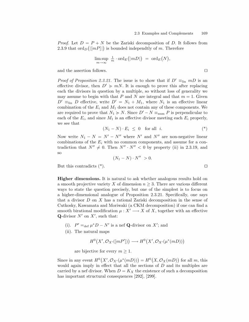
2.3 Examples and Complements 169
Proof. Let D = P + N be the Zariski decomposition of D. It follows from2.3.9 that ordD
(|[mP ]|
)is bounded independtly of m. Therefore
lim supm→∞
1m · ordE
(|mD |
)= ordE
(N),
and the assertion follows. ut
Proof of Proposition 2.3.21. The issue is to show that if D′ ≡lin mD is aneffective divisor, then D′ < mN . It is enough to prove this after replacingeach the divisors in question by a multiple, so without loss of generality wemay assume to begin with that P and N are integral and that m = 1. GivenD′ ≡lin D effective, write D′ = N1 + M1, where N1 is an effective linearcombination of the Ei and M1 does not contain any of these components. Weare required to prove that N1 < N . Since D′−N ≡num P is perpendicular toeach of the Ei, and since M1 is an effective divisor meeting each Ei properly,we see that
(N1 −N) ·Ei ≤ 0 for all i. (*)
Now write N1 − N = N ′ − N ′′ where N ′ and N ′′ are non-negative linearcombinations of the Ei with no common components, and assume for a con-tradiction that N ′′ 6= 0. Then N ′′ · N ′′ < 0 by property (ii) in 2.3.19, andso
(N1 −N) ·N ′′ > 0.
But this contradicts (*). ut
Higher dimensions. It is natural to ask whether analogous results hold ona smooth projective variety X of dimension n ≥ 3. There are various differentways to state the question precisely, but one of the simplest is to focus ona higher-dimensional analogue of Proposition 2.3.21. Specifically, one saysthat a divisor D on X has a rational Zariski decomposition in the sense ofCutkosky, Kawamata and Moriwaki (a CKM decomposition) if one can find asmooth birational modification µ : X ′ −→ X of X, together with an effectiveQ-divisor N ′ on X ′, such that:
(i). P ′ =def µ∗D −N ′ is a nef Q-divisor on X ′; and
(ii). The natural maps
H0(X ′,OX′([mP ′])
)−→ H0
(X ′,OX′(µ∗(mD))
)are bijective for every m ≥ 1.
Since in any event H0(X ′,OX′(µ∗(mD))
)= H0
(X,OX(mD)
)for all m, this
would again imply in effect that all the sections of D and its multiples arecarried by a nef divisor. When D = KX the existence of such a decompositionhas important structural consequences [292], [299].

170 Chapter 2. Linear Series
However Cutkosky [86] showed that such decompositions cannot exist ingeneral. In fact, if D is a big divisor which admits a rational CKM decompo-sition, then it follows as in Corollary 2.3.22 that
volX(D) = volX′(P ′) =(
(P ′)n)X′
is rational. Therefore a big divisor D with irrational volume (Section 2.3.B)does not admit a rational CKM-decomposition. Nakayama [434] constructeda related example where it is impossible to find a decomposition of this typeeven if one allows N ′ and P ′ to be R-divisors. Prokhorov’s survey [466] givesan overview of this circle of ideas.
One can also try to generalize Corollary 2.3.25 by attaching asymptotically-defined multiplicities to components of the stable base-locus of D. This wasfirst carried out by Nakayama [434], whose work is extended in [60] and [138].One can in effect capture the “codimension one” part of the Zariski decompo-sition, but higher codimension phenomena remain difficult to attack. In yetanother direction, Fujita [177] proved a very interesting theorem showing thatone can capture “most” of the sections of a divisor D by a nef bundle on amodification. This result, along with some applications, appears in Section11.4.
The Riemann-Roch problem.Zariski was led to Theorem 2.3.19 in thecourse of his work on the Riemann-Roch problem, which we now survey verybriefly.
Specifically, let D be a divisor on a non-singular projective surface X. Onewants to understand how the dimension h0
(X,OX(m)
)behaves as a function
of m. In this direction Zariksi [572] proves:
Theorem. Assume that D is effective. Then there is a quadratic polynomialP (x) such that for all mÀ 0:
h0(X,OX(mD)
)= P (m) + λ(m)
where λ(m) is bounded function of m.
Zariski’s theorem was completed by Cutkosky and Srinivas [89], who provethat in fact λ(m) is a periodic function of m. The paper [89] also contains anice discussion of several related questions.
It is natural to ask about the function h0(X,OX(mD)
)for a divisor D on
a smooth projective variety of dimension n. This is already very interestingwhen D is ample or nef, in which case the dominant contribution to thedimension in question is (Dn)·mn
n! . Kollar and Matsusaka [338] prove
Theorem. Assume that D is semiample. Then there exists a polynomialQ(m) of degree ≤ n− 1 such that∣∣∣h0
(X,OX(mD)
)−(Dn) ·mn
n!
∣∣∣ ≤ Q(m).

2.4 Graded Linear Series and Families of Ideals 171
Moreover the coefficients of Q(m) depend only on the intersection numbers(Dn)
and(Dn−1 ·KX
).
A somewhat sharper statement was later established by Nielson [440]. Luo[378] showed that the theorem of Kollar-Matsusaka remains valid assumingonly that D is big and nef. Some related results appear in Section 10.2 below.Tsai [527] gives some interesting applications of this circle of ideas to theboundedness of certain families of morphisms.
Example 2.3.26. Let D be a big and nef divisor on a projective variety Xof dimension n. Then given any ε > 0 there is an integer m0 such that∣∣∣h0
(X,OX(mD)
)−(Dn) ·mn
n!
∣∣∣ ≤ ε ·mn
form ≥ m0. (This is an elementary consequence of Asymptotic Riemann-RochIII, Theorem 1.4.41.) ut
2.4 Graded Linear Series and Families of Ideals
We have devoted considerable attention in the previous sections to the asymp-totic behavior of the complete linear series |mD | determined by a divisor D.However it is sometimes important to be able to discuss analogous propertiesfor possibly incomplete series, and we introduce in this section a formalismfor doing so. We also outline a related algebraic concept that allows one tobuild simple local models of many phenomena that can occur for global linearseries. Both of these constructions will play a central role when we develop thetheory of asymptotic multiplier ideals in Chapter 11. Here we focus principallyon definitions and examples.
2.4.A Graded Linear Series
The essential idea of a graded linear series goes at least as far back as Zariski’spaper [572]. More recently the formalism was developed and applied in thepaper [139] of Ein, Nakamaye and the author.
We begin with the definition.
Definition 2.4.1. (Graded linear series). Let X be an irreducible variety.A graded linear series on X consists of a collection
V• = Vm m≥0
of finite dimensional vector subspaces Vm ⊆ H0(X,OX(mD)
), D being some
integer divisor on X. These subspaces are required to satisfy the property
Vk · V` ⊆ Vk+` for all k, ` ≥ 0, (2.18)

172 Chapter 2. Linear Series
where Vk · V` denotes the image of Vk ⊗ V` under the homomorphism
H0(X,OX(kD)
)⊗H0
(X,OX(`D)
)−→ H0
(X,OX((k + `)D)
)determined by multiplication. It is also required that V0 contains all constantfunctions. ut
One can of course replace the divisor D by a line bundle L. Note however thatgiving either D or L is an essential part of the data, since they are neededto determine the multiplication in (2.18). In practice this ambient completelinear series is usually clear from context, but when it is not we will specifyV• as belonging to (or being associated with) the divisor D or bundle L.
Given a graded linear series V• = Vm, set
R(V•) =∞⊕m=0
Vm. (2.19)
Then (2.18) is equivalent to the condition that R(V•) be a graded C-subalgebra of the section ring R(D) = R(X,D) of D (Definition 2.1.16).We call R(V•) the section ring or graded ring associated to V•.
Definition 2.4.2. (Finite generation of a graded linear series). Agraded linear series V• is finitely generated if R(V•) is finitely generated as aC-algebra. ut
We next give some examples and describe some operations on graded linearseries.
Example 2.4.3. (Examples of graded linear series). Let X be an irre-ducible projective variety, and D a divisor on X.
(i). The full space of sections Vm = H0(X,OX(mD)
)defines a graded linear
series which we write Γ•(X,OX(D)
).
(ii). Let b ⊆ OX be an ideal sheaf, and c > 0 a positive real number. Set
Vm = H0(X,OX(mD)⊗ bpmcq
)where as usual prq is the round-up (i.e. least integer greater than orequal to) a real number r. For example, when a = m is the maximal idealof a smooth point x ∈ X, Vm is the subspace of sections of OX(mD)vanishing to order ≥ mc at x. Then V• = Vm is a graded linear series(belonging to D) which we denote by10
Γ•(X,OX(D)⊗ bc
).
Even when R(D) is finitely generated, this graded linear series may failto be so.
10 The notation is purely formal: in particular, we do not try to attach any meaningto bc.

2.4 Graded Linear Series and Families of Ideals 173
(iii). Fix a point x ∈ Pn and for m ≥ 1 define Vm ⊆ H0(Pn,OPn(m)
)to
be space of homogeneous polynomials of degree m that vanish at x.This determines a graded linear series V• on Pn which is not finitelygenerated.
(iv). Suppose Y ⊇ X is a variety which contains X as a subvariety, andD = D′|X is the restriction of a divisor on Y . Then the images
Vm = im(H0(Y,OY (mD′)
)−→ H0
(X,OX(mD)
) )form a graded linear series on X, which we denote by TrY (D′)•.
(v). Keeping the notation of (iv), suppose more generally that W• is a gradedlinear series on Y belonging to D′. Then the restriction V• = W• | X ofW• to X is the graded linear series given by
Vm =(
image of Wm in H0(X,OX(mD)
) ). ut
Example 2.4.4. (Product of two graded linear series). Let V• and W•be graded linear series on X associated to divisors D and E respectively. Thenone gets a graded linear series V• ·W• belonging to D +E by putting(
V• ·W•)m
= Vm ·Wm ⊆ H0(X,OX
(m(D + E)
)).
Here Vm ·Wm denotes (somewhat abusively) the image of Vm⊗Wm under themultiplication
H0(X,OX(mD)
)⊗H0
(X,OX(mE)
)−→ H0
(X,OX
(m(D + E)
)). ut
Example 2.4.5. (Intersection and span of graded linear series). LetV• and W• be graded linear series on a variety X belonging to the same divisorD. Then we get two new graded linear series V• ∩W• and Span(V•,W•) bythe rules (
V• ∩ W•)m
= Vm ∩Wm
Span(V• , W•)m =∑
k+`=m
Vk ·W`,
these both being subspaces of H0(X,OX(mD)
). ut
Example 2.4.6. (Veronese of a graded linear series). If V• is a gradedlinear series belonging to D and p ≥ 1 is a positive integer, then V
(p)• is the
graded series associated to pD whose component of degree m is(V
(p)•)m
= Vmp ⊆ H0(X,OX(mpD)
). ut
The basic asymptotic invariants of complete linear series extend withoutdifficulty to the present setting. In the following X is an irreducible projectivevariety and V• is a graded linear series belonging to a divisor D.

174 Chapter 2. Linear Series
Definition 2.4.7. (Semigroup and exponent of a graded linear se-ries). Let V• be a graded linear series belonging to a divisor D. The semigroupof V• is the set
N(V•) =m ≥ 0 | Vm 6= 0
.
The exponent e(V•) of V• is the greatest common divisor of all the elementsin N(V•). ut
Similarly:
Definition 2.4.8. (Iitaka dimension of V•). If Vm = 0 for all m, putκ(V•) = −∞. Otherwise, given a positive integer m ∈ N(V•), write
φm : X 99K PH0(X,Vm
)for the rational mapping determined by Vm, and denote by φm(X) the closureof its image. Assuming that X is normal, the Iitaka dimension κ(V•) of V• isdefined to be
κ(V•) = maxm∈N(V•)
dimφm(X) . ut
Definition 2.4.9. (Stable base locus of a graded linear series). Thestable base locus B
(V•)
of V• is the algebraic subset
B(V•)
=⋂m≥0
Bs(|Vm|
). ut
The next example shows however that in every case the invariants for agraded linear series can differ from those of the divisor to which it belongs.
Example 2.4.10. Let D be an ample divisor on a smooth projective varietyX.
(i). Put Vm = H0(X,OX(mD)
)when m is even and Vm = 0 when m is
odd. Then e(V•) = 2 but e(D) = 1.
(ii). Assume that there is an effective integral divisor E on X so that 0 <κ(D − E) < dimX. Take a = OX(−E) to be the ideal of E, and applythe construction of Example 2.4.3 (ii) to define V• = Γ•
(X,OX(D)⊗a
).
Then κ(V•) = κ(D − E) < κ(D) = dimX.(iii). Take V• to be the graded linear series belonging to OPn(1) on Pn con-
structed in 2.4.3 (iii). Then B(V•)
= x, whereas of course B(OPn(1)
)is empty. ut
Example 2.4.11. Let V• be a graded linear series on X, and let bm =b(|Vm|
)be the base ideal of Vm (Definition 1.1.8). Then
bk · b` ⊆ bk+` (2.20)
for all k, ` ≥ 0. ut

2.4 Graded Linear Series and Families of Ideals 175
Finally, one can discuss the volume of a graded linear series:
Definition 2.4.12. Let X be a projective variety of dimension n, and V• agraded linear series on X belonging to a divisor D. Then the volume of V• isthe non-negative real number
vol(V•) = lim supm∈N(V•)
dimVmmn/n!
ut
Example 2.4.13. Let D be the hyperplane divisor on X = Pn, let m be theideal of a point x ∈ Pn, and for 0 < c < 1 let V• = Γ•
(Pn,OPn(1)⊗ mc
)be
the graded linear series given by forms of degree m vanishing to order ≥ cmat x (Example 2.4.3.(ii)). Then
vol(V•) = 1− c.
In particular, this volume is irrational if c is. ut
2.4.B Graded Families of Ideals
Much of the geometry of a graded linear series V• is captured by the sequencebm = b
(|Vm|
)of its base ideals. The most important property of these ideals
is the multiplicative behavior summarized in the inclusion (2.20). Taking thisrelation as an axiom leads to an essentially local construction which can beused to model some of the complexity of global linear series. These gradedsystems of ideals are also very natural from an algebraic perspective, and onecan conversely use globally-inspired techniques to study them. This was theviewpoint taken in the papers [140], [141] of Ein, Smith and the author, fromwhich much of the present subsection is adapted.
Definition 2.4.14. (Graded family of ideals). Let X be an irreduciblevariety. A graded family or graded system of ideals a• = am on X is acollection of ideal sheaves am ⊆ OX (m ≥ 1) such that
ak · a` ⊆ ak+` (2.21)
for all k, ` ≥ 1. It is convenient to set a0 = OX . ut
Definition 2.4.15. (Rees algebra and finite generation). The Rees al-gebra of a• is the graded OX -algebra
Rees(a•) =⊕m≥0
am.
We say that a• is finitely generated if Rees(a•) is finitely generated as anOX -algebra. ut

176 Chapter 2. Linear Series
In order to give a feeling for the definition, we present an extended collec-tion of examples. Most of the constructions that follow yield graded familiesthat fail in general to be finitely generated (Remark 2.4.17).
Example 2.4.16. (Examples of graded families of ideals). Let X be anirreducible variety.
(i). If b ⊆ OX is any ideal, then the powers am = bm of b form a gradedfamily, which we denote by Pow•(b). One should view this as a trivialexample, and we will see shortly (Proposition 2.4.27) that any finitelygenerated graded system is essentially of this form.
(ii). Let V• be a graded linear series on X. Then the base ideals bm =b(|Vm | ) form a graded family b(V•). As just suggested, this is one of
the motivating examples.
(iii). Fix an ideal b ⊆ OX and a real number c > 0. Then we get a gradedfamily a• of ideals by putting am = bpmcq.
(iv). Assume that X is smooth, and let Z ⊆ X be a reduced algebraic subset.Thus the ideal sheaf q = IZ ⊆ OX of Z is radical. Given m ≥ 1, recallthat the mth symbolic power q<m> ⊆ OX of q is the ideal consistingof germs of functions that vanish to order ≥ m at a general point (andhence also at every point) of each component of Z.11 These constitutea graded system q<•>: the required inclusion
q<k> · q<`> ⊆ q<k+`>
follows from the observation that if f ∈ OxX has multiplicity ≥ k andg ∈ OxX has multiplicity ≥ ` at a point x ∈ Z, then fg vanishes toorder ≥ k + ` at x.
(v). Assume that X is normal. Let µ : X ′ −→ X be a projective (or proper)birational mapping, and letD ⊂ X be an effective µ-exceptional Cartierdivisor. Then the ideals
am = µ∗OX′(−mD) ⊆ OXform a graded family. The inclusion ak · a` ⊆ ak+` is deduced from thenatural mapping
µ∗OX′(−kD)⊗ µ∗OX′(−`D) −→ µ∗OX′(− (k + `)D
).
Note that the previous example of symbolic powers can be realized inthis fashion. (Take X ′ to dominate the blow-up of IZ , and let D bethe union of the irreducible exceptional divisors corresponding to thevaluations determined by order of vanishing along the components ofZ)
11 In commutative algebra, one defines the symbolic power somewhat differently. Itis a theorem of Nagata and Zariski that in our setting this coincides with thestated definition. See [144, Chapter 3.9] for a nice discussion.

2.4 Graded Linear Series and Families of Ideals 177
(vi). Assume that X is affine and non-singular, and identify ideal sheaveswith ideals in the coordinate ring C[X] of X. Given any non-zero idealb ⊆ C[X], set
am =f ∈ C[X]
∣∣∣ Df ∈ b
∀ differential operators D on X of order < m
.
This graded family reduces to the symbolic powers q<m> when b = qis radical.
(vii). Let a• = am be a graded family, and b ⊆ OX a fixed ideal. Then thecolon ideals
rm =(am : bm
)=def
f ∈ OX | f · bm ∈ am
form a graded family.
(viii). In the setting of (vii), observe that for fixed m the ideals (am : b`) areincreasing in `, and hence stabilize to an ideal denoted by (am : b∞).These stable colon ideals form yet another graded family indexed bym.
(ix). Let < be a term order on C[x1, . . . , xn], and let b ⊆ C[x1, . . . , xn] bean ideal. Then the initial ideals am = in<(bm) of powers of b determinea graded family of monomial ideals. ut
Remark 2.4.17. (Failure of finite generation). Except for (i), most ofthe graded families appearing in the previous Example can fail to be finitelygenerated. For instance the system bpmcq in (ii) is finitely generated if and onlyif c is rational. Goto, Nishida and Watanabe gave an example of a monomialcurve Z ⊆ C3 for which the symbolic power system in (iv) is not finitelygenerated: see [539, §7.3]. It is observed in [539, Corollary 7.2.5] that thestable colon construction in (viii) contains (iv) as a special case, as do (v) and(vi). ut
Example 2.4.18. (Graded systems from valuations). Suppose v is avaluation on the function field C(X) taking values in R, and which is non-negative on regular functions. Then the valuation ideals
am =def
f ∈ OX | v(f) ≥ m
form a graded system of ideal sheaves. When v is a divisorial valuation — i.e.v is given by order of vanishing along a prime divisor on a birational modelof X — one can realize a• as in Example 2.4.16 (iv). However already whenX = C2, so that C(X) = C(x, y), one also gets very interesting examplesfrom non-divisorial valuations.
(i). (Order of vanishing along a transcendental arc). Let p(t) =∑∞i=1
ti
i! ∈C[[t]] be the power series of the function et− 1. Given f ∈ C[x, y] define

178 Chapter 2. Linear Series
v(f) = ordt f(t , p(t)
).
The corresponding valuation ideals are given explicitly by
am =(xm , y − pm−1(x)
),
where p`(t) =∑`i=1
1i! ti is the `th Taylor polynomial of et − 1. Note
that each ak contains an polynomial defining a smooth curve in C2: thisimplies that a• cannot be finitely generated.
(ii). (Valuation by irrational weighted degree). Let am ⊆ C[x, y] be the mono-mial ideal spanned by all monomials xiyj with
i+ j√
2 ≥ m.
Then a• is the graded family of ideals corresponding to the valuation byweighted degree with v(x) = 1 and v(y) =
√2. Here again a• fails to be
finitely generated. ut
Example 2.4.19. (“Diagonal” graded system). Generalizing the previ-ous example, pick any real numbers δ1, . . . , δn > 0 and consider the monomialideal am ⊆ C[x1, . . . , xn] given by
am =⟨xi11 · . . . · xinn
∣∣ ∑ ikδk≥ m
⟩.
When the δi are integers, am is just (the integral closure of) the mth powerof the “diagonal ideal” (xδ11 , . . . , x
δnn ). In general, one can view the resulting
graded system a• = am as being an analogue defined for arbitrary realnumbers δi > 0. ut
Example 2.4.20. (Models of base loci). We illustrate the philosophythat graded systems of ideals can be used to simulate the behavior of baseloci of global linear series. As above, X is an irreducible variety.
(i). Let b ⊆ OX be a fixed ideal, and take am = b for every m ≥ 1. Theresulting graded family a• mirrors the behavior of Zariski’s example inSection 2.3.A of a divisor D for which the base-locus of each of the linearseries |mD | consists of a fixed curve independent of m. Note that if b isnon-trivial then a• is not finitely generated.
(ii). Remaining in the setting of (i), choose for each m ≥ 1 an ideal cm withb ⊆ cm ⊆ OX for every m. Then am = b · cm forms a graded familywhich models Example 2.3.5: there the base loci of |mD | consisted of afixed curve having an embedded point that varies with m.
(iii). Referring to Example 2.3.7, we see that the base-loci of the linear seriesin question are modeled by an instance of Example 2.4.16 with irrationalc > 0. ut

2.4 Graded Linear Series and Families of Ideals 179
Remark 2.4.21. Conversely, in Chapter 11 we use global methods to studygraded systems of ideals. Specifically, we will attach to any graded systema• and coefficient c > 0 a multiplier ideal J
(c · a•
)which carries interesting
information about a•, and can be used to prove some rather surprising results.(See for instance Theorem 11.3.4.) ut
Graded families of ideals give rise to graded linear series:
Example 2.4.22. Let D be a divisor on a projective variety X, and leta• = am be a graded family of ideals on X. Then the spaces
Vm = H0(X,OX(mD)⊗ am
)form a graded linear series (associated to D). Example 2.4.3.(ii) is a specialcase of this construction. utExample 2.4.23. (Realizing ideals as base loci). Keeping the notationof the previous Example, suppose that we are able to choose D so that eachof the sheaves OX(mD) ⊗ am is globally generated. Then we have realizeda• as the family of base ideals of a graded linear series V•. This applies,for example, to the two families appearing in Example 2.4.18 provided thatone compactifies and views each am in the evident way as a sheaf on P2.However there are non-trival global obstructions to realizing a given family ofideals as the base-ideals of a complete linear series. The theorem of Zariski-Fujita (Remark 2.1.31) provides one such. Another, coming from the theoryof multiplier ideals, appears in Corollary 11.2.22. ut
We next spell out some additional definitions. To begin with, there arenatural algebraic operations with graded systems of ideals:
Definition 2.4.24. (Intersection, product and sum). Let a• = amand b• = bm be graded families of ideals on a variety X. The intersection,product and sum of a• and b• are the graded systems given by the rules(
a• ∩ b•)m
= am ∩ bm(a• · b•
)m
= am · bm(a• + b•
)m
=∑
k+`=m
ak · b`. ut
As before, we can define the semigroup and Veronese of a graded system.
Definition 2.4.25. (Semigroup and exponent of a graded system ofideals). Let a• = am be a graded system of ideals on an irreducible varietyX. The semigroup of a• is the set
N(a•) = m ≥ 0 | am 6= (0) .
The exponent e(a•) of a• is the greatest common divisor of the elements inN(a•). ut

180 Chapter 2. Linear Series
Definition 2.4.26. (Veronese of a graded family). Given a graded familya• = am of ideals on X and a positive integer p > 0, the pth Veronese of a•
is the graded system a(p)• defined by(
a(p)•)m
= apm. ut
The next Proposition states that a finitely generated graded system essen-tially looks like the trivial family (Example 2.4.16 (i)) consisting of powers ofa fixed ideal:
Proposition 2.4.27. (Finitely generated graded systems). Let a• =am be a finitely generated graded family of ideals on a variety X. Then thereis an integer p > 0 such that
a(p)• = Pow•(ap).
Proof. Without loss of generality we can assume that X is affine. Then bydefinition the graded ring
Rees(a•) = C[X]⊕ a1 ⊕ a2 ⊕ . . .
is finitely generated as a C[X]-algebra. But quite generally, if a graded ringR• = R0 ⊕ R1 ⊕ R2 ⊕ . . . is finitely generated as an algebra over R0, thenfor suitable p > 0 the Veronese subring R
(p)• is generated over R0 by Rp
[61, Chapter III, Proposition 1.2]. In our situation this means exactly thatapm = amp for all m ≥ 0. ut
Example 2.4.28. (Finite generation of base ideals). Let D be a divisoron a normal projective variety X, and let b• = bm be the graded systemof base-ideals bm = b
(|mD |
). If b• is a finitely generated graded system of
ideals, then there is an integer p > 0 such that the pth-Veronese subring R(p)
of the section ring R = R(X,D) of D is finitely generated. (Use the previousexample to fix p > 0 so that bmp = bmp for all m ≥ 0, and let ν : X+ −→ X bethe normalized blowing-up of X along bp, with exceptional divisor N+. PutD+ = ν∗(pD)−N+. Then D+ is free, and arguing as in Example 2.1.30 theequality bmp = bmp implies that
R(X+, D+) = R(X,D)(p).
Then it follows from 2.1.29 that R(X,D)(p) is finitely generated.) utExample 2.4.29. (Finitely generated graded linear series). Let V• bea graded linear series on a variety X. If V• is finitely generated, then thereexists a positive integer p > 0 such that
Vpk · Vp` = Vp(k+`)
for every k, ` ≥ 1. ut

2.4 Graded Linear Series and Families of Ideals 181
Finally, we discuss an interesting invariant of a family of ideals, analogousto the volume of a graded linear series. In somewhat different language, thisnotion goes back at least to Cutkosky and Srinivas [89].
Let a• = am be a graded system of ideals on a variety X with dimX = n.Assume that all the am vanish only at one point x ∈ X, independent of m.Writing m for the maximal ideal of x, this means that each am is m-primary,and hence of finite colength (i.e. complex codimension) in OxX.
Definition 2.4.30. (Multiplicity of a graded system). Given a gradedsystem a• = am of m-primary ideals, the multiplicty of a• is defined to be
mult(a•) = lim supm→∞
colengthOxX(am)mn/n!
. ut
This was called the volume of a• in [] and [], but the present terminologyseems preferable.12
Example 2.4.31. Suppose that a• = Pow•(b) is the graded system consitingof powers of a fixed m-primary ideal b. Then mult(a•) = e(b) is the Samuelmultiplicity of b. (The limit defining e(a•) is one of the several possible defi-nitions of e(b).) utExample 2.4.32. (i). Let a• be the graded family in 2.4.18 (i) coming from
valuation along a transcendental arc. Then the codimension of am inC[x, y] grows linearly in m, and hence mult(a•) = 0.
(ii). Let a• be the “diagonal” graded system of monomial ideals from Example2.4.19. Then mult(a•) = δ1 · . . . · δn. ut
Example 2.4.33. Let a• = am be an m-primary graded system. If a• isfinitely generated, then mult(a•) is rational. (After verifying that mult(a(p)
• ) =pn ·mult(a•), this follows from 2.4.27 and 2.4.31.) utRemark 2.4.34. (Divisorial valuation with irrational multiplicity).Kuronya [345] constructs an example of a discrete divisorial valuation cen-tered at 0 ∈ C4 such that the corresponding sequence of ideals has irrationalmultiplicity. ut
Example 2.4.31 raises the question of how the multiplicity of a gradedsystem a• relates to the Samuel multiplicities e(am) of each of the terms am.We conclude by stating without proof a theorem showing that – at least whenX is smooth – the answer is as simple as one could hope.
Theorem 2.4.35. Let a• = am be an m-primary graded family of ideals ona smooth variety X of dimension n. Then
mult(a•) = limm→∞
e(am)mn
. ut
12 The notation mult(a•) is intended to avoid conflicts with the exponent e(a•) ofa•.

182 Chapter 2. Linear Series
This was established by Ein, Smith and the author in [141] for the gradedfamilies associated to certain valuations, and by Mustata [423] in general.One would expect the statement to hold also at a singular point of X, butthis isn’t known.
Notes
For Section 2.1, we have drawn on the presentations in [533] and [405].The basic numerical criterion for bigness (Theorem 2.2.15) was origi-
nally proved by Siu [496] (in a slightly weaker formulation) using Demailly’sholomorphic Morse inequalities. Elementary algebraic arguments were sub-sequently given by Ein and the author and by Catanese: here we followCatanese’s formulation (as reported in [110]). The use of this criterion to an-alyze bigness for nef divisors (Theorem 2.2.16) simplifies earlier approaches.Proposition 2.2.35 appears in [139] and [113]. Theorem 2.2.44 is new.
Section 2.3.B is abstracted from a number of papers of Cutkosky andcoauthors, notably [86], [89] and [90]. The proof of the Campana–PeternellTheorem 2.3.18 is new.

3
Geometric Consequences of Positivity
This chapter focuses on a number of results that in one way or anotherexpress geometric consequences of positivity. In the first section we provethe Lefschetz hyperplane theorem following the Morse-theoretic approach ofAndreotti-Frankel [7]. Section 3.2 deals with subvarieties of small codimen-sion in projective space: we prove Barth’s theorem and give an introductionto the conjectures of Hartshorne. The connectedness theorems of Bertini andFulton-Hansen are established in Section 3.3, while applications of the Fulton-Hansen theorem occupy Section 3.4. Like the results from 3.2, these reflectthe positivity of projective space itself. Finally, some extensions and variantsare presented in Section 3.5.
A good deal of this material is classical, and much of it has been surveyedelsewhere (e.g. in [391], [255], [189] and [181], on which we have drawn closely).However many of the results appearing here play a role in later chapters, andwe felt it important to include an account.
3.1 The Lefschetz Theorems
The theme of the Lefschetz hyperplane theorem is that a projective varietypasses on many of its topological properties to any effective ample divisorsitting inside it. As we shall see in Section ??, it is very closely related tothe Kodaira–Nakano vanishing theorem. Lefschetz originally proved his re-sult by studying the topology associated to a fibration of the given varietyby hypersurfaces: nice accounts of this approach appear in [347] and [375].However Thom and Andreotti–Frankel observed that Morse theory leads toa very quick proof, and this is the path we initially follow here. Thus in thefirst subsection we prove the theorem of Andreotti-Frankel that the cohomol-ogy of an affine variety vanishes in degrees above its complex dimension; wealso sketch the alternative approach of Artin-Grothendieck via constructiblesheaves. This result is used in the second subsection to deduce the theorem on

184 Chapter 3. Geometric Consequences of Positivity
hyperplane sections. In the third we briefly discuss (without proof) the HardLefschetz Theorem.
These results constitute the very beginning of a vast and important bodyof research concerning the topology of algebraic varieties. A survey of thisfield lies far beyond the scope of the present volume. The reader interested infurther information might start by consulting [204] or [181] and the referencescited there. In particular, the Introduction to Part II of [204] contains a verynice historical survey of work on the topology of algebraic varieties.
3.1.A Topology of Affine Varieties
We start with an elementary and classical theorem of Andreotti and Frankel[7] concerning the topology of smooth affine varieties. We then briefly surveya related approach to these questions involving constructible sheaves.
The theorem of Andreotti and Frankel. Consider a non-singular com-plex variety V of (complex) dimension n. Then V is a C∞ manifold of realdimension 2n, and hence has the homotopy type of a CW complex of dimen-sion ≤ 2n. The theorem of Andreotti and Frankel states that if V is affine —or more generally, if V is any Stein manifold of dimension n — then in factV is homotopically a CW complex of real dimension ≤ n. In other words, Vhas only “half as much topology” as one might expect:
Theorem 3.1.1. (Submanifolds of affine space). Let V ⊆ Cr be a closedconnected complex submanifold of (complex ) dimension n. Then V has thehomotopy type of a CW complex of real dimension ≤ n. Consequently,
Hi(V ; Z
)= 0 for i > n (3.1)
Hi
(V ; Z
)= 0 for i > n. (3.2)
We emphasize that the theorem applies in particular to any non-singular affinevariety of dimension n.
Example 3.1.2. It is not the case in general that V is homotopic to a finiteCW complex. For example, let V ⊆ C2 be the analytic curve defined by theequation
w · sin(2πz) − 1 = 0.
Then V is isomorphic as a complex manifold to C − Z. However if V ⊆ Cr
is a smooth algebraic subvariety, then V does in fact have the homotopy typeof a finite CW complex of dimension ≤ dimC V (Example 3.1.9). utExample 3.1.3. (Middle-dimensional homology). With V ⊆ Cr as inTheorem 3.1.1, the homology group Hn
(V ; Z
)is torsion-free. (The Theorem
implies that Hi
(V ; F
)vanishes when i > n for any coefficient field F . But
by the universal coefficient theorem, any torsion in Hn
(V ; Z
)would show up
in Hn+1
(V ; F
)for suitable F .) ut

3.1 The Lefschetz Theorems 185
Remark 3.1.4. (Singular varieties). It was established by Karchjauskas[284], [285] (for algebraic varieties) and by Hamm [240] (for Stein spaces) thatTheorem 3.1.1 remains true for arbitrarily singular irreducible V . However forthe most part the elementary case of non-singular varieties will suffice for ourpurposes. The vanishing (3.1) for possibly singular varieties had been verifiedearlier by Kaup [287] and Narasimhan [437]. At least in the algebraic settingthis statement also follows from general results about constructible sheaveswhich we discuss briefly below.
These results for singular varieties are in turn generalized by Goresky andMacPherson using their stratified Morse theory. Among other things, theyextend Theorem 3.1.1 to the setting of a possibly singular variety mappingproperly to an affine variety [204, Theorem II.1.1*]. We recommend Chapter1 of Part II of [204] for an overview of how the classical results generalize tothe singular (or non-compact) setting. Fulton’s survey [181] gives a very niceintroduction to this circle of ideas. ut
Theorem 3.1.1 is a beautiful application of elementary Morse theory, andwe start by recalling the basic facts of this machine. The reader may consultMilnor’s classical book [391, Part I] for details.
Consider then a C∞ manifoldM of real dimension n, and a smooth function
f : M −→ R.
Suppose that p ∈M is a critical point of f , i.e. a point at which dfp = 0. Thenthe Hessian Hessp(f) of f at p is an intrinsically defined symmetric bilinearform on the tangent space TpX: in local coordinates x1, . . . , xn it is representedby the Hessian matrix
(∂2f
∂xi∂xj(p))
of second partials of f . One says that pis a non-degenerate critical point if Hessp(f) is non-degenerate. In this case,the index λ = indexp(f) of f at p is defined to be the number of negativeeigenvalues of the Hessian. Very concretely, Morse’s Lemma ([391, Lemma2.2]) states that in suitable local coordinates centered at a non-degeneratecritical point of index λ, f is given by the quadratic function
f(x1, . . . , xn) = −x21 − . . .− x2
λ + x2λ+1 + . . .+ x2
n.
The proof of Theorem 3.1.1 will call on two basic results from (finite di-mensional) Morse theory. The first states that under suitable compactness hy-potheses, a function on a manifold having only non-degenerate critical pointsallows one to reconstruct the given manifold as a CW complex:
Theorem 3.1.5. (cf. [391, Theorem 3.5]). Let
f : M −→ R
be a smooth function having the property that f−1(−∞, a] is compact for everya ∈ R. Assume that f has only non-degenerate critical points. Then M has

186 Chapter 3. Geometric Consequences of Positivity
the homotopy type of a CW complex with one cell of dimension λ for everycritical point of index λ. ut
The second fact we need is that for submanifolds of Euclidean space, dis-tance (squared) from a general point gives rise to a Morse function:
Theorem 3.1.6. (cf. [391, Theorem 6.6]). Let M ⊆ RN be a closed sub-manifold. Fix a point c ∈ RN and let
φc : M −→ R , x 7→ ‖x− c‖2
be the function given by squared distance from c, where ‖ ‖ denotes the stan-dard Euclidean norm on RN . Then for almost all c ∈ RN , φc has only non-degenerate critical points on M . ut
Observe that the compactness of φ−1c (−∞, a] for every a is evident.
In view of 3.1.5 and 3.1.6, Theorem 3.1.1 reduces to estimating the indexof the squared distance function:
Proposition 3.1.7. (Index estimate). Let V ⊆ Cr be a closed complexsubmanifold of complex dimension n. Fix a point c ∈ Cr = R2r, and consideras in 3.1.6 the squared distance φc(x) = ‖x − c‖2. If p ∈ V is any criticalpoint of φc, then
indexp(φc) ≤ n.
Elegant proofs appear e.g. in [391, §7], [224, p. 158], [204, II.4.A] and [181, p.26]. We will give a down–to–earth direct computation in the spirit of [7].
Proof of Proposition 3.1.7. Writing r = n + k, we can choose complex coor-dinates on Cr in such a way that p = 0 is the origin, V is locally the graphof a holomorphic function f : Cn −→ Ck with df0 = 0, and
c =(0, . . . , 0, 1, 0, . . . , 0
)is the unit vector with all but the (n+ 1)st coordinate zero (Figure 3.1). ThusV is described in local coordinates z = (z1, . . . , zn) at p as the set
V =(z1, . . . , zn, f1(z), . . . , fk(z)
),
with fi(z) holomorphic and ord0(fi) ≥ 2. Then φ = φc is given by
φ(z) = |z1|2 + . . . + |zn|2 + |f1(z)− 1|2 + |f2(z)2| + |fk(z)|2
=(1− 2 · Re(f1(z)
)+
n∑i=1
|zi|2 +k∑i=1
|fi(z)|2. (*)
Since each fi vanishes to order ≥ 2 at 0, the last term in (*) will not affectthe Hessian Hess0(φ). Similarly, if we write

3.1 The Lefschetz Theorems 187
c
Cn
Ck
V
Figure 3.1. Set-up for proof of Proposition 3.1.7
f1(z) = Q(z) +(
higher order terms)
with Q(z) homogeneous of degree 2, then the contribution of the first term in(*) to Hess0(φ) depends only Q. Therefore
Hess0
(φ)
= −2 ·Hess0
(Re(Q(z)
))+ Hess0
(∑|zi|2
)= −2 ·Hess0
(Re(Q(z)
))+ 2 · Id. (**)
The second term in (**) being positive definite, the only potential source ofnegative eigenvalues is from the Hessian of Re(Q). Therefore the Proposition— and with it Theorem 3.1.1 — is a consequence of the next Lemma. ut
Lemma 3.1.8. Let Q(z) be a complex homogeneous form of degree 2 in nvariables z = (z1, . . . , zn). Then
Hess0
(Re(Q(z)
))has ≤ n positive and ≤ n negative eigenvalues.
Proof. To start with an illustrative special case, imagine that Q is the poly-nomial Q(z) = z2
1 + . . . + z2s for some s ≤ n. Writing zj = xj +
√−1yj , one
hasReQ(z) =
(x2
1 − y21
)+ . . . +
(x2s − y2
s
),
from which the assertion is clear. In general, as in [7, p.716], suppose that
Q(z) =∑
ci,jzizj
for complex numbers ci,j = cj,i ∈ C. Taking real and imaginary parts asabove, one finds that the real quadratic form H(x, y) = ReQ(x +
√−1y) is

188 Chapter 3. Geometric Consequences of Positivity
represented by a block matrix of the shape(A −B−B −A
), where A and B are
n × n real symmetric matrices. But such a matrix has as many positive as
negative eigenvalues: if(uv
)is an eigenvector with eigenvalue λ, then
(−vu
)is an eigenvector with eigenvalue −λ. ut
Example 3.1.9. (Finiteness of homotopy type of affine variety). LetV ⊆ Cr be a smooth affine algebraic variety of dimension n. Then V has thehomotopy type of a finite CW complex of real dimension ≤ n. (The functionφc : V −→ R appearing above is real algebraic, and hence its critical locusis a real algebraic subset of V . But the critical points of φc are discrete,and therefore there are only finitely many such.) As observed in 3.1.2, thecorresponding statement can fail for Stein manifolds. ut
Constructible sheaves. We now discuss briefly another approach to someof these questions, via constructible sheaves. The technique originated withArtin and Grothendieck as a mechanism for proving Lefschetz–type theoremsin the setting of `-adic cohomology.
Let X be a complex algebraic variety.
Definition 3.1.10. (Constructible sheaf). A constructible sheaf on Xis a sheaf F of abelian groups having the property that X admits a finitestratification X =
∐i∈I Xi into disjoint Zariski–locally closed subsets Xi
in such a way that the sheaf-theoretic restriction F |Xi to each Xi is a localsystem on Xi. ut
By a local system we mean as usual a locally constant sheaf with respect to theclassical topology on Xi. Note that then F will be locally constant on someunion of the Xi, i.e. on a constructible subset of X. When we talk about thecohomology (or direct images) of F , we always refer to the classical topologyon X.
Example 3.1.11. (Direct images under finite maps). Let f : Y −→ Xbe a finite morphism. Then the direct image f∗Z of the constant sheaf onY is a constructible sheaf on X. More generally, the direct image f∗F ofany constructible sheaf F on Y is a constructible sheaf on X. (For the firststatement observe that f induces a locally closed stratification X =
∐Xi of
X having the property that f is a covering space over each Xi.) ut
Remark 3.1.12. (Direct images under arbitrary maps). Quite generallyif f : Y −→ X is any (finite-type) morphism of algebraic varieties, and if F isa constructible sheaf on Y , then all the direct images Rjf∗F are constructiblesheaves on X: see [102, Theorem 1.1 p. 233]. When F = Z is the constant sheafon Y and f is proper, this follows from the fact [540] that X is stratified bylocally closed sets on which the topological type of the fibres of f is constant.
ut

3.1 The Lefschetz Theorems 189
The theorem of Artin and Grothendieck is a cohomological analogue of3.1.1:
Theorem 3.1.13. (Artin-Grothendieck theorem). Let V be an affinevariety of dimension n, and let F be a constructible sheaf on V . Then
Hi(V,F
)= 0 for i > n.
This of course implies in particular that Hi(V,Z
)= 0 for i > n. Note that
we do not assume here that V is smooth.
Remark 3.1.14. It is not necessary in 3.1.13 to assume that V is irreducible.In fact the statement and proof of this result remain valid for any affinealgebraic set V of dimension n. ut
Sketch of Proof of Theorem 3.1.13. We closely follow the presentations in[549] and [14, Chapter VII, §3]. Choose to begin with a finite map f : V −→Cn. Then
Hi(V,F
)= Hi
(Cn, f∗F
)so it is enough thanks to 3.1.11 to prove the statement for V = Cn. Thus wesuppose that F is a constructible sheaf on Cn, and we prove by induction onn that
Hi(Cn,F
)= 0 for i > n. (3.3)
This is elementary if n = 1, so we assume that n ≥ 2 and that (3.3) is knownfor all constructible sheaves on Cn−1.
By definition there exists a proper closed algebraic subset Z ⊆ Cn suchthat F is locally constant on Cn−Z. Fix a linear projection p : Cn −→ Cn−1
so that the restriction of p to Z is finite (and in particular proper). We assertthat (
Rip∗F)x
= Hi(p−1(x),F | p−1(x)
)(3.4)
for any point x ∈ Cn−1. Grant this for the time being. Then in the firstplace, F | p−1(x) being a constructible sheaf on p−1(x) = C, it follows fromthe induction hypothesis that Rip∗F = 0 for i > 1. On the other hand, thedirect images p∗F and R1p∗F are constructible sheaves on Cn−1: this is aconsequence of the general theorem quoted in Remark 3.1.12, but could alsobe verified directly in the case at hand using (3.4). The required vanishing (3.3)then follows from the induction hypothesis and the Leray spectral sequence.
It remains to establish the isomorphism (3.4). For this, recall that
Hi(p−1(x) , F | p−1(x)
)= lim−→
N
Hi(N,F
),
the limit running over all open neighborhoods N ⊇ p−1(x). Therefore it suf-fices to show that given N there are open neighborhoods U 3 x of x in Cn−1
and N ′ ⊆ N ∩ p−1(U) of p−1(x) in Cn such that

190 Chapter 3. Geometric Consequences of Positivity
Hi(p−1(U),F
)= Hi
(N ′,F
). (*)
To this end write Cn as the product Cn−1 × C, with p the first projection.One starts by constructing a small ball U ⊆ Cn−1 centered at x, and a diskA ⊆ C such that
Z ∩ p−1(U) ⊆ U ×AU ×A ⊆ N.
Here Z ⊆ Cn is the proper subvariety chosen above off of which F is locallyconstant, and in the first inclusion we are using the properness of p |Z. Onenow uses a “tapering” process to extend U × A to a neighborhood N ′ ⊆ Nof p−1(x) having the property that p−1(U) deformation retracts onto N ′ viaa homotopy leaving
Z ∩ p−1(U) = Z ∩N ′
fixed. In fact, fix coordinates on Cn−1 in such a way that x is the origin andU is the ball of radius 1. Now choose a continuous function φ : C −→ (0, 1],with φ |A ≡ 1, such that
N ′ =def
(z, t) | ‖z‖2 < φ(t)
⊆ N.
Then N ′ has the required properties, and (*) follows. We refer to [14, p. 316]for details. ut
Remark 3.1.15. In his interesting recent paper [445], Nori studies the ho-mological properties of constructible sheaves. He uses these to give a new ap-proach to the theorem of Artin-Grothendieck and some related questions. ut
Remark 3.1.16. (Analytic constructible sheaves). With more care onecan extend these definitions and results to the setting of analytically con-structible sheaves. We refer to [244] and the references therein for details. ut
3.1.B The Theorem on Hyperplane Sections
We now come to the Lefschetz hyperplane theorem, which compares the topol-ogy of a smooth projective variety X with that of an effective ample divisorD on X. When we speak of the topological properties of D, we are referringof course to the subspace of X (with its classical topology) determined by thesupport of D.
Theorem 3.1.17. (Lefschetz hyperplane theorem). Let X be a non-singular irreducible complex projective variety of dimension n, and let D beany effective ample divisor on X. Then
Hi(X , D ; Z
)= 0 for i < n. (3.5)

3.1 The Lefschetz Theorems 191
Equivalently, the restriction
Hi(X ; Z
)−→ Hi
(D ; Z
)(3.6)
is an isomorphism for i ≤ n− 2 and injective when i = n− 1.
Note that we do not assume that D is non-singular. However one cannotdispense entirely with the non-singularity of X: see 3.1.33 and 3.1.34.
Proof. Since D is ample, mD is very ample for some m À 0. So we can finda projective embedding X ⊆ Pr together with a hyperplane H ⊆ Pr suchthat X ∩ H = mD. In particular, X − D = X − mD is affine. ThereforeHj(X −D ; Z ) = 0 for j ≥ n+ 1 thanks to 3.1.1. The assertion then followsfrom Lefschetz duality Hi
(X,D
)= H2n−i
(X −D
). ut
Example 3.1.18. In the setting of Theorem 3.1.17, the cokernel of the re-striction
Hn−1(X ; Z
)−→ Hn−1
(D ; Z
)is torsion-free. (Note that the cokernel in question sits as a subgroup insideHn(X,D; Z). Then argue as above using Example 3.1.3 to see that this group
is torsion-free.) utCorollary 3.1.19. (Connectedness of ample divisors). Let X be asmooth irreducible projective variety of dimension n ≥ 2 and D ⊆ X anample divisor. Then D is connected.
Proof. In fact, H0(D; Z) = Z thanks to 3.1.17. ut
Remark 3.1.20. (Lemma of Enriques-Severi-Zariski). The conclu-sion of the preceding Corollary is actually valid without assuming thatX is non-singular. In fact, one can suppose that X is normal and thenH1(X,OX(−mD)
)= 0 for m À 0, from which the assertion follows. See
[256, III.7.7 and III.7.8 ] for details. The connectedness of D also follows fromTheorem 3.3.3 below. ut
As pointed out in [391, Theorem 7.4] one can get a somewhat strongerstatement on the level of homotopy by going back to the proof of Theorem3.1.1:
Theorem 3.1.21. (Lefschetz theorem for homotopy groups). In thesituation of Theorem 3.1.17:
πi(X , D
)= 0 for i < n.
In particular, the homomorphism
πi(D)−→ πi
(X)
induced by inclusion is bijective if i ≤ n− 2 and surjective if i = n− 1.

192 Chapter 3. Geometric Consequences of Positivity
Note that except in the trivial case n = 1 — where the present statementis vacuous — the spaces in question are path-connected by virtue of 3.1.19.Therefore we will ignore base-points.
Remark 3.1.22. Goresky and MacPherson [204, II.1.1] have proven a deepgeneralization of this result which allows for the possibility that X is non-compact. Their result is stated below as Theorem 3.5.9. ut
Proof of Theorem 3.1.21. Choose as above a projective embedding X ⊆ Pr
and a hyperplane H such that X ∩H = mD for some m À 0. Then we canview V = X − D as being embedded in the affine space Cr = Pr − H. Asin the previous subsection squared distance from a general point c ∈ Cr notlying on V determines a Morse function φc : V −→ R. Consider now thefunction f : X −→ R given by
f(x) =
1
φc(x) for x ∈ V = X −D0 for x ∈ D.
The critical points of f off D coincide with those of φc, but the signs of theeigenvalues of the Hessian are reversed. Therefore f has only non-degeneratecritical points away from D, each of index ≥ n. So for any ε > 0, X has thehomotopy type of Xε =def f
−1[0, ε] with finitely many cells of dimensions ≥ nattached. In particular the homomorphism
πi(Xε, D)−→πi
(X,D
)is bijective for i ≤ n− 1.
Now since one can triangulate X with D as a subcomplex, we may fix aneighborhood U of D in X which deformation retracts onto D. Take ε > 0sufficiently small so that Xε ⊆ U , and consider the commutative diagram:
πi(Xε , D
)//
∼= ''NNNNNNNNNNNπi(U , D
)xxppppppppppp
πi(X , D
).
The diagonal map on the left is an isomorphism when i ≤ n− 1 whereas thegroup on the top right vanishes by construction. The assertion follows. ut
Example 3.1.23. Let X be a non-singular simply connected projective vari-ety of dimension ≥ 3, and let D ⊆ X be an ample divisor. Then D is simplyconnected. This applies in particular to hypersurfaces in Pn for n ≥ 3.
Example 3.1.24. (Lefschetz theorem for Hodge groups). Let X be asmooth projective variety of dimension n, andD a non-singular ample effectivedivisor on X. Denote by

3.1 The Lefschetz Theorems 193
rp,q : Hq(X,ΩpX
)−→ Hq
(D,ΩpD
)the natural maps determined by restriction. Then
rp,q is
an isomorphism for p+ q ≤ n− 2injective for p+ q = n− 1.
(Apply the Hodge decomposition on X and on D to the complexification ofthe restriction maps (3.6): see Lemma ??.) The case p = 0 of this statementwill lead very quickly to the Kodaira vanishing theorem in Section ??. ut
Example 3.1.25. (Lefschetz theorem for Picard groups). Let X be asmooth projective variety of dimension ≥ 4, and D ⊆ X a reduced effectiveample divisor. Then the map
Pic(X) −→ Pic(D)
is an isomorphism. (One compares the exponential sequences on X and on D:the reducedness of D guarantees that the exponential sheaf sequence on D isexact. In view of the isomorphisms (3.6) for i = 1, 2 it is enough to show thatthe restrictions
Hi(X,OX
)−→Hi
(D,OD
)(*)
are bijective when i ≤ 2. But this follows from Kodaira vanishing (Theorem??), which implies that Hi
(X,OX(−D)
)= 0 for i ≤ 3. If D is non-singular,
then (*) alternatively follows from 3.1.24.) ut
Remark 3.1.26. (Grothendieck’s Lefschetz-type theorem for Picardgroups). Using different methods, Grothendieck proves in [234, Expose XII,Corollary 3.6] that the statement in 3.1.25 remains true even if the ampledivisor D is non-reduced: see [252, Corollary IV.3.3].1 ut
Example 3.1.27. (Factoriality of homogeneous coordinate rings ofhypersurfaces). Let F ∈ C[X0, . . . , Xn] be a non-zero homogeneous poly-nomial in n + 1 ≥ 5 variables, and assume that the hypersurface D ⊆ Pn
defined by F is non-singular. Then the quotient ring
R = C[X0, . . . , Xn] / (F )
is a unique factorization domain. (Since D is in any event projectively normal,it is well known that R is factorial if and only if Pic(D) = Pic(P) : see [252,Chapter IV, Exercise 3.5].) ut1 Hartshorne assumes that D is non-singular in order to invoke Kodaira vanishing
on D to establish the vanishings Hi(D,OD(mD)
)= 0 for i = 1, 2 and m < 0.
However as in Example 3.1.25 these follow from Kodaira on X.

194 Chapter 3. Geometric Consequences of Positivity
Remark 3.1.28. (Further applications to local algebra). The previousExample hints at the fact that this circle of ideas has interesting applicationsto local algebra, in particular to questions of factoriality. This viewpoint wasgreatly developed by Grothendieck in his seminar [234], especially Expose XI.Among many other things, Grothendieck proves a conjecture of Samuel to theeffect that if A is a local noetherian ring arising as a complete intersection,and if A is factorial in codimension ≤ 3, then A is factorial (loc. cit., CorollaryXI.3.14). Example 3.1.27 is a very special case of this result. We recommendLipman’s survey [370] for a nice overview of this work. ut
Example 3.1.29. (Lefschetz theorems and Nef cones). Let X be asmooth projective variety of dimension ≥ 4 and D ⊆ X a smooth ampledivisor. Then it follows from Example 3.1.24 and the Lefschetz (1, 1)-theorem(Remark 1.1.21) that restriction determines an isomorphism
N1(X)R
∼=−→ N1(D)R
of the Neron-Severi spaces of X and D. One can ask how this isomorphismbehaves with respect to the natural cones of divisors sitting inside these vectorspaces. Since the restriction of a nef divisor is nef, the nef cone of X evidentlymaps into the nef cone of D. However simple examples show that the lattercone can be strictly bigger. For instance, following [258] consider X = P1 ×Pn−1, and let D ⊆ X be a general divisor of type (a, b), with a ≥ n + 1.Then the projection D −→ Pn−1 is finite, and hence OPn−1(1) pulls back toan ample line bundle on D. It follows that if k À 0 then the restriction ofpr∗1OP1(−1)⊗ pr∗2OPn−1(k) to D is ample, but of course this is not nef — oreven big — on X itself. However Kollar [58, Appendix], Wisniewski [563] andHassett-Lin-Wang [258] obtain some positive results by taking into accountthe Mori cone of X. utRemark 3.1.30. (Noether–Lefschetz theorem). Simple examples — e.g.a quadric surface in P3 — show that if D ⊆ X is an ample divisor, then therestriction Pic(X) −→ Pic(D) can fail to be an isomorphism when dimX ≤ 3.However a classical theorem of Noether and Lefschetz states that if D ⊆ P3
is a “very general” hypersurface of degree ≥ 4, then indeed Pic(D) = Pic(P3)(although for special D — e.g. those containing a line — this can fail). See[72], [211] or [73, Chapter 7.5] for a modern discussion of this and relatedresults. utExample 3.1.31. (Lefschetz theorem for complete intersections).Suppose that Y ⊆ Pn is the transversal complete intersection of hypersurfacesD1, . . . , De ⊆ Pr of degrees d1 ≥ d2 ≥ . . . ≥ de. Then
Hi(Pn, Y ; Z
)= 0 for i ≤ n− e.
(Argue that after possibly modifying the Di, one can take each of the inter-mediate intersections D1 ∩ . . .∩Di+1 to be smooth. Then apply the Lefschetztheorem inductively.) ut

3.1 The Lefschetz Theorems 195
Remark 3.1.32. (Arbitrary intersections of ample divisors). Moregenerally, let X be a smooth projective variety of dimension n, and letD1, . . . , De ⊆ X be any effective ample divisors on X. Consider the inter-section
Z = D1 ∩ . . . ∩De
of the given divisors (which we view as a closed subspace of X). Then
Hi(X ,Z ; Z
)= 0 for i ≤ n− e. (3.7)
This is a special case of a result of Sommese which we prove as Theorem7.1.1. Under additional hypotheses on Z and the Di one can establish (3.7)inductively as in the previous example. However in general this approach runsinto problems if the Di are singular or Z has larger than expected dimension.
ut
Example 3.1.33. (Counterexamples for singular varieties). A con-struction due to A. Landman shows that Theorem 3.1.17 need not be validif X is singular. Let Y be a non-singular simply connected variety of dimen-sion ≥ 3, and let p, q ∈ Y be distinct points. Then one can construct a newprojective variety X which is isomorphic to Y with p and q identified to asingular point o ∈ X.2 Thus H1
(X)6= 0, but if D ⊂ X is an ample divisor
whose support does not pass through o, then D — being isomorphic to anample divisor on Y — is simply connected. In particular H1
(X,D
)6= 0. ut
Remark 3.1.34. (Local complete intersections). Using local results ofHamm ([240], [241]), Goresky and MacPherson [204, p. 24 and II.5.2] showthat 3.1.17 and 3.1.21 remain true as stated if X is locally a complete inter-section in some smooth variety. For arbitrarily singular X they introduce anumerical invariant s = s(X) which measures how far X is from being a localcomplete intersection, and they prove that πi
(X,D) = 0 for i < n − s. We
again refer to [181, §2] for a very readable introduction. ut
Remark 3.1.35. (Local theorems of Lefschetz type). Grothendieckstressed in [234, Expose XIII] that the classical results of Lefschetz shouldarise from more general local results, and he proposed a number of prob-lems in this direction. Grothendieck’s program was substantially carried outby Hamm and Le [242], [243] and Goresky-MacPherson [204]. For example,Goresky-MacPherson (loc. cit., p. 26, II.1.3 and II.5.3) prove that if X ⊆ Cr
is an analytic subvariety of pure dimension n+1 having an isolated singularityat the origin 0, and if H is a general hyperplane through 0, then
πi(X ∩ ∂Bε , X ∩H ∩ ∂Bε
)= 0 for i < n,
2 Under a sufficiently positive projective embedding Y ⊆ P, a general point on thesecant line joining p and q will not meet any other secant lines of Y . Then takeX to be the image of Y under projection from this point.

196 Chapter 3. Geometric Consequences of Positivity
Bε being an ball of radius ε ¿ 1 centered at 0. They deduce the classicalLefschetz theorem from this, at least when D is a general divisor in a veryample linear series on X. ut
Remark 3.1.36. (Nori’s connectedness theorem). Nori [444] has estab-lished an interesting variant of 3.1.17 and 3.1.32 which he applied in a sur-prising manner to study algebraic cycles. Specifically, let X be a non-singularcomplex projective variety of dimension n, and D a very ample divisor on X.Given e ≤ n positive integers a1, . . . , ae, denote by
S ⊆ |a1D | × . . .× |aeD |
the variety parameterizing e-tuples of divisors in the corresponding linearseries. Then the universal family D of complete intersections of type a1, . . . , aeon X sits naturally inside XS = X × S:
D =(x,D1, . . . , De
) ∣∣ x ∈ D1 ∩ . . . ∩De
⊆ XS .
For any morphism T −→ S, let DT ⊆ XT = X × T denote the pullback ofD to T . Nori proves that if the ai are sufficiently large, then for any smoothmorphism T −→ S one has the vanishing
Hi(XT , DT ; Q
)= 0 for i ≤ 2(n− e). (*)
In the range i ≤ n− e this follows — for any morphism T −→ S — from 3.7and the Leray spectral sequence. So the essential assertion is that one has astronger statement for locally complete families. The proof of (*) is Hodge-theoretic in nature. Besides Nori’s original paper [444], we recommend [214],[553, Chapter 20] and [73, Chapter 10] for expositions of the theorem and itsapplication to the study of algebraic cycles. ut
Remark 3.1.37. (Lefschetz-type statements for fundamental groupsof subvarieties). In his book [334], Kollar considers an irreducible subvarietyZ ⊆ X of a smooth projective variety X and tries to find geometric expla-nations for the possibility that π1(Z) has small image in π1(X). By studyingfamilies of cycles on X, he proves for example that if ρ(X) = 1 and π1(X) isinfinite, and if Z passes through a very general point of X then in fact theimage of π1(Z ′) −→ π1(X) is infinite, Z ′ −→ Z being the normalization of Z.See [334, Chapter 1] for more information. ut
Remark 3.1.38. (Lefschetz theorem for CR manifolds). In their paper[438], Ni and Wolfson prove an analogue of the Lefschetz hyperplane theo-rem for certain compact CR submanifolds of Pr. This is an example of theemerging principle that the Lefschetz hyperplane theoerm and related resultsdiscussed in the present Chapter have analogues in non-algebraic settings: seeRemarks 3.2.7 and 3.3.11. ut

3.1 The Lefschetz Theorems 197
3.1.C Hard Lefschetz Theorem
On several occasions we will require a second (deeper) theorem of Lefschetz.Here we briefly state this result without proof.
Let X be a smooth projective variety of dimension n, which we viewas a complex manifold. Recall (Definition 1.2.39) that a Kahler form ω onX is a closed positive C∞ (1, 1)-form. Wedge product with ω determines ahomomorphism
L = Lω : Hi(X; C
)−→ Hi+2
(X; C
)which of course depends only on the cohomology class [ω] ∈ H2
(X; C
)of ω.
The result in question is the following:
Theorem 3.1.39. (Hard Lefschetz theorem). For any Kahler form ω onX, the k-fold iterate
Lk : Hn−k(X; C) ∼=−→ Hn+k
(X; C
)(3.8)
of L = Lω is an isomorphism on the indicated cohomology groups.
Note that this applies in particular when ω is a Kahler form representing thefirst Chern class of any ample line bundle on X. See [553, §6.2.3] for a verynice account of the proof via harmonic theory.
Hard Lefschetz is often applied via
Corollary 3.1.40. In the situation of the Theorem, the mapping
Lk : Hi(X; C
)−→Hi+2k
(X; C
)is injective when i ≤ n− k and surjective when i ≥ n− k.
Proof. If i ≤ n− k, the composition
Hi(X; C
) Lk // Hi+2k(X; C
) Ln−k−i // H2n−i(X; C)
is an isomorphism thanks to 3.1.39, and so the first mapping Lk is injective.The second statement is similar. ut
We conclude by outlining an interesting application of Hard Lefschetz dueto Wisniewski [564], and some subsequent developments thereof.
Example 3.1.41. (Semiample deformations of ample line bundles).Let
f : X −→ T
be a smooth projective mapping of algebraic varieties, and let L be a linebundle on X. Assume that Lt is ample on the fibre Xt for general t ∈ T , and

198 Chapter 3. Geometric Consequences of Positivity
semiample (Definition 2.1.25) on X0 for some special point 0 ∈ T . Choose aninteger m > 0 such that L⊗m0 is free, and consider the corresponding morphism
φ0 : X0 −→ Y0 ⊆ P.
Then for any irreducible subvariety Z0 ⊆ X0, one has the inequality
2 · dimZ0 − dimX0 ≤ dimφ(Z0). (3.9)
In other words, a semiample deformation of an ample line bundle cannotcontract too much. (Set n = dimX, a = dimZ0 and b − 1 = dimφ(Z0).Writing η ∈ H2(n−a)
(X; R
)for the cohomology class of Z0, one evidently has
c1(L0)b · η = 0 ∈ H2n−2a+2b(X0; C
).
On the other hand, the homomorphisms
H2n−2a(Xt; C
)−→ H2n−2a+2b
(Xt; C
)given by cup product with c1(Lt)b, being defined over Z and topologicallydetermined, are independent of t ∈ T . So by Corollary 3.1.40 they are injectiveprovided that b ≤ 2a− n.) utRemark 3.1.42. (Topology of semismall maps). A morphism f : X −→Y of irreducible projective varieties is said to be semismall if each of thelocally closed sets
Yk =def
y ∈ Y | dim f−1(y) = k
has codimension ≥ 2k in Y . This is equivalent to asking that
2 · dimZ − dim f(Z) ≤ dimX
for every irreducible subvariety Z ⊆ X. So one can rephrase the conclusion(3.9) of the previous example as asserting that the morphism φ0 appearingthere is semismall. In their paper [92], de Cataldo and Migliorini establisha number of interesting facts about the topology of such maps. For instancethey show that a semiample line bundle L on a smooth projective variety Xof dimension n is the pullback of an ample line bundle under a semismall mapif and only the Hard Lefschetz theorem holds for L in the sense that k-foldcup product with c1(L) determines an isomorphism
Hn−k(X; C) ∼=−→ Hn+k
(X; C
)for every k ≥ 0. In their subsequent paper [93], de Cataldo and Migliorinistudy the Hodge-theoretic properties of arbitrary morphisms f : X −→ Yof projective varieties, with X smooth. Among other things, they arrive atnew proofs of the fundamental theorems of Beilinson, Bernstein, Deligne andGabber [42] concerning the topology of such maps. ut

3.2 Projective Subvarieties of Small Codimension 199
3.2 Projective Subvarieties of Small Codimension
An elementary classical theorem states that any smooth projective variety ofdimension n can be embedded in P2n+1 (cf. [491, II.5.4]). Therefore subva-rieties X ⊆ Pr with codimX > dimX cannot be expected to exhibit anyspecial properties. On the other hand, starting with a theorem of Barth in1970 it became clear that if codimX < dimX, then X must be quite spe-cial. This viewpoint was developed in Hartshorne’s influential article [255].The present section is devoted to some of the properties of projective subvari-eties of small codimension: we start by discussing Barth’s theorem, and thengive a brief account of Hartshorne’s conjecture on complete intersections. TheFulton-Hansen connectedness theorem leads to some related results appearingin Section 3.4.
3.2.A Barth’s Theorem
Let X ⊆ Pr be a smooth irreducible subvariety of dimension n and codimen-sion e = r − n. It follows inductively from the Lefschetz hyperplane theorem(Theorem 3.1.17 and Example 3.1.31) that if X is the transversal completeintersection of e hypersurfaces, then there are isomorphisms
Hi(Pr; Z
) ∼=−→ Hi(X; Z
)for i ≤ n− 1.
In 1970 Barth made the remarkable discovery that a similar statement holds(in a smaller range of degrees) for any smooth variety X having small codi-mension in projective space. Barth’s result sparked a great deal of interest inthe geometry of such subvarieties.
We start by stating the result.
Theorem 3.2.1. (Barth–Larsen theorem). Let X ⊆ Pr be a non-singularsubvariety of dimension n and codimension e = r − n.
(i). Restriction of cohomology classes determines an isomorphism
Hi(Pr; C
) ∼=−→ Hi(X; C
)for i ≤ 2n− r = n− e.
(ii). More generally, one has the vanishing of the relative homotopy groups
πi(Pr, X
)= 0 for i ≤ 2n− r + 1 = n− e+ 1.
In particular, the maps
Hi(Pr; Z
)−→Hi
(X; Z
), Hi
(X; Z
)−→Hi
(Pr; Z
)are isomorphisms for i ≤ 2n− r = n− e.

200 Chapter 3. Geometric Consequences of Positivity
Of course the second statement implies the first: we separate them for histor-ical and expository reasons.
Statement (i) was originally proved by Barth [24] via delicate geomet-ric and sheaf-theoretic arguments. In fact, he showed more generally that ifX,Y ⊆ Pr are any two connected algebraic submanifolds having dimensionsn and m respectively, and if X and Y meet properly, then
Hi(Y,X ∩ Y ; C
)= 0 for i ≤ minn+m− r, 2n− r + 1;
Theorem 3.2.1 (i) is the case Y = Pr. The extension (ii) to higher homo-topy groups was established slightly later by Larsen [354] and Barth–Larsen[26], [25]. Hartshorne [255] found a very quick proof of (i) based on the hardLefschetz theorem: we will present this shortly. In Section 3.5 we outlinean argument from [189, §9] showing that one can deduce (ii) from a non-compact strengthening of the Lefschetz hyperplane theorem due to Goreskyand MacPherson. Some other approaches and generalizations are indicated inRemarks 3.2.5 and 3.2.6.
Note that Theorem 3.2.1 gives no information about subvarieties X ⊆Pr having codimX ≥ dimX. On the other hand, as the codimension of Xbecomes small compared to its dimension, one gets stronger and strongerstatements. For example:
Corollary 3.2.2. Let X ⊆ Pr be a smooth subvariety of dimension n. If2n− r ≥ 1, then X is simply connected. ut
Corollary 3.2.3. Let X ⊆ Pr be a smooth subvariety of dimension n. If2n− r ≥ 2, then restriction determines an isomorphism
Pic(Pr)∼=−→ Pic(X).
Some conjectures concerning subvarieties of small codimension in projectivespace are surveyed in the next subsection.
Proof of Corollary 3.2.3. The restrictions Hi(Pr,Z) −→ Hi
(X,Z) are iso-
morphisms for i ≤ 2 thanks to Theorem 3.2.1. It results from the Hodgedecomposition that the maps
Hi(Pr,OPr
)−→ Hi
(X,OX
)are likewise isomorphisms when i ≤ 2. The Corollary then follows by compar-ing the exponential sequences on Pr and on X. ut
We now turn to Hartshorne’s proof of Barth’s theorem:
Proof of Theorem 3.2.1 (i). We begin with some notation. Write j : X →P = Pr for the inclusion, and H∗(X) , H∗(P) for cohomology with complexcoefficients. Denote by ξ ∈ H2(P) the hyperplane class, and by ξ = j∗(ξ) ∈

3.2 Projective Subvarieties of Small Codimension 201
H2(X) its restriction to X. Assuming X has degree d, then the cohomologyclass ηX of X is given by d times the class of a codimension e = r − n linearspace: ηX = d · ξe.
Hartshorne’s idea is to study the Gysin map
j∗ : Hi(X) −→ Hi+2e(P)
determined by pushforward. One has
j∗j∗(y) = y · j∗(ηX) = y · (d ξe) , j∗j∗(x) = x · ηX = x · (d ξe).
Consider now the commutative diagram:
Hi(P)j∗ //
· dξe
Hi(X)
j∗
yysssssssssssssss
· dξe
Hi+2e(P)
j∗// Hi+2e(X),
and assume that i ≤ n−e. Then the hard Lefschetz theorem (Corollary 3.1.40)implies that the vertical homomorphism on the right is injective. Thereforethe diagonal map j∗ is likewise injective. On the other hand, the vertical mapon the left is an isomorphism by inspection. Therefore j∗ is onto, and hence anisomorphism. This implies that j∗ : Hi(P) −→ Hi(X) is also an isomorphismwhen i ≤ n− e, and the theorem is proved. ut
Example 3.2.4. As Hartshorne [255, §2] notes, one can replace the ambi-ent projective space P in this argument with other varieties having similarcohomological properties. For example, suppose that V ⊂ PN is a smoothcomplete intersection of dimension r, and let X ⊆ V be a non-singular sub-variety of dimension n. The cohomology of V is controlled by the Lefschetzhyperplane theorem, and one finds that Hi(V ) −→ Hi(X) is an isomorphismfor i < 2n− r and injective when i = 2n− r. utRemark 3.2.5. (Other approaches to Barth’s theorem). Ogus [448]gave an algebraic proof of 3.2.1 (i) — allowing X to have local completeintersection singularities — via a study of the local cohomological dimensionof Pr −X. Some related work of Lyubeznik is summarized in Remark 3.5.13below. Schneider and Zintl [484] found a proof using vanishing theorems forvector bundles. In a rather different spirit, Gromov [228, §1.1.2, Exerc. A′]sketched a proof the Barth–Larsen theorem via Morse theory on a suitablepath space. Schoen and Wolfson [485] used an approach along these lines toprove a more general statement, valid also on homogeneous varieties otherthan projective space. This Morse-theoretic approach has also led to non-algebraic analogues of several of the results of this Chapter: see Remarks3.1.38, 3.2.7 and 3.3.11. ut

202 Chapter 3. Geometric Consequences of Positivity
Remark 3.2.6. (Extensions of the Barth–Larsen theorem). There hasbeen considerable work on extending 3.2.1 to ambient varieties other thanprojective space. The situation which has received the most attention is whenprojective space Pr is replaced by a rational homogeneous variety F = G/P .In this case the Barth–Larsen theorem was generalized by Sommese in theseries of papers [507], [509], [510]. Given a subvariety X ⊆ F, the conclusionis that one has a vanishing of the form
πi(F ; X
)= 0 for i ≤ dimX − codimX − λ,
where λ is an explicitly given “defect” which vanishes when X = Pn. Morerecent results along the same lines appear in [449], [512], [485], [?]. Severalauthors have also focused on subvarieties X ⊆ A of an abelian variety, notablySommese [508] and more recently Debarre [95]. We refer to [189, §9] and [181,Chapter III], as well as Section 3.5.A, for further references and historicalremarks.
In a different direction, an analogue of the Barth theorem for branchedcoverings X −→ Pn was given by the author in [356]. In this result, whichappears as Theorem 7.1.15 below, coverings of low degree emerge as analoguesof projective subvarieties of small codimension. Some other related resultsappear later in 3.4.3 and 7.1.12. ut
Remark 3.2.7. (Wilking’s theorem). Wilking [559] established a resultwhich, as pointed out in [162], can be seen as a differential-geometric analogueof the Barth–Larsen theorem. Specifically, let M be a compact r-dimensionalRiemannian manifold of positive sectional curvature, and let N ⊆ M be atotally geodesic compact submanifold of dimension n. Wilking proves thatthen πi(M,N) = 0 for i ≤ 2n− r + 1. Inspired by this, Fang, Mendonca andRong [162] extended many other connectedness statements from algebraic ge-ometry to the setting of totally geodesic submanifolds of manifolds of positivecurvature: see Remark 3.3.11 . ut
3.2.B Hartshorne’s Conjectures
It was observed in the early 1970’s that it is very hard to construct smoothsubvarieties X ⊆ Pr with codimX ¿ dimX other than complete intersec-tions.3 Together with Barth’s theorem, this led to the speculation that anysmooth projective subvariety of sufficiently small codimension must in fact bea complete intersection of hypersurfaces. A precise conjecture was enunciatedby Hartshorne in [255]:
Conjecture 3.2.8. (Hartshorne’s conjecture on complete intersec-tions). Let X ⊆ Pr be a smooth irreducible variety of dimension n. If 3n > 2r,then X is a complete intersection.3 An illustration appears in Example 3.2.10.

3.2 Projective Subvarieties of Small Codimension 203
As of this writing, Hartshorne’s conjecture remains very much open alreadyfor subvarieties of codimension 2. In this case the conjecture asserts that asmooth subvariety X ⊆ Pn+2 of dimension n is a complete intersection assoon as n ≥ 5: in fact even when n = 4 no examples are known other thancomplete intersections.
Example 3.2.9. (Boundary examples). A couple of examples show thatin any event 3.2.8 gives the best possible linear inequality. For instance, thePlucker embedding of the Grassmannian of lines in P4 is a six-dimensionalvariety G ⊆ P9 which is not a complete intersection. Similarly there is aten-dimensional spinor variety S ⊆ P15 which likewise lies on the boundaryof the conjecture. As Mori pointed out, non-homogeneous examples may thenbe constructed by taking pull-backs under branched coverings Pr −→ Pr. ut
Hartshorne’s conjecture has inspired a vast amount of activity: the papers[27], [469], [267], [4], [348] represent a very small sampling. Suffice it to saythat if one imposes additional conditions on X — for example that it havevery low degree compared to its dimension, or that it be defined by equationsof very small degree — then one can show that it must indeed be a completeintersection. However such hypotheses may be seen as changing the nature ofthe problem. Without any additional assumptions, the most striking progressto date is Zak’s theorem on linear normality, to which we turn next.
Recall by way of background that if X ⊆ Pr is a complete intersectionthen X is projectively normal, meaning that the restrictions maps
ρk : H0(Pr,OPr (k)
)−→ H0
(X,OX(k)
)are surjective for all k ≥ 1. In particular, ρ1 is surjective: one says in thiscase that X is linearly normal. Based on some further classical examples,Hartshorne [255] was led to make a subsidiary conjecture:
Let X ⊆ Pr be a smooth projective variety of dimension n. If 3n >2(r − 1), then X is linearly normal.
This was established by Zak [569] in 1979 as an outgrowth of his results ontangencies of algebraic varieties. A presentation of Zak’s work, and a proof ofhis theorem on linear normality, appears in Section 3.4.B.
Example 3.2.10. (Codimension 2 degeneracy loci). The first non-trivialinstance of Zak’s theorem is that a smooth three-dimensional subvariety X ⊆P5 is linearly normal. However a construction of Peskine shows that X needn’tbe projectively normal. In fact, start with any vector bundle E of rank e ≥ 3on P5 having the property that H1
(P5, E
)6= 0: for example, one might take
E = Ω1P5 . Fix next a large integer k À 0, with k + c1(E) > 0, such that
E(k) is globally generated. Now choose e − 1 general sections s1, . . . , se−1 ∈H0(P5, E(k)
), and consider the degeneracy locus
X =s1 ∧ . . . ∧ se−1 = 0

204 Chapter 3. Geometric Consequences of Positivity
consisting of points in P5 at which the sections in question become linearlydependent (cf. Chapter 7.2). The resulting variety X is a smooth three-fold,and the Eagon-Northcott complex (EN0) described in Appendix B gives riseto a resolution:
0 −→ Oe−1P5 −→ E(k) −→ IX(a) −→ 0
with a = ek + c1(E), IX ⊆ OP5 being the ideal sheaf of X. In particular itfollows that H1
(P5, IX(a− k)
)6= 0, and so ρa−k is not surjective. Note that
if one tries to make the analogous construction on Pr when r ≥ 6, then oneexpects the map Oe−1
P −→ E(k) determined by the si to drop rank by twoalong a codimension 6 subset Z ⊆ Pr, and X will be singular along Z. ut
For subvarieties of codimension 2, Hartshorne’s conjecture 3.2.8 is equiva-lent to some interesting questions about rank two vector bundles on projectivespace. Specifically, consider a smooth variety X ⊆ P = Pn+2 of dimensionn. Assume that the canonical bundle of X is the restriction of a line bundlefrom the ambient projective space, i.e. assume that
ωX = OX(k) for some k ∈ Z. (*)
Then a construction of Serre (see [450, Chapter I, Section 5]) produces a ranktwo vector bundle E on P, together with a section s ∈ H0
(P, E
)with the
property that X = Zeroes(s)
is precisely the zero-locus of s. Moreover X isa complete intersection if and only if E is the direct sum of two line bundles.On the other hand, it follows from Corollary 3.2.3 that the condition (*) isautomatic if n = dimX ≥ 4. So in codimension two, 3.2.8 is equivalent toanother conjecture from [255]:
Conjecture 3.2.11. (Hartshorne’s splitting conjecture). If r ≥ 7, anyrank two vector bundle E on Pr must split as a direct sum of line bundles.
One expects that in fact any vector bundle E of rank e ¿ r splits, althoughthere don’t seem to be any specific guesses in the literature about where thissplitting might start. This connection between bundles and subvarieties wasone of the motivations for a great deal of activity in the late 1970’s and early1980’s directed towards the geometry of bundles on projective space. The book[450] gives a nice overview of this work.
Remark 3.2.12. (Theorem of Evans and Griffith, I). Evans and Griffith[155] proved an interesting algebraic theorem which implies (among otherthings) that if E is a vector bundle of rank e on Pr having the property that
Hi(Pr, E(k)
)= 0 for all k ∈ Z
and every 0 < i < e, then E splits as a sum of line bundles. By the discussionabove, this shows that if X ⊆ Pn+2 is a smooth variety of dimension n ≥ 4,then X is a complete intersection if and only if X is projectively normal. Ein

3.3 Connectedness Theorems 205
[123] found a quick proof of the Evans-Griffith criterion based on Castelnuovo-Mumford regularity and vanishing theorems for vector bundles. His argumentis presented in Example 7.3.10 ut
3.3 Connectedness Theorems
In this section we consider some connectedness theorems. A classical result ofBertini states that a general linear space section of an irreducible projectivevariety is irreducible provided that its expected dimension is positive. Byspecialization this implies the connectedness of an arbitrary linear section.Fulton and Hansen [187] realized that a variant of this statement — assertingthe connectedness of the inverse image of the diagonal under maps to Pr×Pr
— has many surprising consequences concerning subvarieties of and mappingsto projective space.
We start with a review of the Bertini theorems, and then prove the Fulton-Hansen theorem. We also discuss without proof a local analogue of Bertini’stheorem due to Grothendieck. Applications of the Fulton-Hansen theoremoccupy Section 3.4.
3.3.A Bertini Theorems
In its simplest form, Bertini’s theorem asserts the irreducibility of a generallinear section of a variety mapping to projective space:
Theorem 3.3.1. (Bertini theorem for general linear sections). LetX be an irreducible variety, and f : X −→ Pr a morphism. Fix an integerd < dim f(X). If L ⊆ Pr is a general (r−d)-plane, then f−1(L) is irreducible.
When we speak of a “general” plane, we mean of course that the statement istrue for all planes L parameterized by a dense open subset of the Grassman-nian of codimension d linear spaces in Pr.
A detailed algebraic proof of this and related Bertini-type results appearsin Jouanolou’s notes [281, §I.6], and the discussion in [166, Chapter 3] is alsovery useful. At the expense of overkill, one could give a very quick proof usingresolution of singularities and vanishing for big and nef line bundles (Theorem??). The argument that follows — a variant of the presentation in [189, §1]— is close to the classical one.
Proof of Theorem 3.3.1. We will assume for simplicity of exposition that f isgenerically finite-to-one, although the argument goes through with only minorchanges in general. Setting n = dimX = dim f(X), it suffices to prove thetheorem in the borderline case d = n−1. To this end fix a general (r−n)-plane
Λ ⊆ Pr.

206 Chapter 3. Geometric Consequences of Positivity
We may assume that Λ is transverse to f in the sense that f−1(Λ) ⊆ Xconsists of a non-empty finite set of smooth points of X, each of which isreduced in its natural scheme structure. The set of all (r − n + 1)-planesL ⊆ Pr passing through Λ is parameterized by a projective space T = Pn−1:given t ∈ T denote by Lt ⊇ Λ the corresponding plane. Consider the set
V =def
(x, t) ∣∣ f(x) ∈ Lt
⊆ X × T.
The issue is to establish the irreducibility of a general fibre of the secondprojection p : V −→ T .
To this end note that the first projection V −→ X realizes V as theblowing up of X along f−1(Λ), and hence V is irreducible. Furthermore, ifO ∈ f−1(Λ) is a fixed point, then the mapping
s : T −→ V , t 7→ (O, t)
defines a section of p whose image lies in the smooth locus of V . Hence thefollowing Lemma applies to give the required irreducibility of fibres of p. ut
Lemma 3.3.2. (Irreducibility of fibres). Let p : V −→ T be a dominatingmorphism of irreducible complex varieties. Assume that p admits a sections : T −→ V whose image does not lie in the singular locus of V i.e. with
s(t) ∈ V − Sing(V ) for a general point t ∈ T.
Then the fibre Vt = p−1(t) is irreducible for general t ∈ T .
Intuitively, suppose that a general fibre Vt were reducible. Then one coulddefine a monodromy action on its irreducible components, and since V itselfis irreducible this action would necessarily be transitive. On the other handthe image of a suitable section will pick out one component in each fibre,leading to a contradiction. The quickest way to make this precise is to useconsiderations of smoothness to reduce to a connectedness statement.
Proof of Lemma 3.3.2. It is enough to prove the statement with V replaced byany non-empty Zariski open subset, since for dimensional reasons removing aproper closed subset can’t affect the irreducibility of a general fibre. This beingsaid, after shrinking T we can first remove the singular locus of V withoutchanging the hypotheses. Then by the theorem on generic smoothness we canassume after further shrinking T that p is a smooth morphism. In this case itsuffices to show that the fibres of p are connected. After shrinking T yet againwe can suppose finally that p is topologically locally trivial ([540, Corollary5.1]). But a locally trivial fibration between path connected spaces whichadmits a section necessarily has connected fibres, and the Lemma follows. ut
Under suitable compactness hypotheses, Theorem 3.3.1 implies the con-nectedness of arbitrary linear sections:

3.3 Connectedness Theorems 207
Theorem 3.3.3. (Connectedness of arbitrary linear sections). Let Xbe an irreducible variety, f : X −→ Pr a morphism, and L ⊆ Pr an arbitrarylinear space of codimension d < dim f(X). If X is complete then f−1(L) isconnected. The same statement holds more generally if X is not completeprovided that f is proper over a Zariski-open subset V ⊆ Pr and L ⊆ V .
Proof. The following simple argument is due to Jouanolou. Denote by G theGrassmannian parameterizing all codimension d linear spaces of Pr, and letW ⊆ G be open set consisting of linear spaces contained in V . We considerthe correspondence
Z =def
(x, L′
) ∣∣ x ∈ f−1(L′)⊆ X ×W.
This is a Zariski-open subset of a Grassmannian bundle over X, and henceirreducible. The second projection p2 : Z −→ W is proper thanks to the factthat f is proper over V . Consider its Stein factorization
Zq−→W ′
r−→W.
By construction q has connected fibres and r is finite. Bertini’s Theorem 3.3.1implies that the general fibre of p2 is irreducible, and therefore r is genericallyone-to-one. But r is a surjective branched covering of the normal variety W ,and hence it must be everywhere one-to-one. The Theorem follows. ut
Remark 3.3.4. (Statements for fundamental groups). By applying sim-ilar arguments to possibly infinite-sheeted covering spaces, the preceding re-sults can be generalized to statements involving the surjectivity of maps onfundamental groups. Assume that X is locally irreducible (in the classicaltopology). Then in the situation of Theorem 3.3.1, the induced homomor-phism
π1
(f−1(L)
)−→ π1
(X)
is surjective. This implies in the setting of 3.3.3 that if U is any (classical)neighborhood of L in Pr, then π1
(f−1(U)
)−→ π1
(X)
is likewise surjective.See [189, §1, §2] for details. These statements are due to Deligne. They arespecial cases of more general results of Goresky and MacPherson which inter-polate between Bertini’s theorem and the Lefschetz theorems discussed in theprevious section: see Theorem 3.5.9 below. ut
Example 3.3.5. (Joining points by irreducible curves). Let X be anirreducible quasi-projective variety, and let x1, x2 ∈ X be distinct points.Then x1 and x2 can be joined by an irreducible curve Γ ⊆ X. Moreoverthere exists a smooth irreducible curve T and a map T −→ X whose imagecontains the points in question. (Let X ′ = Blx1,x2(X) be the blowing up ofX at the two points, with exceptional divisors E1 and E2. Fix a genericallyfinite morphism f : X ′ −→ Pr which is finite along each Ei, and let L ⊆ Pr
be a general linear space of codimension = dimX − 1. By Bertini’s theorem,

208 Chapter 3. Geometric Consequences of Positivity
Γ ′ = f−1(L) is an irreducible curve meeting E1 and E2. Then one can takeΓ ⊆ X to be the image of Γ ′, and T to be the normalization of Γ . ) Thisargument appears in [413, p. 56], and according to [467, p. 11] it is due toRamanujam. ut
3.3.B Theorem of Fulton and Hansen
We now come to the connectedness theorem of Fulton and Hansen. The es-sential interest of the statement lies in its applications, which are discussed inthe next section.
Theorem 3.3.6. (Connectedness theorem of Fulton and Hansen). LetX be an irreducible projective (or complete) variety, and
f : X −→ Pr ×Pr
a morphism. Assume that dim f(X) > r. Then the inverse image f−1(∆) ⊆ Xof the diagonal ∆ ⊆ Pr ×Pr is connected.
Proof. We reproduce the argument in [189], which uses an idea of Deligne’sto pass from the diagonal ∆ ⊆ Pr × Pr to a linear embedding Lr ⊆ P2r+1.Let [x] = [x0, . . . , xr] and [y] = [y0, . . . , yr] be homogeneous coordinateson the the two factors of Pr × Pr, and introduce the coordinates [x, y] =[x0, . . . , xr, y0, . . . , yr] on P2r+1. Denote by V the complement in P2r+1 ofthe two linear spaces defined by x0 = . . . = xr = 0 and y0 = . . . = yr = 0.Then there is a natural morphism
p : V −→ Pr ×Pr , [x, y] 7→(
[x] , [y])
which realizes V as the total space of a C∗-bundle over Pr×Pr. Let L ⊆ V bethe linear space of dimension r defined by the equations xi = yi (0 ≤ i ≤ r):L maps isomorphically to the diagonal ∆ ⊆ Pr ×Pr.
Given f : X −→ Pr×Pr, denote by X∗ = X×Pr×Pr V the pull-back of fvia p, and let q : X∗ −→ X, f∗ : X∗ −→ V be the projections. The situationis summarized in the following diagram:
X∗q //
f∗
X
f
V
p // Pr ×Pr.
L/
?? ∼=p|L
// ∆/
??

3.3 Connectedness Theorems 209
X∗ is irreducible since X is, and f∗ is proper over V since f is proper (Xbeing complete). Viewing f∗ as a map to P2r+1 via the inclusion V ⊆ P2r+1,one has
dim f∗(X∗) > r + 1 = codimV L,
and therefore f∗−1(L) is connected thanks to 3.3.3. But q gives rise to anisomorphism
f∗−1(L) = f−1(∆)
by virtue of the fact that L maps isomorphically to ∆, and the Theorem isproved. ut
Example 3.3.7. (Intersections). LetX,Y ⊆ Pr be irreducible subvarieties.If dim X + dim Y > r, then X ∩ Y is connected. ut
Example 3.3.8. (Several factors). The Fulton-Hansen theorem extends tomore than two factors: one considers a morphism
f : X −→ Pr × . . .×Pr (k-fold product),
and the small diagonal ∆ ⊆ (Pr)k. If X is irreducible and complete anddim f(X) > (k − 1)r, then f−1(∆) is connected. (Modify the constructionappearing in the proof of 3.3.6.) ut
Remark 3.3.9. As before there is a variant of Theorem 3.3.6 involving fun-damental groups. Specifically, assume in the setting of the theorem that X islocally irreducible. Then
π1
(f−1(∆)
)−→ π1
(X)
is surjective. See [189, §3] for details and Section 3.5.B for more general state-ments. ut
Example 3.3.10. (Irreducibility of inverse image of general graph).Let X be an irreducible quasi-projective variety, and let
f : X −→ Pr ×Pr
be a morphism such that dim f(X) > r. Given g ∈ G =def GL(r + 1), whichwe view in the evident way as an automorphism of Pr, let Γg ⊆ Pr ×Pr beits graph. Then f−1(Γg) is irreducible for general g ∈ G. (Returning to theproof of 3.3.6, let Lg ⊆ V be the linear space defined by the equations
yi =∑
aijxj (0 ≤ i ≤ r),
(aij) being the matrix of g. Then Lg maps isomorphically to Γg, so it sufficesto prove the irreduciblity of f∗−1(Lg). But all r-planes in a neigborhood of Lare of the form Lg for some g, so this follows from Theorem 3.3.1.) This is aspecial case of a result of Debarre [97, Lemma 2.1 (2)]. ut

210 Chapter 3. Geometric Consequences of Positivity
Remark 3.3.11. (Analogues for manifolds of positive curvature). Mo-tivated in part by the theorem of Wilking (Remark 3.2.7), Fang, Mendoncaand Rong [162] established an analogue of the Fulton-Hansen theorem in whichprojective space is replaced by a closed smooth manifold of positive sectionalcurvature, and the morphism f : X −→ Pr × Pr is replaced by a minimallyimmersed closed submanifold of large asymptotic index. These authors alsoestablish statements for higher homotopy in the spirit of Section 3.5.B. Amongother things, this leads to uniform formulations of several classical results inthe geometry of positive curvature. ut
3.3.C Grothendieck’s Connectedness Theorem
We conclude by briefly discussing a local result of Grothendieck from [234].Grothendieck’s theorem yields an alternate algebraic approach to theoremsof Bertini-type. It also gives a quantitative bound on the extent to which alinear section of an irreducible variety can fail to be irreducible. We do notgive any proofs: the reader may consult [166, Chapter 3.1] for details andfurther information.
Grothendieck’s idea is to introduce a numerical measure of how far a va-riety is from being irreducible. Because the main result is algebraic in nature,we will deal for the moment with fairly general schemes.
Definition 3.3.12. (Connectedness in dimension k). A Noetherianscheme X is connected in dimension k (or k-connected) if dimX > k andX − T is connected for every closed subset T ⊆ X of dimension < k. ut
For the purposes of this discussion, the empty set ∅ is taken to have dimension= −1.
Example 3.3.13. (i). X is connected if and only if X is 0-connected.(ii). If X is irreducible of dimension n, then X is (n− 1)-connected. ut
Example 3.3.14. X is k-connected if and only if:
(i). Every irreducible component X ′ of X has dimension > k; and(ii). Given any two irreducible components X ′, X ′′ of X, there is a sequence
X ′ = X0 , X1 , . . . , X`−1 , X` = X ′′
of irreducible components such that
dim(Xi−1 ∩Xi
)≥ k
for 1 ≤ i ≤ `. (See [166, Prop.3.1.4].) ut
Grothendieck’s result [234, XIII.2.1] is a local analogue of Bertini’s theo-rem:

3.3 Connectedness Theorems 211
Theorem 3.3.15. (Grothendieck connectedness theorem). Let (A,m)be a complete local Noetherian ring and k ≥ 1 a positive integer. If X =Spec(A) is k-connected, and if f ∈ m, then Spec(A/fA) is (k− 1)-connected.
Observe that the spectrum of an n-dimensional Noetherian domain is (n−1)-connected. So by induction, 3.3.15 yields:
Corollary 3.3.16. Let (A,m) be a complete local Noetherian domain of di-mension n, and fix d ≤ n− 1 elements f1, . . . , fd ∈ m. Then
Spec(A/(f1, . . . , fe)
)is connected in dimension n− d− 1. ut
We refer to [166, Chapter 3.1] for a nice account of the proof of Theorem3.3.15. As explained there and in [234, Expose XIII], one can recover andstrengthen classical statements of Bertini type by normalizing and passing toaffine cones. For example:
Corollary 3.3.17. Let X ⊆ Pr be a closed algebraic subset which is connectedin dimension k, and let L ⊆ Pr be a linear subspace of codimension d. ThenX ∩ L is connected in dimension k − d. ut
Theorem 3.3.15 and related ideas also imply various interesting local state-ments, for instance Hartshorne’s result that if (A,m) is a local ring with depthA ≥ 2, then Spec(A)−m is connected. Again we refer to [166, Chapter 3] formore information.
Example 3.3.18. ([234, Example III.3.10]). Let X ⊆ C6 be the union oftwo 3-planes meeting transversally at the origin 0 ∈ C6. Then X cannnot beset-theoretically cut out near 0 by 4 or fewer equations. ut
Example 3.3.19. (Subsets of normal varieties). Given a complex al-gebraic variety V with irreducible components V1, . . . , Vr, and an index1 ≤ i ≤ r, set
ZV (Vi) =(∪j 6=i Vj
)∩ Vi.
In other words, ZV (Vi) consists of all points of Vi that lie also in some otherirreducible component of V . Now suppose that X is a normal variety of di-mension n, and that W ⊆ X is a closed subset which is locally cut outset-theoretically by e ≤ n− 1 equations. Fix an irreducible component W ′ ofW . Then for any (closed) point x ∈ ZW (W ′),
dimx ZW (W ′) ≥ n− e− 1.
(It is sufficient to prove that Spec(OxW ) is connected in dimension n− e− 1,and this in turn follows from the (n − e − 1)-connectedness of Spec(OxW ),where OxW is the completion of OxW at its maximal ideal.) ut

212 Chapter 3. Geometric Consequences of Positivity
3.4 Applications of the Fulton-Hansen Theorem
In this section we present some of the applications of the Fulton-Hansen theo-rem. Much of this material was surveyed in detail in the notes [189] of Fultonand the author (from which we borrow liberally). So we limit ourselves hereto highlights of the story.
3.4.A Singularities of Mappings
The first collection of results concerns singularities of mappings f : X −→ Pr.The theme is that under mild conditions, singularities of f that one couldexpect on dimensional grounds will actually occur.
We start with some statements that appeared in the original paper [187]of Fulton and Hansen. Recall that a morphism f : X −→ Y of varieties isunramified if the natural homomorphism f∗Ω1
Y −→ Ω1X is surjective. When
X and Y are non-singular, this is equivalent to asking that the derivativedfx : TxX −→ Tf(x)Y be injective at every point, i.e. that f be an immersionin the sense of topologists.
Theorem 3.4.1. (Ramification). Let X be a complete irreducible varietyof dimension n, and f : X −→ Pr an unramified morphism. If 2n > r, thenf is a closed embedding.
The dimensional hypothesis is of course necessary: the typical map from asmooth curve to the plane is an unramified morphism with finitely manydouble points.
Before giving the proof, we present some simple consequences.
Example 3.4.2. If r ≥ 3, there are no irreducible singular hypersurfacesX ⊆ Pr having only normal crossing singularities.4 (If X has only normalcrossing singularities, then the normalization X ′ −→ X is unramified.) ut
Theorem 3.4.1 also shows that the algebraic analogue of 3.2.2 remains truefor singular varieties.
Corollary 3.4.3. (Simple connectivity of singular projective vari-eties). Let X ⊆ Pr be an irreducible subvariety of dimension n. If 2n > rthen X is algebraically simply connected, i.e. X admits no non-trivial con-nected etale covers.
Proof. Suppose that p : Y −→ X is a connected etale cover, and let Y ′ ⊆ Ybe an irreducible component of Y . Then the composition4 Recall that a variety X has only normal crossing singularities if any point has an
analytic neighborhood in which X is locally isomorphic to a union of coordinatehyperplanes in affine space.

3.4 Applications of the Fulton-Hansen Theorem 213
Y ′ → Y −→ X → Pr
is unramified, and hence a closed embedding thanks to 3.4.1. This means thatY ′ maps isomorphically to X. Therefore p sections, and hence is trivial. ut
Remark 3.4.4. The analogue of 3.4.3 for topological fundamental groups istrue: see [189, Corollary 5.3] for a proof following suggestions of Deligne. ut
Fulton and Hansen deduce another striking consequence concerning se-cant and tangent varieties. Given a smooth irreducible subvariety X ⊆ P ofdimension n embedded in a projective space P, denote by
Sec(X) , Tan(X) ⊆ P
the (closure of) the union of all secant and tangent lines to X in P. ThusSec(X) ⊇ Tan(X), and these varieties have expected dimensions 2n + 1 and2n respectively. Their actual dimensions may be smaller, but in this case thesecant and tangent varieties must coincide:
Corollary 3.4.5. (Secant and tangent varieties). With X as above, either
dim Sec(X) = 2n+ 1 and dim Tan(X) = 2n
or else Sec(X) = Tan(X).
Proof. Assuming that Tan(X) 6= Sec(X), it is enough to show that
dim Tan(X) = 2n.
Suppose to the contrary that dim Tan(X) < 2n. Then there exists a linearspace L ⊆ P of codimension ≤ 2n which meets Sec(X) but not Tan(X).Linear projection from L then defines a morphism X −→ Pr with r < 2nwhich is unramified but not an embedding. However Theorem 3.4.1 assertsthat this is impossible. ut
Remark 3.4.6. With a little more care about the definitions, one can allowX to be singular in 3.4.5: see [189, 5.4 and 5.5]. ut
Turning to the proof of Theorem 3.4.1, we start with a heuristic explana-tion. Supposing that
f : X −→ Pr
fails to be one-to-one, the issue is to produce a ramification point of f . Tothis end, one applies the connectedness theorem to the product
F = f × f : X ×X −→ Pr ×Pr.
Observe that
F−1(∆Pr
)=
(x, y)∣∣ f(x) = f(y)
⊆ X ×X,

214 Chapter 3. Geometric Consequences of Positivity
which by assumption contains points other than ∆X . Moreover the di-mensional hypotheses of the Fulton-Hansen theorem are satisfied, and soF−1(∆Pr ) is connected. Putting these facts together, we can find a sequence(xk, yk) ⊆ F−1(∆Pr ) of double points of f , with xk 6= yk, having the prop-erty that
limk→∞
(xk, yk) = (x∗, x∗) ∈ ∆X i.e. limk→∞
xk = limk→∞
yk = x∗
for some x∗ ∈ X. Then one shows that f ramifies at x∗.The formal proof is even quicker:
Proof of Theorem 3.4.1. Recall that a morphism f : X −→ Y is unramifiedif and only if ∆X is an open as well as a closed subscheme of
X ×Y X = (f × f)−1(∆Y )
(cf. [233, IV.17.4.2]). In particular, if f unramified then ∆X is a connectedcomponent of X ×Y X. It follows from the Fulton-Hansen theorem that inthe situation of 3.4.1, f is one-to-one. But a one-to-one proper unramifiedmorphism is a closed embedding (cf. [256, III.7.3]). ut
We discuss next a result of Gaffney and the author from [194] concerningthe ramification of branched coverings of Pn. Let f : X −→ Y be a finitesurjective mapping of irreducible varieties of dimension n, with Y smooth.Recall that for each x ∈ X one can define the local degree ef (x) of f at x,which measures the number of sheets of the covering that come together atx. Specifically, set y = f(x) and let U = U(y) be a small ball (in the classicaltopology) about y. Then the inverse image of U splits as a disjoint union
f−1(U(y)
)=
∐f(x′)=y
V (x′)
of connected neighborhoods of the inverse images of y.
Definition 3.4.7. (Local degree). The local degree ef (x) of f at x ∈ X isthe integer
ef (x) = deg(V (x) −→ U(y)
). ut
Thus ef (x) counts the number of preimages near x of a general point y′ ∈ Ynear y = f(x).
When X is also smooth, one can calculate ef (x) as the codimension inOxX of the inverse image of the maximal ideal my of y = f(x):
ef (x) = dimCOxX
my · OxX. (3.10)
For fixed y ∈ Y one has the basic formula

3.4 Applications of the Fulton-Hansen Theorem 215∑f(x)=y
ef (x) = deg f. (3.11)
The local degrees also satisfy a useful additivity property. Namely, considertwo sequences xk , zk of points in X, with f(xk) = f(zk) for all k. Assumethat xk 6= zk but that
limxk = lim zk = x∗ ∈ X.
If e and f are integers with ef (xk) ≥ e and ef (zk) ≥ f for all k, then
ef (x∗) ≥ e + f. (3.12)
Finally we will be concerned with the higher ramification loci
R`(f) =x ∈ X
∣∣ ef (x) > `.
Thus R1(f) is just the ramification locus of f , and in general the R` arealgebraic subsets of X. We refer to [194] for further details on the definitionand properties of the local degree.
The main theorem of [194] asserts that for branched coverings of projec-tive space, these ramification loci are non-empty whenever it is dimensionallyreasonable to expect them to be so.
Theorem 3.4.8. (Ramification of coverings of projective space). LetX be an irreducible projective variety of dimension n and
f : X −→ Pn
a branched covering of degree d. Then there exists at least one point x ∈ X atwhich
ef (x) ≥ mind , n+ 1
.
More generally, codimX R`(f) ≤ ` provided that ` ≤ mind− 1, n.
The case ` = 1 is just the assertion that Pn is (algebraically) simply connected.As before, we start by presenting some examples and applications.
Example 3.4.9. If f : X −→ Pn is a branched covering of degree d ≤ n+ 1,then there is a subvariety T ⊆ Pn of dimension ≥ n+ 1− d over which f hasonly one preimage. utCorollary 3.4.10. (Simply connectedness of coverings of low degree).Let X be an irreducible normal projective variety of dimension n which can
be expressed as a branched covering f : X −→ Pn of degree d ≤ n. Then X isalgebraically simply connected.
Proof. Suppose to the contrary that p : Y −→ X is a connected etale coveringof degree ≥ 2. Then Y is irreducible since X is normal, and we apply Theorem3.4.8 to the composition

216 Chapter 3. Geometric Consequences of Positivity
g = f p : Y −→ Pn.
The result in question guarantees the existence of a point y ∈ Y at which atleast mindeg g, n+ 1 sheets of g come together. But
min
deg g , n+ 1> d = deg f
and so eg(y) ≥ d+ 1 for some y ∈ Y . On the other hand eg(y)
= ef(p(y)
)for
every y since p is etale, and of course ef (x) ≤ d for all x ∈ X: a contradiction.ut
Example 3.4.11. The result quoted in Remark 3.3.9 implies that in thesetting of 3.4.10, X is actually topologically simply connected. (In fact, letf : X −→ Pn be a normal covering of degree d ≤ n. According to 3.4.9 thereis a one-dimensional subset T ⊆ Pn over which f is one-to-one: let T ∗ −→ Tbe its normalization. Then T ∗ ×Pn X is homeomorphic to T ∗. On the otherhand, the homomorphism
π1
(T ∗ ×Pn X
)−→ π1
(T ∗ ×X
)is surjective thanks to 3.3.9. It follows that π1(X) = 1.) ut
Remark 3.4.12. Corollary 3.4.10 illustrates the principle that branched cov-erings of low degree share some of the properties of projective subvarieties ofsmall codimension. In this spirit, a Barth-type theorem for coverings from[356] is presented in §7.1.C. ut
Example 3.4.13. (A boundary example). Let E ⊆ Pn = P be an ellipticnormal curve of degree n+1. Denoting by P∗ = Pn∗ the dual projective spaceof hyperplanes in P, consider the incidence correspondence
X =(x ,H
) ∣∣ x ∈ H ⊆ E ×P∗.
The second projection f : X −→ Pn∗ is a finite covering of degree n+ 1. Onthe other hand, the first projection realizes X as a projective bundle over E,and hence X is not simply connected. This shows that 3.4.10 is sharp. ut
Proof of Theorem 3.4.8. We argue by induction on n, the statement beingclear if n = 1. Assuming that n ≥ 2, the inverse image X ′ = f−1(L) of ageneral hyperplane L ⊆ Pn is irreducible (Theorem 3.3.1), and so by inductionthe theorem is valid for the covering f ′ : X ′ −→ L = Pn−1. If L is generalthen ef ′(x) = ef (x) for every x ∈ X ′, and it follows that codimX
(R`(f)
)≤ `
when ` ≤ mind − 1, n − 1. It remains to show that Rn is non-empty ifd ≥ n+ 1.
To this end, pick an irreducible component S of Rn−1 having dimensionat least one, and apply the connectedness theorem to the mapping
F = f × f |S : X × S −→ Pn ×Pn.

3.4 Applications of the Fulton-Hansen Theorem 217
Note that the diagonal ∆S ⊆ S × S embeds as an irreducible component ofF−1(∆PN ) = X ×Pn S. If ∆S = F−1(∆PN ) then all the sheets of f cometogether along S, in which case ef (x) = d ≥ n + 1 for every x ∈ S thanksto (3.11). So we may suppose that ∆S $ F−1(∆Pn). Then Theorem 3.3.6implies that there is a component T 6= ∆S of F−1(∆Pn) which meets ∆S . Sowe may fix a sequence of points(
xk, sk)∈ T ⊆ X × S
with xk 6= sk but f(xk) = f(sk), converging to a point (s∗, s∗) ∈ ∆S , so inother words limxk = lim sk = s∗. Since ef (sk) ≥ n for all k, it follows from(3.12) that ef (s∗) ≥ n+ 1, as required. ut
Remark 3.4.14. A variant is given in Example 6.3.56 below. Singularitiesof branched coverings of projective space also appear in the proof of The-orem 7.2.19, where they lead to lower bounds on the degrees of projectiveembeddings of varieties uniformized by bounded domains. ut
Remark 3.4.15. (Codimensions of higher ramification loci). UsingGrothendieck’s connectedness theorem in the form of Example 3.3.19, theauthor proved in [357] an extension to higher ramification loci of the classi-cal theorem on purity of the branch locus. Specifically, consider a branchedcovering f : X −→ Y with X normal and Y non-singular. Then every irre-ducible component of the locus R`(f) has codimension ≤ ` in X. Via a coneconstruction, this also leads to another proof of 3.4.8. ut
3.4.B Zak’s Theorems
Zak found some interesting applications of the connectedness theorems toquestions involving tangencies of projective varieties. Very surprisingly, hethen used these results to prove Hartshorne’s conjecture that smooth subvari-eties of sufficiently small codimension in projective space are linearly normal.This subsection is devoted to a presentation of part of Zak’s work.
We start with some notation and conventions. In the following we considera smooth subvariety X ⊆ Pr of dimension n. Given a point x ∈ X, denoteby Tx ⊆ Pr the embedded tangent space to X at x: thus Tx is a projectivespace of dimension n passing through x. We say that X is tangent to a linearspace L ⊆ Pr at x ∈ X if Tx ⊆ L. If Y ⊆ Pr is a subvariety and y ∈ Y is asmooth point, we write TyY for the embedded tangent space to Y at y.
Zak’s first basic result bounds the dimension of the locus along which Xis tangent to a given linear space:
Theorem 3.4.16. (Zak’s theorem on tangencies). Let X ⊆ Pr be asmooth irreducible variety of dimension n, and assumme that X is non-degenerate, i.e. not contained in any hyperplanes. Fix a linear space L ⊆ Pr
of dimension k with n ≤ k ≤ r − 1. Then the set

218 Chapter 3. Geometric Consequences of Positivityx ∈ X
∣∣ Tx ⊆ L
has dimension ≤ k − n.
Zak’s theorem has several surprising corollaries:
Corollary 3.4.17. (Finiteness of Gauss mappings). In the setting ofthe Theorem, let G denote the Grassmannian parameterizing linear subspacesL ⊆ Pr of dimension n, and consider the Gauss mapping
γ : X −→ G , x 7→ Tx.
Then γ is a finite morphism. utCorollary 3.4.18. (Singularities of arbitrary hyperplane sections).Still in the setting of the Theorem, let H ⊆ Pr be any hyperplane. Then
dim Sing(X ∩H
)≤ r − 1− n.
In particular, if 2n ≥ r + 1 then X ∩ H is reduced, and if 2n ≥ r + 2 thenX ∩H is normal.
Proof. In fact, Sing(X ∩H
)is exactly the set of points at which X is tangent
to H. ut
Corollary 3.4.19. (Dimension of dual variety). With X ⊆ Pr as above,let X∗ ⊆ P∗ = Pr∗ denote the dual variety of X, i.e. the set of hyperplanestangent to X at some point. Then dim X∗ ≥ n.
Proof. Consider the incidence correspondence
P =
(x,H)∣∣ Tx ⊆ H
⊆ X ×P∗.
The first projection realizes P as a Pr−n−1-bundle over X, and hence dimP =r − 1. By Zak’s theorem the fibres of the second projection P −→ X∗ havedimension ≤ r − 1− n, and the assertion follows. ut
Remark 3.4.20. (Tangents to complete intersections). It was observedin [189, Remark 7.5] that if X is a smooth non-degenerate complete intersec-tion (of arbitrary codimension), then in fact a hyperplane can be tangent toX at only finitely many points: see Examples 6.3.6 and 6.3.8. ut
Following Fulton’s presentation in [181], we will deduce Zak’s theoremfrom a generalization of Corollary 3.4.5. Specifically, with X ⊆ Pr as above,consider any closed irreducible subvariety V ⊆ X of dimension v. Define
SecV (X) =def closure
p ∈ Pr
∣∣∣∣∣ p ∈ secant line xv joiningx ∈ X , v ∈ V
TanV (X) =def
⋃x∈V
Tx,

3.4 Applications of the Fulton-Hansen Theorem 219
where as above Tx denotes the embedded tangent space to X at x. These areclosed irreducible subvarieties, with TanV (X) ⊆ SecV (X), having dimensionsat most n+ v + 1 and n+ v respectively.
Proposition 3.4.21. Either
dim SecV (X) = n+ v + 1 and dim TanV (X) = n+ v,
or else SecV (X) = TanV (X).
Proof. Suppose to the contrary that dim TanV (X) = t < n + v but thatTanV (X) 6= SecV (X). A generic linear space L ⊆ Pr of codimension t + 1will then meet SecV (X) but not TanV (X). Linear projection from L definesa finite mapping X −→ Pt, and the Fulton-Hansen theorem applies to theresulting morphism
V ×X −→ Pt ×Pt.
As usual, one deduces the existence of a sequence of distinct points
(vk, xk)⊆
V ×X converging to (v∗, v∗) ∈ ∆V , having the property that the lines vkxkmeet L. Then the limiting line
`∗ = limk→∞
vkxk
also meets L. On the other hand, `∗ — being a limit of secant lines — is atangent line to X at v∗. But this is impossible since we assumed that L didnot meet TanV (X). ut
Zak’s theorem follows at once:
Proof of Theorem 3.4.16. Suppose to the contrary that there is an irreducibleset
V ⊆x ∈ X
∣∣ Tx ⊆ L
having dimension ≥ k+ 1−n. Since evidently TanV (X) ⊆ L, and dimL = k,we find that TanV (X) has less than the expected dimension n+dimV ≥ k+1.Therefore SecV (X) = TanV (X) thanks to the preceding Proposition. But then
X ⊆ SecV (X) = TanV (X) ⊆ L,
contradicting the non-degeneracy of X. ut
Remark 3.4.22. (Join varieties). Flenner, O’Carroll and Vogel [166] provea statement which generalizes Proposition 3.4.21. Given irreducible subvari-eties X,Y ⊆ Pr of dimensions n and m, denote by X ∗ Y ⊆ Pr the join ofX and Y , i.e. the closure of union of all secant lines joining points of X withpoints of Y . Then define
LJoin(X,Y ) ⊆ Pr

220 Chapter 3. Geometric Consequences of Positivity
to be all points lying on a limit of secant lines xkyk as xk ∈ X and yk ∈ Yboth approach a point z ∈ X ∩ Y .5 So for example if Y = V in the setting ofProposition 3.4.21, then X ∗ Y = SecV (X) and LJoin(X,Y ) = TanV (X). Itis established in [166, Theorem 4.3.12] that either
dim X ∗ Y = n+m+ 1 and dim LJoin(X,Y ) = n+m,
or else LJoin(X,Y ) = X∗Y . From the present point of view, the proof of 3.4.21applies with little change. The cited authors also establish a local version ofZak’s theorem on tangencies: see [166, Theorem 4.2.1]. ut
Remark 3.4.23. (Degenerate secant and dual varieties). There is asubstantial body of literature concerning varieties whose tangent, secant ordual varieties exhibit exceptional behavior. The modern starting point is ar-guably the paper [225] of Griffiths and Harris, which relates the degeneracyof the varieties in question to geometric properties of the second fundamentalform. This viewpoint has been systematically developed and applied by Lands-berg: his notes [350] give a nice overview. In [125] and [124], Ein used vectorbundle methods to study smooth projective varieties X ⊆ Pr whose dual va-rieties have smaller than expected dimensions. Among many other things, herecovers an unpublished result of Landman that if X∗ has positive “defect”δ =def (r − 1)− dimX∗ > 0, then δ ≡ dimX (mod 2). The monograph [525]of Tevelev contains a great deal of information about dual varieties and theirproperties. ut
Zak’s most spectacular application of his theorem on tangencies was theproof of Hartshorne’s conjecture on linear normality. Recall from Section 3.2.Bthe statement:
Theorem 3.4.24. (Zak’s theorem on linear normality, I). Let X ⊆ Pr
be a smooth projective variety of dimension n. If 3n > 2(r − 1), then X islinearly normal, i.e. the natural mapping
H0(Pr,OPr (1)
)−→ H0
(X,OX(1)
)is surjective.
Observe that X ⊆ Pr fails to be linearly normal if and only if it is the linearprojection of a non-degenerate embedding X ⊆ Pr+1. Such a projection inturn exists if and only if the secant variety of X is a proper subvariety ofPr+1. Therefore, setting m = r + 1, Theorem 3.4.24 is equivalent to
Theorem 3.4.25. (Zak’s theorem on linear normality, II). Let X ⊆ Pm
be a smooth non-degenerate variety of dimension n. If 3n > 2(m− 2) then
Sec(X) = Pm.
5 Their notation “LJoin” derives from “limits of joins”. See [166, 2.5 and Chapter4] for a detailed account.

3.4 Applications of the Fulton-Hansen Theorem 221
We refer to [569] or [189] for an account of Zak’s proof via Theorem 3.4.16. Wewill reproduce an alternative argument of Fulton and the author from [189]that deduces the result directly from the connectedness theorem for threefactors.
Remark 3.4.26. (Classification of Severi varieties). Zak defines a Severivariety to be a smooth variety which lies on the boundary of Theorem 3.4.25.In other words, a Severi variety is a smooth n-fold X ⊆ Pm with 3n = 2(m−2)having the property that Sec(X) 6= Pm. Zak [571] proved the remarkabletheorem that there are only four such:
• The Veronese surface V ⊆ P5;• The Segre variety S = P2 ×P2 ⊆ P8;• The Grassmannian G = G(P1,P5) ⊆ P14;• The 16-dimensional E6-variety E ⊆ P26, arising as the orbit of a highest
weight vector for an irreducible representation of a simple group of typeE6.
The first three are classical6, and the fourth was pointed out to Zak by theauthor. A detailed account of Zak’s argument appears in [364]. Several otherapproaches have been developed since [571] and [364]. Landsberg [349] givesa proof revolving around a careful analysis of the second fundamental formof X. More recently, Chaput [75] found a very quick argument which beginsby showing that any Severi variety X is homogeneous: the key idea here is toexploit the fact that Sec(X) is a cubic hypersurface. The paper [18] of Atiyahand Berndt gives another view of these four fascinating varieties. ut
Turning to the proof of Theorem 3.4.25, we start with some remarks on tri-secant varieties. Consider as above a smooth variety X ⊆ Pm of dimensionn. Denote by Trisec(X) = Sec3(X) the variety swept out by all tri-secanttwo-planes to X:
Trisec(X) = closure( ⋃x,y,z∈X
xyz),
the union being taken over all triples of distinct non-collinear points in X.This is a closed irreducible subvariety of expected dimension 3n + 2 in Pm.The first point is a classical lemma describing the tangent spaces to Sec(X)and Trisec(X):
Lemma 3.4.27. (Terracini’s lemma). Let X ⊆ Pm be a smooth irreduciblevariety.
(i). Let x, y ∈ X be distinct points of X, and let p be a point on the line xy.Then
6 Hartshorne was led to the inequality in his conjecture on the basis of these threeclassical examples.

222 Chapter 3. Geometric Consequences of Positivity
Span(Tx,Ty
)⊆ Tp Sec(X), (*)
and for general x, y ∈ X and p ∈ xy, equality holds in (* ).
(ii). Similarly, let x, y, z ∈ X be distinct non-collinear points of X, and let qbe a point on the plane xyz. Then
Span(Tx,Ty,Tz
)⊆ Tq Trisec(X), (**)
and again equality holds for general x, y, z ∈ X and q ∈ xyz.
Indication of proof of 3.4.27. It is enough to treat the affine situation in whichX ⊆ Cm, and we focus on (i). Fix open subsets U, V ⊆ Cn and local param-eterizations
φ : U −→ X , ψ : V −→ X
in neighborhoods of the given points. Then
f : U × V ×C −→ Sec(X) , f = tφ+ (1− t)ψ
gives a local parameterization of Sec(X). The lemma follows by computingthe derivative df , and using the fact that f is generically submersive. ut
Corollary 3.4.28. If X ⊆ Pm is a smooth projective variety which is notcontained in any hyperplanes, then Sec(X) = Pm if and only if Sec(X) =Trisec(X).
Proof. Since in any event Sec(X) ⊆ Trisec(X), it is enough to show thatif Sec(X) 6= Pm, then Sec(X) 6= Trisec(X). But this follows from an in-finitesimal calculation using Terracini’s Lemma. Specifically, if x, y ∈ X aregeneral points, then Tx and Ty span a proper subspace Λ ⊆ Pm (namelyΛ = TpSec(X) for general p ∈ xy). Since X ⊆ Pm is non-degenerate, we maychoose a point z ∈ X − Λ, and then
Span(Tx,Ty,Tz
)) Span
(Tx,Ty
).
But by 3.4.27 (ii), this means that dim Trisec(X) > dim Sec(X). ut
Theorem 3.4.25 now follows from
Proposition 3.4.29. Let X ⊆ Pm be a smooth projective variety of dimen-sion n. If 3n > 2(m− 2), then Sec(X) = Trisec(X).
Proof. We reproduce the presentation in [189, §7]. Suppose to the contrarythat Sec(X) 6= Trisec(X), so that we may choose distinct non-collinear pointsx0, y0, z0 ∈ X such that the trisecant plane x0y0z0 they span is not containedin Sec(X). A generic line L ⊆ x0y0z0 is then disjoint from X, and meetsSec(X) at only finitely many points. Fix such a line L, and consider the finitemapping π : X −→ Pm−2 obtained by projection from L to a complementaryPm−2.

3.4 Applications of the Fulton-Hansen Theorem 223
Since 3n > 2(m−2) the connectedness theorem for three factors (Example3.3.8) applies to the map
F = π × π × π : X ×X ×X −→ Pm−2 ×Pm−2 ×Pm−2.
It implies that any irreducible component W of F−1(∆Pm−2) sits in a sequenceW = W0,W1, . . . ,Ws of components such that Wi meets Wi+1, and Ws meetsthe union DX ⊆ X×X×X of the pairwise diagonals. We assume for simplicitythat (x0, y0, z0) lies on a component W that already meets DX : we leave it tothe reader to carry out at the end the slight additional argument needed tohandle the general case. Given this assumption, we can find a family of triplepoints
(xt , yt , zt )t∈T
⊆ X ×Pm−2 X ×Pm−2 X,
parameterized by a smooth irreducible curve T , containing (x0, y0, z0), suchthat xt, yt, zt are distinct for t ∈ T − t∗, while two or more members of thelimiting triple
(x∗, y∗, z∗) =def (xt∗ , yt∗ , zt∗)
coincide.
yt
xt zt
L
a
b
c
xtytzt
Figure 3.2. Proof of Proposition 3.4.29
Now since x0, y0, z0 are non-collinear, and since L ∩ Sec(X) is finite, thepoints of intersection
a = xtyt ∩ L , b = xtzt ∩ L , c = ytzt ∩ L
are distinct and independent of t so long as t 6= t∗ (Figure 3.2). Hence if `∗xy,`∗xz and `∗yz denote the limits of the corresponding secants as t→ t∗, then

224 Chapter 3. Geometric Consequences of Positivity
`∗xy ∩ L = a , `∗xz ∩ L = b , `∗yz ∩ L = c.
In particular, these lines are distinct. But then all three of the limiting pointsx∗, y∗, z∗ must coincide: for if e.g. y∗ = z∗ 6= x∗, then the secants xtyt andxtzt would degenerate as t → t∗ to a common line. On the other hand, if(xt, yt, zt)→ (x∗, x∗, x∗) as t→ t∗, then `∗xy, `
∗xz, `
∗yz are tangent lines to X at
x∗. In particular, the center of projection L meets the tangent space Tx∗ inmore than one point. But in this case L ⊆ Tx∗ ⊆ Sec(X), contradicting thechoice of L. ut
Remark 3.4.30. Faltings [157] and Peternell–Le Potier–Schneider [461] havegiven proofs of Zak’s theorem having a more cohomological flavor. ut
Remark 3.4.31. (Superadditivity of join defects). An alternative ap-proach to some of these questions grows out of work of Zak [570] on superad-ditivity of secant defects. Given irreducible varieties X,Y ⊆ Pm, denote byX ∗Y ⊆ Pr the join variety of X and Y (Remark 3.4.22), so that for instanceX ∗X = Sec(X). Assuming X ∗ Y 6= Pm, consider the join defect
δ(X,Y ) = dimX + dimY + 1 − dimX ∗ Y.
Thus δ(X,Y ) measures the amount by which X ∗Y has less than the expecteddimension. Write also
Seck(X) = X ∗ Seck−1(X) = X ∗ . . . ∗X (k times)
for the variety of k-secant (k − 1)-planes to X. Zak proves that if X ⊆ Pm isa non-degenerate smooth subvariety with Seck+1(X) 6= Pm, then
δ(
Seck+1(X) , X)≥ δ
(Seck(X) , X
)+ δ
(X , X
).
A more general result was obtained by Flenner and Vogel [167, Theorem3.1] (see also [166, Chapter 4, §5]). Specifically, consider irreducible varietiesX,Y, Z ⊆ Pm with Z ⊆ Yreg non-degenerate. If X ∗ Y 6= Pm, then
δ(X ∗ Y , Z
)≥ δ
(X , Z
)+ δ
(Y , Z
)(3.13)
δ(X , Y
)+ δ
(Y , Z
)≤ dim Y. (3.14)
Applying (3.14) with X = Y = Z, one finds that if X ⊆ Pm is a smooth non-degenerate variety whose secant variety Sec(X) = X∗X is a proper subvarietyof Pm, then
2 · δ(X,X) ≤ dimX i.e. 2 · dim Sec(X) ≥ 3 dimX + 2.
The last statement is equivalent to the theorem on linear normality. ut

3.4 Applications of the Fulton-Hansen Theorem 225
3.4.C Zariski’s Problem
One of the most striking applications of the connectedness theorem was dis-covered by Fulton [180], who used it to solve an old problem of Zariski concern-ing the fundamental group of the complement of a nodal curve in the plane.Zariski had proposed a proof to show that this fundamental group is abelianbased on an assertion of Severi to the effect that the space of nodal planecurves of given degree and genus is connected. However the proof of Severi’sassertion was later found to have gaps. The question was studied from an al-gebraic point of view by Abhyanhkar [1] and Serre [490], who developed a lineof attack that worked when every component of C is smooth. Fulton realizedthat one could use Theorem 3.3.6 to complete their argument in general.
Fulton’s result is the following:
Theorem 3.4.32. (Coverings of the complement of a nodal curve).Let C ⊆ P2 be a possibly reducible curve whose only singularities are simplenodal double points, and let f : X −→ P2 be a finite cover which is branchedonly over C. Then f is abelian, i.e. f is Galois and Gal(X/P2) is an abeliangroup.
The theorem asserts that the algebraic fundamental group of P2−C is abelian.By extending Fulton’s argument, Deligne [103] established that the topologicalfundamental group of P2 −C is abelian. Slightly later Harris [248] closed thecircle by proving the assertion of Severi. We refer to [181, Chapter V §4] fora historical overview, and an account of some subsequent developments. Here(following [189]) we run quickly through Fulton’s argument.
We start with some general observations. Let Y be a smooth projectivesurface, and C ⊂ Y a (possibly reducible) curve whose only singularities aresimple double points. Consider a finite cover
f : X −→ Y
branched only over C. We assume that X is normal, and that f is Galois,with group G = Gal(X/Y ). As usual, one says that f is abelian if G is. Givenx ∈ X we write Gx ⊆ G for the subgroup of automorphisms fixing x.
The simple nature of C allows one to understand quite concretely the localstructure of f . Specifically, fix points y ∈ C and x ∈ f−1(y). There is a smallclassical neighborhood U = Uy of y in Y having the property that(
U ,U ∩ C) ∼= (
B , B ∩ Γ)
whereB is a ball about the origin in C2, and Γ is the curve given in coordinatess, t by
Γ =
(s = 0
)if y is a smooth point of C(
st = 0)
if y is a node of C.

226 Chapter 3. Geometric Consequences of Positivity
Denote by V = Vx the connected component of f−1(U) which contains x, andset
U0 = U0y = U −
(U ∩ C
), V 0 = V 0
x = V −(V ∩ f−1(C)
),
fx = f | V : V −→ U , f0 = f0x = f | V 0 : V 0 −→ U0.
Thus f0 is a connected covering space. Note that the subgroup Gx of au-tomorphisms fixing x is naturally embedded in the group Aut(f0) of deck-transformations of f0, which is in turn a quotient of π1(U0).
Via the identification U0 = B− (B∩Γ ), the fundamental group and finitecoverings of U0 are readily described. Specifically, π1(U0) = Z when y is asmooth point of C, and π1(U0) = Z⊕Z when y ∈ C is a node. Moreover withrespect to suitable analytic local coordinates z, w centered at x, fx may beidentified with the covering (
z , w)7→(zd , w
)(3.15)
when y is a smooth point of C. When y ∈ C is a singular point, fx is dominatedby a covering (
z , w)7→(zd , we
)(3.16)
for some d, e > 0.7
Now let D ⊆ X be an irreducible component of f−1(C). The inertiasubgroup
I(D) ⊆ G = Gal(X/Y )
of D is defined to be the set of all automorphisms fixing D pointwise:
I(D) =σ ∈ G
∣∣ σ|D = idD..
Note that if D,D′ ⊆ f−1(C) are two components having the same image,then the corresponding inertia groups I(D), I(D′) are conjugate in G.
We now use the local analysis to make a number of observations.
(i). I(D) is a cyclic group.
In fact, I(D) is determined by the geometry of f at a general point x ∈ Dwhere the normal form (3.15) applies.
(ii). Suppose that two components D,D′ ⊆ f−1(C) meet at a point x ∈ X.Then I(D) and I(D′) commute.
Indeed, I(D) and I(D′) are embedded in the stabilizer Gx of x which in turnembeds in the abelian group Aut(f0).7 The covering (3.16) corresponds to the subgroup
dZ⊕ eZ ⊆ Z⊕ Z = π1(U0).

3.4 Applications of the Fulton-Hansen Theorem 227
(iii). Let N ⊆ Gal(X/Y ) be the (necessarily normal) subgroup generated bythe inertia groups I(D) as D ranges over all irreducible components off−1(C). Then the corresponding covering h : X/N −→ Y is etale.
In fact, all the inertia groups of h are trivial, so it is unramified in codimensionone. As X/N is normal and Y is smooth, the theorem on the purity of thebranch locus implies that h is everywhere etale.
(iv). Let E′ −→ E be the normalization of an irreducible component E ofC. Then X ×Y E′ is locally unibranch, i.e. has only one branch at anypoint.
This can be checked using the local normal forms (3.15) and (3.16).We summarize this discussion in a Lemma.
Lemma 3.4.33. Given f : X −→ Y as above, assume that any two irreduciblecomponents of f−1(C) meet. If Y is algebraically simply connected, i.e. if itadmits no non-trivial connected etale covers, then f is abelian.
Proof. By (i), each of the inertia groups I(D) is abelian. Thanks to (ii), thehypothesis on the components of f−1(C) implies that the group N that theygenerate is abelian. But it follows from (iii) and the simple connectivity of Ythat N = G. ut
Fulton’s theorem now follows immediately:
Proof of Theorem 3.4.32. By passing to a Galois closure, there is no loss ingenerality in assuming that the given cover f is Galois. It is enough to provethat f−1(E) is irreducible for every irreducible component E of C. For sinceany two components of C meet, it will follow that any two components off−1(C) likewise meet, and then Lemma 3.4.33 applies. Let E′ −→ E be thenormalization of E. By (iv) above, E′×P2 X is unibranch, and by the Fulton-Hansen theorem it is connected. Therefore E′×P2 X is irreducible, and henceso too is its image f−1(E) = E ×P2 X. ut
Nori [443] developed a different approach to these questions which givesinformation for coverings of surfaces other than P2. We outline here the sim-plest of his results, namely:
Theorem 3.4.34. (Nori’s theorem). Consider a Galois covering f : X −→Y as above branched only over a nodal curve C ⊆ Y . Suppose that everyirreducible component E ⊆ C of the branch curve satisfies the inequality(
E2)> 2 · r(E),
where r(E) denotes the number of nodes on E. Then any two irreduciblecomponents of f−1(C) meet. Therefore the subgroup N generated by the inertiagroups is abelian, and if Y is algebraically simply connected then f is alsoabelian.

228 Chapter 3. Geometric Consequences of Positivity
This applies in particular when Y = P2 since for any irreducible nodal curveE of degree e ≥ 1 the genus formula gives:
e2 − 2 > e(e− 3) = 2pg(E)− 2 + 2r(E) ≥ 2r(E)− 2.
Sketch of Proof of Theorem 3.4.34. Let E ⊆ X be an irreducible componentof C, and let D ⊆ Y be an irreducible component of f−1(E). Denote by GD ⊆G = Gal(X/Y ) the stabilizer of D, consisting of automorphisms mapping Dto itself. Let V = Y/GD, so that f factors as the composition
Xλ // V
φ // Y
Set F = λ(D) ⊆ V . The first point to check is that φ is everywhere etale alongF , and that F maps birationally to its image E in X. Given an arbitrary pointx ∈ D, it is enough for this to establish the containment
Gx ⊆ GD (*)
of stabilizer subgroups: since X/Gx −→ X is etale over the image of x, (*)implies that φ is etale at λ(x). As for (*), it can be verified using the localanalysis of f presented above.
By what was just proven, V is smooth along F and in particular F is aCartier divisor on V . We assert next that(
F 2)> 0. (**)
This is verified by observing that the map F −→ E is an isomorphism outsideof a certain number – say s – pairs of smooth points on F which map to nodesof E. Then by comparing the normal bundles of F and E one finds that(
F 2)V
=(E2)Y− 2s,
where as usual subscripts indicate on what surface the intersection productsare computed. But of course s ≤ r(E), so the expression on the right is positivethanks to the numerical hypothesis of the Theorem.
By construction, λ∗F = aD for some a > 0. So it follows from (**) that(D2) > 0 on X. But as this holds for any irreducible component D ⊆ f−1(C),the Hodge index theorem implies that(
D1 ·D2
)2 ≥ (D2
1
)·(D2
2
)> 0,
for any two components D1 and D2 of f−1(C). In particular, D1 and D2
meet. ut
3.5 Variants and Extensions
In this final section we summarize some extensions and variants of the Fulton-Hansen theorem.

3.5 Variants and Extensions 229
3.5.A Connectedness Theorems for Homogeneous Varieties
A first line of work has been to extend Theorem 3.3.6 to products of varietiesother than projective space. Most of the existing results deal with homoge-neous target spaces. We survey some of these results without proof.
Suppose to begin with that F = G/P is a rational homogeneous space,where G is a semi-simple linear algebraic group over C and P ⊆ G is aparabolic subgroup. Denote by ` the minimum rank of the semi-simple factorsof G. Faltings [156] proves:
Theorem 3.5.1. (Rational homogeneous spaces). Let X be an irre-ducible complete variety and f : X −→ F× F a morphism. Assume that
codimF×F f(X) < `. (*)
Then the inverse image f−1(∆) of the diagonal ∆ ⊆ F× F is connected. ut
If F = Pr — with G = SLr+1(C) — then ` = r so one recovers the theorem ofFulton and Hansen. In general however dim F is much larger than `, in whichcase the dimensional hypotheses are stronger than in 3.3.6. Hansen [245] hadpreviously established the Theorem when F is a Grassmannian, and he gaveexamples moreover to show that the hypothesis (*) cannot be relaxed in thiscase.
On the other hand, Debarre [97] shows that one can weaken (*) underadditional geometric hypotheses. Specifically, consider a product
P = Pr1 × . . .×Prt
of t projective spaces of various dimensions. For each non-empty subset I ⊆1, . . . , t denote by PI =
∏i∈I Pri the product of the corresponding factors,
with pI : P −→ PI the projection, and write rI =∑ri for the dimension of
PI . Debarre shows that one can modify the proof of 3.3.6 to obtain:
Theorem 3.5.2. (Multi-projective spaces). Let X be an irreducible com-plete variety and f : X −→ P×P a morphism. Writing fI : X −→ PI ×PI
for the composition (pI × pI) f , assume that
dim (fI × fI)(X)> rI
for every I ⊆ [1, r]. Then the inverse image f−1(∆) of the diagonal ∆ ⊆ P×Pis connected. ut
As a corollary, Debarre is able to exhibit many subvarieties of P that satisfythe same sort of connectedness properties that Theorem 3.3.6 and Example3.3.8 express for the small diagonal ∆ ⊆ Pr × . . . × Pr. For instance ([97,Proposition 2.4]):

230 Chapter 3. Geometric Consequences of Positivity
Corollary 3.5.3. Let Y ⊆ P be an irreducible subvariety having the propertythat
dim pi(Y ) = dimY
for every i ∈ [1, t]. If f : X −→ P is a morphism from a complete irreduciblevariety X such that
dim f(X) > codimY,
then f−1(Y ) is connected. ut
Example 3.5.4. (Connectedness and Kunneth components). Supposethat Y ⊆ Pr×Pr is irreducible of dimension r. Then Y satisfies the hypothesisof the previous Corollary if and only if each of the components of [Y ] ∈H2r
(Pr ×Pr,Q
)under the Kunneth decomposition
H2r(Pr ×Pr,Q
)=
⊕j+k=r
H2j(Pr,Q
)⊗H2k
(Pr,Q
)is non-zero. From this perspective, Theorem 3.3.6 reflects a numerical propertyof the diagonal. (Assume that each of the two projections p1, p2 : Y −→ Pr issurjective, and hence generically finite. Then the pull-backs of the hyperplanebundle give big and nef classes h, ` ∈ N1(Y ), and the Hodge index inequality1.6.3 (ii) implies that
(hj · `k
)> 0 whenever j+k = r. This in turn forces the
non-vanishing of all the Kunneth components of [Y ].) ut
Remark 3.5.5. Debarre also proves analogous results for Grassmannians. ut
In a quite different direction, Debarre [95], [96] has established analoguesof the Fulton-Hansen theorem for abelian varieties. For ease of exposition wewill state his result only in the case of simple abelian varieties.8
Theorem 3.5.6. (Simple abelian varieties). Let A be a simple abelianvariety, and let
f : X −→ A , g : Y −→ A
be morphisms from irreducible normal projective varieties X and Y to A, with
dim f(X) + dim g(Y ) > dim A.
Then there is a finite etale covering p : A −→ A, together with factorizations
X−→A−→A , Y−→A−→A
of f and g, such that the fibre product X ×A Y is connected. ut8 Recall that an abelian variety is simple if it contains no non-trivial proper abelian
subvarieties.

3.5 Variants and Extensions 231
Very roughly, the idea — which in a general way goes back to a proof of theFulton-Hansen theorem given by Mumford [189, §3] — is to exploit the actionof A by translation on the diagonal ∆ ⊆ A×A. The statements in [95] and [96]do not assume that A is simple: instead Debarre imposes a non-degeneracycondition on f and g. See [98, Chapter VIII] for a nice account.
Debarre uses 3.5.6 to extend many of the applications of the Fulton-Hansentheorem to the setting of abelian varieties. We indicate two of these.
Example 3.5.7. (Unramified morphisms to abelian varieties). Let f :X −→ A be an unramified morphism from a normal projective variety X toa simple abelian variety A. Assume that 2 · dim X > dim A. Then f factorsas the composition
X → A −→ A,
where A −→ A is an isogeny of abelian varieties. (Argue as in the proof of3.4.1: see [96, Theorem 5.1].) Note that starting with a composition of theindicated type gives an unramified morphism X −→ A which is not one-to-one: this explains the presence of the covering p in Debarre’s Theorem3.5.6. utExample 3.5.8. (Branched coverings of abelian varieties). Let A be asimple abelian variety of dimension n, and f : X −→ A a branched coveringof A by an irreducible normal projective variety X. Assume that f does notfactor through any non-trivial isogenies A −→ A. Then there is at least onepoint x ∈ X at which
ef (x) ≥ min
deg f , n+ 1.
(Argue as in 3.4.8, or see [96, Theorem 7.1].) Example 6.3.59 gives an addi-tional positivity property of coverings of abelian varieties. ut
3.5.B Higher Connectivity for Mappings to Projective Space.
We noted in Remark 3.3.9 that the Fulton-Hansen theorem extends to a state-ment involving fundamental groups. Deligne conjectured a general result —since proven by Goresky-MacPherson [204, II.1.1] — that implies statementsfor higher homotopy groups. Closely following [189, §9] we summarize some ofthese ideas here. While the proof of the theorem of Goresky-MacPherson liesfar beyond the scope of this volume, we do reproduce from [189] the elemen-tary formal arguments by which the result is applied in the present setting.
The Goresky-MacPherson theorem can be seen as a non-compact analogueof the Lefschetz hyperplane theorem (Theorem 3.1.21) for varieties with atworst local complete intersection singularities:
Theorem 3.5.9. (Theorem of Goresky-MacPherson). Let X be a (pos-sibly reducible) local complete intersection of pure dimension n, i.e. an alge-braic scheme of pure dimension n which can locally be embedded as a completeintersection in some smooth variety. Consider a finite-to-one morphism

232 Chapter 3. Geometric Consequences of Positivity
h : X −→ Pr
to projective space, and let L ⊆ Pr be an arbitrary linear space of codimensiond. Denote by Lε an ε-neighborhood of L with respect to some real analyticRiemannian metric on Pr. Then for sufficiently small ε > 0 one has
πi(X , h−1Lε
)= 0 for i ≤ n− d.
As indicated above, this — and more general statements also established in[204] — had been conjectured by Deligne.
Starting with a compact local complete intersection scheme Z, togetherwith a finite map f : Z −→ Pr×Pr, Deligne showed that 3.5.9 easily leads toa statement for the higher homotopy groups of the pair
(Y, f−1(∆Pr )
)([189,
Theorem 9.2]). However the non-vanishing of π2(Pr) causes slight complica-tions. We focus instead on a variant ([189, Theorem 9.6]) for mappings of theform X × Y −→ Pr ×Pr where the statements become a little cleaner.
We start with some notation. Denote by Pr the total space of the naturalC∗-bundle
Pr = Cr+1 − 0 −→ Pr.
If f : X −→ Pr is a morphism, we write
X = X ×Pr Pr
for the pull-back bundle, and f : X −→ Pr for the induced morphism. The es-sential technical result is the following consequence of the theorem of Goresky-MacPherson:
Lemma 3.5.10. Let X and Y be compact local complete intersections of puredimensions n and m respectively, and let
f : X −→ Pr , g : Y −→ Pr
be finite (and hence proper) morphisms. Then
πi(X × Y , X ×Pr Y
)= 0 for i ≤ n+m− r.
Sketch of Proof of Lemma 3.5.10. We return to the set-up of the proof of3.3.6: let V ⊆ P2r+1 be the subset introduced there, and L ⊆ V the linearr-plane mapping isomorphically to the diagonal ∆ ⊂ Pr×Pr. Then there is anatural C∗-bundle map Pr×Pr −→ V , and the diagonal Pr = ∆ ⊆ Pr×Pr isthe inverse image of L. So starting with the finite map F = f ×g : X×X −→Pr×Pr, one obtains the following commutative diagram of fibre squares withmaps as indicated:

3.5 Variants and Extensions 233
X × Y //
F=f×g
Wq //
h
X × Y
f×g=F
Pr × Pr // V
p // Pr ×Pr.
∆/
??// L
/
??
The horizontal maps are C∗-bundles and the vertical morphisms are finite.Theorem 3.5.9 implies that
πi(W,h−1Lε
)= 0 for i ≤ n+m− r,
but since h is proper over L the inclusion(W,h−1(L)
)⊆ (W,h−1(Lε)
)induces
an isomorphism on homotopy groups ([204, II.5.A]). On the other hand,
πi(X × Y , F−1(∆)
)= πi
(W , h−1(L)
)for all i
thanks to the fact that the pair appearing on the left is the pull-back of thepair on the right under a bundle map. Observing that F−1(∆) = X ×Pr Y ,the Lemma follows. ut
One now obtains a statement due to Fulton and the author which unifiesand extends several previous result.
Theorem 3.5.11. Let X be a projective local complete intersection of puredimension n, and f : X −→ Pr a finite mapping. Suppose that Y ⊆ Pr isa closed local complete intersection of pure codimension d. Then the inducedhomomorphism
f∗ : πi(X , f−1(Y )
)−→ πi
(Pr , Y
)(3.17)
is bijective when i ≤ n− d and surjective when i = n− d+ 1.
Before giving the proof, we consider some special cases. Suppose to beginwith that Y = L ⊆ Pr is a linear space of codimension d. Since πi(Pr, L) = 0for i ≤ 2(r − d) + 1, one finds that
πi(X, f−1L) = 0 for i ≤ n− d.
So one recovers9 the Lefschetz-type theorem 3.5.9 of Goresky-MacPherson inthe compact case. On the other hand, take X = Y , with f the inclusion: thenthe group on the left in (3.17) vanishes, and so one arrives at a homotopy-levelBarth–Larsen theorem for local complete intersections.9 Not very surprisingly!

234 Chapter 3. Geometric Consequences of Positivity
Corollary 3.5.12. Let X ⊆ Pr be a closed local complete intersection varietyof pure dimension n. Then
πi(Pr , X
)= 0 for i ≤ 2n− r + 1. ut
Some other applications appear in [189, §9].
Sketch of Proof of Theorem 3.5.11. Keeping notation as in Lemma 3.5.10, itis equivalent to prove the statement after pulling back to the canonical C∗-bundles over the spaces in question. Thus we need to establish that
f∗ : πi(X , f−1(Y )
)−→ πi
(Pr , Y
)(*)
is an isomorphism for i ≤ n− d and surjective when i = n− d+ 1. Considerto this end the long exact sequences of the pairs in question:
. . . // πi(X , f−1(Y )
) //
πi−1
(f−1(Y )
) j∗ //
f∗
πi−1
(X) //
. . .
. . . // πi(Pr , Y
) // πi−1
(Y) // πi−1
(Pr) // . . . ,
where j denotes the inclusion f−1(Y ) → X. Identifying f−1(Y ) with X×Pr Yin the natural way, Lemma 3.5.10 asserts that
j∗ × f∗ : πi−1
(f−1(Y )
)−→ πi−1
(X)× πi−1
(Y)
is bijective for i ≤ n − d and surjective if i = n − d + 1. Thus if i ≤ n − d,then the top row in the diagram above forms a short exact sequence, and f∗restricts to an isomorphism ker(j∗)
∼=−→ πi−1(Y ). Therefore the composition
πi(X , f−1(Y )
)−→ πi−1
(f−1(Y )
)−→ πi−1
(Y)
is bijective when i ≤ n − d; one sees similarly that it is surjective wheni = n−d+ 1. The required isomorphism (*) now follows from the observationthat πi−1(Pr , Y )
∼=−→ πi−1(Y ) when i ≤ n − d + 1 since in fact πk(Pr) =πk(Cr+1 − 0) = 0 for k ≤ 2r. ut
Remark 3.5.13. (Etale cohomological dimension). Lyubeznik [380],Theorem 10.5(iv), has given an algebraic proof of Corollary 3.5.12, in whichX is moreover allowed to be arbitrarily singular along a subset of dimension≤ 1. His approach is to establish more generally upper bounds on the etalecohomological dimension of the complement Pr − X. Lyubeznik also recov-ers and extends results of Peternell [459], [460] dealing with algebraic subsetsX ⊆ Pr having arbitrary singularities: for example that if every componentof X has codimension ≤ c, then πi(Pr, X) = 0 for i ≤ [ rc ]− 1. ut

3.5 Variants and Extensions 235
Remark 3.5.14. (Mappings to homogeneous spaces). In the spirit of3.5.1, Sommese and Van de Ven [512] proved a generalization of Theorem3.5.11 for mappings f : X −→ F from a local complete intersection to arational homogeneous space F = G/P . Their result was in turn extended byOkonek [449], who gave a statement allowing for worse singularities. ut
Notes
The material in Section 3.1 is quite classical. For a beautiful account of theHodge-theoretic ideas leading to the Hard Lefschetz theorem, we recommendVoisin’s book [553], [552]. The presentation in Section 3.2 has been consid-erably influenced by Hartshorne’s articles [255] and [254], while 3.3.A and3.3.B follow [189]. Large parts of Section 3.4 are likewise adapted from [189],although Fulton’s survey [181] has also been helpful. Section 3.5 very closelyfollows §9 of [189].
Special cases of the Fulton–Hansen connectedness theorem (Theorem3.3.6) originally appeared in Barth’s paper [23]. However Barth seems notto have been aware of the many applications of the result, and his paperwas overlooked. Barth’s argument was rediscovered by Fulton and Hansen in[187]. As indicated in the text, the simpler argument appearing here is due toDeligne.


4
Vanishing Theorems
This chapter is devoted to the basic vanishing theorems for integral divisors.The prototype is Kodaira’s result that if A is an ample divisor on a smoothcomplex projective variety X, then OX(KX + A) has vanishing higher coho-mology. An important extension, due to Kawamata and Viehweg, asserts thatthe statement remains true assuming only that A is nef and big. These andrelated vanishing theorems have a vast number of applications to questionscentral to the focus of this book.
We start in Section ?? with some preparatory material, notably involvingcovering constructions of various sorts. Proofs of the classical theorems ofKodaira and Nakano, following the very elementary approach of Ramanujam[468], appear in the second section. In Section ?? we present the extension tonef and big divisors, and give some applications. We conclude in Section ??with an account of one of the generic vanishing theorems of Green and theauthor from [217].
Recent years have seen an explosive growth in the technology surroundingvanishing theorems and the conceptual framework in which to view them. Sev-eral excellent expositions have already appeared — notably [154], [334], [336]— explaining these sophisticated new ideas. By contrast, the present discus-sion is decidedly lowbrow. Our main thrust leans more towards applicationsof vanishing theorems than to the internal working of the results themselves.Therefore we have endeavored to keep the exposition in this chapter as downto earth as possible.1 In this spirit we also separate the theorems for integraldivisors from their Q-divisor analogues (which appear in Chapter 9).
As always, we work with algebraic varieties defined over the complex num-bers. Unless otherwise stated, all varieties are assumed to be non-singular.1 However many of the ideas that play an important role in recent work appear
here in embryonic form. Parts of the present exposition might therefore be usefulto the novice preparing to study the more advanced presentations just cited.

238 Chapter 4. Vanishing Theorems
4.1 Preliminaries
This section is devoted to some preliminary definitions and results. Aftera few remarks about resolutions of singularities, we discuss some coveringconstructions that will be useful on several occasions.
4.1.A Normal Crossing Divisors and Resolution of Singularities
We give some definitions and state some results concerning simple normalcrossing divisors and resolution of singularities.
Let X be a non-singular variety of dimension n.
Definition 4.1.1. (Normal crossing divisor). An effective divisor D =∑Di on X has simple normal crossings (and D is a simple normal crossing
or SNC divisor) if D is reduced, each component Di is smooth, and if Dis defined in a neighborhood of any point by an equation in local analyticcoordinates of the type
z1 · . . . · zk = 0
for some k ≤ n. A divisor E =∑aiDi has simple normal crossing support if
the underlying reduced divisor∑Di has simple normal crossings. ut
In other words, intersections among the components of D should occur “astransversely” as possible, i.e. the singularities of D should locally look noworse that those of a union of coordinate hyperplanes. See Figure ??.
Figure 4.1. A normal crossing divisor
Example 4.1.2. (Hyperplane arrangements). Let D =∑Hi be the
reduced divisor on Pn whose components are a collection of hyperplanes Hi ⊂Pn, corresponding to a finite set of points S ⊂ Pn∗ in the dual projectivespace. Then D is an SNC divisor if and only if the points of S are in linearlygeneral position, i.e. for r < n no r+2 lie on an r-dimensional linear subspaceof Pn∗. ut

4.1 Preliminaries 239
The normal crossing condition derives its importance from the fact thatit singles out a class of divisors whose singularities one can understand com-pletely. Confronted with an arbitrary divisor, the first step in many situationsis to perform some blowings-up to bring it into normal crossing form. Hiron-aka’s theorem on resolution of singularities guarantees that this is possible:
Theorem 4.1.3. (Resolution of singularities). Let X be an irreduciblecomplex algebraic variety (possibly singular), and let D ⊆ X be an effectiveCartier divisor on X.
(i). There is a projective birational morphism
µ : X ′ −→ X,
where X ′ is non-singular and µ has divisorial exceptional locus except(µ),such that
µ∗D + except(µ)
is a divisor with SNC support.
(ii). One can construct X ′ via a sequence of blowings-up along smooth centerssupported in the singular loci of D and X. In particular one can assumethat µ is an isomorphism over
X −(
Sing(X) ∪ Sing(D)).
One calls X ′ an embedded or log resolution of D, or of the pair (X,D). Recallthat the exceptional locus of µ is the set of points at which µ fails to bebiregular. When X itself is non-singular — which is the main case with whichwe shall be concerned — this is the same as the locus of points that lie on apositive dimensional fibre of µ.
Theorem ?? was of course first established in Hironaka’s great paper [264].Bierstone and Milman [50], and Encinas-Villamayor [146], [147], have recentlygiven streamlined arguments. Building on ideas of De Jong from [94], thereare now quite quick proofs of statement (i) due to Abramovich-De Jong andBogomolov-Pantev [2], [57]. Paranjape gives an particularly simple and cleanaccount of the argument in [454].2
Once we are beyond the classical results of Kodaira and Nakano, our workwith vanishing theorems makes repeated and essential use of the existence ofresolutions. As in [340] the (now more elementary) first assertion of Theorem
2 The published versions of the three papers just cited explicitly mention only thepossibility of putting µ∗(D) into normal crossing form. However Paranjape hasposted a revised version of his paper in which the stronger statement involvingexcept(µ) is worked out: see math.AG/9806084 in the math arXiv. In this paperthe exceptional locus of µ is understood to be the µ-saturation of the set of pointswhere µ fails to be biregular. However when X is normal this coincides with thedefinition stated above.

240 Chapter 4. Vanishing Theorems
?? is often sufficient, but on several occasions it will be convenient to invokethe stronger result (ii).3
One advantage of knowing something about the construction of a reso-lution is that it allows one easily to control some of the properties of theresulting map:
Corollary 4.1.4. Assume that X is smooth, and that µ : X ′ −→ X is anembedded resolution of an effective divisor D ⊆ X constructed as in ?? (ii)by a sequence of blowings-up along smooth centers.
(i). Denoting by KX and KX′ the canonical divisor of X and X ′ respectively,one has
µ∗OX′(KX′) = OX(KX) and Rjµ∗OX′(KX′) = 0 for j > 0.
(ii). Assume that X is projective and let H be an ample divisor on X. Thenfor suitable integers pÀ 0 and bj ≥ 0,
µ∗(pH)−∑
bj Ej
is an ample divisor on X ′, the sum being taken over the exceptionaldivisors of µ.
Proof. Working inductively, it is enough to prove the statements for a singleblowing-up of a smooth variety along a smooth center. But in this case theyare elementary (see [256, Theorem II.8.24]). ut
Remark 4.1.5. Statement (ii) of the Corollary holds in fact for any birationalmorphism between smooth projective varieties: see [340, Lemma 2.62]. Thefirst equality in (i) is also an elementary general fact (cf. Lemma 9.2.19) whilethe second is a special case of the Grauert-Riemenschneider vanishing theorem(Theorem ??).
4.1.B Covering Lemmas
On several occasions we will need to be able to extract “roots” of divisors orline bundles. We discuss here some covering constructions that allow one todo this.
Cyclic coverings. We begin with a local description of the m-fold cycliccovering branched along a given divisor on a variety. Suppose then that Xis an affine variety, and s ∈ C[X] is a non-zero regular function. We wishto define a variety Y on which the mth root m
√s of s makes sense. To this
3 Where appropriate we will indicate rearrangements to the arguments that wouldallow one to use only the weaker Hironaka theorem (i).

4.1 Preliminaries 241
end, start with the product X × A1 of X and the affine line. Taking t forthe coordinate on A1, consider the subvariety Y ⊆ X × A1 defined by theequation tm − s = 0:
tm − s = 0
= Y
π
''OOOOOOOOOOOO⊆ X ×A1
pr1wwwwwwwww
X.
The natural mapping π : Y −→ X is a cyclic covering branched along thedivisor D = div(s). Setting s′ = t | Y ∈ C[Y ], one has the equality
(s′)m = π∗s
of functions on Y , so we have indeed extracted the desired root of s.
This local construction globalizes:
Proposition 4.1.6. (Cyclic coverings). Let X be a variety, and L a linebundle on X. Suppose given a positive integer m ≥ 1 plus a non-zero section
s ∈ Γ(X,L⊗m
)which defines a divisor D ⊆ X. Then there exists a finite flat covering
π : Y −→ X,
where Y is a scheme having the property that the pull-back L′ = π∗L of Lcarries a section
s′ ∈ Γ(Y,L′
)with
(s′)m = π∗ s.
The divisor D′ = div(s′) maps isomorphically D. Moreover if X and D arenon-singular, then so too are Y and D′.
As above, one should of course think of s′ as the being the mth root m√s of s.
Proof. One can prove this by taking an affine open covering Ui of X whichlocally trivializes L, and carrying out the preceding construction over eachUi: the fact that s is a section of the mth power of a line bundle allows one toglue together the resulting local coverings. However it is perhaps cleaner tonote that one can directly globalize the local discussion.
Specifically, let L be the total space of the line bundle L with p : L −→ Xthe bundle projection. In other words L = SpecOXSym(L∗).4 Then there isa “tautological” section
T ∈ Γ(L , p∗L
).
4 Note that this is what is called V(L∗) in [256].

242 Chapter 4. Vanishing Theorems
In fact, a section of p∗L is specified geometrically by giving for each pointa ∈ L a vector in the fibre of p over x = p(a). But a is such a vector, and weset T (a) = a. More formally, T is determined by a homomorphism
OL −→ OL ⊗ p∗L
of OL-modules, or equivalently a mapping
SymOX (L∗) −→ L⊗ SymOX (L∗) (*)
of quasi-coherent sheaves on X. The term on the left in (*) is a naturallya summand of that on the right, and the map in question is the canonicalinclusion. One should view T as a “global fibre coordinate” in L: for instanceT = 0 defines the zero-section of L.
Having said this, the proof of the Proposition is immediate. One simplytakes Y ⊆ L to be the divisor of the section
Tm − p∗s ∈ Γ(L , p∗L⊗m
),
and s′ = T | Y . The assertions of the Proposition are then clear from the localconstruction. ut
Remark 4.1.7. It follows from the construction that there is a canonicalisomorphism
π∗OY = OX ⊕ L⊗−1 ⊕ . . .⊕ L⊗(1−d). ut
Remark 4.1.8. It will be useful to note that normal crossing divisors pullback nicely under the covering just constructed. Specifically, assume in thesituation of ?? that X and D are smooth, and suppose that
∑Di is a reduced
effective divisor on X such that D +∑Di has simple normal crossings. Put
D′i = π∗Di. Then it follows from the local discussion that D′ +∑D′i is a
simple normal crossing divisor on Y . ut
Remark 4.1.9. This cyclic covering construction is all that is needed for theclassical Kodaira vanishing theorem in the next section. ut
Bloch-Gieseker and Kawamata coverings. To begin, we complement theprevious result with a rather general construction allowing one to take rootsof arbitrary bundles. It has its genesis in the paper [54] of Bloch and Gieseker,with further refinements by Kollar and Mori [340, Proposition 2.67]:
Theorem 4.1.10. (Bloch-Gieseker coverings). Let X be an irreduciblequasi-projective variety of dimension n, let L be a line bundle on X, and fixany positive integer m. Then there exists a reduced and irreducible variety Y ,a finite flat surjective mapping
f : Y −→ X,

4.1 Preliminaries 243
together with a line bundle N on Y such that
f∗L = N⊗m.
If X is non-singular then we can take Y to be so as well. In this case, givena simple normal crossing divisor
D =∑
Di
on X, we can arrange that its pull-back f∗D be a simple normal crossingdivisor on Y . Finally, if dimX ≥ 2 then we can further ensure that thepreimage D′i = f∗Di of each irreducible component of D is irreducible.
Proof. Suppose first that the result is known for the pull-back of the hy-perplane bundle under a quasi-finite mapping X −→ Pr. We can write anarbitrary bundle L as the difference L = A⊗B∗ of two such bundles, e.g. byasking that A and B be very ample.5 By taking roots first of A and then ofthe pull-back of B, we arrive at the required statement for L.
Thus we may assume that there is a finite-to-one mapping φ : X −→ Pr
such that L = φ∗OP(1). Fix next a branched covering
ν : Pr −→ Pr with ν∗OPr (1) = OPr (m),
e.g. the “Fermat covering” ν( [T0, . . . , Tr ] ) = [Tm0 , . . . , Tmr ]. Given
g ∈ G =def GL(r + 1),
acting on Pr in the natural way, denote by νg : Pr −→ Pr the compositionνg = g ν. Define
Y = Yg = X ×Pr Pr
to be the fibre product of X and Pr with respect to φ and νg, so that one hasthe cartesian square:
Y = Ygφ //
f=fg
Pr
νg
X
φ// Pr.
The indicated map f : Yg −→ X is finite and flat since νg is, and by construc-tion f∗L = φ
∗(OPr (1)⊗m). We will show that if g ∈ G sufficiently general,
then fg : Yg −→ X has all the stated properties.
5 Recall that a line bundle on a quasi-projective variety X is very ample if it therestriction of the hyperplane line bundle under an embedding of X as a locallyclosed subset of projective space.

244 Chapter 4. Vanishing Theorems
Note first that Yg is the inverse image of the graph Γg−1 ⊆ Pr×Pr of g−1
under the mapφ× ν : X ×Pr −→ Pr ×Pr.
So the irreducibility of Yg for general g follows from Example 3.3.10. Forreducedness, we can certainly assume that Yg is generically reduced. Howeverif f : V −→W is a flat mapping of schemes with W integral and V genericallyreduced, then in fact V must be everywhere reduced.6 Thus we can take Yg tobe globally reduced. Given a reduced irreducible Cartier divisor E ⊆ X, thesame argument applied to E in place of X shows that one can arrange for f∗Eto be reduced and irreducible provided that dimX ≥ 2 (so that dimE ≥ 1).
Kleiman’s theorem on the transversality of the generic translate ([316],[256, III.10.8]) immediately implies that one can take Y to be non-singular ifX is so, but it will be convenient to recall the argument. Consider the mapping
m : G×Pr −→ Pr , (g, y) 7→ g · ν(y),
and form the fibre product W = X×Pr (G×Pr). Thus we have a commutativediagram:
W //
b
))
n
G×Prpr1
//
m
G
Xφ
// Pr.
As in [256, III.10.8], m is a smooth morphism, and hence n is smooth as well.Therefore if X is non-singular, then so too is W . On the other hand, the fibreof b over g ∈ G is just Yg, i.e. b−1(g) = Yg. The non-singularity of Yg forgeneral g then follows from the theorem on generic smoothness. Similarly, ifE ⊆ X is a smooth divisor, then for general g its preimage in Y = Yg willlikewise be non-singular.
Finally, assume X non-singular, and suppose that we are given a normalcrossing divisor D =
∑Di on X. We have already seen that we can arrange
that each D′i = f∗Di be reduced and irreducible if dimX ≥ 2. It remains toshow that we can take f∗D to be a simple normal crossing divisor. To this end,note that each component Di is smooth, and any collection of the Di meettransversely or not at all. Referring to the diagram above, the pre-images
Fi = n−1(Di) ⊆ W
6 This is verified by the following algebraic argument, shown to us by Mike Roth.Let A be a domain, and A → B a flat extension of commutative rings. Assumethat there exists an element 0 6= δ ∈ A such that Bδ is reduced. Then B isreduced. For if φ ∈ B is nilpotent, then φ must die in Bδ, i.e. δmφ = 0 for some
m > 0. But multiplication by δm gives an injective map A·δm−→ A, and by flatness
it must remain injective as a mapping B·δm−→ B. So φ = 0.

4.1 Preliminaries 245
are likewise smooth subvarieties, any collection of which meet transversely ornot at all. The following lemma shows that if g ∈ G is sufficiently general,then the same statement holds for the fibres of Fi over g. But these are thecomponents of f∗D, and this implies that f∗D has simple normal crossings.
ut
Lemma 4.1.11. Let b : W −→ G be a morphism of non-singular varieties,and suppose given a finite collection of smooth subvarieties Vi ⊆ W meetingtransversely. Then for general g ∈ G, the fibres (Vi)g of the Vi over g aresmooth and meet transversely (or not at all ) in Wg.
Proof. This follows by applying the theorem on generic smoothness to the Viand all of their intersections. ut
By combining these two constructions, we show that given an SNC divisorD =
∑Di one can pass to a covering on which each of the components Di
becomes divisible by any preassigned integer mi > 0:
Proposition 4.1.12. (Kawamata coverings). Let X be a non-singularquasi-projective variety, let D =
∑ti=1Di be a simple normal crossing divisor
on X, and fix positive integers m1, . . . ,mt > 0. Then there exists a smoothvariety Y and a finite flat covering h : Y −→ X with the property that
h∗Di = miD′i
for some smooth divisor D′i on Y , where D′ =∑D′i has simple normal cross-
ings.
Proof. By induction on the number of components, it suffices to produce acovering h : Y −→ X where
h∗D1 = m1D′1 , h∗Di = D′i for 2 ≤ i ≤ t,
and∑D′i has simple normal crossings. To this end, first take a Bloch-Gieseker
covering f : X1 −→ X to arrange that
D+1 =def f∗D1 ≡lin m1A
+1
for some (possibly ineffective) divisor A+1 on X1, while making sure that f∗D
still has simple normal crossings. Then take an m1-fold cyclic covering p :Y −→ X1 branched along D+
1 , so that p∗D+1 = m1D
′1 for a smooth divisor
D′1. Set h = p f : Y −→ X, and for i ≥ 2 write D′i = h∗Di. It follows fromRemark ?? that
∑D′i still has normal crossings, and we have the required
covering. ut
Remark 4.1.13. (Kawamata’s construction). Kawamata [288, Theorem17] originally proved ?? by an explicit geometric construction. Focusing on

246 Chapter 4. Vanishing Theorems
taking an m1-fold root of D1, fix a divisor H on X which is sufficiently positiveso that m1H −D1 is very ample, and choose n = dimX general divisors
A1, . . . , An ∈ |m1H −D1 |
in such a way that∑Ai+
∑Di has normal crossings. Now construct a tower
of coverings
Y = Znfn−→ . . . −→ Z3
f3−→ Z2f2−→ Z1
f1−→ X,
where:
• f1 : Z1 −→ X is the normalization of the m1-fold cyclic cover of Xbranched along A1 +D1;
• f2 : Z2 −→ Z1 is the normalization of the m1-fold cyclic cover of Z1
branched along f∗1 (A2 +D1);• f3 : Z3 −→ Z2 is the normalization of the m1-fold cyclic cover of X
branched along (f1 f2)∗(A3 +D1);
and so on. Kawamata proves that the final variety Y = Zn is actually non-singular, and has the required properties. An important remark here is thatone can describe Y symmetrically as a suitable Kummer covering of X, sothat in particular one can permute the Ai without changing Y . The interestedreader might enjoy working out the case n = 2. ut
Injectivity. In the pages that follow we will use these covering constructionsto establish vanishing theorems. Starting with a line bundle L on X for whichone wants to prove a vanishing, the general strategy is to pull L back to acovering f : Y −→ X on which the problem simplifies in some way. The nextlemma shows that it will be enough to get the vanishing on Y :
Lemma 4.1.14. (Injectivity lemma). Let f : Y −→ X be a finite surjectivemorphism of irreducible complex projective varieties, with X normal, and letE be a vector bundle on X. Then the natural homomorphism
Hj(X,E
)−→ Hj
(Y, f∗E
)induced by f is injective. In particular, if
Hj(Y, f∗E
)= 0 for some j ≥ 0,
then Hj(X,E
)= 0.
Proof. By passing to its normalization, we can assume without loss of gener-ality that Y is also normal. Note next that
Hj(Y, f∗E
)= Hj
(X, f∗f
∗E)
= Hj(X,E ⊗ f∗OY
)

4.2 Kodaira and Nakano Vanishing Theorems 247
thanks to the projection formula and the finiteness of f . On the other hand,as X and Y are normal there is a trace map
TrY/X : f∗OY −→ OX
which gives rise to a splitting of the natural inclusionOX −→ f∗OY . Thereforethe map E −→ E ⊗ f∗OY likewise splits, and so Hj
(X,E
)embeds as a
summand ofHj(X,E ⊗ f∗OY
)= Hj
(Y, f∗E
).
The stated injectivity follows. ut
4.2 Kodaira and Nakano Vanishing Theorems
In this section we prove the classical vanishing theorems of Kodaira andNakano. We follow the down-to-earth approach of Ramanujam [468], whouses the Hodge decomposition to deduce the results directly from the Lef-schetz hyperplane theorem. Here we require only the elementary cyclic cover-ing construction ?? together with Lemma ??.
Theorem 4.2.1. (Kodaira vanishing theorem). Let X be a smooth ir-reducible complex projective variety of dimension n, and let A be an ampledivisor on X. Then
Hi(X,OX(KX +A)
)= 0 for i > 0.
Equivalently,
Hj(X,OX(−A)
)= 0 for j < n = dimX.
The equivalence of the two vanishings comes from Serre duality.The crucial input to the proof is a holomorphic manifestation of the
Lefschetz hyperplane theorem. The statement already appeared in Example3.1.24, but we repeat it here for the reader’s convenience.
Lemma 4.2.2. Let X be a smooth complex projective variety of dimensionn, and let D ⊆ X be a smooth effective ample divisor. Denote by
rp,q : Hq(X,ΩpX
)−→ Hq
(D,ΩpD
)the natural maps determined by restriction. Then
rp,q is
bijective for p+ q ≤ n− 2injective for p+ q = n− 1.

248 Chapter 4. Vanishing Theorems
Proof. The Lefschetz hyperplane theorem implies that the restriction maps
rj : Hj(X,C
)−→ Hj
(D,C
)are isomorphisms when j ≤ n − 2 and injective when j = n − 1. On theother hand, the Hodge theorem and the Dolbeaut isomorphisms give functorialdecompositions
Hj(X,C
)=
⊕p+q=j
Hq(X,ΩpX
), Hj
(D,C
)=
⊕p+q=j
Hq(D,ΩpD
).
Under these identifications the restriction rj on complex cohomology is thedirect sum ⊕p+q=j rp,q of the corresponding homomorphisms rp,q, and theLemma follows. ut
Proof of Theorem ??. Since A is ample, there exists a smooth divisor
D ∈ |mA|
for m À 0. Let p : Y −→ X be the m-fold cyclic covering branched along Dconstructed in Proposition ??, and set A′ = p∗A. By construction there is asmooth ample divisor
D′ ∈ |A′ |,
and ?? shows that it suffices to to prove that
Hj(Y,OY (−D′)
)= 0 for j < n.
Therefore we are reduced to establishing the Theorem under the additionalhypothesis that the given ample divisor is effective and non-singular.
Suppose then that D ⊆ X is a smooth ample divisor. The case p = 0 andq = j of Lemma ?? asserts that the restriction map
Hj(X,OX
)−→ Hj
(D,OD
)is an isomorphism when j ≤ n− 2 and injective when j = n− 1. But then theexact sequence
0 −→ OX(−D) −→ OX −→ OD −→ 0
shows that Hj(X,OX(−D)
)= 0 when j ≤ n− 1, as required. ut
Observe that the proof just completed uses only part of the informationprovided by Lemma ??. The remaining instances lead to Nakano’s generaliza-tion of Kodaira vanishing:

4.2 Kodaira and Nakano Vanishing Theorems 249
Theorem 4.2.3. (Nakano vanishing theorem). Let X be a smooth com-plex projective variety of dimension n, and let A be an ample divisor on X.Then
Hq(X,ΩpX ⊗OX(A)
)= 0 for p+ q > n. (4.1)
Equivalently,
Hs(X,ΩrX ⊗OX(−A)
)= 0 for r + s < n. (4.2)
Theorem ?? appears as the case p = n of the first statement, and the caser = 0 of the second. The equivalence of the two vanishings again follows fromSerre duality.
As before, the strategy is to use cyclic coverings to reduce to the case whenA is represented by a smooth effective divisor D. For this it will be convenientto make some preliminary remarks about bundles of forms with logarithmicpoles.
Suppose then that X is a smooth variety, and D ⊂ X is a non-singulardivisor. As customary, we denote by Ω1
X
(logD
)the sheaf of one-forms on
X with logarithmic poles along D: if z1, . . . , zn are local analytic coordi-nates on X, with D =
(zn = 0
), then Ω1
X
(logD
)is locally generated by
dz1, . . . , dzn−1,dznzn
. One then puts
ΩpX(logD
)= Λp
(Ω1X
(logD
)).
The next Lemma summarizes the properties we require:
Lemma 4.2.4. Assume as above that D ⊆ X is a smooth divisor.
(i). Viewing ΩpD as a sheaf on X via extension by zero, one has exact se-quences:
0 −→ ΩpX −→ ΩpX(logD
) res−→ Ωp−1D −→ 0. (4.3a)
0 −→ ΩpX(logD
)⊗OX(−D) −→ ΩpX −→ ΩpD −→ 0. (4.3b)
(ii). Let π : Y −→ X be the m-fold cyclic covering branched along D con-structed in ??, and let D′ ⊆ Y be the divisor mapping isomorphically toD, so that π∗D = mD′. Then
π∗(ΩpX(logD
) )= ΩpY
(logD′
).
The homomorphism ΩpX(logD
)−→Ωp−1
D appearing on the right in (??) is theresidue map (c.f. [154, §2]), while the map on the right in (??) is given byrestriction of forms.
Indication of Proof of Lemma ??. The two sequences in (i) are special casesof [154, 2.3]; to give the flavor, we prove (??) when p = 1. Choose local

250 Chapter 4. Vanishing Theorems
analytic coordinates z1, . . . , zn such that D =locally zn = 0 . Then the kernelof Ω1
X −→ Ω1D is locally generated by zn dz1, . . . , zn dzn−1, dzn. But these are
exactly the local generators of the subsheaf ΩpX(logD
)(−D
)⊆ Ω1
X
(logD
).
For (ii) it is enough to prove the stated isomorphism when p = 1, and thislikewise follows immediately from a calculation in local coordinates. ut
Proof of Theorem ??. We will establish (??). Since A is ample, there existsfor mÀ 0 a smooth divisor D ∈ |mA|. We assert first that it suffices to provethe vanishing
Hs(X , ΩrX
(logD
)⊗OX(−A)
)= 0 for r + s < n. (*)
In fact, we can assume by induction on dimX that we already know Nakanovanishing for D, so that
Hs(D,Ωr−1
D ⊗OX(−A))
= 0 for (r − 1) + s < (n− 1).
Using the exact sequence (??), (*) then gives (??) for X.For (*) form the m-fold cyclic covering π : Y −→ X branched along D
(Proposition ??). According to Lemma ?? it suffices to prove that
Hs(Y , π∗
(ΩrX(logD
)⊗OX(−A)
) )= 0 for r + s < n.
Now π∗(ΩrX(logD
))= ΩrY
(logD′
)thanks to ??, and π∗A is represented by
the smooth divisor D′ ⊆ Y . So the question is reduced to the vanishing
Hs(Y , ΩrY
(logD′
)⊗OY (−D′)
)= 0 for r + s < n.
But this follows from Lemma ?? by using the exact sequence (??). ut
Remark 4.2.5. (Bogomolov’s vanishing theorem). Let D be an SNCdivisor on a smooth projective variety X, and let L be any divisor on X.Bogomolov [55] proves that
H0(X,ΩpX(logD)⊗OX(−L)
)= 0 for p < κ(L).
This is one of the principal inputs to Viehweg’s proof in [543] of Kawamata–Viehweg vanishing (Theorem 9.1.18). The paper [543] also contains a proof ofBogomolov’s result. ut
4.3 Vanishing for Big and Nef Line Bundles
This section is devoted to the basic vanishing theorem, due to Kawamata andViehweg, for big and nef divisors. The result is stated and proved in the firstsubsection, while the second is devoted to some applicaions.

4.3 Vanishing for Big and Nef Line Bundles 251
4.3.A Statement and Proof of the Theorem
During the years following the appearance of [325], mathematicians came torealize that one could weaken the amplitude hypotheses appearing in Kodairavanishing. For example, Mumford [412] proved that at least parts of the state-ment of ?? remain true assuming only that A is semiample and big. In thecase of surfaces even stronger results were obtained by Ramanujam [468].
A clean and in some respects definitive statement was discovered by Kawa-mata [289] and Viehweg [543] in the early 1980’s. They showed that Kodairavanishing holds for any nef and big line bundle:
Theorem 4.3.1. (Vanishing for nef and big divisors). Let X be a smoothcomplex projective variety of dimension n, and D a nef and big divisor on X.Then
Hi(X,OX(KX +D)
)= 0 for i > 0. (4.4)
Equivalently,
Hj(X,OX(−D)
)= 0 for j < n = dimX. (4.5)
Remark 4.3.2. Recall from 2.2.16 that a nef divisor D is big if and only ifits top self-intersection is strictly positive:
(Dn)> 0. However we do not use
this fact in the proof of ??. utRemark 4.3.3. (Kawamata-Viehweg vanishing for Q-divisors). Thepapers [289], [543] of Kawamata and Viehweg also contain the fundamentalvanishing theorem for Q-divisors that we discuss in Section 9.1. We could —and eventually will — prove this more general result with little extra effort.However applications of the theorem on Q-divisors have a rather differentflavor than the consequences flowing directly from ??. Therefore we have feltit best to treat the more general statement separately. By the same token,we try to reserve the title Kawamata-Viehweg vanishing for the more generalTheorem 9.1.18, even though ?? is also due to these authors. utExample 4.3.4. By contrast, the analogue of Nakano vanishing can fail forbig and nef divisors. For instance, let X = BlP (P3) be the blowing-up of P3
at a point, and let H ∼= P2 be the pull-back of a general hyperplane to X.Then dimH1
(X,Ω1
X
)= 2 while dimH1
(H,Ω1
H
)= 1. It follows using the
exact sequences in ?? that
H1(X,Ω1
X ⊗OX(−H))6= 0
even though H is nef and big. The point here is that while the groups H0,k(X)are birational invariants of a smooth variety, the spaces Hp,q(X) (p, q ≥ 1) arenot. So one cannot expect Nakano-type statements to hold under essentiallybirational hypotheses of positivity. ut
We now turn to the proof of Theorem ??. Following Kawamata’s originalarticle [289], the plan is to reduce ?? to a statement showing that one canweaken positivity assumptions in the presence of strong geometric hypotheses:

252 Chapter 4. Vanishing Theorems
Lemma 4.3.5. (Norimatsu’s lemma). Let X be a smooth projective vari-ety, A an ample divisor on X, and E an SNC divisor on X. Then
Hi(X,OX(KX +A+ E)
)= 0 for i > 0,
or equivalently,
Hj(X,OX(−A− E)
)= 0 for j < dimX.
Proof. Write E =∑ti=1 Ei. One argues by induction on the number t of
components of E, the case t = 0 being Kodaira vanishing. Assuming theresult known for normal crossing divisors with ≤ k components, consider thenatural exact sequence.
0 −→ OX(−A−
k+1∑i=1
Ei)−→OX
(−A−
k∑i=1
Ei)−→ OEk+1
(−A−
k∑i=1
Ei)−→ 0.
The induction hypothesis, applied on Ek+1 and X, gives:
Hj(Ek+1,OEk+1
(−A−
k∑i=1
Ei))
= 0 for j < (n− 1)
Hj(X,OX
(−A−
k∑i=1
Ei))
= 0 for j < n.
This yields the analogous vanishing for the term on the left, and the Lemmafollows. ut
Proof of Theorem ??. Since D is big, for mÀ 0 we can write
mD ≡lin H +N (4.6)
where H is an ample divisor and N an effective divisor on X. We now proceedin two steps.
Step 1. We argue first that it suffices to prove the Theorem under the addi-tional assumption that the divisor N in (??) has SNC support.
To this end, we will show to begin with that after passing to a birationalmodification µ : X∗ −→ X we can arrange for D∗ = µ∗D — which of courseremains nef and big — to admit an expression of the form
m′D∗ ≡lin H∗ +N∗, (4.7)
where H∗ is ample and N∗ is effective with SNC support. Then we will arguethat knowing the Theorem on X∗ implies the statement on X.
Turning to details, start with an arbitrarily singular divisor N in (??) andconstruct an embedded resolution

4.3 Vanishing for Big and Nef Line Bundles 253
µ : X∗ −→ X
of N via a sequence of blowings-up along smooth centers (Theorem ?? (ii)).7
Thus µ∗N has simple normal crossing support, and moreover
µ∗OX∗(KX∗) = OX(KX) , Rqµ∗OX∗(KX∗) = 0 for q > 0 (4.8)
by virtue of ?? (i). The plan of course is to pull back (??), but we have todeal with the fact that µ∗H is no longer ample. Write
µ∗N =∑
aj Fj ,
where the divisors Fj appearing here include all µ-exceptional divisors, andeach aj ≥ 0. Thanks to ?? (ii), if pÀ 0 then there exist bj ≥ 0 such that
µ∗(pH)−∑
bj Fj
is an ample divisor on X∗. Then
µ∗(pmD
)≡lin
(µ∗(pH)−
∑bjFj
)+( ∑
(paj + bj)Fj)
is the sum of an ample and an effective divisor with SNC support. Thus wehave constructed the promised decomposition (??).
Now suppose we know that the Theorem holds for µ∗D on X∗, i.e. assumethat
Hj(X∗,OX∗(KX∗ + µ∗D)
)= 0 for j > 0.
Then it follows from (??) and the projection formula that
Hj(X,OX(KX +D)
)= 0 for j > 0,
so we get the desired vanishing on X. This completes Step 1: we can assumein (??) that N has SNC support.
Step 2. We now prove (??) assuming that
mD ≡lin H +N,
where H is ample and N has SNC support.Write N =
∑ti=1 eiEi, with ei > 0, and set
e∗ = e1 · . . . · et , e∗i = e∗
ei.
We use Proposition ?? to construct a covering h : Y −→ X of X by a smoothvariety Y , with7 With a little extra work, one can make do with Theorem ?? (i): see Remark ??.

254 Chapter 4. Vanishing Theorems
h∗Ei = me∗i E′i and E′ =def
∑E′i an SNC divisor on Y .
Put D′ = h∗D and H ′ = h∗H, so that
mD′ ≡lin H ′ + me∗E′. (4.9)
Now D′ is nef since D is, and therefore H ′ + m(e∗ − 1)D′ — being the sumof an ample and nef divisor — is ample. So it follows from (??) that
me∗(D′ − E′
)≡lin H ′ +m(e∗ − 1)D′
is ample. Hence D′ ≡lin A′+E′ for some ample divisor A′ on Y , and therefore
Hj(Y,OY (−D′)
)= Hj
(Y,OY (−A′ − E′)
)= 0 for j < n
thanks to Norimatsu’s Lemma ??. The desired vanishing (??) then followsfrom Lemma ??. ut
Remark 4.3.6. We indicate how to modify the argument so as to use onlythe weak Hironaka theorem ?? (i). Keeping the notation of the proof justcompleted, we used ?? (ii) only in order to be able to invoke Corollary ??.As noted in Remark ??, statement (ii) of that Corollary as well as the firstequality in statement (i) hold quite generally. So it is enough to show that thevanishing of the higher direct images in (??) holds for any embedded resolu-tion µ : X∗ −→ X of N . This is a special case of Grauert-Riemenschneidervanishing (Theorem ??) which one can prove directly in the case at hand.Specifically, observe that if we go through the argument with D replaced byD + rH any integer r > 0 then we still get the decomposition (??) with H∗
replaced by H∗+µ∗(mrH). Therefore we can assume in Step 1 that we knowthe vanishing
Hj(X∗,OX∗(KX∗ + µ∗(D + rH))
)= 0 for j > 0 and all r > 0.
But by Lemma ?? below, this implies the vanishing of the higher direct imagesin (??). utExample 4.3.7. (An extension of Theorem ??). Let D be a nef divisoron a smooth projective n-fold X. Assume that
(Dn−k · Hk
)> 0 for some
natural number k and ample divisor H. Then
Hi(X,OX(KX +D)
)= 0 for i > k.
This statement is again due to Kawamata and Viehweg, and contains Theorem?? as the case k = 0. (One can suppose that H is a very ample smooth divisor,and that the result is known for all varieties of dimension < n. Then considerthe exact sequence
0 −→ OX(KX +D) −→ OX(KX +D +H) −→ OH(KH +D) −→ 0.
The induction hypothesis gives vanishings for the term on the right, whereasall the higher cohomology of the term in the middle vanishes thanks to Kodairavanishing.) ut

4.3 Vanishing for Big and Nef Line Bundles 255
Remark 4.3.8. (Kollar’s theorems). In his fundamental papers [328] and[329], Kollar proved several theorems applicable to line bundles that may notbe big. We state here two of these from [328].
Theorem. (Kollar’s injectivity theorem). Let X be a smooth pro-jective variety and L a semiample divisor on X. Given k ≥ 1, fix anydivisor D ∈ |kL|. Then the homomorphisms
Hi(X,OX(KX +mL)
) ·D−→ Hi(X,OX(KX + (m+ k)L)
)determined in the natural way by D are injective for all i ≥ 0 andm > 0.
(Recall from Definition 2.1.25 that a divisor L is semiample if pL is free forsome p > 0.) Observe that this implies Kodaira vanishing, since if L is amplethen
Hi(X,OX(KX + (m+ k)L)
)= 0
when i > 0 and k À 0. The second theorem shows that the direct imagesRjf∗OY (KX) have exceptionally good cohomological properties: in particular,they satisfy the same sort of vanishings as canonical bundles themselves.
Theorem. (Kollar vanishing theorem). Let f : X −→ Y be asurjective morphism of projective varieties, with X smooth. Then:
(i). Rjf∗OX(KX) is torsion-free for all j.(ii). Rjf∗OX(KX) = 0 for j > dimX − dimY.
(iii). For any ample divisor A on Y and every j ∈ N:
Hi(Y , Rjf∗OX(KX)⊗OY (A)
)= 0 for i > 0.
An application of this vanishing appears in Section 6.3.E. Many others, aswell as further results, can be found in [328], [329]. ut
4.3.B Some Applications
In this subsection we present some applications of the vanishing theorem forbig and nef divisors.Theorem of Grauert and Riemenschneider. We start with the Grauert-Riemenschneider vanishing theorem, which one can view as a local version of??.
Theorem 4.3.9. (Grauert-Riemenschneider vanishing). Let f : X −→Y be a generically finite and surjective projective morphism of varieties, withX smooth. Then

256 Chapter 4. Vanishing Theorems
Rif∗OX(KX) = 0 for i > 0.
Our proof of theorem ?? — whose strategy goes back at least to Mumford[418, pp. 258–259] — depends on the possibility of using a global vanish-ing theorem to kill the higher direct images of a sheaf. The next statementsummarizes the principle at work here.
Lemma 4.3.10. Let f : V −→ W be a morphism of irreducible projectivevarieties, and let A be an ample divisor on W . Suppose that F is a coherentsheaf on V with the property that
Hj(V , F ⊗OV (f∗mA)
)= 0 for all j > 0 and all mÀ 0.
Then Rjf∗F = 0 for every j > 0.
Proof of Lemma ??. Choose m sufficiently large so that
Hi(W,Rjf∗F ⊗OW (mA)
)= 0
for all i > 0 and j ≥ 0, and so that in addition the sheaves Rjf∗F⊗OW (mA),if non-zero, are globally generated. Then the Leray spectral sequence degen-erates and shows that
Hj(V , F ⊗OV (f∗mA)
)= H0
(W , Rjf∗F ⊗OW (mA)
).
We have arranged that the group on the right is non-zero if Rjf∗F 6= 0 andmÀ 0 is sufficiently positive. But if j > 0 this would violate the hypothesis,and the Lemma follows. ut
Proof of Theorem ??. Since the Theorem is local on Y , we can assume tobegin with that Y is quasi-projective. The idea then is to “compactify” fin order to reduce to the situation in which both Y and X are projective.Specifically, we assert that one can construct a fibre square
X //
f
X
f
Y
// Y ,
where X,Y are projective, X is smooth, and f is generically finite. In fact,let Y be any projective closure of Y and take X0 to be any projective varietysitting in a Cartesian diagram as above, so that X0 ×Y Y = X. Then takeX −→ X0 to be any resolution of singularities which is an isomorphism overX, as in Theorem ?? (ii). Since
Rif∗OX(KX
)| Y = Rif∗OX
(KX
),

4.3 Vanishing for Big and Nef Line Bundles 257
it is enough to prove ?? for f . Therefore we are reduced to proving the The-orem under the additional assumption that both X and Y are projective.
Now let A be an ample divisor on Y . Then f∗(mA
)is a nef divisor on X,
and it is big thanks to the fact that f is generically finite. Therefore
Hi(X , OX
(KX + f∗(mA)
) )= 0 for i > 0 and all m ≥ 1
by virtue of ??. The Theorem now follows from the previous Lemma. ut
Remark 4.3.11. Once again, with a little more work it would be possibleto invoke only the weak Hironaka theorem ?? (i): see the proof of Theorem9.4.1. ut
Example 4.3.12. (Grauert-Riemenschneider canonical sheaf). Let Xbe an irreducible projective variety, and µ : X ′ −→ X any resolution ofsingularities. Define KX to be the coherent OX -module:
KX = µ∗OX′(KX′).
Then KX is independent of the choice of resolution. Moreover, if D is any bigand nef Cartier divisor on X, then
Hi(X,KX ⊗OX(D)
)= 0 for i > 0. (*)
(For the independence statement, use the facts that any two resolutions canbe dominated by a third, and that if ν : X ′′ −→ X ′ is a birational morphismof smooth varieties, then
ν∗(OX′′(KX′′)
)= OX′(KX′).
For (*), use ?? to reduce to the vanishing Hi(X ′,OX′(KX′ + µ∗D)
)= 0 for
i > 0.) ut
Example 4.3.13. (Vanishing on varieties with rational singularities).Recall that a normal variety V has rational singularities if there exists aresolution µ : V ′ −→ V with
Riµ∗OV ′ = 0 for i > 0. (*)
(It is equivalent to ask that this property hold for every resolution.) If X is aprojective variety having only rational singularities, and if D is a big and nefdivisor on X, then
Hj(X,OX(−D)
)= 0 for j < dimX.
(The hypothesis (*) reduces the question to the vanishing of the cohomologygroup Hj
(X ′,OX′(−f∗D)
).) ut

258 Chapter 4. Vanishing Theorems
Remark 4.3.14. (Fujita’s vanishing theorem). We recall that some ap-plications of these results were presented in Section 1.4.D. ut
A vanishing theorem for smooth subvarieties of projective space.As another application, we prove a vanishing theorem for the ideal sheaf of asmooth subvariety of projective space. It is a special case of the results [49] ofBertram, Ein and the author. We refer to Section 1.8.C — where the resultin question was stated as Theorem 1.8.40 — for an overview of the interest invanishings of this type.
Theorem 4.3.15. Let X ⊆ Pr be a smooth subvariety of dimension n andcodimension e = r − n. Assume that X is scheme-theoretically cut out byhypersurfaces of degree d in the sense that IX(d) is globally generated, IXbeing the ideal sheaf of X. Then
Hi(Pr, IX(k)
)= 0 for i > 0 and k ≥ e · d− r.
We start with a useful lemma that allows one to realize ideals of smoothsubvarieties via a blow-up.
Lemma 4.3.16. Let V be an algebraic variety, and W ⊆ V a non-singularsubvariety contained in the smooth locus of V , with ideal sheaf I = IW ⊆ OV .Consider the blowing-up
µ : V ′ = BlW (V ) −→ V
of V along W , with exceptional divisor E ⊆ V ′. Then for every integer a ≥ 0:
µ∗OV ′(−aE) = Ia and Rjµ∗OV ′(−aE) = 0 when j > 0.
In particular,
Hi(V ′,OV ′(µ∗L− aE)
)= Hi
(V,OV (L)⊗ Ia
)for every integer i and every divisor L on V .
Indication of Proof. One argues inductively on a using the sequences
0 −→ OV ′(−(a+ 1)E) −→ OV ′(−aE) −→ Sa(N∗) −→ 0,
where N∗ = I/I2 is the conormal bundle to W in V . (Compare [256, Propo-sition V.3.4].) ut
Proof of Theorem ??. Let µ : Y = BlX(Pr) −→ Pr be the blowing-up of X,with exceptional divisor E, and denote by H the pull-back of the hyperplaneclass. Thus Y is a smooth projective variety, and
KY ≡lin µ∗(KPr ) + (e− 1)E ≡lin (e− 1)E − (r + 1)H.

4.3 Vanishing for Big and Nef Line Bundles 259
Since IX is globally generated, its inverse image dH−E is free and hence nef.Therefore
D` =def e ·(dH − E
)+ `H
is a big and nef divisor on Y provided that ` ≥ 1. Vanishing then gives
Hi(Y , OY (KY +D`)
)= Hi
(Y , OY
((ed+ `− r − 1)H − E
) )= 0 for i > 0 , ` > 0.
The Theorem then follows from the case a = 1 of ??. ut
Remark 4.3.17. As Kleiman observes, it is enough in ?? to assume thatW ⊆ V is a local complete intersection contained in the smooth locus of V .However if X ⊆ Pr is singular, then the blow-up Y = BlX(Pr) will generallybe so as well, in which case vanishing does not directly apply. Thus Theorem?? does not extend formally to the setting of a local complete intersectionX ⊆ Pr. utExample 4.3.18. (A vanishing for powers). In the situation of the The-orem, given a positive integer a > 0 one has more generally the vanishing
Hi(Pr, IaX(k)
)= 0 for i > 0 and k ≥ d · (e+ a− 1)− r.
(Argue as above, using Lemma ??.) utExample 4.3.19. (Normal generation of “hyper-adjoint” linear se-ries). Let X be a non-singular projective variety of dimension n, and let Bbe a very ample divisor on X. If k ≥ n+ 1 then for every m ≥ 1 the maps
SmH0(X,OX(KX + kB)
)−→ H0
(X,OX(m(KX + kB))
)are surjective. In other words, the the linear series |KX + kB | defines a pro-jectively normal embedding of X for every k ≥ n+ 1.8 This result appears in[49] and [5]. It is generalized to higher syzygies in [134]: see Theorem 1.8.60.(For simplicity we focus on the crucial case m = 2. Consider the productX ×X with projections pr1,pr2 : X ×X −→ X: write
Lk = pr∗1OX(KX + kB) ⊗ pr∗2OX(KK + kB).
It is enough to show that
H1(X ×X,Lk ⊗ I∆
)= 0 when k ≥ n+ 1,
∆ ⊆ X ×X being the diagonal. For this, note first that
OX×X(pr∗1B + pr∗2B)⊗ I∆is globally generated: as B is very ample the assertion reduces to the caseX = Pn where it can be verified explicitly. Then blow up ∆ and argue as inthe proof of ??.) ut8 As noted following Theorem 1.8.60, if X = Pn and B is the hyperplane divisor
then KX +(n+1)B is trivial and so does not define an embedding of X. Howeverin other cases the bundle in question is actually very ample.

260 Chapter 4. Vanishing Theorems
4.4 Generic Vanishing Theorem
We discuss here a theorem of Green and the author from [217] in which oneweakens the positivity hypotheses even further but in return settles for genericstatements.
Let X be a smooth projective variety of dimension n, and denote byPic0(X) the identity component of the Picard variety of X. One thinks ofPic0(X) as parameterizing all topologically trivial holomorphic or algebraicline bundles on X. We seek conditions under which a generic line bundleP ∈ Pic0(X) satisfies a Kodaira-type vanishing
Hj(X,P
)= 0 for j < n = dimX.
However one cannot expect that this holds for every variety X. An elementaryexample illustrates the sort of phenomena that have to be taken into account.
Example 4.4.1. Let C be a smooth projective curve of genus ≥ 2, Y a simplyconnected variety of dimension n− 1, and set X = C ×Y . Then Pic0(Y ) = 0,so Pic0(X) = Pic0(C) i.e. every topologically trivial bundle on X is of theform pr∗1 η for some η ∈ Pic0(C). But then the Kunneth formula shows that
H1(X,P
)6= 0
for every P ∈ Pic0(X). ut
What’s happening in this example is that we’ve exhibited an n-dimensionalvariety that “looks one-dimensional” from the point of view of Pic0. Thisshows that the actual dimension of a variety is not the relevant invariant forthe problem at hand. Instead, we focus on its Albanese dimension.
Recall that the Albanese variety of a smooth projective variety X is theabelian variety
Alb(X) =H0(X,Ω1
X
)∗H1
(X,Z
) .
Integration of one-forms determines a holomorphic mapping
albX : X −→ Alb(X),
called the Albanese mapping of X. It is characterized by the property thatany morphism X −→ T from X to a complex torus or abelian variety factorsthrough albX .
Definition 4.4.2. (Albanese dimension). The Albanese dimension of X,written alb.dim(X), is the dimension of the image albX(X) of X under albX .One says that X has maximal Albanese dimension if
alb.dim(X) = dimX,
or equivalently if albX : X −→ Alb(X) is generically finite over its image. ut

4.4 Generic Vanishing Theorem 261
One then has:
Theorem 4.4.3. (Generic vanishing theorem). Let X be a smooth pro-jective variety of dimension n. If X has maximal Albanese dimension, then
Hj(X,P
)= 0 for j < n and generic P ∈ Pic0(X). (4.10)
In other words, there is a non-empty Zariski-open subset of Pic0(X) parame-terizing line bundles satisfying the vanishing (??).
Remark 4.4.4. The proof will show that if a : X −→ T is a generically finitemapping from X to some complex torus or abelian variety, then (??) holdsfor the pull-back to X of a generic element of Pic0(T ).
Corollary 4.4.5. Assume that X has Albanese dimension k. Then
Hj(X,P
)= 0 for j < k
and generic P ∈ Pic0(X).
Proof. We may suppose that k < n = dimX. In this case, if H ⊆ X is ageneric hyperplane section ofX then alb.dim(H) = alb. dim(X). By inductionon dimension (and Remark ??) we may assume that Hj
(H,P | H
)= 0 for
j < k and generic P ∈ Pic0(X). The assertion then follows from the sequence0 −→ P ⊗ OX(−H) −→ P −→ P | H −→ 0, since the term on the left isgoverned by Kodaira vanishing. ut
The essential idea for the proof of Theorem ?? is to study the deformationtheory of the groups Hj
(X,P
)as P varies over Pic0(X). Roughly speaking,
one wants to argue that if j < alb.dimX then one can “deform away” anynon-zero cohomology class. We will explain here the outline of how one carriesthis out, referring to [217] for full details.
The starting point is Grothendieck’s variational theory of cohomology.Suppose that f : Y −→ S is a flat projective morphism, and L is a linebundle on Y . Given t ∈ S write Yt, Lt for fibres over t. Then Grothendieckshows that there is a bounded complex E• of vector bundles defined locallyon S which computes the cohomology of L. More precisely, assume that S isaffine, with coordinate ring A = C[S]. Then for any A-module M — viewedas a sheaf on S — one can consider the A-modules
Hj(Y,L⊗AM
)= Rjf∗
(L⊗AM
).
Grothendieck proves that there is a complex E•
0 // E0d0 // E1
d1 // . . .dm−1 // Em // 0 (4.11)
of vector bundles on S with the property that

262 Chapter 4. Vanishing Theorems
Hj(E• ⊗AM
)= Rjf∗
(L⊗AM
)(4.12)
as δ-functors of M . We refer to [413, Chapter II.5] or [256, III.12] for excellentpresentations. As a special case, take M = C(t) to be the residue field at apoint t ∈ S: one gets an isomorphism
Hj(Yt, Lt
)= Hj
(E•(t)
),
where E•(t) = E• ⊗ C(t) is the complex of vector spaces obtained from E•
by evaluation at t.Assume now that S is non-singular, and fix a point 0 ∈ S plus a non-zero
tangent vector v ∈ T0S. These data determine a derivative complex Dv
(E•, 0
). . . //Hj−1
(E•(0)
)Dv(dj−1) //Hj(E•(0)
) Dv(dj) //Hj+1(E•(0)
)// . . .
(4.13)of vector spaces at 0. The quickest construction is to recall that v ∈ T0Scorresponds to an embedding D ⊆ S of the dual numbers into S. So one getsa short exact sequence
0 −→ C(0) −→ OD −→ C(0) −→ 0
of OS-modules. Tensoring by E• yields a short exact sequence of complexes,which in turn gives rise to connecting homomorphisms
Hj(E• ⊗C(0)
) Dv(dj) // Hj+1(E• ⊗C(0)
)
Hj(E•(0)
)Hj+1
(E•(0)
). (4.14)
One checks that Dv(dj+1) Dv(dj) = 0, and (??) is established.9
The philosophy is that the derivative complex Dv
(E•, 0
)controls the de-
formation theory of the groups Hj(E•(t)
). A general statement along these
lines appears in [217, Theorem 1.6]. Here we only need a special case:9 For a more concrete construction, start by shrinking S so that each of the bundlesEj is trivial, say
Ej = V j ⊗C OSwhere V j is a complex vector space of dimension pj . Then the differentials dj :Ej −→ Ej+1 are given by pj × pj+1 matrices of functions on S. Differentiatingthe relation dj+1 dj = 0 yields
Dv(dj+1) dj + dj+1 Dv(dj) = 0, (*)
which shows that Dv(dj) maps cycles to cycles and boundaries to boundaries.Hence Dv(dj) induces a homomorphism Hj
(E•(0)
)−→ Hj+1
(E•(0)
)and differ-
entiating (*) shows that the composition of two of these maps is zero.

4.4 Generic Vanishing Theorem 263
Proposition 4.4.6. Always supposing that S is smooth, assume that each ofthe cohomology sheaves Hj
(E•)
is locally free (or zero) in a neighborhood of0 ∈ S. Then for every v ∈ T0S the derivative complex Dv
(E•, 0
)is trivial,
i.e. the mapsDv(dj) : Hj
(E•(0)
)−→ Hj+1
(E•(0)
)are zero.
We remark that the hypothesis on the cohomology sheaves is equivalent toasking that the dimensions hj
(E•(t)
)be constant in a neighborhood of 0 ∈ S.
Proof of Proposition ??. It follows from [256, III.12.5 and III.12.6] that underthe stated hypothesis the functor
M 7→ Hj(E• ⊗AM
)is exact for every j. Therefore the connecting homomorphism in (??) vanishes.(See also [154, Lemma 12.6].) ut
We now return to topologically trivial line bundles on a smooth projectivevariety X, and apply this discussion to the Poincare bundle P on the productX×Pic0(X). Given ξ ∈ Pic0(X), denote by Pξ the corresponding topologicallytrivial line bundle on X, so that Pξ = P | (X × ξ). Fix now a pointξ ∈ Pic0(X) and a tangent vector
v ∈ Tξ Pic0(X) = H1(X,OX
).
Then the associated derivative complex Dv(X,Pξ) takes the form
. . . −→ Hj−1(X,Pξ
)−→ Hj
(X,Pξ
)−→ Hj+1
(X,Pξ
)−→ . . . . (4.15)
It is verified in [217, Lemma 2.3] that the differentials appearing here aredetermined in the expected fashion:
Lemma 4.4.7. The maps in the derivative complex (??) are given by cupproduct with the class v ∈ H1
(X,OX
). ut
Corollary 4.4.8. At a general point ξ ∈ Pic0(X), the homomorphisms
Hj(X,Pξ
)⊗H1
(X,OX
)−→ Hj+1
(X,Pξ
)determined by cup product vanish for every j.
Proof. Like any finite collection of coherent sheaves on Pic0(X), the directimages Rjp2,∗P of the Poincare line bundle under the projection
p2 : X × Pic0(X) −→ X
are locally free (but possibly zero) in a neighborhood of a general point ξ ∈Pic0(X). The assertion then follows from ?? and ??. ut

264 Chapter 4. Vanishing Theorems
Remark 4.4.9. (Arbitrary line bundles). So far we have not used thehypothesis that the line bundle Pξ is topologically trivial. The analogue of ??remains valid for the bundles parameterized by a general point ξ ∈ Picλ(X)of the component of Pic(X) corresponding to any algebraic equivalence classλ. ut
The next step is to reinterpret ?? Hodge-theoretically. Specifically, anytopologically trivial line bundle P ∈ Pic0(X) comes from a unitary represen-tation π1(X) −→ U(1). The Hodge decomposition (and Dolbeaut theorem)for the corresponding twisted coefficient system gives rise to conjugate linearisomorphisms
Hj(X,P
) ∼= H0(X,ΩjX ⊗ P
∗).Moreover these isomorphisms are compatible with the Hodge conjugate-isomorphism
H1(X,OX
) ∼= H0(X,Ω1
X
)in the sense that cup product on cohomology goes over to wedge product offorms. Therefore Corollary ?? is equivalent to a statement on holomorphicforms:
Corollary 4.4.10. At a general point ξ ∈ Pic0(X), the map
H0(X,ΩjX ⊗ P
∗ξ
)⊗H0
(X,Ω1
X
)−→ H0
(X,Ωj+1
X ⊗ P ∗ξ)
(4.16)
determined by wedge product vanishes for every j. ut
A pointwise computation now shows that if X has maximal Albanese di-mension and H0
(X,ΩjX ⊗ P ∗
)6= 0, then the vanishing of the maps in (??) is
only possible when j = n:
Proof of Theorem ??. Suppose that 0 6= s ∈ Γ(X,ΩjX ⊗ P ∗ξ
)is a non-zero
section for general ξ ∈ Pic0(X). Then
s ∧ ω = 0 for all ω ∈ Γ(X,Ω1
X
)(*)
thanks to ??. Now fix a general point x ∈ X. We may suppose to beginwith that s(x) 6= 0. Moreover the assumption that X has maximal Albanesedimension is equivalent to the condition that global holomorphic one-formsspan the cotangent space to X at a general point.10 So we may chooseω1, . . . , ωn ∈ Γ
(X,Ω1
X
)in such a way that
ω1(x), . . . , ωn(x) ∈ T ∗xX
10 Recall that the homomorphism
H0(X,Ω1X
)⊗C OX −→ Ω1
X
determined by evaluation is identified with the coderivative of the Albanese map-ping albX .

4.4 Generic Vanishing Theorem 265
form a basis of T ∗xX. Upon fixing a local trivialization of P ∗ξ near x, we canview s(x) as an element of Λj T ∗xX, and
s(x) ∧ ωi(x) = 0 ∈ Λj+1 T ∗xX
for every i by virtue of (*). But then the following elementary lemma impliesthat j = n, as required. ut
Lemma 4.4.11. Let V be an n-dimensional vector space and u ∈ ΛjV a non-zero vector. If j < n, then there exists a vector w ∈ V such that u∧w 6= 0. ut
Remark 4.4.12. (Further developments). These ideas are developed fur-ther in the papers [217], [39], [220], [40], [495], [12], [67], [84]. For instance,consider the cohomology support loci Vi = ξ ∈ Pic0(X) | Hi
(X,Pξ
)6= 0. It
is established in [220] and [495] that each Vi is a torsion translate of a subtorusof Pic0(X). Applications to the birational geometry of irregular varieties ap-pear in [135], [238], [78], [79]: see Theorem 10.1.8 for one such. Hacon [239]has recently found a new approach to the generic vanishing theorems. ut
Notes
The construction of cyclic coverings (Proposition ??), as well as its use in thepresent context, goes back to Mumford [412, pp. 97–98]. His later paper [418]contains several interesting proofs and applications of vanishing theorems.
As indicated in the text, Theorem ?? is an elaboration of constructionsappearing in [54] and [340]. Our presentation of Theorem ?? draws on notes[?] from Ein’s lectures at Catania, and our account of Theorem ?? follows theexposition in [492].


5
Local Positivity
In this chapter we discuss local positivity. The theory originates with De-mailly’s idea for quantifying how much of the positivity of an ample linebundle can be localized at a given point of a variety. The picture turns outto be considerably richer and more structured than one might expect at firstglance, although the existing numerical results are (presumably!) not optimal.
In the first section we define the Seshadri constants measuring local posi-tivity, and give their formal properties. We prove in Section 4.2 the existenceof universal lower bounds on these invariants which hold at a very generalpoint of any variety of fixed dimension. Section 4.3 focuses on abelian vari-eties, where Seshadri constants are related to metric invariants introduced byBuser and Sarnak. Finally, in Section 4.4 we discuss a variant involving localpositivity along an arbitrary ideal sheaf: here the complexity of the ideal andits powers comes into play.
A word about notation: it seems most natural for these questions to workwith line bundles, but it is also traditional to use additive notation. In keepingwith the convention outlined at the end of Section 1.1.A, we will therefore usesymbols suggestive of bundles, but will speak of divisors.
5.1 Seshadri Constants: Definition and FormalProperties
This section is devoted to the formal properties of Seshadri constants. Westart with the basic definition.
Definition 5.1.1. (Seshadri constants). Let X be an irreducible projectivevariety and L a nef divisor on X. Fix a point x ∈ X, and let
µ : X ′ = Blx(X) −→ X
be the blowing up of x, with exceptional divisor E ⊆ X ′. The Seshadri con-stant

268 Chapter 5. Local Positivity
ε(X , L ; x
)= ε
(L ; x
)of L at x is defined to be the non-negative real number
ε(L;x) = maxε ≥ 0 | µ∗L− ε · E is nef
. ut
By the blowing up of X at a (possibly singular) point, we mean of course theblowing up of X along the maximal ideal sheaf mx ⊆ OX .
Remark 5.1.2. The intuition to keep in mind is that ε(L ; x
)measures how
much of the positivity of L can be concentrated at x. Theorem 4.1.17 gives aconcrete illustration of this idea. utExample 5.1.3. (Numerical nature of Seshadri constants). It followsfrom the definition that ε
(L ; x
)depends only on the numerical equivalence
class of L. utExample 5.1.4. (Homogeneity). Seshadri constants satisfy the homogene-ity property
ε(mL ; x
)= m · ε
(L ; x
)for every m ∈ N and every x ∈ X. ut
The name of these invariants stems from their connection to Seshadri’scriterion for amplitude (Theorem 1.4.13):
Proposition 5.1.5. In the situation of Definition 4.1.1 one has
ε(L ; x
)= inf
x∈C⊆X
(L · C
)multxC
,
the infimum being taken over all reduced irreducible curves C ⊆ X passingthough x.
Proof. As in the proof of Seshadri’s criterion, to establish the nefness of µ∗L−εE on X ′ = Blx(X), it is enough to intersect with the proper transforms ofcurves on X. So let C ⊆ X be an integral curve passing through x, and denoteby C ′ ⊆ X ′ its proper transform. Then
(µ∗L− εE) is nef ⇐⇒(
(µ∗L− εE) · C ′)≥ 0
for every such C. On the other hand(C ′ · E
)= multx(C)
(see Lemma 4.1.10), and the assertion follows. ut
Example 5.1.6. (Very ample divisors). If L is very ample, then ε(L ; x
)≥
1 for every x ∈ X. (If C ⊆ P is a curve sitting in some projective space, thenprojection from a point x ∈ C shows that multx(C) ≤ degC.) See Example4.1.18 for a generalization. ut

5.1 Seshadri Constants 269
Example 5.1.7. (Projective spaces and Grassmannians). Let L be thehyperplane divisor on Pn. Then ε
(Pn , L ; x
)= 1 for every x ∈ Pn. Similarly,
if G is a Grassmannian and L is the divisor defining the Plucker embedding,then ε
(G , L ; x
)= 1 for all x. (The upper bound ε ≤ 1 follows from the
presence of a line passing through every point.) ut
Example 5.1.8. (Principally polarized abelian surfaces). Let A =Pic1(Γ ) be the Jacobian of a smooth curve Γ of genus two, and embed Γin A in the canonical way. Then ε
(A , Γ ; x
)is independent of x ∈ A since A
is homogeneous, and we write simply ε(A , Γ
). Consider the homomorphism
m2 : A −→ A , x 7→ 2x
given by multiplication by two. The six Weierstrass points of Γ all have thesame image under m2, and so
C =def m2(Γ )
has a point of multiplicity 6. One computes that C ≡num 4 · Γ , and therefore
ε(A , Γ
)≤(4Γ · Γ
)6
=43. (*)
This example is due to Steffens [515], who shows that in fact equality holds in(*) at least when ρ(A) = 1 (compare Remark 4.3.13). It is also a special caseof results of Bauer-Szemberg and Bauer concerning the Seshadri constants ofan abelian surface with an arbitrary polarization: see Section 4.3.C. ut
Singular subvarieties of higher dimension also lead to upper bounds onSeshadri constants.
Proposition 5.1.9. Let V ⊆ X be an irreducible subvariety of dimension≥ 1 passing through x. Then
ε(X , L ; x
)≤( (
LdimV · V)
multxV
) 1dimV
. (5.1)
Moreover, equality holds for some V (possibly V = X).
In particular, if n = dimX then one has the basic bound
ε(L ; x
)≤
n√ (
Ln)
multxX. (5.2)
For Proposition 4.1.9 we start by recording a useful characterization of themultiplicity of a variety at a point. It is a special case of [186, p. 79].

270 Chapter 5. Local Positivity
Lemma 5.1.10. Let V be a variety and x ∈ V a fixed point. Denote byµ : V ′ −→ V the blowing-up of V at x, with exceptional divisor E ⊆ V ′. Then
(−1)(1+dimV ) ·(EdimV
)= multx(V ). ut
Proof of Proposition 4.1.9. Let V ′ ⊆ X ′ = Blx(X) be the proper transformof V . Then V ′ = Blx(V ), with exceptional divisor E |V ′. If µ∗L − εE is nef,then ((
µ∗L− εE)dimV · V ′
)≥ 0
by virtue of Kleiman’s Theorem (Theorem 1.4.9), and the inequality (4.1)follows from 4.1.10. If µ∗L − εE is nef but not ample, then the Theorem2.3.18 of Campana and Peternell implies that the divisor in question musthave zero intersection number with some subvariety V ′ ⊆ X ′. In this caseequality holds in (4.1) for V = µ(V ′). ut
Example 5.1.11. (Variation of Seshadri constants in families). Let p :X −→ T be a surjective proper morphism, L a divisor on X, and x : T −→ Xa section of p. Assume that p is smooth along the image of x. Write Xt, Ltfor the indicated fibres over t ∈ T , and xt ∈ Xt for the image of x at t. Thenε(Xt , Lt ; xt
)is constant off the union of countably many proper subvarieties
of T . If t∗ ∈ T is a very general point, then ε(Xt , Lt ; xt
)≤ ε(Xt∗ , Lt∗ ; xt∗
)for every t ∈ T , i.e. Seshadri constants can only “jump down”. (Blow up alongthe image of x, and apply 1.4.14.) ut
Remark 5.1.12. (Computations). It is very difficult to compute ε(L ; x
)except in the simplest situations. In view of 4.1.5 and 4.1.9, upper bounds canbe established by exhibiting suitable singular curves or subvarieties. Howeverlower bounds are generally much harder to come by: in effect one has toprove the non-existence of singular curves or subvarieties of arbitrarily highdegree. ut
Remark 5.1.13. (Irrational Seshadri constants). As an illustration ofthe preceding Remark, we note that there is no instance in which ε
(X , L ; x
)has been shown to be an irrational number. However it seems rather unlikelythat Seshadri constants should always be rational. ut
Remark 5.1.14. (Nagata’s conjecture). These questions are closely re-lated to a celebrated conjecture of Nagata concerning the blow-up
µ : P = Blr(P2) −→ P2
of the projective plane along a finite set S ⊆ P2 consisting of r very generalpoints. Denote by H the pull-back to P of a line, and let E ⊆ P be theexceptional divisor of µ (so that E is a sum of r disjoint (−1)-curves). Nagata[426] conjectured in effect that the R-divisor
H −√
1r · E

5.1 Seshadri Constants 271
is nef on P provided that r ≥ 9. Note that if ε > 1√r
then(
(H − εE)2)< 0,
so the class in question cannot be nef in this case. Therefore the assertionof Nagata’s conjecture is that the Seshadri-like constant associated to a verygeneral set of points is maximal. The statement is elementary — and wasestablished by Nagata — when r is a perfect square.1 However in spite of agreat deal of effort in recent years, the conjecture seems not to be known forany other values of r > 9. See however [565] and [51] for some partial results.A symplectic analogue, discussed in Remark 4.1.23, is solved in [52]. ut
At least when L is ample, Demailly [107], has given a nice interpretationof Seshadri constants in term of jets. We start with a definition:
Definition 5.1.15. (Separation of jets). Let B be a line bundle on aprojective variety X, and fix a smooth point x ∈ X with maximal idealmx ⊆ OX . One says that |B | separates s-jets at x if the natural map
H0(X,B
)−→ H0
(X,B ⊗OX/ms+1
x
)=def Jsx
(B)
taking sections of B to their s-jets is surjective. ut
Thus |B | separates 0-jets if and only if B is free at x, and in this case |B |separates 1-jets if and only if the derivative dxφ|B| at x of the rational mapφ|B| : X 99K PH0
(X,B
)is injective. We also define an invariant measuring
how many jets the linear series in question separates:
Definition 5.1.16. With X and B as in 4.1.15, denote by s(B;x
)the largest
natural number s such that |B | separates s-jets at x. (If x is a base-point of|B |, put s
(B;x
)= −1.) ut
Of course one makes analogous definitions starting from a divisor L or froma possibly incomplete linear series |V | ⊆ |B |.
Now suppose that L is ample. Then one expects |kL| to separate moreand more jets as k grows. Demailly’s observation is that ε
(L ; x
)controls the
rate of growth of s(kL;x
)as a function of k.
Theorem 5.1.17. (Growth of jet separation). Let L be an ample divisoron an irreducible projective variety X, and let x ∈ X be a smooth point. Then
ε(X , L ; x
)= lim
k→∞
s(kL;x
)k
.
Proof. Write ε = ε(L ; x
)and sk = s
(kL;x
). We will prove from left to right
the inequalitiesε ≥ lim sup
skk≥ lim inf
skk≥ ε.
1 If S consists of the d2 points of intersection of two plane curves of degree d, thendH −E is globally generated and hence nef. It follows from 1.4.14 or 4.1.11 thatthis class is also nef when S is any sufficiently general set of d2 points.

272 Chapter 5. Local Positivity
To this end we first show that ε ≥ skk for every k. In fact, fix any reduced
and irreducible curve C 3 x. Since |kL| separates sk-jets at x, we can find adivisor Fk ∈ |kL| with multx(Fk) ≥ sk and C 6⊆ Fk. Then
k(L · C
)=(Fk · C
)≥ multx(Fk) ·multx(C)≥ sk ·multx(C).
Using 4.1.5, this implies that ε ≥ skk , as asserted.
It remains to prove that lim inf skk ≥ ε. To this end, fix integers p0, q0 À 0with 0 < ε − p0
q0¿ 1. As in 4.1.1 write µ : X ′ −→ X for the blowing-up
of x ∈ X, with exceptional divisor E. Then µ∗(q0L) − p0E is ample. So byFujita’s vanishing theorem 1.4.35 there is a natural number m0 such that
H1(X ′ , OX′(m(µ∗(q0L)− p0E) + P )
)= 0 (*)
for every m ≥ m0 and every nef line bundle P . Now given any integer k >m0q0, write k = mq0 + q1 with 0 ≤ q1 < q0. Applying (*) with P = µ∗(q1L)one finds that
H1(X ′ , OX′(µ∗(kL)−mp0E )
)= 0. (**)
The H1 appearing in (**) is isomorphic to the group H1(X,OX(kL)⊗mmp0
x
)whose vanishing implies that |kL| separates (mp0−1)-jets (Lemma ??). There-fore
skk≥ mp0 − 1
k≥ mp0 − 1
(m+ 1)q0=(
m
m+ 1
)p0
q0− 1
(m+ 1)q0.
By first choosing poq0
to closely approximate ε and then taking k — and hencealso m — to be sufficiently large, we can arrange that the last expression onthe right is arbitrarily close to ε. Therefore lim inf skk ≥ ε, and we are done. ut
Example 5.1.18. (Ample and free divisors). Assume that L is ampleand |L| is free. Then ε
(L ; x
)≥ 1 for every x ∈ X. (Given any irreducible
curve C 3 x, there is a divisor Fx ∈ |L| which passes through x but does notcontain C.) This generalizes Example 4.1.6. ut
On smooth varieties, Kodaira-type vanishings lead to more precise resultsfor adjoint bundles.
Proposition 5.1.19. (Seshadri constants and adjoint bundles). Let Xbe a smooth projective variety of dimension n, and let L be a big and nefdivisor on X.
(i). If ε(L ; x
)> n+ s at some point x ∈ X, then KX + L separates s-jets
at x.

5.1 Seshadri Constants 273
(ii). If ε(L ; x
)> 2n at some point x ∈ X, then the rational mapping
φ = φ|KX+L| : X 99K P
defined by KX + L is birational onto its image.
(iii). If ε(L ; x
)> 2n for every x ∈ X, then KX + L is very ample.
Indication of Proof of Proposition 4.1.19. As usual, let µ : X ′ −→ X be theblowing up of x ∈ X, with exceptional divisor E. Then the canonical bundleon X ′ is given by KX′ = µ∗KX + (n− 1)E, and so
KX′ + µ∗L − (n+ s)E = µ∗(KX + L
)− (s+ 1)E.
Now if ε(L ; x
)> n+ s, then µ∗L− (n+ s)E is nef and big, and hence
H1(X ′ , OX′
(µ∗(KX + L)− (s+ 1)E
) )=
H1(X , OX
(KX + L
)⊗ms+1
x
)= 0
thanks to Theorem ?? (and Lemma ??). Therefore KX +L separates s-jets atx, and this proves (i). For (ii), note first that if the stated inequality holds atany one point x, then it holds for a very general point of X (Example 4.1.11).Now let
ν : Blx,y(X) −→ X
be the blowing up of X at very general points x, y ∈ X, with exceptionaldivisors Ex and Ey lying over x and y respectively. Then each of the Q-divisors
ν∗(
12L)− nEx , ν∗
(12L)− nEy
is nef and big, and hence so too is their sum ν∗L − n(Ex + Ey
). Arguing as
above we find that
H1(X,OX(KX + L)⊗mx ⊗my
)= 0,
and hence that KX + L separates x and y. In other words, φ|KX+L| is one-to-one off a countable union of proper subvarieties of X, and statement (ii)follows. Assertion (iii) is similar. (See [130] for details.) ut
Remark 5.1.20. Suppose that L is a big and nef divisor on a smooth pro-jective n-fold X with the property that
ε(L ; x
)>
n+ s
a
for some a ∈ N and some x ∈ X. Then it follows from 4.1.19 and the homo-geneity properties of Seshadri constants that KX + aL separates s-jets at x.Statements (ii) and (iii) of 4.1.19 admit similar generalizations. ut

274 Chapter 5. Local Positivity
Finally, we mention without proof an interesting connection with symplec-tic geometry, due to McDuff and Polterovich. Let X be a smooth projectivevariety of dimension n and L an ample line bundle on X. Choose a Kahlerform ωL representing c1(L) ∈ H2
(X,C
). Then
(X,ωL
)is a symplectic man-
ifold, and it follows from Moser’s Lemma [390, Theorem 3.17] that up tosymplectomorphism it depends only on c1(L), not the particular choice of ωL.
Consider now the open ball
B(λ) ⊆ Cn = R2n (5.3)
of radius λ, i.e. B(λ) =z ∈ Cn | ‖z‖ < λ
. One views B(λ) as a symplectic
manifold by equipping it with the standard symplectic form
ωstd =∑
dxj ∧ dyj
on Cn, zj = xj+√−1yj being the usual coordinates on Cn. In his seminal pa-
per [227], Gromov discovered that it is very interesting to ask how large a ballcan be embedded symplectically into a given symplectic manifold. Specifically,following [390, §12.1], one considers the Gromov width of such a manifold:
Definition 5.1.21. (Gromov width). The Gromov width wG(M,ω
)of a
symplectic manifold(M,ω
)is the supremum of all λ > 0 for which there
exists a C∞ embedding
j : B(λ) →M with j∗ω = ωstd. ut
Returning to the symplectic manifold arising from an ample line bundleL on a smooth projective variety X, McDuff and Polterovich [389, Corollary2.1.D] prove in effect:
Theorem 5.1.22. (Seshadri constants and Gromov width). Set
ε(X,L
)= max
x∈Xε(X , L ; x
).
Then the Gromov width of(X,ωL
)satisfies the inequality
wG(X,ωL
)≥
√ε(X,L
)π
.
In other words, a lower bound on the holomorphic invariant ε(L ; x
)yields
a lower bound on the Gromov width. The reader may consult [389] for theproof, which revolves around the ideas of symplectic blowing up and down.We will draw on an elementary partial converse in Section 4.3 below.
Remark 5.1.23. (Symplectic packings). These matters are also closelyconnected with the symplectic packing problem. Given a symplectic manifold

5.2 Lower Bounds 275
(M,ω) and a natural number r > 0 one asks whether M can be filled by rdisjoint symplectic balls of equal radius.2 This is already very interesting for(M,ω) = (B,ωstd) where B = B(1) is the ball of radius 1. Using the ana-logue of 4.1.22 for several points, McDuff and Polterovich showed in [389] thatNagata’s conjecture (Example 4.1.14) would imply that the four-dimensionalball B admits full packings by r ≥ 9 balls.3
Shortly thereafter, Biran [52] completely solved the symplectic packingproblem in dimension four using Seiberg-Witten technology. In fact, Biranproves that given any symplectic 4-manifold (M,ω), there is a constant r0 =r0(M,ω) such that M admits full packings by any number r ≥ r0 balls.Moreover he gives a geometric interpretation of r0(M,ω): if k0 is a positiveinteger such that the cohomology class k0[ω] is represented by a symplecticallyembedded surface of genus ≥ 1, then one can take r0 = k2
0
∫Mω ∧ω. We refer
to [53] for a nice survey of the symplectic packing problem and its relation toalgebraic geometry. utRemark 5.1.24. (A generalization of Nagata’s conjecture). The the-orem of Biran discussed in the previous remark suggests a natural extensionof Nagata’s conjecture (Remark 4.1.14):
Conjecture. Let X be a smooth projective surface and L an ampledivisor on X. Choose an integer k0 such that there exists a smoothcurve of genus ≥ 1 in the linear system |k0L|, and set r0 = k2
0 · (L2).Consider the blowing-up of
µ : Blr(X) −→ X
of X at r very general points, and denote by E and H respectivelythe exceptional divisor on Blr(X) and the pull-back of L. Then theR-divisor
H −
√(L2)
r· E
is nef provided that r ≥ r0.
Note that when X = P2 this exactly reduces to the statement of 4.1.14. ut
5.2 Lower Bounds
The results of the previous section point to the geometric interest in lowerbounds on Seshadri constants. In this section we discuss a theorem of Ein,2 More precisely, the problem asks whether one can find symplectic embeddings ofr disjoint balls whose volume comes arbitrarily close to the volume of (M,ω).
3 The connection stems from the fact that unit ball B(1) ⊆ Cn is symplectomorphicto Pn −Pn−1 with the Fubini-Study form, Pn−1 ⊆ Pn being a hyperplane.

276 Chapter 5. Local Positivity
Kuchle and the author [130] giving such bounds (which however are not ex-pected to be optimal). Roughly speaking the picture is that there are universalbounds that hold at a very general point of every variety of given dimension,but that at special points Seshadri constants can become arbitrarily small.
The exposition proceeds in three parts. We start by discussing the back-ground and statements of the results. We next present some preparatory ma-terial on multiplicities of points on divisors: we have chosen to go through thisin some detail in the thought that it might find applications in other contextsas well. Finally, we sketch the proof of the existence of universal generic lowerbounds on local positivity.
5.2.A Background and Statements
The first point to note is that there cannot exist lower bounds on Seshadriconstants holding at every point of every variety.
Example 5.2.1. (Miranda’s example). Fix any δ > 0. We produce asmooth surface X, a point x ∈ X, and an ample divisor L on X such that
ε(X , L ; x
)< δ.
To this end, start with a curve Γ ⊆ P2 of degree d having an m-fold point atp ∈ Γ , with m > 1
δ . Choose next a second curve Γ ′ ⊆ P2 of degree d whichmeets Γ transversely. By taking d À 0 and Γ ′ sufficiently general, we cansuppose that all the curves in the pencil spanned by Γ and Γ ′ are irreducible.Now let
µ : X = BlΓ∩Γ ′(P2) −→ P2
be the surface obtained by blowing up the base-points of that pencil. Thus Xadmits a mapping
π : X −→ P1,
and Γ, Γ ′ are isomorphic to curves C , C ′ ⊆ X appearing as fibres of π. Inparticular, C has multiplicity m at a point x ∈ C. The d2 points of intersectionΓ∩Γ ′ in P2 determine sections of π: fix one of them, say S ⊆ X. The situationis illustrated in Figure 4.1.
Now take a ∈ N, and put
L = La = aC + S.
We assert that La is ample provided that a ≥ 2. In fact, the three intersectionnumbers (
L · L)
= 2a− 1 ,(L · S
)= a− 1 ,
(L · C
)= 1
are strictly positive. Moreover if T ⊆ X is any curve dominating P1, then(T · C
)> 0 from which it follows that
(L · T
)> 0, and by construction any

5.2 Lower Bounds 277
C
S
C'
π
X
1P
x
Figure 5.1. Miranda’s example
curve contained in a fibre is numerically equivalent to a positive multiple ofC. So the stated amplitude follows from Nakai’s criterion. But then we find
ε(L ; x
)≤
(L · C
)multx(C)
=1m,
as required. Note that by varying a we can make(L ·L
)as large as we like. ut
Example 5.2.2. (Higher dimensional examples). As Viehweg remarked,examples in dimension two quickly lead to higher dimensional ones as well.Specifically, let (X,L) be the output from 4.2.1 and for n ≥ 3 set
Y = X ×Pn−2 and N = pr∗1L + pr∗2H,
H being the hyperplane divisor on Pn−2. By taking curves in X × z, onesees that
ε(N ; (x, z)
)≤ ε
(L ; x
)for all z ∈ Pn−2.
In particular ε(N ; y
)can be arbitrarily small in codimension two. ut
Note that in Miranda’s example, the Seshadri constant is small only at avery special point. Somewhat surprisingly, Ein and the author showed by asimple argument in [133] that this is a general fact on surfaces.
Proposition 5.2.3. (Seshadri constants on surfaces). Let X be a smoothprojective surface, and L an ample divisor on X. Then
ε(L ; x
)≥ 1
for all except perhaps countably many points x ∈ X.

278 Chapter 5. Local Positivity
An outline of the proof appears at the end of this subsection.The Proposition suggested the following
Conjecture 5.2.4. Let X be any irreducible projective variety, and L anynef and big divisor on X. Then
ε(X , L ; x
)≥ 1
for all x ∈ X outside the union of countably many proper subvarieties of X.
The existence of such a bound would be quite striking. It would mean in effectthat at a very general point, any ample line bundle has at least the same localpositivity as the hyperplane bundle on projective space.
The strongest known result, from [130], proves the existence of universalgeneric bounds in a fixed dimension. However the actual statement is (pre-sumably) suboptimal by a factor of n = dimX:
Theorem 5.2.5. (Universal generic bounds). Let X be an irreducibleprojective variety of dimension n, and L a big and nef divisor on X. Then
ε(X , L ; x
)≥ 1
n(5.4)
for any very general point x ∈ X.
As always, the assertion that (4.4) holds at a very general point means thatit can fail only on a countable union of proper subvarieties of X.
Remark 5.2.6. The main result of [130] is actually slightly more general.Specifically, suppose in the situation of 4.2.5 that there exists a real numberα > 0 together with a countable union B ⊆ X of proper closed subvarietiessuch that (
LdimV · V)≥ (dimV · α) dimV
for every irreducible subvariety V ⊆ X with V 6⊆ B. Then
ε(X , L ; x
)≥ α
for very general x. Theorem 4.4 follows by taking α = 1n and invoking Corol-
lary 2.2.11 to ensure that the restriction of L to V is big (and of course nef)on V . ut
Remark 5.2.7. (Lower bounds on Gromov width). Assume that X issmooth and L is ample, and denote by
(X,ωL) the corresponding symplectic
manifold. In view of the Theorem 4.1.22 of McDuff and Polterovich, 4.2.5 thenleads to the a priori lower bound
wG(X,ωL
)≥√
1π dimX
on the Gromov width of (X,ωL). ut
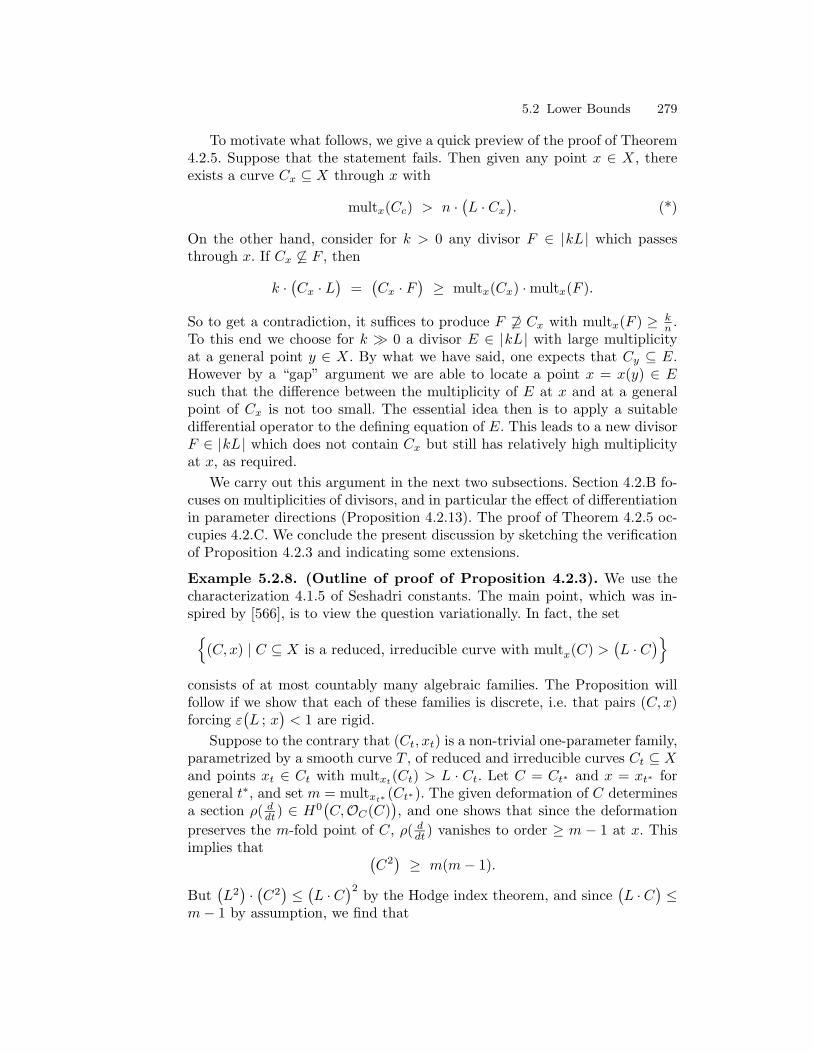
5.2 Lower Bounds 279
To motivate what follows, we give a quick preview of the proof of Theorem4.2.5. Suppose that the statement fails. Then given any point x ∈ X, thereexists a curve Cx ⊆ X through x with
multx(Cc) > n ·(L · Cx
). (*)
On the other hand, consider for k > 0 any divisor F ∈ |kL| which passesthrough x. If Cx 6⊆ F , then
k ·(Cx · L
)=(Cx · F
)≥ multx(Cx) ·multx(F ).
So to get a contradiction, it suffices to produce F 6⊇ Cx with multx(F ) ≥ kn .
To this end we choose for k À 0 a divisor E ∈ |kL| with large multiplicityat a general point y ∈ X. By what we have said, one expects that Cy ⊆ E.However by a “gap” argument we are able to locate a point x = x(y) ∈ Esuch that the difference between the multiplicity of E at x and at a generalpoint of Cx is not too small. The essential idea then is to apply a suitabledifferential operator to the defining equation of E. This leads to a new divisorF ∈ |kL| which does not contain Cx but still has relatively high multiplicityat x, as required.
We carry out this argument in the next two subsections. Section 4.2.B fo-cuses on multiplicities of divisors, and in particular the effect of differentiationin parameter directions (Proposition 4.2.13). The proof of Theorem 4.2.5 oc-cupies 4.2.C. We conclude the present discussion by sketching the verificationof Proposition 4.2.3 and indicating some extensions.
Example 5.2.8. (Outline of proof of Proposition 4.2.3). We use thecharacterization 4.1.5 of Seshadri constants. The main point, which was in-spired by [566], is to view the question variationally. In fact, the set
(C, x) | C ⊆ X is a reduced, irreducible curve with multx(C) >(L · C
)consists of at most countably many algebraic families. The Proposition willfollow if we show that each of these families is discrete, i.e. that pairs (C, x)forcing ε
(L ; x
)< 1 are rigid.
Suppose to the contrary that (Ct, xt) is a non-trivial one-parameter family,parametrized by a smooth curve T , of reduced and irreducible curves Ct ⊆ Xand points xt ∈ Ct with multxt(Ct) > L · Ct. Let C = Ct∗ and x = xt∗ forgeneral t∗, and set m = multxt∗ (Ct∗). The given deformation of C determinesa section ρ( ddt ) ∈ H
0(C,OC(C)
), and one shows that since the deformation
preserves the m-fold point of C, ρ( ddt ) vanishes to order ≥ m − 1 at x. Thisimplies that (
C2)≥ m(m− 1).
But(L2)·(C2)≤(L ·C
)2 by the Hodge index theorem, and since(L ·C
)≤
m− 1 by assumption, we find that

280 Chapter 5. Local Positivity
m(m− 1) ≤(L2)·(C2)≤(L · C
)2 ≤ (m− 1)2.
This is a contradiction when m > 1, and the statement follows. ut
Remark 5.2.9. (Additional results on surfaces). Seshadri constants onsurfaces are studied in a number of papers, including [30], [515], [33], [447].For instance Steffens [515] shows that if (X,L) is a polarized surface havingPicard number ρ(X) = 1, and if x ∈ X is a very general point, then
ε(L ; x
)≥[√(
L2) ],
where [x] denotes as usual the integer part of x. It follows in particular thatif(L2)
= m2 is a perfect square, then ε(L ; x
)= m at a very general point.
Bauer [33] obtains lower bounds for Seshadri constants at arbitrary pointsin terms of geometric invariants of X. Oguiso [447] studies the behavior ofSeshadri constants in families, and shows for instance that if (Xt, Lt, xt) is
any family of pointed polarized surfaces, and if α <√(
L2)
is any fixed
number, then the set of parameter values t at which ε(Xt , Lt ; xt
)≤ α is
Zariski-closed in the parameter variety T . ut
5.2.B Multiplicities of Divisors in Families
We study in this subsection some questions involving multiplicities of divisors.Our presentation closely follows the discussion in [130, §2].
Let M be a smooth variety, and F an effective divisor on M . We denoteby
multx(F ) = multx(M,F )
the multiplicity of F at a point x ∈M . The function x 7→ multx(F ) is Zariskiupper-semicontinuous on M . Therefore one can define the multiplicity of Falong a subvariety:
Definition 5.2.10. (Multiplicity along a subvariety). If Z ⊆ M is anirreducible subvariety, then the multiplicity of F along Z, written multZ(F )or multZ(M,F ), is the multiplicity multx(F ) at a general point x ∈ Z. ut
We start with a result showing that multiplicities of divisors are preservedunder restriction to general fibres of a mapping. As a matter of notation, givena morphism X −→ S of varieties or schemes and a point t ∈ S, write Xt forthe fibre of X over t. Similarly, if F ⊂ X is an effective divisor which does notcontain the fibre Xt, then Ft denotes the restriction F |Xt of F to that fibre.
Lemma 5.2.11. (Multiplicities along fibres). Let p : M −→ T be amorphism of smooth varieties, and suppose that V ⊆M is a smooth irreduciblesubvariety dominating T :

5.2 Lower Bounds 281
V
@@@@@@@@ ⊆ M
p~~
T.
Let F ⊆ M be an effective divisor. Then for a general point t ∈ T , and anyirreducible component Wt ⊆ Vt:
multWt(Mt , Ft) = multV (M , F ).
Proof. Say multV (F ) = m. It is enough to show that for a sufficiently generalpoint t ∈ T , and for any component Wt ⊆ Vt, there is at least one pointy ∈Wt such that multy(Mt, Ft) = m. As V dominates T , we can choose localanalytic coordinates
(z , x) = (z1, . . . , zd , x1, . . . , xe)
on M , and z = (z1, . . . zd) on T , in such a way that p(z, x) = z, V contains anopen neighborhood of the origin in the “z-plane” x1 = . . . = xe = 0, andF has multiplicity m along this plane. Let f(z, x) be a local equation for F ,and given a fixed point t = (t1, . . . , td) ∈ T , write ft(x) = f(t, x). It is enoughto show that there exists t ∈ T such that
ord0ft(x) = ord(t,0) f(z, x).
But this is clear if one writes f in the form
f(z, x) =∑
bI(z)xI ,
where I = (i1, . . . , ie) is a multi-index, and bI(z) is a power series in z. SinceF has multiplicity m along x = 0, the terms of weight |I| < m must vanish,and then it is enough to choose t so that bI(t) 6= 0 for some I with |I| = m.(A less computational argument appears in [130, §2].) ut
Corollary 5.2.12. In the situation of the Lemma, let t ∈ T be a generalpoint. Then
multy(M,F ) = multy(Mt, Ft)
for every y ∈Mt.
Proof. Given k ≥ 0 set
Σk(M,F ) = y ∈M | multy(M,F ) ≥ k ,
and define Σk(Mt, Ft) ⊆ Mt similarly. Writing Σk(M,F )t for the fibre ofthe indicated set over t ∈ T , it follows from the Lemma (applied with V acomponent of Σk(M,F )) that if t ∈ T is a sufficiently general point, then
Σk(M,F )t = Σk(Mt, Ft)
for every k ≥ 0. This implies the assertion of the Lemma. ut

282 Chapter 5. Local Positivity
We now come to a construction that will play a central role in the proofof Theorem 4.2.5. Given a family of divisors in a fixed linear series, the ideais to “differentiate in parameter directions” to lower the multiplicities of thegeneric divisor in the family.
Proposition 5.2.13 (Smoothing divisors in families). Let X and T besmooth irreducible varieties, with T affine, and suppose that
Z ⊆ V ⊆ X × T
are irreducible subvarieties such that V dominates X. Fix a divisor L on X,and suppose given on X × T a divisor F ∈ |pr∗1(L)|. Write
` = multZ(F ) , k = multV (F ).
Then there exists a divisor F ′ ∈ |pr∗1(L)| on X ×T having the property that
multZ(F ′) ≥ `− k , and V * Supp(F ′).
Let σ ∈ Γ(X × T ,pr∗1OX(L)
)be the section defining F . The plan is to obtain
F ′ as the divisor of the section σ′ = Dσ, where D is a general differentialoperator of order k on T . So we begin with some remarks about differentiatingsections of the line bundle pr∗1OX(L) in parameter directions.
Let D be a differential operator of order k on T , i.e. a section of the locallyfree OT -module DkT of all such operators, and let σ ∈ Γ
(X × T ,pr∗1OX(L)
)be a section of pr∗1OX(L). We claim that then D acts naturally on σ todetermine a new section Dσ ∈ Γ
(X × T , pr∗1OX(L)
)of the same bundle. In
fact, choose local coordinates x and t on X and T , and let gα,β(x) be thetransition functions of OX(L) with respect to a suitable open covering of X.Then σ = sα(x, t) is given by a collection of functions sα(x, t) such that
sα(x, t) = gα,β(x) sβ(x, t).
Viewing D locally as a differential operator in the t-variables, one has
Dsα(x, t) = gα,β(x)Dsβ(x, t).
Therefore the Dsα(x, t) patch together to define a section
Dσ ∈ Γ(X × T , pr∗1OX(L)
),
as asserted. We refer to [130, §2] for a more formal discussion.Having said this, we turn to the:
Proof of Proposition 4.2.13. Since T is affine, the vector bundle DkT is globallygenerated. Choose finitely many differential operators
Dα ∈ Γ(T,DkT
)

5.2 Lower Bounds 283
which span DkT at every point of T , and let σ ∈ Γ(X × T , pr∗1OX(L)
)be
the section defining the given divisor F . We claim that if D ∈ Γ (T,DkT ) is asufficiently general C-linear combination of the Dα, then
σ′ =def Dσ ∈ Γ(X × T , pr∗1OX(L)
)does not vanish on V . Granting this for the moment, put F ′ = div(σ′). ThenF ′ does not contain V . On the other hand, differential operators of order ≤ kdecrease multiplicity by at most k. Therefore multZ(F ′) ≥ `− k, as required.
It remains to prove that σ′ does not vanish identically on V . To this end,consider the algebraic subset
X × T ⊇ B =
(x, t) | Dασ(x, t) = 0 for all α
cut out by the common zeroes of all the sections Dασ. It is enough to showthat V * B. For this in turn we study the first projection
pr1 : X × T −→ X.
Fix any point x ∈ X, and consider the fibre Fx ⊆ T of F over x. Assume thatFx 6= T (which will certainly hold for general x), so that Fx is a divisor on T .Given t ∈ T , it follows from the fact that the Dα generate DkT at t that
(x, t) ∈ B ⇐⇒ multt(Fx) > k.
On the other hand, since V dominates X, Lemma 4.2.11 applies to pr1 andwe conclude that
multt(Fx) = multV (F ) = k
for sufficiently general (x, t) ∈ V . This proves that V is not contained in B,and the Proposition follows. ut
Example 5.2.14. (Bertini’s theorem with multiplicities). This circle ofideas leads to a proof of Bertini’s theorem in its original form, which involvesmultiplicities of divisors:
Theorem. Let X be a smooth variety, L an integral divisor on X, andV ⊆ H0
(X,OX(L)
)a finite dimensional subspace defining a linear
series |V | = Psub(V ) on X. If D ∈ |V | is a general divisor, then
multxD ≤ multx |V |+ 1
for every x ∈ X.
Recall (Definition 2.3.11) that the multiplicity of |V | at x ∈ X is by definitionthe minimum of the multiplicities multx(E) of all divisors E ∈ |V |. TheTheorem implies for instance that if a general divisor D ∈ |V | is singular

284 Chapter 5. Local Positivity
at x, then x must be a base-point of |V |. Kleiman’s paper [318] contains aninteresting discussion of this result and its history.
For the proof, let F ⊆ X×|V | be the universal divisor. Fix a point 0 ∈ |V |sufficiently general so that
mult(x,0)
(X × |V | , F
)= multx
(X,F0) (*)
for every x ∈ X (Corollary 4.2.12). Note that in affine coordinates t1, . . . , tron |V | centered at 0, F is defined by the vanishing of the section
s =def s0 + t1s1 + . . .+ trsr, (**)
where s0, . . . , sr ∈ V is a basis with F0 = div(s0); to lighten notation weare writing si in place of the more correct pr∗i (si) in (**). Consider now thederivatives Di(s) = ∂s
∂tiof s with respect to ti. Since differentiation lowers
multiplicity by at most one, we have
ord(x,0)
(Di(s)
)≥ ord(x,0)(s)− 1 = mult(x,0)(F )− 1 (***)
for all i and every x ∈ X. On the other hand, s0 together with the restrictionssi = Di(s)|t=0 span V . Combining (*) and (***) one then finds:
multx|V | = min
ordx(si) , ordx(s0)
≥ min
ord(x,0)(Di(s)) , ord(x,0)(s)
≥ mult(x,0)(X × |V | , F )− 1= multx(X,F0)− 1
for every x ∈ X. Taking D = F0, the Theorem is proved. ut
5.2.C Proof of Theorem 4.2.5
We now outline the proof of Theorem 4.2.5. We will make several simplifyingassumptions, and refer to [130] for some of the verifications.
Step 1: Reductions.We start with some elementary simplifications. By induction on n = dimX
we may assume that the result is known for all irreducible varieties of dimen-sion < n. There is also no loss in assuming that X is smooth, since it is enoughto prove the theorem for a resolution of singularities of X. Fix next any δ > 0and put n′ = n+ δ. We will show that
ε(L ; x
)≥ 1
n′for general x ∈ X. (5.5)
Then the Theorem follows by letting δ → 0. (See [130, (3.2)-(3.4)] for details.)

5.2 Lower Bounds 285
Step 2: Seshadri-exceptional curves.Aiming for a contradiction, assume that (4.5) fails. Then for each point
x ∈ X we can find a reduced and irreducible curve Cx 3 x with the propertythat
multx(Cx)> n′ ·
(L · Cx
). (5.6)
We shall call Cx a Seshadri-exceptional curve based at x. By standard ar-guments with Hilbert schemes, the existence of exceptional curves based atevery point is only possible if most of these curves fit together in an algebraicfamily. More precisely, there exist a smooth affine variety T , a dominatingmap g : T −→ X, and an irreducible subvariety
C ⊆ X × T,
flat over T , such that for every t ∈ T the fibre Ct ⊆ X is a Seshadri-exceptionalcurve based at g(t). In other words, Ct is a reduced and irreducible curve onX, passing through g(t), with
multg(t)
(Ct)> n′ ·
(L · Ct
).
We denote by Γ ⊆ X × T the graph of g, so that Γ ⊆ C.We will henceforth make the simplifying assumption that
T ⊆ X,
with g the inclusion. We then omit mention of g, so that from now on T is anopen subset of X, Ct ⊆ X is a exceptional curve based at t ∈ X, and we havea diagram:
C
???????? ⊆ X × T
xxxxxxxxx
T
.
Step 3: Subvarieties swept out by exceptional curves.We next consider a construction analogous to one used by Kollar, Miyaoka
and Mori in [339]. Given an irreducible subvariety W ⊆ X, the idea is to forma new variety CW ⊇ W by taking the union ∪s∈WCs of all the Seshadri-exceptional curves based in W . However we need to be able to let W varywith parameters.
Lemma 5.2.15. Let Z ⊆ X×T be an irreducible subvariety dominating bothX and T . Then one can construct an irreducible closed subvariety
CZ ⊆ X × T
having the following properties:
(i). Z ⊆ CZ and dimCZ ≤ dimZ + 1.

286 Chapter 5. Local Positivity
(ii). For general t ∈ T , the fibre (CZ)t of CZ over t has the form(CZ)t
= closure( ⋃s∈Zt∩T
Cs
). ut
See [130, 3.5] for the proof.The induction hypothesis now implies that Z ( CZ:
Lemma 5.2.16. Let Z ⊆ X×T be a proper irreducible subvariety dominatingboth X and T , and consider the subvariety CZ ⊆ X × T constructed in theprevious lemma. Then Z is a proper subvariety of CZ.
Proof. Assume to the contrary that CZ = Z, and fix a very general pointt ∈ T . Given a general point s ∈ Zt, it follows from 4.2.15(ii) that there existsa Seshadri-exceptional curve Cs based at s such that Cs lies in Zt =
(CZ)t.
This means that the restriction L |Zt of L to Zt has small Seshadri constantat a general point, i.e.
ε(Zt , L |Zt ; s
)< 1
n′
for a dense open set of points s ∈ Zt. Since dimZt < n, the induction hypoth-esis will give a contradiction as soon as we know that L |Zt is big for generalt. But this follows from Corollary 2.2.11: since the projection Z −→ X isdominating, the fibres Zt are not all contained in any proper subvariety ofX. ut
Step 4: A gap argumentLet t ∈ T ⊆ X be any point. Then by an elementary dimension count,
there exists for k À 0 a divisor Ft ∈ |kL|
multt(Ft) > k · nn′
(Proposition 1.1.31). Moreover an evident globalization of the proof of thatProposition shows that for general t ∈ T one can take the divisors Ft to befibres of a global divisor
F ⊂ X × T , F ∈ |pr∗1 (kL)|
(see [130], 3.8). Note that then multΓ (F ) > k nn′ thanks to Lemma 4.2.11,where as above Γ ⊆ X × T is the graph of T ⊆ X.
We claim now that there exists an irreducible subvariety Z ⊆ X × T ,dominating both X and T , having the property that(
multZ(F ) − multCZ(F ))>
k
n′. (5.7)
In fact, set
Z0 = Γ = graph(T ⊆ X) , Z1 = CZ0 ⊆ X × T,

5.2 Lower Bounds 287
and for 1 ≤ i ≤ n− 1 apply 4.2.15 inductively to form
Zi+1 = CZi ⊆ X × T.
It follows from 4.2.16 that Zi is a proper subvariety of Zi+1, and consequentlyZi has relative dimension i over T . In particular, Zn = X × T . Thus we havea chain
Γ = Z0 ⊆ Z1 ⊆ . . . ⊆ Zn−1 ⊆ Zn = X × Tof irreducible subvarieties of X×T . But consider the multiplicities multZi(F )of F along Zi. By construction:
multZ0(F ) >kn
n′and multZn(F ) = 0.
It follows that there is at least one index i ∈ [0, n− 1] such that(multZi(F ) − multZi+1(F )
)>
k
n′,
so we can take Z = Zi.
Step 5: Exploiting jumps in multiplicityWe now come to the core of the argument. Starting with the variety Z pro-
duced in the previous step, the idea is to differentiate in parameter directionsto produce a new divisor F ′ which does not contain CZ but still has relativelyhigh multiplicity along Z. Then a calculation of intersection numbers gives acontradiction.
Turning to details, fix Z ⊆ X × T as in (4.7). Since Z and hence also CZdominate X, Proposition 4.2.13 implies the existence of a divisor
F ′ ∈ |pr∗1 (kL)|
on X × T with
multZ(F ′) > kn′ , CZ 6⊆ Supp(F ′).
Now fix a general point t ∈ T , and let x ∈ Zt ∩ T be a general point in thefibre of Z over t. Then
multx(F ′t ) >kn′ .
On the other hand, as CZ 6⊆ Supp(F ′), there is a Seshadri-exceptional curveCx through x with
Cx 6⊆ Supp(F ′t ).
Now compute as in the proof of 4.1.17:
k(L · Cx
)=(F ′t · Cx
)≥ multx(F ′t ) ·multx(Cx)
> kn′ ·multx(Cx).
But multx(Cx) ≥ n′·(L·Cx
)by (4.6), and we have the required contradiction.

288 Chapter 5. Local Positivity
Remark 5.2.17. The paper [344] of Kuchle and Steffens establishes somelower bounds via a different approach. ut
5.3 Abelian Varieties
In this section we study local positivity on abelian varieties, where there are in-teresting relations with metric and arithmetic invariants. In §4.3.A and §4.3.Bwe present a theorem of the author [362] showing that the Seshadri constantof a polarized abelian variety is bounded below in terms of the minimal lengthof its periods. Some generalizations and complements are considered in §4.3.C,where in particular we outline the result of Bauer-Szemberg [32, Appendix]and Bauer [33] that the Seshadri constants of abelian surfaces are governedby Pell’s equation.
5.3.A Period lengths and Seshadri constants
The present subsection and the next are devoted to explaining a relationbetween Seshadri constants of abelian varieties and a Riemannian invariantstudied by Buser and Sarnak [66]. Definitions, statements and applicationsare given here, while the proof of the main theorem occupies §4.3.B.
Definitions. We start by setting notation and defining the invariants inquestion. Let A be an abelian variety of dimension g. Viewing A as a complextorus, write
A = V /Λ
where V ∼= Cg is a complex vector space of dimension g, and Λ ∼= Z2g is alattice in V . We identify V with the universal covering space of A, and denoteby π : V −→ A the natural projection.
Fix now an ample divisor L on A. It is classical that L determines apositive definite Hermitian form H = HL on V . For instance, there is a uniquetranslation-invariant Hermitian metric hL on A whose associated Kahler formrepresents the cohomology class of L:
ωL =def −Im(hL) ∼ c1(OA(L)
).
The required form on V can be realized as the pullback HL =def π∗hL. Ev-
idently HL depends only on the algebraic equivalence class of L. Recall alsothat by diagonalizing HL one can associate to L its type, a g-tuple (d1, . . . , dg)of positive integers with d1 | d2 | . . . | dg which determines the algebraic equiv-alence class in question. See [353, Chapters 2 and 4] for details.
The plan is to use HL to define a metric invariant of the polarized abelianvariety (A,L). Specifically, the real part

5.3 Abelian Varieties 289
B = BL =def Re(HL)
is a Euclidean inner product on V : write ‖v‖ = ‖v‖B for the correspondinglength of a vector v ∈ V . Thus the period lattice Λ sits naturally insidethe Euclidean space (V,BL), and in particular one can discuss the lengths oflattice vectors:
Definition 5.3.1. (Buser-Sarnak invariant). The Buser-Sarnak invariantof (A,L) is (the square of) the minimal length of a non-zero lattice vector inΛ:
m(A,L) = min0 6=`∈Λ
‖`‖2B
= min0 6=`∈Λ
HL(`, `). ut
Equivalently, BL determines a translation-invariant Riemannian metric on Awhose volume is fixed by the type of L, and then m(A,L) is the squaredlength of the shortest geodesic on A. For arbitrary Euclidean lattices, theseinvariants have been actively studied at least since Minkowski (see [446], [85]).The nice idea of Buser and Sarnak [66] is to investigate how m(A,L) reflectsthe holomorphic geometry of (A,L).
τ
1
Figure 5.2. Buser-Sarnak invariant for curves
Example 5.3.2. (Elliptic curves). We work out the story in dimensiong = 1. Write
Λ = Λτ = Z + Z τ
where τ = a + ib a point in the upper half plane. Taking the polarization Lon C/Λ to have degree 1, the corresponding Hermitian form is given by
H(v, w) =1b
(v · w).
Now assume that τ lies in the classical fundamental domain for SL2(Z), sothat |τ | ≥ 1 and |Im(τ)| ≤ 1
2 (Figure 4.2). Then 1 ∈ Λ is the minimal vector,and

290 Chapter 5. Local Positivity
m(C/Λτ
)= H(1, 1) = 1
b .
Note that this function approaches zero as τ approaches the cusp at infinitycorresponding to the “boundary” of the moduli space A1 = A1. ut
Work of Buser and Sarnak. We now summarize without proof the mainresults of [66]. Suppose for this that L has type (1, . . . , 1), i.e. that L is aprincipal polarization. In this case h0
(A,OA(L)
)= 1, and following classi-
cal notation we denote by Θ ⊆ A the corresponding divisor. Isomorphismclasses of principally polarized abelian varieties (PPAV’s) of dimension g areparameterized by a moduli space Ag of dimension g(g+1)
2 .Considerations of volume [66, (1.9), (1.10)] show that
m(A,Θ) ≤ 4π
g√g! ≈ 4
π· ge
(5.8)
for any PPAV (A,Θ). Here and subsequently we use the rough approxi-mation g
√g! ≈ g
e coming somewhat abusively from Stirling’s formula g! ∼(√
2πg)(ge
)g. The first main result of Buser-Sarnak estimates the maximumvalue of m(A,Θ) as (A,Θ) ranges over the moduli space Ag:Theorem 5.3.3. (Buser-Sarnak Theorem I). There exist principally po-larized abelian varieties (A,Θ) for which
m(A,Θ) ≥ 21/g
π· g√g! ≈ 21/g
π· ge. (5.9)
This is established by an averaging argument adapted from the geometry ofnumbers. In fact, Buser and Sarnak show that the set of all (A,Θ) for which(4.9) fails is parameterized by a region in Ag whose volume (with respect toa natural metric) decreases exponentially with g.
Remark 5.3.4. (Arbitrary polarizations). Bauer [32, Theorem 1] hasgeneralized Theorem 4.3.3 to abelian varieties carrying a polarization L ofarbitrary type (d1, . . . , dg). Specifically, he shows that there exist (A,L) with
m(A,L) ≥ 21/g
π· g√d · g!, (5.10)
where d = d1 · . . . · dg. ut
The most surprising result of [66] concerns the exceptional behavior ofJacobians. Specifically, let C be a compact Riemann surface of genus g, anddenote by JC the Jacobian of C with its canonical principal polarizationΘC . Fixing a metric on C, the Buser-Sarnak invariant has the alternativeinterpretation [66, (3.1)]
m(JC,ΘC) = minw
∫C
w ∧ ∗w,

5.3 Abelian Varieties 291
the minimum being taken over all closed and non-exact real one-forms w onC with integral periods.
Theorem 5.3.5. (Buser-Sarnak Theorem II). The Buser-Sarnak invari-ant of JC satisfies the upper bound
m(JC,ΘC) ≤ 3π
log(4g + 3). (5.11)
In other words, when g is large Jacobians have periods of exceptionally shortlength among all PPAV’s of dimension g. The proof of 4.3.5 in [66] involvessome delicate constructions with the hyperbolic model of C. Buser and Sarnakalso construct examples of curves C for which m(JC,ΘC) ≥ (constant)·log(g),showing that the inequality (4.11) is essentially best possible. Gromov putsthese results into a broader framework in [230].
Seshadri constants. Turning to Seshadri constants, let (A,L) be a polarizedabelian variety. Then ε
(A , L ; x
)is independent of x ∈ A thanks to 4.1.3 and
the homogeneity of A, and so we write simply ε(A,L). The main result of thepresent section shows that these holomorphic invariants are bounded belowin terms of the minimal period length of A.
Theorem 5.3.6. (Seshadri constants and period lengths). One has theinequality
ε(A,L) ≥ π
4·m(A,L). (5.12)
This is actually very elementary: the proof appears in the next subsection. Forthe remainder of this subsection we indicate some corollaries and applications.
To begin with, we restate the theorem in more classical language. Let
Vk = Γ(A,OA(kL)
)be the space of sections of kL: one can identify Vk with a suitable space ofkth order theta functions. Denote by sk = s(Vk; 0) the number of jets whichVk separates at the origin in the sense of Definition 4.1.16. Then Theorems4.1.17 and 4.3.6 combine to yield
Corollary 5.3.7. (Jets of higher order theta functions). One has
limk→∞
skk≥ π
4·m(A,L). ut
More picturesquely, we may say that if none of the periods of A are smallthen higher order theta functions separate many jets.
Next, putting 4.3.6 together with the first theorem of Buser-Sarnak (andits extension (4.10) by Bauer) one finds:

292 Chapter 5. Local Positivity
Corollary 5.3.8. If (A,L) is a very general abelian variety with a polarizationof type (d1, . . . , dg), then
ε(A,L) ≥ 21/g
4· g√d · g!, (5.13)
where as before d = d1 · . . . · dg. ut
The hypothesis on (A,L) means that the stated inequality holds for all abelianvarieties parameterized by the complement of countably many proper subva-rieties of the moduli space of all abelian varieties of given type. Note also thatthe lower bound appearing in (4.13) differs from the upper bound
ε(L,A) ≤ g√d · g!
coming from (4.2) by a factor of less than 4.
Example 5.3.9. (Very ample polarizations). Assume that
d = d1 · . . . · dg ≥(8g)g
2g!≈ (8e)g
2.
If (A,L) is a general polarized abelian variety of type (d1, . . . , dg), then L isvery ample. (Combine (4.13) and 4.1.19). This is due to Bauer [32, Corollary2]: see [101] for other results along these lines. ut
Example 5.3.10. (Lower bounds for arbitrary abelian varieties). Onehas
ε(A,L) ≥ 1
for any polarized abelian variety (A,L) and if A contains an elliptic curveE ⊆ A with degE(L) = 1 then equality is attained. (Argue much as in 4.1.18using translates of divisors in |L|. Nakamaye [430] shows conversely that if(A,Θ) is a PPAV with ε(A,Θ) = 1, then in fact A contains such a curve. ut
We now come back to Jacobians. Whereas upper bounds on the Buser-Sarnak invariant m(JC,ΘC) require serious effort, it is very easy to obtainbounds on local positivity.
Proposition 5.3.11. (Seshadri constants of Jacobians). Let C be asmooth projective curve of genus g.
(i). The Seshadri constant ε(JC,ΘC) satisfies the bound
ε(JC,ΘC) ≤ √g.
(ii). Assume that C admits a d-fold branched covering φ : C −→ P1. Then
ε(JC,ΘC) ≤ gd
g + d− 1.

5.3 Abelian Varieties 293
Thanks to Theorem 4.3.6, statement (i) leads to a quick and elementary proofthat Jacobians have periods of small length, although the specific inequalitythat comes out is not as strong as (4.11). It also follows that if C is a d-sheetedcovering of P1, then
m(JC,ΘC) ≤ 4dπ.
For hyperelliptic curves (i.e. when d = 2), statement (ii) was established bySteffens [515].
Sketch of proof of Proposition 4.3.11. We assume to begin with that C is non-hyperelliptic. For (i), consider the surface S = C −C ⊆ JC, i.e. the image ofthe subtraction map
s : C × C −→ JC , (x, y) 7→ x− y.
It is elementary and well known that if C is non-hyperelliptic then s is anisomorphism outside the diagonal ∆ ⊆ C ×C which blows down to the origin0 ∈ S, at which S has multiplicity 2g − 2 (see [14, pp. 223, 263]). Moreoverthe cohomology class of S is given by4 [S] = 2
(g−2)! ·θg−2, where θ denotes the
cohomology class of ΘC . Therefore
degΘ(S) =2
(g − 2)!· θg = 2g(g − 1).
Applying Proposition 4.1.9 we find
ε(JC,ΘC) ≤
√degΘ(S)mult0S
=
√2g(g − 1)
2g − 2
=√g,
as required.Turning to (ii), denote by f1, f2, δ ∈ N1(C ×C) respectively the classes of
the fibres of the two projections C × C −→ C and the diagonal ∆C . Then inthe first place
s∗(ΘC)≡num (g − 1)(f1 + f2) + δ.
4 As explained in [14, Exercise V.D-3], when d < g2
the cohomology class of thedifference variety Vd = Cd − Cd is expressed as
vd =
(2dd
)(g − 2d)!
· θg−2d.
(Note that the actual formula stated in loc. cit. is mis-printed.)

294 Chapter 5. Local Positivity
Moreover there is an effective curve Γ ⊆ C × C with
Γ ≡num d(f1 + f2)− δ :
geometrically, Γ is the closure of the set Γ0 = (x, y) | x 6= y, φ(x) = φ(y) .5Now if ε = ε(JC,ΘC) then s∗(Θ)− ε ·∆ is nef, and hence
Γ ·(s∗(ΘC)− ε∆) =
(d(f1 + f2)− δ
)·((g − 1)(f1 + f2) + (1− ε) δ
)≥ 0.
A calculation then leads to the stated inequality. Finally, when C is hyperel-liptic the only thing that needs proof is the case d = 2 of (ii), and this followsby looking at the image in J(C) of the curve Γ just constructed. ut
Remark 5.3.12. (Curves of low genus). Steffens [515] shows that if (A,Θ)is an irreducible principally polarized abelian surface, then ε(A,Θ) = 4
3 , aspredicted by 4.3.11(ii). PPAV’s of dimension three have been studied by Bauerand Szemberg [35]. They establish that ε(A,Θ) = 3
2 if A is a hyperellipticJacobian, and ε(A,Θ) = 12
7 otherwise. Debarre [100] proves that ε(JC,ΘC) =2 for a non-hyperelliptic curve of genus 4. ut
Remark 5.3.13. (Hyperelliptic Jacobians). Debarre [100] proves that ifC is a hyperelliptic curve of genus g, then ε(JC,ΘC) = 2g
g+1 , i.e. the boundin 4.3.11(ii) is attained. It is natural to conjecture that the converse holds,i.e. that if (A,Θ) is an irreducible PPAV of dimension g with ε(A,Θ) ≤ 2g
g+1 ,then in fact (A,Θ) must be a hyperelliptic Jacobian. This would follow from aconjecture of van Geemen and van der Geer [535] using work of Welters [558].Debarre suggests that it should be enough here to assume that ε(A,Θ) < 2.However he points out that there exist non-Jacobian PPAV’s (A,Θ) containingan elliptic curve E ⊂ A with
(E ·Θ
)= 2, for which ε(A,Θ) ≤ 2. So it seems
that in general one can’t hope to recognize Jacobians through their Seshadriconstants. ut
Remark 5.3.14. (Prym varieties). Bauer [32] has generalized 4.3.11 to thesetting of Prym varieties. He shows for example that if (P,Ξ) is the Prymvariety associated to an etale double cover C −→ C of a curve C of genusg ≥ 3, then
ε(P,Ξ) ≤√
2(g − 1) =√
2 dimP . ut
5.3.B Proof of Theorem 4.3.6
We now turn to the proof of Theorem 4.3.6, which is based on ideas from [389,§5]. In effect, we will simply write down explicitly a suitable Kahler form onthe blow-up Bl0(A). A different approach is indicated in Remark 4.3.17. Theexposition is taken from [362] with little change.5 Compare the proof of Kouvidakis’ Theorem 1.5.8.

5.3 Abelian Varieties 295
We begin with a local construction on Cg. Let
V ⊆ Cg ×Pg−1
be the blowing up of the origin 0 ∈ Cg, embedded in the usual way as anincidence correspondence. Write
f : V −→ Cg , q : V −→ Pg−1
for the projections, so that f is the blowing up and q realizes V as the totalspace of the line bundle OPg−1(−1). As in (4.3) let B(λ) ⊆ Cg be the ball ofradius λ, and denote by V (λ) its inverse image in in V , i.e.
V (λ) = f−1B(λ) ⊆ V.
Thus V (λ) is an open neighborhood of the exceptional divisor E = Pg−1 ⊆ V .Finally, let σ be the Fubini-Study Kahler form on Pg−1, normalized so that∫P1 σ = π, the integral being taken over a line in Pg−1. This normalization
is chosen so that if S = S2g−1 ⊆ Cg is the unit sphere, and κ : S −→ Pg−1
is the Hopf map, then κ∗σ = ωstd | S, where as before ωstd is the standardKahler form on Cg.
The first essential point is a local construction:
Lemma 5.3.15. (Local Construction). Fix λ > 0. Given any small η > 0,there exists 0 < δ ¿ 1 together with a Kahler form τ = τ(λ, η) on V such that
(i). τ = f∗(ωstd) on V − V (λ+ η);(ii). τ = f∗(ωstd) + λ2 · q∗(σ) on V (δ).
In other words, τ coincides with the standard form on Cg off a ball of radius(a tiny bit larger than) λ, whereas we are “twisting” by a form representingπλ2 · q∗c1
(OPg−1(1)
)in a neighborhood if E.
Sketch of proof of Lemma 4.3.15. This is a very slight variant of [389, (5.1)],and we refer to that paper or [?, pp. 220 - 221] for details. In brief, choosea monotone increasing smooth function φ(r) such that φ(r) =
√λ2 + r2 for
0 < r < δ ¿ 1 and such that φ(r) = r for r > λ+ η. Let F : Cg −0 −→ Cg
be the smooth mapping defined by
F (z) =φ(|z|)|z| · z.
The pull-back f∗F ∗ωstd is a Kahler form which satisfies the stated propertieson V −E. Then by (ii) it extends over E to give the required form τ on all ofV . ut
The Lemma leads to a lower bound on Seshadri constants of bundles whosefirst Chern class is locally represented by ωstd. Specifically, let X be a smooth

296 Chapter 5. Local Positivity
projective variety of dimension n, L an ample divisor on X, and ωL a Kahlerform onX representing c1
(OX(L)
). We view (X,ωL) as a symplectic manifold.
Given x ∈ X, define a real number λ(ωL;x) ≥ 0 by looking for the largestradius λ > 0 for which there exists a holomorphic and symplectic embedding
j = jλ :(B(λ) , ωstd
)→(X , ωL
)with 0 7→ x. (*)
More precisely, if there is no λ > 0 for which such an embedding exists, setλ(ωL;x) = 0. Otherwise put
λ(ωL;x) = supλ > 0 | ∃ holomorphic and symplectic jλ as in (*).
.
Lemma 5.3.16. One has the inequality
ε(L ; x
)≥ π · λ(ωL ; x)2.
Proof. Let f : Y = Blx(X) −→ X be the blowing-up of x, with exceptional di-visor E ⊆ Y , and fix any λ < λ(ωL;x). It is enough to show that the R-divisorclass f∗L− πλ2E is ample on Y . To this end, fix λ < λ1 < λ(ωL;x). Then bydefinition there exists a holomorphic and symplectic embedding B(λ1) → X,and so for any ν < λ1 we can view the local model V (ν) of the blow-upas being embedded in Y as a neighborhood of the exceptional divisor. Theconstruction 4.3.15 guarantees the existence of a Kahler class ωL on Y whichagrees with ωL off V (λ2) for suitable λ < λ2 < λ1, and which is given by4.3.15(ii) in a neighborhood V (δ) of E. The positivity of f∗L − πλ2E willfollow as soon as we show that the class of ωL satisfies
[ωL ] = [ f∗ωL ] − πλ2[E ]. (**)
But ωL − f∗ωL is supported in a small tubular neighborhood of E, so (**)follows from 4.3.15(ii) and the normalization of σ. ut
Theorem 4.3.6 now follows at once:
Proof of Theorem 4.3.6. Let π : V −→ A be the universal covering, and letH = HL be the Hermitian form on V determined by L. Thus ω = Im(H) =π∗ωL is the pull-back of a Kahler form ωL on A representing c1
(OA(L)
).
Fix a basis of V with respect to which H is the standard Hermitian formH(v, w) = tv·w on Cg, and let zj = xj+iyj be the corresponding coordinates.Then
ω = π∗ωL = ωstd, (5.14)
and H(v, v) = |v|2 is just the usual Euclidean length. In particular,
m(A,L) = min0 6=`∈Λ
|`|2.
Now put λ =√m(A,L)
2 . Then no two points of B(λ) are congruent (moduloΛ), and consequently the composition

5.3 Abelian Varieties 297
jλ : B(λ) → Vπ−→ A
is an embedding. But jλ is of course holomorphic, and thanks to (4.14) it is
symplectic as well. Therefore λ(ωL; 0) ≥√m(A,L)
2 , and the Theorem followsfrom 4.3.16. ut
Remark 5.3.17. (Alternative approach to Theorem 4.3.6). Hwang andTo [278], and independently Demailly, observed that one can deduce Theorem4.3.6 from a result of Federer concerning the volumes of analytic subvarietiesof the ball. Specifically, fix R > 0 and denote by B = B(R) be the open ballof radius R centered at the origin 0 ∈ Cg. Let V ⊆ B be a closed analyticsubvariety of B of pure dimension k passing through the origin. The result inquestion states that
vol(V ) ≥ mult0(V ) · πkR2k
k!, (*)
where vol(V ) denotes the usual 2k-dimensional Euclidean volume of V in Cg:see [], [], or [110, Theorems 2.8 and 2.9]. Given a polarized abelian variety(A,L) and a curve C ⊆ A through 0, one applies (*) to the inverse imageof C under the universal covering π : V −→ A. This leads to the requiredinequality (
C · L)
mult0C≥ π ·
(√m(A,L)2
)2
.
In [278], (*) is generalized to Hermitian symmetric spaces other than Cg. ut
5.3.C Complements
Here we discuss some related results, largely without proof. We begin with thework of Bauer-Szemberg [32, Appendix] and Bauer [33] computing Seshadriconstants of abelian surfaces. Then we turn to analogues of Theorem 4.3.6 forquotients of bounded symmetric domains due to Hwang and To [276], [277].
Abelian surfaces. Let A be an abelian surface and L an ample divisor onA of type (1, d). Thus(
L2)
= 2d and h0(A,L
)= d.
We will assume that A has Picard number ρ(A) = 1 (Definition 1.1.17): thisholds when (A,L) is sufficiently general.
The inequality 4.2 implies that ε(A,L) ≤√
2d. When 2d is a perfect square,results of Steffens [515] quoted in 4.2.9 imply that in fact ε(A,L) =
√2d.
Matters become more interesting when√
2d is irrational. Here one considersPell’s equation
`2 − 2dk2 = 1. (5.15)

298 Chapter 5. Local Positivity
Denote by (`0, k0) the primitive solution to (4.15), i.e. the solution character-ized by ***. Then one has
Theorem 5.3.18. (Seshadri constants of abelian surfaces). Assumingas above that 2d is not a perfect square and that ρ(A) = 1, the Seshadriconstant of (A,L) is given by
ε(A,L) = 2d · k0
`0.
In particular, ε(A,L) is always rational. Some values of ε(A,L) as a functionof d are tabulated in [33, p. 572].
Partial proof of Theorem 4.3.18. We will sketch the inequality
ε(A,L) ≤ 2d · k0`0
established by Bauer and Szemberg in the Appendix to [32]. We can assumefor this that L is a symmetric divisor, and it is enough to prove the existenceof a curve D ⊆ A passing through the origin such that
(D · L
)= 4dk0 and
mult0(D) ≥ 2`0. The idea of Bauer and Szemberg is to consider the spaceΓ(A,OA(2kL)
)+ of even sections of OA(2kL): one may view these as thesections pulling back from the Kummer surface A/±1, and the point is toexploit the fact that the constant term in Riemann-Roch is different on aK3 than on an abelian surface. Specifically, the space of even sections of asymmetric divisor of type (2k, 2kd) has dimension
h0(A,OA(2kL)
)+ = 2 + 2dk2. (*)
On the other hand, an even section vanishes to even order at the origin, sothat it is at most
1 + 3 + . . .+ (m− 1) =(m2
)2conditions on even sections to vanish at the origin to even order m. Thereforeone can find a section of OA(2kL) vanishing to order ≥ m at the origin assoon as
(m2
)2 ≤ (2dk2 + 1
). Noting that `20 = 2dk2
0 + 1, we arrive at therequired curve D. For the reverse inequality, Bauer [33, Theorem 6.1] showsby working on the Kummer surface A/±1 that the curve D just constructed(or a closely related curve) is irreducible. Here one uses the hypothesis thatρ(A) = 1. ut
Quotients of balls and bounded symmetric domains. Hwang and To[276], [277] have obtained interesting bounds for the Seshadri constants of thecanonical bundle on quotients of balls and other bounded symmetric domains.Here we summarize without proof the simplest of their results.

5.4 Local Positivity Along an Ideal Sheaf 299
Consider the unit ball B ⊆ Cn equipped with its Poincare metric. Fix adiscrete torsion-free cocompact subgroup Γ ⊆ PU(1, n), and let X = B/Γ bethe associated smooth compact quotient. Then X carries a canonical Kahlermetric coming from the Poincare metric on B, which in turn allows one todefine two basic metric invariants. First, the injectivity radius ρx of X at apoint x ∈ X is defined to be
ρx = 12 minγ∈Γ
d(x0, γx0),
where x0 ∈ B is a point lying over x ∈ X, and d(·, ·) is the Poincare distancefunction on B. This plays the role of the minimal period length m(X,A) in thecase of abelian varieties. Secondly, define the diameter of X at x ∈ X to beDx = maxy∈X d(x, y), where here d denotes the distance function associatedto the Poincare metric on X. The main result of [276] is the following:
Theorem 5.3.19. Given X as above, together with fixed point x ∈ X, onehas
(n+ 1) · sinh2(ρx) ≤ ε(KX ; x
)≤ (n+ 1) · sinh2(Dx).
The lower bound is established by an analogue of symplectic blowing up,whereas the upper bound is proven by convexity arguments.
Define the global injectivity radius of the ball-quotient X to be ρX =minx∈X ρx. Then the Theorem combines with Proposition 4.1.19 to yield
Corollary 5.3.20. With X as above, suppose that
ρX > sinh−1
√2nn+ 1
.
Then 2KX is very ample. In particular, any ball quotient X admits a finiteetale cover X ′ on which 2KX′ is very ample.
Both the Theorem and Corollary are generalized in [277] to smooth compactquotients of general bounded symmetric domains.
5.4 Local Positivity Along an Ideal Sheaf
This section describes some results of Cutkosky, Ein and the author [87] con-cerning local positivity along an arbitrary ideal sheaf. We define an analogueof the Seshadri constant in which the fixed point x ∈ X is replaced by anideal sheaf I ⊆ OX . The theme loosely speaking is that the resulting invari-ant bounds the complexity of I or its powers. This picture was inspired bywork of Paoletti [], [] who considered ideal sheaves of smooth subvarieties.
The first subsection treats the formal properties of this s-invariant, andpresents some examples. The main results appear in §4.4.B. We follow closelythe presentation in [].

300 Chapter 5. Local Positivity
5.4.A Definition and Formal Properties of the s-Invariant
Let X be an irreducible projective variety, let I ⊆ OX be an ideal sheaf, andfix an ample divisor L on X.
Definition 5.4.1. (The s-invariant of an ideal). Let
µ : X ′ = BlI(X) −→ X (5.16)
be the blowing-up of X along I, with exceptional divisor E. The s-invariantof I with respect to L is the positive real number
sL(I) = mins ∈ R | µ∗(sL)− E is a nef R-divisor on BlI(X) . ut
One can think of sL(I) as measuring how many times one has to twist I byL in order to render it positive. The main case to keep in mind is when Lis a hyperplane divisor on X = Pn. A related invariant for vector bundles isintroduced in Example 6.2.14.
Example 5.4.2. (Relation to Seshadri constants). Let x ∈ X be a fixedpoint, with maximal ideal m ⊆ OX . Then ε
(L ; x
)= 1/sL(m). ut
Remark 5.4.3. (Seshadri constant of an ideal sheaf). By analogy withDefinition 4.1.1, it would be natural to define the Seshadri constant ε(L; I)of L along I to be the largest real number ε > 0 such that µ∗H − ε ·E is nef.Then ε(L; I) = 1
sL(I) . However for present purposes sL(I) is more convenientto work with than its reciprocal. ut
Our immediate goal is to study the formal properties of this invariant, andto give some examples. It is useful to start with an extension of Definition1.8.37.
Definition 5.4.4. (Generating degree of an ideal with respect to anample divisor). With notation as above, the generating degree of I withrespect to L is the natural number
dL(I) = mind ∈ N | I ⊗ OX(dL) is globally generated
. ut
The first observation is that the generating degree of an ideal bounds itss-invariant.
Proposition 5.4.5. (Generating degree and s-invariant). Let I ⊆ OXbe an ideal sheaf on the projective variety X, and let L be any ample divisoron X. Then sL(I) ≤ dL(I). More generally,
sL(I) ≤ dL(Ip)p
for every integer p ≥ 1.

5.4 Local Positivity Along an Ideal Sheaf 301
We will see later (Theorem 4.4.22) that if L is globally generated, then in factsL(I) = lim dL(Ip)
p .
Proof of Proposition 4.4.5. Keeping the notation of (4.16), assume that Ip ⊗OX(dL) is generated by its global sections. This sheaf pulls back on X ′ to theline bundle OX′
(µ∗(dL)− pE
), and hence µ∗(dL)− pE is free. In particular,
sL(I) ≤ dp , as claimed. ut
Example 5.4.6. (Schemes cut out by quadrics). Take X = Pn and L ahyperplane, and suppose that I⊗OPn(2) is globally generated. Assume more-over that the zero-locus Z = Zeroes(I) is not a linear space. Then sL(I) = 2.(By the previous example sL(I) ≤ 2, and examining the proper transform ofa suitable secant line to Z gives the reverse inequality.) ut
Example 5.4.7. (Irrational s-invariants). It is not hard to find exampleswhere the s-invariant of an ideal is irrational. In fact, let X = B × B bethe product of an elliptic curve with itself, so that Nef(X) is a circular cone(Example 1.5.4). Choose very ample divisors L,C ⊆ X, and consider the idealsheaf I = OX(−C) of C. Then the s-invariant of I with respect to L is thelargest root of the quadratic polynomial q(t) =
((tL− C)2
), and for general
choices of L and C this will be irrational. Observe that given L, one can takeC so that the corresponding s-invariant is arbitrary large. We will use thisconstruction in Example 4.4.16 to produce a curve C ⊆ Pn whose ideal sheafhas irrational s-invariant. ut
Example 5.4.8. For any ideal sheaf I ⊆ OX and ample line bundle L, thes-invariant sL(I) is an algebraic integer of degree ≤ dimX. (Set s = sL(I).Then on the blow-up X ′ = BlI(X), the class sL−E is nef but not ample. Inthis case, the Campana-Peternell Theorem 2.3.18 implies that there exists asuvariety V ′ ⊆ X ′ such that
((sL−E)dimV ′ ·V ′
)= 0. But this exhibits sL(I)
as the root of a monic polynomial equation of degree = dimV ′.) ut
Example 5.4.9. (Numerical nature and homogeneity). The s-invariantsL(I) depends only on the numerical equivalence class of L. For any naturalnumber m > 0, one has smL(I) = 1
m · sL(I). ut
Example 5.4.10. (Alternative computation of s-invariants). Let f :Y −→ X be a surjective morphism of projective varieties with the propertythat I · OY = OY (−F ) for some effective Cartier divisor F on Y . Then
sL(I) = mins ∈ R | f∗(sL)− F is nef
.
(The hypothesis implies that f factors through the blowing-up of I.) ut
We next use some definition and facts from Chapter 6 to show that s-invariants behave well with respect to algebraic operations on ideals.

302 Chapter 5. Local Positivity
Proposition 5.4.11. (s-invariants of sums and products). As above letX be an irreducible projective variety, and L an ample divisor on X. Givenideal sheaves I1, I2 ⊆ OX , one has:
sL(I1 · I2
)≤ sL(I1) + sL(I2)
sL(I1 + I2
)≤ max
sL(I1) , sL(I2)
.
Proof. We will apply Example 4.4.10. Let f : Y −→ X be a surjective mappingfrom an irreducible variety Y which dominates the blowings-up of X alongI1, I2 and I1 + I2. Thus Y carries effective Cartier divisors F1, F2 and F12
characterized by
I1 · OY = OY (−F1) , I1 · OY = OY (−F1) ,(I1 + I2
)· OY = OY (−F12).
Note that then (I1I2
)· OY = OY
(− (F1 + F2)
). (*)
Write s1 = sL(I1) and s2 = sL(I2). Then f∗(s1L)− F1 and f∗(s2L)− F2
are nef on Y , and consequently so is their sum f∗((s1 + s2)L
)− (F1 + F2).
The first inequality then follows from (*). For the second, observe that onehas a surjective map
OY (−F1)⊕OY (−F2) −→ OY (−F12)
of vector bundles on Y . Fix any rational number s ≥ maxs1, s2. Then thebundle on the left becomes nef when twisted (in the sense of Chapter 6.2)by the Q-divisor f∗(sL). Since quotients of nef Q-twisted bundles are nef(Theorem 6.2.12), this implies that f∗(sL) − E12 is nef, and the requiredinequality follows. ut
Remark 5.4.12. (s-invariant of the integral closure of an ideal). As-suming that X is normal, denote by I the integral closure of an ideal I ⊆ OX .(Definition ??). Then it is established in [87, Proposition 1.12] that
sL(I) = sL(I). ut
Suppose now thatX is non-singular, and let Y ⊆ X be a smooth subvarietywith ideal sheaf I = IX/Y . We discuss next a geometric interpretation, dueto Paoletti [?, p.487], for the s-invariant of I. Paoletti’s result involves dataassociated to non-constant mappings f : C −→ X from a smooth curve Cto X. Suppose first that f(C) 6⊆ Y . Then f−1I ⊂ OC is an ideal of finitecolength in OC , and we define
s′L(I) = supf :C−→Xf(C) 6⊆Y
colength(f−1I)(C ·f L)
,

5.4 Local Positivity Along an Ideal Sheaf 303
where (C ·f L) denotes the degree of the divisor f∗L on C. Next, write N =NY/X for the normal bundle to Y in X and put
s′′L(I) = inff :C−→Xf(C)⊆Y
t ∈ Q>0
∣∣∣ degM + t · (C ·f L) ≥ 0for all rank 1 quotients M of f∗N∗
.
Proposition 5.4.13. (Paoletti, []). With the notation and hypotheses justintroduced, one has
sL(I) = maxs′L(I) , s′′L(I)
.
Remark 5.4.14. When I = m is the maximal ideal of a point x ∈ X, themappings appearing in the definition of s′′L(m) do not occur. The resultingequality sL(m) = s′L(m) is then a restatement of Proposition 4.1.5. ut
Sketch of Proof of Proposition 4.4.13. Consider a mapping f : C −→ X withf(C) 6⊆ X, and let f ′ : C −→ X ′ = BlY (X) be the proper transform of f .Then colength(f−1I) =
(C ·f ′E
), where as above E is the exceptional divisor
of the blowing-up µ : BlY (X) −→ X. Therefore s′L(I) is the least real numbert > 0 such that µ∗(tL)−E has non-negative degree on every curve not lying inthe exceptional divisor E ⊂ X ′. Similarly, s′′L(I) is the infimum of all rationalnumbers t > 0 such that the Q-twisted vector bundle N∗<tL> is nef in thesense of Chapter 6.2 (Proposition 6.1.18, Remark 6.2.9). But this is equivalentto asking that
(µ∗(tL) − E
)be a nef divisor class on E = P(N∗), and the
Proposition follows. ut
For the purpose of constructing examples, it is useful to understand some-thing about how the s-invariant behaves in chains.
Proposition 5.4.15. Consider smooth projective varieties
Z ⊆ Y ⊆ X,
with ideal sheaves IZ/X , IY/X ⊆ OX and IZ/Y ⊆ OY . Fix an ample divisor Lon X, and write (somewhat abusively) sL(IZ/Y ) for the s-invariant calculatedby blowing up Y along Z and computing with the restriction of L to Y . IfsL(IY/X) < sL(IZ/X) then
sL(IZ/X) = sL(IZ/Y ).
Sketch of Proof. Keep the notation introduced before Proposition 4.4.13. Itis evident from the definitions that
s′L(IZ/X) ≤ max s′L(IZ/Y ) , s′L(IY/X) ,
and using the conormal bundle sequence 0→ N∗Y/X |Z → N∗Z/X → N∗Z/Y → 0it follows from Theorem 6.2.12, (ii), (v), that

304 Chapter 5. Local Positivity
s′′L(IZ/X) ≤ max s′′L(IZ/Y ) , s′′L(IY/X) .
The assertion is then a consequence of 4.4.13. ut
We conclude this subsection by giving a painless construction of a curveC ⊆ Pn with irrational s-invariant. More explicit examples appear in Cutkosky’spaper [].
Example 5.4.16. (Projective curve with irrational s-invariant). Startwith the product A = B × B of an elliptic curve with itself, and fix a veryample divisor on A defining an embedding A ⊆ Pn in which A is cut outby quadrics.6 Then Example 4.4.6 shows that sL(IA/Pn) = 2, L being thehyperplane divisor on Pn. Choose next a curve C ⊆ A having the propertythat sL
(OA(−C)
)is an irrational number s > 2 (Example 4.4.7). Applying the
previous Proposition to the chain C ⊆ A ⊆ Pn, we find that sL(IC/Pn) = sis irrational. ut
Example 5.4.17. (An irrational polyhedral nef cone). Let C ⊆ Pn
be the curve constructed in the previous example, and let X = BlPn(C) bethe blowing-up of Pn along C. Then X has Picard number two, and the nefcone Nef(X) ⊆ N1(X)R = R2 is an irrational polyhedron. (Write E and Hrespectively for the exceptional divisor and the pull-back of the hyperplaneclass L on Pn. Then Nef(X) is spanned by the classes of H and sH − E,where s = sL(IC/Pn).) ut
5.4.B Complexity Bounds
We now present two results illustrating the philosophy that the s-invariant ofan ideal sheaf bounds its complexity. The first is an inequality of Bezout-typethat will be useful in connection with the effective Nullstellensatz (Chapter10.5). The second theorem asserts that the s-invariant of an ideal computes itsasymptotic Castelnuovo-Mumford regularity. These (and related statementsf om [87]) provide a geometric perspective on some of the the results andquestions from Bayer and Mumford’s survey []. As in that paper, we speak ofcomplexity in a purely informal sense.
One can view the number and degrees of the components of an ideal’s zero-locus as a first measure of its complexity. The s-invariant gives some controlover these:
Theorem 5.4.18. (Degree inequality). Let X be an irreducible projectivevariety, I ⊆ OX an ideal sheaf, and L an ample divisor on X. Denote by
Y1 , . . . , Yp ⊆ X
6 For example, one can take the sum of the pull-backs under each projection of adivisor of degree 4 on B.

5.4 Local Positivity Along an Ideal Sheaf 305
the irreducible components (with their reduced scheme structures) of the zero-locus Y = Zeroes(I) of I, and write s = sL(I). Then
p∑j=1
sdimYj · degL(Yj) ≤ sdimX · degL(X). (5.17)
Given an irreducible subvariety V ⊆ X, by degL(V ) we understand the inter-section number
(LdimV ·V
). All of these degrees are positive (L being ample),
and so the Theorem limits the number and degrees of the components in ques-tion:
Corollary 5.4.19. Setting s+ = max1, s, one has
p∑j=1
degL(Yj) ≤ sdimX+ · degL(X). ut
Proof of Theorem 4.4.18. Let X ′′ be the normalization of the blow-up X ′ =BlI(X), and write
ν : X ′′ −→ X
for the natural map. Denote by F the exceptional divisor of ν, so that F is aneffective Cartier divisor on X ′′ with I · OX′′ = OX′′(−F ). Now F determinesan effective Weil divisor [F ] on X ′′, say
[F ] =t∑i=1
ri · [Fi],
where the Fi are the irreducible components of the support of F , and ri ≥ 1is a positive integer. Put
Zi = ν(Fi) ⊆ X,
so that Zi is a reduced and irreducible subvariety of X. Following [?], theZi are called the distinguished subvarieties of I.7 Then evidently Y = ∪Zi,so in particular each irreducible component Yj of Y occurs as one of thedistinguished subvarieties Zi. Therefore it is enough to prove that the Zisatisfy the degree bound
t∑i=1
ri · sdimZi · degL(Zi) ≤ sdimX degL(X). (5.18)
For this, set n = dimX and denote by l,m ∈ N1(X ′′)R the classes of ν∗Land ν∗(sL)− F respectively. Then by definition m is nef, and so
∫X′′
mn ≥ 0
7 Note that several of the Fi may have the same image in X, in which case therewill be repetitions among the Zi. However this doesn’t cause any problems.

306 Chapter 5. Local Positivity
and∫Filj ·mn−1−j ≥ 0 for all i and j. Moreover F ≡num s · l −m. One then
finds that
sn · degL(X) =∫X′′
(s · l)n
≥∫X′′
((s · l)n −mn
)=∫X′′
((s · l)−m
)( n−1∑j=0
(s · l)j ·mn−1−j)
=∫
[F ]
( n−1∑j=0
(s · l)j ·mn−1−j)
≥t∑i=1
ri ·∫Fi
(s · l)dimZi ·mn−1−dimZi .
On the other hand, OX′′(−F ) — being a finite pullback of the ideal of theexceptional divisor of a blow-up — is ample for ν. Therefore m has positivedegree on every fibre of ν, and in particular∫
Fi
ldimZi ·mn−1−dimZi ≥ degL(Zi).
All told, we find that
sn · degL(X) ≥t∑i=1
ri ·∫Fi
(s · l)dimZi ·mn−1−dimZi
≥t∑i=1
ri · sdimZi · degL(Zi),
as required. ut
Remark 5.4.20. Some variants of Theorem 4.4.18 are discussed in [87, §2].In particular, it is observed there that if I is integrally closed then one caninclude in the left-hand side of (4.17) the subvarieties defined by all associatedprimes of I, minimal or embedded. On the other hand, [87, Example 2.8] givesa construction to show that the number of embedded components cannotbe bounded in terms of the s-invariant for ideals which are not integrallyclosed. ut
Assume now that L is free (as well as ample). Then one can discuss theCastelnuovo-Mumford regularity with respect to L of any coherent sheaf onX (Definition 1.8.4), and by analogy with Definition 1.8.17 we put
Definition 5.4.21. The L-regularity regL(I) of an ideal I ⊆ OX is the leastinteger m such that I is m-regular with respect to OX(L). ut

5.4 Local Positivity Along an Ideal Sheaf 307
We refer to Section ?? for a survey of the theory of Castelnuovo-Mumfordregularity, and in particular its role in measuring the complexity of an ideal.
The next result shows that the s-invariant of an ideal computes asymp-totically the regularity and generating degree of its powers:
Theorem 5.4.22. (Asymptotic regularity and s-invariant). Let X bean irreducible projective variety, and fix an ample and free divisor L on X. IfI ⊆ OX is any ideal sheaf, then
lim infp→∞
regL(Ip)p
= limp→∞
dL(Ip)p
= sL(I). (5.19)
One can view this as a geometric analogue of the result of Cutkosky-Herzog-Trung and Kodiyalam (Theorem 1.8.49) concerning the asymptotic regularityof powers of a homogeneous ideal.
Remark 5.4.23. With a little more effort, one can show that the lim infappearing in (4.19) is actually a limit: see [87, §3]. ut
The crucial input to the theorem is a lemma asserting that one can com-pute cohomology of large powers of I in terms of the exceptional divisor onthe blow-up.
Lemma 5.4.24. As before, let µ : X ′ = BlI(X) −→ X be the blowing up ofX, with exceptional divisor E. Then there exists an integer p0 = p0(I) withthe property that if p ≥ p0 then
µ∗(OX′(−pE)
)= Ip, (5.20)
and moreover for any divisor D on X:
Hi(X, Ip(D)
)= Hi
(X ′,OX′(µ∗D − pF )
)(5.21)
for all i ≥ 0.
Remark 5.4.25. Note that if X is non-singular, and I defines a smoothsubvariety of X, then the conclusion of the Lemma holds for all p ≥ 0 (Lemma??). However in general one has to be content with large values of p. ut
Proof of Lemma 4.4.24. Since OX′(−F ) is ample for µ, Grothendieck-Serrevanishing imply that
Rjµ∗(OX′(−pF )
)= 0 for j > 0 and pÀ 0.
The isomorhism on global cohomology groups is then a consequence of (4.20)thanks to the Leray spectral sequence. As for (4.20), we can suppose that Xis affine and that I is generated by functions g1, . . . , gr ∈ OX . The choice ofgenerators gives a surjection OrX −→ I, which in turn determines an embed-ding X ′ ⊆ P(OrX) = Pr−1
X in such a way that OPr−1X
(1) |X ′ = OX′(−E).

308 Chapter 5. Local Positivity
Write π : Pr−1X = X ×Pr−1 −→ X for the projection. Serre vanishing for π,
applied to the ideal sheaf of X ′ in Pr−1X , shows that if pÀ 0 then the natural
homomorphismπ∗(OPr−1
X(p))−→ π∗
(OX′(−pF )
)(*)
is surjective. But recalling that π∗(OPr−1
X(k))
= Symk(OrX) for every k, onesees that the image of the mapping in (*) is exactly Ip. The stated equality(4.20) follows. ut
Proof of Theorem 4.4.22. Set dp = dL(Ip) and rp = regL(Ip). Observe tobegin with that d`+m ≤ d` + dm, from which it follows that lim dp
p exists.
Note next that sL(I) ≤ dpp for all p by Proposition 4.4.5, while dp ≤ rp thanks
to Mumford’s Theorem 1.8.5. Therefore it is enough to show that given anyrational number s′ > s, one has rp ≤ ps′ for all sufficiently large and divisiblep.
But if s′ > s then s′L−E is ample. So if we take p to be sufficiently largeand divisible — so that in particular ps′ ∈ N — then by Serre vanishing wecan suppose that
Hi(X ′,OX′
((ps′ − k)L− pE
))= 0 for all i > 0 and 1 ≤ k ≤ dimX.
Assuming as we may that p is also sufficiently large so that the conclusion ofLemma 4.4.24 holds, it follows from (4.21) that I is ps′-regular with respectto L. Therefore rp ≤ ps′, as required. ut
Notes
Seshadri constants were introduced in [107, §6]. Demailly seems to have beenmotivated here by Fujita’s conjecture (see Section 10.4.A), but the examples ofMiranda soon made it clear that one could not expect any simple applicationin this direction. However in the intervening years it has become increasinglyclear that Seshadri constants are fundamental and interesting invariants intheir own right.
Most of the foundational material in Section 4.1 appears in [107]. Section4.2 generally follows [130], while Section 4.3 is adapted from [362]. Section 4.4is taken from [87].

A
Projective Bundles
We recall here some basic facts about projective bundles.Let X be an algebraic variety or scheme, and let E be a vector bundle of
rank e on X. We denote by
π : P(E) −→ X
the projective bundle of one-dimensional quotients of X. Thus a point in P(E)is determined by specifying a point x ∈ X together with a one-dimensionalquotient of the fibre E(x) of E at x. More algebraically, P(E) is realized asthe scheme
P(E) = SpecOX(Sym(E)
),
where Sym(E) = ⊕Sm(E) denotes the symmetric algebra of E.1
P(E) carries a Serre line bundle OP(E)(1), arising as a “tautological”quotient of π∗E:
π∗E −→ OP(E)(1) −→ 0. (A.1)
When m ≥ 0 one hasπ∗OP(E)(m) = Sm(E),
and Rjπ∗OP(E)(m) = 0 for j > 0, m ≥ 0. If L is a line bundle, then P(E) ∼=P(E ⊗ L) via an isomorphism
Let p : Y −→ X be a variety or scheme mapping to X. Then giving a linebundle quotient π∗E ³ L of the pullback of E is equivalent to specifying amap f : Y −→ P(E) over X:
Y
p @@@@@@@@f // P(E)
π||yyyyyyyy
X.
1 Here and elsewhere we do not distinguish between E and the corresponding locallyfree sheaf of sections.

310 Chapter A. Projective Bundles
Under this correspondence L = f∗OP(E)(1), and the given quotient is thepullback of (A.1). In particular, for each ` > 0 there is a natural Veroneseembedding of P(E) into P(S`E):
P(E)
p""EEEEEEEE
ν` // P(S`E)
πwwwwwwwww
X.
It is determined by the quotient S`π∗E ³ OP(E)(`) arising by taking `th
symmetric products in (A.1).Assume that X is projective. Then the Neron–Severi group of P(E) is
determined byN1(P(E)) = π∗N1(X)⊕ Z · ξE ,
where ξE is the class of a divisor representing OP(E)(1). Writing ξE also forthe corresponding class in HX
(2; Z
), the integral cohomology H∗
(P(E); Z
)of
P(E) is generated as an H∗(X; Z
)-algebra by ξE , subject to the Grothendieck
relation
ξeE − π∗c1(E) · ξe−1E + π∗c2(E) · ξe−2
E ± . . . + (−1)eπ∗ce(E) = 0.
On a few occasions it will be preferable to consider the bundle Psub(E) ofone-dimensional subspaces of E. This is related to the bundles of quotients bythe relation Psub(E) = P(E∗).

B
Cohomology and Complexes
We collect in this Appendix several elementary constructions and results of acohomological nature.
B.1 Cohomology
Resolutions.
Let X be a algebraic variety or scheme. One often attempts to understandthe cohomology of a coherent sheaf F on X in terms of a resolution. Considerthen a complex of coherent sheaves
F• : 0 −→ F` −→ . . . −→ F1 −→ F0ε−→ F −→ 0.
with ε surjective. We record some simple criteria, in increasing order of gener-ality, that allow one to conclude the vanishing of Hk
(X,F
)in terms of data
involving F•.
Proposition B.1.1. (Chasing through complexes). Given some integerk ≥ 0, assume that
Hk(X,F0
)= Hk+1
(X,F1
)= · · · = Hk+`
(X,F`
)= 0, (*)
(i). If F• is exact, then Hk(X,F
)= 0.
(ii). The same conclusion holds assuming that F• is exact off a subset of Xhaving dimension ≤ k.
(iii). More generally still, for i ≥ 0 denote by Hi the homology sheaf
Hi =ker
(Fi −→ Fi−1
)im(Fi+1 −→ Fi
)

312 Chapter B. Cohomology and Complexes
(with F−1 = F). Still assuming (*), the vanishing Hk(X,F
)= 0 holds
provided that
Hk+1(X,H0
)= Hk+2
(X,H1
)= · · · = Hk+`+1
(X,H`
)= 0.
The hypothesis in (ii) means that all the homology sheaves of F• shouldsupported on an algebraic set of dimension ≤ i.
Proof of Proposition B.1.1. This is most easily checked by chopping F• intoshort exact sequences in the usual way and chasing through the resultingdiagram. ut
Remark B.1.2. (Infinite complexes). Note that the vanishingHk+i(X,Fi
)appearing in (*) is automatic if k+i > dimX, and similarly for the hypothesesin (iii). Therefore one can always replace a complex F• of length ` À 0 by asuitable truncation of length ≤ dimX. In particular, the Proposition appliesalso to possibly infinite resolutions of F . ut
Spectral Sequences.
It is sometimes most efficient to organize the cohomological data at hand intoa spectral sequence. Suppose for example that the complex F• above is exact,and denote by F+
• the truncated complex
F+• : 0 −→ F` −→ . . . −→ F1 −→ F0 −→ 0.
Thus F+• is quasi-isomorphic to the single sheaf F , and hence the hypercoho-
mology of F+• is isomorphic to the cohomology of F itself:
Hk(X,F+
•)
= Hk(X,F
).
Then the cohomology of F is computed via the spectral sequence associatedto the hypercohomology of F+
• :
Lemma B.1.3. Assuming that F• is exact, there is a (second quadrant) spec-tral sequence
Ep,q1 = Hq(X,F−p
)=⇒ Hp+q
(X,F
)abutting to the cohomology of F . ut
Example B.1.4. In the situation of the previous Lemma, assume that thereare positive integers r and s such that all the groups Hi
(X,Fj
)vanish except
when i = 0 and j ≥ s or when i = r and j ≥ s+ r + 1. Then the cohomologygroups of F are computed as the cohomology of a complex
. . . −→ Hr(X,Fs+r+2
)−→ Hr
(X,Fs+r+1
)−→ H0
(X,Fs
)−→ H0
(X,Fs−1
)−→ . . . .

B.2 Complexes 313
Filtrations.
Instead of a “resolution” such as F•, one sometimes wishes to infer somethingabout the cohomology of a sheaf in terms of a filtration. Suppose then thatF is a coherent sheaf on X, and that one is given a filtration K• of F bycoherent subsheaves:
0 = Kp+1 ⊆ Kp ⊆ . . . ⊆ K1 ⊆ K0 = F .
As usual, we set Grj = Kj/Kj+1. In general, the cohomology of F is most effi-ciently analyzed via the spectral sequence of a filtered sheaf (cf. [225, Chapter3, §5]), but in the simplest situations it is just as easy to work directly withthe evident short exact sequences linking these data.
Lemma B.1.5. Suppose that there is an integer k ≥ 0 such that all the Grj
have vanishing cohomology in all degrees i 6= k:
Hi(X,Grj
)= 0 for all i 6= k and all 0 ≤ j ≤ p.
Then Hi(X,F
)= 0 for i 6= k, and Hk
(X,F
)has a filtration with graded
pieces isomorphic to Hk(X,Grj
). ut
Direct Images.
Everything here generalizes to the setting of a proper morphism f : X −→ Y(without X or Y necessarily being complete), with cohomology groups beingreplaced by direct image sheaves. We leave the details to the reader.
B.2 Complexes
We next discuss some useful complexes. Throughout this section, X is anirreducible variety or scheme.
Koszul Complex.
Let E be a vector bundle on X of rank e, and let
s ∈ Γ(X,E
)be a section of E. This section gives rise to a zero scheme
Z = Z(s) ⊆ X :
in terms of a local trivialization of E, s is expressed by a vector s = (s1, . . . , se)of regular functions, and the ideal sheaf of Z is locally generated by the

314 Chapter B. Cohomology and Complexes
component functions si. These data determine a Koszul complex K•(E, s)of sheaves on X:
0 −→ ΛeE∗ −→ Λe−1E∗ −→ . . . −→ Λ2E∗ −→ E∗ −→ OX −→ OZ −→ 0.
The map ΛiE∗ −→ Λi−1E∗ is defined via contraction with s. K•(E, s) isalways exact off Z in the sense that its homology sheaves are supported onZ. It is globally exact if X is locally Cohen-Macaulay (e.g. non–singular) andif codimXZ = rankE.
One may deduce several useful variants by transposition and/or twistingby line bundles. For instance, when A is a line bundle a morphism u : E −→ Agives rise to a complex
0 −→ ΛeE∗⊗A⊗−e −→ . . . −→ Λ2E∗⊗A⊗−2 −→ E∗⊗A∗ −→ OX −→ OZ −→ 0
with analogous exactness properties. Similarly, starting with a section OX −→E, one can also form the complex
0 −→ OX −→ E −→ Λ2E −→ . . . −→ ΛeE −→ ΛeE ⊗OZ −→ 0.
Example B.2.1. Given any vector bundle E on X and any positive integerk, there is a long exact sequence
. . . −→ Sk−2E ⊗ Λ2E −→ Sk−1 ⊗ E −→ SkE −→ 0
of bundles on X. (Form the Koszul complex associated to the tautologicalquotient π∗E −→ OP(E)(1) on P(E), twist by OP(E)(k − 1) and take directimages.)
Complexes of Eagon-Northcott Type.
The Koszul complex is a special case of a collection of complexes determinedby a map
u : E −→ F
of bundles of ranks e and f respectively on X. Assume (as we may by transpos-ing if necessary) that e ≥ f , and let Z = Df−1(u) denote the top degeneracylocus of u, i.e. the subscheme
Df−1(u) =x ∈ X | rank u(x) ≤ f − 1
locally defined by the f × f minors of a matrix for u. Recall that Z hasexpected codimension e− f + 1 in X.
The first of the complexes in question is due to Eagon and Northcott, andprovides (in good situations) a resolution of OZ . The second was constructedby Buchsbaum and Rim, and resolves (generically) the cokernel of u. Thefamily as a whole was described independently by Buchsbaum and Eisenbud

B.2 Complexes 315
and by Kirby. We refer to [?, A.2.6] for a discussion from an algebraic pointof view. Following an approach pioneered by Kempf we sketch a geometricderivation.
Kempf’s idea is to pass to the projectivization π : P(F ) −→ X of F , andto form the indicated composition v:
π∗Eπ∗u //
v $$JJJJJJJJJ π∗F
OP(F )(1)
.
View v as a section of π∗E∗ ⊗ OP(F )(1), and let Y ⊂ P(P ) denote the zeroscheme of v. Note that Y projects onto Z, and given x ∈ Z the fibre of Y overx is P(coker u(x)). In particular, if (say) Z is irreducible and u drops rankby one at a generic point of Z, then the map Y −→ Z is birational. If X isnon-singular, and u is sufficiently generic then Y will be smooth, and hence aresolution of singularities of Z.
Now consider the Koszul complex K• = K•(π∗E∗ ⊗ OP(F )(1), v) deter-mined by v, and twist by OP(F )(k) for k ≥ 0:
0 −→ Λeπ∗E(k−e) −→ . . . −→ π∗Λ2E(k−2) −→ π∗E(k−1) −→ OP(F )(k) −→ 0.
Here we are writing π∗E(`) for π∗E ⊗OP(F )(`), and we omitted the cokernelOY (k) of the last map on the right. Now assume that X is locally Cohen-Macaulay (e.g. smooth), and that Y has the expected codimension e in P(F ).Then K• is acyclic, i.e. the only homology is the cokernel of the right-mostmap, and so it is a resolution of OY (k). Therefore the hyper-direct images ofK• simply compute the direct images of OY (k):
Riπ∗K• = Riπ∗OY (k).
On the other hand, observe that
Riπ∗
(Λjπ∗E∗ ⊗OP(F )(`)
)= ΛjE∗ ⊗Riπ∗OP(F )(`).
Bearing in mind that the direct images on the right vanish unless either i = 0and ` ≥ 0 or i = f − 1 and ` ≤ −f , one finds that the (second quadrant)spectral sequence
Ep,q1 = Rqπ∗(Λ−pπ∗E∗(k − e)
)=⇒ Rp+qπ∗K•
gives rise to a single complex (ENk) of sheaves on X computing the directimages of OY (k). All of the complexes are exact off Z (and in sufficientlygeneric situations will be acyclic).
We now write down the complexes explicitly. Note that if 0 ≤ k ≤ e − fthen (ENk) has length e−f+1. The length of each of the subsequent complexesgrows by one until reaching length e when k ≥ e:

316 Chapter B. Cohomology and Complexes
0 −→ΛeE
⊗Se−f (F )∗ ⊗ ΛfF ∗
−→ . . . −→Λf+1E
⊗F ∗ ⊗ ΛfF ∗
−→ΛfE
⊗ΛfF ∗
−→ OX −→ 0.
(EN0)
0 −→ΛeE
⊗Se−f−1(F )∗ ⊗ ΛfF ∗
−→ . . . −→Λf+2E
⊗F ∗ ⊗ ΛfF ∗
−→Λf+1E
⊗ΛfF ∗
−→ E −→ F −→ 0.
(EN1)
0 −→ΛeE
⊗Se−f−2(F )∗ ⊗ ΛfF ∗
−→ . . . −→Λf+2E
⊗ΛfF ∗
−→ Λ2E −→ E⊗F −→ S2F −→ 0.
(EN2)• • •
0 −→ΛeE
⊗ΛfF ∗
−→ Λe−fE −→ . . . −→Λ2E
⊗Se−f−2F
−→ E⊗Se−f−1F −→ Se−fF −→ 0.
(ENe−f )
0 −→ Λe−f+1E −→Λe−fE
⊗F
−→ . . . −→Λ2E
⊗Se−f−1F
−→ E⊗Se−fF −→ Se−f+1F −→ 0.
(ENe−f+1)• • •
0 −→ ΛeE −→Λe−1E
⊗F
−→ . . . −→Λ2E
⊗Se−2F
−→ E ⊗ Se−1F −→ SeF −→ 0.
(ENe)
0 −→ΛeE
⊗F
−→Λe−1E
⊗S2F
−→ . . . −→Λ2E
⊗Se−1F
−→ E ⊗ SeF −→ Se+1F −→ 0.
(ENe+1)• • •
We summarize this discussion in
Theorem B.2.2. For each k ≥ 0, (ENk) is a complex which is exact off Z. IfX is smooth and Z has the expected codimension e− f + 1 in X, then (ENk)is acyclic for k ≤ e − f + 1, and the same holds for k ≥ e − f provided e.g.that the variety Y ⊂ P(F ) constructed above is smooth and maps birationallyto Z.

B.2 Complexes 317
Proof. The only points not covered in the discussion above are the criteria foracyclicity. For the case when k ≤ e−f+1 and Z has the expected codimension,see [144, Corollary A2.12]. The second assertion being local, we can assumethat E and F are trivial. Then Y ⊆ P(F ) is the complete intersection ofe divisors in the linear series |OP(F )(1)|, and hence ωY = OY (e − f). Sowhen k ≥ e− f , the higher direct images of OY (k) vanish thanks to Grauert-Riemannschneider, and this implies the required acyclicity. ut


References
1. Shreeram Abhyankar, Tame coverings and fundamental groups of algebraic va-rieties. I. Branch loci with normal crossings; Applications: Theorems of Zariskiand Picard, Amer. J. Math. 81 (1959), 46–94.
2. Dan Abramovich and A. Johan de Jong, Smoothness, semistability, and toroidalgeometry, J. Algebraic Geom. 6 (1997), no. 4, 789–801.
3. Allen Altman and Steven Kleiman, Introduction to Grothendieck Duality The-ory, Lect. Notes in Math., vol. 146, Springer-Verlag, Berlin, 1970.
4. A. Alzati and G. Ottaviani, A linear bound on the t-normality of codimensiontwo subvarieties of Pn, J. Reine Angew. Math. 409 (1990), 35–40.
5. Marco Andreatta and Andrew J. Sommese, On the projective normality of theadjunction bundles, Comment. Math. Helv. 66 (1991), no. 3, 362–367.
6. Marco Andreatta and JarosÃlaw A. Wisniewski, On manifolds whose tangentbundle contains an ample subbundle, Invent. Math. 146 (2001), no. 1, 209–217.
7. Aldo Andreotti and Theodore Frankel, The Lefschetz theorem on hyperplanesections, Ann. of Math. (2) 69 (1959), 713–717.
8. Aldo Andreotti and Alan Mayer, On period relations for abelian integrals onalgebraic curves, Ann. Scuola Norm. Sup. Pisa (3) 21 (1967), 189–238.
9. Urban Angehrn and Yum Tong Siu, Effective freeness and point separation foradjoint bundles, Invent. Math. 122 (1995), no. 2, 291–308.
10. Flavio Angelini, An algebraic version of Demailly’s asymptotic Morse inequal-ities, Proc. Amer. Math. Soc. 124 (1996), no. 11, 3265–3269.
11. Marian Aprodu and Claire Voisin, Green-Lazarsfeld’s conjecture for genericcurves of large gonality, C. R. Math. Acad. Sci. Paris 336 (2003), no. 4, 335–339.
12. Donu Arapura, Higgs line bundles, Green-Lazarsfeld sets, and maps of Kahlermanifolds to curves, Bull. Amer. Math. Soc. (N.S.) 26 (1992), no. 2, 310–314.
13. Donu Arapura and Dennis S. Keeler, Frobenius amplitude and strong vanishingtheorems for vector bundles, to appear.
14. Enrico Arbarello, Maurizio Cornalba, Phillip Griffiths, and Joe Harris, Geom-etry of Algebraic Curves. Vol. I, Grundlehren Math. Wiss., vol. 267, Springer-Verlag, New York, 1985.

320 References
15. Enrico Arbarello and Corrado De Concini, Another proof of a conjecture of S.P. Novikov on periods of abelian integrals on Riemann surfaces, Duke Math.J. 54 (1987), no. 1, 163–178.
16. V. I. Arnol′d, Mathematical Methods of Classical Mechanics, Graduate Textsin Mathematics, vol. 60, Springer-Verlag, New York, 1989.
17. V. I. Arnol′d, S. M. Guseın-Zade, and A. N. Varchenko, Singularities of Dif-ferentiable Maps. Vol. II: Monodromy and asymptotics of integrals, BirkhauserBoston Inc., Boston, MA, 1988.
18. Michael Atiyah and Jurgen Berndt, Projective planes, Severi varieties andspheres, to appear.
19. Lucian Badescu, Special chapters of projective geometry, Rend. Sem. Mat. Fis.Milano 69 (1999/00), 239–326 (2001).
20. , Algebraic Surfaces, Universitext, Springer-Verlag, New York, 2001.21. Daniel Barlet, A propos d’une conjecture de R. Hartshorne, J. Reine Angew.
Math. 374 (1987), 214–220.22. Daniel Barlet, L. Doustaing, and J. Magnusson, La conjecture de R. Hartshorne
pour les hypersurfaces lisses de Pn, J. Reine Angew. Math. 457 (1994), 189–202.
23. Wolf Barth, Verallgemeinerung des Bertinischen Theorems in abelschen Man-nigfaltigkeiten, Ann. Scuola Norm. Sup. Pisa (3) 23 (1969), 317–330.
24. , Transplanting cohomology classes in complex-projective space, Amer.J. Math. 92 (1970), 951–967.
25. , Larsen’s theorem on the homotopy groups of projective manifolds ofsmall embedding codimension, Algebraic Geometry, Proc. Symp. Pure Math.,Vol. 29, Amer. Math. Soc., Providence, R.I., 1975, pp. 307–313.
26. Wolf Barth and Mogens Larsen, On the homotopy groups of complex projectivealgebraic manifolds, Math. Scand. 30 (1972), 88–94.
27. Wolf Barth and A. Van de Ven, A decomposability criterion for algebraic 2-bundles on projective spaces, Invent. Math. 25 (1974), 91–106.
28. Charles M. Barton, Tensor products of ample vector bundles in characteristicp, Amer. J. Math. 93 (1971), 429–438.
29. Alexander Barvinok, A Course in Convexity, Graduate Studies in Mathemat-ics, vol. 54, American Mathematical Society, Providence, RI, 2002.
30. Thomas Bauer, Seshadri constants of quartic surfaces, Math. Ann. 309 (1997),no. 3, 475–481.
31. , On the cone of curves of an abelian variety, Amer. J. Math. 120(1998), no. 5, 997–1006.
32. , Seshadri constants and periods of polarized abelian varieties, Math.Ann. 312 (1998), no. 4, 607–623, With an appendix by the author and TomaszSzemberg.
33. , Seshadri constants on algebraic surfaces, Math. Ann. 313 (1999),no. 3, 547–583.
34. Thomas Bauer, Alex Kuronya, and Tomasz Szemberg, Zariski chambers, vol-ume and stable base loci, to appear, 2003.
35. Thomas Bauer and Tomasz Szemberg, Local positivity of principally polarizedabelian threefolds, J. Reine Angew. Math. 531 (2001), 191–200.
36. David Bayer and David Mumford, What can be computed in algebraic geome-try?, Computational Algebraic Geometry and Commutative Algebra (Cortona,1991), Cambridge Univ. Press, Cambridge, 1993, pp. 1–48.

References 321
37. David Bayer and Michael Stillman, A criterion for detecting m-regularity, In-vent. Math. 87 (1987), no. 1, 1–11.
38. , On the complexity of computing syzygies, J. Symbolic Comput. 6(1988), no. 2-3, 135–147.
39. Arnaud Beauville, Annulation du H1 et systemes paracanoniques sur les sur-faces, J. Reine Angew. Math. 388 (1988), 149–157.
40. , Annulation du H1 pour les fibres en droites plats, Complex AlgebraicVarieties (Bayreuth, 1990), Lect. Notes in Math., vol. 1507, Springer, Berlin,1992, pp. 1–15.
41. , Vector bundles on curves and generalized theta functions: recent resultsand open problems, Current Topics in Complex Algebraic Geometry (Berkeley,CA, 1992/93), Cambridge Univ. Press, Cambridge, 1995, pp. 17–33.
42. Alexander Beilinson, Joseph Bernstein, and Pierre Deligne, Faisceaux Pervers,Asterisque, vol. 100, Soc. Math. France, Paris, 1982.
43. Mauro Beltrametti, Michael Schneider, and Andrew Sommese, Chern inequal-ities and spannedness of adjoint bundles, Proceedings of the Hirzebruch 65Conference on Algebraic Geometry (Ramat Gan, 1993), 1996, pp. 97–107.
44. Mauro Beltrametti and Andrew Sommese, The Adjunction Theory of ComplexProjective Varieties, Walter de Gruyter & Co., Berlin, 1995.
45. Carlos Berenstein, Roger Gay, Alekos Vidras, and Alain Yger, Residue Currentsand Bezout identities, Progr. Math., vol. 114, Birkhauser Verlag, Basel, 1993.
46. P. Berthelot, Alexander Grothendieck, and Illusie Luc.47. Aaron Bertram, An existence theorem for Prym special divisors, Invent. Math.
90 (1987), no. 3, 669–671.48. Aaron Bertram, Lawrence Ein, and Robert Lazarsfeld, Surjectivity of Gaussian
maps for line bundles of large degree on curves, Algebraic Geometry (Chicago,1989), Lect. Notes in Math., vol. 1479, Springer, Berlin, 1991, pp. 15–25.
49. , Vanishing theorems, a theorem of Severi, and the equations definingprojective varieties, J. Amer. Math. Soc. 4 (1991), no. 3, 587–602.
50. Edward Bierstone and Pierre D. Milman, Canonical desingularization in char-acteristic zero by blowing up the maximum strata of a local invariant, Invent.Math. 128 (1997), no. 2, 207–302.
51. Paul Biran, Constructing new ample divisors out of old ones, Duke Math. J.98 (1999), no. 1, 113–135.
52. , A stability property of symplectic packing, Invent. Math. 136 (1999),no. 1, 123–155.
53. , From symplectic packing to algebraic geometry and back, EuropeanCongress of Mathematics, Vol. II (Barcelona, 2000), Progr. in Math., vol. 202,Birkhauser, Basel, 2001, pp. 507–524.
54. Spencer Bloch and David Gieseker, The positivity of the Chern classes of anample vector bundle, Invent. Math. 12 (1971), 112–117.
55. F. A. Bogomolov, Unstable vector bundles and curves on surfaces, Proceedingsof the International Congress of Mathematicians (Helsinki, 1978) (Helsinki),Acad. Sci. Fennica, 1980, pp. 517–524.
56. Fedor Bogomolov, Holomorphic tensors and vector bundles on projective man-ifolds, Izv. Akad. Nauk SSSR Ser. Mat. 42 (1978), no. 6, 1227–1287, 1439.
57. Fedor Bogomolov and Tony Pantev, Weak Hironaka theorem, Math. Res. Lett.3 (1996), no. 3, 299–307.

322 References
58. Ciprian Borcea, Homogeneous vector bundles and families of Calabi-Yau three-folds. II, Several Complex Variables and Complex Geometry, Part 2, Proc.Symp. Pure Math., vol. 52, Amer. Math. Soc., Providence, RI, 1991, pp. 83–91.
59. Sebastien Boucksom, On the volume of a line bundle, Internat. J. Math. 13(2002), no. 10, 1043–1063.
60. , Higher dimensional Zariski decompositions, preprint, 2003.61. Nicolas Bourbaki, Commutative Algebra. Chapters 1–7, Elements of Mathe-
matics, Springer-Verlag, Berlin, 1998.62. Ana Bravo and Orlando Villamayor, A strong desingularization theorem, to
appear.63. Markus Brodmann and Rodney Sharp, Local Cohomology: an Algebraic Intro-
duction with Geometric Applications, Cambridge studies in advanced mathe-matics, vol. 60, Cambridge University Press, Cambridge, 1998.
64. W. Dale Brownawell, Bounds for the degrees in the Nullstellensatz, Ann. ofMath. (2) 126 (1987), no. 3, 577–591.
65. Winfried Bruns and Jurgen Herzog, Cohen-Macaulay Rings, Cambridge Stud-ies in Advanced Mathematics, vol. 39, Cambridge University Press, Cambridge,1993.
66. P. Buser and Peter Sarnak, On the period matrix of a Riemann surface of largegenus, Invent. Math. 117 (1994), no. 1, 27–56.
67. Frederic Campana, Ensembles de Green-Lazarsfeld et quotients resolubles desgroupes de Kahler, J. Algebraic Geom. 10 (2001), no. 4, 599–622.
68. Frederic Campana and Thomas Peternell, Algebraicity of the ample cone ofprojective varieties, J. Reine Angew. Math. 407 (1990), 160–166.
69. , Projective manifolds whose tangent bundles are numerically effective,Math. Ann. 289 (1991), no. 1, 169–187.
70. , On the second exterior power of tangent bundles of threefolds, Com-positio Math. 83 (1992), no. 3, 329–346.
71. , Rational curves and ampleness properties of the tangent bundle ofalgebraic varieties, Manuscripta Math. 97 (1998), no. 1, 59–74.
72. James Carlson, Mark Green, Phillip Griffiths, and Joe Harris, Infinitesimalvariations of Hodge structure. I, Compositio Math. 50 (1983), no. 2-3, 109–205.
73. James Carlson, Stefan Muller-Stach, and Chris Peters, Period Mappings andPeriod Domains, Cambridge Studies in Advanced Mathematics, vol. 85, Cam-bridge University Press, Cambridge, 2003.
74. Karen Chandler, Regularity of the powers of an ideal, Comm. Algebra 25(1997), no. 12, 3773–3776.
75. Pierre-Emmanuel Chaput, Severi varieties, Math. Z. 240 (2002), no. 2, 451–459.
76. Marc Chardin and Clare D’Cruz, Castelnuovo-Mumford regularity: examplesof curves and surfaces, 2002, preprint.
77. Marc Chardin and Bernd Ulrich, Liaison and Castelnuovo-Mumford regularity,Amer. J. Math. 124 (2002), no. 6, 1103–1124.
78. Jungkai Chen and Christopher Hacon, Characterization of abelian varieties,Invent. Math. 143 (2001), no. 2, 435–447.
79. , Pluricanonical maps of varieties of maximal Albanese dimension,Math. Ann. 320 (2001), no. 2, 367–380.

References 323
80. Jaydeep V. Chipalkatti, A generalization of Castelnuovo regularity to Grass-mann varieties, Manuscripta Math. 102 (2000), no. 4, 447–464.
81. Koji Cho and Ei-ichi Sato, Smooth projective varieties with the ample vectorbundle
∧2 TX in any characteristic, J. Math. Kyoto Univ. 35 (1995), no. 1,1–33.
82. Ciro Ciliberto and Alexis Kouvidakis, On the symmetric product of a curvewith general moduli, Geom. Dedicata 78 (1999), no. 3, 327–343.
83. Herbert Clemens, A local proof of Petri’s conjecture at the general curve, J.Differential Geom. 54 (2000), no. 1, 139–176.
84. Herbert Clemens and Christopher Hacon, Deformations of the trivial line bun-dle and vanishing theorems, Amer. J. Math. 124 (2002), no. 4, 769–815.
85. John Conway and Neil Sloane, Sphere Packings, Lattices and Groups, thirded., Springer-Verlag, New York, 1999.
86. S. Dale Cutkosky, Zariski decomposition of divisors on algebraic varieties, DukeMath. J. 53 (1986), no. 1, 149–156.
87. S. Dale Cutkosky, Lawrence Ein, and Robert Lazarsfeld, Positivity and com-plexity of ideal sheaves, Math. Ann. 321 (2001), no. 2, 213–234.
88. S. Dale Cutkosky, Jurgen Herzog, and Ngo Viet Trung, Asymptotic behaviourof the Castelnuovo-Mumford regularity, Compositio Math. 118 (1999), no. 3,243–261.
89. S. Dale Cutkosky and V. Srinivas, On a problem of Zariski on dimensions oflinear systems, Ann. of Math. (2) 137 (1993), no. 3, 531–559.
90. , Periodicity of the fixed locus of multiples of a divisor on a surface,Duke Math. J. 72 (1993), no. 3, 641–647.
91. Mark de Cataldo, Singular Hermitian metrics on vector bundles, J. ReineAngew. Math. 502 (1998), 93–122.
92. Mark de Cataldo and Luca Migliorini, The hard Lefschetz theorem and thetopology of semismall maps, Ann. Sci. Ecole Norm. Sup. (4) 35 (2002), no. 5,759–772.
93. Mark de Cataldo and Luca Migliorini, The Hodge theory of algebraic maps,preprint, 2003.
94. A. Johan de Jong, Smoothness, semi-stability and alterations, Inst. HautesEtudes Sci. Publ. Math. (1996), no. 83, 51–93.
95. Olivier Debarre, Fulton-Hansen and Barth-Lefschetz theorems for subvarietiesof abelian varieties, J. Reine Angew. Math. 467 (1995), 187–197.
96. , Theoremes de connexite et varietes abeliennes, Amer. J. Math. 117(1995), no. 3, 787–805.
97. , Theoremes de connexite pour les produits d’espaces projectifs et lesgrassmanniennes, Amer. J. Math. 118 (1996), no. 6, 1347–1367.
98. , Tores et Varietes Abeliennes Complexes, Societe Mathematique deFrance, Paris, 1999.
99. , Theoremes de Lefschetz pour les lieux de degenerescence, Bull. Soc.Math. France 128 (2000), no. 2, 283–308.
100. , Higher-Dimensional Algebraic Geometry, Springer-Verlag, New York,2001.
101. Olivier Debarre, Klaus Hulek, and J. Spandaw, Very ample linear systems onabelian varieties, Math. Ann. 300 (1994), no. 2, 181–202.
102. Pierre Deligne, Cohomologie Etale, Lect. Notes in Math., vol. 569, Springer-Verlag, Berlin, 1977, SGA 4 1
2.

324 References
103. , Le groupe fondamental du complement d’une courbe plane n’ayant quedes points doubles ordinaires est abelien (d’apres W. Fulton), Seminaire Bour-baki, Annee 1979/80, Lect. Notes in Math., vol. 842, Springer, Berlin, 1981,pp. 1–10.
104. Jean-Pierre Demailly, Complex Analytic and Algebraic Geometry, forthcoming.105. , Champs magnetiques et inegalites de Morse pour la d′′-cohomologie,
C. R. Acad. Sci. Paris Ser. I Math. 301 (1985), no. 4, 119–122.106. , Vanishing theorems for tensor powers of an ample vector bundle, In-
vent. Math. 91 (1988), no. 1, 203–220.107. , Singular Hermitian metrics on positive line bundles, Complex Alge-
braic Varieties (Bayreuth, 1990), Lect. Notes in Math., vol. 1507, 1992, pp. 87–104.
108. , A numerical criterion for very ample line bundles, J. DifferentialGeom. 37 (1993), no. 2, 323–374.
109. , Effective bounds for very ample line bundles, Invent. Math. 124 (1996),no. 1-3, 243–261.
110. , L2 vanishing theorems for positive line bundles and adjunction theory,Transcendental Methods in Algebraic Geometry (Cetraro, 1994), Lect. Notesin Math., vol. 1464, Springer, Berlin, 1996, pp. 1–97.
111. , Algebraic criteria for Kobayashi hyperbolic projective varieties and jetdifferentials, Algebraic Geometry, Santa Cruz 1995, Proc. Symp. Pure Math.,vol. 62, Amer. Math. Soc., Providence, RI, 1997, pp. 285–360.
112. , Methodes L2 et resultats effectifs en geometrie algebrique, SeminaireBourbaki, Annee 1998/99, no. 266, 2000, pp. Exp. No. 852, 3, 59–90.
113. Jean-Pierre Demailly, Lawrence Ein, and Robert Lazarsfeld, A subadditivityproperty of multiplier ideals, Michigan Math. J. 48 (2000), 137–156.
114. Jean-Pierre Demailly and Janos Kollar, Semi-continuity of complex singular-ity exponents and Kahler-Einstein metrics on Fano orbifolds, Ann. Sci. EcoleNorm. Sup. (4) 34 (2001), no. 4, 525–556.
115. Jean-Pierre Demailly and Mihai Paun, Numerical characterization of theKahler cone of a compact Kahler manifold, preprint.
116. Jean-Pierre Demailly, Thomas Peternell, and Michael Schneider, Compact com-plex manifolds with numerically effective tangent bundles, J. Algebraic Geom.3 (1994), no. 2, 295–345.
117. Jean-Pierre Demailly and Henri Skoda, Relations entre les notions de posi-tivites de P. A. Griffiths et de S. Nakano pour les fibres vectoriels, SeminairePierre Lelong-Henri Skoda. Annee 1978/79, Lect. Notes in Math, vol. 822,1980, pp. 304–309.
118. Michel Demazure, Caracterisations de l’espace projectif (conjectures de Hart-shorne et de Frankel) (d’apres Shigefumi Mori), Seminaire Bourbaki, Annee1979/80, Lect. Notes in Math., vol. 842, Springer, Berlin, 1981, pp. 11–19.
119. Jan Denef and Francois Loeser, Germs of arcs on singular algebraic varietiesand motivic integration, Invent. Math. 135 (1999), no. 1, 201–232.
120. Harm Derksen and Jessica Sidman, A sharp bound for the Castelnuovo-Mumford regularity of subspace arrangements, Adv. Math. 172 (2002), no. 2,151–157.
121. Mireille Deschamps, Courbes de genre geometrique borne sur une surface detype general (d’apres F. A. Bogomolov), Seminaire Bourbaki, Annee 1977/78,Lect. Notes in Math., vol. 710, Springer, 1979, pp. pp. 233–247.

References 325
122. S. K. Donaldson, Anti self-dual Yang-Mills connections over complex algebraicsurfaces and stable vector bundles, Proc. London Math. Soc. (3) 50 (1985),no. 1, 1–26.
123. Lawrence Ein, An analogue of Max Noether’s theorem, Duke Math. J. 52(1985), no. 3, 689–706.
124. , Varieties with small dual varieties. II, Duke Math. J. 52 (1985), no. 4,895–907.
125. , Varieties with small dual varieties. I, Invent. Math. 86 (1986), no. 1,63–74.
126. , Unpublished notes on multiplier ideals, 1995.127. , Multiplier ideals, vanishing theorems and applications, Algebraic
Geometry—Santa Cruz 1995, Proc. Symp. Pure Math., vol. 62, Amer. Math.Soc., Providence, RI, 1997, pp. 203–219.
128. , Linear systems with removable base loci, Comm. Algebra 28 (2000),no. 12, 5931–5934.
129. Lawrence Ein, Bo Ilic, and Robert Lazarsfeld, A remark on projective embed-dings of varieties with non-negative cotangent bundles, Complex Analysis andAlgebraic Geometry, de Gruyter, Berlin, 2000, pp. 165–171.
130. Lawrence Ein, Oliver Kuchle, and Robert Lazarsfeld, Local positivity of ampleline bundles, J. Differential Geom. 42 (1995), no. 2, 193–219.
131. Lawrence Ein and Robert Lazarsfeld, Stability and restrictions of Picard bun-dles, with an application to the normal bundles of elliptic curves, ComplexProjective Geometry (Trieste, 1989/Bergen, 1989), London Math. Soc. LectureNote Series, vol. 179, Cambridge Univ. Press, Cambridge, 1992, pp. 149–156.
132. , Global generation of pluricanonical and adjoint linear series on smoothprojective threefolds, J. Amer. Math. Soc. 6 (1993), no. 4, 875–903.
133. , Seshadri constants on smooth surfaces, Journees de GeometrieAlgebrique d’Orsay (Orsay, 1992), Asterisque, no. 218, 1993, pp. 177–186.
134. , Syzygies and Koszul cohomology of smooth projective varieties of ar-bitrary dimension, Invent. Math. 111 (1993), no. 1, 51–67.
135. , Singularities of theta divisors and the birational geometry of irregularvarieties, J. Amer. Math. Soc. 10 (1997), no. 1, 243–258.
136. , A geometric effective Nullstellensatz, Invent. Math. 137 (1999), no. 2,427–448.
137. Lawrence Ein, Robert Lazarsfeld, and Mircea Mustata, Contact loci in arcspaces, to appear.
138. Lawrence Ein, Robert Lazarsfeld, Mircea Mustata, Michael Nakamaye, andMihnea Popa, Asymptotic invariants of base loci, to appear, 2003.
139. Lawrence Ein, Robert Lazarsfeld, and Michael Nakamaye, Zero-estimates, in-tersection theory, and a theorem of Demailly, Higher-Dimensional ComplexVarieties (Trento, 1994), de Gruyter, Berlin, 1996, pp. 183–207.
140. Lawrence Ein, Robert Lazarsfeld, and Karen E. Smith, Uniform bounds andsymbolic powers on smooth varieties, Invent. Math. 144 (2001), no. 2, 241–252.
141. , Uniform approximation of Abhyankar valuation ideals in smooth func-tion fields, Amer. J. Math. 125 (2003), no. 2, 409–440.
142. Lawrence Ein, Robert Lazarsfeld, Karen E. Smith, and Dror Varolin, Jumpingcoefficients of multiplier ideals, preprint.
143. David Eisenbud, The Geometry of Syzygies, forthcoming.144. , Commutative Algebra, with a View Toward Algebraic Geometry, Grad-
uate Texts in Math, no. 150, Springer-Verlag, New York, 1995.

326 References
145. David Eisenbud and Shiro Goto, Linear free resolutions and minimal multi-plicity, J. Algebra 88 (1984), no. 1, 89–133.
146. Santiago Encinas and Orlando Villamayor, Good points and constructive reso-lution of singularities, Acta Math. 181 (1998), no. 1, 109–158.
147. , A course on constructive desingularization and equivariance, Reso-lution of Singularities (Obergurgl, 1997), Progr. Math., vol. 181, Birkhauser,Basel, 2000, pp. 147–227.
148. Helene Esnault and Eckart Viehweg, Sur une minoration du degre d’hyper-surfaces s’annulant en certains points, Math. Ann. 263 (1983), no. 1, 75–86.
149. , Dyson’s lemma for polynomials in several variables (and the theoremof Roth), Invent. Math. 78 (1984), no. 3, 445–490.
150. , Logarithmic de Rham complexes and vanishing theorems, Invent.Math. 86 (1986), no. 1, 161–194.
151. , Revetements cycliques. II (autour du theoreme d’annulation de J.Kollar), Geometrie algebrique et applications, II (La Rabida, 1984), Travauxen cours, no. 23, Hermann, Paris, 1987, pp. 81–96.
152. , Effective bounds for semipositive sheaves and for the height of pointson curves over complex function fields, Compositio Math. 76 (1990), no. 1-2,69–85, Algebraic geometry (Berlin, 1988).
153. , Ample sheaves on moduli schemes, Algebraic Geometry and AnalyticGeometry (Tokyo, 1990), ICM-90 Satell. Conf. Proc., Springer, Tokyo, 1991,pp. 53–80.
154. , Lectures on Vanishing Theorems, DMV Seminar, vol. 20, BirkhauserVerlag, Basel, 1992.
155. E. Graham Evans and Phillip Griffith, The syzygy problem, Ann. of Math. (2)114 (1981), no. 2, 323–333.
156. Gerd Faltings, Formale Geometrie und homogene Raume, Invent. Math. 64(1981), no. 1, 123–165.
157. , Verschwindungssatze und Untermannigfaltigkeiten kleiner Kodimen-sion des komplex-projektiven Raumes, J. Reine Angew. Math. 326 (1981),136–151.
158. , Diophantine approximation on abelian varieties, Ann. of Math. (2)133 (1991), no. 3, 549–576.
159. , The general case of S. Lang’s conjecture, Barsotti Symposium in Alge-braic Geometry (Abano Terme, 1991), Academic Press, San Diego, CA, 1994,pp. 175–182.
160. , Mumford-Stabilitat in der algebraischen Geometrie, Proceedings of theInternational Congress of Mathematicians, (Zurich, 1994) (Basel), Birkhauser,1995, pp. 648–655.
161. Gerd Faltings and Gisbert Wustholz, Diophantine approximations on projectivespaces, Invent. Math. 116 (1994), no. 1-3, 109–138.
162. Fuquan Fang, Sergio Mendonca, and Xiaochung Rong, A connectedness prin-ciple in the geometry of positive curvature, to appear.
163. Gavril Farkas and Angela Gibney, The Mori cones of moduli spaces of pointedcurves of small genus, Trans. Amer. Math. Soc. 355 (2003), no. 3, 1183–1199.
164. Charles Favre and Mattias Jonsson, Valuative criterion for integrability,preprint.
165. Guillermo Fernandez del Busto, A Matsusaka-type theorem on surfaces, J. Al-gebraic Geom. 5 (1996), no. 3, 513–520.

References 327
166. Hubert Flenner, Liam O’Carroll, and Wolfgang Vogel, Joins and Intersections,Monographs in Mathematics, Springer-Verlag, Berlin, 1999.
167. Hubert Flenner and Wolfgang Vogel, Joins, tangencies and intersections,Math. Ann. 302 (1995), no. 3, 489–505.
168. Jens Franke, Yuri Manin, and Yuri Tschinkel, Rational points of bounded heighton Fano varieties, Invent. Math. 95 (1989), no. 2, 421–435.
169. Takao Fujita, Defining equations for certain types of polarized varieties, Com-plex Analysis and Algebraic Geometry, Cambridge University Press, 1977,pp. 165 – 173.
170. , On Kahler fiber spaces over curves, J. Math. Soc. Japan 30 (1978),no. 4, 779–794.
171. , On Zariski problem, Proc. Japan Acad. Ser. A Math. Sci. 55 (1979),no. 3, 106–110.
172. , Semipositive line bundles, J. Fac. Sci. Univ. Tokyo Sect. IA Math. 30(1983), no. 2, 353–378.
173. , Vanishing theorems for semipositive line bundles, Algebraic geometry(Tokyo/Kyoto, 1982), Springer, Berlin, 1983, pp. 519–528.
174. , Triple covers by smooth manifolds, J. Fac. Sci. Univ. Tokyo Sect. IAMath. 35 (1988), no. 1, 169–175.
175. , Classification Theories of Polarized Varieties, London Math. Soc. Lect.Note Series, vol. 155, Cambridge University Press, Cambridge, 1990.
176. , The Kodaira energy and the classification of polarized manifolds,Sugaku 45 (1993), no. 3, 244–255.
177. , Approximating Zariski decomposition of big line bundles, Kodai Math.J. 17 (1994), no. 1, 1–3.
178. , On Kodaira energy of polarized log varieties, J. Math. Soc. Japan 48(1996), no. 1, 1–12.
179. William Fulton, Ample vector bundles, Chern classes, and numerical criteria,Invent. Math. 32 (1976), no. 2, 171–178.
180. , On the fundamental group of the complement of a node curve, Ann.of Math. (2) 111 (1980), no. 2, 407–409.
181. , On the topology of algebraic varieties, Algebraic Geometry, Bowdoin,1985, Proc. Symp. Pure Math., vol. 46, Amer. Math. Soc., Providence, RI,1987, pp. 15–46.
182. , Flags, Schubert polynomials, degeneracy loci, and determinantal for-mulas, Duke Math. J. 65 (1992), no. 3, 381–420.
183. , Introduction to Toric Varieties, Annals of Math. Studies, vol. 131,Princeton University Press, Princeton, NJ, 1993.
184. , Positive polynomials for filtered ample vector bundles, Amer. J. Math.117 (1995), no. 3, 627–633.
185. , Young Tableaux, London Mathematical Society Student Texts, vol. 35,Cambridge University Press, Cambridge, 1997.
186. , Intersection Theory, second ed., Ergebnisse der Math. und ihrer Gren-zgebiete (3), vol. 2, Springer-Verlag, Berlin, 1998.
187. William Fulton and Johan Hansen, A connectedness theorem for projectivevarieties, with applications to intersections and singularities of mappings, Ann.of Math. (2) 110 (1979), no. 1, 159–166.
188. William Fulton and Joe Harris, Representation Theory, a First Course, Grad-uate Texts in Math., vol. 129, Springer-Verlag, New York, 1991.

328 References
189. William Fulton and Robert Lazarsfeld, Connectivity and its applications inalgebraic geometry, Algebraic Geometry (Chicago, 1980), Lect. Notes in Math.,vol. 862, Springer, Berlin, 1981, pp. 26–92.
190. , On the connectedness of degeneracy loci and special divisors, ActaMath. 146 (1981), no. 3-4, 271–283.
191. , Positivity and excess intersection, Enumerative Geometry and Classi-cal Algebraic Geometry (Nice, 1981), Prog. Math., vol. 24, Birkhauser Boston,Mass., 1982, pp. 97–105.
192. , Positive polynomials for ample vector bundles, Ann. of Math. (2) 118(1983), no. 1, 35–60.
193. William Fulton and Piotr Pragacz, Schubert Varieties and Degeneracy Loci,Lect. Notes in Math., vol. 1689, Springer-Verlag, Berlin, 1998.
194. Terence Gaffney and Robert Lazarsfeld, On the ramification of branched cov-erings of Pn, Invent. Math. 59 (1980), no. 1, 53–58.
195. Francisco Gallego and B. P. Purnaprajna, Projective normality and syzygies ofalgebraic surfaces, J. Reine Angew. Math. 506 (1999), 145–180.
196. , Syzygies of projective surfaces: an overview, J. Ramanujan Math. Soc.14 (1999), no. 1, 65–93.
197. Jørgen Anders Geertsen, Push-forward of degeneracy classes and ampleness,Proc. Amer. Math. Soc. 129 (2001), no. 7, 1885–1890.
198. Anthony V. Geramita, Alessandro Gimigliano, and Yves Pitteloud, GradedBetti numbers of some embedded rational n-folds, Math. Ann. 301 (1995), no. 2,363–380.
199. Angela Gibney, Sean Keel, and Ian Morrison, Towards the ample cone of Mg,n,J. Amer. Math. Soc. 15 (2002), no. 2, 273–294.
200. David Gieseker, p-ample bundles and their Chern classes, Nagoya Math. J. 43(1971), 91–116.
201. , On a theorem of Bogomolov on Chern classes of stable bundles, Amer.J. Math. 101 (1979), no. 1, 77–85.
202. , Stable curves and special divisors: Petri’s conjecture, Invent. Math. 66(1982), no. 2, 251–275.
203. Jacob Eli Goodman, Affine open subsets of algebraic varieties and ample divi-sors, Ann. of Math. (2) 89 (1969), 160–183.
204. Mark Goresky and Robert MacPherson, Stratified Morse Theory, Ergebnisseder Math. und ihrer Grenzgebiete (3), vol. 14, Springer-Verlag, Berlin, 1988.
205. Gerd Gotzmann, Eine Bedingung fur die Flachheit und das Hilbertpolynomeines graduierten Ringes, Math. Z. 158 (1978), no. 1, 61–70.
206. William Graham, Non-emptiness of skew symmetric degeneracy loci, preprint,2003.
207. , Non-emptiness of symmetric degeneracy loci, preprint, 2003.208. Hans Grauert, Uber Modifikationen und exzeptionelle analytische Mengen,
Math. Ann. 146 (1962), 331–368.209. , Mordells Vermutung uber rationale Punkte auf algebraischen Kurven
und Funktionenkorper, Inst. Hautes Etudes Sci. Publ. Math. (1965), no. 25,131–149.
210. Mark Green, Koszul cohomology and the geometry of projective varieties, J.Differential Geom. 19 (1984), no. 1, 125–171.
211. , A new proof of the explicit Noether-Lefschetz theorem, J. DifferentialGeom. 27 (1988), no. 1, 155–159.

References 329
212. , Koszul cohomology and geometry, Lectures on Riemann surfaces (Tri-este, 1987), World Sci. Publishing, Teaneck, NJ, 1989, pp. 177–200.
213. , Restrictions of linear series to hyperplanes, and some results ofMacaulay and Gotzmann, Algebraic Curves and Projective Geometry (Trento,1988), Lect. Notes in Math., vol. 1389, Springer, Berlin, 1989, pp. 76–86.
214. , Infinitesimal methods in Hodge theory, Algebraic Cycles and HodgeTheory (Torino, 1993), Lect. Notes in Math., vol. 1594, Springer, Berlin, 1994,pp. 1–92.
215. , Generic initial ideals, Six Lectures on Commutative Algebra (Bel-laterra, 1996), Progr. Math., vol. 166, Birkhauser, Basel, 1998, pp. 119–186.
216. Mark Green and Robert Lazarsfeld, On the projective normality of completelinear series on an algebraic curve, Invent. Math. 83 (1985), no. 1, 73–90.
217. , Deformation theory, generic vanishing theorems, and some conjecturesof Enriques, Catanese and Beauville, Invent. Math. 90 (1987), no. 2, 389–407.
218. , Special divisors on curves on a K3 surface, Invent. Math. 89 (1987),no. 2, 357–370.
219. , Some results on the syzygies of finite sets and algebraic curves, Com-positio Math. 67 (1988), no. 3, 301–314.
220. , Higher obstructions to deforming cohomology groups of line bundles,J. Amer. Math. Soc. 4 (1991), no. 1, 87–103.
221. Phillip Griffiths, Hermitian differential geometry and the theory of positive andample holomorphic vector bundles, J. Math. Mech. 14 (1965), 117–140.
222. , The extension problem in complex analysis. II. Embeddings with posi-tive normal bundle, Amer. J. Math. 88 (1966), 366–446.
223. , Hermitian differential geometry, Chern classes, and positive vectorbundles, Global Analysis (Papers in Honor of K. Kodaira), Univ. Tokyo Press,Tokyo, 1969, pp. 185–251.
224. Phillip Griffiths and Joseph Harris, Principles of Algebraic Geometry, Wiley-Interscience, New York, 1978.
225. , Algebraic geometry and local differential geometry, Ann. Sci. EcoleNorm. Sup. (4) 12 (1979), no. 3, 355–452.
226. , On the variety of special linear systems on a general algebraic curve,Duke Math. J. 47 (1980), no. 1, 233–272.
227. Mikhael Gromov, Pseudoholomorphic curves in symplectic manifolds, Invent.Math. 82 (1985), no. 2, 307–347.
228. , Partial Differential Relations, Ergebnisse der Math. und ihrer Gren-zgebiete (3), vol. 9, Springer-Verlag, Berlin, 1986.
229. , Convex sets and Kahler manifolds, Advances in Differential Geometryand Topology, World Sci. Publishing, Teaneck, NJ, 1990, pp. 1–38.
230. , Systoles and intersystolic inequalities, Actes de la Table Ronde deGeometrie Differentielle (Luminy, 1992), Soc. Math. France, Paris, 1996,pp. 291–362.
231. Alexander Grothendieck, Elements de Geometrie Algebrique. II. Etude Glob-ale Elementaire de Quelques Classes de Morphismes, Inst. Hautes Etudes Sci.Publ. Math. (1961), no. 8, 222.
232. , Elements de Geometrie Algebrique. III. Etude Cohomologique desFaisceaux Coherents. I, Inst. Hautes Etudes Sci. Publ. Math. (1961), no. 11,167.

330 References
233. , Elements de Geometrie Algebrique. IV. Etude Locale des Schemas etdes Morphismes de Schemas IV, Inst. Hautes Etudes Sci. Publ. Math. (1967),no. 32, 361.
234. , Cohomologie Locale des Faisceaux Coherents et Theoremes de Lef-schetz Locaux et Globaux (SGA 2), Advanced Stud. in Pure Math, vol. 2,North-Holland, Amsterdam, 1968.
235. Laurent Gruson, Robert Lazarsfeld, and Christian Peskine, On a theorem ofCastelnuovo, and the equations defining space curves, Invent. Math. 72 (1983),no. 3, 491–506.
236. Christopher Hacon, Examples of spanned and ample vector bundles with smallnumerical invariants, C. R. Acad. Sci. Paris Ser. I Math. 323 (1996), no. 9,1025–1029.
237. , Divisors on principally polarized abelian varieties, Compositio Math.119 (1999), no. 3, 321–329.
238. , Fourier transforms, generic vanishing theorems and polarizations ofabelian varieties, Math. Z. 235 (2000), no. 4, 717–726.
239. , A derived category approach to generic vanishing, to appear, 2003.240. Helmut Hamm, Lokale topologische Eigenschaften komplexer Raume, Math.
Ann. 191 (1971), 235–252.241. , On the vanishing of local homotopy groups for isolated singularities of
complex spaces, J. Reine Angew. Math. 323 (1981), 172–176.242. Helmut Hamm and Le Dung Trang, Rectified homotopical depth and Grothen-
dieck conjectures, The Grothendieck Festschrift, Vol. II, Birkhauser Boston,Boston, MA, 1990, pp. 311–351.
243. , Relative homotopical depth and a conjecture of Deligne, Math. Ann.296 (1993), no. 1, 87–101.
244. , Vanishing theorems for constructible sheaves. I, J. Reine Angew. Math.471 (1996), 115–138.
245. Johan Hansen, A connectedness theorem for flagmanifolds and Grassmannians,Amer. J. Math. 105 (1983), no. 3, 633–639.
246. Nobuo Hara, Geometric interpretation of tight closure and test ideals, Trans.Amer. Math. Soc. 353 (2001), no. 5, 1885–1906.
247. Nobuo Hara and Ken-Ichi Yoshida, A generalization of tight closure and mu-tiplier ideals, Trans. Amer. Math. Soc. 355 (2003), no. 8, 3143–3174.
248. Joe Harris, On the Severi problem, Invent. Math. 84 (1986), no. 3, 445–461.249. Joe Harris and Loring W. Tu, The connectedness of symmetric degeneracy
loci: odd ranks, Topics in Algebra, Part 2 (Warsaw, 1988), PWN, Warsaw,1990, pp. 249–256.
250. Robin Hartshorne, Ample vector bundles, Inst. Hautes Etudes Sci. Publ. Math.No. 29 (1966), 63–94.
251. , Cohomological dimension of algebraic varieties, Ann. of Math. (2) 88(1968), 403–450.
252. , Ample Subvarieties of Algebraic Varieties, Lect. Notes in Math., vol.156, Springer-Verlag, Berlin, 1970.
253. , Ample vector bundles on curves, Nagoya Math. J. 43 (1971), 73–89.254. , Equivalence relations on algebraic cycles and subvarieties of small codi-
mension, 29 (1973), 129–164.255. , Varieties of small codimension in projective space, Bull. Amer. Math.
Soc. 80 (1974), 1017–1032.

References 331
256. , Algebraic Geometry, Graduate Texts in Math., vol. 52, Springer-Verlag, New York, 1977.
257. Robin Hartshorne (ed.), Algebraic Geometry, Arcata 1974, Proc. Symp. PureMath., vol. 29, Providence, R.I., American Mathematical Society, 1979.
258. Brendan Hassett, Hui-Wen Lin, and Chin-Lung Wang, The weak Lefschetzprinciple is false for ample cones, Asian J. Math. 6 (2002), no. 1, 95–99.
259. Brendan Hassett and Yuri Tschinkel, Rational curves on holomorphic symplec-tic fourfolds, Geom. Funct. Anal. 11 (2001), no. 6, 1201–1228.
260. , On the effective cone of the moduli space of pointed rational curves,Topology and geometry: commemorating SISTAG, Contemp. Math., vol. 314,Amer. Math. Soc., Providence, RI, 2002, pp. 83–96.
261. Stefan Helmke, On Fujita’s conjecture, Duke Math. J. 88 (1997), no. 2, 201–216.
262. , On global generation of adjoint linear systems, Math. Ann. 313 (1999),no. 4, 635–652.
263. Michel Hickel, Solution d’une conjecture de C. Berenstein–A. Yger et invari-ants de contact a l’infini, Ann. Inst. Fourier (Grenoble) 51 (2001), no. 3, 707–744.
264. Heisuke Hironaka, Resolution of singularities of an algebraic variety over afield of characteristic zero. I, II, Ann. of Math. (2) 79 (1964), 109–203; ibid.(2) 79 (1964), 205–326.
265. Andre Hirschowitz, Une conjecture pour la cohomologie des diviseurs sur lessurfaces rationnelles generiques, J. Reine Angew. Math. 397 (1989), 208–213.
266. Melvin Hochster and Craig Huneke, Comparison of symbolic and ordinary pow-ers of ideals, Invent. Math. 147 (2002), no. 2, 349–369.
267. Audun Holme and Michael Schneider, A computer aided approach to codimen-sion 2 subvarieties of pn, n = 6, J. Reine Angew. Math. 357 (1985), 205–220.
268. Jason Howald, Computations with monomial ideals, Ph.D. thesis, University ofMichigan, 2001.
269. , Multiplier ideals of monomial ideals, Trans. Amer. Math. Soc. 353(2001), no. 7, 2665–2671.
270. Reinhold Hubl and Irena Swanson, Discrete valuations centered on local do-mains, J. Pure Appl. Algebra 161 (2001), no. 1-2, 145–166.
271. Craig Huneke, Uniform bounds in Noetherian rings, Invent. Math. 107 (1992),no. 1, 203–223.
272. , Tight Closure and its Applications, CMBS Regional Conference Seriesin Math., vol. 88, Conference Board of the Mathematical Sciences, Washington,DC, 1996.
273. Daniel Huybrechts, Compact hyper-Kahler manifolds: basic results, Invent.Math. 135 (1999), no. 1, 63–113.
274. , Erratum: “Compact hyperkahler manifolds: basic results”, Invent.Math. 152 (2003), no. 1, 209–212.
275. Daniel Huybrechts and Manfred Lehn, The Geometry of Moduli Spaces ofSheaves, Aspects of Mathematics, E31, Friedr. Vieweg & Sohn, Braunschweig,1997.
276. Jun-Muk Hwang and Wing-Keung To, On Seshadri constants of canonical bun-dles of compact complex hyperbolic spaces, Compositio Math. 118 (1999), no. 2,203–215.
277. , On Seshadri constants of canonical bundles of compact quotients ofbounded symmetric domains, J. Reine Angew. Math. 523 (2000), 173–197.
332 References
278. , Volumes of complex analytic subvarieties of Hermitian symmetricspaces, Amer. J. Math. 124 (2002), no. 6, 1221–1246.
279. Bo Ilic and J. M. Landsberg, On symmetric degeneracy loci, spaces of sym-metric matrices of constant rank and dual varieties, Math. Ann. 314 (1999),no. 1, 159–174.
280. Shuzo Izumi, A measure of integrity for local analytic algebras, Publ. Res. Inst.Math. Sci. 21 (1985), no. 4, 719–735.
281. Jean-Pierre Jouanolou, Theoremes de Bertini et Applications, Progr. Math.,vol. 42, Birkhauser Boston Inc., Boston, MA, 1983.
282. Morris Kalka, Bernard Shiffman, and Bun Wong, Finiteness and rigidity theo-rems for holomorphic mappings, Michigan Math. J. 28 (1981), no. 3, 289–295.
283. M. Kapranov, Veronese curves and Grothendieck-Knudsen moduli space M0,n,J. Algebraic Geom. 2 (1993), no. 2, 239–262.
284. K. K. Karcjauskas, A generalized Lefschetz theorem, Funkcional. Anal. iPrilozen. 11 (1977), no. 4, 80–81.
285. , Homotopy properties of algebraic sets, Zap. Nauchn. Sem. Leningrad.Otdel. Mat. Inst. Steklov. (LOMI) 83 (1979), 67–72, 103, Studies in topology,III.
286. Masaki Kashiwara, B-functions and holonomic systems. Rationality of roots ofB-functions, Invent. Math. 38 (1976/77), no. 1, 33–53.
287. Ludger Kaup, Eine topologische Eigenschaft Steinscher Raume, Nachr. Akad.Wiss. Gottingenamath.-Phys. Kl. II 1966 (1966), 213–224.
288. Yujiro Kawamata, Characterization of abelian varieties, Compositio Math. 43(1981), no. 2, 253–276.
289. , A generalization of Kodaira–Ramanujam’s vanishing theorem, Math.Ann. 261 (1982), no. 1, 43–46.
290. , The cone of curves of algebraic varieties, Ann. of Math. (2) 119 (1984),no. 3, 603–633.
291. , Pluricanonical systems on minimal algebraic varieties, Invent. Math.79 (1985), no. 3, 567–588.
292. , The Zariski decomposition of log-canonical divisors, Algebraic geome-try, Bowdoin, 1985 (Brunswick, Maine, 1985), Amer. Math. Soc., Providence,RI, 1987, pp. 425–433.
293. , On Fujita’s freeness conjecture for 3-folds and 4-folds, Math. Ann.308 (1997), no. 3, 491–505.
294. , Subadjunction of log canonical divisors for a subvariety of codimension2, Birational Algebraic Geometry (Baltimore, 1996), Contemp. Math., vol. 207,Amer. Math. Soc., Providence, RI, 1997, pp. 79–88.
295. , Subadjunction of log canonical divisors. II, Amer. J. Math. 120 (1998),no. 5, 893–899.
296. , Deformations of canonical singularities, J. Amer. Math. Soc. 12(1999), no. 1, 85–92.
297. , On the extension problem of pluricanonical forms, Algebraic geome-try: Hirzebruch 70 (Warsaw, 1998), Amer. Math. Soc., Providence, RI, 1999,pp. 193–207.
298. , On a relative version of Fujita’s freeness conjecture, Complex Geom-etry (Gottingen, 2000), Springer, Berlin, 2002, pp. 135–146.
299. Yujiro Kawamata, Katsumi Matsuda, and Kenji Matsuki, Introduction to theminimal model problem, Algebraic Geometry, Sendai, 1985, North-Holland,Amsterdam, 1987, pp. 283–360.

References 333
300. Yujiro Kawamata and Eckart Viehweg, On a characterization of an abelianvariety in the classification theory of algebraic varieties, Compositio Math. 41(1980), no. 3, 355–359.
301. Sean Keel, Intersection theory of moduli space of stable n-pointed curves ofgenus zero, Trans. Amer. Math. Soc. 330 (1992), no. 2, 545–574.
302. , Basepoint freeness for nef and big line bundles in positive character-istic, Ann. of Math. (2) 149 (1999), no. 1, 253–286.
303. , Polarized pushouts over finite fields, preprint, 2002.304. Dennis Keeler, Ample filters of invertible sheaves, J. Algebra 259 (2003), no. 1,
243–283.305. George Kempf, Varieties with rational singularities, The Lefschetz Centennial
Conference, Part I, Comtemp. Math., vol. 58, Amer. Math. Soc., Providence,R.I., 1986, pp. 179–182.
306. , Projective coordinate rings of abelian varieties, Algebraic Analysis,Geometry, and Number Theory, Johns Hopkins Univ. Press, Baltimore, MD,1989, pp. 225–235.
307. A. G. Khovanskiı, Analogues of Aleksandrov-Fenchel inequalities for hyperbolicforms, Dokl. Akad. Nauk SSSR 276 (1984), no. 6, 1332–1334.
308. Meeyoung Kim, A Barth-Lefschetz type theorem for branched coverings ofGrassmannians, J. Reine Angew. Math. 470 (1996), 109–122.
309. , On branched coverings of quadrics, Arch. Math. (Basel) 67 (1996),no. 1, 76–79.
310. Meeyoung Kim and Laurent Manivel, On branched coverings of some homoge-neous spaces, Topology 38 (1999), no. 5, 1141–1160.
311. Meeyoung Kim and Andrew J. Sommese, Two results on branched coveringsof Grassmannians, J. Math. Kyoto Univ. 38 (1998), no. 1, 21–27.
312. Meeyoung Kim and Jon Wolfson, Theorems of Barth-Lefschetz type on Kahlermanifolds of non-negative bisectional curvature, Forum Math. 15 (2003), no. 2,261–273.
313. Steven Kleiman, A note on the Nakai-Moisezon test for ampleness of a divisor,Amer. J. Math. 87 (1965), 221–226.
314. , Toward a numerical theory of ampleness, Ann. of Math. (2) 84 (1966),293–344.
315. , Ample vector bundles on algebraic surfaces, Proc. Amer. Math. Soc.21 (1969), 673–676.
316. , The transversality of a general translate, Compositio Math. 28 (1974),287–297.
317. , Misconceptions about KX , Enseign. Math. (2) 25 (1979), no. 3-4, 203–206.
318. , Bertini and his two fundamental theorems, Rend. Circ. Mat. Palermo(2) Suppl. (1998), no. 55, 9–37, Studies in the history of modern mathematics,III.
319. , Cartier divisors versus invertible sheaves, Comm. Algebra 28 (2000),no. 12.
320. Steven Kleiman and Dan Laksov, On the existence of special divisors, Amer.J. Math. 94 (1972), 431–436.
321. , Another proof of the existence of special divisors, Acta Math. 132(1974), 163–176.
322. Steven Kleiman and Anders Thorup, A geometric theory of the Buchsbaum-Rim multiplicity, J. Algebra 167 (1994), no. 1, 168–231.

334 References
323. , Mixed Buchsbaum-Rim multiplicities, Amer. J. Math. 118 (1996),no. 3, 529–569.
324. Shoshichi Kobayashi, Differential geometry of complex vector bundles, Prince-ton University Press, Princeton, NJ, 1987, Kano Memorial Lectures, 5.
325. K. Kodaira, On a differential-geometric method in the theory of analytic stacks,Proc. Nat. Acad. Sci. U. S. A. 39 (1953), 1268–1273.
326. Vijay Kodiyalam, Asymptotic behaviour of Castelnuovo-Mumford regularity,Proc. Amer. Math. Soc. 128 (2000), no. 2, 407–411.
327. Shoji Koizumi, Theta relations and projective normality of Abelian varieties,Amer. J. Math. 98 (1976), no. 4, 865–889.
328. Janos Kollar, Higher direct images of dualizing sheaves. I, Ann. of Math. (2)123 (1986), no. 1, 11–42.
329. , Higher direct images of dualizing sheaves. II, Ann. of Math. (2) 124(1986), no. 1, 171–202.
330. , Subadditivity of the Kodaira dimension: fibers of general type, Alge-braic Geometry, Sendai, 1985, North-Holland, Amsterdam, 1987, pp. 361–398.
331. , Sharp effective Nullstellensatz, J. Amer. Math. Soc. 1 (1988), no. 4,963–975.
332. , Flips and Abundance for Algebraic Threefolds, Asterisque, vol. 211,1992.
333. , Shafarevich maps and plurigenera of algebraic varieties, Invent. Math.113 (1993), no. 1, 177–215.
334. , Shafarevich Maps and Automorphic Forms, Princeton UniversityPress, Princeton, NJ, 1995.
335. , Rational Curves on Algebraic Varieties, Ergebnisse der Math. undihrer Grenzgebiete (3), vol. 32, Springer-Verlag, Berlin, 1996.
336. , Singularities of pairs, Algebraic Geometry, Santa Cruz 1995, Proc.Symp. Pure Math., vol. 62, Amer. Math. Soc., Providence, RI, 1997, pp. 221–287.
337. , Effective Nullstellensatz for arbitrary ideals, J. Eur. Math. Soc.(JEMS) 1 (1999), no. 3, 313–337.
338. Janos Kollar and T. Matsusaka, Riemann–Roch type inequalities, Amer. J.Math. 105 (1983), no. 1, 229–252.
339. Janos Kollar, Yoichi Miyaoka, and Shigefumi Mori, Rational curves on Fanovarieties, Classification of Irregular Varieties (Trento, 1990), Lect. Notes inMath., vol. 1515, Springer, Berlin, 1992, pp. 100–105.
340. Janos Kollar and Shigefumi Mori, Birational Geometry of Algebraic Varieties,Cambridge Tracts in Math., vol. 134, Cambridge University Press, Cambridge,1998.
341. Alexis Kouvidakis, Divisors on symmetric products of curves, Trans. Amer.Math. Soc. 337 (1993), no. 1, 117–128.
342. Sandor J. Kovacs, The cone of curves of a K3 surface, Math. Ann. 300 (1994),no. 4, 681–691.
343. Henrik Kratz, Compact complex manifolds with numerically effective cotangentbundles, Doc. Math. 2 (1997), 183–193.
344. Oliver Kuchle and Andreas Steffens, Bounds for Seshadri constants, NewTrends in Algebraic Geometry (Warwick, 1996), London Math. Soc. Lect. NoteSeries, vol. 264, Cambridge Univ. Press, Cambridge, 1999, pp. 235–254.
345. Alex Kuronya, A divisorial valuation with irrational volume, J. Algebra 262(2003), no. 2, 413–423.

References 335
346. Sijong Kwak, Castelnuovo regularity for smooth subvarieties of dimensions 3and 4, J. Algebraic Geom. 7 (1998), no. 1, 195–206.
347. Klaus Lamotke, The topology of complex projective varieties after S. Lefschetz,Topology 20 (1981), no. 1, 15–51.
348. J. M. Landsberg, Differential-geometric characterizations of complete intersec-tions, J. Differential Geom. 44 (1996), no. 1, 32–73.
349. , On degenerate secant and tangential varieties and local differentialgeometry, Duke Math. J. 85 (1996), no. 3, 605–634.
350. , Algebraic Geometry and Projective Differential Geometry, Seoul Na-tional University Research Institute of Mathematics Global Analysis ResearchCenter, Seoul, 1999.
351. Serge Lang, Introduction to Complex Hyperbolic Spaces, Springer-Verlag, NewYork, 1987.
352. , Number Theory. III, Diophantine Geometry, Encyclopedia of Math.Sciences, vol. 60, Springer-Verlag, Berlin, 1991.
353. Herbert Lange and Christina Birkenhake, Complex Abelian Varieties, Grund-lehren Math. Wiss., vol. 302, Springer-Verlag, Berlin, 1992.
354. Mogens Larsen, On the topology of complex projective manifolds, Invent. Math.(1973), 251–260.
355. F. Laytimi, On degeneracy loci, Internat. J. Math. 7 (1996), no. 6, 745–754.356. Robert Lazarsfeld, A Barth-type theorem for branched coverings of projective
space, Math. Ann. 249 (1980), no. 2, 153–162.357. , Branched coverings of projective space, Ph.D. thesis, Brown University,
1980.358. , Some applications of the theory of positive vector bundles, Complete
intersections (Acireale, 1983), Springer, Berlin, 1984, pp. 29–61.359. , Brill–Noether–Petri without degenerations, J. Differential Geom. 23
(1986), no. 3, 299–307.360. , A sharp Castelnuovo bound for smooth surfaces, Duke Math. J. 55
(1987), no. 2, 423–429.361. , A sampling of vector bundle techniques in the study of linear series,
Lectures on Riemann surfaces (Trieste, 1987), World Sci. Publishing, Teaneck,NJ, 1989, pp. 500–559.
362. , Lengths of periods and Seshadri constants of abelian varieties, Math.Res. Lett. 3 (1996), no. 4, 439–447.
363. , Lectures on linear series, Complex Algebraic Geometry (Park City,UT, 1993), IAS/Park City Math. Series, vol. 3, Amer. Math. Soc., Providence,RI, 1997, pp. 161–219.
364. Robert Lazarsfeld and A. Van de Ven, Topics in the Geometry of ProjectiveSpace: Recent Work of F. L. Zak, DMV Seminar, vol. 4, Birkhauser Verlag,Basel, 1984.
365. Joseph Le Potier, “Vanishing theorem” pour un fibre vectoriel holomorphe posi-tif de rang quelconque, Journees de Geometrie Analytique (Poitiers, 1972), Soc.Math. France, Paris, 1974, pp. 107–119. Bull. Soc. Math. France Suppl. Mem.,No. 38.
366. , Annulation de la cohomolgie a valeurs dans un fibre vectoriel holo-morphe positif de rang quelconque, Math. Ann. 218 (1975), no. 1, 35–53.
367. Marc Levine, Pluri-canonical divisors on Kahler manifolds, Invent. Math. 74(1983), no. 2, 293–303.

336 References
368. Ben Lichtin, Poles of |f(z, w)|2s and roots of the b-function, Ark. Mat. 27(1989), no. 2, 283–304.
369. David Lieberman and David Mumford, Matsusaka’s big theorem, AlgebraicGeometry – Arcata 1974, Proc. Symp. Pure Math., vol. 29, Amer. Math. Soc.,1975, pp. 513–530.
370. Joseph Lipman, Unique factorization in complete local rings, Algebraic Ge-ometry – Arcata, 1974, Proc. Symp. Pure Math., vol. 29, Amer. Math. Soc.,Providence, R.I., 1975, pp. 531–546.
371. , Adjoints of ideals in regular local rings, Math. Res. Lett. 1 (1994),no. 6, 739–755, With an appendix by Steven Dale Cutkosky.
372. Joseph Lipman and Bernard Teissier, Pseudorational local rings and a theo-rem of Briancon-Skoda about integral closures of ideals, Michigan Math. J. 28(1981), no. 1, 97–116.
373. Joseph Lipman and Keiichi Watanabe, Integrally closed ideals in two-dimen-sional regular local rings are multiplier ideals, preprint, 2002.
374. Francois Loeser and Michel Vaquie, Le polynome d’Alexander d’une courbeplane projective, Topology 29 (1990), no. 2, 163–173.
375. Eduard Looijenga, Cohomology and intersection homology of algebraic vari-eties, Complex Algebraic Geometry (Park City, UT, 1993), IAS/Park CityMath. Series, vol. 3, Amer. Math. Soc., Providence, RI, 1997, pp. 221–263.
376. , Motivic measures, Seminaire Bourbaki, Annee 1999/2000, no. 276,2002, pp. 267–297.
377. Martin Lubke, Beweis einer Vermutung von Hartshorne fur den Fall homo-gener Mannigfaltigkeiten, J. Reine Angew. Math. 316 (1980), 215–220.
378. Tie Luo, Riemann-Roch type inequalities for nef and big divisors, Amer. J.Math. 111 (1989), no. 3, 457–487.
379. , A note on the Hodge index theorem, Manuscripta Math. 67 (1990),no. 1, 17–20.
380. Gennady Lyubeznik, Etale cohomological dimension and the topology of alge-braic varieties, Ann. of Math. (2) 137 (1993), no. 1, 71–128.
381. B. Malgrange, Sur les polynomes de I. N. Bernstein, Seminaire Goulaouic-Schwartz 1973–1974: Equations aux derivees partielles et analyse fonctionnelle,Exp. No. 20, Centre de Math., Ecole Polytech., Paris, 1974, p. 10.
382. , Le polynome de Bernstein d’une singularite isolee, Fourier integraloperators and partial differential equations, Lect. Notes in Math., vol. 459,Springer, Berlin, 1975, pp. 98–119.
383. Laurent Manivel, Theoremes d’annulation sur certaines varietes projectives,Comment. Math. Helv. 71 (1996), no. 3, 402–425.
384. , Vanishing theorems for ample vector bundles, Invent. Math. 127(1997), no. 2, 401–416.
385. Mireille Martin-Deschamps, Proprietes de descente des varietes a fibre cotan-gent ample, Ann. Inst. Fourier (Grenoble) 34 (1984), no. 3, 39–64.
386. Kenji Matsuki, Introduction to the Mori program, Universitext, Springer-Verlag, New York, 2002.
387. T. Matsusaka, Polarized varieties with a given Hilbert polynomial, Amer. J.Math. 94 (1972), 1027–1077.
388. Arthur Mattuck, Symmetric products and Jacobians, Amer. J. Math. 83 (1961),189–206.

References 337
389. Dusa McDuff and Leonid Polterovich, Symplectic packings and algebraic ge-ometry, Invent. Math. 115 (1994), no. 3, 405–434, With an appendix by YaelKarshon.
390. Dusa McDuff and Dietmar Salamon, Introduction to Symplectic Topology, TheClarendon Press Oxford University Press, New York, 1995, Oxford SciencePublications.
391. John Milnor, Morse Theory, Annals of Math. Studies, vol. 51, Princeton Uni-versity Press, Princeton, N.J., 1963.
392. Rick Miranda, Triple covers in algebraic geometry, Amer. J. Math. 107 (1985),no. 5, 1123–1158.
393. , Linear systems of plane curves, Notices Amer. Math. Soc. 46 (1999),no. 2, 192–201.
394. Yoichi Miyaoka, On the Mumford-Ramanujam vanishing theorem on a surface,Journees de Geometrie Algebrique d’Angers, Sijthoff & Noordhoff, Alphen aanden Rijn, 1980, pp. 239–247.
395. , Algebraic surfaces with positive indices, Classification of algebraic andanalytic manifolds (Katata, 1982), Birkhauser Boston, Boston, Mass., 1983,pp. 281–301.
396. , The Chern classes and Kodaira dimension of a minimal variety, Alge-braic Geometry, Sendai, 1985, North-Holland, Amsterdam, 1987, pp. 449–476.
397. , Deformations of a morphism along a foliation and applications, Alge-braic geometry, Bowdoin, 1985, Proc. Symp. Pure Math., vol. 46, Amer. Math.Soc., Providence, RI, 1987, pp. 245–268.
398. Yoichi Miyaoka and Shigefumi Mori, A numerical criterion for uniruledness,Ann. of Math. (2) 124 (1986), no. 1, 65–69.
399. Yoichi Miyaoka and Thomas Peternell, Geometry of higher-dimensional alge-braic varieties, DMV Seminar, vol. 26, Birkhauser Verlag, Basel, 1997.
400. Boris Moishezon, Projective imbeddings of algebraic manifolds, Dokl. Akad.Nauk SSSR 141 (1961), 555–557.
401. , Remarks on projective imbeddings of algebraic manifolds, Dokl. Akad.Nauk SSSR 145 (1962), 996–999.
402. Ngaiming Mok, The uniformization theorem for compact Kahler manifolds ofnonnegative holomorphic bisectional curvature, J. Differential Geom. 27 (1988),no. 2, 179–214.
403. Shigefumi Mori, Projective manifolds with ample tangent bundles, Ann. ofMath. (2) 110 (1979), no. 3, 593–606.
404. , Threefolds whose canonical bundles are not numerically effective, Ann.of Math. (2) 116 (1982), no. 1, 133–176.
405. , Classification of higher-dimensional varieties, Algebraic geometry,Bowdoin, 1985, Proc. Symp. Pure Math., vol. 46, Amer. Math. Soc., Provi-dence, RI, 1987, pp. 245–268.
406. , Flip theorem and the existence of minimal models for 3-folds, J. Amer.Math. Soc. 1 (1988), no. 1, 117–253.
407. Atsushi Moriwaki, Geometric height inequality on varieties with ample cotan-gent bundles, J. Algebraic Geom. 4 (1995), no. 2, 385–396.
408. , Remarks on rational points of varieties whose cotangent bundles aregenerated by global sections, Math. Res. Lett. 2 (1995), no. 1, 113–118.
409. Christophe Mourougane and Francesco Russo, Some remarks on nef and gooddivisors on an algebraic variety, C. R. Acad. Sci. Paris Ser. I Math. 325 (1997),no. 5, 499–504.

338 References
410. Shigeru Mukai, Duality between D(X) and D(X) with its application to Picardsheaves, Nagoya Math. J. 81 (1981), 153–175.
411. David Mumford, Lectures on Curves on an Algebraic Surface, Annals of Math.Studies, vol. 59, Princeton University Press, Princeton, N.J., 1966.
412. , Pathologies. III, Amer. J. Math. 89 (1967), 94–104.413. , Abelian Varieties, Tata Institute Studies in Mathematics, vol. 5, Ox-
ford University Press, 1970.414. , Varieties defined by quadratic equations, Questions on Algebraic Va-
rieties (C.I.M.E., III Ciclo, Varenna, 1969), Edizioni Cremonese, Rome, 1970,pp. 29–100.
415. , Theta characteristics of an algebraic curve, Ann. Sci. Ecole Norm.Sup. (4) 4 (1971), 181–192.
416. , Curves and their Jacobians, The University of Michigan Press, AnnArbor, Mich., 1975.
417. , Hilbert’s fourteenth problem–the finite generation of subrings such asrings of invariants, Mathematical Developments Arising from Hilbert Prob-lems, Proc Symp. Pure Math., vol. 28, Amer. Math. Soc.., 1976, pp. 431–444.
418. , Some footnotes to the work of C. P. Ramanujam, C. P. Ramanujam—atribute, Springer, Berlin, 1978, pp. 247–262.
419. , Algebraic Geometry, I. Complex Projective Varieties, GrundlehrenMath. Wiss., vol. 221, Springer-Verlag, Berlin, 1981.
420. Vicente Munoz and Francisco Presas, Semipositive bundles and Brill-Noethertheory, Bull. London Math. Soc. 35 (2003), no. 2, 179–190.
421. Mircea Mustata, Jet schemes of locally complete intersection canonical singu-larities, Invent. Math. 145 (2001), no. 3, 397–424.
422. , The multiplier ideals of a sum of ideals, Trans. Amer. Math. Soc. 354(2002), no. 1, 205–217.
423. , On multiplicities of graded sequences of ideals, J. Algebra 256 (2002),no. 1, 229–249.
424. , Singularities of pairs via jet schemes, J. Amer. Math. Soc. 15 (2002),no. 3, 599–615.
425. Alan Nadel, The boundedness of degree of Fano varieties with Picard numberone, J. Amer. Math. Soc. 4 (1991), no. 4, 681–692.
426. Masayoshi Nagata, On the 14-th problem of Hilbert, Amer. J. Math. 81 (1959),766–772.
427. Yoshikazu Nakai, Non-degenerate divisors on an algebraic surface, J. Sci. Hi-roshima Univ. Ser. A 24 (1960), 1–6.
428. , A criterion of an ample sheaf on a projective scheme, Amer. J. Math.85 (1963), 14–26.
429. , Some fundamental lemmas on projective schemes, Trans. Amer. Math.Soc. 109 (1963), 296–302.
430. Michael Nakamaye, Multiplicity estimates and the product theorem, Bull. Soc.Math. France 123 (1995), no. 2, 155–188.
431. , Stable base loci of linear series, Math. Ann. 318 (2000), no. 4, 837–847.432. , Base loci of linear series are numerically determined, Trans. Amer.
Math. Soc. 355 (2003), no. 2, 551–566.433. Noboru Nakayama, Invariance of plurigenera of algebraic varieties, to appear.434. , Zariski-decomposition and abundance, unpublished preprint, 1997.

References 339
435. Terrence Napier and Mohan Ramachandran, The L2 ∂-method, weak Lefschetztheorems, and the topology of Kahler manifolds, J. Amer. Math. Soc. 11 (1998),no. 2, 375–396.
436. M. S. Narasimhan and C. S. Seshadri, Stable and unitary vector bundles on acompact Riemann surface, Ann. of Math. (2) 82 (1965), 540–567.
437. Raghavan Narasimhan, On the homology groups of Stein spaces, Invent. Math.2 (1967), 377–385.
438. Lei Ne and Jon Wolfson, The Lefschetz theorem for CR submanifolds and thenonexistence of real analytic levi flat submanifolds, preprint, 2003.
439. P. E. Newstead, Introduction to Moduli Problems and Orbit Spaces, Tata In-stitute of Fundamental Research, Bombay, 1978.
440. Peter A. Nielsen, A sharper Riemann-Roch inequality for big, semi-ample di-visors, Japan. J. Math. (N.S.) 17 (1991), no. 2, 267–284.
441. Junjiro Noguchi, A higher-dimensional analogue of Mordell’s conjecture overfunction fields, Math. Ann. 258 (1981/82), no. 2, 207–212.
442. Junjiro Noguchi and Toshikazu Sunada, Finiteness of the family of rational andmeromorphic mappings into algebraic varieties, Amer. J. Math. 104 (1982),no. 4, 887–900.
443. Madhav V. Nori, Zariski’s conjecture and related problems, Ann. Sci. EcoleNorm. Sup. (4) 16 (1983), no. 2, 305–344.
444. , Algebraic cycles and Hodge-theoretic connectivity, Invent. Math. 111(1993), no. 2, 349–373.
445. , Constructible sheaves, Algebra, Arithmetic and Geometry, Part I, II(Mumbai, 2000), Tata Inst. Fund. Res. Stud. Math., vol. 16, Tata Inst. Fund.Res., Bombay, 2002, pp. 471–491.
446. Joseph Oesterle, Empilements de spheres, Asterisque (1990), no. 189-190, Exp.No. 727, 375–397, Seminaire Bourbaki, Vol. 1989/90.
447. Keiji Oguiso, Seshadri constants in a family of surfaces, Math. Ann. 323(2002), no. 4, 625–631.
448. Arthur Ogus, Local cohomological dimension of algebraic varieties, Ann. ofMath. (2) 98 (1973), 327–365.
449. Christian Okonek, Barth-Lefschetz theorems for singular spaces, J. ReineAngew. Math. 374 (1987), 24–38.
450. Christian Okonek, Michael Schneider, and Heinz Spindler, Vector Bundles onComplex Projective Spaces, Progr. Math., vol. 3, Birkhauser Boston, Mass.,1980.
451. Andrei Okounkov, Why would multiplicities be log-concave?, preprint.452. Gianluca Pacienza, The nef cone of symmetric products of curves, preprint,
2001.453. Roberto Paoletti, The asymptotic growth of equivariant sections of positive and
big line bundles, preprint, 2002.454. Kapil H. Paranjape, The Bogomolov-Pantev resolution, an expository account,
New Trends in Algebraic Geometry (Warwick, 1996), London Math. Soc. Lec-ture Note Ser., vol. 264, Cambridge Univ. Press, Cambridge, 1999, pp. 347–358.
455. Giuseppe Pareschi, Syzygies of abelian varieties, J. Amer. Math. Soc. 13 (2000),no. 3, 651–664.
456. Giuseppe Pareschi and Mihnea Popa, Regularity on abelian varieties. II, toappear.
457. , Regularity on abelian varieties. I, J. Amer. Math. Soc. 16 (2003), no. 2,285–302.

340 References
458. Irena Peeva and Bernd Sturmfels, Syzygies of codimension 2 lattice ideals,Math. Z. 229 (1998), no. 1, 163–194.
459. Mathias Peternell, Ein Lefschetz-Satz fur Schnitte in projektiv-algebraischenMannigfaltigkeiten, Math. Ann. 264 (1983), no. 3, 361–388.
460. , Algebraische Varietaten und q-vollstandige komplexe Raume, Math.Z. 200 (1989), no. 4, 547–581.
461. Thomas Peternell, Joseph Le Potier, and Michael Schneider, Vanishing theo-rems, linear and quadratic normality, Invent. Math. 87 (1987), no. 3, 573–586.
462. Thomas Peternell and Andrew Sommese, Ample vector bundles and branchedcoverings, II, preprint.
463. , Ample vector bundles and branched coverings, Comm. Algebra 28(2000), no. 12, 5573–5599.
464. Henry Pinkham, A Castelnuovo bound for smooth surfaces, Invent. Math. 83(1986), no. 2, 321–332.
465. Piotr Pragacz, Symmetric polynomials and divided differences in formulas ofintersection theory, Parameter Spaces (Warsaw, 1994), Polish Acad. Sci., War-saw, 1996, pp. 125–177.
466. Yuri Prokhorov, On Zariski decomposition problem, 2002, preprint.467. S. Ramanan, A note on C. P. Ramanujam, C. P. Ramanujam—a Tribute, Tata
Inst. Fund. Res. Studies in Math., vol. 8, Springer, Berlin, 1978, pp. 11–13.468. C. P. Ramanujam, Remarks on the Kodaira vanishing theorem, J. Indian Math.
Soc. (N.S.) 36 (1972), 41–51.469. Ziv Ran, On projective varieties of codimension 2, Invent. Math. 73 (1983),
no. 2, 333–336.470. , Local differential geometry and generic projections of threefolds, J.
Differential Geom. 32 (1990), no. 1, 131–137.471. Ziv Ran and Herbert Clemens, A new method in Fano geometry, Internat.
Math. Res. Notices (2000), no. 10, 527–549.472. M. S. Ravi, Regularity of ideals and their radicals, Manuscripta Math. 68
(1990), no. 1, 77–87.473. David Rees and Rodney Sharp, On a theorem of B. Teissier on multiplicities
of ideals in local rings, J. London Math. Soc. (2) 18 (1978), no. 3, 449–463.474. Miles Reid, Canonical 3-folds, Journees de Geometrie Algebrique d’Angers,
Sijthoff & Noordhoff, Alphen aan den Rijn, 1980, pp. 273–310.475. , Young person’s guide to canonical singularities, Algebraic Geometry,
Bowdoin, 1985, Proc. Symp. Pure Math., vol. 46, Amer. Math. Soc., Provi-dence, RI, 1987, pp. 345–414.
476. , Twenty-five years of 3-folds—an old person’s view, Explicit BirationalGeometry of 3-Folds, London Math. Soc. Lecture Note Ser., vol. 281, Cam-bridge Univ. Press, Cambridge, 2000, pp. 313–343.
477. Igor Reider, Vector bundles of rank 2 and linear systems on algebraic surfaces,Ann. of Math. (2) 127 (1988), no. 2, 309–316.
478. Paul C. Roberts, Multiplicities and Chern Classes in Local Algebra, CambridgeTracts in Mathematics, vol. 133, Cambridge University Press, Cambridge, 1998.
479. Francesco Russo, A characterization of nef and good divisors by asymptoticmultiplier ideals, unpublished manuscript.
480. Bernard Saint-Donat, Projective models of K-3 surfaces, Amer. J. Math. 96(1974), 602–639.
481. Michael Schneider, Ein einfacher Beweis des Verschwindungssatzes fur positiveholomorphe Vektorraumbundel, Manuscripta Math. 11 (1974), 95–101.

References 341
482. , Symmetric differential forms as embedding obstructions and vanishingtheorems, J. Algebraic Geom. 1 (1992), no. 2, 175–181.
483. Michael Schneider and Alessandro Tancredi, Almost-positive vector bundles onprojective surfaces, Math. Ann. 280 (1988), no. 4, 537–547.
484. Michael Schneider and Jorg Zintl, The theorem of Barth-Lefschetz as a conse-quence of Le Potier’s vanishing theorem, Manuscripta Math. 80 (1993), no. 3,259–263.
485. Richard Schoen and Jon Wolfson, Theorems of Barth-Lefschetz type and Morsetheory on the space of paths, Math. Z. 229 (1998), no. 1, 77–89.
486. Frank-Olaf Schreyer, Green’s conjecture for general p-gonal curves of largegenus, Algebraic Curves and Projective Geometry (Trento, 1988), Lect. Notesin Math., vol. 1389, Springer, Berlin, 1989, pp. 254–260.
487. Stefan Schroer, Remarks on the existence of Cartier divisors, Arch. Math.(Basel) 75 (2000), no. 1, 35–38.
488. Tsutomu Sekiguchi, On the normal generation by a line bundle on an Abelianvariety, Proc. Japan Acad. Ser. A Math. Sci. 54 (1978), no. 7, 185–188.
489. Jean-Pierre Serre, Faisceaux algebriques coherents, Ann. of Math. (2) 61 (1955),197–278.
490. , Revetements ramifies du plan projectif (d’apres S. Abhyankar),Seminaire Bourbaki, Annee 1959/60, Exp. 204, Soc. Math. France, Paris, 1995,pp. 483–489.
491. Igor R. Shafarevich, Basic Algebraic Geometry. 1. Varieties in Projective Space,second ed., Springer-Verlag, Berlin, 1994.
492. Bernard Shiffman and Andrew Sommese, Vanishing Theorems on ComplexManifolds, Progr. Math., vol. 56, Birkhauser Boston Inc., Boston, MA, 1985.
493. V. V. Shokurov, A nonvanishing theorem, Izv. Akad. Nauk SSSR Ser. Mat. 49(1985), no. 3, 635–651.
494. Jessica Sidman, On the Castelnuovo-Mumford regularity of products of idealsheaves, Adv. Geom. 2 (2002), no. 3, 219–229.
495. Carlos Simpson, Subspaces of moduli spaces of rank one local systems, Ann.Sci. Ecole Norm. Sup. (4) 26 (1993), no. 3, 361–401.
496. Yum-Tong Siu, An effective Matsusaka big theorem, Ann. Inst. Fourier (Greno-ble) 43 (1993), no. 5, 1387–1405.
497. , Effective very ampleness, Invent. Math. 124 (1996), no. 1-3, 563–571.498. , Invariance of plurigenera, Invent. Math. 134 (1998), no. 3, 661–673.499. , Extension of twisted pluricanonical sections with plurisubharmonic
weight and invariance of semipositively twisted plurigenera for manifolds notnecessarily of general type, Complex Geometry (Gottingen, 2000), Springer,Berlin, 2002, pp. 223–277.
500. Yum Tong Siu and Shing Tung Yau, Compact Kahler manifolds of positivebisectional curvature, Invent. Math. 59 (1980), no. 2, 189–204.
501. Karen E. Smith, Fujita’s freeness conjecture in terms of local cohomology, J.Algebraic Geom. 6 (1997), no. 3, 417–429.
502. , The multiplier ideal is a universal test ideal, Comm. Algebra 28 (2000),no. 12, 5915–5929.
503. Roy Smith and Robert Varley, Multiplicity g points on theta divisors, DukeMath. J. 82 (1996), no. 2, 319–326.
504. Ernst Snapper, Polynomials associated with divisors, J. Math. Mech. 9 (1960),123–139.

342 References
505. Martın Sombra, A sparse effective Nullstellensatz, Adv. in Appl. Math. 22(1999), no. 2, 271–295.
506. Andrew Sommese, On manifolds that cannot be ample divisors, Math. Ann.221 (1976), no. 1, 55–72.
507. , Theorems of Barth-Lefschetz type for complex subspaces of homoge-neous complex manifolds, Proc. Nat. Acad. Sci. U.S.A. 74 (1977), no. 4, 1332–1333.
508. , Submanifolds of Abelian varieties, Math. Ann. 233 (1978), no. 3, 229–256.
509. , Complex subspaces of homogeneous complex manifolds. I. Transplant-ing theorems, Duke Math. J. 46 (1979), no. 3, 527–548.
510. , Complex subspaces of homogeneous complex manifolds. II. Homotopyresults, Nagoya Math. J. 86 (1982), 101–129.
511. , On the density of ratios of Chern numbers of algebraic surfaces, Math.Ann. 268 (1984), no. 2, 207–221.
512. Andrew Sommese and A. Van de Ven, Homotopy groups of pullbacks of vari-eties, Nagoya Math. J. 102 (1986), 79–90.
513. Frauke Steffen, A generalized principal ideal theorem with an application toBrill-Noether theory, Invent. Math. 132 (1998), no. 1, 73–89.
514. , Connectedness theorems for determinantal schemes, J. AlgebraicGeom. 8 (1999), no. 1, 169–179.
515. Andreas Steffens, Remarks on Seshadri constants, Math. Z. 227 (1998), no. 3,505–510.
516. Irena Swanson, Powers of ideals. Primary decompositions, Artin-Rees lemmaand regularity, Math. Ann. 307 (1997), no. 2, 299–313.
517. , Linear equivalence of ideal topologies, Math. Z. 234 (2000), no. 4,755–775.
518. L. Szpiro, Lectures on Equations Defining Space Curves, Tata Institute of Fun-damental Research, Bombay, 1979.
519. Shunsuke Takagi, An interpretation of multiplier ideals via tight closure,preprint.
520. Abdelhak Taraffa, Conditions explicites d’amplitude liees au theoreme de Falt-ings, C. R. Acad. Sci. Paris Ser. I Math. 322 (1996), no. 12, 1209–1212.
521. Bernard Teissier, Cycles evanescents, sections planes et conditions de Whitney,Singularites a Cargese, Soc. Math. France, Paris, 1973, pp. 285–362. Asterisque,Nos. 7 et 8.
522. , Sur une inegalite a la Minkowski pour les multiplicites, Ann. Math.(2) 106 (1977), no. 1, 38–44, Appendix to a paper of Eisenbud and Levine.
523. , Bonnesen-type inequalities in algebraic geometry. I. Introduction tothe problem, Seminar on Differential Geometry, Annals of Math. Studies, vol.102, Princeton Univ. Press, Princeton, N.J., 1982, pp. 85–105.
524. , Varietes polaires. II. Multiplicites polaires, sections planes, et con-ditions de Whitney, Algebraic Geometry (La Rabida, 1981), Lect. Notes inMath., vol. 961, Springer, Berlin, 1982, pp. 314–491.
525. Evgueni Tevelev, Projectively dual varieties, to appear, 2001.526. Siu-Kei Tin, Numerically positive polynomials for k-ample vector bundles,
Math. Ann. 294 (1992), no. 4, 579–590.527. I-Hsun Tsai, Dominating the varieties of general type, J. Reine Angew. Math.
483 (1997), 197–219.

References 343
528. Yuri Tschinkel, Fujita’s prorgram and rational points, preprint.529. Hajime Tsuji, On the structure of pluricanonocal systems of projective varieties
of general type, preprint, 1999.530. , Numerically trivial fibration, preprint, 2000.531. Loring W. Tu, The connectedness of symmetric and skew-symmetric degeneracy
loci: even ranks, Trans. Amer. Math. Soc. 313 (1989), no. 1, 381–392.532. , The connectedness of degeneracy loci, Topics in Algebra, Part 2 (War-
saw, 1988), PWN, Warsaw, 1990, pp. 235–248.533. Kenji Ueno, Introduction to classification theory of algebraic varieties and com-
pact complex spaces, Classification of Algebraic Varieties and Compact Com-plex Manifolds, Lect. Notes in Math., vol. 412, Springer, Berlin, 1974, pp. 288–332.
534. K. Uhlenbeck and S.-T. Yau, On the existence of Hermitian-Yang-Mills con-nections in stable vector bundles, Comm. Pure Appl. Math. 39 (1986), no. S,suppl., S257–S293.
535. Bert van Geemen and Gerard van der Geer, Kummer varieties and the modulispaces of abelian varieties, Amer. J. Math. 108 (1986), no. 3, 615–641.
536. Michel Vaquie, Irregularite des revetements cycliques, Singularities (Lille,1991), London Math. Soc. Lecture Note Ser., vol. 201, Cambridge Univ. Press,Cambridge, 1994, pp. 383–419.
537. A. N. Varchenko, Asymptotic Hodge structure on vanishing cohomology, Izv.Akad. Nauk SSSR Ser. Mat. 45 (1981), no. 3, 540–591, 688.
538. , Semicontinuity of the complex singularity exponent, Funktsional. Anal.i Prilozhen. 17 (1983), no. 4, 77–78.
539. Wolmer Vasconcelos, Arithmetic of Blowup Algebras, London MathematicalSociety Lecture Note Series, vol. 195, Cambridge University Press, Cambridge,1994.
540. Jean-Louis Verdier, Stratifications de Whitney et theoreme de Bertini-Sard,Invent. Math. 36 (1976), 295–312.
541. Peter Vermeire, A counterexample to Fulton’s conjecture on M0,n, J. Algebra248 (2002), no. 2, 780–784.
542. Eckart Viehweg, Die Additivitat der Kodaira Dimension fur projektiveFaserraume uber Varietaten des allgemeinen Typs, J. Reine Angew. Math.330 (1982), 132–142.
543. , Vanishing theorems, J. Reine Angew. Math. 335 (1982), 1–8.544. , Weak positivity and the additivity of the Kodaira dimension for certain
fibre spaces, Algebraic Varieties and Analytic Varieties (Tokyo, 1981), North-Holland, Amsterdam, 1983, pp. 329–353.
545. , Weak positivity and the stability of certain Hilbert points, Invent. Math.96 (1989), no. 3, 639–667.
546. , Weak positivity and the stability of certain Hilbert points. II, Invent.Math. 101 (1990), no. 1, 191–223.
547. , Weak positivity and the stability of certain Hilbert points. III, Invent.Math. 101 (1990), no. 3, 521–543.
548. , Quasi-Projective Moduli for Polarized Manifolds, Ergebnisse der Math.und ihrer Grenzgebiete (3), vol. 30, Springer-Verlag, Berlin, 1995.
549. Kari Vilonen, Cohomology of constructible sheaves, Master’s thesis, Brown Uni-versity, 1979.
550. Claire Voisin, Courbes tetragonales et cohomologie de Koszul, J. Reine Angew.Math. 387 (1988), 111–121.

344 References
551. , Green’s generic syzygy conjecture for curves of even genus lying on aK3 surface, J. Eur. Math. Soc. (JEMS) 4 (2002), no. 4, 363–404.
552. , Hodge Theory and Complex Algebraic Geometry. I, Cambridge Studiesin Advanced Mathematics, vol. 76, Cambridge University Press, Cambridge,2002, Translated from the French original by Leila Schneps.
553. , Theorie de Hodge et Geometrie Algebrique Complexe, Cours Special-ises, vol. 10, Societe Mathematique de France, Paris, 2002.
554. Claire Voisin, Green’s canonical syzygy conjecture for generic curves of oddgenus, to appear, 2003.
555. Paul Vojta, Mordell’s conjecture over function fields, Invent. Math. 98 (1989),no. 1, 115–138.
556. J. M. Wahl, A cohomological characterization of Pn, Invent. Math. 72 (1983),no. 2, 315–322.
557. R. O. Wells, Jr., Differential Analysis on Complex Manifolds, second ed., Grad-uate Texts in Mathematics, vol. 65, Springer-Verlag, New York, 1980.
558. Gerald E. Welters, The surface C −C on Jacobi varieties and 2nd order thetafunctions, Acta Math. 157 (1986), no. 1-2, 1–22.
559. Burkhard Wilking, Torus actions on manifolds of positive sectional curvature,preprint.
560. P. M. H. Wilson, On the canonical ring of algebraic varieties, Compositio Math.43 (1981), no. 3, 365–385.
561. , Calabi-Yau manifolds with large Picard number, Invent. Math. 98(1989), no. 1, 139–155.
562. , The Kahler cone on Calabi-Yau threefolds, Invent. Math. 107 (1992),no. 3, 561–583.
563. JarosÃlaw A. Wisniewski, On contractions of extremal rays of Fano manifolds,J. Reine Angew. Math. 417 (1991), 141–157.
564. , On deformation of nef values, Duke Math. J. 64 (1991), no. 2, 325–332.565. Geng Xu, Curves in P2 and symplectic packings, Math. Ann. 299 (1994), no. 4,
609–613.566. , Subvarieties of general hypersurfaces in projective space, J. Differential
Geom. 39 (1994), no. 1, 139–172.567. Tamaki Yano, b-functions and exponents of hypersurface isolated singularities,
Singularities (Arcata, 1981), Proc. Symp. Pure Math., vol. 40, Amer. Math.Soc., Providence, RI, 1983, pp. 641–652.
568. M. G. Zaidenberg and V. Ya. Lin, Finiteness theorems for holomorphic map-pings, Several Complex Variables III, Encyclopedia of Math. Sciences, vol. 9,Springer Verlag, Berlin, 1989, pp. 113 – 172.
569. F. L. Zak, Projections of algebraic varieties, Mat. Sb. (N.S.) 116(158) (1981),no. 4, 593–602, 608.
570. , Linear systems of hyperplane sections on varieties of small codimen-sion, Funktsional. Anal. i Prilozhen. 19 (1985), no. 3, 1–10, 96.
571. , Severi varieties, Mat. Sb. (N.S.) 126(168) (1985), no. 1, 115–132,144.
572. Oscar Zariski, The theorem of Riemann-Roch for high multiples of an effectivedivisor on an algebraic surface, Ann. of Math. (2) 76 (1962), 560–615.

Index
Abelian surface
Nef and effective cones of, 74
Abelian varieties
branched coverings of, 231
connectedness theorems on, 230
singularities of mappings to, 231
Abelian variety
ample cone of, 78–79
Iitaka fibration of subvariety, 133
regularity on, 103
syzygies of, see Syzygies
Abhyankar, Shreeram, 225
Adjoint line bundles
globally generated and very ample,104
nefness and amplitude of, 86
syzygies, 118
Affine variety
topology of, 184–190
index estimate for, 186
middle homology is torsion-free, 184
singular varieties, 185, 189
Algebraic fibre space, 124–126
and function fields, 125
and Stein factorization, 125
injectivity of Picard groups, 126
normality of, 126
pullbacks under, 125
Ample cone, 58–64, see also Nef cone
is interior of Nef cone, 60
of holomorphic symplectic fourfold,80
Ample divisor, 24, see also Ample linebundle
cone of ample classes, see Ample cone
connectedness of, 191
intersection of, 25
on varieties of Picard number = 1, 34
sums of, 27
topology of, 190–193
Ample line bundle, 24–44, see alsoAmple divisor; Amplitude for linebundles and divisors
cohomological properties of, 25
finite pullbacks of, 27, 34
globally generated, 28
on curve, 25
on irreducible components, 28
on product, 27
on reduction of scheme, 28
on variety with Pic = Z, 25
Amplitude of line bundles and divisors,25
cohomological characterization of,25–26
for a mapping, 93–97
cohomological properties, 95
is local on base, 94
is tested fibrewise, 96
Nakai criterion for, 96
further characterizations of, 37
in families, 29–31
metric characterization of, 39–44
numerical characterization of, 33
numerical nature of, 33

346 Index
on non-complete schemes, 26open nature of, 46, 49Seshadri’s criterion for, 54testing by degrees of curves, 54testing via cone of curves (Kleiman’s
criterion), 62Andreotti, Aldo, 183, 184, see also
Andreotti-Frankel theoremAndreotti-Frankel theorem, 183–188Angelini, Flavio, 145Aprodu, Marian, 117Arapura, Donu, 102Artin, Michael, 188, see also Artin-
Grothendieck theoremArtin-Grothendieck theorem, 183,
189–190Associated primes
subvarieties defined by, 10Asymptotic Riemann-Roch theorem,
21–22for ample divisors, 31for nef divisors, 69on reducible schemes, 21via Hirzebruch-Riemann-Roch, 21
Atiyah, Michael, 221
Barth, Wolf, 183, 199, 235, see alsoBarth-Larsen theorem
Barth–Larsen theorem, 199–202, 234analogue for branched coverings, see
Branched coveringsanalogue for manifolds of positive
sectional curvature, 202extensions of, 201, 202
abelian variety, 202mappings to homogeneous varieties,
235mappings to projective space, 233rational homogeneous variety, 202
for local complete intersections, 201,234
other approaches to, 201Base ideal of linear series, 13
inclusions for, 13Base locus, 13
asymptotic invariants of, 170example with moving embedded
point, 160of divisor with irrational volume, 163
of nef and big linear series, 163–165,see also Nakamaye’s theorem onbase loci
boundedness of, 164stable, 127–128
multiples realizing, 127of Q-divisor, 128of multiple, 127
theorem of Zariski-Fujita onremovable base loci, 132
Base scheme, 13Bauer, Thomas, 76, 79, 156Bayer, Dave, 109–111Beilinson, Alexander, 198Berndt, Jurgen, 221Bernstein, Joseph, 198Bertini theorems, 205–208
connectedness of arbitrary linearsection, 207
irreducibility of general linear section,205
irreducibility of inverse image ofgeneric graph, 209
local analogue, 210statements for fundamental group,
207Bertini, Eugenio, 205Bertram, Aaron, 112Big cone, 145–148
is interior of pseudoeffective cone, 147Big line bundles and divisors, 138–148
big Q-divisors, 143big R-divisors, 145
formal properties, 145bigness of nef divisors, 144
alternative characterizations, 144cone of big classes, see Big coneequivalent characterizations of, 141exponent of, 142Kodaira’s lemma, 140numerical criterion for bigness, 143numerical nature of, 141on blow-ups of Pn, 140on non-normal variety, 139open nature of bigness, 146restrictions of, 142variational pathologies, 142with negative intersection numbers,
144

Index 347
Boucksom, Sebastien, 147, 157Branched covering
branched along node curve, see Nodecurve
higher ramification loci, 215codimension of, 217
local degree, 214–215of abelian variety, see Abelian varietyof projective space, see Projective
spaceBrodmann, M., 110
Calabi-Yau variety, 82Campana, Frederic, 48, 79, 81, 82, 157,
165Campana-Peternell theorem, 48, 81–85,
165–166, 182Canonical divisor, 11
nef, 58not nef, 86, 87
Cartan-Serre-Grothendieck theorem,24–26, 98, 141
Cartier divisor, 8, see also Divisoraddition of, 8cycle map, 9effective, 8local equation, 8on non-reduced scheme, 8principal, 9support, 8
Castelnuovo, G., 113, 116Castelnuovo-Mumford regularity,
98–114algebraic pathology, 109and adjoint bundles, 104and complexity, 106–109and Grobner bases, 109and linear resolutions, 100and syzygies, 107asymptotic, 114bounds on regularity, see Regularity
boundscriterion for very ample bundle, 104definition, 98example of doubly exponential
growth, 111Mumford’s theorem, 99, 100of curves of large genus, 116of extensions, 100
of projective subvariety, 108complete intersections, 107disjoint unions, 108finite sets, 108monomial curves, 108
regularity of a sheaf, 103regularity with respect to ample and
free line bundle, 99warning, 102
tensorial properties, 101variants, 103–106
for a mapping, 105for projective bundle, 106on abelian varieties, 103on Grassmannians, 103regularity with respect to vector
bundle, 103Catanese, Fabrizio, 182Chaput, Pierre-Emmanuel, 221Chardin, Marc, 109, 112Chern classes
of line bundle, 15Chipalkatti, Jaydeep, 103Chow’s lemma, 51, 56Ciliberto, Ciro, 76Coherent sheaf
cycle of, 20rank of, 20resolutions of, 32
Cohomology groupsgrowth of, 37, 38holomorphic Morse inequalities, 145
Complete intersectionstangents to, 218
Cone of curves, 61–64example where not closed, 71finiteness of integral classes of
bounded degree, 63hyperplane and halfspace determined
by divisor, 62in KX -negative halfspace, 85is dual to nef cone, 61on blow-up of P2, 80on cartesian product of elliptic curve,
73–74on Fano variety, 86on K3 surface, 80on M0,n, 81on ruled surface, 70–71

348 Index
on smooth surface, 64Cone theorem, 80, 85–87
Cones in real vector space
duality of, 62
extremal rays, 64visualization of, 59
Connectedness, see also Bertini the-orems; Fulton-Hansen theorem;Grothendieck connectednesstheorem
connected in dimension k (k-connected), 210
via Kunneth components, 230
Constructible sheaf, 188–190
analytic, 190
on affine variety, see Artin-Grothendieck theorem
Contraction
of extremal ray, 87
Curvature form
of Hermitian line bundle, 42
Curve, 70
cartesian product, 72–78
of curve of higher genus, 75–78
of elliptic curve, 72–74
Clifford index, 116
hyperelliptic, 77
simple branched covering of, 75
symmetric product of, 77, 78
syzygies, see Syzygiesvector bundle on, see Vector bundle
on curveCutkosky, Dale, 114, 157, 158, 168–170,
181, 182
construction of linear series, 158–163Cycle
1-cycle, 61
k-cycle, 9
of coherent sheaf, 20of scheme, 16
D’Cruz, Claire, 109
Dabarre, Olivier, 231De Cataldo, Mark, 198
Debarre, Olivier, 118, 202, 209, 229–231
Deformation of trivial bundle, 19, 67
Degeneracy loci
codimension two, 203
Deligne, Pierre, 81, 198, 207, 208, 225,231, 232, 235
Demailly, Jean–Pierre, 182Demailly, Jean-Pierre, 27, 83, 87, 145,
147, 166Derksen, Harm, 114Differential forms
Kahler, see Kahler formof type (1, 1), 39positivity of, 39, see also Positive
(1, 1)-formDivisor, 8–12
ample, see Ample divisor, ample linebundle
canonical, see Canonical divisorconstructing singular divisors, 23conventions for, 9finitely generated, 126free, 13graded ring associated to, 126hyperplane and halfspace in N1(X)R
determined by, 62Iitaka dimension of, see Iitaka
dimensionmultiplicity at point, 23nef, see Nef line bundles and divisorsnormal crossing, see Normal crossing
divisornumerical equivalence of, see
Numerical equivalencenumerically trivial, 18of section of line bundle, 10pseudoeffective, 146, see also
Pseudoeffective coneQ-divisor, see Q-divisorR-divisor, see R-divisorsemiample, see Semiamplesemigroup and exponent of, see Line
bundlestable base locus of, see Base locusvolume of, see Volumewith ample normal bundle, 36with nef normal bundle, 52
Dual varietydegenerate, 220dimension of, 218
Effective coneclosure of, see Pseudoeffective cone

Index 349
Ein, Lawrence, 87, 112, 118, 119, 171,175, 182, 205, 220
Eisenbud, David, 114Enriques-Severi-Zariski
lemma of, 191Euler characteristic
etale multiplicativity of, 22–23criterion for amplitude involving, 37
Evans, E. Graham, 204
Faber, Carel, 81Factoriality of homogeneous coordinate
rings, 193Faltings, Gerd, 78, 224, 229Fang, Fuquan, 202, 210Fano variety
cone of curves is polyhedral, 86Farkas, Gavril, 81Fibration
Iitaka, 132–137associated to canonical bundle, 133
semiample, 129–130Finitely generated line bundle or
divisor, see Line bundleFlenner, Hubert, 219Frankel, Theodore, 183, 184, see also
Andreotti-Frankel theoremFree linear series, 13Fubini-Study form, 40–43Fujita, Takao, 19, 65, 66, 104, 116, 132,
167, 170conjectures on adjoint series, 105, 118Fujita approximation theorem, 170rationality conjecture for effective
cone, 147Fulton, William, 81, 87, 119, 183, 185,
205, 208, 218, 221, 225, 227, 233,235
connectedness theorem of Fulton andHansen, see Fulton–Hansen
covering of P2 branched along nodecurve, see Node curve
Fulton-Hansen connectedness theorem,183, 199, 208–210, 235
analogue for manifolds of positivecurvature, 210
applications of, 212–227branched coverings, 215dimension of dual variety, 218
Gauss mapping, 218Hartshorne conjecture on linear
normality, 220secant and tangent varieties, 213singularities of hyperplane sections,
218singularities of mappings, 212–217tangencies, 217work of Zak, 217–224, see also Zak,
F. L.Zariski problem, 225–227
extensions ofabelian varieties, 230multi-projective spaces, 229rational homogeneous varieties, 228
for several factors, 209higher homotopy, 231–235
Gabber, Ofer, 198Gaffney, Terrence, 214Gallego, Francisco, 118Gauss mapping
finiteness of, 218Generating degree of ideal, 110, 114
bounded by degree of smooth variety,111
Generic vanishing theoremseeVanishing theorem, generic, XVIII
Ghione, Franco, 72Gibney, Angela, 81Goodman, Jacob, 164Goresky, Mark, 185, 192, 195, 200, 207,
231, see also Goresky-MacPhersonGoresky-MacPherson
extension of Lefschetz theorem, 185,192, 195, 207, 231–234
Goto, Shiro, 114, 177Gotzmann, Gerd, 110Graded family of ideals, 175–182
as model of base loci, 178examples of, 176–177
base ideals of linear series, 176diagonal graded family, 178from valuations, 177powers of fixed ideal, 176symbolic powers of radical ideal,
176finitely generated, 175, 180
finite generation of base ideals, 180

350 Index
intersection, product and sum, 179multiplicity of, 181–182
can be irrational for divisorialvaluation, 181
is limit of Samuel multiplicities, 181Rees algrebra of, 175Veronese of, 180
Graded linear series, 171–175belonging to divisor or line bundle,
172examples of, 172–173finitely generated, 172, 180from graded families of ideals, 179graded ring associated to, 172Iitaka dimension of, 174operations on
intersection and span, 173product, 173
semigroup and exponent of, 174stable base locus of, 174volume of, 175
Grassmannian varietyglobal generation on, 103regularity on, 103
Grauert-Riemenschneider canonicalsheaf, 66
Grauert-Riemenschneider vanishingtheorem, see Vanishing theorem,Grauert-Riemenschneider
Green, Mark, 114–118conjecture on canonical curves, 117theorem on free subspaces of
polynomials, 102Griffith, Phillip, 204Griffiths, Phillip, 220Gromov, Mikhael, 90, 201Grothendieck, Alexander, 19, 29, 67, 93,
188, 194, 195, 205connectedness theorem of, 210–211Grothendieck–Lefschetz theorem, see
Lefschetz hyplerplane theoremtheorem of Artin-Grothendieck, see
Artin-GrothendieckGround field
algebraic closure of finite field, 132,168
algebraically closed, 24, 39, 50, 64,66, 90, 97, 102
Gruson, Laurent, 113
Hamm, Helmut, 185, 195
Hansen, Johan, 183, 205, 208, 229, 235
connectedness theorem of Fulton andHansen, see Fulton–Hansen
Harris, Joe, 220, 225
Hartshorne, Robin, 24, 36, 71, 93, 118,183, 199–204, 211, 217, 221, 235
conjecture on complete intersections,202–205
boundary examples, 203
conjecture on linear normality, 203,220, see also Zak, theorem onlinear normality
proof of Barth’s theorem, 200
splitting conjecture, 204
Hassett, Brendan, 80, 81, 194
Hermitian metric, 40, 52
Fubini-Study metric on projectivespace, 40
Herzog, Jurgen, 114
Hironaka, Heisuke, 11
Hirschowitz, Andre, 80
Hodge index theorem, 87, 92
Hodge-type inequalities, 87–93
for mixed multiplicities, 90–93
for nef divisors, 87–90
of Khovanskii and Teissier, 90
Holomorphic Morse inequalities, seeInequalities
Holomorphic symplectic variety, 80
Homogeneous variety, 52
connectedness theorem on, 229
Huybrechts, Daniel, 81
Hyperplane line bundle on projectivespace, 24
Fubini-Study metric on, 42–43
Ideal
log resolution of, see Log resolution
symbolic power of, see Symbolicpower
Iitaka dimension, 122–124
and deformations, 124
governs growth of sections, 137
of restrictions, 123
powers achieving, 124
Iitaka fibration, see Fibration
Iitaka, Shigeru, 121

Index 351
Inequalitiesholomorphic Morse inequalities, 145of Hodge type, see Hodge-type
inequalitiesIntersection product for divisors, 15
advice for novice, 17for Q-divisors, see Q-divisorsfor R-divisors, see R-divisorson non-reduced scheme, 16properties of, 16–17respects numerical equivalence, 19Snapper-Kleiman theory, 15, 21topological definition of, 15with k-cycle, 16
Join variety of projective variety, 219superadditivity of join defect, 224
Joining points by irreducible curve, 207Jouanolou, Jean-Pierre, 205, 207
Kahler conenumerical characterization of, 83
Kahler form, 39on projective space, see Fubini-Study
formwedge product with (hard Lefschetz
theorem), 197Karchjauskas, K., 185Kaup, Ludger, 185Kawamata, Yujiro, 58, 86, 87, 134, 147,
169Kawamata–Viehweg vanishing, see
Vanishing theoremKeel, Sean, 81, 132, 168Keeler, Dennis, 97, 102Kempf, George, 104, 118Khovanskii, A., 87Kim, Meeyoung, 103Kleiman, Steven, 11, 15, 19, 22, 33, 37,
51, 52, 58, 60criterion for amplitude, 62Nakai–Moishezon–Kleiman criterion,
see Nakai criteriontheorem on nef divisors, 52, 56–57, 81
Kodaira dimensionof singular variety, 123of smooth variety, 123
Kodaira, Kunihiko, 140Kodaira embedding theorem, 43
Kodaira vanishing theorem, seeVanishing theorem
Kodiyalam, Vijay, 114Koizumi, Shoji, 117Kollar, Janos, 27, 29, 38, 64, 69, 73, 74,
76, 86, 87, 134, 170, 194, 196Kouvidakis, Alexis, 75, 76
theorem of, 75–77Kovacs, Sandor, 80Kuronya, Alex, 156, 181
Landman, Alan, 195, 220Landsberg, J. M., 220, 221Larsen, Mogens, 200, see also
Barth-Larsen theoremLazarsfeld, Robert, 112–115, 117–119,
171, 175, 182, 202, 214, 217, 221,233
xLe Dung Trang, 195Le Potier, Joseph, 224Lefschetz hyperplane theorem, 190–196
analogue for CR manifolds, 196and Nef cones, 194counterexamples for singular varieties,
195for arbitrary intersection of divisors,
195for complete intersections, 194for Hodge groups, 192for homotopy groups, 191for Picard groups, 193Grothendieck-Lefschetz theorem, 193
applications to local algebra,193–194
local analogues, 195Noether-Lefschetz theorem, 194on local complete intersection, 195
Lefschetz, Solomon, 117hard Lefschetz theorem, 197–198
and semismall map, 198Lefschetz (1, 1)-theorem, 19theorem on hyperplane sections, see
Lefschetz hyperplane theoremLin, Hui-wen, 194Line bundle
ample, see Ample line bundle, seeAmple line bundle
associated to Cartier divisor, 10–11big, see Big line bundles and divisors

352 Index
bound on growth of sections, 32
exponent of, 122
finitely generated, 126
becomes semiample on modification,131
criterion for, 165
examples of failure, 158, 160
volume of, 151
globally generated, 13, 26, 51
surjectivity of multiplication maps,131
graded ring associated to, 126
Iitaka dimension of, see Iitakadimension
nef, see Nef line bundles and divisors
not coming from divisor, 11
numerically trivial, see Numericallytrivial line bundle
positive in sense of Kodaira, 42
section ring of, 126
semiample, see Semiample
semigroup of, 122
topologically trivial
vanishings for, see Vanishingtheorem, generic
very ample, see Very ample linebundle
volume of, see Volume
Linear series, 12–14
and projection, 14
base ideal, see Base ideal
base locus, see Base locus
base scheme, see Base scheme
complete, 12
free, see Free linear series
graded, see Graded linear series
log resolution of, see Log resolution
morphism to projective spacedetermined by, 14, 28, 36, 128
multiplicty of, 164
on non-normal varieties, 123
rational mappping to projective spacedetermined by, 122
Lipman, Joseph, 194
Luo, Tie, 171
Lyubeznik, Gennady, 201, 234
MacPherson, Robert, 185, 192,195, 200, 207, 231, see alsoGoresky-MacPherson
Manin, Yuri, 147Matsusaka, T, 87Matsusaka, T., 27, 170
Matsusaka’s theorem, 27, 39Mattuck, A., 116Mayr, Ernst, 111Mendonca, Sergio, 202, 210Meyer, Albert, 111Migliorini, Luca, 198Milnor, John, 185Minimal model program, 58, 87Minimal variety, 58Moishezon, Boris, 33
Nakai-Moishezon–Kleiman criterion,see Nakai criterion
Mordell conjecture, 78Mori, Shigefumi, 29, 58, 61, 80, 85–87,
134, 141, 203cone theorem, see Cone theorem
Moriwaki, Atsushi, 169Morrison, Ian, 81Morse theory, 185–188
index estimate for affine varieties, 186stratified, 185
Mourougane, Christophe, 165Moveable cone in N1(X)
is dual of pseudoeffective cone, 147Mukai, Shigeru, 118Multiplication maps, 13
surjectivity of, 32Multiplicity of ideal
mixed, 90–93Samuel, 91
of graded family, 181of product, 91Teissier’s inequality, 92
Mumford, David, 58, 67, 71, 72, 81, 99,109, 111, 115–117, 157, 158, 231
Mustata, Mircea, 182
Nagata, M., 72, 176conjecture of, 76
Nakai criterion, 24, 33–36, 43, 46, 50, 55for amplitude relative to a map, 96for R-divisors, 48, 84, 165–166on proper scheme, 36

Index 353
testing positivity on curves isinsufficient, 58, 72
Nakai, Yoshikazu, 11, 33Nakai-Moishezon-Kleiman criterion, see
Nakai criterionNakamaye, Michael, 165, 171
theorem on base loci, 165Nakayama, Noboru, 170Narasimhan, M. S., 71Narasimhan, Raghavan, 185Nef boundary, 79, 82–85Nef cone, 58–64, see also Ample cone
boundary of, see Nef boundaryexample where not polyhedral, 73is closure of ample cone, 60is dual to cone of curves, 61large degree hypersurface bounding,
79local structure of, 81–85of abelian variety, 78–79of ample divisor, 194of blow-up of P2, 80of cartesian product of curve of higher
genus, 75–78of cartesian product of elliptic curve,
73–74of M0,n and Mg,n, 81of ruled surface, 70–71of smooth surface, 64of symmetric product of curve, 77, 78
Nef line bundles and divisors, 50–69abundant, 165adding ample divisors to, 53as limits of ample divisors, 53, 60base loci of, see Base locusbehavior in families, 56big
vanishing for, see Vanishing theorembigness of, 144
alternative characterization, 144cohomology of, 38, 68, 69cone of nef classes, see Nef coneformal properties of, 51intersection products of, 57Kleiman’s theorem, see Kleimanmetric characterization of, 52on homogeneous varieties, 52pathology, 165relative to a mapping, 97
vanishing for twists by, see Vanishingtheorem, Fujita
Neron-Severi group, 18Hodge-theoretic interpretation of, 19rank of, see Picard number
Ni, Lei, 196Nielson, Peter, 171Nishida, Kenji, 177Node curve
covering of P2 branched along,225–228
fundamental group of complement,225
Noether’s theorem, 116Noether-Lefschetz theorem, 194Nori, Madhav, 190, 196, 227
Nori connectedness theorem, 196theorem on coverings branched over
node curve, 227Normal generation and presentation,
115Normal variety
connectedness of subvarieties, 211Normality for subvariety of Pr
linear normality, 203projective normality, 203
Null cone, 81bounding Nef cone, 82singularities of, 82
Numerical equivalenceof Q- and R-divisors, see Q-divisor,
R-divisorof curves, 61of divisors and line bundles, 18
Numerical equivalence classesample, 34effective, 148intersection of, 19, 57nef, 51of effective curves, see Cone of curveson non-projective schemes, 20pullback of, 20, 45spanned by ample classes, 50
Numerically effective, see NefNumerically trivial line bundle, 18
boundedness of, 67characterization of, 19, 67
O’Carroll, Liam, 219

354 Index
Ogus, Arthur, 201Okonek, Christian, 235Okounkov, Andrei, 90
Pacienza, Gianluca, 78Pareschi, Giuseppe, 103
theorem on syzygies of abelianvarieties, 118
Paun, Mihai, 83, 147, 166Peeva, Irena, 114Peskine, Christian, 113, 203Peternell, Mathias, 234Peternell, Thomas, 48, 79, 81, 82, 147,
157, 165, 224Petri’s theorem, 116Picard number, 18Pinkham, Henry, 114Popa, Mihnea, 103, 118Positive (1, 1)-form, 39
and Nakai inequalities, 40from Hermitian metric, 40local description, 40
Principal parts, sheaf of, 27Projective space
branched coverings of, 214–217Barth-type theorem for, 202low degree ⇒ simply connected, 215presence of higher ramification, 215
rank two bundles on, 204singularities of mappings to, 212–217subvarieties of small codimension in,
199–205are simply connected, 200, 212Hartshorne’s conjectures, 202–205have Pic = Z, 200topology of, 199
Prokhorov, Yuri, 170Property (Np) for syzygies, 115–118Pseudoeffective cone, 146–148
dual of, 147is interior of big cone, 147of M0,n, 81on surface, 147
Purnaprajna, B. P., 118
Q-divisor, 44–47ample, 46big, 143definition of, 44
effective, 44integral, 44intersection of, 45linear equivalence of, 45, 46log resolution of, see Log resolutionnumerical equivalence of, 45pullback of, 45support of, 44volume of, see Volume
Quot scheme, 19, 67
R-divisor, 47–50ample, 48, 49big, 145definition of, 47effective, 47intersection of, 47Nakai criterion for amplitude, see
Nakai criterionnumerical equivalence of, 47numerically trivial, 49openness of amplitude for, 49pseudoeffective, 146volume of, see Volume
Ramanujam, C. P., 208Ran, Ziv, 114Rational curves
in KX -negative halfspace, 85Rational functions
sheaf of, 8Rationality theorem, 147Ravi, M. S., 109Rees, David, 91Regularity bounds, 109–114
Castelnuovo-type conjecture inarbitrary dimension, 113
Castelnuovo-type bounds, 113–114doubly exponential bound for
arbitrary ideal, 111for high powers of an ideal, 114for space curves, 113from defining equations, 110–113from Hilbert polynomial, 109–110Gotzmann’s theorem, 110linear bound for smooth ideal, 112
borderline examples, 112criterion for projective normality,
112Mumford’s bound, 114

Index 355
Reid, Miles, 51, 58, 86, 87Resolution of singularities, see also Log
resolutionRiemann existence theorem, 76Riemann-Hurwitz formula, 22Riemann-Roch theorem
asymptotic, see AsymptoticRiemann-Roch theorem
estimates for H0 in higher dimensions,170
estimates for H0 on surfaces, 170Hirzebruch-Riemann-Roch, 21
Rong, Xiaochun, 202, 210Russo, Francesco, 165
Saint-Donat, Bernard, 116Samuel, Pierre, 194Schneider, Michael, 201, 224Schoen, Richard, 201Schreyer, Frank, 117Secant and tangent varieties of
projective subvariety, 213degenerate, 220
Segre, B., 72Sekiguchi, Tsutomu, 117Semiample line bundles and divisors,
128–132fibration determined by, see Fibrationare finitely generated, 131semiample deformation of ample line
bundle, 197Semismall mapping
topology of, 198Serre, Jean-Pierre, 225
construction of vector bundles, 204Serre vanishing, see Vanishing
theorem, SerreSeshadri, C. S., 71
criterion for amplitude, 54Severi variety, 221Severi, Francesco, 225Sharp, Rodney, 91Shokurov, V., 58, 86, 87, 147Sidman, Jessica, 108, 114Siu, Yum-Tong, 27, 138, 143, 182Smith, Karen E., 175, 182Snapper, E., 15SNC (simple normal crossing) divisor,
see Normal crossing divisor
Sommese, Andrew, 104, 195, 202, 235Srinivas, V., 168, 170, 181Stein manifold
topology of, 184–188, see also Affinevariety
Stillman, Michael, 109, 111Sturmfels, Bernd, 114Surface
cone of curves of, 64curves on, 37, 64K3, 80, 117minimal, 58nef cone of, 64Riemann-Roch problem on, 170ruled, 70–72Zariski decomposition on, see Zariski
DecompositionSymbolic power
of radical ideal, 176Syzygies, 114–118
and Castelnuovo-Mumford regularity,107
further conjectures for curves, 117Green’s conjecture on canonical
curves, 117of abelian varieties, 117–118of curves of large degree, 116
borderline cases, 116of varieties of arbitrary dimension,
118Szemberg, Tomasz, 76, 156
Taraffa, A., 77Teissier, Bernard, 87, 90–92Teixiodor, Montserrat, 117Terracini’s lemma, 221Tevelev, Evgueni, 220Theorem of the base, 18Thom, Rene, 183Topology of algebraic varieties, 184Total ring of fractions, 9Trung, N., 114Tsai, I-Hsun, 171Tschinkel, Yuri, 80, 81, 147
Ueno, Kenji, 121, 134Ulrich, Bernd, 112
Valuation

356 Index
divisorial valuation with irrationalmultiplicity, 181
graded family of ideals determinedby, 177
Van de Ven, A., 235
Vanishing theorem
for big and nef divisors, 65
Fujita, 19, 65–66, 69, 97
Grauert-Riemenschneider, 66
Kodaira, 104
Serre, 25, 65, see also Cartan-Serre-Grothendieck theorem
Variety of general type, 139
Vector bundle on curve, 70
semistable and unstable, 70
Vermeire, Peter, 81
Very ample line bundle, 24, 27, 74
criterion for, 104
relative to a mapping, 94
equivalent conditions, 95
Vogel, Wolfgang, 219
Voisin, Claire, 78, 117, 235
theorem on syzygies of canonicalcurves, 117
Vojta, Paul, 78
Volume of line bundle or divisor,148–157
birational invariance of, 152, 156
can be arbitrarily small, 161
computed by moving self-intersectionnumbers, 156
continuity of, 153
increases in effective directions, 155
irrational, 149, 161–163
numerical nature of, 151
of difference of nef divisors, 148, 155
of finitely generated divisor, 151
of Q-divisor, 151
of R-divisor, 153
on blow-up of Pn, 148, 153on Kahler manifold, 157on surface, 156, 168on toric varieties, 156properties of, 149, 156volume function volX , 156
is log-concave, 156
Wang, Chin-Lung, 194Watanabe, Kei-ichi, 177Weil divisor, 9
Q-Cartier, 47Weil Q-divisor, 47
Wilking, Burkhard, 202, 210Wilson, Pelham, 82, 163
theorem on base loci of nef and bigdivisors, 163
Wisniewski, JarosÃlaw, 82, 194, 197Wolfson, Jon, 196, 201
Zak, F. L., 203, 217–221, 224classification of Severi varieties, 221theorem on linear normality, 203,
220–224theorem on tangencies, 217–220
dimension of dual variety, 218finiteness of Gauss mapping, 218singularities of hyperplane sections,
218Zariski decomposition
in higher dimensions, 169–170non-existence of, 170
on surfaces, 167–169positive and negative parts of
divisor, 167Zariski, Oscar, 51, 131, 132, 157, 167,
170, 171, 176, 225construction of linear series, 157–158theorem on removable base loci, 132
Zintl, Jorg, 201


