Embed Size (px)
Citation preview
arX
iv:h
ep-t
h/07
0217
6v2
18
Apr
200
7
TUM-HEP-659/07
Mirage torsion
Felix Ploger1,∗, Saul Ramos-Sanchez1,†,
Michael Ratz2,‡ and Patrick K. S. Vaudrevange1,§
1 Physikalisches Institut der Universitat Bonn, Nussallee 12, 53115 Bonn, Germany.
2 Physik Department T30, Technische Universitat Munchen, 85748 Garching, Germany.
AbstractZN × ZM orbifold models admit the introduction of a discrete torsion phase.
We find that models with discrete torsion have an alternative description in terms
of torsionless models. More specifically, discrete torsion can be ‘gauged away’ by
changing the shifts by lattice vectors. Similarly, a large class of the so-called gen-
eralized discrete torsion phases can be traded for changing the background fields
(Wilson lines) by lattice vectors. We further observe that certain models with
generalized discrete torsion are equivalent to torsionless models with the same
gauge embedding but based on different compactification lattices. We also present
a method of classifying heterotic ZN × ZM orbifolds.
∗[email protected]†[email protected]‡[email protected]§[email protected]
1 Introduction
Among the currently available frameworks, superstring theory appears to have the
greatest prospects for yielding a unified description of nature. Optimistically one
may hope to identify a string compactification that reproduces all observations. The
perhaps simplest way to obtain a chiral spectrum in four dimensions, as required by
observation, is to compactify on an orbifold [1, 2]. Although it is straightforward to
compute orbifold spectra, a deep understanding of these constructions, including
an interpretation of the zero-modes, is harder to obtain. Obstructions arise from
the large number of possible gauge embeddings and geometries, as well as other
degrees of freedom. The classification of gauge embeddings has been accomplished
only in prime orbifolds. The generalization to ZN ×ZM orbifolds with or without
Wilson lines has not been discussed in the literature so far. ZN ×ZM orbifolds are
particularly rich as they can be generalized by turning on certain phases which are
known as discrete torsion [3, 4, 5, 6, 7].
Aiming at a systematic understanding of heterotic ZN × ZM orbifolds, we set
out to survey the possibilities arising in these constructions. In the course of our
investigations we obtain rather surprising results. First of all, discrete torsion can
be ‘gauged away’ in the sense that models with discrete torsion have an alterna-
tive description in terms of torsionless models. Moreover, we shall see that the
so-called ‘non-factorizable’ orbifolds are equivalent to factorizable orbifolds with
(generalized) discrete torsion or different gauge embedding.
This paper is organized as follows. In section 2 we collect some basic facts on the
construction of ZN ×ZM orbifold models. We encourage readers who are familiar
with the construction of orbifolds to skip this section. In section 3, we establish the
equivalence between switching on a discrete torsion phase and changing the gauge
embedding by elements of the weight lattice. Section 4 is devoted to the general-
ization to orbifolds with Wilson lines. In section 5 we outline a prescription for a
classification of ZN ×ZM orbifold models. Finally, section 6 contains a discussion
of our results. Some issues concerning the transformation phases are discussed in
the appendix.
2 ZN × ZM orbifold compactifications
2.1 Setup
Let us start by reviewing some basic facts on orbifold compactifications [2]. To
construct an orbifold, one first considers a d-dimensional torus Td, which can be
understood as Rd/Γ, i.e. as the d-dimensional space with points differing by lattice
vectors eα ∈ Γ identified. In this study we will take d = 6 in order to arrive at an
effective four-dimensional theory at low energies. If the torus lattice enjoys one or
2
more discrete rotational symmetries comprising the point group P , one can define
an orbifold as the quotient O = T6/P . Equivalently one can describe the orbifold
by O =R6
S, (1)
where S is the space group. Space group elements consist of discrete rotations and
translations by lattice vectors eα. We will be mostly interested in ZN × ZM orb-
ifolds, in which the torus lattice has two discrete rotational symmetries described
by the independent twists θ and ω, whereby θN = ωM = 1 and N is a multiple
of M . Space group elements g ∈ S are then given by g = (θk1 ωk2, nα eα) where
0 ≤ k1 ≤ N − 1, 0 ≤ k2 ≤ M − 1 and nα ∈ Z. Further, we restrict our analysis to
models with SU(3) holonomy, where the rotations can be diagonalized,
θ zi = exp(2πi vi1) z
i and ω zi = exp(2πi vi2) z
i , (2)
with z1,2,3 being the complex coordinates of the compact space, and∑
i vi1,2 = 0.
Unless stated otherwise, we use
v1 =1
N(1, 0,−1; 0) and v2 =
1
M(0, 1,−1; 0) . (3)
The space group action is to be embedded in the gauge degrees of freedom
according to
g = (θk1 ωk2 , nα eα) → (1, Vg) Vg = k1 V1 + k2 V2 + nαAα , (4)
where V1, V2 are the shifts, Aα are the Wilson lines, and Vg denotes the local shift
corresponding to the twist vg = k1v1 + k2v2. Due to the embedding, they have to
be of appropriate orders:
N V1 ∈ Λ , M V2 ∈ Λ , NαAα ∈ Λ . (5)
Here Λ is the E8 ×E8 or Spin(32)/Z2 weight lattice,1 and Nα denotes the order of
the Wilson line Aα, which is constrained by geometry.
Modular invariance of one–loop amplitudes imposes strong conditions on the
shifts and Wilson lines. In ZN orbifolds, the shift V and the twist v must fulfill [2, 3]:
N(V 2 − v2
)= 0 mod 2 . (6)
1Since these lattices are self-dual, we denote the root and weight lattice by the same symbol.
3
In ZN ×ZM orbifolds with Wilson lines, modular invariance, together with consis-
tency requirements (see appendix A), requires
N(V 2
1 − v21
)= 0 mod 2 , (7a)
M(V 2
2 − v22
)= 0 mod 2 , (7b)
M (V1 · V2 − v1 · v2) = 0 mod 2 , (7c)
Nα (Aα · Vi) = 0 mod 2 , (7d)
Nα
(A2
α
)= 0 mod 2 , (7e)
Qαβ (Aα ·Aβ) = 0 mod 2 (α 6= β) , (7f)
where Qαβ ≡ gcd(Nα, Nβ) denotes the greatest common divisor of Nα and Nβ.
2.2 Spectrum
Given a compactification lattice, the discrete rotations described by v1,2, shifts and
Wilson lines, there exists a standard procedure to calculate the massless spectrum
(cf. [8, 9, 10, 11, 12, 13]). The Hilbert space decomposes in untwisted and various
twisted sectors, denoted by U and T(k1,k2,nα), respectively. The gauge group after
compactification is generated by the 16 Cartan generators plus roots p ∈ Λ (p2 = 2)
fulfilling
p · Vi = 0 mod 1 ∀i , p · Aα = 0 mod 1 ∀α . (8)
Chiral untwisted sector states are described by p ∈ Λ and q ∈ ΛSO(8) (q2 = 1)
satisfying
p · Vi − q · vi = 0 mod 1 , i ∈ 1, 2 , (9a)
q · vi 6= 0 , i = 1 and/or 2 , (9b)
p ·Aα = 0 mod 1 ∀α . (9c)
Twisted sector zero modes are associated to the inequivalent ‘constructing ele-
ments’ g = (θk1ωk2 , nαeα) ∈ S, corresponding to the inequivalent fixed points and
fixed planes. For each such g one solves the mass equations
1
8m2
L =1
2p2sh − 1 + ωi Ng,i + ωi N
∗g,i + δc
!= 0 , (10a)
1
8m2
R =1
2q2sh − 1
2+ δc
!= 0 , (10b)
with the shifted momenta (p ∈ Λ, q ∈ ΛSO(8))
psh = p+ Vg , (11a)
qsh = q + vg . (11b)
Here ωi = (vg)i mod 1 and ωi = −(vg)i mod 1, such that 0 < ωi, ωi ≤ 1. More-
over, Ng,i and N∗g,i are integer oscillator numbers. Finally, δc = 1
2
∑i ωi (1 − ωi).
4
The states |qsh〉R ⊗ |psh〉L, where qsh and psh are solutions of the mass equa-
tions (10), are subject to certain invariance conditions: commuting elements
h = (θt1ωt2 ,mαeα), with [g, h] = 0, have to act as the identity on physical states.
This leads to the projection condition
|qsh〉R ⊗ |psh〉L h7−→ Φ |qsh〉R ⊗ |psh〉L != |qsh〉R ⊗ |psh〉L . (12)
Here the transformation phase Φ is given by
Φ ≡ e2πi [psh·Vh−qsh·vh+( eNg− eN∗
g )·vh] Φvac , (13)
where (cf. appendix A)
Φvac = e2πi [− 1
2(Vg·Vh−vg ·vh)] . (14)
Equation (12) states that the transformation phase Φ has to vanish, which will be
important for the following discussion.
3 Brother models and discrete torsion
In this section we start by examining a new possibility to find inequivalent models.
We discuss under what circumstances models with shifts differing by lattice vectors
have different spectra and are thus inequivalent. Then we review the concept of
discrete torsion, and clarify its relation to models in which shifts differ by lattice
vectors.
3.1 Brother models
Let us start by clarifying under which conditions two models M and M′ are equiv-
alent. First, we restrict to the case without Wilson lines, where the models M and
M′ are described by the set of shifts (V1, V2) and (V ′1 , V
′2), respectively. Clearly, if
the shifts are related by Weyl reflections, i.e.
(V ′1 , V
′2) = (W V1,W V2) , (15)
where W represents a series of Weyl reflections, one does obtain equivalent models.
Let us now turn to comparing the spectra of two models M and M′, where
(V ′1 , V
′2) = (V1 + ∆V1, V2 + ∆V2) , (16)
with ∆V1,∆V2 ∈ Λ. For future reference, we call models related by equation (16)
‘brother models’.
Brother models are also subject to modular invariance constraints. For the sake
of keeping the expressions simple, we restrict here to models fulfilling the following
(stronger) conditions:
V 2i − v2
i = 0 mod 2 (i = 1, 2) , (17a)
V1 · V2 − v1 · v2 = 0 mod 2 . (17b)
5
(In section 4 we will relax these conditions.) Equations (17) imply that Φvac = 1
in the transformation phase (13). The condition that (V ′1 , V
′2) fulfill (17) leads to
the following constraints on (∆V1,∆V2):
Vi · ∆Vi = 0 mod 1 i = 1, 2 , (18a)
V1 · ∆V2 + ∆V1 · V2 + ∆V1 · ∆V2 = 0 mod 2 . (18b)
Consider now the massless spectrum corresponding to the constructing element
g = (θk1ωk2, nαeα) ∈ S (19)
of the models M and M′. For simplicity, we restrict our attention to non-oscillator
states. Physical states arise from tensoring together left- and right-moving solutions
of the masslessness condition equation (10),
|q + k1v1 + k2v2〉R ⊗ |p + k1V1 + k2V2〉L for M , (20)
|q + k1v1 + k2v2〉R ⊗ |p′ + k1V′1 + k2V
′2〉L for M′ , (21)
where p′ = p − k1∆V1 − k2∆V2 and the shifted momenta of the left-movers are
identical for M and M′. According to equation (13) with Φvac = 1, these massless
states transform under the action of a commuting element
h = (θt1ωt2 ,mαeα) ∈ S with [h, g] = 0 (22)
with the phases
Φ = e2πi [(p+k1V1+k2V2)·(t1V1+t2V2)−(q+k1v1+k2v2)·(t1v1+t2v2)] for M ,
Φ′ = e2πi [(p′+k1V ′
1+k2V ′
2)·(t1V ′
1+t2V ′
2)−(q+k1v1+k2v2)·(t1v1+t2v2)] for M′ .
By using the constraints (18) and the properties of an integral lattice, p ·∆Vi ∈ Z
for p,∆Vi ∈ Λ, the mismatch between the phases can be simplified to
Φ′ = Φ e−2πi (k1t2−k2t1)V2·∆V1 . (23)
That is, the transformation phase of states in model M′ differs from the transfor-
mation phase of states in model M by a relative phase
ε = e−2πi(k1t2−k2t1)V2·∆V1 . (24)
According to the nomenclature ‘brother models’, the relative phase ε will be re-
ferred to as ‘brother phase’. It is straightforward to see that the same relative phase
occurs for oscillator states, and the derivation can be repeated for shifts satisfying
(7) rather than (17), yielding the same qualitative result.
The (brother) phase ε has certain properties and the fact that it can be non-
trivial has important consequences. First of all, ε depends on the definition of the
model M′, i.e. on the lattice vectors (∆V1,∆V2). Furthermore, it clearly depends
on the constructing element g and on the commuting element h,
ε = ε(g, h) . (25)
6
It follows from the construction that the brother phase vanishes for g = (1, 0), i.e.
for the untwisted sector. Thus the gauge group and the untwisted sector coincide
for brother models. On the other hand, since the brother phase does not vanish
in general, the brother models M and M′ may have different twisted sectors, and
therefore be inequivalent. This result extends also to the case where we subject the
shifts only to the weaker constraints (7).
A Z3 × Z3 example
Let us now study an example to illustrate the results obtained so far. Consider aZ3 × Z3 orbifold of E8 × E8 with standard embedding [9], i.e. model M is defined
by
V1 =1
3
(1, 0,−1, 05
) (08)
and V2 =1
3
(0, 1,−1, 05
) (08). (26)
The resulting model has an E6 ×U(1)2 ×E8 gauge group, 84 (27,1) and 243 non-
abelian singlets with non-zero U(1) charges.2 Now define the brother model M′ by
∆V1 =(0,−1, 0, 1, 04
) (08)
and ∆V2 =(1, 0, 0, 0, 1, 03
) (08), (27)
which fulfill the conditions (18). From equation (24) we find the following non-
trivial brother phase
ε(g, h) = ε(θk1ωk2, θt1ωt2) = e2πi
3(k1 t2−k2 t1). (28)
As expected, the gauge group and the untwisted matter of model M′ remain the
same as in model M. However, the twisted sectors get modified. The total number of
generations is reduced to 3 (27,1) and 27 (27,1). The number of singlets remains
the same as before, but their localization properties change.
Model M′ is not an unknown construction, but has been studied in the literature
in the context of Z3 × Z3 orbifolds with discrete torsion [4]. As we shall see, the
brother phase, equation (28), is nothing but the discrete torsion phase (equation (4)
in Ref. [4]). To make this statement more precise, we briefly review discrete torsion
in section 3.2, and analyze its relation to the brother phase in section 3.3.
3.2 Discrete torsion phase for ZN × ZM orbifolds
Let us start with a brief review of discrete torsion in orbifolds, following Vafa [3].
The one-loop partition function Z for a ZN ×ZM orbifold has the overall structure
Z =∑
g,h[g,h]=0
ε(g, h)Z(g, h) , (29)
2There are three additional singlets |q〉R ⊗ αi−1
|0〉L from the 10d SUGRA multiplet. All orbifold
spectra are computed using [14].
7
where the sum runs over pairs of commuting space group elements g, h ∈ S and the
ε(g, h) are relative phases between the different terms in the partition function and
thus between the different sectors. Different assignments of phases lead, in general,
to different orbifold models.
Modular invariance strongly constrains the torsion phases [3]:
ε(g1g2, g3) = ε(g1, g3) ε(g2, g3) , (30a)
ε(g1, g2) = ε(g2, g1)−1 . (30b)
Further, we use the convention
ε(g, g) = 1 . (30c)
At two–loop, the partition function allows to switch on analogous phases,
ε(g1, h1; g2, h2). From the requirement of factorizability of the two–loop partition
function one infers [3]
ε(g1, h1; g2, h2) = ε(g1, h1) ε(g2, h2) . (30d)
Following the discussion of Ref. [4], in orbifolds without Wilson lines g, h are
chosen to be elements of the point group P . In ZN orbifolds, due to this choice
and equations (30) the phases have to be trivial,
ε(g, h) = 1 ∀g, h ∈ P . (31)
Therefore, in the case of ZN orbifolds without Wilson lines, non-trivial discrete
torsion cannot be introduced.
In ZN × ZM orbifolds, still without Wilson lines, the situation is different be-
cause there are independent pairs of elements (such that the first element is not a
power of the second) which commute with each other. If we take two point group
elements g = θk1ωk2 and h = θt1ωt2 , the equations (30) determine the shape of the
corresponding phase,
ε(g, h) = ε(θk1ωk2, θt1ωt2) = e2πi m
M(k1t2−k2t1) , (32)
where m ∈ Z [4]. In particular, there are only M inequivalent assignments of ε.
The most important consequence of non-trivial ε-phases for our discussion is
that they modify the boundary conditions for twisted states and thus change the
twisted spectrum. This can be seen from the transformation phase of equation (13),
which is modified in the presence of discrete torsion according to
Φ 7−→ ε(g, h)Φ . (33)
8
model M(V1, V2, ε = 1)
model M′
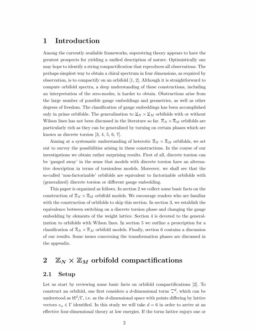
(V1, V2, ε 6= 1)model M′
(V1+∆V1, V2+∆V2, ε = 1)≃
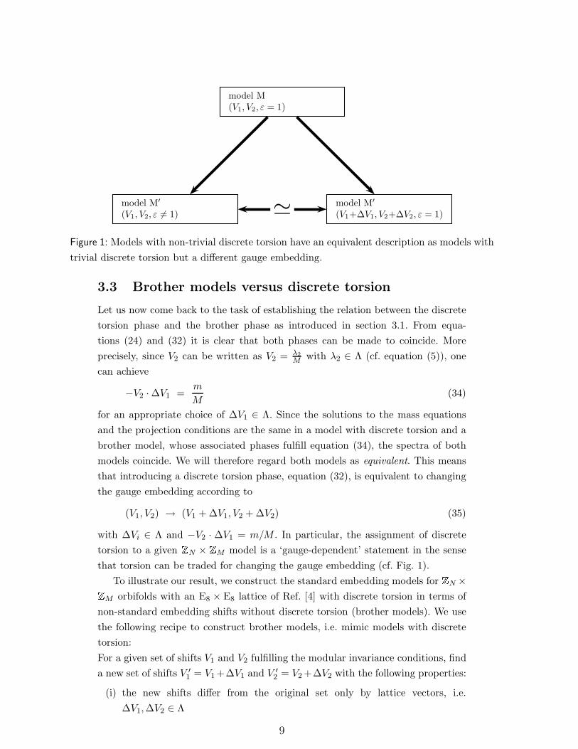
Figure 1: Models with non-trivial discrete torsion have an equivalent description as models with
trivial discrete torsion but a different gauge embedding.
3.3 Brother models versus discrete torsion
Let us now come back to the task of establishing the relation between the discrete
torsion phase and the brother phase as introduced in section 3.1. From equa-
tions (24) and (32) it is clear that both phases can be made to coincide. More
precisely, since V2 can be written as V2 = λ2
M with λ2 ∈ Λ (cf. equation (5)), one
can achieve
−V2 · ∆V1 =m
M(34)
for an appropriate choice of ∆V1 ∈ Λ. Since the solutions to the mass equations
and the projection conditions are the same in a model with discrete torsion and a
brother model, whose associated phases fulfill equation (34), the spectra of both
models coincide. We will therefore regard both models as equivalent. This means
that introducing a discrete torsion phase, equation (32), is equivalent to changing
the gauge embedding according to
(V1, V2) → (V1 + ∆V1, V2 + ∆V2) (35)
with ∆Vi ∈ Λ and −V2 · ∆V1 = m/M . In particular, the assignment of discrete
torsion to a given ZN × ZM model is a ‘gauge-dependent’ statement in the sense
that torsion can be traded for changing the gauge embedding (cf. Fig. 1).
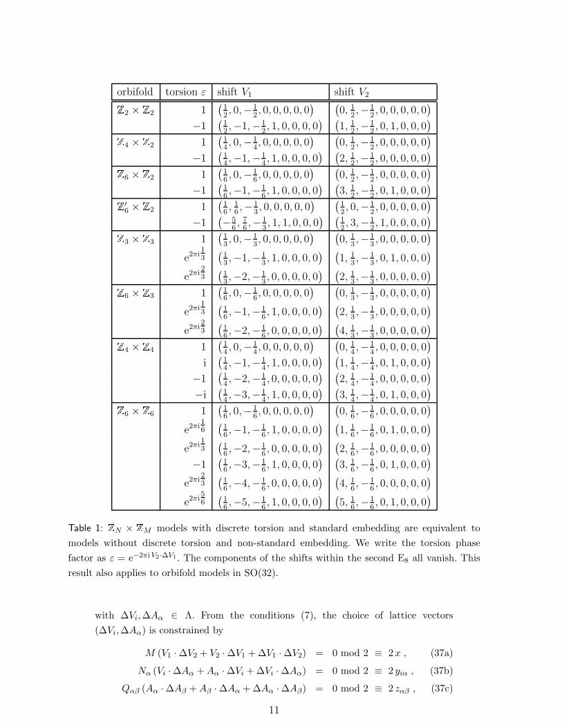
To illustrate our result, we construct the standard embedding models for ZN ×ZM orbifolds with an E8 × E8 lattice of Ref. [4] with discrete torsion in terms of
non-standard embedding shifts without discrete torsion (brother models). We use
the following recipe to construct brother models, i.e. mimic models with discrete
torsion:
For a given set of shifts V1 and V2 fulfilling the modular invariance conditions, find
a new set of shifts V ′1 = V1 +∆V1 and V ′
2 = V2 +∆V2 with the following properties:
(i) the new shifts differ from the original set only by lattice vectors, i.e.
∆V1,∆V2 ∈ Λ
9
(ii) the new shifts also fulfill the modular invariance conditions, and
(iii) the ‘interference term’ V2 · ∆V1 is not an integer.
In practice (and for any N,M), the above properties can be expressed in terms of
linear Diophantine equations for which we always find solutions.
Possible choices for the shifts (V1 + ∆V1, V2 + ∆V2) are shown in Tab. 1, where
we list the shifts of torsionless models equivalent to the discrete torsion model of
Ref. [4].
Our result has important consequences for the classification of ZN × ZM orb-
ifolds. Introducing a discrete torsion phase in the sense of Ref. [4] does not lead
to new models. That is, all models with this discrete torsion can be equivalently
obtained by scanning over torsionless models only. This will be important for our
classification in section 5.
It is also instructive to interpret the equivalence between discrete torsion and
changing the gauge embedding in terms of geometry. Discrete torsion can be re-
garded as a property of the 6D compact space while changing the gauge embedding
affects the (left-moving) coordinates of the gauge lattice only. Hence one might ar-
gue that discrete torsion and choosing a different gauge embedding are two different
features of orthogonal dimensions. However, by embedding the ‘spatial’ twist in the
gauge degrees of freedom, these features get combined in such a way that it is no
longer possible to make a clear separation. Using a more technical language one
might rephrase this statement by saying that, since physical states arise from ten-
soring left- and right-movers together, the phases ε and ε cannot be distinguished.
Consequently, properties of the zero-modes cannot be ascribed neither to the gauge
embedding alone nor to the presence of discrete torsion, but only to both.
4 Generalized discrete torsion
The results of the previous section can be generalized. To see this, we first generalize
the brother phase of section 3.1 for orbifolds with Wilson lines. In a second step,
we compare the emerging phases to what is known as generalized discrete torsion
[7]. As before, we can relate both phases.
4.1 Generalized brother models
Let us turn to the discussion of orbifolds with Wilson lines [15]. A (torsionless)
model M is defined by (V1, V2, Aα). A brother model M′ appears by adding lattice
vectors to the shifts and Wilson lines, i.e. M′ is defined by
(V ′1 , V
′2 , A
′α) = (V1 + ∆V1, V2 + ∆V2, Aα + ∆Aα) , (36)
10
orbifold torsion ε shift V1 shift V2Z2 × Z2 1(
12, 0,−1
2, 0, 0, 0, 0, 0
) (0, 1
2,−1
2, 0, 0, 0, 0, 0
)
−1(
12,−1,−1
2, 1, 0, 0, 0, 0
) (1, 1
2,−1
2, 0, 1, 0, 0, 0
)Z4 × Z2 1(
14, 0,−1
4, 0, 0, 0, 0, 0
) (0, 1
2,−1
2, 0, 0, 0, 0, 0
)
−1(
14,−1,−1
4, 1, 0, 0, 0, 0
) (2, 1
2,−1
2, 0, 0, 0, 0, 0
)Z6 × Z2 1(
16, 0,−1
6, 0, 0, 0, 0, 0
) (0, 1
2,−1
2, 0, 0, 0, 0, 0
)
−1(
16,−1,−1
6, 1, 0, 0, 0, 0
) (3, 1
2,−1
2, 0, 1, 0, 0, 0
)Z′6 × Z2 1
(16, 1
6,−1
3, 0, 0, 0, 0, 0
) (12, 0,−1
2, 0, 0, 0, 0, 0
)
−1(−5
6, 7
6,−1
3, 1, 1, 0, 0, 0
) (12, 3,−1
2, 1, 0, 0, 0, 0
)Z3 × Z3 1(
13, 0,−1
3, 0, 0, 0, 0, 0
) (0, 1
3,−1
3, 0, 0, 0, 0, 0
)
e2πi13(
13,−1,−1
3, 1, 0, 0, 0, 0
) (1, 1
3,−1
3, 0, 1, 0, 0, 0
)
e2πi23(
13,−2,−1
3, 0, 0, 0, 0, 0
) (2, 1
3,−1
3, 0, 0, 0, 0, 0
)Z6 × Z3 1(
16, 0,−1
6, 0, 0, 0, 0, 0
) (0, 1
3,−1
3, 0, 0, 0, 0, 0
)
e2πi13(
16,−1,−1
6, 1, 0, 0, 0, 0
) (2, 1
3,−1
3, 0, 0, 0, 0, 0
)
e2πi23(
16,−2,−1
6, 0, 0, 0, 0, 0
) (4, 1
3,−1
3, 0, 0, 0, 0, 0
)Z4 × Z4 1(
14, 0,−1
4, 0, 0, 0, 0, 0
) (0, 1
4,−1
4, 0, 0, 0, 0, 0
)
i(
14,−1,−1
4, 1, 0, 0, 0, 0
) (1, 1
4,−1
4, 0, 1, 0, 0, 0
)
−1(
14,−2,−1
4, 0, 0, 0, 0, 0
) (2, 1
4,−1
4, 0, 0, 0, 0, 0
)
−i(
14,−3,−1
4, 1, 0, 0, 0, 0
) (3, 1
4,−1
4, 0, 1, 0, 0, 0
)Z6 × Z6 1(
16, 0,−1
6, 0, 0, 0, 0, 0
) (0, 1
6,−1
6, 0, 0, 0, 0, 0
)
e2πi16(
16,−1,−1
6, 1, 0, 0, 0, 0
) (1, 1
6,−1
6, 0, 1, 0, 0, 0
)
e2πi13(
16,−2,−1
6, 0, 0, 0, 0, 0
) (2, 1
6,−1
6, 0, 0, 0, 0, 0
)
−1(
16,−3,−1
6, 1, 0, 0, 0, 0
) (3, 1
6,−1
6, 0, 1, 0, 0, 0
)
e2πi23(
16,−4,−1
6, 0, 0, 0, 0, 0
) (4, 1
6,−1
6, 0, 0, 0, 0, 0
)
e2πi56(
16,−5,−1
6, 1, 0, 0, 0, 0
) (5, 1
6,−1
6, 0, 1, 0, 0, 0
)
Table 1: ZN × ZM models with discrete torsion and standard embedding are equivalent to
models without discrete torsion and non-standard embedding. We write the torsion phase
factor as ε = e−2πiV2·∆V1. The components of the shifts within the second E8 all vanish. This
result also applies to orbifold models in SO(32).
with ∆Vi,∆Aα ∈ Λ. From the conditions (7), the choice of lattice vectors
(∆Vi,∆Aα) is constrained by
M (V1 · ∆V2 + V2 · ∆V1 + ∆V1 · ∆V2) = 0 mod 2 ≡ 2x , (37a)
Nα (Vi · ∆Aα +Aα · ∆Vi + ∆Vi · ∆Aα) = 0 mod 2 ≡ 2 yiα , (37b)
Qαβ (Aα · ∆Aβ +Aβ · ∆Aα + ∆Aα · ∆Aβ) = 0 mod 2 ≡ 2 zαβ , (37c)
11
where x, yiα, zαβ ∈ Z.
Repeating the steps of section 3.1 one arrives at a ‘generalized brother phase’
ε = exp
{−2πi
[(k1 t2 − k2 t1)
(V2 · ∆V1 −
x
M
)
+(k1mα − t1 nα)
(Aα · ∆V1 −
y1α
Nα
)
+(k2mα − t2 nα)
(Aα · ∆V2 −
y2α
Nα
)
+nαmβ
(Aβ · ∆Aα − zαβ
Qαβ
)]}, (38)
corresponding to the constructing element g = (θk1ωk2 , nαeα) and the commuting
element h = (θt1ωt2 ,mαeα). One can see that Dαβ ≡ Aβ · ∆Aα − zαβ/Qαβ is
(almost) antisymmetric in α, β,
Dαβ = −Dβα mod 1 . (39)
Notice that also in the case of orbifolds with lattice-valued Wilson lines, Aα ∈ Λ,
the last three terms of equation (38) can be non-trivial, giving rise to new brother
models.
Brother models in ZN orbifolds
From equation (38), it is clear that the generalized brother phase is also important
for ZN orbifolds. More precisely, in ZN orbifolds with Wilson lines, the second and
fourth lines of equation (38) are not always trivial and thus also lead to brother
models.
Let us illustrate this with an example in Z4 with twist v = 14(−2, 1, 1; 0)
acting on the compactification lattice Γ = SO(4)3, and standard embedding [16].
The gauge group is E6×SU(2)×E8. By turning on the lattice-valued Wilson lines
A1 =(08) (
12, 06), A5 = A6 =
(08) (
0, 12, 05), (40)
a non-trivial generalized brother phase with D15 = D16 = −12 is introduced. The
untwisted and first twisted sectors remain unchanged, but the number of (anti-)
families in the second twisted sector is reduced from 10 (27,1,1) + 6 (27,1,1) to
6 (27,1,1) + 2 (27,1,1).
4.2 Generalized discrete torsion
In section 3.2 we have discussed the discrete torsion phase as introduced in Ref. [4].
More recently, this concept has been extended by introducing a generalized discrete
torsion phase in the context of type IIA/B string theory [7]. This generalized torsion
phase depends on the fixed points of the orbifold. It weights differently terms in
12
the partition function corresponding to the same twisted sector but different fixed
points, and is constrained by modular invariance.
Following the steps of section 3.2 and considering g, h ∈ S, we write down the
general solution of equations (30) for the discrete torsion phase as3
ε(g, h) = e2πi [a (k1 t2−k2 t1)+bα (k1 mα−t1 nα)+cα (k2 mα−t2 nα)+dαβ nα mβ ] . (41)
Modular invariance constrains the values of a, bα, cα, dαβ . Therefore a = a/M, bα =
bα/Nα, cα = cα/Nα, dαβ = dαβ/Nαβ with a, bα, cα, dαβ ∈ Z,Nαβ being the greatest
common divisor of Nα and Nβ . In addition, dαβ must be antisymmetric in α, β.
The parameters bα, cα, dαβ are additionally constrained by the geometry of the
orbifold. It is not hard to see that if eα ≃ eβ on the orbifold, then bα = bβ , cα = cβ
and dαβ = 0 must hold (cf. the examples below).
The generalized discrete torsion is not restricted only to ZN × ZM orbifolds,
as the usual discrete torsion was, but will likewise appear in the ZN case. Clearly,
since in ZN orbifolds there is only one shift, the parameters a and cα vanish.
Examples
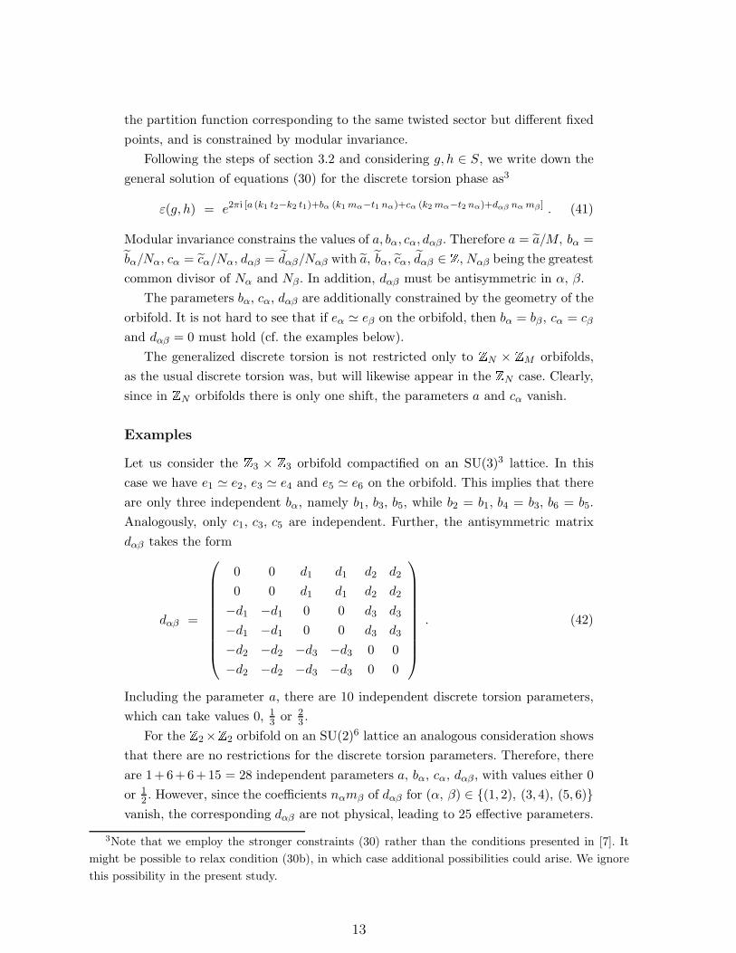
Let us consider the Z3 × Z3 orbifold compactified on an SU(3)3 lattice. In this
case we have e1 ≃ e2, e3 ≃ e4 and e5 ≃ e6 on the orbifold. This implies that there
are only three independent bα, namely b1, b3, b5, while b2 = b1, b4 = b3, b6 = b5.
Analogously, only c1, c3, c5 are independent. Further, the antisymmetric matrix
dαβ takes the form
dαβ =
0 0 d1 d1 d2 d2
0 0 d1 d1 d2 d2
−d1 −d1 0 0 d3 d3
−d1 −d1 0 0 d3 d3
−d2 −d2 −d3 −d3 0 0
−d2 −d2 −d3 −d3 0 0
. (42)
Including the parameter a, there are 10 independent discrete torsion parameters,
which can take values 0, 13 or 2
3 .
For the Z2×Z2 orbifold on an SU(2)6 lattice an analogous consideration shows
that there are no restrictions for the discrete torsion parameters. Therefore, there
are 1+6+6+15 = 28 independent parameters a, bα, cα, dαβ , with values either 0
or 12 . However, since the coefficients nαmβ of dαβ for (α, β) ∈ {(1, 2), (3, 4), (5, 6)}
vanish, the corresponding dαβ are not physical, leading to 25 effective parameters.
3Note that we employ the stronger constraints (30) rather than the conditions presented in [7]. It
might be possible to relax condition (30b), in which case additional possibilities could arise. We ignore
this possibility in the present study.
13
bcb
a = 0
(27,1)3× (1,1)
bcb
a = 1/33× (1,1)
bcba = 2/3
(27,1)3× (1,1)
(a)
bcb bcb
bcb
bα = 1/3
(27,1)3 × (1,1)
3 × (1,1)
(27,1)3 × (1,1)
(b)
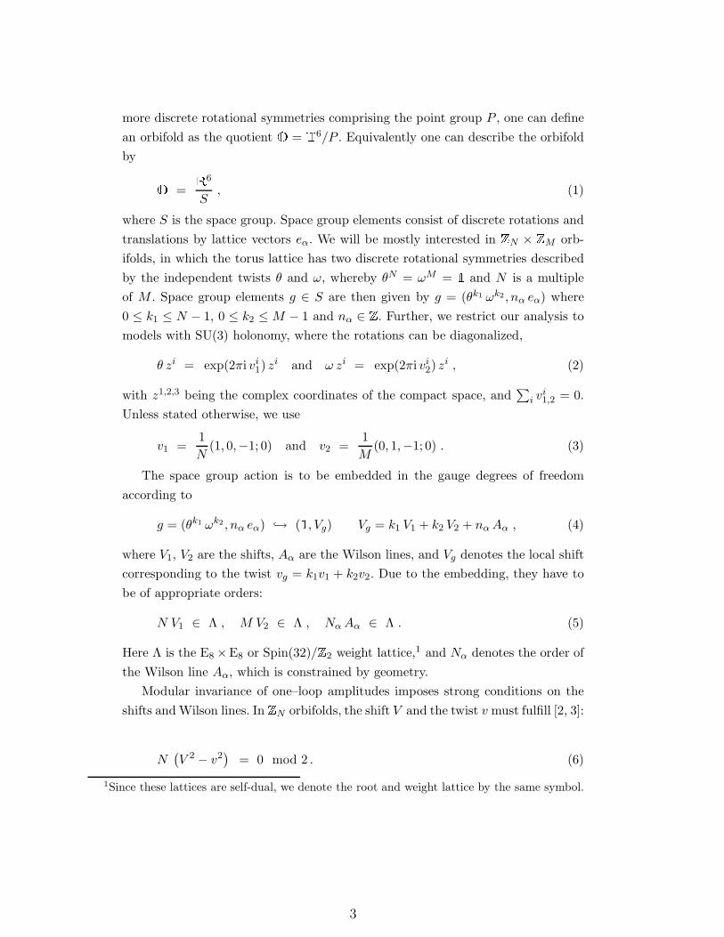
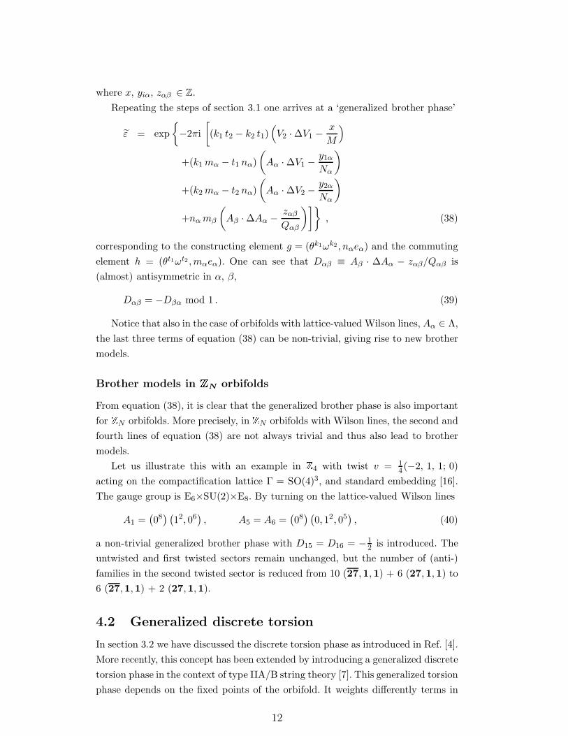
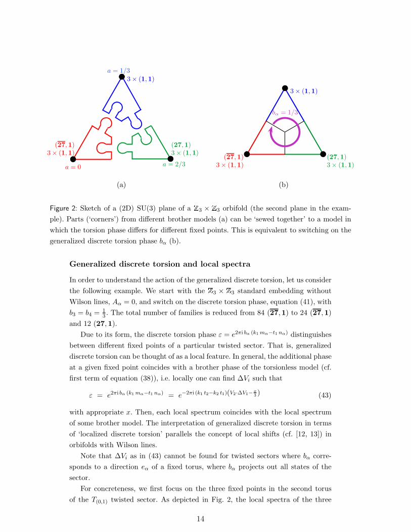
Figure 2: Sketch of a (2D) SU(3) plane of a Z3 × Z3 orbifold (the second plane in the exam-
ple). Parts (‘corners’) from different brother models (a) can be ‘sewed together’ to a model in
which the torsion phase differs for different fixed points. This is equivalent to switching on the
generalized discrete torsion phase bα (b).
Generalized discrete torsion and local spectra
In order to understand the action of the generalized discrete torsion, let us consider
the following example. We start with the Z3 × Z3 standard embedding without
Wilson lines, Aα = 0, and switch on the discrete torsion phase, equation (41), with
b3 = b4 = 13 . The total number of families is reduced from 84 (27,1) to 24 (27,1)
and 12 (27,1).
Due to its form, the discrete torsion phase ε = e2πi bα (k1 mα−t1 nα) distinguishes
between different fixed points of a particular twisted sector. That is, generalized
discrete torsion can be thought of as a local feature. In general, the additional phase
at a given fixed point coincides with a brother phase of the torsionless model (cf.
first term of equation (38)), i.e. locally one can find ∆Vi such that
ε = e2πi bα (k1 mα−t1 nα) = e−2πi (k1 t2−k2 t1)(V2·∆V1−x3) (43)
with appropriate x. Then, each local spectrum coincides with the local spectrum
of some brother model. The interpretation of generalized discrete torsion in terms
of ‘localized discrete torsion’ parallels the concept of local shifts (cf. [12, 13]) in
orbifolds with Wilson lines.
Note that ∆Vi as in (43) cannot be found for twisted sectors where bα corre-
sponds to a direction eα of a fixed torus, where bα projects out all states of the
sector.
For concreteness, we first focus on the three fixed points in the second torus
of the T(0,1) twisted sector. As depicted in Fig. 2, the local spectra of the three
14
brother models, a ≡ −(V2 · ∆V1 − x
3
)= 0, 1
3 ,23 , can be combined consistently into
one model with b3 = b4 = 13 . On the other hand, in the T(1,0) twisted sector there
is a fixed torus in the directions e3, e4; thus the sector is empty.
This procedure can also be applied to the terms cα and dαβ of the generalized
discrete torsion phase, equation (41).
Generalized brother models versus generalized discrete torsion
As in our previous discussion in chapter 3, also the generalized versions of the
discrete torsion phase and the brother phase have a very similar form. Indeed,
whenever there are non-trivial solutions to equations (37), one can equivalently
describe models with generalized discrete torsion phase in terms of generalized
brother models. This is the generic case.
However, there are exceptions. Namely, as we will explain below, models with
dαβ 6= 0 in Z3 × Z3 orbifolds without Wilson lines cannot be interpreted in terms
of brother models.
Consider the fourth part of the generalized discrete torsion phase of equa-
tion (41),
ε = e2πi dαβ nαmβ , (44)
with dαβ ∈{0, 1
3 ,23
}. An analogous term appears in the generalized brother phase
as
ε = exp
[−2πinαmβ
(Aβ · ∆Aα − zαβ
Qαβ
)], (45)
where Qαβ = 3, since the Wilson lines have order 3. In general, both phases can
be made coincide by choosing ∆Aα ∈ Λ such that
−(Aβ · ∆Aα − zαβ
3
)= dαβ . (46)
On the other hand, in the case when Aα = 0 and ∆Aα 6= 0, equation (45) simplifies
to
ε = e2πinαmβ
“zαβ3
”
= e2πi nαmβ
“∆Aα·∆Aβ
2
”
, (47)
where the second equality follows from the definition of zαβ , equation (37c). As
∆Aα are lattice vectors, this equality can only hold if zαβ = 0 mod 3, which implies
that the brother phase equation (47) is trivial. Thus, in this case, the generalized
discrete torsion phase leads to models which cannot arise by adding lattice vectors
to shifts and Wilson lines.
In summary, the generalized discrete torsion phases admit more possible as-
signments than the generalized brother phases. Nevertheless, a large class of the
models with generalized discrete torsion has an equivalent description in terms of
models with a modified gauge embedding.
15
Our results have important implications. By introducing generalized discrete
torsion, or lattice-valued Wilson lines, one can control the local spectra. We there-
fore expect that introducing generalized discrete torsion, or alternatively shifting
the Wilson lines by lattice vectors, will gain a similar importance as discrete Wilson
lines [15] for orbifold model building.
As stated above, switching on generalized discrete torsion can lead to the dis-
appearance of complete local spectra. This raises the question of how to interpret
this fact in terms of geometry. Some of the localized zero-modes can be viewed
as blow-up modes which allow to resolve the orbifold singularity associated to a
given fixed point [17, 18, 5] (see [19, 20, 21] for recent developments). If at a given
fixed point there are no zero modes, one might argue that, therefore, the associated
singularity cannot be ‘blown up’. In what follows, we shall advertise an alternative
interpretation.
4.3 Connection to non-factorizable orbifolds
We find that in many cases orbifold models M with certain geometry, i.e. com-
pactification lattice Γ, and generalized discrete torsion switched on are equivalent
to torsionless models M′ based on a different lattice Γ′. Model M′ has less fixed
points than M, and the mismatch turns out to constitute precisely the ‘empty’
fixed points of model M.
The simplest examples are based on Z2 × Z2 orbifolds with standard embed-
ding and without Wilson lines. As compactification lattice Γ, we choose an SU(2)6
lattice [10]. As we have seen in section 4.2, in this case there are 25 physical param-
eters for generalized discrete torsion, with values either 0 or 12 . For concreteness,
we restrict to the 12 dαβ parameters and scan over all 212 models.
Beside other models with a net number of zero families, we find eight models
(and their mirrors, i.e. models where families and anti-families are exchanged).
They are listed in Tab. 2, where we present the number of (anti-)families for each
twisted sector and the total number of singlets. As discussed in section 4.2, models
with non-trivial dαβ are equivalent to torsionless models with lattice-valued Wilson
lines. Possible representatives of these Wilson lines can be composed out of the
building blocks
W1 = (06, 1, 1) , W2 = (05, 1, 1, 0) , W ′1 = (1, 1, 06) , W ′
2 = (0, 1, 1, 05) ,
S = (12
8) , V = (07, 2) , V ′ = (06, 2, 0) , (48)
and are listed in the last column of Tab. 2.
Models leading to spectra coinciding with what we got in Tab. 2 have already
been discussed in the literature. They appeared first in Ref. [22] in the context
of free fermionic string models related to the Z2 × Z2 orbifold with an additional
freely acting shift. More recently, new Z2 × Z2 orbifold constructions have been
16
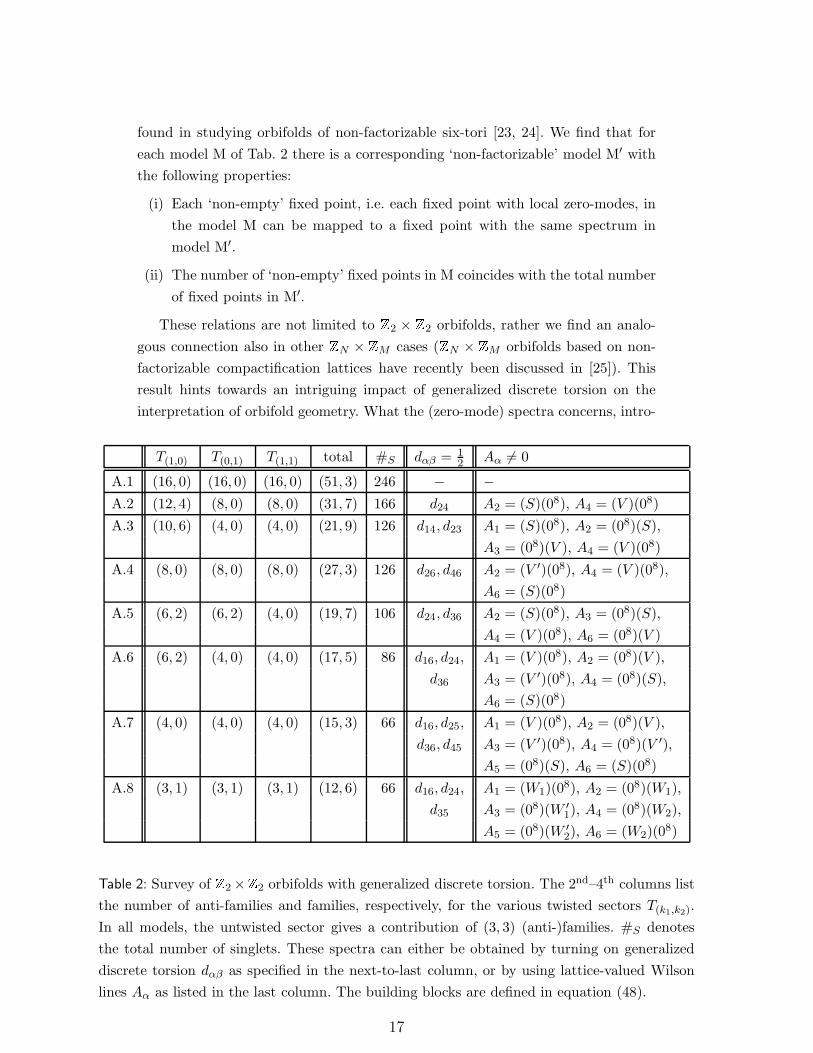
found in studying orbifolds of non-factorizable six-tori [23, 24]. We find that for
each model M of Tab. 2 there is a corresponding ‘non-factorizable’ model M′ with
the following properties:
(i) Each ‘non-empty’ fixed point, i.e. each fixed point with local zero-modes, in
the model M can be mapped to a fixed point with the same spectrum in
model M′.
(ii) The number of ‘non-empty’ fixed points in M coincides with the total number
of fixed points in M′.
These relations are not limited to Z2 × Z2 orbifolds, rather we find an analo-
gous connection also in other ZN × ZM cases (ZN × ZM orbifolds based on non-
factorizable compactification lattices have recently been discussed in [25]). This
result hints towards an intriguing impact of generalized discrete torsion on the
interpretation of orbifold geometry. What the (zero-mode) spectra concerns, intro-
T(1,0) T(0,1) T(1,1) total #S dαβ = 12 Aα 6= 0
A.1 (16, 0) (16, 0) (16, 0) (51, 3) 246 − −A.2 (12, 4) (8, 0) (8, 0) (31, 7) 166 d24 A2 = (S)(08), A4 = (V )(08)
A.3 (10, 6) (4, 0) (4, 0) (21, 9) 126 d14, d23 A1 = (S)(08), A2 = (08)(S),
A3 = (08)(V ), A4 = (V )(08)
A.4 (8, 0) (8, 0) (8, 0) (27, 3) 126 d26, d46 A2 = (V ′)(08), A4 = (V )(08),
A6 = (S)(08)
A.5 (6, 2) (6, 2) (4, 0) (19, 7) 106 d24, d36 A2 = (S)(08), A3 = (08)(S),
A4 = (V )(08), A6 = (08)(V )
A.6 (6, 2) (4, 0) (4, 0) (17, 5) 86 d16, d24, A1 = (V )(08), A2 = (08)(V ),
d36 A3 = (V ′)(08), A4 = (08)(S),
A6 = (S)(08)
A.7 (4, 0) (4, 0) (4, 0) (15, 3) 66 d16, d25, A1 = (V )(08), A2 = (08)(V ),
d36, d45 A3 = (V ′)(08), A4 = (08)(V ′),
A5 = (08)(S), A6 = (S)(08)
A.8 (3, 1) (3, 1) (3, 1) (12, 6) 66 d16, d24, A1 = (W1)(08), A2 = (08)(W1),
d35 A3 = (08)(W ′1), A4 = (08)(W2),
A5 = (08)(W ′2), A6 = (W2)(0
8)
Table 2: Survey of Z2 ×Z2 orbifolds with generalized discrete torsion. The 2nd–4th columns list
the number of anti-families and families, respectively, for the various twisted sectors T(k1,k2).
In all models, the untwisted sector gives a contribution of (3, 3) (anti-)families. #S denotes
the total number of singlets. These spectra can either be obtained by turning on generalized
discrete torsion dαβ as specified in the next-to-last column, or by using lattice-valued Wilson
lines Aα as listed in the last column. The building blocks are defined in equation (48).
17
ducing generalized discrete torsion (or considering generalized brother models) is
equivalent to changing the geometry of the underlying compact space, Γ → Γ′. To
establish complete equivalence between these models would require to prove that
the couplings of the corresponding states are the same, which is beyond the scope
of the present study. It is, however, tempting to speculate that non-resolvable sin-
gularities, as discussed above, do not ‘really’ exist as one can always choose (for
a given spectrum) the compactification lattice Γ in such a way that there are no
‘empty’ fixed points.
5 How to classify ZN × ZM orbifolds
Let us now turn to describing a method of classifying heterotic ZN ×ZM orbifolds,
taking into account generalized discrete torsion. To illustrate our methods, we
focus on Z3 × Z3 orbifold compactifications of the E8 × E8 heterotic string. It is
straightforward to generalize the discussion to other ZN ×ZM orbifolds and to the
SO(32) case.
To classify an orbifold requires an efficient prescription of how to obtain all in-
equivalent models. The first step in a classification is to get all admissible choices
for the shift vector V1. For this purpose, we make use of Dynkin diagram tech-
niques (see e.g. [16]). These techniques are advantageous since, when writing down
V1, one has the freedom of choosing the basis of the weight lattice Λ in such a
way that the shift has a very simple form. Clearly, this freedom is lost when one
introduces the second shift (and Wilson lines). This complicates the construction
of all inequivalent shifts V2.
To obtain all inequivalent V2 we utilize a method introduced by Giedt [26] (see
also [27]), i.e. use an adequate minimal ansatz which avoids redundancies due to
lattice translations and some Weyl reflections. This ansatz restricts the shifts to be
only in a certain cell ΛN of the lattice Λ in such a way that any possible ZN shift
can be written as an element of this cell plus a lattice vector. That is, an arbitraryZN shift has a unique decomposition
V = V + ∆V , where V ∈ ΛN and ∆V ∈ Λ . (49)
Consider now a consistent gauge embedding (V1, V2). According to equation (49)
the shifts can be decomposed into (V1 + ∆V1, V2 + ∆V2) with V1 ∈ ΛN , V2 ∈ ΛM
and ∆Vi ∈ Λ. It is not hard to see that the conditions (7) imply
N(V 2
1 − v21
)= 0 mod 2 , (50a)
M(V 2
2 − v22
)= 0 mod 2 , (50b)
M(V1 · V2 − v1 · v2
)= 0 mod 1 . (50c)
To scan over all possible shift embeddings is therefore reduced to the task of
18
(i) specifying V1 (satisfying (50a)) by Dynkin techniques,
(ii) scanning ΛM for V2 fulfilling equations (50b) and (50c), and
(iii) examining all possible (V1, V2) related to (V1, V2) by lattice translations and
satisfying (7).
At first sight, the last step seems to require a scan over an infinite number of
shifts. However, as we have seen in section 3, given one representative (V1, V2)
satisfying (7), this scan can be replaced by switching on all inequivalent discrete
torsion phases. Since there is only a finite number of torsion phase assignments,
we have found a prescription to obtain all inequivalent models by scanning only
over a finite set of inputs.
As already stated, in a complete classification it is necessary to take into account
generalized discrete torsion as well. Thus, to get all admissible shifts, one has to
scan over all appropriate values for the parameters bα, cα and dαβ .
All statements made for V2 apply also to the Wilson lines. That is, in order
to obtain all inequivalent Wilson line embeddings, one can also scan the finite
cell ΛNα (fulfilling consistency conditions analogous to (50)), and then switch on
generalized discrete torsion.
So far, we have described how to obtain all inequivalent models. However, some
of the inputs, specified by (V1, V2), Wilson lines and generalized torsion phases,
turn out to be equivalent. Apart from the ambiguities related to Weyl reflections
(cf. [26]), in the framework of ZN × ZM orbifolds further complications arise.
For instance, we note that models with shifts related by discrete rotations, i.e.
(V1, V2) → (a1 V1 + a2 V2, b1 V1 + b2 V2) with proper values of ai, bi ∈ Z, can be
equivalent. For example, in Z3 ×Z3 a model with shifts (V1, V2) is equivalent to a
model with shifts (V1, V1 + 2V2).
In our classification below, we consider two models as inequivalent if and only
if their massless spectra are different.4
Sample classification of Z3 × Z3 without Wilson lines
As a concrete application, let us describe the classification of Z3 × Z3 orbifolds
without Wilson lines.5 By using Dynkin diagram techniques, one finds that there
are only five consistent shift vectors V1, which can be written in the generic form
V1 =1
3(0n0 , 1n1 , 2α) (0m0 , 1m1 , 2β), (51)
where α and β can be either 0 or 1, and n0, n1,m0,m1 ∈ Z, such that n0+n1+α =
m0 +m1 + β = 8.
4In practice, we compare the non-Abelian massless spectra and the number of singlets. This under-
estimates the true number of models somewhat.5As we allow for generalized discrete torsion, some of the models can be interpreted as being endowed
with lattice-valued Wilson lines, see section 4.
19
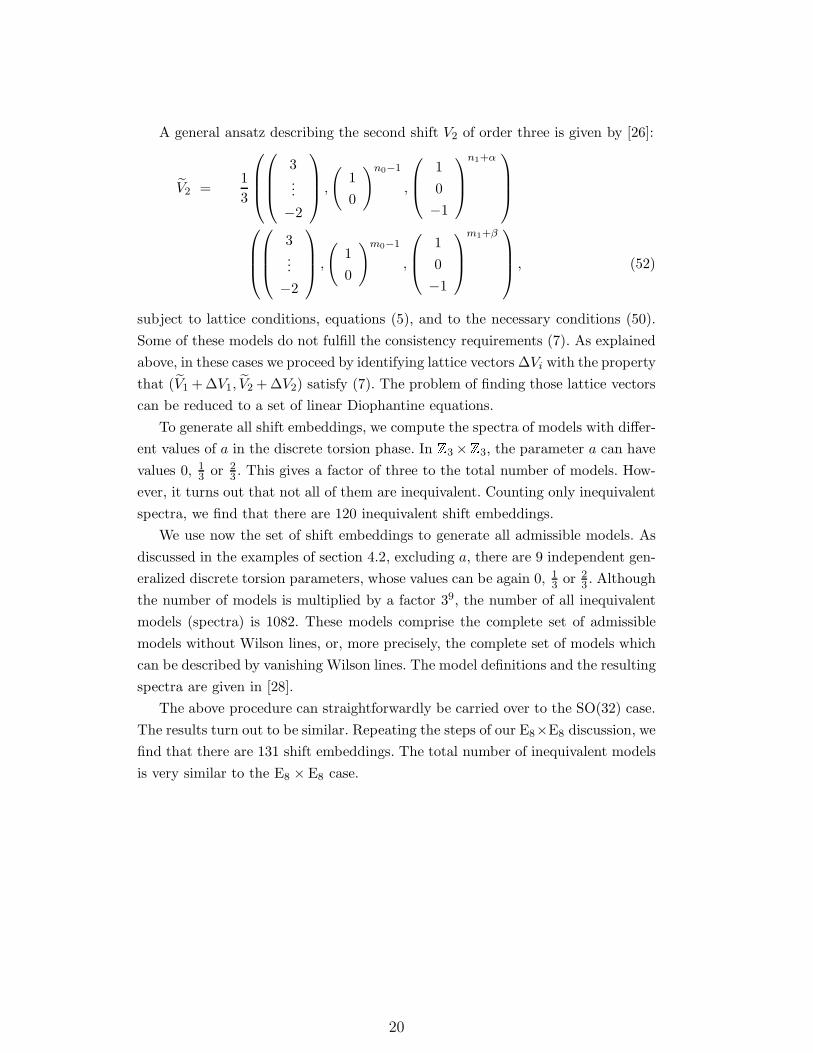
A general ansatz describing the second shift V2 of order three is given by [26]:
V2 =1
3
3...
−2
,
(1
0
)n0−1
,
1
0
−1
n1+α
3...
−2
,
(1
0
)m0−1
,
1
0
−1
m1+β , (52)
subject to lattice conditions, equations (5), and to the necessary conditions (50).
Some of these models do not fulfill the consistency requirements (7). As explained
above, in these cases we proceed by identifying lattice vectors ∆Vi with the property
that (V1 + ∆V1, V2 + ∆V2) satisfy (7). The problem of finding those lattice vectors
can be reduced to a set of linear Diophantine equations.
To generate all shift embeddings, we compute the spectra of models with differ-
ent values of a in the discrete torsion phase. In Z3 ×Z3, the parameter a can have
values 0, 13 or 2
3 . This gives a factor of three to the total number of models. How-
ever, it turns out that not all of them are inequivalent. Counting only inequivalent
spectra, we find that there are 120 inequivalent shift embeddings.
We use now the set of shift embeddings to generate all admissible models. As
discussed in the examples of section 4.2, excluding a, there are 9 independent gen-
eralized discrete torsion parameters, whose values can be again 0, 13 or 2
3 . Although
the number of models is multiplied by a factor 39, the number of all inequivalent
models (spectra) is 1082. These models comprise the complete set of admissible
models without Wilson lines, or, more precisely, the complete set of models which
can be described by vanishing Wilson lines. The model definitions and the resulting
spectra are given in [28].
The above procedure can straightforwardly be carried over to the SO(32) case.
The results turn out to be similar. Repeating the steps of our E8×E8 discussion, we
find that there are 131 shift embeddings. The total number of inequivalent models
is very similar to the E8 × E8 case.
20

6 Discussion
Aiming at a systematic understanding of heterotic ZN × ZM orbifolds, we have
investigated the possibilities arising in these constructions. We find that, unlike
in the case of prime orbifolds, adding elements of the weight lattice to the shifts,
(V1, V2) → (V1+∆V1, V2+∆V2), changes in general the spectrum. Interestingly, the
same spectra are obtained by switching on discrete torsion. Stated differently, one
can trade discrete torsion for a change of the gauge embedding by lattice vectors.
We have extended our analysis such as to include generalized discrete torsion. We
find that a large class of generalized discrete torsion phases can be mimicked by
lattice-valued Wilson lines. Interestingly, an analog of a generalized discrete torsion
phase appears in certain ZN orbifolds which admit at least two discrete Wilson lines
of coinciding orders. Another remarkable result is that switching on certain types
of generalized discrete torsion is equivalent to changing the 6D compactification
lattice. This implies that the field-theoretic interpretation of the model input can
be somewhat subtle. We provided various explicit examples, illustrating all main
statements.
Our results have important consequences. At the more practical side, we were
able to formulate a straightforward method of classifying ZN × ZM orbifolds. We
have also seen that switching on generalized discrete torsion allows to change the
local spectra, i.e. one obtains different twisted states, which correspond to brane
fields in the field-theoretic description. We expect this to become important for orb-
ifold model building, where one can use this observation, for instance, for reducing
the number of generations without modifying the gauge group.
At a more conceptual level, our findings imply that a given spectrum cannot be
ascribed neither to properties of the 6D internal space alone, i.e. whether discrete
torsion is switched on or not, nor to the gauge embedding, but only to both.
This implies that the same models, leading to the same spectra, can be regarded
as resulting from what one might consider as different geometries. Although we
cannot claim to have identified the deeper reasons for these relations, we feel that
our observations constitute some progress in the task of understanding stringy
geometry.
Acknowledgments. We would like to thank S. Forste, A. Micu and H. P. Nilles
for valuable discussions, and T. Kobayashi and K.-J. Takahashi for correspondence.
This work was partially supported by the cluster of excellence “Origin
and Structure of the Universe”, the EU 6th Framework Program MRTN-CT-
2004-503369 “Quest for Unification”, MRTN-CT-2004-005104 “ForcesUniverse”,
MRTN-CT-2006-035863 “UniverseNet” and the Transregios 27 ’‘Neutrinos and Be-
yond” and 33 “The Dark Universe” by Deutsche Forschungsgemeinschaft (DFG).
21
A Transformation phases
The aim of this appendix is to clarify the transformation law of physical states. Let
us start with the simplest example, a ZN orbifold without Wilson lines. Modular
invariance requires [3]
N (V 2 − v2) = 0 mod 2 . (A.1)
To see that there are some subtleties, consider a ‘constructing element’ g =
(θk, nαeα). Zero-modes in the g-twisted sector have to fulfill the masslessness condi-
tion (10). Focus, for simplicity, on non-oscillator states, for which the masslessness
conditions read
1
2p2sh − 1 + δc = 0 , (A.2a)
1
2q2sh − 1
2+ δc = 0 , (A.2b)
where psh = (p + Vg), qsh = (q + vg), Vg = k V + nαAα and vg = k v. Using the
properties p2 = even and q2 = odd one derives
p · Vg = 1 − δc −V 2
g
2+ integer , (A.3a)
q · vg = −δc−v2g
2+ integer . (A.3b)
Now let us study the transformation of a solution of the mass equation |ψ〉. The
shifted momenta psh and qsh represent the gauge and Lorentz (or SO(8)) quantum
numbers. This fixes the transformation phase of the g-twisted string |ψ〉 to be
2π [psh · Vg − qsh · vg] = 2π
[1
2
(V 2
g − v2g
)mod 1
](A.4)
under the action of g. From (A.1) we infer that this phase does not vanish in
general, rather it is of the form 2πm/N with m ∈ Z. This raises the question of
how a state associated to g can be invariant under the action of g. In the literature,
the transformation behavior of states associated to twisted strings has often been
‘repaired’, i.e. an additional transformation phase has been introduced by hand.
In what follows, we present a geometric explanation of how such additional phases
arise.
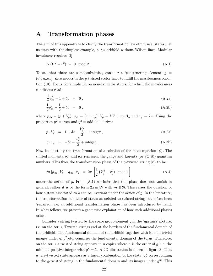
Consider a string twisted by the space group element g in the ‘upstairs’ picture,
i.e. on the torus. Twisted strings end at the borders of the fundamental domain of
the orbifold. The fundamental domain of the orbifold together with its non-trivial
images under g, g2 etc. comprise the fundamental domain of the torus. Therefore,
on the torus a twisted string appears in n copies where n is the order of g, i.e. the
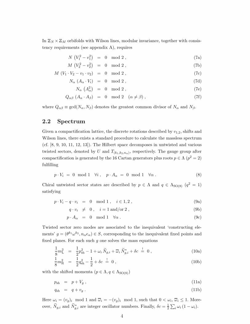
minimal positive integer with gn = 1. A 2D illustration is shown in figure 3. That
is, a g-twisted state appears as a linear combination of the state |ψ〉 corresponding
to the g-twisted string in the fundamental domain and its images under gm. This
22
2π e1
2π e2
bcb
bcb
bcb
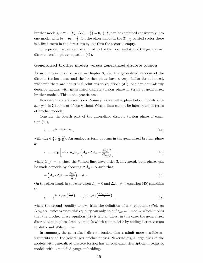
Figure 3:T2SU(3)/Z3 orbifold. The fundamental domain of the torus can be taken to be the darker
area. Transformation of g = (θ, e1 + e2)-twisted strings under (the constructing element) g: the
(red) right string is mapped to the (green) upper, and the (green) upper to the (blue) left, and
the (blue) left back to the (red) upper one.
linear combination can involve phase factors with the constraint being that gn acts
as identity. There are n different linear combinations labeled by m ∈ Z,
|ψ(m)〉 =1√n
(|ψ〉 + e−2πim/n |g ψ〉 + · · · + e−2πi m (n−1)/n |gn−1 ψ〉
), (A.5)
on the torus. In figure 3 this would correspond to a superposition of the red,
green and blue string, weighted by phase factors. It is clear that, under the action
of g, such a linear combination picks up a phase e2πi m/n. In other words, the
transformation phase (A.4) is to be amended by 2πm/n.
It is straightforward to apply these observations to the above-mentioned prob-
lem of g-invariance of states associated to the constructing element g. Clearly, only
the linear combination (A.5) with m = −n2 (V 2
g − v2g) is g-invariant. So we conclude
that for every solution of the mass equation one finds precisely one g-invariant
state. In addition to the phase arising from the gauge and Lorentz quantum num-
bers (A.4), this state picks up a compensating phase
Φvac = exp
{2πi
[−1
2(Vg · Vg − vg · vg)
]}(A.6)
under the action of g.
Before turning to the discussion of the transformation of such states under
commuting elements h, let us briefly comment on a technical simplification that
is possible in many models. It is also clear that, in ZN orbifolds without Wilson
lines, one can ‘transform’ a model M, with a ‘weak’ shift V , to the model M′,
with shift V ′ = V + ∆V where ∆V ∈ Λ. The solutions of the mass equation
coincide in the models M and M′. It is, up to some exceptional cases which we
will discuss below, always possible to find a ∆V with 12 [(V + ∆V )2 − v2] ∈ Z
23
so that (A.4) is automatically fulfilled for any |ψ〉 (and therefore also for trivial
linear combinations). For a large class of constructions one can therefore adopt the
following logic. Models with an input fulfilling only the (‘weak’) modular invariance
constraints (A.1) might not be considered as they have an alternative description
in terms of a model with input fulfilling the stronger constraints
V 2 − v2 = 0 mod 2 . (A.7)
That is, in order to avoid double-counting, one can restrict to the stronger con-
straints (A.7) in many cases. Similar statements apply to the case with non-trivial
Wilson lines (an example has been given in [13]). However, there is a caveat, namely
the above-mentioned exceptional cases in which a ‘weak’ modular invariant input
cannot be transformed to the ‘strong’ form. The simplest example for such a case
is a Z3 orbifold with V = 0. Further examples arise in non-prime ZN ·M orbifolds
(N,M > 1) where N · V ∈ Λ.
Let us now return to the question of how a (g-invariant) state associated to the
constructing element g transforms under the action of a commuting element h. In
the following, we denote the corresponding transformation phase of equation (13)
by Φ(g, h). Clearly, this phase has to comply with the space group multiplication
law, thus
Φvac(g, gp hq) = [Φvac(g, g)]
p [Φvac(g, h)]q . (A.8)
Since Φvac(g, g) is already fixed by (A.6), this leads to the conclusion
Φvac(g, h) = exp
{2πi
[−1
2(Vg · Vh − vg · vh)
]}(A.9)
for any commuting h ∈ S. Therefore, the full transformation phase of the physical
states has to be defined as in equation (13). But there are still some constraints
which have to be fulfilled for the sake of consistency. To illustrate them, let us
consider g, h ∈ S with gn = 1 = hs. From the definition of the full transformation
phase Φ, it is clear that one has to demand
Φ(g, h)!= Φ(gn+1, h) = Φ(g, h)Φvac(g, h)
−n , (A.10)
where the second equality is obtained by replacing, according to the usual embed-
ding, Vg → (n+ 1)Vg and vg → (n+ 1) vg in equation (13). Thus, Φvac(g, h)n !
= 1.
An analogous reasoning starting with Φ(g, hs+1) leads to Φvac(g, h)s !
= 1 and thus
finally to
Φvac(g, h)gcd(n,s) !
= 1 . (A.11)
Formulating equation (A.11) in terms of the gauge embedding shifts leads to the
consistency conditions (7) on shifts and Wilson lines.6
6In the case of two different Z2 Wilson lines we find that (7f) can be relaxed, i.e. gcd(Nα, Nβ) can
be replaced by NαNβ = 4, provided there exists no g ∈ P with the property g eα 6= eα but g eβ = eβ .
Imposing the weaker condition leads, as we find, to anomaly-free spectra.
24
References
[1] L. J. Dixon, J. A. Harvey, C. Vafa, and E. Witten, Nucl. Phys. B261 (1985),
678–686.
[2] L. J. Dixon, J. A. Harvey, C. Vafa, and E. Witten, Nucl. Phys. B274 (1986),
285–314.
[3] C. Vafa, Nucl. Phys. B273 (1986), 592.
[4] A. Font, L. E. Ibanez, and F. Quevedo, Phys. Lett. B217 (1989), 272.
[5] C. Vafa and E. Witten, J. Geom. Phys. 15 (1995), 189–214, [hep-th/9409188].
[6] E. R. Sharpe, Phys. Rev. D68 (2003), 126003, [hep-th/0008154].
[7] M. R. Gaberdiel and P. Kaste, JHEP 08 (2004), 001, [hep-th/0401125].
[8] L. E. Ibanez, J. Mas, H.-P. Nilles, and F. Quevedo, Nucl. Phys. B301 (1988),
157.
[9] A. Font, L. E. Ibanez, F. Quevedo, and A. Sierra, Nucl. Phys. B331 (1990),
421–474.
[10] S. Forste, H. P. Nilles, P. K. S. Vaudrevange, and A. Wingerter, Phys. Rev.
D70 (2004), 106008, [hep-th/0406208].
[11] T. Kobayashi, S. Raby, and R.-J. Zhang, Nucl. Phys. B704 (2005), 3–55,
[hep-ph/0409098].
[12] W. Buchmuller, K. Hamaguchi, O. Lebedev and M. Ratz, Nucl. Phys. B712
(2005), 139, [hep-ph/0412318].
[13] W. Buchmuller, K. Hamaguchi, O. Lebedev, and M. Ratz, (2006),
hep-th/0606187.
[14] S. Ramos-Sanchez, P. K. S. Vaudrevange, and A. Wingerter, C++ Orbifolder
[15] L. E. Ibanez, H. P. Nilles, and F. Quevedo, Phys. Lett. B187 (1987), 25–32.
[16] Y. Katsuki, Y. Kawamura, T. Kobayashi, N. Ohtsubo, Y. Ono, and K. Tan-
ioka, Nucl. Phys. B341 (1990), 611–640.
[17] M. A. Walton, Phys. Rev. D37 (1988), 377.
[18] P. S. Aspinwall, (1994), hep-th/9403123.
[19] D. Lust, S. Reffert, E. Scheidegger, and S. Stieberger, (2006), hep-th/0609014.
[20] G. Honecker and M. Trapletti, JHEP 01 (2007), 051, [hep-th/0612030].
[21] S. G. Nibbelink, M. Trapletti, and M. Walter, (2007), hep-th/0701227.
[22] R. Donagi and A. E. Faraggi, Nucl. Phys. B694 (2004), 187–205,
[hep-th/0403272].
25
[23] A. E. Faraggi, S. Forste, and C. Timirgaziu, JHEP 08 (2006), 057,
[hep-th/0605117].
[24] S. Forste, T. Kobayashi, H. Ohki, and K.-j. Takahashi, (2006),
hep-th/0612044.
[25] K.-j. Takahashi, (2007), hep-th/0702025.
[26] J. Giedt, Ann. Phys. 289 (2001), 251, [hep-th/0009104].
[27] H. P. Nilles, S. Ramos-Sanchez, P. K. S. Vaudrevange, and A. Wingerter,
JHEP 04 (2006), 050, [hep-th/0603086].
[28] F. Ploger, S. Ramos-Sanchez, M. Ratz, and
P. K. S. Vaudrevange, Z3 × Z3 orbifold tables, 2007,
http://www.th.physik.uni-bonn.de/nilles/Z3xZ3orbifold/.
26


