Embed Size (px)
Citation preview

FINITE CAPACITY MATERIAL REQUIREMENT PLANNING SYSTEM FOR SUPPLY CHAIN NETWORK
BY
MS. BENYAPHORN PAOPONGCHUANG
A DISSERTATION SUBMITTED IN PARTIAL FULFILLMENT OF THE REQUIREMENTS FOR THE DEGREE DOCTOR OF
PHILOSOPHY IN ENGINEERING SIRINDHORN INTERNATIONAL INSTITUTE OF TECHNOLOGY
THAMMASAT UNIVERSITY ACADEMIC YEAR 2019
COPYRIGHT OF THAMMASAT UNIVERSITY
Ref. code: 25625222350018CFB

FINITE CAPACITY MATERIAL REQUIREMENT PLANNING SYSTEM FOR SUPPLY CHAIN NETWORK
BY
MS. BENYAPHORN PAOPONGCHUANG
A DISSERTATION SUBMITTED IN PARTIAL FULFILLMENT OF
THE REQUIREMENTS FOR THE DEGREE DOCTOR OF PHILOSOPHY IN ENGINEERING
SIRINDHORN INTERNATIONAL INSTITUTE OF TECHNOLOGY THAMMASAT UNIVERSITY
ACADEMIC YEAR 2019 COPYRIGHT OF THAMMASAT UNIVERSITY
Ref. code: 25625222350018CFB


(1)
Thesis Title FINITE CAPACITY MATERIAL
REQUIREMENT PLANNING SYSTEM FOR
SUPPLY CHAIN NETWORK
Author Ms. Benyaphorn Paopongchuang
Degree Doctor of Philosophy (Engineering)
Faculty/University Sirindhorn International Institute of Technology/
Thammasat University
Thesis Advisor Associate Professor Pisal Yenradee, Ph.D.
Thesis Co-Advisor Associate Professor Jirachai Buddhakulsomsiri,
Ph.D.
Academic Years 2019
ABSTRACT
This research aims to develop a new practical finite capacity material
requirement planning (FCMRP) system including a rescheduling method that considers
finite capacity of work centers and constraints of suppliers and customers. The five-
step algorithm of the system is applied as follows. First, the production and purchasing
plans are generated by the variable lead-time MRP system. Second, dispatching rules
are applied to prioritize the sequence of jobs and operations. There are two types of
dispatching rules, namely, job-based and operation-based rules. Third, all operations
are allocated to their first priority work centers by using a sequence from Step 2 with a
forward scheduling technique. Fourth, if possible, the tardy operations from Step 3 are
moved to their second priority work centers in order to reduce capacity problems on the
first priority work centers. This step presents two allocating methods and three shifting
options. Last, linear programming is applied to determine the optimal start time of each
operation in order to optimize the total cost of the system. The results indicate that all
scheduling mechanisms have significant effect on the overall performance index (i.e.,
total cost of tardiness, inventory holding, work-in-process holding cost) and the
proposed FCMRP system can generate a more realistic schedule than the system
Ref. code: 25625222350018CFB

(2)
without supplier and/or customer constraints. The rescheduling function can effectively
regenerate new schedules.
Keywords: Finite capacity material requirement planning, FCMRP, Supply chain, Scheduling, Linear programming, Supplier constraints, Customer constraints
Ref. code: 25625222350018CFB

(3)
ACKNOWLEDGEMENTS
First of all, the author is especially indebted to the Royal Golden Jubilee PhD
Program of Thailand Research Fund for granting financial support throughout the study
at SIIT and the exchange at NJIT.
The author would like to express sincere appreciation and gratitude to their
advisor, Assoc. Prof. Dr. Pisal Yenradee, for his valuable guidance and constant
encouragement throughout this study. This acknowledgement is also extended to
committee members, Assoc. Prof. Dr. Navee Chiadamrong, Assoc. Prof. Dr. Jirachai
Buddhakulsomsiri, Asst. Prof. Dr. Suchada Rianmora, and Asst. Prof. Dr. Parthana
Parthanadee for their suggestions and comments.
Thanks to Prof. Dr. Sanchoy K Das, from New Jersey Institute of technology
(NJIT), USA for the research assistance, warm welcome, and international work
experiences at NJIT.
Thanks are also expressed to all of the author’s friends in Industrial Engineering
who provided help and feedback throughout the study. Special thanks to Asst. Prof. Dr.
Teeradej Wuttipornpun who recommended the RGJ program, and gave the author
encouragement.
Lastly, the author wishes to express their deepest gratitude to their parents and
family for their unconditional love, financial support, and sincere encouragement.
Ms. Benyaphorn Paopongchuang
Ref. code: 25625222350018CFB

(4)
TABLE OF CONTENTS
Page
ABSTRACT (1)
ACKNOWLEDGEMENTS (3)
LIST OF TABLES (6)
LIST OF FIGURES (7)
CHAPTER 1 INTRODUCTION 1
1.1 Problem statements 2
1.2 Objectives 3
1.3 Overview 3
CHAPTER 2 REVIEW OF LITERATURE 5
2.1 A brief review of MRP, JIT and TOC systems 5
2.1.1 Material Requirement Planning system 5
2.1.2 Just-In-Time system 8
2.1.3 Theory of Constraints system 9
2.2 Manufacturing Resource Planning system 10
2.1.1 Enterprise Resource Planning 13
2.2.2 Supply Chain Management 15
2.2.3 MRPII Shortcomings 16
2.3 Shop Floor Control system 18
2.4 Finite Capacity Scheduling system 19
2.5 Finite Capacity Material Requirement Planning system 20
CHAPTER 3 METHODOLOGY AND CASE STUDY 25
Ref. code: 25625222350018CFB

(5)
3.1 FCMRP with supplier and customer constraints 25
3.2 Illustrative example of the proposed FCMRP system 36
3.3 Rescheduling methodology and illustrative example 45
3.4 Illustration of the FCMRP scheduling software 55
CHAPTER 4 DESIGN OF EXPERIMENTS 59
4.1 Experiment to analyze performance of the proposed FCMRP system 59
4.1.1 ANOVA technique 60
4.1.2 Rank order technique 60
4.2 Experiment to compare the FCMRP systems with supplier and customer
constraints to the FCMRP systems without supplier and customer
constraints, and with only supplier constraints 61
4.3 Experimental case 62
CHAPTER 5 RESULTS AND DISCUSSION 64
5.1 Analysis of the performance of the proposed FCMRP system 64
5.1.1 ANOVA results 64
5.1.2 Results of the rank order method 69
5.2 Comparison of the FCMRP systems with supplier and customer
constraints to the FCMRP systems without supplier and customer
constraints, and with only supplier constraints 72
CHAPTER 6 CONCLUSIONS AND RECOMMENDATIONS 76
6.1 Conclusions 76
6.2 Research contributions 78
6.3 Limitations and recommendations for further studies 78
REFERENCES 80
BIOGRAPHY 86
Ref. code: 25625222350018CFB

(6)
LIST OF TABLES Tables Page
2.1 Summary of the related FCMRP research 24
3.1 Characteristics of suppliers and suitable actions in the FCMRP system 27
3.2 Characteristics of customers and suitable actions in the FCMRP system 28
3.3 Data for the parts manufactured at the manufacturer 38
3.4 Data for the parts manufactured at the customer factory 39
3.5 Data for the parts purchased from the suppliers 40
3.6 Customer Orders 41
3.7 Sequence of operations on each machine, based on the EOD rule 42
3.8 Causes of delays 47
3.9 Data for the parts manufactured at the manufacturer for rescheduling 51
3.10 Data for the parts manufactured at the customer factory for rescheduling 52
3.11 Data for the parts purchased from the suppliers for rescheduling 52
4.1 Customer order data 60
5.1 P-values from the analysis of variance 65
5.2 Average values of the performance measures of the significant main effects 66
5.3 Average score of the top-twenty experimental cases 71
Ref. code: 25625222350018CFB

(7)
LIST OF FIGURES Figures Page
2.1 The MRP schematic 6
2.2 The closed-loop MRP system 7
2.3 A diagram of Manufacturing Requirement Planning (MRP II) 8
3.1 The proposed FCMRP manufacturing network structure 26
3.2 Block diagram of the proposed FCMRP system 30
3.3 Pseudo code of allocating methods and shifting options 32
3.4 BOMs of finished products 37
3.5 Schedule developed after allocating all of the operations to the first 43
priority work center of the EOD rule.
3.6 Schedule after allocating the tardy operations to the second priority 43
work center (Method 1 and Option 1)
3.7 Schedule after allocating the tardy operations to the second priority 44
work center (Method 2 and Option 1)
3.8 Schedule after the adjustment by the LP model with a non-overlapping 45
of production batches
3.9 Schedule after the adjustment by the LP model with an overlapping 45
of production batches
3.10 Types of rescheduling operations 46
3.11 Block diagram of the rescheduling methodology of the proposed 48
FCMRP system
3.12 Rescheduling date and requirements 49
3.13 Rescheduling function of the FCMRP scheduling software 50
3.14 Secondary schedule after allocating all of the operations to the first 53
priority work center for the EOD rule
3.15 Secondary schedule after allocating the tardy operations to the 54
second priority work center (Method 1 and Option 1)
3.16 Secondary schedule after allocating the tardy operations to the 54
second priority work center (Method 2 and Option 1)
Ref. code: 25625222350018CFB
(8)
3.17 Secondary optimized schedule with the non-overlapping of 55
production batches
3.18 Main page of the program 56
3.19 Database imported onto the main page 56
3.20 Step 2: Applying dispatching rules 57
3.21 Step 3: Allocating operations to the priority work centers 57
3.22 Step 4: Allocating methods and shifting options 58
3.23 Exported database for Step 5 58
5.1 The distributions of the residuals 65
5.2 Main effects plot for the total cost 66
5.3 Interaction between the dispatching rules and the allocation methods 68
on the total cost
5.4 Interaction between the dispatching rules and the shifting options 68
on the total cost
5.5 Comparison of average scores the top-twenty experimental cases 72
5.6 Order completion time differences between the FCMRP with the 73
supplier and customer constraints and without the constraints
5.7 Average and SD of the order completion time differences between the 74
FCMRP with the supplier and customer constraints and without the
constraints
5.8 Order completion time differences between the FCMRP with the 74
supplier and customer constraints and with only the supplier constraints
5.9 Average and SD of the order completion time differences between the 75
FCMRP with the supplier and customer constraints and with only the
supplier constraints
Ref. code: 25625222350018CFB

1
CHAPTER 1 INTRODUCTION
Production planning and scheduling plays a key role in manufacturing
industries, linking the tactical and operational levels of production management by
providing many tools and technique to produce products. Production planning is
performed at the tactical level, where production quantities, inventories, and other
production resources have to be decided upon to satisfy the demands at a minimum
cost. At the operational level, production activities need to be scheduled. Due dates
need to be met and demands need to be satisfied by following the production plan
determined at the tactical level. These activities should minimize the total cost (Urrutia
et al., 2014).
Material requirement planning (MRP) is a well-known production planning
system. Ismail et al. (2009) stated that data accuracy has a positive effect on the
successful implementation of MRP systems. Capacity uncertainty, on the other hand,
has a negative effect, in that the MRP cannot guarantee consistency between the tactical
and operational decisions.
Wuttipornpun and Yenradee (2004) discussed two factors that result in a major
drawback of the MRP approach. Firstly, the MRP system assumes constant production
lead times. In practice, the lead times vary and depend on the production lot-size, load
level of the work center, and job priority. Secondly, the MRP system assumes an infinite
capacity of machines. Thus, a production planner has to manually solve capacity
problems by using other scheduling techniques (e.g., Shop Floor Control). Taal and
Wortmann (1997) concluded that the Shop Floor Control system is unable to solve
capacity problems created during the MRP calculation stage. They also suggested that
the capacity problems should be prevented during the MRP calculation stage using an
integrated MRP approach and finite capacity scheduling; this is called a Finite Capacity
Material Requirement Planning (FCMRP) system.
Under the increasing complexity and competitiveness of the modern
manufacturing environment, manufacturing firms have been compelled to develop
novel ways to improve operations and look beyond the walls of the factories. Since the
Ref. code: 25625222350018CFB

2
2000s, the competitive priorities (e.g., quality, delivery, cost) and the flexibility of the
products for the eventual customer at the end of a supply chain have become a common
need. The outlook for planning and control has expanded from internal production
operations to supply chain operations, synchronizing suppliers, manufacturers, and
customers (Olhager, 2013). The management of the supply chain and the coordination
between all issues, material supplies, production arrangements and product delivery,
usually leads to more savings, in comparison to the case where each issue is managed
separately (Jamili et al., 2016).
FCMRP systems are applied in supply chains which are normally complex,
dynamic, and large-scale. Thus, the modelling and optimization of supply chains are
difficult tasks. Baghdasaryan et al. (2010) proposed a graph-based method to
automatically generate and update optimization models for large-scale supply chain
networks. Zhu and Wang (2012) developed a hybrid GA-SA heuristic to determine a
joint schedule of production and delivery that can be applied in supply chains.
To date, no study has developed the FCMRP system to explicitly consider the
capacity constraints of suppliers and customers. In general, the available FCMRP
systems could be used to determine the production schedule, considering the finite
capacity of key work centers in a factory, but cannot consider the production capacity
at the supplier and customer factories. Therefore, it is still possible that the production
schedule is not feasible, since the suppliers cannot deliver the purchased items to the
factory on time. This paper aims to develop a new practical FCMRP system that
considers the finite capacity of work centers alongside the constraints of suppliers and
customers.
1.1 Problem statements The currently available FCMRP systems have the following limitations:
They have been designed to determine production and purchasing plans in only
one factory, not in a multi-level supply chain network. Most systems lack
optimization capabilities. In addition, they do not manage bottlenecks
effectively.
Ref. code: 25625222350018CFB
3
Rescheduling capabilities have never been considered. Possible production
schedules and reliable due dates after the occurrence of interrupting incidents
have not been systematically determined.
1.2 Objectives The objectives of the dissertation are summarized as follows:
To develop a new practical FCMRP system for job shop with assembly
operations that explicitly consider the capacity constraints of suppliers and
customers.
To develop a rescheduling method for the proposed FCMRP system able to
solve system interrupting problems effectively.
To develop scheduling software to apply the proposed FCMRP system under a
realistic situation.
To analyze the performance of the developed FCMRP system to illustrate that
it offers a more realistic schedule than the FCMRP system without supplier
and/or customer constraints.
1.3 Overview This dissertation consists of six chapters. Chapter 1 introduces the research and
provides insight into the background and significance of the FCMRP systems, the
problem statements, the objectives and the overview. Chapter 2 discusses the literature
review. The relevant research topics include the P&IC systems (i.e., Just-In-Time (JIT),
Theory of Constraints (TOC), and Material requirement planning (MRP) system), the
MRP II system, the Shop Floor Control (SFC) system, the Finite Capacity Schedule
(FCS) system, and the Finite Capacity Material Requirement Planning (FCMRP)
system. Differences between the systems are discussed in detail. Chapter 3 presents
the methodology and the case study. This includes the proposed FCMRP system with
supplier and customer constraints and its illustrative example. It also includes the
rescheduling capability of the proposed FCMRP system and its illustrative example.
The FCMRP scheduling software is then displayed.
Ref. code: 25625222350018CFB

4
Chapter 4 presents the design of the two experiments. The first experiment
analyzes the performance of the proposed FCMRP system. Two techniques are used:
the analysis of variance (ANOVA) and rank order. The second experiment compares
the FCMRP systems without constraints, with supplier constraints, and with supplier
and customer constraints. Chapter 5 presents the results and discussion. This includes
an analysis of the performance of the proposed FCMRP system (i.e., ANOVA and rank
order results) and the comparisons of the FCMRP systems without constraints, with
supplier constraints, and with supplier and customer constraints. Chapter 6 discusses
the conclusions. This chapter includes the conclusions, the contributions of the
research, the limitations and the recommendations for further studies.
Ref. code: 25625222350018CFB

5
CHAPTER 2 REVIEW OF LITERATURE
Production and Inventory Control (P&IC) systems involve many well-known
techniques: Material Requirement Planning (MRP), Just-In-Time (JIT) and Theory of
Constraints (TOC) systems. These systems use different approaches to implement the
decision-making process.
Manufacturing industry environments have specific requirements related to
P&IC systems. Olhager and Perrson (2006) stated that each P&IC system is developed
for a specific manufacturing environment. Most complex manufacturing environments
implement more than one technique. Consequently, researchers try to develop the best
P&IC systems by integrating the individual systems together for operational excellence.
The literature review focused on FCMRP systems; these results are organized
into five parts:
1. A brief review of the MRP, JIT and TOC systems
2. The manufacturing resource planning (MRP II) system
3. The Shop Floor Control system
4. The Finite Capacity Scheduling (FCS) system
5. The Finite Capacity MRP (FCMRP) system.
2.1 A brief review of the MRP, JIT and TOC systems 2.1.1 The Material Requirement Planning system
The MRP system attempts to determine material needs. The main purpose of
the MRP is to facilitate the organizational calculations to determine the required
quantity of parts needed in production (Slack et al., 2001). It then determines a schedule
for the operations and raw material purchases. MRP uses four main inputs (i.e.,
purchasing data, master production schedule (MPS), bill of material (BOM), and
inventory records) that flow through the MRP process to create two main outputs (i.e.,
purchase and work).
Ref. code: 25625222350018CFB

6
Figure 2.1 shows the MRP schematic. The evolution of the MRP system can be
divided into four generations. The first generation is the MRP. The second generation
is the closed-loop MRP. The third generation is Manufacturing Resource Planning
(MRP II) and the last generation is Enterprise Resources Planning (ERP).
Figure 2.1 The MRP schematic
The original MRP concept was introduced in 1960. The MRP is typically driven
by the MPS for end products. These plans are transformed into requirements for items
at successively lower BOM levels, one level at a time. In the MRP system, there is no
ability to examine the difference in requirement planning and Shop Floor Controls,
because there is no feedback function to revise the new planning.
In 1970, the MRP was developed to provide feedback on realistic data. Capacity
Requirement Planning (CRP) and Rough-Cut Capacity Planning (RCCP) were
introduced into the MRP system. This approach integrated the MPS, production plan
and purchasing into the capacity plan; it was renamed the closed-loop MRP (Figure
2.2).
MPS BOM
Inventory Records MRP Process
Net Requirements.
Purchase Work
Purchasing Data
Ref. code: 25625222350018CFB
7
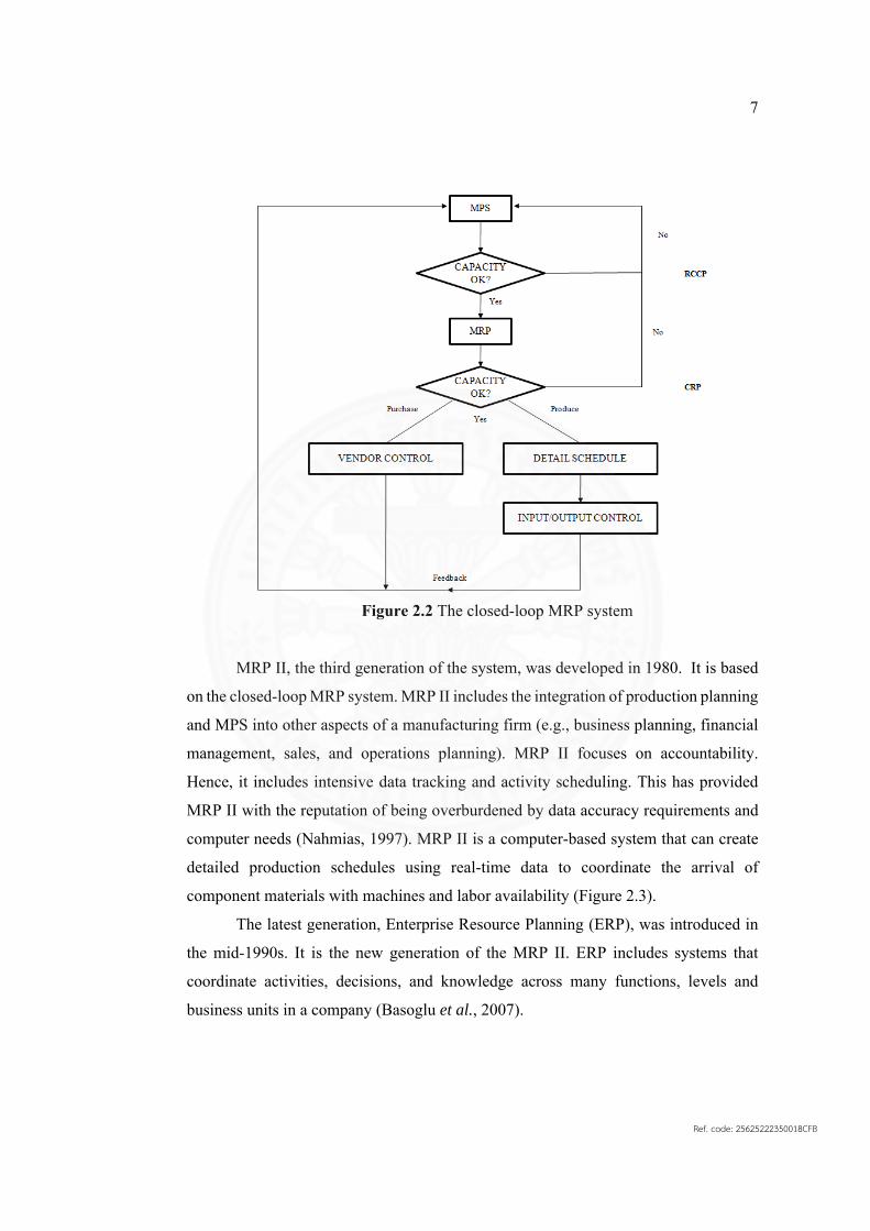
Figure 2.2 The closed-loop MRP system
MRP II, the third generation of the system, was developed in 1980. It is based
on the closed-loop MRP system. MRP II includes the integration of production planning
and MPS into other aspects of a manufacturing firm (e.g., business planning, financial
management, sales, and operations planning). MRP II focuses on accountability.
Hence, it includes intensive data tracking and activity scheduling. This has provided
MRP II with the reputation of being overburdened by data accuracy requirements and
computer needs (Nahmias, 1997). MRP II is a computer-based system that can create
detailed production schedules using real-time data to coordinate the arrival of
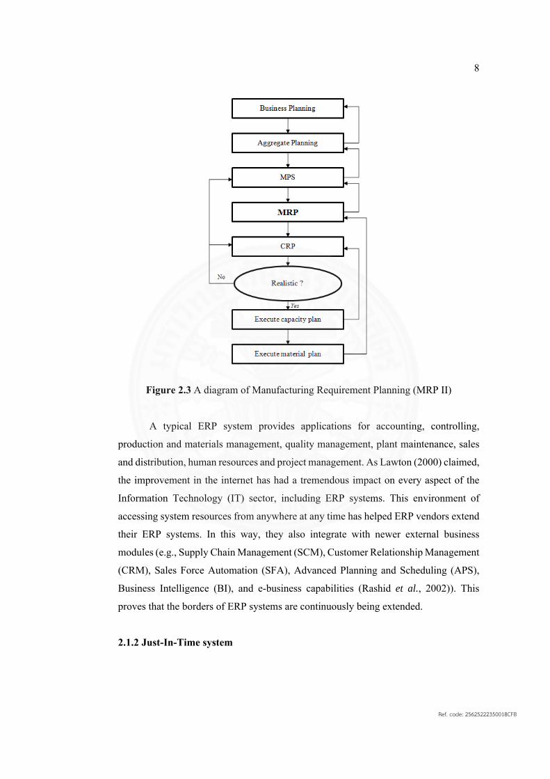
component materials with machines and labor availability (Figure 2.3).
The latest generation, Enterprise Resource Planning (ERP), was introduced in
the mid-1990s. It is the new generation of the MRP II. ERP includes systems that
coordinate activities, decisions, and knowledge across many functions, levels and
business units in a company (Basoglu et al., 2007).
Ref. code: 25625222350018CFB
8
Figure 2.3 A diagram of Manufacturing Requirement Planning (MRP II)
A typical ERP system provides applications for accounting, controlling,
production and materials management, quality management, plant maintenance, sales
and distribution, human resources and project management. As Lawton (2000) claimed,
the improvement in the internet has had a tremendous impact on every aspect of the
Information Technology (IT) sector, including ERP systems. This environment of
accessing system resources from anywhere at any time has helped ERP vendors extend
their ERP systems. In this way, they also integrate with newer external business
modules (e.g., Supply Chain Management (SCM), Customer Relationship Management
(CRM), Sales Force Automation (SFA), Advanced Planning and Scheduling (APS),
Business Intelligence (BI), and e-business capabilities (Rashid et al., 2002)). This
proves that the borders of ERP systems are continuously being extended.
2.1.2 Just-In-Time system
Ref. code: 25625222350018CFB

9
The Just-In-Time (JIT) production system is Toyota’s manufacturing
philosophy to minimize waste. Lummus (1995) stated that changing the production
environment in 1990 required product variety at a minimal cost and the flexibility to
meet changing customer demands. JIT can provide both dedicated production lines and
reduced set-up times. These allow JIT users to enjoy greater flexibility and increase
their ability to provide product variety.
The JIT production system is a sub-system controlled by Kanban. The Kanban
controlled JIT production system was developed to minimize work-in-process
inventories (waste) by reducing or eliminating discrete batches. The reduced lot sizes
contribute to production efficiency and product quality. They also reduce the overall
costs associated with production in the JIT manufacturing environment.
According to Monden (1983), the success of Toyota's Kanban controlled
production system is supported by a smoothing in production, standardization of jobs,
reduction of set-up times, improvement of activities, design of machine layouts, and
automation of processes. The JIT production system is highly recommended for the
repetitive manufacturing environment.
2.1.3 Theory of Constraints system
The Theory of Constraints (TOC) system can be defined as a management
approach which focuses on improving constraints or bottleneck processes to
continuously improve the performance of manufacturing operations. It was developed
by Eliyahu M. Goldratt and introduced in his book, “The Goal.” The methodology was
made available in the production planning system OPT (Optimized Production
Technology).
Goldratt (1990) and Goldratt and Fox (1986) stated that TOC is based on five
steps.
1. Identify the system's constraints(s).
2. Decide how to exploit the system's constraint(s).
3. Subordinate everything else to the decision.
4. Elevate the system's constraint(s).
5. If, in the previous steps, a constraint has been broken, go back to Step 1, and do
not allow inertia to cause a system's constraint.
Ref. code: 25625222350018CFB

10
In 1979, the development of the TOC management philosophy began with the
introduction of Optimized Production Timetables scheduling software (Goldratt and
Cox, 1984). TOC has evolved from this simple production scheduling software
program into a suite of integrated management tools, encompassing three interrelated
areas: logistics/ production, performance measurement, and problem solving/thinking
tools (Spencer and Cox, 1995).
Using the ideas and methods of the TOC, companies have achieved a large
reduction of work-in-process and finished goods inventories, significant improvements
in scheduling performance, and substantial earnings increases. Today, the TOC serves
as a valuable addition to, or even as a substitute for, such well-known manufacturing
systems as MRP and JIT (Radovilsky, 1997). Studies reporting anecdotal evidence
from early adopters suggested that TOC techniques could result in increased output,
while decreasing both inventory and cycle time. Rigorous academic testing has
validated those early findings, revealing that manufacturing systems employing TOC
techniques exceed the performance of those using MRP II, Lean Manufacturing, Agile
Manufacturing, and JIT. The results of these studies indicate that TOC systems produce
greater levels of output, while reducing the inventory, the manufacturing lead time, and
the standard deviation of the cycle time (Watson et al., 2007).
2.2 Manufacturing Resource Planning system Zapfel (1996) stated that Manufacturing Resource Planning (MRP II) is a
hierarchically structured information system based on the idea of controlling all flows
of materials and goods by integrating the plans of sales, finance and operations. The
levels in an MRP II concept are applied to two plans. The first plan is Business
Planning; this plan includes Resource Requirements Planning (RRP). The second plan
is Master Production Scheduling (MPS); it includes Rough-cut Capacity Planning
(RCCP). The business plan integrates the plans from sales, finances and operations. The
planned aggregate sales income, the planned cost of sales and operations, and all other
expenses per planning period provide a basis for calculating the planned net income of
the firm. In this context, the sales plan and planned inventories form the starting point
Ref. code: 25625222350018CFB
11
for the software system, when proposing a feasible production plan. These plans usually
aggregate products into product groups.
The planning horizon is often a year or longer, while the planning period is often
a month or longer. To be feasible, the production plan is examined by the so-called
resource requirements planning (RRP); that is, the resources required by a given
aggregate production plan can be calculated. Technically speaking, MRP II offers
simulation capabilities and marries the operating system with the financial system, so
the what-if questions can be answered using the software system. If the business plan
leads to resource requirements which are not feasible, or are unsatisfactory, the user can
change the plan and a new simulation run is started to calculate the modified resource
requirements. These steps can be repeated until a feasible and satisfactory business plan
is achieved. The aggregate production plan, accepted by the user, forms an important
basis for the master production scheduling.
The master production schedule (MPS) is a plan for end items, as offered to the
customers. The coordination of the aggregate production plan and the MPS is related
by aggregation and disaggregation. One characteristic approach is the disaggregation
of the aggregate production plan using planning percentages. The planning percentages
in the family bill-of-materials represents the average predicted demand fractions of the
MPS items in the product family over a certain time horizon. This disaggregation
ensures that the sum of the MPS items belonging to a certain product family is equal to
the planned quantity of the product group.
To check the feasibility of the MPS, a rough-cut capacity planning procedure
(RCCP) is implemented in an MRP II system. It determines whether the capacities are
sufficient enough to carry out the master production schedule. RCCP is more refined
than RRP. The capacities are observed in more detail. The user has the opportunity to
calculate the work center capacity requirements for all end items from the actual MPS.
If underloaded or overloaded capacities result, the user acts by adjusting the capacity
and/or quantities. The newly planned MPS can be simulated again and again until a
feasible or satisfactory solution is obtained. The production quantities in an MRP II
system are determined in a sequence of user-computer interactions, where the user has
to propose the quantities and the system calculates the resource requirements. If a
feasible and satisfactory solution results for the user, the planning process stops.
Ref. code: 25625222350018CFB

12
Cox and Clark (1984) provided a framework for the MRP II systems. They also
described the potential benefits of a successful system and the problems associated with
operating the system. They classified the problems into managerial, technical, and
behavioral problems.
Trigeiro et al. (1989) studied the effect of set-up time on lot sizing. A
Lagrangian relaxation of the capacity constraints of CLSP (Capacitated Lot Sizing
Problem) enables it to decompose into a set of un-capacitated single product lot sizing
problems. The Lagrangian dual costs are updated by the sub-gradient optimization,
while the single-item problems are solved by dynamic programming. A heuristic
smoothing procedure constructs the feasible solutions, which do not require overtime.
The algorithm solves problems with set-up times or set-up costs. Problems with
extremely tightly binding capacity constraints are much more difficult to solve.
Solutions without overtime could not always be determined. The most significant
results are that the severity of the capacity constraint is a good indicator of problem
difficulty for problems with the set-up time and that the algorithm solves larger
problems better than smaller problems, although they are more time consuming to
solve.
Porter et al. (1996) studied the production planning and control system
development in Germany. Some manufacturing organizations in the process sector,
where bills of materials are generally not complex, will move towards finite capacity
scheduling systems at the shop-floor level. These are integrated into a host system,
which is itself a finite capacity scheduler capable of longer-term planning that contains
all the functionality of the MRPΠ. Whether this is a better way of integrating the order
chain from the forecast, and/or order to planning, to shop-floor scheduling, depends on
the nature of the manufacturing environment. Complex product environments,
especially where the synchronization of activities is important, may be better served by
constraint-based software, which itself must have the associated database, either from
an MRP system or within its own logic.
Absi et al. (2005) studied a mixed integer mathematical formulation to solve
problems for multi item capacitated lot sizing with set-up times and shortage costs.
Demand could not be backlogged, but could be totally or partially lost. Safety stock
was an objective to reach, rather than an industrial constraint to respect. They also
Ref. code: 25625222350018CFB

13
describe fast combinatorial separation algorithms for valid inequalities based on a
generalization. These algorithms were used in a branch and cut framework to solve the
problem. The valid inequalities were generalized to take into account other practical
constraints that occurred frequently in industrial situations, notably minimal production
levels and minimal run constraints.
2.2.1 Enterprise Resource Planning
Due to the MRP II shortcomings, ERP emerged as a more comprehensive
solution (Chen, 2001). In the 1990s, MRP II was further expanded into ERP, a term
coined by the Gartner Group. The intent of ERP is to improve resource planning by
extending the scope of planning to include the supply chain. Thus, a key difference
between MRP II and ERP is that while MRP II has traditionally focused on the planning
and scheduling of internal resources, ERP strives to also plan and schedule supplier
resources, based on the dynamic customer demands and schedules.
Stank and Goldsby (2000) noted that the transition of planning systems from
functionally focused applications (e.g., MRP and Distribution Requirements Planning
(DRP)) to integrated systems (e.g., ERP) may help provide the manager with the needed
information to make better decisions. Nonetheless, this requires technical and
functional additions to the MRP II. Siriginidi (2000) stated that ERP is the latest
enhancement of MRP II. It has the added functionalities of finance, distribution and
human resources development, integrated to handle the global business needs of a
networked enterprise (Siriginidi, 2000).
ERP systems also faced their own implementation and integration problems.
The major difficulties with integration, however, appeared during the augmentation of
the core ERP systems with legacy systems. Themistocleous and Irani (2001) stated that
ERP systems were then introduced to overcome the integration problems. However,
organizations did not abandon their existing systems when adopting an ERP solution,
as ERP systems focused on general processes and initially did not allow much
customization. The problems of integration within the core of the ERP systems have
resulted in multiple shortcomings (DeSisto, 1997). Poor ERP integration resulted in
high order error rates, incorrect billing and shipping addresses, misquoted pricing and
discounts, and misquoted “out of stock” inventory.
Ref. code: 25625222350018CFB

14
Although the integration process within a single ERP system has considerably
improved, the earlier attempts of this integration came with a high price tag.
Consequently, some of the early ERP implementations suffered relatively high rates of
project failure.
One of the major ERP limitations is the lack of communication and integration
between the three major stakeholders: the company where the core ERP resides, the
supplier, and the customer. Due to these integration restrictions in the conventional ERP
systems, the Gartner Group coined a new ERP architecture called ERP II. The main
theme of this new architecture was to upgrade an ERP system by transferring it from
an inwards solution to an outwards solution. This was accomplished through
componentization and the integration of the “front-office” tools (e.g., Customer
Relationship Management (CRM), Supply Chain Management (SCM)), and the
collaboration and coordination platforms with the “back-office,” represented by the
core ERP system.
The new system architecture satisfies the cross-functional alignment between
trading partners. It collapses the distance and time factors that directly affect efficiency,
profitability, and innovation (a key goal of knowledge management). For example,
instead of answering calls from customers about when a shipment will be delivered, a
customer can access the supplier’s delivery information online. Similarly, instead of
suppliers relying on a customer to send updated forecasts, they can work from real-time
information found online.
In addition, ERP II is designed with Knowledge Management (KM) capabilities
in mind. Malhotra (1998) described knowledge management as a process that caters to
the critical issues of organizational adaptation, survival and competence in the face of
increasingly discontinuous environmental changes. Essentially, it embodies
organizational processes that seek synergistic combinations of data; the information
processing capacity of information technologies; and the creative and innovative
capacity of human beings. Hence, while ERP systems are used to integrate and optimize
an organization’s internal manufacturing, financial, distribution and human resource
functions, ERP II systems are used to address the integration of business processes that
extend across an enterprise and its trading partners. Therefore, ERP II forms the basis
of Internet-enabled e-business and collaborative commerce (C-commerce).
Ref. code: 25625222350018CFB
15
2.2.2 Supply Chain Management Nowadays, supply chain design is becoming a core competency. The ERP
system is expected to be an integral component of supply chain management (SCM).
SCM is the integration of key business processes among a network of interdependent
suppliers, manufacturers, distribution centers, and retailers to improve the flow of
goods, services, and information from the original suppliers to the final customers. The
objectives include reducing system-wide costs, while maintaining required service
levels (Simchi-Levi et al., 2000).
The literature on SCM is quite vast and dispersed across many areas. Supply
chain applications contain two general categories: ERP applications from companies
(e.g., SAP, Baan and Oracle) and planning engine applications that support and
integrate flow-based processes (e.g., shop-floor, logistics, and inventory management). Giannoccaro and Pontrandolfo (2002) presented an approach to manage
inventory decisions at all stages of the supply chain in an integrated manner. This
approach aimed to optimize the performance of the whole supply chain. The approach
consists of two techniques: 1) Markov decision processes (MDP) and 2) an artificial
intelligent algorithm used to solve MDPs, based on simulation modeling. In particular,
a model based on MDPs and reinforcement learning (RL) is proposed to simultaneously
design the inventory reorder policies of all SC stages. This is conducted to determine a
near optimal inventory policy under an average reward criterion. The RL technique is
a simulation-based stochastic technique that proves to be very efficient, particularly
when the MDP size is large.
Minner (2003) reviewed inventory models with multiple suppliers to determine
their potential contribution to SCM issues. Discussing strategic aspects of supplier
competition and the role of operational flexibility in global sourcing, inventory models
which use several suppliers to avoid or reduce the effects of shortage situations, are
described. Related inventory problems from the fields of reverse logistics and multi-
echelon systems are presented. Furthermore, issues for future research and a synthesis
of available SCM and multiple supplier inventory models are also discussed in the
research.
Schwartz et al. (2006) developed a simulation-based framework for optimally
tuning these policies in a stochastic, uncertain environment using the concept of
Ref. code: 25625222350018CFB

16
simultaneous perturbation stochastic approximation (SPSA). SPSA is presented as a
means for optimally specifying the parameters of internal model control (IMC) and
model predictive control (MPC) based decision policies for inventory management in
supply chains under conditions involving supply and demand uncertainty. The effective
use of the SPSA technique enhances the performance of the simultaneous optimization
of controller tuning parameters and safety stock levels for supply chain networks
inspired by semiconductor manufacturing. The analysis demonstrates that safety stock
levels can be significantly reduced and financial benefits achieved, while maintaining
a satisfactory operating performance in the supply chain.
Jung et al. (2008) studied the characteristics of, and methodology for, estimating
non-linear performance functions, the interdependence between the service levels at
different stages and the safety capacity. This was accomplished by ensuring the
sustainability of safety stock levels at manufacturing sites, alongside the methodologies
of capturing the system specific characteristic. They also proposed a linear
programming model that solves the problems of the optimal placement of the safety
stocks in a multi-stage supply chain. The model incorporates the non-linear
performance functions, the interdependence between the service level at different
stages of supply chain and the capacity constraint.
2.2.3 MRP II Shortcomings
MRP II is a well-known production and inventory control methodology and
there have been many successful implementations of its methodology. However, many
of its implementations have been failures associated with the following major problems
(Sheikh, 2001):
In the MRP II Plan for Material Requirements First, capacity was an
afterthought. The iterative procedure used for leveling the load on a machine
center and making an MRP schedule workable was not very efficient. Too many
manual adjustments are required. Furthermore, in some industries, the approach
is wrong. If there is a particular process that constrains the system or other
capacity constraints that are difficult to relax, then they should drive the
schedule, rather than the availability, of the materials.
Ref. code: 25625222350018CFB

17
Lead-time in an MRP II system is fixed. These fixed lead-time figures are
typically the average of the past practices, no matter whether that practice
resulted in a good or bad manufacturing performance. Fixed lead-times assume
that lot-sizes will continue to be un-changed or that they have no bearing on the
lead-time. Furthermore, fixed lead-times ignore current loads. Most experts
agree that the Shop Floor Control problems experienced by the MRP II user are
directly related to inaccurate lead-times. Incorrect lead-time information results
in orders being issued at the wrong time, which, in turn, results in parts being
completed late or in an excess waiting time, which is wasteful. The basic MRP
II system has no means of taking the variations in the lead-times into account
beyond placing the best estimates for the lead-time in the item master file.
Some closed loop systems update the system lead-times. In this case, the latest
recorded lead-time may be used or the program may calculate a moving average
adjusted by each new figure. If the load fluctuates, then the lead-times will
change with the load (lead-times grow at times of heavy loads and shrink at
times of light loads). In plants that are always extremely busy, this can cause a
cycle of ever-increasing lead-times, because almost everything is late, causing
the system to extend its lead-time. Therefore, the level of work-in-process
inventory increases, which, in turn, leads to increased queues. By increasing
planned lead-times in response to increasing lead-times, the situation is
worsened, not improved. Thus, the main shortcoming of MRP II, apart from the
necessity of large amounts of accurate data, is that it can lead to extended lead-
times and high inventory levels. It is easy for MRP II to get out of control.
The reporting requirements of MRP II are excessive. MRP II tries to keep track
of the status of all jobs in the system and reschedule jobs as problems occur. In
a manufacturing environment of high-speed processing and small lot-sizes, this
is cumbersome. It might take as long to record the processing of an item at a
workstation as it does to process the item.
The execution capabilities of the MRP II are limited. Perhaps the biggest
problem with MRP II has been its limited success in the execution of shop floor
schedules at a time when JIT has excelled in this endeavor. Manufacturing
Ref. code: 25625222350018CFB

18
experts are now encouraging managers to take advantage of the planning
capabilities of MRP II and the execution capabilities of finite scheduling, or JIT.
2.3 Shop Floor Control system The responsibilities of the Shop Floor Control system primarily involve job
scheduling, progress monitoring, status reporting, and corrective actions (Bauer et al.
1991). Shop Floor Control has to rapidly reflect the current system status to allow job
processing to be controlled in a real-time mode. Shop Floor Control proposes to meet
the promised customer due date. The efficient Shop Floor Control should revise the
critical information (e.g., due date and schedule receipt) to obtain a correct sequence of
jobs in the work order. Many Shop Floor Control techniques have been developed.
Ou-Yang et al. (2000) proposed the Shop Floor Controller model to bridge the
gaps between the planning level and manufacturing level in a computer integrated
manufacturing systems (CIM) environment. In this way, production orders can be
properly carried out by the shop floor equipment using the Object Model Technique
(OMT). There are three OMT modules. The Planning and Scheduling Module takes
charge of transferring the production orders into detailed manufacturing tasks. The
Dispatching and Coordination Module issues production commands to the controllers
of the proper production equipment. The Data Monitoring and Analysis Module
collects and analyzes shop floor data to identify the shop floor dynamic conditions.
Shin et al. (2002) proposed functional architecture for a distributed Shop Floor
Control. They defined the generic functions of a controller in the distributed Shop Floor
Controls and identified more detailed functions specific to each device. Moreover, the
enabling technologies of the device-specific functions were suggested. Su and Shiue
(2003) developed an intelligent scheduling controller (ISC) to support a Shop Floor
Control system (Shop Floor Controls) to make real-time decisions, robust to various
production requirements. The proposed approach integrates genetic algorithms (GAs)
and decision tree (DT) learning to develop a combinatorial optimal subset of features
from possible shop floor information concerning a DT-based ISC knowledge classifier.
In the area of scheduling n jobs to m machine problems, dispatching rules are
widely studied. Because of their strategic role in achieving the optimal management of
manufacturing systems, the dispatching rules are used to select the next job in the queue
Ref. code: 25625222350018CFB

19
of the work center. Many research investigations introduced the dispatching rules in
their implementations. Agliari et al. (1995) proposed an analytical technique, based on
the Markov Chain Theory, enabling the analysis of the behavior of some common-
practice dispatching rules. The possibility of extending the method to the investigation
of such dispatching rules was shown.
Holthaus and Rajendran (1997) presented five new dispatching rules for
scheduling in a job shop, with respect to the objectives of minimizing mean flow time,
maximum flow time, variance of flow time, and the proportion of tardy jobs. Yang
(1998) examined the performance of thirteen dispatching rules for executing a resource-
constrained project. The dispatching rules were tested in environments characterized
by three factors, namely, the order strength of the precedence relationship, the level of
the resource availability and the level of the estimation errors in the activity durations.
Rajendran and Holthaus (1999) presented a comparative study on the
performance of dispatching rules in the following sets of dynamic manufacturing
systems: flow shops and job shops; flow shops with missing operations; and job shops.
Three new dispatching rules were proposed. Chan et al. (2003) proposed a real-time
scheduling approach using a pre-emptive method for machines dispatching rules in a
Flexible Manufacturing System (FMS). The dispatching rule changed dynamically,
through a series of computations and evaluations of the system’s performance criteria.
The performance of the system found by using the dynamic scheduling method was
then compared with the best one found among the static scheduling methods. The idea
was proven through a computer simulation.
Rajendran and Alicke (2007) developed dispatching rules for scheduling by
taking into account the presence of bottleneck machines. The measures of performance
include the minimization of the total flow time of jobs, the minimization of the sum of
the earliness and the tardiness of jobs, and the minimization of the total tardiness of
jobs, considered separately. The results of the experimental investigation illustrate that
the proposed dispatching rules emerged superior to the conventional dispatching rules.
2.4 Finite Capacity Scheduling system Finite Capacity Scheduling (FCS) can be seen as an extension of the approach
used by the CRP system. FCS systems have received increasing attention as a method
Ref. code: 25625222350018CFB

20
improving capacity management in manufacturing environments. FCS is the process of
creating a detailed schedule for the occurrence of future events, subject to resource
availability (Enns, 1996). Generally, the schedule is generated by two approaches:
forward and backward scheduling. In some case studies, the combination of forward
and backward scheduling is implemented effectively as hybrid scheduling. Enns (1996) examined the flow time, schedule stability and delivery
performance results for the FCS systems. Two common schedule construction
approaches, blocked-time and event-driven, were compared. A production shop
simulation model facilitated the testing of these two approaches using either internally
or externally specified due dates. In addition, various due-date dependent loading rules
were used in schedule construction.
Martin and White (2004) summarized a new approach to scheduling activities
where there are alternative and multiple tools and machines that can be chosen to build
a part or product. They also presented the description, partly in terms of principles, and
partly in terms of how to write a computer program to implement the calculations.
Alternatives in the sets of tools and machines are converted into Boolean tree structures
and analyzed in a step-by step process. A placement sequence or loading sequence is
the ordering of jobs on each machine.
Pongcharoen et al. (2004) developed a genetic algorithm-based scheduling tool
for the FCS of complex products with multiple levels of product structure and resource
constraints, in which the data structures and the algorithm used are described. The
appropriate levels for the genetic algorithm parameters, using a full factorial design of
experiments, are also identified. Vanhoucke and Debels (2009) presented a finite
capacity production scheduling algorithm for an integrated steel company. The
algorithm took various case-specific constraints into account. It was aimed at the
optimization of multiple objects, which consisted of two solution steps. First, a machine
assignment step determines the routing of an individual order through the network.
Second, a scheduling step generates a detailed timetable for each operation for all
orders.
2.5 Finite Capacity Material Requirement Planning system
Ref. code: 25625222350018CFB

21
Manufacturing Resource Planning (MRP II) is a widely used method for
production scheduling. However, there are two main drawbacks that resulted in the
MRP II system becoming unsuccessful. Firstly, the MRP II production control concept
is based on fixed production lead times. In reality, these lead times depend on a variety
of dynamic factors (e.g., the workload, the order lot size, and the queue time). MRP- II
ignores capacity constraints and leaves the capacity problems to the planner (Taal and
Wortmann, 1997). Secondly, capacity constraints are not considered in its scheduling
logic. This may lead to an infeasible capacity problem.
The traditional solution for the capacity problem in an MRP system pre/post-
MRP analysis is used for material planning. It then examines the capacity implication.
There are two strategies in the pre/post-approach: rough cut capacity planning (RCCP)
and capacity requirement planning (CRP). RCCP is executed before the MRP
algorithm. It is simply a method for ensuring that bottleneck resources are not
overloaded.
RCCP is often used in practice, but is limited in its effectiveness. CRP, on the
other hand, is executed after the MRP. The CRP first determines whether the schedule
is feasible. This is done via a variety of approaches (e.g., simulations and machine
loading). When a problem is detected, the CRP provides the user with multiple solution
options.
CRP is reported to be unpopular in practice, though several vendors have
significantly improved their CRP models. One reason for the unpopularity is that
considerable user participation is required. However, this system only indicates a
capacity problem on the work center. It does not obtain alternative schedules to solve
the capacity problem (Nagendra et al., 1994).
Another approach for solving the capacity problem is a Shop Floor Control
(SCF) system. Taal and Wortmann (1997) concluded that the SCF system cannot solve
the capacity problem, because Shop Floor Control-scheduling systems only tackles the
symptoms. The real cause, the failing capacity planning at the other MRP II-planning
levels, is ignored. Bakke and Hellebore (1993) stated that the capacity problems must
be solved and prevented at the MRP level using an integrated approach of MRP and
finite capacity scheduling. As such, the FCMRP system has been introduced to resolve
the capacity problems.
Ref. code: 25625222350018CFB

22
Pandy et al. (2000) developed the FCMRP algorithm to capacity-based
production plans executed in two stages. Firstly, capacity-based production schedules
are generated from the input data. Secondly, the algorithm produces an appropriate
material requirement plan to satisfy the schedules obtained from stage one. They
showed that the results of the proposed algorithm were accurate, realistic and easy to
implement.
Nagendra and Das (2001) presented the MRP progressive capacity analyzer
(PCA) in which finite capacity planning and lot sizing are performed concurrently with
the MRP bill of material (BOM) explosion process. PCA is a methodology that can
simultaneously solve the multilevel, dependent demand, lot sizing, and capacity
analysis problem. The PCA procedure is a sequence of two linear programs and a lot
aggregating heuristic. It is designed to work in conjunction with the traditional MRP
explosion. The PCA will generate a production schedule that satisfies the lot size
restrictions, demand requirements, and capacity constraints. The PCA has several
unique modeling capabilities that promote its efficiency.
Wuttipornpun and Yenradee (2004) presented an FCMRP system for assembly
operations. The proposed FCMRP system automatically allocates some jobs from one
machine to another. It also adjusts the timing of the jobs, considering the finite available
time of all machines.
Ornek and Cengiz (2006) used an LP model to generate the capacity feasible
planned order releases of end products and assemblies, then fed into an MRP processor
to generate material plans. Lot size restrictions, alternative production routing, and
overtime decisions are considered. Wuttipornpun et al. (2006) proposed a linear
programming model to determine the optimal start time for each operation to minimize
the weighted average of total earliness, total tardiness, and average flow-time. The
model considers the finite capacity of all work centers and the precedence of the
operations.
Wuttipornpun and Yenradee (2007a) developed a FCMRP system using
heuristics based on the schedules of the bottlenecks to adjust the release and due dates
to ensure capacity feasibility. Furthermore, Wuttipornpun and Yenradee (2007b)
developed another FCMRP system based on the TOC philosophy (TOC-MRP) for a
multi-stage assembly factory that has some bottleneck stations. The proposed TOC-
Ref. code: 25625222350018CFB

23
MRP system tries to load and schedule operations on bottleneck stations in a manner in
that they are free of idle time and overtime.
Lee et al. (2009) applied grid computing technology to produce a grid-enabled
MRP process under the conditions of a finite capacity. The computational grid aims to
utilize unused computing power capacity via internet networking. This technology is
being broadly introduced in business. The proposed system resolves capacity
constraints by applying a simple heuristic called the longest tail first rule, which has
been proven to minimize the total lead time to each distributed cluster, obviating the
need for any rescheduling procedures. Palaniappan and Jawahar (2009) developed a
FCMRP system for a sequence dependent mixed model assembly line.
Wuttipornpun et al. (2010) presented an algorithm of a FCMRP system for a
multi-stage assembly flow shop, which is a combination of scheduling heuristic
techniques to generating the sequence of operations and optimization techniques. This
is applied to determine the optimal start time of each operation. Rossi and Pero (2011)
proposed a simulation-based approach for FCMRP that does not require the lead time
as an input. Sadeghian (2011) developed a continuous MRP (CMRP) approach that
does not require discrete time periods (time buckets) in MRP calculations. Most
FCMRP systems and CMRP are common in the sense that they do not require discrete
time periods.
Wuttipornpun and Yenradee (2014) developed a new FCMRP system for an
assembly flow shop with alternative work centers. This system has many factors that
can be adjusted to generate effective schedules. In addition, the system can solve
industrial problems in a short computational time. Paopongchuang and Yenradee
(2014) developed a new practical FCMRP system that considers the finite capacity of
the work centers and the constraints of the suppliers. The results indicate that the
FCMRP system with supplier constraints can generate a more realistic schedule than
the system without supplier constraints.
Urrutia et al. (2014) presented a combination model of a Lagrangian heuristic,
determining a feasible production plan for a fixed sequence of operations, with a
sequence improvement method, which iteratively feeds the heuristic to address multi-
item multi-period multi-resource single-level lot-sizing and scheduling problems in
manufacturing systems with job-shop configurations. The numerical results
Ref. code: 25625222350018CFB

24
demonstrate that the proposed model is efficient and more appropriate than a standard
solver for solving complex problems, regarding solution quality and computational
requirements.
Sukkerd and Wuttipornpun (2016) proposed a hybrid of the genetic algorithm
(GA) and a tabu search (TS) called HGATS for the FCMRP system that offers a near
optimal solution within a practical computational time. Rossi et al. (2017) introduced a
capacity-oriented MRP procedure, based on a combination of the traditional infinite-
capacity MRP procedure and a mixed-integer linear programming-based (MILP)
approach. The results highlight that the feasible plans of orders are generated without
requiring lead-times as an input and without the relevant computational burden.
In the area of FCMRP systems, the related literature can be classified based on
the features and constraints illustrated in Table 2.1.
Table 2.1 Summary of the related FCMRP research Research topic Features Constraints
Job
shop
Flow
shop
SFC
Non
-op
timiz
atio
n
Opt
imiz
atio
n
Gri
d co
mpu
ting
TOC
Res
ourc
e
Ove
rtim
e
Supp
lier
Cus
tom
er
Lee et al. (2009) × × × Nagendra and Das (2001) × × × Ornek and Cengiz (2006) × × × Palaniappan and Jawahar (2009) × × × Pandey et al. (2000) × × Paopongchuang and Yenradee (2014) * × × × ×Rossi and Pero (2011) × × × × Rossi et al. (2017) × × × Sukkerd and Wuttipornpun (2016) × × × × Sadeghian (2011) × × × Taal and Wortmann (1997) × × × Urrutia et al. (2014) × × × Wuttipornpun and Yenradee (2004) × × × × Wuttipornpun et al. (2005) × × × × Wuttipornpun et al. (2006) × × × Wuttipornpun and Yenradee (2007a) × × × × Wuttipornpun and Yenradee (2007b) × × × × × Wuttipornpun et al. (2010) × × × Wuttipornpun and Yenradee (2014) * × × × This dissertation × × × × ×
Note: *This paper is a part of this dissertation.
Ref. code: 25625222350018CFB

25
CHAPTER 3 METHODOLOGY AND CASE STUDY
This chapter presents the proposed FCMRP system with supplier and customer
constraints. The procedure of the proposed system is detailed in Section 3.1. An
illustrative example is presented in Section 3.2. The rescheduling capability of the
proposed FCMRP system and its illustrative example are described in Section 3.3.
Finally, Section 3.4 details the FCMRP scheduling software.
3.1 FCMRP with supplier and customer constraints
The problem in this section is associated with the proposed FCMRP algorithm
developed by taking into account the finite capacity of some key suppliers and
customers. Figure 3.1 schematically presents a 3-stage supply chain network structure,
which consists of suppliers, a manufacturer, and customers. The suppliers are divided
into 3 types, while the customers are divided into 2 types. The proposed FCMRP system
will handle them differently. The planning and scheduling phases of the proposed
FCMRP system are performed by the manufacturer. Table 3.1 summarizes the
characteristics and suitable actions of the suppliers. Table 3.2 summarizes the
characteristics and suitable actions of the customers.
Supplier Type S1 makes specialized items to order in high volume and sends
them to the manufacturer. This supplier, S1, can dedicate machines to serve the
manufacturer, since the production volume is high enough. All times, or subsets of the
available times, of the machine may be dedicated to serve the manufacturer. In this
case, the manufacturer can assume that the machine at the supplier’s plant is their own
machine and they can schedule any operations on the available time of their machine.
The transportation time from the supplier to the manufacturer, TS1, must also
be considered in the scheduling. This means that the completion time of the product at
the supplier’s factory, plus the transportation time, is equal to the arrival time of the
product at the manufacturer. After the FCMRP is performed, the manufacturer releases
an order, together with the production schedule, on the dedicated machine to the
supplier. This guarantees that the supplier will be able to produce, according to the
Ref. code: 25625222350018CFB

26
plan, since the finite capacity is considered. This proposed method is called
“manufacturer managed supplier scheduling”.
Figure 3.1 The proposed FCMRP manufacturing network structure
Supplier Type S2 also makes specialized items to order, but their volume is not
high enough to dedicate a machine to the manufacturer. In this case, the manufacturer
managed supplier scheduling is not suitable. The suitable FCMRP system for this case
is proposed as follows. The manufacturer runs the FCMRP to determine the required
quantity, release and due dates for the product to be purchased from the supplier and
releases the order to the supplier. Once the order is received, the supplier plans the
production schedule and promises the delivery date, which may be different from the
required due date. The manufacturer then runs the FCMRP system to generate the
production schedule, based on the promised delivery date of the purchased product from
the supplier without considering the finite capacity of the dedicated machine at the
supplier.
Supplier Type S3 makes standard items to stock. Since the supplier maintains
stock at the supplier factory, the product will be delivered on-time whenever the
Ref. code: 25625222350018CFB

27
customer needs it. In this case, the manufacturer just runs the MRP and places the order
to the selected supplier. The FCMRP will be performed for the manufactured parts,
assuming that the purchased parts will be received on-time, and without considering
the finite capacity of the supplier. This case is the easiest to control. Note that if the
selected supplier does not promise to deliver according to the due date, the
manufacturer will switch to another supplier that can.
Table 3.1 Characteristics of suppliers and suitable actions in the FCMRP system
Customer Type C1 processes items from the manufacturer in high volume. This
customer can dedicate a machine to be included into the manufacturer’s production
plan, since the production volume is significantly high. Most of the available machine
times are dedicated to serve the manufacturer’s production plan. In this case, the
manufacturer can assume that the dedicated customer machine is available to schedule
any operations, when needed. A transportation time from the manufacturer to the
Supplier type
Characteristics Suitable actions
S1 Makes specialized items to order in high volume for the manufacturer. Dedicates a machine to serve the manufacturer.
-The manufacturer performs the FCMRP, considering the finite capacity of the dedicated machine at the supplier. -The manufacturer places the order and sends the production schedule to the supplier. This is called “manufacturer managed supplier scheduling.”
S2 Makes specialized items to order in limited volume for the manufacturer. Does not dedicate a machine to serve the manufacturer.
-The manufacturer runs the FCMRP without considering the finite capacity of the dedicated machine at the supplier. -The manufacturer releases the order to the supplier. -The supplier plans the production and promises the delivery date, which may be different from the due date required by the manufacturer -The manufacturer runs the FCMRP system, based on the promised delivery date from the supplier.
S3 Makes standard items to stock. -The manufacturer runs the FCMRP without considering the finite capacity of supplier, since many suppliers can supply the standardized item. -The manufacturer places the order to a selected supplier. -If the supplier does not promise to deliver according to the due date, the manufacturer will switch to another supplier that can.
Ref. code: 25625222350018CFB

28
customer, called TS2, has to be calculated in the schedule. The manufacturer performs
the FCMRP, considering the finite capacity of the dedicated machine at the customer
factory. This proposed method is called “manufacturer managed customer scheduling”.
Customer Type C2 does not dedicate a machine to process items from the
manufacturer, since the production volume is not high enough. The customer can only
release the order to the manufacturer. Once the FCMRP is run at the manufacturer, they
will know the promised delivery date, which may be different from the required due
date.
Table 3.2 Characteristics of customers and suitable actions in the FCMRP system
The proposed FCMRP system is designed to handle industries with the
following characteristics:
1. There are multiple products.
2. Some products may have a multi-level bill of materials (BOM), with sub-
assembly and assembly operations. Other products may only require
fabrication without an assembly operation.
3. Parts can be produced by one of two alternative work centers at the
manufacturer: the first and second priority work centers. The first priority
work center is more efficient in producing the part. The first priority work
center for one part may be the second priority work center for the other part.
4. The structure of a production shop is a job shop with assembly operations.
Customer type
Characteristics Suitable actions
C1 Process item from the manufacturer on a dedicated machine. Dedicates a machine to be included in the manufacturer’s production plan.
-The manufacturer performs the FCMRP, considering the finite capacity of the dedicated machine at the customer factory. -This is called “manufacturer managed customer scheduling.”
C2 Does not dedicate a machine to be included into the manufacturer’s production plan.
-The customer releases the order to the manufacturer. -The manufacturer runs the FCMRP. The promised delivery date may be different from the due date required by the customer.
Ref. code: 25625222350018CFB

29
5. The suppliers can be divided into three types (S1, S2 and S3). The proposed
FCMRP system will use different methods to handle teach type.
6. For Supplier Type S1, the set-up time, processing time, and available time on
the dedicated machine at the supplier factory are known and deterministic.
The supplier allows the customer to manage the schedule on the machine.
The transportation time from the supplier to the customer is also known and
deterministic.
7. The lot-sizing rule is lot-for-lot.
8. The customers can be divided into two types (C1 and C2). The proposed
FCMRP system will use different methods to handle each type.
9. Customer Type C1 can inform the set-up time, processing time, and available
time on the dedicated machines at their factory to the manufacturer and allow
the manufacturer to manage the schedule on the machines. Note that these
times are known and deterministic. The transportation time from the
manufacturer to the customer is also known and deterministic.
10. Customer Type C2 will receive parts from the manufacturer, according to
the schedule generated by the FCMRP system.
11. Overlapping production batches may be allowed at the manufacturer. This
means that when the upstream work centers finish some parts of the
production batch, the finished parts may be delivered immediately to the
downstream work centers without waiting for the entire batch to be finished.
A block diagram of the proposed FCMRP system has five primary steps (Figure
3.2).
The steps for the proposed FCMRP system will subsequently be explained.
Step 1. Generate the production and purchasing plans using a variable lead-time MRP
system, including supplier and customer specific parts
The production and purchasing plans are generated by the variable lead-time
MRP (VMRP) system. Unlike the existing MRP systems, where the lead-time is
assumed to be constant, the VMRP determines the release date and time of the
operations, considering the production batch size. In this way, the production and
purchasing plans are more realistic than that of the conventional MRP system.
Ref. code: 25625222350018CFB

30
Figure 3.2 Block diagram of the proposed FCMRP system
Step 2 Apply dispatching rules to prioritize the job and operation sequences
Some operations, for the manufacturer, suppliers and customers, may be
performed by more than one work center. The most efficient, or most appropriate, work
center is called the ‘first priority work center’. The less appropriate is the ‘second
priority work center.’ This step attempts to generate various sequences of jobs and
operations by applying dispatching rules. Two dispatching rule types, namely job and
operation-based rules, are applied to analyze how the dispatching rules affect the
performance measures.
The job-based dispatching rule assumes a permutation schedule, where the
sequence of operations follows the sequence of jobs. The proposed algorithm applies
five job-based dispatching rules to determine the sequence of the jobs: the earliest due
date (EDD), the minimum slack time (MST), the critical ratio (CR), the earliest start
date (ESD) and the cost over time (COVERTj). Note that the sequence of the jobs
obtained from the job-based dispatching rules are applied to all job operations, as the
permutation schedule concept.
Ref. code: 25625222350018CFB

31
The operation-based dispatching rule determines the sequence of the remaining
operations. The proposed algorithm applies four operation-based dispatching rules: the
earliest operations due date (EOD), the modified operations due date (MOD), the less
slack earlier (LSE) and the cost over time (COVERTo). These rules are used to
determine the sequence of the operations. Note that the sequence of the operations of
each job may be different. This is a non-permutation characteristic. In addition, the
operation to produce the purchased parts at Supplier Type S1 will also be assigned to
the dedicated machine of the supplier.
Step 3 Allocate operations to the first priority work centers by the forward scheduling
technique
Allocate all operations to their first priority work centers by using the sequence
from Step 2 with forward scheduling. Moreover, the operations cannot be started prior
to their release date. The operation that needs the purchased part from Supplier Type
S2 will not be started prior to the promised delivery date confirmed by the supplier.
The output from this step is a detailed schedule of all operations that satisfies the
precedent constraints of the operations and considers the finite capacity of all work
centers.
Step 4 Allocate the tardy operations to the second priority work centers
After scheduling all operations to the first priority work centers, the operation
that is completed later than its due date is called a “tardy operation”. This step tries to
reduce the capacity problems of the first priority work center by moving the tardy
operations to their second priority work center, allowing them to start earlier.
Two allocating methods and three shifting options exist as choices. The pseudo
code in Figure 3.3 presents the algorithm for the allocating methods and shifting
options. Method 1 does not allow the operations to be started prior to the release date,
while Method 2 does. Option 1 has no shifting operation after finishing the allocating
method. Option 2 will be applied after a tardy operation is moved to its second priority
work center, where the moved operation will be shifted earlier, if possible. Option 3
will be applied after all possible tardy operations are moved to their second priority
work centers, where the moved operations that still have tardiness will be shifted earlier,
if possible. Note that Option 3 allows more moved operations to be shifted earlier to
reduce tardiness.
Ref. code: 25625222350018CFB

32
Figure 3.3 Pseudo code of allocating methods and shifting options
Step 5. Determine the optimal start time for each operation using the linear
programming model
This step uses a linear programming (LP) model to determine the optimal start
time for each operation. The objectives of all previous steps are to assign the operations
to work centers in a manner that reduces the capacity problem on work centers (i) and
to determine the sequence of all operations (j) on each work center. However, the start
time of each operation obtained from the previous step has not yet been optimized.
Based on the proposed algorithm, this step is described in terms of a mathematical
formulation. Referring to the manufacturing network structure shown in Figure 1, P is
a set of products and W is a set of work centers. Each product contains a set of
operations defined as O.
There are three subsets of O:
1. The set of last operations for all products (F).
Ref. code: 25625222350018CFB

33
2. The set of first operations for all products (R). The relationships between the
parent and child operations of the proposed FCMRO system are classified
into two types: assembly and fabrication operations.
For the assembly operation, each parent operation is assembled by more
than one child operation. This is known as a many-to-one relationship.
The fabrication operation is a one-to-one relationship between a parent and
child operation.
3. The last subset of O is a set of child operations of a parent operation in the
same bill of material (J).
Moreover, there are three subsets of W: a set of work centers at the supplier
factory (Ws), a set of work centers at the manufacturer (Wo), and a set of work centers
at the customer factory (Wc).
All parameter and variable notations used in the algorithm are defined as
follows:
Sets and parameters
P is the set of products
O is the set of operations
F is the set of the last operations of all products
R is the set of the first operations of all products
J is the set of child operations of any parent operation in the same bill of
materials
W is the set of work centers
Ws is the set of work centers at the supplier factory
Wo is the set of work centers at the manufacturer
Wc is the set of work centers at the customer factory
i is the index of the work center, Wi
pi,j is the processing time of operation 𝑗 on work center 𝑖 (day), OjWi ,
Ref. code: 25625222350018CFB

34
dj is the due date of operation 𝑗 (date), Fj
qj is the order size of operation 𝑗 (unit), Fj
cj is the completion time of operation 𝑗 (date), Fj
tj is the tardiness of operation 𝑗 (day), Fj
ej is the earliness of operation 𝑗 (day), Fj
fj is the flow-time of operation 𝑗 (day), Fj
k is the immediate succeeding operation of operation j
j’ is the parent operation of the child operation(s) j in the same bill of
materials
Ts1 is the transportation time from the supplier to the manufacturer (day)
Ts2 is the transportation time from the manufacturer to the customer (day)
Ct is the tardy cost (baht/unit-day)
Ce is the holding cost of the finished goods (baht/unit-day)
Cf is the holding cost of the work-in-process (baht/unit-day)
Decision variable
xi,j denotes the start time of operation j on work center i (date and time),OjWi ,
Objective
jFj
jjFj
jjFj
j qfCfqeCeqtCtZMinimize
(1)
The objective of the model is to minimize the total cost incurred by three
performance measures, as illustrated in Equation (1). The first performance measure is
the total tardy cost, calculated by the summation of the multiplication of tardiness, order
size, and tardy cost. The second performance measure is the total holding cost of the
finished goods, calculated by the summation of the multiplication of earliness, order
size, and the holding cost of the finished goods. The last performance measure is the
Ref. code: 25625222350018CFB

35
total holding cost of the work-in-process, calculated by the summation of the
multiplication of flow-time, order size, and the holding cost of the work-in-process.
Constraints
xi,k ≥ xi,j + pi,j, OjWi , (2)
xi’,j’ ≥ xi,j + pi,j, JjWciiWoiiWsiii ,,',',' (3)
xi’,j’ ≥ xi,j + 0.2pi,j, JjWciiWoiiWsiii ,,',',' (3')
xi’,j’ ≥ xi,j + pi,j + Ts1, JjWsiWoiii ,,',' (4.1)
xi’,j’ ≥ xi,j + pi,j + Ts2, JjWoiWciii ,,',' , (4.2)
cj = xi,j + pi,j, WcWoiFj , (5)
tj = max (cj – dj, 0), Fj (6)
ej = max (dj – cj, 0), Fj (7)
dj – cj = ej – tj, Fj (8)
fj = cj – xi,r, WoWsiRrFj ,, (9)
xi,j ≥ 0, OjWi , (10)
Constraint (2) illustrates that the work center cannot simultaneously produce
more than one operation. This constraint guarantees that the next operation, at the same
work center, cannot be started until the earlier operation has been finished. The
sequence of operations at each work center must follow what is obtained by the
procedure explained in Step 4. Note that k is an immediate succeeding operation of
operation j, in which the sequence is based on Step 4 of the proposed algorithm.
The precedence relationship between the operations must be maintained. Each
product may have different production routes and require different sets of work centers.
The precedence relationships between the operations are based on the production route.
They can be classified into two basic types: assembly and fabrication. All parent
operations must be started after their child operations are finished. Due to the
manufacturing network structure in Figure 1, this constraint is divided into two cases.
The first case, Constraint (3), presents the precedence relationships between the
operations, where the parent and child operations are conducted in the same factory.
The second case focusses on after the purchased part was finished by the work center
at the supplier factory. Here, it requires a transportation time from Supplier Type 1 to
Ref. code: 25625222350018CFB
36
the manufacturer, Ts1. The purchased part finished by the work center at the
manufacturer requires a transportation time to Customer Type 1, Ts2. Therefore,
Constraints (4.1) and (4.2) describe the precedence relationships between the work
centers, when the parent and child operations are located at different sites.
Constraint (3) can be modified as Constraint (3') to allow for the overlap in the
production batches. Note that a factor of 0.2 refers to an 80% overlap. For example, a
downstream work center is allowed to start after 20% of the work has been finished at
the upstream work center. The overlapping of the production batches of operations
produced at different sites is not possible, since the transportation costs would be
excessive. Thus, Constraints (4.1) and (4.2) cannot be modified.
Based on Figure 1, the completion time, tardiness, earliness, and flow-time of
each job can be formulated as Constraints (5), (6), (7) and (9), respectively. Note that
Constraints (6) and (7) may be written as one constraint: Constraint (8). The related
production operations cannot be started if the purchased parts have not been received
at the manufacturer and that of the customer factory. Note that the purchased parts from
Supplier Type 2 may arrive later than planned at the customer factory. This constraint
is required to simulate the system’s performance under uncertainty. Constraint (10) is
non-negativity condition of the decision variable.
3.2 Illustrative example of the proposed FCMRP system
This section presents an example to illustrate how the algorithm of the proposed
FCMRP system works.
Six products and their BOMs are shown in Figure 3.4. The data for the
manufactured parts from the manufacturer include the part type (finished product or
component part), the first and second priority work centers for each part and the
transportation lead-time of parts D1 and E1 that are delivered to the customer factory
(Table 3.3).
Table 3.4 illustrates the data for the manufactured parts at the customer factory.
This includes the part type (finished product or component part) and the first and second
priority work centers for each part produced at the customer factory. Table 3.5
illustrates the data for the purchased parts. This includes the production and
Ref. code: 25625222350018CFB

37
transportation lead-times of the parts from Supplier Type S1. Moreover, the purchasing
lead-times from Supplier Types S2 and S3 are detailed in this table.
The probability of tardiness and the distribution of tardiness for Supplier Type
S2 are also presented in Table 3.5. There are 4 work centers (WC 1 through 4) at the
manufacturer. Only one is a dedicated work center at the supplier factory; this one is
called WC S. Two other work centers at the customer factory are called WC z1 and WC
z2. The data for the two customer orders are illustrated in Table 3.6. Order X0001
includes six products. Order X0002 includes four products. Thus, there are a total of
ten jobs. Parts Dz1, Dz2 and Dz3 of product D and parts Ez1, Ez2 and Ez3 of product
E are produced by WC z1 and WC z2 at the customer factory.
Figure 3.4 BOMs of finished products
Ref. code: 25625222350018CFB

38
Note: WC is the work center.
Order ID Product Item
Part Item Type Release
Date/Time Due Date/Time 1st
priority WC
Lead-time on 1st priority WC
(days)
2nd priority WC
Lead-time on 2nd priority WC
(days)
Transportation Lead-time
(days)
X0001 A
A1 Finish 22/8.00am 32/8.00am WC1 10 WC3 10 -A2 Component 16/8.00am 22/8.00am WC3 6 WC1 7 -A3 Component 15/8.00am 22/8.00am WC2 7 WC1 7 -A4 Component 12/8.00am 15/8.00am WC4 3 WC2 5 -
B
B1 Finish 29/8.00am 36/8.00am WC1 7 WC2 8 -B2 Component 25/8.00am 29/8.00am WC2 4 WC1 4.5 -B3 Component 23/8.00am 29/8.00am WC3 6 WC4 7.5 -B4 Component 20/8.00am 25/8.00am WC4 5 WC3 5 -B5 Component 20/8.00am 23/8.00am WC2 3 WC1 4.5 -
C C1 Finish 26/10.00am 34/10.00am WC1 8 WC3 8 -C2 Component 21/10.00am 26/10.00am WC2 5 WC1 5 -C3 Component 15/10.00am 21/10.00am WC4 6 WC2 7 -
D
D1 Component 31/1.00pm 37/8.00am WC2 6.5 WC4 7 1D2 Component 28/8.00am 31/1.00pm WC1 3.5 WC3 5 -D3 Component 25/1.00pm 31/1.00pm WC2 6 WC1 7 -D4 Component 20/1.00pm 25/1.00pm WC4 5 WC3 5.5 -
E E1 Component 36/1.00pm 39/8.00am WC4 3.5 WC2 4.5 1E2 Component 30/1.00pm 36/1.00pm WC3 6 WC1 6.5 -E3 Component 25/8.00am 30/1.00pm WC2 5.5 WC4 6 -
G
G1 Finish 39/8.00am 42/8.00am WC3 3 WC1 5 -G2 Component 35/8.00am 39/8.00am WC1 4 WC4 5 -G3 Component 35/1.00pm 39/8.00am WC2 3.5 WC3 3.5 -G4 Component 30/8.00am 35/8.00am WC4 5 WC1 5.5 -G5 Component 31/8.00am 35.5/1.00pm WC3 4.5 WC2 5 -
X0002 A
A1 Finish 41/8.00am 46/8.00am WC1 5 WC3 5 -A2 Component 38/8.00pm 41/8.00am WC3 3 WC1 4 -A3 Component 37/1.00pm 41/8.00am WC2 3.5 WC1 3.5 -A4 Component 36/8.00am 37.5/1.00pm WC4 1.5 WC2 2.5 -
B
B1 Finish 45.5/1.00pm 50/8.00am WC1 4.5 WC2 5 -B2 Component 43/8.00am 45/1.00pm WC2 2.5 WC1 3 -B3 Component 42/8.00am 45.5/1.00pm WC3 3.5 WC4 4 -B4 Component 40/8.00am 43/8.00am WC4 3 WC3 3 -B5 Component 40/8.00am 43/8.00am WC2 2 WC1 2.5 -
D
D1 Component 51/8.00am 54/8.00am WC2 2 WC4 2.5 1D2 Component 49.5/1.00pm 51/8.00am WC1 1.5 WC3 1.5 -D3 Component 49/8.00am 51/8.00am WC2 2 WC1 2 -D4 Component 47/8.00am 49/8.00am WC4 2 WC3 2 -
E E1 Component 53.5/1.00pm 56/8.00am WC4 1.5 WC2 3 1E2 Component 51/8.00am 53.5/1.00pm WC3 2.5 WC1 2.5 -E3 Component 48.5/1.00pm 51/8.00am WC2 2.5 WC4 2.5 -
Table 3.3 Data for the parts manufactured at the manufacturer
Ref. code: 25625222350018CFB

39
Table 3.4 Data for the parts manufactured at the customer factory
Note: WC is the work center.
Order ID
Product Item
Part Item Type Release
Date/Time Due
Date/Time
1st priority
WC
Lead-time on 1st
priority WC (days)
2nd priority
WC
Lead-time on 2nd
priority WC (days)
X0001 D
Dz1 Finish 41/8.00am 44/8.00am WCz1 3 - - Dz2 Component 38/8.00am 41/8.00am WCz1 3 - - Dz3 Component 38/8.00am 41/8.00am WCz2 3 - -
E Ez1 Finish 47/8.00am 49/8.00am WCz2 2 WCz1 2 Ez2 Component 43/8.00am 47/8.00am WCz1 3 WCz2 3 Ez3 Component 40/8.00am 43/8.00am WCz2 3 WCz1 3
X0002 D
Dz1 Finish 55/8.00am 56/8.00am WCz1 1 - - Dz2 Component 54/8.00am 55/8.00am WCz1 1 - - Dz3 Component 54/8.00am 55/8.00am WCz2 1 - -
E Ez1 Finish 59/8.00am 60/8.00am WCz2 1 WCz1 1 Ez2 Component 57.5/1.00pm 59/8.00am WCz1 1.5 WCz2 1.5 Ez3 Component 59/8.00am 57.5/1.00pm WCz2 1.5 WCz1 1.5
Ref. code: 25625222350018CFB

40
Table 3.5 Data for the parts purchased from the suppliers
Order ID
Product Item
Part Item
Supplier Type
Purchasing Lead-time
(days)
Production Lead-time
(days)
Transportation Lead-time
(days)
Probability of
Tardiness
Distribution of Tardiness
(days)
Release Date/Time
Due Date/Time
X0001 A A5 1 - 4 1 - - 10/8.00am 14/8.00amA6 1 - 6 1 - - 4/8.00am 10/8.00am
B B6 1 - 4 1 - - 15/8.00am 19/8.00amB7 1 - 3 1 - - 16/8.00am 19/8.00am
C C4 2 10 - - 0.4 N(3,1) 5/10.00am 15/10.00am
D D5 2 7 - - 0.4 N(3,1) 13/1.00pm 20/1.00pmD6 2 8 - - 0.4 N(3,1) 20/8.00am 28/8.00amDz4 3 4 - - - - 34/8.00am 38/8.00am
E E4 3 4 - - - - 21/8.00am 25/8.00am
G G6 3 3 - - - - 27/8.00am 30/8.00amG7 3 4 - - - - 27/8.00am 31/8.00am
X0002 A A5 1 - 2 1 - - 34/8.00am 36/8.00amA6 1 - 3 1 - - 31/8.00am 34/8.00am
B B6 1 - 2 1 - - 37/8.00am 39/8.00amB7 1 - 1.5 1 - - 37.5/1.00pm 39/8.00am
D D5 2 2 - - 0.4 N(3,1) 45/8.00am 47/8.00amD6 2 2.5 - - 0.4 N(3,1) 47/8.00am 49/1.00pmDz4 3 1 - - - - 53/8.00am 54/8.00am
E E4 3 1.5 - - - - 47/8.00am 48/1.00pm
Ref. code: 25625222350018CFB

41
Table 3.6 Customer Orders
The algorithm for the proposed FCMRP system with supplier and customer
constraints is subsequently illustrated in a step-by-step manner.
Step 1 Generate production and purchasing plans using a variable lead-time MRP
system, considering the manufacturer, the suppliers, and the customers
The VMRP system is applied, based on the customer orders in Table 3.6, the
BOMs in Figure 3.4, and the information that the on-hand and on-order quantities for
each item are zero. This system is used to generate a planned order release date/time
and a due date/time for each operation for both the manufactured and purchased parts
at the suppliers, the manufacturer, and the customers (Tables 3.3, 3.4 and 3.5). Note
that the production lead-times in Tables 3.3, 3.4 and 3.5 are calculated using the VMRP
system. The release date and time of each operation is calculated using Equations (10)
and (11).
Operation lead-time = (Unit processing time × Order quantity) + Set-up time
+ Transportation time (10)
Release date = Due date – Total lead-time of all operations (11)
Note: The set-up time does not include a waiting time
Step 2 Apply job and operation based dispatching rules to determine the sequence of
jobs and operations.
Figure 3.1 illustrates that the proposed FCMRP system determines a production
schedule in the manufacturing network structure that includes the Supplier Type S1,
the manufacturer, and Customer Type C1. This step determines various job sequences
Order No. Product Item Part Item Due Date/Time Order Quantity X0001 A A1 32/8.00am 1,000
B B1 36/8.00am 1,500 C C1 34/10.00am 1,500 D Dz1 44/8.00am 1,500 E Ez1 49/8.00am 1,000 G G1 42/8.00am 1,500
X0002 A A1 46/8.00am 500 B B1 50/8.00am 300 D Dz1 56/8.00am 100 E Ez1 60/8.00am 200
Ref. code: 25625222350018CFB

42
using the job-based dispatching rules (i.e., EDD, MST, CR, ESD, and COVERTj) and
operation sequences using the operation-based rules (i.e., EOD, MOD, LSE, and
COVERTo) to the most appropriate (the first priority) work centers. In this example,
the earliest operation due date (EOD) rule is used to determine the sequence of fifty-
nine operations from the two orders (X0001 and X0002) illustrated in Table 3.7.
Table 3.7 Sequence of operations on each machine, based on the EOD rule
Note: EOD is the earliest operation due date rule and WC is the work center. Step 3 Allocate operations to the first priority work centers by the forward scheduling
technique
The sequence of operations obtained from the EOD rule from Step 2 are
allocated to their first priority work centers by forward scheduling (Table 3.7), as shown
by the Gantt chart in Figure 3.5. In this step, the actual start and completion dates are
computed. Some operations will be tardy. Note that the tardiness of each operation is
illustrated over the operation in the Gantt chart as a positive number. The operation that
needs the purchased part from Supplier Type S2 will not be started prior to the promised
delivery date confirmed by the supplier.
Step 4 Allocate the tardy operations to the second priority work centers
Based on the algorithm in Figure 3.3, if Method 1 and Option 1 are used, the initial
schedule in Figure 3.5 is transformed into the resulting schedule in Figure 3.6. Note
that Operations 1G2, 1G3, 1Ez1 and 1Ez2 of Order X0001 and Operations 2B3, 2B5,
2D2, 2E3, 2Ez1 and 2Ez2 of Order X0002 are moved to the second priority work
centers. Hence, the total tardiness can be reduced significantly from 601 to 548.5 days.
If Method 2 and Option1 are used, the resulting schedule is shown in Figure 3.7.
WC 1 1D2 1A1 1C1 1B1 1G2 2A1 2D2 2B1
WC 2 1A3 1B5 1C2 1B2 1E3 1D3 1D1 1G3 2A3 2B5 2B2 2E3 2D3 2D1 WC 3 1A2 1B3 1G5 100 1G1 2A2 2B3 2E2
WC 4 1A4 1C3 1B4 1D4 1G4 1E1 2A4 2B4 2D4 2E1
WC S 1A6 1A5 1B6 1B7 2A6 2A5 2B6 2B7
WC Z1 1Dz2 1Dz1 1Ez2 2Dz2 2Dz1 2Ez2
WC Z2 1Dz3 1Ez3 1Ez1 2Dz3 2Ez3 2Ez1
Ref. code: 25625222350018CFB
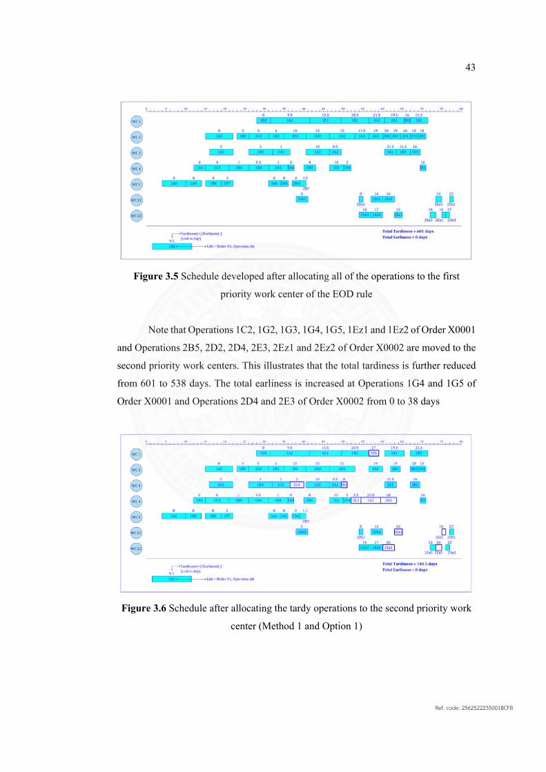
43
Figure 3.5 Schedule developed after allocating all of the operations to the first
priority work center of the EOD rule
Note that Operations 1C2, 1G2, 1G3, 1G4, 1G5, 1Ez1 and 1Ez2 of Order X0001
and Operations 2B5, 2D2, 2D4, 2E3, 2Ez1 and 2Ez2 of Order X0002 are moved to the
second priority work centers. This illustrates that the total tardiness is further reduced
from 601 to 538 days. The total earliness is increased at Operations 1G4 and 1G5 of
Order X0001 and Operations 2D4 and 2E3 of Order X0002 from 0 to 38 days
Figure 3.6 Schedule after allocating the tardy operations to the second priority work
center (Method 1 and Option 1)
Ref. code: 25625222350018CFB

44
Figure 3.7 Schedule after allocating the tardy operations to the second priority work
center (Method 2 and Option 1)
Step 5 Determine the optimal start time for each operation using the linear
programming model
Based on the schedule in Figure 3.7, the linear programming (LP) model is used
to determine the optimal start time for each operation, where the overlapping of the
production batches is not allowed. The resulting schedule is shown in Figure 3.8. It can
be seen that the total tardiness and total earliness can be improved. The total tardiness
and earliness are reduced from 538 to 533 days and 38 to 32.5 days, respectively.
If the LP model allows for the overlapping of the production batches, the
resulting schedule is illustrated in Figure 3.9. It clearly shows that the overlapping of
the batches results in a significant improvement in the total tardiness and total earliness
from 538 to 517.7 days and 38 to 32.9 days, respectively. Although the overlapping of
the batches is allowed for all operations, it actually occurs in some operations (e.g.,
Operations B2 and B4, C2 and C3, G1 and G2, Dz1 and Dz3, Ez1 and Ez2 of Order
X0001, Operations B3 and B5, E1 and E2, Dz1 and Dz3, Ez1 and Ez2 of Order X0002).
Ref. code: 25625222350018CFB

45
Figure 3.8 Schedule after the adjustment by the LP model with a non-overlapping of
production batches
Figure 3.9 Schedule after the adjustment by the LP model with an overlapping of
production batches
3.3 Rescheduling procedure and illustrative example
The procedure for the proposed FCMRP system, described in Section 3.1 as five
main steps, works based on the situation that there are no irregular conditions (or
uncertainties) in the manufacturing process. In a real manufacturing system, critical
incidents sometimes take place and interrupt the system. These could cause unavoidable
Ref. code: 25625222350018CFB

46
delay problems. The rescheduling concept of the proposed FCMRP system is designed
to determine a new schedule based on the various uncertain manufacturing incidents. The rescheduling system can start after the completion of any primary FCMRP
procedure. The date that the rescheduling system is started is called the “Rescheduling
Date”. Based on any specified rescheduling date, the status of the operations can be
divided into the following three types.
Completed operation: the operations were completed.
Ongoing operation: the operations are now in-progress.
Available operation: the operations have yet to start.
Figure 3.10 illustrates how the rescheduling operations are classified into the
three types. When the rescheduling date is 5, A1 and B1 are the completed operations.
A2, C1 and D1 are the ongoing operations. C3, A3 and D2 are the available operations.
Only the available operations will be rescheduled.
Figure 3.10 Types of rescheduling operations
All possible irregular conditions can emerge from the three main parts of a
supply chain network: a supplier factory, the own factory and a customer factory. The
causes of the delays from each main part are identified in four cases as follows:
Raw-material delay: There are two sub-cases, namely the delay from the
supplier factory to the own factory and the delay from the own factory to the
customer factory. As raw materials cannot be delivered on time, partial
production at the own factory and that of the customer factory will be delayed.
Machine breakdown: Loss or damage to a machine, as a result of an accidental
electrical and/or mechanical breakdown in any factory, can cause an
interruption in production.
Ref. code: 25625222350018CFB

47
Preventive maintenance: It is designed to prevent failures and prolong the life
of infrastructure, facilities, machines, software and other entities. Unlike
machine breakdowns, the preventive maintenance period is known in advance.
During this period, manufacturing operations cannot be performed.
Transportation delay: It may occur during the transportation of items from site
to site. There are two sub-cases, namely the delay from the supplier factory to
the own factory and the delay from the own factory to the customer factory.
All causes of delays in the proposed FCMRP system can be differentiated by
the cases and parts of the supply chain network (Table 3.8).
Table 3.8 Causes of delay
Figure 3.11 explains the rescheduling methodology of the proposed FCMRP
system as four main steps. Figure 3.2 illustrates the primary production and purchasing
plans generated using the variable lead-time MRP system. The procedure of the primary
FCMRP proceeds following the main steps and obtains a primary optimized FCMRP
schedule to start manufacturing. While the orders are being produced, the critical
incidents occur. Planners have to identify the cause of the interruption and start the
adjustments of the partial primary production and purchasing plans to generate the new
inputs of the secondary FCMRP system. During this step, the secondary FCMRP
procedure is performed to reschedule the available operations. Finally, after processing
the five main steps of the proposed FCMRP, a secondary optimized FCMRP schedule
is obtained and the manufacturing restarts again. Note that this methodology can be
repeated any time critical incidents occur.
Causes of delay Supplier From supplier to own factory
Own factory
From own factory to customer Customer
Raw-material delay
Machine Breakdown
Preventive Maintenance
Transportation delay
Ref. code: 25625222350018CFB

48
Figure 3.11 Block diagram of the rescheduling methodology of the proposed
FCMRP system
An example of the proposed rescheduling system is illustrated in the following
steps.
Step 1 Requirement of rescheduling on the primary optimized schedule
Based on the results of the example in Section 3.2, Figure 3.12 illustrates the
primary optimized schedule. While the operations on the schedule are in-progress,
assume that there are critical incidents in the manufacturing system. In this illustrative
example, four cases of delays are defined as follows:
Machine breakdown: Work Center S at the supplier factory was producing
Operation B6 of Order X0001 before it stopped working on Day 16. The work
center needs 2 days to repair it.
Raw-material delay: Raw Material B7 of Order X0001 will arrive 2 days late at
the own factory.
Preventive maintenance: Work Center 3 at the own factory has a maintenance
schedule that starts on Day 25 and lasts for 2 days.
Transportation delay: The transportation lead-time for Part D1 of Order X0001
from the own factory to the customer increased from 1 to 2 days. Thus,
Operation Dz3 of Order X0001 at the customer factory will be delayed.
Step 2 Regenerate secondary production and purchasing plans
After all requirements are specified, the adjustments of the primary production
and purchasing plans are required to regenerate the secondary production and
purchasing plans. As such, a rescheduling date has to be identified; in the example, it
is Day 16. In addition, the status of the operations needs to be classified.
Ref. code: 25625222350018CFB

49
Referring to Figure 3.12, Operations 1A4, 1A5 and 1A6 are the completed
operations. Operation 1B6 is the ongoing operation. The other operations are the
available operations. Only the available operations will be rescheduled. Based on the
requirements of the previous step, the secondary production and purchasing plans are
regenerated (Tables 3.9, 3.10 and 3.11). The completed and ongoing operations are
removed from the tables and the raw-material delay and transportation delay are added
to the tables. For example, the additional raw-mat delay of Operation 1B5 is 2 days and
the transportation delay of Operation 1D1 is 1 day.
Lastly, the machine restart dates for each work center must be identified. Work
centers can restart on Day 16, except for WC S, that has to restart on Day 21. This is
the case, since Operation 1B6 is completed after 2 days of repairs; it then takes 3 days
to continue with the rest of the operation. Note that all machine restart dates and
requirements for machine maintenance can be entered into the FCMRP scheduling
software (Figure 3.13). Note that RM DL is a raw-material delay, TS DL is a
transportation delay, M/C MT is preventive maintenance and M/C BD is a machine
breakdown.
Figure 3.12 Rescheduling date and requirements
Ref. code: 25625222350018CFB

50
Figure 3.13 Rescheduling function of the FCMRP scheduling software
Ref. code: 25625222350018CFB

51
Note: WC is the work center.
Order ID
Product Item
Part Item Type Release
Date/Time Due
Date/Time
1st priority
WC
Lead-time on 1st priority
WC (days)
2nd priority
WC
Lead-time on 2nd priority WC
(days)
Transportation Lead-time
(days)
Raw-mat
Delay (days)
Transportation Delay (days)
X0001 A
A1 Finish 22/8.00am 32/8.00am WC1 10 WC3 10 - - -A2 Component 16/8.00am 22/8.00am WC3 6 WC1 7 - - -A3 Component 15/8.00am 22/8.00am WC2 7 WC1 7 - - -
B
B1 Finish 29/8.00am 36/8.00am WC1 7 WC2 8 - - -B2 Component 25/8.00am 29/8.00am WC2 4 WC1 4.5 - - -B3 Component 23/8.00am 29/8.00am WC3 6 WC4 7.5 - - -B4 Component 20/8.00am 25/8.00am WC4 5 WC3 5 - - -B5 Component 20/8.00am 23/8.00am WC2 3 WC1 4.5 - 2 -
C C1 Finish 26/10.00am 34/10.00am WC1 8 WC3 8 - - -C2 Component 21/10.00am 26/10.00am WC2 5 WC1 5 - - -C3 Component 15/10.00am 21/10.00am WC4 6 WC2 7 - - -
D
D1 Component 31/1.00pm 37/8.00am WC2 6.5 WC4 7 1 - 1 D2 Component 28/8.00am 31/1.00pm WC1 3.5 WC3 5 - - -D3 Component 25/1.00pm 31/1.00pm WC2 6 WC1 7 - - -D4 Component 20/1.00pm 25/1.00pm WC4 5 WC3 5.5 - - -
E E1 Component 36/1.00pm 39/8.00am WC4 3.5 WC2 4.5 1 - -E2 Component 30/1.00pm 36/1.00pm WC3 6 WC1 6.5 - - -E3 Component 25/8.00am 30/1.00pm WC2 5.5 WC4 6 - - -
G
G1 Finish 39/8.00am 42/8.00am WC3 3 WC1 5 - - -G2 Component 35/8.00am 39/8.00am WC1 4 WC4 5 - - -G3 Component 35/1.00pm 39/8.00am WC2 3.5 WC3 3.5 - - -G4 Component 30/8.00am 35/8.00am WC4 5 WC1 5.5 - - -G5 Component 31/8.00am 35.5/1.00pm WC3 4.5 WC2 5 - - -
X0002 A
A1 Finish 41/8.00am 46/8.00am WC1 5 WC3 5 - - -A2 Component 38/8.00pm 41/8.00am WC3 3 WC1 4 - - -A3 Component 37/1.00pm 41/8.00am WC2 3.5 WC1 3.5 - - -A4 Component 36/8.00am 37.5/1.00pm WC4 1.5 WC2 2.5 - - -
B
B1 Finish 45.5/1.00pm 50/8.00am WC1 4.5 WC2 5 - - -B2 Component 43/8.00am 45/1.00pm WC2 2.5 WC1 3 - - -B3 Component 42/8.00am 45.5/1.00pm WC3 3.5 WC4 4 - - -B4 Component 40/8.00am 43/8.00am WC4 3 WC3 3 - - -B5 Component 40/8.00am 43/8.00am WC2 2 WC1 2.5 - - -
D
D1 Component 51/8.00am 54/8.00am WC2 2 WC4 2.5 1 - -D2 Component 49.5/1.00pm 51/8.00am WC1 1.5 WC3 1.5 - - -D3 Component 49/8.00am 51/8.00am WC2 2 WC1 2 - - -D4 Component 47/8.00am 49/8.00am WC4 2 WC3 2 - - -
E E1 Component 53.5/1.00pm 56/8.00am WC4 1.5 WC2 2 1 - -E2 Component 51/8.00am 53.5/1.00pm WC3 2.5 WC1 2.5 - - -E3 Component 48.5/1.00pm 51/8.00am WC2 2.5 WC4 2.5 - - -
Table 3.9 Data for the parts manufactured at the manufacturer for rescheduling
Ref. code: 25625222350018CFB

52
Table 3.10 Data for the parts manufactured at the customer factory for rescheduling
Table 3.11 Data for the parts purchased from the suppliers for rescheduling
Order ID
Product Item
Part Item Type Release
Date/Time Due
Date/Time
1st priority
WC
Lead-time on 1st
priority WC (days)
2nd priority
WC
Lead-time
on 2nd priority
WC (days)
Raw-mat
Delay (days)
Transportation Delay (days)
X0001 D
Dz1 Finish 41/8.00am 44/8.00am WCz1 3 - - - -Dz2 Component 38/8.00am 41/8.00am WCz1 3 - - - -Dz3 Component 38/8.00am 41/8.00am WCz2 3 - - - -
E Ez1 Finish 47/8.00am 49/8.00am WCz2 2 WCz1 2 - -Ez2 Component 43/8.00am 47/8.00am WCz1 3 WCz2 3 - -Ez3 Component 40/8.00am 43/8.00am WCz2 3 WCz1 3 - -
X0002 D
Dz1 Finish 55/8.00am 56/8.00am WCz1 1 - - - -Dz2 Component 54/8.00am 55/8.00am WCz1 1 - - - -Dz3 Component 54/8.00am 55/8.00am WCz2 1 - - - -
E Ez1 Finish 59/8.00am 60/8.00am WCz2 1 WCz1 1 - -Ez2 Component 57.5/1.00pm 59/8.00am WCz1 1.5 WCz2 1.5 - -Ez3 Component 59/8.00am 57.5/1.00pm WCz2 1.5 WCz1 1.5 - -
Order ID
Product Item
Part Item
Supplier Type
Purchasing Lead-time
(days)
Production Lead-time
(days)
Transportation Lead-time
(days)
Probability of
Tardiness
Distribution of
Tardiness (days)
Release Date/Time
Due Date/Time
Raw-mat
Delay (days)
Transportation Delay (days)
X0001 B B7 1 - 3 1 - - 16/8.00am 19/8.00am - -X0002 A A5 1 - 2 1 - - 34/8.00am 36/8.00am - -
A6 1 - 3 1 - - 31/8.00am 34/8.00am - -
B B6 1 - 2 1 - - 37/8.00am 39/8.00am - -B7 1 - 1.5 1 - - 37.5/1.00pm 39/8.00am - -
Ref. code: 25625222350018CFB
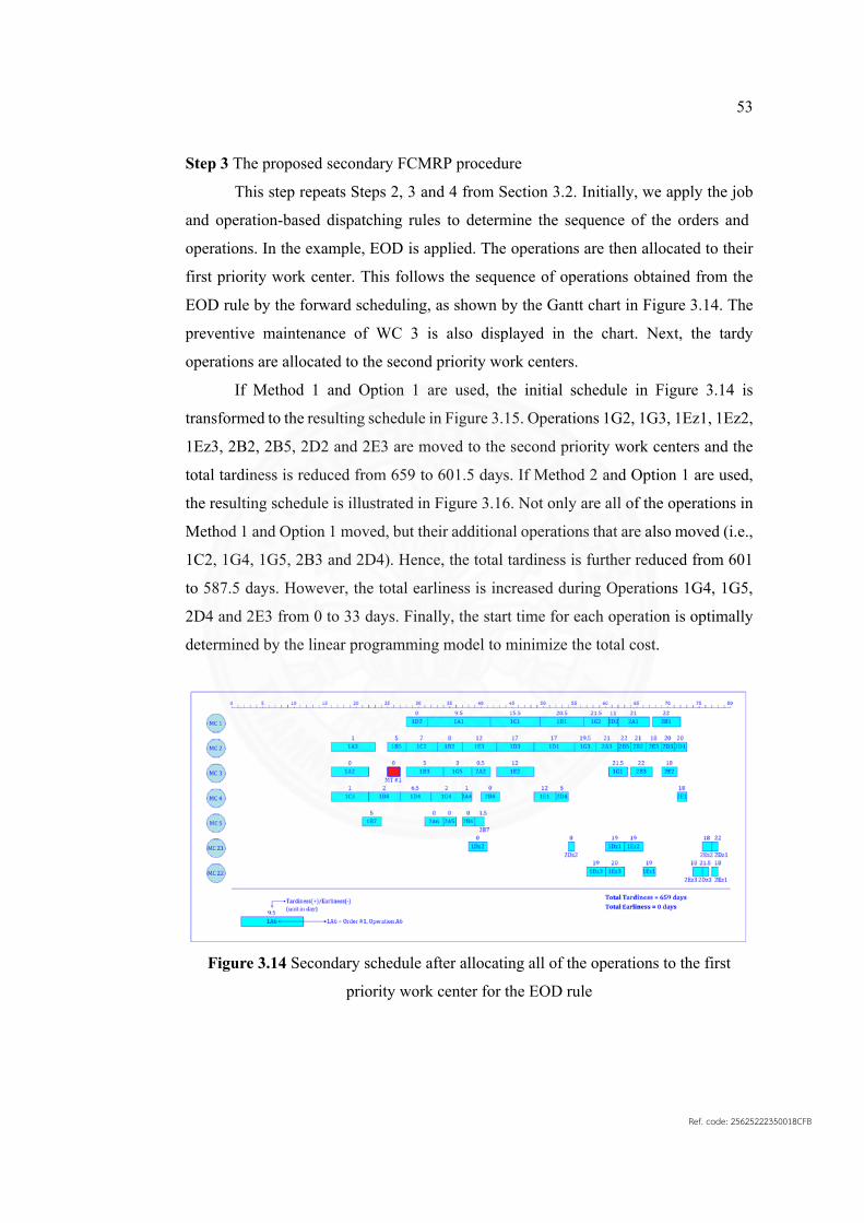
53
Step 3 The proposed secondary FCMRP procedure
This step repeats Steps 2, 3 and 4 from Section 3.2. Initially, we apply the job
and operation-based dispatching rules to determine the sequence of the orders and
operations. In the example, EOD is applied. The operations are then allocated to their
first priority work center. This follows the sequence of operations obtained from the
EOD rule by the forward scheduling, as shown by the Gantt chart in Figure 3.14. The
preventive maintenance of WC 3 is also displayed in the chart. Next, the tardy
operations are allocated to the second priority work centers.
If Method 1 and Option 1 are used, the initial schedule in Figure 3.14 is
transformed to the resulting schedule in Figure 3.15. Operations 1G2, 1G3, 1Ez1, 1Ez2,
1Ez3, 2B2, 2B5, 2D2 and 2E3 are moved to the second priority work centers and the
total tardiness is reduced from 659 to 601.5 days. If Method 2 and Option 1 are used,
the resulting schedule is illustrated in Figure 3.16. Not only are all of the operations in
Method 1 and Option 1 moved, but their additional operations that are also moved (i.e.,
1C2, 1G4, 1G5, 2B3 and 2D4). Hence, the total tardiness is further reduced from 601
to 587.5 days. However, the total earliness is increased during Operations 1G4, 1G5,
2D4 and 2E3 from 0 to 33 days. Finally, the start time for each operation is optimally
determined by the linear programming model to minimize the total cost.
Figure 3.14 Secondary schedule after allocating all of the operations to the first
priority work center for the EOD rule
Ref. code: 25625222350018CFB

54
Figure 3.15 Secondary schedule after allocating the tardy operations to the second
priority work center (Method 1 and Option 1)
Figure 3.16 Secondary schedule after allocating the tardy operations to the second
priority work center (Method 2 and Option 1)
Step 4 Secondary optimized schedule of the proposed FCMRP system
Based on the schedule in Figure 3.16, the linear programming (LP) model is
used to determine the optimal start time for each operation, where the overlapping of
the production batches is not allowed. The resulting schedule is illustrated in Figure
3.17, as the secondary optimized schedule. The total tardiness and earliness can be
improved. That being said, the total tardiness is reduced significantly from 587.5 to
534.5 days.
Ref. code: 25625222350018CFB

55
Figure 3.17 Secondary optimized schedule with the non-overlapping of production
batches
3.4 Illustration of the FCMRP scheduling software FCMRP scheduling software is designed to semi-automatically perform the
procedure of the proposed FCMRP system and the additional rescheduling capability
presented in Sections 3.2 and 3.3. The software is easy to use and can be successfully
configured in a relatively short time. It consists of two functions: the main FCMRP
scheduling function and the additional rescheduling function.
Figure 3.18 illustrates how the program starts. More specifically, it requires a
database file (Excel file) generated from Step 1 in Section 3.2. Figure 3.19 illustrates
the database imported into the program. The main function follows Steps 2 to 5,
described in Section 3.2. Figure 3.20 shows Step 2 that applies the two types of
dispatching rules to prioritize the sequence of jobs and operations. Figure 3.21
illustrates Step 3, where all operations are allocated to their first priority work centers.
Figure 3.22 shows Step 4, consisting of the two allocating methods (Methods 1 and 2).
These methods move tardy operations to their priority work centers. It also includes
three shifting options (Options 1, 2, and 3) to allow the operations to start earlier. Figure
3.23 illustrates the results of the selected combination that can be exported (Excel file)
to work as an input file for Step 5. The rescheduling function can work when it is
enabled on the main page. Figure 3.13 in Section 3.3 shows how the rescheduling data
is entered into the software.
Ref. code: 25625222350018CFB

56
Figure 3.18 Main page of the program
Figure 3.19 Database imported onto the main page
Ref. code: 25625222350018CFB

57
Figure 3.20 Step 2: Applying dispatching rules
Figure 3.21 Step 3: Allocating operations to the priority work centers
Ref. code: 25625222350018CFB

58
Figure 3.22 Step 4: Allocating methods and shifting options
Figure 3.23 Exported database for Step 5
Ref. code: 25625222350018CFB

59
CHAPTER 4 DESIGN OF EXPERIMENTS
This chapter discusses two experiments in detail. The first experiment analyzes
the performance of the proposed FCMRP system. This system consists of two
techniques: an analysis of variance and a rank order. The second experiment compares
the performance of the various FCMRP systems: without supplier and customer
constraints, with only supplier constraints, and with supplier and customer constraints. 4.1 Experiment to analyze the performance of the proposed FCMRP system
A full factorial design is conducted to analyze the effect of the independent
variables on the performance of the proposed FCMRP system. The four independent
variables include:
Dispatching rules: There are two types of dispatching rules: job and
operation-based rules. The job-based type consists of five rules: 1) the
earliest due date (EDD), 2) the minimum slack time (MST), 3) the critical
ratio (CR), 4) the earliest start date (ESD) and 5) the cost over time
(COVERTj). The operation-based type consists of four rules: 1) the earliest
operation due date (EOD), 2) the modified operation due date (MOD), 3)
the less slack earlier (LSE) and 4) the cost over time (COVERTo).
Allocating methods: There are two allocating methods: Methods 1 and 2.
Shifting options: There are three shifting options: Options 1, 2 and 3.
Overlapping of batches: There are two alternatives: overlapping and non-
overlapping.
The dependent variables include the total costs of tardiness, finished product
holdings, and work-in-process holdings (in baht). The independent variable
combinations result in 108 possible experimental cases. The experiment used 10
datasets, which each dataset has 30 customer orders. The datasets were randomly
generated, assuming that the order quantity follows a normal distribution with a
standard deviation equal to 10% of the average order quantity (Table 4.1).
Ref. code: 25625222350018CFB

60
Table 4.1 Customer order data
4.1.1 ANOVA technique The analysis of variance (ANOVA) technique is used to identify the significant
independent variables. The main effect and interaction of the independent variables will
be analyzed. The main effect and interaction plots will be presented. A Tukey’s multiple
comparison test will be used to divide the independent variables into significant subsets.
4.1.2 Rank order technique
Order No. Product Item
Part Item
Average Order Quantity
Due Date/Time
1 A A1 1,000 30/8.00am 2 A A1 1,200 40/8.00am 3 A A1 1,200 50/8.00am 4 A A1 1,500 65/8.00am 5 A A1 2,000 80/8.00am 6 B B1 1,500 45/8.00am 7 B B1 1,200 53/8.00am 8 B B1 1,000 60/8.00am 9 B B1 1,000 67/8.00am 10 B B1 1,000 74/8.00am 11 C C1 1,500 50/8.00am 12 C C1 1,500 58/8.00am 13 C C1 1,200 70/8.00am 14 C C1 1,000 75/8.00am 15 C C1 1,000 80/8.00am 16 D Dz1 1,500 62/8.00am 17 D Dz1 1,000 65/8.00am 18 D Dz1 1,800 70/8.00am 19 D Dz1 2,000 76/8.00am 20 D Dz1 2,000 82/8.00am 21 E Ez1 1,000 66/8.00am 22 E Ez1 1,500 69/8.00am 23 E Ez1 1,500 71.5/1.00pm 24 E Ez1 1,200 73.5/1.00pm 25 E Ez1 1,000 64/8.00am 26 G G1 1,500 58/8.00am 27 G G1 1,800 63/8.00am 28 G G1 2,000 69/8.00am 29 G G1 2,000 75/8.00am 30 G G1 1,500 79.5/1.00pm
Ref. code: 25625222350018CFB

61
The rank order technique will be applied to identify the combinations of
independent variables that consistently generate good results with relatively low total
costs. Since there are 10 sets of randomly generated customer orders, some
combinations of independent variables may not be able to consistently obtain good
results.
The methodology for the rank order technique is explained as follows:
1. Select the top-twenty ranks of the experimental cases from the dataset, based
on the performance measure (i.e., the total cost). Note that the less the total
cost, the lower the rank of the experimental case.
2. Define x as the rank of the top-twenty experimental cases, where x ranges
from 1 to 20.
3. Determine the score of rank x using Equation 12.
Scorex = 10020
21
x
(12)
4. Repeat Steps 1 to 3 for Datasets 2 to 10.
5. Select the top-twenty experimental cases that most frequently appeared in
the 10 datasets. In the case that some experimental cases have the same
frequency, choose the one that has the highest score.
6. Determine the average scores of the twenty experimental cases obtained in
Step 5. Based on the rank order technique, the experimental case
(combination of independent variables) that has the highest average score, or
most frequently obtains the highest score, will be identified.
4.2 Experiment to compare the FCMRP systems with supplier and customer constraints to the FCMRP systems without supplier and customer constraints, and with only supplier constraints
This experiment illustrates that the schedules generated from the FCMRP
systems without supplier and customer constraints, with only supplier constraints, and
with supplier and customer constraints are significantly different. In this experiment,
the FCMRP systems ‘without supplier and customer constraints’ and ‘with only
supplier constraints’ are special cases of the original FCMRP system with both supplier
Ref. code: 25625222350018CFB

62
and customer constraints. Thus, the FCMRP systems ‘without supplier and customer
constraints’ and ‘with only supplier constraints’ are created by relaxing the supplier and
customer constraints.
In Step 2 of the proposed FCMRP system, when operations are assigned to the
first priority work centers, the customer constraint is relaxed. This is accomplished by
not assigning the operations to produce the manufactured parts of customer type C1 at
the dedicated work centers (WC z1 and WC z2) in the customer factory. The supplier
constraint is relaxed by not assigning the operations to produce the purchased parts of
Supplier Type S1 at the dedicated work center (WC S) in the supplier factory. It
assumes that the purchased parts from Supplier Type S1 will arrive when they are
needed. Similarly, the purchased parts from Supplier Type S2 will arrive on-time, when
they are needed.
To show that the schedules generated from these systems are significantly
different, the differences between the order completion times are compared.
4.3 Experimental case
To illustrate how the proposed FCMRP system solves problems, an
experimental case is applied. The situation under consideration is as follows:
1. There are 6 finished products: Products A, B, C, D, E and G. Their bill of
materials is illustrated in Figure 3.
2. There are 30 orders for 6 finished products in this experiment. The customer
order data is shown in Table 9.
3. There are four work centers at the manufacturer: WC 1, WC 2, WC 3 and
WC 4. There is one dedicated work center (i.e., WC S) at the supplier
factory. There are two more work centers at the customer factory: WC z1 and
WC z2.
4. All parts at the manufacturer and at the customer factory can be produced by
one of two alternative work centers: the first or second priority work centers
(Tables 4 and 5).
5. All work centers operate for 8 hours a day. Overtime is not permitted.
6. The probability of tardiness and the distribution of tardiness for Supplier Type
S2 is presented in Table 6.
Ref. code: 25625222350018CFB

63
7. The total cost is a summation of the total tardy cost, the total holding cost of
the finished goods and the total holding cost of the work-in-process. The
tardy cost (Ct), the holding cost of the finished goods (Ce), and the holding
cost of the work-in-process (Cf) are either set by considering the opinions of
the production planner or real data. In this experiment, the estimates for Ct,
Ce and Cf are 5.00, 0.96, and 0.48 baht/unit per day, respectively.
Ref. code: 25625222350018CFB

64
CHAPTER 5 RESULTS AND DISCUSSION
The results and discussion sections are divided in two. The first section covers
the analysis of the performance of the proposed FCMRP system, which consists of two
parts: the ANOVA results and the results of the rank order method. The second section
discusses the comparison of the FCMRP systems without constraints, with supplier
constraints, and with supplier and customer constraints.
5.1 Analysis of the performance of the proposed FCMRP system 5.1.1 ANOVA results
To determine whether the independent variables defined in Section 4.1 are
statistically significant or not, an analysis is completed using an ANOVA test. To meet
the assumptions of the ANOVA and the validity of the results, Figure 5.1 illustrates that
the residuals are normally distributed and the ANOVA test is valid.
The ANOVA results of the experiment are presented in Table 5.1. Tukey’s
multiple comparisons are presented in Table 5.2. The main effect plots for the total cost
(Figure 5.2) and interaction plots (Figures 5.3 and 5.4) are also presented to identify the
significant factors and the relationships between the factors. The significance level is
set at 95% (α = 0.05). Note that the 95% confidence interval of the population mean of
the performance measure (total cost) is within ± 5% of the average performance
measure, as accepted by (Wuttipornpun and Yenradee, 2004; Wuttipornpun and
Yenradee, 2007b; Ross, 2009).
Ref. code: 25625222350018CFB

65
Figure 5.1 The distributions of the residuals
Table 5.1 P-values from the analysis of variance
Note: *The effect is significant at the 0.05 significance level.
Factors P-value Dispatching rule (D) 0.000* Allocating method (A) 0.000* Shifting option (S) 0.000* Overlapping (O) 0.000* Dataset (DS) 0.674 D×A 0.000* D×S 0.000* D×O 0.076 A×S 0.364 A×O 0.094 S×O 0.117 D×A×S 0.215 D×A×O 0.534 D×S×O 0.282 A×S×O 0.096 D×A×S×O 0.155
Ref. code: 25625222350018CFB

66
Table 5.2 Average values of the performance measures of the significant main effects
Note: EDD: Earliest due date rule, MST: Minimum slack time rule, CR: Critical ratio rule, ESD: Earliest start date rule, COVERTj: Job-based cost over time rule, EOD: Earliest operations due date rule, MOD: Modified operations due date rule, LSE: Less slack earlier rule, COVERTo: Operation-based cost over time rule
Figure 5.2 Main effects plot for the total cost
Main effects Level Average total cost (Tukey’s subsets)
Scheduling Rule
EDD 1793.4 (4) MST 1936.4 (5) CR 2035.6 (7)
ESD 1986.4 (6) COVERTj 1783.0 (4)
EOD 1062.1 (2) MOD 1091.2 (3) LSE 1005.3 (1)
COVERTo 1050.9 (2) Allocating
method Method 1 1753.9 (2) Method 2 1300.4 (1)
Shifting option
Option 1 1697.8 (3) Option 2 1554.8 (2) Option 3 1328.9 (1)
Overlapping Non-overlapping 1593.3 (2)
Overlapping 1461.0 (1)
Ref. code: 25625222350018CFB

67
According to Table 5.1, the four main effects (i.e., dispatching rule (D),
allocating method (A), shifting option (S) and the overlapping of batches (O)) were
found to be significant. This means that all four FCMRP system mechanisms have a
significant effect on the total cost. The interactions between the four main effects are
presented in two-way, three-way and four-way interactions. Two of the two-way
interactions were significant: 1) the interaction effect between the dispatching rules and
allocating methods and 2) the interaction effect between the dispatching rules and the
shifting option. The other interactions were not significant.
The average values of the performance measure (total cost) of the significant
main effects and their rank, obtained by the Tukey’s test, are illustrated in Table 5.2.
As the P-values are less than 0.05, the Tukey test is conducted consequently in the 95%
confidence interval. The Tukey test, probably the most conservative multiple
comparison test, works along an ANOVA to differentiate the factors or algorithms that
perform more effectively (Kayvanfar et al., 2017). Note that the ranks are presented in
parentheses. The lower rank has a better performance than the higher rank. The
performance measures with the same rank are not significantly different.
Based on Table 5.2, the operation-based dispatching rules (i.e., EOD, MOD,
LSE and COVERTo) perform better than the job-based dispatching rules (i.e., EDD,
MST, CR, ESD and COVERTj). For the operation-based rules, the LSE performs best.
For the job-based rules, EDD and COVERTj perform best. For the allocating method,
Method 1 performs better than Method 2. For the shifting option, Option 3 performs
best. For the overlapping of batches, the overlapping performs better than the non-
overlapping.
Table 5.1 illustrates two significant two-way interactions. These interactions are
presented in Figures 5.3 and 5.4. Figure 5.3 illustrates the D×A interaction, indicating
that the total cost decreases when Method 2 is applied. The job-based dispatching rules
can reduce the total cost from Method 1 to Method 2 more than the operation-based
dispatching rules. Figure 5.4 shows the D×S interaction, indicating that Option 3 can
reduce the total cost more effectively than Options 2 and 1. The job-based dispatching
rules can reduce the total cost from Method 1 to Method 3 more than the operation-
based dispatching rules.
Ref. code: 25625222350018CFB

68
Figure 5.3 Interaction between the dispatching rules and the allocation methods on
the total cost
Figure 5.4 Interaction between the dispatching rules and the shifting options on the
total cost
Ref. code: 25625222350018CFB

69
Figure 5.2 illustrates that the operation-based dispatching rules outperform the
job-based rules, since its schedule has a non-permutation characteristic, which allows
for more scheduling flexibility than the job-based rules. This can effectively reduce the
total tardiness of the production schedule. Method 2 outperforms Method 1, since it
allows operations to start prior to its release date; this allows more operations to be
moved to the second priority machine. This also reduces the load on the first priority
machine, which is more crowded.
Option 3 outperforms Options 2 and 1. This is because Option 1 does not allow
the moved operations of the second priority work center to be shifted earlier. Thus, the
tardiness is the highest. Option 2 allows the moved operation to be shifted earlier,
immediately after it is moved. Option 3 waits until all possible tardy operations are
moved to the second priority work centers; it allows the moved operations to be shifted
earlier and at the same time. Therefore, Option 3 increases the chance that the operation
will be shifted earlier, since when an operation is shifted earlier, it creates a space for
other operations to also be shifted. The overlapping of the production batches
outperforms the non-overlapping, since it allows for some operations to operate at the
same time, to reduce the tardiness of some customer orders and to minimize the total
cost.
Note that the operations which are allowed to start prior to the release date will
not create scheduling conflicts. When the schedule is adjusted by the LP model, all
operations will satisfy the precedent constraints.
5.1.2 Results of the rank order method The design of the experiment in Section 4.1.2 resulted in 10 datasets with 108
experimental cases, generated from the combination of the independent variables. The
top twenty experimental cases for each set were scored. These twenty high frequency
cases are summarized in Table 5.3. The average scores ranged from 20.5% to 94% and
were classified into four groups, as follows:
• Superior score (81% to 100%): Experimental case numbers 93, 96 and 108.
• Good score (61% to 80%): Experimental case numbers 24, 72, 84 and 107.
• Average score (51% to 60%): Experimental case numbers 21, 69 and 105.
Ref. code: 25625222350018CFB
70
• Below average score (0% to 50%): Experimental case numbers 36, 68, 71, 77,
81, 83, 101, 102, 104 and 106.
As we consider the groups of scores in their entirety, based on the datasets, we
find that the experimental cases with a superior score are recommended for the
proposed FCMRP system. The experimental cases with good and average scores can
be considered optional cases. The experimental cases with superior, good and average
scores illustrate that, for the dispatching rules, LSE, COVERTo, EOD, MST and MOD
outperform the other rules. For the allocating method, Method 2 outperforms Method
1. For the shifting option, Option 3 outperforms the other options. For the overlapping
of batches, the overlapping outperforms the non-overlapping.
A comparison in Figure5.5 clarifies that experimental case number 96, which
used the combination of LSE, Method 2, Option 3 and overlapping, obtained the highest
average score (94%). It also performed the best on the 5 datasets when considering the
10 datasets. Similarly, the top-six lower ranked cases included numbers 93, 108, 72, 24,
84 and 107; they performed with relatively high average scores. Nevertheless, Table
5.3 illustrates that the differences between the maximum and minimum scores of
numbers 93, 108, 72, 24, 84 and 107 range widely, while the difference between the
maximum and minimum scores of number 96 is only 20%. This implies that a high
average score cannot guarantee the overall performance. Therefore, it is recommended
that the difference between the maximum and minimum scores be considered
simultaneously.
The combination of the LSE, Method 2, and Option 3 with the overlapping,
experimental case number 96, analytically performs in a dominant manner.
Consequently, based on the datasets, we recommend that this combination be the first
choice applied to the proposed FCMRP system.
Ref. code: 25625222350018CFB

71
Table 5.3 Average score of the top-twenty experimental cases
Note: EDD: Earliest due date rule, MST: Minimum slack time rule, CR: Critical ratio rule, ESD: Earliest start date rule, COVERTj: Job-based cost over time rule, EOD: Earliest operations due date rule, MOD: Modified operations due date rule, LSE: Less slack earlier rule, COVERTo: Operation-based cost over time rule, M1: Method 1, M2: Method 2, O1: Option 1, O2: Option 2, O3: Option 3
Rank Case No. Experimental Case
Score Max score (%)
Min score (%)
No. of time of
max score
Average score (%)
Data set 1
Data set 2
Data set 3
Data set 4
Data set 5
Data set 6
Data set 7
Data set 8
Data set 9
Data set 10
1 96 LSE*M2*O3*Overlapping 100 95 80 90 90 85 100 100 100 100 100 80 5 94 2 93 LSE*M2*O3*Non-overlapping 50 100 95 100 75 55 85 85 85 85 100 50 2 81.5 3 108 COVERTo*M2*O3*Overlapping 70 90 85 45 95 95 75 80 95 80 95 45 0 81 4 72 EOD*M2*O3*Overlapping 95 55 70 95 100 100 70 60 75 60 100 55 2 78 5 24 MST*M2*O3*Overlapping 90 40 25 85 80 65 45 95 90 95 95 25 0 71 6 84 MOD*M2*O3*Overlapping 55 70 100 50 70 60 25 90 80 90 100 25 1 69 7 107 COVERTo*M2*O2*Overlapping 85 25 65 60 60 80 35 75 70 75 85 55 0 63 8 105 COVERTo*M2*O3*Non-overlapping 65 85 45 70 50 30 90 50 65 50 90 30 0 60 9 69 EOD*M2*O3*Non-overlapping 75 80 90 55 15 20 40 70 50 70 90 15 0 56.5 10 21 MST*M2*O3*Non-overlapping 35 60 10 75 85 40 80 55 60 55 85 10 0 55.5 11 101 COVERTo*M1*O2*Overlapping 30 65 40 30 45 90 60 25 30 25 90 25 0 44 12 81 MOD*M2*O3*Non-overlapping 25 45 75 5 55 15 55 65 25 65 75 5 0 43 13 71 EOD*M2*O2*Overlapping 40 20 60 65 40 35 30 40 40 40 65 20 0 41 14 102 COVERTo*M1*O3*Overlapping 80 30 55 40 35 10 65 5 55 5 80 5 0 38 15 106 COVERTo*M2*O1*Overlapping 10 50 15 10 10 75 95 45 20 45 95 10 0 37.5 16 104 COVERTo*M2*O2*Non-overlapping 60 75 30 20 5 50 15 35 5 35 75 5 0 33 17 36 CR*M2*O3*Overlapping 15 10 50 80 20 45 5 15 35 15 80 5 0 29 18 83 MOD*M2*O2*Overlapping 20 5 20 35 65 25 10 30 45 30 65 5 0 28.5 19 68 EOD*M2*O2*Non-overlapping 45 35 5 25 30 70 20 10 10 10 70 5 0 26 20 77 MOD*M1*O2*Overlapping 5 15 35 15 25 5 50 20 15 20 50 5 0 20.5
Ref. code: 25625222350018CFB

72
Note: EDD: Earliest due date rule, MST: Minimum slack time rule, CR: Critical ratio rule, ESD: Earliest start date rule, COVERTj: Job-based cost over time rule, EOD: Earliest operations due date rule, MOD: Modified operations due date rule, LSE: Less slack earlier rule, COVERTo: Operation-based cost over time rule, M1: Method 1, M2: Method 2, O1: Option 1, O2: Option 2, O3: Option 3.
Figure 5.5 Comparison of average scores the top-twenty experimental cases 5.2 Comparison of the FCMRP systems with supplier and customer constraints to the FCMRP systems without supplier and customer constraints, and with only supplier constraints
Let ijC1 , ijC2 and ijC3 be the completion times for customer order i (i = 1 to
30), based on dataset j (j = 1 to 10) of the FCMRP systems without supplier and
customer constraints, with only supplier constraints, and with supplier and customer
constraints, respectively.
The differences between the order completion times of the systems with
supplier and customer constraints, and without constraints, ijX , is calculated using
Equation (13). The differences between the order completion times of the systems with
supplier and customer constraints, and with supplier constraints, ijY , is calculated using
Equation (14).
Ref. code: 25625222350018CFB

73
ijijij CCX 13 (13)
ijijij CCY 23 (14)
Note that ijX and ijY are random variables dependent on dataset j.
The distributions for ijX, of the 30 customer orders based on the 10 datasets, are
presented in the box plots (Figure 5.6). The box plots illustrate that ijX are all positive.
Their minimum values range from 0.2 to 5.0 days, while their maximum values range
from 5.0 to 7.5 days. The box plots also show that most ijX are symmetrical or right-
skewed. The average and standard deviation values for ijX of the 30 customer orders are
illustrated in Figure 5.7. As can be seen, the average values range from 2.5 to 6.2 days,
while the standard deviations range from 0.2 to 1.8 days.
The distributions for ijY , of the 30 customer orders based on the 10 datasets, are
presented using the box plots (Figure 5.8). The box plots illustrate that ijY are all
positive. Their minimum values range from 0.0 to 1.5 days, while the maximum values
range from 2.5 to 6.0 days. The box plots also illustrate that most ijY are symmetrical or
right-skewed. The average and standard deviation values for ijY of the 30 customer
orders are shown in Figure 5.9. The average values range from 1.2 to 3.4 days and the
standard deviations range from 0.3 to 1.5 days.
Figure 5.6 Order completion time differences between the FCMRP with the supplier and customer constraints and without the constraints
Ref. code: 25625222350018CFB

74
Figure 5.7 Average and SD of the order completion time differences between the
FCMRP with the supplier and customer constraints and without the constraints
Figure 5.8 Order completion time differences between the FCMRP with the supplier and customer constraints and with only the supplier constraints
Ref. code: 25625222350018CFB

75
Figure 5.9 Average and SD of the order completion time differences between the
FCMRP with the supplier and customer constraints and with only the supplier constraints
Figures 5.6 and 5.7 indicate that when the supplier and customer constraints are
considered in the proposed FCMRP system, customer orders are completed
significantly later than when both constraints are not considered. Figures 5.8 and 5.9
reveal the same consequence. More specifically, the customer orders of the proposed
FCMRP, with the supplier and customer constraints, are completed later than they are
with only the supplier constraints.
In reality, many supplier and customer factories have constraints on production
capacity and the ability to deliver on-time. If either the FCMRP, without considering
the supplier and customer constraints, or with only the supplier constraints, is used to
generate production and purchasing schedules, the customer orders will be completed
too early. This is not realistic, since, in practice, the customer orders will be completed
significantly later than the generated schedule. The schedule generated from the
FCMRP with the supplier and customer constraints is more realistic and can reduce the
chance that the customer orders will be completed much later than the scheduled time.
Ref. code: 25625222350018CFB

76
CHAPTER 6 CONCLUSIONS AND RECOMMENDATIONS
This chapter presents the conclusions and contributions of the research. The
contributions are directly relevant to the research objectives. The limitations and
recommendations for further studies are also discussed.
6.1 Conclusions
There were four objectives in this dissertation. The first was to develop a new
practical FCMRP system for a job shop with assembly operations that explicitly
consider the capacity constraints of the suppliers and customers. The second was to
develop the capabilities of rescheduling into a newly developed FCMRP system used
to effectively solve system interrupting problems. The third is to develop the scheduling
software appropriate for the proposed FCMRP system, following the first and second
objectives. The fourth and final objective is to analyze the performance of the newly
developed FCMRP system and illustrate that it offers a significantly more realistic
schedule than the FCMRP system with no constraints and systems with only supplier
constraints. The results of the dissertation indicate that these objectives were satisfied.
The dissertation was divided into three main parts, based on the objectives. The
first objective presents the review of the well-known P&IC system literature (Chapter
2). This part consists of a brief description of the systems, the shortcomings of the MRP
system, and the past work related to Shop Floor Control, FCS, and the FCMRP system.
The literature review revealed that no single P&IC system could be applied to all
production environments. In addition, a capacity problem may occur by using the
conventional MRP system. This led to the development of an FCMRP system for
solving the capacity problem in the MRP system. Moreover, the literature review of the
FCMRP area illustrates that no previous work developed the FCMRP system to
explicitly consider the capacity constraints of the suppliers and the customers.
Basically, the FCMRP system is used to determine the production schedule,
Ref. code: 25625222350018CFB

77
considering the finite capacity of the key work centers in the own factory. It does not
consider the production capacity at the supplier and customer factories.
The second part illustrates the concept of the proposed FCMRP system and its
rescheduling function using a small example. A briefing of the developed FCMRP
scheduling software (Chapter 3) is also presented. This proposed FCMRP system can
be used in a supply chain network. The system explicitly considers the constraints of
the supplier and the customer when generating the finite capacity production schedule.
When the supplier and customer dedicate all of the available time, or the subsets of the
available time, of a work center to serve a customer, it is possible that the own factory
will schedule operations on the dedicated machines as if it is owned by the own factory.
These concepts are called “customer managed scheduling” (the own factory to the
supplier) and “supplier managed scheduling” (the own factory to the customer). When
the supplier does not provide dedicated machines, the own factory will send a purchase
order to the supplier. The supplier may promise a delivery date that is different from
the actual due date of that order. The promised delivery date will affect the schedule
of the FCMRP system, since the first operation cannot be started if the materials from
the suppliers have not been received. Likewise, if the customer does not provide
dedicated machines, the own factory may promise a delivery date that is different from
that of the planned due date. The promised delivery date will affect the customer, since
the first operation cannot be started if the materials from the own factory have not been
received. If the actual due date is affected by uncertainties and it is different from that
of the promised delivery date, it can cause more costs to the system. The proposed
FCMRP system tries to synchronize the operations of the supplier and the customer to
the operations of the own factory in a way that minimizes the total cost.
The third part is to analyze the performance of the proposed FCMRP system
and compare it to a system with no constraints and a system with only supplier
constraints. The proposed FCMRP system performances are evaluated using the sized
problem with 6 finished products, 30 customer orders, and 180 operations on the
production plan (Chapters 4 and 5). The experimental results show that all independent
variables in the FCMRP system, namely dispatching rules, allocating methods, shifting
options and the overlapping of batches, significantly affect the performance of the
Ref. code: 25625222350018CFB

78
system. This indicates that if the system is set-up suitably, it will provide a good
performance for the supply chain network.
Three FCMRP systems, with supplier and customer constraints, with supplier
constraints, and without constraints, are used to generate the production and purchasing
schedules based on the experimental case. The results indicate that the schedules
generated from the FCMRP system with the supplier and customer constraints are the
most realistic. Accordingly, it can reduce the chance that the customer orders will be
completed later than the scheduled time.
6.2 Research contributions This research makes 5 primary contributions to the current literature:
1. This research makes the first attempt to extend the FCMRP system to consider
both supplier and customer capacity constraints.
2. The experimental results reveal that all scheduling mechanisms significantly
affect system performance. These include dispatching rules, allocating methods,
shifting options, and the overlapping of batches provided in the proposed
FCMRP system. This finding motivates researchers to further develop other
scheduling mechanisms to improve system performance.
3. The investigation analyzed 10 datasets and the rank order method. These results
suggest how some combinations of scheduling methods and options to
consistently generate good performance can be selected.
4. The proposed FCMRP system, with the supplier and customer constraints,
provides a more realistic schedule than the system without supplier and/or
customer constraints.
5. The proposed FCMRP system provides the rescheduling method to revise the
schedule based on the rescheduling needs. This includes raw material delays,
machine breakdowns, preventive maintenance, and transportation delays. These
rescheduling needs can occur anywhere in the supply chain.
6.3 Limitations and recommendations for further studies The limitations and recommendations for further studies are as follows:
Ref. code: 25625222350018CFB

79
The sequence of jobs or operations is generated by relatively simple dispatching
rules. Thus, it is recommended that more efficient sequences of operations be
generated by some metaheuristics.
The proposed FCMRP system performances are evaluated using a moderately
sized problem. It is recommended that this be tested on a larger scale case study
to prove that it can be used to solve large industrial problems.
The FCMRP scheduling software was developed as a simple tool on a limited
platform. To support the more complicated features of the system and a larger
scale database, it is recommended that it be developed to fulfill more complex
requirements as a commercial software package.
Ref. code: 25625222350018CFB
80
REFERENCES
Absi, N. and Kedad-Sidhoum, S. (2005). Mip-based heuristics for multi-item capacitated lot-sizing problem with setup times and shortage costs, Retrieved from https://www.optimization-online.org.
Agliari, A., Diligenti, M. and Zavanella, L. (1995). Variable priority dispatching rules: An analytical approach. International Journal of Production Economics, 41(1-3), 51-58. doi: 10.1016/0925-5273(95)00058-5
Baghdasaryan, L., Darabi, H., Schuler, F. and Schaller, A. (2010). A modelling and optimization management tool for large-scale supply chain networks. International Journal of Industrial and Systems Engineering, 5(1), 48-78. doi: 10.1504/IJISE.2010.029756
Bakke, N.A. and Hellberg, R. (1993). The challenges of capacity planning, International Journal of Production Economics, 30(1), 243–264. doi: 10.1016/0925-5273(93)90096-4
Basoglu, N., Daim, T., and Kerimoglu, O. (2007). Organizational Adoption of Enterprise Resource Planning Systems: A Conceptual Framework. Journal of High Technology Management Research, 18(1), 73-97. doi: 10.1016/j.hitech.2007.03.005
Bauer, R.B., Browne, J., Duggan, J. and Lyons G. (1991). Shop Floor Control Systems-Form Design to Implementation. New York: Chapman and Hall.
Chan, F.T.S., Chan, H.K., Lau, H.C.W. and Ip, R.W.L. (2003). Analysis of dynamic dispatching rules for a flexible manufacturing system. Journal of Materials Processing Technology, 138(1-3), 325–331. doi: 10.1016/S0924-0136(03)00093-1
Chen, I. (2001). Planning for ERP systems: Analysis and future trend. Business Process Management Journal, 7, 374.
Cox, J. F. and Clark, S. J. (1984). Problems in implementing and operating an MRP information system. Journal of Management Information Systems, 1(1), 81-101.
DeSisto, R. (1997). ERP Integration Strategies for TES Systems. Gartner: Research Note: TU, 724-344.
Enns, S.T. (1996). Finite Capacity Scheduling Systems: Performance Issues and Comparisons. Computers Industrial Engineering, 30(4), 727-739. doi: 10.1016/0360-8352(96)00025-3
Giannoccaro, I. and Pontrandolfo, P. (2002). Inventory management in supply chains: a reinforcement learning approach. International Journal of Production Economics, 78(2), 153-161. doi: 10.1016/S0925-5273(00)00156-0
Ref. code: 25625222350018CFB

81
Goldratt, E. M and Cox, J. (1984). The Goal: A Process of Ongoing Improvement. New York: North River Press, Croton-on-Hudson.
Goldratt, E.M. (1990). The Haystack Syndrome: Sifting Information Out of the Data Ocean. Massachusetts: North River Press, Great Barrington.
Goldratt, E.M. and Fox, R.E. (1986). The Race. New York: North River Press, Croton-on-Hudson.
Holthaus, O. and Rajendran, C. (1997). Efficient dispatching rules for scheduling in a job shop. International Journal of Production Economics, 48(1), 87-105. doi: 10.1016/S0925-5273(96)00068-0
Ismail, S., Al-sulaiti, K.A. and Abdulrazak, R.S. (2009). An exploratory study of MRP benefit determinant relationships: ACE analysis model, Journal for International Business and Entrepreneurship Development, 4, 119–146. doi: 10.1504/JIBED.2009.022533
Jamili, N., Ranjbar, M. and Salari, M. (2016) A bi-objective model for integrated scheduling of production and distribution in a supply chain with order release date restrictions, Journal of Manufacturing System, 40(1), 105-118. doi: 10.1016/j.jmsy.2016.06.005
Jung, J.Y., Blau, G., Pekny, J.F., Reklaitis, G.V. and Eversdyk, D. (2008). Integrated safety stock management for multi-stage supply chains under production capacity constraints. Computers and Chemical Engineering, 32(11), 2570–2581. doi: 10.1016/j.compchemeng.2008.04.003
Kayvanfar, V., Husseini, S.M.M., Karimi, B. and Sajadieh, M.S. (2017) Bi-objective intelligent water drops algorithm to a practicalmulti-echelon supply chain optimization problem, Journal of Manufacturing System, 44(1), 93-114. doi: 10.1016/j.jmsy.2017.05.004
Lawton, G. (2000). Integrating ERP and CRM via the Web. SW Expert.
Lee, H.-G., Park, N. and Park, J. (2009). A high performance finite capacitated MRP process using a computational grid. International Journal of Production Research, 47(8), 2109-2123. doi: 10.1080/00207540802132775
Lummus, R.R. (1995). A simulation analysis of sequencing alternatives for JIT lines using kanbans. Journal of Operations Management, 13(3), 183-191. doi: 10.1016/0272-6963(95)00026-O
Malhotra, Y. (1998). Knowledge Management for the New World of Business. Journal for Quality & Participation, 21, 58-60.
Mansour, M.A.A.F. and Dessouky, M.M. (2010). A hybrid genetic algorithm for solving the joint batching and scheduling of a batch processor with earliness and tardiness penalties. International Journal of Industrial and Systems Engineering, 5(2), 143–158. doi: 10.1504/IJISE.2010.030745
Ref. code: 25625222350018CFB
82
Martin, R. L. and White C. (2004). Finite capacity scheduling with multiple tools and machines. International Journal of Production Research, 42(8), 1557-1597. doi: 10.1080/00207540310001637588
Minner, S. (2003). Multiple-supplier inventory models in supply chain management: A review. International Journal of Production Economics, 81-82, 265-279. doi: 10.1016/S0925-5273(02)00288-8
Monden, Y. (1983). Toyota Production System, 2nd ed. Institute of Industrial Engineers.
Nagendra, P.B. and Das, S.K. (2001). Finite capacity scheduling method for MRP with lot size restrictions. International Journal of Production Research, 39(8), 1603-1623. doi: 10.1080/00207540010023600
Nagendra, P.B., Das, S.K., and Chao X. (1994). Introducing capacity constraints in the MRP algorithm. Proceedings of 1994 Japan–U.S.A. Symposium on Flexible Automation – A Pacific Rim Conference (pp. 213–216).
Nahmias, S., (1997). Production and Operations Analysis. Illinois: Richard D. Irwin.
Olhager, J. and Persson, F. (2006). Simulating production and inventory control systems: a learning approach to operational excellence. Production Planning & Control, 17(2), 113–127. doi: 10.1080/09537280500223921
Olhager, J. (2013). Evolution of operations planning and control: from production to supply chains. International Journal of Production Research, 51(23-24), 6836–6843. doi: 10.1080/00207543.2012.761363
Ornek, A.M. and Cengiz, O. (2006). Capacitated lot sizing with alternative routings and overtime decisions. International Journal of Production Research, 44(24), 5363–5389. doi: 10.1080/00207540600600106
Ou-Yang, C., Guan, T.Y. and Lin, J.S. (2000). Developing a computer shop floor control model for a CIM system - using object modeling technique. Computers in Industry, 41(3), 213–238. doi: 10.1016/S0166-3615(99)00057-3
Palaniappan, P.K. and Jawahar, N. (2009). A heuristic algorithm for joint optimization of MRP and scheduling in a mixed model assembly line. International Journal of Advanced Operations Management, 1, 224–249. doi: 10.1504/IJAOM.2009.030674
Pandey, P.C., Yenradee, P., and Archariyapruek, S. (2000). A finite capacity material requirement planning system. Production Planning and Control, 11(2), 113–121. doi: 10.1080/095372800232315
Paopongchuang, B. and Yenradee, P. (2014). Finite capacity material requirement planning with supplier constraints. International Journal of Industrial and Systems Engineering, 17(3), 350-375. doi: 10.1504/IJISE.2014.062543
Ref. code: 25625222350018CFB
83
Pongcharoen, P., Hicks, C. and Braiden, P.M. (2004). The development of genetic algorithms for the finite capacity scheduling of complex products, with multiple levels of product structure. European Journal of Operational Research, 152(1), 215–225. doi: 10.1016/S0377-2217(02)00645-8
Porter, J.K., Jarvis, P., Little, D., Laakmann, J., Hannen, C. and Schotten, M. (1996). Production planning and control system developments in Germany. International Journal of Operations & Production Management, 16(1), 27-39.
Radovilsky, Z.D. (1997). A quantitative approach to estimate the size of the time buffer in the theory of constraints. International Journal Production Economics, 55(2), 113- 119. doi: 10.1016/S0925-5273(97)00131-X
Rajendran, C. and Alicke, K. (2007). Dispatching in flowshops with bottleneck machines. Computers & Industrial Engineering, 52(1), 89–106. doi: 10.1016/j.cie.2006.10.006
Rajendran, C. and Holthaus, O. (1999). A comparative study of dispatching rules in dynamic flowshops and jobshops. European Journal of Operational Research, 116(1), 156-170. doi: 10.1016/S0377-2217(98)00023-X
Rashid, M. A., Hossain, L., and Patrick, J. D. (2002). The Evolution of ERP Systems: A Historical Perspective. Pennsylvania: Idea Group Publishing.
Ross, S.M. (2009) Introduction to probability and statistics for engineers and scientists, 4th ed. Massachusetts: Elsevier.
Rossi, T. and Pero, M. (2011). A simulation-based finite capacity MRP procedure not depending on lead time estimation. International Journal of Operational Research, 11(3), 237–261. doi: 10.1504/IJOR.2011.041343
Rossi, T., Pozzi, R., Pero, M. and Cigolini, R. (2017) Improving production planning through finite capacity MRP. International Journal of Production Research, 55(2), 377-391. doi: 10.1080/00207543.2016.1177235
Sadeghian, R. (2011). Continuous materials requirements planning (CMRP) approach when order type is lot for lot and safety stock is zero and its applications. Applied Soft Computing, 11(8), 5621–5629. doi: 10.1016/j.asoc.2011.04.002
Schwartz, J.D., Wang, W. and Rivera, D.E. (2006). Simulation-based optimization of process control policies for inventory management in supply chains. Automatica, 42(8), 1311 – 1320. doi: 10.1016/j.automatica.2006.03.019
Sheikh, K. (2001). Manufacturing Resource Planning (MRP II) with an introduction to ERP, SCM and CRM. New York: Mc-Graw Hill Publishing Limited.
Shin, J., Oh, S. and Cho, H. (2002). Functional architecture and enabling technologies for distributed shop floor control. International Journal Computer Integrated Manufacturing, 15(6), 526-540. doi: 10.1080/09511920210143390
Ref. code: 25625222350018CFB

84
Simchi-Levi, D., Kaminsky, P., and Simchi-Levi, E. (2000). Designing and Management the Supply Chain Concepts, Strategies, and Case Studies. New York: McGraw-Hill, 39-107.
Siriginidi, S.R. (2000). Enterprise Resource Planning in Reengineering Business. Business Process Management Journal, 6(5), 376-391. doi: 10.1108/14637150010352390
Slack, N., Chambers, S. and Johnston, R. (2001). Operation Management, 3rd ed. Essex: Peason Education Limited.
Spencer, M.S. and Cox III, J.F. (1995). Optimum production technology (OPT) and the theory of constraints (TOC): analysis and genealogy. International Journal of Production Research, 33(6), 1495–1504. doi: 10.1080/00207549508930224
Stank, T.P. and Goldsby, T.J. (2000). A framework for transportation decision making in an integrated supply chain. Supply Chain Management: An International Journal, 5(2), 71-78. doi: 10.1108/13598540010319984
Su, C.T. and Shiue, Y.R. (2003). Intelligent scheduling controller for shop floor control systems: a hybrid genetic algorithm/decision tree learning approach. International Journal of Production Research, 41(12), 2619-2641. doi: 10.1080/0020754031000090612
Sukkerd, W. and Wuttipornpun T. (2016) Hybrid genetic algorithm and tabu search for finite capacity material requirement planning system in flexible flow shop with assembly operations. Computers Industrial Engineering, 97, 157-169. doi: 10.1016/j.cie.2016.05.006
Taal, M. and Wortmann, C.W. (1997). Integrating MRP and finite capacity planning. Production Planning and Control, 8(3), 245-254. doi: doi.org/10.1080/095372897235307
Themistocleous, M. and Irani, Z. (2001). Benchmarking the benefits and barriers of application integration. Benchmarking: An International Journal, 8(4), 317-331. doi: 10.1108/14635770110403828
Trigeiro, W., Thomas, L.J. and McClain, J.O. (1989). Capacitated lot sizing with setup times. Management Science, 35(3), 353–366. doi: 10.1287/mnsc.35.3.353
Urrutia, E.D.G., Aggoune R and Dauzere-Peres S. (2014). Solving the integrated lot-sizing and job-shop scheduling problem. International Journal of Production Research, 52(17), 5236-5254. doi: 10.1080/00207543.2014.902156
Vanhoucke, M. and Debels, D. (2009). A finite-capacity production scheduling procedure for a Belgian steel company. International Journal of Production Research, 47(3), 561-584. doi: 10.1080/00207540701441970
Venkataramana, M. and Raghavan, N.R.S. (2009). Scheduling parallel batch processors with incompatible job families to minimise weighted completion time.
Ref. code: 25625222350018CFB

85
International Journal of Industrial and Systems Engineering, 4(1), 76–93. doi: 10.1504/IJISE.2009.021689
Watson, K.J., Blackstone, J.H. and Gardiner, S.C. (2007). The evolution of a management philosophy: The theory of constraints. Journal of Operations Management, 25(2), 387–402. doi: 10.1016/j.jom.2006.04.004
Wuttipornpun, T. and Yenradee, P. (2004). Development of finite capacity material requirement planning system for assembly operations. Production Planning and Control, 15, 534-549.
Wuttipornpun, T. and Yenradee, P. (2007a). A New Approach for a Finite Capacity Material Requirement Planning System. Thammasat International Journal of Science and Technology, 15(5), 28-5. doi: 10.1080/09537280412331270797
Wuttipornpun, T. and Yenradee, P. (2007b). Performance of TOC based finite capacity material requirement planning system for a multi-stage assembly factory. Production Planning and Control, 18(8), 703-715. doi: 10.1080/09537280701702061
Wuttipornpun, T., Wangrakdiskul, U. and Songserm, W. (2010). An Algorithm of Finite Capacity Material Requirement Planning System for Multi-stage Assembly Flow Shop. Journal of Mechanical, Aerospace, Industrial, Mechatronic and Manufacturing Engineering, 4(10), 993-1003.
Wuttipornpun, T., Yenradee, P. (2014). Finite capacity material requirement planning system for assembly flow shop with alternative work centers. International Journal of Industrial and Systems Engineering, 18(1), 95-124. doi: 10.1504/IJISE.2014.064343
Wuttipornpun, T., Yenradee, P., Beullens, P., and Oudheusden, D. (2006). Finite Capacity Material Requirement Planning System for a Multi-stage Automotive-Part Assembly Factory. Journal of Science Asia, 32(3), 303-313.
Yang, K.K. (1998). A Comparison of Dispatching Rules for Executing a Resource-constrained Project with Estimated Activity Durations. Omega International Journal Management Science, 26(6), 729-738. doi: 10.1016/S0305-0483(98)00021-8
Zapfel, G. (1996). Production Planning in the Case of Uncertain Individual Demand Extension for an MRP II Concept. International Journal of Production Economics, 46, 153-164. doi: 10.1016/0925-5273(95)00192-1
Zhu, K.J. and Wang, D.Y. (2012). Application of hybrid GA-SA heuristics for single-job production-delivery scheduling problem with inventory and due date considerations. International Journal of Industrial and Systems Engineering, 12(3), 259–279. doi: 10.1504/IJISE.2012.049411
Ref. code: 25625222350018CFB

86
BIOGRAPHY
Name Ms. Benyaphorn Paopongchuang
Date of Birth August 06, 1987
Education 2008: Bachelor of Engineering in Computer
Engineering, King Mongkut's University of
Technology Thonburi Publications
Publications
Paopongchuang, B. and Yenradee, P. (2011). A finite capacity material requirement
planning for assembly job shop. Proceedings of the 3rd International
Conference on Logistics and Transport (ICLT) & the 4th International
Conference on Operations and Supply Chain Management (OSCM) 2011, 15-
17 December 2011, Malé, Maldives, 11 p.
Paopongchuang, B. and Yenradee, P. (2012). A finite capacity material requirement
planning for supply chain network. Proceedings of the 2012 International
Conference on Business and Information (BAI 2012) [CD-ROM], 3-5 July
2012, Sapporo, Japan, D901-D916.
Paopongchuang, B. and Yenradee, P. (2014). Finite capacity material requirement
planning with supplier constraints. International Journal of Industrial and
Systems Engineering, 17(3), 350-375.
Ref. code: 25625222350018CFB


