Embed Size (px)
Citation preview

892 Seismological Research Letters Volume 81, Number 6 November/December 2010 doi: 10.1785/gssrl.81.6.892
Fast determination of Moment tensors and rupture History: what Has been learned from the 6 april 2009 l’aquila earthquake sequenceLaura Scognamiglio, Elisa Tinti, Alberto Michelini, Douglas S. Dreger, Antonella Cirella, Massimo Cocco, Salvatore Mazza, and Alessio Piatanesi
Laura Scognamiglio,1 Elisa Tinti,1 Alberto Michelini,1 Douglas S. Dreger,2 Antonella Cirella,1 Massimo Cocco,1 Salvatore Mazza,1 and Alessio Piatanesi1
INTRODUCTION
On 6 April 2009, a magnitude Mw = 6.1 earthquake struck the Abruzzi region in central Italy. Despite its moderate size, the earthquake caused more than 300 fatalities and partially destroyed the city of L’Aquila and many surrounding vil-lages. The mainshock was preceded by an earthquake swarm that started at the end of 2008. The largest earthquakes of the swarm included an Mw = 4.0, which occurred on 2009/03/30 at 13:38:26 (UTC), and Mw = 3.9 and Mw = 3.5 events that occurred on 2009/04/05 at 20:48 and 22:39 (UTC), respec-tively. By the end of November 2009, more than 16,000 after-shocks with ML > 0.5 had been recorded by the INGV seismic network (Figure 1).
Current advances in data transmission and communica-tion yield high-quality broadband velocity and strong-motion waveforms in near real time. These data are all crucial for rapid determination of earthquake source parameters (e.g., fault geometry, focal depth, and seismic moment). For the L’Aquila mainshock, the velocimeter data of the Italian National Seismic Network (INSN, code IV), MedNet (code MN, station PDG), the North-East Italy Broadband Network (code NI, stations ACOM and PALA), and the SudTirol Province (code SI, sta-tion KOSI) were available in real time. In the following days, the strong-motion data of the RAN network (Rete Accelerometrica Nazionale) and, in addition, the displacement data recorded by the Istituto Nazionale di Geofisica e Vulcanologia (INGV) GPS network (Anzidei et al. 2009) also become available.
In this study we present a retrospective analysis of the rapid source parameters determination procedure developed at INGV (Scognamiglio et al. 2009) as applied to the L’Aquila seismic sequence. Our approach consists of two stages: the near real-time determination of the seismic moment tensor, which is already routinely performed for all ML ≥ 3.5 earthquakes
(Scognamiglio et al. 2009); and the rapid imaging of the rup-ture history on a finite fault for earthquakes with ML ≥ 6.0.
First we present the moment tensor solutions deter-mined for all the earthquakes of the L’Aquila sequence with ML ≥ 3.5 and examine the effect of the velocity structure on the mainshock moment magnitude. Then we provide a detailed description of the kinematic source model of the main event by inverting both strong-motion and GPS data. The main pur-pose of this paper is to quantitatively assess the robustness of the adopted procedure for near real-time retrieval of rupture history on a finite fault; to this end we take advantage of some already published source models of the L’Aquila mainshock for comparison. Overall, this offers a unique opportunity to verify whether near real-time availability of strong-motion and GPS data can grant the retrieval of reliable images of the rupture history for M 6+ earthquakes in Italy.
MOMENT TENSOR SOLUTIONS FOR THE L’AQUILA MAINSHOCK AND THE SEISMIC SEQUENCE
We compute the moment tensor solutions using the time-domain moment tensor (TDMT) full waveform inversion tech-nique proposed by Dreger and Helmberger (1993) and Pasyanos et al. (1996) and implemented at INGV (Scognamiglio et al. 2009). The algorithm performs the inversion of integrated band-pass ground velocity waveforms (or just ground velocity) gath-ered in real time by INSN. Velocity waveforms are typically used for 3.5 ≤ ML ≤ 3.9 events, whereas displacement is adopted for larger magnitudes. The frequency range for the inversion is also selected on the basis of the local magnitude assigned to the event as estimated by the INGV 24-hour seismic center, that is 0.02–0.05 Hz for ML ≥ 4.1 and 0.02–0.1 Hz for 3.5 ≤ ML < 4.1. The isotropic component is constrained to be zero, and the moment tensor solution provides the percentage of double-couple (DC) and compensated linear vector dipole (CLVD). The pre-calcu-lated Green’s functions used in this procedure have been com-puted using the frequency-wavenumber integration code devel-oped by Saikia (1994), and the 1-D velocity model adopted by
1. Istituto Nazionale di Geofisica e Vulcanologia, Rome, Italy2. Berkeley Seismological Laboratory, University of California Berkeley,
Berkeley, California, U.S.A.

Seismological Research Letters Volume 81, Number 6 November/December 2010 893
Scognamiglio et al. (2009) (red line in Figure 2). During the sequence Herrmann and Malagnini (2009) developed a 1-D velocity model (nnCIA) calibrated for the central Apennines target source region (Figure 2, blue line). We have tested the two velocity models by computing the MT solutions for several earth-quakes of the sequence. It was found that the solutions compare well to each other although nnCIA was found to provide gener-ally improved fits to the smaller earthquakes (3.5 ≤ ML ≤ 3.9) and it was thus adopted throughout the whole set of events with ML ≤ 3.9. Our test has shown that by adopting this regional velocity model it became possible to lower the magnitude thresh-old for computing reliable moment tensors in the region.
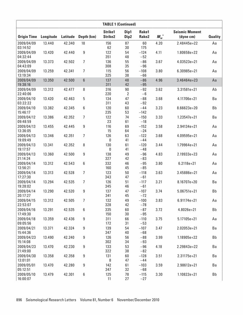
We list in Table 1 and show in Figure 1 the 64 moment tensor solutions obtained for both the largest magnitude fore-shocks and the aftershocks (i.e., ML ≥ 3.5). The complete infor-mation and the fit to recorded waveforms are available on the dedicated Web page (http://earthquake.rm.ingv.it/tdmt.php). Most of the fault plane solutions display a dominant normal faulting in agreement with the tectonic setting of the area. Some events, however, display minor strike-slip motion.
The Web page http://www.eas.slu.edu/Earthquake_Center/MECH.IT, managed by Robert Herrmann, contains independent moment tensor results for all but five of the earthquakes listed in Table 1 computed with the nnCIA veloc-ity model. We have compared the solutions of the 59 events we have in common by using the mean difference (Δ) of the P, T, and B axes, defined as the average of the differences in the orientation of the principal axes (Bernardi et al. 2004). We assume that the focal parameters between the two solutions are consistent when Δ ≤ 30° (see Bernardi et al. 2004). Among all the compared events, we have found that 70% have Δ ≤ 10°, demonstrating a very good agreement between the solutions. Just one event, the 2009/05/10 16:00:07, Mw 3.30 earthquake, resulted in a larger value (Δ ≤ 34.5°).
The mainshock moment tensor solution has been com-puted using the INGV revised hypocentral determination available within 24 hours of the earthquake: lat 42.339° N, lon 13.381° E, and depth 8.3 km. Figure 3A shows the stations used for the mainshock TDMT solution, while Figure 4 shows the TDMT solution along with the comparison between observed
▲ Figure 1. Epicentral map of the L’Aquila 2009 seismic sequence. The seismicity (from 2008/12/01 to 2009/11/30) is shown using gray dots. The fault plane mechanisms determined using the TDMT technique are shown as beach balls with different colors depending on Mw. The mainshock mechanism is red.

894 Seismological Research Letters Volume 81, Number 6 November/December 2010
and synthetic waveforms. The focal parameters were found to be strike 139°, dip 48°, rake –87. A good waveform fit (variance reduction, VR, of 71.8 %, and percentage of double couple, DC, of 94%) was found using 11 stations in the distance range 113–489 km. The azimuthal gap is relatively small (110°). The preferred depth, 9 km, agrees with the one in the INGV bul-letin implying that hypocenter and centroid depths are consis-tent. The solution features a normal fault mechanism with a
seismic moment of M0 = 1.62e+25 dyne cm, corresponding to a moment magnitude of Mw = 6.08 (Kanamori 1977).
We note that the resolved moment magnitude under-estimates the Regional Centroid Moment Tensor (RCMT) (Pondrelli et al. 2010) by 0.2 units. Magnitude differ-ences between TDMT and CMT methodologies had been already observed by Scognamiglio et al. (2009) and Kubo et al. (2002). In particular, the latter authors have compared
▲ Figure 2. Velocity structures used to retrieve moment tensors, scalar seismic moment sensitivity, and finite fault rupture param-eters. Red lines show the model used by Scognamiglio et al. (2009), blue lines indicate the nnCIA model of Herrmann and Malagnini (2009), and green lines refer to the Prem81 velocity model (Dziewonski and Anderson 1981).
(A) (B)
▲ Figure 3. A) Stations used to compute the moment tensor solution of the L’Aquila mainshock. B) Map showing strong-motion (gray triangles) and GPS stations (black squares) used for the finite fault kinematic inversion. All the strong-motion stations belong to the national strong-motion network (RAN) with the exception of AQU station (MedNet).

Seismological Research Letters Volume 81, Number 6 November/December 2010 895
TABLE 1Moment tensor solutions obtained using the TDMT technique. Events highlighted have Mw ≥ 5.0. The quality code in the last column takes into account the variance reduction (VR) and the percentage of double-couple of the MT solution (for details
see Scognamiglio et al. 2009 or http://earthquake.rm.ingv.it/tdmt.php).
Origin Time Longitude Latitude Depth (km)Strike1Strike2
Dip1Dip2
Rake1Rake2 Mw
*Seismic Moment
(dyne cm) Quality
2009/03/17 01:12:50
14.021 41.986 7 316 54
88 13
–77 –172
3.59 3.00587e+21 Aa
2009/03/29 08:43:07
14.009 41.989 10 319 89
84 10
–82 –140
3.67 4.00434e+21 Aa
2009/03/30 13:38:38
13.360 42.320 12 117 357
62 47
–129 –40
3.95 1.05655e+22 Ba
2009/03/30 13:43:26
13.364 42.303 13 149 323
53 37
–86 –95
3.46 1.89702e+21 Ba
2009/04/05 20:48:54
13.382 42.325 10 119 0
62 48
–131 –40
3.88 8.14644e+21 Ab
2009/04/05 22:39:41
13.385 42.329 9 15 124
61 60
–35 –145
3.50 2.21157e+21 Bb
2009/04/06 01:32:39
13.381 42.339 9 139 314
48 42
–87 –94
6.08 1.62258e+25 Aa
2009/04/06 02:37:04
13.340 42.360 9 140 340
53 39
–103 –74
4.85 2.33529e+23 Aa
2009/04/06 03:56:45
13.386 42.335 8 143 330
55 35
–94 –84
4.29 3.35682e+22 Ab
2009/04/06 04:47:53
13.356 42.356 7 129 1
59 44
–123 –48
3.82 6.70979e+21 Ba
2009/04/06 07:17:10
13.383 42.356 7 118 329
59 36
–108 –64
4.07 1.59581e+22 Aa
2009/04/06 10:12:35
13.384 42.317 9 144 339
51 40
–100 –78
3.63 3.43935e+21 Ba
2009/04/06 16:38:09
13.330 42.360 6 138 342
51 42
–106 –72
4.25 2.92116e+22 Aa
2009/04/06 21:56:53
13.323 42.396 5 140 340
46 46
–104 –76
3.68 4.06379e+21 Ab
2009/04/06 22:47:14
13.303 42.326 10 104 332
58 42
–120 –51
3.62 3.39916e+21 Ba
2009/04/06 23:15:36
13.360 42.450 9 154 316
57 34
–80 –106
4.98 3.68884e+23 Aa
2009/04/07 09:26:28
13.387 42.336 9 143 326
63 27
–91 –88
4.93 3.058e+23 Aa
2009/04/07 17:47:37
13.460 42.270 18 338 93
73 36
–58 –151
5.37 1.4193e+24 Aa
2009/04/07 21:34:29
13.370 42.370 6 310 120
46 44
–83 –97
4.29 3.34973e+22 Aa
2009/04/07 21:39:06
13.360 42.356 8 127 3
64 41
–123 –42
3.62 3.29316e+21 Ba
2009/04/08 03:00:34
13.462 42.293 9 131 8
73 30
–115 –36
3.63 3.47775e+21 Aa
2009/04/08 04:27:41
13.467 42.305 7 124 355
71 29
–113 –43
3.80 6.2682e+21 Ba
2009/04/08 11:35:57
13.322 42.352 8 107 11
79 63
–152 –13
3.27 1.01508e+21 Ba
2009/04/08 22:56:50
13.364 42.507 7 329 117
47 47
–67 –113
3.85 7.30844e+21 Aa
2009/04/09 00:52:59
13.340 42.480 9 322 149
46 45
–95 –85
5.21 8.25135e+23 Aa
896 Seismological Research Letters Volume 81, Number 6 November/December 2010
TABLE 1 (Continued)
Origin Time Longitude Latitude Depth (km)Strike1Strike2
Dip1Dip2
Rake1Rake2 Mw
*Seismic Moment
(dyne cm) Quality
2009/04/09 03:14:52
13.440 42.340 18 156 62
87 30
60 175
4.20 2.48445e+22 Aa
2009/04/09 04:32:44
13.420 42.440 9 122 351
54 48
–124 –52
4.11 1.80658e+22 Aa
2009/04/09 04:43:09
13.373 42.502 7 136 308
55 35
–86 –96
3.67 4.03523e+21 Aa
2009/04/09 13:19:34
13.259 42.341 7 115 325
56 38
–108 –66
3.80 6.30985e+21 Aa
2009/04/09 19:38:16
13.350 42.500 6 137 311
48 42
–86 –95
4.96 3.46464e+23 Aa
2009/04/09 22:40:06
13.312 42.477 8 316 220
90 2
–92 –6
3.62 3.31581e+21 Ab
2009/04/10 03:22:22
13.420 42.463 5 134 311
47 43
–88 –92
3.68 4.11706e+21 Ba
2009/04/10 15:46:17
13.382 42.345 6 120 235
60 53
–44 –142
3.23 8.66623e+20 Bb
2009/04/12 09:48:59
13.386 42.352 7 122 23
74 61
–150 –18
3.33 1.23547e+21 Ba
2009/04/13 13:36:05
13.455 42.445 9 116 15
69 64
–152 –24
3.58 2.94134e+21 Aa
2009/04/13 19:09:49
13.346 42.351 7 126 0
63 41
–122 –44
3.68 4.09595e+21 Aa
2009/04/13 19:17:57
13.341 42.352 8 130 0
61 41
–120 –48
3.44 1.79964e+21 Aa
2009/04/13 21:14:24
13.360 42.500 9 138 327
49 42
–96 –83
4.83 2.19933e+23 Aa
2009/04/14 13:56:21
13.312 42.543 6 332 160
46 45
–95 –85
3.80 6.2118e+21 Aa
2009/04/14 17:27:30
13.313 42.528 7 123 343
50 47
–118 –61
3.63 3.45886e+21 Aa
2009/04/14 19:28:02
13.294 42.535 7 126 345
51 46
–117 –61
3.21 8.16707e+20 Ba
2009/04/14 20:17:27
13.290 42.520 9 137 341
47 45
–107 –72
3.74 5.06751e+21 Bb
2009/04/15 22:53:07
13.312 42.505 7 132 328
49 42
–100 –78
3.83 6.91174e+21 Aa
2009/04/16 17:49:30
13.291 42.535 6 335 150
60 30
–87 –95
3.72 4.8026e+21 Bb
2009/04/18 09:05:56
13.359 42.436 9 311 172
66 31
–110 –53
3.75 5.17105e+21 Aa
2009/04/21 15:44:36
13.371 42.324 9 139 347
54 40
–107 –68
3.47 2.02053e+21 Ba
2009/04/23 15:14:08
13.490 42.240 9 126 302
56 34
–88 –93
3.99 1.18905e+22 Bb
2009/04/23 21:49:00
13.470 42.230 9 133 322
53 38
–96 –82
4.18 2.29843e+22 Ba
2009/04/30 13:01:01
13.358 42.358 9 131 8
60 47
–128 –44
3.51 2.31175e+21 Ba
2009/05/01 05:12:51
13.470 42.280 9 142 347
61 32
–103 –68
3.59 2.98612e+21 Ba
2009/05/10 16:00:07
13.479 42.301 6 125 11
78 27
–115 –27
3.30 1.10822e+21 Bb

Seismological Research Letters Volume 81, Number 6 November/December 2010 897
common events between the National Research Institute for Earth Science and Disaster Prevention (NIED) moment tensor catalog and the Harvard Global Centroid Moment Tensor (GCMT) catalog. They have found that earthquakes with seismic moment below 2 × 10¹⁷ Nm display a systematic difference in moment magnitude of 0.1 units (NIED being always smaller). They attribute this difference to lower quali-ties of GCMT solution in the smaller size earthquakes result-ing from long-period noise contamination. As we believe that this cannot be the case for the L’Aquila earthquake, we have addressed the problem by testing the dependency of the scalar moment on the adopted velocity models. We have used three velocity models—the two described above and the Prem81 model (Dziewonski and Anderson 1981; green line in Figure 2), which is similar to that used by Pondrelli et al. (2010). In order to directly compare the solutions, we have inverted the waveforms using the same set of 11 stations, source depth (9 km) and frequency band (0.02–0.05 Hz) for all three veloc-ity models (Figure 2). The resulting moment tensors (Figure 4 and 5A–B) show very comparable focal mechanisms solutions and a good fit to the data (VR > 58 % and DC > 85 %). We have found, however, that the scalar moment estimates range within a factor of two, that is, between M0 = 1.62e+25 and M0 = 3.25e+25 corresponding to Mw = 6.08 and Mw = 6.28, respectively.
The observed difference can be attributed to the adopted velocity structure. In fact, given the same seismic moment and the same mid-crust velocities, larger seismogram amplitudes result from models featuring slow shallow velocity layers, which trap the seismic energy and produce amplifications (e.g., Aki and Richards 2002). It follows that lower scalar moments are required to fit seismograms when using improved local velocity models that account for such shallow structure.
FAST DETERMINATION OF THE MAINSHOCK RUPTURE HISTORY
We use the L’Aquila mainshock as a case study to test the poten-tial of the procedure recently implemented at INGV to rapidly determine finite fault rupture models. The code, based on the work of Hartzell and Heaton (1983) and subsequently devel-oped by Dreger and Kaverina (2000), consists of a non-negative least-squares inversion method with simultaneous smoothing and damping. It is currently in use at the Berkeley Seismological Laboratory, where automatic models are obtained within a few tens of minutes after the origin time, and analyst-reviewed pre-liminary slip models are released a few hours after the occur-rence of the event (e.g., Dreger et al. 2005).
To determine the extended fault model for the L’Aquila mainshock, we have inverted the recordings from 13 three-com-
TABLE 1 (Continued)
Origin Time Longitude Latitude Depth (km)Strike1Strike2
Dip1Dip2
Rake1Rake2 Mw
*Seismic Moment
(dyne cm) Quality
2009/05/14 06:30:22
13.406 42.501 7 154 328
48 42
–86 –94
3.44 1.77539e+21 Ab
2009/05/30 02:55:10
13.341 42.356 10 139 345
56 37
–106 –68
3.56 2.73409e+21 Ba
2009/06/07 19:21:34
13.483 42.350 2 303 107
49 42
–79 –102
3.33 1.21756e+21 Ca
2009/06/22 20:58:40
13.356 42.446 18 316 55
88 14
–76 –170
4.36 4.36983e+22 Aa
2009/06/23 00:41:56
13.369 42.441 7 315 201
85 12
–101 –24
3.70 4.47397e+21 Aa
2009/06/25 21:00:08
13.206 42.570 5 143 301
52 40
–76 –107
3.48 2.07363e+21 Ba
2009/07/03 09:43:53
13.361 42.328 9 145 318
54 36
–86 –96
3.32 1.17475e+21 Ba
2009/07/03 11:03:07
13.387 42.409 4 289 111
46 44
–91 –88
3.74 5.09064e+21 Ba
2009/07/12 08:38:51
13.370 42.340 9 138 341
61 31
–101 –71
4.16 2.17681e+22 Aa
2009/07/12 22:14:24
13.398 42.338 10 116 339
60 39
–115 –54
3.65 3.73769e+21 Ab
2009/07/31 11:05:40
13.505 42.247 7 145 333
60 30
–94 –83
3.88 8.23978e+21 Aa
2009/09/24 16:14:57
13.330 42.450 18 178 359
49 41
–91 –89
3.92 9.29486e+21 Aa
2009/10/20 05:07:30
13.240 42.398 4 20 114
81 67
–23 –171
3.49 2.17119e+21 Ba
* Moment magnitude computed by using the Kanamori (1977) relation.

898 Seismological Research Letters Volume 81, Number 6 November/December 2010
ponent digital accelerometers of the RAN Network and the AQU (MedNet) accelerogram; moreover, in the final inversion attempts (see the section below on joint inversion of strong-motion and GPS data), we have also inverted 27 GPS horizontal displace-ments retrieved by the permanent stations of the INGV geodetic network (Figure 3B). The hypocentral distances of the selected recording sites and GPS benchmarks are less than ~100 km.
The observed accelerograms are integrated in time to obtain ground velocities and bandpass filtered between 0.02 and 0.5 Hz using a two-pole Butterworth filter. We do not model higher frequencies since site effects (present in the area for frequencies higher than 0.6 Hz; see De Luca et al. 1998) and complex propagation paths do not allow for the adoption of reliable Green’s functions. In order to apply this procedure in near real time, the Green’s functions have been precalculated and stored. The code used for calculating the Green’s functions is the same used for the TDMT analysis. They are computed on a regular grid sampling the focal volume every 2 km horizon-tally and 1 km vertically and filtered between 0.02 and 0.5 Hz, the same as for the recorded data.
IDENTIFYING THE FAULT PLANE
To determine the rapid source parameters, we need first to select the effective rupture plane between the two provided by the moment tensor solution. The main objective consists of
imaging the gross features of the earthquake rupture history in terms of heterogeneous distribution of slip amplitudes and direction, while slip duration and rupture velocity are taken constant on the fault plane (the values of the latter parameters have been selected by trial and error). The local slip velocity is modeled by imposing a triangular source-time function. Although some of the assumptions above are very simplistic, they are nonetheless required to perform a rapid preliminary inversion of the recorded seismograms.
To identify the rupture plane, we perform a series of inver-sions using only the strong-motion waveform data, adopting an overly-large-dimension fault plane and the standard regional crustal velocity model (the same adopted for the routine retrieval of moment tensors). The chosen fault dimensions are nearly twice the expected rupture length for an earthquake of this size (i.e., 40 × 20 km2 along strike and dip, respectively) and are centered at the hypocenter to allow for rupture in either strike direction, which enables the data to resolve the main fea-tures of rupture directivity and propagation on the fault plane. We set rise time and rupture velocity ranges to be between 0.7 ÷ 2.8 s and 1.6 ÷ 4.0 km/s, respectively. The rake has been allowed to be heterogeneous throughout the fault between –45° and –135°. The fault was parameterized using 200 subfaults each having a 2 × 2 km2 area. The top of the fault is 0.8 km deep.
We identify the actual rupture plane by means of the solu-tion with the largest variance reduction (VR) (see Dreger and
▲ Figure 4. Time domain moment tensor solution for the L’Aquila mainshock. Black and red solid lines indicate the recorded data and synthetics, respectively.

Seismological Research Letters Volume 81, Number 6 November/December 2010 899
▲ Figure 5. Time domain moment tensor solution for the L’Aquila mainshock computed with the (A) nnCia and (B) Prem81 velocity models.

900 Seismological Research Letters Volume 81, Number 6 November/December 2010
Kaverina 2000). We have found that most of the solutions adopting the southwest-dipping plane (striking 139o and dip-ping 48o) result in values of VR around 50%, which are signifi-cantly larger than the ~20% obtained when using the alterna-tive northeast-dipping plane. The southwest-dipping plane is in good agreement with the alignment of the aftershock locations, the satellite line-of-sight pattern retrieved from InSAR data, and the observed mainshock surface offsets on the Paganica fault (Emergeo Working Group 2010).
Figure 6 displays the slip and rupture time distribution imaged on the southwest-dipping plane. This preliminary source model displays a main slip concentration near the hypo-center and a second, deeper slip patch located a few kilometers southeastward. The position of slip patches on the fault plane suggests a nearly unilateral southeast rupture propagation. In this rupture model the rupture velocity is 2.6 km/s; however, a similar fit to the data and variance reduction (~54%) has been obtained for rupture velocities between 2.5 and 4.0 km/s.
To assess the quality of our results, we take advantage of the published kinematic source models (Cirella et al. 2009 and the updated version of Piatanesi et al. 2009). It is difficult, how-ever, to quantitatively and fairly compare the models because the geometries (strike and dip) of these models are slightly different (<10°), and in the following discussion we will focus only on the gross features of the slip distribution. First, we note that the slip patch that we observe close to the hypocenter has been also found in the studies mentioned before. In contrast, the southeastern patch is too deep when compared to the seis-micity distribution. All the inversions employ different velocity models for the Green’s functions and this is the likely origin for the diverse slip distributions.
CALIBRATED LOCAL VELOCITY MODEL
For the reasons explained above, and similar to what we have done for the moment tensor analysis, we have tested how the velocity model affects the solution by re-running the inversions with the Green’s functions computed using the nnCIA model—the same velocity model adopted by Piatanesi et al. (2009).
We again apply the above analysis on the 40 × 20 km2 fault to assess the effect of crustal velocity structure on the inferred slip pattern. Figure 7 shows the imaged rupture history for this fault parameterization and the calibrated velocity model. The inferred slip distribution is now more consistent with the slip models proposed in the literature, and the variance reduction using this velocity model improves to 68.5%. Both the main slip patches (near the hypocenter and southeastward) are shallower than those imaged with the regional velocity model. This sug-gests that the choice of the crustal velocity model significantly affects the inferred rupture history. The rupture velocity of the model displayed in Figure 7 is equal to 2.2 km/s. This model also suggests nearly unilateral rupture propagation toward the southeast.
In order to refine the rupture model, and because the assumed fault dimensions are certainly too large for an Mw 6.1 event, we have performed a second set of inversions for a
smaller fault plane enclosing the dimensions of the main area of slip. Thus, the fault length has been reduced to 26 km, while a down-dip extension has been assumed of 16 km. Figure 8A shows the resulting rupture model. This model is character-ized by a rise time of 0.7 s, a rupture velocity of 2.2 km/s, and a seismic moment of 2.238e+25 dyne cm corresponding to an Mw 6.17. It features a large, main slip patch located 2 km updip from the hypocenter and a second slip patch located ~8 km southeast from the hypocenter, but at least 6–7 km shallower than that shown in Figure 6. This slip model is very much like that obtained by Piatanesi et al. (2009). We find also a deeper and smaller patch of slip located at 4 km downdip from the hypocenter. The main patch updip from the hypocenter has a maximum slip of 88.5 cm, an average rake of –100°. Figure 8B shows the resulting fits to the recorded velocity time histories. The synthetic seismograms match the recorded waveforms well and the variance reduction is 68%, that is, significantly better than what was obtained using the regional velocity model.
To investigate the rupture velocity variability among the best-fitting models, we have carefully examined the entire ensemble of inverted rupture histories. The results of this analy-sis are summarized in Figure 9A, showing the VR as a function of the rupture velocity for all explored models, where different colors have been assigned to the investigated rise-time values. Despite a broad range of rupture velocities associated with high values of variance reduction (similar to that of our best model, shown in Figure 8), this test allows the identification of two dis-tinct maxima of VR. Models around the first maximum (black arrow in Figure 9A) are characterized by low rupture velocities and short rise times; conversely, models close to the second max-imum (green arrow in Figure 9A) display high rupture veloci-ties and long rise time. This result corroborates the trade-off between rupture velocity and rise time. We emphasize the dif-ficulty of keeping the rupture velocity constant for the L’Aquila mainshock; this might be partially explained by considering the heterogeneity of rupture speed inferred for this event by other studies (see Cirella et al. 2009; Ellsworth and Chiaraluce 2009).
We show in Figure 8B the slip and rupture time distri-bution for a model characterized by a rise time of 1.9 s and a rupture velocity of 3.2 km/s and therefore belonging to the second peak in Figure 9A. The resulting variance reduction is 66.8%. The comparison between the two models in Figures 8A and 9B demonstrates that despite the well-known trade-off between rupture velocity and the position of slip concen-trations (see Bouin et al. 2000), the two main slip patches are poorly affected by the biases among model parameters.
JOINT INVERSION OF STRONG-MOTION AND GPS DATA
Finally, we carry out a set of joint inversions combining strong-motion and GPS data. All the kinematic parameters are varied within the same range of the previous finite fault inversion. Figure 10A shows the retrieved best-fitting rupture model, while Figure 10B is the corresponding map view. The resulting variance reduction is 73.2%. This model has a rise time of 2.1 s

Seismological Research Letters Volume 81, Number 6 November/December 2010 901
and a rupture velocity of 3.1 km/s. The scalar seismic moment is 2.515e+25 dyne cm corresponding to Mw 6.2. Figures 10C and D display the comparison between recorded and synthetic ground velocity time histories and the coseismic GPS horizon-tal displacements, respectively. The maximum slip is 88 cm. The average rake angles are 103° and 92° for the updip and south-east patches, respectively. The inferred slip pattern might sug-gest a smaller fault plane, roughly 20 km long and 16 km wide. It is noteworthy that the best model obtained from the joint inversion belongs to the second peak (i.e., high rupture velocity and long rise time) of Figure 9A. The diminished spatial extent of the southeast slip patch makes it comparable with the slip distribution of Cirella et al. (2009) (see Figure 4 in that paper).
DISCUSSION
The object of this study is twofold : 1) test the real-time source mechanism procedures that have been recently implemented at INGV, and 2) verify the potential for rapid finite source-time history inversion. The fast and routine time-domain moment tensor determinations rely on the methodology proposed by Dreger and Helmberger (1993) and Pasyanos et al. (1996) (see Scognamiglio et al. 2009), while the fast finite-fault estimation is based on the methodology by Dreger and Kaverina (2000) and Dreger et al. (2005).
With regard to the moment tensor determination, we have shown that TDMT solutions can be obtained auto-
▲ Figure 6. Finite fault slip distribution and rupture time obtained by using strong-motion data, the regional velocity model, and the southwest-dipping plane of the TDMT solution in Figure 4. The fault dimension is 40 × 20 km2. The fit to the data from this model is 54.5%.
▲ Figure 7. Finite fault slip distribution and rupture time obtained by using strong motion data, the nnCia velocity model, and the south-west-dipping plane of the TDMT solution in Figure 4. The fault dimension is 40 × 20 km2. The fit to the data from this model is 68.5%.

902 Seismological Research Letters Volume 81, Number 6 November/December 2010
▲ Figure 8. A) Mainshock rupture history obtained by inverting strong-motion data with the nnCIA velocity model. The fault dimension is reduced to 26 × 16 km2. Rupture time is indicated at -s intervals as solid white lines. B) Comparison between observed (black) and synthetic (red) seismograms. Numbers indicate the maximum amplitude of recorded data.
(A)
(B)

Seismological Research Letters Volume 81, Number 6 November/December 2010 903
(A)
(B)
▲ Figure 9. A) Plot of the variance reduction as a function of rupture velocity and rise time for all the models investigated. The arrows point to the two maxima. B) Finite fault kinematic model relative to the second maximum (green arrow) of panel (A). The rupture time is indicated at 1-s intervals as solid white lines.

904 Seismological Research Letters Volume 81, Number 6 November/December 2010
matically and that the use of refined, locally calibrated veloc-ity structures allows us to lower the magnitude threshold at which reliable moment tensors can be computed. In our case the ML 3.5 threshold was achieved after adopting the nnCIA model developed by Herrmann and Malagnini (2009). For the mainshock, the preferred TDMT fault plane solution is: strike 139°, dip 48°, and rake –87°. The resulting moment magnitude, Mw = 6.08, is 0.2 units smaller than the solution provided by Pondrelli et al. (2010), who use the regional centroid moment tensor technique and a global velocity model. Such a difference, already detected for smaller earthquakes in Italy (Scognamiglio et al. 2009), prompted us to investigate the effect of the velocity structure on the seismic moment determination and, specifi-cally, on its scalar value. Our results demonstrate that the dif-ferences (Figures 4 and 5A,B) can be attributed to the velocity models—the locally calibrated model results in the best wave-form fits and smaller scalar seismic moment.
The 64 TDMT solutions show prevalent normal faulting in agreement with the present-day active stress field in this sector of the Apennines (Mariucci et al. 1999). A relevant exception appears in the largest Mw 5.4 aftershock of 7 April 2009 (17:47 UTC) located at 17 km depth, where the solution features a conspicuous strike-slip component. Overall, the obtained moment tensors can provide good constraints on the orienta-tion of the active stress field in the seismogenic volume, and the method is a robust and practical tool for real-time determina-tions of the point-source focal parameters and magnitude.
For the finite fault, our primary goal was to verify whether the procedure we have employed here could be applied without human intervention. This follows from the need to quantify the extension of the fault and the primary features of the rupture (i.e., main slip rupture patches and rupture propagation) in the imme-diate aftermath of an earthquake such as the one in L’Aquila. These rupture features are very valuable for rapid determination of the areas affected by the largest strong ground motion.
In our methodology, the first step is to identify the actual rupture plane starting from the mainshock moment tensor solu-tion. Our automatic procedure identifies the southwest-dipping plane as the main one and indicates a southeast directivity of the source rupture. At this stage, however, manual intervention is required since more accurate Green’s functions are necessary to retrieve the rupture details in a fully automatic way.
Using the locally calibrated velocity model, we have pur-sued the analysis further and investigated whether a procedure based on fixed source model parameters (such as rupture veloc-ity and source-time function) can be used to estimate complex rupture histories such as that of the L’Aquila earthquake. To this end we have included GPS data in addition to the strong-motion recordings. Our final rupture model shows well-con-strained rupture directivity both updip from the hypocenter and southeast along strike propagation. In particular, the slip patch located southeast of the hypocenter and rupturing between 2 and 3 seconds is found to be a main feature of the rupture model and is consistent with both the slip models obtained using similar datasets (Cirella et al. 2009; Piatanesi et al. 2009) and those using only satellite data (Atzori et al. 2009;
Cheloni et al. 2010). In addition, focusing on the other main slip patch rupturing between 0 and 2 seconds and updip from the hypocenter, we have found that it is mainly required to fit the ground motion time histories recorded at AQU and AQG, which are located nearly above and to the north-northwest of the patch, respectively.
With regard to the rupture velocities, our two best-fitting inversions (with and without GPS data) suggest similar and alternative fits respectively using two different rupture veloci-ties. This result can be explained by a heterogeneous distribu-tion of these parameters on the fault plane. That is, we can account for the variability and the uncertainties in constrain-ing rupture velocity only if we introduce dynamic heterogenei-ties and/or geometrical complexities. Geometrical complexi-ties, however, are not included in our solutions since a single planar fault model was adopted, although they are not unreal-istic—field evidence of surface movements up to 50 mm along the northeast-dipping Mt. Bazzano fault surface trace (anti-thetic to the Paganica fault; Emergeo Working Group 2010) suggests the activation of additional, shallow rupture planes. Despite the complexity of the rupture history of the L’Aquila mainshock (confirmed by our results), we have found that the adopted procedure can image the main energy release patches on the fault plane.
CONCLUSIONS
The application of the above source methods to the 6 April 2009 L’Aquila earthquake is a retrospective validation test use-ful for assessing the performance of a quasi automatic proce-dure for future near real-time applications in Italy.
The results we have presented indicate that the most deli-cate point of the analysis is represented by the choice of Green’s functions to be adopted. The finite fault procedure can be easily automated so that the fault is properly centered to the patches of prominent slip and its size is consistent with the earthquake magnitude. Then, if a proper velocity model is not available, the solution still provides the main rupture pattern, in the best case, but it can be biased along depth.
Our results thus show that the inferred solution for L’Aquila earthquake contains many of the relevant features for understanding the ground shaking and the radiated energy, even with approximate and uncalibrated Green’s functions. This implies that if the ground motion time histories had been available in real time or very rapidly, it would have been pos-sible to provide quick evaluations of the ground shaking in the epicentral area and to obtain first-order scenarios of the rupture characteristics within less than one hour from the mainshock origin time. This latter result has implications for the rapid generation of more accurate maps of strong ground motion (e.g., Michelini et al. 2008), which could be very valu-able in organizing rescue teams in the immediate aftermath of earthquakes of similar size in Italy.
The final model obtained, using strong-motion and GPS data, reveals two main rupture patches updip and southeast of the hypocenter. Although the assumption of a constant rupture

Seismological Research Letters Volume 81, Number 6 November/December 2010 905
▲ Figure 10. A) Finite fault source model resulting from the joint inversion of strong-motion and GPS data. The rupture time is indicated at 1-s intervals as solid white lines. B) Surface pro-jection of the slip on the fault. C) Comparison between the observed (black) and the obtained synthetic (red) seismograms. D) Comparison between observed (black) and synthetic (blue) horizontal displacement. The black rectangle is the surface pro-jection of the rupture plane
(A)
(C)
(B)
(D)

906 Seismological Research Letters Volume 81, Number 6 November/December 2010
velocity throughout the plane obscures the rupture heteroge-neity, we have found that the resulting model closely matches those of Cirella et al. (2009) and Piatanesi et al. (2009), both of which are derived using more sophisticated inversion algo-rithm.
ACKNOWLEDGMENTS
We would like to thank the people managing the Italian National Seismic Network, the MedNet, the North-East Italy Broadband Networ, and the SudTirol Province who provided the velocimetric data for this study. Similarly, we would like to thank Antonella Gorini and Elisa Zambonelli of the Italian Civil Protection Agency for providing the RAN strong-motion data. We would also like to thank Robert Herrmann for the review of the manuscript and the suggestions he provided. Some figures were made using the Generic Mapping Tools version 4.2.1 (http://www.soest.hawaii.edu/gmt). Part of this work has been supported through the DPC-INGV (2007–2009) project S3.
REFERENCES
Aki, K., and P. G. Richards (2002). Quantitative Seismology. 2nd ed. Sausalito, CA: University Science Books.
Anzidei, M., E Boschi, V. Cannelli, R. Devoti, A. Esposito, A. Galvani, D. Melini, G. Pietrantonio, F. Riguzzi, V. Sepe, and E. Serpelloni (2009). Coseismic deformation of the destructive April 6, 2009 L’Aquila earthquake (central Italy) from GPS data. Geophysical Research Letters 36, L17307; doi:10.1029/2009GL039145.
Atzori, S., I. Hunstad, M. Chini, S. Salvi, C. Tolomei, C. Bignami, S. Stramondo, E. Transatti, A. Antonioli, and E. Boschi (2009). Finite fault inversion of DInSAR coseismic displacement of the 2009 L’Aquila earthquake (Central Italy). Geophysical Research Letters 36, L15305; doi:10.1029/2009GL039293.
Bernardi, F., J. Braunmiller, U. Kradolfer, and D. Giardini (2004). Automatic regional moment tensor inversion in the European-Mediterranean region. Geophysical Journal International 157, 703–716.
Bouin, M. P., M. Cocco, G. Cultrera, H. Sekiguchi, K. Irikura, A. Cirella, A. Piatanesi, E. Tinti, and M. Cocco (2008). Rupture process of the 2007 Niigata-ken Chuetsu-oki earthquake by non-linear joint inversion of strong motion and GPS data. Geophysical Research Letters 35, L16306; doi:10.1029/2008GL034756.
Cheloni, D., N. D’Agostino, E. D’Anastasio, A. Avallone, S. Mantenuto, R. Giuliani, M. Mattone, S. Calcaterra, P. Gambino, D. Dominici, F. Radicioni and G. Fastellini (2010). Coseismic and initial post-seismic slip of the 2009 Mw 6.3 L’Aquila earthquake, Italy, from GPS measurements. Geophysical Journal International 181 (3), 1,539–1,546; doi: 10.1111/j.1365-246X.2010.04584.x.
Cirella, A., A. Piatanesi, M. Cocco, E. Tinti, L. Scognamiglio, A. Michelini, A. Lomax, and E. Boschi (2009). Rupture history of the 2009 L’Aquila earthquake from non-linear joint inversion of strong motion and GPS data. Geophysical Research Letters 36, L19304, doi:10.1029/2009GL039795.
De Luca, G., E. Del Pezzo, F. Di Luccio, L. Margheriti, G. Milana, and R. Scarpa (1998). Site response study in Abruzzo (central Italy): Underground array versus surface stations. Journal of Seismology 2, 223–236.
Dreger, D. S., L. Gee, P. Lombard, M. H. Murray, and B. Romanowicz (2005). Rapid finite-source analysis and near-fault strong ground
motions: Application to the 2003 Mw 6.5 San Simeon and 2004 Mw 6.0 Parkfield earthquakes. Seismological Research Letters 76 (1), 40–48.
Dreger, D. S., and D. V. Helmberger (1993). Determination of source parameters at regional distances with three-component sparse net-work data. Journal of Geophysical Research 98, 8,107–8,125.
Dreger, D. S., and A. Kaverina (2000). Seismic remote sensing for the earthquake source process and near-source strong shaking: A case study of the October 16, 1999 Hector Mine earthquake. Geophysical Research Letters 27 (13), 1,941–1,944.
Dziewonski, A. M., and D. L. Anderson (1981) Preliminary reference Earth model. Physics of the Earth and Planetary Interiors 25 (4), 297–356.
Ellsworth, W., and L. Chiaraluce (2009). Supershear During Nucleation of the 2009 M 6.3 L’Aquila, Italy Earthquake. Eos, Transactions, American Geophysical Union 90 (52), Fall Meeting Supplement, Abstract U13C-07.
Emergeo Working Group (2010). Evidence for surface rupture associ-ated with the Mw 6.3 L’Aquila earthquake sequence of April 2009 (central Italy). Terra Nova 22, 43–51.
Hartzell, S. H., and T. H. Heaton (1983). Inversion of strong ground motion and teleseismic waveform data for the fault rupture history of the 1979 Imperial Valley California, earthquake. Bulletin of the Seismological Society of America 73, 1,553–1,583.
Herrmann, B., and L. Malagnini (2009). Systematic determination of moment tensor of the April 6th, 2009 L’Aquila earthquake sequence. Eos, Transactions, American Geophysical Union 90 (52), Fall Meeting Supplement, Abstract U23A-0029.
Kanamori, H. (1977). The energy release in great earthquakes. Journal of Geophysical Research 92 (20), 2,981–2,987.
Kubo, A., E. Fukuyama, H. Kawai, and K. Nonomura (2002). NIED seismic moment tensor catalogue for regional earthquakes around Japan: Quality test and application. Tectonophysics 356, 23–48.
Mariucci, M. T., A. Amato, and P. Montone (1999). Recent tectonic evolution and present stress in the northern Apennines (Italy). Tectonics 18, 108–118.
Michelini, M., L. Faenza, V. Lauciani, and L. Malagnini (2008). ShakeMap implementation in Italy. Seismological Research Letters 79 (5), 688–697.
Pasyanos, M. E., D. S. Dreger, and B. Romanowicz (1996). Toward real-time estimation of regional moment tensors. Bulletin of the Seismological Society of America 86, 1,255–1,269.
Piatanesi, A., A. Cirella, M. Cocco, E. Tinti, L. Scognamiglio, A. Michelini, and A. Lomax (2009). The rupture history of the 2009 L’Aquila earthquake by non-linear joint inversion of strong motion and GPS data. Eos, Transactions, American Geophysical Union 90 (52), Fall Meeting Supplement, Abstract U13C-05.
Pondrelli, S., S. Salimbeni, A. Morelli, G. Ekström, M. Olivieri, and E. Boschi (2010). Seismic moment tensors of the April 2009, L’Aquila (central Italy), earthquake sequence. Geophysical Journal International 180 (1), 238–242.
Saikia, C. K. (1994). Modified frequency-wave-number algorithm for regional seismograms using Filon’s quadrature: Modeling of Lg waves in eastern North America. Geophysical Journal International 118, 142–158.
Scognamiglio, L., E. Tinti, and A. Michelini (2009). Real-time determi-nation of seismic moment tensor for the Italian region. Bulletin of the Seismological Society of America 99 (4); doi:10.1785/0120080104.
Istituto Nazionale di Geofisica e VulcanologiaVia di Vigna Murata, 605
00143 Rome, Italy [email protected]
(L. S.)


