The L'Aquila 2009 event: :the GPS deformations

105

The L’Aquila 2009 event: the GPS deformations

L. BIAGI1, S. CALDERA1, D. DOMINICI2 and F. SANSÒ1

1 Politecnico di Milano, Como, Italy2 Università de L’Aquila, L’Aquila, Italy

(Received: April 14, 2010; accepted: November 10, 2010)

ABSTRACT In the night of April 6, 2009, an earthquake of MW 6.3 magnitude occurred in theAbruzzo region. The hypocenter was estimated by the INGV at 42,35° N, 13,38° E, ata 9.5 km depth; moreover, at least one month of pre-seismic events preceded the mainshock and aftershocks continued for at least 6 months. For the understanding of thegeodetic and geodynamic implications of the earthquake, the temporal and spatialanalyses of the phenomenon are fundamental; our research group has collected theGNSS data provided by about 50 permanent stations in the earthquake area andneighbouring regions; all the data have been processed in order to investigate thestations displacements and, if possible, the deformation pattern. In particular, the timeseries (two months of data both before and after the earthquake) of the dailycoordinates were interpolated for each station in order to estimate the displacement atthe main shock epoch: particular attention has been paid to carry out a propercovariance empirical estimation, in order to evaluate the displacement significance.Finally, the displacements of all the stations have been spatially analyzed to indentifythe areas with similar displacements and the main discontinuities between them.Thirteen stations that significantly displace horizontally have been found: a roughclustering allows us to discriminate between a near field area that displaces mainlysouthwards, a south-western region that displaces in a SWdirection and a northeastregion with an opposite motion. Only four station in the epicenter area significantlydisplace vertically, with drops between 3 and 12 cm.

1. Introduction

The L’Aquila event is identified here by the main shock of the Abruzzo earthquake, whichtook place on April 6, 2010 at 1.33 UTC, with a magnitude of MW 6.3 (Anzidei et al., 2009;EMERGEO Working Group, 2009; INGV, 2009); this was preceded by foreshocks and followedby aftershocks. The event was catastrophic, as it could only be, considering that the epicenter(42,35° N, 13,38° E, depth of 9.5 km) is placed in the middle of a populated area, with historicalbuildings, inadequate to withstand such strong dynamics. Scientists are analyzing the existingdata to take one step forward along the hard road of understanding the physics and predictingsuch phenomena. The data that allow us to reconstruct the displacements and the deformationpattern of the Earth’s surface in the earthquake area are of great importance, because they canprovide input information for geophysical analyses and inversions (Okada, 1985): nowadays theyare mainly of two types, referring to the GNSS and inSAR techniques. The latter is stuck in timeto the repeat cycle of SAR satellites (≈ 35 days), meaning that the deformation story is somewhatforcedly discontinuous in time. On the other hand SAR, in both its versions, interferometric

Bollettino di Geofisica Teorica ed Applicata Vol. 52, n. 1, pp. 105-121; March 2011

© 2011 – OGS

106

Boll. Geof. Teor. Appl., 52, 105-121 Biagi et al.

(Hanssen, 2001) and Permanent Scatterers (Ferretti et al., 2001), is capable of providing a realarea-wise picture of the deformation pattern. On the other hand, data acquired by permanentGNSS stations (PS’s) are almost continuous in time (typically up to 1 Hz rate, though in this paperthe 30 s acquisition interval has been analyzed), their disadvantages being related to theirsparseness in the area and to the fact that, when placed on the roof of a building, they describethe kinematics of the building coupled through foundations with the ground, rather than the directdisplacement of the ground itself. A combined analysis of data for both techniques is obviouslythe optimal solution for an accurate reconstruction of the deformation story: yet, in the presentwork we present the image of the ground motion derived from GNSS data only.

Only in the Abruzzo region, we can collect data from 33 PS’s: in particular, five of them are lessthan 10 km away from the epicenter; moreover, we have another 17 additional PS’s within 50 kmfrom the region's boundaries and the three nearest Italian IGS stations of Matera, Cagliari andMedicina have been included, to provide a proper link to ITRS. All the stations already belong tosome permanent network: ASI-Geodaf, (geodaf.mt.asi.it, Vespe et al., 2000), INGV-RING(ring.gm.ingv.it, Avallone et al., 2010), Leica ItalPoS (www.italpos.it), TopCon GeoTop(www.geotop.it), GPS Abruzzo (gpsnet.regione.abruzzo.it), GPS Umbria (opos6.agora.ng.unipg.it),ResNap (w3.uniroma1.it/resnap-gps); the authors want to gratefully acknowledge theseorganizations for providing the data.

This relative abundance of data allows a sufficient reconstruction of the deformation fieldwith a spatial resolution of about 10 km, particularly in the epicenter area, and a time resolutionof 30 s; note that the spatial consistency of the estimated displacements of different stationsshould confirm that we are not seeing the motion of the individual structures. In Sect. 2, wepresent the data used in the work, and outline the analysis strategy. In Sect. 3, we perform theanalysis of the time series of the displacements, in a local (east, north, up) coordinate system ofthe individual stations. In Sect. 4, we make some considerations on the deformation pattern andits spatial discontinuities, both in the plane and in the vertical direction. Provisory conclusionsand outlooks of future work are presented in Sect. 5.

2. The data set and processing strategy

The data used in this work are the daily (with a 30 s acquisition interval) RINEX files of allthe PS's listed in the previous section. The data have been processed by daily adjustments of thenetwork from Sunday February 1 (Day Of the Year 32, GPS Week 1517, day of the GPSW 0) toSaturday June 6 (DOY 157, GPSW 1534, DOW 6), namely 64 days before the event and 61 daysafter the event: in this way, two months of results are available both before and after the mainshock.

Ancillary data for the processing were the final IGS products for ephemerides, Earthorientation parameters and phase center variations. The network adjustment has been performedby the Bernese 5.0 software [BSW5.0, Dach et al. (2007)]; in the design of the multibase graphthe minimum baseline length principle has been adopted; in the raw data processing the approachdescribed in Benciolini et al. (2008) and the usual international guidelines (Kouba, 2003) havebeen followed. To remove the intrinsic rank deficiency of this local network, minimal constraintshave been imposed to each daily solution, by fixing the 3 translation parameters to the barycenter

107

The L’Aquila 2009 event: the GPS deformations Boll. Geof. Teor. Appl., 52, 105-121

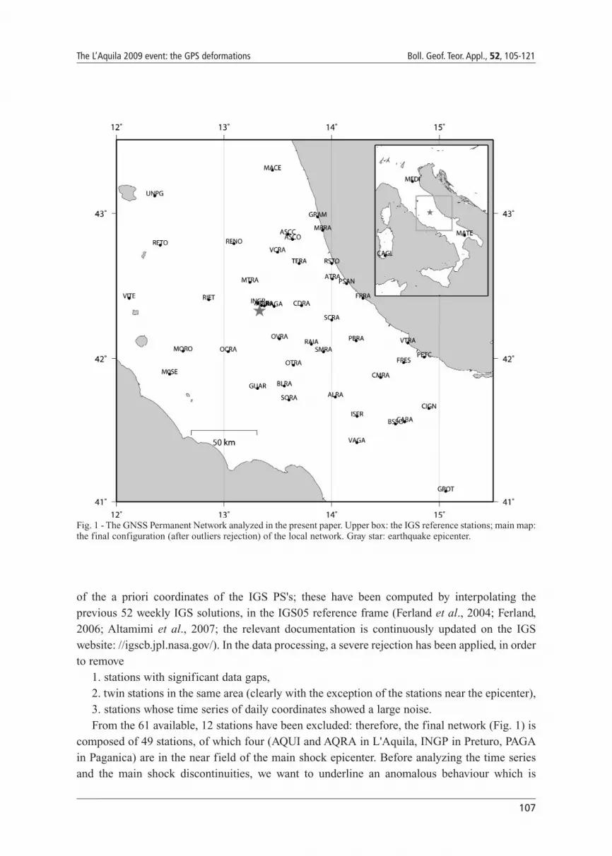
of the a priori coordinates of the IGS PS's; these have been computed by interpolating theprevious 52 weekly IGS solutions, in the IGS05 reference frame (Ferland et al., 2004; Ferland,2006; Altamimi et al., 2007; the relevant documentation is continuously updated on the IGSwebsite: //igscb.jpl.nasa.gov/). In the data processing, a severe rejection has been applied, in orderto remove

1. stations with significant data gaps, 2. twin stations in the same area (clearly with the exception of the stations near the epicenter),3. stations whose time series of daily coordinates showed a large noise. From the 61 available, 12 stations have been excluded: therefore, the final network (Fig. 1) is

composed of 49 stations, of which four (AQUI and AQRA in L'Aquila, INGP in Preturo, PAGAin Paganica) are in the near field of the main shock epicenter. Before analyzing the time seriesand the main shock discontinuities, we want to underline an anomalous behaviour which is

Fig. 1 - The GNSS Permanent Network analyzed in the present paper. Upper box: the IGS reference stations; main map:the final configuration (after outliers rejection) of the local network. Gray star: earthquake epicenter.

108


present in several daily solutions of week 1521, well before the earthquake (see the example inthe following Figs. 3, 4, 5 and 6); probably the anomalous results are caused by some irregularityin the adjustment and seem totally independent of the geophysical event we want to analyze:indeed, they are common both to the IGS and local PS's, irrespective of their position, and do notshow a clear temporal signal.

3. The individual displacements of the stations

The first analysis concerns the time series of the daily coordinates of each station. At first, thedaily estimated coordinates of the three IGS stations were compared with their a priori values, inorder to assess the reference frame accuracy and stability: the statistics (Table 1) are completelysatisfying, showing standard deviations of about 2 mm in the local horizontal components and 4mm in height.

Our first purpose is to estimate the pattern of the time evolution of the coordinates before andafter the main shock, trying then to reconstruct the amplitude of the relevant discontinuity. The

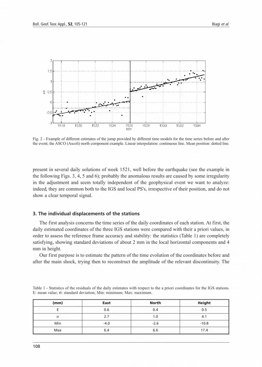
Fig. 2 - Example of different estimates of the jump provided by different time models for the time series before and afterthe event; the ASCO (Ascoli) north component example. Linear interpolation: continuous line. Mean position: dotted line.

(mm) East North Height

E 0.6 0.4 0.5

σ 2.7 1.0 4.1

Min -4.0 -2.6 -10.8

Max 6.4 6.6 17.4

Table 1 - Statistics of the residuals of the daily estimates with respect to the a priori coordinates for the IGS stations.E: mean value; σ: standard deviation; Min: minimum; Max: maximum.

109


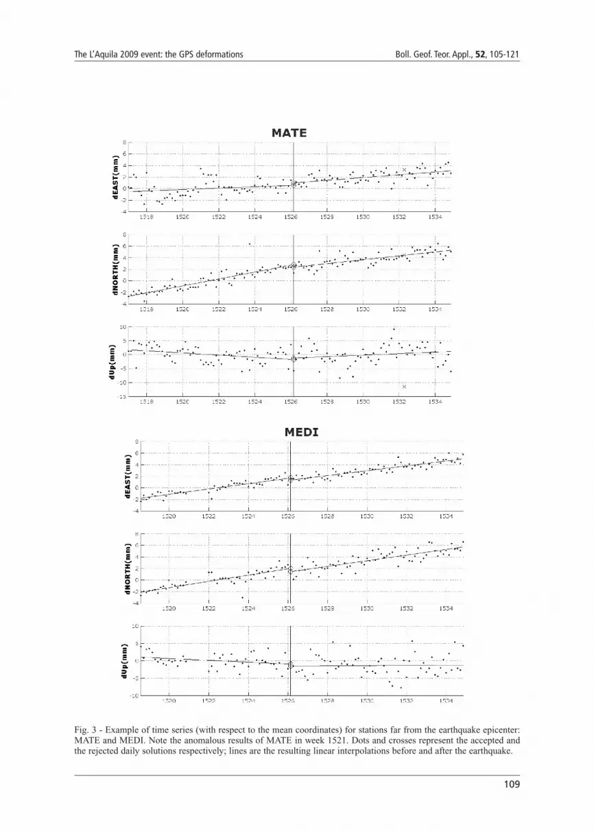
Fig. 3 - Example of time series (with respect to the mean coordinates) for stations far from the earthquake epicenter:MATE and MEDI. Note the anomalous results of MATE in week 1521. Dots and crosses represent the accepted andthe rejected daily solutions respectively; lines are the resulting linear interpolations before and after the earthquake.

110


interpolation of the time series can be easily accomplished by Least Squares [LS: see, forexample, Koch (1987)]; in this regard, the choice of the model to interpolate the time series ofthe daily solutions before and after the earthquake is of an overlay importance. Generally, tointerpolate long time series, the adoption of the linear model [Eq. (1)] is suggested. However, fordata sets that span a few months, the typical praxis is to simply estimate the mean coordinates:indeed, the estimated velocities are not significant from a geophysical point of view and containalso the effects of seasonal effects (Blewitt and Lavallèe, 2002; Ray et al., 2008). In our case, thesimple computation of the mean coordinates could produce an estimate of the main shockdiscontinuity dramatically different from that provided by the linear model; an example is givenby the north coordinate of the ASCO station (Fig. 2): the difference between the mean coordinatesbefore and after the main shock is of 13 mm, while the discontinuity estimated by the adoptionof two linear models is just of 5 mm and is clearly more realistic. So, despite the shortness of ourdata set, in order to improve the estimates of the discontinuities at the main shock epoch, we havedecided to use the complete linear model.

Estimated discontinuities should always be accomplished by their covariance matrices in orderto rigorously understand which points have really significantly displaced; this is not an easy task,because in GNSS data processing, the space and time stochastic model of the residuals is usuallyover simplified, resulting in a strong underestimation of the variance of the daily coordinates ofthe adjusted stations (Barzaghi et al., 2004): it is well known that LS solutions tend tounderestimate the variances of the parameters, when the prior covariance model of theobservations is not correctly provided. So, in our test, some empirical estimation of thecovariance should be performed.

Generally, a joint estimation of the parameters and of the stochastic model involves simplifiedassumptions and typically is performed by iterative approaches. In our case, we assume that thecovariance matrix of the daily network solutions is the same every day and that the networksolutions of different days are not correlated: under these hypotheses, in Biagi and Dermanis(2006) it is proved that a closed solution for both parameters and covariances can be computedwithout iterations; the approach is briefly summarized here. Let us call ηηkj the vector of the Dcoordinates of station k derived by the network adjustment at day ti: D=3 in the case of acomplete three dimensional analysis, D=2 in the case of a pure horizontal analysis; let us defineT the number of days and S the number of stations. The vectors ηηkj satisfy a linear model in timeand have a covariance structure, inherited from the GPS observations, which according to ourhypotheses can be written as

(1)

where i,j are time indexes, k,l are station indexes,⎯t and ηη−− are respectively some reference epochand the relevant coordinates: a typical choice is to put⎯ t equal to the mean epoch of theinterpolated data; ⋅ηη is the velocity. The daily observations can be further put in vectors ηηi thatinclude all the coordinates of the PS's at day ti:

ηη ηη ηη νν νν νν δδk i k i k k i k i l jT

ij klt t E, , , ,( ) , { }== ++ −− ++ ==� ΣΣδ

111


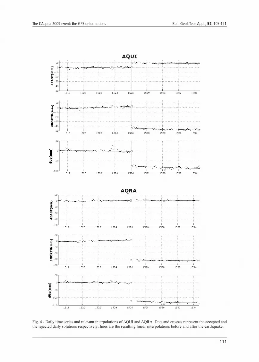
Fig. 4 - Daily time series and relevant interpolations of AQUI and AQRA. Dots and crosses represent the accepted andthe rejected daily solutions respectively; lines are the resulting linear interpolations before and after the earthquake.

112


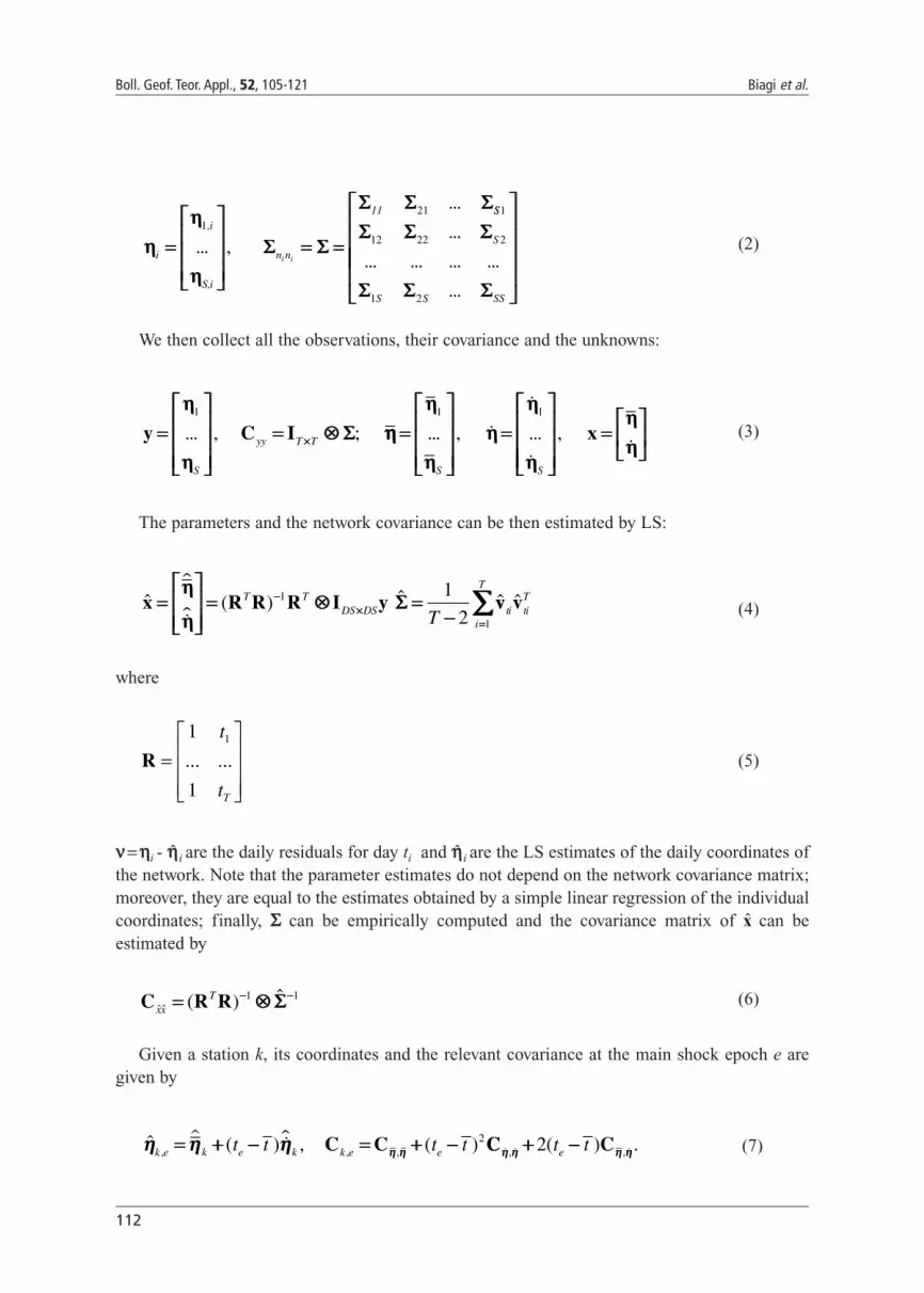
(2)

We then collect all the observations, their covariance and the unknowns:

(3)

The parameters and the network covariance can be then estimated by LS:

(4)

where

(5)

νν = ηηi - ηη̂i are the daily residuals for day ti and ηη̂i are the LS estimates of the daily coordinates ofthe network. Note that the parameter estimates do not depend on the network covariance matrix;moreover, they are equal to the estimates obtained by a simple linear regression of the individualcoordinates; finally, ΣΣ can be empirically computed and the covariance matrix of x̂ can beestimated by

(6)

Given a station k, its coordinates and the relevant covariance at the main shock epoch e aregiven by

(7) ˆ ( ) , ( ), , ,ηη ηη ηη ηη ηηk e k e k k e et t t t== ++ −− == ++ −−� �� C C 2CC C� � �ηη ηη ηη ηη, ,( ) .++ −−2 t te

C R Rˆˆ ( ) ˆxx

T== ⊗⊗−− −−1 1ΣΣ

R =⎡

⎣

⎢⎢⎢

⎤

⎦

⎥⎥⎥

1

1

1t

tT

... ...

ˆ ( ) ˆ ˆx R R R I y==⎡⎡

⎣⎣⎢⎢⎢⎢

⎤⎤

⎦⎦⎥⎥⎥⎥

== ⊗⊗ ==−−

−−××

ηη

ηη

�

��T T

DS DS T1 1

2ΣΣ vv vti ti

T

i

T

ˆ==∑∑

1

y C I==⎡⎡

⎣⎣

⎢⎢⎢⎢⎢⎢

⎤⎤

⎦⎦

⎥⎥⎥⎥⎥⎥

== ⊗⊗××

ηη

ηη

1

... , ;

S

yy T T ΣΣ ηηηηηη

ηηηη

ηη

ηη==

⎡⎡

⎣⎣

⎢⎢⎢⎢⎢⎢

⎤⎤

⎦⎦

⎥⎥⎥⎥⎥⎥

==⎡⎡

⎣⎣

⎢⎢⎢⎢

1 1

... , ...

S S

��

�⎢⎢⎢⎢

⎤⎤

⎦⎦

⎥⎥⎥⎥⎥⎥

==⎡⎡

⎣⎣⎢⎢

⎤⎤

⎦⎦⎥⎥, x

ηηηη�

ηηηη

ηηi n n==

⎡⎡

⎣⎣

⎢⎢⎢⎢⎢⎢

⎤⎤

⎦⎦

⎥⎥⎥⎥⎥⎥

== ==1

21,i

S,i

11

i i... ,

...

ΣΣ ΣΣ

ΣΣ ΣΣ ΣΣSS

S

S S SS

1

12 22 2

1 2

ΣΣ ΣΣ ΣΣ

ΣΣ ΣΣ ΣΣ

...

... ... ... ...

...

⎡⎡

⎣⎣

⎢⎢⎢⎢⎢⎢⎢⎢⎢⎢

⎤⎤

⎦⎦

⎥⎥⎥⎥⎥⎥⎥⎥

113


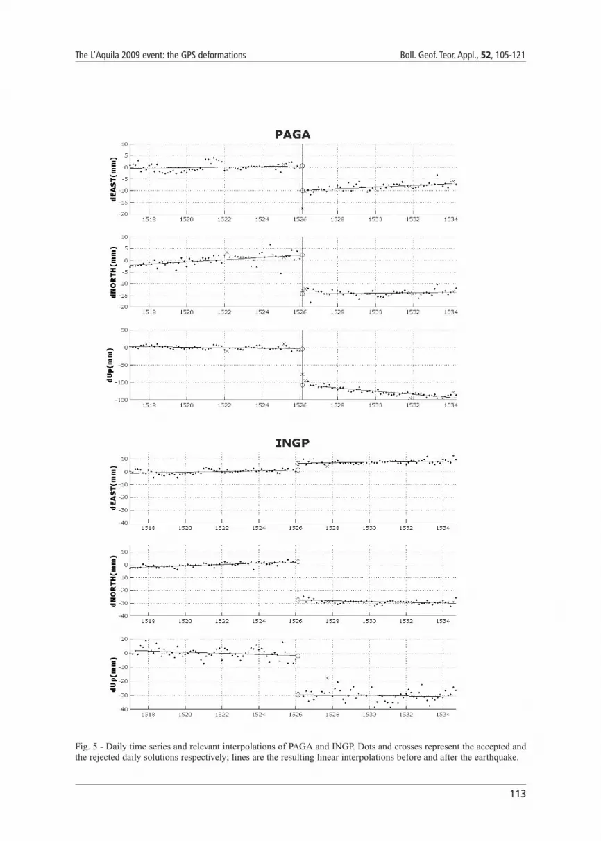
Fig. 5 - Daily time series and relevant interpolations of PAGA and INGP. Dots and crosses represent the accepted andthe rejected daily solutions respectively; lines are the resulting linear interpolations before and after the earthquake.

114


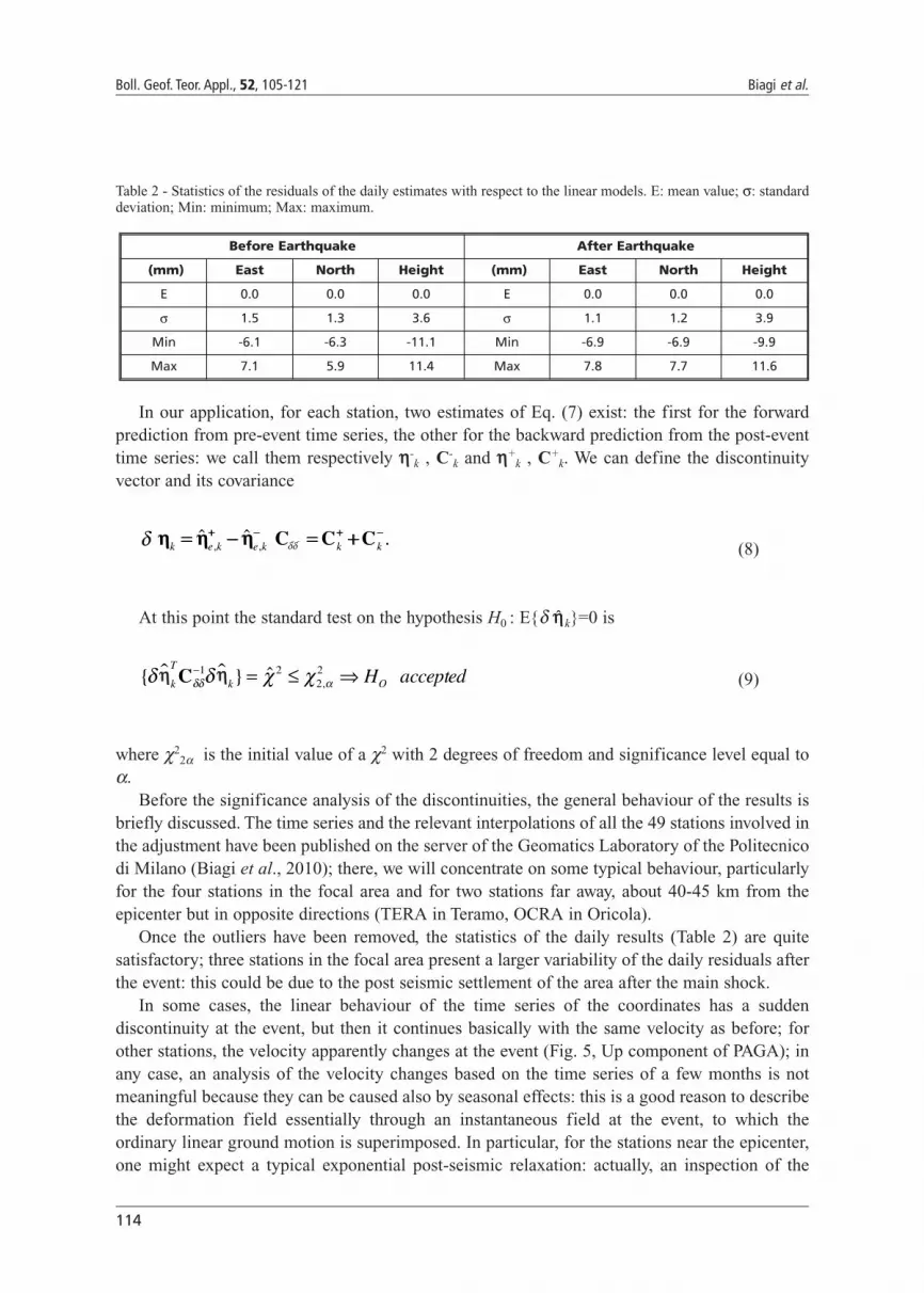
In our application, for each station, two estimates of Eq. (7) exist: the first for the forwardprediction from pre-event time series, the other for the backward prediction from the post-eventtime series: we call them respectively ηη-

k , C-k and ηη+

k , C+k. We can define the discontinuity

vector and its covariance

(8)

At this point the standard test on the hypothesis H0 : E{δ ηη̂k}=0 is

(9)

where χ22α is the initial value of a χ2 with 2 degrees of freedom and significance level equal to

α. Before the significance analysis of the discontinuities, the general behaviour of the results is

briefly discussed. The time series and the relevant interpolations of all the 49 stations involved inthe adjustment have been published on the server of the Geomatics Laboratory of the Politecnicodi Milano (Biagi et al., 2010); there, we will concentrate on some typical behaviour, particularlyfor the four stations in the focal area and for two stations far away, about 40-45 km from theepicenter but in opposite directions (TERA in Teramo, OCRA in Oricola).

Once the outliers have been removed, the statistics of the daily results (Table 2) are quitesatisfactory; three stations in the focal area present a larger variability of the daily residuals afterthe event: this could be due to the post seismic settlement of the area after the main shock.

In some cases, the linear behaviour of the time series of the coordinates has a suddendiscontinuity at the event, but then it continues basically with the same velocity as before; forother stations, the velocity apparently changes at the event (Fig. 5, Up component of PAGA); inany case, an analysis of the velocity changes based on the time series of a few months is notmeaningful because they can be caused also by seasonal effects: this is a good reason to describethe deformation field essentially through an instantaneous field at the event, to which theordinary linear ground motion is superimposed. In particular, for the stations near the epicenter,one might expect a typical exponential post-seismic relaxation: actually, an inspection of the

{ } ˆ,δη δη χ χδδ α

� �k

T

k OH acceptedC− = ≤ ⇒1 222

δη η η δδk e k e k k k= − = ++ − + −� �, , C C C

Before Earthquake After Earthquake

(mm) East North Height (mm) East North Height

E 0.0 0.0 0.0 E 0.0 0.0 0.0

σ 1.5 1.3 3.6 σ 1.1 1.2 3.9

Min -6.1 -6.3 -11.1 Min -6.9 -6.9 -9.9

Max 7.1 5.9 11.4 Max 7.8 7.7 11.6

Table 2 - Statistics of the residuals of the daily estimates with respect to the linear models. E: mean value; σ: standarddeviation; Min: minimum; Max: maximum.

ηη ηη ηη δδδδk e k e k k k== −− == ++++ −− ++ −−ˆ ˆ ., , C C Cδδ

ηη ηη

115


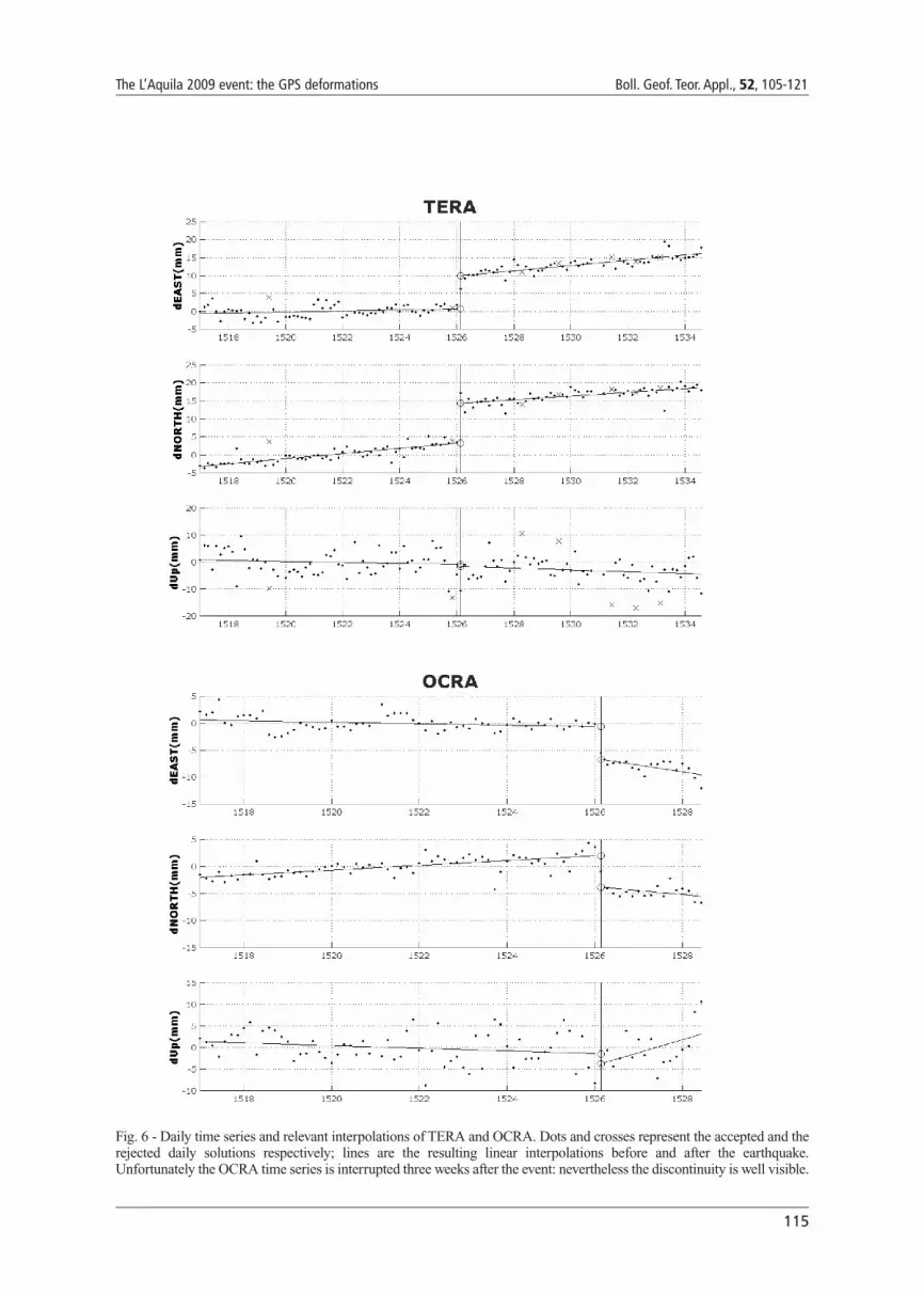
Fig. 6 - Daily time series and relevant interpolations of TERA and OCRA. Dots and crosses represent the accepted and therejected daily solutions respectively; lines are the resulting linear interpolations before and after the earthquake.Unfortunately the OCRA time series is interrupted three weeks after the event: nevertheless the discontinuity is well visible.

116


residuals of the linear interpolation reveals that this phenomenon is present in two stations of theepicentral area. In AQUI (Fig. 4), an exponential behaviour appears in the north component, withan amplitude of about 6 mm and a time constant of 1~2 days; some relaxation, but not a clearexponential signal, could be present in the Up component. In PAGA (Fig. 5), the Up shows a clearexponential, with amplitude of 10 mm and time constant of 2 days; the east component shows aresidual of 8 mm the first day after the main shock, but not a correlated pattern for the followingdays; the north residuals are correlated, but do not show an exponential behaviour. The other twosites near the epicenter (AQRA and INGP) show irregularities but not a clear relaxation. Therigorous analysis of long term relaxations requires the separation between any possible seasonaleffect, a long term exponential and the linear trend: it will be possible when time series longerthan one year after the event are available.

In the following discontinuity analysis, we have decided to separate the horizontal and thevertical analysis, because their spatial behaviours are very different (compare Figs. 7 and 8). Asthe horizontal discontinuities are concerned, the stations that significantly displace, and therelevant displacements, are reported in Table 3. A totally equivalent, but graphically more

Fig. 7 - Horizontal displacements of the local network stations. The gray ellipses depict the 99% confidence regions ofthe vectors; the dotted segment roughly highlights the main discontinuity line in the horizontal displacements field.The names of the stations that significantly displace are reported.

117


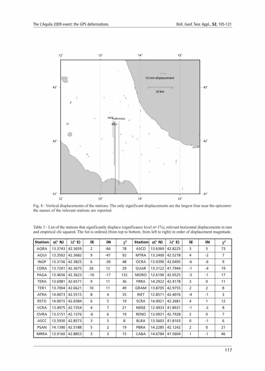
Fig. 8 - Vertical displacements of the stations. The only significant displacements are the largest four near the epicenter:the names of the relevant stations are reported.

Station ϕ(° N) λ(° E) δE δN χ2 Station ϕ(° N) λ(° E) δE δN χ2

AQRA 13.3743 42.3659 2 -66 78 ASCO 13.6369 42.8225 3 5 73

AQUI 13.3502 42.3682 9 -47 92 MTRA 13.2400 42.5278 4 -2 7

INGP 13.3156 42.3825 6 -30 48 OCRA 13.0390 42.0495 -6 -6 9

CDRA 13.7201 42.3675 26 12 29 GUAR 13.3122 41.7944 -1 -4 19

PAGA 13.4656 42.3623 -10 -17 132 MORO 12.6190 42.0525 -3 -1 17

TERA 13.6981 42.6571 9 11 36 FRRA 14.2922 42.4178 3 0 11

TER1 13.7004 42.6621 10 11 49 GRAM 13.8705 42.9755 2 2 8

ATRA 14.0073 42.5515 8 4 35 RIET 12.8571 42.4076 -4 -1 3

RSTO 14.0015 42.6584 6 5 19 SCRA 14.0021 42.2681 4 1 12

VCRA 13.4975 42.7354 4 7 21 M0SE 12.4933 41.8931 -1 -2 8

OVRA 13.5151 42.1376 -6 6 19 RENO 13.0931 42.7928 2 0 7

ASCC 13.5930 42.8573 3 5 8 BLRA 13.5603 41.8103 0 -1 6

PSAN 14.1390 42.5188 5 2 19 PBRA 14.2285 42.1242 2 0 21

MRRA 13.9160 42.8853 3 3 15 CABA 14.6784 41.5604 1 -1 46

Table 3 - List of the stations that significantly displace (significance level α=1%), relevant horizontal displacements in mmand empirical chi squared. The list is ordered (from top to bottom, from left to right) in order of displacement magnitude.

118


readable representation of the test of Eq. (9), is to draw the confidence region around theobserved discontinuity δ ηη̂k, behaving a probability 1−α; when this region includes the originof δ ηη̂k, the jump is not significant, otherwise it is: the results can be seen in Fig. 7. The signatureof the displacements near the epicenter is quite clear: PAGA moves SW, while the other threestations are displaced basically southwards. If we move from the epicenter for about 40 km SW,we find, for instance, OCRA while at a slightly larger distance northeast, 47 km, we meet TERA.These two stations have a nicely opposite behaviour: OCRA moves by about 0.9 cm SW whileTERA moves about 1.5 cm NE (Fig. 6). This behaviour seems to be quite systematic, and we candraw a line across which the horizontal displacement field undergoes a sharp discontinuity (Figs.7 and 9); just two stations show different motion trends with respect to the surrounding ones; thefirst is about 25 km north from the epicenter (MTRA), the second (OVRA) is at the same distancein the south direction. Of course there is no pretence of accuracy in the design of the abovesegment, yet we observe that its direction and position appear to be consistent with the faultingsystem in the area (Serpelloni et al., 2005; Anzidei et al., 2009).

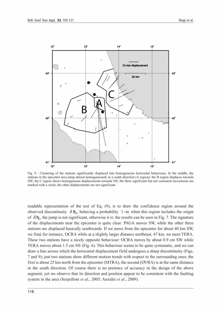
Fig. 9 - Clustering of the stations significantly displaced into homogeneous horizontal behaviours. In the middle, thestations in the epicenter area jump almost homogeneously in a south direction (A region); the B region displaces towardsSW; the C region shows homogeneous displacements towards NE; the three significant but not consistent movements aremarked with a circle; the other displacements are not significant.

119


A rigorous significance analysis could be repeated for the displacements in the verticaldiscontinuities; in any case, as Fig. 8 clearly shows, the visual analysis by itself allows us toidentify the four stations, all those near the epicenter, that significantly displace in the Upcomponent: INGP (-2.7 cm), AQUI (-7.3 cm), PAGA (-10.4 cm) and AQRA (-11.9 cm); no othersignificant vertical motions occur, with a range between -3 mm and 3 mm.

4. Spatial analysis of the displacements

The object of this section is the spatial analysis of the instantaneous displacement field, asreconstructed from the discontinuities in the individual time series.

The ground displacements (Fig. 7) clearly show a discontinuous behaviour and not a spatialsmooth pattern: a preliminary cluster analysis is required to define at least the subregions with aconsistent internal pattern. In this way, as far the horizontal displacements (with the exception ofMTRA and OVRA, mentioned in Sect. 3, and RENO, less evident) we have found 3 mainsubregions that could be characterized in the following way (Fig. 8):

- the focal region (A region), where three stations (AQRA, AQUI and INGP) show an intensemotion towards south (20-70 mm), one station (PAGA) experiences a SW motion of about20 mm;

- the SW region (B region), where at least 6 stations experience a moderate but significantSW motion (up to 30 mm); only OVRA displaces toward NW, by about 9 mm;

- the NE region (C region), where at least 14 stations experience a moderate but significantNE motion (up to 30 mm).

The results are similar to those found by Anzidei et al. (2009), Atzori et al. (2009) and Cheloniet al. (2010); in particular, in their works, detailed discussions and geophysical interpretations ofthe dynamics in the near field A region are provided.

In both B and C subregions, the number of stations is always too small to allow a consistentprediction of the inner displacement field, based on the analysis of the spatial covariance. Oneremark is that apparently the diameter of the B region is smaller than that of the C region, whichis reaching the sea and where the jump vector undergoes a rotation from NE to E while we movethe application point from north to south. From Fig. 9, we see clearly that outside the region ofsignificant movements, there is a belt where the displacement vectors are still coherent as fortheir directions, although the amplitude of the vector is too small to be significant. In any case,our results confirm the already known (see for example: D'Agostino et al., 2008; Devoti et al.,2008) SW-NE extension phenomena that interest the Apennines. As far the vertical movementsare concerned, no real clustering is possible because in front of a very intense fall of the stationsin the focal area no significant vertical motions can be found anywhere else.

5. Conclusions

A first conclusion can be drawn on the kinematics of the event; in particular, our results aresummarized in the following 4 points.

1. The most intense displacement is a vertical fall of the focal area of about 10 cm; no othersignificant vertical motion is present.

120


2. This is accompanied by a movement, mainly to the south of the four stations in the focalarea, which propagates into a SW pattern, in the neighbouring SW district, fading out at about 50km; OVRA, near the epicenter, is an exception and moves NW-wards.

3. Immediately over the focal area, in the north-eastern district, a NE displacement is presentand remains significant in the Adriatic coastal region up to a distance of about 80 km.

4. The kinematics of the stations appear to be linear with a good approximation and, inparticular, the velocities seem to continue with no significant change across the event epoch; fewexceptions are present in the stations near the main shock; small relaxations are visible but deeperanalyses will be possible only with longer time series.

Basically, our results confirm the main shock displacements obtained by other groups andquoted in the references: the complete time series and the graphs of all the stations are freelyavailable on line.

Acknowledgments. This research was supported by the "Galileo and the modernized satellite positioning"Italian PRIN 2006 project and by the “The new Italian geodetic reference frame: continuous monitoringand use in environment management” Italian PRIN 2008 project. The preliminary results were presentedorally at the EUREF2009 and ASITA2009 symposia. The corrections and the suggestions of the twoanonymous reviewers really helped to improve the quality of the paper.

REFERENCESAltamimi Z., Collilieux X., Legrand J., Garayt B. and Boucher C.; 2007: ITRF2005: a new release of the International

Terrestrial Reference Frame based on time series of station positions and Earth Orientation Parameters. J.Geophys. Res., 112, B09401, doi:10.1029/2007JB00494.

Anzidei M., Boschi E., Cannelli V., Devoti R., Esposito A., Galvani A., Melini D., Pietrantonio G., Riguzzi F., Sepe V.and Serpelloni E.; 2009: Coseismic deformation of the destructive April 6, 2009 L’Aquila earthquake (central Italy)from GPS data. Geophys. Res. Lett., 36, L17307.

Atzori S., Hunstad I., Chini M., Salvi S., Tolomei C., Bignami C., Stramondo S., Trasatti E., Antonioli A. and BoschiE.; 2009: Finite fault inversion of DinSAR coseismic displacement of the 2009 L'Aquila earthquake (central Italy).Geophys. Res. Lett., 36, L15305.

Avallone A., Selvaggi G., D'Anastasio E., D'Agostino N., Pietrantonio G., Riguzzi F., Serpelloni E., Anzidei M., CasulaG., Cecere G., D'Ambrosio C., De Martino P., Devoti R., Falco L., Mattia M., Rossi M., Obrizzo F., Tammaro U.and Zarrilli L.; 2010: The RING network: improvements to a GPS velocity field in the central Mediterranean.Annales of Geophysics, 53, 39-64, doi:10.4402/ag-4549.

Barzaghi R., Borghi A., Crespi M., Pietrantonio G. and Riguzzi F.; 2004: GPS Permanent network solution: the impactof temporal correlations. In: V Hotine-Marussi Symposium on Mathematical Geodesy, International Associationof Geodesy Symposia, vol. 127, Springer.

Benciolini B., Biagi L., Crespi M., Manzino A. and Roggero M.; 2008: Reference frames for GNSS positioningservices: some problems and proposals. J. Appl. Geodesy, 2, 53-62.

Biagi L. and Dermanis A.; 2006: The treatment of time continuous GPS observations for the determination of regionaldeformation parameters. In: ISDGM Proceedings, IAG Symposia, Springer-Verlag. 131, pp. 83-94.

Biagi L., Caldera S., Dominici D. and Sansò F.; 2010: Detailed report relevant to the paper The L’Aquila 2009 event:the GPS displacements. http://geomatica.como.polimi.it/prin/2008/.

Blewitt G. and Lavallée D.: 2002: Effects of annual signals on geodetic velocity. J. Geophys. Res., 107, 2145-2155.

Cheloni D., D'Agostino N., D'Anastasio E., Avallone A., Mantenuto S., Giuliani R., Mattone M., Calcaterra S.,Gambino P., Dominici D., Radicioni F. and Fastellini G.; 2010: Coseismic and initial post seismic slip of the 2009Mw 6.3 L'Aquila earthquake, Italy, from GPS measurements. Geophys. J. Int., 181, 1539-1546.

Dach R., Hugentobler U., Fridez P. and Meindl M.; 2007: Bernese GPS Software Version 5.0. Astronomical Institute,University of Berne.

121


D'Agostino N., Avallone A., Cheloni D., D'Anastasio E., Mantenuto S. and Selvaggi G.; 2008: Active tectonics of theAdriatic region from GPS and earthquake slip vectors. J. Geophys. Res., 113, B12413, doi:10.1029/2008JB005860.

Devoti R., Riguzzi F., Cuffaro M. and Doglioni C.; 2008: New GPS constraints on the kinematics of the Apenninessubductions. Earth Planet Sci. Lett., 273, 163-274.

EMERGEO Working Group; 2009: Field geological survey in the epicentral area of the Abruzzi (central Italy) seismicsequence of April 6th, 2009. Quaderni di Geofisica, vol. 70, Ist. Naz. di Geofis. e Vulcanol, 79 pp.

Ferland R.; 2006: IGSMail 5447. http://igscb.jpl.nasa.gov/mail/igsmail/.

Ferland R., Gendt G. and Schone T.; 2004: IGS reference frame maintenance. Proceedings of IGS: Celebrating a decadeof the International GPS Service, Berne, March 1-5, 2004, AIUB, Berne.

Ferretti A., Prati C. and Rocca F.; 2001: Permanent scatterers in SAR interferometry. IEEE T. Geoscience Remote, 39,8-20.

Hanssen R.; 2001: Radar Interferometry. Kluwer Academic Publishers, Dordrecht, The Nederlands, 328 pp.

INGV; 2009: The L’Aquila seismic sequence. Ist. Naz. di Geofisica e Vulcanologia, Rome. //portale.ingv.it/.

Koch K.R.; 1987: Parameter estimation and hypothesis testing in linear models. Springer Verlag.

Kouba J.; 2003: A guide to using International GPS Service (IGS) products.ftp://igscb.jpl.nasa.gov/igscb/resource/pubs/GuidetoUsingIGSProducts.pdf.

Okada Y.; 1985: Surface deformation due to shear and tensile faults a a half space. Bull. Seism. Soc. Am., 75, 1135-1154.

Ray J., Altamimi Z., Collilieux X. and Van Dam T.; 2008: Anomalous harmonics in the spectra of GPS positionestimates. GPS Solutions, 12, 55–64.

Serpelloni E., Anzidei M., Baldi P., Casula G. and Galvani A.; 2005: Crustal velocity and strain-rate fields in Italy andsurrounding regions: new results from the analysis of permanent and non-permanent GPS networks. Geophys. J.Int., 161, 861-880.

Vespe F., Bianco G., Fermi M., Ferraro C., Nardi A. and Sciarretta C.; 2000: The Italian Fiducial network: services andproducts. J. Geodynamics, 30, 327-336.

Corresponding author: Ludovico Biagi Politecnico di Milano - DIIARc/o Polo Regionale di ComoVia Valleggio 11, 22100 Como, ItalyPhone: +39 031 3327562; fax: +39 031 3327519; e-mail: [email protected]

Documents

The L'Aquila 2009 event: :the GPS deformations