arX

iv:m

ath/

0103

103v

2 [

mat

h.D

G]

14

Apr

200

1

Contractions: Nijenhuis and Saletan tensors for

general algebraic structures

Jose F. Carinena

Departamento de Fısica Teorica, Univ. de Zaragoza50.009 Zaragoza, Spain

e-mail: jfc@posta.unizar.es

Janusz Grabowski∗

Institute of Mathematics, Warsaw University

ul. Banacha 2, 02-097 Warszawa, Poland.and

Mathematical Institute, Polish Academy of Sciences

ul. Sniadeckich 8, P. O. Box 137, 00-950 Warszawa, Polande-mail: jagrab@mimuw.edu.pl

Giuseppe Marmo†

Dipartimento di Scienze Fisiche, Universita Federico II di Napoli

andINFN, Sezione di Napoli

Complesso Universitario di Monte Sant’AngeloVia Cintia, 80126 Napoli, Italy

e-mail: marmo@na.infn.it

October 28, 2013

Abstract

In this note we study generalizations in many directions of the contractionprocedure for Lie algebras introduced by Saletan [Sa]. We consider productsof arbitrary nature, not necessarily Lie brackets, and we generalize to infinitedimension, considering a modification of the approach by Nijenhuis tensors tobilinear operations on sections of finite-dimensional vector bundles. We applyour general procedure to Lie algebras, Lie algebroids, and Poisson brackets. Wepresent also results on contractions of n-ary products and coproducts.

∗Supported by KBN, grant No. 2 P03A 031 17.†Supported by PRIN SINTESI.

1

1 Introduction

For a general (real) topological algebra, i.e., a topological vector space A over R (butother topological fields, like C, can be considered in a similar way as well) with acontinuous bilinear operation

µ : A×A → A, (X, Y ) 7→ X ∗ Y, (1)

one considers contraction procedures as follows.If U(λ) : A → A is a family of linear morphisms which continuously depends on the

parameter λ ∈ R from a neighbourhood U of 0 and U(λ) are invertible for λ ∈ U \ 0,then we can consider the continuous family of products X ∗λ Y defined by

X ∗λ Y = U(λ)−1(U(λ)(X) ∗ U(λ)(Y )), (2)

for λ ∈ U \ 0. All these products are isomorphic by definition, since

U(λ)(X ∗λ Y ) = U(λ)(X) ∗ U(λ)(Y ) (3)

and if N = U(0) is invertible, then clearly

limλ→0

X ∗λ Y = N−1(N(X) ∗ N(Y )). (4)

But sometimes, the limit limλ→0 X ∗λ Y may exist for all X, Y ∈ A even if N is notinvertible and (4) does not make sense. We say then that limλ→0 X ∗λ Y is a contractionof the product X∗Y . Of course, the problem of existence and the form of the contractedproduct heavily depends on the family U(λ). In [Sa] this problem has been solved forlinear families U(λ) = λ I + N and A – a finite-dimensional Lie algebra.

Here we study generalizations in various directions of the contraction procedureintroduced by Saletan [Sa]. First of all, we consider products of arbitrary nature, notnecessarily Lie brackets. Second, we generalize to infinite dimension, considering amodification of the approach by Nijenhuis tensors to bilinear operations on sections offinite-dimensional vector bundles. The motivation stems from physics, since infinite-dimensional algebras of sections of some bundles arise frequently as models both inClassical and Quantum Physics. In particular, we were confronted with this problemwithin the framework of Quantum Bihamiltonian Systems [CGM]. According to Dirac[Di], a ”quantum Poisson bracket” necessarily arises from the associative product onthe space of operators. Similarly, by Ado’s theorem, any finite-dimensional Lie algebraarises as an algebra of matrices. It is therefore quite natural to investigate contractionsof associative algebras along with contractions of Lie algebras and their generalizationsto Lie algebroids. We concentrate mainly on smooth sections, but this particular choiceplays no definite role in our approach.

The paper is organized as follows. In the next section we present the general schemewe are working with and the main result (Theorem 2) on contractions for algebras ofsections of vector bundles. We make some remarks on contractions with respect tomore general linear families U(λ) = λ A + N .

Section 3 is devoted to examples and Section 4 to more detailed studies of hierarchiesof contractions. We develop an algebraic technique which allows us to produce muchsimpler proofs of facts about hierarchies than those available in the literature.

2

In Section 5 we comment on the behaviour of algebraic properties under contractions.Contractions of Lie algebras and Lie algebroids, as particular cases of our general

procedure, are studied in Sections 6 and 7.In Section 8 we use our knowledge on contractions of Lie algebroids to define con-

tractions of Poisson structures. The approach is very natural and leads to structuresvery similar (but slightly different) to those which are known under the name of Poisson-Nijenhuis structures (cf. [MM, KSM]).

We end up with observations on contractions of n-ary products and coproducts.

2 Linear contractions of products on sections of vec-

tor bundles

Let us assume that E is a smooth vector bundle with fibers of dimension n0, over asmooth manifold M . Denote by ∗ a bilinear operation µ : A×A → A,

µ : (X, Y ) ∈ A⊗A 7→ X ∗ Y ∈ A ,

on the space of smooth sections of E which is, at least point-wise, continuous. Inpractice, we shall deal with local products, therefore being defined by bilinear differentialoperators. We shall use both notations for the product according to which one is moreconvenient when treating particular cases.

Let N : E → E be a smooth vector bundle morphism over idM . One refers also to Nas to a (1,1)–tensor field, i.e., a section of E∗⊗E. Since Np : Ep → Ep is a morphism ofthe finite-dimensional vector space Ep, where Ep denotes the fiber over the point p ∈ M ,we have the Riesz decomposition Ep = E1

p ⊕ E2p into invariant subspaces of Np in such

a way that Np is invertible on E1p and nilpotent of order q on E2

p , i.e., N q(Xp) = 0,

for Xp ∈ E2p . One can take E1

p = Np(Ep), E2p = ker Np, where Np = (Np)

n0 , withn0 = dim Ep. In this way we get the decomposition E = E1 ⊕ E2 of the vector bundleE into two supplementary generalized distributions. Note that the dimension of E1

p

may vary from point to point. Nevertheless, E1 is a smooth distribution, i.e., it isgenerated locally by a finite number of smooth sections of E. Indeed, if e1, . . . , en0

is

a local basis of smooth sections of E, then N(e1), . . . , N(en0) is a set of local smooth

sections generating locally E1.

Theorem 1 The (generalized) distribution E2 is smooth if and only if it is regular,i.e., of constant rank: dim E2

p = const.

Proof.- Since the rank of a smooth distribution is semi-continuous from above:

limp→p0

inf dim E2p ≥ dim E2

p0, (5)

and the complementary distribution E1 is smooth, so that

limp→p0

sup dim E2p ≤ dim E2

p0, (6)

we see that both conditions (5) and (6) are satisfied if and only if E2 is of constantrank.

3

Conversely, if E2 is of constant rank, say n0 − l, take a basis e1, . . . , en0 of

smooth local sections of E such that the elements of N(e1), . . . , N(el) span E1p . Then

N(e1), . . . , N(el) is a basis of local sections of E1 near p ∈ M . Write

N(ei) =l∑

j=1

fij N(ej) .

Then the functions fij are smooth and the smooth sections

ei = ei −

l∑

j=1

fij ej , i = l + 1, . . . , n0 ,

span locally E2. Indeed, N(ei) = 0 and the elements ei, for i = l+1, . . . , n0, are linearlyindependent.

Note that in general no one of the distributions E1 and E2 has to be “involutive”in the sense that smooth sections of E1 (resp. E2) are closed with respect to thecomposition law ∗.

Consider now a new (1,1)-tensor U(λ) = λ I + N depending on a real parameter λ.Since the spectrum of N is finite and continuously depends on p, in a sufficiently smallneighbourhood of p all of U(λ)p are invertible for sufficiently small λ, but λ 6= 0. Thus,we can locally define, for λ 6= 0, a new operation

X ∗λN Y = U(λ)−1(U(λ)(X) ∗ U(λ)(Y ))

= U(λ)−1((λ X + N(X)) ∗ (λ Y + N(Y )))= U(λ)−1(λ2 X ∗ Y + λ (N(X) ∗ Y + X ∗ N(Y )) + N(X) ∗ N(Y )) . (7)

We would like to find conditions assuring that the limit

X ∗N Y = limλ→0

X ∗λN Y

exists for all X, Y ∈ A and find the corresponding contraction X ∗N Y .Using the identity U(λ)−1(λ I + N) = I, i.e.,

U(λ)−1(λ X) = X − U(λ)−1N(X) ,

we get from (7) that

X ∗λN Y = λ X ∗ Y + (N(X) ∗ Y + X ∗ N(Y ) − N(X ∗ Y ))

+ U(λ)−1(N(X) ∗ N(Y ) − N(N(X) ∗ Y + X ∗ N(Y ) − N(X ∗ Y ))) . (8)

Denoting

δNµ(X, Y ) = X ∗NY = N(X) ∗ Y + X ∗ N(Y ) − N(X ∗ Y ) ,

and by TNµ(X, Y ) – the Nijenhuis torsion of N:

TNµ(X, Y ) = N(X) ∗ N(Y ) − N(X ∗NY ) ,

4

we can rewrite (8) in the form

X ∗λN Y = λ X ∗ Y + X ∗NY + U(λ)−1TNµ(X, Y ) .

Hence, the limitlimλ→0

X ∗λN Y

exists if and only if

limλ→0

U(λ)−1TNµ(X, Y ) exists for every X, Y ∈ A . (9)

Denote by A1, A2, the spaces of smooth sections of E1 and E2, respectively. Ofcourse, in general A 6= A1 ⊕ A2. We may have A2 = 0 even in the case E2 6= 0.Since E1 and E2 are invariant distributions of U(λ), hence of U(λ)−1, the existence ofthe limit (9) may be checked separately on the corresponding parts of TNµ. On E2 thetensor N is nilpotent, so for Xp ∈ E2

p ,

(λ I + N)−1p (Xp) = (λ(I − (−N/λ)))−1

p (Xp) =1

λ

∞∑

n=0

(−

1

λ

)n

Nnp (Xp) , (10)

where the sum is in fact finite, and

limλ→0

q−1∑

n=0

(−1)n

λn+1Nn

p (Xp)

exists if and only if Xp = 0. Thus, a necessary condition for existence of the limit (9)is that TNµ(X, Y ) ∈ A1 for every X, Y ∈ A.

Since on E1 the tensor N is invertible, we have clearly

limλ→0

(λ I + N)−1 = N−1

on E1, so that, assuming TNµ(X, Y ) ∈ A1,

limλ→0

U(λ)−1TNµ(X, Y ) = N−1TNµ(X, Y ) = τNµ(X, Y ) .

Here τNµ(X, Y ) = N−1TNµ(X, Y ) is the unique section of E1 determined by the con-dition

N(τNµ(X, Y )) = TNµ(X, Y ) .

In order to get a new product on A we have to assume that τNµ(X, Y ) is smooth, whichis a priori not automatic, even if we have TNµ(X, Y ) ∈ A1. Note that if N is regular,i.e., E1 is of constant dimension, then, as we shall show in Theorem 3, N(A1) = A1

and τNµ(X, Y ) is smooth automatically.Let us summarize the above as follows:

Theorem 2 Let µ : A×A → A be a point-wise continuous bilinear product of smoothsections of a vector bundle E over a manifold M (we will write also X ∗ Y instead ofµ(X, Y )) and let N : E → E be a smooth (1,1)–tensor. Denote by U(λ) = λ I + N a

5

deformation of N , by E = E1 ⊕E2 the Riesz decomposition of E relative to N , and byA1 the set of smooth sections of E1. Then, the limit

limλ→0

U(λ)−1(U(λ)(X) ∗ U(λ)(Y ))

exists for all X, Y ∈ A and defines a new (contracted) bilinear operation

DNµ(X, Y ) = X ∗N Y

on A if and only if the Nijenhuis torsion

TNµ(X, Y ) = N(X) ∗ N(Y ) − N(N(X) ∗ Y + X ∗ N(Y )) + N2(X ∗ Y )

takes values in N(A1). If this is the case, then

X ∗N Y = X ∗NY + τNµ(X, Y ) , (11)

where X ∗NY is a new bilinear operation δNµ on A defined by

δNµ = X ∗NY = N(X) ∗ Y + X ∗ N(Y ) − N(X ∗ Y ) ,

and τNµ(X, Y ) = N−1TNµ(X, Y ) is the unique section of A1 such that

N(τNµ(X, Y )) = TNµ(X, Y ) .

Moreover, N constitutes a homomorphism of (A, µN) into (A, µ):

N(X ∗N Y ) = N(X) ∗ N(Y ) .

Remark. Let us note that our procedure is not just applying the finite–dimensionallinear one to every fiber, since the operation ∗ need not act fiber-wise. Also, this is notdirect application to infinite–dimensional algebra A, since we have not, in general, theRiesz decomposition A = A1 ⊕ A2 with respect to N . On the other hand, the wholeprocedure can be applied directly to infinite-dimensional cases for which we are giventhe Riesz decomposition of N .

Definition 1 The tensor N satisfying the assumptions of Theorem 2, i.e., such thatTNµ takes values in N(A1), will be called a Saletan tensor. If Nk is a Saletan tensor forevery k = 1, 2, 3, . . ., then N will be called a strong Saletan tensor. In the case TNµ = 0we shall call N a Nijenhuis tensor.

Remark. It is obvious from the proof of Theorem 2 that Nijenhuis tensors definecontractions even in the case of infinite-dimensional algebras A without any assumptionthat A consists of sections of a finite-dimensional vector bundle. Indeed, with TNµ = 0we have no obstructions, the Riesz decomposition is irrelevant, and X ∗N Y = X ∗NY .Of course,

(Nijenhuis) ⇒ (strong Saletan) ⇒ (Saletan).We shall call N regular, if E1 (hence also E2) is of constant rank. This is always thecase when E is a bundle over a single point, i.e., E = A.

6

Theorem 3 In the regular case, i.e., when E1 is of constant rank, N(A1) = A1, sothat N is a Saletan tensor if and only if TNµ(X, Y ) takes values in A1.

Remark. We shall prove a stronger result in Theorem 6.Proof.- Indeed, according to Theorem 1, both E1 and E2 are smooth distributions.Locally we have a basis of smooth sections of E1, and N acts on this basis as invertiblematrix of smooth functions. Indeed, since regularity of E1 implies that there is a localbasis e1, . . . , el of sections of E1, in this basis N acts simply as invertible matrix ofsmooth functions (fij), so for X =

∑gi ei,

N

(l∑

i=1

hi ei

)= X,

where the smooth functions hi are defined by

l∑

j=1

fij hj = gi .

Hence, N−1(X) is locally, thus globally, smooth section of E1 for any smooth sectionX of E1.

Remark. For a fiber bundle over a single point Theorem 2 gives exactly the Saletanresult [Sa] in case µ is a Lie bracket. Saletan writes X ∗N Y in the form

X ∗N Y = (X ∗NY )2 + N−1 ((N(X) ∗ N(Y ))1) , (12)

where X = X1 + X2 is the decomposition of X ∈ A into sections of E1 and E2. Ofcourse, (12) is formally the same as (11) for the decomposition into sections of E1 andE2. However, in general the summands of the right hand side of (12) are not smooth,while the decomposition (11) is into smooth parts. In the regular case both formulaecoincide.

Theorem 4 (a) Theorem 2 remains valid when we consider the family U(λ) in aslightly more general form: U(λ) = λ I + f(λ) N , where f is continuous and f(0) = 1.

(b) If we consider instead of U(λ) the family U1(λ) = λA + N , then the contractionprocedure for U1(λ) and the product ∗ is equivalent to the contraction procedure of theabove type for a new N and a new product. In particular, if A is invertible, we get ourstandard contraction for A−1N and the product X ∗A Y = A−1(A(X) ∗A(Y )). In otherwords, the contraction procedure for the family U1(λ) = λ A + N can be reduced to thecontraction described in Theorem 2.

Proof.-(a) Let us write U(λ) = U1(ε)

f(λ), where U1(ε) = ε I + N and ε = λ

f(λ), so that λ → 0 is

equivalent to ε → 0. Since

U(λ)−1(U(λ)(X) ∗ U(λ)(Y )) =1

f(λ)U1(ε)

−1(U1(ε)(X) ∗ U1(ε)(Y )) (13)

7

and limλ→0 f(λ) = 1, both contraction procedures are equivalent.(b) Assume first that A is invertible. Since λ A + N = A(λ I + A−1N), we can use

Theorem 2 for N := A−1N and the product ∗A. In fact, we can skip the assumptionthat A is invertible. For, take λ0 for which A + λ0N is invertible. Then, we write

U(λ) = λ A + N = (A + λ0 N) (λ I + (1 − λ λ0)(A + λ0 N)−1N) , (14)

and we can proceed as before and using (a) of the Theorem.

3 Examples

Many interesting physical applications are based on the idea of contraction by Inonu andWigner [IW]. We will call a smooth distribution E1 in the vector bundle E involutiveif the space A1 of sections of E1 is closed with respect to the product ∗, i.e., A1 is asubalgebra of A.

Theorem 5 Let E1 be a smooth regular and involutive distribution in E. Take E2 to beany supplementary smooth distribution and let N = PE1 be the projection on E1 alongE2. Then N is a Saletan tensor which is Nijenhuis if and only if E2 is also involutive.The contracted product reads

X ∗N Y = X1 ∗ Y1 + (X1 ∗ Y2 + X2 ∗ Y1)2, (15)

where X = X1+X2, etc., is the decomposition with respect to the splitting E = E1⊕E2.

Proof.- It is obvious that the Nijenhuis tensor TN (X, Y ) = N(X) ∗ N(Y ) − N(X ∗NY )takes values in A1, since E1 is involutive. Due to regularity, the corresponding contrac-tion exists (Theorem 3). It is easy to see that

X ∗NY = X1 ∗ Y1 + (X1 ∗ Y2 + X2 ∗ Y1)2 − (X2 ∗ Y2)1 . (16)

Hence, TN (X, Y ) = τN (X, Y ) = (X2 ∗ Y2)1, so that N is a Nijenhuis tensor if and onlyif E2 is also involutive. Finally,

X ∗N Y = X ∗NY + τN (X, Y ) = X1 ∗ Y1 + (X1 ∗ Y2 + X2 ∗ Y1)2 . (17)

Example 1. Consider a manifold M with two foliations F1,F2 corresponding to asplitting into complementary distributions TM = E1 ⊕ E2. The projection N of TMonto E1 along E2 is a Nijenhuis tensor (Theorem 5). The contracted bracket is trivialfor two vector fields which are tangent to F2, it is the standard one for two vector fieldswhich are tangent to F1 and it is the projection onto E2 of the standard bracket of twovector fields of which one belongs to F1 and the second to F2.

Example 2. Let E be just 1–dimensional trivial bundle over R, i.e., A = C∞(R). Takef ∗ g = f ′ g′ and N = ϕ I, where ϕ ∈ A. Then E1

p = TpR if ϕ(p) 6= 0 and E1p = 0

otherwise, so the distribution need not to be regular. We have

f ∗Ng = ϕ f ′ g′ + ϕ′ (f ′ g + f g′)

8

and TNµ(f, g) = ϕ′ ϕ′ f g. For instance, if ϕ(p) = p2 (non–regular case), then

TNµ(f, g) = 4ϕ f g ,

i.e., N is not Nijenhuis but satisfies the assumptions of the Theorem. We get

f ∗N g = f ∗Ng + N−1(TNµ(f, g)) = ϕ f ′ g′ + ϕ′(f ′g + fg′) + 4f g .

Example 3. It is easy to see that if ∗ is an associative product, the multiplication byany K ∈ A:

NK : A → A, NK(X) = KX,

is a Nijenhuis tensor. In view of Remark 4, the corresponding contraction yields

X ∗NKY = X ∗ K ∗ Y.

This product has been recently used as an alternative product of operators in QuantumMechanics in connection with deformed oscillators [MMSZ], taking up an old idea ofWigner [Wi].

Example 4. Another alternative product for Quantum Mechanics can be constructedas a contraction as follows (cf. [CGM]). Let now the algebra A be the algebra of n× nmatrices, n = 1, 2, . . . ,∞. In the case n = ∞ we consider infinite matrices concentratedon the diagonal, i.e., matrices which are null outside a strip of the diagonal. The algebraA represents then unbounded operators on a Hilbert space H with a common densedomain. We choose A1 to be a subalgebra of upper-triangular matrices and for A2 wetake the supplementary algebra of strict lower-triangular matrices. Then, the mapping

Nα(A) = (1 − α)A1 + αA (18)

is a Nijenhuis tensor on A for every α ∈ C. For example, for n = 2, the new associativematrix multiplication has the form

(a bc d

)

(a′ b′

c′ d′

)=

(aa′ + αbc′ ab′ + bd′

ca′ + dc′ dd′ + αcb′

). (19)

Note that the unit matrix I remains the unit for this new product and that innerderivations given by diagonal matrices are the same for both products.

Since the corresponding deformed associative products ∗Nαgive all the same result

if one of factors is a diagonal matrix, in the infinite case n = ∞ the Hamiltonian H forthe harmonic oscillator, H | en〉 = n | en〉, describes the same motion for all deformedbrackets. This time, however, a† ∗Nα

a = αH , so a† and a commute for α = 0.

4 Hierarchy of contractions

Let us have a look at the process of constructing contracted products in a more sys-tematic way. For, denote the linear space of all bilinear products on A by B, the linearsubspace of all bilinear products µ such that µ(X, Y ) ∈ Nk(A1) by B1

k. Note that the

9

distribution E1 associated with the (1,1)–tensor field N(N will be fixed) is the same forall positive powers of N . Let AN , BN , CN : B → B be given by

(ANµ)(X, Y ) = N(µ(X, Y )) , (20)

(BNµ)(X, Y ) = µ(N(X), Y ) , (21)

(CNµ)(X, Y ) = µ(X, N(Y )) . (22)

It is easy to see that AN , BN , CN generate a commutative algebra of linear operatorson B for which B1

k are invariant subspaces. Moreover, ANk = (AN)k, etc. Observe thatfor the derived product,

(δNµ)(X, Y ) = µ(N(X), Y ) + µ(X, N(Y )) − N(µ(X, Y )) ,

we can writeδN = BN + CN − AN ,

and for the Nijenhuis torsion,

(TNµ)(X, Y ) = µ(N(X), N(Y )) − N(δNµ(X, Y )) ,

we can writeTN = BNCN − ANδN = (AN − BN )(AN − CN) .

The contracted product DNµ is defined via the formula

µN = DNµ = δNµ + τNµ ,

where τNµ ∈ B1 is such that ANτNµ = TNµ . Hence

ANDNµ = (ANδN + TN)µ = BNCNµ. (23)

If we use Nk instead of N , we can define the corresponding contracted product DNkµif only TNkµ ∈ B1

k. If this is the case, we call such (1,1)–tensor field N a strong Saletantensor (for µ). We have the following:

Theorem 6 If N is regular (e.g. E is over a single point) and TNµ takes values in A1

(i.e., N is a Saletan tensor), then N is a strong Saletan tensor.

Proof.- Indeed, in this case,

TNkµ = (AkN − Bk

N )(AkN − Ck

N) = ω(AN , BN , CN) (AN − BN)(AN − CN)µ ,

where ω is a polynomial and (AN −BN)(AN −CN)µ = TNµ ∈ B10, since N is a Saletan

tensor. We have then TNkµ ∈ B10, since B1

0 is an invariant subspace with respect toAN , BN , CN . But in the regular case Nk(A1) = A1 (Theorem 3), so B1

0 = B1k.

There is a nice algebraic condition which assures that the tensor is regular.

Theorem 7 Suppose that there is a finite-dimensional N-invariant subspace V in Awhich generates A as a C∞(M) − module, i.e., the sections from V span the bundleE. Then the tensor N is regular and it is a strong Saletan tensor if and only if itsNijenhuis torsion takes values in A1.

10

Proof.- Let V = V1⊕V2 be the Riesz decomposition of V with respect to N (as acting onV ). Since Nk(V2) = 0 for a sufficiently large k, V2 ⊂ A2. Similarly, since N(V1) = V1,V1 ⊂ A1. Since V generates E, we have the decomposition E(p) = V1(p) ⊕ V2(p) forany p ∈ M . By the dimension argument, V2(p) = E2(p) for every p ∈ M , so E2 is asmooth distribution and its dimension is constant due to Theorem 1.

For Nijenhuis tensors we have the following.

Theorem 8 If N is a Nijenhuis tensor for the product µ and w, v are polynomials,then w(N) is a Nijenhuis tensor for δv(N)µ.

Proof.- N a is Nijenhuis tensor for µ, so TNµ = 0. Since Aw(N) = w(AN), etc., we have

Tw(N)δv(N)µ = δv(N)W (AN , BN , CN)µ,

where

W (x, y, z) = (w(x) − w(y))(w(x) − w(z)) = W1(x, y, z)(x − y)(x− z)

for certain polynomial W1. Hence,

Tw(N)δv(N)µ = δv(N)W1(AN , BN , CN)TNµ = 0.

For any strong Saletan tensor N we get a whole hierarchy of contracted products

DNkµ = δNkµ + τNkµ , k = 1, 2, . . .

We will show that this is exactly the same hierarchy if we apply the contraction proce-dure inductively:

µ0 = µ , µk+1 = DNµk .

For the case of Nijenhuis tensors, it is very easy. Indeed, as above, Nk are Nijenhuistensors for µ for any k = 1, 2, . . . and DNkµ = δNkµ. To see that δNkµ = (δN)kµ, it issufficient to check that

(δNk − (δN)k

)µ =

((Bk

N + CkN − Ak

N) − (BN + CN − AN )k)µ = 0 .

But the polynomial (xk + yk − zk) − (x + y − z)k vanishes for x = z and for y = z, sothat it can be written in the form ω(x, y, z)(z − x)(z − y). Hence,

(δNk − (δN )k

)µ = ω(AN , BN , CN)(AN − BN)(AN − CN)µ = 0 ,

since (AN −BN)(AN −CN)µ = 0. For an arbitrary strong Saletan tensor the situationis a little bit more complicated. First, we show the following:

Lemma 1 With the previous notation, for any strong Saletan tensor and any coupleof natural numbers i, k ∈ N, we have

TN iDNkµ = AiN(DNk+iµ − δN i DNkµ) . (24)

11

Proof.- First of all, let us observe that both sides belong to B10.

Indeed, the left hand side equals

TN i(δNkµ + τNkµ) = δNkTN iµ + TN iτNkµ ,

and TN iµ, τNkµ ∈ B10, so the left hand side also belongs to B1

0, due to the invariance ofB1

0. As for the right hand side, we write

AiN(DNk+iµ − δN iDNkµ) = Ai

N(δNk+iµ − δN iδNkµ + τNk+iµ − δN iτNkµ) .

Since, similarly as above, τNk+iµ and δN iτNkµ belong to B10, it suffices to check that

(δNk+i − δN iδNk) µ ∈ B10 ,

which is straightforward, since

(δNk+i − δN iδNk) µ = (Bk+iN + Ck+i

N − Ak+iN − (Bi

N + CiN − Ai

N )(BkN + Ck

N − AkN))µ

= ω(AN , BN , CN)(AN − BN)(AN − CN)µ = ω(AN , BN , CN)TNµ ∈ B10 ,

where we use an analogous polynomial factor argument as above and the invariance ofB1

0. Hence, we can check the following by applying AkN to both sides of (24) (AN is

invertible on E1):

AkNTN iDNkµ = Ai+k

N (DN i+kµ − δN iDNkµ) .

Writing down expressions for DNkµ and DNk+iµ explicitly, and using

AkNDNkµ = (Ak

NδkN + TNk)µ = Bk

NCkNµ,

etc., we get

AkNTN iDNkµ = TN iBk

NCkNµ = (Bi

NCiN − δN iAi

N)BkNCk

Nµ (25)

= (Bi+kN Ci+k

N − AiNδN iBk

NCkN)µ (26)

= Ai+kN (DN i+kµ − δN iDNkµ) .

Corollary 1 The tensor N is a strong Saletan tensor for any of DNkµ, k = 0, 1, 2 . . ..

Theorem 9 If N is a strong Saletan tensor for µ, theni) We have a well–defined hierarchy of contracted products DNkµ, k = 0, 1, 2 . . ..ii) N is a strong Saletan tensor for every DNkµ, k = 0, 1, 2 . . ..iii) DN iDNkµ = DN i+kµ, for any couple of natural numbers i, k ∈ N.iv) Nk is a homomorphism of the product DN i+kµ into DN iµ, for any couple of

natural numbers i, k ∈ N.

12

Proof.- We get i) by definition and ii) is just the Corollary above. To prove iii), let uswrite (24) from Lemma 1 in the form

τN iDNkµ = DNk+iµ − δN iDNkµ .

Hence,DNk+iµ = δN iDNkµ + τN iDNkµ = DN iDNkµ .

Finally, iv) is straightforward. By the result of Lemma 1,

N i(DNk+iµ(X, Y )) = (AiNDNk+iµ)(X, Y ) = (Ai

NδN i + TN i)DNkµ(X, Y )= Bi

NCiNDNkµ(X, Y ) = DNkµ(N i(X), N i(Y )) . (27)

Corollary 2 For any strong Saletan tensor N for µ,i) Nk(A) is a subalgebra with respect to the product DN iµ;ii) ker Nk = X ∈ A | Nk(X) = 0 is an ideal of DN iµ, for all i > k.

5 Behaviour of properties of algebraic structures

under contraction

Assume that our product µ is a specific one, satisfying some general axioms (aiµ) of

the form(ai

µ) ∀x1, . . . , xni∈ A [wi

µ(x1, . . . , xni) = 0], (28)

where wiµ are µ-polynomial functions, and using only universal quantifiers, like

(a1µ) ∀x, y, z,∈ A [µ(x, µ(y, z)) + µ(y, µ(z, x)) + µ(z, µ(x, y)) = 0],

or

(a2µ) ∀x, y ∈ A [µ(x, y) + µ(y, x) = 0] ,

or

(a3µ) ∀x, y, z ∈ A [µ(x, µ(y, z)) − µ(µ(x, y), z) = 0] ,

but not using existential quantifiers like

(a4µ) ∃1 ∈ A ∀y ∈ A [µ(1, y) = y = µ(y, 1)] .

An algebra satisfying (a1µ) and (a2

µ) is a Lie algebra, an algebra satisfying (a3µ) is asso-

ciative, and (a4µ) says that A is unital.

Theorem 10 If the product µ satisfies axioms of the form (28), then the contractedproduct µN satisfies these axioms.

13

Proof.- The products µλN = U(λ)−1 µU(λ)⊗2 are isomorphic to µ, so that they satisfy

the same axioms, and equations wiµλ

N

(x1, . . . , xni) = 0 are going to wi

µN(x1, . . . , xni

) = 0

by passing to the limit as λ → 0.

Remark. The above theorem implies that a contraction of a Lie algebra is a Lie algebraand a contraction of an associative algebra is an associative algebra. However, it iscrucial that the axioms use the universal quantifiers only. For example, the existence ofunity (a4

µ) is, in general, not preserved by contractions as shows the case N = 0. Thisis because the unit for the product µλ

N is U(λ)−1(1) which may have no limit as λ → 0.

Definition. We say that products µ, µ′ satisfying axioms (28) are compatible, if anylinear combination µ+αµ′ satisfies these axioms. For instance, two associative productsare compatible if and only if its sum is associative as well, etc.

Theorem 11 If N is a Nijenhuis tensor for µ, then the products µ and µN = δNµ arecompatible.

Proof.- According to Theorem 3, I + α N is a Nijenhuis tensor for µ for any α ∈ R.Using now Theorem 10 we see that the product

µ(I+αN) = δ(I+αN)µ = µ + α µN

satisfies the axioms of µ.

Remark. If N is only a Saletan tensor, the products µ and µN are, in general, notcompatible. For example, the associative products X ∗ Y and X ∗N Y = N−1(N(X) ∗N(Y )), for invertible N , are in general not compatible, i.e., X ∗ Y + X ∗N Y is, ingeneral, not associative.

6 Contractions of Lie algebras

Let us consider now the very important particular case of a finite-dimensional Liealgebra (E, [·, ·]). This corresponds to the vector bundle E over a single point withA = E and µ = [·, ·]. The family U(ε) of endomorphisms of the underlying vectorspace V considered by Inonu and Wigner [IW] is U(ε) = P + ε(I − P ), where P is aprojection, and it was later studied by Saletan [Sa] in the more general case

U(ǫ) = ǫ I + (1 − ǫ)N,

for which U(0) = N and U(1) = I. By reparametrizing it with a new parameterλ = ǫ

1−ǫ, it is, as shows Theorem 4, equivalent to the contraction

[X, Y ]N = limλ→0

U(λ)−1[U(λ)X, U(λ)Y ], (29)

with U(λ) = λ I + N . In this particular case, the Riesz decomposition E = E1 ⊕ E2

with respect to N is regular and, according to our general Theorem 2 and Theorem 3,the necessary and sufficient condition for the existence of such a limit is that

TNµ(X, Y ) = [NX, NY ] − N [NX, Y ] − N [X, NY ] + N2[X, Y ] ∈ E1 . (30)

14

Moreover, we obtain the following expression for the new bracket:

[X, Y ]N = N |−1E1

[NX, NY ]1 − N [X, Y ]2 + [NX, Y ]2 + [X, NY ]2,

where the subscripts refer to the projections onto E1 or E2. Consequently, Theorem 2implies

N [X, Y ]N = [NX, NY ] . (31)

Therefore, a necessary condition for the existence of a contraction leading from a Liealgebra to become another one is the existence of a Lie algebra homomorphism of thesecond into the first one. However, as Levy–Nahas pointed out this is not a sufficientcondition [LN].

The necessary and sufficient condition as expressed by Gilmore in [Gi]:

the contraction exists if and only if

Np+s[X, Y ]2 − Np[X, N sY ]2 = N s[NpX, Y ]2 − [NpX, N sY ]2 for all p, s > 0 , (32)

can be easily obtained using techniques developed in Section 4. Indeed, in the notationof Section 4, (32) reads

(Ap+sN − Ap

NCsN)µ2 = (As

NBpN − Bp

NCsN)µ2, (33)

where µ2 is the projection of the bracket onto E2. Since all operators commute amongthemselves and with the projection, we can write (33) in the form

(AsN − Cs

N)(ApN − Bp

N)µ2 = w(AN , BN , CN)((AN − CN)(AN − BN)µ)2

= w(AN , BN , CN)(TNµ)2 = 0,

which is true for all p, s > 0 if and only if (TNµ)2 = 0, since the polynomial w equals 1for p = s = 1.

Example 5. Using Theorem 5 we get the Inonu-Wigner contraction for Lie algebras.Consider just a splitting E = E1 ⊕ E2 of the Lie algebra E into a subalgebra E1 anda complementary subspace E2. According to Theorem 5, the projection N of E ontoE1 along E2 is a Saletan tensor with the splitting being also the Riesz decomposition.The resulting bracket is

[X, Y ]N = [X1, Y1] + [X1, Y2]2 + [X2, Y1]2. (34)

To have a particular example, take E = su(2) with the basis X1, X2, X3 satisfying thecommutation rules

[X1, X2] = X3, [X2, X3] = X1, [X3, X1] = X2. (35)

As for E1, take the 1-dimensional subalgebra spanned by X1, and let E2 be spannedby X2, X3. According to (34), the commutation rules for the contracted algebra read

[X1, X2] = X3, [X2, X3] = 0, [X3, X1] = X2. (36)

15

One recognizes easily the Lie algebra e(2) of Euclidean motions in in a two-dimensionalspace.

As there were some contractions that could not be explained neither in the frame-work of Inonu–Wigner [IW] nor in that of Saletan [Sa], Levy–Nahas proposed a moresingular contraction procedure by assuming families U(λ) = λp Us(λ), where p ∈ N andUs(λ) = N + λ I. Following a quite similar path to that of Saletan contractions, oneobtains as a necessary and sufficient condition for the existence of the limit in the p = 1case,

N(TN (X, Y )2) = 0 , (37)

whereTN(X, Y )2 = [NX, NY ]2 − N [X, NY ]2 − N [NX, Y ]2 + N2[X, Y ]2

is the projection of the Nijenhuis torsion onto E2 (cf. with the condition TN(X, Y )2 = 0in the standard case). The new bracket is then TN(X, Y )2 For general p, the conditionfor the existence of the contraction is Np(TN(X, Y )2) = 0, and the resulted bracket is(−N)p−1TN(X, Y )2.

For the sake of completeness we will finally mention that other generalized Inonu-Wigner contractions were proposed in [DM] and [WW].

7 Contractions of Lie algebroids

Lie algebroids, which are very common structures in geometry, should be very niceobjects for contractions in our sense, since they are, by definition, certain algebrastructures on sections of vector bundles. They were introduced by Pradines [Pr] asinfinitesimal objects for differentiable groupoids, but one can find similar notions pro-posed by several authors in increasing number of papers (which proves their importanceand naturalness). For basic properties and the literature on the subject we refer to thesurvey article by Mackenzie [Mac].

Definition 2 A Lie algebroid on a smooth manifold M is a vector bundle τ : E → M ,together with a bracket µ = [·, ·] : A × A → A on the C∞(M)-module A = Γ(E) ofsmooth sections of τ , and a vector bundle morphism aµ : E → TM , over the identityon M , from E to the tangent bundle TM , called the anchor of the Lie algebroid, suchthat

(i) the bracket µ is a Lie algbera bracket on A over R;(ii) for all X, Y ∈ A and all smooth functions f on M we have

µ(X, f Y ) = f µ(X, Y ) + aµ(X)(f) Y ; (38)

(iii) For all X, Y ∈ A,

aµ(µ(X, Y )) = [aµ(X), aµ(Y )], (39)

where the square bracket is the Lie bracket of vector fields. In other words, aµ is a Liealgebra homorphism.

16

Example 6. Every finite-dimensional Lie algebra E is a Lie algebroid as a bundle overa single point with the trivial anchor. More generally, any bundle of Lie algebras is aLie algebroid with the trivial anchor.

Example 7. There is a canonical Lie algebroid structure on every tangent bundle TMwith the bracket being the standard bracket of vector fields and the anchor being justthe identity map on TM .

Example 8. There is a natural Lie algebroid associated with a realization of a Liealgebra in terms of vector fields. Suppose V is a Lie algebra with the bracket [·, ·]with a realization ˆ : V → X(M) in terms of vector fields on a manifold M . We canview V as a subspace of sections on the trivial bundle E = M × V over M , regardingX ∈ V as constant sections of E. There is uniquely defined Lie algebroid structureon A = Γ(E) = C∞(M, V ) such that the Lie algebroid bracket µ and the anchor aµ

satisfy:(i) µ(X, Y ) = [X, Y ] for all X, Y ∈ V ;(ii) aµ(X) = X for every X ∈ V .

In other words, identifying A with C∞(M) ⊗ V , the Lie algebroid bracket reads

µ(f ⊗ X, g ⊗ Y ) = fg ⊗ [X, Y ] + fX(g) ⊗ Y − gY (f) ⊗ X. (40)

Example 9. There is a canonical Lie algebroid structure on the cotangent bundleT ∗M associated with a Poisson tensor P on M . This is the unique Lie algebroidbracket [·, ·]P of differential 1-forms for which [df, dg]P = df, gP , where ·, ·P is thePoisson bracket of functions for P , and the anchor map is just P viewed as a bundlemorphism P : T ∗M → TM . Explicitly,

[α, β]P = LP (α)β −LP (β)α − d〈P, α ∧ β〉. (41)

This Lie bracket was defined first by Fuchssteiner [Fu]. We shall comment more on thisstructure in the next section.

It is interesting that any contraction of a Lie algebroid bracket gives again a Liealgebroid bracket. We start with the following lemma.

Lemma 2 If µ is a Lie algebroid bracket on A = Γ(E) and aµ : E → TM is thecorresponding anchor, then for any (1, 1)–tensor N on E we have

(i) δNµ(X, f Y ) = f δN(X, Y ) + aµ(N(X))(f) Y ;(ii) TNµ(X, f Y ) = f TNµ(X, Y ),

for any X, Y ∈ A, f ∈ C∞(M).

Proof.- (i) By definition and properties of Lie algebroid brackets,

δNµ(X, f Y ) = µ(N(X), f Y ) + µ(X, N(f Y )) − Nµ(X, f Y )

= f µ(N(X), Y ) + aµ(N(X))(f) Y + f µ(X, N(Y ))

+aµ(X)(f) N(Y ) − f Nµ(X, Y ) + aµ(X)(f) N(Y )

= f (µ(N(X), Y ) + µ(X, N(Y )) − Nµ(X, Y )) + aµ(N(X))(f)Y

= f δNµ(X, Y ) + aµ(N(X))(f) Y.

17

Here we have used the fact that the multiplication by a function commutes with N (i.e.,N is a tensor).

(ii) We have

TNµ(X, f Y ) = µ(N(X), N(f Y )) − NδNµ(X, f Y )

= f µ(N(X), N(Y )) + aµ(N(X))(f) N(Y )

−f NδNµ(X, Y ) − aµ(N(X))(f) N(Y )

= f (µ(N(X), N(Y )) − NδNµ(X, Y )) = fTNµ(X, Y ),

where we have used (i).

Theorem 12 If N is a Saletan tensor for a Lie algebroid bracket µ on A = Γ(E), withan anchor map aµ : E → TM , then the contracted bracket µN is again a Lie algebroidbracket on A with the anchor aµN

= aµ N .

Proof.- We already know that the contracted bracket µN = δNµ + τNµ is a Lie bracket.Since N is a Saletan tensor, τNµ = N−1TNµ is well-defined and clearly satisfies also (ii)of the above Lemma. Thus, using also (i),

µN(X, fY ) = δNµ(X, fY ) + τNµ(X, fY )

= fδNµ(X, Y ) + aµ(N(X))(f)Y + fτNµ(X, Y )

= f(δNµ(X, Y ) + τNµ(X, Y )) + aµ(N(X))(f)Y

= fµN(X, Y ) + aµ(N(X))(f)Y,

so that aµN= aµ N can serve for the anchor of µN . It suffices to check the condition

(39):

[aµN(X), aµN

(Y )] = [aµ(N(X)), aµ(N(Y ))]

= aµ(µ(N(X), N(Y )) = aµ(NµN (X, Y )).

We have used the identity µ(N(X), N(Y )) = NµN (X, Y ) which holds for Saletan ten-sors.

Note that this type of contractions of Lie algebroids has been already studied byKosmann-Schwarzbach and Magri in [KSM] in the case of Nijenhuis tensors. All resultsof this section can also be applied to general algebroids as defined in [GU].

Example 10. The contracted bracket of vector fields defined in Example 1 defines anew Lie algebroid structure on TM with the anchor map being the projection onto thesubbundle E1 of TM .

Example 11. Any Saletan contraction of a Lie algebra V leads to a contraction of theLie algebroid associated with an action of V on M , which was described in Example 8.More precisely, if N0 is a Saletan tensor for V , then

N : M × V → M × V, N(f ⊗ X) = f ⊗ N0(X), (42)

18

is a Saletan tensor for the canonical Lie algebroid bracket on A = C∞(M)⊗V . Indeed,if V = V 1 ⊕ V 2 is the Riesz decomposition for N0, then E = E1 ⊕ E2, with Ei =C∞(M) ⊗ V i, is the Riesz decomposition for N . Moreover, the Nijenhuis torsion TNµtakes values in A1. Indeed, by Lemma 2(ii), the Nijenhuis torsion TNµ is tensorial, soit suffices to check that on V it takes values in A1. But on V the Nijenhuis torsion of Nwith respect to µ is the same as the Nijenhuis torsion of N0 with respect to the bracketon V , so it takes values in V 1 ⊂ A1. Finally, E1 is of constant rank, so N is regularand hence a Saletan tensor due to Theorem 3. The anchor map for µN is aµ N , so

aµN(f ⊗X) = fN0(X) and the contracted anchor takes values in the module of vector

fields generated by the action of the subalgebra N0(V ) on M . In fact, what we get is theLie algebroid structure on M × V associated with the contracted Lie algebra structureon V and the anchor map aµ N .

As a particular example let us take the Lie algebroid on S2 × su(2) associated withthe action of the Lie algebra su(2) on the 2-dimensional sphere S2 = (x, y, z) ∈ R3 :x2 + y2 + z2 = 1 given by (in the notation of Example 5)

X1 = y∂z − z∂y, X2 = x∂z − z∂x, X3 = x∂y − y∂x. (43)

From the contraction of su(2) into e(2), as described in Example 5, we construct acontraction of this Lie algebroid. For the Lie bracket we get

µN

(∑fi ⊗ Xi,

∑gj ⊗ Xj

)= (f1X1(g1) − g1X1(f1)) ⊗ X1

+(f3g1 − f1g3 + f1X1(g2) − g1X1(f2)) ⊗ X2

+(f1g2 − f2g1 + f1X1(g3) − g1X1(f3)) ⊗ X3

and the anchor reads

aµN

(3∑

i=1

fi ⊗ Xi

)= f1X1. (44)

This is the Lie algebroid structure on S2 × e(2) associated with the representation

(Xi)N = δi1X1 of e(2) in terms of vector fields on S2.

8 Poisson contractions

Poisson brackets, being defined on functions, are brackets of sections of 1-dimensionalbundles and seem, at the first sight, not to go under our contraction procedures. Weshall show that this is not true and that our contraction method shows precisely whatcontraction of a Poisson tensor should be. The crucial point is that we should thinkabout a Poisson tensor P on M as defining certain Lie algebroid structure on T ∗Mrather than defining just the Poisson bracket ·, ·P on functions. Recall from Example9 that the Lie algebroid bracket on differential forms, associated with P , reads

[α, β]P = LP (α)β −LP (β)α − d〈P, α ∧ β〉. (45)

The anchor map of this Lie algebroid is just P , viewed as a bundle morphism P :T ∗M → TM , so that P can be easily decoded from the Lie algebroid structure. Of

19

course, not all Lie algebroid structures on T ∗M , even having a Poisson tensor for theanchor map, are of this kind. We just mention that an elegant characterization ofLie algebroid brackets associated with Poisson structures is that the exterior derivativeacts as a graded derivative on the corresponding Schouten-like bracket of differentialforms, or that this Lie algebroid structure constitutes a Lie bialgebroid (in the senseof Mackenzie and Xu [MX]) together with the canonical Lie algebroid structure on thedual, i.e., the tangent bundle TM .

One can think differently. Suppose we have a skew-symmetric 2-vector field P ,viewed as a bundle morphism P : T ∗M → TM , and we write formally the bracket (45).When do we obtain a Lie algebroid bracket? The answer is very simple (cf.[KSM]):

Theorem 13 If P is a skew 2-vector field, then formula (45) gives a Lie algebroidbracket if and only if P is a Poisson tensor.

Let us fix now a Poisson structure P on M and the Lie algebroid bracket µP = [·, ·]P .Given Saletan tensor N for µP , we get the contracted bracket µP

N . It is natural, in thecase when µP

N is again a Lie algebroid bracket associated with a Poisson tensor (we shallspeak about Poisson contraction), to call this tensor a contracted Poisson structure bymeans of N . By tN we shall denote the dual bundle morphism of N : T ∗M → T ∗M .In particular, tN : TM → TM . We almost follow the notation of [MM, KSM] butwith exchanged roles for N and tN which, as it will be seen later, seems to be moreappropriate in our case.

Theorem 14 A necessary and sufficient condition for the contraction of the Lie alge-broid µP associated with a Saletan tensor N to be a Poisson contraction is that

(i) PN = tNPand(ii) µP

N = µPN .

Proof.- First, assume that the contraction according to N is a Poisson contraction.Hence, µP

N = µP1 for a Poisson tensor P1. But the anchor of µP1 is P1 and the anchorof µP

N is PN (Theorem 12). We get then P1 = PN and (ii). Since PN must beskew-symmetric, t(PN) = −PN . But t(PN) = tN tP = −tNP and we get (i).

Suppose now (i) and (ii). Since (i) means that PN is skew-symmetric and µPN is a

Lie algebroid bracket, in view of Theorem 13, the tensor PN is a Poisson tensor.

Remark. Bihamiltonian systems, as noticed by Magri [Mag], play an important rolein the discussion of complete integrability in the sense of Liouville. A geometricalapproach to this questions, proposed in [MM] (see also [KSM]), uses the notion of aPoisson-Nijenhuis structure, i.e., a pair (P, N), where P is a Poisson tensor on M andN is a Nijenhuis tensor on the tangent bundle TM , which satisfy certain compatibilityconditions. For contractions of µP , we use N being a morphism of T ∗M rather than ofTM , but of course, by duality, tN : TM → TM .

In the case when N is a Nijenhuis tensor for µP , our conditions (i) and (ii) arethe same as the compatibility conditions for Poisson-Nijenhuis structure of [MM, KSM]with N replaced by tN . In this case µPN − µP

N is exactly what in [KSM] is denoted byby C(P, tN). Note that Poisson-Nijenhuis structures can be described in terms of Liebialgebroids [KS] (cf. also [GU1] for a more general setting).

20

We do not assume that tN (in our notation) is a Nijenhuis tensor for the canonicalLie algebroid TM , but that N is a Saletan tensor for µP on T ∗M . It is natural to calla pair (P, N), where P is a Poisson structure on M and N is a Saletan tensor for µP

satisfying (i) and (ii) of the above theorem, a Poisson-Saletan structure. If (P, N) isa Poisson-Saletan structure, then (P, tN) need not be a Poisson-Nijenhuis structure inthe sense of [KSM], even if we impose that N is a Nijenhuis tensor for µP , as shows thefollowing example. However, this weaker assumption is sufficient to perform a Poissoncontraction and to obtain the contracted Poisson structure PN . In the case when Nis a Nijenhuis tensor for µP , according to Theorem 11, Lie algebroid brackets µP andµP

N = µPN are compatible, so also the Poisson tensors P and PN are compatible. Wecan also get a whole hierarchy of compatible Poisson tensors using the results of Section4.

Example 12. Let M = M1 × M2, where Mi, i = 1, 2, is a manifold. On the productmanifold consider the product Poisson structure P = P1 × 0, where P1 is a Poissonstructure on M1. Let N2 : T ∗M2 → T ∗M2 be any (1 − 1)–tensor on M2. It induces atensor N : T ∗M → T ∗M which on

T ∗(m1,m2)M = T ∗

m1M1 ⊕ T ∗

m2M2 (46)

acts by identity on T ∗m1

M1 and by (N2)m2on T ∗

m2M2. The C∞(M)-module Ω1(M) of

1-forms on M is generated by Ω1(M1) and Ω1(M2) and, as can be easily seen from (45),µP (α, β) = µP1(α, β) for α, β ∈ Ω1(M1), and µP (α, β) = 0 when α ∈ Ω1(M2). SinceΩ1(M1) and Ω1(M2) are invariant subspaces for N , and since N acts by identity onΩ1(M1), it follows that N is a Nijenhuis tensor for µP and that µP

N = µP = µPN . Thus(P, N) is a Poisson-Saletan structure. On the other hand, tN = id × tN2 need not tobe a Nijenhuis tensor for TM , since N2 is arbitrary.

However, we have the following weaker result.

Theorem 15 If N : T ∗M → T ∗M is a Nijenhuis tensor for µP , then the Nijenhuistorsion of tN : TM → TM vanishes on the vector fields from the image of P : T ∗M →TM . In particular, if P is invertible, i.e., comes from a symplectic structure, then(P, tN) is a Poisson-Nijenhuis structure is the sense of [KSM].

Proof.- Writing down TNµP = 0, we get

µP (N(α), N(β)) = N(µP (N(α), β) + µP (α, N(β)) − NµP (α, β)). (47)

Applying the anchor P to both sides, we get, according to (39),

[PN(α), PN(β)] = PN(µP (N(α), β) + µP (α, N(β)) − NµP (α, β)). (48)

Using now PN = tNP and the fact that anchor is a homomorphism of the bracketsonce more, we get

[tNP (α), tNP (β)] = tN([tNP (α), P (β)] + [P (α), tNP (β)] − tN [P (α), P (β)]). (49)

The last means exactly that

TtN(P (α), P (β)) = 0, (50)

21

where TtN is the Nijenhuis torsion of tN with respect to the bracket of vector fields.

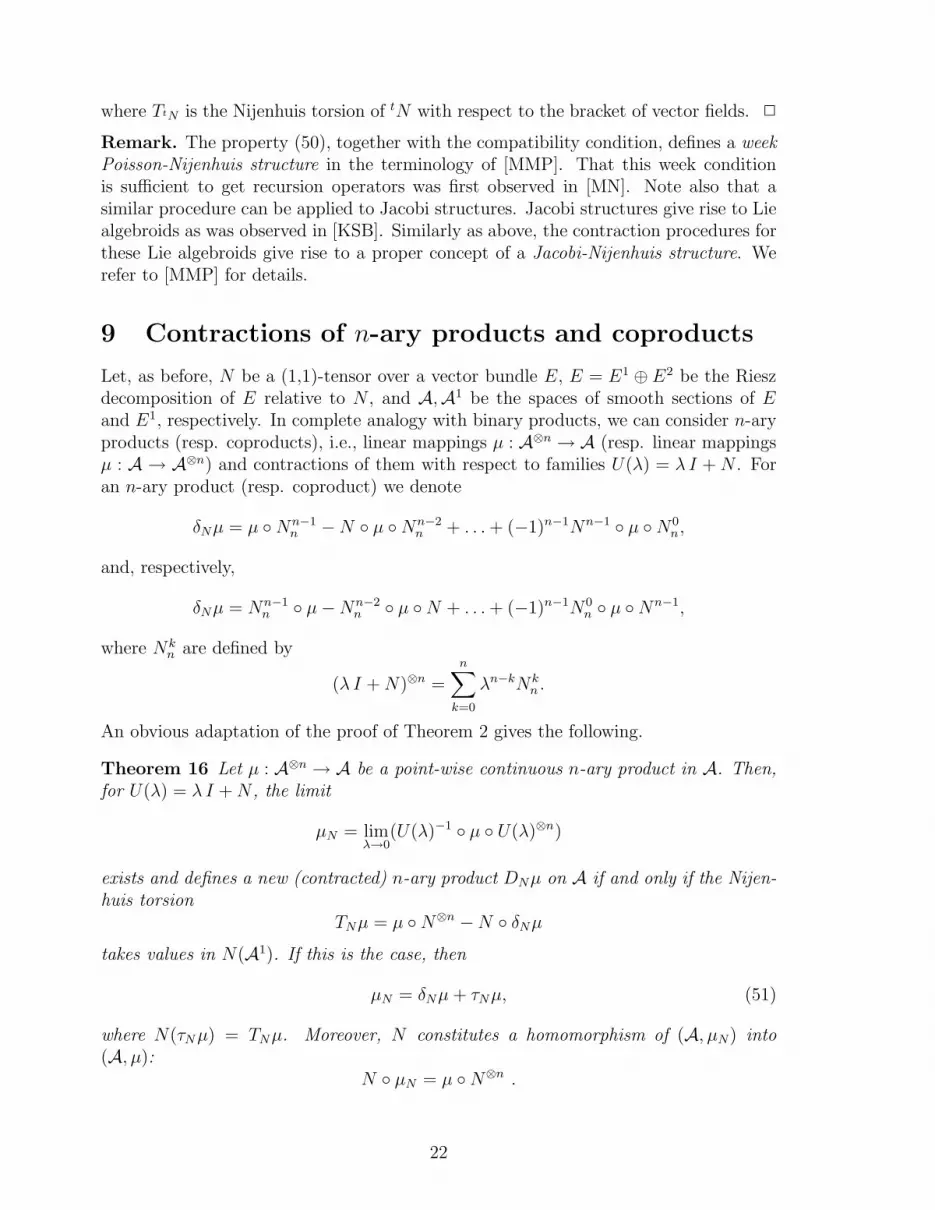
Remark. The property (50), together with the compatibility condition, defines a weekPoisson-Nijenhuis structure in the terminology of [MMP]. That this week conditionis sufficient to get recursion operators was first observed in [MN]. Note also that asimilar procedure can be applied to Jacobi structures. Jacobi structures give rise to Liealgebroids as was observed in [KSB]. Similarly as above, the contraction procedures forthese Lie algebroids give rise to a proper concept of a Jacobi-Nijenhuis structure. Werefer to [MMP] for details.

9 Contractions of n-ary products and coproducts

Let, as before, N be a (1,1)-tensor over a vector bundle E, E = E1 ⊕ E2 be the Rieszdecomposition of E relative to N , and A,A1 be the spaces of smooth sections of Eand E1, respectively. In complete analogy with binary products, we can consider n-aryproducts (resp. coproducts), i.e., linear mappings µ : A⊗n → A (resp. linear mappingsµ : A → A⊗n) and contractions of them with respect to families U(λ) = λ I + N . Foran n-ary product (resp. coproduct) we denote

δNµ = µ Nn−1n − N µ Nn−2

n + . . . + (−1)n−1Nn−1 µ N0n,

and, respectively,

δNµ = Nn−1n µ − Nn−2

n µ N + . . . + (−1)n−1N0n µ Nn−1,

where Nkn are defined by

(λ I + N)⊗n =

n∑

k=0

λn−kNkn .

An obvious adaptation of the proof of Theorem 2 gives the following.

Theorem 16 Let µ : A⊗n → A be a point-wise continuous n-ary product in A. Then,for U(λ) = λ I + N , the limit

µN = limλ→0

(U(λ)−1 µ U(λ)⊗n)

exists and defines a new (contracted) n-ary product DNµ on A if and only if the Nijen-huis torsion

TNµ = µ N⊗n − N δNµ

takes values in N(A1). If this is the case, then

µN = δNµ + τNµ, (51)

where N(τNµ) = TNµ. Moreover, N constitutes a homomorphism of (A, µN) into(A, µ):

N µN = µ N⊗n .

22

A similar theorem for coproducts can be obtained by duality. Since it is much harderto put conditions for existence of contraction at arguments of the Nijenhuis torsion, forsimplicity we give an explicit version for the regular case only.

Theorem 17 Let µ : A → A⊗n be a point-wise continuous n-ary coproduct in A. If Nis regular, i.e., E1 is of constant dimension, then, for U(λ) = λ I + N , the limit

µN = limλ→0

(U(λ)⊗n µ U(λ)−1)

exists and defines a new (contracted) n-ary coproduct DNµ on A if and only if theNijenhuis torsion

TNµ = N⊗n µ − δNµ N

vanishes on A2-the space of sections of E2. If this is the case, then

µN = δNµ + τNµ, (52)

where (τNµ) = TNµ N−1 on A1 and τNµ = 0 on A2. Moreover, N constitutes ahomomorphism of (A, µN) into (A, µ):

µN N = N⊗n µ .

One can consider more general algebraic structures of the form µ : A⊗k → A⊗n, butthis leads to more conditions of contractibility and we will not study these cases in thepresent paper. Note only that contractions of coproducts, as a part of contractions ofLie bialgebras, appeared already in [BGHOS].

10 Conclusions

Motivated by physical examples from Quantum Mechanics, we have studied contrac-tions of general binary (or n-ary) products with respect to one-parameter families oftransformations of the form U(λ) = λ A + N , generalizing pioneering work by Inonu,Wigner, and Saletan. Our generalization can be applied to many infinite-dimensionalcases, especially Lie algebroids and Poisson brackets, however, it does not deal with ageneric dependence of the contraction parameter. The problem of describing contrac-tions with respect to general U(λ), or even differentiable with respect to λ, is muchmore complicated.

The contraction procedure can be viewed as an inverse of a deformation procedure.Deformations of associative and Lie algebras, at least on the infinitesimal level, arerelated to some cohomology. It would be interesting to relate formally deformations tocontractions and connect the cohomology also to contractions.

We postpone these problems to a separate paper.

References

[BGHOS] Ballesteros A.; Gromov N. A.; Herranz F. J.; del Olmo M. A. and San-tander M., Lie bialgebra contractions and quantum deformations, J. Math.Phys. 36 (1995), 5916–5937.

23

[CGM] Carinena, J. F.; Grabowski, J. and Marmo, G., Quantum bihamiltoniansystems, to appear in Int. J. Mod. Phys. A.

[Di] Dirac, P.A.M., The Principles of Quantum Mechanics, Oxford UniversityPress, 1958.

[DM] Doebner H.D. and Melsheimer O. On a Class of Generalized Group Con-tractions Il Nuovo Cimento 49 (1967), 306–311.

[Fu] Fuchssteiner B., The Lie algebra structure of degenerate Hamiltonian andbi-Hamiltonian systems, Progr. Theoret. Phys. 68 (1982), 1082–1104.

[Gi] Gilmore R., Lie Groups, Lie Algebras, and Some of their Applications,John Wiley & Sons, 1974.

[GU] Grabowski J. and Urbanski P., Algebroids – general differential calculi onvector bundles, J. Geom. Phys. 31 (1999), 111-141.

[GU1] Grabowski J. and Urbanski P., Lie algebroids and Poisson-Nijenhis struc-tures, Rep. Math. Phys. 40 (1997), 195–208.

[IW] Inonu E. and Wigner E.P., On the contraction of Groups and their repre-sentations, Proc. Nat. Acad. Sci. 39 (1953), 510–524.

[KS] Kosmann-Schwarzbach Y., The Lie bialgebroid of a Poisson-Nijenhuismanifold, Lett. Math. Phys. 38 (1996), 421–428.

[KSB] Kerbat Y. and Souici-Benhammadi Z., Varietes de Jacobi et groupoıdes decontact, C. R. Acad. Sci. Paris, Ser., I 317 (1993), 81–86.

[KSM] Kosmann-Schwarzbach Y. and Magri F., Poisson-Nijenhuis structures,Ann. Inst. H. Poincare Phys. Theor. 53 (1990), 35–81.

[LN] Levy-Nahas M., Deformation and Contraction of Lie Algebras, J. Math.Phys. 8 (1967), 1211-1222.

[Mac] Mackenzie K. C. H, Lie algebroids and Lie pseudoalgebras, Bull. LondonMat. Soc. 27 (1995), 97–147.

[MX] Mackenzie K. C. H. and Xu P., Lie bialgebroids and Poisson groupoids,Duke Math. J. 73 (1994), 415-452.

[Mag] Magri, F., A simple model of the integrable Hamiltonian equation, J. Math.Phys. 19 (1978), 1156–52.

[MM] Magri F. and Morosi C., A geometrical characterization of integrableHamiltonian systems through the theory of Poisson-Nijenhuis manifolds,Quaderno S19, University of Milan, 1984.

[MN] Marle C.-M. and Nunes da Costa J. M., Reduction of bihamiltonian mani-folds and recursion operators, in: Diff. Geom. Appl. (Brno 1995), MasarykUniv., Brno 1996, 523–538.

24

[MMP] Marrero J. C.; Monterde J. and Padron E., Jacobi-Nijenhuis manifolds andcompatible Jacobi structures, C. R. Acad. Sci. Paris, Ser. I, 329 (1999),797–802.

[MMSZ] Man’ko, V. I.; Marmo, G.; Sudarshan, E. C. G. and Zaccaria, F., Wigner’sproblem and alternative commutation relations for quantum mechanics,Int. Jour. Mod. Phys. B 11 (1997), 1281–1296.

[Pr] Pradines J., Theorie de Lie pour les groupoıdes differentiables. Calculdifferentiel dans la categorie des groupoıdes infinitesimaux, C. R. Acad.Sci. Paris Ser A 264 (1967), 245–248.

[Sa] Saletan E.J., Contractions of Lie Groups, J. Math. Phys. 2 (1961), 1–21.

[WW] Weimar-Woods E., The three-dimensional real Lie algebras and their con-tractions, J. Math. Phys. 32 (1991), 2028–33.

[Wi] Wigner, E. P., Do the equations of Motion determine the quantum me-chanical commutation relations?, Phys. Rev. 77 (1950), 711–12.

25