Embed Size (px)
Citation preview
FRIEDRICH-ALEXANDER-UNIVERSITÄT ERLANGEN-NÜRNBERGTECHNISCHE FAKULTÄT DEPARTMENT INFORMATIK
Lehrstuhl für Informatik 10 (Systemsimulation)
Extension of the ExaStencils Framework with Tensors
Martin Zeus
Bachelor Thesis
Extension of the ExaStencils Framework with Tensors
Martin ZeusBachelor Thesis
Aufgabensteller: Prof. Dr. H. Köstler
Betreuer: Dr. Ing. S. Kuckuk
Bearbeitungszeitraum: 1.4.2020 30.09.2020
Erklärung:
Ich versichere, dass ich die Arbeit ohne fremde Hilfe und ohne Benutzung anderer als der angegebe-nen Quellen angefertigt habe und dass die Arbeit in gleicher oder ähnlicher Form noch keineranderen Prüfungsbehörde vorgelegen hat und von dieser als Teil einer Prüfungsleistung angenom-men wurde. Alle Ausführungen, die wörtlich oder sinngemäÿ übernommen wurden, sind als solchegekennzeichnet.
Der Universität Erlangen-Nürnberg, vertreten durch den Lehrstuhl für Systemsimulation (Infor-matik 10), wird für Zwecke der Forschung und Lehre ein einfaches, kostenloses, zeitlich und örtlichunbeschränktes Nutzungsrecht an den Arbeitsergebnissen der Bachelor Thesis einschlieÿlich et-waiger Schutzrechte und Urheberrechte eingeräumt.
Erlangen, den 31. Oktober 2020 . . . . . . . . . . . . . . . . . . . . . . . . . . . . . . . . . . . . . .
Contents
1 Abstract 5
2 Introduction 5
3 Theoretical background 73.1 Dyadic product . . . . . . . . . . . . . . . . . . . . . . . . . . . . . . . . . . . . . . . 73.2 Denition Tensor . . . . . . . . . . . . . . . . . . . . . . . . . . . . . . . . . . . . . . 7
3.2.1 Denition via multilinear map . . . . . . . . . . . . . . . . . . . . . . . . . . 83.3 Einstein notation . . . . . . . . . . . . . . . . . . . . . . . . . . . . . . . . . . . . . . 93.4 Basic arithmetic operations on tensors . . . . . . . . . . . . . . . . . . . . . . . . . . 9
3.4.1 Multiplication with scalars . . . . . . . . . . . . . . . . . . . . . . . . . . . . 93.4.2 Division with scalars . . . . . . . . . . . . . . . . . . . . . . . . . . . . . . . . 93.4.3 Addition with vectors/matrix . . . . . . . . . . . . . . . . . . . . . . . . . . . 103.4.4 Multiplication with vectors/matrix . . . . . . . . . . . . . . . . . . . . . . . . 103.4.5 Multiplication/Addition between two tensors . . . . . . . . . . . . . . . . . . 10
3.5 Algebra of tensors . . . . . . . . . . . . . . . . . . . . . . . . . . . . . . . . . . . . . 113.6 Tensor calculus . . . . . . . . . . . . . . . . . . . . . . . . . . . . . . . . . . . . . . . 11
3.6.1 Double contraction . . . . . . . . . . . . . . . . . . . . . . . . . . . . . . . . . 113.6.2 Kronecker delta . . . . . . . . . . . . . . . . . . . . . . . . . . . . . . . . . . . 113.6.3 Trace . . . . . . . . . . . . . . . . . . . . . . . . . . . . . . . . . . . . . . . . 113.6.4 Determinant . . . . . . . . . . . . . . . . . . . . . . . . . . . . . . . . . . . . 113.6.5 Eigenvalues . . . . . . . . . . . . . . . . . . . . . . . . . . . . . . . . . . . . . 12
3.7 General functionality and wording . . . . . . . . . . . . . . . . . . . . . . . . . . . . 123.7.1 Abstract syntax tree . . . . . . . . . . . . . . . . . . . . . . . . . . . . . . . . 123.7.2 Steps in generation pipeline . . . . . . . . . . . . . . . . . . . . . . . . . . . . 133.7.3 PrettyPrintable . . . . . . . . . . . . . . . . . . . . . . . . . . . . . . . . . . . 143.7.4 Progressable . . . . . . . . . . . . . . . . . . . . . . . . . . . . . . . . . . . . 143.7.5 Transformation . . . . . . . . . . . . . . . . . . . . . . . . . . . . . . . . . . . 143.7.6 Layer handler . . . . . . . . . . . . . . . . . . . . . . . . . . . . . . . . . . . . 15
4 Examples for special tensors 154.1 Cauchy stress tensor . . . . . . . . . . . . . . . . . . . . . . . . . . . . . . . . . . . . 164.2 Inertia tensor . . . . . . . . . . . . . . . . . . . . . . . . . . . . . . . . . . . . . . . . 164.3 Electromagnetic eld tensor . . . . . . . . . . . . . . . . . . . . . . . . . . . . . . . . 16
5 Representation in ExaSlang 175.1 The tensor datatype . . . . . . . . . . . . . . . . . . . . . . . . . . . . . . . . . . . . 175.2 The tensor expression . . . . . . . . . . . . . . . . . . . . . . . . . . . . . . . . . . . 175.3 Element access . . . . . . . . . . . . . . . . . . . . . . . . . . . . . . . . . . . . . . . 185.4 Arithmetic operations . . . . . . . . . . . . . . . . . . . . . . . . . . . . . . . . . . . 195.5 Other functions . . . . . . . . . . . . . . . . . . . . . . . . . . . . . . . . . . . . . . . 195.6 Dyadic product . . . . . . . . . . . . . . . . . . . . . . . . . . . . . . . . . . . . . . . 205.7 Einstein notation . . . . . . . . . . . . . . . . . . . . . . . . . . . . . . . . . . . . . . 205.8 Double contraction . . . . . . . . . . . . . . . . . . . . . . . . . . . . . . . . . . . . . 22
6 Implementation in ExaStencils 226.1 Coorperative work . . . . . . . . . . . . . . . . . . . . . . . . . . . . . . . . . . . . . 226.2 Modules . . . . . . . . . . . . . . . . . . . . . . . . . . . . . . . . . . . . . . . . . . . 236.3 Layer 4 . . . . . . . . . . . . . . . . . . . . . . . . . . . . . . . . . . . . . . . . . . . 23
6.3.1 About the parser . . . . . . . . . . . . . . . . . . . . . . . . . . . . . . . . . . 236.3.2 Tensor datatype . . . . . . . . . . . . . . . . . . . . . . . . . . . . . . . . . . 246.3.3 Tensor expression . . . . . . . . . . . . . . . . . . . . . . . . . . . . . . . . . . 256.3.4 Element access . . . . . . . . . . . . . . . . . . . . . . . . . . . . . . . . . . . 27
6.4 IR Layer . . . . . . . . . . . . . . . . . . . . . . . . . . . . . . . . . . . . . . . . . . . 29
4
6.4.1 Tensor datatype . . . . . . . . . . . . . . . . . . . . . . . . . . . . . . . . . . 296.4.2 Tensor expression . . . . . . . . . . . . . . . . . . . . . . . . . . . . . . . . . . 296.4.3 Element access . . . . . . . . . . . . . . . . . . . . . . . . . . . . . . . . . . . 306.4.4 Einstein notation . . . . . . . . . . . . . . . . . . . . . . . . . . . . . . . . . . 316.4.5 Contraction . . . . . . . . . . . . . . . . . . . . . . . . . . . . . . . . . . . . . 386.4.6 Arithmetic operators . . . . . . . . . . . . . . . . . . . . . . . . . . . . . . . . 386.4.7 Other compile time functions . . . . . . . . . . . . . . . . . . . . . . . . . . . 406.4.8 Eigenvalues . . . . . . . . . . . . . . . . . . . . . . . . . . . . . . . . . . . . . 41
7 Tests 41
8 Results and outlook 42
1 Abstract
The eld of system simulation is growing continuously. This matter is comprehensible to the extentthat the size of problems, especially in physics and technology, is increasing. To tackle the resultingsoftware demand, frameworks for code generation were developed. As an example, ExaStencils[Kuc19], which can generate massive parallel C++ Code out of ExaSlang [Sch+14], a domain-specic script language. The framework transcends in 4 steps the linguistic gap between formalmathematical denitions and fast hardware near code. Each step is adjusted to the needs of a singleuser class. ExaStencils based on the functional language Scala [Sca].
Mr. Kuckuk described in his work [Kuc19] how ExaSlang can be transformed into a processornear and faster language (e.g. C++). The doctoral thesis also shows which benets are included inthis category of tools for scientic calculation, especially for numerical solvers who nd the solutionof partial dierential equations [Noac] (e.g. Navier-stokes-equation [Tem01])
ExaStencils has a four-layer approach, which means that each layer transfers the code peu à peufrom an abstract mathematical description to a technical view. A fth layer, named IR, representsthe concrete implementation. This implements a print function, which writes the transformed layersinto correct target code.
Tensors are a complex mathematical data structure related to a matrix. Theoretically, it assignsa vector- or matrix- associated structure to a coordinate space. The main goal of the thesis wasto implement those tensors to ExaStencils. It approaches the problem from the short theoreticalview over the fourth layer to the implementation. This work denes tensor and its operations,whereas, for proofs, it is referencing the literature. The thesis discusses where the type is used andhow it can be represented and dened in ExaSlang. Concertedly with the ExaSlang part comes thedenition of the parser rules and further the implementation in the fourth layer.At this part, thebiggest changes for those complex datatype are possible in the context of code generation. Hence,one of the work was to seek for achievements of unique tensors in ExaStencils.
The rst achievement was to improve the usability of complex data structures. The thesisgives an insight into how modern access methods are implementable in ExaStencils. Further, itdescribes the implementation of operations on tensors, notably that there was a strong focus onusing compilation time algorithmic instead of increasing the runtime in this connection.
The Einstein notation played a signicant role in this task. In numerous literature, this ab-breviated notation is used to formulate sentences with tensors. One eort was to implement thenotation in the IR-layer.
As a result, it has been shown that it is possible to integrate such complex data type intoExaStencils without dangling the runtime and improving the usability of the tool itself.
2 Introduction
Many physical and technical issues are described with tensors. For example, continuous mechanics isa wide used formalism, especially in the theory of elasticity (strain tensor), which uses tensors. Otherapplications can be found widely, for instance in electrodynamics (electromagnetic eld tensor).
Tensors describe the relationship between a vector- or matrix-related data structure and itsspace. Usually used spaces are classical coordinate spaces in R, e.g., the cartesian vector space in
5
N dimensions, but more non-classical spaces comparable to topological spaces are possible. Thecode and thesis only include spaces that store numerical data types in array-like storages relatedto Euclidean space. Tensors can easily describe points or objects in an ecosystem because of thetensor values' inherent bounding with the coordinate system. For this reason, they are commonlyused to represent locations in a grid. As an instance, in the theory of elasticity, they are used tocalculate the deformation of the mesh if the temperature has changed. The examples part givesherefore a more concrete insight.
ExaSlang is a domain-specic language (apr. DSL) for high-performance computing related tothe known language Julia [Noae]. DSLs are scripting or programming languages, which have a con-crete scope of application, for instance, high-performance computing. In contrast, C++, a classicalprogramming language, is used for a broad eld. Possible use-cases are desktop applications, com-puter games, embedded solutions, or also scientic computing. DSLs' development is driven by theproblem that classical languages often work not optimal enough in specic elds or need expensivedevelopment eort or libraries. Distinctive to other languages, ExaSlang is not constructed to becompiled to byte code. ExaStencils parses ExaSlang and generates dierent target code, dependingon the target system. Such target code can be C++ to run on CPUs, or also OpenGL is possibleif the calculation has to be done at graphic processors. As a dierence between code-generationtechnology and classical software development is where intelligence and functionality are based.When the software is directly written in the target language, every called method, data types, andlibraries are also in the same language. The compiler transfers the whole project together into bytecode. That diers from ExaStencils, where the application development is in ExaSlang and com-piled to source code again. In the moment of parsing the ExaSlang-code, the functionality which isimplemented in the code-generator directly can be used. So, operations on the graph and complexdata types can be done before printing and later compiling the target code. This procedural man-ner is an inuential possibility to reduce calculation eort on the target system because necessaryoperations for the application can be moved to the generation time and consequently to away fromruntime.
Runtime on a high-performance cluster is expensive, especially for small companies, which areoften not able to operate on an own small cluster economical. Only a few concerns have theproperties to acquire a high-performance workstation. Supercomputers not only cost money for thepurchase, but they also require maintenance and, in particular, energy for working. The issue ofenergy consumption in IT can also be viewed from an environmental side. To reduce the amountof humans energy consumption, software development should avoid unnecessary computationalactivity.
As written, ExaSlang and ExaStencils are conceptually tailored for the usage in the eld ofhigh-performance computing. Frameworks for scientic calculation implicit needs mathematicaldata types because models described mathematically. This thesis shows in some small exampleswhere tensors can be found in such models. It also displays why moving operational work to thegeneration time is worthwhile.
The rst part of this work aims to perceive all necessary content a tensor in a code generationframework. The part of the theoretical background is a result of this step. This part is homogenouslydesigned to obtain an easy reading on the one hand and the other a clear and formal correctstructure. Denitions follow brief instructions and them again compact examples. This task endswith a short introduction in the usual wording and ground standing functionality of the codegeneration tool. The later parts, the representation and the implementation, repeat the topicsfrom the theoretical background for fast searching. The representation precise the tensor type andfunctionality in ExaSlang. It also indicates how tensors can be expressed in a formal language.From now on, there is a limitation. When discussing ExaSlang and also ExaStencils, this thesisonly includes the fourth layer of ExaSlang and in ExaStencils only the fourth and the IR layer. Thelast and also most signicant part of this work is the implementation. The main part describesat rst the parser and the fourth layer, which includes more precisely how ExaSlang-code will beparsed and how objects will be created out of the source. At the third topic of the implementation,the thesis describes the development on the IR layer. Although the topic starts with the tensordata type and the expression, the main exertion was the transformations. A relevant point is therealization of the functionality, which claims most of the whole working time. The thesis explainsthe algorithm of Einstein notation extensively. This algorithm and the deduced contraction is oneof the most complicated elements of the thesis. After the IR layer, the thesis lists the tests of the
6
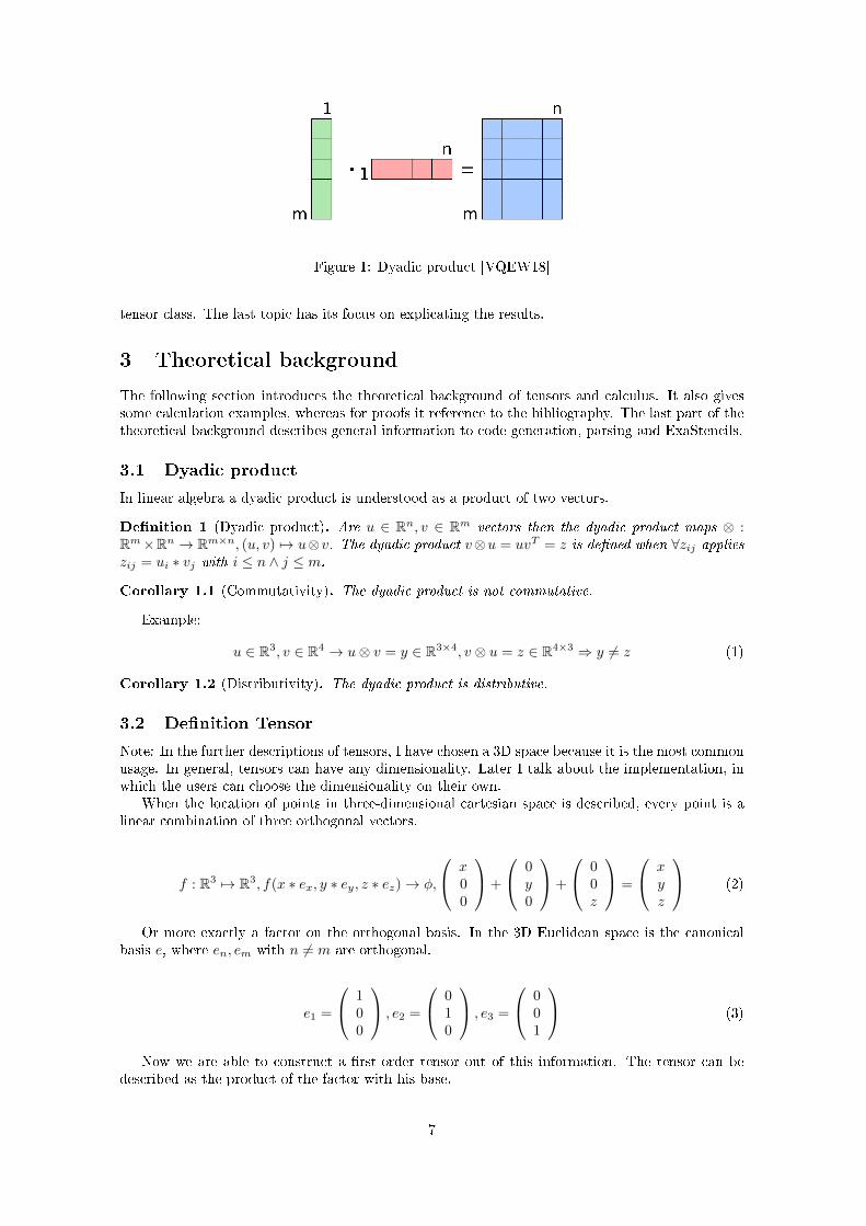
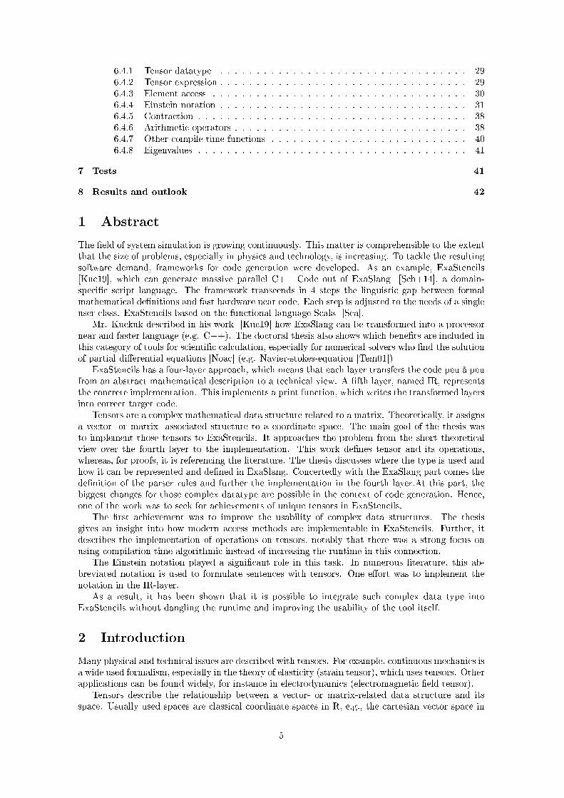
Figure 1: Dyadic product [VQEW18]
tensor class. The last topic has its focus on explicating the results.
3 Theoretical background
The following section introduces the theoretical background of tensors and calculus. It also givessome calculation examples, whereas for proofs it reference to the bibliography. The last part of thetheoretical background describes general information to code generation, parsing and ExaStencils.
3.1 Dyadic product
In linear algebra a dyadic product is understood as a product of two vectors.
Denition 1 (Dyadic product). Are u ∈ Rn, v ∈ Rm vectors then the dyadic product maps ⊗ :Rm×Rn → Rm×n, (u, v) 7→ u⊗v. The dyadic product v⊗u = uvT = z is dened when ∀zij applieszij = ui ∗ vj with i ≤ n ∧ j ≤ m.
Corollary 1.1 (Commutativity). The dyadic product is not commutative.
Example:
u ∈ R3, v ∈ R4 → u⊗ v = y ∈ R3×4, v ⊗ u = z ∈ R4×3 ⇒ y 6= z (1)
Corollary 1.2 (Distributivity). The dyadic product is distributive.
3.2 Denition Tensor
Note: In the further descriptions of tensors, I have chosen a 3D space because it is the most commonusage. In general, tensors can have any dimensionality. Later I talk about the implementation, inwhich the users can choose the dimensionality on their own.
When the location of points in three-dimensional cartesian space is described, every point is alinear combination of three orthogonal vectors.
f : R3 7→ R3, f(x ∗ ex, y ∗ ey, z ∗ ez)→ φ,
x00
+
0y0
+
00z
=
xyz
(2)
Or more exactly a factor on the orthogonal basis. In the 3D Euclidean space is the canonicalbasis e, where en, em with n 6= m are orthogonal.
e1 =
100
, e2 =
010
, e3 =
001
(3)
Now we are able to construct a rst-order tensor out of this information. The tensor can bedescribed as the product of the factor with his base.
7
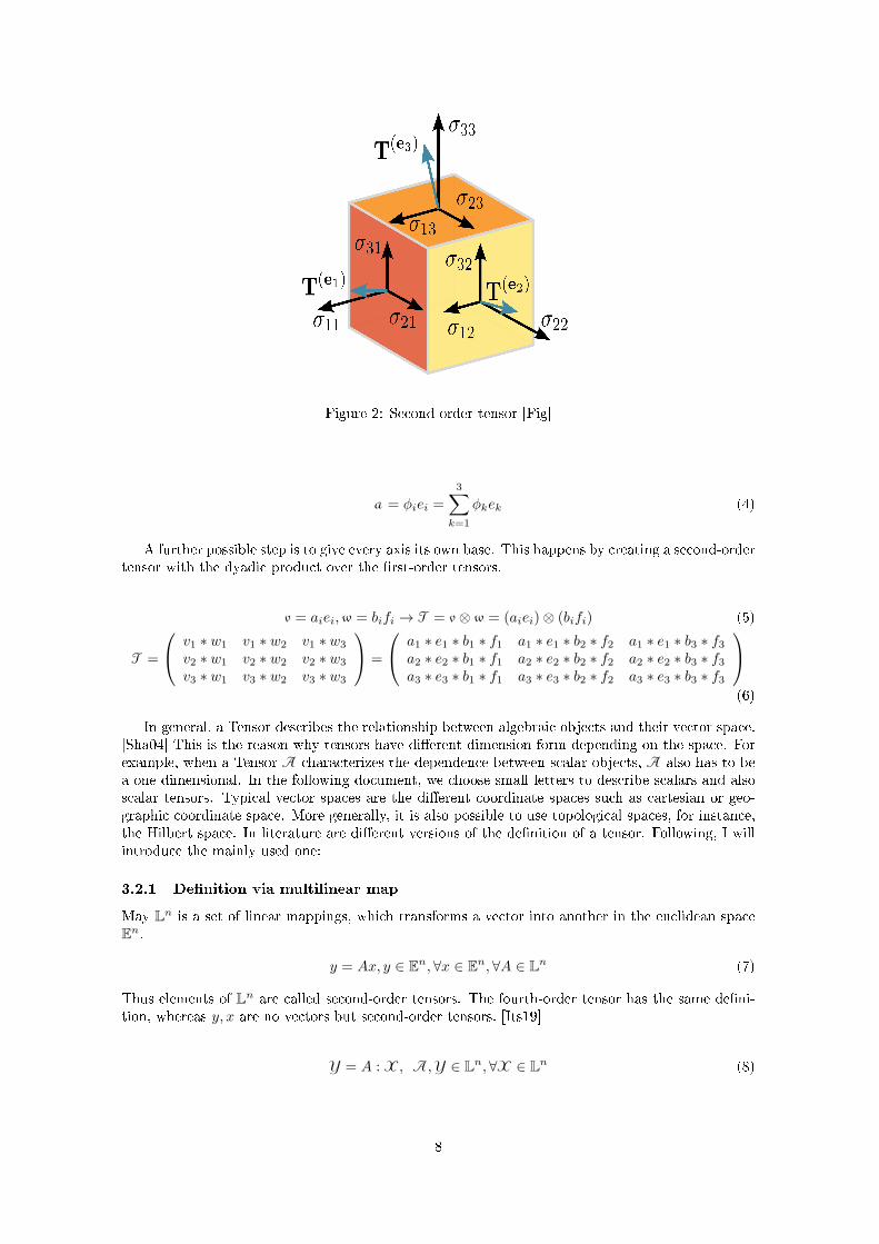
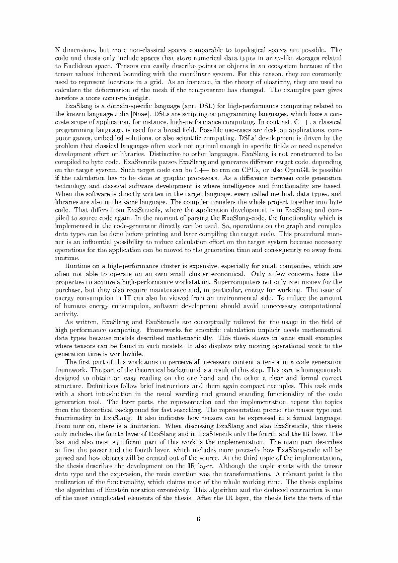
Figure 2: Second order tensor [Fig]
a = φiei =
3∑k=1
φkek (4)
A further possible step is to give every axis its own base. This happens by creating a second-ordertensor with the dyadic product over the rst-order tensors.
v = aiei,w = bifi → T = v ⊗ w = (aiei)⊗ (bifi) (5)
T =
v1 ∗ w1 v1 ∗ w2 v1 ∗ w3
v2 ∗ w1 v2 ∗ w2 v2 ∗ w3
v3 ∗ w1 v3 ∗ w2 v3 ∗ w3
=
a1 ∗ e1 ∗ b1 ∗ f1 a1 ∗ e1 ∗ b2 ∗ f2 a1 ∗ e1 ∗ b3 ∗ f3a2 ∗ e2 ∗ b1 ∗ f1 a2 ∗ e2 ∗ b2 ∗ f2 a2 ∗ e2 ∗ b3 ∗ f3a3 ∗ e3 ∗ b1 ∗ f1 a3 ∗ e3 ∗ b2 ∗ f2 a3 ∗ e3 ∗ b3 ∗ f3
(6)
In general, a Tensor describes the relationship between algebraic objects and their vector space.[Sha04] This is the reason why tensors have dierent dimension form depending on the space. Forexample, when a Tensor A characterizes the dependence between scalar objects, A also has to bea one dimensional. In the following document, we choose small letters to describe scalars and alsoscalar tensors. Typical vector spaces are the dierent coordinate spaces such as cartesian or geo-graphic coordinate space. More generally, it is also possible to use topological spaces, for instance,the Hilbert space. In literature are dierent versions of the denition of a tensor. Following, I willintroduce the mainly used one:
3.2.1 Denition via multilinear map
May Ln is a set of linear mappings, which transforms a vector into another in the euclidean spaceEn.
y = Ax, y ∈ En,∀x ∈ En,∀A ∈ Ln (7)
Thus elements of Ln are called second-order tensors. The fourth-order tensor has the same deni-tion, whereas y, x are no vectors but second-order tensors. [Its19]
Y = A : X, A,Y ∈ Ln,∀X ∈ Ln (8)
8
3.3 Einstein notation
The Einstein notation is a simplication formulated by Einstein in 1916 [Åh02]. The abbreviationis widely used in tensor calculus, which is why it has to be mentioned here.
Denition 2 (Einstein notation). May i ∈ N limited and
f =∑l∈i
φ(l)ψ(l)
then the term can also be written as φiψi. Where i is the domain of the sum.
Examples:
(ai + bi) ∗ ak =
i∑l=1
(al + bl) ∗ ak (9)
(ai + bi) + (ck ∗ dk) + el =
i∑m=1
(am + bm) +
k∑n=1
(cn ∗ dn) + el (10)
In the second example, i is not at the index but in the superscript. Important is for the notationonly that a collective iteration variable exists, not that a part is indexed related to vectors or matrix.In addition to the classical Einstein notation, the module in ExaStencils will allow more than twocomponents. For instance t1i ∗ t2i ∗ t3i is also allowed.
3.4 Basic arithmetic operations on tensors
The most common calculation rules for tensors with order up to 2 are also dened in commonmatrix space for their expression.
3.4.1 Multiplication with scalars
Denition 3 (Multiplication tensor with scalar). May T,Z tensors with the same order and di-mensionality and t ∈ T, z ∈ Z elements of the tensors. May also a scalar x ∈ R. Then Z = T ∗ xif i ∈ N is an iterator over all indices of a tensor and zi = ti ∗ x, ∀i. .
Example:
a ∈ R,T =
t11 t21 t31t12 t22 t32t13 t23 t33
, then: U = a ∗ T =
a ∗ t11 a ∗ t21 a ∗ t31a ∗ t12 a ∗ t22 a ∗ t32a ∗ t13 a ∗ t23 a ∗ t33
(11)
3.4.2 Division with scalars
Denition 4 (Division tensor with scalar). May T,Z tensors with the same order and dimension-ality and t ∈ T, z ∈ Z elements of the tensors. May also a scalar a ∈ R. Then Z = T/a if i ∈ N isan iterator over all indices of a tensor and zi = ti/x,∀i. .
Example:
a ∈ R,T =
t11 t21 t31t12 t22 t32t13 t23 t33
, then: U = T/a =
t11/a t21/a t31/at12/a t22/a t32/at13/a t23/a t33/a
(12)
A simple resulting operator is an inversion under a given scalar. If the scalar is 1 than theresultig tensor is the inverse of multiplication.
Denition 5 (Inverse division tensor with scalar). May T,Z tensors with the same order anddimensionality and t ∈ T, z ∈ Z elements of the tensors. May also a scalar a ∈ R. Then Z = a/Tif i ∈ N is an iterator over all indices of a tensor and zi = ti/x,∀i. .
9
Example:
a ∈ R,T =
t11 t21 t31t12 t22 t32t13 t23 t33
, then: U = a/T =
a/t11 a/t21 a/t31a/t12 a/t22 a/t32a/t13 a/t23 a/t33
(13)
This functionality is not standard for tensors, and so the denition is made for this thesis.Tensors will mostly be used with matrixes and scalars side by side, so the tensor module shouldsupport enough rudimental functionality to build more complex statements. For instance, thisfunction can be used to calculate the inverse of a diagonal tensor.
3.4.3 Addition with vectors/matrix
Both the addition of two vectors/matrix and one of a tensor and an vector/matrix is only denedfor those with the same dimensions. Therefore it is only possible to add a n-order tensor to a matrixwithin R3n .
Denition 6 (Addition tensor with matrix). May A ∈ R3n and T,Z tensors with the order n anda ∈ A, t ∈ T, z ∈ Z elements of A, T, Z. Then Z = T +A if ∀z ∈ Z : z = t+ a where a, t, z has thesame location in the tensor of matrix.
Example:
A =
a1a2a3
,T =
t1t2t3
, then: Z = A+ T =
a1 + t1a2 + t2a3 + t3
(14)
3.4.4 Multiplication with vectors/matrix
Both the addition of two vectors/matrix and one of a tensor and a vector/matrix is only denedfor those with the same dimensions. Therefore it is only possible to multiply a n-order tensor to amatrix within R3n .
Denition 7 (Multiplication tensor with matrix). May A ∈ R3n and T,Z tensors with the ordern and a ∈ A, t ∈ T, z ∈ Z elements of A, T, Z. Then Z = T ∗ A if ∀z ∈ Z : z = t ∗ a where a, t, zhas the same location in the tensor of matrix.
Example:
A =
a1a2a3
,T =
t1t2t3
, then: Z = A ∗ T =
a1 ∗ t1a2 ∗ t2a3 ∗ t3
(15)
3.4.5 Multiplication/Addition between two tensors
To develop higher functions, or more generally linear transformations, it is necessary to denearithmetic operators. Therefore, I have to note that multiplication is not similar to tensor product.They are basically dierent concepts. Multiplication in that context means an elementwise operatorsimilar to the Addition.
Denition 8 (Addition two tensors). May T,U, Z tensors with the same order and dimensionalityand t ∈ T, u ∈ U, z ∈ Z elements of the tensors. Then Z = T + U if i ∈ N is an iterator over allindices of a tensor and zi = ti + ui,∀i.
Example:
T =
t1t2t3
,U =
u1u2u3
, then: Z = T + U =
t1 + u1t2 + u2t3 + u3
(16)
Denition 9 (Elementwise multiplication two tensors). May T,U, Z tensors with the same orderand dimensionality and t ∈ T, u ∈ U, z ∈ Z elements of the tensors. Then Z = T ∗ U if i ∈ N is aniterator over all indices of a tensor and zi = ti ∗ ui,∀i.
10
Example:
T =
t1t2t3
,U =
u1u2u3
, then: Z = T ∗U =
t1 ∗ u1t2 ∗ u2t3 ∗ u3
(17)
3.5 Algebra of tensors
Tensors are commutative groups in the context of addition [8] and multiplication [9]. [Its19]May 1,Φ,T,U tensors with order k and dimension n, then 1 is the Kronecker Delta [11] with
the order k ∈ N, so 1 is the generalization of the identity matrix in the tensor room. 1 is the neutralelement of multiplication. May also Φ a zero tensor with order k ∈ N and dimension n, and α, βscalars. Then applies,
T ∗ 1 = 1 ∗ T = T (18)
T + Φ = Φ +T = T (19)
T− T = Φ (20)
T + U = U + T (21)
(T + U) + V = T + (U + V) (22)
α ∗ (T + U) = α ∗ T + α ∗ U (23)
α ∗ (β ∗ T) = (α ∗ β) ∗ T (24)
3.6 Tensor calculus
3.6.1 Double contraction
Denition 10 (Double contraction). May A a tensor with order 4∨ 2 and B second-order tensors,then : is a double Contraction if A : B = AijklBkl and A has a fourth-order or if A : B = AklBkl
and A has a second-order [Hol00].
For some particular cases the contraction of a fourth-order with a second-order tensor is needed(e.g. elasticity). The syntax of the contraction is similar to Einstein notation. [2].
3.6.2 Kronecker delta
Denition 11 (Kronecker delta). May δij and i, j ∈ N a function then it is called Kronecker delta,when
δij =
0, i 6= j
1, i = j
There a reasonable generalisation if for objects with a higher-order correspondingly, more indicesare allowed.
3.6.3 Trace
Denition 12 (Trace, 2nd order Tensor). May A a second order tensor, then tr is a trace iftrA = Aii = a11 + a22 + a33 [Hol00]
Denition 13 (Trace, n-th order Tensor). May A a tensor with order n, then tr is a trace iftrA = Σ (δi,.. ∗ Ai,...) and δ is the Kronecker delta [11] over all index dimension.
3.6.4 Determinant
Denition 14 (Determinant). May A a second order tensor and A ∈ R3×3 a matrix of tensorcomponents, then det is a determinant of A if
detA = detA = det
A11 A12 A13
A21 A22 A23
A31 A32 A33
11
3.6.5 Eigenvalues
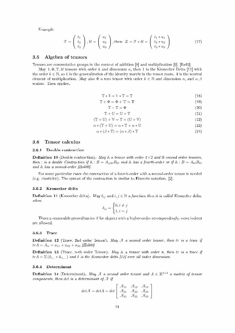
Considering the workload, I only determine the eigenvalues for tensors with order two. So it ispossible to use algorithms for the determination of matrix eigenvalues.
For the calculation of the eigenvalues I chose the QR-algorithm which basically computes anupper Hesseberg-matrix in limited steps. In practical applications it is unusual to have very highdimensional tensors, because of the common 3D-Euclidean-vectorspace. Given that limitation, Ichoose the basic QR-Algorithm with a single shift and a linear matrix polynomial as the result.[Arb]
Algorithm 1: QR-Algorithm with single shiftData: Tensor 2nd order TResult: output data pA0 := T
for i ∈ 1, 2, ..., dims− 1 dodetermine pi in Acompute QR decomposition of pi(Ai) = QiRi
compute Ai+1 = Q−1i AiQi + κiIend
Denition 15 (Single shifted QR-Algorithm for eigenvalue calculation ).
3.7 General functionality and wording
3.7.1 Abstract syntax tree
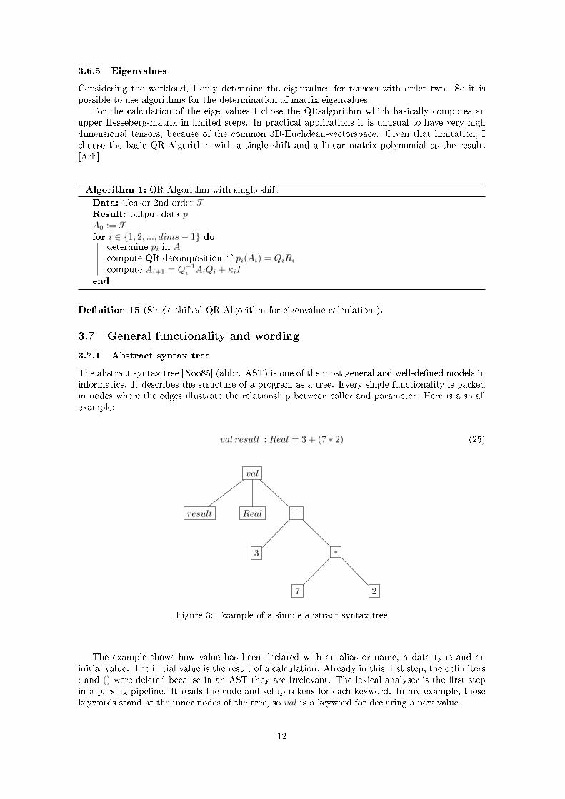
The abstract syntax tree [Noo85] (abbr. AST) is one of the most general and well-dened models ininformatics. It describes the structure of a program as a tree. Every single functionality is packedin nodes where the edges illustrate the relationship between caller and parameter. Here is a smallexample:
val result : Real = 3 + (7 ∗ 2) (25)
val
result Real +
∗3
7 2
Figure 3: Example of a simple abstract syntax tree
The example shows how value has been declared with an alias or name, a data type and aninitial value. The initial value is the result of a calculation. Already in this rst step, the delimiters: and () were deleted because in an AST they are irrelevant. The lexical analyser is the rst stepin a parsing pipeline. It reads the code and setup tokens for each keyword. In my example, thosekeywords stand at the inner nodes of the tree, so val is a keyword for declaring a new value.
12
Declaration
Name Datatype Addition
MultiplicationConstant
Constant Constant
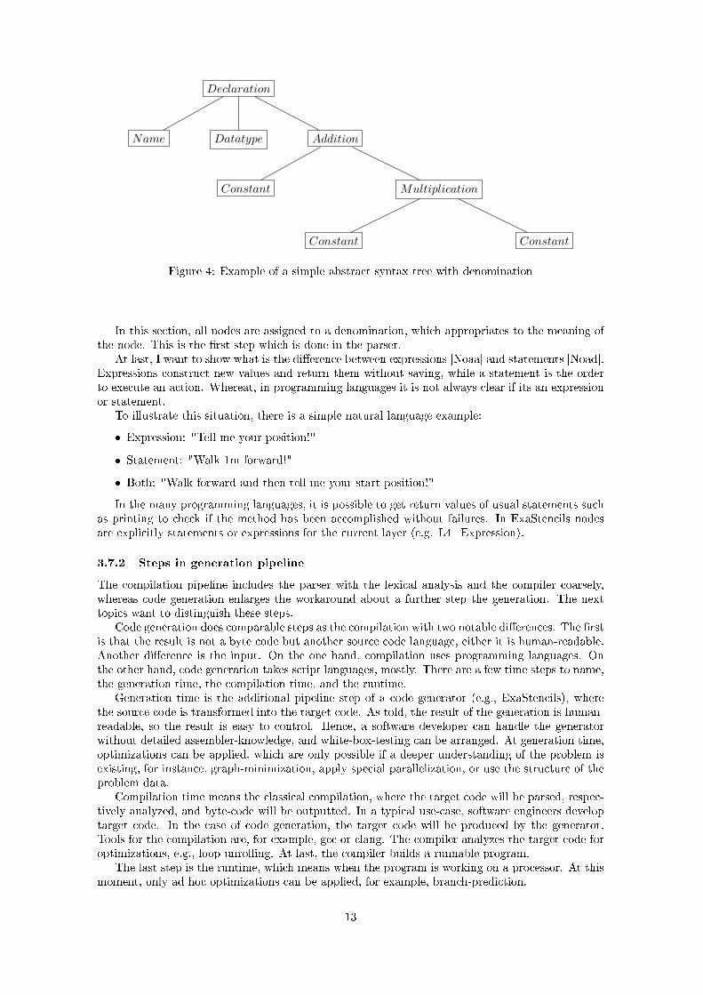
Figure 4: Example of a simple abstract syntax tree with denomination
In this section, all nodes are assigned to a denomination, which appropriates to the meaning ofthe node. This is the rst step which is done in the parser.
At last, I want to show what is the dierence between expressions [Noaa] and statements [Noad].Expressions construct new values and return them without saving, while a statement is the orderto execute an action. Whereat, in programming languages it is not always clear if its an expressionor statement.
To illustrate this situation, there is a simple natural language example:
Expression: "Tell me your position!"
Statement: "Walk 1m forward!"
Both: "Walk forward and then tell me your start position!"
In the many programming languages, it is possible to get return values of usual statements suchas printing to check if the method has been accomplished without failures. In ExaStencils nodesare explicitly statements or expressions for the current layer (e.g. L4_Expression).
3.7.2 Steps in generation pipeline
The compilation pipeline includes the parser with the lexical analysis and the compiler coarsely,whereas code generation enlarges the workaround about a further step the generation. The nexttopics want to distinguish these steps.
Code generation does comparable steps as the compilation with two notable dierences. The rstis that the result is not a byte code but another source code language, either it is human-readable.Another dierence is the input. On the one hand, compilation uses programming languages. Onthe other hand, code generation takes script languages, mostly. There are a few time steps to name,the generation time, the compilation time, and the runtime.
Generation time is the additional pipeline step of a code generator (e.g., ExaStencils), wherethe source code is transformed into the target code. As told, the result of the generation is human-readable, so the result is easy to control. Hence, a software developer can handle the generatorwithout detailed assembler-knowledge, and white-box-testing can be arranged. At generation time,optimizations can be applied, which are only possible if a deeper understanding of the problem isexisting, for instance, graph-minimization, apply special parallelization, or use the structure of theproblem data.
Compilation time means the classical compilation, where the target code will be parsed, respec-tively analyzed, and byte-code will be outputted. In a typical use-case, software engineers developtarget code. In the case of code generation, the target code will be produced by the generator.Tools for the compilation are, for example, gcc or clang. The compiler analyzes the target code foroptimizations, e.g., loop-unrolling. At last, the compiler builds a runnable program.
The last step is the runtime, which means when the program is working on a processor. At thismoment, only ad hoc optimizations can be applied, for example, branch-prediction.
13
Apparently, the most signicant potential for optimization and failure prevention is at compila-tion time. Consequently, for the work with a code-generator, these capabilities have to be ensured.
3.7.3 PrettyPrintable
1 case c l a s s L4_Scope ( var body : L i s tBu f f e r [ L4_Statement ] ) extends L4_Statement 2 ove r r i d e de f p r e t t yp r i n t ( out : PpStream ) : Unit = 3 out << "\n"4 out <<< (body , "\n" )5 out << "\n"6 7
8 ove r r i d e de f p rog r e s s = Progres sLocat ion ( IR_Scope ( body .map(_. p rog r e s s ) ) )9
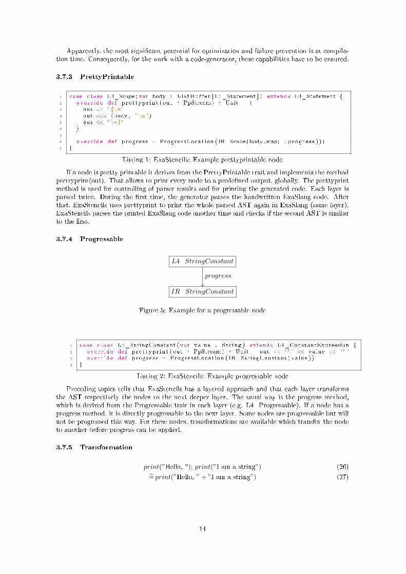
Listing 1: ExaStencils: Example prettyprintable node
If a node is pretty printable it derives from the PrettyPrintable trait and implements the methodprettyprint(out). That allows to print every node to a predened output, globally. The prettyprintmethod is used for controlling of parser results and for printing the generated code. Each layer isparsed twice. During the rst time, the generator parses the handwritten ExaSlang code. Afterthat, ExaStencils uses prettyprint to print the whole parsed AST again in ExaSlang (same layer).ExaStencils parses the printed ExaSlang code another time and checks if the second AST is similarto the rst.
3.7.4 Progressable
L4_StringConstant
IR_StringConstant
progress
Figure 5: Example for a progressable node
1 case c l a s s L4_StringConstant ( var va lue : S t r ing ) extends L4_ConstantExpression 2 ove r r i d e de f p r e t t yp r i n t ( out : PpStream ) : Unit = out << ' " ' << value << ' " '3 ove r r i d e de f p rog r e s s = Progres sLocat ion ( IR_StringConstant ( va lue ) )4
Listing 2: ExaStencils: Example progressable node
Preceding topics tells that ExaStencils has a layered approach and that each layer transformsthe AST respectively the nodes to the next deeper layer. The usual way is the progress method,which is derived from the Progressable trait in each layer (e.g. L4_Progressable). If a node has aprogress method, it is directly progressable to the next layer. Some nodes are progressable but willnot be progressed this way. For these nodes, transformations are available which transfer the nodeto another before progress can be applied.
3.7.5 Transformation
print(”Hello, "); print(”I am a string”) (26)
= print(”Hello, ” + ”I am a string”) (27)
14
print(ConstString1) print(ConstString2)
;
print(ConstantString1 + ConstantString2)
transform
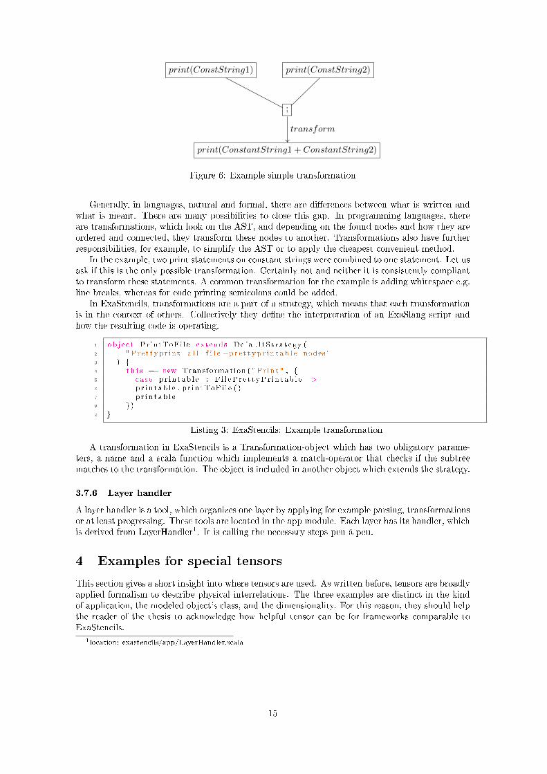
Figure 6: Example simple transformation
Generally, in languages, natural and formal, there are dierences between what is written andwhat is meant. There are many possibilities to close this gap. In programming languages, thereare transformations, which look on the AST, and depending on the found nodes and how they areordered and connected, they transform these nodes to another. Transformations also have furtherresponsibilities, for example, to simplify the AST or to apply the cheapest convenient method.
In the example, two print statements on constant strings were combined to one statement. Let usask if this is the only possible transformation. Certainly not and neither it is consistently compliantto transform these statements. A common transformation for the example is adding whitespace e.g.line breaks, whereas for code printing semicolons could be added.
In ExaStencils, transformations are a part of a strategy, which means that each transformationis in the context of others. Collectively they dene the interpretation of an ExaSlang script andhow the resulting code is operating.
1 ob j e c t Pr intToFi le extends De fau l tSt ra tegy (2 " Pre t typr in t a l l f i l e −p r e t t yp r i n t ab l e nodes "3 ) 4 t h i s += new Transformation ( "Pr int " , 5 case p r i n t ab l e : F i l eP r e t t yPr i n t ab l e =>6 p r i n t ab l e . p r in tToFi l e ( )7 p r i n t ab l e8 )9
Listing 3: ExaStencils: Example transformation
A transformation in ExaStencils is a Transformation-object which has two obligatory parame-ters, a name and a scala function which implements a match-operator that checks if the subtreematches to the transformation. The object is included in another object which extends the strategy.
3.7.6 Layer handler
A layer handler is a tool, which organizes one layer by applying for example parsing, transformationsor at least progressing. These tools are located in the app module. Each layer has its handler, whichis derived from LayerHandler1. It is calling the necessary steps peu á peu.
4 Examples for special tensors
This section gives a short insight into where tensors are used. As written before, tensors are broadlyapplied formalism to describe physical interrelations. The three examples are distinct in the kindof application, the modeled object's class, and the dimensionality. For this reason, they should helpthe reader of the thesis to acknowledge how helpful tensor can be for frameworks comparable toExaStencils.
1location: exastencils/app/LayerHandler.scala
15
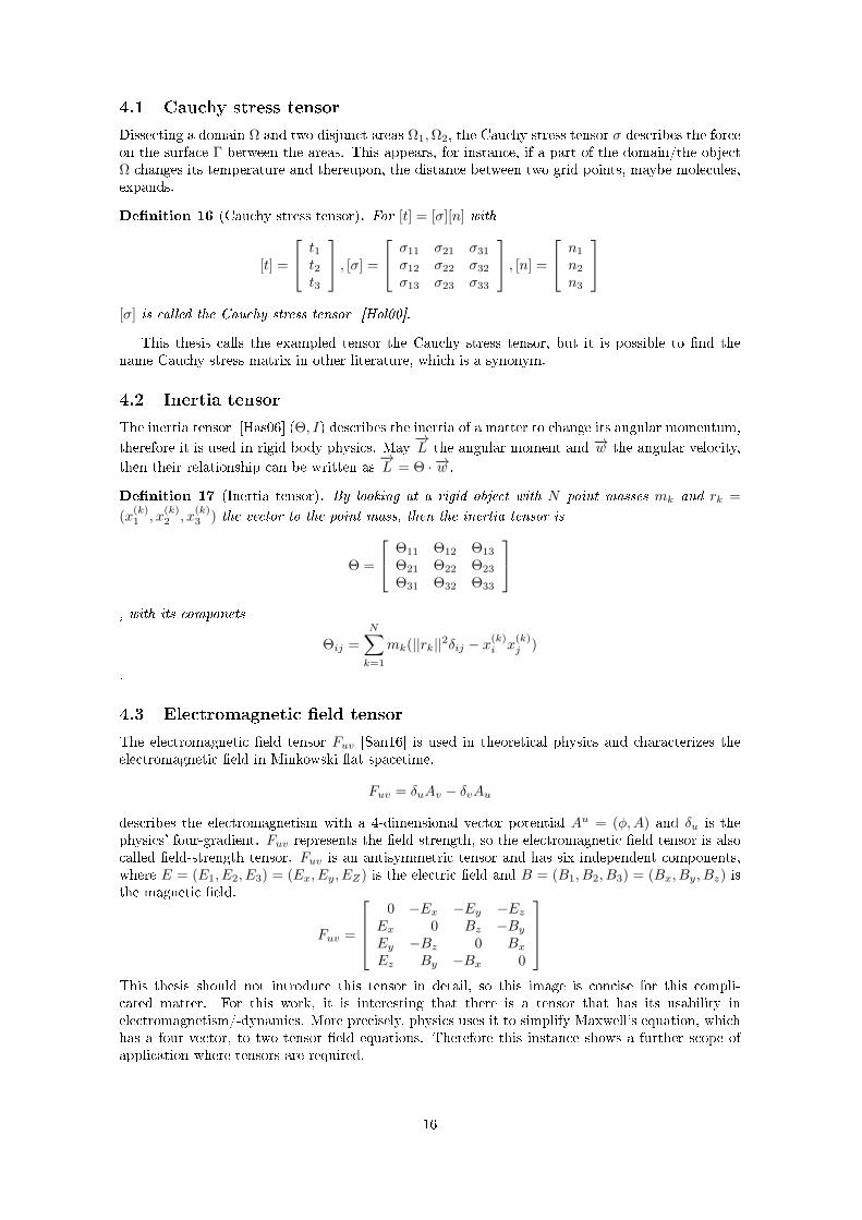
4.1 Cauchy stress tensor
Dissecting a domain Ω and two disjunct areas Ω1,Ω2, the Cauchy stress tensor σ describes the forceon the surface Γ between the areas. This appears, for instance, if a part of the domain/the objectΩ changes its temperature and thereupon, the distance between two grid points, maybe molecules,expands.
Denition 16 (Cauchy stress tensor). For [t] = [σ][n] with
[t] =
t1t2t3
, [σ] =
σ11 σ21 σ31σ12 σ22 σ32σ13 σ23 σ33
, [n] =
n1n2n3
[σ] is called the Cauchy stress tensor [Hol00].
This thesis calls the exampled tensor the Cauchy stress tensor, but it is possible to nd thename Cauchy stress matrix in other literature, which is a synonym.
4.2 Inertia tensor
The inertia tensor [Has06] (Θ, I) describes the inertia of a matter to change its angular momentum,therefore it is used in rigid body physics. May
−→L the angular moment and −→w the angular velocity,
then their relationship can be written as−→L = Θ · −→w .
Denition 17 (Inertia tensor). By looking at a rigid object with N point masses mk and rk =
(x(k)1 , x
(k)2 , x
(k)3 ) the vector to the point mass, then the inertia tensor is
Θ =
Θ11 Θ12 Θ13
Θ21 Θ22 Θ23
Θ31 Θ32 Θ33
, with its componets
Θij =
N∑k=1
mk(||rk||2δij − x(k)i x(k)j )
.
4.3 Electromagnetic eld tensor
The electromagnetic eld tensor Fuv [San16] is used in theoretical physics and characterizes theelectromagnetic eld in Minkowski at spacetime.
Fuv = δuAv − δvAu
describes the electromagnetism with a 4-dimensional vector potential Au = (φ,A) and δu is thephysics' four-gradient. Fuv represents the eld strength, so the electromagnetic eld tensor is alsocalled eld-strength tensor. Fuv is an antisymmetric tensor and has six independent components,where E = (E1, E2, E3) = (Ex, Ey, EZ) is the electric eld and B = (B1, B2, B3) = (Bx, By, Bz) isthe magnetic eld.
Fuv =
0 −Ex −Ey −Ez
Ex 0 Bz −By
Ey −Bz 0 Bx
Ez By −Bx 0
This thesis should not introduce this tensor in detail, so this image is concise for this compli-cated matter. For this work, it is interesting that there is a tensor that has its usability inelectromagnetism/-dynamics. More precisely, physics uses it to simplify Maxwell's equation, whichhas a four-vector, to two tensor eld equations. Therefore this instance shows a further scope ofapplication where tensors are required.
16
5 Representation in ExaSlang
This section describes the transformation from a mathematical denition through the L4 to IR layer.I have chosen to illustrate the transformation in the natural working direction, whereas softwaredevelopment began on the last layer.
With the representation comes implicit the denition in the parser, therefore I am always givingthis specication at hand.
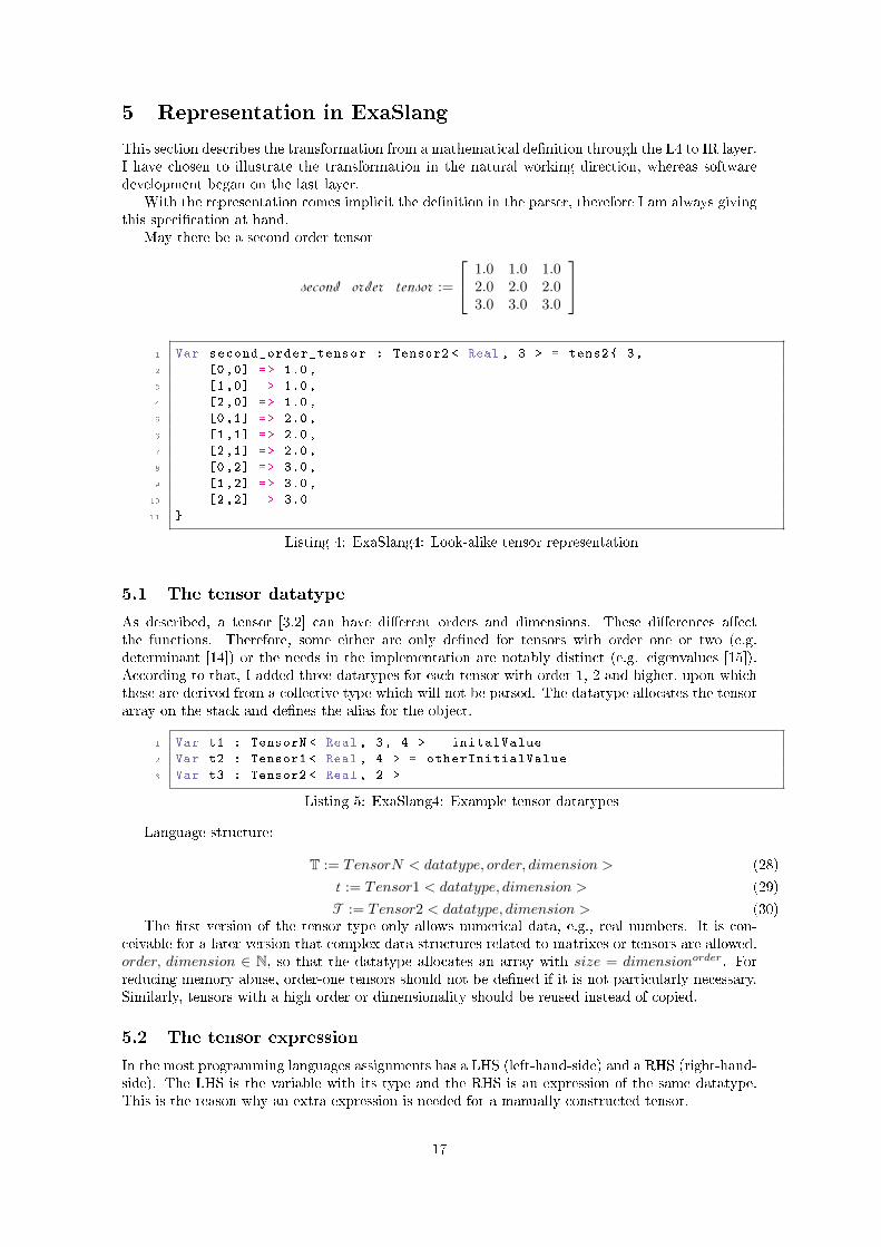
May there be a second order tensor
second_order_tensor :=
1.0 1.0 1.02.0 2.0 2.03.0 3.0 3.0
1 Var second_order_tensor : Tensor2 < Real , 3 > = tens2 3,
2 [0,0] => 1.0,
3 [1,0] => 1.0,
4 [2,0] => 1.0,
5 [0,1] => 2.0,
6 [1,1] => 2.0,
7 [2,1] => 2.0,
8 [0,2] => 3.0,
9 [1,2] => 3.0,
10 [2,2] => 3.0
11
Listing 4: ExaSlang4: Look-alike tensor representation
5.1 The tensor datatype
As described, a tensor [3.2] can have dierent orders and dimensions. These dierences aectthe functions. Therefore, some either are only dened for tensors with order one or two (e.g.determinant [14]) or the needs in the implementation are notably distinct (e.g. eigenvalues [15]).According to that, I added three datatypes for each tensor with order 1, 2 and higher, upon whichthese are derived from a collective type which will not be parsed. The datatype allocates the tensorarray on the stack and denes the alias for the object.
1 Var t1 : TensorN < Real , 3, 4 > = initalValue
2 Var t2 : Tensor1 < Real , 4 > = otherInitialValue
3 Var t3 : Tensor2 < Real , 2 >
Listing 5: ExaSlang4: Example tensor datatypes
Language structure:
T := TensorN < datatype, order, dimension > (28)
t := Tensor1 < datatype, dimension > (29)
T := Tensor2 < datatype, dimension > (30)The rst version of the tensor type only allows numerical data, e.g., real numbers. It is con-
ceivable for a later version that complex data structures related to matrixes or tensors are allowed.order, dimension ∈ N, so that the datatype allocates an array with size = dimensionorder. Forreducing memory abuse, order-one tensors should not be dened if it is not particularly necessary.Similarly, tensors with a high order or dimensionality should be reused instead of copied.
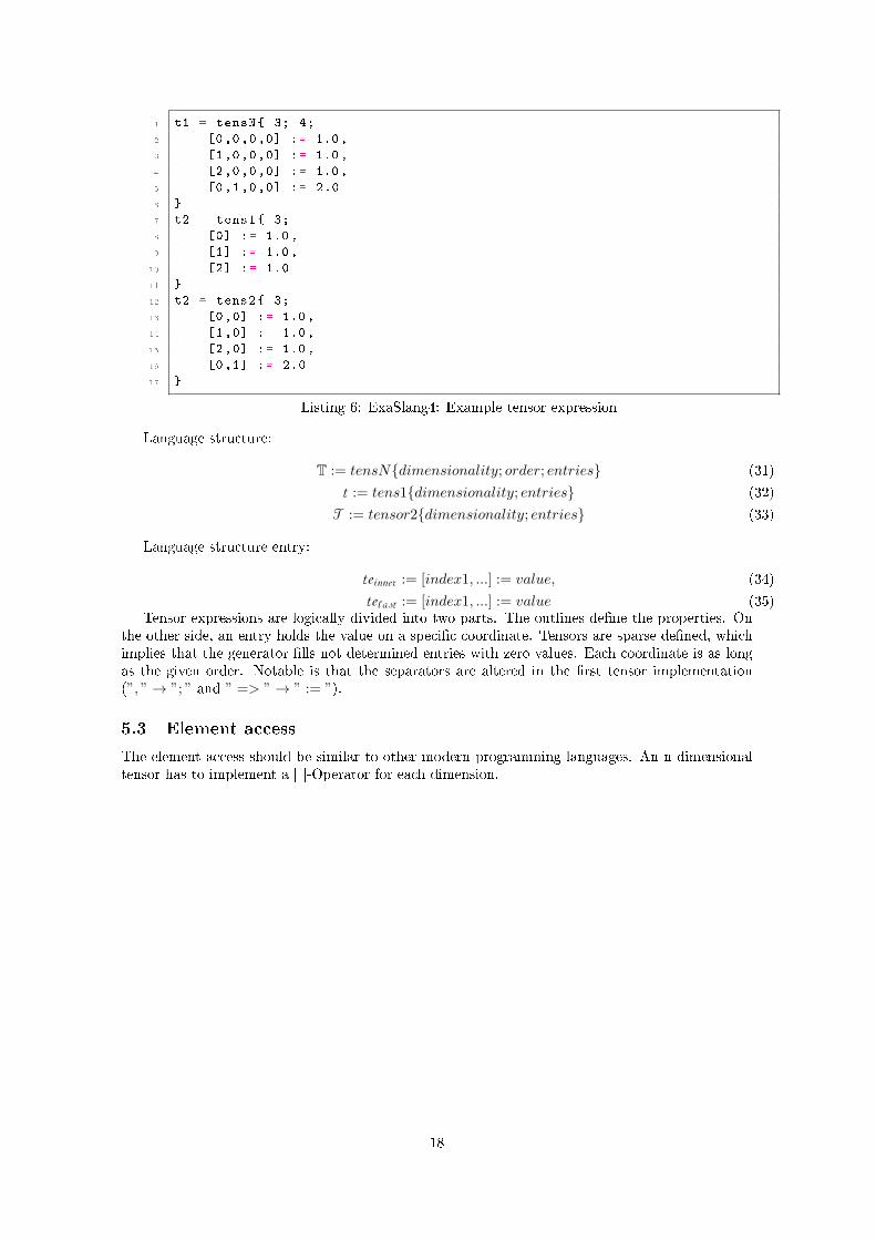
5.2 The tensor expression
In the most programming languages assignments has a LHS (left-hand-side) and a RHS (right-hand-side). The LHS is the variable with its type and the RHS is an expression of the same datatype.This is the reason why an extra expression is needed for a manually constructed tensor.
17
1 t1 = tensN 3; 4;
2 [0,0,0,0] := 1.0,
3 [1,0,0,0] := 1.0,
4 [2,0,0,0] := 1.0,
5 [0,1,0,0] := 2.0
6
7 t2 = tens1 3;
8 [0] := 1.0,
9 [1] := 1.0,
10 [2] := 1.0
11
12 t2 = tens2 3;
13 [0,0] := 1.0,
14 [1,0] := 1.0,
15 [2,0] := 1.0,
16 [0,1] := 2.0
17
Listing 6: ExaSlang4: Example tensor expression
Language structure:
T := tensNdimensionality; order; entries (31)
t := tens1dimensionality; entries (32)
T := tensor2dimensionality; entries (33)
Language structure entry:
teinner := [index1, ...] := value, (34)
telast := [index1, ...] := value (35)Tensor expressions are logically divided into two parts. The outlines dene the properties. On
the other side, an entry holds the value on a specic coordinate. Tensors are sparse dened, whichimplies that the generator lls not determined entries with zero values. Each coordinate is as longas the given order. Notable is that the separators are altered in the rst tensor implementation(”, ”→ ”; ” and ” => ”→ ” := ”).
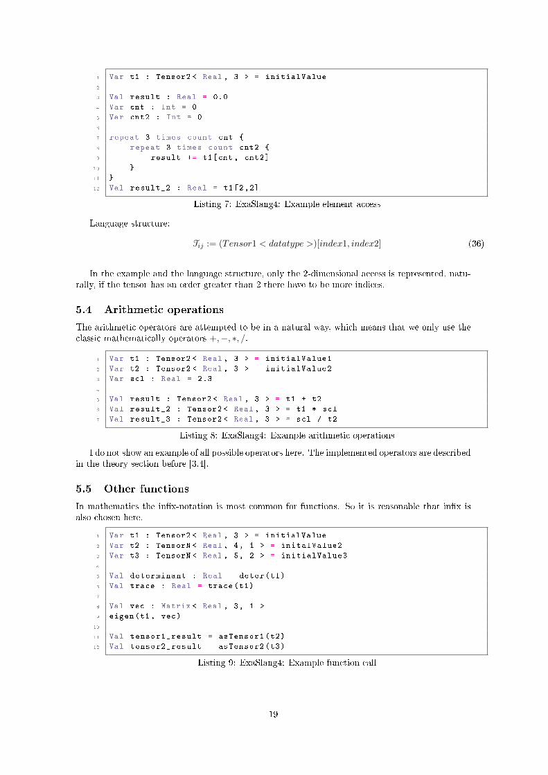
5.3 Element access
The element access should be similar to other modern programming languages. An n-dimensionaltensor has to implement a [ ]-Operator for each dimension.
18
1 Var t1 : Tensor2 < Real , 3 > = initialValue
2
3 Val result : Real = 0.0
4 Var cnt : Int = 0
5 Var cnt2 : Int = 0
6
7 repeat 3 times count cnt
8 repeat 3 times count cnt2
9 result += t1[cnt , cnt2]
10
11
12 Val result_2 : Real = t1[2,2]
Listing 7: ExaSlang4: Example element access
Language structure:
Tij := (Tensor1 < datatype >)[index1, index2] (36)
In the example and the language structure, only the 2-dimensional access is represented, natu-rally, if the tensor has an order greater than 2 there have to be more indices.
5.4 Arithmetic operations
The arithmetic operators are attempted to be in a natural way, which means that we only use theclassic mathematically operators +,−, ∗, /.
1 Var t1 : Tensor2 < Real , 3 > = initialValue1
2 Var t2 : Tensor2 < Real , 3 > = initialValue2
3 Var scl : Real = 2.3
4
5 Val result : Tensor2 < Real , 3 > = t1 + t2
6 Val result_2 : Tensor2 < Real , 3 > = t1 * scl
7 Val result_3 : Tensor2 < Real , 3 > = scl / t2
Listing 8: ExaSlang4: Example arithmetic operations
I do not show an example of all possible operators here. The implemented operators are describedin the theory section before [3.4].
5.5 Other functions
In mathematics the inx-notation is most common for functions. So it is reasonable that inx isalso chosen here.
1 Var t1 : Tensor2 < Real , 3 > = initialValue
2 Var t2 : TensorN < Real , 4, 1 > = initalValue2
3 Var t3 : TensorN < Real , 5, 2 > = initialValue3
4
5 Val determinant : Real = deter(t1)
6 Val trace : Real = trace(t1)
7
8 Val vec : Matrix < Real , 3, 1 >
9 eigen(t1 , vec)
10
11 Val tensor1_result = asTensor1(t2)
12 Val tensor2_result = asTensor2(t3)
Listing 9: ExaSlang4: Example function call
19
The functions deter [14] and trace [12] return their results, instead of eigen [15] were the resultvector has been passed as a parameter. The eigenvalue method is the only function that works onruntime, all other functions were calculated on generation-time.
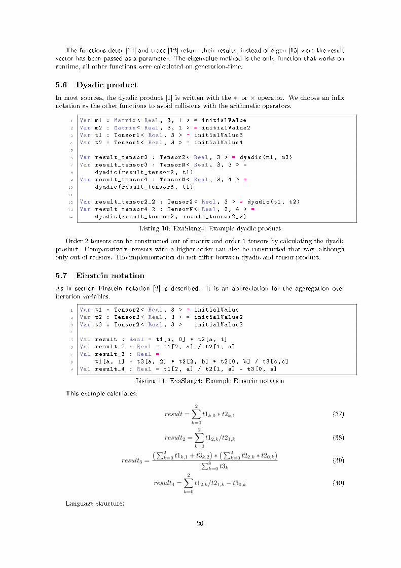
5.6 Dyadic product
In most sources, the dyadic product [1] is written with the ∗, or × operator. We choose an inxnotation as the other functions to avoid collisions with the arithmetic operators.
1 Var m1 : Matrix < Real , 3, 1 > = initialValue
2 Var m2 : Matrix < Real , 3, 1 > = initialValue2
3 Var t1 : Tensor1 < Real , 3 > = initialValue3
4 Var t2 : Tensor1 < Real , 3 > = initialValue4
5
6 Var result_tensor2 : Tensor2 < Real , 3 > = dyadic(m1 , m2)
7 Var result_tensor3 : TensorN < Real , 3, 3 > =
8 dyadic(result_tensor2 , t1)
9 Var result_tensor4 : TensorN < Real , 3, 4 > =
10 dyadic(result_tensor3 , t1)
11
12 Var result_tensor2_2 : Tensor2 < Real , 3 > = dyadic(t1 , t2)
13 Var result_tensor4_2 : TensorN < Real , 3, 4 > =
14 dyadic(result_tensor2 , result_tensor2_2)
Listing 10: ExaSlang4: Example dyadic product
Order 2 tensors can be constructed out of matrix and order 1 tensors by calculating the dyadicproduct. Comparatively, tensors with a higher order can also be constructed that way, althoughonly out of tensors. The implementation do not dier between dyadic and tensor product.
5.7 Einstein notation
As in section Einstein notation [2] is described. It is an abbreviation for the aggregation overiteration variables.
1 Var t1 : Tensor2 < Real , 3 > = initialValue
2 Var t2 : Tensor2 < Real , 3 > = initialValue2
3 Var t3 : Tensor2 < Real , 3 > = initialValue3
4
5 Val result : Real = t1[a, 0] * t2[a, 1]
6 Val result_2 : Real = t1[2, a] / t2[1, a]
7 Val result_3 : Real =
8 t1[a, 1] + t3[a, 2] * t2[2, b] * t2[0, b] / t3[c,c]
9 Val result_4 : Real = t1[2, a] / t2[1, a] - t3[0, a]
Listing 11: ExaSlang4: Example Einstein notation
This example calculates:
result =
2∑k=0
t1k,0 ∗ t2k,1 (37)
result2 =
2∑k=0
t12,k/t21,k (38)
result3 =
(∑2k=0 t1k,1 + t3k,2
)∗(∑2
k=0 t22,k ∗ t20,k)∑8
k=0 t3k(39)
result4 =
2∑k=0
t12,k/t21,k − t30,k (40)
Language structure:
20
tensor1[index1, index2] tensor2[index3, index4] (41)
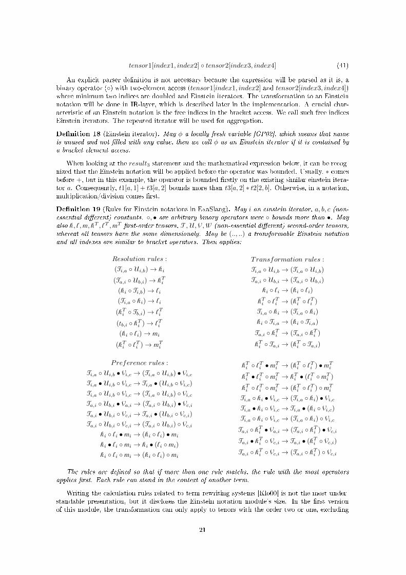
An explicit parser denition is not necessary because the expression will be parsed as it is, abinary operator () with two-element access (tensor1[index1, index2] and tensor2[index3, index4])where minimum two indices are doubled and Einstein iterators. The transformation to an Einsteinnotation will be done in IR-layer, which is described later in the implementation. A crucial char-acteristic of an Einstein notation is the free indices in the bracket access. We call such free indicesEinstein iterators. The repeated iterator will be used for aggregation.
Denition 18 (Einstein iterator). May φ a locally fresh variable [GP02], which means that nameis unused and not lled with any value, then we call φ as an Einstein iterator if it is contained bya bracket element access.
When looking at the result3 statement and the mathematical expression below, it can be recog-nized that the Einstein notation will be applied before the operator was bounded. Usually, ∗ comesbefore +, but in this example, the operator is bounded rstly on the existing similar einstein itera-tor a. Consequently, t1[a, 1] + t3[a, 2] bounds more than t3[a, 2] ∗ t2[2, b]. Otherwise, in a notation,multiplication/division comes rst.
Denition 19 (Rules for Einstein notations in ExaSlang). May i an einstein iterator, a, b, c (non-essential dierent) constants. , • are arbitrary binary operators were bounds more than •. Mayalso k, l,m, kT , lT ,mT rst-order tensors, T,U,V,W (non-essential dierent) second-order tensors,whereat all tensors have the same dimensionaly. May be (.., ..) a transformable Einstein notationand all indexes are similar to bracket operators. Then applies:
Resolution rules :
(Ti,a Ui,b)→ ki
(Ta,i Ub,i)→ kTi
(ki Ti,b)→ li
(Ti,a ki)→ li
(kTi Tb,i)→ lTi
(tb,i kTi )→ lTi
(ki li)→ mi
(kTi lTi )→ mT
i
Transformation rules :
Ti,a Ui,b → (Ti,a Ui,b)
Ta,i Ub,i → (Ta,i Ub,i)
ki li → (ki li)kTi lTi → (kT
i lTi )
Ti,a ki → (Ti,a ki)ki Ti,a → (ki Ti,a)
Ta,i kTi → (Ta,i kT
i )
kTi Ta,i → (kT
i Ta,i)
Preference rules :
Ti,a Ui,b • Vi,c → (Ti,a Ui,b) • Vi,cTi,a •Ui,b Vi,c → Ti,a • (Ui,b Vi,c)Ti,a Ui,b Vi,c → (Ti,a Ui,b) Vi,cTa,i Ub,i • Va,i → (Ta,i Ub,i) • Vc,iTa,i •Ub,i Vc,i → Ta,i • (Ub,i Vc,i)Ta,i Ub,i Vc,i → (Ta,i Ub,i) Vc,i
ki li • mi → (ki li) • mi
ki • li mi → ki • (li mi)
ki li mi → (ki li) mi
kTi lTi • mT
i → (kTi lTi ) • mT
i
kTi • lTi mT
i → kTi • (lTi mT
i )
kTi lTi mT
i → (kTi lTi ) mT
i
Ti,a ki • Vi,c → (Ti,a ki) • Vi,cTi,a • ki Vi,c → Ti,a • (ki Vi,c)Ti,a ki Vi,c → (Ti,a ki) Vi,cTa,i kT
i • Va,i → (Ta,i kTi ) • Vc,i
Ta,i • kTi Vc,i → Ta,i • (kT
i Vc,i)Ta,i kT
i Vc,i → (Ta,i kTi ) Vc,i
The rules are dened so that if more than one rule matchs, the rule with the most operatorsapplies rst. Each rule can stand in the context of another term.
Writing the calculation-rules related to term rewriting systems [Klo00] is not the most under-standable presentation, but it discloses the Einstein notation module's size. In the rst versionof this module, the transformation can only apply to tenors with the order two or one, excluding
21
double contraction, which is described below. There are some possible meaningful extensions forthe future, which were not implementable at the time of the thesis. For instance, another iterationvariables could be applied, or instead of the summation at the end, the user could save the resultedvector from the last transformation. Another interesting topic could be the universal rule denitionof an Einstein notation from an informatic view so that it is possible to use any tensors in themodule.
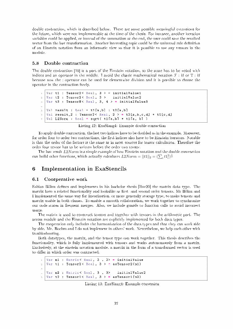
5.8 Double contraction
The double contraction [10] is a part of the Einstein notation, so the state has to be noted withindices and an operator in the middle. I avoid the classic mathematical notation T : U or T : Ubecause now the : operator can be used for elementwise division and it is possible to choose theoperator in the contraction freely.
1 Var t1 : Tensor2 < Real , 3 > = initialValue1
2 Var t2 : Tensor2 < Real , 3 > = initialValue2
3 Var t3 : TensorN < Real , 3, 4 > = initialValue3
4
5 Val result : Real = t1[a,b] : t2[a,b]
6 Val result_2 : Tensor2 < Real , 2 > = t3[a,b,c,d] * t1[c,d]
7 Val L2Norm : Real = sqrt( t1[a,b] * t1[a, b] )
Listing 12: ExaSlang4: Example double conraction
To apply double contraction, the last two indices have to be doubled as in the example. Moreover,for order four to order two contractions, the rst indices also have to be Einstein iterators. Notableis that the order of the factors is the same as in most sources for tensor calculation. Therefore theorder four tensor has to be written before the order two tensor.
The last result L2Norm is a simple example of how Einstein notation and the double contractioncan build other functions, which actually calculates L2Norm = ||t1||2 = (
∑i t1
2i )
12
6 Implementation in ExaStencils
6.1 Coorperative work
Fabian Böhm denes and implements in his bachelor thesis [Boe20] the matrix data type. Thematrix have a related functionality and lookalike as rst- and second-order tensors. Mr Böhm andI implemented the same way for linearization, or more generally storage type, to make tensors andmatrix usable in both classes. To enable a smooth collaboration, we work together to synchronizeour code states in frequent merges. Also, we include guards to function calls to avoid incorrectusage.
The matrix is used to construct tensors and together with tensors in the arithmetic part. Theaccess module and the Einstein notation are explicitly implemented for both data types.
The cooperation only includes the harmonization of the data types and that they can work sideby side. Mr. Boehm and I do not implement in others' work. Nevertheless, we help each other withtroubleshooting.
Both datatypes, the matrix, and the tensor type can work together. This thesis describes thefunctionality, which is fully implemented with tensors and works autonomously from a matrix.Exclusively, at the einstein notation module, a matrix in the form of a transformed vector is usedto dier in which order was contracted.
1 Var m1 : Matrix < Real , 3 , 3> = initialValue
2 Var t1 : Tensor2 < Real , 3 > = asTensor2(m1)
3
4 Var m2 : Matrix < Real , 3 , 3> = initialValue2
5 Var t2 : Tensor1 < Real , 3 > = asTensor1(m2)
Listing 13: ExaSlang4: Example conversion
22
Module Desription
Constructors Uses matrix as an input type for dyadic product.
Arithmetic Uses matrix for all classical arithmetic operators(+,−, ∗, /).
Access The classic bracket operator works also with ma-trix. matrix are used in the complex access mod-ule.
EinsteinNotation With the Einstein notation matrix can be used in-stead of tensors.
HigherFunctions matrix can be convertet to rst- and second ordertensors
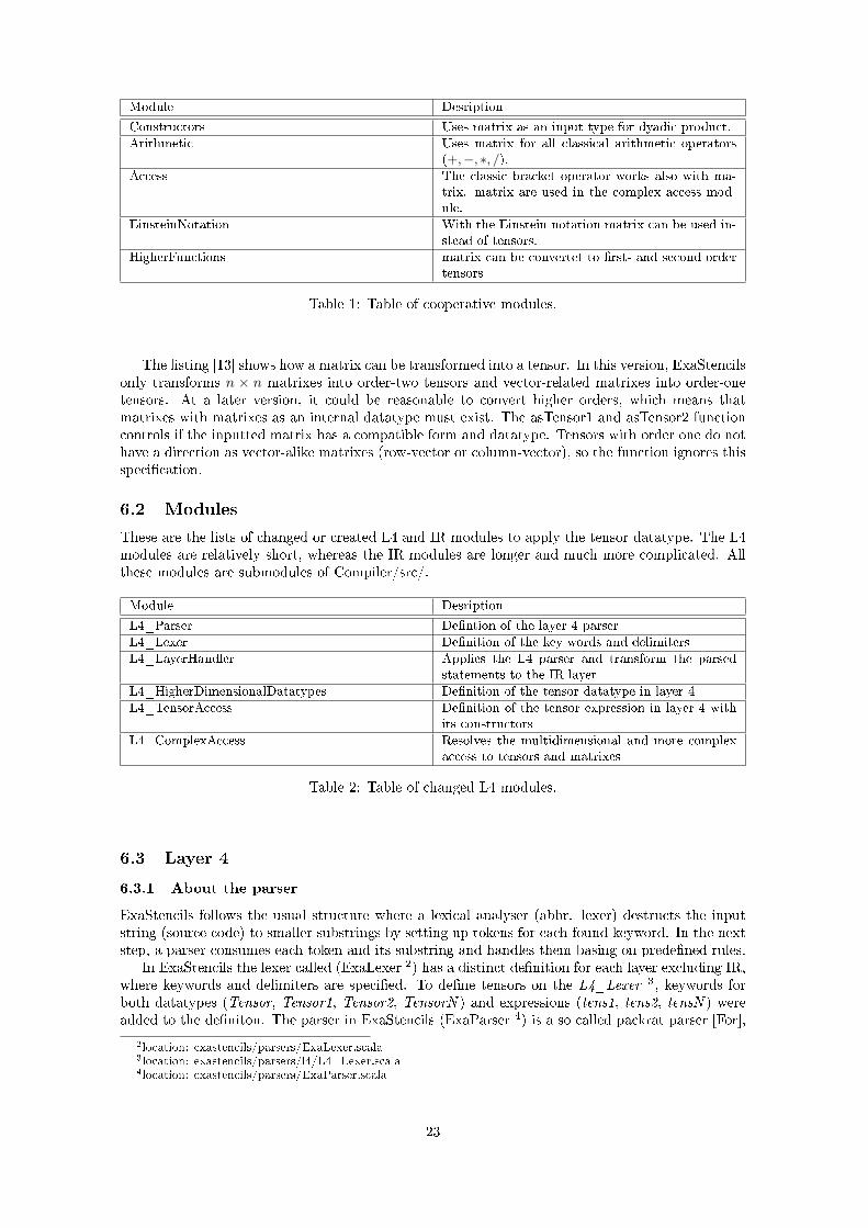
Table 1: Table of cooperative modules.
The listing [13] shows how a matrix can be transformed into a tensor. In this version, ExaStencilsonly transforms n × n matrixes into order-two tensors and vector-related matrixes into order-onetensors. At a later version, it could be reasonable to convert higher orders, which means thatmatrixes with matrixes as an internal datatype must exist. The asTensor1 and asTensor2 functioncontrols if the inputted matrix has a compatible form and datatype. Tensors with order one do nothave a direction as vector-alike matrixes (row-vector or column-vector), so the function ignores thisspecication.
6.2 Modules
These are the lists of changed or created L4 and IR modules to apply the tensor datatype. The L4modules are relatively short, whereas the IR modules are longer and much more complicated. Allthese modules are submodules of Compiler/src/.
Module Desription
L4_Parser Dention of the layer 4 parser
L4_Lexer Denition of the key words and delimiters
L4_LayerHandler Applies the L4 parser and transform the parsedstatements to the IR layer
L4_HigherDimensionalDatatypes Denition of the tensor datatype in layer 4
L4_TensorAccess Denition of the tensor expression in layer 4 withits constructors
L4_ComplexAccess Resolves the multidimensional and more complexaccess to tensors and matrixes
Table 2: Table of changed L4 modules.
6.3 Layer 4
6.3.1 About the parser
ExaStencils follows the usual structure where a lexical analyser (abbr. lexer) destructs the inputstring (source code) to smaller substrings by setting up tokens for each found keyword. In the nextstep, a parser consumes each token and its substring and handles them basing on predened rules.
In ExaStencils the lexer called (ExaLexer 2) has a distinct denition for each layer excluding IR,where keywords and delimiters are specied. To dene tensors on the L4_Lexer 3, keywords forboth datatypes (Tensor, Tensor1, Tensor2, TensorN ) and expressions (tens1, tens2, tensN ) wereadded to the deniton. The parser in ExaStencils (ExaParser 4) is a so called packrat parser [For],
2location: exastencils/parsers/ExaLexer.scala3location: exastencils/parsers/l4/L4_Lexer.scala4location: exastencils/parsers/ExaParser.scala
23
Module Desription
IR_LayerHandler Applies the transformations on the AST and printsout the resulting c++ code.
IR_HigherDimensionalDatatypes Denition of the tensor datatype in the IR layer
IR_TensorAccess Denition of the tensor expression in the IR layerwith its constructors
IR_ResultingDatatype Determines the resulting datatype
IR_TensorAssingments Resolves the assignments of tensor accesses and ex-pressions
IR_ResolveTensorReturnValues Denes the names of the tensor member functionsand implements their return
IR_ResolveTensorCompiletimeFunctions Denes, implements and resolves the tensor mem-ber functions, which has been calculated to compiletime (e.g. multiplication)
IR_ResolveTensoreRuntimeFunctions Denes, implements and resolves the tensor mem-ber functions, which has been calculated to run-time (e.g. eigenvalures)
IR_ComplexAccess Implements and resolves the multidimensional andmore complex access to tensors and matrix. It alsoevaluates the return of an Einstein notations
IR_ResolveEinsteinNotation Resolves the Einstein notation, by mapping thesimilar char-like indices of a complex access
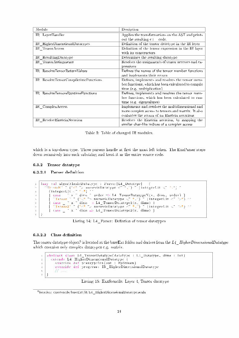
Table 3: Table of changed IR modules.
which is a top-down type. Those parsers handle at rst the most left token. The ExaParser stepsdown recursively into each substring and treat it as the entire source code.
6.3.2 Tensor datatype
6.3.2.1 Parser denition
1 l a zy va l a lgor i thmicDatatype : Parser [ L4_Datatype ] = (2 "TensorN" ~ ( "<" ~> numericDatatype <~ " , " ) ~ ( i n t e g e rL i t <~ " , " ) ~3 ( i n t e g e rL i t <~ ">" ) ^^4 case _ ~ x ~ dims ~ order => L4_TensorDatatypeN (x , dims , order ) 5 | | | "Tensor1" ~ ( "<" ~> numericDatatype <~ " , " ) ~ ( i n t e g e rL i t <~ ">" ) ^^6 case _ ~ x ~ dims => L4_TensorDatatype1 (x , dims ) 7 | | | "Tensor2" ~ ( "<" ~> numericDatatype <~ " , " ) ~ ( i n t e g e rL i t <~ ">" ) ^^8 case _ ~ x ~ dims => L4_TensorDatatype2 (x , dims ) 9 )
Listing 14: L4_Parser: Dention of tensor datatypes
6.3.2.2 Class denition
The tensor datatype object5 is located at the baseExt folder and derives from the L4_HigherDimensionalDatatypewhich contains only complex datatypes e.g. matrix.
1 abs t r a c t c l a s s L4_TensorDatatype ( datatype : L4_Datatype , dims : Int )2 extends L4_HigherDimensionalDatatype 3 ove r r i d e de f p r e t t yp r i n t ( out : PpStream )4 ove r r i d e de f p rog r e s s : IR_HigherDimensionalDatatype5 // . . .6
Listing 15: ExaStencils: Layer 4, Tensor datatype
5location: exastencils/baseExt/l4/L4_HigherDimensionalDatatype.scala
24
6.3.2.3 Description
As previously explained, there are three types of tensors and an abstract tensor where the oth-ers have derived from. The member functions of the tensor overwrite the functions from theL4_Datatype class, where all data types are derived. The data type has obligatorily two pa-rameters datatype, which determines the inner type, and dims that held the dimensionality of thetensor. For the n-th-order tensor, a third parameter is relevant, the so called order parameterwhich indicates the order of the tensor. The listing [14] shows the parser denition for the tensordatatype. TensorN, Tensor1, and Tensor2 are the keywords for the tensor. These are dened atthe L4_Lexer. ” <>, () are delimiters, which also noted at the lexer denition.
6.3.3 Tensor expression
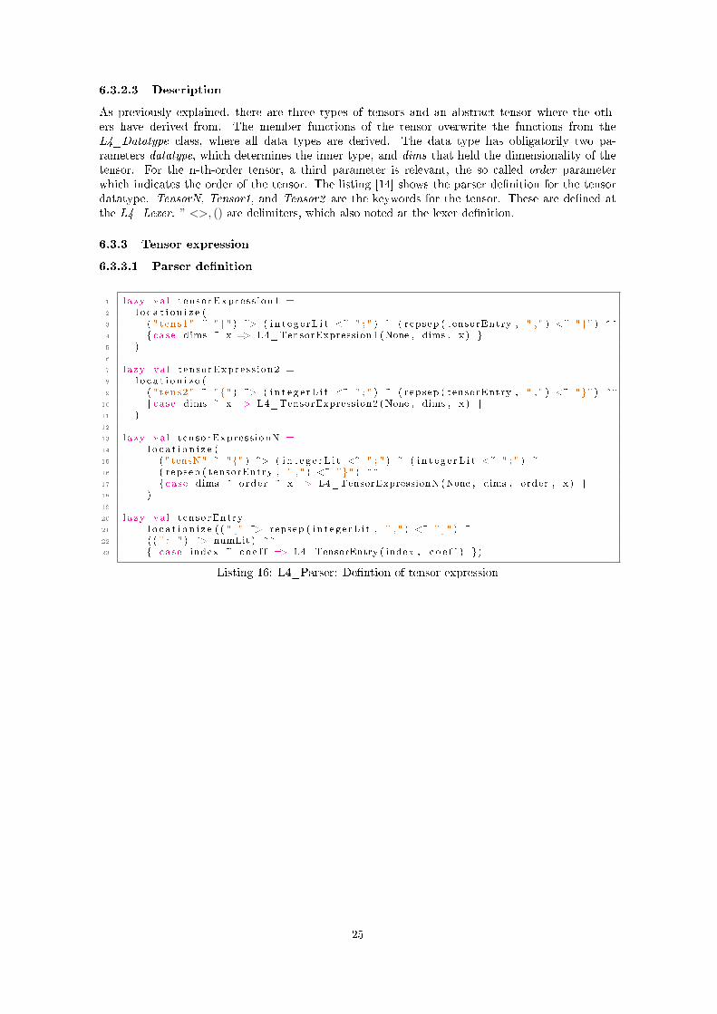
6.3.3.1 Parser denition
1 l a zy va l t ensorExpre s s i on1 =2 l o c a t i o n i z e (3 ( " tens1 " ~ "" ) ~> ( i n t e g e rL i t <~ " ; " ) ~ ( repsep ( tensorEntry , " , " ) <~ "" ) ^^4 case dims ~ x => L4_TensorExpression1 (None , dims , x ) 5 )6
7 l a zy va l t ensorExpre s s i on2 =8 l o c a t i o n i z e (9 ( " tens2 " ~ "" ) ~> ( i n t e g e rL i t <~ " ; " ) ~ ( repsep ( tensorEntry , " , " ) <~ "" ) ^^
10 case dims ~ x => L4_TensorExpression2 (None , dims , x ) 11 )12
13 l a zy va l tensorExpress ionN =14 l o c a t i o n i z e (15 ( " tensN" ~ "" ) ~> ( i n t e g e rL i t <~ " ; " ) ~ ( i n t e g e rL i t <~ " ; " ) ~16 ( repsep ( tensorEntry , " , " ) <~ "" ) ^^17 case dims ~ order ~ x => L4_TensorExpressionN (None , dims , order , x ) 18 )19
20 l a zy va l tensorEntry =21 l o c a t i o n i z e ( ( " [ " ~> repsep ( i n t e g e rL i t , " , " ) <~ " ] " ) ~22 ( ( " :=" ) ~> numLit ) ^^23 case index ~ c o e f f => L4_TensorEntry ( index , c o e f f ) )
Listing 16: L4_Parser: Dention of tensor expression
25
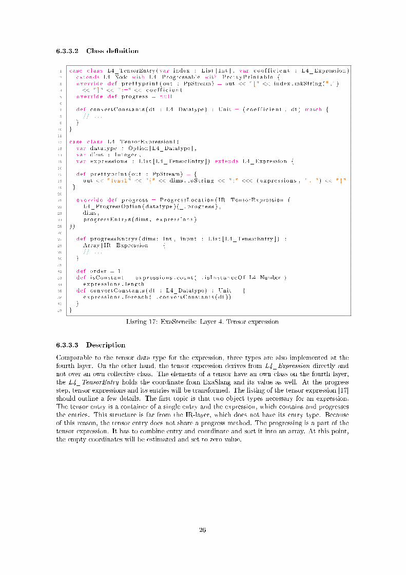
6.3.3.2 Class denition
1 case c l a s s L4_TensorEntry ( var index : L i s t [ Int ] , var c o e f f i c i e n t : L4_Expression )2 extends L4_Node with L4_Progressable with Pre t tyPr in tab l e 3 ove r r i d e de f p r e t t yp r i n t ( out : PpStream ) = out << " [ " << index . mkString ( " , " )4 << " ] " << " :=" << c o e f f i c i e n t5 ove r r i d e de f p rog r e s s = nu l l6
7 de f convertConstants ( dt : L4_Datatype ) : Unit = ( c o e f f i c i e n t , dt ) match 8 // . . .9
10 11
12 case c l a s s L4_TensorExpression1 (13 var datatype : Option [ L4_Datatype ] ,14 var dims : Integer ,15 var exp r e s s i on s : L i s t [ L4_TensorEntry ] ) extends L4_Expression 16
17 de f p r e t t yp r i n t ( out : PpStream ) = 18 out << " tens1 " << "" << dims . t oS t r i ng << " ; " <<< ( expre s s i on s , " , " ) << ""19 20
21 ove r r i d e de f p rog r e s s = Progres sLocat ion ( IR_TensorExpression1 (22 L4_ProgressOption ( datatype ) (_. p rog r e s s ) ,23 dims ,24 progre s sEntrys ( dims , e xp r e s s i on s )25 ) )26
27 de f progre s sEntrys ( dims : Int , input : L i s t [ L4_TensorEntry ] ) :28 Array [ IR_Expression ] = 29 // . . .30 31
32 de f order = 133 de f i sConstant = exp r e s s i on s . count (_. i s In s t anc eOf [ L4_Number ] ) ==34 exp r e s s i on s . l ength35 de f convertConstants ( dt : L4_Datatype ) : Unit = 36 exp r e s s i on s . f o r each (_. convertConstants ( dt ) )37 38
Listing 17: ExaStencils: Layer 4, Tensor expression
6.3.3.3 Description
Comparable to the tensor data type for the expression, three types are also implemented at thefourth layer. On the other hand, the tensor expression derives from L4_Expression directly andnot over an own collective class. The elements of a tensor have an own class on the fourth layer,the L4_TensorEntry holds the coordinate from ExaSlang and its value as well. At the progressstep, tensor expressions and its entries will be transformed. The listing of the tensor expression [17]should outline a few details. The rst topic is that two object types necessary for an expression.The tensor entry is a container of a single entry and the expression, which contains and progressesthe entries. This structure is far from the IR-layer, which does not have its entry type. Becauseof this reason, the tensor entry does not share a progress method. The progressing is a part of thetensor expression. It has to combine entry and coordinate and sort it into an array. At this point,the empty coordinates will be estimated and set to zero value.
26
6.3.4 Element access
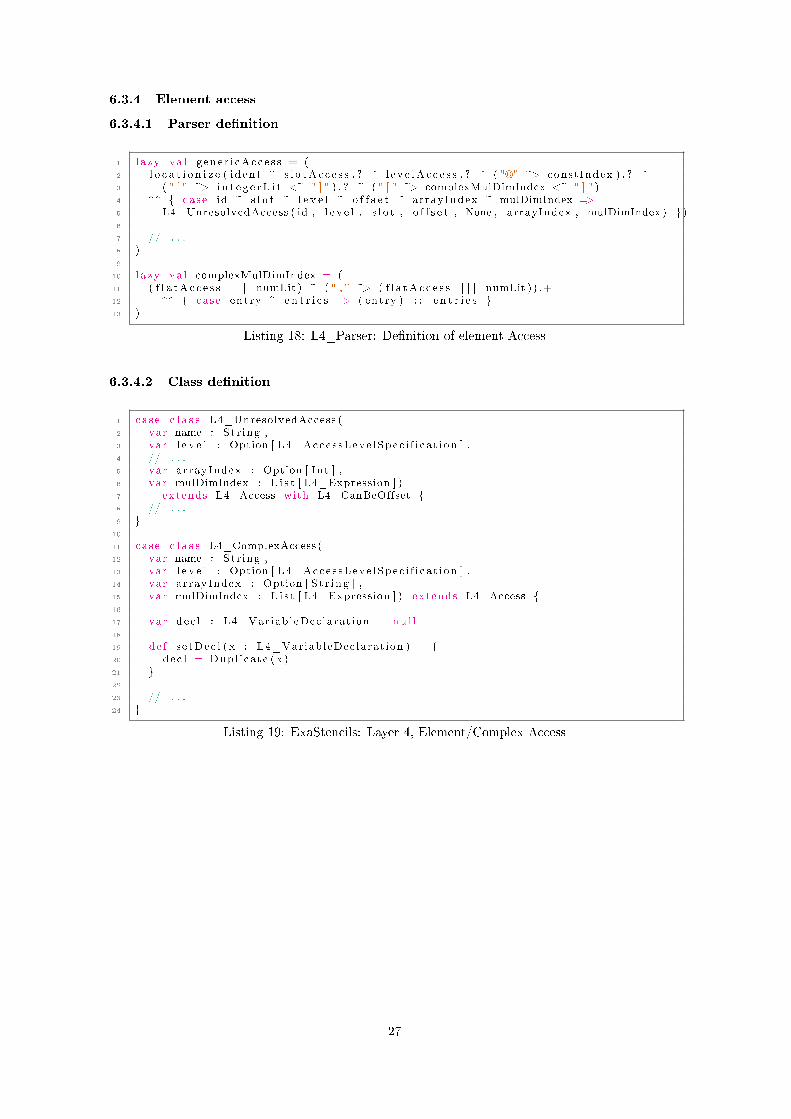
6.3.4.1 Parser denition
1 l a zy va l g ene r i cAcce s s = (2 l o c a t i o n i z e ( ident ~ s l o tAcc e s s . ? ~ l e v e lAc c e s s . ? ~ ( "@" ~> constIndex ) . ? ~3 ( " [ " ~> i n t e g e rL i t <~ " ] " ) . ? ~ ( " [ " ~> complexMulDimIndex <~ " ] " )4 ^^ case id ~ s l o t ~ l e v e l ~ o f f s e t ~ arrayIndex ~ mulDimIndex =>5 L4_UnresolvedAccess ( id , l e v e l , s l o t , o f f s e t , None , arrayIndex , mulDimIndex ) )6
7 // . . .8 )9
10 l a zy va l complexMulDimIndex = (11 ( f l a tAc c e s s | | | numLit ) ~ ( " , " ~> ( f l a tAc c e s s | | | numLit )) .+12 ^^ case entry ~ e n t r i e s => ( entry ) : : e n t r i e s 13 )
Listing 18: L4_Parser: Denition of element Access
6.3.4.2 Class denition
1 case c l a s s L4_UnresolvedAccess (2 var name : Str ing ,3 var l e v e l : Option [ L4_Acces sLeve lSpec i f i ca t i on ] ,4 // . . .5 var arrayIndex : Option [ Int ] ,6 var mulDimIndex : L i s t [ L4_Expression ] )7 extends L4_Access with L4_CanBeOffset 8 // . . .9
10
11 case c l a s s L4_ComplexAccess (12 var name : Str ing ,13 var l e v e l : Option [ L4_Acces sLeve lSpec i f i ca t i on ] ,14 var arrayIndex : Option [ S t r ing ] ,15 var mulDimIndex : L i s t [ L4_Expression ] ) extends L4_Access 16
17 var dec l : L4_VariableDeclarat ion = nu l l18
19 de f s e tDec l ( x : L4_VariableDeclarat ion ) = 20 dec l = Dupl icate ( x )21 22
23 // . . .24
Listing 19: ExaStencils: Layer 4, Element/Complex Access
27
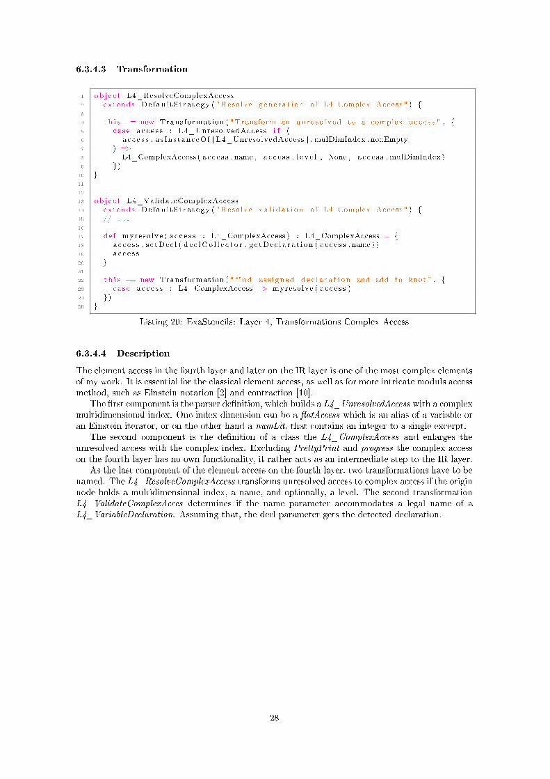
6.3.4.3 Transformation
1 ob j e c t L4_ResolveComplexAccess2 extends De fau l tS t ra tegy ( "Resolve gene ra t i on o f L4 Complex Access " ) 3
4 t h i s += new Transformation ( "Transform an unreso lved to a complex ac c e s s " , 5 case a c c e s s : L4_UnresolvedAccess i f (6 ac c e s s . as InstanceOf [ L4_UnresolvedAccess ] . mulDimIndex . nonEmpty7 ) =>8 L4_ComplexAccess ( a c c e s s . name , a c c e s s . l e v e l , None , a c c e s s . mulDimIndex )9 )
10 11
12
13 ob j e c t L4_ValidateComplexAccess14 extends De fau l tS t ra tegy ( "Resolve v a l i d a t i o n o f L4 Complex Access " ) 15 // . . .16
17 de f myresolve ( a c c e s s : L4_ComplexAccess ) : L4_ComplexAccess = 18 ac c e s s . s e tDec l ( d e c lCo l l e c t o r . g e tDec l a ra t i on ( a c c e s s . name ) )19 ac c e s s20 21
22 t h i s += new Transformation ( " f i nd as s i gned d e c l a r a t i on and add to knot" , 23 case a c c e s s : L4_ComplexAccess => myresolve ( a c c e s s )24 )25
Listing 20: ExaStencils: Layer 4, Transformations Complex Access
6.3.4.4 Description
The element access in the fourth layer and later on the IR layer is one of the most complex elementsof my work. It is essential for the classical element access, as well as for more intricate moduls accessmethod, such as Einstein notation [2] and contraction [10].
The rst component is the parser denition, which builds a L4_UnresolvedAccess with a complexmultidimensional index. One index dimension can be a atAccess which is an alias of a variable oran Einstein iterator, or on the other hand a numLit, that contains an integer to a single excerpt.
The second component is the denition of a class the L4_ComplexAccess and enlarges theunresolved access with the complex index. Excluding PrettyPrint and progress the complex accesson the fourth layer has no own functionality, it rather acts as an intermediate step to the IR layer.
As the last component of the element access on the fourth layer, two transformations have to benamed. The L4_ResolveComplexAccess transforms unresolved access to complex access if the originnode holds a multidimensional index, a name, and optionally, a level. The second transformationL4_ValidateComplexAcces determines if the name parameter accommodates a legal name of aL4_VariableDeclaration. Assuming that, the decl parameter gets the detected declaration.
28
6.4 IR Layer
6.4.1 Tensor datatype
6.4.1.1 Class denition
1 abs t r a c t c l a s s IR_TensorDatatype ( datatype : IR_Datatype , dims : Int )2 extends IR_HigherDimensionalDatatype with IR_HasTypeAlias 3
4 ove r r i d e de f p r e t t yp r i n t ( out : PpStream )5 ove r r i d e de f prettyprint_mpi = s "INVALID DATATYPE: "6 + th i s . p r e t t yp r i n t ( )7
8 ove r r i d e de f d imens i ona l i t y : Int9 ove r r i d e de f getS izeArray : Array [ Int ]
10 ove r r i d e de f reso lveDec lType : IR_Datatype11 ove r r i d e de f r e s o l v eDe c lPo s t s c r i p t : S t r ing = ""12 ove r r i d e de f r e s o l v eF l a t t endS i z e : Int13 ove r r i d e de f t yp i c a lBy t eS i z e : Int14
15 ove r r i d e de f a l i a sFo r = datatype . p r e t t yp r i n t16 + ' [ ' + t h i s . r e s o l v eF l a t t endS i z e + ' ] '17 de f getDims : Int = dims18
Listing 21: ExaStencils: IR Layer, Tensor datatype
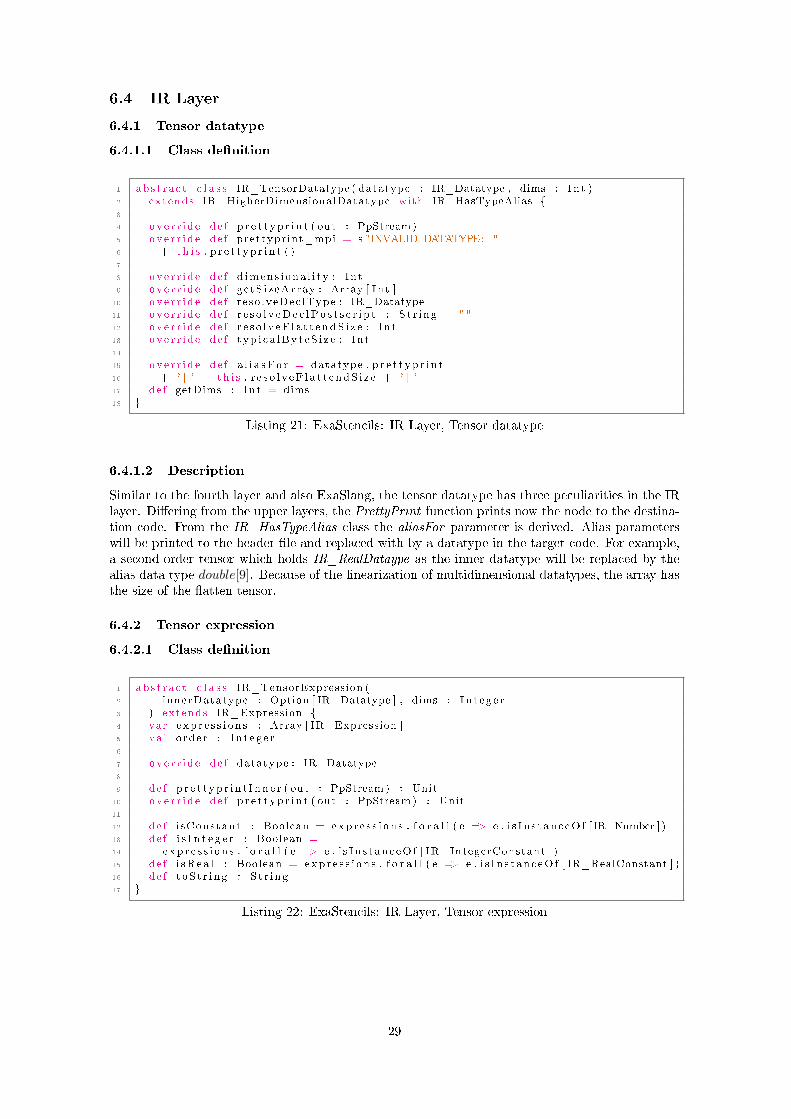
6.4.1.2 Description
Similar to the fourth layer and also ExaSlang, the tensor datatype has three peculiarities in the IRlayer. Diering from the upper layers, the PrettyPrint function prints now the node to the destina-tion code. From the IR_HasTypeAlias class the aliasFor parameter is derived. Alias parameterswill be printed to the header le and replaced with by a datatype in the target code. For example,a second-order tensor which holds IR_RealDataype as the inner datatype will be replaced by thealias data type double[9]. Because of the linearization of multidimensional datatypes, the array hasthe size of the atten tensor.
6.4.2 Tensor expression
6.4.2.1 Class denition
1 abs t r a c t c l a s s IR_TensorExpression (2 innerDatatype : Option [ IR_Datatype ] , dims : In t eg e r3 ) extends IR_Expression 4 var exp r e s s i on s : Array [ IR_Expression ]5 va l order : I n t eg e r6
7 ove r r i d e de f datatype : IR_Datatype8
9 de f p r e t t yp r i n t I nne r ( out : PpStream) : Unit10 ove r r i d e de f p r e t t yp r i n t ( out : PpStream ) : Unit11
12 de f i sConstant : Boolean = exp r e s s i on s . f o r a l l ( e => e . i s I n s t anc eOf [ IR_Number ] )13 de f i s I n t e g e r : Boolean =14 exp r e s s i on s . f o r a l l ( e => e . i s I n s t anc eOf [ IR_IntegerConstant ] )15 de f i sRea l : Boolean = exp r e s s i on s . f o r a l l ( e => e . i s I n s t anc eOf [ IR_RealConstant ] )16 de f t oS t r i ng : S t r ing17
Listing 22: ExaStencils: IR Layer, Tensor expression
29
6.4.2.2 Description
The tensor expression in the IR layer is not so complicated, respectively it is the result of theprogress step from the fourth layer. For the practical use of tensors in the IR layer are the functionsisInteger and isReal crucial. With them it is possible to dier between a test on 'is similar' or on'is similar in an epsilon environment'.
6.4.3 Element access
6.4.3.1 Class denition
1 case c l a s s IR_ComplexAccess (2 var name : Str ing ,3 var dec l : IR_VariableDeclarat ion ,4 var arrayIndex : Option [ S t r ing ] ,5 var mulDimIndex : L i s t [ IR_Expression ] ,6 deep : Int7 ) extends IR_Access 8
9 ove r r i d e de f p r e t t yp r i n t ( out : PpStream ) : Unit =10 out << "\n −−− NOT VALID ; NODE_TYPE = " <<11 t h i s . g e tC la s s . getName << "\n"12 ove r r i d e de f datatype : IR_Datatype = dec l . datatype13
14 de f r e s o l v e ( ) : IR_Expression = 15 // . . .16
Listing 23: ExaStencils: IR Layer, Element/Complex Access
6.4.3.2 Transformation
1 ob j e c t IR_ResolveComplexAccess2 extends De fau l tS t ra tegy ( "Resolve transormat ion o f Complex Access " ) 3
4 de f r e s o l v e ( a c c e s s : IR_ComplexAccess ) : IR_Expression = 5 ac c e s s . r e s o l v e ( )6 7 t h i s += new Transformation (8 "add ass ignments / dec l to func t i on r e tu rn s to arguments" , 9 case a c c e s s : IR_ComplexAccess => r e s o l v e ( a c c e s s )
10 )11
Listing 24: ExaStencils: IR Layer, Transformations Complex Access
6.4.3.3 Description
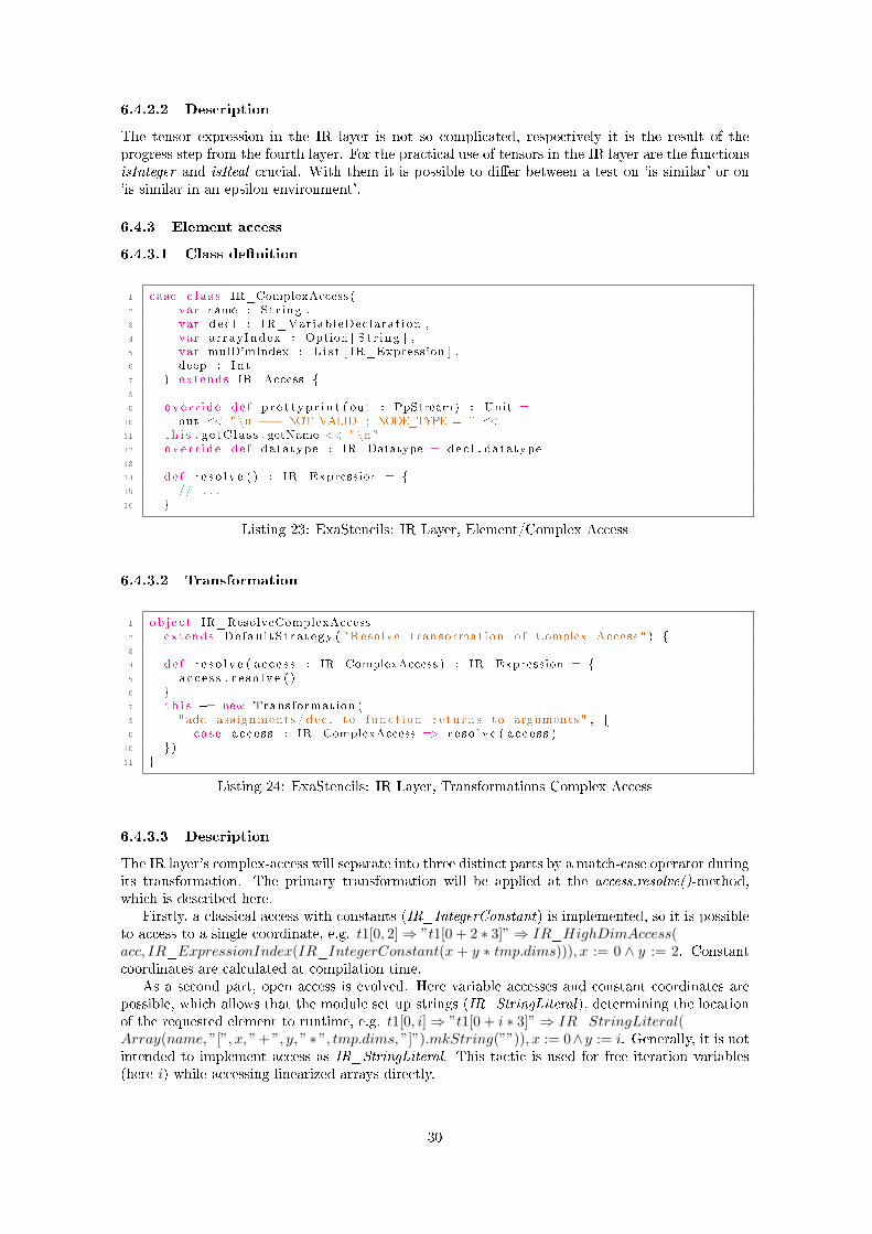
The IR layer's complex-access will separate into three distinct parts by a match-case operator duringits transformation. The primary transformation will be applied at the access.resolve()-method,which is described here.
Firstly, a classical access with constants (IR_IntegerConstant) is implemented, so it is possibleto access to a single coordinate, e.g. t1[0, 2]⇒ ”t1[0 + 2 ∗ 3]”⇒ IR_HighDimAccess(acc, IR_ExpressionIndex(IR_IntegerConstant(x + y ∗ tmp.dims))), x := 0 ∧ y := 2. Constantcoordinates are calculated at compilation time.
As a second part, open access is evolved. Here variable accesses and constant coordinates arepossible, which allows that the module set up strings (IR_StringLiteral), determining the locationof the requested element to runtime, e.g. t1[0, i]⇒ ”t1[0 + i ∗ 3]”⇒ IR_StringLiteral(Array(name, ”[”, x, ” + ”, y, ”∗”, tmp.dims, ”]”).mkString(””)), x := 0∧y := i. Generally, it is notintended to implement access as IR_StringLiteral. This tactic is used for free iteration variables(here i) while accessing linearized arrays directly.
30
Finally, if only a single Einstein iterator was found at an index, the transformation wouldsummarize overall objects at this dimension. This part is only a return state of the Einsteinnotation, hence in detail, it will be delineated there.
At this state, an ArrayIndex exists at the parser denition and the class of the L4_ComplexAccess,but it is unused. The value is needed at the next version, where tensors and matrixes with one axiscan be added to Einstein notation.
6.4.4 Einstein notation
6.4.4.1 Transformation
1 ob j e c t IR_ResolveEinste inNotat ion2 extends De fau l tS t ra tegy ( "Resolve E in s t e i n Notation " ) 3
4 de f r e s o l v e (5 acce s s1 : IR_ComplexAccess ,6 acce s s2 : IR_ComplexAccess ,7 operator : Char8 ) : IR_Expression = 9
10 // . . .11
12 13
14 t h i s += new Transformation ( "Apply Binary Operator f o r E in s t e i n Notation " , 15 case c a l l : IR_Mult ip l i cat ion i f16 ( ( c a l l . a s InstanceOf [ IR_Mult ip l i cat ion ] . f a c t o r s ( 0 ) . i s I n s t anc eOf [ IR_ComplexAccess ] ) &&17 ( c a l l . a s InstanceOf [ IR_Mult ip l i cat ion ] . f a c t o r s ( 1 ) . i s I n s t anc eOf [ IR_ComplexAccess ] ) ) =>18 va l tmp = c a l l . a s InstanceOf [ IR_Mult ip l i cat ion ]19 i f ( tmp . f a c t o r s . l ength > 2) 20 var mul_l ist = myresolve (21 tmp . f a c t o r s ( 0 ) . as InstanceOf [ IR_ComplexAccess ] ,22 tmp . f a c t o r s ( 1 ) . as InstanceOf [ IR_ComplexAccess ] ,23 ' * '24 )25 f o r ( i <− 2 un t i l tmp . f a c t o r s . l ength )26 mul_l ist = r e s o l v e (27 mul_l ist . as InstanceOf [ IR_ComplexAccess ] ,28 tmp . f a c t o r s ( i ) . as InstanceOf [ IR_ComplexAccess ] ,29 ' * '30 )31 mul_l ist32 e l s e 33 r e s o l v e (tmp . f a c t o r s ( 0 ) . as InstanceOf [ IR_ComplexAccess ] ,34 tmp . f a c t o r s ( 1 ) . as InstanceOf [ IR_ComplexAccess ] , ' * ' )35 36
37 // . . .38
39 )40
Listing 25: ExaStencils: IR Layer, Transformations Einstein notation
6.4.4.2 Description
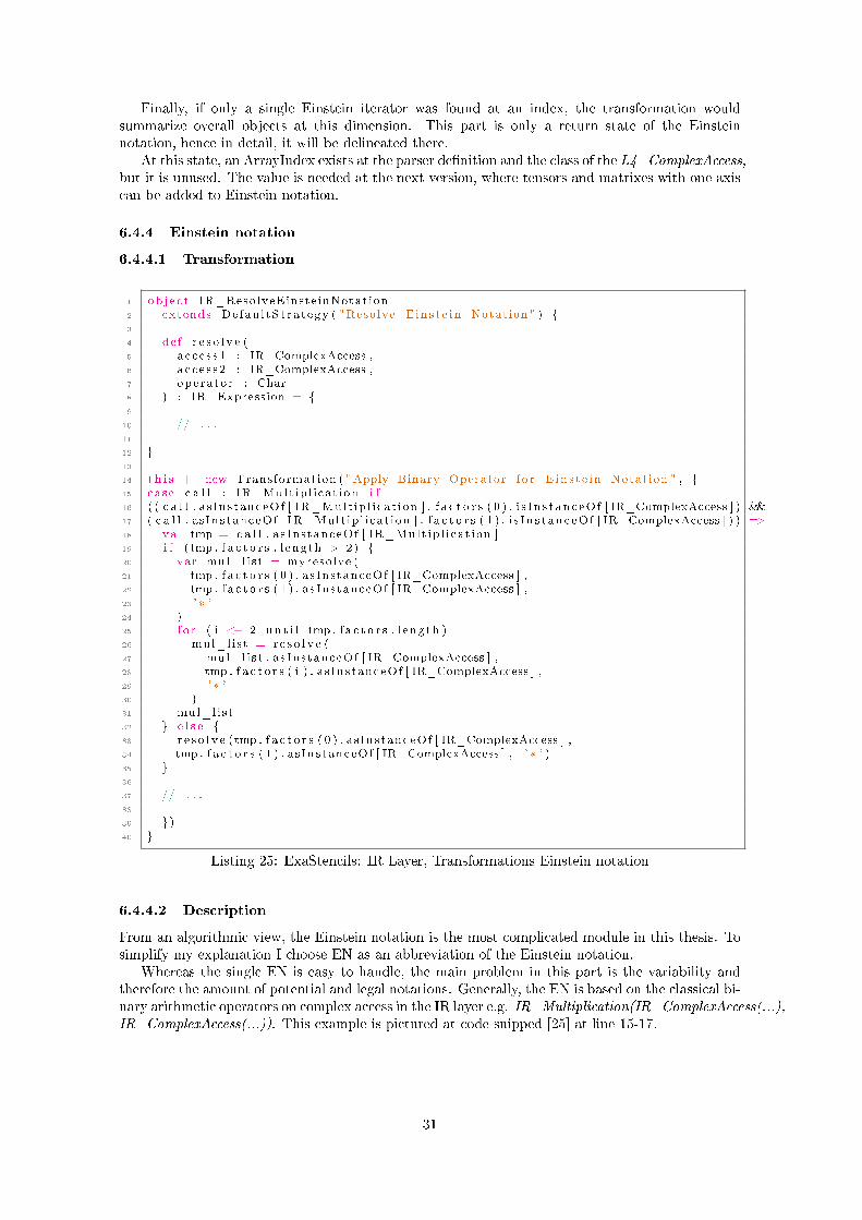
From an algorithmic view, the Einstein notation is the most complicated module in this thesis. Tosimplify my explanation I choose EN as an abbreviation of the Einstein notation.
Whereas the single EN is easy to handle, the main problem in this part is the variability andtherefore the amount of potential and legal notations. Generally, the EN is based on the classical bi-nary arithmetic operators on complex access in the IR layer e.g. IR_Multiplication(IR_ComplexAccess(...),IR_ComplexAccess(...)). This example is pictured at code snipped [25] at line 15-17.
31
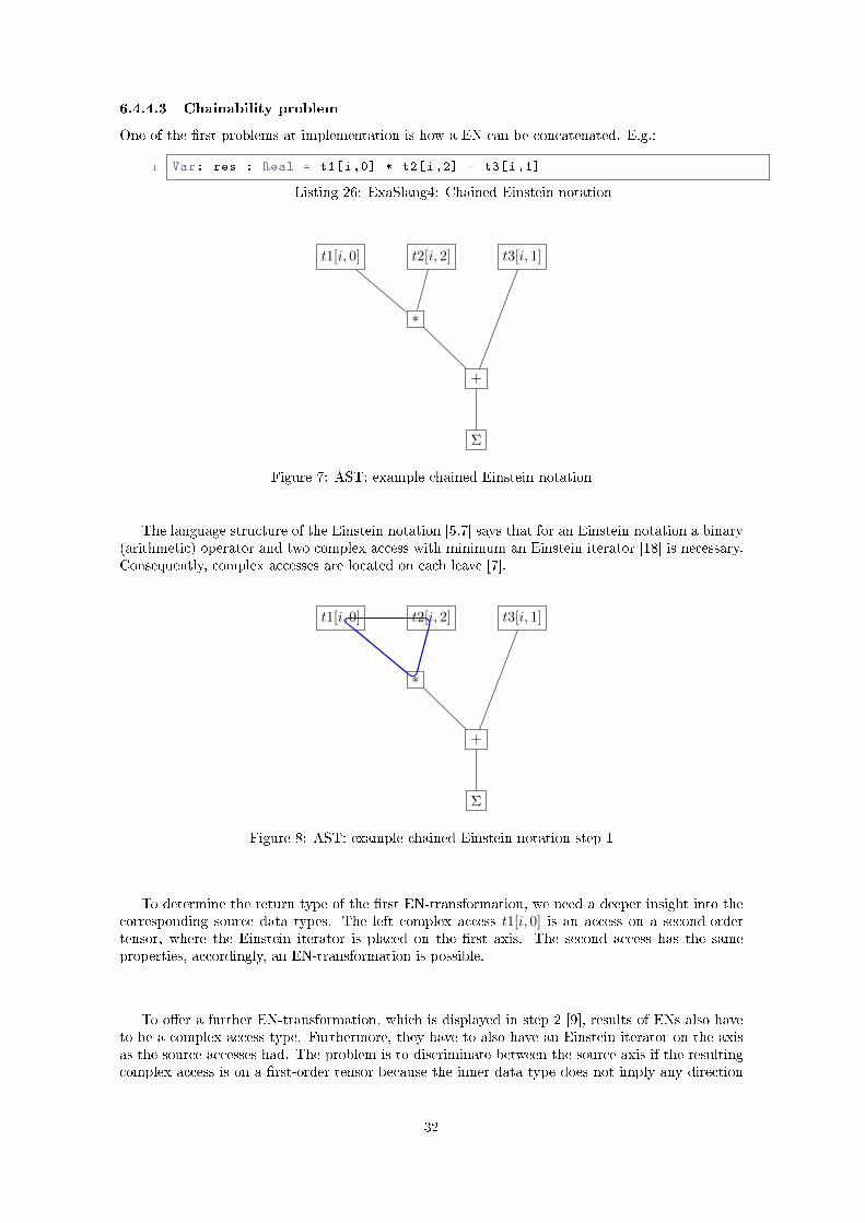
6.4.4.3 Chainability problem
One of the rst problems at implementation is how a EN can be concatenated. E.g.:
1 Var: res : Real = t1[i,0] * t2[i,2] + t3[i,1]
Listing 26: ExaSlang4: Chained Einstein notation
t1[i, 0] t2[i, 2] t3[i, 1]
∗
+
Σ
Figure 7: AST: example chained Einstein notation
The language structure of the Einstein notation [5.7] says that for an Einstein notation a binary(arithmetic) operator and two complex access with minimum an Einstein iterator [18] is necessary.Consequently, complex accesses are located on each leave [7].
t1[i, 0] t2[i, 2] t3[i, 1]
∗
+
Σ
Figure 8: AST: example chained Einstein notation step 1
To determine the return type of the rst EN-transformation, we need a deeper insight into thecorresponding source data types. The left complex access t1[i, 0] is an access on a second-ordertensor, where the Einstein iterator is placed on the rst axis. The second access has the sameproperties, accordingly, an EN-transformation is possible.
To oer a further EN-transformation, which is displayed in step 2 [9], results of ENs also haveto be a complex access type. Furthermore, they have to also have an Einstein iterator on the axisas the source accesses had. The problem is to discriminate between the source axis if the resultingcomplex access is on a rst-order tensor because the inner data type does not imply any direction
32
res1[i] t3[i, 1]
+
Σ
Figure 9: AST: example chained Einstein notation step 2
and axis. To treat this issue, I choose a transformed vector as the inherent return type of theconcluded complex access, which holds the former Einstein iterator.
Here an illustration for the problem:
t1[i, 2] ∗ t2[i, 0] ∗ t3[i, 2] ∗ t4[i, 0]→ res1[i] ∗ res2[i] (42)
6= (43)
t1[2, i] ∗ t2[0, i] ∗ t3[2, i] ∗ t4[0, i]→ res1[i] ∗ res2[i] (44)
This example shows the reason why the return value has to be able to determine the former axisof the iterator.
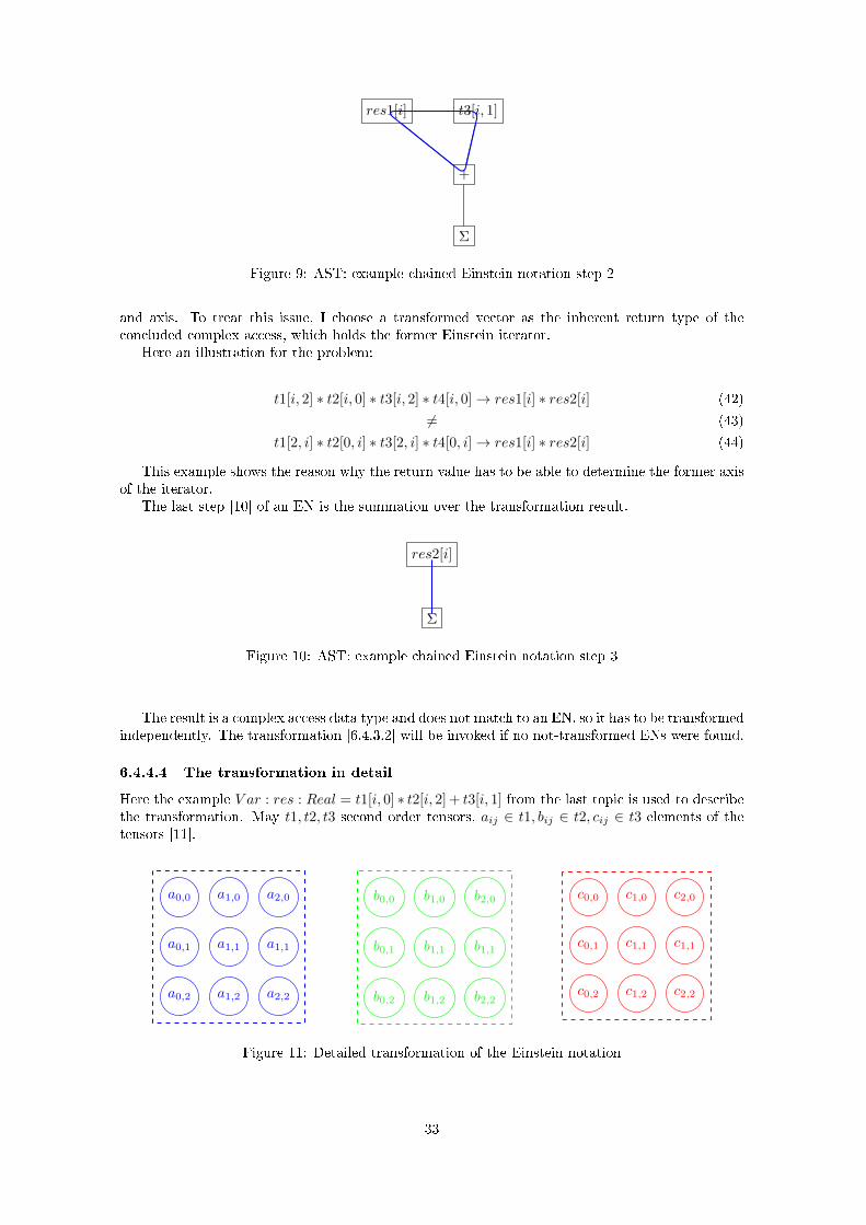
The last step [10] of an EN is the summation over the transformation result.
res2[i]
Σ
Figure 10: AST: example chained Einstein notation step 3
The result is a complex access data type and does not match to an EN, so it has to be transformedindependently. The transformation [6.4.3.2] will be invoked if no not-transformed ENs were found.
6.4.4.4 The transformation in detail
Here the example V ar : res : Real = t1[i, 0] ∗ t2[i, 2] + t3[i, 1] from the last topic is used to describethe transformation. May t1, t2, t3 second order tensors, aij ∈ t1, bij ∈ t2, cij ∈ t3 elements of thetensors [11].
a0,0 a1,0 a2,0
a0,1 a1,1 a1,1
a0,2 a1,2 a2,2
b0,0 b1,0 b2,0
b0,1 b1,1 b1,1
b0,2 b1,2 b2,2
c0,0 c1,0 c2,0
c0,1 c1,1 c1,1
c0,2 c1,2 c2,2
Figure 11: Detailed transformation of the Einstein notation
33
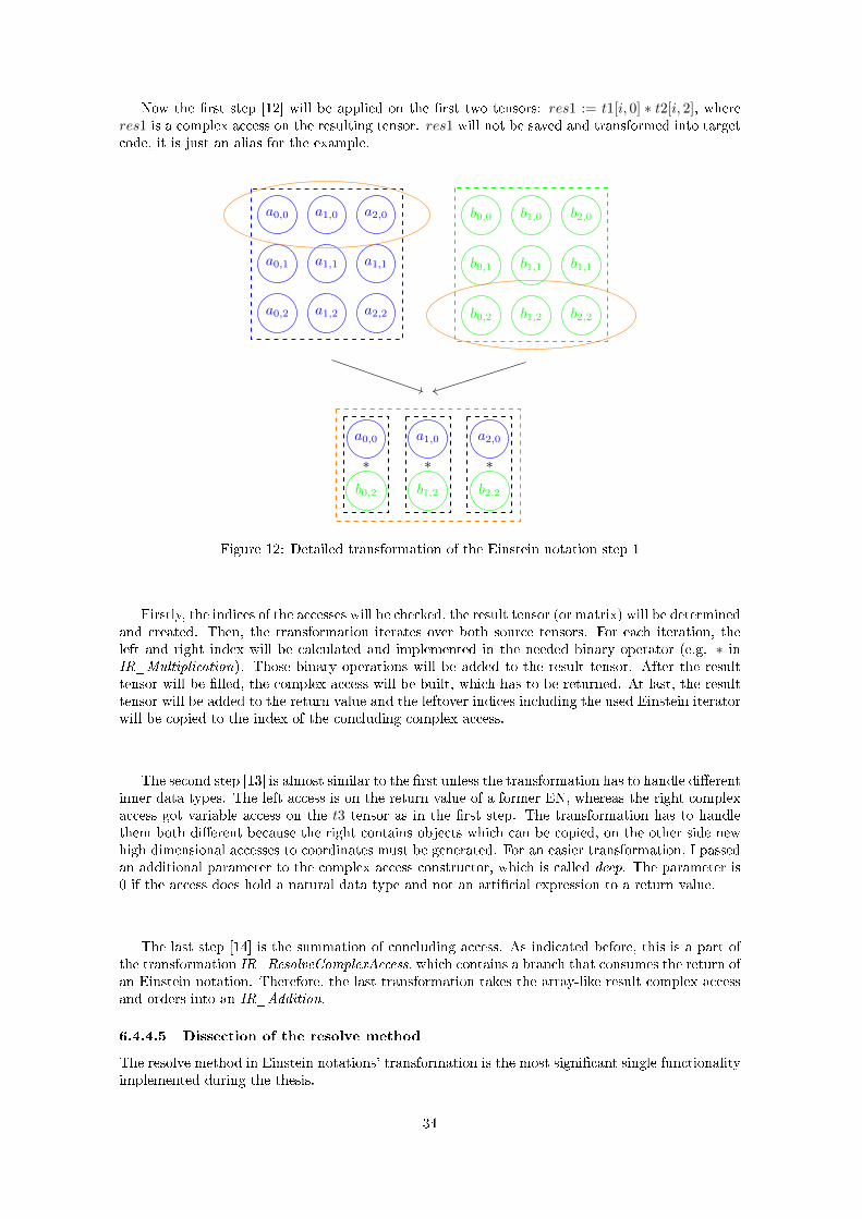
Now the rst step [12] will be applied on the rst two tensors: res1 := t1[i, 0] ∗ t2[i, 2], whereres1 is a complex access on the resulting tensor. res1 will not be saved and transformed into targetcode, it is just an alias for the example.
a0,0 a1,0 a2,0
a0,1 a1,1 a1,1
a0,2 a1,2 a2,2
b0,0 b1,0 b2,0
b0,1 b1,1 b1,1
b0,2 b1,2 b2,2
a1,0a0,0 a2,0
∗∗ ∗
b0,2 b1,2 b2,2
Figure 12: Detailed transformation of the Einstein notation step 1
Firstly, the indices of the accesses will be checked, the result tensor (or matrix) will be determinedand created. Then, the transformation iterates over both source tensors. For each iteration, theleft and right index will be calculated and implemented in the needed binary operator (e.g. ∗ inIR_Multiplication). Those binary operations will be added to the result tensor. After the resulttensor will be lled, the complex access will be built, which has to be returned. At last, the resulttensor will be added to the return value and the leftover indices including the used Einstein iteratorwill be copied to the index of the concluding complex access.
The second step [13] is almost similar to the rst unless the transformation has to handle dierentinner data types. The left access is on the return value of a former EN, whereas the right complexaccess got variable access on the t3 tensor as in the rst step. The transformation has to handlethem both dierent because the right contains objects which can be copied, on the other side newhigh dimensional accesses to coordinates must be generated. For an easier transformation, I passedan additional parameter to the complex access constructor, which is called deep. The parameter is0 if the access does hold a natural data type and not an articial expression to a return value.
The last step [14] is the summation of concluding access. As indicated before, this is a part ofthe transformation IR_ResolveComplexAccess, which contains a branch that consumes the return ofan Einstein notation. Therefore, the last transformation takes the array-like result complex accessand orders into an IR_Addition.
6.4.4.5 Dissection of the resolve method
The resolve method in Einstein notations' transformation is the most signicant single functionalityimplemented during the thesis.
34
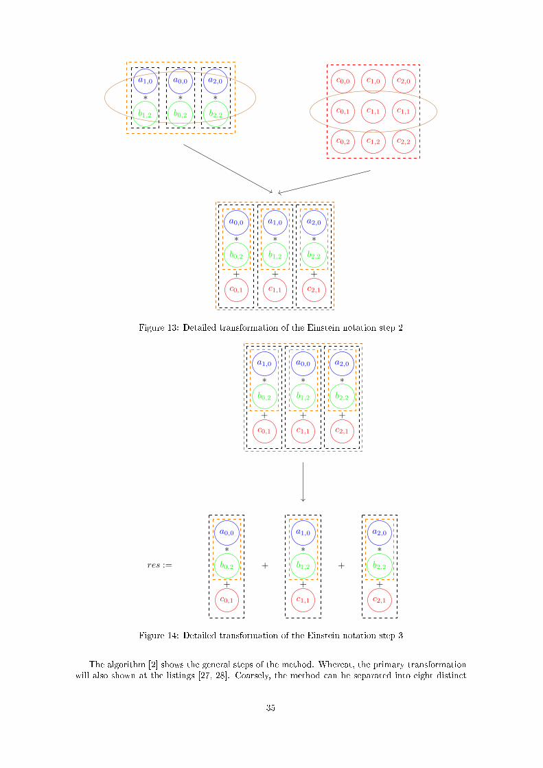
a0,0a1,0 a2,0
∗∗ ∗
b0,2b1,2 b2,2
c0,0 c1,0 c2,0
c0,1 c1,1 c1,1
c0,2 c1,2 c2,2
a1,0a0,0 a2,0
∗∗ ∗
b1,2b0,2 b2,2
++ +
c1,1c0,1 c2,1
Figure 13: Detailed transformation of the Einstein notation step 2
a0,0a1,0 a2,0
∗∗ ∗
b1,2b0,2 b2,2
++ +
c1,1c0,1 c2,1
a1,0a0,0 a2,0
∗∗ ∗
b1,2b0,2 b2,2
++ +
c1,1c0,1 c2,1
+ +res :=
Figure 14: Detailed transformation of the Einstein notation step 3
The algorithm [2] shows the general steps of the method. Whereat, the primary transformationwill also shown at the listings [27, 28]. Coarsely, the method can be separated into eight distinct
35
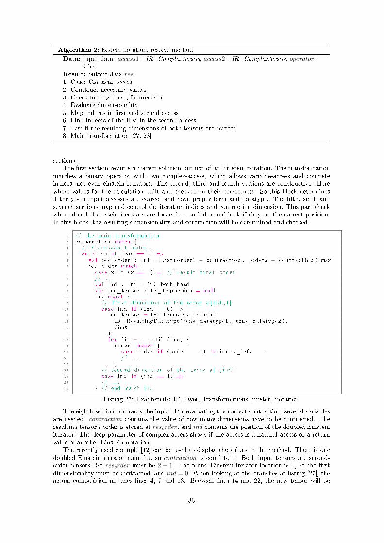
Algorithm 2: Eistein notation, resolve methodData: input data: access1 : IR_ComplexAccess, access2 : IR_ComplexAccess, operator :
CharResult: output data res1. Case: Classical access2. Construct necessary values3. Check for edgecases, failurecases4. Evaluate dimensionality5. Map indeces in rst and second access6. Find indeces of the rst in the second access7. Test if the resulting dimensions of both tensors are correct8. Main transformation [27, 28]
sections.The rst section returns a correct solution but not of an Einstein notation. The transformation
matches a binary operator with two complex-access, which allows variable-access and concreteindices, not even einstein iterators. The second, third and fourth sections are constructive. Herewhere values for the calculation built and checked on their correctness. So this block determinesif the given input accesses are correct and have proper form and datatype. The fth, sixth andseventh sections map and control the iteration indices and contraction dimension. This part checkwhere doubled einstein iterators are located at an index and look if they on the correct position.In this block, the resulting dimensionality and contraction will be determined and checked.
1 // the main t rans fo rmat ion2 con t ra c t i on match 3 // Contracts 1 order4 case con i f ( con == 1) =>5 va l res_order : Int = L i s t ( order1 − cont rac t i on , order2 − con t ra c t i on ) .max6 res_order match 7 case x i f ( x == 1) => // r e s u l t f i r s t order8 // . . .9 va l ind : Int = ind_both . head
10 var res_tensor : IR_Expression = nu l l11 ind match 12 // f i r s t dimension o f the array a [ ind , 1 ]13 case ind i f ( ind == 0) =>14 res_tensor = IR_TensorExpression1 (15 IR_ResultingDatatype ( tens_datatype1 , tens_datatype2 ) ,16 dims17 )18 f o r ( i <− 0 un t i l dims ) 19 order1 match 20 case order i f ( order == 1) => index_le f t += i21 // . . .22 23 // second dimension o f the array a [ 1 , ind ]24 case ind i f ( ind == 1) =>25 // . . .26 // end match ind
Listing 27: ExaStencils: IR Layer, Transformations Einstein notation
The eighth section contracts the input. For evaluating the correct contraction, several variablesare needed. contraction contains the value of how many dimensions have to be contracted. Theresulting tensor's order is stored at resorder, and ind contains the position of the doubled Einsteiniterator. The deep parameter of complex-access shows if the access is a natural access or a returnvalue of another Einstein notation.
The recently used example [12] can be used to display the values in the method. There is onedoubled Einstein iterator named i, so contraction is equal to 1. Both input tensors are second-order tensors. So resorder must be 2 − 1. The found Einstein iterator location is 0, so the rstdimensionality must be contracted, and ind = 0. When looking at the branches at listing [27], theactual composition matches lines 4, 7 and 13. Between lines 14 and 22, the new tensor will be
36
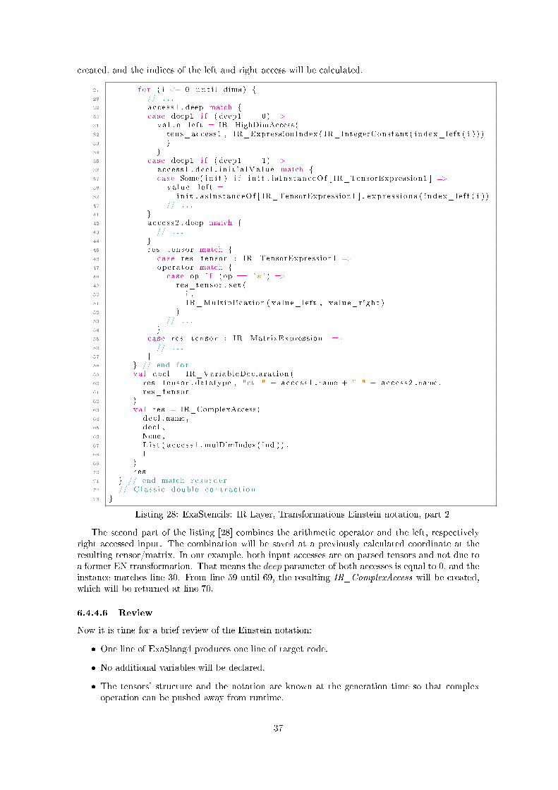
created, and the indices of the left and right access will be calculated.
27 f o r ( i <− 0 un t i l dims ) 28 // . . .29 acce s s1 . deep match 30 case deep1 i f ( deep1 == 0) =>31 va lue_ l e f t = IR_HighDimAccess (32 tens_access1 , IR_ExpressionIndex ( IR_IntegerConstant ( index_le f t ( i ) ) )33 )34 )35 case deep1 i f ( deep1 == 1) =>36 acce s s1 . de c l . i n i t i a lV a l u e match 37 case Some( i n i t ) i f i n i t . i s I n s t anc eO f [ IR_TensorExpression1 ] =>38 va lue_ l e f t =39 i n i t . a s InstanceOf [ IR_TensorExpression1 ] . e xp r e s s i on s ( index_le f t ( i ) )40 // . . .41 42 acce s s2 . deep match 43 // . . .44 45 res_tensor match 46 case res_tensor : IR_TensorExpression1 =>47 operator match 48 case op i f ( op == ' * ' ) =>49 res_tensor . s e t (50 i ,51 IR_Mult ip l i cat ion ( va lue_le f t , va lue_r ight )52 )53 // . . .54 55 case res_tensor : IR_MatrixExpression =>56 // . . .57 58 // end f o r59 va l dec l = IR_VariableDeclarat ion (60 res_tensor . datatype , "ct_" + acce s s1 . name + "_" + acce s s2 . name ,61 res_tensor62 )63 va l r e s = IR_ComplexAccess (64 dec l . name ,65 dec l ,66 None ,67 L i s t ( a c c e s s1 . mulDimIndex ( ind ) ) ,68 169 )70 r e s71 // end match r e s o rd e r72 // C l a s s i c double con t ra c t i on73
Listing 28: ExaStencils: IR Layer, Transformations Einstein notation, part 2
The second part of the listing [28] combines the arithmetic operator and the left, respectivelyright accessed input. The combination will be saved at a previously calculated coordinate at theresulting tensor/matrix. In our example, both input accesses are on parsed tensors and not due toa former EN transformation. That means the deep parameter of both accesses is equal to 0, and theinstance matches line 30. From line 59 until 69, the resulting IR_ComplexAccess will be created,which will be returned at line 70.
6.4.4.6 Review
Now it is time for a brief review of the Einstein notation:
One line of ExaSlang4 produces one line of target code.
No additional variables will be declared.
The tensors' structure and the notation are known at the generation time so that complexoperation can be pushed away from runtime.
37
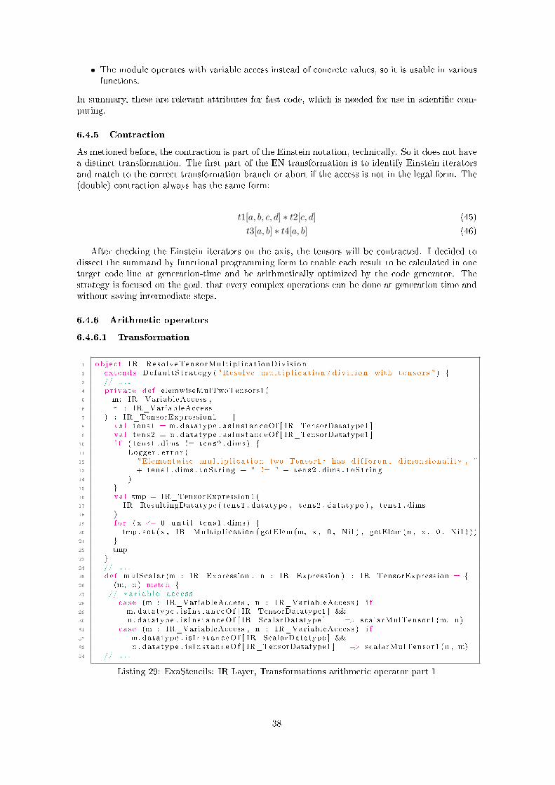
The module operates with variable access instead of concrete values, so it is usable in variousfunctions.
In summary, these are relevant attributes for fast code, which is needed for use in scientic com-puting.
6.4.5 Contraction
As metioned before, the contraction is part of the Einstein notation, technically. So it does not havea distinct transformation. The rst part of the EN transformation is to identify Einstein iteratorsand match to the correct transformation branch or abort if the access is not in the legal form. The(double) contraction always has the same form:
t1[a, b, c, d] ∗ t2[c, d] (45)
t3[a, b] ∗ t4[a, b] (46)
After checking the Einstein iterators on the axis, the tensors will be contracted. I decided todissect the summand by functional programming form to enable each result to be calculated in onetarget code line at generation-time and be arithmetically optimized by the code generator. Thestrategy is focused on the goal, that every complex operations can be done at generation time andwithout saving intermediate steps.
6.4.6 Arithmetic operators
6.4.6.1 Transformation
1 ob j e c t IR_Reso lveTensorMult ip l i cat ionDiv i s ion2 extends De fau l tS t ra tegy ( "Resolve mu l t i p l i c a t i o n / d i v i t i o n with t en so r s " ) 3 // . . .4 pr i va t e de f elemwiseMulTwoTensors1 (5 m: IR_VariableAccess ,6 n : IR_VariableAccess7 ) : IR_TensorExpression1 = 8 va l tens1 = m. datatype . as InstanceOf [ IR_TensorDatatype1 ]9 va l tens2 = n . datatype . as InstanceOf [ IR_TensorDatatype1 ]
10 i f ( tens1 . dims != tens2 . dims ) 11 Logger . e r r o r (12 "Elementwise mu l t i p l i c a t i o n two Tensor1 : has d i f f e r e n t d imens iona l i ty , "13 + tens1 . dims . t oS t r i ng + " != " + tens2 . dims . t oS t r i ng14 )15 16 va l tmp = IR_TensorExpression1 (17 IR_ResultingDatatype ( tens1 . datatype , tens2 . datatype ) , tens1 . dims18 )19 f o r ( x <− 0 un t i l tens1 . dims ) 20 tmp . s e t (x , IR_Mult ip l i cat ion ( getElem (m, x , 0 , Ni l ) , getElem (n , x , 0 , Ni l ) ) )21 22 tmp23 24 // . . .25 de f mulScalar (m : IR_Expression , n : IR_Expression ) : IR_TensorExpression = 26 (m, n) match 27 // va r i ab l e a c c e s s28 case (m : IR_VariableAccess , n : IR_VariableAccess ) i f29 m. datatype . i s I n s t anc eOf [ IR_TensorDatatype1 ] &&30 n . datatype . i s I n s t anc eOf [ IR_ScalarDatatype ] => scalarMulTensor1 (m, n)31 case (m : IR_VariableAccess , n : IR_VariableAccess ) i f32 m. datatype . i s I n s t anc eO f [ IR_ScalarDatatype ] &&33 n . datatype . i s I n s t anc eOf [ IR_TensorDatatype1 ] => scalarMulTensor1 (n , m)34 // . . .
Listing 29: ExaStencils: IR Layer, Transformations arithmetic operator part 1
38
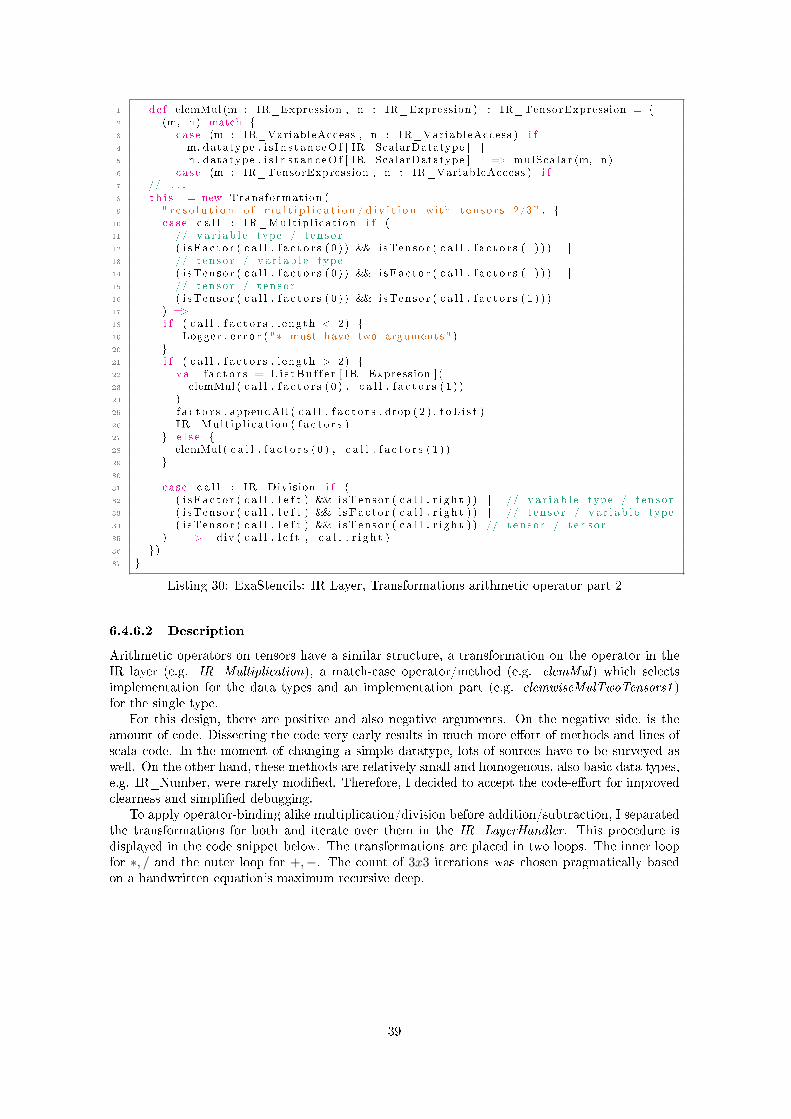
1 de f elemMul (m : IR_Expression , n : IR_Expression ) : IR_TensorExpression = 2 (m, n) match 3 case (m : IR_VariableAccess , n : IR_VariableAccess ) i f4 m. datatype . i s I n s t anc eO f [ IR_ScalarDatatype ] | |5 n . datatype . i s I n s t anc eOf [ IR_ScalarDatatype ] => mulScalar (m, n)6 case (m : IR_TensorExpression , n : IR_VariableAccess ) i f7 // . . .8 t h i s += new Transformation (9 " r e s o l u t i o n o f mu l t i p l i c a t i o n / d i v i t i o n with t en s o r s 2/3" ,
10 case c a l l : IR_Mult ip l i cat ion i f (11 // va r i ab l e type / t enso r12 ( i sFac to r ( c a l l . f a c t o r s ( 0 ) ) && isTensor ( c a l l . f a c t o r s ( 1 ) ) ) | |13 // tenso r / va r i ab l e type14 ( i sTensor ( c a l l . f a c t o r s ( 0 ) ) && i sFac to r ( c a l l . f a c t o r s ( 1 ) ) ) | |15 // tenso r / t enso r16 ( i sTensor ( c a l l . f a c t o r s ( 0 ) ) && isTensor ( c a l l . f a c t o r s ( 1 ) ) )17 ) =>18 i f ( c a l l . f a c t o r s . l ength < 2) 19 Logger . e r r o r ( "* must have two arguments" )20 21 i f ( c a l l . f a c t o r s . l ength > 2) 22 va l f a c t o r s = L i s tBu f f e r [ IR_Expression ] (23 elemMul ( c a l l . f a c t o r s ( 0 ) , c a l l . f a c t o r s ( 1 ) )24 )25 f a c t o r s . appendAll ( c a l l . f a c t o r s . drop ( 2 ) . t oL i s t )26 IR_Mult ip l i cat ion ( f a c t o r s )27 e l s e 28 elemMul ( c a l l . f a c t o r s ( 0 ) , c a l l . f a c t o r s ( 1 ) )29 30
31 case c a l l : IR_Division i f (32 ( i sFac to r ( c a l l . l e f t ) && isTensor ( c a l l . r i g h t ) ) | | // va r i ab l e type / t enso r33 ( i sTensor ( c a l l . l e f t ) && i sFac to r ( c a l l . r i g h t ) ) | | // t enso r / va r i ab l e type34 ( i sTensor ( c a l l . l e f t ) && isTensor ( c a l l . r i g h t ) ) // t enso r / t enso r35 ) => div ( c a l l . l e f t , c a l l . r i g h t )36 )37
Listing 30: ExaStencils: IR Layer, Transformations arithmetic operator part 2
6.4.6.2 Description
Arithmetic operators on tensors have a similar structure, a transformation on the operator in theIR layer (e.g. IR_Multiplication), a match-case operator/method (e.g. elemMul) which selectsimplementation for the data types and an implementation part (e.g. elemwiseMulTwoTensors1 )for the single type.
For this design, there are positive and also negative arguments. On the negative side, is theamount of code. Dissecting the code very early results in much more eort of methods and lines ofscala code. In the moment of changing a simple datatype, lots of sources have to be surveyed aswell. On the other hand, these methods are relatively small and homogenous, also basic data types,e.g. IR_Number, were rarely modied. Therefore, I decided to accept the code-eort for improvedclearness and simplied debugging.
To apply operator-binding alike multiplication/division before addition/subtraction, I separatedthe transformations for both and iterate over them in the IR_LayerHandler. This procedure isdisplayed in the code snippet below. The transformations are placed in two loops. The inner loopfor ∗, / and the outer loop for +,−. The count of 3x3 iterations was chosen pragmatically basedon a handwritten equation's maximum recursive deep.
39
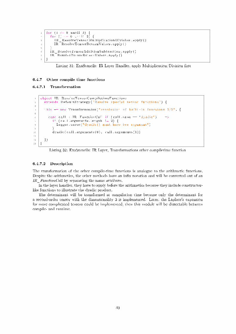
1 f o r ( i <− 0 un t i l 3) 2 f o r ( j <− 0 un t i l 3) 3 IR_Reso lveTensorMult ip l i cat ionDiv i s ion . apply ( )4 IR_ResolveTensorReturnValues . apply ( )5 6 IR_ResolveTensorAddit ionSubtract ion . apply ( )7 IR_ResolveTensorReturnValues . apply ( )8
Listing 31: ExaStencils: IR Layer Handler, apply Multiplication/Division rst
6.4.7 Other compile time functions
6.4.7.1 Transformation
1 ob j e c t IR_ResolveTensorCompiletimeFunctions2 extends De fau l tS t ra tegy ( "Resolve s p e c i a l t en so r f unc t i on s " ) 3
4 t h i s += new Transformation ( " r e s o l u t i o n o f bu i l t−in f unc t i on s 2/2" , 5
6 case c a l l : IR_FunctionCall i f ( c a l l . name == "dyadic " ) =>7 i f ( c a l l . arguments . l ength != 2) 8 Logger . e r r o r ( " dyadic ( ) must have two argument" )9
10 dyadic ( c a l l . arguments ( 0 ) , c a l l . arguments ( 1 ) )11
12 )13
Listing 32: ExaStencils: IR Layer, Transformations other compiletime function
6.4.7.2 Description
The transformation of the other compile-time functions is analogue to the arithmetic functions.Despite the arithmetics, the other methods have an inx notation and will be converted out of anIR_FunctionCall by separating the name attribute.
In the layer handler, they have to apply before the arithmetics because they include constructor-like functions to illustrate the dyadic product.
The determinant will be transformed at compilation time because only the determinant fora second-order tensor with the dimensionality 3 is implemented. Later, the Laplace's expansionfor more complicated tensors could be implemented, then this module will be dissectable betweencompile- and runtime.
40
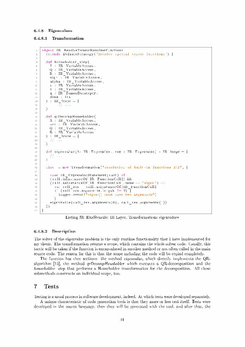
6.4.8 Eigenvalues
6.4.8.1 Transformation
1 ob j e c t IR_ResolveTensorRuntimeFunctions2 extends De fau l tS t ra tegy ( "Resolve s p e c i a l t en so r f unc t i on s " ) 3
4 de f householder_step (5 I : IR_VariableAccess ,6 Q : IR_VariableAccess ,7 R : IR_VariableAccess ,8 s i gn : IR_VariableAccess ,9 alpha : IR_VariableAccess ,
10 v : IR_VariableAccess ,11 i : IR_VariableAccess ,12 q : IR_TensorDatatype2 ,13 dims : Int14 ) : IR_Scope = 15 // . . .16 17
18 de f qrDecompHouseholder (19 A : IR_VariableAccess ,20 r e s : IR_VariableAccess ,21 Q : IR_VariableAccess ,22 R : IR_VariableAccess23 ) : IR_Scope = 24 // . . .25 26
27 de f e i g enva lue (A: IR_Expression , r e s : IR_Expression ) : IR_Scope = 28 // . . .29 30
31 t h i s += new Transformation ( " r e s o l u t i o n o f bu i l t−in f unc t i on s 2/2" , 32
33 case IR_ExpressionStatement ( c a l l ) i f34 ( c a l l . i s I n s t anc eOf [ IR_FunctionCall ] ) &&35 ( c a l l . a s InstanceOf [ IR_FunctionCall ] . name == " e igen " ) =>36 va l c a l l_ r e s = c a l l . a s InstanceOf [ IR_FunctionCall ]37 i f ( c a l l_ r e s . arguments . l ength != 2) 38 Logger . e r r o r ( " e i gen ( ) must have two arguments" )39 40 e i g enva lue ( c a l l_ r e s . arguments ( 0 ) , c a l l_ r e s . arguments ( 1 ) )41 )42
Listing 33: ExaStencils: IR Layer, Transformations eigenvalues
6.4.8.2 Description
The solver of the eigenvalue problem is the only runtime functionality that I have implemented formy thesis. The transformation returns a scope, which contains the whole solver code. Usually, thistactic will be taken if the function is encapsulated in another method or not often called in the mainsource code. The reason for this is that the scope including the code will be copied completely.
The function has thee sections: the method eigenvalue, which directly implements the QR-algorithm [15], the method qrDecompHousholder which executes a QR-decomposition and thehouseholder_step that performs a Householder transformation for the decomposition. All thesesubmethods constructs an individual scope, too.
7 Tests
Testing is a usual process in software development, indeed. At which tests were developed separately.A unique characteristic of code generation tools is that they more or less test itself. Tests were
developed in the source language, then they will be generated with the tool, and after that, the
41
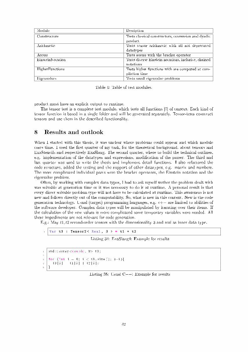
Module Desription
Constructors Tests classical constructors, conversion and dyadicproduct
Arithmetic Tests tensor arithmetic with all not deprecateddatatypes
Access Tests access with the bracket operator
EinsteinNotation Tests diverse Einstein notations, inclusive, chainednotations
HigherFunctions Tests higher functions with are computed at com-pilation time
Eigenvalues Tests small eigenvalue problems
Table 4: Table of test modules.
product must have an explicit output to runtime.The tensor test is a complete test module, which tests all functions [7] of tensors. Each kind of
tensor function is based in a single folder and will be generated separately. Tensor-tests constructtensors and use them in the described functionality.
8 Results and outlook
When I started with this thesis, it was unclear where problems could appear and which modulecosts time. I used the rst quarter of my task, for the theoretical background, about tensors andExaStencils and respectively ExaSlang. The second quarter, where to build the technical outlines,e.g. implementation of the datatypes and expressions, modication of the parser. The third andlast quarter was used to write the thesis and implement detail functions. I also refactored thecode structure, added the testing and the support of other datatypes, e.g. matrix and numbers.The most complicated individual parts were the bracket operators, the Einstein notation and theeigenvalue problem.
Often, by working with complex data types, I had to ask myself wether the problem dealt withwas solvable at generation time or it was necessary to do it at runtime. A personal result is thatevery direct solvable problem type will not have to be calculated at runtime. This awareness is notnew and follows directly out of the computability. So, what is new in this context. New is the codegeneration technology. Usual (target) programming languages, e.g. c++ are limited to abilities ofthe software developer. Complex data types will be manipulated by iterating over their items. Ifthe calculation of the new values is more complicated some temporary variables were needed. Allthese impediments are not relevant for code generation.
E.g.: May t1, t2 second-order tensors with the dimensionality 3 and real as inner data type.
1 Var t3 : Tensor2 < Real , 3 > = t1 + t2
Listing 34: ExaSlang4: Example for results
1 std : : array<double , 9> t3 ;2
3 f o r ( i n t i = 0 ; i < t3 . s i z e ( ) ; ++i )4 t3 [ i ] = t1 [ i ] + t2 [ i ] ;5
Listing 35: Usual C++: Example for results
42
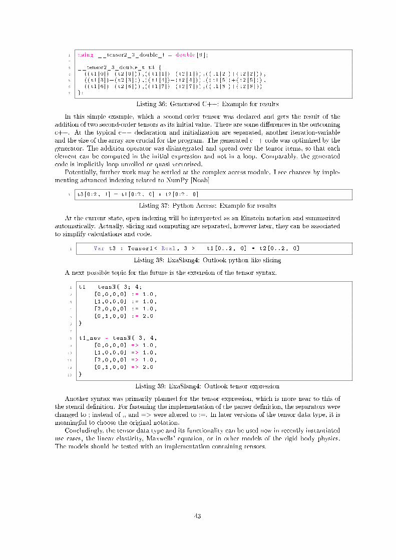
1 us ing __tensor2_3_double_t = double [ 9 ] ;2
3 __tensor2_3_double_t t3 4 ( ( t1 [ 0 ] )+( t2 [ 0 ] ) ) , ( ( t1 [ 1 ] )+( t2 [ 1 ] ) ) , ( ( t1 [ 2 ] )+( t2 [ 2 ] ) ) ,5 ( ( t1 [ 3 ] )+( t2 [ 3 ] ) ) , ( ( t1 [ 4 ] )+( t2 [ 4 ] ) ) , ( ( t1 [ 5 ] )+( t2 [ 5 ] ) ) ,6 ( ( t1 [ 6 ] )+( t2 [ 6 ] ) ) , ( ( t1 [ 7 ] )+( t2 [ 7 ] ) ) , ( ( t1 [ 8 ] )+( t2 [ 8 ] ) )7 ;
Listing 36: Generated C++: Example for results
In this simple example, which a second-order tensor was declared and gets the result of theaddition of two second-order tensors as its initial value. There are some dierences in the outcomingc++. At the typical c++ declaration and initialization are separated, another iteration-variableand the size of the array are crucial for the program. The generated c++ code was optimized by thegenerator. The addition operator was disintegrated and spread over the tensor items, so that eachelement can be computed in the initial expression and not in a loop. Comparably, the generatedcode is implicitly loop unrolled or quasi vectorised.
Potentially, further work may be settled at the complex access module. I see chances by imple-menting advanced indexing related to NumPy [Noab]
1 t3 [ 0 : 2 , 1 ] = t1 [ 0 : 2 , 0 ] * t2 [ 0 : 2 , 0 ]
Listing 37: Python Access: Example for results
At the current state, open indexing will be interpreted as an Einstein notation and summarizedautomatically. Actually, slicing and computing are separated, however later, they can be associatedto simplify calculations and code.
1 Var t3 : Tensor1 < Real , 3 > = t1[0..2, 0] * t2[0..2, 0]
Listing 38: ExaSlang4: Outlook python-like slicing
A next possible topic for the future is the extension of the tensor syntax.
1 t1 = tensN 3; 4;
2 [0,0,0,0] := 1.0,
3 [1,0,0,0] := 1.0,
4 [2,0,0,0] := 1.0,
5 [0,1,0,0] := 2.0
6
7
8 t1_new = tensN 3, 4,
9 [0,0,0,0] => 1.0,
10 [1,0,0,0] => 1.0,
11 [2,0,0,0] => 1.0,
12 [0,1,0,0] => 2.0
13
Listing 39: ExaSlang4: Outlook tensor expression
Another syntax was primarily planned for the tensor expression, which is more near to this ofthe stencil denition. For fastening the implementation of the parser denition, the separators werechanged to ; instead of ,, and => were altered to :=. In later versions of the tensor data type, it ismeaningful to choose the original notation.
Concludingly, the tensor data type and its functionality can be used now in recently instantiateduse cases, the linear elasticity, Maxwells' equation, or in other models of the rigid body physics.The models should be tested with an implementation containing tensors.
43
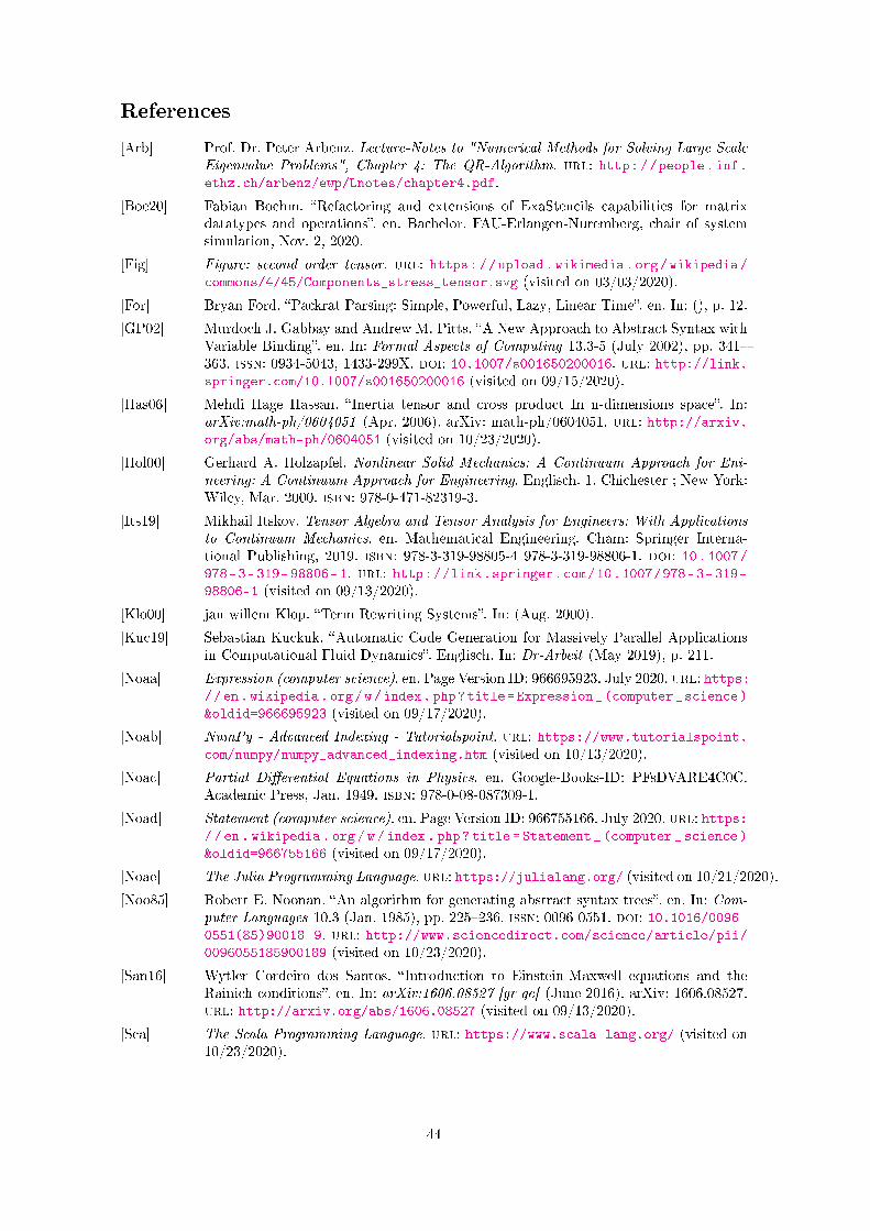
References
[Arb] Prof. Dr. Peter Arbenz. Lecture-Notes to "Numerical Methods for Solving Large ScaleEigenvalue Problems", Chapter 4: The QR-Algorithm. url: http://people.inf.ethz.ch/arbenz/ewp/Lnotes/chapter4.pdf.
[Boe20] Fabian Boehm. Refactoring and extensions of ExaStencils capabilities for matrixdatatypes and operations. en. Bachelor. FAU-Erlangen-Nuremberg, chair of systemsimulation, Nov. 2, 2020.
[Fig] Figure: second order tensor. url: https://upload.wikimedia.org/wikipedia/commons/4/45/Components_stress_tensor.svg (visited on 03/03/2020).
[For] Bryan Ford. Packrat Parsing: Simple, Powerful, Lazy, Linear Time. en. In: (), p. 12.
[GP02] Murdoch J. Gabbay and Andrew M. Pitts. A New Approach to Abstract Syntax withVariable Binding. en. In: Formal Aspects of Computing 13.3-5 (July 2002), pp. 341363. issn: 0934-5043, 1433-299X. doi: 10.1007/s001650200016. url: http://link.springer.com/10.1007/s001650200016 (visited on 09/15/2020).
[Has06] Mehdi Hage Hassan. Inertia tensor and cross product In n-dimensions space. In:arXiv:math-ph/0604051 (Apr. 2006). arXiv: math-ph/0604051. url: http://arxiv.org/abs/math-ph/0604051 (visited on 10/23/2020).
[Hol00] Gerhard A. Holzapfel. Nonlinear Solid Mechanics: A Continuum Approach for Eni-neering: A Continuum Approach for Engineering. Englisch. 1. Chichester ; New York:Wiley, Mar. 2000. isbn: 978-0-471-82319-3.
[Its19] Mikhail Itskov. Tensor Algebra and Tensor Analysis for Engineers: With Applicationsto Continuum Mechanics. en. Mathematical Engineering. Cham: Springer Interna-tional Publishing, 2019. isbn: 978-3-319-98805-4 978-3-319-98806-1. doi: 10.1007/978-3-319-98806-1. url: http://link.springer.com/10.1007/978-3-319-98806-1 (visited on 09/13/2020).
[Klo00] jan willem Klop. Term Rewriting Systems. In: (Aug. 2000).
[Kuc19] Sebastian Kuckuk. Automatic Code Generation for Massively Parallel Applicationsin Computational Fluid Dynamics. Englisch. In: Dr-Arbeit (May 2019), p. 211.
[Noaa] Expression (computer science). en. Page Version ID: 966695923. July 2020. url: https://en.wikipedia.org/w/index.php?title=Expression_(computer_science)
&oldid=966695923 (visited on 09/17/2020).
[Noab] NumPy - Advanced Indexing - Tutorialspoint. url: https://www.tutorialspoint.com/numpy/numpy_advanced_indexing.htm (visited on 10/13/2020).
[Noac] Partial Dierential Equations in Physics. en. Google-Books-ID: PFsDVARE4C0C.Academic Press, Jan. 1949. isbn: 978-0-08-087309-1.
[Noad] Statement (computer science). en. Page Version ID: 966755166. July 2020. url: https://en.wikipedia.org/w/index.php?title=Statement_(computer_science)
&oldid=966755166 (visited on 09/17/2020).
[Noae] The Julia Programming Language. url: https://julialang.org/ (visited on 10/21/2020).
[Noo85] Robert E. Noonan. An algorithm for generating abstract syntax trees. en. In: Com-puter Languages 10.3 (Jan. 1985), pp. 225236. issn: 0096-0551. doi: 10.1016/0096-0551(85)90018-9. url: http://www.sciencedirect.com/science/article/pii/0096055185900189 (visited on 10/23/2020).
[San16] Wytler Cordeiro dos Santos. Introduction to Einstein-Maxwell equations and theRainich conditions. en. In: arXiv:1606.08527 [gr-qc] (June 2016). arXiv: 1606.08527.url: http://arxiv.org/abs/1606.08527 (visited on 09/13/2020).
[Sca] The Scala Programming Language. url: https://www.scala-lang.org/ (visited on10/23/2020).
44
[Sch+14] Christian Schmitt et al. ExaSlang: A Domain-Specic Language for Highly ScalableMultigrid Solvers. en. In: 2014 Fourth International Workshop on Domain-SpecicLanguages and High-Level Frameworks for High Performance Computing. New Or-leans, LA, USA: IEEE, Nov. 2014, pp. 4251. isbn: 978-1-4673-6757-8. doi: 10.1109/WOLFHPC.2014.11. url: http://ieeexplore.ieee.org/document/7101662/ (visitedon 01/12/2020).
[Sha04] Ruslan Sharipov. Quick introduction to tensor analysis. In: arXiv:math/0403252(Mar. 2004). arXiv: math/0403252. url: http://arxiv.org/abs/math/0403252(visited on 10/23/2020).
[Tem01] Roger Temam. Navier-Stokes equations: theory and numerical analysis. en. Providence,R.I: AMS Chelsea Pub, 2001. isbn: 978-0-8218-2737-6.
[VQEW18] https://commons.wikimedia.org/w/index.php?curid=27645908 Von Quartl Eigenes WerkCC BY-SA 3.0. Figure Dyadisches Produkt. de. Page Version ID: 176713475. Apr. 2018.url: https://upload.wikimedia.org/wikipedia/commons/thumb/8/8d/Matrix_multiplication_qtl3.svg/1920px-Matrix_multiplication_qtl3.svg.png (vis-ited on 03/03/2020).
[Åh02] K. Åhlander. Einstein summation for multidimensional arrays. en. In: Computers& Mathematics with Applications 44.8 (Oct. 2002), pp. 10071017. issn: 0898-1221.doi: 10.1016/S0898-1221(02)00210-9. url: http://www.sciencedirect.com/science/article/pii/S0898122102002109 (visited on 10/23/2020).
45


