Dual tensors based solutions for rigid bodymotion parameterization

D. Condurache a, A. Burlacu b,⁎a Dept. of Theoretical Mechanics, Technical University of Iasi, D. Mangeron Street No.59, 700050, Iasi Romaniab Dept. of Automatic Control and Applied Informatics, Technical University of Iasi, D. Mangeron Street No.27, 700050, Iasi Romania

a r t i c l e i n f o a b s t r a c t

Article history:Received 10 November 2013Received in revised form 30 November 2013Accepted 16 December 2013Available online xxxx

Rigid body displacement and motion parameterization is a research subject with continuousdevelopment inmany theoretical and applied fields. A very important objective for the designof parameterization methods is to obtain a reduced number of algebraic equations and fewervariables for a more compact notation. This criterion increased the interest into tensorialbased approaches for rigid motion parameterization. The present research analyzes theperformance of tensorial parameterization and proposes new methods to compute therigid-body motion parameters. Our rigid body motion parameterization solutions aredeveloped using rigid bases of dual vectors, a new notion defined in this paper. Consideringa rigid body motion, computational techniques are proposed for the orthogonal dual tensor,the screw parameters and the instantaneous screw parameters. The parameterizationtechniques proposed in this paper are described both algebraically and geometrically. Oursolutions are sustained by the symbolic and numerical results gathered from Matlabimplementations.

© 2013 Elsevier Ltd. All rights reserved.

Keywords:Rigid body motionDual tensorRigid dual basesDyadic productScrew parameters

1. Introduction

Parameterization of rigid body displacement and motion [1–3] represents an important research subject in multiple areas(e.g. robotics, theoretical mechanics or computer vision). Rigid bodies represent basic primitives in the modeling of roboticplants [4]. A rigid body can be characterized through different types of features, among them being points and lines. Startingwith classical manipulator robot kinematics and dynamics description [5] and finishing with the new results obtained inrobotics [6–8], machine vision [9,10], biomechanics [11,12], relative orbital motion [13,14] or neuroscience [15], the range ofapplications involving points or lines transformation is very large. If points are considered then any coordinates transformationcan be parameterized using homogeneous transformations [2]. For line features, parameterization techniques were developedusing the dual numbers theory [16–19]. A parameterization performance analysis over dual orthogonal matrices, dual unitquaternions, dual special unitary matrices and dual Pauli spinmatrices was conducted in [20]. The combination of dual numbers,dual vectors or dual matrices calculus with elements of screw theory generates different techniques for rigid body motionmodeling [21,22]. The desire to create a complete framework for rotation and rigidmotion parameterization leads to closer inspectionof linear invariants of the dual rotationmatrix and thedual Euler–Rodriques parameters of rigidmotion [23,24].Motor transformation

Mechanism and Machine Theory 74 (2014) 390–412

⁎ Corresponding author. Tel.: +40 766643536; fax: +40 232230751.E-mail addresses: daniel.condurache@gmail.com (D. Condurache), aburlacu@ac.tuiasi.ro (A. Burlacu).

0094-114X/$ – see front matter © 2013 Elsevier Ltd. All rights reserved.http://dx.doi.org/10.1016/j.mechmachtheory.2013.12.016

Contents lists available at ScienceDirect

Mechanism and Machine Theory

j ourna l homepage: www.e lsev ie r .com/ locate /mechmt

rules and the dual inertia operator can also be used to design a general expression for the three-dimensional dynamic equation of arigid body [25], when an arbitrary reference frame is considered.

Tensor analysis expresses the invariance of the laws of physics with respect to the change of basis and change of frameoperations [26]. Orthogonal dual tensors are a complete tool for computing rigid body displacement and motion parameters. Areduced number of algebraic equations and a more compact notation with fewer variables are two of the advantages oforthogonal dual tensor based parameterization methods. Until now, only a few papers that analyze methods for rigid bodymotion parameterization using tensors were published [27,28]. The first goal of our research is to give a more compact algebraicdescription regarding rigid body motion parameterization using tensors and to discuss the advantages over the methodsinvolving dual matrices [17,23,28–30]. Our tensorial parameterization method is generated by the properties of the dyadicproduct between dual vectors.

Rigid bases of dual vectors (which will be named “dual rigid bases”) represent bases with internal properties copied bytheir reciprocals. These types of bases are the core of the proposed methods. Working with dual rigid bases allows aparameterization of rigid body motion without the assumptions of orthonormal reference frames. This property generatesan increase in the flexibility of the rigid body motion parameterization. Also, all the methods proposed in this paper are freeof coordinates and only use calculus with dual numbers and dual vectors. The use of dual rigid bases for parameterization ofrigid body displacement and motion lead to three contributions which are related to tensorial parameterization, screwparameters and instantaneous screw parameters computation. The paper for the first time reveals a method for computingorthogonal dual tensors using the motion laws of both points and lines attached to the rigid body. These features are used tocompute time depending dual rigid bases and represent the input of the orthogonal dual tensors computational technique.The second contribution implies the computation of the screw parameters. Screw representation of motion [3] is a veryeffective tool for kinematic analysis and can be used in applications of multiple areas [31,32]. The rigid body motionparameterization using dual rigid bases gives the possibility of constructing new computational methods for the screw axis(SA) and instantaneous screw axis (ISA) motion parameters. These methods are different than any other approachesdeveloped for screw-parameters evaluation [24,33–39], because the computational algorithms are developed using onlydual numbers and dual vectors generated by different types of rigid body features (lines, points or combination of lines withpoints). The new solutions are based on two results: the computation of SA is equivalent to the computation of thelogarithm of an orthogonal dual tensor; the computation of ISA is equivalent with the computation of an algebraic entitynamed “the velocity dual tensor”. The computational algorithms for SA and ISA do not necessitate the computation of theorthogonal dual tensor. For the infinitesimal motion case, Poisson like formulae for the dual angular velocity vector areprovided.

Next, the mathematical preliminaries and the notations are presented in Section 2. Different algebraic sets were used toconstruct the parameterization methods proposed in this paper, their most important properties being detailed in theappendixes. The construction of the dual tensors module using the dyadic product between a dual basis and its reciprocal isdiscussed in Section 3. Section 4 focuses on a new rigid body motion parameterization using dual rigid bases. The construction oforthogonal dual tensors, screw and instantaneous screw parameters computation using dual rigid bases techniques are detailed.Also, using dual tensors, a short and constructive proof of the famous Mozzi–Chasles theorem is presented. In Section 4.5, thealgorithms that can be used to put into practice the methods described in Section 4 are detailed. The paper ends with multiplesymbolic and numerical experiments conducted in Matlab, which support the theoretical methods. Section 6 contains theconclusions and future work.

2. Mathematical preliminaries and notation

This section outlines briefly the notations used in the rest of the paper and the algebraic properties of dual numbers, dualvectors and dual tensors. Regarding notation, in order to avoid name clashes, the following are considered: x denotes a dualnumber, x a dual vector, ε represents the imaginary entity which fulfills ε2 = 0. Details over the dual numbers, dual vectors anddual tensors sets can be found in [19,24,35,39,40], while in the Appendix D we highlight the properties that were used in thispaper.

• Dual numbersLet the set of real dual numbers be denoted by:

ℝ ¼ ℝþ εℝ ¼ a ¼ aþ εa0 a; a0∈ℝ; ε2 ¼ 0!!!

o:

nð1Þ

where a ¼ Re að Þ is the real part of a and a0 ¼ Du að Þ the dual part.Any differentiable function of a dual number variable x ¼ xþ εx0 [23] can be decomposed as:

f xð Þ ¼ f xð Þ þ εx0 f′ xð Þ: ð2Þ

The inverse of a∈ℝ, denoted by a−1∈ℝ, exists if and only if Re að Þ≠0 and is computed using a−1 ¼ 1a¼ 1

a−ε

a0a2. Also, a∈ℝ is a

zero divisor if and only if Re að Þ ¼ 0.

391D. Condurache, A. Burlacu / Mechanism and Machine Theory 74 (2014) 390–412

For any dual numbers a; b, that fulfill a2 þ b2 ¼ 1, the atan2 function is defined by

atan2 a; bð Þ ¼atan2 a; bð Þ þ ε

a0b

b≠0

atan2 a; bð Þ−εb0a

b ¼ 0; a≠0;where atan2 ðsinα; cosαÞ ¼ α :

8><

>:ð3Þ

The main properties of dual numbers are presented in Appendix A.

• Dual vectorsIn the Euclidean space, the linear space of free vectors with dimension 3 will be denoted by V3. The ensemble of dual vectors isdefined as

V3 ¼ V3 þ εV3 ¼ a ¼ aþ εa0; a; a0∈V3; ε2 ¼ 0g;

nð4Þ

where a ¼ Re að Þ is the real part of a and a0 ¼ Du að Þ the dual part. For dual vectors, three products will be considered: scalarproduct (denoted by a % b), cross product (denoted by a & b) and triple scalar product (denoted by a;b; ch i).The magnitude of a, denoted by aj j, is the dual number which fulfills aj j % aj j ¼ a % a and can be computed using

aj j ¼ ak kþ εa0 % aak k

;Re að Þ≠0

ε a0k k; Re að Þ ¼ 0;

8<

: ð5Þ

where ‖.‖ is the Euclidean norm. If aj j ¼ 1 then a is called unit dual vector.Thus, based on these properties results that ℝ;þ; %ð Þ is a commutative and unitary ring and any element a∈ℝ is either invertibleor zero divisor, while V 3;þ; %ℝ

! "is a free ℝ-module [18]. More on dual vectors can be found in Appendix B.

• Dual tensorsAn ℝ-linear application of V 3 into V 3 is called an Euclidean dual tensor:

T λ1v1 þ λ2v2ð Þ ¼ λ1T v1ð Þ þ λ2T v2ð Þ;∀λ1;λ2∈ℝ;∀v1; v2∈V1:

ð6Þ

From now on, the Euclidean dual tensor T will be shortly called dual tensor and L V 3;V 3ð Þwill denote the freeℝ-module of dualtensors. To the authors knowledge, the properties of L V 3;V 3ð Þ can be found only in a few articles like [27], thus in Appendix Cthe most important properties of dual tensors are detailed.

3. Dual tensor construction using dual vectors bases

The rigid body displacement and motion parameterization methods proposed in Section 4 are based on the properties of dualtensors. Thus, the present section the design of the dual tensor set is discussed. The key of the chosen design is the combinationbetween dual bases and the dyadic product of dual vectors. In order to set-up the base of the dual tensor construction technique,we first uncover some algebraic results for dual bases.

Theorem 1. If a∈V3 then a dual numberλ∈ℝ and a unit dual vectoru∈V3 exist in order to have a ¼ λu. Also, if Re að Þ≠0 thenλ anduare unique up to a sign change.

Proof. If ‖.‖ denotes the Euclidean norm then

'λ ¼ aj jand' u ¼

aak k

þ εa& a0 & að Þ

ak k3Re að Þ≠0

a0a0k k

þ εv & a0a0k k

;∀v∈V3 Re að Þ ¼ 0:

8>><

>>:□

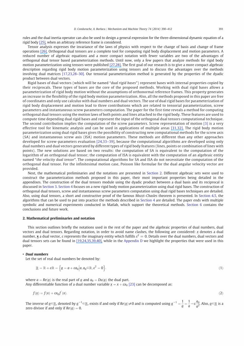
The previous result allows one to geometrically describe any dual vector from the 3D Euclidean space (Fig. 1). For a dual vector afromV 3, withRe að Þ≠0, a labeled line in the Euclidean three dimensional space can be associated. The elements of the unit dual vector

u ¼ uþ εu0 give a line parameterized by Plucker coordinates [1], while the dual numberλ ¼ aj j ¼ ak kþ εa0 % aak k

represents the label.

If Re að Þ ¼ 0 then the geometrical interpretation is a set of parallel lines described bya0a0k k

and labeled with λ ¼ aj j ¼ ε a0k k.

Definition 1. A set of three dual vectors B ¼ e1; e2; e3f gwill be called dual basis if the dual vectors are ℝ linear independent and alsorepresent a span set for V 3.

Proposition 1. Any ek∈V 3; k ¼ 1;3 that fulfill Re e1; e2; e3h ið Þ≠0 are ℝ linear independent.

392 D. Condurache, A. Burlacu / Mechanism and Machine Theory 74 (2014) 390–412

Proof. Consider the dual numbers α i ¼ αi þ εαi0; i ¼ 1;3 which can lead to

α1e1 þ α2e2 þ α3e3 ¼ 0 ð7Þ

Based on the definition of dual numbers results that:

α1e1 þ α2e2 þ α3e3 ¼ 0 ð8Þ

and

X3

i¼1

αiei0 þ αi0eið Þ ¼ 0 ð9Þ

From Re e1; e2; e3h ið Þ≠0 results that ⟨e1,e2,e3⟩ ≠ 0, which combined with Eq. (8) make α1 = α2 = α3 = 0. Further, adding Eq.

(9) generates ∑i = 1

3αi0ei = 0. The previous result combined with the fact that ⟨e1,e2,e3⟩ ≠ 0, show that α10 = α02 = α30 = 0,

which proves our proposition. □

Proposition 2. If any three dual vectors ek∈V 3; k ¼ 1;3, fulfill Re e1; e2; e3h ið Þ≠0 then there are uniquely determined e1; e2; e3! "

using the conditions ei % e j ¼ δ ji ; i; j ¼ 1;3, where δij is the Kronecker symbol.

Proof. Let e1; e2; e3f g be a set constructed by the following rules:

e1 ¼ e2 & e3e1; e2; e3h i

; e2 ¼ e3 & e1e1; e2; e3h i

; e3 ¼ e1 & e2e1; e2; e3h i

: ð10Þ

Using Eq. (10) the conditions ei % e j ¼ δ ji ; i; j ¼ 1;3 are fulfilled. □

Theorem 2. The ensemble V3 together with the sum of dual vectors and the multiplication of dual vectors with dual numbers, is a freeℝ-module and its rank is 3.

Proof. Let e1; e2; e3f g be three dual vectors that fulfill Re e1; e2; e3h ið Þ≠0. For any v∈V 3 there are uniquely determined α i∈ℝ; i¼ 1;3 as so v ¼ α i % ei . Previous the Einstein's rule for mute indexes summation was considered. The values of α i; i ¼ 1;3 arecomputed using α i ¼ v % ei . Thus it results that V 3;þ; %ℝ

# $is a free ℝ -module (Appendix B) with rank 3, while the set B

¼ e1; e2; e3f g is a dual basis in this module. □

Remark 1. For a dual basis B ¼ e1; e2; e3f g, the set B' ¼ e1; e2; e3! "represents its reciprocal dual basis. The dual basis B coincides

with B⁎ if and only if B is an orthonormal basis (aka ei % e j ¼ δij).

Given two dual vectors a and b∈V3 ; a⊗b denotes a dual tensor called tensor (dyadic) product and is defined by:

a⊗b : V 3 & V 3→V 3; a⊗bð Þv ¼ v % bð Þa;∀v∈V3 : ð11Þ

a0

u0u

0a a|| a ||

|| a ||ε ⋅+

0|| a ||ε

( )a 0Re ≠ ( )a 0Re =

OO

Fig. 1. Geometrical interpretation of Theorem 1.

393D. Condurache, A. Burlacu / Mechanism and Machine Theory 74 (2014) 390–412

An important property of Eq. (11) is that a⊗bð Þ c⊗dð Þ ¼ b $ cð Þa⊗d. From this point on we uncover how the dyadic product can beused to construct a dual tensor.

Theorem 3. The following statements are true:

1. A dual tensor T : V 3→V 3 is uniquely determined by the values obtained after T is applied to the elements of the dual basisB ¼ e1; e2; e3f g:

T ¼ Teið Þ⊗ei: ð12Þ

2. The ensemble L V 3;V 3ð Þ is a free ℝ-module of rank equal to 9.

Proof. Starting with Eq. (12) the Einstein's rule for mute indexes summation, when i varies from 1 to 3, will be used. Let v∈V 3 bean arbitrary vector that has the following expression in the basis B ¼ e1; e2; e3f g:

v ¼ v $ e j! "

e j: ð13Þ

Using Eqs. (6) and (11) it results that

Tv ¼ T v $ e j! "

e j

! "h i¼ v $ e j

! "Te j

! "¼

¼ Te j

! "⊗e j

h iv;

ð14Þ

which proves the first part of the theorem.

If T is a dual tensor then the dual vectors Te j; j ¼ 1;3 can be written as

Te j ¼ ei $ Te j

! "h iei; i ¼ 1;3: ð15Þ

Denoting with Tij ¼ ei $ Te j

! "; Ti

j∈ℝ and combining Eqs. (15) with (12) generates

T ¼ Tijei⊗e j

; ð16Þ

which represents a linear combination of tensors ei⊗e jn o

i; j¼1;3that is equivalent with a spanning set. The previous result,

together with the remark (which can be easily proven) that ei⊗e jn o

i; j¼1;3are ℝ linearly independent in L, imply that

ei⊗e jn o

i; j¼1;3is a basis in L V 3;V 3ð Þ and rankℝL V 3;V 3ð Þ ¼ 9. □

Any dual tensor T can be characterized by three dual numbers which are its principal invariants (TI,TII,TIII). The principalinvariants can be computed using:

Tv ¼ λv;λ∈ℝ; v∈V 3;Re vð Þ≠0: ð17Þ

From Eq. (17) it derives that

T−λI½ &v ¼ 0; ð18Þ

where I is the identity dual tensor. Because I ¼ ei⊗ei it follows that:

Tei−λei½ &⊗ein o

v ¼ 0: ð19Þ

Applying Eqs. (11) to (16) leads to:

v $ ei! "

Tei−λei½ & ¼ 0;Re vð Þ≠0: ð20Þ

This result emerges from the fact that when Re vð Þ≠0, at least one of the scalars v $ ei; i ¼ 1;3 is not zero, and it can be concludedthat vectors Tei−λei½ &; i ¼ 1;3 are linearly dependent. Therefore, their scalar triple product is null:

Te1−λei; Te2−λe2;Te3−λe3h i ¼ 0: ð21Þ

394 D. Condurache, A. Burlacu / Mechanism and Machine Theory 74 (2014) 390–412

Based on the properties of the scalar triple product the characteristic equation of T is

λ3−T Iλ2 þ T IIλ−T III ¼ 0; ð22Þ

where the dual numbers TI, TII, TIII are:

T I ¼Te1; e2; e3h iþ e1;Te2; e3h iþ e1; e2;Te3h i

e1; e2; e3i;hð23Þ

T II ¼e1;Te2;Te3h iþ Te1; e2; Te3h iþ Te1; Te2; e3h i

e1; e2; e3i;hð24Þ

T III ¼Te1; Te2; Te3h ie1; e2; e3i:h

ð25Þ

The dual scalars TI, TII, TIII do not depend on how the basisB ¼ e1; e2; e3gf is chosen, thus making them suitable to characterize thedual tensor T. The first scalar invariant is usually denoted TI = traceT and the third one by TIII = detT. Based on the Cayley–Hamilton's theorem, which states that any tensor verifies its characteristic equation, results that

T3−T IT2 þ T IIT−T IIII ¼ O; ð26Þ

where O is the null tensor.For any dual vector a∈V 3 the associated skew-symmetric dual tensor will be denoted by ea and defined by:

eab ¼ a % b;∀b∈V 3: ð27Þ

The set of skew-symmetric dual tensors is structured as a free ℝ -module of rank 3, module which is isomorph with V 3 . Thefollowing notations are considered a ¼ vectea; ea ¼ spina [41].

For an arbitrary dual tensor T following entities can be computed

symT ¼ 12

T þ TTh i

; skewT ¼ 12

T−TTh i

; ð28Þ

where “sym” is the symmetricpart of thedual tensor and “skew” is its skew-symmetricpart. Also, theaxialdual vectorof tensorT is givenby:

vectT ¼ vect12

T−TTh i

: ð29Þ

Both vectT and traceT have theℝ-linearity property: ∀λ1;λ2∈ℝ;∀T1; T2∈L V 3;V 3Þð

vect λ1T1 þ λ2T2Þ ¼ λ1vectT1 þ λ2vectT2; trace λ1T1 þ λ2T2Þ ¼ λ1traceT1 þ λ2traceT2:ðð ð30Þ

The previous information is a second class of invariants that can be used to describe the dual tensor, and are called linear invariants [2]. Consideringthe skew-symmetric dual tensor ea, its principal invariants eaI and eaIII are equal to 0, while eaII ¼ aj j2. Thus, Eq. (26) leads to

ea3 ¼ − aj j2ea ð31Þ

The linear invariants are vectea ¼ a and traceea ¼ 0. Ifu is the unit dual vector then eu3 ¼ −eu.If the dual tensor defined by Eq. (11) is analyzed, thefollowing results emerge: a⊗bð ÞT ¼ b⊗a,vect a⊗bð Þ ¼ 1

2 b % að Þ andtrace a⊗bð Þ ¼ a & b. These results combinedwithEq. (30),whenT is givenby Eq. (12), lead to:

TT ¼ ei⊗ TeiÞ;ð ð32Þ

vectT ¼ 12ei % Tei; ð33Þ

traceT ¼ ðTeiÞ & ei: ð34Þ

In Eqs. (32), (33), (34) the Einstein's rule formute indexes summation has been used, where i varies from 1 to 3.

4. Rigid body motion parameterization using dual rigid bases

Parameterization of the rigid body motion is a problem strongly connected with the definition and properties of properorthogonal dual tensors [28]. In this section a new rigid body motion parameterization method is proposed. This method is basedon orthogonal dual tensors generated by dual rigid bases. The logarithm and natural invariants of an orthogonal dual tensor arediscussed, while for screw and instantaneous screw parameters new computational techniques are proposed.

395D. Condurache, A. Burlacu / Mechanism and Machine Theory 74 (2014) 390–412

4.1. Rigid motion parameterization through orthogonal dual tensors

Inorder tohaveamore intuitiveviewof theequations thatwill beused in this subsection, the followingnotationsmustbe considered:

f : ℝ→V3f g ¼ Vℝ3 ; f : ℝ→SO3f g ¼ SOℝ

3 : ð35Þ

In Eq. (35), SO3 denotes the special orthogonal group of real tensors [26].The method proposed by the authors emerges from the remark that any rigid body motion can be modeled using elements

from the set of proper orthogonal dual tensors denoted by

SO3 ¼ R∈L V3;V3ÞjRRT ¼ I;detR ¼ 1

! onð36Þ

and time depending functions, which can be grouped in a set denoted by SOℝ3 :

f : ℝ→SO3f g ¼ SOℝ3 : ð37Þ

The internal structure of any dual tensor function R∈SOℝ3 is illustrated by the following result:

Theorem 4. For any R∈SOℝ3 , an unique decomposition is viable

R ¼ Q þ εeρQ ; ð38Þ

where Q ¼ Q tð Þ∈SOℝ3 and ρ = ρ(t) ∈ V3

ℝ.

Proof. Let Q, Q0 ∈ L(V3,V3) so that R = Q + εQ0. Using RRT = I results that:

QQT þ ε QQT0 þ Q0Q

T! "

¼ I: ð39Þ

This implies that QQT = I, which makes Q to be orthogonal. Also, from Eq. (39) results that Q0QT + (Q0QT)T = O, which makesQ0QT to be skew symmetric. This observation generates Eq. (38), where Q0Q

T ¼ eρ, and ρ ¼ vecteρ.

The final step in proving thatQ∈SO3 is the evaluation of detQ. FromR ¼ I þ εeρ# $

Q results that the determinant of R is given bydetR ¼ detQdet I þ εeρ

# $, which combined with detR = 1 leads to detQ = 1. □

z

y

x

O

z’ y’

P(t0)

P(t)

ρ

ρP

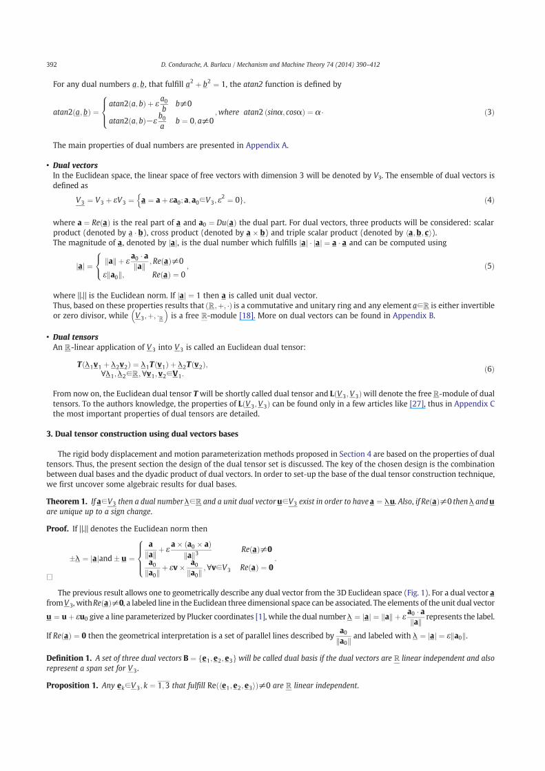
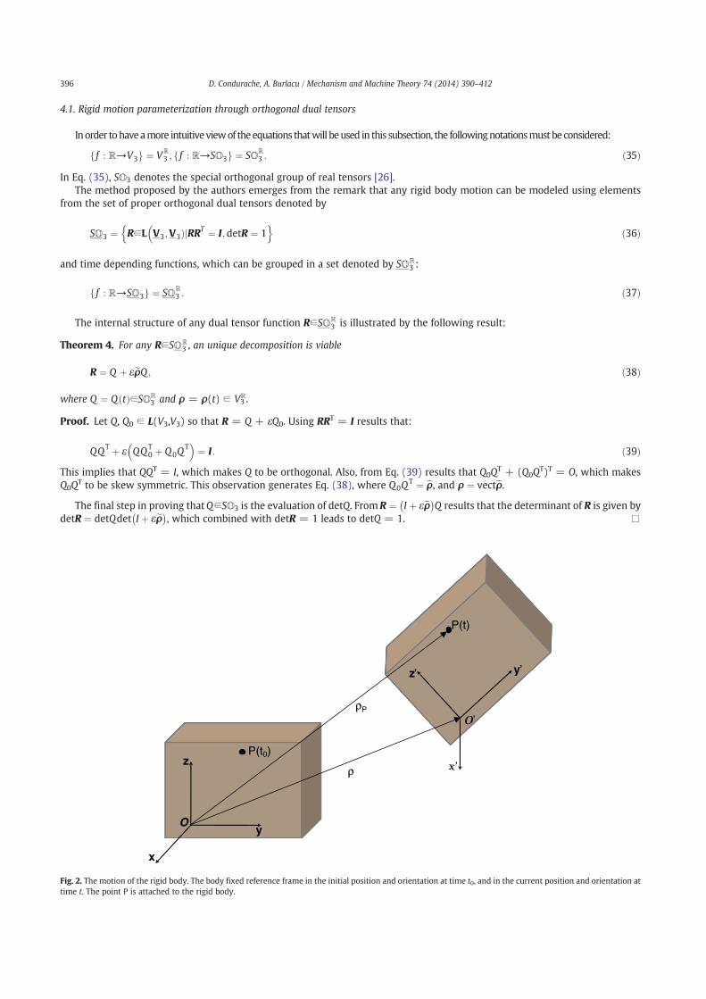
Fig. 2. The motion of the rigid body. The body fixed reference frame in the initial position and orientation at time t0, and in the current position and orientation attime t. The point P is attached to the rigid body.

396 D. Condurache, A. Burlacu / Mechanism and Machine Theory 74 (2014) 390–412

Remark 2. Based on the construction of SO3 and the multiplication of dual tensors (Eq. (C.3)), a direct conclusion is the Lie groupstructure of Eq. (36). This Lie group parameterizes all rigid motions. Thus, a rigid body motion (Fig. 2) [23] can be modeled usingEq. (38).

Based on Theorem 4, a representation of any dual tensor from SO3 can be given:

Theorem 5. For any orthogonal dual tensor R defined as in Eq. (38), a dual number α ¼ α þ ϵd and a dual unit vector u ¼ uþ εu0

exists in order to have the following expression

R ¼ I þ sinαeu þ 1−cosαð Þeu2; ð40Þ

where u and α are recovered from the linear invariants of Q, while d = ρ ⋅ u and

u0 ¼12ρ% uþ 1

2cot

α2u% ρ% uð Þ α≠0;

12ρ% u α ¼ 0;

:

8><

>:

Proof. Using Eq. (38) and the properties of vectR and traceR it results that:

traceR ¼ traceQ þ εtrace eρQ! "

vectR ¼ vectQ þ εvect eρQ! "

:ð41Þ

From Eq. (40) it is obvious that

traceR ¼ 1þ 2cosαvectR ¼ sinαu ð42Þ

which combined with [2]

trace eρQ! "

¼ −2ρ & vectQ

vect eρQ! "

¼ 12

traceQI−Q½ (ρð43Þ

leads to:

traceQ þ ε −2ρ & vectQð Þ ¼ 1þ 2cosα

vectQ þ ε12

traceQI−Q½ (ρ ¼ sinαu: ð44Þ

Two important functions of dual number variable must be considered: cosα ¼ cosα−εdsinα and sinα ¼ sinα þ εdcosα.

Because Q∈SO3 it can be decomposed as Q ¼ I þ sinαeuþ 1−cosαð Þeu2 (Rodrigues formulae [2]). This decomposition leadsto traceQ = 1 + 2cosα and skewQ ¼ sinαeu . Using Eq. (28) results that vectQ = sinαu. All the previous information leadto:

1þ 2cosα þ ε −2ρ & vectQð Þ ¼ 1þ 2cosα

sinαuþ ε12

cosαρ−sinαu% ρ− 1−cosαð Þeu u% ρð Þ# $

¼ sinαu:ð45Þ

The dual parts of α ¼ α þ εd and u ¼ uþ εu0, can be recovered using

u0 ¼12ρ% uþ 1

2cot

α2u% ρ% uð Þ α≠0;

12ρ% u α ¼ 0;

8><

>:ð46Þ

d ¼ ρ & u ð47Þ

while for the real parts the logarithm of real orthogonal tensors is employed [42]:

u ¼

)vect1ffiffiffiffiffiffiffiffiffiffiffiffiffiffiffiffiffiffiffiffiffiffiffiffiffiffiffiffiffiffiffiffiffiffiffiffiffiffiffiffiffiffiffiffiffiffiffiffiffiffiffiffiffi

1þ traceQð Þ 3−traceQð Þp Q−QT

& ' !

; traceQ∈ −1;3ð Þ;

Qv þ vQv þ vk k

;∀v∈V3; traceQ ¼ −1 Q issymmetricð Þ;ρρk k

; traceQ ¼ 3 Q ¼ Ið Þ;ρ∈V3

8>>>>>>><

>>>>>>>:

ð48Þ

α ¼ atan2 )12

ffiffiffiffiffiffiffiffiffiffiffiffiffiffiffiffiffiffiffiffiffiffiffiffiffiffiffiffiffiffiffiffiffiffiffiffiffiffiffiffiffiffiffiffiffiffiffiffiffiffiffiffiffi1þ traceQð Þ 3−traceQð Þ

p;traceQ−1

2

( ): ð49Þ

□

397D. Condurache, A. Burlacu / Mechanism and Machine Theory 74 (2014) 390–412

Using Eq. (40) and the fact that eu ! u ¼ 0, for an unit dual vector u, the following remark is valid:

Remark 3. For every choice of an orthogonal dual tensor R∈SO3 a unit dual vector u∈V 3 exists so that Ru ¼ u.

The fundamental Mozzi–Chasles [2] theorem states that:“any rigid displacement may be represented by a planar rotationabout a suitable axis passing through that point, followed by a translation along that axis”. Theorem 5 and Remark 3 are in fact thesteps of a very short, elegant and constructive proof of this famous theorem.

A screw axis is characterized by an unit dual vectoru and the screw parameters (angle of rotation about the screw, denoted byα, and the translation along the screw axis, denoted by d) structured an a dual angleα. For the following results, lets recall that the

SO3 is a Lie group and its Lie algebra can be identified by the skew-symmetric dual tensors set so3 ¼ eα∈L V3;V3Þjeα ¼ −eαΤg!n

,

where the internal mapping is eα1; eα2" #

¼ geα1α2.

Theorem 6. The mapping

exp : so3→SO3; exp eα$ %

¼ eeα ¼X∞

k¼0

eαk

k!ð50Þ

is well defined and surjective.

Proof. From eeα! &T

¼ eeαT

and eα ¼ −eαT results that eeα! &T

! eeα ¼ I . The computation of det eeα! &

is in fact the computation of

e traceeα$ %

¼ e0 ¼ 1. These two statements prove that Eq. (50) is well defined. For anyR∈SO3 the parametersα ;u exist so that Eq. (40) is

fulfilled. From eeα ¼ Iþ∑∞

k¼1

eαk

k1combinedwith Eq. (31) and a choice for eα like eα ¼ αeu results thateαeu ¼ I þ sinαeu þ 1−cosαð Þeu2 ¼ R.□

The screw parameters computation is linked with the problem of finding the logarithm of an orthogonal dual tensor R, amultifunction defined by

log : SO3→so3; logR ¼ eψ∈so3jexp eψ! &

¼ Rgn

ð51Þ

and is the inverse of Eq. (50).If the dual vector ψ ¼ ψþ εψ0 is computed as ψ ¼ vect eψ

! &then using Theorem 1 results that ψ ¼ α ! u, where

&α ¼ψk kþ ε

ψ ! ψ0ψk k

; Re ψ! &

≠0

ε ψ0k k; Re ψ! &

¼ 0

8><

>:ð52Þ

and

&u ¼

ψψk k

þ εψ' ψ0 ' ψð Þ

ψk k3Re ψ

! &≠0

ψ0ψ0k k

þ εv ' ψ0ψ0k k

;∀v∈V3 Re ψ! &

¼ 0:

8>><

>>:ð53Þ

Thus, the screw dual vector ψ can be used to parameterize any type of rigid motion.Before computing the logarithm of an orthogonal dual tensor, we need to analyze the behavior and influence of its natural

invariants.

Remark 4. A direct result of Theorems 5 and 6 is that the logarithm of a dual tensor is the productαeu. The parametersα andu arecalled the natural invariants of R and can be recovered from the linear invariants [2] using Eq. (40):

u sin α ¼ vectR; ð54Þ

1þ 2 cosα ¼ traceR: ð55Þ

The above equations can be transformed into

u sin α ¼ vectR

cos α ¼ 12

traceR−1½ ) ð56Þ

and the parameters α ;u. The unit dual vector u gives the Plucker representation of the Mozzi–Chasles axis, while the dual angleα ¼ α þ εd contains the rotation angle α and the translation distance d.

398 D. Condurache, A. Burlacu / Mechanism and Machine Theory 74 (2014) 390–412

The computational formulas for α ;u are extracted from Eq. (56) and Theorem 5:

u ¼

" vectRvectRj j

; Re vectRð Þ≠0;

Qv þ vQv þ vk k

þ ε12ρ& Qv þ v

Qv þ vk k;∀v∈V3; Re vectRð Þ ¼ 0andtraceQ ¼ −1;

ρρk k

; Re vectRð Þ ¼ 0andtraceQ ¼ 3;

8>>>>>><

>>>>>>:

ð57Þ

α ¼ atan2 " vectRj j;12

traceR−1½ (! "

: ð58Þ

and represent different computational method for logR than the one proposed in [30].

4.2. Instantaneous motion analysis using orthogonal dual tensors

The line containing the points of a rigid body undergoing minimum-magnitude velocities is called the instant screw axis (ISA)of the body under a given motion. The instantaneous motion of the body is equivalent to that of the bolt of a screw of ISA and iscalled instantaneous screw. An instantaneous screw axis, which will be defined as a dual vector denoted byω, is characterized byan unit dual vector uω , a dual number ωj j called magnitude and a number p called the pitch.

Let h0 embed the Plucker coordinates of a line at t = t0 then:

h tð Þ ¼ R tð Þh0: ð59Þ

Theorem 7. In a general rigid motion, described by an orthogonal dual tensor function R, the velocity dual tensor function Φ isdefined as

h¼ Φh ð60Þ

is expressed by:

Φ ¼RRT: ð61Þ

Proof. The time differential of Eq. (59), with respect to the temporal variable t, is

h¼Rh0 ð62Þ

where, for h0 ¼ RTh results that:

h¼R RTh: ð63Þ

LetΦ ¼RRT then by differentiating Eq. (84) results that RRT þ RT R¼ O⇔ΦþΦT ¼ O, which shows thatΦ∈soℝ3 . □

The form of the velocity dual tensor described by Eq. (61) can be taken a step further if R is decomposed as in Eq. (38). Thisimplies

R¼Qþ ε eρQ þ eρQ! "

: ð64Þ

Because Φ∈soℝ3 results that we can consider Φ ¼ eω , which gives:

eω ¼QQT þ εg

ρ−QQTρ! "

: ð65Þ

Let eω ¼QQT and ev ¼g

ρ−QQTρ, then

eω ¼ eωþ εev: ð66Þ

This equation leads to the internal structure of the dual angular velocity vector ω

ω ¼ ωþ εv; ð67Þ

399D. Condurache, A. Burlacu / Mechanism and Machine Theory 74 (2014) 390–412

where ω is the instantaneous angular velocity of the rigid body and v represents the linear velocity of the point of the body thatcoincides instantaneously with the origin of the reference frame.

The dual angular velocity vectorω completely characterize, at a certain time, the velocity field of an rigid body in motion. Let vPbe the linear velocity of a point described by the position vector ρP:

vP ¼ v þω# ρP : ð68Þ

Based on Theorem 1, for ||ω|| ≠ 0 the instantaneous screw axis unit dual vector is

uω ¼ ωωj jj j

þ εω# v #ωð Þ

jjωjj3ð69Þ

and

jωj ¼ jjωjjþ εv &ωωj jj j

: ð70Þ

For v&ωωj jj j ¼

vP &ωωj jj j ¼ vmin, the magnitude ofω is jωj ¼ jjωjjþ εvmin. If p¼ v&ω

jjωjj2 ¼vminωj jj j denote the pitch of the screw axis [2] then

jωj ¼ jjωjj 1þ εpð Þ. For ||ω|| = 0 the structure of the dual angular velocity vector is ω ¼ εv, which represents an instantaneouspure translation.

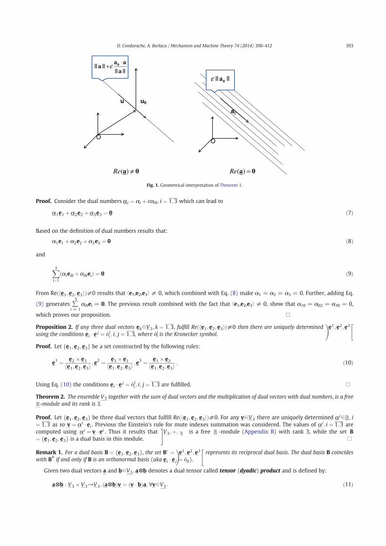
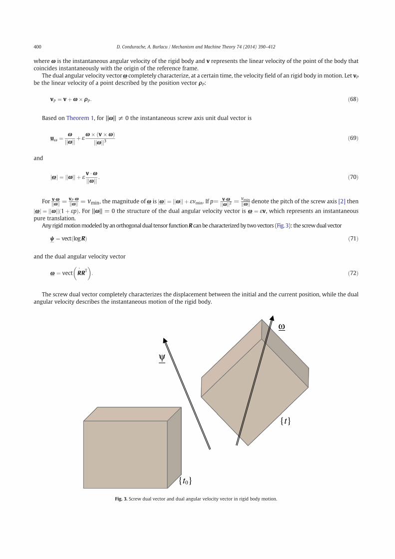
Anyrigidmotionmodeledbyanorthogonaldual tensor functionR canbecharacterizedby twovectors (Fig. 3): the screwdual vector

ψ ¼ vect logRð Þ ð71Þ

and the dual angular velocity vector

ω ¼ vect RRT! "

: ð72Þ

The screw dual vector completely characterizes the displacement between the initial and the current position, while the dualangular velocity describes the instantaneous motion of the rigid body.

ψ

ω

{t0}

{t}

Fig. 3. Screw dual vector and dual angular velocity vector in rigid body motion.

400 D. Condurache, A. Burlacu / Mechanism and Machine Theory 74 (2014) 390–412

4.3. Rigid body motion parameterization using dual rigid bases

All the previous results represent the main inputs in the construction of orthogonal dual tensors using rigid bases of dualvectors. This new algebraic entity is defined next:

Definition 2. A basis B ¼ e1; e2; e3gf from Vℝ3 will be referred to as a dual rigid basis if

ei " e j ¼ e0i " e0 j; i; j ¼ 1;3;

be1; e2; e3N ¼ be01; e02; e03N ;

(

ð73Þ

where e0i ¼ ei t0ð Þ.

Remark 5. If B ¼ e1; e2; e3gf is a dual rigid basis then B% ¼ e1; e2; e3g!

, its reciprocal dual basis, is also rigid.

Working with rigid dual bases generates an increase in the flexibility of the rigid body motion parameterization because noassumptions of orthonormal reference frames is needed. Also, this approach is free of coordinates and only uses calculus with dualnumbers and dual vectors, which implies a reduced number of algebraic equations and a more compact notation with fewervariables. Using point and line features of a rigid body, the dual rigid bases are constructed and new methods for computingorthogonal dual tensors, screw parameters and instantaneous screw parameters are proposed.

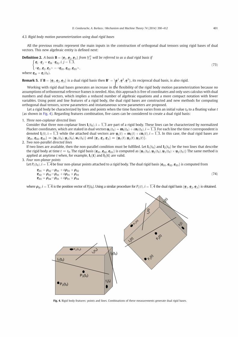
Let a rigid body be characterized by lines and points when the time function varies from an initial value t0 to a floating value t(as shown in Fig. 4). Regarding features combination, five cases can be considered to create a dual rigid basis:

1. Three non-coplanar directed linesConsider that three non-coplanar lines li t0ð Þ; i ¼ 1;3 are part of a rigid body. These lines can be characterized by normalizedPlucker coordinates, which are staked in dual vectorsui t0ð Þ ¼ mi t0ð Þ þ εni t0ð Þ; i ¼ 1;3. For each line the time t correspondent isdenoted li tð Þ; i ¼ 1;3 while the attached dual vectors are ui tð Þ ¼ mi tð Þ þ εni tð Þ; i ¼ 1;3. In this case, the dual rigid bases aree01; e02; e03gf = u1 t0ð Þ;u2 t0ð Þ;u3 t0ð Þgf and e1; e2; e3gf = u1 tð Þ;u2 tð Þ;u3 tð Þgf .

2. Two non-parallel directed linesIf two lines are available, then the non-parallel condition must be fulfilled. Let l1(t0) and l2(t0) be the two lines that describethe rigid body at time t = t0. The rigid basis e01; e02; e03gf is computed as u1 t0ð Þ;u2 t0ð Þ;u1 t0ð Þ ' u2 t0ð Þgf The same method isapplied at anytime t when, for example, l1(t) and l2(t) are valid.

3. Four non-planar pointsLet Pi t0ð Þ; i ¼ 1;4 be four non-planar points attached to a rigid body. The dual rigid basis e01; e02; e03gf is computed from

e01 ¼ ρ02−ρ01 þ ερ01 ' ρ02e02 ¼ ρ03−ρ01 þ ερ01 ' ρ03e03 ¼ ρ04−ρ01 þ ερ01 ' ρ04

ð74Þ

where ρ0i; i ¼ 1;4 is the position vector of Pi(t0). Using a similar procedure for Pi tð Þ; i ¼ 1;4 the dual rigid basis e1; e2; e3gf is obtained.

P2(t0)

P3(t0)

l1(t0)

l2(t0)

Fig. 4. Rigid body features: points and lines. Combinations of these measurements generate dual rigid bases.

401D. Condurache, A. Burlacu / Mechanism and Machine Theory 74 (2014) 390–412

4. Three non-collinear pointsIn case of non-availability of one point from the four points set, if the remaining three points are non-collinear (e.g. P1(t0),P2(t0), P3(t0) are known) then e01 and e02 are computed using Eq. (74). For e03 the following equation is used:

e03 ¼ e01 " e02: ð75Þ

The same approach is valid for e1; e2; e3gf generated by {P1(t), P2(t), P3(t)}.5. One point and one directed line

Let the P1(t0) and l1(t0) be the available measurements on the rigid body. First, the constraint P1(t0) ∉ l1(t0) must be fulfilled. Ifu ¼ uþ εu0 is the unit dual vector of l1(t0) thene01 ¼ u,e02 ¼ u"w0 þ ερP1 t0ð Þ " u"w0ð Þande03 ¼ e01 " e02. The vectorw0 isdefined as w0 ¼ u0−ρP1 t0ð Þ " u. The same approach is used to compute e1; e2; e3gf when P1(t) and l1(t) are known.

The following result shows how dual rigid bases can be used to uniquely construct orthogonal dual tensors:

Theorem 8. If B ¼ e1; e2; e3gf is a dual rigid basis in Vℝ3 and ei are continuous functions, then the dual tensor

R ¼ ei⊗ei0 ð76Þ

is proper orthogonal and uniquely defined by:

R e0ið Þ ¼ ei; i ¼ 1;3: ð77Þ

Proof. From Eq. (77) and (76) it results that:

R e0ið Þ ¼ e j⊗e j0

! "e0i ¼ e0i & e

j0

! "e j ¼ δ j

i e j ¼ ei ð78Þ

Let v∈V 3 be an arbitrary vector function. Having v expressed in the basis B0 ¼ e01; e02; e03gf as

v ¼ v & ei0

! "e0i; ð79Þ

allows for

Rv ¼ v & ei0

! "Re0i ¼ v & ei

0

! "ei ¼ ei⊗ei

0

! "v; ð80Þ

which proves hypothesis(77).

Using Eq. (32) it results that

RT ¼ ei0⊗ei ð81Þ

and, further on:

RRT ¼ ei⊗ei0

! "e j0⊗e j

! "¼ ei

0 & ej0

! "ei⊗e j: ð82Þ

From Eq. (73), combined with Eq. (10), the following relation emerges

ei & e j ¼ ei0 & e

i0; i; j ¼ 1;3; ð83Þ

and thus Eq. (82) becomes:

RRT ¼ ei & e j! "

ei⊗e j ¼ e j⊗e j ¼ I: ð84Þ

This leads to det RRT = 1 and det R2 = 1, thus resulting det R ∈ {−1, 1}. From Eq. (76) and (25) the det R can be computedas:

det R ¼ be1; e2; e3N

be01; e02; e03N :ð85Þ

Because ek; k ¼ 1;3 are continuous functions, it results that

limt→t0

ek tð Þ ¼ e0k; ð86Þ

402 D. Condurache, A. Burlacu / Mechanism and Machine Theory 74 (2014) 390–412

which leads to

detR ¼ 1; ð87Þ

and proves that R is a proper orthogonal dual tensor. □

Remark 6. For any orthogonal dual tensor defined as in Eq. (76), the values of Q∈SO3 and eρ∈so3 can be recovered using theprocedure detailed next. If ei ¼ ei þ εe%i and ei

0 ¼ ei0 þ εei%0 , then

R ¼ ei⊗ei0 þ ε ei⊗ei%0 þ e%i ⊗ei0h i

ð88Þ

which leads to Q = ei ⊗ e0i and eρ ¼ Q0 ei0⊗ei! "

, where Q0 = ei ⊗ e0i∗ + ei∗ ⊗ e0i .

Based on the dual tensors properties, eρ can also be computed using eρ ¼ Q0ei0! "

⊗ei which gives the recovering formula ofρ ¼ vect eρ:

ρ ¼ 12ei & Q0e

i0: ð89Þ

4.4. Screw parameters generated by dual rigid bases

Next we present a new method for computing the screw parameters when the orthogonal dual tensor, that models the rigidbody motion, is generated by dual rigid bases.

Remark 7. Using Eqs. (33), (34), (54), (55) and (76) the following equations emerge:

u sin α ¼ 12ei0 & ei; ð90Þ

cosα ¼ 12

ei0 ' ei−1

h i: ð91Þ

Eqs. (90) and (91) solve the problem of finding the logarithm of the orthogonal dual tensor, while the following theorem givesa computational procedure of finding u and α without the computation of the dual tensor.

Theorem 9. The natural invariants of the proper orthogonal tensor R ¼ ei⊗ei0 are

u ¼

( ei0 & ei

jei0 & eij

; Re ei0 & ei

# $≠0

e0 þ ee0 þ ej jj j

þ ε12ρ& e0 þ e

e0 þ ej jj j; Re ei

0 & ei

# $¼ 0 and Re ei

0 ' ei

# $¼ −1

ρρj jj j

; Re ei0 & ei

# $¼ 0 and Re ei

0 ' ei

# $¼ 3

8>>>>>>>>>><

>>>>>>>>>>:

ð92Þ

α ¼ atan2 (12jei

0 & eij;12

ei0 ' ei−1

h i !

; ð93Þ

where ρ is given by Eq. (89) and the sum e0 + e is properly chosen to maximize norm of any of the three sums e0i þ ei; i ¼ 1;3.

Proof. Consider B0 ¼ e01; e02; e03gf a dual rigid basis and B0% ¼ e1

0; e20; e

30g

%its reciprocal dual basis. A correspondent of B0 at a

generic time t will be denoted by B ¼ e1; e2; e3gf .

Three types of motion cases can be considered:

• if Re ei0 & ei

# $≠0 then a general Mozzi–Chasles type motion is active;

• if Re ei0 & ei

# $¼ 0 and Re ei

0 ' ei

# $¼ −1 then the Mozzi–Chasles motion is in fact a translation combined with a rotation of an

angle equal to π;

• if Re ei0 & ei

# $¼ 0 and Re ei

0 ' ei

# $¼ 3 then the Mozzi–Chasles motion represents a pure translation;

403D. Condurache, A. Burlacu / Mechanism and Machine Theory 74 (2014) 390–412

For Re ei0 ! ei

!≠0

"the combination between Eq. (90) and Theorem 1 gives the values of u and α . When Re ei0 ! ei

# $¼ 0 and

Re ei0 # ei

!¼ −1

"the solution is given by any of the three vectors e0i + ei. In order to avoid singularitieswewill choose e0 + e to be the

pair e0i + ei, i ¼ 1;3 with the maximum norm. The validation of Eqs. (92) and (93) is provided by Eqs. (90), (91) and Remark 6. □The result illustrated by Theorem 9 represents a new algebraic technique for computing the screw parameters of a rigid

body motion. This technique is based on dual rigid bases and illustrates all the cases that can occur during screw parameterdetection.

4.5. Instantaneous screw parameters generated by dual rigid bases

In this subsection a new dual rigid bases based method for computing the instantaneous screw parameters is presented.If R is defined by Eq. (76) then

R¼ e:i⊗ei

0; ð94Þ

which together with Eqs. (94), (81) and (61) give:

Φ ¼ e:i⊗ei

0

" !e j0⊗e j

" !¼ ei

0 # ej0

" !e:i⊗e j

" !: ð95Þ

Based on Remark 5 results that

Φ ¼ ei # e j" !

e:i⊗e j

" !¼ e

:i⊗ ei # e j

" !e j

h i¼ e

:i⊗ei

; ð96Þ

Denoting by Φ ¼ eω , Theorem 7 leads to the following representation for the angular velocity dual tensor:

eω ¼ e:i⊗ei

: ð97Þ

If ω ¼ vecteω then the following theorem can be stated:

Theorem 10. If a dual rigid basis B ¼ e1; e2; e3gf is given, then a dual vector ω exists and is expressed by

ω ¼ 12ei ! e

:i ð98Þ

so that

e:i ¼ ω ! ei; ð99Þ

Proof. Combining ω ! ei ¼ eωei with eω ¼ ei: ⊗ei results that ω ! ei ¼ e j

: ⊗e j" !

ei . Using Eq. (11), the definition of the dyadicproduct, we can conclude that ω ! ei ¼ ei # e j

" !ei:¼ δ j

i e j:¼ ei

:. □

The result from Theorem 10 is the dual version of the Poisson like formulae [43] for non-orthogonal bases. Using basic dualvectors calculus, Eq. (98) can be transformed into

ω ¼e:2 # e3

" !e1 þ e

:3 # e1

" !e2 þ e

:1 # e2

" !e3

be1; e2; e3N ;ð100Þ

which has the advantage of computing the dual angular velocity vector without involving the reciprocal dual basis. From Eqs. (69)and (70) the ISA parameters, uω and ωj j, are recovered.

Eq. (100) gives a new compact form for ω, which can also be written as

ω ¼ K1e:1 þ K2e

:2 þ K3e

:3; ð101Þ

where the dual tensors K i; i ¼ 1;3 are K1 ¼ e3⊗e2<e1; e2; e3N

, K2 ¼ e1⊗e3<e1; e2; e3N

, K3 ¼ e2⊗e1<e1; e2; e3N

.

5. Numerical results

Next we present the algorithms (pseudo code version) that put the methods, from Section 4, into practice. Also, symbolic andnumerical computational examples are presented and discussed.

404 D. Condurache, A. Burlacu / Mechanism and Machine Theory 74 (2014) 390–412

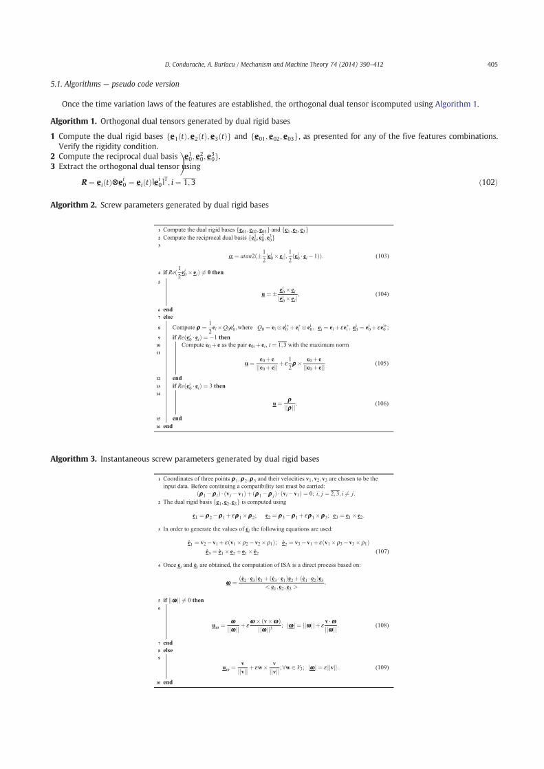
5.1. Algorithms — pseudo code version

Once the time variation laws of the features are established, the orthogonal dual tensor iscomputed using Algorithm 1.

Algorithm 1. Orthogonal dual tensors generated by dual rigid bases

1 Compute the dual rigid bases e1 tð Þ; e2 tð Þ; e3 tð Þgf and e01; e02; e03gf , as presented for any of the five features combinations.Verify the rigidity condition.

2 Compute the reciprocal dual basis e10; e

20; e

30g

!.

3 Extract the orthogonal dual tensor using

R ¼ ei tð Þ⊗ei0 ¼ ei tð Þ⌉ei

0⌉T; i ¼ 1;3 ð102Þ

Algorithm 2. Screw parameters generated by dual rigid bases

Algorithm 3. Instantaneous screw parameters generated by dual rigid bases

405D. Condurache, A. Burlacu / Mechanism and Machine Theory 74 (2014) 390–412

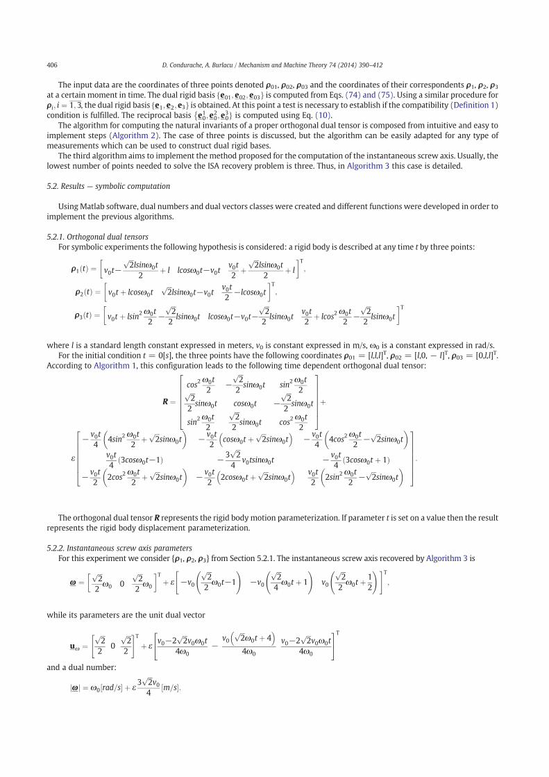
The input data are the coordinates of three points denoted ρ01, ρ02, ρ03 and the coordinates of their correspondents ρ1, ρ2, ρ3

at a certain moment in time. The dual rigid basis e01; e02; e03gf is computed from Eqs. (74) and (75). Using a similar procedure forρi; i ¼ 1;3, the dual rigid basis e1; e2; e3gf is obtained. At this point a test is necessary to establish if the compatibility (Definition 1)condition is fulfilled. The reciprocal basis e1

0; e20; e

30g

!is computed using Eq. (10).

The algorithm for computing the natural invariants of a proper orthogonal dual tensor is composed from intuitive and easy toimplement steps (Algorithm 2). The case of three points is discussed, but the algorithm can be easily adapted for any type ofmeasurements which can be used to construct dual rigid bases.

The third algorithm aims to implement the method proposed for the computation of the instantaneous screw axis. Usually, thelowest number of points needed to solve the ISA recovery problem is three. Thus, in Algorithm 3 this case is detailed.

5.2. Results — symbolic computation

Using Matlab software, dual numbers and dual vectors classes were created and different functions were developed in order toimplement the previous algorithms.

5.2.1. Orthogonal dual tensorsFor symbolic experiments the following hypothesis is considered: a rigid body is described at any time t by three points:

ρ1 tð Þ ¼ v0t−ffiffiffi2

plsinω0t2

þ l lcosω0t−v0tv0t2

þffiffiffi2

plsinω0t2

þ l

# $T;

ρ2 tð Þ ¼ v0t þ lcosω0tffiffiffi2

plsinω0t−v0t

v0t2

−lcosω0t# $T

;

ρ3 tð Þ ¼ v0t þ lsin2 ω0t2

−ffiffiffi2

p

2lsinω0t lcosω0t−v0t−

ffiffiffi2

p

2lsinω0t

v0t2

þ lcos2ω0t2

−ffiffiffi2

p

2lsinω0t

# $T

where l is a standard length constant expressed in meters, v0 is constant expressed in m/s, ω0 is a constant expressed in rad/s.For the initial condition t = 0[s], the three points have the following coordinates ρ01 = [l,l,l]T, ρ02 = [l,0, − l]T, ρ03 = [0,l,l]T.

According to Algorithm 1, this configuration leads to the following time dependent orthogonal dual tensor:

R ¼

cos2ω0t2

−ffiffiffi2

p

2sinω0t sin2 ω0t

2ffiffiffi2

p

2sinω0t cosω0t −

ffiffiffi2

p

2sinω0t

sin2 ω0t2

ffiffiffi2

p

2sinω0t cos2

ω0t2

2

6666664

3

7777775þ

ε

− v0t4

4sin2 ω0t2

þffiffiffi2

psinω0t

% &− v0t

2cosω0t þ

ffiffiffi2

psinω0t

' (− v0t

44cos2

ω0t2

−ffiffiffi2

psinω0t

% &

v0t4

3cosω0t−1ð Þ −3ffiffiffi2

p

4v0tsinω0t − v0t

43cosω0t þ 1ð Þ

− v0t2

2cos2ω0t2

þffiffiffi2

psinω0t

% &− v0t

22cosω0t þ

ffiffiffi2

psinω0t

' ( v0t2

2sin2 ω0t2

−ffiffiffi2

psinω0t

% &

2

6666664

3

7777775:

The orthogonal dual tensor R represents the rigid body motion parameterization. If parameter t is set on a value then the resultrepresents the rigid body displacement parameterization.

5.2.2. Instantaneous screw axis parametersFor this experiment we consider {ρ1, ρ2, ρ3} from Section 5.2.1. The instantaneous screw axis recovered by Algorithm 3 is

ω ¼ffiffiffi2

p

2ω0 0

ffiffiffi2

p

2ω0

# $Tþ ε −v0

ffiffiffi2

p

2ω0t−1

!−v0

ffiffiffi2

p

4ω0t þ 1

!v0

ffiffiffi2

p

2ω0t þ

12

!" #T;

while its parameters are the unit dual vector

uω ¼ffiffiffi2

p

20

ffiffiffi2

p

2

" #Tþ ε

v0−2ffiffiffi2

pv0ω0t

4ω0−

v0ffiffiffi2

pω0t þ 4

' (

4ω0

v0−2ffiffiffi2

pv0ω0t

4ω0

2

4

3

5T

and a dual number:

jωj ¼ ω0 rad=s½ & þ ε3

ffiffiffi2

pv0

4m=s½ &:

406 D. Condurache, A. Burlacu / Mechanism and Machine Theory 74 (2014) 390–412

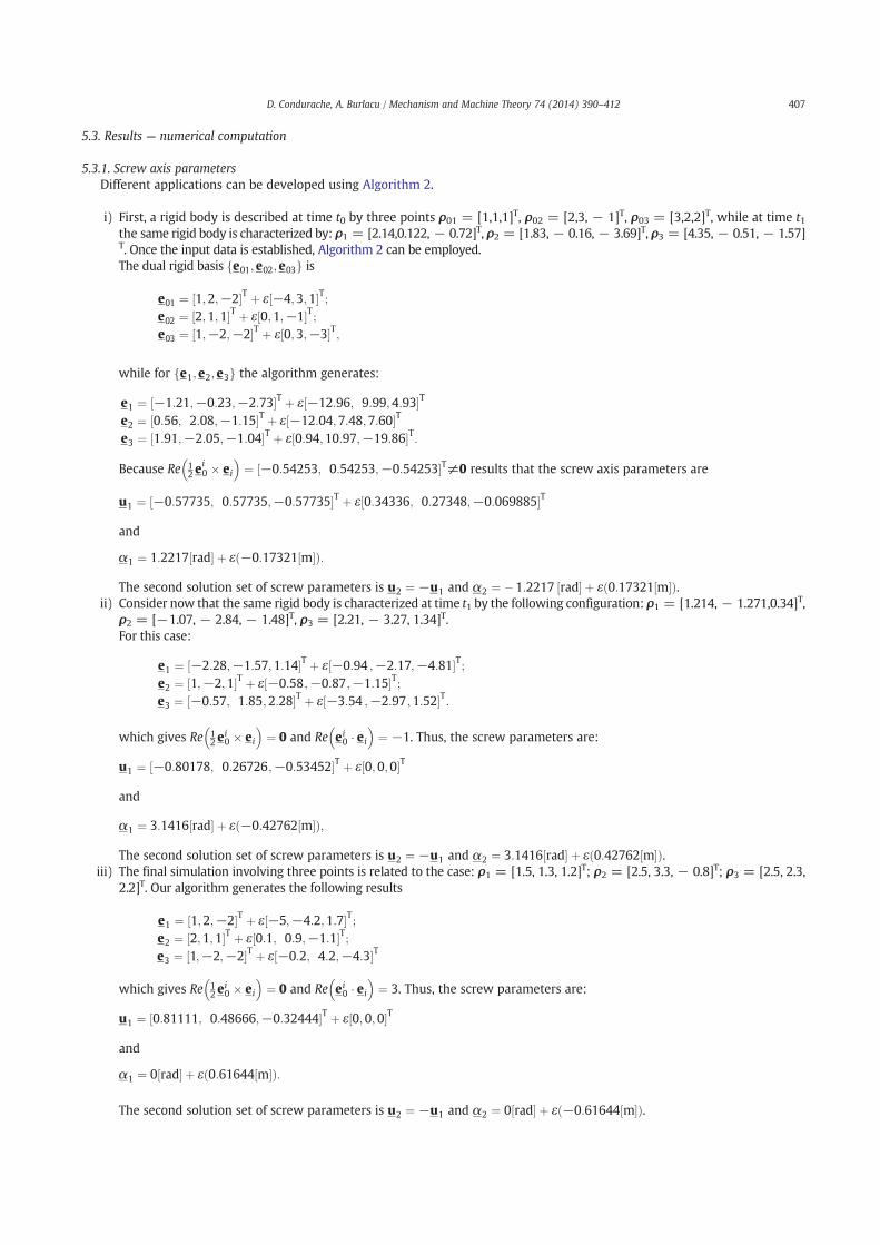
5.3. Results — numerical computation

5.3.1. Screw axis parametersDifferent applications can be developed using Algorithm 2.

i) First, a rigid body is described at time t0 by three points ρ01 = [1,1,1]T, ρ02 = [2,3, − 1]T, ρ03 = [3,2,2]T, while at time t1the same rigid body is characterized by: ρ1 = [2.14,0.122, − 0.72]T, ρ2 = [1.83, − 0.16, − 3.69]T, ρ3 = [4.35, − 0.51, − 1.57]T. Once the input data is established, Algorithm 2 can be employed.The dual rigid basis e01; e02; e03gf is

e01 ¼ 1;2;−2½ #T þ ε½−4;3;1#T;e02 ¼ 2;1;1½ #T þ ε½0;1;−1#T;e03 ¼ 1;−2;−2½ #T þ ε½0;3;−3#T;

while for e1; e2; e3gf the algorithm generates:

e1 ¼ −1:21;−0:23;−2:73½ #T þ ε½−12:96; 9:99;4:93#T

e2 ¼ 0:56; 2:08;−1:15½ #T þ ε½−12:04;7:48;7:60#T

e3 ¼ 1:91;−2:05;−1:04½ #T þ ε½0:94;10:97;−19:86#T:

Because Re 12 e

i0 % ei

! "¼ −0:54253; 0:54253;−0:54253½ #T≠0 results that the screw axis parameters are

u1 ¼ −0:57735; 0:57735;−0:57735½ #T þ ε 0:34336; 0:27348;−0:069885½ #T

and

α1 ¼ 1:2217 rad½ # þ ε −0:17321 m½ #ð Þ:

The second solution set of screw parameters is u2 ¼ −u1 and α2 ¼ (1:2217 rad½ # þ ε 0:17321 m½ #ð Þ.ii) Consider now that the same rigid body is characterized at time t1 by the following configuration: ρ1 = [1.214, − 1.271,0.34]T,

ρ2 = [−1.07, − 2.84, − 1.48]T, ρ3 = [2.21, − 3.27, 1.34]T.For this case:

e1 ¼ −2:28;−1:57;1:14½ #T þ ε½−0:94 ;−2:17;−4:81#T;e2 ¼ 1;−2;1½ #T þ ε½−0:58;−0:87;−1:15#T;e3 ¼ −0:57; 1:85;2:28½ #T þ ε½−3:54 ;−2:97 ;1:52#T:

which gives Re 12 e

i0 % ei

"¼ 0

!and Re ei

0 ) ei

"¼ −1

!. Thus, the screw parameters are:

u1 ¼ −0:80178; 0:26726;−0:53452½ #T þ ε 0;0;0½ #T

and

α1 ¼ 3:1416 rad½ # þ ε −0:42762 m½ #ð Þ;

The second solution set of screw parameters is u2 ¼ −u1 and α2 ¼ 3:1416 rad½ # þ ε 0:42762 m½ #ð Þ.iii) The final simulation involving three points is related to the case: ρ1 = [1.5, 1.3, 1.2]T; ρ2 = [2.5, 3.3, − 0.8]T; ρ3 = [2.5, 2.3,

2.2]T. Our algorithm generates the following results

e1 ¼ 1;2;−2½ #T þ ε½−5;−4:2;1:7#T;e2 ¼ 2;1;1½ #T þ ε½0:1; 0:9;−1:1#T;e3 ¼ 1;−2;−2½ #T þ ε½−0:2; 4:2;−4:3#T

which gives Re 12 e

i0 % ei

! "¼ 0 and Re ei

0 ) ei

! "¼ 3. Thus, the screw parameters are:

u1 ¼ 0:81111; 0:48666;−0:32444½ #T þ ε 0;0;0½ #T

and

α1 ¼ 0 rad½ # þ ε 0:61644 m½ #ð Þ:

The second solution set of screw parameters is u2 ¼ −u1 and α2 ¼ 0 rad½ # þ ε −0:61644 m½ #ð Þ.

407D. Condurache, A. Burlacu / Mechanism and Machine Theory 74 (2014) 390–412

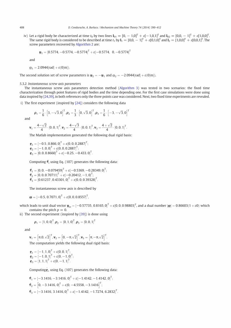
iv) Let a rigid body be characterized at time t0 by two lines l01 = [0, − 1,0]T + ε[−1,0,1]T and l02 = [0,0, − 1]T + ε[1,0,0]T.The same rigid body is considered to be described at time t1 by l1 = [0,0, − 1]T + ε[0,1,0]T and l2 = [1,0,0]T + ε[0,0,1]T. Thescrew parameters recovered by Algorithm 2 are:

u1 ¼ 0:5774;−0:5774;−0:5774½ #T þ ε −0:5774; 0;−0:5774½ #T

and

α1 ¼ 2:0944 rad½ # þ ε 0 m½ #ð Þ:

The second solution set of screw parameters is u2 ¼ −u1 and α2 ¼ −2:0944 rad½ # þ ε 0 m½ #ð Þ.

5.3.2. Instantaneous screw axis parametersThe instantaneous screw axis parameters detection method (Algorithm 3) was tested in two scenarios: the fixed time

characterization through point features of rigid bodies and the time depending one. For the first case simulations were done usingdata inspired by [24,39], in both references only the three points casewas considered. Next, two fixed time experiments are revealed.

i) The first experiment (inspired by [24]) considers the following data

ρ1 ¼ 16' 3;−

ffiffiffi3

p;0

h iT;ρ2 ¼ 1

3' 0;

ffiffiffi3

p;0

h iT;ρ3 ¼ 1

6' −3;−

ffiffiffi3

p;0

h iT

and

v1 ¼ 4−ffiffiffi2

p

4' 0;0;1½ #T; v2 ¼ 4−

ffiffiffi3

p

4' 0;0;1½ #T; v3 ¼ 4þ

ffiffiffi2

p

4' 0;0;1½ #T:

The Matlab implementation generated the following dual rigid basis:

e1 ¼ −0:5 ;0:866;0½ #T þ ε½0;0;0:2887#T;e2 ¼ −1;0;0½ #T þ ε½0;0;0:2887#T;e3 ¼ 0;0;0:8660½ #T þ ε½−0:25;−0:433;0#T:

Computing e:i using Eq. (107) generates the following data:

e:1 ¼ 0;0;−0:079459½ #T þ ε½−0:5369;−0:28349;0#T;

e:2 ¼ 0;0;0:70711½ #T þ ε½−0:20412;−1;0#T;

e:3 ¼ 0:61237 ;0:43301;0½ #T þ ε½0;0;0:39328#T:

The instantaneous screw axis is described by

ω ¼ −0:5; 0:7071;0½ #T þ ε 0;0;0:8557½ #T;

which leads to unit dual vector uω ¼ −0:57735; 0:8165;0½ #T þ ε 0;0;0:98803½ #T, and a dual number jωj ¼ 0:86603 1þ ε0ð Þ whichcontains the pitch p = 0.

ii) The second experiment (inspired by [39]) is done using

ρ1 ¼ 1;0;0½ #T;ρ2 ¼ 0;1;0½ #T;ρ3 ¼ 0;0;1½ #T

and

v1 ¼ π;0;ffiffiffi2

ph iT; v2 ¼ 0;−π;

ffiffiffi2

ph iT; v3 ¼ π;−π;

ffiffiffi2

ph iT:

The computation yields the following dual rigid basis:

e1 ¼ −1;1;0½ #T þ ε½0;0;1#T;e2 ¼ −1;0;1½ #T þ ε½0;−1;0#T;e3 ¼ 1;1;1½ #T þ ε½0;−1;1#T:

Computing e¯i using Eq. (107) generates the following data:

e:1 ¼ −3:1416;−3:1416; 0½ #T þ ε −1:4142;−1:4142 ;0½ #T;

e:2 ¼ 0;−3:1416; 0#T þ ε½0;−4:5558;−3:1416

h iT;

e:3 ¼ −3:1416; 3:1416;0½ #T þ ε −1:4142;−1:7274; 6:2832½ #T:

408 D. Condurache, A. Burlacu / Mechanism and Machine Theory 74 (2014) 390–412

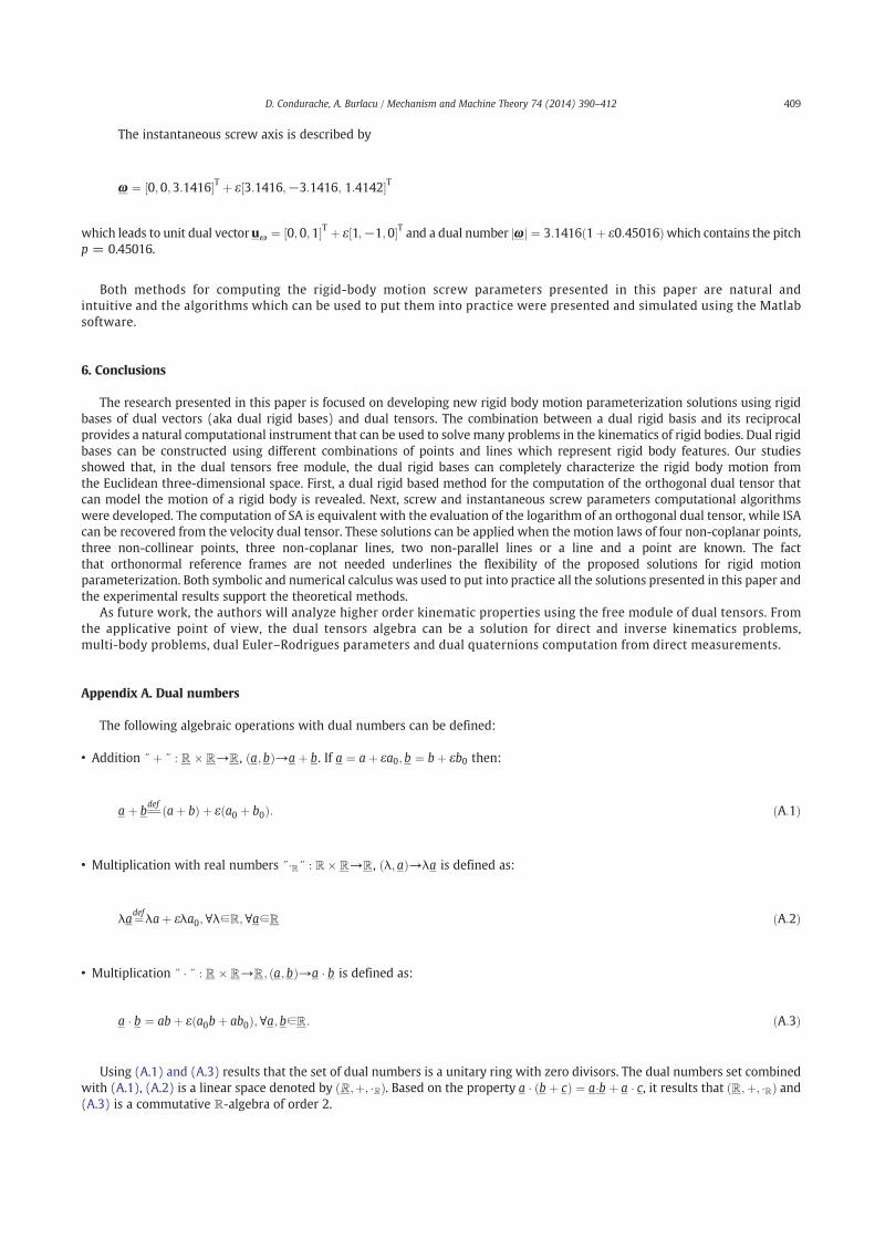
The instantaneous screw axis is described by

ω ¼ 0;0;3:1416½ #T þ ε 3:1416;−3:1416; 1:4142½ #T

which leads to unit dual vectoruω ¼ 0;0;1½ #T þ ε 1;−1;0½ #T and a dual number jωj ¼ 3:1416 1þ ε0:45016ð Þwhich contains the pitchp = 0.45016.

Both methods for computing the rigid-body motion screw parameters presented in this paper are natural andintuitive and the algorithms which can be used to put them into practice were presented and simulated using the Matlabsoftware.

6. Conclusions

The research presented in this paper is focused on developing new rigid body motion parameterization solutions using rigidbases of dual vectors (aka dual rigid bases) and dual tensors. The combination between a dual rigid basis and its reciprocalprovides a natural computational instrument that can be used to solve many problems in the kinematics of rigid bodies. Dual rigidbases can be constructed using different combinations of points and lines which represent rigid body features. Our studiesshowed that, in the dual tensors free module, the dual rigid bases can completely characterize the rigid body motion fromthe Euclidean three-dimensional space. First, a dual rigid based method for the computation of the orthogonal dual tensor thatcan model the motion of a rigid body is revealed. Next, screw and instantaneous screw parameters computational algorithmswere developed. The computation of SA is equivalent with the evaluation of the logarithm of an orthogonal dual tensor, while ISAcan be recovered from the velocity dual tensor. These solutions can be applied when the motion laws of four non-coplanar points,three non-collinear points, three non-coplanar lines, two non-parallel lines or a line and a point are known. The factthat orthonormal reference frames are not needed underlines the flexibility of the proposed solutions for rigid motionparameterization. Both symbolic and numerical calculus was used to put into practice all the solutions presented in this paper andthe experimental results support the theoretical methods.

As future work, the authors will analyze higher order kinematic properties using the free module of dual tensors. Fromthe applicative point of view, the dual tensors algebra can be a solution for direct and inverse kinematics problems,multi-body problems, dual Euler–Rodrigues parameters and dual quaternions computation from direct measurements.

Appendix A. Dual numbers

The following algebraic operations with dual numbers can be defined:

• Addition }þ } : ℝ 'ℝ→ℝ, a; bð Þ→a þ b. If a ¼ aþ εa0; b ¼ bþ εb0 then:

a þ bdef

aþ bð Þ þ ε a0 þ b0ð Þ: ðA:1Þ

• Multiplication with real numbers }(ℝ} : ℝ'ℝ→ℝ, λ; að Þ→λa is defined as:

λa¼defλaþ ελa0;∀λ∈ℝ;∀a∈ℝ ðA:2Þ

• Multiplication } ( } : ℝ 'ℝ→ℝ; a; bð Þ→a ( b is defined as:

a ( b ¼ abþ ε a0bþ ab0ð Þ;∀a; b∈ℝ: ðA:3Þ

Using (A.1) and (A.3) results that the set of dual numbers is a unitary ring with zero divisors. The dual numbers set combinedwith (A.1), (A.2) is a linear space denoted by ℝ;þ; (ℝð Þ. Based on the property a ( b þ cð Þ ¼ a(b þ a ( c, it results that ℝ;þ; (ℝð Þ and(A.3) is a commutative ℝ-algebra of order 2.

409D. Condurache, A. Burlacu / Mechanism and Machine Theory 74 (2014) 390–412

Appendix B. Dual vectors

The following algebraic operations can be defined for dual vectors:

• Addition }þ } : V3 " V3→V3 ; a;bð Þ→a þ b as:

a þ b ¼ aþ bð Þ þ ε a0 þ b0ð Þ: ðB:1Þ

• Multiplication with dual numbers }&ℝ} : ℝ " V3→V3 λ; að Þ→λa, where λ ¼ λþ ελ0; a ¼ aþ εa0, is defined as:

λa ¼ λaþ ε λ0aþ λa0ð Þ: ðB:2Þ

The dual vectors set combined with (B.1) forms a commutative group. Using the properties

λ a þ bð Þ ¼ λa þ λb;∀λ∈ℝ;∀a;b∈V 3

λ þ μ! "

a ¼ λa þ μa;∀λ; μ∈ℝ;∀a∈V 3

λ μa! "

¼ λμ! "

a;∀λ; μ∈ℝ;∀a∈V 3

1a ¼ a;∀a∈V 3

results that V 3;þ; &ℝÞ#

is a module over the unitary ring ℝ, also called ℝ-module [18].In V3 three products for dual vectors can be defined. First, the scalar product } & } : V3 " V3→ℝ:

a;bð Þ→a & b ¼ a & bþ ε a0 & bþ a & b0ð Þ: ðB:3Þ

From (B.3) it results that a unit dual vector is a dual vector u∈V3 with u2 ¼ u & u ¼ 1. The second product is the cross product} " } : V3 " V3→V3

a " bdef a" bþ ε a0 " bþ a" b0ð Þ: ðB:4Þ

The last product, scalar triple, is a combination between (B.3) and (B.4):

ba;b; cN ¼ a & b " cð Þ: ðB:5Þ

If Re ba;b; cNð Þ≠0 then the three dual vectors are linear independent. Otherwise, if from αa þ βb þ γc ¼ 0, in which at leastone of α ;β;γ

n ohas the real part ≠0, implies that ba;b; cN ¼ 0 then a;b; cf g are linear dependent.

Appendix C. Dual tensors

Remark 8. Any T∈L V 3;V 3Þð can be decomposed as T = T + εT0, with T, T0 ∈ L(V3,V3).

The following algebraic operation can be defined:

• addition of two dual tensors

}þ } : L V 3;V 3Þ " L V 3;V 3Þ→L V 3;V 3Þ; T1;T2ð Þ→T1 þ T2; T1 þ T2ð Þ : V 3→V 3; T1 þ T2ð Þ vð Þ ¼ T1v þ T2v;∀v∈V3ððð ðC:1Þ

• multiplication of a dual tensor with a dual number

}&ℝ} : ℝ " L V 3;V 3Þ→L V 3;V 3Þ; λ; Tð Þ→λT; λTð Þ : V3→V3; λTð Þ vð Þ ¼ λ Tvð Þ;∀λ∈ℝ;∀v∈V3ðð ðC:2Þ

• multiplication of dual tensors

} & } : L V 3;V 3Þ " L V 3;V 3Þ→L V 3;V 3Þ; T1;T2ð Þ→T1T2; T1T2ð Þ : V 3→V 3; T1T2ð Þ vð Þ ¼ T1 T2vð Þ;∀v∈V 3ððð ðC:3ÞThe set L together with (C.1) and (C.2) is an ℝ-module.For any dual tensor T∈L V 3;V 3Þð the following entities emerge:

410 D. Condurache, A. Burlacu / Mechanism and Machine Theory 74 (2014) 390–412

• the dual transposed tensor denoted by TT is defined by:

v1 ! Tv2ð Þ ¼ v2 ! ðTTv1Þ;∀v1; v2∈V 3: ðC:4Þ

• the dual symmetric tensor TT = T.• the dual skew-symmetric tensor TT = –T.• the dual orthogonal tensor TTT = TTT = I.

Appendix D. Matrix of dual vectors and dual tensors

Consider v to be a generic dual vector. If B ¼ e1; e2; e3gf is a dual basis then v ¼ vkek. The components vk can be stacked as amatrix with one column

v⌉ ¼v1

v2

v3

2

64

3

75: ðD:1Þ

For any dual tensor T ¼ Tijei⊗e j the decomposition Eq. (16) leads to the following matrix

T½ & ¼T11 T1

2 T13

T21 T2

2 T23

T31 T3

2 T33

2

64

3

75: ðD:2Þ

If a dual tensor is applied to a dual vector, u ¼ Tv, the matrix of the resulting dual vector can be computed by: T½ & ! v⌉. If twodual tensors T and K are composed then the attached matrix of the resulting dual tensor is recovered from: [T]∙[K].

For a ¼ aiei and b ¼ b je j, the dyadic product a⊗b is characterize by a matrix which can be computed from:

a⊗b½ & ¼ a⌉Gb⌉T ðD:3Þ

where G ¼ gij

! "; g

ij¼ ei ! e j. If B is orthonormal then G = I and a⊗b½ & ¼ a⌉b⌉T.

References

[1] In: B. Siciliano, O. Khatib (Eds.), Springer Handbook of Robotics, Springer, Berlin, Heidelberg, 2008.[2] J. Angeles, Fundamentals of Robotic Mechanical Systems Theory, Methods, and Algorithms, Third edition Springer, 2007.[3] J. Davidson, K. Hunt, Robots and Screw Theory Applications of Kinematics and Statistics to Robotics, Oxford University Press, New York, 2004.[4] T. De Laet, S. Bellens, S. Ruben, E. Aertbelien, H. Bruyninckx, J. De Schutter, Geometric relations between rigid bodies, IEEE Robot. Autom. Mag. 20 (2013)

84–93.[5] C. Rocha, A comparison between the Denavit Hartenberg and the screw-based methods used in kinematic modeling of robot manipulators, Robot. Comput.

Integr. Manuf. 27 (2011) 723–728.[6] L. Cui, J. Dai, A coordinate-free approach to instantaneous kinematics of two rigid objects with rolling contact and its implications for trajectory planning,

Proc. of IEEE International Conference on Robotics and Automation, 2009, pp. 612–617.[7] E. Sariyilidiz, H. Temeltas, A new formulation method for solving kinematic problems of multiarm robot systems using quaternion algebra in the screw

theory framework, Turk. J. Electr. Eng. Comput. Sci. 20 (2012) 607–628.[8] J. Pan, L. Zhang, D. Manocha, Collision-free and smooth trajectory computation in cluttered environments, Int. J. Robot. Res. 31 (2012) 1155–1175.[9] Z. Zhao, Y. Liu, A hand eye calibration algorithm based on screw motions, Robotica 27 (2009) 217–223.

[10] R. Dahmouche, N. Andreff, Y. Mezouar, P. Martinet, O. Ait-Aider, Dynamic visual servoing from sequential regions of interest acquisition, Int. J. Robot. Res. 31(2012) 520–537.

[11] A. Page, V. Mata, J. Hoyos, R. Porcar, Experimental determination of instantaneous screw axis in human motions. Error analysis, Mech. Mach. Theory 42(2007) 429–441.

[12] E. Pennestri, P. Valentini, Dual quaternions as a tool for rigid body motion analysis: A tutorial with an application to biomechanics, Arch. Mech. Eng. LVII(2010) 187–205.

[13] J. Wang, H. Liang, Z. Sun, S. Zhang, M. Liu, Finite-time control for spacecraft formation with dual-number-based description, J. Guid. Control. Dyn. 35 (2012)950–962.

[14] D. Condurache, A. Burlacu, On six d.o.f relative orbital motion parametrization using rigid bases of dual vectors, Proc. of AAS/AIAA Astrodynamics SpecialistConference, Hilton Head, South Carolina, 2013, pp. 1–20.

[15] G. Leclercq, P. Lefevre, G. Blohm, 3D kinematics using dual quaternions: theory and applications in neuroscience, Front. Behav. Neurosci. 7 (2013) 1–25.[16] Y.-L. Gu, J. Luh, Dual-number transformation and its applications to robotics, IEEE J. Robot. Autom. 3 (1987) 615–623.[17] J. McCarthy, Dual orthogonal matrices in manipulator kinematics, Int. J. Robot. Res. 5 (1986) 45–51.[18] D.P. Chevallier, Lie algebras, modules, dual quaternions and algebraic methods in kinematics, Mech. Mach. Theory 26 (1991) 613–627.[19] I. Fischer, Dual-Number Methods in Kinematics, Statics and Dynamics, CRC Press, 1999.[20] J. Funda, R. Paul, A computational analysis of screw transformations in robotics, IEEE Trans. Robot. Autom. 3 (1990) 348–356.[21] S. Bandyopadhyay, A. Ghosal, Analytical determination of principal twists in serial, parallel and hybrid manipulators using dual vectors and matrices, Mech.

Mach. Theory 39 (2004) 1289–1305.[22] Y. Zhang, K.-L. Ting, On point-line geometry and displacement, Mech. Mach. Theory 39 (2004) 1033–1050.[23] L. Trainelli, An attempt at a systematic framework for the parameterization of rotation and rigid motion, Proc. of the 6th World Congress on Computational

Mechanics, Beijing, 2004.[24] J. Angeles, The application of dual algebra to kinematic analysis, Comput. Methods Mech. Syst. 161 (1998) 3–31.[25] V. Brodsky, M. Shoham, Dual numbers representation of rigid body dynamics, Mech. Mach. Theory 34 (1999) 693–718.

411D. Condurache, A. Burlacu / Mechanism and Machine Theory 74 (2014) 390–412

[26] M. Itskov, Tensor Algebra and Tensor Analysis for Engineering with Applications to Continuum Mechanics, Springer, 2009.[27] T. Merlini, M. Morandini, The helicoidal modeling in computational finite elasticity. Part I: Variational formulation, Int. J. Solids Struct. 41 (2004) 5351–5381.[28] O. Bauchau, L. Li, Tensorial parameterization of rotation and motion, J. Comput. Nonlinear Dyn. 6 (2011) 1–8.[29] A. Samuel, P. McAree, K. Hunt, Unifying screw geometry and matrix transformations, Int. J. Robot. Res. 10 (1991) 454–472.[30] J. Dai, Finite displacement screw operators with embedded Chasles motion, J. Mech. Robot. 4 (2012) 1–9.[31] A. Wolf, A. Degani, Classifying knee pathologies using instantaneous screws of the six degrees-of-freedom knee motion, Proc. of IEEE International

Conference on Robotics and Automation, 2006, pp. 2946–2951.[32] A. Wolf, M. Shoham, Screw theory tools for the synthesis of the geometry of a parallel robot for a given instantaneous task, Mech. Mach. Theory (2006)

656–670.[33] J. Angeles, Automatic computation of the screw parameters of rigid-body motions. Part I: Finitely-separated positions, ASME J. Dyn. Syst. Meas. Control 108

(1986) 32–38.[34] J. Angeles, Automatic computation of the screw parameters of rigid-body motions. Part II: Infinitesimally-separated positions, ASME J. Dyn. Syst. Meas.

Control 108 (1986) 39–43.[35] M. Keler, On the theory of screws and the dual method, Proc. of A Symposium Commemorating the Legacy, Works and Life of Sir Robert Stawell Ball Upon

the 100th Anniversary of A Treatise on the Theory of Screws, 2000, pp. 1–12.[36] D. Condurache, M. Matcovschi, Algebraic computation of the twist of a rigid body through direct measurements, Comput. Methods Appl. Mech. Eng. 190

(2001) 5357–5376.[37] D. Condurache, M. Matcovschi, Computation of angular velocity and acceleration tensors by direct measurements, Acta Mech. 153 (2002) 147–167.[38] R. Vertechy, V. Parenti-Castelli, Accurate and fast body pose estimation by three point position data, Mech. Mach. Theory 42 (2007) 1170–1183.[39] E. Pennestri, P.P. Valentini, Linear dual algebra algorithms and their application to kinematics, Multibody Dyn. Comput. Methods Appl. 12 (2009) 207–229.[40] K. Al-Widyan, X. Ma, J. Angeles, The robust design of parallel spherical robots, Mech. Mach. Theory 46 (2011) 335–343.[41] M. Geradin, A. Cardona, Flexible Multibody Dynamics A Finite Element Approach, Wiley, 2000.[42] D. Condurache, V. Martinusi, Computing the logarithm of homegenous matrices in SE(3), Proc. of 1st International Conference on Computational Mechanics

and Virtual Engineering, Brasov, 2005, pp. 1–6.[43] D. Condurache, New generalization of Poisson formulae, Buletinul Intitutului Politehnic din Iasi XLIV1998. 75–89.

412 D. Condurache, A. Burlacu / Mechanism and Machine Theory 74 (2014) 390–412