Embed Size (px)
Citation preview
TwelfthInternational
BankingConference
Federal Reserve Bank of Chicago
federal Reserve Bank of St, Louis
ihm i 2009
Second Quarter 2009
Economicperspectives
2 From tail fins to hybrids: How Detroit lost its dominance of the U.S. auto marketThomas H. Klier
18 Comparing patterns of default among prime and subprime mortgages Gene Amromin and Anna L. Paulson
38 Policymaking under uncertainty: Gradualism and robustnessGadi Barlevy

Economic .perspectives
PresidentCharles L. EvansSenior Vice President and Director of ResearchDaniel G. SullivanResearch DepartmentFinancial StudiesDouglas D. Evanoff, Vice PresidentMacroeconomic Policy ResearchJonas D. M. Fisher, Vice PresidentMicroeconomic Policy ResearchDaniel Aaronson, Vice PresidentRegional ProgramsWilliam A. Testa, Vice PresidentEconomics EditorAnna L. Paulson, Senior Financial EconomistEditorsHelen O’D. KoshyHan Y. ChoiGraphics and LayoutRita MolloyProductionJulia Baker
Economic Perspectives is published by the Economic Research Department of the Federal Reserve Bank of Chicago. The views expressed are the authors’ and do not necessarily reflect the views of the Federal Reserve Bank of Chicago or the Federal Reserve System.
© 2009 Federal Reserve Bank of ChicagoEconomic Perspectives articles may be reproduced in whole or in part, provided the articles are not reproduced or distributed for commercial gain and provided the source is appropriately credited. Prior written permission must be obtained for any other reproduction, distribution, republication, or creation of derivative works of Economic Perspectives articles. To request permission, please contact Helen Koshy, senior editor, at 312-322-5830 or email Helen.Koshy@chi. frb.org.
Economic Perspectives and other Bankpublications are available at www.chicagofed.org.
& chicagofed. orgISSN 0164-0682
Contents
Second Quarter 2009, Volume XXXIII, Issue 2
2 From tail fins to hybrids: How Detroit lost its dominance of the U.S. auto market Thomas H. Klier
This article explores the decline of the Detroit Three (Chrysler, Ford, and General Motors).The author identifies three distinct phases of the decline—the mid-1950s to 1980, 1980 to 1996, and 1996 to 2008—culminating in the bankruptcy of Chrysler in early 2009. In showing how the U.S. auto industry has evolved since the mid-1950s, this article provides a historical frame of reference for the ongoing debate about the future of this industry.
18 Comparing patterns of default among prime and subprime mortgages Gene Amromin and Anna L. Paulson
This article compares default patterns among prime and subprime mortgages, analyzes the factors correlated with default, and examines how forecasts of defaults are affected by alternative assumptions about trends in home prices. The authors find that extremely pessimistic forecasts of home price appreciation could have generated predictions of subprime defaults that were closer to the actual default experience for loans originated in 2006 and 2007. However, for prime loans one would have also had to anticipate that defaults would become much more sensitive to home prices.
38 Policymaking under uncertainty: Gradualism and robustnessGadi BarlevySome economists have recommended the robust control approach to the formulation of monetary policy under uncertainty when policymakers cannot attach probabilities to the scenarios that concern them. One critique of this approach is that it seems to imply aggressive policies under uncertainty, contrary to the conventional wisdom of acting more gradually in an uncertain environment. This article argues that aggressiveness is not a generic feature of robust control.
56 International Banking ConferenceThe International Financial Crisis: Have the Rules of Finance Changed?
� �Q/�009, Economic Perspectives
From tail fins to hybrids: How Detroit lost its dominance of the U.S. auto market
Thomas H. Klier
Thomas H. Klier is a senior economist in the Economic Research Department at the Federal Reserve Bank of Chicago. He thanks William Testa, Rick Mattoon, and Anna Paulson, as well as seminar participants at Temple University, for helpful comments. Vanessa Haleco-Meyer provided excellent research assistance.
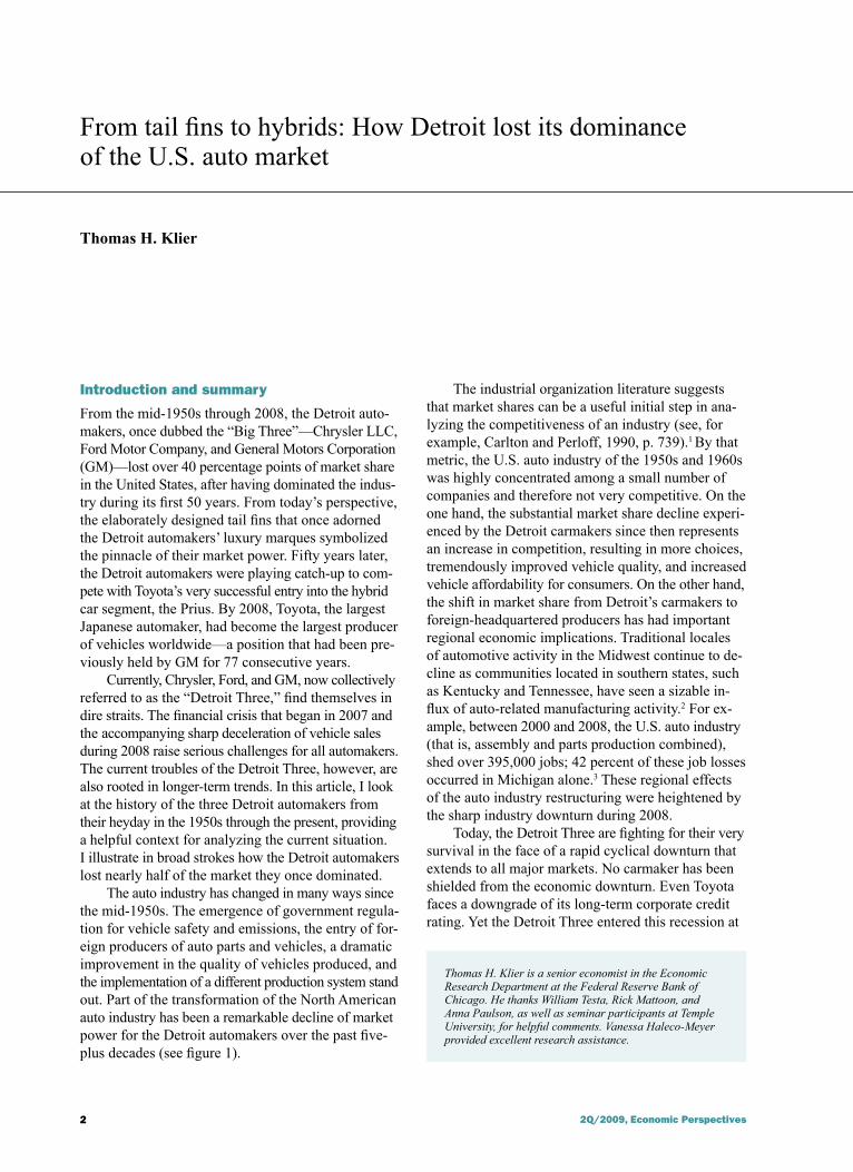
Introduction and summary
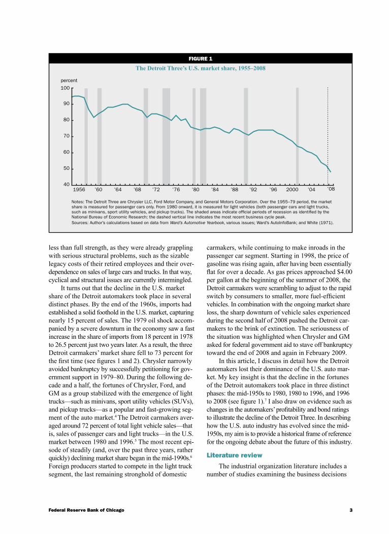
From the mid-1950s through 2008, the Detroit auto-makers, once dubbed the “Big Three”—Chrysler LLC, Ford Motor Company, and General Motors Corporation (GM)—lost over 40 percentage points of market share in the United States, after having dominated the indus-try during its first 50 years. From today’s perspective, the elaborately designed tail fins that once adorned the Detroit automakers’ luxury marques symbolized the pinnacle of their market power. Fifty years later, the Detroit automakers were playing catch-up to com-pete with Toyota’s very successful entry into the hybrid car segment, the Prius. By 2008, Toyota, the largest Japanese automaker, had become the largest producer of vehicles worldwide—a position that had been pre-viously held by GM for 77 consecutive years.
Currently, Chrysler, Ford, and GM, now collectively referred to as the “Detroit Three,” find themselves in dire straits. The financial crisis that began in 2007 and the accompanying sharp deceleration of vehicle sales during 2008 raise serious challenges for all automakers. The current troubles of the Detroit Three, however, are also rooted in longer-term trends. In this article, I look at the history of the three Detroit automakers from their heyday in the 1950s through the present, providing a helpful context for analyzing the current situation. I illustrate in broad strokes how the Detroit automakers lost nearly half of the market they once dominated.
The auto industry has changed in many ways since the mid-1950s. The emergence of government regula-tion for vehicle safety and emissions, the entry of for-eign producers of auto parts and vehicles, a dramatic improvement in the quality of vehicles produced, and the implementation of a different production system stand out. Part of the transformation of the North American auto industry has been a remarkable decline of market power for the Detroit automakers over the past five-plus decades (see figure 1).
The industrial organization literature suggests that market shares can be a useful initial step in ana-lyzing the competitiveness of an industry (see, for example, Carlton and Perloff, 1990, p. 739).1 By that metric, the U.S. auto industry of the 1950s and 1960s was highly concentrated among a small number of companies and therefore not very competitive. On the one hand, the substantial market share decline experi-enced by the Detroit carmakers since then represents an increase in competition, resulting in more choices, tremendously improved vehicle quality, and increased vehicle affordability for consumers. On the other hand, the shift in market share from Detroit’s carmakers to foreign-headquartered producers has had important regional economic implications. Traditional locales of automotive activity in the Midwest continue to de-cline as communities located in southern states, such as Kentucky and Tennessee, have seen a sizable in-flux of auto-related manufacturing activity.2 For ex-ample, between 2000 and 2008, the U.S. auto industry (that is, assembly and parts production combined), shed over 395,000 jobs; 42 percent of these job losses occurred in Michigan alone.3 These regional effects of the auto industry restructuring were heightened by the sharp industry downturn during 2008.
Today, the Detroit Three are fighting for their very survival in the face of a rapid cyclical downturn that extends to all major markets. No carmaker has been shielded from the economic downturn. Even Toyota faces a downgrade of its long-term corporate credit rating. Yet the Detroit Three entered this recession at
�Federal Reserve Bank of Chicago
less than full strength, as they were already grappling with serious structural problems, such as the sizable legacy costs of their retired employees and their over-dependence on sales of large cars and trucks. In that way, cyclical and structural issues are currently intermingled.
It turns out that the decline in the U.S. market share of the Detroit automakers took place in several distinct phases. By the end of the 1960s, imports had established a solid foothold in the U.S. market, capturing nearly 15 percent of sales. The 1979 oil shock accom-panied by a severe downturn in the economy saw a fast increase in the share of imports from 18 percent in 1978 to 26.5 percent just two years later. As a result, the three Detroit carmakers’ market share fell to 73 percent for the first time (see figures 1 and 2). Chrysler narrowly avoided bankruptcy by successfully petitioning for gov-ernment support in 1979–80. During the following de-cade and a half, the fortunes of Chrysler, Ford, and GM as a group stabilized with the emergence of light trucks—such as minivans, sport utility vehicles (SUVs), and pickup trucks—as a popular and fast-growing seg-ment of the auto market.4 The Detroit carmakers aver-aged around 72 percent of total light vehicle sales—that is, sales of passenger cars and light trucks—in the U.S. market between 1980 and 1996.5 The most recent epi-sode of steadily (and, over the past three years, rather quickly) declining market share began in the mid-1990s.6 Foreign producers started to compete in the light truck segment, the last remaining stronghold of domestic
carmakers, while continuing to make inroads in the passenger car segment. Starting in 1998, the price of gasoline was rising again, after having been essentially flat for over a decade. As gas prices approached $4.00 per gallon at the beginning of the summer of 2008, the Detroit carmakers were scrambling to adjust to the rapid switch by consumers to smaller, more fuel-efficient vehicles. In combination with the ongoing market share loss, the sharp downturn of vehicle sales experienced during the second half of 2008 pushed the Detroit car-makers to the brink of extinction. The seriousness of the situation was highlighted when Chrysler and GM asked for federal government aid to stave off bankruptcy toward the end of 2008 and again in February 2009.
In this article, I discuss in detail how the Detroit automakers lost their dominance of the U.S. auto mar-ket. My key insight is that the decline in the fortunes of the Detroit automakers took place in three distinct phases: the mid-1950s to 1980, 1980 to 1996, and 1996 to 2008 (see figure 1).7 I also draw on evidence such as changes in the automakers’ profitability and bond ratings to illustrate the decline of the Detroit Three. In describing how the U.S. auto industry has evolved since the mid-1950s, my aim is to provide a historical frame of reference for the ongoing debate about the future of this industry.
Literature review
The industrial organization literature includes a number of studies examining the business decisions
FIguRE 1
The Detroit Three’s U.S. market share, 1955–2008
Notes: The Detroit Three are Chrysler LLC, Ford Motor Company, and General Motors Corporation. Over the 1955–79 period, the market share is measured for passenger cars only. From 1980 onward, it is measured for light vehicles (both passenger cars and light trucks, such as minivans, sport utility vehicles, and pickup trucks). The shaded areas indicate official periods of recession as identified by the National Bureau of Economic Research; the dashed vertical line indicates the most recent business cycle peak.Sources: Author’s calculations based on data from Ward’s Automotive Yearbook, various issues; Ward’s AutoInfoBank; and White (1971).
40
50
60
70
80
90
100
1956 ’60 ’64 ’68 ’72 ’76 ’80 ’84 ’88 ’92 ’96 2000 ’04 ’08
percent
� �Q/�009, Economic Perspectives
of the Detroit automakers from 1945 through the early 1980s. White (1972) explains in great detail how for-eign carmakers first entered the U.S. market during the second half of the 1950s by offering small cars. Impor-tantly, according to a report by the National Academy of Engineering and National Research Council (1982), at that time small cars were just as expensive to pro-duce as large cars for the Detroit carmakers; as a result, the domestic automakers were not able to compete profitably with the foreign producers in this market segment. Kwoka (1984) argues that the concentration of market power among Chrysler, Ford, and GM during the 1950s and 1960s influenced their response to com-petition in the following decades. This concentration of market power, Kwoka (1984, p. 509) writes, “ren-dered the companies vulnerable to outside forces and ultimately induced responses that proved damaging to the entire U.S. industry.” Since the Detroit carmakers had such great market power back then, they were complacent and not quick to change their automo-biles to match their new competitors’ innovations and the public’s changing tastes during the 1970s. Writing in the mid-1980s, Kwoka (1984, p. 521) contends that, “there seems abundant reason for continuing concern over the long-run competitive properties of the U.S. auto industry.”
Related literature focuses on structural changes in the industry. Womack, Jones, and Roos (1990) document the arrival of lean manufacturing techniques and their implications for competition in the auto industry. Lean manufacturing is a production system pioneered in Japan. It emphasizes production quality, speedy response to market conditions, low levels of inventory, and frequent deliveries of parts (Klier, 1994). Baily et al. (2005) attempt to measure the contribution of lean manufacturing to productivity improvements in the auto industry.8 Rubenstein (1992) illustrates how the market for motor vehicles has become more fragmented as the number of sales per individual model has fallen. He goes on to show how that particular trend helped reconcentrate the geography of car pro-duction in North America. Helper and Sako (1995) highlight the growing role of automaker–supplier re-lations, especially as a source of competitive advantage for certain automakers. McAlinden (2004; 2007a, b) provides analysis of the relations between the Detroit automakers and their principal union, the United Auto Workers (UAW),9 as they grappled with the issue of legacy costs of their retirees early in the twenty-first century. McCarthy (2007) presents an environmental history of the automobile, highlighting the interplay of consumer preferences, government regulations, and the business interests of carmakers. Klier and Linn (2008)
estimate the demand for fuel efficiency by consumers and suggest that up to half of the market share decline of the Detroit carmakers between 2002 and 2007 can be attributed to the rising price of gasoline. Klier and McMillen (2008) analyze the evolving geography of the motor vehicle parts sector. They document the emergence of “auto alley,” a north–south corridor in which the industry is concentrated. Auto alley ex-tends from Detroit to the Gulf of Mexico, with fingers reaching into Ontario, Canada.
Furthermore, a number of popular business books document the struggles of the U.S. automakers over the past two decades (for example, Ingrassia and White, 1994; and Maynard, 2003). As I mentioned previously, my contribution to this vast and varied literature is to further detail how the Detroit automakers lost their dominance of the U.S. automobile market in three distinct phases: the mid-1950s to 1980, 1980 to 1996, and 1996 to 2008. In the subsequent sections, I discuss what happened in each of these phases.
From mid-1950s to 1980: Imports and oil prices challenge Detroit
The dominance of Chrysler, Ford, and GM in the U.S. automobile market peaked in 1955, when their market share reached 94.5 percent.10 The three com-panies continued to dominate the U.S. auto industry for many years, yet their collective influence slowly began to wane.
Imports first make inroadsWhile the three Detroit automakers had more
than once considered producing small cars since 1945, they regularly dismissed these plans as being unprof-itable. In addition, neither Chrysler, Ford, nor GM wanted to enter the market for small cars on its own. The Detroit automakers felt the market for small cars needed to be big enough to accommodate all three of them (White, 1972; and Kwoka, 1984). Gomez-Ibanez and Harrison (1982, pp. 319–320) suggest that, tradi-tionally, the U.S. carmakers had been insulated from international competition by catering to the domestic demand for larger and more luxurious cars than those made elsewhere. Higher per capita incomes, lower gaso-line prices, longer driving distances, and wider roads all accounted for the fact that vehicles purchased in the U.S. market tended to be larger than those in other mar-kets. Conversely, a foreign producer would be somewhat reluctant to produce a U.S.-style automobile that it could not sell in significant numbers in its home mar-ket. According to Gomez-Ibanez and Harrison (1982, p. 320), imported vehicles “thus were largely restricted to small cars (which could also be sold in the foreign
5Federal Reserve Bank of Chicago
producer’s home market) and sports or specialty cars (where economy of scale may be less important).”
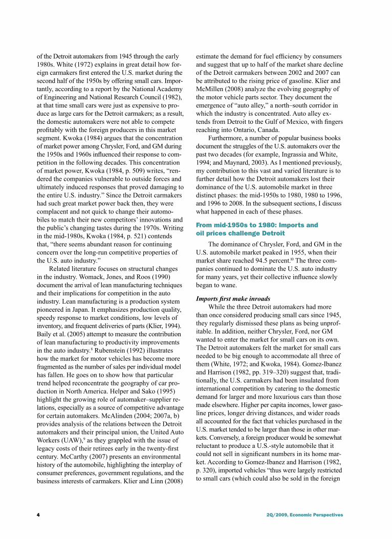
It took the independent American carmakers (at the time they were the Nash-Kelvinator Corporation, Kaiser-Frazer Corporation, Willys-Overland Motors, and Hudson Motor Car Company) to introduce small cars during 1950.11 However, as White (1972, p. 184) noted, “by setting prices that were above those of full-size sedans, the independents virtually eliminated any chances that their small cars might succeed.” Only a few years later, during the mid-1950s, small cars made their first significant appearance in the U.S. market by way of imports (figure 2). As the U.S. economy moved into recession during the second half of 1957, small, inexpensive European cars quickly became very suc-cessful in the American marketplace.12 According to McCarthy (2007, p. 142), “a substantial change in consumer preferences took place between 1955 and 1959.” Led by Germany’s Volkswagen (VW) Beetle, imports rose quickly during the second half of the 1950s, reaching 10.1 percent of the U.S. market in 1959. At the time, imports represented 75 percent to 80 percent of smaller economy cars in the United States (McCarthy, 2007, p. 144).
The Detroit automakers respondThe Detroit automakers responded by first import-
ing products from their European subsidiaries during 1957. In the fall of 1959, they introduced domestically produced compact cars in the U.S. market, such as the Chevrolet Corvair, the Ford Falcon, and the Plymouth Valiant. These vehicles were significantly smaller than
what Detroit carmakers had offered before. Their strategy of producing compact cars succeeded, quickly pushing back the level of imports—they fell to 4.9 percent of the U.S. market in 1962.
However, starting in the mid-1960s, the Detroit carmakers decided to make their compacts slightly larger. According to a report by the National Academy of Engineering and National Research Council (1982, p. 70), “the large domestic companies sought to fill a segment of the market just above the imports in terms of price and size.” These new models were produced in the United States and first introduced through the car companies’ middle-level brands. Within a few years, the Detroit automakers’ low-priced compacts started to grow in size and cost. Kwoka (1984, p. 517) notes the following: “By 1966, the Corvair had grown by 3.8 inches, the Falcon by 3.1 inches, and the Valiant by 4.6 inches. By the end of the 1960s, these vehicles would weigh from 250 to 600 pounds more than at introduction, and it was doubtful consumers perceived them as small cars any longer.” White (1972, p. 189) suggests that this response was prompted by the obser-vation that many consumers who bought small cars were willing to pay a premium for a deluxe interior and exterior trim. In effect the Detroit automakers grew their “small” vehicles in size after having beaten back the original entry of foreign small cars; as McCarthy (2007, p. 145) contends, “Detroit’s commitment to this market went no further than stemming the inroads of the imports.” It is not surprising that the victory over imported small cars proved to be only temporary.13
FIguRE �
Foreign brand import share of U.S. passenger car sales, 1955–80
Source: Author’s calculations based on data from Ward’s Automotive Yearbook, various issues.
percent
0
5
10
15
20
25
30
1955 ’56 ’57 ’58 ’59 ’60 ’61 ’62 ’63 ’64 ’65 ’66 ’67 ’68 ’69 ’70 ’71 ’72 ’73 ’74 ’75 ’76 ’77 ’78 ’79 ’80
� �Q/�009, Economic Perspectives
Déjà vu Continued preference for small cars among con-
sumers prompted a second wave of import growth, beginning in the mid-1960s.14 Spearheaded by VW’s success, import sales began to rise again, surpassing the previous record in 1968, when they had reached 10.8 percent of the U.S. market (see figure 2, p. 5). In response, the Detroit automakers again initially im-ported products from Europe (White, 1972). Only two years later, Detroit introduced the first U.S.-made sub-compacts: the GM Vega (in September 1970); the Ford Maverick (in April 1969) and Pinto (in September 1970); and the American Motors Corporation (AMC) Hornet (in August 1969) and Gremlin (in February 1970).15
This time the Detroit carmakers’ product strategy was not able to lower the import penetration of foreign nameplate products. By the early 1970s, import brands had become quite entrenched in the U.S. market. They had established stronger dealer networks as well as a solid reputation for quality among consumers (Kwoka 1984, p. 517; and National Academy of Engineering and National Research Council, 1982, pp. 72–73). Looking back at Detroit’s response to the two waves of imports, Kwoka (1984, p. 517) writes that “the domestic small cars did, however, manage to halt the growth of imports for about five years.” Unlike in the early 1960s, the imports did not get beaten back this time. The early 1970s also saw the Japanese nameplate imports out-sell those of VW, which had pioneered the segment of the small car import with its Beetle car in the 1950s.16
Around the same time, the safety of automobiles, especially that of the Detroit automakers’ products, re-ceived widespread attention as a result of Ralph Nader’s 1965 book, Unsafe at Any Speed: The Designed-In Dangers of the American Automobile. Nader (1965) detailed the reluctance of American car manufactur-ers to improve vehicle safety. In the wake of the en-suing public debate, the federal government for the first time established safety as well as environmental standards for motor vehicles—for example, mandating standards for bumpers in 1973 or requiring the instal-lation of equipment such as the catalytic converter (a device used to reduce the toxicity of emissions from an internal combustion engine) in 1975.
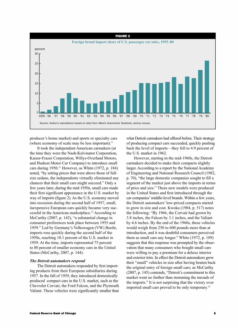
Similar to what the Detroit carmakers did with their compact cars introduced during the late 1950s, they grew their subcompacts launched during 1969 and 1970 in size and weight within a few years.17 In light of the two oil crises experienced during the 1970s, the timing of that decision was quite unfortunate. Be-tween October 1973 and May 1974, the real price of gasoline rose 28 percent. After flattening out, it increased again sharply during 1978 (figure 3). The market share of import brands started to grow again by the mid-1970s. It increased quite rapidly toward the end of the decade, breaking 25 percent for the first time in 1980 (figure 2, p. 5).
Consumers respondConsumers quickly responded to the rapid in-
crease in the price of gasoline following the Iran oil
FIguRE �
U.S. retail gasoline prices, 1970–2008
Notes: Real dollar values are in 2000 dollars. The shaded areas indicate official periods of recession as identified by the National Bureau of Economic Research; the dashed vertical line indicates the most recent business cycle peak.Sources: Author’s calculations based on data from the U.S. Department of Energy, Energy Information Administration; and White (1971).
dollars per gallon
0
0.5
1.0
1.5
2.0
2.5
3.0
3.5
1970 ’72 ’74 ’76 ’78 ’80 ’82 ’84 ’86 ’88 ’90 ’92 ’94 ’96 ’98 2000 ’02 ’04 ’06 ’08
Real
Nominal
�Federal Reserve Bank of Chicago
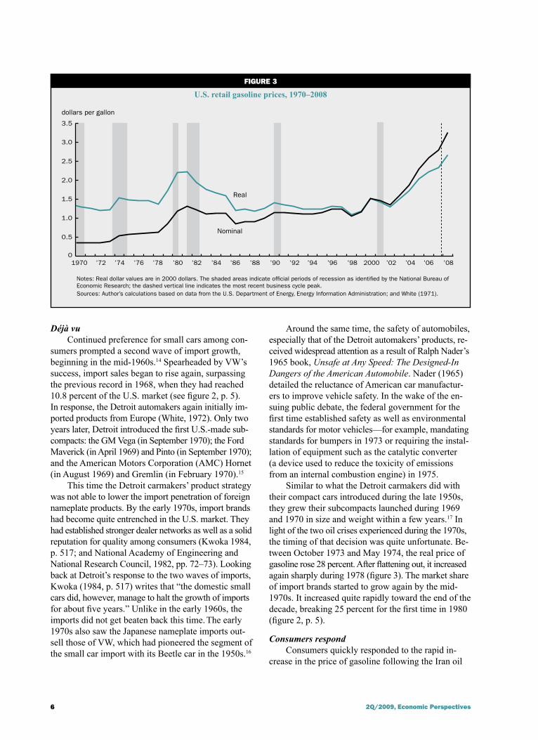
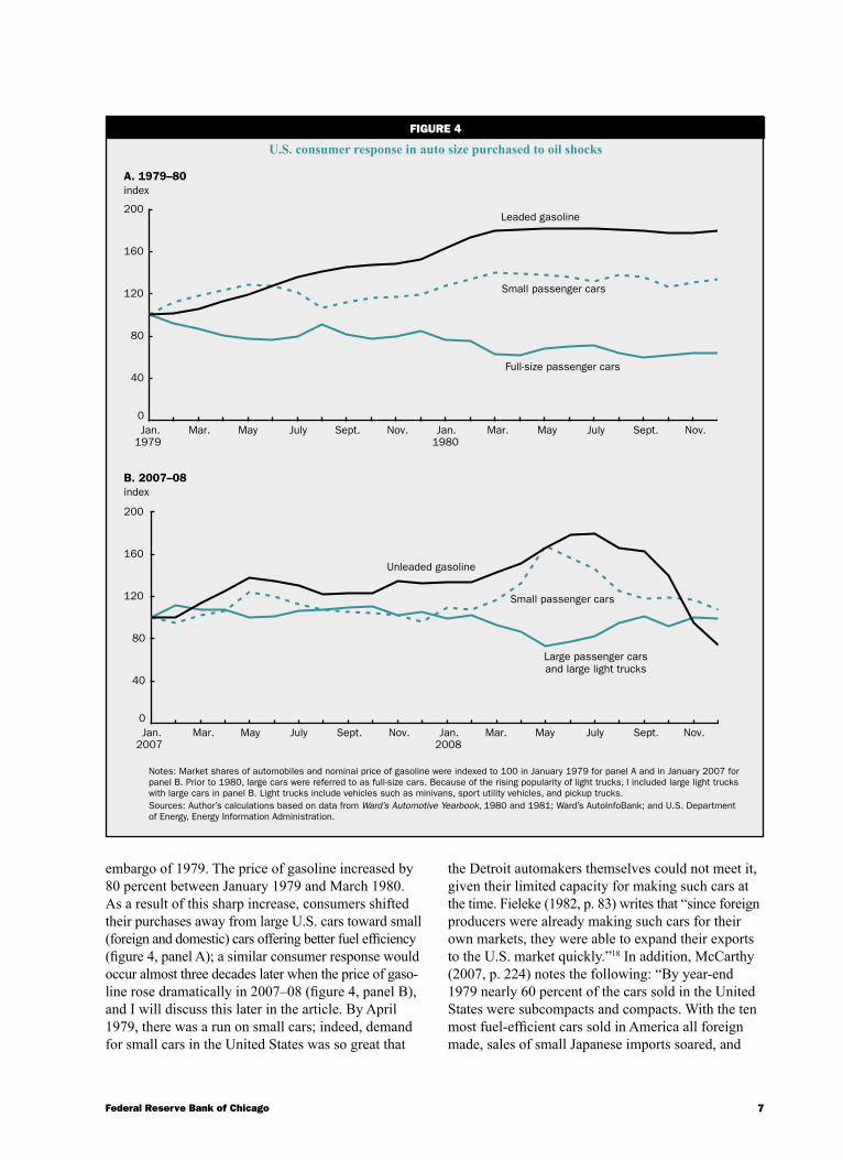
embargo of 1979. The price of gasoline increased by 80 percent between January 1979 and March 1980. As a result of this sharp increase, consumers shifted their purchases away from large U.S. cars toward small (foreign and domestic) cars offering better fuel efficiency (figure 4, panel A); a similar consumer response would occur almost three decades later when the price of gaso-line rose dramatically in 2007–08 (figure 4, panel B), and I will discuss this later in the article. By April 1979, there was a run on small cars; indeed, demand for small cars in the United States was so great that
the Detroit automakers themselves could not meet it, given their limited capacity for making such cars at the time. Fieleke (1982, p. 83) writes that “since foreign producers were already making such cars for their own markets, they were able to expand their exports to the U.S. market quickly.”18 In addition, McCarthy (2007, p. 224) notes the following: “By year-end 1979 nearly 60 percent of the cars sold in the United States were subcompacts and compacts. With the ten most fuel-efficient cars sold in America all foreign made, sales of small Japanese imports soared, and
4 FIguRE �
U.S. consumer response in auto size purchased to oil shocks
A. 1979–80index
Small passenger cars
0
40
80
120
160
200
Jan. Mar. May July Sept. Nov. Mar. May July Sept. Nov.Jan.1979 1980
B. 2007–08index
0
40
80
120
160
200
Jan. Mar. May July Sept. Nov. Mar. May July Sept. Nov.Jan.2007 2008
Notes: Market shares of automobiles and nominal price of gasoline were indexed to 100 in January 1979 for panel A and in January 2007 for panel B. Prior to 1980, large cars were referred to as full-size cars. Because of the rising popularity of light trucks, I included large light trucks with large cars in panel B. Light trucks include vehicles such as minivans, sport utility vehicles, and pickup trucks.Sources: Author’s calculations based on data from Ward’s Automotive Yearbook, 1980 and 1981; Ward’s AutoInfoBank; and U.S. Department of Energy, Energy Information Administration.
Leaded gasoline
Full-size passenger cars
Small passenger cars
Unleaded gasoline
Large passenger cars and large light trucks
8 �Q/�009, Economic Perspectives
foreign sales—70 percent of them by Japanese makers—approached the 25 percent market-share barrier for the first time.”
Foreign cars sold well in the United States not only because they offered better fuel efficiency, but also be-cause they were competitively priced and widely per-ceived to be of superior quality (Fieleke, 1982, p. 88). By the end of the 1970s, the Japanese automakers dominated the domestic producers in product quality ratings for every auto market segment, representing a formidable competitive advantage (National Academy of Engineering and National Research Council, 1982, p. 99). The quality gap between U.S.-produced cars and foreign cars was beyond dispute (Kwoka, 1984, p. 518).
Regulatory responseThe energy crisis subsequent to the 1973 Arab oil
embargo turned fuel economy into an important auto-mobile policy goal for the U.S. government (McCarthy, 2007, p. 217). In 1975, Congress imposed mandatory corporate average fuel economy (CAFE) standards for the first time. The standards were to become effec-tive by model year 1978 and result in an average fuel efficiency of passenger cars of 27.5 miles per gallon by 1985. To check for compliance, the U.S. Environmental Protection Agency was to test the vehicles in a lab and continues to do so today.
According to the CAFE requirements, for a given model year each manufacturer’s vehicles for sale in the United States are divided into three fleets: domestic passenger cars, foreign-produced passenger cars, and light trucks. Passenger cars were subject to a stricter fuel efficiency standard than light trucks.19 The origi-nal justification for establishing a different and more lenient fuel efficiency standard for light trucks was their primary usage as commercial and agricultural vehicles (Cooney and Yacobucci, 2005, p. 87). Subse-quently, the existence of two different standards has affected the ways in which new vehicles are designed (and classified).20
To sum up, by the early 1980s, foreign competi-tors had successfully challenged Chrysler, Ford, and GM in their home market, irrevocably changing the industry. Differences in product mix and product quality were key to the success of foreign carmakers. “The huge increase in the price of gasoline from 1979 to 1980 sharply exacerbated a long-run deterioration in the competitive position of the U.S. [auto] industry,” notes Fieleke (1982, p. 91). The auto sector, along with the rest of the economy, was pummeled by a severe recession; unit sales of motor vehicles fell by 18 per-cent from 1979 to 1980. Caught between competition from rising imports and a deteriorating economy, the
three Detroit automakers were reeling. Chrysler, on the verge of financial collapse, applied for federal loan guarantees in 1979 and received them in the amount of $1.5 billion in 1980 (Cooney and Yacobucci, 2005, p. 55). Ford and the UAW sought relief from the in-creased number of vehicle imports by filing a trade safeguard case in 1980. That request was denied by the U.S. International Trade Commission, which determined that imports were not the major cause of the industry’s troubles. Subsequently, a bill was proposed in 1981 that would have enacted quotas on motor vehicle imports from Japan. Following a suggestion by the Reagan administration, Japan instead agreed to impose a so-called voluntary export restraint, or VER.21
A National Academy of Engineering and National Research Council (1982, p. 4) report sums up the changes that had occurred in the U.S. auto industry during the 1970s and early 1980s as follows: “Com-petition in the U.S. auto industry has undergone fun-damental changes in the last 10 years, primarily because of increased market penetration by foreign manufac-turers and drastic shifts in the price of oil.”22
From 1980 to 199�: Detroit stages a comeback
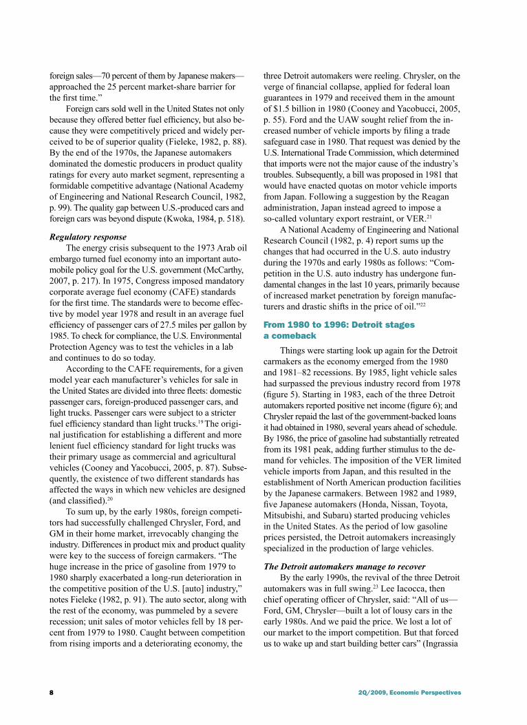
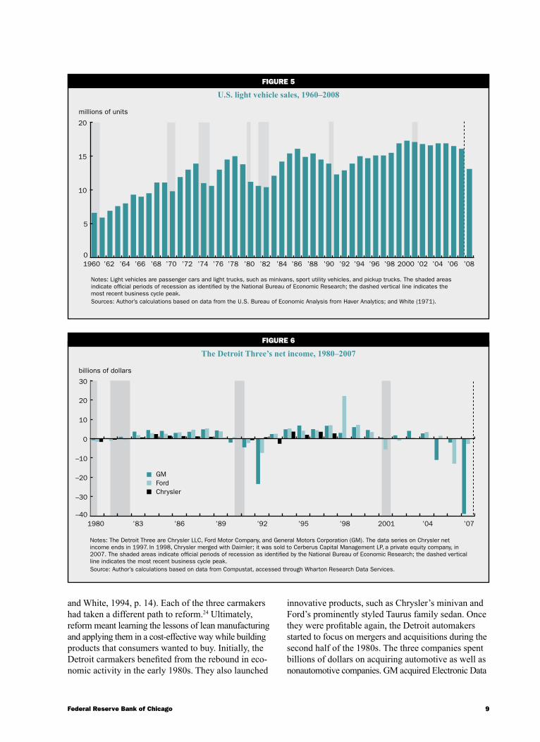
Things were starting look up again for the Detroit carmakers as the economy emerged from the 1980 and 1981–82 recessions. By 1985, light vehicle sales had surpassed the previous industry record from 1978 (figure 5). Starting in 1983, each of the three Detroit automakers reported positive net income (figure 6); and Chrysler repaid the last of the government-backed loans it had obtained in 1980, several years ahead of schedule. By 1986, the price of gasoline had substantially retreated from its 1981 peak, adding further stimulus to the de-mand for vehicles. The imposition of the VER limited vehicle imports from Japan, and this resulted in the establishment of North American production facilities by the Japanese carmakers. Between 1982 and 1989, five Japanese automakers (Honda, Nissan, Toyota, Mitsubishi, and Subaru) started producing vehicles in the United States. As the period of low gasoline prices persisted, the Detroit automakers increasingly specialized in the production of large vehicles.
The Detroit automakers manage to recoverBy the early 1990s, the revival of the three Detroit
automakers was in full swing.23 Lee Iacocca, then chief operating officer of Chrysler, said: “All of us—Ford, GM, Chrysler—built a lot of lousy cars in the early 1980s. And we paid the price. We lost a lot of our market to the import competition. But that forced us to wake up and start building better cars” (Ingrassia
9Federal Reserve Bank of Chicago
and White, 1994, p. 14). Each of the three carmakers had taken a different path to reform.24 Ultimately, reform meant learning the lessons of lean manufacturing and applying them in a cost-effective way while building products that consumers wanted to buy. Initially, the Detroit carmakers benefited from the rebound in eco-nomic activity in the early 1980s. They also launched
innovative products, such as Chrysler’s minivan and Ford’s prominently styled Taurus family sedan. Once they were profitable again, the Detroit automakers started to focus on mergers and acquisitions during the second half of the 1980s. The three companies spent billions of dollars on acquiring automotive as well as nonautomotive companies. GM acquired Electronic Data
FIguRE 5
U.S. light vehicle sales, 1960–2008
Notes: Light vehicles are passenger cars and light trucks, such as minivans, sport utility vehicles, and pickup trucks. The shaded areas indicate official periods of recession as identified by the National Bureau of Economic Research; the dashed vertical line indicates the most recent business cycle peak. Sources: Author’s calculations based on data from the U.S. Bureau of Economic Analysis from Haver Analytics; and White (1971).
millions of units
0
5
10
15
20
1960 ’72 ’74 ’76 ’78 ’80 ’82 ’84 ’86 ’88 ’90 ’92 ’94 ’96 ’98 2000 ’02 ’04 ’06 ’08’62 ’64 ’66 ’68 ’70
FIguRE �
The Detroit Three’s net income, 1980–2007
Notes: The Detroit Three are Chrysler LLC, Ford Motor Company, and General Motors Corporation (GM). The data series on Chrysler net income ends in 1997. In 1998, Chrysler merged with Daimler; it was sold to Cerberus Capital Management LP , a private equity company, in 2007. The shaded areas indicate official periods of recession as identified by the National Bureau of Economic Research; the dashed vertical line indicates the most recent business cycle peak.Source: Author’s calculations based on data from Compustat, accessed through Wharton Research Data Services.
billions of dollars
1980 ’83 ’86 ’89 ’92 ’95 ’98 2001 ’04 ’07–40
–30
–20
–10
0
10
20
30
GMFordChrysler
10 2Q/2009, Economic Perspectives
Systems (EDS) in 1984, as well as Hughes Aircraft in 1985. Chrysler bought Gulfstream in 1985 and AMC in 1987. All three automakers acquired major stakes in car rental companies during the late 1980s. Ford bought Jaguar in 1990, and GM acquired a majority of Saab in the same year. However, most of these transactions were unwound within a decade, and with the exception of the AMC acquisition,25 the car com-panies then acquired have since either been sold or are currently for sale. In any case, the acquisitions took up valuable time and attention of the companies’ management back then. And so the recovery of the three Detroit carmakers took twists and turns along the way. It also involved changes in top management and leadership. GM is a case in point.
During the early 1980s, GM’s leadership decided the best way to beat the foreign-based competition was to automate the production of automobiles when-ever possible with the help of sophisticated technology. As a result, the company invested heavily in new capital equipment. It turned out to be a costly experiment, since it raised GM’s cost structure to the point that its North American auto business was barely breaking even during the late 1980s—a time of very strong industry
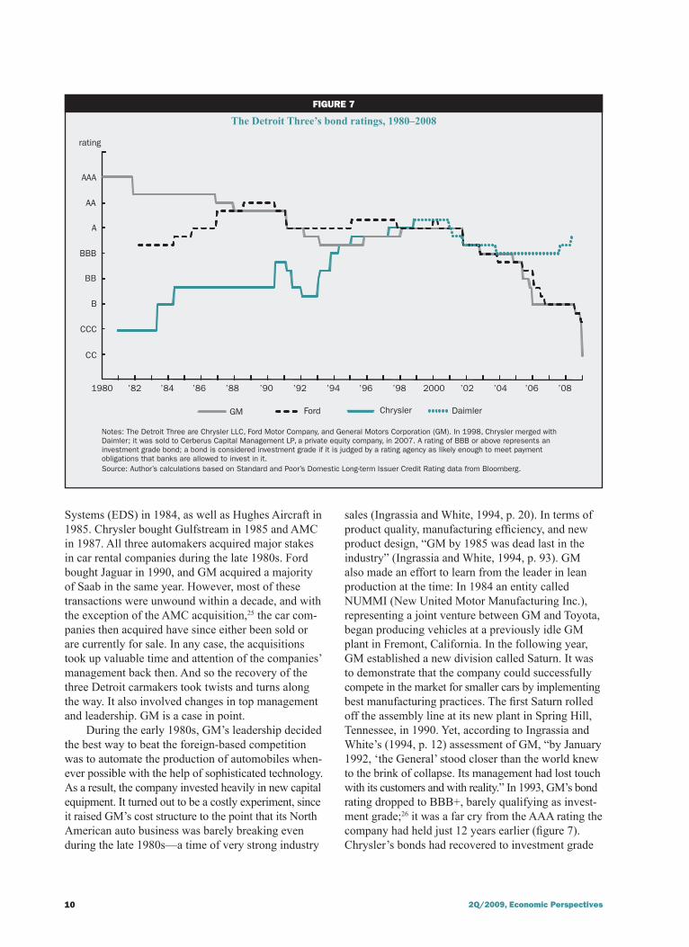
sales (Ingrassia and White, 1994, p. 20). In terms of product quality, manufacturing efficiency, and new product design, “GM by 1985 was dead last in the industry” (Ingrassia and White, 1994, p. 93). GM also made an effort to learn from the leader in lean production at the time: In 1984 an entity called NUMMI (New United Motor Manufacturing Inc.), representing a joint venture between GM and Toyota, began producing vehicles at a previously idle GM plant in Fremont, California. In the following year, GM established a new division called Saturn. It was to demonstrate that the company could successfully compete in the market for smaller cars by implementing best manufacturing practices. The first Saturn rolled off the assembly line at its new plant in Spring Hill, Tennessee, in 1990. Yet, according to Ingrassia and White’s (1994, p. 12) assessment of GM, “by January 1992, ‘the General’ stood closer than the world knew to the brink of collapse. Its management had lost touch with its customers and with reality.” In 1993, GM’s bond rating dropped to BBB+, barely qualifying as invest-ment grade;26 it was a far cry from the AAA rating the company had held just 12 years earlier (figure 7). Chrysler’s bonds had recovered to investment grade
figurE 7
The Detroit Three’s bond ratings, 1980–2008
Notes: The Detroit Three are Chrysler LLC, Ford Motor Company, and General Motors Corporation (GM). In 1998, Chrysler merged with Daimler; it was sold to Cerberus Capital Management LP , a private equity company, in 2007. A rating of BBB or above represents an investment grade bond; a bond is considered investment grade if it is judged by a rating agency as likely enough to meet payment obligations that banks are allowed to invest in it.Source: Author’s calculations based on Standard and Poor’s Domestic Long-term Issuer Credit Rating data from Bloomberg.
rating
AAA
AA
A
BBB
BB
B
CCC
CC
1980 ’02’98 2000 ’04 ’06 ’08’88 ’90 ’92 ’94 ’96’82 ’84 ’86
GM Ford Chrysler Daimler
11Federal Reserve Bank of Chicago
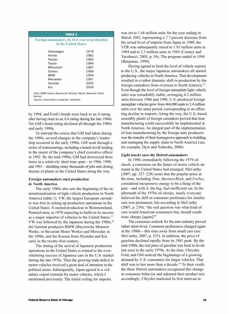
TaBLE 1
Foreign automakers, by first year of production in the United States
Volkswagen 1978 Honda 1982 Nissan 1983 Toyota 1984 Mitsubishi 1987 Subaru 1989 BMW 1994 Mercedes 1997 Hyundai 2005 Kia 2009
Note: BMW means Bayerische Motoren Werke (Bavarian Motor Works).Source: Automobile companies’ websites.
by 1994, and Ford’s bonds were back to an A rating after having risen to an AA rating during the late 1980s. Yet GM’s bond rating declined all through the 1980s and early 1990s.
To unwind the course that GM had taken during the 1980s, several changes in the company’s leader-ship occurred in the early 1990s. GM went through a series of restructurings, including a board revolt leading to the ouster of the company’s chief executive officer in 1992. By the mid-1990s, GM had downsized three times in a relatively short time span—in 1986, 1990, and 1991—shedding many thousands of jobs and closing dozens of plants in the United States along the way.
Foreign automakers start production in North America
The early 1980s also saw the beginning of the in-ternationalization of light vehicle production in North America (table 1). VW, the largest European carmak-er was first in setting up production operations in the United States. It started production in Westmoreland, Pennsylvania, in 1978 expecting to build on its success as a major importer of vehicles to the United States.27
VW was followed by the Japanese during the 1980s,28 the German producers BMW (Bayerische Motoren Werke, or Bavarian Motor Works) and Mercedes in the 1990s, and the Korean firms Hyundai and Kia early in the twenty-first century.
The timing of the arrival of Japanese production operations in the United States is related to the over-whelming success of Japanese cars in the U.S. market during the late 1970s. Then the growing trade deficit in motor vehicles received a great deal of attention in the political arena. Subsequently, Japan agreed to a vol-untary export restraint for motor vehicles, which I mentioned previously. The initial ceiling for imports
was set to 1.68 million units for the year ending in March 1982, representing a 7.7 percent decrease from the actual level of imports from Japan in 1980; the VER was subsequently raised to 1.83 million units in 1984 and to 2.3 million units in 1985 (Cooney and Yacobucci, 2005, p. 56). The program ended in 1994 (Benjamin, 1999).
Having agreed to limit the level of vehicle exports to the U.S., the major Japanese automakers all started producing vehicles in North America. That development resulted in a rather dramatic shift in production by the foreign carmakers from overseas to North America.29 Even though the level of foreign nameplate light vehicle sales was remarkably stable, averaging 4.2 million units between 1986 and 1996, U.S.-produced foreign nameplate vehicles grew from 466,000 units to 2.4 million units over the same period, corresponding to an offset-ting decline in imports. Along the way, the U.S.-based assembly plants of foreign carmakers proved that lean manufacturing could successfully be implemented in North America. An integral part of the implementation of lean manufacturing by the foreign auto producers was the transfer of their homegrown approach to building and managing the supply chain to North America (see, for example, Dyer and Nobeoka, 2000).
Light trucks save the Detroit automakers In 1980, immediately following the 1979 oil
shock, a consensus on the future of motor vehicle de-mand in the United States had emerged. McCarthy (2007, pp. 227–228) notes that the popular press at the time, including Time, BusinessWeek, and Forbes, considered inexpensive energy to be a thing of the past—and with it, the big, fuel-inefficient car. In the aftermath of the 1970s oil shocks, nearly everyone believed the shift in consumer preference for smaller cars was permanent, but according to McCarthy (2007, p. 230), “the real question was what kind of cars would American consumers buy should condi-tions change [again]?”
The consensus outlook for the auto industry proved rather short-lived. Consumer preferences changed again in the 1980s—this time away from small cars (see McCarthy, 2007, p. 235). In addition, the price of gasoline declined rapidly from its 1981 peak. By the mid-1980s, the real price of gasoline was back to levels last seen in the early 1970s. At the time, Chrysler, Ford, and GM noticed the beginnings of a growing demand by U.S. consumers for larger vehicles. That shift was to last more than a decade.30 To their credit, the three Detroit automakers recognized this change in consumer behavior and adjusted their product mix accordingly. Chrysler marketed its first minivan in
1� �Q/�009, Economic Perspectives
1983. Ford launched the Explorer, an SUV, in 1990; that year Ford produced more light trucks than cars at its U.S. assembly plants (Cooney and Yacobucci, 2005, p. 27). Light trucks turned out to be very profitable for the Detroit automakers. Foreign producers faced a 25 percent tariff on imported pickup trucks; yet they continued to focus on the production of cars in their North American plants.
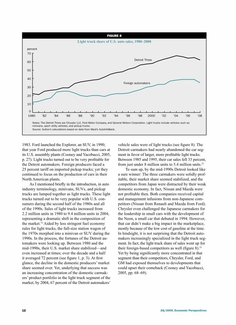
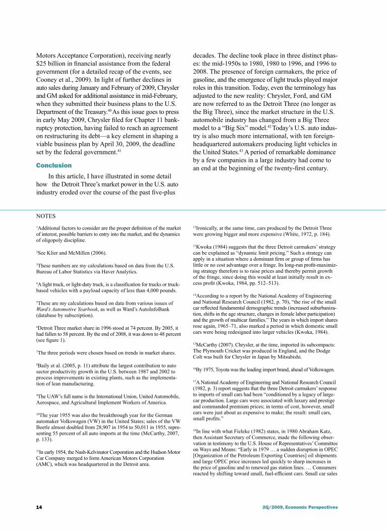
As I mentioned briefly in the introduction, in auto industry terminology, minivans, SUVs, and pickup trucks are lumped together as light trucks. These light trucks turned out to be very popular with U.S. con-sumers during the second half of the 1980s and all of the 1990s. Sales of light trucks increased from 2.2 million units in 1980 to 9.4 million units in 2004, representing a dramatic shift in the composition of the market.31 Aided by less stringent fuel economy rules for light trucks, the full-size station wagon of the 1970s morphed into a minivan or SUV during the 1990s. In the process, the fortunes of the Detroit au-tomakers were looking up. Between 1980 and the mid-1990s, their U.S. market share stabilized—and even increased at times; over the decade and a half it averaged 72 percent (see figure 1, p. 3). At first glance, the decline in the domestic producers’ market share seemed over. Yet, underlying that success was an increasing concentration of the domestic carmak-ers’ product portfolio in the light truck segment of the market; by 2004, 67 percent of the Detroit automakers’
vehicle sales were of light trucks (see figure 8). The Detroit carmakers had nearly abandoned the car seg-ment in favor of larger, more profitable light trucks. Between 1985 and 1995, their car sales fell 33 percent, from just under 8 million units to 5.4 million units.32
To sum up, by the mid-1990s Detroit looked like a sure winner: The three carmakers were solidly prof-itable, their market share seemed stabilized, and the competitors from Japan were distracted by their weak domestic economy. In fact, Nissan and Mazda were not profitable then. Both companies received capital and management infusions from non-Japanese com-petitors (Nissan from Renault and Mazda from Ford). Chrysler even challenged the Japanese carmakers for the leadership in small cars with the development of the Neon, a small car that debuted in 1994. However, that car didn’t make a big impact in the marketplace, mostly because of the low cost of gasoline at the time. In hindsight, it is not surprising that the Detroit auto-makers increasingly specialized in the light truck seg-ment. In fact, the light truck share of sales went up for their foreign-based competitors as well (figure 8).33 Yet by being significantly more concentrated in that segment than their competitors, Chrysler, Ford, and GM had exposed themselves to developments that could upset their comeback (Cooney and Yacobucci, 2005, pp. 68–69).
FIguRE 8
Light truck share of U.S. auto sales, 1980–2008
Notes: The Detroit Three are Chrysler LLC, Ford Motor Company, and General Motors Corporation. Light trucks include vehicles such as minivans, sport utility vehicles, and pickup trucks.Source: Author’s calculations based on data from Ward’s AutoInfoBank.
percent
1980 ’82 ’84 ’86 ’88 ’90 ’92 ’94 ’96 ’98 2000 ’02 ’04 ’06 ’080
10
20
30
40
50
60
70
Foreign automakers
Detroit Three
1�Federal Reserve Bank of Chicago
From 199� to �008: Detroit on the defensive—again
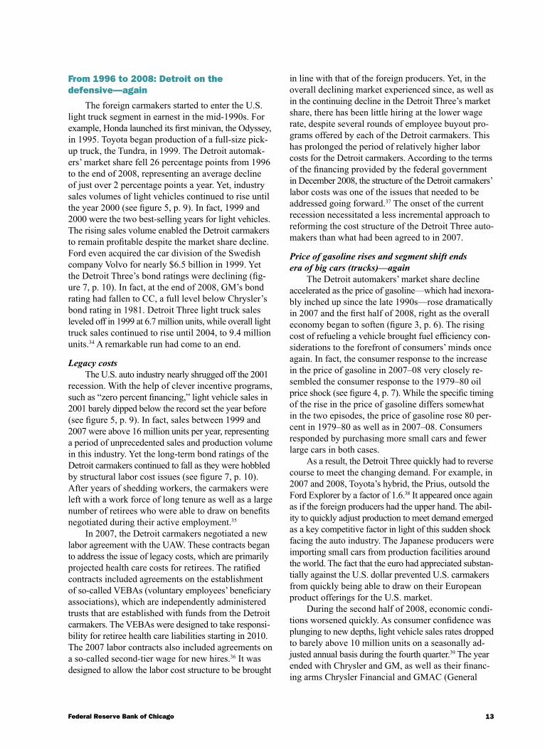
The foreign carmakers started to enter the U.S. light truck segment in earnest in the mid-1990s. For example, Honda launched its first minivan, the Odyssey, in 1995. Toyota began production of a full-size pick-up truck, the Tundra, in 1999. The Detroit automak-ers’ market share fell 26 percentage points from 1996 to the end of 2008, representing an average decline of just over 2 percentage points a year. Yet, industry sales volumes of light vehicles continued to rise until the year 2000 (see figure 5, p. 9). In fact, 1999 and 2000 were the two best-selling years for light vehicles. The rising sales volume enabled the Detroit carmakers to remain profitable despite the market share decline. Ford even acquired the car division of the Swedish company Volvo for nearly $6.5 billion in 1999. Yet the Detroit Three’s bond ratings were declining (fig-ure 7, p. 10). In fact, at the end of 2008, GM’s bond rating had fallen to CC, a full level below Chrysler’s bond rating in 1981. Detroit Three light truck sales leveled off in 1999 at 6.7 million units, while overall light truck sales continued to rise until 2004, to 9.4 million units.34 A remarkable run had come to an end.
Legacy costsThe U.S. auto industry nearly shrugged off the 2001
recession. With the help of clever incentive programs, such as “zero percent financing,” light vehicle sales in 2001 barely dipped below the record set the year before (see figure 5, p. 9). In fact, sales between 1999 and 2007 were above 16 million units per year, representing a period of unprecedented sales and production volume in this industry. Yet the long-term bond ratings of the Detroit carmakers continued to fall as they were hobbled by structural labor cost issues (see figure 7, p. 10). After years of shedding workers, the carmakers were left with a work force of long tenure as well as a large number of retirees who were able to draw on benefits negotiated during their active employment.35
In 2007, the Detroit carmakers negotiated a new labor agreement with the UAW. These contracts began to address the issue of legacy costs, which are primarily projected health care costs for retirees. The ratified contracts included agreements on the establishment of so-called VEBAs (voluntary employees’ beneficiary associations), which are independently administered trusts that are established with funds from the Detroit carmakers. The VEBAs were designed to take responsi-bility for retiree health care liabilities starting in 2010. The 2007 labor contracts also included agreements on a so-called second-tier wage for new hires.36 It was designed to allow the labor cost structure to be brought
in line with that of the foreign producers. Yet, in the overall declining market experienced since, as well as in the continuing decline in the Detroit Three’s market share, there has been little hiring at the lower wage rate, despite several rounds of employee buyout pro-grams offered by each of the Detroit carmakers. This has prolonged the period of relatively higher labor costs for the Detroit carmakers. According to the terms of the financing provided by the federal government in December 2008, the structure of the Detroit carmakers’ labor costs was one of the issues that needed to be addressed going forward.37 The onset of the current recession necessitated a less incremental approach to reforming the cost structure of the Detroit Three auto-makers than what had been agreed to in 2007.
Price of gasoline rises and segment shift ends era of big cars (trucks)—again
The Detroit automakers’ market share decline accelerated as the price of gasoline—which had inexora-bly inched up since the late 1990s—rose dramatically in 2007 and the first half of 2008, right as the overall economy began to soften (figure 3, p. 6). The rising cost of refueling a vehicle brought fuel efficiency con-siderations to the forefront of consumers’ minds once again. In fact, the consumer response to the increase in the price of gasoline in 2007–08 very closely re-sembled the consumer response to the 1979–80 oil price shock (see figure 4, p. 7). While the specific timing of the rise in the price of gasoline differs somewhat in the two episodes, the price of gasoline rose 80 per-cent in 1979–80 as well as in 2007–08. Consumers responded by purchasing more small cars and fewer large cars in both cases.
As a result, the Detroit Three quickly had to reverse course to meet the changing demand. For example, in 2007 and 2008, Toyota’s hybrid, the Prius, outsold the Ford Explorer by a factor of 1.6.38 It appeared once again as if the foreign producers had the upper hand. The abil-ity to quickly adjust production to meet demand emerged as a key competitive factor in light of this sudden shock facing the auto industry. The Japanese producers were importing small cars from production facilities around the world. The fact that the euro had appreciated substan-tially against the U.S. dollar prevented U.S. carmakers from quickly being able to draw on their European product offerings for the U.S. market.
During the second half of 2008, economic condi-tions worsened quickly. As consumer confidence was plunging to new depths, light vehicle sales rates dropped to barely above 10 million units on a seasonally ad-justed annual basis during the fourth quarter.39 The year ended with Chrysler and GM, as well as their financ-ing arms Chrysler Financial and GMAC (General
1� �Q/�009, Economic Perspectives
NOTES
Motors Acceptance Corporation), receiving nearly $25 billion in financial assistance from the federal government (for a detailed recap of the events, see Cooney et al., 2009). In light of further declines in auto sales during January and February of 2009, Chrysler and GM asked for additional assistance in mid-February, when they submitted their business plans to the U.S. Department of the Treasury.40 As this issue goes to press in early May 2009, Chrysler filed for Chapter 11 bank-ruptcy protection, having failed to reach an agreement on restructuring its debt—a key element in shaping a viable business plan by April 30, 2009, the deadline set by the federal government.41
Conclusion
In this article, I have illustrated in some detail how the Detroit Three’s market power in the U.S. auto industry eroded over the course of the past five-plus
1Additional factors to consider are the proper definition of the market of interest, possible barriers to entry into the market, and the dynamics of oligopoly discipline.
2See Klier and McMillen (2006).
3These numbers are my calculations based on data from the U.S. Bureau of Labor Statistics via Haver Analytics.
4A light truck, or light-duty truck, is a classification for trucks or truck-based vehicles with a payload capacity of less than 4,000 pounds.
5These are my calculations based on data from various issues of Ward’s Automotive Yearbook, as well as Ward’s AutoInfoBank (database by subscription).
6Detroit Three market share in 1996 stood at 74 percent. By 2005, it had fallen to 58 percent. By the end of 2008, it was down to 48 percent (see figure 1).
7The three periods were chosen based on trends in market shares.
8Baily et al. (2005, p. 11) attribute the largest contribution to auto sector productivity growth in the U.S. between 1987 and 2002 to process improvements in existing plants, such as the implementa-tion of lean manufacturing.
9The UAW’s full name is the International Union, United Automobile, Aerospace, and Agricultural Implement Workers of America.
10The year 1955 was also the breakthrough year for the German automaker Volkswagen (VW) in the United States; sales of the VW Beetle almost doubled from 28,907 in 1954 to 50,011 in 1955, repre-senting 55 percent of all auto imports at the time (McCarthy, 2007, p. 133).
11In early 1954, the Nash-Kelvinator Corporation and the Hudson Motor Car Company merged to form American Motors Corporation (AMC), which was headquartered in the Detroit area.
decades. The decline took place in three distinct phas-es: the mid-1950s to 1980, 1980 to 1996, and 1996 to 2008. The presence of foreign carmakers, the price of gasoline, and the emergence of light trucks played major roles in this transition. Today, even the terminology has adjusted to the new reality: Chrysler, Ford, and GM are now referred to as the Detroit Three (no longer as the Big Three), since the market structure in the U.S. automobile industry has changed from a Big Three model to a “Big Six” model.42 Today’s U.S. auto indus-try is also much more international, with ten foreign-headquartered automakers producing light vehicles in the United States.43 A period of remarkable dominance by a few companies in a large industry had come to an end at the beginning of the twenty-first century.
12Ironically, at the same time, cars produced by the Detroit Three were growing bigger and more expensive (White, 1972, p. 184).
13Kwoka (1984) suggests that the three Detroit carmakers’ strategy can be explained as “dynamic limit pricing.” Such a strategy can apply in a situation where a dominant firm or group of firms has little or no cost advantage over a fringe. Its long-run profit-maximiz-ing strategy therefore is to raise prices and thereby permit growth of the fringe, since doing this would at least initially result in ex-cess profit (Kwoka, 1984, pp. 512–513).
14According to a report by the National Academy of Engineering and National Research Council (1982, p. 70), “the rise of the small car reflected fundamental demographic trends (increased suburbaniza-tion, shifts in the age structure, changes in female labor participation) and the growth of multicar families.” The years in which import shares rose again, 1965–71, also marked a period in which domestic small cars were being redesigned into larger vehicles (Kwoka, 1984).
15McCarthy (2007). Chrysler, at the time, imported its subcompacts: The Plymouth Cricket was produced in England, and the Dodge Colt was built for Chrysler in Japan by Mitsubishi.
16By 1975, Toyota was the leading import brand, ahead of Volkswagen.
17A National Academy of Engineering and National Research Council (1982, p. 3) report suggests that the three Detroit carmakers’ response to imports of small cars had been “conditioned by a legacy of large-car production. Large cars were associated with luxury and prestige and commanded premium prices; in terms of cost, however, small cars were just about as expensive to make; the result: small cars, small profits.”
18In line with what Fieleke (1982) states, in 1980 Abraham Katz, then Assistant Secretary of Commerce, made the following obser-vation in testimony to the U.S. House of Representatives’ Committee on Ways and Means: “Early in 1979 … a sudden disruption in OPEC [Organization of the Petroleum Exporting Countries] oil shipments and large OPEC price increases led quickly to sharp increases in the price of gasoline and to renewed gas station lines. … Consumers reacted by shifting toward small, fuel-efficient cars. Small car sales
15Federal Reserve Bank of Chicago
32In 2002, foreign nameplate cars outsold domestic nameplate cars for the first time. By 2008, domestic nameplates represented only 35 percent of all U.S. auto sales. See note 31 for source.
33For example, early in the twenty-first century, Toyota built an assembly plant in San Antonio, Texas, that was dedicated to the production of the Tundra, its full-size pickup truck.
34These numbers are from Ward’s AutoInfoBank.
35See Cooney (2005) for a comparison of the steel and auto industries with regard to legacy costs. McAlinden (2007b) calculates the health care costs for active and retired employees per vehicle produced in 2005 to amount to $1,268 for GM and $945 for Ford.
36All entry hires’ base wages were set to range between $11.50 and $16.23 per hour, nearly half of the hourly base wage according to the existing pay scale (McAlinden, 2007a).
37On March 11, 2009, Ford announced that it had reached an agree-ment with the UAW on labor cost savings amounting to $500 million annually. According to the new agreement, Ford’s compensation (including benefits, pensions, and bonuses) will be $55 per hour; that compares with $48 per hour paid by foreign automakers pro-ducing in the United States (Bennett and Terlep, 2009).
38This number is my calculation based on data from Ward’s AutoInfoBank.
39Ibid.
40On March 30, 2009, the Obama administration announced it had found the business plans submitted by Chrysler and GM to be not viable. The administration extended the original deadline of March 31, 2009, for the two automakers to demonstrate their future viability—by 30 days for Chrysler and by 60 days for GM. Both companies were required to draw up more aggressive restruc-turing plans by their new respective deadlines. Until then, Chrysler and GM would be provided with working capital if needed. The administration’s assessment stated that, absent more drastic re-structuring, the two carmakers’ “best chance of success may well require utilizing the bankruptcy court in a quick and surgical way.” See www.whitehouse.gov/assets/documents/Fact_Sheet_GM_Chrysler_FIN.pdf.
41For more details on Chrysler entering bankruptcy, see www.whitehouse.gov/the_press_office/Obama-Administration-Auto- Restructuring-Initiative/.
42The Big Six consist of Chrysler, Ford, GM, Honda, Nissan, and Toyota.
43Despite the increase in the number of companies selling vehicles in the United States, the share of vehicles produced in North America since 1980 has remained remarkably stable at approximately 80 percent, according to my calculations using data from Ward’s AutoInfoBank.
jumped to a 57 percent share of the market in 1979. U.S. small car production ran virtually at capacity, but was unable to keep up with demand. With an inadequate supply of domestic small cars, many con-sumers turned to imports, the traditional source of small, fuel-efficient cars. Their present success in the United States is a case of being in the right place at the right time with the right product” (Katz, 1980).
19For cars, the standard stands at 27.5 miles per gallon for model year 2009; for light trucks, the standard is set at 23.1 miles per gallon for model year 2009 (Yacobucci, 2009).
20A set of stricter fuel efficiency regulations, CAFE II, was passed by Congress in December 2007. It established a new fleet average fuel efficiency standard of 35 miles per gallon by the model year 2020. While CAFE II will likely impose significant costs to meet compliance, it is not clear how individual carmakers will be affected, since the rules for implementing the new law have not been released yet (Yacobucci and Bamberger, 2008, p. 1).
21See Cooney and Yacobucci (2005, p. 56).
22Incidentally, increased foreign competition influenced the decision by the Federal Trade Commission to end its five-year antitrust investigation of automobile manufacturing in the United States (Fieleke, 1982, p. 89).
23This section draws on Ingrassia and White (1994).
24See Ingrassia and White (1994) for a wealth of examples describing the three companies’ travails during the 1980s.
25The Jeep brand is all that survived into the twenty-first century from what was once AMC.
26A bond is considered investment grade if it is judged by a rating agency as likely enough to meet payment obligations that banks are allowed to invest in it.
27These expectations were not borne out as VW closed that plant in 1989. The company recently announced its return to the United States as a producer. It will build a new assembly operation in Chattanooga, Tennessee, to begin production by 2010.
28Honda started producing cars in central Ohio in 1982. In 1989, its family sedan, the Honda Accord, became the best-selling car in the United States.
29According to my analysis using data from Ward’s AutoInfoBank, foreign nameplate vehicles represented 6 percent of U.S. production in 1985; 13 percent in 1990; 22 percent in 2000; and 41 percent in 2008.
30The groundswell of interest in sport utility vehicles began in 1983 (McCarthy, 2007, p. 233).
31By 1990, the share of light trucks among light vehicle sales had risen to 35 percent, according to my analysis using data from Ward’s AutoInfoBank. Between 2001 and 2008, light truck sales represented more than half the market.
1� �Q/�009, Economic Perspectives
Baily, Martin Neil, Diana Farrell, Ezra Greenberg, Jan-Dirk Henrich, Naoko Jinjo, Maya Jolles, and Jaana Remes, 2005, Increasing Global Competition and Labor Productivity: Lessons from the U.S. Automotive Industry, McKinsey Global Institute, report, November.
Benjamin, Daniel K., 1999, “Voluntary export re-straints on automobiles,” PERC Reports, Property and Environment Research Center, Vol .17, No. 3, September, pp. 16–17, available at www.perc.org/ articles/article416.php.
Bennett, Jeff, and Sharon Terlep, 2009, “Ford pact to even out labor costs with Toyota’s,” Wall Street Journal, March 12, available at http://online.wsj.com/article/SB123677910696394787.html, accessed on March 17, 2009.
Carlton, Dennis W., and Jeffrey M. Perloff, 1990, Modern Industrial Organization, New York: Harper Collins.
Cooney, Stephen, 2005, “Comparing automotive and steel industry legacy cost issues,” CRS Report for Congress, Congressional Research Service, No. RL33169, November 28.
Cooney, Stephen, James M. Bickley, Hinda Chaikind, Carol A. Pettit, Patrick Purcell, Carol Rapaport, and Gary Shorter, 2009, “U.S. motor vehicle industry: Federal financial assistance and restructuring,” CRS Report for Congress, Congressional Research Service, No. R40003, March 31.
Cooney, Stephen, and Brent D. Yacobucci, 2005, “U.S. automotive industry: Policy overview and re-cent history,” CRS Report for Congress, Congressional Research Service, No. RL32883, April 25.
Dyer, Jeffrey H., and Kentaro Nobeoka, 2000, “Creating and managing a high-performance knowl-edge-sharing network: The Toyota case,” Strategic Management Journal, Vol. 21, No. 3, March, pp. 345–367.
Fieleke, Norman S., 1982, “The automobile industry,” ANNALS of the American Academy of Political and Social Science, Vol. 460, No. 1, March, pp. 83–91.
Gomez-Ibanez, Jose A., and David Harrison, Jr., 1982, “Imports and the future of the U.S. automobile industry,” American Economic Review, Vol. 72, No. 2, May, pp. 319–323.
Helper, Susan, and Mari Sako, 1995, “Supplier rela-tions in Japan and the United States: Are they con-verging?,” Sloan Management Review, Vol. 36, No. 3, pp. 77–84.
Ingrassia, Paul, and Joseph B. White, 1994, Comeback: The Fall and Rise of the American Automobile Industry, New York: Simon and Schuster.
Katz, Abraham, 1980, statement of Assistant Secretary of Commerce for International Economic Policy before the Subcommittee on Trade, Committee on Ways and Means, U.S. House of Representatives, Washington, DC, March 18, quoted in National Academy of Engineering and National Research Council (1982, p. 12).
Klier, Thomas H., 1994, “The impact of lean manufacturing on sourcing relationships,” Economic Perspectives, Federal Reserve Bank of Chicago, Vol. 18, No. 4, July/August, pp. 8–18.
Klier, Thomas H., and Joshua Linn, 2008, “The price of gasoline and the demand for fuel efficiency: Evidence from monthly new vehicles sales data,” University of Illinois at Chicago, mimeo, September.
Klier, Thomas H., and Daniel P. McMillen, 2008, “Evolving agglomeration in the U.S. auto supplier in-dustry,” Journal of Regional Science, Vol. 48, No. 1, pp. 245–267.
__________, 2006, “The geographic evolution of the U.S. auto industry,” Economic Perspectives, Federal Reserve Bank of Chicago, Vol. 30, No. 2, Second Quarter, pp. 2–13.
Kwoka, John E., Jr., 1984, “Market power and market change in the U.S. automobile industry,” Journal of Industrial Economics, Vol. 32, No. 4, June, pp. 509–522.
Maynard, Micheline, 2003, The End of Detroit: How the Big Three Lost Their Grip on the American Car Market, New York: Doubleday.
McAlinden, Sean P., 2007a, “Initial thoughts on the 2007 GM/UAW labor agreement,” Center for Automotive Research, presentation, October 12.
__________, 2007b, “The big leave: The future of automotive labor relations,” presentation at the Center for Automotive Research breakfast briefing, Ypsilanti, MI, February 20.
REFERENCES
1�Federal Reserve Bank of Chicago
__________, 2004, “The meaning of the 2003 UAW–automotive pattern agreement,” Center for Automotive Research, report, June, available at www.cargroup.org/pdfs/LaborPaperFinal.pdf, accessed on October 15, 2007.
McCarthy, Tom, 2007, Auto Mania: Cars, Consumers, and the Environment, New Haven, CT: Yale University Press.
Nader, Ralph, 1965, Unsafe at Any Speed: The Designed-In Dangers of the American Automobile, New York: Grossman Publishers.
National Academy of Engineering, Committee on Technology and International Economic and Trade Issues of the Office of the Foreign Secretary, Auto-mobile Panel; and National Research Council, Commission on Engineering and Technical Systems, 1982, The Competitive Status of the U.S. Auto Industry: A Study of the Influences of Technology in Determining International Industrial Competitive Advantage, Washington, DC: National Academy Press.
Rubenstein, James M., 1992, The Changing U.S. Auto Industry: A Geographical Analysis, New York: Routledge.
White, Lawrence J., 1972, “The American automo-bile industry and the small car, 1945–70,” Journal of Industrial Economics, Vol. 20, No. 2, April, pp. 179–192.
__________, 1971, The Automobile Industry since 1945, Cambridge, MA: Harvard University Press.
Womack, James P., Daniel T. Jones, and Daniel Roos, 1990, The Machine that Changed the World, New York: Rawson Associates.
Yacobucci, Brent D., 2009, email message to Thomas H. Klier, March 23.
Yacobucci, Brent D., and Robert Bamberger, 2008, “Automobile and light truck fuel economy: The CAFE standards,” CRS Report for Congress, Congressional Research Service, No. RL33413, May 7.
18 2Q/2009, Economic Perspectives
Comparing patterns of default among prime and subprime mortgages
Gene Amromin and Anna L. Paulson
Gene Amromin is a senior financial economist in the Financial Markets Group and Anna L. Paulson is a senior financial economist in the Economic Research Department at the Federal Reserve Bank of Chicago. The authors are grateful to Leslie McGranahan for very helpful feedback and to Edward Zhong and Arpit Gupta for excellent research assistance.
Introduction and summary
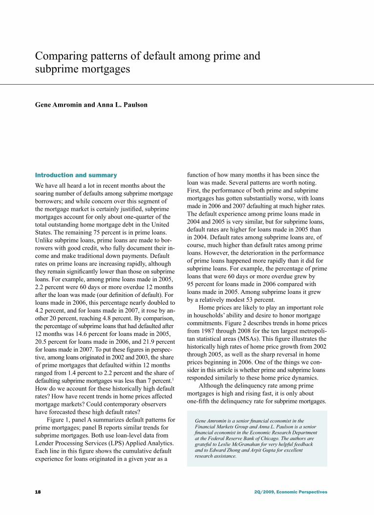
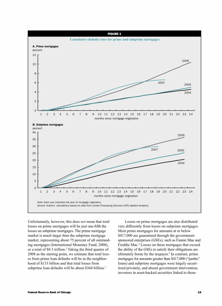
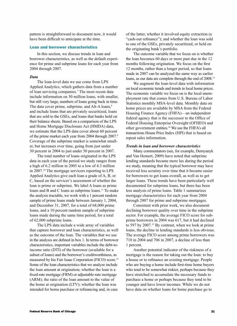
We have all heard a lot in recent months about the soaring number of defaults among subprime mortgage borrowers; and while concern over this segment of the mortgage market is certainly justified, subprime mortgages account for only about one-quarter of the total outstanding home mortgage debt in the United States. The remaining 75 percent is in prime loans. Unlike subprime loans, prime loans are made to bor-rowers with good credit, who fully document their in-come and make traditional down payments. Default rates on prime loans are increasing rapidly, although they remain significantly lower than those on subprime loans. For example, among prime loans made in 2005, 2.2 percent were 60 days or more overdue 12 months after the loan was made (our definition of default). For loans made in 2006, this percentage nearly doubled to 4.2 percent, and for loans made in 2007, it rose by an-other 20 percent, reaching 4.8 percent. By comparison, the percentage of subprime loans that had defaulted after 12 months was 14.6 percent for loans made in 2005, 20.5 percent for loans made in 2006, and 21.9 percent for loans made in 2007. To put these figures in perspec-tive, among loans originated in 2002 and 2003, the share of prime mortgages that defaulted within 12 months ranged from 1.4 percent to 2.2 percent and the share of defaulting subprime mortgages was less than 7 percent.1 How do we account for these historically high default rates? How have recent trends in home prices affected mortgage markets? Could contemporary observers have forecasted these high default rates?
Figure 1, panel A summarizes default patterns for prime mortgages; panel B reports similar trends for subprime mortgages. Both use loan-level data from Lender Processing Services (LPS) Applied Analytics. Each line in this figure shows the cumulative default experience for loans originated in a given year as a
function of how many months it has been since the loan was made. Several patterns are worth noting. First, the performance of both prime and subprime mortgages has gotten substantially worse, with loans made in 2006 and 2007 defaulting at much higher rates. The default experience among prime loans made in 2004 and 2005 is very similar, but for subprime loans, default rates are higher for loans made in 2005 than in 2004. Default rates among subprime loans are, of course, much higher than default rates among prime loans. However, the deterioration in the performance of prime loans happened more rapidly than it did for subprime loans. For example, the percentage of prime loans that were 60 days or more overdue grew by 95 percent for loans made in 2006 compared with loans made in 2005. Among subprime loans it grew by a relatively modest 53 percent.
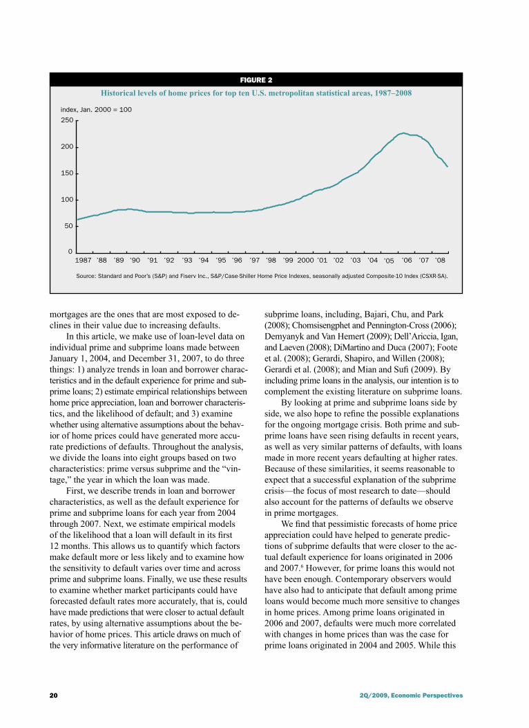
Home prices are likely to play an important role in households’ ability and desire to honor mortgage commitments. Figure 2 describes trends in home prices from 1987 through 2008 for the ten largest metropoli-tan statistical areas (MSAs). This figure illustrates the historically high rates of home price growth from 2002 through 2005, as well as the sharp reversal in home prices beginning in 2006. One of the things we con-sider in this article is whether prime and subprime loans responded similarly to these home price dynamics.
Although the delinquency rate among prime mortgages is high and rising fast, it is only about one-fifth the delinquency rate for subprime mortgages.
19Federal Reserve Bank of Chicago
Unfortunately, however, this does not mean that total losses on prime mortgages will be just one-fifth the losses on subprime mortgages. The prime mortgage market is much larger than the subprime mortgage market, representing about 75 percent of all outstand-ing mortgages (International Monetary Fund, 2008), or a total of $8.3 trillion.2 Taking the third quarter of 2008 as the starting point, we estimate that total loss-es from prime loan defaults will be in the neighbor-hood of $133 billion and that total losses from subprime loan defaults will be about $364 billion.3
Losses on prime mortgages are also distributed very differently from losses on subprime mortgages. Most prime mortgages for amounts at or below $417,000 are guaranteed through the government-sponsored enterprises (GSEs), such as Fannie Mae and Freddie Mac.4 Losses on these mortgages that exceed the ability of the GSEs to satisfy their obligations are ultimately borne by the taxpayer.5 In contrast, prime mortgages for amounts greater than $417,000 (“jumbo” loans) and subprime mortgages were largely securi-tized privately, and absent government intervention, investors in asset-backed securities linked to those
4 FIguRE 1
Cumulative default rates for prime and subprime mortgages
A. Prime mortgagespercent
B. Subprime mortgagespercent
Note: Each year indicates the year of mortgage origination.Source: Authors’ calculations based on data from Lender Processing Services (LPS) Applied Analytics.
1 2 3 4 5 6 7 8 9 10 11 12 13 14 15 16 17 18 19 20 21 22 23 240
2
4
6
8
10
12
1 2 3 4 5 6 7 8 9 10 11 12 13 14 15 16 17 18 19 20 21 22 23 240
5
10
15
20
25
30
35
40
2006
20052007
2004
20052007
2004
2006
months since mortgage origination
months since mortgage origination
20 2Q/2009, Economic Perspectives
mortgages are the ones that are most exposed to de-clines in their value due to increasing defaults.
In this article, we make use of loan-level data on individual prime and subprime loans made between January 1, 2004, and December 31, 2007, to do three things: 1) analyze trends in loan and borrower charac-teristics and in the default experience for prime and sub-prime loans; 2) estimate empirical relationships between home price appreciation, loan and borrower characteris-tics, and the likelihood of default; and 3) examine whether using alternative assumptions about the behav-ior of home prices could have generated more accu-rate predictions of defaults. Throughout the analysis, we divide the loans into eight groups based on two characteristics: prime versus subprime and the “vin-tage,” the year in which the loan was made.
First, we describe trends in loan and borrower characteristics, as well as the default experience for prime and subprime loans for each year from 2004 through 2007. Next, we estimate empirical models of the likelihood that a loan will default in its first 12 months. This allows us to quantify which factors make default more or less likely and to examine how the sensitivity to default varies over time and across prime and subprime loans. Finally, we use these results to examine whether market participants could have forecasted default rates more accurately, that is, could have made predictions that were closer to actual default rates, by using alternative assumptions about the be-havior of home prices. This article draws on much of the very informative literature on the performance of
subprime loans, including, Bajari, Chu, and Park (2008); Chomsisengphet and Pennington-Cross (2006); Demyanyk and Van Hemert (2009); Dell’Ariccia, Igan, and Laeven (2008); DiMartino and Duca (2007); Foote et al. (2008); Gerardi, Shapiro, and Willen (2008); Gerardi et al. (2008); and Mian and Sufi (2009). By including prime loans in the analysis, our intention is to complement the existing literature on subprime loans.
By looking at prime and subprime loans side by side, we also hope to refine the possible explanations for the ongoing mortgage crisis. Both prime and sub-prime loans have seen rising defaults in recent years, as well as very similar patterns of defaults, with loans made in more recent years defaulting at higher rates. Because of these similarities, it seems reasonable to expect that a successful explanation of the subprime crisis—the focus of most research to date—should also account for the patterns of defaults we observe in prime mortgages.
We find that pessimistic forecasts of home price appreciation could have helped to generate predic-tions of subprime defaults that were closer to the ac-tual default experience for loans originated in 2006 and 2007.6 However, for prime loans this would not have been enough. Contemporary observers would have also had to anticipate that default among prime loans would become much more sensitive to changes in home prices. Among prime loans originated in 2006 and 2007, defaults were much more correlated with changes in home prices than was the case for prime loans originated in 2004 and 2005. While this
FIguRE 2
Historical levels of home prices for top ten U.S. metropolitan statistical areas, 1987–2008
Source: Standard and Poor’s (S&P) and Fiserv Inc., S&P/Case-Shiller Home Price Indexes, seasonally adjusted Composite-10 Index (CSXR-SA).
index, Jan. 2000 = 100
0
50
100
150
200
250
1987 ’88 ’89 ’90 ’91 ’92 ’93 ’94 ’95 ’96 ’97 ’98 ’99 2000 ’01 ’02 ’03 ’04 ’05 ’06 ’07 ’08
21Federal Reserve Bank of Chicago
pattern is straightforward to document now, it would have been difficult to anticipate at the time.
Loan and borrower characteristics
In this section, we discuss trends in loan and borrower characteristics, as well as the default experi-ence for prime and subprime loans for each year from 2004 through 2007.
DataThe loan-level data we use come from LPS
Applied Analytics, which gathers data from a number of loan servicing companies.7 The most recent data include information on 30 million loans, with smaller, but still very large, numbers of loans going back in time. The data cover prime, subprime, and Alt-A loans,8 and include loans that are privately securitized, loans that are sold to the GSEs, and loans that banks hold on their balance sheets. Based on a comparison of the LPS and Home Mortgage Disclosure Act (HMDA) data, we estimate that the LPS data cover about 60 percent of the prime market each year from 2004 through 2007.9 Coverage of the subprime market is somewhat small-er, but increases over time, going from just under 30 percent in 2004 to just under 50 percent in 2007.
The total number of loans originated in the LPS data in each year of the period we study ranges from a high of 6.2 million in 2005 to a low of 4.3 million in 2007.10 The mortgage servicers reporting to LPS Applied Analytics give each loan a grade of A, B, or C, based on the servicer’s assessment of whether the loan is prime or subprime. We label A loans as prime loans and B and C loans as subprime loans.11 To make the analysis tractable, we work with a 1 percent random sample of prime loans made between January 1, 2004, and December 31, 2007, for a total of 68,000 prime loans, and a 10 percent random sample of subprime loans made during the same time period, for a total of 62,000 subprime loans.
The LPS data include a wide array of variables that capture borrower and loan characteristics, as well as the outcome of the loan. The variables that we use in the analysis are defined in box 1. In terms of borrower characteristics, important variables include the debt-to-income ratio (DTI) of the borrower (available for a subset of loans) and the borrower’s creditworthiness, as measured by his Fair Isaac Corporation (FICO) score.12 Some of the loan characteristics that we analyze include the loan amount at origination; whether the loan is a fixed-rate mortgage (FRM) or adjustable-rate mortgage (ARM); the ratio of the loan amount to the value of the home at origination (LTV); whether the loan was intended for home purchase or refinancing and, in case
of the latter, whether it involved equity extraction (a “cash-out refinance”); and whether the loan was sold to one of the GSEs, privately securitized, or held on the originating bank’s portfolio.
The outcome variable that we focus on is whether the loan becomes 60 days or more past due in the 12 months following origination. We focus on the first 12 months, rather than a longer period, so that loans made in 2007 can be analyzed the same way as earlier loans, as our data are complete through the end of 2008.13
We augment the loan-level data with information on local economic trends and trends in local home prices. The economic variable we focus on is the local unem-ployment rate that comes from U.S. Bureau of Labor Statistics monthly MSA-level data. Monthly data on home prices are available by MSA from the Federal Housing Finance Agency (FHFA)—an independent federal agency that is the successor to the Office of Federal Housing Enterprise Oversight (OFHEO) and other government entities.14 We use the FHFA’s all transactions House Price Index (HPI) that is based on repeat sales information.
Trends in loan and borrower characteristicsMany commentators (see, for example, Demyanyk
and Van Hemert, 2009) have noted that subprime lending standards became more lax during the period we study, meaning that the typical borrower may have received less scrutiny over time that it became easier for borrowers to get loans overall, as well as to get larger loans. These trends have been particularly well documented for subprime loans, but there has been less analysis of prime loans. Table 1 summarizes mortgage characteristics for each year from 2004 through 2007 for prime and subprime mortgages.
Consistent with prior work, we also document declining borrower quality over time in the subprime sector. For example, the average FICO score for sub-prime borrowers in 2004 was 617, but it had declined to 597 by 2007.15 By contrast, when we look at prime loans, the decline in lending standards is less obvious. The average FICO score among prime borrowers was 710 in 2004 and 706 in 2007, a decline of less than 1 percent.
Another potential indicator of the riskiness of a mortgage is the reason for taking out the loan: to buy a house or to refinance an existing mortgage. People who are buying a home include first-time home buyers who tend to be somewhat riskier, perhaps because they have stretched to accumulate the necessary funds to purchase a home or perhaps because they tend to be younger and have lower incomes. While we do not have data on whether loans for home purchase go to
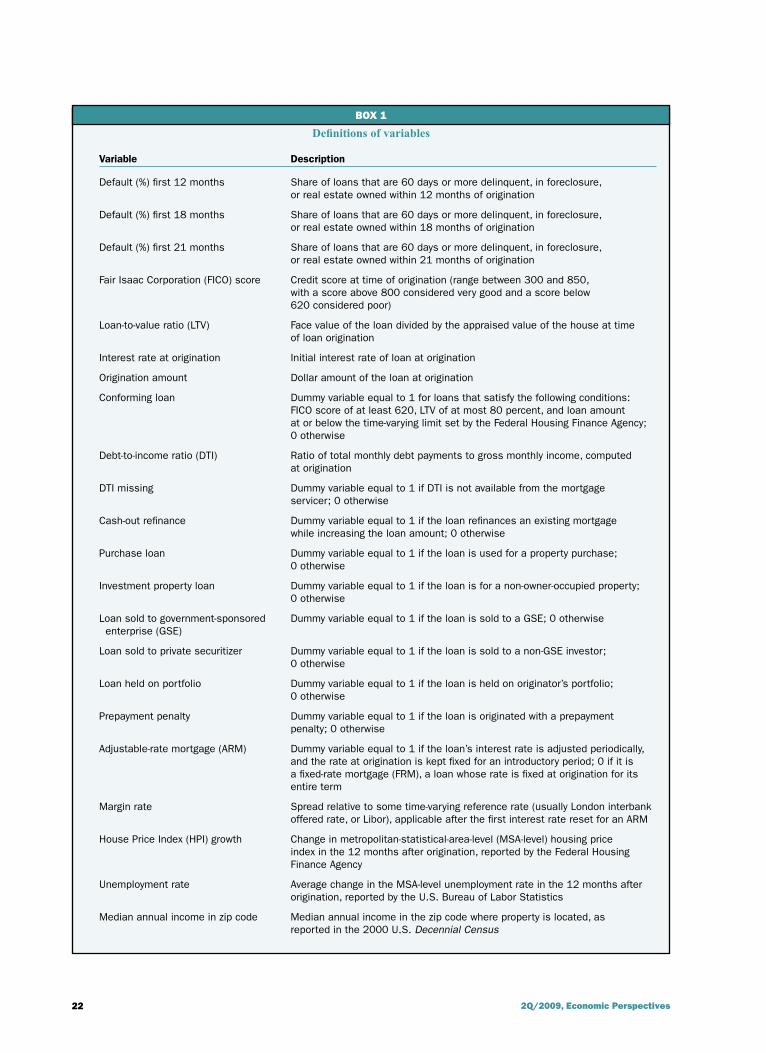
22 2Q/2009, Economic Perspectives
BOX 1
Definitions of variables
Variable Description
Default (%) first 12 months Share of loans that are 60 days or more delinquent, in foreclosure, or real estate owned within 12 months of origination
Default (%) first 18 months Share of loans that are 60 days or more delinquent, in foreclosure, or real estate owned within 18 months of origination
Default (%) first 21 months Share of loans that are 60 days or more delinquent, in foreclosure, or real estate owned within 21 months of origination
Fair Isaac Corporation (FICO) score Credit score at time of origination (range between 300 and 850, with a score above 800 considered very good and a score below 620 considered poor)
Loan-to-value ratio (LTV) Face value of the loan divided by the appraised value of the house at time of loan origination
Interest rate at origination Initial interest rate of loan at origination
Origination amount Dollar amount of the loan at origination
Conforming loan Dummy variable equal to 1 for loans that satisfy the following conditions: FICO score of at least 620, LTV of at most 80 percent, and loan amount at or below the time-varying limit set by the Federal Housing Finance Agency; 0 otherwise
Debt-to-income ratio (DTI) Ratio of total monthly debt payments to gross monthly income, computed at origination
DTI missing Dummy variable equal to 1 if DTI is not available from the mortgage servicer; 0 otherwise
Cash-out refinance Dummy variable equal to 1 if the loan refinances an existing mortgage while increasing the loan amount; 0 otherwise
Purchase loan Dummy variable equal to 1 if the loan is used for a property purchase; 0 otherwise
Investment property loan Dummy variable equal to 1 if the loan is for a non-owner-occupied property; 0 otherwise
Loan sold to government-sponsored Dummy variable equal to 1 if the loan is sold to a GSE; 0 otherwise enterprise (GSE)
Loan sold to private securitizer Dummy variable equal to 1 if the loan is sold to a non-GSE investor; 0 otherwise
Loan held on portfolio Dummy variable equal to 1 if the loan is held on originator’s portfolio; 0 otherwise
Prepayment penalty Dummy variable equal to 1 if the loan is originated with a prepayment penalty; 0 otherwise
Adjustable-rate mortgage (ARM) Dummy variable equal to 1 if the loan’s interest rate is adjusted periodically, and the rate at origination is kept fixed for an introductory period; 0 if it is a fixed-rate mortgage (FRM), a loan whose rate is fixed at origination for its entire term
Margin rate Spread relative to some time-varying reference rate (usually London interbank offered rate, or Libor), applicable after the first interest rate reset for an ARM
House Price Index (HPI) growth Change in metropolitan-statistical-area-level (MSA-level) housing price index in the 12 months after origination, reported by the Federal Housing Finance Agency
Unemployment rate Average change in the MSA-level unemployment rate in the 12 months after origination, reported by the U.S. Bureau of Labor Statistics
Median annual income in zip code Median annual income in the zip code where property is located, as reported in the 2000 U.S. Decennial Census
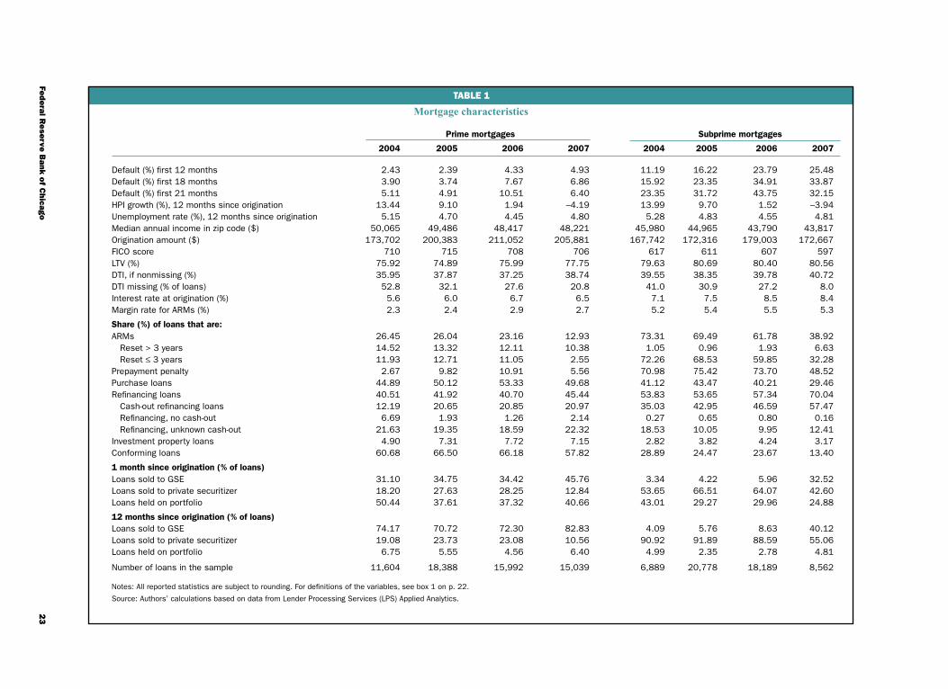
23
Fede
ral Rese
rve B
ank of C
hicago
TABLE 1
Mortgage characteristics
Prime mortgages Subprime mortgages
2004 2005 2006 2007 2004 2005 2006 2007
Default (%) first 12 months 2.43 2.39 4.33 4.93 11.19 16.22 23.79 25.48Default (%) first 18 months 3.90 3.74 7.67 6.86 15.92 23.35 34.91 33.87Default (%) first 21 months 5.11 4.91 10.51 6.40 23.35 31.72 43.75 32.15HPI growth (%), 12 months since origination 13.44 9.10 1.94 –4.19 13.99 9.70 1.52 –3.94Unemployment rate (%), 12 months since origination 5.15 4.70 4.45 4.80 5.28 4.83 4.55 4.81Median annual income in zip code ($) 50,065 49,486 48,417 48,221 45,980 44,965 43,790 43,817Origination amount ($) 173,702 200,383 211,052 205,881 167,742 172,316 179,003 172,667FICO score 710 715 708 706 617 611 607 597LTV (%) 75.92 74.89 75.99 77.75 79.63 80.69 80.40 80.56DTI, if nonmissing (%) 35.95 37.87 37.25 38.74 39.55 38.35 39.78 40.72DTI missing (% of loans) 52.8 32.1 27.6 20.8 41.0 30.9 27.2 8.0Interest rate at origination (%) 5.6 6.0 6.7 6.5 7.1 7.5 8.5 8.4Margin rate for ARMs (%) 2.3 2.4 2.9 2.7 5.2 5.4 5.5 5.3
Share (%) of loans that are: ARMs 26.45 26.04 23.16 12.93 73.31 69.49 61.78 38.92 Reset > 3 years 14.52 13.32 12.11 10.38 1.05 0.96 1.93 6.63 Reset ≤ 3 years 11.93 12.71 11.05 2.55 72.26 68.53 59.85 32.28Prepayment penalty 2.67 9.82 10.91 5.56 70.98 75.42 73.70 48.52Purchase loans 44.89 50.12 53.33 49.68 41.12 43.47 40.21 29.46Refinancing loans 40.51 41.92 40.70 45.44 53.83 53.65 57.34 70.04 Cash-out refinancing loans 12.19 20.65 20.85 20.97 35.03 42.95 46.59 57.47 Refinancing, no cash-out 6.69 1.93 1.26 2.14 0.27 0.65 0.80 0.16 Refinancing, unknown cash-out 21.63 19.35 18.59 22.32 18.53 10.05 9.95 12.41Investment property loans 4.90 7.31 7.72 7.15 2.82 3.82 4.24 3.17Conforming loans 60.68 66.50 66.18 57.82 28.89 24.47 23.67 13.40
1 month since origination (% of loans) Loans sold to GSE 31.10 34.75 34.42 45.76 3.34 4.22 5.96 32.52Loans sold to private securitizer 18.20 27.63 28.25 12.84 53.65 66.51 64.07 42.60Loans held on portfolio 50.44 37.61 37.32 40.66 43.01 29.27 29.96 24.88
12 months since origination (% of loans) Loans sold to GSE 74.17 70.72 72.30 82.83 4.09 5.76 8.63 40.12Loans sold to private securitizer 19.08 23.73 23.08 10.56 90.92 91.89 88.59 55.06Loans held on portfolio 6.75 5.55 4.56 6.40 4.99 2.35 2.78 4.81
Number of loans in the sample 11,604 18,388 15,992 15,039 6,889 20,778 18,189 8,562
Notes: All reported statistics are subject to rounding. For definitions of the variables, see box 1 on p. 22.
Source: Authors’ calculations based on data from Lender Processing Services (LPS) Applied Analytics.
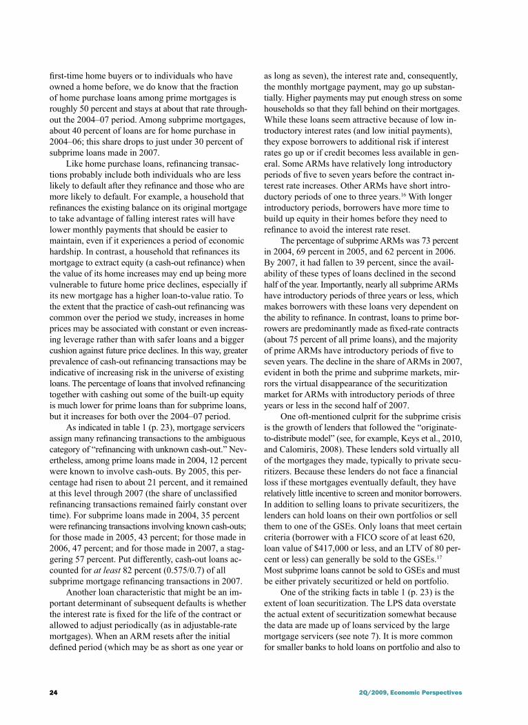
24 2Q/2009, Economic Perspectives
first-time home buyers or to individuals who have owned a home before, we do know that the fraction of home purchase loans among prime mortgages is roughly 50 percent and stays at about that rate through-out the 2004–07 period. Among subprime mortgages, about 40 percent of loans are for home purchase in 2004–06; this share drops to just under 30 percent of subprime loans made in 2007.
Like home purchase loans, refinancing transac-tions probably include both individuals who are less likely to default after they refinance and those who are more likely to default. For example, a household that refinances the existing balance on its original mortgage to take advantage of falling interest rates will have lower monthly payments that should be easier to maintain, even if it experiences a period of economic hardship. In contrast, a household that refinances its mortgage to extract equity (a cash-out refinance) when the value of its home increases may end up being more vulnerable to future home price declines, especially if its new mortgage has a higher loan-to-value ratio. To the extent that the practice of cash-out refinancing was common over the period we study, increases in home prices may be associated with constant or even increas-ing leverage rather than with safer loans and a bigger cushion against future price declines. In this way, greater prevalence of cash-out refinancing transactions may be indicative of increasing risk in the universe of existing loans. The percentage of loans that involved refinancing together with cashing out some of the built-up equity is much lower for prime loans than for subprime loans, but it increases for both over the 2004–07 period.
As indicated in table 1 (p. 23), mortgage servicers assign many refinancing transactions to the ambiguous category of “refinancing with unknown cash-out.” Nev-ertheless, among prime loans made in 2004, 12 percent were known to involve cash-outs. By 2005, this per-centage had risen to about 21 percent, and it remained at this level through 2007 (the share of unclassified refinancing transactions remained fairly constant over time). For subprime loans made in 2004, 35 percent were refinancing transactions involving known cash-outs; for those made in 2005, 43 percent; for those made in 2006, 47 percent; and for those made in 2007, a stag-gering 57 percent. Put differently, cash-out loans ac-counted for at least 82 percent (0.575/0.7) of all subprime mortgage refinancing transactions in 2007.
Another loan characteristic that might be an im-portant determinant of subsequent defaults is whether the interest rate is fixed for the life of the contract or allowed to adjust periodically (as in adjustable-rate mortgages). When an ARM resets after the initial defined period (which may be as short as one year or
as long as seven), the interest rate and, consequently, the monthly mortgage payment, may go up substan-tially. Higher payments may put enough stress on some households so that they fall behind on their mortgages. While these loans seem attractive because of low in-troductory interest rates (and low initial payments), they expose borrowers to additional risk if interest rates go up or if credit becomes less available in gen-eral. Some ARMs have relatively long introductory periods of five to seven years before the contract in-terest rate increases. Other ARMs have short intro-ductory periods of one to three years.16 With longer introductory periods, borrowers have more time to build up equity in their homes before they need to refinance to avoid the interest rate reset.
The percentage of subprime ARMs was 73 percent in 2004, 69 percent in 2005, and 62 percent in 2006. By 2007, it had fallen to 39 percent, since the avail-ability of these types of loans declined in the second half of the year. Importantly, nearly all subprime ARMs have introductory periods of three years or less, which makes borrowers with these loans very dependent on the ability to refinance. In contrast, loans to prime bor-rowers are predominantly made as fixed-rate contracts (about 75 percent of all prime loans), and the majority of prime ARMs have introductory periods of five to seven years. The decline in the share of ARMs in 2007, evident in both the prime and subprime markets, mir-rors the virtual disappearance of the securitization market for ARMs with introductory periods of three years or less in the second half of 2007.
One oft-mentioned culprit for the subprime crisis is the growth of lenders that followed the “originate-to-distribute model” (see, for example, Keys et al., 2010, and Calomiris, 2008). These lenders sold virtually all of the mortgages they made, typically to private secu-ritizers. Because these lenders do not face a financial loss if these mortgages eventually default, they have relatively little incentive to screen and monitor borrowers. In addition to selling loans to private securitizers, the lenders can hold loans on their own portfolios or sell them to one of the GSEs. Only loans that meet certain criteria (borrower with a FICO score of at least 620, loan value of $417,000 or less, and an LTV of 80 per-cent or less) can generally be sold to the GSEs.17 Most subprime loans cannot be sold to GSEs and must be either privately securitized or held on portfolio.
One of the striking facts in table 1 (p. 23) is the extent of loan securitization. The LPS data overstate the actual extent of securitization somewhat because the data are made up of loans serviced by the large mortgage servicers (see note 7). It is more common for smaller banks to hold loans on portfolio and also to
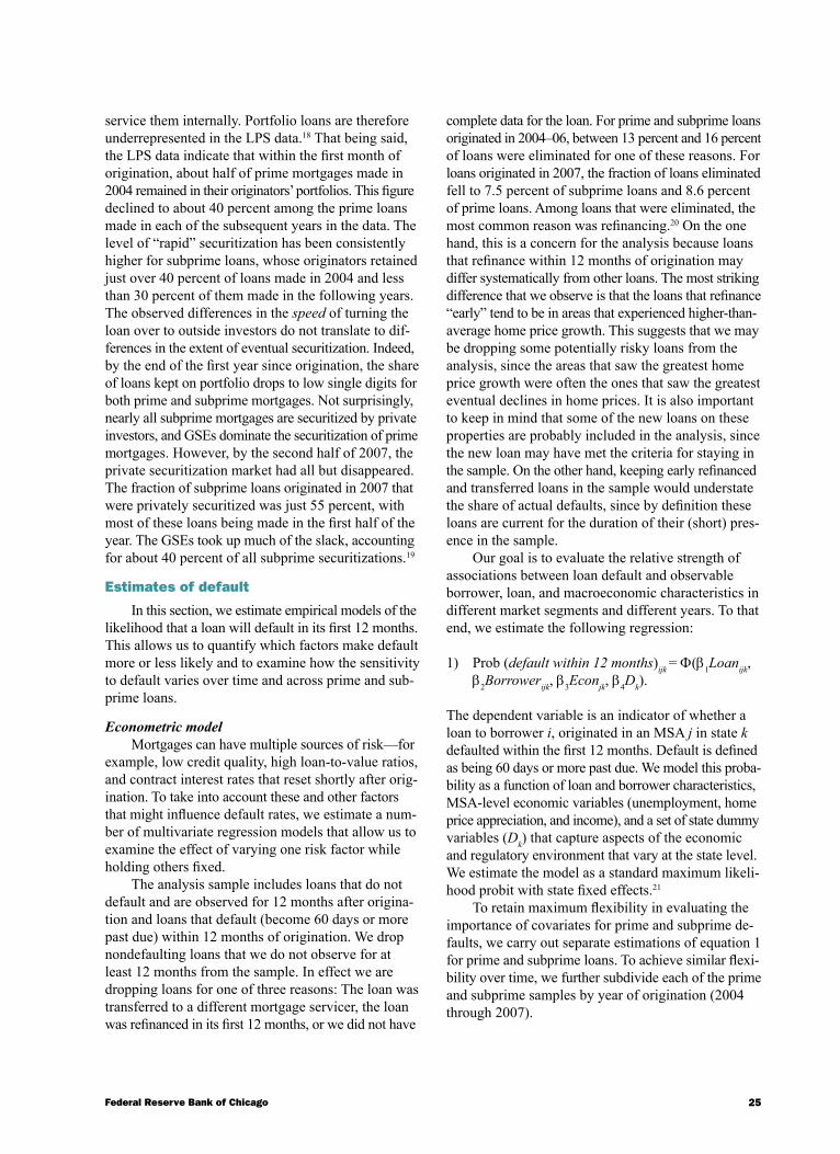
25Federal Reserve Bank of Chicago
service them internally. Portfolio loans are therefore underrepresented in the LPS data.18 That being said, the LPS data indicate that within the first month of origination, about half of prime mortgages made in 2004 remained in their originators’ portfolios. This figure declined to about 40 percent among the prime loans made in each of the subsequent years in the data. The level of “rapid” securitization has been consistently higher for subprime loans, whose originators retained just over 40 percent of loans made in 2004 and less than 30 percent of them made in the following years. The observed differences in the speed of turning the loan over to outside investors do not translate to dif-ferences in the extent of eventual securitization. Indeed, by the end of the first year since origination, the share of loans kept on portfolio drops to low single digits for both prime and subprime mortgages. Not surprisingly, nearly all subprime mortgages are securitized by private investors, and GSEs dominate the securitization of prime mortgages. However, by the second half of 2007, the private securitization market had all but disappeared. The fraction of subprime loans originated in 2007 that were privately securitized was just 55 percent, with most of these loans being made in the first half of the year. The GSEs took up much of the slack, accounting for about 40 percent of all subprime securitizations.19
Estimates of default
In this section, we estimate empirical models of the likelihood that a loan will default in its first 12 months. This allows us to quantify which factors make default more or less likely and to examine how the sensitivity to default varies over time and across prime and sub-prime loans.
Econometric modelMortgages can have multiple sources of risk—for
example, low credit quality, high loan-to-value ratios, and contract interest rates that reset shortly after orig-ination. To take into account these and other factors that might influence default rates, we estimate a num-ber of multivariate regression models that allow us to examine the effect of varying one risk factor while holding others fixed.
The analysis sample includes loans that do not default and are observed for 12 months after origina-tion and loans that default (become 60 days or more past due) within 12 months of origination. We drop nondefaulting loans that we do not observe for at least 12 months from the sample. In effect we are dropping loans for one of three reasons: The loan was transferred to a different mortgage servicer, the loan was refinanced in its first 12 months, or we did not have
complete data for the loan. For prime and subprime loans originated in 2004–06, between 13 percent and 16 percent of loans were eliminated for one of these reasons. For loans originated in 2007, the fraction of loans eliminated fell to 7.5 percent of subprime loans and 8.6 percent of prime loans. Among loans that were eliminated, the most common reason was refinancing.20 On the one hand, this is a concern for the analysis because loans that refinance within 12 months of origination may differ systematically from other loans. The most striking difference that we observe is that the loans that refinance “early” tend to be in areas that experienced higher-than-average home price growth. This suggests that we may be dropping some potentially risky loans from the analysis, since the areas that saw the greatest home price growth were often the ones that saw the greatest eventual declines in home prices. It is also important to keep in mind that some of the new loans on these properties are probably included in the analysis, since the new loan may have met the criteria for staying in the sample. On the other hand, keeping early refinanced and transferred loans in the sample would understate the share of actual defaults, since by definition these loans are current for the duration of their (short) pres-ence in the sample.
Our goal is to evaluate the relative strength of associations between loan default and observable borrower, loan, and macroeconomic characteristics in different market segments and different years. To that end, we estimate the following regression:
1) Prob (default within 12 months)ijk = Φ(β1Loanijk, β2Borrowerijk, β3Econjk, β4Dk).
The dependent variable is an indicator of whether a loan to borrower i, originated in an MSA j in state k defaulted within the first 12 months. Default is defined as being 60 days or more past due. We model this proba-bility as a function of loan and borrower characteristics, MSA-level economic variables (unemployment, home price appreciation, and income), and a set of state dummy variables (Dk) that capture aspects of the economic and regulatory environment that vary at the state level. We estimate the model as a standard maximum likeli-hood probit with state fixed effects.21
To retain maximum flexibility in evaluating the importance of covariates for prime and subprime de-faults, we carry out separate estimations of equation 1 for prime and subprime loans. To achieve similar flexi-bility over time, we further subdivide each of the prime and subprime samples by year of origination (2004 through 2007).
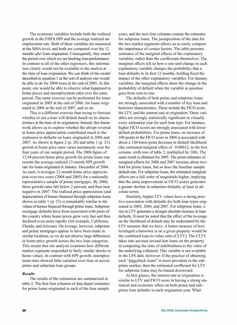
26 2Q/2009, Economic Perspectives
The economic variables include both the realized growth in the FHFA HPI and the average realized un-employment rate. Both of these variables are measured at the MSA level, and both are computed over the 12 months after loan origination. Consequently, they match the period over which we are tracking loan performance. In contrast to all of the other regressors, this informa-tion clearly would not be available to the analyst at the time of loan origination. We can think of the model described in equation 1 as the sort of analysis one would be able to do for 2004 loans at the end of 2005. At this point, one would be able to observe what happened to home prices and unemployment rates over the same period. The same exercise can be performed for loans originated in 2005 at the end of 2006, for loans origi-nated in 2006 at the end of 2007, and so on.
This is a different exercise than trying to forecast whether or not a loan will default based on its charac-teristics at the time of its origination. Instead, this frame-work allows us to explore whether the abrupt reversal in home price appreciation contributed much to the explosion in defaults on loans originated in 2006 and 2007. As shown in figure 2 (p. 20) and table 1 (p. 23), growth in home price rates varies enormously over the four years of our sample period. The 2004 figure of 13.44 percent home price growth for prime loans rep-resents the average realized 12-month HPI growth rate for loans originated in January–December of 2004. As such, it averages 12-month home price apprecia-tion over two years (2004 and 2005) for a nationally representative sample of prime mortgages. By 2006, these growth rates fall below 2 percent, and then turn negative in 2007. The realized price appreciation (and depreciation) of homes financed through subprime loans shown in table 1 (p. 23) is remarkably similar to the values of homes financed through prime loans. Subprime mortgage defaults have been associated with parts of the country where home prices grew very fast and then declined even more rapidly (for example, California, Florida, and Arizona). On average, however, subprime and prime mortgages appear to have been made in similar locations, so we do not observe large differences in home price growth across the two loan categories. This means that our analysis examines how different market segments responded to fairly similar shocks to home values. In contrast with HPI growth, unemploy-ment rates showed little variation over time or across prime and subprime loan groups.
ResultsThe results of the estimation are summarized in
table 2. The first four columns of data depict estimates for prime loans originated in each of the four sample
years, and the next four columns contain the estimates for subprime loans. The juxtaposition of the data for the two market segments allows us to easily compare the importance of certain factors. The table presents estimates of the marginal effects of the explanatory variables, rather than the coefficients themselves. The marginal effects tell us how a one-unit change in each explanatory variable changes the probability that a loan defaults in its first 12 months, holding fixed the impact of the other explanatory variables. For dummy variables, the marginal effects show the change in the probability of default when the variable in question goes from zero to one.
The defaults of both prime and subprime loans are strongly associated with a number of key loan and borrower characteristics. These include the FICO score, the LTV, and the interest rate at origination. These vari-ables are strongly statistically significant in virtually every estimation year for each loan type. For instance, higher FICO scores are strongly associated with lower default probabilities. For prime loans, an increase of 100 points in the FICO score in 2004 is associated with about a 120-basis-point decrease in default likelihood (the estimated marginal effect of –0.00012, in the first column, sixth row of table 2, multiplied by 100). The same result is obtained for 2005. The point estimates of marginal effects for 2006 and 2007 increase about two-fold for prime loans, but so does the baseline sample default rate. For subprime loans, the estimated marginal effects are a full order of magnitude higher, implying that the same improvement in FICO scores generates a greater decline in subprime defaults, at least in ab-solute terms.
Similarly, higher LTV values have a strong posi-tive association with defaults for both loan types orig-inated in 2005, 2006, and 2007. For subprime loans, a rise in LTV generates a stronger absolute increase in loan defaults. It must be noted that the effect of the leverage on the likelihood of default may be understated by the LTV measure that we have. A better measure of how leveraged a borrower is on a given property would be the combined loan-to-value ratio (CLTV). The CLTV takes into account second-lien loans on the property in computing the ratio of indebtedness to the value of the underlying collateral. This variable is not available in the LPS data, however. If the practice of obtaining such “piggyback loans” is more prevalent in the sub-prime market, then the estimated coefficient for LTV for subprime loans may be biased downward.
At first glance, the interest rate at origination is similar to LTV and FICO score in having a strong sta-tistical and economic effect on both prime and sub-prime loan defaults in each origination year. What
27Federal Reserve Bank of Chicago
stands out is the sheer magnitude of the estimated effects. However, one must be cautious in interpret-ing hypothetical marginal effects of the interest rate. While LTV and FICO score cover fairly wide ranges for both prime and subprime loans, interest rate values are more tightly distributed.22 For example, the stan-dard deviation of interest rates on prime loans across all years of our sample is 81 basis points: A one stan-dard deviation increase in the interest rate for prime loans would raise the average rate from 6.25 percent to 7.06 percent. The equivalent one standard deviation increase in interest rates for subprime loans would raise the average rate from 7.93 percent to 9.24 percent. If we see two loans with otherwise identical characteristics but one has a higher interest rate, a likely explanation is that the lender has additional information about the credit quality of the borrower and is charging a higher interest rate to take into account additional risk factors, over and above those that are captured by the borrower’s FICO score.
There are also a number of notable differences between the prime and subprime samples. Perhaps the most interesting finding is the different sensitivity of defaults to changes in home prices. For subprime loans, defaults are much lower when home price growth is higher for three out of the four sample years. This re-lationship is particularly striking for 2006 loan origi-nations, many of which experienced home price declines over their first 12 months. For prime loans, 2006 is the only year of origination in which changes in home prices are significantly correlated with loan defaults. These results suggest that, relative to subprime defaults, prime defaults have a weaker relationship with home prices, once key borrower and loan characteristics (LTV, FICO score, and so on) are taken into account.
The contrast between prime and subprime loans is even sharper for the debt-to-income ratio and loan margin rate. The DTI is widely considered to be one of the main determinants of loan affordability, since it relates household monthly income to debt service flows. The DTI for prime loans is not significantly correlated with defaults, except for loans originated in 2007, but it matters consistently for subprime loans. The absence of any measurable effects of DTI even on defaults of prime loans originated in 2006 can be interpreted as a sign of the resilience of prime borrowers who experi-enced significant changes in the prices of their homes.
The loan margin rate is one of the key terms in an ARM contract. It defines the spread to a reference rate (usually the London interbank offered rate, or Libor). At reset, the ARM’s interest rate goes up to the sum of Libor and the loan margin. The margin is set by the lender, and is often thought to capture additional aspects
of a borrower’s creditworthiness. This is consistent with the fact that the margin rate is, on average, sub-stantially higher for subprime borrowers (see table 1, p. 23). We find that this variable has no association with defaults among prime loans, with the exception of loans originated in 2006. In contrast, defaults on subprime loans originated in every year except 2007 are significantly higher for loans with higher margin rates, all else being equal. This suggests that, for the subprime borrower, the margin rate contains addition-al information on borrower quality not reflected in FICO scores and other loan characteristics. It is also interesting that ARMs with introductory periods of three years or less—the most common mortgage con-tract in the subprime market—have the same correla-tion with subprime defaults as fixed-rate mortgages do. Put differently, once loan and borrower character-istics are accounted for, the choice of an ARM with a short introductory period is not associated with higher subprime defaults.
Several other results merit comment. For prime loans, being securitized within one month of origination (as opposed to remaining in the lender’s portfolio) is associated with lower defaults for loans made in 2004, 2005, and 2006. This does not necessarily mean that the securitization process has been successful in iden-tifying loans of higher quality. Since nearly all loans in the sample are securitized over the 12-month default horizon (see table 1, p. 23), the difference in defaults probably captures differences between fast-to-securi-tize and slow-to-securitize originators, rather than differences between securitized loans and those held on portfolio. We find similar results for securitized subprime loans made in 2005, 2006, and 2007. Sub-prime loans also have extremely high rates of eventual securitization, and the relationship between subprime default and securitization can be interpreted in the same way. This hints at the possibility that originators with business models focused on securitization are better at screening loan quality. These originators would have more to lose if their reputations were damaged by weak ex post performance of the loans they originated.
Finally, we note that purchase loans, as opposed to refinance loans, are consistently associated with higher defaults in nearly all sample years, in both the prime and subprime market segments. This may seem surprising, since borrowers who extract equity from their homes in cash-out refinancings may be particu-larly vulnerable to economic shocks and experience higher defaults as a result. However, not all cash-out refinancing is done by borrowers who need to finance current consumption. Since a prerequisite for any cash-out transaction is the availability of positive home
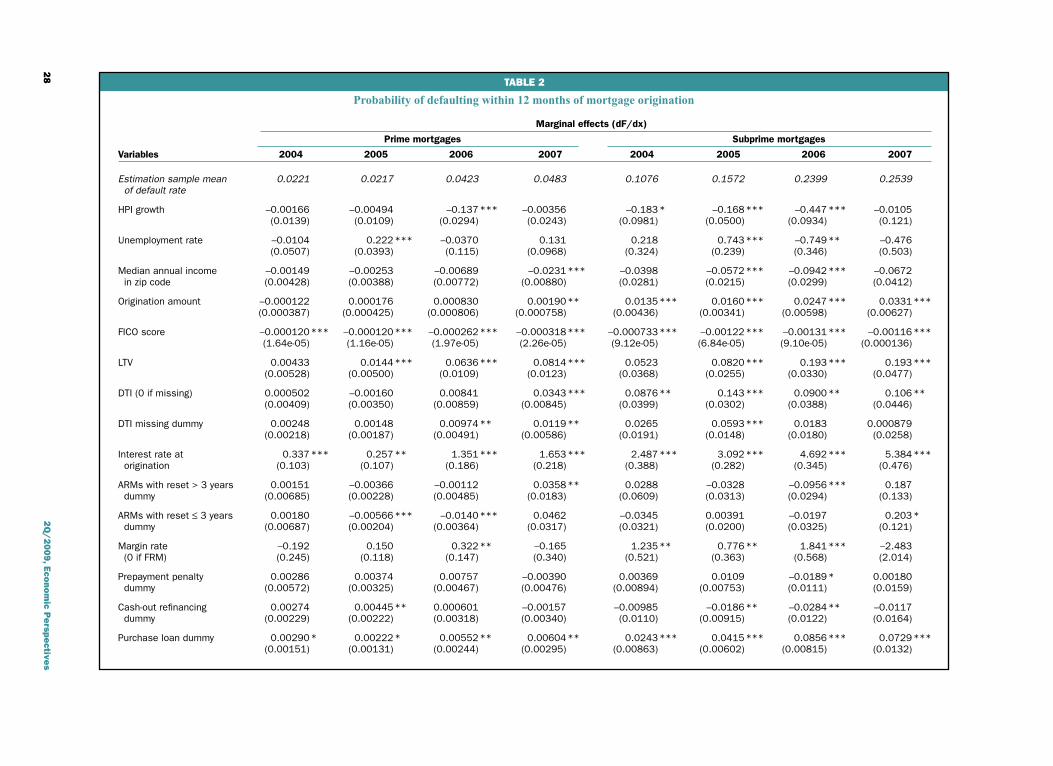
28
2Q
/2
00
9, E
cono
mic P
erspe
ctives
TABLE 2
Probability of defaulting within 12 months of mortgage origination
Marginal effects (dF/dx)
Prime mortgages Subprime mortgages
Variables 2004 2005 2006 2007 2004 2005 2006 2007
Estimation sample mean 0.0221 0.0217 0.0423 0.0483 0.1076 0.1572 0.2399 0.2539 of default rate
HPI growth –0.00166 –0.00494 –0.137 *** –0.00356 –0.183 * –0.168 *** –0.447 *** –0.0105 (0.0139) (0.0109) (0.0294) (0.0243) (0.0981) (0.0500) (0.0934) (0.121)
Unemployment rate –0.0104 0.222 *** –0.0370 0.131 0.218 0.743 *** –0.749 ** –0.476 (0.0507) (0.0393) (0.115) (0.0968) (0.324) (0.239) (0.346) (0.503)
Median annual income –0.00149 –0.00253 –0.00689 –0.0231 *** –0.0398 –0.0572 *** –0.0942 *** –0.0672 in zip code (0.00428) (0.00388) (0.00772) (0.00880) (0.0281) (0.0215) (0.0299) (0.0412)
Origination amount –0.000122 0.000176 0.000830 0.00190 ** 0.0135 *** 0.0160 *** 0.0247 *** 0.0331 *** (0.000387) (0.000425) (0.000806) (0.000758) (0.00436) (0.00341) (0.00598) (0.00627)
FICO score –0.000120 *** –0.000120 *** –0.000262 *** –0.000318 *** –0.000733 *** –0.00122 *** –0.00131 *** –0.00116 *** (1.64e-05) (1.16e-05) (1.97e-05) (2.26e-05) (9.12e-05) (6.84e-05) (9.10e-05) (0.000136)
LTV 0.00433 0.0144 *** 0.0636 *** 0.0814 *** 0.0523 0.0820 *** 0.193 *** 0.193 *** (0.00528) (0.00500) (0.0109) (0.0123) (0.0368) (0.0255) (0.0330) (0.0477)
DTI (0 if missing) 0.000502 –0.00160 0.00841 0.0343 *** 0.0876 ** 0.143 *** 0.0900 ** 0.106 ** (0.00409) (0.00350) (0.00859) (0.00845) (0.0399) (0.0302) (0.0388) (0.0446)
DTI missing dummy 0.00248 0.00148 0.00974 ** 0.0119 ** 0.0265 0.0593 *** 0.0183 0.000879 (0.00218) (0.00187) (0.00491) (0.00586) (0.0191) (0.0148) (0.0180) (0.0258)
Interest rate at 0.337 *** 0.257 ** 1.351 *** 1.653 *** 2.487 *** 3.092 *** 4.692 *** 5.384 *** origination (0.103) (0.107) (0.186) (0.218) (0.388) (0.282) (0.345) (0.476)
ARMs with reset > 3 years 0.00151 –0.00366 –0.00112 0.0358 ** 0.0288 –0.0328 –0.0956 *** 0.187 dummy (0.00685) (0.00228) (0.00485) (0.0183) (0.0609) (0.0313) (0.0294) (0.133)
ARMs with reset ≤ 3 years 0.00180 –0.00566 *** –0.0140 *** 0.0462 –0.0345 0.00391 –0.0197 0.203 * dummy (0.00687) (0.00204) (0.00364) (0.0317) (0.0321) (0.0200) (0.0325) (0.121)
Margin rate –0.192 0.150 0.322 ** –0.165 1.235 ** 0.776 ** 1.841 *** –2.483 (0 if FRM) (0.245) (0.118) (0.147) (0.340) (0.521) (0.363) (0.568) (2.014)
Prepayment penalty 0.00286 0.00374 0.00757 –0.00390 0.00369 0.0109 –0.0189 * 0.00180 dummy (0.00572) (0.00325) (0.00467) (0.00476) (0.00894) (0.00753) (0.0111) (0.0159)
Cash-out refinancing 0.00274 0.00445 ** 0.000601 –0.00157 –0.00985 –0.0186 ** –0.0284 ** –0.0117 dummy (0.00229) (0.00222) (0.00318) (0.00340) (0.0110) (0.00915) (0.0122) (0.0164)
Purchase loan dummy 0.00290 * 0.00222 * 0.00552 ** 0.00604 ** 0.0243 *** 0.0415 *** 0.0856 *** 0.0729 *** (0.00151) (0.00131) (0.00244) (0.00295) (0.00863) (0.00602) (0.00815) (0.0132)
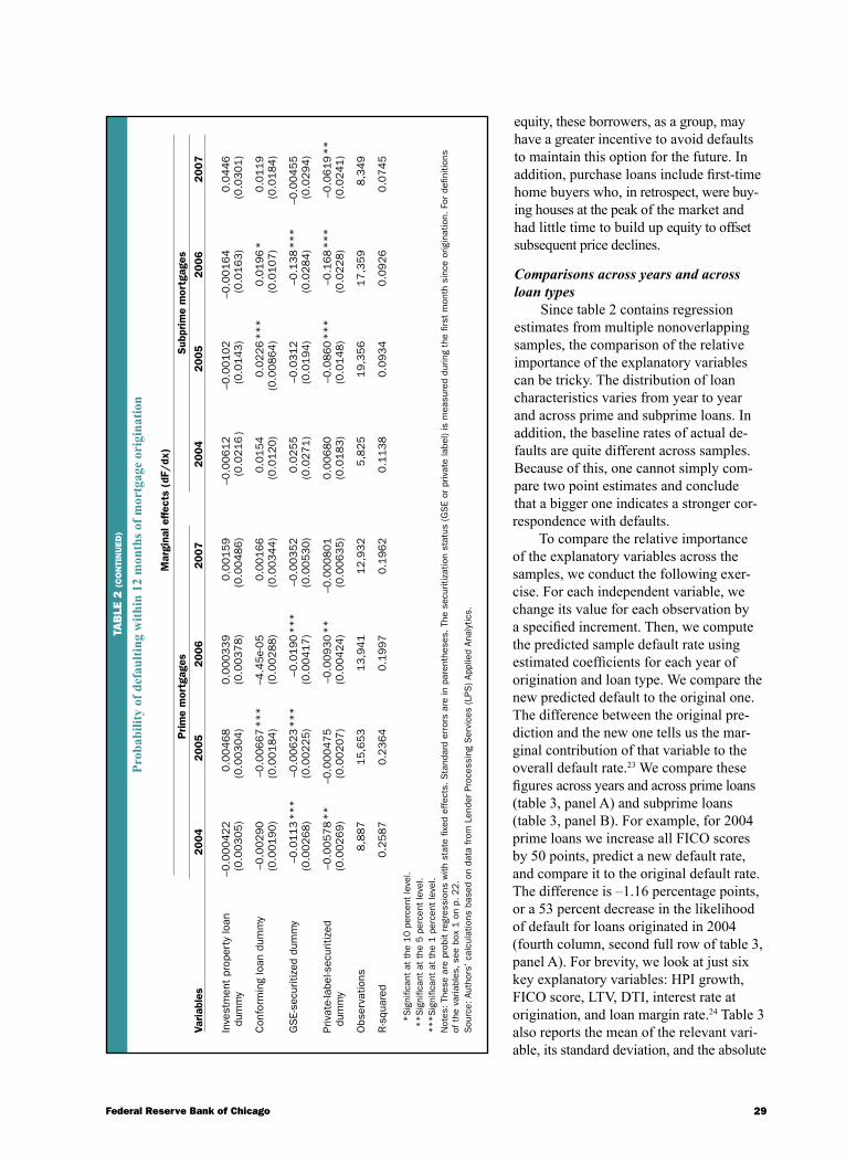
29Federal Reserve Bank of Chicago
TA
BLE
2 (C
ON
TIN
UE
D)
Prob
abili
ty o
f def
aulti
ng w
ithin
12
mon
ths o
f mor
tgag
e or
igin
atio
n
M
argi
nal e
ffec
ts (
dF/dx
)
P
rim
e m
ortg
ages
Sub
prim
e m
ortg
ages
Variab
les
2004
2005
2006
2007
2004
2005
2006
2007
Inve
stm
ent
prop
erty
loan
–0
.000422
0.0
0468
0.0
00339
0.0
0159
–0.0
0612
–0.0
0102
–0.0
0164
0.0
446
du
mm
y (0
.00305)
(0.0
0304)
(0.0
0378)
(0.0
0486)
(0.0
216 )
(0.0
143)
(0.0
163)
(0.0
301)
Con
form
ing
loan
dum
my
–0
.00290
–0.0
0667 *
**
–4.4
5e-
05
0.0
0166
0.0
154
0.0
226 *
**
0.0
196 *
0.0
119
(0.0
0190)
(0.0
0184)
(0.0
0288)
(0.0
0344)
(0.0
120)
(0.0
0864)
(0.0
107)
(0.0
184)
GS
E-se
curit
ized
dum
my
–0.0
113 *
**
–0.0
0623 *
**
–0.0
190 *
**
–0.0
0352
0.0
255
–0.0
312
–0.1
38 *
**
–0.0
0455
(0.0
0268)
(0.0
0225)
(0.0
0417)
(0.0
0530)
(0.0
271)
(0.0
194)
(0.0
284)
(0.0
294)
Priv
ate-
labe
l-sec
uriti
zed
–0
.00578 *
*
–0.0
00475
–0.0
0930 *
*
–0.0
00801
0.0
0680
–0.0
860 *
**
–0.1
68 *
**
–0.0
619 *
*
du
mm
y (0
.00269)
(0.0
0207)
(0.0
0424)
(0.0
0635)
(0.0
183)
(0.0
148)
(0.0
228)
(0.0
241)
Obs
erva
tions
8,8
87
15,6
53
13,9
41
12,9
32
5,8
25
19,3
56
17,3
59
8,3
49
R-s
quar
ed
0.2
587
0.2
364
0.1
997
0.1
962
0.1
138
0.0
934
0.0
926
0.0
745
*S
igni
fican
t at
the
10 p
erce
nt le
vel.
*
*S
igni
fican
t at
the
5 p
erce
nt le
vel.
**
*S
igni
fican
t at
the
1 p
erce
nt le
vel.
Not
es: Th
ese
are
prob
it re
gres
sion
s w
ith s
tate
fixe
d ef
fect
s. S
tand
ard
erro
rs a
re in
par
enth
eses
. Th
e se
curit
izat
ion
stat
us (
GS
E or
priv
ate
labe
l) is
mea
sure
d du
ring
the
first
mon
th s
ince
orig
inat
ion.
For
defi
nitio
ns
of t
he v
aria
bles
, see
box
1 o
n p.
22.
Sou
rce:
Aut
hors
’ ca
lcul
atio
ns b
ased
on
data
fro
m L
ende
r Pr
oces
sing
Ser
vice
s (L
PS)
Appl
ied
Anal
ytic
s.
equity, these borrowers, as a group, may have a greater incentive to avoid defaults to maintain this option for the future. In addition, purchase loans include first-time home buyers who, in retrospect, were buy-ing houses at the peak of the market and had little time to build up equity to offset subsequent price declines.
Comparisons across years and across loan types
Since table 2 contains regression estimates from multiple nonoverlapping samples, the comparison of the relative importance of the explanatory variables can be tricky. The distribution of loan characteristics varies from year to year and across prime and subprime loans. In addition, the baseline rates of actual de-faults are quite different across samples. Because of this, one cannot simply com-pare two point estimates and conclude that a bigger one indicates a stronger cor-respondence with defaults.
To compare the relative importance of the explanatory variables across the samples, we conduct the following exer-cise. For each independent variable, we change its value for each observation by a specified increment. Then, we compute the predicted sample default rate using estimated coefficients for each year of origination and loan type. We compare the new predicted default to the original one. The difference between the original pre-diction and the new one tells us the mar-ginal contribution of that variable to the overall default rate.23 We compare these figures across years and across prime loans (table 3, panel A) and subprime loans (table 3, panel B). For example, for 2004 prime loans we increase all FICO scores by 50 points, predict a new default rate, and compare it to the original default rate. The difference is –1.16 percentage points, or a 53 percent decrease in the likelihood of default for loans originated in 2004 (fourth column, second full row of table 3, panel A). For brevity, we look at just six key explanatory variables: HPI growth, FICO score, LTV, DTI, interest rate at origination, and loan margin rate.24 Table 3 also reports the mean of the relevant vari-able, its standard deviation, and the absolute
30 2Q/2009, Economic Perspectives
change that we impose. We tried to keep the magni-tude of the absolute changes reasonably close to the standard deviations.
An increase of 10 percentage points in home price appreciation (HPI growth) substantially lowers default probabilities (first full row of each panel in table 3). This effect is more consistent for subprime loans origi-nated in various years, where it translates to decreases of between 10 percent and 18 percent relative to the baseline default rate in 2004, 2005, and 2006. For prime loans, the 10-percentage-point increase in the HPI has a big effect only for loans originated in 2006, where the estimates imply that defaults would have been 1.78 percentage points, or 42 percent, lower. The effect of FICO score stands out. A 50-point uniform increase in FICO scores (second full row of each panel) is asso-ciated with a 41 percent to 53 percent decline in pre-dicted default rates relative to the baseline for prime loans, and a 20 percent to 34 percent relative decline for subprime loans. The average marginal effects of the LTV are greater (in a relative sense) for prime loans than for subprime loans.25 Finally, higher interest rates at origination appear to generate incredible increases in defaults for both market segments. For instance, a 1 percentage point increase in interest rates translates into a jump in defaults on 2007 prime loans of more than 3 percentage points—a rise of 66 percent relative to the actual default rate. Increasing everyone’s interest rates by 1 percentage point is equivalent to a substan-tial deterioration in the quality of the borrower pool, and thus translates into much higher predicted defaults. As mentioned earlier, the DTI and the margin rate do not have strong associations with prime mortgage defaults. In contrast, higher values of these variables consis-tently indicate higher default rates for subprime mort-gages. However, the economic magnitude of marginal effects of DTI and the margin rate on defaults (fourth and sixth full rows of each panel) is somewhat muted.
What if?
In this section, we use the estimates discussed previously to do two things. First, we examine how much (or how little) of the increase in mortgage de-faults from 2004 through 2007 can be explained by changes in the characteristics of loans and borrowers, as opposed to changes in the responsiveness of de-faults to those characteristics. Next, we examine how forecasts of prime and subprime mortgage defaults vary with different assumptions about the future path of home prices.
Predicted versus actual defaultsThe descriptive regressions in the previous section
provide insights into the factors that are associated with realized defaults for different types of loans originated in different years. An open question is how useful these relationships could have been in forecasting the defaults of future loans. To address this, we conduct the fol-lowing thought experiment. For each set of estimates, we compute predicted defaults using observed loan, borrower, and economic characteristics from other origination years. For instance, we take the relationship between borrower characteristics and loan character-istics that we estimate using data from prime loans originated in 2004 (the marginal effects reported in the first column of table 2, pp. 28–29) and see what it would imply for defaults for prime loans originated in 2007. In other words, we pick a particular year and fix the relationship (that is, the estimated coefficients) between defaults and characteristics, but let the charac-teristics vary as they actually did in the data. This ex-ercise lets us see to what extent higher defaults on loans originated in 2007 can be explained by changes in characteristics alone. We show these results in table 4, where this exercise is carried out separately for prime loans (panels A and B) and subprime loans (panels C and D). Panels A and C of the table show the predicted default rate for loans originated in each of the sample years (rows) using the coefficients estimated with data from each of the sample years (columns). The numbers in bold that run diagonally through the panels are pre-dictions that use characteristics and coefficients from the same year. A useful way to summarize the results is to look at predictions below and above the diagonal bold entries. Those below the diagonal bold entries are forecasts of future defaults using historical models (for example, relationships between characteristics and defaults from 2004 and characteristics from 2007). Those above the diagonal run this exercise in reverse—they ap-ply recent model estimates to loans from earlier years (for example, relationships between characteristics and defaults from 2007 and characteristics from 2004). These two groups of predictions are strikingly differ-ent in terms of their predictions relative to the actual realized default rates.
Perhaps the easiest way to see this is in panels B and D of table 4, which express predicted defaults as a percentage of realized defaults. The diagonal forecasts in those two panels are close to 100 percent. This is a feature of the estimation procedure. However, forward-looking forecasts—those below the diagonal bold entries—are nearly always less than 100 percent for both prime and subprime loans.26 This means that predic-tions based on relationships between characteristics
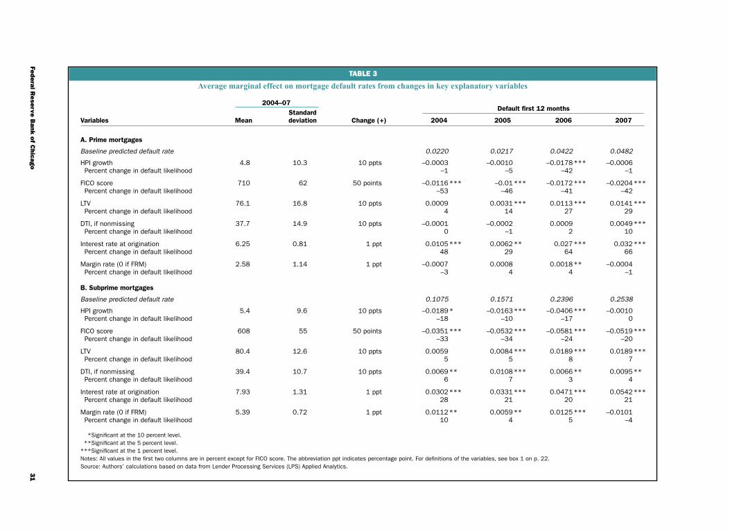
31
Fede
ral Rese
rve B
ank of C
hicago
TABLE 3
Average marginal effect on mortgage default rates from changes in key explanatory variables
StandardVariables Mean deviation Change (+) 2004 2005 2006 2007
A. Prime mortgages
Baseline predicted default rate 0.0220 0.0217 0.0422 0.0482
HPI growth 4.8 10.3 10 ppts –0.0003 –0.0010 –0.0178 *** –0.0006 Percent change in default likelihood –1 –5 –42 –1
FICO score 710 62 50 points –0.0116 *** –0.01 *** –0.0172 *** –0.0204 *** Percent change in default likelihood –53 –46 –41 –42
LTV 76.1 16.8 10 ppts 0.0009 0.0031 *** 0.0113 *** 0.0141 *** Percent change in default likelihood 4 14 27 29
DTI, if nonmissing 37.7 14.9 10 ppts –0.0001 –0.0002 0.0009 0.0049 *** Percent change in default likelihood 0 –1 2 10
Interest rate at origination 6.25 0.81 1 ppt 0.0105 *** 0.0062 ** 0.027 *** 0.032 *** Percent change in default likelihood 48 29 64 66
Margin rate (0 if FRM) 2.58 1.14 1 ppt –0.0007 0.0008 0.0018 ** –0.0004 Percent change in default likelihood –3 4 4 –1
B. Subprime mortgages
Baseline predicted default rate 0.1075 0.1571 0.2396 0.2538
HPI growth 5.4 9.6 10 ppts –0.0189 * –0.0163 *** –0.0406 *** –0.0010 Percent change in default likelihood –18 –10 –17 0
FICO score 608 55 50 points –0.0351 *** –0.0532 *** –0.0581 *** –0.0519 *** Percent change in default likelihood –33 –34 –24 –20
LTV 80.4 12.6 10 ppts 0.0059 0.0084 *** 0.0189 *** 0.0189 *** Percent change in default likelihood 5 5 8 7
DTI, if nonmissing 39.4 10.7 10 ppts 0.0069 ** 0.0108 *** 0.0066 ** 0.0095 ** Percent change in default likelihood 6 7 3 4
Interest rate at origination 7.93 1.31 1 ppt 0.0302 *** 0.0331 *** 0.0471 *** 0.0542 *** Percent change in default likelihood 28 21 20 21
Margin rate (0 if FRM) 5.39 0.72 1 ppt 0.0112 ** 0.0059 ** 0.0125 *** –0.0101 Percent change in default likelihood 10 4 5 –4
*Significant at the 10 percent level. **Significant at the 5 percent level.***Significant at the 1 percent level.Notes: All values in the first two columns are in percent except for FICO score. The abbreviation ppt indicates percentage point. For definitions of the variables, see box 1 on p. 22.Source: Authors’ calculations based on data from Lender Processing Services (LPS) Applied Analytics.
Default first 12 months 2004–07
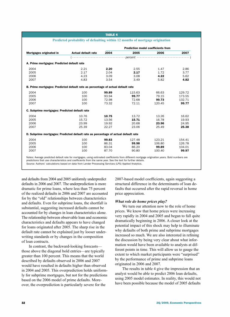
32 2Q/2009, Economic Perspectives
TABLE 4
Predicted probability of defaulting within 12 months of mortgage origination
Prediction model coefficients from
Mortgages originated in Actual default rate 2004 2005 2006 2007 ( - - - - - - - - - - - - - - - - - - - - - - - - - - - - - - - - - - percent - - - - - - - - - - - - - - - - - - - - - - - - - - - - - - - - - - )
A. Prime mortgages: Predicted default rate
2004 2.21 2.20 2.55 1.47 2.86 2005 2.17 2.04 2.17 1.72 3.77 2006 4.23 3.09 3.08 4.22 5.62 2007 4.83 3.54 3.49 5.82 4.82 B. Prime mortgages: Predicted default rate as percentage of actual default rate
2004 100 99.89 115.63 66.63 129.72 2005 100 93.94 99.77 79.15 173.55 2006 100 72.98 72.68 99.73 132.71 2007 100 73.32 72.11 120.45 99.77 C. Subprime mortgages: Predicted default rate
2004 10.76 10.75 13.72 13.26 16.62 2005 15.72 13.56 15.71 16.78 19.93 2006 23.99 19.92 20.68 23.96 24.95 2007 25.39 22.27 23.06 25.49 25.38 D. Subprime mortgages: Predicted default rate as percentage of actual default rate
2004 100 99.83 127.48 123.21 154.41 2005 100 86.31 99.98 106.80 126.78 2006 100 83.04 86.20 99.89 104.01 2007 100 87.70 90.80 100.40 99.97
Notes: Average predicted default rate for mortgages, using estimated coefficients from different mortgage origination years. Bold numbers are predictions that use characteristics and coefficients from the same year. See the text for further details.Source: Authors’ calculations based on data from Lender Processing Services (LPS) Applied Analytics.
and defaults from 2004 and 2005 uniformly underpredict defaults in 2006 and 2007. The underprediction is more dramatic for prime loans, where less than 75 percent of the realized defaults in 2006 and 2007 are accounted for by the “old” relationships between characteristics and defaults. Even for subprime loans, the shortfall is substantial, suggesting increased defaults cannot be accounted for by changes in loan characteristics alone. The relationship between observable loan and economic characteristics and defaults appears to have changed for loans originated after 2005. The sharp rise in the default rate cannot be explained just by looser under-writing standards or by changes in the composition of loan contracts.
In contrast, the backward-looking forecasts—those above the diagonal bold entries—are typically greater than 100 percent. This means that the world described by defaults observed in 2006 and 2007 would have resulted in defaults higher than observed in 2004 and 2005. This overprediction holds uniform-ly for subprime mortgages, but not for the predictions based on the 2006 model of prime defaults. More-over, the overprediction is particularly severe for the
2007-based model coefficients, again suggesting a structural difference in the determinants of loan de-faults that occurred after the rapid reversal in home price appreciation.
What role do home prices play? We turn our attention now to the role of home
prices. We know that home prices were increasing very rapidly in 2004 and 2005 and began to fall quite dramatically beginning in 2006. A closer look at the potential impact of this shock may help to illuminate why defaults of both prime and subprime mortgages increased so much. We are also interested in refining the discussion by being very clear about what infor-mation would have been available to analysts at dif-ferent points in time. This will allow us to gauge the extent to which market participants were “surprised” by the performance of prime and subprime loans originated in 2006 and 2007.
The results in table 4 give the impression that an analyst would be able to predict 2006 loan defaults, using 2005 model estimates. In reality, this would not have been possible because the model of 2005 defaults
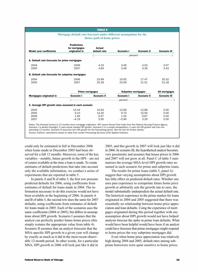
33Federal Reserve Bank of Chicago
TABLE 5
Mortgage default rate forecasts under different assumptions for the future path of home prices
Predictions for mortgages ActualModel year coefficients originated in default rate Scenario I Scenario II Scenario III
( - - - - - - - - - - - - - - - - - - - - - - - - - - percent - - - - - - - - - - - - - - - - - - - - - - - - - )
A. Default rate forecasts for prime mortgages
2004 2006 4.23 3.09 3.03 3.07 2005 2007 4.83 3.49 3.39 3.43
B. Default rate forecasts for subprime mortgages
2004 2006 23.99 19.92 17.47 20.32 2005 2007 25.39 23.06 21.51 22.18 Prime mortgages Subprime mortgages All mortgages
Mortgages originated in Scenario I Scenario II Scenario I Scenario II Scenario III
( - - - - - - - - - - - - - - - - - - - - - - - - - - - - - - - - - - - percent - - - - - - - - - - - - - - - - - - - - - - - - - - - - - - - - - - )
C. Average HPI growth rates assumed in each scenario
2004 13.44 10.63 13.99 12.89 0.00 2005 9.10 14.30 9.70 15.00 0.00 2006 1.94 9.57 1.52 9.87 0.00 2007 –4.19 2.65 –3.94 3.29 0.00 Notes: The forecast horizon is 12 months since mortgage origination. HPI means House Price Index from the Federal Housing Finance Agency. Scenario I is perfect foresight; it uses actual realized HPI growth. Scenario II is a simple extrapolation; it uses the HPI growth rate from the preceding 12 months. Scenario III assumes zero HPI growth for the forecasting period. See the text for further details.Source: Authors’ calculations based on data from Lender Processing Services (LPS) Applied Analytics.
could only be estimated in full in December 2006 when loans made in December 2005 had been ob-served for a full 12 months. Moreover, some of the key variables—notably, future growth in the HPI—are not of course available at the time a loan is made. To create estimates of default predictions that take into account only the available information, we conduct a series of experiments that are reported in table 5.
In panels A and B of table 5, the first row presents predicted defaults for 2006, using coefficients from estimates of default for loans made in 2004. The in-formation necessary to do this exercise would not have been available at the beginning of 2006. In panels A and B of table 5, the second row does the same for 2007 defaults, using coefficients from estimates of default for loans made in 2005. Each of the scenarios uses the same coefficients (2004 or 2005), but differs in assump-tions about HPI growth. Scenario I assumes that the analyst can perfectly predict future home prices (this simply restates the appropriate value from table 4). Scenario II assumes that an analyst forecasts that the MSA-specific HPI growth in a given year will change by exactly as much as it did in the most recent observ-able 12-month period. In other words, for a particular MSA, HPI growth in 2006 will look just like it did in
2005, and this growth in 2007 will look just like it did in 2006. In scenario III, the hypothetical analyst becomes very pessimistic and assumes that house prices in 2006 and 2007 will not grow at all. Panel C of table 5 sum-marizes the average MSA-level HPI growth rates as-sumed in each scenario for prime and subprime loans.
The results for prime loans (table 5, panel A) suggest that varying assumptions about HPI growth has little effect on predicted default rates. Whether one uses past experience to extrapolate future home price growth or arbitrarily sets the growth rate to zero, the model substantially underpredicts the actual default rate. The historical experience in the prime market for loans originated in 2004 and 2005 suggested that there was essentially no relationship between home price appre-ciation and loan defaults. Using the experience of mort-gages originated during this period together with any assumption about HPI growth would not have helped analysts forecast the spike in prime loan defaults. What would have been helpful would have been if an analyst could have foreseen that prime mortgages might respond to home prices the way subprime mortgages did.
Even when home price appreciation was relatively high during 2004 and 2005, default rates among sub-prime borrowers were quite sensitive to home prices.

34 2Q/2009, Economic Perspectives
Indeed, the results for the subprime loans, shown in table 5, panel B, suggest that assuming zero price growth would have gone a long way in closing the gap be-tween forecasts based on simple extrapolation of past growth and actual defaults. This is especially true for loans originated during 2006, which proved to be the pivotal year for home prices and loan performance. For those loans, extrapolation of past trends using coeffi-cients from estimates of default for loans made in 2004 predicted default rates of 17.5 percent. With the assump-tion of zero growth, the same model produced default rates of 20.3 percent, much closer to the actual rate of 24 percent. Even relying on the somewhat stale coef-ficient estimates, it appears to have been possible to forecast a sharp deterioration in default rates on sub-prime loans with fairly mild HPI growth assumptions. However, the same cannot be said for prime loans.
Conclusion
We have analyzed the default experience of prime and subprime loans originated over the period 2004–07. Similar to other studies, we document some decline in underwriting standards during this period for both prime and subprime loans. We also find that character-istics such as the loan-to-value ratio, FICO score, and interest rate at origination are important predictors of defaults for both prime and subprime loans. However,
changes in loan and borrower characteristics are not enough to have predicted the incredible increase we have seen in prime and subprime mortgage defaults. While changes in borrower and loan characteristics can get us closer to observed default rates for sub-prime loans than they can for prime loans, for both market segments there were other factors at work.
Home prices play a very important role in deter-mining mortgage outcomes; this became particularly evident for subprime loans by the end of 2005. For prime loans, it is only when we analyze data through the end of 2007 (that is, evaluate the performance of loans originated in 2006) that we are able to docu-ment this sensitivity. Even very pessimistic assump-tions about the future path of home prices would not have been enough to substantially improve contem-poraneous forecasts of prime mortgage defaults for loans made in 2006 and 2007. In hindsight, of course, it appears self-evident that the relationships between HPI growth and defaults on prime loans might be dif-ferent in periods with declining home prices. However, recognizing this in real time would not have been possible using the available data from the recent past. It could, perhaps, have been done by analyzing data that included earlier episodes of substantial regional home price declines.
35Federal Reserve Bank of Chicago
NOTES
1These numbers are based on authors’ calculations using data from Lender Processing Services (LPS) Applied Analytics, described in detail later in the article.
2This figure is equal to 75 percent of total home mortgage debt outstanding of $11,121.2 billion in the third quarter of 2008, reported in table L.2, line 11 of the Board of Governors of the Federal Reserve System’s Z.1 release, dated March 12, 2009, available at www.federalreserve.gov/releases/z1/.
3We emphasize that these are estimates of the direct costs from mortgage defaults, not the cost to society. These estimates use data from the Mortgage Bankers Association on the fraction of prime and subprime mortgages that are past due or in foreclosure as of the end of the third quarter of 2008. For prime mortgages, 4.34 percent are 30 days past due, 2.11 percent of prime mortgages are 60 days or more past due, and 1.58 percent are in foreclosure. For subprime mortgages, the analogous figures are 20.03 percent, 11.47 percent, and 12.55 percent. See www.mortgagebankers.org/NewsandMedia/PressCenter/66626.htm. We assume that 70 percent of subprime mortgages that are 60 days or more past due will eventually go into foreclosure and that 40 percent of subprime loans that are 30 days past due will become seriously delinquent. For prime mortgages, we assume that 25 percent of loans that are 30 days past due become seriously delinquent and that 50 percent of seriously delinquent loans eventually foreclose. For both prime and subprime mortgages, we assume that lenders lose 50 percent of the outstanding value of the loan in foreclosure. These estimates are of course very sensitive to the assumptions. If we assume that a higher fraction of past due subprime loans eventually default compared with prime loans, the difference in the loss amounts will be larger. Note also that these estimates do not include any mark-to-market losses on securities associated with the underlying mortgages.
4The full official name for Fannie Mae is the Federal National Mortgage Association. The full official name for Freddie Mac is the Federal Home Loan Mortgage Corporation.
5Note that we are abstracting from the potential role of private mort-gage insurers here.
6In our pessimistic forecasts, home prices stay flat in 2006 and 2007. Although such forecasts must have looked gloomy in 2005, the actual experience for home prices turned out to be quite a bit worse, particularly in 2007.
7The servicers included in the data set are those that participate in the HOPE NOW alliance (www.hopenow.com/members.html#mortgage). This alliance includes some of the country’s largest home lenders—Bank of America, Citibank, JPMorgan Chase, and Wells Fargo.
8Alt-A loans are a middle category of loans—riskier than prime and less risky than subprime. They are generally made to borrowers with good credit ratings, but the loans have characteristics that make them ineligible to be sold to the GSEs—for example, limited docu-mentation of the income or assets of the borrower or higher loan-to-value ratios than those specified by GSE limits.
9Note that the HMDA data do not represent the entire universe of home mortgages originated in a given year either. The HMDA data include all mortgages originated by lenders that have a home or branch office in a metropolitan statistical area and exceed exemption thresholds
on the size and the number of home purchase or refinancing loans made in a calendar year. For depository institutions, the threshold on asset size is adjusted annually on the basis of changes in the Consumer Price Index for Urban Wage Earners and Clerical Workers (CPI-W). For 2008 loan reporting, it was set at $39 million. Also, for depository institutions, the threshold for the number of loans is one per year. For nondepository institutions, the threshold on asset size is set at $10 million, and the threshold for the number of loans is 100 per year. In our comparison of the LPS data with the HMDA data, we have dropped LPS loans made in zip codes out-side of an MSA. However, loans made outside of an MSA may still be included in the HMDA data if the lender is based in an MSA.
10Note that these numbers include loans made outside of an MSA.
11B loans might arguably be considered near prime, but for convenience, we group both B and C loans together as subprime in this article.
12As Bajari, Chu, and Park (2008) emphasize, an important feature of the FICO score is that it measures a borrower’s creditworthiness prior to taking out the mortgage. FICO scores range between 300 and 850. Typically, a FICO score above 800 is considered very good, while a score below 620 is considered poor. As reported on the Fair Isaac Corporation website (www.myfico.com), borrowers with FICO scores above 760 are able to take out 30-year fixed-rate mortgages with interest rates that are 160 basis points lower, on average, than those available for borrowers with scores in the 620–639 range.
13If we repeat the analysis using alternative outcome variables and different time periods (in default after 18 months, in foreclosure, 30 days or more past due, and so on), the results are very similar.
14As part of the Housing and Economic Recovery Act of 2008 (HERA), the Federal Housing Finance Regulatory Reform Act of 2008 established a single regulator, the FHFA, for GSEs in-volved in the home mortgage market, namely, Fannie Mae, Freddie Mac, and the 12 Federal Home Loan Banks. The FHFA was formed by a merger of the Office of Federal Housing Enterprise Oversight, the Federal Housing Finance Board (FHFB), and the U.S. Department of Housing and Urban Development’s government-sponsored enterprise mission team (see www.fhfa.gov for additional details).
15Note that we are looking at a relatively short period, and other researchers document changes in underwriting criteria that oc-curred prior to 2004 (see, for example, Gerardi et al., 2008).
16Such mortgages are known as “hybrid ARMs.” They are also commonly identified as “2/28” and “3/27” loans, referring to 30-year ARMs that reset after two and three years, respectively.
17The maximum dollar value for loans that can be securitized by GSEs (the conforming loan limit) is set annually by the Federal Housing Finance Agency. Prior to 2008, the conforming loan limit was set at the same level throughout most of the country. (In Alaska and Hawaii, the limit is equal to 150 percent of the limit for the other states.) The Housing and Economic Recovery Act of 2008 allowed the limit to increase to 115 percent of local median housing prices, not to exceed 150 percent of the standard loan limit of $417,000. This provision affected a number of counties in certain high-cost areas.
36 2Q/2009, Economic Perspectives
18As of December 2008, the LPS data are estimated to cover about 18 percent of the total value of loans held on portfolio.
19In September 2007, when the private securitization market had all but shut down, the GSEs were encouraged by members of Congress to expand their portfolios to support the market; see the correspondence from James B. Lockhart, the director of the OFHEO, to Senator Charles E. Schumer (D-NY), at www.fhfa. gov/webfiles/2298/Schumerletter810attachment.pdf.
20Early refinancings were more common among loans originated in 2004 and 2007. Consequently, early refinancings accounted for the vast majority of loans dropped from the sample—about two-thirds of all dropped prime loans originated in 2004 and 2007 (and more than 90 percent of all dropped subprime loans). By comparison, among the loans eliminated from the sample, just over 50 percent of the prime loans originated in 2005 and 2006 (and 78 percent of the subprime loans) were dropped for this reason.
21In effect, we are taking a slice through the two panels in figure 1 (p. 19) at 12 months. An alternative modeling approach would be to estimate loan-level time to default as a function of a similar ar-ray of characteristics, using a proportional hazard model. This ap-proach is chosen by Demyanyk and Van Hemert (2009) and Gerardi et al. (2008), among others. As there are few time-varying covariates, the results from a straightforward probit model are like-ly to be qualitatively similar.
22Keep in mind that, for simplicity, the analysis uses the actual interest rate at loan origination and not the difference between this rate and some reference risk-free rate.
23This exercise amounts to computing the average of marginal effects for individual loans, instead of the marginal effect at the mean, which is obtained by multiplying a hypothetical change in an explanatory variable by its regression coefficient. 24The loan margin is increased for only ARMs, since fixed-rate loans by definition have a zero margin under all circumstances. Similarly, we incremented DTI for only those loans that had nonmissing DTI values.
25As discussed earlier, this may be due to our inability to account for piggyback loans.
26Forecasts of 2007 loan defaults using 2006 model coefficients are the only exceptions.

37Federal Reserve Bank of Chicago
REFERENCES
Bajari, Patrick, Sean Chu, and Minjung Park, 2008, “An empirical model of subprime mortgage default from 2000 to 2007,” University of Minnesota, manuscript.
Calomiris, Charles, 2008, “The subprime turmoil: What’s old, what’s new, and what’s next,” Columbia Business School, working paper.
Chomsisengphet, Souphala, and Anthony Pennington-Cross, 2006, “The evolution of the sub-prime mortgage market,” Review, Federal Reserve Bank of St. Louis, Vol. 88, No. 1, January/February, pp. 31–56.
Dell’Ariccia, Giovanni, Deniz Igan, and Luc Laeven, 2008, “Credit booms and lending standards: Evidence from the subprime mortgage market,” Center for Economic Policy Research, discussion paper, No. DP6683, February.
Demyanyk, Yuliya, and Otto Van Hemert, 2009, “Understanding the subprime mortgage crisis,” Review of Financial Studies, forthcoming.
DiMartino, Danielle, and John V. Duca, 2007, “The rise and fall of subprime mortgages,” Economic Letter, Federal Reserve Bank of Dallas. Vol. 2, No. 11, November.
Foote, Christopher L., Kristopher S. Gerardi, Lorenz Goette, and Paul S. Willen, 2008, “Just the facts: An initial analysis of subprime’s role in the housing crisis,” Journal of Housing Economics, Vol. 17, No. 4, December, pp. 291–305.
Gerardi, Kristopher S., Andreas Lehnert, Shane M. Sherlund, and Paul S. Willen, 2008, “Making sense of the subprime crisis,” Brookings Papers on Economic Activity, Vol. 2008, No. 2, pp. 69–159.
Gerardi, Kristopher S., Adam Hale Shapiro, and Paul S. Willen, 2008, “Subprime outcomes: Risky mortgages, homeownership experiences, and foreclo-sures,” Federal Reserve Bank of Boston, working paper, No. 07-15, revised May 4, 2008.
International Monetary Fund, 2008, Global Financial Stability Report: Containing Systemic Risks and Restoring Financial Soundness, World Economic and Financial Surveys, Washington, DC, April, available at www.imf.org/external/pubs/ft/gfsr/2008/01/pdf/text.pdf.
Keys, Benjamin J., Tanmoy K. Mukherjee, Amit Seru, and Vikrant Vig, 2010, “Did securitization lead to lax screening? Evidence from subprime loans,” Quarterly Journal of Economics, Vol. 125, No. 1, forthcoming.
Mian, Atif R., and Amir Sufi, 2009, “The conse-quences of mortgage credit expansion: Evidence from the U.S. mortgage default crisis,” Quarterly Journal of Economics, Vol. 124, No. 4, forthcoming.
38 2Q/2009, Economic Perspectives
Policymaking under uncertainty: Gradualism and robustness
Gadi Barlevy
Gadi Barlevy is a senior economist and economic advisor in the Economic Research Department at the Federal Reserve Bank of Chicago. He thanks Marco Bassetto, Lars Hansen, Charles Manski, and Anna Paulson for their comments on earlier drafts.
Introduction and summary
Policymakers are often required to make decisions in the face of uncertainty. For example, they may lack the timely data needed to choose the most appropriate course of action at a given point in time. Alternatively, they may be unable to gauge whether the models they rely on to guide their decisions can account for all of the issues that are relevant to their decisions. These concerns obviously arise in the formulation of mone-tary policy, where the real-time data relevant for de-ciding on policy are limited and the macroeconomic models used to guide policy are at best crude simpli-fications. Not surprisingly, a long-standing practical question for monetary authorities concerns how to adjust their actions given the uncertainty they face.
The way economists typically model decision-making under uncertainty assumes that policymakers can assign probabilities to the various scenarios they might face. Given these probabilities, they can com-pute an expected loss for each policy—that is, the expected social cost of the outcomes implied by each policy. The presumption is that policymakers would prefer the policy associated with the smallest expected loss. One of the most influential works on monetary policy under uncertainty based on this approach is Brainard (1967). That paper considered a monetary authority trying to meet some target—for example, an inflation target or an output target. Brainard showed that under certain conditions, policymakers who face uncertainty about their economic environment should react less to news that they are likely to miss their tar-get than policymakers who are fully informed about their environment. This prescription is often referred to as “gradual” policy. Over the years, gradualism has come to be viewed as synonymous with caution. After all, it seems intuitive that if policymakers are unsure about their environment, they should avoid reacting too much to whatever information they do receive,
given that they have only limited knowledge about the rest of the environment.
Although minimizing expected loss is a widely used criterion for choosing policy, in some situations it may be difficult for policymakers to assign expected losses to competing policy choices. This is because it is hard to assign probabilities to rare events that offer little historical precedent by which to judge their exact likelihood. For this reason, some economists have con-sidered an alternative approach to policymaking in the face of uncertainty that does not require knowing the probability associated with all possible scenarios. This approach is largely inspired by work on robust control of systems in engineering. Like policymakers, engineers must deal with significant uncertainty—specifically, about the systems they design; thus they are equally concerned with how to account for such uncertainty in their models. Economic applications based on this approach are discussed in a recent book by Hansen and Sargent (2008). The policy recommen-dations that emerge from this alternative approach are referred to as robust policies, reflecting the fact that this approach favors policies that avoid large losses in all relevant scenarios, regardless of how likely they are. Interestingly, early applications of robust control to monetary policy seemed to contradict the gradualist prescription articulated by Brainard (1967), suggesting that policymakers facing uncertainty should respond more aggressively to news that they are likely to miss their target than policymakers facing no uncertainty. Examples of such findings include Sargent (1999), Giannoni (2002), and Onatski and Stock (2002);
39Federal Reserve Bank of Chicago
their results contradict the conventional wisdom based on Brainard (1967), which may help to explain the tepid response to robust control in some monetary policy circles.
In this article, I argue that aggressiveness is not a general feature of robust control and that the results from early work on robust monetary policy stem from particular features of the economic environments those papers studied.1 Similarly, gradualism is not a generic feature of the traditional approach to dealing with un-certainty based on minimizing expected losses—a point Brainard (1967) himself was careful to make. I explain that the way policymakers should adjust their response to news that they are likely to miss their target depends on asymmetries in the uncertain environment in which they operate. As we shall see, both the traditional and robust control approaches dictate gradualism in the environment Brainard (1967) considered, while both dictate being more aggressive in other environments that capture elements in the more recent work on ro-bust control.
My article is organized as follows. First, I review Brainard’s (1967) original result. Then, I describe the robust control approach, including a discussion of some of its critiques. Next, I apply the robust control approach to a variant of Brainard’s model and show that it implies a gradualist prescription for that environment—just as Brainard found when he derived optimal policy, assuming policymakers seek to minimize expected losses. Finally, using simple models that contain some of the features from the early work on robust monetary policy, I show why robustness can recommend aggres-sive policymaking under some conditions.
Brainard’s model and gradualism
I begin my analysis by reviewing Brainard’s (1967) model. Brainard considered the problem of a policy-maker who wants to target some variable that he can influence so that the variable will equal some prespeci-fied level. For example, suppose the policymaker wants to maintain inflation at some target rate or steer out-put growth toward its natural rate. Various economic models suggest that monetary policy can affect these variables, at least over short horizons, but that other factors beyond the control of monetary authorities can also influence these variables. Meeting the desired target will thus require the monetary authority to in-tervene in a way that offsets changes in these factors. Brainard focused on the question of how this interven-tion should be conducted when the monetary authority is uncertain about the economic environment it faces but can assign probabilities to all possible scenarios
it could encounter and acts to minimize expected losses computed using these probabilities.
Formally, let us refer to the variable the monetary authority wants to target as y. Without loss of gener-ality, we can assume the monetary authority wants to target this variable to equal zero. The variable y is affected by a policy variable set by the policymaker, which I denote by r. In addition, y is affected by some variable x that the policymaker can observe prior to setting r. For simplicity, suppose y depends on these two variables linearly; that is,
1) y = x – kr,
where k measures the effect of changes in r on y and is assumed to be positive. For example, y could reflect inflation, and r could reflect the short-term nominal interest rate set by the monetary authority. Equation 1 then implies that raising the nominal interest rate would lower inflation, but that inflation is also deter-mined by other variables, as summarized by x. These variables could include shocks to productivity or the velocity of money. If x rises, the monetary authority would simply have to set r to equal x/k to restore y to its target level of 0.
To incorporate uncertainty into the policymaker’s problem, suppose y is also affected by random variables whose values the policymaker does not know, but whose distributions are known to him in advance. Thus, let us replace equation 1 with
2) y = x – (k + εk) r + εu,
where εk and εu are independent random variables with means 0 and variances σk
2 and σu2 , respectively. This
formulation assumes the policymaker is uncertain both about the effect of his policy, as captured by the εk term that multiplies his choice of r, and about factors that directly affect y, as captured by the additive term εu. The optimal policy depends on how much loss the policymaker incurs from missing his target. Suppose the loss is quadratic in the deviation between the ac-tual value of y and its target—that is, the loss is equal to y2. The policymaker will then choose r so as to minimize his expected loss, that is, to solve
3 2 2) min min .
r r k uE y E x k r
( )
= − + +ε ε
Brainard (1967) showed that the solution to this problem is given by
42
) .rx
k kk
=+ /σ
40 2Q/2009, Economic Perspectives
Equation 4 is derived in appendix 1. Uncertainty about the effect of policy will lead the policymaker to attenuate his response to x relative to the case where he knows the effect of r on y with certainty. In partic-ular, when σk
2 0= , the policymaker will set r to undo the effect of x by setting r = x/k. But when σk
2 0> , the policy will not fully offset x. This is what is common-ly referred to as gradualism: A policymaker who is unsure about the effect of his policy will react less to news about missing the target than he would if he were fully informed. By contrast, the degree of uncer-tainty about εu, as captured by σu
2 , has no effect on policy, as evident from the fact that the optimal rule for r in equation 4 is identical regardless of σu
2 .To understand this result, note that the expected
loss in equation 3 is essentially the variance of y. Hence, a policy that leads y to be more volatile will be con-sidered undesirable given the objective of solving equation 3. From equation 2, the variance of y is equal to r k u
2 2 2σ σ+ , which is increasing in the absolute value of r. An activist (aggressive) policy that uses r to off-set nonzero values of x thus implies a more volatile outcome for y, while a passive (gradual) policy that sets r = 0 implies a less volatile outcome for y. This asymmetry introduces a bias toward less activist poli-cies. Even though a less aggressive response to x would cause the policymaker to miss the target on average, he is willing to do so in order to make y less volatile. Absent this asymmetry, there would be no reason to attenuate policy. This explains why uncertainty in εu has no effect on policy: It does not involve any asym-metry between being aggressive and being gradual, since neither affects volatility. Although Brainard (1967) was careful to point out that gradualism is an optimal reaction to certain types of uncertainty, his result is sometimes misleadingly cited as a general rule for coping with uncertainty regardless of its nature.
The robust control approach
An important assumption underlying Brainard’s (1967) analysis is that the policymaker knows the probability distribution of the variables that he is uncertain about. More recent work on policy under uncertainty is instead motivated by the notion that policymakers may not know what probability to at-tach to scenarios they are uncertain about. For example, there may not be enough historical data to infer the likelihood of various situations, especially those that have yet to be observed but remain theoretically pos-sible. Without knowing these probabilities, it will be impossible to compute an expected loss for different policy choices as in equation 3. This necessitates an alternative criterion to judge what constitutes a good
policy. The robust control approach argues for picking the policy that minimizes the damage that the policy could possibly inflict—that is, the policy under which the largest possible loss across all potential outcomes is smaller than the largest possible loss under any alternative policy. A policy chosen under this criteri-on is known as a robust policy (or a robust strategy). Such a policy ensures the policymaker will not incur a bigger loss than the unavoidable bare minimum. This rule is often associated with Wald (1950, p. 18), who argued that this approach, known as the minimax (or minmax) rule, is “a reasonable solution of the de-cision problem when an a priori distribution ... does not exist or is unknown.” For a discussion of eco-nomic applications of robust control as well as related references, refer to Hansen and Sargent (2008).
Before I consider the consequences of adopting the robust control approach for choosing a target as in Brainard (1967), I first consider an example of an application of robust control both to help illustrate what it means for a policy to be robust in this manner and to discuss some of the critiques of this approach. The example is known as the “lost in a forest” problem, which was first posed by Bellman (1956) and which spawned a subsequent literature that is surveyed in Finch and Wetzel (2004).2 Although this example differs in several respects from typical applications of robust control in economics, it remains an instructive introduc-tion to robust control. I will point out some of these differences throughout my discussion when relevant.
The lost in a forest problem can be described as follows. A hiker treks into a dense forest. He starts his trip from the main road that cuts through the forest, and he travels in a straight line for one mile into the forest. He then lies down to take a nap, but when he wakes up he realizes he forgot which direction he came from. He wishes to return to the road—not necessari-ly to the point where he started, but anywhere on the road where he can flag down a car and head back to town. He would like to do so using the shortest possi-ble route, which if he knew the location of his start-ing point would be exactly one mile. But he does not know where the road lies, and because the forest is dense with trees, he cannot see the road from afar. So, he must physically reach the road in order to find it. What strategy should he follow in searching for the road? A geometric description of the problem is pro-vided in box 1, although these details are not essential for following the remainder of this discussion.
Solving this problem requires establishing a crite-rion by which a strategy can qualify as “best” among all possible strategies. In principle, if the hiker knew his propensity to lie down in a particular orientation
41Federal Reserve Bank of Chicago
relative to the direction he travelled from, he could assign a probability that his starting point could be found in any given direction. In that case, an obvious candidate for the optimal strategy is the one that min-imizes the expected distance to reach some point on the road. But most people would be unlikely to know their likelihood of lying down in any particular direc-tion or the odds they don’t turn in their sleep. While it might seem tempting to simply treat all locations as equally likely, this effectively amounts to making as-sumptions on just these likelihoods. It is therefore arguable that we cannot assign probabilities that the starting point lies in any particular direction, imply-ing we cannot calculate an expected travel distance for each strategy and choose an optimum. As an alter-native criterion, Bellman (1956) proposed choosing the strategy that minimizes the amount of walking required to ensure reaching the road regardless of where it is located. That is, for any strategy, we can compute the longest distance one would have to walk to make sure he reaches the main road regardless of where it is located. We then pick the strategy for which this distance is shortest. This rule ensures we do not have to walk any more than is absolutely necessary to reach the road. While other criteria have been proposed for the lost in a forest problem, many have found the criterion of walking no more than is absolutely neces-sary to be intuitively appealing. But this is precisely the robust control approach. The worst-case scenario for any search strategy involves exhaustively search-ing through every wrong location before reaching the true location. Bellman’s suggestion thus amounts to using the strategy whose worst-case scenario requires less walking than the worst-case scenario of any other strategy. In other words, the “best” strategy is the one that minimizes the amount of walking needed to run through the gamut of all possible locations for the hiker’s original starting point.
Although Bellman (1956) first proposed this rule as a way of solving the lost in a forest problem, it was Isbell (1957) who derived the strategy that meets this criterion. His solution is presented in box 1. The hiker can ensure he finds the road by walking out one mile and, if he doesn’t reach the road, continue walking along the circle of radius one mile around where he woke up. While this strategy ensures finding the road even-tually, it turns out that deviating from this scheme in a particular way still ensures finding the road eventually, but with less walking.
Note that in the lost in a forest problem, the set of possibilities the hiker must consider to compute the worst-case scenario is an objective feature of the environment: The main road must lie somewhere
along a circle of radius one mile around where the hiker fell asleep (we just don’t know exactly where). By contrast, in most economic applications, the re-gion that a decision-maker is uncertain about is not an objective feature of the environment but an artificial construct. In particular, the decision-maker is assumed to contemplate the worst-case scenario from a restricted set of economic models that he believes can capture his environment. This setup has the decision-maker ruling out some models with certainty even as he admits other arbitrarily close models that would be hard to distinguish empirically from those he rejected. Unfortunately, changing the admissible set of models often affects the worst-case scenario and thus the im-plied policy recommendation. The lost in a forest problem provides a relatively clean motivating exam-ple in which we can apply the robust control approach, although this problem obscures important issues that arise in economic applications, such as how to construct the set of scenarios from which a decision-maker calculates the worst case.
As noted previously, many mathematicians re-gard the robust strategy as a satisfactory solution for the lost in a forest problem. However, this strategy has been criticized in ways that mirror the criticisms of robust control applications in economics. One such critique is that the robust policy is narrowly tailored to do well in particular scenarios rather than in most scenarios. This critique is sometimes described as “perfection being the enemy of the good”: The robust strategy is chosen because it does well in the one state of the world that corresponds to the worst-case sce-nario, even if that state is unlikely and even if the strategy performs much worse than alternative strate-gies in most if not all remaining states of the world.3 In the lost in a forest problem, the worst-case scenar-io for any search strategy involves guessing each and every one of the wrong locations first before finding the road. Arguably, guessing wrong at each possible turn is rather unlikely. But the robust policy is tailored to this scenario, and because of this, the hiker does not take advantage of shortcuts that allow him to search through many locations without having to walk a great distance. As discussed in box 1, such shortcuts exist, but they would involve walking a longer distance if the spot on the road where the hiker started from happened to be situated at the last possible location he tries, and so the robust strategy avoids them. Viewed this way, the robust strategy might seem less appealing.
The problem with this critique is that the lost in a forest problem assumes it is not possible to assign a probability distribution to which direction the nearest point on the road lies. Absent such a distribution, one

42 2Q/2009, Economic Perspectives
BOX 1
The lost in a forest problem
The lost in a forest problem formally amounts to choosing a path starting from an initial point (the hiker’s location when he wakes up) that must ultimately in-tersect with an infinite straight line (the road that cuts through the forest) whose closest distance to the initial point is one mile. That is, we need to choose a path starting from the center of a circle of radius one mile to any point on a particular straight line that is tangent to this circle. The fact that the hiker forgot where he came from corresponds to the stipulation that the lo-cation of the tangency point on the circle is unknown.
This situation is illustrated graphically in panel A of figure B1, which shows three of the continuum of possible locations for the road.
Because the forest is dense with trees, the hiker is assumed not to know where the main road is until he actually reaches it. Bellman (1956) was the first to suggest choosing the path that minimizes the longest distance needed to reach the line with absolute cer-tainty regardless of the location of the tangency point on the unit circle. To better appreciate this criterion, consider the strategy of walking a straight path for
FIguRE B1
The geometry of the lost in a forest problem
1
1
1270˚
B
C
A
210˚
30˚
1
A. Graphical representation of the problem B. Path that improves on travelling the circle
C. Minimax path, derived by Isbell (1957) D. Conjectured min-mean path by Gluss (1961)
Note: In panel D, the path up to B covers all locations in arc AC.
2
3
13
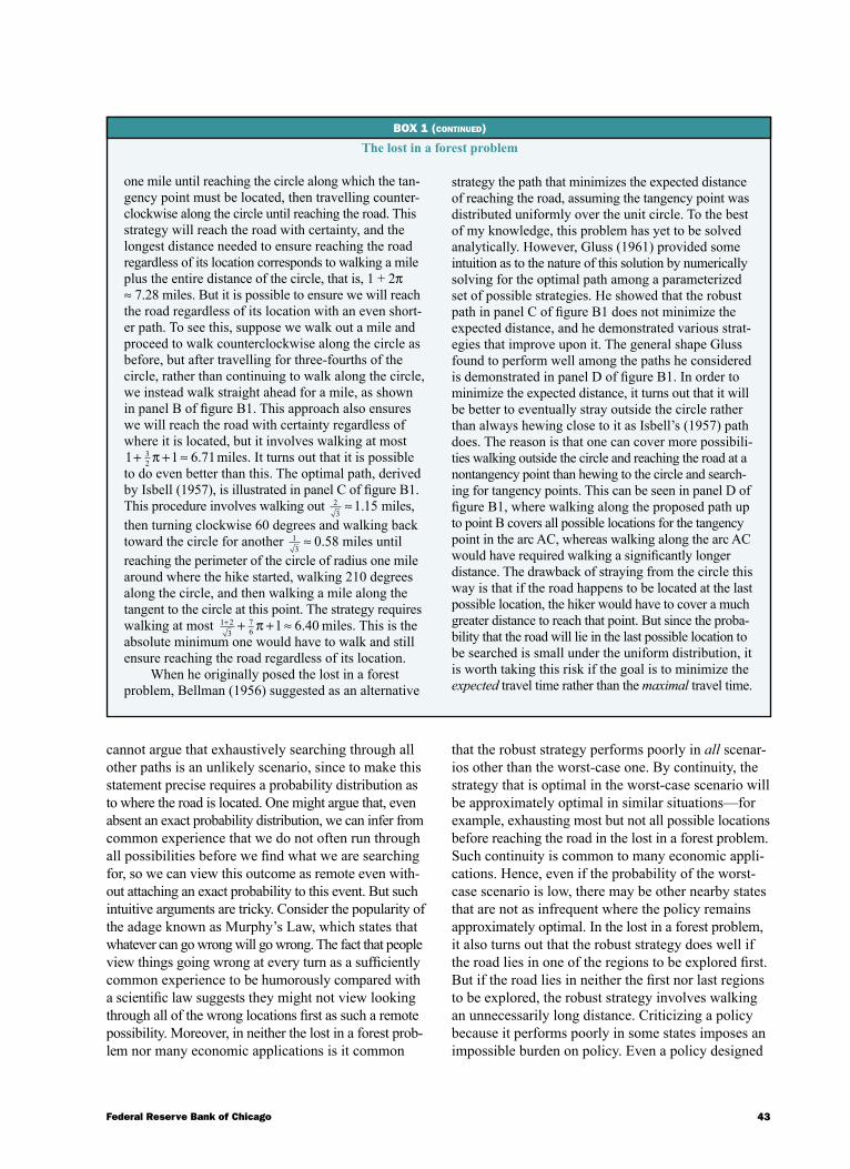
43Federal Reserve Bank of Chicago
cannot argue that exhaustively searching through all other paths is an unlikely scenario, since to make this statement precise requires a probability distribution as to where the road is located. One might argue that, even absent an exact probability distribution, we can infer from common experience that we do not often run through all possibilities before we find what we are searching for, so we can view this outcome as remote even with-out attaching an exact probability to this event. But such intuitive arguments are tricky. Consider the popularity of the adage known as Murphy’s Law, which states that whatever can go wrong will go wrong. The fact that people view things going wrong at every turn as a sufficiently common experience to be humorously compared with a scientific law suggests they might not view looking through all of the wrong locations first as such a remote possibility. Moreover, in neither the lost in a forest prob-lem nor many economic applications is it common
that the robust strategy performs poorly in all scenar-ios other than the worst-case one. By continuity, the strategy that is optimal in the worst-case scenario will be approximately optimal in similar situations—for example, exhausting most but not all possible locations before reaching the road in the lost in a forest problem. Such continuity is common to many economic appli-cations. Hence, even if the probability of the worst-case scenario is low, there may be other nearby states that are not as infrequent where the policy remains approximately optimal. In the lost in a forest problem, it also turns out that the robust strategy does well if the road lies in one of the regions to be explored first. But if the road lies in neither the first nor last regions to be explored, the robust strategy involves walking an unnecessarily long distance. Criticizing a policy because it performs poorly in some states imposes an impossible burden on policy. Even a policy designed
BOX 1 (continued)
The lost in a forest problem
one mile until reaching the circle along which the tan-gency point must be located, then travelling counter-clockwise along the circle until reaching the road. This strategy will reach the road with certainty, and the longest distance needed to ensure reaching the road regardless of its location corresponds to walking a mile plus the entire distance of the circle, that is, 1 + 2π ≈ 7.28 miles. But it is possible to ensure we will reach the road regardless of its location with an even short-er path. To see this, suppose we walk out a mile and proceed to walk counterclockwise along the circle as before, but after travelling for three-fourths of the circle, rather than continuing to walk along the circle, we instead walk straight ahead for a mile, as shown in panel B of figure B1. This approach also ensures we will reach the road with certainty regardless of where it is located, but it involves walking at most 1 1 6 713
2+ + ≈ .π miles. It turns out that it is possible to do even better than this. The optimal path, derived by Isbell (1957), is illustrated in panel C of figure B1. This procedure involves walking out 2
31 15≈ . miles,
then turning clockwise 60 degrees and walking back toward the circle for another 1
30 58≈ . miles until
reaching the perimeter of the circle of radius one mile around where the hike started, walking 210 degrees along the circle, and then walking a mile along the tangent to the circle at this point. The strategy requires walking at most 1 2
376 1 6 40+ + + ≈ .π miles. This is the
absolute minimum one would have to walk and still ensure reaching the road regardless of its location.
When he originally posed the lost in a forest problem, Bellman (1956) suggested as an alternative
strategy the path that minimizes the expected distance of reaching the road, assuming the tangency point was distributed uniformly over the unit circle. To the best of my knowledge, this problem has yet to be solved analytically. However, Gluss (1961) provided some intuition as to the nature of this solution by numerically solving for the optimal path among a parameterized set of possible strategies. He showed that the robust path in panel C of figure B1 does not minimize the expected distance, and he demonstrated various strat-egies that improve upon it. The general shape Gluss found to perform well among the paths he considered is demonstrated in panel D of figure B1. In order to minimize the expected distance, it turns out that it will be better to eventually stray outside the circle rather than always hewing close to it as Isbell’s (1957) path does. The reason is that one can cover more possibili-ties walking outside the circle and reaching the road at a nontangency point than hewing to the circle and search-ing for tangency points. This can be seen in panel D of figure B1, where walking along the proposed path up to point B covers all possible locations for the tangency point in the arc AC, whereas walking along the arc AC would have required walking a significantly longer distance. The drawback of straying from the circle this way is that if the road happens to be located at the last possible location, the hiker would have to cover a much greater distance to reach that point. But since the proba-bility that the road will lie in the last possible location to be searched is small under the uniform distribution, it is worth taking this risk if the goal is to minimize the expected travel time rather than the maximal travel time.
44 2Q/2009, Economic Perspectives
to do well on average (assuming the distribution of outcomes is known) may perform poorly in certain states of the world.
Another critique of robust control holds that, rather than choosing a policy that is robust, decision-makers should act like Bayesians; that is, they should assign subjective beliefs to the various possibilities they con-template, compute an implied expected loss for each strategy, and then choose the strategy that minimizes the expected loss. For example, Sims (2001) argued decision-makers should avoid rules that violate the sure-thing principle, which holds that if one action is preferred to another action regardless of which event is known to occur, it should remain preferred if the event were unknown. The robust control approach can violate this principle, while subjective expected utility does not. The notion of assigning subjective probabilities to different scenarios is especially compelling in the lost in a forest problem, where assigning equal proba-bilities to all locations seems natural given there is no information to suggest that any one direction is more likely than the other. In fact, when Bellman (1956) originally posed his question, he suggested both mini-mizing the longest path (minimax) and minimizing the expected path assuming a uniform prior (min-mean) as ways of solving this problem. This approach need not contradict the policy recommendation that emerges from the robust control approach. In particular, if the cost of effort involved in walking rises steeply with the distance one has to walk, a policy that eliminates the possibility of walking very long distances would naturally emerge as desirable. But at shorter distanc-es, assigning a probability distribution to the location of the road might lead to a different strategy from the robust one. This critique is not aimed at a particular strategy per se, but against using robustness as a cri-terion for choosing which policy to pursue.4
The problem with this critique is that it is not clear that decision-makers would always agree with the recommendation that they assign subjective prob-abilities to scenarios whose likelihood they do not know. As an example, assigning a distribution to the location of the road in the lost in a forest problem is incompatible with the notion of Murphy’s Law. Inherent in Murphy’s Law is the notion that the location of the road depends on where the hiker chooses to search. But the Bayesian approach assumes a fixed distribu-tion regardless of what action the hiker chooses. Thus, to a person who finds Murphy’s Law appealing, pro-ceeding like a Bayesian would ring false. As another example, consider the “Ellsberg paradox,” which is due to Ellsberg (1961). This paradox is based on a thought experiment in which people are asked to
choose between a lottery with a known probability of winning and another lottery featuring identical prizes but with an unknown probability of winning. Ellsberg argued that most people would prefer to avoid the lot-tery whose probability of winning they do not know and would not choose as if they assigned a fixed sub-jective probability to the lottery with an unknown prob-ability of winning. In other words, the preferences exhibited by most people would seem paradoxical to someone who behaved like a Bayesian. Subsequent researchers who conducted experiments offering these choices to real-life test subjects, starting with Becker and Brownson (1964), confirmed this conjecture. The saliency of these findings suggests that the failure to behave like a Bayesian may reflect genuine discomfort by test subjects with the Bayesian approach of assign-ing subjective probabilities to outcomes whose prob-abilities they do not know. But if this is so, we cannot objectively fault decision-makers for not adopting the Bayesian approach, since any recommendation we make to them would have to respect their preferences.
Of course, even accepting that policymakers may not always find the Bayesian approach appealing, it does not automatically follow that they should favor the robust control approach in particular. The relevant question is whether there is a compelling reason for decision-makers to specifically prefer the robust poli-cy. One result often cited by advocates of robust con-trol is the work of Gilboa and Schmeidler (1989). They show that if decision-makers’ preferences over lotteries satisfy a particular set of restrictions, it will be possible to represent their choices as if they chose the action that minimizes the largest possible expected loss across a particular set of probability distributions. However, this result is not an entirely satisfactory argument for why policymakers should adopt the robust control approach. First, there is little evidence to suggest that standard preferences obey the various restrictions derived by Gilboa and Schmeidler (1989). While the Ellsberg paradox suggests many people have preferences different from those that would lead them to behave like Bayesians, it does not by itself confirm that preferences accord with each one of the restrictions in Gilboa and Schmeidler (1989). Second, Gilboa and Schmeidler (1989) show that the set of scenarios from which the worst case is calculated depends on the pref-erences of the decision-makers. This is not equivalent to arguing that policymakers, once they restrict the set of admissible models that could potentially account for the data they observe, should always choose the action that minimizes the worst-case outcome from this set.
In the lost in a forest problem, Gilboa and Schmeidler’s (1989) result only tells us that if an
45Federal Reserve Bank of Chicago
individual exhibited particular preferences toward lotter-ies whose outcomes dictate distances he would have to walk, he would in fact prefer the minimax solution to this problem. It does not say that whenever he faces un-certainty more generally—for example, if he also forgot how far away he was from the road when he lay down—that he would still choose the strategy dictated by the robust control approach. In short, Gilboa and Schmeidler (1989) show that opting for a robust strategy is coherent in that we can find well-posed preferences that ratio-nalize this behavior, but their analysis does not imply such preferences are common or that robustness is a desirable criterion whenever one is at a loss to assign probabilities to various possible scenarios.5
The theme that runs through the discussion thus far is that if the decision-makers cannot assign proba-bilities to scenarios they are uncertain about, there is no inherently correct criterion on how to choose a policy. As Manski (2000, p. 421) put it, “there is no compelling reason why the decision maker should or should not use the maximin rule when [the probability distribution] is a fixed but unknown objective function. In this setting, the appeal of the maximin rule is a per-sonal rather than normative matter. Some decision makers may deem it essential to protect against worst-case scenarios, while others may not.”6 One can point to unappealing elements about robust control, but these do not definitively rule out this approach. Conversely, individuals with particular preferences toward lotteries might behave as if they were following a minimax rule, but this does not imply that they will adopt such a rule whenever they are unable to assign probabilities to possi-ble scenarios. Among engineers, the notion of designing systems that minimize the worst-case scenario among the set of possible states whose exact probability is un-known has carried some appeal. Interestingly, Murphy’s Law is also an export from the field of engineering.7 The two observations may be related: If worst-case outcomes are viewed not as rare events but as common experiences, robustness would naturally seem like an appealing criterion. Policymakers who are nervous about worst-case outcomes would presumably find appeal in the notion of keeping the potential risk exposure to the bare minimum. More generally, studying robust policies can help us to understand the costs and bene-fits of maximally aggressive risk management so that policymakers can contemplate their desirability.
Recasting the Brainard model as a robust control problem
Now that I have described what it means for a policy to be robust, I can return to the question of how a policymaker concerned about robustness should act
when trying to target a variable in an uncertain environ-ment. In particular, I will now revisit the environment that Brainard (1967) considered, but with one key differ-ence: The policymaker is assumed to be unable to assign probabilities to the scenarios he is uncertain about. In what follows, I introduce uncertainty in a way that Hansen and Sargent (2008) and Williams (2008) describe as structured uncertainty; that is, I assume the policymaker knows the model but is un-certain about the exact value of one of its parameters. More precisely, he knows that the parameter lies in some range, but he cannot ascribe a probability distri-bution to the values within this range. By contrast, un-structured uncertainty corresponds to the case where a model is defined as a probability distribution over outcomes, and where the policymaker is unsure about which probability distribution from some set represents the true distribution from which the data are drawn.8
Once again, I begin by assuming that the variable in question, y, is affected linearly by a policy variable, r; various factors that the policymaker can observe prior to setting policy, x; and other factors that the policymaker cannot observe prior to setting his policy but whose distribution is known, εu:
5) y = x – kr + εu.
As before, I assume εu has mean 0 and variance σu2 .
To capture uncertainty about the effect of policy, I modify the coefficient on r to allow for uncertainty:
6) y = x – (k + εk) r + εu.
In contrast to Brainard’s (1967) setup, I assume that rather than knowing the distribution of εk, the policy-maker only knows that its support is restricted to theinterval ε ε, that includes 0, that is, ε ε< <0 . In other words, the effect of r on y can be less than, equal to, or higher than k. Beyond this, he will not be able to assign probabilities to particular values within this interval.
Since the support of εk will figure prominently in formulating the robust strategy, it is worth commenting on where it might come from. In practice, information about k + εk is presumably compiled from past data. That is, given time-series data on y, x, and r, we can estimate k + εk by using standard regression techniques. With a finite history, our estimate would necessarily be noisy due to variation from εu. However, we might still be able to reject some values for k + εk as implau-sible—for example, values that are several standard errors away from our point estimate. Still, there is something seemingly arbitrary in classifying some values of k as possible while treating virtually identical
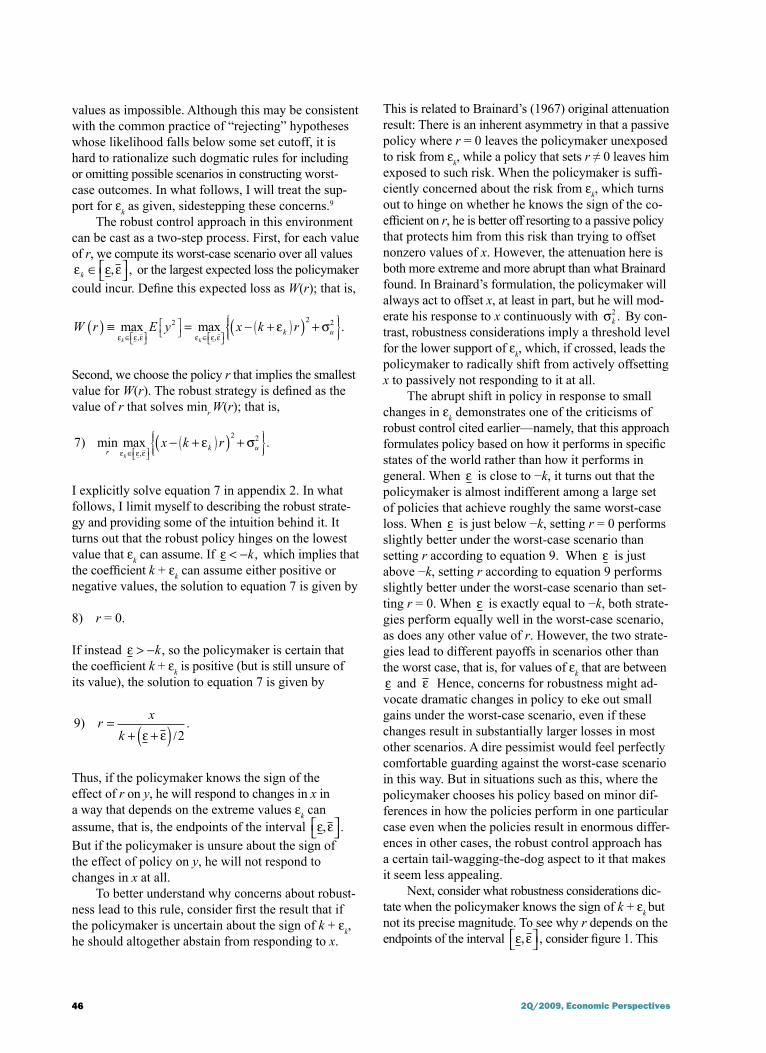
46 2Q/2009, Economic Perspectives
values as impossible. Although this may be consistent with the common practice of “rejecting” hypotheses whose likelihood falls below some set cutoff, it is hard to rationalize such dogmatic rules for including or omitting possible scenarios in constructing worst-case outcomes. In what follows, I will treat the sup-port for εk as given, sidestepping these concerns.9
The robust control approach in this environment can be cast as a two-step process. First, for each value of r, we compute its worst-case scenario over all values ε ε εk ∈ , , or the largest expected loss the policymakercould incur. Define this expected loss as W(r); that is,
W r E y x k rk k
k u( ) ≡ = − +( ) +∈ ,
∈ ,
( )max max
ε ε ε ε ε εε σ2 2 2
.
Second, we choose the policy r that implies the smallest value for W(r). The robust strategy is defined as the value of r that solves minr W(r); that is,
72 2) min max .
r k uk
x k rε ε ε
ε σ∈ ,
( )
− +( ) +
I explicitly solve equation 7 in appendix 2. In what follows, I limit myself to describing the robust strate-gy and providing some of the intuition behind it. It turns out that the robust policy hinges on the lowest value that εk can assume. If ε < −k, which implies that the coefficient k + εk can assume either positive or negative values, the solution to equation 7 is given by
8) r = 0.
If instead ε > −k, so the policymaker is certain that the coefficient k + εk is positive (but is still unsure of its value), the solution to equation 7 is given by
92
) .rx
k=
+ +( ) /ε ε
Thus, if the policymaker knows the sign of the effect of r on y, he will respond to changes in x in a way that depends on the extreme values εk can assume, that is, the endpoints of the interval ε ε, .But if the policymaker is unsure about the sign of the effect of policy on y, he will not respond to changes in x at all.
To better understand why concerns about robust-ness lead to this rule, consider first the result that if the policymaker is uncertain about the sign of k + εk, he should altogether abstain from responding to x.
This is related to Brainard’s (1967) original attenuation result: There is an inherent asymmetry in that a passive policy where r = 0 leaves the policymaker unexposed to risk from εk, while a policy that sets r ≠ 0 leaves him exposed to such risk. When the policymaker is suffi-ciently concerned about the risk from εk, which turns out to hinge on whether he knows the sign of the co-efficient on r, he is better off resorting to a passive policy that protects him from this risk than trying to offset nonzero values of x. However, the attenuation here is both more extreme and more abrupt than what Brainard found. In Brainard’s formulation, the policymaker will always act to offset x, at least in part, but he will mod-erate his response to x continuously with σk
2 . By con-trast, robustness considerations imply a threshold level for the lower support of εk, which, if crossed, leads the policymaker to radically shift from actively offsetting x to passively not responding to it at all.
The abrupt shift in policy in response to small changes in εk demonstrates one of the criticisms of robust control cited earlier—namely, that this approach formulates policy based on how it performs in specific states of the world rather than how it performs in general. When ε is close to −k, it turns out that the policymaker is almost indifferent among a large set of policies that achieve roughly the same worst-case loss. When ε is just below −k, setting r = 0 performs slightly better under the worst-case scenario than setting r according to equation 9. When ε is just above −k, setting r according to equation 9 performs slightly better under the worst-case scenario than set-ting r = 0. When ε is exactly equal to −k, both strate-gies perform equally well in the worst-case scenario, as does any other value of r. However, the two strate-gies lead to different payoffs in scenarios other than the worst case, that is, for values of εk that are between ε and ε. Hence, concerns for robustness might ad-vocate dramatic changes in policy to eke out small gains under the worst-case scenario, even if these changes result in substantially larger losses in most other scenarios. A dire pessimist would feel perfectly comfortable guarding against the worst-case scenario in this way. But in situations such as this, where the policymaker chooses his policy based on minor dif-ferences in how the policies perform in one particular case even when the policies result in enormous differ-ences in other cases, the robust control approach has a certain tail-wagging-the-dog aspect to it that makes it seem less appealing.
Next, consider what robustness considerations dic-tate when the policymaker knows the sign of k + εk but not its precise magnitude. To see why r depends on the endpoints of the interval ε ε, , consider figure 1. This
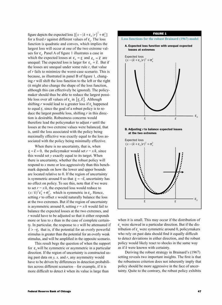
47Federal Reserve Bank of Chicago
figure depicts the expected loss [ ]2 2x k rk u− +( ) +( )ε σ
for a fixed r against different values of εk. The loss function is quadratic and convex, which implies the largest loss will occur at one of the two extreme val-ues for εk. Panel A of figure 1 illustrates a case in which the expected losses at ε εk = and ε εk = are unequal: The expected loss is larger for ε εk = . But if the losses are unequal under some rule r, that value of r fails to minimize the worst-case scenario. This is because, as illustrated in panel B of figure 1, chang-ing r will shift the loss function to the left or the right (it might also change the shape of the loss function, although this can effectively be ignored). The policy-maker should thus be able to reduce the largest possi-ble loss over all values of εk in ε ε, .[ ] Although shifting r would lead to a greater loss if εk happened to equal ε, since the goal of a robust policy is to re-duce the largest possible loss, shifting r in this direc-tion is desirable. Robustness concerns would therefore lead the policymaker to adjust r until the losses at the two extreme values were balanced, that is, until the loss associated with the policy being maximally effective was exactly equal to the loss as-sociated with the policy being minimally effective.
When there is no uncertainty, that is, whenε ε= = 0, the policymaker would set r = x/k, since this would set y exactly equal to its target. When there is uncertainty, whether the robust policy will respond to x more or less aggressively than this bench-mark depends on how the lower and upper bounds are located relative to 0. If the region of uncertainty is symmetric around 0 so that ε ε= − , uncertainty has no effect on policy. To see this, note that if we were to set r = x/k, the expected loss would reduce to ( / ) ,x k k u
2 2 2ε σ+ which is symmetric in εk. Hence, setting r to offset x would naturally balance the loss at the two extremes. But if the region of uncertainty is asymmetric around 0, setting r = x/k would fail to balance the expected losses at the two extremes, and r would have to be adjusted so that it either responds more or less to x than in the case of complete certain-ty. In particular, the response to x will be attenuated if ε ε> − , that is, if the potential for an overly powerful stimulus is greater than the potential for an overly weak stimulus, and will be amplified in the opposite scenario.
This result begs the question of when the support for εk will be symmetric or asymmetric in a particular direction. If the region of uncertainty is constructed us-ing past data on y, x, and r, any asymmetry would have to be driven by differences in detection probabili-ties across different scenarios—for example, if it is more difficult to detect k when its value is large than
when it is small. This may occur if the distribution of εu were skewed in a particular direction. But if the dis-tribution of εu were symmetric around 0, policymakers who rely on past data should find it equally difficult to detect deviations in either direction, and the robust policy would likely react to shocks in the same way as if k were known with certainty.
Deriving the robust strategy in Brainard’s (1967) setting reveals two important insights. The first is that the robustness criterion does not inherently imply that policy should be more aggressive in the face of uncer-tainty. Quite to the contrary, the robust policy exhibits
FIguRE 1
Loss functions for the robust Brainard (1967) model
A. Expected loss function with unequal expected losses at extremes
Expected loss( ( ) )x k rk u− + +ε σ2 2
B. Adjusting r to balance expected losses at the two extremes
Expected loss( ( ) )x k rk u− + +ε σ2 2
ε εεk
ε εεk
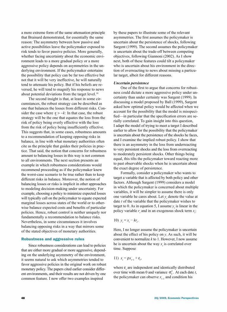
48 2Q/2009, Economic Perspectives
by these papers to illustrate some of the relevant asymmetries. The first assumes the policymaker is uncertain about the persistence of shocks, following Sargent (1999). The second assumes the policymaker is uncertain about the trade-off between competing objectives, following Giannoni (2002). As I show next, both of these features could tilt a policymaker who is uncertain about his environment in the direc-tion of overreacting to news about missing a particu-lar target, albeit for different reasons.
Uncertain persistenceOne of the first to argue that concerns for robust-
ness could dictate a more aggressive policy under un-certainty than under certainty was Sargent (1999). In discussing a model proposed by Ball (1999), Sargent asked how optimal policy would be affected when we account for the possibility that the model is misspeci-fied—in particular that the specification errors are se-rially correlated. To gain insight into this question, I adapt the model of trying to meet a target I described earlier to allow for the possibility that the policymaker is uncertain about the persistence of the shocks he faces, and I examine the implied robust policy. I show that there is an asymmetry in the loss from underreacting to very persistent shocks and the loss from overreacting to moderately persistent shocks. Other things being equal, this tilts the policymaker toward reacting more to past observable shocks when he is uncertain about the exact degree of persistence.
Formally, consider a policymaker who wants to target a variable that is affected by both policy and other factors. Although Sargent (1999) considers a model in which the policymaker is concerned about multiple variables, it will be simpler to assume there is only one variable he cares about. Let yt denote the value at date t of the variable that the policymaker wishes to target to 0. As in equation 5, I assume yt is linear in the policy variable rt and in an exogenous shock term xt:
10) yt = xt − krt.
Here, I no longer assume the policymaker is uncertain about the effect of his policy on y. As such, it will be convenient to normalize k to 1. However, I now assume he is uncertain about the way xt is correlated over time. Suppose
11) xt = ρxt−1 + εt,
where εt are independent and identically distributed over time with mean 0 and variance σε
2 . At each date t, the policymaker can observe xt–1 and condition his
a more extreme form of the same attenuation principle that Brainard demonstrated, for essentially the same reason: The asymmetry between how passive and active possibilities leave the policymaker exposed to risk tends to favor passive policies. More generally, whether facing uncertainty about the economic envi-ronment leads to a more gradual policy or a more aggressive policy depends on asymmetries in the un-derlying environment. If the policymaker entertains the possibility that policy can be far too effective but not that it will be very ineffective, he will naturally tend to attenuate his policy. But if his beliefs are re-versed, he will tend to magnify his response to news about potential deviations from the target level.10
The second insight is that, at least in some cir-cumstances, the robust strategy can be described as one that balances the losses from different risks. Con-sider the case where ε > −k: In that case, the robust strategy will be the one that equates the loss from the risk of policy being overly effective with the loss from the risk of policy being insufficiently effective. This suggests that, in some cases, robustness amounts to a recommendation of keeping opposing risks in balance, in line with what monetary authorities often cite as the principle that guides their policies in prac-tice. That said, the notion that concerns for robustness amount to balancing losses in this way is not common to all environments. The next section presents an example in which robustness considerations would recommend proceeding as if the policymaker knew the worst-case scenario to be true rather than to keep different risks in balance. Moreover, the notion of balancing losses or risks is implicit in other approaches to modeling decision-making under uncertainty. For example, choosing a policy to minimize expected losses will typically call on the policymaker to equate expected marginal losses across states of the world or to other-wise balance expected costs and benefits of particular policies. Hence, robust control is neither uniquely nor fundamentally a recommendation to balance risks. Nevertheless, in some circumstances it involves balancing opposing risks in a way that mirrors some of the stated objectives of monetary authorities.
Robustness and aggressive rules
Since robustness considerations can lead to policies that are either more gradual or more aggressive, depend-ing on the underlying asymmetry of the environment, it seems natural to ask which asymmetries tended to favor aggressive policies in the original work on robust monetary policy. The papers cited earlier consider differ-ent environments, and their results are not driven by one common feature. I now offer two examples inspired
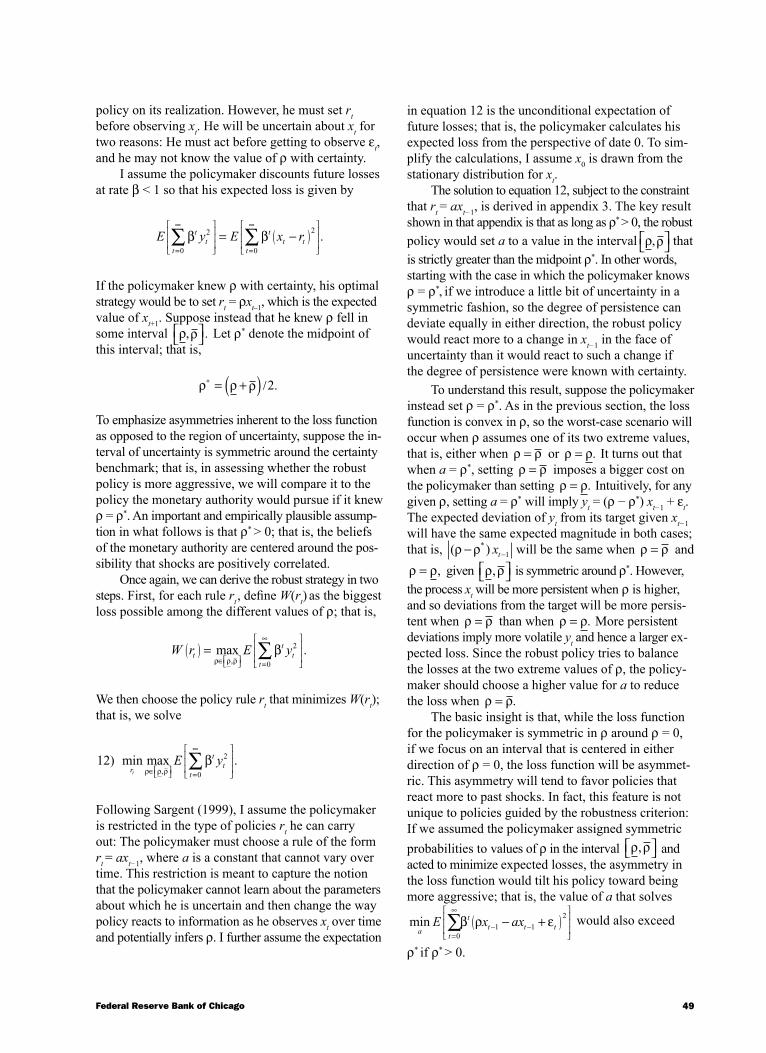
49Federal Reserve Bank of Chicago
policy on its realization. However, he must set rt before observing xt. He will be uncertain about xt for two reasons: He must act before getting to observe εt, and he may not know the value of ρ with certainty.
I assume the policymaker discounts future losses at rate β < 1 so that his expected loss is given by
E y E x rt
tt
t
tt t
=
∞
=
∞
( )
∑ ∑= −
0
2
0
2β β .
If the policymaker knew ρ with certainty, his optimal strategy would be to set rt = ρxt–1, which is the expected value of xt+1. Suppose instead that he knew ρ fell in some interval ρ ρ, . Let ρ* denote the midpoint of this interval; that is,
ρ ρ ρ∗ = +( ) /2.
To emphasize asymmetries inherent to the loss function as opposed to the region of uncertainty, suppose the in-terval of uncertainty is symmetric around the certainty benchmark; that is, in assessing whether the robust policy is more aggressive, we will compare it to the policy the monetary authority would pursue if it knew ρ = ρ*. An important and empirically plausible assump-tion in what follows is that ρ* > 0; that is, the beliefs of the monetary authority are centered around the pos-sibility that shocks are positively correlated.
Once again, we can derive the robust strategy in two steps. First, for each rule rt , define W(rt) as the biggest loss possible among the different values of ρ; that is,
W r E ytt
tt( )
∈ , =
∞
= ∑max .ρ ρ ρ
β0
2
We then choose the policy rule rt that minimizes W(rt); that is, we solve
120
2) min max .r
t
tt
t
E yρ ρ ρ
β∈ , =
∞
∑
Following Sargent (1999), I assume the policymaker is restricted in the type of policies rt he can carry out: The policymaker must choose a rule of the form rt = axt−1, where a is a constant that cannot vary over time. This restriction is meant to capture the notion that the policymaker cannot learn about the parameters about which he is uncertain and then change the way policy reacts to information as he observes xt over time and potentially infers ρ. I further assume the expectation
in equation 12 is the unconditional expectation of future losses; that is, the policymaker calculates his expected loss from the perspective of date 0. To sim-plify the calculations, I assume x0 is drawn from the stationary distribution for xt.
The solution to equation 12, subject to the constraint that rt = axt−1, is derived in appendix 3. The key result shown in that appendix is that as long as ρ* > 0, the robustpolicy would set a to a value in the interval ρ ρ, thatis strictly greater than the midpoint ρ*. In other words, starting with the case in which the policymaker knows ρ = ρ*, if we introduce a little bit of uncertainty in a symmetric fashion, so the degree of persistence can deviate equally in either direction, the robust policy would react more to a change in xt−1 in the face of uncertainty than it would react to such a change if the degree of persistence were known with certainty.
To understand this result, suppose the policymaker instead set ρ = ρ*. As in the previous section, the loss function is convex in ρ, so the worst-case scenario will occur when ρ assumes one of its two extreme values, that is, either when ρ ρ= or ρ ρ= . It turns out that when a = ρ*, setting ρ ρ= imposes a bigger cost on the policymaker than setting ρ ρ= . Intuitively, for any given ρ, setting a = ρ* will imply yt = (ρ − ρ*) xt−1 + εt. The expected deviation of yt from its target given xt−1 will have the same expected magnitude in both cases; that is, ( )*ρ ρ− −xt 1 will be the same when ρ ρ= andρ ρ= , given ρ ρ, is symmetric around ρ*. However, the process xt will be more persistent when ρ is higher, and so deviations from the target will be more persis-tent when ρ ρ= than when ρ ρ= . More persistent deviations imply more volatile yt and hence a larger ex-pected loss. Since the robust policy tries to balance the losses at the two extreme values of ρ, the policy-maker should choose a higher value for a to reduce the loss when ρ ρ= .
The basic insight is that, while the loss function for the policymaker is symmetric in ρ around ρ = 0, if we focus on an interval that is centered in either direction of ρ = 0, the loss function will be asymmet-ric. This asymmetry will tend to favor policies that react more to past shocks. In fact, this feature is not unique to policies guided by the robustness criterion: If we assumed the policymaker assigned symmetricprobabilities to values of ρ in the interval ρ ρ, and acted to minimize expected losses, the asymmetry in the loss function would tilt his policy toward being more aggressive; that is, the value of a that solves
mina
t
tt t tE x ax
=
∞
− −( )
∑ − +
0
2
1 1β ρ ε would also exceed ρ* if ρ* > 0.
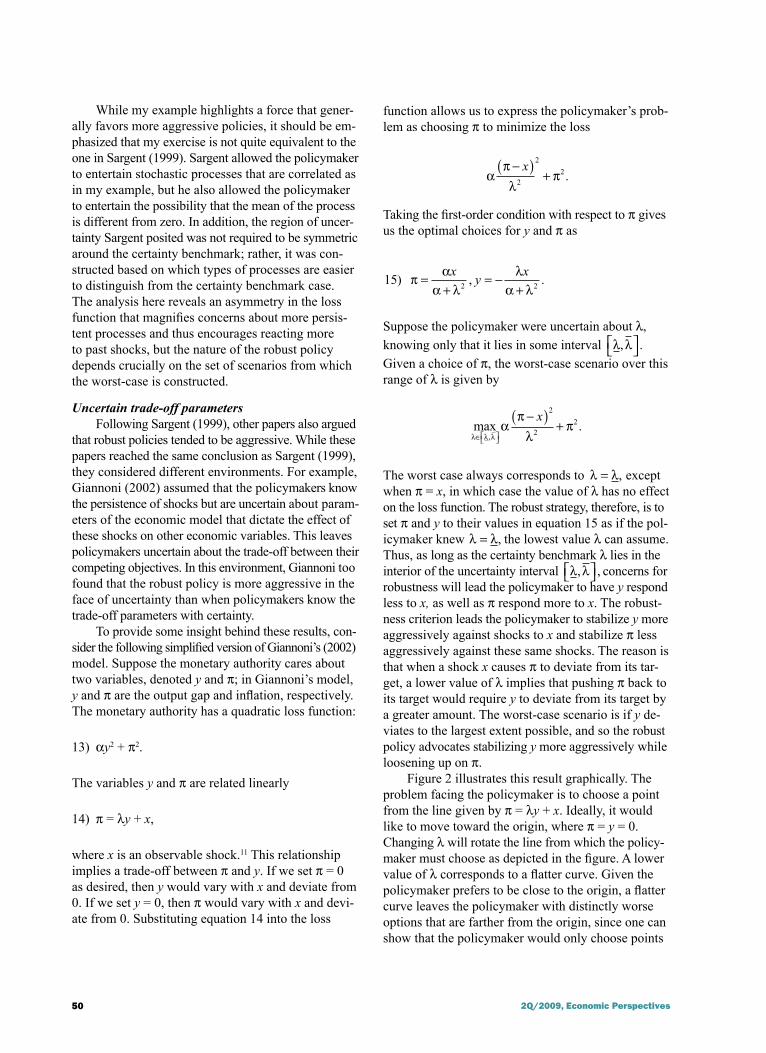
50 2Q/2009, Economic Perspectives
function allows us to express the policymaker’s prob-lem as choosing π to minimize the loss
απλ
π−( )
+x
2
2
2 .
Taking the first-order condition with respect to π gives us the optimal choices for y and π as
152 2
) , .π αα λ
λα λ
=+
= −+
xy
x
Suppose the policymaker were uncertain about λ, knowing only that it lies in some interval λ λ, . Given a choice of π, the worst-case scenario over this range of λ is given by
max .λ λ λ
απ
λπ
∈ ,
−( )+
2
22x
The worst case always corresponds to λ λ= , except when π = x, in which case the value of λ has no effect on the loss function. The robust strategy, therefore, is to set π and y to their values in equation 15 as if the pol-icymaker knew λ λ= , the lowest value λ can assume. Thus, as long as the certainty benchmark λ lies in the interior of the uncertainty interval λ λ, , concerns for robustness will lead the policymaker to have y respond less to x, as well as π respond more to x. The robust-ness criterion leads the policymaker to stabilize y more aggressively against shocks to x and stabilize π less aggressively against these same shocks. The reason is that when a shock x causes π to deviate from its tar-get, a lower value of λ implies that pushing π back to its target would require y to deviate from its target by a greater amount. The worst-case scenario is if y de-viates to the largest extent possible, and so the robust policy advocates stabilizing y more aggressively while loosening up on π.
Figure 2 illustrates this result graphically. The problem facing the policymaker is to choose a point from the line given by π = λy + x. Ideally, it would like to move toward the origin, where π = y = 0. Changing λ will rotate the line from which the policy-maker must choose as depicted in the figure. A lower value of λ corresponds to a flatter curve. Given the policymaker prefers to be close to the origin, a flatter curve leaves the policymaker with distinctly worse options that are farther from the origin, since one can show that the policymaker would only choose points
While my example highlights a force that gener-ally favors more aggressive policies, it should be em-phasized that my exercise is not quite equivalent to the one in Sargent (1999). Sargent allowed the policymaker to entertain stochastic processes that are correlated as in my example, but he also allowed the policymaker to entertain the possibility that the mean of the process is different from zero. In addition, the region of uncer-tainty Sargent posited was not required to be symmetric around the certainty benchmark; rather, it was con-structed based on which types of processes are easier to distinguish from the certainty benchmark case. The analysis here reveals an asymmetry in the loss function that magnifies concerns about more persis-tent processes and thus encourages reacting more to past shocks, but the nature of the robust policy depends crucially on the set of scenarios from which the worst-case is constructed.
Uncertain trade-off parametersFollowing Sargent (1999), other papers also argued
that robust policies tended to be aggressive. While these papers reached the same conclusion as Sargent (1999), they considered different environments. For example, Giannoni (2002) assumed that the policymakers know the persistence of shocks but are uncertain about param-eters of the economic model that dictate the effect of these shocks on other economic variables. This leaves policymakers uncertain about the trade-off between their competing objectives. In this environment, Giannoni too found that the robust policy is more aggressive in the face of uncertainty than when policymakers know the trade-off parameters with certainty.
To provide some insight behind these results, con-sider the following simplified version of Giannoni’s (2002) model. Suppose the monetary authority cares about two variables, denoted y and π; in Giannoni’s model, y and π are the output gap and inflation, respectively. The monetary authority has a quadratic loss function:
13) αy2 + π2.
The variables y and π are related linearly
14) π = λy + x,
where x is an observable shock.11 This relationship implies a trade-off between π and y. If we set π = 0 as desired, then y would vary with x and deviate from 0. If we set y = 0, then π would vary with x and devi-ate from 0. Substituting equation 14 into the loss
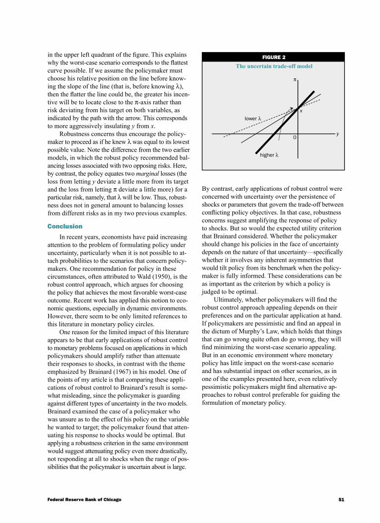
51Federal Reserve Bank of Chicago
By contrast, early applications of robust control were concerned with uncertainty over the persistence of shocks or parameters that govern the trade-off between conflicting policy objectives. In that case, robustness concerns suggest amplifying the response of policy to shocks. But so would the expected utility criterion that Brainard considered. Whether the policymaker should change his policies in the face of uncertainty depends on the nature of that uncertainty—specifically whether it involves any inherent asymmetries that would tilt policy from its benchmark when the policy-maker is fully informed. These considerations can be as important as the criterion by which a policy is judged to be optimal.
Ultimately, whether policymakers will find the robust control approach appealing depends on their preferences and on the particular application at hand. If policymakers are pessimistic and find an appeal in the dictum of Murphy’s Law, which holds that things that can go wrong quite often do go wrong, they will find minimizing the worst-case scenario appealing. But in an economic environment where monetary policy has little impact on the worst-case scenario and has substantial impact on other scenarios, as in one of the examples presented here, even relatively pessimistic policymakers might find alternative ap-proaches to robust control preferable for guiding the formulation of monetary policy.
in the upper left quadrant of the figure. This explains why the worst-case scenario corresponds to the flattest curve possible. If we assume the policymaker must choose his relative position on the line before know-ing the slope of the line (that is, before knowing λ), then the flatter the line could be, the greater his incen-tive will be to locate close to the π-axis rather than risk deviating from his target on both variables, as indicated by the path with the arrow. This corresponds to more aggressively insulating y from x.
Robustness concerns thus encourage the policy-maker to proceed as if he knew λ was equal to its lowest possible value. Note the difference from the two earlier models, in which the robust policy recommended bal-ancing losses associated with two opposing risks. Here, by contrast, the policy equates two marginal losses (the loss from letting y deviate a little more from its target and the loss from letting π deviate a little more) for a particular risk, namely, that λ will be low. Thus, robust-ness does not in general amount to balancing losses from different risks as in my two previous examples.
Conclusion
In recent years, economists have paid increasing attention to the problem of formulating policy under uncertainty, particularly when it is not possible to at-tach probabilities to the scenarios that concern policy-makers. One recommendation for policy in these circumstances, often attributed to Wald (1950), is the robust control approach, which argues for choosing the policy that achieves the most favorable worst-case outcome. Recent work has applied this notion to eco-nomic questions, especially in dynamic environments. However, there seem to be only limited references to this literature in monetary policy circles.
One reason for the limited impact of this literature appears to be that early applications of robust control to monetary problems focused on applications in which policymakers should amplify rather than attenuate their responses to shocks, in contrast with the theme emphasized by Brainard (1967) in his model. One of the points of my article is that comparing these appli-cations of robust control to Brainard’s result is some-what misleading, since the policymaker is guarding against different types of uncertainty in the two models. Brainard examined the case of a policymaker who was unsure as to the effect of his policy on the variable he wanted to target; the policymaker found that atten-uating his response to shocks would be optimal. But applying a robustness criterion in the same environment would suggest attenuating policy even more drastically, not responding at all to shocks when the range of pos-sibilities that the policymaker is uncertain about is large.
FIguRE 2
The uncertain trade-off model
π
x
y0
lower λ
higher λ
52 2Q/2009, Economic Perspectives
NOTES
1Onatski and Stock (2002) also argue that aggressiveness is not a generic feature of robust policies, but they note that in their framework, aggressiveness will arise for many classes of perturbations.
2The problem is sometimes referred to as the “lost at sea” problem. Richard Bellman, who originally posed the problem, is well-known among economists for his work on dynamic programming, a tool used by economists to analyze sequential decision problems that unfold over time. I refer to this example only because of its intui-tive appeal and not to draw any analogies between the practice of conducting monetary policy and the situation of being lost.
3An example of this critique can be found in Svensson (2007), who writes “if a Bayesian prior probability measure were to be assigned to the feasible set of models, one might find that the probability assigned to the models on the boundary are exceedingly small. Thus, highly unlikely models can come to dominate the outcome of robust control.” Bernanke (2007) also refers to (but does not invoke) this critique of robust control.
4In this spirit, Sims (2001) suggested using robust control to aid Bayesian decision-makers who for convenience rely on procedural rules rather than explicit optimization. The idea is to figure out under what prior beliefs about the models it would be optimal to pursue the robust strategy, and then reflect on whether this prior distribution seems sensible. As Sims notes, deriving the robust strategy “may alert decision-makers to forms of prior that, on re-flection, do not seem far from what they actually might believe, yet imply decisions very different from that arrived at by other simple procedures.” Interestingly, Sims’ prescription cannot be applied to the lost in a forest problem: There is no distribution over the location of the road for which the minimax path minimizes expected distance. However, an analogous argument can be made regarding the cost of effort needed to walk various distances. If the hiker relies on procedural rules, he can back out how steeply the cost of effort must rise with distance to justify the minimax path. This will alert him to paths that are different from recommen-dations arrived at by other simple procedures but rely on plausible cost of effort functions.
5Strictly speaking, Gilboa and Schmeidler (1989) only consider a static one-shot decision, while the lost in a forest problem is a dynamic problem in which the hiker must constantly choose how to search given the results of his search at each point in time. However, the problem can be represented as a static decision in which the hiker chooses his search algorithm before starting to search. This is because he would never choose to revise his plans as a result of what he learns; if he did, he could have designed his search algorithm that way before starting to search. This will not be true in many economic applications, where there may be prob-lems with time inconsistency that complicate the task of how to extend the minimax notion to such choices. For a discussion of axiomatic representations of minimax behavior in dynamic envi-ronments, see Epstein and Schneider (2003) and Maccheroni, Marinacci, and Rustichini (2006).
6For the purposes of this article, the terms “minimax rule” and “robust strategy” can be viewed as interchangeable with the term “maximin rule” that Manski (2000) uses.
7According to Spark (2006), the law is named after aerospace engineer Edward Murphy, who complained after a technician attached a pair of sensors in a precisely incorrect configuration during a crash test Murphy was observing. Engineers on the team Murphy was working with began referring to the notion that things will inevitably go wrong as Murphy’s Law, and the expression gained public notoriety after one of the engineers used it in a press conference.
8For example, the set of distributions the policymaker is allowed to entertain might be those whose relative entropy to the distribu-tion of some benchmark model falls below some threshold. There are other papers that similarly focus on structured uncertainty because of its simplicity—for example, Svensson (2007).
9One way to avoid this issue is to model concerns for robustness in a different way. In particular, rather than restrict the set of sce-narios policymakers can entertain to some set, we can allow the set to be unrestricted but introduce a penalty function that punishes scenarios continuously depending on how much they differ from some benchmark scenario—for example, the point estimates from an empirical regression. This formulation is known as multiplier preferences, since the penalty function is scaled by a multiplicative parameter that captures concern for model misspecification. See Hansen and Sargent (2008) for a more detailed discussion.
10Rustem, Wieland, and Zakovic (2007) also consider robust con-trol in asymmetric models, although they do not discuss the impli-cations of this for gradual policy versus aggressive policy.
11This relationship is a simplistic representation of the New Keynesian Phillips curve Giannoni (2002) uses, in which inflation at date t depends on the output gap at date t, expected inflation at date t + 1, and a shock term; that is, πt = λyt + βEtπt+1+ xt. If xt is in-dependent and identically distributed over time, expected inflation would just enter as a constant, and the results would be identical to those in the simplified model I use.
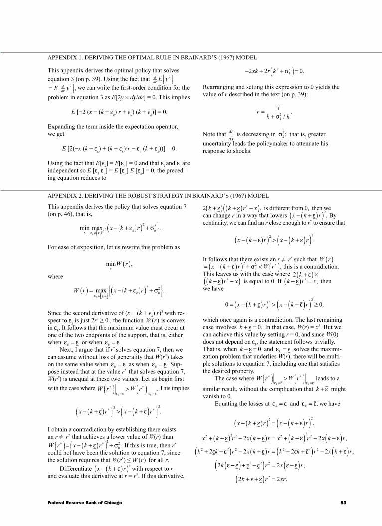
53Federal Reserve Bank of Chicago
This appendix derives the optimal policy that solves equation 3 (on p. 39). Using the fact that d
dr E y2
=
E yddr
2 , we can write the first-order condition for the problem in equation 3 as E[2y × dy/dr] = 0. This implies
E [−2 (x − (k + εk) r + εu) (k + εk)] = 0.
Expanding the term inside the expectation operator, we get
E [2(−x (k + εk) + (k + εk)2r − εu (k + εk))] = 0.
Using the fact that E[εk] = E[εu] = 0 and that εk and εu are independent so E [εk
εu] = E [εu] E [εk] = 0, the preced-ing equation reduces to
APPENDIX 1. DErIvING ThE OPTIMAL rULE IN BrAINArD’S (1967) MODEL
− + + =
2 2 02 2xk r k kσ .
Rearranging and setting this expression to 0 yields the value of r described in the text (on p. 39):
rx
k kk
=+ /σ2
.
Note that drdx
is decreasing in σk2 ; that is, greater
uncertainty leads the policymaker to attenuate his response to shocks.
APPENDIX 2. DErIvING ThE rOBUST STrATEGy IN BrAINArD’S (1967) MODEL
This appendix derives the policy that solves equation 7 (on p. 46), that is,
min max .r k u
k
x k rε ε ε
ε σ∈ ,
( )
− +( ) +
2 2
For ease of exposition, let us rewrite this problem as
min ,r
W r( )where
W r x k rk
k u( ) = − +( ) +∈ ,
( )
max .
ε ε εε σ
2 2
Since the second derivative of (x − (k + εk) r)2 with re-spect to εk is just 2r2 ≥ 0 , the function W r( ) is convex in εk. It follows that the maximum value must occur at one of the two endpoints of the support, that is, either when ε εk = or when ε εk = .
Next, I argue that if r* solves equation 7, then we can assume without loss of generality that W(r*) takes on the same value when ε εk = as when ε εk = . Sup-pose instead that at the value r* that solves equation 7, W(r*) is unequal at these two values. Let us begin first with the case where
ε ε ε εk k
W r W r=
∗
=
∗
> . This implies
2 2
x k r x k r− +( ) > − +( )∗
∗
ε ε .
I obtain a contradiction by establishing there exists an r ≠ r* that achieves a lower value of W(r) than W r x k r u
∗
∗
= − +( ) +2 2ε σ . If this is true, then r*
could not have been the solution to equation 7, since the solution requires that W(r*) ≤ W r( ) for all r.
Differentiate 2
x k r− +( )( )ε with respect to r and evaluate this derivative at r = r*. If this derivative,
2 k k r x+( ) +( ) −( )∗ε ε , is different from 0, then we
can change r in a way that lowers 2
x k r− +( )( )ε . By continuity, we can find an r close enough to r* to ensure that
2 2
x k r x k r− +( )( ) > − +( )( )ε ε .
It follows that there exists an r ≠ r* such that W r( ) = − +( )( ) + < ∗
2 2x k r W ruε σ ; this is a contradiction.
This leaves us with the case where 2 k +( ) ×εk r x+( ) −( )∗ε is equal to 0. If k r x+( ) =∗ε , then
we have
0 02 2
= − +( )( ) > − +( )( ) ≥x k r x k rε ε ,
which once again is a contradiction. The last remaining case involves k + =ε 0. In that case, W(r) = x2. But we can achieve this value by setting r = 0, and since W(0) does not depend on εk, the statement follows trivially. That is, when k + =ε 0 and ε εk = solves the maximi-zation problem that underlies W(r), there will be multi-ple solutions to equation 7, including one that satisfies the desired property.
The case where ε ε ε εk k
W r W r=
∗
=
∗
> leads to a
similar result, without the complication that k + ε might vanish to 0.
Equating the losses at ε εk = and ε εk = , we have
2 2
2 2 2 22
22 2
x k r x k r
x k r x k r x k r
− +( )( ) = − +( )( )+ +( ) − +( ) = + +( ) −
ε ε
ε ε ε
,
xx k r
k k r x k r k k r x k r
k
+( )+ +( ) − +( ) = + +( ) − +( )
ε
ε ε ε ε ε ε
ε
,
,2 2 2 2 2 22 2 2 2
2 −−( ) + −( ) = −( )+ +( ) =
ε ε ε ε ε
ε ε
2 2 2
2
2
2 2
r x r
k r xr
,
.
54 2Q/2009, Economic Perspectives
The roots of this quadratic equation are r = 0 and r
x
k=
+ +( ) /ε ε 2. Substituting in each of these two
values yields
W r
x r
kx r
x
k
u
u
( ) =
+ =
−+ +
+ =
+ +( ) /
2 2
2
2 2
0
2 2
σ
ε εε ε
σε ε
if
if
.
Define
Φ = −+ +ε ε
ε ε2k.
Of the two candidate values for r, the one where r = 0 will minimize W(r) if Φ > 1 and the one where
rx
k=
+ +( ) /ε ε 2 will minimize W(r) if Φ < 1..
Since ε ε< <0 , the numerator for Φ is always positive. Hence, Φ will be negative if and only if 2 0k + + <ε ε . But if 2 0k + + <ε ε , then Φ < −1. The solution to equation 7 will thus set r = 0 when Φ < 0. Since ε > 0, a necessary condition for Φ < 0 is for
ε < −2k.
The only case in which the optimal policy will set r ≠ 0 is if 0 1≤ <Φ . This in turn will only be true if 2k + + > −ε ε ε ε, which reduces to
ε > −k.
This implies the robust strategy will set r = 0 whenever ε > −k but not otherwise.
APPENDIX 3. DErIvING ThE rOBUST rULE WITh UNCErTAIN PErSISTENCE
This appendix derives the policy that solves equation 12 (on p. 49). Substituting in for yt, xt, and rt = axt−1, we can rewrite equation 12 as
A10
2
1) min max .a
t
tt tE a x
ρβ ρ ε
=
∞
−
∑ −( ) +
Since x0 is assumed to be drawn from the stationary dis-tribution, the unconditional distribution of xt is the same for all t. In addition, xt−1 and εt are independent. Hence, equation A1 can be rewritten as
min maxa
t
t
aρ
εεβ
ρ σρ
σ=
∞
∑ −( )−
+
0
2 2
22
1
or just
min max .a
aρ
εεβ
ρ σρ
σ1
1 1
2 2
22
−−( )−
+
By differentiating the function
2
21
ρρ
−( )−
a, one can show
that it is convex in ρ for ρ ∈ [−1,1] and a ∈ [−1,1]. Hence, the biggest loss will occur at the extreme values, that is, when ρ is equal to either ρ or ρ. By the same argument as in appendix 2, the robust strategy must set a in order to equate the losses at these two extremes,
which are given by 2
21
ρ
ρ
−( )−
awhen ρ ρ= and to
2
21
ρ
ρ
−( )−
a when ρ ρ= . If we equate these two expressions
and rearrange, the condition a would have to satisfy
A21
1
2 2
2) .ρρ
ρρ
−−
=
−−
a
a
Given that ρ and ρ are symmetric around ρ* > 0, the expression on the right-hand side of equation A2 is less than 1. Then the left-hand side of equation A2 must be less than 1 as well. Using the fact that a ∈ , ρ ρ , it follows that this in turn requires
ρ ρ− < −a a
or, upon rearranging,
a > +( ) / = ∗ρ ρ ρ2 .
By contrast, if the policymaker knew ρ = ρ* with certainty, he would set a = ρ*. The policymaker thus responds more aggressively to past shocks with uncertainty than if he knew ρ was equal to the midpoint of the set with certainty.
Finally, note that if ρ* = 0, the symmetry require-ment would imply ρ ρ= − , in which case the solution to equation A2 would imply a = 0 = ρ*. Hence, the aggres-sive response stems from the fact that ρ* is assumed to be strictly positive; that is, the region of uncertainty is parameterized to be asymmetric with respect to no auto-correlation. This asymmetry drives the result that the robust strategy is more aggressive under uncertainty than under certainty.
55Federal Reserve Bank of Chicago
rEFErENCES
Ball, Laurence, 1999, “Policy rules for open econo-mies,” Monetary Policy Rules, John Taylor (ed.), National Bureau of Economic research Studies in Business Cycles, Vol. 31, Chicago: University of Chicago Press, pp. 127–144.
Becker, Selwyn, and Fred Brownson, 1964, “What price ambiguity? Or the role of ambiguity in decision-making,” Journal of Political Economy, Vol. 72, No. 1, February, pp. 62–73.
Bellman, Richard, 1956, “Minimization problem,” Bulletin of the American Mathematical Society, vol. 62, No. 3, p. 270.
Bernanke, Ben, 2007, “Monetary policy under uncertainty,” speech at the 32nd Annual Economic Policy Conference, Federal Reserve Bank of St. Louis, October 19, available at www.federalreserve.gov/newsevents/speech/bernanke20071019a.htm.
Brainard, William, 1967, “Uncertainty and the effectiveness of policy,” American Economic Review, vol. 57, No. 2, May, pp. 411–425.
Ellsberg, Daniel, 1961, “Risk, ambiguity, and the Savage axioms,” Quarterly Journal of Economics, vol. 75, No. 4, November, pp. 643–669.
Epstein, Larry, and Martin Schneider, 2003, “Recursive multiple-priors,” Journal of Economic Theory, vol. 113, No. 1, November, pp. 1–31.
Finch, Steven, and John Wetzel, 2004, “Lost in a forest,” American Mathematical Monthly, Vol. 111, No. 8, October, pp. 645–654.
Giannoni, Marc, 2002, “Does model uncertainty justify caution? Robust optimal monetary policy in a forward-looking model,” Macroeconomic Dynamics, vol. 6, No. 1, February, pp. 111–144.
Gilboa, Itzhak, and David Schmeidler, 1989, “Maxmin expected utility with nonunique prior,” Journal of Mathematical Economics, vol. 18, No. 2, April, pp. 141–153.
Gluss, Brian, 1961, “An alternative solution to the ‘lost at sea’ problem,” Naval Research Logistics Quarterly, vol. 8, No. 1, March, pp. 117–121.
Hansen, Lars, and Thomas Sargent, 2008, Robustness, Princeton, NJ: Princeton University Press.
Isbell, John, 1957, “An optimal search pattern,” Naval Research Logistics Quarterly, vol. 4, No. 4, December, pp. 357–359.
Maccheroni, Fabio, Massimo Marinacci, and Aldo Rustichini, 2006, “Dynamic variational prefer-ences,” Journal of Economic Theory, vol. 128, No. 1, May, pp. 4–44.
Manski, Charles, 2000, “Identification problems and decisions under ambiguity: Empirical analysis of treatment response and normative analysis of treat-ment choice,” Journal of Econometrics, Vol. 95, No. 2, April, pp. 415–442.
Onatski, Alexi, and James Stock, 2002, “Robust monetary policy under model uncertainty in a small model of the U.S. economy,” Macroeconomic Dynamics, vol. 6, No. 1, February, pp. 85–110.
Rustem, Berc, Volker Wieland, and Stan Zakovic, 2007, “Stochastic optimization and worst-case analysis in monetary policy design,” Computational Economics, vol. 30, No. 4, November, pp. 329–347.
Sargent, Thomas, 1999, “Comment on ‘Policy rules for open economies’ by Laurence Ball,” in Monetary Policy Rules, John Taylor (ed.), National Bureau of Economic Research Studies in Business Cycles, Vol. 31, Chicago: University of Chicago Press, pp. 144–154.
Sims, Christopher, 2001, “Pitfalls of a minimax approach to model uncertainty,” American Economic Review, vol. 91, No. 2, May, pp. 51–54.
Spark, Nick, 2006, A History of Murphy’s Law, Los Angeles: Periscope Film.
Svensson, Lars, 2007, “Robust control made simple: Lecture notes,” Princeton University, February.
Wald, Abraham, 1950, Statistical Decision Functions, New york: Wiley.
Williams, Noah, 2008, “Robust control,” in The New Palgrave Dictionary of Economics, Steven Durlauf and Lawrence Blume (eds.), 2nd ed., 8 vols., New york: Palgrave Macmillan.