Embed Size (px)
Citation preview

EARTHQUAKE RESISTANT DESIGN
OF REINFORCED CONCRETE WTi.
A thesis submitted for the degree of Doctor of Philosophy
in the Faculty of Engineering of the University of London
and for the Diploma of membership of Imperial College
IF
K1ypros Pilakoutas BSc (Eng), ACGI
Engineering Seismology and Earthquake Engineering Section
Civil Engineering Department
Imperial College of Science Technology and Medicine
University of London
May 1990
1

'to mg fathcr -rov uxtcpa pou
for taachLng me flO) ,LE &8ac
Pursuit of Knowledge
Awcq iaza9iai
Who as a young boy jumped off flo'rii8cKatwaitoto7to51awwu
the bicycle of his rich uncle who XODOtOU Octou rou, ica9 o6ov ow
was taking him to be registered YDI.LVaOtO yta Cyypa4fll.
at the secondary school.
'to mg grand father -rov 7rcx1tcou pou
for teachLng me tou pc &&xe
Courage and Perseverance
eappoç xai sirijiovr
and
iccxt
'to mg mothtr tTV initpcx 1OL)
for taachtnq me 1tO%) JLE &8cXC
Patience
Yro4uovi7
2

ABSTRACVF
This thesis deals with aspects of earthquake resistance of reinforcedconcrete (RC) walls, including experimental testing results, analyticalstudies and design considerations.
The experimental research programme was conducted on scaled RCmodels, which were tested under shaking table and cyclic loadingconditions. A procedure suitable for small scale dynamic modelling of RCmembers was developed. A comprehensive presentation of theexperimental set-up, instrumentation, control and manufacture of modelsis undertaken and a full description of the experiments and results isprovided. A number of reinforcement patterns were employed and differentfailure modes were observed.
A computer program was developed for the analysis of the testedelements based on the method of section analysis. Cyclic material modelswere used for both steel and concrete. For steel, a modified massing modelwith stiffness degradation was developed and calibrated to experimentalresults. For concrete, the cyclic model implemented takes into account thebeneficial effects of the confining reinforcement. The flexural deformationsare established first and a shear model is proposed for calculating theshear deformations. The flexural model was used in conducting aparametric study which included the main quantities that affect thebehaviour of RC members.
The results from both the experimental and analytical programmesare critically appraised. Good agreement between the analytical andexperimental limit states was observed. Differences in the results arisemainly due to the expansion of the wall as a consequence of imperfect crackclosure. Comparisons and discussion of all results is presented.
A method of assessing of the plastic hinge length is proposed. Aprocedure for designing for ductility is discussed. A new approach todesign for shear was developed from first principles and demostrated toyield significant reduction in shear reinforcement without affectingductility and energy absorption capacity. The different parameters affectingthe shear capacity are discussed.
3

ACKNOWLEDGEMENTS
I would like to express my deepest gratitude to my supervisors, Dr.Amr S. Elnashai for his continuous support and inspiration, even when theproject seemed to be starved of funding at birth, and Professor Nicholas N.Ambraseys for his encouragement and lateral thinking.
I would also like to acknowledge all the researchers of room 411, whoprovided a pleasant and intellectual working environment. Especially, Iwould like to thank Mario Lopes and Ahmed El-Ghazouli for the manyuseful discussions and their patience and assistance during the long hoursof testing.
Having worked in the laboratories I have made many friends whom Iam indebted for their expert technical support. I thank in particular:
The supervisors of the Concrete Laboratory Peter Jellis and TonyBoxall for the technical support, Stefan Algar for doing an excellentjob in setting up the test-rig with minimum resourses, Bill Bobinskiand Andrew Hearnshaw for their help and patience during theexperiments, Mike Hobbins for his steel fixing and assisting incasting and Roby Wilson for fabricating the formwork.
- Jack Neale, George Scopes and Bob Philpott, for their technicalsupport in the structures laboratory.
- Clive Hargreaves for his help during the shake-table experiments.
Finally the Science and Engineering Research Council isacknowledged for the partial support of the experimental programme.
4

TABLE OF CONTENTS
PageAB&flACf
3ACKNOWLEDGEMENTS
4
TABLE OF CONI'ENTS
5LIST OF TABLRS
10LIST OF FIGURES
11ABBREVIATIONS
ISNOTATION
19ERRATA
25
1 INTRODUCTION
26
1.1 Introductory remarks 261.2 Research objectives 271.3 Layout of the thesis 26
2 LITERATURE REVIEW ON TESTING AND DESIGN OF RC31
2.1 Experimental Investigations on Flexural RC Walls 312.1.1 US Portland Cement Association 312.1.2 Earthquake Engineering Research Center at the University of
California, Berkley 332.1.3 Other American and Japanese programmes 362.1.4 New Zealand 372.1.5 Europe 39
2.2 Design philosophies 462.2.1 Truss model 472.2.2 Compressive force path approach 49
2.3 Design of RC Walls 512.3.1 Section Flexural Capacity 522.3.2 Detailing for ductility 532.3.3 Shear design 57
2.4 Discussion
3 EXPERIMENTAL METHODOLOGY
613.1 Introduction 643.2 Small scale reinforced concrete modelling procedure in dynamics 64
3.2.1 Geometry similitude 663.2.2 Force similitude 66
5
3.2.3 Dynamic similitude 673.3 Experimental set-up
3.3.1 Shake-table test-rig3.3.2 Small scale cyclic test-rig 723.3.3 Experimental set-up for cyclic experiments on 1:2.5 scale
models 723.4 Model manufacture and materials 75
3.4.1 Concrete 763.4.2 Steel reinforcement and details 79
3.5 Instrumentation and control3.5.1 Shake-table test
833.5.2 Cyclic tests at scale 1:5
83
3.5.3 Cyclic tests at scale 1:2.5
833.6 Analysis of measurements 84
3.6.1 Shear and flexure deformation evaluation 843.7 Choice of loading regime 86
4 EXPERIMENTAL RESULTS
884.1 Shake-table model SW1
89
4.1.1 Shake-table results 904.2 Static cyclic loading - Scale 1:5 model SW2
95
4.2.1 Cracking of SW2
96- 4.2.2 Load-displacement curves 97
4.2.3 Strain gauge results 974.3 Static cyclic loading - Scale 1:5 model SW3
97
4.3.1 Cracking of SW3
984.3.2 Load-displacement curves4.3.3 Strain gauge results 100
4.4 Static cyclic loading - Scale 1:2.5 model SW4
1004.4.1 General observations 1014.4.2 Load-displacement curves 1044.4.3. Strain gauge results 104
4.5 Static cyclic loading - Scale 1:2.5 model SW5
1044.5.1 General observations 1054.5.2 Load-displacement curves 1084.5.3 Strain gauge results 108
4.6 Static cyclic loading - Scale 1:2.5 model SW6
1094.6.1 General observations 1094.6.2 Load-displacement curves 1124.6.3 Strain gauge results 112
6

4.7 Static cyclic loading - Scale 1:2.5 model SW7
1134.7.1 General observations 1134.7.2 Load-displacement curves 1164.7.3 Strain gauge results 116
4.8 Static cyclic loading - Scale 1:2.5 model SW8 1174.8.1 General observations 1174.8.2 Load-displacement curves 1204.8.3 Strain gauge results 120
4.9 Static cyclic loading - Scale 1:2.5 model SW9 1204.9.1 General observations 1204.9.2 Load-displacement curves 1234.9.3 Shear and flexural deformation components 1234.9.4 Strain gauge results 124
5 REINFORCED CONCRETE ANALYSIS MODEL
1255.1 Introduction 1255.2 Section analysis method
126
5.2.1 Plane sections assumption 1275.2.2 Strain compatibility 1295.2.3 Independence of flexural deformation 129
5.3 Flexural model implementation 1315.3.1 Steel model
131- 5.3.2 Concrete model
134
5.3.2.1 Concrete confinement
134
5.3.2.2 Monotonic concrete model
141
5.3.2.3 Concrete model for cyclic loading 142
5.3.2.3.1 Unloading regime 143
5.3.2.3.2 Reloading regime 1445.3.3 Ultimate compression strain 1475.3.4 Dynamic effects 148
5.4 Computer program CRECASIC
1485.4.1 A test run for wall SW9
150
5.4.2 Discussion of program results 1505.5 Shear model
153
6 ANALYTICAL PARAMETRIC STUDY 1576.1 Introduction 1576.2 Geometry 1576.3 Volumetric ratio and distribution of steel within the cross section 1586.4 Concrete characteristics 164
7

6.5 Steel characteristics 168
6.6 Axial load
1736.7 Cyclic loading
1776.7.1 Confinement
1776.7.2 Axial load
181
7 COMPARISONS AND DISCUSSION OF RESULTS
1867.1 Introduction 1867.2 Stiffness characteristics of specimens 186
7.2.1 Experimentally obtained stiffness 1867.2.2 Elastic uncracked stiffness 190
7.3 Limit states 1927.3.1 Yield level
1987.3.2 Ultimate limit states 195
7.4 Horizontal deformations 1987.4.1 Flexural and shear components of deformation 1997.4.2 Strains of lateral reinforcement
202
7.5 Base rotation 2047.6 Vertical deformations 205
7.6.1 Vertical displacements 2057.6.2 Vertical strains 207
7.6.2.1 Bottom extreme fibre strains 207
7.6.2.2 Bottom boundary strains 208
7.6.2.3 Bottom web strains 209
7.6.2.4 Mid-height strains 209
7.6.2.5 Top wall strains 210
7.7 Plastic hinge length
2107.8 Out-of plane displacements 2137.9 Ductility 2137.10 Effect of cyclic loading 2167.11 Energy dissipation capacity 217
8 DESIGN IMPLICATIONS AND RECOMMENDATIONS
2218.1 Introduction 2218.2 Dimensioning of RC wall sections 2218.3 Flexural capacity 223
8.3.1 Moment capacity 2238.3.2 Ductility 224
8.4 Design for shear 2268.4.1 Shear resistance of concrete in compression 227
8

8.4.2 Shear resistance of concrete under tensile axial strain 2308.4.3 Comparison with experimental results 2338.4.4 Parameters influencing shear resistance 235
9 CLOSURE
2409.1 General conclusions 2409.2 Suggestions for future work
244
246
APPENDIX 'A' : EXPERIMENTAL RESULTS
252
A.(2) Load-displacement curves - Scale 1:5 model SW2
252A.(2) Strain gauge readings - Scale 1:5 model SW2
256
A.(3) Load-displacement curves - Scale 1:5 model SW3
259A.(3) Strain gauge readings - Scale 1:5 model SW3
22
A.(4) Load-displacement curves - Scale 1:5 model SW4
265A.(4) Strain gauge readings - Scale 1:5 model SW4
273
A.(5) Load-displacement curves - Scale 1:5 model SW5
279A.(5) Strain gauge readings - Scale 1:5 model SW5
286
A.(6) Load-displacement curves - Scale 1:5 model SW6
293A.(6) Strain gauge readings - Scale 1:5 model SW6
301
A.(7) Load-displacement curves - Scale 1:5 model SW7
307A.(7) Strain gauge readings - Scale 1:5 model SW7
315
A.(8) Load-displacement curves - Scale 1:5 model SW8A.(8) Strain gauge readings - Scale 1:5 model SW8
329
A.(9) Load-displacement curves - Scale 1:5 model SW9
336A.(9) Strain gauge readings - Scale 1:5 model SW9
346
APPENDIX 'B' : ANALYTICAL RESULTS 353
9

LI OF TABLESPage
2.1 Experimental results of monotonic tests (Lefas, 1988) 412.2 Experimental results of cyclic tests (Lefas, 1988) 422.3 Rothe and Konig (1988) experimental test progr pmme of RC walls 432.4 Relation between q-values and curvature ductility (Tassios, 1989) 56
3.1 Summary of experimental programme 673.2 Small scale dynamic modelling ratios for reinforced concrete 683.3 Concrete design mix 783.4 Concrete compressive strength
78
3.5 Steel reinforcement properties 803.6 Strong motion characteristics 87
4.1 Shake-table tests on model SW1
89
6.1 Volumetric % of reinforcement for parametric study walls 1586.2 Position and distribution of reinforcement in walls 1606.3 Variation of steel amount and distribution 1616.4 Variation of concrete strength and confinement 1656.5 Variation of steel characteristics 1706.6 Variation of axial load and effect of confinement 1746.7 Variation of cyclic loading and effect of confinement 1786.8 Variation of axial loads for cyclic and monotonic lateral loading 182
7.1 RC wall stiffness at top wall level
1927.2 Yield limit quantities 2937.3 Confinement data
1957.4 Ultimate limit state 1967.5 Foundation rotations7.6 Vertical maximum deformations7.7 Plastic hinge height
211
8.1 Dimensioning equation results8.2 Shear strength capacity of tested walls according to SRS
approach
2348.3 Predicted and actual model wall capacities 235
10

LIST OF FIGURESPage
2.1 EERCIUBC Details of testing arrangement and walls 342.2 Test assembly and loading arrangement (Goodsir, 1985) 382.3 Test rig arrangement and wall geometry (Lefas, 1988) 402.4 Schematic representation of RC wall failure (Lefas, 1988) 432.5 Test set-up for dynamic and static-cyclic tests and arrangement of
reinforcement and cross-sections of Rothe and Konig (1988) 452.6 Truss models for resisting shear 482.7 The compressive force path in a RC wall (Lefas, 1988) 502.8 The variation of curvature ductility at the base of cantilever
shear walls with aspect ratio of the walls and the imposedductility demand (Paulay and Uzumeri, 1975) 55
2.9 Failure modes of RC walls critical regions (EC8 1988) 613.1 Influence of the variations in material properties of a reinforced
concrete shear wall model (Menu and Elnashai, 1988) 67
3.2 Shake-table test rig arrangement and wall reinforcement details3.3 Model SW1 in the test-rig on the shake-table 703.4 Test-rig for models SW2 and SW3 713.5 Schematic representation of test rig arrangement and
instrumentation used for 1:2.5 scale tests 733.6 A detailed diagram of the 1:2.5 scale test-rig assembly 743.7 Plate of the 1:2.5 scale test-rig 743.8 Wall SW4 - SW9 : dimensions and details of lateral reinforcement 773.9 Reinforcement properties 803.10 Reinforcement details for walls SW4 through SW9 813.11 Top wall deflections assuming fixed base 853.12 Cantilever wall rotations 864.(1).1
Equivalent shear force and top wall displacement for ElCentro (50%) of SW1 and MDL-2 of SW2 92
4.(1).2
Equivalent shear force and top wall displacement forMontenegro 100% of SW1 and MDL-5 of SW2 92
4.(1).3
Translation and rotation of the inertia mass4.(2).1
Loading history for SW2 954.(2).2
Cracking stages for wall SW2 964.(3).1
Loading history for SW3 984.(3).2
Cracking stages for wall SW34.(4). 1
Loading history for SW4 1014.(4).2
Crack pattern of wall SW4 at MDL-2 and MDL-4 1024.(4).3
Crack pattern of wall SW4 at MDL-8 and MDL-16 103
11

4.(4).4
Crack pattern of wall SW4 at MDL-22 and failure 1034.(5).1
Loading history for SW5
1054.(5).2
Crack pattern of wall SW5 at MDL-2 and MDL-4
1064.(5).3
Crack pattern of wall SW5 at MDL-8 and MDL- 10
174.(5).4
Crack pattern of wall SW5 at MDL-14 and MDL-24
1084.(6).l
Loading history for SW6
1094.(6).2
Crack pattern of wall SW6 at MDL-2 and MDL-4
1104.(6).3
Crack pattern of wall SW6 at MDL-8 and MDL- 16
1114.(6).4
Crack pattern of wall SW6 at MDL-18 and MDL-22
1124.(7). 1
Loading history for SW7
1144.(7).2
Crack pattern of wall SW7 at MDL-2 and MDL-4
1144.(7).3
Crack pattern of wall SW7 at MDL-8 and MDL-14
1154.(7).4
Crack pattern of wall SW7 at MDL-22
1164.(8).1
Loading history for SW8
1174.(8).2
Crack pattern of wall SW8 at MDL-2 and MDL-4
1184.(8).3
Crack pattern of wall SW8 at MDL-6 and MDL- 12
1194.(8).4
Crack pattern of wall SW8 at MDL-22 and failure 1194.(9).1
Loading history for SW9
1214.(9).2
Crack pattern of wall SW9 at MDL-2 and MDL-4
1214.(9).3
Crack pattern of wall SW9 at MDL-6 and MDL- 14
14.(9).4
Crack pattern of wall SW9 at MDL-18 and failure 1235.1 Cantilever subjected to shear force 1275.2 Stress-strain diagram for steel used in analysis 1325.3 Santhanam's a- model for the uniaxial inelastic behaviour
of mild steel
1335.4 Analytical model and experimental results for confined concrete
by Vallenas, Bertero and Popov (1977)
1355.5 Effectively confined concrete area (Sheikh and Uzumeri, 1982)
136
5.6 Strain and stress distribution along the RC wall boundaryelement
1385.7 Confined strength determination from lateral confining stresses
for rectangular sections (Mander et al, 1988a)
1405.8 Stress strain model for monotonic loading unconflned and
confined concrete
1425.9 Determination of plastic strain CpJ and the unloading branch of
the cyclic stress-strain curve for concrete 1435.10 Stress-strain curves for reloading cases 1465.11 Flow chart of computer program CRELIC
149
5.12 Positions of data presented from program CRELIC
1505.13 Cumulative energy dissipated versus MDL 151
12

5.14 Energy dissipated per cycle 1525.15 Shear deformations of a wall element
154
5.16 Reduced shear modulus versus tensile normal strain (ASCE,1982) 155
6.1 Normalised section capacity versus percentage of flexuralreinforcement for different types of distributions 12
6.2 Normalised section yield to ultimate capacity versus percentageof flexural reinforcement for different types of distributions 12
6.3 Normalised neutral axis depth at ultimate capacity versuspercentage of flexural reinforcement for different types ofdistributions 163
6.4 Curvature ductility versus percentage of flexural reinforcementfor different types of distributions 163
6.5 Displacement ductility versus percentage of flexural
reinforcement for different types of distributions 1646.6 Normalised section capacity versus mechanical confinement
ratio 0d for different concrete strengths 1666.7 Normalised section yield to ultimate capacity versus mechanical
confinement ratio COwd for different concrete strengths 1666.8 Normalised neutral axis depth at ultimate capacity versus
mechanical confinement ratio 0wd for different concretestrengths 167
6.9 Curvature ductility versus mechanical confinement ratio Wwd
for different concrete strengths 1676.10 Displacement ductility versus mechanical confinement ratio
C0wd for different concrete strengths 1686.11 Normalised section capacity versus steel yield stress for different
ultimate to yield stress ratios 1716.12 Normalised section yield to ultimate capacity versus steel yield
stress for different ultimate to yield stress ratios 1716.13 Normalised neutral axis depth at ultimate capacity steel yield
stress for different ultimate to yield stress ratios 1726.14 Curvature ductility versus steel yield stress for different
ultimate to yield stress ratios 1726.15 Displacement ductility versus steel yield stress for different
ultimate to yield stress ratios 1736.16 Normalised section capacity versus normalised axial force for
different confinement values 1756.17 Normalised section yield to ultimate capacity versus normalised
axial force for different confinement values 175
13

6.18 Normalised neutral axis depth versus normalised axial forcefor different confinement values 176
6.19 Curvature ductility versus normalised axial force for differentconfinement values 176
6.20 Displacement ductility versus normalised axial force fordifferent confinement values 177
6.21 Normalised section capacity versus confinement level fordifferent IMDL values 179
6.22 Normalised section yield to ultimate capacity versusconfinement level for different LMDL values 179
6.23 Normalised neutral axis depth versus confinement level fordifferent LMDL values 180
6.24 Curvature ductility versus confinement level for different zMDLvalues 180
6.25 Displacement ductility versus confinement level for differentAMDL values 181
6.26 Normalised section capacity versus axial load for monotonic andcyclic loading 183
6.27 Normalised section yield to ultimate capacity versus axial loadfor monotonic and cyclic loading 183
6.28 Normalised neutral axis depth versus axial load for monotonic- and cyclic loading 1846.29 Curvature ductility versus axial load for monotonic and cyclic
loading 1846.30 Displacement ductility versus axial load for monotonic and
cyclic loading 1857.1 Secant stiffness of SW1, SW2 and SW3 versus maximum
displacement level
1877.2 Secant stiffness of SW3, SW4 and SW6 versus maximum
displacement level
1887.3 Secant stiffness of SW5 and SW7 versus maximu.m displacement
level
1897.4 Secant stiffness of SW8 and SW9 versus maximum displacement
level
1897.5 Elastic deformations of RC walls 1907.6 SW5 deformations at different MDLs 1997.7 Force versus deformations at peak displacement
201
7.8 Ratios of component to total deformation versus MDL
2017.9 Deformations at zero force versus MDL
202
14

7.10 Curvature versus displacement ductility for all parametricstudies of chapter 6
2147.11 Curvature distribution for control specimen at ultimate load
215
7.12 - 7.17 Energy dissipation per MDL for SW4 through to SW9
2197.18- 7.23 Cumulative energy dissipation versus MDL for SW4
through to SW98.1 Stress and strain diagram at yield level8.2 Stresses in the compressive zone 2288.3 Mohr-Coulomb failure envelope for concrete8.4 Direction of failure in the tensile zone 2318.5 Possible minimum SRS
2
8.6 Shear strength of concrete according to BS8 100 and SRS methodfor the different percentages of flexural reinforcement 236
8.7 Shear strength versus compressive strength
2378.8 Shear strength versus normalised axial load
238
A.(2).1 Load versus top wall horizontal displacement
252A.(2).2 Load versus top mass horizontal displacement
253
A.(2).3 Top mass versus top wall horizontal displacement
253A.(2).4 Load versus top left wall vertical displacement
254
A.(2).5 Load versus top right wall vertical displacement 254A.(2).6 Load versus top average wall vertical displacement
255
A.(2).7 Top horizontal versus top-average vertical displacement 255A.(2).8 Top wall shear deformation 256A.(2).9 - A.(2).15 Force versus strain gauge 1 through to 7
256
A.(3).1 Load versus top wall horizontal displacement
259A.(3).2 Load versus mid-wall horizontal displacement
259
A.(3).3 Mid-wall versus top wall displacement
260A.(3).4 Load versus top-left wall vertical displacement
260
A.(3).5 Load versus top-right wall vertical displacement
261A.(3).6 Load versus top-average wall vertical displacement
261
A.(3).7 Top wall shear deformations versus load
262A.(3).8 - A.(3).15 Force versus strain gauge 1 through to 8
262
A.(4).1 - A.(4).10 Load versus wall SW4 displacement 3 through to 12 265A.(4).11 Load versus wall SW4 displacement 15
270
A.(4).12 Load versus wall SW4 displacement 16
271A.(4).13 Force versus top wall average vertical displacement for
wall SW4
271A.(4).14 Force versus mid-height average vertical displacement for
wall SW4 272
15

A.(4).15 Force versus quarter-height average verticaldisplacement for wall SW4 Z72
A.(4).16 - A.(4).38 Load versus strain 1 through to 23 273A.(5).1 - A.(5).10 Load versus wall SW5 displacement 3 through to 12 279A.(5).11 Load versus wall SW5 displacement 15 284A.(5).12 Load versus wall SW5 displacement 16 284A.(5).13 Force versus top wall average vertical displacement for
wall SW5 285A.(5).14 Force versus mid-height average vertical displacement for
wall SW5 285A.(5).15 Force versus quarter-height average vertical
displacement for wall SW5 286A.(5).16 - A.(5).39 Load versus strain 1 through to 24 286A.(6).1 - A.(6).1O Load versus wall SW6 displacement 3 through to 12 293A.(6).11 Load versus wall SW6 displacement 15 298A.(6).12 Load versus wall SW6 displacement 16 299A.(6).13 Force versus top wall average vertical displacement for
wall SW6 299A.(6).14 Force versus mid-height average vertical displacement for
wall SW6 300A.(6).15 Force versus quarter-height average vertical- displacement for wall SW6 300A.(6).16 - A.(6).38 Load versus strain 1 through to 23 301A.(7).1 - A.(7).1O Load versus wall SW7 displacement 3 through to 12 307A.(7).11 Load versus wall SW7 displacement 15 312A.(7).12 Load versus wall SW7 displacement 16 313A.(7).13 Force versus top wall average vertical displacement for
wall SW7 313A.(7).14 Force versus mid-height average vertical displacement for
wall SW7 314A.(7).15 Force versus quarter-height average vertical
displacement for wall SW7 314A.(7).16 - A.(7).41 Load versus strain 1 through to 26 315A.(8).1 - A.(8).1O Load versus wall SW8 displacement 3 through to 12 372A.(8).11 Load versus wall SW8 displacement 15 327A.(8).12 Load versus wall SW8 displacement 16 327A.(8).13 Force versus top wall average vertical displacement for
wall SW8 328A.(8).14 Force versus mid-height average vertical displacement for
wall SW8 328
16
A.(8).15 Force versus quarter-height average verticaldisplacement for wall SW8
A.(8).16 - A.(8).39 Load versus strain 1 through to 24A.(9).1 - A.(9).1O Load versus wall SW9 displacement 3 through to 12 336A.(9).11 Load versus wall SW9 displacement 15
341
A.(9).12 Load versus wall SW9 displacement 16
341A.(9).13 Force versus top wall average vertical displacement for
wall SW9
342A.(9).14 Force versus mid-height average vertical displacement for
wall SW9
342A.(9).15 Force versus quarter-height average vertical
displacement for wall SW9
343A.(9).16 Force versus flexural component of top horizontal
displacement by using method of area al
343A.(9).17 Force versus flexural component of top horizontal
displacement by using method of area a2
344A.(9).18 Top displacement versus flexural component of top
horizontal displacement 8a2 by using method of area a2 344A.(9).19 Top displacement versus shear component of top
horizontal displacement by using method of area a2
345A.(9).20 Flexural displacement 8fa2 versus shear component of top- horizontal displacement by using method of area a2
345
A.(9).21 Force versus shear component of top horizontaldisplacement by using method of area a2
346
A.(9).22 - A.(9).44 Load versus strain 1 through to 23
346B.1 Top wall horizontal flexural displacement versus force 353B.2 Top wall vertical displacement versus force 354B.3 Top wall average vertical displacement versus force 354B.4 Quarter height horizontal flexural displacement versus force 355B.5 Quarter height vertical displacement versus force 355B.6 Quarter height average vertical displacement versus force 356B.7 - B.1O Bottom strain 1 through to 4 versus force 356B.11 Quarter height strain 1 versus force 358B.12 Top strain 1 versus force 359B.13 Force versus shear component of top horizontal displacement
359
B.14 Flexural displacement versus shear component of top horizontaldisplacement
360
17

ABBREVIATIONS
ACI--CB -CFP--CRELICDC -LtMDL
EC -EQ--LHS--MDL-OPYM-PCA-RC -RHS--SW--UBC--UB--UD--
American Concrete InstitudeReinforcement concentrated in the boundariesCompressive Force PathCyclic REinforced Concrete Analysis Imperial CollegeDuctility ClassIncrement in maximum displacement level.Rate of increase of the cumulative energy per cycle.EurocodeEarthquakeLeft hand side (Negative displacements)Maximum displacement level in mmOut-of-plane yield momentPortland Cement AssociationReinforced concreteRight hand side (positive displacements)Shear wallUniform Building CodeUniform distribution of reinforement in the boundariesUniform distribution of reinforcement in the cross-section
18

NOTATION
A = Area of the cross-section.A = Concrete gross area along confined length.Af:s = Ratio of flexural to shear capacity of a section.Ag = Gross area of section.Ach = Cross-sectional area of a structural member measured
out-of-plane of transverse reinforcement.A0 = Core concrete area along confined length.ar = Ratio of heigth of application of shear force to height of
wall.as = Modelling ratios.A 5 = Cross-sectional area of a reinforcement bar.A5h = Total cross-sectional area of rectangular hoop
A55 =
A==
A5 =
reinforcement.Cross-sectional area of shear reinforcement per unitlength.Area of horizontal shear reinforcement per distance s.Flexural reinforcement area.Confinement reinforcement area in y direction.Confinement reinforcement area in z direction.
b = Fundamental quantities for modeling.
b = Confined thickness of the wall (figure 5.6).
B = Thickness of the wall.C = Distance from extreme compressive fibre to neutral axis.
d = Confined width of the wall or column (figure 5.6).
D = Width of wall.
de = Wall effective witdh.
dL = Hoop diameter.
dH = Hoop diameter.E = Elastic modulus.E = Tangent elastic modulus for concrete.
Ere = Reloading modulus of elasticity for concrete (figure 5.10).
E51 = Steel stiffness after yield level.
Esa = Steel reloading stiffness.
= Secant modulus for concrete.E = Steel initial stiffness.
E5 = Ultimate steel strain.
Et = Composite elastic moduli.
19

F(r) =
fre =
CO
fi
fo
fq)
Initial unloading modulus of elasticity for concrete(figure 5.9).Concrete compressive stress.Confined concrete compressive cylinder strength.Unconfined concrete compressive cylinder strength.Unconfined concrete compressive cube strength.Effective lateral concrete confining stress.Foundamental frequency of response.A function of q (representing a number of phenomena ina physical system).A function of r (non-dimensional variables, representingthe phenomena in a physical system).Return point on monotonic stress-strain curve forconcrete cyclic model (figure 5.10).
ro = Concrete stress at reloading reversal (figure 5.10).
4" = Ultimate yield stress of steel.
= Initial yield stress of steel (before plastic strainaccumulation).
F1 = Confinement force in y direction.
F8 = Confinement force in z direction.
ft = Concrete tensile strenght.
= Value of stress at maximum compressive strainachieved in concrete (figure 5.9).
fh = Specified yield strenght of transverse reinforcement.
g = Accelaration due to gravity.
G = Elastic modulus for shear or Modulus of rigitity.
GNL = Nonlinear modulus for shear.
H = Height of cantelever wall.
h = Cross-sectional dimension of core measured centre-to-
centre of confining reinforcement.
H = Height of the plastic hinge area.
I = Second moment of area of a cross section.
IG = Rotational inertia.
I8 = Second moment of area of steel in a RC section.
k = Curvature at a section.
Ke = Elastic stiffness.
kh = Elastic top wall horizontal stiffness.
K0 = Rotational stiffness.
= Rotational stiffness at the foundation level.
Ia = Lever arm.

lc =m =
=M =
Mcontroi=
Mdo =M0 =
=
M5d =
Mit =M =
N =P =q =
=
Ucc =Ue =
Uf =
UfH=
UH =
us =
=
USC =
Confined length in EC8.Value of moment.Value of vitrual moment.Factored moment capacity at section.Section ultimate moment capacity for control specimen.Bending shear capacity of the unreinforced section.Decompression moment, at the extreme tension fibre.Maximum probable moment capacity at section.Virtual moment due to a unit point load at the point.Design moment.Section ultimate moment capacity.Yield moment at first yield of reinforcement.Axial load.Axial load in member.A physical quantity.A non-dimensional term, representing physicalquantities.
S
= Structural type factor as given in NZS 4203:1984.S = Spacing of transverse reinforcement measured along
the longitudinal axis of the structural member.S = Spacing of transverse reinforcement measured along
the longitudinal axis of the structural member.Sj = Distance of steel bar from the centre of inertia of a
section.Tt = Total shear resistance of a particular shear resistance
surface in the tensile zone.u = Deformation inthe x-direction.U€ 0 = Energy stored per unit volume of unconfined concrete
core.Energy stored per unit volume of confined concrete core.Expansion at the top beam.Flexural component of horizontal displacementincluding base rotation.Lateral displacement at top of wall due to flexure.Total lateral displacement at top of wall.Shear component of horizontal displacement.Strain energy due to secondary bending in thelongitudinal reinforcement in compression.Additional energy required to maintain yield in thelongitudinal reinforcement in compression.
21

UsH = Lateral displacement at top of wall due to shear.
U5h = Energy stored in transverse reinforcement.
Ut = Top wall horizontal displacement.v = Deformation inthe y-direction.
= Concrete shear resistance.
V = Applied shear force.
Vd = Ratio of maximum axial force to concrete compressive
Vf =
Vj =
V1 =
VMRD=
V0 =
VRD=
capacity at the critical section.Flexural deformation inthe y-direction.Total shear stress.Ideal shear force derived from total shear stress Vj•
Minimum design shear strength against shear failuremodes.Virtual shear due to a unit point load at the point wheredeflections are required.Minimum design shear strength against shear failuremodes.
Vs = Reinforcement contribution to shear resistance.
Vs = Shear deformation inthe y-direction.
= Design shear force.
= Ultimate shear force corresponding to M.
= Shear force corresponding to M.
Greek Symbols
a =
Confinement coefficient depending on spacing andconfiguration of stirrups.
a = Stiffness degradation parameter for steel reinforcement(figure 5.2).
a5 = Shear ratio (Moment to shear force ratio).13 = Yield growth factor (figure 5.3).131 = Factor accounting for presense of axial force in Eurocode
8 p.118.
= Shear strain rate of change.
AEay = Rate of increase of energy dissipated per MDL afteryield.
8 = Increment of a certain quantitie.
8fal = Flexural component of top horizontal displacementcalculated by method of area al.

8fa2 = Flexural component of top horizontal displacementcalculated by method of area a2.
8ste = Elastically recoverable shear deformation.
= Permanent (plastic) shear deformation.
= Elastic properties' scaling factor.
= Strain in the direction i.
= Concrete compressive strain in the longitudinaldirection.
= Concrete compressive strain in the longitudinaldirection at peak confined stress.
= Concrete compressive strain in the longitudinaldirection at peak unconfined stress.
= Ultimate confined concrete compressive strain in thelongitudinal direction.
= Ultimate unconfined concrete compressive strain in thelongitudinal direction.
= Plastic strain in concrete model.
Ere = Return point strain on monotonic stress strain curve forconcrete cyclic model.
Ero = Concrete strain at reloading reversal.
= Concrete compressive spalling strain in the longitudinaldirection for unconfined concrete.
tirn = Maximum compressive strain achieved in concrete(figure 5.9).
Esu = Fracture steel strain.
tsy = Initial yield steel strain.
Li = Strain in the longitudinal direction.K = Curvature at a section.
ice = Coefficient of confinement effectiveness.
= Geometric scale factor for modelling.
= Displacement ductility factor.
J.LJJro = Reference curvature ductility factor for the unconfinedsection.
.L1/r = Curvature ductility factor.v = Poisson's ratio.v = Velocity scale factor in modelling.
= Normalised value of neutral axis depth with respect tothe section width D.
p = Density scale factor.
23

Ph =
Pv =acy =0cz =
amax ===
ox =
az =Oxy =
tc ==
Ratio of horizontal shear reinforcement to gross concretearea of vertical section.Vertical web reinforcement.Confinement stress in y direction.Confinement stress in z direction.Maximum expected hoop stress.Normal stress.Stress in steel.Stress in the x direction.Stress in the z direction.Shear stress.Average concrete shear stress capacity.Average concrete shear stress capacity in the tensilezone.
tRd = Shear stress obtained from table 4.1 of EC2.
rxy = Shear stress.
• = Angle of crack direction with respect to the horizontal.
•0 = Flexural overstrength factor.
Wwd = Volumetric mechanical ratio of hoops.
= Volumetric mechanical ratio of shear reinforcement.
24

Pare Par. Lhie4 3 17 3227 3 4
5
131
1
331
2
1241
1
248
1
2
1
451
4
960
2
460 3 1
63 2
463 2 575
2
4
1
885
1
991
3
591
3
591
3
1293
2
3
93 equation 4.394 4 1103 Figure 4.(4).4106 1 U108 Figure 4.(5).4117 Section title
118 3 11124 5 2125 1 13128 3 2128 4 1132 Figure 5.2132 2 1133 2 3
134 1 4139 2 4139 3 6143 1 1
ERRATA
whomCRECASICloading.
parametresto the thoseis outlined areSW5ties1very noIt is evidentcapacityneithernorauthorsas consequence aa-priorythenare4.1 and 4.2fiqure 4.3
= —1c0 0+ (u - sO) sthisMLD-22which goesMDL-26
figure 4.(8).5in theimputaxisplainDegridated stiffnessmassing[missing line]
it'sWinkerand 5.20Ca
Correctionto whomCRELICloading for isolatedflexural walls of similarconfinement levels.parametersto thoseare outlined inSW25struds1'very littleIt is possibledemandeitherorauthoras a consequencea-priorisystem, thenis4.(1).1 and 4.(1).2figure 4.(1).3l8=—k9 0+ K(U —sO)stheseMDL-22whichMDL-244.8 Static cyclic loadinc -Scale 1:25 model SW8 -figure 4.(8).4ininputaxis towards theplaneReloading stiffnessMassingpermanent strains arerequired to establish thestress from the currentstrain.itsWinklerand 5.21Ccx
25

143 equation 5.25 a a143 2 1147 2 2150 Figure 5.13151 Figure 5.14151 2 1152 5 8154 4 2154 5 6155 3 1157 1 8157 2 21W 1 11W 3 21W 3 31W 3 7ia 1 9191 4 2192 2 5193 2 1197 1 6197 5 4203 5 3204 1 2205 4 4206 footnote §206 footnotes2(77 1 8208 1 12216 1 3216 1 4224 a) 2224 b) 2224 Section title224 9 8'225 5 4230 4 7244 2 2249 14 1
Ca
buildaaB2results.dependedofgivechapter 8qualitativelyyield to ultimate stressextendmm2isdepended1:5significant.while yieldingmost of theprinciplefigure 3.7have contributeThe isis a netdisplacementmechanism.occurstrenghtstrenghtequals 9.3of 1.258.3.3 DuctilityFormused atprincipleprincipleWinker
Ca
builtaaB.2results in chapter 7.dependentof a shear dominateddefinechapter 7 and 8quantitavelyultimate stress to yieldextentmm2aredependent1:2.5significance.whilst yielding hadmostprincipalfigure 3.8have contributedThis isifanetdisplacementsmechanisms.occursstrengthstrengthequals 0.93of 0.1258.3.2 DuctilityFromused asprincipalprincipalWinkler
25

CHAPTER 1
1 INTRODUCTION
1.1 Introductory remarks
Seismic forces are induced in buildings due to the inertia of thestructural mass, responding to displacements imposed at ground level. Thelevel of the maximum forces depends not only on the earthquake (EQ)characteristics, but also on the stiffness characteristics of the structure. In thepast, relatively flexible structures were thought to perform better underearthquake loading due to the fact that in general they attract less seismicforces. However, following destructive earthquakes, it was observed that suchstructures sustain high storey drifts and consequently severe non-structuraldamage. Moreover, failure can be induced as a result of excessive ductilitydemands and from second order forces generated at large deformations.
Adequately designed reinforced concrete (RC) walls have been shown toreduce storey drifts and consequently non-structural damage. Due to theirhigh stiffness RC walls attract a large proportion of the seismic forces at thecritical lower storeys and, as a result, reduce the demand on the otherstructural components. However, the occurrence of brittle shear failures of RCwalls led to the conservatism that exists in most codes of practice at present,where base shear coefficients are increased for wall or wall-frameconfigurations.
Existing analysis tools, such as simple equivalent models, hystereticmodels, section analysis and finite element procedures, show different degreesof accuracy in predicting the flexural capacity, but fail to predict satisfactorilythe shear behaviour of RC walls. Recent research in the subject hascontributed to the better understanding of the behaviour of RC walls, but mostof the available design procedures are still based on out dated methods andphilosophies.
26

Under-estimates of the actual flexural capacity in design was shown toarise due to the simplification of the material models employed. In the designfor shear, more precise determination for the ultimate capacity is required. Itis generally accepted that the flexural capacity, ductility and energydissipation capability of RC walls is considerably enhanced by the provision ofconfinement reinforcement in the critical zones. Modern codes, such asEurocode 8 (EC8, 1988), proposed for the first time, design procedures thatwould allow specific ductility levels, determined from the overall structuralbehaviour, to be achieved by suitable detailing.
As far as shear resistance of walls is concerned, codes of practice stilluse empirical methods developed originally for beams and modified to accountfor the special features of RC walls. Different views exist amidst researchersas to the suitability of the existing methods and which direction researchshould be taking. A number of new approaches have been proposed in recentyears but have not yet been widely accepted.
12 Research obecthes
The work presented in this thesis was preceded, in the samedepartment, by the work of Lefas (1988). Consequently, the research objectiveswere initially directed towards the clarification of some of the conclusionsarrived at in the above-mentioned thesis, under severe cyclic loading. Theseare summarised below:
The flexural overstrength observed in RC wall is primarily due to highconcrete compressive stresses in the confined area.
The ultimate capacity of RC members is independent of the concretestrength and loading history.
The shear resistance of RC walls is provided by the confined area incompression and shear reinforcement, according to the 'compressiveforce path' method, is only necessary where the 'path' changesdirection.
27

On the other hand, the independent objectives of the current project,notwithstanding previous work at IC, were identified to be the following:
- Development of a dynamic small scale modelling procedure forreinforced concrete.
- Development of an analytical program capable of estimating sectioncapacity and flexural deformations for cyclic and monotonic loading.
- Development of a methodology suitable for estimating sheardeformations based on normal strains obtained from the flexural model.
- Appraisal of the current design procedures and provision of improveddesign guidance.
- Assessment of the effectiveness of the different flexural distributions ofsteel and the role of web reinforcement in contributing towards shearresistance and energy dissipation capacity.
- Investigation of the parameters that affect the ductility and energydissipation capability of RC walls.
- Assessment of the effect of different parameters on the shear resistanceof concrete.
Calibration of the analytical model by comparison to the experimentaldata and use of the model for parametric studies covering a range andvariation of parameters that would be difficult to conductexperimentally.
The above objectives are addressed in the subsequent chapters, followingthe layout given below.
13 Layout of the thesis
In chapter 2, a literature survey is presented. The chapter begins with abrief historical note on research in RC walls and, subsequently, emphasis is

given to the research of selected establishments. Various design philosophiesare also presented. The design procedures in some of the most important codesof practice are discussed, thus highlighting the differences in designapproaches.
The development of a small scale dynamic modelling procedure forreinforced concrete walls is given in chapter 3. The same chapter contains allthe information concerning the experimental work including description ofthe different test-rigs designed and built for this progrnmme, instrumentationof the specimens, control of the tests, details of model manufacture, propertiesof materials used, and the choice of loading. The procedures for processing theresults are also outlined.
The description of each experiment is presented in chapter 4, togetherwith details of the loading procedure, the crack development and of theimmediate observations, as well as special difficulties encountered duringtesting. All figures from the experimental results are given in Appendix A.
Chapter 5 provides details on the analytical part of this work. The choiceof the analysis method and assumptions made are firstly considered. A cyclicsteel model is developed for use with the implemented concrete model. Thelatter was chosen from literature due to its direct applicability to the sectionanalysis method used. Some modifications were included in theimplementation of the model, especially with respect to the effects ofconfinement. The main features of the developed computer program areoutlined and comparisons are made for a chosen test case. A shear modelsuitable for the method of section analysis is finally developed and results arepresented and discussed for a test case. For the sake of compactness, figuresfrom analytical data are given in Appendix B.
In chapter 6, an analytical parametric study is undertaken..The choice ofparametres and the range of variation is followed by presentation of all theresults in tabular and graphical forms.
Comparison between analysis and experiments as well as generaldiscussion of the results is made in chapter 7. The stiffness characteristics arecompared with results obtained from analytical predictions and the differentlimit states are given. Deformational characteristics are investigated bymaking reference to the experimental results and observations are discussed.

The separation of shear and flexural deformations is given for one of the walls.A method for estimating the plastic hinge length is developed. The resultsfrom the parametric study on the ductility are compared with the Eurocode 8(EC8, 1988) recommendations. The effects of cydic loading are also discussedas well as the energy dissipation capacity of the tested walls.
Chapter 8 is concerned mainly with design recommendations. RC walldimensioning and design procedures for flexure are proposed. Afterexamining the method of design for ductility given in EC8 (1988) a modificationis proposed. A model for shear design is developed from first principles, basedon the estimation of the surface of lowest shear resistance. The differentparameters affecting shear strength are examined and compared with theresults given by the model. Comparisons are also made with the experimentaldata.
In the final chapter, the general conclusions from the present study aredrawn together with recommendations for further research and developmentsin the subject.
30

CHAPTER 2
2 LITERATURE REVIEW ON TESTING AND DESIGN OF RCWALLS
In this chapter, the most relevant literature available on design andtesting of RC walls is presented. Emphasis is given to experiments onflexural isolated rectangular walls of similar nature to the thoseundertaken for the purposes of this research. A brief description of designphilosophies is then followed by a discussion of the design procedures of themost important codes of practice.
2.1 Exnerimental 1nvesthafions on Flexural RC Walls
Experiments investigating the behaviour of RC walls under EQloading have been conducted mainly in the TJSA, Japan, New Zealand, andEurope. Prior to the 1970s, research in this field has been very limited andwas mainly part of the investigations for shear in RC members. Thepioneers in research on RC walls were Benjamin and Williams (1957) whotested squat walls. Publication SP-42 (ACI,1974) of the American ConcreteInstitute and two reports by Regan (1971 a & b) to CIRIA include asignificant amount of the state-of-the-art on shear in USA and the UK untilthen. After 1970 much more attention was given to the behaviour of RCwalls, either isolated or coupled with the structural frame. A few of themain research programmes on flexural type isolated walls published since1970 in the USA and other more recent work elsewhere is outlined are thissection.
2.1.1 Us Portland Cement Association
Researchers at the US Portland Cement Association (PCA) wereamongst the pioneers in the field in the 1970s. Cardenas et al (1973) testedthirteen RC walls at a scale of 1:2. Four of the specimens had a shear ratioof 2 and were subjected to monotonic loading. The wall shear reinforcementwas kept constant while the flexural reinforcement amount and
31

distribution was varied. The effect of axial load has been found to increasemoment capacity but reduce ultimate curvature. It was noted that higherductility can be achieved if vertical reinforcement is concentrated near theedge boundaries of RC walls. Minimum shear reinforcement (0.27% of thecross section area) was demonstrated to be adequate in walls for thedevelopment of flexural capacity. Specimens with lower shear ratiosresisted in general higher shear stresses which were attributed to a highercontribution to the shear resistance by concrete.
Oesterle, Fiorato, and Corley, (1983), and Oesterle, Aristizabal-Ochoa, Sbiu, and Corley (1984) reported an extensive test progrpmme onflexural isolated walls of scale 1:3, having as the primary aim investigationof the strength, ductility and energy dissipation of walls under cyclicloading. The walls had a length of 190 cm (75") a width of 10 cm (4") and ashear ratio of 2.4. In this series the total number of tests was twenty one asreported by Oesterle and Fiorato (1984). Variables included axial load,quantity of reinforcement, concrete strength and loading history. Flanged,barbell, and rectangular sections were investigated.
The first two types of section were found to be susceptible to webcrushing while one of the rectangular sections suffered out-of-planeinstability. Walls with 'low nominal shear stress' (less than 0.25 'Jf MPa)were reported to develop near horizontal cracks and flexural failure modeswere observed. Walls with 'high nominal shear stress' (more than 0.58 JfMPa) developed inclined cracks forming compression strut systems fortransferring shear in a truss mechanism. Failure occurred either by webcrushing or diagonal tension failure. Sliding shear was also observed inone of the cyclic experiments.
Flexural capacities of walls subjected to inelastic load reversals were15% less than monotonic capacities. Monotonic tests also yielded largerdeformation capacities. In cyclic tests, the behaviour of walls was observedto be more dependent on the level of prior maximum deformation sustainedthan on the sequence of load application.
The moment capacity of a wall section and the correspondingmaximum applied shear was found to be dependent on the amount anddistribution of the vertical flexural reinforcement. The design flexuralcapacity was shown to underestimate the actual capacity since the actualmaterial properties were higher than the specified properties. It wasconcluded that this could lead to an underestimate of the actual shear force.The concentration of flexural reinforcement into the wall boundaries was

again proved to lead to higher moment capacities and ultimate curvaturesthan uniformly distributed reinforcement.
It was also concluded that shear reinforcement supplied according tocorrect estimates of the nislyimum possible flexural capacity is sufficient toavoid shear failure. Any extra amount of shear reinforcement would havelittle effect on other possible modes of failure such as diagonal tension, webcrushing and sliding shear. It was also reported that hoop reinforcementimproved the inelastic behaviour of RC walls. The functions of hoopreinforcement as demonstrated by the experiments, according to Oesterle etal (1983), in addition to increasing concrete strain capacity are:
a) Support vertical reinforcement against buckling.
b) Together with vertical bars, it contains fractured concretewithin a confined core.
c) Improves shear capacity and stiffness of boundary elements.
Axial loads of less than 10% of the axial capacity also proved to have abeneficial efFect on the flexural capacity. Shear deformations were reducedand larger base rotations were sustained prior to web crushing.
Concrete strength was reported to affect the web crushing capacityand the abrasion resistance along crack interfaces.
More recently (Daniel, Shiu and Corley, 1985), experiments wereconducted to investigate the effect of openings on the behaviour of RC walls.Two comparable isolated wall specimens, one with openings and onewithout, were tested at a scale of 1:3 under cyclic loading. Failure occurreddue to shear deterioration after achieving the flexural capacity andundergoing several cycles in the post-elastic range.
2.1.2 Earthauake Enineerin Research Center at the University ofCalifornia. Berkeley
Significant experimental research in the 1970s has also taken placeat the Earthquake Engineering Research Centre, University of CaliforniaBerkeley (EERCItJCB). A total of eight walls were tested. Research startedby Wang, Bertero and Popov (1975) with two scale 1:3 framed barbell wallswith spirally reinforced boundary elements. The walls represented the firstthree floors of a lO-storey building designed according to the 1973 Uniform
33

TLOAD
CELLS JADG D ANCb 5.302m
iI_&fOG1J
LJ--4
cfl._LOADCELL
2.769 m AT-4j1
t L.-iT4 —2O466N
_ ANCHBOXp .
I.5m 2.451m U18m 238m
(a) P1ai
rTt..I RC IE :• SPECIMEN
J-8-wi LOAD
N
I GO7I— HOOPS
h4-FOOTiG
'I 82.'i-. s...,
3.089mELEfl0N
EERCIUBC Details of
Building Code. The walls were tested horizontally as shown in figure 2.1.After testing all walls were repaired and retested.
ICRZON7AI CROSS-SECTION
GAGE PO 7 AT34nvvi-' Q279m
O1I4m9 —r-,i-
iBimil- 2.142m L0I6m i LOIGm
094m
I -+-rri ..a4o6m_____ 75im SLAB
2IO2O.IS2mSLAB
iii:i aII4mWAU.
LL II4,viiTHQ(
- l5nvn SLAB
102mm
L219m
75mm SLAB
I— O.II4mXO.279m LIMd95mm II WITH 95
iJLr °iki
95 fFOOflNGL_. 0JL0j
1 J O.660m95mm
YERTAL CROSS SECTION
ting arrangement and walls
Vallenas, Bertero and Popov (1979) tested two models similar to theabove-discussed, in addition to two rectangular walls (figure 2.1). Theparameters under investigation included, the shape, boundary element
34

confinement, shear stress and loading history. Higher flexural capacitythan predicted by code formulae was reported. However, it was proposedthat analysis based on realistic material mechanical properties and theassumption that plane sections remain plane, can give good predictions ofstrength at various limit states.
It was observed that when the walls were subjected to very highmoment and shear, wide flexural and diagonal cracks opened on thetension side of the neutral axis. The interface shear transfer along thesecracks was thought to be very low and hence, it was suggested that shearshould be resisted in the confined compressed area with higher stressesthan prescribed by codes. It was also noted that code recommendations,which are based on monotonic tests, do not account for aggregate interlockdeterioration which occurs under cyclic loading. In the rectangular walls,the maximum nominal shear stresses resisted without shear failure were0.783 Jf MPa.
Fixed end rotations were reported to be responsible for between 7 and11% of the total deflections. For the rectangular sections, the ratio of shearto flexural deformations was 0.43 for the monotonic tests and increasedwith load reversals to 0.87.
As far as local buckling of the reinforcement is concerned it wasproposed that it is determined mainly by the diameter of the longitudinalreinforcement, the spacing of the lateral confinement and the strain levelsto be reached. Overall wall buckling was observed to be governed by the ratioof the unsupported wall height to width and the compressive strain that canbe achieved.
fliya and Bertero (1980) continued by investigating the effects of theamount and arrangement of the web reinforcement on the hystereticbehaviour of two flanged walls. Good agreement between observed andestimated flexural capacity was reported. Estimates of the flexural capacityby code were however, lower due to the fact that strain hardening of thereinforcement and true concrete strength was not included. It was alsoconcluded that boundary confinement was more important to the ductilityof RC walls than the web reinforcement and that diagonal reinforcementcan improve the displacement ductility significantly.
35

2.1.3 Other American and JaDanese trorammes
In the more recent joint U.S.-Japan Research programme, tests onRC walls were undertaken under static, cyclic, pseudo-dynamic and shake-table loading on both full scale and scaled models. The experiments onisolated and framed walls were directly related to the full-scale seven storybuilding tested during the programme. Hiraishi, Nakata, Kitagawa andElsiniinosono (1985) reported tests on 1:2 scale models representing the wall-beam assemblies of the prototype. Six tests were carried out; two static-cyclic, two on the shake-table and two pseudo-dynamic tests. Morgan,Hiraishi and Corley (1985) tested 1:3.5 scale models of isolated walls andwall-beam assemblies. Wallace and Krawinkler (1984) tested at 1:12.5 scale.The first reports from this research programme indicate that the modeltests simulated the prototype structural behaviour satisfactorily in terms ofcapacity as well as in qualitative terms. However, less success in predictingthe stiffness and the initial dynamic characteristics was reported.
Yainaguchi, Sugano, Higashibata and Nagashima (1980) testedsixteen scale 1:5 models of isolated barbell walls with main variables theshear span ratio, the axial stress and the amount of longitudinalreinforcement. Ten cycles were applied at each displacement which wasprogressively increased. Different modes of failure were observed,depending on the values of the main variables. Empirical equations wereproposed to estimate the flexural and shear capacity. The ratio of the twocapacities 'Af:s', was found to determine the type of failure. It was proposedthat for values of Af:g less than 0.86 shear failure is expected while forvalues of Af:s more than 1.10 a flexural mode is likely to prevail.
Aoyama and Yoshimura (1980) tested eight reinforced concrete wallsunder bi-axial loading. The degree of out-of plane loading varied from zeroto a load corresponding to the out-of plane yield moment (OPYM) indifferent experiments. It was reported that moments less than half theOPYM had no effect on the in-plane behaviour of walls. On the contrary, forout-of plane moments more than half the OPYM, ultimate in-planestrength and displacement was reduced and failure occurred by out-ofplane bending.
In Mexico, Hernandez and Zermeno (1980) tested 22 scale 1:8 modelsof isolated RC walls under cyclic loading failing in shear. Eight of thespecimens were rectangular in cross section and the rest were barbellshaped. Other variables of the investigation included the shear span ratio,

concrete strength, amount and distribution of the reinforcement, axial loadand the presence of intermediate slabs on wall height. It was concludedthat RC walls failing in shear have inadequate hysteretic behaviour by theirprogressive deterioration in strength under cyclic loading. Intermediateslabs acted as stiffeners, increasing initial stiffness but not strength. Basedon the experiments equations for concrete shear resistance were developedwhich take into account only the shear ratio and axial load. For walls ofshear ratio 1.9 or more and no axial load, concrete shear resistance wasobserved to be equal to 0.5
2.1.4 New Zealand
Over the years, a number of researchers at the University ofCanterbury, New Zealand, have contributed to the understanding of thebehaviour of reinforced concrete. Recently, Goodsir (1985) tested 1:3 scalecantilever walls under eccentric axial and lateral loading. Threerectangular sections (100 x 1500 mm) and a tee section, were tested under acyclic lateral load history simulating seismic actions. The test assemblyand loading arrangement is shown in figure 2.2.
The research aims were to examine the premature inelastic wallinstability and the effect of hoop reinforcement for confining the highlycompressed zones.
Out-of-plane displacements were observed in all walls and lateralinstability was the cause of failure of at least one of the specimens. It wasproposed that the conditions leading to lateral instability due to buckling arecomplex and include:
a) The reinforcement stress-strain condition after considerableinelasticity.
b) The imperfect closing of cracks in concrete especially in thepresence of shear.
c) The effect of cyclic loading and level of axial load.
d) The uneven spalling of the concrete cover.
e) The spacing of the hoop reinforcement (Local buckling).
37

1500
foll iccø.feclo1
Instn'min?frm —
Lso' peNsemfh,si flee'
N.Ct,efls
t,ii dts , Ca,'.r us.gh?
F f,on*
••\ teed cri / /Laedng iliad /
I biecfr i/i
Wail ur.t /fl500tX /R.cIer /ICIICVII /
—F web /
II R,iien.8015 f / I,.,,.b* //
tiegoitwi Loteel LoadLieck an CWrI-.SSa,I
M.gahbedefcI,o,,1 r-i
c—i\1 1'
ilLit (Goodsir, 1985)
meclwleNTS ck: 500kN cmx'
- - mociwi.I j 1 ( Hoar3 o / __jT.si mOCHo)5 rOSIbolts 2 10 M' coc,?,
ELEVATION
—ireWEj
_____ M:4'.e _____
DHTk H[1IJ
M,:Fj'.e-V,h
[
• (a) • (b)
Bending Moment Patterns Applied to Test Specimens.
Z.re W.ral LOOd Wire! LoadIack an tension I
O.FI.c"on
LA8OPA1DY.4SSEP48LY
b,gfri,reni I RiøT7W I F
osiol od!hre
r selecTion i 1IIr
ANALOGOUS I I FbsieCAPIT.FVER
ISIIOr
2.2 Test assembly and loading arrangemer

One of the main conclusions was that the 1:10 breadth to width ratiorecommended by codes offers a reasonable degree of protection againstsection instability.
It was proposed that the hoop reinforcement be extended further intothe cross-section than the outer half of the compressive block (strain of0.0015), as is currently recommended in the New Zealand standards (NZS3101:1982). This was considered necessary as an increase in the idealneutral axis depth (as calculated by the ACI methodology) is expected, dueto:
a) Reduction of the cross-section due to loss of concrete cover afterspalling translates the compressive area further in the section.
b) Out-of-plane displacements.
c) The increase in concrete compressive area required tomaintain flexural capacity under the effect of strengthdegradation.
The shear reinforcement provided proved to be adequate even though,the required demand exceeded the code allowable concrete shear resistanceof 0.6 'I(PIAg) a by 35%.
2.1.5 Euroi,e
Lefas (1988) at Imperial College tested fifteen scale 1:2.5 isolatedwalls of aspect ratios of one and two. Twelve of the tests were monotonic andthree cyclic (with a small number of reversals) with load control, as shownin figure 2.3. The first six monotonic tests (SW1-SW6) were conducted onsquat walls of shear ratio of about 1 and the remaining walls (SW21-SW26and SW31-SW33) with shear ratio of about 2. Of direct interest are the latterones, since the current study is considered to be an extension of the abovementioned work, to deal with earthquake loading conditions.
All nine specimens had dimensions as shown in figure 2.3. Theparameters under investigation were the variation of vertical loading, theconcrete strength and the amount of shear reinforcement. SpecimensSW21-SW25 had identical flexural and shear reinforcement and weredesigned according to ACI-318 1983. Specimen SW26 contained half theamount of shear reinforcement provided in the other walls.
39

A1
A
52 a 100 a5—1 r
Scal.
3 — O (914mm)
0a 0
I ].iIHi j N250 S3 200
0150
ScTN : . = Jos
OLO 310
S03
LaII -.
sI
2!0 osoL 4 r -I
203 1150
SECT Olda-a SECTION
I :
1- ItO 370 ItO
I550
e
LU57 5 55 17 S
200
SECT ON
2.3 Test and wall geometry (Lefas, 1988)
40

A summary of the experimental results is given in table 2.1 below.
Table 2.1 Experimentalresults of monotonic tests (Lefas, 1988) _________
Specimen Axial Axial Yield Yield Ultimate UltimateCode Load Load Displ Load Dispi Load
________ (KN) Normalised (mm) (KN) (mm) (RN)
SW21 0 0 5.81 80 20.61 127
SW22 182.0 0.1 4.91 110 15.30 150
SW23 343.1 0.2 5.20 120 13.19 180
SW24 0 0 6.23 80 18.13 120
SW25 324.8 0.2 5.87 130 9.47 150
SW26 0 0 5.51 68 20.94 123
In all walls failure was due to crushing of concrete in thecompressive area. Wall SW5 failed prematurely, due to eccentricity of theaxial load.The effect of the axial load, apart from increasing the ultimatemoment capacity, was to reduce the yield and ultimate displacements. Theanalytical predictions based on the finite element method, for both lateraland axial stiffness were higher than the experimental results.
Specimens SW31-SW33 had similar dimensions and boundaryflexural reinforcement as the previous walls of the same aspect ratio.However, shear reinforcement supplied was 0.35% of the cross-section andweb reinforcement was 60% of that used before. The cube strength ofconcrete was a variable in these experiments being 35.2 N/mm 2, 53.6N/mm 2 and 49.2 N/mm2, in SW31, SW32 and SW33, respectively.The wallswere subjected to a small number of load controlled reversals. SpecimensSW31 and 5W32 were subjected to 4 cycles to a ductility level of 1 and 2respectively before being tested to failure. Specimen SW33 was subjected to 2cycles at ductility level of 2, 2 cycles at ductility level 4 and then half cycle toa ductility of about 3 before taken to failure. A summary of the cyclicexperimental results is given in table 2.2 below.
41

Table 2.2 Experimental results of cyclic tests (Lefas, 1988) _________
Specimen No of No of Yield Yield Ultimate UltimateCode cycles cycles Displ Load Displ Load
________ _______ _______ (mm) (KN) (mm) (KN)
SW31 4 - 4.19 64.9 22.22 115.8
SW32 - 4 4.40 64.9 24.51 111.0
SW33 2 2 5.73 71.5 24.97 111.5
Failure of the specimens tested under cyclic loading was also due tocrushing of concrete in compression. Unexpectedly, a higher ultimate loadwas achieved in the specimens with lower concrete cube strength.
In all cases, significant flexural overstrength was reported whichlead to the conclusion that the triaxial compressive stresses in the confinedboundary element can be several times the uniaxial compressive strength.For example according to results presented based on triangulardistribution of stresses within the concrete compressed area, the maximumconcrete compressive stress in specimen SW26 was calculated as threetimes the uniaxial strength.
It should be noted here, that the unconventional use of the triangularstress distribution is not customary in ultimate capacity analysis of RCmembers. Furthermore, back analysis of this type should not be based onthe unconfined concrete ultimate strain, but the confined strain should beestimated through an iterative procedure.
By using a three dimensional concrete model by Kotsovos andNewman (1981), confining stresses necessary to develop the calculatedconcrete stresses were evaluated. The three normal stresses were thentransformed to the octahedral stress space. A failure criterion (Kotsovos,1980) in terms of the octahedral stress shown in equation 2.1 was then usedto obtain the ultimate octahedral shear stress ' t0, 1t'. By comparing actualto ultimate octahedral shear stresses it was observed that the latter wasalways greater than the former.
F O.724I Uo
= 0.9441 —+0.05'Cu
(2.1)
42

Failure was reported to occur when tensile cracks propagate into thetriaxially confined area. A proposed failure mechanism for thedevelopment of tensile stresses in the compressive area is shown in figure2.4. As a result of bond failure between concrete and tensile reinforcement,the equilibrium conditions are perturbed. Extension of the lower crack isnecessary to increase the lever arm length and hence higher compressivestresses are induced in this area. When the critical stress is reached,volume dilation in concrete will induce tensile stresses. When thesestresses exceed the tensile strength of concrete vertical cracking will occurand failure will follow.
Fh z
Fh j Cc
TFhiT.r
Cc
I—-41
Cc
ii
Cc
z
befor, bond failure
alter bond failure
2.4 Schematic of RC wall failure (Lefas, 1988)
From the cyclic experiments, it was concluded that the strength andresponse of the walls is independent of the cyclic loading regime as well asof the concrete strength. The verification of this radical conclusion is one ofthe objectives of this thesis.
Extension of the results through a finite element parametric studyalso showed that code provisions overestimate the shear capacity of wallswith high percentages of reinforcement. It was suggested that the omissionof axial force in the calculation of wall shear strength can lead touneconomical design. The results were consistent with the 'compressiveforce path' (CFP) approach for shear design discussed in subsequentsections.
43
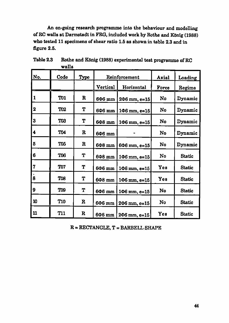
An on-going research progrpmme into the behaviour and modellingof RC walls at Darmstadt in FRG, included work by Rothe and Konig (1988)who tested 11 specimens of shear ratio 1.5 as shown in table 2.3 and infigure 2.5.
Table 2.3 Rothe and Konig (1988) experimental test programme of RCwalls
_______ Reinforcement Axial Loading
Ne _______ Vertical Horizontal Force Regime
1 TOl R 66 mm 2cb6 mm, e=15 No Dynamic
2 T02 T 6c16 mm 1cD6 mm, e=15 No Dynamic
3 T03 T 6cb8 mm 1c16 mm, e=15 No Dynamic
4 'fl)4 R 66 mm - No Dynamic
5 TO5 R 6cb8 mm 6cb6 mm, e=15 No Dynamic
6 TOG T 6cb8 mm 16 mm, e=15 No Static
7 T 6cb6 mm 1c16 mm, e=15 Yes Static
8 TO8 T 68 mm 1cD6 mm, e=15 Yes Static
9 TO9 T 6cb6 mm 16 mm, e=15 No Static
1k) T1O R 6cb6 mm 26 mm, e=15 No Static
11 Til R 66 mm 26 mm, e=15 Yes Static
R = RECTANGLE, T = BARBELL SHAPE
44

1 .1
Figure 2.5 Test set-up for dynamic and static-cyclic tests and arrangementof reinforcement and cross-sections of Rothe and Konig (1988)
- For the five walls that were tested on the shake-table a single degree-of-freedom system was assumed as shown in figure 2.5. The mass of 7.2tons was supported by external columns so that no axial force was taken bythe walls. The inertia of the mass was transferred to the wall throughsprings which were intended to reduce the response frequency andrepresent upper stories in a building. The El Centre 1940 acceleration timehistory was imposed on the specimens once until cracking and once untilyield. In the final run a harmonic sinusoidal waveform was used.Equivalent thmping up to 5% for virgin cycles and 2-3% for subsequentcycles was calculated.
For the cyclic static tests the load was applied through adisplacement controlled hydraulic jack. For comparison purposes the topdisplacements obtained from the shake table tests were used as input insome of the dynamic tests. Axial load was applied through externalprestressing reds in three of the walls.
Failure modes varied depending on the cross section, axial force andreinforcement ratio. Bar fracture was observed in under-reinforced walls.
45

Sudden web failure was observed in the barbell sections while therectangular sections failed in a more ductile manner. For well designedwalls stable hysteretic behaviour was observed up to a stiffnessdeterioration of 10.
2.2 Design Dhiloscrnbies
Several RC design philosophies which exist on the global structurallevel as well as on the methods of analysis are discussed in this section.
The 'Capacity design philosophy' advocated by Park and Paulay(1975), is now fully incorporated in the New Zealand Standards. The criticalsections of the structure at which plastic hinging would develop and wheremost of the energy dissipation is expected to take place, are pre-selected andsuitably designed. Sufficient reserve strength is provided to the rest of thestructure so as to avoid any significant inelastic deformation demand andpreclude the formation of an alternative mechanism.
In order to achieve the above, the strength of the section iscategorised in a number of different ways. 'Ideal' strength, is the strengthobtained by using the code theory for analysis and the actual dimensionsand specified material strengths. A 'dependable' strength would be a lowerbound of strength and is lower than the 'ideal' strength. 'Probable' strengthuses probable strength of materials and is the expected strength to be usedfor dynamic considerations. 'Overstrength' is an upper limit to the strengththat can be achieved and is used to calculate the shear forces acting on thecritical section.
The capacity design is incorporated in the draft EC8 (1988), and asignificant amount of the section of code referring to reinforced concrete isbased on research from New Zealand.
Similar to the above design methodology is the 'Conceptual designprocedure' proposed by Aktan and Bertero (1985). The sources ofoverstrength from the structural and element level should be estimated soas to establish the shear 'demand' on the member. The 'supply' should takeinto account all the different limit states.
46

In general, flexural design of RC members is based on sectionanalysis. Several simplifications are allowed by codes to facilitate design,such as the use of an elastic perfectly plastic model for steel, and triangularor equivalent rectangular stress blocks for concrete. The controlling strainis usually the concrete crushing strain at the extreme fibre. In confinedmembers enhancement of the crushing strain and stress can be achieved,which leads to higher moment capacity and ductility.
Both the 'Capacity' and 'Conceptual' design methodologies assumethat the plastic hinge zone will be adequately designed and detailed tosustain the rotational ductility demand. However,only recently, in theproposed EC8 (1988) the provisions for member ductility has been related tothe overall structural behaviour and design for a specific ductility ispossible.
The design for shear is still the subject of research and debate, andseveral different philosophies exist. The most widely accepted and usedmethodology is based on the truss model, and is discussed in the followingsection. The compressive path method advocated in the researchprogrpmme at Imperial College prior to the current one, is also presented.
2.2.1 Truss model
The conventional truss model shown in figure 2.6 (a) and (b) is stillused by most codes for calculating the amount of shear reinforcement. Themodel considers that the RC wall will behave along its length as if itconsisted of tensile horizontal ties and diagonal compression struts. Webcrushing due to failure of diagonal compression struts and yielding of thehorizontal ties provide the limits for shear capacity of such a member.
47

T = TensionC = Compression
LV
C
L
1
IIV
T
Iv
IkT4r Ib-
ILII (1II
III.II
It%
II 'CII
TImII
(a)
(b)
(c)
2.6
Truss models for resisting shear
However, for low aspect ratios the top beams or slabs of walls couldact as ties and the arching effect is more effective in transferring forces. Analternative truss model could be employed for low aspect ratios as shown infigure 2.6 (c). As a result the effectiveness of the conventional truss model isvery much reduced. Many of the codes recognise this, and hence emphasizethe contribution of the vertical web reinforcement in such cases of lowaspect ratios.
In all codes, the contribution to shear resistance by concrete alone iscalculated by considering average shear stress 'tc' over the entire width ofthe member section. For RC walls where the reinforcement could beuniformly distributed, a slightly reduced width is used so as to account forthe reduced lever arm.
The values of 'r used by codes are empirically derived fromexperimental work on beams and walls. In deriving these values thecontribution of any existent lateral reinforcement is subtracted and the restis assumed to be resisted uniformly by concrete. However, it is widelyaccepted that the distribution of shear stresses within the section is neitherlinear nor parabolic, as given by elasticity. Furthermore, dowel action of thelongitudinal reinforcement cannot be easily decoupled from concrete shear
48

resistance. Despite the over-simplicity and empirical nature of the methodit still has very few credible adversaries.
2.2.2 Comnressive force Dath aporoach
The 'compressive force path' concept (Kotsovos, 1983) considers thatshear resistance is available only in areas of concrete compression. Theregion of compressive stresses is called the 'compressive force path' (CFP).A figure depicting the CFP in a wall is shown in figure 2.7. Failure willoccur when tensile stresses develop within the CFP. Lefas (1988) gives themain reasons for the development of such stresses as:
(a) Change in the CFP direction.
For equilibrium purposes a change in the CFP direction would leadto the development of tensile stresses. The location of such change indirection is a central aspect of the method, and depends on the aspectand shear ratio.
(b) Varying intensity of the compressive stress field along the CFP.
The level of compressive stress is highest when the cross-section ofthe CFP is minimum. When the compressive stress reaches acritical level, concrete dilation will induce tensile stresses to thesurrounding concrete. This would be considered by other researchersas compressive failure.
(c) Tip of inclined cracks.
From fracture mechanics principles, tensile stress concentrationswill develop at crack tips in the direction of the crack adjacent to thecompressive zones.
(d) Bond failure.
Bond failure of the vertical reinforcement will reduce the crosssection of the CFP and hence lead to the same results as (b) above.
49

compression induced
in concrete block
tension sustained byl
izontol reinforcement
h
C
I-Fhj T
2.7 The compressive force path in a RC wall (Lefas, 1988)
The mechanism of load transfer, shown in figure 2.7, comprises aninclined branch and a vertical branch. The concrete between the cracks inthe web are considered to be 'comb teeth' tied by the reinforcement andcapable of bending resistance. The length of 21' (where 1' is as defined infigure 2.7) for the inclined branch is considered to be equal to 2 D/3 and 3 D/4plus the depth of the neutral axis for aspect ratios of 1 and 2respectively.Wa]l strength is predominantly provided by the tied frame withthe concrete 'teeth' between cracks mRking only a small contribution towall load-carrying capacity through the bond forces which develop betweenconcrete and tensile reinforcement.
A flexural mode is expected for aspect ratios higher than 2.Furthermore, the stress and strain enhancement due to the presence ofconfinement should also be taken into account when calculating theflexural capacity 'Me'.
The shear capacity of the unreinforced section in terms of bending,'Ma', is to be obtained by an empirical equation derived for beams byBobrowski and used by Lefas (1988) for RC walls. If M is higher than M,then only nominal reinforcement is required.
50

In order to avoid the development of tensile forces at the point ofchange of direction of the CFP, horizontal reinforcement should be providedto neutralise the horizontal component of the inclined compression strut.According to the method (figure 2.7), this reinforcement also subjects theshaded web area to compression. The area of reinforcement required maybe calculated from the difference between the applied shear force and theshear force resisted by concrete. It is recommended that this area isdistributed over a length equal to the width of the wall.
In the vertical part of the CFP, no horizontal reinforcement isrequired, but in order to prevent tensile stresses developing, confinementreinforcement should be provided.
None of the RC walls tested by Lefas (1988) have been designedaccording to the CFP method. None of the walls failed in shear despitehaving less reinforcement than required by ACI-318 (1983) which meansthat the concrete possessed higher shear strength than assumed by thiscode. The fact that the Bobrowski equation gave a lower prediction for theconcrete shear strength was considered as vindication of the CFP methodfor walls.
There seems to be a gap between the CFP theory and straincompatibility in the area of the inclined branch of the CFP. By using basicprinciples of mechanics it can be shown that it is not possible to develop aninclined compressive strut at the top of a wall, without inducingcompressive stresses in the extreme fibres. Moreover, in order to changethe direction of the applied horizontal shear force at the top of the wall asshown in figure 2.7, a tensile force is also required which is not beingaccounted for. Additionally, the design equation seems to have noassociation with the CFP theory, and very no information is provided on itsorigins. Finally, tests conducted by Lopes (1990), on a wall designed anddetailed according to the CFP gave a capacity 10% lower than the code-designed counterpart; the wall failing in shear.
2.3 Design of RC Walls
The state-of-practice as represented by existing codes is outlinedhere, in view of the fact that one of the purposes of this research is to
51

contribute towards the enhancement of code provisions. Different aspects ofdesign are presented with reference to the American Concrete Institutecode (ACI 318-83), the Uniform Building Code (UBC 1988), the New ZealandStandard (NZS 3101: 1982) and the Eurocodes (EC). The number of codes inthe current World List of Earthquake resistant regulations (IAEE, 1988) is36, and in order to avoid excessive repetition, the number to be discussedhas been narrowed down to the most relevant to the current work.
In all the chosen codes the aim of earthquake resistant design is toavoid brittle failures in RC walls by ensuring that steel yielding occursprior to the attainment of the shear capacity. If this is achieved,considerable energy dissipation and reduction of the maximum expectedforces can therefore be expected. The first stage in design, however, is toobtain a section that can resist the required ultimate bending moment,whilst the second stage is to detail the member for the required ductility.The final step is to ensure that the shear capacity is higher than the sheardemand.
Material safety factors and capacity reduction factors are notincluded in the following section so that the methodologies and designphilosophies used by the various codes in order to realise the ultimatecapacity may be compared.
2.3.1 Section Flexural CaDacitv
The design assumptions as given by the ACI 3 18-83 and UBC (1988)are as follows:
a) For flexural members of aspect ratio more than 0.4, linearstrain distribution to be used for both steel and concrete.
b) For ultimate flexure calculations the maximum strain inconcrete compression 'ce,' to be 0.003.
c) The tensile strength of concrete is neglected.
d) Any shape of stress-strain distribution for concrete may beused as long as it agrees with comprehensive tests. Codes ingeneral suggest simplified distributions for use such as theequivalent rectangular block.
e) Steel behaviour is linear elastic perfectly plastic.52

(2.2)
(2.3)
In EC2 (1984) the value of c is 0.0035. EC8 (1988) recognises anincrease in depending on the available confinement. The same codegives different limiting values of minimum strain in reinforcementdepending on the ductility class (DC). For DC high, "H", a minimumelongation of 0.0 12 is specified. Additionally, for the same ductility class thecode requires the ratio of tensile failure to yield ratio to be between 1.3 and1.45 with actual to nominal yield ratio not to exceed 1.15.
Based on the above assumptions, some of the codes, as well as most ofthe handbooks of concrete design, provide simplified equations forassessing the strength of a section, and guidance for dimensioning andsupplying reinforcement for achieving the required strength. However,such equations usually apply to a specific types of section within a limitedrange of steel distributions and hence should be used with care. Analternative to using design charts is to conduct section analysis, accountingfor the exact area and location of reinforcement and concrete stress-strainrelationship, as described in chapter 5.
2.3.2 Detailin2 for ductility
In order to achieve ductile behaviour through the development of ajilastic hinge, codes impose dimensional limitations and include provisionsfor hoop reinforcement. As part of the special provisions for seismic designof RC walls, both ACI 3 18-83 and UBC (1988) require the provision ofboundary elements where the compressive stress is more than 0.2 f0.Theseboundary elements should be designed to resist all the axial loads imposedon the member and are to be designed as columns. The minimum area ofrectangular hoop reinforcement 'A8h' shall not be less than that given byeither of the following equations.
(shf 0 \r( Ag \Ah=0.3I yh JRAch)]
A=0.l2sh.fCO/fYh
The spacing of transverse reinforcement should not exceed B/4 or 100mm (where B is the thickness of the wall), and should be over a length notless than the width of the wall 'D' or H/6 or 450 mm (where H is the heightof the wall).
53

The NZS 3101 (1982) code requires confinement for the outer half ofthe compression zone where strains exceed 0.00 15, provided the neutralaxis depth exceeds a given limit. The area of hoop reinforcement, Ash', tobe provided is obtained by multiplying equations 2.2 and 2.3 by (0.5+0.9 c /D)(to account for an increase in neutral axis depth 'c' due to the presence ofan axial load P'). The spacing of the hoop reinforcement should not exceedB/3 or 150 mm or six times the diameter of vertical bars confined. Hoopreinforcement should be provided over a length equal to D. By complyingwith the above requirements, the designer avoids further detailedcalculation for curvature ductility capacity
From experiments conducted on columns in New Zealand, Zahn,Park, Priestley and Chapman (1986) reported that code prescribedconfinement would yield a value of pjj . of about 20. The relation betweencurvature ductility and displacement ductility is shown to be dependent notonly on the aspect ratio of the wall but also on the length of the plastichinge. Paulay and Uzu.meri (1975) considered two different equations forthe length of the plastic hinge, which form the limits of the shaded bandsdepicted in figure 2.8. The above work has been used in the design forductility of EC8 (1988).
54

20--
3
____ 16
3S S
14 -I.
12 -
- 10
U3a
6
S4
3U
2
-
1:pa
-
2
I I
2 4 6 8 10 12 14 6
Shear Wall height To Length
Figure 2.8 The variation of curvature ductility at the base of cantilevershear walls with aspect ratio of the walls and the imposedductility demand (Paulay and Uzumeri, 1975)
- The proposed EC8 (1988) assigns behaviour values 'q' values fordifferent structural systems and different ductility classes. Havingassigned the q-value the required displacement ductility '' can beobtained directly. Based on the assumption that for a cantilever wall plasticyielding would occur in the bottom 10% of the height, the curvature ductilityis given by:
I LIJr = 1+3.5 ( - 1) (2.4)
Table 2.4 shows the relationship between the q-values and .t]Jr for thedifferent ductility classes as given by Tassios (1989) in a backgrounddocument on the EC8 for both coupled and isolated walls. Two methods areused yielding two different values for displacement ductility, andThe first value is based on the equal energy principle (Tassios andChronopoulos, 1988), but the average is used to calculate the curvatureductilities.
55

Table 2.4 Relation between q-values and curvature ductility______ _____ (Tassios, 1989) ___________ _____________ _______________
DC q L1/r 1L1/r
O.5(q2+1) q O.50tai +2) 1+2.5(1 16.1) 1+3.5(116.1)
_______ ______ ____________ ________ _____________ (coupled walls) (isolated walls)
"L" 1.5 1.63 1.5 1.56 2.40 2.97
_____ 2.0 2.5 2.0 2.35 4.13 _____________
"M" 2.5 3.63 2.5 3.06 6.16 8.22
_____ 3.0 5.0 3.0 4.00 8.50 --
3.5 6.63 3.5 5.06 11.16 15.21
"H" 4.0 8.5 4.0 6.25 14.13 _____________
_____ 4.5 10.63 4.5 7.56 17.41
Approximation H 1LlJr q2 P.JJr 1.2 q2
The curvature ductility is used to obtain the required confinementvolumetric mechanical ratio, 'Od', by using equation 2.5.
wd = ° 9 3av L l,1 [ 0.01 .t y + 0.15 vd_o.4] ^ 0.2A0 (2.5)
where A is the concrete gross area and A 0 is the core concrete area alongthe confined length 'la'. The confined area should be extended horizontallyso as to cover concrete with expected maximum strains equal to 1.5%.Vertically, l should be greater than D, a sixth of the wall height, or storeysheight. Detailing of hoops over this height is specified as for columns. Theminimum diameter, 'dH', allowed for hoops is 6 mm, at spacing of B/4, 6 dL(where dL is the diameter of the longitudinal reinforcement) or 100 mmwhichever is less. The diameter of dH should be about 0.4 dL. Strict
provisions for hoop arrangements are to be used. Single hoop is not allowedfor DC "H".
EC8 recognises an increase of the concrete strain at failure due tohoop reinforcement as shown in the equation 2.6.
56

= 0.0035 + 0.10 w,d a (2.6)
The value of 'a' depends on the hoop configuration. Confinement isalso considered to enhance the ultimate concrete strength as well as thestrain at which this is achieved.
2.3.3 Shear design
The design against brittle shear failure is the aim of all codes. It istherefore important, that the design shear force 'Vu' is not just the forcerequired to induce the maximum applied design moment 'Me', but the forcecorresponding to the maximum probable section strength 'M 0'. For thiseffect, the NZS 3101 (1982) code considers the flexural overstrength (M/M)when determining V. The ideal section shear force 'V 1', is calculated fromthe equation below:
V Vj B de (2.7)
where the effective depth, 'de', is to be taken as 0.8 D unless determined bystrain compatibility analysis. To calculate the section shear stress capacity.'Vj' the separate contributions from concrete 'vc' and steel 'v 8' are summed-up as shown below:
Vj = V + V
(2.8)
The American codes use section shear forces instead of stresses forthe same effect. However, the potential flexural overstrength of the memberis not taken into account directly by the above codes.
Upper limits for the maximum permitted shear capacity arespecified in all codes. The value of Vj according to the more conservativeNZS 3101 (1982) should not exceed 0.2 f, 6 MPa or the value from equations2.9 and 2.10.
= 0.9 fl
(2.9)
v, = ( 0.3 4, S + 0.16 )(2.10)
The American codes use a value of 0.83 Jf in equation 2.9. The abovelimiting equations are introduced so as to prevent web failure due todiagonal compression.
57

The structural type factor (equation 2.10), S, as given in NZS 4203(1984) accounts implicitly for the ductility demand on the section. For singlecantilever walls, the value of S ranges between 1.2 and 2. The higher thevalue, the lower the ductility demand and hence, higher shear can beresisted. Similarly, the value of $ (flexural overstrength factor) being about1.4 for high strength reinforcement, is expected to reduce the ductilitydemand and hence, increase the shear capacity.
For walls of ductility class UHI, the proposed EC8 (1988) requireschecks for three limiting equations corresponding to three different types offailure as discussed below:
(a) For web diagonal compression failure, the code differentiatesbetween critical and non-critical sections. The average shear stressshall not exceed:
(i) 0.2 f in critical sections and
(ii) 0.3 1 0 in non-critical sections.
(b) For web diagonal tension failure, the code considers differentmechanisms of shear resistance from the steel reinforcement forshear ratios 'a3' on either side of a value of 1.3. The concretecontribution to shear resistance, is independent of the value of a3,and the section capacity is limited according to the following criteria:
(i) average axial stress less than 0.1 f
- zero in the critical sections of the wall and
- 2.5 'rp., (tp4, stress obtained from table 4.1 of EC2) for sectionsoutside the potential hinge areas.
(ii) average axial stress more than 0.1
- 2.5 'rp ('rRd, stress obtained from table 4.1 of EC2) for criticalsections and
- 2.5 tEd i (i = 1 + Mdo /M3d ^ 2 as defined in notation) forsections outside the potential hinge areas.
(1) For a8 more than 1.3, only the contribution of horizontal shearreinforcement, according to the truss analogy, is taken intoaccount. Vertically distributed reinforcement of an amount
58

equal to the horizontal should be provided when the axial loadis zero. The amount of this reinforcement can be reduced bythe equivalent minimum axial force on the section.
(2) For a8 less than 1.3, the contribution of horizontal shearreinforcement is linearly reduced to zero for a8 of 1.3 - 0.3,whilst the contribution of vertical reinforcement is linearlyincreased to the sectional yield strength for the same range ofa8.
The minimum amount of Ph and Pv is 2.5%, of diameter less thanB/10 but not less than 8 mm, at a spacing not more than 20 bardiameters or 200 mm.
(c) For shear sliding failure at the bottom horizontal section, the codeconsiders resistance from the dowel action of vertical and diagonal webbars, as well as the effect of the axial load. Dowel action for each vertical baris defined as 1.5 A8 'I( f f8 ) and for inclined bars 2 A8 f8 cos 0 ( 0 angle tothe horizontal). One third of the average minimum axial stress isconsidered to be a safe lower value of concrete-to-concrete friction undercyclic loading.
The New Zealand code, in a section for special provisions forearthquake resisting walls, requires that within the potential plastic hingezone a more stringent equation for concrete shear resistance is to be used.The height over which the special provisions should be applied is given asthe largest of D or one sixth of the height of the wall, up to a maximumheight of 2D. The concrete contribution to shear 'Vs' over this height isconsidered to be dependent only on the level of axial stress, as given inequation 2.11.
= 0.6(2.11)
The ACI 318-83 and LJBC (1988) link the nominal shear strength tothe wall aspect or shear ratio (the larger of the two) rather than axial load.For a value higher than 2, the concrete shear resistance is given as0.166 whilst an increase of 50% of this resistance is allowed for adecrease in the shear or aspect ratio from 2 to 1.5, linearly interpolated forintermediate values.
59

In the NZS 3101(1982), for the area outside the plastic hinge zone, theordinary provisions for shear apply. The value of v should be the lesser ofequations 2.12 and 2.13, given below
vC=0.27d1?+ 4A5(2.12)
D(0.1/i+0.2..)v = 0.05 .f? +
(M D1) (2.13)
where P is negative in tension. Equation 2.13 does not apply when thedenominator is negative. These equations are the same as given in the ACI3 18-83 code which, however, does not differentiate between the plastic hingezone and the rest of the wall. It is evident, therefore, that even though theNZS 3101 (1982) is more conservative in the plastic hinge area, it mayoverall be a more economic code than the American codes.
In all codes when the shear capacity 'v is greater than the sheardemand 'vi', then horizontal shear reinforcement is required. The amountof reinforcement is calculated according to the principles of the trussanalogy and is similar in all codes of practice (except for walls of shearratio a5 less than 1.3 in EC8, as mentioned already) as shown below.
A- - (v1—v)Bs2
'yh
(2.14)
where 'A' is the area of horizontal shear reinforcement within a verticalspacing The spacing, 's', should not exceed D/5, 3B, nor 450 mm.
In the plastic hinge zone, the NZS 3101 (1982) requires this amountnot to be less than given by the equation 2.15 below, which corrects for thecentre of forces in the hypothetical truss which is supposed to be formed inthe section.
4I(laVfynpn'\ v1Mfh (2.15)
The American codes require the horizontal reinforcement ratio, 'Ph'snot to be less than the vertical web reinforcement ratio, 'Pv', (for walls withshear or aspect ratio less than 2 but not less than 0.0025. Codes recognizethe contribution of vertical web reinforcement in controlling the shear
60

crack width. The value of p, is given by equation 2.16, but should not be lessthan 0.0025 and not more than 0.06.
= 0.0025 + 0.5 ( 2.5 - H/D)( ph - 0.0025) (2.16)
The NZS 3101 (1982) code requires that the ratio of PI,tO gross concretearea of horizontal section not to be less than O.7lfyh and not more thanl6Ifh. The spacing of this reinforcement shall not exceed D/3, 3B, nor450 mm.
An interesting distinction between slender and squat walls is basedon the expected type of failure mode by EC8 (1988) as shown in figure 2.9.
2.9 Failure modes of RC walls critical regions (EC8, 1988)
The probability of a particular type of failure is associated with thelevel of shear resistance available in the section. Failure is related to avalue 'u', which is the ratio of minimum design shear strength, 'VRD', tothe single shear force, 'VMRr?,that would cause the design moment, asshown in equation 2.16.
U=VRD/('YRD.VMRD ) 2.16
The value of 'Yro' represents the uncertainties in estimating the level of theexact forces. For walls of DC 'M" and "H" the value of YRD. is 1.3 and 1.4
61

respectively. For these two ductility classes the different probable failuresare as follows:
1.00 cu Flexure type of failure is highly probable
0.75 cu ^ 1.00 Mixed type of failure of a prevailing flexuralcharacter is probable
0.50 cu ^ 0.75 Shear type of failure is probable
^ 0.50 Shear type of failure is certain
Based on the above, walls of aspect ratio higher than 1.5 areconsidered 'slender' and of aspect ratio less than 0.5 are considered 'squat'.The more conservative New Zealand standards consider walls of aspectratio higher than 2 as 'slender' and impose a higher penalty through thestructural factor for 'squat' walls of aspect ratio less than 2.
Dimensional limitations in the codes are provided in order toeliminate lateral instability. For rectangular walls an effective height towidth ratio of 10 is considered adequate for stability considerations.
2.4 Discussion
The actual flexural capacity of RC wall sections is higher than thedesign flexural capacity due to the simplifications used in the designprocess and material variability. During EQ loading the ultimate flexuralcapacity may be reached and hence an accurate estimate of the shear forcesis necessary for the shear design of the member. Several factors contributetowards the overstrength, and in this thesis their effect are investigated, inview of the conclusions drawn by Lefas (1988).
It is recognised, by previous researchers as well as by the presentauthor, that concentrating the reinforcement at the boundaries is a costeffective means of utilising flexural reinforcement; such arrangements donot seem to be widely researched. A reason for this may be the assumptionthat web reinforcement is necessary for enhancing the shear resistance ofwalls. This aspect of wall behaviour is further investigated in the currentthesis.

Estimation of the stiffness of RC walls is an issue that fewresearchers addressed. In several dynamic investigations of small scaleRC members, more flexible behaviour than expected was encountered.Since the determination of the dynamic characteristics depends on thestiffness of the structural components, the relation between the predictedand initial stiffness, as well as the stiffness deterioration, is worthy ofinvestigation.
The shear resistance of RC members continues to be a subject ofresearch. Considerable controversy surrounds the applicability and indeedthe validity of the truss analogy. The CFP method, advocated by Lefas (1988)for the design of RC walls, has not been linked adequately neither to theexperiments nor to the design equation. A more detailed study of theproblem is necessary and is presented in this thesis.
A number of new design ideas have been put forwards in theproposed in EC8 (1988). Design for ductility and prediction of the mode offailure are two of the ideas that are investigated, through the analysis andexperiments conducted in the course of the current research progrinme.
Finally, a significant part of the research on which coderecommendations are based was based on monotonic test observations.More severe loading conditions are expected during earthquakes, andhence, a severe cyclic regime is more appropriate when the research isdirected towards EQ resistant design.
In conclusion, whereas significant advancement in understandingthe behaviour of RC walls under EQ loading was achieved, there is still apressing need for work directed towards the resolution of a number of keyissues. This is particularly important due to the significance of the roleplayed by RC walls in the overall response of buildings to strong groundmotion.
63

CHAPrrEK 3
3 EXPERIMENTAL METHODOLOGY
3.1 Introduction
The experimental progrnime comprised nine tests as shown inTable 3.1 below. In this chapter, the modelling procedures and choice of theexperimental parameters, the test-rig set-up and the design and materialstrength of the specimens are presented.
Table 3.1 Summary ofexperimental_programme ____________
WALL MODEL DIMENSIONS ASPECT M/VL LOADING
NUMBER RATIO (cm) RATIO ar REGIME
- SW1 1:5 60 x 30 x 3. 2 2.92 SHAKE-TABLE
SW2 1:5 60 x 30 x 3.0 2 2.92 CYCLIC
SW3 1:5 60x30x3 2 2.10 CYCLIC
SW4-SW9 1:2.5 120 x 60 x 6 2 2.10 CYCLIC
3.2 Smzill scale reinforced concrete modelling procedure in dvnsimics
Experiments SW1-SW3 were performed on 1:5 scale models. SW1 wastested on the shake-table while SW2 and SW3 were tested under cyclicdisplacement control loading. In this section, the development of a smallscale dynamic modelling procedure for RC walls, necessary for shake-tabletesting, is presented.
64

(3.6)
(3.7)
(3.8)
Small scale model analysis is based on dimensional analysis(Elnashal, Pilakoutas and Axnbraseys, 1988 a). Given the basic modelratios, the similitude relationships can be determined by usingBuckingham 'fl' theorem. The theorem considers that any nwnber of 'ii'different quantities 'q' that represent the phenomena in a given physicalsystem are represented by a certain function 'fq)', as shown below.
1Xqi,q ........ .q1) = 0
(3.1)
This function can be transformed into a new function 'F(r)', having 's' non-dimensional independent terms 4r', by using powers of the quantities 1q' interms of chosen fundamental quantities 'b', i.e.,
F(rj,r2.........r8) = 0
(3.2)
The difference 's' between the number of variable quantities 'n' and thenumber of fundamental quantities is given by:
s = n-b
(3.3)
The theory of models is developed herein by using the principlesdescribed above. Equation 3.2 becomes the relationship for both the prototype(subscript ) (equation 3.4) and model (subscript m) (equation 3.5), where theindependent non-dimensional terms have to include the 'b' fundamentalquantities to be modelled.
F (rip,r2p.........rgp) = 0
(3.4)
Fm (rlm,r2m.........rsm) = 0
(3.5)
The above two equations can be rearranged to give equations 3.6 and 3.7.
F' (r2p,r3p.........Tsp) = rip
F'm (r2m,r3m.........rsm) = rim
The general design or prediction equation, therefore, becomes:
r5 Fr,' (re)a=—= ..
Tsm rm rm)
Since there are three fundamental dimensions, length, time andforce, for true modelling, only three independent scale factors can be
65

chosen arbitrarily. The ratios between the three fundamental quantifiescan be selected freely but all secondary equations should be satisfied, subjectto technological and financial constraints. Provided that this is achieved,the model is called 'complete' and the prediction equations and model ratios'a8' can be used to calculate the required prototype quantities from themodel measurements, and vice versa. It is not necessary to know thefunction F'(r) and it is only required to record the necessary variablequantities 'ram' for the interpretation of results.
For dynamic and shake-table testing, the three arbitrarily chosenmodel ratios should relate to the geometric, force and dynamic similituderelationships. The technological limitations of small shake-tables usuallygovern the first two model ratios.
3.2.1 Geometry similitude
The size of the model is limited by the maximum shake-table forceand hence, the geometric scale factor '' is determined by consideration ofthe force similitude. A lower bound value for the scale factor is imposed bythe material properties.
3.2.2 Force similitude
Force scaling is necessary to reproduce stresses of interest and as aresult, it is influenced by material properties such as the stress-strainrelationship, shear transfer, creep, bond, cracking and crushing. In orderto avoid material scaling effects, the same concrete mix was usedthroughout the experimental programme. For the same reason, speciallymanufactured model reinforcement (Noor, Raveendran and Evans, 1985)was utilized. As a result, the elastic properties' scaling factor 'e' waschosen as unity. However, it has been demonstrated analytically by Menuand Elnashai (1988), that a 30% variation in the concrete elastic modulus ofRC walls will influence the overall stiffness and result in fundamentalfrequency variations of up to 15% as shown in figure 3.1. The effect ofPoisson ratio variation has no effect on the dynamic characteristics. Thissuggested that final "tuning" of the experimental programme and choice of
66

the modelling ratio that affects the dynamic behaviour is better performedafter material properties have been measured.
FUNDAMENTAL FREQUENCY
HIGHER HARMONIC
£ Yuib N.rn.i.. S .iit
I Puw. I.u.
Miterial parameter ratios Material parameter ratios
Figure 3.1 Influence of the variations in material properties of areinforced concrete shear wall model (Menu and Elnashai,1988)
3.2.3 Dynamic similitude
In small scale modelling on shake-tables, the exact andsimultaneous reproduction of stiffliess and inertia forces is not possible. InRC walls, however, self-weight gravity (or inertia) forces in shear walls aregenerally negligible compared to the overall building gravity forces to beresisted and hence, the scaling factor 'p' which determines these forces canbe neglected. As a result, a similitude relationship which uses 'p' as thethird variable model scale factor is usually used. This factor, when usedtogether with '' and 'E', influences only time-dependent quantitiesincluding the velocity. Since for a material such as concrete the velocity ofloading and propagation of cracks is an important dynamic parameter, it isproposed that the velocity scale factor 'v' should be chosen as the thirdmodelling parameter. The resulting model parameters are given in table3.2.
67

Table 3.2 Small scale dynamic modelling ratios for reinforced concrete
QUANTITY 1DIMENSION MODEL SCALE FACTORLengthL _________ ________ ________ElasticE F L-2 _________ C ________Density F L-4 T2__________ £ v-2AreaL2 __________ _________ _________VolumeL3 __________ _________ _________MassFL-1 T2 __________ £ ________Force F _____________ eMomentF L __________ c _________StressFL-2____________ £ __________TimeT _________ ________ ________Frequency T1 -1 __________ VVelocityLT-1 __________ _________ vAcceleration L T-2 _____________ v2
3.2.4 Choice of model parameters
The geometric and dynamic model parameters must yield modelquantities within the shake-table capabilities. For horizontal excitation themaximum dynamic force of the Imperial College shake-table is 48 KN andthe maximum payload is 4895 Kg at a height of 1 metre. The frequencyrange is 1-40 Hz and the minimum time interval 'At' that would allow anadequate number of data acquisition channels to be used is 0.005 seconds.Preliminary analysis of a full size isolated RC wall of aspect ratio 2 yieldeda strength of about 1000 KN, hence, a model scale force factor of 25 waschosen. Since the elastic properties scale factor was chosen as unity, itfollows that 'L' is 5. For 'v' of 1 the time 'r' and acceleration scale factor 'a'would be 5 and 1/5 respectively. In order to avoid very high accelerations,for the pilot experiment, the inertia mass was chosen to be 2000 Kg and 'a'set to unity. Additionally, earthquakes of original At = 0.02 s were scaled to0.005 a rather than 0.004 a in order to maintain the required dataacquisition capability. This deviation from the proposed modellingprocedure would result in a different prototype real scale. However, sincethe only objective of this pilot experiment is the comparison with models
68

4
.1 I
•1 I:f *1 I
600mm 850mm
.1 I
I I I* I
Ii,
1000mm
tested statically, full satisfaction of the dynamic similitude conditions is notof utmost significance.
3.3 Exnerimental set-up
8OOnm ...3OOmm
- - - .500mm - - - -
A-A Section A-A
IFigure 3.2
Shake-table test rig arrangement and wall reinforcementdetails
3.3.1 Shake-table test-rig
The design of the shake-table test-rig shown in figure 3.2 wasintended to satisfr the following:
(a) Support the 2000 Kg mass at a centre of gravity of 1 metre or lessabove the table platform.

(b) Allow free translation and rotation in the direction of shaking tosatisfy the isolated wall boundary conditions.
(c) Prevent all out-of-plane degrees of freedom.
(d) Be stable during all stages of assembly and testing including impactloading due to brittle wall failure.
Additionally, the test-rig lateral stiffness (in the absence of the walland with the mass locked) was designed to coincide with the expected initialwall stiffness. With this approach, time-history matching was performedon the test-rig without damaging the reinforced concrete specimen.
LjL-.-
-
Figure 3.3 Model SW1 in the test-rig on the shake-table
Fifty per cent of the volume of steel required as mass should be belowthe centre of gravity. Consequently, the top part of the wall model isconcealed as seen from figures 3.2 and 3.3. The test plates which comprisethe mass were prestressed together on a central extended plate throughwhich both support and degrees of freedom are provided. This was achievedby welding a rod in the line of the axis of gravity on the central plate. Therotational degree of freedom was offered by a circular roller encased in arectangular steel plate. The horizontal degree of freedom was ensured byflat rollers at the base of the rectangular steel plate. The axial load was
70

LdadCell
Ivel1000mm
Level
- _ _ - _ _ -$ r• I I
8II
1
+
- 300mm -
transferred to the test rig columns by the beam which was in contact withthe rollers as shown in figure 3.2. There were several reasons for notallowing the wall to support the axial load of the inertia mass. A matter ofprimary importance was safety, since the unexpected consequences of acatastrophic wall failure should be avoided. Moreover an axial load was notintended to be applied on the models tested subsequently under cyclicloading conditions.
Screw DoubleJack Hinge
WI 1LLI.ALL
SW2
I755mm
for modelSW3
3.4
Te for models SW2 and SW3
Several levels of safety were implemented for the shake-tableexperiment. Cushioned end beams were introduced connecting thecolumns in the front and back elevations. The beams were designed towithstand the impact of the mass at an acceleration of 3 g in the unlikelyevent of a sudden loss of strength and stiffness of the wall. Before hitting theend beams, the mass would trigger the emergency stops on twodisplacement limits; first a digital and then a mechanical one.
71

Additionally, the prestressing rods connecting the inertia mass wereextended downwards, to just a few centimetres from the base, making theremote possibility of overturning of the mass impossible.
3.3.2 Small scale cyclic test-rig
The shake-table test-rig was adjusted for the 1:5 scale cyclic tests byclamping it onto the laboratory strong floor. A double hinge with a load cellin the centre was then fitted at the required level, as shown in figure 3.4.The screw jack assembly described in section 3.3.3 was lowered to theappropriate height and attached to the test-rig through the hinge. Forspecimen SW2 the load was applied at the height of 1 m, similar to thecentre of gravity of the shake-table test. For specimen SW3 the load wasapplied at a height of 756 mm which was equivalent to the height at whichthe load was applied in all scale 1:2.5 experiments.
3.3.3 Exnerimental set-un for cyclic exneriments on 1:2.5 scale models
The six walls SW4-SW9 were tested as isolated cantilever walls in apecial1y designed and constructed test-rig. The schematic representation
of the testing arrangement and transducer location is shown in figure 3.5.A detailed drawing is presented in figure 3.6, and the actual set-up infigure 3.7.
A reaction wall was assembled from standard concrete blocksavailable in the laboratory. Two columns of three blocks were bedded on athin layer of cement grout and were prestressed onto the concrete strongfloor on the 90 x 90 cm (3' x 3') grid. Forty tonnes prestressing force wasapplied presenting thus the capacity of resisting rigidly a moment of 720 KNm. A yoke of two 30 cm x 20 cm RHS's were stressed at the right height onthe reaction blocks so as to provide the push and pull capability for the jack.
72

LOAD CELL
s_L
CYLINDRICAl. STIFFCYLINDRICALROLLER /
TOP BEAM FREE(ADJUSTABLE)
VDISPLACEMENT
CONTROLCYCLIC LOADING
CONCRETEWALL
SCALE 1:51200 x 600 x 60 mm
BOTTOM BEAM FECED TO ThE FLOOR
Figure 3.5 Schematic representation of test rig arrangement andinstrumentation used for 1 :2.5 scale tests
73

TZ3T-R1G
ELXVATION
It
coiicm IZACT!OMI].00Z
EAL? - PLAN
0 4;
-j1 ------
3.6 A detailed
gram of the 1 :2.5 scale test-ri g assembly
74

The load was applied by a seven inch (17.5 cm) stroke, 20 tonnecapacity screw jack reacting against the concrete blocks. The jack wasdriven by an electrical motor at a constant speed of about 0.1 mm persecond. A 10 volt (strain gauged cylinder type) load cell was connectedbetween the jack and the stiff collar RHS frame containing the rollers.
The boundary conditions at the top, as shown in Figure 3.6, assume ahorizontal load at a constant height. The load had to be applied through apin so as to eliminate tangential frictional forces due to the extension of thewall, a problem that was recognised by the authors in previous tests (Lefas,1988). This was accomplished by cylindrical rollers made of solid steel andfitted with two circular bearings at either end. A roller was used at eachend of the loading beam. In order to avoid local crushing, a steel spreaderplate was fixed at each end of the beam. The front roller was embedded inthe collar frame while the end roller had an adjustable horizontal positionthrough a screw arrangement. The loading collar frame was free withrespect to in-plane horizontal movement, but was restrained fromdisplacing vertically and out-of-plane by a system of flat rollers reactingagainst two standard laboratory assembly portal frames. With thisarrangement the specimen and the load transferring members were totallyencased in a safe way.
The full fixity condition required at the base was achieved byprestressing two hollow section beams on top of the central frame bolts. Atotal of 100 tonne prestressing force was distributed by a pair of spreaderbeams on the bottom concrete beam which was designed accordingly.
The horizontal load was applied through the top beam which wasintended to spread the load in the wall panel. It is inevitable that the beamstiffness will influence the local stress conditions. However, this would notaffect the behaviour of the critical zones of the wall.
3.4 Model manufacture and materials
The specimen beams were designed to provide fixity at the bottom,transfer the load uniformly to the wall, provide anchorage for the
75

longitudinal wall reinforcement and, for the shake-table test, preventuplifting of the inertia mass.
The scale 1:5 (SW1 - SW3) wall dimensions were as shown in figure3.2. The thickness of wall SW3 was chosen to be 30 mm and 4 mmundeformed reinforcement was used instead of 2.8 mm modelreinforcement. The scale 1:2.5 (SW4-SW9) wall dimensions are shown infigure 3.8.
3.4.1 Concrete
The moulds were manufactured from 3/4" (19 mm) plywood. Beforeeach cast, the inside of the mould was coated with a releasing agent.Concrete was mixed in the laboratory by using suitable size concretemixers. All models were cast horizontally in a single cast. The 1:5 scalemodels were vibrated on the vibrating table, whilst for the 1:2.5 scalemodels, pocket and hsmmer vibrators were used. The wet concrete wasplaced and vibrated in three layers. First the bottom third of the beams,followed by the wall area and the middle of the beams, and finally the topthird of the beams. Control specimens were taken from the same batchprior to casting the wall. Strict compacting and levelling was imposed onthe wall surface, so as to eliminate voids and minimize geometricirregularities.
The specimens were trowel finished two hours after completion ofcasting and covered with wet hessian and nylon after about 4 hours. Thistype of curing was maintained for a week until a control cube was crushed.Control specimens were demolded the day after casting and placed on top ofthe horizontal wall for identical curing conditions. Curing was stopped onthe seventh day unless a weaker strength than expected was recorded.Subsequently, the wall and control specimens were stored under standardlaboratory conditions next to the test-rig.
76
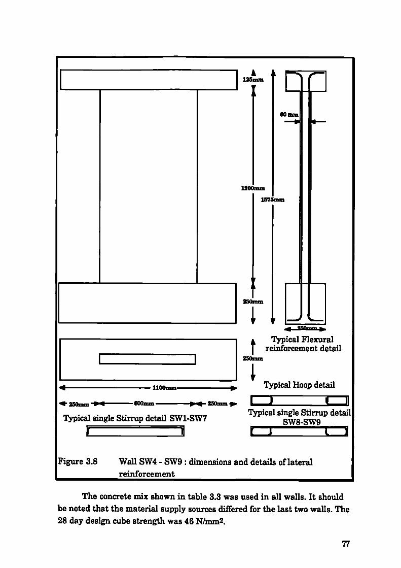
A125mm
1200mm1575mm
TTypical Flexural
reinforcement detail______________________ 'II I 250mm
____________________ ______________ I4 1100mm Typical Hoop detail
*250mm : 600mm pu 25OmmØ' J I IITypical single Stirrup detail
Typical single Stirrup detail SW1-SW7 SW8-SW91 ii
Figure 3.8 Wall SW4 - SW9: dimensions and details of lateralreinforcement
The concrete mix shown in table 3.3 was used in all walls. It shouldbe noted that the material supply sources differed for the last two walls. The28 day design cube strength was 46 N/m.m2.
77

Table 3.3 Concrete desi mix
MIX PROPORTIONS DESIGN MIX
BY WEIGHT RATIO
O.P.Cement 1.00
10 mm aggregate 3.15
Coarse sand 2.00
Fine sand 0.89
Free water 0.68
Table 3.4 Concrete compressive strength ___________ ___________
SPECIMEN DAY OF CUBE CYLINDER PEAKCODE TESTING STRENGTH STRENGTH STRAIN
_______________ ___________ f -N/mm2 f -N/mm2 c x 1E06
SW1 80 47.2 38.9 -
SW2 146 47.2 - -
SW3 232 47.2 - -
SW4___________ 49.5 36.9 2093
SW5 48 47.5 31.8 2286
SW6 47 49.6 38.6 2141
SW7 74 45.2 320 1950
SW8 76 53.7 45.8 1960
SW9 33 53.7 38.9 2400
MEAN VALUE - 49.0 37.6 2138
STANDARD - 2.98 4.78 178DEVIATION________ ________ ________
MEAN VALUE - 47.6 35.64 2117SW1-SW7 ______ ______ ______ ______
STANDARD - 1.52 3.5 138DEVIATION________ ________ ________ ________
78

Two 4"x 10" cylinders and six 4" cubes were cast and used as controlspecimens. At least three of the cubes were tested at the end of eachexperiment. The cylinders for the 1:2.5 scale walls were all tested at the endof the experimental progrpmme. For strain measurement, a singletransducer was mounted at the centre third of the cylinders between a pairof collars 10 centimetres apart. The strengths and peak strains obtained areshown in table 3.4.
3.4.2 Steel reinforcement and details
Model reinforcement was used for shear reinforcement in scale 1:5models. Commonly available British reinforcement was used in all othercases with a characteristic strength of 460 N/mm2. The actual properties ofreinforcement used is shown in table 3.5 and figure 3.9. The yield strengthis not very well defined in bars less than 12 mm in diameter, with a gradualchange to the yield plateau. In order to account for any significantreduction in the cross section due to the grinding necessary for placing .'strain-gauges, six bars were tested for each diameter. Two were leftunground and four were ground in two positions within the stressed area.The loss in strength was only significant in the six millimetre diameterbars which subsequently failed at less than half the ultimate strain of theunground specimens. Strains were measured both by strain gauges and bya device utilising a transducer to measure extension within a samplelength of 250 mm. The extension device proved much more successful inmonitoring strains during the entire strain-controlled test. Most of thestrain gauges were unstuck after about 20,000 microstrains whilst otherswere unreliable after yield. The analytical model used in subsequentchapters utilises a tri-linear representation for steel stress-strainproperties. For this reason a value for E1 was determined as shown infigure 3.2. As with the value of yield strength, difficulties in obtaining thetangent of a slowly changing curve mean that the tri-linear representationof the stress-strain characteristics may differ from the actualcharacteristics near the yield point.
79

Table 3.5 Steel reinforcement_properties ________ _____________
Eo f8 Ei Lul
TYPE N/mm2 N/mm2 N/mm2 N/mm2 Strain xlOE6
2.8 Deformed 200,000 480 1100 590 85000
4 Round 200,000 400 2600 480 60,000
6 Deformed 200,000 545 Z200 590 20,000
10 Deformed 200,000 430-530 3000 660 42000
12 Deformed 200,000 470-500 1300 600 85000
16 Deformed 205,000 535 1075 590 75000
800
c
I
400
200
00 20000 40000 60000 80000 100(
Microsain
3.9 Reinforcement
The reinforcement details and strain gauge locations are shown infigure 3.2 for the 1:2.5 scale and in figure 3.10 for the 1:5 scale models.
80

2 HT16 I
5 liT 6 ES
I - II 4HT]2ES
5R6ES
5 liT 6 EF 9 R4 EF
5R4ES I
2HT6EF
4 HT 12 ES9R4EF
6 HT 10 ES
2 HT 6 EF
8R4EF@100
12 R4 ES@100
6HTIGEPI
2 HT 6 EF
16 R 4 EF@70
9R4ES@70
4R4EF
@140
I 6F 5HT6EF
5 R4 ES
5HT6EFfl 11Ii..2HT16EF}I t HI---
I_I ' I WI5HT6EFI I
H i II1OHT6ES
9
3.10 Reinforcement details for walls SW4
SW9
81

Walls were designed in three pairs; each pair having identicalflexural reinforcement but different shear reinforcement. In all cases anattempt was made to concentrate the reinforcement in the boundaryelements so as to maximise the flexural capacity for the particular type ofreinforcement. The web reinforcement was always nominal. Shearreinforcement was varied in each pair of walls so as to investigate the effectof various degrees of safety margins in shear. The confinement of theboundary elements varied as consequence a of the variation of shearreinforcement.
3.5 Instrumentation and control
3.5.1 Shake-table test
As already pointed out, the choice of modelling parameters has takeninto consideration the data acquisition system characteristics and controltime interval. A total of 10 channels can be sampled at an interval (zt) of 5milliseconds. Four of these channels were dedicated to the control of theshake-table; two accelerometers and two displacement transducers. Theother six channels were used for data acquisition. Vertical and horizontalaccelerations and displacements were measured at the top beam level andaccelerations only at the bottom beam level. Ten channels were recordedindependently as an analogue signal; eight strain gauges were fixed at thebottom main reinforcement bars and two out-of-plane accelerometers. Afrequency analyser was used to determine the dominant responsefrequency of the wall during testing. For damping measurements, anoscilloscope was used to record the acceleration signal from the freevibration response due to a pendulum impact. High speed video as well asordinary video recorders were used to film the tests.

3.5.2 Cyclic tests at scale 1:5
The instrumentation and control were similar to the one describedfor the 1:2.5 scale models in section 3.5.3. However, only eight strain gaugeswere used, as in the shake-table experiment.
3.5.3 Cyclic tests at scale 1:2.5
The load applied to the wall through the stiff collar frame wasmeasured by a tension/compression electrical load cell. A single voltageoutput was obtained in the same way as with the linear voltage differentialtransducers (LVDT's). Sixteen 10 Volt LVDT's of stroke lengths ± 25 mmand ±37 mm were used. The positions of the transducers are shown inFigure 3.6. The transducers were fixed on a firm scaffold pole frame whichis independent of the loading arrangement. In this way absolutedisplacements are measured. A separate ±5 mm transducer was used tomeasure strains between Demac points at 80 mm spacing.
Strain on the steel reinforcement was measured at 30 locations asshown in the force versus strain diagrams in chapter 4. The strain gaugelength was chosen so as to avoid averaging the varying strains of a flexuralmember. However, it is anticipated that due to the large number of cycles,following yield, the local strains may be affected by permanent plasticstraining. Different types of electrical strain gauges were used for thedifferent types and diameters of steel reinforcement. All gauges werelocated facing the centre of the wall so as to avoid damaging them duringcasting and levelling of the concrete. The deformed bars were ground at thestrain gauge locations. The gauges and wiring were subsequentlywaterproofed. The gauges were connected to a quarter bridge circuitavailable with the data logger.
Data acquisition was performed through a Hewlett Packard datalogging system. Fifty channels were monitored in each reading. Due to thelarge amount of data obtained in each cycle, it was necessary to store thedata on tape every cycle and hence, the loading had to be stopped whilstperforming data acquisition. Calculation of measured quantities fromvoltages was performed at the same time for control purposes. An X-Yplotter was also used for load vs top displacement piots. The stored data
83

were subsequently transferred through the College network (PAD) to themain frame computers for further processing and presentation. The crackswere marked on the specimens after every cycle
The Loan Pool, Science and Engineering Research Council AGAThermovision inf'ra-red heat-sensing camera was used to investigate theenergy dissipated in the plastic hinge zones.
3.6 Analysis of measurements
3.6.1 Shear and flexure deformation evaluation
The LVDT measurements are total displacements at a point withreference to an external fixed frame of reference. For analytical purposes itis desirable that these measurements can be decomposed into the differentcomponents of deformation as shown in equation 3.9.
Ut =Uf+ Us+ Ue (3.9)
Where 'us' is the top displacement, 'uf is the flexural component includingbase rotation, 'u5' is the shear component and 'ue' is the possible expansionat the top beam. Figure 3.11 (subscripts i & r stand for left and right) showstop wall deflections.
84

'i ((u,v11) (Uflj'j)PVfr (UfrjIf)
=(i+a) Total b) Flexural c) Shear
3.11 wall deflections fixed base
The existence of the top beam will prevent any significant expansionoccurring at the top level. Expansion in the middle of the wall should berestrained by the shear reinforcement, thus establishing the procedure forseparating shear from flexure remains the only objective in this section.Shear deformation does not cause section rotations and hence, in theabsence of expansion it is best demonstrated by its effect on the diagonals.Many researchers make use of diagonal measurements to determineshear. In fact, these measurements are not sufficient to determine sheardeformations, unless the flexural deformations are known a-priory, or theeffect of flexural deformations on the diagonals is known. It is, therefore,more objective to determine the flexural deformations first and utilise themto obtain shear deformations. As shown in equation 3.6, flexuraldeformations can be obtained from section rotations, hence from thevertical displacements. In a cantilever wall element, the distribution ofrotations along the height can be assumed as shown in figure 3.12.
85

7 yy
Robc e Rolation 0 1tion0
3.12 Cantilever wall rotations
The accuracy of calculating flexural deformations depends on theinformation available on the shape of the rotation diagram. If the areaunder the curve 'a' (figure 3.12) is known then the flexural deformation isdetermined exactly. If only the rotation at the top is available or only thedifference of the two diagonals is used (Hiraishi, 1984), then, by using area'cxl', flexural deformation would be underestimated. Consequently, sheardeformation would be overestimated. In the scale 1:2.5 experiments,rotations were measured at three heights; at the top, at mid-height and atquarter-height. The area under this curve 'a2' is very close to the actualarea 'a' and hence, an accurate estimate of flexural deformation can beobtained.
3.7 Choice ofloadincireime
For the shake-table test, careful consideration was given to a numberof parameters relating to the characteristics of the input signal which canbe chosen from a large number of EQ records available from the ImperialCollege strong-motion data bank. The length of the record could not exceed1024 points due to computer storage limitations. The response of the wall inprototype quantities was expected to be in the range of 2-2.5 Hz andaccounting for an inevitable decrease in frequency due to stiffnessdeterioration, the predominant frequencies required in the 5% dampingacceleration elastic response spectra should be between 1-2.5 Hz. Response
86

accelerations in the expected range of frequencies should not exceed 1.0 g atultimate load testing. Table 3.6 shows the strong-motion characteristicsafter time history matching. The records used were scaled in time from0.02 to 0.005 seconds and were matched at an acceleration gain of 25-100%.
Table 3.6 motion characteristics
SM RECORD DATE I CODE I MAX. BASE I MAX. RESPONSE
El Centro
Parkfield
Montenegro
San Fernando
l9May4Ol (EC)
28 Jun 661 (PA)
15Apr79 (MO)
O9Feb 711 (SA)
ACCEL.
0.335
0.499
0.440
1.121
ACCEL.
1.1
1.6
1.9
3.0
For the cyclic tests, a loading regime that would represent theextreme conditions experienced during a severe EQ was desired. Duringstrong shaking, a large number of load reversals is expected at the lowerdisplacement levels, decreasing with increased displacement. For the firstcyclic experiment (SW2) ten cycles were imposed at MDL-1 mm. Ten cycleswere imposed for every 1 mm increment (LMDL) in MDL until yield. Theimmediate observation was that insignificant deterioration occurred afterthe second cycle up to the yield level. It was, therefore, decided that aloading regime of two cycles at each displacement level is to be followed, upto failure. The tMDL was 1 mm and 2 mm, for scale 1:5 and 1:2.5 models,respectively.
87

CHAPTER 4
4 EXPERIMENTAL RESULTS
The experiments on the 1:5 scale models were designed to be the linkbetween the 1:2.5 scale models and shake-table experiments. Thedescription of the models and the experimental procedure is given inChapter 3. Due to funding restrictions, only one model was tested on theshake-table. It is expected that more shake-table experiments will beundertaken at a later stage so that the experience from the pilot experimentis further utilised.
For each of the cyclic tests, a brief description of the experimentcarried out is given. This is followed by a general description of theexperiment including details of the cracking pattern and mode of failure.The graphs for displacements and strains versus load are included inAppendix A. In order to assist in the identification of experimental results,figure numbers include the experiment number in parenthesis (e.g. 4.(3).2refers to figure 2 of SW3 in chapter 4). In all the figures, the solid linerepresents the virgin cycle at the particular maximum displacement whilethe dotted line represents subsequent cycles. Maximum displacement levelsMDL - millimeters) are levels imposed in both directions. Displacement
increments to a new MDL were 1 mm and 2 mm each at scale 1:5 and 1:2.5,respectively.
The degree of success of instrumentation in different experimentswas variable. A large number of the strain gauges failed after significantinelastic excursions, while some of them failed just after the yield strainwas achieved. There are several reasons for strain gauge failure rangingsuch as workmanship, ageing of adhesive, loss of waterproofing duringsteel fixing, breaking of the bridge wires at high strains and loss of bond,gauge physical limits in strain, cyclic loading and local plasticity. In thischapter, only readings from strain gauges that were registering the correctresistance at the beginning of the tests are presented. When failureoccurred due to interruption of the electric current passing through theresistance, the readings are not shown. However, for other types of failureit is not easy to determine the exact point of gauge breakdown and hence,the full results are presented.
88

Difficulties with the transducer readings, though less, wereassociated with the reference points on the walls. Spalling of the concrete oropening of stirrups near a reference point affected some of the transducers.Additionally, a very small number of parasitic readings arising from noiseor errors in the data acquisition equipment were not totally eliminatedfrom the presented results.
4.1 Shake-table model SW1
The model was subjected originally to a very low excitation signal, forwhich the response acceleration did not exceed 0.05 g. This was necessaryfor checking the instrumentation and control of the shake-table. Even atthis stage, some degree of stiffness deterioration was indicated by a drop inresponse frequency from about 8.8 Hz to 8.0 Hz. Table 4.1 shows the mainparameters for the earthquake time histories imposed on the wall untilfailure. The record codes given in the first column of this table aredescribed in table 3.6. Due to the fact that the stiffness was much lower thaninitially thought, the chosen earthquakes for the shake-table experimentwere not as effective as expected. However, significant stiffnessdeterioration occurred before reaching steel yield limits. This isdemonstrated by the drop in the response frequency as obtained by thefrequency analyser.
Table 4.1 Shake-table tests on model SW1
RECORD GAIN Max. Wall Max. Wall Response DampingCODE Freq.(Hz)
(Table 3.6) ______ Displ.mm Accel.(g) Before - After ________
EC 25% 0.62 0.09 8.0 - 6.0 3.2EC 50% 1.38 0.190 6.0 - 5.6 3.9EC 100% 3.44 0.4 5.6 - 5.2 5.2PA 50% 2.11 0.266 5.2 - -MO 50% 2.65 0.333 4.8 - 4.8 5.4MO 100% 4.50 0.476 4.8 -4.8 5.4SA 100% 6.91 4.8 - 4.0 5.9SA 100% 7.62 4.0 - 3.6 -
Harmonic 3.4 Hz 12.2 1.2 3.6 - 3.4 -
89

Due to high frequency noise originating from metal to metal contact,the acceleration records have been contaminated with parasitic peaks.Unfortunately, such peaks triggered the shake-table emergency shut downmechanism during the San Fernando EQ experiment, hence the peakacceleration could not be obtained even after filtering. High energyharmonic excitations were used to break the wall at very highdisplacements.
An attempt to calculate damping was made by swinging a pendulumfrom a constant angle, imposing an impact load onto the wall. The decay ofthe ensuing free vibration was used to estimate the damping coefficientshown in table 4.1. One of the disadvantages of this method, however, isthat the energy input by the pendulum is very low. As a result, the motionis at very low excitation levels and cannot represent accurately the realdamping of the component in the nonlinear range. This highlights acommon dilemma in estimating dynamic characteristics from forcedvibration measurements. On the one hand, if the amplitude is too small,linear elastic values are obtained. On the other hand, damage of the modelwill increase if large amplitude vibrations are used to assess damping inthe nonlinear range.
The obtained experimental results have been plotted versus time. Dueto the large amount of data obtained and the limited information relevant tothis thesis, these results are not presented here. As noted earlier, it wasalso clear from these results that the acceleration readings werecontaminated with high frequency noise, arising most probably from metalto metal contact. Consequently, the results were transferred to themainframe computers for digital filtering. An elliptic filtering program(Menu, 1987) was applied to all acceleration records. The filteredacceleration results were plotted against top wall displacement. Theseresults are discussed in the following section.
4.1.1 Shake-table results
Before focusing on the experimental results, the elastic dynamicbehaviour of the system is reviewed in order to assess the completeness ofthe obtained data.
90

By assuming a simple single degree-of-freedom system and ignoringviscous damping, the first mode of vibration is expected at a frequency 'f0'of:
1oV m) 2ic (4.1)
The uncracked top wall elastic stiffness 'kh' based on code designelastic properties is of the order of 10 KN/mm, hence the corresponding f0 is11.25 Hz (mass 'in' is 2 tonnes). If the tensile strength of concrete isignored, as can be assumed for cracked sections then the stiffness obtainedis about 3.2 KM/mm and the corresponding f0 is 6.4 Hz. The initial responsefrequency indicates that the stiffness of the specimen lies between these twovalues.
By using the experimental results of SW2, the relation between thedisplacements at the point of application of the load and the top of the wall isknown. From figure A.(2).3 the ratio of the two displacements is about 1.5.Assuming that, at least initially, the wall-mass assembly responds as asingle degree-of-freedom then the acceleration at the centre of gravity aredirectly proportional to the acceleration at the top wall level where therecordings were made. This assumption is supported also by using theresults of table 4.1 with equation 4.1 to predict the response frequency.Therefore, the equivalent shear force can be calculated by multiplying thewall inertia with the top wall acceleration. Forces obtained from suchcalculations using the filtered accelerations are shown for two of the testsprior to yielding of the main reinforcement, in figures 4.1 and 4.2.
91

Figure 4.(1).2 Equivalent shear force and top wall displacement for______ - Montenegro 100% of SW1 and MDL-5 of SW2

x
Y
4.(1).3 Trans
x
Y
the inertia mass
The accuracy of the results is surprising, bearing in mind the factthat actual mass accelerations were not recorded. However, the real inertiamass is not concentrated at a point as the single degree-of-freedom systemmodel assumes and the rotational inertia may induce rocking modes whenthe rotations of the top mass become significant. As a result, theassumptions used would be invalidated.
The cantilever nature of the wall provides both translational stiffnesskh and rotational stiffness Ice , corresponding to the degrees of freedom of theinertia mass as shown in a simplified diagram in figure 4.3.
The modes and frequencies of rocking vibration can be found by usinga two degree-of-freedom system. Beginning by considering equilibrium offorces in y-direction and moments about the inertia mass centroid,respectively, equations 4.2 and 4.3 are derived.
mu =—kh(u— se) (4.2)
I 0= —k0 0 + (u - se) s (4.3)
Wakabayashi (1986) solved the problem as shown below by assuming
that u and e are u e'° and 0 e0 , respectively. By substituting in equations4.2 and 4.3 and rearranging the following is obtained:
(.-o)2m+k)—ksO=O (4.4)
—khsii+(-<o2Io+ke+khs2)O=O (4.5)
93

In order to solve the simultaneous equations for the non-trivialsolution the determinant of the coefficient matrix should be zero and hence,
(4.6)
where h2 = Iq/m, i 2 = I(J/m, and e02 = kO/kh. From this equation, thenatural frequencies wj and c02 are obtained as:
I e 2
of 2 1 10 10
I e 2
1 1 10
1
( e e2
'¼ 10 1) 10
1
( e 2"
I'--iI-4-i-'¼ 10 1) 10
(4.7)
(4.8)
From these frequencies the rocking mode shapes are obtained for therigid body by substituting in equations 4.4 and 4.5. The rotation centres forthe first and second rocking modes are given by.
S1=
(4.9)
I- _____
1—((4.10)
According to this equations it has been demonstrated that the centreof rotation of the first mode lies below the centroid of the inertia mass andthe second above. A significant contribution from the second mode ofvibration will render the problem much more complicated to instrument inpractice. The second mode of vibration could be seen from the high speedvideo recordings to be present in the response of SW1 at high inputaccelerations. Since experimental results obtained for SW1 were limited bythe data acquisition capabilities, further correlation of the shake-tableresults with the static-cyclic results is difficult to achieve.
94

1210864
-6-8
-10-12
4.2 Static cyclic loadinø - Scale 1:5 model 5W2
The loading regime imposed on this model was initially intended toinvestigate the importance of a large number of load reversals prior toyielding of the main reinforcement. This was an attempt to simulate theeffect of the low amplitude earthquake signals imposed on SW1 and deducewhether they had an impact on the stiffness characteristics.
The first load reversal was at MDL-1. The initial stiffness at MDL-1was about 5 KN/mm. A typical loop had a thickness at the zero load axis of0.25 mm. The 'virgin' loop had a larger area than all subsequent loopswhich differed very little from each other. Frequent interruptions of loadingwere made so as to perform data acquisition. During all these halts,displacement was maintained by the nature of the loading arrangement.However, there was a slight load drop in the carried load, attributable torelaxation of the specimen and possibly of the test-rig. On increasing thedisplacement, the drop in load was recovered instantaneously. At themaximum displacement level, initial unloading was almost vertical beforethe normal stiffness was recovered.
The number of load reversals at each displacement level was reducedto five for displacements 3 mm to 5 mm, then to three for displacements 6mm to 9 mm and to two until failure, as shown in figure 4.(2).1. Failureoccurred after achieving MDL-12 by fracture of the end main bars.
05 1015303540455O55CycleNo
Figure 4.(2).1 Loading history for SW2
95

4.2.1 Cracking of SW2
At MDL-2 extensive cracking was observed spreading from thebottom of the wall upwards. First cracking was nearly horizontal and waslocated at the bottom half of the wall in the tensile zone. On reversal, cracksdeveloped in the other half of the wall in a symmetric manner as shown infigure 4.(2).2. More surface cracking became apparent even after the virgincycle, up to the third cycle at this MDL.
WALL.SW2 WALL-SW2 I I WALL-SW2
MDL-2 I I BEFORE YIELD I I BEFORE FAILURE
.2 Cracking stages for wall SW2
An increase in cracking continued in a similar manner untilyielding of the main reinforcement. Cracks at the boundaries of the wallwere less inclined and more dense than cracks in the web of the wall.Cracking seemed to initiate from the location of the lateral reinforcement.In the web, the cracks took a rather sharp change in direction andtraversed the web at about 45 degrees to the horizontal, this value beinglower at the lower sections of the wall and higher further up. After yield,the density and distribution of cracking increased. Cracks spreadthroughout the height of the wall, even though it was only possible to markthem up to the accessible level. Flexural cracks originating from the higherregions of the wall progressed through the web up to the opposingcompressive area and being unable to penetrate, they progressed at muchsharper angles. Some vertical cracking appeared in the bottom end zones ofthe wall, which were seen later to be a result of concrete spalling.
96

4.2.2 Load-disDiacement curves
The load versus top wall displacement graph is given in figureA.(2).1. The graph of load versus displacement at the height of loadapplication is shown in figure A.(2).2. For comparison purposes, the abovementioned two displacements are plotted in figure A.(2).3. Verticaldisplacements are shown in figures A.(2).4 and A.(2).5. The average of thetwo vertical displacements is also shown versus the load and horizontal topwall displacement in figures A.(2).6 and A.(2).7, respectively.
Yielding was not marked by a distinct change in the loaddisplacement curve but seems to have started in some bars just beforeachieving MDL-5. Section rotations can only be determined at the top andhence, flexural deformations can only be obtained at this stage by using themethod of area 'al' from figure 3.12. Shear deformations obtained by usingthis method are given in figure A.(2).8.
4.2.3 Strain aue readins
The strain gauge readings in microstrains are given in figuresA.(2).9 to A.(2).15. The gauge numbers refer to the location shown in eachfigure. All gauges were located on the flexural reinforcement at the bottomlevel.
4.3 Static cyclic loading - Scale 1:5 model SW3
The geometry and loading boundary conditions of model SW3represent a scaled down version of wall SW4. The loading regime imposedon this model was intended to confirm that until yield, only two cycles arenecessary at each displacement level. Five cycles were imposed at MDL-1and three cycles for subsequent displacement levels until yield. After firstyield, two cycles were imposed at each displacement level until failure, asshown in figure 4.(3).1. As in SW2 failure occurred after MDL-12 byfracture of the end main bars.
97

12
1086
4
-4-6-8
-10-12
0 5 10 15 2) 25 30CycleNo
4.(3).1 Loading history of SW3
The first load reversal was at MDL-l. The initial stiffness at thismaximum displacement was about 7.5 KNImm. The 'virgin' loop had alarger area than all subsequent loops which differed very little from eachother as observed in SW2.
4.3.1 Cracking of SW3
At MDL-2, extensive cracking occurred, spreading from the bottom ofthe wall upwards. First cracking was almost nearly horizontal and waslocated in the tensile zones. On reversal, cracks developed in the other halfof the wall in an almost symmetric manner as shown in figure 4.(3).2.More surface cracking became apparent even after the virgin cycle,including the third cycle at the early MDL's.
98

WALL..SW3I I WALL..SW3 I I WALL-SW3
MDL-2 I I BEFORE YIELD I I BEFORE FAILURE
4.(3).2 Cracking stages for wall SW3
Until yielding of the main reinforcement, crack spreading continuedin a similar way as for SW2. Cracks at the boundaries of the wall were lessinclined and more dense than cracks in the web of the wall. In the web, thecracks took a rather sharp change in direction and crossed the web at about45 degrees to the horizontal, this value being lower at the lower sections ofthe wall and higher further up. The extent of cracking just before yield washigher than for SW2, the main difference being due to cracks thatoriginated in the upper half of the wall progressing at steeper angles. Thesame pattern of cracking prevailed until failure. The density of crackingwas higher than for SW2 at failure. In each direction, one main crackoriginating in the top half seemed to penetrate the compression area.Vertical cracking was also observed near the boundaries at the bottom dueto spalling of the cover concrete.
4.3.2 Load-displacement curves
The load versus top wall displacement graph is given in figureA.(3).1. The load versus displacement at mid-wall height is shown in figureA.(3).2. Mid-height and top wall displacement are shown in figure A.(3).3.The vertical displacements at both ends of the wall are shown in figuresA.(3).4 and A.(3).5. The average of the two vertical displacements is alsoshown against load in figure A.(3).6.

Yielding was not marked by a distinct change in the load-displacement curve, but was initiated in the extreme tensile bars whendisplacement was increased from 5 mm to 6 mm. After reaching theultimate load, it became apparent that the mid-height transducer wasbeing affected by the stirrup, which was opening at the anchored end.Shear deformations by using the method of area 'al' are given in figureA.(3).7.
4.3.3 Strain aue readings
The strain gauge readings are given in figures A.(3).8 to A.(3).15.Four strain gauges were located on the flexural reinforcement at the bottomand four at the top of the wall.
4.4 tgffr, (!Vc!lfr! 1oidinc' - S'ale 1 95 ninlel SWS
Wall SW4 was the first to be tested at this scale and the number ofchannels for data acquisition was tripled. With more space available alongthe height of the wall, the number of LVDTs increased to the maximumallowed by the data acquisition system used. Contact of the transducer shaftwith the wall was established by glueing metal strips perpendicular to theLVDT shaft and bearing on circular rods glued on the wall. Verticaltransducers had to be positioned out of the wall plane so as to avoid contactwith the moving wall, and hence, the circular rods were protrudingoutward from the wall plane. The adhesive used did not prove to besatisfactory and as a result a number of vertical transducers lost contactwith the wall at different stages of the experiment. This made processing ofthe results more difficult and less complete than for the rest of theexperiments.
As in all subsequent experiments, two full cycles were imposed ateach MDL until failure. The loading regime for SW4 is shown in figure4.(4). 1.
100

2420
16128
-8-12-16-20-24
o 2 4 6 8 10 12 14 16 18 20 Z2 24CycleNo
4.(4).1 Loading story for SW4
4.4.1 General observations
- Unlike the scale 1:5 experiments, cracking was observed beforereaching the first MDL, after 1 mm of displacement. The initial wallstiffness as calculated at 0.5 mm was 31 KN/mm. The stiffness at MDL-2was 19.3 KM/mm.
Cracking at MDL-2 is shown in figure 4.(4).2. Cracks propagatedfrom the wall boundaries towards the centres and from the bottomupwards. Near the boundaries, cracks were nearly horizontal whilefurther away they were inclined to the horizontal. The inclinationincreased along with the height. Cracking was apparent up to just abovethe middle of the wall. By MDL-4, cracks propagated to the entire wallheight. At the boundaries, the density of the cracks increased while in theweb, the number of main cracks was limited to about three to four on eachside. The propagation of these main web cracks towards the opposite sidewas more in the lower part of the wall. Consequently, traversing of crackswas more frequent in this area. The same pattern of cracking continueduntil yield.
hi
101

4.(4).2 Crack pattern of wall SW4 at MDL-2 and MDL-4
First yield occurred just before MDL-6, but MDL-8 will be presentedas the first post-yield displacement in figure 4.(4).3. Following yield,cracking became denser and several boundary cracks joined to meet theend of the web cracks. The number of web cracks increased and so did theapparent inclination of the wall. The latter was due to the joining of webciacks with cracks originating higher up in the boundaries. By MDL- 16(figure 4.(4).3) the lower web cracks had opened up considerably more thanall the others. Vertical cracking also appeared near the bottom of the wallat the boundaries, approximately at the position of the main reinforcement.This may indicate that there was spalling of the concrete cover at theselocations.
With increasing MDL, the concrete in the lower part of the wallbegan to show signs of deterioration. At MDL-22 (figure 4.(4).4), just beforefailure, the concrete confined by the lowest two hoops in both boundaryelements was spalling considerably. Failure occurred in this area, duringcycles at MDL-24, by crushing of core concrete (figure 4.(4).4). By MDL-22the stroke of the control LVDT's was also exhausted in one direction andhence, results are only presented up to the latter level.
102
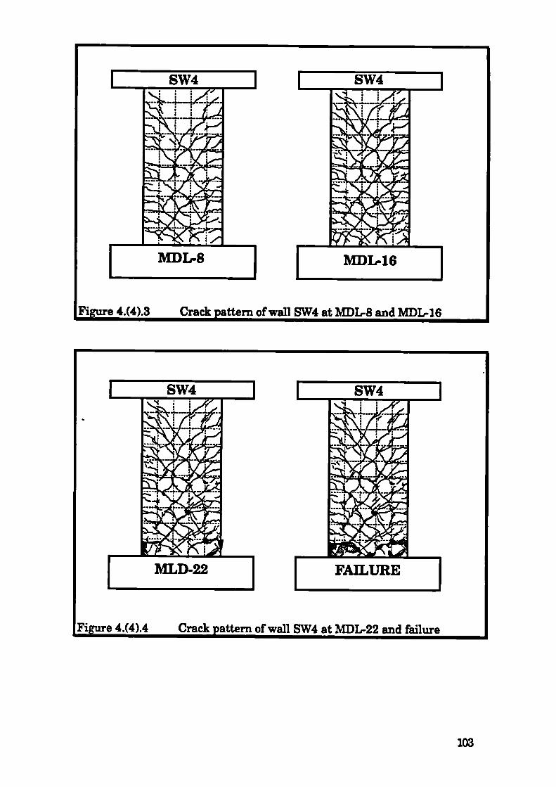
4.(4).3 Crack pattern of wall SW4 at MDL-8 and MDL-16
Figure 4.(4).4 Crack pattern of wall SW4 at MDL-22 and failure
103

4.4.2 Load-disDiacement curves
The load-displacement curves are given in figures A.(4).1 - A.(4).1Ofor displacements 3 to 12. Base vertical and out-of-plane displacements areshown in figures A.(4).11 and A.(4).12, respectively. The wall extensions attop, half and quarter height locations is shown in figures A.(4).13 - A.(4).15,respectively.
4.4.3. Strain aue results
Strain gauge readings are plotted against force in figures A.(4).16 toA.(4).38. The value of strain is always given in microstrain. Very few of thestrain gauges lasted long after yield level, which means that all straingauges located on the flexural reinforcement at the bottom level stoppedfunctioning before achieving the ultimate load. Six of the strain gaugeswere located on the stirrups but only number 19 seemed to be operationalthroughout the test.
4.5 Static cyclic loading . Scale 1:2.5 model SW5
Wall SW5 has more of the main reinforcement concentrated at theboundaries, hence was expected to sustain a higher flexural load if shearfailure did not predominate. In order to avoid problems with the fixing ofthe reference rods, as encountered in SW4, a different type of adhesive wasused, whilst the perpendicular plates were soldered at the end of thetransducer shaft
Two full cycles were imposed at each MDL until failure. Thereafter adifferent loading regime was imposed so as to avoid excessive deteriorationat early stages as explained later. The loading regime for SW5 is shown infigure 4.(5).1.
104

2824a)1612
-8-12-16-20-24-28
0 1 2 3 4 5 6 7 8 9 10 11 12 13 14Cyc]eNo
1 Loading history for SW5
4.5.1 General observations
- Cracking was observed before reaching the first MDL at 1 mm ofdisplacement. The initial wall stiffness as calculated at 0.5 mm was about34 KNImm. The stiffness at MDL-2 was 21.7 KN/mm.
Cracking at MDL-2 is shown in figure 4.(5).2. Cracks propagatedfrom the wall boundaries towards the centre and from the bottom upwards.Cracking was apparent up to three quarters of the height of the wall. In thelower half, the frequency of cracks near the boundary was higher than inthe web. However, the inclination of these cracks was steeper than that forwall SW4. The inclination of the main web cracks was about 30° to thehorizontal. By MDL-4 cracks propagated to the whole wall length as shownin figure 4.(5).2. In the lower half of the wall, at the boundaries, the densityof the cracks increased while in the web the number of main cracks waslimited to about four to five in each direction. The inclination of these mainweb cracks was about 45° in the lower part of the wall. Higher up, theinclination was much steeper up to 60°, indicating the shear nature of thesecracks.
105

4.(5).2 Crack pattern of wall SW5 at MDL-2 and MDL-4
By MDL-8 the frequency of cracking in the boundaries increasedconsiderably as shown in figure 4.(5).3. The main web cracks startedjoining with cracks originating higher in the boundary than before andhence, increased their apparent inclination.The most precarious crackseemed to be that originating at the top right hand side of the wall. MDL-1Owas achieved in one direction at a load of 117.3 KN. Yield level was justachieved in the shear reinforcement, but the flexural reinforcement wasjust below yield. On attempting to achieve MDL-1O in the reverse direction,abrupt failure occurred at a load of about 110 KN. At this stage two of themain web cracks opened up significantly as shown in figure 4.(5).3.However, the crack that caused failure was the lower one which goespenetrated the compressive area.
106

3 Crack pattern of wall SW5 at MDL-8 and MDL-1O
Following failure in one direction, it was decided to avoid cycling thewall twice at the same MDL and failure in the other direction wasimmediate after exceeding MDL-10 at a load of about 108 KM. The last MDLimposed in both directions was MDL-12. For the sake of demonstrating theeffect of cycling on a wall that failed in shear, displacements wereincreased by 2 mm in each direction as shown in figure 4.(5).1, until thelimits of the control transducers were reached. The state of the wall atMDL-14 is shown in figure 4.(5).4, demonstrating failure in the forwarddirection which was caused by the crack originating at the top left corner.Again two main cracks have opened considerably. After failure, severalhoops and stirrups opened up and considerable opening was noticed in themiddle sections of the wall. Additionally, it could be seen that the wall wasdisplacing in a rigid body mode above the main cracks. The considerabledegradation of the wall at MDL. 26 is shown in figure 4.(5).4.
107

SW5
SW5
POST-FAILURE
POST-FAILUREMDL-14
MDL-24
4
Crack of wall SW5 at MDL-14 and MDL-26
4.5.2 Load-displacement curves
The load-displacement curves are given in figures A.(5).1 - A.(5).1Ofor displacements 3 to 12. Base vertical and out-of-plane displacements areshown in figures A.(5).11 and A.(5).12 respectively. The wall extensions attop, mid and quarter height locations is shown in figures A.(5).13 - A.(5).15,respectively.
4.5.3 Strain gauge results
Strain gauge readings are plotted against force in figures A.(5).16 toA.(5).40. The value of strain is given in microstrain. Two of the straingauges were located on the hoop reinforcement, very close to the bottom ofthe beam. Four gauges were located on the stirrups Interestingly, thestrain gauge located very near the top beam indicated that no significantstrains excist at that level.
108

2420
16128
4.6 Stg k' eyr1fr! 1n1iiict - Si1e 1 !95 nindel SWR
Wall SW6 had identical flexural reinforcement to wall SW4 butconsiderably less lateral reinforcement, identical to the one used in wallSW5. The loading regime for SW6 is shown in figure 4.(6).1.
-8-12-16-20-24
0246810 12 14 16 18 20CycleNo
4.(6).1
for SW6
4.6.1 General observations
Cracking was again observed before reaching the first MDL, at 1 mmof displacement. The initial wall stiffness as calculated at 0.5 mm wasabout 33.5 KN/mm and at MDL-2 was 20 KN/mm. These two stiffnesses areboth slightly higher than the corresponding values of SW4.
The pattern of cracking at MDL-2 is shown in figure 4.(6).2. Despitethe apparent slightly higher stiffness, cracking was as extensive as in SW4at this stage. The pattern and extent was also almost identical. It is worthnoting that web cracks in both walls propagated deeper into the section inthe RHS by MDL-2. At MDL-4 cracking increased its density, progresseddeeper into the section and propagated to the whole length exactly as inSW4. The pattern of cracking was maintained until yielding of the mainflexural reinforcement just before MDL-6.
109

4.(6).2 Crack pattern of wall SW6 at MDL-2 and MDL-4
After yield, the extent of cracking in the web increased considerablyas shown in figure 4.(6).3. The main web cracks started joining with cracksoriginating higher in the boundary, hence increased more their apparentinclination than in SW4. Following MDL-8, the width of cracking started toopen considerably more than in SW4. However, by MDL-16 (figure 4.(6).3)the maximum load achieved was 107 KN which was higher than theultimate for SW4. Diagonal cracking propagated from the web into theopposite boundaries and seemed to have pushed the neutral axis, at least inthe surface, very close to the edge. Concrete spalling was also noted in thebottom end of the wall.
110

4.(6).3 Crack pattern of wall SW6 at MDL-8 and MDL-16
By MDL-18 (figure 4.(6).4), the concrete deterioration started affectingthe strength and even though the maximum load was achieved during theBHS MDL, less load was resisted when the displacement was reversed. Anopening of the stirrup in the lower level was observed at this MDL as well asprogression of the cracks through the compressed area. Crushing ofconcrete was initiated just before achieving MDL-20 in the LHS. The loss ofstrength continued in the subsequent cycles and by MDL-22 the load wasbelow 75% of ultimate in the RHS direction as well. In this direction, a widecrack crossing through the bottom boundary area was observed. MDL-22(figure 4.(6).4) was the last displacement to be imposed since the wall wasconsidered to have failed.
111
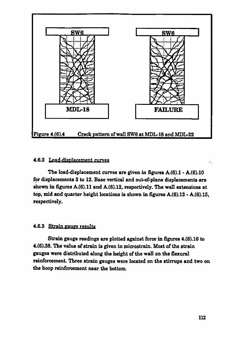
Figure 4.(6).4 Crack pattern of wall SW6 at MDL-18 and MDL-22
4.6.2 Load-displacement curves
The load-displacement curves are given in figures A.(6).1 - A.(6).1Ofor displacements 3 to 12. Base vertical and out-of-plane displacements areshown in figures A.(6).11 and A.(6).12, respectively. The wall extensions attop, mid and quarter height locations is shown in figures A.(6).13 - A.(6).15,respectively.
4.6.3 Strain gauge results
Strain gauge readings are plotted against force in figures 4.(6).16 to4.(6).38. The value of strain is given in microstrain. Most of the straingauges were distributed along the height of the wall on the flexuralreinforcement. Three strain gauges were located on the stirrups and two onthe hoop reinforcement near the bottom.
112

4.7 tqtir' (!Vclfr! 1pndjni - S"a1e 1 !9•5 'nndel SW7
Wall SW7 had most of the main reinforcement concentrated at theboundaries, similar to SW5, but had a higher shear reinforcementpercentage, similar to that of wall SW4. The expected flexural strength washigher than all other specimens. During the process of this experimentseveral technical problems were encountered. The voltmeter of the dataacquisition system developed some problems at the early stages of theexperiment and had to be repaired. As a result, an insignificant number ofdata was lost at the end of MDL-4. The other problems were associated withthe transmission box between the electrical motor and the screw jack. Dueto ageing and the high repeated loading imposed on the gear box, the motorcould not drive the jack on reverse high loads. Manufacturing new partsmeant additional delay in the completion of this particular experiment.
4.7.1 General observations
Cracking was observed before reaching the first MDL at 1 mm ofdisplacement. The initial wall stiffness as calculated at 0.5 mm was about33 KN/mm, dropping to 21.3 KN/mm at MDL-2. The loading regime for SW7is shown in figure 4.(7).1.
Cracking for MDL-2 is shown in figure 4.(7).2. Cracks initiallypropagated in a similar manner to wall SW5. Cracking was observed up tothree quarters of the height of the wall. In the lower half the intensity ofcracking near the boundary was higher than in the web. By MDL-4, crackspropagated to the whole wall length as shown in figure 4.(7).2. In the lowerhalf of the wall, at the boundaries, the density of the cracks increased whilein the web the number of main cracks was limited to about four to five ineach direction. The inclination of these main web cracks was less than orequal to 45°, and in general less steep than for SW5.
113

24
1612
g 8
-8-12-16
-240246 810121416182O24
CycleNo4.(7).1 Loading history for SW7
4.(7).2 Crack pattern of wall SW7 at MDL-2 and MDL-4
At MDL-8, the extent of cracking at the boundaries increasedconsiderably as shown in figure 4.(7).3. The main web cracks startedjoining with cracks originating higher in the boundary, hence increased
114

their apparent inclination but not to the extent seen for SW5. FollowingMDL-8, cracking continued to become denser at the boundaries with anaverage inclination of more than 45°, 'millie for wails SW4 and SW6 wherethe boundaries were wider. By MDL-14 (figure 4.(7).3), the miin web crackswere wider than before and seemed to have penetrated the compressivearea, at least on the surface.
4.(7).3 Crack pattern of wall SW7 at MDL-8 and MDL-14
The load capacity peaked at MDL-18 corresponding to a load of 127.3KM. Following thatthe widening of the web cracks increased and there wassome loss of strength at MDL-22 in the RHS direction. However, failureoccurred at MDL-22 by fracturing of a 6 mm reinforcement bar on the LHSvirgin cycle. A second bar snapped during the completion of this MDL andthe strength was reduced to less than half .The considerable degradation ofthe wail at MDL-22 is shown in figure 4.(7).4.
115

4.(7).4 Crack pattern of wall SW7 at MDL-22
4.7.2 Load-displacement curves
The load-displacement curves are given in figures A.(7).1 - A.(7).1Ofor displacements 3 to 12. Base vertical and out-of-plane displacements areshown in figures A.(7).11 and A.(7).12, respectively. The wall extensions attop, mid and quarter height locations is shown in figures A.(7).13 - A.(7).15,respectively.
4.7.3 Strain gauge results
Strain gauge readings are plotted against force in figures A.(7).16 toA.(7).41. The value of strain is given in microstrain. Almost all the straingauges in this wall lasted until considerable plastic strains were achieved.Seven strain gauges were located on stirrups and one on the bottom LHShoop.
116

2622181410
-6-10-14-18-22-26
Wall SW8 was designed so that the flexural reinforcement wasconcentrated in the edge members. Shear reinforcement was distributedaccording to the SRS method described in chapter 8. The amount of shearreinforcement was half of that required by EC2 and was distributed onlyover two thirds of the wall height. The loading regime for SW8 is shown in
4.(8).1.
0 2 4 6 8 10 12 14 16 18 20 22 24 26CycleNo
4.(8).1 Loading history for SW8
4.8.1 General observations
Cracking was observed before reaching the first MDL after 1 m.m ofdisplacement. The initial wall stiffness as calculated at 0.5 mm was about27.8 KM/mm dropping to 18.6 KM/mm at MDL-2.
Cracking at MDL-2 is shown in figure 4.(8).2. Cracks initiallypropagated in a similar maimer to wall SW4. Cracking was apparent up tojust over half the height of the wall. In the lower half, the density of cracksnear the boundary was higher than in the web and were most probablylocated above the hoop reinforcement. By MDL-4, cracks propagated to thewhole wall length as shown in figure 4.(8).2. In the lower half of the wall,more cracks propagated from the boundaries towards the web, compared toall other walls. The inclination of the main web cracks was about 450
117

4.(8).2 Crack pattern of wall SW8 at MDL2 and MDL-4
At MDL-6, a crack originating from the top corner propagatedthrough the web at an angle slightly higher then 45° to meet the web crackbelow, as shown in figure 4.(8).3. After MDL-6, craiking continued tobecome denser at the boundaries but the number of opening msin cracks inthe web stabilised to about four to five. By MDL-12 (figure 4.(8).3), the samepattern of cracking continued, but the main web cracks were wider thanbefore.
By MDL-18, the lower web cracks were opening more than the oneshigher up. Spelling of the concrete on the inside of the boundary elementindicated the degradation of the concrete at that location. At this stage,vertical cracks which appeared by MDL-14 at the bottom end mainreinforcement level were also visible (figure 4.(8).4). Following MDL-18, thewidening of the web cracks increased and more spalling of concrete withinthe web took place at the intersection of the main cracks. Loss of theconcrete cover at the extreme bottom parts of the wall exposed the flexuralreinforcement by MDL. 24. Due to the considerable degradation, the wall lostsome strength by the second cycle LHS MDL-24 and RHS MDL-26, as shownin figure 4.(8).5 The test was stopped at MDL-26 as soon as the load droppedbelow 75% of the ultimate, so as to avoid excessive dmfige to the specimen.
118

Crack pattern of wall SW8 at MDLI and MDL-12
4.(8).4 Crack pattern of wall SW8 at MDL-18 and failure
119

4.8.2 Load-distlacement curves
The load-displacement curves are given in figures A.(8).1 - A.(8).1Ofor displacements 3 to 12. Base vertical and out-of-plane displacements areshown in figures A.(8).11 and A.(8).12 respectively. The wall extensions attop, mid and quarter height locations is shown in figures A.(8).13 - A.(8).15,respectively.
4.8.3 Strain gauge results
Strain gauge readings, in microstrain, are plotted against force infigures A.(8).16 to A.(8).39. The stirrup reinforcement extended only up totwo thirds of the height and seven out of eight strain gauges located onthem were operational at the beginning of the test, five of which surviveduntil the final stages of the test, even after yield strains were recorded.
4.9 tgtk' I!Vlic loadjiw - Snle 1 !9.5 model SW!)
Wall SW9 had identical main reinforcement to wall SW8, but thelateral reinforcement was designed according to the requirements of EC2.The loading regime for SW9 is shown in figure 4.(9). 1.
4.9.1 General observations
Cracking was observed before reaching the first MDL after 1 mm ofdisplacement. The initial wall stiffness, as calculated at 0.5 mm, was about38 KNImm. The stiffness by MDL-2 was a little higher than for SW8, at 29.8KN/mm. Cracking at MDL-2 and MDL-4 is shown in figure 4.(9).2. Crackspropagated in a similar manner to wall SW8.
120

2622181410
-6-10-14-18-22-26
0246810 12 14 16 18 )22 24 26CydeNo
1
hi
for SW9
4.(9).2 Crack pattern of wall SW9 at MDL-2 and MDL-4
By MDL-6, the frequency of cracking in the boundaries increasedconsiderably as shown in figure 4.(9).3. However, the top crack, which alsoappeared in SW8 at this stage, had a shallower angle. After MDL-6,
121
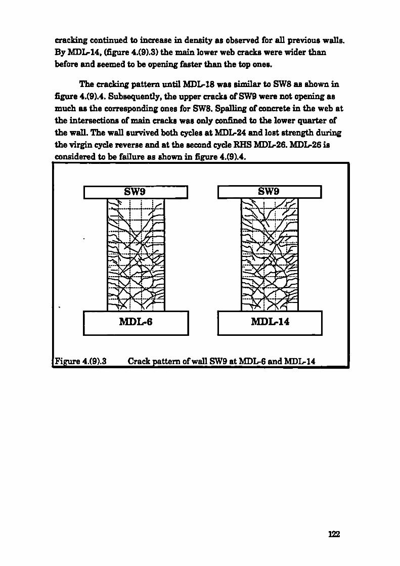
cracking continued to increase in density as observed for all previous walls.By MDL-14, (figure 4.(9).3) the main lower web cracks were wider thanbefore and seemed to be opening faster than the top ones.
The cracking pattern until MDL. 18 was similar to SW8 as shown infigure 4.(9).4. Subsequently the upper cracks of SW9 were not opening asmuch as the corresponding ones for SW8. Spalling of concrete in the web atthe intersections of main cracks was only confined to the lower quarter ofthe wall. The wall survived both cycles at MDL-24 and lost strength duringthe virgin cycle reverse and at the second cycle RHS MDL-26. MDL-26 isconsidered to be failure as shown in figure 4.(9).4.
4.(9).3 Crack vattern of wall SW9 at MDL-6 and MDL-14
122

Crack pattern of wall SW9 at MDL-18 and failure
4.9.2 Load-disDiacement curves
The load-displacement curves are given in figures A.(9).1 - A.(9).1Ofor displacements 3 to 12. Base vertical and out-of-plane displacements areshown in figures A.(9).11 and A.(9).12 respectively. The wall extensions attop, half and quarter height locations is shown in figures A.(9).13 - A.(9).15,respectively.
4.9.3 Shear and flexural deformation comDonents
As discussed in section 3.6, shear deformations can be separatedfrom the total horizontal deformations after calculating the flexuralcontribution. The flexural contribution in scale 1:5 walls was calculated byusing area 'al' of figure 3.12 since only top displacements were available.The shear deformation diagrams as calculated by this method are given insections 4.2 and 4.3. For scale 1:2.5 walls, the flexural contribution could beobtained by using the improved approximation of area 'cz2'. The results ofwall SW9 can be used as an example to demonstrate the differences between
123

the two methods. Figures A.(9).16 and A.(9).17 show the force versus thefiexural component of the top horizontal displacement, by using areas 'al'and 1a2', respectively.
As expected, the results from method of area 'al' yield much lowervalues for the flexural component. The ratio of displacements &a : &f(x1
varies within the same cycle and with increasing MDL. At peakdisplacements the value of this ratio varies from about 1.4 before yield toabout 1.7 at ultimate displacements. The effect on this on the calculationsfor shear deformation is not, however, straightforward, since therelationship between the different components of the horizontaldisplacement is not linear, as demonstrated by figures A.(9).18 to A.(9).20.
The ratio of 8 to 63 is nearly constant up to yield. Subsequently, theratio becomes smaller as the shear deformations become more dominant.In order to relate the discussion to an independent variable, the componentof shear is plotted against force in figure A.(9).21.
4.9.4 Strain aue results
Strain gauge readings, in microstrain, are plotted against force infigures A.(9).22 to A.(9).44. Five strain gauges were located on the stirrups,but none of the hoop strain gauges gave any meaningfull results.
The discussion of all the experimental results and comparisons withthe analytical studies described in chapters 5 and 6 is presented in thechapter 7.
124

CHAPIER 5
5 REINFORCED CONCRETE ANALYSIS MODEL
5.1 Infroduetion
The analysis of RC structures under transient loading requires theuse of a mathematical model representing the structure and a suitableanalytical tool for providing the solution of the ensuing equations. Indesign, a common practice is to simplifr the structure into 2-dimensionalframes and to reduce the dynamic loading into equivalent static loading. Byassuming elastic material properties, structural analysis results can beobtained either through the solution of closed form equations or by finiteelement analysis. More elaborate elastic methods solve the dynamicproblem by either using a suitable time history as input loading, or byemploying spectral analysis. In elastic methods, output member forcesmay be reduced by a factor depending on the ductility of the particularmember and structural form. Alternatively, a 'design spectrum',accounting for excursions into the nonlinear range is used as imput tomodal analysis.
The main disadvantage of elastic methods in reinforced concreteanalysis is the fact that the elastic properties of reinforced concreterepresent an over-simplification of the nonlinear behaviour of the material.Furthermore, a structure in not in the assumed elastic state even before theearthquake forces are imposed. It is also certain that as soon as thestructure is subjected to even moderate lateral loading, the change instiffness will affect the dynamic characteristics, hence elastic dynamicanalysis depart significantly from the anticipated behaviour. Consequently,inelastic analysis is essential for predicting the behaviour of reinforcedconcrete under both static and dynamic analysis. The structuralrepresentation of the building will not vary from that used in the elasticcase, but the analytical tool will have to take into account the materialinelasticity.
125

In the past two decades, with the advancement of computers andcomputational methods, the finite element method has been usedextensively in both linear and nonlinear structural analysis. Sophisticatedmaterial models have been implemented and various approaches have beendeveloped to transform the essentially discontinuous problem of crackedconcrete into a continuum mechanics model. However, a number ofproblems still remain to be solved before a particular model is deemedaccurate in predicting the inelastic behaviour of RC members. Inparticular for members such as walls, with high shear stresses andsignificant shear deterioration, following severe cyclic loading poses aformidable problem. Moreover, extensive parametric studies aimed atcomplimenting existing experimental data require more efficient andeconomical solutions than finite element analysis can offer. The samerequirement exists in design practices, where simplified solutions aremore suitable than detailed modelling techniques.
Based on section analysis, a simple computational tool for reinforcedconcrete analysis has been developed for the purpose of this researchprogrmnie. In subsequent sections, the description and assumptions ofthis method alongside material models used, are presented. Verificationand error analysis of the model as well as recommendations for futurework form the concluding section of this chapter.
5.2 Section rnuilvsis method
The assumptions on which the section analysis method is based areas follows:
a) Plane sections remain plane.
b) Full strain compatibility exists between concrete and steelreinforcement.
c) Flexural deformations are independent of shear deformations.
d) The total deformation is the sum of shear and flexuraldeformation.
126
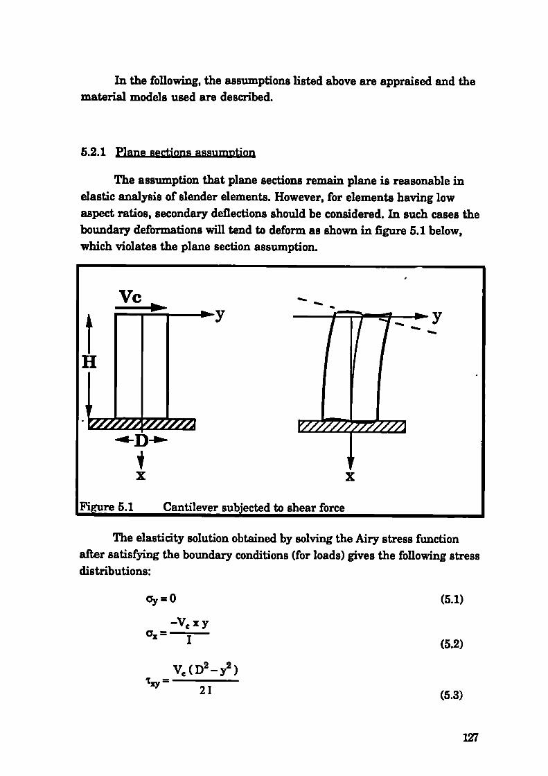
Vc
y y
I]
I.
x x
(5.1)
In the following, the assumptions listed above are appraised and thematerial models used are described.
5.2.1 Plane sections assumttion
The assumption that plane sections remain plane is reasonable inelastic analysis of slender elements. However, for elements having lowaspect ratios, secondary deflections should be considered. In such cases theboundary deformations will tend to deform as shown in figure 5.1 below,which violates the plane section assumption.
5.1 Cantilever subjected to shear force
The elasticity solution obtained by solving the Airy stress functionafter satisfring the boundary conditions (for loads) gives the following stressdistributions:
—VxyI (5.2)
V(D2—y2)txy =
2!
(5.3)
127

This solution is the equivalent of the classical beam theory approachand is valid for the parabolic shear distribution of equation 5.3 (Timoshenkoand Goodier, 1982). By integrating the plane-stress equations thedisplacements u and v in the x and y directions, respectively, may beobtained, as detailed in the following equations. The centre of the beam at y= H is taken as fixed and having no rotation with respect to the vertical axisas shown in figure 5.1.
Vx2 y vv1 y3 Vy3 (vH2 VCD2E1 - 6E1 + 6G1 2E1 - 2G1 )Y
vVy2 v 3 VC H VxD2v— 2E1 ^ 6E1 + 3E1 - 2E1 (55)
As expected at the centre of the free end (x=O, y=O) the horizontaldeflection v is V H3 / 3E1. However, the gradient of du/dy is not independentof y, as assumed by plane sections remain plane. Furthermore, in order toimpose compatibility at the boundaries, the top and bottom beams will exerta certain amount of moment and hence, deform. The exact deformed shapeis a function of the relative stiffness between the beams and the panel. Thelocal effect of the beam stiffness is a redistribution of both the shear andnormal stresses. A brief investigation by using a fine finite element meshand imposing plane sections at the top and bottom of the cantilever showedthat the shear stress is not any more parabolic (as obtained from equation5.3) but peaks very near the ends, where the normal stresses are also muchhigher than predicted by the beam theory.
In the case of reinforced concrete, the loss of the tensile strength dueto cracking causes a shift of the neutral axis compression side. Therefore,as far as the compressive area is concerned, the depth of the section isconsiderably reduced and hence, the secondary strains are minimised. Inthe tensile side, the plane section condition is imposed at the fixed and topends by the presence of the stiff beams. However, at mid-height of thecantilever, higher normal strains may be obtained at the extreme fibres dueto the plane section assumption. Following yield of the reinforcement, thiseffect is negligible for equilibrium purposes.
It can, therefore, be expected that the plain sections assumptionwould yield accurate results for flexure, even in deep reinforced concretemembers. However, the shear stress distribution is not expected any more
128

to comply with the parabolic distribution obtained by elasticity and hence,should be dealt separately.
5.2.2 Strain comDatibilitv
The strain compatibility of reinforced concrete under temperaturechanges is due to a coincidence in the thermal expansion properties of steeland concrete, but when external loads are imposed the compatibilitybetween strains has to be mRintained by bond forces at the interface.Modern high tensile steels for reinforcement are always deformed, andhence, provide bond through the effective process of mechanicalinterlocking rather than chemical adhesion and friction. Additionally, insection analysis, strain compatibility is more important when the materialsare sharing the resistance to normal stresses, i.e. only in compression. It isexpected that until a considerable compressive strain is induced, bondwould be sufficient to transmit the forces between the materials.
It should be noted that during load reversals, if bond is lost in themain bars of a RC wall, the stress distribution will not obey the beam theorybut will be in accordance with a combination of the beam and 'arch and tie'mechanisms. The arch and tie situation arises in the case of totaldebonding so that the force in the tensile bars is uniform throughout. Theimplications of the 'arch and tie' mechanism are further discussed inchapter 7.
5.2.3 Indetendence of flexural deformation
By using the principle of virtual work, flexural deformations arecalculated by integrating the product of virtual moment m0 end curvature kover the length under consideration i.e:
VfJlflokdX(5.6)
Assuming that the maximum moment is known, curvature atdifferent levels can be established by satisfying equilibrium. Numericalintegration can then be used to obtain flexural deflections. In order toestablish equilibrium from an assumed curvature value, only normal
129

strains and stresses can be used rendering the method uniaxial. Thestresses in steel bars can be determined accurately in this manner, butstresses in concrete are a function of the triaxial state of stress. Two-dimensional elasticity yields no stresses laterally as shown in equation 5.1.Nevertheless, the confinement and shear reinforcement, when provided,induce lateral stresses and should be accounted for. In the compressivearea, both types of reinforcement contribute towards higher confinement ofthe concrete which improves normal and shear stress resistance, asdiscussed hereafter.
The existence of shear stresses in the compressive area is usuallyassumed not to influence the stiffness characteristics of concrete. Inelasticity, the addition of a shear stress component leads to a rotation of theprincipal stress axis system and an increase in the major axis stress aswell as a decrease in the minor axis stress. This may influence theaccuracy of obtaining ultimate stresses and hence, indirectly affect thecalculations for flexure. Direct stress section analysis is incapable ofpredicting shear deformations, and need arises for an independent sheardeformation model.
The assumed boundary condition at the bottom is fixity, and norotations are allowed. In reality fixity is achieved for equilibrium purposes.In practice, however, in order to develop the boundary stresses, especiallytensile stresses in the reinforcement, a certain degree of extension as wellas compression deformation will occur within the foundation. Theresultant rotation at this level could have a significant effect on the overalldeflection. Paulay and Williams (1980) suggested that anchoragedeformations could be as high as 20% of the flexural deformations. Baserotation can also be a result of uplifting of the bottom beam in the case ofexperimental work. For the purposes of this test programme the bottombeams were prestressed to the floor with forces higher than the expecteduplift forces due to moment, and, hence the axial stiffness of the beam isassumed to be infinite. The effectiveness of the used method is examined inchapter 7.
If the assumption that flexural deformations are independent ofshear deformations is accepted, then the total deflection can be obtained bysuperposition of the flexural and shear components.
130

5.3 Flexural model imniementation
The method of section analysis assumes a certain strain distributionwithin a particular section, which is varied until force equilibrium isestablished. In order to achieve this, material models are used to calculatestresses for given strains. The cyclic models used for steel and concrete arediscussed below.
5.3.1 Steel model
The most commonly used steel model in design is the linear elasticperfectly plastic model. There are two significant draw-backs in simpli1ringthe steel behaviour to an elastoplastic model:
a) Ignoring strain hardening.
b) Ignoring stiffness degradation after inelastic load reversals.
The extent of strain hardening varies considerably in different steelsand modern codes have identified this discrepancy and recommend limitsfor the ratio of ultimate to yield stress of steels. The effect of ignoring strainhardening is to lead to an under-estimate of the section strength.Consequently, the accuracy in estimating the flexural strength, requiredfor the shear design may be forfeited.
The degradation of stiffness under cyclic loading exceeding yieldstresses is a material property that cannot be estimated from standardmonotonic testing. The degree of degradation has significant impact on theenergy dissipated by the steel and hence, by the structural member.Additionally, the stiffness of steel on reloading will determine the load levelat which concrete will be re-mobilised following the load reversal and,consequently, influences indirectly the behaviour of the reinforced concretemember in shear.
In order to represent simply the behaviour of the variety of steelsused, a tri-linear cyclic model has been formulated as shown in figure 5.2.Monotonic experiments, as described in chapter 3, are used to obtain themodel envelope. A yield level is determined by using the monotonic yield
131

load and the strain hardening stiffness E8 J'. A maximum stress 'fsu' isnot to be exceeded at any value of strain. Exceeding an ultimate strain 'e'will result in the bar fracture and total loss of strength. Loading andunloading up to the yield level and down to zero follows the initial stiffness'E 0'. On reloading, a stiffness 'Esa' is used. Once the yield level is achieved,stress increases according to stiffness 'E81'.
1 9 Yieldlevel__ai J
1!
so
A Esa
Strain Axis esu7 E .StiffiieuptoyieldlevelI: E55 .Degridatadstiffness: E -Stiffnessafteryieidlevel
1su -Maximum stressf5 -Initialyieldstress
-' - - - - a - - - -
al
5.2 Stress-strain diagram for steel used in
The above simple model was developed by using the massing model(Hays, 1981) in a slightly modified form and the stiffness degradation factor'a' from the work of Santhanam (1979). However, the latter reference usedmild steel and as a result the monotonic model includes a yield plateauprior to the onset of strain hardening. This plateau was observed in some ofthe tests on steel described in chapter 3, but not in alL Consequently, thisplateau was removed from the present model for all bar diameters for thesake of simplicity. This implies that the need of the yield growth factor '3'used by Santhanam to increase the yield stress on reloading above the yield
132

reloading above the yield plateau level, as shown in figure 5.3, iseliminated. Based on the experimental work of Popov and Peterson (1978) onsteel tubes subjected to torsional loading, the range of 0.15 - 0.3 for the valueof'a' has been proposed. The stiffness degradation model proposed byClough (1966), made use of a degraded stiffness equivalent to a value of 'a'of unity. In the absence of cyclic data for the steels used in the experiments,the value of 'a' is obtained herein by making use of the actual experimentaldata.
Figure 5.3 Santhanam's a— model for the uniaxial inelasticbehaviour of mild steel
The implementation of the steel model in a computer program issimple and only the current and previous maximum and minimum
133

5.3.2 Concrete model
The concrete model used is based on the work of Mander et al(Mander J.B, Priestley J.N. & Park R. 1988 a & b). It was chosen for itsdirect applicability to the method of sections and was implemented withsome modifications. The model though uniaxial in it's formulation, takesinto account the confining stresses.
5.3.2.1 Concrete confinement
Experimental work on confinement of concrete has been carried outby many researchers and there is a large number of biaxial and triaxialconcrete models. However, in most of these experiments active confiningstress was applied as a uniform hydraulic pressure. The effect of steelreinforcement in providing passive confinement has long been recognisedand several models have been presented based on RC column experiments.A description of early work is given by Vallenas, Bertero and Popov (1977).Their own experiments were conducted on rectangular RC columns despitethe fact that the objective was to obtain a model that would be used in theresearch work on RC walls. Their model is shown in figure 5.4 below andcontains the basic features of models to follow, such as an increased strainfor the increased maximum stress and extended unloading branch to anultimate strain.
134

REGION AB (EL1O)
• f €J E0
I.1-21 (!Lkf J
B
k
4
EXPERIMENTAL
,IIII
C
REGION BC: (c0 c E) REGION CD (ç3ç)
II . k [i_zc4 1i-u)] 4.3k
ICWIERE:
to0024'05 (i - .734(s))'IC
Ii .I..(I_.245 (p''fp) f;
.5ZR
.pJ",(3 ..002f\ .
I fIOOO I
o
£1.
0
.01 .02 .03 .04 D5 .061 In. • 25.4 •ui
NEW ANALYTICAL CURVE AND EXP!R1IENTAL RESULTS FOR CO'4FINED CONCRETEWITH LONGITUDINAL REINFORCEFCNT
Figure 5.4 Analytical model and experimental results for confinedconcrete by Vallenas, Bertero and Popov (1977)
Sheikh and Uzumeri (1980) conducted experiments at the Universityof Toronto and developed a model (Sheikh and Uzumeri, 1982) which placedparticular emphasis on the effect of the rectilinear reinforcement, asshown in figure 5.5 below.
I
Co.if
5.5 Effecti confined concrete area (Sheikh and Uzumeri, 1982)
135

Mander et al placed equal emphasis on the effect of confinement andproposed a confinement model similar to Sheikh and Uzumeri. Theobjective of a confinement model is to estimate an equivalent effective stressdue to the maximum confining steel force at the least confined section of thecolumn. The area of the least confined section can be calculated provided anassumed confinement profile is used. At ultimate conditions theunconfined area is expected to spall off, and hence the increased capacity iscounter-balanced by the reduction in cross section. Consequently, twodiscrete areas are considered, namely confined and unconfined areas.
Despite the elaborate calculations and assumptions of the existingconfinement models, several points of concern remain for RC walls undercydic loading, as discussed below:
a) The compressed area of walls under bending is loaded by avarying strain through the section and not constant as incolumns.
b) The variation of the confining stress along the height is nottaken into account.
c) The confinement force of the steel is not related to the normalstress and material properties of the concrete.
d) The initial prestress of the reinforcement due to shrinkage isnot accounted for.
e) The effect on the stiffness of the confined elements is not easy toevaluate.
f) The models and the experiments on which they are based aremonotonic with either active or passive uniform confiningpressure.
As shown in figure 5.6, the development of the lateral force in thesteel depends on the elastic properties of concrete as well as the axialstrain. It would be expected that initial shrinkage of concrete would leavesome initial prestress in the steel reinforcement. The exact initial value ofthis compressive strain is difficult to estimate but it is not expected to belarge and as a result it will only reduce the effect of confinement only at theearly stages of loading.
136

'I - '. I- 'I
• •_I -1•• •- - - -
•1
.. --
=
an• U UI U U III UI
• U I I I II I U II
I I I U I U U II II
I I I ii,
C
-. y
IT '—U—a--c0
N ? ? ?4ff14f1Tf4
aad
4ASZGSZ = 11 addJoJo
Figure 5.6 Strain and stress distribution along the RC wall boundaryelement
137

As a first estimate, the lateral strains 'cj and 'ci' and stress 'a8' canbe calculated from elasticity as the product of normal strain 'c,j andPoisson's ratio 'v'
(5.7 & 5.8)
a8=vCxE
(5.9)
The resulting forces 'F,' and 'F 8 ' due to the confinement are givenby
= A8 asy =A8 V Cx E50 (5.10 & 5.11)
F = A5 asz =A5 V C, E50 (5.12 & 5.13)
This force spreads into the concrete and consequently, the confiningstress will decrease. This effect was not considered by many of the previousresearchers even though it is likely to have a similar or larger impact thanthe reduction of the confined area at the critical sections.
For the purposes of section analysis the average values of concreteconfinement stresses (Ocy, Gcz) are required between sections so that thestiffness and deformations are estimated correctly.
a,=1ceAsyvcxEso/(bs)
(5.14)
= iCe A v c E50 / (ds)
(5.15)
For elastic sections where the confinement steel is distributed evenlyand linear distribution of strain prevails, the value of confinementeffectiveness 'ice' is equal to 0.5. For the critical section, 'Ice' should take intoaccount not only the variation of the effectively confined area but also thevariation of the confining stress along the section.
In order to avoid the elaborate calculations proposed by manyresearchers for evaluating the confinement factors, the effectiveness of theconfinement is provided to the section analysis program as an input.Simple calculations to account for the hoop pattern and spacing in squarecolumns are given by Tassios (1989) in a background document to EC8(1988).
138

"-U
0
('I
10"I
L0-J
Experimental work on triaxial compressive properties of concrete isconducted with equal confining lateral pressures and hence, it isconvenient to use a single value for the confining stress fl'. The value of 'fi'is calculated by using the confining stresses and a as shown in figure5.7 below. An alternative simple equation is used in the programproportional to (/c + Jac)2.
Confined Strength Ratio
1.0 1.5 2.0
0 0.1 0.2 0.3Smallest Confining Stress ,
IFigure 5.7 Confined strength determination from lateral confiningstresses for rectangular sections (Mander et al
Mander et al (1988 a) used equation 5.16 for the confined compressiveconcrete strength 'f' (f0 is the unconfined concrete compressive cylinderstrength). This is based on the failure surface model of Wilain and Warnke(1975), the experimental results of Schickert and Winker (1979) and wasimplemented by Elwi and Murray (1979).
—2—Ifx=f(-1.2M+2.254 /7-.;.f0) (5.16)
From the formulation of the solution providing variable confinementit can be seen that the level of confinement is dependent on the axial strain'Ci' and the Poison's ratio V (equations 5.14 and 5.15). Furthermore, allconfinement models assume that the maximum axial strain is a functionof the maximum confinement stress as defined by the yield of the hoopreinforcement (equation 5.16 and 5.20 or equation 5.17). This is best
139

illustrated by considering the simplified equation 2.6 for confinement givenin Appendix A of EC8 (1988), where 'O)wd' is the volumetric mechanicalratio of hoops and 'a' is a coefficient depending on the hoop steelconfiguration.
= 0.0035 + 0.10 CUwd a=c1(5.17)
Substituting in 5.14 (assuming equal lateral reinforcement in y and zdirections) gives the maximum expected hoop stress Cm.
Gmax = (0.0035 + 0.10 0wd a) ic v E / (b s) (5.18)
If it is accepted that the value of v will be about 0.5 at failure, equation5.18 shows that for a given amount and distribution of confinementreinforcement, a certain level of stress will be induced at ultimateconditions. If the stress in the hoop is not to exceed the yield level, then for agiven type of reinforcement, a certain critical volumetric mechanical hoopratio (0wcrit exists, over which further enhancement of the axial strain andstress is not possible. In fact, it appears that the level of confinement isdependent on the hoop yield strain as well as on the volumetric ratio. Thishas not been reported in the literature. Hence, the lateral strain is assumeato vary with the axial strain in such a way that they will both reach themaximum values simultaneously, whilst initially they are related to theinitial value of the Poisson's ratio. This assumption will give accurateresults at low levels of axial loads as well as at the ultimate conditions, butfurther research is required to determine the accuracy intermediately.
5.3.2.2 Monotonic concrete model
For a uniform confining stress, the monotonic confined compressivestress-strain curve is as shown in figure 5.8 and is given by:
fxr
- r - 1 + x'
(5.19)
where
ccI = -
Ccc(5.20)
140

Confinedconcrete
f, •1-•- - - -cc
I'Uncon finedconcrete
I
j 1Assumed for
Firs thoopfractu
U)U)
V)
.-U)U)
£ =cco[ 1+51&_1)]
(5.21)
T• E—E (5.22)
E = 5,OOO/? (MPa)(5.23)
E.4(5.24)
r
St cc
Compressive ,
Figure 5.8 Stress strain model for monotonic loading; unconfined andconfined concrete
For the unconfined areas, such as the cover and the web area of RCwalls, the falling branch after twice E )1 (concrete compressive strain inthe longitudinal direction at peak unconfined stress) is defined as a straightline which reaches zero stress at the strain of 'c51,'. In the computerprogram, concrete was considered to crush instantaneously, and hence,there is no unloading branch.
For monotonic tensile loading, concrete can carry tensile stresses upto a limit of '4' with stiffness equivalent to the tangent modulus of elasticityE'. The tensile strength may be affected by micro-cracking initially, and
141

will be lost at the initial stages of cyclic loading. Therefore, in theimplementation of the above model the tensile strength has been ignored.
5.3.2.3 Concrete model for cyclic loading
It is generally accepted that the monotonic stress-strain curve can beconsidered to be the envelope to the cyclic loading response. To describe acyclic model, the unloading and reloading branches should be defined asfollows.
5.3.2.3.1 Unloading regime
On complete unloading, the stress drops to zero at a plastic strain'Epi'. The value of the plastic strain depends on the previous maximumreversal point f) and strain 'Ca.' as shown in figure 5.9. For strainsless than 'Epi', the stress is considered to be zero.
vcI
- - - - -C.-I.-u
IfIl /1
E 0 ./JEp'
I I
I I'I
I I
PH
//
Figure 5.9 Determination of plastic strain £p1 and the unloading branch ofthe cyclic stress-strain curve for concrete
142

The strain Ca' is given as:
(5.25)
Where, in order to suit the confinement model, the value of 'a' is thegreatest of the two values given in equation 5.26.
C O.O9cor
C+C 1Ccc
(5.26)
Strain 'Ca' is used to define a pivot point in the stress-strain space byusing the initial tangent modulus which in turn is used to obtain the plasticunloading secant slope. The plastic strain lies at the intersection of the linethrough the return point f) and pivot point, with the zero stress lineand is given by:
(+)f£g=C—
(f+Ee) (5.27)
The unloading path is of similar form to the monotonic loading ofequation 5.19 as shown in figure 5.8, but is modified to pass through thepoint (0, Cpl), as shown in figure 5.9 and below:
xrrr— 1+x
where
r_E
(5.28)
(5.29)
E=(5.30)
Cc—Cun
Cp1—Cun (5.31)
E = bcE (5.32)
143

(5.35)
(5.36)
The value of the initial unloading modulus of elasticity 'E U' has beencalibrated by Mander, Priestly and Park (1984) on experimental results withthe following parameters:
b=—^1Lco (5.33)
(5.34)
5.3.2.3.2 Reloadin g regime
Reloading can occur from different previous unloading history casesand hence the different possibilities ought to be examined.
a) Reloading from a strain less than cpj.
b) Reloading from a strain 'ero' and stress 'ff0' where 'CTO' is lessthan 'Crni' and greater than 'Epi'.
c) Reloading to a strain higher than 'irn'.
d) Reloading to a strain higher than 'Cre'.
For case (a) the stress remains zero until c1 is exceeded and then thecase (b) is used to obtain the stresses. A linear stress strain relation isassumed between the return point (Cro,fro) and a new target point (Cun,fnew)
which accounts for the cyclic degradation in strength as shown in figure5.10 and the following equations:
= 0.92 + 0.08
where
- ronewEr— £roC (5.37)
For a strain exceeding 'C' and up to 'Cre', Mander et al (1988a)suggested a parabolic transition curve between the target point (Eun,fnew)and a common return point (Cre,fye) as shown in equation 5.38.
144

unew
E(2+.ç)
(5.38)
The value of'Ere' as obtained from this equation is found by using astiffness higher than the reloading linear branch E,since the value of(2+fIf 0) in the denominator is at least three. This does not conform withobservations from a number of cyclic experiments conducted on the controlcylinders and probably that was not the intention of the authors of thepaper. For the purposes of this work the value Of'Ere' was obtained bydividing 'Er' by the parenthesis value (instead of multiplying it) and amodified parabolic transition curve has been derived on the sameprinciples. To derive this second order equation, the three boundaryconditions used were the two end points (Eun,fnew) & (Cre ,fre) and thegradient at the first point being Er. The modified transition curve is givenby
where
=f.i-Ex+Ax2
x=(c—c1.)
A— (fnewre)re(tuntre)
-
(5.39)
(5.40)
(5.41)
For strains higher than 'Cre' reloading continues on the monotoniccurve as shown is figure 5.10.
145

5.3.3 Ultimate comoression strain
The ultimate compression strain for confined concrete is necessaryas to define the failure of a certain section provided some other type offailure has not taken place. A number of empirical equations are availablein literature for this, the most comprehensive of which link concrete failureto the hoop reinforcement fracture. Mander et al (1984) progressed furtherand proposed an energy balance approach. According to this method, theextra energy per unit volume of concrete core available under the confinedstress-strain curve for concrete (Ucc - Uco) 'plus additional energy requiredto maintain yield in the longitudinal reinforcement in compression' dtJ',
is equivalent to the energy stored in the transverse reinforcement 'Ush' asshown below:
U5h = U - U0 + U5(5.41)
The contribution of the transverse reinforcement to the increase inenergy capacity of confined concrete is well-established. Additionally, thestrain energy due to secondary bending 'U 5b' of the longitudinal
146

reinforcement can have a similar effect as the transverse reinforcement,but has been ignored. Moreover, the strain energy due to longitudinalreinforcement should not be included in the energy balance of confinedconcrete, since for a given strain this energy is present irrespective of thestate of confinement, and is also not included when deriving the stress-strain curves for confined concrete. Hence, a proposed modified energybalance equation becomes:
Ush+Usb = UcUco (5.42)
The above equation is equivalent to considering that all additionalenergy in confined concrete is equivalent to the steel strain energy build upin confining the concrete laterally. The solution of the above equation isbeyond the scope of the current thesis. However, it is considered that thecritical importance in solving the above equation is the exact determinationof the lateral strains in the longitudinal reinforcement.
5.3.4 Dynamic effects
Both the strength and stiffness of confined and unconfined concretehave been observed to increase with the increase in strain-rate. Mander etal (1984) proposed that the quasi-static stress-strain relationships can beused to describe the behaviour of the problem under high strain rates bymodifjing only the main material control parameters. This approachprovides the necessary simplicity and versatility that is necessary for themethod of section analysis. A number of equations have been calibrated toexperimental results by Mander et al (1984) representing:
a) Dynamic strength f
b) Dynamic stiffness E
c) Dynamic strain at peak stress i
147

Evaluatereinforcement
levelCalculate load
for a given
5.4 Commiter nroram CREUC
The computer program CRELIC (Cyclic REinforced concreteanaLysis Imperial College) developed on the basis of section analysis andmaterial models described in earlier sections was implemented on theMicrovax computer of the ESEE section in Fortran 77. The solutionprocedure is outlined by the flow chart in figure 5.11.
DATA INPUT
caioalatecorete efrain
at maximumconfinement
Establish forceequilibrium by
varying the neutralaxis 1sition for
anaxat level H • 0
Calculate the momentat level H • 0
EstabJish U requiredmoments at difforent
levels H • all
Fix curvature andestablish forceequilibrkunby
varying the neutrsaxis position
Calculate themoment and compare
against moment required.Calculate new
% curvature if
Integrate thecurvatures to obtain
flexural displacement
OTJPLJT RESULTSoFrIO?S
IFI
Vary Material Calculate shearParameters deformations
e 5.11 Flow chart of computer CRELIC
148

o 8
l200mn
Data input include information on the geometry, loading, materialcharacteristics, and confinement. Control data are also required, toindicate desired accuracy for the different iterations. The analysis can beperformed as a remote operation or interactively.
After reading the data input, the program calculates automaticallythe displacement corresponding to the maximum confined strain inconcrete. Following that, control is returned to the user through variousoptions. For cyclic loading, the displacement control option allows forfollowing the hysteretic behaviour of the member at prescribeddisplacements or automatic cycling.
5.4.1 A test run for wall SW9
The program was checked by using SW9 as a test case. Theexperimental flexural deformations, obtained by the improved methodsuggested in Chapter 3, were imposed at the top of the wall. Only a smallportion of the output information is possible to be presented here ingraphical form, and is included in Appendix B. Results for key locationsselected for output are shown in figure 5.12 below.
5.12 Positions of data Dresented from roram CRELIC
The top horizontal flexural displacement 83, the verticaldisplacement 84 and the top average displacement are shown in figures B 1 -
149

B3, while the corresponding displacements at quarter height are shown infigures B4 - B6. Strains at the locations shown are presented in figures B7 -B12.
5.4.2 Discussion of Dr02ram results
The load versus flexural displacements 83 compare well with theexperimental data. A slightly higher load is achieved in the analyticalresults. This may be attributed to the simplification of the post-yield steelbehaviour in the analytical model. The relaxation at peak displacement,observed in the experimental results is not seen in the analytical resultssince this effect has not been modelled. The reloading stiffness isreproduced accurately, and this indicates that the used value of 0.5 for thesteel stiffness degradation factor 'a' is reasonable. Lower values of 'a' gavehigher initial reloading stiffness and more energy dissipation as shown infigures 5.13 and 5.14. The energy dissipation from the analytical results at'a' equal 0.5, is still higher than the one from the flexure experimentalcurves. This is mostly due to the higher strength and no relaxation effectsin the analytical model. It is however, less than the overall energydissipated by the experimental model.
-30000
20000
p000
10000
5000
0
0 2 4 6 8 10 12 14 16 18 2) 24
CycleNo
5.13 Cumulative energy dissipated versus MDL
Of particular interest is the difference exhibited by the hystereticenergy per cycle in the early loops as shown in figure 5.14. The analytical
150

results indicate much less hysteretic energy being absorbed, probably due tothe absence of tensile strength in the concrete model used.
3o
2O
15
j1OOO
r!500
00 2 4 6 8 10 12 14 16 18 Z) 24
CycleNo
5.14 Energy dis
The load versus top vertical displacement 84 (figure B2) plotdemonstrates that a significant difference exists between the analysis andexperiments in the compression displacements. Whilst, experimentally thecompressive loads do not completely reverse the tensile plasticdisplacements, in analysis compressive displacements are alwaysrecovered even after yield. The same effect is observed in strains of theextreme fibre reinforcement (B.7), whilst for bars located further inside thewall section (B.8 to B.1O), the reversal of tensile strains is still much lessthan in the experiments. The net wall extension, however, seems to be lessaffected by this effect. A difference worth noting in the wall extensions (B.3)is that in the analytical results, the minimum extension for a particularcycle after significant inelasticity occurs on reloading at a much higherload than in the experiments.
All the above observations may be a result of concrete dilation atcrack interfaces. Due to shear deformations, the opposing crack surfaces donot match on closure and due to their roughness, contact is establishedeven when tensile strains in the reinforcement are still observed. Thismechanism, termed 'aggregate interlock', is considered to be responsiblefor shear transfer through cracks as a consequence of the co-existentnormal stresses. Tassios and Vintzeleou (1987) demonstrated
151

experimentally the shear transfer mqchanism and concrete dilatancy ofcracked surfaces during cycling for low constant normal stresses.Dilatancy degradation was also noted to occur during cycling and'formalistic' models were proposed for different crack roughness surfaces.
An attempt to evaluate the dilatancy effects on the concrete stress-strain cyclic relationship has been made by Thu, Wu and Zhang (1980) whoproposed an empirical model based on a limited number of experimentalresults. Unfortunately, as with many other shear stiffness formulations,explicit use is made of a crack width, something which can not becalculated directly by the method of sections.
The strains at the extreme fibre at quarter height (B.11) werepredicted accurately by the analytical model. A tensile shift of the strains inthe experiment is attributed to the initiation of cracking and the resultingdilatancy.
The strains at the extreme fibre at the top of the wall (B.12) arepredicted to be slightly higher than the average of the experimental data.This may indicate that total loss of the tensile strength does not occur soclose to the point of zero moment. In fact, the initiation of cracking isclearly identifiable in the experimental results. This occurs during theincrease of the load over the yield value with a distinct deviation from thenearly elastic uncracked behaviour to the cracked behaviour.
The results from the flexural analytical model seem to reproduceaccurately the strength state of the cyclic model, and reasonably accuratelythe general behaviour of reinforced concrete walls subjected to cyclicloading. The flexural model is utilised further in chapter 6, to investigate awide range of parameters which is beyond the scope of the experimentalinvestigation undertaken in the course of this project. The model is alsoutilised for further comparisons with the experimental results in thegeneral discussion of the results.
5.5 Shear model
Elastic shear stresses can be calculated by making use of the virtualwork method. For a unit element shown in figure 5.15 these can be
152

.1 S Vi-
oh
calculated as the integral of the product of shear strains and a virtual shearforce at the level of desired shear deformations given by:
IVc '!I
-qII
II
:
I- ---------
lvi- ---DI l-
•1II
III
Unitelement
-A - -D_
5.15
Shear deformations of a wall element
8=f'vOydx(5.43)
where
vi3GA
(5.44)
For a rectangular section, '' is about 5/6. Equations 5.43 and 5.44show that the elastic shear strain rate of change ' is independent of thenormal stresses since 'G', the modulus of rigidity (or modulus of elasticityin shear), is as shown below:
E2(1+v) (5.45)
Nevertheless, the stiffness of concrete is neither linear nor elasticand a nonlinear value of shear modulus 'GNL' is assumed. The total sheardeformation can be integrated from the deformations of the slice elements
as shown in the equation below.
153

V18h
• GB8j(5.46)
Within a section of height '6h', '8' is constant, and the sum of 'Vi'should be equal to 'Va' as shown below.
D B 8VCVj
8h G(d) 8d
(5.47)
This implies that '6' can be calculated as a function of 'GNL(d)' asbelow:
6
811= D
Gjd) 8d(5.48)
The total deformation can be calculated by suniming the sectional •deformations over the height. By assuming constant '8D' and '8H' '8t'becomes:
H6VHV5A .4 D
h=O '-'24 G(h,d)d= 0 (5.49)
The above formulation requires the determination of 'GNI'. Since themodulus of rigidity is depended on the normal stiffness, it follows thatnonlinear shear stiffness is a function of the flexural stiffness. Areasonable assumption is to consider the secant stiffiiess of concrete asin equation (5.45).
There are, however, a number of difficulties arising from the aboveassumption. The first one is associated with the shear stiffness of thereinforcing bars. In the absence of concrete, due to its slenderness, the steelcage is capable of resisting a very low level of shear force because of bendingdeformations. In reinforced concrete, the amount of shear resistance by thesteel is expected to increase as a result of the different deformed shape. In
154

order to simplify the problem, in the current study, the steel shear stiffnessis considered to be identical to the concrete stiffness.
The second difficulty arises from the formulation of the fiexuralmodel. As expected from the flexural cyclic results, the concrete sectionwill have a tangent stiffness of' zero below the value of 'tpl'. As a result, theshear displacements will be infinite. However, in practice, due to contacteffects, reinforcement and aggregate interlock, there is always a degree ofshear stiffness even for an open crack.
A possible solution to the above problem is to give 'Gj as a distinctfunction of normal strain. Such approach is used extensively in finiteelement analysis. Figure 5.16. below (ASCE, 1982) shows diagrRnimaticallya number of such models.
05
OJ- IY j,6.2L(t1/c,)
_____. --. -- deep beenL24
edoim and Del ll ihollOw bean.___ ___ ______ ___ YuzuguI iuid&MoIdt
° 2r \Lc1c'
I25 -- _____ _____ _____
- ---a.01
-. iheor H7E,mesystem
ToiiIeitroun nornl to crock c. 10
Figure 5.16 Reduced shear modulus versus tensile normal strain (ASCE,1982)
The equation given by Al-Mahaidi (ASCE, 1982), was used for therange of strains shown in figure 5.16. In the range of strains not covered bythe above-mentioned model, the secant stiffness as obtained from theflexural model was used, with a value of G not less than 0.4 times theelastic value.
The third difficulty associated with equation 5.48 is that the sheardeformation is zero at zero values of shear force. This cannot be the case,especially if there are permanent or plastic shear deformations. Such
0
II
155
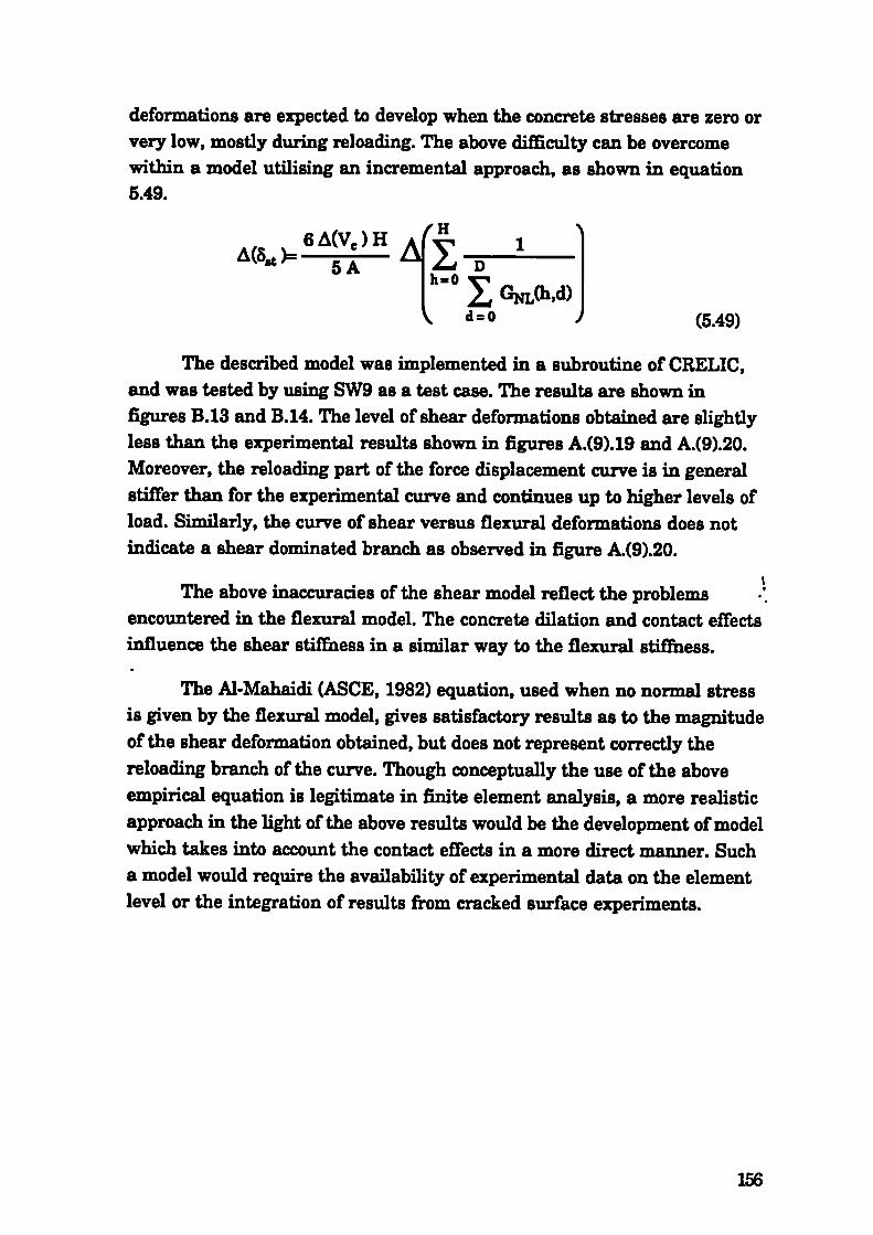
deformations are expected to develop when the concrete stresses are zero orvery low, mostly during reloading. The above difficulty can be overcomewithin a model utilising an incremental approach, as shown in equation5.49.
6zMV)H fH
15A
L\JD I
h=OGjh,d) I
d=O ) (5.49)
The described model was implemented in a subroutine of CRELIC,and was tested by using SW9 as a test case. The results are shown infigures B.13 and B.14. The level of shear deformations obtained are slightlyless than the experimental results shown in figures A.(9).19 and A.(9).20.Moreover, the reloading part of the force displacement curve is in generalstiffer than for the experimental curve and continues up to higher levels ofload. Similarly, the curve of shear versus flexural deformations does notindicate a shear dominated branch as observed in figure A.(9).20.
The above inaccuracies of the shear model reflect the problemsencountered in the flexural model. The concrete dilation and contact effectsinfluence the shear stiffness in a similar way to the flexural stiffness.
The Al-Mahaidi (ASCE, 1982) equation, used when no normal stressis given by the flexural model, gives satisfactory results as to the magnitudeof the shear deformation obtained, but does not represent correctly thereloading branch of the curve. Though conceptually the use of the aboveempirical equation is legitimate in finite element analysis, a more realisticapproach in the light of the above results would be the development of modelwhich takes into account the contact effects in a more direct manner. Sucha model would require the availability of experimental data on the elementlevel or the integration of results from cracked surface experiments.
156

CHAPTER 6
6 ANALYTICAL PARAMETRIC STUDY
6.1 Introduclf on
The parametric study of this chapter was undertaken msking use ofthe cyclic reinforced concrete section analysis computer program (CRELIC)discussed in chapter 5. The choice and range of parameters are discussedand the results, normalised whenever possible, are subsequently presentedin graphical form. In normalising the moment capacity, the control modelsection capacity is used. The control model was chosen to represent wallssimilar to the ones tested previously. Discussion of the results and theirimplications is given in chapter 8.
6.2 Geometry
For analytical purposes the actual scale of the model will notinfluence the results qualitatively but only qualitatively. As a result, themodel dimensions used in the experiments were retained to facilitatefuture comparisons. For stability purposes, the ratio of DIB is the importantparameter, and a value of 1:10 is the limit of some codes. This value wasfound by Goodsir (1985) to provide a reasonable degree of protection againstlateral instability. Therefore, the experimental cross-sectional dimensionsof 60 mm x 600 mm were used for the parametric study.
For simplicity, the aspect and shear ratios were kept equal. Thisimplies that there is no top beam as required in the experiments. The shearratio value is irrelevant in moment capacity calculations since the onlyaffected quantities are displacements. Shear displacements are dependenton the product of shear force and the height, hence would be constant for acertain cross section irrespective of the shear ratio. However, the flexuraldisplacements are proportional to the square of the shear ratio. The
157

deterministic nature of the component displacements does not require anadditional parametric study but is discussed further in chapter 7.
The lower limit to which section analysis applies is for shear ratios ofabout 1. For lower aspect ratios, the basic assumption of plane sectionsremain plane is not valid. Additionally, the boundary effects will influencethe stresses in a larger portion of the wall.
6.3 Volumetric ratio and distribution of steel within the section
The volumetric ratio of steel within the cross section should not be auniversal parameter in design since the yield strength of steel varies.Nonetheless, it is widely accepted since it is easy to use in practice. Valuesvary with a minimum of 0.25% and up to a maximum of 4% (sometimesrelated to yield strength 16If). The walls in the experimental part of thecurrent research were tested at about 3%. A lower value of 1% has beenchosen, with a mid-value of 2%.
Realistically, it is not always possible to arrange reinforcement inexact integer percentage values. For the purposes of this study, a minimumbar diameter of 4 mm (10 mm for a full scale wall) is assumed as the unitbar. The numbers of unit bars and exact percentages used in the section aregiven in the table below:
Table 6.1 Volumetric percentage of reinforcement for parametric studywalls
CODE Design Design Number of$ Actual
area (mm2) bars & area
Wi 1 360 30-377 1.05
W2 2 720 60-754 2.1
W3 3 1080 90-1131 3.15
W4 4 1440 120 - 1508 4.2
158

One of the most important parameters which influence the overallbehaviour of the section is the distribution of the flexural reinforcementwithin the section. The uniform distribution (UD), though not a veryefficient way of utilising reinforcement, is a common lower bound referencepoint. A good second distribution is based in supplying minimumreinforcement to the web and distributing evenly the rest in the confinedarea CUB) as was done in walls SW4, 6, 8,9. Finally, the upper extremedistribution, not recommended in design, is based in supplying minimumreinforcement to the web and concentrating the remainder in the wallextreme fibres (CB). Such an arrangement was used in walls SW5, 7.
The reinforcement was distributed according to table 6.2. Theconcrete cover thickness at the boundaries was assumed to be 10mm. Theminimum spacing was 60 mm. The amount of reinforcement is given inunits of 4 mm diameter bars only for comparison purposes. As an example,the 8 mm and 16 mm diameter bars are equivalent to 4 and 16 unit barsrespectively.
159

Table 6.2 Position and distribution of reinforcement in walls- - - - - - - - - - -
10 60 120 120 240 300 360 420 480 540 590 R/ment Position
CODE
Distribution- - - - - - - - - - -
W1UD 3 3 2 3 3 2 3 3 2 3 3 Uniform
W1UB 4 4 4 1 1 2 1 1 4 4 4 Boundaries
W1CB 10 1 1 1 1 2 1 1 1 1 10 Concentrated- - = = - - - - - - -
- - - = = - - - - - -
W2UD 6 5 6 5 5 6 5 5 6 5 6 Uniform
W2UB 9 9 9 1 1 2 1 1 9 9 9 Boundaries
W2CB 25 1 1 1 1 2 1 1 1 1 25 Concentrated
- - = - - - - - - - =
W3UD 8 8 8 9 8 8 8 9 8 8 8 Uniform
W3UB 14 14 14 1 1 2 1 1 14 14 14 Boundaries
W3CB 40 1 1 1 1 2 1 1 1 1 40 Concentrated- - = = - - - - = = -
- - - - - - - - - = =
W4tJD 11 11 11 11 11 10 11 11 11 11 11 Uniform
W4UB 19 19 19 1 1 2 1 1 19 19 19 Boundaries
W4CB 55 1 1 1 1 2 1 1 1 1 55 Concentrated
The first parametric study involved the above 12 cases, as shown intable 6.3. The results of the parametric study concerned with the variationof the steel volumetric ratio and distribution are presented in figures 6.1 to6.5.
160

Table 6.3 Variation of steel amount and distribution
U)
-
Cd
—
.a g
.11 0 ___ ___ __ ___
LI .2
.U)
.C4
"-'- E '
z_____ _____ ___ _____
C')
—
•— — I
. .I -LI LI ,• 0
2 • •
161

1.0
0.9
0.8
0.7
0.6
0.50 1 2 3 4 5
2.0 • UD
I 1.6 ______
1.4 CB ______ _______
1.8S UB _____ _____ ______
0
1 2 3 4 5p%
Figure 6.1 Norma]ised section capacity versus percentage of flexuralreinforcement for different types of distributions
Figure 6.2 Normalised section yield to ultimate capacity versuspercentage of flexural reinforcement for different types ofdistributions
1

0.3
0.2
0.1
0.00 1 2 3 4 5
p%
Figure 6.3 Normalised neutral axis depth at ultimate capacity versuspercentage of flexural reinforcement for different types ofdistributions
.-
.1
A10
00
1 2 3 4 5p%
Figure 6.4 Curvature ductility versus percentage of flexuralreinforcement for different types of distributions
163

6
10 1 2p%3 4 5
Figure 6.5 Displacement ductility versus percentage of flexuralreinforcement for different types of distributions
6.4 Concrete thiracteristics
Most codes of practice consider the strain of 0.0035 to be the ultimateBtrain of concrete, in bending. The value of varies slightly with theunconfined concrete compressive strength f0 but a far more importantvariation occurs with different amounts of lateral confinementreinforcement available in the element under compression.
The current parametric study investigated the variation of concretestrength and ultimate unconflned concrete compressive strain 'E 01. Forthe concrete strength 'f0' values between 20 and 50 N/mm2 are used. Asfar as 'C,' is concerned, there are a number of models that can be used toconvert the supplied confinement into enhanced concrete strength 'f', andultimate concrete compressive strain 'c'. However, in order to facilitatecomparisons with the modern trends in Europe, the EC8 Appendix Aequations discussed in Chapters 2 and 5 are used in this section. The rangeof values is chosen so as to cover both branches of the bilinear confinementmodel given. An upper limit on strength enhancement factor of 2.5 is used.The confinement effectiveness factor 'a' is taken as 0.25. One wouldprobably expect a slightly higher value for higher confinement ratios, but asingle value is used for simplicity. Table 6.4 shows the parameters used.The results of this parametric study are presented in figures 6.6 to 6.10.
164

Table 6.4 Variation of concrete strength and confinement
l C'.4CD
IiCa
C
N
'C-0
N
'I-
-o '.4 N ID C0 0 0
e' c
— _
C
C C '
o o CC.)
165

0.2 0.4 0.6 0.8 1.0 1.2Conf5neTnent
0.900.0
0.95
1.05
Figure 6.6 Normalised section capacity versus mechanical confinementratio COwd for different concrete strengths
F 0.80
0.78
0.76
0.74
0.72
0.700.0
0.2 0.4 0.6 0.8 1.0 1.2Coifinement
Figure 6.7 Normalised section yield to ultimate capacity versusmechanical confinement ratio (Owd for different concretestrengths
166

0.25
0.20
0.15
0.10
0.05
0.000.0 0.2 0.4 0.6 0.8 1.0 1.2
Conf5n'inent
4OS
30
120
10
00.0 0.2 0.4 0.6 0.8 1.0 1.2
ConfineTnPnt
60I:
50
Figure 6.8 Normalised neutral axis depth at ultimate capacity versusmechanical confinement ratio co,d for different concretestrengths
Figure 6.9 Curvature ductility versus mechanical confinement ratio (Owdfor different concrete strengths
167

10
p8
00.0
0.2 0.4 0.6 0.8 1.0 1.2Confinement
I Figure 6.10 Displacement ductility versus mechanical confinement ratiofor different concrete
6.5 Steel ithsracteristics
Variation in nominal yield strength as well as unintentionalvariations can be investigated by varying the yield strength of flexuralreinforcement. The value of actual to nominal yield strength is required byEC8 to be less than 1.25. The maximum yield strength used in this sectionis 575 N/mm2 (1.25 x 460 N/mm2) and the minimum 355 N/mm2.
Of great significance to the section characteristics are also the steelyield to ultimate ratio, strain hardening stiffness, degradation parameter'a' and ultimate strain of reinforcement. However, these parameters areinterrelated in affecting strength, ductility, and energy dissipation. Indefining the steel characteristics from the experiments described inchapter 3, a simple trilinear envelope model was used. However, only thereinforcement used in the tests was tested, and hence, the possiblevariability of these parameters could not be assessed for the more generalpurpose of this parametric study.
168

The EC8 limitation on the ratio of the yield to ultimate stress of 1.45 isused as an upper bound for this parameter.
The value of ultimate strain of 0.012, which is recommended by EC8for the high ductility class walls, is used for the parametric studies.However, this variable is only a check on the mode of failure and does notaffect otherwise the behaviour.
The strain hardening stiffness for the experiments was in the rangeof 1000 - 3000 N/mm2. In order to limit the extend of the parametric studythe higher value of 3000 N/mm2 was used, in an attempt to achieve theultimate capacity without exceeding the ultimate strain limit. In fact, thisis just possible for steels with the higher values of yield stress and highvalues of ultimate to yield stress ratio. In the limit, the results of thisparametric study is expected to highlight the limitations of the used model,as well as the lack of comprehensive experimental data on steelreinforcement. Table 6.5 shows the parameters used and the results arepresented in figures 6.11 to 6.15.
1

Table 6.5 Variation of steel characteristics
.-
- -I--- ------- ---- ----
- .
U
w
..! 4.a —
I.'
170

L3
1.2
0.7320 355 390 425 460
Yield stress
- 1.1
1.0
0.9
0.8
495530565
0.9
I:
0.8
0.7
Figure 6.11 Normalised section capacity versus steel yield stress fordifferent ultimate to yield stress ratios
0.6 I I I I I I425460495530565600
Yield Stress
Figure 6.12 Normalised section yield to ultimate capacity versus steel yieldstress for different ultimate to yield stress ratios
171

I:
16
114
10
0.20
0.19
0.18
0.17
0.16
0.15 I I I I I425460495530565600
Yield stress
Figure 6.13 Normalised neutral axis depth at ultimate capacity steel yieldstress for different ultimate to yield stress ratios
18
1.0_ __ - =- -
• ___ ___ -I -_Ifl ___
_____ _____
— - 1. 5 _____
•___ ___
•____ _
8355 390 425 460 495 530 565 600
Yield stress
Figure 6.14 Curvature ductility versus steel yield stress for differentultimate to yield stress ratios
172

5I'3
21 I I 1 1 1460 495 530 565 600
Yield stress
Figure 6.15 Displacement ductility versus steel yield stress for differentultimate to yield stress ratios
6.6 Axial load
Most codes limit the value of the axial load normalised with respect toaxial crushing capacity to 0.35. As a result, the full interaction curvetraditionally used for load bearing members is not required. The effects oftension are investigated through the lower range value of this parametricstudy. Since, the variation in the depth of the neutral axis is expected to bemuch higher than for the other cases, the confined area is extended to coverthe whole section so as to avoid the possibility of web crushing. The amountof confinement is the second variable as shown in table 6.6. Results of thisparametric study are presented in figures 6.16 to 6.20.
173

Table 6.6 Variation of axial load and effect of confinement
U) 00 C U) 00 '-I C U) 00 C It) 00 '-I C1 U) 00 C It) 0.
- = _______ _________ _________ _________ _________
'I ..-'I
. )>I
174

1.50
11.25
0.75.0.2 -0.1 0.0 0.1 0.2 0.3 0.4
Axial
Figure 6.16 Normalised section capacity versus normalised axial force fordifferent confinement values
I : 1.0
0.9
0.8
0.7
-0.1 0.0 0.1 0.2 0.3 0.4Axial
Figure 6.17 Normalised section yield to ultimate capacity versusnormalised axial force for different confinement values
0.6-0.2
175

0.5
0.4
0.3
0.2
0.1
0.0-0.2 -0.1 0.0 0.1 0.2 0.3 0.4
Axial
180
60
j40
20
0-0.2 -0.1 0.0 0.1 0.2 0.3 0.4
Axial
120
Figure 6.18 Normalised neutral axis depth versus normalised axial forcefor different confinement values
Figure 6.19 Curvature ductility versus normaiised axial force for differentconfinement values
176

110
.5
0-0.2 -0.1 0.0 0.1 0.2 0.3 0.4
Axial
Figure 6.20 Displacement ductility versus normalised axial force fordifferent confinement values
6.7 Cyclic loa!inct
6.7.1 Confinement
The effect of cyclic loading on the wall behaviour was investigated fordifferent increments in MDL. As with the experiments two cycles areimposed at each displacement level. The effects of the amount ofconfinement is again the second variable as shown in table 6.7. The resultsare shown in figures 6.21 to 6.25.
177

Table 6.7 Variation of cyclic loading and effect of confinement
Ji __
QC.I
. 0
•- eq
0
eq
Lt
- o-cq o-cq o-eq
.
U?
'44.a
0— — .- .-
.0
178

1.01
0.96
0.950.0
1.00
0.998
0.98
0.97
0.1 0.2Confinement
0.76
0.75
0.74
0.73
0.72
0.710.0 0.1 0.2
Confinement
Figure 6.21 Normalised section capacity versus confinement level fordifferent EMDL values
Figure 6.22 Normalised section yield to ultimate capacity versusconfinement level for different b.MDL values
179

0.20
0.18
0.16
0.14
0.12
0.100.0 0.1 0.2
Qjn1nIn1flt
I.1
r
00.0 0.1 0.2
Figure 6.23 Normalised neutral axis depth versus confinement level fordifferent EMDL values
cnnen'nt
Figure 6.24 Curvature ductility versus confinement level for differentMDL values
180

5
p4
-fl
J2
.'1
00.0 0.1 0.2
Con15nipmet
Figure 6.25 Displacement ductility versus confinement level for differentMDL values
6.7.2 Axial load
The effect of cyclic loading on the wall behaviour is investigated foran increment of 2 mm in MDL on walls with different axial load levels asshown in table 6.8. As with the experiments two cycles are imposed at eachdisplacement level. The confinement of the wall is considered to cover theentire section, so as to avoid web crushing. The results together with themonotonic curves, are shown in figures 6.26 to 6.30.
181

Table 6.8 Variation of axial loads for cyclic and monotonic lateral
loading
II
C
O OOOU 0000L().. oeooç000c
.- c.1
d
C'3
= =
- - - - C
e•1.
182

-0.1 0.0 0.1 0.2 0.3 0.4Axial
1.0
0.8
0.6-0.2
1.4
1.0
0.9
0.8
0.7
0.6
Figure 6.26 Nornialised section capacity versus axial load for monotonicand cyclic loading
U MonronicCycli1
Steel fracture
.'____
-0.2 -0.1 0.0 0.1 0.2 0.3 0.4Axial
Figure 6.27 Normalised section yield to ultimate capacity versus axial loadfor monotonic and cyclic loading
183

0.5
0.4
0.3
0.2
0.1
0.0-0.2 -0.1 0.0 0.1 0.2 0.3 0.4
Axial
Figure 6.28 Normalised neutral axis depth versus axial load for monotonicand cyclic loading
40
______ ______ Monot ic ______Cyclic
S
I
10
0 - I-0.2 -0.1 0.0 0.1 0.2 0.3 0.4
Axial
Figure 6.29 Curvature ductility versus axial load for monotonic and cyclicloading
184

6
.5
1-0.2 -0.1 0.0 0.1 0.2 0.3 0.4
Axial
Figure 6.30 Displacement ductility versus axial load for monotonic and
The results of chapter 6 will be discussed together with theexperimental results in chapter 7.
185

CHAP'rEit 7
7 COMPARISONS AND DISCUSSION OF RESULTS
7.1 Introduction
In this chapter a general discussion of the experimental andanalytical results is presented. Design implications are also mentionedwhere relevant, however, a more design oriented discussion will beprovided in chapter 8.
7.2 Stiffness characteristics of sDedmens
7.2.1 Exoerimental stiffness
The specimen secant stiffness during the cyclic loading is variable,depending on the loading history. However, due to the consistency indisplacement of the loading regime employed, the secant stiffness at theMDL can be used to monitor the overall stiffness deterioration. The crackedsection stiffness, shown in some of the figures, is calculated by using theflexural model presented in chapter 5 (by using computer programCRELIC).
For the shake-table test, the equivalent stiffness at the centre of masshas been calculated from the response frequency by assuming that thesystem is behaving elastically. The results have been plotted on the samegraph as for SW2 and SW3, as shown in figure 7.1.
186

14
12
1:2
0
£ SW1
0
I *
0 1 2 3 4 5 6 7 8 9 10 11 12 13MDL
IFigure 7.1 Secant stiffness of SW1, SW2 and 5W3 versus maximumlevel
As depicted in figure 7.1, the calculated stiffness of SW1 is in generalless than the corresponding static-cyclic test. One of the reasonscontributing to the decrease in pre-yleld stiffness may be the large numberof cycles imposed by the earthquake time histories prior to yield. In order toexplore this further, during the first cyclic test SW2 a large number of loadreversals was applied at low displacement levels. As can be seen fromfigure 7.1, the stiffness deterioration is insignificant, despite the largenumber of load reversals at the same MDL. It can be concluded, therefore,that prior to yield the stiffness degradation is more depended on the MDLrather than the number of cycles at a particular MDL. This conclusion isnot expected to be valid after yielding due to the accumulation of plasticstrains in the reinforcement.
The secant stiffness of SW3 at top wall level is higher, since the testwas conducted at a different shear ratio from the other scale 1:5 walls(figure 7.1). This test was necessary as a link between the two scales usedand comparisons can only be made with the walls SW4 and SW6 for whichthis wall can be considered to be a half scale model.
The secant stiffness of SW3 (scaled by 2:1), SW4 and SW6 is shown infigure 7.2. The initial stiffness of SW6, as obtained from information prior toMDL-2, is much closer to the uncracked section than all other walls.
187

However, after MDL-16 the same wall is showing faster stiffnessdeterioration. A comparison with SW3 indicates that at the smaller scale,the initial stiffness is reduced much more than at a larger scale. A possibleexplanation for this is the effect of micro-cracking due to shrinkage. Thesubsequent stiffness deterioration is similar at both scales, which indicatesthat the scaling was performed successfully.
I csw
I SW
• SW c2
- - - - - - - - - - a -
i Cr ck ISiffnss
10
rb
0o 2 4 681012141518 ) 2426
MDL
Figure 7.2 Secant stiffness of SW3, SW4 and SW6 versus maximumdisplacement level
Walls SW5 and SW7 (figure 7.3) have a higher elastic stiffness thanall the other walls because of the concentration of the reinforcement nearthe boundaries. The stifFness of wall SW7, after initial cracking remainshigher than all other walls. As expected the stiffness of SW5 drops sharplywhen shear failure occurs at MDL-1O.
188

40
10
00 2 4 6 8 10 12 14 16 18 20 24 26
MDL
Figure 7.3 Secant stiffness of SW5 and SW7 versus maximumdisplacement level
No significant difference between the stiffness of walls SW8 and SW9is noticeable in figure 7.4 at all load stages. This is despite the fact that wallSW8 had much less shear reinforcement than SW9. This is contrary to theidea that walls with low reserve in shear capacity will deteriorate in shearas proposed in EC8 (1988) and presented in chapter 2.
40
0ack :d S iffi ss
----
-
10 •-
10
0.0
2 4 6 8 10 12 14 16 18 20 24 26MDL
Figure 7.4 Secant stiffness of SW8 and SW9 versus maximumdisplacement level
189

—11
—14
H m m
l ye —
I
-. Vc
aji
(7.1)
(7.2)
(7.3)
7.2.2 Elastic uncracked stiffness
The elastic uncracked stiffness 'Ke' of an RC wall can be readilyobtained in a closed form solution. By using the principles of virtual workand figure 7.5, shear deformations are given by equation 7.1.
D
Real Real
Virtual Virtualmoment shear moment shear
Elastic deformations of RC walls
U1H=J
H V 'H' 2.76V(H\V*GAdx=GB)= EB
which is obtained by assuming v = 0.15 in equation 7.2.
EG— 2(1+v)
Flexural deformations are given by equation 7.3.
um=JH m VH
m*rTdx=6I(3arH2_H2)
(2 V
= t EBJ()(3ar_1)
The total deformations are the sum of equation 7.1 and 7.3, as givenby equation 7.4.
(V= U1H + Uffi = I EB ) (..)[ (6 aT —2) (H)2 + 2.76]
The composite value of elastic Modulus Et is given by equation 7.5,190

(7.5)
(7.6)
[EI+E.I.lE
where
I=(Aj s)
and s is the distance of the ith bar from the centre.
From equation 7.4, the elastic lateral stiffness Ke can be determinedfrom,
vcK,=-
UH
By using equation 3.21 to evaluate the concrete elastic modulus andassuming E1 to be 200,000 KNImm2, the elastic stifihess is calculated asshown in table 7.1. The cracked section stiffness is calculated by usingthe flexural model presented in chapter 5 (by using computer programCRELIC). The value of stiffness given is in KN/mm.
The ratio between the experimental stiffness obtained at firstnRyimum displacement level 'K1' (MDL-1 at scale 1:5 & MDL-2 at scale 1:5)
and the elastic analytical stiffness 'Ke', is about 1:4 and 1:3, for models atscale 1:5 and 1:2.5 respectively. It is obvious that from a very early stage ofloading, the elastic stiffliess does not represent the true stiffness. Thedeviation from linearity is likely to be dependent not only on the loadinghistory but also on the material characteristics, dimensions and curingconditions.
The cracked stiffliess, as obtained by the section analysis method , ismuch closer to the initial specimen stiffness than the elastic stiffness. Theestimates of the cracked section stiffness would be further reduced byadding a reliable shear displacement estimate and allowing for the rotationat foundation level. For design purposes, it is therefore advisable to use thecracked stiffness rather than the elastic stiffness in the calculations notonly for the static analysis but for the dynamic analysis.
(7.7)
191

Table 7.1 RC wall stiffness at to wall level ______ _____ ______
WALL Is F Ke KCT K1 KL Ke1K1 KeIKL
CODE mm 4 N/mm2 KN/riirn KNIrnm KN/mni
SW1 3.15E06 39568 19.94 - - 1.25 _____ 16.0
SW2 3.15E06 39568 19.94 4.5 3.0 1.25 6.6 16.0
SW3 3.15E06 39568 29.66 11.7 7.4 2.51 4.0 11.8
SW4 50.53E06 39576 59.33 23.2 19.3 4.6 3.1 12.9
SW5 75.78E06 43551 65.29 29.0 21.7 2.9 3.0 22.5
SW6 50.53E06 39576 59.33 23.1 20.0 3.4 3.0 17.5
SW'? 75.78E06 43551 65.29 29.0 21.3 4.6 3.1 14.2
SW8 51.84E06 39782 59.64 23.7 18.6 4.0 3.2 14.9
SW9 51.84E06 39782 59.64 23.7 18.7 4.0 3.2 14.9
The stiffness at MDL-11 and MDL-22 are considered as an indicationof stiffliess at ultimate conditions for scale 1:5 and 1:2.5, respectively. Forthe aspect ratio 2 walls, the ratio of the elastic to ultimate stiffness wasbetween 10 and 15, for specimens that failed in bending. A higher value wasshown for SW6 which deteriorated due to shear, and was even higher forSW5 which failed in shear. For well designed walls, stiffness deteriorationis a function of displacement ductility. In EQ resistant design, the expectedshift in the response frequency, due to stiffness deterioration, should betaken into consideration since it may result into higher design forces.
7.3 TJmit states
The different limit states achieved by the walls are presented in thissection. The crack level is usually given by many researchers as the firstlimit state. As seen from section 7.2, some degree of micro-cracking waspresent in all specimens prior to testing and, consequently, defining thestage at which initial cracking is observed bears little significant.
192

7.3.1 Yield level
Yield level is defined here as the level at which the first mainreinforcement bar yields. Table 7.2 shows the quantities at the yield limit forboth experimental and analytical results. Top displacement 34 (figure 3.5)is given for comparison purposes.
Table7.2 Yield limit uantities _______ _______ _______ __________
WALL Bar Yield Exp. Anal. Exp. Anal. CommentsCODE $ strain 84 84 Load Load
____ (mm) ___ (mm) (mm) (KN) (KN) _____
SW16 7750 ______ -- SA100 _______ EQ
SW2 6 7750 1.8 1.12 17.5 16.2 _________
SW3 6 2750 1.8 0.85 22.5 22.4 _________
SW4 12 2500 2.2 1.55 76 75.0 Estimate §
SW5 16 2600 2.5 1.74 110 105.9 Failure•
SW6 12 2500 2.4 1.54 74 75 _________
SW7 16 2600 3.0 1.75 17 105.9 Bending 91
SW8 10 2150 2.4 1.42 71 70.6 Estimate §
SW9 10 2150 2.4 1.42 70 70.6 Bending 91
* Both critical strain gauges were unreliable for walls SW4 and SW8. The experimentalvalues given !or these walls in the above table are estimates based on the remainingdata and information from similar walls.
I In walls SW? and SW9, one of the main extreme end bars yielded at a lowerdisplacement than the other, hence out-of-plane bending is suspected to be one of themain reasons for non-uniform distribution of strains at the same section location.
• Shear failure prior to achieving the ultimate load.
SW5 failed just before achieving yield for LHS sway while yieldingalready started for RHS sway. For this wall strain gauge number 4 yieldedat about 110 KN, which may indicate that the strain gauge readings of thebottom extreme locations are not very reliable and that a better correlationbetween experimental and analytical results may exist.
193

As shown in table 7.2, despite the difficulties in defining precisely theexperimental yield load, there is a close agreement between theexperimental and analytical values. Nevertheless, the top verticaldisplacements 84 vary significantly. The experimental displacements aremuch higher than predicted analytically. Since at this load the bottom levelstrains are similar in analysis and experiments, the implication is thatmuch higher levels of strain are present throughout the height of the wallin the experiments. This indicates that some type of concrete dilation isoccurring even before yield during cyclic loading. As discussed in chapter5, this dilation occurs due to the imperfect closing of the crack surfacesmostly as a consequence of shear deformation.
The level of yield load is an important design parameter, since it canbe easily calculated. It can be used to predict the ultimate capacity, theplastic hinge zone and the ductility of a section. A number of parametersdetermine the absolute value of the yield moment M, as well as the ratio ofyield to ultimate moment MIMit.
Both M and MIMit increase with increased percentage of flexuralreinforcement p%. The same effect is brought about by increasing theconcentration of reinforcement near the wall extremities since theieduction of the lever arm after yield is minimised.
Increased concrete confinement does not increase M7 significantly,
since the development of the confining stress does not occur at the earlycurvatures for walls with no axial loads. On the contrary, M varies almostproportionally with the steel yield stress.
In the useful range of variation, increased axial loads cause anincrease in the section capacity. However, the increase in M is much moredramatic. At high axial loads, compressive yielding precedes tensileyielding, which, in some instances, does not occur at all.
Both experimental and analytical results indicate that the effect ofcycling does not alter the level of M significantly. Experimentally, it hasbeen shown, that prior to yield, cycling does not lead to significantdeterioration of strength and stiffness. Nonetheless, some net extensiondoes occur as will be discussed in section 7.5.
194

7.3.2 Ultimate limit states
The analytical calculations were based on ultimate strains given byequation 5.17, as shown in table 7.3 below. The confinement factor 'a' asgiven by the draft EC8 is considered to yield conservative results, and hence,for analytical flexural deformations these values were chosen so as toachieve a better . correlation with the experimental values.
Table 7.3 Confinement data
WALL Hoop$ (wd a £cc Ecu•__j(mm)m) _______ x 10E06 N/mm2
SW1 - 3 2.8 0.185 0.5 3032 17750 49.25
SW4 6 0.24 0.5 3251 15500 51.00
SW5 4 0.12 0.25 2311 6500 43.00
SW6 4 0.085 0.5 2447 7750 ________
SW7 6 0.31 o.25 2850 iro ________
= SW8 4 0.125 0.5 2674 9750 46.25
SW9 4 0.18 0.5 3001 12500 49.00
The ultimate load and corresponding displacement is shown in table7.4 for the experimental and analytical results. Displacement & refers tothe top wall horizontal displacement as shown in figure 3.5.
The analytical ultimate forces are higher than the experimental onesfor all scale 1:2.5 walls (except SW6). This is expected since the effects ofcyclic load as well as shear are not considered in the analytical results. Theultimate capacity of SW6 is higher than the corresponding wall SW4 whichhas higher confinement and shear reinforcement. The only plausibleexplanation of this may be a higher than average steel strength. In fact, thedefinition of the experimental yield strength in the 12 mm diameter barswas not distinct. In the analysis the lower value of yield strength shown intable 3.6 has been used. The ultimate strength of the wall becomes 108.5 KNwhen the higher value of yield strength is used in the analysis, a valuewhich is in better agreement with the experimental result.
195

The analytical predictions are very close to the experimental resultsfor all the walls that failed by steel fracture. This is to be expected, since thereinforcement strength is known exactly at failure strain.
Table 7.4 Ultimate limit state
WALL Exp. 83 at Exp. 83 at Anal. 83 Exp. Anal. CommentsCODE Vcmax failure at Vcmax Vcmax Vcmax on exp.
________ (mm) § (mm) § (mm) (KN) (KN) failure
SW1 - 13.4 8.1 .24• 21.2 Steelfracture 91
________ ________ _________ (10.4) ________ (20.6) __________
SW2 9 12 8.0 22.5 22.22 Steelfracture 91
_________ _________ __________ (10.15) _________ (21.6) ___________
SW3 10 13 4.54 30.4 30.95 Steelfracture 91
________ ________ _________ (6.18) ________ (30.3) __________
SW4 10 24 16.03 104.0 112.8 Crushing
SW5 10 9.6 9.37 117.3 131.4 Shearfailure #
_________ _________ __________ (4.00) _________ (116.0) ___________
SW6 18 22 9.10 107.8 103.7 Crushing /_______ _______ _______ _______ _______ _______ Shear
SW7 18 22 10.44 1272 128.3 Steelfracture 91
________ _________ _________ (13.82) ________ (134.3) __________
SW8 22 26 12.16 95.3 107.0 Crushing
SW9 22 26 16.5 -97.4 112.1 Crushing* Two values are given for experimental displacements, one corresponding the to
ultimate load and one to the displacement at failure. For the analytical results thesetwo displacements are the same.
I Failure in all scale 1:5 models was due to fracture of the extreme 6 mm bars at the levelof the bottom strain gauges. The failure of specimen SW7 was also due to failure of the 6mm bars even though they were not positioned at the extremes. The values inparenthesis represent the analytical results with the steel ultimate strain as control.
• The shake-table wall failed at an equivalent force of about 24 KN, as estimated fromfiltered accelerations.
0 The values in parenthesis represent the analytical results close to the experimentalfailure load.
196

The ultimate moment capacity M it is required not only for flexuralbut also for shear design purposes. In calculating Mit, a certain controlparameter has to be satisfied. Limits are Usually imposed on steel ultimatestrain by codes, so as to avoid fracture of steel. Concrete ultimate strainbecomes, therefore, the control parameter for the determination of Mit.Moreover, other parameters also influence the value of Malt, the most of theimportant of which are discussed below.
In the parametric study of chapter 6 the flexural moment capacitywas normalised with respect to a control specimen. Hence, the resultsbecome independent of the wall scale, or even the shear ratio.
An almost linear increase in Mit is shown in figure 6.1 withincrease in the percentage of reinforcement. Charts derived in a similarmanner can prove useful guides in design, enabling the rapid estimate ofpercentage of reinforcement for given wall dimensions. It is interesting tonote that the uniform distribution 'UD' of reinforcement is effectively alower bound, while the extreme boundary concentration 'BC" is an upperbound to the moment capacity. In design, it can be easily determined whichtype of distribution applies by comparing with the three given cases.
The effect of concrete strength f0 is more important in unconflnedconcrete walls than for moderately confined walls. Nonetheless, the overalleffect of f0 is not very important. A 100% increase in the concrete strengthincreases Mit by less than 5%, as shown in figure 6.6. The same effect canbe achieved by increasing the ultimate concrete strain through confinementreinforcement.
The above highlights a common error by researchers who back-calculate the concrete strength from the section capacity. A 5% error in thevalue of Mit, which can easily arise in experimental work, can lead to100% overestimate of the concrete strength. Hence, one of the principleconclusions from the work of Lefas (1988), that the capacity of RC walls isindependent of the uniaxial concrete strength, can only be a result of sucherrors. In fact, frictional forces due to the direct application of forces to thespecimens in the above-mentioned research programme, are estimated tohave increased the section capacity by up to 10%. Such errors castconsiderable doubts regarding the shear strength calculations which werebased on the large concrete overstrength reported.
197

The increase in Mit is much less for high confinement levels, sincethe peak steel strength will control. Hence, the significance of the steelultimate strain limits is demonstrated.
Increase in steel yield strength 'fr' and ratio fdt/fy also increases themoment capacity. However, for the value of strain hardening stiffness usedin the analytical model (3000 N/mm 2), the ultimate steel stress was notachieved for the fit/f ratios higher than 1.3. This highlights the followingissue that should be considered in design. The post-yield capacity of steelwill not necessarily be developed if it only occurs at very high strains.
A very significant variation in moment capacity may occur due to thepresence of axial loads as shown in figure 6.16. Where a variable axial loadis applied, such as in earthquake loading, the bending capacity should bedesigned with consideration of both lateral and axial forces. Alternatively,dimensioning should be undertaken based on the moment corresponding tothe least compressive force.
7.4 Horizontal deformations
Horizontal measurement analysis has been discussed in section 3.6.It has been suggested that expansion at the top beam is negligible. This hasbeen verified in the experiments by comparing top horizontal displacements3 and 18 (figure 3.5). However, displacements within the wall height werenot checked for expansion. It became obvious during the experiments thatspalling of concrete and opening of the 4 mm diameter stirrups wasaffecting measurement reference points at post-yield displacement levels.This makes the obtained data difficult to utilise for shear calculations.
The deformed shape of the wall can be obtained by using the values ofthe displacements at the different heights. An interesting case isdemonstrated for SW5 in figure 7.6. The effect of spalling, after failure inthis case, is seen at the base level. Failure occurred on the reverse MDL-10and the change in the deformed shape is clear. Deformation componentsattributed to each deformation mechanism (flexure and shear) arediscussed hereafter.
198

7.4.1 Flexural and shear components of deformation
The decomposition of flexural and shear displacements wasperformed for wail SW9. The general observations from the five graphs
resenthd in Appendix A (Figures A.(9).16 - A.(9).21) are as follows:
(a) The flexural stiffness decreases at a very slow rate prior to yield.Thereafter, the unloading stiffness progressively decreases at a slowrate.
(b) The reloading flexural stiffness decreases much faster after yield.Near failure it is only about one third the level of the unloadingstiffness.
(c) Shear stiffness decreases progressively until yield. As with thefiexura] unloading stiffness, following yield it progressivelydecreases at a slow rate.
(d) After yield, the shear deformations in reloading exhibit two distinctlydifferent portions. In SW9, up to about one third of the reloadingforce, the shear stiffness is very low and a considerable reversal ofdisplacement takes place. Up to this load level, the strains in allflexural bars are positive. The stress in the extreme bars should be ata state just before yielding in compression and hence, the average
199
strain of the bottom sections is positive. Under these conditions thecompressive stresses in concrete should ideally be zero, in whichcase the moment is resisted purely by the steel cage. However,imperfect closing of cracks may induce some compression inconcrete.
(e) The second portion of the reloading shear stiffness is much stifferthsin the first , but is still lower that the unloading shear stiffness.The increase in stiffness may be attributed to the increasedcontribution of concrete in resisting shear. At this level the cracks inthe compressive area from the previous loading direction would haveclosed.
(f) The area within the hysteresis loops which represents the energydissipation is considerably higher in flexure than in shear.
(g) The flexural deformations given by using the method of area al, arelower than predicted by method of area a2. This implies thatcalculations made by using information from just the top level canlead to inaccurate results.
The results were further processed at peak displacements. Figure 7.7below shows the component displacements versus applied force.
It is dear that both the flexural and shear components ofdeformation increase much more rapidly after yield, despite the fact thatthe force increases only slightly. The above graph shows the results for bothcycles at the same MDL, the load being higher on the virgin cycle ratherthan the second cycle. As it can be seen, especially in the post-yield stages,the shear deformations increase in the second cycle, and hence, the drop inthe force is partly due to the drop in flexural deformations.
200

1.0
0.8
0.6
0.4
0.2
0.0-24 -20 -16 -12 -8 -4 0 4 8 12 16 20 24
MDL
100
a)
a)
-20
-40
-60
-80
-100-26 -22 -18 -14 -10 -6 -2 2
Deformation (mm)6 10 14 18 22 261
7.7 Force versus deformations at peak di
Of particular interest in understanding the components of eachdeformation, is the plot of the ratios with respect to the total deformationshown in figure 7.8.
7.8 Ratios of component to total deformation versus MDL
The shear ratio is increasing from about 0.15 as obtained fromelasticity calculations (section 7.2.2), to about 0.4 at ultimate conditions.
201

However, the deformations are not symmetric in both directions of loading.This implies a shift of the permanent shear deformations locked in afterunloading. This is best illustrated in figure 7.9 showing the permanentdeformations at zero load with respect to MDL.
16
12
I -12
8
4
0
-4
-8
-16
•____Shar
P
4. •
* iI
_______ _______ _______ Fle ure
-30 -20 -10 0 10 2) 30MDL
7.9 Deformations at zero force versus MDL
As seen from figure 7.9, the permanent shear deformations arehigher for RHS than LHS MDL. Up to MDL-16 the RHS permanent sheardeformations do not seem to be reversed. Reversal of permanent sheardeformations is, nonetheless, observed after MDL-16. However, spalling ofthe concrete cover may be contributing towards the indicated reversal, sincethe horizontal transducer readings will be biased. It is therefore verydifficult to condude that shear deformations would be reversed at allduring such type of loading. The above is a strong indication of theelastoplastic nature of shear deformations. Moreover, it seem that thestiffness during the low levels of load at which the permanent deformationsare developed, is equal in both directions.
7.4.2 Strains in lateral reinforcement
The gauges on lateral reinforcement were used only in the 1:2.5experiments. In general the readings are very low prior to web cracking.The opening of the web cracks causes a noticeable increase of the tensilestrains when increasing the MDL at load levels prior to yield. At both RHSand LHS values of maximum force the strain is maximum and decreaseswith decreasing shear force. After cracking the tensile strain at zero load
202

progressively increases with increasing MDL. The lateral dilation of thewall is another indication of incomplete closing of the flexural cracks. Thelateral extension of the wall induces additional tensile stresses in the shearreinforcement. This effect is equivalent to prestressing the wall laterallyand may increase the shear stiffness prior to yielding of the shearreinforcement. Nonetheless, following yield of the lateral reinforcement, itseffectiveness may be reduced in resisting shear in the opposite direction.
For the walls which eventually failed in flexure, following yield, thelateral strains varied almost linearly with the absolute value of the shearforce. The maximum strain achieved was in general dependent on theamount of reinforcement available and the location of the stirrup. Thestirrup closest to the top beam was not stressed at high strains. This is mostprobably due to the confining effect of the stiff top beam, as well as thepresence of lower axial strains and fewer cracks.
In wall SW5 the lateral reinforcement yielded at mid-height of thewall just after yielding of the flexural reinforcement during RHS directionof loading. The consequence was an abrupt shear failure in the reversedirection. The stirrup closest to the bottom beam did not yield at failure butonly afterwards. It is clear that stirrups not spanning the portion of thecritical shear crack in the web do not contribute towards the ultimate shearresistance of the member. This is further discussed in chapter 8.
In SW6, gauge 21 (figure A.(6).36) indicated that the stirrup at threequarter height of the wall yielded after the wall exceeded the yield load. Theother strain gauges on stirrups of this wall did not continue to operate afteryield load. The yielding of the stirrups, was also followed by opening ofstirrups at the boundary at very high MDLs. The consequence of theanchorage inadequacy of stirrups was the progressive deterioration of theshear stiffness of this wall.
In SW8, yielding of the top stirrup took place following MDL-1O. Untilthen the behaviour of the wall was similar to SW9. Both these walls wereconstructed with the improved stirrup detail shown in figure 3.7. Yieldingof stirrups progressed eventually downwards. The increase in post-yieldstrain was not high enough to allow damaging shear cracks to develop.Since following MDL-1O the ultimate load did not increase significantly, it isconcluded that the spread of yield during cycling was not due to increasedapplied shear stresses. It is, therefore, a consequence of the deterioration ofconcrete shear strength with cycling. However, the extra strains due to the
203

imperfect closing of the cracks crossing the shear reinforcement is likely tohave contribute to the same observation.
7.5. Base rotation
In experimental work some degree of rotation is unavoidable at thefoundation level since, both the bending and axial stiffness of the bottombeam is not infinite. The base vertical transducers (514 - 815 location shownin figure 3.5 & figures A.(4-9).11) were used to estimate the rotation and theequivalent vertical '8vtop' and horizontal '8htop' displacements at the top ofthe wall as well as the rotational stiffness.
Table 7.5 Foundation rotations
WALL Ultimate Svtop at 8htop at 8htop/8h 8htop/8hCODE rotational Vcmax Vcmax at yield at failure
stiffness (mm) (mm)_________ KN/rad __________ _________ _________ __________
- SW4 343900 0.175 0.35 4.8 1.5
SW5 900000 0.08 0.16 2.0 1.6
SW6 540000 0.12 0.24 2.9 1.3
SW7 331000 0.23 0.46 4.8 2.0
SW8 712500 0.08 0.16 2.2 0.6
SW9 650000 0.09 0.18 2.5 0.7
The rotational stiffness 'KOb' of the base varies with the level ofmaximum load applied to the specimen. Even though initially there seemsto be softening of the stiffness prior to achieving the ultimate loads, KOb canbe considered to be constant. The contribution of the base rotations to thelateral deformations at yield and ultimate loads does not exceed 5% and 2%,respectively. This was achieved by holding the foundation beam down closeto the areas of transmission of the forces through the clamping systemdescribed in chapter 3. The effect of the base rotation can, therefore, be
204

considered to be negligible for the purposes of comparisons of experimentalwith analytical results.
7.6 Vertical deformations
7.6.1 Vertical disrlacements
As expected, top wall displacements in tension are much higherthan displacements in compression. Whilst the experimental tensiledeformations 84 progressively increased with increasing MDL, thecompressive deformations 85 tend to stabilise to a maximum value. Table7.6 gives the maximum tensile values of 84,88, &ii and maximumcompressive values of 85, 89, 812 for cyclic experiments at scale 1:2.5 and thecorresponding top values for the remaining models, including themonotonic analytical results.
The cyclic loading is expected to affect the vertical extension to someextent. However, it is obvious from the above table that expectedcompressive displacements are also much smaller than the experimental.This suggests that the dilation of concrete causes extension in the entirewall and not just the tensile area. However, most of the net extension is aresult of inelastic strains building up in the steel as will be seen in the nextsection 7.6.2.
The net wall extension as given by the average vertical displacementsare included with the experimental results in Appendix A. It is clear fromthose figures that the net extension of the wall is concentrated in the bottomquarter where yielding of the flexural reinforcement takes place. The istrue, to a lesser extent, for wall SW6 which has yielding occurring higherthan the remaining models.
205

Table 7.6 Vertical maximum deformationsWALL Exp. Anal. Exp. Anal. CommentsCODE 84 (ixiiii) 84 (ThEn) 85 (mm) 85 (mm) on exp.
88 (mm) 89 (mm) results____________ 8n (mm) ___________ 812 (mm) ___________ ___________
SW1 3.5 2.9 -.93 -0.82 BCs §SW2 5.3 2.8 -1.65 -0.87 BCe §
SW35.3 2.4 -0.9 -0.75 __________SW4 11.1 8.3 -0.7 -2.3 Accuracy
3.9 -0.7 91__________ 4.25 _________ -0.9 _________ _________
SW5 3.2 2.0 -0.75 -0.80 Shear
2.2 -1.0 failure________ 1.6 ________ -.75 ________ ________
SW6 7.8 4.77 -0.75 -1.44 Not
5.8 -2.0 symmetric__________ 5.0 _________ -2.0 __________ •
SW7 8.75 5.72 -1.1 -1.4
7.3 -1.0__________ 6.7 _________ -1.0 __________ __________
SW8 11.0 6.14 -0.75 -1.7
10.5 -0.9__________ 10.2 __________ -1.2 __________ __________
SW9 10.8 8.15 -0.75 -2.1
10.4 -0.65__________ 10.5 __________ -0.7 __________ __________* The boundary conditions of the test-ng used necessitate that the inertia mass will be
taken by the specimen is a net positive vertical displacement occursIi The transducer readings were affected by loss of contact with the reference plates, and
hence the accuracy is not good.• The vertical displacement were not symmetric for the two directions of displacement.
Up to the yield load, net extension is very small at the quarter-heightlevel and it seem that it is almost linear with height. At this stage, any netextension can only be attributed to concrete dilation. Near failure, the netextension deviates from its consistent increase. In the case of SW5, whichfailed in shear, the average of the vertical deformations sharply reverses tonet shortening. This has a serious implication on adjacent structuralcomponents which will have to take not only the extra lateral load but alsoany axial load that the wall may have been carrying.
206

7.6.2 Vertical strains
7.6.2.1 Bottom extreme fibre strains
At the extreme fibres the load versus strain loops bear similaritieswith the load versus vertical displacement loops. The compressive strainsincrease until yield and then they seem to stabilise to a certain maximumvalue before they reduce, sometimes becoming tensile strains. In tension,the strains increase progressively and most of the times exceed the limits ofthe strain gauges used. The area inside each inelastic loop is considerable.This points towards the fact that the main steel reinforcement at theextremities constitutes one of the major energy dissipation mechanism.
At the lower quarter of the wall, the bars at the extremities weresubjected to the highest reversals of strain. As a result, a large number ofthese gauges were not functioning properly, many of them failing justbefore yield. Since the strain gauges are located at a slightly weaker sectiondue to grinding of the reinforcement, it is expected that slightly higherstrains would be recorded than at adjacent sections. The effect ofpermanent plastic strains (both locally under the strain gauge and overallin the material) makes the determination of actual stresses from strainsimpossible.
From the limited number of gauges working after a very highnumber of excursions in the inelastic range (SW2 gauge 1,2,7; SW3 gauge1,3,4; SW6 gauge 2; SW9 gauge 1,8,9), it is interesting to note the following:
(a) Initial unloading in tension and compression is at a constant sharpgradient; the latter being sharper.
(b) The gradient decreases when crossing the zero load from unloading.
(c) On reloading in compression a low gradient is followed up to about50% of the ultimate load.
(d) On reloading in compression an increase in the gradient occurs after50% of the ultimate load in reloading.
(e) On reloading in tension there is a gradual softening of the gradient.Increase in the maximum plastic strain occurs in general when anew MDL is applied.
207

The above observations are also valid for the analytical results givenin Appendix B. Initial unloading takes place at the maximum stiffness bothfor steel and concrete and it is therefore expected to be almost identical tothe initial loading stiffness. On complete unloading, the strains in thetensile reinforcement will start to reverse beginning first with the extremefibre. Initial reloading occurs at a lower stiffness which depends on theprevious values of maximum plastic strains. When the yield strength isexceeded, an even lower stifihess is present. In the analytical model, theconcrete does not carry any stresses until the previous unloading plasticstrain is reached. When the concrete on either side of the crack establishescontact during reloading, the stiffness increases. This occurs at about 50%in the experiments due to concrete dilation at the crack interfaces but occurat about 80% in analysis.
7.6.2.2 Bottom boundary strains
The gauges on the main longitudinal bars further away from theends were subjected to less severe strain reversals ( SW2 gauges 3,4,5,6;SW3 gauge 2; SW6 gauges 3,4,7; SW7 gauges 3,7; SW8 gauges 3,5; SW9gauges 7) and hence, lasted longer than the ones at the extremities. Themost important features of the force versus strain curves of these bars issummarised below:
(a) After the yield load, the plastic tensile strain is not recovered andhence, a progressive increase in the value of strain is observed. Thisimplies a continuous extension of these bars.
(b) Reloading in tension is at an almost linear gradient until yield.Increase in tensile plastic strains occurs when there is an increasein MDL.
(c) Unloading in tension is of similar gradient to reloading. Moreover,after yield at the end of the tensile half non-virgin cycle, the gain inmaximum plastic strain is in general nearly zero.
(d) On reloading in compression the tensile unloading gradient ismaintained until about 50% of the load. Following that, the strainremains almost constant, while in some cases a loop is observed inthe force versus strain curve near the maximum load.
(e) During most of the unloading regime in compression, the strainsremain almost unchanged.
208

(1) The energy in non-virgin cycles is very close to zero.
The above observations are less applicable to the longitudinal webreinforcement in walls SW8 and SW9. Additionally, the boundary bars inSW7 being closer to the ends of the wall, dissipate more energy and reversepart of the accumulated tensile plastic strains.
The analytical results comply in principle with most of the aboveobservations. The main difference is in the accumulation of tensile plasticstrains which is much less than in the experiments. Additionalinformation that can be obtained from the analytical results is that at veryhigh strain levels (not possible to monitor with the strain gauges used), thereloading stiffness in tension deteriorates in a similar manner to theextreme fibre bars.
The very sharp gradients and loops observed in the force versusstrain curves at high compressive loads, are due to a shift of the neutralaxis from one side of bar through to the other. In fact, this can be used as aguide for the location of the neutral axis depth.
7.6.2.3 Bottom web strains
The number of strain gauges in the web reinforcement is much lessthan in the boundaries. Gauges were placed only in the scale 1:5 walls.Gauges nearer to the boundaries behaved similar to the gauges described inthe previous section. Only gauge 5 of SW7 was located exactly at the centreand in the limited number of inelastic excursions it was yielding in tensionin both directions of loading. This implies a continuous extension of bars inthe centre. Much higher levels of net plastic tensile stresses are alsoobserved in the analytical results.
7.6.2.4 Mid-height strains
Gauge readings at mid-height levels are available only for the scale1:2.5 walls. All strain gauges at this level were placed on the mainreinforcement, most of them at the ends. The strain readings indicate thatin general the flexural reinforcement remained elastic above the quarterheight with the exception of wall SW6. The typical shape of force versusstrain at this level consists of two nearly linear portions with two differentgradients. Change of gradient occurs on reversal of load. The gradient inthe sense of loading causing tension is four to five times less than the
209

opposite sense; this value being less for bars further in the section. All theabove points are also observed in the analytical results for wall SW9.
In the experimental results a small shift of strains at zero loadOCCU5 progressively. Most of this shift occurs during the initial incrementsin MDL. It is attributed to the opening of cracks and the subsequentimperfect closing, leaving small residual tensile strains in thereinforcement.
7.6.2.5 Ton wall strains
The top of the wall is subject to low levels of moment and as a resultthe flexural stresses should be small. However, for compatibility with therelatively stiff beam, a local state of distribution of stresses may prevail.
At the very early stages of loading the strains of the longitudinalreinforcement indicate a near elastic uncracked stiffness. The loss oftensile strength in concrete is indicated by a large increase of the tensilestrain during the increase of MDL prior to yield. Following cracking ofconcrete, the shape of the curves are similar to the ones at mid-height atlower levels of strain and compare well with the analytical results.Surprisingly, the values of tensile strain reach many times more than halfthe value of yield strain. The implication of this is that the main flexuralbars have achieved more than 50% of the ultimate force at the beam level.
7.7 Plastic hinge length
The most significant part of the overall vertical extension &vt IS
developed in the lowest quarter of the wall. In this portion of the wallconsiderable yielding of the flexural reinforcement occurs. The extent ofspreading of yield in the main reinforcement 'Ho' (height of the plastichinge zone) can be calculated from the experimental results by assumingthat:
(a) The section will yield at a given level, if the applied moment exceedsthe yield moment M as obtained at the base (or maximum momentlocation in the case of beams).
(b) The deterioration of the section and plastic strains in the part of thewall which has not yielded, or failed in shear, is insignificant.
210

(c) The ultimate moment capacity M of the section is known or can becalculate d.Then,
(M-M) =( 1_!)HH= v
U
By using tables 7.2 and 7.3 and equation 7.8, the length of the plastichinge is calculated as shown in table 7.7. The difference between ultimate toyield stress as a ratio is also given since it is one of the variables thatinfluences the plastic hinge length.
Table7.7 Plastic hin e hei ht __________ __________ _________
WALL .Exp. Ana. Exp. Ana.CODE H /arH Hp/arH H(mm) H(min)
SW1 0.08 -- 0.26 ---
SW2 0.08 0.22 0.27 193 235
SW3 0.08 0.26 0.27 164 170
SW4 0.16 - 0.21 0.27 0.34 340 429
SW5 0.09 0 0.1 0 126
SW6 0.16 - 0.21 0.31 0.28 391 354
SW7 0.09 0.16 0.17 202 215
SW8 0.21 - 0.28 0.25 0.34 278 430
SW9 0.21 - 0.28 0.28 0.37 303 468
Despite the difference in the reinforcement properties and thepredictions of analysis, specimens SW3 and SW4 have a similar spread ofthe plastic hinge. The concentration of main reinforcement near theextreme fibres in SW7 also seems to have reduced the height of the plastichinge. In SW9 both gauges indicate yielding at quarter height. In SW8 onegauge showed considerable accumulation of plasticity which may be theresult of out-of-plane bending. In SW6 the plastic hinge spreading above theone quarter height of the wall is seen from the strain gauge 10- 13readings.
(7.8)
211

The analytical results for all walls, with the exception of SW6, predicta longer plastic hinge length than determined experimentally. This is dueto the higher ultimate moments calculated. For design purposes, theproposed method would therefore be on the conservative side, and can beused for determining and detailing the plastic hinge zone.
The heat sensing camera detected some temperature increase in theplastic hinge zones, but the increase was very close to the lower limits of thecamera, and hence the measurements cannot be used for determination ofthe plastic hinge length. However, no heat was detected in the web area andhence, the energy dissipation in this area must be considerably lower thanin the boundaries.
As shown above, the yield to ultimate moment capacity M3,IMit ratiois also the ratio of the unyielding part of the wall; the remainder of the wallbeing considered as the plastic hinge zone. In the parametric study ofchapter 6, M3,IMit was plotted against all the variables.
The extent of the plastic hinge zone is observed to decrease withincreasing percentage of flexural reinforcement p%, as well as withincreasing the concentration of the same reinforcement in the extremefibres. An increase in the plastic hinge zone would occur with increasingamounts of confining reinforcement with a tendency to stabilise at highvalues of confinement since the steel full plastic capacity will be reached.
Predictions from an elastoplastic steel model with no strainhardening will underestimate the extent of the plastic hinge zone. Highvalues of fit/f, will result in larger plastic hinge zone.
If calculations for the M7 and Mit are not available, 50% of theheight from the base of the wall to the point of contraflexure can beconsidered as a safe upper bound for the extent of the plastic hinge zone fordesign purposes.
At high axial loads the plastic stresses will be present only incompression zone and the extent of the plastic hinge zone may be low.However, the detailing requirements for walls to resist high axial forcesshould be similar to the detailing of columns, unless the level of normalisedaxial load is limited to about 0.2.
212

7.8 Out?of-plane displacements
The out-of-plane displacements recorded were a consequence of thetest-rig layout. The slightest misalignment between the loading frame andthe ends of the beams, would tend to cause twisting of the top beam duringloading. This can be seen in figures A.(4-9).14 as a change of slope whenreversing the loading direction. However, during reversal of the loading,when the load is transferred from one end of the frame to the other, the wallis totally free from any forces. Consequently, if any of the out-of-planedeformations were due to the stiffness of the wall in that direction, arecovery of the elastic deformations could have occurred. This reversal didnot take place after yielding since some of these deformations were lockedin. In the last experiment it was possible to reverse the direction ofmovement in these deformations by adapting the adjustable end of theframe.
The initial stiffness of the wall out-of-plane is about 100 times lessthan for loading in-plane. The extra strains at the extreme fibres associatedwith 10 mm out-of-plane displacement are equivalent to 0.1 mm in-plane,and hence, cannot be considered to play any significant role in the overallbehaviour. As discussed in section 2.2.3 Aoyama and Yoshimura (1982)demonstrated experimentally that the effect of out-of-plane loading was onlyimportant if it exceeded 50% of the out-of-plane yield moment OPYM. Inthis case even if the full out-of-plane deformation is considered to be due to amoment, this moment would not have exceeded 20% of the OPYM.
7.9 Ductffitv
The ductility of a section is dependent on the controlling strain atfailure. Steel fracture can limit the ductility levels, as observed in wallsSW1, SW2, SW3 and SW7. However, the culpable reinforcing bars hadultimate strains far lower than specified by earthquake resistant codes. Byassuming that neither steel fracture nor shear failure will occur, theductility of a section is limited only by the ultimate concrete strain.
213

•a5O
40
203040
50
UDUBCB
0.0
0.1
0.2
0.5
1.0
1.15
1.31.45
By examining the results of the parametric study in Chapter 6,reference is made both to the curvature (JT) and displacement ductility(). The basic difference between the two ductilities lie in the fact thatcan be calculated easily from the section properties, while is related tothe member properties, and includes implicitly the length of the plastichinge zone. Additionally, the correct determination of LA requires anaccurate estimate of the shear deformation. The latter has not beenincluded in the parametric study, and hence the value of represents onlythe flexural component of deformation.
The relation between the two ductilities is shown in figure 7.10 for allthe parametric studies of chapter 6.
0 2 4 6 8 10
Displacement ductility
Figure 7.10 Curvature versus displacement ductility for all parametricstudies of chapter 6
The EC8 equation (2.4) is based on the approximation that thecurvature in the plastic hinge zone is constant as shown in figure 7.11. InCRELIC the curvature is calculated at 8 locations over the height of the walland the curvature distribution at ultimate load for the control specimen ofchapter 6 is also shown in figure 7.11. The analytical results indicate alower value of displacement ductility than expected by the EC8 equation forthe same curvature ductility. Nonetheless, accounting for the fact that theratio of shear to the overall top displacement increases from yield to
214

ultimate levels, the displacement ductility will increase as well, and hence,the EC8 equation is on the right side of the expected shift of the results.
L000
0.875
0.750H
0.625
0.500
0.375
0.250
0.125
0.000O.000e+0 1.000e-5 2.000e-5 3.000e-5 4.000e-5 5.000e-5 6.000e-5
Cuathre
7.11 Curvature distribution for control specimen at ultimate load
The EC8 equation (2.5) for estimating the amount of confinementrequired to achieve a certain ductility seems to consider curvature ductilityas a constant for a particular section. The other parameter in the equationd (ratio of maximum axial force to concrete compressive capacity at the
critical section), takes into account implicitly the effects of axial load andshear ratio. From the parametric study it can be seen (figures 6.4 and 6.5)that ductility in general decreases with increasing percentage ofreinforcement, despite the increase in ultimate moment. The distribution ofreinforcement with higher amounts of steel closer to the boundaries isshown to exhibit much higher ductility than the uniform distribution. Thisis an indication of an improved utilisation of the material demonstrated bysuch distributions.
As expected, additional confinement of concrete is the mostimportant parameter in enhancing ductility (figures 6.9 and 6.10). Theincrease in ductility is almost linear with increasing confinement.Moreover, the unconfined concrete strength seems to influence very littlethe ductility levels.
The steel characteristics also affect the ductility levels as seen fromfigures 6.14 and 6.15. A decrease in ductility is observed with increasingyield stress of the flexural reinforcement. This is despite the fact that theultimate strain in steel was not the control strain. This highlights the fact
215

that high tensile steels even though they might be highly ductile on thematerial level, produce less ductile reinforced concrete members than theequivalent members with lower tensile yield strenght . Thus, a differentdesign approach should be used in order to utiise the strenght advantagesoffered by this type of reinforcement.
An interesting point to note in figures 6.14 and 6.15 is the fact that theelastic perfectly plastic reinforcement gives a higher I]Jr than steel withstrain hardening, while it yields a lower . This is due to the fact that suchreinforcement gives a shorter length of plastic hinge, and henceconcentrates the rotation at the lower level.
An increasing axial load has a knock-down effect on the ductility of asection, as shown in figures 6.19 and 6.20. Higher confinement is clearlybeneficial, but yielding of the tensile reinforcement is reduced at highconfinements and high axial loads. Tensile loads enhance the ductilitysignificantly, but the duration of their occurrence is not normallyprolonged.
7.10 Effect of cyclic loading
The envelope of the cyclic load displacement curves is considered bymany researchers to be within the of monotonic curve. For certain criticalMDL increments (AMDL), depending on the material plastic properties, thevirgin cyclic curves may recover the plastic strains and hence, the loadachieved will be identical to the monotonic load. In a non-linear case wherethe stiffness is decreasing it is more likely that the MDL required to shiftthe cyclic curve back to the monotonic increases with MDL. By closeexamination of the actual load displacement curves for SW4 (obtained by theplotter), for MDLs up to yield, the critical value of AMDL was about 0.5.Hence, up to the yield load the difference between the cyclic and monotonicload-displacement envelope is not expected to be significant.
The results of the parametric study of chapter 6 (figures 6.24, 6.25,6.29 and 6.30) show that the ductility of the section is higher for the cyclicloading than for the monotonic. This can be attributed to the softening of thematerials under cyclic loading. However, the program used did not takeinto account shear deformation deterioration which may lead to failureprior to achieving flexural ultimate limits. The noted increase in ductility
216

can not be utilised for design purposes and monotonic calculations can beconsidered adequate.
7.11 Enerl!ir dissipation cirnadtv
Of particular significance to the dynamic behaviour of RC buildingsis the energy dissipation capacity, or 'reserve energy' according to Blume,Newmark, and Corning (1961). The energy dissipated by a member isusually calculated by the area under the moment-rotation or force-displacement graph. This is summed up by the definition (Probst andComrie 1951) which states that the increase in the kinetic energy of amoving rigid body is equal to the work done by the forces and momentsacting on it. The external work done should also be equal to the internalwork done or strain energy.
In the case of RC walls, the most convenient means of calculating theenergy is by using the area under the force displacement curves. It shouldbe noted that in the energy calculations for the experimental results, topwall displacement will be used instead of the actual screw-jackdisplacement. The area of a ioop is calculated from the force top walldisplacement data by using the trapezoidal rule. Since the number of pointsobtained per loop is variable, the values obtained are a lower bound for theexact integral. Two types of graphs are presented. Firstly, the energydissipation per MDL, since at each MDL, two cycles are imposed, the virgincycles (marked with a dot) are plotted separately from the second cycle(marked with a triangle) as shown in figures 7.12 to 7.17. Secondly,cumulative energy dissipated per cycle is shown in figures 7.18 to 7.23.
From the first set of figures, the immediate observations indicatethat:
(a) a very small amount of energy is dissipated before yield,
(b) the virgin cycles dissipate much more energy than subsequent cyclesbefore yield,
(c) in flexure dominated walls, there is a sharper rate of increase ofenergy dissipated per MDL after yield (Eay) which is almostconstant up to failure,
217

(d) a drop in AEay is a manifestation of shear deterioration,
(e) as demonstrated by SW5, AEay is zero or negative after shear failure,
U) the virgin cycles dissipate more energy than second cycles after yield,
(g) the rate of increase of the cumulative energy per cycle AXE isprogressively increasing with MDL,
(h) shear deterioration or failure reduces the total cumulative energysignificantly, but this can only be observed in comparison withflexure dominated walls.
As it can seen the energy dissipated per cycle, prior to failure,increases in two almost linear branches. The first branch reaches up toyield load and has a much lower gradient than the branch after yield.When failure occurs or shear deterioration takes place, the gradient of thebranch after yield drops significantly, as seen for walls SW5, SW6 and SW7.Consequently, the capability to dissipate energy is dependent primarily onthe ability of the member to resist the shear forces successfully during loadreversals. Provided shear deterioration does not occur, energy dissipationbecomes a function of the maximum displacement achieved. Figure 5.13indicates that the energy dissipated by flexural deformations for SW9 are upto 85% of the total energy, even though shear deformations accounted for upto 40% of the total.
Comparatively low levels of energy is dissipated until yield, hencehigh displacement ductility would imply necessarily high energydissipation. However, it is not advisable to consider the effect of sheardeformations in the calculations for displacement ductility, since, asmentioned in the previous paragraph, very little energy is dissipated by theshear mechanism of deformation.
The total cumulative energy dissipation is dependent on the loadingregime imposed, and cannot on its own be used as a comparative measurefor assessing performance. For earthquake resistant design based onenergy considerations, the rate of energy input is the important parameter.Failure will occur when the rate of energy input is higher than the rate ofenergy the structure can dissipate at the instant the demand is made. Thusthe problem is related both to the previous MDL achieved as well as tomaximum MDL that can be obtained prior to failure.
218

Figure 7.12 Energy dissipation per Figure 7.13 Energy dissipation perMDL for SW4 MDL for SW5
...1. .11101 - Ml 1101 -Ml
Figure 7.14 Energy dissipation per Figure 7.15 Energy dissipation perMDL for SW6 MDL for SW7
1101- Ml) 1101- Ml)
Figure 7.16 Energy dissipation per Figure 7.17 Energy dissipation perMDL for SW8 MDL for SW9
2i9

Figure 7.18 Cumulative energy Figure 7.19 Cumulative energydissipation versus MDL for SW4 dissipation versus MDL for SW5
Figure 7.20 Cumulative energy Figure 7.21 Cumulative energydissipation versus MDL for SW6 dissipation versus MDL for SW7
CYXS Is_I cYzs
Figure 7.22 Cumulative energy Figure 7.23 Cumulative energydissipation versus MDL for SW8 dissipation versus MDL for SW9
. .Is_I CIcLES

CHAPTEIC 8
8 DESIGN IMPLICATIONS AND RECOMMENDATIONS
8.1 Introduction
In this chapter it is assumed that the design forces to be resisted byan RC wall have been determined by using a suitable method of analysis. Amethod for dimensioning the cross section and quantifying the amount ofreinforcement to be used is proposed. Designing for ductility based on thedraft EC8 (1988) is discussed and modifications are proposed. Finally, ashear design procedure is developed and design recommendations aregiven.
8.2 T1 pnqjptjyic, of T w11 artiong
Dimensioning of the cross-section is often unnecessary since thearchitectural considerations often dictate the layout and dimensions ofstructural members. In such a case, only checking the adequacy of themember to sustain the design loads is necessary. As with most designguidance, the equations given here can be used for the specified section,bearing in mind the following assumptions used in the derivation.
a) The main flexural reinforcement is symmetric and concentratedwithin boundary columns which are to be detailed separately forductility.
b) Minimum web reinforcement of strength equivalent to 2% of thesection compressive strength is to be provided, at maximum spacingspecified by codes.
It has been found, through the parametric study of chapter 6, that forwalls with uniform distribution in the boundary and minimum webreinforcement CUB), minimum confinement (0wd of 0.1, the area of flexural
221

steel reinforcement 'A5 ' required to resist a certain moment 'M 8d' in theabsence of axial load, can be estimated from the following equation:
A=2Md/(O.9f,D)-BD/1000 (8.1)
The above equation was used to calculate the reinforcement requiredby the walls employed in the parametric study and the experimental work.Table 8.1 below shows the amounts required compared to the amounts used(B = 60 and D= 600).
Table 8.1 Dimensioning equation results _________ __________
WALL f8 Analytical A 5A8 Ratio ofCODE N/mm2 Moment Used Calculated calculated to
__________ __________ (KNm) _________ (Equation 8.1) used Asx
W1UB 460 52.4 377 386 1.02
W2UB 480 101.4 754 780 1.03
W3UB 480 147.8 1131 1154 1.02
W4TJB 460 193.1 1508 1519 1.01
- SW4 470 142.7 1018 1088 1.07
SW5 535 166.2 1086 1115 1.03
SW8 430 128.4 1056 1070 1.01
The results of table 8.1 indicate equation 8.1 gives a very accurateestimate of the reinforcement required to achieve a certain design moment.The maximum error is 3% for all walls except SW4 which has higherconfinement than assumed by the method.
Alternatively, the above equation can be used to calculate thedimensions of the wall, by assuming a percentage of flexuralreinforcement, in an iterative procedure. If stiffness considerations arealso necessary, then the freedom in dimensioning is further reduced.Evaluation of shear capacity can only be undertaken after the dimensionsand flexural reinforcement are established as will be discussed in section8.4.
2Z2

F
8.3 Flexural canadtv
8.3.1 Moment caDacitv
For design purposes, the yield load can be estimated accurately, bysection analysis, by using the unconfined properties of concrete and thesteel yield strain as the control strain for calculations as shown in figure8.1 below.
IStrain distribution
8.1
Stress and strain
IStress distribution
at yield level
An initial value of neutral axis depth is assumed in order to obtainthe initial strain distribution and the stresses are then determined. Forcesare then calculated from stresses, and the horizontal equilibrium ischecked. The neutral axis depth is varied until horizontal equilibrium isachieved and then the moment is calculated. For linear distributions ofstress with strain as shown in the figure above, the neutral axis depth canfound in a deterministic manner, by setting up the appropriate equations.
The exact wall ultimate flexural capacity can also be calculated bythe method of section analysis taking into account the effects ofconfinement, especially in increasing the ultimate strains in concrete, andthe true characteristics of steel. Nonetheless, this is not an easy designoption, and the results are also very much dependent on the assumptionsused. However, this has to be incorporated in design either by usingcomputer programs like CRELIC, or design charts obtained from extensiveparametric studies covering a wide spectrum of possible wall dimensions
223

and reinforcement arrangements.
For example the ultimate capacity of wall SW8 was to be estimatedbased on the results of the parametric study which are to be used as designcharts then the following steps are to be followed:
a) Obtain a factor Fl from the percentage and type of distribution fromfigure 6.1. For 2.8% and UB distribution Fl equals 9.3.
b) Obtain a factor F2 from the confinement level and concrete strengthfrom figure 6.6. For Wwd of 1.25 and f0 of 45 N/mm2, F2 equals 1.0.
c) Obtain a factor F3 based on the steel characteristics from figure 6.11.For of 430 and fsu/fsy of 1.45, F3 equal to 0.95.
d) Obtain a factor F4 depending on the axial load present. In this casesince there is no axial load this factor equals to 1.
e) The moment capacity is then calculated by multiplying all factors bythe control moment. The value of Msd is then equal to 0.93 x 0.95 x147.8 = 130.5 KN/mm2.
The above value is very close to the one calculated by using CRELICand demonstrates the simplicity and accuracy of the method.
8.3.3 Ductility
A significant step towards designing for ductility is made in the draftEC8 (1988). There are four stages necessary in the design. The first stage isthe determination of a behaviour 'q' factor, which is to be estimated on theoverall structural level. The second stage is the estimation of the expecteddisplacement ductility from the assigned 'q' factor. The third stage convertsthe displacement ductility to curvature ductility. The final stage involvesthe calculation of the required confinement to achieve the calculatedcurvature ductility. Form the results of the current study, stages three andfour can be assessed.
The equation for converting displacement to curvature ductility givenfor isolated walls has been discussed in chapter 7 (figure 7.10). Since theanalytical results do not account for shear, and the effect of shear is toincrease the value of displacement ductility for the same value of curvatureductility, then the code equation is on the side of expected shift of the
224

analytical results. Typically for wall SW9 (of shear ratio 2) for which shearincreased from 0.25 to 0.4 of the total deformation from yield to ultimateconditions, the increase in the actual value of displacement ductility will beabout 25%.
However, the relative increase of shear to total deformations is afunction of a number of parameters including the shear ratio, the level ofaxial force, the amount and detailing of the shear reinforcement as well asthe cyclic regime to be imposed on a member. In order to be on theconservative side for all shear ratios, the increase in displacement ductilitydue to shear deformations should be ignored. This is not only due to theuncertainty in assessing the total displacement ductility but also due to thefact that shear deformations do not dissipate much energy. Consequently, itis recommended that the code should allow for a steeper gradient as shownin the proposed curve (figure 7.10) and equation 8.2 below.
L]fr = 7 ( jt 1) + 1
(8.2)
The above equation is based on the assumption that the curvaturewithin the plastic binge zone varies linearly from the yield level to theultimate moment curvature as shown in figure 7.11.
The final stage of converting curvature ductility to confinement is amore difficult task, since many parameters influence the ductility of anunconfined section, as discussed in chapter 7. It is proposed that areference curvature ductility LIJ is calculated first for the unconfined
section, in which all the important section parameters are included, asshown in the equation below:
LLIfro = F ( f 0, f5, f5, as, py, N) (8.3)
The parametric study of chapter 6 could be used to determine theabove function, in the same manner demonstrated for the ultimate momentcapacity, provided that all the different ranges are investigated extensively.Alternatively, section analysis should be used at to determine thecurvatures at yield and ultimate moments.
The final equation for calculating the confinement should include theratio of ductility demand to as well as the confinement pattern asshown below:
0)wd F QL I/r4L ]Iro) /a (8.4)
225

The above equation implies that the confinement reinforcementenhances the ductility of the u.nconflned section. By using figure 6.9 anequation of the above format can be determined as shown in equation 8.5,where the value of a can be obtained as given in EC8 (1988).
1 1ihwd= tjLi/ro132a
&4 Desinforshear
As mentioned in chapter 2, the classical approaches to designagainst shear failure separate the total shear resistance into componentsarising from concrete and shear reinforcement. The resistance of concreteto shear is determined as a function of a number of parameters includingconcrete strength, amount of flexural reinforcement and the level of axialforce. Once this is determined, shear reinforcement has to be provided toresist the excess forces. The amount of shear reinforcement is determinedby using the truss analogy principles and some factor is usually included toaccount for the internal lever arm of the theoretical truss.
In all RC codes, the shear resistance of concrete is always given inthe plane of resisted shear force. This is probably a result of historicaldevelopments in design. However, in analytical terms, this approach canonly lead to an upper bound solution. For design purposes, empiricalrelationships were developed based on the most conservative experimentalresults from series of tests mostly on beams for which failure must haveoccurred in different planes. In order to exemplify that the method is anupper bound, a comparison can be made with the yield line theory in RCslabs. By assuming a yield line it is possible to determine the strength of aparticular yield pattern. It does not exclude the possibility of another yieldline giving a weaker solution. Similarly, designing against shear on ahorizontal plane in RC walls cannot always be a guarantee against failureon an inclined plane. In fact in flexural RC walls, shear failure will alwaysoccur in a diagonal line. Consequently, the design method developedhereafter has as one of the principle objectives the determination of theminimum "shear resistance surface" (SRS), as detailed below.
(8.5)
226

8.4.1 Shear resistance of concrete in comDression
In considering a horizontal section, contrary to implicit codephilosophy, most of the shear resistance is provided in the compressivezone. This is not just because of the compatibility of shear deformationswithin that level, but also due to the fact that tensile forces developed in theflexural bars are higher than expected from elasticity. This is equivalent tothe development within the concrete member of the arch and tiemechanism, which transfers all the shear through the compressive area.Evidence of the high tensile forces at the top levels of walls was given in thepreceding experimental and analytical results, as well as in the discussionof chapter 7. However, it should be emphasised that this phenomenon doesnot necessarily apply in the same way to walls with lower aspect ratios, andthus deserves further research efforts.
It is important for the determination of shear resistance to knowaccurately the amount of shear forces transmitted to the compressiveelement. As a first estimate it can be conservatively considered that theunreinforced horizontally tensile zone does not resist any shear. Hence, byconsidering the equilibrium of forces as shown in the figure 8.2 below, theangle 8, at which the maximum shear stress 'max' is given byequilibrium, can be determined as a function of the geometry. In derivingthis angle it has been assumed that the stress is uniform within thecompressive zone.
227

Compression areaI ; aI IlI J II1 f SII SII S II j S SI 1 5 II I SI S I
C
'C
H
--I'-s
8.2 Stresses in the compressive zone
The resistance of concrete in shear can be obtained in terms of theprincipal normal stress through a Mohr-Coulomb type failure envelope asshown in the figure below. The value of shear resistance at zero axial load,to, is a unique value characteristic of the concrete used. For concrete inëompression, 'r, is the minimum value that can be resisted, and it occurswhen the second principal stress is in tension. In flexural walls this valuecan be considered as a lower value for the shear resistance of concrete.Confining reinforcement will almost certainly impose compressive stressesin the lateral direction and hence, will enhance the shear resistance.
228

By considering a certain value for the neutral axis depth D, (where, is the normalised neutral axis depth with respect to the section width)
then the shear resistance T9 as well as the applied shear force V 0 along thisparticular failure line can be determined as follows:
T9 =; D / cos 8
(8.6)
V0 =V/cos8
(8.7)
Shear failure in sections without shear reinforcement occurs whenV0 is greater than T0. It can be seen that the determination of the exactdirection of the principal stress within the compression zone does not affectthe value of minimum shear resistance since the term cos 8 exists in bothequations. This implies that this method applies not only to a uniformstress distribution but to the general case of stress distribution within thecompressive zone, since what matters is the projection of the minimumSRS to the horizontal.
Consequently, the neutral axis depth is the only quantity requiredfrom the properties of the section. It is expected that the depth of the neutralaxis increases with the distance from the base of the wall. However, fordesign purposes, it is safe to use the value of determined at the criticalsection.
The value of; is a material property and is dependent on theconcrete strength. The actual concrete compressive strength is a function ofthe confinement, and hence, an increase in strength due to confinement
229

should have a corresponding increase in to. For design purposes, if theenhanced strength is unknown, it is conservative to use the value oft0calculated for unconfined concrete. The normalised value of 'r with respectto f as given in the literature varies between 0.15 and 0.2 (Wagner andBertero, 1982, Elnashai, 1984, Divakar, Fafitis and Shah, 1987) and thevalues of 0.15 and 0.20 will be used here for design and analysis purposes,respectively.
Additional conservatism of the method presented arises from theeffect of the reinforcement present in the compressive area. By assumingthat prior to failure, compatibility of strains exists within the compressivezone it can be demonstrated by using elasticity that the steel reinforcementstiffness is higher than that of concrete. This is expected to remain highereven after yield, but at a lower level due to plasticity and loss of bond. Forvery high percentages of flexural reinforcement in the compressive area(e.g. for composite walls), the actual shear resistance will be much higherthan assumed by the above method and allowance should be made for thatin analysis calculations by including the steel shear resistance.
8.4.2 Shear resistance of concrete under tensile axial strain
- As depicted in figure 8.3, concrete when subjected to tensile stresseshigher than the tensile strength ft, cannot resist any stress, includingshear. Notwithstanding, it does not crack totally but only in blocks. Thedistance between cracks depends on many parameters including material,strain state and geometric characteristics. The direction of these cracks isnormal to the direction of principal tensile stress at the time of fracture.Ideally, no shear transfer can occur through tensile cracks. In practice,this is true only in cases when the crack widths are such that anydeformations due to shear strains do not cause contact between the surfaceson either side of a crack. This 'aggregate interlock' is discarded in theproposed design method which aims to give conservative results.
The direction of principal tensile stress in the tensile zone is notknown in a deterministic way, since it depends not only on the lateral stress'ac' but also, on the shear stress 'a8' imposed in the direction shown infigure 8.4. Lateral compressive forces arise from lateral or 'shear'reinforcement. As was seen from the experimental results, this type ofreinforcement is mobilised after the occurrence of web cracking. Thedetermination of the direction of the principle tensile stresses is, therefore,
230

central in evaluating the shear resistance of a member. For flexural wallswith uniform shear reinforcement the above will determine the minimumSRS.
'C
C
'.ulI
IIII
8.4 Direction of failure in the tensile zone
Under axial tensile stress conditions, if no shear stress is appliedthen the angle of tensile cracking '$' will be zero. This is the case initially atthe wall extremities. As the imposed shear stress increases, $ increasesuntil a maximum angle of 45° is reached. A function relating shearresistance in the tension zone 'tct' to an angle '0' and '' (both angles arewith respect to the horizontal) can be determined in terms of the lateralcompressive stress ac as shown below.
tO.5(aft )sjn(2024)
(8.7)
However, the value of ac cannot increase more than the value givenin equation 8.8 below (the tensile stress is assumed to be 0.1 f) since thefailure envelope will be exceeded as shown in figure 8.4 above.
acmax = 2.2 rc - ft = 0.22 f 0 (8.8)
The above criterion is in agreement with code restrictions on the
231

maximum level of shear strength that a section can resist without webfailure. The difference is that this restriction should be imposed as amaximum on the volumetric mechanical ratio 'w, 3' of shearreinforcement.
Assuming that the angle of zero concrete shear resistance is at 45°then, for a uniform reinforcement pattern, the minimum SRS can bedefined as shown in figure 8.5 below.
Compression area C
b=(1-)DarctancD
a=Darctan8
A I
lv
I S
I I
I I S
I I
-:4,11 ii
4 D
8.5
Possible minimum SRS
The total shear resistance in the tensile zone 'Tt' will be theresistance of concrete in tension plus the resistance offered by the shearreinforcement spanning the crack in tension. Any additional shearreinforcement above the crack is irrelevant for the shear resistance alongthis surface as shown in the equation 8.9 below.
Tt = b A f/s+t(1-)DB
(8.9)
The above represents a force in the direction of applied shearforcewhere A 8 is the shear reinforcement per unit length at a spacing 's',B is the section width and 'a' and 'b' are as defined in figure 8.5.
The value of the angle 0 in the tensile zone should be varied until theminimum value of Tt is obtained. For uniform distribution of shearreinforcement, and by assuming a value of 0 and equal to 45° in equation8.8, the minimum value of Tt reduces to:

Tt = ( 1- ) D A88 f / s (8.10)
The above equation is equivalent to the results from the trussanalogy. However, in order to determine the minimum SRS for non-uniform distributions of reinforcement, several possible SRS should beconsidered, since failure will occur on the one offering least resistance.
It is now apparent that for walls with an aspect ratio of less than(a + b) I D (see figure 8.5), the SRS will have to follow a path avoiding the topbeam, and hence, the shear contribution of the concrete in tension becomessignificant. Lopes and Elnashai (1990) recognised that and haveundertaken testing of walls of aspect ratio close to 1 without a confiningbeam at the level of the point of contraflexure.
The value of(a + b ) ID is expected to be around 1.3. It is worth notingthat for shear ratios less than 1.3 the draft EC8 (1988) considers thecontribution of lateral reinforcement to be reduced to zero for a 8 of 1.3 - 0.3,whilst the contribution of vertical reinforcement is linearly increased up tothe sectional yield strength for the same range of a8. It is clear from figure8.5 that the effect of lateral reinforcement over the decreasing length b isless significant in resisting shear, hence alternative reinforcement thatwould enhance the shear resistance in a different manner is required.
Frictional forces that may develop at the cracked surface due to'aggregate interlock' as well as the dowel effect of the flexuralreinforcement bars, have been ignored in the above derivations. It has beendemonstrated experimentally that under cyclic loading, dilation of concretetakes place at crack interfaces, and as a result of the net wall extension, thereinforcement will impose higher compressive forces on the concrete.However, since it is not certain to what extent the frictional forces will beavailable to provide the extra resistance through cracks, for designpurposes it is safe not take them into consideration. Analysts, however,who may wish to determine the actual resistance of a member, shouldallow for all the extra contributions that are available.
8.4.3 Comparison with experimental results
An evaluation of the shear strength available in the walls tested inthe process of this research based on the SRS approach is given in the table8.2.
233

Table 8.2 Shear strength capacity of tested walls according to SRS_______ approacn ________ _______ ________ __________
WALL Concrete Steel SRS Exp. CommentsCODE shear Force Force § Vcmax Vcmaz on failure
______ ______ (KN) (KN) (KN) (KN) mode
swi 0.195 11.23 17.73 29.0 24 Steel_______ _______ ____________ (62.8) ________ ________ fracture
SW2 0.20 11.52 17.73 29.25 22.5 Steel_______ _______ ____________ (6$2.8) ________ _________ fracture
SW3 0.21 11.34 30.16 41.50 30.4 Steel_______ _______ ____________ (6 $4) ________ ________ fracture
0.20 43.20 92.46 135.66 104.0 CrushingSW4_____ _________ (6$6) ______ ______ ________
0.15 32.40 50.27 82.67 117.3 Shear
SW5 (10$ 4) failure[0.23] [66.90] [57.8] [124.70] ¶0.20 43.20 50.27 107.8 Crushing /
SW6 (10$ 4) Shear
[57.60] [57j [115.40] ¶0.15 32.40 92.46 124.86 127.3 Steel
SW7 (6 $6) fracture
[43.20] [100.01] [143.21] ¶
0.20 43.20 60.32 103.52 95.3 CrushingSW8_____ _________ (12$4) ______ _______ ________
0.20 43.20 70.37 113.57 97.4 CrushingSW9_______ ______ ___________ (14 $4) _______ ________ __________
§ The estimated number of bars crossed by the SRS is shown in parenthesis.'1 The values shown in square brackets are the expected values by assuming the
compression shear resistance to be up to 0.2 co, and the ultimate stress for the shearreinforcement.For SW5 the expected strength is based on the neutial axis depth calculated at the loadachieved in the experiments.
It should be pointed out that in the analysis the effect of cyclic loadingwas not taken into account. The strength enhancement due to confinement,the increase of the neutral axis over the depth, dowel action and frictionforces due to aggregate interlock were also ignored which are conservativeassumptions.
As can be seen in table 8.2, the SRS design method yields conservativeresults in cases of shear failure (SW5) and shear deterioration (SW6).Despite the simplicity of the method, the expected values predict accurately
234

all the modes of failure. The predicted and actual capacities for the testedwalls are also shown in table 8.3 including to the unfactored capacities ofEC2 (1984) and ACI 318-83.
Table 8.3 Predicted and actual model wall capacities _________WALL ACTUAL FLEXURAL SRS SHEAR SHEARCODE CAPACITY CAPACITY DESIGN CAPACITY CAPACITY
[EXPERIMENTAL] [CALCULATED] (j) [EC2] [ACI-83]__ nan nan ryan () nan () nan ()
SW4 104.0 112.8 135.7(1.30) 111(1.07) 94(0.90)
SW5 117.3 131.4 82.7(0.70) 78(0.66) 61(0.52)______ ______________ _____________ (124.7) (1.07) ____________ __________
SW6 107.8 103.7 93.5(0.9) 78(0.7) 61(0.57)______ ______________ ____________ (115.4) (1.07) ___________ __________
SW7 127.3 128.3 124.9(0.98) 111(0.87) 95(0.75)______ ______________ _____________ (143.2) (1.12) ____________ __________
SW8 95.3 107.0 103.5(1.09) 74(0.78) 56(0.59)
SW9 97.4 112.1 113.6(1.17) 115(1.18) 98(1.01)* The normalised force with respect to the actual capacity is given in parenthesis.¶ The expected value by assuming the compression shear resistance to be 0.2 f0, and the
ultimate stress for the shear reinforcement, is given in bracketsO.
Compared with the other codes of practice, the predictions are closerth the experimental results, yet are always on the conservative side.
8.4.4 Parameters influencing shear resistance
Here, the way in which the different parameters used in theparametric study of chapter 6 influence the shear resistance are discussedand design recommendations are given.
According to BS 8110 code of practice, one of the most importantparameters influencing the shear resistance of concrete, apart from theaxial force, is the amount of flexural reinforcement. The shear stressesgiven in the code in a tabulated form were based on experimental results onbeams.
The results of BS 8100 for the control specimen of the parametricstudy are shown in figure 8.6.
235

1.2
1.1
1.0
0.91
0.8
0.7
0.6
0.20
0.18
0.16
0.14
0.12
0.100 1 2 3 4 5
p%
Figure 8.6 Shear strength of concrete according to BS8100 and SRSmethod for the different percentages of flexural reinforcement
The closeness of the results up to p of 3% is of significance. Thedifference at p of 4% is due to the fact that BS8 100 does not consider values ofp greater that 3%. Moreover, by making reference to figure 6.3 it can be seenthat the SRS method would take into consideration not only the amount offlexural reinforcement but also the distribution of the reinforcement withinthe section. For this particular case the SRS method would give moreconservative results for walls with concentrated reinforcement at theextremities, and allow for higher capacity in walls with distributedreinforcement. In fact the view held by some researchers that webreinforcement assists in resisting shear may arise partly from the fact thatone effect of uniform reinforcement is to increase the neutral axis depth of asection.
The compressive strength of concrete is another parameter related tothe shear resistance of concrete, and the relationship is demonstrated infigure 8.7.
236

112
cl.0
•10.8
0.6
-- U1J88
10
30 40 50 a)fco N/Tnm2)
8.7 Shear stren versus comnressive
As mentioned in chapter 2, the equation used by UBC (1988) is thesame as for ACI 3 18-83 and is used here for a shear ratio of 2. Thenormalised value of 'to was kept constant for the different strengths ofconcrete which may not necessarily be true at all values. In figure 8.7, theshear strength is overestimated slightly with respect to the above-mentioned codes of practice for the high values of f0.
The effect of confinement in enhancing the shear strength is notincluded in any code of practice. As shown in figure 6.8, increasing theconfinement does not significantly change the neutral axis position, eventhough the increase in the concrete compressive strength is very high. Ifthe enhanced compressive strength can be assessed accurately, the SRSmethod can be easily used to evaluate the corresponding increase in shearresistance.
The steel characteristics also appear to affect the position of theneutral axis as shown in figure 6.13. However, this does not seem to haveattracted the attention of researchers in shear behaviour, since thetraditional concepts only consider the volumetric ratio of steel andsometimes the yield strength but not other material characteristics.
The variation of the axial load is one of the parameters that implicitlyconsider the stress conditions within the member. The shear strength asobtained by using the NZ code for the plastic hinge zone, by the ACI 3 18-83
237

• NZ (P H Zone)ACI 3 18-83SRS-Cyclic
-°- SRS-Monotonic
0
3
12
'1
code and by the SRS method is shown below for the control specimen of theparametric study.
-0.2 -0.1 0.0 0.1 0.2 0.3
0.4Normalised Ain1 Load
8.8 Shear versus normalised axial load
The closeness between the ACI 3 18-83 and the SRS method results isagain worth commenting on. The ACI approach gives more conservativeresults for the high axial loads while for the lower values of axial load theresults are identical with the SRS cyclic results. However, in theparametric study, fracture of the tensile reinforcement occurred for thecyclic case of negative axial force and hence the value of shear resistance isgiven as zero.
Appreciably more conservative results are given by the New Zealandcode for the shear resistance of the plastic hinge zone. For zero axial loadthe concrete shear resistance is considered to be zero. This is an attempt toallow for the deterioration of strength that is expected after cycling in theinelastic range. The effect of different cyclic loading regimes on thebehaviour of walls without any axial load was investigated in chapter 6. Asshown in figure 6.23 a significant reduction in the neutral axis depthoccurs for all examined cases. The equivalent reduction in shear strengthwas never less than 50% of the monotonic strength, and consequently theNew Zealand code seems to be over-conservative in its approach.
The excessive strain demands on the flexural reinforcement duringcyclic loading with negative axial forces should be of concern to the
238
designer, but not necessarily in the design for shear.
For design purposes the approach used by NZS 3101 (1982) and EC8(1988) of treating the plastic hinge zone differently seems to be the best wayof concentrating the attention of the designer on the critical areas as well asavoiding over-reinforcing the rest of the structure.
It is, therefore, recommended that the SRS monotonic results be usedfor the areas in which yielding is not expected. Until further experimentaland analytical results are available, in the plastic hinge zone, a 50%reduction of the monotonic shear resistance is proposed.
239

cHAP'rER 9
9 CLOSURE
9.1 General condusions
A summary of the general conclusions is presented hereafter.Specific conclusions were discussed in the process of the development of themodels and presentation of work, but are not included here for the sake ofcompactness.
Experimental research into the behaviour of RC walls had identifiedseveral aspects in which current design procedures are lacking. Thehigher ultimate capacity of RC members compared with designestimates was attributed to the unrealistic models used in design. Inthis respect the draft Eurocode 8 proposed equations for thedetermination of the enhancement in concrete stress and strain due
- to confinement and for the first time direct design procedure forspecific levels of ductility.
Notwithstanding the criticism directed towards the truss analogymodel, it is still in use for the design for shear. On the other hand, analternative behavioural model, termed the 'compressive force path',seems to recognise many of the salient parameters, but has notadequately been substantiated nor used to derive robust designexpressions.
A computer program was developed based on section analysis. Cyclicmodels were implemented for both steel and concrete. The steelmodel implemented is a modified 'massing' model with stiffnessdegradation, based on a tri-linear monotonic envelope. The stiffnessdegradation parameter was calibrated using the experimentalresults. Modifications were made to the technique including theeffect of confinement. The analytical results from the flexural modelcompared well with the experimental results for a trial case.Significant differences in results were observed in vertical
240

deformations, for which the dilation of concrete due to the improperclosure of cracks during cyclic loading, was considered responsible.
Significant progress has been achieved in the development of shearmodels for analysis by the method of sections. A model for sheardeformations was developed from first principles which utilises thenormal strains and stresses given by the flexural model to estimatethe shear stiffness.
A small scale modelling procedure suitable for RC members underdynamic loading was developed. The procedure was based on theassumption that the member self weight is insignificant comparedwith the inertia forces to be resisted. The three fundamentalquantities modelled were geometry, stiffness and velocity.
• A total of nine isolated RC wall models were tested at scales 1:5 and1:2.5. One model (scale 1:5) was subjected to earthquake loading onthe IC shaking table during a pilot experiment, whilst all the otherswere subjected to a displacement-controlled severe cyclic loadingregime. The link between the two scales was achieved by testingsimilar models at both scales. Modelling was performedsuccessfully; the only significant difference was observed in theinitial stiffness for which a larger deviation from elasticity wasshown by the smaller scale. This was attributed to higher shrinkageeffects.
• The initial stiffness of all models was much lower than predicted byelasticity. By the first maximum displacement level imposed on thespecimens, the secant stiffness was closer to the cracked memberstiffness, thus, the use of this stiffness is recommended in the staticand dynamic analysis of structures.
• The yield moment was estimated accurately by section analysis, andthe effects of confinement were shown not to be important in thecalculations at this level. Prior to yield, stiffness deterioration wasmore dependent on the maximum displacement level and less on thenumber of cycles at a particular displacement level.
It was demonstrated analytically that the effect of concrete strengthon the section moment capacity is not important for moderatelyconfined walls. However, the use of moment capacity to predict theconcrete compressive peak stress was demonstrated to be prone to
241

gross inaccuracies. Hence, doubts are cast over conclusions arrivedby previous researchers at Imperial College regarding the shearcapacity based on large concrete overstrength calculated by using themoment capacity.
• The expected moment capacity enhancement under axial loads wasshown to be counterbalanced by a drop in ductility. Tensile axialloads demonstrated the opposite effects but imposed a high tensilestrain demand on the flexural reinforcement. It was recommendedthat dimensioning of RC sections is undertaken by considering themaximum expected tensile axial loads
Decomposition of flexural and shear deformations was shown to beperformed accurately only if information on rotations is availablethroughout the height of the wall. It was demonstrated that by usingrotations obtained only from the top, the shear deformationscalculated were much higher than in reality.
• Shear reinforcement was activated only after the initiation ofcracking. Dilation of concrete through imperfect closure of cracksmeant that a permanent tensile strain was maintained even at zeroshear load. The strain in this reinforcement increased almostlinearly with the applied load. Inadequacy of shear reinforcement led
- to failure of wall SW5. Inadequacy of the anchorage of the samereinforcement led to shear deterioration of wall SW6 after theultimate load was achieved. Yielding of this reinforcement in wallSW8 did not affect the deformational behaviour.
• Base wall rotations accounted for less than 2% of the total horizontaldisplacement at ultimate conditions. Out-of-plane deformations weredemonstrated not to have any effect on the in-plane behaviour.
• Vertical dilation of the wall took place even prior to yield. This canonly attributed to improper closure of the cracks due to the effect ofshear deformations. Following yield, vertical extension took placemostly in the lower quarter of walls where most of the yielding wasconcentrated.
• Most of the strain energy was dissipated in the main flexural bars atthe bottom extremities. Strains of bars further into the section wereprogressively increasing in tension.
242

High levels of strains were also detected at the top of the wall. This isan indication of the partial development of the arch and tiemechanism within the member where less shear is required to beresisted in tension than in compression.
• A simple method for calculating the plastic hinge length was shownto yield good agreement with experimental results. Furthermore, therelationship between displacement and curvature ductility wasinvestigated in the light of the results obtained from the analyticalparametric study. Lower levels of displacement ductility wereobtained than those predicted by simple method used in the draft EC8(1988). This was found to be a result of lower calculated curvatureswithin the plastic hinge zone than assumed in the simplifiedmethod. A modified equation for converting displacement tocurvature ductility was proposed. The ductility of a member wasdemonstrated to be enhanced by concentrating the flexuralreinforcement at the extremities, by increased confinement and bydecreasing the yield strength of the flexural reinforcement.
• A procedure for obtaining the amount confinement required toachieve a certain curvature ductility was outlined. This was based onproviding a reliable estimate of the available ductility of the
- unconfined section in an equation developed which determines theconfinement reinforcement for the required enhancement inductility.
• The contribution of pre-yield cycling and shear deformations to theoverall energy dissipation capacity was shown to be rather low. Highenergy dissipation capability was considered to be a result of plasticflexural deformations and high displacement ductilities.
• Based on the parametric study, an equation for allocating flexuralreinforcement was proposed, yielding accurate results for walls withno axial loads. Ways in which the flexural capacity can be estimatedin design were also outlined.
• A method for design against shear failure was proposed based on theevaluation of the minimum shear resistance surface (SRS).Comparisons with the experimental data showed that the abovementioned method yielded good results. The contribution of concrete
243

to shear resistance was evaluated separately for areas incompression and areas in tension.
• The minimum SRS in the compressive area is considered to be in thedirection of principle compressive stress. The value of the minimumshear capacity, however, was shown to be dependent on the depth ofthe neutral axis and the concrete strength only. Parametersinfluencing the depth of the neutral axis were shown through theparametric study to be the amount and distribution of flexuralreinforcement, the concrete strength and confinement, the steelmaterial characteristics, the level of axial load and the effect of cyclicloading.
In tension, concrete is only capable of resisting shear if appropriatereinforcement is available. The maximum level of shear resistance isdependent on the state of stress and a limit was given as to themaximum level of stress that can be achieved without web failure. Byignoring the effect of aggregate interlock or friction along crackedsurfaces, it was shown that the shear resistance in tension is givenby the truss analogy.
In sunimary, the current thesis has contributed towards theunderstanding of the behaviour of RC walls under repeated loading byidentifying the causes of flexural overstrength as obtained from simplifieddesign models, by providing a critical review and new ideas for the newdesign procedures for ductility and by proposing an original simple designmethod for shear design in RC members.
9.2 Suesfions for future work
A number of interesting questions still remain unanswered, newtopics of research have been opened for investigation and severalpropositions require validation. Further investigation and development arerequired in the following:
• Development of a cyclic variable confinement model for concrete thattakes into account accurately the effect of confinement with variableaxial stress. Derivation of a concrete model that takes into accountthe contact effects of concrete due to the improper closure of cracks asa result of shear deformations. The further development of the
244

proposed shear model so as to make it totally independent ofempirical relationships.
• The verification of the proposed design method for shear throughfurther experimental studies. The extension of the method for shearin squat walls.
• Production of design charts and/or simple design equations for theestimate of the yield and ultimate capacities of RCmembers.Derivation of a simple equations for the estimation of theavailable ductility in unconfined members. The use of an energybalance method to arrive at equations relating the amount of requiredconfinement to achieve a certain level of curvature ductility.
• The experimental study of walls with high percentages ofreinforcement in the extremities including composite walls withchannel or rectangular perforated hollow sections as boundaryelements.
As an extension of the current work with a more global objective inEarthquake Engineering and Reinforced Concrete the following arerecommended for future studies:
• Development of verifiable structural unit models for shear andflexure and their full interaction.
• Formulation of fully validated and efficient finite element cyclicmodels in two and three dimensions.
• The experimental and analytical investigation of the effect of thelikely variability in concrete and steel material properties.
The investigation of repair and strengthening techniques fordamaged RC walls and the development of appropriate design andanalysis techniques for assessment of the effect of intervention.
245

REFERENCES
ACI 318-83, Building Code Requirement for Reinforced Concrete",American Concrete Institute, Detroit,1983, 111 pp.
Ad, "Shear in reinforced concrete", American Concrete Institute,Publication SP-42, Vols 1-2,Detroit,1974
Aktan, A.E. and Bertero, V.V., "RC Structural Walls: Seismic design forshear", Journal of Structural Engineering, ASCE, Vol. 111, No. 8, August1985, pp 1775-1791
Aoyama, H. and Yoshimura, M., "Tests on RC walls subjected to bi-axialloading", 7th World Conference in Earthquake Engineering, Vol. 7,Istanbul, Turkey, 1980, pp 511-518
ASCE, "Finite element analysis of reinforced concrete",State of the Artreport, American Society of Civil Engineers, New York,1982, p.292
Benjamin, J.R. and Williams, H.A., "Behaviour of One-Storey ReinforcedConcrete Shear Walls", Journal of Structural Division, ASCE,Vol. 83, ST3,May 1957, pp 1-49
Blume, J.A., Newmark, N.M. and Corning, L.H., "Design of MultistoreyReinforced Concrete Buildings for Earhtquake Motions", Portland CementAssociation, Skokie,fllinois,1961
Cardenas, A.E.,Hanson, J.M., Corley, W.G. and Hognestad, E., "DesignProvisions for Shear Walls", ACI Journal Proc., 70(3), American Concreteinstitute, Detroit, March 1973, pp 221-230
Cardenas, A.E.,Russel, H.G and Corley, W.G., "Strength of low risestructural walls", SP-63, American Concrete Institute, Detroit, 1980, pp 221-241
Clough, R.W., "Effects of Stiffness Degradation on Earthquake DuctilityRequirements", Report No. 66-16, Department of Civil Engineering,University of California, Berkley, October 1966
Daniel, J.I., Shiu, K.N. and Corley, W.G., "Openings in Earthquake-Resistant Structural Walls", Journal of Structural Engineering, ASCE,Vol. 112, No. 7, July 1986, pp 1660-1676
Divakar, M.P., Fafitis A. and Shah, S.P., "Constitutive model for sheartransfer in cracked concrete", Journal of Structural Engineering, ASCE,Vol. 113, No.5, May 1987, pp 1046-1062
EC2, "Eurocode No.2 : Common Unified Rules for Concrete Structures",Report EUR 8848 DE, EN, FR, Industrial Processes, Building and CivilEngineering, Commission of the European Communities, 1984
EC8, "Eurocode No.8 : Structures in seismic regions - Design ", Part 1,General and building, Report EUR 12266 EN, Industrial Processes,Building and Civil Engineering, Commission of the EuropeanCommunities, May 1988
246
Elnashai, AS., "Nonlinear analysis of composite tubular joints", PhDThesis, University of London, 1984
Elnashai, A.S., Pilakoutas, K. and Ambraseys, N.N., "Design of SmallScale Reinforced Concrete Structural Wall Models for Shake-table Testing",Civil Engineering Dynamics Conference, SECED, March Bristol, 1988 a
Elnashai, A.S., Pilakoutas, K., Ambraseys, N.N., "Shake-table testing ofsmall scale structural walls", Procs of 9th World Conference on EarthquakeEngineering, Vol. IV, Tokyo-Kyoto, 1988 b pp54l-546
Elwi, A.A., and Murray, D.W., "A 3D hypoelastic concrete constitutiverelationship." Journal of Engineering Mechanics, ASCE, Vol. 105, No. 4,pp 623-641
Goodsir, W.J., "The design of coupled frame-wall structures for seismicactions", PhD Thesis, University of Canterbury, Chistchurch, NewZealand,1985
Hays,C.O., "Inelastic Material Models in Earthquake Response", Journal ofStructural Engineering, ASCE, Vol. 107, No. 1, January 1981, pp 13-28
Hernandez, O.B. and Zermeno, de L.M.E., "Strength and behaviour ofstructural wall with shear failure", Proc. 7th World Conference onEarthquake Engineering, Vol.4, Istanbul,Turkey, September 1980, pp. 121-124
Hiraisbi, H., "Evaluation of shear and flexural deformations of flexuraltype shear walls", 8th World Conference on Earthquake Engineering, SanFrancisco, 1984, pp 677-685
Hiraishi, H., Nakata, S., Kitagawa, Y.and Kaminosono, T., "Static tests onshear walls and beam-column assemblies and study between shaking tabletests and pseudo-dynamic tests", Publication SP-84, American ConcreteInstitute, Detroit, 1985, pp 11-48
lliya, R.and Bertero, V.V., "Effects of amount and arrangement of wall-panel reinforcement on hysteretic behaviour of reinforced concrete walls",Report No EERC -80/04, Earthquake Engineering Research Centre,University of California, Berkeley, February 1980
International Association for Earthquake Engineering, "Earthquakeresistant regulations", A World List-1988, Tokyo, Japan, July 1988
Kenneally, R.M. and Burns, Jr J.J., "Experimental investigation into theseismic behaviour of nuclear power plant shear wall structures", NuclearEngineering and Design, 107, Amsterdam, North-Holland, 1988, pp 95-107
Kotsovos, M.D., "A mathematical model of the deformational behaviour ofconcrete under generalised stress based on fundamental materialproperties", Materiaux and Construction, RILEM, Vol. 13, No 76, 1980, pp28298
Kotsovos, M.D., "Mechanisms of shear failure", Magazine of ConcreteResearch, Vol. 35, No. 123, 1983 pp 99-106
247

Kotsovos, M.D. and Newman, J.B., "Fracture mechanics and concretebehaviour", Magazine of Concrete Research, Vol. 33, 1981, pp 103-112
Lefas, I., "Behaviour of Reinforced Concrete Structural Walls", PhD Thesis,University of London, 1988
Lefas, L and Kotsovos, M.D., "Behaviour of reinforced concrete structuralwalls: A new interpretation.",Proceedings, Computational Mechanics ofConcrete Structures, Advances and applications, IABSE Colloquim, Deift,1987
Lopes, M.M., "Design of reinforced concrete walls subjected to high cyclicshear",PhD Thesis, University of London, (To be submitted 1991)
Lopes, M.M. and Elnashai, A.S., "Behaviour of reinforced concrete wallssubjected to high cyclic shear", Ninth European Conference on EarthquakeEngineering, Moscow, 1990, (paper accepted for presentation)
Mander, J.B, Priestley, M.J.N. & Park, R., "Seismic design of bridge piers",Research Report No. 84-2, University of Canterbury, New Zealand, 1984
Mander, J.B, Priestley, M.J.N. & Park, R., "Theoretical Stress-StrainModel for Confined Concrete", Journal of Structural Engineering, ASCE,Vol. 114, No.8, August 1988a, pp 1804-1826
Mander, J.B, Priestley, M.J.N. & Park R., "Observed Stress-StrainBehaviour of Confined Concrete", Journal of Structural Engineering,ASCE, Vol. 114, No.8, August 1988b, pp 1827-1849
Menu, J.M., "Interpolation, Fourier analysis and elliptic filtering of strong-motion records", ESEE 87.5, Civil Engineering Department, ImperialCollege, December 1987.
Menu, J. and Elnashai, A.S., "Earthquake time-history transformation forsmall-scale dynamic testing", Civil Engineering Dynamics Conference,SECED, March 1988, Bristol
Morgan, B., Hiraishi, H. and Corley, W.G., "Medium scale wall assemblies: Comparison of analysis and results", Publication SP-84, AmericanConcrete Institute, Detroit, 1985, pp 241-269
NZS 3101:1982, Parts 1 &2, "Code of Practice for the Design of ConcreteStructures", Standards Association of New Zealand, Wellington, 1982, 283pp.
NZS 4203: 1984, "Code of Practice for General Structural Design and DesignLoadings for Buildings", Standards Association of New Zealand,Wellington, 1984, 100 pp.
Noor, F.A., Raveendran, S. and Evans, W., "Production and use of highyield model reinforcement." In Design of concrete structures : The use ofmodel analysis, The informal study group - Model analysis as a design tool,Institution of Structural Engineers, 1985, pp 69-78
Oesterle, R.G., Aristizabal-Ochoa, J.D., Shiu, K.N and Corley, W.G., "Web
248

crushing of reinforced concrete structural walls", ACI Journal, Vol81,Detroit Michigan, 1984, pp 231-241
Oesterle, R.G.and Fiorato, A.E., "Seismic design of reinforced concretewalls", 8th World Conference on Earthquake Engineering, San Francisco,1984, pp 515-522
Oesterle, R.G., Fiorato, A.E., and Corley, W. G., "Design of earthquakeresistant structural walls", Proceedings of the Fourth CanadianConference on Earthquake Engineering, Vancouver, Canada, June 1983,pp.81-91
Park, R. and Paulay, T., "Reinforced Concrete Structures"John Wiley andSons, New York, 1975, 769 pp.
Paulay, T. and Uzumeri, S.M., "A Critical Review of the Seismic DesignProvisions for Ductile Shear Walls of the Canadian Code and Comments",Canadian Journal of Civil Engineering, Vol.2, December 1975, pp. 592-601
Paulay, T. and Williams, R.L., "The analysis and design of and theevaluation of design actions for reinforced concrete ductile shear wallstructures", Bulletin of the New Zealand National Society for EarthquakeEngineering, Vol. 13 No. 2, June 1980, pp 103-143
Pilakoutas, K., Elnashai A.S. and Ambraseys, N.N., "Experimentalobservations on the behaviour of reinforced concrete walls under cyclic andearthquake loading", Ninth European Conference on EarthquakeEngineering, Moscow, 1990, (paper accepted for presentation)
Popov, E.P. & Peterson, H., "Cyclic Metal Plasticity : Experiments andTheory", Journal of Engineering Mechanics, ASCE, Vol. 104, No.6,December 1978, pp 137 1-1888
Probst, E.H. and Combrie, J., (eds), "Civil Engineering Reference Book",Butterworths Scientific Publications, London,195 1
Regan, P., "Shear in Reinforced Concrete ; an experimental study", Areport to the Construction Industry Research ans Information Association,Imperial College, Department of Civil Engineering, April 1971 a
Regan, P., "Shear in Reinforced Concrete ; an analytical study", A report tothe Construction Industry Research ans Information Association,Imperial College, Department of Civil Engineering, 1971 b
Rothe, D. and Konig G., "Behaviour of reinforced concrete structural wallelements", Procs of 9th World Conference on Earthquake Engineering, Vol.VI, Tokyo-Kyoto, 1988, pp 47-52
Santhanam, T.K., "Model for Mild Steel in Inelastic Frame Analysis",Journal of Structural Engineering, ASCE, Vol. 105, No. 1 January 1979, pp199-220
Schickert, G., and Winker, H., "Results of tests concerning strength andstrain of concrete subjected to multiaxial compressive stresses." DeutscherAusschuss fur Stahibeton, Heft 277, Berlin, West Germany, 1979
249

Sheikh, S.A. and Uzumeri, S.M., "Strength and Ductility of Tied Concretecolumn?, Journal of Structural Engineering, ASCE, Vol. 106, No. 5, May1980, pp 1079-1102
Sheikh, S.A. and Uzumeri, S.M., "Analytical Model for ConcreteConfinement in Tied Column?, Journal of Structural Engineering, ASCE,Vol. 108, No. 12, December 1982, pp 2703-2722
Tassios, T.P., "Specific rules for concrete structures", In BackroundDocument for Eurocode 8 - Part 1, Volume 2- Design Rules, Commission ofEuropean Communities, 1989, pp 1-123
Tassios, T.P.and Chronopoulos, M.P., "RC wall cross-section design for agiven behaviour factor of the building", Procs of the 9 th World Conferenceon Earthquake Engineering, Vol.5, Tokyo-Kyoto, 1988, pp 1125-1130
Tassios, T.P. and Vintzeleou E., "Concrete to Concrete Friction", Journal ofStructural Engineering, ASCE, Vol. 113, No.4, April 1987, pp 832-849
Timoshenko, S.P. and Goodier, J.N., "Theory of Elasticity", McGraw-HillBook Co., 3rd Edition, Singapore, 1982
Uniform Building Code, International Conference of Building Officials,Whittier, California, 1988
Vallenas, J.M., Bertero, V.V. and Popov, E.P., "Concrete confined byrectangular hoops and subjected to axial loads", Report No EERC-77/13,Earthquake Engineering Research Centre, University of California,Berkeley, August 1977
Yallenas, J.M., Bertero, V.V. and Popov, E.P., "Hysteretic behaviour ofreinforced concrete walls", Report No EERC-79/20, Earthquake EngineeringResearch Centre, University of California, Berkeley, August 1979
Wagner, T.M. and Bertero V.V., "Mechanical behavior of shear wallvertical boundary members: an experimental investigation", Report NoEERC-82118, Earthquake Engineering Research Centre, University ofCalifornia, Berkeley, October 1982
Wakabayashi, M., "Design of Earthquake Resistant Buildings", McGraw-Hill Inc., USA, 1986
Wallace, B. and Krawinkler, H., "Small scale model tests of structuralcomponents and assemblies", Publication SP-84, American ConcreteInstitute, Detroit, 1985, pp 305-346
Wang, T.T., Bertero, V.V., and Popov, E.P., "Hysteretic behaviour ofreinforced concrete framed walls", Report No EERC 75-23, EarthquakeEngineering Research Centre, University of California, Berkeley,December 1975
Willam, K.J., and Warnke, E.P., "Constitutive model for the triaxialbehaviour of concrete." Proc., International Association for Bridge andStructural Engineering, Vol. 19, 1975, pp.1-30
Yamaguchi, I., Sugano, S., Higashibata, Y. and Nagashima, T.,
250

"Inelastic, cyclic behaviour of reinforced concrete frame-wall structuressubjected to lateral forces", Proc. 7th World Conference on EarthquakeEngineering, Vol. 7, Istanbul,Turkey, September 1980, PP. 333-340
Zahn, F.A., Park, R., Priestley, J.N. and Chapman, H.E., "Development ofdesign prcedures for the flexural strength and ductility of reinforcedconcrete bridge columns", Bulletin of the New Zealand Society forEarthquake Engineering, Vol. 19, No.3, September 1986, pp. 200-2 12
Zhu, B., Wu, M. and Zhang, K., "A Study of Hysteretic Curve of ReinforcedConcrete members under Cyclic Loading", 7th World Conference inEarthquake Engineering, Vol. 6, Istanbul, Turkey, 1980, Pp 509-5 16
251

(K
(mi
APPENDIX A
A Experimental results
A.(2) Load-dist,lacement curves - Scale 1:5 model SW2
Figure A.(2).1 Load versus top wall horizontal displacement
252

(n
(
5
A.(2).3 Top mass versus top wall horizontal di
253

(mm)
A.(2).4 Load versus top left wall vertical displacement
254

(nun)
(mm)
(mm)
zwU
0Li.
(EN)8W2
A.(2).6
Load versus wall vertical di
IFigure A.(2).7
horizontal versus vertical di
255

A.(2) Strain gauge readings - Scale 1:5 model SW2
256

V
VT.
GAUC!
V
VTS
CAUCI
A
IFigure A.(2).1O Force versus strain gauge 2
GAUGI
A
A.(2).11 Force versus strain gauge 3
IFigure A.(2).12 Force versus strain gauge 4
257

re A.(2).13 Force versus strain aue 5
ETS
CAUC!
I)
A.(2).15 Force versus strain gauge 7
'igure A.(2).14 Force versus strain gauge 6
V
TS
CAUC!
't I)
258

(yT'
A.(3) Load-disDiacement curves - Scale 1:5 model SW3
V.
3).1 Load versus top wall horizontal di
V0! swa—I(KN) I
A.(3).2 Load versus mid-wall horizontal di
259

I.
(mm)
Ihm(mm)
15 1O ?25
DISPLACEMENT (MM)
Figure A.(3).3 Mid-wall versus wall displacement
(KN)
(mm)
A.(3).4 Load versus left wall vertical dis
260

(mm)
V.(KN)
A.(3).5 Load versus top-right wall vertical displacement
-V.(KN)
A.(3).6 Load versus top-average wall vertical displac nt
261

V(KN)
BARITS
3).7 Toi wall shear deformations versus load
A.(3) Load-strain curves - Scale 1:5 model SW3
A.(3).8 Force versus strain
262

A.(3).9 Force versus strain gauge 2
-aiu'.1 II IH(RN) __
fl IRI VTI
IA
v_I,1 111111
F4-1 VT.
.4
Figure A.(3).1O Force versus strain gauge 3
263

r.GAUC!
V
Va;)
A.(3).12 Force versus strain gauge 5
A.(3).14 Force versus strain gauge 7
r1,MR
rsGAUGE
264

A.(4) Load-displacement curves - Scale 1:2.5 Model SW4
265

A.(4).3 Load versus wall SW4 dis placement 5
266

(KN)
A.(4).4 Load versus wall SW4 displacement 6
ua)
(D
-'12.5
Figure A.(4).5 Load versus wall SW4 displacement 7
267

(KN)
(mm)
A.(4).6 Load versus wall SW4 displacement 8
(KN)
A.(4).7 Load versus wall SW4 displacement 9
268

(mm)
(KN)
(J
Figure A.(4).8 Load versus wall SW4 disDiacement 10
A.(4).9 Load versus wall SW4 displacement 11

A.(4).1O Load versus wall SW4 disDlacement 12
270

A.(4).12 Load versus wall SW4 displacement 16
Figure A.(4).13 Load versus wall SW4 top wall average verticaldisplacement
271

C'.
Figure A.(4).14 Load versus wall SW4 mid heigth average verticaldisDiacement
Figure A.(4).15 Load versus wall SW4 quarter heigth average verticaldisplacement
272

.rTT
ETII
I GAUGE
I1)
FT1I
V
BARVT"
GAUGE
A.(4) Strain gau ge results of wafi SW4
IFigure A.(4).16 Load versus strain 1
'igure A.(4).17 Load versus strain 2
V
A.(4).18 Load versus strain 3
273

IIIiLKN) fl4A
E.U a "KFII
IFigure A.(4).22 Load versus strain 7
A.(4).20
Load versus strain 5
A.(4).2 1
Load versus strain 6
V
V
V
A.(4).19
Load versus strain 4
274

A.(4).23 Load versus strain 8
V
A.(4).24 Load versus strain 9
V
KN
[Figure A.(4).25 Load versus strain 10
V
A.(4).26 Load versus strain 11
V
275

A.(4).30 Load versus strain 15
A.(4).27 Load versus strain 12
).28 Load versus strain 134
A.(4).29 Load versus strain 14
V
V
1P
II? 11
V
V
276

4).31 Load versus strain 16
V
V
ITSiaio
V
HT 1101 N1O
Figure A.(4).32
Load versus link strain 17
V
IT&iars
1 PLa
A.(4).33 Load versus link strain 18
[figure A.(4).34 Load versus link strain 19
277

V
Pft'HTSIPL1I
A.(4).35 Load versus link strain 20
A.(4).38 Load versus hoop strain 23
. RAftHTU
CAU pia.
278

A.(5) I
V.(KN)
HORIZONTAL (MM)
).1 Load versus wall SW5 displacement 3

280

(KN
A.(5).5 Load versus wall SW5 displacement 7
sP
(KN)
(mm)
Figure A.(5).6 Load versus wall SW5 displacement 8
281

('I
A.(5).7 Load versus wall SW5 disDiacement 9
(KN)
A.(5).8 Load versus wall SW5 displacement 10
282

A.(5).1O Load versus wall SW5 dis placement 12
283

Figure A.(5).12 Load versus wall SW5 disDiacernent 16
284

Figure A.(5).13 Load versus wall SW5 top wall average vertical
- displacement
Figure A.(5).14 Load versus wall SW5 mid heigth average verticalcement
285

Figure A.(5).16 Load versus strain 1
V
Figure A.(5).15 Load versus wall SW5 quarter heigth average verticaldisDiacement
A.(5) Strain gauge results - Scale 1:2.5 model SW5
286

.18 Load versus strain 3
A.(5).19 Load versus strain 4
III
A.(5).17 Load versus strain 2
z
r
I V
BARrc
GAUGE
IFigure A.(5).20 Load versus strain 5
V
V()
II.BAR
V
287

V
irisGAUGE
SA
A.(5).22 Load versus strain 7
ui.
V
V
(T1.
GAUCI
IA
V
A.(5).21 Load versus strain 6
w5IIA.(5).23 Load versus strain 8
A.(5).24 Load versus strain 9 5
288

7 __II
(J)wI.II
GAuc
V
(KN)"l "i"
Figure A.(5).27 Load versus strain 12
V
A.(5).28 Load versus strain 13
V
igure A.(5).25 Load versus strain 10
A.(5).26 Load versus strain 11
289

29 Load versus strain 14
A.(5).30 Load versus strain 15
igure A.(5).31 Load versus strain 16
9'14'
VT'.
V
8W5
V
V
6
f,aL.l
Br'.
A.(5).32 Load versus link strain 17
V(
290

Figure A.(5).33 Load versus strain 18
34 Load versus strain 19
V
V(4
V
GAUGI na..
A.(5).36 Load versus strain 21
291
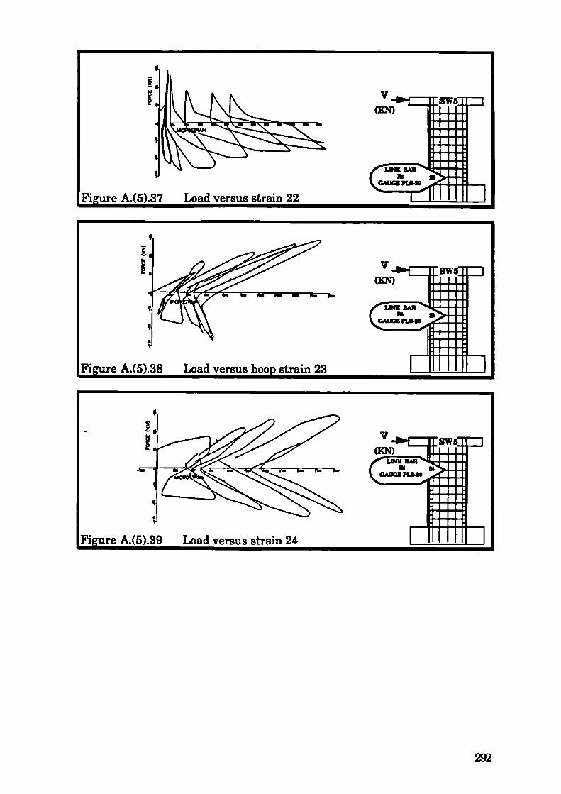
V
LD1Z MX
GAUGE PLa.IS
I
V
Lt4X&4R
GAUGE P1*10
V
GAUGE via.
A.(5).37
Load versus strain 22
A.(5).38 Load versus strain 23
A.(5).39 Load versus strain 24
292

A.(5).40 Load versus hoop strain 25
(
V
(ir
A.(6) I
V.(KN)
FiEure A.(6).1 Load versus wall SW6 disDiacement 3
293

294

295

(mm)
(KN)
Figure A.(6).6 Load versus wall SW6 displacement 8
V.KN)
(mm)
A.(6).7 Load versus wall SW6 displacement 9

(KN)
(mm)
CCd
Figure A.(6).9
Load versus wall SW6 displacement 11
297

298

I'
P
'Figure A.(6).13 Load versus wall SW6 top wall average verticaldisDiacement
299

Figure A.(6).14 Load versus wall SW6 mid heigth average verticaldisDiacement
-J
Figure A.(6).15 Load versus wall SW6 quarter heigth average verticaldisplacement
300

v-i
HTII
rii
v-I
Rn'
CAUG!
IA
VKN)
VT"
GAUC!--p
A.(6) Strain gauge results - Scale 1:2.5 model SW6
A.(6).16 Load versus strain 1
Figure A.(6).17 Load versus strain 2
Figure A.(6).18 Load versus strain 3 I I I"
301

v-I
MRRTII
GAUGE
4A
VKN)
MRVT'
GAUGE
IA
V-I
MRXII
GAUGE
11114.1(KN) II1(I;
n-rn MRVT II
GAUGEPLL
A.(6).19 Load versus strain 4
A.(6).20 Load versus strain 5
Figure A.(6).21 Load versus strain 6
Figure A.(6).22 Load versus strain 7 I I
302

v-I
HT ii
GAUGE
I4
v-I
lIT II
V
I GAUGE
I
A.(6).23 Load versus strain 8
SW6
A.(6).24 Load versus strain 9
IFigure A.(6).25 Load versus strain 10
303
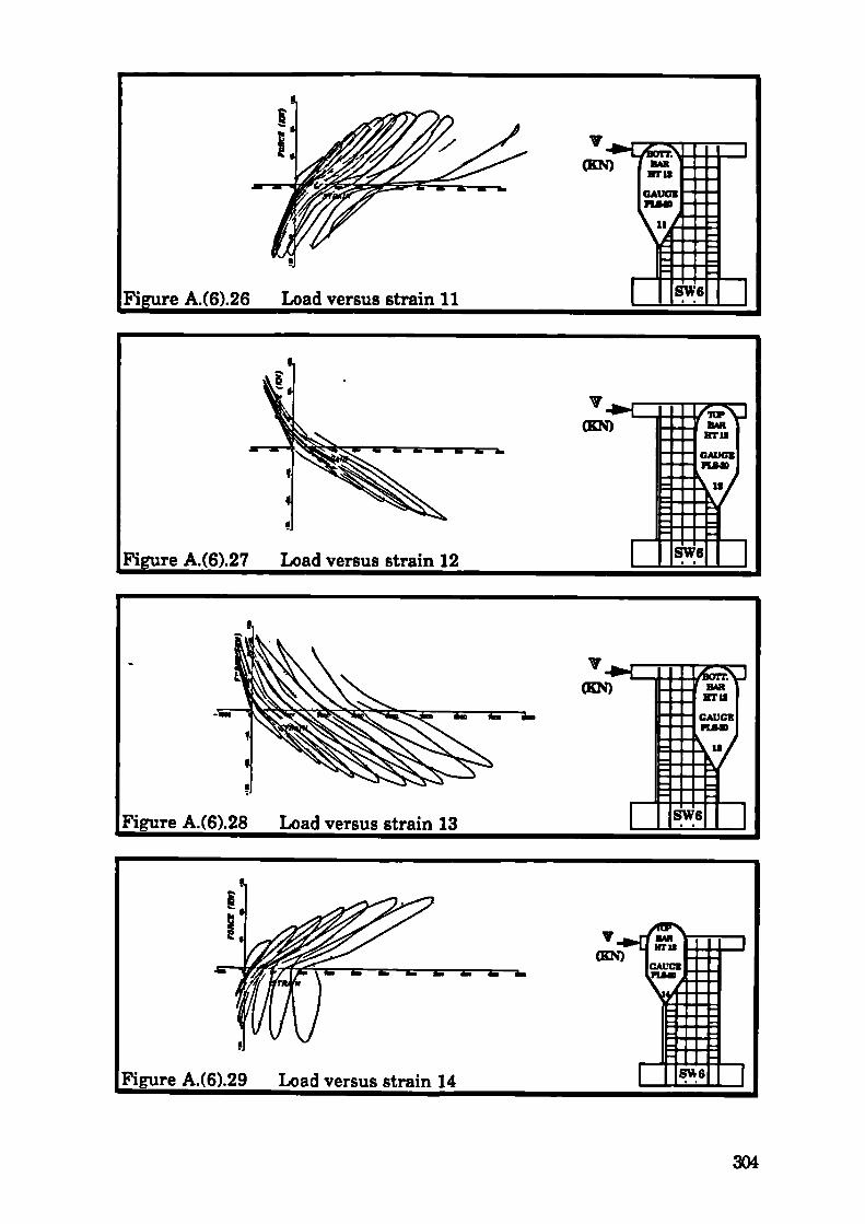
V
cRo:?3
GAUCZ
11
I i,cIIVR
11 A
ii icGN)
Oh1H
U
IcAuc!
I\ )
V'fill
A.(6).26 Load versus strain 11
IFigure A.(6).27 Load versus strain 12
A.(6).28 Load versus strain 13 SW6
A.(6).29 Load versus strain 14
SVP 6
304

A.(6).30 Load versus strain 15
V
-
Figure A.(6).31 Load versus strain 16
V
V-I
MRRFII
CAUG!PL&a
2 Load versus link strain 17 SW6
6).33 Load versus strain 18
305

v-I
iarr.
v-I
, WIT. a.a•1
A.(6).37 Load versus strain 22
A.(6).34 Load versus strain 19
A.(6).35 Load versus strain 20
306

A.(7)
V(KN
A.(7).1 Load versus wa1l SW7 di
307

308

V.(KN)
(mm)
- - 6 9.
DISPLA CEMENT
Figure A.(7).5 Load versus wall SW7 displacement 7
309

(mm)
(KN)
(KN)
IFigure A.(7).6 Load versus wall SW7 displacement 8
(mm)
- I.
0
IFigure A.(7).7
Load versus wall SW7 displacement 9
310

=(KN)
(m
IFigure A.(7).9 Load versus wall SW7 displacement 11
311

11CEMENT (MM)
[I. .....'.\N
-.5 -.4 -.3
(KN)
6li(mm)
(KN)
(E
DISPL4
A.(7).1O Load versus wall SW7
A.(7).11 Load versus wall SW7 displacement 15
322

Figure A.(7).13 Load versus wall SW7 top wall average verticaldisDiacement
313

Figure A.(7).14 Load versus wall SW7 mid heigth average verticaldisplacement
Figure A.(7).15 Load versus wall SW7 quarter heigth average verticaldisplacement
314

16 Load versus strain 1
igure A.(7).17 Load versus strain 2
V
2711
GAUGE2
IAA
V
V
271
GAUGE
ti)
A.(7) Strain gauge results - Scale 1:2.5 model SW7
IFigure A.(7).18 Load versus strain 3 I II
315

V
RTS
GAUC!
41
20 Load versus strain 5
V
V
HTS
GAUGE
V
HTS
GAUGE
" ,)
A.(7).19 Load versus strain 4
A.(7).21 Load versus strain 6
A.(7).22 Load versus strain 7
316

A.(7).24 Load versus strain 9
aiRVT'.
.4
aiRETIS
hIA
Load versus strain 8
STRaIN
S
IFigure A.(7).25 Load versus strain 10
IFigure A.(7).26 Load versus strain 11
V
V
V
V
317

U(KN) j (NTIS
Fl I GAUGE
II IEl iiA
1.1 1cKN) j (Fri.
II Ic*ucgLI IPL&
El \1.ø
V .r4a
IFigure A.(7).30 Load versus strain 15
V
IFigure A.(7).27 Load versus strain 12
A.(7).28 Load versus strain 13
A.(7).29 Load versus strain 14
- I
318

A.(7).34 Load versus strain 19 I II ?
1 Load versus strain 16
A.(7).32 Load versus link strain 17
Figure A.(7).33 Load versus strain 18
V
()
gr ii
V
VKN
319

()
TCP ftRB B
WG1 PlAID d
I -
U
(4)
WIT. B M
B BAU PlAID 4
Load versus strain 20
A.(7).36 Load versus strain 21
A.(7).37 Load versus strain 22 SW7
A.(7).38 Load versus hoop strain 23 I II 1
()
GAUGIPLIB
BGAUGB FLaB

V
A.(7).39 Load versus strain 24
A.(7).41 Load versus hoop strain 26
v-I
()
321

(KN)
(KN)
A.(8) Load-distlacement curves - Scale 1:2.5 model SW8
IFigure A.(8).1 Load versus wall SW8 displacement 3
Figure A.(8).2 Load versus wall SW8 displacement 4

(KN)
(r
8).4 Load versus wall SW8 displacement 6
323

(KN)
(I
(1
A.(8).5 Load versus wall SW8 displacement 7
Figure A.(8).6 Load versus wall SW8 displacement 8
324

V.(KN)
8).7 Load versus wall SW8 displacement 9
325

A.(8).1O Load versus wall 8W8 displacement 12
326

327

Figure A.(8).13 Load versus wall SW8 top wall average verticaldisplacement - -
Figure A.(8).14 Load versus wall SW8 mid heigth average verticaldisplacement
328

16 Load versus strain 1
V
Figure A.(8).15 Load versus wall SW8 quarter heigth average vertical
A.(8) Strain gauge results - Scale 1:2.5 model SW8

V
Vt'.
IA
V
BARFY31
GAUGE
I)
V
r1
BARHIS
GAUGE
k
18 Load versus strain 3
IFigure A.(8).19 Load versus strain 4
I -
V
BARHIll
GAUGE--H
"SI
A.(8).17 Load versus strain 2
A.(8).20 Load versus strain 5
330

igure A.(8).22 Load versus strain 7
V
I -
V
3arMR
ETlO
CAUGE
SI
MREr ii
21 Load versus strain 6
IFigure A.(8).23 Load versus strain 8
V
MRWill
I
4 Load versus strain 9
V
331

IUIIIIAR
1141 I I XTII
A.(8).26 Load versus strain 11
V
cK
A.(8).27
Load versus strain 12
V
A.(8).28
Load versus strain 13
V(
A.(8).25 Load versus strain 10
332

[Figure A.(8).32 Load versus link strain 17
A.(8).29 Load versus strain 14
.30 Load versus strain 15
A.(8).31 Load versus strain 16
GAUGE PZJIQ
V
V
V
V
tfl
333

V
V
BAR
GAUG!
V
GAUGI P1IS .4
V'D
IiCAUC! iais
a
A.(8).33 Load versus strain 18
IFigure A.(8).34 Load versus strain 19
.35 Load versus strain 20
igure A.(8).36 Load versus strain 21
334

IFigure A.(8).37 Load versus strain 22
V
GAUGE P1J'N
V
W4K EAR
UGAUGE PL&1O
V
- ROOP EAR
UGAUGE PLJ4S _
Figure A.(8).38 Load versus
strain 23
Figure A. Load versus strain 24
335

A.(9) LoaddisDlacernent curves - Scale 1:2.5 model SW9
T.(KN)
-
(mm)
IFigure A.(9).2 Load versus wall SW9 displacement 4
336

337

(KN)
(flu
Figure A.(9).5 Load versus wall SW9 displacement 7
V.(KN)
(mm)
Figure A.(9).6 Load versus wall SW9 displacement 8
338

339
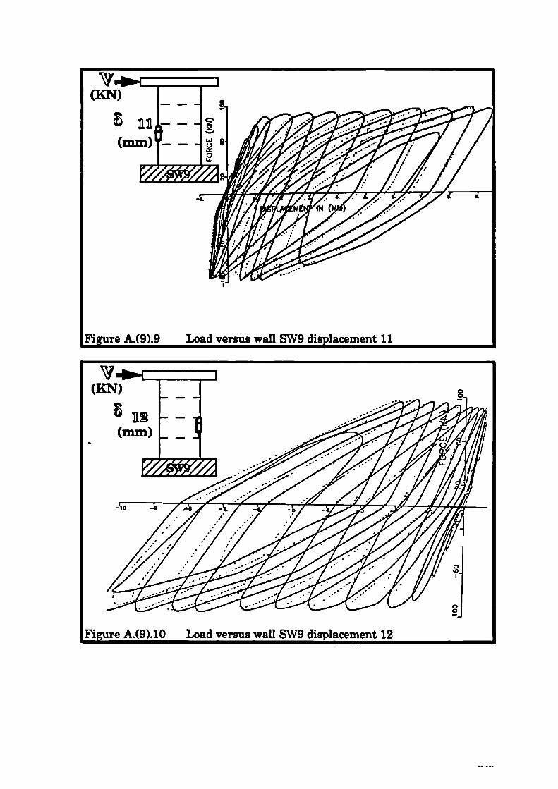

(KN)
Figure A.(9).11 Load versus wall SW9 displacement 15

II.
Figure A.(9).13 Load versus wall SW9 top wall average verticaldisolacement
Figure A.(9).14 Load versus wall SW9 mid heigth average verticaldisplacement
342

Figure A.(9).15 Load versus wall SW9 quarter heigth average verticaldisplacement
Figure A.(9).16 Force versus flexural component of top horizontaldisplacement 6fE1 by using method of area al
343

344

Figure A.(9).20 Flexural displacement &f versus shear component oftop horizontal displacement by using method of area a2
345

V
ETIO
GAUGE
VUCN)
BARFT 10
GAUGE
A
A.(9) Strain gauge results
I IIISV
A.(9).22 Load versus strain 1 1 III •
IFigure A.(9).23 Load versus strain 2
346

)).24 Load versus strain 3
V
ftftVT'.
GAUGE
V
rrT.,
GAUGE
A.(9).26 Load versus strain 5
V
V
KN)
VI• IS
SA
A.(9).25 Load versus strain 4
Ui
A.(9).27 Load versus strain 6
347

V
MRBT1S
GAUGE
tSI
I - V
MRITIS
GAUGE
VMR
NTIS
GAUGE
I. I
28 Load versus strain 7
Figure A.(9).29 Load versus strain 8
A.(9).30 Load versus strain 9
igure A.(9).31 Load versus strain 10
V
IMIUT IS
GAUGE--U
k71
348

A.(9).33 Load versus strain 12
A.(9).34 Load versus strain 13
S.
A.(9).35 Load versus strain 14
V
V
349

(18
wr'.
Figure A. 6 Load versus strain 15
V
V
A.(9).38 Load versus link strain 17
V
V
KN)Is
lIT II
GAUGE
A.(9).37 Load versus strain 16
IFigure A.(9).39 Load versus strain 18
350

iV
V
LD3Aa
CAU PI
V
GAUCI ria
SCA! PL&1O
OAU PI
A.(9).40 Load versus strain 19
A.(9).41 Load versus strain 20
igure A.(9).42 Load versus strain 21
A.(9).43 Load versus strain 22
351

V
•
A.(9).44 Load versus strain 23
352

APPENDIX B
B Reinforced Concrete Analysis Model Results
353

354

355

356

357

358

359

Figure B.14 Flexural displacement versus shear component of tophorizontal disniacement
360