Geotechnical Earthquake Engineering

Geotechnical Earthquake Engineering Prof. Deepankar Choudhury

Department of Civil Engineering Indian Institute of Technology, Bombay

Module - 9

Lecture - 40 Seismic Analysis and Design of Various

Geotechnical Structures (Contd…)

Let me start our today’s lecture, for this NPTEL video course on Geotechnical

Earthquake Engineering. Currently, we are going through module nine of this course,

which is seismic analysis and design of various geotechnical structures. So, within this

module, in the previous lecture, what we have studied? Let me do a quick recap.

(Refer Slide Time: 00:52)

So, in the previous lecture first, we have discussed about seismic stability of finite soil

slopes. In that, first we started with basic concept of Newmark’s sliding block analysis,

which was proposed in 1965. It is available in the journal geo-technique; that is how a

sliding block mass, can tend to slide through a sloping ground, and how to determine the

factor of safety considering this, additional pseudo static inertia force. So, in terms of

factor of safety, once we equate it with respect to one, then whatever the acceleration we

are getting the seismic pseudo static acceleration; that is referred as yield acceleration.


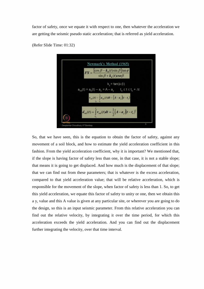
So, that we have seen, this is the equation to obtain the factor of safety, against any

movement of a soil block, and how to estimate the yield acceleration coefficient in this

fashion. From the yield acceleration coefficient, why it is important? We mentioned that,

if the slope is having factor of safety less than one, in that case, it is not a stable slope;

that means it is going to get displaced. And how much is the displacement of that slope;

that we can find out from these parameters; that is whatever is the excess acceleration,

compared to that yield acceleration value; that will be relative acceleration, which is

responsible for the movement of the slope, when factor of safety is less than 1. So, to get

this yield acceleration, we equate this factor of safety to unity or one, then we obtain this

a y, value and this A value is given at any particular site, or wherever you are going to do

the design, so this is an input seismic parameter. From this relative acceleration you can

find out the relative velocity, by integrating it over the time period, for which this

acceleration exceeds the yield acceleration. And you can find out the displacement

further integrating the velocity, over that time interval.


So, we have seen this is the variation of factor of safety, for any finite slope of

inclination 20 degree, and different phi value of the soil 20 degree, 30 degree, and 40

degree. As we know for phi equals to 20 degree factor of safety, will always be less than

1, because the slope inclination is also 20 degree. For stability we have discussed, phi

value must be greater than the slope angle. So, for higher phi values, you will get the

factor of safety more than the one at static condition; that is when k h equals to 0, but as

k h increases the factor of safety, keep on decreasing. So, that is the critical factor of

safety. And from this chart you can find out, corresponding to factor of safety value

equals to 1, what are the yield acceleration values for phi equals to 30 degree, for phi

equals to 40 degree and so on. So, beyond this point, if acceleration exceeds, you will get

the relative displacement which can be calculated, as I have mentioned just now.


So, this is the way how to calculate the relative displacement, as I have already discussed

in previous lecture. Suppose this is your ay value, so whatever acceleration is exceeds

that ay value, for that shaded zone in this figure, whatever is the black shaded portion,

over that time interval you integrate it and get the velocity, further you integrate it get the

displacement, only during that time interval. And as displacement is additive, it remains

and keep on staying at that value.


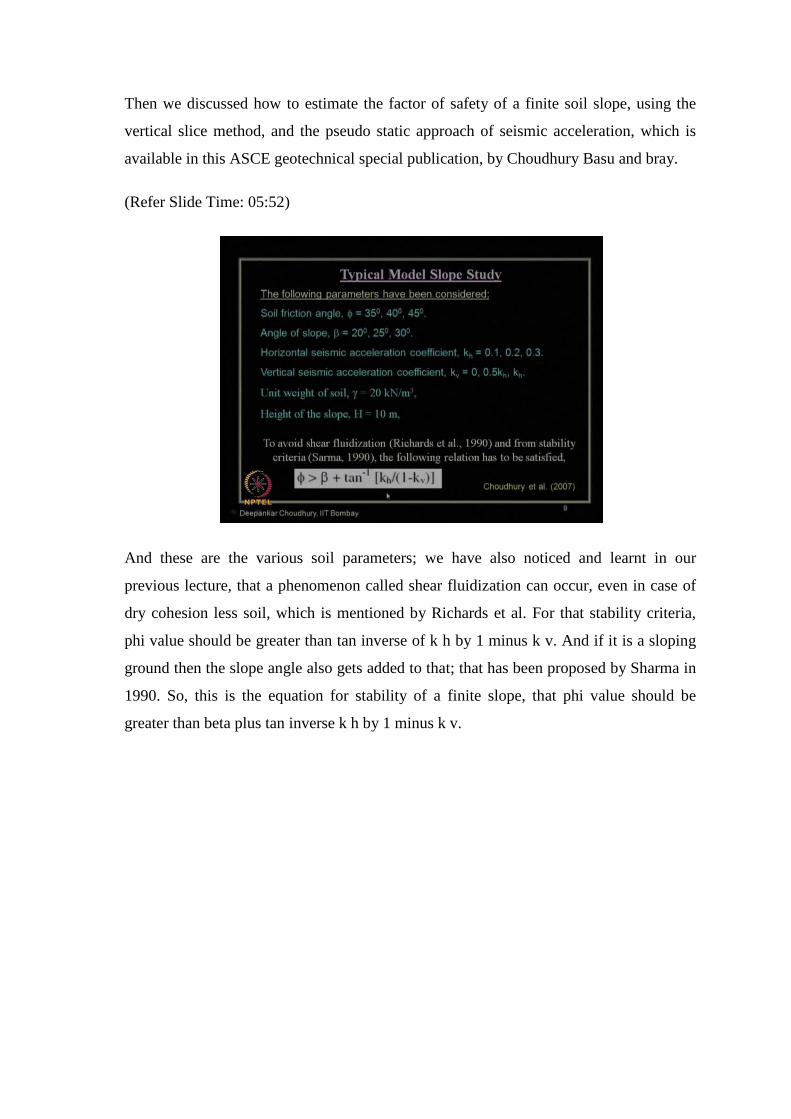
Then we discussed how to estimate the factor of safety of a finite soil slope, using the

vertical slice method, and the pseudo static approach of seismic acceleration, which is

available in this ASCE geotechnical special publication, by Choudhury Basu and bray.


And these are the various soil parameters; we have also noticed and learnt in our

previous lecture, that a phenomenon called shear fluidization can occur, even in case of

dry cohesion less soil, which is mentioned by Richards et al. For that stability criteria,

phi value should be greater than tan inverse of k h by 1 minus k v. And if it is a sloping

ground then the slope angle also gets added to that; that has been proposed by Sharma in

1990. So, this is the equation for stability of a finite slope, that phi value should be

greater than beta plus tan inverse k h by 1 minus k v.


We have also seen how this dynamic factor of safety, varies with respect to not only the

horizontal seismic acceleration coefficient, but also with the vertical seismic acceleration

coefficient, for different input values of soil friction angle, and for a given slope angle.

Then in our previous lecture, we also discussed and learnt about the concepts for the

seismic stability of tailing dam, and what are the extra safety measurements we need to

consider for tailing dam design, that also we discussed compared to the earthen dam

design.


Because in this case, in the tailing portion you are storing, mostly the waste material, so

it should not cause any environmental hazards also. So, safety of the dam, is needs to be

fully ensured even under the seismic condition. And this picture shows how the upstream

method of construction, and failure of dam is possible, and what are the devastation area,

which, it can get affected like this.


Then as per the Indian seismic design code, for IS 7894 of 1975 it suggest the, pseudo

static approach to be used for the seismic design of this earthen dam. And there are basic

two methods can be performed like; one is circular arc method, another is sliding wage

method. Sliding wedge method is nothing, but the Newmark’s block method, and

circular arc method is similar to what I have mentioned this modified Swedish circle

method, or using the vertical slice equilibrium approach. So, this is the factor of safety

for circular arc method, using the pseudo static approach. And as far as IS 1893 of 1984

is concerned, based on the assumption of the portion of the dam and rapture surface, the

analysis needs to be carried out as outlined over here.


Then we discussed thoroughly in our previous lecture about a case study. This is for our

real problem, real field problem, as well as another model problem for academic

purpose, and another is actual field implemented problem. So, this is the field

implemented problem, which was analyzed by Chakraborty and Choudhury in 2011.

This is the ASCE geotechnical special publication, number 2000 211. This tailing dam,

is proposed to be constructed at the eastern part of India, under seismic zone two; that is

the most safest zone as far as Indian seismic zonation is concerned, as per current IS

1893 2002 version. So, in two stages of height, it is proposed to be constructed; one is 10

meter, another is 28 meter. First phase is 10 meter, and it will be constructed by

downstream approach or downstream method. This analysis is carried out, using the

finite difference based software FLAC 3D, as well as the analytical method of pseudo

static as well as pseudo dynamic method of analysis was carried out, for seismic design

of this tailing dam. And these are all input parameters, for the dam sections and the

tailing portions.


So, for the stability criteria, we mentioned that we considered, seven different possible

combinations, which can arise for this tailing dam. These are all seven different

combinations. So, for each of them, we have to ensure the stability; that is factor of

safety should be greater than 1.15, or displacement should be within the permissible

range.


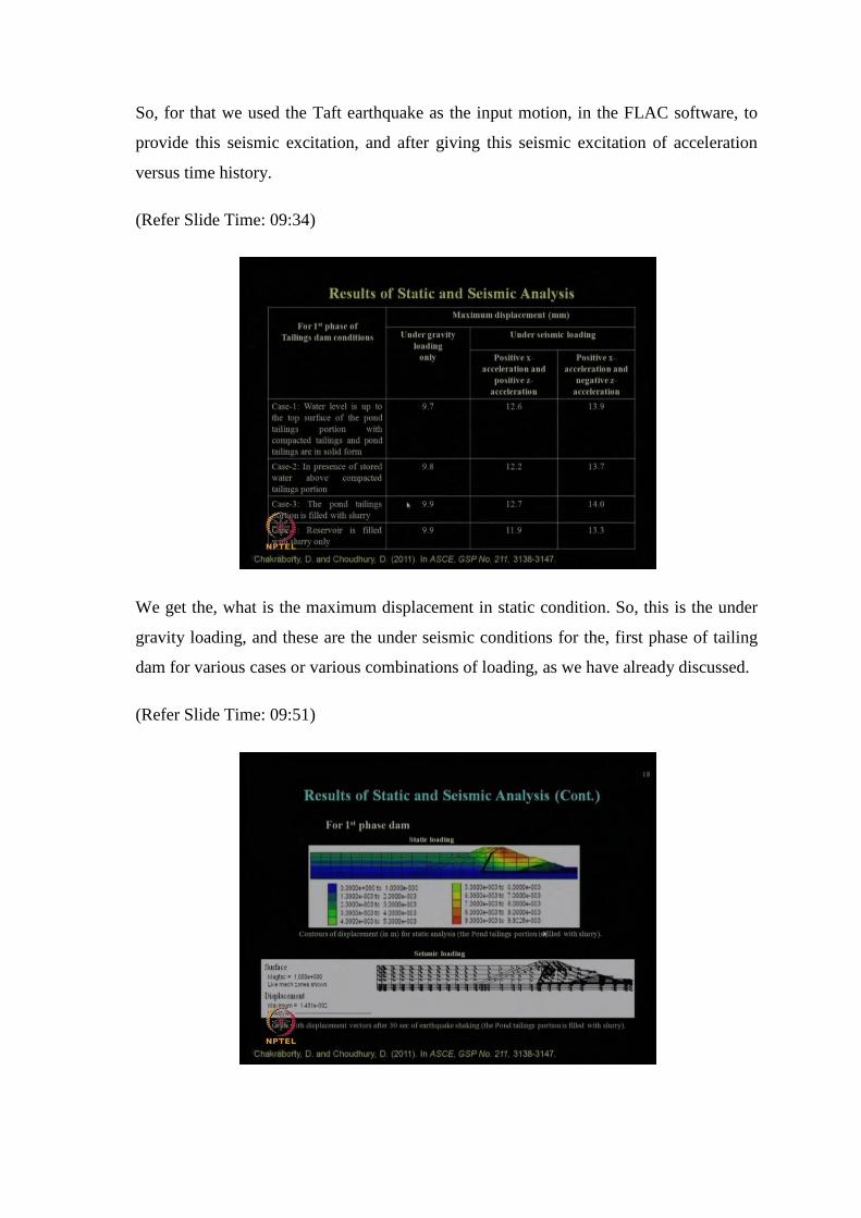
So, for that we used the Taft earthquake as the input motion, in the FLAC software, to

provide this seismic excitation, and after giving this seismic excitation of acceleration

versus time history.


We get the, what is the maximum displacement in static condition. So, this is the under

gravity loading, and these are the under seismic conditions for the, first phase of tailing

dam for various cases or various combinations of loading, as we have already discussed.


This is the FLAC displacement contours, for the static case; that is under the gravity

loading condition, what is the displacement behavior at various portions of this tailing

dam. Also under the seismic loading condition after the thirty seconds of earthquake

shaking, how much will be the displacement vector, in FLAC. These results are available

for the first phase of the dam. And the output shows, that at different height of this tailing

dam, like if we consider the dam base, suppose this one at ground level, then at various

height that is 5 meter and 10 meter, at different height we have obtained, what is the

acceleration versus time history.


So, by doing the ground response analysis so by doing ground response analysis, you can

get acceleration time history and FLAC also like this. And peak horizontal acceleration

is found to be at 5 meter of height is this much, whereas, at 10 meter height, it is

obtained to be like this much. So, that automatically shows, when the seismic earthquake

acceleration travels through this height of this tailing dam, there is an amplification of

about 4 times, from the bed rock motion, or at base level whatever excitation was

provided.


Also, we need to calculate the fundamental time period of the entire system, or the entire

tailing dam. To calculate that FLAC 3D analysis directly gives us the results of

fundamental time period, this is for the first phase of the dam, this is for the second

phase, when it is 28 meter height, what are the fundamental time period? Also IS code

the b IS 1893 1984 version; that also gives us this formula, to calculate analytically what

is the fundamental time period of any structured, like tailing dam like this. So, for first

phase, this is the value. For second phase, this is the value, which is very well

comparable as obtained in the FLAC 3D analysis, as you can see. So, when somebody is

starting any design, they should either follow this IS code. And in addition to that I will

suggest, they should do some numerical analysis, rigorous dynamic analysis, and some

analytical solution also for the stability, and dynamic behavior of the dam.


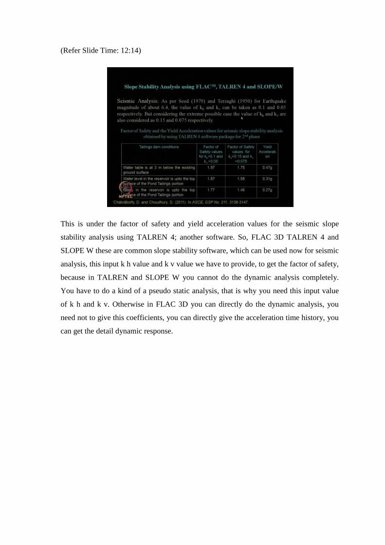
This is under the factor of safety and yield acceleration values for the seismic slope

stability analysis using TALREN 4; another software. So, FLAC 3D TALREN 4 and

SLOPE W these are common slope stability software, which can be used now for seismic

analysis, this input k h value and k v value we have to provide, to get the factor of safety,

because in TALREN and SLOPE W you cannot do the dynamic analysis completely.

You have to do a kind of a pseudo static analysis, that is why you need this input value

of k h and k v. Otherwise in FLAC 3D you can directly do the dynamic analysis, you

need not to give this coefficients, you can directly give the acceleration time history, you

can get the detail dynamic response.


So, in previous lecture we have also learnt, another important criteria for the tailing dam

design, which is the liquefaction behavior, or how this tailing dam behaves during a soil,

possible soil liquefaction during earthquake. So, the assessment of this liquefaction

potential we discussed, which is given by Chakraborty and Choudhury 2012 paper. So,

this is for the first phase of the dam, this is for the second phase of the tailing dam. And

these are various points in the tailing portion, why we have chosen the tailing portion as I

said, it is mostly in the unconsolidated state or in the loose state, because you dump the

waste material in the water. So that is why, there are high chances of getting these

material liquefied, and that is why we carried out the liquefaction potential, not only that

you have to do for foundation soil also, that you have to make sure.

So, in terms of maximum value of pore pressure ratio, if this pore pressure ratio R u,

equates to 1 means, it is going to liquefy, if it is less than 1, then it is not liquefying, but

we should not have a very close to one value, so that is another criteria. Then there is

always a chance, that it may get liquefied, if there is a input value of soil parameters or a

site condition anything gets changed. So, we ensure that, what are the values of possible

liquefaction potential to make, and recommend the safety issues of this tailing dam.


This is the behavior of first phase as well as second phase of dam, under liquefaction

condition in FLAC 3D, this is the typical output you will get, for liquefaction analysis at

different height and locations.


Also we had conducted the seismic slope stability analysis of this tailing dam, using both

pseudo static approach, as well as the new method of pseudo dynamic approach we have

elaborated in couple of previous lectures. And this is a just assumed tailing dam section;

this is not the actual one. The previous one was the actual one, this is the assumed one.

So, these results are available in the publications Chakraborty and Choudhury 2013, in

the proceedings of National Academy of Sciences, Springer publications. This is the

volume and the page number.


So, the factor of safety as we know is nothing, but ratio of resisting force by driving

force. So, resisting force expressions and driving force expression from that the factor of

safety using both pseudo static and pseudo dynamic, we will get the results. And, if it is

more than 1.5, then we will call it as safe. If it is going to be less than 1, we need to find

out the displacement. So, coming to our today’s lecture, we will start today with another

sub topic, on this module, which is another important subtopic is seismic design of pile

foundation. This is very important, because for several high rises and very important

structures, and mostly in the urban areas where there is a scarcity of space, and you do

not have the luxury to, get the buildings or new construction constructed horizontally,

but you have to go vertically up and up. Like places, like Mumbai, places like New

York, places like Tokyo. So, all this places there is a space crunch, so always you need to

go in the vertically up direction, and hence pile foundation is the only solution.


So, now, in the introduction as we know where pile foundations etcetera are going to get

used. Now for the soft soil, and the supporting structures in liquefying soil, where pile,

this pile foundations of this super structure. When they pass through some liquefiable

layer, then what happens, when you are designing the capacity of the pile. Suppose you

have taken the skin friction component also, to calculate the capacity of the pile. But if

that portion of the soil, gets liquefied during earthquake condition; obviously, it is not

going to provide, any kind of frictional forces, or any kind of resistance. In that case you

have actually in the design, calculated and overestimated value, which is not exactly

acting at the site. That causes several times the failures of the pile.

So, this is one of the major criteria why, the pile foundations fail at several earthquake

conditions, around the world in big earthquake, even including the various Japan

earthquake, even our Indian earthquake also. During Bhuj earthquake in Ahmedabad

several buildings collapsed, and the pile foundation got damaged. Even earlier when in

the introductory lectures of this course, I have discussed that for a Nigata earthquake for

Kobe earthquake, various earlier Japan earthquakes, several pile foundations got failure.

So, those are basically or majorly, due to the liquefiable strata, which was lying in

between, and that reduces the capacity or strength of the pile, which was estimated

during the design. So, we should know how much extra bending movement, how much

displacement is going to come, for those type of pile, when you are going to design, or

when you are going to construct any pile, which is a having a possibility to pass through

a liquefiable layer.

In addition to that, what are the other possible ways that pile foundation get failed,

because during the seismic loading, the major load is nothing, but lateral load. As I have

already mentioned, mostly the lateral force comes into picture; that is the major one; of

course, there will be a vertical component as well. So that, lateral seismic inertia force;

that will cause extra lateral loading on this pile foundation. And if your pile is not

designed properly, to take care of this extra lateral load, obviously it is going to bend

excessively and finally fail, or it is going to displace excessively and finally fail. So,

these are another way or mode of failure for the pile, during the earthquake condition.

So, these two are the major things, somebody is trying to design any pile foundation

needs to take care of.


So, let us discuss about the design philosophy etcetera. Before that, let me show through

this picture, it is photo cards see from NISEE, like pile foundation of million dollar

bridge of 1964 Alaska earthquake in U S A. This is the Showa bridge of 1964 Nigata

earthquake in Japan, which earlier I have mentioned in one of the introductory lecture.

This is the pile tanks after 1995 Kobe earthquake. You can see, the failure of pile

foundation can, make several important buildings or structures to collapse.


So, there is a paper by Madabhushi et al in 2010. This paper discusses about the

performances of pile foundations, during various recent earthquakes; that is before 2010.

Like in which cases piles performed very well, so good performance and bad

performance. So, these are the various case history of during Nigata earthquake, some of

the pile they performed well. So, they have done a study, why those structures or why

those pile foundations performed well, and why others could not perform. So, this is an

important paper one can go through.


And these are the examples, where the pile provided or pile could not perform well. So,

poor performance during Nigata earthquake and Kobe earthquake, for different pile

conditions.


Also some more poor performance during Kobe earthquake, including you can see over

here, as I have mentioned, during Bhuj earthquake also, like in Kandla port area, harbor

area, several pile foundations. They were totally devastated and damaged, and also in

Ahmadabad region, several pile foundations were damaged. So, these are the examples

of poor performance of pile during earthquake.


Now, how this pile behave under lateral load, and in liquefying soil. So, this picture

typically shows, how to do a force based method of estimation for pile foundation

design, this is actually proposed by JRA Japan Road Resource Association 1996

recommendation, how to do the design of pile passing through liquefiable layers. So, this

is an idealization of pile, for the design in liquefied soil. Suppose you have a super

structure like this, which is supported on various pile as. So, this is the pile foundation

group of pile, and you have at this portion, a non liquefiable layer, so this layer is not

going to liquefy. We know how to estimate the liquefiable potential of any particular

soil; that we all know about it. And it is followed by some soft layer, or some layer

which is supposed to be prone to liquefaction under certain magnitude of earthquake.

Then followed by another stiff layer, which is non liquefiable.

So, basically if you have a end bearing pile, you will go and end it up to a strong or stiff

strata, or even rock, soft rock; a dense strata, dense sand. So, in between this liquefiable

layer, will drastically reduce the capacity of the pile, if somebody has considered the

friction of the this portion of the soil, on the pile capacity in the design. And the

additional horizontal load will also come into picture on this pile, due to the earthquake

condition. So, how to take care of that? So, JRA proposed that whatever is the searched

passive earth pressure is acting, consider 30 percent of the overburden pressure, is acting

during the liquefiable layer. So, this is a design proposition, but later on, many other

researches has mentioned, this is not always correct, and one needs to do a case specific

analysis, for individual ground response and the soil profile is concerned, because this

soil profile you should know, through which your pile is going to get constructed, and

also the dynamic response at each layer. So, I will go through that detail very soon.


So, the seismic analysis of pile foundations in liquefiable soil. The initial researches they

mentioned about Winkler type model. As we know from the basic concept of any soil

structure interaction code; that soil structure interaction courses always discuss or start

with basic concept of Winkler beam model. So, Winkler springs are considered for

below a foundation analysis, when we considered the foundation, how it interacts with

the basic foundation soil. So, foundation with respect to soil, we calculate through the

Winkler springs. So, that concept of Winkler spring model, is extended for the pile

foundation also in liquefiable soil by various researches; like Winkler type model has

been developed, by Kagawa in 1992, Yao and Nogami in 1994, Fuji et al in 1998,

Liyanapathirana and Poulos in 2005. So, for piles in the non liquefiable soil, so, when

you do not have any liquefiable layer, but still it is under the earthquake condition or

seismic condition, you still have the additional horizontal load, which needs to be

considered. So, these are the researchers who used like, Abghari and Chai in 1995, and

Tabesh and Poulos in 2001 had developed pseudo static approaches.

As we know Prof. Harry Poulos; a very famous pile engineer and Professor, and

practitioner, who developed the theory of pile foundation extensively as we read for,

even the pile foundation design and analysis, even in this static condition; the book by

Prof. Poulos and Prof. Davis, Poulos and Davis of 1980. He Prof. Poulos extended with

his several researchers and the students, how to extend the static analysis to, the pseudo

static concept of analysis under the seismic condition. So, these are very basic work and

fundamental work, in the area of earthquake engineering for the pile foundation design.

So, one must go through this details, to understand the basic concept of behavior is of

this pile foundation, under pseudo static seismic loading condition. Liyanapathirana and

Poulos in 2005 developed this pseudo static approach, which has two solution stages; so

carry out the ground response analysis; that is their recommendation.

So, you can see, the importance of ground response analysis, because at specific site you

will get different ground response. You should have different amplification criteria, you

should have different acceleration versus time history at different level etcetera should be

known. And pile is analyzed, as non-linear beam on elastic foundation, considering the

both kinematic approach and inertial interaction. So, now, let me explain you, when any

pile foundation is subjected to an earthquake loading, there are two cases, or two

combinations of loading, will arrive at the pile foundation. What are those things; one is

kinematic condition another is inertial condition. Inertial condition as we have already

learnt, what is inertia. When there is any seismic force, the seismic acceleration, times

the mass involved in it, gives you the seismic inertia force.

So, that is the inertial component, which of course, your pile, when it is subjected to any

earthquake excitation, it is going to get experience, but what is the kinematic behavior;

like when the pile and soil, they interact in between. So, soil also is subjected to some

kind of earthquake acceleration. So, that acceleration in the free field we call, when

suppose there is no structure exit. So, that is nothing but free field condition, the soil is

going to displace or going to move. So, that movement of the soil along with the

movement of the pile, how it is getting interacted, that gives us the movement or

kinematic interaction. So, this kinematic interaction, along with the inertial interaction,

needs to be considered combinedly, to get the combined effect, of this earthquake forces

on the pile foundation, and in the design we need to consider both the aspects of,

kinematic as well as the inertial loading conditions in the design of pile foundation.


So, let us look at this picture once again, this is again from the JRA proposal, like soil

liquefies, it loses its strength and starts flowing and dragging with it, any non liquefiable

crust above it. So, this is a non liquefiable soil, then liquefiable soil, then again non

liquefiable soil. So, when there is free field soil deflection. So, this is the free field, when

there is no structure available. So, that gives us the kinematic interaction as I was telling,

and on this, inertial portion or the structural component whatever the seismic load is

acting, that gives us the inertial movement, or inertial displacement, or inertial bending.

So, this is the deformed shape of the pile, you can see there is will be a difference

between these two movements, so that is why the combined movement is to be

considered, and there will be a dragging, because this portion of the soil when it gets

liquefies.

So, between two non liquefiable layers; two non liquefiable layers, if one liquefiable

layer is there. After liquefaction, because of the slope of the ground etcetera, it will start

flowing. So, lateral spreading, as we have already discussed, after liquefaction, after

effect is immediate, after effect is lateral spreading. So, once the soil entire things flow

out, the fluid portion flowed out what will happen. There will be a relative movement

between the upper and lower non liquefiable layer. So, that is why, it will try to drag the

structure, which is constructed already inside that liquefiable layer, because when it is

moving from upper gradient to a lower gradient. So, that is why, that needs to be

considered, when we are designing this pile foundation, under earthquake loading and in

liquefiable soil.


So, the concept of pile failure under earthquake, is given by Ishihara; Prof. Ishihara in

1997. He gave the details about two basic concepts; one is called top down effect,

another is called bottom up effect. So, what is top down effect like at the onset of

shaking, inertia forces are transferred to the top of the pile, and then it goes to the soil.

So, this is one way of approach of analyzing it, another bottom up effect is, seismic

motion had already passed the, pick and shaking may be still be persistent with the lesser

intensity, and therefore, the inertia force transmitted from the super structure will be

significant, so this is from the bottom of effect. Under such a loading condition the

maximum bending moment, induced by the pile may not occur near the pile head, but at

a lower portion at some depth, and this is referred as the bottom up effect. So, this

picture once again, the GRA method as I have already discussed.


Now let us look and understand, what is the basic failure theory of this pile foundation

under earthquake loading, let us look at this slide. So, this failure theory of pile

foundation was proposed by Tokimatsu et al in 1998. Prof. Tokimatsu gave this details,

like if you see this is your super structure, which is constructed on pile. Now during

shaking, before the soil gets liquefied; that is before your soil gets liquefied, when just

the earthquake came, so inertia forces acting. So, pile is getting extra bending moment,

because of extra lateral load. Now, during shaking after liquefaction, when the soil gets

liquefied, there will be a displacement of the soil also. So, this will be still inertia force

will act and soil gets displaced, so what will be the combined effect. So, lateral

movement after earthquake and liquefaction will be something like this.

So, it will have both this bending moment, due to the extra loading lateral load, due to

earthquake, as well as it will have extra bending moment due to this, ground movement

for the liquefaction of the soil and movement of the soil. So, those aspects need to be

considered, which are discussed over here. So, if you are interested, you can go through

this review paper also Choudhury et al 2009, it is available in the journal, proceedings of

National Academy of Science Springer publication, section A, physical sciences. So, in

this paper, this is the February issue of this 2009, issue two. In this paper, all the review

and discussing about, how this philosophy failure theory etcetera, holds good for the pile

foundation under earthquake is discussed thoroughly.

Now let us come to a case specific design, so why I am telling case specific design for

pile foundation under earthquake condition. As I said already it is also recommended by

various earlier researchers, like Prof. poolers; that for pile foundation design, a ground

response analysis is a must, because you should know how that local soil is going to

behave under earthquake condition, which are supposed to come, or from the past history

earthquake data you can provide at that soil condition, knowing the local soil site

condition. So, it is not a generalized case, it should not be used for important structure.

Of course, for small structure you can use it, or less important structure you can use it,

but for important structure you should never use gross design approach, you should go

for case specific individual design approach. So, that I am going to discuss now.


So, let us go back to the work of Dr. V S Phanikanth, who did PhD at IIT Bombay 2011.

He completed his PhD; I am referring here his PhD thesis. He did his PhD under my

supervision at IIT Bombay. So, we have already discussed that, for various bore holed

data at different sites at Mumbai city, like Mangalwadi site, this basic soil information

data soil layers SPT N value were collected, and the dynamic soil properties later on

were obtained.


From that, you will get the equivalent linear ground response analysis to do that, the

important input parameters you require is, the modulus reduction curve, which is

nothing, but G by G max verses cyclic strain.


Also, the damping curve you require, damping curve verses cyclic strain for your

equivalent linear analysis.


As I have said, we used deep soil software, deep soil version 3.5 was used that time, with

all these input values like; shear wave velocity is important parameter, needs to be given,

unit weight also needs to be given, layer wise damping ratio reference person strain, with

which you start, and then converge the solution, we have discussed this things already in

the equivalent ground response analysis earlier, in one of the module.


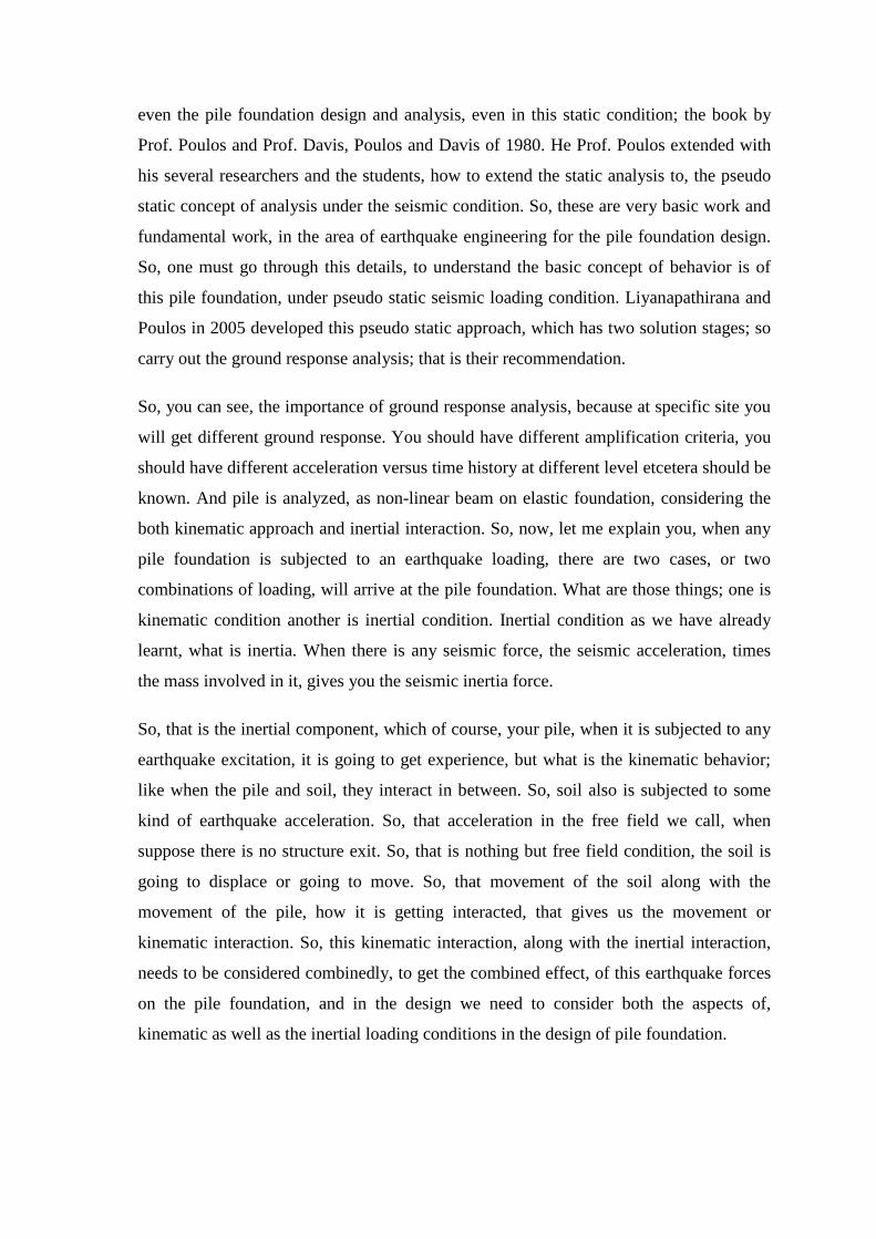
This is the snap short of the ground response analysis, how it is done in deep soil. Like,

you can go for either linear analysis, or equivalent linear analysis, or non-linear analysis.

So, here equivalent linear analysis has been chosen. Also you can, either use total stress

type, effective stress type etcetera.


And you can your inputs soil parameter layer wise. So, this is the basic layer wise

information, which you are getting from your bore hole data. Once you get and do the

analysis, you have to give the input earthquake motion.


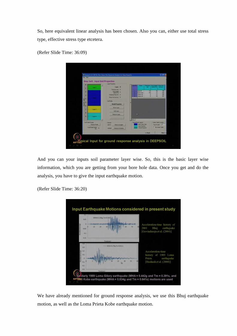
We have already mentioned for ground response analysis, we use this Bhuj earthquake

motion, as well as the Loma Prieta Kobe earthquake motion.


And finally, the output were obtained, for different bore hole locations at different level,

like what is the amplification. So, this amplification compared to the bedrock level to

ground surface how much, this horizontal acceleration is going to get amplified, we had

also seen that.


Like, this is another picture of different acceleration, verses period spectral acceleration

response, and the Forier acceleration Specta, verses frequency curve for bore hole data.


Also this is the depth wise variation of the amplification; that also we have already

discussed earlier in one of the module.


And this gives us the acceleration time history at ground surface, for different bore hole

location, like Mangalwadi, wall k shear, Vijay Marg.


So, how the model study has been developed. So, this is an analytical method, which has

been proposed by Dr. Phanikanth in his PhD work. So, this work suggest, this

publication is getting available now, Phanikanth et al 2013, our publication which is

available in international journal of Geo-mechanics published by ASCE U S A. So, you

can search in ASCE, currently it is available online, very soon the paper will be

published. It is published accepted available online, but the hard copy issue will come

very soon. So, this is the single pile model. He did the analysis only for single pile he

started with.

So, a single pile which is passing through, suppose a typical layered soil, and among that

layered soil, let us say this one is non liquefiable layer, this middle portion is a

liquefiable layer, and again a non liquefiable layer. So, their corresponding length or

depth of this soil layers are; L 1, L 2 and L 3. So, L 2 is the liquefied layered depth of the

soil. So, that depth of L 2 has been compared, or the variation or parametric variation of

this L 2 over the entire length L of the pile, has been done in our analysis, for various soil

site at Mumbai, using the local soil condition, and different input seismic acceleration

how this analysis is, obtained for the single pile foundation design, in terms of bending

moment and deflection. As we know basic design parameters for pile foundation, we

should get bending moment profile, along the depth, also the deflection profile of the pile

along the depth; that is what we do in the static case also.

So, in seismic case also, similarly we need to find out. So, this is the soil pile analysis

considering the ground deformation, using finite difference technique. He uses the finite

difference technique, like he subdivided the entire pile into a number of small segments;

n number of segments, and different node pints. So, there will be two imaginary nodes

upwards here and two imaginary nodes downward here, as we know in the finite

difference concept, it is used. So, based on your assumed ground deformation, where

from you get this ground assumed ground deformation, or you can get an actual ground

deformation. Form your free filled analysis of ground under a subjected to some

earthquake acceleration. So, you know the ground displacement profile.


So, from that you can find out what are the behavior of individual sections, and how to

get that? Let me show you the basic governing equation, which needs to be solved, for

the basic differential equation, for laterally loaded pile, in a liquefiable zone. So, all of us

are aware about this finite difference approach of pile analysis, which is available even in

the book, by Prof. Poulos and Prof. Devis. So, Poulos and Devis 1980 book pile

foundation, which is available the finite difference approach, but it is available for static

case only.

So, we have extended that in the case of seismic analysis, so how the extension was

done. This is the basic governing equation as we know E I d 4 y by d z 4 equals to minus

k h d times y minus y g. So, what is extra here you can see, in the basic pile equation

considering as a beam, this y g comes into picture under seismic condition, in static case

only this much portion is remaining. So, y g comes here for this seismic case; why. This

y g is nothing, but your ground displacement; that is free filled motion. And this d is

diameter of the pile, and k h is the sub grade modulus, and y is the lateral displacement

of the entire pile. So, compared to a ground how much is the relative displacement of

your pile; that interaction needs to be considered, as you can see. z is the depth from the

ground surface and E I is the flexural rigidity of the pile as we know.

And how to consider this k h value that is the another important criteria, under seismic

loading or this liquefiable zone condition. Under static loading condition, this k h value

or sub grade modulus value we know, from the codel recommendations we can get, but

this sub grade modulus also drastically reduces, or changes under earthquake condition,

and even in the liquefiable condition, as given by Tokimatsu et al in 1998; that this sub

grade modulus changes to k h n, with a scaling factor or the reduction factor, due to this

liquefiable condition, which is proposed by Ishihara and Cubrinovski in 1998. These are

the factors; range of this s f is 0.001 to 0.01 you can see. So, how much reduction of the

sub grade modulus will take place, under this liquefiable condition for the soil, when

there is no liquefaction, compared to that.


Now this is the result which Dr. Phanikanth in his PhD thesis work he got, as I said these

are the authors, with three authors; Dr. Phanikanth, myself as the supervisor from IIT

Bombay, and Dr. G R Reddy from BRC, the external supervisor, because he is a scientist

at BRC, they should have another external supervisor. This is our international journal of

Geo-mechanics paper ASCE 2013, is a profile of the bending movement the result along

the depth of the pile. So, we have chosen some pile length, and also different length of

the pile was chosen as 10 meter, radius of the pile as 0.25 meter, this is the E value of the

pile material. You can see different input motions were given, like Bhuj earthquake,

Loma Prieta earthquake, Loma Gilory earthquake, and Kobe earthquake motion, which

we have also considered for the ground response analysis. Also, you will see these data

are only for the, only one particular bore hole data; that is what type of soil is present

there; like Mangalwadi site bore hole number one.

Like, if you want to do for another site, obviously the behavior will be completed

different, even though your input seismic motions may be same. So, any one of these is

changing, and suppose for this Mangalwadi site, even this for MBH one, if I use another

earthquake input motion; say Taft earthquake, Orel Centro earthquake, or the Sikkim

earthquake motion, even the analysis will be different. So, you have to take care that, this

case specific; that is why I was so particular about mentioning, whenever we are doing

any important pile foundation design, this case specific analysis needs to be considered,

but the approach remains same of course,. So, these are the values of this s f, you can see

s f value one means, there is no liquefaction. So, under no liquefaction condition, these

are the bending moment curves, see this solid lines or dark lines. And this dotted line

shows the bending moment under the liquefied condition, when s f value is considered as

0.01.

So, you can see, there is a significant increase of the pile bending moment. So, when you

have provided the pile reinforcement and designed a pile, probably you have done only

for this non liquefiable condition, and under liquefied condition it is subjected to, several

times of that bending moment. So, obviously, this is the reason why the piles

automatically fails, when the soil gets liquefied. Can you see that, huge changes in the

magnitude of the speed bending moment, and the bending moment profile with the

depth. So, unless we know about a site condition, and from that from expected or earlier

historical analysis of seismic hazard analysis, if you do not do this liquefaction study for

a possible liquefied zone, you will end up with getting excessive pile bending, and final

the failure like this, because of this sudden increase or excessive increase of the pile

bending moment.


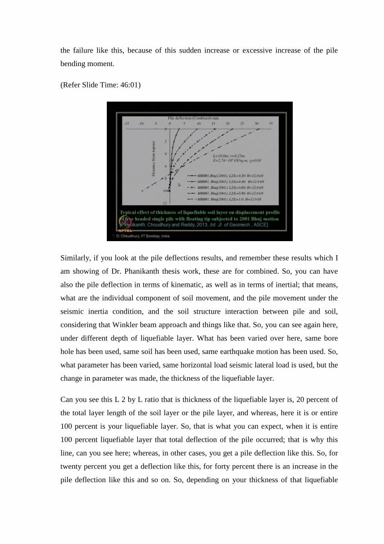
Similarly, if you look at the pile deflections results, and remember these results which I

am showing of Dr. Phanikanth thesis work, these are for combined. So, you can have

also the pile deflection in terms of kinematic, as well as in terms of inertial; that means,

what are the individual component of soil movement, and the pile movement under the

seismic inertia condition, and the soil structure interaction between pile and soil,

considering that Winkler beam approach and things like that. So, you can see again here,

under different depth of liquefiable layer. What has been varied over here, same bore

hole has been used, same soil has been used, same earthquake motion has been used. So,

what parameter has been varied, same horizontal load seismic lateral load is used, but the

change in parameter was made, the thickness of the liquefiable layer.

Can you see this L 2 by L ratio that is thickness of the liquefiable layer is, 20 percent of

the total layer length of the soil layer or the pile layer, and whereas, here it is or entire

100 percent is your liquefiable layer. So, that is what you can expect, when it is entire

100 percent liquefiable layer that total deflection of the pile occurred; that is why this

line, can you see here; whereas, in other cases, you get a pile deflection like this. So, for

twenty percent you get a deflection like this, for forty percent there is an increase in the

pile deflection like this and so on. So, depending on your thickness of that liquefiable

layer compared to, the entire depth or entire length of the pile, you will get how much

your pile foundation is going to deflect, and what different depth that deflection will

occur like this.


So, these are some more results you can see over here. These are the combined values,

and these are the inertia values. What it shows the deflection for this particular case; that

MBH bore hole one under this input motion. Mostly the combined deflection is, because

of the inertial component, can you see that. That means, here the kinematic component is

not that significant, but it is not always depends on your local bore hole soil condition,

and input condition also. So, this is a type of understanding, that at what site you are

going to address which problem. Like suppose, in this site somebody suggests, like as a

civil engineer you have to propose the remediation technique also. What will be the

remediation technique in this case?

Suppose, some unknown person; unknown in the sense, those who are not so conversant

with the, geotechnical earthquake engineering, or the pile foundation under earthquake

condition, what they will propose, they will say improve the soil, go for ground

improvement, dynamic improvement etcetera, which we have discussed in our previous,

another course or soil dynamics; that is possible, that is one way possible. But suppose

with that what you are doing, you are rectifying the possibility of liquefaction in the soil,

but lateral load, whatever is coming the inertial components still remains, you are not

controlling on that. And, whereas for this particular site of Mumbai, which we are

analyzing here, Mangalwadi site. Here the major component of deflection comes from

the inertial portion.

So, do you think that anybody suggests here a ground improvement will help too much;

no. In that case, you have to go for better pile design itself, so that it can takes care of

this additional inertia force, but if you have a soil where, the kinematic component is

more, what you can do, probably by going for ground improvement technique, or

dynamic compaction etcetera. You can reduce that component of that chances, or amount

of deflection due to kinematic portion for the pile. So, an engineer you should give a

remedial measure also, because people will not only stay at this analysis level or design

level. They have to implement it, they should know, what are the ways out, they know

that it is going to fail, but how to protect it.

So, these are the guidelines these are the recommendations one should give, when they

are going through this type of rigorous analysis, analytically as well as numerically, and

there can be also some validation, through some experimental method, but as you know

under earthquake condition, it is very difficult to carry out the experimental method, and

reliable value, because in field it is not possible to do earthquake experiment on pile,

because when you are going to measure by that time it is all damaged. So, what people

do, people use the centrifuge test on this pile, under dynamic loading conditions, so

dynamic centrifuge test not the static one. So, under dynamic condition, what are the

extra bending movements, what are the displacements available? So, many researchers

like Prof. Bolenger at UC Devis. He and his research group have done extensive work in

this area. Prof. Tarek up down at RPI, he and his research group has done extensive work

in this area. So, their publications one can see, how the behavior of pile and pile group

under earthquake loading condition, their bending movement, their displacement profile,

how it has been observed through the dynamic centrifuge test.


So, now, we can see over here the results. You can see the comparison of pile response

in liquefiable soil, as well as non liquefiable soil; non liquefiable, we know all about it.

So, under, when the soil is there, there is no chance of liquefying it, under different

ground motion condition these are your top deflection and peak bending movement, but

when the soil gets liquefied; see the amount of increase in the deflection, see the amount

of increase in the bending movement. So, if we take this ratio of deflection of the pile, in

liquefiable soil to non liquefiable soil, we can call it as a kind of deflection amplification,

due to liquefaction of the soil.

And similarly we can call peak bending movement amplification, due to liquefaction of

the ground. You can see there is huge amount of amplification. So, this amplification of

displacement, as well as amplification of peak bending moment can occurs, when your

soil condition just change from non liquefiable to liquefiable, under the same input

earthquake motion condition. So, these details are available in the publication by

Choudhury et al 2013. This is a key note paper at Bandung Indonesia conference a pile

2013.


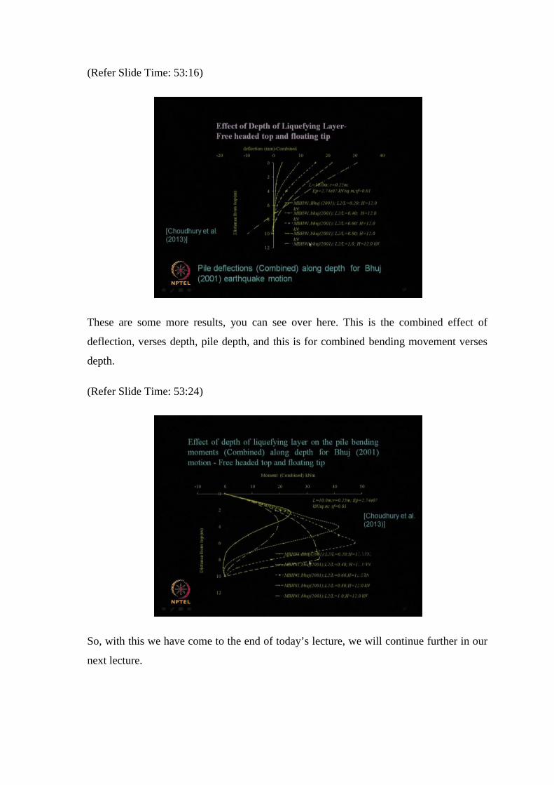
These are some more results, you can see over here. This is the combined effect of

deflection, verses depth, pile depth, and this is for combined bending movement verses

depth.


So, with this we have come to the end of today’s lecture, we will continue further in our

next lecture.

Documents

Geotechnical Earthquake Engineering