Distributed Stable Marriage Problem ?

Ismel Brito and Pedro Meseguer

Institut d’Investigacio en Intel.ligencia ArtificialConsejo Superior de Investigaciones Cientıficas

Campus UAB, 08193 Bellaterra, Spain.{ismel|pedro}@iiia.csic.es

Abstract. The Stable Marriage Problem is a combinatorial problemwhich can be solved by a centralized algorithm in polynomial time. Thisrequires to make public lists of preferences which agents would like tokeep private. With this aim, we define the distributed version of this prob-lem, and we provide a constraint-based approach that solves it keepingprivacy. We give empirical results on the proposed approach.

1 Introduction

The Stable Marriage Problem is a classical combinatorial problem, also of in-terest for Economics and Operations Research. It consists of finding a stablematching between n men and n women, each having his/her own preferenceson every member of the other sex. A matching is not stable if there exist aman m and a woman w not matched with each other, such that each of themstrictly prefers the other to his/her partner in the matching. Any instance of thisproblem has a solution, and it can be computed by the centralized Gale-Shapleyalgorithm in polynomial time.

This problem, by its own nature, appear to be naturally distributed. Eachperson may desire to act independently. For obvious reasons, each person wouldlike to keep private his/her own preferences. However, in the classical case eachperson has to follow a rigid role, making public his/her preferences to achieve aglobal solution. This problem is very suitable to be treated by distributed tech-niques, trying to provide more autonomy to each person, and to keep preferencesprivate. This paper is a contribution to this aim.

The structure of the paper is as follows. We summarize basic concepts ofStable Marriage and Gale-Shapley algorithm, together with a constraint for-mulation for this problem from [4] (Section 2). Then, we define the DistributedStable Marriage problem and provide means to solve it trying to enforce privacy.Thus, we present a distributed version of the Gale-Shapley algorithm, and a dis-tributed constraint formulation under the TCK and PKC models (Section 3).We show how the problem can be solved using the Distributed Forward Check-ing algorithm with the PKC model, keeping private values and constraints.Experimental results show that, when applicable, the distributed Gale-Shapley? Supported by the Spanish REPLI project TIC-2002-04470-C03-03.

algorithm is more efficient than the distributed constraint formulation (Section4), something also observed in the centralized case. However, the distributedconstraint formulation is generic and can solve that problem.

2 The Stable Marriage Problem

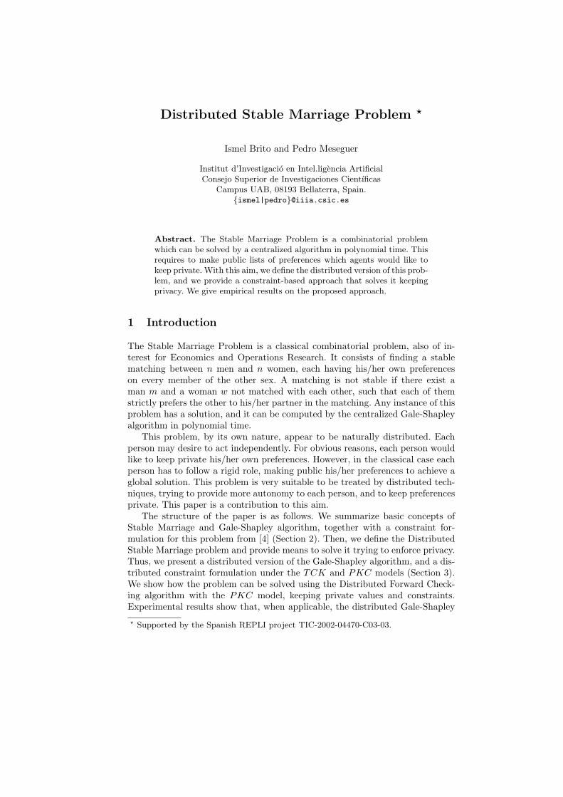
The Stable Marriage Problem (SM) was first studied by Gale and Shapley [2].A SM instance consists of two finite equal-sized sets of players, called men andwomen. Each man mi (1 ≤ i ≤ n, n is the number of men) ranks women in strictorder forming his preference list. Similarly, each woman wj (1 ≤ j ≤ n) ranksmen in strict order forming her preference list. An example of SM appears inFigure 1. A matching M is just a complete one-to-one mapping between the twosexes. The goal is to find a stable matching M . A matching M is stable if thereis no pair (m,w) of man m and a woman w satisfying the following conditions:

C1. m and w are not married in M ,C2. m prefers w to his current partner in M ,C3. w prefers m to her current partner in M .

If this pair (m, w) exists, M is unstable and the pair (m,w) is called a blockingpair. For the example of Figure 1, the matching M = {(m1,w1),(m2, w2), (m3,w3)} is not stable because the pair (m1, w2) blocks M . For that problem, there isonly one stable matching: M1 = {(m1,w2), (m2,w1), (m3,w3)}. Gale and Shapleyshowed that each SM instance admits at least one stable matching [2].

A relaxed version of SM occurs when some persons may declare one or moremembers of the opposite sex to be unacceptable, so they do not appear in thecorresponding preference lists. This relaxed version is called the Stable MarriageProblem with Incomplete Lists (SMI). In SMI instances, the goal is also tofind a stable matching. Like in the case of SM , SMI admits at least one stablematching. However, some specific features of stable matchings for SMI have tobe remarked. First, condition C1 of the definition of blocking pair given abovehave to be changed as follows:

C1’. m and w are not married in M , and m belongs to w’s preferencelist, and w belongs to the m’s preference list.

Second, it can not be assured that all the persons can find a partner. So astable matching of a SMI instance needs not to be complete. However, all thestable matchings involve the same men and women [3].

m1 : w2 w3 w1 w1 : m1 m2 m3

m2 : w1 w2 w3 w2 : m1 m3 m2

m3 : w2 w1 w3 w3 : m2 m1 m3

Fig. 1. A SM instance with three men and three women. Preference lists are in de-creasing order, the most-preferred partner is on the left.

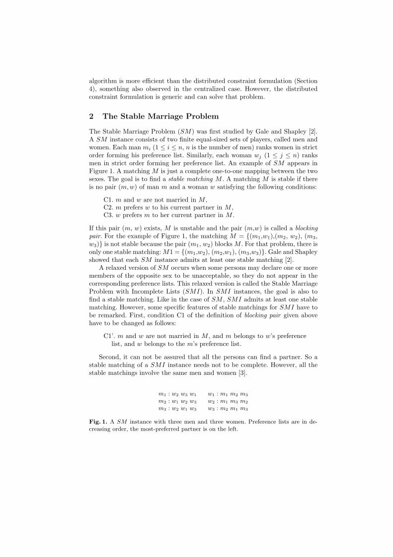
1. assign each person to be free;2. while some man m is free and m has a nonempty list loop3. w := first woman on m’s list; {m proposes to w}4. if m is not on w’s preference list then5. delete w from m’s preference list;6. goto line 37. end if8. if some man p is engaged to w then9. assign p to be free;10. end if11. assign m and w to be engaged to each other;12. for each each successor p of m on w’s list loop13. delete p from w’s list;14. delete w from p’s list;15. end loop;16. end loop;

Fig. 2. The man-oriented Gale-Shapley algorithm for SM and SMI.

2.1 The Gale-Shapley algorithm

Gale and Shapley showed that at least one stable matching exists for everySM (or SMI) instance. They obtained the Gale-Shapley algorithm ([2]), withO(n2) temporal complexity. The Extended Gale-Shapley algorithm (EGS) isan extended version of it, that avoids some extra steps by deleting from thepreference lists certain pairs that cannot belong to a stable matching [6]. Aman-oriented version of EGS 1 appears in Figure 2.

EGS involves a sequence of proposals from men to women. It starts by settingall persons free (line 1). EGS iterates until all the men are engaged or, for SMIinstances, there are some free men because they have an empty preference list(line 2). A man always proposes marriage to his most-preferred woman (line 3).When a woman w receives a proposal from a man m, she accepts it if m is onher preference list. Otherwise, m deletes w from his preference list (line 5) andthen a new proposal is started (line 6). Whether m is on w’s preference list andw is already engaged to p, she discards the previous proposal with p and p is setfree (line 8-9). Afterwards, m and w are engaged each other (line 11). Womanw deletes from her preference list each man p that is less preferred than m (line13). Conversely, man p deletes w from his preference list (line 14). Finally, ifthere is a free man with non-empty preference list a new proposal is started.Otherwise, men are engaged or have empty preference lists and the algorithmterminates.1 For privacy requirements, that will be discussed later in this work, we prefer not

assuming for SMI instances, like in [6], that if man m is not acceptable for a womanw, woman w is not acceptable for man m. For avoiding this assumption, we haveadded Lines 4-7 to the original EGS.

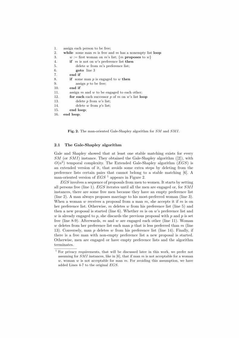
m1 : w2 w1 : m2

m2 : w1 w2 : m1

m3 : w3 w3 : m3

Fig. 3. GS-Lists for the SM of Figure 1.

During EGS execution, some people are deleted from preference lists. Thereduced preference lists that result of applying man-oriented Gale-Shapley algo-rithm are called man-oriented Gale-Shapley lists or MGS-lists. On termination,each man is engaged to the first woman in his (reduced) list, and each womanto the last man in hers. These engaged pairs constitute a stable matching, andit is called man-optimal (or woman-pessimal) stable matching since there is notother stable matching where a man can achieve a better partner (according tohis ranking). Similarly, exchanging the role of men and women in EGS (whichmeans that women propose), we obtain the woman-oriented Gale-Shapley listsor WGS-lists. On termination, each woman is engaged to the first man in her(reduced) list, and each man to the last woman in his. These engaged pairsconstitute a stable matching, and it is called woman-optimal (or man-pessimal)stable matching.

The intersection of MGS-lists and WGS-lists is known as the Gale-Shapleylists (GS-lists). These lists have important properties (see Theorem 1.2.5 in [6]):

– all the stable matchings are contained in the GS-lists,– in the man-optimal (woman-optimal), each man is partnered by the first

(last) woman on his GS-list, and each woman by the last (first) man on hers.

Figure 3 shows the GS-lists for the example given in Figure 1. For this in-stance, the reduced lists of all persons have only one possible partner whichmeans that only one solution exits. In that case, the man-optimal matching andwoman-optimal matching are the same.

2.2 Constraint Formulation

A constraint satisfaction problem (CSP ) is defined by a triple (X ,D, C), whereX = {x1, . . . , xn} is a set of n variables, D = {D(x1), . . . , D(xn)} is the setof their respective finite domains, and C is a set of constraints specifying theacceptable value combinations for variables. A solution to a CSP is a completeassignment that satisfies all constraints in C. When constraints involve two vari-ables they are called binary constraints.

The SM problem can be modeled as a binary CSP . In [4] authors proposea constraint encoding for SM problems, that we summarize next. Each personis represented by a variable: variables x1, x2, ..., xn represent the men (m1, m2,..., mn) and variables y1, y2, ..., yn represent the women (w1, w2 ..., wn). PL(q)is the set of people that belong to q’s preference list. Domains are as follows:

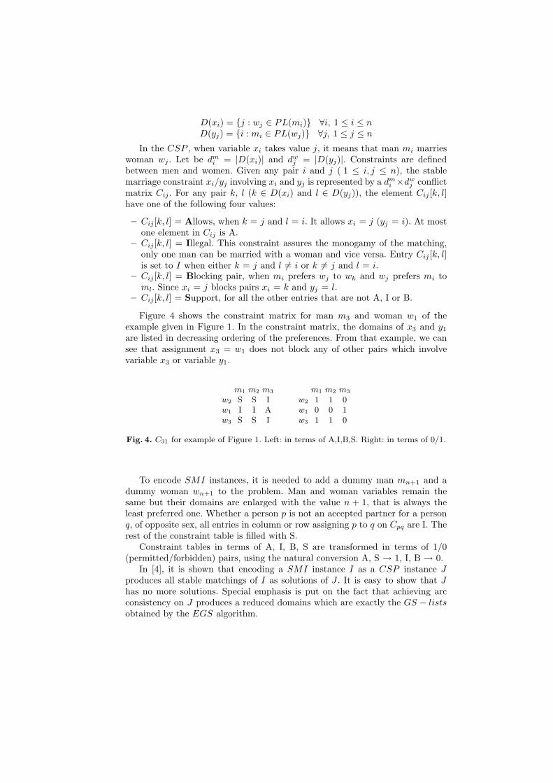
D(xi) = {j : wj ∈ PL(mi)} ∀i, 1 ≤ i ≤ nD(yj) = {i : mi ∈ PL(wj)} ∀j, 1 ≤ j ≤ n

In the CSP , when variable xi takes value j, it means that man mi marrieswoman wj . Let be dm

i = |D(xi)| and dwj = |D(yj)|. Constraints are defined

between men and women. Given any pair i and j ( 1 ≤ i, j ≤ n), the stablemarriage constraint xi/yj involving xi and yj is represented by a dm

i ×dwj conflict

matrix Cij . For any pair k, l (k ∈ D(xi) and l ∈ D(yj)), the element Cij [k, l]have one of the following four values:

– Cij [k, l] = Allows, when k = j and l = i. It allows xi = j (yj = i). At mostone element in Cij is A.

– Cij [k, l] = Illegal. This constraint assures the monogamy of the matching,only one man can be married with a woman and vice versa. Entry Cij [k, l]is set to I when either k = j and l 6= i or k 6= j and l = i.

– Cij [k, l] = Blocking pair, when mi prefers wj to wk and wj prefers mi toml. Since xi = j blocks pairs xi = k and yj = l.

– Cij [k, l] = Support, for all the other entries that are not A, I or B.

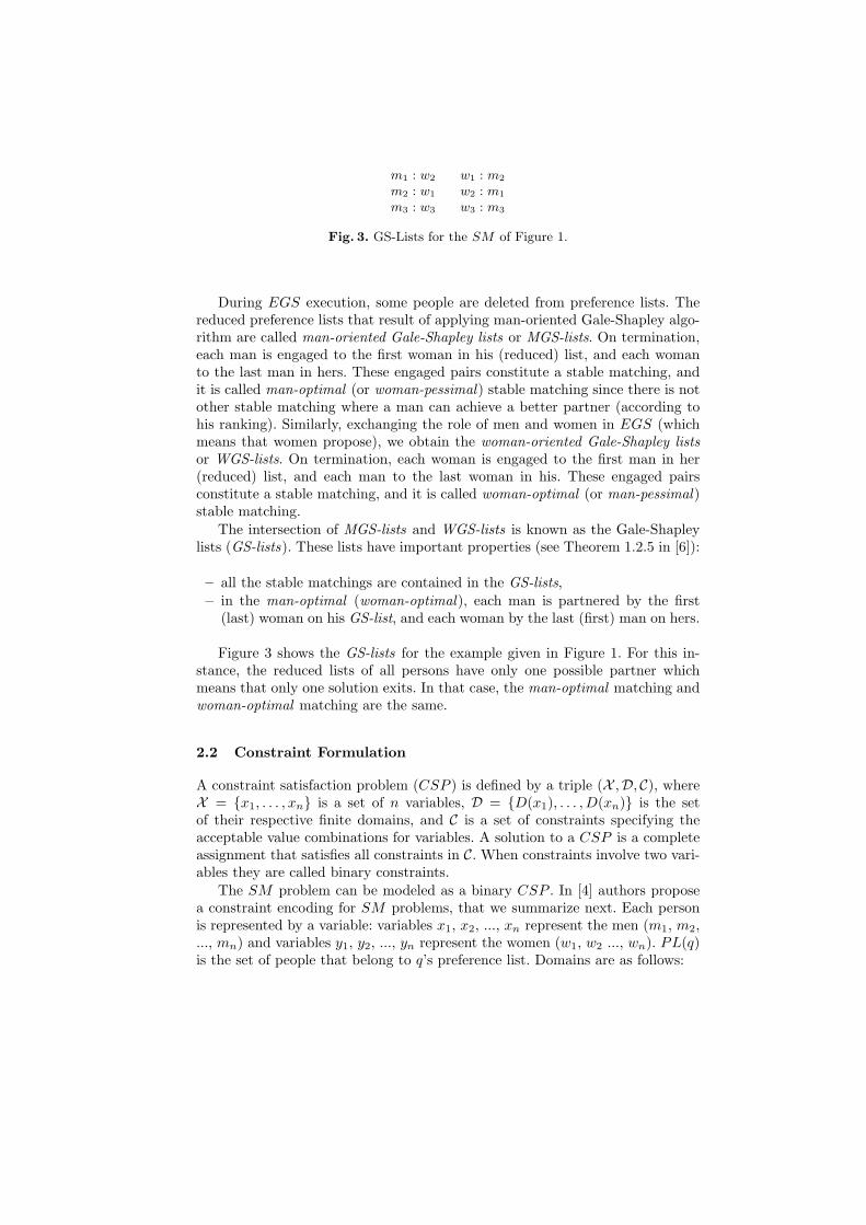
Figure 4 shows the constraint matrix for man m3 and woman w1 of theexample given in Figure 1. In the constraint matrix, the domains of x3 and y1

are listed in decreasing ordering of the preferences. From that example, we cansee that assignment x3 = w1 does not block any of other pairs which involvevariable x3 or variable y1.

m1 m2 m3

w2 S S Iw1 I I Aw3 S S I

m1 m2 m3

w2 1 1 0w1 0 0 1w3 1 1 0

Fig. 4. C31 for example of Figure 1. Left: in terms of A,I,B,S. Right: in terms of 0/1.

To encode SMI instances, it is needed to add a dummy man mn+1 and adummy woman wn+1 to the problem. Man and woman variables remain thesame but their domains are enlarged with the value n + 1, that is always theleast preferred one. Whether a person p is not an accepted partner for a personq, of opposite sex, all entries in column or row assigning p to q on Cpq are I. Therest of the constraint table is filled with S.

Constraint tables in terms of A, I, B, S are transformed in terms of 1/0(permitted/forbidden) pairs, using the natural conversion A, S → 1, I, B → 0.

In [4], it is shown that encoding a SMI instance I as a CSP instance Jproduces all stable matchings of I as solutions of J . It is easy to show that Jhas no more solutions. Special emphasis is put on the fact that achieving arcconsistency on J produces a reduced domains which are exactly the GS − listsobtained by the EGS algorithm.

3 The Distributed Stable Marriage Problem

The Distributed Stable Marriage problem (DisSM) is defined as in the classical(centralized) case by n men {m1, . . . , mn} and n women {w1, . . . , wn}, eachhaving a preference list where all members of the opposite sex are ranked, plus aset of r agents {a1, . . . , ar}. The n men and n women are distributed among theagents, such that each agent owns some persons and every person is owned by asingle agent. An agent can access and modify all the information of the ownedpersons, but it cannot access the information of persons owned by other agents.To simplify description, we will assume that each agent owns exactly one person(so there are 2n agents). As in the classical case, a solution is a stable matching(a matching between the men and women such that no blocking pair exists). Acomplete stable matching always exists.

Analogously to the classical case, we define the Distributed Stable Marriagewith Incomplete lists problem (DisSMI) as a generalization of DisSM that oc-curs when preference lists do not contain all persons of the opposite sex (some op-tions are considered unacceptable). A solution is a stable matching, and it alwaysexists, although it is not guaranteed to be a complete one (some men/womenmay remain unmatched).

This problem, by its own nature, appears to be naturally distributed. First,each person may desire to act as an independent agent. Second, for obvious rea-sons each person would like to keep private his/her preference list ranking theopposite sex options. However, in the classical case each person has to follow arigid role, making public his/her preferences to achieve a global solution. There-fore, this problem is very suitable to be treated by distributed techniques, tryingto provide more autonomy to each person, and to keep private the informationcontained in the preference lists.

3.1 The Distributed Gale-Shapley Algorithm

The EGS algorithm that solves the classical SMI can be easily adapted to dealwith the distributed case. We call this new version the Distributed ExtendedGale/Shapley (DisEGS) algorithm. As in the classical case, the DisEGS al-gorithm has two phases, the man-oriented and the woman-oriented, which areexecuted one after the other. Each phase produces reduced preference lists foreach person. The intersection of these lists produces a GS − list per person. Asin the classical case, the matching obtained after executing the man-orientedphase is a stable matching (man-optimal).

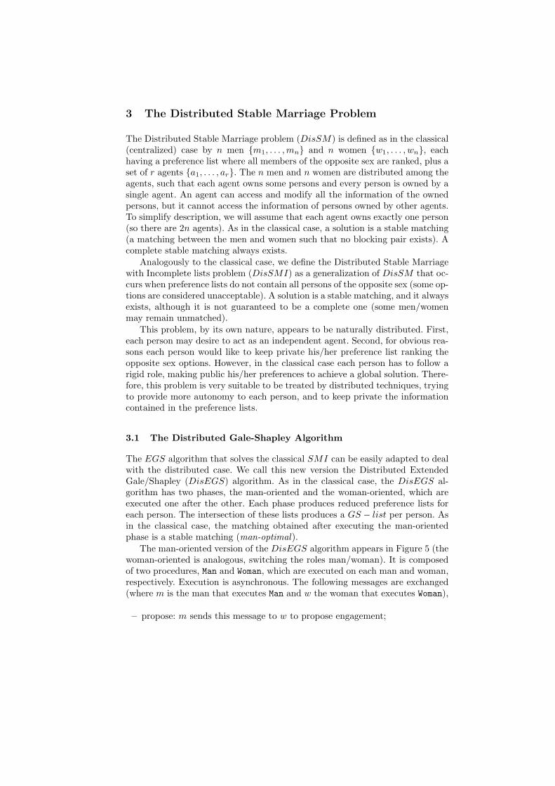
The man-oriented version of the DisEGS algorithm appears in Figure 5 (thewoman-oriented is analogous, switching the roles man/woman). It is composedof two procedures, Man and Woman, which are executed on each man and woman,respectively. Execution is asynchronous. The following messages are exchanged(where m is the man that executes Man and w the woman that executes Woman),

– propose: m sends this message to w to propose engagement;

procedure Man()m ← free;end ← false;while ¬end do

if m = free and list(m) 6= ∅ thenw ← first(list(m));sendMsg(propose,m,w);m ← w;

msg ← getMsg();switch msg.type

accept : do nothing;delete : list(m) ← list(m)−msg.sender;

if msg.sender = w then m ← free;stop : end ← true;

procedure Woman()w ← free;end ← false;while ¬end do

msg ← getMsg();switch msg.type

propose: m ← msg.sender;if m /∈ list(w) thensendMsg(delete,w,m);

elsesendMsg(accept,w,m);w ← m;for each p after m in list(w) dosendMsg(delete,w,p);list(w) ← list(w)− p;

stop : end ← true;

Fig. 5. The man-oriented version of the DisEGS algorithm.

– accept: w sends this message to m after receiving a propose message to notifyacceptance;

– delete: w sends this message to m to notify that w is not available for m;this occurs either (i) proposing m an engagement to w but w has a betterpartner or (ii) w accepted an engagement with other man more preferredthan m;

– stop: this is an special message to notify that execution must end; it is sentby an special agent after detecting quiescence.

Procedure Man, after initialization, performs the following loop. If m is freeand his list is not empty, he proposes to be engaged to w, the first woman in hislist. Then, m waits for a message. If the message is accept and it comes fromw, then m confirms the engagement (nothing is done in the algorithm). If the

message is delete, then m deletes the sender from his list, and if the sender is wthen m becomes free. The loop ends when receiving a stop message.

Procedure Woman is executed on woman w. After initialization, there is amessage receiving loop. In the received message comes from a man m proposingengagement, w rejects the proposition if m is not in her list. Otherwise, w accepts.Then, any man p that appears after m in w list is asked to delete w from hislist, while w removes p from hers. This includes a previous engagement m′, thatwill be the last in her list. The loop ends when receiving a stop message.

Algorithm DisEGS is a distributed version of EGS, where each person canaccess to his/her own information only. For this reason there are two differentprocedures, one for men and one for women. In addition, actions performed byEGS on persons different from the current one are replaced by message sending.Thus, when m assigns woman w is replaced by sendMsg(propose,m,w); whenw deletes herself from the list of p is replaced by sendMsg(delete,w,p). Sinceprocedures exchange messages, operations of message reception are included ac-cordingly.

DisEGS algorithm guarantees privacy in preferences and in the final assign-ment: each person knows the assigned person, and no person knows more thanthat. In this sense, it is a kind of ideal algorithm because it assures privacy invalues and constraints.

3.2 Distributed Constraint Formulation

In [1] we presented an approach to privacy that differentiates between valuesand constraints. Briefly, privacy on values implies that agents are not aware ofother agent values during the solving process and in the final solution. Thiswas achieved using the Distributed Forward Checking algorithm (DisFC), anABT -based algorithm that, after the assignment of an agent variable, insteadof sending to lower priority agents the value just assigned, it sends the domainsubset that is compatible with the assigned value. In addition, it replaces actualvalues by sequence numbers in backtracking messages. In this way, the assign-ment of an agent is kept private at any time.

Regarding privacy on constraints, two models were considered. The TotallyKnown Constraints (TKC) model assumes that when two agents i, j share aconstraint Cij , both know the constraint scope and one of them knows completelythe relational part of the constraint (the agent in charge of constraint evaluation).The Partially Known Constraints (PKC) model assumes that when two agentsi, j share a constraint Cij , none of them knows completely the constraint. Onthe contrary, each agent knows the part of the constraint that it is able to build,based on its own information. We say that agent i knows Ci(j), and j knowsCj(i). This implies that the identification of the other agent is neutral. In thefollowing, we apply these two models to the DisSM problem using the constraintformulation of Section 2.2 from [4].

Totally Known Constraints Solving a DisSMI problem is direct under theTKC model. For each pair xi, yj , representing a man and a woman, there is a

i1 . . . 1 0 1 . . . 1

. . .1 . . . 1 0 1 . . . 1

j 0 . . . 0 1 0 . . . 01 . . . 1 0 0 . . . 0

. . .1 . . . 1 0 0 . . . 0

i1/0 . . . 1/0 0 1/0 . . . 1/0

. . .1/0 . . . 1/0 0 1/0 . . . 1/0

j 0 . . . 0 1 0 . . . 01/0 . . . 1/0 0 1/0 . . . 1/0

. . .1/0 . . . 1/0 0 1/0 . . . 1/0

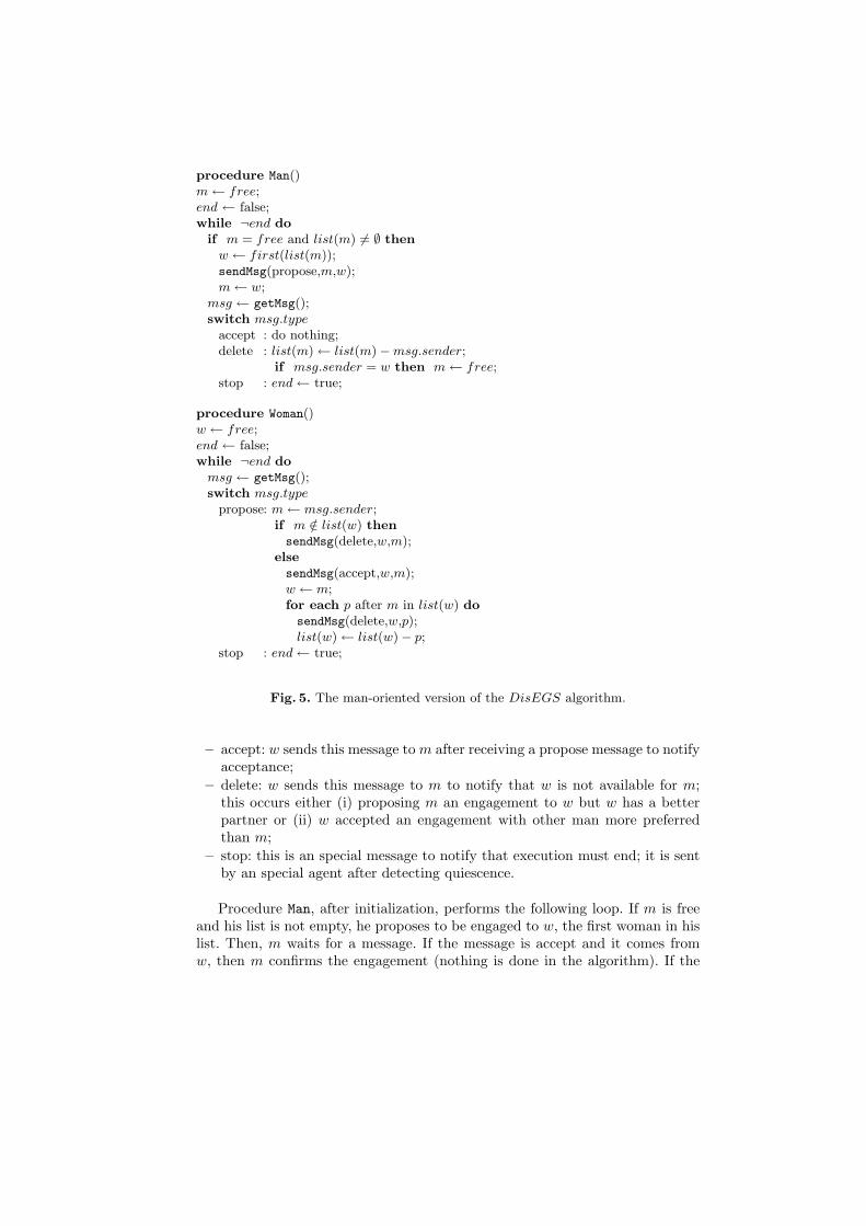
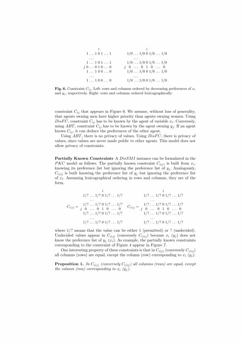
Fig. 6. Constraint Cij . Left: rows and columns ordered by decreasing preferences of xi

and yj , respectively. Right: rows and columns ordered lexicographically.

constraint Cij that appears in Figure 6. We assume, without loss of generality,that agents owning men have higher priority than agents owning women. UsingDisFC, constraint Cij has to be known by the agent of variable xi. Conversely,using ABT , constraint Cij has to be known by the agent owning yj . If an agentknows Cij , it can deduce the preferences of the other agent.

Using ABT , there is no privacy of values. Using DisFC, there is privacy ofvalues, since values are never made public to other agents. This model does notallow privacy of constraints.

Partially Known Constraints A DisSMI instance can be formulated in thePKC model as follows. The partially known constraint Ci(j) is built from xi,knowing its preference list but ignoring the preference list of yj . Analogously,C(i)j is built knowing the preference list of yj but ignoring the preference listof xi. Assuming lexicographical ordering in rows and columns, they are of theform,

Ci(j) =

i1/? . . . 1/? 0 1/? . . . 1/?

. . .1/? . . . 1/? 0 1/? . . . 1/?

j 0 . . . 0 1 0 . . . 01/? . . . 1/? 0 1/? . . . 1/?

. . .1/? . . . 1/? 0 1/? . . . 1/?

C(i)j =

i1/? . . . 1/? 0 1/? . . . 1/?

. . .1/? . . . 1/? 0 1/? . . . 1/?

j 0 . . . 0 1 0 . . . 01/? . . . 1/? 0 1/? . . . 1/?

. . .1/? . . . 1/? 0 1/? . . . 1/?

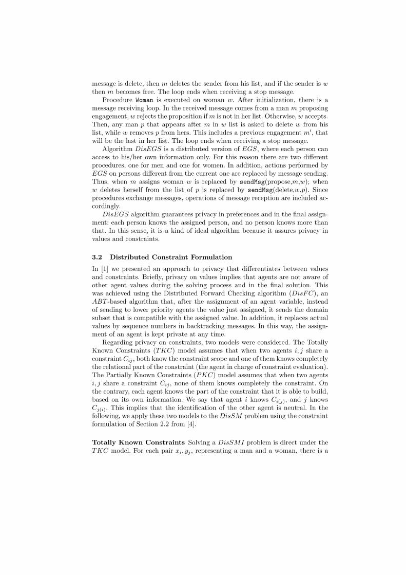
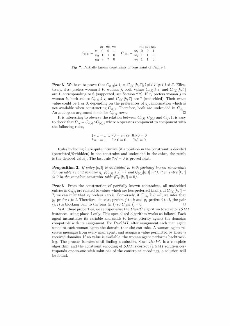
where 1/? means that the value can be either 1 (permitted) or ? (undecided).Undecided values appear in Ci(j) (conversely C(i)j) because xi (yj) does notknow the preference list of yj (xi). As example, the partially known constraintscorresponding to the constraint of Figure 4 appear in Figure 7.

One interesting property of these constraints is that in Ci(j) (conversely C(i)j)all columns (rows) are equal, except the column (row) corresponding to xi (yj).

Proposition 1. In Ci(j) (conversely C(i)j) all columns (rows) are equal, exceptthe column (row) corresponding to xi (yj).

C3(1) =

m1 m2 m3

w1 0 0 1w2 1 1 0w3 ? ? 0

C(3)1 =

m1 m2 m3

w1 0 0 1w2 1 1 0w3 1 1 0

Fig. 7. Partially known constraints of constraint of Figure 4.

Proof. We have to prove that Ci(j)[k, l] = Ci(j)[k, l′], l 6= i, l′ 6= i, l 6= l′. Effec-tively, if xi prefers woman k to woman j, both values Ci(j)[k, l] and Ci(j)[k, l′]are 1, corresponding to S (supported, see Section 2.2). If xi prefers woman j towoman k, both values Ci(j)[k, l] and Ci(j)[k, l′] are ? (undecided). Their exactvalue could be 1 or 0, depending on the preferences of yj , information which isnot available when constructing Ci(j). Therefore, both are undecided in Ci(j).An analogous argument holds for C(i)j rows. 2

It is interesting to observe the relation between Ci(j), C(i)j and Cij . It is easyto check that Cij = Ci(j)¦C(i)j , where ¦ operates component to component withthe following rules,

1 ¦ 1 = 1 1 ¦ 0 = error 0 ¦ 0 = 0? ¦ 1 = 1 ? ¦ 0 = 0 ?¦? = 0

Rules including ? are quite intuitive (if a position in the constraint is decided(permitted/forbidden) in one constraint and undecided in the other, the resultis the decided value). The last rule ?¦? = 0 is proved next.

Proposition 2. If entry [k, l] is undecided in both partially known constraintsfor variable xi and variable yj (Ci(j)[k, l] =? and C(i)j [k, l] =?), then entry [k, l]is 0 in the complete constraint table (Cij [k, l] = 0).

Proof. From the construction of partially known constraints, all undecidedentries in Ci(j) are related to values which are less preferred than j. If Ci(j)[k, l] =?, we can infer that xi prefers j to k. Conversely, if C(i)j [k, l] =?, we infer thatyj prefer i to l. Therefore, since xi prefers j to k and yj prefers i to l, the pair(i, j) is blocking pair to the pair (k, l) so Cij [k, l] = 0. 2

With these properties, we can specialize the DisFC algorithm to solve DisSMIinstances, using phase I only. This specialized algorithm works as follows. Eachagent instantiates its variable and sends to lower priority agents the domainscompatible with its assignment. For DisSMI, after assignment each man agentsends to each woman agent the domain that she can take. A woman agent re-ceives messages from every man agent, and assigns a value permitted by these nreceived domains. If no value is available, the woman agent performs backtrack-ing. The process iterates until finding a solution. Since DisFC is a completealgorithm, and the constraint encoding of SMI is correct (a SMI solution cor-responds one-to-one with solutions of the constraint encoding), a solution willbe found.

In the previous argument, something must be scrutinized in more detail. Afterassignment, what kind of compatible domain can a man agent send? If agent iassigns value k to xi, it sends to j the row of Ci(j) corresponding to value k.This row may contain 1’s (permitted values for yj), 0’s (forbidden values foryj), and ? (undecided values for yj). If the compatible domain has 1 or 0 valuesonly, there is no problem and the yj domain can be easily computed. But whathappens when the domain contains ? (undecided) values? In this case, agent jcan disambiguate the domain as follows. When agent j receives a compatibledomain with ? (undecided) values, it performs the ¦ operation with a row ofC(i)j different from i. Since all rows in C(i)j are equal, except row correspondingto value i (see Proposition 1), all will give the same result. Performing the ¦operation j will compute the corresponding row in the complete constraint Cij ,although j does not know to which value this row corresponds (in other words,j does not know the value assigned to xi). After the ¦ operation the resultingreceived domain will contain no ? (undecided) values, and the receiving agentcan operate normally with it.

4 Experimental Results

We give empirical results on the DisEGS and DisFC algorithm with PKCmodel for DisSMI random instances. In our experiments, we use four differentclasses of instances. Each class is defined by a pair 〈n, p1〉, which means the prob-lem has n men and n women on DisSMI and the probability of incompletenessof the preference list is p1. Class < n, 0.0 > groups instances where all the npersons has complete preference list. If p1 = 1.0, preferences lists are empty. Westudy 4 different classes with n = 10 and p1 = 0.0, 0.2, 0.5 and 0.8. For eachclass, 100 instances were generated following the random instance generationpresented in [5] considering p2, the probability of ties, equals to 0.0.

Algorithm is modeled using 2n agents, each one represents a man or a woman.In DisEGS, each agent only knows its preference list. In DisFC, each agentonly knows its partial constraint tables. In both, agents exchange different kind ofmessages to find a stable matching. When DisEGS finishes the stable matchingfound is the men-optimal one. DisFC, like others asynchronous backtrackingalgorithms, requires a total ordering among agents. In our experiments, menagents have higher priority than women agents.

Algorithmic performance is evaluated by communication and computationeffort. Communication effort is measured by the total number of exchangedmessages (msg). Since both algorithms are asynchronous, computation cost ismeasured by the number of concurrent constraint checks (ccc) (for DisEGS, anagent performs a constraint check when it checks if one person is more preferredthat other), as defined in [7], following Lamport’s logic clocks [8].

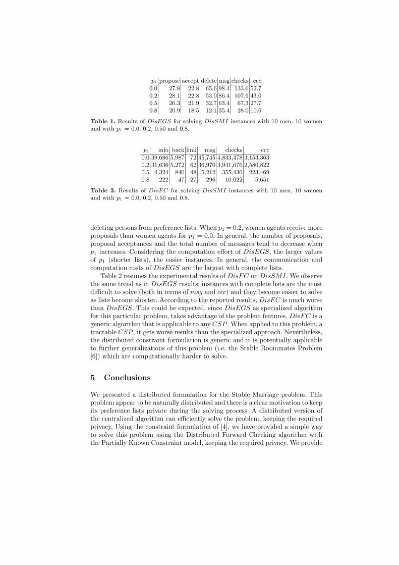
Table 1 details the experimental results of DisEGS on DisSMI. Besidesmsg and ccc, we provide the total number of messages for each kind of messageand the total number of checks. Regarding the communication effort, exceptfor instances with p1 = 0.8, the larger number of exchanged messages are for

p1 propose accept delete msg checks ccc

0.0 27.8 22.8 65.6 98.4 133.6 52.70.2 28.1 22.8 53.0 86.4 107.9 43.00.5 26.3 21.9 32.7 63.4 67.3 27.70.8 20.9 18.5 12.1 35.4 28.0 10.6

Table 1. Results of DisEGS for solving DisSMI instances with 10 men, 10 womenand with p1 = 0.0, 0.2, 0.50 and 0.8.

p1 info back link msg checks ccc

0.0 39,686 5,987 72 45,745 4,833,478 3,153,3630.2 31,636 5,272 62 36,970 3,941,676 2,580,8220.5 4,324 840 48 5,212 355,436 223,4690.8 222 47 27 296 10,022 5,651

Table 2. Results of DisFC for solving DisSMI instances with 10 men, 10 womenand with p1 = 0.0, 0.2, 0.50 and 0.8.

deleting persons from preference lists. When p1 = 0.2, women agents receive moreproposals than women agents for p1 = 0.0. In general, the number of proposals,proposal acceptances and the total number of messages tend to decrease whenp1 increases. Considering the computation effort of DisEGS, the larger valuesof p1 (shorter lists), the easier instances. In general, the communication andcomputation costs of DisEGS are the largest with complete lists.

Table 2 resumes the experimental results of DisFC on DisSMI. We observethe same trend as in DisEGS results: instances with complete lists are the mostdifficult to solve (both in terms of msg and ccc) and they become easier to solveas lists become shorter. According to the reported results, DisFC is much worsethan DisEGS. This could be expected, since DisEGS as specialized algorithmfor this particular problem, takes advantage of the problem features. DisFC is ageneric algorithm that is applicable to any CSP . When applied to this problem, atractable CSP , it gets worse results than the specialized approach. Nevertheless,the distributed constraint formulation is generic and it is potentially applicableto further generalizations of this problem (i.e. the Stable Roommates Problem[6]) which are computationally harder to solve.

5 Conclusions

We presented a distributed formulation for the Stable Marriage problem. Thisproblem appear to be naturally distributed and there is a clear motivation to keepits preference lists private during the solving process. A distributed version ofthe centralized algorithm can efficiently solve the problem, keeping the requiredprivacy. Using the constraint formulation of [4], we have provided a simple wayto solve this problem using the Distributed Forward Checking algorithm withthe Partially Known Constraint model, keeping the required privacy. We provide

experimental results of this approach. The generic constraint formulation opensnew directions for distributed encodings of harder versions of this problem.

References

1. Brito, I. and Meseguer, P. Distributed Forward Checking. Proc. CP-2003, 801–806,2003.

2. Gale D. and Shapley L.S. College admissions and the stability of the marriage.American Mathematical Monthly. 69:9–15, 1962.

3. Gale D. and Sotomayor M. Some remarks on the stable matching problem. DiscreteApplied Mathematics. 11:223–232, 1985.

4. Gent, I. P. and Irving, R. W. and Manlove, D. F. and Prosser, P. and Smith,B. M. A constraint programming approach to the stable marriage problem. Proc.CP-2001, 225-239, 2001.

5. Gent,I. and Prosser,P. An Empirical Study of the Stable Marriage Problem withTies and Incomplete Lists. Proc. ECAI-2002, 141–145, 2002.

6. Gusfield D. and Irving R. W. The Stable Marriage Problem: Structure and Algo-rithms. The MIT Press, 1989.

7. Meisels A., Kaplansky E., Razgon I., Zivan R. Comparing Performance of Dis-tributed Constraint Processing Algorithms. AAMAS-02 Workshop on DistributedConstraint Reasoning, 86–93, 2002.

8. Lamport L. Time, Clock, and the Ordering of Evens in a Distributed System.Communications of the ACM, 21(7), 558–565, 1978.