Electronic copy available at: http://ssrn.com/abstract=1101946Electronic copy available at: http://ssrn.com/abstract=1101946Electronic copy available at: http://ssrn.com/abstract=1101946

WEIGHTED RISK CAPITAL ALLOCATIONS

Edward Furman1

Department of Mathematics and Statistics, York University, Toronto, Ontario M3J 1P3,

Canada. E-mail: efurman@mathstat.yorku.ca

Ricardas Zitikis

Department of Statistical and Actuarial Sciences, University of Western Ontario,

London, Ontario N6A 5B7, Canada. E-mail: zitikis@stats.uwo.ca

Abstract. By extending the notion of weighted premium calculation prin-

ciples, we introduce weighted risk capital allocations, explore their prop-

erties, and develop computational methods. When achieving these goals,

we find it particularly fruitful to relate the weighted allocations to general

Stein-type covariance decompositions, which are of interest on their own.

Keywords and phrases : Weighted distributions, weighted premiums, weighted

allocations, Stein’s Lemma, general covariance decomposition, regression

function.

1Corresponding author.

Electronic copy available at: http://ssrn.com/abstract=1101946Electronic copy available at: http://ssrn.com/abstract=1101946Electronic copy available at: http://ssrn.com/abstract=1101946

2

1. Introduction and motivation

Let X ≥ 0 be a risk random variable (rv) with cumulative distribution function (cdf)

FX , and let X denote the set of all such rv’s. Consider a functional H : X → [0,∞].

When loaded, that is, H[X] ≥ E[X] for every X ∈ X , then the functional H is called

premium calculation principle (pcp). There is a great variety of pcp’s in the literature; see,

e.g., Gerber (1979), Buhlmann (1980, 1984), Goovaerts et al. (1984), Denneberg (1994),

Kaas et al. (1994), Wang (1995, 1996, 1998), Tsanakas and Desli (2003), Heilpern (2003),

Young (2004), Denuit et al. (2005), Denuit et al. (2006), Dhaene et al. (2006), Furman

and Landsman (2006), Furman and Zitikis (2008).

Research in the area of financial risk measurement has fruitfully utilized the concept of

actuarial pcp’s and introduced additional challenging and interesting problems. Specifi-

cally, consider the pool {X1, . . . , XK} of insurance risks Xk, and denote the overall risk as-

sociated with the pool by Y , which can, for example, be the linear combination∑K

k=1 ckXk

or, simply, the sum S =∑K

k=1 Xk. A non-trivial problem is to quantify the supporting

capital, also known as the risk or economic capital, for a contract X ∈ {X1, . . . , XK}. We

denote the capital by A[X,Y ] and refer to the corresponding functional

A : X × X → [0,∞]

as the risk capital allocation. It should be noted that allocating risk capital is not the

final but rather an intermediate step, which often aims at distinguishing most profitable

business units and thus contributes to the overall efficiency of the decision making process;

for details, see, e.g., Tasche (1999), Laeven and Goovaerts (2004), Venter (2004), Filipovic

and Kupper (2008).

In this paper (see Section 2) we formulate a class of allocations Aw : X × X →[0,∞], which we call weighted risk capital allocations. The allocations are related to

the ‘weighted’ functionals Hw : X → [0,∞] defined by (see Furman and Zitikis, 2008)

Hw[X] =E[Xw(X)]

E[w(X)], (1.1)

where w : [0,∞) → [0,∞) is a function, called weight function, which is usually chosen by

the decision maker depending on the problem at hand. (All weight functions throughout

this paper are deterministic, non-negative, and Borel-measurable.) It is important to

note that if the weight function w is non-decreasing, which is usually the case, then the

3

weighted functional Hw is loaded and thus defines a rich class of actuarial ‘weighted’ pcp’s.

In view of the above, the present paper is therefore a natural continuation of the research

by Furman and Zitikis (2008).

The rest of the paper is organized as follows. In Section 2 we formally introduce the

weighted allocation Aw : X × X → [0,∞] and present a number of illustrative examples.

In Section 3 we study, discuss, and verify properties of the weighted allocation. In Sec-

tion 4 we address computational aspects of Aw[X,Y ] for various choices of random pairs

(X,Y ) and weight functions w. As a by-product, we suggest a route, which relies on a

modification of Stein’s Lemma, for disentangling the dependence structure between the

rv’s X and Y from the weight function w. This, in turn, relates our current research

to the capital asset pricing model (CAPM) of Sharpe (1964), Lintner (1965), and Black

(1972). Section 5 concludes the paper with an overview of main contributions.

2. Weighted allocations

The allocation problem appears in various fields including operation research, eco-

nomics, finance. Naturally, the definitions of the phenomenon vary from field to field.

In the present paper we define the risk capital allocation induced by a risk measure

H : X → [0,∞] as a map A : X × X → [0,∞] such that

A[X,X] = H[X] for all X ∈ X . (2.1)

We next specialize this definition and introduce the weighted allocation, which is the main

object of our study in the present paper.

Definition 2.1. Let X, Y ∈ X , and let w : [0,∞) → [0,∞) be a deterministic Borel

function. We call the functional Aw : X × X → [0,∞], defined by the equation

Aw[X,Y ] =E[Xw(Y )]

E[w(Y )], (2.2)

the weighted allocation induced by the weighted pcp Hw : X → [0,∞]; see equation (1.1).

A number of well known allocation rules are special cases of Aw : X ×X → [0,∞] under

appropriate choices of the weight function w, which can be independent of, or dependent

on, the cdf’s FX and/or FY ; see Table 2.1. An example of the weighted allocation when

w does not depend on any cdf is Esscher’s allocation, whose detailed study with further

references can be found in, e.g., Buhlmann (1980, 1984), Wang (2002, 2007), Goovaerts et

4

al. (2004), Young (2004), Denuit et al. (2005), Pflug and Romisch (2007), Goovaerts and

Laeven (2008). For another example of the weighted allocation when w is independent

of any cdf, we refer to Kamps (1998) where we find a discussion of a pcp that induces

Kamps’s allocation (see Table 2.1). For examples of the weighted allocation when w does

depend on FY , we refer to, e.g., Tsanakas and Barnett (2003), Tsanakas (2008) where

the distorted allocation is studied (see Table 2.1); to Denault (2001), Panjer and Jing

(2001) for the TCE allocations (see Table 2.1); to Furman and Landsman (2006) for the

modified tail covariance (MTCov) allocation (see Table 2.1). We note in passing that the

TCE allocation E[X|Y ≥ F−1Y (p)] is closely related to the absolute concentration curve

(ACC) p 7→ E[X1{Y ≤ F−1Y (p)}], which has played a prominent role in financial portfolio

management; see Shalit and Yitzhaki (1994), Schechtman et al. (2008), and references

therein.

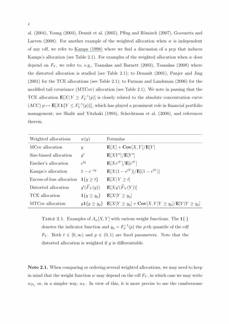
Weighted allocations w(y) Formulas

MCov allocation y E[X] + Cov[X, Y ]/E[Y ]

Size-biased allocation yt E[XY t]/E[Y t]

Esscher’s allocation ety E[XetY ]/E[etY ]

Kamps’s allocation 1− e−ty E[X(1− etY )]/E[(1− etY )]

Excess-of-loss allocation 1{y ≥ t} E[X|Y ≥ t]

Distorted allocation g′(F Y (y)) E[Xg′(F Y (Y ))]

TCE allocation 1{y ≥ yp} E[X|Y ≥ yp]

MTCov allocation y1{y ≥ yp} E[X|Y ≥ yp] + Cov[X,Y |Y ≥ yp]/E[Y |Y ≥ yp]

Table 2.1. Examples of Aw[X, Y ] with various weight functions. The 1{·}denotes the indicator function and yp = F−1

Y (p) the p-th quantile of the cdf

FY . Both t ∈ [0,∞) and p ∈ (0, 1) are fixed parameters. Note that the

distorted allocation is weighted if g is differentiable.

Note 2.1. When comparing or ordering several weighted allocations, we may need to keep

in mind that the weight function w may depend on the cdf FY , in which case we may write

wFYor, in a simpler way, wY . In view of this, it is more precise to use the cumbersome

5

notation AwY[X,Y ] instead of Aw[X, Y ], but we prefer the latter one. However, if we feel

that this might cause a confusion, then we shall use AwY[X, Y ] as we do, for example, in

Proposition 3.1 below.

In general, the weighted allocation Aw[X, Y ] can be interpreted in several ways. First,

it can be viewed as the solution in a to the minimization problem mina E[(X − a)2w(Y )].

Second, Aw[X, Y ] can be viewed as the mean∫

ρ(y)dFw,Y (y) of the regression function

ρ(y) = E[X|Y = y] with respect to the weighted cdf

Fw,Y (y) =E[1{Y ≤ y}w(Y )]

E[w(Y )]. (2.3)

Third, it is useful, and indeed crucial for our following discussion, to observe that the

weighted allocation Aw[X,Y ] can be written, and thus interpreted accordingly, as follows:

Aw[X,Y ] = E[X] +Cov[X,w(Y )]

E[w(Y )]. (2.4)

Hence, the ratio Cov[X,w(Y )]/E[w(Y )] can be thought of as a safety loading due to

the risk X. When the random variables X and w(Y ) are positively correlated, i.e.,

Cov[X, w(Y )] ≥ 0, then we have the bound

Aw[X,Y ] ≥ E[X], (2.5)

which we call the loading property, following the accepted terminology in the context of

pcp’s. In particular, bound (2.5) holds when the rv’s X and Y are positively quadrant

dependent and the weight function w is non-decreasing (see Lehmann, 1966). We shall

discuss further properties of weighted allocations later in this paper. At the moment we

only briefly note that while desirable properties of risk measures have been extensively

studied in the literature for a long time (see, e.g., Goovaerts, 1984; Artzner et al., 1999,

Denuit et al. (2005), Dhaene et al., 2006; and references therein), properties of allocations

have only relatively recently been postulated and discussed (see, e.g., Denault, 2001;

Hesselager and Andersson, 2002; Valdez and Chernih, 2003; Goovaerts et al., 2003; Dhaene

et al., 2008).

We conclude this section with a note that there are also good reasons to consider a

more general functional Av,w : X × X → [0,∞] obtained by augmenting the definition of

6

Aw with a function v : [0,∞] → [0,∞] as follows:

Av,w[X, Y ] =E[v(X)w(Y )]

E[w(Y )].

We may think of v as a utility function, which is usually non-decreasing and concave. Con-

siderations involving conditional tail variance and higher order moments lead to v(x) = xt

with various t ≥ 0. The allocation Av,w[Y, Y ] with v(x) = 1{x ≤ y} is the weighted cdf

Fw,Y (y); see definition (2.3). In the purely actuarial case, i.e., when X = Y , the allocation

Av,w[X,Y ] reduces (as it should, see property (2.1)) to the generalized weighted premium

Hv,w[X] =E[v(X)w(X)]

E[w(X)],

which can be traced back to Heilmann (1989); see also Section 4 in Furman and Zitikis

(2008).

3. Properties

Let X1, X2, . . . , XK be risks in a portfolio whose aggregate risk is S =∑K

k=1 Xk. We

are interested in properties of the allocation Aw[Xk, S]. We start with several elementary

properties such as the already noted non-negative loading and consistency, and then focus

on more complex properties by first formulating them for the generic allocation A[Xk, S]

and then specializing them to the weighted allocation Aw[Xk, S].

3.1. Non-negative loading. In general risk measures may not be non-negatively loaded.

Nevertheless, in many situations it is desirable to have this property, especially in in-

surance pricing context. Likewise, if we are interested in using allocations in insurance

pricing, then it is natural to require the bound

A[Xk, S] ≥ E[Xk] (3.1)

to hold for all pairs (Xk, S) under consideration. In the context of the weighted alloca-

tion Aw[Xk, S], we have bound (3.1) provided that (see Lemma 1(iii) and Lemma 3 in

Lehmann, 1966) the weight function w is non-decreasing and the pair (Xk, S) is positively

quadrant dependent. For discussions of this and other dependence structures, we refer to,

e.g., Lehmann (1966), and Mari and Kotz (2001).

7

3.2. No unjustified loading. It is reasonable to require that the risk capital due to any

constant risk should be equal to the risk itself. Specifically, if Xk = c (a constant), then

the no-unjustified loading property means that

A[Xk, S] = c. (3.2)

The weighted allocation Aw obviously satisfies this property.

3.3. Full additivity. It is often natural (e.g., in order for the balance sheet computations

to sum up) to require the allocation A to be fully additive, that is,

K∑

k=1

A[Xk, S] = H[S](

= A[S, S]). (3.3)

The weighted allocation Aw obviously satisfies this property.

3.4. Consistency. A more general condition than the full additivity is that of consistency

(see Hesselager and Andersson, 2002, for a general definition). Namely, the allocation A

is consistent if, for every subset ∆ ⊆ {1, . . . , K},∑

k∈∆

A[Xk, S] = A[S∆, S], (3.4)

where S∆ =∑

k∈∆ Xk. Obviously, the weighted allocation Aw satisfies this property. Note

also that consistency implies full additivity.

3.5. No undercut. Since we are often interested in aggregation benefits, it is natural for

the allocation A to allow for the diversification effect. We say that the allocation A satisfies

the no-undercut property (see Denault, 2001) if, for every subset ∆ ⊆ {1, . . . , K},∑

k∈∆

A[Xk, S] ≤ A[S∆]. (3.5)

Equation (3.5) ensures that the risk capital due to a stand alone risk is not smaller than

the risk capital due to the same risk when it is a part of the risk pool {X1, . . . , XK}. We

shall discuss the verification of bound (3.5) in the case of the weighted allocation later in

this section.

8

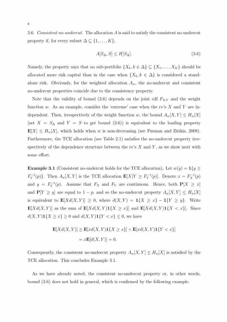
3.6. Consistent no-undercut. The allocation A is said to satisfy the consistent no-undercut

property if, for every subset ∆ ⊆ {1, . . . , K},

A[S∆, S] ≤ H[S∆]. (3.6)

Namely, the property says that no sub-portfolio {Xk, k ∈ ∆} ⊆ {X1, . . . , XK} should be

allocated more risk capital than in the case when {Xk, k ∈ ∆} is considered a stand-

alone risk. Obviously, for the weighted allocation Aw, the no-undercut and consistent

no-undercut properties coincide due to the consistency property.

Note that the validity of bound (3.6) depends on the joint cdf FX,Y and the weight

function w. As an example, consider the ‘extreme’ case when the rv’s X and Y are in-

dependent. Then, irrespectively of the weight function w, the bound Aw[X,Y ] ≤ Hw[X]

(set X = S∆ and Y = S to get bound (3.6)) is equivalent to the loading property

E[X] ≤ Hw[X], which holds when w is non-decreasing (see Furman and Zitikis, 2008).

Furthermore, the TCE allocation (see Table 2.1) satisfies the no-undercut property irre-

spectively of the dependence structure between the rv’s X and Y , as we show next with

some effort.

Example 3.1 (Consistent no-undercut holds for the TCE allocation). Let w(y) = 1{y ≥F−1

Y (p)}. Then Aw[X, Y ] is the TCE allocation E[X|Y ≥ F−1Y (p)]. Denote x = F−1

X (p)

and y = F−1Y (p). Assume that FX and FY are continuous. Hence, both P[X ≥ x]

and P[Y ≥ y] are equal to 1 − p, and so the no-undercut property Aw[X,Y ] ≤ Hw[X]

is equivalent to E[Xd(X, Y )] ≥ 0, where d(X, Y ) = 1{X ≥ x} − 1{Y ≥ y}. Write

E[Xd(X,Y )] as the sum of E[Xd(X, Y )1{X ≥ x}] and E[Xd(X,Y )1{X < x}]. Since

d(X, Y )1{X ≥ x} ≥ 0 and d(X, Y )1{Y < x} ≤ 0, we have

E[Xd(X, Y )] ≥ E[xd(X, Y )1{X ≥ x}] + E[xd(X,Y )1{Y < x}]

= xE[d(X, Y )] = 0.

Consequently, the consistent no-undercut property Aw[X, Y ] ≤ Hw[X] is satisfied by the

TCE allocation. This concludes Example 3.1.

As we have already noted, the consistent no-undercut property or, in other words,

bound (3.6) does not hold in general, which is confirmed by the following example.

9

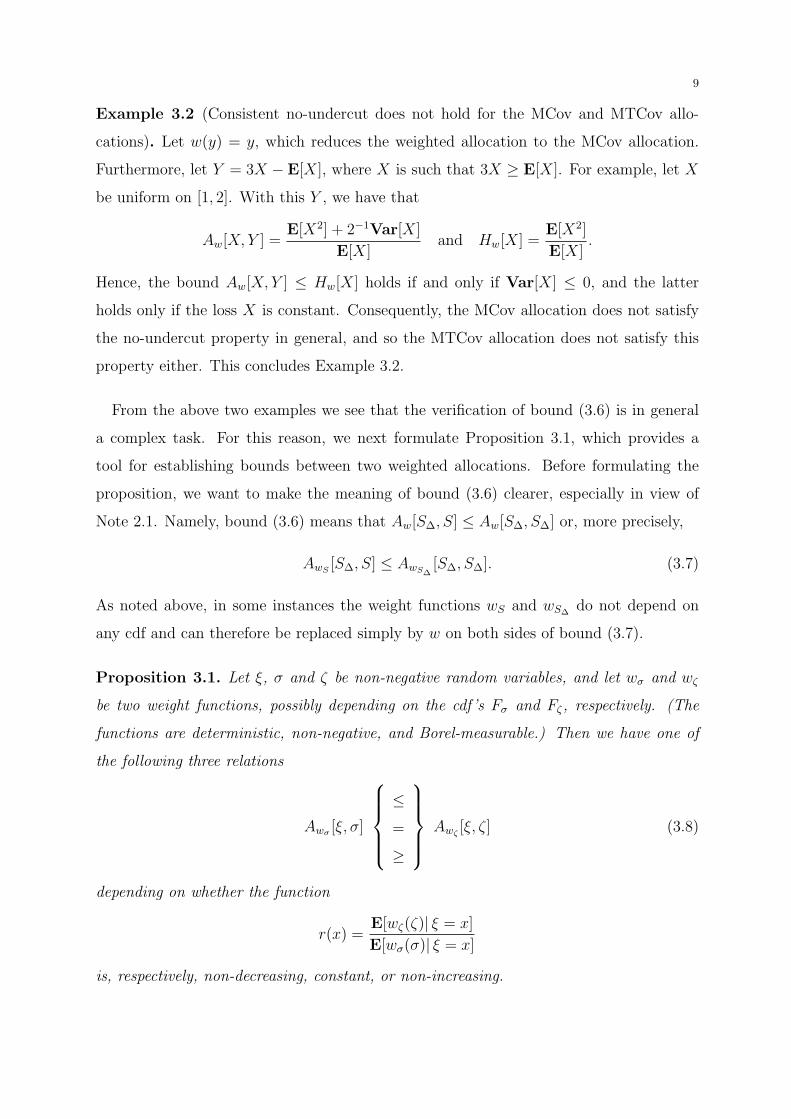
Example 3.2 (Consistent no-undercut does not hold for the MCov and MTCov allo-

cations). Let w(y) = y, which reduces the weighted allocation to the MCov allocation.

Furthermore, let Y = 3X −E[X], where X is such that 3X ≥ E[X]. For example, let X

be uniform on [1, 2]. With this Y , we have that

Aw[X, Y ] =E[X2] + 2−1Var[X]

E[X]and Hw[X] =

E[X2]

E[X].

Hence, the bound Aw[X,Y ] ≤ Hw[X] holds if and only if Var[X] ≤ 0, and the latter

holds only if the loss X is constant. Consequently, the MCov allocation does not satisfy

the no-undercut property in general, and so the MTCov allocation does not satisfy this

property either. This concludes Example 3.2.

From the above two examples we see that the verification of bound (3.6) is in general

a complex task. For this reason, we next formulate Proposition 3.1, which provides a

tool for establishing bounds between two weighted allocations. Before formulating the

proposition, we want to make the meaning of bound (3.6) clearer, especially in view of

Note 2.1. Namely, bound (3.6) means that Aw[S∆, S] ≤ Aw[S∆, S∆] or, more precisely,

AwS[S∆, S] ≤ AwS∆

[S∆, S∆]. (3.7)

As noted above, in some instances the weight functions wS and wS∆do not depend on

any cdf and can therefore be replaced simply by w on both sides of bound (3.7).

Proposition 3.1. Let ξ, σ and ζ be non-negative random variables, and let wσ and wζ

be two weight functions, possibly depending on the cdf’s Fσ and Fζ, respectively. (The

functions are deterministic, non-negative, and Borel-measurable.) Then we have one of

the following three relations

Awσ [ξ, σ]

≤=

≥

Awζ[ξ, ζ] (3.8)

depending on whether the function

r(x) =E[wζ(ζ)| ξ = x]

E[wσ(σ)| ξ = x]

is, respectively, non-decreasing, constant, or non-increasing.

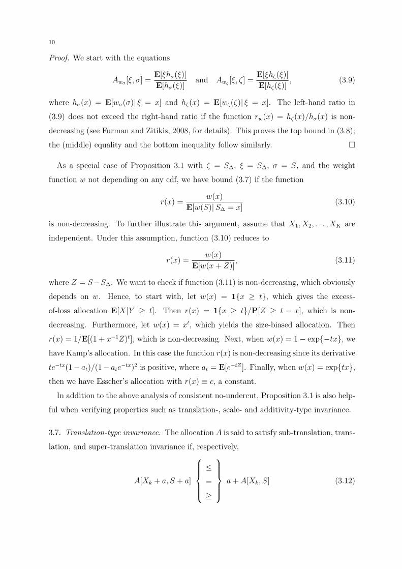
10

Proof. We start with the equations

Awσ [ξ, σ] =E[ξhσ(ξ)]

E[hσ(ξ)]and Awζ

[ξ, ζ] =E[ξhζ(ξ)]

E[hζ(ξ)], (3.9)

where hσ(x) = E[wσ(σ)| ξ = x] and hζ(x) = E[wζ(ζ)| ξ = x]. The left-hand ratio in

(3.9) does not exceed the right-hand ratio if the function rw(x) = hζ(x)/hσ(x) is non-

decreasing (see Furman and Zitikis, 2008, for details). This proves the top bound in (3.8);

the (middle) equality and the bottom inequality follow similarly. ¤

As a special case of Proposition 3.1 with ζ = S∆, ξ = S∆, σ = S, and the weight

function w not depending on any cdf, we have bound (3.7) if the function

r(x) =w(x)

E[w(S)|S∆ = x](3.10)

is non-decreasing. To further illustrate this argument, assume that X1, X2, . . . , XK are

independent. Under this assumption, function (3.10) reduces to

r(x) =w(x)

E[w(x + Z)], (3.11)

where Z = S−S∆. We want to check if function (3.11) is non-decreasing, which obviously

depends on w. Hence, to start with, let w(x) = 1{x ≥ t}, which gives the excess-

of-loss allocation E[X|Y ≥ t]. Then r(x) = 1{x ≥ t}/P[Z ≥ t − x], which is non-

decreasing. Furthermore, let w(x) = xt, which yields the size-biased allocation. Then

r(x) = 1/E[(1 + x−1Z)t], which is non-decreasing. Next, when w(x) = 1− exp{−tx}, we

have Kamp’s allocation. In this case the function r(x) is non-decreasing since its derivative

te−tx(1− at)/(1− ate−tx)2 is positive, where at = E[e−tZ ]. Finally, when w(x) = exp{tx},

then we have Esscher’s allocation with r(x) ≡ c, a constant.

In addition to the above analysis of consistent no-undercut, Proposition 3.1 is also help-

ful when verifying properties such as translation-, scale- and additivity-type invariance.

3.7. Translation-type invariance. The allocation A is said to satisfy sub-translation, trans-

lation, and super-translation invariance if, respectively,

A[Xk + a, S + a]

≤=

≥

a + A[Xk, S] (3.12)

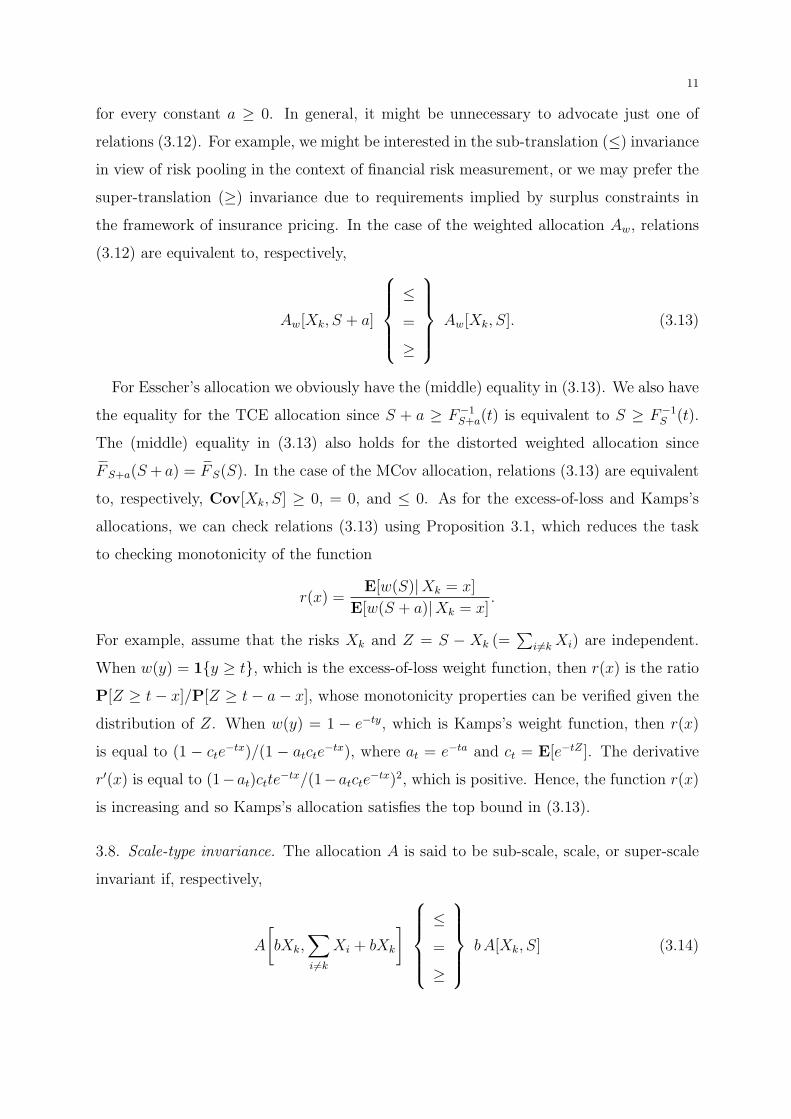
11

for every constant a ≥ 0. In general, it might be unnecessary to advocate just one of

relations (3.12). For example, we might be interested in the sub-translation (≤) invariance

in view of risk pooling in the context of financial risk measurement, or we may prefer the

super-translation (≥) invariance due to requirements implied by surplus constraints in

the framework of insurance pricing. In the case of the weighted allocation Aw, relations

(3.12) are equivalent to, respectively,

Aw[Xk, S + a]

≤=

≥

Aw[Xk, S]. (3.13)

For Esscher’s allocation we obviously have the (middle) equality in (3.13). We also have

the equality for the TCE allocation since S + a ≥ F−1S+a(t) is equivalent to S ≥ F−1

S (t).

The (middle) equality in (3.13) also holds for the distorted weighted allocation since

F S+a(S + a) = F S(S). In the case of the MCov allocation, relations (3.13) are equivalent

to, respectively, Cov[Xk, S] ≥ 0, = 0, and ≤ 0. As for the excess-of-loss and Kamps’s

allocations, we can check relations (3.13) using Proposition 3.1, which reduces the task

to checking monotonicity of the function

r(x) =E[w(S)|Xk = x]

E[w(S + a)|Xk = x].

For example, assume that the risks Xk and Z = S − Xk (=∑

i6=k Xi) are independent.

When w(y) = 1{y ≥ t}, which is the excess-of-loss weight function, then r(x) is the ratio

P[Z ≥ t− x]/P[Z ≥ t− a− x], whose monotonicity properties can be verified given the

distribution of Z. When w(y) = 1 − e−ty, which is Kamps’s weight function, then r(x)

is equal to (1 − cte−tx)/(1 − atcte

−tx), where at = e−ta and ct = E[e−tZ ]. The derivative

r′(x) is equal to (1−at)ctte−tx/(1−atcte

−tx)2, which is positive. Hence, the function r(x)

is increasing and so Kamps’s allocation satisfies the top bound in (3.13).

3.8. Scale-type invariance. The allocation A is said to be sub-scale, scale, or super-scale

invariant if, respectively,

A

[bXk,

∑

i6=k

Xi + bXk

]

≤=

≥

bA[Xk, S] (3.14)

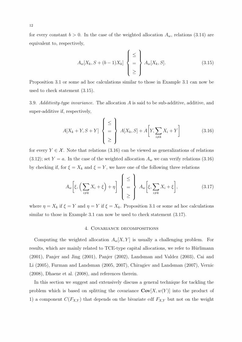
12

for every constant b > 0. In the case of the weighted allocation Aw, relations (3.14) are

equivalent to, respectively,

Aw[Xk, S + (b− 1)Xk]

≤=

≥

Aw[Xk, S]. (3.15)

Proposition 3.1 or some ad hoc calculations similar to those in Example 3.1 can now be

used to check statement (3.15).

3.9. Additivity-type invariance. The allocation A is said to be sub-additive, additive, and

super-additive if, respectively,

A[Xk + Y, S + Y ]

≤=

≥

A[Xk, S] + A

[Y,

∑

i 6=k

Xi + Y

](3.16)

for every Y ∈ X . Note that relations (3.16) can be viewed as generalizations of relations

(3.12); set Y = a. In the case of the weighted allocation Aw we can verify relations (3.16)

by checking if, for ξ = Xk and ξ = Y , we have one of the following three relations

Aw

[ξ,

( ∑

i6=k

Xi + ξ)

+ η

]

≤=

≥

Aw

[ξ,

∑

i6=k

Xi + ξ

], (3.17)

where η = Xk if ξ = Y and η = Y if ξ = Xk. Proposition 3.1 or some ad hoc calculations

similar to those in Example 3.1 can now be used to check statement (3.17).

4. Covariance decompositions

Computing the weighted allocation Aw[X, Y ] is usually a challenging problem. For

results, which are mainly related to TCE-type capital allocations, we refer to Hurlimann

(2001), Panjer and Jing (2001), Panjer (2002), Landsman and Valdez (2003), Cai and

Li (2005), Furman and Landsman (2005, 2007), Chiragiev and Landsman (2007), Vernic

(2008), Dhaene et al. (2008), and references therein.

In this section we suggest and extensively discuss a general technique for tackling the

problem which is based on splitting the covariance Cov[X, w(Y )] into the product of

1) a component C(FX,Y ) that depends on the bivariate cdf FX,Y but not on the weight

13

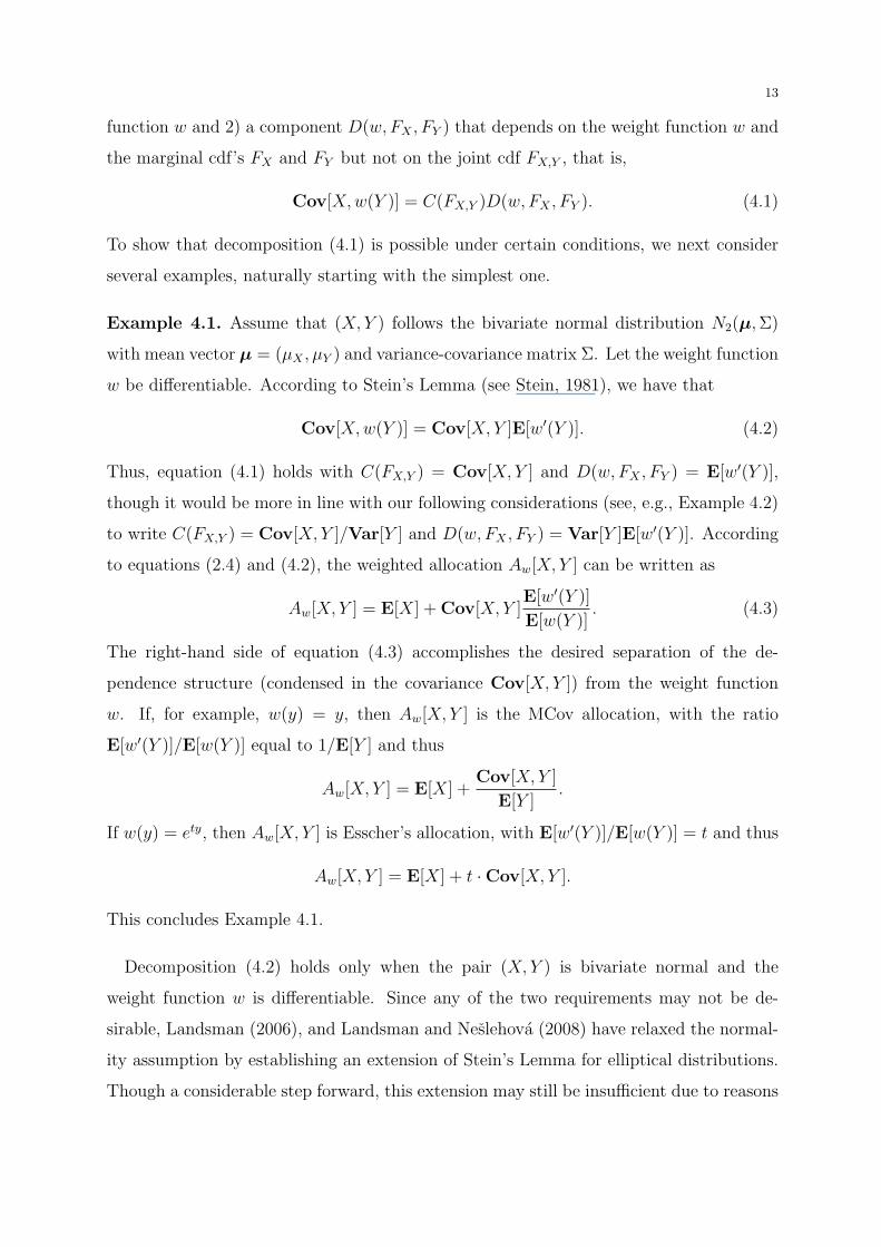
function w and 2) a component D(w, FX , FY ) that depends on the weight function w and

the marginal cdf’s FX and FY but not on the joint cdf FX,Y , that is,

Cov[X, w(Y )] = C(FX,Y )D(w,FX , FY ). (4.1)

To show that decomposition (4.1) is possible under certain conditions, we next consider

several examples, naturally starting with the simplest one.

Example 4.1. Assume that (X, Y ) follows the bivariate normal distribution N2(µ, Σ)

with mean vector µ = (µX , µY ) and variance-covariance matrix Σ. Let the weight function

w be differentiable. According to Stein’s Lemma (see Stein, 1981), we have that

Cov[X,w(Y )] = Cov[X, Y ]E[w′(Y )]. (4.2)

Thus, equation (4.1) holds with C(FX,Y ) = Cov[X, Y ] and D(w, FX , FY ) = E[w′(Y )],

though it would be more in line with our following considerations (see, e.g., Example 4.2)

to write C(FX,Y ) = Cov[X,Y ]/Var[Y ] and D(w, FX , FY ) = Var[Y ]E[w′(Y )]. According

to equations (2.4) and (4.2), the weighted allocation Aw[X,Y ] can be written as

Aw[X, Y ] = E[X] + Cov[X,Y ]E[w′(Y )]

E[w(Y )]. (4.3)

The right-hand side of equation (4.3) accomplishes the desired separation of the de-

pendence structure (condensed in the covariance Cov[X, Y ]) from the weight function

w. If, for example, w(y) = y, then Aw[X,Y ] is the MCov allocation, with the ratio

E[w′(Y )]/E[w(Y )] equal to 1/E[Y ] and thus

Aw[X, Y ] = E[X] +Cov[X, Y ]

E[Y ].

If w(y) = ety, then Aw[X,Y ] is Esscher’s allocation, with E[w′(Y )]/E[w(Y )] = t and thus

Aw[X,Y ] = E[X] + t ·Cov[X, Y ].

This concludes Example 4.1.

Decomposition (4.2) holds only when the pair (X, Y ) is bivariate normal and the

weight function w is differentiable. Since any of the two requirements may not be de-

sirable, Landsman (2006), and Landsman and Neslehova (2008) have relaxed the normal-

ity assumption by establishing an extension of Stein’s Lemma for elliptical distributions.

Though a considerable step forward, this extension may still be insufficient due to reasons

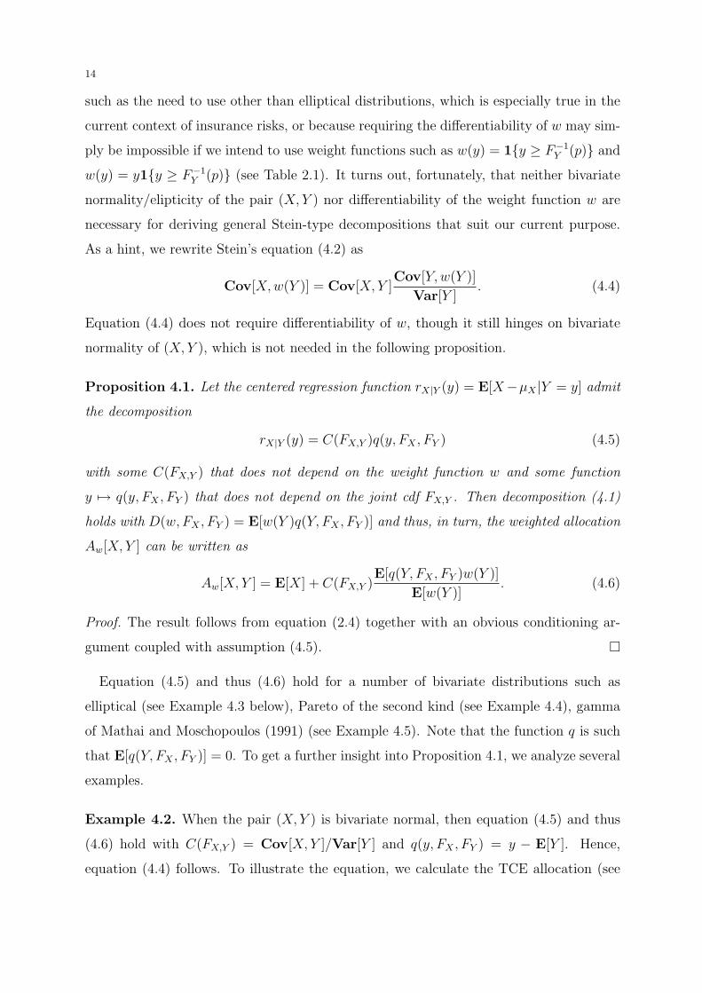
14

such as the need to use other than elliptical distributions, which is especially true in the

current context of insurance risks, or because requiring the differentiability of w may sim-

ply be impossible if we intend to use weight functions such as w(y) = 1{y ≥ F−1Y (p)} and

w(y) = y1{y ≥ F−1Y (p)} (see Table 2.1). It turns out, fortunately, that neither bivariate

normality/elipticity of the pair (X, Y ) nor differentiability of the weight function w are

necessary for deriving general Stein-type decompositions that suit our current purpose.

As a hint, we rewrite Stein’s equation (4.2) as

Cov[X, w(Y )] = Cov[X, Y ]Cov[Y, w(Y )]

Var[Y ]. (4.4)

Equation (4.4) does not require differentiability of w, though it still hinges on bivariate

normality of (X, Y ), which is not needed in the following proposition.

Proposition 4.1. Let the centered regression function rX|Y (y) = E[X−µX |Y = y] admit

the decomposition

rX|Y (y) = C(FX,Y )q(y, FX , FY ) (4.5)

with some C(FX,Y ) that does not depend on the weight function w and some function

y 7→ q(y, FX , FY ) that does not depend on the joint cdf FX,Y . Then decomposition (4.1)

holds with D(w, FX , FY ) = E[w(Y )q(Y, FX , FY )] and thus, in turn, the weighted allocation

Aw[X,Y ] can be written as

Aw[X, Y ] = E[X] + C(FX,Y )E[q(Y, FX , FY )w(Y )]

E[w(Y )]. (4.6)

Proof. The result follows from equation (2.4) together with an obvious conditioning ar-

gument coupled with assumption (4.5). ¤

Equation (4.5) and thus (4.6) hold for a number of bivariate distributions such as

elliptical (see Example 4.3 below), Pareto of the second kind (see Example 4.4), gamma

of Mathai and Moschopoulos (1991) (see Example 4.5). Note that the function q is such

that E[q(Y, FX , FY )] = 0. To get a further insight into Proposition 4.1, we analyze several

examples.

Example 4.2. When the pair (X, Y ) is bivariate normal, then equation (4.5) and thus

(4.6) hold with C(FX,Y ) = Cov[X, Y ]/Var[Y ] and q(y, FX , FY ) = y − E[Y ]. Hence,

equation (4.4) follows. To illustrate the equation, we calculate the TCE allocation (see

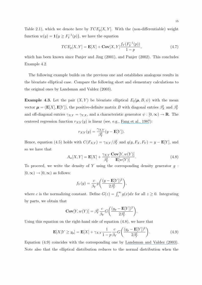
15

Table 2.1), which we denote here by TCEp[X,Y ]. With the (non-differentiable) weight

function w(y) = 1{y ≥ F−1Y (p)}, we have the equation

TCEp[X,Y ] = E[X] + Cov[X, Y ]fY (F−1

Y (p))

1− p, (4.7)

which has been known since Panjer and Jing (2001), and Panjer (2002). This concludes

Example 4.2.

The following example builds on the previous one and establishes analogous results in

the bivariate elliptical case. Compare the following short and elementary calculations to

the original ones by Landsman and Valdez (2003).

Example 4.3. Let the pair (X, Y ) be bivariate elliptical E2(µ, B, ψ) with the mean

vector µ = (E[X],E[Y ]), the positive-definite matrix B with diagonal entries β2X and β2

Y

and off-diagonal entries γX,Y = γY,X , and a characteristic generator ψ : [0,∞) → R. The

centered regression function rX|Y (y) is linear (see, e.g., Fang et al., 1987):

rX|Y (y) =γX,Y

β2Y

(y − E[Y ]).

Hence, equation (4.5) holds with C(FX,Y ) = γX,Y /β2Y and q(y, FX , FY ) = y − E[Y ], and

so we have that

Aw[X, Y ] = E[X] +γX,Y

β2Y

Cov[Y,w(Y )]

E[w(Y )]. (4.8)

To proceed, we write the density of Y using the corresponding density generator g :

[0,∞) → [0,∞) as follows:

fY (y) =c

βY

g

((y − E[Y ])2

2β2Y

),

where c is the normalizing constant. Define G(z) =∫∞

zg(x)dx for all z ≥ 0. Integrating

by parts, we obtain that

Cov[Y, w(Y )] = β2Y

c

βY

G

((yp − E[Y ])2

2β2Y

).

Using this equation on the right-hand side of equation (4.8), we have that

E[X|Y ≥ yp] = E[X] + γX,Y1

1− p

c

βY

G

((yp − E[Y ])2

2β2Y

). (4.9)

Equation (4.9) coincides with the corresponding one by Landsman and Valdez (2003).

Note also that the elliptical distribution reduces to the normal distribution when the

16

density generator is g(y) = e−y, in which case G(y) = e−y and the normalizing constant

c = 1/√

2π. Equation (4.9) becomes (4.7). This concludes Example 4.3.

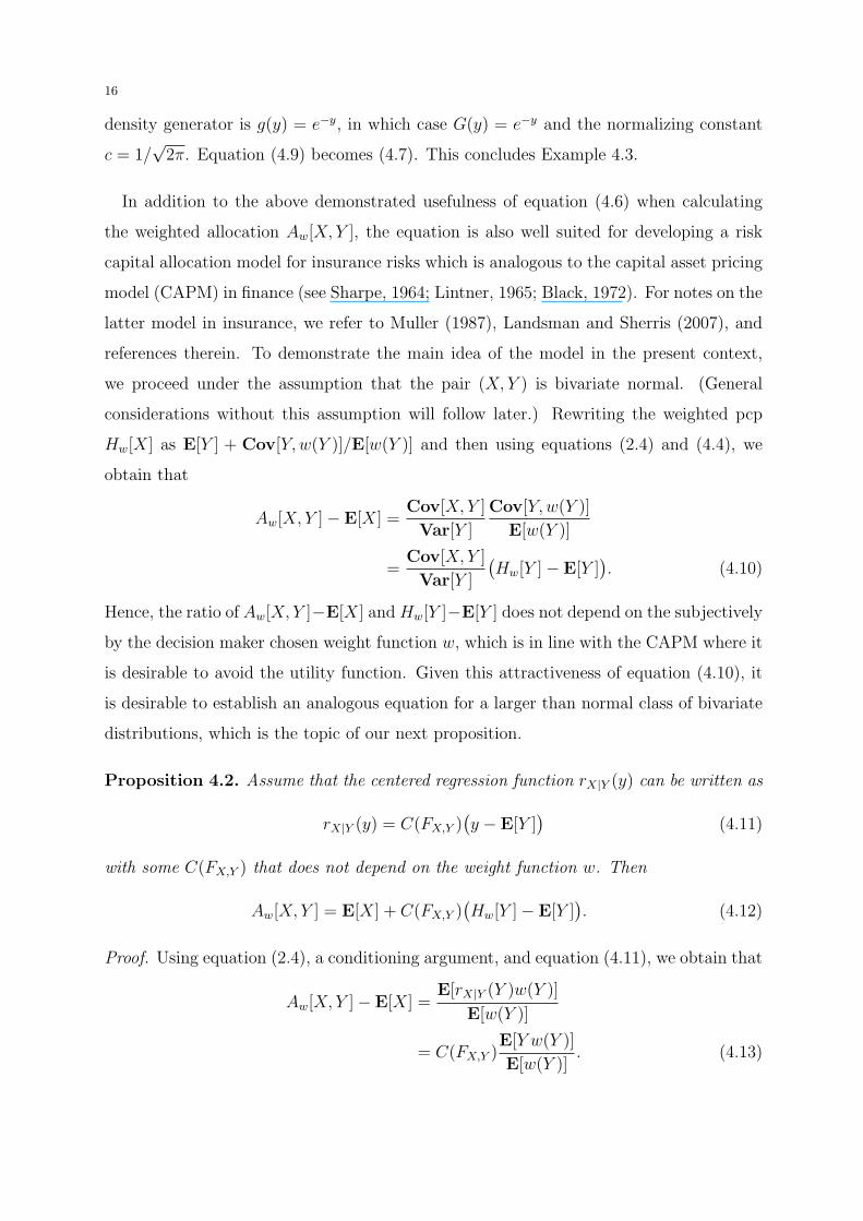
In addition to the above demonstrated usefulness of equation (4.6) when calculating

the weighted allocation Aw[X, Y ], the equation is also well suited for developing a risk

capital allocation model for insurance risks which is analogous to the capital asset pricing

model (CAPM) in finance (see Sharpe, 1964; Lintner, 1965; Black, 1972). For notes on the

latter model in insurance, we refer to Muller (1987), Landsman and Sherris (2007), and

references therein. To demonstrate the main idea of the model in the present context,

we proceed under the assumption that the pair (X, Y ) is bivariate normal. (General

considerations without this assumption will follow later.) Rewriting the weighted pcp

Hw[X] as E[Y ] + Cov[Y,w(Y )]/E[w(Y )] and then using equations (2.4) and (4.4), we

obtain that

Aw[X,Y ]− E[X] =Cov[X, Y ]

Var[Y ]

Cov[Y, w(Y )]

E[w(Y )]

=Cov[X, Y ]

Var[Y ]

(Hw[Y ]− E[Y ]

). (4.10)

Hence, the ratio of Aw[X, Y ]−E[X] and Hw[Y ]−E[Y ] does not depend on the subjectively

by the decision maker chosen weight function w, which is in line with the CAPM where it

is desirable to avoid the utility function. Given this attractiveness of equation (4.10), it

is desirable to establish an analogous equation for a larger than normal class of bivariate

distributions, which is the topic of our next proposition.

Proposition 4.2. Assume that the centered regression function rX|Y (y) can be written as

rX|Y (y) = C(FX,Y )(y − E[Y ]

)(4.11)

with some C(FX,Y ) that does not depend on the weight function w. Then

Aw[X,Y ] = E[X] + C(FX,Y )(Hw[Y ]− E[Y ]

). (4.12)

Proof. Using equation (2.4), a conditioning argument, and equation (4.11), we obtain that

Aw[X, Y ]− E[X] =E[rX|Y (Y )w(Y )]

E[w(Y )]

= C(FX,Y )E[Y w(Y )]

E[w(Y )]. (4.13)

17

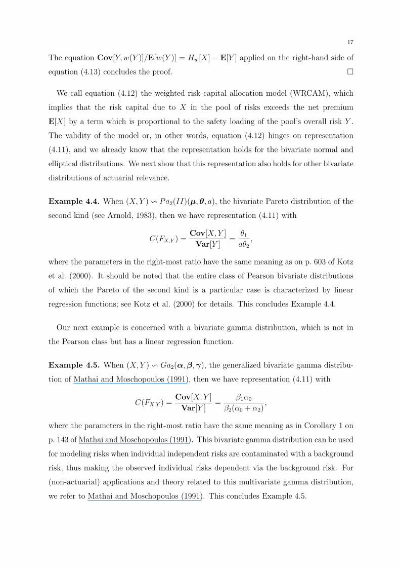
The equation Cov[Y, w(Y )]/E[w(Y )] = Hw[X] − E[Y ] applied on the right-hand side of

equation (4.13) concludes the proof. ¤

We call equation (4.12) the weighted risk capital allocation model (WRCAM), which

implies that the risk capital due to X in the pool of risks exceeds the net premium

E[X] by a term which is proportional to the safety loading of the pool’s overall risk Y .

The validity of the model or, in other words, equation (4.12) hinges on representation

(4.11), and we already know that the representation holds for the bivariate normal and

elliptical distributions. We next show that this representation also holds for other bivariate

distributions of actuarial relevance.

Example 4.4. When (X,Y ) v Pa2(II)(µ,θ, a), the bivariate Pareto distribution of the

second kind (see Arnold, 1983), then we have representation (4.11) with

C(FX,Y ) =Cov[X,Y ]

Var[Y ]=

θ1

aθ2

,

where the parameters in the right-most ratio have the same meaning as on p. 603 of Kotz

et al. (2000). It should be noted that the entire class of Pearson bivariate distributions

of which the Pareto of the second kind is a particular case is characterized by linear

regression functions; see Kotz et al. (2000) for details. This concludes Example 4.4.

Our next example is concerned with a bivariate gamma distribution, which is not in

the Pearson class but has a linear regression function.

Example 4.5. When (X,Y ) v Ga2(α,β, γ), the generalized bivariate gamma distribu-

tion of Mathai and Moschopoulos (1991), then we have representation (4.11) with

C(FX,Y ) =Cov[X, Y ]

Var[Y ]=

β1α0

β2(α0 + α2),

where the parameters in the right-most ratio have the same meaning as in Corollary 1 on

p. 143 of Mathai and Moschopoulos (1991). This bivariate gamma distribution can be used

for modeling risks when individual independent risks are contaminated with a background

risk, thus making the observed individual risks dependent via the background risk. For

(non-actuarial) applications and theory related to this multivariate gamma distribution,

we refer to Mathai and Moschopoulos (1991). This concludes Example 4.5.

18

We conclude this section with another notable consequence of Proposition 4.2. Suppose

we are interested in comparing the safety loadings of two risks X∗ and X∗∗. In view of

equation (2.4), the ratio of the loadings Aw[X∗, Y ] − E[X∗] and Aw[X∗∗, Y ] − E[X∗∗]

is the ratio of the covariances Cov[X∗, w(Y )] and Cov[X∗∗, w(Y )]. When the function

y 7→ q(y, FX , FY ) does not depend on FX , then the ratio of the covariances reduces to

the ratio of C(FX∗,Y ) and C(FX∗∗,Y ), which is free of the (subjective) weight function w.

This is a useful fact when analyzing the relative risk sharing of X∗ and X∗∗ when these

risks are constituents of the insurer’s aggregate risk Y .

5. Conclusions

In this paper we have suggested a risk capital allocation rule, called the weighted allo-

cation, which stems from the weighted premium calculation principle. Hence, the present

work is a natural continuation of Furman and Zitikis (2008). We have shown that many

well known allocation rules are special cases of the weighted allocation. We have also

demonstrated that the weighted allocation is additive, consistent, satisfies the no un-

justified loading property and, under certain conditions, the (consistent) no-undercut.

Moreover, we have explored invariance properties of the weighted allocation such as

translation-, scale-, and additivity-type invariance, and also discussed methods for their

verification. Furthermore, via a natural reformulation of the weighted allocation in terms

of a covariance, we have established a direct link between the weighted allocation and

the capital asset pricing model and, in turn, suggested a weighted risk capital allocation

model. Though general in formulation, the model can readily be calculated in a variety

of interesting situations.

Acknowledgments

The authors are grateful to an anonymous referee for advice and suggestions that aided

in reshaping the manuscript and inspired its considerable augmentation. The present

research is a part of the project entitled “Weighted Premium Calculation Principles and

Risk Capital Allocations”, which has been supported by the Actuarial Education and

Research Fund (AERF) and the Society of Actuaries Committee on Knowledge Extension

Research (CKER). The authors also gratefully acknowledge the support of their research

by the Natural Sciences and Engineering Research Council (NSERC) of Canada.

19

References

Arnold, B.C., 1983. Pareto Distributions. International Cooperative Publishing House,

Silver Spring, Maryland.

Artzner, P., Delbaen, F., Eber, J.M., Heath, D., 1999. Coherent measures of risk. Math-

ematical Finance 9, 203–228.

Black, F., 1972. Capital market equilibrium with restricted borrowing. Journal of Busi-

ness 45, 444–455.

Buhlmann, H., 1980. An economic premium principle. ASTIN Bulletin 11, 52–60.

Buhlmann, H., 1984. The general economic premium principle. ASTIN Bulletin 14,

13–21.

Cai, J., Li, H., 2005. Conditional tail expectations for multivariate phase-type distribu-

tions. Journal of Applied Probability 42, 810–825.

Chiragiev, A., Landsman, Z., 2007. Multivariate Pareto portfolios: TCE-based capital

allocation and divided differences. Scandinavian Actuarial Journal 4, 261–280.

Denault, M. 2001. Coherent allocation of risk capital. Journal of Risk 4, 7–21.

Denneberg, D. 1994. Non-additive Measure and Integral. Kluwer, Dordrecht.

Denuit, M., Dhaene, J., Goovaerts, M., Kaas, R. 2005. Actuarial Theory for Dependent

Risks: Measures, Orders and Models. Wiley, Chichester.

Denuit, M., Dhaene, J., Goovaerts, M., Kaas, R., Laeven, R. 2006. Risk measurement

with equivalent utility principles. Statistics and Decisions 24, 1–25.

Dhaene, J., Henrard, L., Landsman, Z., Vandendorpe, A. and Vanduffel, S. 2008. Some

results on the CTE-based capital allocation rule. Insurance: Mathematics and Eco-

nomics 42, 855–863.

Dhaene, J., Laeven, R., Vanduffel, S., Darkiewicz, G., Goovaerts, M., 2008. Can a coher-

ent risk measure be too subadditive? Journal of Risk and Insurance 75, 365–386.

Dhaene, J., Vanduffel, S., Goovaerts, M., Kaas, R., Tang, Q., Vyncke, D. 2006. Risk

measures and comonotonicity: a review. Stochastic Models 22, 573–606.

Fang, K.T., Kotz, S., Ng, K.W. 1987. Symmetric Multivariate and Related Distributions.

Chapman & Hall, London.

Filipovic, D., Kupper, M., 2008. Optimal capital and risk transfers for group diversifica-

tion. Mathematical Finance 18, 55–76.

20

Furman, E., Landsman, Z., 2005. Risk capital decomposition for a multivariate dependent

gamma portfolio. Insurance: Mathematics and Economics 37, 635–649.

Furman, E., Landsman, Z., 2006. Tail variance premium with applications for elliptical

portfolio of risks. ASTIN Bulletin 36, 433–462.

Furman, E., Landsman, Z., 2007. Economic capital allocations for non-negative portfolios

of dependent risks. Proceedings of the 37-th International ASTIN Colloquium, Orlando.

http://www.actuaries.org/ASTIN/Colloquia/Orlando/Papers/Furman.pdf

Furman, E., Zitikis, R., 2008. Weighted premium calculation principles. Insurance: Math-

ematics and Economics 42, 459–465.

Gerber, H.U., 1979. An Introduction to Mathematical Risk Theory. University of Penn-

sylvania, Philadelphia.

Goovaerts, M., de Vylder, F., Haezendonck, J., 1984. Insurance Premiums: Theory and

Applications. North-Holland, Amsterdam.

Goovaerts, M., Kaas, R., Dhaene, J., 2003. Economical capital allocation derived from

risk measures. North American Actuarial Journal 7(2), 44–59.

Goovaerts, M., Kaas, R., Laeven, R., Tang, Q., 2004. A comonotonic image of indepen-

dence for additive risk measures. Insurance: Mathematics and Economics 35, 581–594.

Goovaerts, M., Laeven, R., 2008. Actuarial risk measures for financial derivative pricing.

Insurance: Mathematics and Economics 42, 540–547.

Heilmann, W.R., 1989. Decision theoretic foundations of credibility theory. Insurance:

Mathematics and Economics 8, 77–95.

Heilpern, S., 2003. A rank-dependent generalization of zero utility principle. Insurance:

Mathematics and Economics 33, 67–73.

Hesselager, O., Andersson, U., 2002. Risk sharing and risk capital allocation. Working

paper, Tryg Insurance, Ballerup, Denmark.

Hurlimann, W., 2001. Analytical evaluation of economic risk capitals for portfolio of

gamma risks. ASTIN Bulletin 31, 107–122.

Kaas, R., van Heerwaarden, A.E., and Goovaerts, M.J. 1994. Ordering of Actuarial Risks.

CAIRE Education Series, Brussels.

Kamps, U., 1998. On a class of premium principles including the Esscher principle.

Scandinavian Actuarial Journal 1, 75–80.

21

Kotz, S., Balakrishnan, N., Johnson, N.L., 2000. Continuous Multivariate Distributions.

Wiley, New York.

Laeven, R., Goovaerts, M., 2004. An optimization approach to the dynamic allocation of

economic capital. Insurance: Mathematics and Economics 35, 299–319.

Landsman, Z., 2006. On the generalization of Stein’s Lemma for elliptical class of distri-

butions. Statistics and Probability Letters 76, 1012–1016.

Landsman, Z., Neslehova, J., 2008. Stein’s lemma for elliptical random vectors. Journal

of Multivariate Analysis 99, 912–927

Landsman, Z., Sherris, M., 2007. An actuarial premium pricing model for nonnormal

insurance and financial risks in incomplete markets. North American Actuarial Journal

11(1), 119–135.

Landsman, Z., Valdez, E., 2003. Tail conditional expectation for elliptical distributions.

North American Actuarial Journal 7(4), 55–71.

Lehmann, E.L., 1966. Some concepts of dependence. Annals of Mathematical Statistics

37, 1137–1153.

Lintner, J., 1965. Security prices, risk, and maximal gains from diversification. Journal

of Finance 20(4), 587–615.

Mari, D.D., Kotz, S., 2001. Correlation and Dependence. Imperial College Press, London.

Mathai, A.M., Moschopoulos, P.G., 1991. On a multivariate gamma. Journal of Multi-

variate Analysis 39, 135–153.

Muller, H.H., 1987. Economic premium principles in insurance and the capital asset

pricing model. ASTIN Bulletin 17, 141–150.

Panjer, H.H. 2002. Measurement of Risk, Solvency Requirements and Allocation of Cap-

ital within Financial Conglomerates. Institute of Insurance and Pension Research Re-

port 01-15. University of Waterloo, Waterloo.

Panjer, H., Jing, J., 2001. Solvency and capital allocation. University of Waterloo,

Institute of Insurance and Pension Research, Research Report 01-14, 1–8.

Pflug, G.Ch., Romisch, W. 2007. Modeling, Measuring and Managing Risk. World

Scientific, Singapore.

Schechtman, E., Shelef, A., Yitzhaki, S., Zitikis, R., 2008. Testing hypotheses about abso-

lute concentration curves and marginal conditional stochastic dominance. Econometric

Theory 24, 1044–1062.

22

Shalit, H., Yitzhaki, S., 1994. Marginal conditional stochastic dominance. Management

Science 40, 670–684.

Sharpe, W.F., 1964. Capital asset prices: A theory of market equilibrium under conditions

of risk. Journal of Finance 19, 425–442.

Stein, C.M., 1981. Estimation of the mean of a multivariate normal distribution. Annals

of Statistics 9, 1135–1151.

Tasche, D., 1999. Risk contributions and performance measurement. Technical Report,

pp. 1-26. Zentrum Mathematik (SCA), TU Munchen, Munchen.

Tsanakas, A., 2008. Risk measurement in the presence of background risk. Insurance:

Mathematics and Economics 42, 520–528.

Tsanakas, A., Barnett, C., 2003. Risk capital allocation and cooperative pricing of insur-

ance liabilities. Insurance: Mathematics and Economics 33, 239-254

Tsanakas, A., Desli, E., 2003. Risk measures and theories of choice. British Actuarial

Journal 9, 959–991.

Valdez, E., Chernih, A., 2003. Wang’s capital allocation formula for elliptically contoured

distributions. Insurance: Mathematics and Economics 33(3), 517–532.

Venter, G.G., 2004. Capital allocation survey with commentary. North American Actu-

arial Journal 8(2), 96–107.

Vernic, R., 2008. Multivariate skew-normal distributions with applications in insurance.

Insurance: Mathematics and Economics 38, 413–426.

Wang, S., 1995. Insurance pricing and increased limits ratemaking by proportional haz-

ards transforms. Insurance: Mathematics and Economics 17, 43–54.

Wang, S., 1996. Premium calculation by transforming the layer premium density. ASTIN

Bulletin 26, 71–92.

Wang, S., 1998. An actuarial index of the right-tail risk. North American Actuarial

Journal 2(2), 88–101.

Wang, S., 2002. A set of new methods and tools for enterprize risk capital manage-

ment and portfolio optimization. CAS Summer Forum, Dynamic Financial Analysis

Discussion Papers, 43–78.

Wang, S., 2007. Normalized exponential tilting: pricing and measuring multivariate risks.

North American Actuarial Journal 11(3), 89–99.

23

Young, V.R., 2004. Premium principles. In: Encyclopedia of Actuarial Science (eds.: J.L.

Teugels and B. Sundt). Wiley, New York.