Design of adaptive Takagi-Sugeno-Kang fuzzy models

Applied Soft Computing 2 (2002) 89–103

Design of adaptive Takagi–Sugeno–Kang fuzzy models

Dragan Kukolj∗Faculty of Engineering, University of Novi Sad, Trg D. Obradovica 6, 21000 Novi Sad, Yugoslavia

Received 13 December 2001; received in revised form 18 September 2002; accepted 20 September 2002

Abstract

The paper describes a method of fuzzy model generation using numerical data as a starting point. The algorithm generatesa Takagi–Sugeno–Kang fuzzy model, characterised with transparency, high accuracy and small number of rules. The trainingalgorithm consists of three steps: partitioning of the input–output space using a fuzzy clustering method; determination ofparameters of the consequent part of a rule from over-determined batch least-squares (LS) formulation of the problem, usingsingular value decomposition algorithm; and adaptation of these parameters using recursive least-squares method. Threeillustrative well-known benchmark modelling problems serve the purpose of demonstrating the performance of the generatedmodels. The achievable performance is compared with similar existing models, available in literature.© 2002 Elsevier Science B.V. All rights reserved.

Keywords:Fuzzy model; On-line learning; Benchmark modelling problems; Prediction

1. Introduction

Fuzzy models that one designs are expected to becharacterised with: (1) an accurate and fast procedurefor calculation of the desired quantity; (2) a generaland flexible procedure, applicable to a wide class ofvery diverse problems. Fuzzy model generation basedon learning by examplesapproach is achieved duringthe structure identification and model parameter iden-tification step[1,2]. In cases when the input quantitiesare known, structure identification step reduces todetermination of the required number of rules anddetermination of the conditional part of the rule. Therequired number of rules can be determined usingcluster validity measures[3,4], or cluster removaland/or merging techniques[5,6]. Determination ofthe conditional part of the rule necessitates definingof the fuzzy sets of input variables. This can be done

∗ Tel.: +381-21-350-701; fax:+381-21-350-610.E-mail address:[email protected] (D. Kukolj).

using grid-type space partitioning[7] and fuzzy clus-tering methods[8,9]. During the model parameteridentification step, various learning methods are ap-plied. Gradient descent methods (GD) represent anefficient method for simpler problems[10–12]. How-ever, they can easily end up in local minima and aresensitive with respect to the form of the selected ob-jective function, fuzzy set shapes and the type of thefuzzy operator. GD methods are frequently appliedin combination with the least-squares (LS) method[7,13]. Recursive or batch variants of LS algorithmsare characterised with faster convergence[14,15].Genetic algorithms (GA) search a wide space of pos-sible solutions, so that there is a high probability thatthe found optimum is global or near-global[16–20].The most successful realisations of fuzzy modelsare adaptive fuzzy models, frequently obtained usingclustering methods for partitioning the input–outputspace, combined with GA[20], GD [8], LS [6,14]or GD–LS [7,13] optimisation methods for modelparameter adaptation. Structural identification is a

1568-4946/02/$ – see front matter © 2002 Elsevier Science B.V. All rights reserved.PII: S1568-4946(02)00032-7

90 D. Kukolj / Applied Soft Computing 2 (2002) 89–103

more difficult task, which is usually executed off-line.However, there exist approaches in which both stepstake place on-line. One example of such a realisationis NeuroFAST, a Takagi–Sugeno–Kang (TSK) fuzzymodel, where the input space is automatically par-titioned using a modified fuzzy adaptive resonancetheory mechanism[21].

The most of the listed fuzzy models are character-ized with high accuracy and interpretability. However,during the learning stage, i.e. tuning of premise andconsequent parameters, gradient or GA optimiza-tion methods are frequently used. These methodsare very demanding, in contrast to the batch and re-cursive LS methods applied here. These proceduresare much faster and therefore much better suited toon-line applications. In addition, partitioning of fea-ture space takes place with a fuzzy clustering methodover the input–output space, instead of just over theinput space. This enables better location of the clus-ter centers, thus creating the possibility of arrivingat models with smaller number of rules and withhigher interpretability. The vast majority of industrialprocesses are characterised with constant parameterand/or structure change in time. Required system per-formance can then be maintained by means of fuzzymodel on-line adaptation. The aim of this paper is todescribe a computationally efficient and accurate al-gorithm for fuzzy model generation that is applicableto a variety of problems. The algorithm for TSK fuzzymodel generation is described first. The algorithmcombines clustering of the numerical input–outputdata, batch LS and weighted recursive least-squares(WRLS) procedures. The learning algorithm consistsof three steps. The first step is identification of thestructure of the rule base. This step performs group-ing of the input–output space, using fuzzy clustering.Procedures for selection of the input variables and op-timal number of rules are not discussed (these issuesare covered in considerable depth in, for example[1]).

The next step consists of identification of parame-ters of the consequent part of the rule base. Keepingthe conditional part of the rule fixed, consequent pa-rameters are determined using the LS method on theglobal level. Globally formulated LS yields the mini-mal parameter error estimate of the model of the com-plete system. The last step encompasses adaptation ofthe parameters of the consequent part of the rules. Theadaptation is useful when some significant changes

appear, that were not considered in the previous algo-rithmic step. Global and local learning are combinedby this step. Using every newly acquired sample, inconjunction with WRLS algorithm, adaptation of theconsequent part of the rules is performed. This re-quires calculation of the normalised firing strength ofall rules for a given input sample. Region (or regime)in which the system happens to be is determined onthe basis of the firing strength of the rules. It becomesthen possible to obtain the new adapted values of pa-rameters in the consequent part of the activated rulesusing the existing parameter values (arrived at in thesecond step), every new input sample, and the WRLSmethod. The third step does not contain componentsof the structure identification for two reasons: par-titioning of input–output space is a time-consumingand difficult task; and, generally, output part of theinput–output data pair is frequently not available.

The paper is organised as follows:Section 2con-tains a short description of the general concept ofthe TSK fuzzy models.Section 3describes all thethree steps of the fuzzy model training, as well asthe general algorithm.Section 4 contains illustra-tion of the algorithm performance, for three bench-mark problems, and comparison of the performancewith the one obtainable using the existing methods.Finally, discussion of the algorithm performance andthe conclusions are provided inSections 5 and 6.

2. General description of the TSK fuzzy model

Takagi–Sugeno–Kang fuzzy rule based model re-quires only a small number of rules to describecomplex, highly non-linear models. The number ofrules can be significantly smaller than when Mamdanifuzzy model type is applied[22,23]. A shortcomingof the TSK fuzzy model is its less understandablepresentation, when compared with Mamdani fuzzymodel type. The basic idea of the TSK model is thefact that an arbitrarily complex system is a com-bination of mutually inter-linked sub-systems. IfKregions, corresponding to individual sub-systems, aredetermined in the state-space under consideration,then the behaviour of the system in these regions canbe described with simpler functional dependencies. Ifthe dependence is linear and if one rule is assigned toeach sub-system, the TSK fuzzy model is represented

D. Kukolj / Applied Soft Computing 2 (2002) 89–103 91

with K rules of the following form:

Ri : If x1 isAi1 and x2 isAi2 and . . . and

xn isAin thenyi = aix + bi, i = 1,2, . . . , K (1)

whereRi is the ith rule, x1, x2, . . . , xn are the inputvariables,Ai1, Ai2, . . . , Ain are the fuzzy sets as-signed to corresponding input variables, variableyirepresents the value of theith rule output, andai andbi are parameters of the consequent function. Thefinal output of the TSK fuzzy model (yk) for an arbi-traryxk input sample is calculated using the followingexpression:

yk =∑k

i=1[βi(xk)yi(xk)]∑ki=1βi(xk)

, k = 1,2,3, . . . , N (2)

whereyi(xk) is output of ith rule for xk (kth) inputsample, andβi represent the firing strength of theithrule.

Most of the methods for TSK fuzzy model trainingare of global nature, since the model parameters aredetermined on the basis of all the samples in one al-gorithmic step. Assuming that the available samplescover the complete modelled problem, any of the al-ready cited algorithms can yield a model of high orsatisfactory accuracy. However, a global model gen-erated in this way cannot guarantee representation ofthe actual system that is satisfactory under all circum-stances. Regions may appear in the state-space, whichare not represented with required quality with the gen-erated model. Such a situation may arise due to someaposteriori changes in the real system, due to incom-pleteness of the training set or due to too small num-ber of rules. It is therefore desirable to correct themodel parameters using new samples, obtained fromthe current operating regime of the system. In otherwords, this means that the correction of the parametersof the consequent part of the rule, that accounts forthe rule firing strengths and for the results of globallearning, can influence the quality of the final modeloutput. Eq. (2) can be written in a form that showsmore explicitly the concept of the system descriptionusing local models[24]. This expression then takesthe form:

yk =K∑i=1

[wi (xk)(xkai + bi)], k = 1,2, . . . , N (3)

wherewi(xk) represents normalised firing strength ofthe ith rule for thekth sample. The rule normalisedfiring strength, given withEq. (4), shows that (2) and(3) are identical for the final output.

wi (xk) = βi(xk)∑kj=1βj (xk)

, k = 1,2,3, . . . , N (4)

TSK fuzzy rule based model, as a set of local mod-els, enables application of linear LS method[7,10].LS algorithm requires a model that is linear in the pa-rameters. However, that does not imply that the modelitself must be linear. Combination of the stated globaland local learning models is realised using WRLS al-gorithm and a carefully selected forgetting factor, thatcan balance the impact of the current regime and thepast states[7,10,24].

3. TSK fuzzy model generation

3.1. Step I—structure identification

Partitioning of the input–output space is performedin the first step, using the selected clustering method.The method utilises training data that containNinput–output sampleszk = [xT

k ; yk]T, k = 1, . . . , N ,whereN is the total number of samples. Let the inputvector be of dimensionn and let the number of out-puts be one. Each obtained cluster represents a certainoperating region of the system, where input–outputdata values are highly concentrated. The learningdata, divided into these information clusters, are theninterpreted as rules. Methods of fuzzy clustering, suchas fuzzy c-means (FCM)[25] and Gustafson–Kessel(GK) [6,14], are convenient tools for the process ofpartitioning of the input space[1,13] or input–outputspace[9,14].

FCM algorithm requires that the number of clus-ters K is given beforehand. The problem of optimalnumber of cluster determination is known as partitionvalidation. Various cluster validity criteria have beenproposed, such as partition entropy[25], and othermeasures[1,3,4]. Determination of a suitable numberof clusters for a given data set, during the process ofstructural identification of the fuzzy model, can be re-garded as an issue equivalent to finding the optimalnumber of the fuzzy rules. Fuzzy models with higher


number of rules have higher accuracy, but a weakercomputational efficiency and interpretability. It is forthis reason that the FCM algorithm is connected withthe identification step of the consequent parameters,with the aim of finding the most acceptable fuzzymodel. Sequence of the FCM algorithm—the identifi-cation of consequent parameters, repeats itself for therecommended range of maximum–minimum numberof rules. The adopted value of the number of rulesKis the one, which satisfies the required accuracy andefficiency.

Central part of the fuzzy clustering algorithm[25]consists of calculation of the distance between thekthsample, currently under consideration, and the centrevi of a givenith cluster. This distance is calculated inthe case of FCM algorithm using Euclidean distance,and is in thelth iteration of the algorithm of the form:

d2ik =

n+1∑j=1

(zjk − v(l)ji)2, i = 1,2, . . . , K,

k = 1,2, . . . , N (5)

FCM algorithm forms hyper-spherical clusters inspace, while GK method create more general,hyper-ellipsoid clusters. However, FCM method isless numerically complex and therefore faster. It isfor these reasons that FCM method is utilised here.

Result of the clustering process is, apart fromthe matrix of cluster centres, a fuzzy partition ma-trix UK×N . This matrix contains valuesµik ∈[0,1], for 1 ≤ i ≤ K and 1≤ k ≤ N , that representdegree of membership of thekth sample to theithcluster. Elements of the matrixU are calculated usingthe following expression:

µ(l)ik = 1∑k

j=1(d2ik/d

2jk)

1/(m−1)for dik > 0, or

µ(l)ik = 1 for dik = 0 (6)

Columns of the matrixU are characterised with thefollowing condition:

K∑i=1

µik = 1, k = 1,2,3, . . . , N (7)

This condition corresponds to the condition of orthog-onality of the input or input–output vector fuzzy sets.

3.2. Step II—Identification of parameters of theconsequent part of the rule

Parameter identification encompasses procedure forcalculation of parameters of the TSK fuzzy model,the parameters being those of the consequent part ofthe rule. The crucial problem is determination of thenormalised firing strength of the rules, that is, deter-mination of the contribution of each rule to the fi-nal model output. It is necessary to at first determineone-dimensional fuzzy setsAij from the conditionalpart of the rule. One-dimensional fuzzy setsAij areobtained from multidimensional fuzzy clusters (givenby U ) by point-wise projection onto the space of theinput variablexj [14]

µAij (xkj) = projj (µik) (8)

whereµik is the level of belonging of thekth sample(vector xk) to the ith cluster, whileµAij (xkj) is thevalue of the membership level of thejth input variableof the kth sample (jth co-ordinate of the vectorxk)to the fuzzy setAij . Since all the functionsµAij (xkj)

under consideration represent membership function,the conditionµAij (xkj) : R → [0,1] must hold true.Value of the firing strength of theith rule for eachkth input sample is calculated asand-conjunctionbymeans of the product operator:

βik = βi(xk) =n∏

j=1

µAij (xkj) k = 1,2,3, . . . , N (9)

In the application of (9) a thresholdξ is introduced(ξ = 0.01, for example) for the fulfillment of the con-dition: µAij (xkj) ≤ ξ ⇒ µAij (xkj) = 0. If µAij (xkj) >

0.01, then only these values are included in (9). Fi-nally, normalised firing strengthwik of a ruleRi for akth sample is obtained using theEq. (4).

The kth element on the main diagonal of the diag-onal matrixW i (i = 1, . . . , K) of N × N dimensionis formed using the values of the normalised firingstrength, obtained from (4). Hence a matrix composi-tion X′ of dimensionsN × K(n + 1) is formed[14]:

X′=[(W1Xe), (W2Xe), (W3Xe), . . . , (WKXe)] (10)

where matrixXe = [X,1] contains rows [xTk ,1]. Fi-

nally, parametersaTi andbi of (1) and (3), that are in

the consequent part of all TSK fuzzy rules, are grouped


into a vectorθ ′ of dimensionsK(n + 1). The parame-ters are organised within the vectorθ ′ in the followingway:

�′ = [�T

1 �T2 · · · �T

K

]T(11)

where θTi = [

aTi ; bi

], for i = 1, . . . , K. Problem

described with (2) and (3) can now be stated as re-gression model of the formY = X′�′ + ε, whereε isthe approximation error. Vector of unknown parame-ters θ ′ is determined using the least-squares methodand the expression�′ = [(X′)TX′]−1(X′)TY . Caseswith very low or zero firing strength for certain rulesfrequently appear in practice. Partition matrix thenhas zero columns or linearly dependent columns. Thisleads to occurrence of singular or near-singular valuesof the matrixX′. It is better to apply singular valuedecomposition (SVD) method then Gauss–Newtonor LU decomposition in such cases. SVD is a nu-merically more robust and reliable orthogonal trans-formation method, originally proposed by Golub[26,27].

3.3. Step III—adaptation of parameters of theconsequent part of the rules

The third step of the algorithm of the adaptive TSKfuzzy model consists of: (1) location of regions (clus-ters) in which the system is at present (kth sample);(2) determination of the firing strength of the rules as-sociated with individual clusters; and (3) applicationof the WRLS method for calculation of parameters ofthe consequent part. In contrast to the first two stepsthat take place only once, during the initial learningphase, this step in the algorithm repeats itself for eachnew sample.

The first required action performs calculation of theEuclidian distance of the current sample from the cen-tres of all clusters in the input space. Expression (2)indicates that each rule describes local model of thesystem. The impact of individual local models is notthe same and depends on the system current state. It istherefore important to determine relative participationof individual local models in the final output. This isthe second action within this step, performed usingthe expression (3). It is, of course, necessary to at firstdetermine Euclidean distance and firing strength ofeach rule for the current sample (Eqs. (5)–(6) and (9)).

It is important to note that the input sample, ratherthan input–output sample is under consideration.

As the last stage of this phase, the WRLS algorithmis applied. This algorithm enables calculation of thenew, adapted values ofθ ′(k+1), on the basis of the newsample and the known parameter valuesθ ′(k) withoutthe computationally expensive matrix inversion oper-ation. The recursive expressions of the WRLS algo-rithm are:

Φ(k + 1)

= 1

λ

[Φ(k) − Φ(k)x′(k + 1)x′T (k + 1)Φ(k)

λ + x′(k + 1)T Φ(k)x′(k + 1)

]

(12)

θ ′(k + 1) = θ ′(k) + Φ(k + 1)′(k + 1)

× [y(k + 1) − x′T (k + 1)θ ′(k)]

wherex′ is the vector obtained by organizing the cur-rent values of the input vector into a form of the com-posite matrix’s row given in (14); the adaptationgain matrix; and 0< λ ≤ 1 is a constant forgettingfactor. TheEq. (12) have an intuitive interpretation:the new parameter vectorθ ′(k + 1) is equal to the oldparameter vectorθ ′(k) plus a correcting term based onthe new datax′. It is interesting to note that the cor-rection term contains the prediction error of the oldmodel with θ ′(k) parameters. A parameterλ in (12)is introduced with the idea of enabling better follow-ing of the time-varying system. The parameterλ iscalled forgetting factor, since it gives higher weightson more recent samples in the optimization. The valueof the forgetting factor is problem dependent (it is al-ways close to unity), while for a time-invariant systemits value should be equal to one. The initial values ofθ ′(0) are taken as being equal to the values obtainedin the second step of the algorithm, whileΦ(0) =(X′T X′)−1 (already calculated in the previous step).A more detailed description of the WRLS method isavailable in[7,10].

Application of the WRLS method enables balancedadaptation of theaT

i and bi parameters of activatedfuzzy rules (wi �= 0, i = 1, K). The meaning of the‘balanced adaptation’ in this context is that the algo-rithm considers both current system state and the gen-eral model description achieved in the previous stepof the algorithm. Balancing is achieved by selecting asuitable value for the forgetting factorλ.


Two important facts are to be emphasised beforeproceeding further: (a) degree of membership of thecurrent sample to the given cluster is calculated on theinput vector basis (Eqs. (5) and (6)). It is for this reasonthat the summation in (5) containsn, rather thann+1elements; (b) parameter adaptation performed using(12) is based on the current input vector. Thus newsamples do not increase the size of the initial trainingset.

3.4. General formulation of the algorithm forTSK fuzzy model generation

The algorithm for TSK fuzzy model generation as-sumes that an initial set of input–output data, whichcan be used for training purposes, is available. Thequality of the final output of the generated fuzzy modelwill be affected not only by the numerical data, but bythe number of generated rules and the forgetting fac-tor value as well. Exploitation phase of the algorithmassumes iterative repetition of the third step only.

The learning algorithm is described, on the step-by-step basis, as follows:

Step I. Partitioning of the input–output space. In-cludes initialisation of the complete learning algo-rithm.

(I.1) Initialisation: a set of pairs of input–output sam-ples (xk, yk), k = 1, . . . , N , maximal andminimal number of rules, cluster fuzzinessm,and forgetting factorλ are given (parametersmandλ remain constant further on).

(I.2) Fuzzy partition matrix and matrix of the clustercentres are determined using the FCM algorithm.

Step II. Identification of the parameters of the con-sequent part:

(II.1) Firing strength of each rule for all samples(Eq. (9)) is calculated and normalising firingstrengthswi(xk) are obtained using (4).

(II.2) Composite matrixX′ (10) is formed, com-posed of diagonal matrices of normalised firingstrengths of all rulesW i and correspondinginput values.

(II.3) Unknown vector of consequent parametersθ ′ isdetermined fromY = X′�′+ε using LS methodand SVD algorithm.

(II.4) Previous steps (I.2/II .3) are repeated for thegiven range of maximum–minimum numberof rules. Once when a number of rulesK isadopted, the parameters of the adequate ‘initial’model are saved.

Step III. Adaptation of the consequent parameters isan iterative, on-line process. Each new samplexk isused to adapt existing fuzzy model (1) on the basis ofthe following procedure:

(III.1) Membership degree (6) of each sample to eachcluster is determined on the basis of the dis-tance from their centres (5).

(III.2) Normalised level of firing strength of each rulewik (4) is calculated.

(III.3) Vector x′(k) is formed using (10).(III.4) The recursive expressions (12) are applied.(III.5) Final output yk of the adaptive TSK fuzzy

model (2) is calculated.

4. Illustrative examples

Developed fuzzy model is applied here in conjunc-tion with three problems: approximation of a staticnon-linear function, prediction of Mackey–Glasschaotic time series and prediction of stock prices.Well-known benchmark examples are used for thesake of an easy comparison with the existing models.The data related to these benchmark examples areavailable on the web site of the Working Group onData Modelling Benchmark-IEEE Neural NetworkCouncil [28].

4.1. Approximation of a non-linear function

A non-linear static benchmark modelling problem[1,28] is under consideration. The system is describedwith the equation:

y = (1 + x−21 + x−1.5

2 )2, 1 ≤ x1, x2 ≤ 5 (13)

The approximation is formulated using 50 training and50 testing samples of the form

{xk

1, xk2, y

k}. Fig. 1

shows influence of the number of rules on accuracyof the adaptive and non-adaptive (without the thirdlearning step) TSK models. The non-adaptive models


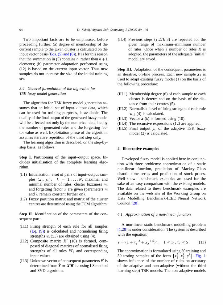
Fig. 1. Impact of the number of rules on MSE for adaptive and non-adaptive TSK fuzzy model for the non-linear function approximation(m = 2, λ = 1).

always show slightly lower mean square error (MSE=(1/N)

∑N1 (y(k) − y(k))2).

The non-adaptive model, defined with 10 rules(with achieved MSE= 0.00156 and the maximumresidual error of 0.00453), is adopted as representa-tive structure of the proposed TSK fuzzy model (seebreaking point of the MSE curve onFig. 1). Sincethe conditional and consequent parts of the rules aredefined with cluster centres, that is with polynomi-als of the first degree, respectively, the non-adaptivemodel defined with 10 rules has 60 adjustable param-eters (2× no. of rules× (no. of inputs+ 1) = 60).Generated TSK fuzzy model with ten rules is listedbelow

R1: If x belongs to [1.439 1.621]T thany1 = −2.847x1 − 2.018x2 + 11.311R2: If x belongs to [1.633 2.693]T thany2 = −2.109x1 − 0.365x2 + 6.989R3: If x belongs to [1.605 4.353]T thany3 = −1.893x1 − 0.809x2 + 8.960R4: If x belongs to [0.439 0.621]T thany4 = 47.7x1 + 100.36x2 − 160.63R5: If x belongs to [2.745 1.25]T thany5 = 0.243x1 − 2.728x2 + 6.161R6: If x belongs to [2.907 4.14]T thany6 = −0.149x1 − 0.076x2 + 2.259R7: If x belongs to [2.31 1.95]T thany7 = −0.402x1 − 1.582x2 + 6.520R8: If x belongs to [3.77 2.234]T thany8 = −0.015x1 − 0.648x2 + 3.400R9: If x belongs to [4.11 1.530]T thany9 = −0.072x1 − 1.596x2 + 5.279R10: If x belongs to [4.524 4.346]T thany10 = −0.024x1 − 0.086x2 + 1.814

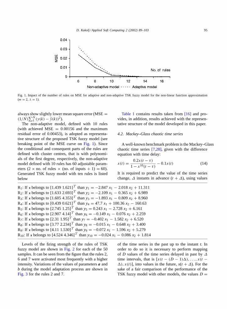
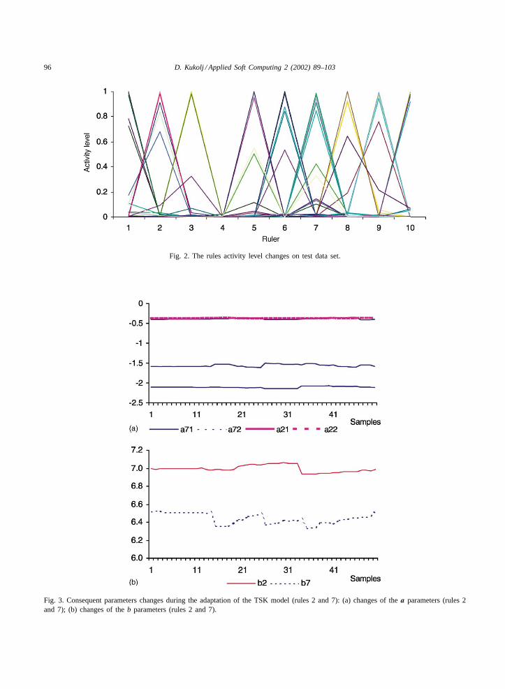
Levels of the firing strength of the rules of TSKfuzzy model are shown inFig. 2 for each of the 50samples. It can be seen from the figure that the rules 2,6 and 7 were activated most frequently with a higherintensity. Variations of the values of parametersa andb during the model adaptation process are shown inFig. 3 for the rules 2 and 7.

Table 1contains results taken from[16] and pro-vides, in addition, results achieved with the represen-tative structure of the model developed in this paper.

4.2. Mackey–Glass chaotic time series

A well-known benchmark problem is the Mackey–Glasschaotic time series[7,28], given with the differenceequation with time delay:

x(t) = 0.2x(t − τ)

1 − x10(t − τ)− 0.1x(t) (14)

It is required to predict the value of the time serieschange,∆ instants in advance (t + ∆), using values

of the time series in the past up to the instantt. Inorder to do so it is necessary to perform mappingof D values of the time series delayed in past by∆

time intervals, that is [x(t − (D − 1)'), . . . , x(t −'), x(t)], into values in the future,x(t + ∆). For thesake of a fair comparison of the performance of theTSK fuzzy model with other models, the valuesD =


Fig. 2. The rules activity level changes on test data set.

Fig. 3. Consequent parameters changes during the adaptation of the TSK model (rules 2 and 7): (a) changes of thea parameters (rules 2and 7); (b) changes of theb parameters (rules 2 and 7).


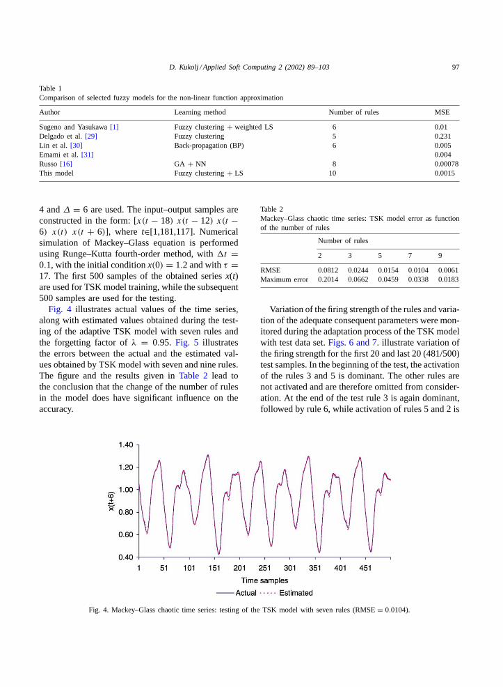
Table 1Comparison of selected fuzzy models for the non-linear function approximation

Author Learning method Number of rules MSE

Sugeno and Yasukawa[1] Fuzzy clustering+ weighted LS 6 0.01Delgado et al.[29] Fuzzy clustering 5 0.231Lin et al. [30] Back-propagation (BP) 6 0.005Emami et al.[31] 0.004Russo[16] GA + NN 8 0.00078This model Fuzzy clustering+ LS 10 0.0015

4 and∆ = 6 are used. The input–output samples areconstructed in the form: [x(t − 18) x(t − 12) x(t −6) x(t) x(t + 6)], where t∈[1,181,117]. Numericalsimulation of Mackey–Glass equation is performedusing Runge–Kutta fourth-order method, with't =0.1, with the initial conditionx(0) = 1.2 and withτ =17. The first 500 samples of the obtained seriesx(t)are used for TSK model training, while the subsequent500 samples are used for the testing.

Fig. 4 illustrates actual values of the time series,along with estimated values obtained during the test-ing of the adaptive TSK model with seven rules andthe forgetting factor ofλ = 0.95. Fig. 5 illustratesthe errors between the actual and the estimated val-ues obtained by TSK model with seven and nine rules.The figure and the results given inTable 2 lead tothe conclusion that the change of the number of rulesin the model does have significant influence on theaccuracy.

Fig. 4. Mackey–Glass chaotic time series: testing of the TSK model with seven rules (RMSE= 0.0104).

Table 2Mackey–Glass chaotic time series: TSK model error as functionof the number of rules

Number of rules

2 3 5 7 9

RMSE 0.0812 0.0244 0.0154 0.0104 0.0061Maximum error 0.2014 0.0662 0.0459 0.0338 0.0183

Variation of the firing strength of the rules and varia-tion of the adequate consequent parameters were mon-itored during the adaptation process of the TSK modelwith test data set.Figs. 6 and 7. illustrate variation ofthe firing strength for the first 20 and last 20 (481/500)test samples. In the beginning of the test, the activationof the rules 3 and 5 is dominant. The other rules arenot activated and are therefore omitted from consider-ation. At the end of the test rule 3 is again dominant,followed by rule 6, while activation of rules 5 and 2 is


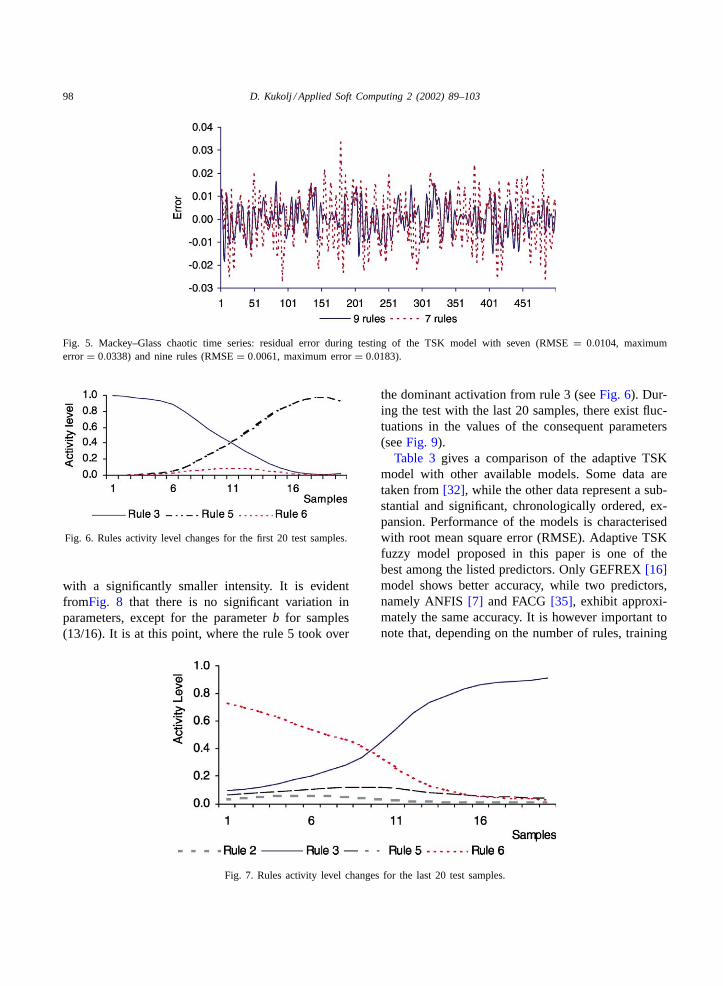
Fig. 5. Mackey–Glass chaotic time series: residual error during testing of the TSK model with seven (RMSE= 0.0104, maximumerror= 0.0338) and nine rules (RMSE= 0.0061, maximum error= 0.0183).

Fig. 6. Rules activity level changes for the first 20 test samples.

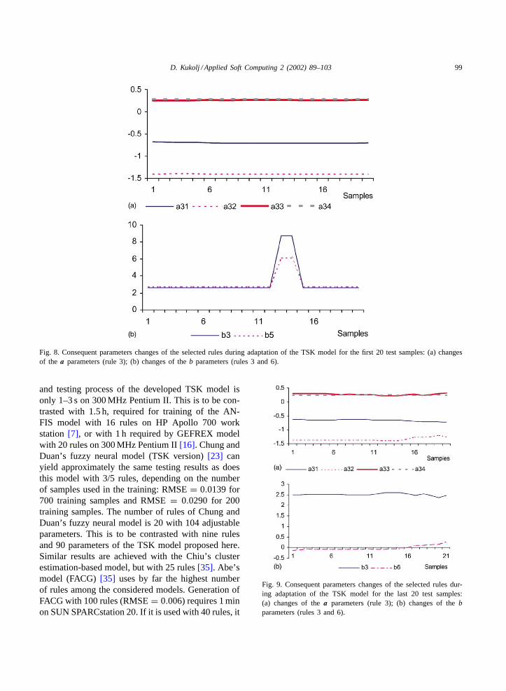
with a significantly smaller intensity. It is evidentfromFig. 8 that there is no significant variation inparameters, except for the parameterb for samples(13/16). It is at this point, where the rule 5 took over

Fig. 7. Rules activity level changes for the last 20 test samples.

the dominant activation from rule 3 (seeFig. 6). Dur-ing the test with the last 20 samples, there exist fluc-tuations in the values of the consequent parameters(seeFig. 9).

Table 3 gives a comparison of the adaptive TSKmodel with other available models. Some data aretaken from[32], while the other data represent a sub-stantial and significant, chronologically ordered, ex-pansion. Performance of the models is characterisedwith root mean square error (RMSE). Adaptive TSKfuzzy model proposed in this paper is one of thebest among the listed predictors. Only GEFREX[16]model shows better accuracy, while two predictors,namely ANFIS[7] and FACG[35], exhibit approxi-mately the same accuracy. It is however important tonote that, depending on the number of rules, training


Fig. 8. Consequent parameters changes of the selected rules during adaptation of the TSK model for the first 20 test samples: (a) changesof the a parameters (rule 3); (b) changes of theb parameters (rules 3 and 6).

and testing process of the developed TSK model isonly 1–3 s on 300 MHz Pentium II. This is to be con-trasted with 1.5 h, required for training of the AN-FIS model with 16 rules on HP Apollo 700 workstation[7], or with 1 h required by GEFREX modelwith 20 rules on 300 MHz Pentium II[16]. Chung andDuan’s fuzzy neural model (TSK version)[23] canyield approximately the same testing results as doesthis model with 3/5 rules, depending on the numberof samples used in the training: RMSE= 0.0139 for700 training samples and RMSE= 0.0290 for 200training samples. The number of rules of Chung andDuan’s fuzzy neural model is 20 with 104 adjustableparameters. This is to be contrasted with nine rulesand 90 parameters of the TSK model proposed here.Similar results are achieved with the Chiu’s clusterestimation-based model, but with 25 rules[35]. Abe’smodel (FACG)[35] uses by far the highest numberof rules among the considered models. Generation ofFACG with 100 rules (RMSE= 0.006) requires 1 minon SUN SPARCstation 20. If it is used with 40 rules, it

Fig. 9. Consequent parameters changes of the selected rules dur-ing adaptation of the TSK model for the last 20 test samples:(a) changes of thea parameters (rule 3); (b) changes of thebparameters (rules 3 and 6).


Table 3Mackey–Glass chaotic time series: results of the comparative analysis

Author/model Learning method Number of rules RMSE

Wang (product operator) 0.0907Min operator 0.0904Jang/ANFIS (Fuzzy NN)/ LS+ BP 16 0.007Auto regressive model 0.19Cascade correlation NN 0.06Back-propagation NN 0.02Sixth-order polynomial 0.04Linear predictive method 0.55Lin and Lee/fuzzy NN/(91)[32] Self-organized learning+ BP 144 0.0359Wang and Mendels[2] Direct matching 121 0.08Kosko/AVQ with BP (92)[33] Different competitive learning+ BP 100 0.09Chiu/cluster estimation/(94)[34] Cluster estimation 25 0.014Kim and Kim [17] GA 9 0.0264Lin and Lin/FALCON-ART/(97)[8] Fuzzy ART 30 0.04Juang and Lin/SONFIN/(98)[13] Clustering+ LS/RLS + BP 4 0.018Abe/FACG/(99)[35] 100 0.006Lo and Yang/TSK model/(99)[36] Heuristic estimation 2 0.0161Yamauchi et al. feedforward NN/(99)[37] Incremental learning 4a 0.045Chung and Duan/MamdaniF-N/(00) [23] Competitive learning+ BP 25 0.0253Chung and Duan/TSKF-N/(00) [23] LS 20 0.0139Russo/GEFREX/(00)[16] GA + NN 20 0.00061This model Fuzzy cluster+ LS + WRLS 9 0.0061

a Remark: number of hidden nodes.

yields approximately the same accuracy as this modelwith seven rules (RMSE= 0.013) in 20 s. Furtherreduction of the number of rules increases the error,which becomes RSME= 0.263 for 20 rules.

4.3. Share prices on the stock exchange

The problem of prediction of daily data of a stockmarket is discussed next. There are 100 data pointstaken from[1,28]. Original data consist of ten inputsand one output. These are:

x1: past change of moving average over a middle periodx2: present change of moving average over a middle periodx3: past separation ratio with respect to moving average over a middle periodx4: present separation ratio with respect to moving average over a middle periodx5: present change of moving average over a short periodx6: past change of price, for instance, change on the previous dayx7: present change of pricex8: past separation ratio with respect to moving average over a short periodx9: present change of moving average over a short periodx10: present separation ratio with respect to moving average over a short periody: prediction of stock price

Valuesx4, x2, x5, x8, x10 andx1 are selected as inputsto the model, as suggested in[38]. From given dataset, first 80 data points are used as training data andrest of 20 data points as testing data. The performanceindex [38]

J = 1

2N(ymaximum− yminimum)2

N∑1

(y(k) − y(k))2

(15)


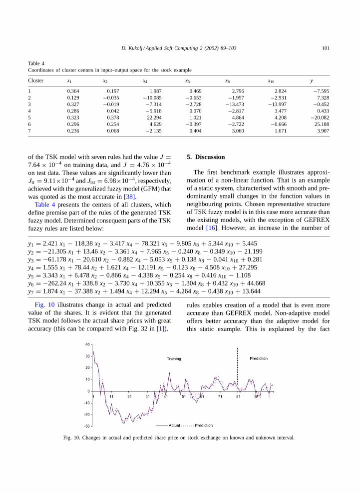
Table 4Coordinates of cluster centers in input–output space for the stock example

Cluster x1 x2 x4 x5 x8 x10 y

1 0.364 0.197 1.987 0.469 2.796 2.824 −7.5952 0.129 −0.035 −10.085 −0.653 −1.957 −2.931 7.3283 0.327 −0.019 −7.314 −2.728 −13.473 −13.997 −0.4524 0.286 0.042 −5.918 0.070 −2.817 3.477 0.4335 0.323 0.378 22.294 1.021 4.864 4.208 −20.0826 0.296 0.254 4.629 −0.397 −2.722 −0.666 25.1887 0.236 0.068 −2.135 0.404 3.060 1.671 3.907

of the TSK model with seven rules had the valueJ =7.64× 10−4 on training data, andJ = 4.76× 10−4

on test data. These values are significantly lower thanJtr = 9.11×10−4 andJtst = 6.98×10−4, respectively,achieved with the generalized fuzzy model (GFM) thatwas quoted as the most accurate in[38].

Table 4presents the centers of all clusters, whichdefine premise part of the rules of the generated TSKfuzzy model. Determined consequent parts of the TSKfuzzy rules are listed below:

y1 = 2.421x1 − 118.38x2 − 3.417x4 − 78.321x5 + 9.805x8 + 5.344x10 + 5.445y2 = −21.305x1 + 13.46x2 − 3.361x4 + 7.965x5 − 0.240x8 − 0.349x10 − 21.199y3 = −61.178x1 − 20.610x2 − 0.882x4 − 5.053x5 + 0.138x8 − 0.041x10 + 0.281y4 = 1.555x1 + 78.44x2 + 1.621x4 − 12.191x5 − 0.123x8 − 4.508x10 + 27.295y5 = 3.343x1 + 6.478x2 − 0.866x4 − 4.338x5 − 0.254x8 + 0.416x10 − 1.108y6 = −262.24x1 + 338.8x2 − 3.730x4 + 10.355x5 + 1.304x8 + 0.432x10 + 44.668y7 = 1.874x1 − 37.388x2 + 1.494x4 + 12.294x5 − 4.264x8 − 0.438x10 + 13.644

Fig. 10 illustrates change in actual and predictedvalue of the shares. It is evident that the generatedTSK model follows the actual share prices with greataccuracy (this can be compared with Fig. 32 in[1]).

Fig. 10. Changes in actual and predicted share price on stock exchange on known and unknown interval.

5. Discussion

The first benchmark example illustrates approxi-mation of a non-linear function. That is an exampleof a static system, characterised with smooth and pre-dominantly small changes in the function values inneighbouring points. Chosen representative structureof TSK fuzzy model is in this case more accurate thanthe existing models, with the exception of GEFREXmodel [16]. However, an increase in the number of

rules enables creation of a model that is even moreaccurate than GEFREX model. Non-adaptive modeloffers better accuracy than the adaptive model forthis static example. This is explained by the fact


that the global LS estimate gives best overall perfor-mance on a static problem. By adapting, the focusis changed by emphasising the importance of newdata, the consequence being that the overall per-formance on static data deteriorates. Adaptation ofthe models in this kind of static case is not nec-essary. Proposed TSK fuzzy model required morerules for this example than for the other presentedcases.

The other two examples are both related to theproblem of prediction. The TSK fuzzy model in-troduced here has generated a prediction of highaccuracy for the Mackey–Glass time series, using thesmallest number of rules when compared to the otheravailable models. Only GEFREX[16] method man-aged to yield a smaller error, however, at the expenseof a more complex structure with a larger number ofrules and subsequent considerably longer time neededfor model generation. The example of the share priceprediction further confirms already stated observa-tions. Results given in[38] for a number of models(the best one being GFM) are considerably worsethan the results achieved here with adaptive TSKmodel.

Numerous tests of the developed adaptive TSKfuzzy model algorithm have shown that adaptive fea-ture always leads to an increase in the accuracy inall the studied cases. The exception is the exampleof the static function approximation, for the reasonsthat have already been explained. An increase in thenumber of rules of a TSK fuzzy model predominantlyleads to the significant improvement in the accuracy.Many simulation results have shown that the differ-ent choices for parameterm (seeEq. (5)) have littleinfluence on the identification of the fuzzy model(the same conclusion is stated in[9]). Selection ofthe forgetting factor is problem dependent (it is sug-gested here that the value of 0.95 is a good choice)and its value does not vary during fuzzy modelutilisation.

It is important to emphasise that partition of theinput–output space takes place during the phase ofstructure identification. However, during the on-lineadaptation of the TSK fuzzy model the actual outputdoes not need to be known. Calculation of the degreeof belonging of the current sample to a given cluster isbased entirely on the last input vector, rather than onthe input–output data pair. It is due to this important

change that the fuzzy model gains on the generalityand wider applicability.

6. Conclusion

The paper describes a method for Takagi–Sugeno–Kang fuzzy model generation. The method is charac-terised with a very high modelling accuracy and withthe very fast learning process. A TSK fuzzy modelformed in this way can be used to characterise a wideclass of very diverse problems. The algorithm was ex-amined using three frequently discussed benchmarkmodelling problems. The obtained results are com-pared with those available in literature for a variety ofsimilar models. The quality of the proposed method,when compared with existing models, is further veri-fied in this way.

The proposed TSK fuzzy model generation proce-dure has already been successfully applied by the au-thor to a number of real-world problems. The first oneis prediction of the natural gas consumption and itsreserve in a gas transport system[39]. Generated TSKfuzzy models are incorporated in a supervisory con-trol and data acquisition system. It is shown by exper-iments that, among many different factors, samplingtime and the number of inputs have the greatest im-pact on the model error.

The second application of this model is speed es-timation in DC motor drives[40]. TSK fuzzy modelbased speed estimator is implemented in MicronasMASC 3500 DSP. Examination of the speed estima-tor performance, using six known and six unknownoperating regimes, has revealed very good accuracyeven on this very low-priced DSP platform. Further,the TSK fuzzy model is used as s speed controllersof a speed-sensorless DC motor drive. In[41], thistype of speed controller is compared with controllersdesigned using the feed-forward neural network andneuro-fuzzy network. Simulation of all the drivestructures for a number of operating regimes leads tothe conclusions that the TSK fuzzy controller appearsto be the best solution since it: (1) exhibits the bestaccuracy in the majority of operating regimes; (2)requires the shortest training time; (3) is character-ized with the simple final structure that is convenientfor real-time implementation. A couple of imple-mentations of the algorithm, in the areas of process


industry and communication protocols, are currentlyunder way.

References

[1] M. Sugeno, T. Yasukawa, A fuzzy-logic-based approach toqualitative modeling, IEEE Trans. Fuzzy Syst. 1 (1993) 7–31.

[2] L.X. Wang, J.M. Mendel, Generating fuzzy rules by learningfrom examples, IEEE Trans. Syst. Man Cybern 22 (6) (1992)1414–1427.

[3] I. Gath, A.B. Geva, Unsupervised optimal fuzzy clustering,IEEE Trans. Pattern Anal. Machine Intell. 11 (1989) 773–781.

[4] X.L. Xie, G.A. Beni, Validity measure for fuzzy clustering,IEEE Trans. Pattern Anal. Machine Intell. 13 (1991) 841–846.

[5] R.N. Dave, R. Krishnapuram, Robust clustering methods: aunified view, IEEE Trans. Fuzzy Syst. 5 (2) (1997) 270–293.

[6] M. Setnes, Supervised fuzzy clustering for rule extraction,IEEE Tran. Fuzzy Syst. 8 (4) (2000) 416–424.

[7] J.R. Jang, C. Sun, E. Mizutani, Neuro-Fuzzy and Soft Compu-ting, Prentice-Hall, Englewood Cliffs, NJ, 1997.

[8] C.J. Lin, C.T. Lin, An ART-based fuzzy adaptive learningcontrol network, IEEE Trans. Fuzzy Syst. 5 (4) (1997) 477–496.

[9] J. Chen, Y. Xi, Z. Zhang, A clustering algorithm for fuzzymodel identification, Fuzzy Sets Syst. 98 (1998) 319–329.

[10] K.M. Passino, S. Yurkovich, Fuzzy Control, Addison-Wesley,Longman, Menlo Park, CA, 1998.

[11] W. Pedrycz, M. Reformat, Rule-based modelling of nonlinearrelationship, IEEE Trans. Fuzzy Syst. 5 (2) (1997) 256–269.

[12] Y. Wang, G. Rong, A self-organizing neural-network-basedfuzzy system, Fuzzy Sets Syst. 103 (1999) 1–11.

[13] C.F. Juang, C.T. Lin, An on-line self-constructing neural fuzzyinference network and its applications, IEEE Trans. FuzzySyst. 6 (1) (1998) 12–32.

[14] M. Setnes, R. Babuška, H.B. Verburger, Rule-based modeling:precision and transparency, Cybern, Part C 28 (1) (1998)165–169.

[15] J.V. Oliveira, J.M. Lemos, A comparison of some adaptive-predictive fuzzy-control strategies, IEEE Trans. Syst. ManCybern, Part C 30 (1) (2000) 138–145.

[16] M. Russo, Generic fuzzy learning, IEEE Trans. Evol. Comput.4 (3) (2000) 259–273.

[17] D. Kim, C. Kim, Forecasting time series with genetic fuzzypredictor ensemble, IEEE Trans. Fuzzy Syst. 5 (4) (1997)523–535.

[18] S.J. Kang, C.H. Woo, H.S. Hwang, K.B. Woo, Evolutionarydesign of fuzzy rule base for nonlinear system modeling andcontrol, IEEE Trans. Fuzzy Syst. 8 (2000) 37–45.

[19] P. Sierry, F. Guely, A genetic algorithm for optimizing Takagi–Sugeno fuzzy rule bases, Fuzzy Sets Syst. 99 (1998) 37–47.

[20] M. Setnes, H. Roubos, GA-Fuzzy modelling and classifi-cation: complexity and performance, IEEE Trans. Fuzzy Syst.8 (5) (2000) 509–522.

[21] S.G. Tzafestas, K.C. Zikidis, NeuroFAST: on-line neuro-fuzzyART-based structure and parameter learning TSK model, ManCybern, Part B 31 (5) (2001) 797–802.

[22] C.C. Lee, Fuzzy logic in control systems: fuzzy logic con-troller-Part I and II, IEEE Trans. Syst. Man Cybern 20 (2)(1990) 404–435.

[23] F.L. Chung, J.C. Duan, On multistage fuzzy neural networkmodeling, IEEE Trans. Fuzzy Syst. 8 (2) (2000) 125–142.

[24] J. Yen, L. Wang, C.W. Gillespie, Improving the interpretabilityof TSK fuzzy models by combining global learning andlocal learning, IEEE Trans. Fuzzy Syst. 6 (4) (1998) 531–537.

[25] J.G. Bezdek, Pattern Recognition with Fuzzy ObjectiveFunction Algorithms, Plenum Press, New York, 1981.

[26] G.E. Forsythe, M.A. Malcolm, C.B. Moler, ComputerMethods for Mathematical Computations, Prentice-Hall,Englewood Cliffs, NJ, 1977.

[27] G.H. Golub, C.F. Van Loan, Matrix Computations, JohnsHopkins University Press, Baltimore, 1989.

[28] Working Group on Data Modeling Benchmark, StandardCommittee of IEEE Neural Network Council,http://neural.cs.nthu.edu.tw/jang/benchmark/.

[29] M. Delgado, A.F. Gomez-Skarmeta, F. Martin, Fuzzy cluster-ing-based rapid prototyping for fuzzy rule-based modeling,IEEE Trans. Fuzzy Syst. 5 (2) (1997) 223–233.

[30] Y. Lin, G.A. Cunningham Jr., S.V. Coggeshall, Using fuzzypartitions to create fuzzy systems from input–output data andset the initial weights in a fuzzy neural network, IEEE Trans.Fuzzy Syst. 5 (4) (1997) 614–621.

[31] M.R. Emami, I.B. Turksen, A.A. Goldberg, Development ofa systematic methodology of fuzzy logic modeling, IEEETrans. Fuzzy Syst. 6 (1998) 346–361.

[32] C.T. Lin, C.S.G. Lee, Neural-network-based fuzzy logic anddecision system, IEEE Trans. Comput. 40 (1991) 1320–1336.

[33] B. Kosko, Neural Networks and Fuzzy Systems, Prentice-Hall, Englewood Cliffs, NJ, 1992.

[34] S.L. Chiu, Fuzzy model identification based on clusterestimation, J. Intell. Fuzzy Syst. 2 (1994) 267–278.

[35] S. Abe, Fuzzy function approximators with ellipsoidalregions, IEEE Trans. Syst. Man Cybern, Part B 29 (4) (1999)654–661.

[36] J.C. Lo, C.H. Yang, A heuristic error-feedback learningalgorithm for fuzzy modeling, Cybern 29 (6) (1999) 686–691.

[37] K. Yamauchi, N. Yamaguchi, N. Ishii, Incremental learningmethods with retrieving of interfered patterns, IEEE Trans.Neural Netw. 10 (6) (1999) 1351–1365.

[38] M.F. Azeem, M. Hanmandlu, N. Ahmad, Generalization ofadaptive neuro-fuzzy inference systems, IEEE Trans. NeuralNetw. 11 (6) (2000) 1332–1346.

[39] D. Kukolj, M. Berko-Pusic, Advanced supervisory controlfunctions based on computational intelligence, IFAC Sympo-sium on Artificial Intelligence in Real Time ControlAIRTC-2000, Budapest, 2–4 October 2000.

[40] D. Kukolj, E. Levi, A self-organizing neuro-fuzzy speedestimator for DC motor drives, in: Proceedings of theEuropean Conference on Power Electronics and ApplicationsEPE 2001, Graz, 2001 CD-ROM, PP00306.

[41] D. Kukolj, F. Kulic, E. Levi, Design of the speed controllersfor sensorless electric drives based on AI techniques: acomparative study, Artif. Intell. Eng. 14 (2) (2000) 165–174.

http://neural.cs.nthu.edu.tw/jang/benchmark

http://neural.cs.nthu.edu.tw/jang/benchmark

Documents

Design of adaptive Takagi-Sugeno-Kang fuzzy models