ISA Transactions 49 (2010) 447–461

Contents lists available at ScienceDirect

ISA Transactions

journal homepage: www.elsevier.com/locate/isatrans

Robust fuzzy Lyapunov stabilization for uncertain and disturbedTakagi–Sugeno descriptorsT. Bouarar, K. Guelton ∗, N. ManamanniCReSTIC, EA3804, University of Reims, Moulin de la House BP1039, 51687 Reims Cedex 2, France

a r t i c l e i n f o

Article history:Received 17 November 2009Received in revised form15 June 2010Accepted 23 June 2010Available online 20 July 2010

Keywords:Takagi–SugenoRedundancyDescriptorsRobust fuzzy controlNon-quadraticFuzzy Lyapunov functionLMIH∞ criterion

a b s t r a c t

In this paper, new robust H∞ controller design methodologies for Takagi–Sugeno (T–S) descriptors isconsidered. Based on Linear Matrix Inequalities, two different approaches are proposed. The first oneinvolves a ‘‘classical closed-loop dynamics’’ formulation and the second one a ‘‘redundancy closed-loopdynamics’’ approach. The provided conditions are obtained through a fuzzy Lyapunov function candidateand a non-PDC control law. Both the classical and redundancy approaches are compared. It is shownthat the latter leads to less conservative stability conditions. The efficiency of the proposed robustcontrol approaches for T–S descriptors as well as the benefit of the redundancy approach are shownthrough an academic example. Then, to show the applicability of the proposed approaches, the benchmarkstabilization of an inverted pendulum on a cart is considered.

© 2010 ISA. Published by Elsevier Ltd. All rights reserved.

1. Introduction

In the past three decades, Takagi–Sugeno (T–S) fuzzy mod-els [1] have attracted a great of deal interest in the controlcommunity since they are able to approximate some nonlinearsystems based on fuzzy logic paradigm. Indeed, a T–S fuzzy modelis a collection of a set of linear ones blended together by nonlinearmembership functions. Moreover, it is well known that an affinenonlinear system can be exactly matched on a compact set of thestate space using for instance the sector nonlinearity approach [2].The main interest of such an approach is that it allows extendingsome of the linear control concepts to the case of nonlinear analy-sis. Taking benefit of that property, T–S models have been appliedin various processes [3–6] and, regarding to theoretical results, sev-eral works have dealt with stability analysis and controller de-sign; see e.g. [7–11]. These are often based on the well-knownParallel Distributed Compensation (PDC) paradigm [10] and stabil-ity conditions are obtained from the Lyapunov theory in terms ofLinear or BilinearMatrix Inequalities (LMI, BMI). Sufficient LMI sta-bility conditions have been proposed using a quadratic Lyapunovfunction (see e.g. [2,12] and the references therein). Nevertheless,these studies lead to conservatism since the existence of a common

∗ Corresponding author. Tel.: +33 3 26 91 32 61; fax: +33 3 26 91 31 06.E-mail address: kevin.guelton@univ-reims.fr (K. Guelton).

0019-0578/$ – see front matter© 2010 ISA. Published by Elsevier Ltd. All rights reservdoi:10.1016/j.isatra.2010.06.003

Lyapunov matrix has to be checked to ensure the stability of theconsidered systems; see [13] for a review of the conservatismsources. Many ways have been investigated to reduce the con-servatism. Some of them propose to relax quadratic conditionsusing transformations within the summation structure of theclosed-loop T–S systems [14,15]. Some others propose to introduceadditional decision variables in the LMI problem [16,17]. More re-cently, another type of Lyapunov function candidate has been pro-posed. In thisway, LMI stability conditions and controller synthesisbased on the piecewise Lyapunov function have beenproposed [18,19] but remain irrelevant when analyzing a T–S model obtainedfrom the sector nonlinearity approach [2]. With the same inten-tion of reducing the conservatism of LMI conditions, non-quadraticLyapunov functions (NQLF) have been considered for non-PDC con-troller design in [20–25]. Due to its adequacy with the sector non-linearity approach, NQLF has proved a tremendous success withthe T–S control community since they share the same fuzzy struc-ture as the model to be analyzed.The above referenced papers are mostly focusing on standard

T–S systems (explicit systems) which remain to Ordinary Dif-ferential Equations. A wider class of dynamical systems calleddescriptors, are constituted by a set of Algebraic Differential Equa-tions [26–30]. These are useful to represent implicit or singularsystems as well as many physical systems like, for instance, me-chanical [5,6,28] and electrical processes [29]. Despite numerousworks dealing with standard T–S systems analysis, fewer stud-ies have been done concerning T–S descriptors. Therefore, some

ed.

448 T. Bouarar et al. / ISA Transactions 49 (2010) 447–461

closed problems for standard systems are still open for descrip-tors. Quadratic stability of such systems has been firstly studiedin [31,32]. Robust quadratic stability conditions for uncertain T–Sdescriptor systems have been proposed in terms of BMI [33] orLMI [34–36]. Some relaxed quadratic conditions introducing fuzzyinferred slack variables have been proposed in [37]. And more re-cently, with the intention to reduce the conservatism of LMI baseddescriptor stability analysis, NQLF based analysis have been firstlyproposed in [38].The purpose of this paper reaches two objectives. The first one is

to extend the previous works to robust fuzzy Lyapunov based non-quadratic controller design for the class of uncertain and disturbedT–S descriptors. On the other hand, based on a redundancy prop-erty, new approaches have been proposed to relax and reduce thecomputational cost of LMI conditions for standard T–S fuzzy mod-els [39,40]. The main interest of such approaches is that they facil-itate achieving LMI conditions since they avoid the appearance ofcrossing terms in the closed-loop dynamics. Thus, the second con-tribution of this paper aims at extending redundancy approaches tothe stability analysis and robust controller design of T–S descrip-tors. Moreover the superiority of redundancy approaches will bedemonstrated regarding to classical ones.The paper is organized as follows. At first, the problem state-

ment of classical and redundancy closed-loop descriptor dynam-ics, using a non-PDC control law, is proposed in the next section.In Section 3, both the classical and redundancy non-quadratic ap-proaches for non-PDC controller design are derived in terms ofLMI for the class of uncertain descriptors without external distur-bances. Afterward, an H∞ criterion is employed in Section 4 toextend the proposed results to robust controllers design ensuringthe attenuation of external disturbances. Finally, in the last sectiontwo examples are provided. The first one considers an academicnonlinear system devoted to compare the proposed classical andredundancy approaches in terms of conservatism as well as to il-lustrate the performances of the proposed robust controller design.The second example is devoted to show the applicability of the pro-posed approaches on a realistic nonlinear system. Therefore, thestudy of the well-known benchmark of an inverted pendulum ona cart is proposed.

2. Uncertain T–S descriptor systems and problem statement

Let us consider the following bounded nonlinear uncertain anddisturbed descriptor systems represented by:

(E(x(t))+1E(x(t)))x(t) = (A(x(t))+1A(x(t)))x(t)+ (B(x(t))+1B(x(t)))u(t)+W (x(t))ϕ(t) (1)

with x(t) ∈ Rn, u(t) ∈ Rm and ϕ(t) ∈ Rd respectively the state,the input and the unknown bounded external disturbances vec-tors; E(x(t)) ∈ Rn×n, A(x(t)) ∈ Rn×n, B(x(t)) ∈ Rn×m andW (x(t))∈ Rd×n are norm bounded known nonlinear matrices describingthe nominal part of the considered system; 1E(x(t)) ∈ Rn×n,1A(x(t)) ∈ Rn×n and 1B(x(t)) ∈ Rn×m are unknown Lebesguemeasurable matrices describing the model uncertainties.A convenient way to tackle the stabilization of (1) is to rewrite

it as a T–S fuzzy model. There is many ways to obtain a T–S modelfrom a nonlinear one. Note that a well-known systematic way towrite a T–Smodel representing (1) is called the sector nonlinearityapproach [2]. It allows a T–S model matching exactly a nonlinearone on a compact set of the state space. In order to cope withthe nonlinear model structure (1), a T–S fuzzy model of descriptorsystems has been firstly proposed in [31,32]. This one includesspecific membership structures respectively for the left and theright hand side of the nonlinear descriptor model (1). In this case,one can define respectively l and r the numbers of fuzzy rules inthe left and the right hand side of the resulting T–S fuzzy descriptorgiven by:

l∑k=1

vk(z(t))(Ek +1Ek(t))x(t) =r∑i=1

hi(z(t))((Ai +1Ai(t))x(t)

+ (Bi +1Bi(t))u(t)+Wiϕ(t)) (2)where vk(z(t)) ≥ 0, hi(z(t)) ≥ 0 are the membership functionsverifying the following convex sum properties

∑lk=1 vk(z(t)) = 1

and∑ri=1 hi(z(t)) = 1, Ai ∈ Rn×n, Bi ∈ Rn×m and Wi ∈ Rd×n

are time invariant matrices, 1Ek(t) ∈ Rn×n,1Ai(t) ∈ Rn×n and1Bi(t) ∈ Rn×m are unknown Lebesgue measurable uncertaintymatrices bounded such that 1Ek(t) = Hke f

ke (t)N

ke ,1Ai(t) =

H iafia(t)N

ia and 1Bi(t) = H

ibfib(t)N

ib with H

ke ,H

ia,H

ib,N

ke ,N

ia and N

ib

are known real matrices and f ke (t), fia(t) and f

ib(t) are unknown

time varying normalized functions such that f i,kTe,a,b(t)f

i,ke,a,b(t) ≤ I .

Remark 1. In this study, one assumes that (2) is regular and im-pulse free [28].

Remark 2. For more details on the well-known T–S fuzzy modelrepresentation of nonlinear systems and how to obtain it, thereader can refer to [2]. Moreover, an example is proposed in thelast section of this paper to illustrate how to obtain an uncertainand disturbed T–S fuzzy descriptor (2) from a nonlinear system ofthe form (1) using the well-known sector nonlinearity approach.A modified PDC (Parallel Distributed Compensation) control

law has been proposed for the quadratic stabilization of T–S de-scriptors [32]. In that case, the designed fuzzy controller sharesthe samemembership functions regarding to the considered fuzzymodel. Note that, in order to derive non-quadratic stability con-ditions for standard T–S fuzzy models, a Lyapunov dependentnonlinear matrix must be introduced in the PDC scheme for LMIpurpose [20,24,33,39]. In the present study, to deal with T–S fuzzydescriptors non-quadratic stabilization, one proposes the follow-ing modified non-PDC control law:

u(t) = −l∑k=1

r∑i=1

vk(z(t))hi(z(t))Fik

×

(l∑k=1

r∑i=1

vk(z(t))hi(z(t))X1ik

)−1x(t) (3)

where Fik and X1ik > 0 are real gain matrices with appropriate di-mensions to be synthesized.

Notations. Along this paper, in order to improve the readabilityof the involved mathematical expressions, the following notationswill be used. Let us consider, for i = 1, . . . , r and k = 1, . . . , l,the scalarmembership functions hi(z(t)) and vk(z(t)), thematricesYk,Gi, Tik and Lijk with appropriate dimensions, we will denote:

Yv =l∑k=1

vk(z(t))Yk,

Gh =r∑i=1

hi(z(t))Gi,

Thv =l∑k=1

r∑i=1

vk(z(t))hi(z(t))Tik

and

Lhhv =l∑k=1

r∑i=1

r∑j=1

vk(z(t))hi(z(t))hj(z(t))Lijk.

As usual a star (∗) indicates a transpose quantity in a symmetricmatrix.Following previous studies on descriptor systems [31–33], the

stability is investigating by considering an extended state vector

T. Bouarar et al. / ISA Transactions 49 (2010) 447–461 449

x(t) =[xT(t) xT(t)

]T. Thus (2) can be rewritten with the above-defined notations as:

Ex(t) = Ahvx(t)+ Bhu(t)+W hϕ(t) (4)

with

E =[I 00 0

], Ahv =

[0 I

Ah +1Ah(t) −Ev −1Ev(t)

],

Bh =[

0Bh +1Bh(t)

]and W h =

[0Wh

].

Following the same way, the control law (3) can be rewritten as:

u(t) = −K hvx(t) (5)

with K hv =[Fhv(X1hv)

−1 0].

Note that two ways are possible to express the closed-loopdynamics. The first one, usually employed in previous studies [31–35,38], is called ‘‘classical closed-loop dynamics’’ in the presentstudy. That one is obtained by substituting (5) in (4) and is givenby:

Ex(t) = (Ahv − BhK hv)x(t)+W hϕ(t). (6)

In this paper, one proposes another way to express the closed-loop dynamics of T–S fuzzy descriptors. That one is called the‘‘redundancy closed-loop dynamics’’. It is obtained by introducinga virtual dynamics in themodified non-PDC control law (5). That isto say, (5) can be rewritten as:

0u(t) = u(t)+ K hvx(t) (7)

where 0 ∈ Rm×m is a zero matrix.Thus, considering a new extended state vector x(t) =

[xT(t)

uT(t)]T, combining (4) and (7), the ‘‘redundancy closed-loop dyna-

mics’’ can be expressed as:

E ˙x(t) = Ahv x(t)+ Whϕ(t) (8)

with

E =[E 00 0

], Ahv =

[Ahv BhK hv I

]and Wh =

[W h0

].

Remark 3. Let us point out that the ‘‘classical closed-loop dyna-mics’’ (6) involves crossing terms between the gain and the inputmatrices K hv and Bh which constitute a source of conservatismwhen designing a fuzzy controller. For more details and acomplete review of conservatism sources, see [13]. Unlike the‘‘classical closed-loop dynamics’’, the ‘‘redundancy closed-loop dy-namics’’ (8) allows decoupling these matrices and so, it leads toless conservatism. This point will be demonstrated and shown inwhat follows. Moreover, note finally that, apart from our prelimi-nary study [38], to the best of the author’s knowledge, there are noexisting results in the literature for T–S descriptor stabilization inthe non-quadratic framework.

The goal now is to provide Linear Matrix Inequalities (LMI) sta-bility conditions allowing to design a controller (3) stabilizing (2).In the following sections, both sufficient stability conditions us-ing the ‘‘classical closed-loop dynamics’’ (6) and the ‘‘redundancyclosed-loop dynamics’’ (8) will be investigated, compared and dis-cussed.

3. LMI based stabilization for uncertain and disturbed T–Sdescriptors

In this section, non-quadratic stability conditions will beproposed using first the ‘‘classical closed-loop dynamics’’ (6), then

the ‘‘redundancy closed-loop dynamics’’ (8). The following lemmawill be useful to prove the LMI conditions proposed in the sequel.

Lemma 1 ([41]). For any real matrices X and Y with appropriatedimensions, there exist a positive scalar σ such that the followinginequality holds:

XTY + Y TX ≤ σXTX + σ−1Y TY . (9)

3.1. Stabilization based on the ‘‘classical closed-loop dynamics’’

LMI non-quadratic stability conditions have been firstly derivedfrom a fuzzy Lyapunov function (FLF) for uncertain T–S descriptorsin our preliminary study [38] using a ‘‘classical closed-loopdynamics’’ described by (6) without external disturbances (ϕ(t) =0). In [24], LMI stability conditions of less conservatism have beenproposed for standard T–S fuzzy systems in the non-quadraticframework. Based on this approach, the following theoremimproved the LMI conditions proposed in [38] for uncertain T–Sdescriptor systems.

Theorem 1. Assume that ∀ z(t) ξ = 1, . . . , r hξ (z(t)) ≥ φξ andψ = 1, . . . , l, vψ (z(t)) ≥ θψ . The uncertain T–S descriptor (2) isglobally asymptotically stable via the non-PDC control law (3), if thereexist the matrices X1jk = (X1jk)

T > 0, X3ij , X4ij > 0 (or < 0), R1 =

RT1, R2 = RT2 and Fjk, the positive scalars τ

1ijk, τ

2ijk, τ

3ijk and τ

4ijk such

that the following LMIs are satisfied for all i, j = 1, . . . , r and k =1, . . . , l:

Φijk < 0 (10)

X1jk + R1 ≥ 0 (11)

X1jk + R2 ≥ 0 (12)

whereΦijk is as given in Box I.

Proof. Let us consider the following candidate fuzzy Lyapunovfunction (FLF):

V (x(t)) = xT(t)E(Xhhv)−1x(t). (13)

In what follows, for space convenience, the time t in a time varyingvariable will be omitted when there is no ambiguity.From (13), one needs:

E(Xhhv)−1 = (Xhhv)−TE > 0. (14)

This condition leads, as classical for descriptor systems (see e.g.

[38]), to Xhhv =[X1hv 0X3hh X4hh

]with X1hv = (X1hv)

T > 0. Moreover,

(Xhhv)−1 exists if the matrix X4hh is invertible, i.e. if X4hh > 0 or

X4hh < 0. Note that the fuzzy interconnection structure of X1hv, X

3hh

and X4hh is chosen for LMI purpose (see below Eq. (22)).Then, the closed-loop system (6) is stable if:

V (x) = xTE(Xhhv)−1x+ xTE(Xhhv)−1x+ xTE

˙(Xhhv)−1x

< 0. (15)

According to (14) and (6), (15) yields:

(Ahv − BhK hv)T(Xhhv)−1

+ ((Xhhv)−1)T(Ahv − BhK hv)+ E˙

(Xhhv)−1x < 0. (16)

Multiplying left and right respectively by XThhv and Xhhv , and

considering (14), (16) becomes:

XThhv(A

Thv − K

ThvB

Th)+ (Ahv − BhK hv)Xhhv

+ E(Xhhv)˙

(Xhhv)−1Xhhv < 0. (17)

450 T. Bouarar et al. / ISA Transactions 49 (2010) 447–461

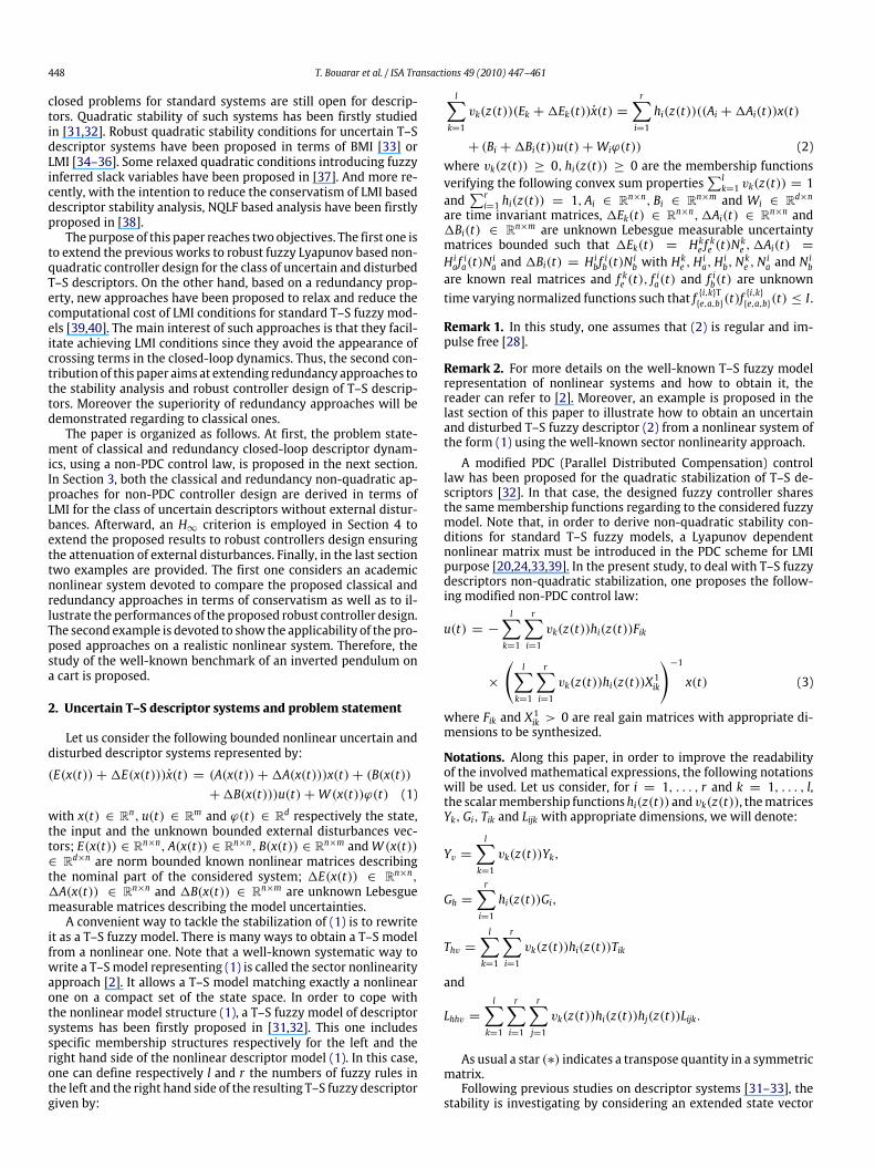
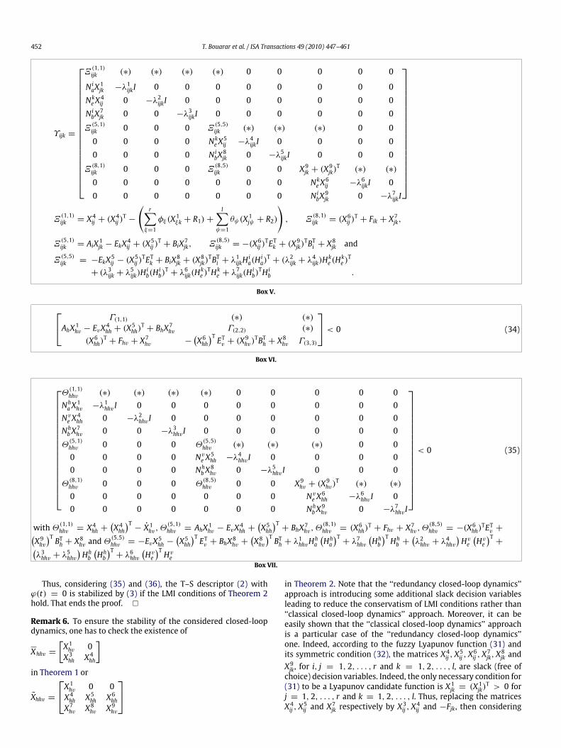
Φijk =

Ω(1,1)ijk (∗) (∗) (∗) (∗) 0N iaX

1jk −τ 1ijkI 0 0 0 0

N ibFjk 0 −τ 2ijkI 0 0 0NkeX

3ij 0 0 −τ 3ijkI 0 0

(X4ij )T+ AiX1jk − EkX

3ij − BiFjk 0 0 0 Ω

(5,5)ijk (∗)

0 0 0 0 NkeX4ij −τ

4ijkI

Ω(1,1)ijk = X

3ij + (X

3ij )T−

(r∑ξ=1

φξ (X1ξk + R1)+l∑

ψ=1

θψ (X1iψ + R2)

)and

Ω(5,5)ijk = −(X

4ij )TETk − EkX

4ij + τ

1ijkH

ia(H

ia)T+ τ 2ijkH

ib(H

ib)T+ τ 3ijkH

ke (H

ke )T+ τ 4ijkH

ke (H

ke )T.

Box I.

Now, since

−˙

(Xhhv)−1 =ddt

(Xhhv)−1Xhhv

(Xhhv)−1 − (Xhhv)−1

=˙

(Xhhv)−1Xhhv(Xhhv)−1

+ (Xhhv)−1 ˙Xhhv(Xhhv)−1 −˙

(Xhhv)−1

= (Xhhv)−1 ˙Xhhv(Xhhv)−1 (18)

inequality (17) becomes:

XThhv(A

Thv − K

ThvB

Th)+ (Ahv − BhK hv)Xhhv − E

˙Xhhv < 0 (19)

which can be extended, with the matrices defined in (4) and (5),under the condition in Box II.Applying Lemma 1, (20) is satisfied as in Box III.Then, applying the Schur complement, one obtains the inequalityin Box IV.Note that the minimal interconnection structure for (22) is a triplesum (hhv). This justify the choice made on the interconnectionof the Lyapunov matrices X1hv, X

3hh and X

4hh. Therefore, since the

membership functions verify the convex sum properties, one has:

X1hv =r∑j=1

l∑k=1

hjvkX1jk +r∑j=1

l∑k=1

hjvkX1jk

=

l∑k=1

r∑j=1

hjvk

(r∑ξ=1

hξX1ξk +l∑

ψ=1

vψX1jψ

). (23)

Moreover, following the relaxation scheme proposed in [24], oneconsiders R1 and R2 real constant matrices. Therefore, one has∑r

ξ=1 hξ (z(t))R1 = 0 and∑l

ψ=1 vψ (z(t))R2 = 0 and so, withoutloss of generality, (23) can be rewritten such that:

X1hv =l∑k=1

r∑j=1

hjvk

(r∑ξ=1

hξ (X1ξk + R1)+l∑

ψ=1

vψ (X1jψ + R2)

). (24)

Then, let us consider, for i = 1, . . . , r, φi the lower bounds ofhi(z(t)) and, for k = 1, . . . , l, θk the lower bounds of vk(z(t)), (24)can be bounded such that:

− X1hv ≤ −l∑k=1

r∑j=1

hjvk

(r∑ξ=1

φξ (X1ξk + R1)

+

l∑ψ=1

θψ (X1jψ + R2)

)(25)

for which, the condition (11) and (12) are necessary.

Now, from (22) and (25), one has

V (x) ≤r∑i=1

r∑j=1

l∑k=1

hihjvkΦijk < 0 (26)

withΦijk defined in (10).Finally, (26) is sufficiently satisfied if (10) holds. That ends the

proof.

Remark 4. In previous works [38], one has considered:

− X1hv ≤ −l∑k=1

r∑j=1

hjvk

(r−1∑ξ=1

φξ (X1ξk − X1rk)

+

l−1∑ψ=1

θψ (X1jψ − X1jl )

)(27)

instead of (25) to derive LMI stability conditions. As shown in [24],this kind of boundary remains conservative and may be easilyimproved. Therefore, extending this works to descriptors systems,Theorem 1 provides less conservative results since (25) obviouslyinclude (27). Indeed, R1 and R2 being free slack matrices, (27) is aparticular case of (25) where R1 = −X1rk and R2 = −X

1jl . Note also

that the quadratic cases [34,35,37] are included in Theorem 1 byconsidering X1jk = X

1 common matrix for all i, j and R1 = R2 =−X1.

Remark 5. For i = 1, . . . , r and k = 1, . . . , l, hi(z(t)) andvk(z(t)) are required to be at least C1. This is obviously satisfiedfor fuzzymodels constructed via a sector nonlinearity approach [2]if the system (1) is at least C1 or, for instance when membershipfunctions are chosen with a smoothed Gaussian shape.

3.2. Stability conditions based on ‘‘redundancy closed-loop dynamics’’

Now, LMI conditions for non-quadratic controller (3) designfor uncertain T–S descriptor (2) (without external disturbances)being established by Theorem 1 based on the ‘‘classical closed-loop dynamics’’ (6) approach, one proposes to extend them byconsidering the ‘‘redundancy closed-loop dynamics’’ (8). The resultis proposed in the following theorem.

Theorem 2. Assume that, ∀ z(t) ξ ∈ 1, . . . , r hξ (z(t)) ≥ φξand ψ ∈ 1, . . . , l, vψ (z(t)) ≥ θψ . The uncertain T–S descriptorsystem (2) (with ϕ(t) = 0) is globally asymptotically stable viathe non-PDC control law (3) if there exist, for i = 1, . . . , r and fork = 1, . . . , l, the matrices X1jk = (X1jk)

T > 0, X4ij , X5ij > 0 (or <

0), X6ij , X7jk, X

8jk, X

9jk > 0 (or < 0), R1 = RT1, R2 = RT2 and Fik,

T. Bouarar et al. / ISA Transactions 49 (2010) 447–461 451

0)

(X3hh)

T+ X3hh − X

1hv (∗)(X

4hh)T+ AhX1hv − EvX

3hh

− BhFhv + Hha fha (t)N

haX1hv

−Hve fve (t)N

ve X3hh − H

hb fhb (t)N

hb Fhv

(−(X4hh)

TETv − EvX4hh

−(X4hh)T(Nve )

T(f ve )T(t)(Hve )

T− Hve f

ve (t)N

ve X4hh

) < 0 (2

Box II.

1)

(X3hh)T+ X3hh + (τ

1hvv)−1(X1hv)

T(Nha )TNhaX

1hv

+ (τ 2hhv)−1F Thv(N

hb )TNhb Fhv

+ (τ 3hhv)−1(X3hh)

T(Nve )TNve X

3hh − X

1hv

(∗)

(X4hh)T+ AhX1hv − EvX

3hh − BhFhv

−(X4hh)TETv − EvX

4hh + τ

1hhvH

ha (H

ha )T

+ τ 2hhvHhb (H

hb )T+ (τ 4hhv)

−1(X4hh)T(Nve )

TNve X4hh

+ τ 3hhvHve (H

ve )T+ τ 4hhvH

ve (H

ve )T

< 0 (2

Box III.

2)

X3hh + (X3hh)T− X1hv (∗) (∗) (∗) (∗) 0

NhaX1hv −τ 1hhv I 0 0 0 0

Nhb Fhv 0 −τ 2hhv I 0 0 0Nve X

3hh 0 0 −τ 3hhv I 0 0(

(X4hh)T+ AhX1hv

− EvX3hh − BhFhv

)0 0 0

−(X4hh)TETv − EvX4hh+ τ 1hhvHha (H

ha )T+ τ 2hhvH

hb (H

hb )T

+ τ 3hhvHve (H

ve )T+ τ 4hhvH

ve (H

ve )T

(∗)

0 0 0 0 Nve X4hh −τ 4hhv I

< 0 (2

Box IV.

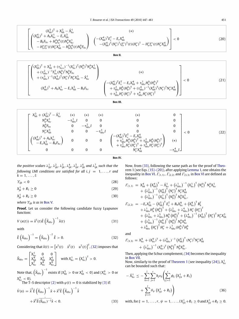
the positive scalars λ1ijk, λ2ijk, λ

3ijk, λ

4ijk, λ

5ijk, λ

6ijk and λ

7ijk such that the

following LMI conditions are satisfied for all i, j = 1, . . . , r andk = 1, . . . , l:

Υijk < 0 (28)

X1jk + R1 ≥ 0 (29)

X1jk + R2 ≥ 0 (30)

where Υijk is as in Box V.

Proof. Let us consider the following candidate fuzzy Lyapunovfunction:

V (x(t)) = xT(t)E(Xhhv

)−1x(t) (31)

with

E(Xhhv

)−1=

(Xhhv

)−TE > 0. (32)

Considering that x(t) =[xT(t) xT(t) uT(t)

]T, (32) imposes thatXhhv =

X1hv 0 0X4hh X5hh X6hhX7hv X8hv X9hv

with X1hv =(X1hv)T> 0.

Note that,(Xhhv

)−1exists if (X5hh > 0 or X

5hh < 0) and (X

9hv > 0 or

X9hv < 0).The T–S descriptor (2) with ϕ(t) = 0 is stabilized by (3) if:

V (x) = ˙xTE(Xhhv

)−1x+ xTE

(Xhhv

)−1˙x

+ xTE˙

(Xhhv)−1x < 0. (33)

Now, from (33), following the same path as for the proof of Theo-rem 1 (see Eqs. (15)–(20)), after applying Lemma 1, one obtains theinequality in Box VI. Γ(1,1),Γ(2,2) and Γ(3,3) in Box VI are defined asfollows:

Γ(1,1) = X4hh +(X4hh)T− X1hv +

(λ1hhv

)−1 (X1hv)T (Nha)TNhaX

1hv

+(λ2hhv

)−1 (X4hh)T (Nve)T Nve X4hh

+(λ3hhv

)−1 (X7hv)T (Nhb)TNhbX

7hv,

Γ(2,2) = −EvX5hh −(X5hh)TETv + BhX

8hv +

(X8hv)TBTh

+ λ1hhvHha

(Hha)T+(λ2hhv + λ

4hhv

)Hve(Hve)T

+(λ3hhv + λ

5hhv

)Hhb(Hhb)T+(λ4hhv

)−1 (X5hh)T (Nve)T Nve X5hh

+(λ5hhv

)−1 (X8hv)T (Nhb)TNhbX

8hv

+ λ6hhv(Hve)T Hve + λ7hhv(Hhb )THhb

and

Γ(3,3) = X9hv + (X9hv)T+ (λ6hhv)

−1 (X6hh)T (Nve )TNve X6hh+(λ7hhv

)−1(X9hv)

T (Nhb )T NhbX9hv.Then, applying the Schur complement, (34) becomes the inequalityin Box VII.Now, similarly to the proof of Theorem 1 (see inequality (24)), X1hvcan be bounded such that:

− X1hv ≤ −l∑k=1

r∑j=1

hjvk

(r∑ξ=1

φξ(X1ξk + R1

)+

l∑ψ=1

θψ(X1jψ + R2

))(36)

with, for ξ = 1, . . . , r, ψ = 1, . . . , l X1ξk+R1 ≥ 0 and X1jψ+R2 ≥ 0.

452 T. Bouarar et al. / ISA Transactions 49 (2010) 447–461

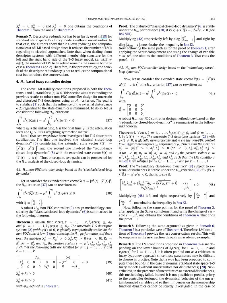
Υijk =

Ξ(1,1)ijk (∗) (∗) (∗) (∗) 0 0 0 0 0

N iaX1jk −λ1ijkI 0 0 0 0 0 0 0 0

NkeX4ij 0 −λ2ijkI 0 0 0 0 0 0 0

N ibX7jk 0 0 −λ3ijkI 0 0 0 0 0 0

Ξ(5,1)ijk 0 0 0 Ξ

(5,5)ijk (∗) (∗) (∗) 0 0

0 0 0 0 NkeX5ij −λ

4ijkI 0 0 0 0

0 0 0 0 N ibX8jk 0 −λ5ijkI 0 0 0

Ξ(8,1)ijk 0 0 0 Ξ

(8,5)ijk 0 0 X9jk + (X

9jk)T (∗) (∗)

0 0 0 0 0 0 0 NkeX6ij −λ6ijkI 0

0 0 0 0 0 0 0 N ibX9jk 0 −λ7ijkI

Ξ(1,1)ijk = X4ij + (X

4ij )T−

(r∑ξ=1

φξ (X1ξk + R1)+l∑

ψ=1

θψ (X1jψ + R2)

), Ξ

(8,1)ijk = (X6ij )

T+ Fik + X7jk,

Ξ(5,1)ijk = AiX1jk − EkX

4ij + (X

5ij )T+ BiX7jk, Ξ

(8,5)ijk = −(X6ij )

TETk + (X9jk)TBTi + X

8jk and

Ξ(5,5)ijk = −EkX5ij − (X

5ij )TETk + BiX

8jk + (X

8jk)TBTi + λ

1ijkH

ia(H

ia)T+ (λ2ijk + λ

4ijk)H

ke (H

ke )T

+ (λ3ijk + λ5ijk)H

ib(H

ib)T+ λ6ijk(H

ke )THke + λ

7ijk(H

ib)TH ib .

Box V.

4)

Γ(1,1) (∗) (∗)

AhX1hv − EvX4hh + (X

5hh)T+ BhX7hv Γ(2,2) (∗)

(X6hh)T+ Fhv + X7hv −

(X6hh)TETv + (X

9hv)TBTh + X

8hv Γ(3,3)

< 0 (3

Box VI.

5)

Θ(1,1)hhv (∗) (∗) (∗) (∗) 0 0 0 0 0NhaX

1hv −λ

1hhv I 0 0 0 0 0 0 0 0

Nve X4hh 0 −λ2hhv I 0 0 0 0 0 0 0

NhbX7hv 0 0 −λ3hhv I 0 0 0 0 0 0

Θ(5,1)hhv 0 0 0 Θ

(5,5)hhv (∗) (∗) (∗) 0 0

0 0 0 0 Nve X5hh −λ

4hhv I 0 0 0 0

0 0 0 0 NhbX8hv 0 −λ5hhv I 0 0 0

Θ(8,1)hhv 0 0 0 Θ

(8,5)hhv 0 0 X9hv + (X

9hv)T (∗) (∗)

0 0 0 0 0 0 0 Nve X6hh −λ6hhv I 0

0 0 0 0 0 0 0 NhbX9hv 0 −λ7hhv I

< 0 (3

with Θ(1,1)hhv = X

4hh +

(X4hh)T− X1hv,Θ

(5,1)hhv = AhX

1hv − EvX

4hh +

(X5hh)T+ BhX7hv,Θ

(8,1)hhv = (X

6hh)T+ Fhv + X7hv,Θ

(8,5)hhv = −(X

6hh)TETv +(

X9hv)T BTh + X8hv and Θ(5,5)

hhv = −EvX5hh −

(X5hh)T ETv + BhX8hv + (X8hv)T BTh + λ1hhvHha (Hha )T + λ7hhv (Hhb )T Hhb + (λ2hhv + λ4hhv)Hve (Hve )T +(

λ3hhv + λ5hhv

)Hhb(Hhb)T+ λ6hhv

(Hve)T Hve

Box VII.

Thus, considering (35) and (36), the T–S descriptor (2) withϕ(t) = 0 is stabilized by (3) if the LMI conditions of Theorem 2hold. That ends the proof.

Remark 6. To ensure the stability of the considered closed-loopdynamics, one has to check the existence of

Xhhv =[X1hv 0X3hh X4hh

]in Theorem 1 or

Xhhv =

X1hv 0 0X4hh X5hh X6hhX7hv X8hv X9hv

in Theorem 2. Note that the ‘‘redundancy closed-loop dynamics’’approach is introducing some additional slack decision variablesleading to reduce the conservatism of LMI conditions rather than‘‘classical closed-loop dynamics’’ approach. Moreover, it can beeasily shown that the ‘‘classical closed-loop dynamics’’ approachis a particular case of the ‘‘redundancy closed-loop dynamics’’one. Indeed, according to the fuzzy Lyapunov function (31) andits symmetric condition (32), the matrices X4ij , X

5ij , X

6ij , X

7jk, X

8jk and

X9jk, for i, j = 1, 2, . . . , r and k = 1, 2, . . . , l, are slack (free ofchoice) decision variables. Indeed, the only necessary condition for(31) to be a Lyapunov candidate function is X1jk = (X1jk)

T > 0 forj = 1, 2, . . . , r and k = 1, 2, . . . , l. Thus, replacing the matricesX4ij , X

5ij and X

7jk respectively by X

3ij , X

4ij and −Fjk, then considering

T. Bouarar et al. / ISA Transactions 49 (2010) 447–461 453

X6ij = 0, X8jk = 0 and X9jk = 0, one obtains the conditions ofTheorem 1 from the ones of Theorem 2.

Remark 7. Descriptor redundancy has been firstly used in [39] forstandard state space T–S fuzzy models without uncertainties. Inthat case, the authors show that it allows reducing the computa-tional cost of LMI based design since it reduces the number of LMIsregarding to classical approaches. Note that, when dealing aboutdescriptor systems with different membership structure for theleft and the right hand side of the T–S fuzzy model, i.e. vi(z) 6=hi(z), the number of LMI to be solved remains the same in both thecases (Theorems 1 and2). Therefore, in the present study, the bene-fit of the descriptor redundancy is not to reduce the computationalcost but to reduce the conservatism.

4. H∞ based fuzzy controller design

The above LMI stability conditions, proposed in both the Theo-rems 1 and 2, stand forϕ(t) = 0. This section aims at extending theprevious results to robust non-PDC controller design for uncertainand disturbed T–S descriptors using an H∞ criterion. The goal isto stabilize (1) such that the influence of the external disturbanceϕ(t) regarding to the state dynamics is minimized. To do so, let usconsider the following H∞ criterion:∫ tf

t0xT(t)Qx(t)− µ2

∫ tf

t0ϕT(t)ϕ(t) ≤ 0 (37)

where t0 is the initial time, tf is the final time, µ is the attenuationlevel and Q > 0 is a weighting symmetric matrix.Recall that twoways have been investigated for T–S descriptors

stabilization. The first one involved the ‘‘classical closed-loopdynamics’’ (6) considering the extended state vector x(t) =[xT(t) xT(t)

]T and the second one involved the ‘‘redundancyclosed-loop dynamics’’ (8) with the extended state vector x(t) =[xT(t) uT(t)

]T. Thus, once again, two paths can be prospected forthe H∞ analysis of the closed-loop dynamics.

4.1. H∞ non-PDC controller design based on the ‘‘classical closed-loopdynamics’’

Let us consider the extended state vector x(t) = [xT(t) xT(t)]T,the H∞ criterion (37) can be rewritten as:∫ tf

t0xT(t)Qx(t)− µ2

∫ tf

t0ϕT(t)ϕ(t) ≤ 0 (38)

with Q =[Q 00 0

].

A robust H∞ non-PDC controller (3) design methodology con-sidering the ‘‘classical closed-loop dynamics’’ (6) is summarized inthe following theorem.

Theorem 3. Assume that, ∀ z(t), ξ = 1, . . . , r, hξ (z(t)) ≥ φξand ψ = 1, . . . , l, vψ (z(t)) ≥ θψ . The uncertain T–S descriptorsystems (2) (with ϕ(t) 6= 0) is globally asymptotically stable via thenon-PDC control law (3) guaranteeing the H∞ performanceµ, if thereexist the matrices X1jk = X

1jkT> 0, X3ij , X

4ij > 0 (or < 0), R1 =

RT1, R2 = RT2, and Fjk, the positive scalars ε = µ2, τ 1ijk, τ

2ijk, τ

3ijk, τ

4ijk

such that the following LMIs are satisfied for all i, j = 1, . . . , r andk = 1, . . . , l: Φijk (∗)

X1jk 0 0 0 0 00 0 0 0 W Ti 0

−Q−1 00 −εI

< 0 (39)

X1jk + R1 ≥ 0 (40)

X1jk + R2 ≥ 0 (41)

withΦijk defined in Theorem 1.

Proof. The disturbed ‘‘classical closed-loop dynamics’’ (6) is stableunder the H∞ performance (38) if V (x)+ xTQx− µ2ϕTϕ < 0 (seeBox VIII).Multiplying (42) respectively left by diag

[XThhv I

]and right by

diag[Xhhv I

], one obtains the inequality in Box IX.

Now, following the same path as for the proof of Theorem 1, afterapplying the Schur complement and using the change of variableε = µ2, one obtains the conditions of Theorem 3. That ends theproof.

4.2. H∞ non-PDC controller design based on the ‘‘redundancy closed-loop dynamics’’

Now, let us consider the extended state vector x(t) =[xT(t)

xT(t) uT(t)]T, the H∞ criterion (37) can be rewritten as:∫ tf

t0xT(t)Q x(t)− µ2

∫ tf

t0ϕT(t)ϕ(t) ≤ 0 (44)

with

Q =

[Q 0 00 0 00 0 0

].

A robust H∞ non-PDC controller designmethodology based on the‘‘redundancy closed-loop dynamics’’ is summarized in the follow-ing theorem.

Theorem 4. ∀ z(t), ξ = 1, . . . , r, hξ (z(t)) ≥ φξ and ψ = 1, . . . ,l, vψ (z(t)) ≥ θψ . The uncertain T–S descriptor systems (2) (withϕ(t) 6= 0) is globally asymptotically stable via the non-PDC controllaw (3) guaranteeing theH∞ performanceµ, if there exist thematricesX1jk = (X1jk)

T > 0, X4ij , X5ij > 0 (or < 0), X6ij , X

7jk, X

8jk, X

9jk >

0 (or < 0), R1 = RT1, R2 = RT2 and Fik the positive scalars ε =

µ2, λ1ijk, λ2ijk, λ

3ijk, λ

4ijk, λ

5ijk, λ

6ijk and λ

7ijk such that the LMI conditions

in Box X are satisfied for all i, j = 1, . . . , r and for k = 1, . . . , l.Proof. The ‘‘redundancy closed-loop dynamics’’ (8) subject to ex-ternal disturbances is stable under the H∞criterion (38) if V (x) +xTQ x− µ2ϕTϕ < 0, that is to say if:[AThv X

−1hhv + (X

−1hhv)

TAhv + E˙

(Xhhv)−1 + Q (∗)

W Th (Xhhv)−1

−µ2I

]< 0. (48)

Multiplying (48) left and right respectively by[XThhv 00 I

]and[

Xhhv 00 I

], one obtains the inequality in Box XI.

Now, following the same path as for the proof of Theorem 2,after applying the Schur complement and using the change of vari-able ε = µ2, one obtains the conditions of Theorem 4. That endsthe proof.

Remark 8. Following the same argument as given in Remark 6,Theorem 3 is a particular case of Theorem 4. Therefore, LMI condi-tions of Theorem 4 provide the less conservatism results. This willbe emphasis in the next section through an academic example.

Remark 9. The LMI conditions proposed in Theorems 1–4 are de-pending on the lower bounds of hi(z(t)) for i = 1, . . . , r andvk(z(t)) for k = 1, . . . , l. It is often pointed out as a criticism tofuzzy Lyapunov approach since these parameters may be difficultto choose in practice. Note that a way has been proposed to com-pute these bounds in the case of nominal standard state space T–Sfuzzy models (without uncertainties nor disturbances) [20]. Nev-ertheless, in the presence of uncertainties or external disturbances,this methodology failed. Indeed, it is not possible to predict, prioryto the controller designed, the dynamical behavior of the uncer-tain bounded variables and so their influences on the membershipfunction dynamics cannot be strictly investigated. In the case of

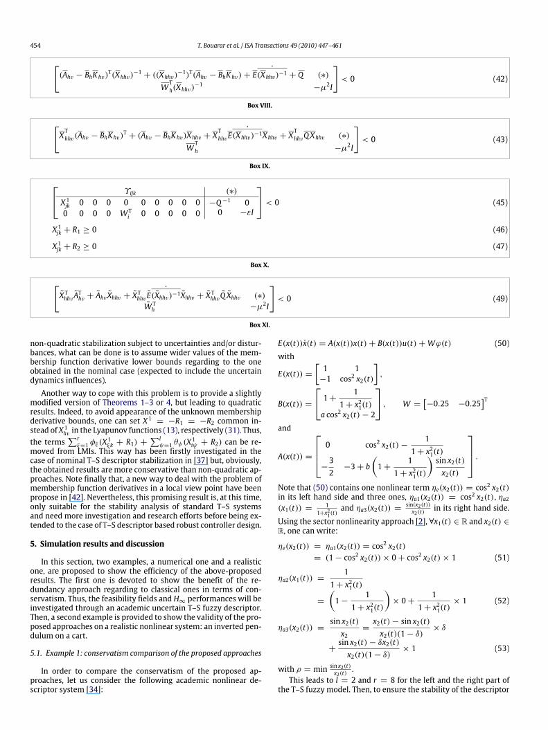
454 T. Bouarar et al. / ISA Transactions 49 (2010) 447–461

2)

[(Ahv − BhK hv)T(Xhhv)−1 + ((Xhhv)−1)T(Ahv − BhK hv)+ E

˙(Xhhv)−1 + Q (∗)

WTh(Xhhv)

−1−µ2I

]< 0 (4

Box VIII.

3)

[XThhv(Ahv − BhK hv)

T+ (Ahv − BhK hv)Xhhv + X

ThhvE

˙(Xhhv)−1Xhhv + X

ThhvQXhhv (∗)

WTh −µ2I

]< 0 (4

Box IX.

5)

6)

7)

Υijk (∗)

X1jk 0 0 0 0 0 0 0 0 00 0 0 0 W Ti 0 0 0 0 0

−Q−1 00 −εI

< 0 (4

X1jk + R1 ≥ 0 (4

X1jk + R2 ≥ 0 (4

Box X.

9)

[XThhv A

Thv + Ahv Xhhv + X

Thhv E

˙(Xhhv)−1Xhhv + XThhvQ Xhhv (∗)

W Th −µ2I

]< 0 (4

Box XI.

non-quadratic stabilization subject to uncertainties and/or distur-bances, what can be done is to assume wider values of the mem-bership function derivative lower bounds regarding to the oneobtained in the nominal case (expected to include the uncertaindynamics influences).Another way to cope with this problem is to provide a slightly

modified version of Theorems 1–3 or 4, but leading to quadraticresults. Indeed, to avoid appearance of the unknown membershipderivative bounds, one can set X1 = −R1 = −R2 common in-stead of X1hv in the Lyapunov functions (13), respectively (31). Thus,the terms

∑rξ=1 φξ (X

1ξk + R1) +

∑lψ=1 θψ (X

1iψ + R2) can be re-

moved from LMIs. This way has been firstly investigated in thecase of nominal T–S descriptor stabilization in [37] but, obviously,the obtained results are more conservative than non-quadratic ap-proaches. Note finally that, a new way to deal with the problem ofmembership function derivatives in a local view point have beenpropose in [42]. Nevertheless, this promising result is, at this time,only suitable for the stability analysis of standard T–S systemsand need more investigation and research efforts before being ex-tended to the case of T–S descriptor based robust controller design.

5. Simulation results and discussion

In this section, two examples, a numerical one and a realisticone, are proposed to show the efficiency of the above-proposedresults. The first one is devoted to show the benefit of the re-dundancy approach regarding to classical ones in terms of con-servatism. Thus, the feasibility fields and H∞ performances will beinvestigated through an academic uncertain T–S fuzzy descriptor.Then, a second example is provided to show the validity of the pro-posed approaches on a realistic nonlinear system: an inverted pen-dulum on a cart.

5.1. Example 1: conservatism comparison of the proposed approaches

In order to compare the conservatism of the proposed ap-proaches, let us consider the following academic nonlinear de-scriptor system [34]:

E(x(t))x(t) = A(x(t))x(t)+ B(x(t))u(t)+Wϕ(t) (50)

with

E(x(t)) =[1 1−1 cos2 x2(t)

],

B(x(t)) =

1+ 11+ x21(t)

a cos2 x2(t)− 2

, W =[−0.25 −0.25

]Tand

A(x(t)) =

0 cos2 x2(t)−1

1+ x21(t)

−32−3+ b

(1+

11+ x21(t)

)sin x2(t)x2(t)

.Note that (50) contains one nonlinear term ηe(x2(t)) = cos2 x2(t)in its left hand side and three ones, ηa1(x2(t)) = cos2 x2(t), ηa2(x1(t)) = 1

1+x21(t)and ηa3(x2(t)) =

sin(x2(t))x2(t)

in its right hand side.

Using the sector nonlinearity approach [2], ∀x1(t) ∈ R and x2(t) ∈R, one can write:

ηe(x2(t)) = ηa1(x2(t)) = cos2 x2(t)= (1− cos2 x2(t))× 0+ cos2 x2(t)× 1 (51)

ηa2(x1(t)) =1

1+ x21(t)

=

(1−

11+ x21(t)

)× 0+

11+ x21(t)

× 1 (52)

ηa3(x2(t)) =sin x2(t)x2

=x2(t)− sin x2(t)x2(t)(1− δ)

× δ

+sin x2(t)− δx2(t)x2(t)(1− δ)

× 1 (53)

with ρ = min sin x2(t)x2(t).

This leads to l = 2 and r = 8 for the left and the right part ofthe T–S fuzzy model. Then, to ensure the stability of the descriptor

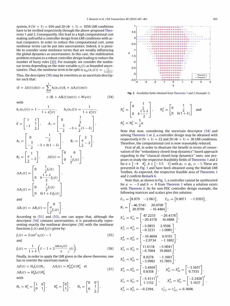
T. Bouarar et al. / ISA Transactions 49 (2010) 447–461 455

system, lr(5r + 1) = 656 and 2lr(4r + 1) = 1056 LMI conditionshave to be verified respectively through the above-proposed Theo-rems 1 and 2. Consequently, this lead to a high computational costmaking unfruitful a controller design from LMI conditions with ac-tual computers. In order to reduce this computational cost, somenonlinear terms can be put into uncertainties. Indeed, it is possi-ble to consider some nonlinear terms that are weakly influencingthe global dynamics as uncertainties. In this case, the stabilizationproblem remains to a robust controller design leading to reduce thenumber of fuzzy rules [35]. For example, we consider the nonlin-ear terms depending on the state variable x2(t) as bounded uncer-tainties. Thus, the nonlinear term to be split is ηa2(x1(t)) = 1

1+x21(t).

Thus, the descriptor (50)may be rewritten as an uncertain descrip-tor such that:

(E +1E(t))x(t) =2∑i=1

hi(x1)((Ai +1Ai(t))x(t)

+ (Bi +1Bi(t))u(t))+Wϕ(t) (54)with

h1(x1(t)) = 1−1

1+ x21(t), h2(x1(t)) =

11+ x21(t)

,

E =

[1 1

−112

], A1 =

0 12

−32−3+

b2(1− δ)

,

A2 =

0 −12

−32−3+ b(1− δ)

, B1 =

[2a2− 2

],

B2 =

[1a2− 2

], 1E(t) =

0 0

012f1(t)

,1A1(t) =

0 12f1(t)

0 b1+ δ2f2(t)

,1A2(t) =

0 12f1(t)

0 b(1+ δ)f2(t)

and

1B1(t) = 1B2(t) =

[0

a2f1(t)

].

According to (51) and (53), one can argue that, although thedescriptor (54) contains uncertainties, it is paradoxically repre-senting exactly the nonlinear descriptor (50) with the nonlinearfunctions f1(t) and f2(t) given by:

f1(t) = 2 cos2 x2(t)− 1 (55)and

f2(t) =11+ δ

(δ − 1+ 2

sin x2(t)x 2

(t)). (56)

Finally, in order to apply the LMI given in the above theorems, onehas to rewrite the uncertain matrix

1E(t) = Hefe(t)Ne, 1Ai(t) = H iafia(t)N

ia et

1Bi(t) = H ibfb(t)Nib

(57)

with

He = H ia =[1 00 1

], H ib =

[01

], Ne =

[0 0

012

],

1

0.5

0

-0.5

-1

-1.5

b

-2

-2.5

-3

-3.5-4 -3 -2 -1 0

a1 2 3 4

Theorem 2Theorem 1

Fig. 1. Feasibility fields obtained from Theorems 1 and 2 (Example 1).

N1a =

0 12

0 b1+ δ2

, N2a =

[0

12

0 b(1+ δ)

]and

N1b = N2b =

12a.

Note that now, considering the uncertain descriptor (54) andsolving Theorem 1 or 2, a controller design may be obtained withrespectively lr(5r + 1) = 22 and 2lr(4r + 1) = 36 LMI conditions.Therefore, the computational cost is now reasonably reduced.First of all, in order to illustrate the benefit in terms of conser-

vatism of the ‘‘redundancy closed-loop dynamics’’ based approachregarding to the ‘‘classical closed-loop dynamics’’ ones, one pro-poses to study the respective feasibility fields of Theorems 1 and 2for a ∈

[−4 4

], b ∈

[−3.5 1

]with φ1 = φ2 = −1. These are

presented in Fig. 1 and have been obtained using the Matlab LMIToolbox. As expected, the respective feasible area of Theorems 1and 2 confirm Remark 6.Note that, as shown in Fig. 1, a controller cannot be synthesized

for a = −3 and b = 0 from Theorem 1 when a solution existswith Theorem 2. As for non-PDC controller design example, thefollowing matrices and scalars give this solution:

F11 =[8.879 −2.061

], F21 =

[9.0071 −1.9393

],

R1 =[−46.5741 20.070920.0709 −16.4484

],

X111 = X121 =

[47.2233 −20.4178−20.4178 16.6888

],

X411 = X412 =

[−5.0855 2.9506−0.3231 −1.0085

],

X421 = X422 =

[−10.4604 6.9191−2.9734 −1.1802

],

X511 = X512 =

[11.6118 −5.9041−6.7604 19.8665

],

X521 = X522 =

[8.0278 −1.1601−3.9982 15.7893

],

X611 = X612 =

[−3.45690.8358

], X621 = X

622 =

[−3.56570.7555

],

X711 = X721 =

[−5.41111.1152

]T, X811 = X

821 =

[−2.24283.1637

]T,

X911 = X921 = −0.2394, τ 1111 = τ

1121 = 0.3608,

456 T. Bouarar et al. / ISA Transactions 49 (2010) 447–461

0 1 2 3 4 5 6 7 8 9 10

0 1 2 3 4 5 6 7 8 9 10

0 1 2 3 4 5Time

6 7 8 9 10

0

0.5

u(t)

1

x 2(t

)

-2

-1

0

1

-4

-2

x 1(t

)

0

Fig. 2. Evolution of the state vector (without external disturbance) and the controlsignal (Example 1).

τ 1211 = τ1221 = 0.9369, τ 2111 = τ

2121 = 0.976,

τ 2211 = τ2221 = 1.7785, τ 3111 = τ

3121 = 10.5924,

τ 3211 = τ3221 = 4.6813, τ 4111 = τ

4121 = 4.1892,

τ 4211 = τ4221 = 4.7994, τ 5111 = τ

5121 = 6.5847,

τ 5211 = τ5221 = 3.7544, τ 6111 = τ

6121 = 0.935,

τ 6211 = τ6221 = 1.4624, τ 7111 = τ

7121 = 0.749 and

τ 7211 = τ7221 = 1.1434.

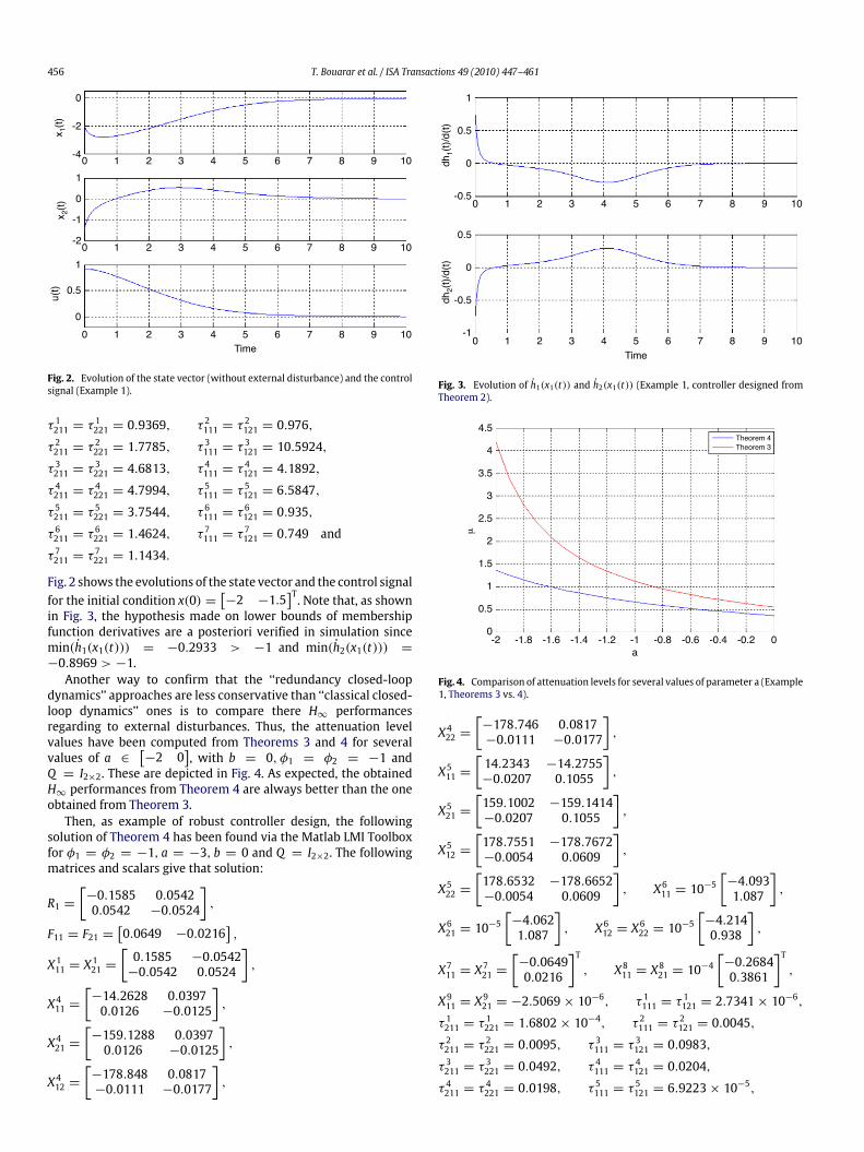
Fig. 2 shows the evolutions of the state vector and the control signalfor the initial condition x(0) =

[−2 −1.5

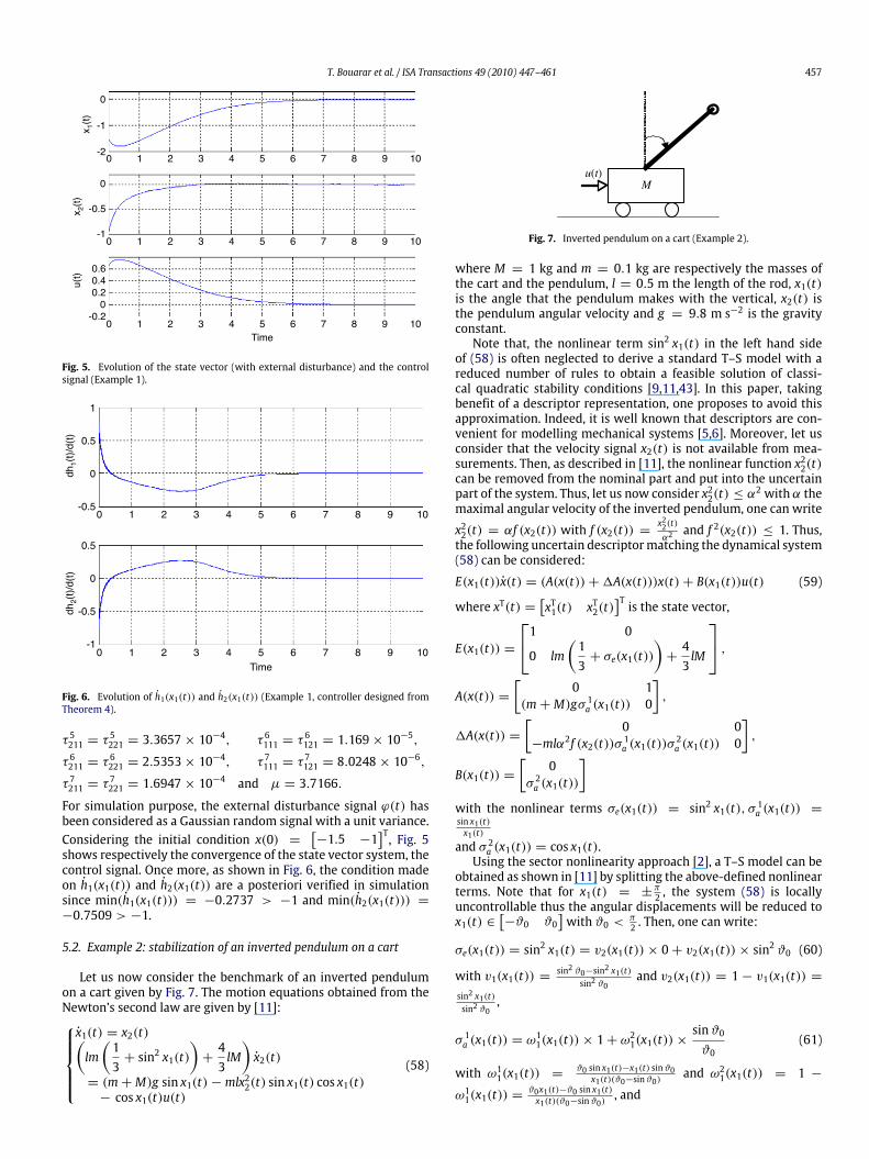
]T. Note that, as shownin Fig. 3, the hypothesis made on lower bounds of membershipfunction derivatives are a posteriori verified in simulation sincemin(h1(x1(t))) = −0.2933 > −1 and min(h2(x1(t))) =−0.8969 > −1.Another way to confirm that the ‘‘redundancy closed-loop

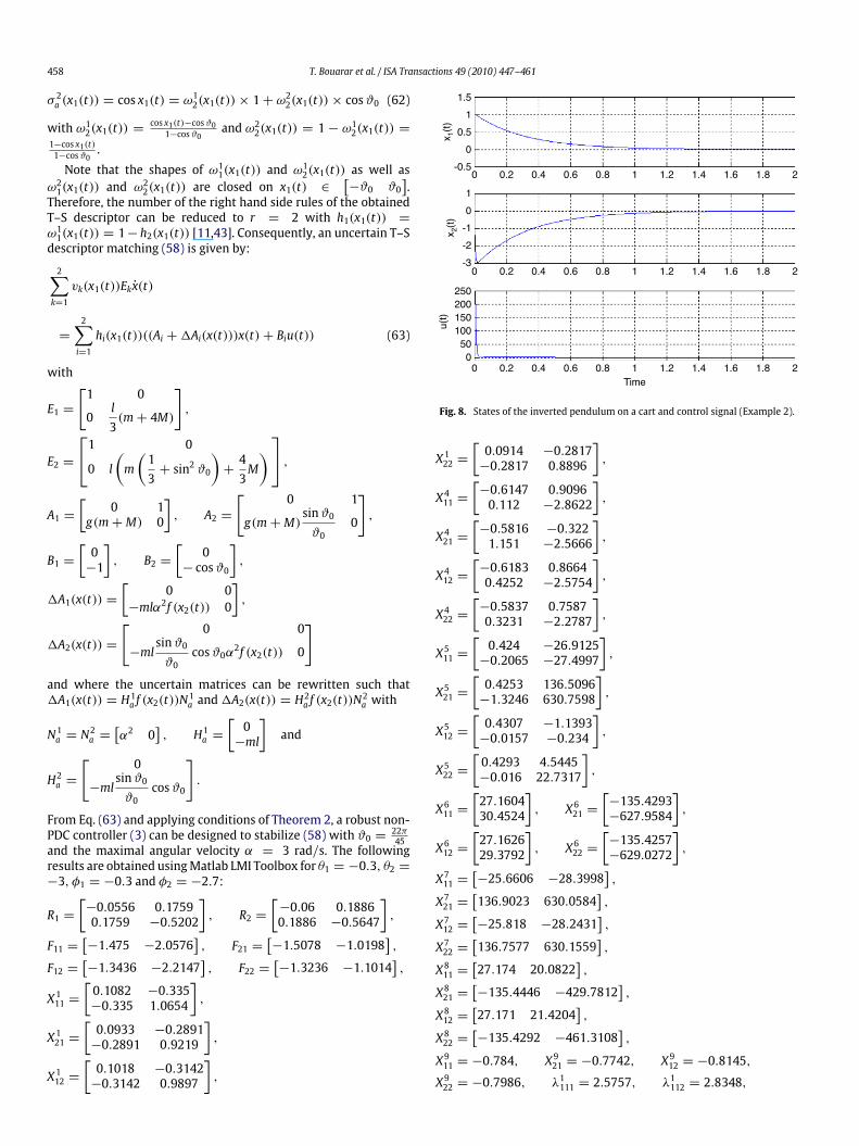
dynamics’’ approaches are less conservative than ‘‘classical closed-loop dynamics’’ ones is to compare there H∞ performancesregarding to external disturbances. Thus, the attenuation levelvalues have been computed from Theorems 3 and 4 for severalvalues of a ∈

[−2 0

], with b = 0, φ1 = φ2 = −1 and

Q = I2×2. These are depicted in Fig. 4. As expected, the obtainedH∞ performances from Theorem 4 are always better than the oneobtained from Theorem 3.Then, as example of robust controller design, the following

solution of Theorem 4 has been found via the Matlab LMI Toolboxfor φ1 = φ2 = −1, a = −3, b = 0 and Q = I2×2. The followingmatrices and scalars give that solution:

R1 =[−0.1585 0.05420.0542 −0.0524

],

F11 = F21 =[0.0649 −0.0216

],

X111 = X121 =

[0.1585 −0.0542−0.0542 0.0524

],

X411 =[−14.2628 0.03970.0126 −0.0125

],

X421 =[−159.1288 0.03970.0126 −0.0125

],

X412 =[−178.848 0.0817−0.0111 −0.0177

],

1

0.5

0dh1(

t)/d

(t)

-0.5

0.5

0

-0.5dh2(

t)/d

(t)

-1

0 1 2 3 4 5 6 7 8 9 10

0 1 2 3 4 5Time

6 7 8 9 10

Fig. 3. Evolution of h1(x1(t)) and h2(x1(t)) (Example 1, controller designed fromTheorem 2).

-2 -1.8 -1.6 -1.4 -1.2 -1a

-0.8 -0.6 -0.4 -0.2 00

0.5

1

1.5

2

µ

2.5

3

3.5

4

4.5Theorem 4Theorem 3

Fig. 4. Comparison of attenuation levels for several values of parameter a (Example1, Theorems 3 vs. 4).

X422 =[−178.746 0.0817−0.0111 −0.0177

],

X511 =[14.2343 −14.2755−0.0207 0.1055

],

X521 =[159.1002 −159.1414−0.0207 0.1055

],

X512 =[178.7551 −178.7672−0.0054 0.0609

],

X522 =[178.6532 −178.6652−0.0054 0.0609

], X611 = 10

−5[−4.0931.087

],

X621 = 10−5[−4.0621.087

], X612 = X

622 = 10

−5[−4.2140.938

],

X711 = X721 =

[−0.06490.0216

]T, X811 = X

821 = 10

−4[−0.26840.3861

]T,

X911 = X921 = −2.5069× 10

−6, τ 1111 = τ1121 = 2.7341× 10

−6,

τ 1211 = τ1221 = 1.6802× 10

−4, τ 2111 = τ2121 = 0.0045,

τ 2211 = τ2221 = 0.0095, τ 3111 = τ

3121 = 0.0983,

τ 3211 = τ3221 = 0.0492, τ 4111 = τ

4121 = 0.0204,

τ 4211 = τ4221 = 0.0198, τ 5111 = τ

5121 = 6.9223× 10

−5,

T. Bouarar et al. / ISA Transactions 49 (2010) 447–461 457

0

-1x 1(t

)

-2

x 2(t

)

0

-0.5

-1

u(t) 0.4

0.6

00.2

-0.20 1 2 3 4 5

Time6 7 8 9 10

0 1 2 3 4 5 6 7 8 9 10

0 1 2 3 4 5 6 7 8 9 10

Fig. 5. Evolution of the state vector (with external disturbance) and the controlsignal (Example 1).

1

0.5

0dh1(

t)/d

(t)

-0.5

0.5

0

-0.5dh2(

t)/d

(t)

-1

0 1 2 3 4 5 6 7 8 9 10

0 1 2 3 4 5Time

6 7 8 9 10

Fig. 6. Evolution of h1(x1(t)) and h2(x1(t)) (Example 1, controller designed fromTheorem 4).

τ 5211 = τ5221 = 3.3657× 10

−4, τ 6111 = τ6121 = 1.169× 10

−5,

τ 6211 = τ6221 = 2.5353× 10

−4, τ 7111 = τ7121 = 8.0248× 10

−6,

τ 7211 = τ7221 = 1.6947× 10

−4 and µ = 3.7166.

For simulation purpose, the external disturbance signal ϕ(t) hasbeen considered as a Gaussian random signal with a unit variance.Considering the initial condition x(0) =

[−1.5 −1

]T, Fig. 5shows respectively the convergence of the state vector system, thecontrol signal. Once more, as shown in Fig. 6, the condition madeon h1(x1(t)) and h2(x1(t)) are a posteriori verified in simulationsince min(h1(x1(t))) = −0.2737 > −1 and min(h2(x1(t))) =−0.7509 > −1.

5.2. Example 2: stabilization of an inverted pendulum on a cart

Let us now consider the benchmark of an inverted pendulumon a cart given by Fig. 7. The motion equations obtained from theNewton’s second law are given by [11]:x1(t) = x2(t)(lm(13+ sin2 x1(t)

)+43lM)x2(t)

= (m+M)g sin x1(t)−mlx22(t) sin x1(t) cos x1(t)− cos x1(t)u(t)

(58)

u(t)M

Fig. 7. Inverted pendulum on a cart (Example 2).

where M = 1 kg and m = 0.1 kg are respectively the masses ofthe cart and the pendulum, l = 0.5 m the length of the rod, x1(t)is the angle that the pendulum makes with the vertical, x2(t) isthe pendulum angular velocity and g = 9.8 m s−2 is the gravityconstant.Note that, the nonlinear term sin2 x1(t) in the left hand side

of (58) is often neglected to derive a standard T–S model with areduced number of rules to obtain a feasible solution of classi-cal quadratic stability conditions [9,11,43]. In this paper, takingbenefit of a descriptor representation, one proposes to avoid thisapproximation. Indeed, it is well known that descriptors are con-venient for modelling mechanical systems [5,6]. Moreover, let usconsider that the velocity signal x2(t) is not available from mea-surements. Then, as described in [11], the nonlinear function x22(t)can be removed from the nominal part and put into the uncertainpart of the system. Thus, let us now consider x22(t) ≤ α

2 with α themaximal angular velocity of the inverted pendulum, one can write

x22(t) = αf (x2(t)) with f (x2(t)) =x22(t)α2and f 2(x2(t)) ≤ 1. Thus,

the following uncertain descriptormatching the dynamical system(58) can be considered:

E(x1(t))x(t) = (A(x(t))+1A(x(t)))x(t)+ B(x1(t))u(t) (59)

where xT(t) =[xT1(t) xT2(t)

]T is the state vector,E(x1(t)) =

1 0

0 lm(13+ σe(x1(t))

)+43lM

,A(x(t)) =

[0 1

(m+M)gσ 1a (x1(t)) 0

],

1A(x(t)) =[

0 0−mlα2f (x2(t))σ 1a (x1(t))σ

2a (x1(t)) 0

],

B(x1(t)) =[

0σ 2a (x1(t))

]with the nonlinear terms σe(x1(t)) = sin2 x1(t), σ 1a (x1(t)) =sin x1(t)x1(t)

and σ 2a (x1(t)) = cos x1(t).Using the sector nonlinearity approach [2], a T–S model can be

obtained as shown in [11] by splitting the above-defined nonlinearterms. Note that for x1(t) = ±π

2 , the system (58) is locallyuncontrollable thus the angular displacements will be reduced tox1(t) ∈

[−ϑ0 ϑ0

]with ϑ0 < π

2 . Then, one can write:

σe(x1(t)) = sin2 x1(t) = v2(x1(t))× 0+ v2(x1(t))× sin2 ϑ0 (60)

with v1(x1(t)) =sin2 ϑ0−sin2 x1(t)

sin2 ϑ0and v2(x1(t)) = 1 − v1(x1(t)) =

sin2 x1(t)sin2 ϑ0

,

σ 1a (x1(t)) = ω11(x1(t))× 1+ ω

21(x1(t))×

sinϑ0ϑ0

(61)

with ω11(x1(t)) =ϑ0 sin x1(t)−x1(t) sinϑ0x1(t)(ϑ0−sinϑ0)

and ω21(x1(t)) = 1 −

ω11(x1(t)) =ϑ0x1(t)−ϑ0 sin x1(t)x1(t)(ϑ0−sinϑ0)

, and

458 T. Bouarar et al. / ISA Transactions 49 (2010) 447–461

σ 2a (x1(t)) = cos x1(t) = ω12(x1(t))× 1+ ω

22(x1(t))× cosϑ0 (62)

with ω12(x1(t)) =cos x1(t)−cosϑ01−cosϑ0

and ω22(x1(t)) = 1 − ω12(x1(t)) =

1−cos x1(t)1−cosϑ0

.Note that the shapes of ω11(x1(t)) and ω

12(x1(t)) as well as

ω21(x1(t)) and ω22(x1(t)) are closed on x1(t) ∈

[−ϑ0 ϑ0

].

Therefore, the number of the right hand side rules of the obtainedT–S descriptor can be reduced to r = 2 with h1(x1(t)) =ω11(x1(t)) = 1− h2(x1(t)) [11,43]. Consequently, an uncertain T–Sdescriptor matching (58) is given by:

2∑k=1

vk(x1(t))Ekx(t)

=

2∑i=1

hi(x1(t))((Ai +1Ai(x(t)))x(t)+ Biu(t)) (63)

with

E1 =

[1 0

0l3(m+ 4M)

],

E2 =

1 0

0 l(m(13+ sin2 ϑ0

)+43M) ,

A1 =[

0 1g(m+M) 0

], A2 =

[ 0 1

g(m+M)sinϑ0ϑ0

0

],

B1 =[0−1

], B2 =

[0

− cosϑ0

],

1A1(x(t)) =[

0 0−mlα2f (x2(t)) 0

],

1A2(x(t)) =

[ 0 0

−mlsinϑ0ϑ0

cosϑ0α2f (x2(t)) 0

]and where the uncertain matrices can be rewritten such that1A1(x(t)) = H1a f (x2(t))N

1a and1A2(x(t)) = H

2a f (x2(t))N

2a with

N1a = N2a =

[α2 0

], H1a =

[0−ml

]and

H2a =

[ 0

−mlsinϑ0ϑ0

cosϑ0

].

From Eq. (63) and applying conditions of Theorem 2, a robust non-PDC controller (3) can be designed to stabilize (58) with ϑ0 = 22π

45and the maximal angular velocity α = 3 rad/s. The followingresults are obtained usingMatlab LMI Toolbox for θ1 = −0.3, θ2 =−3, φ1 = −0.3 and φ2 = −2.7:

R1 =[−0.0556 0.17590.1759 −0.5202

], R2 =

[−0.06 0.18860.1886 −0.5647

],

F11 =[−1.475 −2.0576

], F21 =

[−1.5078 −1.0198

],

F12 =[−1.3436 −2.2147

], F22 =

[−1.3236 −1.1014

],

X111 =[0.1082 −0.335−0.335 1.0654

],

X121 =[0.0933 −0.2891−0.2891 0.9219

],

X112 =[0.1018 −0.3142−0.3142 0.9897

],

1.5

1

0.5x 1(t

)

0

-0.5

1

0

-1x 2(t

)

-2

-3

u(t)

0 0.2 0.4 0.6 0.8 1 1.2 1.4 1.6 1.8 2

0 0.2 0.4 0.6 0.8 1 1.2 1.4 1.6 1.8 2

0 0.2 0.4 0.6 0.8 1Time

1.2 1.4 1.6 1.8 2

250200150100

050

Fig. 8. States of the inverted pendulum on a cart and control signal (Example 2).

X122 =[0.0914 −0.2817−0.2817 0.8896

],

X411 =[−0.6147 0.90960.112 −2.8622

],

X421 =[−0.5816 −0.3221.151 −2.5666

],

X412 =[−0.6183 0.86640.4252 −2.5754

],

X422 =[−0.5837 0.75870.3231 −2.2787

],

X511 =[0.424 −26.9125−0.2065 −27.4997

],

X521 =[0.4253 136.5096−1.3246 630.7598

],

X512 =[0.4307 −1.1393−0.0157 −0.234

],

X522 =[0.4293 4.5445−0.016 22.7317

],

X611 =[27.160430.4524

], X621 =

[−135.4293−627.9584

],

X612 =[27.162629.3792

], X622 =

[−135.4257−629.0272

],

X711 =[−25.6606 −28.3998

],

X721 =[136.9023 630.0584

],

X712 =[−25.818 −28.2431

],

X722 =[136.7577 630.1559

],

X811 =[27.174 20.0822

],

X821 =[−135.4446 −429.7812

],

X812 =[27.171 21.4204

],

X822 =[−135.4292 −461.3108

],

X911 = −0.784, X921 = −0.7742, X912 = −0.8145,

X922 = −0.7986, λ1111 = 2.5757, λ1112 = 2.8348,

T. Bouarar et al. / ISA Transactions 49 (2010) 447–461 459

1.5

1

0.5

dh1(

t)/d

(t)

0

-0.5

3

2

1

dv1(

t)/d

(t)

0

-1

0 0.5 1Time

1.5 2

1

0

-1

dh2(

t)/d

(t)

-2

-30 0.5 1

Time1.5 2

1

0

-1

dv2(

t)/d

(t)

-2

-30 0.5 1

Time1.5 20 0.5 1

Time1.5 2

Fig. 9. Membership function derivatives’ evolutions (Example 2).

0.2

0

-0.2x 1(t

)

-0.4

-0.60 0.2 0.4 0.6 0.8 1 1.2 1.4 1.6 1.8 2

1.5

1

0.5x 2(t

)

0

-0.50 0.2 0.4 0.6 0.8 1 1.2 1.4 1.6 1.8 2

5

0

-5u(t)

-10

-150 0.2 0.4 0.6 0.8 1 1.2 1.4 1.6 1.8 2

Time

Fig. 10. States of the externally disturbed inverted pendulum on a cart and controlsignal (Example 2).

λ1121 = 2.4544, λ1122 = 2.8265, λ1211 = 2.3822,

λ1212 = 2.5864, λ1221 = 2.2067, λ1222 = 2.5428

and finally λsijk = 1.5833 for i, j, k = 1, 2 and s = 2, . . . , 7.A simulation is proposed in Fig. 8 for the initial condition

xT(0) =[1 −1

]T. The lower bounds of the membership func-tion derivatives are shown in Fig. 9. This allows verifying the hy-pothesis made for the controller since one always has v1(x1(t)) ≥θ1, v2(x1(t)) ≥ θ2, h1(x1(t)) ≥ φ1, h2(x1(t)) ≥ φ2.Now, in order to show the benefit of the proposed H∞ robust

controller design methodology, one proposes to minimize theinfluences of external disturbances on the system (58). Therefore,the considered T–S descriptor (63) can be extended to an uncertain

and disturbed one such that:2∑k=1

vk(x1(t))Ekx(t) =2∑i=1

hi(x1(t))((Ai +1Ai(x(t)))x(t)

+ Biu(t))+Wϕ(t) (64)

whereϕ(t) is an external disturbance andW =[0.50

]is aweighting

matrix related to the transfer of the disturbance to the system’sstates.A non-PDC controller (3) is design from Theorem 4 with the

parameter ϑ0 = 22π45 , the maximal angular velocity α = 3 rad/s

and the weighting matrix Q = I2×2. The following results areobtained using Matlab LMI Toolbox for θ1 = −1.5, θ2 = −3, φ1 =−0.3 and φ2 = −1.8:

R1 =[−0.2637 0.5940.594 4.6789

], R2 =

[−0.2868 0.73540.7354 0.6298

],

F11 =[−5.5557 −697.8622

],

F21 =[−5.6152 −612.1218

],

F12 =[−4.9294 −712.552

],

F22 =[−4.8915 −617.9565

],

X111 =[0.3665 −0.9861−0.9861 4.3226

],

X121 =[0.3318 −0.9077−0.9077 3.9894

],

X112 =[0.3261 −0.8982−0.8982 3.8838

],

X122 =[0.3199 −0.8694−0.8694 3.6645

],

X411 =[−33.8138 −0.87584.5238 −164.4794

],

X421 =[−33.7267 1.83311.4872 −163.014

],

460 T. Bouarar et al. / ISA Transactions 49 (2010) 447–461

Time0 0.5 1 1.5 2

Time0 0.5 1 1.5 2

0.4

0.3

0.2

dh1(

t)/d

(t)

0.1

0

-0.1

2

1.5

1

dv1(

t)/d

(t)

0.5

0

-0.5

Time0 0.5 1 1.5 2

0.5

0

-0.5

dv2(

t)/d

(t)

-1

-1.5

-2

Time0 0.5 1 1.5 2

dh2(

t)/d

(t)

0.5

0

-0.5

-1

-1.5

Fig. 11. Membership function derivatives’ evolutions with external disturbances (Example 2).

X412 =[−33.7845 7.83−1.9401 −74.3159

],

X422 =[−33.6988 4.99960.142 −72.5163

],

X511 =[33.1228 −0.9827−3.7463 68.0491

],

X521 =[33.166 −3.615−1.2391 61.0384

],

X512 =[33.1896 −3.20864.2722 26.0719

],

X522 =[33.2178 −1.54561.7548 26.158

],

X611 =[3.2988326.9778

], X621 =

[4.5287334.366

],

X612 =[3.2983236.8412

], X622 =

[4.5382244.0597

],

X711 =[2.2926 372.9012

], X721 =

[1.0487 365.4295

],

X712 =[1.5698 383.8648

], X722 =

[0.413 376.1634

],

X811 =[3.2503 161.9123

], X821 =

[4.5588 166.2511

],

X812 =[3.2869 169.4526

], X822 =

[4.563 174.304

],

X911 = −65.8333, X921 = −65.9864, X912 = −66.5649,

X922 = −66.6869, λ1111 = 136.0795, λ1112 = 133.8833,

λ1121 = 133.8167, λ1122 = 133.4936, λ1211 = 132.6845,

λ1212 = 128.6769, λ1221 = 130.5547, λ1222 = 130.3676,λsijk = 132.4891

for i, j, k = 1, 2 and s = 2, . . . , 7, the attenuation level µ =0.8832.For simulation purpose, we choose as external disturbances

a white noise with a unit covariance, i.e. ϕ(t) = rand(1, 1),the states of the disturbed inverted pendulum on a cart and the

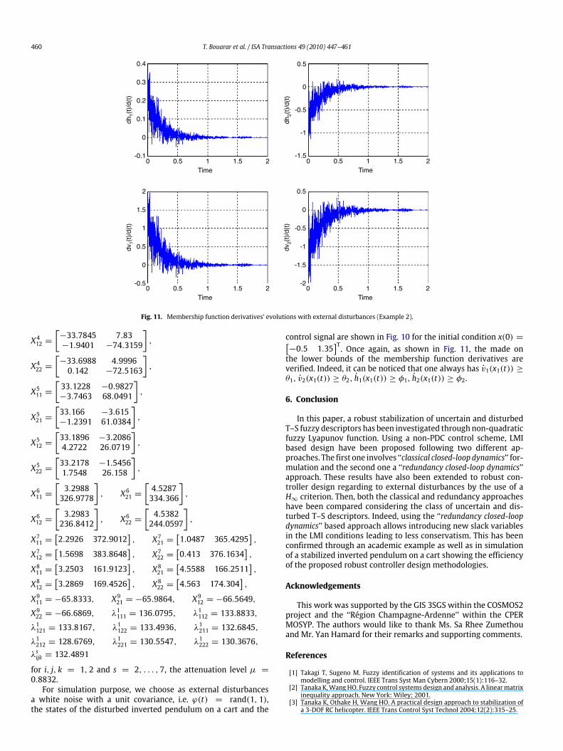
control signal are shown in Fig. 10 for the initial condition x(0) =[−0.5 1.35

]T. Once again, as shown in Fig. 11, the made onthe lower bounds of the membership function derivatives areverified. Indeed, it can be noticed that one always has v1(x1(t)) ≥θ1, v2(x1(t)) ≥ θ2, h1(x1(t)) ≥ φ1, h2(x1(t)) ≥ φ2.

6. Conclusion

In this paper, a robust stabilization of uncertain and disturbedT–S fuzzy descriptors has been investigated through non-quadraticfuzzy Lyapunov function. Using a non-PDC control scheme, LMIbased design have been proposed following two different ap-proaches. The first one involves ‘‘classical closed-loop dynamics’’ for-mulation and the second one a ‘‘redundancy closed-loop dynamics’’approach. These results have also been extended to robust con-troller design regarding to external disturbances by the use of aH∞ criterion. Then, both the classical and redundancy approacheshave been compared considering the class of uncertain and dis-turbed T–S descriptors. Indeed, using the ‘‘redundancy closed-loopdynamics’’ based approach allows introducing new slack variablesin the LMI conditions leading to less conservatism. This has beenconfirmed through an academic example as well as in simulationof a stabilized inverted pendulum on a cart showing the efficiencyof the proposed robust controller design methodologies.

Acknowledgements

This work was supported by the GIS 3SGS within the COSMOS2project and the ‘‘Région Champagne-Ardenne’’ within the CPERMOSYP. The authors would like to thank Ms. Sa Rhee Zumethouand Mr. Yan Hamard for their remarks and supporting comments.

References

[1] Takagi T, Sugeno M. Fuzzy identification of systems and its applications tomodelling and control. IEEE Trans Syst Man Cybern 2000;15(1):116–32.

[2] Tanaka K,WangHO. Fuzzy control systems design and analysis. A linearmatrixinequality approach. New York: Wiley; 2001.

[3] Tanaka K, Othake H, Wang HO. A practical design approach to stabilization ofa 3-DOF RC helicopter. IEEE Trans Control Syst Technol 2004;12(2):315–25.

T. Bouarar et al. / ISA Transactions 49 (2010) 447–461 461

[4] Khiar D, Lauber J, Floquet T, Colin G, Guerra TM, Chamaillard Y. RobustTakagi–Sugeno fuzzy control of a spark ignition engine. Control Eng Pract2007;15(12):1446–56.

[5] Guelton K, Delprat S, Guerra TM. An alternative to inverse dynamics jointtorques estimation in human stance based on a Takagi–Sugeno unknowninputs observer in the descriptor form. Control Eng Pract 2008;16(12):1414–26.

[6] Schulte H, Guelton K. Descriptor modelling towards control of a two linkpneumatic robot manipulator: a T–S multimodel approach. Nonlinear AnalHybrid Syst 2009;3(2):124–32.

[7] Chang WJ, Yeh YL, Tsai KH. Covariance control with observed-state feedbackgains for continuous nonlinear systems using T–S fuzzy models. ISA Trans2004;43(3):389–98.

[8] Wu SM, Sun CC, Chang WJ, Chung HY. T–S region-based fuzzy control withmultiple performance constraints. ISA Trans 2007;46(1):85–93.

[9] Wang HO, Tanaka K, Griffin MF. An approach to fuzzy control of nonlinearsystems: stability and the design issues. IEEE Trans Fuzzy Syst 1996;4(1):14–23.

[10] Ho HF, Wong YK, Rad AB. Adaptive fuzzy approach for a class of uncertainnonlinear systems in strict-feedback form. ISA Trans 2008;47(3):286–99.

[11] Mansouri B, Manamanni N, Guelton K, Kruszewski A, Guerra TM. Outputfeedback LMI tracking control conditions with H∞ criterion for uncertain anddisturbed T–S models. Inform Sci 2009;179(4):446–57.

[12] Sala A, Guerra TM, Babuska R. Perspectives of fuzzy systems and control.In: 40th anniversary of fuzzy sets. Fuzzy Sets and Systems 2005;153(3):432–44 [special issue].

[13] Sala A. On the conservativeness of fuzzy and fuzzy-polynomial control ofnonlinear systems. Annu Rev Control 2009;33(1):48–58.

[14] Tuan HD, Apkarian P, Narikiyo T, Yamamoto Y. Parameterized linear matrixinequality techniques in fuzzy control design. IEEE Trans Fuzzy Syst 2001;9(2):324–32.

[15] Ariño C, Sala A. Relaxed LMI conditions for closed-loop fuzzy systems withtensor product structure. Eng Appl Artif Intell 2007;20(8):1036–46.

[16] Liu X, Zhang Q. New approaches to H∞ controller design based on fuzzyobservers for fuzzy T–S systems via LMI. Automatica 2003;39(9):1571–82.

[17] Kim E, Lee H. New approaches to relaxed quadratic stability condition of fuzzycontrol systems. IEEE Trans Fuzzy Syst 2007;8(5):523–34.

[18] Johansson M, Rantzer A, Arzen KE. Piecewise quadratic stability of fuzzysystems. IEEE Trans Fuzzy Syst 1999;7(6):713–22.

[19] Ji Z, Zhou Y, Shen Y. Stabilization of a class of fuzzy control systems viapiecewise fuzzy Lyapunov function approach. In: Proc. ACC’07, Americancontrol conference. 2007.

[20] Tanaka K, Hori T, Wang HO. A multiple Lyapunov function approach tostabilization of fuzzy control systems. IEEE Trans Fuzzy Syst 2003;11(4):582–9.

[21] Guerra TM, Vermeiren L. LMI based relaxed non quadratic stabilizations fornon-linear systems in the Takagi–Sugeno’s form. Automatica 2004;40(5):823–9.

[22] Rhee BJ, Won S. A new Lyapunov function approach for a Takagi–Sugeno fuzzycontrol system design. Fuzzy Sets and Systems 2006;157(9):1211–28.

[23] Feng G. A survey on analysis and design ofmodel-based fuzzy control systems.IEEE Trans Fuzzy Syst 2006;14(5):676–97.

[24] Mozelli LA, Palhares RM, Souza FO,Mendes EMAM. Reducing conservativeness

in recent stability conditions of T–S fuzzy systems. Automatica 2009;45(6):1580–3.

[25] Ding B, Sun H, Yang P. Further studies on LMI-based relaxed stabilizationconditions for nonlinear systems in Takagi–Sugeno’s form. Automatica 2006;42(3):503–8.

[26] Luenberger DG. Dynamic equation in descriptor form. IEEE Trans AutomatControl 1977;AC-22:312–21.

[27] Louis FL. A survey of linear singular systems. J Circuits Syst Comput 1986;5(1):3–36.

[28] Dai L. Singular control systems. Lecture notes in control and informationsciences, Berlin: Springer; 1989.

[29] Campbell SL. Singular systems of differential equations II. Research notes inmathematics, London: Pitman Publishing Inc.; 1982.

[30] Wang HS, Yung CF, Chang FR. H∞ control for nonlinear descriptor systems.Lecture notes in control and information sciences, London: Springer-Verlag;2006.

[31] Taniguchi T, Tanaka K, Yamafuji K, Wang HO. Fuzzy descriptor systems:stability analysis and design via LMIs. In: Proceedings of the 1999 Americancontrol conference. 1999.

[32] Taniguchi T, Tanaka K, Wang HO. Fuzzy descriptor systems and nonlinearmodel following control. IEEE Trans Fuzzy Syst 2000;8(4):442–52.

[33] Ma BP, Sun J. Robust stabilization of uncertain T–S fuzzy descriptor systems.In: Proceedings of the 3rd IEEE international conference on machine learningand cybernetics. 2004.

[34] Bouarar T, Guelton K, Mansouri B, Manamanni N. LMI stability condition foruncertain descriptors. In: Proceedings of the international conference on fuzzysystems. FUZZ-IEEE. 2007.

[35] Bouarar T, Guelton K, Manamanni N. LMI based H-infinity controller designfor uncertain Takagi–Sugeno descriptors subject to external disturbances. In:Proceedings of the 3rd IFACworkshop on advanced fuzzy/neural control. 2007.

[36] Yoneyama J, Ichikawa A. H∞ control for Takagi–Sugeno fuzzy descriptorsystems. In: Proceedings of the IEEE int. conf. syst. man cybem. 1999.

[37] Guerra TM, Bernal M, Kruszewski A, Afroun M. A way to improve results forthe stabilization of continuous-time fuzzy descriptor models. In: Proceedingsof the 46th IEEE conference on decision and control. 2007.

[38] Bouarar T, Guelton K, Manamanni N, Billaudel P. Stabilization of uncertainTakagi–Sugeno descriptors: a fuzzy Lyapunov approach. In: Proceedings of the16th mediterranean conference on control and automation. IEEE MED 2008.2008.

[39] Tanaka K, Ohtake H, Wang HO. A descriptor system approach to fuzzy controlsystemdesign via fuzzy Lyapunov functions. IEEE Trans Fuzzy Syst 2007;15(3):333–41.

[40] Guelton K, Bouarar T, Manamanni N. Robust dynamic output feedback fuzzyLyapunov stabilization of Takagi–Sugeno systems—a descriptor redundancyapproach. Fuzzy Sets and Systems 2009;160(19):2796–811.

[41] Zhou K, Khargonekar PP. Robust stabilization of linear systems with norm-bounded time-varying uncertainty. Systems Control Lett 1988;10(1):17–20.

[42] Guerra TM, Bernal M. A way to escape from the quadratic framework. In:Proceedings of the international conference on fuzzy systems. FUZZ-IEEE.2009.

[43] Guerra TM, Vermeiren L. Stabilité et stabilisation à partir de modèles flous.In: Foulloy L, Galichet S, Titli A, editors. Commande Floue 1: de la stabilisationà la supervision. Traités IC2, Paris: Hermes Lavoisier; 2001. p. 59–98.