On the continuous-time Takagi-Sugeno fuzzy systems stability analysis

Applied Soft Computing 11 (2011) 2102–2116

Contents lists available at ScienceDirect

Applied Soft Computing

journa l homepage: www.e lsev ier .com/ locate /asoc

On the continuous-time Takagi–Sugeno fuzzy systems stability analysis

Iman Zamani ∗, Mohammad Hadad ZarifDepartment of Electrical Engineering, Shahrood University of Technology, Shahrood, Iran

a r t i c l e i n f o

Article history:Received 11 January 2008Received in revised form14 September 2009Accepted 25 July 2010Available online 4 August 2010

Keywords:Continuous-time T-S fuzzy systemsStability analysisBilinear matrix inequality (BMI)Parametric uncertainties

a b s t r a c t

In this paper, a new approach for the stability analysis of continuous-time Takagi–Sugeno (T-S) fuzzysystem is proposed. The universe set is divided to subregions, and piecewise quadratic Lyapunov func-tion is then found for each of them. This class of Lyapunov function candidates is much richer than thecommon quadratic Lyapunov function. By exploiting the piecewise continuous Lyapunov function, wederive stability conditions that can be verified via convex optimization over linear matrix inequalities(LMIs) or bilinear matrix inequalities (BMIs). These conditions are shown to be less conservative thansome quadratic stabilization conditions published recently in the literature. Since this method uses lownumbers of LMIs or BMIs and less computation Lyapunov functions, it is highly applicable and has lesscomputation. This approach is not dependent on the shape of fuzzy sets and also, stability of the system isguaranteed in the presence of state feedbacks. At first, in order to decrease length of computation (amountof LMIs (BMIs)), an approach is introduced based on properties of the T-S system with two-overlappedfuzzy sets. Some criterions are obtained for stability analysis, stability analysis in the presence of para-metric uncertainties and a stability criterion is presented to provide a reasonable performance for thesystem. To demonstrate the new approach, an illustrative example is presented.

© 2010 Elsevier B.V. All rights reserved.

1. Introduction

Fuzzy sets and systems were developed and extensively applied in previous decades [30] and relevant methods were developed andapplied with more or less success depending on the specific problem, and recently, fuzzy control has been successfully applied to a varietyof industrial processes. Certainly, without carrying out an in-depth analysis, the design of the system and controller may come with noguarantee of system stability. So, performance and stability are important aspects of designing these kinds of systems. Based on theseremarks, researches, application of fuzzy systems and this fact that any nonlinear systems can be modeled by a fuzzy system [6], fuzzymodel can be a reasonable model of nonlinear systems in huge number of modeling problems.

Among these models, Takagi–Sugeno–Kang (T-S) system is mentioned which was presented by [21] as a new fuzzy system after adventof Mamdani model. Because of linear state form of consequents in the rules of this system and applicable of many linear control theory, thismodel (i.e. T-S) was prospered at a high rate. Thereafter, Parallel Distributed Compensation (PDC) technique was presented in [22] as a newmethod for designing and controlling for such type of fuzzy systems. Arrival of these type of fuzzy models required new methods for stabilityanalysis and controlling subsequently. Extended and innovative methods and relevant conditions for stability analysis of continuous anddiscrete fuzzy systems were found. Some methods and conditions for stability in continuous and discrete fuzzy systems are presented in[4,10,19,20,23,28]. There is also shown some controlling methods based on PDC in [15,24,25]. Among other researches, we can mention atype of nonlinear controllers for fuzzy systems was presented by [8,31] which have low computation, a new approach based on conceptof fuzzy positive definite and negative definite function that proposed by [17,18] and other approaches based on Lyapunov function andLMIs (BMIs) as important role in the synthesis of T-S fuzzy systems [26,29].

In this evolution, most of results require the existence of a common quadratic Lyapunov function. For instance Tanaka and Sugenoproposed a design and stability method for fuzzy systems via Lyapunov direct method [22]. A common positive definite symmetric matrixP must be found to satisfy the Lyapunov equation for all local linear models. In many cases, it is difficult to find a matrix P when the numberof rules for fuzzy system is large and conditions for existence of such functions are restrictive and difficult to establish. Also, some of thesemethods cannot be used directly for designing because of pre-designed feedback gains (e.g. [15]) and the method must be to check stabilityfor pre-designed system that requires trial-and-error for control design. Another important observation is that the length of computation

∗ Corresponding author. Tel.: +98 21 64543398.E-mail addresses: [email protected], [email protected] (I. Zamani), [email protected] (M.H. Zarif).

1568-4946/$ – see front matter © 2010 Elsevier B.V. All rights reserved.doi:10.1016/j.asoc.2010.07.009

dx.doi.org/10.1016/j.asoc.2010.07.009

http://www.sciencedirect.com/science/journal/15684946

www.elsevier.com/locate/asoc

mailto:[email protected]



dx.doi.org/10.1016/j.asoc.2010.07.009

I. Zamani, M.H. Zarif / Applied Soft Computing 11 (2011) 2102–2116 2103

and the number of LMIs (BMIs) should be low. Some researches and literatures present ideas and approaches which have high computationthat make these methods unusable just as they are innovative and fair [4,22]. Another important subject that should be attended is stabilityanalysis with desired performance. Surely, much attempts focus to remove these faults and flaws [18,20], however, it is still necessary tofind a practical method to guarantee stability and provide performance. So, it is expected to continue growing in this field at an estimatedrate of high in coming years.

The contributions of this paper are organized as follows: After introduction of T-S systems, in Section 3, we introduce the concept ofOperating Subregion (OS) and Two-Overlapped fuzzy sets, then an approach is proposed for decreasing the number of LMIs (BMIs). Forshowing the benefits of this approach, we shall give a comparison with known methods. In the second part of this section, this approachis used to obtain sufficient conditions for stability analysis, stability analysis in presence of parametric uncertainties and so on, stabilityanalysis with reasonable performance together.

In Section 4, an illustrative example will be given to verify the result of this paper. Finally, results are argued in Section 5.Nomenclature. Throughout this paper, Rn and Rn×m denote, the n dimensional Euclidean space and the set of all n × m real matrices

respectively. The superscript “T” denotes “matrix transpose” and the notation X ≥ Y (respectively, X > Y) where X and Y are matrix, meansthat X − Y is positive semi-definite (respectively, positive definite). V denotes ∂V/∂t where V is a n × 1 function vector with respect toargument t.

||A||p means p-norm of matrix A. “min” and “max” are abbreviations for minimum and maximum respectively, (�min(A), �max(A)) denotesto (minimum Eigen value of A, maximum Eigen value of A), consequently. Also, |a| means absolute value of a and “:=” indicates “definedas”.

2. Preliminaries

In this section, we introduce the concepts and definitions we need to introduce T-S fuzzy systems. The basic idea of fuzzy modeling forT-S fuzzy models is to decompose the input space into a number of fuzzy regions in which the systems behavior is approximated by locallinear model. The overall fuzzy model is then a fuzzy blending of the local model interconnected by a set of membership functions. In thecontinuous case, T-S fuzzy model can be described by the following fuzzy rules:

Plant rules:

if p1(t) is Mi1 and p2(t) is Mi

2 and . . . and ps(t) is Mis

then

{x(t) = Aix(t) + Biu(t)

yi(t) = Cix(t)(i = 1, 2, . . . , r)

(1)

where r is the number of fuzzy rules, and p(t) is vector of premise variables such that p(t) = [p1(t), p2(t), . . . , ps(t)]T = Ox(t), rank(O) =s(1 ≤ s ≤ n). x(t) = [x1(t), x2(t), . . . , xn(t)]T ∈Rn is state vector at time t, n is the number of states variable, (Ai, Bi) are the system matricesthat are controllable, yi(t) is output of ith subsystem and Ci is output gain.

u(t) = [u1(t), u2(t), . . . , um(t)]T ∈Rm is control input at time t with appropriate dimension, Mij

(i = 1, 2, . . ., r; j = 1, 2, . . ., s) stands for thefuzzy set of jth antecedent variable in the ith rule.

By the singleton fuzzifier, product inference and the center average defuzzifier, the final output of the fuzzy systems can be representedas:

x(t) =r∑

i=1

([ωi(p(t))∑rj=1ωj(p(t))

](Aix(t) + Biu(t))

)(2)

where ωi(p(t)) =∏s

j=1(�Mij(p(t))) and

∑rj=1ωj(p(t)) /= 0 for all t ≥ 0. �Mi

j(p(t)) is grade of p(t) by Mi

j. Based on the PDC technique [22], the

following control laws are usually employed for the stabilization of T-S fuzzy models:Controller rules:



then u(t) = Kiyi(t) (i = 1, 2, . . . , r)(3)

where Ki(i = 1, 2, . . . , r) ∈Rm×n are the output feedback gains to be designed. Consequently, the overall fuzzy output feedback controllerlaw can be expressed as:

u(t) =r∑

i=1

[ωi(x(t))∑rj=1ωj(x(t))

]Kiyi(t) (4)

For the sake of convenience we denote(ωi(p(t))∑rj=1ωj(p(t))

):=˛i(p(t)) (5)

Obviously it holds: 0 ≤ ˛i(p(t)) ≤ 1 for all i = 1, 2, . . ., r and∑r

i=1˛i(p(t)) = 1. In general, ˛i(p(t)) can be regarded as the matching degreebetween the state variable and the antecedent of the ith fuzzy rule. By substituting u(t), we obtain the following formulation of theclosed-loop models:

x(t) =r∑

i=1

r∑j=1

˛i(p(t))˛j(p(t))(Ai + BiKjCj)x(t) (6)

2104 I. Zamani, M.H. Zarif / Applied Soft Computing 11 (2011) 2102–2116

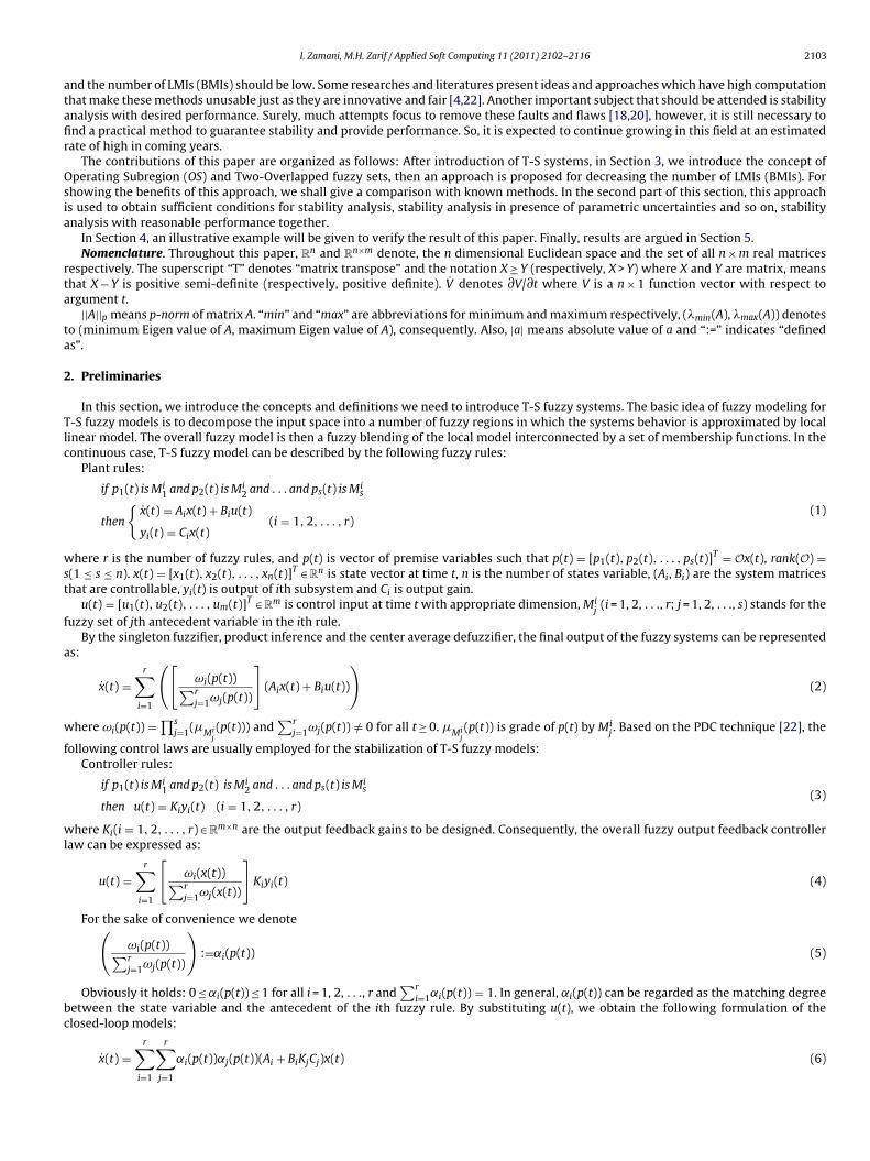
Fig. 1. Two types of fuzzy sets satisfy two-overlapped condition (solid line shows normalized triangular fuzzy sets and dashed line shows another fuzzy sets).

3. Main results

3.1. On the operating subregion

In this section, due to concepts of fuzzy sets, the ideas of two-overlapped fuzzy sets, the operating subregion and finally two propositionsare derived.

Consider normalized fuzzy sets of triangular form which are presented by [19] as follows (and see Fig. 1):

Mij =

⎧⎪⎪⎪⎪⎨⎪⎪⎪⎪⎩

pj(t) − dj(i − 1)dj(i) − dj(i − 1)

dj(i − 1) ≤ pj(t) ≤ dj(i)

dj(i + 1) − pj(t)dj(i + 1) − dj(j)

dj(i) ≤ pj(t) ≤ dj(i + 1)

0 otherwise

(7)

where �Mij(pj(t)) + �

Mi+1j

(pj(t)) = 1 (j = 1, 2, . . ., s; i = 1, 2, . . ., mi), mi is the number of fuzzy sets of ith premise variable.

Definition 1 (Definition of “two-overlapped fuzzy sets”). A cluster of fuzzy sets {Mi, i = 1, 2, . . ., mi} are said to be a two-overlapped fuzzysets if each of Mi overlaps with its neighboring fuzzy sets, but does not overlap with its non-neighboring fuzzy sets (mi is the number offuzzy sets of ith premise variable).

It is clear, definition is independent of normalization and shape (“shape” indicates the shape of fuzzy sets similar triangular) of fuzzysets (see Fig. 1).

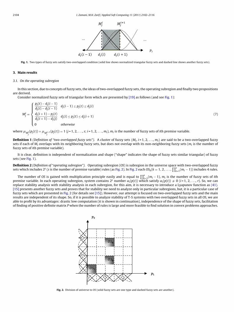
Definition 2 (Definition of “operating subregion”). Operating subregion (OS) is subregion in the universe space with two-overlapped fuzzysets which includes 2s (s is the number of premise variable) rules (as Fig. 2). In Fig. 2 each OSk(k = 1, 2, . . . ,

∏si=1(mi − 1)) includes 4 rules.

The number of OS is gained with multiplication principle easily and is equal to∏s

i=1(mi − 1), mi is the number of fuzzy sets of ithpremise variable. In each operating subregion, system contains 2s number ˛i(p(t)) which satisfy ˛i(p(t)) /= 0 (i = 1, 2, . . ., r). So, we canreplace stability analysis with stability analysis in each subregion, for this aim, it is necessary to introduce a Lyapunov function as (41).[15] presents another fuzzy sets and proves that for stability we need to analyze only in particular subregions, but, it is a particular case offuzzy sets which are presented in Fig. 2 (for details see [15]). However, our attempt is focused on two-overlapped fuzzy sets and the mainresults are independent of its shape. So, if it is possible to analyze stability of T-S systems with two overlapped fuzzy sets in all OS, we areable to profit by its advantages: drastic low computation (it is shown in continuation), independence of the shape of fuzzy sets, facilitationof finding of positive definite matrix P when the number of rules is large and more feasible to find solution in convex problems approaches.

Fig. 2. Division of universe to OS (solid fuzzy sets are one type and dashed fuzzy sets are another).


To illustrate aspects of proposed approach, consider two known methods for stability analysis which were presented by Tanaka andco-workers [22]. These methods are based on finding positive definite matrix P that must be found to satisfy the Lyapunov equation for alllocal linear models:⎧⎪⎪⎪⎪⎪⎪⎨

⎪⎪⎪⎪⎪⎪⎩

method 1. ((Ai + BiKj)T P + P(Ai + BiKj) < 0, ∀i, j = 1, 2, . . . , r)

method 2.

⎧⎪⎪⎪⎨⎪⎪⎪⎩

(Ai + BiKi)T P + P(Ai + BiKi) < 0 i = 1, 2, . . . , r(

(Ai + BiKj) + (Aj + BjKi)2

)T

P + P

((Ai + BiKj) + (Aj + BjKi)

2

)< 0

i < j ≤ r, i, j = 1, 2, . . . , r

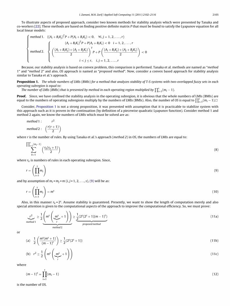
Because, our stability analysis is based on convex problem, this comparison is performed. Tanaka et al. methods are named as “method1” and “method 2” and also, OS approach is named as “proposed method”. Now, consider a convex based approach for stability analysissimilar to Tanaka et al.’s approach.

Proposition 1. The whole numbers of LMIs (BMIs) for a method that analyzes stability of T-S systems with two-overlapped fuzzy sets in eachoperating subregion is equal to:

The number of LMIs (BMIs) that is presented by method in each operating region multiplied by∏s

i=1(mi − 1).

Proof. Since, we have confined the stability analysis in the operating subregion, it is obvious that the whole numbers of LMIs (BMIs) areequal to the numbers of operating subregions multiply by the numbers of LMIs (BMIs). Also, the number of OS is equal to

∏si=1(mi − 1).�

Consider, Proposition 1 is not a strong proposition, it was presented with assumption that it is practicable to stabilize system withthis approach such as it is proven in the continuation (by definition of a piecewise quadratic Lyapunov function). Consider method 1 andmethod 2 again, we know the numbers of LMIs which must be solved are as:

method 1 : r2

method 2 :(

r(r + 1)2

)where r is the number of rules. By using Tanaka et al.’s approach (method 2) in OS, the numbers of LMIs are equal to:∏s

i=1(mi−1)∑

k=1

(rk(rk + 1)

2

)(8)

where rk is numbers of rules in each operating subregion. Since,

r =(

s∏i=1

mi

)(9)

and by assumption of mi = mj = m (i, j = 1, 2, . . ., s), (9) will be as:

r =(

s∏i=1

mi

)= ms (10)

Also, in this manner rk = 2s. Assume stability is guaranteed. Presently, we want to show the length of computation merely and alsospecial attention is given to the computational aspects of the approach to improve the computational efficiency. So, we must prove:

r2︸︷︷︸method 1

≥ 12

(ms

(ms︸︷︷︸

r

+ 1

))︸︷︷︸

method 2

≥ 12

(2s(2s + 1)(m − 1)s)︸︷︷︸proposed method

(11a)

or

(a)12

(ms(ms + 1)

(m − 1)s

)≥ 1

2(2s(2s + 1)) (11b)

(b) r2 ≥ 12

(ms

(ms︸︷︷︸

r

+ 1

))(11c)

where

(m − 1)s =s∏

i=1

(mi − 1) (12)

is the number of OS.


Table 1method 1, method 2 in comparison with proposed method when s = 2.

s = 2

mi = 2 mi = 3 mi = 4 mi = 5 mi = 6

method 1 16 81 256 625 1296method 2 10 45 136 325 666proposed method 10 40 90 160 250

Proof. By using inductive method (m > 1 and s > 1) and by assumption of s = constant:

I. If m = 2 then above relation is correct.II. Assumption: The (11b) is correct for m = k. Theorem: The (11b) is correct for m = k + 1. Since,

12

(ks(ks + 1)(k − 1)s

)≥ 1

2(2s(2s + 1))

and noticing that

f (m) = ms(ms + 1)(m − 1)s (13)

Differentiating with respect to m, we can get:

∂f

∂m= sms−1

(m − 1)s+1(ms+1 − 2ms − 1) (14)

and for

{m > 2

n ≥ 2then ∂f

∂m> 0, therefore f is an increasing function. Thus, m1 > m2 ⇒ f(m1) > f(m2). Let

m1 = k + 1 > m2 = k ⇒ f (k + 1) > f (k)

So,

12

((k + 1)s((k + 1)s + 1)

((k + 1) − 1)s

)>

12

(ks(ks + 1)(k − 1)s

)≥(

12

(2s(2s + 1)))

= constant (15)

The part (11a) was proven. Also,(r(r + 1)

2≤ r2

)⇒ r2 + r ≤ 2r2 ⇒ r(r − 1) ≥ 0 (16)

Since, this relation is correct and recursive, therefore part (11b) is proven, too. Then

12

(2s(2s + 1)(m − 1)s) ≤(

r(r + 1)2

)≤ r2 (17)

Thus, we complete the proof.�

In general, above inequalities are correct even mi /= mj (i, j = 1, 2, . . ., s, i /= j) i.e. when r(∏s

i=1mi

).

Proposition 2. When s ≥ 2 and mi ≥ 2 (i = 1, 2, . . ., s), then

s∏i=1

mi ≥s∏

i=1

mi

(s∏

i=1

mi + 1

)≥ 2s(2s + 1)

s∏i=1

(mi − 1) (18)

Proof. Please refer to Appendix A.�

As mentioned beforehand, the following inequalities show the length of computation.

proposed method ≤ method 2 ≤ method 1

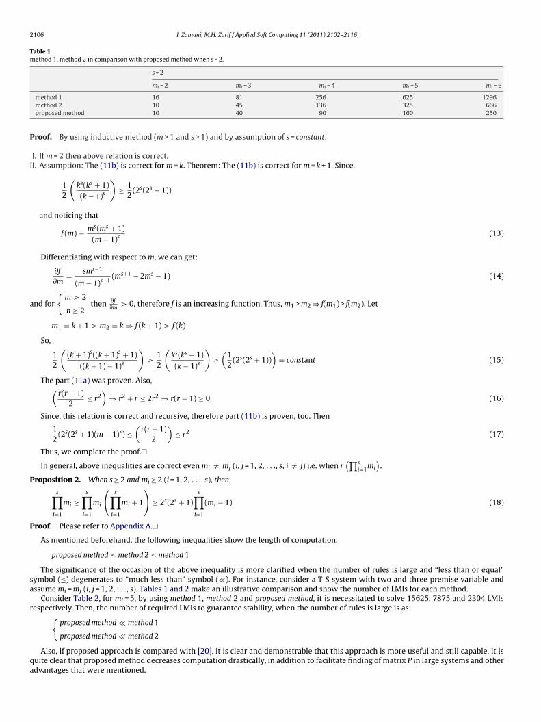
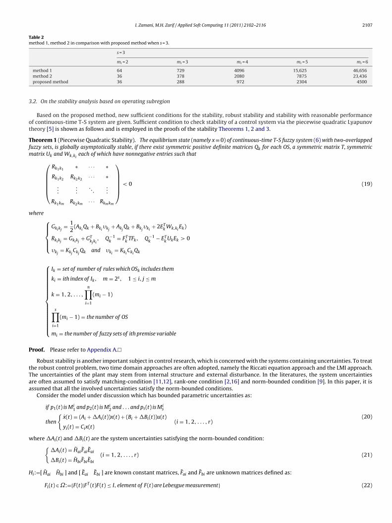
The significance of the occasion of the above inequality is more clarified when the number of rules is large and “less than or equal”symbol (≤) degenerates to “much less than” symbol (�). For instance, consider a T-S system with two and three premise variable andassume mi = mj (i, j = 1, 2, . . ., s). Tables 1 and 2 make an illustrative comparison and show the number of LMIs for each method.

Consider Table 2, for mi = 5, by using method 1, method 2 and proposed method, it is necessitated to solve 15625, 7875 and 2304 LMIsrespectively. Then, the number of required LMIs to guarantee stability, when the number of rules is large is as:{

proposed method � method 1

proposed method � method 2

Also, if proposed approach is compared with [20], it is clear and demonstrable that this approach is more useful and still capable. It isquite clear that proposed method decreases computation drastically, in addition to facilitate finding of matrix P in large systems and otheradvantages that were mentioned.


Table 2method 1, method 2 in comparison with proposed method when s = 3.

s = 3

mi = 2 mi = 3 mi = 4 mi = 5 mi = 6

method 1 64 729 4096 15,625 46,656method 2 36 378 2080 7875 23,436proposed method 36 288 972 2304 4500

3.2. On the stability analysis based on operating subregion

Based on the proposed method, new sufficient conditions for the stability, robust stability and stability with reasonable performanceof continuous-time T-S system are given. Sufficient condition to check stability of a control system via the piecewise quadratic Lyapunovtheory [5] is shown as follows and is employed in the proofs of the stability Theorems 1, 2 and 3.

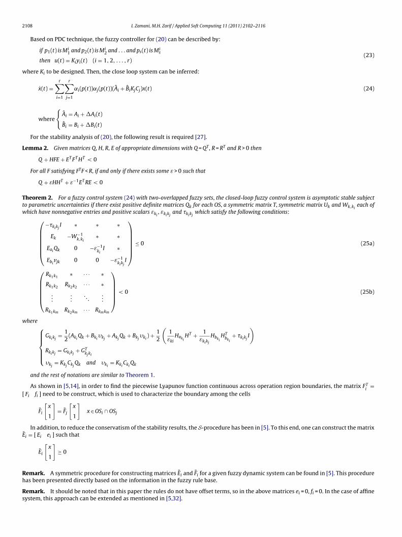
Theorem 1 (Piecewise Quadratic Stability). The equilibrium state (namely x ≡ 0) of continuous-time T-S fuzzy system (6) with two-overlappedfuzzy sets, is globally asymptotically stable, if there exist symmetric positive definite matrices Qk for each OS, a symmetric matrix T, symmetricmatrix Uk and Wk,ki

each of which have nonnegative entries such that⎛⎜⎜⎜⎜⎝

Rk1k1∗ · · · ∗

Rk1k2Rk2k2

· · · ∗...

.... . .

...

Rk1km Rk2km · · · Rkmkm

⎞⎟⎟⎟⎟⎠ < 0 (19)

where⎧⎪⎪⎨⎪⎪⎩

Gkikj= 1

2(Aki

Qk + Bki�kj

+ AkjQk + Bkj

�ki+ 2ET

k Wk,kiEk)

Rkikj= Gkikj

+ GTkjki

, Q−1k

= FTk

TFk, Q−1k

− ETk

UkEk > 0

�kj= Kkj

CkjQk and �ki

= KkiCki

Qk

⎧⎪⎪⎪⎪⎪⎪⎪⎪⎪⎪⎪⎪⎨⎪⎪⎪⎪⎪⎪⎪⎪⎪⎪⎪⎪⎩

Ik = set of number of rules which OSk includes them

ki = ith index of Ik, m = 2s, 1 ≤ i, j ≤ m

k = 1, 2, . . . ,

n∏i=1

(mi − 1)

s∏i=1

(mi − 1) = the number of OS

mi = the number of fuzzy sets of ith premise variable

Proof. Please refer to Appendix A.�

Robust stability is another important subject in control research, which is concerned with the systems containing uncertainties. To treatthe robust control problem, two time domain approaches are often adopted, namely the Riccati equation approach and the LMI approach.The uncertainties of the plant may stem from internal structure and external disturbance. In the literatures, the system uncertaintiesare often assumed to satisfy matching-condition [11,12], rank-one condition [2,16] and norm-bounded condition [9]. In this paper, it isassumed that all the involved uncertainties satisfy the norm-bounded conditions.

Consider the model under discussion which has bounded parametric uncertainties as:



then

{x(t) = (Ai + �Ai(t))x(t) + (Bi + �Bi(t))u(t)

yi(t) = Cix(t)(i = 1, 2, . . . , r)

(20)

where �Ai(t) and �Bi(t) are the system uncertainties satisfying the norm-bounded condition:{�Ai(t) = HaiFaiEai

�Bi(t) = HbiFbiEbi

(i = 1, 2, . . . , r) (21)

Hi:=[ Hai Hbi ] and [ Eai Ebi ] are known constant matrices, Fai and Fbi are unknown matrices defined as:

Fi(t) ∈ ˝:={F(t)|FT (t)F(t) ≤ I, element of F(t) are Lebesgue measurement} (22)


Based on PDC technique, the fuzzy controller for (20) can be described by:



then u(t) = Kiyi(t) (i = 1, 2, . . . , r)(23)

where Ki to be designed. Then, the close loop system can be inferred:

x(t) =r∑

i=1

r∑j=1

˛i(p(t))˛j(p(t))(Ai + BiKjCj)x(t) (24)

where

{Ai = Ai + �Ai(t)

Bi = Bi + �Bi(t)

For the stability analysis of (20), the following result is required [27].

Lemma 2. Given matrices Q, H, R, E of appropriate dimensions with Q = QT, R = RT and R > 0 then

Q + HFE + ET FT HT < 0

For all F satisfying FTF < R, if and only if there exists some ε > 0 such that

Q + εHHT + ε−1ET RE < 0

Theorem 2. For a fuzzy control system (24) with two-overlapped fuzzy sets, the closed-loop fuzzy control system is asymptotic stable subjectto parametric uncertainties if there exist positive definite matrices Qk for each OS, a symmetric matrix T, symmetric matrix Uk and Wk,ki

each ofwhich have nonnegative entries and positive scalars εki

, εkikjand kikj

which satisfy the following conditions:⎛⎜⎜⎜⎜⎜⎝

−kikjI ∗ ∗ ∗

Ek −W−1k,ki

∗ ∗

EaiQk 0 −ε−1

kiI ∗

Ebivjk 0 0 −ε−1

kikjI

⎞⎟⎟⎟⎟⎟⎠ ≤ 0 (25a)

⎛⎜⎜⎜⎜⎝

Rk1k1∗ · · · ∗

Rk1k2Rk2k2

· · · ∗...

.... . .

...


⎞⎟⎟⎟⎟⎠ < 0 (25b)

where⎧⎪⎪⎪⎨⎪⎪⎪⎩

Gkikj= 1

2(Aki

Qk + Bki�kj

+ AkjQk + Bkj

�ki) + 1

2

(1

εkiHaki

HT + 1εkikj

HbkiHT

bki+ kikj

I

)Rkikj

= Gkikj+ GT

kjki

�kj= Kkj

CkjQk and �ki

= KkiCki

Qk

and the rest of notations are similar to Theorem 1.

As shown in [5,14], in order to find the piecewise Lyapunov function continuous across operation region boundaries, the matrix FTi

=[ Fi fi ] need to be construct, which is used to characterize the boundary among the cells

Fi

[x

1

]= Fj

[x

1

]x ∈ OSi ∩ OSj

In addition, to reduce the conservatism of the stability results, the S-procedure has been in [5]. To this end, one can construct the matrixEi = [ Ei ei ] such that

Ei

[x

1

]≥ 0

Remark. A symmetric procedure for constructing matrices Ei and Fi for a given fuzzy dynamic system can be found in [5]. This procedurehas been presented directly based on the information in the fuzzy rule base.

Remark. It should be noted that in this paper the rules do not have offset terms, so in the above matrices ei = 0, fi = 0. In the case of affinesystem, this approach can be extended as mentioned in [5,32].


Now, for OSk, the piecewise quadratic function candidate that are continuous across the OS boundaries can be parameterized

V(x(t)) = xT (t)Pkx(t) x ∈ OSk

And in the case of affine system

V(x(t)) =(

x(t)

1

)T

Pk

(x(t)

1

)x ∈ OSk

with

Pk = FTk TFk

Pk = FTk TFk

where the free parameters of the piecewise quadratic function candidates are characterized by symmetric matrix T. In this paper, sincethere is no offset term in OSk so, V(x(t)) = xT(t)Pkx(t).

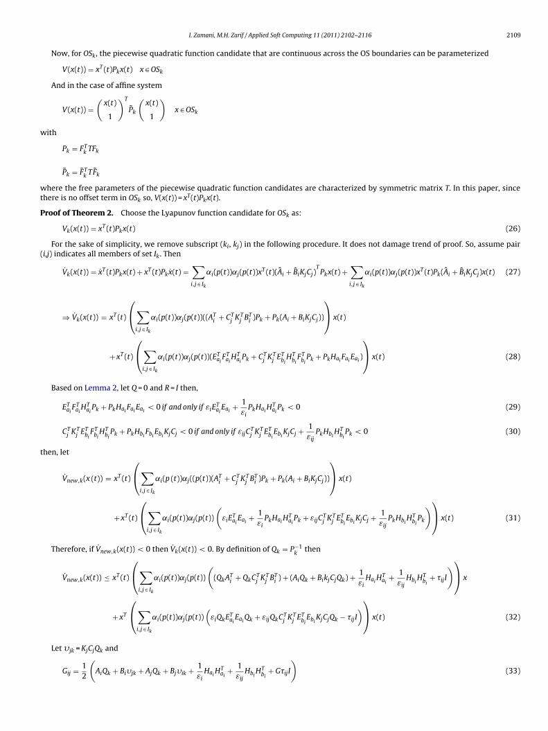
Proof of Theorem 2. Choose the Lyapunov function candidate for OSk as:

Vk(x(t)) = xT (t)Pkx(t) (26)

For the sake of simplicity, we remove subscript (ki, kj) in the following procedure. It does not damage trend of proof. So, assume pair(i,j) indicates all members of set Ik. Then

Vk(x(t)) = xT (t)Pkx(t) + xT (t)Pkx(t) =∑i,j ∈ Ik

˛i(p(t))˛j(p(t))xT (t)(Ai + BiKjCj)TPkx(t) +

∑i,j ∈ Ik

˛i(p(t))˛j(p(t))xT (t)Pk(Ai + BiKjCj)x(t) (27)

⇒ Vk(x(t)) = xT (t)

⎛⎝∑

i,j ∈ Ik

˛i(p(t))˛j(p(t))((ATi + CT

j KTj BT

i )Pk + Pk(Ai + BiKjCj))

⎞⎠ x(t)

+ xT (t)

⎛⎝∑

i,j ∈ Ik

˛i(p(t))˛j(p(t))(ETai

FTai

HTai

Pk + CTj KT

j ETbi

HTbi

FTbi

Pk + PkHaiFai

Eai)

⎞⎠ x(t) (28)

Based on Lemma 2, let Q = 0 and R = I then,

ETai

FTai

HTai

Pk + PkHaiFai

Eai< 0 if and only if εiE

Tai

Eai+ 1

εiPkHai

HTai

Pk < 0 (29)

CTj KT

j ETbi

FTbi

HTbi

Pk + PkHbiFbi

EbiKjCj < 0 if and only if εijC

Tj KT

j ETbi

EbiKjCj + 1

εijPkHbi

HTbi

Pk < 0 (30)

then, let

Vnew,k(x (t)) = xT (t)

⎛⎝∑

i,j ∈ Ik

˛i(p (t))˛j((p(t))(ATi + CT

j KTj BT

i )Pk + Pk(Ai + BiKjCj))

⎞⎠ x(t)

+ xT (t)

⎛⎝∑

i,j ∈ Ik

˛i(p(t))˛j(p(t))

(εiE

Tai

Eai+ 1

εiPkHai

HTai

Pk + εijCTj KT

j ETbi

EbiKjCj + 1

εijPkHbi

HTbi

Pk

)⎞⎠ x(t) (31)

Therefore, if Vnew,k(x(t)) < 0 then Vk(x(t)) < 0. By definition of Qk = P−1k

then

Vnew,k(x(t)) ≤ xT (t)

⎛⎝∑

i,j ∈ Ik

˛i(p(t))˛j(p(t))

((QkAT

i + QkCTj KT

j BTi ) + (AiQk + BikjCjQk) + 1

εiHai

HTai

+ 1εij

HbiHT

bi+ ijI

)⎞⎠ x

+ xT

⎛⎝∑

i,j ∈ Ik

˛i(p(t))˛j(p(t))(

εiQkETai

EaiQk + εijQkCT

j KTj ET

biEbi

KjCjQk − ijI)⎞⎠ x(t) (32)

Let �jk = KjCjQk and

Gij = 12

(AiQk + Bi�jk + AjQk + Bj�ik + 1

εiHai

HTai

+ 1εij

HbiHT

bi+ GijI

)(33)


then

Vnew,k(x(t)) ≤ xT (t)

⎛⎝∑

i,j ∈ Ik

˛i(p(t))2(Gii + GTii ) + 2

∑i,j ∈ Ik

˛i(p(t))˛j(p(t))(Gij + GTji)

⎞⎠ x(t)

+ xT (t)

⎛⎝∑

i,j ∈ Ik

˛i(p(t))˛j(p(t))(

εiQkETai

EaiQk + εijQkCT

j KTj ET

biEbi

KjCjQk − ijI + ETk Wk,ki

Ek

)⎞⎠ x(t) (34)

Now, if the first term and the second term are negative definite, then, Vnew,k(x(t)) < 0, and so, Vk(x(t)) < 0. With Schur’s complement(for second term):

εiQkETai

EaiQk + εijQkCT

j KTj ET

biEbi

KjCjQk − ijI + ETk Wk,ki

Ek ≤ 0 ⇒

⎛⎜⎜⎜⎜⎝

−ijI ∗ ∗ ∗Ek −W−1

k,ki∗ ∗

EaiQk 0 −ε−1

iI ∗

Ebijk 0 0 −ε−1

ijI

⎞⎟⎟⎟⎟⎠ ≤ 0 (35)

Consider all above relations are for OSk, so, we can use indexes ki and kj and now, we can extract (25a) easily. For the first term, letRij = Gij + GT

ji, then this term is equal to:

xT (t)

⎛⎝∑

i ∈ Ik

˛i(p(t))2Rii + 2∑i,j ∈ Ik

˛(p(t))˛j(p(t))Rij

⎞⎠ x(t) (36)

By using index ki and kj and following [7], the previous term is equal to:

xT (t)

⎛⎜⎜⎜⎜⎝

˛k1(p(t))I

˛k2(p(t))I

...

˛km (p(t))I

⎞⎟⎟⎟⎟⎠

T⎛⎜⎜⎜⎜⎝

Rk1k1Rk1k2

· · · Rk1km

Rk1k2Rk2k2

· · · Rk2km

......

. . ....


⎞⎟⎟⎟⎟⎠

︸︷︷︸Rk

⎛⎜⎜⎜⎝

˛k1(p(t))I

˛k2(p(t))I

...

˛km (p(t))I

⎞⎟⎟⎟⎠ x(t) ≤ �max(Rk)(˛k1

(p(t))2 + ˛k2(p(t))2 + · · · + ˛km (p(t))2)||x(t)||2

(37)

So, if �max(Rk) < 0 then, the first term is negative definite and this condition must be satisfied consequently.⎛⎜⎜⎜⎜⎝

Rk1k1∗ · · · ∗

Rk1k2Rk2k2

· · · ∗...

.... . .

...


⎞⎟⎟⎟⎟⎠ < 0 (38)

Thus, we complete the proof.�

From the proposed method, proofs of Theorem 1 and Theorem 2, it is easy to see:

(i) Theorem 1 and Theorem 2 present a BMIs constraint (that is solvable with BMI algorithm [3]) and if all Cj = I and with pre-defined Uk andWk,ki

, the BMI constraint of (19) and (25b) degenerate to LMI with respect to parameters (�ki, Qk) for (19) and (�ki

, Qk, εki, εkikj

, kikj)

for (25a) and (25b). Also, if O = I then p(t) = x(t) and so, the case of state feedback controller is presented. It is obvious that this methodis not dependent on the shape of fuzzy sets and also, chance of finding matrix P increased in comparison with [10,22], specially whilethe number of rules is large.

(ii) The BMI constraint (19) and (25b) does not require Rkikj= Gkikj

+ GTkikj

< 0 for the pairs of (ki, kj) such that ˛ki(p(t))˛kj

(p(t)) /= 0.

(iii) By introducing additional parameter kikj> 0 and replace Rkikj

by (Rkikj+ kikj

I), the chance of finding the feasible solution of (19) willbe increased. Consider (Rkikj

)2s×2s

< 0 implies that there exist kikj> 0 such that (Rkikj

+ kikjI) < 0, but the inverse of this statement

does not hold since kikjI is a non-positive symmetric definite matrix.

(iv) By using J.J. Sylvester criterion [13] for negative definite matrix and expansion of the (19), (25b), it is obvious that theses inequalitieshave (2s) BMI (LMI) in each subregions, so, the whole number of BMI (LMI) is equal to:

2s ×(

s∏i=1

(mi − 1)

)


In comparison with method 1, method 2 and [20,22] the number of theses BMI (LMI) is decreased drastically, because of:

s∏i=1

mi ≥s∏

i=1

mi

(s∏

i=1

mi + 1

)≥ 2s(2s + 1)

s∏i=1

(mi − 1) ≥ 2s ×(

s∏i=1

(mi − 1)

)(39)

(v) Since, the proposed method use different Qk in the different operating subregion, the whole Lyapunov function is piecewise quadraticLyapunov function and more flexible than common quadratic Lyapunov function. So, the stability results are less conservative thanbased on the common quadratic Lyapunov function.

3.3. Stability and performance together

In linear control theory, the purpose of many design problems is to place the closed-loop poles in desired region. So, for a reasonableperformance of T-S systems, we can generalize this linear control theory to each local linear of T-S system correspond to desired parameterssuch as damping and response time etc., but in the beginning, the following lemma is introduced [1].

Lemma 3. The closed-loop poles lie in the LMI region

D = {z ∈ C|fD(z):=L + Mz + MT z < 0}

iff there exist a symmetric positive matrix xpol satisfying

[�ijxpol + �ij(A + BK)xpol + �ijxpol(A + BK)T ]1≤i,j≤l< 0

Here z is a complex variable, A, B and K are system feedback gain matrices of a linear system, respectively, and L = LT = [�ij]1 ≤ i,j ≤ l andM = [�ij]1 ≤ i,j ≤ l are known real matrices which can be determined by specifying the desired closed-loop pole region in s-plane. The size of abovematrix (l × l), is determined by the subjective way of representing the closed-loop regions in the s-plane.

Theorem 3. To guarantee global asymptotic stability with desired performance of T-S fuzzy systems (6) with two-overlapped fuzzy sets, a PDCtype continuous-time controller can be designed by satisfying following conditions:

[�pqQk + �pqAkiQk + �pqBki

vki+ �pqQkAT

ki+ �pqvT

kiBT

ki]1≤p,q≤l

< 0 (40a)

⎛⎜⎜⎜⎜⎝

Rk1k1Rk1k2

· · · Rk1km

Rk1k2Rk2k2

· · · Rk2km

......

. . ....


⎞⎟⎟⎟⎟⎠ < 0 (40b)

Qk > ˛kI, ˛k = positive constant (40c)

where L = LT = [�ij]1 ≤ i,j ≤ l and M = [�ij]1 ≤ i,j ≤ l correspond to desired LMI region and the rest notations are similar to Theorem 1.

Proof. Let xpol = Qk and use Lemma 3 in each OS, this theorem is proven easily.�

Remark. Advantages of these theorems which are based on operating subregion are low computation and because of using Lyapunovtheorem in Operating Subregion, the chance of finding solutions (positives definite symmetric matrices, gains and other parameters) areincreased and independence of the shape of fuzzy sets is another merit just as mentioned previously. Theorems 1, 2 and 3 that whichindicate these merits, show usable and applicable of proposed method and also, presenting the illustrative example in the next sectionemphasizes theses particulars.

4. An illustrative example

In order to illustrate usefulness of proposed approach, we consider a T-S fuzzy system as follows:The ith rule is given by:Rule i:

If x1(t) is Mi1 and x2(t) is Mi

2 then

x(t) = Aix(t) + Biu(t) (i = 1, 2, . . . , 25)(41)


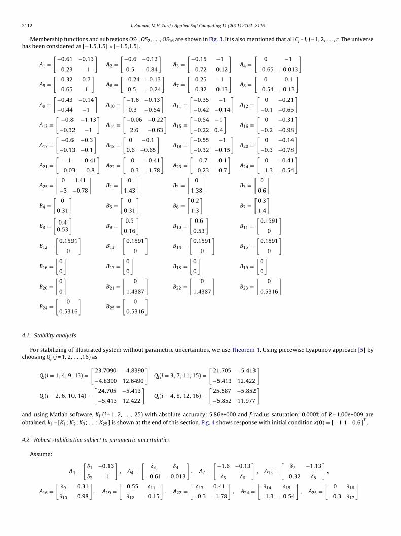
Membership functions and subregions OS1, OS2, . . ., OS16 are shown in Fig. 3. It is also mentioned that all Cj = I, j = 1, 2, . . ., r. The universehas been considered as [−1.5,1.5] × [−1.5,1.5].

A1 =[−0.61 −0.13

−0.23 −1

]A2 =

[−0.6 −0.12

0.5 −0.84

]A3 =

[−0.15 −1

−0.72 −0.12

]A4 =

[0 −1

−0.65 −0.013

]

A5 =[−0.32 −0.7

−0.65 −1

]A6 =

[−0.24 −0.13

0.5 −0.24

]A7 =

[−0.25 −1

−0.32 −0.13

]A8 =

[0 −0.1

−0.54 −0.13

]

A9 =[−0.43 −0.14

−0.44 −1

]A10 =

[−1.6 −0.13

0.3 −0.54

]A11 =

[−0.35 −1

−0.42 −0.14

]A12 =

[0 −0.21

−0.1 −0.65

]

A13 =[ −0.8 −1.13

−0.32 −1

]A14 =

[−0.06 −0.22

2.6 −0.63

]A15 =

[−0.54 −1

−0.22 0.4

]A16 =

[0 −0.31

−0.2 −0.98

]

A17 =[ −0.6 −0.3

−0.13 −0.1

]A18 =

[0 −0.1

0.6 −0.65

]A19 =

[−0.55 −1

−0.32 −0.15

]A20 =

[0 −0.14

−0.3 −0.78

]

A21 =[ −1 −0.41

−0.03 −0.8

]A22 =

[0 −0.41

−0.3 −1.78

]A23 =

[ −0.7 −0.1

−0.23 −0.7

]A24 =

[0 −0.41

−1.3 −0.54

]

A25 =[

0 1.41

−3 −0.78

]B1 =

[0

1.43

]B2 =

[0

1.38

]B3 =

[0

0.6

]

B4 =[

0

0.31

]B5 =

[0

0.31

]B6 =

[0.2

1.3

]B7 =

[0.3

1.4

]

B8 =[

0.40.53

]B9 =

[0.5

0.16

]B10 =

[0.6

0.53

]B11 =

[0.1591

0

]

B12 =[

0.1591

0

]B13 =

[0.1591

0

]B14 =

[0.1591

0

]B15 =

[0.1591

0

]

B16 =[

0

0

]B17 =

[0

0

]B18 =

[0

0

]B19 =

[0

0

]

B20 =[

0

0

]B21 =

[0

1.4387

]B22 =

[0

1.4387

]B23 =

[0

0.5316

]

B24 =[

0

0.5316

]B25 =

[0

0.5316

]

4.1. Stability analysis

For stabilizing of illustrated system without parametric uncertainties, we use Theorem 1. Using piecewise Lyapunov approach [5] bychoosing Qj (j = 1, 2, . . .,16) as

Qi(i = 1, 4, 9, 13) =[

23.7090 −4.8390

−4.8390 12.6490

]Qi(i = 3, 7, 11, 15) =

[21.705 −5.413

−5.413 12.422

]

Qi(i = 2, 6, 10, 14) =[

24.705 −5.413

−5.413 12.422

]Qi(i = 4, 8, 12, 16) =

[25.587 −5.852

−5.852 11.977

]and using Matlab software, Ki (i = 1, 2, . . ., 25) with absolute accuracy: 5.86e+000 and f-radius saturation: 0.000% of R = 1.00e+009 areobtained. k1 = [K1; K2; K3; . . .; K25] is shown at the end of this section. Fig. 4 shows response with initial condition x(0) = [ −1.1 0.6 ]T .

4.2. Robust stabilization subject to parametric uncertainties

Assume:

A1 =[

ı1 −0.13

ı2 −1

], A4 =

[ı3 ı4

−0.61 −0.013

], A7 =

[−1.6 −0.13

ı5 ı6

], A13 =

[ı7 −1.13

−0.32 ı8

],

A16 =[

ı9 −0.31

ı10 −0.98

], A19 =

[−0.55 ı11

ı12 −0.15

], A22 =

[ı13 0.41

−0.3 −1.78

], A24 =

[ı14 ı15

−1.3 −0.54

], A25 =

[0 ı16

−0.3 ı17

]


Fig. 3. State space and membership functions for the illustrated system.

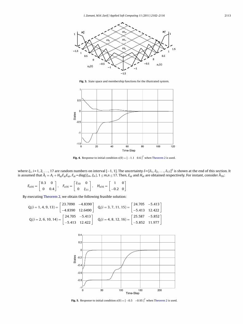
Fig. 4. Response to initial condition x(0) = [ −1.1 0.6 ]T

when Theorem 2 is used.

where �i, i = 1, 2, . . ., 17 are random numbers on interval [−1, 1]. The uncertainty ı = [ı1, ı2, . . ., ı17]T is shown at the end of this section. Itis assumed that Ai = Ai + HaiFaiEai, Fai = diag(�m, �n), 1 ≤ m,n ≤ 17. Then, Eai and Hai are obtained respectively. For instant, consider A16:

Ea16 =[

0.3 0

0 0.4

], Fa16 =

[�10 0

0 �11

], Ha16 =

[1 0

−0.2 0

]By executing Theorem 2, we obtain the following feasible solution:

Qi(i = 1, 4, 9, 13) =[

23.7090 −4.8390

−4.8390 12.6490

]Qi(i = 3, 7, 11, 15) =

[24.705 −5.413

−5.413 12.422

]

Qi(i = 2, 6, 10, 14) =[

24.705 −5.413

−5.413 12.422

]Qi(i = 4, 8, 12, 16) =

[25.587 −5.852

−5.852 11.977

]

Fig. 5. Response to initial condition x(0) = [ −0.5 −0.95 ]T

when Theorem 2 is used.


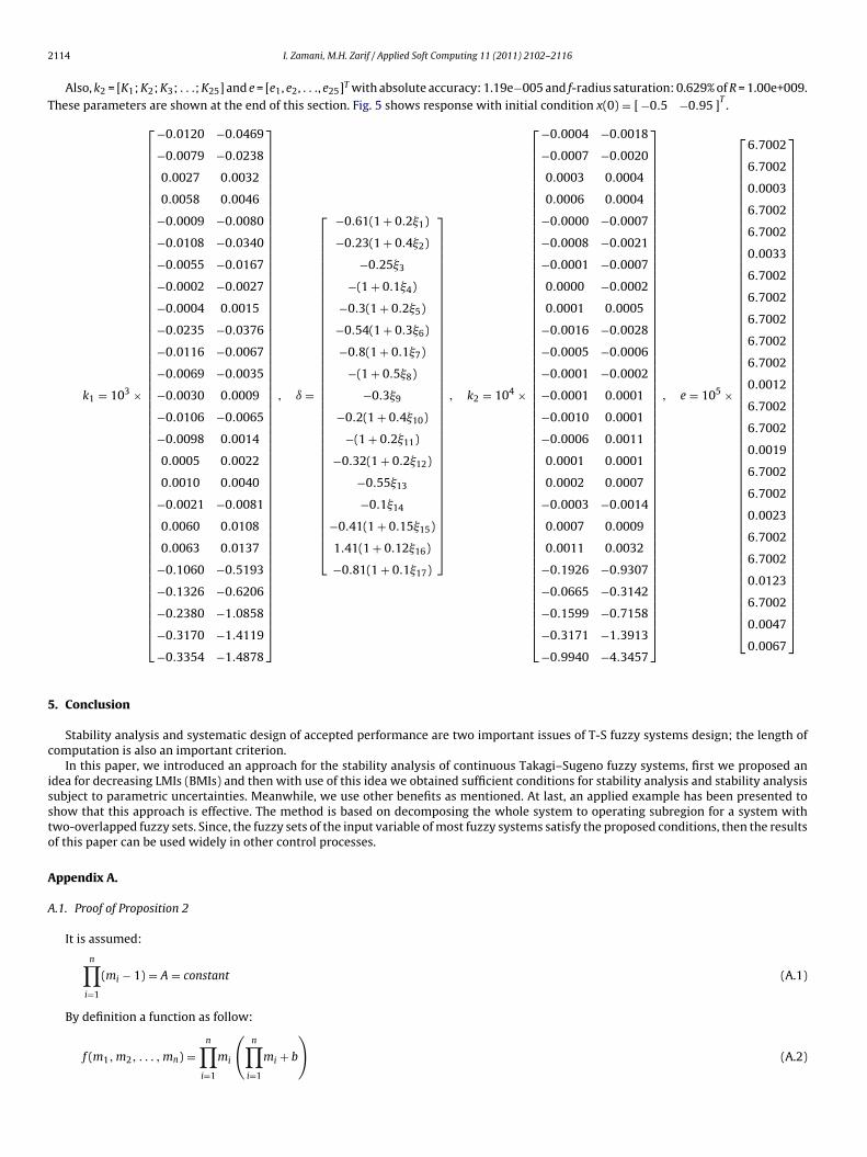
Also, k2 = [K1; K2; K3; . . .; K25] and e = [e1, e2, . . ., e25]T with absolute accuracy: 1.19e−005 and f-radius saturation: 0.629% of R = 1.00e+009.These parameters are shown at the end of this section. Fig. 5 shows response with initial condition x(0) = [ −0.5 −0.95 ]T .

k1 = 103 ×

⎡⎢⎢⎢⎢⎢⎢⎢⎢⎢⎢⎢⎢⎢⎢⎢⎢⎢⎢⎢⎢⎢⎢⎢⎢⎢⎢⎢⎢⎢⎢⎢⎢⎢⎢⎢⎢⎢⎢⎢⎢⎢⎢⎢⎢⎢⎢⎢⎢⎢⎢⎢⎢⎢⎢⎢⎣

−0.0120 −0.0469

−0.0079 −0.0238

0.0027 0.0032

0.0058 0.0046

−0.0009 −0.0080

−0.0108 −0.0340

−0.0055 −0.0167

−0.0002 −0.0027

−0.0004 0.0015

−0.0235 −0.0376

−0.0116 −0.0067

−0.0069 −0.0035

−0.0030 0.0009

−0.0106 −0.0065

−0.0098 0.0014

0.0005 0.0022

0.0010 0.0040

−0.0021 −0.0081

0.0060 0.0108

0.0063 0.0137

−0.1060 −0.5193

−0.1326 −0.6206

−0.2380 −1.0858

−0.3170 −1.4119

−0.3354 −1.4878

⎤⎥⎥⎥⎥⎥⎥⎥⎥⎥⎥⎥⎥⎥⎥⎥⎥⎥⎥⎥⎥⎥⎥⎥⎥⎥⎥⎥⎥⎥⎥⎥⎥⎥⎥⎥⎥⎥⎥⎥⎥⎥⎥⎥⎥⎥⎥⎥⎥⎥⎥⎥⎥⎥⎥⎥⎦

, ı =

⎡⎢⎢⎢⎢⎢⎢⎢⎢⎢⎢⎢⎢⎢⎢⎢⎢⎢⎢⎢⎢⎢⎢⎢⎢⎢⎢⎢⎢⎢⎢⎢⎢⎢⎢⎢⎣

−0.61(1 + 0.2�1)

−0.23(1 + 0.4�2)

−0.25�3

−(1 + 0.1�4)

−0.3(1 + 0.2�5)

−0.54(1 + 0.3�6)

−0.8(1 + 0.1�7)

−(1 + 0.5�8)

−0.3�9

−0.2(1 + 0.4�10)

−(1 + 0.2�11)

−0.32(1 + 0.2�12)

−0.55�13

−0.1�14

−0.41(1 + 0.15�15)

1.41(1 + 0.12�16)

−0.81(1 + 0.1�17)

⎤⎥⎥⎥⎥⎥⎥⎥⎥⎥⎥⎥⎥⎥⎥⎥⎥⎥⎥⎥⎥⎥⎥⎥⎥⎥⎥⎥⎥⎥⎥⎥⎥⎥⎥⎥⎦

, k2 = 104 ×

⎡⎢⎢⎢⎢⎢⎢⎢⎢⎢⎢⎢⎢⎢⎢⎢⎢⎢⎢⎢⎢⎢⎢⎢⎢⎢⎢⎢⎢⎢⎢⎢⎢⎢⎢⎢⎢⎢⎢⎢⎢⎢⎢⎢⎢⎢⎢⎢⎢⎢⎢⎢⎢⎢⎢⎢⎣

−0.0004 −0.0018

−0.0007 −0.0020

0.0003 0.0004

0.0006 0.0004

−0.0000 −0.0007

−0.0008 −0.0021

−0.0001 −0.0007

0.0000 −0.0002

0.0001 0.0005

−0.0016 −0.0028

−0.0005 −0.0006

−0.0001 −0.0002

−0.0001 0.0001

−0.0010 0.0001

−0.0006 0.0011

0.0001 0.0001

0.0002 0.0007

−0.0003 −0.0014

0.0007 0.0009

0.0011 0.0032

−0.1926 −0.9307

−0.0665 −0.3142

−0.1599 −0.7158

−0.3171 −1.3913

−0.9940 −4.3457

⎤⎥⎥⎥⎥⎥⎥⎥⎥⎥⎥⎥⎥⎥⎥⎥⎥⎥⎥⎥⎥⎥⎥⎥⎥⎥⎥⎥⎥⎥⎥⎥⎥⎥⎥⎥⎥⎥⎥⎥⎥⎥⎥⎥⎥⎥⎥⎥⎥⎥⎥⎥⎥⎥⎥⎥⎦

, e = 105 ×

⎡⎢⎢⎢⎢⎢⎢⎢⎢⎢⎢⎢⎢⎢⎢⎢⎢⎢⎢⎢⎢⎢⎢⎢⎢⎢⎢⎢⎢⎢⎢⎢⎢⎢⎢⎢⎢⎢⎢⎢⎢⎢⎢⎢⎢⎢⎢⎢⎢⎢⎢⎢⎢⎢⎣

6.7002

6.7002

0.0003

6.7002

6.7002

0.0033

6.7002

6.7002

6.7002

6.7002

6.7002

0.0012

6.7002

6.7002

0.0019

6.7002

6.7002

0.0023

6.7002

6.7002

0.0123

6.7002

0.0047

0.0067

⎤⎥⎥⎥⎥⎥⎥⎥⎥⎥⎥⎥⎥⎥⎥⎥⎥⎥⎥⎥⎥⎥⎥⎥⎥⎥⎥⎥⎥⎥⎥⎥⎥⎥⎥⎥⎥⎥⎥⎥⎥⎥⎥⎥⎥⎥⎥⎥⎥⎥⎥⎥⎥⎥⎦

5. Conclusion

Stability analysis and systematic design of accepted performance are two important issues of T-S fuzzy systems design; the length ofcomputation is also an important criterion.

In this paper, we introduced an approach for the stability analysis of continuous Takagi–Sugeno fuzzy systems, first we proposed anidea for decreasing LMIs (BMIs) and then with use of this idea we obtained sufficient conditions for stability analysis and stability analysissubject to parametric uncertainties. Meanwhile, we use other benefits as mentioned. At last, an applied example has been presented toshow that this approach is effective. The method is based on decomposing the whole system to operating subregion for a system withtwo-overlapped fuzzy sets. Since, the fuzzy sets of the input variable of most fuzzy systems satisfy the proposed conditions, then the resultsof this paper can be used widely in other control processes.

Appendix A.

A.1. Proof of Proposition 2

It is assumed:

n∏i=1

(mi − 1) = A = constant (A.1)

By definition a function as follow:

f (m1, m2, . . . , mn) =n∏

i=1

mi

(n∏

i=1

mi + b

)(A.2)


and with variation of f, we must find min(f)

g(m1, m2, . . . , mn) =n∏

i=1

(mi − 1) − A and fmj = ∂f

∂mj= �gmj

= �∂g

∂mj∀j

fmj =n∏

i = 1

i /= j

mi

(n∏

i=1

mi + b

)+

n∏i = 1

i /= j

mi ×n∏

i=1

mi and �gmj= �

n∏i = 1

i /= j

(mi − 1) ∀j (A.3)

now, mj is multiplied to each side of (A.3)

n∏i=1

mi

(n∏

i=1

mi + b

)+

⎛⎜⎜⎜⎜⎜⎜⎝

n∏i = 1

i /= j

mi

⎞⎟⎟⎟⎟⎟⎟⎠

2

= �mj

mj − 1

n∏i=1

(mi − 1) ∀j (A.4)

The left side is constant, therefore

m1

m1 − 1= m2

m2 − 1= · · · = mn

mn − 1⇒ m1 = m2 = · · · = mn (A.5)

from (A.2) we have:

mi = n√A + 1 = m0 ∀i (A.6)

now, we must find m0 such that

f (m1, m2, . . . , mn) ≥ f (m0, m0, . . . , m0) ∀mi f (m0, m0, . . . , m0) = ( n√A + 1)

n(( n√

A + 1)n + 1) (A.7)

so, it must be proven that

( n√A + 1)

n(( n√

A + 1)n + 1) ≥ 2n(2n + 1)A (A.8)

With definition of

h(A) = ( n√A + 1)n(( n√A + 1)

n + 1)A

(A.9)

min h(A) must be found. Derivation of h(A) is:

h′(A) = (n/n( n√An−1))( n√A + 1)

n−1(( n√A + 1)

n + 1)A2

+ (n/n( n√An−1))( n√A + 1)

n−1(( n√A + 1)

n)

A2− ( n√A + 1)

n(( n√A + 1)

n + 1)A2

(A.10)

Let h′(A) = 0, then

1A2

( n√A + 1)

n−1[ n√

A(( n√A + 1)

n + 1) + n√A( n√

A + 1)n − ( n√

A + 1)(( n√A + 1)

n + 1)] = 0 ⇒ n√A( n√

A + 1)n − ( n√

A + 1)n − 1 = 0 (A.11)

Let ( n√A + 1) = B

⇒ (B − 1)B2 − B − 1 = 0 ⇒ B2 − 2B − 1 = 0 (A.12)

Therefore, if A ≥ 2n then, n√A ≥ 2 ⇒ B ≥ 3n. Since, Bn ≥ 1 and (B − 2) ≥ 1 ⇒ Bn(B − 2) > 1

⇒ B2 − 2B − 1 > 0 (A.13)

So, h(A) is an increasing function and we have: If p > q ⇒ h(p) > h(q). It is assumed that h(A0) = min(h(A)) and since, it have been assumedA > 2n thus, it is obvious that A0 < 2n.

Therefore the above relation is true.�

A.2. Proof of Theorem 1

Similar to proof of Theorem 2, let

Vk(x(t)) = xT (t)Pkx(t) (A.14)


Then,

Vk(x(t)) = x(t)T Pkx(t) + x(t)T Pkx(t) = x(t)T

⎛⎝∑

i,j ∈ Ik

˛i(p(t))˛j(p(t))(Ai + BiKjCj)T Pk

⎞⎠ x(t)

+ x(t)T

⎛⎝∑

i,j ∈ Ik

˛i(p(t))˛j(p(t))Pk(Ai + BiKjCj)

⎞⎠ x(t) (A.15)

Let Rkikj= Gkikj

+ GTkjki

, Q−1k

= FTk

TFk, Q−1k

− ETk

UkEk > 0, �kj= Kkj

CkjQk, �ki

= KkiCki

Qk and

Gkikj= 1

2(Aki

Qk + Bki�kj

+ AkjQk + Bkj

�ki+ 2ET

k Wk,kiEk) (A.16)

Then, this term is equal to:

xT (t)

⎡⎢⎢⎢⎢⎣

˛k1(p(t))I

˛k2(p(t))I

...

˛km (p(t))I

⎤⎥⎥⎥⎥⎦

T⎡⎢⎢⎢⎢⎣

Rk1k1∗ · · · ∗

Rk1k2Rk2k2

· · · ∗...

.... . .

...


⎤⎥⎥⎥⎥⎦

︸︷︷︸Rk

⎡⎢⎢⎢⎢⎣

˛k1(p(t))I

˛k2(p(t))I

...

˛km (p(t))I

⎤⎥⎥⎥⎥⎦ x(t) ≤ �max(Rk)(˛k1

(p(t))2 + ˛k2(p(t))2 + · · · + ˛km (p(t))2)||x(t)||2

(A.17)

and the whole stability is similar to proof of Theorem 2.�

References

[1] M. Chilali, P. Gahinet, H∞ design with pole placement constraints: an LMI approach, in: Proc. 33rd IEEE Conf. on Decision and Control, vol. 1, Lake Buena Vista, 1994, pp.553–558.

[2] H. Choi, M.Y. Chung, Memory less stabilization of uncertain dynamic system with time-varying delayed states and control, Automatica 31 (9) (1995)1349–1351.

[3] L.E. Ghaoui, V. Balakrishnan, Synthesis of fixed-structure controllers via numerical optimization, in: Proc. 33rd IEEE Conf. on Decision and Control, vol. 3, Orlando, FL,1994, pp. 2678–2683.

[4] F.H. Hsiao, J.D. Hwang, Stability analysis of fuzzy large-scale systems, IEEE Trans. Syst. Man Cybern. 32 (1) (2002) 122–126.[5] M. Johansson, A. Rantzer, K.E. Arze’n, Piecewise quadratic stability of fuzzy systems, IEEE Trans. Fuzzy Syst. 7 (6) (1999) 713–722.[6] S. Kawamoto, K. Tada, A. Ishigame, T. Taniguchi, Construction of exact fuzzy system for nonlinear system and its stability analysis, in: Proc. 8th Fuzzy Syst. Symp.,

Hiroshima, Japan, 1992, pp. 517–520.[7] H.K. Khalil, Nonlinear Systems, 3rd ed., Prentice-Hall, Upper Saddle River, NJ, 2002.[8] H.K. Lam, F.H. Leung, P.K.S. Tam, Nonlinear state feedback controller for nonlinear systems: stability analysis and design based on fuzzy plant model, IEEE Trans. Fuzzy

Syst. 9 (4) (2001) 657–661.[9] H.J. Lee, J.B. Park, G. Chen, Robust fuzzy control of nonlinear systems with parametric uncertainties, IEEE Trans. Fuzzy Syst. 9 (2) (2001) 369–379.

[10] F. Matia, B.M. Al-Hadithi, A. Jime’nez, Generalization of stability criterion for Takagi–Sugeno continuous fuzzy model, Fuzzy Sets Syst. 129 (3) (2002)295–309.

[11] M.S. Mohamud, A.A. Bahnasawi, Asymptotic stability for a class of nonlinear discrete systems with bounded uncertainties, IEEE Trans. Automatic Control 33 (6) (1988)572–575.

[12] M.L. Ni, M.J. Er, Comments on: A new robust control for a class of uncertain discrete-time system, IEEE Trans. Automatic Control 46 (3) (2001) 509–511.[13] K. Ogata, Discrete Time Control Systems, Prentice-Hall, 1995.[14] S. Pettersson, B. Lennartson, Stability analysis of nonlinear and hybrid systems using discontinuous Lyapunov functions, in: Workshop on Multiple Model Approach to

Modeling Control, Trondheim, Norway, 1997, pp. 29–30.[15] G. Ren, Z.H. Xiu, Analytical design of Takagi–Sugeno fuzzy control systems, in: Proc. American Control Conf., vol. 3, Portland, USA, 2005, pp. 1733–1738.[16] J.C. Shen, B.S. Chen, F.C. Kung, Memory less stabilization of uncertain dynamic delay systems: Riccati equation approach, IEEE Trans. Automatic Control 36 (2) (1991)

638–640.[17] A.H. Sonbol, M.S. Fadali, Stability analysis to discrete TSK type II/III systems, IEEE Trans. Syst. Man Cybern. Part B: Cybern. 14 (5) (2006) 640–653.[18] A.H. Sonbol, M.S. Fadali, TSK fuzzy systems type II and type III stability analysis: continuous case, IEEE Trans. Syst. Man Cybern. Part B: Cybern. 36 (1) (2006)

2–12.[19] M. Sugeno, On stability of fuzzy systems expressed by fuzzy rules with singleton consequents, IEEE Trans. Fuzzy Syst. 7 (2) (1999) 201–224.[20] C.H. Sun, W.J. Wang, An improved stability criterion for T-S fuzzy discrete systems via vertex expression, IEEE Trans. Syst. 36 (3) (2006) 672–678.[21] K. Tanaka, M. Sugeno, Stability analysis and design of fuzzy control system, Fuzzy Sets Syst. 45 (2) (1992) 135–156.[22] H.O. Wang, K. Tanaka, M. Griffin, An analytical framework of fuzzy modeling and control of nonlinear systems: stability and design issues, in: Proc. American Control

Conf., vol. 3, Seattle, WA, 1995, pp. 2272–2276.[23] W.J. Wang, Y.J. Chen, Stabilization analysis for discrete-time T-S fuzzy systems based on the possible region transitions, in: Proc. IEEE Int. Conf. on Fuzzy Systems,

Vancouver, BC, Canada, 2006, pp. 789–794.[24] W.J. Wang, W.W. Lin, Decentralized PDC for large-scale T-S fuzzy systems, IEEE Trans. Fuzzy Syst. 13 (6) (2005) 779–786.[25] W.J. Wang, C.H. Sun, A weighting dependent Lyapunov function based relaxed stability criterion for T-S fuzzy discrete systems, in: Proc. IEEE Conf. on Networking,

Sensing and Control, 2005, pp. 135–140.[26] Y. Wang, Z.Q. Sun, F.C. Sun, Stability analysis and control of discrete-time fuzzy systems: a fuzzy Lyapunov function approach, in: Proc. 5th Asian Control Conf., vol. 3,

Melbourne, Australia, 2004, pp. 1855–1860.[27] L. Xie, Output feedback H∞ control of systems with parameter uncertainty, Int. J. Control 63 (4) (1996) 741–750.[28] Z.H. Xiu, G. Ren, Stability analysis and systematic design of Takagi–Sugeno fuzzy control system, Fuzzy Sets Syst. 151 (1) (2005) 119–138.[29] G.H. Yang, J. Dong, Quadratic stability analysis of fuzzy control systems, in: Proc. of American Control Conf., Minneapolis, MN, USA, 2006, 6 pp (1657402).[30] L.A. Zadeh, Outline of a new approach to the analysis of complex systems and decision processes, IEEE Trans. Fuzzy Syst. 6 (1998) 346–360.[31] I. Zamani, M.H. Zarif, Nonlinear controller for fuzzy model of double inverted pendulums, Int. J. Mech. Syst. Sci. Eng. 1 (1) (2008) 1–7.[32] H. Zhang, C. Li, X. Liao, Stability analysis and H∞ controller design of fuzzy large-scale systems based on piecewise Lyapunov functions, IEEE Trans. Syst. Man Cybern.

Part B: Cybern. 36 (3) (2006) 685–698.

Documents

On the continuous-time Takagi-Sugeno fuzzy systems stability analysis