Embed Size (px)
Citation preview

Low-Latency Proactive Continuous VisionYiming Gan
[email protected] of RochesterRochester, NY,USA
Yuxian [email protected]
Shanghai Jiao Tong UniversityShanghai, China
Lele [email protected] of RochesterRochester, NY,USA
Jingwen [email protected]
Shanghai Jiao Tong UniversityShanghai, China
Yuhao [email protected]
University of RochesterRochester, NY,USA
Abstract
Continuous vision is the cornerstone of a diverse range of intelli-gent applications found on emerging computing platforms such asautonomous machines and Augmented Reality glasses. A criticalissue in today’s continuous vision systems is their long end-to-endframe latency, which significantly impacts the system agility anduser experience. We find that the long latency is fundamentallycaused by the serialized execution model of today’s continuousvision pipeline, whose key stages—sensing, imaging, and visioncomputations—execute sequentially, leading to long frame latency.
This paper seeks to reduce the end-to-end latency of continu-ous vision tasks. Our key idea is a new proactive vision executionmodel that breaks the sequential execution of the vision pipeline.Specifically, we propose to allow the pipeline front-end (sensing andimaging) to predict future frames; the pipeline back-end (vision al-gorithms) then predictively operates on the future frames to reduceframe latency. While the proactive execution model is generallyapplicable to any vision systems, we demonstrate its effectivenessusing an implementation on resource-constrained mobile Systems-on-a-chips (SoC). Our system, PVF, incorporates two techniques toovercome key challenges that arise in deploying proactive vision inmobile systems: it enables multiple outstanding speculative frames byexploiting the hardware heterogeneities in mobile SoCs; it reducesthe energy overhead of prediction by exploiting the error-resilientnature of vision algorithms. We show that PVF reduces the framelatency by up to 92% under the same energy.
CCS Concepts
•Computer systems organization→Heterogeneous (hybrid)
systems; Special purpose systems.
Keywords
Computer vision, Continuous vision, Speculation, Proactive execu-tion, Image signal processing, Image sensor, SoC, Deep learning
Permission to make digital or hard copies of all or part of this work for personal orclassroom use is granted without fee provided that copies are not made or distributedfor profit or commercial advantage and that copies bear this notice and the full citationon the first page. Copyrights for components of this work owned by others than ACMmust be honored. Abstracting with credit is permitted. To copy otherwise, or republish,to post on servers or to redistribute to lists, requires prior specific permission and/or afee. Request permissions from [email protected] ’20, October 3–7, 2020, Virtual Event, GA, USA© 2020 Association for Computing Machinery.ACM ISBN 978-1-4503-8075-1/20/10. . . $15.00https://doi.org/10.1145/3410463.3414650
ACM Reference Format:
Yiming Gan, Yuxian Qiu, Lele Chen, Jingwen Leng, and Yuhao Zhu. 2020.Low-Latency Proactive Continuous Vision. In Proceedings of the 2020 Inter-national Conference on Parallel Architectures and Compilation Techniques(PACT ’20), October 3–7, 2020, Virtual Event, GA, USA. ACM, New York, NY,USA, 13 pages. https://doi.org/10.1145/3410463.3414650
1 Introduction
Domain specific architectures (DSA) provide more compute capabil-ity with lower energy consumption under the same silicon budget.A significant implication of DSAs is the high non-recurring engi-neering (NRE) cost of designing custom architectures and hardwarechips [33]. Therefore, we must identify key application domainswhose demands and social impacts are high enough to justify theefforts of designing DSAs. This paper focuses on the domain ofcontinuous vision, which processes real-time images from camerasensors to extract visual insights that guide high-level decisionmaking. Continuous vision is key to many emerging applications inboth consumer mobile devices and “always-on” embedded systemssuch as robotics, Augmented Reality, and smart-city sensing.
Today’s continuous vision system is bottlenecked by its longframe latency, which is fundamentally caused by its serialized exe-cution model. The three major stages in a vision pipeline – sensing,imaging, and vision computation – process a frame sequentially,leading to high per-frame latencies. Existing system optimizationssuch as pipelining and batching are designed to improve throughput(i.e., frame rate), but further exacerbate the frame latency.
The long frame latency is detrimental to vision-enabled embed-ded systems. For instance, a typical embedded robot today has a200 ms responsive latency from event to command, in which 100 msis attributed to the vision sub-system [13]. Such a high latency puts ahard bound on the agility of the robot, limiting user-experience andfunctionalities [12, 25]. Improving the latency of continuous visionsystems, however, is mainly constrained by the tight energy andpower budgets because embedded computing platforms routinelyoperate without active cooling or constant power supply [28].
This paper seeks to reduce the end-to-end latency of continuousvision tasks. Our key idea is to break the sequential execution chain.Specifically, we propose a new vision execution model where thevision front-end, i.e., the sensing and imaging stages, predicts futureframes, and the vision computation stage operates proactively onpredicted future frames. Once the actual frame is generated by thefront-end and vindicates the predicted frame, the vision results arelikely already available, reducing the frame latency.

While proactive vision is applicable to general vision systems,we present an important case-study on mobile Systems-on-a-chip(SoCs), which are widely used in many devices such as AR/VR head-sets, smartphones, robots that are latency- and energy-constrained.We introduce PVF, a proactive mobile vision system, which signifi-cantly reduces the end-to-end frame latency with low energy whilelargely relying on existing mobile SoC hardware.
In its efficient realization of the proactive vision pipeline, PVFaddresses two key challenges. First, the proactive execution modelexposes more concurrent computations (frames) on the fly, increas-ing the hardware resource contention. PVF exploits the hardwareheterogeneities available on mobile SoCs, which naturally exposesdifferent IP blocks (e.g., GPU, DSP, NPU), to execute multiple out-standing frames concurrently, mitigating the resource contention.
Second, predictive execution introduces new computations dueto frame prediction and thus increases the energy consumption.To reduce the speculation-induced energy overhead, PVF exploitsthe error-resilient nature of the image formation process (i.e., thesensing and imaging stages) and allows the predicted frames to bedirectly consumed by the vision algorithms without being checkedwith the captured frames. This relaxation saves energy by switch-ing off the sensor and the Image Signal Processors (ISP), which inmany use-cases could consume up to 50% of the total energy [42].This form of approximation is different from conventional approxi-mation in computer vision that approximates the vision algorithmitself. Instead, we approximate the inputs to the vision algorithms,an opportunity uniquely enabled by prediction, and in turn miti-gates the prediction-induced energy overhead.
Leveraging the SoC heterogeneities while approximating thevision front-end exposes a complex scheduling problem to PVF.The scheduler must 1) control the approximation to meet accuracyrequirements, and 2) optimize for latency under energy constraintsby wisely mapping multiple outstanding frames onto multiple ex-ecution targets (i.e., IP blocks). To that end, PVF uses an offline-online collaborative strategy. The offline component identifies keyaccuracy-sensitive knobs and empirically constructs a model be-tween the knobs and the accuracy. The online component schedulesthe frames on the SoC and dynamically tunes the knobs to minimizethe latency while meeting the energy budget and accuracy goals.
To enable efficient implementation of the speculative executionmodel, PVF extends today’s mobile SoC only minimally. We demon-strate the effectiveness of PVF on two common vision tasks: objecttracking and object detection. We show that PVF is able to achieveup to 92% latency reduction under the same energy budget, or 60.3%energy reduction at same frame latency, all with negligible accuracyloss. In summary, this paper makes four contributions:
• We propose the proactive continuous vision execution modelthat predicts the vision front-end to reduce the end-to-endframe latency.
• We propose a front-end approximation technique that ap-proximates the image formation process to mitigate the en-ergy overhead introduced by speculation.
• We design an offline-online collaborative software systemthat controls the accuracy while minimizing the frame la-tency in proactive vision executions.
• We demonstrate PVF, an efficient implementation of theproactive vision execution model. PVF reduces the frame
Neural Processing Unit
Image Signal Processor
Camera Sensor
Sensing Imaging Vision Computation
RAWPixels
RGBFrames
Semantic ResultsLight
Front-End Back-End
Fig. 1: The conventional sequential execution model of the
continuous vision pipeline.
latency under the same or lower energy budget with littlehardware overhead.
2 Background and Motivation
Continuous vision refers to a class of applications that performcomputer vision (CV) tasks on live camera video streams. Differentfrom offline video processing, continuous vision performs CV tasksin real-time and thus has much tighter performance and energy con-straints. This section introduces the bottleneck of continuous visionsystems, and describes the insufficiency of existing optimizations.
2.1 Latency Bottleneck in Continuous Vision
A typical continuous vision pipeline consists of three main stages:sensing, imaging, and vision computation, as Fig. 1 shows. Thesensing stage uses an image sensor to convert photons to RAWpixels, which are then processed by an Image Signal Processor(ISP) at the imaging stage to generate RGB frames. The visioncomputation stage processes the generated RGB frames to extractsemantic information (e.g., object location) for high-level decisionmaking. We call the sensing and imaging stages the vision “front-end”, and the vision computation stage “back-end.”
The three stages execute sequentially because there is a strictdependency between any two adjacent stages. For instance, thevision computation stage cannot start until the RGB frames are gen-erated by the ISP. The serialized execution limits the frame latency.That is, the time between when the sensor starts the sensing andwhen the vision results are available is limited by the cumulativeexecution time of all three stages.
Unfortunately, today’s vision system optimizations further exac-erbate the frame latency. For instance, pipelining the three stagesincreases the throughput, but introduces additional control andbookkeeping overhead that increases latency. In addition, batch-ing multiple frames improves hardware utilization and data reuse,but also increases the per-frame latency. As a result, even if allthree stages individually operate in real time, e.g., 30 frames persecond (FPS), the end-to-end per frame latency could add up toover 100 ms. Long frame latency severely limits the applicability ofvision-enabled systems. For instance, an autonomous vehicle needsto respond to an event within 100 ms as it can travel 2-3 metersduring the interval. Similarly, a 100 ms rendering latency causesnausea and is intolerable to AR users [20].
2.2 Limitations of Optimizing Only Vision
Algorithms
To reduce the frame latency, prior work has mostly focused on im-proving the performance of the vision computation stage, i.e., theback-end of the vision pipeline. Back-end optimization techniquesinclude designing more efficient vision algorithms (e.g., simplified

80
60
40
20
0Late
ncy
Red
uctio
n (%
)
DetectionTracking
High Res.Low Res.
DifferentTasks
DifferentResolutions
Fig. 2: Per-frame latency
reductions using a back-
end optimization (motion
extrapolation) to different
tasks and input resolutions.
100
80
60
40
20
0
Nor
m. E
nerg
y (%
)
100
80
60
40
20
0Baseline
w/ BE Opt.Baseline
w/ BE Opt.
FE BEDetection Tracking
Fig. 3: Per-frame energy
breakdown between the
front-end (FE) and back-end
(BE) before and after apply-
ing motion extrapolation.
Deep Neural Network (DNN) models [16, 35, 52, 67], compress-ing/pruning DNN models [29, 31]) andleveraging motion informa-tion [10, 22, 71]. Back-end optimizations are effective when theback-end dominates the frame latency. However, in many cases,depending on the complexity of the vision task and the image res-olution, the front-end could contribute significantly to the framelatency, making the back-end optimizations ineffective.
We use the examples of the object detection and the object track-ing task to illustrate the point. We assume that both the sensor andthe ISP operate at a typical 30 FPS, and use a systolic-array-basedDNN accelerator operating at 500 MHz to process vision DNNs(see Sec. 5 for detailed experimental setup). The detection task usesYOLOv2 [53], the state-of-the-art detection DNN, as the vision algo-rithm, while the tracking task uses the classic KCF algorithm [34].
YOLOv2 is compute-intensive, and operates at only 10 FPS; theKCF algorithm is much simpler and operates at 60 FPS. As a re-sult, the frame latency of the detection task is back-end-dominantand the frame latency of the tracking task is front-end-dominant.Applying back-end optimizations would thus lead to less latencyreduction for the tracking task than for the detection task. For in-stance, we apply the motion-extrapolation optimization proposedin Euphrates [71], which reduces the latency of the vision stage bya factor of 2. Fig. 2 compares the frame latency reductions betweendetection and tracking. A 2× vision stage latency reduction trans-lates to only 9% frame latency reduction for tracking, much lowercompared to the 62% reduction for detection.
Even for the same task, the latency distribution changes as the in-put resolution changes. Using object detection as an example, Fig. 2compares the latency reductions of motion-extrapolation when ap-plied to a 608 × 608 image and a 256 × 128 image. The latter spendssignificantly less time in the back-end, and thus gets improved onlyby 6% as compared to 49% observed on higher resolution inputs.
Along with latency reductions, most of the back-end optimiza-tions also reduce the back-end’s energy consumption. The energyreduction, however, is even less significant compared to latencyreduction. This is because the vision front-end (sensor and ISP) usu-ally contributes significantly to the total energy consumption. Fig. 3shows the energy breakdown between the front-end and the back-end for object detection and tracking. The back-end energy con-tributes to only about 50% in detection and about 20% in tracking.
Sensing Imaging Vision Computation
Sensing Imaging
Vision Computation
Event Event
Pred
Vision Computation
Sensing Imaging
Check
Check
Frame 1
Frame 2
Frame 3
Event
Frame Latency
Frame LatencyFrame Latency
Fig. 4: The speculative execution model. Pred denotes the
frame predictor, and Check denotes the checking module.
Applying the motion-extrapolation optimization to the back-endthus reduces the overall energy consumption only marginally.
We propose to improve the latency and energy efficiency at thesame time by breaking the sequential executionmodel. It is meant tocomplement, not replace, back-end optimizations to achieve greaterlatency and energy reductions.
3 Proactive Vision Execution Model
To overcome the sequential bottleneck in continuous vision pipelines,we propose the proactive execution model (Sec. 3.1). However, thenew execution model introduces two roadblocks that obstruct ef-ficient implementations. We discuss two enabling mechanisms,exploiting SoC heterogeneities (Sec. 3.2) and approximating visionfront-end (Sec. 3.3), that remove the roadblocks and pave the wayfor efficient proactive execution in continuous vision.
3.1 Proactive Execution model
The key idea of the predictive execution model is to allow the visioncomputation stage to operate speculatively on predicted futureframes before the sensing and imaging stages generate the actualframes. Once an actual frame is generated, it is used to validatethe predicted frame. If the predicted frame is checked to match theactual frame under certain metrics, the vision task results are likelyalready available and can be directly used, reducing the end-to-endframe latency. Otherwise, the speculated work is discarded, and thesystem executes the vision stage using the actual frame.
We illustrate the new predictive execution model in Fig. 4 withan example of three frames. The system starts with the sequentialmodel where the vision computation in Frame 1 waits for the actualframe. In contrast, Frame 2 and 3 are executed predictively wherethe vision stage operates on the predicted frames. Compared tothe conventional sequential model, the predictive execution modelnow requires two new system components: a frame predictor anda checker (Pred and Check in Fig. 4, respectively).
First, the frame predictor predicts future frames to enable specula-tion. Frame predictors range from simple motion-based approaches(e.g., extrapolation and optical flow) that are computation-efficientespecially in constrained environments [51] to recent generic ap-proaches that use deep learning [9, 24, 44, 47, 49, 51, 58]. Critically,

many frame prediction algorithms could predict multiple futureframes in a sequence [9, 24, 44]. This allows us to speculativelyprocess multiple outstanding frames at the same time (Frame 2 and3 in Fig. 4), further reducing the latency.
Second, the predictive vision pipeline requires a checking com-ponent which commits vision results on predicted frames only ifthe predicted frames are validated to be similar to the actual framescaptured by the sensor and ISP. This is similar to processor specu-lation that commits instructions on the predicted path only if theprediction is true. Many image similarity metrics and algorithmshave been proposed in the computer vision literatures, rangingfrom pixel-level comparison (e.g., Sum of Absolute Differences [54])to feature-level correlation [19, 44]. These algorithms are usuallylightweight to calculate, enabling efficient checks.
3.2 Mitigating Resource Contention
Predictive execution enables multiple outstanding frames to beprocessed concurrently. However, it leads to hardware resourcecontention at the vision computation stage. For instance in Fig. 4,the vision stages of Frame 2 and Frame 3 are overlapped. If only oneIP block is available to execute vision algorithms, the vision stageof the two frames must be serialized (similar to structure hazardsin a processor pipeline), defeating the purpose of speculation.
To address the resource contention in the vision computationstage introduced by prediction, we propose to exploit the hardwareheterogeneities available on today’s mobile SoCs. State-of-the-artmobile SoCs such as Qualcomm Snapdragon 835 and Apple A11all provide multiple IP blocks that can be used to execute visionalgorithms, including the GPU, DSP, and NPU. Nvidia’s XavierSoC even provides dedicated accelerators for non-NN-based visionalgorithms as well as an accelerator dedicated to stereo vision algo-rithms [5], further increasing the SoC hardware heterogeneities.
The heterogeneities are not fully exploited by today’s vision sys-tems, especially when the front-end dominates the frame latency,in which case there will be only one outstanding frame in the visionstage, and thus only one IP block is needed. In the predictive exe-cution model, however, the frame predictor could predict multiplefuture frames in a sequence, exposing more outstanding framesthat could make effective use of the multitude of the IP blocks. Forinstance in Fig. 4, the vision computations of Frame 1, 2, and 3are concurrent, and could be scheduled to different IP blocks. Howexactly the frames are scheduled is critical to ensuring that thelatency target is met in an energy-efficient manner. We discuss ourrun-time scheduling mechanisms in Sec. 4.3.
3.3 Mitigating Energy Overhead
While the predictive execution model reduces the frame latency,it increases the energy consumption, for three reasons. First, spec-ulation fundamentally trades energy for latency by performingextra work (e.g., prediction and checking). Second, using multi-ple IP blocks, while alleviating resource contention, also increasesthe energy consumption because CPU/GPU/DSP are less energy-efficient than NPU for executing vision algorithms (e.g., DNNs).Finally, mis-prediction wastes energy on executing frames whoseresults are eventually discarded.
Precise Frames Unchecked-Predicted Frames
Checked-PredictedFrames
Time
Predicted Sequence
Fig. 5: Precise frames refer to non-predicted frames, which
are used to predict future frames. Some predicted frames
are unchecked against the actual frames while the rest are
checked using a relaxed similarity measure.
To mitigate the energy overhead, we observe that the predictiveexectuion is precise only if 1) the checking module enforces apixel-perfect match between the predicted and the captured frame,and 2) every predicted frame is checked against the actual framecaptured by the vision front-end. However, both are unnecessarybecause computer vision tasks are known to tolerate low-qualityimages [11, 18, 68, 71]. We relax both constraints, and allow inexactframes to be consumed by the vision algorithms to save energy.
• Relax Checking Criterion The strictest form of checkingis to accept a predicted frame only when it is a pixel-perfectmatch with the actual frame. This would lead to an unneces-sarily high mis-prediction rate and also significant energywaste. Instead, we propose to relax the checking processby thresholding the similarity metric. A predicted frame isregarded as mis-prediction only if its similarity measure isbelow the threshold.
• Relax Checking Frequency Taking relaxed checking onestep further, we could forego the checking for a subset of pre-dicted frames that are likely to be similar to the actual frames.In this way, not only the checking energy could be saved, thesensor and ISP that generate the actual frames could also beswitched off, making up for the energy overhead introducedelsewhere. Since the sensor and ISP could take up to 50% ofthe total system power consumption [71], relaxing the framechecking frequency saves energy significantly.
Overall, there are three types of frames as Fig. 5 shows. Preciseframes are frames that are generated from the sensor and ISP, andare used to predict future frames by the frame predictor. Amongthe predicted frames, the first few frames are unchecked-predictedframes, which are speculatively executed and do not require check-ing against the actual frames, thus saving both the checking andfront-end energy. The rest frames in the prediction sequence arechecked-predicted frames, which must be checked with the actualframes, albeit using a relaxed similarity measure. We make thedesign decision that the unchecked-predicted frames always pre-cede the checked-predicted frames, because most frame predictorswork in a recurrent fashion that use past frames to predict futureframes [60]. As prediction progresses, prediction accuracy graduallydrops and checking against actual frames becomes important.
Overall, two key parameters dictate the trade-off between accu-racy and latency: the similarity threshold used in checking predictedframes, and the number of frames in a predicted sequence that areunchecked, which we dub “unchecked-degree.” Sec. 4.2 will describeour offline-online collaboratively scheme to tune the two knobs tobound the accuracy while reducing latency.

Mobile SoC
Frame Predictor
Static Accuracy Control
Scheduling Substrate
Visi
on A
pplic
atio
n
Run-time System
CPU GPU
DSPExecution
Profile
Schedule
ISP
Memory
Image Sensor
PFB
PRB
Scheduler(MCU)
Checking Logic(Hard-wired)
Accuracy Target
Similarity Metric
T
K
Predicted Frame
NPU
Actual Frame
Latency/Energy Target
DynamicStatic
Tuning Approx. Degree (K)
Tuning Similarity Threshold (T)
Accuracy Metric
Dynamic Accuracy Control (MCU)
K
Fig. 6: Overview of the PVF system. Augmentations are colored. PFB: Pending Frame Buffer; PRB: Pending Result Buffer.
4 PVF framework
PVF is our system design that efficiently realizes the proactiveexecution model. We first provide a framework overview (Sec. 4.1),which consists components for accuracy control (Sec. 4.2), resourcescheduling (Sec. 4.3), and mis-prediction handling (Sec. 4.4). Theywork together to minimize the latency of a vision task while sustainits accuracy target. We then discuss the hardware support to enablean efficient implementation of PVF (Sec. 4.5).
4.1 System Overview
Fig. 6 provides an overview of PVF. The goal of the PVF frameworkis to deliver a given latency target using the least energy whilemeeting the accuracy requirement. Accordingly, there are two maintasks of PVF: 1) ensuring the accuracy, and 2) delivering the latencytarget in an energy-efficient manner.
At run time, a frame predictor first predicts multiple futureframes, which are directly fed to the back-end to perform visiontasks without waiting for the vision front-end. While a predictedframe could be executed by any IP block provided by the hard-ware, we propose a run-time design that intelligently maps thepredicted frames to the IP blocks in a way that minimizes the over-all frame latency while meeting a given energy budget. When anactual frame is produced by the front-end and matches with a pre-dicted frame by the checking logic, the corresponding speculativeresult is committed. Upon a frame mis-prediction, the run timediscards the current result, and re-starts the vision pipeline fromthe mis-predicted frame.
The vision task could experience accuracy drop due to the relax-ations introduced in Sec. 3.3. PVF relies on static-dynamic collabo-ration to control accuracy. The static component identifies a set ofknobs that accuracy is most sensitive to, and uses the profiling datato empirically set the knobs to meet the accuracy target with theleast compute cost. With the “initial guess”, the run-time systemmonitors the program execution, and dynamically tunes the knobsto adapt to run-time dynamisms and to meet the accuracy target.
4.2 Accuracy Control
Proactive execution is precise if every predicted frame is checked tobe a pixel-perfect match with the actual captured frame. As estab-lished in Sec. 3.3, however, PVF exploits the error-resilient nature of
vision tasks and introduces two sources of inexactness to improveefficiency. First, a portion of the predicted frames, controlled by theunchecked-degree K , are not checked against the actual frames. Sec-ond, the checking module does not enforce a pixel-perfect match;rather, it accepts a predicted frame if its similarity measure is abovea similarity threshold T . PVFmust carefully calibrate the two knobs,to control the accuracy while improving efficiency.
To balance the overhead and effectiveness of accuracy control,PVF uses the profile-guided optimization, where offline profilingdata is used to guide the initial calibration of the knobs, which arefurther calibrated at run time to adapt to online dynamisms.Static Control PVF first uses representative sample data to obtaininitial values of K and T offline. To that end, PVF requires usersto specify an image similarity metric (e.g., SSIM [61]), an accuracymetric (e.g., mean average precision, mAP, for object detection [40]),and an accuracy target. The offline accuracy control componentprofiles the vision pipeline against the sample input frames whilesweepingT andK . The samples could either come from the trainingdata or be supplied from users who have particular use-cases inmind. In the end, we obtain the combination of T and K that meetsthe accuracy requirement using the least compute. The staticallytuned T and K are then used as the initial setting at run time.Dynamic Control It is possible that the accuracy knob settingobtained/profiled offline is occasionally overly aggressive or con-servative at run time. Therefore, PVF introduces a dynamic controlmechanism to respond to run-time dynamisms that are not cap-tured by offline profiling. Intuitively, if frame prediction is accurate,PVF could approximate the front-end more aggressively, and viceversa. In our design, if the mis-prediction rate is higher than athreshold in a predicted sequence, PVF will increase the checkingfrequency (i.e., increase the unchecked-degree K), and vice versa.Other more complex mechanisms such as using control theory [23]is also possible, but we empirically find that this simple mechanismperforms well in practice.
4.3 Runtime Scheduling
Proactive execution exposes a complex scheduling problem to therun-time systemwhere multiple predicted frames are to be executedon a heterogeneous SoC with multiple execution targets (i.e., IPblocks). The scheduler must intelligently map frames to IP blocks

in order to minimize the average frame latency without violatingthe energy budget. The scheduler could be easily extended to con-sider the dual problem of minimizing the energy under a latencyconstraint. Here we describe the former, but will evaluate both later.
Essentially, the scheduling task can be formulated as a con-strained optimization problem.Without losing generality, assumingthat the frame predictor predictsM frames, which are to be sched-uled onto N IP blocks, and the unchecked-degree is K (i.e., the firstK frames in the M predicted frames are not checked against theactual frames). The scheduling problem is:
min(K∑i=1
LUi +M∑
i=K+1LCi ) s .t . E < Ebudдet (1)
whereLUi andLCi denote the frame latency of an unchecked-predictedframe and a checked-predicted frame, respectively. E is the totalenergy consumes across all the frames:
E =K∑i=1
N∑n=1
βin × En +M∑
i=K+1
N∑n=1
βin × En (2)
where En denotes the inherent energy consumption of IP block n,which could be dynamically profiled once at run time. The binaryvariable βin denotes whether the frame i is scheduled to IP blockn. The collection ϕ = {βin } (i ∈ {1, 2, ...,M}, n ∈ {1, 2, ...,N })thus uniquely determines an execution schedule for theM predictedframes. LUi and LCi are both expressed as functions of βin ; pleaserefer to Appendix A for a detailed derivation.
Overall, our formulation optimizes over the schedule ϕ = {βin }(i ∈ {1, 2, ...,M}, n ∈ {1, 2, ...,N }). Unfortunately, this optimizationformulation is non-convex due to the complex interactions among{βin }. Solving it by exhaustive search would require an algorithmwith a time complexity of O(NM ).
Instead, we use a lightweight greedy algorithm that works wellin practice. Algorithm 1 describes the pseudo-code. Specifically, thescheduler schedules frames one at a time. Each frame is scheduledto the IP block that would provide the lowest frame latency —provided that the rest of the frames can possibly finish with theremaining energy budget using the least energy-consuming IPblock; otherwise the rest of the frames are scheduled to the leastenergy-consuming IP. This algorithm is also lightweight to compute.It takes about tens of microseconds to execute on a micro-controller,as will be discussed in the hardware architecture later.
Note that scheduling (i.e., frames to IPs mapping) must be doneat run time, because PVF assumes no prior knowledge of the energyconsumption of each IP block.
4.4 Checking and Handling Mis-predictions
The run-time scheduler itself operates under the assumption thatno frame mis-prediction occurs. While mis-predictions are rare aswe will quantify in Sec. 6, they must be dealt with in a lightweightfashion. Upon a mis-prediction, the run-time system takes twoactions. First, it discards the result generated for the mis-predictedframe. Second, it replaces the predicted frame with the actual frameand re-executes its vision stage. We define mis-prediction penaltyas the time (energy) wasted in executing mis-predicted framesthat are eventually discarded. As we will quantify in Sec. 6.8, themis-prediction penalty is low. Note that it is possible that when
Algorithm 1: Greedy Frame Scheduling Algorithm.Input: Energy Budget Ebudдet ; Predicted sequence length
M ; Number of IPs N ; Latency for each IP L1, . . . ,Ln ;Energy consumption for each IP E1, . . . ,En ; Earliestavailable time for each IP A1, . . . ,An ;Unchecked-degree K ; ISP finish time for each frameT1, . . . ,Tm ; Checking latency C .
Result: IP selection βi for all the predicted frames.if Ebudдet < M ×min(E1, . . . ,En ) then
return -1;end
else
for i = 1 toM do
t =∞
for j = 1 to N do
if Ebudдet - Ej ≥ (M-1) ×min(E1, . . . ,En ) thenif i < K then
if Aj + Lj < t thenβi = j;t = Aj + Lj ;
end
end
else
f =max (Aj+Lj ,Tj+C)if f < t then
βi = j;t = f ;
end
end
end
end
Ebudдet = Ebudдet - Eβi ;for j = 1 to N do
Aj = Aj + ( j == βj ) ? Lj : 0;end
end
end
an actual frame is generated the predicted frame have started itsvision stage yet (i.e., waiting for the availability of the IP block thatit is scheduled onto), in which case the mis-predicted frames aresimply discarded, and there is no mis-prediction penalty.
4.5 Architectural Augmentations and
Implementation Details
A key design objective of PVF is to maximally reuse existing mobileSoC architecture. PVF requires four principled augmentations toexisting mobile systems as shown in Fig. 6.Frame Predictor PVF requires a frame predictor. While any frameprediction algorithms would be compatible with the PVF frame-work, we choose to a CNN-based frame prediction algorithm Pred-net [43]. The recurrent model predicts a sequence of consecutiveframes by using both the current frame and the hidden state thatcontains historical information. Intuitively, predicting more framesincreases the scheduling window, but also introduces more mis-predictions. We empirically find that 10 frames are desirable (i.e.,

M in Equ. 1), which in turns leads to about 81 million MAC oper-ations, indicating a compute cost over two orders of magnitudelower than that of a typical vision task such as object tracking anddetection [71]. Other even lighter predictors (e.g., using motionvectors [54]) could be used in ultra-low power systems.
To not compete for the resources with the vision tasks, the framepredictor is executed using a dedicated NPU rather than reusingthe main NPU. Compared to hard-wiring the predictor logic, usinga programmable NPU allows PVF to support other predictors inthe future if needed.Checking Logic The frame checking is done in hardware. Weuse the widely-used SSIM metric [61] to assess the quality of thepredicted frames compared to the actual frames. SSIM is lightweightto compute compared to other system components. Given an inputresolution of 608 × 608, calculating the SSIM requires only 7.4million MAC operations, a few orders of magnitude lower than thevision algorithms.Memory The proactive execution model requires two new datastructures: the Pending Frame Buffer that stores predicted framesand the Pending Result Buffer that stores finished results that arenot yet committed. In our implementation, we reserve two regionsin the physical memory for the two data structures. Sec. 6.1 willshow that the memory overhead is negligible.MCUWe execute the run-time scheduler on a micro-controller unit(MCU), which is common to mobile SoCs. The run-time system islightweight in computation and requires programmability to adaptto future changes in the run-time policy, which a MCU provides.
5 Experimental Methodology
We describe the experimental setup (Sec. 5.1), the baselines (Sec. 5.2),and the evaluation scenarios (Sec. 5.3).
5.1 Basic Setup
Software SetupWe evaluate PVF using two common vision tasks:object detection and object tracking. We use YOLO [53], a state-of-the-art CNN as the detection algorithm. We conduct the objectdetection applications on the widely-used KITTI dataset [26]. Weevaluate two input resolutions: 608 × 608 and 256 × 128. We usethe common mean Average Precision (mAP) as the accuracy met-ric [21], which is the mean of the average precisions across allthe object classes. We use ECO [17], a state-of-the-art CNN as thetracking algorithm. We use VOT challenge 2017 benchmark as ourdataset [40] and use the commonly used Expected Average Overlap(EAO) as the accuracy metric [39], which is the mean of the averageper-frame overlap across sequences with typical lengths.Hardware SetupWe develop an in-house simulator parameterizedwith real hardware measurements for modeling the continuousvision pipeline. We model the baseline as a typical mobile SoCconsisting of key IP blocks including the CPU, GPU, ISP, and DSP.Wemodel the AR1335 image sensor [1], and use the energy numbersreported in the data sheet. The ISP power is measured from theNvidia Jetson TX2 module. Given a 256 × 128 low resolution image,the sensor and ISP are set to run at 40 FPS, and consume 4.5 mJ and3.8 mJ per frame, respectively. Given a 608 × 608 high resolutionimage, the sensor and ISP are set to run at 30 FPS, and consume6.5 mJ and 5.4 mJ per frame, respectively.
We model an NPU in the baseline to execute vision DNNs anda separate NPU for the frame predictor (Sec. 4.5). Any existingNPUs could be integrated into PVF, since PVF does not change themicroarchitecture of a NPU. For the purpose of our evaluation, weuse ScaleSim [56], a RTL-validated DNN accelerator simulator, tomodel the behaviors of both NPUs. The NPU has an array size of20 × 20 operating at 500 MHz with a SRAM size of 1.5 MB. Thepredictor NPU has an array size of 10 × 10 operating at 350 MHzwith a SRAM size of 128 KB. We implement the checking moduleas a 6-way SIMD MAC units running at 500 MHz.
PVF uses other non-NPU IP blocks during scheduling. We modela Qualcomm Hexagon 680 DSP, whose power consumption is mod-eled through direct measurement from the Open-Q 820 HardwareDevelopment Kit [6]. We model the Pascal GPU from the JetsonTX2 [3], whose power consumption is modeling through directmeasurement using its built-in power measurement. The DRAMis modeled after four Micron 16 GB LPDDR3-1600 channels [4].Finally, we model an ARM M4-like micro-controller [2], which isused to execute the PVF run-time scheduler. Appendix B shows themeasurement results that we use for parameterizing the simulator.
5.2 Baselines
We compare with three different baselines:• Base, which is the baseline system without predictive execu-tion. Base uses YOLO [53] for object detection and ECO [17]for object tracking.
• BO, which optimizes Base by optimizing the vision back-end,i.e., the vision algorithm. It represents a common strategytoday to reduce the frame latency. While there are manyback-end optimization techniques such as model compres-sion [15, 30, 37] and motion compensation [71], they all havethe same effect of reducing the vision algorithm’s latency. Inour evaluation we choose to replace complex but accurateDNN models with simplified but less accurate DNN models.
In particular, we train a simplified version of YOLO, whichwe call O-YOLO, which has 41.1% fewer MAC operationsthan YOLO with only 0.15 mAP loss on low resolution in-puts and 2.3 mAP loss on high resolution inputs. For objecttracking, we use KCF [34], which uses hand-crafted featuresand has 80% lower compute cost with 0.03 EAO drop onlow resolution inputs and 0.153 on high resolution inputscompared to ECO.
• FCFS, which improves BO by utilizing all the IP blocks avail-able for vision computation but without prediction capabil-ities. Therefore, comparing PVF with FCFS will show thebenefits of the proactive execution model. The FCFS sched-uler maps incoming frames to the fastest available IP blockusing a First-Come-First-Serve policy.
5.3 Evaluation Scenarios
Since PVF predicts and sometimes even skips the vision front-end,its effectiveness is naturally sensitive to the latency distributionbetween the front-end and the back-end. To understand when andwhy PVF provides latency reduction, we evaluate it under threedifferent usage scenarios:

• Back-End Dominant, which refers to a scenario where theback-end dominates the original vision pipeline (i.e., a high-latency but accurate vision algorithm is used). Object detec-tion with high resolution falls into this category.
• Front-End Dominant, which refers to a scenario where thefront-end dominates the original vision pipeline. Objecttracking with low resolution falls into this category.
• Mixed, which refers to a scenario where the back-end domi-nates the original vision pipeline, but front-end becomes thebottleneck when an optimal vision algorithm is used. Objecttracking (both high and low resolutions) fits this scenario.
6 Evaluation
We first show the software and hardware overhead of PVF (Sec. 6.1).We then show that with careful accuracy tuning, the accuracydrop of front-end approximation is negligible (Sec. 6.2). We furtherdemonstrate that PVF achieves latency reduction with the same orlower energy budget in different scenarios. (Sec. 6.3, Sec. 6.4, andSec. 6.5). We apply the same run-time optimization formulation tothe duel problem of saving energy under latency budgets (Sec. 6.6).We show how sensitive PVF is to different accuracy knobs (Sec. 6.8).Finally, we compare PVF with an alternative that simply lows theimage resolution in an iso-accuracy setting (Sec. 6.7), and compareour PVF implementation with an ideal implementation that has anoracle predictor (Sec. 6.8).
6.1 Overheads
Hardware Overhead PVF adds two new hardware components:predictor and checker. In a 16 nm technology node, the predictoris about 170,000 um2 in area and the checking module is about1,500 um2 in area. Both combined contribute to less than 0.15% ofthe total SoC die area [7]. In addition, the two pending buffers arepinned in the DRAM (Sec. 4.5). The Pending Frame Buffer has asize of 1.5 MB and the Pending Result Buffer has a size of 200 Bytes.Prediction Overhead The prediction overhead is low. For highresolution inputs, the latency of the predictor is 12.5 ms per frame,which is about 5 × faster than the front-end; the energy overhead isless than 0.5 mJ per frame, which is 22 × lower than the front-end.For low resolution inputs, the latency and energy overhead is lessthan 1.0 ms and 0.1 mJ per frame, respectively, which are about 50× faster and consumes 83 × lower energy than the front-end.Checking Overhead Checking also have insignificant overhead,with a mere 2.5 ms and 0.2 ms latency for high and low resolutioninputs, respectively.SchedulingOverheadThe run-time scheduler uses a simple greedyalgorithm. The run-time scheduler executes within 100 µs on anM4-like micro-controller.
6.2 Accuracy Results
We evenly split the dataset into an offline profiling set and an onlinetest set. The profiling set is used by the static accuracy controlmodule to empirically decide the two accuracy knobs, similaritythreshold T and unchecked-degree K , while the test set is used atrun-time evaluation.Object Detection We set an accuracy target of less than 1.5 mAPloss compared to Base, on par with the accuracy drop in prior
1.6
1.2
0.8
0.4
0.0
mA
P dr
op
1.00.80.60.40.20.0SSIM Threshold
1.0
0.8
0.6
0.4
0.2
0.0
Misprediction rate
(a)Accuracy sensitivity to differ-
ent similarity (SSIM) thresholds.
1.6
1.2
0.8
0.4
0.0
mA
P dr
op
1086420Unchecked-Degree
(b)Accuracy sensitivity to differ-
ent unchecked-degrees.
Fig. 7: Accuracy sensitivity in object detection.
50x10-3
40
30
20
10
0
EA
O d
rop
1.00.80.60.40.20.0SSIM Threshold
1.0
0.8
0.6
0.4
0.2
0.0
Misprediction rate
(a)Accuracy sensitivity to differ-
ent similarity (SSIM) threshold.
50x10-3
40
30
20
10
0
EA
O d
rop
1086420 Unchecked-Degree
(b)Accuracy sensitivity to differ-
ent unchecked-degree.
Fig. 8: Accuracy sensitivity in object tracking.
work [10, 71]. Fig. 7 shows how the mAP drop (left y-axis) andmis-prediction rate (right y-axis) vary with the SSIM (similarity)threshold for the profiling set. As the SSIM threshold relaxes fromright to left, the mis-prediction rate decreases and therefore PVFaccepts more inexact input frames. At the same time, the accuracydrop also increases. Similarly, Fig. 7b shows how the mAP changeswith the unchecked-degree. As more frames are predicted withoutbeing checked, the mAP drop increases.
The offline accuracy control module tunes both knobs togetherand settles for the configuration with T = 0.5 and K = 6. Wefind that this setting is stable at run time. The average number ofunchecked frames increases by only 0.72 in each predicted sequence.Overall, the static-dynamic collaborative approach in PVF leadsto an 1.13 mAP loss on the test set, which would have been 4.4%higher if only the static component is employed.Object TrackingWe set an accuracy target of less than 0.1 EAOloss compared to Base, which is better than switching from a CNN-based tracker to the best non-CNN tracker [38]. Fig. 8a and Fig. 8bshow how the accuracy drop varies with the SSIM threshold andthe unchecked-degree for the profiling set. The offline tuning mod-ule chooses 0.7 as the SSIM threshold T and 6 as the unchecked-degree K , which again is stable at run time. The average numberof unchecked frames increases by only 0.57 in each predicted se-quence. Overall, the static-dynamic scheme in PVF leads to leads to0.051 EAO loss on the test set, which would have been 13.7% higherif the accuracy knobs are tuned only offline.
6.3 Latency in Back-End Dominant Scenario
PVF run-time system schedules frames in a predicted sequenceonto different IP blocks given a specific energy budget in order tominimize latency. We show in this section the results of PVF underdifferent energy budgets when the vision back-end dominates the
100
80
60
40
20
0 Lat
ency
Red
uctio
n (%
)
5040302010 Energy Constraint (mJ)
Base BO FCFS PVF
Better
(a) Latency reduction under different energy
budgets in back-end dominant scenario.
100
80
60
40
20
0Late
ncy
Red
uctio
n (%
)
1612840Energy Constraint (mJ)
Base BO FCFS PVF
Better
(b) Latency reduction under different energy
budgets in front-end dominant scenario.
100
95
90
85
80Late
ncy
Red
uctio
n (%
)
14012010080604020Energy Constraint (mJ)
Base BO FCFS PVF
Better
(c) Latency reduction under different energy
budgets in mixed scenario.
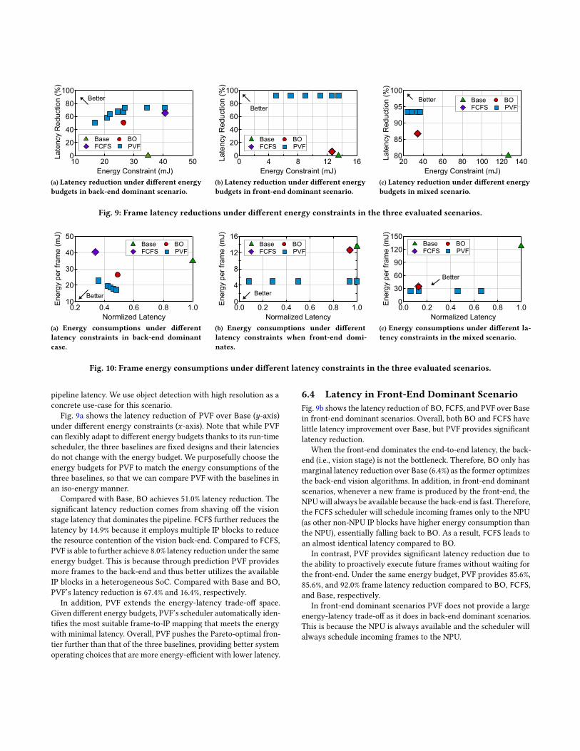
Fig. 9: Frame latency reductions under different energy constraints in the three evaluated scenarios.
50
40
30
20
10Ene
rgy
per f
ram
e (m
J)
1.00.80.60.40.2Normlized Latency
Base BO FCFS PVF
Better
(a) Energy consumptions under different
latency constraints in back-end dominant
case.
16
12
8
4
0Ene
rgy
per f
ram
e (m
J)
1.00.80.60.40.20.0Normalized Latency
Base BO FCFS PVF
Better
(b) Energy consumptions under different
latency constraints when front-end domi-
nates.
150
120
90
60
30
0Ene
rgy
per f
ram
e (m
J)
1.00.80.60.40.20.0 Normalized Latency
Base BO FCFS PVF
Better
(c) Energy consumptions under different la-
tency constraints in the mixed scenario.
Fig. 10: Frame energy consumptions under different latency constraints in the three evaluated scenarios.
pipeline latency. We use object detection with high resolution as aconcrete use-case for this scenario.
Fig. 9a shows the latency reduction of PVF over Base (y-axis)under different energy constraints (x-axis). Note that while PVFcan flexibly adapt to different energy budgets thanks to its run-timescheduler, the three baselines are fixed designs and their latenciesdo not change with the energy budget. We purposefully choose theenergy budgets for PVF to match the energy consumptions of thethree baselines, so that we can compare PVF with the baselines inan iso-energy manner.
Compared with Base, BO achieves 51.0% latency reduction. Thesignificant latency reduction comes from shaving off the visionstage latency that dominates the pipeline. FCFS further reduces thelatency by 14.9% because it employs multiple IP blocks to reducethe resource contention of the vision back-end. Compared to FCFS,PVF is able to further achieve 8.0% latency reduction under the sameenergy budget. This is because through prediction PVF providesmore frames to the back-end and thus better utilizes the availableIP blocks in a heterogeneous SoC. Compared with Base and BO,PVF’s latency reduction is 67.4% and 16.4%, respectively.
In addition, PVF extends the energy-latency trade-off space.Given different energy budgets, PVF’s scheduler automatically iden-tifies the most suitable frame-to-IP mapping that meets the energywith minimal latency. Overall, PVF pushes the Pareto-optimal fron-tier further than that of the three baselines, providing better systemoperating choices that are more energy-efficient with lower latency.
6.4 Latency in Front-End Dominant Scenario
Fig. 9b shows the latency reduction of BO, FCFS, and PVF over Basein front-end dominant scenarios. Overall, both BO and FCFS havelittle latency improvement over Base, but PVF provides significantlatency reduction.
When the front-end dominates the end-to-end latency, the back-end (i.e., vision stage) is not the bottleneck. Therefore, BO only hasmarginal latency reduction over Base (6.4%) as the former optimizesthe back-end vision algorithms. In addition, in front-end dominantscenarios, whenever a new frame is produced by the front-end, theNPUwill always be available because the back-end is fast. Therefore,the FCFS scheduler will schedule incoming frames only to the NPU(as other non-NPU IP blocks have higher energy consumption thanthe NPU), essentially falling back to BO. As a result, FCFS leads toan almost identical latency compared to BO.
In contrast, PVF provides significant latency reduction due tothe ability to proactively execute future frames without waiting forthe front-end. Under the same energy budget, PVF provides 85.6%,85.6%, and 92.0% frame latency reduction compared to BO, FCFS,and Base, respectively.
In front-end dominant scenarios PVF does not provide a largeenergy-latency trade-off as it does in back-end dominant scenarios.This is because the NPU is always available and the scheduler willalways schedule incoming frames to the NPU.

10080604020
0
Late
ncy
Red
uctio
n (%
)
3 5 7 3 5 7Unchecked-Degree (K)
High Resolution Low Resolution
TLF
(a) Latency reductions under dif-
ferent unchecked-degrees K .
10080604020
0
Late
ncy
Red
uctio
n (%
)
0.2 0.5 0.8 0.2 0.5 0.8 Similarity Threshold (T)
High Resolution Low Resolution
TLF
(b) Latency reductions under dif-
ferent similarity thresholds T .
Fig. 11: Sensitivity Analysis. TLF denotes “too low to finish.”
6.5 Latency in Mixed Scenario
Fig. 9c shows the latency reductions of BO, FCFS, PVF over Basein the mixed scenario. In this scenario, the back-end dominatesthe pipeline latency with the original vision algorithm in Base.Therefore, by optimizing the vision algorithm BO significantlyoutperforms Base, reducing the latency by 86.8%. However, oncethe vision algorithm is optimized, the front-end dominates thelatency. Thus, FCFS has no latency improvement over BO, and thePVF achieves only 6.7% further latency reduction over FCFS.
6.6 Energy Improvements
So far, we have been evaluating PVF under the objective of minimiz-ing latency under different energy budgets. PVF could also operateunder a dual problem of minimizing energy consumption underlatency constraints. We briefly evaluate PVF under this objective.
Fig. 10a, Fig. 10b, and Fig. 10c show how PVF can reduce theframe energy consumption under given latency constraints for thesame three scenarios as described in Sec. 5.3, respectively. Simi-larly to the latency-oriented optimization, PVF shows the mostsignificant energy savings when the front-end dominates the visionpipeline latency, such as the scenario shown in Fig. 10b. In that case,PVF is able to achieve 55.6%, 52.4%, and 52.4% per frame energysaving compared to Base, BO, and FCFS, respectively.
6.7 Comparison With Lower Image Resolution
PVF out-performs an alternative that simply lowers the imageresolution. Due to the space limit, we show the results of the front-end dominant scenario (i.e., object detection with low resolution).We designed an iso-accuracy experiment, in which we lower theinput image resolution by 25%. Compare against simply loweringthe resolution, PVF reduces latency by 90.0%, slightly lower thanthe 92.0% reduction on the original resolution but is still significant.
6.8 Sensitivity Study
We study the sensitivity of PVF with respect to K and T , the twoknobs that affect the accuracy-latency trade-offs. Due to limitedspace, we use object detection as a case-study, but the general trendholds. Fig. 7 shows the accuracy sensitivity, and this section focuseson the latency and energy sensitivities.Unchecked-Degree Fig. 11a shows the latency reduction of PVFwith different unchecked-degrees (K ) under the same energy con-straint (21.0 mJ for high resolution inputs and 5.0 mJ for low res-olution inputs). Generally, as K increases, the front-end could beswitched off more often, leaving more energy budget for the back-end to active more IP blocks to reduce the frame latency. For high
100
80
60
40
20
0
Late
ncy
Red
uctio
n (%
)
PVF Oracle
30
29
28
27
26
25
Energy P
er Frame (m
J)
(a) Back-end dominant case.
100
80
60
40
20
0
Late
ncy
Red
uctio
n (%
)
PVF Oracle
5
4
3
2
1
0
Energy P
er Frame (m
J)
(b) Front-end dominant case.
Fig. 12: Oracle Analysis using object detection.
resolution inputs, the latency reduction improves from 51.0% to57.8% as K increases from 3 to 5. The improvement plateaus as Kincreases to 7. The reason is that by then the saved energy fromswitching off the front-end is not enough to allow the scheduler toactivate another IP block to gain more latency reduction.
For low resolution inputs, under a K of 3 the energy budgetis not enough to let the system finish all the frames (denoted as“too-low to finish”, TLF). As K increases, the energy saved fromswitching off the front-end let the system finish all the frames andachieve significant latency reduction. Similar to the high resolutionscenario, the latency reduction plateaus beyond K = 5.Similarity Threshold A higher SSIM threshold (T ) would resultin more mis-predictions, leading to higher energy waste since thevision results calculated on the mis-predicted frames will be dis-carded. Thus, the latency reduction would decrease because theback-end has less energy to activate new IP blocks to reduce la-tency. Fig. 11b shows the latency reduction with different T s underthe same energy constraint (22.8 mJ for high resolution input and5.0 mJ for low resolution input). As T increases, the latency reduc-tion decreases. For the low resolution case as T increases to 0.8 theenergy budget is too small for the system to finish all the frames.
6.9 Oracle Analysis and Mis-Prediction Penalty
The effectiveness of PVF is correlated with the accuracy of theframe predictor. We now assess how PVF would perform with anoracle predictor (Oracle), which uses the same prediction algo-rithm [43] and the same hardware, but has a perfect predictionaccuracy. That is, the only difference between PVF and Oracle isthat the latter does not pay the mis-speculation penalty (the energywasted on executing vision algorithms on mis-predicted frames).By comparing PVF with Oracle, we can not only assess the fullpotential of PVF, but also understand its mis-speculation penalty.
Fig. 12a shows the results of the back-end dominant scenario, inwhich Oracle consume 5.2% lower energy (right y-axis) than PVF,equivalent to PVF’s mis-speculation energy penalty. PVF has almostidentical latency reduction compared to Oracle. This is becausewhen the back-end dominates speculating the front-end has littleimpact on improving the frame latency. The gap between Oracleand PVF is more notable in the front-end dominant case, whichbenefits from a more accurate frame predictor. The results of thefront-end dominant case are shown in Fig. 12b. Oracle consumes12.3% lower energy and 8.0% lower latency compare to PVF.

7 Limitation and Discussion
Applicability The accuracy loss of PVF in its current is similarto prior work on approximating vision computations [10, 71]. PVFcurrently does not target mission-critical systems that have tightaccuracy requirements. PVF could be used in vision systems suchas AR and robotics navigation that are less accuracy sensitive. Notethat PVF is compatible with any frame predictor. Therefore, PVFcan readily benefit from a higher quality frame predictor with thealgorithmic innovations from the vision community.Predictor Alternatives PVF predict future frames. However, ob-taining the exact pixels in future frames is not always necessary.We discuss two alternatives here for future developments.
First, one could directly predict frame features rather than pix-els [59]. This is potentially efficient as CNNs extract features frompixels anyways, and operate on features rather than raw pixels. Thechallenge is that there is no well-established comparison metric inthe feature space, unlike the SSIM metric used in the pixel space.We empirically find that simply comparing the Euclidean distancebetween two feature vectors leads to high error rates.
Second, for applications where the semantics output is a region-of-interest (ROI), we could directly predict the ROI location. How-ever, predicting images allows PVF to be generally applicable toany backend vision algorithms, including those that generate morethan ROIs (e.g., the object class in object detection).Security Vulnerabilities The proposed speculative vision systemdoes not share the security vulnerabilities introduced by specula-tions in CPU microarchitecture such as Spectre and Meltdown. Thefundamental reason is that Spectre and Meltdown exploit specula-tion at the microarchitecture-level (branch prediction and out-of-order execution) to leak information, whereas the proposed specu-lative vision execution is an application-level technique, in whichthe predicted frames are in non-speculative states from the microar-chitecture’s perspective. Thus, our proposal does not expose newsecurity vulnerabilities to Spectre and Meltdown attacks.
However, predictive execution does expose mis-predicted frames,which could be potentially be exploited to infer system internalbehaviors. The security implication of predictive vision executionshould be carefully studied, which we leave for future work.
8 Related Work
Vision Optimizations Literature is rich with techniques that op-timize or approximate the vision algorithms. Classic techniquesinclude using smaller, simplified models [35, 52, 67], model com-pression [15, 30, 37], quantization [36, 63–65], and using specializedhardware [14, 27, 48]. Recent developments have also leveragedthe temporal/spatial redundancies in real-time frames to simplifycomputations [10, 22, 46, 55, 71].
PVF differs from prior work in two key ways. First, PVF expandsthe optimization scope from optimizing only the back-end visionstage to the whole continuous vision pipeline. Specifically, PVFpredicts the front-end, and is complementary to existing back-endoptimization techniques. Second, PVF presents a new form of visionapproximation by relaxing the checking constraint of the visionpipeline front-end, saving energy from the vision front-end.Heterogeneity in Mobile Computing Mobile SoCs are rich inarchitectural heterogeneity to deal with a wide variety of use-cases
that have different compute intensities. Industry has provided ma-ture programming frameworks [50]. The heterogeneity has beenexploited in various contexts such as Web browsing [69, 70] andmachine learning [32, 41, 57].
Critical to exploiting hardware heterogeneity is scheduling, whichdecides which tasks are executed on which IP block to meet a givenobjective. While task scheduling in heterogeneous system has beenextensively studied before [8, 45, 62, 66], PVF introduces uniquechallenges because the scheduler must deal with a stream of incom-ing tasks that have dependencies. We formulate the scheduling taskin PVF as a constrained-optimization problem and demonstrate anefficient greedy algorithm that performs well in practice.
9 Conclusion
Long frame latency is detrimental to real-time vision systems. Thispaper argues that the sequential execution model is the culprit ofthe long latency. We propose PVF, a speculative vision executionmodel that reduces the frame latency under the same or lowerenergy budget. The key to PVF is to break the sequential executionbetween vision front-end and back-end. We present an efficientimplementation of PVF by leveraging the heterogeneities in mobileSoCs and exploiting the error-tolerance nature of vision tasks.
10 Acknowledgement
We thank the anonymous reviewers for their valuable feedback. Wealso thank Arm for their equipment donation. Jingwen Leng is thecorresponding author of the paper. All opinions expressed in thismaterial are those of the authors and do not necessarily reflect theviews of the sponsor.
Appendices
A Latency Derivation in Scheduling
The latencies in Equ. 1 are calculated as the time difference betweenthe start time SUi (SCi ) and the finish time FUi (FCi ). For both checked-and unchecked-predicted frames, a frame start when its sensingstage starts. Thus, we have:
LUi = FUi − Si , LCi = FCi − Si (3)
Si = (i − 1) ×Tsense (4)
where Tsense is sensing stage time, which is statically determinedgiven a particular sensor frame rate.
A frame’s finish time depends on its type. An unchecked-predictedframe finishes when its vision stage finishes. If two frames’ visionstages are mapped to the same IP block, the latter starts only afterthe former finishes. Thus:
FUi =i−1∑k=1
αik × (Fk +Ti ),αik ∈ {0, 1},i−1∑k=1
αik = 1 (5)
whereTi represents the vision stage time of frame i, and the binaryvariable αik denotes whether or not Frame i is executed right afterFrame k on the same IP block. Frame k itself could either be anapproximate frame or a predicted frame.
For a checked-predicted frame, it finishes when the checkingfinishes, which depends on whether the vision stage finishes before

Table 1: Latency of object detection and object tracking us-
ing both high and low input resolution on different IPs. All
numbers are in milliseconds.
High-Res Low-Res
IP YOLO O-YOLO ECO KCF Yolo O-YOLO ECO KCF
NPU 173 100 - - 13 7 - -GPU 651 491 - - 447 421 - -DSP 743 650 - - 521 490 - -CPU >2000 >2000 83 22 >2000 >2000 72 14
or after the actual frame is generated:
FCi =max (i−1∑k=1
αik × (Fk +Ti ), i ×Tsense +Tisp ) +Ci ,
αik ∈ {0, 1},i−1∑k=1
αik = 1 (6)
where Tisp is imaging stage time, which is statically determinedgiven the ISP frame rate;Ci is the checking time, which is also stat-ically determined given the similarity metric and image resolution.
Ti , the vision stage execution time of a frame i, depends on theparticular IP block that is scheduled to execute the frame. Thus,they can be expressed as follows:
Ti =N∑n=1
βin × Ln , βin ∈ {0, 1},N∑n=1
βin = 1 (7)
where Ln denotes IP block n’s latency, which is profiled given a par-ticular image resolution. The binary variable βin denotes whetherthe frame i is scheduled to IP block n. The collection ϕ = {βin }(i ∈ {1, 2, ...,M}, n ∈ {1, 2, ...,N }) thus uniquely determines anexecution schedule for theM predicted frames.
Note that αik is not an independent variable; it could be derivedfrom βin and βkn . If both βin and βkn are 1 and βzn is 0 for anyz ∈ (k, i), indicating that frame k and frame i are scheduled toexecute on the same IP block n consecutively, αik has to be 1.Leveraging the arithmetic properties of binary values, αik could beexpressed as:
αik =!N∏n=1
(βin × βkn × (k∑z=i
βzn − 1) − 1) (8)
where ! is the logic negate that returns 0 for any non-zero values.
B Latency and Energy Characterizations
Table 1 and Table 2 show the latency and energy measurementresults used to parameterize the simulator described in Sec. 5.1.
References
[1] [n. d.]. AR1335: CMOS Image Sensor, 13 MP, 1/3".https://www.onsemi.com/PowerSolutions/product.do?id=AR1335.
[2] [n. d.]. Cortex-M4.https://developer.arm.com/ip-products/processors/cortex-m/cortex-m4.
[3] [n. d.]. Jetson TX2 Module.http://www.nvidia.com/object/embedded-systems-dev-kits-modules.html.
[4] [n. d.]. Micron 178-Ball, Single-Channel Mobile LPDDR3 SDRAM Features.https://www.micron.com/-/media/client/global/documents/products/data-sheet/dram/mobile-dram/low-power-dram/lpddr3/178b_8-16gb_2c0f_mobile_lpddr3.pdf.
Table 2: Energy of object detection and object tracking us-
ing both high and low input resolution on different IPs. All
numbers are in millijoules.
High-Res Low-Res
IP YOLO O-YOLO ECO KCF YOLO O-YOLO ECO KCF
NPU 21 13 - - 3 2 - -GPU 77 70 - - 35 21 - -DSP 57 51 - - 25 16 - -CPU >160 >160 118 20 >160 >160 101 18
[5] [n. d.]. NVIDIA Reveals Xavier SOC Details. https://bit.ly/2qq0TWp.https://www.forbes.com/sites/moorinsights/2018/08/24/nvidia-reveals-xavier-soc-details/amp/
[6] [n. d.]. Open-Q 820 Development Kit.https://www.intrinsyc.com/snapdragon-embedded-development-kits/snapdragon-820-development-kitsnapdragon-820-apq8096/.
[7] [n. d.]. Qualcomm Snapdragon 835 First to 10 nm.https://www.wired.com/story/apples-neural-engine-infuses-the-iphone-with-ai-smarts/.
[8] Cédric Augonnet, Samuel Thibault, Raymond Namyst, and Pierre-André Wacre-nier. 2011. StarPU: a unified platform for task scheduling on heterogeneousmulticore architectures. Concurrency and Computation: Practice and Experience23, 2 (2011), 187–198.
[9] Mohammad Babaeizadeh, Chelsea Finn, Dumitru Erhan, Roy H Campbell, andSergey Levine. 2018. Stochastic Variational Video Prediction. Proc. of ICLR (2018).
[10] Mark Buckler, Philip Bedoukian, Suren Jayasuriya, and Adrian Sampson. 2018.EVA2: Exploiting Temporal Redundancy in Live Computer Vision. In Proc. ofISCA.
[11] Mark Buckler, Suren Jayasuriya, and Adrian Sampson. 2017. Reconfiguring theImaging Pipeline for Computer Vision. In Proc. of ICCV.
[12] Martin Buehler, Karl Iagnemma, and Sanjiv Singh. 2009. The DARPA urbanchallenge: autonomous vehicles in city traffic. Vol. 56. springer.
[13] Andrea Censi and Davide Scaramuzza. 2014. Low-latency event-based visualodometry. In Proc. of ICRA.
[14] Y. Chen, T. Krishna, J. S. Emer, and V. Sze. 2017. Eyeriss: An Energy-EfficientReconfigurable Accelerator for Deep Convolutional Neural Networks. IEEEJournal of Solid-State Circuits 52, 1 (Jan 2017), 127–138. https://doi.org/10.1109/JSSC.2016.2616357
[15] Yoojin Choi, Mostafa El-Khamy, and Jungwon Lee. 2018. Universal deep neuralnetwork compression. arXiv preprint arXiv:1802.02271 (2018).
[16] François Chollet. 2017. Xception: Deep learning with depthwise separable con-volutions. In Proceedings of the IEEE conference on computer vision and patternrecognition. 1251–1258.
[17] Martin Danelljan, Goutam Bhat, Fahad Shahbaz Khan, and Michael Felsberg.2017. Eco: Efficient convolution operators for tracking. In Proceedings of the IEEEConference on Computer Vision and Pattern Recognition. 6638–6646.
[18] Steven Diamond, Vincent Sitzmann, Stephen Boyd, Gordon Wetzstein, and FelixHeide. 2017. Dirty Pixels: Optimizing Image Classification Architectures for RawSensor Data. In Proc. of CVPR.
[19] Alexey Dosovitskiy and Thomas Brox. 2016. Generating images with perceptualsimilarity metrics based on deep networks. In Advances in Neural InformationProcessing Systems. 658–666.
[20] David Drascic and Paul Milgram. 1996. Perceptual issues in augmented reality.In Stereoscopic displays and virtual reality systems III, Vol. 2653. InternationalSociety for Optics and Photonics, 123–135.
[21] Mark Everingham, Luc Van Gool, Christopher KI Williams, John Winn, andAndrew Zisserman. 2010. The pascal visual object classes (voc) challenge. Inter-national journal of computer vision 88, 2 (2010), 303–338.
[22] Yu Feng, Paul Whatmough, and Yuhao Zhu. 2019. ASV: Accelerated Stereo VisionSystem. In Proceedings of the 52nd Annual IEEE/ACM International Symposium onMicroarchitecture.
[23] Laurent Fesquet and Hatem Zakaria. 2009. Controlling energy and processvariability in system-on-chips: needs for control theory. In 2009 IEEE ControlApplications,(CCA) & Intelligent Control,(ISIC). IEEE, 302–307.
[24] Chelsea Finn and Sergey Levine. 2017. Deep visual foresight for planning robotmotion. In Proc. of ICRA.
[25] Emilio Frazzoli, Munther A Dahleh, and Eric Feron. 2002. Real-time motion plan-ning for agile autonomous vehicles. Journal of Guidance, Control, and Dynamics25, 1 (2002), 116–129.
[26] Andreas Geiger, Philip Lenz, Christoph Stiller, and Raquel Urtasun. 2013. Visionmeets robotics: The KITTI dataset. The International Journal of Robotics Research32, 11 (2013), 1231–1237.

[27] Cong Guo, Yangjie Zhou, Jingwen Leng, Yuhao Zhu, Zidong Du, Quan Chen,Chao Li, Minyi Guo, and Bin Yao. 2020. Balancing Efficiency and Flexibility forDNN Acceleration via Temporal GPU-Systolic Array Integration. arXiv preprintarXiv:2002.08326 (2020).
[28] Matthew Halpern, Yuhao Zhu, and Vijay Janapa Reddi. 2016. Mobile CPU’s Riseto Power: Quantifying the Impact of Generational Mobile CPU Design Trendson Performance, Energy, and User Satisfaction. In Proc. of HPCA.
[29] Song Han, Huizi Mao, and William J. Dally. 2015. Deep Compression: Compress-ing Deep Neural Network with Pruning, Trained Quantization and HuffmanCoding. CoRR abs/1510.00149 (2015). arXiv:1510.00149 http://arxiv.org/abs/1510.00149
[30] Song Han, Huizi Mao, and William J. Dally. 2015. Deep Compression: Compress-ing Deep Neural Network with Pruning, Trained Quantization and HuffmanCoding. CoRR abs/1510.00149 (2015). arXiv:1510.00149 http://arxiv.org/abs/1510.00149
[31] Song Han, Jeff Pool, John Tran, and William Dally. 2015. Learning bothWeights and Connections for Efficient Neural Network. In Advances inNeural Information Processing Systems 28, C. Cortes, N. D. Lawrence, D. D.Lee, M. Sugiyama, and R. Garnett (Eds.). Curran Associates, Inc., 1135–1143. http://papers.nips.cc/paper/5784-learning-both-weights-and-connections-for-efficient-neural-network.pdf
[32] Gopalakrishna Hegde, Siddhartha, and Nachiket Kapre. 2017. CaffePresso: Accel-erating Convolutional Networks on Embedded SoCs. ACM Trans. Embed. Comput.Syst. 17, 1, Article 15 (Nov. 2017), 26 pages. https://doi.org/10.1145/3105925
[33] John L Hennessy and David A Patterson. 2018. Computer architecture: a quanti-tative approach, Sixth Edition. Elsevier.
[34] João F Henriques, Rui Caseiro, Pedro Martins, and Jorge Batista. 2015. High-speedtracking with kernelized correlation filters. IEEE transactions on pattern analysisand machine intelligence 37, 3 (2015), 583–596.
[35] Andrew G Howard, Menglong Zhu, Bo Chen, Dmitry Kalenichenko, WeijunWang, Tobias Weyand, Marco Andreetto, and Hartwig Adam. 2017. Mobilenets:Efficient convolutional neural networks for mobile vision applications. arXivpreprint arXiv:1704.04861 (2017).
[36] Itay Hubara, Matthieu Courbariaux, Daniel Soudry, Ran El-Yaniv, and YoshuaBengio. 2017. Quantized neural networks: Training neural networks with lowprecision weights and activations. The Journal of Machine Learning Research 18,1 (2017), 6869–6898.
[37] Yong-Deok Kim, Eunhyeok Park, Sungjoo Yoo, Taelim Choi, Lu Yang, andDongjun Shin. 2015. Compression of deep convolutional neural networks forfast and low power mobile applications. arXiv preprint arXiv:1511.06530 (2015).
[38] Matej Kristan, Ales Leonardis, Jiri Matas, Michael Felsberg, Roman Pflugfelder,Luka Cehovin Zajc, Tomas Vojir, Gustav Hager, Alan Lukezic, AbdelrahmanEldesokey, et al. 2017. The visual object tracking vot2017 challenge results. InProceedings of the IEEE International Conference on Computer Vision. 1949–1972.
[39] Matej Kristan, Jiri Matas, Ales Leonardis, Michael Felsberg, Luka Cehovin,Gustavo Fernandez, Tomas Vojir, Gustav Hager, Georg Nebehay, and RomanPflugfelder. 2015. The visual object tracking vot2015 challenge results. In Pro-ceedings of the IEEE international conference on computer vision workshops. 1–23.
[40] Matej Kristan, Jiri Matas, Aleš Leonardis, Tomas Vojir, Roman Pflugfelder, Gus-tavo Fernandez, Georg Nebehay, Fatih Porikli, and Luka Čehovin. 2016. A NovelPerformance Evaluation Methodology for Single-Target Trackers. IEEE Transac-tions on Pattern Analysis and Machine Intelligence 38, 11 (Nov 2016), 2137–2155.https://doi.org/10.1109/TPAMI.2016.2516982
[41] Nicholas D Lane, Sourav Bhattacharya, Petko Georgiev, Claudio Forlivesi, LeiJiao, Lorena Qendro, and Fahim Kawsar. 2016. Deepx: A software accelerator forlow-power deep learning inference on mobile devices. In Proceedings of the 15thInternational Conference on Information Processing in Sensor Networks. IEEE Press,23.
[42] Robert LiKamWa, Bodhi Priyantha, Matthai Philipose, Lin Zhong, and ParamvirBahl. 2013. Energy characterization and optimization of image sensing towardcontinuous mobile vision. In Proceeding of the 11th annual international conferenceon Mobile systems, applications, and services. ACM, 69–82.
[43] William Lotter, Gabriel Kreiman, and David Cox. 2016. Deep predictive cod-ing networks for video prediction and unsupervised learning. arXiv preprintarXiv:1605.08104 (2016).
[44] Chaochao Lu, Michael Hirsch, and Bernhard Schölkopf. 2017. Flexible Spatio-Temporal Networks for Video Prediction. In Proc. of CVPR.
[45] Muthucumaru Maheswaran, Shoukat Ali, HJ Siegal, Debra Hensgen, andRichard F Freund. 1999. Dynamic matching and scheduling of a class of in-dependent tasks onto heterogeneous computing systems. In Proceedings. EighthHeterogeneous Computing Workshop (HCW’99). IEEE, 30–44.
[46] Mostafa Mahmoud, Kevin Siu, and Andreas Moshovos. 2018. Diffy: a Déjà vu-FreeDifferential Deep Neural Network Accelerator. In 2018 51st Annual IEEE/ACMInternational Symposium on Microarchitecture (MICRO). IEEE, 134–147.
[47] Michael Mathieu, Camille Couprie, and Yann LeCun. 2015. Deep multi-scalevideo prediction beyond mean square error. Proc. of ICLR (2015).
[48] Angshuman Parashar, Minsoo Rhu, Anurag Mukkara, Antonio Puglielli, Rang-harajan Venkatesan, Brucek Khailany, Joel Emer, Stephen W Keckler, andWilliam J Dally. 2017. SCNN: An Accelerator for Compressed-sparse Convolu-tional Neural Networks. In Proc. of ISCA.
[49] Viorica Patraucean, Ankur Handa, and Roberto Cipolla. 2015. Spatio-temporalvideo autoencoder with differentiable memory. Proc. of ICLR Workshop (2015).
[50] Inc. Qualcomm Technologies. 2018. Qualcomm Snapdragon HeterogeneousCompute SDK Documentation and Interface Specification: Documentation andInterface Specification. (2018).
[51] MarcAurelio Ranzato, Arthur Szlam, Joan Bruna, Michael Mathieu, Ronan Col-lobert, and Sumit Chopra. 2014. Video (language) modeling: a baseline forgenerative models of natural videos. arXiv preprint arXiv:1412.6604 (2014).
[52] Mohammad Rastegari, Vicente Ordonez, Joseph Redmon, and Ali Farhadi. 2016.Xnor-net: Imagenet classification using binary convolutional neural networks.In European Conference on Computer Vision. Springer, 525–542.
[53] Joseph Redmon, Santosh Divvala, Ross Girshick, and Ali Farhadi. 2016. You onlylook once: Unified, real-time object detection. In Proc. of CVPR.
[54] Iain E Richardson. 2004. H. 264 and MPEG-4 video compression: video coding fornext-generation multimedia. John Wiley & Sons.
[55] Marc Riera, Jose-Maria Arnau, and Antonio González. 2018. Computation reusein DNNs by exploiting input similarity. In Proceedings of the 45th Annual Interna-tional Symposium on Computer Architecture. IEEE Press, 57–68.
[56] Ananda Samajdar, Yuhao Zhu, Paul Whatmough, Matthew Mattina, and TusharKrishna. 2018. SCALE-Sim: Systolic CNN Accelerator Simulator. arXiv preprintarXiv:1811.02883 (2018).
[57] Chenguang Shen, Supriyo Chakraborty, Kasturi Rangan Raghavan, Haksoo Choi,and Mani B. Srivastava. 2013. Exploiting Processor Heterogeneity for EnergyEfficient Context Inference on Mobile Phones. In Proceedings of the Workshop onPower-Aware Computing and Systems (HotPower ’13). ACM, New York, NY, USA,Article 9, 5 pages. https://doi.org/10.1145/2525526.2525856
[58] Nitish Srivastava, Elman Mansimov, and Ruslan Salakhudinov. 2015. Unsuper-vised learning of video representations using lstms. In International conferenceon machine learning. 843–852.
[59] Carl Vondrick, Hamed Pirsiavash, and Antonio Torralba. 2016. Anticipatingvisual representations from unlabeled video. In Proceedings of the IEEE Conferenceon Computer Vision and Pattern Recognition. 98–106.
[60] Vedran Vukotić, Silvia-Laura Pintea, Christian Raymond, Guillaume Gravier, andJan C Van Gemert. 2017. One-step time-dependent future video frame predictionwith a convolutional encoder-decoder neural network. In International Conferenceon Image Analysis and Processing. Springer, 140–151.
[61] Zhou Wang, Alan C Bovik, Hamid R Sheikh, and Eero P Simoncelli. 2004. Imagequality assessment: from error visibility to structural similarity. IEEE transactionson image processing 13, 4 (2004), 600–612.
[62] Ryo Watanabe, Masaaki Kondo, Masashi Imai, Hiroshi Nakamura, and TakashiNanya. 2007. Interactive presentation: Task scheduling under performanceconstraints for reducing the energy consumption of the GALS multi-processorSoC. In Proceedings of the conference on Design, automation and test in Europe.EDA Consortium, 797–802.
[63] Jiaxiang Wu, Cong Leng, Yuhang Wang, Qinghao Hu, and Jian Cheng. 2016.Quantized convolutional neural networks for mobile devices. In Proceedings ofthe IEEE Conference on Computer Vision and Pattern Recognition. 4820–4828.
[64] Haichuan Yang, Yuhao Zhu, and Ji Liu. 2019. ECC: Energy-Constrained DeepNeural Network Compression via a Bilinear Regression Model. InternationalConference on Computer Vision and Pattern Recognition (CVPR) (2019).
[65] Haichuan Yang, Yuhao Zhu, and Ji Liu. 2019. Energy-Constrained Compressionfor Deep Neural Networks via Weighted Sparse Projection and Layer InputMasking. International Conference on Learning Representations (ICLR) (2019).
[66] Matei Zaharia, Andy Konwinski, Anthony D Joseph, Randy H Katz, and Ion Stoica.2008. Improving MapReduce performance in heterogeneous environments.. InOsdi, Vol. 8. 7.
[67] Shuchang Zhou, Yuxin Wu, Zekun Ni, Xinyu Zhou, He Wen, and Yuheng Zou.2016. Dorefa-net: Training low bitwidth convolutional neural networks with lowbitwidth gradients. arXiv preprint arXiv:1606.06160 (2016).
[68] Yiren Zhou, Sibo Song, and Ngai-Man Cheung. 2017. On classification of distortedimages with deep convolutional neural networks. arXiv preprint arXiv:1701.01924(2017).
[69] Yuhao Zhu, MatthewHalpern, and Vijay Janapa Reddi. 2015. Event-based schedul-ing for energy-efficient qos (eqos) inmobile web applications. InHigh PerformanceComputer Architecture (HPCA), 2015 IEEE 21st International Symposium on. IEEE,137–149.
[70] Yuhao Zhu and Vijay Janapa Reddi. 2013. High-performance and energy-efficientmobile web browsing on big/little systems. In IEEE International Symposium onHigh Performance Computer Architecture. 13–24.
[71] Yuhao Zhu, Anand Samajdar, Matthew Mattina, and Paul Whatmough. 2018.Euphrates: Algorithm-soc co-design for low-power mobile continuous vision. InProc. of ISCA.


