Fuzzy Sets and Systems 160 (2009) 2796–2811www.elsevier.com/locate/fss

Robust dynamic output feedback fuzzy Lyapunov stabilization ofTakagi–Sugeno systems—A descriptor redundancy approach

Kevin Guelton∗, Tahar Bouarar, Noureddine ManamanniCReSTIC, EA3804, URCA, Université de Reims Champagne-Ardenne, Moulin de la House BP1039, 51687 Reims Cedex 2, France

Received 4 July 2008; received in revised form 17 December 2008; accepted 11 February 2009Available online 24 February 2009

Abstract

This paper deals with Takagi–Sugeno (T–S) systems stabilization based on dynamic output feedback compensators (DOFC). Infact, only few results consider DOFC for T–S systems and most of them propose quadratic Lyapunov functions to provide stabilityconditions, which may lead to conservatism. In this work, to overcome this drawback and to enhance the closed-loop transientresponse, we provide for T–S uncertain closed-loop systems non-quadratic stability conditions. Based on a fuzzy Lyapunov candidatefunction and the descriptor redundancy property, these stability conditions are written in terms of linear matrix inequalities (LMI).Afterward, the DOFC is designed with H∞ criterion in order to minimize the influence of external disturbances. Finally, a fewacademic examples illustrate the efficiency of the proposed approaches.© 2009 Elsevier B.V. All rights reserved.

Keywords: Fuzzy control; Takagi–Sugeno systems; Dynamic output feedback; Non-quadratic stabilization; Fuzzy Lyapunov function; Descriptorredundancy

0. Introduction

In the past few decades, with the growing complexity of dynamic systems, nonlinear control theory has attracted agreat interest. Among nonlinear control theory, the Takagi–Sugeno (T–S) fuzzy model-based approach has nowadaysbecome popular since it constitutes universal approximators of nonlinear systems. Indeed, Takagi and Sugeno haveproposed a class of fuzzy models to describe nonlinear systems as a collection of linear time invariant LTI modelsblended together with nonlinear functions [32]. Based on this modeling approach, stability conditions have been derivedfrom the direct Lyapunov methodology [33]. Then T–S control laws have been proposed to stabilize such nonlinearsystems. The most commonly used are based on the so-called parallel distributed compensation (PDC) scheme andremain to associate inferred state feedback to each local subsystem [42].The stability of T–S models and the design of T–S control laws are, in most of the case, investigated via the direct

Lyapunov approach leading to a set of linear matrix inequalities (LMI), in the better case, or bilinear matrix inequalities(BMI) [5]. These matrix inequalities can be solved, when a solution exists, by classical convex optimization algorithms[10]. Most of the proposed approaches consider a quadratic Lyapunov function where common matrices to eachsubsystem have to be found (see, e.g. [30,36] and references therein). The interest of these approaches is that the

∗Corresponding author. Tel.: +33326913261; fax : +33326913106.E-mail address: kevin.guelton@univ-reims.fr (K. Guelton).

0165-0114/$ - see front matter © 2009 Elsevier B.V. All rights reserved.doi:10.1016/j.fss.2009.02.008

K. Guelton et al. / Fuzzy Sets and Systems 160 (2009) 2796–2811 2797

obtained solutions are not depending on the nonlinearities (membership functions) allowing to extend the involvedlinear control theory to nonlinear control design. Nevertheless, the obtained conditions lead to conservatism. Thus,numerous works have been proposed to relax (reduce the conservatism) of such conditions. Some of them propose theuse of matrix transformations on the sum structure of the closed-loop T–S system [41]. Some others introduce newdecision variables in order to provide much more degrees of freedom to the LMI problem [19,21]. One other way isto reconsider stability conditions on the basis of other candidate Lyapunov functions. Thus, stability and stabilizationhave been considered via piecewise quadratic Lyapunov functions (PWLF) [18], non-quadratic or fuzzy Lyapunovfunctions (FLF) [8,13,29,37]. More recently, it has been shown that using a descriptor redundancy approach may leadto less computational cost of LMI solutions [11,38]. Moreover, descriptor redundancy may also be interesting sinceusing a descriptor formulation may lead to less conservatism [9,12].Complementary to the works related to the relaxation of LMI conditions and with the growing interest on engineer-

ing applications of T–S models based stabilization, some studies have been done regarding to robust and/or outputstabilization of T–S fuzzy models. Indeed, a lot of works involving various specifications are now available for statefeedback. Robustness with bounded uncertainties [7,27,34], time delay models with or without uncertainties [6,43],performance specification using an H2 or an H∞ criterion [21,26], using the circle criterion [3] or the Popov criterion[4], adaptive control [39], decentralized control [40], etc.Output stabilization can be considered through three approaches. The first one is based on the introduction of a state

observer [22–24,35,44]. This approach is interesting when the state is not entirely available from measurements and aseparation principle is only available when the premises variables are measurable. However, stability conditions havebeen proposed in the case of non-measurable premises variables [14,25,45]. The second approach for output stabilizationis called “static output feedback”. This one is interesting to reduce real time computational cost when implementingpractical applications since it does not need any ODE solving [31]. Thus, static output feedback controller design forfuzzy T–Smodels has been recently proposed [16,17] but the results are provided in terms of BMI. Finally, the third wayto address the problem of output feedback stabilization is to use a “dynamic output feedback compensator” (DOFC)[31]. To improve the closed-loop dynamics control law’s performances, robust control based on DOFC controllershas been extensively studied in various kinds of linear systems (linear time invariant, LTI, linear parameter varying,LPV, linear time varying, LTV, etc.), see, e.g. [1,48]. Indeed, due to its dynamical behavior, this kind of controller isa good way to improve the closed-loop transient response. These techniques are often based on the linear fractionaltransformation (LFT) paradigm [28]. Nevertheless, few tractable results have been proposed in the case of T–S fuzzycontrol. In fact, using the Redheffer product to write the closed-loop dynamic of a DOFC T–S fuzzy control plant leadsto high conservatism since the obtained LMI or BMI stability conditions involve numerous crossing terms betweensystem’s and controller’s matrices and lead to a strong membership interconnection structure [2,20,46]. Moreover, onecan point out that, in the previous literature, LMI DOFC based design approaches are only suitable for a restrictive classof nonlinear systems. The latter consider models where the output equation is supposed to be linear (with a commonoutput matrix) and without direct transfer between inputs and outputs. Note that the presence of crossing terms ruinstentative to derive non-quadratic Lyapunov LMI stability condition when using the Redheffer product. These lack ofresults regarding to DOFC design, understood as the deficiency of LMI formulation in the general case, lead to the aimof this paper.Recently, a preliminary study has introduced new conditions for the stabilization of T–S fuzzy systems via a DOFC

using the descriptor redundancy [11]. In the present paper, a generalization of this preliminary work is proposed withnew LMI conditions for a robust DOFC design for uncertain and disturbed T–S fuzzy models. It will be shown that,using a descriptor representation of the closed-loop systems allows avoiding numerous crossing terms in the LMIformulation since the Redheffer product is no longer required. Thus, unlike to the previous works on T–S DOFC basedstabilization, it is now possible to provide less conservative LMI conditions by the use of a FLF for a large class of T–Ssystems with parametric uncertainties, subject to external disturbances, including both a nonlinear behavior within theoutput equation and a direct transfer between inputs and outputs.The paper is organized as follows. The next section provides useful notations and lemmas. Rewriting the closed-loop

dynamics in the descriptor form, the problem statement of the proposed dynamic output feedback controller design isformulated in Section 3. Afterward, in Section 4, the design of DOFC controllers for uncertain T–S systems withoutexternal disturbance is provided through a non-quadratic FLF approach. Then, these conditions are extended with awell-known H∞ criterion in order to design a DOFC controller minimizing the influence of the external disturbances onthe state. Finally, in the last section, designed examples are given to illustrate the efficiency of the proposed approaches.

2798 K. Guelton et al. / Fuzzy Sets and Systems 160 (2009) 2796–2811

1. Useful notations and lemmas

Let us consider the scalar functions hi (z), the matrices Yi and Ti j for i ∈ {1, . . . , r} and j ∈ {1, . . . , l} withappropriate dimensions, we will denote Yh = ∑r

i=1 hi (z)Yi , Thv = ∑lk=1

∑ri=1 vk(z)hi (z)Tik . Moreover, in some

cases, a subscript h will be used to indicate submatrices that are depending on the same summation structure, forinstance Mh = XhYh = ∑r

i=1 hi (z(t))XiYi . Note that h and h will be identically used as subscript or superscript inorder to lighten the notations. Also for more simplicity, we will use the subscript h to indicate a matrix depending oninverse summation structures as Qhh = Lh(Mh)−1. Finally, as usual, in a matrix, (∗) indicates a symmetrical transposequantity.In the sequel, when there is no ambiguity, the time t in a time-varying variable will be omitted for space

convenience.

Lemma 1 (Zhou and Khargonekar [47]). For real matrices X, Y with appropriate dimensions and a positive scalar �,the following inequality holds:

XT Y + Y T X��XT X + �−1Y T Y (1)

Lemma 2 (Tuan et al. [41]). Consider the proposition “For all combinations of i, j = 1, 2, . . . , r we have �i j < 0”.This proposition is equivalent to: “For all combinations of i, j = 1, 2, . . . , r , we have �i i < 0 and for 1� i� j�r ,

we have (1/(r − 1))�i i + 12 (�i j + � j i ) < 0”.

2. Problem statement

Let us consider the class of uncertain and disturbed T–S fuzzy systems described by⎧⎪⎪⎨⎪⎪⎩x(t) =

r∑i=1

hi (z(t))[(Ai + �Ai (t))x(t) + (Bi + �Bi (t))u(t) + Fi�(t)],

y(t) =r∑

i=1hi (z(t))[(Ci + �Ci (t))x(t) + (Di + �Di (t))u(t) + Gi�(t)],

(2)

where r represents the number of fuzzy rules. x(t) ∈ Rn , u(t) ∈ Rm , y(t) ∈ Rq and�(t) ∈ Rd�n represent, respectively,the state, the input, the output and the external disturbances vectors. hi (z(t)) are positivemembership functions satisfyingthe convex sum proprieties 0�hi (z(t))�1 and

∑ri=1 hi (z(t)) = 1. Ai ∈ Rn×n , Bi ∈ Rn×m , Ci ∈ Rq×n , Di ∈ Rq×m ,

Fi ∈ Rd×n , Gi ∈ Rd×q are real matrices. �Ai (t) ∈ Rn×n , �Bi (t) ∈ Rn×m , �Ci (t) ∈ Rq×n and �Di (t) ∈ Rq×m areLesbegue measurable uncertainties defined as [47]:�Ai (t) = Hi

a fa(t)Nia ,�Bi (t) = Hi

b fb(t)Nib,�Ci (t) = Hi

c fc(t)Nic,

�Di (t) = Hid fd (t)N

id . In that case, for the subscript s = a, b, c or d, one has Hi

s , Nis constant matrices with appropriate

dimensions and fs(t) uncertain matrices bounded such as: f Ts (t) fs(t)� I .Let us consider the following non-PDC DOFC:⎧⎪⎪⎪⎨⎪⎪⎪⎩

x∗(t) =(

r∑i=1

hi (z(t))A∗i

)(r∑

i=1hi (z(t))Wi

6

)−1

x∗(t) +(

r∑i=1

hi (z(t))B∗i

) (r∑

i=1hi (z(t))Wi

11

)−1

y(t),

u(t) =(

r∑i=1

hi (z(t))C∗i

)(r∑

i=1hi (z(t))Wi

6

)−1

x∗(t) +(

r∑i=1

hi (z(t))D∗i

)(r∑

i=1hi (z(t))Wi

11

)−1

y(t),

(3)

where x∗(t) ∈ Rn is the controller state vector. A∗i ∈ Rn×n , B∗

i ∈ Rn×q , C∗i ∈ Rm×n and D∗

i ∈ Rm×q are real matricesto be synthesized as well asWi

6 ∈ Rn×n andWi11 ∈ Rq×q where

∑ri=1 hi (z(t))Wi

6 and∑r

i=1 hi (z(t))Wi11 are nonlinear

Lyapunov dependent non-singular matrices (see Remark 3, Section 4).In [38], LMI based design for state feedback controller using the descriptor redundancy has been proposed to reduce

computational cost. To take advantage of a descriptor redundancy formulation, (2) and (3) can be easily rewritten withthe above defined notations respectively as{

x(t) = (Ah + �Ah(t))x(t) + (Bh + �Bh(t))u(t) + Fh�(t),0 y(t) = −y(t) + (Ch + �Ch(t))x(t) + (Dh + �Dh(t))u(t) + Gh�(t),

(4)

K. Guelton et al. / Fuzzy Sets and Systems 160 (2009) 2796–2811 2799

and {x∗(t) = A∗

h(Wh6 )

−1x∗(t) + B∗h (W

h11)

−1y(t),0u(t) = −u(t) + C∗

h (Wh6 )

−1x∗(t) + D∗h (W

h11)

−1y(t).(5)

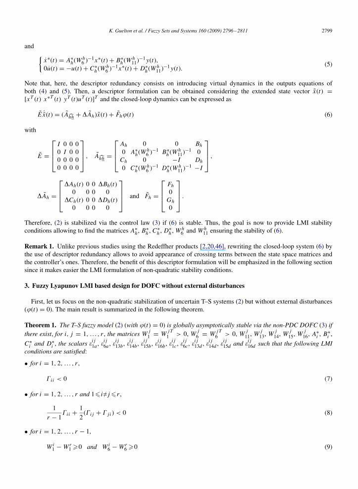
Note that, here, the descriptor redundancy consists on introducing virtual dynamics in the outputs equations ofboth (4) and (5). Then, a descriptor formulation can be obtained considering the extended state vector x(t) =[xT (t) x∗T (t) yT (t)uT (t)]T and the closed-loop dynamics can be expressed as

E ˙x(t) = ( Ahh + � Ah)x(t) + Fh�(t) (6)

with

E =

⎡⎢⎢⎣I 0 0 00 I 0 00 0 0 00 0 0 0

⎤⎥⎥⎦ , Ahh =

⎡⎢⎢⎣Ah 0 0 Bh

0 A∗h(W

h6 )

−1 B∗h (W

h11)

−1 0Ch 0 −I Dh

0 C∗h (W

h6 )

−1 D∗h (W

h11)

−1 −I

⎤⎥⎥⎦ ,

� Ah =

⎡⎢⎢⎣�Ah(t) 0 0 �Bh(t)

0 0 0 0�Ch(t) 0 0 �Dh(t)

0 0 0 0

⎤⎥⎥⎦ and Fh =

⎡⎢⎢⎣Fh0Gh

0

⎤⎥⎥⎦ .

Therefore, (2) is stabilized via the control law (3) if (6) is stable. Thus, the goal is now to provide LMI stabilityconditions allowing to find the matrices A∗

h , B∗h , C

∗h , D

∗h , W

h6 and Wh

11 ensuring the stability of (6).

Remark 1. Unlike previous studies using the Redeffher products [2,20,46], rewriting the closed-loop system (6) bythe use of descriptor redundancy allows to avoid appearance of crossing terms between the state space matrices andthe controller’s ones. Therefore, the benefit of this descriptor formulation will be emphasized in the following sectionsince it makes easier the LMI formulation of non-quadratic stability conditions.

3. Fuzzy Lyapunov LMI based design for DOFC without external disturbances

First, let us focus on the non-quadratic stabilization of uncertain T–S systems (2) but without external disturbances(�(t) = 0). The main result is summarized in the following theorem.

Theorem 1. The T–S fuzzy model (2) (with �(t) = 0) is globally asymptotically stable via the non-PDC DOFC (3) ifthere exist, for i, j = 1, . . . , r , the matrices W j

1 = W jT1 > 0, W j

6 = W jT6 > 0, W j

11, Wj13, W

j14, W

j15, W

j16, A

∗i , B

∗i ,

C∗i and D∗

i , the scalars �i j1a , �i j6a , �i j13b, �i j14b, �i j15b, �i j16b, �i j1c, �i j6c, �i j13d , �i j14d , �i j15d and �i j16d such that the following LMIconditions are satisfied:

• for i = 1, 2, . . . , r ,

�i i < 0 (7)

• for i = 1, 2, . . . , r and 1� i� j�r ,

1

r − 1�i i + 1

2(�i j + � j i ) < 0 (8)

• for i = 1, 2, . . . , r − 1,

Wi1 − Wr

1 �0 and Wi6 − Wr

6 �0 (9)

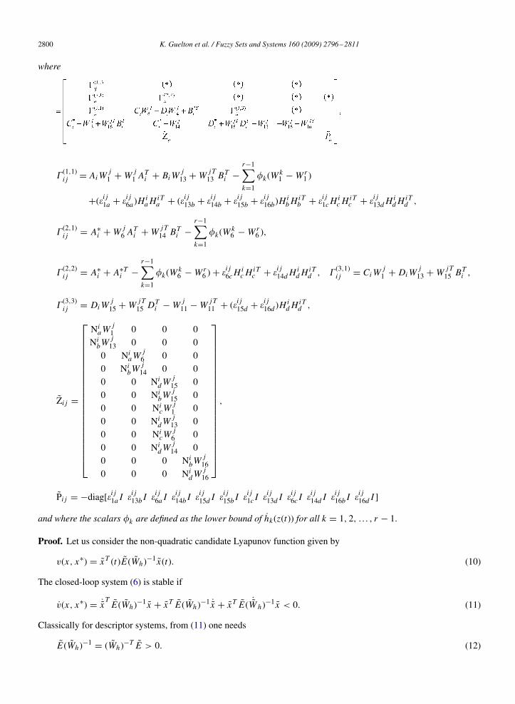
2800 K. Guelton et al. / Fuzzy Sets and Systems 160 (2009) 2796–2811

where

�(1,1)i j = AiW

j1 + W j

1 ATi + BiW

j13 + W jT

13 BTi −

r−1∑k=1

�k(Wk1 − Wr

1 )

+(�i j1a + �i j6a)HiaH

iTa + (�i j13b + �i j14b + �i j15b + �i j16b)H

ibH

iTb + �i j1cH

ic H

iTc + �i j13d H

id H

iTd ,

�(2,1)i j = A∗

i + W j6 A

Ti + W jT

14 BTi −

r−1∑k=1

�k(Wk6 − Wr

6 ),

�(2,2)i j = A∗

i + A∗Ti −

r−1∑k=1

�k(Wk6 − Wr

6 ) + �i j6cHic H

iTc + �i j14d H

id H

iTd , �(3,1)

i j = CiWj1 + DiW

j13 + W jT

15 BTi ,

�(3,3)i j = DiW

j15 + W jT

15 DTi − W j

11 − W jT11 + (�i j15d + �i j16d )H

id H

iTd ,

Zi j =

⎡⎢⎢⎢⎢⎢⎢⎢⎢⎢⎢⎢⎢⎢⎢⎢⎢⎢⎢⎢⎢⎢⎣

NiaW

j1 0 0 0

NibW

j13 0 0 0

0 NiaW

j6 0 0

0 NibW

j14 0 0

0 0 NidW

j15 0

0 0 NibW

j15 0

0 0 NicW

j1 0

0 0 NidW

j13 0

0 0 NicW

j6 0

0 0 NidW

j14 0

0 0 0 NibW

j16

0 0 0 NidW

j16

⎤⎥⎥⎥⎥⎥⎥⎥⎥⎥⎥⎥⎥⎥⎥⎥⎥⎥⎥⎥⎥⎥⎦

,

Pi j = −diag[�i j1a I �i j13b I �i j6a I �i j14b I �i j15d I �i j15b I �i j1c I �i j13d I �i j6c I �i j14d I �i j16b I �i j16d I ]

and where the scalars �k are defined as the lower bound of hk(z(t)) for all k = 1, 2, . . . , r − 1.

Proof. Let us consider the non-quadratic candidate Lyapunov function given by

v(x, x∗) = x T (t)E(Wh)−1 x(t). (10)

The closed-loop system (6) is stable if

v(x, x∗) = ˙xT E(Wh)−1 x + x T E(Wh)

−1 ˙x + x T E( ˙Wh)−1 x < 0. (11)

Classically for descriptor systems, from (11) one needs

E(Wh)−1 = (Wh)

−T E > 0. (12)

K. Guelton et al. / Fuzzy Sets and Systems 160 (2009) 2796–2811 2801

Let us consider

Wh =

⎡⎢⎢⎣Wh

1 Wh2 Wh

3 Wh4

Wh5 Wh

6 Wh7 Wh

8Wh

9 Wh10 Wh

11 Wh12

Wh13 Wh

14 Wh15 Wh

16

⎤⎥⎥⎦ .

Multiplying (12), left by W Th and right by Wh , one has W T

h E = E Wh > 0 which leads to Wh1 = WhT

1 > 0,Wh

6 = WhT6 > 0, Wh

2 = WhT5 , Wh

3 = Wh4 = Wh

7 = Wh8 = 0. Considering (6), (11) is obviously satisfied if

( AThh + � AT

h )(Wh)−1 + (Wh)

−T ( Ahh + � Ah) + E( ˙Wh)−1 < 0. (13)

Multiplying left by W Th and right by Wh and since W T

h E = E Wh > 0, (13) yields

W Th ( AT

hh + � ATh ) + ( Ahh + � Ah)Wh + E Wh(

˙Wh)−1Wh < 0. (14)

It is well known that Wh(˙Wh)−1Wh = − ˙Wh , see, e.g. [11]. Thus (14) can be rewritten as

�hhh + ��hh − E ˙Wh < 0 (15)

with �hhh = W Th AT

hh + AhhWh and ��hh = W Th � AT

h + � Ah Wh

Extending �hhh , it yields

�hhh =

⎡⎢⎢⎢⎣�(1,1)

hh (∗) (∗) (∗)�(2,1)

hhh �(2,2)hhh (∗) (∗)

�(3,1)hh �(3,2)

hh �(3,3)hh (∗)

�(4,1)hhh �(4,2)

hhh �(4,3)hh �(4,4)

hhh

⎤⎥⎥⎥⎦ (16)

with

�(1,1)hh = AhW

h1 + Wh

1 ATh + BhW

h13 + WhT

13 BTh ,

�(2,1)hhh = A∗

h(Wh6 )

−1WhT2 + Wh

2 ATh + B∗

h (Wh11)

−1Wh9 + WhT

14 BTh ,

�(2,2)hhh = A∗

h + A∗Th + B∗

h (Wh11)

−1Wh10 + WhT

10 (Wh11)

−T B∗Th ,

�(3,1)hh = ChW

h1 − Wh

9 + DhWh13 + WhT

15 BTh ,

�(3,2)hh = ChW

h2 − Wh

10 + DhWh14 + B∗T

h ,

�(3,3)hh = DhW

h15 + WhT

15 DTh − Wh

11 − WhT11 ,

�(4,1)hhh = C∗

h (Wh6 )

−1WhT2 + D∗

h (Wh11)

−1Wh9 − Wh

13 + WhT16 BT

h ,

�(4,2)hhh = C∗

h − Wh14 + D∗

h (Wh11)

−1Wh10 + WhT

12 (Wh11)

−T B∗Th ,

�(4,3)hh = D∗

h + WhT16 DT

h − Wh15 − WhT

12

and

�(4,4)hhh = D∗

h (Wh11)

−1Wh12 + WhT

12 (Wh11)

−T D∗Th − Wh

16 − WhT16 .

Let us recall that, due to the nature of the candidate Lyapunov function (10), Wh9 , W

h10, . . . ,W

h16 are slack decision

matrices which are free of choice. At a first glance on (16), in order to run to LMI conditions, a solution should beto choose, for instance Wh

9 = Wh10 = Wh

11 = Wh12. Nevertheless, in that case, the problem remains more restrictive

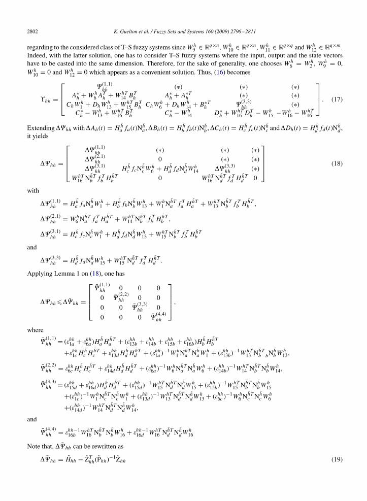
2802 K. Guelton et al. / Fuzzy Sets and Systems 160 (2009) 2796–2811

regarding to the considered class of T–S fuzzy systems sinceWh9 ∈ Rq×n ,Wh

10 ∈ Rq×n ,Wh11 ∈ Rq×q andWh

12 ∈ Rq×m .Indeed, with the latter solution, one has to consider T–S fuzzy systems where the input, output and the state vectorshave to be casted into the same dimension. Therefore, for the sake of generality, one chooses Wh

6 = Wh2 , W

h9 = 0,

Wh10 = 0 and Wh

12 = 0 which appears as a convenient solution. Thus, (16) becomes

�hh =

⎡⎢⎢⎣�(1,1)

hh (∗) (∗) (∗)A∗h + Wh

6 ATh + WhT

14 BTh A∗

h + A∗Th (∗) (∗)

ChWh1 + DhWh

13 + WhT15 BT

h ChWh6 + DhWh

14 + B∗Th �(3,3)

hh (∗)C∗h − Wh

13 + WhT16 BT

h C∗h − Wh

14 D∗h + WhT

16 DTh − Wh

15 −Wh16 − WhT

16

⎤⎥⎥⎦ . (17)

Extending��hh with�Ah(t) = Hha fa(t)Nh

a ,�Bh(t) = Hhb fb(t)Nh

b ,�Ch(t) = Hhc fc(t)Nh

c and�Dh(t) = Hhd fd (t)Nh

d ,it yields

��hh =

⎡⎢⎢⎢⎣��(1,1)

hh (∗) (∗) (∗)��(2,1)

hh 0 (∗) (∗)��(3,1)

hh H hc fcNh

c Wh6 + Hh

d fdNhdW

h14 ��(3,3)

hh (∗)WhT

16 NhTb f Tb H hT

b 0 WhT16 NhT

d f Td H hTd 0

⎤⎥⎥⎥⎦ (18)

with

��(1,1)hh = Hh

a faNhaW

h1 + Hh

b fbNhbW

h13 + Wh

1 NhTa f Ta H hT

a + WhT13 NhT

b f Tb H hTb ,

��(2,1)hh = Wh

6 NhTa f Ta H hT

a + WhT14 NhT

b f Tb H hTb ,

��(3,1)hh = Hh

c fcNhc W

h1 + Hh

d fdNhdW

h13 + WhT

15 NhTb f Tb H hT

b

and

��(3,3)hh = Hh

d fdNhdW

h15 + WhT

15 NhTd f Td H hT

d .

Applying Lemma 1 on (18), one has

��hh ���hh =

⎡⎢⎢⎢⎣�

(1,1)hh 0 0 0

0 �(2,2)hh 0 0

0 0 �(3,3)hh 0

0 0 0 �(4,4)hh

⎤⎥⎥⎥⎦ ,

where

�(1,1)hh = (�hh1a + �hh6a )H

ha H

hTa + (�hh13b + �hh14b + �hh15b + �hh16b)H

hb H

hTb

+�hh1c Hhc H

hTc + �hh13d H

hd H

hTd + (�hh1a )

−1Wh1 N

hTa Nh

aWh1 + (�hh13b)

−1WhT13 NhT

b bNhbW

h13,

�(2,2)hh = �hh6c H

hc H

hTc + �hh14d H

hd H

hTd + (�hh6a )

−1Wh6 N

hTa Nh

aWh6 + (�hh14b)

−1WhT14 NhT

b NhbW

h14,

�(3,3)hh = (�hh15d + �hh16d )H

hd H

hTd + (�hh15d )

−1WhT15 NhT

d NhdW

h15 + (�hh15b)

−1WhT15 NhT

b NhbW

h15

+(�hh1c )−1Wh

1 NhTc Nh

c Wh1 + (�hh13d )

−1WhT13 NhT

d NhdW

h13 + (�hh6c )

−1Wh6 N

hTc Nh

c Wh6

+(�hh14d )−1WhT

14 NhTd Nh

dWh14,

and

�(4,4)hh = �hh−1

16b WhT16 NhT

b NhbW

h16 + �hh−1

16d WhT16 NhT

d NhdW

h16

Note that, ��hh can be rewritten as

��hh = Hhh − ZThh(Phh)

−1Zhh (19)

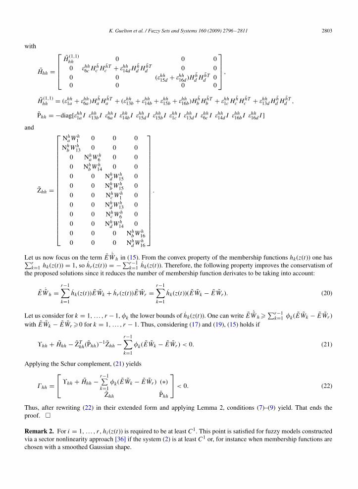
K. Guelton et al. / Fuzzy Sets and Systems 160 (2009) 2796–2811 2803

with

Hhh =

⎡⎢⎢⎢⎣H (1,1)hh 0 0 0

0 �hh6c Hhc H

hTc + �hh14d H

hd H

hTd 0 0

0 0 (�hh15d + �hh16d )Hhd H

hTd 0

0 0 0 0

⎤⎥⎥⎥⎦ ,

H (1,1)hh = (�hh1a + �hh6a )H

ha H

hTa + (�hh13b + �hh14b + �hh15b + �hh16b)H

hb H

hTb + �hh1c H

hc H

hTc + �hh13d H

hd H

hTd ,

Phh = −diag[�hh1a I �hh13b I �hh6a I �hh14b I �hh15d I �hh15b I �hh1c I �hh13d I �hh6c I �hh14d I �hh16b I �hh16d I ]

and

Zhh =

⎡⎢⎢⎢⎢⎢⎢⎢⎢⎢⎢⎢⎢⎢⎢⎢⎢⎢⎢⎢⎢⎢⎢⎣

NhaW

h1 0 0 0

NhbW

h13 0 0 0

0 NhaW

h6 0 0

0 NhbW

h14 0 0

0 0 NhdW

h15 0

0 0 NhbW

h15 0

0 0 NhcW

h1 0

0 0 NhdW

h13 0

0 0 NhcW

h6 0

0 0 NhdW

h14 0

0 0 0 NhbW

h16

0 0 0 NhdW

h16

⎤⎥⎥⎥⎥⎥⎥⎥⎥⎥⎥⎥⎥⎥⎥⎥⎥⎥⎥⎥⎥⎥⎥⎦

.

Let us now focus on the term E ˙Wh in (15). From the convex property of the membership functions hk(z(t)) one has∑rk=1 hk(z(t)) = 1, so hr (z(t)) = − ∑r−1

k=1 hk(z(t)). Therefore, the following property improves the conservatism ofthe proposed solutions since it reduces the number of membership function derivates to be taking into account:

E ˙Wh =r−1∑k=1

hk(z(t))E Wk + hr (z(t))E Wr =r−1∑k=1

hk(z(t))(E Wk − E Wr ). (20)

Let us consider for k = 1, . . . , r − 1, �k the lower bounds of hk(z(t)). One can write E˙Wh �

∑r−1k=1 �k(E Wk − E Wr )

with E Wk − E Wr �0 for k = 1, . . . , r − 1. Thus, considering (17) and (19), (15) holds if

�hh + Hhh − ZThh(Phh)

−1Zhh −r−1∑k=1

�k(E Wk − E Wr ) < 0. (21)

Applying the Schur complement, (21) yields

�hh =⎡⎣ �hh + Hhh −

r−1∑k=1

�k(E Wk − E Wr ) (∗)Zhh Phh

⎤⎦ < 0. (22)

Thus, after rewriting (22) in their extended form and applying Lemma 2, conditions (7)–(9) yield. That ends theproof. �

Remark 2. For i = 1, . . . , r , hi (z(t)) is required to be at least C1. This point is satisfied for fuzzy models constructedvia a sector nonlinearity approach [36] if the system (2) is at least C1 or, for instance when membership functions arechosen with a smoothed Gaussian shape.

2804 K. Guelton et al. / Fuzzy Sets and Systems 160 (2009) 2796–2811

Remark 3. From (3), Wh6 and Wh

11 are needed to be non-singular. If, for i = 1, . . . , r , Wi6 are solutions of theorem 1,

then we have Wi6 = WiT

6 > 0 imposed by (12). Thus Wh6 is a non-singular matrix. Moreover, if (10) is a Lyapunov

functional, i.e. (7), (8) and (9) are verified, Wh is a non-singular matrix satisfying (11) and W−1h exists. Recall that

Wh =

⎡⎢⎢⎣Wh

1 Wh6 0 0

Wh6 Wh

6 0 00 0 Wh

11 0Wh

13 Wh14 Wh

15 Wh16

⎤⎥⎥⎦ .

Therefore, Wh11 is a non-singular matrix and so (Wh

11)−1 exists.

Remark 4. Introducing the bounds of the time derivative membership functions in (21) with formulation (20)instead of

∑rk=1 �k E Wk allows providing LMI conditions (7), (8) and (9) which obviously include the

quadratic case. Thus the proposed fuzzy Lyapunov approach is obviously reducing the conservatism of quadraticapproach.

Remark 5. To the best of authors’ knowledge, expects our preliminary study [11], Theorem1 is the first result regardingto non-quadratic DOFC stabilization for T–S fuzzy models. Moreover, there were no tractable LMI conditions in theprevious literature which consider matrices Ci that have not to be common or identity as well as Di that have not to bezero in Eq. (2). Only few results exists using the Redheffer product in order to write the closed-loop system dynamics[2,20,46]. Nevertheless, these results are resorting to model transformation, bounding techniques for some cross termsand products between decision variables which are sources of conservatism and ruins tentative to derive non-quadraticLMI conditions. The non-quadratic DOFC design methodology depicted in Theorem 1 has been obtained thanks to therewriting of the closed-loop system (6). This has been done using the descriptor redundancy which avoids appearanceof crossing terms between the state space matrices and the controller’s ones.

4. H∞ based DOFC synthesis

The conditions proposed in Theorem 1 are for �(t) = 0. This section extends the above proposed results by the useof an H∞ criterion. The goal is to stabilize (2) such that the influence of the external disturbance �(t) on the outputbehavior is minimized. Let us consider the following H∞ criterion [36,48]:∫ ∞

0(yT (t)y(t) − �2�T (t)�(t)) dt�0. (23)

Recall that x(t) = [xT (t) x∗T (t) yT (t) uT (t)]T , thus (23) can be rewritten as∫ ∞

0(x T (t)Qx(t) − �2�T (t)�(t)) dt�0 (24)

with

Q =

⎡⎢⎢⎣0 0 0 00 0 0 00 0 I 00 0 0 0

⎤⎥⎥⎦ .

In that case, the stability of the closed-loop system (6) is guaranteed under constraint (24) if the LMI conditionssummarized in the following theorem hold.

Theorem 2. The T–S fuzzy model (2) is globally asymptotically stable via the non-PDC DOFC (3) and guarantee theattenuation level � = √

if there exist, the matrices W j1 = W jT

1 > 0, W j6 = W jT

6 > 0, W j11, W

j13, W

j14, W

j15, W

j16,

A∗i , B

∗i , C

∗i and D∗

i , for i = 1, . . . , r , the scalars , �i j1a , �i j6a , �

i j13b, �

i j15b, �

i j16b, �

i j14b, �

i j1c, �

i j6c, �

i j13d , �

i j14d , �

i j15d and �i j16d such

that the following LMI conditions are satisfied:

K. Guelton et al. / Fuzzy Sets and Systems 160 (2009) 2796–2811 2805

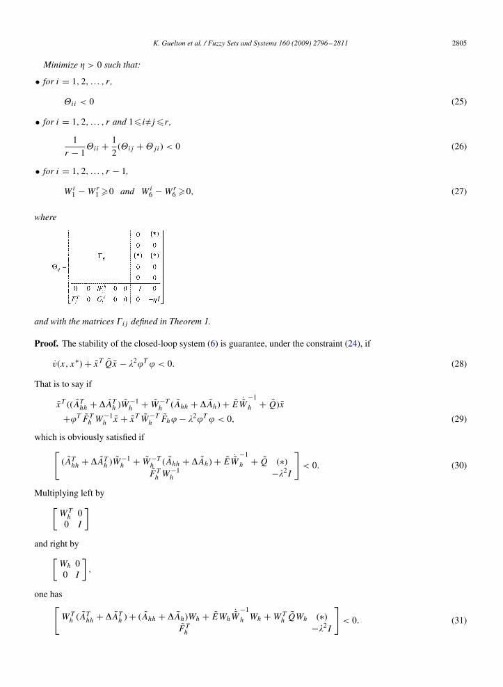
Minimize > 0 such that:

• for i = 1, 2, . . . , r ,

i i < 0 (25)

• for i = 1, 2, . . . , r and 1� i� j�r ,

1

r − 1i i + 1

2(i j + j i ) < 0 (26)

• for i = 1, 2, . . . , r − 1,

W i1 − Wr

1 �0 and Wi6 − Wr

6 �0, (27)

where

and with the matrices �i j defined in Theorem 1.

Proof. The stability of the closed-loop system (6) is guarantee, under the constraint (24), if

v(x, x∗) + x T Qx − �2�T� < 0. (28)

That is to say if

x T (( AThh + � AT

h )W−1h + W−T

h ( Ahh + � Ah) + E ˙W−1

h + Q)x

+�T FTh W−1

h x + x T W−Th Fh� − �2�T� < 0, (29)

which is obviously satisfied if[( AT

hh + � ATh )W

−1h + W−T

h ( Ahh + � Ah) + E ˙W−1

h + Q (∗)FTh W−1

h −�2 I

]< 0. (30)

Multiplying left by[WT

h 00 I

]and right by[

Wh 00 I

],

one has[WT

h ( AThh + � AT

h ) + ( Ahh + � Ah)Wh + EWh˙W−1

h Wh + WTh QWh (∗)

FTh −�2 I

]< 0. (31)

2806 K. Guelton et al. / Fuzzy Sets and Systems 160 (2009) 2796–2811

Following the same way as for the proof of theorem 1, with for k = 1, . . . , r − 1, E Wk − E Wr �0 leads to (27),(31) is satisfied if⎡⎣ �hh + Hhh − ZT

hh P−1hh Zhh + WT

h QWh −r−1∑k=1

�k(E Wk − E Wr ) (∗)FTh −�2 I

⎤⎦ < 0. (32)

Note that

WTh QWh =

⎡⎢⎢⎣0 0 0 00 0 0 00 0 WhT

11 Wh11 0

0 0 0 0

⎤⎥⎥⎦ ,

using the Schur complement and Lemma 2, (25) and (26) yield. That ends the proof. �

Remark 6. The LMI conditions proposed in Theorems 1 and 2 are depending on the lower bounds of hk(z(t)) fork = 1, . . . , r − 1. Even if it is often pointed out as a criticism to fuzzy Lyapunov approach since these parameters maybe difficult to choose, a way to obtain these bounds has been proposed in [37]. Moreover, let us recall that this approachremains one of the least conservative in terms of LMI based design. In [15], a fuzzy Lyapunov candidate function hasbeen reduced leading to relaxed quadratic stability conditions in the case of descriptor systems. Indeed, some elementsin the Lyapunov matrix can be set common in order to make the LMI free of membership function’s lower bounds.In the present study, this remains on setting W1 and W6 common matrices in the previous theorems. Note finally that,obviously, the “price” to pay for more practical applicability is an increase of the conservatism.

5. Simulation results

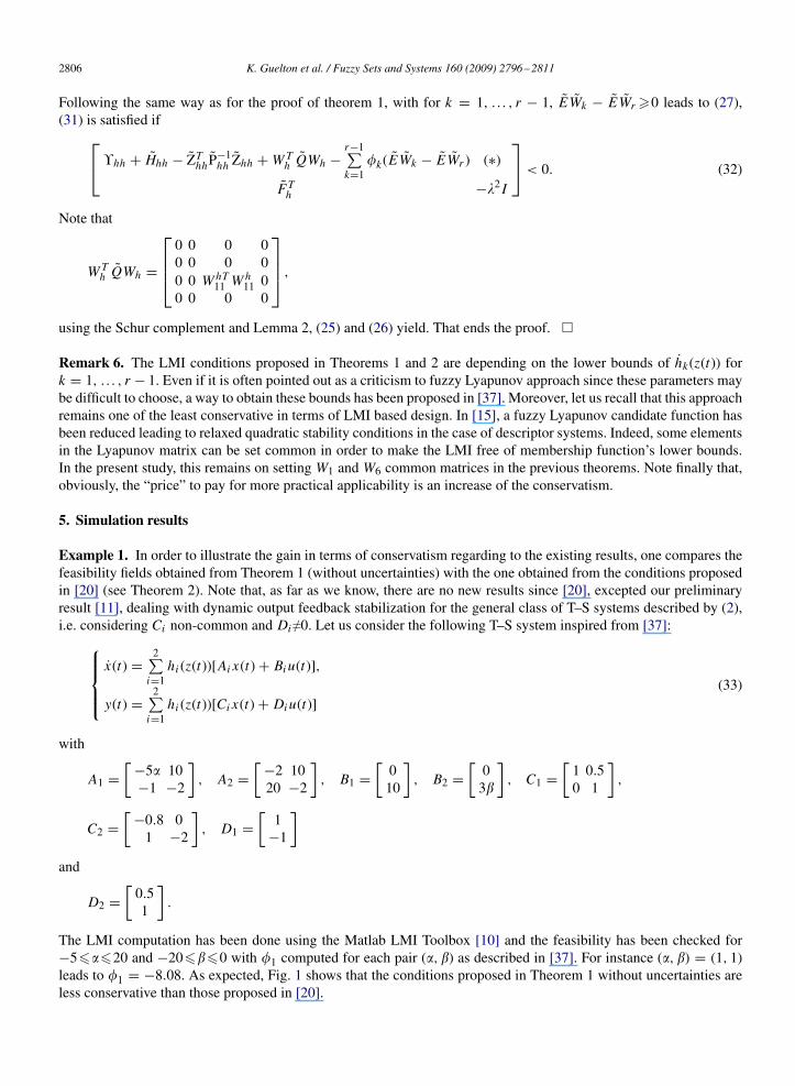
Example 1. In order to illustrate the gain in terms of conservatism regarding to the existing results, one compares thefeasibility fields obtained from Theorem 1 (without uncertainties) with the one obtained from the conditions proposedin [20] (see Theorem 2). Note that, as far as we know, there are no new results since [20], excepted our preliminaryresult [11], dealing with dynamic output feedback stabilization for the general class of T–S systems described by (2),i.e. considering Ci non-common and Di�0. Let us consider the following T–S system inspired from [37]:⎧⎪⎪⎨⎪⎪⎩

x(t) =2∑

i=1hi (z(t))[Ai x(t) + Biu(t)],

y(t) =2∑

i=1hi (z(t))[Ci x(t) + Diu(t)]

(33)

with

A1 =[ −5� 10

−1 −2

], A2 =

[ −2 1020 −2

], B1 =

[010

], B2 =

[03�

], C1 =

[1 0.50 1

],

C2 =[ −0.8 0

1 −2

], D1 =

[1

−1

]and

D2 =[0.51

].

The LMI computation has been done using the Matlab LMI Toolbox [10] and the feasibility has been checked for−5���20 and −20���0 with �1 computed for each pair (�, �) as described in [37]. For instance (�, �) = (1, 1)leads to �1 = −8.08. As expected, Fig. 1 shows that the conditions proposed in Theorem 1 without uncertainties areless conservative than those proposed in [20].

K. Guelton et al. / Fuzzy Sets and Systems 160 (2009) 2796–2811 2807

-5 0 5 10 15 20-20

-18

-16

-14

-12

-10

-8

-6

-4

-2

0Theorem 2 in [20]Theorem 1

Fig. 1. Feasibility fields from Theorem 1 without uncertainties and LMI conditions provided in [20].

Example 2. In this example, the design of a DOFC is considered for an uncertain and disturbed T–S fuzzy modelgiven by⎧⎪⎪⎨⎪⎪⎩

x(t) =2∑

i=1hi (z(t))[(Ai + �Ai (t))x(t) + (Bi + �Bi (t))u(t) + Fi�(t)],

y(t) =2∑

i=1hi (z(t))[(Ci + �Ci (t))x(t) + (Di + �Di (t))u(t) + Gi�(t)]

(34)

with

A1 =[ −5 −4

−1 −2

], A2 =

[ −2 −420 −2

], B1 =

[010

], B2 =

[03

], C1 =

[2 −105 −1

],

C2 =[ −3 20

−7 −2

], D1 =

[3

−1

]and

D2 =[ −10.5

], F1 = F2 =

[0

−0.25

], G1 =

[ −0.50.5

], G2 =

[0.350.5

],

�A1(t) = H1a fa(t)N1

a , �A2(t) = H2a fa(t)N2

a , �B1(t) = H1b fb(t)N1

b, �B2(t) = H2b fb(t)N2

b, �C1(t) = H1c fc(t)N1

c ,�C2(t) = H2

c fc(t)N2c , �D1(t) = H1

d fd (t)N1d and �D2(t) = H2

d fd (t)N2d with

H1a =

[01

], H2

a =[

0−1

], H1

b =[

0−2

], H2

b =[

0−1

], H1

c =[

1−1

],

H2c =

[ −11

], H1

d =[

0.5−0.5

], H2

d =[ −1

1

],

N1a = [1 1], N2

a = [−1 1], N1b = 1, N2

b = −0.75,

N1c=[1 1], N2

c=[−1 −1], N1d= − 1, N2

d=0.5, h1(z(t))=(1+sinc(x1(t)))/2 and h2(z(t))=1 − h1(z(t)).

Note that, the lower bound of the membership function derivative can be found for the nominal part of the consideredfuzzy system using the approaches proposed in [37], i.e. �1 = −3.68. Obviously, the considered model includes somebounded uncertainties and disturbances which are unknown. Thus, even if their effects are attenuated regarding to thestate, it is not possible to conclude on the time derivative of the membership function. At least, what can be done forinstance is choosing an assumed “greater” value than the one obtained from the nominal part. In the present example

2808 K. Guelton et al. / Fuzzy Sets and Systems 160 (2009) 2796–2811

0 0.5 1 1.5 2 2.5 3 3.5 4 4.5 5-0.4-0.2

00.20.40.60.8

1

time (sec)

x 1 (t

)

0 0.5 1 1.5 2 2.5 3 3.5 4 4.5 5-0.5

0

0.5

1

1.5

time (sec)

x 2 (t

)

with uncertainties and disturbanceswithout uncertainties and disturbances

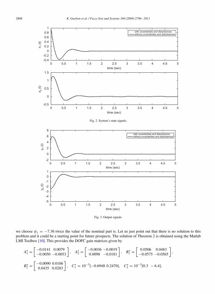
Fig. 2. System’s state signals.

0 0.5 1 1.5 2 2.5 3 3.5 4 4.5 5-2

0

2

4

6

8

time (sec)

y 1 (t

)

0 0.5 1 1.5 2 2.5 3 3.5 4 4.5 5-5-4-3-2-101

time (sec)

y 2 (t

)

with uncertainties and disturbanceswithout uncertainties and disturbances

Fig. 3. Output signals.

we choose �1 = −7.36 twice the value of the nominal part is. Let us just point out that there is no solution to thisproblem and it could be a starting point for future prospects. The solution of Theorem 2 is obtained using the MatlabLMI Toolbox [10]. This provides the DOFC gain matrices given by

A∗1 =

[ −0.0141 0.0079−0.0050 −0.0053

], A∗

2 =[ −0.0036 −0.0019

0.0098 −0.0181

], B∗

1 =[

0.0506 0.0483−0.0575 −0.0565

],

B∗2 =

[ −0.0090 0.01060.0435 0.0283

], C∗

1 = 10−3[−0.6948 0.2470], C∗2 = 10−3[0.3 − 6.4],

K. Guelton et al. / Fuzzy Sets and Systems 160 (2009) 2796–2811 2809

0 0.5 1 1.5 2 2.5 3 3.5 4 4.5 5-1

-0.50

0.51

1.52

2.53

x 10-3

time (sec)

x*1

(t)

0 0.5 1 1.5 2 2.5 3 3.5 4 4.5 5-2-10123456

x 10-4

time (sec)

x*2

(t)

with uncertainties and disturbanceswithout uncertainties and disturbances

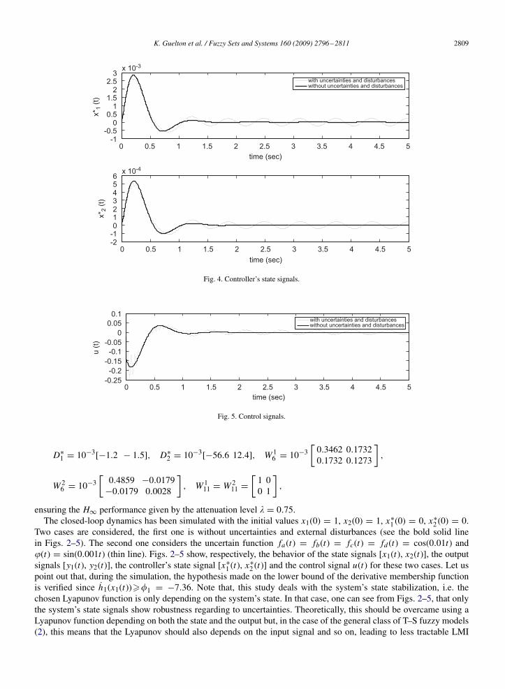
Fig. 4. Controller’s state signals.

0 0.5 1 1.5 2 2.5 3 3.5 4 4.5 5-0.25

-0.2-0.15

-0.1-0.05

00.05

0.1

time (sec)

u (t)

with uncertainties and disturbanceswithout uncertainties and disturbances

Fig. 5. Control signals.

D∗1 = 10−3[−1.2 − 1.5], D∗

2 = 10−3[−56.6 12.4], W 16 = 10−3

[0.3462 0.17320.1732 0.1273

],

W 26 = 10−3

[0.4859 −0.0179

−0.0179 0.0028

], W 1

11 = W 211 =

[1 00 1

],

ensuring the H∞ performance given by the attenuation level � = 0.75.The closed-loop dynamics has been simulated with the initial values x1(0) = 1, x2(0) = 1, x∗

1 (0) = 0, x∗2 (0) = 0.

Two cases are considered, the first one is without uncertainties and external disturbances (see the bold solid linein Figs. 2–5). The second one considers the uncertain function fa(t) = fb(t) = fc(t) = fd (t) = cos(0.01t) and�(t) = sin(0.001t) (thin line). Figs. 2–5 show, respectively, the behavior of the state signals [x1(t), x2(t)], the outputsignals [y1(t), y2(t)], the controller’s state signal [x∗

1 (t), x∗2 (t)] and the control signal u(t) for these two cases. Let us

point out that, during the simulation, the hypothesis made on the lower bound of the derivative membership functionis verified since h1(x1(t))��1 = −7.36. Note that, this study deals with the system’s state stabilization, i.e. thechosen Lyapunov function is only depending on the system’s state. In that case, one can see from Figs. 2–5, that onlythe system’s state signals show robustness regarding to uncertainties. Theoretically, this should be overcame using aLyapunov function depending on both the state and the output but, in the case of the general class of T–S fuzzy models(2), this means that the Lyapunov should also depends on the input signal and so on, leading to less tractable LMI

2810 K. Guelton et al. / Fuzzy Sets and Systems 160 (2009) 2796–2811

formulation. One other solution should be rewriting the considered nonlinear model using a convenient diffeomorphismallowing moving all uncertainties in the state equation, that is to say free of uncertainties in the output equations.

6. Conclusion

In this paper, the problem of dynamic output feedback stabilization of uncertain and disturbed T–S models hasbeen considered. A non-PDC DOFC has been proposed. The controller was then designed based on a fuzzy Lyapunovapproach. Thanks to the descriptor redundancy, strict LMI conditions have been easily obtained. This approach leadsto less conservative result and is valuable for uncertain and disturbed T–S fuzzy models through an H∞ criterion.Finally, two academic examples were proposed to show the conservativeness as well as to illustrate the efficiency ofthe proposed approach.

Acknowledgment

This work was supported by the French Ministry of Research, the “Département des Ardennes” and the region“Champagne-Ardenne” within the CPERMOSYP. The authors would like to thankMs. Belma Triks for her supportingcomments.

References

[1] P. Apkarian, J.M. Biannic, P. Gahinet, Self-scheduled H∞ control of a missile via linear matrix inequalities, J. Guidance Control Dyn. 18 (3)(1993) 532–538.

[2] W. Assawinchaichote, S.K. Nguang, P. Shi, Output feedback control design for uncertain singularly perturbed systems: an LMI approach,Automatica 40 (12) (2004) 2147–2152.

[3] X. Ban, X.Z. Gao, X. Huang, A.V. Vasilakos, Stability analysis of the simplest Takagi–Sugeno fuzzy control system using circle criterion,Inform. Sci. 177 (20) (2007) 4387–4409.

[4] X. Ban, X. Gao, X. Huang, H. Yin, Stability analysis of the simplest Takagi–Sugeno fuzzy control system using Popov criterion, Internat.J. Innovative Comput. Inform. Control 3 (5) (2007) 1087–1096.

[5] S. Boyd, L. El Ghaoui, E. Feron, V. Balakrishnan, Linear Matrix Inequalities in System and Control Theory, SIAM, Philadelphia, PA, 1994.[6] S.G. Cao, N.W. Rees, G. Feng, H∞ control of uncertain fuzzy continuous-time systems, Fuzzy Sets and Systems 115 (2) (2000) 171–190.[7] B.S. Chen, C.S. Tseng, H.J. Uang, Mixed H2/H∞ fuzzy output feedback control design for nonlinear dynamic systems: an LMI approach,

IEEE Trans. Fuzzy Systems 8 (3) (2000) 249–265.[8] G. Feng, A survey on analysis and design of model-based fuzzy control systems, IEEE Trans. Fuzzy Systems 14 (5) (2006) 676–697.[9] E. Fridman, New Lyapunov–Krasovskii functionals for stability of linear retarded and neutral type systems, Systems Control Lett. 43 (4) (2001)

309–319.[10] P. Gahinet, A. Nemirovski, A.J. Laub, M. Chilali, LMI control toolbox for use with MATLAB, The Mathworks Partner Series, 1995.[11] K. Guelton, T. Bouarar, N. Manamanni, Fuzzy Lyapunov LMI based output feedback stabilization of Takagi–Sugeno systems using descriptor

redundancy, in: Proc. FUZZ-IEEE 08, IEEE Internat. Conf. on Fuzzy Systems, Hong Kong, 2008.[12] K. Guelton, S. Delprat, T.M. Guerra, An alternative to inverse dynamics joint torques estimation in human stance based on a Takagi–Sugeno

unknown inputs observer in the descriptor form, Control Eng. Practice 16 (12) (2008) 1414–1426.[13] T.M. Guerra, L. Vermeiren, LMI based relaxed nonquadratic stabilizations for non-linear systems in the Takagi–Sugeno’s form, Automatica

40 (5) (2004) 823–829.[14] T.M. Guerra, A. Kruszewski, L. Vermeiren, H. Tirmant, Conditions of output stabilization for nonlinear models in the Takagi–Sugeno’s form,

Fuzzy Sets and Systems 157 (9) (2006) 1248–1259.[15] T.M. Guerra, M. Bernal, A. Kruszewski, M. Afroun, A way to improve results for the stabilization of continuous-time fuzzy descriptor models,

in: Proc. 46th IEEE Conf. on Decision and Control, New Orleans, USA, 2007.[16] D. Huang, S.K. Nguang, Robust H∞ static output feedback control of fuzzy systems: an ILMI approach, IEEE Trans. Systems Man Cybernet.

B 36 (1) (2006) 216–222.[17] D. Huang, S.K. Nguang, Static output feedback controller design for fuzzy systems: an ILMI approach, Inform. Sci. 177 (14) (2007)

3005–3015.[18] M. Johansson, A. Rantzer, K.E. Arzen, Piecewise quadratic stability of fuzzy systems, IEEE Trans. Fuzzy Systems 7 (6) (1999) 713–722.[19] E. Kim, H. Lee, New approaches to relaxed quadratic stability condition of fuzzy control systems, IEEE Trans. Fuzzy Systems 8 (5) (2000)

523–534.[20] J. Li, H.O. Wang, D. Niemann, K. Tanaka, Dynamic parallel distributed compensation for Takagi–Sugeno fuzzy systems: an LMI approach,

Inform. Sci. 123 (3–4) (2000) 201–221.[21] X. Liu, Q. Zhang, New approaches to H∞ controller design based on fuzzy observers for fuzzy T–S systems via LMI, Automatica 39 (9) (2003)

1571–1582.[22] N. Manamanni, B. Mansouri, A. Hamzaoui, J. Zaytoon, Relaxed conditions in tracking control design for T–S fuzzy model, J. Intelligent Fuzzy

Systems 18 (2) (2007) 185–210.

K. Guelton et al. / Fuzzy Sets and Systems 160 (2009) 2796–2811 2811

[23] B. Mansouri, A. Kruszewski, K. Guelton, N. Manamanni, Sub-optimal tracking control for uncertain T–S fuzzy models, in: Proc. AFNC 07,Third IFAC Workshop on Advanced Fuzzy and Neural Control, Valenciennes, France, 2007.

[24] B. Mansouri, N. Manamanni, K. Guelton, A. Kruszewski, T.M. Guerra, Output feedback LMI tracking control conditions with H∞ criterionfor uncertain and disturbed T–S models, Inform. Sci. 179 (4) (2009) 446–457.

[25] S.K. Nguang, P. Shi, Fuzzy H∞ output feedback control of nonlinear systems under sampled measurements, Automatica 39 (12) (2003)2169–2174.

[26] S.K. Nguang, P. Shi, Robust output feedback control design for Takagi–Sugeno systems with Markovian jumps: a linear matrix inequalityapproach, J. Dynamic Systems Measurement Control 128 (3) (2006) 617–625.

[27] C.-W. Park, LMI-based robust stability analysis for fuzzy feedback linearization regulators with its applications, Inform. Sci. 152 (2003)287–301.

[28] R.M. Redheffer, On a certain linear fractional transformation, J. Math. Phys. 39 (1960) 269–286.[29] B.J. Rhee, S. Won, A new Lyapunov function approach for a Takagi–Sugeno fuzzy control system design, Fuzzy Sets and Systems 157 (9)

(2006) 1211–1228.[30] A. Sala, T.M. Guerra, R. Babuska, Perspectives of fuzzy systems and control, Fuzzy Sets and Systems 153 (3) (2005) 432–444 (Special Issue:

40th Anniversary of Fuzzy Sets).[31] V.L. Syrmos, C.T. Abdallah, P. Dorato, K. Grigoriadis, Static output feedback—a survey, Automatica 33 (2) (1997) 125–137.[32] T. Takagi, M. Sugeno, Fuzzy identification of systems and its applications to modeling and control, IEEE Trans. System Man Cybernet. 15 (1)

(1985) 116–132.[33] K. Tanaka, M. Sugeno, Stability analysis and design of fuzzy control systems, Fuzzy Sets and Systems 45 (2) (1992) 135–156.[34] K. Tanaka, T. Ikeda, H.O. Wang, Robust stabilization of a class of uncertain nonlinear systems via fuzzy control: quadratic stabilizability, H∞

control theory, and linear matrix inequalities, IEEE Trans. Fuzzy Systems 4 (1) (1996) 1–13.[35] K. Tanaka, T. Ikeda, H.O. Wang, Fuzzy regulators and fuzzy observers: relaxed stability conditions and LMI-based designs, IEEE Trans. Fuzzy

Systems 6 (2) (1998) 1–16.[36] K. Tanaka, H.O. Wang, Fuzzy Control Systems Design and Analysis. A Linear Matrix Inequality Approach, Wiley, New York, 2001.[37] K. Tanaka, T. Hori, H.O. Wang, A multiple Lyapunov function approach to stabilization of fuzzy control systems, IEEE Trans. Fuzzy Systems

11 (4) (2003) 582–589.[38] K. Tanaka, H. Ohtake, H.O. Wang, A descriptor system approach to fuzzy control system design via fuzzy Lyapunov functions, IEEE Trans.

Fuzzy Systems 15 (3) (2007) 333–341.[39] S. Tong, Y. Li, Direct adaptive fuzzy backstepping control for a class of nonlinear systems, Int. J. Innovative Comput. Inform. Control 3 (4)

(2007) 887–896.[40] S. Tong, W. Wang, L. Qu, Decentralized robust control for uncertain T–S fuzzy large-scale systems with time-delay, Int. J. Innovative Comput.

Inform. Control 3 (3) (2007) 657–672.[41] H.D. Tuan, P. Apkarian, T. Narikiyo, Y. Yamamoto, Parametrized linear matrix inequality techniques in fuzzy control design, IEEE Trans.

Fuzzy Systems 9 (2001) 324–332.[42] H.O. Wang, K. Tanaka, M.F. Griffin, An approach to fuzzy control of nonlinear systems: stability and the design issues, IEEE Trans. Fuzzy

Systems 4 (1) (1996) 14–23.[43] S. Xu, J. Lam, Robust H∞ control for uncertain discrete-time-delay fuzzy systems via output feedback controllers, IEEE Trans. Fuzzy Systems

13 (1) (2005) 82–93.[44] J. Yoneyama, M. Nishikawa, H. Katayama, A. Ichikawa, Output stabilization of Takagi–Sugeno fuzzy systems, Fuzzy Sets and Systems 111

(2) (2000) 253–266.[45] J. Yoneyama, M. Nishikawa, H. Katayama, A. Ichikawa, Design of output feedback controllers for Takagi–Sugeno fuzzy systems, Fuzzy Sets

and Systems 121 (2001) 127–148.[46] M. Zerar, K. Guelton, N. Manamanni, Linear fractional transformation based H-infinity output stabilization for Takagi–Sugeno fuzzy models,

Mediterranean J. Measurement Control 4 (3) (2008) 111–121.[47] K. Zhou, P.P. Khargonekar, Robust stabilization of linear systems with norm-bounded time-varying uncertainty, Systems Control Lett. 10 (1)

(1988) 17–20.[48] K. Zhou, J. Doyle, K. Glover, Robust and Optimal Control, Prentice-Hall, New Jersey, 1996.