Convolutional dictionary learning based auto-encoders for

Convolutional dictionary learning based auto-encodersfor natural exponential-family distributions

Bahareh Tolooshams * 1 Andrew H. Song * 2 Simona Temereanca 3 Demba Ba 1

Abstract

We introduce a class of auto-encoder neural net-works tailored to data from the natural exponen-tial family (e.g., count data). The architecturesare inspired by the problem of learning the filtersin a convolutional generative model with spar-sity constraints, often referred to as convolutionaldictionary learning (CDL). Our work is the firstto combine ideas from convolutional generativemodels and deep learning for data that are natu-rally modeled with a non-Gaussian distribution(e.g., binomial and Poisson). This perspectiveprovides us with a scalable and flexible frame-work that can be re-purposed for a wide range oftasks and assumptions on the generative model.Specifically, the iterative optimization procedurefor solving CDL, an unsupervised task, is mappedto an unfolded and constrained neural network,with iterative adjustments to the inputs to accountfor the generative distribution. We also show thatthe framework can easily be extended for dis-criminative training, appropriate for a supervisedtask. We 1) demonstrate that fitting the genera-tive model to learn, in an unsupervised fashion,the latent stimulus that underlies neural spikingdata leads to better goodness-of-fit compared toother baselines, 2) show competitive performancecompared to state-of-the-art algorithms for super-vised Poisson image denoising, with significantlyfewer parameters, and 3) characterize the gradientdynamics of the shallow binomial auto-encoder.

*Equal contribution 1School of Engineering and AppliedSciences, Harvard University, Cambridge, MA 2MassachusettsInstitute of Technology, Cambridge, MA 3Brown Univer-sity, Boston, MA. Correspondence to: Bahareh Tolooshams<[email protected]>.

Proceedings of the 37 th International Conference on MachineLearning, Online, PMLR 119, 2020. Copyright 2020 by the au-thor(s).

1. IntroductionLearning shift-invariant patterns from a dataset has givenrise to work in different communities, most notably in signalprocessing (SP) and deep learning. In the former, this prob-lem is referred to as convolutional dictionary learning (CDL)(Garcia-Cardona & Wohlberg, 2018). CDL imposes a lineargenerative model where the data are generated by a sparselinear combination of shifts of localized patterns. In thelatter, convolutional neural networks (NNs) (LeCun et al.,2015) have excelled in identifying shift-invariant patterns.

Recently, the iterative nature of the optimization algorithmsfor performing CDL has inspired the utilization of NNsas an efficient and scalable alternative, starting with theseminal work of (Gregor & Lecun, 2010), and followedby (Tolooshams et al., 2018; Sreter & Giryes, 2018; Sulamet al., 2019). Specifically, the iterative steps are expressedas a recurrent NN, and thus solving the optimization simplybecomes passing the input through an unrolled NN (Hersheyet al., 2014; Monga et al., 2019). At one end of the spectrum,this perspective, through weight-tying, leads to architectureswith significantly fewer parameters than a generic NN. Atthe other end, by untying the weights, it motivates newarchitectures that depart, and could not be arrived at, fromthe generative perspective (Gregor & Lecun, 2010; Sreter &Giryes, 2018).

The majority of the literature at the intersection of generativemodels and NNs assumes that the data are real-valued andtherefore are not appropriate for binary or count-valued data,such as neural spiking data and photon-based images (Yanget al., 2011). Nevertheless, several works on Poisson im-age denoising, arguably the most popular application in-volving non real-valued data, can be found separately inboth communities. In the SP community, the negative Pois-son data likelihood is either explicitly minimized (Salmonet al., 2014; Giryes & Elad, 2014) or used as a penalty termadded to the objective of an image denoising problem withGaussian noise (Ma et al., 2013). Being rooted in the dic-tionary learning formalism, these methods operate in anunsupervised manner. Although they yield good denois-ing performance, their main drawbacks are scalability andcomputational efficiency.

Convolutional dictionary learning based auto-encoders for natural exponential-family distributions

In the deep learning community, NNs tailored to imagedenoising (Zhang et al., 2017; Remez et al., 2018; Fenget al., 2018), which are reminiscent of residual learning,have shown great performance on Poisson image denoising.However, since these 1) are not designed from the generativemodel perspective and/or 2) are supervised learning frame-works, it is unclear how they can be adapted to the classicalCDL, where the task is unsupervised and the interpretabilityof the parameters is important. NNs with a generative flavor,namely variational auto-encoders (VAEs), have been ex-tended to utilize non real-valued data (Nazábal et al., 2020;Liang et al., 2018). However, these architectures cannot beadapted to solve the CDL task.

To address this gap, we make the following contributions1:

Auto-encoder inspired by CDL for non real-valued dataWe introduce a flexible class of auto-encoder (AE) archi-tectures for data from the natural exponential-family thatcombines the perspectives of generative models and NNs.We term this framework, depicted in Fig. 1, the deep convo-lutional exponential-family auto-encoder (DCEA).

Unsupervised learning of convolutional patterns Weshow through simulation that DCEA performs CDL andlearns convolutional patterns from binomial observations.We also apply DCEA to real neural spiking data and showthat it fits the data better than baselines.

Supervised learning framework DCEA, when trained in asupervised manner, achieves similar performance to state-of-the-art algorithms for Poisson image denoising with ordersof magnitude fewer parameters compared to other baselines,owing to its design based on a generative model.

Gradient dynamics of shallow exponential auto-encoderGiven some assumptions on the binomial generative modelwith dense dictionary and “good” initializations, we provein Theorem 1 that shallow exponential auto-encoder (SEA),when trained by gradient descent, recovers the dictionary.

2. Problem FormulationNatural exponential-family distribution For a given ob-servation vector y ∈ RN , with meanµµµ ∈ RN , we define thelog-likelihood of the natural exponential family (McCullagh& Nelder, 1989) as

log p(y|µ) = f(µµµ)Ty + g(y)−B

(µµµ), (1)

where we have assumed that, conditioned onµµµ, the elementsof y are independent. The natural exponential family in-cludes a broad family of probability distributions such asthe Gaussian, binomial, and Poisson. The functions g(·),B(·), as well as the invertible link function f(·), all dependon the choice of distribution.

1The code can be found at https://github.com/btolooshams/dea

Convolutional generative model We assume that f(µµµ)is the sum of scaled and time-shifted copies of C finite-length filters (dictionary) {hc}C

c=1 ∈ RK , each localized,i.e., K � N . We can express f(µµµ) in a convolutional form:f(µµµ) =

∑Cc=1 hc ∗ xc, where ∗ is the convolution opera-

tion, and xc ∈ RN−K+1 is a train of scaled impulses whichwe refer to as code vector. Using linear-algebraic notation,f(µµµ) =

∑Cc=1 hc ∗ xc = Hx, where H ∈ RN×C(N−K+1)

is a matrix that is the concatenation of C Toeplitz (i.e.,banded circulant) matrices Hc ∈ RN×(N−K+1), c =1, . . . , C, and x = [(x1)T, . . . , (xC)T]T ∈ RC(N−K+1).

We refer to the input/output domain of f(·) as the data anddictionary domains, respectively. We interpret y as a time-series and the non-zero elements of x as the times wheneach of the C filters are active. When y is two-dimensional(2D), i.e., an image, x encodes the spatial locations wherethe filters contribute to its mean µµµ.

Exponential convolutional dictionary learning (ECDL)Given J observations {yj}J

j=1, we estimate {hc}Cc=1

and {xj}Jj=1 that minimize the negative log-likelihood∑J

j=1 l(xj) = −∑J

j=1 log p(yj |{hc}Cc=1,xj) under the

convolutional generative model, subject to sparsity con-straints on {xj}J

j=1. We enforce sparsity using the `1 norm,which leads to the non-convex optimization problem

min{hc}Cc=1{xj}Jj=1

J∑j=1

l(xj)︷︸︸︷−(Hxj)Tyj +B(f−1(Hxj)

)+λ‖xj‖1,

(2)where the regularizer λ controls the degree of sparsity. Apopular approach to deal with the non-convexity is to mini-mize the objective over one set of variables, while the othersare fixed, in an alternating manner, until convergence (Agar-wal et al., 2016). When {xj}J

j=1 is being optimized withfixed H, we refer to the problem as convolutional sparsecoding (CSC). When H is being optimized with {xj}J

j=1fixed, we refer to the problem as convolutional dictionaryupdate (CDU).

3. Deep convolutional exponential-familyauto-encoder

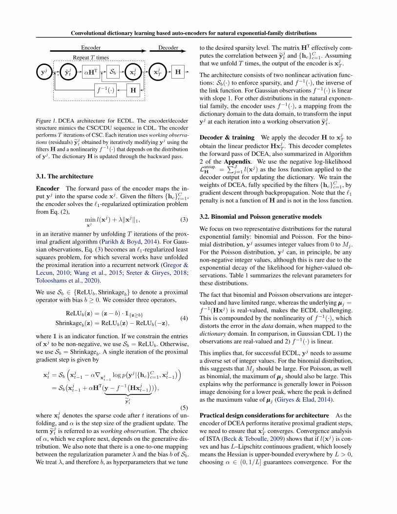
We propose a class of auto-encoder architectures to solvethe ECDL problem, which we term deep convolutionalexponential-family auto-encoder (DCEA). Specifically, wemake a one-to-one connection between the CSC/CDU stepsand the encoder/decoder of DCEA depicted in Fig. 1. Wefocus only on CSC for a single yj , as the CSC step can beparallelized across examples.


yj yjt αHT Sb xj

t xjT H

Hf−1(·)

DecoderEncoder

-

Repeat T times

Figure 1. DCEA architecture for ECDL. The encoder/decoderstructure mimics the CSC/CDU sequence in CDL. The encoderperforms T iterations of CSC. Each iteration uses working observa-tions (residuals) yj

t obtained by iteratively modifying yj using thefilters H and a nonlinearity f−1(·) that depends on the distributionof yj . The dictionary H is updated through the backward pass.

3.1. The architecture

Encoder The forward pass of the encoder maps the in-put yj into the sparse code xj . Given the filters {hc}C

c=1,the encoder solves the `1-regularized optimization problemfrom Eq. (2),

minxj

l(xj) + λ‖xj‖1, (3)

in an iterative manner by unfolding T iterations of the prox-imal gradient algorithm (Parikh & Boyd, 2014). For Gaus-sian observations, Eq. (3) becomes an `1-regularized leastsquares problem, for which several works have unfoldedthe proximal iteration into a recurrent network (Gregor &Lecun, 2010; Wang et al., 2015; Sreter & Giryes, 2018;Tolooshams et al., 2020).

We use Sb ∈ {ReLUb,Shrinkageb} to denote a proximaloperator with bias b ≥ 0. We consider three operators,

ReLUb(z) = (z− b) · 1{z≥b}

Shrinkageb(z) = ReLUb(z)− ReLUb(−z),(4)

where 1 is an indicator function. If we constrain the entriesof xj to be non-negative, we use Sb = ReLUb. Otherwise,we use Sb = Shrinkageb. A single iteration of the proximalgradient step is given by

xjt = Sb

(xj

t−1 − α∇xjt−1

log p(yj |{hc}C

c=1,xjt−1))

= Sb

(xj

t−1 + αHT(y− f−1(Hxjt−1)︸︷︷︸

yjt

)),

(5)where xj

t denotes the sparse code after t iterations of un-folding, and α is the step size of the gradient update. Theterm yj

t is referred to as working observation. The choiceof α, which we explore next, depends on the generative dis-tribution. We also note that there is a one-to-one mappingbetween the regularization parameter λ and the bias b of Sb.We treat λ, and therefore b, as hyperparameters that we tune

to the desired sparsity level. The matrix HT effectively com-putes the correlation between yj

t and {hc}Cc=1. Assuming

that we unfold T times, the output of the encoder is xjT .

The architecture consists of two nonlinear activation func-tions: Sb(·) to enforce sparsity, and f−1(·), the inverse ofthe link function. For Gaussian observations f−1(·) is linearwith slope 1. For other distributions in the natural exponen-tial family, the encoder uses f−1(·), a mapping from thedictionary domain to the data domain, to transform the inputyj at each iteration into a working observation yj

t .

Decoder & training We apply the decoder H to xjT to

obtain the linear predictor HxjT . This decoder completes

the forward pass of DCEA, also summarized in Algorithm2 of the Appendix. We use the negative log-likelihoodLunsup.

H =∑J

j=1 l(xj) as the loss function applied to thedecoder output for updating the dictionary. We train theweights of DCEA, fully specified by the filters {hc}C

c=1, bygradient descent through backpropagation. Note that the `1penalty is not a function of H and is not in the loss function.

3.2. Binomial and Poisson generative models

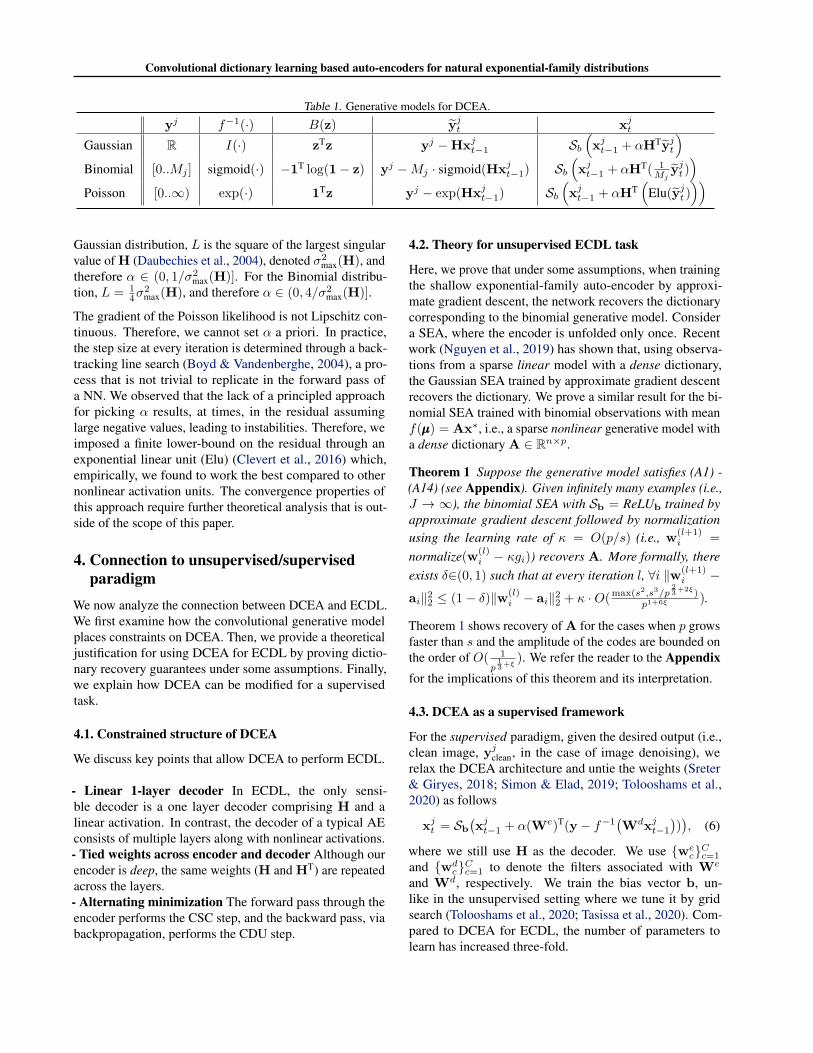
We focus on two representative distributions for the naturalexponential family: binomial and Poisson. For the bino-mial distribution, yj assumes integer values from 0 to Mj .For the Poisson distribution, yj can, in principle, be anynon-negative integer values, although this is rare due to theexponential decay of the likelihood for higher-valued ob-servations. Table 1 summarizes the relevant parameters forthese distributions.

The fact that binomial and Poisson observations are integer-valued and have limited range, whereas the underlyingµµµj =f−1(Hxj) is real-valued, makes the ECDL challenging.This is compounded by the nonlinearity of f−1(·), whichdistorts the error in the data domain, when mapped to thedictionary domain. In comparison, in Gaussian CDL 1) theobservations are real-valued and 2) f−1(·) is linear.

This implies that, for successful ECDL, yj needs to assumea diverse set of integer values. For the binomial distribution,this suggests that Mj should be large. For Poisson, as wellas binomial, the maximum of µµµj should also be large. Thisexplains why the performance is generally lower in Poissonimage denoising for a lower peak, where the peak is definedas the maximum value of µµµj (Giryes & Elad, 2014).

Practical design considerations for architecture As theencoder of DCEA performs iterative proximal gradient steps,we need to ensure that xj

T converges. Convergence analysisof ISTA (Beck & Teboulle, 2009) shows that if l(xj) is con-vex and has L–Lipschitz continuous gradient, which looselymeans the Hessian is upper-bounded everywhere by L > 0,choosing α ∈ (0, 1/L] guarantees convergence. For the


Table 1. Generative models for DCEA.

yj f−1(·) B(z) yjt xj

t

Gaussian R I(·) zTz yj −Hxjt−1 Sb

(xj

t−1 + αHTyjt

)Binomial [0..Mj ] sigmoid(·) −1T log(1− z) yj −Mj · sigmoid(Hxj

t−1) Sb

(xj

t−1 + αHT( 1Mj

yjt ))

Poisson [0..∞) exp(·) 1Tz yj − exp(Hxjt−1) Sb

(xj

t−1 + αHT(

Elu(yjt )))

Gaussian distribution, L is the square of the largest singularvalue of H (Daubechies et al., 2004), denoted σ2

max(H), andtherefore α ∈ (0, 1/σ2

max(H)]. For the Binomial distribu-tion, L = 1

4σ2max(H), and therefore α ∈ (0, 4/σ2

max(H)].

The gradient of the Poisson likelihood is not Lipschitz con-tinuous. Therefore, we cannot set α a priori. In practice,the step size at every iteration is determined through a back-tracking line search (Boyd & Vandenberghe, 2004), a pro-cess that is not trivial to replicate in the forward pass ofa NN. We observed that the lack of a principled approachfor picking α results, at times, in the residual assuminglarge negative values, leading to instabilities. Therefore, weimposed a finite lower-bound on the residual through anexponential linear unit (Elu) (Clevert et al., 2016) which,empirically, we found to work the best compared to othernonlinear activation units. The convergence properties ofthis approach require further theoretical analysis that is out-side of the scope of this paper.

4. Connection to unsupervised/supervisedparadigm

We now analyze the connection between DCEA and ECDL.We first examine how the convolutional generative modelplaces constraints on DCEA. Then, we provide a theoreticaljustification for using DCEA for ECDL by proving dictio-nary recovery guarantees under some assumptions. Finally,we explain how DCEA can be modified for a supervisedtask.

4.1. Constrained structure of DCEA

We discuss key points that allow DCEA to perform ECDL.

- Linear 1-layer decoder In ECDL, the only sensi-ble decoder is a one layer decoder comprising H and alinear activation. In contrast, the decoder of a typical AEconsists of multiple layers along with nonlinear activations.- Tied weights across encoder and decoder Although ourencoder is deep, the same weights (H and HT) are repeatedacross the layers.- Alternating minimization The forward pass through theencoder performs the CSC step, and the backward pass, viabackpropagation, performs the CDU step.

4.2. Theory for unsupervised ECDL task

Here, we prove that under some assumptions, when trainingthe shallow exponential-family auto-encoder by approxi-mate gradient descent, the network recovers the dictionarycorresponding to the binomial generative model. Considera SEA, where the encoder is unfolded only once. Recentwork (Nguyen et al., 2019) has shown that, using observa-tions from a sparse linear model with a dense dictionary,the Gaussian SEA trained by approximate gradient descentrecovers the dictionary. We prove a similar result for the bi-nomial SEA trained with binomial observations with meanf(µµµ) = Ax∗, i.e., a sparse nonlinear generative model witha dense dictionary A ∈ Rn×p.

Theorem 1 Suppose the generative model satisfies (A1) -(A14) (see Appendix). Given infinitely many examples (i.e.,J → ∞), the binomial SEA with Sb = ReLUb trained byapproximate gradient descent followed by normalizationusing the learning rate of κ = O(p/s) (i.e., w(l+1)

i =normalize(w(l)

i − κgi)) recovers A. More formally, thereexists δ∈(0, 1) such that at every iteration l, ∀i ‖w(l+1)

i −

ai‖22 ≤ (1− δ)‖w(l)

i − ai‖22 + κ ·O( max(s2,s3/p

23 +2ξ)

p1+6ξ ).

Theorem 1 shows recovery of A for the cases when p growsfaster than s and the amplitude of the codes are bounded onthe order of O( 1

p13 +ξ ). We refer the reader to the Appendix

for the implications of this theorem and its interpretation.

4.3. DCEA as a supervised framework

For the supervised paradigm, given the desired output (i.e.,clean image, yj

clean, in the case of image denoising), werelax the DCEA architecture and untie the weights (Sreter& Giryes, 2018; Simon & Elad, 2019; Tolooshams et al.,2020) as follows

xjt = Sb

(xj

t−1 + α(We)T(y− f−1(Wdxjt−1))), (6)

where we still use H as the decoder. We use {wec}C

c=1and {wd

c}Cc=1 to denote the filters associated with We

and Wd, respectively. We train the bias vector b, un-like in the unsupervised setting where we tune it by gridsearch (Tolooshams et al., 2020; Tasissa et al., 2020). Com-pared to DCEA for ECDL, the number of parameters tolearn has increased three-fold.


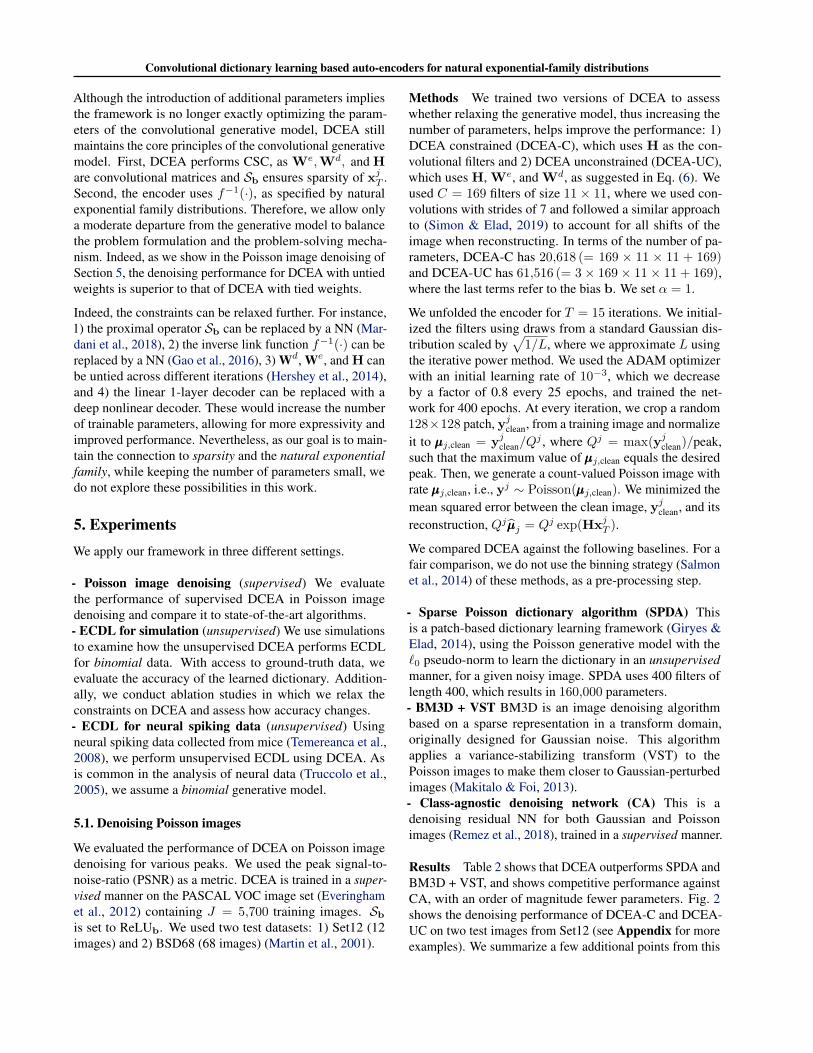
Although the introduction of additional parameters impliesthe framework is no longer exactly optimizing the param-eters of the convolutional generative model, DCEA stillmaintains the core principles of the convolutional generativemodel. First, DCEA performs CSC, as We,Wd, and Hare convolutional matrices and Sb ensures sparsity of xj

T .Second, the encoder uses f−1(·), as specified by naturalexponential family distributions. Therefore, we allow onlya moderate departure from the generative model to balancethe problem formulation and the problem-solving mecha-nism. Indeed, as we show in the Poisson image denoising ofSection 5, the denoising performance for DCEA with untiedweights is superior to that of DCEA with tied weights.

Indeed, the constraints can be relaxed further. For instance,1) the proximal operator Sb can be replaced by a NN (Mar-dani et al., 2018), 2) the inverse link function f−1(·) can bereplaced by a NN (Gao et al., 2016), 3) Wd, We, and H canbe untied across different iterations (Hershey et al., 2014),and 4) the linear 1-layer decoder can be replaced with adeep nonlinear decoder. These would increase the numberof trainable parameters, allowing for more expressivity andimproved performance. Nevertheless, as our goal is to main-tain the connection to sparsity and the natural exponentialfamily, while keeping the number of parameters small, wedo not explore these possibilities in this work.

5. ExperimentsWe apply our framework in three different settings.

- Poisson image denoising (supervised) We evaluatethe performance of supervised DCEA in Poisson imagedenoising and compare it to state-of-the-art algorithms.- ECDL for simulation (unsupervised) We use simulationsto examine how the unsupervised DCEA performs ECDLfor binomial data. With access to ground-truth data, weevaluate the accuracy of the learned dictionary. Addition-ally, we conduct ablation studies in which we relax theconstraints on DCEA and assess how accuracy changes.- ECDL for neural spiking data (unsupervised) Usingneural spiking data collected from mice (Temereanca et al.,2008), we perform unsupervised ECDL using DCEA. Asis common in the analysis of neural data (Truccolo et al.,2005), we assume a binomial generative model.

5.1. Denoising Poisson images

We evaluated the performance of DCEA on Poisson imagedenoising for various peaks. We used the peak signal-to-noise-ratio (PSNR) as a metric. DCEA is trained in a super-vised manner on the PASCAL VOC image set (Everinghamet al., 2012) containing J = 5,700 training images. Sbis set to ReLUb. We used two test datasets: 1) Set12 (12images) and 2) BSD68 (68 images) (Martin et al., 2001).

Methods We trained two versions of DCEA to assesswhether relaxing the generative model, thus increasing thenumber of parameters, helps improve the performance: 1)DCEA constrained (DCEA-C), which uses H as the con-volutional filters and 2) DCEA unconstrained (DCEA-UC),which uses H, We, and Wd, as suggested in Eq. (6). Weused C = 169 filters of size 11 × 11, where we used con-volutions with strides of 7 and followed a similar approachto (Simon & Elad, 2019) to account for all shifts of theimage when reconstructing. In terms of the number of pa-rameters, DCEA-C has 20,618 (= 169 × 11 × 11 + 169)and DCEA-UC has 61,516 (= 3× 169× 11× 11 + 169),where the last terms refer to the bias b. We set α = 1.

We unfolded the encoder for T = 15 iterations. We initial-ized the filters using draws from a standard Gaussian dis-tribution scaled by

√1/L, where we approximate L using

the iterative power method. We used the ADAM optimizerwith an initial learning rate of 10−3, which we decreaseby a factor of 0.8 every 25 epochs, and trained the net-work for 400 epochs. At every iteration, we crop a random128×128 patch, yj

clean, from a training image and normalizeit to µµµj,clean = yj

clean/Qj , where Qj = max(yj

clean)/peak,such that the maximum value of µµµj,clean equals the desiredpeak. Then, we generate a count-valued Poisson image withrate µµµj,clean, i.e., yj ∼ Poisson(µµµj,clean). We minimized themean squared error between the clean image, yj

clean, and itsreconstruction, Qjµµµj = Qj exp(Hxj

T ).

We compared DCEA against the following baselines. For afair comparison, we do not use the binning strategy (Salmonet al., 2014) of these methods, as a pre-processing step.

- Sparse Poisson dictionary algorithm (SPDA) Thisis a patch-based dictionary learning framework (Giryes &Elad, 2014), using the Poisson generative model with the`0 pseudo-norm to learn the dictionary in an unsupervisedmanner, for a given noisy image. SPDA uses 400 filters oflength 400, which results in 160,000 parameters.- BM3D + VST BM3D is an image denoising algorithmbased on a sparse representation in a transform domain,originally designed for Gaussian noise. This algorithmapplies a variance-stabilizing transform (VST) to thePoisson images to make them closer to Gaussian-perturbedimages (Makitalo & Foi, 2013).- Class-agnostic denoising network (CA) This is adenoising residual NN for both Gaussian and Poissonimages (Remez et al., 2018), trained in a supervised manner.

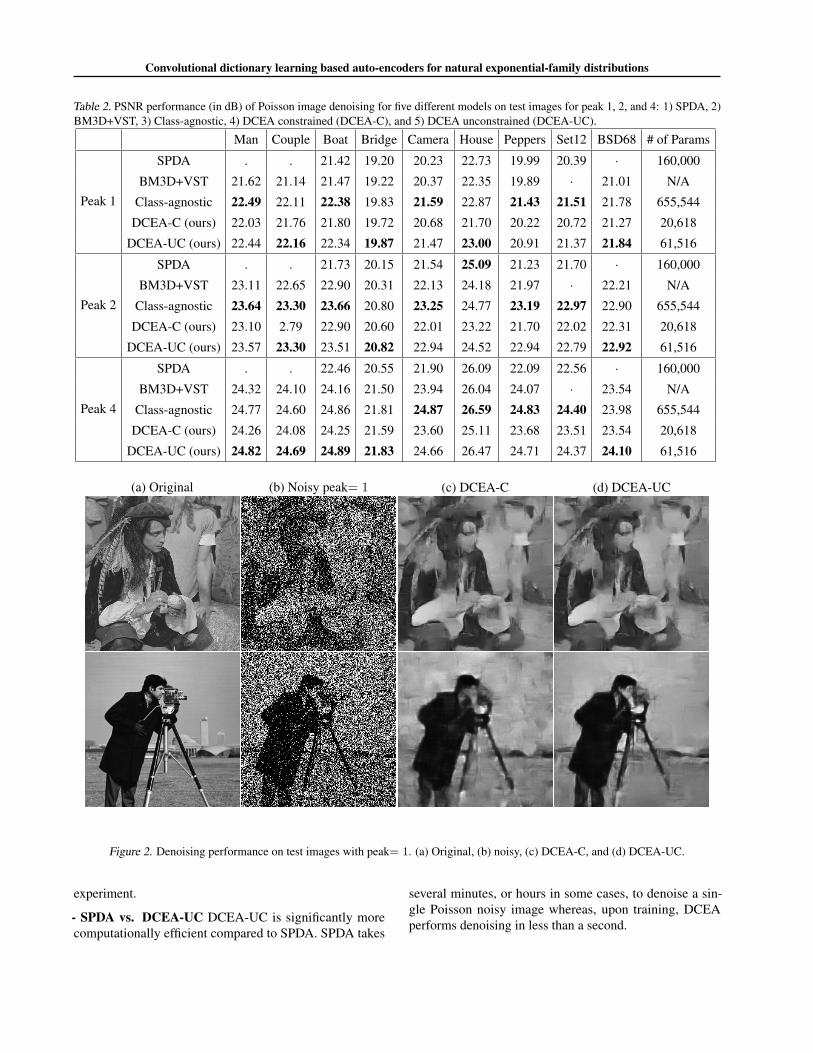
Results Table 2 shows that DCEA outperforms SPDA andBM3D + VST, and shows competitive performance againstCA, with an order of magnitude fewer parameters. Fig. 2shows the denoising performance of DCEA-C and DCEA-UC on two test images from Set12 (see Appendix for moreexamples). We summarize a few additional points from this


Table 2. PSNR performance (in dB) of Poisson image denoising for five different models on test images for peak 1, 2, and 4: 1) SPDA, 2)BM3D+VST, 3) Class-agnostic, 4) DCEA constrained (DCEA-C), and 5) DCEA unconstrained (DCEA-UC).

Man Couple Boat Bridge Camera House Peppers Set12 BSD68 # of Params

Peak 1

SPDA . . 21.42 19.20 20.23 22.73 19.99 20.39 · 160,000

BM3D+VST 21.62 21.14 21.47 19.22 20.37 22.35 19.89 · 21.01 N/A

Class-agnostic 22.49 22.11 22.38 19.83 21.59 22.87 21.43 21.51 21.78 655,544

DCEA-C (ours) 22.03 21.76 21.80 19.72 20.68 21.70 20.22 20.72 21.27 20,618

DCEA-UC (ours) 22.44 22.16 22.34 19.87 21.47 23.00 20.91 21.37 21.84 61,516

Peak 2

SPDA . . 21.73 20.15 21.54 25.09 21.23 21.70 · 160,000

BM3D+VST 23.11 22.65 22.90 20.31 22.13 24.18 21.97 · 22.21 N/A

Class-agnostic 23.64 23.30 23.66 20.80 23.25 24.77 23.19 22.97 22.90 655,544

DCEA-C (ours) 23.10 2.79 22.90 20.60 22.01 23.22 21.70 22.02 22.31 20,618

DCEA-UC (ours) 23.57 23.30 23.51 20.82 22.94 24.52 22.94 22.79 22.92 61,516

Peak 4

SPDA . . 22.46 20.55 21.90 26.09 22.09 22.56 · 160,000

BM3D+VST 24.32 24.10 24.16 21.50 23.94 26.04 24.07 · 23.54 N/A

Class-agnostic 24.77 24.60 24.86 21.81 24.87 26.59 24.83 24.40 23.98 655,544

DCEA-C (ours) 24.26 24.08 24.25 21.59 23.60 25.11 23.68 23.51 23.54 20,618

DCEA-UC (ours) 24.82 24.69 24.89 21.83 24.66 26.47 24.71 24.37 24.10 61,516

(a) Original (b) Noisy peak= 1 (c) DCEA-C (d) DCEA-UC

Figure 2. Denoising performance on test images with peak= 1. (a) Original, (b) noisy, (c) DCEA-C, and (d) DCEA-UC.

experiment.

- SPDA vs. DCEA-UC DCEA-UC is significantly morecomputationally efficient compared to SPDA. SPDA takes

several minutes, or hours in some cases, to denoise a sin-gle Poisson noisy image whereas, upon training, DCEAperforms denoising in less than a second.


0 200 400

(a) µj

0 200 400Time [ms]

h1

(b) hc

h2

0 20 40Time [ms]

h3

0 500 1000Epochs

0.2

0.4

0.6

0.8

1.0(c) err(hc, hc)

c = 1

c = 2

c = 3

0 500 1000Number of Groups J

0

5

10

15

20

(d) Runtime [s]

DCEA

BCOMP

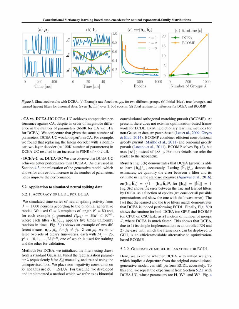
Figure 3. Simulated results with DCEA. (a) Example rate functions, µµµj , for two different groups. (b) Initial (blue), true (orange), andlearned (green) filters for binomial data. (c) err(hc, hc) over 1, 000 epochs. (d) Total runtime for inference for DCEA and BCOMP.

- CA vs. DCEA-UC DCEA-UC achieves competitive per-formance against CA, despite an order of magnitude differ-ence in the number of parameters (650K for CA vs. 61Kfor DCEA). We conjecture that given the same number ofparameters, DCEA-UC would outperform CA. For example,we found that replacing the linear decoder with a nonlin-ear two-layer decoder (≈ 120K number of parameters) inDCEA-UC resulted in an increase in PSNR of ∼0.2 dB.

- DCEA-C vs. DCEA-UC We also observe that DCEA-UCachieves better performance than DCEA-C. As discussed inSection 4.3, the relaxation of the generative model, whichallows for a three-fold increase in the number of parameters,helps improve the performance.

5.2. Application to simulated neural spiking data

5.2.1. ACCURACY OF ECDL FOR DCEA

We simulated time-series of neural spiking activity fromJ = 1,000 neurons according to the binomial generativemodel. We used C = 3 templates of length K = 50 and,for each example j, generated f(µµµj) = Hxj ∈ R500,where each filter {hc}3

c=1 appears five times uniformlyrandom in time. Fig. 3(a) shows an example of two dif-ferent means, µµµj1 , µµµj2 for j1 6= j2. Given µµµj , we simu-lated two sets of binary time-series, each with Mj = 25,yj ∈ {0, 1, . . . , 25}500, one of which is used for trainingand the other for validation.

Methods For DCEA, we initialized the filters using drawsfrom a standard Gaussian, tuned the regularization parame-ter λ (equivalently b for Sb) manually, and trained using theunsupervised loss. We place non-negativity constraints onxj and thus use Sb = ReLUb. For baseline, we developedand implemented a method which we refer to as binomial

convolutional orthogonal matching pursuit (BCOMP). Atpresent, there does not exist an optimization-based frame-work for ECDL. Existing dictionary learning methods fornon-Gaussian data are patch-based (Lee et al., 2009; Giryes& Elad, 2014). BCOMP combines efficient convolutionalgreedy pursuit (Mailhé et al., 2011) and binomial greedypursuit (Lozano et al., 2011). BCOMP solves Eq. (2), butuses ‖xj‖0 instead of ‖xj‖1. For more details, we refer thereader to the Appendix.

Results Fig. 3(b) demonstrates that DCEA (green) is ableto learn {hc}3

c=1 accurately. Letting {hc}3c=1 denote the

estimates, we quantify the error between a filter and itsestimate using the standard measure (Agarwal et al., 2016),

err(hc, hc) =√

1− 〈hc, hc〉2, for ‖hc‖ = ‖hc‖ = 1.Fig. 3(c) shows the error between the true and learned filtersby DCEA, as a function of epochs (we consider all possiblepermutations and show the one with the lowest error). Thefact that the learned and the true filters match demonstratesthat DCEA is indeed performing ECDL. Finally, Fig. 3(d)shows the runtime for both DCEA (on GPU) and BCOMP(on CPU) on CSC task, as a function of number of groupsJ , where DCEA is much faster. This shows that DCEA,due to 1) its simple implementation as an unrolled NN and2) the ease with which the framework can be deployed toGPU, is an efficient/scalable alternative to optimization-based BCOMP.

5.2.2. GENERATIVE MODEL RELAXATION FOR ECDL

Here, we examine whether DCEA with untied weights,which implies a departure from the original convolutionalgenerative model, can still perform ECDL accurately. Tothis end, we repeat the experiment from Section 5.2.1 withDCEA-UC, whose parameters are H, We, and Wd. Fig. 4


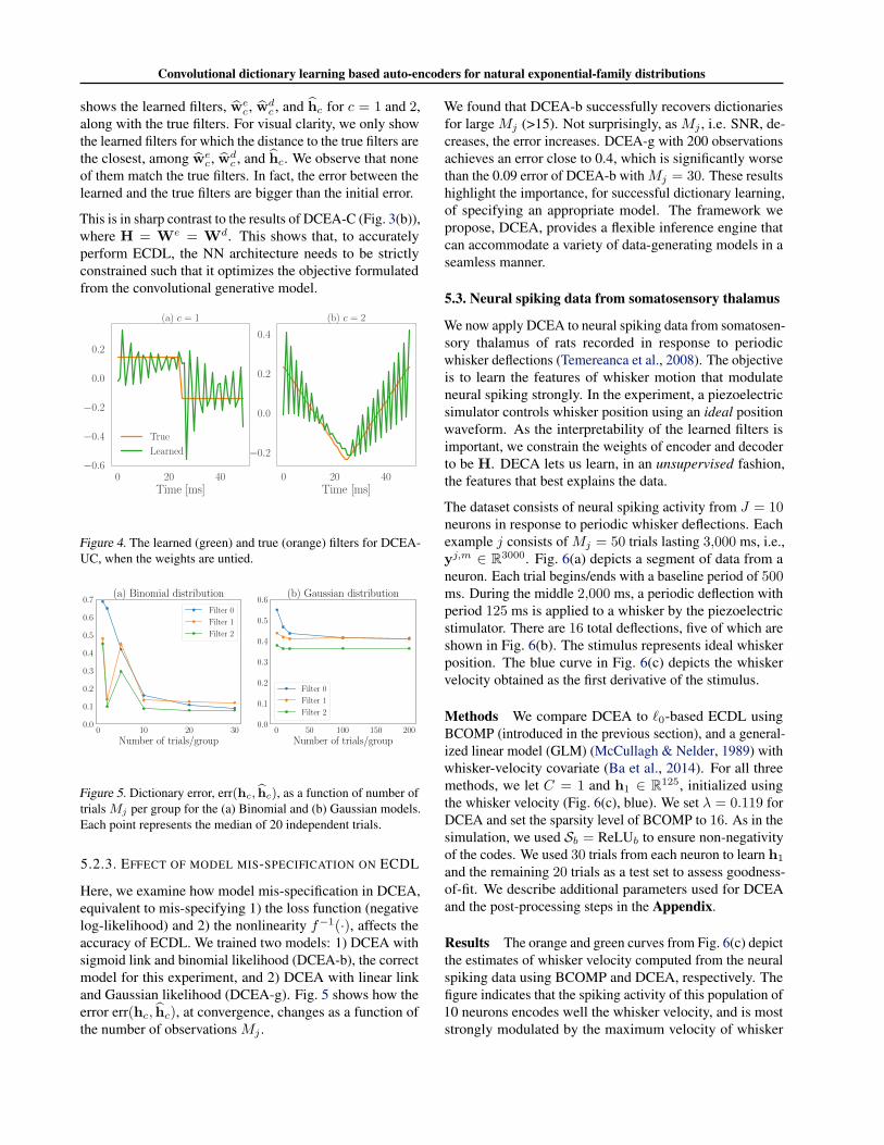
shows the learned filters, wec, wd

c , and hc for c = 1 and 2,along with the true filters. For visual clarity, we only showthe learned filters for which the distance to the true filters arethe closest, among we

c, wdc , and hc. We observe that none

of them match the true filters. In fact, the error between thelearned and the true filters are bigger than the initial error.

This is in sharp contrast to the results of DCEA-C (Fig. 3(b)),where H = We = Wd. This shows that, to accuratelyperform ECDL, the NN architecture needs to be strictlyconstrained such that it optimizes the objective formulatedfrom the convolutional generative model.

0 20 40Time [ms]

−0.6

−0.4

−0.2

0.0

0.2

(a) c = 1

True

Learned

0 20 40Time [ms]

−0.2

0.0

0.2

0.4

(b) c = 2

Figure 4. The learned (green) and true (orange) filters for DCEA-UC, when the weights are untied.

0 10 20 30

Number of trials/group

0.0

0.1

0.2

0.3

0.4

0.5

0.6

0.7(a) Binomial distribution

Filter 0

Filter 1

Filter 2

0 50 100 150 200

Number of trials/group

0.0

0.1

0.2

0.3

0.4

0.5

0.6(b) Gaussian distribution

Filter 0

Filter 1

Filter 2

Figure 5. Dictionary error, err(hc, hc), as a function of number oftrials Mj per group for the (a) Binomial and (b) Gaussian models.Each point represents the median of 20 independent trials.

5.2.3. EFFECT OF MODEL MIS-SPECIFICATION ON ECDL

Here, we examine how model mis-specification in DCEA,equivalent to mis-specifying 1) the loss function (negativelog-likelihood) and 2) the nonlinearity f−1(·), affects theaccuracy of ECDL. We trained two models: 1) DCEA withsigmoid link and binomial likelihood (DCEA-b), the correctmodel for this experiment, and 2) DCEA with linear linkand Gaussian likelihood (DCEA-g). Fig. 5 shows how theerror err(hc, hc), at convergence, changes as a function ofthe number of observations Mj .

We found that DCEA-b successfully recovers dictionariesfor large Mj (>15). Not surprisingly, as Mj , i.e. SNR, de-creases, the error increases. DCEA-g with 200 observationsachieves an error close to 0.4, which is significantly worsethan the 0.09 error of DCEA-b withMj = 30. These resultshighlight the importance, for successful dictionary learning,of specifying an appropriate model. The framework wepropose, DCEA, provides a flexible inference engine thatcan accommodate a variety of data-generating models in aseamless manner.

5.3. Neural spiking data from somatosensory thalamus

We now apply DCEA to neural spiking data from somatosen-sory thalamus of rats recorded in response to periodicwhisker deflections (Temereanca et al., 2008). The objectiveis to learn the features of whisker motion that modulateneural spiking strongly. In the experiment, a piezoelectricsimulator controls whisker position using an ideal positionwaveform. As the interpretability of the learned filters isimportant, we constrain the weights of encoder and decoderto be H. DECA lets us learn, in an unsupervised fashion,the features that best explains the data.

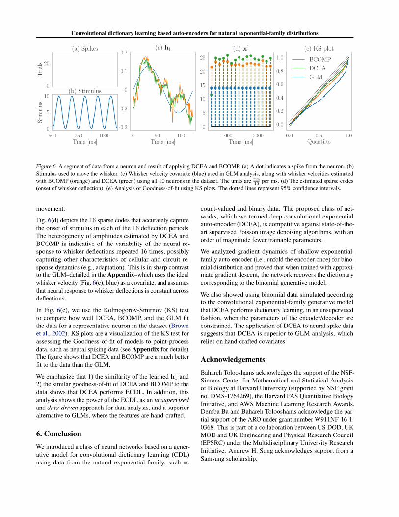
The dataset consists of neural spiking activity from J = 10neurons in response to periodic whisker deflections. Eachexample j consists of Mj = 50 trials lasting 3,000 ms, i.e.,yj,m ∈ R3000. Fig. 6(a) depicts a segment of data from aneuron. Each trial begins/ends with a baseline period of 500ms. During the middle 2,000 ms, a periodic deflection withperiod 125 ms is applied to a whisker by the piezoelectricstimulator. There are 16 total deflections, five of which areshown in Fig. 6(b). The stimulus represents ideal whiskerposition. The blue curve in Fig. 6(c) depicts the whiskervelocity obtained as the first derivative of the stimulus.

Methods We compare DCEA to `0-based ECDL usingBCOMP (introduced in the previous section), and a general-ized linear model (GLM) (McCullagh & Nelder, 1989) withwhisker-velocity covariate (Ba et al., 2014). For all threemethods, we let C = 1 and h1 ∈ R125, initialized usingthe whisker velocity (Fig. 6(c), blue). We set λ = 0.119 forDCEA and set the sparsity level of BCOMP to 16. As in thesimulation, we used Sb = ReLUb to ensure non-negativityof the codes. We used 30 trials from each neuron to learn h1and the remaining 20 trials as a test set to assess goodness-of-fit. We describe additional parameters used for DCEAand the post-processing steps in the Appendix.

Results The orange and green curves from Fig. 6(c) depictthe estimates of whisker velocity computed from the neuralspiking data using BCOMP and DCEA, respectively. Thefigure indicates that the spiking activity of this population of10 neurons encodes well the whisker velocity, and is moststrongly modulated by the maximum velocity of whisker


0

20

Tri

als

(a) Spikes

500 750 1000Time [ms]

0

5

10

Sti

mu

lus

(b) Stimulus

0 50 100Time [ms]

-0.2

-0.2

0

0.1

0.2(c) h1

1000 2000Time [ms]

0

5

10

15

20

25

(d) x1

0.0 0.5 1.0Quantiles

0.0

0.2

0.4

0.6

0.8

1.0

(e) KS plot

BCOMP

DCEA

GLM

Figure 6. A segment of data from a neuron and result of applying DCEA and BCOMP. (a) A dot indicates a spike from the neuron. (b)Stimulus used to move the whisker. (c) Whisker velocity covariate (blue) used in GLM analysis, along with whisker velocities estimatedwith BCOMP (orange) and DCEA (green) using all 10 neurons in the dataset. The units are mm

10 per ms. (d) The estimated sparse codes(onset of whisker deflection). (e) Analysis of Goodness-of-fit using KS plots. The dotted lines represent 95% confidence intervals.

movement.

Fig. 6(d) depicts the 16 sparse codes that accurately capturethe onset of stimulus in each of the 16 deflection periods.The heterogeneity of amplitudes estimated by DCEA andBCOMP is indicative of the variability of the neural re-sponse to whisker deflections repeated 16 times, possiblycapturing other characteristics of cellular and circuit re-sponse dynamics (e.g., adaptation). This is in sharp contrastto the GLM–detailed in the Appendix–which uses the idealwhisker velocity (Fig. 6(c), blue) as a covariate, and assumesthat neural response to whisker deflections is constant acrossdeflections.

In Fig. 6(e), we use the Kolmogorov-Smirnov (KS) testto compare how well DCEA, BCOMP, and the GLM fitthe data for a representative neuron in the dataset (Brownet al., 2002). KS plots are a visualization of the KS test forassessing the Goodness-of-fit of models to point-processdata, such as neural spiking data (see Appendix for details).The figure shows that DCEA and BCOMP are a much betterfit to the data than the GLM.

We emphasize that 1) the similarity of the learned h1 and2) the similar goodness-of-fit of DCEA and BCOMP to thedata shows that DCEA performs ECDL. In addition, thisanalysis shows the power of the ECDL as an unsupervisedand data-driven approach for data analysis, and a superioralternative to GLMs, where the features are hand-crafted.

6. ConclusionWe introduced a class of neural networks based on a gener-ative model for convolutional dictionary learning (CDL)using data from the natural exponential-family, such as

count-valued and binary data. The proposed class of net-works, which we termed deep convolutional exponentialauto-encoder (DCEA), is competitive against state-of-the-art supervised Poisson image denoising algorithms, with anorder of magnitude fewer trainable parameters.

We analyzed gradient dynamics of shallow exponential-family auto-encoder (i.e., unfold the encoder once) for bino-mial distribution and proved that when trained with approxi-mate gradient descent, the network recovers the dictionarycorresponding to the binomial generative model.

We also showed using binomial data simulated accordingto the convolutional exponential-family generative modelthat DCEA performs dictionary learning, in an unsupervisedfashion, when the parameters of the encoder/decoder areconstrained. The application of DCEA to neural spike datasuggests that DCEA is superior to GLM analysis, whichrelies on hand-crafted covariates.

AcknowledgementsBahareh Tolooshams acknowledges the support of the NSF-Simons Center for Mathematical and Statistical Analysisof Biology at Harvard University (supported by NSF grantno. DMS-1764269), the Harvard FAS Quantitative BiologyInitiative, and AWS Machine Learning Research Awards.Demba Ba and Bahareh Tolooshams acknowledge the par-tial support of the ARO under grant number W911NF-16-1-0368. This is part of a collaboration between US DOD, UKMOD and UK Engineering and Physical Research Council(EPSRC) under the Multidisciplinary University ResearchInitiative. Andrew H. Song acknowledges support from aSamsung scholarship.


ReferencesAgarwal, A., Anandkumar, A., Jain, P., Netrapalli, P., and

Tandon, R. Learning sparsely used overcomplete dictio-naries via alternating minimization. SIAM Journal onOptimization, 26:2775–2799, 2016.

Ba, D., Temereanca, S., and Brown, E. Algorithms forthe analysis of ensemble neural spiking activity usingsimultaneous-event multivariate point-process models.Frontiers in Computational Neuroscience, 8:6, 2014.

Beck, A. and Teboulle, M. A fast iterative shrinkage-thresholding algorithm for linear inverse problems. SIAMjournal on imaging sciences, 2(1):183–202, 2009.

Boyd, S. and Vandenberghe, L. Convex Optimization. Cam-bridge University Press, 2004.

Brown, E. N., Barbieri, R., Ventura, V., Kass, R. E., andFrank, L. M. The time-rescaling theorem and its applica-tion to neural spike train data analysis. Neural Computa-tion, 14(2):325–346, 2002.

Clevert, D., Unterthiner, T., and Hochreiter, S. Fast and ac-curate deep network learning by exponential linear units(elus). In 4th International Conference on Learning Rep-resentations, 2016.

Daubechies, I., Defrise, M., and De Mol, C. An iterativethresholding algorithm for linear inverse problems with asparsity constraint. Communications on Pure and AppliedMathematics, 57(11):1413–1457, 2004.

Everingham, M., Van Gool, L., Williams, C. K. I., Winn, J.,and Zisserman, A. The PASCAL Visual Object ClassesChallenge 2012 (VOC2012) Results, 2012.

Feng, W., Qiao, P., and Chen, Y. Fast and accurate pois-son denoising with trainable nonlinear diffusion. IEEETransactions on Cybernetics, 48(6):1708–1719, 2018.

Gao, Y., Archer, E. W., Paninski, L., and Cunningham, J. P.Linear dynamical neural population models through non-linear embeddings. In Advances in Neural InformationProcessing Systems 29, pp. 163–171. Curran Associates,Inc., 2016.

Garcia-Cardona, C. and Wohlberg, B. Convolutional dictio-nary learning: A comparative review and new algorithms.IEEE Transactions on Computational Imaging, 4(3):366–381, September 2018.

Giryes, R. and Elad, M. Sparsity-based poisson denoisingwith dictionary learning. IEEE Transactions on ImageProcessing, 23(12):5057–5069, 2014.

Gregor, K. and Lecun, Y. Learning fast approximations ofsparse coding. In International Conference on MachineLearning, pp. 399–406, 2010.

Hershey, J. R., Roux, J. L., and Weninger, F. Deep unfold-ing: Model-based inspiration of novel deep architectures.arXiv:1409.2574, pp. 1–27, 2014.

LeCun, Y., Bengio, Y., and Hinton, G. Deep learning. Na-ture, 521:436–444, 2015.

Lee, H., Raina, R., Teichman, A., and Ng, A. Y. Exponen-tial family sparse coding with applications to self-taughtlearning. In Proc. the 21st International Jont Conferenceon Artificial Intelligence, IJCAI, pp. 1113–1119, 2009.

Liang, D., Krishnan, R. G., Hoffman, M. D., and Jebara,T. Variational autoencoders for collaborative filtering. InProceedings of the 2018 World Wide Web Conference, pp.689–698, 2018.

Lozano, A., Swirszcz, G., and Abe, N. Group orthogo-nal matching pursuit for logistic regression. Journal ofMachine Learning Research, 15:452–460, 2011.

Ma, L., Moisan, L., Yu, J., and Zeng, T. A dictionary learn-ing approach for poisson image deblurring. IEEE Trans-actions on medical imaging, 32(7):1277–1289, 2013.

Mailhé, B., Gribonval, R., Vandergheynst, P., and Bimbot, F.Fast orthogonal sparse approximation algorithms over lo-cal dictionaries. Signal Processing, 91:2822–2835, 2011.

Makitalo, M. and Foi, A. Optimal inversion of the general-ized anscombe transformation for poisson-gaussian noise.IEEE Transactions on Image Processing, 22(1):91–103,Jan 2013.

Mardani, M., Sun, Q., Vasawanala, S., Papyan, V., Mon-ajemi, H., Pauly, J., and Donoho, D. Neural proximalgradient descent for compressive imaging. In Proc. Ad-vances in Neural Information Processing Systems 31, pp.9573–9683, 2018.

Martin, D., Fowlkes, C., Tal, D., and Malik, J. A databaseof human segmented natural images and its applicationto evaluating segmentation algorithms and measuringecological statistics. In Proc. 8th Int’l Conf. ComputerVision, volume 2, pp. 416–423, July 2001.

McCullagh, P. and Nelder, J. Generalized Linear Models.Chapman & Hall/CRC, 1989.

Monga, V., Li, Y., and Eldar, Y. C. Algorithm unrolling:Interpretable, efficient deep learning for signal and imageprocessing. arXiv:1912.10557, 2019.

Nazábal, A., Olmos, P. M., Ghahramani, Z., and Valera,I. Handling incomplete heterogeneous data using vaes.Pattern recognition, 107:107501, 2020. ISSN 0031-3203.


Nguyen, T. V., Wong, R. K. W., and Hegde, C. On thedynamics of gradient descent for autoencoders. In Proc.Machine Learning Research, volume 89, pp. 2858–2867.PMLR, 16–18 Apr 2019.

Parikh, N. and Boyd, S. Proximal algorithms. Found. TrendsOptim., 1(3):127–239, January 2014.

Remez, T., Litany, O., Giryes, R., and Bronstein, A. M.Class-aware fully-convolutional gaussian and poisson de-noising. CoRR, abs/1808.06562, 2018.

Salmon, J., Harmany, Z., Deledalle, C.-A., and Willett, R.Poisson noise reduction with non-local pca. Journal ofMathematical Imaging and Vision, 48(2):279–294, Feb2014.

Simon, D. and Elad, M. Rethinking the csc model fornatural images. In Proc. Advances in Neural InformationProcessing Systems 33 (NeurIPS), pp. 2271–2281, 2019.

Sreter, H. and Giryes, R. Learned convolutional sparsecoding. In Proc. 2018 IEEE International Conference onAcoustics, Speech and Signal Processing (ICASSP), pp.2191–2195, 2018.

Sulam, J., Aberdam, A., Beck, A., and Elad, M. On multi-layer basis pursuit, efficient algorithms and convolutionalneural networks. IEEE transactions on pattern analysisand machine intelligence, 2019.

Tasissa, A., Theodosis, E., Tolooshams, B., and Ba, D.Dense and sparse coding: Theory and architectures.arXiv:2006.09534, 2020.

Temereanca, S., Brown, E. N., and Simons, D. J. Rapidchanges in thalamic firing synchrony during repetitivewhisker stimulation. Journal of Neuroscience, 28(44):11153–11164, 2008.

Tolooshams, B., Dey, S., and Ba, D. Scalable convolutionaldictionary learning with constrained recurrent sparse auto-encoders. In Proc. 2018 IEEE 28th International Work-shop on Machine Learning for Signal Processing (MLSP),pp. 1–6, 2018.

Tolooshams, B., Dey, S., and Ba, D. Deep residual au-toencoders for expectation maximization-inspired dic-tionary learning. IEEE Transactions on Neural Net-works and Learning Systems, pp. 1–15, 2020. doi:10.1109/TNNLS.2020.3005348.

Truccolo, W., Eden, U. T., Fellows, M., Donoghue, J., andBrown, E. N. A Point Process Framework for Relat-ing Neural Spiking Activity to Spiking History, NeuralEnsemble, and Extrinsic Covariate Effects. Journal ofNeurophysiology, 93(2):1074–1089, 2005.

Wang, Z., Liu, D., Yang, J., Han, W., and Huang, T. Deepnetworks for image super-resolution with sparse prior. InProc. the IEEE International Conference on ComputerVision, pp. 370–378, 2015.

Yang, F., Lu, Y. M., Sbaiz, L., and Vetterli, M. Bits fromphotons: Oversampled image acquisition using binarypoisson statistics. IEEE Transactions on image process-ing, 21(4):1421–1436, 2011.

Zhang, K., Zuo, W., Chen, Y., Meng, D., and Zhang, L.Beyond a gaussian denoiser: Residual learning of deepcnn for image denoising. IEEE Transactions on ImageProcessing, 26(7):3142–3155, July 2017.

Documents

Convolutional dictionary learning based auto-encoders for