IEEE TRANSACTIONS ON EVOLUTIONARY COMPUTATION, VOL. 5, NO. 3, JUNE 2001 271

Brief Papers_______________________________________________________________________________

Combined Evolution Strategies for Dynamic Calibration of Video-BasedMeasurement Systems

P. Cerveri, A. Pedotti, and N. A. Borghese

Abstract—Calibration is a crucial step to obtaining three-dimen-sional (3-D) measurement using video camera-based stereo sys-tems. Approaches based on epipolar geometry are particularly ap-pealing as there is no need to know the 3-D position of the controlpoints a priori and because the solution is found by solving a set oflinear equations through matrix manipulation. Indeed, all the pa-rameters can be determined except for the pair of principal points,which poses a considerable drawback. Whereas in low-accuracysystems (two-dimensional measurement error 0.2 pixels) suchpoints can be assumed to lie at the image center without degradingthe overall 3-D accuracy, in high-accuracy systems their true posi-tion must be computed accurately. In this case, all the calibrationparameters (including the principal points) can still be estimatedthrough epipolar geometry, but it is necessary to minimize a highlynonlinear cost function. It is shown here that by combining two evo-lutionary optimization strategies this minimization can be carriedout, both efficiently (in quasi-real time) and reliably (avoiding localminima). The resulting strategy, which we call enhanced evolu-tionary search (EES), allows the full calibration of a stereo systemusing only a rigid bar; this simplicity is a definite step forwardin stereo-camera calibration. Moreover, EES can be applied to awide range of applications where the cost function contains com-plex nonlinear relationships among the optimization variables.

Index Terms—Covariance matrix, epipolar geometry, evolutionstrategies, optimization, stereo camera calibration.

I. INTRODUCTION

Video camera-based stereo systems are used widely in manydifferent fields, including close-range photogrammetry, roboticvision, computer-aided design, biomechanics, and virtual re-ality. Two major applications are the measurement of the three-dimensional (3-D) shape of objects (3-D scanners [1]) and the3-D reconstruction of motion (trackers or motion capture [2]).The input for most systems is a set of matched features fromeach of the two camera image streams. Tailored low-level hard-ware [3] or software processing [4] detects these features andreturns their accurate 3-D measurement. To transform a pair oftwo-dimensional (2-D) features into a feature positioned within

Manuscript received February 28, 2000; revised November 9, 2000.P. Cerveri is with the Bioengineering Department, Politecnico di Milano

and Centro di Bioingegneria, Fondazione ProJuventute, 20148 Milano, Italy(e-mail: cerveri@biomed.polimi.it) and also with the Laboratory of HumanMotion Analysis and Virtual Reality, (MAVR), Istituto Neuroscienze eBioimmagini CNR, 20090 Segrate, Milano, Italy.

A. Pedotti is with the Bioengineering Department, Politecnico di Milano andCentro di Bioingegneria, Fondazione ProJuventute, 20148 Milano, Italy.

N. A. Borghese is with the Laboratory of Human Motion Analysis and VirtualReality (MAVR), Istituto Neuroscienze e Bioimmagini CNR, 20090 Segrate,Milano, Italy (e-mail: borghese@inb.mi.cnr.it).

Publisher Item Identifier S 1089-778X(01)02397-9.

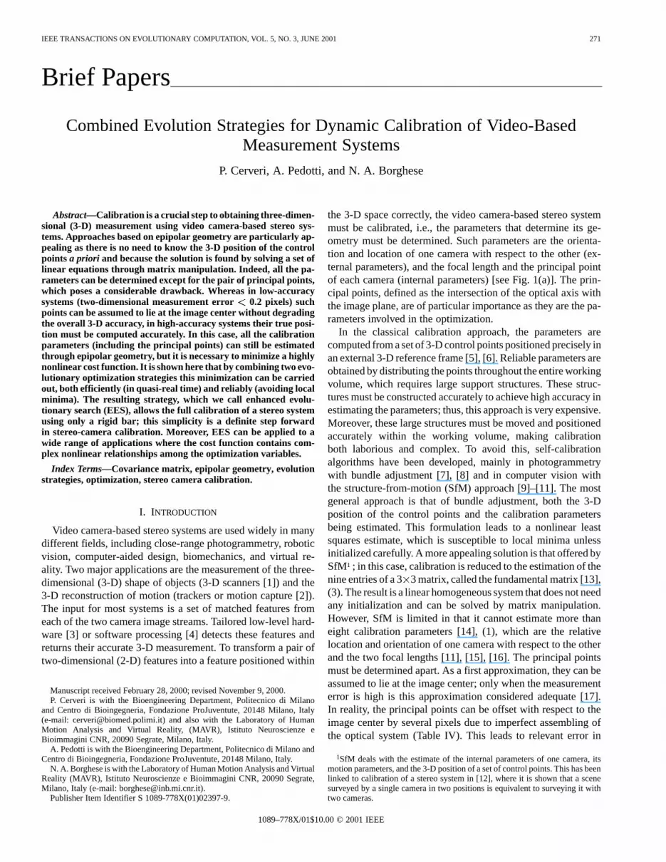
the 3-D space correctly, the video camera-based stereo systemmust be calibrated, i.e., the parameters that determine its ge-ometry must be determined. Such parameters are the orienta-tion and location of one camera with respect to the other (ex-ternal parameters), and the focal length and the principal pointof each camera (internal parameters) [see Fig. 1(a)]. The prin-cipal points, defined as the intersection of the optical axis withthe image plane, are of particular importance as they are the pa-rameters involved in the optimization.

In the classical calibration approach, the parameters arecomputed from a set of 3-D control points positioned precisely inan external 3-D reference frame [5], [6]. Reliable parameters areobtained by distributing the points throughout the entire workingvolume, which requires large support structures. These struc-tures must be constructed accurately to achieve high accuracy inestimating the parameters; thus, this approach is very expensive.Moreover, these large structures must be moved and positionedaccurately within the working volume, making calibrationboth laborious and complex. To avoid this, self-calibrationalgorithms have been developed, mainly in photogrammetrywith bundle adjustment [7], [8] and in computer vision withthe structure-from-motion (SfM) approach [9]–[11]. The mostgeneral approach is that of bundle adjustment, both the 3-Dposition of the control points and the calibration parametersbeing estimated. This formulation leads to a nonlinear leastsquares estimate, which is susceptible to local minima unlessinitialized carefully. A more appealing solution is that offered bySfM1 ; in this case, calibration is reduced to the estimation of thenine entries of a 33 matrix, called the fundamental matrix [13],(3). The result is a linear homogeneous system that does not needany initialization and can be solved by matrix manipulation.However, SfM is limited in that it cannot estimate more thaneight calibration parameters [14], (1), which are the relativelocation and orientation of one camera with respect to the otherand the two focal lengths [11], [15], [16]. The principal pointsmust be determined apart. As a first approximation, they can beassumed to lie at the image center; only when the measurementerror is high is this approximation considered adequate [17].In reality, the principal points can be offset with respect to theimage center by several pixels due to imperfect assembling ofthe optical system (Table IV). This leads to relevant error in

1SfM deals with the estimate of the internal parameters of one camera, itsmotion parameters, and the 3-D position of a set of control points. This has beenlinked to calibration of a stereo system in [12], where it is shown that a scenesurveyed by a single camera in two positions is equivalent to surveying it withtwo cameras.

1089–778X/01$10.00 © 2001 IEEE

272 IEEE TRANSACTIONS ON EVOLUTIONARY COMPUTATION, VOL. 5, NO. 3, JUNE 2001

(a)

(b)

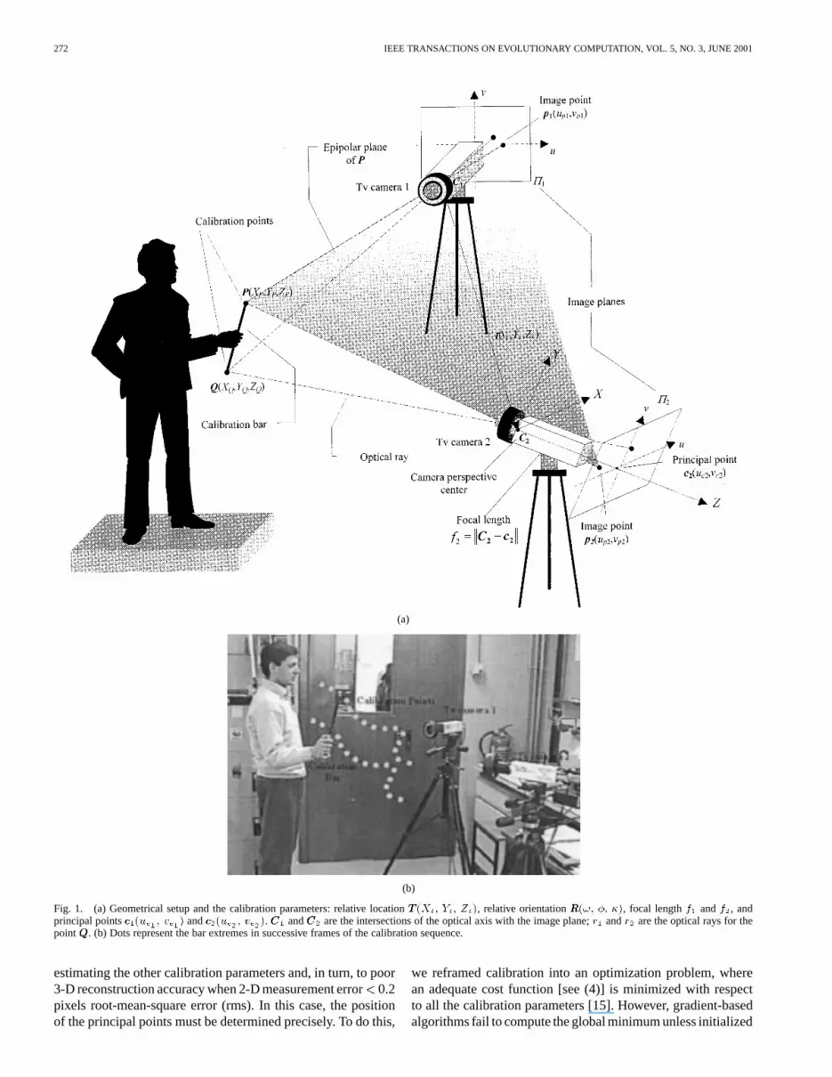
Fig. 1. (a) Geometrical setup and the calibration parameters: relative locationTTT (X ; Y ; Z ), relative orientationRRR(!; �; �), focal lengthf andf , andprincipal pointsccc (u ; v ) andccc (u ; v ).CCC andCCC are the intersections of the optical axis with the image plane;r andr are the optical rays for thepointQQQ. (b) Dots represent the bar extremes in successive frames of the calibration sequence.

estimating the other calibration parameters and, in turn, to poor3-D reconstruction accuracy when 2-D measurement error0.2pixels root-mean-square error (rms). In this case, the positionof the principal points must be determined precisely. To do this,

we reframed calibration into an optimization problem, wherean adequate cost function [see (4)] is minimized with respectto all the calibration parameters [15]. However, gradient-basedalgorithms fail to compute the global minimum unless initialized

CERVERIet al.: COMBINED EVOLUTION STRATEGIES FOR DYNAMIC CALIBRATION OF VIDEO-BASED MEASUREMENT SYSTEMS 273

carefully (Section V-A and Table III) and global search algo-rithms (that have to work in a 12-fold parameter space) are tooslow for such an application.

This prompted us to derive a cost function where only the twoprincipal points are the optimization parameters, all the othercalibration parameters being determined by SfM [see (5)]. Thisreduces the optimization space to four dimensions. The price tobe paid is that the resulting cost function is hard to optimizethrough gradient-descent algorithms, as SfM involves matrixoperations like singular value decomposition and sign checks.We show here that combining two different evolutionary opti-mization algorithms generates a reliable and global optimiza-tion procedure that efficiently solves the calibration problem.The procedure requires only pairs of matched points and one3-D metric information. Thus, the calibration tool we are nowproposing is a simple rigid bar carrying markers at its ends.Moving the bar within the working volume [see Fig. 1(b)] col-lects the required calibration points and 3-D metric informationeasily [14].

The paper is arranged as follows: Section II briefly describesthe stereo-camera calibration problem, Section III introducesthe cost function and the optimization problem, Section IV de-scribes the enhanced evolutionary search (EES) optimization,and Section V reports and discusses the results on simulated andreal data in terms of computational load, reliability, and 3-D ac-curacy. The conclusions are drawn in Section VI and a full tax-onomy is summarized in Appendix A.

II. CALIBRATION OF A STEREO–CAMERA SYSTEM

The image of a 3-D point on thetarget of a video-camera can be described asa perspective projection of on [see Fig. 1(a)] through thecenter , expressed in homogenous notation in a single matrixequation [10]

(1)

The matrix defines a linear projective mapping model thatis adequate if distortions are sufficiently weak or corrected in ad-vance [5], [19]. Equation (1) contains the following calibrationparameters: is the location of the camera,

is the orientation (function of the three inde-pendent orientation angles ), is the focal length, and

is the principal point of the camera.When the 3-D coordinate system is located in the perspective

center of one camera with two axes parallel to those of the imageplane, for that camera, (1) can be rewritten as

for the first camera (2a)

for the second camera. (2b)

Let us now consider the three vectors , ,(Fig. 1). These lie in a single plane; taking into account Eq. (2a)and (2b), Eq. (1) can be written as the following homogeneouslinear system [11]

(3)

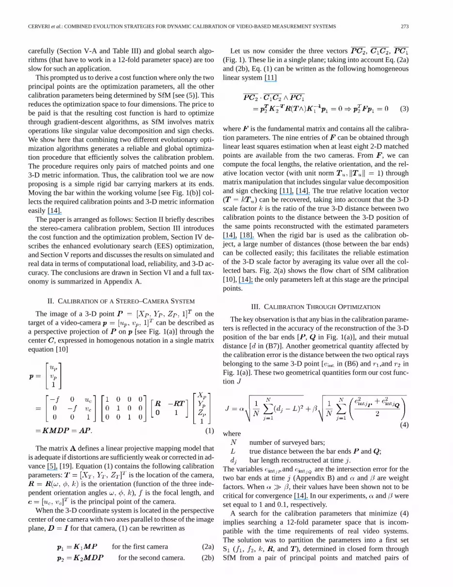
where is the fundamental matrix and contains all the calibra-tion parameters. The nine entries ofcan be obtained throughlinear least squares estimation when at least eight 2-D matchedpoints are available from the two cameras. From, we cancompute the focal lengths, the relative orientation, and the rel-ative location vector (with unit norm ) throughmatrix manipulation that includes singular value decompositionand sign checking [11], [14]. The true relative location vector( ) can be recovered, taking into account that the 3-Dscale factor is the ratio of the true 3-D distance between twocalibration points to the distance between the 3-D position ofthe same points reconstructed with the estimated parameters[14], [18]. When the rigid bar is used as the calibration ob-ject, a large number of distances (those between the bar ends)can be collected easily; this facilitates the reliable estimationof the 3-D scale factor by averaging its value over all the col-lected bars. Fig. 2(a) shows the flow chart of SfM calibration[10], [14]; the only parameters left at this stage are the principalpoints.

III. CALIBRATION THROUGH OPTIMIZATION

The key observation is that any bias in the calibration parame-ters is reflected in the accuracy of the reconstruction of the 3-Dposition of the bar ends [, in Fig. 1(a)], and their mutualdistance [ in (B7)]. Another geometrical quantity affected bythe calibration error is the distance between the two optical raysbelonging to the same 3-D point [ in (B6) and ,and inFig. 1(a)]. These two geometrical quantities form our cost func-tion

(4)where

number of surveyed bars;true distance between the bar endsand ;bar length reconstructed at time.

The variables and are the intersection error for thetwo bar ends at time (Appendix B) and and are weightfactors. When , their values have been shown not to becritical for convergence [14]. In our experiments,and wereset equal to 1 and 0.1, respectively.

A search for the calibration parameters that minimize (4)implies searching a 12-fold parameter space that is incom-patible with the time requirements of real video systems.The solution was to partition the parameters into a first setS ( , , , , and ), determined in closed form throughSfM from a pair of principal points and matched pairs of

274 IEEE TRANSACTIONS ON EVOLUTIONARY COMPUTATION, VOL. 5, NO. 3, JUNE 2001

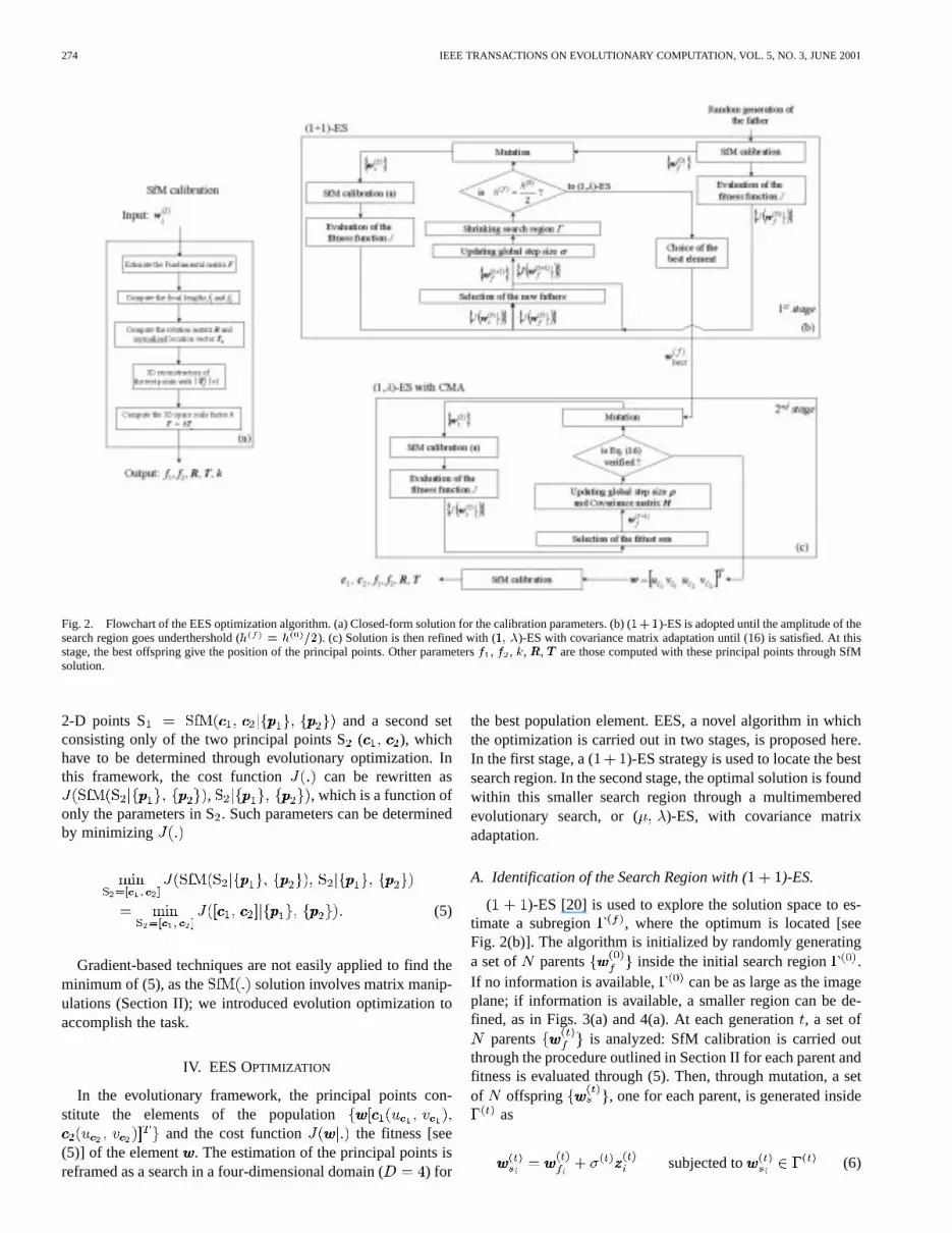
Fig. 2. Flowchart of the EES optimization algorithm. (a) Closed-form solution for the calibration parameters. (b) (1+1)-ES is adopted until the amplitude of thesearch region goes underthershold (h = h =2). (c) Solution is then refined with (1; �)-ES with covariance matrix adaptation until (16) is satisfied. At thisstage, the best offspring give the position of the principal points. Other parametersf , f , k, RRR, TTT are those computed with these principal points through SfMsolution.

2-D points S and a second setconsisting only of the two principal points S( ), whichhave to be determined through evolutionary optimization. Inthis framework, the cost function can be rewritten as

, , which is a function ofonly the parameters in S. Such parameters can be determinedby minimizing

(5)

Gradient-based techniques are not easily applied to find theminimum of (5), as the solution involves matrix manip-ulations (Section II); we introduced evolution optimization toaccomplish the task.

IV. EES OPTIMIZATION

In the evolutionary framework, the principal points con-stitute the elements of the population

and the cost function the fitness [see(5)] of the element . The estimation of the principal points isreframed as a search in a four-dimensional domain ( ) for

the best population element. EES, a novel algorithm in whichthe optimization is carried out in two stages, is proposed here.In the first stage, a ( )-ES strategy is used to locate the bestsearch region. In the second stage, the optimal solution is foundwithin this smaller search region through a multimemberedevolutionary search, or ( )-ES, with covariance matrixadaptation.

A. Identification of the Search Region with ( )-ES.

( )-ES [20] is used to explore the solution space to es-timate a subregion , where the optimum is located [seeFig. 2(b)]. The algorithm is initialized by randomly generatinga set of parents inside the initial search region .If no information is available, can be as large as the imageplane; if information is available, a smaller region can be de-fined, as in Figs. 3(a) and 4(a). At each generation, a set of

parents is analyzed: SfM calibration is carried outthrough the procedure outlined in Section II for each parent andfitness is evaluated through (5). Then, through mutation, a setof offspring , one for each parent, is generated inside

as

subjected to (6)

CERVERIet al.: COMBINED EVOLUTION STRATEGIES FOR DYNAMIC CALIBRATION OF VIDEO-BASED MEASUREMENT SYSTEMS 275

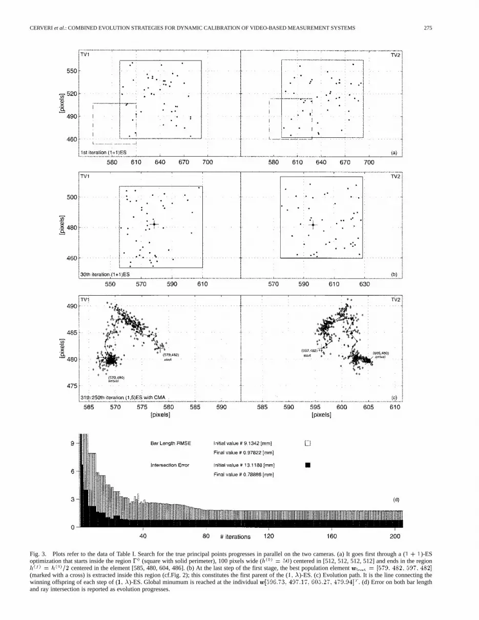
Fig. 3. Plots refer to the data of Table I. Search for the true principal points progresses in parallel on the two cameras. (a) It goes first through a (1 + 1)-ESoptimization that starts inside the region� (square with solid perimeter), 100 pixels wide (h = 50) centered in [512, 512, 512, 512] and ends in the regionh = h =2 centered in the element [585, 480, 604, 486]. (b) At the last step of the first stage, the best population elementwww = [579; 482; 597; 482](marked with a cross) is extracted inside this region (cf.Fig. 2); this constitutes the first parent of the (1; �)-ES. (c) Evolution path. It is the line connecting thewinning offspring of each step of (1; �)-ES. Global minumum is reached at the individualwww[596:73; 497:17; 605:27; 479:94] . (d) Error on both bar lengthand ray intersection is reported as evolution progresses.

276 IEEE TRANSACTIONS ON EVOLUTIONARY COMPUTATION, VOL. 5, NO. 3, JUNE 2001

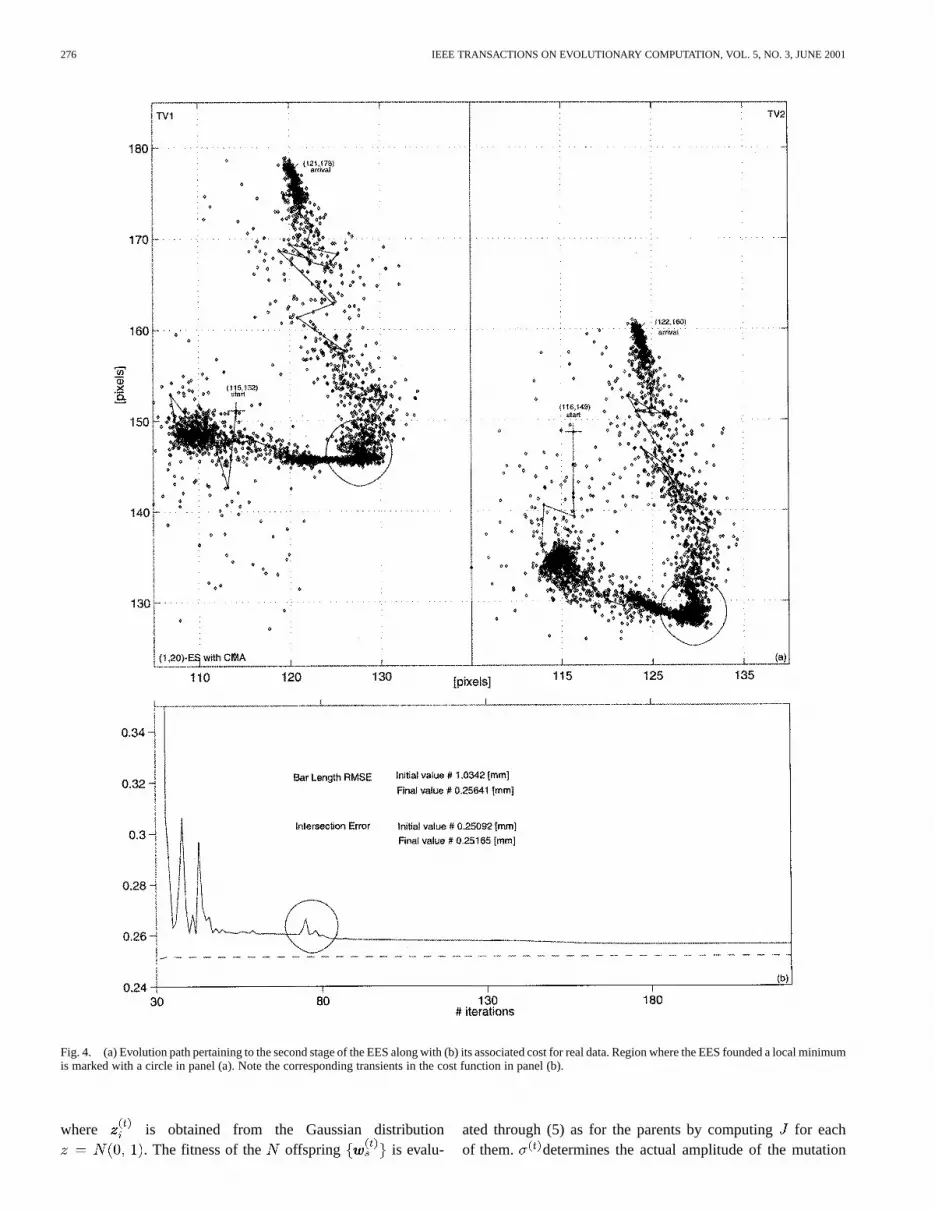
Fig. 4. (a) Evolution path pertaining to the second stage of the EES along with (b) its associated cost for real data. Region where the EES founded a localminimumis marked with a circle in panel (a). Note the corresponding transients in the cost function in panel (b).

where is obtained from the Gaussian distribution. The fitness of the offspring is evalu-

ated through (5) as for the parents by computingfor eachof them. determines the actual amplitude of the mutation

CERVERIet al.: COMBINED EVOLUTION STRATEGIES FOR DYNAMIC CALIBRATION OF VIDEO-BASED MEASUREMENT SYSTEMS 277

[see (6)] and is updated according to the Rechenberg 1/5 rule[20] as

(7)

where is the ratio between the number of winning offspringand winning parents. Setting gives a heuristicvalue resulting in linear order convergence rates [20]. The off-spring are then placed in competition with the correspondingparent: the one that exhibits higher fitness (lower value of)survives and becomes the parent in the next generation

(8)

At each step, the resolution of the search is increased by re-ducing the search region amplitude according to the followingschedule [see Figs. 3(a) and (b) and 4(a) and (b)]

(9)

The logarithmic function allows a faster reduction in the firstgenerations. The reduction is complemented with a translationof the search region , which at each generation, is centeredat the fittest element of the previous generation. However, as noinformation on the topology of the solution space is considered,the convergence is slow. We arbitrarily stop this first stage when

( ). The best population element at the laststep of this stage becomes the parent for the ( )-ESalgorithm [see Figs. 2(b), 3(b), and 4(b)].

B. Local Search Through ( )-ES

The key element here is the runtime adaptation of the bestsearch path in the -dimensional solution space; this is donethrough an analysis of the population elements and the fitnesshistory. For this task, two strategic variables are defined: the co-variance matrix and the global step size .learns the local topology of the objective function and deter-mines the actual shape of the search region. It is a-dimen-sional ellipsoid oriented in the solution space through thatcontains the eigenvectors of

(10)

contains the square root of the eigenvalues of andsets the elongation of the ellipsoid in the principal di-rections determined by .

The value modulates the amplitude of the ellipsoid; itsrole is to widen the search region rapidly when better fitness isfound repeatedly in a certain direction and to restrict it when fit-ness variability increases around a certain element, performinga local search at higher resolution. and are used in themutation process as in [21]

(11)

where is the number of offspring. As in ( )-ES, isextracted from the Gaussian distribution . Aftermutation, the fittest of the offspring is picked as the parentof the next generation and the strategic variables andare updated using theevolutionary path [22], [23]. Such apath is achieved through a discounted sum of the displacementsof the winning offspring (derandomization[21]) in the previousevolutionary steps

(12)

The weights and balance the effects of past history andinnovation, smoothing out random deviations that could other-wise greatly disturb adaptation. The weights are chosen so thatthe variance of , is normalized [see also(13)]: . By choosing (see later),

. In the same way, is computedas the discounted sum of the actual covariance matrix of the evo-lution path, and the covariance matrix computed in theprevious step

(13)

Equations (12) and (13) are very similar to the discounted re-ward adopted by reinforcement learning paradigms in machinelearning [24]. Such paradigms ensure that only mutation stepsmoving in the same direction and chosen repeatedly will be re-inforced over time: the mutation distribution and the evo-lutionary path will be elongated in this direction.

The role of global variance is to detect discontinuity in thedirection of the evolution path. When there are repeated changesin path direction, updating follows the principal: “reasonableadaptation has to reduce the difference between the distributionof the actual evolution path and an evolution path under randomselection” [22]. At each step, is updated as

(14)

where is the normalized path containing pure directionalinformation [cf. (12) and (15)]

(15)

and is the second-order approxi-mation of the expectation value of the length distribution of vec-tors extracted from . From (14), it can be seen thatis decreased when the evolution path direction changes often.When the same direction is chosen repeatedly, the mutation stepis made larger.

At this stage, the parameters , , and have to be setproperly. As the updating of is regulated by , whichdepends on parameters, could be a possible set-ting choice. However, as the role of is to detect when theevolutionary process finds regions where the best direction haschanged or a minimum found, it is safer to give it an even shortertime span by choosing . To avoid an uncontrolledincrease in global step size,should be larger than zero andsmaller than . We chose . As far as is concerned,as it is defined by ( ) free parameters, the time scaleof adaptation is in the order and a suitable choice of

278 IEEE TRANSACTIONS ON EVOLUTIONARY COMPUTATION, VOL. 5, NO. 3, JUNE 2001

TABLE ICALIBRATION RESULTS WITH SIMULATED DATA (ZOOM LENSES)

in (13) is . This guarantees that high-frequency vari-ability in the mutation direction disturbs the adaptation ofminimally. As a result of these choices, is smaller than ,reflecting the different time span on which the two strategic vari-ables and operate.

Fig. 2 summarizes the overall combined evolution strategy.The algorithm stops when the residual normalized increment inthe parameters goes below the threshold

(16)

where is the th calibration parameter ( ); in ourcase, .

V. EXPERIMENTAL RESULTS

The algorithm has been tested on simulated and real data.

A. Simulations

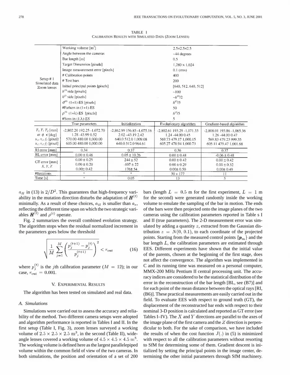
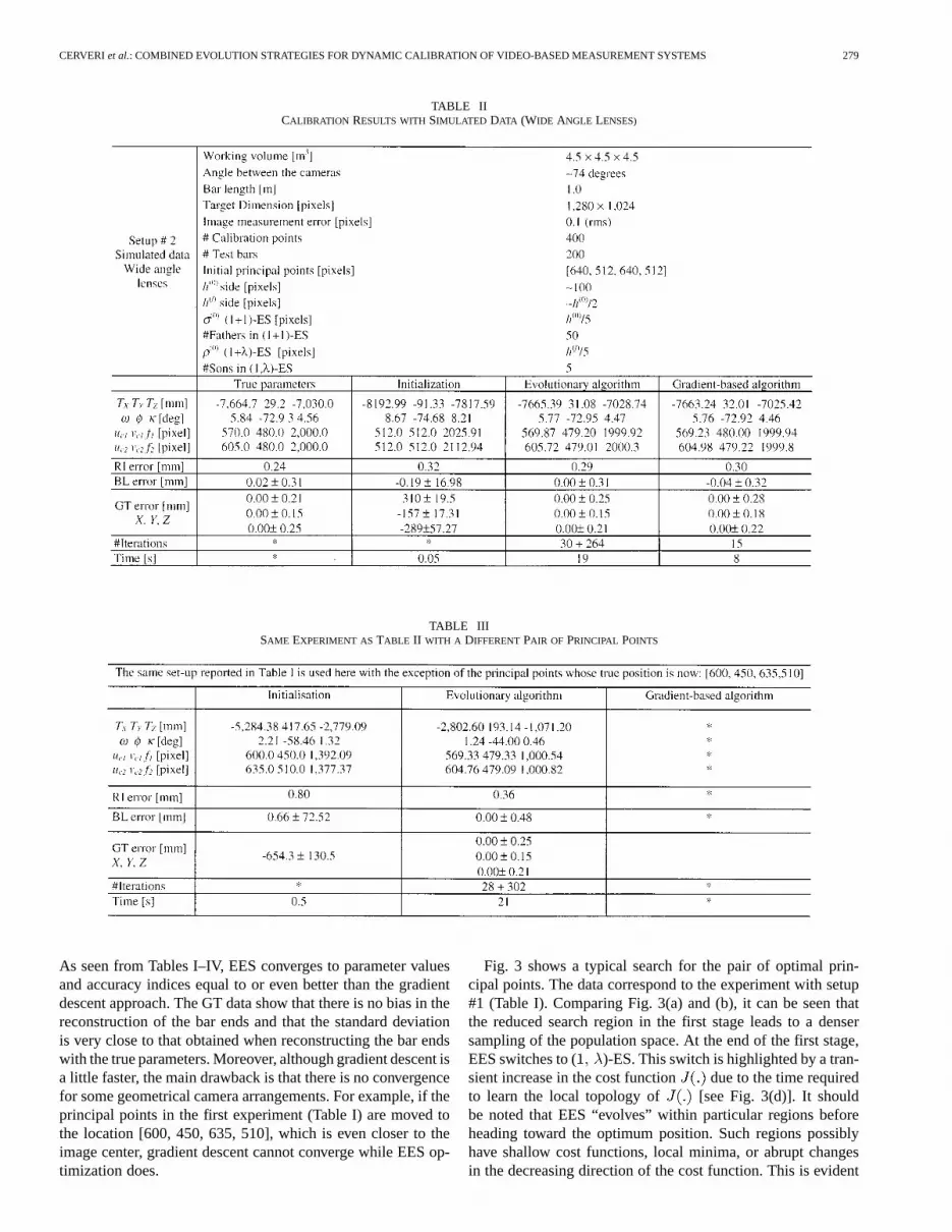
Simulations were carried out to assess the accuracy and relia-bility of the method. Two different camera setups were adoptedand algorithm performance is reported in Tables I and II. In thefirst setup (Table I, Fig. 3), zoom lenses surveyed a workingvolume of , in the second (Table II), wide-angle lenses covered a working volume of .The working volume is defined here as the largest parallelepipedvolume within the common field of view of the two cameras. Inboth simulations, the position and orientation of a set of 200

bars (length m for the first experiment, mfor the second) were generated randomly inside the workingvolume to emulate the sampling of the bar in motion. The endsof the bars were then projected onto the image planes of the twocameras using the calibration parameters reported in Table s Iand II (true parameters). The 2-D measurement error was sim-ulated by adding a quantity, extracted from the Gaussian dis-tribution , to each coordinate of the projectedpoints. Starting from the measured control points and thebar length , the calibration parameters are estimated throughEES. Different experiments have shown that the initial valueof the parents, chosen at the beginning of the first stage, doesnot affect the convergence. The algorithm was implemented inC and its running time was measured on a personal computer,MMX-200 MHz Pentium II central processing unit. The accu-racy indices are considered to be the statistical distribution of theerror in the reconstruction of the bar length [BL, see (B7)] andfor each point of the mean distance between the optical rays [RI,(B6)]. These practical measurements are easily carried out in thefield. To evaluate EES with respect to ground truth (GT), thedisplacement of the reconstructed bar ends with respect to theirnominal 3-D position is calculated and reported as GT error (seeTables I–IV). The and directions are parallel to the axes ofthe image plane of the first camera and thedirection is perpen-dicular to both. For the sake of comparison, we have includedthe results of when the cost function in (5) is minimizedwith respect to all the calibration parameters without resortingto SfM for determining some of them. Gradient descent is ini-tialized by setting the principal points in the image center, de-termining the other initial parameters through SfM machinery.

CERVERIet al.: COMBINED EVOLUTION STRATEGIES FOR DYNAMIC CALIBRATION OF VIDEO-BASED MEASUREMENT SYSTEMS 279

TABLE IICALIBRATION RESULTS WITH SIMULATED DATA (WIDE ANGLE LENSES)

TABLE IIISAME EXPERIMENT AS TABLE II WITH A DIFFERENTPAIR OF PRINCIPAL POINTS

As seen from Tables I–IV, EES converges to parameter valuesand accuracy indices equal to or even better than the gradientdescent approach. The GT data show that there is no bias in thereconstruction of the bar ends and that the standard deviationis very close to that obtained when reconstructing the bar endswith the true parameters. Moreover, although gradient descent isa little faster, the main drawback is that there is no convergencefor some geometrical camera arrangements. For example, if theprincipal points in the first experiment (Table I) are moved tothe location [600, 450, 635, 510], which is even closer to theimage center, gradient descent cannot converge while EES op-timization does.

Fig. 3 shows a typical search for the pair of optimal prin-cipal points. The data correspond to the experiment with setup#1 (Table I). Comparing Fig. 3(a) and (b), it can be seen thatthe reduced search region in the first stage leads to a densersampling of the population space. At the end of the first stage,EES switches to ( )-ES. This switch is highlighted by a tran-sient increase in the cost function due to the time requiredto learn the local topology of [see Fig. 3(d)]. It shouldbe noted that EES “evolves” within particular regions beforeheading toward the optimum position. Such regions possiblyhave shallow cost functions, local minima, or abrupt changesin the decreasing direction of the cost function. This is evident

280 IEEE TRANSACTIONS ON EVOLUTIONARY COMPUTATION, VOL. 5, NO. 3, JUNE 2001

TABLE IVCALIBRATION RESULTS WITH REAL DATA (ZOOM LENSES)

in the plot of the evolution path [see Fig. 3(c)] that is the lineconnecting the winning offspring at each evolution step.

B. Real Data Experiments

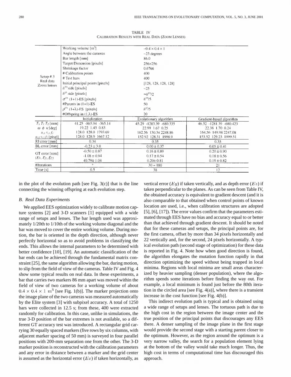
We applied EES optimization widely to calibrate motion cap-ture systems [2] and 3-D scanners [1] equipped with a widerange of setups and lenses. The bar length used was approxi-mately 1/20th to 1/10th of the working volume diagonal and thebar was moved to cover the entire working volume. During mo-tion, the bar is oriented in the depth direction, although neverperfectly horizontal so as to avoid problems in classifying theends. This allows the internal parameters to be determined withbetter confidence [10], [19]. An automatic classification of thebar ends can be achieved through the fundamental matrix con-straint [25], the same algorithm allowing the bar, during motion,to slip from the field of view of the cameras. Table IV and Fig. 4show some typical results on real data. In these experiments, abar that carries two markers 86 mm apart was moved within thefield of view of two cameras for a working volume of about

[see Fig. 1(b)]. The marker projection ontothe image plane of the two cameras was measured automaticallyby the Elite system [3] with subpixel accuracy. A total of 1250bars were collected in 12.5 s; from these, 400 were extractedrandomly for calibration. In this case, unlike in simulations, thetrue 3-D position of the bar extremes is not available, so a dif-ferent GT accuracy test was introduced. A rectangular grid car-rying 30 equally spaced markers (five rows by six columns, withadjacent marker spacing of 50 mm) is surveyed in four parallelpositions with 200-mm separation one from the other. The 3-Dmarker position is reconstructed with the calibration parametersand any error in distance between a marker and the grid centeris assumed as the horizontal error () if taken horizontally, as

vertical error ( ) if taken vertically, and as depth error () iftaken perpendicular to the planes. As can be seen from Table IV,the obtained accuracy is equivalent to gradient descent (and it isalso comparable to that obtained when control points of knownlocation are used, i.e., when calibration structures are adopted[5], [6], [17]). The error values confirm that the parameters esti-mated through EES have no bias and accuracy equal to or betterthan that achieved through gradient descent. It should be notedthat for these cameras and setups, the principal points are, forthe first camera, offset by more than 34 pixels horizontally and22 vertically and, for the second, 24 pixels horizontally. A typ-ical evolution path (second stage of optimization) for these datais reported in Fig. 4. Note how when good direction is found,the algorithm elongates the mutation function rapidly in thatdirection optimizing the speed without being trapped in localminima. Regions with local minima are small areas character-ized by heavier sampling (denser population), where the algo-rithm spends some iterations before finding the way out. Forexample, a local minimum is found just before the 80th itera-tion in the circled area [see Fig. 4(a)], where there is a transientincrease in the cost function [see Fig. 4(b)].

This indirect evolution path is typical and is obtained usinga wide range of setups and lenses. The tortuous path is due tothe high cost in the region between the image center and thetrue position of the principal points that discourages any EESthere. A denser sampling of the image plane in the first stagewould provide the second stage with a starting parent closer tothe optimum. However, as the region around the optimum is avery narrow valley, the search for a population element lyingat the bottom of the valley would take much longer. Thus, thehigh cost in terms of computational time has discouraged thisapproach.

CERVERIet al.: COMBINED EVOLUTION STRATEGIES FOR DYNAMIC CALIBRATION OF VIDEO-BASED MEASUREMENT SYSTEMS 281

VI. SUMMARY

EES optimization was applied to calibrate motion capture sys-tems [3] and 3-D scanners [1] that had a wide range of setupsand lenses. Cumbersome calibration grids [6] were substitutedby a simple bar that moves within the working volume; this newpowerful calibration technique has the same accuracy and relia-bility as the grids, but expends much less time and effort. It canbe applied in many fields, allowing motion capture systems and3-D scanner instruments to be calibrated easily in the most vari-able working conditions. The combination of a stochastic search,such as the one implemented in the ( )-ES and the covariancematrix-based search in ( )-ES, led to a solution in quasi-realtime and, above all, to the avoidance of local minima, which canoriginate from poor initialization. The EES technique is suitablefor all those optimization problems where the cost function con-tains complex nonlinear relationships between the optimizationvariables. Discovering when and where EES optimization is themost, or the least, suitable technique remains for future work.

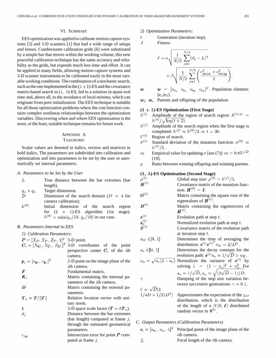
APPENDIX ATAXONOMY

Scalar values are denoted in italics, vectors and matrices inbold italics. The parameters are subdivided into calibration andoptimization and into parameters to be set by the user or auto-matically set internal parameters.

A. Parameters to be Set by the User

True distance between the bar extremes (barlength).Target dimension.Dimension of the search domain ( forcamera calibration).Initial dimension of the search regionfor ( )-ES algorithm (1st stage).

in our case.

B. Parameters Internal to EES

1) Calibration Parameters:3-D point.3-D coordinates of the pointperspective center of the thcamera.2-D point on the image plane of theth camera.

Fundamental matrix.Matrix containing the internal pa-rameters of theth camera.Matrix containing the external pa-rameters.Relative location vector with uni-tary norm.3-D space scale factor ( ).Distance between the bar extremes(bar length) computed at frame.through the estimated geometricalparameters.Intersection error for point com-puted at frame .

2) Optimization Parameters:

Generation (iteration step).Fitness

. Population element:[ ].Parents and offspring of the population.

( )-ES Optimization (First Stage)Amplitude of the region of search region:

.Amplitude of the search region when the first stage iscompleted: .Region of search.Standard deviation of the mutation function:

.Empirical value for updating [see (7)]:[19].Ratio between winning offspring and winning parents.

( )-ES Optimization (Second Stage)Global step size: .Covariance matrix of the mutation func-tion: .Matrix containing the square root of theeigenvalues of .Matrix containing the eigenvectors of

.Evolution path at step.Normalized evolution path at step.Covariance matrix of the evolution pathat iteration step.Determines the time of averaging thedistribution:Determines the decay constant for theevolution path: .Normalizes the variance of bysolving . For

, .Damping of the step size variation be-tween successive generations: .

Approximates the expectation of thedistribution, which is the distributionof the length of a distributedrandom vector in .

C. Output Parameters (Calibration Parameters)

Principal point of the image plane of theth camera.

Focal length of theth camera.

282 IEEE TRANSACTIONS ON EVOLUTIONARY COMPUTATION, VOL. 5, NO. 3, JUNE 2001

Relative orientation (a function of threeindependent rotations: ).

Relative location (base line).

APPENDIX B3-D RECONSTRUCTION

When the stereo-camera parameters have been estimated the3-D position of a point can be determined as the intersectionpoint of the two optical rays. These are the straight lines [and in Fig. 1(a)] through the projection of , and ontothe image plane of the two cameras and the perspective centers

and . Due to noise on and , these two straight linesgenerally do not intersect and the 3-D reconstruction ofliesin the midpoint of the minimal distance segment [6]. The twostraight lines have the following:

(B1)

whereequals zero;equals ;director cosines.

Minimizing the 3-D distance between and

(B2)

a linear system is obtained, where

(B3a)

(B3b)

The 3-D reconstruction of is obtained as

(B4)

where the s are a function of the calibration parameters

(B5)

where for the first camera and for the secondcamera. [10]. The minimum distance be-tween the two intersecting rays can be obtained from (B4)

(B6)

The distance between two 3-D pointsand is computed as

(B7)

ACKNOWLEDGMENT

The authors would like to thank Dr. Hansen for his criticalreading of the manuscript and an anonymous referee for the sug-gestions.

REFERENCES

[1] N. A. Borghese, G. Ferrigno, G. Baroni, R. Savarè, S. Ferrari, and A. Pe-dotti, “AUTOSCAN: A flexible and portable scanner of 3-D surfaces,”IEEE Comput. Graph. Appl., vol. 18, pp. 2–5, May/June 1998.

[2] N. A. Borghese, M. Di Rienzo, G. Ferrigno, and A. Pedotti, “Elite: Agoal-oriented vision system for moving objects detection,”Robotica,vol. 9, pp. 275–282, Sept. 1990.

[3] G. Ferrigno and A. Pedotti, “Modularly expansible system for real-timeprocessing of a TV display, useful in particular for the acquisition ofcoordinates of known shapes objects,” U.S. Patent 4 706 296, 1990.

[4] X. Hu and N. Ahuja, “Matching point features with ordered geometric,rigidity and disparity constraints,”IEEE Trans. Patt. Anal. Machine In-tell., vol. 16, pp. 1041–1045, Oct. 1994.

[5] J. Weng, P. Cohen, and M. Herniou, “Camera calibration with distortionmodels and accuracy evaluation,”IEEE Trans. Pattern Anal. MachineIntell., vol. 14, pp. 965–979, Oct. 1992.

[6] N. A. Borghese and G. Ferrigno, “An algorithm for 3-D automaticmovement detection by means of standard TV cameras,”IEEE Trans.Bio-Med. Eng., vol. 37, pp. 1221–1225, Dec. 1990.

[7] A. Gruen and H. A. Beyer, “System calibration through self-calibration,”in Proc. Workshop on Camera Calibration and Orientation in ComputerVision, Washington, DC, Aug. 1992, pp. 218–233.

[8] H. G. Maas, “Dynamic photogrammetric calibration of industrialrobots,” inProc. Videometrics V, vol. 3174, 1997, pp. 106–112.

[9] H. C. Longuet-Higgins, “A computer algorithm for reconstructing ascene from two projections,”Nature, vol. 293, pp. 133–135, Sept. 1981.

[10] O. D. Faugeras,Three-Dimensional Computer Vision. Cambridge,MA: M.I.T. Press, 1992.

[11] R. I. Hartley, “In defence of 8-point algorithm,”IEEE Trans. PatternAnal. Machine Intell., vol. 19, pp. 580–593, June 1997.

[12] N. A. Borghese and P. Perona, “Calibration of a stereo system with pointsof unknown location,” inProc. 14th Int. Conf. Soc. Biomech. ISB, Paris,France, June 1993, pp. 202–203.

[13] Q. T. Luong and O. D. Faugeras, “The fundamental matrix: Theory, al-gorithms, and stability analysis,”Int. J. Comp. Vision, vol. 17, no. 1, pp.43–76, 1996.

[14] N. A. Borghese and P. Cerveri, “Calibrating a video camera pair with arigid bar,” Pattern Recognit., vol. 33, pp. 81–95, Jan. 2000.

[15] S. Bougnoux, “From projective to Euclidean space under any practicalsituation, a criticism of self-calibration,” inProc. 1998 IEEE Int. Conf.Computer Vision, Bombay, India, Sept. 1998, pp. 790–796.

[16] R. I. Hartley, “Kruppa equations derived from the fundamental matrix,”IEEE Trans. Pattern Anal. Machine Intell., vol. 19, pp. 133–135, Feb.1997.

[17] R. K. Lenz and R. Y. Tsai, “Techniques for calibration of the scale factorand image center for high accuracy 3-D machine vision metrology,” inProc. IEEE Int. Conf. Robotics Automation, Raleigh, NC, July 1987, pp.68–75.

[18] P. Cerveri, N. A. Borghese, and A. Pedotti, “Complete calibration of astereo photogrammetric system through control points of unknown co-ordinates,”J. Biomech., vol. 31, no. 10, pp. 935–940, 1998.

[19] P. R. Wolf, Elements of Photogrammetry. New York: McGraw-Hill,1983.

[20] T. Bäck, G. Rudolph, and H.-P. Schwefel, “Evolutionary programmingand evolution strategies: similarities and differences,” inProceedingsof the Second Annual Conference on Evolutionary Programming, D. B.Fogel and W. Atmar, Eds. La Jolla, CA: Evol. Programm. Soc., 1993,pp. 11–22.

[21] N. Hansen and A. Ostermeier, “Completely derandomised self- adapta-tion in evolution strategies,” Evol. Comput., to be published.

[22] A. Ostermeier, A. Gawelczyk, and N. Hansen, “A derandomized ap-proach to self-adaptation of evolution strategies,”Evol. Comput., vol.2, no. 4, pp. 369–380, 1994.

[23] N. Hansen and A. Ostermeier, “Adapting arbitrary normal mutation dis-tributions in evolution strategies: The covariance matrix adaptation,”in Proc. 1996 IEEE Int. Conf. Evolutionary Computation, 1996, pp.312–317.

[24] L. P. Kaelbing, M. L. Littman, and A. W. Moore, “Reinforcementlearning: A survey,”J. Artif. Intell. Res., vol. 4, pp. 237–285, June 1996.

[25] Z. Zhang, R. Deriche, O. Faugeras, and Q.-T. Luong, “A robust tech-nique for matching two uncalibrated images through the recovery of theunknown epipolar geometry,”Artif. Intel. J., vol. 78, pp. 87–119, Oct.1995.