Chemical and Biochemical Sensors

KARL CAMMANN, Institut für Chemo- und Biosensorik, Münster, Federal Republic of

Germany (Chap. 1. Introduction to the Field of Sensors and Actuators, 4. Actuators

and Instrumentation, 5. Future Trends and Outlook, Sections 2.2. Molecular

Recognition Processes and Corresponding Selectivities, 2.4. Problems Associated

with Chemical Sensors, 2.5. Multisensor Arrays and Pattern-Recognition Analysis)

BERND ROSS, Institut für Chemo- und Biosensorik, Münster, Federal Republic of

Germany (Sections 2.3. Transducers for Molecular Recognition: Processes and

Sensitivities, 2.3.1. Electrochemical Sensors, 2.3.1.2. Voltammetric and

Amperometric Cells)

WOLFGANG HASSE, Institut für Chemo- und Biosensorik, Münster, Federal Republic of

Germany (Section 2.3.1.3. Conductance Devices)

CHRISTA DUMSCHAT, Institut für Chemo- und Biosensorik, Münster, Federal Republic

of Germany (Section 2.3.1.4. Ion-Sensitive Field-Effect Transistors (ISFETs))

ANDREAS KATERKAMP, Institut für Chemo- und Biosensorik, Münster, Federal

Republic of Germany (Section 2.3.2. Optical Sensors)

JÖRG REINBOLD, Institut für Chemo- und Biosensorik, Münster, Federal Republic of

Germany (Sections 2.2.2. Reactions at Semiconductor Surfaces and Interfaces

Influencing Surface or Bulk Conductivities, 2.3.3. Mass-Sensitive Devices)

GUDRUN STEINHAGE, Institut für Chemo- und Biosensorik, Münster, Federal Republic

of Germany (Section 2.3.4. Calorimetric Devices)

BERND GRÜNDIG, Institut für Chemo- und Biosensorik, Münster, Federal Republic of

Germany (Sections 3.1. Definitions, General Construction, and Classification–

3.2.3. Enzyme Sensors for Inhibitors, 3.5. Problems and Future Prospects)

REINHARD RENNEBERG, Institut für Chemo- und Biosensorik, Münster, Federal

Republic of Germany (Sections 3.1. Definitions, General Construction, and

Classification, 3.2.4. Biosensors Utilizing Intact Biological Receptors–3.4.

Whole-Cell Biosensors)

NORBERT BUSCHMANN, Westfälische Wilhelms-Universität, Münster, Federal

Republic of Germany (Section 2.3.1.1. Self-Indicating Potentiometric Electrodes)

1. Introduction to the Field of Sensors and Actuators

When a person suffers the loss of one of the five senses it is recognized as a serious

obstacle to carrying out everyday activities. In the case of blindness and deafness the

expression "disabled" is even used as an indication of the severity of the loss, just as with

those whose limbs (legs or arms) or other crucial body components are incapable of

functioning properly. In the animate world generally, sensing and then acting or reacting

is closely linked with the very essence of life, where input from some type of sensory

system always precedes intelligent action. From the earliest days of mankind it was the

availability of a powerful "coping mechanism" that constituted the driving force leading

first to intelligent action and later to the unbiased accumulation of knowledge.

Any intellectual information structure capable of producing theories is dependent upon a

reliable input of information. Imperfect observations, or perceptual processes subject to

frequent errors, will never provide a satisfactory basis for working theories subject to

verification by others. In this respect analytical chemistry can be regarded as one of the

cognitive means available to the chemist interested in ascertaining the composition of the

material world and the distribution and arrangement of atoms and molecules within a

particular sample. Since both the nature and the three-dimensional arrangement of atoms

determine the characteristics of matter, reliable information with respect to both is crucial

for understanding the whole of the material world. This observation is equally valid for

the inorganic, the organic, and also the living world. A high level of structured

information is essential to the work of most natural scientists. The ability to describe in

detail a complex chemical process (e.g., the combustion of fuel in an engine or waste in a

municipal incinerator, the synthesis of minerals deep within the earth, or the course of

biochemical reactions taking place in living systems) is crucially dependent on the quality

of the information available. High technology is impossible without detailed information

on the state of the system in question, as has been amply demonstrated in semiconductor

technology, where knowledge of the purity of the materials and the state of cleanliness in

the production plant is absolutely essential.

Complex and especially dynamic systems involving chemical processes are often

described in terms of simplified models. The more chemical information is available, the

better will be the model—and consequently the more complete the understanding

and control over the system. Chemical analysis constitutes the primary source of

information for characterizing the various states of such a system.

As a result of a tremendous increase in the demand for analytical chemical information,

the number of analyses conducted for acquiring information about particular samples is

increasing dramatically. It is thought that worldwide more than 109 analyses are now

performed every day—with a double-digit growth rate. Many complex systems are

governed by time-dependent parameters, which makes it essential that as much

information as possible be acquired within a particular period of time so that the various

reactions taking place within the system can be followed, and to provide insight into the

dynamics of the mechanisms involved. Devices designed to permit continuous

measurement of a quantity are called sensors. Various types of sensors have been

developed for monitoring many important physical parameters, including temperature,

pressure, speed, flow, etc. The number of potential interferences is rather limited in these

cases, so it is not surprising that the corresponding sensors offer a level of reliability

considerably higher that that for sensors that measure chemical quantities (e.g., the

concentration of a certain species, the activity of an ion, or the partial pressure of a

gaseous material).

There are two major fields of application for chemical sensors: environmental studies

and biomedical analysis. In the field of environmental analysis there is a great demand for

the type of continuous monitoring that only a sensor can provide, since the relevant

parameter for toxicological risk assessment is always the dose (i.e., a concentration

multiplied by an exposure time). The study of environmental chemistry also depends upon

a continuous data output that provides not only baseline levels but also a reliable record of

concentration outbursts. Data networks can be used to accumulate multiple

determinations of a particular analyte regardless of whether these are acquired

simultaneously or at different times within a three-dimensional sampling space (which

may have dimensions on the order of miles), thereby providing information about

concentration gradients and other factors essential for pinpointing the location of an

emission source. The inevitable exponential increase in the number of chemical analyses

associated with this work threatens to create serious financial and also ecological

problems, since most classical analytical techniques themselves produce a certain amount

of chemical waste.

Our society is characterized by a population with an average age that is continuously

increasing. This has stimulated the widespread biomedical application of chemical sensors

for monitoring the health of the elderly without confining them to hospitals. Sensors for

determining the concentrations of such key body substances as glucose, creatinine, or

cholesterol could prove vitally important in controlling and maintaining personal health,

at the same time enhancing the quality of the patient's life. The same principle underlies

sensor applications in intensive care wards. Sensors also offer the potential for significant

cost reductions relative to conventional laboratory tests, and they can even improve the

quality of the surveillance because continuous monitoring can lower the risk of

complications. For example, the monitoring of blood potassium levels can give early

warning of the steady increase that often precedes an embolism, providing sufficient time

for clinical countermeasures.

It should be noted at the outset, however, that the development costs associated with a

chemical sensor are typically many orders of magnitude higher than those for a sensor

measuring a physical quantity. A satisfactory return on investment therefore presupposes

either mass production in the case of low-cost sensors or special applications that

would justify an expensive sensor.

Another important field of application for chemical sensors is process control. Here the

sensor is expected to deliver some crucial signal to the actuators (valves, pumps, etc.) that

control the actual process. Fully automated process control is feasible with certain types

of feedback circuits. Since key chemical parameters in many chemical or biochemical

processes are not subject to sufficiently accurate direct determination by the human

senses, or even via the detour of a physical parameter, sensor technology becomes the key

to automatic process control. Often the performance of an entire industrial process

depends on the quality and reliability of the sensors employed. Successful adaptation of a

batch process to flow-through reactor production technology is nearly impossible without

chemical sensors for monitoring the input, the product quality, and also—an

increasingly important consideration—the waste. Municipal incinerators would

certainly be more acceptable if they offered sensor-based control of SO2, NO

x, and,

even more important, the most hazardous organic compounds, such as dioxines.

Compared to the high construction costs for a plant complete with effective exhaust

management, an extra investment in sensor research can certainly be justified.

These few examples illustrate the increasing importance of chemical sensor development

as a key technology in various closed-looped sensor/actuator-based process control

applications. Rapid, comprehensive, and reliable information regarding the chemical state

of a system is indispensable in many high technology fields; for this reason there is also

an increasing need for intelligent or "smart" sensors capable of controlling their own

performance automatically.

Finally, there is an urgent and growing demand for analytical chemists and engineers

skilled in producing reliable chemical sensors delivering results that are not only

reproducible but also accurate (free of systematic errors attributable to interferences from

the various sample matrices).

2. Chemical Sensors [1][2][3][4][5]

2.1. Introduction

Until the introduction in the 1980s of the lambda probe [6][7][8] for oxygen measurement

in the exhaust systems of cars employing catalytic convertors (see Section 2.2.3. Selective

Ion Conductivities in Solid-State Materials), the prototype for the most successfully

applied chemical sensor was certainly the electrochemical pH electrode, introduced over

50 years ago and discussed in detail in Section 2.3.1.1. Self-Indicating Potentiometric

Electrodes. This device can be used to illustrate the identification and/or further

optimization of all the critical and essential features characterizing sensor performance,

including reversibility, selectivity, sensitivity, linearity, dynamic working range, response

time, and fouling conditions.

Electrochemical electrodes for chemical analysis have actually been known for over 100

years (the Nernst equation was published as early as 1889), and they can therefore be

considered as the forerunners of chemical sensors. In general, a chemical sensor is a small

device placed directly on or in a sample and designed to produce an electrical signal that

can be correlated in a specific way with the concentration of the analyte, the substance to

be determined. If the analyte concentration varies in the sample under investigation, the

sensor should faithfully follow the variation in both directions; i.e., it should function in

a reversible way, and it should deliver analytical data at a rate greater than the rate of

change of the system (quasi-reversible case). From the standpoint of practical

applications, complete thermodynamic reversibility is relatively unimportant so long as

measurements are acquired with sufficient rapidity compared to changes in the analyte

concentration. Another restriction arises from the demand for a reagent-free

measurement: an extremely selective or specific cooperation between the analyte atom,

ion, or molecule and the surface of a receptor-like sensor element should be the sole basis

for gaining information about the analyte concentration.

The general construction principle of a chemical sensor is illustrated in Figure (1). The

most important part is the sensing element (receptor) at which the molecular or ionic

recognition process takes place, since this defines the overall selectivity of the entire

sensor. The sensing-element surface is sometimes covered by an additional surface layer

acting as a protective device to improve the lifetime and/or dynamic range of the sensor,

or to prevent interfering substances from reaching the sensing-element surface. The

analyte recognition process takes place either at the surface of the sensing element or in

the bulk of the material, leading to a concentration-dependent change in some physical

property that can be transformed into an electrical signal by the appropriate transducer.

Since there should be no direct contact between the sample and the transducer, the latter

cannot itself improve the selectivity, but it is responsible for the sensitivity of the sensor,

and it functions together with the sensing element to establish a dynamic concentration

range. The electrical signal of the transducer is usually amplified by a device positioned

close to the transducer or even integrated into it. If extensive electrical wiring is required

between the sensor and the readout–control unit, the electrical signal might also be

digitized as one way of minimizing noise pick-up during signal transmission. Several

chemical signals produced by multiple sensing elements, each connected to its own

specific transducer, can be transmitted via modern multiplexing techniques, which require

only a two-wire electrical connection to the control unit.

If a biochemical mechanism is used in the molecular recognition step, the sensor is called

a biosensor. Systems of this type are dealt with in Chapter 3. Biochemical Sensors

(Biosensors).

Key features of chemical sensors subject to specification are, in order of decreasing

importance:

1) Selectivity (accuracy; better: truthfulness of the result)

2) Limit of detection (LOD) for the analyte

3) Sensitivity

4) Dynamic response range

5) Stability

6) Response time

7) Reliability (maintenance-free working time)

8) Lifetime

Selectivity. The selectivity of a chemical sensor toward the analyte is often expressed in

terms of a dimension that compares the concentration of the corresponding interfering

substance with an analyte concentration that produces the same sensor signal. This factor

is obtained by dividing the sensitivity of the sensing device toward the analyte (=slope

of the calibration curve; see below) by the sensitivity for the corresponding interfering

substance. Typical selectivities range from 10–3

to <10–6

. In order to estimate the error

attributable to limited selectivity the concentration of the interferent must be multiplied by

the selectivity coefficient. If, for example, a sodium-selective glass electrode shows a

typical selectivity coefficient toward potassium ions on the order of 10–3

, a thousand-fold

excess of potassium- over sodium-ion concentration would produce an equivalent sensor

signal, therefore doubling the reading and leading to an error of 100%. It should be

noted, however, that such selectivities are themselves concentration- and matrix-

dependent. This means that near the limit of detection of a particular sensor an interfering

species will disrupt the measurement of an analyte to a greater extent than it will at higher

concentrations. Therefore, true response factors can rarely be used for correction

purposes.

The selectivity is the most important parameter associated with a chemical sensor since it

largely determines the truthfulness of the analytical method. Truthfulness (or accuracy) is

more than simply precision, repeatability, or reproducibility: it represents agreement

with the true content of the sample. All the other parameters mentioned are subject to

systematic error, which can only be recognized if an analyte is determined by more than

one method. Since selectivity is always limited, all chemical sensors are prone to report

higher concentrations than a sample actually contains. In the case of environmental

analysis this positive error can be regarded as a safety margin if relevant interferents are

also present. In such a situation the sensor acts as a probe for establishing when a sample

should be taken to be analyzed in the laboratory. The reproducibility of chemical sensor

measurements is often well below 1% relative.

However, it should also be noted that sensing elements are subject to poisoning, resulting

in a diminished response for the analyte. Sensor poisons are substances that either cover

the sensing surfaces, thereby influencing the analyte recognition process or, in the case of

catalytic sensors, decrease the activity of the catalyst. Since these fouling effects are not

linear, predictable, or mathematically additive, great care is necessary whenever data from

a sensor array are treated by the methods of mathematical data management (e.g., pattern

recognition, neural networks, etc.). The influence of sensor poisoning can be completely

different and unpredictable for every single sensing element. There is no simple theory

that permits the transfer of poisoning effects with respect to one sensing element to other

parts of a sensing array as a way of avoiding recalibration. Thus, any attempt to overcome

insufficient selectivity by the use of a sensor array with multiple sensor elements

displaying slightly differing selectivities for the analyte and the interferents, followed by

the application of chemometrics to correct for selectivity errors, is very dangerous in the

context of unknown and variable sample matrices. Unfortunately, this is usually the

situation in environmental analysis. In the learning and/or calibration phase of sensor-

array implementation it is essential that the sample matrix be understood. In the case of a

known matrix and a closed system, and if the number of possible interferents is >5, the

number of calibration steps (involving different mixtures of the interfering compounds,

selected to cover all possible concentration and mixture variations) required to provide

reliable information on the 5-dimensional response space of the sensor array for a

5+N array is extremely large (usually several hundred). With real samples the time

necessary for calibrating the sensors might exceed the period of stability. Since with open

environmental systems the type and number of interferents is not known, any attempt to

correct for inadequate sensor selectivity by use of a sensor array increases the risk of

systematic errors. This assertion is valid for every type of mathematical data treatment

(pattern recognition, neural networks, etc.) for samples of unknown and/or variable

matrices. However, for trace analysis in the sub-ppm range all analytical methods (with

the exception of isotope dilution) are subject to systematic errors, as has been

demonstrated with interlaboratory comparison tests using even the most sophisticated

techniques [10].

Limit of Detection (LOD) for the Analyte. In analytical chemistry the limit of detection

(LOD) is exceeded when the signal of the analyte reaches at least three times the general

noise level for the reading. No quantitative measurement is possible at this low

concentration; only the presence of the analyte can be assumed with a high probability

(>99%) in this concentration range. The range of quantification ends at ten times the

LOD. Therefore, the LOD of an analytical instrument must always be ten times smaller

than the lowest concentration to be quantified. It is worth mentioning in this context that

LOD values reported by most instrument manufacturers disregard the influence of

interfering compounds. Furthermore, the LOD is often worse when an analyte must be

determined within its characteristic matrix.

In some cases with extremely sensitive sensors a zero-point calibration might be difficult

to perform, because traces of the analyte would always be present or might easily be

carried into the calibration process by solvents or reagents. The lowest measurable level

is called the blank value. The LOD is then defined as three times the standard deviation of

the blank value, expressed in concentration units (not in the units of the signal, as is

sometimes improperly suggested).

Normally the LOD becomes worse as a sensor ages.

Sensitivity. As mentioned above, the sensitivity of a sensor is defined by the signal it

generates, expressed in the concentration units of the substance measured. This

corresponds to the slope of the corresponding calibration curve when the substance is the

analyte, or to the so-called response curve for interferents. With some sensors the

sensitivity rises to a maximum during the device's lifetime. A check of the sensitivity is

therefore a valuable quality-assessment step. Intelligent sensors are expected to carry out

such checks automatically in the course of routine performance tests. Since in most cases

the sensitivity depends on such other parameters as the sample matrix, temperature,

pressure, and humidity, certain precautionary measurements are necessary to ensure that

all these parameters remain constant both during calibration and in the analysis of real

samples.

Dynamic Response Range. The dynamic response range is the concentration range over

which a calibration curve can be described by a single mathematical equation. A

potentiometric sensing device follows a logarithmic relationship, while amperometric and

most other electrochemical sensors display linear relationships. Both types of signal-to-

concentration relationship are possible with optical sensors; in absorption

measurements it is the absorbance with its logarithmic base that is the determining factor,

whereas a fluorescence measurement can be described by a linearized function. The

broader the concentration range subject to measurement with a given sensing system, the

less important are dilution or enrichment steps during sample preparation. The

measurement range is limited by the LOD at the low concentration end, and by saturation

effects at the highest levels. Modern computer facilities make it possible also to use the

nonlinear portion of a calibration curve as a way of saving sample preparation time, but

analytical chemists are very reluctant to follow this course because experience has shown

that the initial and final parts of a calibration curve are generally most subject to influence

by disturbances (electronic and chemical). A good chemical sensor should function over

at least one or two concentration decades. Sensors with excellent performance

characteristics include the lambda oxygen probe and the glass pH electrode, both of which

cover analyte concentration ranges exceeding twelve decades!

Stability. Several types of signal variation are associated with sensors. If the signal is

found to vary slowly in two directions it is unlikely to be regarded as having acceptable

stability and reproducibility, especially since it would probably not be subject to

electronic correction.

Output variation in a single direction is called drift. A steadily drifting signal can be

caused by a drifting zero point (if no analyte is present) and/or by changes in sensor

sensitivity (i.e., changes in the slope of the calibration curve). Drift in the sensor zero-

concentration signal (zero-point drift) can be corrected by comparison with a signal

produced by a sensor from the same production batch that has been immersed in an

analyte-free solution.

When drift observed in a sensor signal is attributable exclusively to zero-point drift, and

there has been no change in the sensitivity, a one-point calibration is permissible: that

is, either the instrumental zero point must itself be adjusted prior to the measurement, or

else the sensor signal for a particular calibration mixture must be recorded. Assuming

there is no change in the slope of the calibration curve, this procedure is equivalent to

effecting a parallel shift in the calibration curve. If the sensor is routinely stored in a

calibrating environment between measurements then such a one-point calibration

becomes particularly easy to perform.

Special attention must be directed toward the physical and chemical mechanisms that

cause a sensor signal to drift. Differential techniques are satisfactory only if the effect to

be compensated has the same absolute magnitude and the same sign with respect to both

devices. A consideration often neglected in potentiometry is proper functioning of the

reference electrode. Several authors [11][12][13] have suggested that in ion-selective

potentiometry a "blank membrane" electrode (one with the same ion-selective membrane

composition as the measuring electrode but without the selectivity-inducing electroactive

compound) would create the same phase-boundary potential for all interfering compounds

as the measuring electrode itself. This is definitely not the case, however. At the

measuring electrode, analyte ions establish a relatively high exchange-current density,

which fixes the boundary potential. The effect of a particular interfering ion will depend

on its unique current–voltage characteristics at such an interface. Therefore, interfering

ions may establish different phase-boundary potentials depending on the particular mixed

potential situations present at the membranes in question, which means that a differential

measuring technique will almost certainly fail to provide proper compensation.

If both the zero point of a sensor and its sensitivity change with time, a two-point

calibration is necessary. The combination of a changing slope for the calibration curve

and a change in the intercept is generally unfavorable, but this is often the situation with

catalytic gas sensors. If the slope of the calibration curve also depends on the sample

matrix, only standard addition techniques will help.

The stability of a chemical sensor is usually subject to a significant aging process. In the

course of aging most sensors lose some of their selectivity, sensitivity, and stability. Some

sensors, like the glass pH electrode, can be rejuvenated, while others must be replaced if

certain specifications are no longer fulfilled.

Response Time. The response time is not defined in an exact way. Some manufacturers

prefer to specify the time interval over which a signal reaches 90% of its final value

after a ten-fold concentration increase, while authors sometimes prefer the 95% or even

99% level. The particular percentage value chosen represents a pragmatic decision,

since most signal–time curves follow an exponential increase of the form:

where the true final value is unknown and/or will never be reached in a mathematical

sense. Therefore, specification in terms of the time constant k is clearer. This corresponds

to the time required for a signal to reach about 67% of its final value, which can be

ascertained without waiting for a final reading: as the slope of the curve ln(signal) vs.

time. If the response is constant and independent of the sample matrix, this equation can

be used to calculate a final reading immediately after the sensor has been introduced into

the sample.

Typical response times for chemical sensors are in the range of seconds, but some

biosensors require several minutes to reach a final reading. At the other extreme, certain

thin-film strontium titanate oxygen sensors show response times in the millisecond range.

The response time for a sensor is generally greater for a decreasing analyte concentration

than for an increasing concentration. This effect is more pronounced in liquids than in

gaseous samples. Both the surface roughness of the sensor and/or the dead volume of the

measuring cell have some influence on the response time. Small cracks in the walls of a

measuring cell can function as analyte reservoirs and diminish the rate of analyte dilution.

With certain sensors the response time can also depend on the sample matrix. In the

presence of strongly interfering substances the response time for a chemical sensor might

increase as a result of an increase in the time required to reach final equilibrium.

Reliability. There are various kinds of reliabilities. One involves the degree of trust that

can be placed in an analytical result delivered by a particular chemical sensor. Another is

a function of the real time during which the sensor actually performs satisfactorily without

a breakdown and/or need for repair.

There is no way to judge fairly the analytical reliability of a chemical sensor, since this

depends strongly upon the expert ability of the analyst to choose a suitable sensor and a

suitable sample preparation routine in order to circumvent predictable problems.

With respect to the first generation of sensors, the ion-selective electrodes, the experience

of many users has led to the following "reliability hit list", with the most reliable devices

cited first: glass pH electrodes, followed by fluoride, sodium glass, valinomycin-based

potassium, sulfide, and iodide electrodes, and culminating in the electrodes for divalent

ions. In a general way, sometimes very personal judgements regarding reliability have

always been linked to a particular sensor's specificity toward the analyte in question.

Reliability can be improved considerably if analytical conclusions are based on

measurements obtained by different methods. For example, it is possible to determine

sodium either with an appropriate glass-membrane electrode or with a neutral carrier-

based membrane electrode. If both give the same analytical results, the probability of a

systematic error is very low. Likewise, potassium might be measured using selective

membrane electrodes with different carrier molecules. This is of course different from

analysis based on a sensor array, in which the selectivities of the individual sensors differ

only slightly, and different also in the sense that no correction procedure is invoked in

case two results are found to disagree. Use of the Nernst–Nikolsky equation (see

Section 2.3.1.1. Self-Indicating Potentiometric Electrodes), together with the introduction

of additional electrodes for determining the main interferents, has been shown to be an

effective way of correcting errors in the laboratory with synthetic samples. Since

selectivity numbers (i.e., parameters like the selectivity coefficient) are influenced by the

sample matrix through its ionic strength, content of surface-active or lipophilic

compounds, or interfering ions, it is dubious whether data from real environmental

samples should be corrected by this method.

The length of time over which a chemical sensor can be expected to function reliably can

be remarkably great (in the range of years), as in the case of glass-membrane or solid-

state membrane electrodes, the lambda probe (Section 2.2.3. Selective Ion Conductivities

in Solid-State Materials), and the Taguchi gas sensor (see Section 2.2.2. Reactions at

Semiconductor Surfaces and Interfaces Influencing Surface or Bulk Conductivities). On

the other hand, a biosensor that depends upon a cascade of enzymes to produce an analyte

signal will usually have a short span of proper functioning (a few days only).

Potentiometric ion-selective membrane electrodes and optical chemosensors have

lifetimes of several months. In the case of biosensors it should be noted that anything that

changes the quarternary space-orientation of the recognition biomolecules will destroy the

proper functioning of the sensor. Enzymes can be influenced by such factors as pH,

certain heavy-metal ions, certain inhibitors, and high temperature (resulting in

denaturation).

Lifetime. As already mentioned above, some rugged solid-state sensors have lifetimes of

several years. Certain sensors can also be regenerated when their function begins to

deteriorate. The shortest lifetimes are exhibited by biosensors. Because of the huge

amount of effort invested worldwide in building an implantable glucose sensor it has been

possible to develop a biosensor for this purpose that can operate satisfactorily for nearly

six months provided certain precautions are taken. Ion-selective electrodes and optical

sensors based on membrane-bound recognition molecules often lose their ability to

function by a leaching-out effect. In optical sensors the photobleaching effect may also

reduce the lifetime to less than a year. On the other hand, amperometric cells work well

for many years, albeit with restricted selectivities.

Problems associated with inadequate lifetimes are best overcome with mass-produced

miniaturized replacement sensors based on inexpensive materials. Minimizing

replacement costs may well represent the future of biosensors. Installation of a new sensor

to replace one that is worn-out can also circumvent surface fouling, interfering layers of

proteins, and certain drift and poisoning problems.

Comparison of Sensor Data with that Obtained by Traditional Analytical Methods.

It is extremely difficult to compare sensor data with traditional data; indeed,

generalizations of this type are rarely possible anywhere in the field of analytical

chemistry. Sensor developers are often confronted with the customer's tendency to

consider use of a sensor only if all else has failed. This means that the most adverse

conditions imaginable are sometimes proposed for the application of a chemical sensor. It

is also not fair to compare a device costing a few dollars with the most expensive and

sophisticated instrumentation available, nor is it appropriate to compare the performance

of a chemical sensor with techniques involving time-consuming separations. In this

case only the corresponding detector should be compared with the sensor. Sometimes the

very simple combination of a selective chemical sensor with an appropriate separation

technique is the most effective way to obtain the redundant data that offer the highest

reliability.

Chemical sensors are generally superior to simple photometric devices because they are

more selective or faster (as in the case of optical sensors based on the photometric

method), more flexible, more economical, and better adapted to continuous sensing. The

latter advantage can also be achieved by traditional means via flow-through measuring

cells, but this leads to a waste of material and sample, and also to the production of

chemical waste. Reagent-free chemical sensors show their greatest advantages in

continuous-monitoring applications, in some of which they are called upon to fulfill a

control function without necessarily reporting an analytical result, as in the case of the

lambda probe described below (Section 2.2.3. Selective Ion Conductivities in Solid-State

Materials).

2.2. Molecular Recognition Processes and Corresponding

Selectivities

In any sensing element the functions to be fulfilled include sampling, sample preparation,

separation, identification, and detection. Therefore, successful performance in these

various capacities largely determines the quality of the chemical sensor as a whole.

Selective recognition of an analyte ion or molecule is not an easy task considering that

there are more than five million known compounds. Recognition can be accomplished

only on the basis of unique characteristics of the analyte in question. Several different

recognition processes are relevant to the field of chemical sensors, ranging from energy

differences (in spectroscopy) to thermodynamically determined variables (in

electrochemistry), including kinetic parameters (in catalytic processes). The most specific

interactions are those in which the form and the spatial arrangement of the various atoms

in a molecule play an important role. This is especially true with biosensors based on the

complementary (lock-and-key) principle. Here the analyte molecule and its counterpart

have exactly complementary geometrical shapes and come so close together that they

interact on the basis of the weak van der Waals interaction forces.

2.2.1. Catalytic Processes in Calorimetric Devices

Pellistors are chemical sensors for detecting compounds that can be oxidized by oxygen.

A catalyst is required in this case because the activation energy for splitting a doubly-

bonded oxygen molecule into more reactive atoms is too high for the instantaneous

"burning" of oxidizable molecules. In most cases platinum is the catalyst of first choice

because of its inertness. The principle underlying oxidizable-gas sensors involves

catalytic burning of the gaseous analyte, which leads to the production of heat that can in

turn be sensed by various temperature-sensitive transducers. Often what is actually

measured is the increase in electrical resistance of a metal wire heated to an elevated

temperature (ca. 300–400°C) by the current flowing through it. However, it is also

possible to use more sensitive semiconductor devices or even thermopiles in order to

register temperature changes of <10–4°C.

In order to understand the selectivity displayed by a pellistor toward various flammable

compounds it is necessary to consider the elementary steps in the corresponding catalytic

oxidation of analyte at the catalyst surface. Since this is in fact a surface reaction, various

adsorption processes play a dominant role. First, oxygen must be adsorbed, permitting the

oxygen double bond to be weakened by the catalyst. Then the species to be oxidized must

be adsorbed onto the same catalyst surface where it can subsequently react with the

activated oxygen atoms. The process of adsorption may follow one of two known types of

adsorption isotherms, as reflected in the calibration curves for these devices. An

equilibrium consisting of adsorption, catalyzed reaction, and desorption of the oxidized

product leads to a constant signal at a constant analyte concentration. The sensor response

function is influenced by any change in the type or number of active surface sites, since

this in turn affects both the adsorption processes and the catalytic efficiency. Likewise,

compounds that have an influence on any of the relevant equilibria will also alter the

calibration parameters. Especially problematic are strongly adsorbed oxidation products,

which lower the turnover rate of analyte molecules and thus the sensitivity of the gas

sensor.

Given the sequence of events that must occur when an organic molecule is oxidized by

atmospheric oxygen, thereby delivering the heat that is actually to be measured, one can

readily understand the importance of changes in the adsorption and desorption equilibria.

The selectivity observed with such a calorimetric device arises not because some gas

reactions are associated with larger enthalpy changes than others, but rather because those

gas molecules that exhibit the most rapid adsorption and desorption kinetics are

associated with the highest turnover rates. The latter of course depend on molecular-

specific heats of ad- and desorption, which have a major influence on the overall reaction

kinetics. A change in these specific heats always results in a corresponding change in

sensor selectivity. Consequently, any change in the catalyst material, its physical form, or

its distribution within the mostly ceramic pellet will in turn alter the gas selectivity and

sensitivity. The same is true for variations in the working temperature. On the other hand,

nonreacting compounds can also influence a sensor's response and thereby the calibration

function if they in some way affect one of the relevant equilibria and/or the catalytic

power of the catalyst. Such catalyst poisons as hydrogen sulfide show a strongly

detrimental effect on sensor response.

Summarizing the selectivity characteristics of these calorimetric gas sensors, any gas will

be subject to detection if it can be catalytically oxidized with a high turnover rate by

atmospheric oxygen at elevated temperature. From a kinetic point of view, smaller

molecules like carbon monoxide or methane are favored. In contrast to biosensors there is

here no precise molecular "tight-fit" recognition of the geometrical form of the analyte.

The selectivity of this type of gas sensor is therefore rather limited. Differences in the

often reaction-rate controlled adsorption and desorption processes for different oxidizable

gas molecules are not sufficiently large to allow selective detection of only a single

compound. However, this is not necessarily a disadvantage in certain sensor applications,

such as detecting the absence of explosive gases (especially important in the mining

industry) or carbon monoxide in an automobile garage. In the latter case any positive error

resulting from gasoline interference could in fact be regarded as providing a safety

margin, since unburned gasoline should be absent from such locations as well.

2.2.2. Reactions at Semiconductor Surfaces and Interfaces

Influencing Surface or Bulk Conductivities

Introduction. Since the early 1960s it has been known that the electrical conductance of

certain semiconductor materials such as binary and ternary metal oxides (e.g., SnO2

[14], ZnO [15], Fe2O

3 [16]—all of which are n-semiconductor materials—

and CuO or NiO [17]—p-semiconductors) depends on the adsorption of gases on

their solid surfaces. The underlying principle here involves a transfer of electrons between

the semiconductor surface and adsorbed gas molecules, together with charge transduction

in the interior of the material. Typical gases detected by semiconducting devices include

oxidizable substances such as hydrogen, hydrogen sulfide, carbon monoxide, and alkanes

(SnO2, ZnO, etc.), as well as reducible gases like chlorine, oxygen, and ozone (NiO,

CuO).

In 1967 both SHAVER [18] and LOH [19] described effects achievable with oxide

semiconductors modified by the addition of noble metals (e.g., Pt, Pd, Ir, Rh), and since

that time the sensitivity and selectivity of semiconductor sensing devices has been

significantly enhanced. Intense efforts in this direction, coupled with the further addition

of metal oxides [20][21][22], resulted in widespread application of semiconductor gas

sensors beginning in the 1970s.

One of the earliest SnO2 sensors, designed by N. TAGUCHI, is referred to as the "Figaro

sensor" (see below). Sensors of this type make it possible to detect as little as 0.2 ppm of

an oxidizable compound such as carbon monoxide or methane [23]. Nevertheless, certain

details of the associated sensing mechanism are still not understood theoretically. An

important aim of current research is to overcome limitations of the present generation of

sensors, especially instability, irreproducibility, and nonselectivity [24].

Construction and Characterization of Semiconductor Sensors. Semiconductor gas

sensors are characterized by their simple construction. A schematic overview of the

construction principle of a homogeneous semiconducting gas sensor is provided in Figure

(2)A [25]. Sensor operation is based on a change in the resistance (or conductance)

of an oxidic semiconductor in the presence of interacting gases. A time-dependent record

reflecting transient exposure of a sensor to a gas leading to an increase in conductance is

illustrated in Figure (2)B. The sensitivity of a semiconductor sensor is strongly affected

by its operating temperature, which is normally in the range 200–400°C. Chemical

regeneration of the oxide surface is possible by a reheating process.

A commercial sensor of the "Figaro" type (TGS 813) is shown in Figure (3)A;

400000 such sensors were sold in 1988 [26].

Miniaturization leads to a more modern version of the SnO2 sensor, normally prepared by

thick-film techniques (Fig. (3)B) in which thin SnO2 films, insulator layers (SiO

2), and

integrated heating films are sputtered onto silicon substrates. This approach is compatible

with high rates of heating and low-cost production [9].

Working Principles and Theory. The mechanisms responsible for semiconductor gas-

sensor operation can be divided into two classes. The first class involves changes in bulk

conductance (transducer function), while the second relies on changes in surface

conductance (receptor function). The physical phenomena associated with these two

mechanisms are shown schematically in Figure (4)A [27]; Figure (4)B addresses

the same problem at the microstructural level [28].

The description of functional principles that follows relates directly to n-semiconductors,

but its application to p-semiconductors is straightforward. In a first step, oxygen

molecules from the air form a layer of more or less strongly adsorbed (ionisorbed) oxygen

molecules at the surface, resulting in a local excess of electrons. In other words, oxygen

acts as a surface acceptor, binding electrons from the surface space–charge layer.

With respect to the principal energy states (levels) of the electrons in the surface space–

charge layer, ionisorption results in a decrease in the electron concentration and an

increase in the electronic energy (Fig. (5)) [26].

Subsequent reaction with reducing gases (e.g., CH4 or CO) leads to an increase in charge

density (and therefore an increase in conductivity), associated with three possible

mechanisms [17], [25], [29]:

1) Adsorption of the reducing molecules as donors, causing electrons to be shifted into

the conductance band of the oxide

2) Reaction of the reducing molecules with ionisorbed oxygen under conditions leading

to the production of bound electrons

3) Reduction of oxidic oxygen by the reducing molecules, resulting in oxygen vacancies

which act as donors, thereby increasing the conductance

Cases 1) and 2) alter the amount of charge stored in the surface states, and therefore the

amount of charge of opposite sign in deeper parts of the region. For a theoretical

derivation of the relationship between the conductance of a semiconducting oxide layer

and the composition of the gaseous surroundings, the following facts must be considered

[24], [30]:

Oxygen must be present; that is, these sensors respond only to nonequilibrium gas

mixtures containing both combustible gases (CO, hydrocarbons, H2

, etc.) and

oxygen.

There exists a temperature of maximum response; that is, the relative change in

conductivity upon introduction of a combustible gas increases with increasing

temperature, but falls to zero at sufficiently high temperature

With respect to the relationship between conductivity () and gas partial pressure,

Equation (1) has been found to apply:

(1)

where p is the partial pressure of the combustible gas and is generally in the range

0.5–1.0 depending on the mechanism.

This microscopic model is limited to idealized thin films (10–100 nm of, for

example, SnO2). Here the gas–solid interactions can be described in terms of the

electronic surface states, which are related to energy levels in the band gap model (Fig.

(5)). Other surface phenomena involved are lattice defect points, trace impurities, and

material segregations near the surface. Crystal dislocations and adsorbed atoms or

molecules also play an important role in states at the gas–solid interface. As far as n-

semiconductors are concerned, both adsorbed hydrogen and oxygen vacancies can

function as surface donors, whereas ionisorbed oxygen is a surface acceptor. A surface

potential difference develops as a consequence of negatively charged adsorbed oxygen

(O2

– and O

2–) and positively charged oxygen vacancies within the space–charge

region below the surface layer. Increasing the amount of negatively charged oxygen at the

surface causes the surface potential to increase up to the Fermi level (the highest level

occupied by electrons). This defines the surface potential and represents the surface state,

but the precise magnitude of the potential is a function of the oxygen partial pressure. The

distribution of the various adsorbed oxygen species depends on the temperature, and is

influenced by the presence of hydrogen and other gaseous compounds. With respect to the

two possible charged oxygen species, O2

– and O

–, it can be assumed that only O

– is

reactive, and that the rate of interconversion of the species is low compared to the rate of

the surface combustion reaction, consistent with the following kinetic scheme [27],

[31]:

At low temperature the adsorbed species is mainly O2

–, which is converted into O

– when

the temperature is increased above 450 K.

If a combustible gas R reacts with the adsorbed oxygen species, a steady state occupancy

of the surface state is established, which is less than the equilibrium occupancy in air.

The following mechanism can be assumed:

where n denotes a conductance electron.

Necessary conditions for sensitivity with respect to the partial pressure p of the

combustible gas are then:

(2)

in which case

(3)

The third case described above is somewhat different: here the observed effect is

related to a change in bulk conductance as a function of stoichiometric changes in oxygen

activity in the interior of the crystal lattice. The change in conductivity can be described

by the relationship [27]:

(4)

where 0 denotes the electrical conductivity in air, k denotes the Boltzmann constant, T

is the temperature in Kelvin, EA is an activation energy, and the sign and value of n

depend on the nature of the point defects arising when oxygen is removed from the lattice.

At low temperature (<500°C) the rate-determining step is interfacial combustion,

whereas oxygen vacancies within the lattice dominate at higher temperatures below ca.

1000°C.

Thus, the observed overall conductance represents a combination of surface effects (both

electronic and ionic) together with grain-boundary and volume-lattice effects. The

principles elaborated above have been applied widely in the control of oxygen in

combustion processes at high temperatures, as in automobile engines.

Parameters. Under a constant set of conditions (temperature, air, pressure, humidity, etc.) the ratio of the conductance in sample air to that in pure air (G/G

0) is proportional to the

analyte concentration (Fig. (6)). Apart from the concentration of adsorbed gases, other

parameters, both physical and chemical, may also have an influence on the conductance

and the optimum working conditions. Considering both components of the conductance

change described above, the most important factors influencing conductance are:

1) The microstructure of the semiconducting particles and the surface composition, both

of which are characterized by the crystallite size D, the grain-size distribution, and the

coagulation structure, all subject to some control through the inclusion of additives

2) The working temperature of the material, which has a unique optimum (maximum)

value for a particular material composition, and must therefore be determined

separately for every analyte gas and every substrate composition (Fig. (7))

Tin dioxide has become the favorite material for sensor applications of this type because

of its simple preparation and high sensitivity at low operating temperature. Commercially

available sensors are usually sintered 700°C to ensure sufficient mechanical

strength; the cross-sectional diameter of the SnO2 particles is typically 20 nm.

Unfortunately there is a sharp decrease in gas sensitivity (corresponding to a decrease in the resistance of the SnO

2) when the particle size D increases beyond about 6 nm (Fig.

(8)A) [28]. Additives such as barium, phosphorus, or lanthanum oxides can be used

to restrict thermal growth of the SnO2 particles to a limit of ca. 10 nm (Fig. (8)B)

[28].

Various approaches have been applied to interpreting the parameters influencing gas

sensitivity. Models that relate gas sensitivity to grain size (D) and the geometry of contacts between the SnO

2 particles include the intergrain model and the neck model. An

extended approach taking into account both models has been developed by YAMAZOE

[28], in which gas sensitivity is related to electron charge transfer within the

microstructure of the polycrystalline elements (cf. Fig. (4)B).

Selectivity. The selectivity of all semiconductor gas sensors is very limited, but it can be

optimized within narrow limits by choosing the best operating temperature and the most

appropriate dopant. As in the case of pellistors, overall selectivity is controlled by the

ultimate rate-determining step; i.e., the compound that shows the highest oxidation rate

determines the selectivity. As is generally the case, the slowest step controls the overall

reaction rate. In order to construct a sensor that selectively transforms only the analyte

into another product, side reactions must be prevented between the compound that is

actually detected (here oxygen) and compounds other than the analyte. This is nearly

impossible to achieve in the case of a considerable excess of interfering compounds.

Since the physicochemical phenomenon underlying heterogeneous catalysis is based on

adsorption–desorption steps and subject to the kinetics of the heterogeneous chemical

reaction itself, no known mechanism displays exceptional selectivity. It is not generally

possible for a solid-state surface to recognize a single class of molecules because the

forces involved in the ad- and desorption steps are rather strong, and are influenced only

by overall molecular design and not by details of molecular structure, in contrast to the

situation with biocatalysts. It must also be kept in mind that every compound can be

considered as a potential interferant, since it might influence the heterogeneous rate

constant for catalysis even if it does not itself react with oxygen. This also means that

every catalyst poison, or even dust blocking the active surface, is likely to interfere in a

measurement, which in turn limits the possibility of using chemometric methods to

correct for errors caused by lack of selectivity.

2.2.3. Selective Ion Conductivities in Solid-State Materials

The lambda probe, based on selective oxygen ion diffusion through solid yttrium-doped

ZrO2 above 400°C, is an extremely selective sensor for gaseous oxygen. Frequently

used for measuring the residual oxygen content in exhaust gases from internal combustion

engines, the lambda probe is a potentiometric device that functions as a concentration cell

in which gaseous oxygen is in equilibrium with lattice oxygen in the solid electrolyte (Fig.

(9)). A higher concentration of oxygen on one side of the membrane leads to a potential

difference which, according to the Nernst equation, is proportional to the ratio of the two

oxygen concentrations. Likewise the fluoride ion-selective electrode based on selective fluoride-ion diffusion through solid-state (crystalline) LaF

3 is an extremely selective

sensor for fluoride ions in solution.

Selectivity in both of these cases is controlled by the size and the charge of the diffusing

ion. The diffusion process takes place via discrete ion jumps to nonoccupied lattice

positions and/or from and to interstitial positions. Ion selection here can be regarded as a

filtering process, with the additional requirement for an appropriate ionic charge to

prevent overall electroneutrality. Because the analyte molecules and ions involved are

rather small, they can be separated quite readily from larger molecules or ions. Thus, the

solid-state material functions like an ideal permselective membrane. Any solid state

material characterized by exceptionally high ionic conductivity, such as Ag2S (which has

extremely high Ag+-ion conductivity), will be a very good sensor for that ion. In the case

of the ion-selective membrane electrodes used as Nernstian potentiometric sensors in

solution, however, more detailed consideration is necessary (see Section 2.3.1.1. Self-

Indicating Potentiometric Electrodes).

Since the analyte recognition process is here rather straightforward, and because the

filtering effect is accompanied by additional restrictions (appropriate charge and multiple

straining), the selectivities obtained through this approach to measuring are extremely

high. Many of the compounds that interfere do so not through direct participation in the

solid-state diffusion process but rather by affecting the analyte concentration on the

sensor surface by other means (e.g., reactions with the analyte, etc.).

2.2.4. Selective Adsorption–Distribution and

Supramolecular Chemistry at Interfaces

Supramolecular chemistry has been a source of fascinating new molecular recognition

processes. At the active center of a biocatalyst (enzyme) and/or in the binding region of a

large antibody macromolecule, the recognition process is attributable mainly to a perfect

bimolecular approach of complementary structures. Association or binding occurs only if

the relatively weak intermolecular forces involved (dipole–dipole and van der Waals

forces) are further supported by a uniquely favorable bimolecular approach that

encourages interatomic interactions. A selective reaction of this type requires that the host

molecule be carefully tailored so that it matches the guest molecule perfectly. Molecular

modeling with attention to the activation energies for closest approach is an especially

valuable tool in the design of synthetic host molecules for particular analytes. The analyte

can be either a charged or an uncharged species. In the case of an uncharged molecule,

however, selective binding of the analyte to the host molecule must be detected with the

aid of a mass-sensitive transducer.

Further research in the field of supramolecular chemistry for sensors seems warranted

given the prospect for improved selectivity based on custom-tailored synthetic guest

molecules for the selective binding of particular host molecules (analytes). Even

differentiation between enantiomers may be achievable.

2.2.5. Selective Charge-Transfer Processes at Ion-Selective

Electrodes (Potentiometry)

An important aim of quantitative analytical chemistry is the selective detection of specific

types of ions in aqueous solution. An electrode capable of selectively detecting one type

of ion is called an ion-selective electrode (ISE). The operating principle of a particular

ISE depends upon the nature of the interaction between ions in solution and the surface of

that electrode. Consistent with thermodynamic distribution, the ion in question crosses the

phase boundary and interacts with the electrode phase after first discarding its hydrate

shell, which results in a net flow of ions across the boundary. Ideally, the counterion

would not take part in this flow, so a charge separation would develop, causing the

counterion to remain in the neighboring border area. The resulting electrode potential

(difference) can be described thermodynamically and kinetically—again, in the ideal

case—by the Nernst equation.

The selectivity of such a potentiometric device is that of an ideal Nernstian sensor, the

potential of which remains stable irrespective of whatever current may be flowing through

the sensor interface. An ideal Nernstian sensor is characterized by a current–voltage

curve that is very steep and nearly parallel to the current axis.

The selectivity of a potentiometric ion-selective interface is controlled largely by

interfacial charge-transfer kinetics and not by the stability constant for reaction of the

analyte ion with the electroactive compound (e.g., valinomycin in the case of potassium

ion). The exchange-current density for the analyte ion relative to interfering ions

determines the extent of potentiometric selectivity. Any factor that increases the former

(conditioning of the electrode with the measuring ion, ion-pair formation by lipophilic

counterions, etc.) leads to a better and more selective Nernstian sensor. The ideal

electroactive compound apparently behaves like a selective charge-transfer catalyst for

the analyte ion. Advantages that might perhaps be gained from tailored host molecules for

accelerating the transfer of analyte ions into the surface of the electrode have not yet been

fully investigated. Recognition of an analyte ion depends upon size and charge as well as

the speed with which the ion loses its solvent sphere prior to entering the electrode phase.

Therefore, the electroactive compounds most suitable for embedding in the membrane of

an ion-selective electrode (usually consisting of PVC containing a plasticizer) are those

that play an active role in successive replacement of the often firmly held hydrate shells of

the analyte ions.

2.2.6. Selective Electrochemical Reactions at Working Electrodes

(Voltammetry and Amperometry)

Depending on the potential range at the working electrode, as many as about ten different

electrode processes can be separated voltammetrically based on the typical resolution of a

polarographic curve, which requires a difference voltage of 200 mV for the half-wave

potential and a concentration-dependent limiting current. Selectivity in the process is

therefore rather limited, and depends on such thermodynamic parameters as the reaction

enthalpy for reduction or oxidation at the electrode surface. The potential of the working

electrode determines whether a particular compound (analyte) can be oxidized or reduced,

and compounds with similar redox characteristics might interfere.

The problem of interference is of course greatest when extremely positive or negative

working electrode potentials are applied at the working electrode, since at high potential

the small differences between electrochemical reaction rates become negligable. The

"resolution" of a typical current–voltage curve is diminished if the electrochemical

reaction is kinetically hindered, resulting in so-called irreversible current steps that are

less steep. Irreversible electroactive species require a greater overpotential before the

diffusion-controlled limiting current plateau is reached, therefore increasing the chance

that an interfering compound will become electrochemically active.

In certain biosensors an irreversible heterogeneous reaction is transformed into a

homogeneous redox reaction via a very reversible redox system. The latter can be

transformed back at the working electrode by a much lower overpotential, thereby

reducing the chance of co-oxidation or co-reduction of interfering compounds. Since the

limiting current is strictly proportional to the analyte concentration and also to the

concentrations of interfering compounds, chemometric data treatment and/or differential

measurements may be used to correct for errors.

2.2.7. Molecular Recognition Processes Based on Molecular

Biological Principles

Metabolic biosensors are based on special enzyme-catalyzed reactions of the analyte.

The recognition process, also known as the lock-and-key principle, is extremely selective,

permitting differentiation even between chiral isomers of a molecule. Recognition in this

case demands a perfect geometrical fit as well as the appropriate dipole and/or charge

distribution to permit binding of the analyte molecule inside the generally much larger

biomolecule (host). Since fitting is associated with all three dimensions, a very large

biomolecule with its stabilized structure is more effective than the smaller host molecules

commonly encountered in supramolecular chemistry. The selectivity of a specific

biocatalytic reaction can be further improved by ensuring detection of only the

transformed analyte or a stoichiometric partner molecule through a chemical transducer

located behind the recognition layer. In a certain sense, this type of biosensor represents

the highest possible level of selectivity, and comparable results would be difficult to

achieve by other means.

Immunosensors based on mono- or polyclonal antibodies constitute the second best

choice with respect to high selectivity. Depending on the amount of effort expended in

screening and choosing the desired antibodies from among the millions of different

antibody molecules available, the selectivity can be remarkably high. On the other hand, it

is also possible to choose antibody molecules that bind only to a certain region (epitope)

of the analyte molecule, leading to biomolecules capable of recognizing all members of

some class of compounds sharing similar molecular structures. This type of sensor,

though it cannot be calibrated, is very valuable for screening purposes. The application of

antibody molecules has been considerably simplified by the large-scale preparation of

monoclonal versions with precisely identical features. It has even become possible to

construct immunosensor arrays based on monoclonal antibody molecules with exactly

matched selectivities. Results obtained from such arrays must be evaluated by modern

methods of pattern recognition.

In order to overcome the limited stability of large protein molecules, research is currently in progress to isolate only the binding region of the F

ab part (antibody-binding fragment)

of an antibody molecule. Smaller molecules are of course likely to display somewhat

more limited recognition ability, however, with selectivities approaching those of

supramolecular host molecules synthesized in the traditional way.

2.3. Transducers for Molecular Recognition: Processes and

Sensitivities

2.3.1. Electrochemical Sensors

Electrochemical sensors constitute the largest and oldest group of chemical sensors.

Although many such devices have reached commercial maturity, others remain in various

stages of development. Electrochemical sensors will be discussed here within the broadest

possible framework, with electrochemistry interpreted simply as any interaction involving

both electricity and chemistry. Sensors as diverse as enzyme electrodes, high-temperature

oxide sensors, fuel cells, and surface-conductivity sensors will be included. Such

sensors can be subdivided based on their mode of operation into three categories:

potentiometric (measurement of voltage), amperometric (measurement of current), and

conductometric (measurement of conductivity) [9], [34].

Electrochemistry implies the transfer of charge from an electrode to some other phase,

which may be a solid or a liquid. During this process chemical changes take place at the

electrodes, and charge is conducted through the bulk of the sample phase. Both the

electrode reactions themselves and/or the charge transport phenomenon can be modulated

chemically to serve as the basis for a sensing process. Certain basic rules apply to all

electrochemical sensors, the cardinal one being the requirement of a closed electrical

circuit. This means that an electrochemical cell must consist of at least two electrodes,

which can be regarded from a purely electrical point of view as a sensor electrode and a

signal return.

Another important general characteristic of electrochemical sensors is that charge

transport within the transducer portion of the sensor and/or inside the supporting

instrumentation (which constitutes part of the overall circuit) is always electronic. On the

other hand, charge transport in the sample under investigation may be electronic, ionic, or

mixed. In the latter two cases electron transfer takes place at the electrode–sample

interface, perhaps accompanied by electrolysis, and the corresponding mechanism

becomes one of the most critical aspects of sensor performance.

The overall current – voltage relationship is complex, and it can vary as the conditions

change. The relationship is affected primarily by the nature and concentration of the

electroactive species, the electrode material, and the mode of mass transport. A total

observed current can be analyzed in terms of its cathodic and anodic components. If the

two currents are equal in magnitude but opposite in sign, there must be an exchange

current passing through the electrode-surface/sample interface.

Both the charge-transfer resistance and the exchange-current density are critically

important parameters in the operation of most electrochemical sensors. These parameters

are directly proportional to the electrode area, so the smaller the electrode the higher will

be the resistance, all other parameters remaining unchanged. Therefore, it is the

electrochemical process taking place at the smaller electrode that determines the absolute

value of the current flowing through the entire circuit. The auxiliary electrode will begin

to interfere only if its charge-transfer resistance becomes comparable to that of the

working electrode. Microelectrodes represent one approach to avoiding such interferences

(see Section 2.3.1.2. Voltammetric and Amperometric Cells).

On the other hand, in zero-current potentiometry the relative sizes of the two electrodes

is immaterial. Acquiring useful information in this case requires only that the potential of

the working electrode be measured against a well-defined and stable potential from a

reference electrode. Any foreign potential inadvertently present within the measuring

circuit can contaminate the information, so it is mandatory that the reference electrode be

placed as close to the working electrode as is practically possible. Thus, in an

amperometric (or conductometric) measurement the source of information can be

localized by choosing a small working electrode, whereas it cannot be localized with

zero-current potentiometric measurements.

2.3.1.1. Self-Indicating Potentiometric Electrodes

Fundamental Considerations. Within the context of this chapter "potentiometry" is

understood to mean the measurement of potential differences across an indicator electrode

and a reference electrode under conditions of zero net electrical current. Such a

measurement can be used either for determining an analyte ion directly (direct

potentiometry) or for monitoring a titration (see below).

In recent years potentiometry has proven to be well suited to the routine analysis of a

great number and variety of analytes [4],

[35][36][37][38][39][40][41][42][43][44][45][46][47][48]. Ion-selective electrodes

(ISEs) are commercially available for many anions and cations, as indicated in Tables

(3)(4)(5)(6). Other analytes can be determined using ISEs in an indirect way. Chapter 3.

Biochemical Sensors (Biosensors) deals with various types of potentiometric biosensors.

A special advantage of ion-selective potentiometry is the possibility of carrying out

measurements even in microliter volumes without any loss of analyte.

At present, most ISEs unfortunately do not provide absolute selectivity for a single ion.

This fact requires that one have access to very detailed information regarding the nature

of samples to be analyzed so that interferences can be either eliminated or otherwise taken

into account.

The theory of (ion-selective) potentiometry has already been introduced in Section 2.2.5.

Selective Charge-Transfer Processes at Ion-Selective Electrodes (Potentiometry). Here it

is necessary only to remind the reader of the Nernst equation and the Nernst–

Nikolsky equation, both of which are used in the evaluation of potentiometric

measurements.

The Nernst equation is valid only under ideal conditions (with no interfering ions, etc.):

(5a)

(5b)

The Nernst–Nikolsky equation on the other hand takes into consideration the

influence of interfering ions on the potential of an ISE:

(6)

where

E =Potential of the ISE, measured with zero net

current

E0 =Standard potential of the ISE

R =Gas constant (8.314 Jmol–1K

–1)

T =Absolute temperature (K)

F =Faraday constant (96485 Cmol–1

)

aM

=Activity of the ion to be measured

aI =Activity of an interfering ion

zM, z

I =Electrical charges of the measured and

interfering ions

KMI

=Selectivity coefficient

The value of KMI

depends both on the activity aM

and on the particular combination of

analyte ion and interfering ion.

Types of Ion-Selective Electrodes. Simple metal-ion electrodes such as those based on

silver, gold, platinum, etc., will not be dealt with in this discussion since they are used

mainly for indicating purposes in potentiometric titrations. Apart from these, the

following types of ISEs can be distinguished:

1) Glass-membrane electrodes

2) Solid-membrane electrodes

3) Liquid-membrane electrodes (including PVC-membrane electrodes)

4) ISEs based on semiconductors (ion-selective field-effect transistors, etc.)

These four types will be the subject of more detailed consideration.

Glass-Membrane Electrodes [41]. The best-known glass-membrane electrode is the pH

electrode. Its most important component is a thin glass membrane made from a sodium-

rich type of glass. Depending on the intended application the membrane may take one of

several geometric forms: spherical, conical, or flat. For applications in process streams,

special pH electrodes have been devised that are resistant to high pressures, and

sterilizable pH electrodes are available for biotechnological applications.

Examples of the different types of pH electrodes are illustrated in Figure (10). The

spherical type is most frequently used for the direct measurement of pH or for acid–

base monitoring. It is robust and appropriate for most routine applications. Conical

electrodes can be used as "stick-in electrodes" for pH measurements in meat, bread,

cheese, etc. A conical membrane can easily be cleaned, which is important if

measurements are to be made in highly viscous or turbid media. A flat membrane

facilitates pH measurements on surfaces, such as on human skin.

The pH electrode must be combined with a reference electrode [42] that provides a

constant potential for completing the electrical circuit. A suitable reference system is

frequently integrated into the body of the pH electrode itself. Combined electrodes of this

type are particularly easy to handle. pH Measurements by means of glass electrodes are

subject to interference by alkalimetal ions, especially Na+. The selectivity coefficient K

MI

for interference by the sodium ion is 10–13

. This means that a 1013

-fold concentration of

sodium is required to produce the same potential as a given concentration of protons.

It is important that the surface of a glass membrane be swollen before measurements are

taken. Prior to first use the electrode should therefore be allowed to swell overnight in a 3

mol/L KCl solution. For the same reason the electrodes should also be stored in a solution

of this type between measurements and after measurements have been conducted in

nonaqueous solvents.

Apart from the pH-selective glass-membrane electrodes, other commercially available

glass-membrane electrodes are responsive to sodium ions, although the selectivity of a

pNa electrode is much lower than that of a pH electrode. Approximate selectivity

coefficients KMI

in this case are 103 for interference by H

+ and 10

–3 for interference by

Li+, K

+, and Cs

+.

Solid-Membrane Electrodes. The sensing element of a solid-membrane electrode consists

of a material showing ionic conductivity for the particular ions that are to be determined.

Such a device may be manufactured from a single crystal, as in the well-known fluoride-

selective electrode, where the sensing element is a single crystal of lanthanum fluoride

doped with europium(II) fluoride to lower the electrical resistance. Alternatively, a

membrane can be produced by grinding the crystalline sensor material together with an

appropriate additive (PTFE powder, silicone rubber), followed by solidification either by

application of high pressure or by addition of a cross-linking agent. The membrane is then

fixed to the electrode body. Electrical contact is established either by a conducting

adhesive or by an internal reference system. Figure (11)illustrates schematically the

construction of two types of solid-membrane electrodes. A detailed compilation of

commercially available solid-state electrodes is provided in Tables (3)(4)(5)(6) at the end

of this section.

Generally speaking, interference must be anticipated from any ion that tends to react with

the membrane material to form compounds less soluble than the membrane itself. Thus, the chloride electrode, which consists of a AgCl/Ag

2S membrane, is poisoned by

mercury(II) ions. Due to the solid state of the membrane the reaction rate is rather low, so

a poisoned membrane can be repaired by carefully polishing it with an appropriate

polishing powder (as described in instruction manuals furnished with the electrodes).

Liquid-Membrane Electrodes. The electroactive phase in this type of electrode consists of

a liquid that has been stabilized mechanically. For this purpose the electroactive

components may be dissolved in a highly viscous and apolar organic solvent such as one

of the higher alcohols or paraffin. A porous material (e.g., a membrane filter) is then

soaked with this solution and introduced in place of the solid membrane in an electrode of

the type described above. More frequently, however, the liquid is not fixed in a porous

material, but rather embedded into a high molecular mass polymer like PVC. In this case

the plasticizer acts as a solvent for the electroactive component. Simplified construction

schemes for these two types of electrodes are illustrated in Figure (12).

For applications like those discussed in Sections 2.2.4. Selective Adsorption–

Distribution and Supramolecular Chemistry at Interfaces and 2.2.5. Selective Charge-

Transfer Processes at Ion-Selective Electrodes (Potentiometry) the electroactive

component of a liquid-membrane electrode would consist of a (charged) ion exchanger or

an (uncharged) ion carrier. In both cases the electroactive component must have a rather

high affinity for the ion to be determined, but at the same time display the greatest

possible selectivity with respect to interfering ions. Table (1) lists ion exchangers and ion

carriers frequently used in liquid-membrane ISEs.

ISEs Based On Semiconductors (ISFETs). Devices based on ion-selective field-effect

transistors (ISFETs) are sufficiently distinctive to warrant separate treatment in Section

2.3.1.4. Ion-Sensitive Field-Effect Transistors (ISFETs).

Instrumentation. The discussion here of instrumentation required for potentiometric

measurements will be limited to a brief overview of suitable reference electrodes [42].

The conventional reference electrode consists of an electrode of the second kind, like the

Ag/AgCl/KCl system. Much effort has been devoted to the development of miniaturized

reference systems suited to direct integration into ISFETs, but most systems of this type

fail to fulfill all the requirements for a "true" reference electrode with a well-defined and

stable potential difference relative to the standard hydrogen electrode. Reference

electrodes with gel-stabilized internal electrolytes are produced for applications in process

analysis.

Table (2) provides an overview of the most frequently used reference electrodes.

Evaluation of Potentiometric Results. The aim of all methods for the evaluation of

potentiometric data is the computation of substrate activities from potential differences

observed between an ISE and a reference electrode. Generally speaking, two different

approaches are possible: (1) the direct potentiometric measurement of activities, and (2)

monitoring during the course of a titration.

A determination by direct potentiometric measurement is accomplished either by

calibrating the electrode with solutions of known concentration, or by using the

techniques of standard addition or standard subtraction. Since calibration with standard

solutions usually involves solutions of pure salts, thorough knowledge of the samples to

be analyzed is a prerequisite to avoiding erroneous results due to interfering ions present

in the sample matrix. Influences attributable to other substances present in the sample that

do not interfere directly with the determination but produce changes in ionic strength can

be minimized by adding a total ionic strength adjusting buffer ("TISAB solution") to both

standard solutions and samples. Standard-addition or -subtraction methods should be

invoked whenever it is not possible to make appropriate standard solutions (owing to a

very complex matrix, for example). Figure (13) illustrates the evaluation of a standard-

addition analysis.

Monitoring a titration by means of an ISE has the advantage over direct potentiometric

measurement that the accuracy is determined largely by the titration reaction and not

simply by the calibration function of the electrode. This is especially important for ISEs

with changing or unknown slopes. For this reason the determination of a surfactant should

always be carried out as a titration and not as a direct measurement.

Commercially Available ISEs. Tables (3)(4)(5)(6) provide an overview of ISEs

commercially available in early 1993. ISEs described only in the literature, and which

must therefore be selfconstructed, have not been included in the tables. Instructions for

the preparation of PVC-membrane elecrodes can be found in the literature [3], [4],

[11].

2.3.1.2. Voltammetric and Amperometric Cells

Information is obtained with this type of electrochemical sensor from either the combined

current/potential–concentration relationship (voltammetry) or from the current–

concentration relationship alone (amperometry).

A voltammetric measurement is accomplished by scanning the potential difference across

an electrochemical cell from one preset value to another and recording the cell current as

a function of the applied potential. A curve so generated is known as a voltammogram.

Amperometric measurements are made by recording the current flow in a cell at a single

applied potential.

The essential operational function of a transducer for this purpose is the transfer of one or

more electrons to or from the transducer surface. The flow of these electrons is what

constitutes the output signal. Voltammetric and amperometric devices are also capable of

conferring a degree of selectivity on the overall sensing process. Furthermore they are

relatively simple: in the most elementary case, the transducer (electrochemical cell)

consists of nothing more than two electrodes immersed in a suitable electrolyte. A more

complex arrangement might involve the use of a three-electrode cell, with one of the

electrodes providing a reference potential.

In spite of the inherent diagnostic advantages of voltammetry, a transducer based on this

technique represents a rather cumbersome approach to sensing, mainly because of the

electronic circuitry required to scan the applied potential. Accordingly, most sensing

applications involve cells operating in an amperometric mode.

Voltammetry. When a slowly changing potential is applied to an electrode immersed in

an electrolyte solution containing a redox species, a current will be observed to flow as

soon as the applied potential reaches a certain value. This current arises from a

heterogeneous electron transfer between the electrode and the redox couple, resulting in

either oxidation or reduction of the electroactive species. At a sufficiently oxidizing or

reducing potential the magnitude of the current may become a function of mass transfer of

the redox species to the electrode. Redox couples that give rise to such currents are

frequently referred to as reversible couples. If the rate of electron transfer between the

redox couple and the electrode is high compared with the rate of mass transfer, then the

electrode reaction is reversible. Under these circumstances the concentration ratio for

oxidized and reduced forms of the couple at the electrode surface is described by the

Nernst equation (Eqs. 5a and 5b).

If electron transfer between the redox species and electrode is very slow relative to the

mass transport of solution species to the electrode, then the observed current will not be a

function of mass transport. In this case, the low rate of electron transfer results in a

concentration ratio of the two forms of the redox couple at the electrode surface that no

longer conforms to the Nernst equation. Current–voltage curves of these so-called

irreversible processes are of limited analytical utility.

An intermediate situation arises when the electron-transfer and mass-transport rates are

comparable. Such quasi-reversible electrode reactions are quite common, and their

analytical utility depends to a large extent on careful control of the mass-transfer rate in

the electroanalytical method used for their study.

Instruments suitable for voltammetry and amperometry consist of three basic

components: a wave-form generator, some form of potential control, and an

electrochemical cell. Modern electroanalytical systems employ a three-electrode

arrangement for the electrochemical cell. A device called a potentiostat is used to

maintain a programmed or fixed potential difference between the two current-carrying

electrodes (the working electrode and the auxiliary electrode) relative to a third electrode

(reference electrode), the function of which is to provide a fixed potential reference in the

cell [49], [50].

Both potentiostats and waveform generators have benefited substantially in recent years

from the introduction of operational amplifiers, as well as from the availability of desktop

computers. Electrochemical cell design is now wellestablished both for static systems and

for detectors situated in flowing reagent streams.

Despite the fact that solid electrodes have been in use for electroanalytical purposes for

some time and are well documented, selection of an appropriate electrode material and its

preparation before use remains an area of considerable interest and great controversy

among electroanalytical chemists [51]. Solid electrodes for analytical use should always

be prepared in a rigorous and reproducible manner. This generally involves polishing the

electrode physically with successively finer grades of carborundum or diamond paste. The

polished electrode should then be rinsed thoroughly to remove as completely as possible

all traces of the polishing materials.

Many different applied potential waveforms have been employed for analytical purposes,

but only a few are of mainstream significance [52], [53]. These are presented in Table

(7).*=Point at which the current is measured; =Portion of the staircase

during which pulses of width /2 are superimposed; Esw=Square-wave amplitude.

In linear-sweep voltammetry the current is recorded while the potential of the working

electrode is swept from one selected limit to another at a rate between 1 mV/s and 1000

mV/s. In cyclic voltammetry, two linear sweeps are recorded, as shown in Table (7). The

distinguishing feature of cyclic voltammetry is that electrogenerated species formed in the

forward sweep are subject to the reverse electrochemical reaction in the return sweep

[54]. Figure (14) shows a typical cyclic voltammetric curve together with the important

parameters. In both methods, as the potential is swept to the electroactive region of the

redox couple, the current response rises to a peak value before decaying. This decay is

caused by depletion of the electroactive species in the zone close to the electrode surface,

which means that the diffusion zone spreads out further into the bulk solution.

Pulse and square-wave voltammetry [55] are much better candidates for incorporation

into a chemical sensor than linear-sweep or cyclic voltammetry, primarily because of the

possibility of discriminating between faradaic and capacitive currents. When a potential

pulse is applied to an electrode, the capacitive current that flows is proportional to the

magnitude of the pulse, and it decays exponentially with time. The faradaic current, on the

other hand, decays according to the square root of time. Figure (15) illustrates the

expected decreases in faradaic and capacitive currents.

Proper selection of the measuring time permits a signal-to-noise ratio to be improved

dramatically. This characteristic is exploited in normal-pulse, differential-pulse, and

square-wave voltammetry. In the first of these techniques it represents the only

mechanism for decreasing the effect of capacitive current. Further elimination of the

capacitive current can be achieved in differential-pulse voltammetry by limiting the

duration of the applied pulse and by subtracting the current observed immediately prior to

the imposition of the pulse. Increased rejection of the charging current leads to improved

detection limits; indeed, this variant of voltammetry permits concentrations as low as

10–8–10

–7 mol/L to be measured quite readily. In order to avoid problems associated

with the electroactive species, the delay between application of successive pulses must be

approximately one-half second. This in turn imposes a limit on the scan rate in

differential-pulse voltammetry, thereby decreasing its usefulness in sensor applications.

The technique of square-wave voltammetry offers greater promise as a voltammetric

method for probing selective chemistry because of the high rate at which the

corresponding scan can be executed. The analytical signal in this technique constitutes a

difference between the current for the forward pulse and the current for the reverse pulse.

Because of the large amplitude of the square wave in a reversible reduction, a reduced

electroactive species formed at the electrode during the forward pulse is reoxidized by the

reverse pulse. Consequently, the sensitivity of the method is enhanced relative to

differential-pulse voltammetry.

This element of speed is crucial to square-wave voltammetry, because, like all

voltammetric techniques based on pulse waveforms, the measured current is proportional

to t–1/2

. However, in contrast to the other pulsed voltammetric techniques, square-wave

voltammetry causes very little of the depletion that gives rise to distortion of the

current–voltage waveform. Accordingly, square-wave voltammetry is uniquely

capable of benefiting from high scan rates. A typical compromise frequency for the

waveform is 200 Hz. Coupled with a dE value of 10 mV, this gives rise to a scan rate of 2

V/s. The scan rate is limited by a concomitant increase in the capacitive current. At a solid

electrode, the square-wave method is no better than pulsed-voltammetric techniques with

respect to rejection of the capacitive current.

Another significant advantage of square-wave technology is the possibility of rejecting a

wide range of background currents. With respect to capacitive currents this is achieved by

the subtraction of two currents in a manner analogous to differential-pulse voltammetry.

Slowly varying capacitive currents that arise when surface groups reorganize on certain

types of solid electrodes are also eliminated provided the rate of variance is sufficiently

low.

Amperometry. Amperometry has traditionally been concerned with maintaining a fixed

potential between two electrodes, but pulsed techniques have recently attracted

considerable attention as well. The applied potential at which current measurements are

made is usually selected to correspond to the mass-transport-limited portion of the

corresponding voltammetric scan. Table (8) summarizes the various amperometric

methods.

Theoretically, the current obtained in a quiescent solution at a conventional set of

electrodes gradually decays to zero according to the Cottrell equation [56]:

(7)

where t is the elapsed time from application of the potential pulse.

The observed decrease in current is due to a slow spread of the diffusion layer out into the

bulk solution, with a concomitant decrease in the concentration gradient. In practice, this

process continues for ca. 100 s, after which random convection processes in the solution

take over, putting an end to further movement of the diffusion layer. Waiting nearly two

minutes to obtain a steady-state current is not a particularly attractive alternative.

Accordingly, in amperometric measurements for sensor applications the spread of the

diffusion layer is controlled by invoking one or more of the following mechanisms:

1) Convective Diffusion. From a practical point of view, convective diffusion can be

achieved in two ways: by moving the solution relative to the electrode, or moving

the electrode relative to the solution. Of the systems developed to move the electrode,

only one merits consideration here, the rotating disc electrode (RDE), but there are

few possibilities for realizing this electrode in a sensor.

2) Imposition of a Physical Barrier in the Form of a Membrane. There are four primary

advantages to covering the electrodes of an amperometric device with a membrane

permeable only to the analyte: (a) poisoning of the electrodes by electroactive or

surface active species is limited; (b) the resolution of the system is enhanced,

because extraneous electroactive species that might otherwise undergo electron

transfer at the electrode are excluded; (c) the composition of the electrolyte

occupying the space between the membrane and the electrodes remains constant;

and (d) the membrane forms a physical barrier to prevent the diffusion layer from

spreading into the bulk solution.

The limiting current obtained at a membrane-covered amperometric device is a

function of time, reaching in due course a steady-state value. The current–time

transient cannot be described by a single equation, because different transport

mechanisms operate during this time interval. For a typical membrane-covered

amperometric oxygen detector with an electrolyte thickness of 10 m, a membrane

thickness of 20 m, an electrode radius >2 mm, and a diffusion coefficient for the

analyte two orders of magnitude lower in the membrane than in the electrolyte

solution, it can be shown that the current–time transient can be described by three

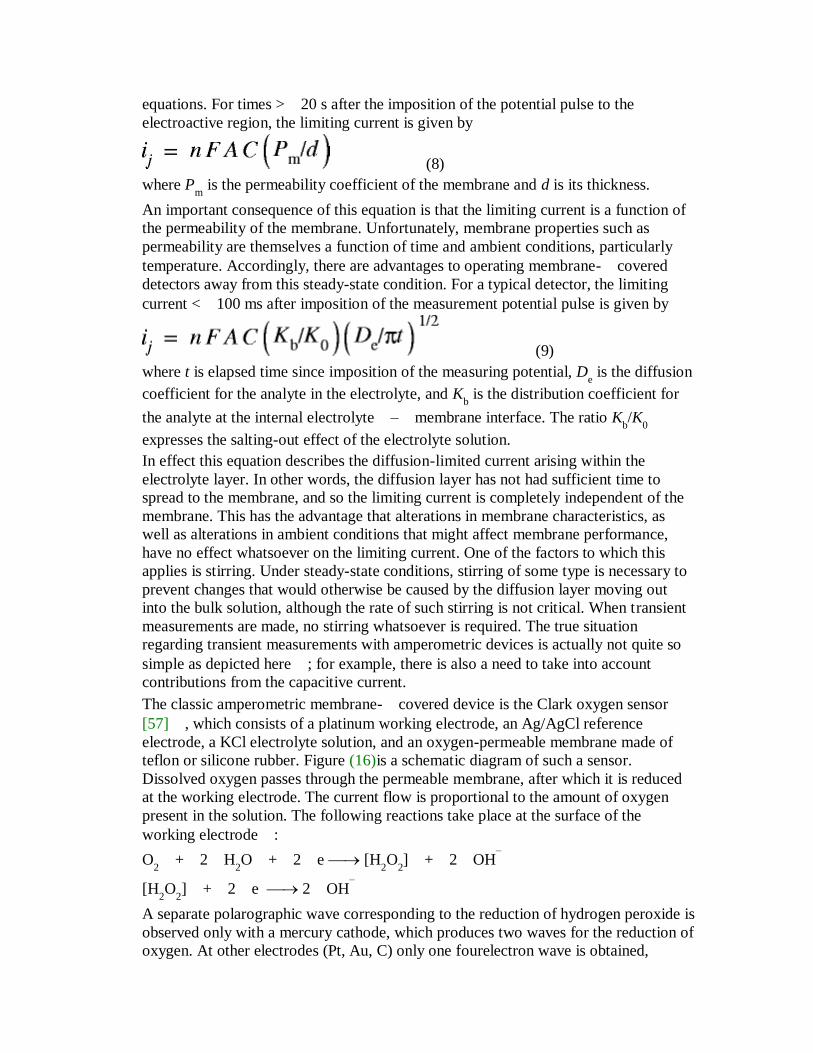
equations. For times >20 s after the imposition of the potential pulse to the

electroactive region, the limiting current is given by

(8)

where Pm is the permeability coefficient of the membrane and d is its thickness.

An important consequence of this equation is that the limiting current is a function of

the permeability of the membrane. Unfortunately, membrane properties such as

permeability are themselves a function of time and ambient conditions, particularly

temperature. Accordingly, there are advantages to operating membrane-covered

detectors away from this steady-state condition. For a typical detector, the limiting

current <100 ms after imposition of the measurement potential pulse is given by

(9)

where t is elapsed time since imposition of the measuring potential, De is the diffusion

coefficient for the analyte in the electrolyte, and Kb is the distribution coefficient for

the analyte at the internal electrolyte–membrane interface. The ratio Kb/K

0

expresses the salting-out effect of the electrolyte solution.

In effect this equation describes the diffusion-limited current arising within the

electrolyte layer. In other words, the diffusion layer has not had sufficient time to

spread to the membrane, and so the limiting current is completely independent of the

membrane. This has the advantage that alterations in membrane characteristics, as

well as alterations in ambient conditions that might affect membrane performance,

have no effect whatsoever on the limiting current. One of the factors to which this

applies is stirring. Under steady-state conditions, stirring of some type is necessary to

prevent changes that would otherwise be caused by the diffusion layer moving out

into the bulk solution, although the rate of such stirring is not critical. When transient

measurements are made, no stirring whatsoever is required. The true situation

regarding transient measurements with amperometric devices is actually not quite so

simple as depicted here; for example, there is also a need to take into account

contributions from the capacitive current.

The classic amperometric membrane-covered device is the Clark oxygen sensor

[57], which consists of a platinum working electrode, an Ag/AgCl reference

electrode, a KCl electrolyte solution, and an oxygen-permeable membrane made of

teflon or silicone rubber. Figure (16)is a schematic diagram of such a sensor.

Dissolved oxygen passes through the permeable membrane, after which it is reduced

at the working electrode. The current flow is proportional to the amount of oxygen

present in the solution. The following reactions take place at the surface of the

working electrode:

O2+2H

2O+2e [H

2O

2]+2OH

–

[H2O

2]+2e 2OH

–

A separate polarographic wave corresponding to the reduction of hydrogen peroxide is

observed only with a mercury cathode, which produces two waves for the reduction of

oxygen. At other electrodes (Pt, Au, C) only one fourelectron wave is obtained,

corresponding to complete reduction to four hydroxide ions [58]. The potential E of

the working electrode (at the diffusion-limiting current plateau) usually lies between –

0.6 and –0.9 V vs. Ag/AgCl.

Progress in semiconductor technology during recent years has made it possible to

miniaturize the classical oxygen sensor [59][60][61][62] for use as a transducer in

several chemical and biochemical sensors.

3) Pulsing the Electrode from a Region of Electroinactivity to a Region of Transport-

Controlled Electroactivity, after which the Potential is Restored to the Electroinactive

Region. For electrochemical sensors without membranes, applying a potential pulse

from a region of electroinactivity to a region of electroactivity has several advantages.

For example, the duty cycle of the pulse can be arranged in such a way that the

electrode spends the majority of its time at the electroinactive potential. Under these

circumstances electrode reactions give rise to products that poison the electrode, but

these products are of minimal significance because they are produced at a very low

rate. Moreover, natural processes of convection are able to redistribute the

electroactive species during the time that the electrode is at the rest potential, thus

limiting the spread of the diffusion layer into the bulk solution. The drawback to this

technique is the appearance of a capacitive current. Limiting the size of the pulse

decreases the contribution of this current, but a small pulse from a rest potential to the

electroactive potential is achievable only for reversible electrode reactions. The

alternative is to allow sufficient time for the capacitive current to decay away between

imposition of the potential pulse and measurement of the current.

4) Pulsed Amperometric Detection [63]. This is a relatively new technique that has made

possible the direct amperometric determination of many compounds formerly

considered unsuitable for analysis in this way. The corresponding waveform is

illustrated in Table (8). This rather complex waveform serves several purposes. On

platinum, for example, and at the extreme anodic potential, surface-confined

oxidation products that tend to poison the electrode are desorbed. This process occurs

concurrently with the formation of PtO2 on the surface. At the cathodic potential the

surface oxide is subsequently reduced, and a clean platinum surface is regenerated. In

some cases, sorption of the analyte occurs at this cathodic potential, so the analytical

signal is recorded at an intermediate potential. Several different mechanisms can give

rise to this signal. Electroactive species that are not adsorbed at the electrode may

undergo conventional oxidative electrode reactions. Alternatively, electroactive

species that are adsorbed at the electrode during the cathodic swing of the cleaning

cycle may undergo either conventional oxidative desorption or oxidative desorption

catalyzed by an oxide species on the surface of the electrode. For many compounds

the latter reaction is much more favorable from a thermodynamic point of view than

oxidation in the absence of a catalyst. This type of reaction occurs most readily when

both the analyte and the oxide are confined to the surface. Finally, adsorbed

electroinactive analytes may also be detected by virtue of their ability to block the

electrode sites at which the PtOH formation occurs. Consequently, any faradaic

current arising from the oxidation of platinum is diminished in the presence of

adsorbed electroinactive analyte.

5) Microelectrodes. Electroanalytical applications using microelectrodes have become

more common in recent years [64][65][66][67][68] as silicon technology has opened

new possibilities for constructing electrodes with micrometer and submicrometer

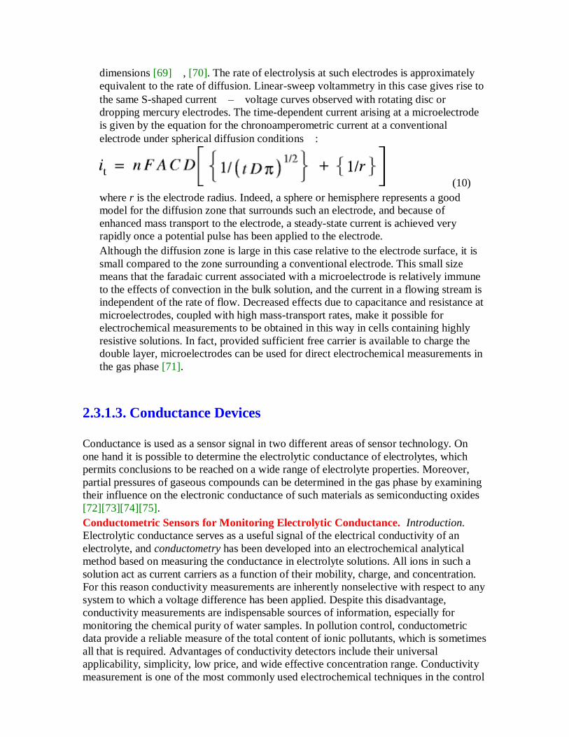
dimensions [69], [70]. The rate of electrolysis at such electrodes is approximately

equivalent to the rate of diffusion. Linear-sweep voltammetry in this case gives rise to

the same S-shaped current–voltage curves observed with rotating disc or

dropping mercury electrodes. The time-dependent current arising at a microelectrode

is given by the equation for the chronoamperometric current at a conventional

electrode under spherical diffusion conditions:

(10)

where r is the electrode radius. Indeed, a sphere or hemisphere represents a good

model for the diffusion zone that surrounds such an electrode, and because of

enhanced mass transport to the electrode, a steady-state current is achieved very

rapidly once a potential pulse has been applied to the electrode.

Although the diffusion zone is large in this case relative to the electrode surface, it is

small compared to the zone surrounding a conventional electrode. This small size

means that the faradaic current associated with a microelectrode is relatively immune

to the effects of convection in the bulk solution, and the current in a flowing stream is

independent of the rate of flow. Decreased effects due to capacitance and resistance at

microelectrodes, coupled with high mass-transport rates, make it possible for

electrochemical measurements to be obtained in this way in cells containing highly

resistive solutions. In fact, provided sufficient free carrier is available to charge the

double layer, microelectrodes can be used for direct electrochemical measurements in

the gas phase [71].

2.3.1.3. Conductance Devices

Conductance is used as a sensor signal in two different areas of sensor technology. On

one hand it is possible to determine the electrolytic conductance of electrolytes, which

permits conclusions to be reached on a wide range of electrolyte properties. Moreover,

partial pressures of gaseous compounds can be determined in the gas phase by examining

their influence on the electronic conductance of such materials as semiconducting oxides

[72][73][74][75].

Conductometric Sensors for Monitoring Electrolytic Conductance. Introduction.

Electrolytic conductance serves as a useful signal of the electrical conductivity of an

electrolyte, and conductometry has been developed into an electrochemical analytical

method based on measuring the conductance in electrolyte solutions. All ions in such a

solution act as current carriers as a function of their mobility, charge, and concentration.

For this reason conductivity measurements are inherently nonselective with respect to any

system to which a voltage difference has been applied. Despite this disadvantage,

conductivity measurements are indispensable sources of information, especially for

monitoring the chemical purity of water samples. In pollution control, conductometric

data provide a reliable measure of the total content of ionic pollutants, which is sometimes

all that is required. Advantages of conductivity detectors include their universal

applicability, simplicity, low price, and wide effective concentration range. Conductivity

measurement is one of the most commonly used electrochemical techniques in the control

of industrial chemical processes. Conductivity detectors are also employed in ion

chromatography and HPLC as a way of detecting separated ions in the eluate from a

column [76]. Furthermore, conductometric analyzers are used in the monitoring of

atmospheric pollutants such as acidic or alkaline gases (e.g., HCl, CO2, SO

2, SO

3,

NH3) after these have been transferred into aqueous solution [77], [78]. Conductivity

measurements are nondestructive with respect to the sample, and they are always

advantageous when electrolytes must be determined in a medium of low self-

conductivity.

Definitions. The electrolytic conductivity of a solution is defined as the conductance G

of the electrolyte between two electrodes, each with an area A, separated by a distance d.

The conductivity is then given by

(11)

The traditional unit of electrolytic conductivity, Siemens per centimeter (S/cm), has

recently been replaced by S/m [79], but the new unit has not yet been accepted widely

by the instrument-producing industry, nor by the users of conductivity measurement

devices. The English-language literature has historically made use of the "mho"

(reciprocal ohm), which is another way of expressing the conductance G. The quotient

d/A (cm–1

) is defined as the cell constant k, and depends on the geometry of the cell. The

electric field is never homogeneous over the cross section of a real cell, so it is not in fact

possible to calculate a cell constant k directly from geometric dimensions; it must

instead be determined with calibration solutions of known conductivity [80].

The temperature dependence of can be deduced from ionic mobilities. This dependence

is expressed in terms of the temperature coefficient =(d/dT )(1/), which

generally has a positive value between 1 and 3% per degree Celsius. Knowledge of in

turn makes it possible to calculate conductivities at temperatures other than the

temperature of measurement. Whenever the need arises to determine the conductivity of a

solution with a very low electrolyte concentration it is essential also to take into account

the self-dissociation of pure water, which has a conductivity 25=0.05483 S/cm.

Measurement Principles. The equipment used for measuring conductance usually consists

of a conductivity sensor, a measuring attachment, and a temperature-compensation unit.

Conductance values are obtained by establishing either the current flow between a set of

electrodes subjected to a constant AC voltage, or the current induced in the secondary coil

of a transformer connected to the primary coil by the electrolyte of interest. Capacitive

coupled cells have been developed as well, but because of their expensive construction

they are no longer of interest [81][82][83][84].

Two-Electrode Cells. Two-electrode cells are equipped with a pair of electrodes across

which both the voltage and the current can be measured. Use of an AC voltage source is a

convenient way of avoiding polarization effects and electrolyte decomposition. Figure

(17) illustrates a typical construction together with the corresponding equivalent circuit.

The advantage of this design is the simplicity of both the cell and the measuring

attachment.

Disadvantages are associated with the need for measuring both the current and the voltage

at a single electrode, which may lead to electrode polarization and a measured

conductivity lower than the true value. The resistance contributed by a cell in contact with

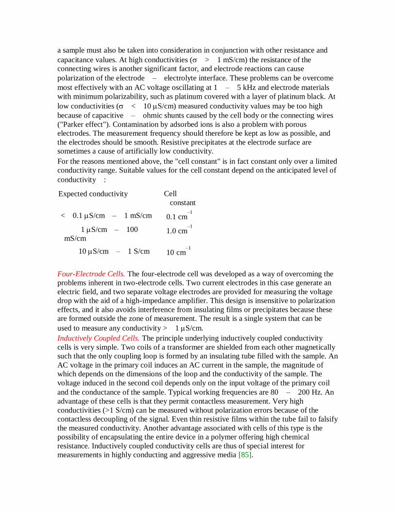
a sample must also be taken into consideration in conjunction with other resistance and

capacitance values. At high conductivities (>1 mS/cm) the resistance of the

connecting wires is another significant factor, and electrode reactions can cause

polarization of the electrode–electrolyte interface. These problems can be overcome

most effectively with an AC voltage oscillating at 1–5 kHz and electrode materials

with minimum polarizability, such as platinum covered with a layer of platinum black. At

low conductivities (<10 S/cm) measured conductivity values may be too high

because of capacitive–ohmic shunts caused by the cell body or the connecting wires

("Parker effect"). Contamination by adsorbed ions is also a problem with porous

electrodes. The measurement frequency should therefore be kept as low as possible, and

the electrodes should be smooth. Resistive precipitates at the electrode surface are

sometimes a cause of artificially low conductivity.

For the reasons mentioned above, the "cell constant" is in fact constant only over a limited

conductivity range. Suitable values for the cell constant depend on the anticipated level of

conductivity:

Expected conductivity Cell

constant

<0.1 S/cm–1 mS/cm 0.1 cm–1

1 S/cm–100

mS/cm 1.0 cm

–1

10 S/cm–1 S/cm 10 cm–1

Four-Electrode Cells. The four-electrode cell was developed as a way of overcoming the

problems inherent in two-electrode cells. Two current electrodes in this case generate an

electric field, and two separate voltage electrodes are provided for measuring the voltage

drop with the aid of a high-impedance amplifier. This design is insensitive to polarization

effects, and it also avoids interference from insulating films or precipitates because these

are formed outside the zone of measurement. The result is a single system that can be

used to measure any conductivity >1 S/cm.

Inductively Coupled Cells. The principle underlying inductively coupled conductivity

cells is very simple. Two coils of a transformer are shielded from each other magnetically

such that the only coupling loop is formed by an insulating tube filled with the sample. An

AC voltage in the primary coil induces an AC current in the sample, the magnitude of

which depends on the dimensions of the loop and the conductivity of the sample. The

voltage induced in the second coil depends only on the input voltage of the primary coil

and the conductance of the sample. Typical working frequencies are 80–200 Hz. An

advantage of these cells is that they permit contactless measurement. Very high

conductivities (>1 S/cm) can be measured without polarization errors because of the

contactless decoupling of the signal. Even thin resistive films within the tube fail to falsify

the measured conductivity. Another advantage associated with cells of this type is the

possibility of encapsulating the entire device in a polymer offering high chemical

resistance. Inductively coupled conductivity cells are thus of special interest for

measurements in highly conducting and aggressive media [85].

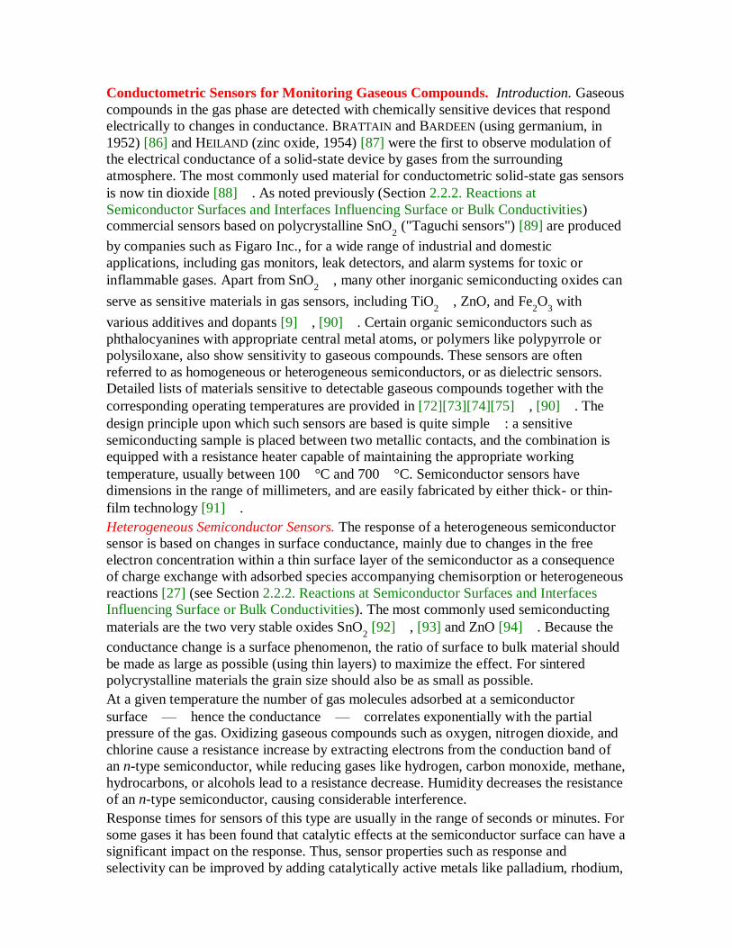
Conductometric Sensors for Monitoring Gaseous Compounds. Introduction. Gaseous

compounds in the gas phase are detected with chemically sensitive devices that respond

electrically to changes in conductance. BRATTAIN and BARDEEN (using germanium, in

1952) [86] and HEILAND (zinc oxide, 1954) [87] were the first to observe modulation of

the electrical conductance of a solid-state device by gases from the surrounding

atmosphere. The most commonly used material for conductometric solid-state gas sensors

is now tin dioxide [88]. As noted previously (Section 2.2.2. Reactions at

Semiconductor Surfaces and Interfaces Influencing Surface or Bulk Conductivities) commercial sensors based on polycrystalline SnO

2 ("Taguchi sensors") [89] are produced

by companies such as Figaro Inc., for a wide range of industrial and domestic

applications, including gas monitors, leak detectors, and alarm systems for toxic or

inflammable gases. Apart from SnO2, many other inorganic semiconducting oxides can

serve as sensitive materials in gas sensors, including TiO2, ZnO, and Fe

2O

3 with

various additives and dopants [9], [90]. Certain organic semiconductors such as

phthalocyanines with appropriate central metal atoms, or polymers like polypyrrole or

polysiloxane, also show sensitivity to gaseous compounds. These sensors are often

referred to as homogeneous or heterogeneous semiconductors, or as dielectric sensors.

Detailed lists of materials sensitive to detectable gaseous compounds together with the

corresponding operating temperatures are provided in [72][73][74][75], [90]. The

design principle upon which such sensors are based is quite simple: a sensitive

semiconducting sample is placed between two metallic contacts, and the combination is

equipped with a resistance heater capable of maintaining the appropriate working

temperature, usually between 100°C and 700°C. Semiconductor sensors have

dimensions in the range of millimeters, and are easily fabricated by either thick- or thin-

film technology [91].

Heterogeneous Semiconductor Sensors. The response of a heterogeneous semiconductor

sensor is based on changes in surface conductance, mainly due to changes in the free

electron concentration within a thin surface layer of the semiconductor as a consequence

of charge exchange with adsorbed species accompanying chemisorption or heterogeneous

reactions [27] (see Section 2.2.2. Reactions at Semiconductor Surfaces and Interfaces

Influencing Surface or Bulk Conductivities). The most commonly used semiconducting

materials are the two very stable oxides SnO2 [92], [93] and ZnO [94]. Because the

conductance change is a surface phenomenon, the ratio of surface to bulk material should

be made as large as possible (using thin layers) to maximize the effect. For sintered

polycrystalline materials the grain size should also be as small as possible.

At a given temperature the number of gas molecules adsorbed at a semiconductor

surface—hence the conductance—correlates exponentially with the partial

pressure of the gas. Oxidizing gaseous compounds such as oxygen, nitrogen dioxide, and

chlorine cause a resistance increase by extracting electrons from the conduction band of

an n-type semiconductor, while reducing gases like hydrogen, carbon monoxide, methane,

hydrocarbons, or alcohols lead to a resistance decrease. Humidity decreases the resistance

of an n-type semiconductor, causing considerable interference.

Response times for sensors of this type are usually in the range of seconds or minutes. For

some gases it has been found that catalytic effects at the semiconductor surface can have a

significant impact on the response. Thus, sensor properties such as response and

selectivity can be improved by adding catalytically active metals like palladium, rhodium,

silver, or platinum. This doping of the semiconductor surface is one important way of

modifying the selectivity of a sensor [95][96][97], but another possibility for adjusting

sensor properties for a particular application is careful selection of the working

temperature [98].

The influence of temperature on the selectivity of a sensor depends on the fact that each

gas has its own characteristic temperature: a temperature at which the reversible

relationship between gas concentration and the concentration of electrons at the

semiconductor surface (and therefore the conductance) reaches a maximum [92].

Working temperatures for SnO2-based sensors usually lie between 200°C and 450°C

depending on the application.

Various techniques are used for the fabrication of semiconductor sensors. Conductance

sensors from structurized sintered polycrystalline ceramics can be produced by thick- or

thin-film technology. Chemically sensitive materials in the form of single crystals or

whiskers can be attached to electrodes by thin- or thick-film techniques as well. Mass

production of sensors requires that the resulting devices be characterized by a defined level of conductance. For example, the conductance of polycrystalline SnO

2 can be

adjusted by subsequent thermal treatment >800°C under a controlled partial pressure

of oxygen. Another approach to defined conductance involves doping the semiconductor

with antimony or fluorine. The reproducibility and stability of a sensor signal is generally

diminished by irreversible changes in the defect structure of the semiconductor surface.

Homogeneous Semiconductor Sensors. The effectiveness of this type of semiconductor

sensor depends on changes in bulk conductance. The stoichiometry and concentration of

bulk point defects, and thus the conductance of such materials, is a function of the partial

pressure of a gaseous analyte. Conductance changes arise through reversible changes in

small deviations from ideal stoichiometry, which in turn influence the concentrations of

bulk point defects and free electrons [27]. The deviation from ideal stoichiometric

composition is usually very small; for example, in Cu2–xO the deficit x in the Cu ratio is

on the order of 0.001. Since conductance and deviation from ideal stoichiometry are

proportional, a measured conductance can be used to determine a corresponding partial

pressure. Regarding the kinetics of these sensors, an important factor is diffusion of a

compound like oxygen or the corresponding lattice defects that compensate for nonideal

stoichiometry within the bulk of the semiconductor. Any gaseous reaction involving point

defects at the surface of the semiconductor must also be appropriately fast. Both

requirements can be met through the combination of high temperature and a catalytic

coating (e.g., Pt).

Most bulk-conductance sensors consist of semiconducting oxides the conductance of

which changes with the partial pressure of oxygen. They are used primarily for

monitoring oxygen partial pressures in the air or in combustion gases. Titanium dioxide (TiO

2) is one of the most commonly used homogeneous sensor materials for the

determination of oxygen partial pressures [99]. At 900°C and an oxygen partial

pressure of 0.1 MPa, TiO2 has precisely the stoichiometric composition. At lower oxygen

partial pressures TiO2 has an oxygen deficit x expressed by the formula TiO

2–x. This

oxygen deficit specifies the number of unoccupied oxygen sites and the corresponding

excess of trivalent titanium in the lattice. Both defects act as electron donors, thereby

contributing to the concentration of free electrons in the conductance band of the

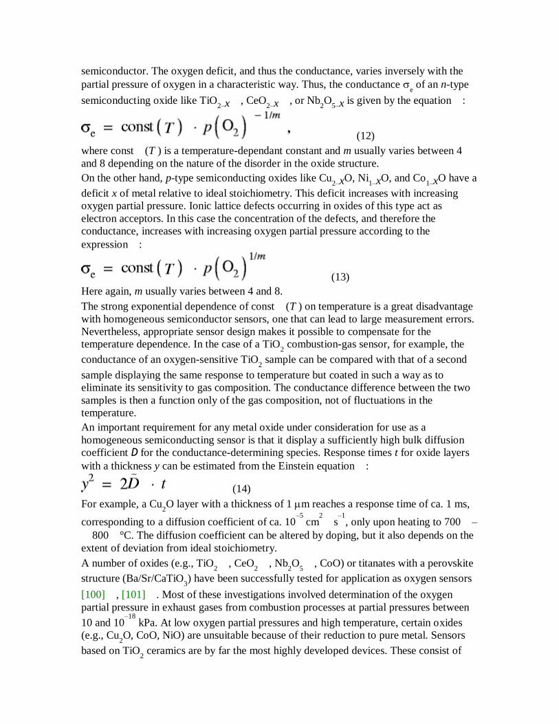
semiconductor. The oxygen deficit, and thus the conductance, varies inversely with the

partial pressure of oxygen in a characteristic way. Thus, the conductance e of an n-type

semiconducting oxide like TiO2–x, CeO

2–x, or Nb2O

5–x is given by the equation:

(12)

where const(T ) is a temperature-dependant constant and m usually varies between 4

and 8 depending on the nature of the disorder in the oxide structure.

On the other hand, p-type semiconducting oxides like Cu2–xO, Ni

1–xO, and Co1–xO have a

deficit x of metal relative to ideal stoichiometry. This deficit increases with increasing

oxygen partial pressure. Ionic lattice defects occurring in oxides of this type act as

electron acceptors. In this case the concentration of the defects, and therefore the

conductance, increases with increasing oxygen partial pressure according to the

expression:

(13)

Here again, m usually varies between 4 and 8.

The strong exponential dependence of const(T ) on temperature is a great disadvantage

with homogeneous semiconductor sensors, one that can lead to large measurement errors.

Nevertheless, appropriate sensor design makes it possible to compensate for the

temperature dependence. In the case of a TiO2 combustion-gas sensor, for example, the

conductance of an oxygen-sensitive TiO2 sample can be compared with that of a second

sample displaying the same response to temperature but coated in such a way as to

eliminate its sensitivity to gas composition. The conductance difference between the two

samples is then a function only of the gas composition, not of fluctuations in the

temperature.

An important requirement for any metal oxide under consideration for use as a

homogeneous semiconducting sensor is that it display a sufficiently high bulk diffusion

coefficient D for the conductance-determining species. Response times t for oxide layers

with a thickness y can be estimated from the Einstein equation:

(14)

For example, a Cu2O layer with a thickness of 1 m reaches a response time of ca. 1 ms,

corresponding to a diffusion coefficient of ca. 10–5

cm2s

–1, only upon heating to 700–

800°C. The diffusion coefficient can be altered by doping, but it also depends on the

extent of deviation from ideal stoichiometry.

A number of oxides (e.g., TiO2, CeO

2, Nb

2O

5, CoO) or titanates with a perovskite

structure (Ba/Sr/CaTiO3) have been successfully tested for application as oxygen sensors

[100], [101]. Most of these investigations involved determination of the oxygen

partial pressure in exhaust gases from combustion processes at partial pressures between

10 and 10–18

kPa. At low oxygen partial pressures and high temperature, certain oxides

(e.g., Cu2O, CoO, NiO) are unsuitable because of their reduction to pure metal. Sensors

based on TiO2 ceramics are by far the most highly developed devices. These consist of

porous sintered ceramic materials with a platinum surface doping, and are used to

determine air–fuel ratios in the exhaust gases of combustion engines.

Apart from TiO2, a number of other semiconducting oxides might be useful as sensor

materials for special applications over limited ranges of oxygen partial pressure, as in

monitoring the level of oxygen in inert gases. There is also a good possibility of

optimizing various ternary and higher oxide combinations for sensor application by

suitable choice of composition with respect to stability, diffusion, and surface properties

[102][103][104]. Thus, barium and strontium ferrates show conductances with

considerably less temperature dependence relative to TiO2or CoO.

Organic Conductometric Sensors. For several years, certain organic semiconducting

polymers have attracted attention in the search for new chemical sensors [105]. The

possibility of utilizing conductivity changes induced by gases adsorbed on organic

materials is interesting for a number of reasons. For example, it might permit the

detection of very low levels of atmospheric pollutants. Moreover, organic materials are

much more easily modified than inorganic materials with respect to such characteristics as

sensitivity, working temperature, and selectivity. The greatest disadvantage of organic

materials in gas detection is that they are usually very poor conductors, and conductivity

measurements would be correspondingly difficult. Also, organic materials are thermally

unstable, so it is often impossible to use them at temperatures at which gas–solid

interactions proceed rapidly and reversibly.

Phthalocyanines constitute one group of organic materials with thermal stability

>400°C, and they are usually considered to have semiconducting rather than

insulating properties. Thin layers of phthalocyanine complexes based on metals like lead

[106] and copper [107] have been particularly carefully studied as potential gas sensors

[108]. The conductance of these films is a very sensitive function of gases with

electron-acceptor properties, including nitrogen dioxide, chlorine, and iodine. Films of

phthalocyanines with various central metal atoms can be deposited on substrates by

sublimation or screen printing. Changing the nature of the central metal atom makes it

possible to adjust the sensitivity and selectivity of a phthalocyanine film in accordance

with the proposed application [109][110][111][112][113][114].

Another organic semiconductor with gas-sensitive properties is polypyrrole.

Chemiresistors with ambient-temperature gas sensitivity to both electron-donating and

electron-accepting gases have been achieved using thin polypyrrole films prepared by

electrochemical polymerization on electrodes. Sensitivities have been investigated toward

such gases as nitrogen dioxide [115], ammonia [116], and methanol [117],

[118]. A wide variety of polymers of this type is available, including substituted

polypyrroles, polythiophenes, polyindoles, and polyanilines.

Humidity Sensors. Humidity sensors are devices that respond to changes in water-vapor

pressure by a change in electrical resistance, capacitance, or a combination of the two as

reflected in the impedance. The sensitive material might be an electrolyte, an organic

polymer, or a metal oxide subject to a change in ionic–electronic conductivity or

capacitance with respect to humidity as a consequence of physical adsorption or

absorption of water molecules. In general these devices offer a very cost-effective

continuous or spot-check approach to monitoring humidity in air and other gases

[119], [120].

Electrolyte humidity sensors. Electrolyte humidity sensors are based on an electrolyte

solution (e.g., LiCl) the ion conductivity of which changes as a result of evaporation or

condensation of water in response to changes in the relative humidity of the surrounding

atmosphere. The fabrication of these sensors is quite straightforward. A porous substrate

or an organic binder is impregnated with the electrolyte in such a way as to prevent

electrolyte from flowing out of the sensor even at very high humidity. Contact is

maintained with platinum electrodes on both sides of the substrate. Even thin films of

potassium metaphosphate or barium fluorite are suitable for humidity measurements.

Despite their slow response and limited linear range these sensors have an outstanding

reputation due to good reproducibility, long-term stability, and low cost.

Ceramic Humidity Sensors. The first widely-used ceramic humidity sensor was the

aluminum oxide sensor, in which aluminum is oxidized anodically in an acidic solution to

form a porous oxide film, sometimes less than 1 m thick, that displays the necessary

hygroscopicity. Adsorption of water molecules causes a decrease in resistance and an

increase in capacitance, which is reversed by subsequent desorption. Other materials are

also used in humidity sensors, including ZnO with added Li2O and V

2O

5, colloidal

Fe3O

4, -Fe

2O

3, mixed oxides of TiO

2 and SnO

2, MgCr

2O

4–TiO

2, TiO

2–

V2O

5, ZnCr

2O

4–LiZnVO

4, MgAl

2O

3, MgFe

2O

4, or H

3PO

4–

ZrSiO2, as well as PbCrO

4 with added alkali oxide [121]. Sometimes the signal of

such a sensor is subject to drift as a result of changes in the surface structure or

contamination from other adsorbed gases. Nevertheless, reproducibility can be restored by

heat cleaning.

The most important considerations with respect to sensor characteristics are surface

properties (hydrophilic–hydrophobic), pore-size distribution, and electrical

resistance. To ensure adequate sensitivity and response a sensor of this type should

consist of a very thin film of porous ceramic with a porosity >30%. The contacting

electrodes may be interdigitated or porous sandwich-type structures made from noble

metals (e.g., Pd, Pt, Au) and so constructed that they do not obstruct the pores of the oxide

film. Humidity affects not only the resistance of a porous ceramic but also its capacitance

by extending the surface area in contact with the electrodes. The high dielectric constant

of adsorbed water molecules also plays an important role.

Polymeric Humidity Sensors. Certain polymers are capable of taking up water as a

function of the relative humidity of the surrounding atmosphere, leading to changes in

such mechanical and electrical properties as volume, resistance, and dielectric

characteristics. A number of polymers have been used as sensitive materials in this regard,

including ion-exchange resins, polymer electrolytes, hydrophilic polymers, and

hygroscopic resins [122]. Hydrophilic polymers [e.g., poly(ethylene oxide)–

sorbitol] swell by absorption of water. If such a polymer is filled (mixed) with carbon

or metal powder of very small particle size, the resistance observed depends on the

distance and the number of particles that are in contact with each other. Uptake of water

leads to swelling of the polymer and disturbance of the ohmic contacts between

conducting particles, which in turn increases the resistance. For this reason the resistance

correlates with humidity. Useful materials include cellulose esters and polyalcohols.

The resistance of polymers with dissociable groups (e.g., sulfonates, amines, amides, or

even hydroxides) also depends on humidity. The resistance of such polymers in fact

decreases with absorption of water because of ionic dissociation and an increase in ionic

conduction.

The absorption of water by polymers is especially suited to the development of a

capacitive humidity sensor based on the high dielectric constant of water, since

capacitance depends on the area, the thickness, and the dielectric constant of a dielectric.

Uptake of water causes an increase in the dielectric constant followed by an increase in

capacitance. Polyimide is a suitable sensitive material, but so are certain inorganic

ceramics such as Al2O

3 [123] and low-density Ta

2O

5, which change their capacitance

with the formation of water dipoles. Low-density Ta2O

5 layers can be formed by anodic

oxidation of sputtered tantalum films, whereas polyimide films are deposited by spin

coating and subsequent polymerization.

2.3.1.4. Ion-Sensitive Field-Effect Transistors (ISFETs)

As described in Section 2.3.1.1. Self-Indicating Potentiometric Electrodes, with

conventional ion-sensitive electrodes (ISEs) the ion-sensitive membrane is placed

between the analyte and the internal reference solution. An internal reference electrode

makes electrical connection to the internal reference solution, and the measurement

system is completed by a second reference electrode in contact with the analyte solution.

In any modern pH meter the internal reference electrode is connected to the gate metal of

a metal-oxide semiconductor field-effect transistor (MOSFET), which acts as an

impedance-converting device (Fig. (18)). Normally, a conventional ISE functions very

well. However, in certain applications problems can arise due to large size, high cost, and

sensitive construction.

These problems might be resolved by the ion-sensitive field-effect transistor (ISFET). In

an ISFET the ion-sensitive membrane is placed directly on the gate insulator of the field-

effect transistor; alternatively, the gate insulator itself, acting as a pH-sensitive

membrane, may be exposed to the analyte solution (Fig. (19)). If one compares an ISFET

with the conventional ISE measurement system, the gate metal, connecting leads, and

internal reference system have all been eliminated. An ISFET is a small, physically

robust, fast potentiometric sensor, and it can be produced by microelectronic methods,

with the future prospect of low-cost bulk production. More than one sensor can be

placed within an area of a few square millimeters. The first ISFETs were described

independently by BERGVELD [124] and MATSUO, ESASHI, and INUMA [125].

ISFET Operation. The ISFET can be regarded as a special type of MOSFET. To

understand the operation of an ISFET it is therefore necessary first to understand the

operation of a MOSFET.

An n-channel MOSFET (Fig. (20)) consists of a p-type silicon substrate with two n-

type diffusions, the source (c) and the drain (d). The structure is covered with an

insulating layer (b), on top of which a gate electrode (a) is deposited over the area

between the source and the drain. A voltage is applied to the gate that is positive with

respect to both the source and the bulk material. This voltage produces a positive charge

at the gate electrode and a negative charge at the surface of the silicon under the gate. The

negative charge is formed by electrons, which are the minority carriers in the substrate,

and this in turn creates a conducting channel between the source and the drain. The

density of electrons in the channel, and thus the conductivity of the channel, is modulated by the applied gate voltage (V

G). If a constant voltage (V

D) is applied between the source

and the drain a change in the conductivity of the channel leads to a change in current

between source and drain. The drain current ID in the unsaturated region (V

D<V

G–

VT) of a MOSFET is equal to:

(15)

=Electron mobility in the

channel

Cox =Oxide capacitance per unit

area

W/L =Ratio of channel width to

length

VT =Threshold voltage

A detailed description of the MOSFET is provided in [126].

In an ISFET (Fig. (21)) the gate metal is replaced by a sensitive membrane and an

electrolyte solution, or simply by the electrolyte solution, which is in contact with a

reference electrode. The potential of the gate with respect to the substrate is the sum of the

potentials of the various electronic and electrochemical processes that occur in the

external path between the silicon substrate and the gate; i.e., the reference electrode

half-cell potential Eref, the solution–membrane or solution–insulator

interfacial potential M, and the metal–silicon contact potential. These voltages are

added to the externally applied voltages Vg, and the resulting voltage has the same

significance and function as that defined in the theory of MOSFET operation. VT*, the

threshold voltage of the ISFET, can be described as:

(16)

From Equation (15) we obtain the following relationship:

(17)

M, the solution–membrane or solution–insulator interfacial potential,

depends on the activity of the ions in the analyte solution according to the Nernst–

Nikolsky equation [Eq. (6), Section 2.3.1.1. Self-Indicating Potentiometric Electrodes]

for ISFETs with an additional membrane, or according to a similar equation (see below)

for ISFETs with a solution–insulator interface.

If all parameters in equation (17) apart from M

are kept constant, changes in ID are

caused exclusively by changes in the activity of ions in the analyte solution. Thus, in an

ISFET, the drain current is modulated by the ionic activity in the analyte solution. A

detailed description of ISFET operation is presented in [127].

pH-Sensitive ISFETs. Gate insulators such as Si3N

4, Al

2O

3, and Ta

2O

3 have been

found to be pH sensitive, so FETs in which bare gate insulators of this type are exposed to

a solution respond to changes in pH. The pH response can be explained by the "site-

binding theory." This model assumes that there are ionizable binding sites present at the

surface of an insulator, and that these can exhibit amphoteric behavior with respect to the

potential-determining ion (i.e., H+):

A–OHA–O–+H

S

+

A–OH+HS

+A–OH

2

+

According to this model the pH dependence of M

is given by the following equation:

(18)

under the condition that qM

/kT. pHpzc

is the pH value for which M=0;

is a parameter that reflects the chemical sensitivity of the outer gate insulator, with a value

dependent on the density of hydroxyl groups and the surface reactivity. Surfaces with a

high value show Nernstian behavior. For a detailed description of the site-binding

model, see [127].

ISFETs Sensitive to Other Ions. Deposition of an ion-selective membrane on top of the

gate insulator opens the way to measurement of ions other than H+. Most of the sensitive

materials for ISE applications described in Section 2.3.1.1. Self-Indicating Potentiometric

Electrodes have been used in conjunction with ISFETs, providing sensors covering a wide

variety of species. Thus, ISFETs with solid membranes have been described with

AgCl–AgBr membranes sensitive to Ag+, Cl

–, and Br

– [128], for example, or with

LaF3 membranes sensitive to fluoride [129]. Ion-sensitive polymer-matrix membranes

(liquid membranes with a polymer matrix) have also been used as sensitive membranes

for ISFETs. The first experiments involved mainly PVC membranes [130], [131],

but these membranes show poor adhesion and poor mechanical strength. To improve

membrane adhesion, modified PVC was utilized as a matrix material [132]. The use of

silicones as matrix materials has made it possible to prepare very durable ISFETs with

polymer-matrix membranes [133]. Other reports describe the use of photopolymerized

polymers as matrix materials [134], [135].

Problems. The commercial development of ISFETs has been slow despite intensive

research. From the standpoint of broad commercialization the ISFET is in competition

with conventional ISEs with respect to price, performance, and reliability, and it is

essential that some means be devised for producing ISFETs by commercially acceptable

methods. Reaching this stage requires that several problems be solved, however.

ISFETs have so far been used primarily in conjunction with conventional macro reference

electrodes. This fact greatly limits the potential benefits to be gained from miniaturization

of the sensor. An optimal reference electrode for ISFETs should be miniaturizable and

display long-term stability, and it should be subject to fabrication with microelectronic

techniques. Attempts have been made to miniaturize macro reference electrodes [136],

or to use modified surfaces with extremely low surface-site densities as reference FETs

[137], but to date the above-mentioned requirements have not been met.

A further problem relates to encapsulation. The ion-sensitive gate area is exposed to the

analyte solution, but all other parts of the sensor must be insulated from the solution. In

most cases encapsulation is carried out by hand using epoxy resins, but it is impossible to

produce ISFETs at low cost by this technique. Both photolithographic methods [138],

[139] and an electrochemical method [140] have been proposed for the solution of this

problem. One very promising development is the backside-contacted ISFET [141].

The electrical contacts in this case are protected from the analyte solution by means of O-

rings, thereby circumventing the need for resins.

As noted previously, ISFETs sensitive to ions other than H+ are prepared by deposition of

an additional membrane on top of the gate insulator. If such ISFETs are to be

commercialized this membrane must be deposited by a mass-production technique, which

will be difficult to achieve with polymer membranes. One possible solution is the

development of photolithographically patternable ion-sensitive membranes [142], but

such membranes have so far been developed only for a few ions, and problems in the

photolithographic deposition of more than one type of membrane on a single chip have

not been resolved. The interface between an insulator and a sensitive membrane is also ill-

defined in a thermodynamic sense, but this problem was solved by introducing a hydrogel

between the sensing membrane and the insulator. Futhermore, ISFETs suffer from drift.

The influence of this effect would be eliminated if the sensor were to be used in flow-

injection analysis (FIA), so successful applications can be anticipated for ISFETs in the

field of dynamic measurement [143].

Only if all the problems cited are successfully resolved will the ISFET live up to the

promises that have been held out for it for more than two decades: low cost,

multifunctionality, and a robust and reliable construction.

2.3.2. Optical Sensors

2.3.2.1. Fiber-Optical Sensors

In recent years the use of optical fibers has become increasingly important in the field of

chemical and biochemical sensors. This is clearly due to the fact that fiber-optical sensors

combine the strengths of well-known bulk optical analytical methods with the unique

advantages of optical fibers. More specifically:

1) An enormous technology base already exists for familiar optical methods of chemical

analysis. There is probably no class of chemical analyte that has not at some time been

the subject of optical determination through absorption or fluorescence spectroscopy.

Methods also exist for labeling a target analyte with an appropriate chromophore or a

fluorophore, a common practice in immunoassays.

2) Fiber-optic techniques offer increased sensitivity relative to conventional bulk optic

approaches. For example, evanescent wave (EW) spectroscopy is significantly more

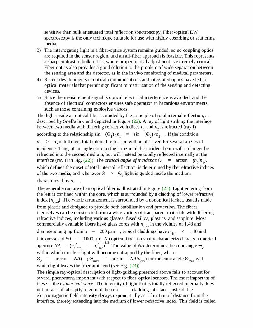
sensitive than bulk attenuated total reflection spectroscopy. Fiber-optical EW

spectroscopy is the only technique suitable for use with highly absorbing or scattering

media.

3) The interrogating light in a fiber-optics system remains guided, so no coupling optics

are required in the sensor region, and an all-fiber approach is feasible. This represents

a sharp contrast to bulk optics, where proper optical adjustment is extremely critical.

Fiber optics also provides a good solution to the problem of wide separation between

the sensing area and the detector, as in the in vivo monitoring of medical parameters.

4) Recent developments in optical communications and integrated optics have led to

optical materials that permit significant miniaturization of the sensing and detecting

devices.

5) Since the measurement signal is optical, electrical interference is avoided, and the

absence of electrical connectors ensures safe operation in hazardous environments,

such as those containing explosive vapors.

The light inside an optical fiber is guided by the principle of total internal reflection, as

described by Snell's law and depicted in Figure (22). A ray of light striking the interface between two media with differing refractive indices n

1 and n

2 is refracted (ray I)

according to the relationship sin(1)×n

1=sin(

2)×n

2. If the condition

n1>n

2 is fulfilled, total internal reflection will be observed for several angles of

incidence. Thus, at an angle close to the horizontal the incident beam will no longer be

refracted into the second medium, but will instead be totally reflected internally at the

interface (ray II in Fig. (22)). The critical angle of incidence c=arcsin(n

2/n

1),

which defines the onset of total internal reflection, is determined by the refractive indices

of the two media, and whenever >c light is guided inside the medium

characterized by n1.

The general structure of an optical fiber is illustrated in Figure (23). Light entering from

the left is confined within the core, which is surrounded by a cladding of lower refractive

index (nclad

). The whole arrangement is surrounded by a nonoptical jacket, usually made

from plastic and designed to provide both stabilization and protection. The fibers

themselves can be constructed from a wide variety of transparent materials with differing

refractive indices, including various glasses, fused silica, plastics, and sapphire. Most commercially available fibers have glass cores with n

core in the vicinity of 1.48 and

diameters ranging from 5–200 m; typical claddings have nclad<1.48 and

thicknesses of 50–1000 m. An optical fiber is usually characterized by its numerical

aperture NA= (nc

2

ore–n

c

2

lad)

1/2. The value of NA determines the cone angle

c

within which incident light will become entrapped by the fiber, where

c=arccos(NA);

max=arcsin(NA/n

env) for the cone angle

max with

which light leaves the fiber at its end (see Fig. (23)).

The simple ray-optical description of light-guiding presented above fails to account for

several phenomena important with respect to fiber-optical sensors. The most important of

these is the evanescent wave. The intensity of light that is totally reflected internally does

not in fact fall abruptly to zero at the core–cladding interface. Instead, the

electromagnetic field intensity decays exponentially as a function of distance from the

interface, thereby extending into the medium of lower refractive index. This field is called

the evanescent field, and its penetration depth d is defined by the distance from the

interface within which it decays to a fraction 1/e of its value at the interface. The angle of

incidence strongly influences the penetration depth. Values for d vary from 50–

200 nm, increasing as decreases; d reaches its maximum when is very close to

the critical angle.

Fiber-optical sensors can be constructed in either of two fundamentally different optical

configurations with respect to the sensing area. The first is a wave-guide-binding

configuration, in which recognition occurs at the surface of the fiber core via the

evanescent field. This is achieved by removing the jacket and cladding from the fiber and

causing the analyte molecules to bind to the core surface, as in the example described

below. Such an arrangement is described as an evanescent wave sensor or intrinsic fiber-

optical sensor. The resulting sensitivity depends greatly on the value of NA [144].

Alternatively, the fiber-end configuration might be considered, in which analyte is

released for recognition purposes into the illuminated space at the end of the fiber. In this

case the fiber acts only as a light pipe, resulting in what is known as an extrinsic fiber-

optical sensor.

Both configurations entail similar optical systems: a spectral light source for excitation

(e.g., a xenon or tungsten lamp equipped with a monochromator or optical filter, an LED,

or a laser) and a spectral light-detection device consisting of a monochromator or filter

together with a photomultiplier or photodiode. A schematic diagram applicable to the

optical systems for these two sensor configurations is presented in Figure (24).

More detailed information regarding the physical principles of fiber-optical chemical and

biochemical sensors and the corresponding detection systems is available in [145] and

[146].

Biochemical Sensors. Antibodies are widely used as recognition elements in fiber-optical

biosensor applications. This is due to the high specificity of the binding reaction between

an antibody and an analyte (antigen). To determine this reaction optically, labeling agents

such as fluoresceine, rhodamine, or phycoerythrine are used, all of which show absorption

and emission bands in the visible region of the spectrum. Linear amplification can be

achieved by binding more than one label. Depending on the circumstances, either the

antigen or the antibody might be tagged (see below).

The evanescent wave (intrinsic) configuration is most important for biosensors because it

permits the antibody or antigen to be immobilized directly on the core surface, and it

extends the path for possible interaction between the light and the recognition elements.

Accordingly, only tagged molecules inside the evanescent field are subject to excitation.

The amount of light energy absorbed, or the light emitted from these molecules and

collected by the fiber, gives rise to the measurement signal. In contrast to the extrinsic

sensor approach, the intrinsic arrangement therefore reduces noise that would otherwise

result from free labeled molecules or intrinsic fluorescence within the environment

[146]. Despite these advantages, however, extrinsic biosensors have also been

constructed, with binding devices placed in front of the fiber as a way of fixing the

recognition elements. These devices can be either glass plates or transparent membranes.

This offers the advantage of easy removal and replacement of the recognition elements

[147].

Figure (25) provides an example of a biosensor of the intrinsic type. Here the antigen has

been immobilized at the fiber core surface where it has been allowed to bind with a

labeled antibody. Energy from the evanescent wave is absorbed by the labels, generating a

detectable fluorescence signal. Addition of unlabeled analyte to the surrounding solution

leads to competition for the binding sites. This permits some of the labeled antibody

molecules to diffuse away from the surface, causing the fluorescence signal to decrease.

The same general approach is also applicable to immobilized antibodies and tagged

antigens [148].

Competition between a labeled antigen and an unlabeled analyte can also be effected in an

external column, where the labeled antigen has previously been bound to an antibody.

Once the competition reaches equilibrium any labeled antigen that has been released can

be detected with antibody immobilized on a fiber. In this case the fluorescence signal

would be expected to increase with an increased concentration of analyte.

Enzymes are in some cases also useful for recognition and labeling purposes. For

example, glucose oxidase has been used to determine glucose on the basis of free oxygen

that is consumed, where the disappearance of oxygen is measured with a fiber-optical

oxygen subsensor [149]. Labeling of antibodies or antigens with urease or alkaline

phosphatase and subsequent addition of a fluoro- or chromogenic substrate leads to

detectable production of fluorophores or chromophores. The signal in this case is subject

to multiple enhancement since it is proportional to the concentrations of both labeled

antigen and antibody as well as to incubation time.

Chemical Sensors. Recognition with a chemical sensor is achieved via an analyte-

specific reaction involving chemical compounds located inside the sensing area. The

reaction must be one that is accompanied by changes in absorbance or fluorescence

characteristics. Several examples are described below. A common physical arrangement

utilizes a fiber-end approach and two single fibers or two fiber bundles, one for guiding

light into the sensing area and the other to carry it away. The chemical reagents are

confined within a transparent membrane or a small segment of the fiber itself, near its end

and shielded by a membrane.

A particularly wide variety of fiber-optical sensors has been developed for measuring pH

values, and many of these sensors are also used as subsensors for other analytes. Sensors

for pH determination can be divided into two general types. The first relies on

colorimetric acid–base indicators to produce changes in absorbance. For example,

the dye phenol red can be copolymerized with acrylamide and bisacrylamide to yield dyed

polyacrylamide microspheres. These are in turn packed into a length of cellulose dialysis

tubing placed at the end of a pair of fibers that can serve as a vehicle for monitoring

changes in absorbance [150]. Bromothymol blue immobilized on styrene–

divinylbenzene copolymer has been similarly employed [151]. Alternatively,

fluorometric acid–base indicators can be used to detect changes in fluorescence

intensity that accompany protonation. Thus, one pH sensor was based on fluorescence

quenching by H+ of the excited state of immobilized fluoresceinamine [152]. 8-

Hydroxypyrene-1,3,6-trisulfonate (HPTS) fixed on ethylene vinyl acetate has also been

invoked as a fluorescence pH sensor [153].

Chemical sensors for other ions have been reported as well, including the halides and

pseudohalides [154]. A sensor of this type is based on the dynamic quenching of

fluorescence emission from glass-immobilized, heterocyclic, acridinium and quinolinium

indicators. The fluorometric process involved is known to obey the Stern–Volmer

equation [155]. Al(III) ions have been determined with morin (3,5,7,2,4-

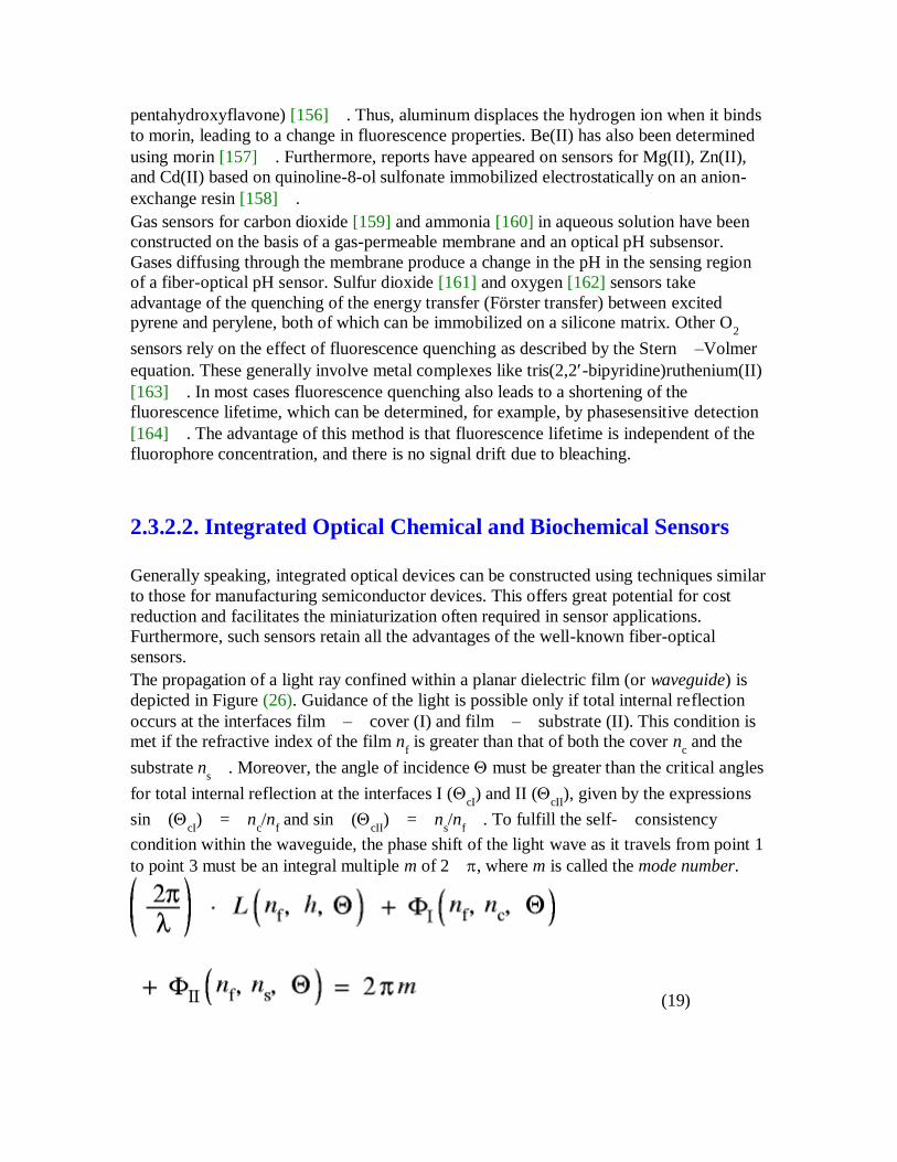
pentahydroxyflavone) [156]. Thus, aluminum displaces the hydrogen ion when it binds

to morin, leading to a change in fluorescence properties. Be(II) has also been determined

using morin [157]. Furthermore, reports have appeared on sensors for Mg(II), Zn(II),

and Cd(II) based on quinoline-8-ol sulfonate immobilized electrostatically on an anion-

exchange resin [158].

Gas sensors for carbon dioxide [159] and ammonia [160] in aqueous solution have been

constructed on the basis of a gas-permeable membrane and an optical pH subsensor.

Gases diffusing through the membrane produce a change in the pH in the sensing region

of a fiber-optical pH sensor. Sulfur dioxide [161] and oxygen [162] sensors take

advantage of the quenching of the energy transfer (Förster transfer) between excited pyrene and perylene, both of which can be immobilized on a silicone matrix. Other O

2

sensors rely on the effect of fluorescence quenching as described by the Stern–Volmer

equation. These generally involve metal complexes like tris(2,2-bipyridine)ruthenium(II)

[163]. In most cases fluorescence quenching also leads to a shortening of the

fluorescence lifetime, which can be determined, for example, by phasesensitive detection

[164]. The advantage of this method is that fluorescence lifetime is independent of the

fluorophore concentration, and there is no signal drift due to bleaching.

2.3.2.2. Integrated Optical Chemical and Biochemical Sensors

Generally speaking, integrated optical devices can be constructed using techniques similar

to those for manufacturing semiconductor devices. This offers great potential for cost

reduction and facilitates the miniaturization often required in sensor applications.

Furthermore, such sensors retain all the advantages of the well-known fiber-optical

sensors.

The propagation of a light ray confined within a planar dielectric film (or waveguide) is

depicted in Figure (26). Guidance of the light is possible only if total internal reflection

occurs at the interfaces film–cover (I) and film–substrate (II). This condition is

met if the refractive index of the film nf is greater than that of both the cover n

c and the

substrate ns. Moreover, the angle of incidence must be greater than the critical angles

for total internal reflection at the interfaces I (cI) and II (

cII), given by the expressions

sin(cI)=n

c/n

f and sin(

cII)=n

s/n

f. To fulfill the self-consistency

condition within the waveguide, the phase shift of the light wave as it travels from point 1

to point 3 must be an integral multiple m of 2, where m is called the mode number.

(19)

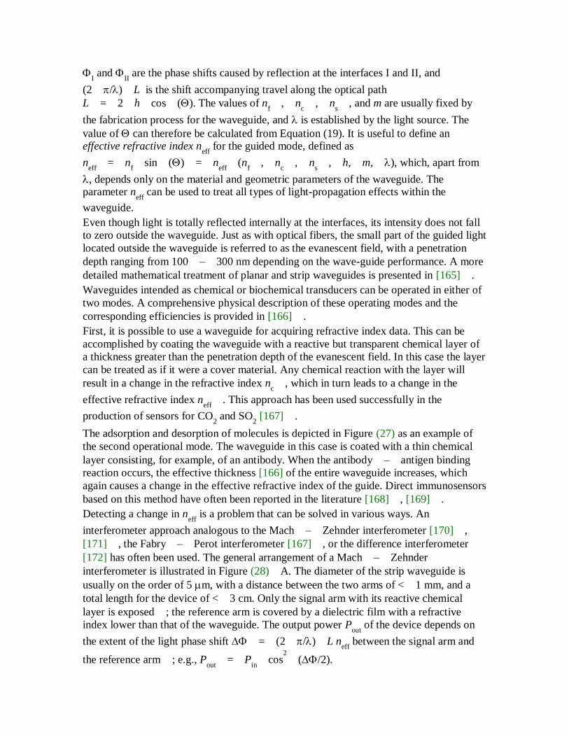
I and

II are the phase shifts caused by reflection at the interfaces I and II, and

(2/)L is the shift accompanying travel along the optical path

L=2hcos(). The values of nf,n

c,n

s, and m are usually fixed by

the fabrication process for the waveguide, and is established by the light source. The

value of can therefore be calculated from Equation (19). It is useful to define an effective refractive index n

eff for the guided mode, defined as

neff=n

fsin()=n

eff(n

f,n

c,n

s,h,m,), which, apart from

, depends only on the material and geometric parameters of the waveguide. The parameter n

eff can be used to treat all types of light-propagation effects within the

waveguide.

Even though light is totally reflected internally at the interfaces, its intensity does not fall

to zero outside the waveguide. Just as with optical fibers, the small part of the guided light

located outside the waveguide is referred to as the evanescent field, with a penetration

depth ranging from 100–300 nm depending on the wave-guide performance. A more

detailed mathematical treatment of planar and strip waveguides is presented in [165].

Waveguides intended as chemical or biochemical transducers can be operated in either of

two modes. A comprehensive physical description of these operating modes and the

corresponding efficiencies is provided in [166].

First, it is possible to use a waveguide for acquiring refractive index data. This can be

accomplished by coating the waveguide with a reactive but transparent chemical layer of

a thickness greater than the penetration depth of the evanescent field. In this case the layer

can be treated as if it were a cover material. Any chemical reaction with the layer will

result in a change in the refractive index nc, which in turn leads to a change in the

effective refractive index neff. This approach has been used successfully in the

production of sensors for CO2 and SO

2 [167].

The adsorption and desorption of molecules is depicted in Figure (27) as an example of

the second operational mode. The waveguide in this case is coated with a thin chemical

layer consisting, for example, of an antibody. When the antibody–antigen binding

reaction occurs, the effective thickness [166] of the entire waveguide increases, which

again causes a change in the effective refractive index of the guide. Direct immunosensors

based on this method have often been reported in the literature [168], [169].

Detecting a change in neff

is a problem that can be solved in various ways. An

interferometer approach analogous to the Mach–Zehnder interferometer [170],

[171], the Fabry–Perot interferometer [167], or the difference interferometer

[172] has often been used. The general arrangement of a Mach–Zehnder

interferometer is illustrated in Figure (28)A. The diameter of the strip waveguide is

usually on the order of 5 m, with a distance between the two arms of <1 mm, and a

total length for the device of <3 cm. Only the signal arm with its reactive chemical

layer is exposed; the reference arm is covered by a dielectric film with a refractive

index lower than that of the waveguide. The output power Pout

of the device depends on

the extent of the light phase shift =(2/)L neff

between the signal arm and

the reference arm; e.g., Pout=P

incos

2(/2).

Grating couplers can also be used to determine the value of neff, as depicted

schematically in Figure (28)B. For efficient light incoupling the angle must be

consistent with the expression neff=n

0sin()+l(/), where l is the

diffraction order and the grating period. According to this relationship, a change in neff

leads to a change in the angle that will reinforce light guided within the waveguide. A

grating coupler can also be used in an outcoupling arrangement. In this case it is the angle

for the outcoupled light that would conform to the grating equation. A detailed description

of grating-coupler methods is presented elsewhere [173].

2.3.2.3. Surface Plasmon Resonance

Transducers for optical sensing systems in chemical and biochemical sensors have also

been developed based on the sensitivity of surface plasmon resonance (SPR) devices.

Since first described in 1983 [174], SPR transducers have been used in many different

applications, including immunoassays [174], [175] and sensors for gases [174], [176]

and liquids [177].

Electron charges located at a metal–dielectric interface can be caused to undergo

coherent fluctuations known as surface plasma oscillations or surface plasmons (SP). The

frequency of such longitudinal oscillations is related to the wave vector ksp

by the

dispersion relationship.

(20)

where M() is the permittivity of the metal and

D() that of the surrounding

dielectric (cf. Fig. (29)); c is the velocity of light in a vacuum. The permittivity of the

metal (M=

M1+i ·

M2) is complex and the value of

D=n

D

2 is real, where

nD is the refractive index of the dielectric. A surface plasmon can be excited only if the

conditions M1<0 and |

M1|>

M2 are fulfilled. For example, gold, silver, and

palladium are potentially applicable metals with negative values of M1

for frequencies

corresponding to visible light [178].

SP excitation can be accomplished in several ways. A very simple and often used

approach is illustrated in Figure (29). RATHER [178] has described this as the attenuated

total reflection (ATR) coupler. Here the base of a prism is coated with a thin metal film

approximately 50 nm thick. Incident monochromatic light is reflected at this interface in

such a way that a projection of the light vector k0 on the interface becomes

kx=k

0n

psin(). If the resonance (Re) condition k

x=Rek

sp is fulfilled, the

evanescent field of the incident light excites an SP at the metal–dielectric interface,

although this is only possible with light polarized parallel to the plane of incidence (p-

polarized). The excitation is observed as a sharp minimum in the intensity of the reflected

light, and it can be detected by scanning the incident angle.

Using such an ATR device, small changes in D=n

D

2 and the build-up of a thin layer

at the metal–dielectric interface can easily be detected by measuring the shift in the

resonance angle .

For an immunosensing application the metal layer would be coated with appropriate

antibodies, either immobilized covalently or embedded into a matrix layer. Upon

exposure to a specific antigen the resonance angle should shift relative to that observed in

an analyte-free environment due to the increase in layer thickness that accompanies

binding of the analyte. For example, a thickness change of 0.1 nm results in a 0.01°

change in the resonance angle, a shift that can be measured quite accurately (see also

Section 3.3.1. Direct-Sensing Immunosensors without Marker Molecules).

If an ATR device is to be used for chemical sensing, the metal surface must be coated

with a thick dielectric layer of a reactive chemical. Chemical reaction within the layer

then produces changes in nD that can be detected by the corresponding shift in .

2.3.3. Mass-Sensitive Devices

2.3.3.1. Introduction

Mass changes are usually detected with the aid of a gravimetric device, such as a balance.

Ideally, balance sensitivity can be extended down into the microgram range, but the desire

for further improvements in sensitivity and miniaturization of the experimental setup has

led to the development of other mass-sensitive devices: the so-called quartz

microbalance (QMB), which is the best-known system, and other, more recent devices

such as the surface acoustic wave oscillator (SAW), the Lamb wave oscillator (LW), and

the acoustic plate-mode oscillator (APM), which represent the present state of the science

(Section 2.3.3.2. Fundamental Principles and Basic Types of Transducers). These devices

are all based on the piezoelectricity of solids, (see Section 2.3.3.3. Theoretical

Background), a phenomenon that permits the generation of vibrations or the propagation

of waves. A piezoelectric substrate, usually a quartz plate, is stimulated to vibration by an

oscillating electric circuit. This corresponds to an interconversion of electrical and

mechanical vibrations (deformations of the crystal), resulting in a device that can be

regarded as either an oscillator or a resonator.

Bulk waves, surface waves, and waves of other types (see Section 2.3.3.3. Theoretical

Background) are associated with characteristic resonance frequencies corresponding to

the most stable frequencies of vibration. Such a resonance frequency is itself highly

dependent on the mass of the oscillating plate. A slight change in the mass of the plate

will result in a considerable change in the resonance frequency, which can be measured

very accurately. An oscillator of this type can therefore be used as a mass-sensitive

transducer. Other factors that may influence the observed frequency shift include changes

in the viscosity and density of surface layers as well as such physical parameters as

forces, temperature, and pressure.

To construct a mass-sensitive sensor the surface of a piezoelectric material must be coated

with an appropriate chemically or biochemically reactive layer capable of interacting with

the proposed analyte and—ideally—recognizing it as well (see Section 2.3.3.4.

Technical Considerations). Such an interaction causes the mass of the crystal to increase,

resulting in a measurable shift in the resonance frequency. A relationship thus exists

between the amount of analyte adsorbed or absorbed and the frequency shift of the

oscillating system. Resonance frequency changes can be established very accurately, so

very small changes in mass can be detected. A theoretical approach applicable to simple

cases is described in [179].

To date, mass-sensitive devices have been used mainly for sensing analytes in the gas

phase; they are also applicable in principle to liquids, but this presupposes a more

sophisticated physical arrangement and complicated signal control. Many published

papers have dealt with the potential use of QMB, SAW, and, more recently, APM and

LW devices as mass-sensitive detectors in chemical and biochemical sensors, but no such

device has yet established itself commercially— with the exception of QMBs employed

for thin-layer thickness measuring, which cannot be regarded as chemosensors in the

strictest sense of the term [180].

Historical Development. The first report concerning the use of piezoelectric resonance

from a quartz crystal in a gravimetric microbalance is by J. STRUTT (Lord RAYLEIGH),

who in 1885 described a shift in resonance frequency accompanying an infinitesimal mass

change in a mechanical oscillator [181]. Fundamental studies into the mass sensitivity

of quartz resonators and their potential application for measuring the thickness of thin

layers were reported in 1959 by SAUERBREY [179], [182]. KING was the first to use a

quartz microbalance (in 1964) as a gas-phase detector in an analytical application

[183], [184]. Numerous more recent papers discuss the fundamentals

[185][186][187][188][189][190][191][192] and applicability [193][194][195][196] of

bulk acoustic wave (BAW) piezoelectric resonators as chemical and biochemical sensors

in the gas phase as well as in liquids, but physical devices for the measurement of

pressure, temperature, or distance have attracted greater commercial interest [197],

[198]. Nevertheless, quartz microbalances based on bulk acoustic waves do find

frequent use in analytical research and development.

RAYLEIGH in an early paper [181] also noted the existence of waves that are propagated

only in relatively thin surface layers, but it was not until 1979 that WOHLTJEN and DESSY

adapted these so-called surface acoustic waves (SAWs) for incorporation into a

chemical gas sensor [199][200][201]. The chief advantages of SAWs are increased

sensitivity relative to BAWs and a greater potential for miniaturization. On the other

hand, SAWs are associated with a variety of circuitry problems resulting from the

relatively high operating frequencies required for adequate sensor sensitivity. A

modification of this type of wave was introduced by CHUANG and WHITE [202],

[203], who adapted a SAW sensor by creating an exceptionally thin membrane-like

piezoelectric region in the substrate directly beneath the acoustic path. This in turn led to

the production of L amb waves, which proved to be particularly suitable for chemical

sensor applications, opening the way to the so-called plate-mode oscillator, a device

representing the present state of the art.

2.3.3.2. Fundamental Principles and Basic Types of Transducers

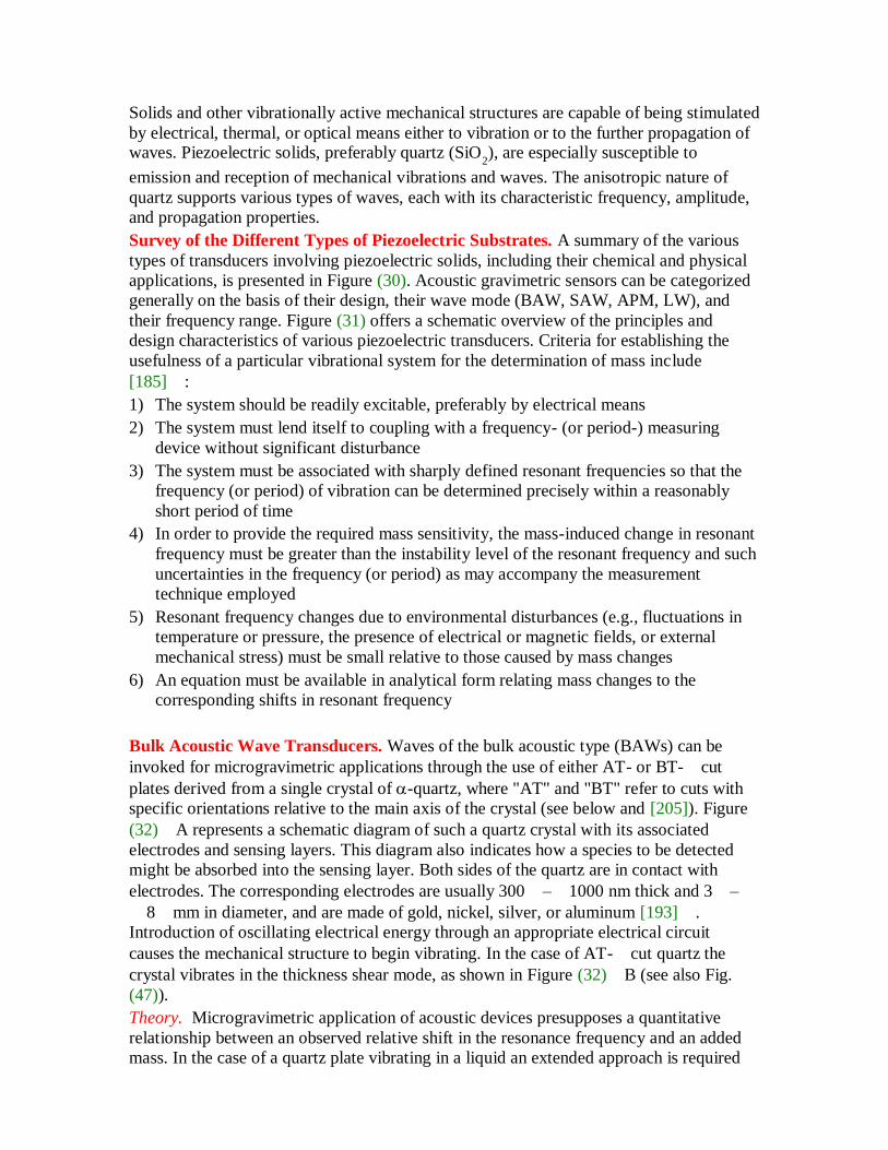
Solids and other vibrationally active mechanical structures are capable of being stimulated

by electrical, thermal, or optical means either to vibration or to the further propagation of waves. Piezoelectric solids, preferably quartz (SiO

2), are especially susceptible to

emission and reception of mechanical vibrations and waves. The anisotropic nature of

quartz supports various types of waves, each with its characteristic frequency, amplitude,

and propagation properties.

Survey of the Different Types of Piezoelectric Substrates. A summary of the various

types of transducers involving piezoelectric solids, including their chemical and physical

applications, is presented in Figure (30). Acoustic gravimetric sensors can be categorized

generally on the basis of their design, their wave mode (BAW, SAW, APM, LW), and

their frequency range. Figure (31) offers a schematic overview of the principles and

design characteristics of various piezoelectric transducers. Criteria for establishing the

usefulness of a particular vibrational system for the determination of mass include

[185]:

1) The system should be readily excitable, preferably by electrical means

2) The system must lend itself to coupling with a frequency- (or period-) measuring

device without significant disturbance

3) The system must be associated with sharply defined resonant frequencies so that the

frequency (or period) of vibration can be determined precisely within a reasonably

short period of time

4) In order to provide the required mass sensitivity, the mass-induced change in resonant

frequency must be greater than the instability level of the resonant frequency and such

uncertainties in the frequency (or period) as may accompany the measurement

technique employed

5) Resonant frequency changes due to environmental disturbances (e.g., fluctuations in

temperature or pressure, the presence of electrical or magnetic fields, or external

mechanical stress) must be small relative to those caused by mass changes

6) An equation must be available in analytical form relating mass changes to the

corresponding shifts in resonant frequency

Bulk Acoustic Wave Transducers. Waves of the bulk acoustic type (BAWs) can be

invoked for microgravimetric applications through the use of either AT- or BT-cut

plates derived from a single crystal of -quartz, where "AT" and "BT" refer to cuts with

specific orientations relative to the main axis of the crystal (see below and [205]). Figure

(32)A represents a schematic diagram of such a quartz crystal with its associated

electrodes and sensing layers. This diagram also indicates how a species to be detected

might be absorbed into the sensing layer. Both sides of the quartz are in contact with

electrodes. The corresponding electrodes are usually 300–1000 nm thick and 3–

8mm in diameter, and are made of gold, nickel, silver, or aluminum [193].

Introduction of oscillating electrical energy through an appropriate electrical circuit

causes the mechanical structure to begin vibrating. In the case of AT-cut quartz the

crystal vibrates in the thickness shear mode, as shown in Figure (32)B (see also Fig.

(47)).

Theory. Microgravimetric application of acoustic devices presupposes a quantitative

relationship between an observed relative shift in the resonance frequency and an added

mass. In the case of a quartz plate vibrating in a liquid an extended approach is required

with respect to changes in the viscosity and density. The first useful relationship of this

type was developed by SAUERBREY, who treated the added mass as an "added thickness"

of the oscillator. The relationship itself was based on a quartz crystal vibrating in its

thickness shear mode in the gas phase (Fig. (33)). The observed oscillation frequency ( fq)

is inversely proportional to the thickness tq of the crystal; f

q=N/t

q, where N is a

frequency constant (N=0.168 MHz cm for AT-cut quartz at room temperature).

The mass of the crystal is m=Atq, where is the crystal density and A its

cross-sectional area. In this derivation the mass increment due to a foreign mass m is

treated as an equivalent change in the mass of the crystal. Invoking the approximation

q=

f leads to the equation:

(21)

which finally provides the following expression for an AT-cut crystal:

(22)

where fq is expressed in megahertz, m in grams, and A in square centimeters. Since f

q for

a quartz crystal is typically 10 MHz, and a frequency change of 0.1 Hz can be readily

detected by modern electronics, it is possible in this way to detect mass changes of as

little as about 10–10

g/cm2 [206].

LU has developed a model involving propagation velocities for sound waves in the

substrate (for quartz, vq) and in the sensing layer (v

f) [192]. Reflection and refraction

occur at the interface between the crystal (q) and the film (f) (Fig. (33)) analogous to

the optical reflection and refraction observed at a boundary between two materials with

different optical densities. The shear velocities in the quartz crystal and the film coating,

respectively, are:

(23)

Given a knowledge of the shear moduli f and

q, Equation (23) can be used to

calculate the shear velocity of the wave. Ideal wave-propagation behavior is observed

with a crystal upon which such a film has been deposited provided there is a negligible

amount of frictional loss. In this case the resonance condition is valid, which leads to

Equation (24):

(24)

where fc=/2 is the resonance frequency of the crystal upon which material has

been deposited. The terms f · v

f and

q · v

q are the acoustic impedances Z

f and Z

q of

the film and crystal, respectively. Their ratio, Z=Zf/Z

q, is an important parameter

with respect to acoustic matching of the materials. For optimum resonance conditions Z

should be as close as possible to unity, because its value affects the resilience of the whole

assembly, and maximum stability corresponds to Z~1 [207].

For example, Z has a value of 1.08 for a piezoelectric crystal covered with aluminum

electrodes (shear-mode impedance of SiO2: Z

SiO

2= 8.27×10

6 kgsm

–2; that of

Al: ZAl= 8.22×10

6 kgsm

–2), indicative of the good match associated with this

material combination. Deposition of gold electrodes on an SiO2 surface leads to a Z-value

of 0.381, which is barely acceptable (shear-mode impedance of gold:

ZAu=23.2×10

6kgsm

–2) [207].

From a practical point of view it is important to develop a relationship involving more

experimentally common parameters influencing the frequency response. The frequency

response of a piezoelectric sensor in the presence of a gas at a particular pressure can be

related generally to three effects: the hydrostatic effect (p), the impedance effect (x),

and the sorption effect (m):

(25)

For gravimetric measurements and sensor applications, the latter effect (that is, to added

mass) is the most important, and the other two effects can be viewed as nonspecific

interferences. Because both of these terms are three orders of magnitude smaller than the

mass term, the mass relationship alone is sufficient for characterizing measurements in the

gas phase. However, situations do exist in which the other two effects cannot be ignored.

For instance, if the pressure is changed from that of the surrounding air to a vacuum the

first term is no longer negligible, and in the case of liquids any change in viscosity or

density alters the impedance, so this term must be taken into consideration.

Other theoretical approaches relevant to applications in the gas phase and dealing with

thickness-shear mode acoustic wave quartz sensors are presented in [189],

[208][209][210][211][212][213].

Bulk Acoustic Waves in L iquids. When a quartz crystal is placed in a liquid, there is a

significant change in both the density and the viscosity of the surrounding medium. Both

become much larger than in the gas phase, and the consequences must be taken into

account with respect to the second term in Equation (25). Thus, the Sauerbrey equation is

no longer applicable if the viscoelastic properties of the contacting medium (liquid and/or

film) change during the course of an experiment. The liquid now represents an additional

mass load, which produces coupling between the substrate elastic shear wave and the

liquid. KANAZAWA derived the first theoretical relationship linking the properties of a

liquid to the frequency response of a piezoelectric crystal. In a liquid medium, the shear

motion of the crystal causes motion to occur in the adjacent layer of solvent molecules

(usually water). Up to a layer thickness of approximately 1 m the solvent molecules

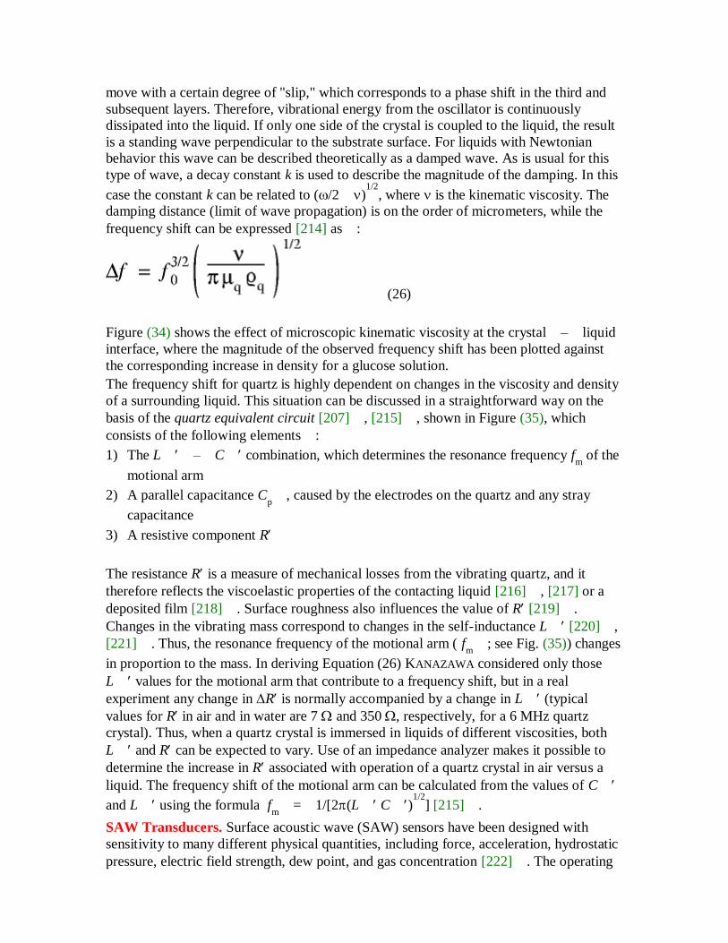
move with a certain degree of "slip," which corresponds to a phase shift in the third and

subsequent layers. Therefore, vibrational energy from the oscillator is continuously

dissipated into the liquid. If only one side of the crystal is coupled to the liquid, the result

is a standing wave perpendicular to the substrate surface. For liquids with Newtonian

behavior this wave can be described theoretically as a damped wave. As is usual for this

type of wave, a decay constant k is used to describe the magnitude of the damping. In this

case the constant k can be related to (/2)1/2

, where is the kinematic viscosity. The

damping distance (limit of wave propagation) is on the order of micrometers, while the

frequency shift can be expressed [214] as:

(26)

Figure (34) shows the effect of microscopic kinematic viscosity at the crystal–liquid

interface, where the magnitude of the observed frequency shift has been plotted against

the corresponding increase in density for a glucose solution.

The frequency shift for quartz is highly dependent on changes in the viscosity and density

of a surrounding liquid. This situation can be discussed in a straightforward way on the

basis of the quartz equivalent circuit [207], [215], shown in Figure (35), which

consists of the following elements:

1) The L–C combination, which determines the resonance frequency fm of the

motional arm

2) A parallel capacitance Cp, caused by the electrodes on the quartz and any stray

capacitance

3) A resistive component R

The resistance R is a measure of mechanical losses from the vibrating quartz, and it

therefore reflects the viscoelastic properties of the contacting liquid [216], [217] or a

deposited film [218]. Surface roughness also influences the value of R [219].

Changes in the vibrating mass correspond to changes in the self-inductance L [220],

[221]. Thus, the resonance frequency of the motional arm ( fm; see Fig. (35)) changes

in proportion to the mass. In deriving Equation (26) KANAZAWA considered only those

L values for the motional arm that contribute to a frequency shift, but in a real

experiment any change in R is normally accompanied by a change in L (typical

values for R in air and in water are 7 and 350 , respectively, for a 6 MHz quartz

crystal). Thus, when a quartz crystal is immersed in liquids of different viscosities, both

L and R can be expected to vary. Use of an impedance analyzer makes it possible to

determine the increase in R associated with operation of a quartz crystal in air versus a

liquid. The frequency shift of the motional arm can be calculated from the values of C

and L using the formula fm=1/[2(L C)

1/2] [215].

SAW Transducers. Surface acoustic wave (SAW) sensors have been designed with

sensitivity to many different physical quantities, including force, acceleration, hydrostatic

pressure, electric field strength, dew point, and gas concentration [222]. The operating

principle of an SAW for use with gases is conceptually quite simple. A surface acoustic

wave—a periodic deformation perpendicular to the material surface—is

transmitted across the surface of some appropriate solid that has been exposed to the

atmosphere subject to analysis. With a homogeneous substrate, usually a piezoelectric

solid like quartz or LiNbO3, the required SAW (sometimes also called a Rayleigh

wave) is generated by means of an interdigital transducer (IDT).

In contrast to a quartz microbalance, the requisite IDT components are deposited only on

one side of the crystal. These take the form of planar, interleaved, metal electrode

structures, (with permission from Plenum Publishing, New York)where adjacent

electrodes are supplied with equal but opposite potentials (Fig. (36)A). Application of a

time-varying r. f. potential causes the crystal to undergo physical deformations, and if

these are confined to the surface region of the crystal, the result is a surface acoustic wave

(Fig. (36)B) [224]. Such vibrations will interfere constructively only if the distance L

/2 between two adjacent "fingers" (see Fig. (28)A) is equal to one-half the elastic

wavelength. The frequency f=vR/L that corresponds to such a cumulative effect is

called the synchronous frequency or resonance frequency ( f ) [206].

The waves that are generated have their mechanical and electrical components in a single

plane, the sagittal plane, which is perpendicular to the substrate surface. The phase

velocity (vR) and the amplitude (A) of an SAW are determined by elastic, piezoelectric,

dielectric, and conductive properties of the substrate as well as by its mass. If one of these

parameters can be modulated in an appropriate way by the quantity of interest, a sensing

device can be constructed. Such a modulation could be induced in the transducer itself

and/or in the transmission region (waveguide or delay line). With layered substrates the

physical properties of each layer as well as the thicknesses of the layers determine the

phase velocity and the amplitude of the resulting SAW [206]. Various energy-loss

mechanisms also operate on the propagating SAW: scattering loss due to finite grain

size, thermoelastic loss due to nonadiabatic behavior of the acoustic conductor, viscous

loss caused by the dissipation of energy in a direction perpendicular to the transducer–

environment interface, and hysteresis absorption due to irreversible coupling between

SAW energy and an adsorbate [207]. Any addition of mass during the sensing step may

change the magnitude of one or more of these phenomena, and may also lead to changes

in vR and A, especially a frequency shift (f ) or a relative frequency shift (f/f ). An

exact description of the physical processes involved in the generation, propagation, and

detection of SAWs is complex, and is available from such sources as [224], [225].

The considerations presented above provide the basis for using SAWs in gas-monitoring

devices, because observed frequency shifts are proportional to added mass. However, the

characteristic frequency of an SAW is also sensitive to changes in temperature or

pressure. The ideal substrate would be one with a zero temperature delay coefficient but a

high piezoelectric coupling effect. Despite extensive materials research efforts, it is

currently necessary to choose between these parameters; e.g., ST-cut quartz is the

preferred substrate if a zero temperature coefficient is most important, and cuts of lithium

niobate are selected for high piezoelectric coupling.

Sensor Configurations. A single SAW sensor may sometimes suffice for a gas sensing

application (Fig. (37)A), but often the sensors display undesirable sensitivity to such

effects as temperature, pressure, and ambient humidity. Overcoming these problems

requires the establishment of a relative signal output. For example, VETELINO et al. have

described a dual-line SAW gas sensor [206], [226], [227]. One delay line in this

case is used for measuring, while the other acts as a reference (see Fig. (37)B). The

advantage of a dual delay-line configuration is that it transforms the output signal into a

relative change in oscillator frequency, which can be attributed only to the effects of the

analyte. D'AMICO et al. have described a system based on a three-transducer delay line

(see Fig. (37)C). This device also has two dual-delay lines, but the paths are established

in this case by one input IDT and two output IDTs. Again, one path of the delay line is

coated and the other remains uncoated as a way of minimizing the effects of both

temperature and pressure [228].

The first use of an SAW resonator sensor was reported by MARTIN et al. [229]. The

corresponding resonator incorporated a single IDT located between two acoustically

reflecting mirrors. The distance between the mirrors was so adjusted as to ensure

constructive interference between successive reflections, resulting in a maximum for one

particular frequency (Fig. (37)D).

Theory. The SAW velocity vR can be affected by many factors, each of which is

associated with a potential sensor response:

(27)

where vR is the phase velocity unperturbed by such external factors as m, c, , and (the

mass, elastic constant, electrical conductivity, and dielectric constant of the solid medium,

respectively), as well as T and p, the environmental temperature and pressure [222].

Three types of films have been considered for use as reactive layers:

1) Nonconductive isotropic overlay film

2) Electrically conducting overlay film

3) Metal-oxide semiconducting film

A theoretical treatment can be developed for each of these film types with respect to its

properties, involving, in the nonconductive case, the thickness tf, the mass density ,

(the Lamé constant), and (the shear modulus).

Regarding the relationship v/v=–f/f between SAW velocity and the variation

in the SAW dual-delay line oscillator frequency, perturbation analysis leads to the

following result for the relative frequency shift [225]:

(28)

where k1 and k

2 are material constants for the SAW substrate. Additional information with

respect to these equations is available from [200], [222], [225].

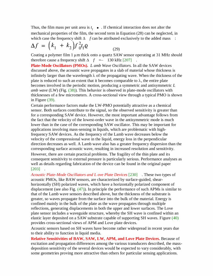
Thus, the film mass per unit area is tf. If chemical interaction does not alter the

mechanical properties of the film, the second term in Equation (28) can be neglected, in

which case the frequency shift f can be attributed exclusively to the added mass:

(29)

Coating a polymer film 1 m thick onto a quartz SAW sensor operating at 31 MHz should

therefore cause a frequency shift f=–130 kHz [207].

Plate-Mode Oscillators (PMOs). L amb Wave Oscillators. In all the SAW devices

discussed above, the acoustic wave propagates in a slab of material whose thickness is

infinitely larger than the wavelength of the propagating wave. When the thickness of the

plate is reduced to such an extent that it becomes comparable to , the entire plate

becomes involved in the periodic motion, producing a symmetric and antisymmetric L

amb wave (LW) (Fig. (38)). This behavior is observed in plate-mode oscillators with

thicknesses of a few micrometers. A cross-sectional view through a typical PMO is shown

in Figure (39).

Certain performance factors make the LW-PMO potentially attractive as a chemical

sensor. Both surfaces contribute to the signal, so the observed sensitivity is greater than

for a corresponding SAW device. However, the most important advantage follows from

the fact that the velocity of the lowest-order wave in the antisymmetric mode is much

lower than in the case of the corresponding SAW oscillator. This may be important for

applications involving mass-sensing in liquids, which are problematic with high-

frequency SAW devices. As the frequency of the Lamb wave decreases below the

velocity of the compressional wave in the liquid, energy loss in the perpendicular

direction decreases as well. A Lamb wave also has a greater frequency dispersion than the

corresponding surface acoustic wave, resulting in increased resolution and sensitivity.

However, there are certain practical problems. The fragility of the thin plate and its

consequent sensitivity to external pressure is particularly serious. Performance analyses as

well as details regarding fabrication of the device can be found in the original paper

[203].

Acoustic Plate-Mode Oscillators and L ove Plate Devices [230]. These two types of

acoustic PMOs, like BAW sensors, are characterized by surface-guided, shear-

horizontally (SH) polarized waves, which have a horizontally polarized component of

displacement (see also Fig. (47)). In principle the performance of such APMs is similar to

that of the Lamb wave sensors described above, but the thickness of the substrate is

greater, so waves propagate from the surface into the bulk of the material. Energy is

confined mainly in the bulk of the plate as the wave propagates through multiple

reflections, generating displacements in both the upper and lower surfaces. The Love

plate sensor includes a waveguide structure, whereby the SH wave is confined within an

elastic layer deposited on a SAW substrate capable of supporting SH waves. Figure (40)

provides cross-sectional views of APM and Love plate devices.

Acoustic sensors based on SH waves have become rather widespread in recent years due

to their ability to function in liquid media.

Relative Sensitivities of BAW, SAW, LW, APM, and Love Plate Devices. Because of

excitation and propagation differences among the various transducers described, the mass-

deposition sensitivity of the several devices would be expected to vary considerably, with

some geometries proving more attractive than others for particular sensing applications.

Table (9) offers a performance comparison for these transducers. Table (9) also

summarizes the calculated frequency-to-mass sensitivities for the various devices.

Sensitivity variations can be explained on the basis of energy confinement on the sensing

surface and a particular device's operating frequency. A decrease in the thickness of the

substrate leads to a sensitivity increase, which can be realized with either an acoustic

plate-mode or a Lamb wave device. These are therefore associated with the highest

sensitivities, followed by the Love plate, which also has a very thin layer. Less sensitivity

is available with BAW devices, for which the sensitivity depends on the thickness of the

crystal.

2.3.3.3. Theoretical Background

Piezoelectricity. The Piezoelectric Effect. Because all acoustic gravimetric sensors are

based on the phenomenon of piezoelectricity, it seems appropriate to discuss briefly the

effect itself. Piezoelectricity was first observed by the CURIE brothers (JAQUES and

PIERRE) in 1880 [233]. It is a reversible phenomenon, consisting of linear

electromechanical interactions between mechanical and electrical properties in certain

crystals (Fig. (41)).

A piezoelectric effect occurs only with those ionic crystalline solids whose crystals

contain a polar axis along which the physical properties are not constant. The direct

piezoelectric effect is observed when an applied force (F) produces an electrical

polarization (P), and a converse (reciprocal) piezoelectric effect results when an

applied electrical field (E) induces a strain (S, deformation of the crystal) (Fig. (42)).

A simplified view of piezoelectricity at the microscopic level is provided by the example

of -quartz (Fig. (43)). Here a net dipole moment will arise if the hexagonal structure is

stretched or compressed along a direction parallel (Fig. (43)B) or perpendicular (Fig.

(43)C) to one of the three in-plane symmetry axes. When symmetry is achieved, the net

dipole moment of the molecule vanishes.

Structural Aspects of Piezoelectric Solids. In order for a crystal to be piezoelectric it must

be noncentrosymmetric; i.e., it cannot contain a center of symmetry. Solids are usually

grouped for structural characterization purposes into seven crystal systems (from lowest

to highest symmetry: triclinic, monoclinic, orthorhombic, tetragonal, trigonal,

hexagonal, and cubic), which can in turn be divided into 32 point groups, depending upon

point symmetry. Of these, 11 classes are centrosymmetric and 20 are piezoelectric. An

exceptional case is class 432 from the cubic crystal system, because it is neither

centrosymmetric nor piezoelectric. In addition to the 21 noncentrosymmetric classes, 11

classes can be distinguished on the basis that they possess no plane of symmetry. This

means that they are associated with both right- and left-handed forms, which cannot be

interconverted by simple rotation, a phenomenon known as enantiomorphism [236].

Table (10) summarizes on the basis of international point-group symbols the structural

distribution with respect to piezoelectric classes, centrosymmetric classes, and

enantiomorphism. For example, LiNbO3, which belongs to the class 3m, is

piezoelectric, but not enantiomorphic, whereas -quartz, in class 32, is both piezoelectric

and enantiomorphic. The latter characteristic is illustrated in Figure (44).

Not every solid material associated with a piezoelectric class is suitable for practical

applications, because in some cases the piezoeffect is too weak. Large piezoelectric

coefficients are a prerequisite for an electromechanical transducer, like those found, for

example, with -quartz or LiNbO3. Therefore, these are the solids most often used as

mass-sensitive plates or substrates.

Theory and Physics of Piezoelectricity. The discussion that follows constitutes a very

brief introduction to the theoretical formulation of the physical properties of crystals. If a

solid is piezoelectric (and therefore also anisotropic), acoustic displacement and strain

will result in electrical polarization of the solid material along certain of its dimensions.

The nature and extent of the changes are related to the relationships between the electric

field (E) and electric polarization (P), which are treated as vectors, and such elastic

factors as stress Tand strain (S), which are treated as tensors. In piezoelectric crystals

an applied stress produces an electric polarization. Assuming the dependence is linear, the

direct piezoelectric effect can be described by the equation:

(30)

The quantities dijk

and eijk

are known as the piezoelectric strain and piezoelectric stress

coefficients, respectively.

Conversely, if such a crystal is placed in an electrical field it will become deformed, a

phenomenon known as the converse or reciprocal piezoelectric effect (Fig. (42)B). The

contributions of stress and strain in this case can be expressed:

(31)

Since the stress and strain tensors are symmetric, the piezoelectric coefficients can be

converted from tensor to matrix notation. Table (11) provides the piezoelectric matrices

for -quartz together with several values dijk

and eijk, including the corresponding

temperature coefficients [234], [236].

For sensor applications, the magnitudes of dijk

and eijk

should be as great as possible, and

the temperature dependence should be as small as possible. Although lithium niobate

displays larger stress and strain constants than -quartz, the temperature influence in this

case is also great. Therefore, -quartz is the material most often selected for piezoelectric

sensor applications. Because of the anisotropic behavior of a piezoelectric material,

properties like resonance frequency and temperature dependence can be optimized by

cutting a plate from a single crystal in a particular way. Figure (45)shows two possible

cuts with respect to a natural -quartz crystal. For use as acoustic gravimetric sensors,

only ATand BT-cut quartz plates are useful. These y-rotated cuts provide two different

high-frequency plates that vibrate in a shear mode along an axis parallel to the major

surface, as indicated previously (see also Fig. (32)B). Minimizing temperature effects

requires that the plate be cut at a very precise orientation. The temperature dependence of

the relative frequency for various cuts of quartz crystal is shown as a function of the angle

of cut in Figure (46) [237].

More detailed theoretical treatments of piezoelectric solids and their properties are

provided by [198], [238][239][240]. Another more sophisticated approach based on

dynamic quantum mechanics is presented in [241]. Interest has also developed in recent

years in piezoelectric polymers, especially as a result of their strongly piezoelectric

properties [198].

Vibrations and Waves. The theory of acoustic waves in solids is well understood, and

many comprehensive descriptions exist [225], [242]. The description presented here

should suffice to explain sensor function despite the fact that it is limited and qualitative.

Acoustic waves in solids consist of oscillatory motions of the material comprising the

solid. The stress–strain relationship treated in the preceding section leads ultimately

to two types of acoustic displacements: longitudinal or tensile motions that cause the

dimensions of the solid body to change along a single direction without accompanying

changes along the orthogonal directions, and shear motion, which produces changes in

the shape of the solid body. Figure (47) illustrates these two types of motion [232].

In piezoelectric solids, an applied force generally creates both quasi-longitudinal and

quasishear waves, where the acoustic displacement in a wave will be largely either

longitudinal or shear. Pure longitudinal (L) and shear waves (SH = horizontally polarized

shear waves; SV = vertically polarized shear waves) are generated if wave propagation

occurs along certain crystallographic axes or with specific orientations. The generation of

mixed wave types is also possible, but normally not desirable for sensor applications.

As far as microgravimetric sensors are concerned, two types of wave-propagation devices

can be distinguished: those characterized by wave propagation perpendicular to the

plate surface (BAW) and those in which the waves propagate along the surface (SAW) or

in the bulk of the substrate (LW, APM). Transducers of the former type are normally

resonators. A given device might be designed to utilize either longitudinal or shear waves

propagated between the faces, as in microbalances based on AT- or BT-cut quartz

plates operating in their SH high-frequency fundamental mode. Only acoustic waves

satisfying boundary conditions for the resonator surfaces will propagate efficiently across

such a device. The waves can be visualized as standing sinusoidal waves with

displacement nodes at the resonator surfaces (see 2.3.3.2. Fundamental Principles and

Basic Types of Transducers).

Transducers in the second category include wave delay-line oscillators (see Figs. (31) and

(36)), which are based primarily on two types of waves. One is a coupled linear

combination of two wave-equation solutions, an L-wave and an SV-wave. In this wave,

also called a Rayleigh wave, particle displacement takes the form of an elliptical motion

in the plane perpendicular to the surface (sagittal plane) and containing the direction of

propagation. Some displacement also occurs outside the sagittal plane, but the deviations

are minor (Fig. (48)). Two of the most important cuts providing these wave types, and

which are used in chemical sensors, have been illustrated in Figure (45). Waveguides that

rely on Rayleigh wave devices for their operation are often referred to as surface acoustic

wave (SAW) devices, and they have been extensively employed as sensors.

The second type of wave in this context is a horizontal shear (SH) wave, whose acoustic

displacement is in the plane of the waveguide. An SH wave generally travels at a different

velocity than a Rayleigh wave, and for piezoelectric waveguides the SH wave becomes a

true surface wave provided the acoustic impedance at the surface differs from that in the

substrate bulk. Such a difference can be caused by piezoelectric stiffening of the SH

mode, deposition of a layer of dissimilar material on the surface, the presence of a surface

grating, or liquid in contact with the surface. Depending on their origin, SH surface waves

are referred to in the literature as Bleustein–Gulayev (BG) waves, Stoneley waves,

SH-SAW, or surface transverse waves. Pure surface transverse waves (shear waves)

appear to show promise for applications in liquids, especially biosensor applications,

because the dissipation of energy across the phase boundary into the liquid is

approximately zero, which greatly reduces the generation of longitudinal sound waves in

the liquid itself.

Plate-mode waves are analogous in form to Rayleigh and SH waves in a semi-infinite

waveguide. Two groups of plate modes can be distinguished: the first consists of Lamb

waves or flexural waves, where the acoustic displacement is a combination of longitudinal

and vertical shear motion; a second family involves SH acoustic displacement [232].

Because of their frequency range (100 kHz to the GHz region) these sound waves fall in

the ultrasound category, with a propagation velocity of 1–10 km/s (cf. electrical

signals, which travel at 100000–300000 km/s).

2.3.3.4. Technical Considerations

The (Bio)Chemical Interface. A piezoelectric transducer is transformed into a mass-

sensitive sensor by coating it with an appropriate (bio)chemical film or layer, which may

be inorganic, organic, or even metallic in nature. Ideally the film should be strongly

adherant and deposited in such a way as to obtain a plane surface. The thickness of such a

layer is usually on the order of 1–100 m depending upon the nature of the

transducer. The chemically sensitive layer serves as an interface between the environment

and a data-processing system, and it is responsible for both the sensitivity and the

selectivity of the sensor. This layer should display the following properties:

1) Reversibility, sensitivity, and selectivity

2) Inertness with respect to chemical cross-influences, such as humidity or carbon

dioxide

3) Ease of coating, strong adhesion, and long life

Most chemically sensitive layers are insulators, such as organic substances with special

functionalities, but conducting materials such as metal films are also useful. Examples

include:

1) Donor–acceptor functionalities; e.g., carbocations [243], M(II)porphyrins

[244], or betaines [245]

2) Host–guest binding systems (supramolecular compounds); e.g., molecular

cavities [246], clathrate systems [247]

3) Pure metallic layers; e.g., palladium for the detection of hydrogen [248]

Interaction of the Chemical L ayer with an Analyte. Interaction with an analyte can take

many forms ranging from adsorption–absorption to chemisorption, including the

compromise of coordination chemistry. The following types of chemical interactions can

be distinguished [249]:

1) Absorption

Here the analyte is distributed between the chemical interface (a liquid film,

amorphous solid, or polymer, analogous to the stationary phase in gas

chromatography) and the surrounding medium. In the case of a gas interacting with

the chemical interfacial layer, once equilibrium has been achieved the amount of

analyte present in the layer is a function of the partition coefficient between the gas

and the interface (as specified by Raoult's and Henry's laws) as well as the thickness

and area of the interface. Because distribution tends to be determined mainly by the

polarity of the chemical interface and the analyte, little selectivity is expected.

2) Adsorption

The analyte in this case interacts only at the surface of the interfacial layer, and no

chemical bonds are formed or broken. Attraction energies are usually in the range

0–10 kJ/mol (i.e., attributable to van der Waals forces), extending in the case of

hydrogen bonds to as much as 40 kJ/mol. Adsorption may result from physical

attraction between a nonreactive gaseous analyte and a metal surface, for example, or

formation of a donor–acceptor association (H+ or e

–). Adsorption is a universal

phenomenon, and it is quite nonselective. The basic principles of gas adsorption have

been described by LANGMUIR [250] and DE BOER [251].

3) Chemisorption [252]

Chemisorption involves very strong interaction—up to ca. 300 kJ/mol—

developed at the surface of the chemical interface, including the formation and

breaking of chemical bonds. High selectivities can therefore be anticipated, but there

is a simultaneous loss of reversibility. Because of the partially irreversible nature of

bond formation, such a sensor would actually behave more like a dosimeter, although

this might be advantageous in some applications.

4) Coordination chemistry [249]

A compromise offering both selectivity and reversibility of analyte binding is

presented by the area of coordination chemistry. A typical coordination compound

consists of a central metal ion M surrounded by a neutral or charged (often organic)

ligand. The extent of selectivity can often be influenced by the choice of the metal ion

as well as by the choice of the ligand—taking into account both electronic and

steric factors. Complexation with an analyte produces changes in the properties of the

coordination compound, and these changes can be subject to detection. The selectivity

is a function of structural, topological, and polarity parameters.

Other types of chemical interfaces have also been used for microgravimetric gas

detection, including polymeric phthalocyanines [253], porphyrins [254], ferrocenes

[255], metal clusters [256], crown ethers [257], and cyclodextrins [258].

In many cases it has proven to be very difficult to find a selective chemical interface for a

particular analyte, so the use of sensor arrays has been proposed. Numerous papers have

dealt with this approach, invoking both BAW and SAW sensors. Pattern-recognition

techniques employing increasingly powerful microprocessors are required to generate the

appropriate signals [259].

Coating Methods. The stability of a (bio)chemical interface depends heavily on the

attachment of the material to the surface of the sensor device. One or more of the

following coating methods is employed according to the nature of the sensitive layer:

Smearing [200]

Spin coating [260]

Solvent evaporation [261]

Spraying [262]

Langmuir–Blodgett film formation [263]

Physical vapor deposition [264]

Sputtering [265]

Chemical immobilization [266]

The first four methods listed involve simple coating procedures in which the interfacial

material (usually nonpolar) is dissolved in an organic solvent and then deposited directly

onto the substrate surface. Evaporation of the solvent leaves a film that adheres to the

surface of the substrate by physical bonds. The Langmuir–Blodgett technique makes

it possible to achieve very thin films. This is a dipping procedure in which molecules are

transferred with great accuracy from the surface of a liquid to the surface of the substrate.

Even monolayers can be prepared in this way. More complicated methods include

physical vapor deposition (PVD) and chemical vapor deposition (CVD). Very planar

layers can be achieved in this way, but the reaction conditions are usually quite drastic, so

the technique is essentially restricted to materials that are relatively inert, such as

inorganic compounds or metals.

2.3.3.5. Specific Applications

Having reviewed the fundamental aspects of microgravimetric transducers and

piezoelectric solids with respect to the generation and propagation of vibrations and

waves, it is now appropriate to turn to the practical considerations of instrumentation and

application, addressing first the BAW devices.

Bulk Acoustic Wave Sensors. Experimental Arrangement. A typical experimental setup

involving a piezoelectric mass-sensitive quartz crystal detector is depicted schematically

in Figure (49) [193]. The piezoelectric quartz crystal (a) is shown here inserted directly

in a gas stream (b) with a flow velocity of ca. 10–100 mL/min, but a measuring cell

containing a stationary atmosphere of the analyte gas is also useful. The oscillator (e) is

usually powered by a regulated power supply (d; e.g., 5–15 V) that drives the

quartz crystal. The frequency output from the oscillator is monitored with a frequency

counter (f), which should be modified by a digital-to-analog converter (g) to permit the

frequency data to be recorded.

Parameters that adversely affect the performance of a piezoelectric sensor include the

mass of the chemical layer, built-in stress produced by the chemical layer, stress from the

electrodes (clamping), and changes in temperature. A more sophisticated device such as a

microprocessor-controlled dual-crystal instrument would be required to eliminate

these undesirable effects [267].

The device described is designed for measurements in the gas phase; applications in a

liquid medium demand an extended version, including a liquid-tight box, an oscilloscope

or network analyzer, and provisions for more detailed signal analysis (impedance

analysis). Improvements in the oscillating circuit are particularly important for obtaining

satisfactory results with liquids [268][269][270].

Applications. This section will be limited to a brief consideration of the use of BAW

sensors in gas-sensing devices and as sensors for liquid phases. Piezoelectric

microbalances can also be used for monitoring such heterogeneous samples as aerosols

and suspensions, as discussed in [237].

Gas-Phase Sensing. In principle, both inorganic and organic analytes are subject to

detection. Figure (50) provides an example of results obtained from a piezoelectric quartz

microbalance (QMB) resonator used to detect gaseous tetrachloroethylene (C2Cl

4).

Observed response curves are illustrated as a function of time and for various analyte

concentrations. A wide variety of solvent vapors can be detected with high sensitivity (in

the ppm range), indicating the potential of this approach to gas-phase monitors and

sensors for applications in environmental analysis or process control.

Table (12) provides an overview of the detection of selected gaseous analytes.

Information regarding interfering gases can be found in the original literature. The effect

of changes in the relative humidity of the environment tends to be a general problem.

Applications in L iquids. Apart from the classical sensors designed for detecting ions,

piezoelectric crystal resonators are the preferred devices for conducting biochemical

measurements in liquids. Figure (51) illustrates results for the detection of human

immunodeficiency virus (HIV) antibodies by means of a synthetic HIV peptide (p 24)

immobilized on a piezoelectric quartz sensor. The data refer to the frequency shift

observed upon addition of authentic HIV antibody. The quartz device was operated in this

case in its fun-damental thickness shear mode at 20 MHz, with an oscillator circuit

stability of ca. 0.5 Hz. The quartz plate was coated with HIV peptide (p 24) dissolved in

phosphate buffer at a dilution of 1:1000. Figure (52) shows the corresponding

response as a function of different concentrations of monoclonal HIV antibodies.

Surface Acoustic Wave Sensors. Many reports have appeared regarding the use of

SAWs as gas detectors. These reports also discuss problems associated with the choice of

a coating, achieving adequate specificity, selecting a coating thickness, and depositing

reproducible levels of polymer coating on the surface of the sensing element. The variety

of coatings used is as diverse as the nature of the analytes, covering the range from simple

polymers through metallocyanines to metal films [283]. The application of SAW

sensors in liquid systems is still an active area of research, so this topic will not be treated.

Information regarding liquid applications for mass-sensitive devices, especially SAW,

APM, and LW devices, is provided in [284], [285].

Experimental Arrangement. A schematic representation of a SAW sensing device is

provided in Figure (53). This particular resonator was used by D'AMICO et al. [286] for

the detection of hydrogen. It consists of a dual delay-line structure in which one of the propagation paths (l

S) is coated with a thin palladium film to act as the sensing channel,

while the other (lR) is uncoated and serves as a reference.

Applications. The type of results to be expected with a variety of analytes in the gas phase is illustrated by the example of an NO

2-SAW sensor. The device in question was

developed by NIEUWENHUIZEN and VENEMA [287], and had an operating frequency of

79 MHz with a metal-free phthalocyanine coating. A frequency change of ca. 670 Hz was

observed upon exposure of the sensor to 88 ppm of nitrogen dioxide in air at 150°C.

Figure (54)A demonstrates the sensitivity of the device as a function of nitrogen

dioxide concentration, while Figure (54)B shows the response of a typical sensor as a

function of time with alternating exposure to nitrogen dioxide and air. Possible

interferences were also investigated, as described in a similar report published earlier by

the same authors [288].

A summary of selected papers describing the use of SAWs for gas sensing is provided in

Table (13), subdivided according to the type of analyte.

2.3.3.6. Conclusions and Outlook

Mass-sensitive devices offer great promise as chemical sensors, particularly since they

rely on the most basic physical effect that accompanies the interaction of one chemical

substance with another: the mass effect.

Both BAWs and SAWs have already been successfully applied to the monitoring of many

gases, vapors, and more recently, liquids. One of the most critical aspects of chemical

sensor research is the search for a suitable chemical interface. The selectivity and

sensitivity of mass-sensitive devices can be improved by the use of more carefully

designed polymers and other special coating materials. Correction algorithms might also

be developed to compensate for variations due to changes in humidity, temperature,

pressure, etc. Humidity poses one of the greatest problems with respect to most sensing

devices. Better design of the electronic oscillator circuits might also increase the stability

of the signal in response to a gas or vapor, thereby improving the signal-to-noise ratio and

raising the level of sensitivity.

Research on chemical sensors tends to be unusually multidisciplinary. Such new

techniques as the use of Love plates and LW-APM make it possible to combine the

advantages of microcompatibility, high sensitivity, and suitability for work in both the gas

and liquid phases. Nevertheless, anyone proposing to conduct investigations in this area

should be aware of the complexity of interpreting data accumulated from multicomponent

gas mixtures over a prolonged period of time, and of parameter identification and

interpretation in the case of liquids [206], [283].

2.3.4. Calorimetric Devices

Introduction. Most chemical as well as enzyme-catalyzed reactions are accompanied

by changes in enthalpy. For this reason, calorimetric transducers represent a universally

applicable approach to chemical or biochemical sensors.

Thermal devices for detecting an enthalpimetric effect (either exo- or endothermic) are

insensitive to changes in optical properties of the sample, so colored solutions and

turbidity do not constitute interferences. There is also no need for a detectable reaction

product, whereas amperometric sensors, for example, require the formation of some

product subject to transformation at an electrode. Amplification can be achieved by

immobilization of a catalyzing reagent that enhances the rate of enthalpy change. Thermal

transducers are especially suitable for continuous measurements in flow systems. An

important disadvantage, however, is the requirement for thermostatic control of the

device. For this reason calorimetric systems tend to be rather large. In addition,

calorimetric sensors are relatively complicated to use [301], [302]. Table (14)

provides molar enthalpies for several important types of chemical reactions.

The measurement signal in this case, T, is related to the change in enthalpy H, but also

to the heat capacity of the system cs, according to the following equation:

This means that the heat capacity of the sensor itself should be minimized to ensure

sensitive measurements. A temperature change can easily be transduced into an electrical

signal. The usual measuring device is based on a reference thermal transducer

incorporated into a Wheatstone bridge.

Thermal Transducers Commonly Utilized in Chemical and Biochemical Sensors.

Metal-Resistance Thermometers. The electrical resistance of many metals rises sharply

with increasing temperature. Resistors made of platinum (called "Pt 100" because they

provide a resistance of 100 at 0°C) are often used for temperature measurement in

the range from –220°C to +750°C. Other metals like nickel or copper are also

applicable for temperatures 150°C. Self-heating, caused by a current flow,

interferes with the measurement, and the response time of a metal resistor is relatively

long (ca. 5 s). The advantages of such resistors are high sensitivity and long-term stability.

Platinum resistance devices are especially common in catalytic chemical sensors. A

reducing gas may be oxidized in the presence of a heated catalyst (e.g., Rh, Pd, or Pt) in

order to increase the reaction rate. In 1962 BAKER [305] described a device called a

pellistor that effectively separates the catalyst from the platinum wire (see Fig. (55)). The

detection limit for methane with this device was found to be 20 ppm.

Thermistors. These are semiconductor resistances with temperature coefficients

sufficiently high to make them suitable for use in temperature measurement. Many

semiconductors have negative temperature coefficients (NTC), which means that their

resistance decreases with increasing temperature. Thermistors with reproducible

temperature coefficients are difficult to produce, and self-heating within the sensor is

always a problem. On the other hand, thermistors are usually both inexpensive and

sensitive, and they can be used over a wide temperature range (0–1000°C).

The thermistor most commonly used in chemical or biochemical sensors, known as an

enzyme thermistor (ET), was designed in 1974 by MOSBACH et al. [306]; it consists of

an enzyme reactor specially adapted for use in a flow system. A split-flow arrangement

was suggested in 1976 [307], whereby one portion of the analyte solution serves as a

reference and flows through a blank column, while another passes through the enzyme

reactor itself. The reference signal is subtracted from the signal produced by the enzyme

reactor (Fig. (56)) [308]. Samples are analyzed at a rate of ca. 20/h. Since the enzyme

reaction and the detecting system are separated in space, an enzyme sensor of this type

cannot be strictly interpreted as a "biosensor" according to the definition provided in

Chapter 3. Biochemical Sensors (Biosensors).

Many other devices featuring lower detection limits have been developed in recent years,

including a four-channel enzyme-based thermistor that permits the detection of four

substrates simultaneously [309]. Another approach involves fabrication of a thermal

microbiosensor on a silicon chip. In this case the sensor consists of a micromachined

enzyme reactor, inlet and outlet flow channels, and a microthermistor [310].

Thermocouples/Thermopiles . Thermocouples operate on the basis of the Seebeck effect.

If wires fabricated from two different metals or semiconductors are soldered together to

form a circuit, any temperature difference that exists between the joined points leads to a

measurable potential difference, the magnitude of which depends on the extent of the

temperature difference and the materials involved. The use of several thermocouples

connected in series (thermopiles) increases the sensitivity of the sensor, but if a single

thermocouple is damaged the entire sensor is affected. It is more difficult to miniaturize

thermoelectric sensors than resistance devices, and the long-term stability of

thermocouples is often not good. A typical response time is less than one second, and

sensors of this type can be used over a temperature range from –200°C to

+1600°C.

Thermal devices based on thermocouples have been extensively investigated in recent

years. GUILBEAU et al. described in 1987 a thermoelectric sensor for the measurement of

glucose [311]. This device incorporated an antimony–bismuth thin-film

thermopile with enzyme immobilized on the side containing the active junc-tions but not

on that of the reference junctions (see Fig. (57)). Exposing the sensor to a solution

containing the substrate causes the enzyme-catalyzed reaction to take place, resulting in

heat exchange that is detected by the thermoelectric transducer.

Summary. Most chemical calorimetric sensors in use today are based on the pellistor

device, and are designed for monitoring gases; sensor systems of this type have been

subjected to intensive investigation [312]. In general, however, sensor determination of

the heat of a reaction is rare, primarily because of the availability of other, more sensitive

transducers. On the other hand, thermometric biosensors are applicable to a wide range of

analytes, including enzyme substrates, enzymes, vitamins, and antigens. Many

applications have been reported in clinical analysis, process and fermentation control, and

environmental analysis [313]. Thermal biosensors are seldom used in industry because

they are difficult to control and relatively expensive. Universal applicability and new

techniques for fabricating microthermosensors suggest that these may find wider use in

the future.

2.4. Problems Associated with Chemical Sensors

All nonbiochemical sensors suffer from a lack of that selectivity which would permit their

wide application without detailed knowledge regarding the matrix composition of the

samples under investigation. Application is therefore restricted to those areas in which the

sample matrix is thoroughly understood and not subject to change. Compared to the

selectivity problem, all other problems (e.g., stability, sensitivity, lifetime) are relatively

unimportant, since they can be resolved by incorporating the sensor into some type of

intelligent instrument capable of carrying out all necessary corrections, recalibrations, and

performance tests. In some cases insufficient selectivity of a chemical sensor can be

circumvented by integrating a selective chemical reaction into the instrumental design. In

this way any interfering compounds are eliminated and/or the analyte of interest is

selectively transformed into a species capable of being detected unambiguously. A simple

approach to this end takes advantage of the flow-injection analysis (FIA) technique.

Any chemometric method of error correction with respect to lack of selectivity must be

checked very carefully, especially if it is to be applied to an open system with varying

and/or unknown interfering compounds. In some cases a prior chemical separation and/or

selection step is required.

Despite the superb selectivity or even specificity of biochemical sensors for recognizing

particular analyte molecules, interfering compounds must be dealt with even here in real

sample applications. The compounds in this case do not disturb the actual measurement of

the analyte; instead they influence the recognition process. For this reason it is

important to ensure the use of a stable and well-defined host molecule with an analyte-

fitting geometry that is not subject to change. Anything that might alter the host would

influence analyte recognition. Thus, any compound or measuring condition capable of

changing the tertiary structure of the sensitive protein skeleton of some biomolecule used

for recognition purposes would disturb the measurement: first by modifying the

selectivity, but also by altering the sensitivity. It is well established that most selective

biomolecules are very stable only in a physiological environment similar to the one in

which they were produced; even changes in the ionic strength can influence the tertiary

structure of a delicate protein macromolecule. Furthermore, certain metal ions (e.g., Hg2+

,

Pb2+

, Ag+, Cu

2+) are known to degrade recognition and thus strongly interfere. A similar

effect is produced by surface-active molecules (detergents). Bearing these complications

in mind, the superb selectivity of biochemical sensors must be evaluated in a broader

perspective.

2.5. Multisensor Arrays and Pattern-Recognition Analysis

Theoretically, and under ideal conditions, a sensor array containing several similar

sensors with slightly different selectivities and sensitivities towards the analyte and its

main interferences should make it possible to compensate for errors caused by the limited

selectivity of each individual sensor. One additional but slightly different sensor is

required for each interfering compound. The task then becomes one of solving n

equations for n unknowns, which can be accomplished with an algorithm for matrix

calculations and an electronic calculator. However, there are several restrictions that limit

the use of this compensating technique.

First, the interfering components must be known in advance so that one can prepare a set

of calibration mixtures for obtaining the individual analytical functions for each sensor

under variable interference (matrix) concentrations. The approach is therefore limited to a

closed sample location, and it presupposes complete information regarding potential

interferents within the volume in question. This may prove applicable in certain

production control situations, but certainly not in cases where the sample matrix is not

sufficiently known a priori, as in the case of most environmental and some clinical

analyses. Such precautions cannot be circumvented even with the use of the most

sophisticated modern approaches to pattern-recognition analysis and/or neural-network

treatment. All potentially interfering compounds must be known in advance and

introduced into the array during the so-called learning phase through a permutation of

all possible types of mixtures. Much time may be consumed in the preparation of the

necessary mixtures and in performing the measurements, and the drift associated with

most sensors and the limited lifetimes of biochemical sensors could render the whole

procedure meaningless!

Second, the linearity and true independence of all effects cannot be guaranteed. In some

cases of sensor poisoning all analytical functions (selectivities and sensitivities) obtained

during prior calibration and/or learning are rendered invalid for every individual sensor.

How is a sensor array to distinguish between irreversible poisoning effects and the

normally reversible disturbances attributable to ordinary interferents? How should it

differentiate between the effects of a positive error (where a portion of the signal is due to

interferents) and general matrix effects resulting in diminished sensitivity? Especially

in environmental trace analysis (<10 ppm) each sample is very likely to contain more than

ten interfering compounds. Intimate knowledge of each, as well as the availability of

appropriate standards to permit extensive permutation at various concentrations

presupposes the preparation of countless mixtures to be utilized in the training process for

the sensor array. It must also be recognized that even trace amounts of certain compounds

may totally disrupt the analyte recognition process.

Taking all this into consideration, as well as the fact that most chemists lack fundamental

experience with sensor arrays in real open-environmental trace analysis, considerable

caution is warranted with respect to this approach to increasing the selectivity of sensors

and correcting for interferants. In general, application of a simple and rapid preliminary

separation step will be more productive with respect to the goal of achieving a reliable

analytical result. Literature examples of successful sensor-array applications related to the

identification of beverages or the characterization of odors [314][315][316] should not be

extrapolated to the quantitative analysis of a single analyte. Many of the sensor-array

applications described in the literature [317][318][319][320][321][322][323][324][325]

involve problems that could have been solved by much simpler means, such as exact

density measurement, possible now with extreme accuracy. Differentiation among various

samples with similar compositions in the context of a closed system (i.e., without the

variability associated with an open matrix) can usually be achieved more economically on

the basis of simple physical measurements.

3. Biochemical Sensors (Biosensors)

3.1. Definitions, General Construction, and Classification

Biosensors are devices based on a direct spatial coupling between a biologically active

compound and a signal transducer equipped with an electronic amplifier (Fig. (58)).

Biological systems at various levels of integration are used to recognize a particular

substance that is to be determined in a specific way. Different types of biologically

sensitive materials can be used for selective recognition, including enzymes, multienzyme

systems, organelles, photosensitve membranes from plants and bacteria, membranes

generally, protoplasts, whole intact cells, tissue slices, antibodies, lectins, DNA, and

transport protein or receptor systems isolated from cell membranes. The macromolecular

biological compound is ordinarily immobilized in close proximity to the transducer

surface, thereby facilitating direct or mediated signal transfer to the transducer. Besides

fixing the receptor on the transducer surface this immobilization also serves the important

function of stabilizing the biological material.

The first indicating step is specific complex formation between the immobilized

biologically active compound (in a broader sense, the receptor R) and the analyte (A).

This selective and usually reversible interaction produces secondary chemical or physical

signals that are recognizable by a suitable electrochemical, optical, enthalpimetric,

conductometric, or piezoelectric transducer. The transducer of choice depends on the

nature of the molecular-level binding affinity with respect to the analyte, which may

cause changes in such parameters as the redox state of the receptor compounds, the

concentrations of electrochemically or optically active substances that are consumed or

produced, or heat, mass, or electromagnetic radiation (see Table (15))

[326][327][328][329].

Depending upon the mechanism of biochemical interaction between the receptor and the

analyte, two basic types of biosensors can be distinguished: biocatalytic (metabolic)

sensors, and bioaffinity sensors (Table (16)).

Among the analytes detectable with biosensors are carbohydrates, organic acids, alcohols,

phenols, amines, heterocyclic compounds, proteins, enzymes, cofactors, inorganic ions,

hormones, vitamins, peptides, drugs, xenobiotics, microorganisms, gases, and pesticides.

Analyte concentrations measurable with various types of biosensors range from 10–7

molL–1

(biocatalytic sensors) to as little as 10–15

molL–1

(affinity sensors). Based on

their level of integration, biosensors can be subdivided into three generations:

1) First Generation

. The receptor is entrapped between or bound to membranes, and the combination is

fixed on the surface of an appropriate transducer.

2) Second Generation. The receptor is bound covalently to the transducer's surface,

thereby eliminating the need for a semipermeable membrane.

3) Third Generation. The receptor is bound to an electronic device that transduces and

amplifies the signal (e.g., the gate of a field-effect transistor, an array of amperometric

ultramicroelectrodes, or interdigitated microelectrodes), utilizing the techniques of

microelectronics and micromechanics.

3.2. Biocatalytic (Metabolic) Sensors

Metabolic biosensors are based on the specific recognition of some enzyme substrate and

its subsequent chemical conversion to the corresponding product(s). The biocatalytic

reaction itself accomplishes specific binding between the active site of the enzyme and the

substrate, conversion of the substrate to product, and release of the product from the

active center, which in turn leads to regeneration of the binding affinity and catalytic state

of the enzyme.

The linear measuring range for metabolic sensors depends on the "apparent"

Michaelis–Menten constant (KMapp

) of the immobilized enzyme, which describes a

particular substrate concentration associated with half the maximum rate of the enzyme

reaction. The reaction rate of an immobilized receptor enzyme is controlled by the rate of

substrate and product diffusion through both the semipermeable membrane covering the

enzyme and the layer of immobilized enzyme itself, resulting in a higher KM

value than

that anticipated under conditions of kinetic control. Enzymes, coupled enzyme sequences,

organelles, microorganisms, or tissue slices can all be used as receptor materials for

metabolic sensors. Under certain conditions, cosubstrates, effectors (inhibitors,

activators), and enzyme activities can also be determined by metabolic sensors.

3.2.1. Monoenzyme Sensors

Enzyme sensors rely on an immobilized enzyme as the biologically active component.

Many biocatalytic reactions, especially those of oxidoreductases, hydrolases, and lyases,

are associated with the consumption or formation of electroactive substrates or products

in concentrations proportional to the analyte concentration. For this reason most

commercially available biosensors are enzyme sensors based on electrochemical

transducers.

Typical electrochemically detectable (co-) substrates and products include oxygen,

hydrogen peroxide, hydrogen ion, ammonia, carbon dioxide, reduced or oxidized

cofactors, and redox-active (oxidized or reduced) prosthetic groups in oxidoreductases, all

of which can easily be converted into electrical signals by suitable transducers (e.g.,

amperometric or potentiometric electrodes or conductometric sensors, Table (17)).

Immobilization of an enzyme in or at an artificial matrix or a membrane usually stabilizes

the biocompound, thereby increasing the half-life for activity. Techniques of enzyme

immobilization include physical or chemical adsorption, ionic and covalent bonding

(perhaps to functionalized transducer surfaces), crosslinking by bifunctional agents, and

entrapment in such polymer matrices as natural or artificial gels and conducting polymers.

The first biosensor was described by CLARK and LYONS in 1962, who introduced the term

"enzyme electrode" [330]. In this first enzyme sensor, an oxidase enzyme in a sandwich

membrane was placed next to a platinum redox electrode. A platinum anode polarized at

+0.6 V (vs. SCE) responded to peroxide produced by the resulting enzyme reaction with

the substrate. Application of a polarization voltage of –0.6 V permitted the

amperometric detection of oxygen consumption. The primary target substrate was -D-

glucose (Fig. (59)). Stoichiometric turnover of the glucose oxidase-catalyzed reaction yields a sensor response proportional to the glucose concentration up to the apparent K

M

value of the immobilized enzyme. This in turn led to the first glucose analyzer for

measuring glucose in dilute blood on the basis of an amperometric enzyme sensor. A

commercial analog, the Yellow Springs Instrument Model 23YSI, appeared on the

market in 1974. The same indicating technique has more recently been applied to many

other oxygen-mediated oxidase systems, which constitute the most widely exploited

enzyme classes for the construction of biosensors.

Amperometric Biosensors Using Artificial Electron Mediators. Amperometric

biosensors for monitoring oxidase-catalyzed oxygen consumption or the production of

hydrogen peroxide are, under certain circumstances, restricted in their use because of a

limited availability of dissolved oxygen. This may necessitate careful pretreatment of the

sample with rigorous exclusion of oxygen-consuming compounds, as well as

application of a high polarization voltage, which may cause interfering currents in

complex matrices.

It should be possible to overcome such problems by direct electron transfer between the

redox-active prosthetic group of an enzyme and the electrode surface. In a few cases,

especially ones involving small redox proteins such as cytochrome c, efficient electron

transfer has been achieved in this way with promotors that direct the active redox centers

to the electrode surface. Macromolecular redox proteins exhibit rather low rates of

heterogeneous electron transfer, and the transfer is often accompanied by a large

overpotential, but the use of redox mediators may increase the electron-transfer rate

dramatically. These low-molecular-mass (in)organic redox species undergo facile

reversible redox reactions with both the prosthetic groups of the enzyme and the electrode

surface according to the general scheme depicted in Figure (60). The resulting electron

shuttle reduces the overvoltage of the biological redox system to the formal potential of

the mediator. Suitable redox mediators include quinoid redox dyes, quinones,

organometallic compounds, and fulvalenes (see Table (18)) [331][332][333][334][335].

In constructing such a biosensor the redox mediators can be immobilized at the electrode

surfaces in various ways, including chemisorption or covalent bonding, chemical or

physical deposition of a polymer film containing the mediator molecules, or physical

incorporation of the redox mediators (which are only slightly water soluble) directly into

the electrode material. One ingenious approach involves covalent binding of the mediator

to the electrode via an appropriate spacer, or electrical "wiring" of the enzyme through an

electron-relaying redox polymer network. In both cases electron transfer from the redox

centers to the electrode surface is thought to occur by electron tunneling

[336][337][338]. The use of a redox mediator increases the dynamic range of a sensor,

minimizes interferences, and provides an indicator reaction that is usually independent of

the oxygen content of the matrix. Furthermore, such mediators undergo reversible redox

reactions with redox-active coenzymes, dehydrogenases, reductases, and hydrogenases, as

well as the redox-active products of enzyme-catalyzed reactions, which opens many

new possibilities for incorporating these classes of oxidoreductases into new types of

biosensors.

3.2.2. Multienzyme sensors

Coupled enzyme reactions mimic certain metabolic situations in organelles and cells that

have themselves already been exploited in biosensors [339], [340]. The use of

enzyme sequences facilitates:

1) Broadening the scope of detectable analytes

2) Improving selectivity

3) Increasing both sensitivity and dynamic range

4) Eliminating interferences

Depending on the target analyte, sample matrix, required measuring range, etc., enzymes

can be coupled to produce reaction sequences operating either in series or in parallel. An

alternative approach to realizing multienzyme sensors is the use of cell complexes, whole

cells, or tissue slices comprising physiologically integrated enzyme systems (see below).

Enzyme Sequences Operating in Series. The number of substances that can be

determined directly by monoenzyme sensors is limited, because many enzyme-

catalyzed reactions involve no physicochemically detectable substances. To form

readily detectable compounds it is often necessary, therefore, to couple together several

different enzyme reactions in a sequential way. The analyte of interest is first converted

by some specifically catalyzing enzyme into a product that is itself convertable in the

course of one or more subsequent enzyme reactions involving detectable secondary

(co)substrates or products. Biosensors based on such enzyme sequences have been

developed for the determination of many substrates, including disaccharides (sucrose,

maltose, cellulose, lactose), cholesterol, creatinine, and nucleic acids [328].

With certain enzyme sequences it is possible to achieve chemical signal amplification

through the accumulation of a particular product by cycling the substrates or cofactors.

The sensitivity of some biosensors can be enhanced in this way by as much as three

orders of magnitude. Signal-amplifying enzyme systems have been based on oxidase–

dehydrogenase, dehydrogenase–transferase, and phosphorylase–

phosphatase–oxidase sequences, permitting the determination, for example, of

lactate, ATP, and phosphate at the picomole per liter level (Fig. (61))

[329][330][331][332][333][334][335][336][337][338][339][340][341].

Enzyme Sequences Operating in Parallel. Multienzyme sequences operating in parallel

are used for the elimination of interfering agents, expansion of the dynamic measuring

range, and (in principle) the indirect detection of an electrochemically inactive reaction

catalyzed by one of the enzymes in a substrate competition. Anti-interference enzyme

systems are the most important. Substances interfering with an indicating reaction can be

eliminated as one way of improving the analytical quality of the measurement by covering

the immobilized enzyme with an anti-interference enzyme layer, in which a second

enzyme converts the disturbing substance into an inert product. This strategy has made it

possible to remove such interfering agents as ascorbic acid and endogenous glucose

[339].

Biosensors Based on Integrated Biological Enzyme Systems. Cellular organelles and

membranes, as well as whole cells or tissue slices from animal or plant sources

comprising physiologically coupled multienzyme systems are often employed as receptor

materials in biosensors based on electrochemical detection. Native physiologically

integrated enzyme systems display enhanced stability due to their in vivo environment.

Biological material of this type offers the potential for low cost and simple preparation.

Furthermore, this opens the way to analytes that are converted to electrochemically

detectable products not by simple enzyme reactions, but rather by complex multienzyme

reactions within an intact biological structure. Analytes subject to such receptor systems

include chloroaromatics, caprolactam, naphthalene, tryptophan, several hormones, and

acetic acid [326], [342].

3.2.3. Enzyme Sensors for Inhibitors

Sensors for inhibitors are based on competitive inhibition between a substrate and an

inhibitor for an enzyme binding site, inhibition of an enzyme reaction by product

accumulation, irreversible binding of an inhibitor to an active binding site, or redox-active

heme or SH groups of enzymes that lead to the blocking of enzyme activity.

When thylakoid membranes, protoplasts, or whole cells are used as receptor materials,

various inhibitors cause metabolic "short circuits," or inhibition of the (photosynthetic)

electron-transport system, which results in a decrease in such metabolic parameters as

oxygen consumption or production, photocurrent development, dehydrogenase activity, or

fluorescence. In contrast to metabolic sensors, the first sensing step here is a result of

binding of the inhibitor to an active binding site or redox center on the enzyme. Sensors of

this type usually operate at low enzyme-loading factors and with substrate saturation in

order to ensure a highly sensitive signal of limitation in the kinetically controlled reaction

due to the presence of an inhibitor. Examples of such inhibitors (analytes) include toxic

gases, pesticides, chloroorganic compounds, phenols, and heavy-metal ions [343],

[344].

3.2.4. Biosensors Utilizing Intact Biological Receptors

Molecular receptors are cellular proteins (often membrane-bound) that bind specific

chemicals in such a way as to produce a conformational change in the protein structure.

This conformational change in turn triggers a cellular response: opening of an ion

channel, for example, or secretion of an enzyme. In general, molecular receptors can be

distinguished from other types of receptors (including larger multicomponent systems) on

the basis of their composition, which is a single protein, though this protein may contain

more than one subunit. Among the important receptors known to date are receptors for

hormones (control agents for a wide range of cellular and body functions), amino acids,

insulin, and neurochemical transmitters, in addition to receptors capable of binding

synthetic bioactive chemicals, such as drugs [345], [346].

Molecular receptors have two important properties relevant to their possible incorporation

into biosensor devices: intrinsic signal amplification and high specificity. The

specificity is a consequence of a highly evolved binding region within the receptor that is

fully optimized for binding one particular ligand by a variety of electrostatic, hydrogen

bonding, van der Waals, and hydrophobic forces.

Limitations affecting the study and use of molecular receptors include:

1) Relatively difficult experimental procedures for the isolation of the receptor proteins

(even prior to purification), which are both time-consuming and expensive, and

often require animal sources

2) An absence of techniques for obtaining more than very small amounts of pure

receptors

3) The rapid loss of biological function that usually follows isolation

Molecular biology has brought considerable progress in the isolation and purification of

receptors, while advances in artificial membrane technology and reconstitution have

recently reduced the problem of instability.

Comparatively few biosensors of this type have been reported [345], [346], primarily

because of problems associated with the successful isolation of molecular receptors (in

sufficient quantity and purity) and their subsequent stabilization in artificial environments

in such a way that appreciable biological activity is retained.

A clear exception, however, is a fiber-optic sensor based on evanescent fluorescence

developed by ELDEFRAWI et al. [346], [347] that contains nicotinic acetylcholine

receptor (nAChR). This was the first neurotransmitter receptor to be purified and

characterized in vitro, and it is involved in chemical signalling. The sensor in question

consisted of nAChR immobilized on the surface of a quartz fiber. Determination of the

concentration of acetylcholine and other natural neurotransmitters (e.g., nicotine) was

accomplished by measuring the extent to which they inhibited the binding of a standard

solution of a fluorescence-labeled toxin (fluorescein isothiocyanate--bungarotoxin,

FITC--BGT). Binding determinations were based on measurements of fluorescence

intensity in the region of the evanescent wave (that is, at the fiber–solution interface,

see Section 2.3.2.1. Fiber-Optical Sensors), where the nAChR was immobilized. The

sensor had an acceptable signal-to-noise ratio of 102 and an analysis time <10 min

(based on the initial rate of signal increase rather than a steady-state value), and it was

capable of operating under conditions of high ionic strength. However, it suffered from

the problem of nonregeneration of the sensing element because of the irreversibility of

FITC--BGT binding to the nAChR.

A similar receptor-based biosensor using electrochemical detection was reported for the

detection and measurement of riboflavin (vitamin B2) [345], [346]. This device is

based on the competition for aporiboflavin-binding protein (apoRBP) between riboflavin

present in the sample subject to analysis and a riboflavin analogue bound in a membrane.

In the absence of riboflavin all the apoRBP is bound to the analogue on the membrane.

When riboflavin solution is added, the five-fold greater affinity of apoRBP for its natural

cofactor (riboflavin) results in displacement of apoRBP from the membrane into the

solution, causing a change in the electrical potential of the membrane. A riboflavin

measurement range of 0.1–2×10–6

mol/L was reported.

Further progress in molecular receptor-based sensors will be a function of advances in

molecular biology with respect to enhancing the quantity, purity, and stability of receptors

that can be used in vitro.

3.3. Affinity Sensors

Affinity sensors take advantage of physicochemical changes that accompany complex

formation (e.g., changes in layer thickness, refractive index, light absorption, or electrical

charge). Once a measurement has been made the initial state must be regenerated by

splitting off the complex.

Examples include immunosensors utilizing antibodies or antigens for recognition

purposes, lectins, and "true" biological receptors in matrix-bound form (see Section 3.2.4.

Biosensors Utilizing Intact Biological Receptors).

Immunosensors Based on Antibody Molecules. Biosensors based on the antigen–

antibody interaction are called immunosensors. The high specificity and high sensitivity

that typifies an antigen–antibody (Ag–Ab) reaction has been used in a vast

range of laboratory-based tests incorporating antibody components (immunoassays). The

analytes detected and measured have included many medical diagnostic molecules, such

as hormones (e.g., pregnancy-related steroids), clinical disease markers, drugs

(therapeutic and abused), bacteria, and such environmental pollutants as pesticides. A

crucial distinction must be made between an immunoassay and an immunosensor,

however, with respect to the technology relevant to the analysis. The ultimate aim is a

low-cost, disposable immunosensor, with the entire device being used only once. For

example, it has now proven possible in practice to develop an instrument containing a

disposable "sensor chip" that can be used for Ab or Ag tests.

Two different types of immunosensors have been described:

1) Direct immunosensors register immunochemical complex formation at the transducer

surface via electrochemical or optical changes. The advantage of a direct

immunosensor is that measurement of the antigen–antibody interaction can be

accomplished immediately without any need for additional antibodies or markers

(enzymes, fluorescent labels, etc.).

2) Indirect immunosensors are based (like homogeneous and heterogeneous

immunoassays) on labeling of one of the partners in an immune interaction. One class

of indirect immunosensors derived mainly from enzyme immunoassays (EIA)

encompasses the enzyme immunosensors. These combine the high selectivity of an

immunoreaction with the high sensitivity characteristic of the enzymatic amplification

effect.

3.3.1. Direct-Sensing Immunosensors without Marker Molecules

Among direct immunosensors the most favored are optical sensors, because they

incorporate the advantages of fiber optics or optoelectronic transducers. The nonelectrical

properties of optical systems offer important safety advantages for medical, industrial, and

military applications. Remote sensing is clearly advantageous, for example, for explosives

and toxins. Optical-fiber probes are also mechanically flexible, small, inexpensive, and

disposable.

The detection of an evanescent field in an optical waveguide (see Section 2.3.2.1. Fiber-

Optical Sensors) is a highly sensitive technique especially suitable for monitoring the

antibody–antigen interaction [345], [346]. One partner of the immuno pair (e.g.,

the antibody) is immobilized at the surface of the waveguide, and its reaction with the

other partner in the test sample is monitored. An evanescent wave generally penetrates a

distance of several hundred nanometers extending the full length of an antibody–

antigen complex, so in contrast to conventional techniques there is no need to carry out

a prior separation of the non-specific biological components.

One example of a commercial immunosensor is produced by Serono Diagnostics. This

fluorescence-based evanescent-wave immunosensor [345], [346], [348] incorporates

a novel capillary-fill design. The system consists of two glass plates separated by a

narrow capillary gap of 100 m. The lower plate acts as an optical waveguide and

contains on its surface an immobilized layer of antibodies. The system benefits from its

capillary-fill system, by means of which a fixed volume of sample is drawn into the space

between the plates regardless of the volume of the bulk sample (a blood droplet for

example). Delivery of a highly reproducible volume of sample eliminates a significant

source of error in analyte measurement. The Serono immunosensing format constitutes a

competitive assay, though a sandwich-type assay could also be used. The upper plate

contains on its surface a layer of fluorescence-labeled analyte trapped in a water-soluble

matrix. On addition of sample the labeled analyte is released into solution, where it

competes for antibody sites on the lower plate with any unlabeled analyte present in the

sample. After a fixed incubation period the fluorescence signal of the evanescent waves is

measured and related to analyte concentration.

This technology does have shortcomings, however, some of which are related to the

practical problems associated with carrying out measurements on whole blood. These

include poor capillary flow because of the "stickiness" of blood compared with water,

increased incubation time resulting from slow dissolution of the labeled analyte matrix,

and the presence of fluorescent and highly colored molecules in blood, such as

hemoglobin. Drawbacks include the necessity for an incubation period of several minutes

(due to Ag–Ab interaction) and increased manufacturing costs (each analyte to be

tested requires a dedicated sensor, which involves labeling and immobilization prior to

physical construction).

The technique of surface plasmon resonance (SPR) represents a very sensitive alternative,

and its feasibility has been adequately demonstrated [349]. As noted previously

(Section 2.3.2.3. Surface Plasmon Resonance), SPR is a phenomenon produced by a beam

of light directed onto a glass–metal interface, usually a glass prism in contact with a

layer of gold or silver (Fig. (62)). At some specific angle (the resonance angle) a

component of the electromagnetic light wave propagates in the metal along the plane of

the interface, taking the form of surface plasmons. The resonance angle is quite sensitive

to changes in refractive index and dielectric constant at the interface up to a distance of

several hundred nanometers from the actual metal surface, with the sensitivity decreasing

exponentially as a function of distance from the surface. Immobilization of an antibody on

the surface causes a measurable shift in the resonance angle, and binding of a high-

molecular antigen to the immobilized antibody leads to a further change. For typical

biological systems this binding-induced shift in resonance angle (expressed in resonance

units) is approximately linearly proportional to the concentration of bound antigen (or

antibody if antigen has been pre-immobilized).

The SPR-based biosensor systems BIAcore and BIAlite, developed by Pharmacia

Biosensor AB and now available commercially, represent a breakthrough in

immunosensor technology, particularly in the use of SPR techniques. Apart from high

cost, the only limitation associated with this technique is that the sensitivity depends on

the molecular mass of the adsorbed layer, which in turn controls the optical thickness, so

low concentrations of small molecules (molecular mass <250, including most haptens)

are unlikely to be measurable directly without additional labeling. In addition to SPR,

Mach–Zehnder interferometers and so-called grating couplers are also used for

optical immunosensing.

Alternative transducer technologies that have been applied in immunosensor research

include piezoelectric and electrochemical systems. Piezoelectric immunosensors [350],

[351] (see Section 2.3.3. Mass-Sensitive Devices) tend to suffer from significant levels of

nonspecific binding to the piezoelectric substrate, which makes accurate analyte

quantification difficult. However, this type of immunosensor may have an important role

to play in the search for traces of volatile drugs in security monitoring, and it offers the

advantages of relatively small size and low manufacturing cost. The main disadvantage

from the standpoint of immunosensing is that reproducible measurements have so far

been achieved only in the gas phase, whereas the Ab–Ag interaction is restricted to

aqueous solution.

Potentiometric immunosensors [328] (see Section 2.3.1.1. Self-Indicating Potentiometric

Electrodes) are unfortunately associated with a low signal-to-noise ratio as a result of the

low charge density on most biomolecules relative to such background interferences as

ions. These sensors also show a marked dependence of signal response on sample

conditions, including pH and ionic strength. Similarly, immunoFET devices (see Section

2.3.1.4. Ion-Sensitive Field-Effect Transistors (ISFETs)), which measure very small

changes in an electric field when an Ab–Ag binding reaction occurs, tend to suffer

from practical problems associated with membrane performance and various artifacts.

Amperometric immunotechnology (immunoelectrodes, for example) has shown more

promising results at the research prototype stage than other types of electrochemical

systems. The preferred technique continues to be the indirect amperometric

immunosensor approach described below, which uses enzymes as markers.

3.3.2. Indirect-Sensing Immunosensors using Marker Molecules

The most satisfactory marker molecules for use in this context have been fluorophores

and enzymes. As regards the sensors themselves, several fundamental types exist.

Reactor immunosensors are based on a cartridge or microcolumn packed with appropriate

immobilized antibodies (which serve as so-called catching antibodies). As in the case

of enzyme immunoassays, the competition, sandwich, and replacement principles are all

subject to exploitation. The amount of bound (or replaced) antigen is determined via the

extent of enzyme activity remaining after substrate addition, which can be established

with an electrochemical or optical sensor. For many applications (on-line measurements,

coupling with flow-injection analysis), repeated and automated measurements are

required. Because of the extremely high loading of catching antibodies, reactor

immunosensors have the advantages of high sensitivity, regenerability, and

reproducibility. On average they can be reused 50–100 times without loss of activity.

Membrane immunosensors employ antibodies immobilized directly at the surface of a

sensor, or at a membrane covering the sensor, as shown in Figure (63). An example of the

use of this type of immunosensor is illustrated schematically in Figure (64). The analyte

to be detected is an early myocardial infarction marker, the fatty acid binding protein

(FABP). A modified Clark electrode is covered by a membrane bearing immobilized

monoclonal catching antibodies directed against FABP. After binding of the analyte and

washing, a secondary polyclonal antibody is added to the solution. This secondary

antibody is conjugated with glucose oxidase (GOD). The next step is incubation followed

by further washing, after which glucose is added to the measuring solution. Glucose is

oxidized by GOD in an amount directly proportional to the amount of FABP, yielding

H2O

2, the concentration of which is monitored with an amperometric sensor, as shown

in Figure (65).

3.4. Whole-Cell Biosensors

Biological cells can be regarded as small membrane-bound structures containing a high

concentration of chemicals, including enzymes, nucleic acids, ions, many types of protein,

small organic molecules, and a host of others. A major challenge in exploiting whole

(intact) cells in biosensor research is the problem of achieving selective transduction of a

specific biochemical event or process within the context of this complex cellular

chemistry [329], [342], [345], [346], [353] (Fig. (66)).

The sensitivity and specificity of a particular cell with respect to a particular chemical

varies enormously depending on the type, source, and environment of the cell and the

precise nature of the chemical itself. It is not possible to provide any universal guidelines

beyond such generalizations as the observation that most mammalian cells respond to a

range of highly toxic chemicals, including cyanides. Even in this case it is known that

hydrogen cyanide can interact with a number of different cellular components (such as

electron transport proteins and enzymes) because of its small molecular size (which

facilitates diffusion through biological membranes) and the ability of the cyanide anion to

bind strongly to a wide variety of biomolecules.

The stability of biological cells is of critical importance in biosensor applications. In

general, cells derived from higher organisms are rather difficult to isolate and maintain in

a viable form for the extended periods of time required in most sensor formulations. The

most biologically robust cells are derived from less complex organisms, particularly yeast,

bacteria, and algae. Cells from these organisms can generally be stabilized in an in vitro

environment more easily than complex cells; indeed, many of the organisms

themselves are unicellular (yeast, bacteria, algae), leading to biosensors incorporating

truly "living" biological components.

Natural cell differentiation and the growth characteristics of such whole-cell biosensors

sometimes cause problems associated with signal drift over time. Nevertheless, there are

potential advantages to be gained by exploiting whole cells in a sensor format,

including:

1) Versatility (cells respond to a wide range of chemicals)

2) The presence in situ of biological structures supporting multicomponent or multistep

biological reaction sequences useful for detection purposes and ensuring optimum

enzyme activity (many enzymes lose activity when isolated in vitro)

3) Low preparation cost; i.e., growth in culture

For the reasons outlined above, nearly all whole-cell biosensors reported to date have

employed relatively simple bacterial or algal cells [344], [354], [355]. Existing

whole-cell biosensor technology has also been based exclusively on electrochemical

transduction of cellular responses.

The increasing interest in whole-cell biosensors since the first reports in 1975 [354] has

led to the development of a large number of analyte-specific amperometric and

potentiometric sensors. In these devices an immoblized layer of whole cells (entrapped in

a gel, for example, or membrane-supported) is placed at the surface of an electrode. The

cells then function as an enzyme source, where the enzyme of interest is present at a high

relative concentration and is effectively able to function in its natural optimized

environment. Bacterial cells in particular may contain very large amounts of particular

enzymes relative to all others, especially if they are grown on a single source of carbon or

nitrogen.

RECHNITZ and KARUBE [354] have pioneered in the development of many bacterial

electrodes based on this principle using various bacteria depending on the target analyte.

Ion-selective electrodes for NH3, O

2, CO

2, H

2S and H

+ have all been used in

conjunction with immobilized whole cells. RIEDEL et al. [355] have recently demonstrated

that preincubation of certain bacterial electrodes with the desired analyte (substrate) can

enhance the sensitivity of a sensor toward that chemical by a factor of as much as 25. This

induction approach may prove to be widely applicable. The shelf-life of a whole- cell

electrochemical sensor can extend up to several weeks with fully optimized storage

conditions (low temperature, for example). Microbe thermistors (sensors that respond to

the heat evolved during bacterial metabolism of a substrate) have also been developed,

but these present problems once again with respect to analyte specificity.

A significant advance in whole-cell biosensor technology accompanied the

development by RAWSON et al. [344] of a mediated electrochemical sensor employing a

layer of blue-green algae (cyanobacteria). These authors demonstrated that a low

molecular mass redox-active mediator, such as Fe(CN)6

3– or benzoquinone, could accept

electrons from the photosynthetic energy chain of a cyanobacterium and relay them, via

diffusion, to an electrode. The sensor proved capable of detecting aqueous herbicides on

the basis of their inhibition of electron transport in the cells. This resulted in a dramatic

fall in current, since fewer electrons reached the mediator and hence the electrode. The

advantage of this approach to the use of whole cells is that it permits reasonably specific

detection of a group of chemicals (herbicides, in this case) rather than limited-range

detection of a single substance.

The principal application at the present time for cell sensors is in the measurement of

biochemical oxygen demand (BOD) in wastewater. For this purpose yeast and/or bacterial

cells (mainly the yeasts Trichosporon sp. or Issatchenkia and the bacterium

Rhodococcus erythropolis [342], [353]) are immobilized on top of a Clark oxygen

electrode and the oxygen consumption is measured. The great advantage of BOD sensors

is a short measurement time (20 s to several minutes) compared with the classical BOD

test in wastewater treatment, which requires five days. The main disadvantage is that a

BOD sensor reflects only low molecular mass and easily assimilable substrates. High

molecular mass substrates such as proteins and starch cannot penetrate the protective

dialysis membrane of the sensor. Pretreatment with hydrolytic enzymes could solve this

problem. In general, however, BOD sensors, represent a promising approach to the

control of wastewater facilities.

3.5. Problems and Future Prospects

Compared with traditional sensors and classical methods of analysis, biosensors offer an

attractive alternative for the rapid, selective, and highly sensitive assay of a wide variety

of analytes. Further advantages of this cheap and economical tool emerge with the

possibility of direct measurements within complex matrices, demanding only a

rudimentary sample pretreatment, and the prospect of an uncomplicated measuring

procedure that avoids the use of toxic reagents and organic solvents. Potential fields of

application for biosensors are suggested in Table (19).

Current biosensor research is concerned with a variety of unsolved problems posing

barriers to further expansion within the analytical market. Until recently, biosensors were

available for only a few analytes (roughly ten). This is mainly a consequence of

insufficient reliability associated with poor stability of the biomaterial, including a

dependence on physical and chemical parameters in the environment and interferences

within the transducers. In the case of implantable biosensors for in vivo monitoring of

metabolites or feedback control of artificial organs (e.g., the pancreas), a lack of

biocompatibility with the body environment, organic interferences, and inadequate

stability of the biological receptor have so far prevented long-term implantation.

Nevertheless, with respect to rapid, sensitive, and selective low-cost determination of a

great variety of relevant compounds no suitable alternative to the principle of biosensors

is apparent at this time.

Constructing biosensors with greater reliability requires a better understanding of the

basic principles of enzyme catalysis and immunochemical reactions, protein structures,

pathways for receptor-based signal amplification, and the interfacial behavior of

biocompounds at the artificial transducer surface. Biosensor research must therefore be

directed toward the following points:

1) Protein engineering, with the aim of enhancing the stability of enzymes, catalytic

antibodies, and bifunctional enzymes

2) Screening stable enzymes from microorganisms (extremophiles)

3) Utilization of antibody fragments (Fab, Fab), bispecific antibodies, and single-

chain and single-domain antibodies (tailored through genetic engineering and its

expression in bacteria)

4) Modification of the efficiency, specificity, and modulation of antibodies by site-

directed mutagenesis

5) Use of DNA libraries for the production of monoclonal antibodies to meet specific

demands of the desired transducer

6) Selection and specification of biological receptor systems applicable to the

quantification of olfaction and taste

7) Manipulating enzymes and cofactors by electrically wiring redox-active centers to

transducer surfaces, utilizing the principles of both molecular electronics and

biological electron transfer

8) Investigation of interfacial effects and interactions between biocompounds and

transducer surfaces at the molecular and atomic levels by exploiting new methods of

surface analysis (e.g., scanning microscopy techniques, fast-atomic-bombardment

mass spectrometry, laser-assisted mass spectrometry, time-of-flight secondary ion

mass spectrometry, Fourier-transform infrared spectrometry, ellipsometry, X-ray

photoelectron spectroscopy, and electron microscopy)

9) Materials research, including biocompatible membranes (based on compounds found

within the body) and redox-active electrically conducting (metal)organics and

conjugated polymers

10) Development of (multifunctional) silicon-based ultramicroelectrodes covalently

linked to biomaterials

Concerning methodological applications of biosensors, most of the recent developments

relate to enzyme electrodes integrated into laboratory analyzers for the determination of

low molecular mass compounds in the medical and biotechnological fields. A further

important line of development is directed toward disposable biosensors for screening and

semiquantitative analysis in environmental control, patient home diagnostics, and food-

quality control. Direct testing would avoid the time-consuming procedures of sample

storage and transfer as well as expensive laboratory analyses. A medium-term application

is expected to be the use of biosensors in (quasi)continuously operating random-process

analyzers based on micromachined fluidics elements, together with low-maintenance

systems for the control and monitoring of water supplies and clinical bedside monitoring.

Finally, a long-term target is the development of highly reliable implantable biosensors

for long-term implantation. Biosensor applications in the field of instrumentation should

also contribute to the solution of many important problems in conventional measuring

techniques, opening major new areas to modern analysis.

4. Actuators and Instrumentation

The instrumentation associated with chemical sensors is rather simple and inexpensive,

especially in the case of electrochemical transducers. All that is normally required is a

high-ohmic voltmeter (pH meter), a conductometer, and/or polarographic equipment.

Fiber-optical devices, on the other hand, can be quite expensive depending on quality

requirements with respect to the monochromatic light source. Spectrophotometers with

fiber-optical inputs and outputs are already commercially available. A laser source is

required in certain cases of sensitive fluorescence measurements with small-volume

samples. Exploiting the modern techniques of acoustic wave modulation also requires

more than a simple frequency counter. For example, a network analyzer can be of great

help in following the shift in a resonance curve caused by interaction of an analyte with

the transducer surface.

The highest costs are usually related to development of a selective analyte recognition

layer, perhaps the most important part of a complete chemical sensor. Transducer

technology is much more highly developed; indeed, there seems to be little need here

for further improvement without equivalent improvements in the selectivity of sensor

elements.

One of the most important areas of current sensor research is microsystem technology

(mst). A microsystem is defined as one too small to be fabricated by traditional

miniaturized mechanical techniques, especially one that is dependent on modern mass-

production techniques involving silicon or LIGA technology. A system must, by

definition, consist of at least two interactive processes. A typical example is the

antiblocking brake system (ABS) in an automobile, in which acceleration sensors are

capable of detecting a blocked wheel and selectively controlling the brake power to that

wheel via actuators.

Examples of analogous complete systems in chemistry are still rare. The best example is

perhaps the "artificial pancreas," in which a glucose sensor measures current blood-

glucose concentrations in order to control an appropriate actuator, the insulin pump.

Bedside devices for this purpose have operated successfully for many years, but all

attempts at implantation have so far failed, mainly because of the limited lifetime of the

glucose biosensor.

A complete system providing both a sensor and an actuator would be ideal in the field of

process control, but because of a lack of truly reliable chemical sensors on the market the

concept has not been widely implemented. One exception relates to the analytical method

of coulometry, a technique that offers great potential for delivering chemical compounds

to a controlled reaction. Especially attractive in this context is the method of constant-

current coulometry, which can be carried out with an end-point sensor and a

coulometric actuator for maintaining a generator current until the end-point has been

reached. In this case both of the required devices can be miniaturized and constructed

with the same technology.

5. Future Trends and Outlook

Surveys that have been conducted on the subject of chemical sensors all predict a growing

market during the late 1990s and the early years of the 21st century [356][357][358].

Anticipated developments in automation, environmental protection, health care, and high

technology ensure a strong demand for sensors. However, devices of this type must

become increasingly reliable and even simpler to use. Japanese researchers see the first

area for mass application of sensors to be the health care industry, especially with respect

to the elderly. The demographic prospect of an increasing number of retirees and a lack of

sufficient care centers may trigger the use of many sensors for monitoring the health of

people living for as long as possible in their own homes.

With respect to environmental chemistry, controls over the emission of organic

compounds will undoubtedly be strengthened in the future. For example, municipal

incinerators without provisions for the effective measurement of all hazardous organic

compounds will soon be strictly forbidden everywhere. It seems likely that a large

fraction of the moneys previously spent for defense purposes will be redirected toward

improvements in continuous measurement technology. Sensors will be required to

compete in this respect with such fast separation methods as capillary electrophoresis,

which permits the separation of most compounds within ca. 10 min.

One critical remark is in order regarding papers published in the field of chemical sensors.

Many such reports reflect a lack of input from qualified analytical chemists during the

development and testing stages. Insufficient understanding is often apparent with respect

to the analytical process itself and the difficulties involved in obtaining a truly reliable

result; indeed, many sensor researchers seem to be unaware of such basic problems as

sample–matrix effects. Anyone who claims to have developed a new sensor should

be required to demonstrate its effectiveness with a real sample under real conditions!

Publications that fail to reveal the most important features of a sensor are also essentially

worthless. Chemical sensors are analytical devices, so they should be subject to the same

standards of characterization as other instrumental tools. Quality-control considerations

mandate critical evaluation of any new molecular sensor presented to the scientific

community. Every report concerning a new sensor development should clearly delineate

the crucial features, with none omitted.

The most important parameters for characterizing a chemical sensor or a biosensor

include:

1) Selectivity.

The selectivity with respect to important known interferents for the particular

application in question should always be expressed numerically; expressions like

"relative selectivity" toward the analyte, or "not affected by typical concentrations of

interfering compounds" are inappropriate.

2) Sensitivity and Limit of Detection (LOD).

The slope of a calibration curve expressed in the appropriate units (e.g. microamps,

millivolts, or hertz) per millimole or micromole should always be provided both for a

matrix-free solution and for a sample in its matrix. The corresponding LOD should

also be reported in both cases.

3) Stability of the Analytical Function (Drift).

A zero-point drift value should be provided for a sensor in a matrix-free solution and

also with respect to real samples involving a matrix. The same applies to the stability

of the slope (varying sensor sensitivity).

4) Response Time.

Since response time is also a function of the sample matrix it should be measured

both in pure calibration solutions and with real samples. Generally two different

response times are observed, one for a concentration rise and one for decreasing

analyte concentration, with the latter usually slightly greater. Since IUPAC has not yet

recommended a specific procedure for measuring this parameter, one should express

the response time in the form of a time constant (=1/e of the final value), since this is

the approach taken with electronic circuits. Only in the case of a sensor that never

reaches its final value should other approaches be considered for characterizing the

rate of response to a changing analyte concentration.

5) Sensor Lifetime.

Especially in the field of biosensors the lifetime of a sensor in contact with a

calibration solution or a real sample, or during storage in a refrigerator with an

optimal conditioning solution, is of considerable interest, and it should always be

mentioned. Conditions leading to rapid sensor fouling should also be identified in

order to permit appropriate precautions to be taken. Examples include the fouling of

certain enzymes by inhibitors or heavy metals, or microbiological attack. Any use of

conditioning solutions containing metal complexation reagents, inhibitor scavengers,

sodium azide, etc., should be clearly described.

Other important information might include total power consumption, auxiliary equipment

costs, total elapsed time between failures, temperature compensation measures, or

maintenance requirements.

Finally, sensor developers must remain aware of progress within instrumental analytical

chemistry generally, especially in the area of fast high-resolution chromatography.

Indeed, progress has already been so great in the latter field that more than 20 anions

(including phosphate) can now be separated completely in less time than would be

required for a response from a multienzyme phosphate biosensor! The serious

challenge this poses to sensor advocates will be obvious.

6. References

[1] W. Göpel, J. Hesse, J. N. Zemel (eds.): Sensors – A Comprehensive Survey,

vols. 1–7, VCH Verlagsgesellschaft, Weinheim 1989–1991.

[2] R. W. Murray et al.: "Chemical Sensors and Microinstrumentation," ACS Symp.

Ser. 403 (1989).

[3] J. Janata: Principles of Chemical Sensors, Plenum Press, New York 1989.

[4] K. Cammann: Das Arbeiten mit ionenselektiven Elektroden, 2nd ed., Springer

Verlag, Berlin 1977.

[5] J. Janata, R. Huber: Solid State Chemical Sensors, Academic Press, New York

1985.

[6] T. Takeuchi, Sens. Actuators 14 (1988) 109.

[7] G. Hötzel, H. M. Wiedemann, Sens. Rep. 4 (1989) 32.

[8] J. P. Pohl, GIT Fachz. Lab. 5 (1987) 379.

[9] K. Cammann et al., Angew. Chem. 103 (1991) 519;Angew. Chem. Int. Ed. Engl.

30 (1991) 516–539.

[10] W. Masing: Handbuch der Qualitätssicherung, Hanser Verlag, München 1988.

[11] K. Cammann: Working with Ion-Selective Electrodes, Springer Verlag, Berlin

1979.

[12] A. K. Corington: Ion Selective Electrode Methodology, vols. I and II, CRC

Press, Boca Raton, Fla., 1979.

[13] H. Freiser (ed.): Ion Selective Electrodes in Analytical Chemistry, Plenum

Press, New York 1979.

[14] N. Taguchi, JP 4538200, 1962.

[15] T. Seiyama, A. Kato, K. Fujiishi, M. Nagatani, Anal. Chem. 34 (1962) 1502.

[16] Y. Nakatani, M. Sakai, M. Matsuoka in T. Seyama et al. (eds.): Proc. Int.

Meet. Chem. Sensors (Fukuoka, Japan), Elsevier, Amsterdam, Sept. 1983, pp.

147–152.

[17] S. R. Morrison: "Semiconductor Gas Sensors," Sens. Actuators 2 (1982) 329.

[18] P. J. Shaver, Appl. Phys. Lett. 11 (1967) 255.

[19] J. C. Loh, JP 4328560; FR 1545292, 1967.

[20] N. Yamazoe, Y. Krakowa, T. Seiyama: "Effects of Additives on

Semiconductor Gas Sensors," Sens. Actuators 4 (1983) 283.

[21] S. Matsushima, Y. Teraoka, N. Miura, N. Yamazoe, Jpn. J. Appl. Phys. 27 (1988)

1798.

[22] M. Nitta, S. Kanefusa, S. Ohtani, M. Haradome, J. Electr. Mater. 13 (1984) 15.

[23] A. Chiba: "Development of the TGS Gas Sensor," in S. Yamauchi (ed.):

Chemical Sensor Technology, vol. 4, Elsevier, Amsterdam 1992, pp. 1–18.

[24] T. A. Jones: "Characterisation of Semiconductor Gas Sensors," in P. T.

Moseley, B. C. Tofield (eds.): Solid State Gas Sensors, Adam Hilger, Bristol

1987.

[25] G. Heiland, D. Kohl, Sens. Actuators 8 (1985) 227.

[26] W. Weppner: "Halbleiter-Sensoren" in R. Grabowski (ed.): Sensoren und

Aktoren, VDE-Verlag, Berlin 1991, pp. 167–183.

[27] D. E. Williams: "Characterization of Semiconductor Gas Sensors," in P. T.

Moseley, B. C. Tofield (eds.): Solid State Gas Sensors, Adam Hilger, Bristol

1987.

[28] N. Yamazoe, N. Miura: "Some Basic Aspects of Semiconductor Gas Sensors,"

in S. Yamauchi (ed.): Chemical Sensor Technology, vol. 4, Elsevier,

Amsterdam 1992, pp. 19–41.

[29] G. Heiland: "Homogeneous Semiconducting Gas Sensors," Sens. Actuators 2

(1982) 343.

[30] H. Windischmann, P. Mark, J. Electrochem. Soc. 126 (1979) 627.

[31] S. Chang, J. Vac. Sci. Technol. 17 (1980) 366.

[32] J. Watson: "The Tin Dioxide Gas Sensor and Its Applications," Sens. Actuators

5 (1984) 29.

[33] N. Komori, S. Sakai, K. Konatsu in T. Seyama et al. (eds.): Proc. Int. Meet.

Chem. Sensors (Fukuoka, Japan), Elsevier, Amsterdam, Sept. 1983, p. 57.

[34] M. L. Hitchmann, H. A. O. Hill, Chem. Br. 22 (1986) 1177.

[35] D. Ammann: Ion Selective Microelectrodes – Principles, Design and

Application, Springer Verlag, Berlin 1986.

[36] P. L. Bailey: Analysis with Ion-Selective Electrodes, Heyden & Sons, London

1976.

[37] R. Bock: "Nachweis- und Bestimmungsmethoden," in Methoden der

Analytischen Chemie, vol. 2, part 2, Verlag Chemie, Weinheim 1984, pp. 33–

83.

[38] K. Cammann: "Fehlerquellen bei Messungen mit ionenselektiven Elektroden,"

in Analytiker-Taschenbuch, vol. 1, Springer Verlag, Berlin 1980.

[39] R. A. Durst: "Ion-Selective Electrodes," NBS Special Publication No. 314,

1969.

[40] S. Ebel, W. Parzefall: Experimentelle Einführung in die Potentiometrie, Verlag

Chemie, Weinheim 1975.

[41] G. Eisenman: Glass Electrodes for Hydrogen and Other Cations, Principles

and Practice, Marcel Dekker, New York 1967.

[42] D. J. G. Ives, J. Janz: Reference Electrodes, Academic Press, New York 1961.

[43] R. Koryta: Ion Selective Electrodes, Cambridge University Press, Cambridge

1975.

[44] T. S. Ma, S. S. M. Hassan: Organic Analysis Using Ion-Selective Electrodes, 2

vols., Academic Press, New York 1982.

[45] G. J. Moody, J. D. R. Thomas: Selective Ion Electrodes, Merrow Publishing,

Watford 1977.

[46] F. Oehme: Ionenselektive Elektroden: CHEMFETs – ISFETs – pH-FETs,

Grundlagen, Bauformen und Anwendungen, Hüthig Verlag, Heidelberg 1991.

[47] E. Pungor: Ion-Selective Electrodes, Akadémiai Kiadó, Budapest 1973.

[48] K. Umezawa, Y. Umezawa: Selectivity Coefficients for Ion Selective

Electrodes, University of Tokyo Press, Tokyo 1983.

[49] A. J. Bard, L. R. Faulkner: Electrochemical Methods, J. Wiley, New York

1980.

[50] A. M. Bond, H. B. Greenhill, I. D. Heritage, J. B. Reust, Anal. Chim. Acta 165

(1984) 209.

[51] A. J. Bard: Electroanalytical Chemistry, vol. 9, Marcel Dekker, New York

1976.

[52] G. Henze, R. Neeb: Elektrochemische Analytik, Springer Verlag, Berlin 1985.

[53] K. Cammann: "Elektrochemische Verfahren," in H. Naumer, W. Heller

(eds.): Untersuchungsmethoden in der Chemie, Thieme Verlag, Stuttgart 1986.

[54] P. T. Kissinger, W. R. Heinemann, J. Chem. Educ. 60 (1983) 702.

[55] J. Osteryoung, J. J. O'Dea in A. J. Bard (ed.): Electroanalytical Chemistry, vol.

14, Marcel Dekker, New York 1986, pp. 209–308.

[56] P. Vadgama, G. Davis, Med. Lab. Sci. 42 (1985) 333.

[57] L. C. Clark, US 2913386, 1958.

[58] H. Suzuki et al., Sens. Actuators B 2 (1990) 297.

[59] S. C. Cha, M. J. Shao, C. C. Liu, Sens. Actuators B 2 (1990) 239.

[60] W. Sansen et al., Sens. Actuators B 1 (1990) 298.

[61] H. Suzuki et al., Sens. Actuators B 1 (1990) 528.

[62] H. Suzuki et al., Sens. Actuators B 1 (1990) 275.

[63] D. S. Austin et al. J. Electroanal. Chem. Interfacial Electrochem. 168 (1984)

227.

[64] R. M. Wightman, Anal. Chem. 53 (1981) 1125.

[65] T. Hepel, J. Osteryoung, J. Electrochem. Soc. 133 (1986) 752.

[66] L. Zhaohui et al., J. Electroanal. Chem. Interfacial Electrochem. 259 (1989) 39.

[67] C. L. Colyer, J. C. Myland, K. B. Oldham, J. Electroanal. Chem. Interfacial

Electrochem. 263 (1989) 1.

[68] J. Osteryoung, S. T. Singleton, Anal. Chem. 61 (1989) 1211.

[69] R. E. Howard, E. Hu: Science and Technology of Microfabrication, Materials

Research Society, Pittsburgh 1987.

[70] C. D. Baer, N. J. Stone, D. A. Sweigart, Anal. Chem. 58 (1988) 78.

[71] J. Ghoroghchiana et al., Anal. Chem. 58 (1988) 2278.

[72] W. Göpel, J. Hesse, J. N. Zemel: Sensors, vol. 2, VCH Verlagsgesellschaft,

Weinheim 1991.

[73] W. Göpel, J. Hesse, J. N. Zemel: Sensors, vol. 3, VCH Verlagsgesellschaft,

Weinheim 1991.

[74] P. T. Moseley, B. C. Tofield: Solid State Gas Sensors, Adam Hilger, Bristol

1987.

[75] P. T. Moseley, J. O. W. Norris, D. E. Williams: Techniques and Mechanisms

in Gas Sensing, Adam Hilger, Bristol 1991.

[76] H. Emons, G. Jokuszies, Z. Chem. 28 (1988) 197.

[77] R. Kalvoda, Electroanalysis 2 (1990) 341.

[78] F. Opekar, A. Trojanek, Anal. Chim. Acta 203 (1987) 1.

[79] ISO/TC 147 (draft):Electrolytic Conductivity, Beuth Verlag, Berlin.

[80] DIN 38404:Deutsche Verfahren zur Wasser-, Abwasser- und

Schlammuntersuchung, VCH Verlagsgesellschaft, Weinheim 1993.

[81] F. Oehme in W. Göpel, J. Hesse, J. N. Zemel (eds.): Sensors, vol. 2, VCH

Verlagsgesellschaft, Weinheim 1991.

[82] F. Oehme, R. Bänninger: ABC der Konduktometrie, Polymetron AG,

Mönchaltorf (Switzerland).

[83] K. Rommel, VGB Kraftwerkstech. 65 (1985) 417.

[84] K. Rommel: Kleine Leitfähigkeitsfibel, Wissenschaftlich-Technische Werke,

Weilheim 1988.

[85] F. Oehme, M. Jola, Betriebsmeßtechnik, Hüthig Verlag, Heidelberg 1982.

[86] W. H. Brattain, J. Bardeen, Bell Syst. Tech. J. 32 (1952) 1.

[87] G. Heiland, Z. Phys. 138 (1954) 459.

[88] J. Watson, Sens. Actuators B8 (1992) 173.

[89] N. Taguchi, US 3644795, 1972.

[90] D.-D. Lee, D.-H. Choi, Sens. Actuators B1 (1990) 231.

[91] B. C. Tofield in P. T. Moseley, B. C. Tofield (eds.): Solid State Gas Sensors,

Adam Hilger, Bristol 1987.

[92] R. Lalauze, C. Pijolat, S. Vincent, L. Bruno, Sens. Actuators B8 (1992) 237.

[93] J. Watson, Sens. Actuators 5 (1984) 29.

[94] R. M. Geatches, A. V. Chadwick, J. D. Wright, Sens. Actuators B4 (1991) 467.

[95] S. R. Morrison, Sens. Actuators 12 (1987) 425.

[96] S. Matsushima et al., Sens. Actuators B9 (1992) 71.

[97] T. Maekawa et al., Sens. Actuators B9 (1992) 63.

[98] S. Nakata, H. Nakamura, K. Yoshikawa, Sens. Actuators B8 (1992) 187.

[99] U. Kirner et al., Sens. Actuators B1 (1990) 103.

[100] N. Li, T.-C. Tan, Sens. Actuators B9 (1992) 91.

[101] N. Koshizaki, K. Yasumoto, K. Suga, Sens. Actuators B9 (1992) 17.

[102] M. Egashira, Y. Shimizu, Y. Takao, Sens. Actuators B1 (1990) 108.

[103] P. T. Moseley, D. E. Williams, Sens. Actuators B1 (1990) 113.

[104] E. Ye. Gutman, I. A. Myasnikov, Sens. Actuators B1 (1990) 210.

[105] R. S. Tieman, W. R. Heineman, J. Johnson, R. Seguin, Sens. Actuators B8

(1992) 199.

[106] Y. Sadaoka, T. A. Jones, W. Göpel, Sens. Actuators B1 (1990) 148.

[107] S. Dogo, J. P. Germain, C. Maleysson, A. Pauly, Sens. Actuators B8 (1992)

257.

[108] J. W. Gardner, M. Z. Iskandarani, B. Bott, Sens. Actuators B9 (1992) 133.

[109] M. Trometer et al., Sens. Actuators B8 (1992) 129.

[110] J. D. Wright, Prog. Surf. Sci. 31 (1989) 1.

[111] T. A. Temofonte, K. F. Schoch, J. Appl. Phys. 65 (1989) 1350.

[112] S. Kanefusa, M. Nitta, Sens. Actuators B9 (1992) 85.

[113] W. Göpel, K. D. Schierbaum, D. Schmeisser, D. Wiemhöfer, Sens. Actuators 17

(1989) 377.

[114] B. Bott, S. C. Thorpe in P. T. Moseley, J. O. W. Norris, D. E. Williams (eds.):

Techniques and Mechanisms in Gas Sensing, Adam Hilger, Bristol 1991.

[115] T. Hanawa, S. Kuwabata, H. Yoneyama, J. Chem. Soc. Faraday Trans. 1 84

(1988) 1587.

[116] C. Nylander, M. Armgarth, I. Lundström, Anal. Chem. Symp. Ser. 17 (1983)

203.

[117] P. N. Bartlett, P. B. M. Archer, S. K. Ling-Chung, Sens. Actuators 19 (1989)

125.

[118] P. N. Bartlett, P. B. M. Archer, S. K. Ling-Chung, Sens. Actuators 19 (1989)

141.

[119] H. Arai, T. Seiyama: "Humidity Control," in W. Gö-pel, J. Hesse, J. N. Zemel

(eds.): Sensors, vol. 2, VCH Verlagsgesellschaft, Weinheim 1991.

[120] A. K. Michell in P. T. Moseley, J. O. W. Norris, D. E. Williams (eds.):

Techniques and Mechanisms in Gas Sensing, Adam Hilger, Bristol 1991.

[121] T. Nenov, S. Yordanov, Sens. Actuators B8 (1992) 117.

[122] Y. Sakai, Y. Sadaoka, H. Fukumoto, Sens. Actuators 13 (1988) 243.

[123] P. Bergveld, IEEE Trans. Biomed. Eng. BME-17 (1970) 70.

[124] J. E. Moneyron, A. De Roy, J. P. Besse, Solid State Ionics 46 (1991) 175.

[125] T. Matsuo, M. Esashi, K. Inuma, Proc. Dig. Joint Meeting, Tohoku Sect. IEEEJ,

Oct. 1971.

[126] S. M. Sze: Physics of Semiconductor Devices, Wiley, New York 1981.

[127] P. Bergveld, A. Sibbald: Analytical and Biomedical Applications of Ion

Sensitive Field Effect Transistors, Elsevier, Amsterdam 1988.

[128] Y. G. Vlasov, D. E. Hackleman, R. P. Buck, Anal. Chem. 51 (1979) 1579.

[129] W. Moritz, I. Meierhöffer, L. Müller, Sens. Actuators 15 (1988) 211.

[130] S. D. Moss, J. Janata, C. C. Johnson, Anal. Chem. 47 (1975) 2238.

[131] A. Sibbald, P. D. Whalley, A. K. Covington, Anal. Chim. Acta 159 (1984) 47.

[132] D. J. Harrison et al., J. Electrochem. Soc. 135 (1988) 2473.

[133] P. D. van der Wal et al., Anal. Chim. Acta 231 (1990) 41.

[134] A. van den Berg, A. Griesel, E. Verney-Norberg, Sens. Actuators B4 (1991)

235.

[135] R. W. Catrall, P. I. Iles, J. C. Hamilton, Anal. Chim. Acta 169 (1985) 403.

[136] R. Smith, D. C. Scott, IEEE Trans. Biomed. Eng. BME 33 (1986) 83.

[137] A. van den Berg, P. Bergveld, D. N. Reinhoudt, E. J. R. Sudhölter, Sens.

Actuators 8 (1985) 129.

[138] N. J. Ho, J. Kratochvil, G. F. Blackburn, J. Janata, Sens. Actuators 4 (1983) 413.

[139] C. Dumschat et al., Sens. Actuators B2 (1990) 271.

[140] K. Domansky, J. Janata, M. Josowicz, D. Petelenz, Analyst (London) 118 (1993)

335.

[141] H. H. van den Vlekkert et al., Sens. Actuators 14 (1988) 165.

[142] C. Dumschat et al., Anal. Chim. Acta 243 (1991) 179.

[143] P. Bergveld, Sens. Actuators B4 (1991) 125.

[144] W. F. Love, L. J. Button, R. E. Slovacek: "Optical Characteristics of

Fiberoptic Evanescent Wave Sensors," in D. L. Wise, L. B. Wingard (eds.):

Biosensors with Fiberoptics, Humana Press, Clifton, N.J., 1991.

[145] S. J. Lackie, T. R. Glass, M. J. Block: "Instrumentation for Cylindrical

Waveguide Evanescent Fluorosensors," in D. L. Wise, L. B. Wingard (eds.):

Biosensors with Fiberoptics, Humana Press, Clifton, N.J., 1991.

[146] I. M. Walczak, W. F. Love, T. A. Cook, R. E. Slovacek: "The Application of

Evanescent Wave Sensing to a High-sensitivity Fluoroimmunoassay," Biosensors

Bioelectron. 7 (1992) 39–47.

[147] B. J. Tromberg, M. J. Sepaniak, T. Vo-Dinh, G. D. Griffin: "Fiberoptic Probe

for Competitive Binding Fluoroimmunoassay," Anal. Chem. 59 (1987) 1226–

1230.

[148] R. B. Thompson, F. S. Ligler: "Chemistry and Technology of Evanescent

Wave Biosensors," in D. L. Wise, L. B. Wingard (eds.): Biosensors with

Fiberoptics, Humana Press, Clifton, N.J., 1991.

[149] W. Trettnak, P. J. M. Leiner, O. S. Wolfbeis: "Fiberoptic Glucose Biosensor

with an Oxygen Optrode as the Transducer," Analyst (London) 113 (1988)

1519–1523.

[150] I. J. Peterson, S. R. Goldstein, R. V. Fitzgerald, D. K. Buckhold: "Fiberoptic

pH Probe for Physiological Use," Anal. Chem. 52 (1980) 864–869.

[151] G. F. Kirkbright, R. Narayanaswamy, N. A. Welti: "Studies with Immobilized

Chemical Reagents Using a Flow-cell for the Development of Chemically

Sensitive Fiberoptic Devices," Analyst (London) 109 (1984) 12–19.

[152] L. A. Saari, W. R. Seitz: "pH Sensor Based on Immobilized

Fluoresceinamine," Anal. Chem. 54 (1982) 821–823.

[153] Z. Zhujun, W. R. Seitz: "A Fluorescence Sensor for Quantifying pH in the

Range from 6.5 to 8.5," Anal. Chim. Acta 160 (1984) 47–55.

[154] E. Urbano, M. Offenbacher, O. S. Wolfbeis: "Optical Sensor for Continuous

Determination of Halides," Anal. Chem. 56 (1984) 427–430.

[155] O. S. Wolfbeis, E. Urbano: "Fluorescence Quenching Method for

Determination of Two or Three Components in Solution," Anal. Chem. 55 (1983)

1904–1907.

[156] L. A. Saari, W. R. Seitz: "Immobilized Morin as Fluorescense Sensor for

Determination of Aluminum(III)," Anal. Chem. 55 (1983) 667–670.

[157] L. A. Saari, W. R. Seitz: "Optical Sensor for Beryllium Based on

Immobilized Morin Fluorescence," Analyst (London) 109 (1984) 655–657.

[158] Z. Zhujun, W. R. Seitz: "A Fluorescent Sensor for Aluminum(III),

Magnesium(II), Zinc(II) and Cadmium(II) Based on Electrostatically Immobilized

Quinolin-8-ol-sulfonate," Anal. Chim. Acta 171 (1985) 251–258.

[159] Z. Zhujun, W. R. Seitz: "A Carbon Dioxide Sensor Based on Fluorescence,"

Anal. Chim. Acta 170 (1984) 209–216.

[160] M. A. Arnold, T. J. Ostler: "Fiberoptic Ammonia Gas Sensing Probe," Anal.

Chem. 58 (1986) 1137–1140.

[161] A. Sharma, O. S. Wolfbeis: "Fiberoptic Fluorosensor for Sulfur Dioxide

Based on Energy Transfer and Exciplex Quenching," Proc. SPIE Int. Soc. Opt.

Eng. 990 (1989) 116–120.

[162] A. Sharma, O. S. Wolfbeis: "Fiberoptic Oxygen Sensor Based on

Fluorescence Quenching and Energy Transfer," Appl. Spectrosc. 42 (1988)

1009–1011.

[163] O. S. Wolfbeis, M. J. P. Leiner, H. E. Posch: "A New Sensing Material for

Optical Oxygen Measurement, with Indicator Embedded in an Aqueous Phase,"

Mikrochim. Acta 1986, no. 3, 359–366.

[164] K. W. Berndt, J. R. Lakowiz: "Electroluminescent Lamp-Based Phase

Fluorometer and Oxygen Sensor," Anal. Biochem. 201 (1992) 319–325.

[165] "Integrated Optics" in T. Tamir (ed.): Topics in Applied Physics, Springer

Verlag, Berlin 1975.

[166] K. Tiefenthaler, W. Lukosz: "Sensitivity of Grating Couplers as Integrated-

optical Chemical Sensors," J. Opt. Soc. Am. B Opt. Phys. B6 (1975) 209–

220.

[167] A. Brandenburg, R. Edelhauser, F. Hutter: "Integrated Optical Gas Sensors

Using Organically Modified Silicates as Sensitive Films," Sens. Actuators B 11

(1993) 361–374.

[168] D. Schlatter et al.: "The Difference Interferometer: Application as a Direct

Immunosensor," in: The Second World Congress on Biosensors, Oxford,

Elsevier Advanced Technology, 1992, pp. 347–355.

[169] Ph. Nellen, K. Tiefenthaler, W. Lukosz: "Integrated Optical Input Grating

Couplers As Biochemical Sensors," Sens. Actuators B 15 (1988) 285–295.

[170] R. G. Heidemann, R. P. H. Kooyman, J. Greve: "Performance of a Highly

Sensitive Optical Waveguide Mach–Zehnder Interferometer Immunosensor,"

Sens. Actuators B 10 (1993) 209–217.

[171] N. Fabricius, G. Gaulitz, J. Ingenhoff: "A Gas Sensor Based on an Integrated

Optical Mach–Zehnder Interferometer," Sens. Actuators B 7 (1992) 672–

676.

[172] Ch. Fattinger, H. Koller, P. Wehrli, W. Lukosz: "The Difference

Interferometer: A Highly Sensitive Optical Probe for Molecular Surface-

Coverage Detection," in: The Second World Congress on Biosensors, Oxford,

Elsevier Advanced Technology, 1992, pp. 339–346.

[173] K. Tiefenthaler: "Integrated Optical Couplers As Chemical Waveguide

Sensors," Adv. Biosensors 2 (1992) 261–289.

[174] B. Liedberg, C. Nylander, I. Lundström: "Surface Plasmon Resonance for

Gas Detection and Biosensing," Sens. Actuators 4 (1983) 299–304.

[175] P. B. Daniels, J. K. Deacon, M. J. Eddowes, D. Pedley: "Surface Plasmon

Resonance Applied to Immunosensing," Sens. Actuators 14 (1988) 11–17.

[176] J. Gent et al.: "Optimization of a Chemooptical Surface Plasmon Resonance

Based Sensor," Appl. Opt. 29 (1990) 2343–2849.

[177] K. Matsubaru, S. Kawata, S. Minami: "Optical Chemical Sensor Based on

Surface Plasmon Measurement," Appl. Opt. 27 (1988) 1160–1163.

[178] H. Rather: Surface Plasmons, Springer Verlag, Berlin 1988.

[179] G. Sauerbrey, Z. Phys. 155 (1959) 206–222.

[180] H. K. Pulker, J. P. Decostered in C. Lu, A. W. Czanderna (eds.):

"Applications of Piezoelectric Quartz Crystal Microbalances," Methods and

Phenomena, vol. 7, Elsevier, Amsterdam 1984, Chap. 3.

[181] Lord Rayleigh, Proc. London Math. Soc. 17 (1885) 4–11.

[182] G. Sauerbrey, Z. Phys. 178 (1964) 457.

[183] W. H. King, Jr., Anal. Chem. 36 (1964) 1735–1739.

[184] W. H. King, Jr., US 3164004, 1965.

[185] A. W. Czanderna, C. Lu: "Applications of Piezoelectric Quartz Crystal

Microbalances," in C. Lu, A. W. Czanderna (eds.): Methods and Phenomena,

vol. 7, Elsevier, Amsterdam 1984. chap. I.

[186] M. Thompson et al. Analyst (London) 116 (1991) 881–890.

[187] L. Wimmer, S. Hertl, J. Hemetsberger, E. Benes, Rev. Sci. Instrum. 55 (1984)

605–609.

[188] C.-S. Lu, O. Lewis, J. Appl. Phys. 43 (1972) 4385–4390.

[189] J. G. Miller, D. I. Bolef, J. Appl. Phys. 39 (1968) 5815–5816.

[190] E. Benes, J. Appl. Phys. 56 (1984) 608–626.

[191] D. R. Denison, J. Vac. Sci. Technol. 10 (1973) 126–129.

[192] C.-S. Lu, J. Vac. Sci. Technol. 12 (1975) 578–583.

[193] G. G. Guilbault: "Applications of Piezoelectric Quartz Crystal

Microbalances," in C. Lu, A. W. Czanderna (eds.): Methods and Phenomena,

vol. 7, Elsevier, Amsterdam 1984, chap. 8.

[194] H. Beitnes, K. Schrøder, Anal. Chim. Acta 158 (1984) 57–65.

[195] A. Kindlund, H. Sundgren, I. Lundström, Sens. Actuators 6 (1984) 1–17.

[196] G. G. Guilbault: Ion-Selective Electrode Review, vol. 2, Pergamon Press,

Oxford 1980, pp. 3–16.

[197] R. M. Langdon: "Resonator Sensors—a Review," J. Phys. E 18 (1985)

103–115.

[198] J. Tichy, G. Gautschi: Piezoelektrische Meßtechnik, Springer Verlag, Berlin

1980.

[199] H. Wohltjen, R. Dessy, Anal. Chem. 51 (1979) 1458–1464.

[200] H. Wohltjen, R. Dessy, Anal. Chem. 51 (1979) 1465–1470.

[201] H. Wohltjen, R. Dessy, Anal. Chem. 51 (1979) 1470–1478.

[202] C. T. Chang, R. M. White: "Excitation and Propagation of Plate Mode in an

Acoustically Thin Membrane," Proc. IEEE Ultrasonics Symp. 1982, 295–

298.

[203] R. M. White, P. W. Wicher, S. W. Wenzel, E. T. Zellers: "Plate-Mode

Ultrasonic Oscillator Sensors," IEEE Trans. Ultrason. Dev. Ferroelectr. Freq.

Contr. UFFC-34 (1987) 162–171.

[204] T. G. Giesler, J.-U. Meyer: Fachbeilage Mikroperipherik, vol. 6 (1992)

XLVI.

[205] IEEE Standard on Piezoelectricity (ANSI/IEEE Std. 176-1987), The Institute of

Electrical and Electronics Engineers, New York 1987.

[206] M. S. Nieuwenhuizen, A. Venema: Sensors–A Comprehensive Survey,

vol. II, VCH Verlagsgesellschaft, Weinheim 1991, p. 652.

[207] J. Janata: Principles of Chemical Sensors, Plenum Press, New York 1989, pp.

55–80.

[208] J. G. Miller, D. I. Bolef, J. Appl. Phys. 39 (1968) 45.

[209] K. H. Behrndt, J. Vac. Sci. Technol. 8 (1971) 622.

[210] A. P. M. Glassford in A. M. Smith (ed.): Progress in Astronautics and

Aeronautics, vol. 56, American Institute of Aeronautics and Astronautics, New

York 1977, p. 175.

[211] A. P. M. Glassford, J. Vac. Sci. Technol. 15 (1978) 1836.

[212] V. Mecea, R. V. Bucur, Thin Solid Films 60 (1979) 73.

[213] R. A. Crane, G. Fischer, J. Phys. D 12 (1979) 2019.

[214] K. K. Kanazawa, J. G. Gordon, Anal. Chem. 57 (1985) 1770.

[215] C. Fruböse, K. Doblhofer, C. Soares, Ber. Bunsen-Ges. Phys. Chem. 97 (1993)

475–478.

[216] R. Beck, U. Pittermann, K. G. Weil, Ber. Bunsen-Ges. Phys. Chem. 92 (1988)

1363–1368.

[217] F. Eggers, Th. Funck, J. Phys. E 20 (1987) 523–530.

[218] A. Glidle, R. Hillman, S. Bruckenstein, J. Electroanal. Chem. Interfacial

Electrochem. 318 (1991) 411–420.

[219] R. Beck, U. Pittermann, K. G. Weil, J. Electrochem. Soc. 139 (1992) no. 2,

453–461.

[220] R. Beck, U. Pittermann, K. G. Weil, Ber. Bunsen-Ges. Phys. Chem. 92 (1988)

1363–1368.

[221] D. Salt: Handbook of Quartz Crystal Devices, van Nostrand Reinhold, New

York 1987.

[222] Z. P. Khlebarov, A. I. Stoyanova, D. I. Topalova, Sens. Actuators B8 (1992)

33–40.

[223] V. M. Ristic: Principles of Acoustic Devices, J. Wiley and Sons, New York

1983.

[224] P. Hauptmann, Sens. Actuators A25 (1991) 371–377.

[225] B. A. Auld: Acoustic Fields and Waves in Solids, vol. II, J. Wiley and Sons,

New York 1973.

[226] J. F. Vetelino, D. L. Lee, WO 831511, 1983.

[227] A. Bryant, D. L. Lee, J. F. Vetelino, Ultrason. Symp. Proc. 1981, 171–174.

[228] A. D'Amico, Sens. Actuators 3 (1982/83) 31–39.

[229] S. J. Martin, S. S. Schwartz, R. L. Gunshor, R. F. Pierret, J. Appl. Phys. 54

(1983) 561–569.

[230] E. Gizeli, A. C. Stevenson, N. J. Goddard, C. R. Lowe: Chemical Sensors,

Waseda University Int. Conference Center, Tokyo, Sept. 13–17, 1992.

[231] P. Hauptmann: Sensoren, Prinzipien und Anwendungen, Hanser Verlag,

München 1990.

[232] G. J. Bastiaans in S. Yamauchi (ed.): Chemical Sensor Technology, Elsevier,

Amsterdam 1992, pp. 181–204.

[233] J. Curie, P. Curie, Bull. Soc. Min. Paris 3 (1880) 90.

[234] R. A. Heising: Quartz Crystal for Electrical Circuits – Their Design and

Manufacture, van Nostrand, New York 1947, p. 16.

[235] S. Büttgenbach: Mikromechanik, Teubner, Stuttgart 1991, p. 39.

[236] L. E. Halliburton, J. J. Martin in E. A. Gerber, A. Ballato (eds.): Precision

Frequency Control, vol. 1, Acoustic Resonators and Filters, Academic Press, New

York 1985.

[237] M. H. Ho: "Applications of Quartz Crystal Microbalances in Aerosol

Measurements," in C. Lu, A. W. Czanderna (eds.): "Applications of

Piezoelectric Quartz Crystal Microbalances," Methods and Phenomena, vol. 7,

Elsevier, Amsterdam 1984.

[238] W. G. Cady: Piezoelectricity, McGraw Hill, New York 1946.

[239] J. F. Nye: Physical Properties of Crystals, Oxford University Press, London

1957.

[240] J. C. Brice: "Crystals for Quartz Resonators," Rev. Mod. Phys. 57 (1985) 105.

[241] M. Born, K. Huang: Dynamical Theory of Crystal Lattices, Clarendon Press,

Oxford 1954.

[242] E. K. Sittig: "Acoustic Wave Devices," in Encyclopedia of Physical Science

and Technology, vol. 1, Academic Press, New York 1987, pp. 83–109.

[243] F. L. Dickert, M. Vonend, H. Kimmel, G. Mages, Fresenius Z. Anal. Chem. 333

(1989) 615–618.

[244] A. W. Snow, J. R. Griffith, N. P. Marullo, Macromolecules 17 (1984) 1614.

[245] F. L. Dickert, Chem. Unserer Zeit 26 (1992) 138–143.

[246] B. A. Cavic-Vlasak, L. J. Rajakovic, Fresenius J. Anal. Chem. 343 (1992)

339–347.

[247] E. Weber, A. Ehlen, C. Wimmer, J. Bargon, Angew. Chem. 105 (1993) 116–

117.

[248] I. Lundström, M. S. Shivaraman, C. M. Stevenson, J. Appl. Phys. 46 (1975)

3876–3881.

[249] M. S. Nieuwenhuizen, W. Barendsz, Sens. Actuators 11 (1987) 45–62.

[250] I. Langmuir: "The Adsorption of Gases on Plane Surfaces of Glass, Mica and

Pt," J. Am. Chem. Soc. 40 (1918) 1361.

[251] J. H. de Boer: The Dynamical Aspects of Adsorption, Academic Press, Oxford

1953.

[252] A. Clark: The Chemisorptive Bond, Academic Press, New York 1974.

[253] F. M. Moser, A. L. Thomas: Phthalocyanine Compounds, Reinhold Publ.

Co., New York 1963, chap. 8.

[254] L. F. Barringer, D. P. Rillema, J. H. Ham IV, J. Inorg. Biochem. 21 (1984) 195.

[255] J. R. Lenhard, R. W. Murvay: "Chemically Modified Electrodes," J. Am.

Chem. Soc. 100 (1978) 7880.

[256] J. S. Miller (ed.), ACS Symp. Ser. 182 (1981) part 15.

[257] M. T. Reed et al.: "Thermodynamic and Kinetic Data for Cation Macrocyclic

Interactions," Chem. Rev. 85 (1985) 271.

[258] D. W. Armstrong, J. Liq. Chromatogr. 7, Suppl. 2 (1984) 353–376.

[259] M. S. Nieuwenhuizen, A. Venema: "Mass-Sensitive Devices," in W. Göpel et

al. (eds.): Sensors, vol. II, chap. 13, VCH Verlagsgesellschaft, Weinheim 1991,

pp. 657–658.

[260] J. G. Brace, T. S. Sanfelippo, S. Joshi, Sens. Actuators 14 (1988) 47–68.

[261] E. T. Zellers, R. M. White, S. M. Rappaport, S. W. Wenzel, Proc. Int. Conf.

Sens. Actuators 4th 1987, Tokyo: IEE Japan, pp. 459–461.

[262] M. S. Nieuwenhuizen, A. J. Nederlof, Sens. Actuators B2 (1990) 97–

101.

[263] A. W. Snow et al., Langmuir 2 (1986) 513–519.

[264] A. J. Ricco, S. J. Martin, T. E. Zipperian, Sens. Actuators 8 (1985) 105–

111.

[265] A. Byrant et al., Sens. Actuators 4 (1983) 105–111.

[266] M. Janghorbani, H. Freund, Anal. Chem. 45 (1973) 325–332.

[267] A. Kindlund, H. Sundgren, I. Lundström, Sens. Actuators 6 (1984) 1.

[268] D. Soares, J. Phys. E, in press.

[269] C. Barnes, Sens. Actuators A 29 (1991) 59–69.

[270] S. Bruckenstein, M. Shay, Electrochim. Acta 30 (1985) 1295–1300.

[271] F. L. Dickert, A. Haunschild, V. Maune, Sens. Actuators B12 (1993) 169–

173.

[272] M. Ho, G. G. Guilbault, E. P. Scheide, Anal. Chem. 52 (1982) 1998–2002.

[273] J. M. Jordan, Dissertation, University of New Orleans 1985.

[274] A. Suleiman, G. G. Guilbault, Anal. Chim. Acta 162 (1984) 97–102.

[275] J. F. Alder, A. E. Bentley, P. K. P. Drew, Anal. Chim. Acta 182 (1986) 123–

131.

[276] Y. Tomita, M. H. Ho, G. G. Guilbault, Anal. Chem. 51 (1979) 1475–1478.

[277] J. A. O. Sanchez-Pedreno, P. K. P. Drew, J. F. Alder, Anal. Chim. Acta 182

(1986) 285–291.

[278] G. M. Varga, Jr., US NTIS AD Report 780171/5GA, 1974.

[279] E. C. Hahn, A. Suleiman, G. G. Guilbault, J. R. Cananaugh, Anal. Chim. Acta

197 (1987) 195–202.

[280] G. G. Guilbault, Anal. Chem. 55 (1983) 1682–1684.

[281] M. J. van Sant, Dissertation, University of New Orleans 1985.

[282] C. Kößlinger et al., Biosens. Bioelectron. 7 (1992) 397–404.

[283] C. G. Fox, J. F. Alder: "Surface Acoustic Wave Sensors for Atmospheric Gas

Monitoring," in P. T. Moseley, J. Norris, D. E. Williams (eds.): Techniques and

Mechanism in Gas Sensing, Adam Hilger, Bristol 1991, chap. 13.

[284] J. Auge, P. Hauptmann, F. Eichelbaum, S. Rösler, Sens. Actuators, in press.

[285] J. W. Grate, S. J. Martin, R. M. White, Anal. Chem. 65 (1993) 987–996.

[286] A. D'Amico, A. Palma, E. Verona, Sens. Actuators 3 (1982/83) 31–39.

[287] A. Venema et al., Sens. Actuators 10 (1986) 47.

[288] A. Venema et al., Electron. Lett. 22 (1986) 184.

[289] A. D'Amico, A. Palma, E. Verona, Appl. Phys. Lett. 41 (1982) 300–301.

[290] A. D'Amico, M. Gentilli, P. Veradi, E. Verona, Proc. Int. Meet. Chem. Sens.

2nd 1986, 743–746.

[291] A. W. Snow et al., Langmuir 2 (1986) 513–519.

[292] J. G. Brace, T. S. Sanfelippo, S. Joshi, Sens. Actuators 14 (1988) 47–68.

[293] J. G. Brace, T. S. Sanfelippo, Proc. 4th Int. Conf. Sens. Actuators 1987, 467–

470.

[294] M. S. Nieuwenhuizen, A. J. Nederlof, M. J. Vellekoop, A. Venema, Sens.

Actuators 19 (1989) 385–392.

[295] H. Wohltjen, Sens. Actuators 5 (1984) 307–325.

[296] A. W. Snow, H. Wohltjen, Anal. Chem. 56 (1984) 1411–1416.

[297] S. J. Martin, S. S. Schwartz, R. L. Gunshor, R. F. Pierret, J. Appl. Phys. 54

(1983) 561–569.

[298] S. J. Martin, K. S. Schweizer, S. S. Schwartz, R. L. Gunshor, Ultrason. Symp.

Proc. 1984, 207–212.

[299] A. J. Ricco, S. J. Martin, T. E. Zipperian, Sens. Actuators 8 (1985) 319–

333.

[300] J. W. Grate et al., Anal. Chem. 60 (1988) 869–875.

[301] K. Mosbach, Biosens. Bioelectron. 6 (1991) 179.

[302] P. T. Walsh, T. A. Jones in W. Göpel et al. (eds.): Sensors: A

Comprehensive Survey, vol. 2, VCH Verlagsgesellschaft, Weinheim 1991, p. 529.

[303] A. F. Hollemann, E. Wiberg: Lehrbuch der anorganischen Chemie, De

Gruyter, Berlin 1985.

[304] B. Danielsson, F. Winquist in A. E. Cass (ed.): Biosensors: A Practical

Approach, Oxford University Press, Oxford 1989, p. 191.

[305] A. R. Baker, GB 892530, 1962.

[306] K. Mosbach et al., Biochim. Biophys. Acta 364 (1974) 140.

[307] B. Mattiasson et al., Anal. Lett. 9 (1976) 217.

[308] B. Danielsson et al., Appl. Biochem. Bioeng. 3 (1981) 103.

[309] H.G. Hundeck et al., GBF Monogr. Ser. 17 (1992) 321.

[310] B. Xie et al., Sens. Actuators B 6 (1992) 127.

[311] E. J. Guilbeau et al., Trans. Am. Soc. Artif. Intern. Organs 33 (1987) 329.

[312] M. G. Jones, T. G. Nevell, Sens. Actuators 16 (1989) 215.

[313] B. Danielsson et al., Methods Enzymol. 137 (1988) 181.

[314] S. Wold et al.: Food Research and Data Analysis, Applied Sciences, Barking

1983, pp. 147–188.

[315] T. Nakamoto, K. Fukunishi, T. Moriizumi, Sens. Actuators B 1 (1989) 473.

[316] K. Ema et al., Sens. Actuators B 1 (1989) 291.

[317] J. R. Stetter, P. C. Jurs, S. L. Rose, Anal. Chem. 58 (1986) 860.

[318] U. Weimar et al., Sens. Actuators B 1 (1990) 93.

[319] W. P. Carey et al., Sens. Actuators 9 (1986) 223.

[320] D. Wienke, K. Danzer, Anal. Chim. Acta 184 (1986) 107.

[321] B. R. Kowalski, Anal. Chem. 47 (1975) 1152.

[322] B. R. Kowalski, Anal. Chem. 52 (1980) 112R.

[323] E. Frank, B. R. Kowalski, Anal. Chem. 54 (1982) 232R.

[324] K. R. Beebe, B. R. Kowalski, Anal. Chem. 59 (1987) 1007A.

[325] D. W. Osten, B. R. Kowalski, Anal. Chem. 57 (1985) 908.

[326] A. F. P. Turner, I. Karube, G. S. Wilson (eds.): Biosensors – Fundamentals

and Applications, Oxford University Press, Oxford 1987.

[327] H.-L. Schmidt, R. Kittsteiner-Eberle, Naturwissenschaften 73 (1986) 314–

321.

[328] F. Scheller, F. Schubert: Biosensors, Techniques and Instrumentation in

Analytical Chemistry, vol. 11, Elsevier, Amsterdam 1992.

[329] E. A. H. Hall: Biosensors, Open University Press, Buckingham 1990.

[330] L. C. Clark, Jr., C. Lyons: Ann. N. Y. Acad. Sci. 102 (1962) 29–45.

[331] J.J. Kulys, A.S. Samalius, G.J.S. Sviermikas, FEBS Lett. 114 (1980)

7–10.

[332] M. J. Eddows, H. A. O. Hill, Biosci. Rep. 1 (1981) 521–532.

[333] M. L. Fultz, R. A. Durst, Anal. Chim. Acta 140 (1982) 1–18.

[334] L. Gorton, J. Chem. Soc. Faraday Trans. 1 82 (1986) 1245–1258.

[335] B. Gründig et al., in F. Scheller, R. D. Schmid (eds.): "Biosensors:

Fundamentals, Technologies and Applications," GBF Monogr. 17 (1992) 275–

285.

[336] Y. Degani, A. Heller, J. Phys. Chem. 91 (1987) no. 6, 1285–1289.

[337] Y. Degani, A. Heller, J. Am. Chem. Soc. 111 (1989) 2357–2358.

[338] W. Schuhmann, T. J. Ohara, H.-L. Schmidt, A. Heller, J. Am. Chem. Soc. 113

(1991) no. 4, 1394–1397.

[339] F. W. Scheller, R. Renneberg, F. Schubert, in S. Colowick, N. O. Kaplan, K.

Mosbach (eds.): Methods in Enzymology, vol. 137, Academic Press, San Diego

1988, pp. 29–44.

[340] F. Schubert, D. Kirstein, K. L. Schröder, F. W. Scheller, Anal. Chim. Acta 169

(1985) 391–406.

[341] A. Warsinke, B. Gründig, DE 4227569, 1993.

[342] K. Riedel, B. Neumann, F. Scheller, Chem. Ing. Tech. 64 (1992) no. 6, 518–

528.

[343] M. H. Smit, A. E. G. Cass, Anal. Chem. 62 (1990) 2429–2436.

[344] D. M. Rawson, A. J. Willmer, Biosensors 4 (1989) 299–311.

[345] R. S. Sethi: Biosensors & Bioelectronics, in press.

[346] M. P. Byfield, R. A. Abuknesha: "Biochemical Aspects of Biosensors," GEC

J. Res. 9 (1991) 97–117.

[347] M. E. Eldefrawi et al., Anal. Lett. 21 (1988) 1665–1680.

[348] R. A. Badley et al., Phil. Trans. R. Soc. London B 316 (1987) 143–160.

[349] S. Lofas, B. Johnsson, J. Chem. Soc. Chem. Commun. 1990, 1526–1528.

[350] J. E. Roederer, G. J. Bastiaans, Anal. Chem. 55 (1983) 2333–2336.

[351] G. G. Guilbault, J. H. Luong, J. Biotechnol. 9 (1988) 1–10.

[352] M. P. Byfield, R. A. Abuknesha, GEC J. of Res. 9 (1991) 108.

[353] M. Hikuma et al. Biotechnol. Bioeng. 21 (1979) 1845–1850.

[354] I. Karube, S. Suzuki, Ion Sel. Electrode Rev. 6 (1984) 15–58.

[355] K. Riedel, R. Renneberg, F. Scheller, Anal. Lett. 53 (1990) 757–770.

[356] Frost & Sullivan: The European Market for Industrial Gas Sensors and The

European Market for Portable and Transportable Analytical Instruments, Frost &

Sullivan Eigenverlag, Frankfurt 1992.

[357] INFRATEST: Chemische und biochemische Sensoren – Marktübersicht,

Infratest Industria, 1992.

[358] MIRC: The European Market for Process Control Equipment and

Instrumentation, Frost & Sullivan Eigenverlag, Frankfurt 1992.

Es fehlen noch 19 Tabellen und 66 Bilder.