arX

iv:1

111.

1053

v1 [

cs.S

I] 4

Nov

201

1

Modelling and Performance analysis of a Network of Chemical

Sensors with Dynamic Collaboration

Alex Skvortsov

HPP Division, Defence Science and Technology Organisation, 506 Lorimer Street, Fishermans Bend,

Vic 3207, Australia

Branko Ristic

ISR Division, Defence Science and Technology Organisation, 506 Lorimer Street, Fishermans Bend,

Vic 3207, Australia

Abstract

The problem of environmental monitoring using a wireless network of chemical sensors

with a limited energy supply is considered. Since the conventional chemical sensors in ac-

tive mode consume vast amounts of energy, an optimisation problem arises in the context

of a balance between the energy consumption and the detection capabilities of such a net-

work. A protocol based on “dynamic sensor collaboration” is employed: in the absence

of any pollutant, majority of sensors are in the sleep (passive) mode; a sensor is invoked

(activated) by wake-up messages from its neighbors only when more information is re-

quired. The paper proposes a mathematical model of a network of chemical sensors using

this protocol. The model provides valuable insights into the network behavior and near

optimal capacity design (energy consumption against detection). An analytical model of

the environment, using turbulent mixing to capture chaotic fluctuations, intermittency

and non-homogeneity of the pollutant distribution, is employed in the study. A binary

model of a chemical sensor is assumed (a device with threshold detection). The outcome

of the study is a set of simple analytical tools for sensor network design, optimisation,

and performance analysis.

1. Introduction

Development of wireless sensor network (WSN) for a particular operation scenario

is a complex scientific and technical problem [1], [2]. Very often this complexity resides

Preprint submitted to International Journal of Distributed Sensor Networks December 17, 2013

in establishing a balance between the peak performances of the WSN prescribed by the

operational requirements (e.g. minimal detection threshold, size of surveillance region,

detection time, rate of false negatives, etc) and various resource constrains (e.g. limited

energy supply, limited number of sensors, limited communication range, fixed detection

threshold of individual sensors, limited budget for the cost of hardware, maintenance,

etc). The issue of resource constraints becomes even more relevant for a network of

chemical sensors that are used for the continuous environmental monitoring (air and

water pollution, hazardous releases, smoke etc). The reason is that a modern chemical

sensor is usually equipped with a sampling unit (a fan for air and a pump for water),

which turns on when the sensor is active. The sampling unit usually requires a significant

amount of energy to operate as well as frequent replacement of some consumable items

(i.e. cartridges, filters). This leads to the critical requirement in the design of a WSN to

reduce the active (i.e. sampling) time of its individual sensors.

One attractive way to achieve an optimal balance between the peak performance

of the WSN and its constraints in resources, mentioned above is to exploit the idea of

Dynamic Sensor Collaboration (DSC) [3], [4]. The DSC implies that a sensor in the

network should be invoked (or activated) only when the network will gain information

by its activation [4]. For each individual sensor this information gain can be evaluated

against other performance criteria of the sensor system, such as the detection delay or

detection threshold, to find an optimal solution in the given circumstances.

While the DSC-based approach is a convenient framework for the development of

algorithms for optimal scheduling of constrained sensing resources, the DSC-based al-

gorithms involve continuous estimation of the state of each sensor in the network and

usually require extensive computer simulations [3], [4]. These simulations may become

unpractical as the number of sensors in the network increases (e.g. “smart dust” sensors).

Even when feasible, the simulations can provide only the numerical values for optimal

network parameters, which are specific for an analysed scenario, but without any an-

alytical framework for their consistent interpretation and generalisation. For instance,

the scaling properties of a network (the functional relationship between the network

parameters) still remain undetermined, which prevents any comprehensive optimisation

study.

2

This motivates the development of another, perhaps less rigorous, but certainly sim-

pler approach to the problem of network analysis and design. The main idea is to

phenomenologically employ the so-called bio-inspired (epidemiology, population dynam-

ics) or physics inspired (percolation and graph theory) models of DSC in the sensor

network in order to describe the dynamics of collaboration as a single entity [5], [6], [7],

[9], [10],[11]. Since the theoretical framework for the bio- or physics- inspired models is

already well established, we are in the position to make significant progress in the ana-

lytical treatment of these models of DSC (including their optimisation). From a formal

point of view the derived equations are ones of the “mean-field” theory, meaning that

instead of working with dynamic equations for each individual sensor we only have a

small number of equations for the “averaged” sensor state (i.e. passive, active, faulty

etc), regardless of the number of the sensors in the system. A reveling example of the

efficiency of this approach is the celebrated SIR model in epidemiology [12]. For any size

of population, the SIR model describes the spread of an infection by using only three

equations, corresponding to three “infectious” classes of the population: susceptible,

infectious and recovered.

The analytic or “equation-based” approach, often leads to valuable insights into the

performance of the proposed sensor network system by providing simple analytical expres-

sions to calculate the vital network parameters, such as detection threshold, robustness,

responsiveness and stability and their functional relationships.

In the current paper we develop a simple model of a wireless network of chemical

sensors, where dynamic sensor collaboration is driven by the level of concentration of

a pollutant (referred to as the “external challenge”) at each individual sensor. Our

approach is based on the known analogy [11] between the information spread in a sensor

network and the epidemics propagation across a population. In this analogy, the infection

transmission process corresponds to message passing among the sensors. A chain reaction

in transmission of an infection is called the epidemic. In the context of a sensor network,

a chain reaction will trigger the network (as a whole) to move from the “no pollutant”

state to the “pollutant present” state, which will indicate the presence of an external

challenge.

The paper shows that the adopted epidemics or population inspired approach can

3

provide a reliable description of the dynamics of such a sensor network. The simple ana-

lytical formulas (scaling laws) derived from the model express the relationships between

the parameters of the network (e.g. number of sensors, their density, sensing time etc),

the network performance (probability of detection, response time of a network) and the

parameters of the external challenge (environment, pollutant). As an example of appli-

cation of the proposed framework we performed a simple optimisation study. Numerical

simulations are carried out and presented in the paper in support of analytic expressions.

Although the model presented in this paper is specific to a network of chemical

sensors, the underlying analytical approach can be easily adapted to other applications

and other types of networks by a simple change of the model of environment and sensor.

2. The Model of Environment

The external challenges are modeled by a random time series which mimics the tur-

bulent fluctuation of concentration at each sensor of the network. In this approach the

fluctuations in concentration C are modeled by the probability density function (pdf) of

C with the mean C0 as a parameter (i.e. C0 is a mean concentration of the tracer in the

area) [13] :

f(C|C0) = (1− ω)δ(C) +ω2

C0

(γ − 1)

(γ − 2)

(

1 +ω

(γ − 2)

C

C0

)

−γ

. (1)

Here the value γ = 26/3 can be chosen to make it compliant with the theory of tracer

dispersion in Kolmogorov turbulence (see [13]), but it may vary with the meteorological

conditions. The parameter ω, which models the tracer intermittency in the turbulent

flow, can be in the range [0, 1], with ω = 1 corresponding to the non-intermittent case.

In general it also depends on a sensor position within a chemical plume, thus ω is in the

range 0.95 − 0.98 near the plume centroid and may drop to 0.3 − 0.5 near the plume

edge. For ω 6= 0, the pdf f of (1) has a delta impulse in zero, meaning that the measured

concentration in the presence of intermittency can be zero on some occasions. It can be

easily shown that the pdf of (1) integrates to unity, so it is appropriately normalized.

The measured concentration time series can be generated by drawing random samples

from the probability density function given in (1) at each time step. The random number

4

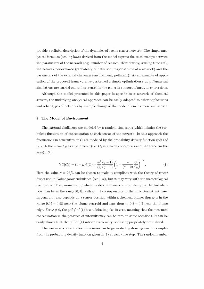
x (a.u.)

y (

a.u

.)

50 100 150 200

50

100

150

200

0.94

0.96

0.98

1

1.02

1.04

1.06

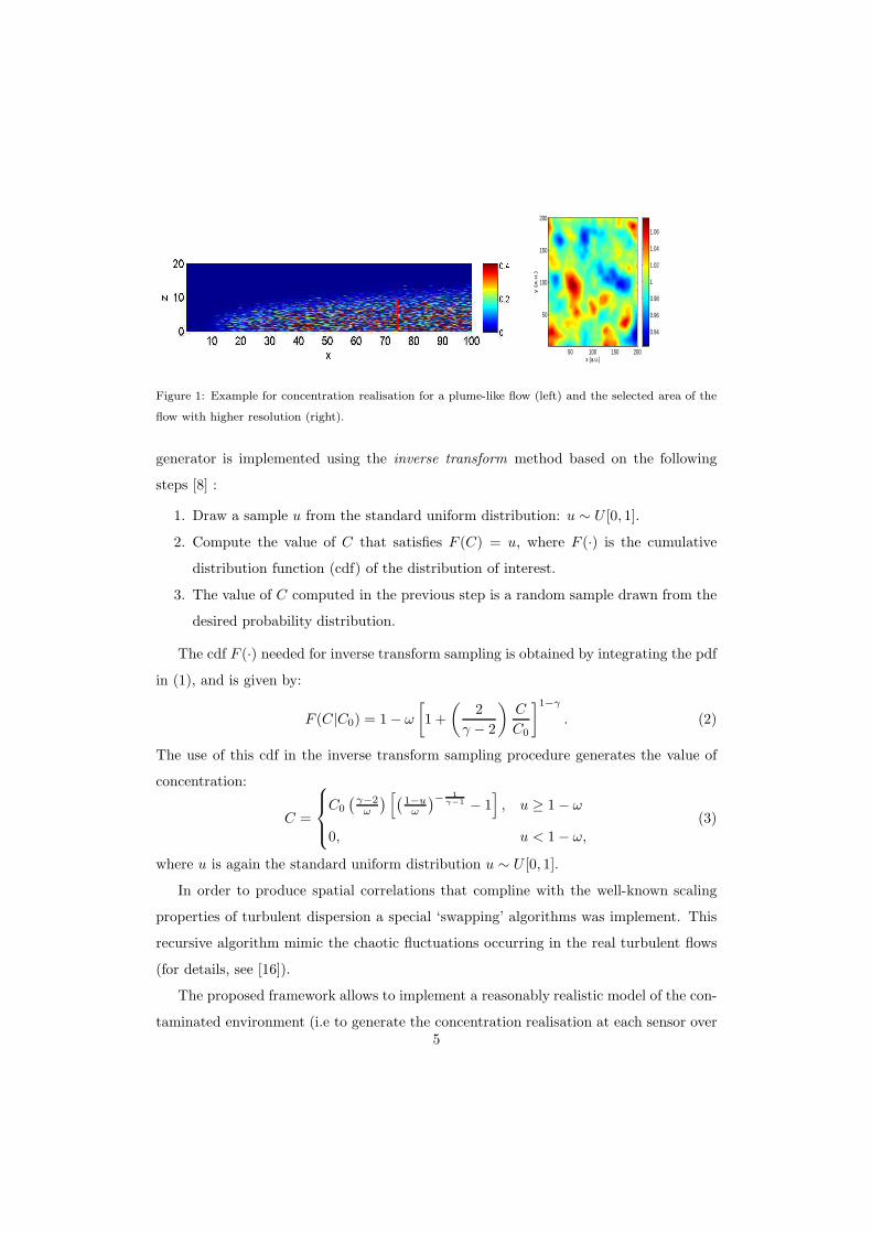
Figure 1: Example for concentration realisation for a plume-like flow (left) and the selected area of the

flow with higher resolution (right).

generator is implemented using the inverse transform method based on the following

steps [8] :

1. Draw a sample u from the standard uniform distribution: u ∼ U [0, 1].

2. Compute the value of C that satisfies F (C) = u, where F (·) is the cumulative

distribution function (cdf) of the distribution of interest.

3. The value of C computed in the previous step is a random sample drawn from the

desired probability distribution.

The cdf F (·) needed for inverse transform sampling is obtained by integrating the pdf

in (1), and is given by:

F (C|C0) = 1− ω

[

1 +

(

2

γ − 2

)

C

C0

]1−γ

. (2)

The use of this cdf in the inverse transform sampling procedure generates the value of

concentration:

C =

C0

(

γ−2ω

)

[

(

1−uω

)

−1

γ−1 − 1]

, u ≥ 1− ω

0, u < 1− ω,

(3)

where u is again the standard uniform distribution u ∼ U [0, 1].

In order to produce spatial correlations that compline with the well-known scaling

properties of turbulent dispersion a special ‘swapping’ algorithms was implement. This

recursive algorithm mimic the chaotic fluctuations occurring in the real turbulent flows

(for details, see [16]).

The proposed framework allows to implement a reasonably realistic model of the con-

taminated environment (i.e to generate the concentration realisation at each sensor over5

time), see Fig 1. Due to a universal nature of turbulence it can be used to simulate

performance of WSN in detection of either airborne and waterborne releases. The pa-

rameters γ and ω are typically estimated from geophysical observation (meteorological

and organological) and will be assumed known.

The geometrical complexity of the turbulent flow can be incorporated in the theo-

retical framework (2) by assuming a temporal and spatial variability of the mean con-

centration filed C0 ≡ C0(r, t). This way we can simulate various morphologies of the

flow (jet, wake, boundary layer, compartment flow, etc) as well as various scenarios of

hazardous release (plume, puff ), for details see [8] , [17]. For the sake of simplicity in

the current paper we consider only case C0 = const. This assumption corresponds to the

approximation when the size of WSN is less that the width of hazardous plume (see Fig

1), or to an important practical case of a ‘highly distributed’ source of pollutant (traffic,

extended industrial site or urban area [18]).

3. The Model of a Chemical Sensor

We adopt a simple binary (or “threshold”) model of a sensor, with the sensor reading

V given by:

V =

1, C ≥ C∗

0, C < C∗.

(4)

We emphasize that threshold C∗ is an internal characteristic of the sensor, unrelated to

C0 in (1). This threshold is another important parameter of our model. A chemical sensor

with bar readings, which includes many subsequent levels for concentration thresholds

mapped into a discrete sensor output, is an evident generalisation of (4).

Using (3) and (4) it is straightforward to derive the probability of detection for an

individual sensor embedded in the environment characterised by (2):

p = 1− F (C∗|C0). (5)

This aggregated parameter links the characteristics of a specific sensor C∗, the parameter

of the external challenge C0 and the environment (F (·), γ, ω).

6

4. Modeling and Analysis of Network Performance

Our focus is a wireless network of chemical sensors with dynamic collaboration. We

assume that N identical sensors (i.e with the same detection threshold C∗ and sampling

time τ∗) are uniformly distributed over the surveillance domain of area S with density

ρ = N/S.

We will model the following network protocol for dynamic collaboration. Each sensor

can be only in one of the two states: active or passive. The sensor can be activated

only by a message it receives from another sensor. Once activated, the sensor remains

in the active state during an interval of time τ∗; then it returns to the passive (sleep)

state. While being in the active state, the sensor senses the environment and if the

chemical tracer is detected (binary detection), it broadcasts a (single) message. If a sensor

receives an activation message while it is in the active state, it will ignore this message.

The broadcast capability of the sensor is characterized by its communication range r∗,

which is another important parameter of the model. The described protocol assumes

that certain sensors of the network are permanently active. The number of permanently

active sensors in the network is fixed but the actual permanently active sensors vary over

time in order to equally distribute the energy consumption of individual sensors.

The WSN following this protocol can be considered as a system of agents, interacting

with each other (by means of message exchange) and with the stochastic environment

(by means of sampling and probing). The interactions can change the state of agents

(active and passive). From this perspective this WSN is similar to the epidemic SIS

(susceptible-infected-susceptible) model [12], in which an individual can be in only two

states (susceptible or infected), and the change of state is a result of interaction (mixing)

between the individuals (which corresponds to the exchange of messages in our case).

Thus a dynamic (population) model for our system [12] is as follows:

dN+

dt= αN+N− − N+

τ∗, (6)

dN−

dt= −αN+N− +

N+

τ∗, (7)

where N+, N− denote the number of active and passive sensors, respectively. The nonlin-

ear terms on the RHS of (6) and (7) are responsible for the interaction between individuals

7

(i.e. sensors), with the parameter α being a measure of this interaction. The population

size (i.e. the number of sensors) is conserved, that is N+ +N− = N = const.

The next step is to express α in terms of the parameters of our system by invok-

ing physics based arguments used in population dynamics [12] . It is well-known that

parameter α in (6) describes the intensity (contact rate) of social interaction between

individuals in the community, so we can propose (see [12], [15])

α ∝ mp

Nτ∗, (8)

where m is the number of contacts made by an “infected” sensor during the infectious

period τ∗ (i.e the number of sensors receiving a message from an alerting sensor). In our

case we have m = πr2∗ρ. Then using N = Sρ we can write

α = Gπr2

∗

τ∗Sp, (9)

where G is a constant calibration factor, being of order unity (it must be estimated during

the network calibration); p was defined by (5). In order to simplify notation, from now

on we will assume that G is absorbed in the definition of r∗.

It is worth noting that by introducing non-dimensional variables n+ = N+/N, n− =

N−/N, τ = t/τ∗ the system (6)-(7) can be rewritten in a compact non-dimensional form

dn+

dτ= R0n+n− − n+, n− = 1− n+, (10)

with only one non-dimensional parameter

R0 = ατ∗N. (11)

The parameter R0 is well-known in epidemiology where it has the meaning of a basic

reproductive number [12].

The system (6)-(7) combined with the condition N+ + N− = N can be reduced to

one equation for y = N+

dy

dt= αy(N − y)− y

τ∗= y(b− αy), (12)

where

b = αN − 1/τ∗ = (R0 − 1)/τ∗. (13)

8

By simple change of variables z = αy/b this equation can be reduced to the standard

logistic equationdz

dt= bz(1− z), (14)

which has the well-known solution

z(t) =z0

(1 − z0) exp(−bt) + z0, (15)

where z0 = z(0).

We can see that if b < 0 then z → 0 as t → ∞ for any z0, so any individual sensor

activation in the network will “die out”, that is the network will not be able to detect

the external challenge. The same is valid for b = 0 when z = z0 = const (no response

to external challenges). Only if the condition b > 0 is satisfied, then z → 1 as t → ∞(independently of z0). In this case, after a certain transition interval, the network will

reach a new steady state with

N+

N= 1− θ,

N−

N= θ, θ =

1

ατ∗N≡ 1

R0. (16)

A fraction of active sensorsN+ at this new state is a measure of the network (positive)

response to the event of chemical contamination. From (15) it is clear that the time scale

for the network to reach the new state can be estimated from the condition e−bt ≪ 1, so

τ ≥ 1

b=

τ∗R0 − 1

. (17)

This equation provides the relationship between the scale of activation time and param-

eter R0. One can see that this scale decreases as R0 increases.

From (14), (17) it follows that an “epidemic threshold” for the sensor network is

simply ατ∗N > 1 or in terms of the ’basic reproductive number’ (11)

R0 = ατ∗N = pNπr2

∗

S> 1. (18)

Observe that sensor sampling time τ∗ has disappeared from the expression for R0. This

means that it is possible to create an information epidemic (i.e. detect a chemical pol-

lutant) for any value of τ∗, provided this time is long enough for a sensor to detect the

chemical tracer. But according to (17), the responsiveness of the whole network to the

external challenges (i.e. the time constant of detection) is, indeed, strongly dependent

on the sensor sampling time τ = τ∗/(R0 − 1).9

The expressions (16), (17) and (18) are the main analytical results of the paper. For a

given level of external challenges (i.e. C0) and meteorological conditions (i.e. γ, ω), these

expressions provide a simple yet rigorous way to estimate how a change in the network

and sensor parameters (i.e. N,C∗, τ∗) will affect the network performance (i.e. N+, τ).

We can also see that for a given external challenge the network of chemical sensors will

respond in the most effective way when its parameters are selected in the combination

which meets the criterion for ‘information epidemic” (18).

The final analytical expressions enable us to maximize the network information gain

and optimize other parameters. For example, from (16), we can readily infer the impor-

tant scaling properties of the network performance:

N−

N∼ 1

r2∗

,N−

N∼ 1

N,

N−

N∼ 1

p. (19)

For instance, if we double the communication range of an individual sensor r∗, the fraction

of inactive sensors in the network will drop four times. Likewise, if we need to reach a

specified fraction of active sensors (1 − N−/N) to be able to reliably detect a given

level of pollutant concentration, these formulas describe all possible ways of changing

the parameters of the model in order to achieve this goal.

5. Information Gain of Collaboration

We have explained earlier that the concept of DSC is important for a network with

limited energy/material resources. But the question remains will a network with DSC

be inferior (in terms of detection performance) in comparison with a benchmark network

where all sensors operate independently of each other and only report their (positive)

detections of chemical pollution to the central processor for decision making? Clearly,

such a benchmark network would be very expensive to run (all sensors would have to be

active all the time), but could provide excellent detection performance.

In this section we show that, under a certain condition, the network with DSC can

provide superior detection performance compared to the benchmark network. Let us

assume that we have δN senors continuously operating (0 ≤ δ ≤ 1). For a benchmark

network, on average, we have pδN sensors detecting pollutant. For the network with DSC

the same quantity can be estimated as p(1 − θ)N (since as we have seen the saturation

10

level of N+ does not depend on initial conditions). From here we can then deduce that

the network with DSC will provide more information (for detection of chemical pollution)

than the benchmark network if the following condition is satisfied:

θ =1

ατ∗N≤ (1− δ), (20)

which is eventually reduced to the condition of “epidemic threshold”(18) for the small

value of δ.

The value of the parameter δ can be also estimated based on the following arguments.

Let us assume that our aim is to detect a level concentration C0 associated with a

hazardous release within the time T (the constraint on time is driven by the requirement

to mitigate the toxic effect of the release). Then we can write a simple condition for the

information ‘epidemic’ in the WSN to occur during time T :

δpNT/τ∗ ≥ 1, (21)

where p is given by (5), i.e. p = 1−F (C∗|C0). Evidently, for information epidemic to be

observable, the number of continuously active sensors should be less that the number of

sensors activated due to the hazardous release. Thus from (20) we can write the following

‘consistency’ condition for the minimum value of δ

δmin ≈ τ∗pNT

≤ (1− 1

ατ∗N), (22)

or by re-writing it in terms of R0, see (16),

δmin ≈ τ∗pNT

≤ (1− 1

R0). (23)

It can be seen, that with other conditions being equal the fraction of ‘stand-by’ sensors

δmin can be made however small (since R0 ≥ 1). It implies that only a small fraction

of WSN will be active most of the time and is a clear demonstration of the energy

consumption gain associated with the ‘epidemic’ protocol.

Another important criteria for epidemic protocol can be derived by comparison of

amplitude of “detectable events” for the same number of sensors in the network with

DSC with the system of N independent sensors. For the network with DSC it is (1−θ)N

(since we use N+ to retrieve information about the environment) and for the system of

11

the same independent sensors it is still pN (since N+ is simply equal to N). Then instead

of (20) we can write

θ < (1− p) (24)

Under this condition more detectable events will occur in the presence of chemical pol-

lution by the described network with DSC (activation messages) then in a network of

stand alone sensors (signals of positive detection). This leads to the interesting threshold

condition on the number of sensors in the network

N >S

πr2∗

1

p(1− p). (25)

The last term in RHS (p(1− p))−1 has an obvious minimum 4 corresponding to p = 1/2,

so finally we arrive at the simple universal condition

N > N∗ =4

π

S

r2∗

. (26)

This condition reads that if the number of sensors in the system is greater than N∗ then

networking with DSC can provide an information gain over the benchmark network. Un-

der this condition, the network with DSC in not only desirable from the aspect of energy

conservation, but also provides better detection performance through the information

gain.

The condition p = 1/2 minimizing RHS of (25) can be considered as a criterion for an

“optimal” sensor for a given network with DSC and for a given concentration of pollutant

to be detected. Namely, from the equation F (C∗|C0) = 1/2 and using (2) we can write

C∗ = C0

(

γ − 2

2

)

[

(

1

2ω

)1/(1−γ)

− 1

]

. (27)

Given environmental parameters (γ, ω) and given the level of concentration to be de-

tected (C0), formula (27) also specifies a simple condition on detection threshold for an

individual sensor to maximize an information gain by being networked.

6. Numerical Simulations

In support of analytical derivations presented above, a network of chemical sensors

operating according to the adopted protocol for dynamic collaboration was implemented

12

in MATLAB. A comprehensive report with numerical simulations result will be published

elsewhere; here we present only some illustrative examples.

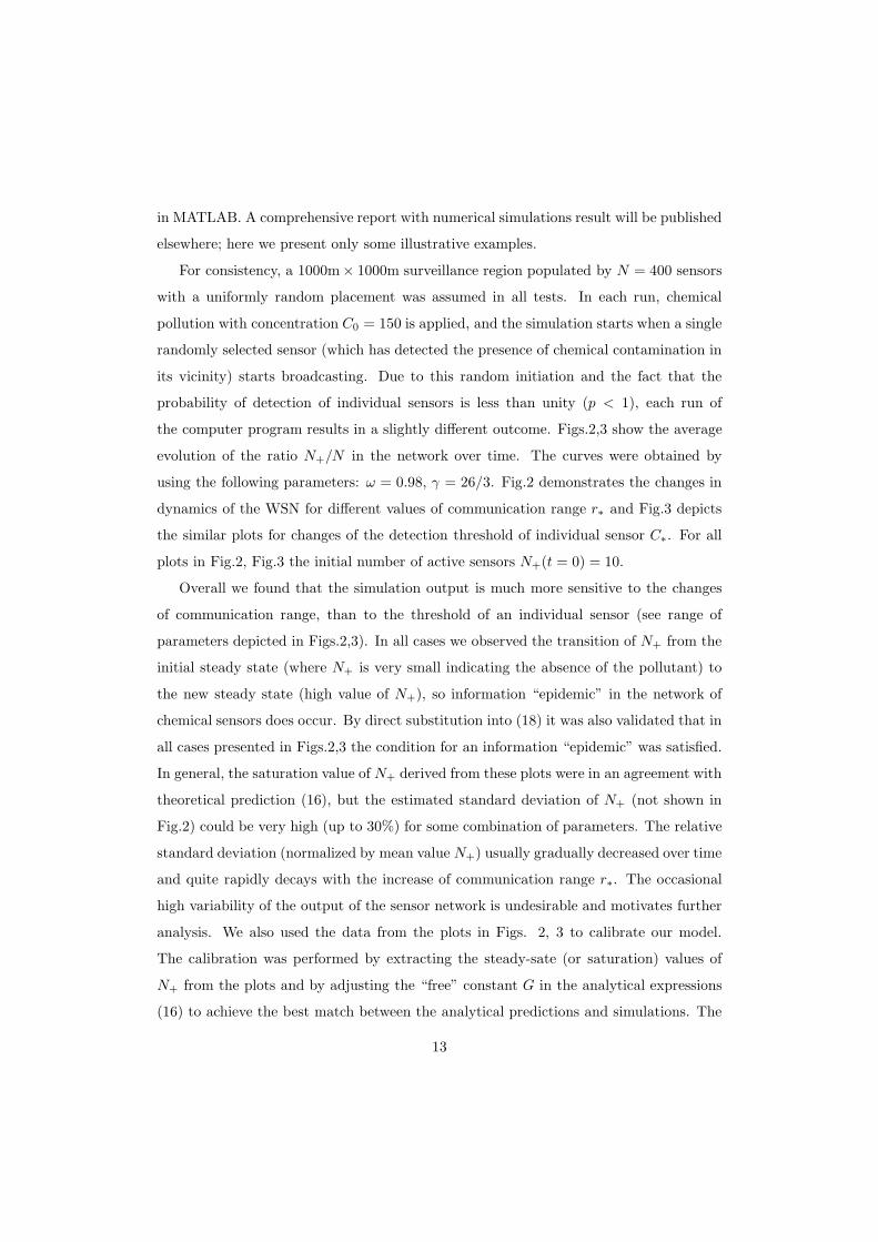
For consistency, a 1000m× 1000m surveillance region populated by N = 400 sensors

with a uniformly random placement was assumed in all tests. In each run, chemical

pollution with concentration C0 = 150 is applied, and the simulation starts when a single

randomly selected sensor (which has detected the presence of chemical contamination in

its vicinity) starts broadcasting. Due to this random initiation and the fact that the

probability of detection of individual sensors is less than unity (p < 1), each run of

the computer program results in a slightly different outcome. Figs.2,3 show the average

evolution of the ratio N+/N in the network over time. The curves were obtained by

using the following parameters: ω = 0.98, γ = 26/3. Fig.2 demonstrates the changes in

dynamics of the WSN for different values of communication range r∗ and Fig.3 depicts

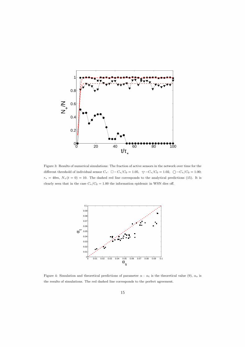
the similar plots for changes of the detection threshold of individual sensor C∗. For all

plots in Fig.2, Fig.3 the initial number of active sensors N+(t = 0) = 10.

Overall we found that the simulation output is much more sensitive to the changes

of communication range, than to the threshold of an individual sensor (see range of

parameters depicted in Figs.2,3). In all cases we observed the transition of N+ from the

initial steady state (where N+ is very small indicating the absence of the pollutant) to

the new steady state (high value of N+), so information “epidemic” in the network of

chemical sensors does occur. By direct substitution into (18) it was also validated that in

all cases presented in Figs.2,3 the condition for an information “epidemic” was satisfied.

In general, the saturation value of N+ derived from these plots were in an agreement with

theoretical prediction (16), but the estimated standard deviation of N+ (not shown in

Fig.2) could be very high (up to 30%) for some combination of parameters. The relative

standard deviation (normalized by mean value N+) usually gradually decreased over time

and quite rapidly decays with the increase of communication range r∗. The occasional

high variability of the output of the sensor network is undesirable and motivates further

analysis. We also used the data from the plots in Figs. 2, 3 to calibrate our model.

The calibration was performed by extracting the steady-sate (or saturation) values of

N+ from the plots and by adjusting the “free” constant G in the analytical expressions

(16) to achieve the best match between the analytical predictions and simulations. The

13

0 20 40 60 80 1000

0.2

0.4

0.6

0.8

1

t/τ*

N+/N

Figure 2: Results of numerical simulations: The fraction of active sensors in the network over time for

the different communication range r∗: ♦− r∗ = 40m, �− r∗ = 30m, ▽−r∗ = 27m, ©−r∗ = 20m;

C∗/C0 = 1.03, N+(t = 0) = 10. The dashed red line corresponds to the analytical predictions (15). It

is clearly seen that in the case r∗ = 20m the information epidemic in WSN dies off.

value G ≈ 0.7 seems to provide an optimal agreement with the presented simulations.

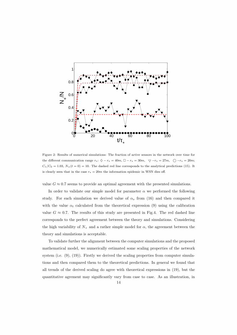
In order to validate our simple model for parameter α we performed the following

study. For each simulation we derived value of αs from (16) and then compared it

with the value αt calculated from the theoretical expression (9) using the calibration

value G ≈ 0.7. The results of this study are presented in Fig.4. The red dashed line

corresponds to the perfect agreement between the theory and simulations. Considering

the high variability of N+ and a rather simple model for α, the agreement between the

theory and simulations is acceptable.

To validate further the alignment between the computer simulations and the proposed

mathematical model, we numerically estimated some scaling properties of the network

system (i.e. (9), (19)). Firstly we derived the scaling properties from computer simula-

tions and then compared them to the theoretical predictions. In general we found that

all trends of the derived scaling do agree with theoretical expressions in (19), but the

quantitative agrement may significantly vary from case to case. As an illustration, in

14

0 20 40 60 80 1000

0.2

0.4

0.6

0.8

1

t/τ*

N+/N

Figure 3: Results of numerical simulations: The fraction of active sensors in the network over time for the

different threshold of individual sensor C∗: �−C∗/C0 = 1.05, ▽−C∗/C0 = 1.02, ©−C∗/C0 = 1.00;

r∗ = 40m, N+(t = 0) = 10. The dashed red line corresponds to the analytical predictions (15). It is

clearly seen that in the case C∗/C0 = 1.00 the information epidemic in WSN dies off.

0 0.01 0.02 0.03 0.04 0.05 0.06 0.07 0.08 0.09 0.10

0.01

0.02

0.03

0.04

0.05

0.06

0.07

0.08

0.09

0.1

αs

α t

Figure 4: Simulation and theoretical predictions of parameter α : αt is the theoretical value (9), αs is

the results of simulations. The red dashed line corresponds to the perfect agreement.

15

0 0.1 0.2 0.3 0.4 0.5 0.6 0.7−0.2

0

0.2

0.4

0.6

0.8

1

1.2

p

α

Figure 5: Parameter α as a function of p extracted from numerical simulations in log-log scale. The

dashed line corresponds to the power-law fit α ∝ pq, q = 1.27, theoretical prediction corresponds to

q = 1, see (8).

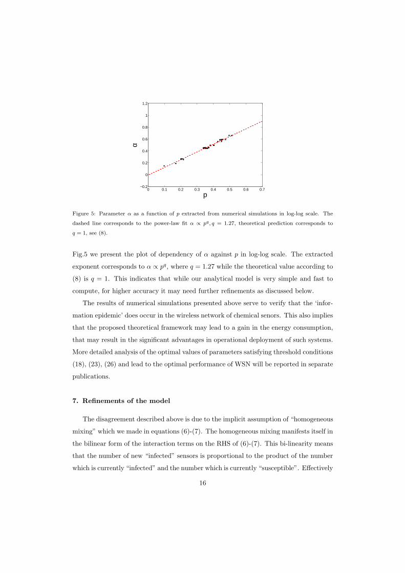
Fig.5 we present the plot of dependency of α against p in log-log scale. The extracted

exponent corresponds to α ∝ pq, where q = 1.27 while the theoretical value according to

(8) is q = 1. This indicates that while our analytical model is very simple and fast to

compute, for higher accuracy it may need further refinements as discussed below.

The results of numerical simulations presented above serve to verify that the ‘infor-

mation epidemic’ does occur in the wireless network of chemical senors. This also implies

that the proposed theoretical framework may lead to a gain in the energy consumption,

that may result in the significant advantages in operational deployment of such systems.

More detailed analysis of the optimal values of parameters satisfying threshold conditions

(18), (23), (26) and lead to the optimal performance of WSN will be reported in separate

publications.

7. Refinements of the model

The disagreement described above is due to the implicit assumption of “homogeneous

mixing” which we made in equations (6)-(7). The homogeneous mixing manifests itself in

the bilinear form of the interaction terms on the RHS of (6)-(7). This bi-linearity means

that the number of new “infected” sensors is proportional to the product of the number

which is currently “infected” and the number which is currently “susceptible”. Effectively

16

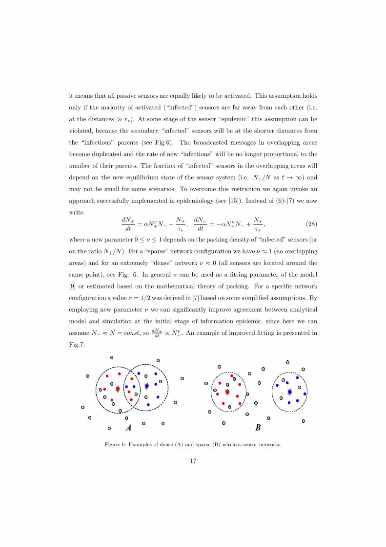
it means that all passive sensors are equally likely to be activated. This assumption holds

only if the majority of activated (“infected”) sensors are far away from each other (i.e.

at the distances ≫ r∗). At some stage of the sensor “epidemic” this assumption can be

violated, because the secondary “infected” sensors will be at the shorter distances from

the “infectious” parents (see Fig.6). The broadcasted messages in overlapping areas

become duplicated and the rate of new “infections” will be no longer proportional to the

number of their parents. The fraction of “infected” sensors in the overlapping areas will

depend on the new equilibrium state of the sensor system (i.e. N+/N as t → ∞) and

may not be small for some scenarios. To overcome this restriction we again invoke an

approach successfully implemented in epidemiology (see [15]). Instead of (6)-(7) we now

writedN+

dt= αNν

+N− − N+

τ∗,

dN−

dt= −αNν

+N− +N+

τ∗, (28)

where a new parameter 0 ≤ ν ≤ 1 depends on the packing density of “infected” sensors (or

on the ratio N+/N). For a “sparse” network configuration we have ν ≈ 1 (no overlapping

areas) and for an extremely “dense” network ν ≈ 0 (all sensors are located around the

same point), see Fig. 6. In general ν can be used as a fitting parameter of the model

[9] or estimated based on the mathematical theory of packing. For a specific network

configuration a value ν = 1/2 was derived in [7] based on some simplified assumptions. By

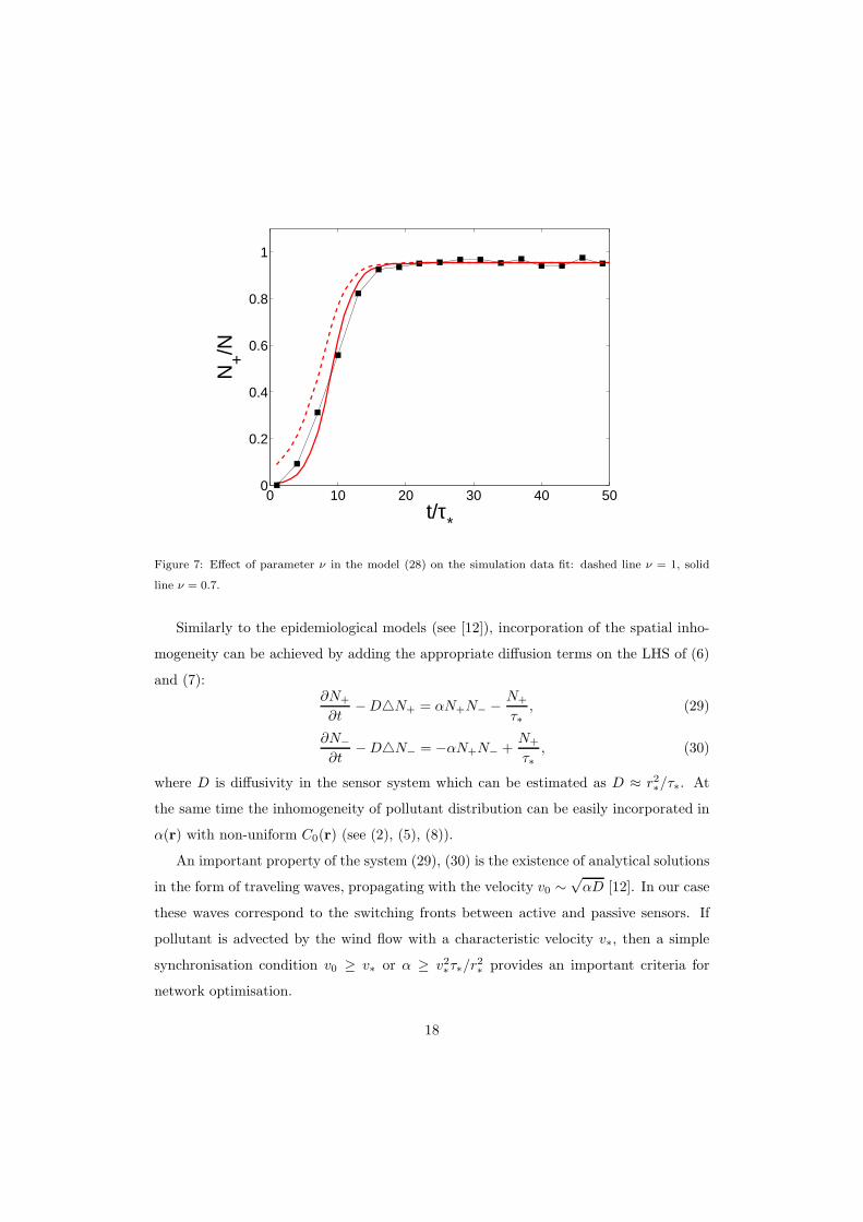
employing new parameter ν we can significantly improve agreement between analytical

model and simulation at the initial stage of information epidemic, since here we can

assume N− ≈ N = const, so dN+

dt ∝ Nν+. An example of improved fitting is presented in

Fig.7.

A B

Figure 6: Examples of dense (A) and sparse (B) wireless sensor networks.

17

0 10 20 30 40 500

0.2

0.4

0.6

0.8

1

t/τ*

N+/N

Figure 7: Effect of parameter ν in the model (28) on the simulation data fit: dashed line ν = 1, solid

line ν = 0.7.

Similarly to the epidemiological models (see [12]), incorporation of the spatial inho-

mogeneity can be achieved by adding the appropriate diffusion terms on the LHS of (6)

and (7):∂N+

∂t−D△N+ = αN+N− − N+

τ∗, (29)

∂N−

∂t−D△N− = −αN+N− +

N+

τ∗, (30)

where D is diffusivity in the sensor system which can be estimated as D ≈ r2∗/τ∗. At

the same time the inhomogeneity of pollutant distribution can be easily incorporated in

α(r) with non-uniform C0(r) (see (2), (5), (8)).

An important property of the system (29), (30) is the existence of analytical solutions

in the form of traveling waves, propagating with the velocity v0 ∼√αD [12]. In our case

these waves correspond to the switching fronts between active and passive sensors. If

pollutant is advected by the wind flow with a characteristic velocity v∗, then a simple

synchronisation condition v0 ≥ v∗ or α ≥ v2∗τ∗/r

2∗provides an important criteria for

network optimisation.

18

Another interesting extension of the proposed model is the introduction of the con-

cept of a faulty sensor, a sensor which is no longer available for sensing and networking.

This state of a sensor would correspond to the removed population segment in the epi-

demiological framework and can be attributed to any kind of faults (flat battery, software

malfunction, hardware defects etc). As in the celebrated SIR epidemiological model [12],

a new state results in the third equation for N0 in the system (6)-(7) with a new temporal

parameter - an average operational time (the lifespan) of a sensor. The total number

of sensors will be still conserved: N = N+ + N− + N0 = const. This model provides a

more realistic representation of an operational sensor systems and allows us to estimate

such important parameters as the operational lifetime of the network and the reliability

of the network.

8. Conclusions

We developed a “bio-inspired” model of a network of chemical sensors with dynamic

collaboration for the purpose of energy conservation and information gain. The proposed

model leverages on the existing theoretical discoveries from epidemiology resulting in a

simple analytical model for the analysis of network dynamics. The analytical model

enabled us to formulate analytically the conditions for the network performance. Thus

we found an optimal configuration which, within the underlying assumptions, yields a

balance between the number of sensors, detected concentration, the sampling time and

the communication range. The findings are partly supported by numerical simulations.

Further work is required to address the model refinements and generalisations.

9. Acknowledgement

The authors would like to thank Ralph Gailis, Ajith Gunatilaka and Chris Woodruff

for helpful technical discussions and Champake Mendis for his assistance in the software

implementation of the proposed model.

References

[1] C. S. Raghavendra, K. M. Sivalingam, Taieb Znati. (2005) Wireless Sensor Networks. Springer,

USA, 2005.

19

[2] P. E. Bieringer, A. Wyszogrodzki, J. Weil and G. Bieberbach. An Evaluation of Propylene Sampler

Grid Designs for the FFT07 Field Program(2006), Tech. Report, National Center for Atmospheric

Research, Boulder, USA.

[3] E. Ertin, J. W. Fisher, L. C. Potter.(2003) Maximum Mutual Information Principle for Dynamic

Sensor Query Problems. Lecture Notes in Computer Science: Information Processing in Sensor

Networks, 2003 2634, pp. 91-104.

[4] F. Zhao, J. Shin, J. Reich. (2002) Information-Driven Dynamic Sensor Collaboration for Tracking

Applications. IEEE Signal Processing Magazine, 2002, 19, 2, pp. 61–72.

[5] J. Mathieu, G. Hwang, J. Dunyak (2006). The State of the Art and the State of the Practice:

Transferring Insights from Complex Biological Systems to the Exploitation of Netted Sensors in

Command and Control Enterprises, 2006 MITRE Technichal Papers, July, 2006, MITRE Corpo-

ration, USA.

[6] A. Khelil, C. Becker, J. Tian, K. Rothermel.(2002) An Epidemic Model for Information Diffusion

in MANETs.In MSWiM 2002: Proceedings of the 5th ACM international workshop on Modeling

analysis and simulation of wireless and mobile systems, Atlanta, Georgia, USA, 2002, pp. 54–60.

[7] P. De, Y. Liu, S. K. Das. (2007) An Epidemic Theoretic Framework for Evaluating Broadcast Pro-

tocols in Wireless Sensor Networks. In MASS 2007: Proceedings of IEEE Internatonal Conference

on Mobile Adhoc and Sensor Systems, Pisa, Italy, 2007, pp 1–9.

[8] A. Gunatilaka, B.Ristic, A.Skvortsov, M. Morelande. (2008) Parameter Estimation of a Continuous

Chemical Plume Source. in Fusion 2008: 11th International Conference on Information Fusion,

Cologne, Germany, 2008, pp. 1-8.

[9] B.Ristic, A.Skvortsov, M.Morelande. (2009) Predicting the Progress and the Peak of an Epidemics.

in ICASSP 2009: Proceedings of 2009 IEEE International Conference on Acoustics, Speech and

Signal Processing, Taiwan, April, 2009.

[10] A.Dekker, A.Skvortsov. (2009) Topological Issues in Sensor Networks. in MODSIM 2009: 2009

MSSANZ International Congress on Modelling and Simulation, Cairns, Australia, 2009.

[11] S. Eubank, V. S. Anil Kumar, M. Marathe. (2008) Epidemiology and Wireless Communication:

Tight Analogy or Loose Metaphor? Lecture Notes in Computer Science: Bio-Inspired Computing

and Communication, 2008, 5151, pp. 91-104.

[12] J. D. Murray.(2002) Mathematical Biology, Springer, USA, v 1,2. 2002

[13] V. Bisignanesi, M.S. Borgas (2007). Models for integrated pest management with chemicals in

atmospheric surface layers. Ecological modelling, 2007, 201, 1, pp. 2–10.

[14] P. D. Stroud, S. J. Sydoriak, J. M. Riese, J. P. Smith, S. M. Mniszewski, and P. R. Romero.

(2006) Semi-empirical Power-law Scaling of New Infection Rate to Model Epidemic dynamics with

Inhomogeneous Mixing, Mathematical Biosciences, 203, pp. 301–318.

[15] A.T. Skvortsov, R.B.Connell, P.D. Dawson, R.M. Gailis. (2007) Epidemic Spread Modeling: Align-

ment of Agent-Based Simulation with a Simple Mathematical Model. in BIOCOMP 2007: Proceed-

ings of International Conference on Bioinformatics and Computational Biology, Las Vegas Nevada,

USA, CSREA Press, 2007, 2, pp 487–490.

20

[16] A. Gunatilaka, A. Skvortsov, and R. Gailis. (2008) Progress in DSTO CBR simulation environment

development, Land Warfare Conference (LWC2008), Brisbane, 2008, pp. 62–68.

[17] A.Skvortsov, E.Yee. Scaling laws of peripheral mixing of passive scalar in a wall-shear layer (2008).

Phys. Rev. E 83, 036303–11.

[18] M. Jamriska, T. C. DuBois, A. Skvortsov Statistical characterisation of bio-aerosol background in

an urban environment (2011), http://www.arxiv.org/pdf/1110.4184

21