Embed Size (px)
Citation preview
Calculations in SCIA EngineerTypes of analysis, FE mesh, Soil-In, Seismicity, Plasticity, AutoDesign, Optimisation
Contacts 12Introduction to calculation 14Checking the data 15
Introduction to check of data 15
Parameters of data check 15
Checkof nodes 15
Checkof 1Dmembers 16
Checkof structure 16
Checkof additional data 16
Performing the check of data 17
Collision between entities 17
Checkof one group of entities 18
Checkof two groupsof entities 18
Clash checkparameters 18
Generating the FE mesh 20Parameters of FE mesh 20
Mesh 20
1D elements (1Dmembers) 20
2D elements (slabs) 21
Average number of tilesof 1D element 22
Division on haunchesand arbitrarybeams 22
Generation of eccentricelementsonmemberswith variable height 22
Average size of cables, tendons, elementson subsoil 22
Previewing the FE mesh 23
TabStructure >GroupMesh 23
TabStructure >Group Local axes 23
Tab Labels>GroupMesh 23
Tab Labels>Group Labelsof local axes 23
Analysis of a haunch versus mesh size 24
Analysis of a haunch with reference to eccentric elements 27
Natural vibration analysis versus mesh size 29
Analysis of a beam on elastic foundation versus mesh size 32
- 2 -
Mesh refinement 36
Mesh refinement 36
Refinement around a node 36
Refinement along a line 36
Refinement acrossan area 37
Calculation types 38General calculation parameters 38
Number of result sections per member 39
Static linear calculation 41
Static non-linear calculation 41
Setup parameters 41
Solver parameters 42
Limitsof the calculation 43
Sample analysis - guyed mast 43
Initial stress options 48
Initial deformation and curvature 48
Initial deformation and curvature 48
Simple inclination 49
Inclination and curvature of beams 50
Inclination functions 51
Inclination function and curvature of beams 54
Deformation from load case 54
Dynamic natural vibration calculation 56
Calculation for selectedmasscombinations 58
Dynamic forced harmonic vibration 58
Harmonic band analysis 58
Context - Typical usage 58
Description 59
Output of results 59
(Little) Theoretical background 60
Combinationwith other load cases 60
Input of the load case for theHarmonicBandAnalysis 60
- 3 -
Chapter 0
Performing theHarmonicBandAnalysis 61
Displayof resultsof HarmonicBandAnalysis 61
Calculation model for dynamic analysis 64
Dynamic seismic calculation 66
Buckling analysis 66
Calculation for selected stability combinations 66
Assumptionsof linear buckling calculation 67
Sample analysis - column 67
Nonlinear stability calculation 70
Non uniform damping in dynamic calculation 71
Non uniformdamping 71
Damper setup 73
Defining a new damping group 74
Defining a new damper 74
Performing the calculation 76Calculation dialog for v16 and earlier 77
Single analysis / Batch analysis 78
Typesof calculations 78
Buttons 78
Calculation dialog for v17 79
General description 79
Selection of load casesor nonlinear combinations for calculation 81
Typesof calculations 83
Typesof other processes 83
Buttons 83
Adjusting the calculation parameters 83
Performing the calculation 84
Controlling and reviewing the calculation process 84
Performing the repetitious calculations 84
Repairing the instability of model 85
Maximumdisplacement hasbeen reached 85
Singular stiffnessmatrix 85
- 4 -

Solution methods 88Direct solution 88
Iterative solution 88
Timoshenko theory 89
Newton-Raphson method 89
Modified_Newton_Raphson_method 90
Picard_method 91
Smoothening of non-averaged values 92
a) Standard averaging 94
b) Smoothening along edges 96
c) Shear forces 98
d) Moments 99
Initial deformations 104Introduction to initial deformations 104
Initial-deformation manager 104
Initial deformation curve 104
Defining a new initial deformation curve 105
Applying the initial deformation 106
Soil-In 107Introduction 107
The influence of subsoil in the vicinityof the structure 107
Soil-in output 107
C parameters (explanation from theoretical background of FEMsolver) 108
Support on surface 109
The surface support properties 110
Subsoil in the 3D model 111
Soil borehole 111
Settlement input data 116
Geological areas 116
Foundation base 118
Soil surface 119
Surface support 120
- 5 -
Chapter 0
Subsoil library 122
Required parameters for Soil-in calculation 122
Soil-in settings in theSolver setup 123
Soil-in calculation 124
Soil-in iterative cycle 124
Quadraticnorm to compare the results from the last and the previous iteration 126
Theoryabout the derivation process 127
The results of soil-in 128
2D data viewer 128
Results 129
Results for each iteration cycle 133
Soil-in and Pile design 135
Advanced tips 136
Foundation at great depth 136
The effect of the subsoil outside the structure 136
Pad foundation and soil-in 137
What if themodel is correct but the iteration isnot finished 140
What if the load iswrongly inserted? 140
What if the symmetrical structure givesnon-symmetrical results? 141
What if geological fault in the subsoil isneeded? 141
How to use additional plates 143
How to calculate the platewithout soilin 146
How to calculate the platewith soilin. 149
How to create the additional platesaround 153
Seismic Analysis of Buildings 159Introduction 159
Reduced Analysis Model 159
Introduction: themodified IRSmethod 159
Benchmarks 161
Using the IRSmodel in SCIAEngineer 165
IRS: Toomanyeigen values requested / Non-associatedR-node detected 171
Storey Results 178
- 6 -
Summarystorey results 179
Detailed StoreyResults 181
SummaryStoreyResults 182
Result typeStoreyData 183
Result typesDisplacements&Accelerations 188
Detailed StoreyResults 192
Result type Internal forces 194
Result typeResulting forces–Member grouping per member 203
Result typeResulting forces–Member grouping per storey 205
Output of total vertical forces in all storeys (load descending) 206
Internal forces in all supportingmembersof a storey 207
Average forces in all supportingmembersof a storey 208
Resulting forces in all supportingmembersof a storey 209
Modal Superposition 209
Introduction – theoretical background 209
Modal superposition in SCIAEngineer 213
Accidental Eccentricity 215
Introduction 215
Definition of the accidental eccentricity 215
Calculation of the effectsof eccentricity 217
Analysis& resultsof accidental eccentricity 220
Equivalent Lateral Forces (ELF) 222
Introduction 222
Defining anELF seismic load case 223
Calculation of the Equivalent Lateral Forces 225
Results 229
References 230
General Plastic Analysis 230Theoretical background 232
Tresca yield criterion 232
VonMisesyield criterion 232
Drucker-Prager yield criterion 234
- 7 -

Chapter 0
Mohr-Coulomb yield criterion 235
Finite elementmodel 236
Using general plasticity in SCIA Engineer 236
Project settings 237
Nonlinear propertiesofmaterials 237
Assigning plasticbehaviour to a 2D member 243
Plastic hinges 244Introduction to plastic hinges 244
Plastic hinges to EC3 244
Plastic hinges to DIN 18800 245
Plastic hinges to NEN 245
For IPEsections 245
For other sections 246
Calculating with plastic hinges 246
AutoDesign - Global optimization 247Introduction 247
Principles of Autodesign 247
Autodesign types 247
Autodesign manager 249
Defining a new optimisation 254
Autodesign parameters and criteria 257
Property 258
Parameters 258
Edit AdvancedAutodesign 261
Picture 262
Control buttons 263
Concrete – Automatic member reinforcement design (AMRD) 263
Autodesign inConcrete Advanced service 264
Theoretical background for AMRD 265
Illustrative example 269
Steel – Cross-section AutoDesign 272
Autodesign in Steel service 273
- 8 -
Illustrative example 274
Steel - Fire resistance AutoDesign 278
Autodesign in Steel service 279
Illustrative example 280
Steel - Corrugated web AutoDesign 284
Autodesign in SIN beamcheckservice 285
Illustrative example 286
Steel - Lapped purlin/girt AutoDesign (only IBC code) 290
Autodesign inCheckLRFD service 291
Illustrative example 292
Steel connection - Bolted diagonal AutoDesign 297
Autodesign in Bolted diagonal service 298
Illustrative example 299
Timber – Cross-section AutoDesign 303
Autodesign in Timber service 303
Illustrative example 304
Aluminium – Cross-section AutoDesign 307
Autodesign in Aluminium service 308
Illustrative example 309
Geotechnics – Pad foundation AutoDesign 312
Autodesign inGeotechnicsservice 313
Illustrative example 314
Steel hall - Frame Autodesign 317
Frame –CSSheight Autodesign 319
Frame –webAutodesign 321
Frame - flangeAutodesign 325
Frame - flange thicknessAutodesign 327
Frame - deflection Autodesign 330
Frame –Autodesignmanager 333
SCIA Optimizer 337Introduction 337
About SCIAEngineer Optimizer 337
- 9 -
Chapter 0
Motivation 338
Worked example 339
Structure modelling 339
Starting the project in SCIAEngineer 339
Calculation andAutodesign 343
Parameters 346
XML documents 349
Input XML 351
Output XML 351
Optimizing tool 353
SCIAEngineer project link 354
Formulas 355
Optimization analysis 356
User Solution 358
Optimization in progress 358
Result 359
Conclusion 360
Steel frame design 363Getting started 363
Starting a project 363
Structure definition 366
Cross-sections, listsandmatricesdefinition 366
Geometry 373
CheckStructure data 382
Loads and combinations 383
LoadCasesand LoadGroups 384
Load 386
Combinations 394
Classes 397
Steel 400
LTB restrains 400
Optimization 402
- 10 -

Check of designed structure 406
Calculation 406
Steel checks 407
Displacementsof nodes 410
Global optimisation 413Introduction 413
AutoDesign manager 413
Defining a new optimisation 413
AutoDesign parametersand criteria 414
- 11 -
Contacts
Belgium HeadquartersSCIA nv
Industrieweg 1007
B-3540 Herk-de-Stad
Tel: +32 13 55 17 75
E-mail: [email protected]
Support Phone
CAE (SCIA Engineer)
Tel: +32 13 55 09 90
CAD (Allplan)
Tel: +32 13 55 09 80
Support E-mail:
FranceSCIA France sarl
Centre d'Affaires
16, place du Général de Gaulle
FR-59800 Lille
Tel.: +33 3.28.33.28.67
Fax: +33 3.28.33.28.69
E-mail: [email protected]
Agence commerciale
8, Place des vins de france
FR-75012 Paris
Tel.: +33 3.28.33.28.67
Fax: +33 3.28.33.28.69
E-mail: [email protected]
BrazilSCIA do Brasil Software Ltda
Rua Dr. LuizMigliano, 1986 - sala 702 , CEP
SP 05711-001 São Paulo
Tel.: +55 11 4314-5880
E-mail: [email protected]
GermanySCIA Software GmbH
Technologie ZentrumDortmund, Emil-Figge-Strasse 76-80
D-44227 Dortmund
Tel.: +49 231/9742586
Fax: +49 231/9742587
E-mail: [email protected]
NetherlandsSCIA Nederland B.V.
Wassenaarweg 40
NL-6843 NWARNHEM
Tel.:+31 26 320 12 30
Fax.: +31 26 320 12 39
E-mail: [email protected]
SwitzerlandSCIA SwissOffice
Dürenbergstrasse 24
CH-3212 Gurmels
Tel.: +41 26 341 74 11
Fax: +41 26 341 74 13
E-mail: [email protected]
Czech RepublicSCIA CZ s.r.o. Praha
Evropská 2591/33d
160 00 Praha 6
Tel.: +420 226 205 600
Fax: +420 226 201 673
E-mail: [email protected]
SCIA CZ s.r.o. Brno
Slavickova 827/1a
638 00 Brno
Tel.: +420 530 501 570
Fax: +420 226 201 673
SlovakiaSCIA SK s.r.o.
Murgašova 1298/16
SK-010 01 Žilina
Tel.: +421 415 003 070
Fax: +421 415 003 072
E-mail: [email protected]
- 12 -

Contacts
E-mail: [email protected]
AustriaSCIA Datenservice Ges.m.b.H.
Dresdnerstrasse 68/2/6/9
A-1200 WIEN
Tel.: +43 1 7433232-11
Fax: +43 1 7433232-20
E-mail: [email protected]
Support
Tel.: +43 1 7433232-12
E-mail: [email protected]
All information in this document is subject to modification without prior notice. No part of this manual may be reproduced,stored in a database or retrieval system or published, in any form or in anyway, electronically, mechanically, by print, photoprint, microfilm or anyother meanswithout prior written permission from the publisher. SCIAis not responsible for anydirector indirect damage because of imperfections in the documentation and/or the software.
©Copyright 2018SCIAnv. All rights reserved.
Document created: 06 / 05 / 2018
SCIAEngineer 18.0
- 13 -

Chapter 1
Introduction to calculation
Once themodel of an analysed structure is created, the calculation of required typemaybe performed.
SCIA Engineer applies the deformation variant of finite element method. The employed beam finite element takes accountof shear deformation.
Detailed information about the applied calculationmethodsmaybe found:
l in the following chaptersand
l in a separate bookAdvanced calculationsaccessible viamenu functionHelp >Contents>Advanced calculations.
- 14 -

Checking the data
Checking the data
Introduction to check of dataIt is a good practice and sometimes even necessity to check the data of the model from time to time or at least before cal-culation. Especially for excessive models that have been modified by means of various manipulation functions, it may hap-pen that themodel containssome invalid or obsolete data. Such data should be removed from the project as they:
l occupymemoryunnecessarily,
l couldmislead some functions.
SCIA Engineer provides aN easy- to-use wizard that automatically searches the project and reveals improper or invaliddata.
Note : The check of data is important from one more point of view. By default the inter-secting 1D members are not joined to each other. If they are supposed to act together, alinked node must be defined in their intersection. The Check of data function traces suchplaces and suggests the user to make an automatic connection of affected 1D members.This operation may thus resolve possible future problems with numerically unstable solu-tion.
Parameters of data checkTheCheckdata function tries to reveal invalid data in the project.
Check of nodesSearchnodes
This option is ALWAYS ON. This check ensures that nodal data are correct. This option is a kind of pro-tection against possible damage of saved data.
Searchduplicatenodes
If ON, the program searches for nodes with identical co-ordinates If two nodes of identical position arefound they are merged into a single node (i.e. one of them is removed).
The value defined in Minimal distance between two points in the Mesh Setup dialogue is used for thischeck.
Ignoreparameters
This option is effective only if parametric nodes have been defined in the project.
If ON, only the co-ordinates (calculated from input parameters) are checked. If two nodes of the same co-ordinates are found, they are merged into one node.
If OFF, the check procedure consists of two steps. First, the co-ordinates are checked. If any two nodes ofthe same co-ordinates are discovered, the defining parameters are check in the second step. If the twonodes are defined by means of the same parameters, they are considered duplicate and merged into one.If, however, the two nodes are defined using different parameters or different formulas, the nodes are letunchanged.
If theCheckof nodesdiscoversanydisorder or "mess" in nodal data, another dialogue isdisplayed.
Members with This item shows the number of discovered undefined nodes. Such nodes MUST always be corrected
- 15 -
Chapter 2
undefinednodes
and therefore the checkbox is ALWAYS ON.
Free nodes
If any free nodes are found in the project (i.e. nodes that do not belong to any member) the user maydelete them.
It is recommended to delete any free nodes unless the user has a specific reason for their existence inthe project (e.g. free nodesmay represent a temporary state during the definition of a complexmodel).
Duplicatenodes
Any duplicate nodes found in the project are reported here and it up to the user whether they will bedeleted or not.
It is recommended to delete duplicate nodes.
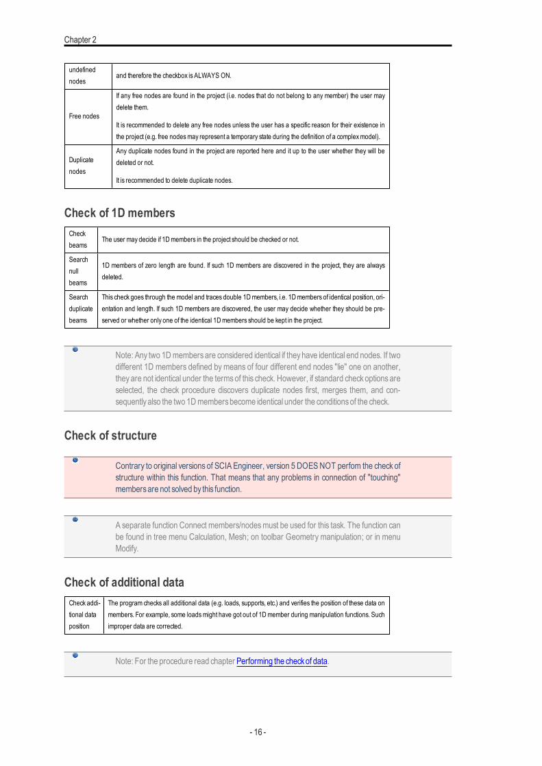
Check of 1D membersCheckbeams
The user may decide if 1Dmembers in the project should be checked or not.
Searchnullbeams
1D members of zero length are found. If such 1D members are discovered in the project, they are alwaysdeleted.
Searchduplicatebeams
This check goes through the model and traces double 1Dmembers, i.e. 1Dmembers of identical position, ori-entation and length. If such 1D members are discovered, the user may decide whether they should be pre-served or whether only one of the identical 1Dmembers should be kept in the project.
Note: Any two 1Dmembersare considered identical if theyhave identical end nodes. If twodifferent 1D members defined by means of four different end nodes "lie" one on another,they are not identical under the termsof this check. However, if standard checkoptions areselected, the check procedure discovers duplicate nodes first, merges them, and con-sequentlyalso the two 1Dmembersbecome identical under the conditionsof the check.
Check of structure
Contrary to original versions of SCIA Engineer, version 5 DOESNOT perfom the check ofstructure within this function. That means that any problems in connection of "touching"membersare not solved by this function.
A separate function Connect members/nodesmust be used for this task. The function canbe found in tree menu Calculation, Mesh; on toolbar Geometry manipulation; or in menuModify.
Check of additional dataCheck addi-tional dataposition
The program checks all additional data (e.g. loads, supports, etc.) and verifies the position of these data onmembers. For example, some loadsmight have got out of 1Dmember during manipulation functions. Suchimproper data are corrected.
Note: For the procedure read chapter Performing the checkof data.
- 16 -
Checking the data
Performing the check of dataThe procedure for the check of data
1. Start functionCheckof data:
1. either usingmenu function Tree >Calculation,mesh >Checkstructure data,
2. or using treemenu functionCalculation,mesh >Checkstructure data.
2. TheCheckdatawizard opens the setup dialogue on the screen.
3. Select the data types that should be searched and verified.
4. Start the checkwith button [Check].
5. The programscrutinisesall the project data.
6. If no disproportion is revealed amessage telling that no problemshave been found is issued.
7. If something suspicious has been discovered, the wizard displays the statistics in the dialogue. Numbers of invalid entitiesfor individual data typesare stated.
8. Now, decide which data types should be corrected and which ones left unchanged (i.e. put a tick to the data type thatshould be corrected and remove the tick from those types that should be skipped during the correction phase).
9. Finish theData checkwith button [Continue].
10. The invalid data are removed from the project.
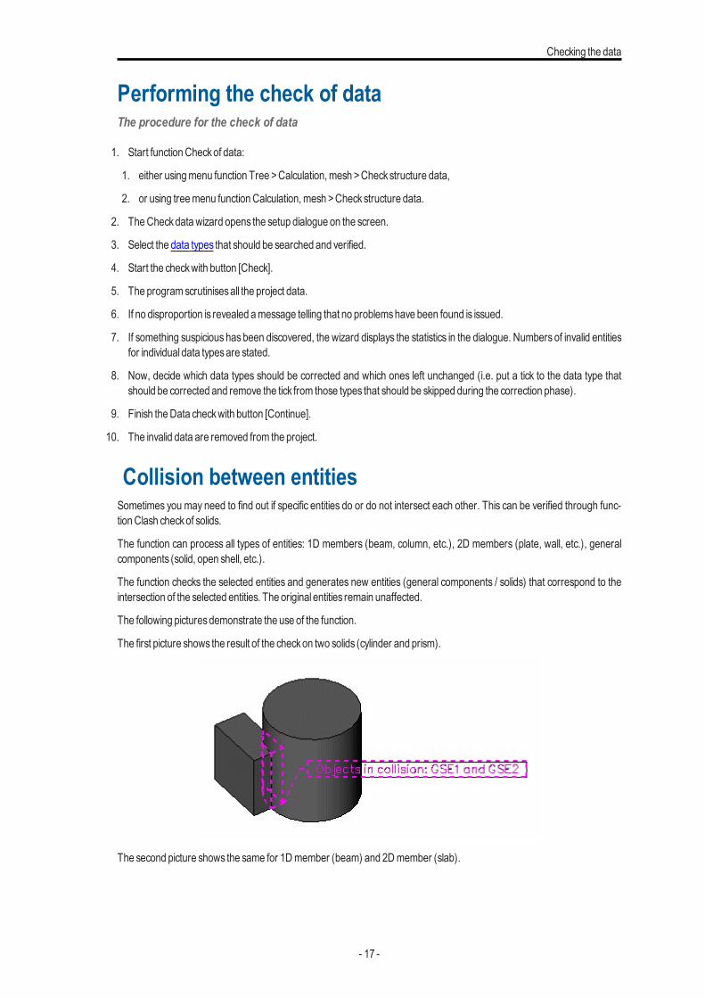
Collision between entitiesSometimes you may need to find out if specific entities do or do not intersect each other. This can be verified through func-tionClash checkof solids.
The function can process all types of entities: 1D members (beam, column, etc.), 2D members (plate, wall, etc.), generalcomponents (solid, open shell, etc.).
The function checks the selected entities and generates new entities (general components / solids) that correspond to theintersection of the selected entities. The original entities remain unaffected.
The following picturesdemonstrate the use of the function.
The first picture shows the result of the checkon two solids (cylinder and prism).
The second picture shows the same for 1Dmember (beam) and 2Dmember (slab).
- 17 -

Chapter 2
The last picture demonstrates the existence of the newly generated solid in the intersection of the checked entities. Here,the beam and slab from the previous picture were removed. What remains is a new entity (general solid) representing theintersection of the two above-mentioned entities.
The function can be used to checkone or two groupsof entities.
Check of one group of entitiesIf just one group of entities is selected, all the selected entities are checked if they collide with any other entity from the selec-tion.
Check of two groups of entitiesIf two groups of entities are selected, the function checkswhether any entity from the first group collideswith any entity fromthe second group. If two entities in the same group collide, it is not reported.
Clash check parametersShow tree of clashesIf ON, a list of clashing entities is displayed in a separate floating window. When a particular entity or clash isclicked in this tree, the corresponding entityor clash ishighlighted in the graphicalwindow.Show collision descriptionIf ON, each collision isdisplayed including a label.Show transparent structureIf ON, the structure isdisplayed as transparent to allow for clearer view of the clashes.Type of selectionEach group for the clash check can be defined as a (i) user selection (i.e. the user must manually select therequired entities), (ii) layer (i.e. all the entities from the selected layer are in the group), (iii) named selection (i.e.the entities from the selected named selection are in the group), or (iv) element type (i.e. all the entities of theselected type, such as1Dmembers, are in the group).
The procedure to check the collision of entities1) Open branchBIM toolboxand start function Evaluate - Clash check.
2) Select the entities for the first group to be checked.
3) Press [Esc] to complete the selection of the first group.
- 18 -

Checking the data
4) Select the entities for the second group to be checked. If onlyone-group check is requested, simply ignore this step
5) Press [Esc] to complete the selection of the second group.
6) The collisionsare displayed on the screen.Moreover, theyare selected.
7) If required, clear the selection, or dowhatever necessarywith the collisions.
Note: This function also checks collisions between free reinforcement bars. For moreinformation on free bars read the documentation for ConcreteCodeCheck.
- 19 -
Chapter 3
Generating the FE mesh
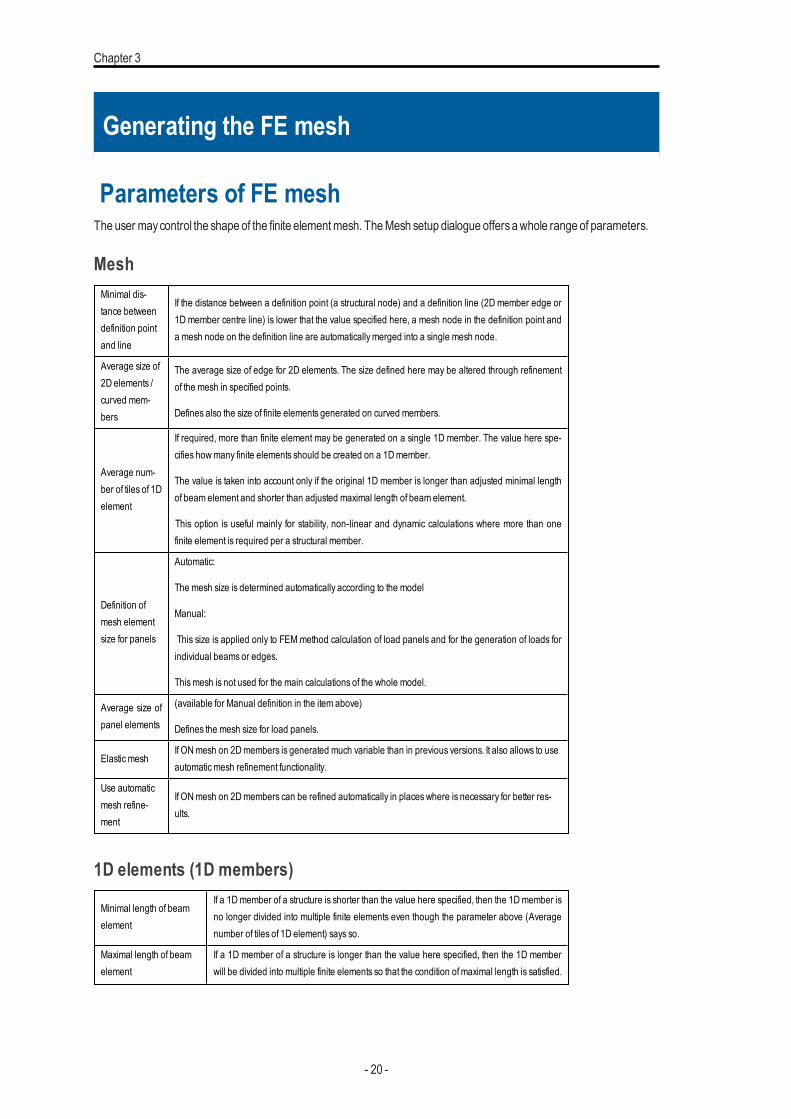
Parameters of FE meshThe user maycontrol the shape of the finite elementmesh. TheMesh setup dialogue offersawhole range of parameters.
MeshMinimal dis-tance betweendefinition pointand line
If the distance between a definition point (a structural node) and a definition line (2D member edge or1D member centre line) is lower that the value specified here, a mesh node in the definition point anda mesh node on the definition line are automatically merged into a single mesh node.
Average size of2D elements /curved mem-bers
The average size of edge for 2D elements. The size defined here may be altered through refinementof the mesh in specified points.
Defines also the size of finite elements generated on curved members.
Average num-ber of tiles of 1Delement
If required, more than finite element may be generated on a single 1D member. The value here spe-cifies howmany finite elements should be created on a 1Dmember.
The value is taken into account only if the original 1D member is longer than adjusted minimal lengthof beam element and shorter than adjusted maximal length of beam element.
This option is useful mainly for stability, non-linear and dynamic calculations where more than onefinite element is required per a structural member.
Definition ofmesh elementsize for panels
Automatic:
The mesh size is determined automatically according to the model
Manual:
This size is applied only to FEMmethod calculation of load panels and for the generation of loads forindividual beams or edges.
Thismesh is not used for the main calculations of the whole model.
Average size ofpanel elements
(available for Manual definition in the item above)
Defines the mesh size for load panels.
Elastic meshIf ONmesh on 2Dmembers is generated much variable than in previous versions. It also allows to useautomaticmesh refinement functionality.
Use automaticmesh refine-ment
If ONmesh on 2Dmembers can be refined automatically in places where is necessary for better res-ults.
1D elements (1D members)
Minimal length of beamelement
If a 1Dmember of a structure is shorter than the value here specified, then the 1Dmember isno longer divided into multiple finite elements even though the parameter above (Averagenumber of tiles of 1D element) says so.
Maximal length of beamelement
If a 1D member of a structure is longer than the value here specified, then the 1D memberwill be divided into multiple finite elements so that the condition ofmaximal length is satisfied.
- 20 -
Generating the FEmesh
Average size of cables,tendons, elements on sub-soil
It is necessary to generate more than one finite element on cables, tendons (prestressedconcrete) and 1Dmembers on subsoil.
For more information about this issue see book Advanced calculations, chapter Analysis of abeam on elastic foundation versusmesh size.
NOTE: This parameter also controls the size of finite elements for beams with a phasedcross-section.
Generation of nodes inconnections of beams
If this option is ON, a check for "touching" 1D members is performed. If an end node of one1D member "touches" another 1D member in a point where there is no node, the two 1Dmembers are connected by a FE node.
If the option is OFF, such a situation remains unsolved and the 1D members are not con-nected to each other.
The function has the same effect as performing function Check of data.
Generation of nodesunder concentrated loadson beam elements
If this option is ON, finite elements nodes are generated in points where concentrated load isacting.
This option is not normally required and it is off as default.
Generation of eccentricelements on memberswith variable height
If a beam is of variable height, the generator automatically generates eccentric finite ele-ments along the haunch.
Moreover, if this option is ON, the eccentricity of the elements may vary along the element,i.e. the start-node of the elementmay have different eccentricity than the end-node of the ele-ment.
If this option is off, the eccentricity along individual finite elements is constant and the eccent-ricity changes in steps in nodes along the haunch.
Division on haunches andarbitrarymembers
Specifies the number of FE generated on a haunch.
Division for 2D - 1Dupgrade
Specifies the number of section which are generated on beam after 2D-1D upgrade per-formance.
Mesh refinement followingthe beam type
Specifies the mode of refinement on 1Dmembers.
None
The refinement is applied to 2Dmembers only.
Beams and columns
The refinement applied to 1D members the type of which is adjusted to "beam (80)" or"column (100)
All 1Dmembers
The refinement applied to all 1Dmembers.
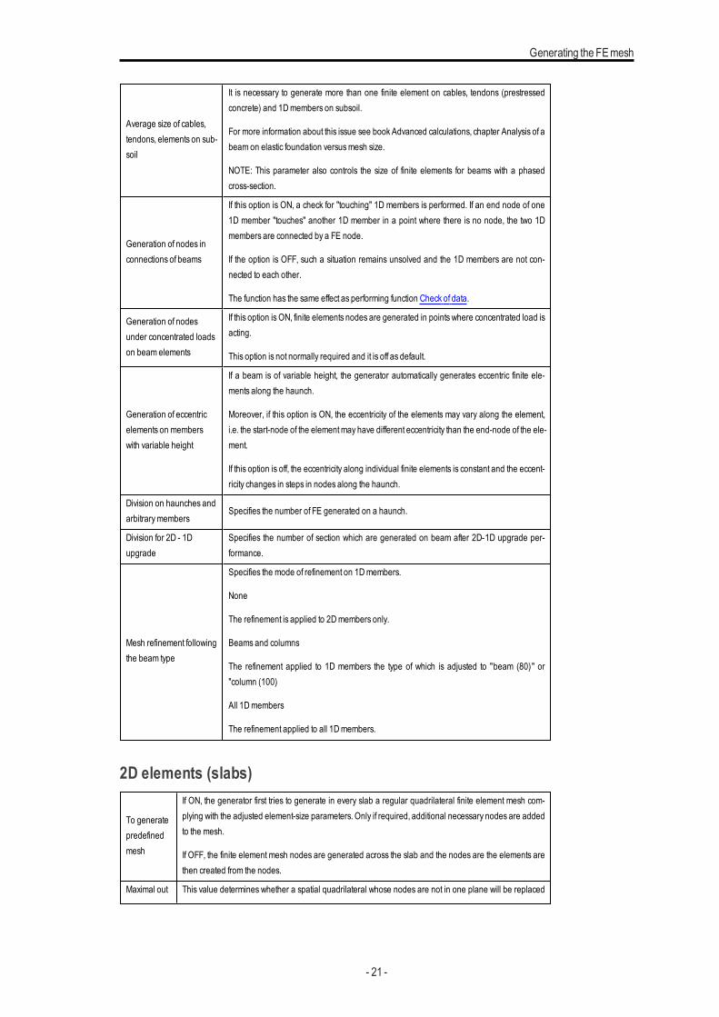
2D elements (slabs)
To generatepredefinedmesh
If ON, the generator first tries to generate in every slab a regular quadrilateral finite element mesh com-plying with the adjusted element-size parameters. Only if required, additional necessary nodes are addedto the mesh.
If OFF, the finite element mesh nodes are generated across the slab and the nodes are the elements arethen created from the nodes.
Maximal out This value determines whether a spatial quadrilateral whose nodes are not in one plane will be replaced
- 21 -

Chapter 3
of planeangle of aquadrilateral
by triangular elements. This parameter is meaningful only for out- of- plane surfaces – shells. Theassessed angle ismeasured between the plane made of three nodes of the quadrilateral and the remain-ing node of this quadrilateral.
Predefinedmesh ratio
Defines the relative distance between the predefined mesh formed by regular quadrilateral elements andthe nearest edge. The edge may consist of an internal edge, external edge or border of refined area. Thefinal distance is calculated as a multiple of the defined ratio and adjusted average element size for 2D ele-ments.
Average number of tiles of 1D elementFor static linear calculation, value 1 is normally satisfactory. On the other hand, there are several configurations when finerdivision is required in order to obtain accurate results.
These are:
l beam laid on foundation requiresa fine division – see chapter Analysisof a beamon foundation versusmesh size.
l dynamic calculation when a great number of eigenfrequencies is required – see chapter Natural vibration analysis versusmesh size
l buckling calculation
l non-linear calculations
Division on haunches and arbitrary beamsThe number defined here determines the "precision" that is applied in modelling of the variable cross-section along ahaunch. The higher the number, themore themodel reflects the real shape. See chapter Analysis of a haunch versusmeshsize.
In addition, the same rulesas for a standardmember must be followed here aswell.
Generation of eccentric elements on members with variable heightThe midline of the finite element model of a haunch-beammay be either straight (following the midline of the original "non-haunched" beam) or "curved" (following the real midline of the haunch beam corresponding to the centre of gravity of thecross-section).
See chapter Analysisof a haunch versuseccentricelements.
Average size of cables, tendons, elements on subsoilSpecifies the number of finite elementsgenerated on a beam laid on foundation.
See chapter Analysisof a beamon foundation versusmesh size.
The procedure for the adjustment of mesh parameters
1. Callmenu function Setup >Mesh.
2. Adjust the parameters (see above).
3. Confirmwith [OK].
The finite elementmeshmaybe previewed using functionMesh generation under treemenuCalculation.07/10/2013
- 22 -
Generating the FEmesh
Previewing the FE meshFor complexstructures it maybe useful to review the FEmesh before the resultsare scrutinised in detail.
It is possible to control the displaystyle of themesh through a set of view parameters.
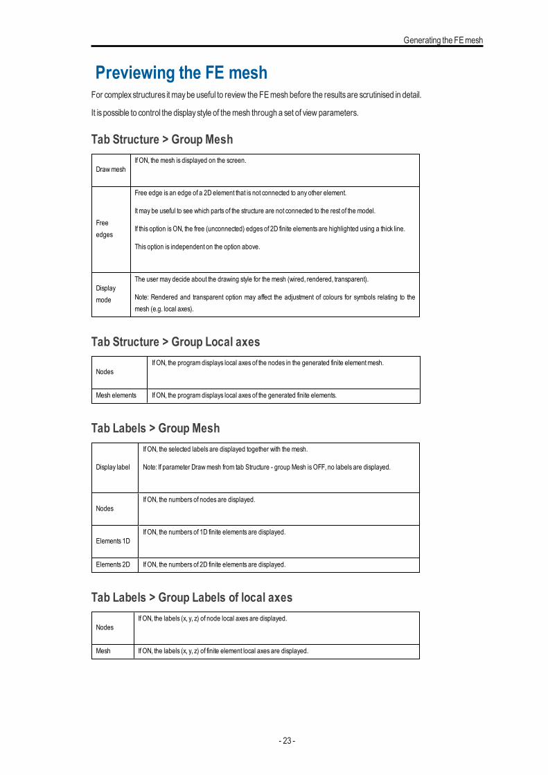
Tab Structure > Group Mesh
DrawmeshIf ON, the mesh is displayed on the screen.
Freeedges
Free edge is an edge of a 2D element that is not connected to any other element.
It may be useful to see which parts of the structure are not connected to the rest of the model.
If this option is ON, the free (unconnected) edges of 2D finite elements are highlighted using a thick line.
This option is independent on the option above.
Displaymode
The user may decide about the drawing style for the mesh (wired, rendered, transparent).
Note: Rendered and transparent option may affect the adjustment of colours for symbols relating to themesh (e.g. local axes).
Tab Structure > Group Local axes
NodesIf ON, the program displays local axes of the nodes in the generated finite elementmesh.
Mesh elements If ON, the program displays local axes of the generated finite elements.
Tab Labels > Group Mesh
Display label
If ON, the selected labels are displayed together with the mesh.
Note: If parameter Drawmesh from tab Structure - group Mesh is OFF, no labels are displayed.
NodesIf ON, the numbers of nodes are displayed.
Elements 1DIf ON, the numbers of 1D finite elements are displayed.
Elements 2D If ON, the numbers of 2D finite elements are displayed.
Tab Labels > Group Labels of local axes
NodesIf ON, the labels (x, y, z) of node local axes are displayed.
Mesh If ON, the labels (x, y, z) of finite element local axes are displayed.
- 23 -
Chapter 3
The procedure for the preview of finite element mesh
1. OpenView parameterssetting dialogue.
2. Select TabStructure or Labels.
3. In the required group adjust the required parameters.
4. Confirm the settings.
5. Check themesh.
6. If required, switch themesh off again.
Note:When themesh generator has createdmesh elementswith an angle smaller than 5°an arrow is shown on the screen so the user can easily find such elements (elements withthe angle smaller than 5° can sometimes lead to inaccurate results) Mesh refinement func-tion is then recommended to generate a better mesh..
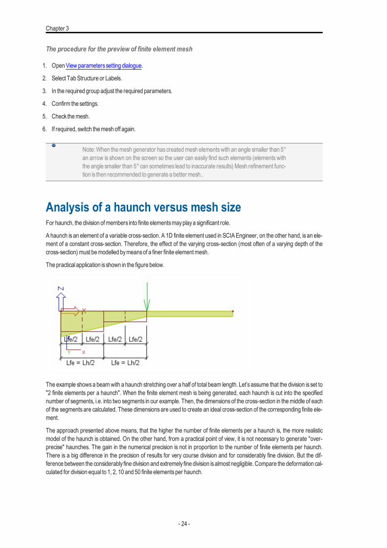
Analysis of a haunch versus mesh sizeFor haunch, the division ofmembers into finite elementsmayplaya significant role.
A haunch is an element of a variable cross-section. A 1D finite element used in SCIAEngineer, on the other hand, is an ele-ment of a constant cross-section. Therefore, the effect of the varying cross-section (most often of a varying depth of thecross-section) must bemodelled bymeansof a finer finite elementmesh.
The practical application is shown in the figure below.
The example showsa beamwith a haunch stretching over a half of total beam length. Let’s assume that the division is set to"2 finite elements per a haunch". When the finite element mesh is being generated, each haunch is cut into the specifiednumber of segments, i.e. into two segments in our example. Then, the dimensionsof the cross-section in themiddle of eachof the segments are calculated. These dimensions are used to create an ideal cross-section of the corresponding finite ele-ment.
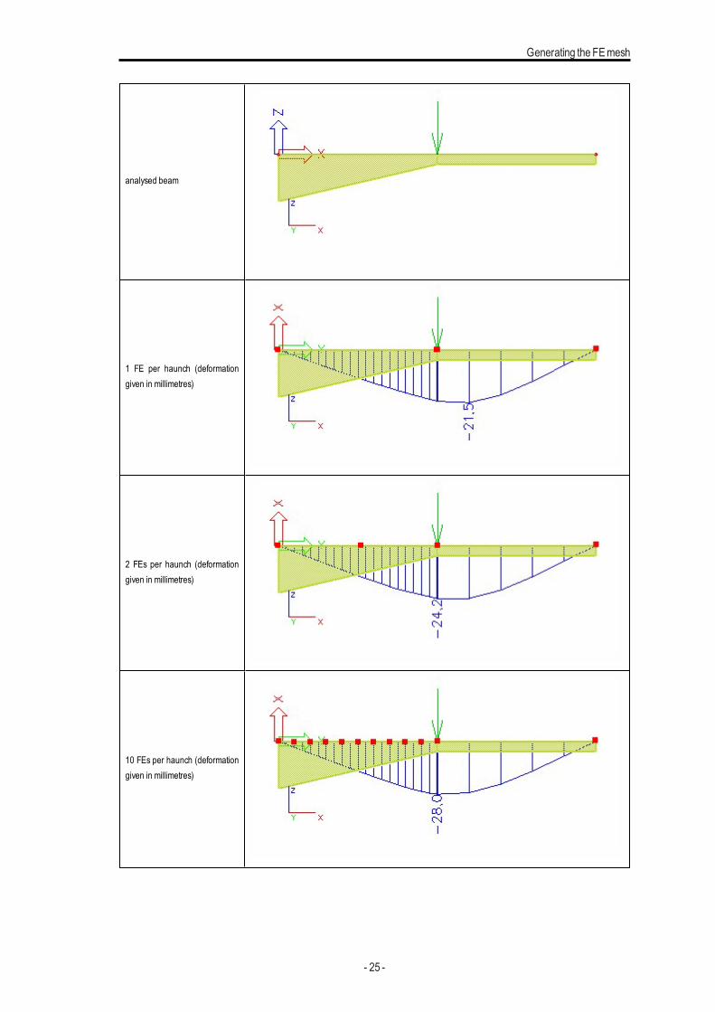
The approach presented above means, that the higher the number of finite elements per a haunch is, the more realisticmodel of the haunch is obtained. On the other hand, from a practical point of view, it is not necessary to generate "over-precise" haunches. The gain in the numerical precision is not in proportion to the number of finite elements per haunch.There is a big difference in the precision of results for very course division and for considerably fine division. But the dif-ference between the considerably fine division and extremely fine division isalmost negligible. Compare the deformation cal-culated for division equal to 1, 2, 10 and 50 finite elementsper haunch.
- 24 -
Generating the FEmesh
analysed beam
1 FE per haunch (deformationgiven in millimetres)
2 FEs per haunch (deformationgiven in millimetres)
10 FEs per haunch (deformationgiven in millimetres)
- 25 -
Chapter 3
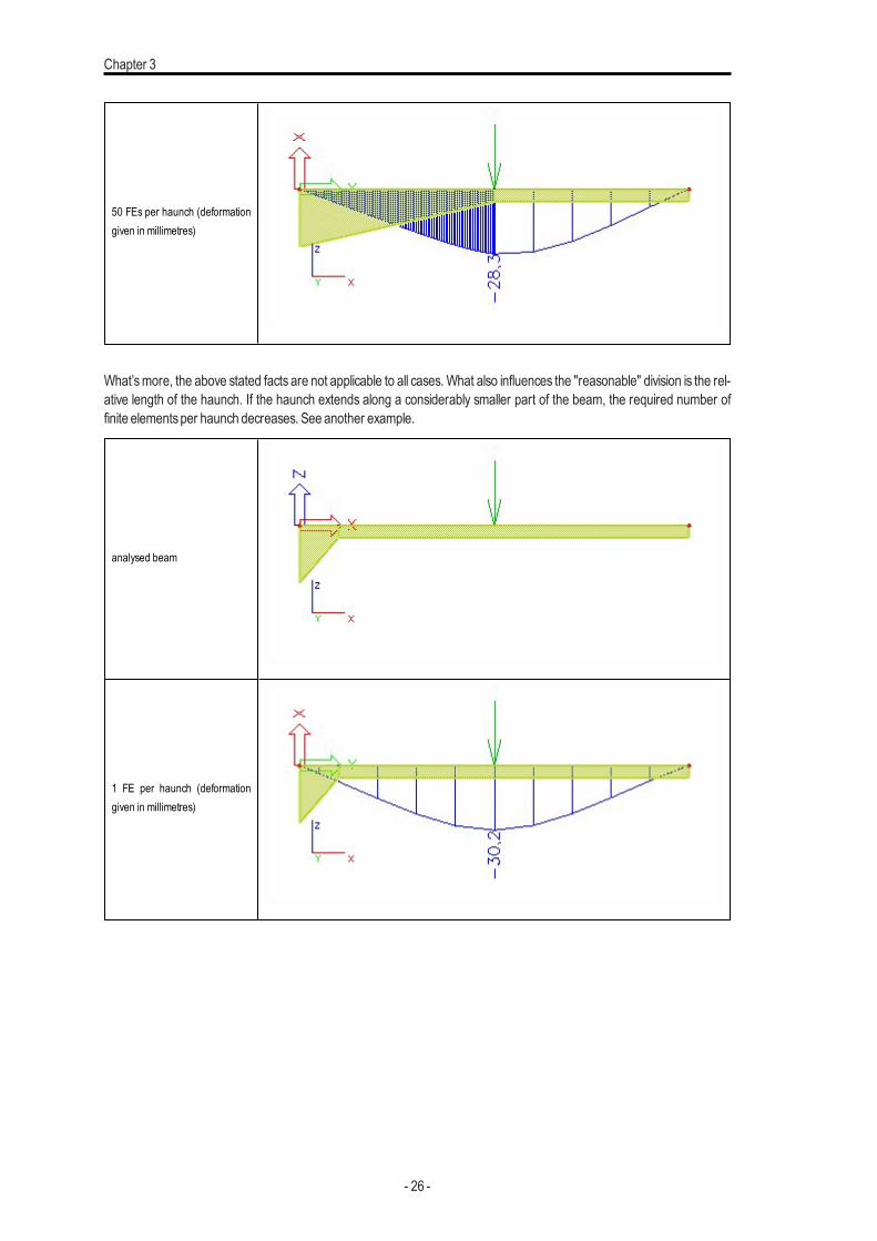
50 FEs per haunch (deformationgiven in millimetres)
What’smore, the above stated facts are not applicable to all cases. What also influences the "reasonable" division is the rel-ative length of the haunch. If the haunch extends along a considerably smaller part of the beam, the required number offinite elementsper haunch decreases. See another example.
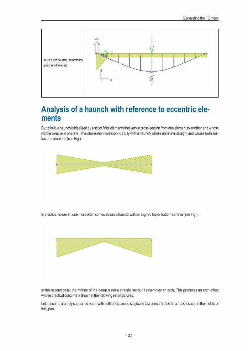
analysed beam
1 FE per haunch (deformationgiven in millimetres)
- 26 -
Generating the FEmesh
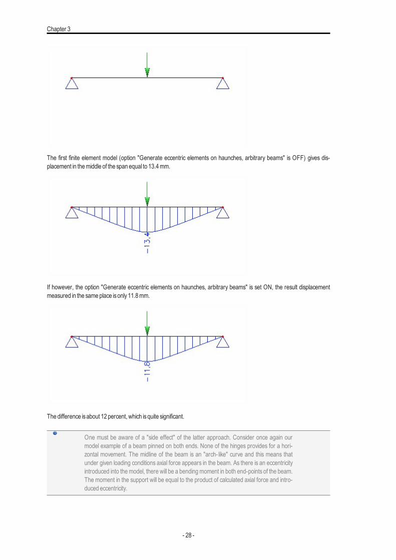
10 FEs per haunch (deformationgiven in millimetres)
Analysis of a haunch with reference to eccentric ele-mentsBydefault, a haunch is idealised bya set of finite elements that vary in cross-section fromone element to another andwhosemiddle axes lie in one line. This idealisation corresponds fully with a haunch whose midline is straight and whose both sur-facesare inclined (see Fig.).
In practice, however, onemore often comesacrossa haunchwith an aligned top or bottom surface (see Fig.).
In this second case, the midline of the beam is not a straight line but it resembles an arch. This produces an arch effectwhose practical outcome isshown in the following set of pictures.
Let’sassume a simplysupported beamwith both endspinned subjected to a concentrated force load located in themiddle ofthe span.
- 27 -
Chapter 3
The first finite element model (option "Generate eccentric elements on haunches, arbitrary beams" is OFF) gives dis-placement in themiddle of the span equal to 13.4mm.
If however, the option "Generate eccentric elements on haunches, arbitrary beams" is set ON, the result displacementmeasured in the same place isonly11.8mm.
The difference isabout 12 percent, which isquite significant.
One must be aware of a "side effect" of the latter approach. Consider once again ourmodel example of a beam pinned on both ends. None of the hinges provides for a hori-zontal movement. The midline of the beam is an "arch- like" curve and this means thatunder given loading conditions axial force appears in the beam. As there is an eccentricityintroduced into the model, there will be a bending moment in both end-points of the beam.The moment in the support will be equal to the product of calculated axial force and intro-duced eccentricity.
- 28 -
Generating the FEmesh
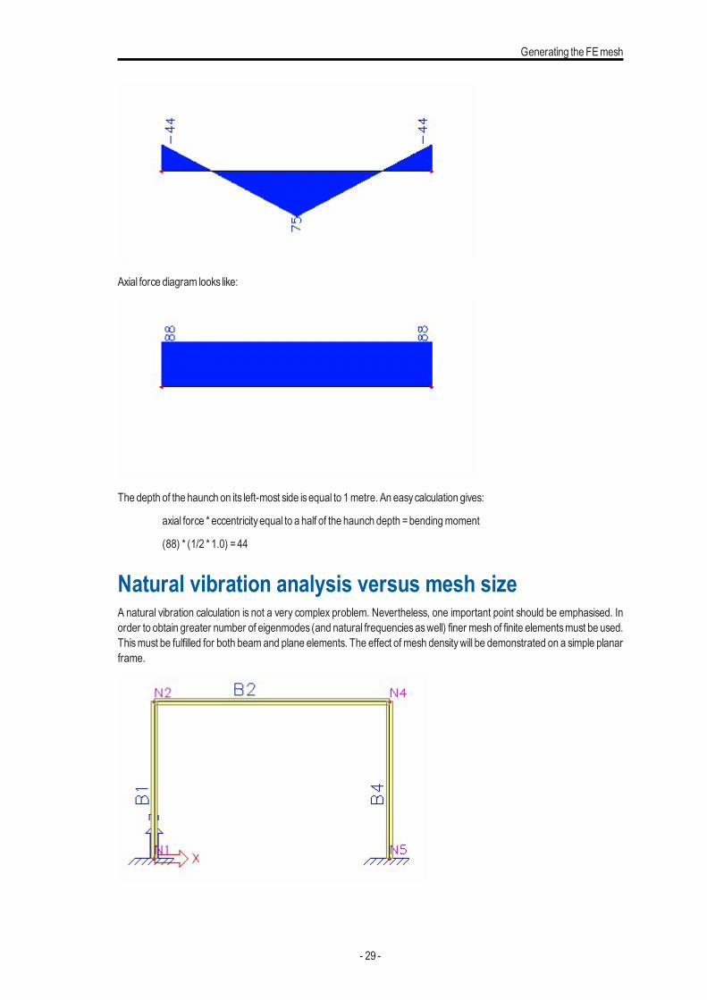
Axial force diagram looks like:
The depth of the haunch on its left-most side isequal to 1metre. An easycalculation gives:
axial force * eccentricityequal to a half of the haunch depth =bendingmoment
(88) * (1/2 * 1.0) =44
Natural vibration analysis versus mesh sizeA natural vibration calculation is not a very complex problem. Nevertheless, one important point should be emphasised. Inorder to obtain greater number of eigenmodes (and natural frequenciesaswell) finer mesh of finite elementsmust be used.Thismust be fulfilled for both beam and plane elements. The effect of mesh densitywill be demonstrated on a simple planarframe.
- 29 -
Chapter 3
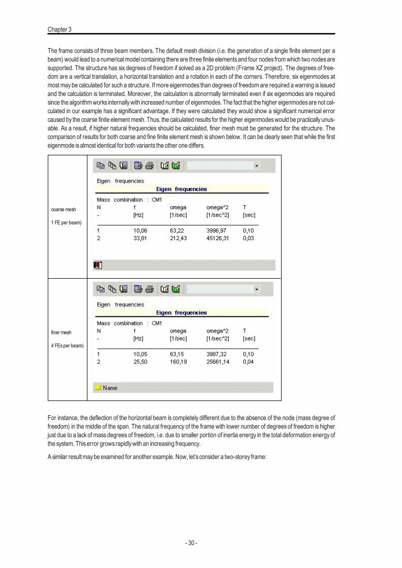
The frame consists of three beam members. The default mesh division (i.e. the generation of a single finite element per abeam) would lead to a numericalmodel containing there are three finite elementsand four nodes fromwhich two nodesaresupported. The structure has six degrees of freedom if solved as a 2D problem (Frame XZ project). The degrees of free-dom are a vertical translation, a horizontal translation and a rotation in each of the corners. Therefore, six eigenmodes atmost maybe calculated for such a structure. If more eigenmodes than degreesof freedom are required a warning is issuedand the calculation is terminated. Moreover, the calculation is abnormally terminated even if six eigenmodes are requiredsince the algorithmworks internallywith increased number of eigenmodes. The fact that the higher eigenmodesare not cal-culated in our example has a significant advantage. If they were calculated they would show a significant numerical errorcaused by the coarse finite elementmesh. Thus, the calculated results for the higher eigenmodeswould be practically unus-able. As a result, if higher natural frequencies should be calculated, finer mesh must be generated for the structure. Thecomparison of results for both coarse and fine finite element mesh is shown below. It can be clearly seen that while the firsteigenmode isalmost identical for both variants the other one differs.
coarse mesh
1 FE per beam)
finer mesh
4 FEs per beam)
For instance, the deflection of the horizontal beam is completely different due to the absence of the node (mass degree offreedom) in the middle of the span. The natural frequency of the frame with lower number of degrees of freedom is higherjust due to a lack of mass degrees of freedom, i.e. due to smaller portion of inertia energy in the total deformation energy ofthe system. Thiserror grows rapidlywith an increasing frequency.
A similar result maybe examined for another example. Now, let’s consider a two-storey frame:
- 30 -
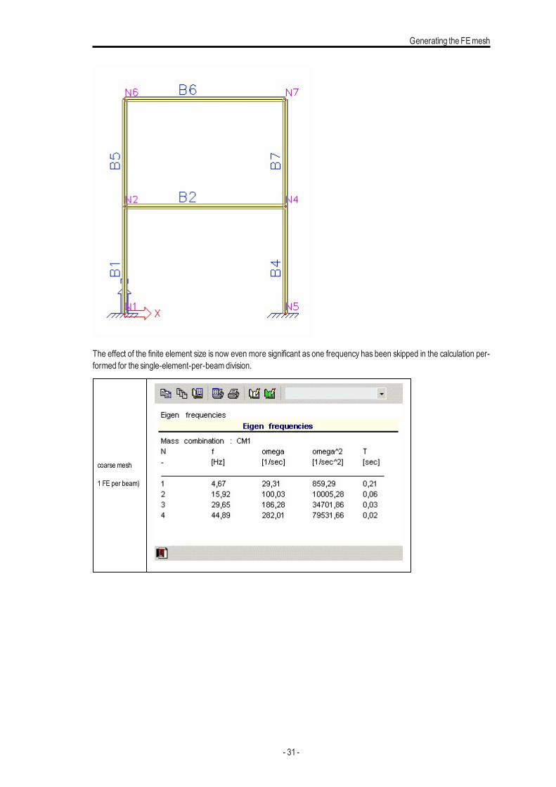
Generating the FEmesh
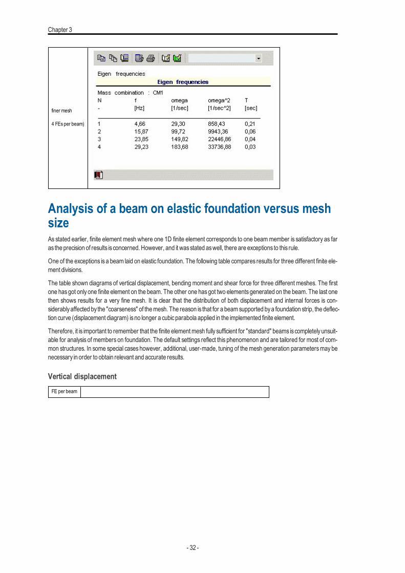
The effect of the finite element size is now even more significant as one frequency has been skipped in the calculation per-formed for the single-element-per-beamdivision.
coarse mesh
1 FE per beam)
- 31 -
Chapter 3
finer mesh
4 FEs per beam)
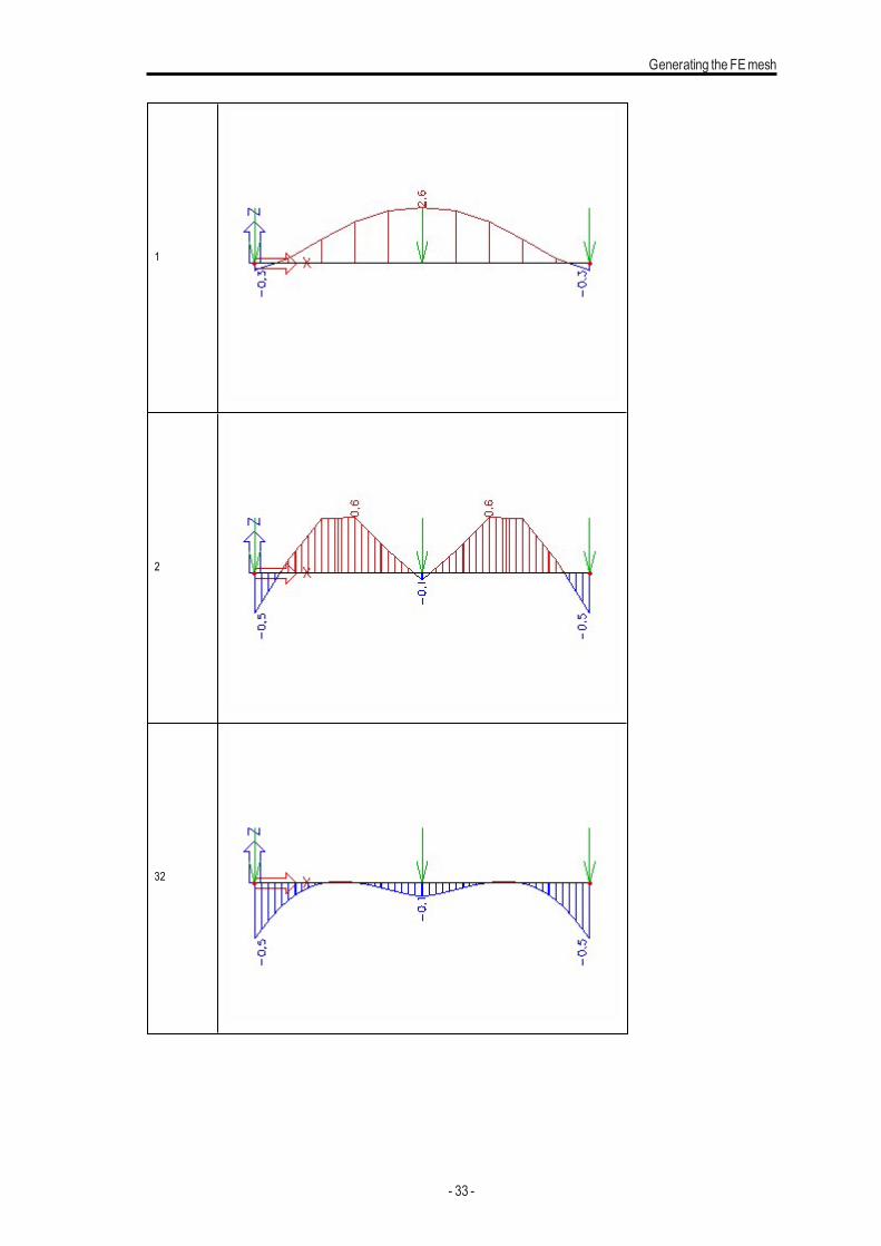
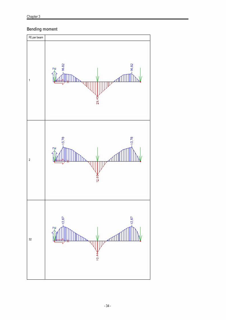
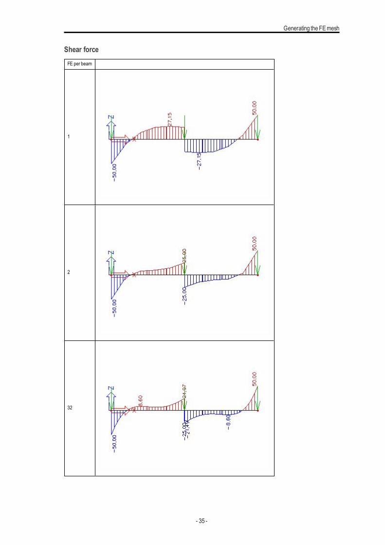
Analysis of a beam on elastic foundation versus meshsizeAs stated earlier, finite element mesh where one 1D finite element corresponds to one beammember is satisfactory as faras the precision of results is concerned. However, and it wasstated aswell, there are exceptions to this rule.
One of the exceptions is a beam laid on elastic foundation. The following table compares results for three different finite ele-ment divisions.
The table shown diagrams of vertical displacement, bending moment and shear force for three different meshes. The firstone hasgot only one finite element on the beam. The other one hasgot two elements generated on the beam. The last onethen shows results for a very fine mesh. It is clear that the distribution of both displacement and internal forces is con-siderablyaffected by the "coarseness" of themesh. The reason is that for a beamsupported bya foundation strip, the deflec-tion curve (displacement diagram) isno longer a cubicparabola applied in the implemented finite element.
Therefore, it is important to remember that the finite element mesh fully sufficient for "standard" beams is completely unsuit-able for analysis of members on foundation. The default settings reflect this phenomenon and are tailored for most of com-mon structures. In some special cases however, additional, user-made, tuning of the mesh generation parametersmay benecessary in order to obtain relevant and accurate results.
Vertical displacementFE per beam
- 32 -
Generating the FEmesh
1
2
32
- 33 -
Chapter 3
Bending momentFE per beam
1
2
32
- 34 -
Generating the FEmesh
Shear forceFE per beam
1
2
32
- 35 -

Chapter 3
Mesh refinementMesh refinementThe finer the finite element mesh is, the more accurate the obtained results are (i.e. the closer to the theoretically correctones) and the more time consuming the solution is and the more disk space is needed both during the calculation and forstorage of the results. The mesh size should be adjusted considering the load the structure is subject to and taking accountof the requirementson the calculation.
The generation of the mesh is based on the adjusted size for 2D elements. The generator creates such elements whoseedge size is as close to the adjusted value as possible. Also the division of slab / shell borders and internal edges is based onthis. Any internal nodesof slabs / shellsare taken into account aswell.
Themeshmust bemade finer in certain areas. Themeshmaybe refines in a circular area around a specific point, in a bandalong a defined line or over thewhole slab / shell.
If any two refinement areasoverlap anywhere, the smaller element size is used. The refinement area doesnot have be fullyinside the "master" slab /shell. Onlya part of the refinement areamaybe located inside it.
Refinement around a nodeThe refinement area is circular with its centre in a specified point. The finite element size outside the circle is the standard FEsize for 2D elements adjusted in FE mesh setup dialogue. The element size in the centre of the circle is the given refinedvalue. The size of elements in between varies linearly from the two limits.
Name Identifies the refinement.
Radius Defines the radius of circular area where the mesh will be refined.
RatioDefines the ratio between the average element edge size in the centre of refinement area and theaverage preset element size.
dx, dy, dzDefines possible shift of the centre of refinement area from the specified point. Thus the refinementarea may be placed anywhere in the structure.
Type of pointmeshrefinement
Linear increment = elements at the end are larger, elements in the middle are smaller
Equidistant - only 1D element = the elements are uniformly refined
The procedure for the adjustment of node refinement
1. Call function Node mesh refinement using tree menu function Calculation, mesh > Local mesh refinement > Node meshrefinement.
2. Adjust the parameters (see above).
3. Confirmwith [OK].
4. Select nodeswhere the refinement should be used.
5. Close the function.
If you want to refine alsomesh of 1D members , youmust allow this inMesh setup - see theParameters_of_FE_mesh chapter.
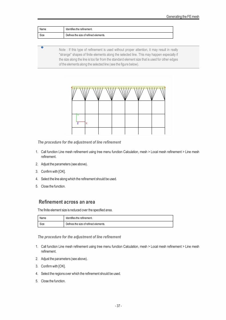
Refinement along a lineThe finite element size is reduced along the specified line.
- 36 -
Generating the FEmesh
Name Identifies the refinement.
Size Defines the size of refined elements.
Note : If this type of refinement is used without proper attention, it may result in really"strange" shapes of finite elements along the selected line. This may happen especially ifthe size along the line is too far from the standard element size that is used for other edgesof the elementsalong the selected line (see the figure below).
The procedure for the adjustment of line refinement
1. Call function Line mesh refinement using tree menu function Calculation, mesh > Local mesh refinement > Line meshrefinement.
2. Adjust the parameters (see above).
3. Confirmwith [OK].
4. Select the line alongwhich the refinement should be used.
5. Close the function.
Refinement across an areaThe finite element size is reduced over the specified area.
Name Identifies the refinement.
Size Defines the size of refined elements.
The procedure for the adjustment of line refinement
1. Call function Line mesh refinement using tree menu function Calculation, mesh > Local mesh refinement > Line meshrefinement.
2. Adjust the parameters (see above).
3. Confirmwith [OK].
4. Select the regionsover which the refinement should be used.
5. Close the function.
- 37 -
Chapter 4
Calculation types
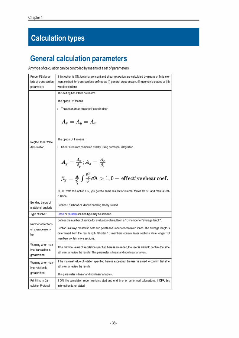
General calculation parametersAny type of calculation can be controlled bymeansof a set of parameters.
Proper FEM ana-lysis of cross-sectionparameters
If this option is ON, torsional constant and shear relaxation are calculated by means of finite ele-ment method for cross-sections defined as (i) general cross-section, (ii) geometric shapes or (iii)wooden sections.
Neglect shear forcedeformation
This setting has effects on beams.
The option ONmeans
o The shear areas are equal to each other
The option OFFmeans :
o Shear areas are computed exactly, using numerical integration.
NOTE: With this option ON, you get the same results for internal forces for SE and manual cal-culation.
Bending theory ofplate/shell analysis
Defines if Kirchhoff or Mindlin banding theory is used.
Type of solver Direct or iterative solution type may be selected.
Number of sectionson average mem-ber
Defines the number of section for evaluation of results on a 1Dmember of "average length".
Section is always created in both end points and under concentrated loads. The average length isdetermined from the real length. Shorter 1D members contain fewer sections while longer 1Dmembers contain more sections.
Warning when max-imal translation isgreater than
If the maximal value of translation specified here is exceeded, the user is asked to confirm that s/hestill want to review the results. This parameter is linear and nonlinear analysis .
Warning when max-imal rotation isgreater than
If the maximal value of rotation specified here is exceeded, the user is asked to confirm that s/hestill want to review the results.
This parameter is linear and nonlinear analysis .
Print time in Cal-culation Protocol
If ON, the calculation report contains start and end time for performed calculations. If OFF, thisinformation is not stated.
- 38 -
Calculation types
Note: The adjustment of these parametersmayaffect the layout of the calculation dialoguethat openson the screenwhen a calculation is started.
Note: For Mindlin bending theory of shell is used a mixed interpolation of transverse dis-placements, section rotations and transverse shear strains. It is an extension of a pure dis-placement formulation. For curvatures there is used an interpolation as the puredisplacement on based elementsbut for shear strain are used another one. Themixed ele-mentsare not locked and do not contain anyspuriouszero energymode.
Number of result sections per memberThe principle of finite element method is that the solution of the problem (in other words, the internal forces and deform-ations in the analysed structure) is given in finite number of points, i.e. in nodes of finite elements. These valuesmay be fur-ther processed and result values for intermediate points of individual finite elementsmay be interpolated. In SCIA Engineerthe user may decide how many intermediate points should be evaluated. This ismade bymeans of solver option: Numberof sections on average member.
When adjusting thisoption, one should remember that:
too few intermediate points:
l generates little data, saves the computer memory, increases the speed of the programme,
l maymore or lessdistort the results.
toomany intermediate points:
l generatesa huge amount of data andmay lead to slower response of the programme,
l givenmore accurate distribution of result quantities.
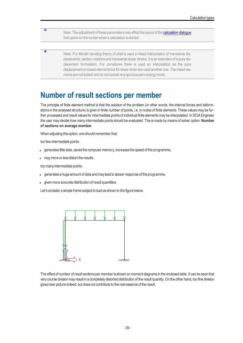
Let’s consider a simple frame subject to load asshown in the figure below.
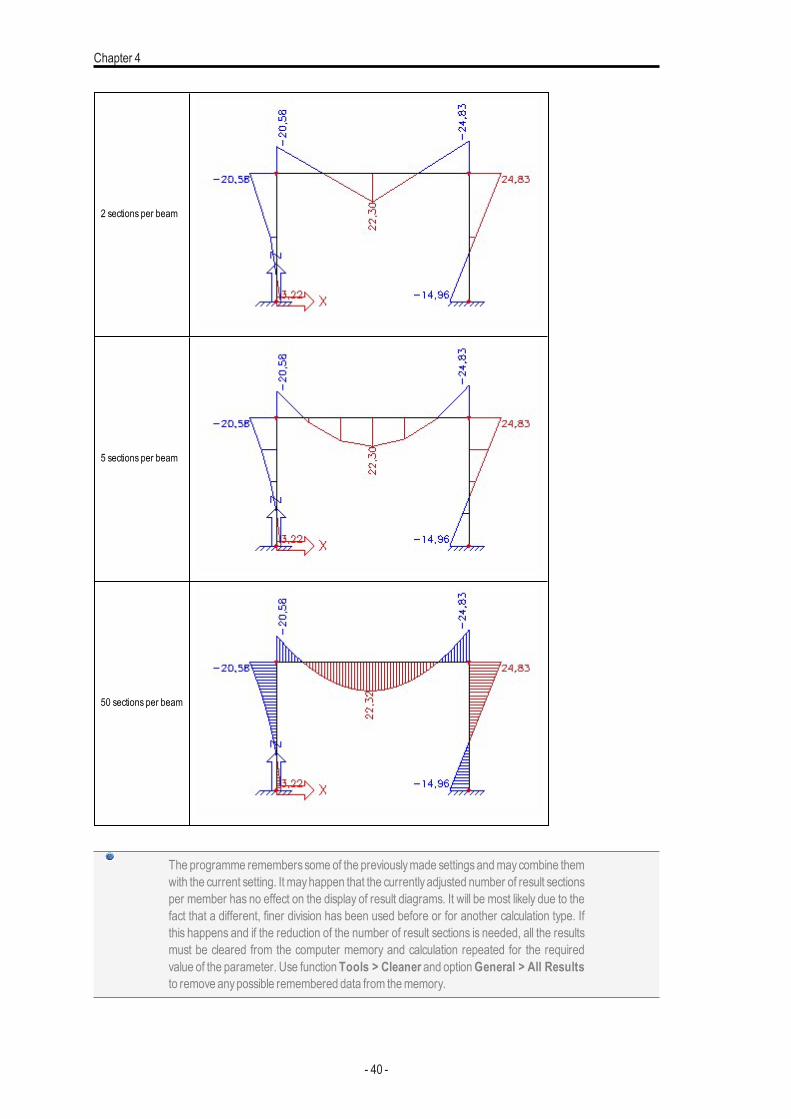
The effect of number of result sectionsper member is shown onmoment diagrams in the enclosed table. It can be seen thatvery course divisionmay result in a completelydistorted distribution of the result quantity. On the other hand, too fine divisiongivesnicer picture indeed, but doesnot contribute to the real essence of the result.
- 39 -
Chapter 4
2 sections per beam
5 sections per beam
50 sections per beam
The programme remembers some of the previouslymade settingsandmaycombine themwith the current setting. It mayhappen that the currently adjusted number of result sectionsper member has no effect on the display of result diagrams. It will be most likely due to thefact that a different, finer division has been used before or for another calculation type. Ifthis happens and if the reduction of the number of result sections is needed, all the resultsmust be cleared from the computer memory and calculation repeated for the requiredvalue of the parameter. Use function Tools > Cleaner and optionGeneral > All Resultsto remove anypossible remembered data from thememory.
- 40 -
Calculation types
Static linear calculationWhen performing the static linear calculation, the user may specify the general calculation parameter to control the cal-culationmethod and process.
Static non-linear calculationThemain difference between a linear and non-linear calculation is that the non-linear calculation givessuch resultsof deflec-tionsand internal forces for which equilibrium conditionsare satisfied on a deformed structure. The user should thinkbefore-hand whether the load applied on the structure would lead to such a state of deformation that affects the resultant internalforcesand deflections. If the user thinksso, theyshould use the non-linear calculation at least for one selected load and com-pare the results with those for linear calculation. Thus, the user can evaluate the effect on non-linearity on behaviour of thestructure.
The non-linear calculation in SCIAEngineer isbased on the following assumptions:
l equilibrium conditionsare satisfied for deformed shape of a structure,
l effect of axial forceson flexural stiffnessof beams is taken into account aswell,
l non-linear supportsare taken into consideration,
l material of the structure is considered as linearlyelastic.
Setup parametersIf anykind of non-linearity should be taken into account in a project, it is necessary to select appropriate option (or options) intheProject data setup dialogue.
The options related to non-linearityare listed on tabFunctionality.
In order to make the options accessible, the main option Non-linearitymust be chosen. Once this is done, a list of options(or theymaybe called sub-options) is shown.
Initial deformation and curvatureThisoption enables the user to define an initial deformation of a structure.2nd order - gGeometrical non-linearityThisoption enables the user to performgeometricallynon-linear calculation of analysed structure.Physical non-linearity for reinforced concreteThisoption enables the user to perform iterative calculation of interaction between concrete and reinforcement.Beam local non-linearityThisoption provides for the introduction of local non-linearitieson individual beams.Support non-linearity/soil springIf thisoption isON, it ispossible take account of non-linearities in supports.Friction support/soil springIf thisoption isON, it ispossible take account of non-linearities in supports.Membrane elementsThisoption enables the user to calculate 2Dmemberswithmembrane effects.Press only 2D membersThisoption enables the user to add nonlinear behavior "pressonly" on 2Dmembers.Sequential analysis
- 41 -
Chapter 4
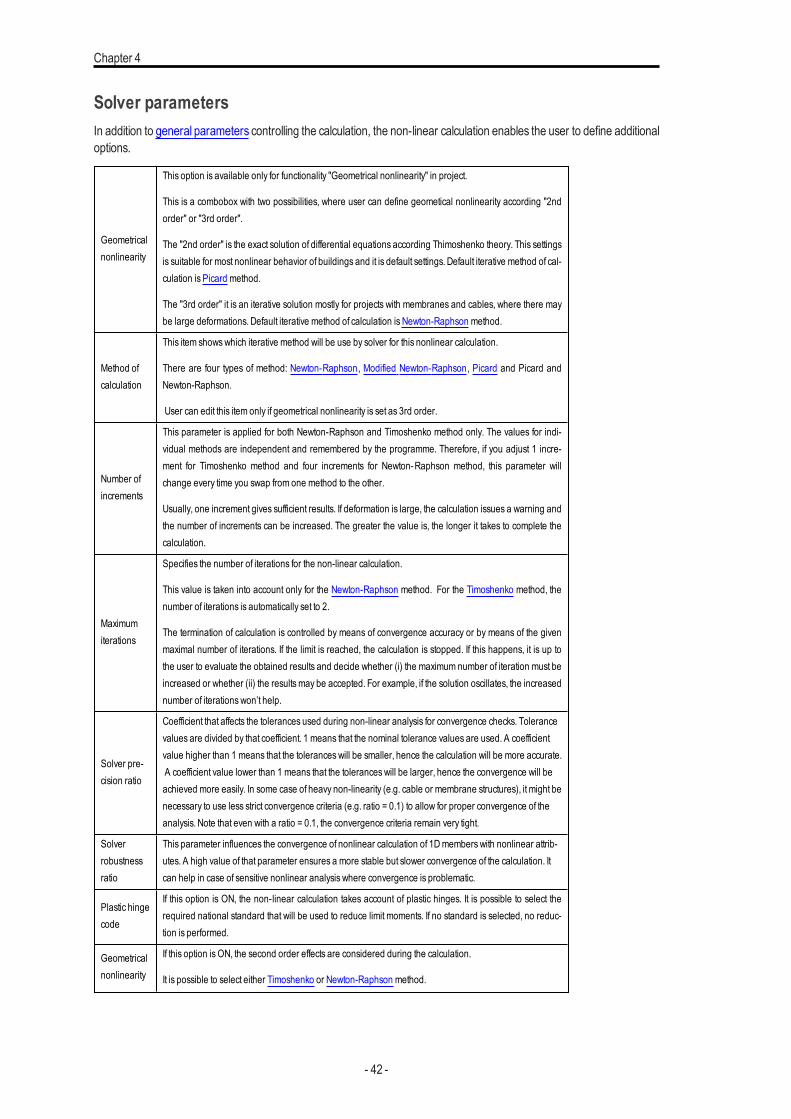
Solver parametersIn addition to general parameters controlling the calculation, the non-linear calculation enables the user to define additionaloptions.
Geometricalnonlinearity
This option is available only for functionality "Geometrical nonlinearity" in project.
This is a combobox with two possibilities, where user can define geometical nonlinearity according "2ndorder" or "3rd order".
The "2nd order" is the exact solution of differential equations according Thimoshenko theory. This settingsis suitable for most nonlinear behavior of buildings and it is default settings. Default iterative method of cal-culation is Picard method.
The "3rd order" it is an iterative solution mostly for projects with membranes and cables, where there maybe large deformations. Default iterative method of calculation is Newton-Raphson method.
Method ofcalculation
This item showswhich iterative method will be use by solver for this nonlinear calculation.
There are four types of method: Newton-Raphson, Modified Newton-Raphson, Picard and Picard andNewton-Raphson.
User can edit this item only if geometrical nonlinearity is set as 3rd order.
Number ofincrements
This parameter is applied for both Newton-Raphson and Timoshenko method only. The values for indi-vidual methods are independent and remembered by the programme. Therefore, if you adjust 1 incre-ment for Timoshenko method and four increments for Newton-Raphson method, this parameter willchange every time you swap from one method to the other.
Usually, one increment gives sufficient results. If deformation is large, the calculation issues a warning andthe number of increments can be increased. The greater the value is, the longer it takes to complete thecalculation.
Maximumiterations
Specifies the number of iterations for the non-linear calculation.
This value is taken into account only for the Newton-Raphson method. For the Timoshenko method, thenumber of iterations is automatically set to 2.
The termination of calculation is controlled by means of convergence accuracy or by means of the givenmaximal number of iterations. If the limit is reached, the calculation is stopped. If this happens, it is up tothe user to evaluate the obtained results and decide whether (i) the maximum number of iteration must beincreased or whether (ii) the resultsmay be accepted. For example, if the solution oscillates, the increasednumber of iterations won’t help.
Solver pre-cision ratio
Coefficient that affects the tolerances used during non-linear analysis for convergence checks. Tolerancevalues are divided by that coefficient. 1 means that the nominal tolerance values are used. A coefficientvalue higher than 1 means that the toleranceswill be smaller, hence the calculation will be more accurate.A coefficient value lower than 1 means that the toleranceswill be larger, hence the convergence will beachieved more easily. In some case of heavy non-linearity (e.g. cable or membrane structures), it might benecessary to use less strict convergence criteria (e.g. ratio = 0.1) to allow for proper convergence of theanalysis. Note that even with a ratio = 0.1, the convergence criteria remain very tight.
Solverrobustnessratio
This parameter influences the convergence of nonlinear calculation of 1Dmembers with nonlinear attrib-utes. A high value of that parameter ensures a more stable but slower convergence of the calculation. Itcan help in case of sensitive nonlinear analysis where convergence is problematic.
Plastic hingecode
If this option is ON, the non-linear calculation takes account of plastic hinges. It is possible to select therequired national standard that will be used to reduce limit moments. If no standard is selected, no reduc-tion is performed.
Geometricalnonlinearity
If this option is ON, the second order effects are considered during the calculation.
It is possible to select either Timoshenko or Newton-Raphson method.
- 42 -
Calculation types
For both methods, the exact solution of 1Dmembers is implemented. It takes account of normal forces andshear deformation for any kind of loading. Transformation of internal forces into the deformed 1Dmemberaxis is included.
In addition, also available are:Modified Newton-Raphson method and Picard method.
The Picard method is regarded as complementary method. It can be used when the Newton-Raphsonmethod fails. The method is more robust but slower. The Picard method can be use alone (the direct iter-ation method, using the secant stiffnessmatrix) or in the combination with the Newton-Raphson method. Inthis case the calculation starts with Newton-Raphson and then switches to Piccard.
Main differences: the Newton Raphons method uses tangent stiffnesses, but Picards method uses secantstiffnesses.
Allow com-pression inmembranemembers
If this checkbox is ON, the compression in membran elements is taken into account.
Limits of the calculationTotal number of nodes and finite elements unlimited
Total number of non-linear combinations 1000
Maximal number of iterations (in one increment) 999
Maximal number of increments 99
Note: Static non-linear calculation can ONLY be performed after the static calculation ofthe same project hasbeen carried out successfully. In other words, non-linear calculation isa two-step procedure: (i) linear calculation must be completed, (ii) non-linear calculationcan be started.
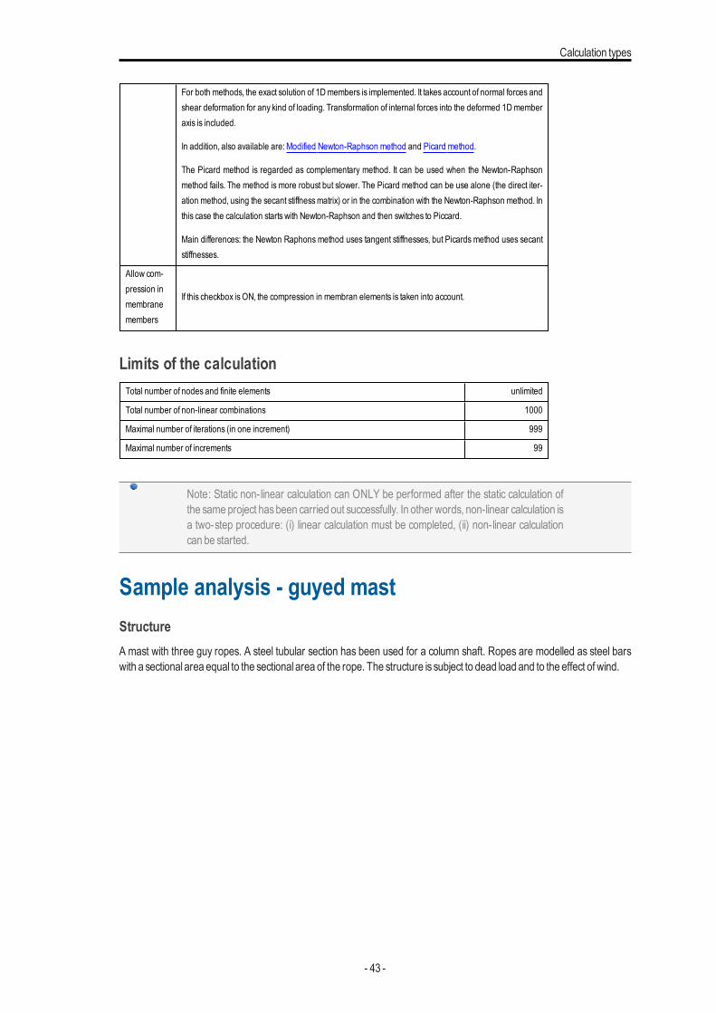
Sample analysis - guyed mastStructureA mast with three guy ropes. A steel tubular section has been used for a column shaft. Ropes are modelled as steel barswith a sectional area equal to the sectional area of the rope. The structure is subject to dead load and to the effect of wind.
- 43 -
Chapter 4
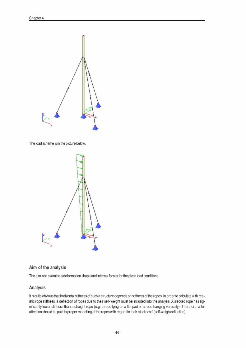
The load scheme is in the picture below.
Aim of the analysisThe aim is to examine a deformation shape and internal forces for the given load conditions.
AnalysisIt is quite obvious that horizontal stiffnessof such a structure dependson stiffnessof the ropes. In order to calculatewith real-istic rope stiffness, a deflection of ropes due to their self-weight must be included into the analysis. A slacked rope has sig-nificantly lower stiffness than a straight rope (e.g. a rope lying on a flat pad or a rope hanging vertically). Therefore, a fullattention should be paid to proper modelling of the ropeswith regard to their ‘slackness’ (self-weigh deflection).
- 44 -
Calculation types
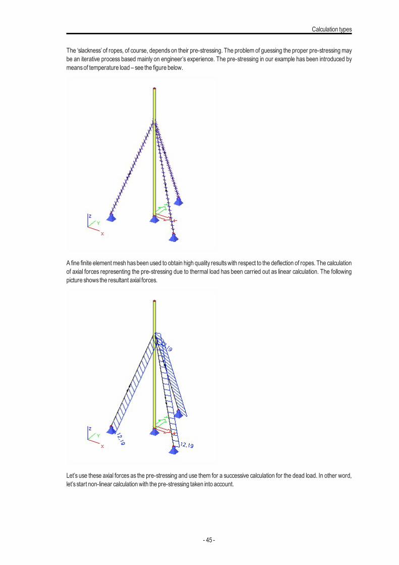
The ‘slackness’ of ropes, of course, depends on their pre-stressing. The problem of guessing the proper pre-stressing maybe an iterative process based mainly on engineer’s experience. The pre-stressing in our example has been introduced bymeansof temperature load – see the figure below.
A fine finite elementmesh hasbeen used to obtain high quality resultswith respect to the deflection of ropes. The calculationof axial forces representing the pre-stressing due to thermal load has been carried out as linear calculation. The followingpicture shows the resultant axial forces.
Let’s use these axial forces as the pre-stressing and use them for a successive calculation for the dead load. In other word,let’s start non-linear calculationwith the pre-stressing taken into account.
- 45 -
Chapter 4
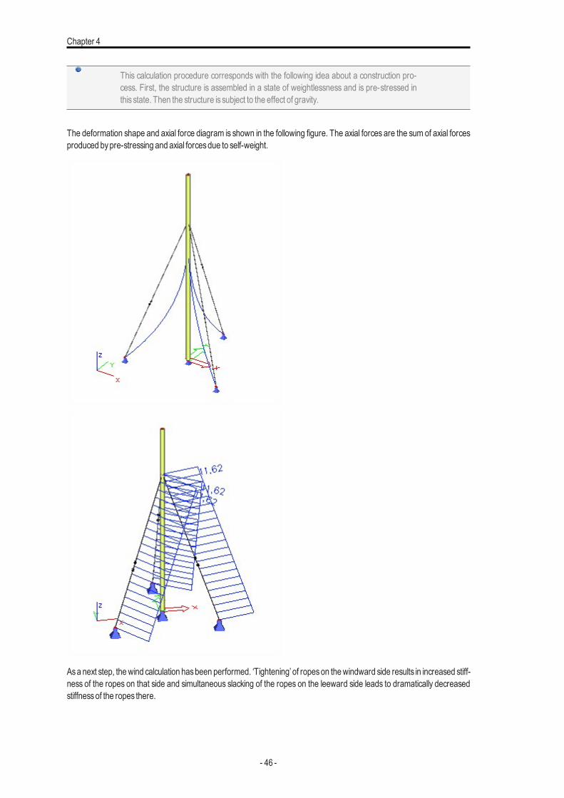
This calculation procedure corresponds with the following idea about a construction pro-cess. First, the structure is assembled in a state of weightlessness and is pre-stressed inthis state. Then the structure is subject to the effect of gravity.
The deformation shape and axial force diagram is shown in the following figure. The axial forces are the sum of axial forcesproduced bypre-stressing and axial forcesdue to self-weight.
Asa next step, thewind calculation hasbeen performed. ‘Tightening’ of ropeson thewindward side results in increased stiff-ness of the ropes on that side and simultaneous slacking of the ropes on the leeward side leads to dramatically decreasedstiffnessof the ropes there.
- 46 -
Calculation types
The superposition principle cannot be applied in the non-linear analysis. Therefore, the effect of the self-weight and thewind cannot be analysed separately and then combined in the postprocessor. A combination must be created in advanceand the calculationmust be carried out for thisnon-linear combination.
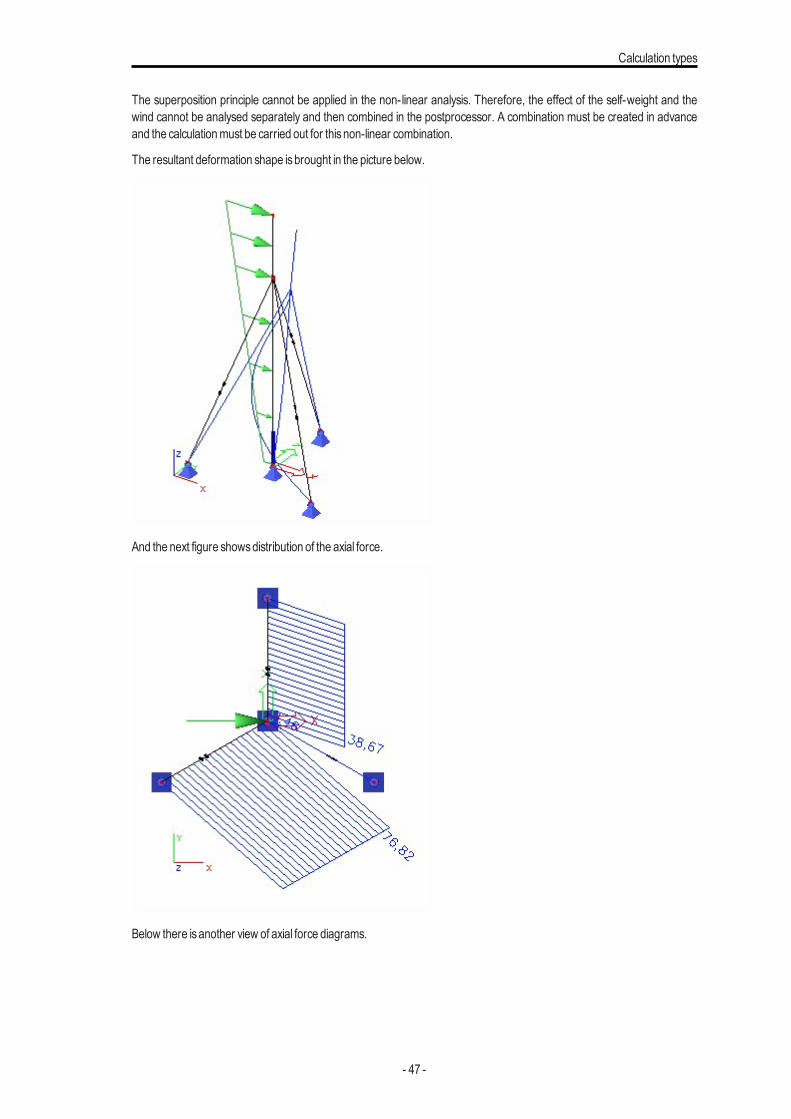
The resultant deformation shape isbrought in the picture below.
And the next figure showsdistribution of the axial force.
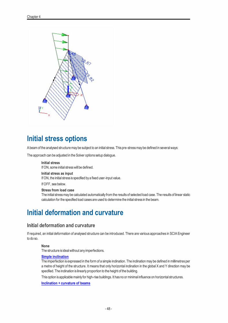
Below there isanother view of axial force diagrams.
- 47 -
Chapter 4
Initial stress optionsAbeamof the analysed structuremaybe subject to an initial stress. Thispre-stressmaybe defined in severalways:
The approach can be adjusted in theSolver optionssetup dialogue.
Initial stressIf ON, some initial stresswill be defined.Initial stress as inputIf ON, the initial stress is specified bya fixed user-input value.If OFF, see below.Stress from load caseThe initial stressmaybe calculated automatically from the results of selected load case. The results of linear staticcalculation for the specified load casesare used to determine the initial stress in the beam.
Initial deformation and curvatureInitial deformation and curvatureIf required, an initial deformation of analysed structure can be introduced. There are various approaches in SCIA Engineerto do so.
NoneThe structure is idealwithout any imperfections.Simple inclinationThe imperfection is expressed in the form of a simple inclination. The inclinationmaybe defined inmillimetres pera metre of height of the structure. It means that only horizontal inclination in the global X and Y direction may bespecified. The inclination is linearlyproportion to the height of the building.Thisoption isapplicablemainly for high-rise buildings. It hasno or minimal influence on horizontal structures.Inclination + curvature of beams
- 48 -
Calculation types
If this option is selected, the initial deformation may be defined the same way as above PLUS the curvature ofbeamsmaybe specified aswell. The curvature is the same for all the beams in the structure.Inclination functionsThe initial imperfection isdefined bya function (or curve). The user inputs the curve bymeansof height-to-imper-fection diagram.Thisoption isapplicablemainly for high-rise buildings. It hasno or minimal influence on horizontal structures.Functions + curvature of beamsThe initial imperfection isexpressed asa sumof inclination function and curvature. It isanalogous to option Inclin-ation and curvature of beams.Deformation from load caseThis option requires two-step calculation. First, a calculation for a required load case must be performed. Thedeformation due to this load case is then used as the initial imperfection for further calculation.Buckling shapeThis option requires two-step calculation. First, a stability calculationmust be performed. The calculated bucklingshape is then used as the initial imperfection for further calculation.
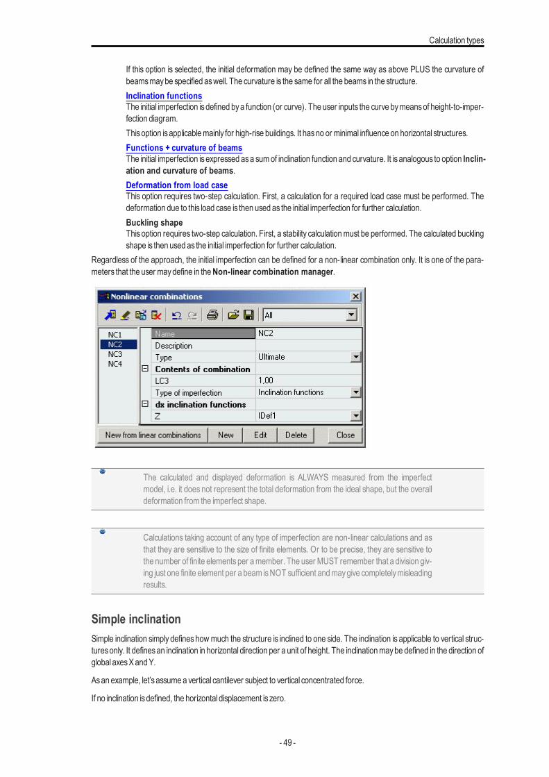
Regardless of the approach, the initial imperfection can be defined for a non-linear combination only. It is one of the para-meters that the user maydefine in theNon-linear combination manager.
The calculated and displayed deformation is ALWAYS measured from the imperfectmodel, i.e. it does not represent the total deformation from the ideal shape, but the overalldeformation from the imperfect shape.
Calculations taking account of any type of imperfection are non-linear calculations and asthat they are sensitive to the size of finite elements. Or to be precise, they are sensitive tothe number of finite elementsper amember. The user MUST remember that a division giv-ing just one finite element per a beam isNOT sufficient andmaygive completelymisleadingresults.
Simple inclinationSimple inclination simply defines how much the structure is inclined to one side. The inclination is applicable to vertical struc-turesonly. It definesan inclination in horizontal direction per a unit of height. The inclinationmaybe defined in the direction ofglobal axesXandY.
Asan example, let’sassume a vertical cantilever subject to vertical concentrated force.
If no inclination isdefined, the horizontal displacement is zero.
- 49 -
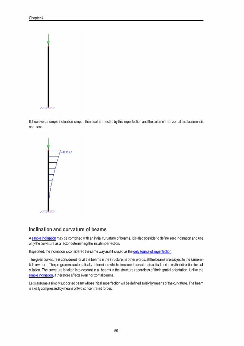
Chapter 4
If, however, a simple inclination is input, the result is affected by this imperfection and the column’shorizontal displacement isnon-zero.
Inclination and curvature of beamsA simple inclination may be combined with an initial curvature of beams. It is also possible to define zero inclination and useonly the curvature asa factor determining the initial imperfection.
If specified, the inclination is considered the samewayas if it is used as the onlysource of imperfection.
The given curvature is considered for all the beams in the structure. In other words, all the beamsare subject to the same ini-tial curvature. The programmeautomaticallydetermineswhich direction of curvature is critical and uses that direction for cal-culation. The curvature is taken into account in all beams in the structure regardless of their spatial orientation. Unlike thesimple inclination, it therefore affectseven horizontal beams.
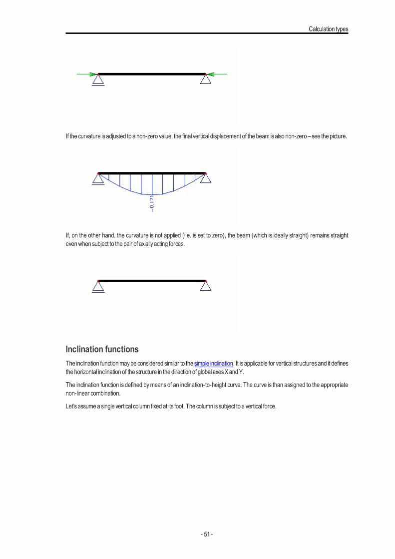
Let’sassume a simplysupported beamwhose initial imperfectionwill be defined solelybymeansof the curvature. The beamisaxially compressed bymeansof two concentrated forces.
- 50 -
Calculation types
If the curvature isadjusted to a non-zero value, the final vertical displacement of the beam isalso non-zero – see the picture.
If, on the other hand, the curvature is not applied (i.e. is set to zero), the beam (which is ideally straight) remains straightevenwhen subject to the pair of axiallyacting forces.
Inclination functionsThe inclination functionmaybe considered similar to the simple inclination. It isapplicable for vertical structuresand it definesthe horizontal inclination of the structure in the direction of global axesXandY.
The inclination function is defined bymeans of an inclination-to-height curve. The curve is than assigned to the appropriatenon-linear combination.
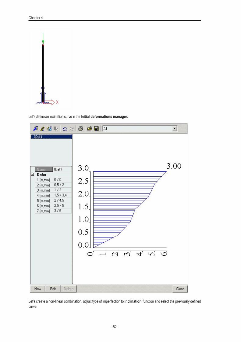
Let’sassume a single vertical column fixed at its foot. The column issubject to a vertical force.
- 51 -
Chapter 4
Let’sdefine an inclination curve in the Initial deformations manager.
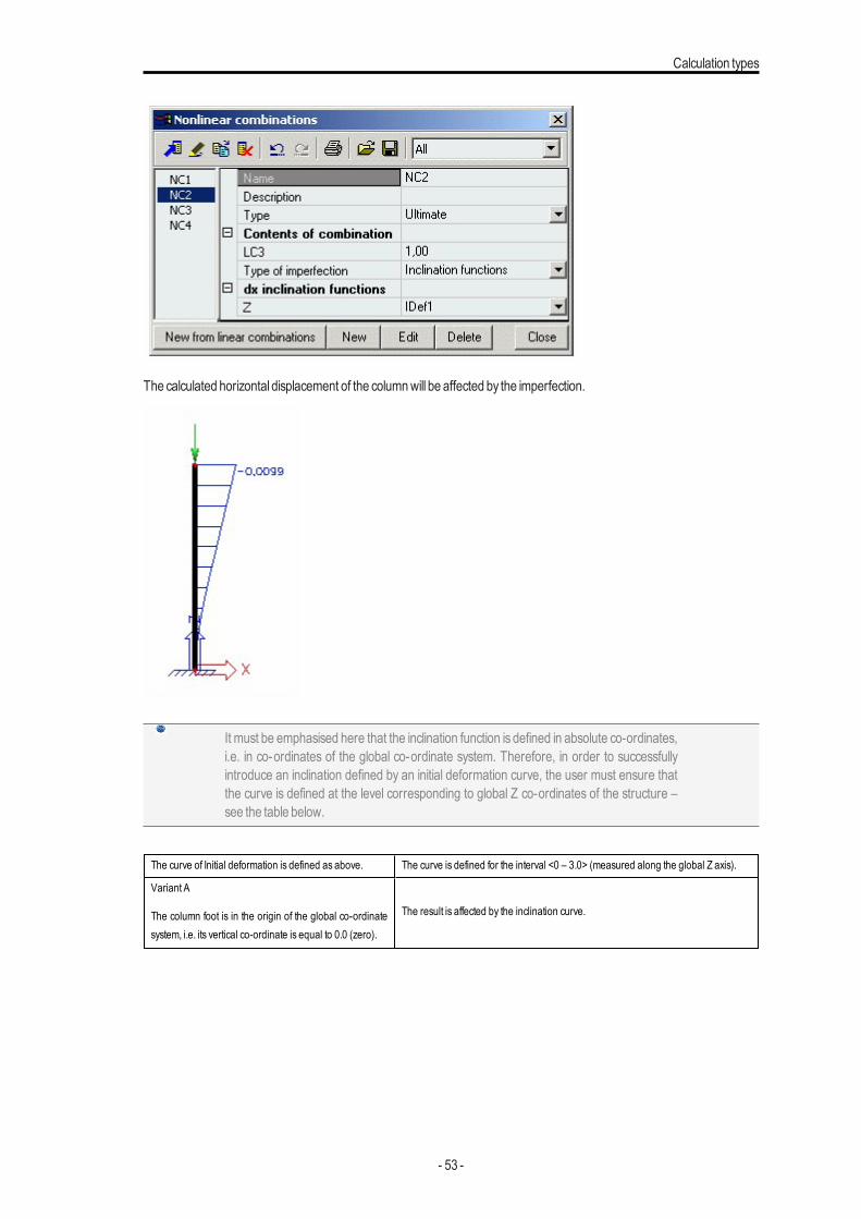
Let’s create a non-linear combination, adjust type of imperfection to Inclination function and select the previously definedcurve.
- 52 -
Calculation types
The calculated horizontal displacement of the columnwill be affected by the imperfection.
It must be emphasised here that the inclination function is defined in absolute co-ordinates,i.e. in co-ordinates of the global co-ordinate system. Therefore, in order to successfullyintroduce an inclination defined by an initial deformation curve, the user must ensure thatthe curve is defined at the level corresponding to global Z co-ordinates of the structure –see the table below.
The curve of Initial deformation is defined as above. The curve is defined for the interval <0 – 3.0> (measured along the global Z axis).
Variant A
The column foot is in the origin of the global co-ordinatesystem, i.e. its vertical co-ordinate is equal to 0.0 (zero).
The result is affected by the inclination curve.
- 53 -
Chapter 4
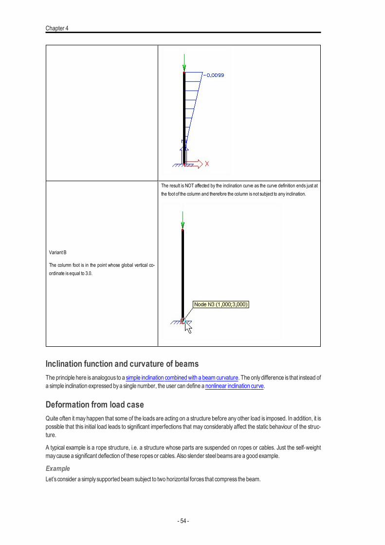
Variant B
The column foot is in the point whose global vertical co-ordinate is equal to 3.0.
The result is NOT affected by the inclination curve as the curve definition ends just atthe foot of the column and therefore the column is not subject to any inclination.
Inclination function and curvature of beamsThe principle here isanalogous to a simple inclination combinedwith a beamcurvature. The onlydifference is that instead ofa simple inclination expressed bya single number, the user can define a nonlinear inclination curve.
Deformation from load caseQuite often it may happen that some of the loads are acting on a structure before any other load is imposed. In addition, it ispossible that this initial load leads to significant imperfections that may considerably affect the static behaviour of the struc-ture.
A typical example is a rope structure, i.e. a structure whose parts are suspended on ropes or cables. Just the self-weightmaycause a significant deflection of these ropesor cables. Also slender steel beamsare a good example.
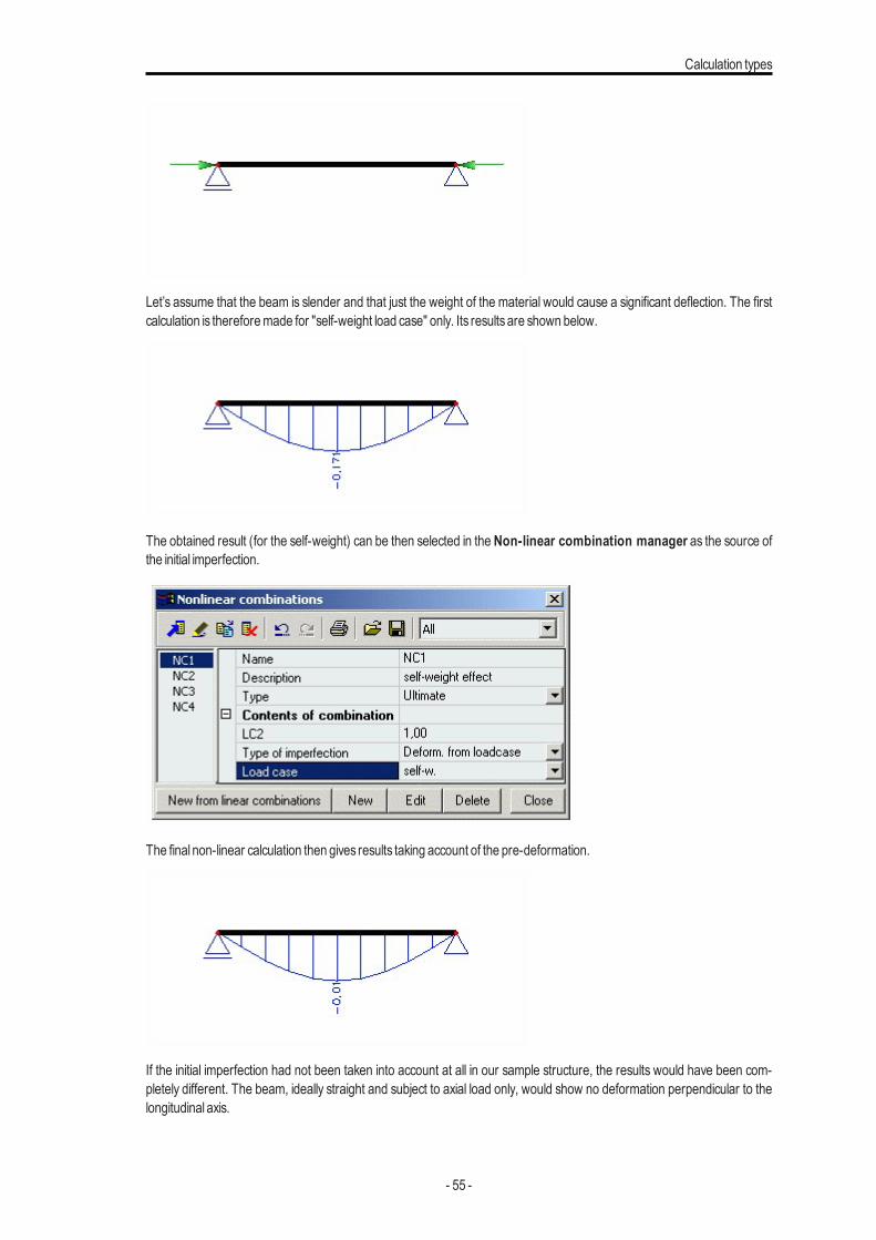
ExampleLet’s consider a simplysupported beamsubject to two horizontal forces that compress the beam.
- 54 -
Calculation types
Let’s assume that the beam is slender and that just the weight of the material would cause a significant deflection. The firstcalculation is thereforemade for "self-weight load case" only. Its resultsare shown below.
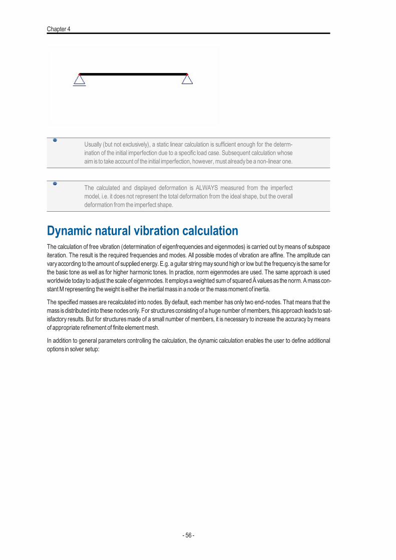
The obtained result (for the self-weight) can be then selected in the Non-linear combination manager as the source ofthe initial imperfection.
The final non-linear calculation then gives results taking account of the pre-deformation.
If the initial imperfection had not been taken into account at all in our sample structure, the results would have been com-pletely different. The beam, ideally straight and subject to axial load only, would show no deformation perpendicular to thelongitudinal axis.
- 55 -
Chapter 4
Usually (but not exclusively), a static linear calculation is sufficient enough for the determ-ination of the initial imperfection due to a specific load case. Subsequent calculation whoseaim is to take account of the initial imperfection, however, must alreadybe a non-linear one.
The calculated and displayed deformation is ALWAYS measured from the imperfectmodel, i.e. it does not represent the total deformation from the ideal shape, but the overalldeformation from the imperfect shape.
Dynamic natural vibration calculationThe calculation of free vibration (determination of eigenfrequencies and eigenmodes) is carried out bymeans of subspaceiteration. The result is the required frequencies and modes. All possible modes of vibration are affine. The amplitude canvaryaccording to the amount of supplied energy. E.g. a guitar stringmaysound high or low but the frequency is the same forthe basic tone as well as for higher harmonic tones. In practice, norm eigenmodes are used. The same approach is usedworldwide today to adjust the scale of eigenmodes. It employsaweighted sumof squaredÄvaluesas the norm. Amasscon-stantM representing theweight iseither the inertialmass in a node or themassmoment of inertia.
The specified masses are recalculated into nodes. By default, each member has only two end-nodes. That means that themass isdistributed into these nodesonly. For structuresconsisting of a huge number ofmembers, thisapproach leads to sat-isfactory results. But for structuresmade of a small number of members, it is necessary to increase the accuracy bymeansof appropriate refinement of finite elementmesh.
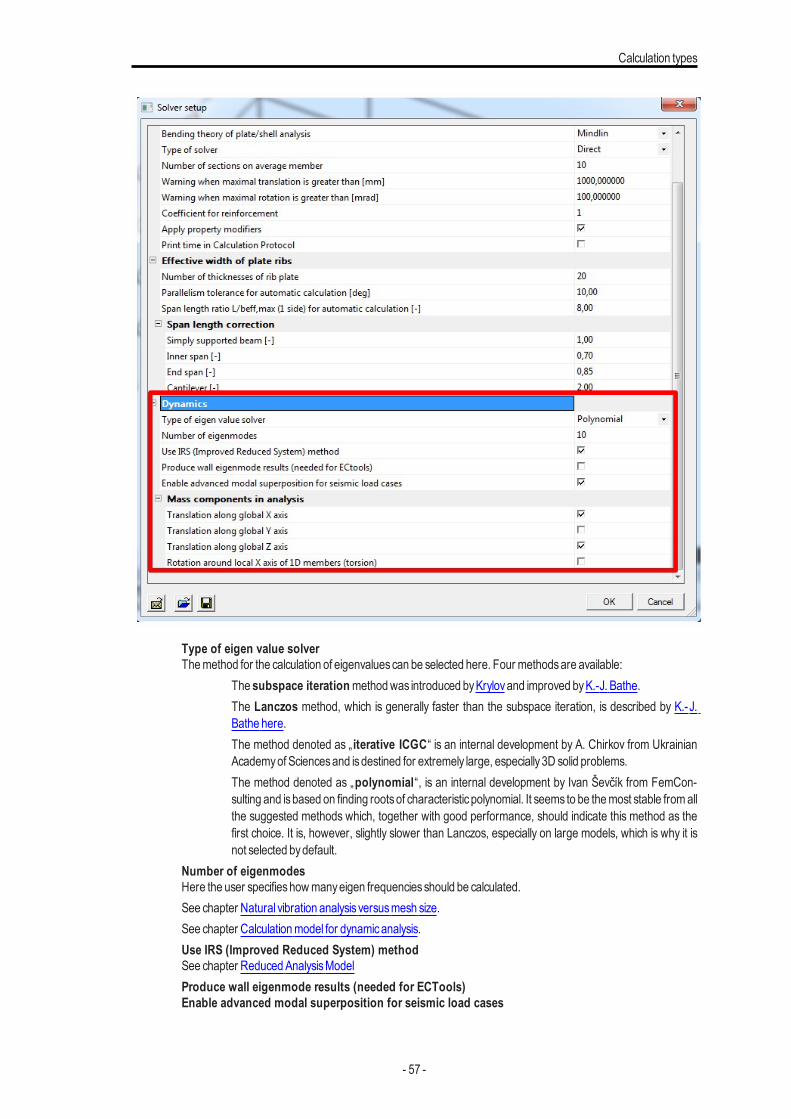
In addition to general parameters controlling the calculation, the dynamic calculation enables the user to define additionaloptions in solver setup:
- 56 -
Calculation types
Type of eigen value solverThemethod for the calculation of eigenvaluescan be selected here. Four methodsare available:
The subspace iterationmethodwas introduced byKrylovand improved byK.-J. Bathe.The Lanczos method, which is generally faster than the subspace iteration, is described by K.-J.Bathe here.The method denoted as „ iterative ICGC“ is an internal development by A. Chirkov from UkrainianAcademyof Sciencesand isdestined for extremely large, especially3D solid problems.The method denoted as „polynomial“, is an internal development by Ivan Ševčík from FemCon-sulting and isbased on finding rootsof characteristicpolynomial. It seems to be themost stable fromallthe suggested methods which, together with good performance, should indicate this method as thefirst choice. It is, however, slightly slower than Lanczos, especially on large models, which is why it isnot selected bydefault.
Number of eigenmodesHere the user specifieshowmanyeigen frequenciesshould be calculated.See chapter Natural vibration analysis versusmesh size.See chapter Calculationmodel for dynamicanalysis.Use IRS (Improved Reduced System) methodSee chapter ReducedAnalysisModelProduce wall eigenmode results (needed for ECTools)Enable advanced modal superposition for seismic load cases
- 57 -
Chapter 4
Method for time history analysisThemethod for the time historyanalysis can be selected here. Twomethodsare available:
The direct time integration method is standard Newmark algorithm. Theoretical backgroundabout direct time integration here.The modal superposition method, it is necessary in some cases to filter out local, high frequencymodes and avoid irrelevant behaviour, especially for fast train dynamic analysis. Modal superpositionisa powerful idea of obtaining solutions. It isapplicable to both free vibration and forced vibration prob-lems. The basic idea To use free vibrations mode shapes to uncouple equations of motion. Theuncoupled equations are in terms of new variables called the modal coordinates. Solution for themodal coordinates can be obtained by solving each equation independently. A superposition of modalcoordinates then gives solution of the original equations. Notices It is not necessary to use all modeshapes for most practical problems. Good approximate solutions can be obtained via superpositionwith only first fewmode shapes.
Mass components in analysisThissettings in solver setup is for optional removal ofmasscomponents in dynamicanalysis. There are four itemswith checkboxes, where user can choose, which partsofmassshould be taken to dynamiccalculation: (asdefaultallmassesare selected)
Translation along global X axisTranslation along global Y axisTranslation along global Z axisRotation around local X axis of 1D members (torsion)
Calculation for selected mass combinationsIf general optionSingle nonlinear analysis is ON, the user may specify which mass combinations will be calculated. Other-wise, all non-calculated are alwayscalculated.
Note: The dynamiccalculation can be carried out for masscombinationsonly.
Dynamic forced harmonic vibrationThe principlesof how SCIAEngineer dealswith a structure subject to a harmonic load are given in chapters:
l Loads>Load types>Dynamic loads>Harmonic load
l Loads>Load cases>Dynamic load cases>Defining the harmonic load case
l Results>Evaluating the results for harmonic load
And the core of dynamiccalculations is laid down in:
l Loads>Load cases>Dynamic load cases>Dynamic load cases
l Loads>Load cases>Dynamic load cases>Defining a new dynamic load case
Harmonic band analysisContext - Typical usageIn a nutshell, harmonic band analysis, aka Third Octave Analysis, is about assessing the sensitivity of a structure to anexternal source of vibration.
- 58 -
Calculation types
For example: a microsurgery room is located in a building close to a metro line. The metro line is the external vibrationsource, and the harmonicband analysiswill:
- generate a seriesof harmonic load casesat a support (or close to it, not sure anymore, I think it wasa spring support)
- filter them to get RMSvaluesper band
- display the resulting spectrum in a particular point of themicrosurgery room
- this spectrum is transfer function: for a given external vibration, typically at the foundation level, one can see the localimpact in anypoint of the structure acrossa range of frequencies.
A transfer function is usually computed for a unit input at the foundation. It basically tells, for a unit action applied in a givenpoint of the structure at a given frequency, how the response of the structure will be amplified or damped in another point ofthe structure. The amplification of the response usuallydependson the frequency.
Harmonic Band Analysis is not meant for generating harmonic load cases that could be used in combination with otheractions. It is solely designed to generate the transfer function, as described above. It does, however, carry out the cal-culation through a set of harmonic load case calculationson a range of frequencies.
DescriptionThis calculation represents a new way of dealing with the calculations in harmonic analysis. Multiple analyses on a range offrequenciesare carried out. The harmonicanalysis ispossible for a range of frequenciescontrolled by the user. In the stand-ard harmonic analysis, the forces and the frequency are defined. In this type (Harmonic Band Analysis) of analysis, the fre-quencyof the harmonic force varied over a range and the harmonicanalysis isperformed for multiple values in that range.
To fit the needs of this type of calculation, a new load case type named "Harmonic Band Analysis" has been introduced intoSCIA Engineer. the properties of this load case are similar to the standard harmonic load case. But, instead of the fre-quency, there are 5 new parameters: A, n1, n2, C, N (explained below). The input of loads is the same as for the standardharmonic load cases.
SCIAEngineer generatesa set of extra load cases:
1. one set ofmain F frequencies (their number isn=n2-n1+1) and
2. n setsof secondary frequencies (each of themwith 2N items).
The secondary load casesare the standard SCIAEngineer harmonic load casesand have standard results.
The results of the main load cases are calculated byRMS (root mean square) method from the appropriate set of the sec-ondary load cases.
SCIAEngineer generates the following result classes:
1. onewith allmain load casesand
2. nwith the setsof the secondary load cases.
Output of results
Alphanumerical outputAll the results of themain and secondary load casesare presented in the standard SCIAEngineer way in result tables usingthe generated results classes.
Graphical outputThe results of the main frequencies or results of the bands around the main frequency can be presented also graphically inthe formof a diagram. For that purpose a new tool hasbeen integrated into SCIAEngineer.
- 59 -

Chapter 4
Refresh after modifications of the structure and changes in other input valuesWhen the user changes parameters n1, n2 or N, all the generated load cases and all the generated result classes aredeleted and all the document items with band analysis load cases are not valid any more. If any other project data arechanged, all generated items remain in the project and their content isupdated after next calculation.
(Little) Theoretical backgroundThe user definesconstantsA,n1,n2,C,N.
The default valuesare: A=2, n1 =6, n2 =30, C =3, N =10.
From these data, a geometric seriesare generated using the following formula
where n varies fromn1 to n2with a step of 1.
The result is a series of so-called main frequencies F. The default set is: 4,00; 5,04; 6,35; 8,00; 10,08; etc. Around each ofthese values, an intervalFi- - Fi+ isdefined:
The interval [Fi- - F] isnow divided intoN steps to generate the secondary frequencies "f".
For each value of "f" a harmonic analysis is carried out. The displacement or inner force in a specified node in a given dir-ection is calculated, givingN result values. The same isdone for the interval [F – Fi+]. From these 2N values, one value is cal-culated usingRMS (rootmean square) and assigned to themain frequencyF.
Combination with other load casesThe resultsof thisanalysis can not be combinedwith other staticand dynamicanalyses.
Input of the load case for the Harmonic Band AnalysisThe input of the load case for theHarmonicBandAnalysis requiressimilar prerequisitesasother dynamic load cases.
Procedure do define a new load case for the Harmonic Band Analysis
1. In theProject setup dialogue, on tab Functionality, select DynamicsandHarmonicband analysis.
2. In theDynamicsbranch of the treemenu define at least oneMassgroup and at least oneCombination ofmassgroups.
3. Then youmayopen the Load casemanager and input a new load case for theHarmonicBandAnalysis.
4. Select the following optionsand define the appropriate parameters:
1. Action type =variable
2. Load group =as required in the particular project
3. Load type =dynamic
4. Specification =Harmonicband analysis
5. Parameters=as required in the particular project
- 60 -
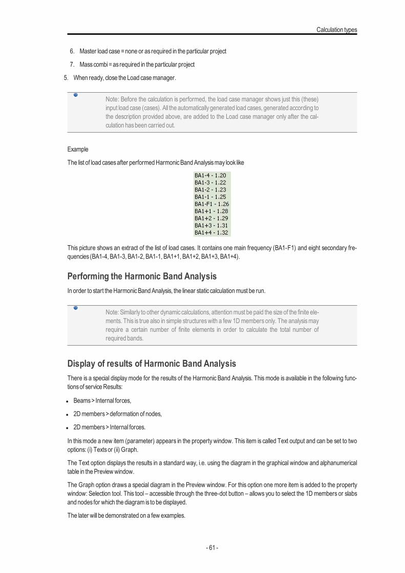
Calculation types
6. Master load case =none or as required in the particular project
7. Masscombi=as required in the particular project
5. When ready, close the Load casemanager.
Note: Before the calculation is performed, the load case manager shows just this (these)input load case (cases). All the automaticallygenerated load cases, generated according tothe description provided above, are added to the Load case manager only after the cal-culation hasbeen carried out.
Example
The list of load casesafter performedHarmonicBandAnalysismay look like
This picture shows an extract of the list of load cases. It contains one main frequency (BA1-F1) and eight secondary fre-quencies (BA1-4, BA1-3, BA1-2, BA1-1, BA1+1, BA1+2, BA1+3, BA1+4).
Performing the Harmonic Band AnalysisIn order to start theHarmonicBandAnalysis, the linear static calculationmust be run.
Note: Similarly to other dynamiccalculations, attentionmust be paid the size of the finite ele-ments. This is true also in simple structureswith a few 1Dmembers only. The analysismayrequire a certain number of finite elements in order to calculate the total number ofrequired bands.
Display of results of Harmonic Band AnalysisThere is a special display mode for the results of the Harmonic Band Analysis. This mode is available in the following func-tionsof serviceResults:
l Beams> Internal forces,
l 2Dmembers>deformation of nodes,
l 2Dmembers> Internal forces.
In this mode a new item (parameter) appears in the property window. This item is called Text output and can be set to twooptions: (i) Textsor (ii) Graph.
The Text option displays the results in a standard way, i.e. using the diagram in the graphical window and alphanumericaltable in thePreviewwindow.
The Graph option draws a special diagram in the Preview window. For this option one more item is added to the propertywindow: Selection tool. This tool – accessible through the three-dot button – allows you to select the 1D members or slabsand nodes for which the diagram is to be displayed.
The later will be demonstrated on a few examples.
- 61 -
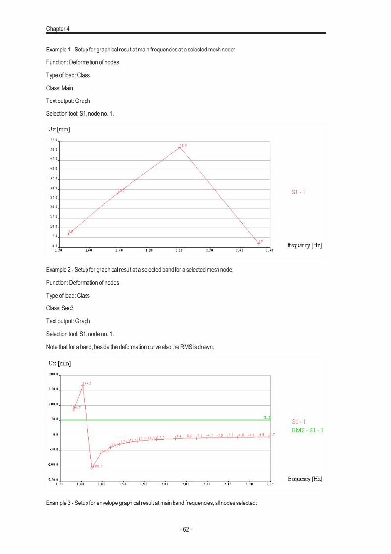
Chapter 4
Example 1 - Setup for graphical result at main frequenciesat a selectedmesh node:
Function: Deformation of nodes
Type of load: Class
Class:Main
Text output: Graph
Selection tool: S1, node no. 1.
Example 2 - Setup for graphical result at a selected band for a selectedmesh node:
Function: Deformation of nodes
Type of load: Class
Class: Sec3
Text output: Graph
Selection tool: S1, node no. 1.
Note that for a band, beside the deformation curve also theRMS isdrawn.
Example 3 - Setup for envelope graphical result at main band frequencies, all nodesselected:
- 62 -
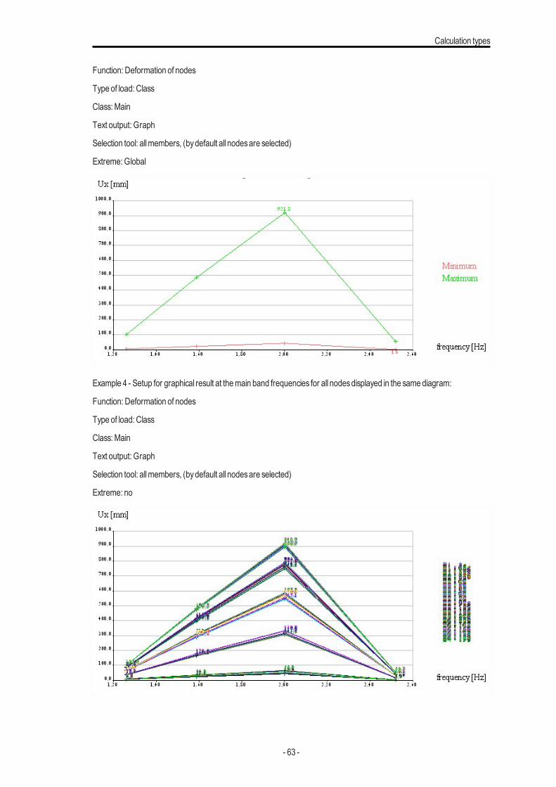
Calculation types
Function: Deformation of nodes
Type of load: Class
Class:Main
Text output: Graph
Selection tool: allmembers, (bydefault all nodesare selected)
Extreme:Global
Example 4 - Setup for graphical result at themain band frequencies for all nodesdisplayed in the samediagram:
Function: Deformation of nodes
Type of load: Class
Class:Main
Text output: Graph
Selection tool: allmembers, (bydefault all nodesare selected)
Extreme: no
- 63 -
Chapter 4
Calculation model for dynamic analysisWhen a staticanalysis isbeing performed, there are usuallyno problemswith the creation of a satisfactorymodel of the ana-lysed structure. BUT, in dynamicanalysiswe have to thinkabout the problema bit more. Here’swhy.
Statics deals with the equilibrium of the structureThe imposed load and internal forces arising due to the elastic deformation of the structure must be balanced. In dynamics,the equilibrium isalso required, but nowwith additional forces– inertial and damping.
Inertial forcesAt school, they taught us about Newton Law – force is equal to mass multiplied by acceleration. This means that if themasses of a structure move with acceleration, inertial forces act on the structure. In order to analyse dynamic behaviour ofthe structure, we have to complete the calculationmodel and add data related tomasses in the structure.
Damping forcesNature has provided uswith an invaluable principle. As soon as anything starts to move, it is stopped in a while. Against themotion the resistance of environment is acting – external and internal friction. The mechanical energy is transformed intoanother form, usually into the thermal one. In civil engineering practice, structuresof higher damping capacity aremore suit-able – the higher damping capacity, the lower vibration. Steel structureshave lower damping capacity than concrete or wod-den ones. It is generally difficult to take damping forces into account in calculation. The user’s point of view is that this task israther simply s/he just defines a damping coefficient, e.g. logarithmic decrement. But nothing is as simple as it may seem tobe.We’ve got just one coefficient, but itsprecision is rather arguable.
To conclude, dynamic calculationsdiffer from static ones in one principle point. We do not seekonly the equilibrium betweenimposed load and internal forces, but we also introduce inertial and damping forces. The outcome is that we have to com-plete the calculationmodel created for a staticanalysiswith other data:
l masses in the structure (used for determination of inertial forces)
l damping data (for calculation of damping forces)
Method of decomposition into eigemodesDynamic calculations in SCIAEngineer are based onmethod of decomposition into eigemodes (calledmodal analysis). Thebasic task is therefore the solution of free vibration problem. The calculation findseigenfrequenciesand eigenmodes.
There exist bizarre conceptions among structural engineers of what the eigenfrequency and eigenmode actually is. It isimportant to realise that free vibration gives usonly the conception of structure properties and allowsus to predict the beha-viour under time varying load conditions. In nature, each body prefers to remain in a standstill. If forced to move, it prefersthe way requiringminimal energy consumption. Thesewaysof motion are called eigenmodes. The eigenmodesdo not rep-resent the actual deformation of the structure. Theyonly show deformation that is "natural" for the structure. This iswhy themagnitudes of calculated displacement and internal forces are dimensionless numbers. The numbers provided areorthonormed, i.e. theyhave a particular relation to themasses in the structure. The absolute value of the individual numbersisnot important.Whatmatter is their mutual proportion.
Let’s assume that there is an engine mounted on a structure. The engine is equipped with a eccentrically connected partsrevolvingwith frequencyof 8 Hz.We determine that eigenfrequencyof the structure is7.7 Hz. This informationmeans that itis natural for the structure to vibrate close to 8Hzand that the applied load is too dangerous. The eigenmode correspondingto frequency 7.7 Hz can inform us only about the mode of the vibration. In other words, it can show us where the dis-placement due to vibration will be largest and where minimal. It suggests nothing about the real size of displacement orinternal forces. These pieces of information can only be obtained from the calculation of the structure subjected to a par-ticular load.
- 64 -

Calculation types
In order to consider the effect of inertial forces, we have to add masses to the calculation model. We can choose from con-centratedmasses in nodesor concentrated point and linear masseson beams.
In SCIA Engineer a concept of consistent mass matrix has been applied. This concept means that not only diagonal ele-ments of mass matrix are considered in the calculation. Consequently, this solution is more precise than for matrix calledlumpedmassmatrix. Thisadvantage issignificant e.g. when rigid armsare used in themodel.
Self-weight of the structure due to cross-sections and material is not input. It is taken into account automatically. We onlyinput masses attached to the structure, masses that will move with the structure when it moves. So be careful with sus-pended loads hanging on longer suspensions. Problemsmay arise with imposed load on floors, charges of tanks and othermasses that may or may not be present. A safe side does not exist, which was already stated earlier. A very useful option inSCIAEngineer is the generation ofmasses fromdefined static load.
Masses on the structure may be sorted into several groups that can be combined in mass combinations in a way similar tostandard load cases. For simple structures where all the masses are in a single group, this approach may be a small com-plication. On the other hand, it will be considerably advantageous for more complex structures. Masses in individual groupsmaybe defined in nodesor on beams. The latter maybe either concentrated or distributed.
The next step in the specification of mass distribution across the structure is the definition of mass groups. The combinationthen defines themasses in the dynamiccalculationmodel. The combinationsare input the samewayasstatic load case com-binations.We select appropriatemassgroupsand specify their coefficient.Why is thisneeded?
Let’s consider an example of a structure supporting a large liquid tank. The amount of liquid in the tank will range betweentwo limits: from an empty tank to a full tank. The dynamic behaviour of the structure will be different for the two limit states. Ifwe need to perform a seismic analysis, we do not know when the earthquake happens. It is therefore suitable to evaluateboth limit states, but also an intermediate one with the tank e.g. half full. It would mean three separate calculations. In SCIAEngineer however, we just need to define threemass combinations and run one calculation. We include all the masses cor-responding to a full tank into one mass group. Then we define three combinations. The first one will contain the mentionedgroup with coefficient equal to 1.0. The second one will contain the mentioned group with coefficient equal to 0.5. And thethird combinationwill not contain the group at all.
Other examples:
l Bridge – dynamic analysis of an "empty" bridge and bridge loaded with a vehicle or train (even though the mass of largerbridges is significantlybigger that themassof vehicles),
l Building frame – response to vibration for variousdistribution of floor variable load.
The calculation of eigenmodes is usually carried out together with a static calculation. Each of the eigenmodes refers to aparticular calculation model that is defined bymeans of a combination of mass groups and a corresponding model for staticanalysis.
The calculation of eigenmodes and eigenfrequencies is made on the finite element model of the structure. The structure isdiscretised, which means that instead of a general structure with an infinite number of degrees of freedom, a calculationmodel with a finite number of degrees of freedom is analysed. The number of degrees of freedom can be normally determ-ined by a simple multiplication: number of nodes is multiplied by the number of possible displacements in the node (trans-lation, rotation). It is important to know that the accuracy of the model is in proportion to the "precision of discretisation", i.e.to the number of elements of the finite element mesh. This refinement has almost no practical reason in static calculations.However, for dynamic and non-linear analyses, it significantly affects the accuracy of results (but also the calculation’s timeconsumption).
The user must decide what number of eigenfrequencies should be calculated. The frequencies are always calculated fromthe lowest one. Generally, the number of frequencies that can be calculated for a discretised model is equal to the numberof degrees of freedom. Due to the applied method, this is not always true in SCIA Engineer. Another problem is that thehigher the frequency is, the less accuracy is achieved. Therefore, it is sensible to calculate only a few lowest frequencies.Usually, it is good enough to select the number frequencies as 1/20 to 1/10 of the number of degrees of freedom. On theother hand, it is not practical to select too high number of frequenciesbecause it prolongs the calculation non-proportionally.Once again, no precise and strict limit can be established, but it can be said that 20 frequenciesare usually sufficient even forexcessive projects.
- 65 -
Chapter 4
See also chapter Natural vibration analysis versusmesh size.
In eigenfrequencyproblem, the following equation system issolved:
M . r.. + K . r = 0
where:
r is the vector of translationsand rotations in nodes,
r.. is the vector of corresponding accelerations,
K is the stiffnessmatrixassembled already for static calculation,
M is themassmatrixassembled during the dynamiccalculation.
The solution itself is carried out bymeansof subspace iterationmethod.
Dynamic seismic calculationThe principlesof how SCIAEngineer dealswith a structure subject to a seismic load are given in chapters:
l Loads>Load types>Dynamic loads>Seismic load
l Loads>Load cases>Dynamic load cases>Defining the seismic load case
And the core of dynamiccalculations is laid down in:
l Loads>Load cases>Dynamic load cases>Dynamic load cases
l Loads>Load cases>Dynamic load cases>Defining a new dynamic load case
Information about automaticallygenerated combinationsaccording code are here:
l Seismiccombination according EN code
l Seismiccombination according IBC code
Information about several seismicspectrumsare here:
l Defining a seismic response spectrum
Information about variousaspectsof the seismicanalysisof buildings isavailable here:
l SeismicAnalysisof Buildings
Information about theoretical background,modelization & troubleshooting of dynamicanalysis
l Dynamicanalysis troubleshooting
Buckling analysisAdjustment of general parametersmaycontrol the calculation.
Calculation for selected stability combinationsIf general optionAdvanced solver option is ON, the user may specify which stability combinations will be calculated. Other-wise, all non-calculated are alwayscalculated.
- 66 -
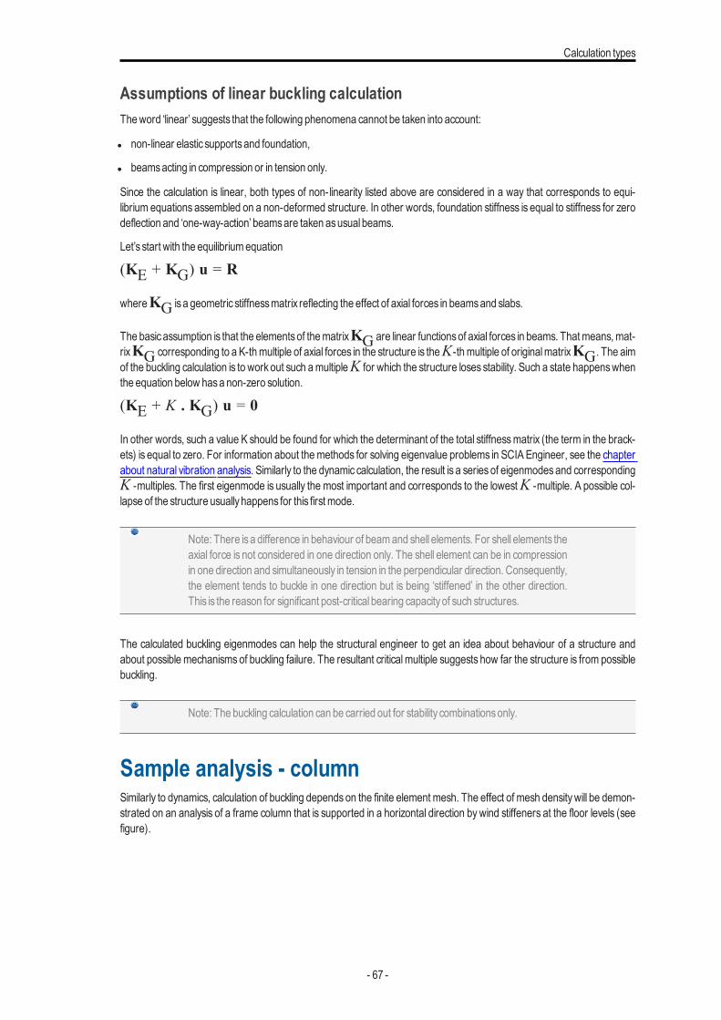
Calculation types
Assumptions of linear buckling calculationTheword ‘linear’ suggests that the following phenomena cannot be taken into account:
l non-linear elastic supportsand foundation,
l beamsacting in compression or in tension only.
Since the calculation is linear, both types of non-linearity listed above are considered in a way that corresponds to equi-librium equations assembled on a non-deformed structure. In other words, foundation stiffness is equal to stiffness for zerodeflection and ‘one-way-action’ beamsare taken asusual beams.
Let’s start with the equilibriumequation
(KE + KG) u = R
whereKG is a geometric stiffnessmatrix reflecting the effect of axial forces in beamsand slabs.
The basicassumption is that the elementsof thematrixKG are linear functionsof axial forces in beams. Thatmeans,mat-rixKG corresponding to a K-thmultiple of axial forces in the structure is theK-thmultiple of originalmatrixKG. The aimof the buckling calculation is to work out such amultipleK for which the structure loses stability. Such a state happenswhenthe equation below hasa non-zero solution.
(KE + K . KG) u = 0
In other words, such a value K should be found for which the determinant of the total stiffnessmatrix (the term in the brack-ets) is equal to zero. For information about themethods for solving eigenvalue problems in SCIAEngineer, see the chapterabout natural vibration analysis. Similarly to the dynamic calculation, the result is a series of eigenmodesand correspondingK -multiples. The first eigenmode is usually the most important and corresponds to the lowestK -multiple. A possible col-lapse of the structure usuallyhappens for this first mode.
Note: There isa difference in behaviour of beamand shell elements. For shell elements theaxial force is not considered in one direction only. The shell element can be in compressionin one direction and simultaneously in tension in the perpendicular direction. Consequently,the element tends to buckle in one direction but is being ‘stiffened’ in the other direction.This is the reason for significant post-critical bearing capacityof such structures.
The calculated buckling eigenmodes can help the structural engineer to get an idea about behaviour of a structure andabout possible mechanisms of buckling failure. The resultant critical multiple suggests how far the structure is from possiblebuckling.
Note: The buckling calculation can be carried out for stability combinationsonly.
Sample analysis - columnSimilarly to dynamics, calculation of buckling depends on the finite element mesh. The effect of mesh densitywill be demon-strated on an analysis of a frame column that is supported in a horizontal direction by wind stiffeners at the floor levels (seefigure).
- 67 -
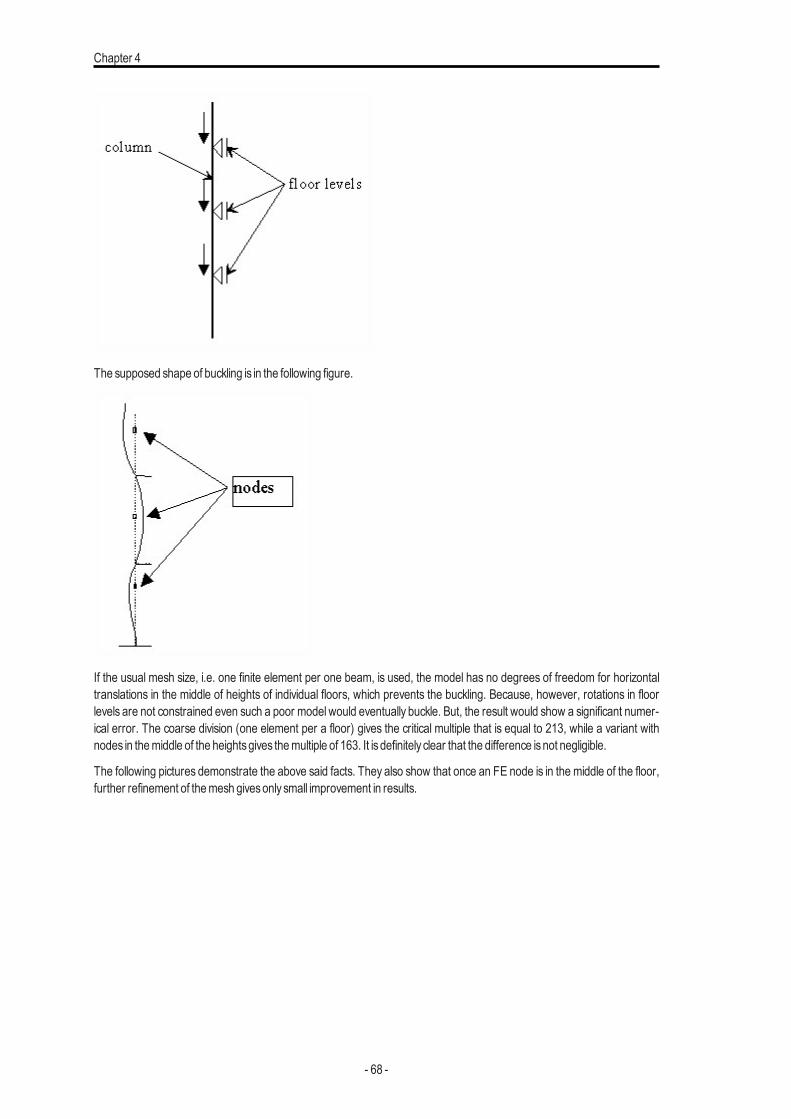
Chapter 4
The supposed shape of buckling is in the following figure.
If the usual mesh size, i.e. one finite element per one beam, is used, the model has no degrees of freedom for horizontaltranslations in the middle of heights of individual floors, which prevents the buckling. Because, however, rotations in floorlevels are not constrained even such a poor model would eventually buckle. But, the result would show a significant numer-ical error. The coarse division (one element per a floor) gives the critical multiple that is equal to 213, while a variant withnodes in themiddle of the heightsgives themultiple of 163. It isdefinitely clear that the difference isnot negligible.
The following pictures demonstrate the above said facts. They also show that once an FE node is in the middle of the floor,further refinement of themesh givesonlysmall improvement in results.
- 68 -
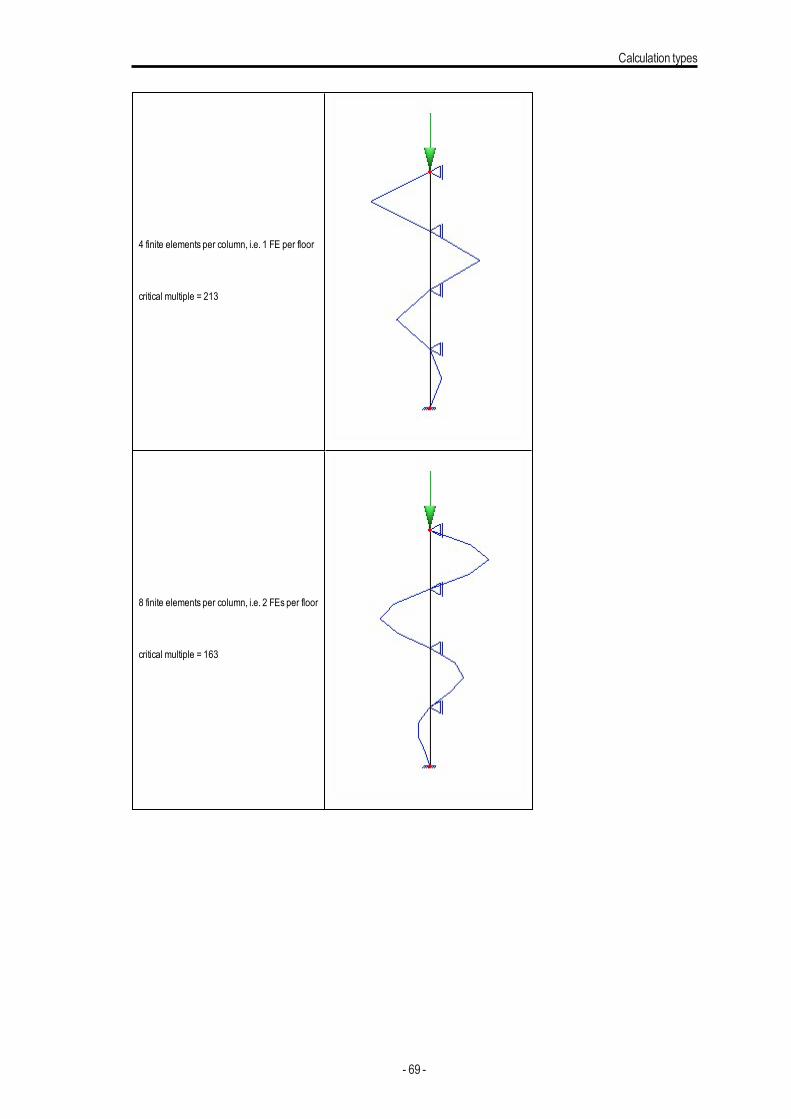
Calculation types
4 finite elements per column, i.e. 1 FE per floor
critical multiple = 213
8 finite elements per column, i.e. 2 FEs per floor
critical multiple = 163
- 69 -
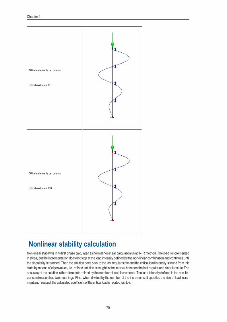
Chapter 4
10 finite elements per column
critical multiple = 161
50 finite elements per column
critical multiple = 160
Nonlinear stability calculationNon-linear stability is in its first phase calculated asnormal nonlinear calculation using N-Rmethod. The load is incrementedin steps, but the incrementation does not stop at the load intensity defined by the non-linear combination and continues untilthe singularity is reached. Then the solution goesback to the last regular state and the critical load intensity is found from thisstate bymeans of eigenvalues, i.e. refined solution is sought in the interval between the last regular and singular state.Theaccuracy of the solution is therefore determined by the number of load increments. The load intensity defined in the non-lin-ear combination has two meanings. First, when divided by the number of the increments, it specifies the size of load incre-ment and, second, the calculated coefficient of the critical load is related just to it.
- 70 -
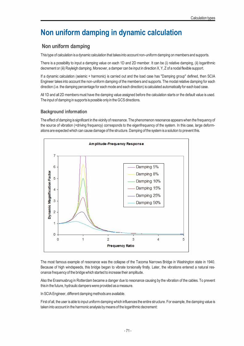
Calculation types
Non uniform damping in dynamic calculationNon uniform dampingThis type of calculation isa dynamiccalculation that takes into account non-uniformdamping onmembersand supports.
There is a possibility to input a damping value on each 1D and 2D member. It can be (i) relative damping, (ii) logarithmicdecrement or (iii) Rayleigh damping.Moreover, a damper can be input in direction X, Y, Z of a nodal flexible support.
If a dynamic calculation (seismic + harmonic) is carried out and the load case has "Damping group" defined, then SCIAEngineer takes into account the non-uniform damping of the members and supports. The modal relative damping for eachdirection (i.e. the damping percentage for eachmode and each direction) is calculated automatically for each load case.
All 1D and all 2D membersmust have the damping value assigned before the calculation starts or the default value is used.The input of damping in supports ispossible only in theGCSdirections.
Background informationThe effect of damping is significant in the vicinityof resonance. The phenomenon resonance appearswhen the frequencyofthe source of vibration (=driving frequency) corresponds to the eigenfrequency of the system. In this case, large deform-ationsare expectedwhich can cause damage of the structure. Damping of the system isa solution to prevent this.
The most famous example of resonance was the collapse of the Tacoma Narrows Bridge in Washington state in 1940.Because of high windspeeds, this bridge began to vibrate torsionally firstly. Later, the vibrations entered a natural res-onance frequencyof the bridgewhich started to increase their amplitude.
Also the Erasmusbrug in Rotterdam became a danger due to resonance causing by the vibration of the cables. To preventthis in the future, hydraulicdamperswere provided asameasure.
In SCIAEngineer, different dampingmethodsare available.
First of all, the user isable to input uniform dampingwhich influences the entire structure. For example, the damping value istaken into account in the harmonicanalysisbymeansof the logarithmicdecrement:
- 71 -
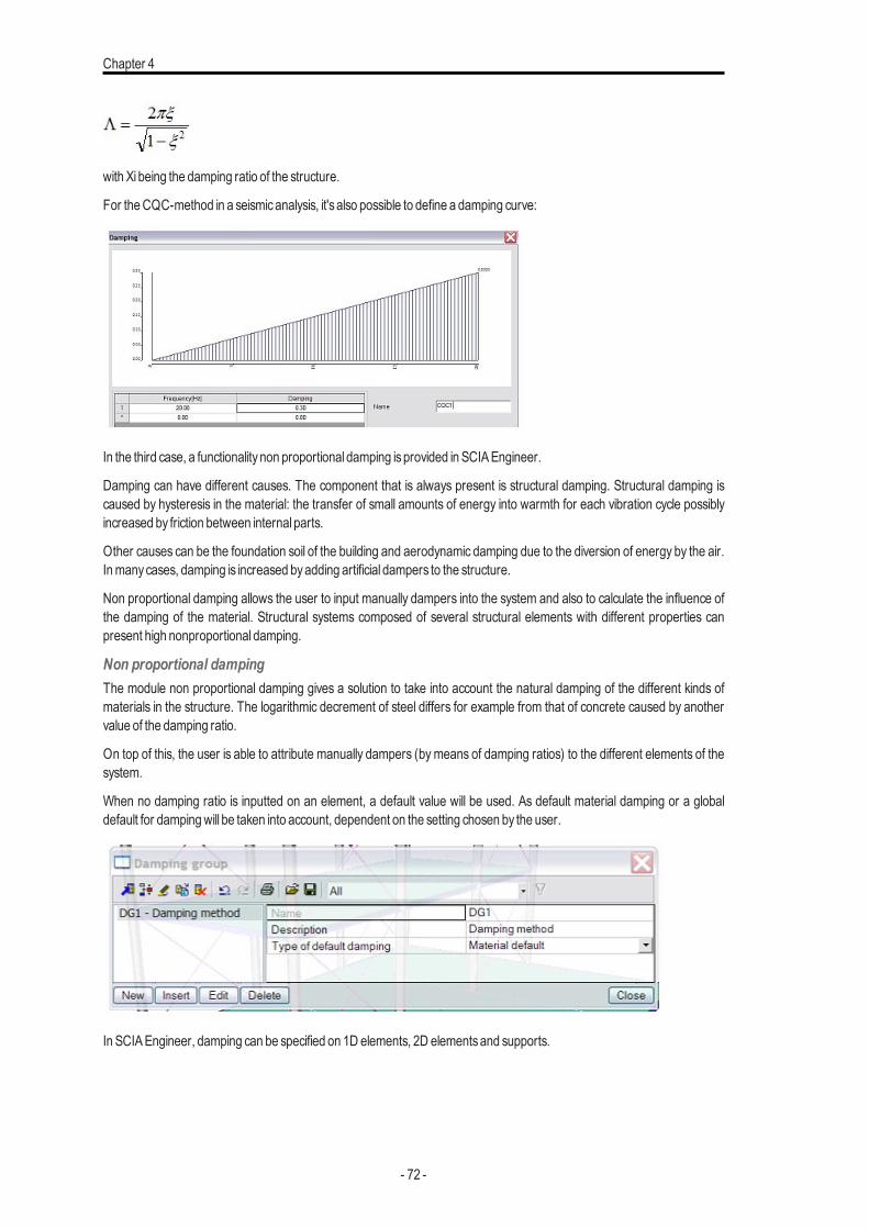
Chapter 4
with Xi being the damping ratio of the structure.
For theCQC-method in a seismicanalysis, it's also possible to define a damping curve:
In the third case, a functionalitynon proportional damping isprovided in SCIAEngineer.
Damping can have different causes. The component that is always present is structural damping. Structural damping iscaused by hysteresis in the material: the transfer of small amounts of energy into warmth for each vibration cycle possiblyincreased by friction between internal parts.
Other causes can be the foundation soil of the building and aerodynamic damping due to the diversion of energy by the air.Inmanycases, damping is increased byadding artificial dampers to the structure.
Non proportional damping allows the user to input manually dampers into the system and also to calculate the influence ofthe damping of the material. Structural systems composed of several structural elements with different properties canpresent high nonproportional damping.
Non proportional dampingThe module non proportional damping gives a solution to take into account the natural damping of the different kinds ofmaterials in the structure. The logarithmic decrement of steel differs for example from that of concrete caused by anothervalue of the damping ratio.
On top of this, the user is able to attribute manually dampers (bymeans of damping ratios) to the different elements of thesystem.
When no damping ratio is inputted on an element, a default value will be used. As default material damping or a globaldefault for dampingwill be taken into account, dependent on the setting chosen by the user.
In SCIAEngineer, damping can be specified on 1D elements, 2D elementsand supports.
- 72 -
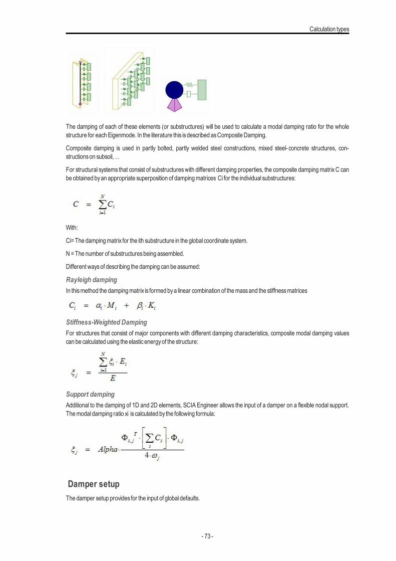
Calculation types
The damping of each of these elements (or substructures) will be used to calculate a modal damping ratio for the wholestructure for eachEigenmode. In the literature this isdescribed asComposite Damping.
Composite damping is used in partly bolted, partly welded steel constructions, mixed steel- concrete structures, con-structionson subsoil, ...
For structural systems that consist of substructureswith different damping properties, the composite damping matrix C canbe obtained byan appropriate superposition of dampingmatrices Ci for the individual substructures:
With:
Ci=The dampingmatrix for the ith substructure in the global coordinate system.
N =The number of substructuresbeing assembled.
Different waysof describing the damping can be assumed:
Rayleigh dampingIn thismethod the dampingmatrix is formed bya linear combination of themassand the stiffnessmatrices
Stiffness-Weighted DampingFor structures that consist of major components with different damping characteristics, composite modal damping valuescan be calculated using the elasticenergyof the structure:
Support dampingAdditional to the damping of 1D and 2D elements, SCIA Engineer allows the input of a damper on a flexible nodal support.Themodal damping ratio xi is calculated by the following formula:
Damper setupThe damper setup provides for the input of global defaults.
- 73 -

Chapter 4
Base value – logarithmic decrement Default value of logarithmic decrement.
Alpha factor for supports Factor for supports.
Must be >0; default 1.
Maximal modal damping Is used to limit the calculated damping.
Default 30%.
Defining a new damping groupProcedure to define a new damping group
1. In theProject setup dialogue > tab FunctionalityoptionsDynamicsandNon proportional dampingmust be selected.
2. Open serviceDynamics.
3. Start functionDamping group.
4. TheDamping groupmanager isopened on the screen.
5. Clickbutton [New].
6. Anew damping group isadded to the list of defined groups.
7. If necessary, change the nameand/or other group parameters.
Damping group parametersName Specifies the name of the group.
Description Provides a short description of the group.
Type of default damping Global default
The default values are taken from the Damper setup.
Material default
The default values are taken frommaterial properties.
Defining a new damperAdamper can be defined in a support, on a beammembe, on a slab.
Procedure to define a new damper
1. Open serviceDynamics.
2. Start functionDampers.
3. If no damping hasbeen defined so far, theDamping groupsmanager isopened on the screen. Define at least one damp-ing group.
4. TheDampersbranch isopened in the treemenu bar.
5. Select and start the function corresponding to the required type of damper:
1. 1D damping,
2. 2D damping,
3. Node damping.
- 74 -

Calculation types
6. Fill in the parameters.
7. Select the appropriate 1Dmember/slab/support where the damper is to be installed.
8. End the function.
1D dampingName Specifies the name of the damper.
Type Select the type of the damping parameter.
Logarithmic decrement
Relative damping
Rayleigh damping
Value
Alpha /Beta
Specifies the value of the parameter selected in the item above.
Note: The Rayleigh damping requires the definition of two parameters. The remaining two types need justone value.
2D dampingName Specifies the name of the damper.
Type Select the type of the damping parameter.
Logarithmic decrement
Relative damping
Rayleigh damping
Value
Alpha /Beta
Specifies the value of the parameter selected in the item above.
Note: The Rayleigh damping requires the definition of two parameters. The remaining two types need justone value.
Node dampingName Specifies the name of the damper.
Damping X
Damping Y
Damping Z
Defines the damping in individual directions of the global coordinate system.
- 75 -

Chapter 5
Performing the calculation
- 76 -
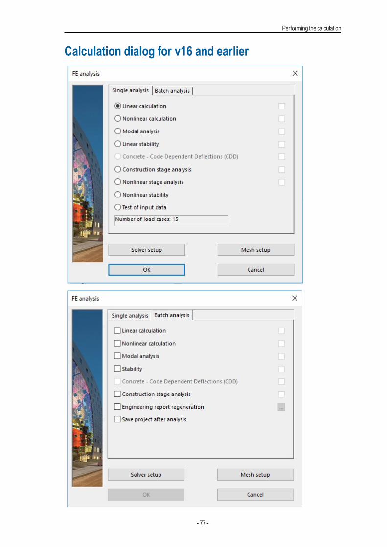
Performing the calculation
Calculation dialog for v16 and earlier
- 77 -
Chapter 5
Single analysis / Batch analysisIn calculation dialog for version 16 and earlier there are twomain view on list of possible analysis.
Single analysis where it is possible to choose one type of calculation and Batch analysis where it is possible to choose morethan one type of calculation and these calculationswill be performbehind a row.
Types of calculationsThese itemsdefine all possible typesof calculations, which can be performed on currentmodel.
Linear cal-culation
Linear calculation
Dynamic seismic calculation
Harmonic band analysis
Karman vibration
Dynamic natural vibration calculation
Nonlinear cal-culation
Nonlinear calculation
Modal analysis Calculation model for dynamic analysis
Linear stability Stability combination
Concrete - CodeDependentDeflections(CDD)
Concrete - Code Dependent Deflections (CDD)
Constructionstage analysis
Construction stage analysis
Linear versus Non-linear construction stages
Nonlinear stageanalysis
Nonlinear stage analysis
Nonlinear sta-bility
Nonlinear stability
Test of inputdata
It is basically preparation of data from model for Linear calculation. It can be something like check if everything is OK beforerun of calculation. After performing it, new service "2D data viewer" is available in service "Calculation, mesh", where it is pos-sible to check generated loads on members and other parameters ofmodel.
ButtonsSolver setup Settings for calculation - Solver setup
Mesh setup Settings for FEMmesh on members - Mesh setup
OK This button starts calculation.
Cancel This button closes calculation dialog without calculation.
- 78 -
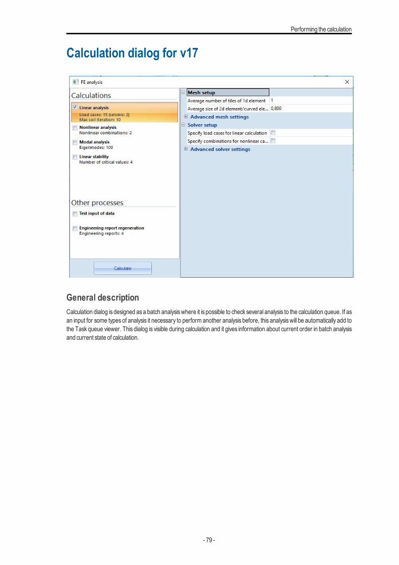
Performing the calculation
Calculation dialog for v17
General descriptionCalculation dialog is designed as a batch analysiswhere it is possible to check several analysis to the calculation queue. If asan input for some types of analysis it necessary to perform another analysis before, this analysis will be automatically add tothe Task queue viewer. This dialog is visible during calculation and it gives information about current order in batch analysisand current state of calculation.
- 79 -
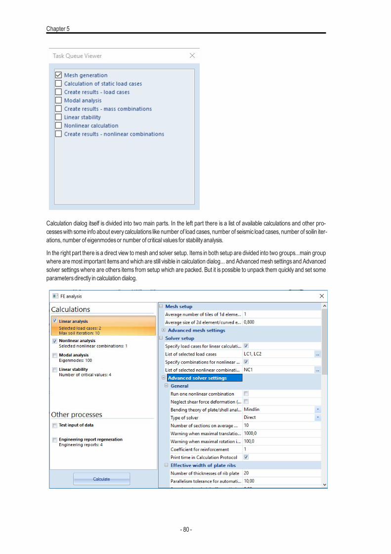
Chapter 5
Calculation dialog itself is divided into two main parts. In the left part there is a list of available calculations and other pro-cesseswith some info about everycalculations like number of load cases, number of seismic load cases, number of soilin iter-ations, number of eigenmodesor number of critical values for stability analysis.
In the right part there is a direct view tomesh and solver setup. Items in both setup are divided into two groups...main groupwhere aremost important itemsandwhich are still visible in calculation dialog... and Advancedmesh settingsand Advancedsolver settings where are others items from setup which are packed. But it is possible to unpack them quickly and set someparametersdirectly in calculation dialog.
- 80 -

Performing the calculation
Selection of load cases or nonlinear combinations for calculationFor solver setup there are visible two items : "Specify load cases for linear calculation" and if there are some nonlinear com-binations in model there is item "Specify combinations for nonlinear calculation". After check these items new dialog "Makeselection" will appear with all possible load cases or nonlinear combinations and it is possible to make a selection for this cal-culation. After that selected itemsare displayed in solver setup and in info text before analysis there is new info for example :Selected load cases : 2 .
After calculation in service results there are available results only for load cases and nonlinear combinations which wereselected. Othershave symbol * before name, whichmeansno results.
- 81 -
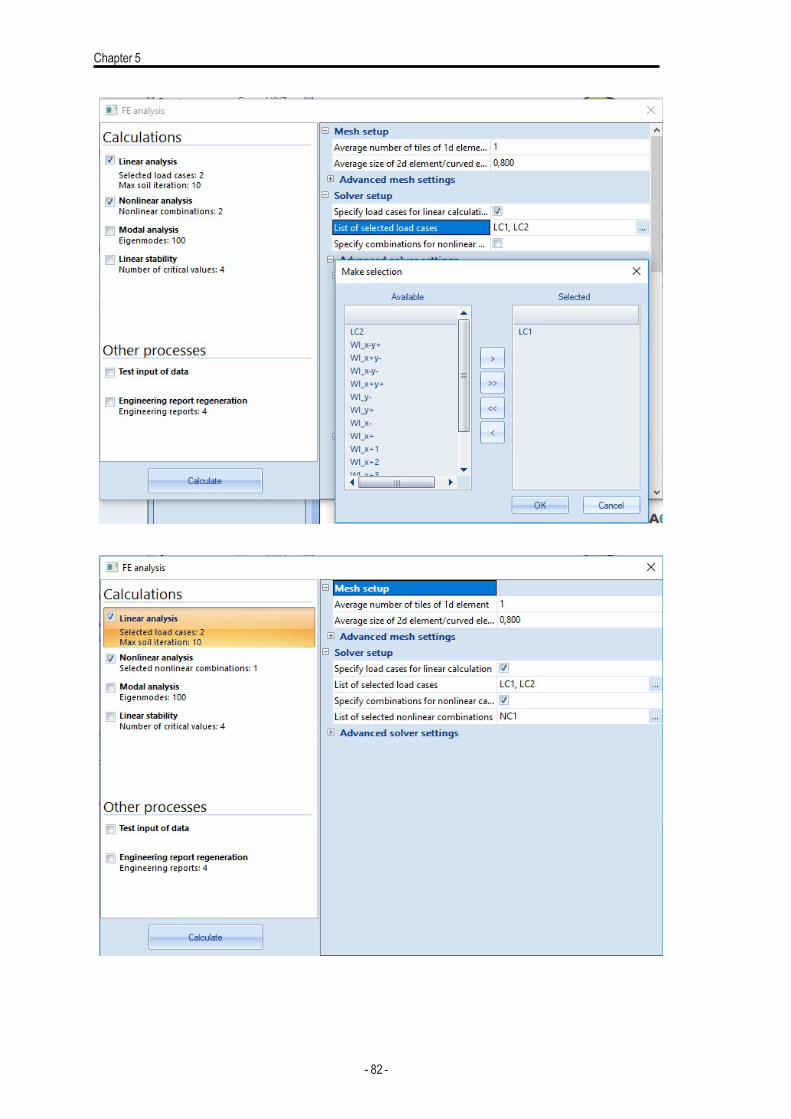
Chapter 5
- 82 -
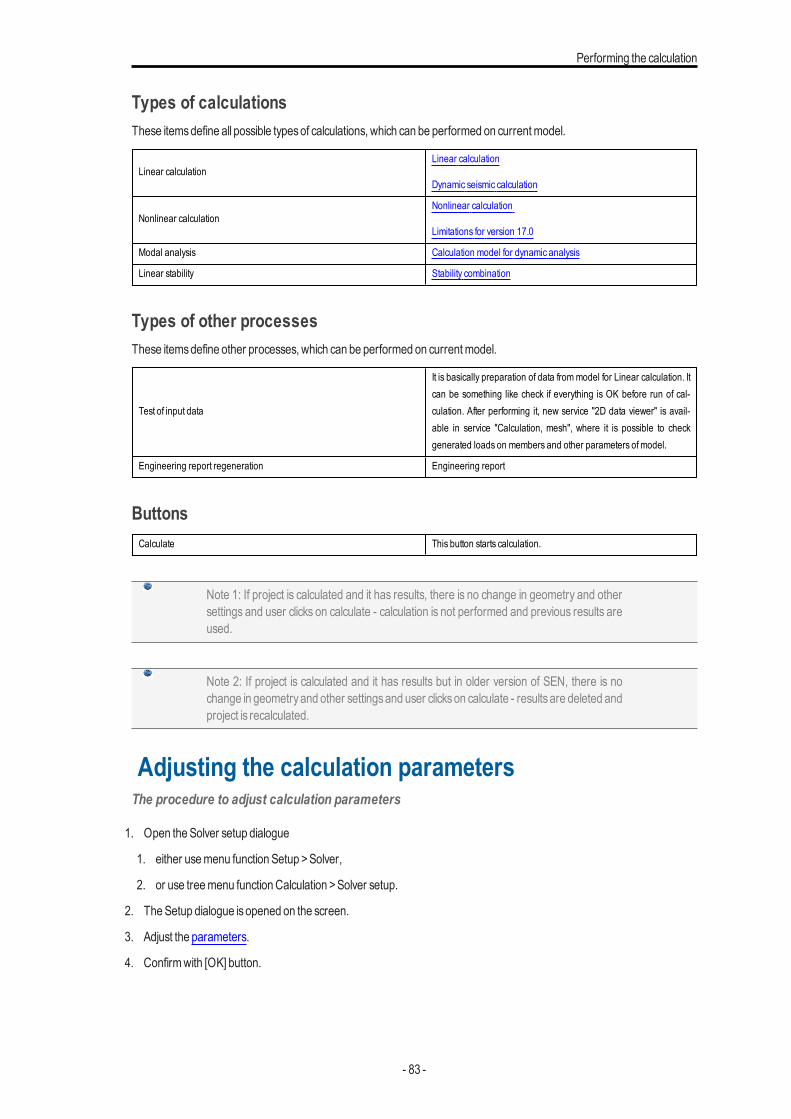
Performing the calculation
Types of calculationsThese itemsdefine all possible typesof calculations, which can be performed on currentmodel.
Linear calculationLinear calculation
Dynamic seismic calculation
Nonlinear calculationNonlinear calculation
Limitations for version 17.0
Modal analysis Calculation model for dynamic analysis
Linear stability Stability combination
Types of other processesThese itemsdefine other processes, which can be performed on currentmodel.
Test of input data
It is basically preparation of data frommodel for Linear calculation. Itcan be something like check if everything is OK before run of cal-culation. After performing it, new service "2D data viewer" is avail-able in service "Calculation, mesh", where it is possible to checkgenerated loads on members and other parameters ofmodel.
Engineering report regeneration Engineering report
ButtonsCalculate This button starts calculation.
Note 1: If project is calculated and it has results, there is no change in geometry and othersettings and user clicks on calculate - calculation is not performed and previous results areused.
Note 2: If project is calculated and it has results but in older version of SEN, there is nochange in geometryand other settingsand user clickson calculate - resultsare deleted andproject is recalculated.
Adjusting the calculation parametersThe procedure to adjust calculation parameters
1. Open theSolver setup dialogue
1. either usemenu function Setup >Solver,
2. or use treemenu functionCalculation >Solver setup.
2. TheSetup dialogue isopened on the screen.
3. Adjust the parameters.
4. Confirmwith [OK] button.
- 83 -
Chapter 5
Note: The adjustment of these parametersmayaffect the layout of the calculation dialoguethat openson the screenwhen a calculation is started.
Performing the calculationThe procedure for performing of the calculation
1. Call functionCalculation:
1. either usingmenu function Tree >Calculation,Mesh >Calculation,
2. or using treemenu functionCalculation,Mesh >Calculation.
2. TheCalculation settingsdialogue openson the screen (see below).
3. Adjust the parameters for calculation.
4. Confirmwith [OK].
5. The calculation is started and solver report dialogue is opened on the screen (for small models the dialogue may justflash).
6. When the calculation hasbeen finished, close the calculation report dialogue.
9. Proceed to evaluation of result.
Note: All the calculation parametersmaybe adjusted in the "Solver Setup"
Controlling and reviewing the calculation processOnce a calculation hasbeen started aSolver report dialogue openson the screen.
For smallmodels the dialoguemay just "flash" on the screen and disappear again.
On finishing the calculation, the programshows the dialoguewith the result of the calculation.
If everything is OK, the Solver report dialogue can be closed and the user may proceed to the evaluation of results. If any-thingwent wrong during the calculation, amessage isdisplayed and it’sup to the user to resolve the situation.
Performing the repetitious calculationsVery often it may be necessary to repeat the calculation with the same calculation settings. It is possible to repeat a normalcalculation. In addition, SCIA Engineer offers function Hidden calculation. This function starts the calculation without show-ing any information on the screen. Once the calculation is finished, all possible openwindowswith displayed resultsare auto-matically regenerated.
TheHidden calculation can be performed bymeansof:
l either menu function Tree >Calculation,Mesh >Hidden calculation,
l or treemenu functionCalculation,Mesh >Hidden calculation,
l or button [Hidden calculation] ( ) on toolbar Project.
- 84 -
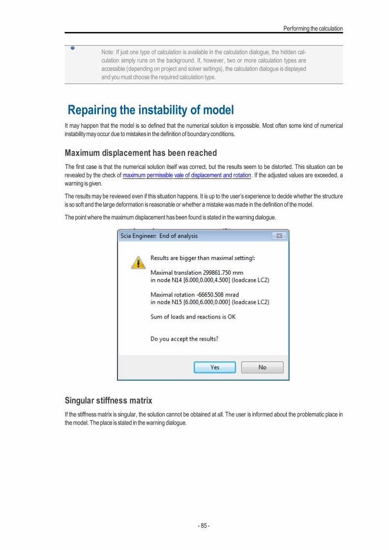
Performing the calculation
Note: If just one type of calculation is available in the calculation dialogue, the hidden cal-culation simply runs on the background. If, however, two or more calculation types areaccessible (depending on project and solver settings), the calculation dialogue is displayedand youmust choose the required calculation type.
Repairing the instability of modelIt may happen that the model is so defined that the numerical solution is impossible. Most often some kind of numericalinstabilitymayoccur due tomistakes in the definition of boundaryconditions.
Maximum displacement has been reachedThe first case is that the numerical solution itself was correct, but the results seem to be distorted. This situation can berevealed by the check of maximum permissible vale of displacement and rotation. If the adjusted values are exceeded, awarning isgiven.
The resultsmay be reviewed even if this situation happens. It is up to the user’s experience to decide whether the structureis so soft and the large deformation is reasonable or whether amistakewasmade in the definition of themodel.
The point where themaximumdisplacement hasbeen found isstated in thewarning dialogue.
Singular stiffness matrixIf the stiffnessmatrix is singular, the solution cannot be obtained at all. The user is informed about the problematic place inthemodel. The place is stated in thewarning dialogue.
- 85 -
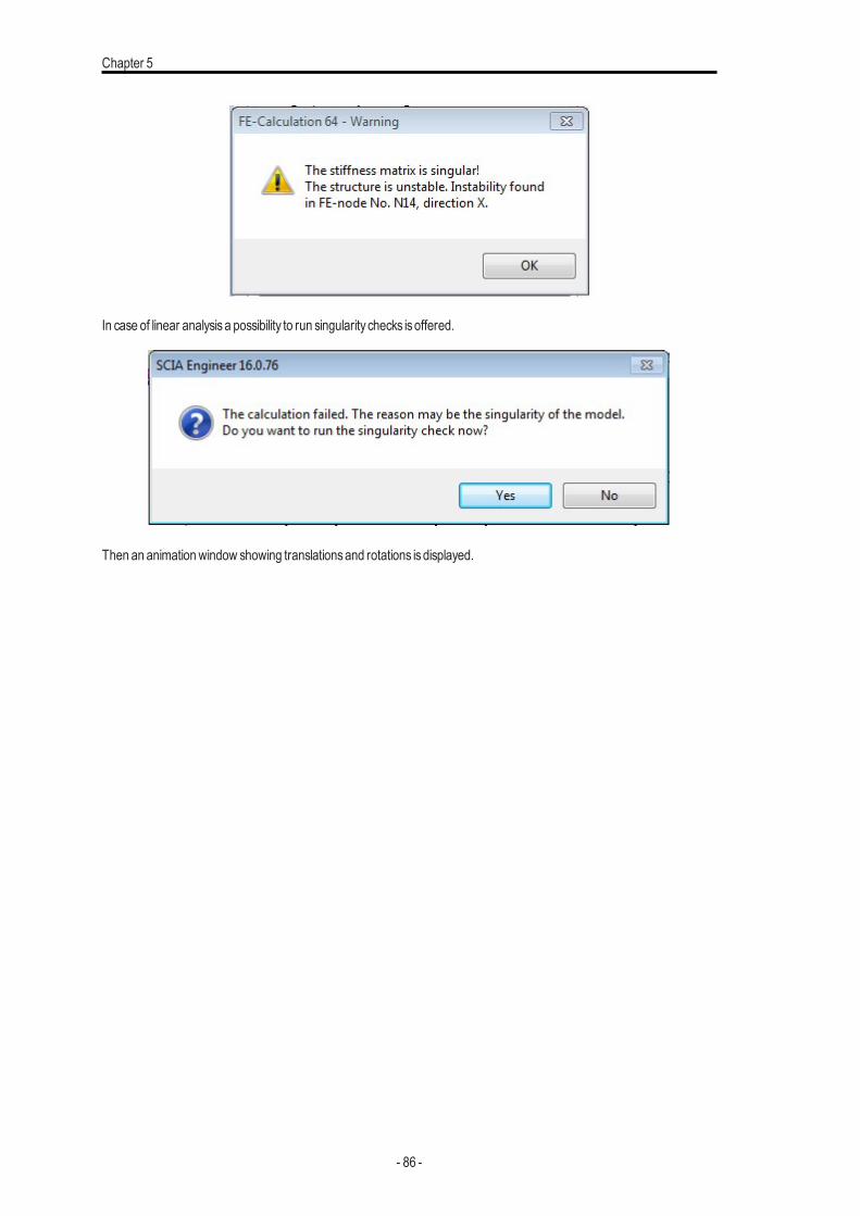
Chapter 5
In case of linear analysisa possibility to run singularity checks isoffered.
Then an animationwindow showing translationsand rotations isdisplayed.
- 86 -
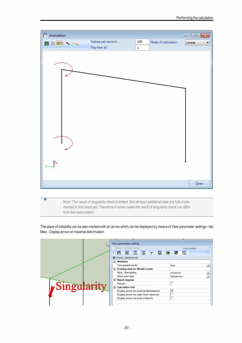
Performing the calculation
Note: The result of singularity check is limited. Not all input additional data are fully imple-mented in this check yet. Therefore in some cases the result of singularity check can differfrom the real problem.
The place of instability can be alsomarked with an arrow which can be displayed bymeansof View parameter settings - tabMisc.- Displayarrow onmaximal deformation.
- 87 -
Chapter 6
Solution methods
Direct solutionThis isa standardCholeskysolution based on a decomposition of thematrix of the system. The advantage is that it can solveseveral right sidesat the same time. This type of solution is effective especially for small andmiddle-size problemswhen diskswapping isnot necessary. The limit dependson the size of the problemand on the size of available RAMmemory.
It can be said that this solution ismore convenient for most of problems.
Disadvantage of this solution mayemerge with extremely large problems. The calculation timemay rise significantly if RAMsize is insufficient.What’smore, if the available diskspace isnot large enough, the problem cannot be solved at all.
If the problem is excessive and of poor numerical condition, the rounding error may be so big that it exceeds the acceptablelimit. Thismay result in imbalance between resultants of load and reactions. The difference between the total sumsof loadsand reactions should not be greater than about 0.5%. But even the value of 0.1% suggests that the results may be sus-picious.
Generally, the direct solver should be used only for beam structures (without any2Dmem-bers) or planar structure composed of 2D members (i.e. a plate or a wall). In other casesthe direct solver should be used as a default solution method. The application of iterativesolution depends on the total number of nodes, band width and memory size of the par-ticular computer. If the direct solution leads to an excessive disk swapping, the process isslowed down sifgnificantlyand the iterative solutionmust be employed. Thissolver doesnotrequire so much memory – 150 000 nodes needs about 250 MB RAM. Other reason forthe application of iterative solution may be poor determinetness of the equation system.These numerical problems can result in a discrepancy between the total load and sum ofreactions. If this difference is greater than 5%, a warning is issued and the direct solvershould be replaced by the iterative one.
Iterative solutionThe IncompleteCholeskyconjugate gradientmethod isapplied.
Its advantage isminimal demand on RAM and disk size. Therefore, the solution is convenient especially for extremely largeproblems that cannot be solved by means of direct solution or whose calculation time would be enormous for that kind ofsolution due to excessive diskoperations.
Another advantage is that due to the ability of continuous improvement of accuracy the method is able to find technicallyaccurate solution even for equation systems that would be numericallyunstable in the direct solution.
The disadvantage is that themethod can employonly one right side at a time and this increases the time demands for equa-tion systemswith several right sides.
Note: See the note in theDirect solution.
- 88 -
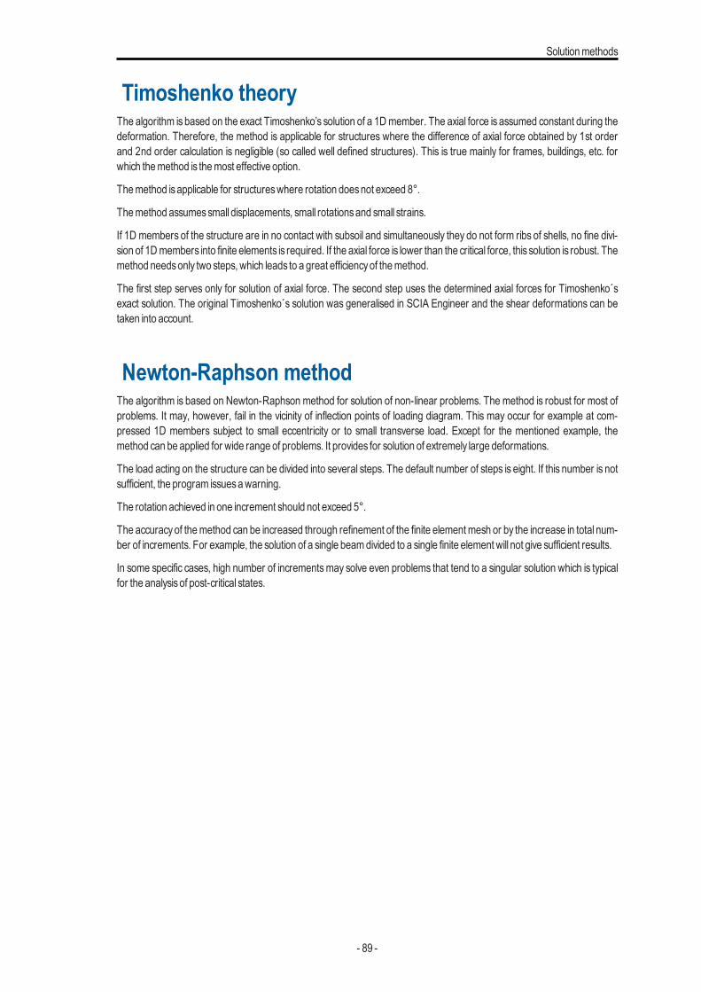
Solutionmethods
Timoshenko theoryThe algorithm is based on the exact Timoshenko’s solution of a 1Dmember. The axial force is assumed constant during thedeformation. Therefore, the method is applicable for structures where the difference of axial force obtained by 1st orderand 2nd order calculation is negligible (so called well defined structures). This is true mainly for frames, buildings, etc. forwhich themethod is themost effective option.
Themethod isapplicable for structureswhere rotation doesnot exceed 8°.
Themethod assumessmall displacements, small rotationsand small strains.
If 1D members of the structure are in no contact with subsoil and simultaneously they do not form ribs of shells, no fine divi-sion of 1Dmembers into finite elements is required. If the axial force is lower than the critical force, this solution is robust. Themethod needsonly two steps, which leads to a great efficiencyof themethod.
The first step serves only for solution of axial force. The second step uses the determined axial forces for Timoshenko´sexact solution. The original Timoshenko´s solution was generalised in SCIA Engineer and the shear deformations can betaken into account.
Newton-Raphson methodThe algorithm is based on Newton-Raphson method for solution of non-linear problems. The method is robust for most ofproblems. It may, however, fail in the vicinity of inflection points of loading diagram. This may occur for example at com-pressed 1D members subject to small eccentricity or to small transverse load. Except for the mentioned example, themethod can be applied for wide range of problems. It provides for solution of extremely large deformations.
The load acting on the structure can be divided into several steps. The default number of steps is eight. If this number is notsufficient, the program issuesawarning.
The rotation achieved in one increment should not exceed 5°.
The accuracyof themethod can be increased through refinement of the finite elementmesh or by the increase in total num-ber of increments. For example, the solution of a single beamdivided to a single finite element will not give sufficient results.
In some specific cases, high number of incrementsmay solve even problems that tend to a singular solution which is typicalfor the analysisof post-critical states.
- 89 -
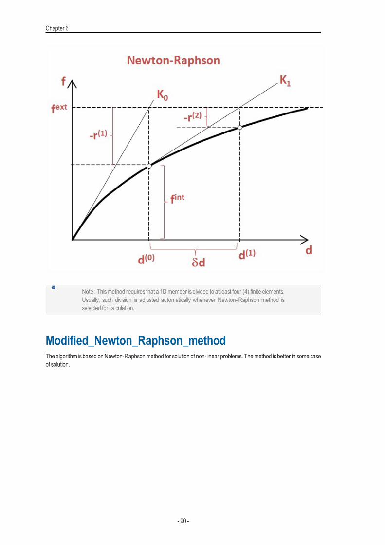
Chapter 6
Note : Thismethod requires that a 1Dmember is divided to at least four (4) finite elements.Usually, such division is adjusted automatically whenever Newton-Raphson method isselected for calculation.
Modified_Newton_Raphson_methodThe algorithm isbased onNewton-Raphsonmethod for solution of non-linear problems. Themethod isbetter in some caseof solution.
- 90 -
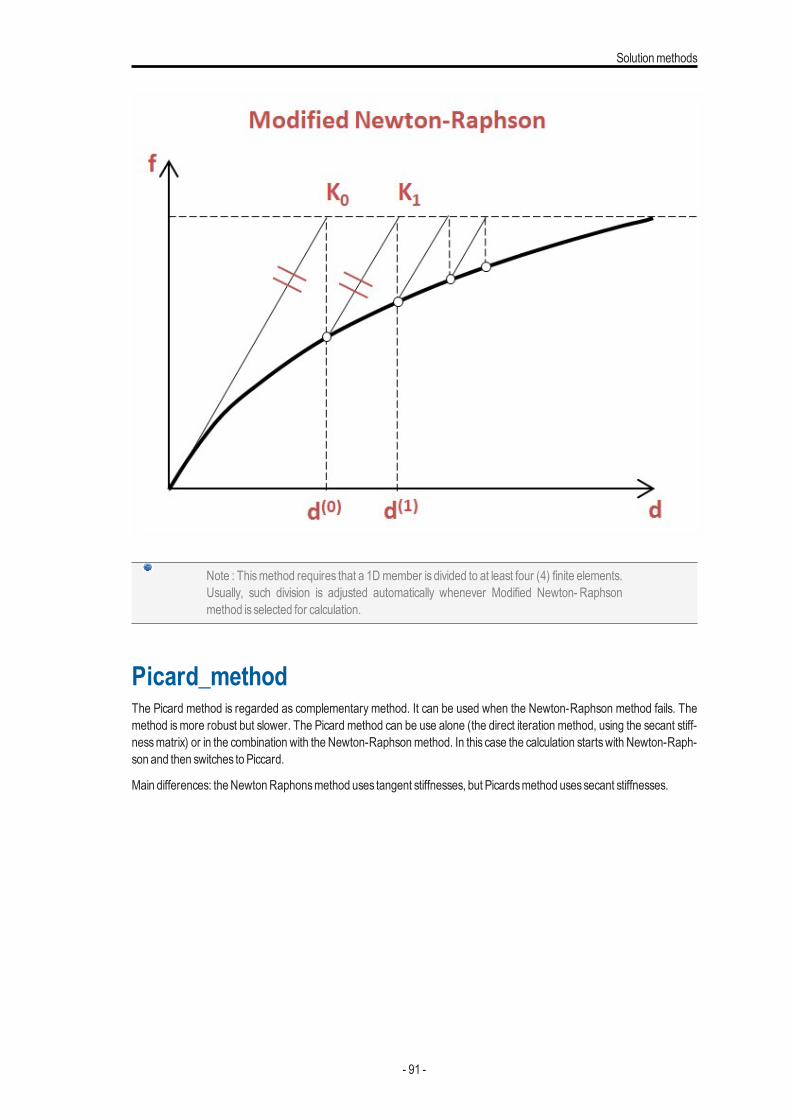
Solutionmethods
Note : Thismethod requires that a 1Dmember is divided to at least four (4) finite elements.Usually, such division is adjusted automatically whenever Modified Newton- Raphsonmethod isselected for calculation.
Picard_methodThe Picard method is regarded as complementary method. It can be used when the Newton-Raphson method fails. Themethod ismore robust but slower. The Picard method can be use alone (the direct iteration method, using the secant stiff-nessmatrix) or in the combination with the Newton-Raphsonmethod. In this case the calculation startswith Newton-Raph-son and then switches to Piccard.
Main differences: theNewtonRaphonsmethod uses tangent stiffnesses, but Picardsmethod usessecant stiffnesses.
- 91 -
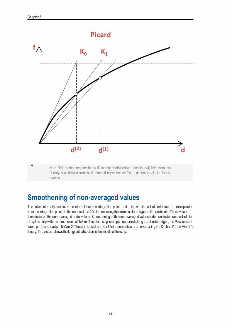
Chapter 6
Note : Thismethod requires that a 1Dmember is divided to at least four (4) finite elements.Usually, such division is adjusted automaticallywhenever Picard method is selected for cal-culation.
Smoothening of non-averaged valuesThe solver internally calculates the internal forces in integration points and at the end the calculated values are extrapolatedfrom the integration points to the nodes of the 2D element using the formulas for a hyperbolic paraboloid. These values arethen declared the non-averaged nodal values. Smoothening of the non-averaged values is demonstrated on a calculationof a plate strip with the dimensions of 4x3 m. The plate strip is simply supported along the shorter edges, the Poisson coef-ficient μ =0, and load p =5 kNm-2. The strip is divided to 4 x3 finite elementsand is solved using the Kirchhoff's andMindlin'stheory. The picture shows the longitudinal section in themiddle of the strip.
- 92 -
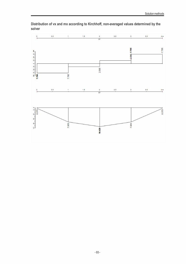
Solutionmethods
Distribution of vx and mx according to Kirchhoff, non-averaged values determined by thesolver
- 93 -
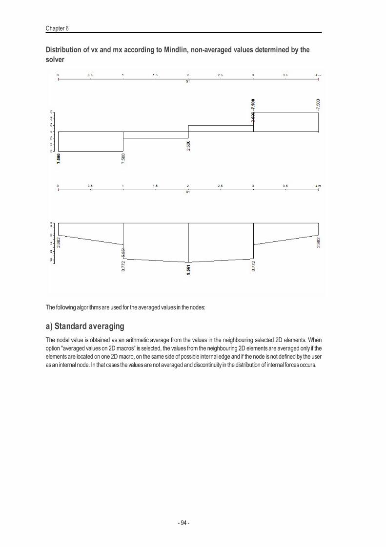
Chapter 6
Distribution of vx and mx according to Mindlin, non-averaged values determined by thesolver
The following algorithmsare used for the averaged values in the nodes:
a) Standard averagingThe nodal value is obtained as an arithmetic average from the values in the neighbouring selected 2D elements. Whenoption "averaged values on 2D macros" is selected, the values from the neighbouring 2D elements are averaged only if theelements are located on one 2Dmacro, on the same side of possible internal edge and if the node is not defined by the userasan internal node. In that cases the valuesare not averaged and discontinuity in the distribution of internal forcesoccurs.
- 94 -
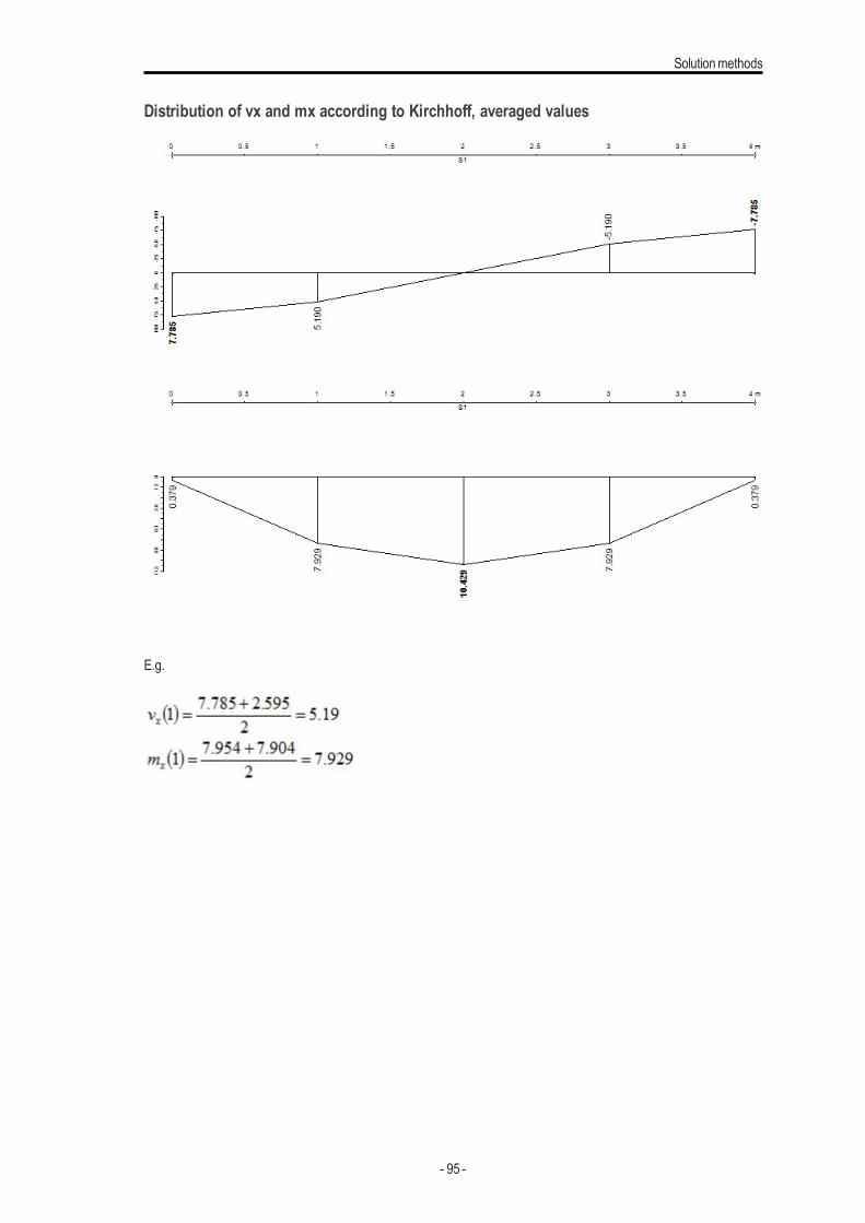
Solutionmethods
Distribution of vx and mx according to Kirchhoff, averaged values
E.g.
- 95 -
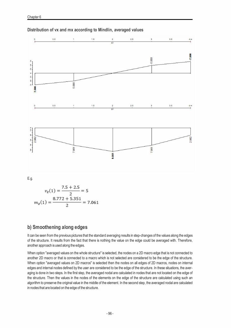
Chapter 6
Distribution of vx and mx according to Mindlin, averaged values
E.g.
b) Smoothening along edgesIt can be seen from the previous pictures that the standard averaging results in step-changes of the values along the edgesof the structure. It results from the fact that there is nothing the value on the edge could be averaged with. Therefore,another approach isused along the edges.
When option "averaged values on the whole structure" is selected, the nodes on a 2D macro edge that is not connected toanother 2D macro or that is connected to a macro which is not selected are considered to be the edge of the structure.When option "averaged values on 2D macros" is selected then the nodes on all edges of 2D macros, nodes on internaledges and internal nodes defined by the user are considered to be the edge of the structure. In these situations, the aver-aging is done in two steps. In the first step, the averaged nodal are calculated in nodes that are not located on the edge ofthe structure. Then the values in the nodes of the elements on the edge of the structure are calculated using such analgorithm to preserve the original value in the middle of the element. In the second step, the averaged nodal are calculatedin nodes that are located on the edge of the structure.
- 96 -
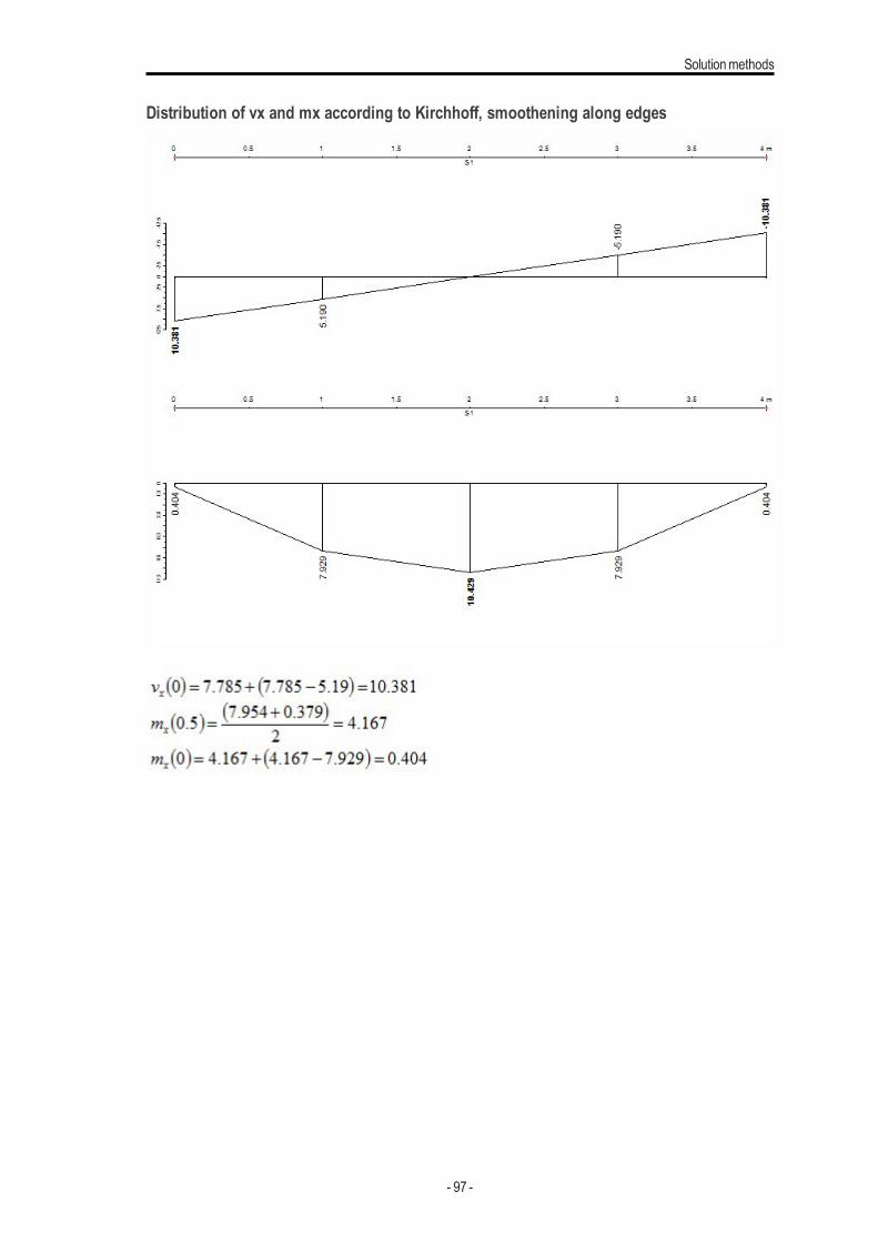
Solutionmethods
Distribution of vx and mx according to Kirchhoff, smoothening along edges
- 97 -
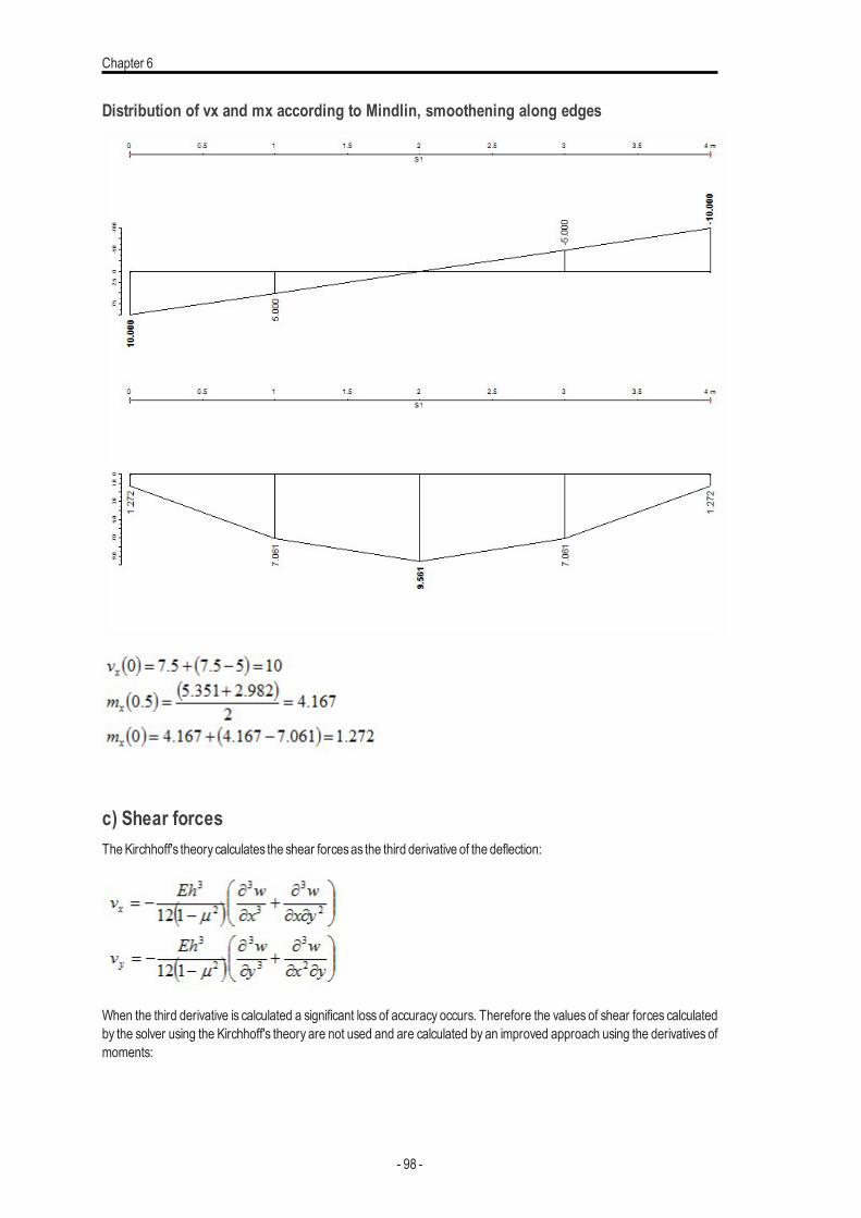
Chapter 6
Distribution of vx and mx according to Mindlin, smoothening along edges
c) Shear forcesTheKirchhoff's theorycalculates the shear forcesas the third derivative of the deflection:
When the third derivative is calculated a significant loss of accuracy occurs. Therefore the values of shear forces calculatedby the solver using the Kirchhoff's theory are not used and are calculated by an improved approach using the derivatives ofmoments:
- 98 -
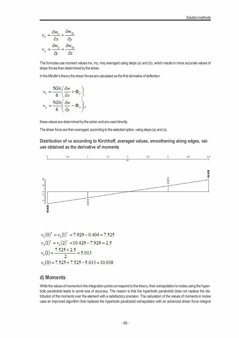
Solutionmethods
The formulas use moment valuesmx, my, mxy averaged using steps (a) and (b), which results in more accurate values ofshear forces than determined by the solver.
In theMindlin's theory the shear forcesare calculated as the first derivative of deflection.
these valuesare determined by the solver and are used directly.
The shear force are then averaged, according to the selected option, using steps (a) and (s).
Distribution of vx according to Kirchhoff, averaged values, smoothening along edges, val-ues obtained as the derivative of moments
d) MomentsWhile the valuesof moments in the integration points correspond to the theory, their extrapolation to nodesusing the hyper-bolic paraboloid leads to some loss of accuracy. The reason is that the hyperbolic paraboloid does not replace the dis-tribution of the moments over the element with a satisfactory precision. The calculation of the values of moments in nodesuses an improved algorithm that replaces the hyperbolic paraboloid extrapolation with an advanced shear-force-integral
- 99 -
Chapter 6
method. As the distribution of shear forces over the surface of the element is assumed to follow the shape of the hyperbolicparaboloid (second order surface), the integral of this surface represents a third order surface that approximates themoment distribution with a higher accuracy. This is based on the above-mentioned formulas for the calculation of shearforcesusing the derivative ofmoments.Momentsare thenwritten from these formulas:
Integration constantsmx,0,my,0 are calculated from the condition of the value in themiddle of the element.
where S is the area of the element. The valuesof internal forcesare calculated using steps (a), (b) and (c), the integrals areevaluated using numerical integration. The obtained values of moments in nodes are then, using the selected averagingoption, averaged according to step (a).
- 100 -
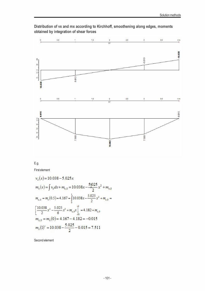
Solutionmethods
Distribution of vx and mx according to Kirchhoff, smoothening along edges, momentsobtained by integration of shear forces
E.g.
First element
Second element
- 101 -
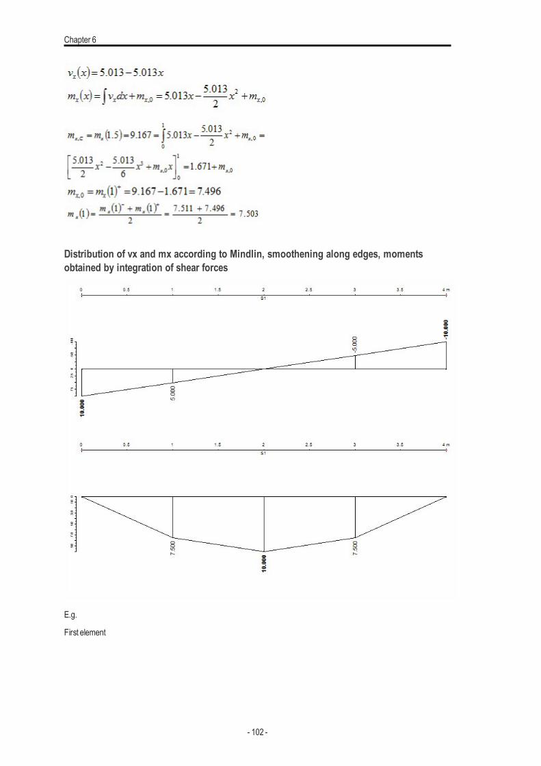
Chapter 6
Distribution of vx and mx according to Mindlin, smoothening along edges, momentsobtained by integration of shear forces
E.g.
First element
- 102 -
Solutionmethods
Second element
- 103 -
Chapter 7
Initial deformations
Introduction to initial deformationsThe initial deformationmaybe used in non-linear calculation to define the shape of the structure at the beginning of the ana-lysis. Thusa state of initial imperfection in shape can be easilymodelled.
Initial-deformation managerThe initial deformation curves can be defined and edited in the Initial-deformation manager. Thismanager is one the SCIAEngineer numerousdatabasemanagers. Itsoperation and layout are analogous to other databasemanagers.
In the Initial-deformationmanager the user may:
l define a new initial deformation curve,
l edit an existing initial deformation curve,
l copyan existing initial deformation curve,
l delete an existing initial deformation curve,
l save the existing initial deformation curve to an external file.
The Initial-deformationmanager can be opened in twoways:
l using treemenu function Libraries> Initial deformations,
l usingmenu function Libraries> Initial deformations.
Initial deformation curveThe initial deformation isdefined in the editing dialogue bymeansof a position-deformation curve.
The curvemaybe defined in a simple operated dialogue.
- 104 -
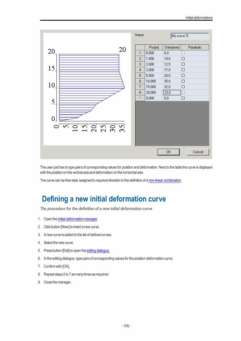
Initial deformations
The user just has to type pairs of corresponding values for position and deformation. Next to the table the curve is displayedwith the position on the vertical axisand deformation on the horizontal axis.
The curve can be then later assigned to required direction in the definition of a non-linear combination.
Defining a new initial deformation curveThe procedure for the definition of a new initial deformation curve
1. Open the Initial-deformationmanager.
2. Clickbutton [New] to insert a new curve.
3. Anew curve isadded to the list of defined curves.
4. Select the new curve.
5. Pressbutton [Edit] to open the editing dialogue.
6. In the editing dialogue, type pairsof corresponding values for the position-deformation curve.
7. Confirmwith [OK].
8. Repeat steps2 to 7 asmany timesas required.
9. Close themanager.
- 105 -

Chapter 7
Applying the initial deformationThe initial deformation curvemaybe used in a non-linear combination to define the initial imperfect shape of the structure.
The procedure for the application of the initial deformation curve
1. Create a new non-linear combination or edit the existing one.
2. Item Type of imperfection set to an option requiring the input of an initial deformation curve (i.e. either Functions +curvature on beamsor Inclination functions).
3. In the appropriate items choose the required initial deformation curve (each direction can use different initial deformationcurve).
4. Finish the definition or editing of the non-linear combination.
5. Use the combination for calculation.
- 106 -
Soil-In
Soil-In
IntroductionThe analysis of foundation structures is challenged by the problem ofmodelling of the part of the foundation that is in contactwith subsoil. The best solution is to use 2D model of the subsoil that properly represents the deformation properties of thewhole under-foundation massif by means of surface model. The properties of such model are expressed by what is calledinteraction parametersmarkedC. These parameters are assigned directly to structure elements that are in contact with thesubsoil and they influence the stiffnessmatrix.
To simplify thematter, wemay imagine that C is the characteristicsof elastic, more preciselypseudo-elastic, links, or surfacespring constants that change according to the actual state of the analysed system. We may also use the professional slangthat calls it "support on C parameters", which is the generalisation of standard Winkler idea of the supporting in the form ofthick liquid g = C1 (MNm-3) or in the form of infinitely dense system of vertical springs. The generalisation is very importantand dealsmainlywith the consideration of significant shear distribution in the subsoil that is neglected byWinkler model. Theparameters of the interaction between the foundation and the subsoil depends on the distribution and loading level, or thecontact stress between the structure surface and the surrounding subsoil, on the geometry of the footing surface and onmechanical propertiesof the soil.
Calculationmodule Soil-in takesaccount of all thementioned dependencies.
As the C parameters influence the contact stress and vice versa – the distribution of the contact stress have impact on thesettlement of the footing surface and thus theC parameters, it is necessary to use an iterative solution.
The influence of subsoil in the vicinity of the structureThemodelling of the interaction between a structure and subsoil requires that the influence of the subsoil outside of the struc-ture be taken into account. This outside-subsoil supports the edgesof the foundation slab due to shear stiffness. In the past,special procedureswere recommended tomodel thisphenomenon. The current versionsof SCIAEngineer employa soph-isticated solutionwhose principle isdescribed in the following paragraph.
The program automatically adds to the edge of the analysed foundation slab springs that approximately substitute the effectof what is termed support elements (1 to 2 metre wide strip located along the edges of the foundation slab, the thickness ofthis strip is almost zero). The solution obtained through this approach takes into account the effect of the subsoil outside (inthe vicinity) of the analysed foundation slab.
In comparison with a solution without such springs, the results obtained with the springs gives smaller deformation of thefoundation-slab edgeswhichmeans larger bendingmoments in the foundation slab.
The springs oriented in the global z-direction are assigned to all edge nodes except the situation when a node already hasanother spring assigned or if a rotation of a node is specified. In that case, the program assumes that the user has alreadydefined a special type of support and that it is not wanted to alter that special configuration automaticallyon the background.
These exceptions can be used to deliberately suppress the implementation of edge-springs along certain lines. The usercan define very small line springsalong required lines (edges) and thuseliminate the effect of the surrounding subsoil (e.g. ifa sheet pile wall is installed).
Soil-in outputThe results from the soil-in iteration are theC parametersC1z, C2x andC2y.
ParametersC1x andC1y are alwaysdefined by the user.
C1z - resistance of environment against wP (mm) [C1z inMN/m3]
- 107 -
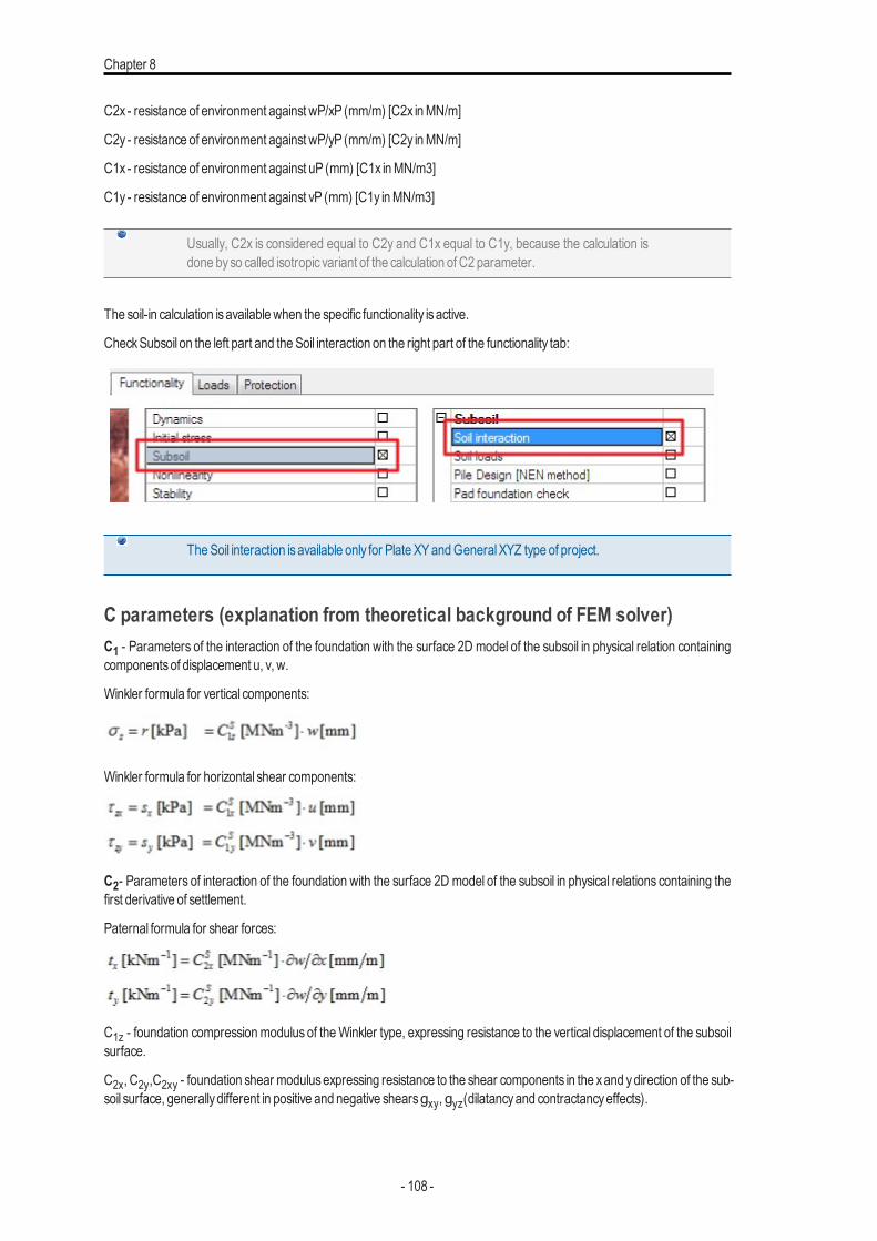
Chapter 8
C2x - resistance of environment against wP/xP (mm/m) [C2x inMN/m]
C2y - resistance of environment against wP/yP (mm/m) [C2y inMN/m]
C1x - resistance of environment against uP (mm) [C1x inMN/m3]
C1y - resistance of environment against vP (mm) [C1y inMN/m3]
Usually, C2x is considered equal to C2y and C1x equal to C1y, because the calculation isdone byso called isotropic variant of the calculation of C2 parameter.
The soil-in calculation isavailable when the specific functionality isactive.
CheckSubsoil on the left part and theSoil interaction on the right part of the functionality tab:
TheSoil interaction isavailable only for Plate XYandGeneralXYZ type of project.
C parameters (explanation from theoretical background of FEM solver)C1 - Parameters of the interaction of the foundation with the surface 2D model of the subsoil in physical relation containingcomponentsof displacement u, v, w.
Winkler formula for vertical components:
Winkler formula for horizontal shear components:
C2- Parameters of interaction of the foundation with the surface 2D model of the subsoil in physical relations containing thefirst derivative of settlement.
Paternal formula for shear forces:
C1z - foundation compression modulus of theWinkler type, expressing resistance to the vertical displacement of the subsoilsurface.
C2x, C2y,C2xy - foundation shear modulusexpressing resistance to the shear components in the xand ydirection of the sub-soil surface, generallydifferent in positive and negative shearsgxy,gyz(dilatancyand contractancyeffects).
- 108 -
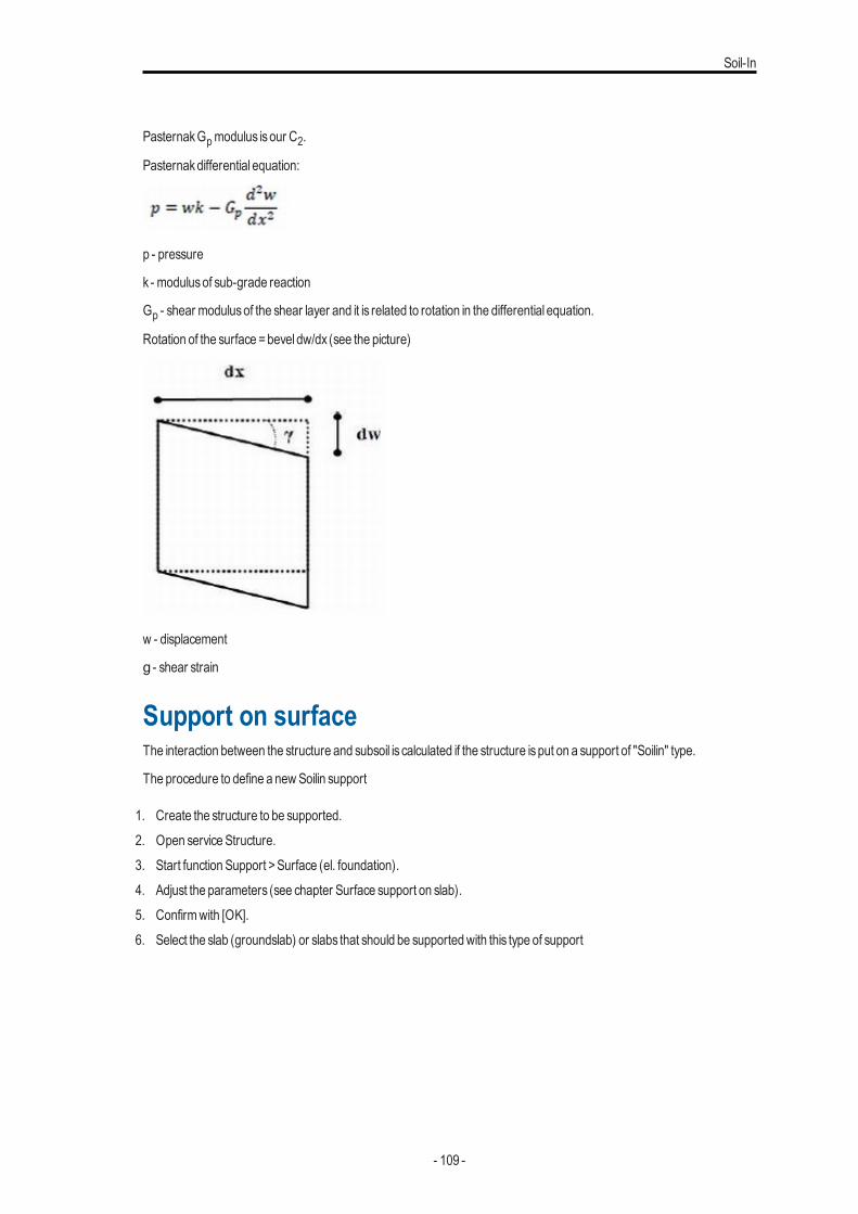
Soil-In
PasternakGpmodulus isour C2.
Pasternakdifferential equation:
p - pressure
k - modulusof sub-grade reaction
Gp - shear modulusof the shear layer and it is related to rotation in the differential equation.
Rotation of the surface =bevel dw/dx (see the picture)
w - displacement
g - shear strain
Support on surfaceThe interaction between the structure and subsoil is calculated if the structure isput on a support of "Soilin" type.
The procedure to define a newSoilin support
1. Create the structure to be supported.2. Open service Structure.3. Start function Support >Surface (el. foundation).4. Adjust the parameters (see chapter Surface support on slab).5. Confirmwith [OK].6. Select the slab (groundslab) or slabs that should be supportedwith this type of support
- 109 -
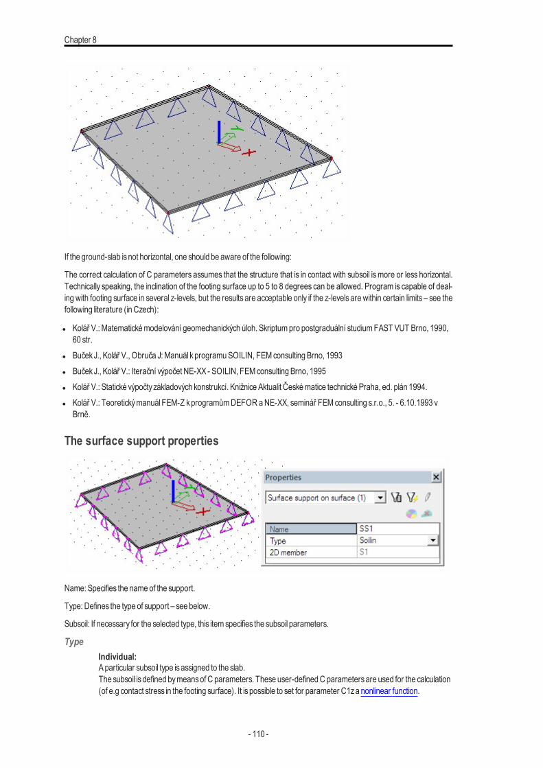
Chapter 8
If the ground-slab isnot horizontal, one should be aware of the following:
The correct calculation of C parameters assumes that the structure that is in contact with subsoil is more or less horizontal.Technically speaking, the inclination of the footing surface up to 5 to 8 degrees can be allowed. Program is capable of deal-ing with footing surface in several z-levels, but the results are acceptable only if the z-levels are within certain limits – see thefollowing literature (in Czech):
l Kolář V.: Matematickémodelování geomechanických úloh. Skriptumpro postgraduální studiumFAST VUT Brno, 1990,60 str.
l BučekJ., Kolář V., Obruča J:Manuál kprogramuSOILIN, FEMconsulting Brno, 1993l BučekJ., Kolář V.: Iterační výpočet NE-XX - SOILIN, FEMconsulting Brno, 1995l Kolář V.: Statické výpočtyzákladových konstrukcí. Knižnice Aktualit Českématice technickéPraha, ed. plán 1994.l Kolář V.: TeoretickýmanuálFEM-Z kprogramůmDEFOR aNE-XX, seminář FEMconsulting s.r.o., 5. - 6.10.1993 v
Brně.
The surface support properties
Name: Specifies the nameof the support.
Type: Defines the type of support – see below.
Subsoil: If necessary for the selected type, this item specifies the subsoil parameters.
TypeIndividual:Aparticular subsoil type isassigned to the slab.The subsoil isdefined bymeansof C parameters. These user-definedC parametersare used for the calculation(of e.g contact stress in the footing surface). It is possible to set for parameter C1za nonlinear function.
- 110 -
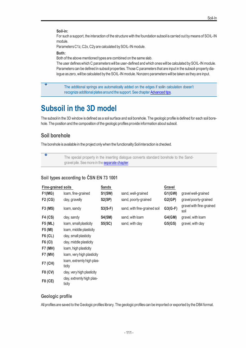
Soil-In
Soil-in:For such a support, the interaction of the structure with the foundation subsoil is carried out bymeansof SOIL-INmodule.ParametersC1z, C2x, C2yare calculated bySOIL-INmodule.Both:Both of the abovementioned typesare combined on the same slab.The user defineswhichC parameterswill be user-defined andwhich oneswill be calculated bySOIL-INmodule.Parameterscan be defined in subsoil properties. ThoseC parameters that are input in the subsoil-propertydia-logue aszero, will be calculated by theSOIL-INmodule. Nonzero parameterswill be taken as theyare input.
The additional springs are automatically added on the edges if soilin calculation doesn’trecognize additional platesaround the support. See chapter Advanced tips.
Subsoil in the 3D modelThe subsoil in the 3D window is defined asa soil surface and soil borehole. The geologic profile is defined for each soil bore-hole. The position and the composition of the geologicprofilesprovide information about subsoil.
Soil boreholeThe borehole isavailable in the project onlywhen the functionalitySoil interaction is checked.
The special property in the inserting dialogue converts standard borehole to the Sand-gravel pile. Seemore in the separate chapter.
Soil types according to ČSN EN 73 1001
Fine-grained soils Sands GravelF1(MG) loam, fine-grained S1(SW) sand, well-grained G1(GW) gravelwell-grainedF2 (CG) clay, gravelly S2(SP) sand, poorly-grained G2(GP) gravel poorly-grained
F3 (MS) loam, sandy S3(S-F) sand, with fine-grained soil G3(G-F) gravelwith fine-grainedsoil
F4 (CS) clay, sandy S4(SM) sand, with loam G4(GM) gravel, with loamF5 (ML) loam, small plasticity S5(SC) sand, with clay G5(GS) gravel, with clayF5 (MI) loam,middle plasticityF6 (CL) clay, small plasticityF6 (CI) clay,middle plasticityF7 (MH) loam, high plasticityF7 (MV) loam, veryhigh plasticity
F7 (CH) loam, extremlyhigh plas-ticity
F8 (CV) clay, veryhigh plasticity
F8 (CE) clay, extremlyhigh plas-ticity
Geologic profileAll profilesare saved to theGeologicprofiles library. The geologicprofilescan be imported or exported by theDB4 format.
- 111 -
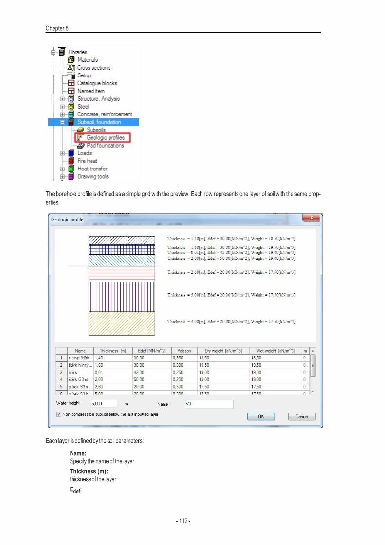
Chapter 8
The borehole profile is defined as a simple grid with the preview. Each row represents one layer of soil with the same prop-erties.
Each layer isdefined by the soil parameters:
Name:Specify the nameof the layerThickness (m):thicknessof the layerEdef:
- 112 -

Soil-In
The module of deformation Edef is defined as deformation characteristic of the soil. It is a ratio of the normalstress increment to the increment a linear transformation. For geotechnical categories 1 and 2 the indicativevalue from e.g. ČSN 73 1001 can be used, for category 3 a survey should be carried out to provide for the value.The valueEm fromEurocode 7 can be used instead of Edef.
Edef according toČSN 73 1001:
Class of the subsoil Edef (MPa)
F6-F8 (soft, medium consistency) 1,5-4
F6-F8 (stiff consistency) 6-8
F6-F8 (hard consistency) 10-15
F3-F5 (soft, medium consistency) 3-5
F3-F5 (stiff consistency) 8-10
F3-F4 (hard consistency) based on survey
F5 (hard consistency) 10-20
F1, F2 (soft, medium consistency) 5-15
F1, F2 (stiff consistency) 12-25
F1, F2 (hard consistency) based on survey
S4, S5 5-12
S3 12-19
S2 15-35
S1 30-60
G5 40-60
G4 60-80
G3 80-90
G2 100-190
G1 250-390
R6 10-75
R5 20-250
R4 40-750
R3 70-2500
R2 130-7500
R1 250-25000
TheEdef for R isderived from the number of discontinuousparts in the soil.
Poisson:Poisson’s ratio, coefficient of transverse deformation, an indicative value or experimentally found value can beused, predefined range is0 – 0.5
Poisson according toČSN 73 1001:
Class of the subsoil Poisson ν
F8 (soft, medium, stiff consistency) 0,42
F8 (hard consistency) based on survey
F5-F7 (soft, medium, stiff consistency) 0,40
F5-F7 (hard consistency) based on survey
- 113 -

Chapter 8
Class of the subsoil Poisson ν
F1-F4 (soft, medium, stiff consistency) 0,35
F1-F4 (hard consistency) based on survey
S5 0,35
S4, S3 0,30
S1, S2 0,28
G4,G5 0,30
G3 0,25
G1,G2 0,20
R6 0,40-0,25
R4, R5 0,30-0,20
R3 0,25-0,15
R1, R2 0,20-0,10
Dry weight:weight for the drysoil, normallywithin the range from18 to 23 kN/m3, range is0 – 10000000000 kN/m3
Wet weight:weight for the wet (saturated) soil, this value is mostly about 2-3 kN/m3 higher than the dry weight, range of thevalues is10 – 10000000 kN/m3
m coefficient:structural strength coefficient, according to the Eurocode7 is 0,2 (ČSN 73 1001 defines a table). The m coef-ficientmaybemodified for thewhole Eurocode.
Coefficientmaccording toČSN 73 1001:
Class of the subsoil m
F1-F8 with Edef<4MPa, not over consolidated and soft or solid consistencyR1, R2 and R4, R5 not affected by erosion
0,1
F1-F8 which don’t belong to the first groupS1, S2,G1,G2 under the water levelR3
0,2
S1, S2,G1,G2 above the water levelS3-S5G3-G5R4, R5 which don’t belong to the first group
0,3
R6 0,4
Loess, loess loam 0,5
Geologic profile must be defined up to such a depth where the bearing pressure is still act-ive, otherwise the programdoesnot have sufficient information.
The defined parametersare displayed in the libraryasproperties.
- 114 -
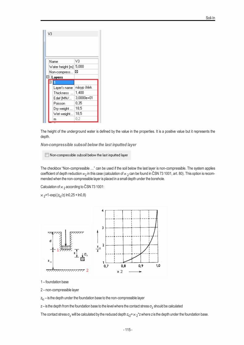
Soil-In
The height of the underground water is defined by the value in the properties. It is a positive value but it represents thedepth.
Non-compressible subsoil below the last inputted layer
The checkbox “Non-compressible …” can be used if the soil below the last layer is non-compressible. The system appliescoefficient of depth reductionϰ2 in this case (calculation of ϰ 2 can be found in ČSN 73 1001, art. 80). This option is recom-mendedwhen the non-compressible layer isplaced in a small depth under the borehole.
Calculation ofϰ 2 according toČSN 73 1001:
ϰ 2=1-exp((zic/z) ln0,25 + ln0,8)
1 – foundation base
2 – non-compressible layer
zic – is the depth under the foundation base to the non-compressible layer
z– is the depth from the foundation base to the levelwhere the contact stressσz should be calculated
The contact stressσz will be calculated by the reduced depth zr2=ϰ 2*zwhere z is the depth under the foundation base.
- 115 -
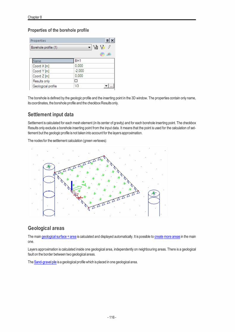
Chapter 8
Properties of the borehole profile
The borehole is defined by the geologic profile and the inserting point in the 3D window. The properties contain only name,its coordinates, the borehole profile and the checkboxResultsonly.
Settlement input dataSettlement is calculated for eachmesh element (in its center of gravity) and for each borehole inserting point. The checkboxResults only exclude a borehole inserting point from the input data. It means that the point is used for the calculation of set-tlement but the geologicprofile isnot taken into account for the layersapproximation.
The nodes for the settlement calculation (green vertexes):
Geological areasThemain geological surface = area is calculated and displayed automatically. It is possible to create more areas in the mainone.
Layers approximation is calculated inside one geological area, independently on neighbouring areas. There is a geologicalfault on the border between two geological areas.
TheSand-gravel pile isa geological profile which isplaced in one geological area.
- 116 -
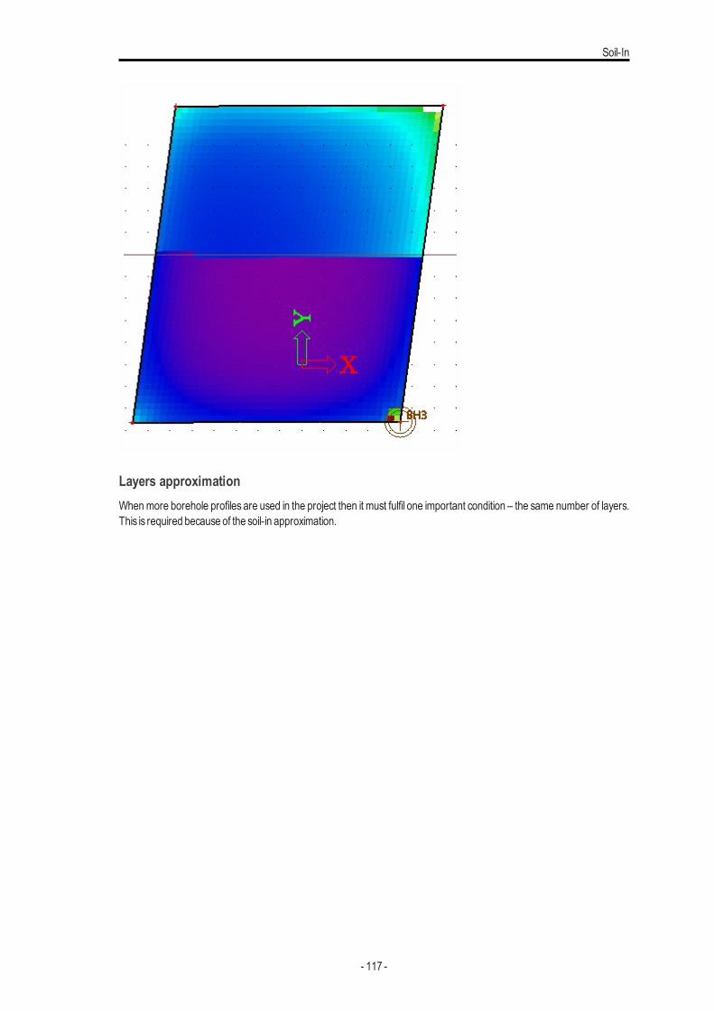
Soil-In
Layers approximationWhenmore borehole profiles are used in the project then it must fulfil one important condition – the same number of layers.This is required because of the soil-in approximation.
- 117 -
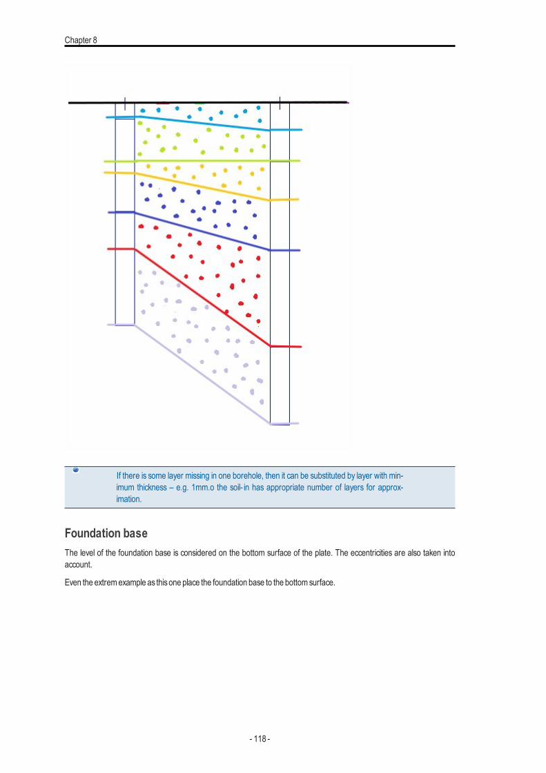
Chapter 8
If there is some layer missing in one borehole, then it can be substituted by layer with min-imum thickness – e.g. 1mm.o the soil- in has appropriate number of layers for approx-imation.
Foundation baseThe level of the foundation base is considered on the bottom surface of the plate. The eccentricities are also taken intoaccount.
Even the extremexample as thisone place the foundation base to the bottom surface.
- 118 -
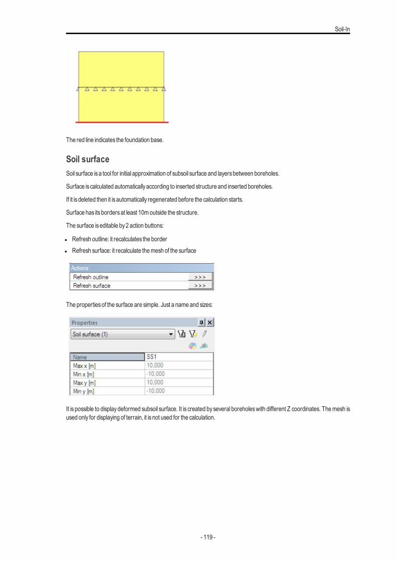
Soil-In
The red line indicates the foundation base.
Soil surfaceSoil surface isa tool for initial approximation of subsoil surface and layersbetween boreholes.
Surface is calculated automaticallyaccording to inserted structure and inserted boreholes.
If it is deleted then it isautomatically regenerated before the calculation starts.
Surface has itsbordersat least 10moutside the structure.
The surface iseditable by2 action buttons:
l Refresh outline: it recalculates the borderl Refresh surface: it recalculate themesh of the surface
The propertiesof the surface are simple. Just a nameand sizes:
It is possible to displaydeformed subsoil surface. It is created by several boreholeswith different Z coordinates. Themesh isused only for displaying of terrain, it is not used for the calculation.
- 119 -
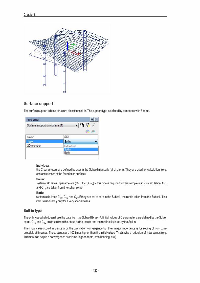
Chapter 8
Surface supportThe surface support isbasic structure object for soil-in. The support type isdefined bycomboboxwith 3 items.
Individual:the C parameters are defined by user in the Subsoil manually (all of them). They are used for calculation. (e.g.contact stressesof the foundation surface)Soilin:system calculates C parameters (C1z, C2x, C2y) – this type is required for the complete soil-in calculation, C1xandC1y are taken from the solver setupBoth:system calculates C1z, C2x and C2y if they are set to zero in the Subsoil; the rest is taken from the Subsoil. Thisitem isused rarelyonly for a veryspecial cases.
Soil-in typeThe only type which doesn’t use the data from the Subsoil library. All initial values of C parameters are defined by the Solversetup. C1x andC1y are taken from this setup as the resultsand the rest is calculated by theSoil-in.
The initial values could influence a bit the calculation convergence but their major importance is for setting of non-com-pressible stiffnesses. These values are 100 times higher than the initial values. That’s why a reduction of initial values (e.g.10 times) can help in a convergence problems (higher depth, small loading, etc.)
- 120 -
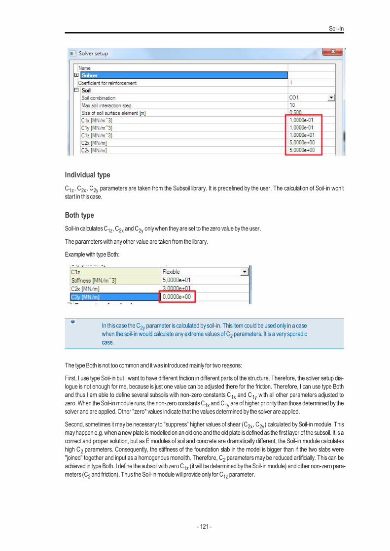
Soil-In
Individual typeC1z , C2x , C2y parameters are taken from the Subsoil library. It is predefined by the user. The calculation of Soil-in won’tstart in this case.
Both typeSoil-in calculatesC1z, C2x andC2y onlywhen theyare set to the zero value by the user.
The parameterswith anyother value are taken from the library.
Examplewith typeBoth:
In this case theC2y parameter is calculated bysoil-in. This item could be used only in a casewhen the soil-in would calculate any extreme values of C2 parameters. It is a very sporadiccase.
The typeBoth isnot too common and it was introducedmainly for two reasons:
First, I use type Soil-in but I want to have different friction in different parts of the structure. Therefore, the solver setup dia-logue is not enough for me, because is just one value can be adjusted there for the friction. Therefore, I can use type Bothand thus I am able to define several subsoils with non-zero constants C1x and C1y with all other parameters adjusted tozero.When the Soil-inmodule runs, the non-zero constantsC1x andC1y are of higher priority than those determined by thesolver and are applied. Other "zero" values indicate that the valuesdetermined by the solver are applied.
Second, sometimes it may be necessary to "suppress" higher values of shear (C2x, C2y) calculated bySoil-in module. Thismayhappen e.g. when a new plate ismodelled on an old one and the old plate isdefined as the first layer of the subsoil. It is acorrect and proper solution, but as E modules of soil and concrete are dramatically different, the Soil-in module calculateshigh C2 parameters. Consequently, the stiffness of the foundation slab in the model is bigger than if the two slabs were"joined" together and input as a homogenousmonolith. Therefore, C2 parameters may be reduced artificially. This can beachieved in typeBoth. I define the subsoilwith zeroC1z (it will be determined by theSoil-inmodule) and other non-zero para-meters (C2 and friction). Thus theSoil-inmodulewill provide only for C1z parameter.
- 121 -
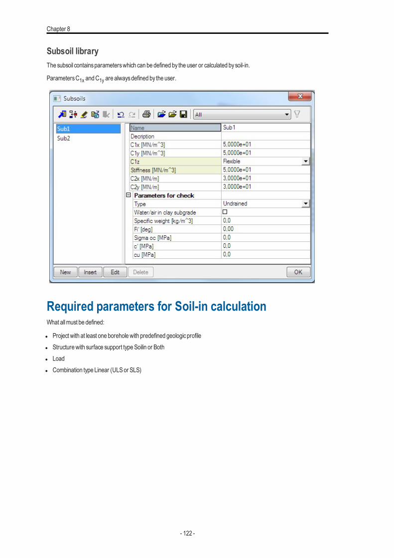
Chapter 8
Subsoil libraryThe subsoil containsparameterswhich can be defined by the user or calculated bysoil-in.
ParametersC1x andC1y are alwaysdefined by the user.
Required parameters for Soil-in calculationWhat allmust be defined:
l Project with at least one boreholewith predefined geologicprofilel Structurewith surface support typeSoilin or Bothl Loadl Combination type Linear (ULSor SLS)
- 122 -
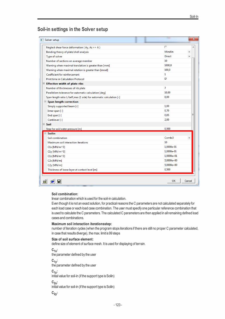
Soil-In
Soil-in settings in the Solver setup
Soil combination:linear combinationwhich isused for the soil-in calculation.Even though it isnot an exact solution, for practical reasons theC parametersare not calculated separately foreach load case or each load case combination. The user must specifyone particular reference combination thatisused to calculate theC parameters. The calculatedC parametersare then applied in all remaining defined loadcasesand combinations.Maximum soil interaction iterationsstep:number of iteration cycles (when the program stops iterations if there are still no proper C parameter calculated,in case that resultsdiverge), themax. limit is99 stepsSize of soil surface element:define size of element of surfacemesh. It isused for displaying of terrain.C1x:the parameter defined by the userC1y:the parameter defined by the userC1z:initial value for soil-in (if the support type isSoilin)C2x:initial value for soil-in (if the support type isSoilin)C2y:
- 123 -

Chapter 8
initial value for soil-in (if the support type isSoilin)Thickness of loose layer at contact level [m]:setting in solver settings for automatic definition of loose layer at contact stress level for better handling of found-ation at great depth and faster convergence of soilin iterations. This layer is automatically created and managedby soilin to handle the fact, that a thin layer of soil is always somewhat damaged and loose, just at the contactlevel. This item isset 0 asdefault. User can choose this layer 0 - 10m.
The source of not calculated parametersdependson the support type. It is described in thepreviouschapter.
Soil-in calculationSoil-in iterative cycleThe values from the top structure and the foundation are calculated byFEM. The valuesare used as the source data for thesoil-in.
The iterative process is finishedwhen the contact stressσz and displacement uz doesnot change significantly in the two sub-sequent iterations. The special quadraticnormsare evaluated in the each iteration cycle to find out if this condition is fulfilled.
Diagramof the iterative cycle:
- 124 -
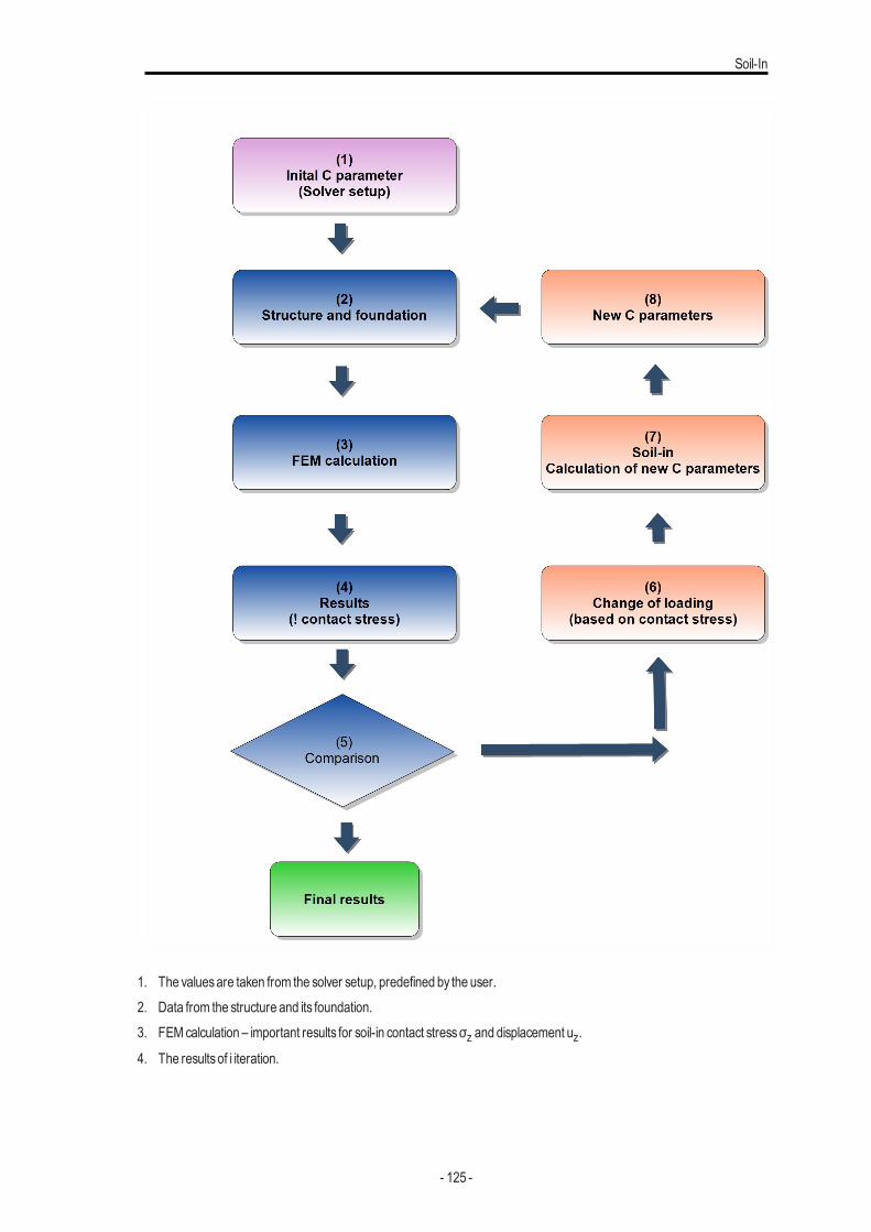
Soil-In
1. The valuesare taken from the solver setup, predefined by the user.2. Data from the structure and its foundation.3. FEMcalculation – important results for soil-in contact stressσz and displacement uz.
4. The resultsof i iteration.
- 125 -
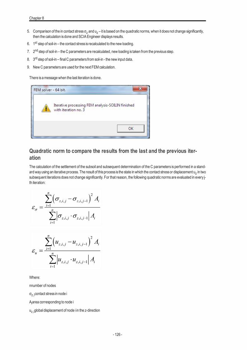
Chapter 8
5. Comparison of the in contact stressσz and uz – it isbased on the quadraticnorms, when it doesnot change significantly,then the calculation isdone andSCIAEngineer displays results.
6. 1st step of soil-in – the contact stress is recalculated to the new loading.
7. 2nd step of soil-in – theC parametersare recalculated, new loading is taken from the previousstep.
8. 3rd step of soil-in – finalC parameters from soil-in - the new input data.
9. NewC parametersare used for the next FEMcalculation.
There isamessagewhen the last iteration isdone.
Quadratic norm to compare the results from the last and the previous iter-ationThe calculation of the settlement of the subsoil and subsequent determination of the C parameters is performed in a stand-ardwayusing an iterative process. The result of thisprocess is the state in which the contact stressor displacement uz in twosubsequent iterationsdoesnot change significantly. For that reason, the following quadratic normsare evaluated in every j-th iteration:
Where:
nnumber of nodes
σz,icontact stress in node i
Aiarea corresponding to node i
uz,iglobal displacement of node i in the z-direction
- 126 -
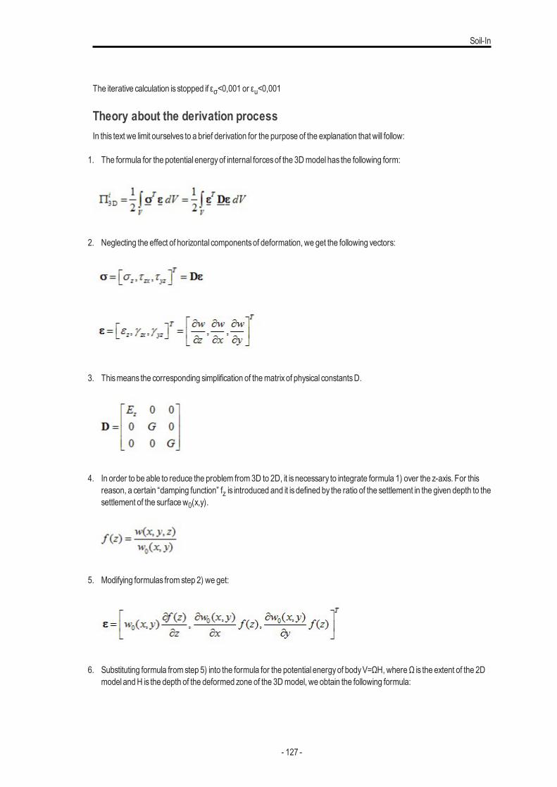
Soil-In
The iterative calculation is stopped if εσ<0,001 or εu<0,001
Theory about the derivation processIn this text we limit ourselves to a brief derivation for the purpose of the explanation that will follow:
1. The formula for the potential energyof internal forcesof the 3Dmodel has the following form:
2. Neglecting the effect of horizontal componentsof deformation, we get the following vectors:
3. Thismeans the corresponding simplification of thematrixof physical constantsD.
4. In order to be able to reduce the problem from3D to 2D, it isnecessary to integrate formula 1) over the z-axis. For thisreason, a certain “damping function” fz is introduced and it isdefined by the ratio of the settlement in the given depth to thesettlement of the surfacew0(x,y).
5. Modifying formulas from step 2) we get:
6. Substituting formula from step 5) into the formula for the potential energyof bodyV=ΩH,whereΩ is the extent of the 2Dmodel andH is the depth of the deformed zone of the 3Dmodel, we obtain the following formula:
- 127 -
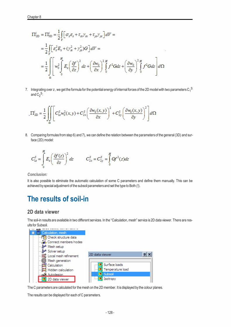
Chapter 8
7. Integrating over z , we get the formula for the potential energyof internal forcesof the 2Dmodelwith two parametersC1SandC2S:
8. Comparing formulas from step 6) and 7), we can define the relation between the parametersof the general (3D) and sur-face (2D) model:
Conclusion:It is also possible to eliminate the automatic calculation of some C parameters and define them manually. This can beachieved byspecial adjustment of the subsoil parametersand set the type to Both (!).
The results of soil-in2D data viewerThe soil-in results are available in two different services. In the “Calculation, mesh” service is 2D data viewer. There are res-ults for Subsoil.
TheC parametersare calculated for themesh on the 2Dmember. It isdisplayed by the colour planes.
The results can be displayed for each of C parameters.
- 128 -
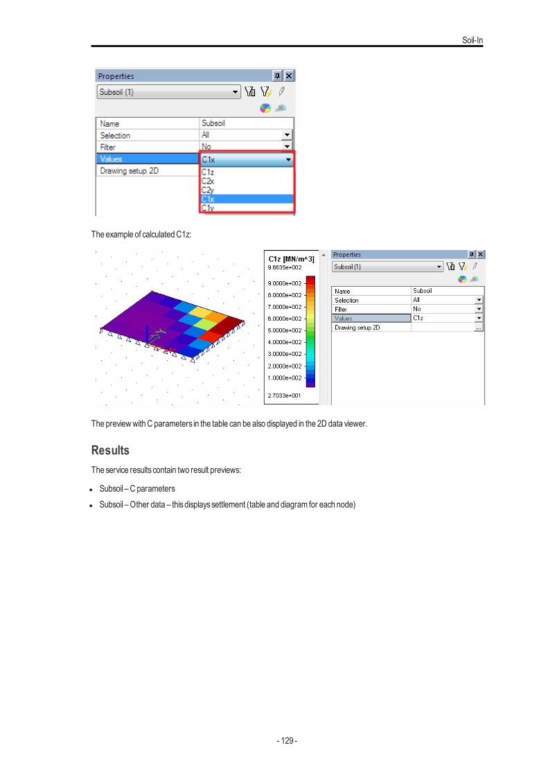
Soil-In
The example of calculatedC1z:
The previewwithC parameters in the table can be also displayed in the 2D data viewer.
ResultsThe service results contain two result previews:
l Subsoil – C parametersl Subsoil –Other data – thisdisplayssettlement (table and diagram for each node)
- 129 -
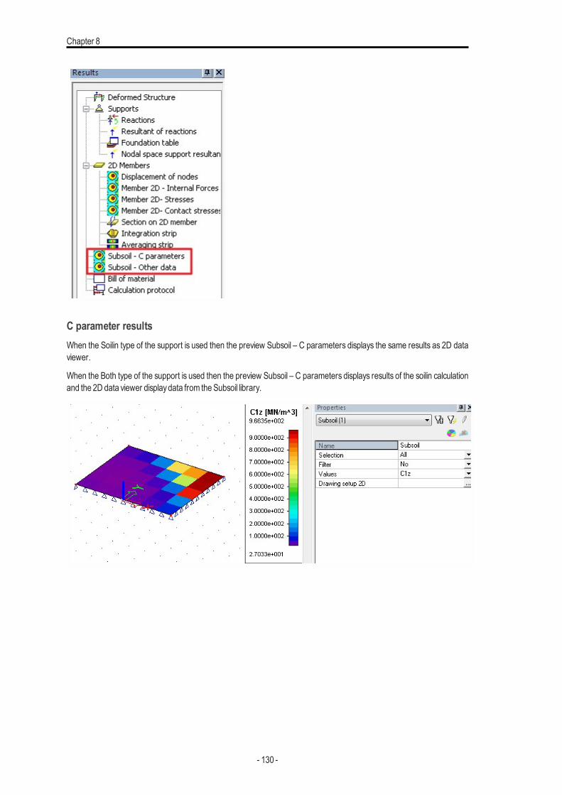
Chapter 8
C parameter resultsWhen the Soilin type of the support is used then the preview Subsoil – C parameters displays the same results as 2D dataviewer.
When the Both type of the support is used then the preview Subsoil – C parameters displays results of the soilin calculationand the 2D data viewer displaydata from theSubsoil library.
- 130 -
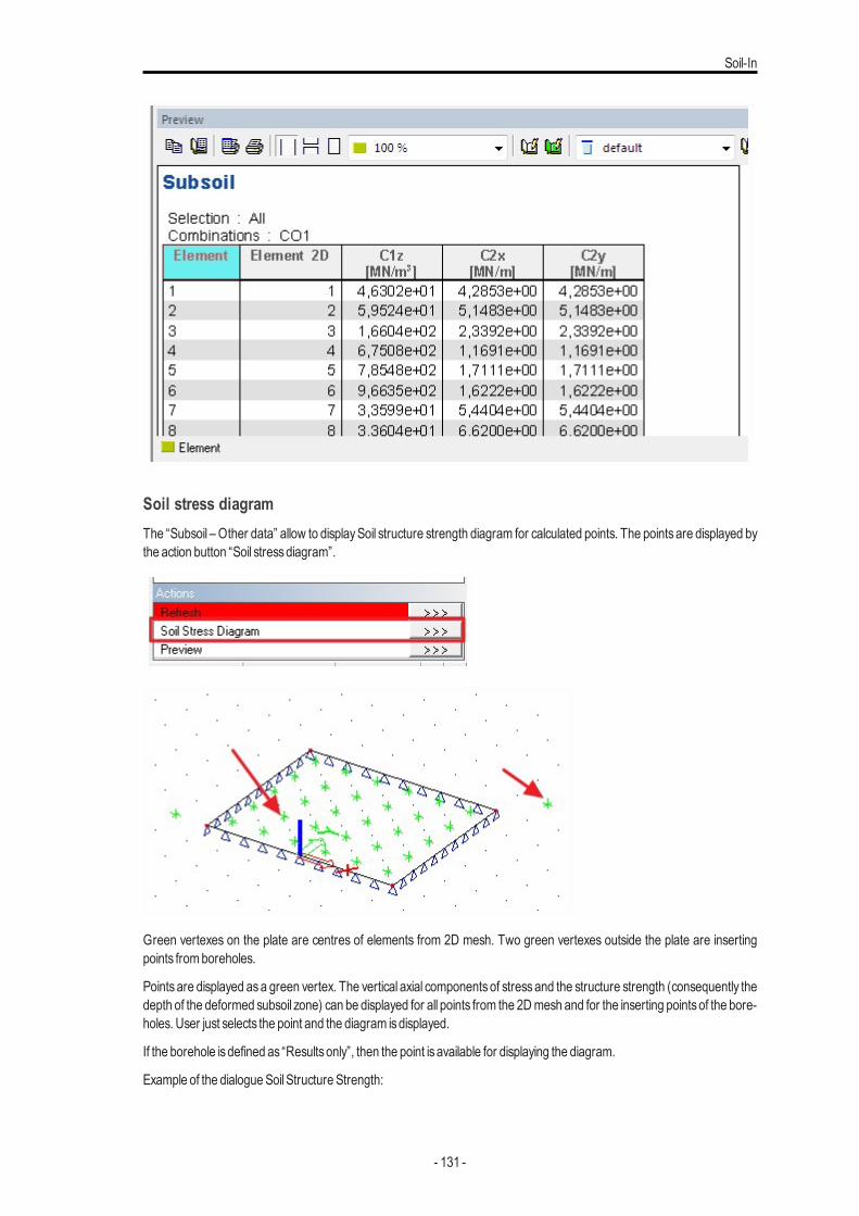
Soil-In
Soil stress diagramThe “Subsoil – Other data” allow to displaySoil structure strength diagram for calculated points. The points are displayed bythe action button “Soil stressdiagram”.
Green vertexes on the plate are centres of elements from 2D mesh. Two green vertexes outside the plate are insertingpoints fromboreholes.
Points are displayed asa green vertex. The vertical axial componentsof stressand the structure strength (consequently thedepth of the deformed subsoil zone) can be displayed for all points from the 2Dmesh and for the inserting pointsof the bore-holes. User just selects the point and the diagram isdisplayed.
If the borehole isdefined as “Resultsonly”, then the point isavailable for displaying the diagram.
Example of the dialogueSoilStructure Strength:
- 131 -
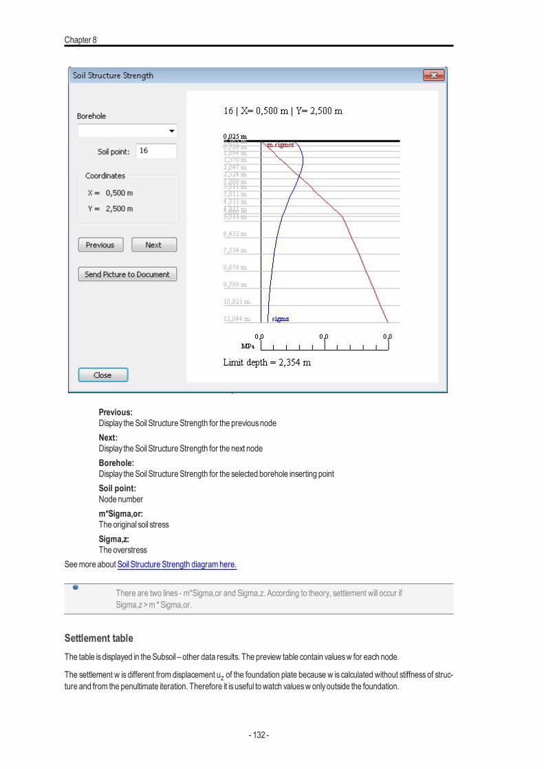
Chapter 8
Previous:Display theSoilStructure Strength for the previousnodeNext:Display theSoilStructure Strength for the next nodeBorehole:Display theSoilStructure Strength for the selected borehole inserting pointSoil point:Node numberm*Sigma,or:The original soil stressSigma,z:The overstress
Seemore about SoilStructure Strength diagramhere.
There are two lines - m*Sigma,or and Sigma,z. According to theory, settlement will occur ifSigma,z>m *Sigma,or.
Settlement tableThe table isdisplayed in theSubsoil – other data results. The preview table contain valuesw for each node.
The settlement w is different from displacement uz of the foundation plate because w is calculated without stiffness of struc-ture and from the penultimate iteration. Therefore it isuseful to watch valuesw onlyoutside the foundation.
- 132 -
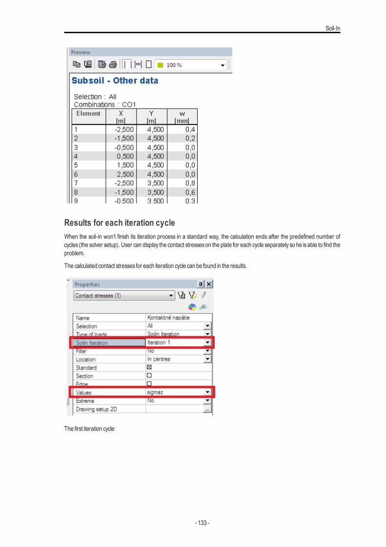
Soil-In
Results for each iteration cycleWhen the soil- in won’t finish its iteration process in a standard way, the calculation ends after the predefined number ofcycles (the solver setup). User can display the contact stresseson the plate for each cycle separately so he is able to find theproblem.
The calculated contact stresses for each iteration cycle can be found in the results.
The first iteration cycle
- 133 -
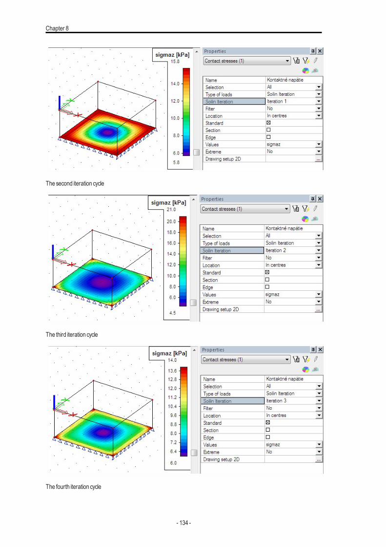
Chapter 8
The second iteration cycle
The third iteration cycle
The fourth iteration cycle
- 134 -
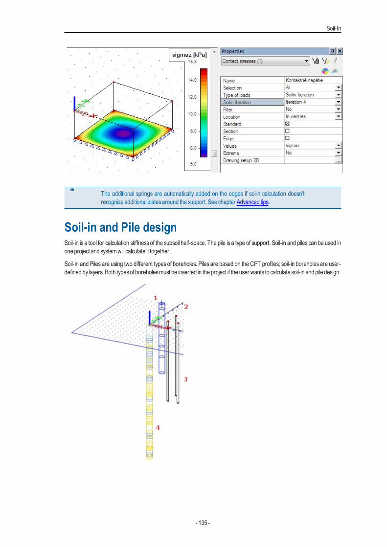
Soil-In
The additional springs are automatically added on the edges if soilin calculation doesn’trecognize additional platesaround the support. See chapter Advanced tips.
Soil-in and Pile designSoil-in is a tool for calculation stiffness of the subsoil half-space. The pile is a type of support. Soil-in and piles can be used inone project and systemwill calculate it together.
Soil-in and Piles are using two different types of boreholes. Piles are based on the CPT profiles; soil-in boreholes are user-defined by layers. Both typesof boreholesmust be inserted in the project if the user wants to calculate soil-in and pile design.
- 135 -
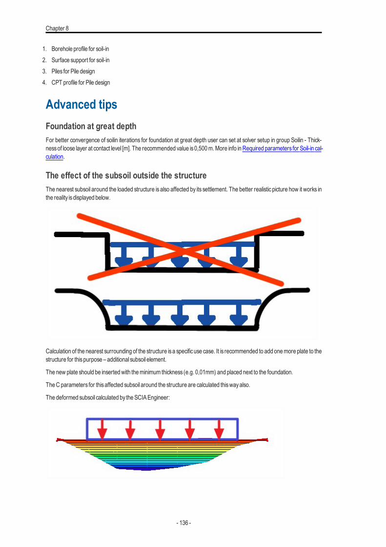
Chapter 8
1. Borehole profile for soil-in2. Surface support for soil-in3. Piles for Pile design4. CPT profile for Pile design
Advanced tipsFoundation at great depthFor better convergence of soilin iterations for foundation at great depth user can set at solver setup in group Soilin - Thick-nessof loose layer at contact level [m]. The recommended value is0,500m.More info in Required parameters for Soil-in cal-culation.
The effect of the subsoil outside the structureThe nearest subsoil around the loaded structure is also affected by its settlement. The better realistic picture how it works inthe reality isdisplayed below.
Calculation of the nearest surrounding of the structure isa specificuse case. It is recommended to add onemore plate to thestructure for thispurpose – additional subsoil element.
The new plate should be insertedwith theminimum thickness (e.g. 0,01mm) and placed next to the foundation.
TheC parameters for thisaffected subsoil around the structure are calculated thiswayalso.
The deformed subsoil calculated by theSCIAEngineer:
- 136 -
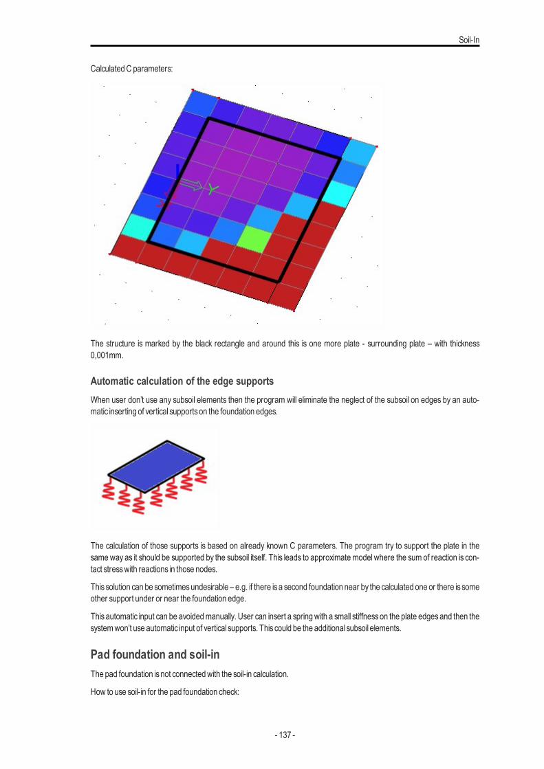
Soil-In
CalculatedC parameters:
The structure is marked by the black rectangle and around this is one more plate - surrounding plate – with thickness0,001mm.
Automatic calculation of the edge supportsWhen user don’t use any subsoil elements then the program will eliminate the neglect of the subsoil on edges by an auto-matic inserting of vertical supportson the foundation edges.
The calculation of those supports is based on already known C parameters. The program try to support the plate in thesame way as it should be supported by the subsoil itself. This leads to approximate model where the sum of reaction is con-tact stresswith reactions in those nodes.
This solution can be sometimesundesirable – e.g. if there isa second foundation near by the calculated one or there is someother support under or near the foundation edge.
Thisautomatic input can be avoidedmanually. User can insert a spring with a small stiffnesson the plate edgesand then thesystemwon’t use automatic input of vertical supports. This could be the additional subsoil elements.
Pad foundation and soil-inThe pad foundation isnot connectedwith the soil-in calculation.
How to use soil-in for the pad foundation check:
- 137 -
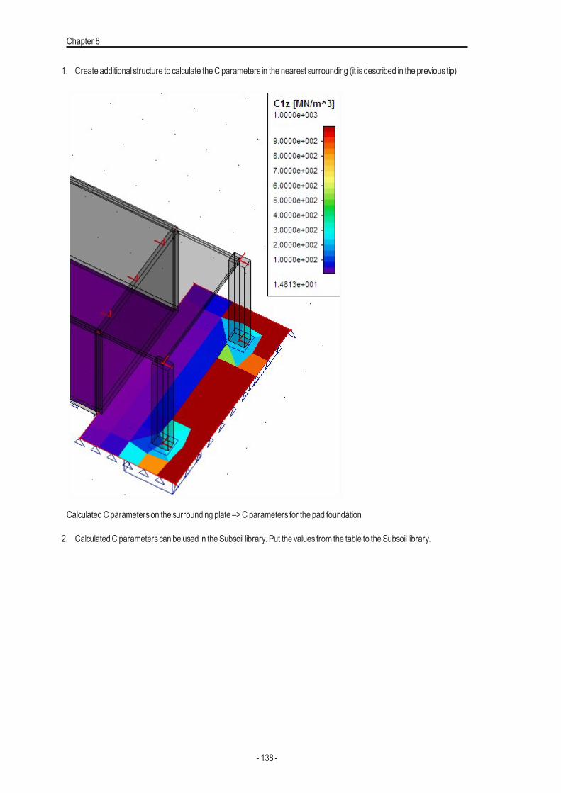
Chapter 8
1. Create additional structure to calculate theC parameters in the nearest surrounding (it isdescribed in the previous tip)
CalculatedC parameterson the surrounding plate –>C parameters for the pad foundation
2. CalculatedC parameterscan be used in theSubsoil library. Put the values from the table to theSubsoil library.
- 138 -
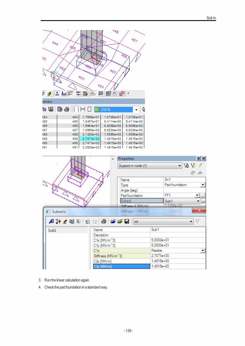
Soil-In
3. Run the linear calculation again.4. Check the pad foundation in a standardway.
- 139 -
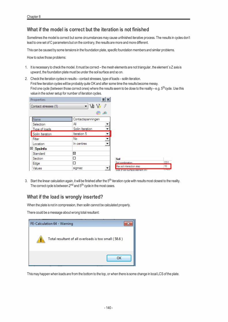
Chapter 8
What if the model is correct but the iteration is not finishedSometimes the model is correct but some circumstancesmay cause unfinished iterative process. The results in cycles don’tlead to one set of C parametersbut on the contrary, the resultsaremore andmore different.
This can be caused bysome tensions in the foundation plate, specific foundationmembersand similar problems.
How to solve those problems:
1. It isnecessary to check themodel. It must be correct – themesh elementsare not triangular, the element´sZ axis isupward, the foundation platemust be under the soil surface and so on.
2. Check the iteration cycles in results– contact stresses, type of loads– soilin iteration.First few iteration cycleswill be probablyquiteOKand after some time the resultsbecomemessy.Find one cycle (between those correct ones) where the results seem to be close to the reality– e.g. 5thcycle. Use thisvalue in the solver setup for number of iteration cycles.
3. Start the linear calculation again, it will be finished after the 5th iteration cyclewith resultsmost closest to the reality.The correct cycle isbetween 2nd and 5th cycle in themost cases.
What if the load is wrongly inserted?When the plate isnot in compression, then soilin cannot be calculated properly.
There could be amessage about wrong total resultant:
Thismayhappenwhen loadsare from the bottom to the top, or when there is some change in local LCSof the plate.
- 140 -

Soil-In
What if the symmetrical structure gives non-symmetrical results?Thismayhappenwhen additional subsoil elementsare not added around the structure.
Also when the soilin didn’t find the correct result and calculation is stopped too soon. (For example when solver setupdefinesonly few soilin cycles.)
What if geological fault in the subsoil is needed?Themain subsoil surface is created automatically when a structure and a borehole is inserted to the project. The size of thesubsoil outline is calculated from the structure size, positionsof boreholesand someoffset around.
The geological fault is createdwhen the second area is inserted to themain one.
1. Create structure and insert boreholes.2. Themain subsoil surface is created.
- 141 -
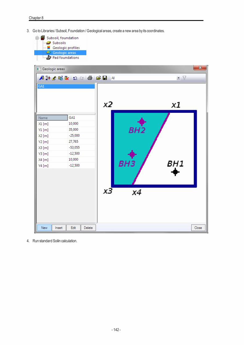
Chapter 8
3. Go to Libraries / Subsoil, Foundation / Geological areas, create a new area by its coordinates.
4. Run standard Soilin calculation.
- 142 -
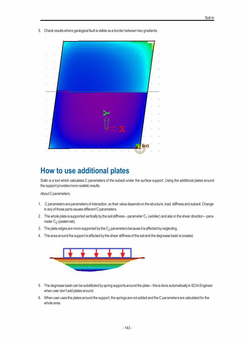
Soil-In
5. Check resultswhere geological fault is visible asa border between two gradients.
How to use additional platesSoilin is a tool which calculates C parameters of the subsoil under the surface support. Using the additional plates aroundthe support providesmore realistic results.
About C parameters:
1. C parametersare parametersof interaction, so their value dependson the structure, load, stiffnessand subsoil. Changein anyof those parts causesdifferent C parameters.
2. Thewhole plate is supported verticallyby the soil stiffness– parameter C1 (winkler) and also in the shear direction – para-meter C2 (pasternak).
3. The plate edgesaremore supported by theC2 parametersbecause it isaffected byneglecting.
4. The area around the support isaffected by the shear stiffnessof the soil and the degrease basin is created.
5. The degrease basin can be substituted byspring supportsaround the plate – this isdone automatically in SCIAEngineerwhen user don’t add platesaround.
6. When user uses the platesaround the support, the springsare not added and theC parametersare calculated for thewhole area.
- 143 -
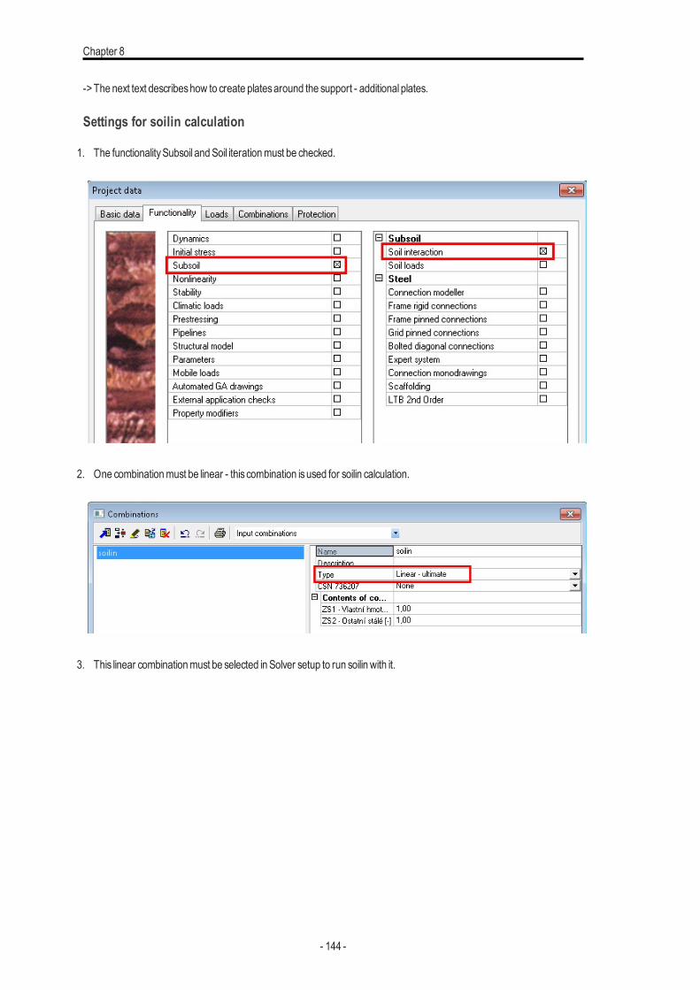
Chapter 8
->The next text describeshow to create platesaround the support - additional plates.
Settings for soilin calculation
1. The functionalitySubsoil andSoil iterationmust be checked.
2. One combinationmust be linear - this combination isused for soilin calculation.
3. This linear combinationmust be selected in Solver setup to run soilin with it.
- 144 -
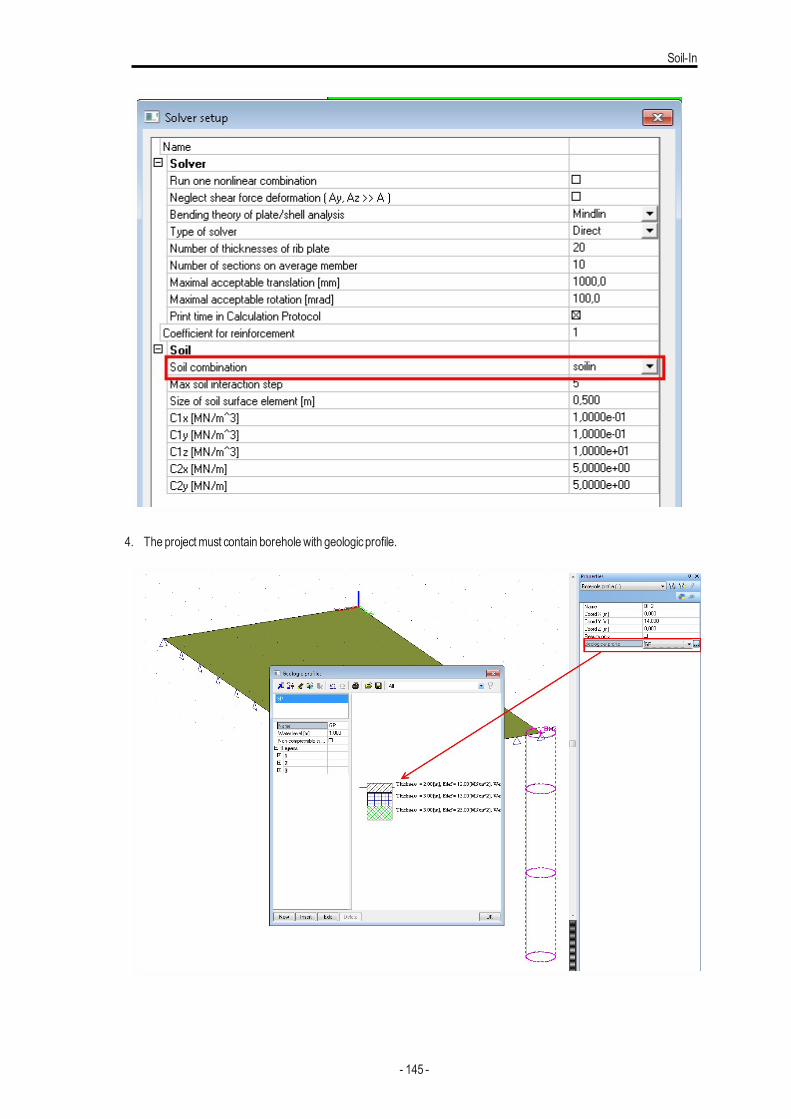
Soil-In
4. The projectmust contain boreholewith geologicprofile.
- 145 -
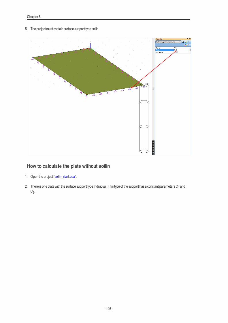
Chapter 8
5. The projectmust contain surface support type soilin.
How to calculate the plate without soilin
1. Open the project “soilin_start.esa”.
2. There isone platewith the surface support type Individual. This type of the support hasa constant parametersC1 andC2.
- 146 -
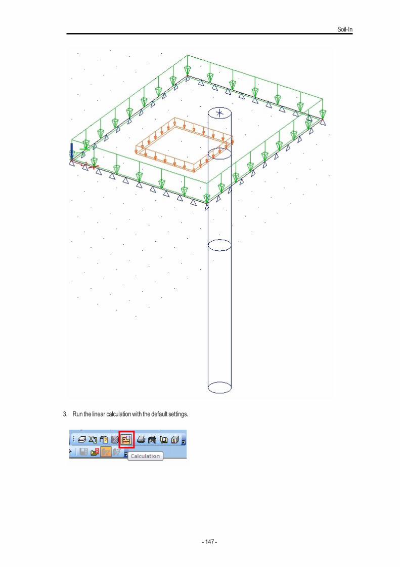
Soil-In
3. Run the linear calculationwith the default settings.
- 147 -
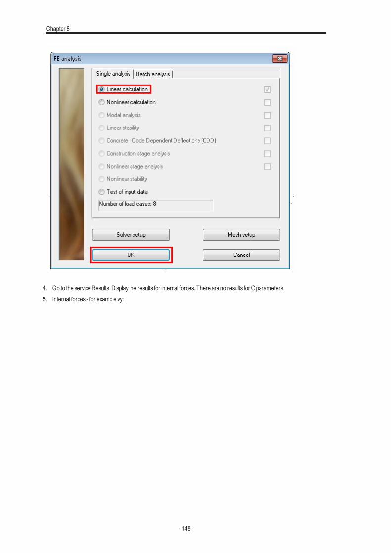
Chapter 8
4. Go to the serviceResults. Display the results for internal forces. There are no results for C parameters.5. Internal forces - for example vy:
- 148 -

Soil-In
How to calculate the plate with soilin.
1. Change the support type to soilin.2. Run the linear calculation again.3. Go to the serviceResults. Display the results for internal forcesand soilin for combinationC01.
- 149 -
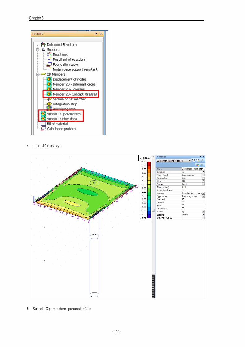
Chapter 8
4. Internal forces - vy:
5. Subsoil - C parameters - parameter C1z:
- 150 -
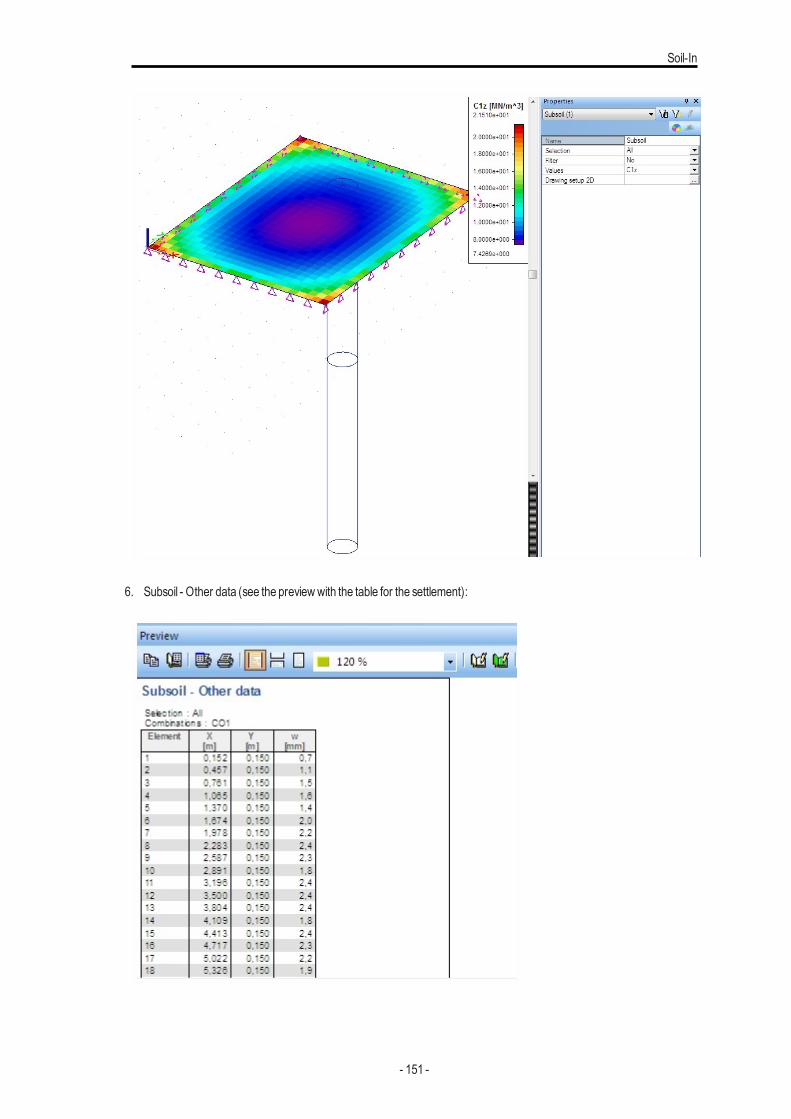
Soil-In
6. Subsoil - Other data (see the previewwith the table for the settlement):
- 151 -
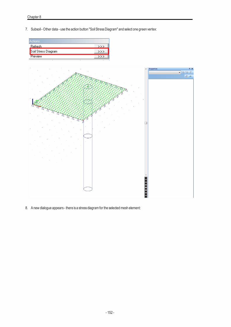
Chapter 8
7. Subsoil - Other data - use the action button "SoilStressDiagram" and select one green vertex:
8. Anew dialogue appears - there isa stressdiagram for the selectedmesh element:
- 152 -
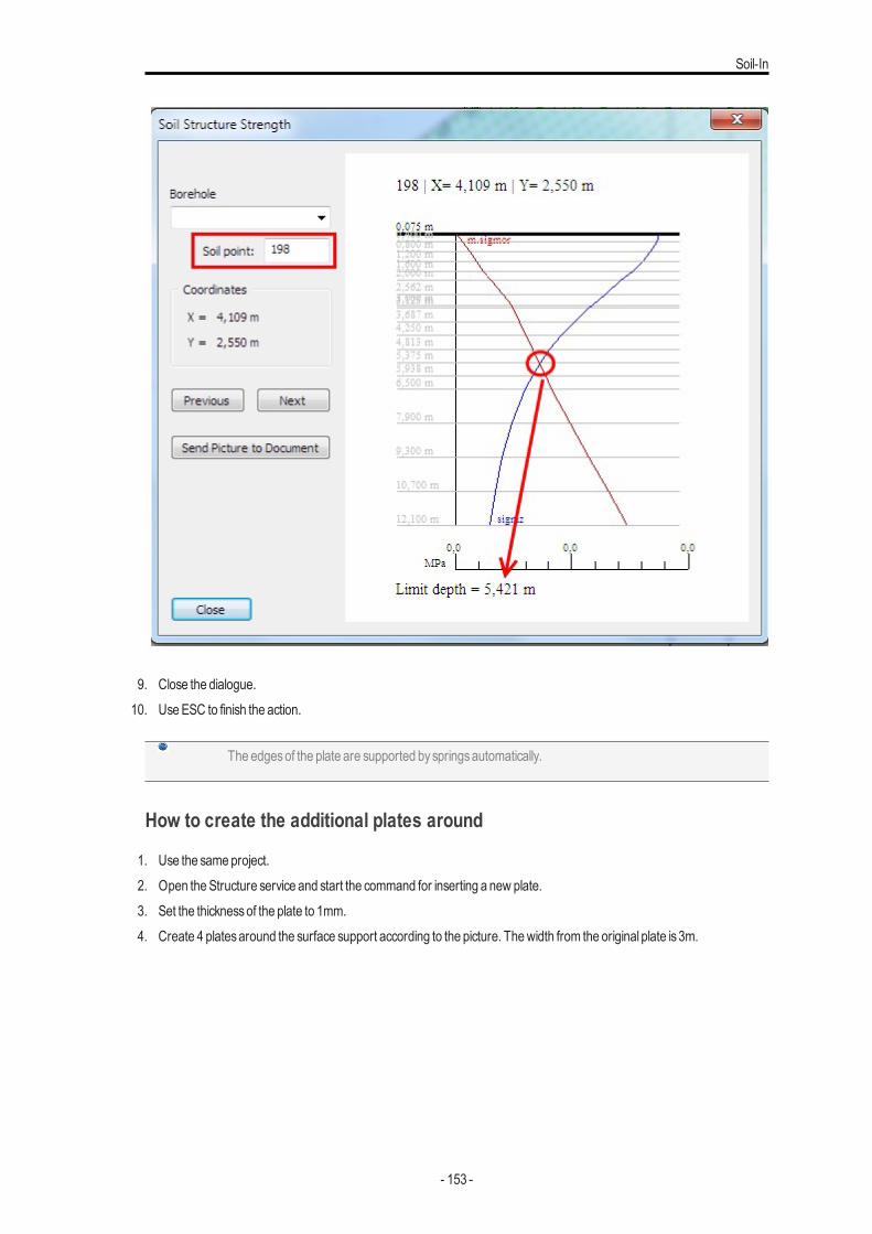
Soil-In
9. Close the dialogue.10. UseESC to finish the action.
The edgesof the plate are supported byspringsautomatically.
How to create the additional plates around
1. Use the sameproject.2. Open theStructure service and start the command for inserting a new plate.3. Set the thicknessof the plate to 1mm.4. Create 4 platesaround the surface support according to the picture. Thewidth from the original plate is3m.
- 153 -
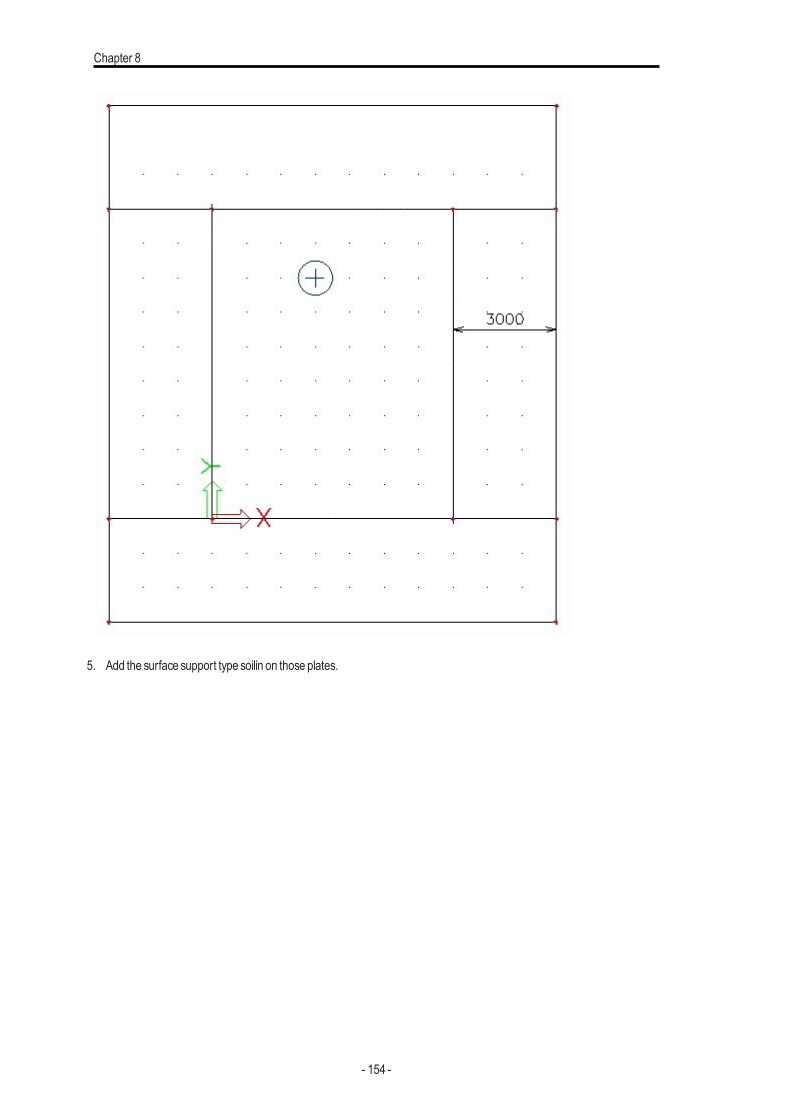
Chapter 8
5. Add the surface support type soilin on those plates.
- 154 -
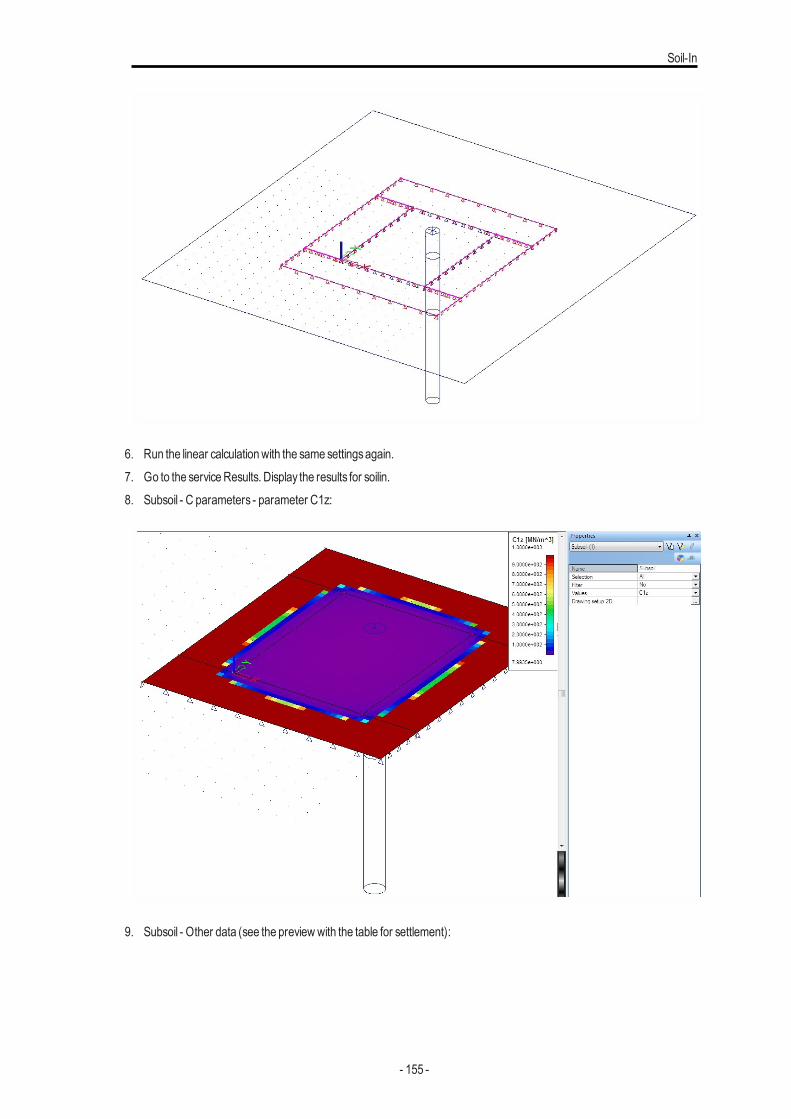
Soil-In
6. Run the linear calculationwith the same settingsagain.7. Go to the serviceResults. Display the results for soilin.8. Subsoil - C parameters - parameter C1z:
9. Subsoil - Other data (see the previewwith the table for settlement):
- 155 -
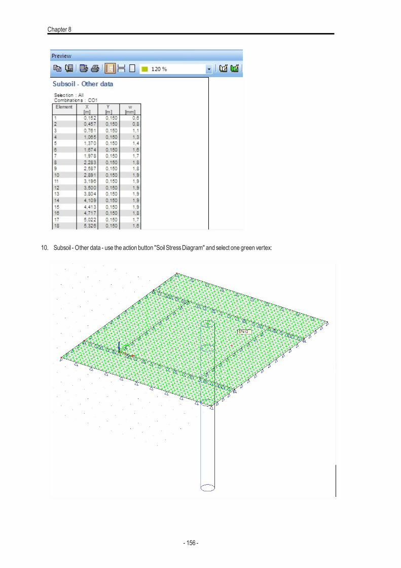
Chapter 8
10. Subsoil - Other data - use the action button "SoilStressDiagram" and select one green vertex:
- 156 -
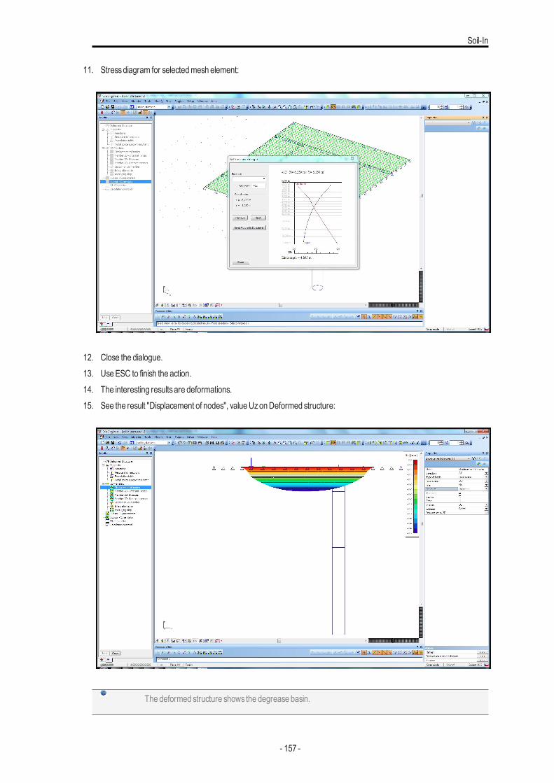
Soil-In
11. Stressdiagram for selectedmesh element:
12. Close the dialogue.13. UseESC to finish the action.14. The interesting resultsare deformations.15. See the result "Displacement of nodes", valueUzonDeformed structure:
The deformed structure shows the degrease basin.
- 157 -

Chapter 8
16. The result is in project "soilin_finished.esa".
- 158 -
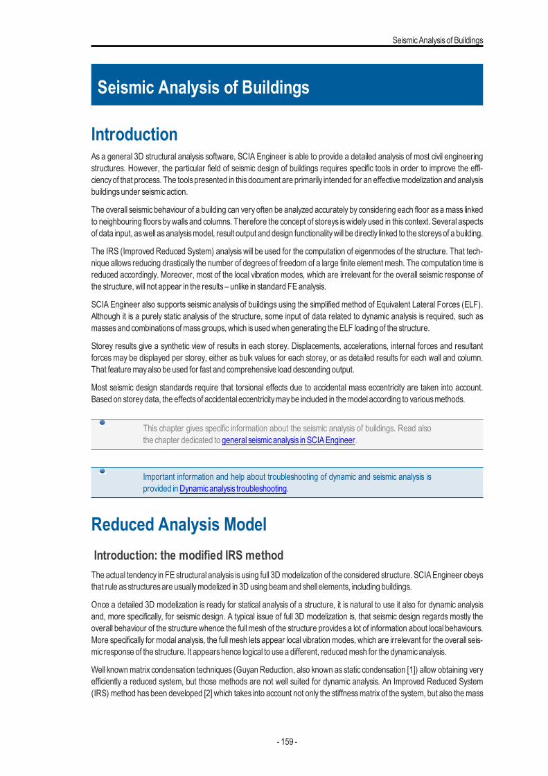
SeismicAnalysisof Buildings
Seismic Analysis of Buildings
IntroductionAs a general 3D structural analysis software, SCIA Engineer is able to provide a detailed analysis of most civil engineeringstructures. However, the particular field of seismic design of buildings requires specific tools in order to improve the effi-ciencyof that process. The toolspresented in thisdocument are primarily intended for an effectivemodelization and analysisbuildingsunder seismicaction.
The overall seismic behaviour of a building can very often be analyzed accurately by considering each floor as amass linkedto neighbouring floors bywalls and columns. Therefore the concept of storeys iswidely used in this context. Several aspectsof data input, aswell asanalysismodel, result output and design functionalitywill be directly linked to the storeysof a building.
The IRS (Improved Reduced System) analysis will be used for the computation of eigenmodes of the structure. That tech-nique allows reducing drastically the number of degrees of freedom of a large finite element mesh. The computation time isreduced accordingly. Moreover, most of the local vibration modes, which are irrelevant for the overall seismic response ofthe structure, will not appear in the results– unlike in standard FEanalysis.
SCIA Engineer also supports seismic analysis of buildings using the simplified method of Equivalent Lateral Forces (ELF).Although it is a purely static analysis of the structure, some input of data related to dynamic analysis is required, such asmassesand combinationsofmassgroups, which isusedwhen generating theELF loading of the structure.
Storey results give a synthetic view of results in each storey. Displacements, accelerations, internal forces and resultantforces may be displayed per storey, either as bulk values for each storey, or as detailed results for each wall and column.That featuremayalso be used for fast and comprehensive load descending output.
Most seismic design standards require that torsional effects due to accidental mass eccentricity are taken into account.Based on storeydata, the effectsof accidental eccentricitymaybe included in themodel according to variousmethods.
This chapter gives specific information about the seismic analysis of buildings. Read alsothe chapter dedicated to general seismicanalysis in SCIAEngineer.
Important information and help about troubleshooting of dynamic and seismic analysis isprovided inDynamicanalysis troubleshooting.
Reduced Analysis ModelIntroduction: the modified IRS methodThe actual tendency in FE structural analysis is using full 3Dmodelization of the considered structure. SCIAEngineer obeysthat rule asstructuresare usuallymodelized in 3D using beamand shell elements, including buildings.
Once a detailed 3D modelization is ready for statical analysis of a structure, it is natural to use it also for dynamic analysisand, more specifically, for seismic design. A typical issue of full 3D modelization is, that seismic design regards mostly theoverall behaviour of the structure whence the full mesh of the structure provides a lot of information about local behaviours.More specifically for modal analysis, the full mesh lets appear local vibration modes, which are irrelevant for the overall seis-mic response of the structure. It appearshence logical to use a different, reducedmesh for the dynamicanalysis.
Well knownmatrix condensation techniques (Guyan Reduction, also known as static condensation [1]) allow obtaining veryefficiently a reduced system, but those methods are not well suited for dynamic analysis. An Improved Reduced System(IRS) method hasbeen developed [2] which takes into account not only the stiffnessmatrix of the system, but also themass
- 159 -
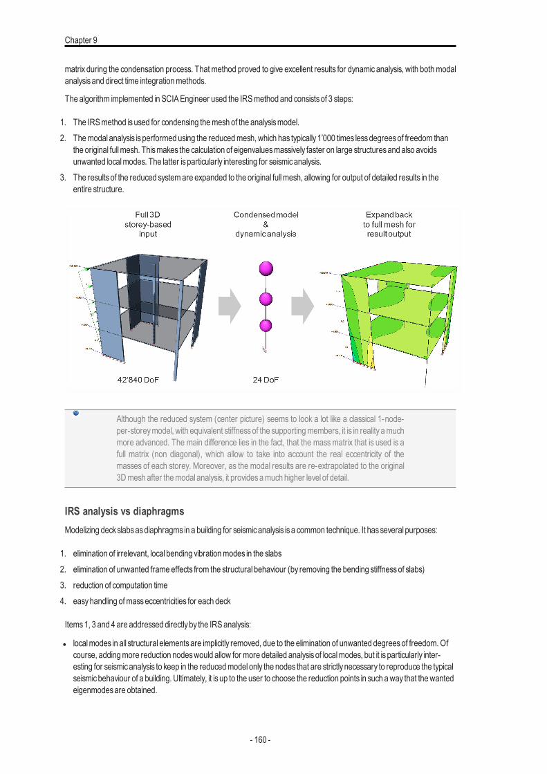
Chapter 9
matrix during the condensation process. That method proved to give excellent results for dynamic analysis, with both modalanalysisand direct time integrationmethods.
The algorithm implemented in SCIAEngineer used the IRSmethod and consistsof 3 steps:
1. The IRSmethod isused for condensing themesh of the analysismodel.2. Themodal analysis isperformed using the reducedmesh, which has typically1’000 times lessdegreesof freedom than
the original fullmesh. Thismakes the calculation of eigenvaluesmassively faster on large structuresand also avoidsunwanted localmodes. The latter isparticularly interesting for seismicanalysis.
3. The resultsof the reduced systemare expanded to the original fullmesh, allowing for output of detailed results in theentire structure.
Although the reduced system (center picture) seems to look a lot like a classical 1-node-per-storeymodel, with equivalent stiffnessof the supportingmembers, it is in reality amuchmore advanced. The main difference lies in the fact, that the mass matrix that is used is afull matrix (non diagonal), which allow to take into account the real eccentricity of themasses of each storey. Moreover, as the modal results are re-extrapolated to the original3D mesh after themodal analysis, it providesamuch higher level of detail.
IRS analysis vs diaphragmsModelizing deckslabsasdiaphragms in a building for seismicanalysis isa common technique. It hasseveral purposes:
1. elimination of irrelevant, local bending vibrationmodes in the slabs2. elimination of unwanted frame effects from the structural behaviour (by removing the bending stiffnessof slabs)3. reduction of computation time4. easyhandling ofmasseccentricities for each deck
Items1, 3 and 4 are addressed directlyby the IRSanalysis:
l localmodes in all structural elementsare implicitly removed, due to the elimination of unwanted degreesof freedom.Ofcourse, addingmore reduction nodeswould allow for more detailed analysisof localmodes, but it is particularly inter-esting for seismicanalysis to keep in the reducedmodel only the nodes that are strictlynecessary to reproduce the typicalseismicbehaviour of a building. Ultimately, it is up to the user to choose the reduction points in such away that thewantedeigenmodesare obtained.
- 160 -

SeismicAnalysisof Buildings
l the computation time is reduced, due to the drastic reduction of the number of degreesof freedom; actually, the reductionisevenmore important thanwith diaphragms, assupportingmembersare also condensed. The reduction of com-putation time affectsonly the computation of the eigenmodes itself. The pre- and post-processing times remain practicallyunchanged, which include overall data preparation,mesh generation andmodal superposition of local results. Theseoperationsare, obviously, still performed on the fullmesh of themodel and can be quite time consuming.
l the IRSanalysisusesa fullmassmatrix, which allows for exact implementation ofmasseccentricity in each node of thereduced system
Item 2 – removal of frame effects – is not addressed by the IRS analysis in itself, as it does not modify the mechanical beha-viour of the structure. However, as unwanted local bending modes are implicitly removed from the reduced system, so-called flexible diaphragmsmaybe easily simulated bysignificantly reducing the bending stiffnessof deckslabs. Not onlydoesthat allow to obtains classical diaphragm behaviour by means of a very low bending stiffness, but also intermediate beha-viour where the bending stiffness is less drastically reduced and frame effects are therefore reduced, but not completelyremoved.
Using diaphragms and IRS analysis together is actually possible in theory - although notsupported yet in SCIAEngineer.
Using diaphragms and IRS analysis together is actually possible. Diaphragm constraintsmaybe used to eliminate completely frame effects due to the bending stiffness of the slabs,and still benefit from the other advantages of the reduced system. Diaphragms are cur-rently supported only for composite decks in SCIAEngineer.
Benchmarks
Example 1: simple platformThe structure is a simple platform, with 9 steel columns and a thin plate on the top. This academic example only intends toillustrate some aspectsof themethod.
The reducedmodel consistsof 2R-nodes, located at the top and at the bottomof themiddle column.
- 161 -
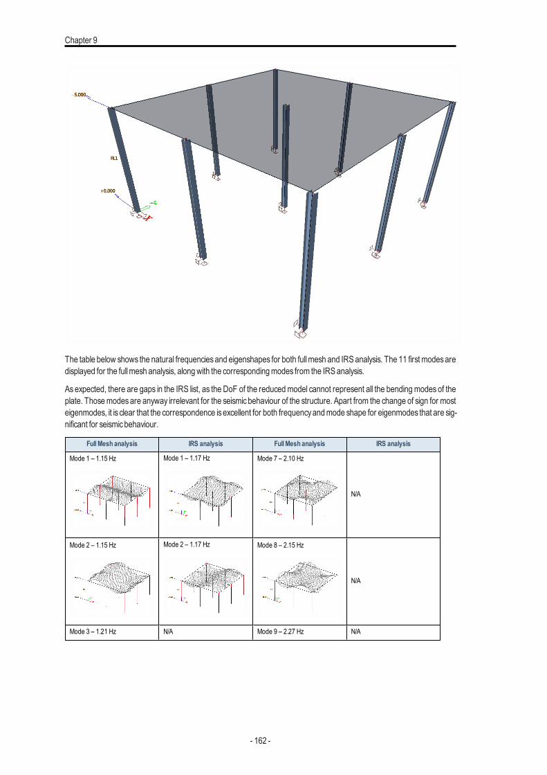
Chapter 9
The table below shows the natural frequenciesand eigenshapes for both fullmesh and IRSanalysis. The 11 first modesaredisplayed for the fullmesh analysis, alongwith the correspondingmodes from the IRSanalysis.
As expected, there are gaps in the IRS list, as the DoF of the reducedmodel cannot represent all the bending modes of theplate. Thosemodesare anyway irrelevant for the seismic behaviour of the structure. Apart from the change of sign for mosteigenmodes, it is clear that the correspondence isexcellent for both frequencyandmode shape for eigenmodes that are sig-nificant for seismicbehaviour.
FullMesh analysis IRS analysis Full Mesh analysis IRS analysis
Mode 1 – 1.15 Hz Mode 1 – 1.17 Hz Mode 7 – 2.10 Hz
N/A
Mode 2 – 1.15 Hz Mode 2 – 1.17 Hz Mode 8 – 2.15 Hz
N/A
Mode 3 – 1.21 Hz N/A Mode 9 – 2.27 Hz N/A
- 162 -
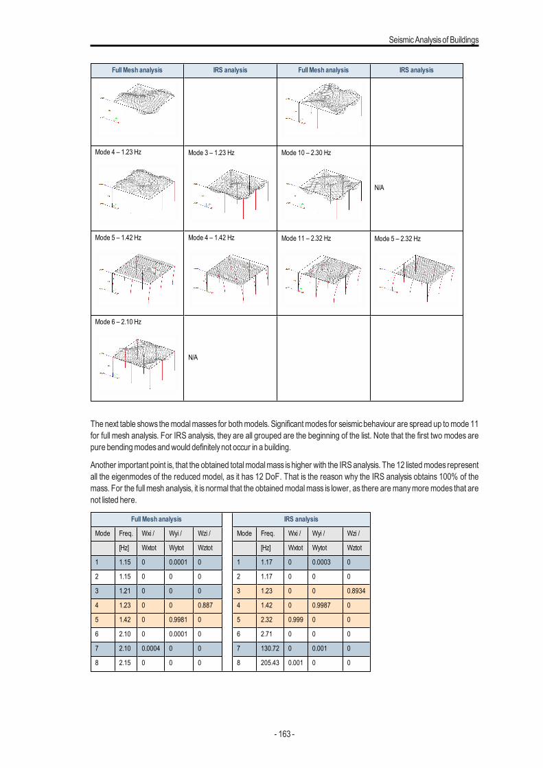
SeismicAnalysisof Buildings
FullMesh analysis IRS analysis Full Mesh analysis IRS analysis
Mode 4 – 1.23 Hz Mode 3 – 1.23 Hz Mode 10 – 2.30 Hz
N/A
Mode 5 – 1.42 Hz Mode 4 – 1.42 Hz Mode 11 – 2.32 Hz Mode 5 – 2.32 Hz
Mode 6 – 2.10 Hz
N/A
The next table shows themodalmasses for bothmodels. Significant modes for seismicbehaviour are spread up tomode 11for full mesh analysis. For IRS analysis, they are all grouped are the beginning of the list. Note that the first two modes arepure bendingmodesandwould definitelynot occur in a building.
Another important point is, that the obtained totalmodalmass ishigher with the IRSanalysis. The 12 listedmodes representall the eigenmodes of the reduced model, as it has 12 DoF. That is the reason why the IRS analysis obtains 100% of themass. For the fullmesh analysis, it is normal that the obtainedmodalmass is lower, as there aremanymoremodes that arenot listed here.
FullMesh analysis IRS analysis
Mode Freq. Wxi / Wyi / Wzi / Mode Freq. Wxi / Wyi / Wzi /
[Hz] Wxtot Wytot Wztot [Hz] Wxtot Wytot Wztot
1 1.15 0 0.0001 0 1 1.17 0 0.0003 0
2 1.15 0 0 0 2 1.17 0 0 0
3 1.21 0 0 0 3 1.23 0 0 0.8934
4 1.23 0 0 0.887 4 1.42 0 0.9987 0
5 1.42 0 0.9981 0 5 2.32 0.999 0 0
6 2.10 0 0.0001 0 6 2.71 0 0 0
7 2.10 0.0004 0 0 7 130.72 0 0.001 0
8 2.15 0 0 0 8 205.43 0.001 0 0
- 163 -
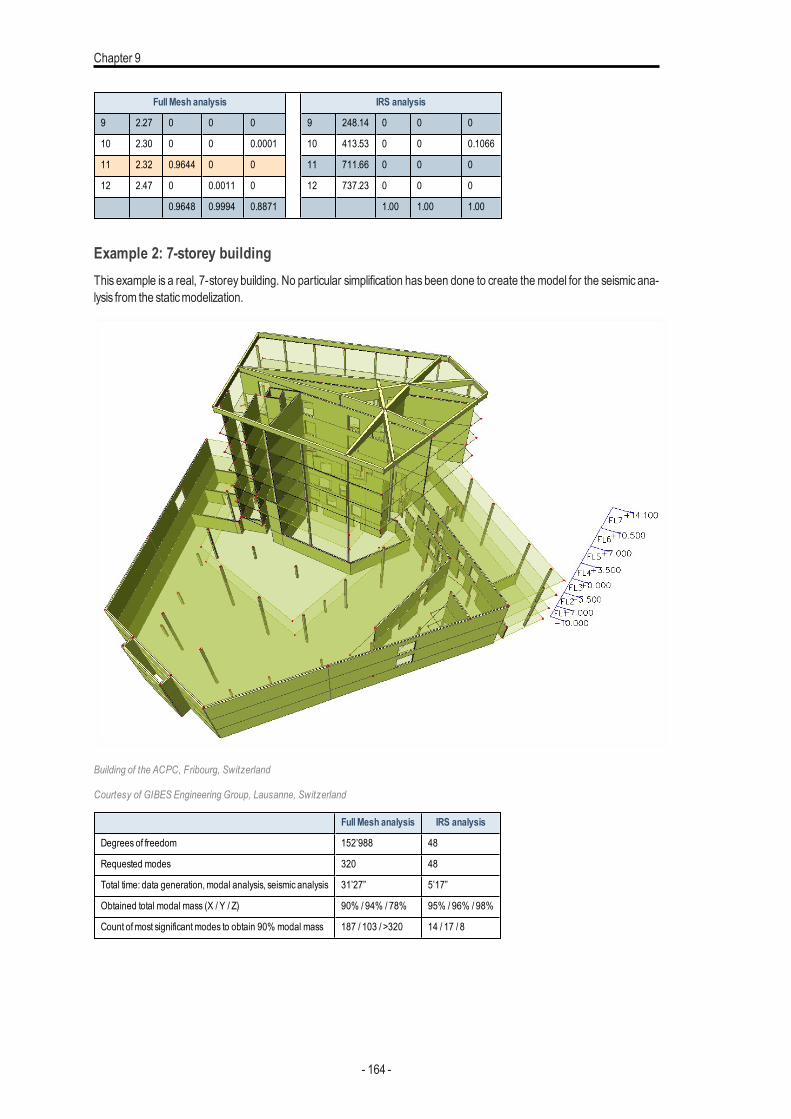
Chapter 9
FullMesh analysis IRS analysis
9 2.27 0 0 0 9 248.14 0 0 0
10 2.30 0 0 0.0001 10 413.53 0 0 0.1066
11 2.32 0.9644 0 0 11 711.66 0 0 0
12 2.47 0 0.0011 0 12 737.23 0 0 0
0.9648 0.9994 0.8871 1.00 1.00 1.00
Example 2: 7-storey buildingThis example is a real, 7-storey building. No particular simplification has been done to create the model for the seismic ana-lysis from the staticmodelization.
Building of the ACPC, Fribourg, Switzerland
Courtesy of GIBES Engineering Group, Lausanne, Switzerland
FullMesh analysis IRS analysis
Degrees of freedom 152’988 48
Requested modes 320 48
Total time: data generation,modal analysis, seismic analysis 31’27” 5’17”
Obtained total modal mass (X / Y / Z) 90% / 94% / 78% 95% / 96% / 98%
Count ofmost significantmodes to obtain 90% modal mass 187 / 103 / >320 14 / 17 / 8
- 164 -
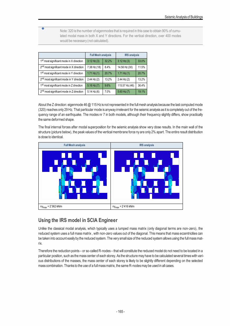
SeismicAnalysisof Buildings
Note: 320 is the number of eigenmodes that is required in this case to obtain 90% of cumu-lated modal mass in both X and Y directions. For the vertical direction, over 400 modeswould be necessary (not calculated).
FullMesh analysis IRS analysis
1stmost significantmode in X direction 3.12 Hz (3) 32.2% 3.12 Hz (3) 33.0%
2ndmost significantmode in X direction 7.38 Hz (18) 8.4% 14.56 Hz (30) 11.5%
1stmost significantmode in Y direction 1.71 Hz (1) 20.7% 1.71 Hz (1) 20.7%
2ndmost significantmode in Y direction 2.44 Hz (2) 13.2% 2.44 Hz (2) 13.2%
1stmost significantmode in Z direction 5.16 Hz (7) 9.6% 115.57 Hz (46) 36.4%
2ndmost significantmode in Z direction 5.14 Hz (6) 7.0% 5.60 Hz (7) 19.1%
About the Z direction: eigenmode 46@115Hz isnot represented in the fullmesh analysisbecause the last computedmode(320) reachesonly 29 Hz. That particular mode is anyway irrelevant for the seismic analysis as it is completely out of the fre-quency range of an earthquake. The modes nr 7 in both models, although their frequency slightly differs, show practicallythe same deformed shape.
The final internal forces after modal superposition for the seismic analysis show very close results. In the main wall of thestructure (picture below), the peakvaluesof the verticalmembrane force nyare only 2% apart. The entire result distributionis close to identical.
FullMesh analysis IRS analysis
nymax = 2’362 kN/m nymax = 2’416 kN/m
Using the IRS model in SCIA EngineerUnlike the classical modal analysis, which typically uses a lumped mass matrix (only diagonal terms are non-zero), thereduced system uses a full massmatrix , with non-zero values out of the diagonal. Thismeans that mass eccentricities canbe taken into account easilyby the reduced system. The verysmall size of the reduced systemallowsusing the fullmassmat-rix.
Therefore the reduction points – or so-called R-nodes– that will constitute the reducedmodel do not need to be located in aparticular position, such as themasscenter of each storey. As the structuremayhave to be calculated several timeswith vari-ous distributions of the masses, the mass center of each storey is likely to be slightly different depending on the selectedmasscombination. Thanks to the use of a fullmassmatrix, the sameR-nodesmaybe used in all cases.
- 165 -
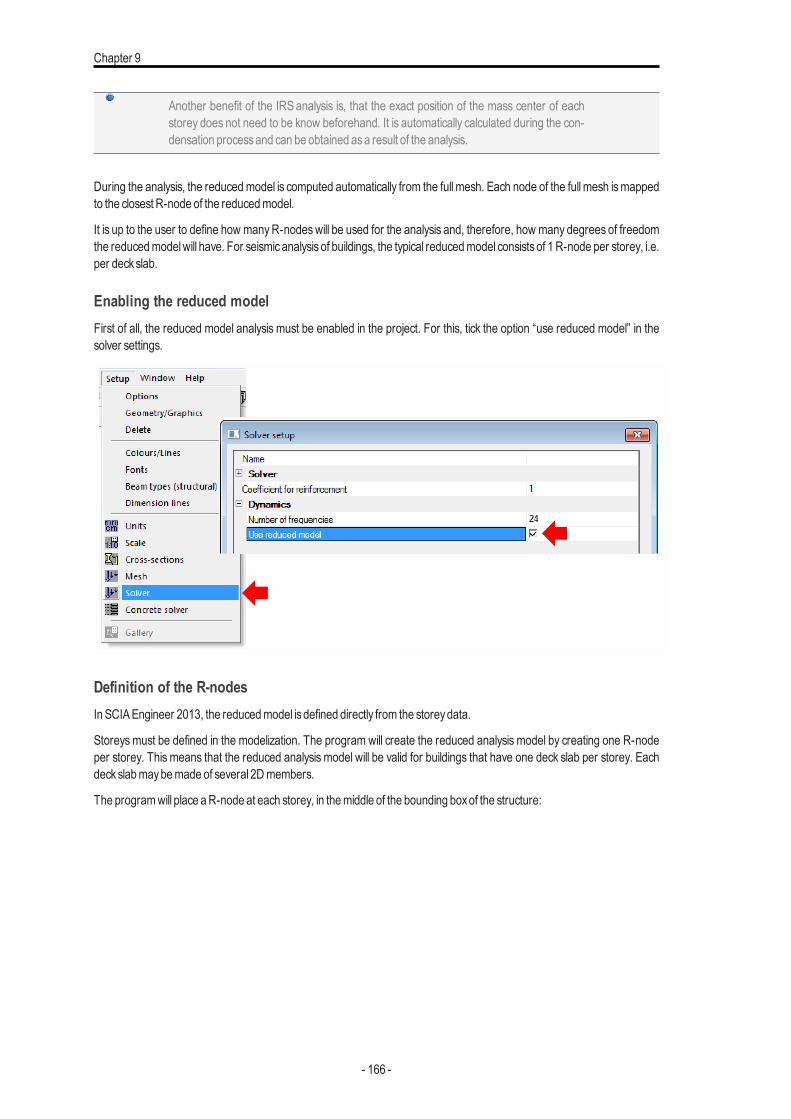
Chapter 9
Another benefit of the IRS analysis is, that the exact position of the mass center of eachstorey does not need to be know beforehand. It is automatically calculated during the con-densation processand can be obtained asa result of the analysis.
During the analysis, the reducedmodel is computed automatically from the full mesh. Each node of the full mesh ismappedto the closest R-node of the reducedmodel.
It is up to the user to define how manyR-nodeswill be used for the analysis and, therefore, how many degrees of freedomthe reducedmodelwill have. For seismicanalysisof buildings, the typical reducedmodel consistsof 1 R-node per storey, i.e.per deckslab.
Enabling the reduced modelFirst of all, the reduced model analysis must be enabled in the project. For this, tick the option “use reduced model” in thesolver settings.
Definition of the R-nodesIn SCIAEngineer 2013, the reducedmodel isdefined directly from the storeydata.
Storeys must be defined in the modelization. The program will create the reduced analysis model by creating one R-nodeper storey. This means that the reduced analysis model will be valid for buildings that have one deck slab per storey. Eachdeckslabmaybemade of several 2Dmembers.
The programwill place aR-node at each storey, in themiddle of the bounding boxof the structure:
- 166 -
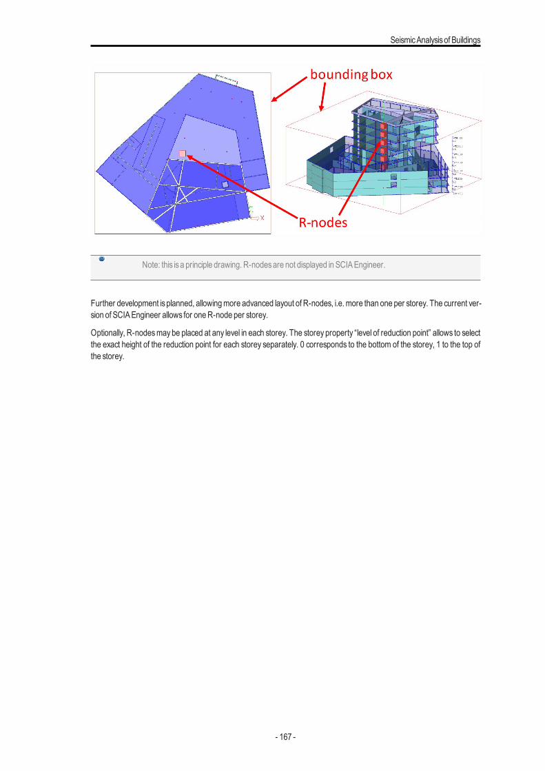
SeismicAnalysisof Buildings
Note: this isa principle drawing. R-nodesare not displayed in SCIAEngineer.
Further development isplanned, allowingmore advanced layout of R-nodes, i.e. more than one per storey. The current ver-sion of SCIAEngineer allows for oneR-node per storey.
Optionally, R-nodesmaybe placed at any level in each storey. The storey property “level of reduction point” allows to selectthe exact height of the reduction point for each storey separately. 0 corresponds to the bottom of the storey, 1 to the top ofthe storey.
- 167 -
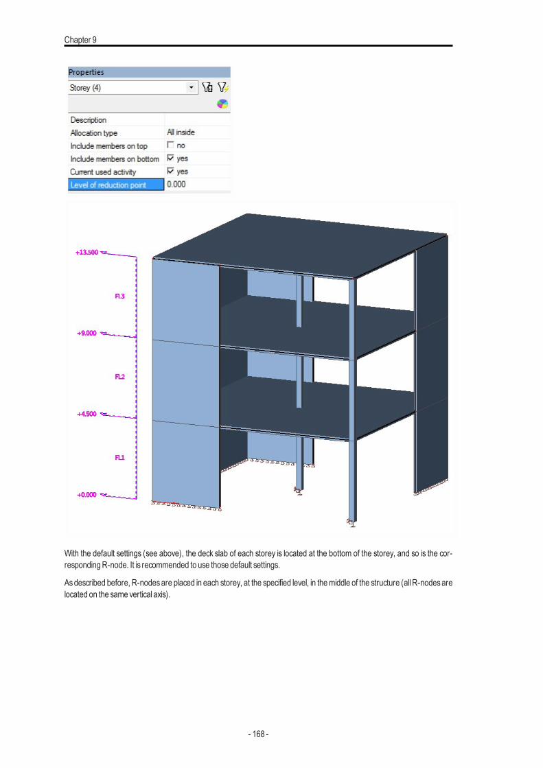
Chapter 9
With the default settings (see above), the deck slab of each storey is located at the bottom of the storey, and so is the cor-respondingR-node. It is recommended to use those default settings.
Asdescribed before, R-nodesare placed in each storey, at the specified level, in themiddle of the structure (all R-nodesarelocated on the same vertical axis).
- 168 -
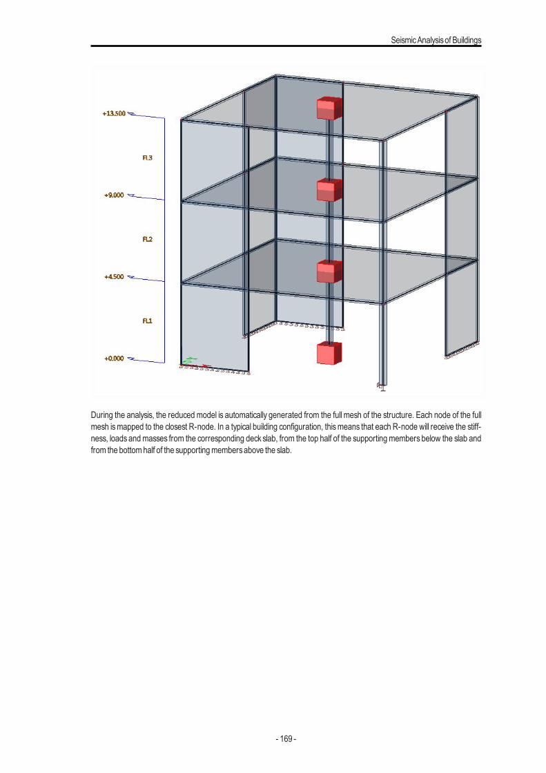
SeismicAnalysisof Buildings
During the analysis, the reduced model is automatically generated from the full mesh of the structure. Each node of the fullmesh ismapped to the closest R-node. In a typical building configuration, thismeans that each R-node will receive the stiff-ness, loads andmasses from the corresponding deck slab, from the top half of the supporting members below the slab andfrom the bottomhalf of the supportingmembersabove the slab.
- 169 -
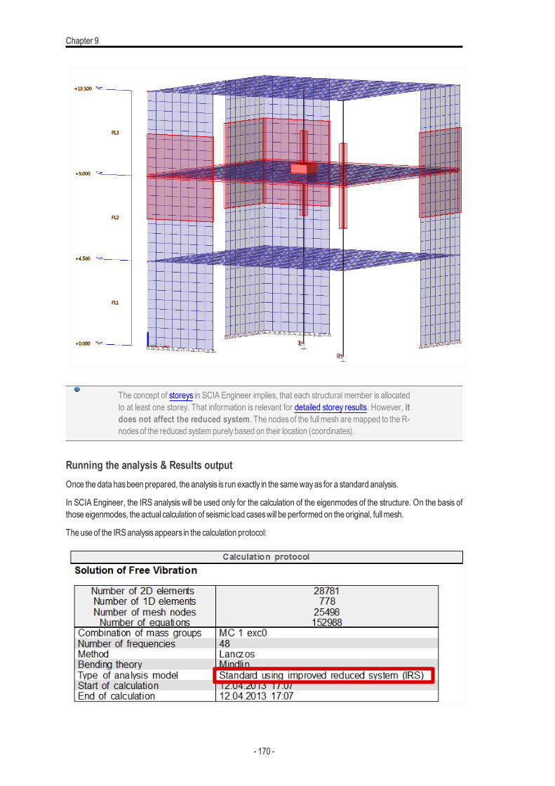
Chapter 9
The concept of storeys in SCIA Engineer implies, that each structural member is allocatedto at least one storey. That information is relevant for detailed storey results. However, itdoes not affect the reduced system. The nodesof the fullmesh aremapped to the R-nodesof the reduced systempurelybased on their location (coordinates).
Running the analysis & Results outputOnce the data hasbeen prepared, the analysis is run exactly in the samewayas for a standard analysis.
In SCIA Engineer, the IRS analysis will be used only for the calculation of the eigenmodes of the structure. On the basis ofthose eigenmodes, the actual calculation of seismic load caseswill be performed on the original, fullmesh.
The use of the IRSanalysisappears in the calculation protocol:
- 170 -

SeismicAnalysisof Buildings
There are fundamentally two typesof resultsavailable after an IRSanalysis:
l The resultsof the reducedmodel are automaticallyexpanded to the originalmesh and are accessible through standardoutput. Thiswill not be detailed here.
l Somededicated results, coming directly from the reducedmodel, are available in the result service SummaryStoreyRes-ults. This typicallygives information about themasses, displacementsand accelerationsat themasscenter each storey inthe reducedmodel.
See information about typical solver error when using IRS with a model that is not properly configured: non-associated R-node.
IRS: Too many eigen values requested / Non-associated R-node detected
IssueWhen running IRS dynamicanalysis, the calculation failswith the error message:
IRSmodal reduction: Detect of nonassociated r-node
or
IRSmodal reduction:More then computed eigen valuesare demand
MeaningDuring the generation of the IRS analysis model, the solver detected one or more degree of freedom of some reductionpoint (R-node) without any mass associated to it. It means that all the nodes of the original finite element mesh that arelinked to that R-node have a zeromassvalue for the component corresponding to that degree of freedom.
SolutionThiscan happen in several cases. The solution dependson the root cause.
- 171 -
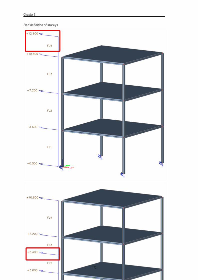
Chapter 9
Bad definition of storeys
- 172 -
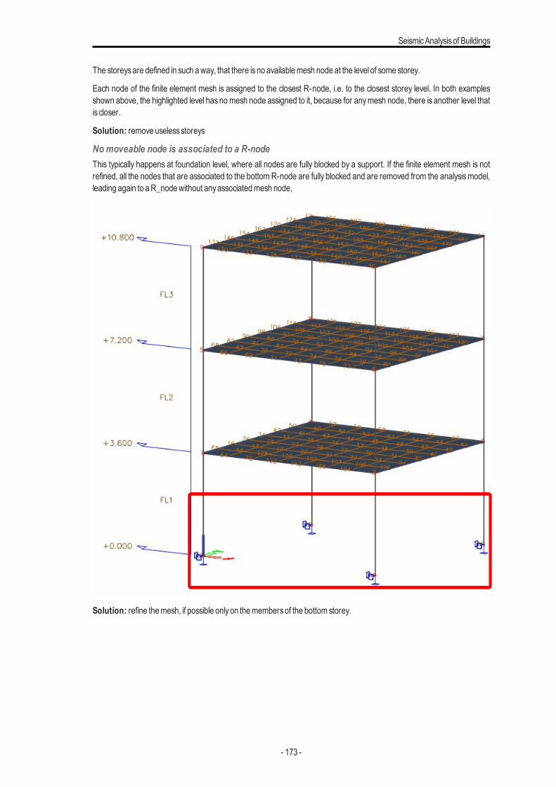
SeismicAnalysisof Buildings
The storeysare defined in such away, that there isno availablemesh node at the level of some storey.
Each node of the finite element mesh is assigned to the closest R-node, i.e. to the closest storey level. In both examplesshown above, the highlighted level has nomesh node assigned to it, because for anymesh node, there is another level thatis closer.
Solution: remove uselessstoreys
Nomoveable node is associated to a R-nodeThis typically happens at foundation level, where all nodes are fully blocked by a support. If the finite element mesh is notrefined, all the nodes that are associated to the bottom R-node are fully blocked and are removed from the analysismodel,leading again to aR_nodewithout anyassociatedmesh node,
Solution: refine themesh, if possible onlyon themembersof the bottom storey.
- 173 -
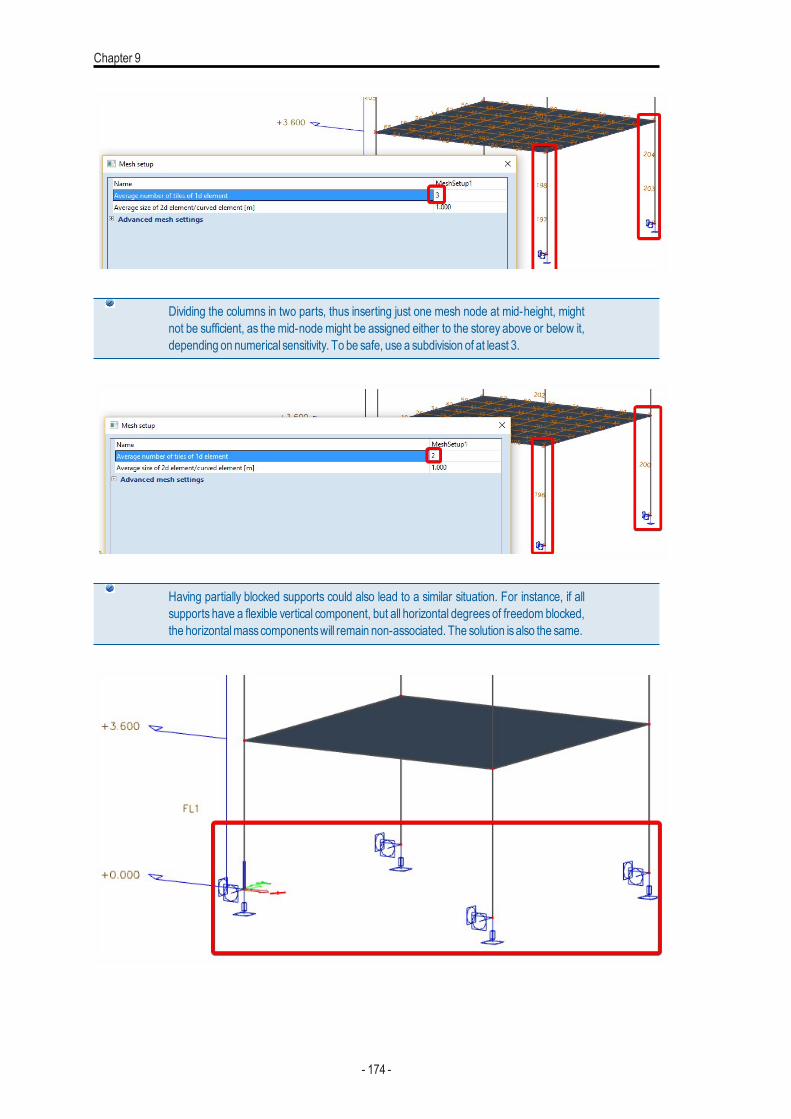
Chapter 9
Dividing the columns in two parts, thus inserting just one mesh node at mid-height, mightnot be sufficient, as the mid-node might be assigned either to the storey above or below it,depending on numerical sensitivity. To be safe, use a subdivision of at least 3.
Having partially blocked supports could also lead to a similar situation. For instance, if allsupports have a flexible vertical component, but all horizontal degrees of freedom blocked,the horizontalmasscomponentswill remain non-associated. The solution isalso the same.
- 174 -
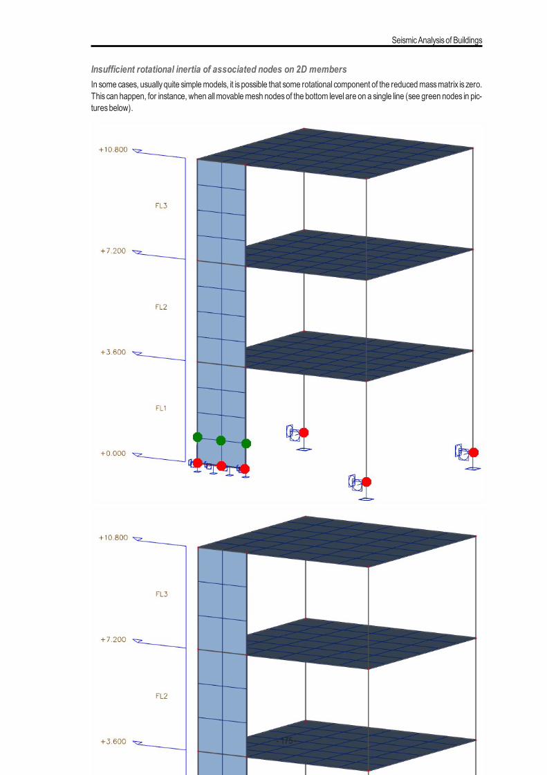
SeismicAnalysisof Buildings
Insufficient rotational inertia of associated nodes on 2D membersIn some cases, usually quite simplemodels, it is possible that some rotational component of the reducedmassmatrix is zero.This can happen, for instance, when allmovablemesh nodesof the bottom level are on a single line (see green nodes in pic-turesbelow).
- 175 -
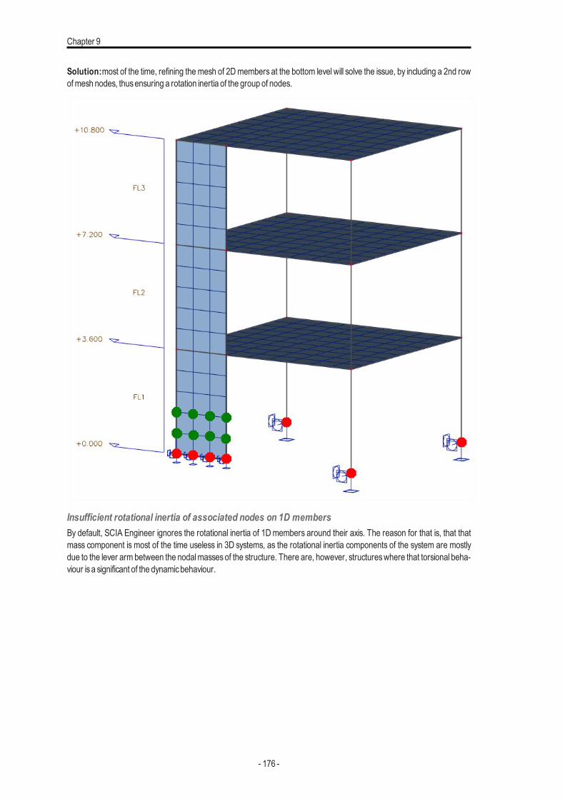
Chapter 9
Solution:most of the time, refining the mesh of 2D members at the bottom level will solve the issue, by including a 2nd rowofmesh nodes, thusensuring a rotation inertia of the group of nodes.
Insufficient rotational inertia of associated nodes on 1D membersBy default, SCIA Engineer ignores the rotational inertia of 1D members around their axis. The reason for that is, that thatmass component is most of the time useless in 3D systems, as the rotational inertia components of the system are mostlydue to the lever arm between the nodalmassesof the structure. There are, however, structureswhere that torsional beha-viour isa significant of the dynamicbehaviour.
- 176 -
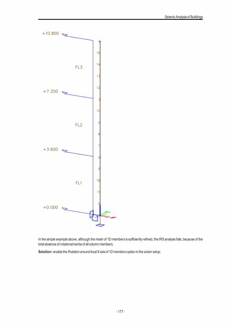
SeismicAnalysisof Buildings
In the simple example above, although themesh of 1D members is sufficiently refined, the IRS analysis fails, because of thetotal absence of rotational inertia of all columnmembers.
Solution: enable theRotation around localX axisof 1D membersoption in the solver setup.
- 177 -
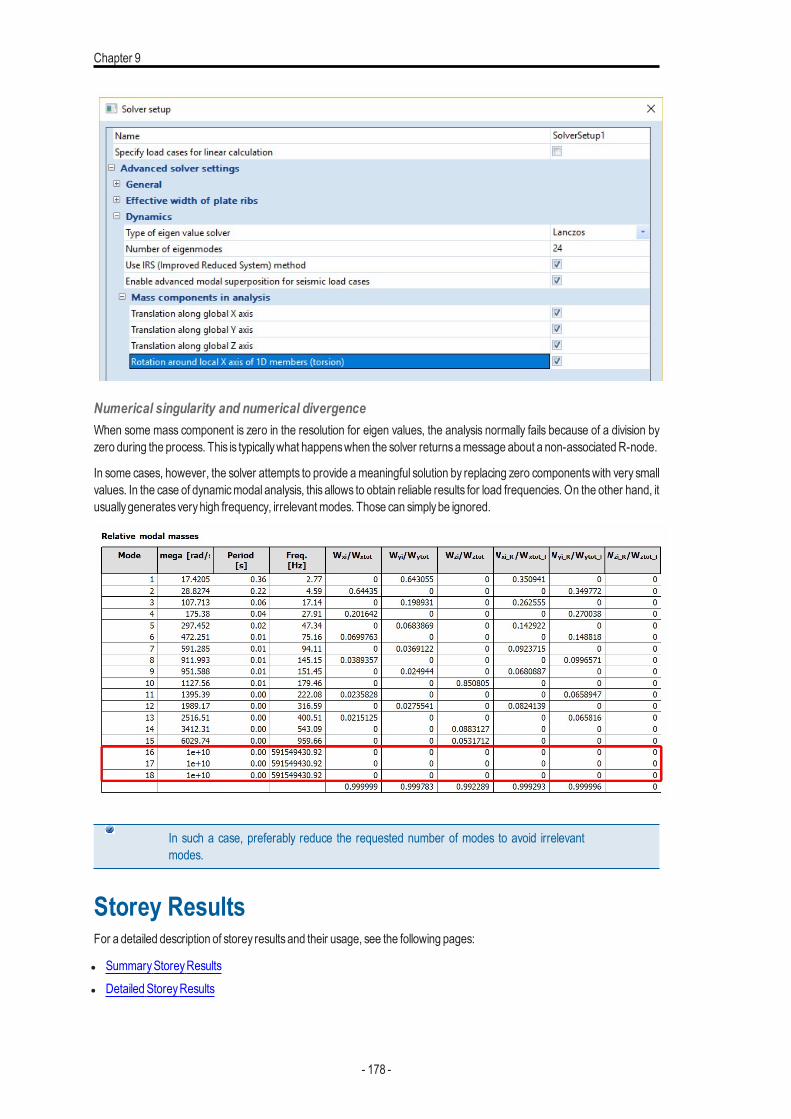
Chapter 9
Numerical singularity and numerical divergenceWhen some mass component is zero in the resolution for eigen values, the analysis normally fails because of a division byzero during the process. This is typicallywhat happenswhen the solver returnsamessage about a non-associatedR-node.
In some cases, however, the solver attempts to provide ameaningful solution by replacing zero componentswith very smallvalues. In the case of dynamicmodal analysis, this allows to obtain reliable results for load frequencies. On the other hand, itusuallygeneratesveryhigh frequency, irrelevantmodes. Those can simplybe ignored.
In such a case, preferably reduce the requested number of modes to avoid irrelevantmodes.
Storey ResultsFor a detailed description of storey resultsand their usage, see the following pages:
l SummaryStoreyResultsl Detailed StoreyResults
- 178 -
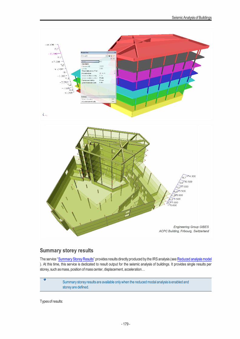
SeismicAnalysisof Buildings
Summary storey resultsThe service “SummaryStoreyResults” provides results directly produced by the IRSanalysis (see Reduced analysismodel). At this time, this service is dedicated to result output for the seismic analysis of buildings. It provides single results perstorey, such asmass, position ofmasscenter, displacement, acceleration…
Summarystorey resultsare available onlywhen the reducedmodal analysis isenabled andstoreyare defined.
Typesof results:
- 179 -
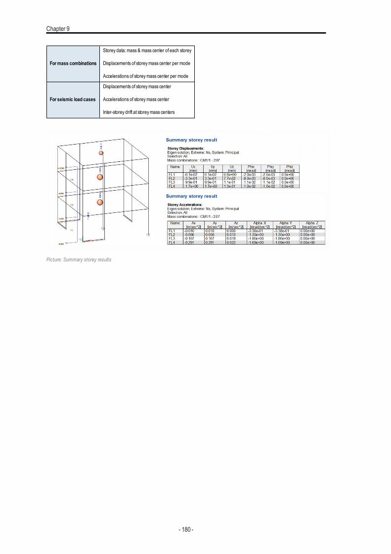
Chapter 9
Formass combinations
Storey data:mass & mass center of each storey
Displacements of storeymass center per mode
Accelerations of storeymass center per mode
For seismic load cases
Displacements of storeymass center
Accelerations of storeymass center
Inter-storey drift at storeymass centers
Picture: Summary storey results
- 180 -
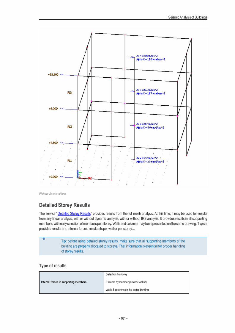
SeismicAnalysisof Buildings
Picture: Accelerations
Detailed Storey ResultsThe service “Detailed Storey Results” provides results from the full mesh analysis. At this time, it may be used for resultsfrom any linear analysis, with or without dynamic analysis, with or without IRS analysis. It provides results in all supportingmembers, with easyselection ofmembersper storey.Wallsand columnsmaybe represented on the samedrawing. Typicalprovided resultsare: internal forces, resultantsper wall or per storey…
Tip: before using detailed storey results, make sure that all supporting members of thebuilding are properly allocated to storeys. That information is essential for proper handlingof storey results.
Type of results
Internal forces in supportingmembers
Selection by storey
Extreme bymember (also for walls !)
Walls & columns on the same drawing
- 181 -
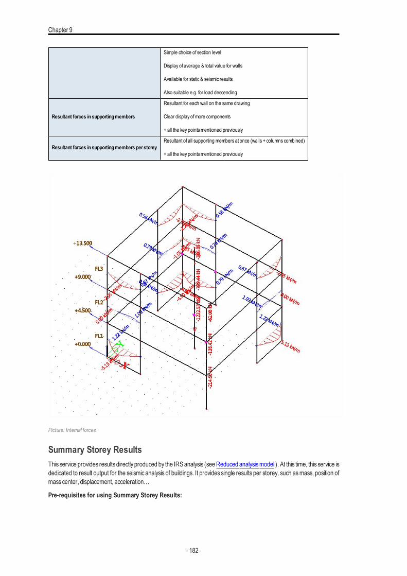
Chapter 9
Simple choice of section level
Display of average & total value for walls
Available for static & seismic results
Also suitable e.g. for load descending
Resultant forces in supportingmembers
Resultant for each wall on the same drawing
Clear display ofmore components
+ all the key pointsmentioned previously
Resultant forces in supportingmembers per storeyResultant of all supporting members at once (walls + columns combined)
+ all the key pointsmentioned previously
Picture: Internal forces
Summary Storey ResultsThis service provides results directly produced by the IRSanalysis (seeReduced analysismodel ). At this time, this service isdedicated to result output for the seismic analysis of buildings. It provides single results per storey, such asmass, position ofmasscenter, displacement, acceleration…
Pre-requisites for using Summary Storey Results:
- 182 -

SeismicAnalysisof Buildings
l storeys must be definedl the reduced analysis model must be enabled in the solver settings
The service may be found in the Results service. It is available only after a successful dynamic analysis using the reducedmodel.
Output SettingsThe output settings are presented here according to the various types of results that can be obtained from this service.There are 4 typesof results:
l StoreyData: information of the reduced analysismodel, such as themassand the position of themasscenter of eachstorey
l Displacements: displacementsat themasscenter of each storeyl Accelerations: accelerationsat themasscenter of each storeyl Inter-storeydrift: relative displacementsat themasscenter of each storey, relative to the storey immediatelybelow
Result type Storey DataFor masscombinations, it displays for each storey the totalmassand the coordinatesof themasscenter.
For ELF seismic load cases, it displayssummary information about computed storey forces.
Type of loadsselection of the type of loadMass combinationsselection of the combination ofmassgroupsor eigenmode for a given combination ofmassgroups.Selectiontype of selection; the possible choicesare
l All storeysl Named selectionl Single storey
- 183 -

Chapter 9
Named selectionnamed selection that containsa set of storeys; only if Selection =Named selectionStoreydropdownmenu for selection of a single one; only if Selection =Single storeyDraw valuestick to draw valueson the drawingDraw unitstick to draw valueswith their unitson the drawingResult typetypesof results; possible choicesare
l Displacementsl Inter-storeydriftl Accelerationsl StoreyData
Valuesmain component to be displayed; onlywhen anELF seismic load case isselectedFx, Fy, Fz : componentsof the seismicstorey forcesFtot : resultant seismic force per storeyM : massof each storeyAdditional valuesallow to showmore than one result component simultaneouslyon the drawing.
- 184 -
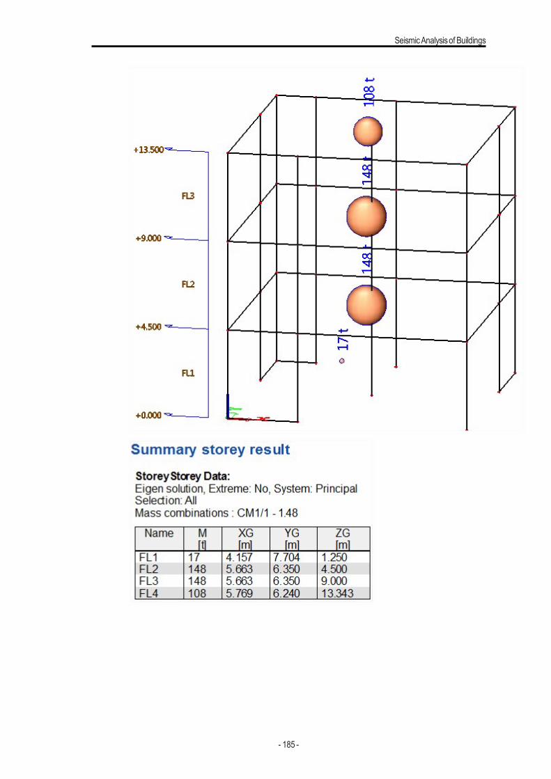
SeismicAnalysisof Buildings
- 185 -
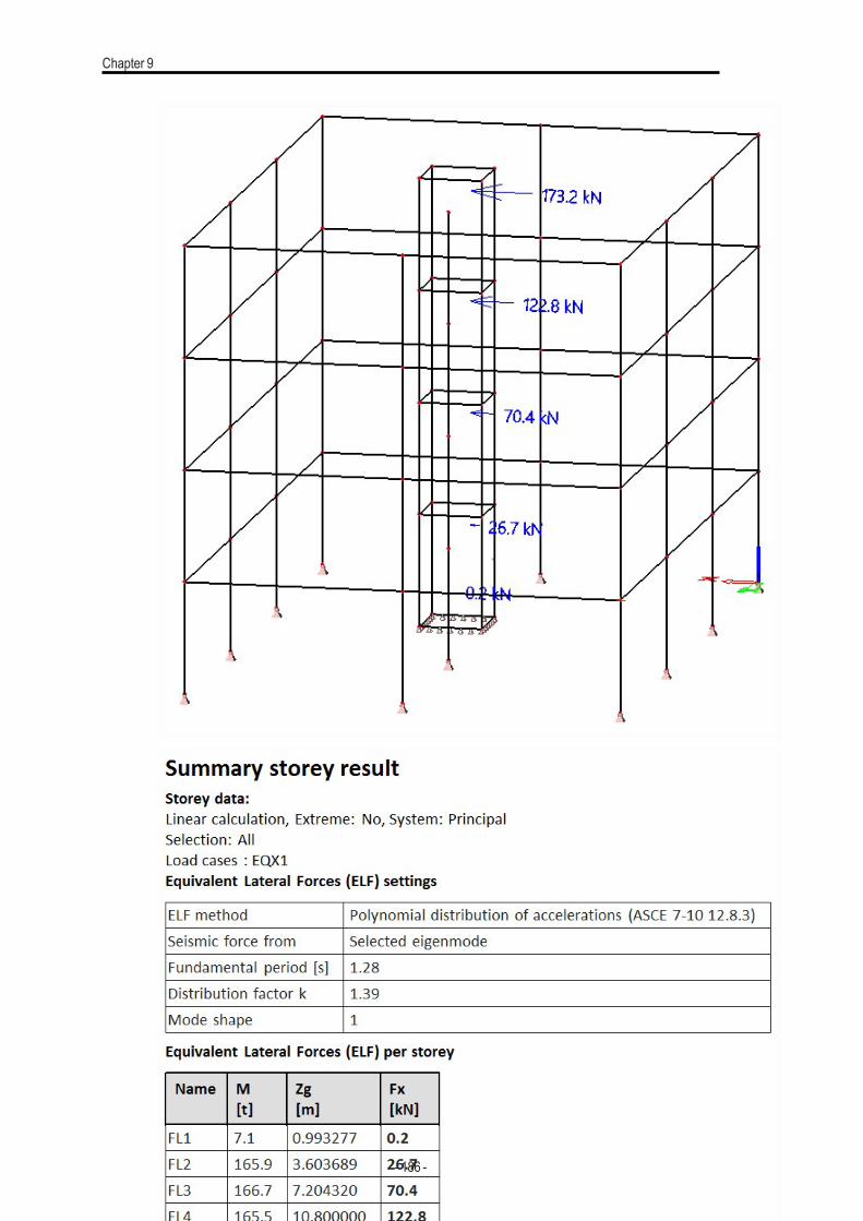
Chapter 9
- 186 -
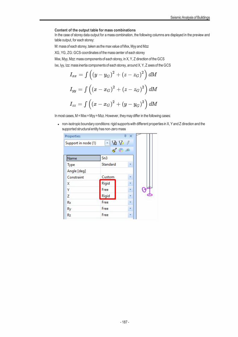
SeismicAnalysisof Buildings
Content of the output table for mass combinationsIn the case of storey data output for a mass combination, the following columns are displayed in the preview andtable output, for each storey:M: massof each storey, taken as themaxvalue ofMxx,MyyandMzzXG, YG, ZG: GCS-coordinatesof themasscenter of each storeyMxx,Myy,Mzz: masscomponentsof each storey, in X, Y, Z direction of theGCSIxx, Iyy, Izz: mass inertia componentsof each storey, aroundX, Y, Z axesof theGCS
Inmost cases,M= Mxx= Myy=Mzz. However, theymaydiffer in the following cases:
l non-isotropicboundaryconditions: rigid supportswith different properties in X, Y and Z direction and thesupported structural entityhasnon-zeromass
- 187 -
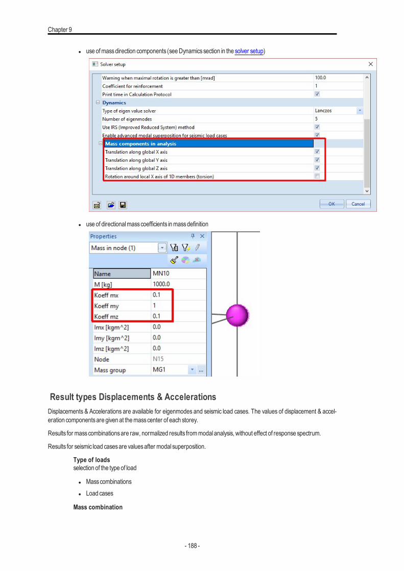
Chapter 9
l use ofmassdirection components (seeDynamicssection in the solver setup)
l use of directionalmasscoefficients inmassdefinition
Result types Displacements & AccelerationsDisplacements & Accelerations are available for eigenmodes and seismic load cases. The values of displacement & accel-eration componentsare given at themasscenter of each storey.
Results for masscombinationsare raw, normalized results frommodal analysis, without effect of response spectrum.
Results for seismic load casesare valuesafter modal superposition.
Type of loadsselection of the type of load
l Masscombinationsl Load cases
Mass combination
- 188 -
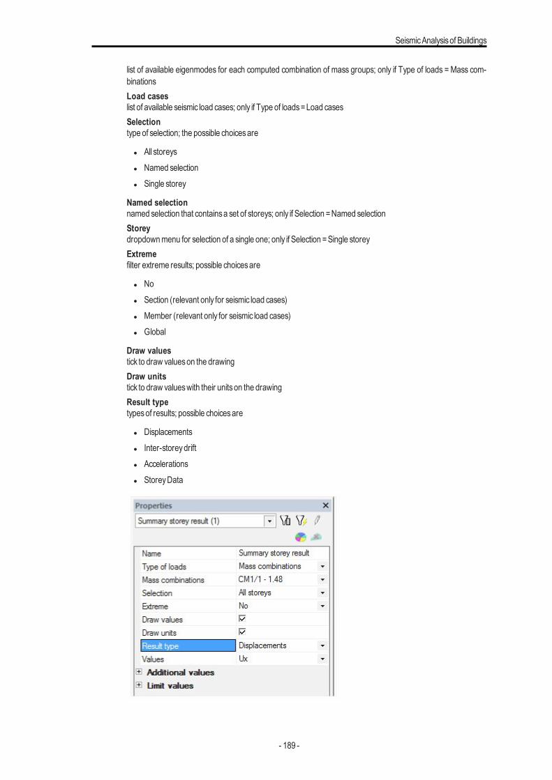
SeismicAnalysisof Buildings
list of available eigenmodes for each computed combination of mass groups; only if Type of loads = Mass com-binationsLoad caseslist of available seismic load cases; only if Type of loads=Load casesSelectiontype of selection; the possible choicesare
l All storeysl Named selectionl Single storey
Named selectionnamed selection that containsa set of storeys; only if Selection =Named selectionStoreydropdownmenu for selection of a single one; only if Selection =Single storeyExtremefilter extreme results; possible choicesare
l Nol Section (relevant only for seismic load cases)l Member (relevant only for seismic load cases)l Global
Draw valuestick to draw valueson the drawingDraw unitstick to draw valueswith their unitson the drawingResult typetypesof results; possible choicesare
l Displacementsl Inter-storeydriftl Accelerationsl StoreyData
- 189 -
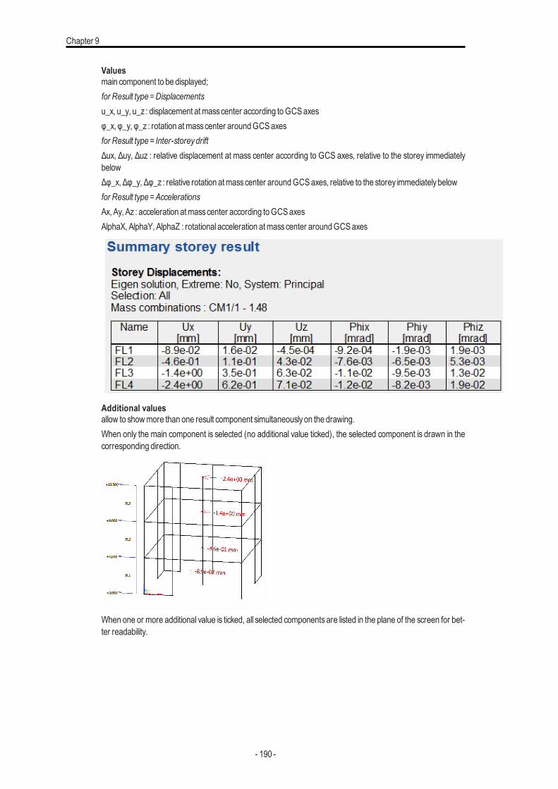
Chapter 9
Valuesmain component to be displayed;for Result type =Displacementsu_x, u_y, u_z : displacement atmasscenter according toGCSaxesφ_x, φ_y, φ_z : rotation atmasscenter aroundGCSaxesfor Result type = Inter-storeydriftΔux, Δuy, Δuz : relative displacement at mass center according to GCS axes, relative to the storey immediatelybelowΔφ_x, Δφ_y, Δφ_z : relative rotation atmasscenter aroundGCSaxes, relative to the storey immediatelybelowfor Result type =AccelerationsAx, Ay, Az : acceleration atmasscenter according toGCSaxesAlphaX, AlphaY, AlphaZ : rotational acceleration atmasscenter aroundGCSaxes
Additional valuesallow to showmore than one result component simultaneouslyon the drawing.When only the main component is selected (no additional value ticked), the selected component is drawn in thecorresponding direction.
When one or more additional value is ticked, all selected components are listed in the plane of the screen for bet-ter readability.
- 190 -
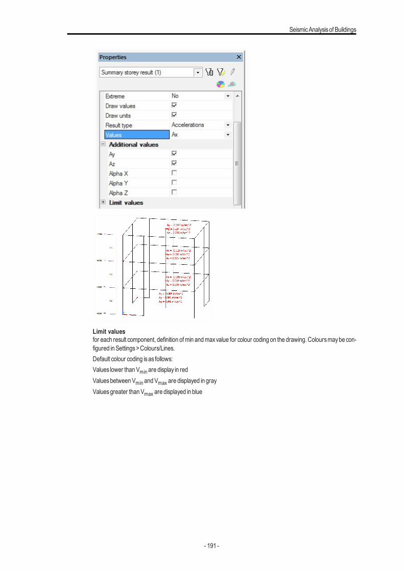
SeismicAnalysisof Buildings
Limit valuesfor each result component, definition ofmin andmaxvalue for colour coding on the drawing. Coloursmaybe con-figured in Settings>Colours/Lines.Default colour coding isas follows:Values lower thanVmin are display in redValuesbetweenVmin andVmax are displayed in grayValuesgreater thanVmax are displayed in blue
- 191 -
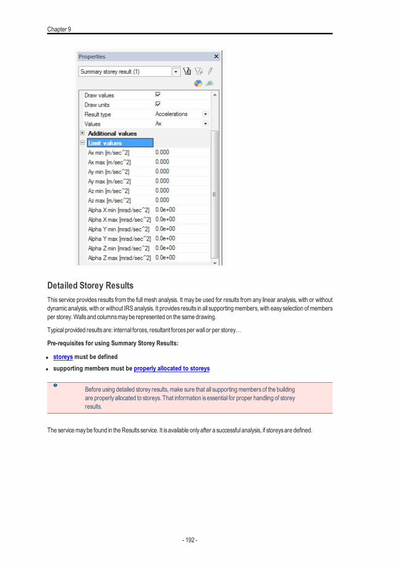
Chapter 9
Detailed Storey ResultsThis service provides results from the full mesh analysis. It may be used for results from any linear analysis, with or withoutdynamicanalysis, with or without IRSanalysis. It provides results in all supportingmembers, with easyselection of membersper storey.Wallsand columnsmaybe represented on the samedrawing.
Typical provided resultsare: internal forces, resultant forcesper wall or per storey…
Pre-requisites for using Summary Storey Results:
l storeys must be definedl supporting members must be properly allocated to storeys
Before using detailed storey results, make sure that all supporting members of the buildingare properly allocated to storeys. That information is essential for proper handling of storeyresults.
The servicemaybe found in theResults service. It isavailable onlyafter a successful analysis, if storeysare defined.
- 192 -

SeismicAnalysisof Buildings
Output SettingsMainly2 typesof resultsare available in this service:
l Internal forces in supportingmembersl Resulting forces
For resulting forces, theMember groupingmaybe selected:
l per member: compute the resulting forces for each supportingmember separatelyl per storey: compute the resulting forces for each entire storeyat once, combining 1D and 2Dmembers
- 193 -
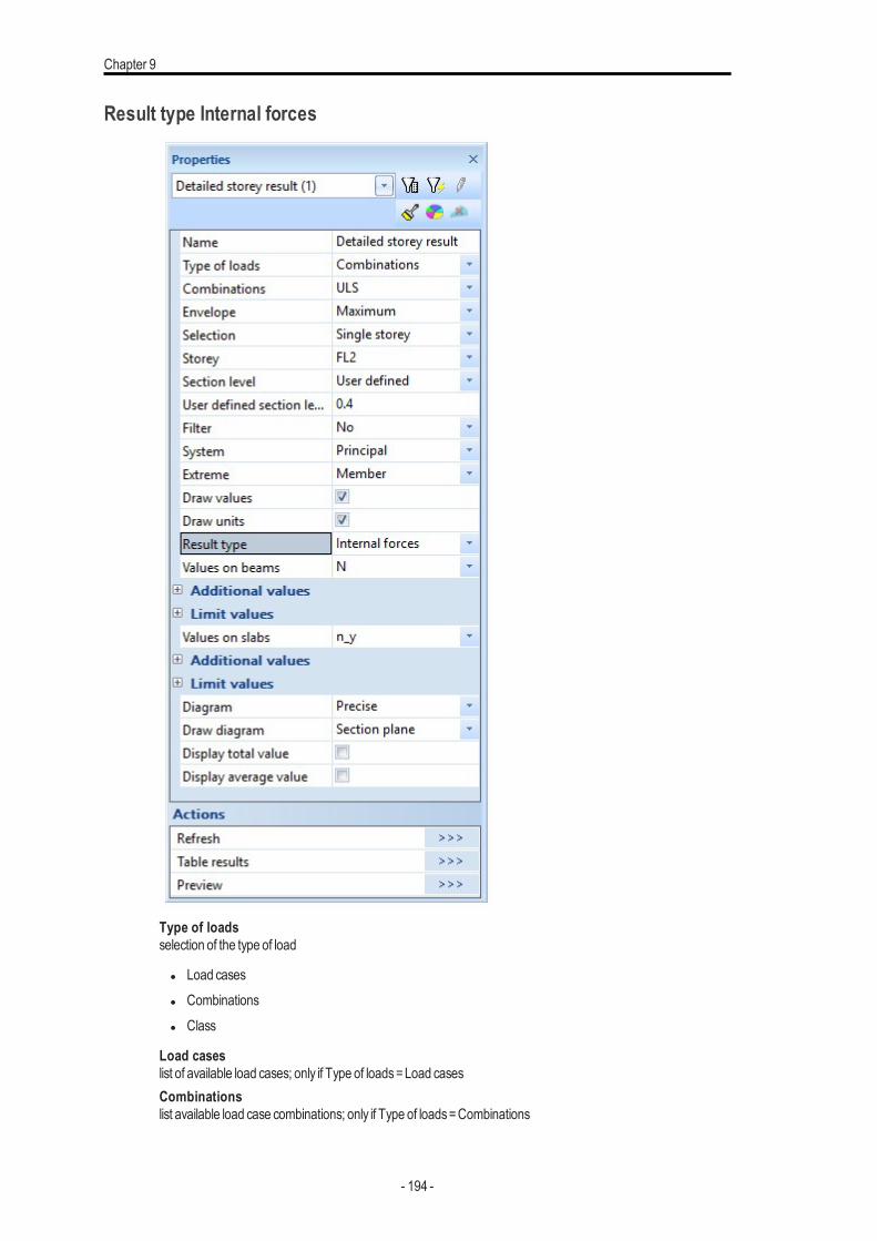
Chapter 9
Result type Internal forces
Type of loadsselection of the type of load
l Load casesl Combinationsl Class
Load caseslist of available load cases; only if Type of loads=Load casesCombinationslist available load case combinations; only if Type of loads=Combinations
- 194 -

SeismicAnalysisof Buildings
Classlist of available result classes; only if Type of loads=ClassEnvelopeMaximum /Minimum; select themaximumor minimumvalue of an envelope; only if Type of loads=Combinationsor ClassSelectiontype of selection; the possible choicesare
l All storeysl Named selectionl Single storey
Named selectionnamed selection that containsa set of storeys; only if Selection =Named selectionStoreydropdownmenu for selection of a single storey; only if Selection =Single storeySection levellevelwhere the sectionmust bemade across the supportingmembers in each storey; possible choices:
l Top (section at the top of each storey)l Middle (section atmid-height of the each storey)l Bottom (section at the bottomof each storey)l User defined
- 195 -
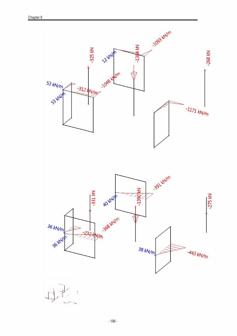
Chapter 9
- 196 -

SeismicAnalysisof Buildings
User defined section levellevel of section in each storey; 0 =bottomof the storey, 1 = top of the storeyFilterfiltering of supportingmembers for the output; possible choicesare
l Nol Wildcardl Materiall Thickness / CSSl Layer
Wildcardwildcard for name filtering ofmembers; only if Filter =WildcardMateriallist of availablematerials for material filtering ofmembers; only if Filter =MaterialThicknessvalue of thickness for thickness filtering ofmembers; only if Filter =Thickness/CSS; 0 =all thicknessvaluesCSSlist of available cross-sections for filtering ofmembers; only if Filter =Thickness/CSSLayerlist of available layers for filtering ofmembers; only if Filter =LayerSystemselection of coordinate system for output of internal forces in 1Dmembers; possible choicesare
l principal (principal axesof the cross-section)l LCS (LCSof the 1Dmember)
for 2Dmembers, the LCS isalwaysusedExtremefilter extreme results; possible choicesare
l Nol Sectionl Memberl Global
Draw valuestick to draw valueson the drawingDraw unitstick to draw valueswith their unitson the drawing
- 197 -
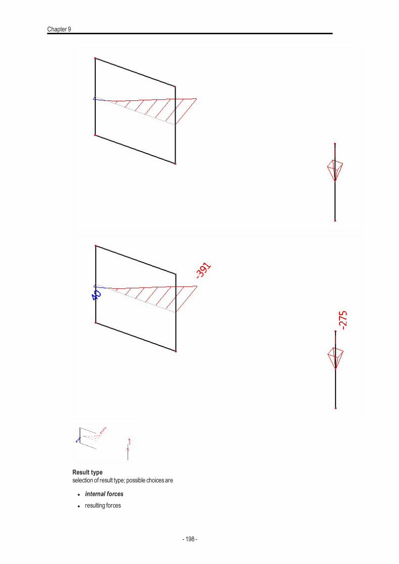
Chapter 9
Result typeselection of result type; possible choicesare
l internal forcesl resulting forces
- 198 -
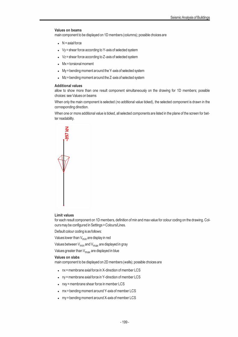
SeismicAnalysisof Buildings
Values on beamsmain component to be displayed on 1Dmembers (columns); possible choicesare
l N=axial forcel Vy=shear force according to Y-axisof selected systeml Vz=shear force according to Z-axisof selected systeml Mx= torsionalmomentl My=bendingmoment around theY-axisof selected systeml Mz=bendingmoment around the Z-axisof selected system
Additional valuesallow to show more than one result component simultaneously on the drawing for 1D members; possiblechoices: seeValueson beamsWhen only the main component is selected (no additional value ticked), the selected component is drawn in thecorresponding direction.When one or more additional value is ticked, all selected components are listed in the plane of the screen for bet-ter readability.
Limit valuesfor each result component on 1Dmembers, definition ofmin andmaxvalue for colour coding on the drawing. Col-oursmaybe configured in Settings>Colours/Lines.Default colour coding isas follows:Values lower thanVmin are display in redValuesbetweenVmin andVmax are displayed in grayValuesgreater thanVmax are displayed in blueValues on slabsmain component to be displayed on 2Dmembers (walls); possible choicesare
l nx=membrane axial force in X-direction ofmember LCSl ny=membrane axial force in Y-direction ofmember LCSl nxy=membrane shear force inmember LCSl mx=bendingmoment aroundY-axisofmember LCSl my=bendingmoment aroundX-axisofmember LCS
- 199 -

Chapter 9
l mxy= torsionalmoment according tomember LCSl vx=shear force according to X-axisofmember LCSl vy=shear force according to Y-axisofmember LCS
Additional valuesallow to show more than one result component simultaneously on the drawing for 2D members; possiblechoices: seeValueson slabsLimit valuesfor each result component on 2Dmembers, definition ofmin andmaxvalue for colour coding on the drawing; seedetailed description aboveDiagramstyle of diagram for internal forces in 2Dmembers; possible choicesare
l Precise: raw computed results, without alterationl Trapezoidal: trapezoidal regression of diagram, for each 2Dmember separatelyl None: the diagram ishidden
- 200 -
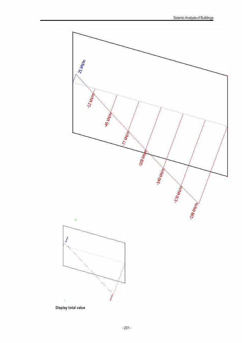
SeismicAnalysisof Buildings
Display total value
- 201 -
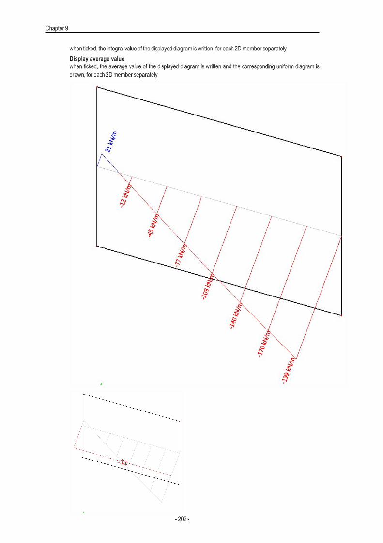
Chapter 9
when ticked, the integral value of the displayed diagram iswritten, for each 2Dmember separatelyDisplay average valuewhen ticked, the average value of the displayed diagram is written and the corresponding uniform diagram isdrawn, for each 2Dmember separately
- 202 -
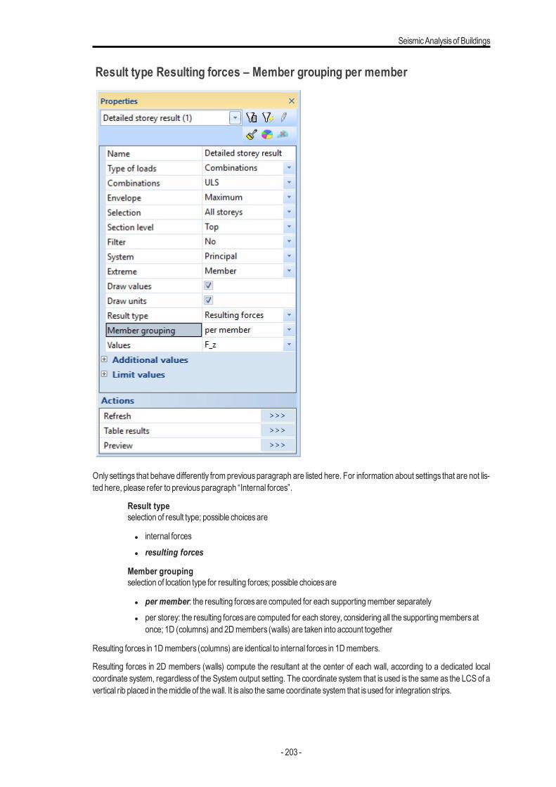
SeismicAnalysisof Buildings
Result type Resulting forces – Member grouping per member
Only settings that behave differently from previousparagraph are listed here. For information about settings that are not lis-ted here, please refer to previousparagraph “Internal forces”.
Result typeselection of result type; possible choicesare
l internal forcesl resulting forces
Member groupingselection of location type for resulting forces; possible choicesare
l per member: the resulting forcesare computed for each supportingmember separatelyl per storey: the resulting forcesare computed for each storey, considering all the supportingmembersat
once; 1D (columns) and 2Dmembers (walls) are taken into account together
Resulting forces in 1Dmembers (columns) are identical to internal forces in 1Dmembers.
Resulting forces in 2D members (walls) compute the resultant at the center of each wall, according to a dedicated localcoordinate system, regardless of the System output setting. The coordinate system that is used is the same as the LCS of avertical rib placed in themiddle of thewall. It is also the same coordinate system that isused for integration strips.
- 203 -
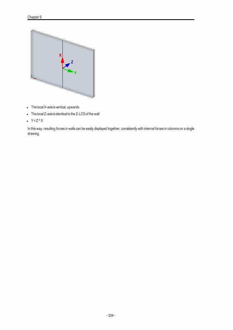
Chapter 9
l The localX-axis is vertical, upwardsl The localZ-axis is identical to the Z-LCSof thewalll Y=Z ^X
In this way, resulting forces in walls can be easily displayed together, consistently with internal forces in columns on a singledrawing.
- 204 -
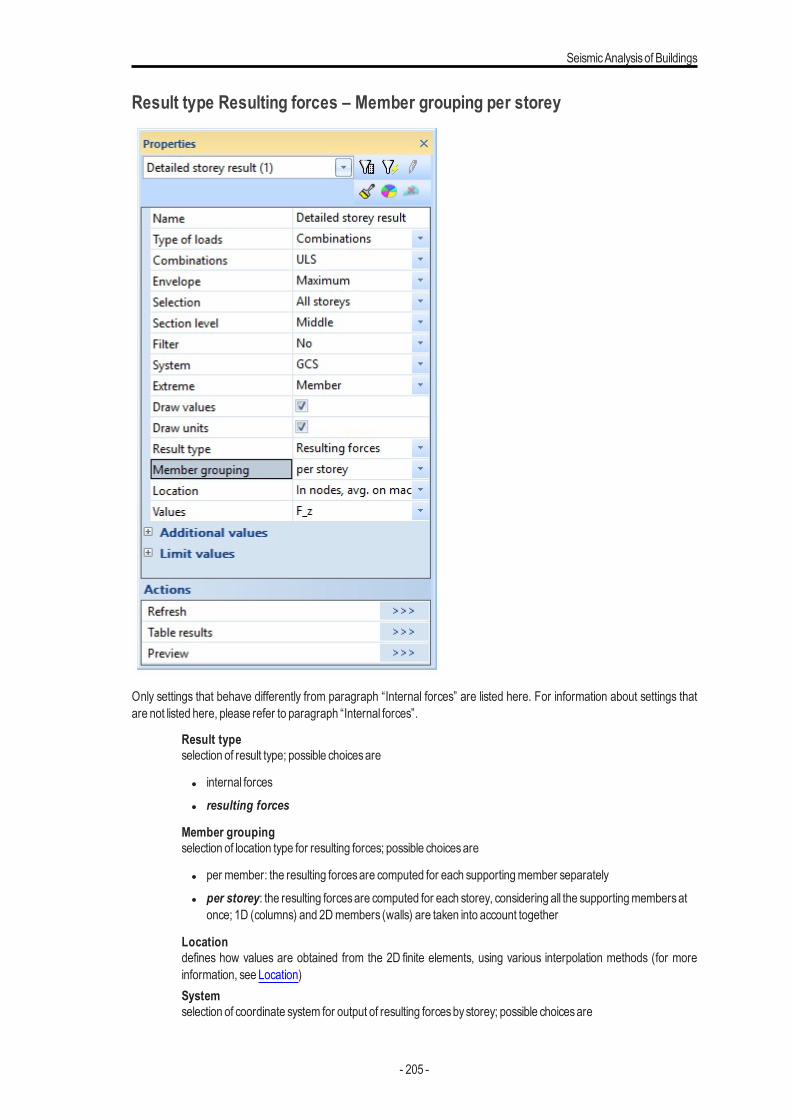
SeismicAnalysisof Buildings
Result type Resulting forces – Member grouping per storey
Only settings that behave differently from paragraph “Internal forces” are listed here. For information about settings thatare not listed here, please refer to paragraph “Internal forces”.
Result typeselection of result type; possible choicesare
l internal forcesl resulting forces
Member groupingselection of location type for resulting forces; possible choicesare
l per member: the resulting forcesare computed for each supportingmember separatelyl per storey: the resulting forcesare computed for each storey, considering all the supportingmembersat
once; 1D (columns) and 2Dmembers (walls) are taken into account together
Locationdefines how values are obtained from the 2D finite elements, using various interpolation methods (for moreinformation, see Location)Systemselection of coordinate system for output of resulting forcesbystorey; possible choicesare
- 205 -
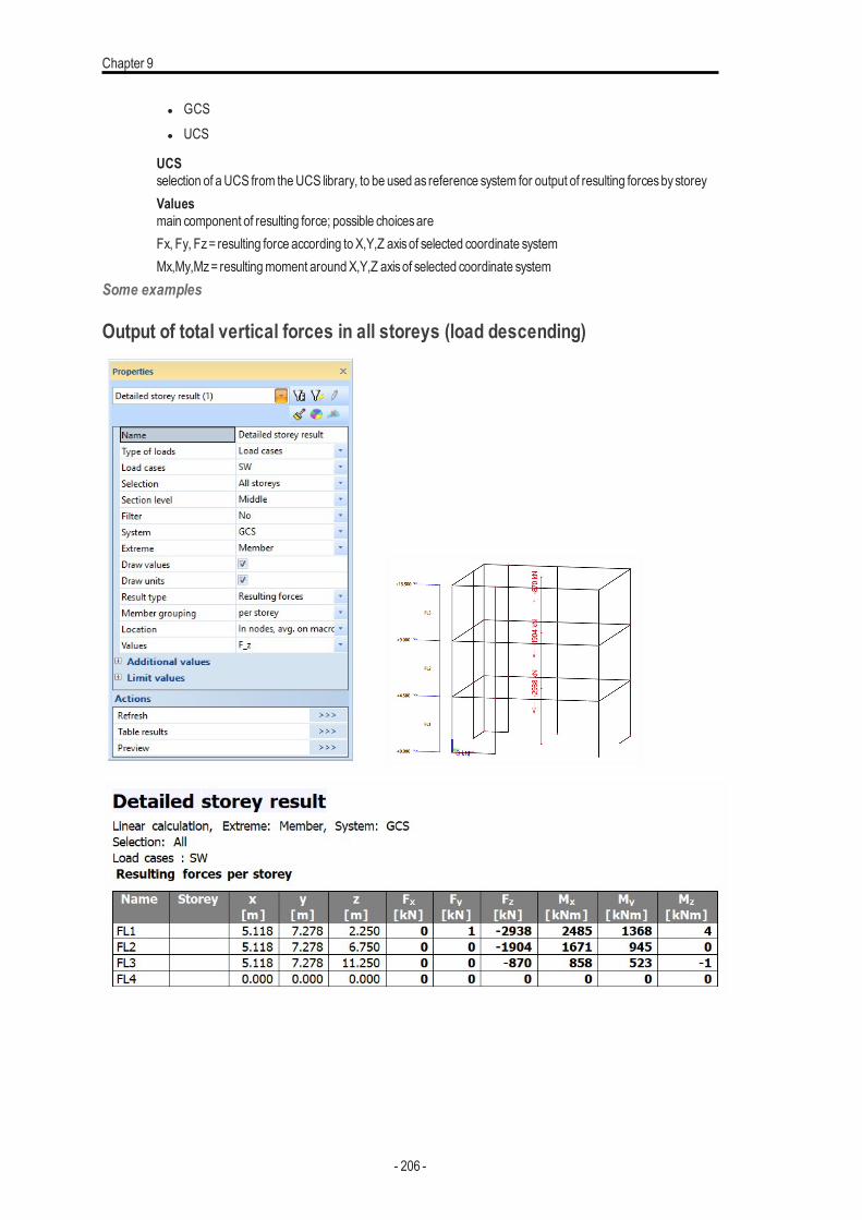
Chapter 9
l GCSl UCS
UCSselection of aUCS from theUCS library, to be used as reference system for output of resulting forcesbystoreyValuesmain component of resulting force; possible choicesareFx, Fy, Fz= resulting force according to X,Y,Z axisof selected coordinate systemMx,My,Mz= resultingmoment aroundX,Y,Z axisof selected coordinate system
Some examples
Output of total vertical forces in all storeys (load descending)
- 206 -
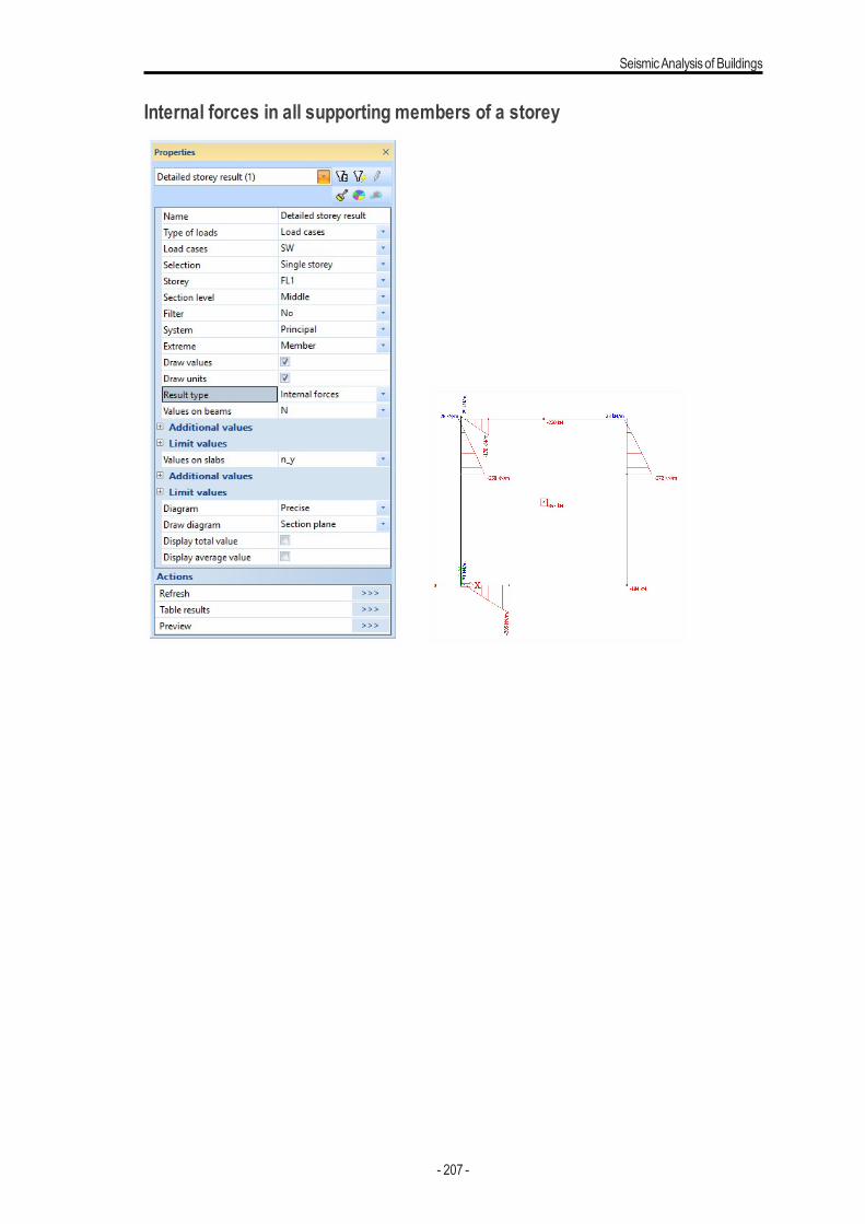
SeismicAnalysisof Buildings
Internal forces in all supporting members of a storey
- 207 -
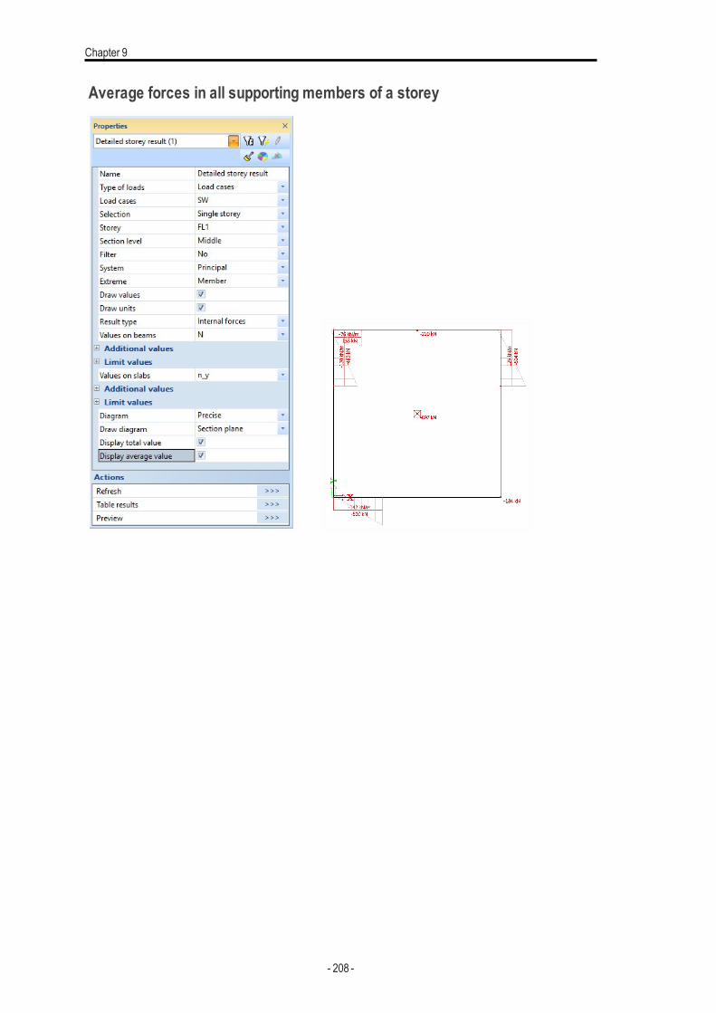
Chapter 9
Average forces in all supporting members of a storey
- 208 -
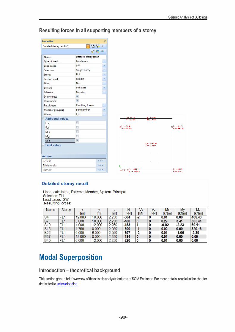
SeismicAnalysisof Buildings
Resulting forces in all supporting members of a storey
Modal SuperpositionIntroduction – theoretical backgroundThissection givesa brief overview of the seismicanalysis featuresof SCIAEngineer. For more details, read also the chapterdedicated to seismic loading.
- 209 -
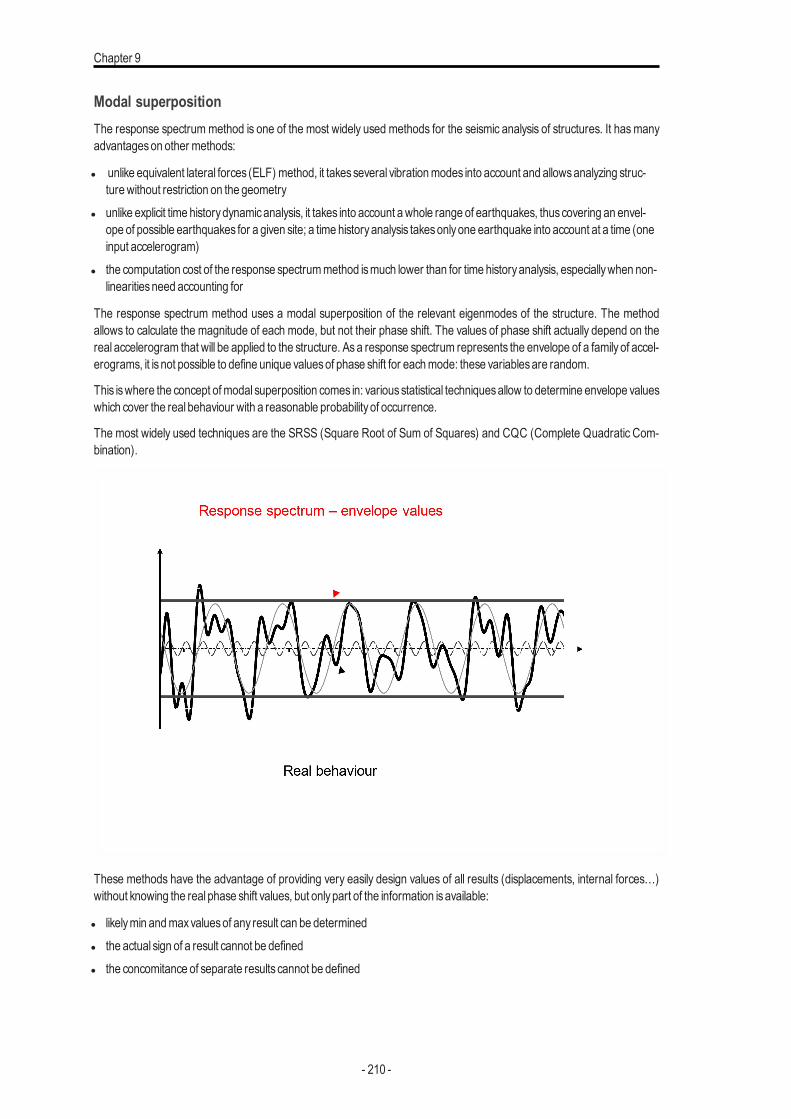
Chapter 9
Modal superpositionThe response spectrum method is one of the most widely used methods for the seismic analysis of structures. It hasmanyadvantageson other methods:
l unlike equivalent lateral forces (ELF) method, it takesseveral vibrationmodes into account and allowsanalyzing struc-turewithout restriction on the geometry
l unlike explicit time historydynamicanalysis, it takes into account awhole range of earthquakes, thuscovering an envel-ope of possible earthquakes for a given site; a time historyanalysis takesonlyone earthquake into account at a time (oneinput accelerogram)
l the computation cost of the response spectrummethod ismuch lower than for time historyanalysis, especiallywhen non-linearitiesneed accounting for
The response spectrum method uses a modal superposition of the relevant eigenmodes of the structure. The methodallows to calculate the magnitude of each mode, but not their phase shift. The values of phase shift actually depend on thereal accelerogram that will be applied to the structure. Asa response spectrum represents the envelope of a family of accel-erograms, it isnot possible to define unique valuesof phase shift for eachmode: these variablesare random.
This iswhere the concept ofmodal superposition comes in: variousstatistical techniquesallow to determine envelope valueswhich cover the real behaviour with a reasonable probability of occurrence.
The most widely used techniques are the SRSS (Square Root of Sum of Squares) and CQC (Complete Quadratic Com-bination).
These methods have the advantage of providing very easily design values of all results (displacements, internal forces…)without knowing the real phase shift values, but onlypart of the information isavailable:
l likelymin andmaxvaluesof any result can be determinedl the actual sign of a result cannot be definedl the concomitance of separate results cannot be defined
- 210 -
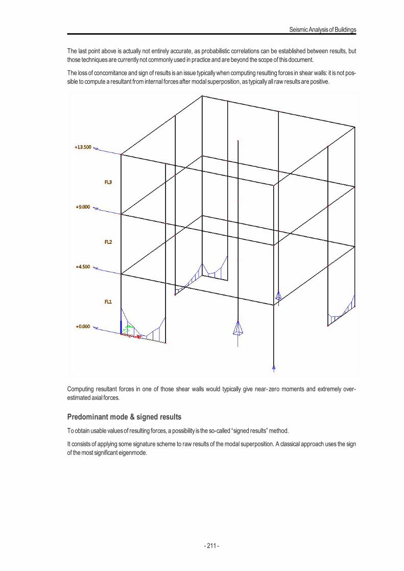
SeismicAnalysisof Buildings
The last point above is actually not entirely accurate, as probabilistic correlations can be established between results, butthose techniquesare currentlynot commonlyused in practice and are beyond the scope of thisdocument.
The lossof concomitance and sign of results is an issue typicallywhen computing resulting forces in shear walls: it is not pos-sible to compute a resultant from internal forcesafter modal superposition, as typicallyall raw resultsare positive.
Computing resultant forces in one of those shear walls would typically give near- zero moments and extremely over-estimated axial forces.
Predominant mode & signed resultsTo obtain usable valuesof resulting forces, a possibility is the so-called “signed results” method.
It consists of applying some signature scheme to raw results of the modal superposition. A classical approach uses the signof themost significant eigenmode.
- 211 -
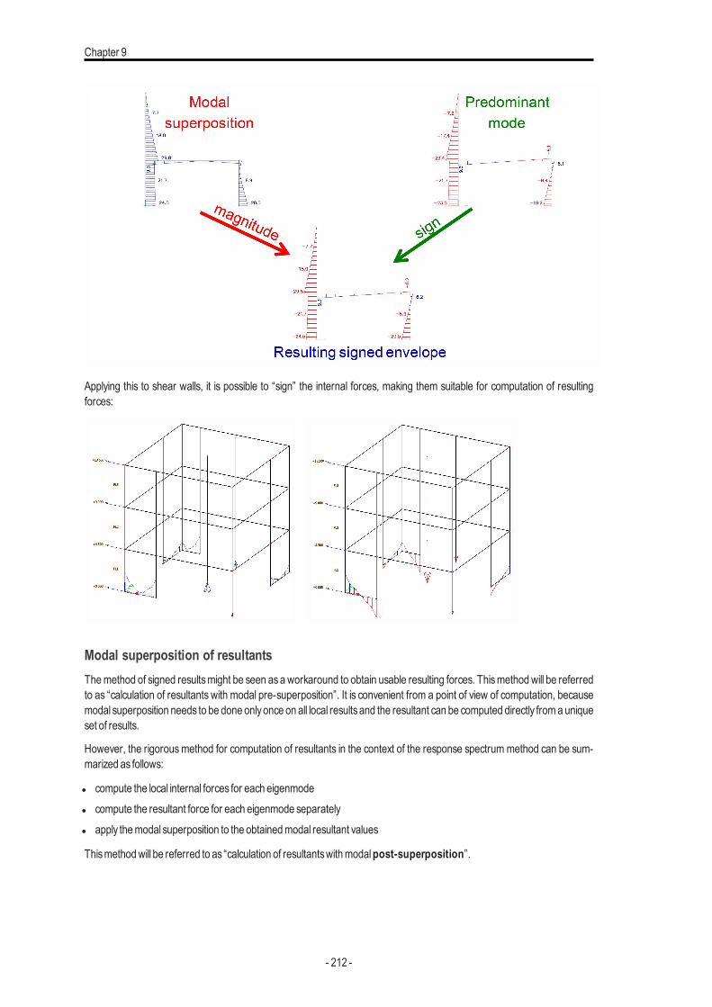
Chapter 9
Applying this to shear walls, it is possible to “sign” the internal forces, making them suitable for computation of resultingforces:
Modal superposition of resultantsThemethod of signed resultsmight be seen asa workaround to obtain usable resulting forces. Thismethod will be referredto as “calculation of resultants with modal pre-superposition”. It is convenient from a point of view of computation, becausemodal superposition needs to be done onlyonce on all local resultsand the resultant can be computed directly froma uniqueset of results.
However, the rigorousmethod for computation of resultants in the context of the response spectrum method can be sum-marized as follows:
l compute the local internal forces for each eigenmodel compute the resultant force for each eigenmode separatelyl apply themodal superposition to the obtainedmodal resultant values
Thismethodwill be referred to as “calculation of resultantswithmodalpost-superposition”.
- 212 -
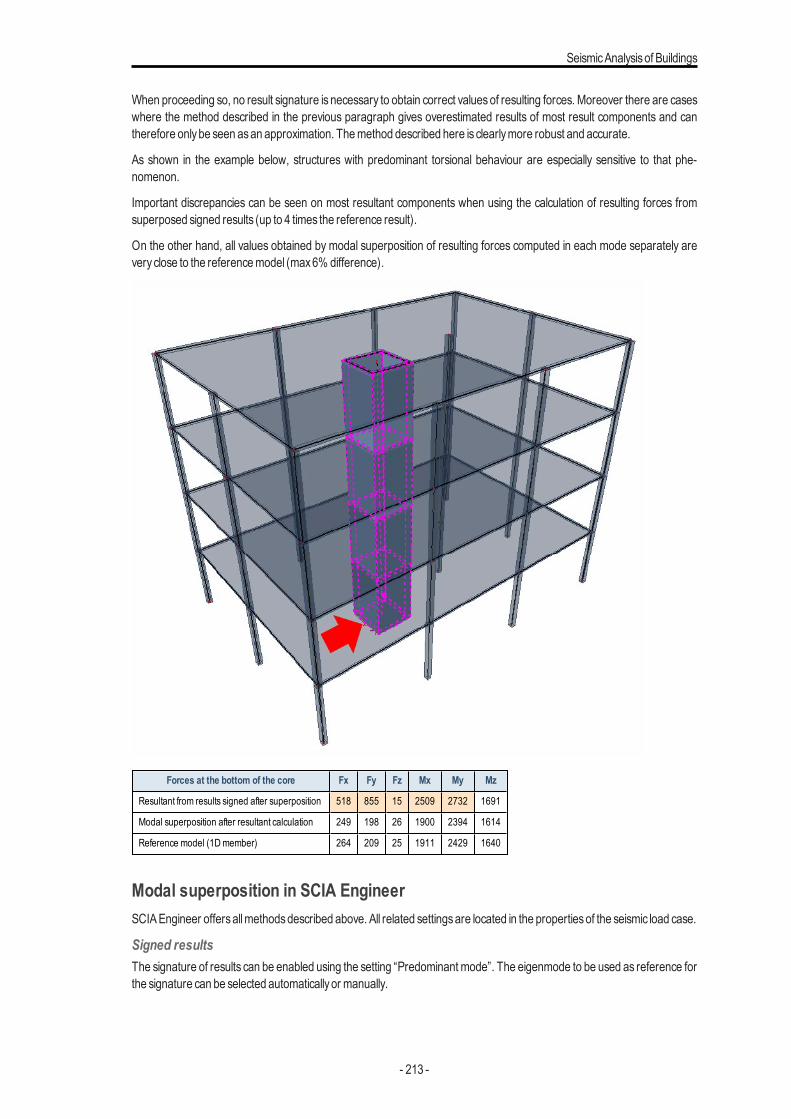
SeismicAnalysisof Buildings
When proceeding so, no result signature is necessary to obtain correct valuesof resulting forces. Moreover there are caseswhere the method described in the previous paragraph gives overestimated results of most result components and cantherefore onlybe seen asan approximation. Themethod described here is clearlymore robust and accurate.
As shown in the example below, structures with predominant torsional behaviour are especially sensitive to that phe-nomenon.
Important discrepancies can be seen on most resultant components when using the calculation of resulting forces fromsuperposed signed results (up to 4 times the reference result).
On the other hand, all values obtained by modal superposition of resulting forces computed in each mode separately areveryclose to the referencemodel (max6% difference).
Forces at the bottom of the core Fx Fy Fz Mx My Mz
Resultant from results signed after superposition 518 855 15 2509 2732 1691
Modal superposition after resultant calculation 249 198 26 1900 2394 1614
Reference model (1Dmember) 264 209 25 1911 2429 1640
Modal superposition in SCIA EngineerSCIAEngineer offersallmethodsdescribed above. All related settingsare located in the propertiesof the seismic load case.
Signed resultsThe signature of results can be enabled using the setting “Predominant mode”. The eigenmode to be used as reference forthe signature can be selected automaticallyor manually.
- 213 -
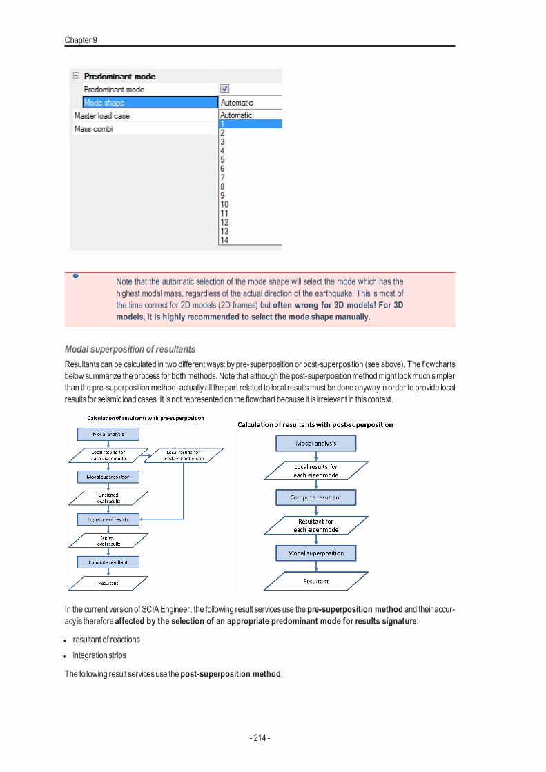
Chapter 9
Note that the automatic selection of the mode shape will select the mode which has thehighest modal mass, regardless of the actual direction of the earthquake. This is most ofthe time correct for 2D models (2D frames) but often wrong for 3D models! For 3Dmodels, it is highly recommended to select the mode shape manually.
Modal superposition of resultantsResultants can be calculated in two different ways: by pre-superposition or post-superposition (see above). The flowchartsbelow summarize the process for bothmethods. Note that although the post-superpositionmethodmight lookmuch simplerthan the pre-superpositionmethod, actually all the part related to local resultsmust be done anyway in order to provide localresults for seismic load cases. It isnot represented on the flowchart because it is irrelevant in this context.
In the current version of SCIAEngineer, the following result services use the pre-superposition method and their accur-acy is therefore affected by the selection of an appropriate predominant mode for results signature:
l resultant of reactionsl integration strips
The following result servicesuse thepost-superposition method:
- 214 -
SeismicAnalysisof Buildings
l resultant of forces in a section on 2D membersl detailed storey results, resultant per memberl detailed storey results, resultant per storeyl seismic resultant in calculation protocol
Accidental EccentricityIntroductionMost of the seismic standards require that structuresare checked for torsion due tomasseccentricity including an additionaleccentricity– so-called accidental eccentricity. This is required to cover inaccuraciesbetween the real structure and themod-elization, aswell as the fact thatmasses that are linked to service loadsmayvaryduring the life of the structure.
Two typesof eccentricitymust be distinguished for the analysis: the structural eccentricityand the accidental eccentricity.
The structural eccentricity is the offset between the center of massand the center of stiffnessof the structure. It is part of thestructure. In a simplified seismic analysis via 2D models, where typically the X and Y directions are analyzed separately, theimpact of the structural eccentricity is taken into account by manually distributing the torsional effects on the structure. Anadditional safety factor isusuallyapplied to the structural eccentricity to cover inaccuraciesdue to that simplifiedmethod.
When using a 3D modelization of the structure, the structural eccentricity is automatically taken into account due to the factthat the X and Y and linked and analyzed together, allowing torsional effects to appear directly in the analysiswithout havingto add themmanuallyafterwards.
The accidental eccentricity accounts for inaccuracies in the distribution of masses in the structure. Design standards usuallytake it into account asan additionalmasseccentricity that isdefined asa fraction of the size of the structure.
In the Eurocode 8, the accidental eccentricity for a given floor is defined as5% of the width of the floor perpendicularly to thedirection of the acting seismicaction.
In simplified modelizations where the structural eccentricity appears explicitly, it is very simple to add the accidental eccent-ricity in the calculation. In general 3D modelizations, the structural eccentricity does not appear as such and it is thereforemore complex to take itseffects into account in such a case.
In SCIA Engineer, using the IRS condensed model allows introducing accidental eccentricity easily, since the condensedmodel uses only one R-node per storey. The accidental eccentricity may be taken into account either as real mass eccent-ricityor asadditional torsional actions (simplifiedmethod according to the design codes).
However, themethod using realmasseccentricity in themodal analysishasnot been implemented yet in SCIAEngineer.
For now, only the simplifiedmethod using additional torsionalmoment isavailable.
Definition of the accidental eccentricityFirst of all, please note, that accidental eccentricitymay be used only together with the reduced model analysis. See how toenable it in Enabling the reducedmodel.
The accidental eccentricity settings are defined in the properties of the considered seismic load case, in the sub-group .”Ac-cidental eccentricity”. Accidental eccentricity isdisabled bydefault.
- 215 -
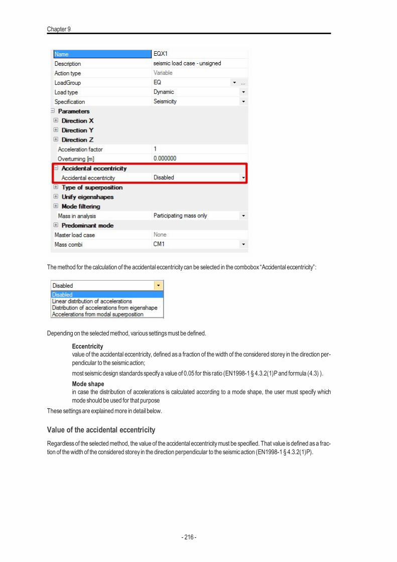
Chapter 9
Themethod for the calculation of the accidental eccentricity can be selected in the combobox “Accidental eccentricity”:
Depending on the selectedmethod, varioussettingsmust be defined.
Eccentricityvalue of the accidental eccentricity, defined asa fraction of the width of the considered storey in the direction per-pendicular to the seismicaction;most seismicdesign standardsspecifya value of 0.05 for this ratio (EN1998-1 § 4.3.2(1)Pand formula (4.3) ).Mode shapein case the distribution of accelerations is calculated according to a mode shape, the user must specify whichmode should be used for that purpose
These settingsare explainedmore in detail below.
Value of the accidental eccentricityRegardlessof the selectedmethod, the value of the accidental eccentricitymust be specified. That value isdefined asa frac-tion of thewidth of the considered storey in the direction perpendicular to the seismicaction (EN1998-1 § 4.3.2(1)P).
- 216 -
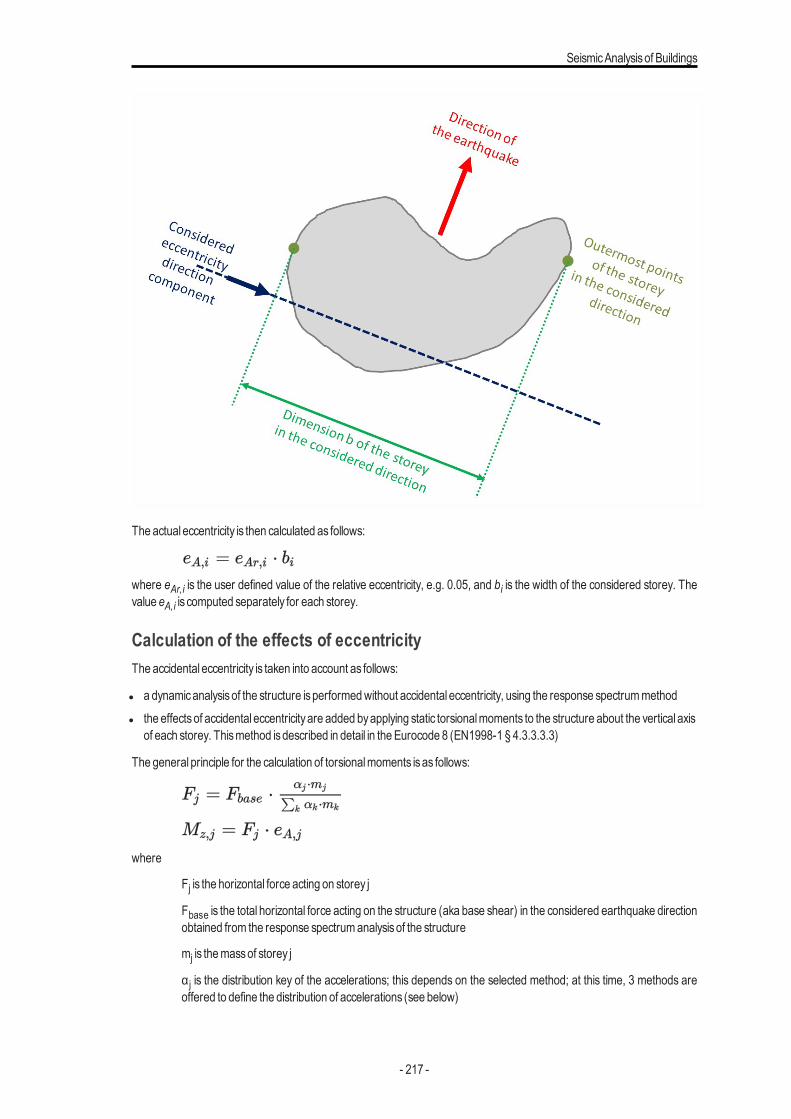
SeismicAnalysisof Buildings
The actual eccentricity is then calculated as follows:
where eAr,i is the user defined value of the relative eccentricity, e.g. 0.05, and bi is the width of the considered storey. Thevalue eA,i is computed separately for each storey.
Calculation of the effects of eccentricityThe accidental eccentricity is taken into account as follows:
l a dynamicanalysisof the structure isperformedwithout accidental eccentricity, using the response spectrummethodl the effectsof accidental eccentricityare added byapplying static torsionalmoments to the structure about the vertical axis
of each storey. Thismethod isdescribed in detail in the Eurocode 8 (EN1998-1 § 4.3.3.3.3)
The general principle for the calculation of torsionalmoments isas follows:
where
Fj is the horizontal force acting on storey j
Fbase is the total horizontal force acting on the structure (aka base shear) in the considered earthquake directionobtained from the response spectrumanalysisof the structure
mj is themassof storey j
α j is the distribution key of the accelerations; this depends on the selected method; at this time, 3 methods areoffered to define the distribution of accelerations (see below)
- 217 -
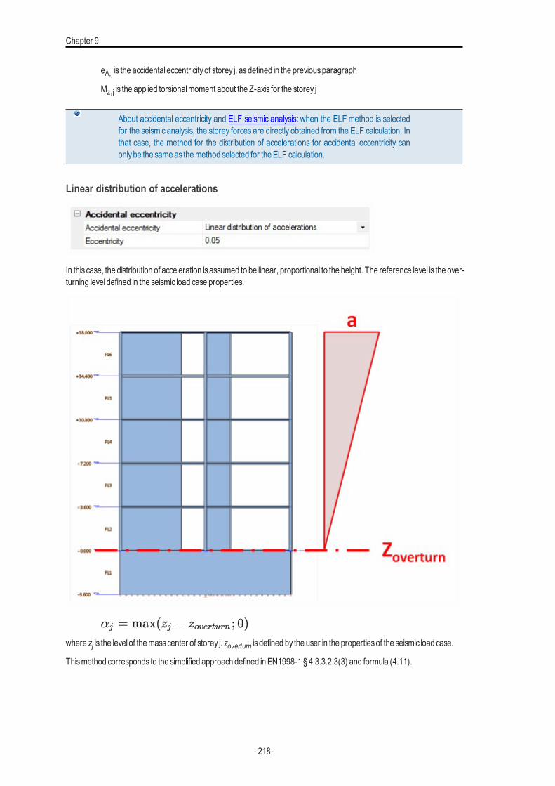
Chapter 9
eA,j is the accidental eccentricityof storey j, asdefined in the previousparagraph
Mz,j is the applied torsionalmoment about the Z-axis for the storey j
About accidental eccentricity and ELF seismic analysis: when the ELF method is selectedfor the seismic analysis, the storey forces are directly obtained from the ELF calculation. Inthat case, the method for the distribution of accelerations for accidental eccentricity canonlybe the sameas themethod selected for the ELF calculation.
Linear distribution of accelerations
In this case, the distribution of acceleration isassumed to be linear, proportional to the height. The reference level is the over-turning level defined in the seismic load case properties.
where zj is the level of themasscenter of storey j. zoverturn is defined by the user in the propertiesof the seismic load case.
Thismethod corresponds to the simplified approach defined in EN1998-1 § 4.3.3.2.3(3) and formula (4.11).
- 218 -
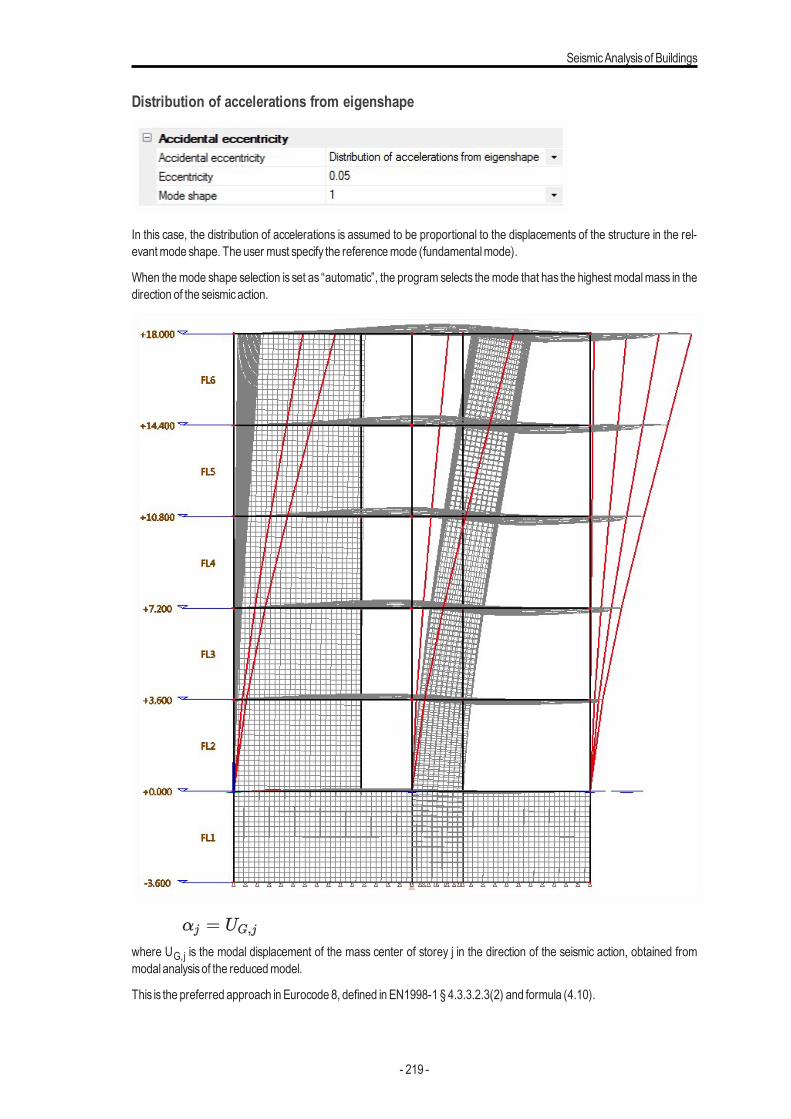
SeismicAnalysisof Buildings
Distribution of accelerations from eigenshape
In this case, the distribution of accelerations is assumed to be proportional to the displacements of the structure in the rel-evantmode shape. The user must specify the referencemode (fundamentalmode).
When themode shape selection is set as “automatic”, the program selects themode that has the highest modalmass in thedirection of the seismicaction.
where UG,j is the modal displacement of the mass center of storey j in the direction of the seismic action, obtained frommodal analysisof the reducedmodel.
This is the preferred approach in Eurocode 8, defined in EN1998-1 § 4.3.3.2.3(2) and formula (4.10).
- 219 -
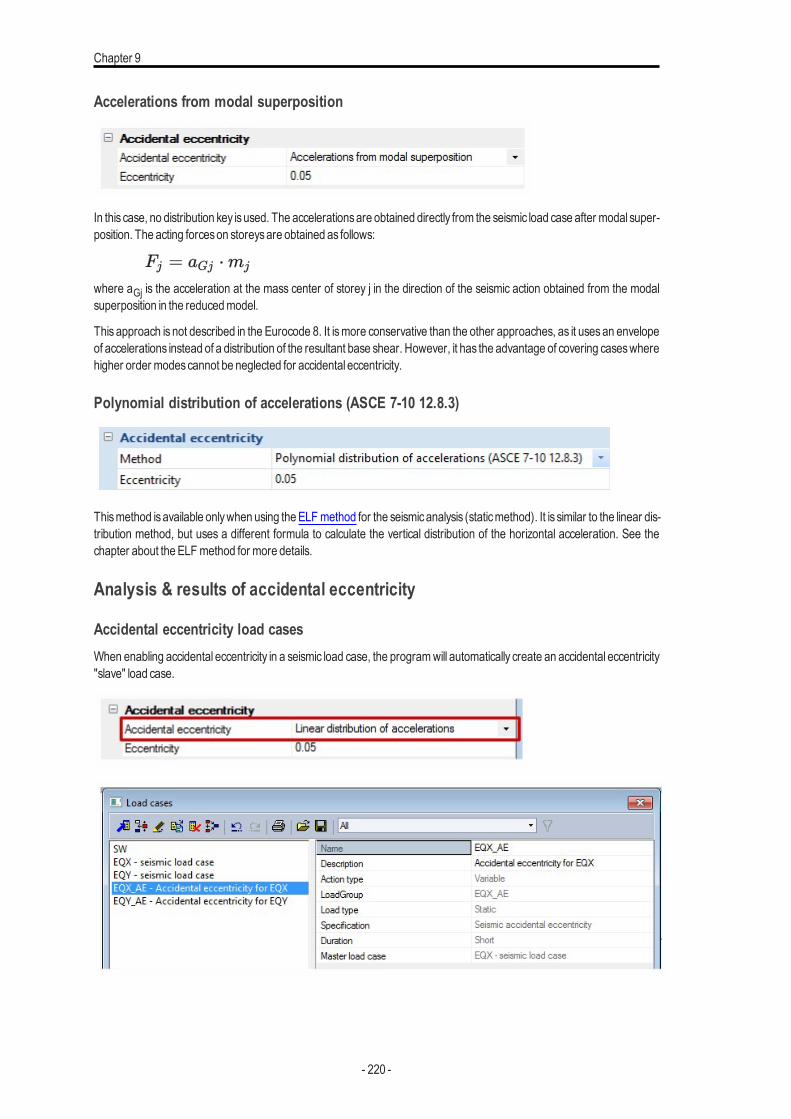
Chapter 9
Accelerations from modal superposition
In this case, no distribution key isused. The accelerationsare obtained directly from the seismic load case after modal super-position. The acting forceson storeysare obtained as follows:
where aGj is the acceleration at the mass center of storey j in the direction of the seismic action obtained from the modalsuperposition in the reducedmodel.
This approach is not described in the Eurocode 8. It ismore conservative than the other approaches, as it usesan envelopeof accelerations instead of a distribution of the resultant base shear. However, it has the advantage of covering caseswherehigher order modescannot be neglected for accidental eccentricity.
Polynomial distribution of accelerations (ASCE 7-10 12.8.3)
Thismethod isavailable onlywhen using theELF method for the seismicanalysis (staticmethod). It is similar to the linear dis-tribution method, but uses a different formula to calculate the vertical distribution of the horizontal acceleration. See thechapter about the ELF method for more details.
Analysis & results of accidental eccentricity
Accidental eccentricity load casesWhen enabling accidental eccentricity in a seismic load case, the programwill automatically create an accidental eccentricity"slave" load case.
- 220 -
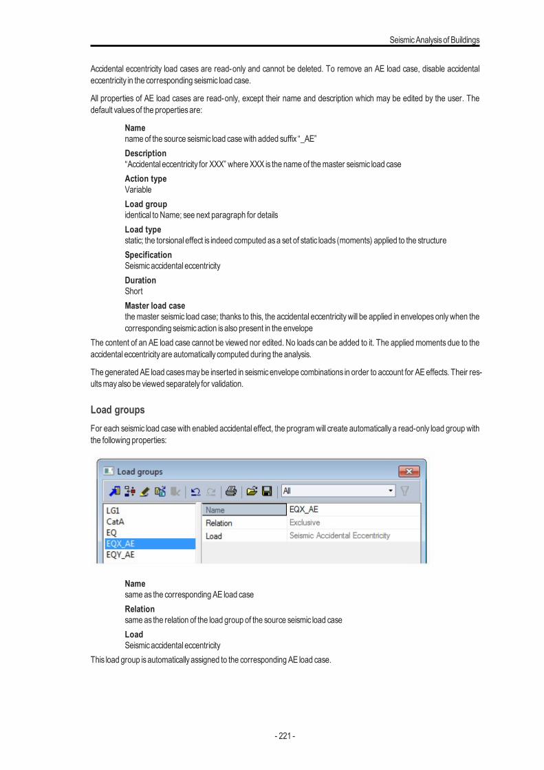
SeismicAnalysisof Buildings
Accidental eccentricity load cases are read-only and cannot be deleted. To remove an AE load case, disable accidentaleccentricity in the corresponding seismic load case.
All properties of AE load cases are read-only, except their name and description which may be edited by the user. Thedefault valuesof the propertiesare:
Namenameof the source seismic load casewith added suffix “_AE”Description“Accidental eccentricity for XXX” where XXX is the nameof themaster seismic load caseAction typeVariableLoad groupidentical to Name; see next paragraph for detailsLoad typestatic; the torsional effect is indeed computed asa set of static loads (moments) applied to the structureSpecificationSeismicaccidental eccentricityDurationShortMaster load casethe master seismic load case; thanks to this, the accidental eccentricitywill be applied in envelopes onlywhen thecorresponding seismicaction isalso present in the envelope
The content of an AE load case cannot be viewed nor edited. No loads can be added to it. The applied moments due to theaccidental eccentricityare automatically computed during the analysis.
The generatedAE load casesmaybe inserted in seismicenvelope combinations in order to account for AEeffects. Their res-ultsmayalso be viewed separately for validation.
Load groupsFor each seismic load case with enabled accidental effect, the programwill create automatically a read-only load group withthe following properties:
Namesame as the corresponding AE load caseRelationsame as the relation of the load group of the source seismic load caseLoadSeismicaccidental eccentricity
This load group isautomaticallyassigned to the corresponding AE load case.
- 221 -
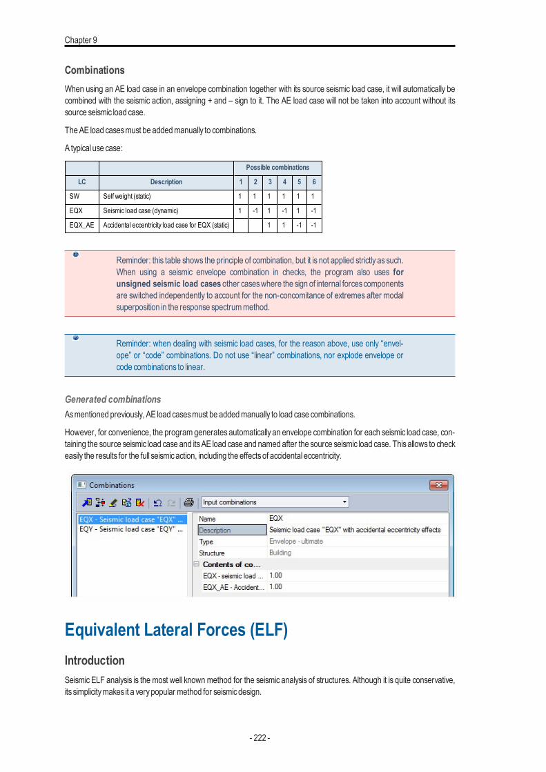
Chapter 9
CombinationsWhen using an AE load case in an envelope combination together with its source seismic load case, it will automatically becombined with the seismic action, assigning + and – sign to it. The AE load case will not be taken into account without itssource seismic load case.
TheAE load casesmust be addedmanually to combinations.
A typical use case:
Possible combinations
LC Description 1 2 3 4 5 6
SW Self weight (static) 1 1 1 1 1 1
EQX Seismic load case (dynamic) 1 -1 1 -1 1 -1
EQX_AE Accidental eccentricity load case for EQX (static) 1 1 -1 -1
Reminder: this table shows the principle of combination, but it is not applied strictly as such.When using a seismic envelope combination in checks, the program also uses forunsigned seismic load cases other caseswhere the sign of internal forcescomponentsare switched independently to account for the non-concomitance of extremes after modalsuperposition in the response spectrummethod.
Reminder: when dealing with seismic load cases, for the reason above, use only “envel-ope” or “code” combinations. Do not use “linear” combinations, nor explode envelope orcode combinations to linear.
Generated combinationsAsmentioned previously, AE load casesmust be addedmanually to load case combinations.
However, for convenience, the program generates automatically an envelope combination for each seismic load case, con-taining the source seismic load case and itsAE load case and named after the source seismic load case. Thisallows to checkeasily the results for the full seismicaction, including the effectsof accidental eccentricity.
Equivalent Lateral Forces (ELF)IntroductionSeismic ELF analysis is the most well known method for the seismic analysis of structures. Although it is quite conservative,its simplicitymakes it a verypopular method for seismicdesign.
- 222 -
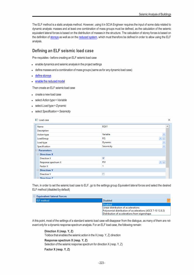
SeismicAnalysisof Buildings
The ELF method is a static analysismethod. However, using it in SCIA Engineer requires the input of some data related todynamic analysis: masses and at least one combination of mass groups must be defined, as the calculation of the seismicequivalent lateral forces is based on the distribution of masses in the structure. The calculation of storey forces is based onthe definition of storeys as well as on the reduced system, which must therefore be defined in order to allow using the ELFanalysis.
Defining an ELF seismic load casePre-requisites - before creating anELF seismic load case
l enable dynamicsand seismicanalysis in the project settingsl definemassesand a combination ofmassgroups (same as for anydynamic load case)l define storeysl enable the reducedmodel
Then create anELF seismic load case
l create a new load casel selectAction type = Variablel select Load type = Dynamicl selectSpecification = Seismicity
Then, in order to set the seismic load case to ELF, go to the settings group Equivalent lateral forces and select the desiredELF method (disabled bydefault)
A this point, most of the settings of a standard seismic load case will disappear from the dialogue, asmany of them are rel-evant only for a dynamic response spectrumanalysis. For anELF load case, the following remain:
Direction X (resp. Y, Z)Tickbox that enables the seismicaction in theX (resp. Y, Z) directionResponse spectrum X (resp. Y, Z)Selection of the seismic response spectrum for direction X (resp. Y, Z)Factor X (resp. Y, Z)
- 223 -

Chapter 9
Multiplying factor for the seismicaction in direction X (resp. Y, Z)Acceleration factorMultiplying factor for the entire seismicactionOverturning reference levelReference level for the calculation of overturning moments. Also used as reference level when using a linear orpolynomial distribution of accelerationsAccidental eccentricityAccidental eccentricity settingsact the same as for dynamicseismicanalysisMass combiMasscombination selected for the calculation of the seismicaction
Specific settings for an ELF seismic load caseEquivalent lateral forces
ELF methodDefineshow the distribution of accelerationswill be calculated in the building. The variousmethodsare detailed inthe next section. The available choicesare:
DisabledELF calculation of the seismic load case is disabled, i.e. the load case will use dynamic, multi-modalresponse spectrumanalysisLinear distribution of accelerationsThe acceleration is increasing linearly with the global Z coordinate, starting with zero at the over-turning reference level (see above)Polynomial distribution of accelerations (ASCE 7-10 12.8.3)The acceleration is increasing according to a polynomial function, according to ASCE 7-10 standard,startingwith zero at the overturning reference level (see above)Distribution of accelerations from eigenshapeThe acceleration isdistributed proportionally to themode shape of an eigenmode selected by the user
Seismic force fromDefines how the total seismic force (base shear) is calculated. The available options depend on the selectedELF method.
Max acceleration of spectrumThemaximumacceleration of the selected response spectrum isusedInput fundamental periodThe acceleration corresponding to a user input value of fundamental period isusedSelected eigenmodeThe acceleration corresponding to the period of the user selected eigenmode is used; please note,that this impliesamodal analysisof the structureApproximate fundamental period (ASCE 7-10 12.8-7)The acceleration corresponding to approximate fundamental period according ASCE 7-10 eq. 12.8-7. This is available only when ELF method = Polynomial distribution of accelerations (ASCE 7-1012.8.3)
Fundamental periodUser input fundamental period to be used for the calculation of the seismic force whenSeismic force from = Inputfundamental periodMode shapeEigenmode to be used for the distribution of the accelerationsand/or the calculation of the seismic force
ASCE additional parametersStructure typeThis item is for valuesof approximate period parameters, seeASCE7-10 table 12.8-2
Steel moment frame
- 224 -
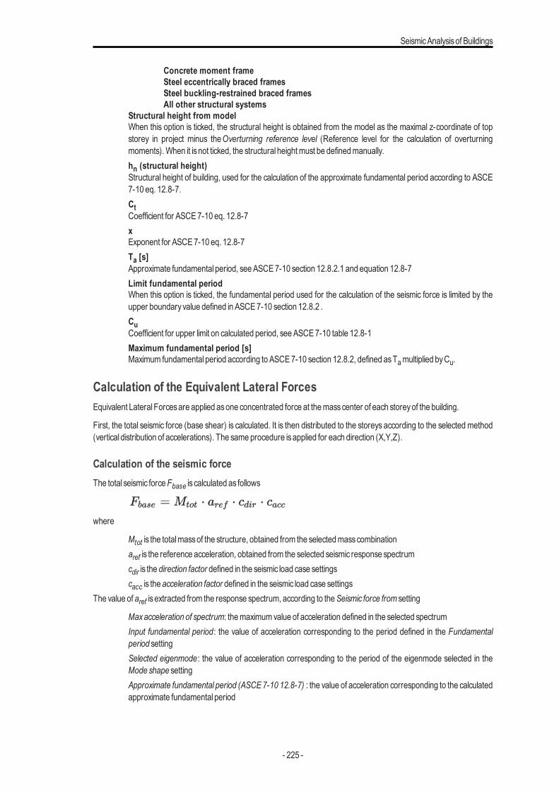
SeismicAnalysisof Buildings
Concrete moment frameSteel eccentrically braced framesSteel buckling-restrained braced framesAll other structural systems
Structural height from modelWhen this option is ticked, the structural height is obtained from the model as the maximal z-coordinate of topstorey in project minus theOverturning reference level (Reference level for the calculation of overturningmoments).When it isnot ticked, the structural heightmust be definedmanually.hn (structural height)Structural height of building, used for the calculation of the approximate fundamental period according to ASCE7-10 eq. 12.8-7.CtCoefficient for ASCE7-10 eq. 12.8-7xExponent for ASCE7-10 eq. 12.8-7Ta [s]Approximate fundamental period, seeASCE7-10 section 12.8.2.1 and equation 12.8-7Limit fundamental periodWhen this option is ticked, the fundamental period used for the calculation of the seismic force is limited by theupper boundaryvalue defined in ASCE 7-10 section 12.8.2 .CuCoefficient for upper limit on calculated period, seeASCE7-10 table 12.8-1Maximum fundamental period [s]Maximum fundamental period according to ASCE 7-10 section 12.8.2, defined asTamultiplied byCu.
Calculation of the Equivalent Lateral ForcesEquivalent Lateral Forcesare applied asone concentrated force at themasscenter of each storeyof the building.
First, the total seismic force (base shear) is calculated. It is then distributed to the storeys according to the selected method(vertical distribution of accelerations). The sameprocedure isapplied for each direction (X,Y,Z).
Calculation of the seismic forceThe total seismic forceFbase is calculated as follows
where
Mtot is the totalmassof the structure, obtained from the selectedmasscombinationaref is the reference acceleration, obtained from the selected seismic response spectrumcdir is the direction factor defined in the seismic load case settingscacc is the acceleration factor defined in the seismic load case settings
The value of aref is extracted from the response spectrum, according to theSeismic force from setting
Maxacceleration of spectrum: themaximumvalue of acceleration defined in the selected spectrumInput fundamental period: the value of acceleration corresponding to the period defined in the Fundamentalperiod settingSelected eigenmode: the value of acceleration corresponding to the period of the eigenmode selected in theMode shape settingApproximate fundamental period (ASCE 7-10 12.8-7) : the value of acceleration corresponding to the calculatedapproximate fundamental period
- 225 -
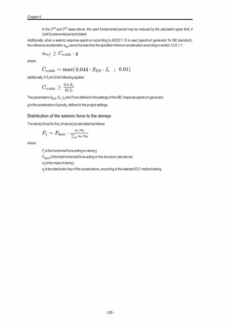
Chapter 9
In the 2nd and 3rd cases above, the used fundamental period may be reduced by the calculated upper limit, ifLimit fundamental period is ticked
Additionally, when a seismic response spectrum according to ASCE 7-10 is used (spectrum generator for IBC standard),the reference acceleration aref cannot be less than the specifiedminimumacceleration according to section 12.8.1.1:
where
additionally, ifS1≥0.6 the following applies:
The parametersSDS,S1, Ie andR are defined in the settingsof the IBC response spectrumgenerator.
g is the acceleration of gravity, defined in the project settings.
Distribution of the seismic force to the storeysThe storey force for the j-th storey j is calculated as follows
where
Fj is the horizontal force acting on storey jFbase is the total horizontal force acting on the structure (see above)mj is themassof storey jαj is the distribution keyof the accelerations, according to the selectedELF method setting
- 226 -
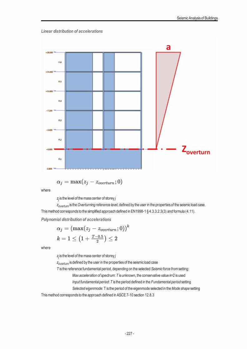
SeismicAnalysisof Buildings
Linear distribution of accelerations
where
zj is the level of themasscenter of storey jzoverturn is theOverturning reference level, defined by the user in the propertiesof the seismic load case.
Thismethod corresponds to the simplified approach defined in EN1998-1 § 4.3.3.2.3(3) and formula (4.11).
Polynomial distribution of accelerations
where
zj is the level of themasscenter of storey jzoverturn is defined by the user in the propertiesof the seismic load caseT is the reference fundamental period, depending on the selectedSeismic force from setting:
Maxacceleration of spectrum: T is unknown, the conservative value k=2 isusedInput fundamental period:T is the period defined in theFundamental period settingSelected eigenmode: T is the period of the eigenmode selected in theMode shape setting
Thismethod corresponds to the approach defined in ASCE 7-10 section 12.8.3
- 227 -
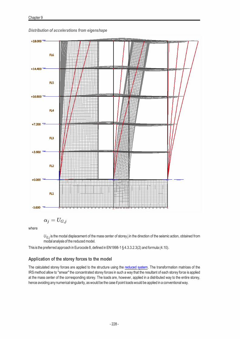
Chapter 9
Distribution of accelerations from eigenshape
where
UG,j is the modal displacement of the mass center of storey j in the direction of the seismic action, obtained frommodal analysisof the reducedmodel.
This is the preferred approach in Eurocode 8, defined in EN1998-1 § 4.3.3.2.3(2) and formula (4.10).
Application of the storey forces to the modelThe calculated storey forces are applied to the structure using the reduced system. The transformation matrices of theIRS method allow to "smear" the concentrated storey forces in such a way that the resultant of each storey force is appliedat the mass center of the corresponding storey. The loads are, however, applied in a distributed way to the entire storey,hence avoiding anynumerical singularity, aswould be the case if point loadswould be applied in a conventionalway.
- 228 -
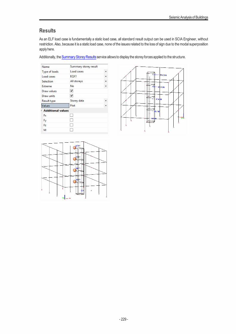
SeismicAnalysisof Buildings
ResultsAs an ELF load case is fundamentally a static load case, all standard result output can be used in SCIA Engineer, withoutrestriction. Also, because it is a static load case, none of the issues related to the loss of sign due to the modal superpositionapplyhere.
Additionally, the SummaryStoreyResults service allows to display the storey forcesapplied to the structure.
- 229 -
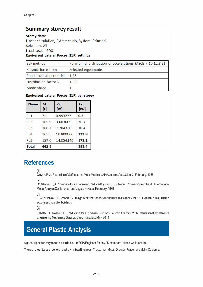
Chapter 9
References[1]Guyan, R.J., Reduction of StiffnessandMassMatrices, AIAAJournal, Vol. 3, No. 2, February, 1965[2]O’Callahan, j., A Procedure for an Improved Reduced System (IRS) Model, Proceedings of the 7th InternationalModalAnalysisConference, LasVegas, Nevada, February, 1989[3]EC-EN 1998-1, Eurocode 8 - Design of structures for earthquake resistance - Part 1: General rules, seismicactionsand rules for buildings[4]Kabeláč, J., Rossier, S., Reduction for High-Rise Buildings Seismic Analysis, 20th International ConferenceEngineeringMechanics, Svratka, CzechRepublic, May, 2014
General Plastic Analysis
Ageneral plasticanalysis can be carried out in SCIAEngineer for any2D members (plates, walls, shells).
There are four typesof general plasticity in Scia Engineer : Tresca, vonMises, Drucker-Prager andMohr-Coulomb.
- 230 -
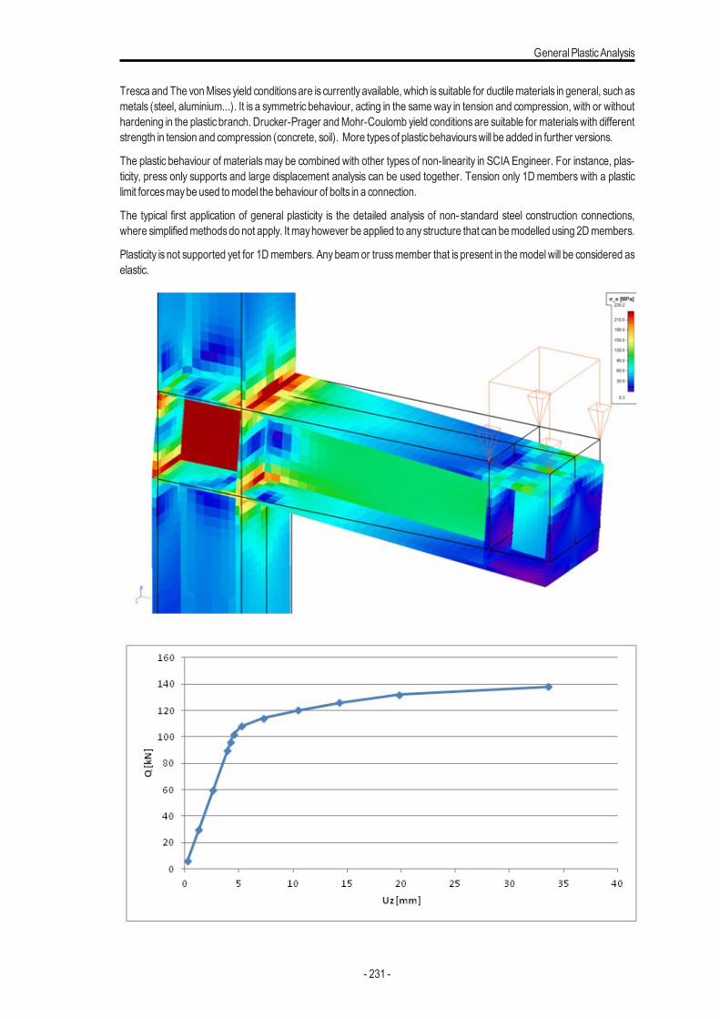
GeneralPlasticAnalysis
Tresca and The vonMisesyield conditionsare is currently available, which is suitable for ductilematerials in general, such asmetals (steel, aluminium...). It is a symmetric behaviour, acting in the same way in tension and compression, with or withouthardening in the plastic branch. Drucker-Prager andMohr-Coulomb yield conditionsare suitable for materialswith differentstrength in tension and compression (concrete, soil). More typesof plasticbehaviourswill be added in further versions.
The plastic behaviour of materialsmay be combined with other types of non-linearity in SCIA Engineer. For instance, plas-ticity, press only supports and large displacement analysis can be used together. Tension only 1D members with a plasticlimit forcesmaybe used tomodel the behaviour of bolts in a connection.
The typical first application of general plasticity is the detailed analysis of non-standard steel construction connections,where simplifiedmethodsdo not apply. It mayhowever be applied to anystructure that can bemodelled using 2D members.
Plasticity is not supported yet for 1D members. Anybeam or trussmember that is present in themodelwill be considered aselastic.
- 231 -
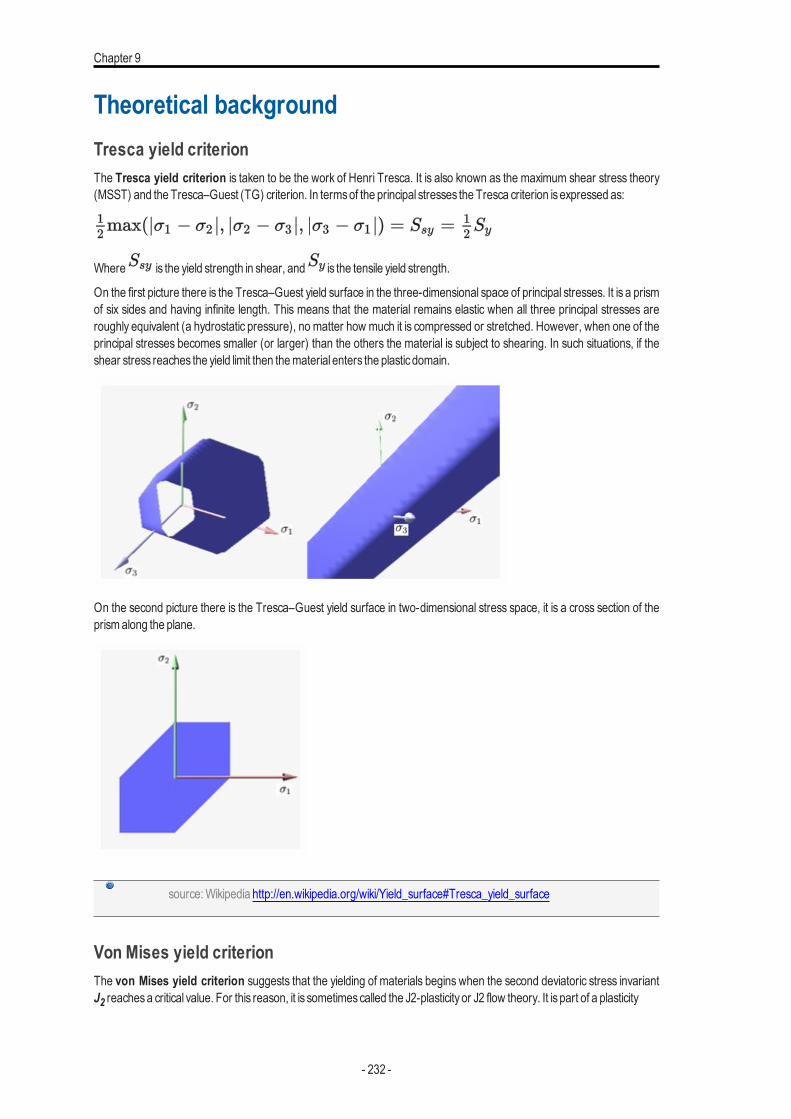
Chapter 9
Theoretical backgroundTresca yield criterionThe Tresca yield criterion is taken to be the work of Henri Tresca. It is also known as the maximum shear stress theory(MSST) and the Tresca–Guest (TG) criterion. In termsof the principal stresses the Tresca criterion isexpressed as:
Where is the yield strength in shear, and is the tensile yield strength.
On the first picture there is the Tresca–Guest yield surface in the three-dimensional space of principal stresses. It is a prismof six sides and having infinite length. This means that the material remains elastic when all three principal stresses areroughly equivalent (a hydrostatic pressure), no matter how much it is compressed or stretched. However, when one of theprincipal stresses becomes smaller (or larger) than the others the material is subject to shearing. In such situations, if theshear stress reaches the yield limit then thematerial enters the plasticdomain.
On the second picture there is the Tresca–Guest yield surface in two-dimensional stress space, it is a cross section of theprismalong the plane.
source: Wikipedia http://en.wikipedia.org/wiki/Yield_surface#Tresca_yield_surface
Von Mises yield criterionThe von Mises yield criterion suggests that the yielding of materials begins when the second deviatoric stress invariantJ2 reachesa critical value. For this reason, it is sometimescalled the J2-plasticity or J2 flow theory. It is part of a plasticity
- 232 -
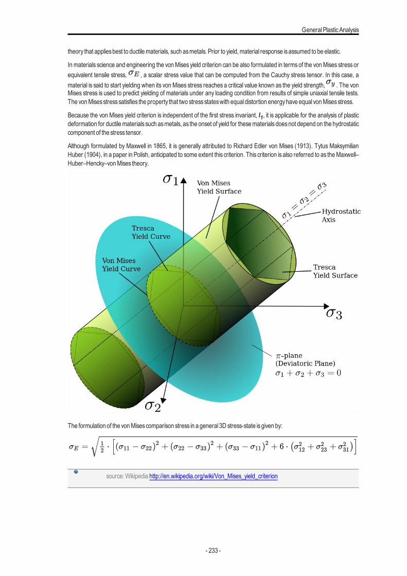
GeneralPlasticAnalysis
theory that appliesbest to ductilematerials, such asmetals. Prior to yield, material response isassumed to be elastic.
In materials science and engineering the vonMises yield criterion can be also formulated in termsof the vonMises stress orequivalent tensile stress, , a scalar stress value that can be computed from the Cauchy stress tensor. In this case, amaterial is said to start yielding when its von Mises stress reaches a critical value known as the yield strength, . The vonMises stress is used to predict yielding of materials under any loading condition from results of simple uniaxial tensile tests.The vonMisesstresssatisfies the property that two stressstateswith equal distortion energyhave equal vonMisesstress.
Because the von Mises yield criterion is independent of the first stress invariant, I1, it is applicable for the analysis of plasticdeformation for ductilematerials such asmetals, as the onset of yield for thesematerials doesnot depend on the hydrostaticcomponent of the stress tensor.
Although formulated by Maxwell in 1865, it is generally attributed to Richard Edler von Mises (1913). Tytus MaksymilianHuber (1904), in a paper in Polish, anticipated to some extent this criterion. This criterion is also referred to as theMaxwell–Huber–Hencky–vonMises theory.
The formulation of the vonMisescomparison stress in a general 3D stress-state isgiven by:
source: Wikipedia http://en.wikipedia.org/wiki/Von_Mises_yield_criterion
- 233 -
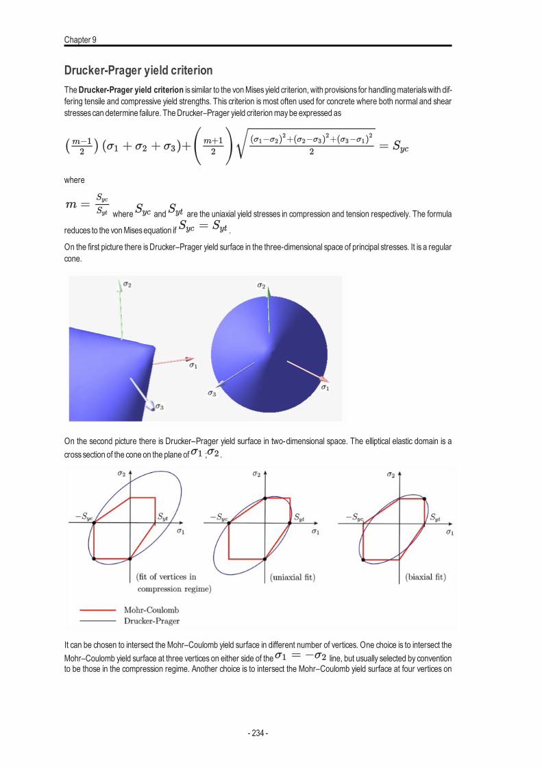
Chapter 9
Drucker-Prager yield criterionTheDrucker-Prager yield criterion is similar to the vonMisesyield criterion, with provisions for handlingmaterialswith dif-fering tensile and compressive yield strengths. This criterion is most often used for concrete where both normal and shearstressescan determine failure. TheDrucker–Prager yield criterionmaybe expressed as
where
where and are the uniaxial yield stresses in compression and tension respectively. The formula
reduces to the vonMisesequation if .
On the first picture there isDrucker–Prager yield surface in the three-dimensional space of principal stresses. It is a regularcone.
On the second picture there is Drucker–Prager yield surface in two-dimensional space. The elliptical elastic domain is acrosssection of the cone on the plane of ; .
It can be chosen to intersect the Mohr–Coulomb yield surface in different number of vertices. One choice is to intersect theMohr–Coulomb yield surface at three vertices on either side of the line, but usually selected by conventionto be those in the compression regime. Another choice is to intersect the Mohr–Coulomb yield surface at four vertices on
- 234 -
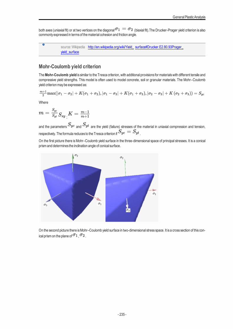
GeneralPlasticAnalysis
both axes (uniaxial fit) or at two vertices on the diagonal (biaxial fit).The Drucker-Prager yield criterion is alsocommonlyexpressed in termsof thematerial cohesion and friction angle.
source: Wikipedia http://en.wikipedia.org/wiki/Yield_ surface#Drucker.E2.80.93Prager_yield_surface
Mohr-Coulomb yield criterionTheMohr-Coulomb yield is similar to the Tresca criterion, with additional provisions for materialswith different tensile andcompressive yield strengths. This model is often used to model concrete, soil or granular materials. The Mohr–Coulombyield criterionmaybe expressed as:
Where
;
and the parameters and are the yield (failure) stresses of the material in uniaxial compression and tension,
respectively. The formula reduces to the Tresca criterion if .
On the first picture there is Mohr–Coulomb yield surface in the three-dimensional space of principal stresses. It is a conicalprismand determines the inclination angle of conical surface.
On the second picture there isMohr–Coulomb yield surface in two-dimensional stress space. It is a crosssection of this con-ical prismon the plane of , .
- 235 -
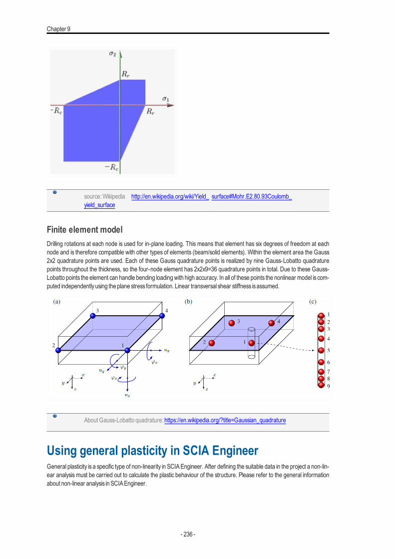
Chapter 9
source: Wikipedia http://en.wikipedia.org/wiki/Yield_ surface#Mohr.E2.80.93Coulomb_yield_surface
Finite element modelDrilling rotations at each node is used for in-plane loading. This means that element has six degrees of freedom at eachnode and is therefore compatible with other types of elements (beam/solid elements). Within the element area the Gauss2x2 quadrature points are used. Each of these Gauss quadrature points is realized by nine Gauss-Lobatto quadraturepoints throughout the thickness, so the four-node element has 2x2x9=36 quadrature points in total. Due to these Gauss-Lobatto points the element can handle bending loading with high accuracy. In all of these points the nonlinear model is com-puted independentlyusing the plane stress formulation. Linear transversal shear stiffness isassumed.
About Gauss-Lobatto quadrature: https://en.wikipedia.org/?title=Gaussian_quadrature
Using general plasticity in SCIA EngineerGeneral plasticity is a specific type of non-linearity in SCIA Engineer. After defining the suitable data in the project a non-lin-ear analysis must be carried out to calculate the plastic behaviour of the structure. Please refer to the general informationabout non-linear analysis in SCIAEngineer.
- 236 -
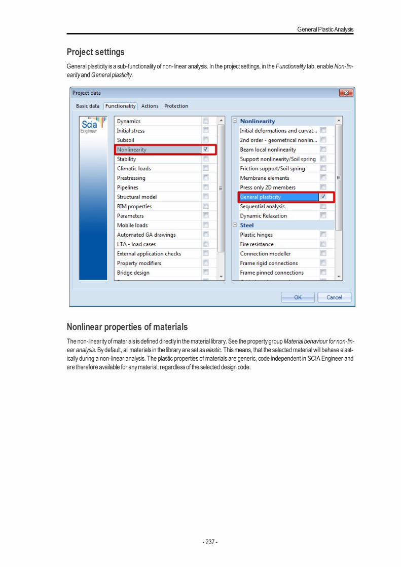
GeneralPlasticAnalysis
Project settingsGeneral plasticity is a sub-functionality of non-linear analysis. In the project settings, in the Functionality tab, enableNon-lin-earityandGeneral plasticity.
Nonlinear properties of materialsThe non-linearityofmaterials isdefined directly in thematerial library. See the propertygroupMaterial behaviour for non-lin-ear analysis. By default, allmaterials in the library are set aselastic. Thismeans, that the selectedmaterial will behave elast-ically during a non-linear analysis. The plastic properties of materials are generic, code independent in SCIA Engineer andare therefore available for anymaterial, regardlessof the selected design code.
- 237 -
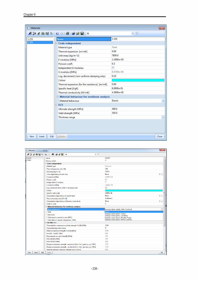
Chapter 9
- 238 -
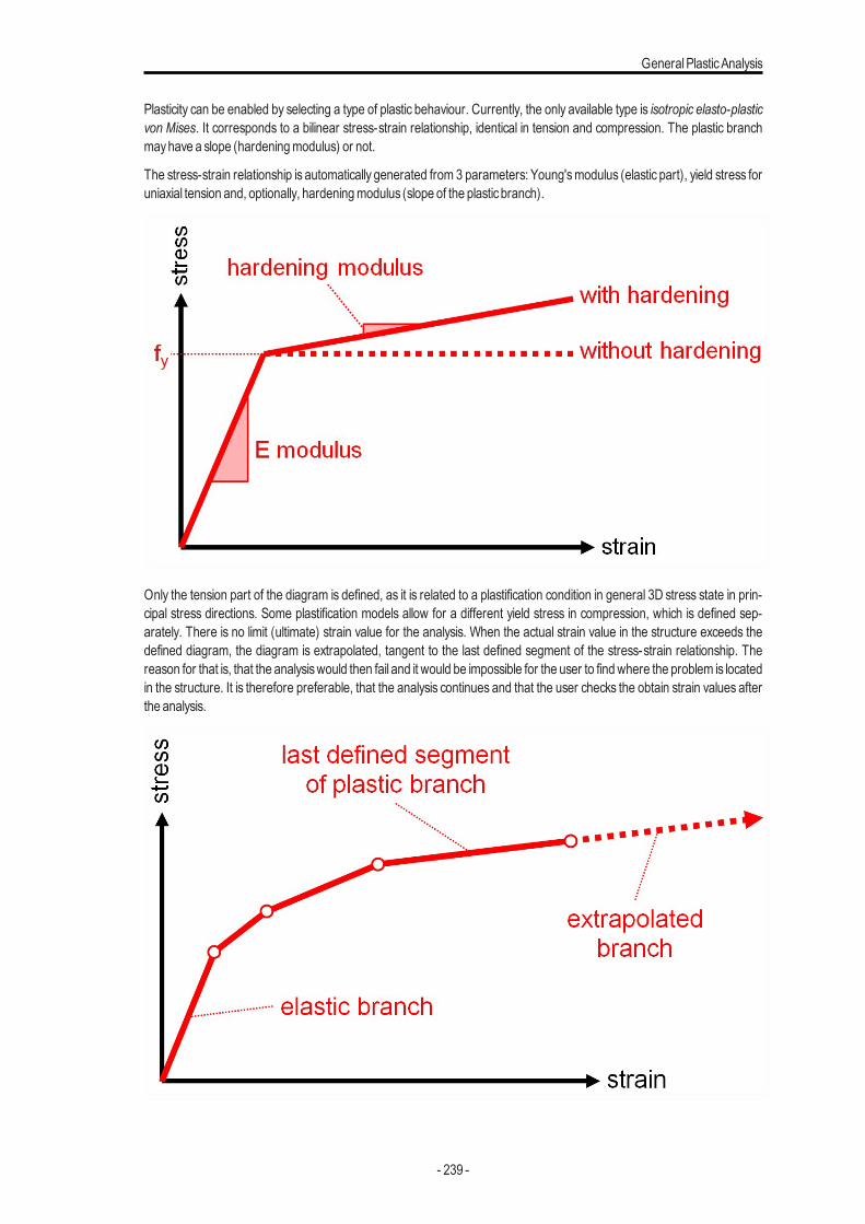
GeneralPlasticAnalysis
Plasticity can be enabled by selecting a type of plastic behaviour. Currently, the only available type is isotropic elasto-plasticvon Mises. It corresponds to a bilinear stress-strain relationship, identical in tension and compression. The plastic branchmayhave a slope (hardeningmodulus) or not.
The stress-strain relationship is automatically generated from 3 parameters: Young'smodulus (elastic part), yield stress foruniaxial tension and, optionally, hardeningmodulus (slope of the plasticbranch).
Only the tension part of the diagram is defined, as it is related to a plastification condition in general 3D stress state in prin-cipal stress directions. Some plastification models allow for a different yield stress in compression, which is defined sep-arately. There is no limit (ultimate) strain value for the analysis. When the actual strain value in the structure exceeds thedefined diagram, the diagram is extrapolated, tangent to the last defined segment of the stress-strain relationship. Thereason for that is, that the analysiswould then fail and it would be impossible for the user to findwhere the problem is locatedin the structure. It is therefore preferable, that the analysis continues and that the user checks the obtain strain values afterthe analysis.
- 239 -
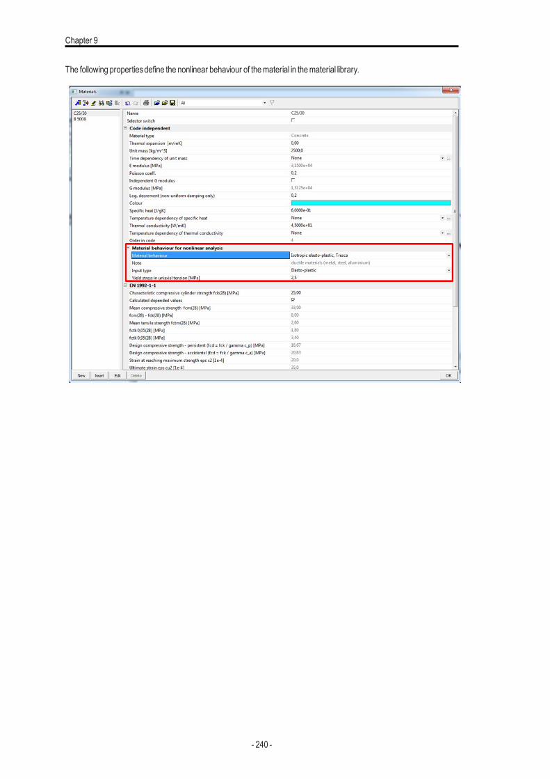
Chapter 9
The following propertiesdefine the nonlinear behaviour of thematerial in thematerial library.
- 240 -
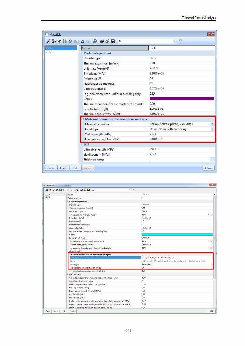
GeneralPlasticAnalysis
- 241 -
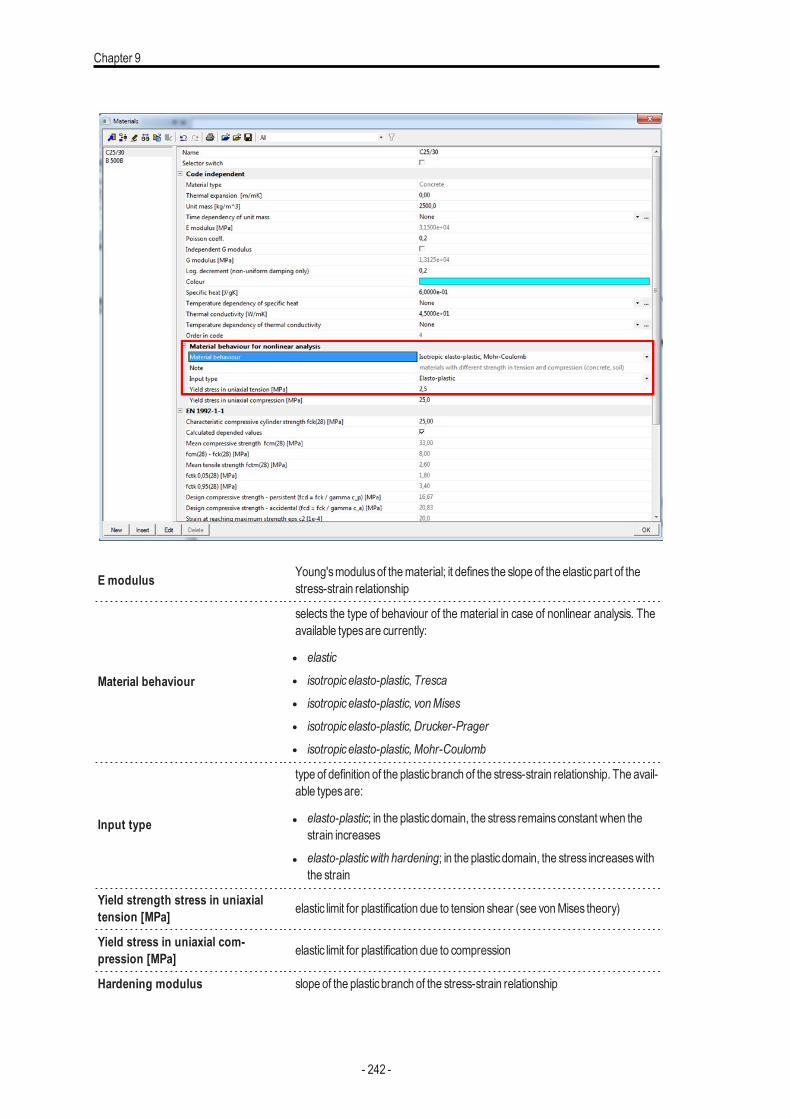
Chapter 9
E modulus Young'smodulusof thematerial; it defines the slope of the elasticpart of thestress-strain relationship
Material behaviour
selects the type of behaviour of the material in case of nonlinear analysis. Theavailable typesare currently:
l elasticl isotropicelasto-plastic, Trescal isotropicelasto-plastic, vonMisesl isotropicelasto-plastic, Drucker-Pragerl isotropicelasto-plastic, Mohr-Coulomb
Input type
type of definition of the plasticbranch of the stress-strain relationship. The avail-able typesare:
l elasto-plastic; in the plasticdomain, the stress remainsconstant when thestrain increases
l elasto-plasticwith hardening; in the plasticdomain, the stress increaseswiththe strain
Yield strength stress in uniaxialtension [MPa] elastic limit for plastification due to tension shear (see vonMises theory)
Yield stress in uniaxial com-pression [MPa] elastic limit for plastification due to compression
Hardening modulus slope of the plasticbranch of the stress-strain relationship
- 242 -
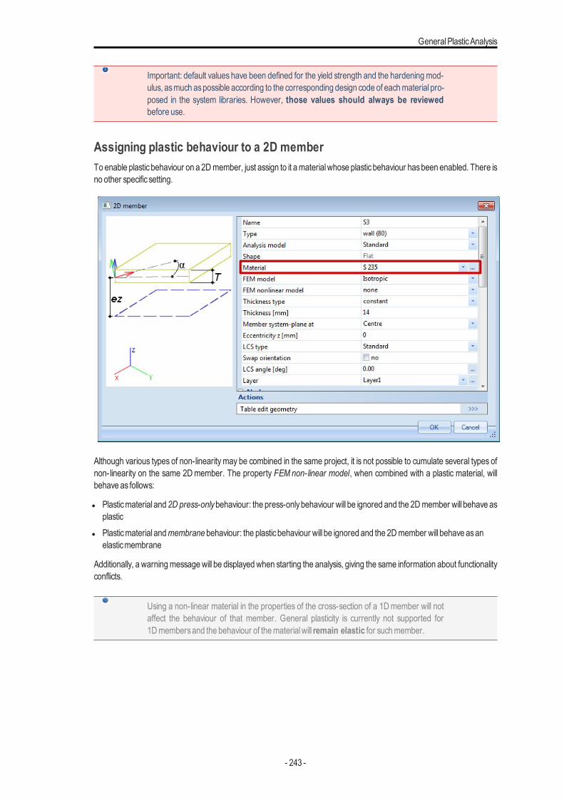
GeneralPlasticAnalysis
Important: default values have been defined for the yield strength and the hardening mod-ulus, asmuch aspossible according to the corresponding design code of eachmaterial pro-posed in the system libraries. However, those values should always be reviewedbefore use.
Assigning plastic behaviour to a 2D memberTo enable plasticbehaviour on a 2D member, just assign to it amaterialwhose plasticbehaviour hasbeen enabled. There isno other specific setting.
Although various types of non-linearity may be combined in the same project, it is not possible to cumulate several types ofnon-linearity on the same 2D member. The property FEM non-linear model, when combined with a plastic material, willbehave as follows:
l Plasticmaterial and 2D press-onlybehaviour: the press-onlybehaviour will be ignored and the 2D member will behave asplastic
l Plasticmaterial andmembrane behaviour: the plasticbehaviour will be ignored and the 2D member will behave asanelasticmembrane
Additionally, a warningmessage will be displayed when starting the analysis, giving the same information about functionalityconflicts.
Using a non-linear material in the properties of the cross-section of a 1D member will notaffect the behaviour of that member. General plasticity is currently not supported for1D membersand the behaviour of thematerialwill remain elastic for suchmember.
- 243 -

Chapter 10
Plastic hinges
Introduction to plastic hingesIf a normal linear calculation isperformed and limit stress isachieved in anypart of the structure, the dimension of critical ele-ments must be increased. If however, plastic hinges are taken into account, the achievement of limit stress causes thatplastic hinges are inserted into appropriate joints and the calculation can continue with another iteration step. The stress isredistributed to other partsof the structure and better utilisation of overall load bearing capacityof the structure isobtained.
On the other hand, there is a risk in this approach. If a hinge is added to the structure, its statical indeterminateness isreduced. If other hingesare added, it mayhappen that the structure becomesamechanism. Thiswould lead to a collapse ofthe structure and the calculation is stopped.
Plastic hinges can be thus used to calculate the plastic reliability margin of the structure. The applied load can be increasedlittle by little (e.g. by increasing the load case coefficients in load case combination) until the structure collapses. Thisapproach can be used to determine themaximum loadmultiple that the structure can sustain.
Plastic hinges are considered only at ends of individual 1D members. No selection of 1D members is made for the cal-culationwith plastichinges. If this type of calculation is selected, all 1Dmembers in the structure are tested .
The calculation is similar to the calculation of beams with gaps. All 1D members in the structure are tested and if the limitstress is reached, the plastic hinge is inserted. If however the stress lowers in the next iteration step, the plastic hingemayberemoved.
The Solver setup offers an item where a particular national code can be selected for correction of the limit moments. IfoptionNoCode isselected , themodification of the limit moments isperformed as for option EC (Eurocode).
Approachesdescribed in EC3, DIN 18800 andNEN codesare implemented in SCIAEngineer.
Plastic hinges to EC3
Axis Axial load V =<0.5 V_ V>0.5 V_
yy NSd=<0.25 NRd Mpl,y,Rd Mpl,y,Rd (1-r)
yy Nsd >0.25 NRd Mpl,y,Rd1.11 (1-n) Mpl,y,Rd1.11 (1-n-r)
zz NSd=<0.25 NRd Mpl,z,Rd Mpl,z,Rd(1-r)
zz NSd>0.25 NRdMpl,z,Rd1.56 .
. (1-n)(n+0.6)
Mpl,z,Rd1.56 .
. (1-n-r)(0.6+n/(1-r))
where:
r (2 VSd / VRd –1)2
a NSd / NRd
Nsd axial force
VSd shear force
Mpl,y,Rd full plastic moment around yy axis
Mpl,z,Rd full plastic moment around zz axis
- 244 -
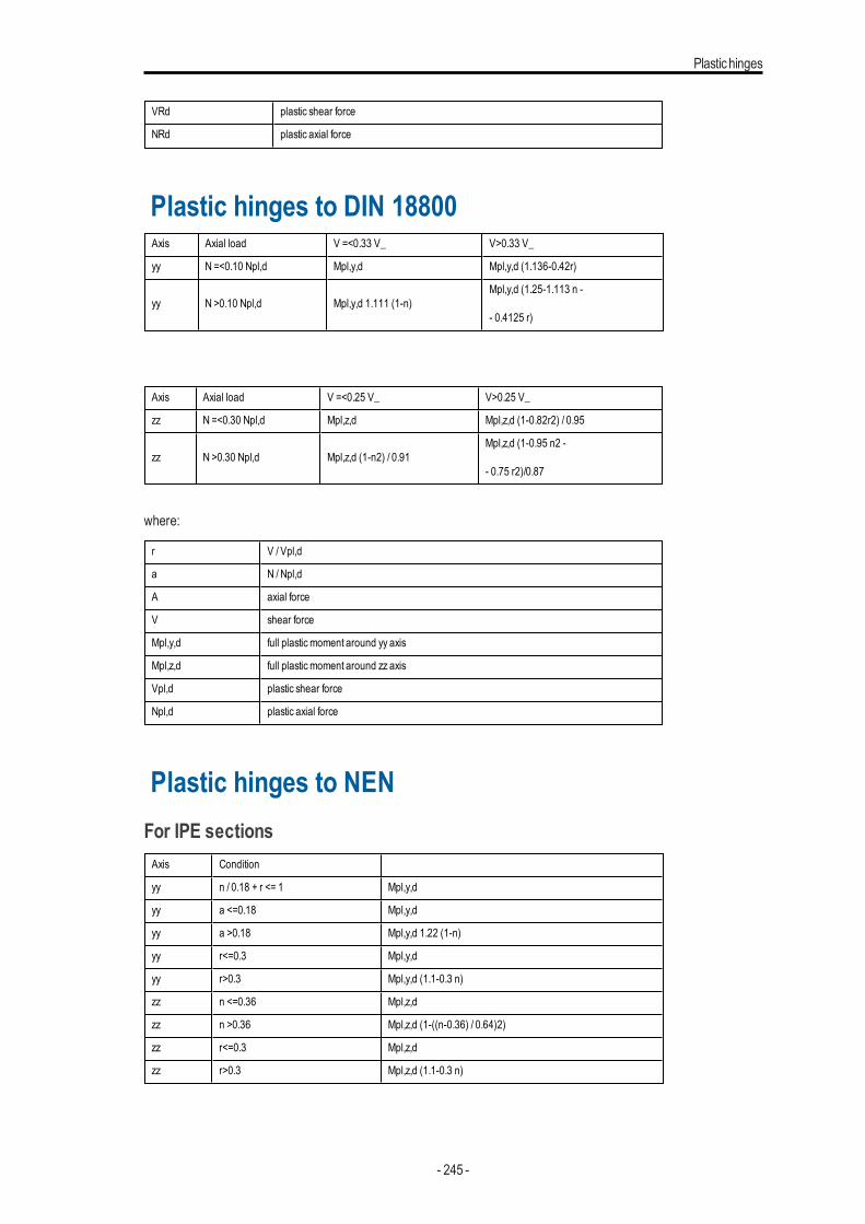
Plastichinges
VRd plastic shear force
NRd plastic axial force
Plastic hinges to DIN 18800Axis Axial load V =<0.33 V_ V>0.33 V_
yy N =<0.10 Npl,d Mpl,y,d Mpl,y,d (1.136-0.42r)
yy N >0.10 Npl,d Mpl,y,d 1.111 (1-n)Mpl,y,d (1.25-1.113 n -
- 0.4125 r)
Axis Axial load V =<0.25 V_ V>0.25 V_
zz N =<0.30 Npl,d Mpl,z,d Mpl,z,d (1-0.82r2) / 0.95
zz N >0.30 Npl,d Mpl,z,d (1-n2) / 0.91Mpl,z,d (1-0.95 n2 -
- 0.75 r2)/0.87
where:
r V / Vpl,d
a N / Npl,d
A axial force
V shear force
Mpl,y,d full plastic moment around yy axis
Mpl,z,d full plastic moment around zz axis
Vpl,d plastic shear force
Npl,d plastic axial force
Plastic hinges to NENFor IPE sectionsAxis Condition
yy n / 0.18 + r <= 1 Mpl,y,d
yy a <=0.18 Mpl,y,d
yy a >0.18 Mpl,y,d 1.22 (1-n)
yy r<=0.3 Mpl,y,d
yy r>0.3 Mpl,y,d (1.1-0.3 n)
zz n <=0.36 Mpl,z,d
zz n >0.36 Mpl,z,d (1-((n-0.36) / 0.64)2)
zz r<=0.3 Mpl,z,d
zz r>0.3 Mpl,z,d (1.1-0.3 n)
- 245 -

Chapter 10
For other sectionsAxis Condition
yy n / 0.10 + r <= 1 Mpl,y,d
yy n <=0.10 Mpl,y,d
yy n >0.10 Mpl,y,d 1.11 (1-n)
yy r<=0.3 Mpl,y,d
yy r>0.3 Mpl,y,d (1.1-0.3 n)
zz n <=0.20 Mpl,z,d
zz n >0.20 Mpl,z,d (1-((n-0.20) / 0.80)2)
zz r<=0.3 Mpl,z,d
zz r>0.3 Mpl,z,d (1.1-0.3 n)
where:
r V / Vpl,d
a N / Npl,d
A axial force
V shear force
Mpl,y,d full plastic moment around yy axis
Mpl,z,d full plastic moment around zz axis
Vpl,d plastic shear force
Npl,d plastic axial force
Calculating with plastic hingesTo perform the calculationwith plastichinges taken into account, it is necessary to:
l select Nonlinearity in Project Setup dialogue,
l select required Plastichinge code in Solver setup dialogue,
l define non-linear load case combination / combinations,
l have linear calculation of the structure successfully completed,
l start nonlinear calculation and obtain successful solution.
- 246 -
AutoDesign - Global optimization
AutoDesign - Global optimization
IntroductionIn many cases, the design of a building involves a typical calculation with only some variation in certain predefined para-meters, such as the buildingsdimensions, loading, boundary conditions, etc. Often, the principle of the analysis in all projectsis the same. If all these principles can easily be defined, parameterized and stored, the design of the building can be mademuch faster than in the traditional way of engineering. In SCIA Engineer it is easily possible to parameterize structures andsave them in a library for later reuse in other projects. Parameters, such as height of a section, length of a beam/column,span, cross-section data (including built-up sections), etc. can be easily defined without the need for programming or script-ing. The designer can choose the required structural element from the library and easily edit its boundary conditions, loads(wind, snow, etc.) according to a chosen code and the code specific combinations are applied automatically to enable thedesign of the structure. Once the structure is defined, SCIA Engineer Autodesign capabilitieswill automatically run the ana-lysisand find the optimal definition of the structure according to the specificdesign rules that are chosen by the user.
Steel and concrete members can be designed individually or within a common set of elements to satisfy the criteria of theappropriate code. The Autodesign capabilities in SCIA Engineer offer a lot of flexibility. They offer the users different levelsof control. They considerably reduce the time needed to select appropriate sections. For example, the user can select themaximum check value and type of cross-section, including I-sections, angles and welded sections. Then SCIA Engineer willdetermine the optimal profile that satisfies the code check. Automatic profile optimization can be applied to all standard andparametric sections. For parametric sections, the user chooseswhich parameter - whether height, flange thicknessor other– should be adapted. The program displays the check values graphically in the 3D view of the structure with colours giving aclear overview of (over-)dimensioned and (un)satisfactorypartsof the construction.
Principles of AutodesignOnce a structure has been designed and calculated, it is the time to perform checking and usually a kind of optimisation ofthe original design. SCIA Engineer contains a powerful tool for this task. The optimisation of applied profiles may be doneautomatically or semi-automatically. The processof Autodesign results in what maybe called an economical and good solu-tion.
Autodesign in general represents a complex task. A full, complete and really "optimal" optimisation would usually lead to along and often recursive process. Therefore, SCIAEngineer implementsa kind of compromise.
One Autodesign step takes account of a single cross-section onlyIt is possible to optimise one cross-section at a time. The user selects the cross-section froma list of all cross-sectionsused inthe structure.
One Autodesign step considers only "selected" membersIt is possible to limit the Autodesign process to only a set of selected members. The user may make a selection to specifywhich beamsof the given cross-section should be considered for the Autodesign calculations.
One Autodesign step affects the whole structureOnce the optimised cross-section is found, it is applied to ALL members in the structure that are of the specified cross-sec-tion. It is of no importance whether the Autodesign calculation was limited to a selected number of beams or not. The finaleffect of the Autodesign is that the original cross-section is simply replacedwith the new, i.e. optimised, cross-section.
Autodesign typesWithin SCIA Engineer, there are different possibilities that guide you through the optimization process. The basic option isthe use of parameters. Again, almost each entity in SCIA Engineer can be covered by a parameter. Once a project is
- 247 -
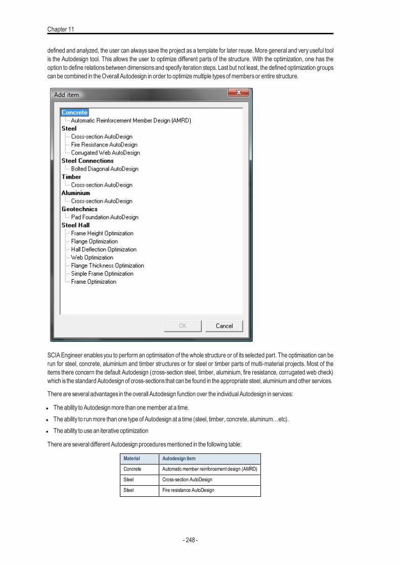
Chapter 11
defined and analyzed, the user can always save the project as a template for later reuse. More general and very useful toolis the Autodesign tool. This allows the user to optimize different parts of the structure. With the optimization, one has theoption to define relationsbetween dimensionsand specify iteration steps. Last but not least, the defined optimization groupscan be combined in theOverall Autodesign in order to optimizemultiple typesofmembersor entire structure.
SCIAEngineer enables you to perform an optimisation of the whole structure or of its selected part. The optimisation can berun for steel, concrete, aluminium and timber structures or for steel or timber parts of multi-material projects. Most of theitems there concern the default Autodesign (cross-section steel, timber, aluminium, fire resistance, corrugated web check)which is the standard Autodesign of cross-sections that can be found in the appropriate steel, aluminiumand other services.
There are several advantages in the overall Autodesign function over the individualAutodesign in services:
l The ability to Autodesignmore than onemember at a time.l The ability to runmore than one type of Autodesign at a time (steel, timber, concrete, aluminum…etc).l The ability to use an iterative optimization
There are several different Autodesign proceduresmentioned in the following table:
Material Autodesign item
Concrete Automaticmember reinforcement design (AMRD)
Steel Cross-section AutoDesign
Steel Fire resistance AutoDesign
- 248 -

AutoDesign - Global optimization
Material Autodesign item
Steel Corrugated web AutoDesign
Steel Lapped purlin/girt Autodesign (only IBC code)
Steel connection Bolted diagonal Autodesign
Timber Cross-section Autodesign
Aluminium Cross-section Autodesign
Geotechnics Pad foundation Autodesign
Steel hall In-block Autodesign item
Steel hall Frame - Autodesign manager
Steel hall Frame – CSS height Autodesign
Steel hall Frame - deflection Autodesign
Steel hall Frame - flange Autodesign
Steel hall Frame – web Autodesign
Steel hall Frame - flange thickness Autodesign
It is also possible to perform several of the abovementioned optimisation types and then compare the results. And it is up toyou to select the cross-section types and bolted diagonal connections that are relevant to your work. It is also your respons-ibility to think in advance and define and assign to 1D members as many cross-section types as necessary for a properdesign and optimisation of the project.
Note: In order to perform theAutodesign, calculationmust be alreadyperformed.
Note: Autodesign for material concrete use Automatic member reinforcement design(AMRD) fromConcrete Advanced service.
Autodesign managerAsstated in the introduction youmayperform several different optimisations. Youmay run the Autodesign and compare theresults for different parts of the structure, for different optimisation types (e.g. standard and fire resistance code check).Therefore, all the defined optimisations are stored in the Autodesign manager. Thus you do not have to define all theAutodesign criteria and parametersagain and again. TheAutodesignmanager isa standard SCIAEngineer databaseman-ager with usual featuresand functions.
Procedure to open the Autodesign manager1. Open serviceCalculation,Mesh.
2. Start (double-click) function Autodesign.
- 249 -
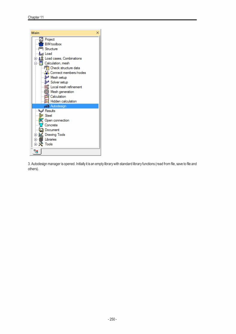
Chapter 11
3. Autodesignmanager is opened. Initially it is an empty librarywith standard library functions (read from file, save to file andothers).
- 250 -

AutoDesign - Global optimization
4. After defining the procedure (see next chapter) the following dialogue isdisplayed.
- 251 -
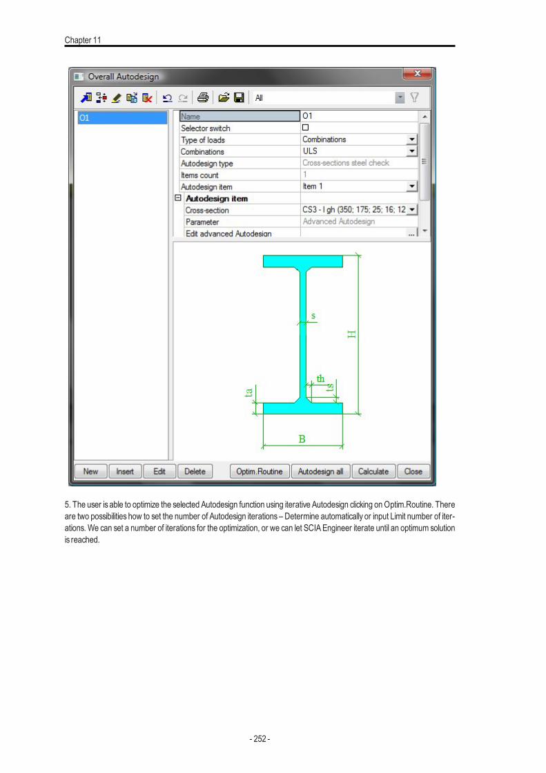
Chapter 11
5. The user is able to optimize the selected Autodesign function using iterative Autodesign clicking onOptim.Routine. Thereare two possibilities how to set the number of Autodesign iterations – Determine automatically or input Limit number of iter-ations. We can set a number of iterations for the optimization, or we can let SCIA Engineer iterate until an optimum solutionis reached.
- 252 -
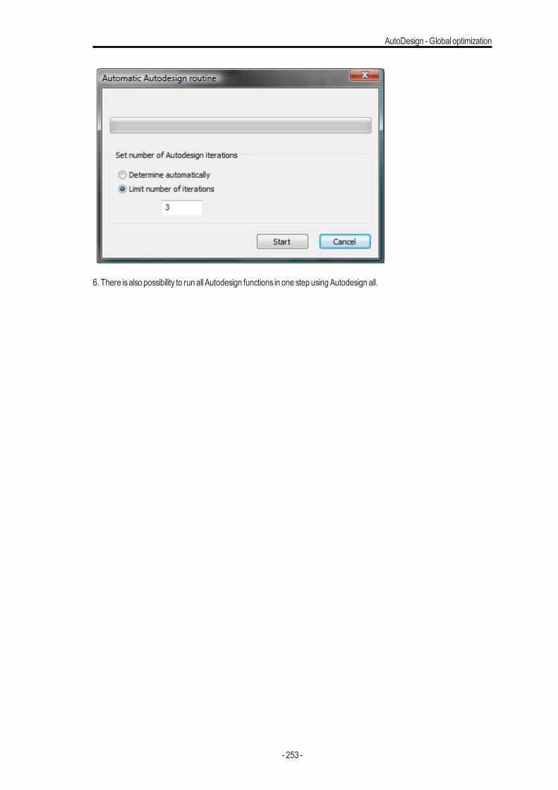
AutoDesign - Global optimization
6. There isalso possibility to run allAutodesign functions in one step usingAutodesign all.
- 253 -
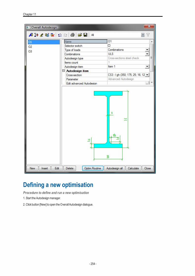
Chapter 11
Defining a new optimisationProcedure to define and run a new optimisation1. Start the Autodesignmanager.
2. Clickbutton [New] to open theOverall Autodesign dialogue.
- 254 -
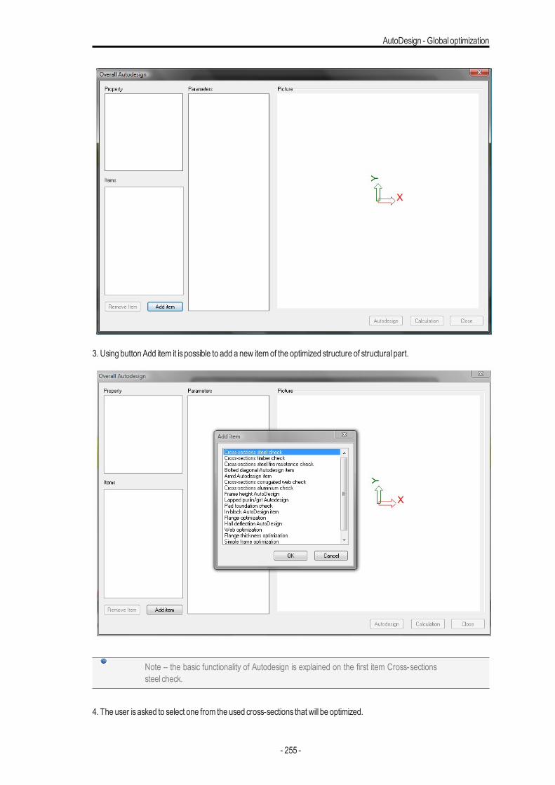
AutoDesign - Global optimization
3. Using button Add item it ispossible to add a new itemof the optimized structure of structural part.
Note – the basic functionality of Autodesign is explained on the first item Cross-sectionssteel check.
4. The user isasked to select one from the used cross-sections that will be optimized.
- 255 -
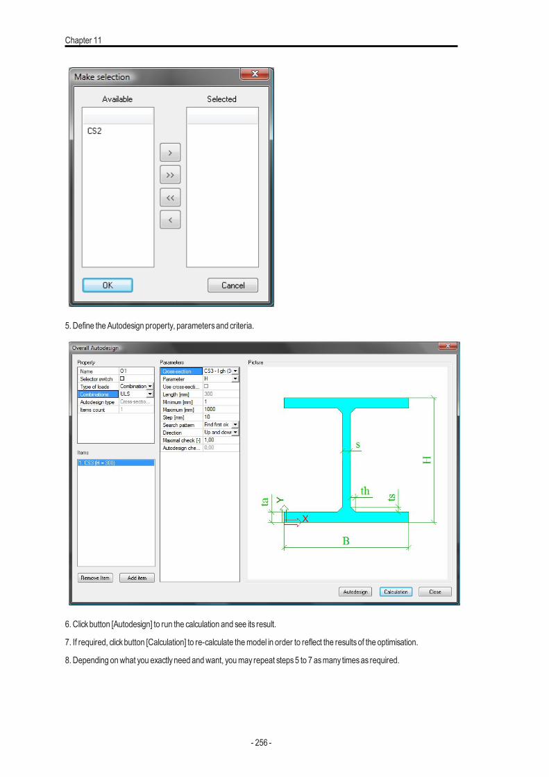
Chapter 11
5. Define theAutodesign property, parametersand criteria.
6. Clickbutton [Autodesign] to run the calculation and see its result.
7. If required, clickbutton [Calculation] to re-calculate themodel in order to reflect the resultsof the optimisation.
8. Depending onwhat you exactlyneed andwant, youmay repeat steps5 to 7 asmany timesas required.
- 256 -
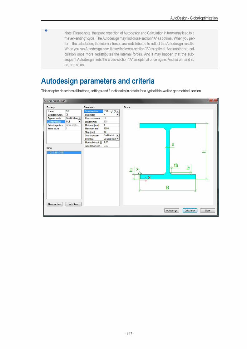
AutoDesign - Global optimization
Note: Please note, that pure repetition of Autodesign andCalculation in turnsmay lead to a"never-ending" cycle. TheAutodesignmay find cross-section "A" asoptimal.When you per-form the calculation, the internal forces are redistributed to reflect the Autodesign results.When you runAutodesign now, it may find cross-section "B" asoptimal. And another re-cal-culation once more redistributes the internal forces. And it may happen that the sub-sequent Autodesign finds the cross-section "A" as optimal once again. And so on, and soon, and so on.
Autodesign parameters and criteriaThischapter describesall buttons, settingsand functionality in details for a typical thin-walled geometrical section.
- 257 -
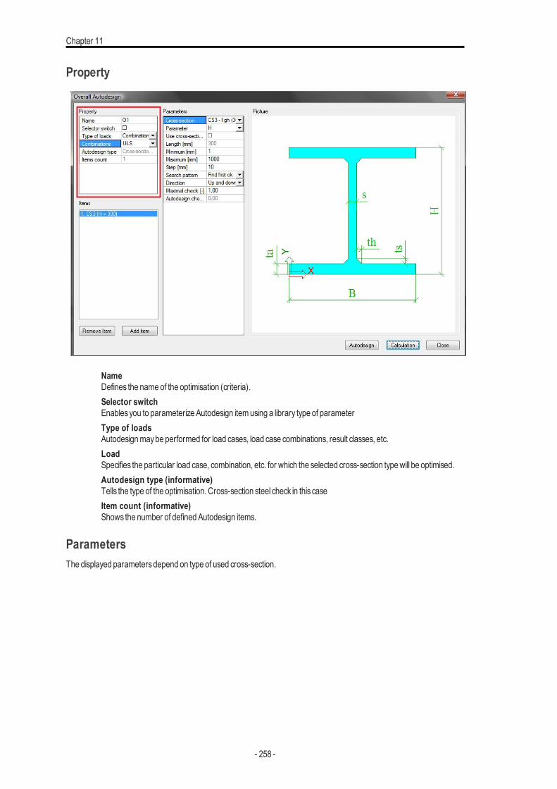
Chapter 11
Property
NameDefines the nameof the optimisation (criteria).Selector switchEnablesyou to parameterize Autodesign itemusing a library type of parameterType of loadsAutodesignmaybe performed for load cases, load case combinations, result classes, etc.LoadSpecifies the particular load case, combination, etc. for which the selected cross-section typewill be optimised.Autodesign type (informative)Tells the type of the optimisation. Cross-section steel check in this caseItem count (informative)Shows the number of definedAutodesign items.
ParametersThe displayed parametersdepend on type of used cross-section.
- 258 -
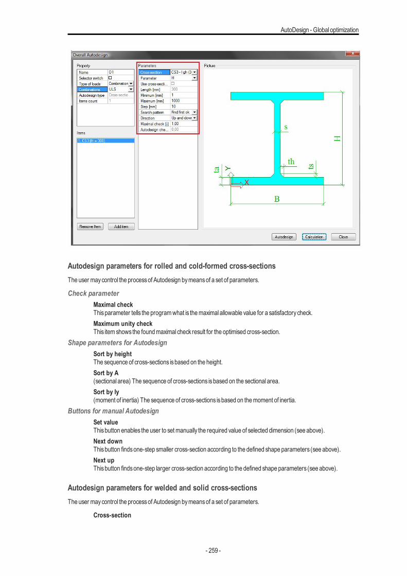
AutoDesign - Global optimization
Autodesign parameters for rolled and cold-formed cross-sectionsThe user maycontrol the processof Autodesign bymeansof a set of parameters.
Check parameterMaximal checkThisparameter tells the programwhat is themaximal allowable value for a satisfactorycheck.Maximum unity checkThis item shows the foundmaximal check result for the optimised cross-section.
Shape parameters for AutodesignSort by heightThe sequence of cross-sections isbased on the height.Sort by A(sectional area) The sequence of cross-sections isbased on the sectional area.Sort by Iy(moment of inertia) The sequence of cross-sections isbased on themoment of inertia.
Buttons for manual AutodesignSet valueThisbutton enables the user to setmanually the required value of selected dimension (see above).Next downThisbutton findsone-step smaller cross-section according to the defined shape parameters (see above).Next upThisbutton findsone-step larger cross-section according to the defined shape parameters (see above).
Autodesign parameters for welded and solid cross-sectionsThe user maycontrol the processof Autodesign bymeansof a set of parameters.
Cross-section
- 259 -
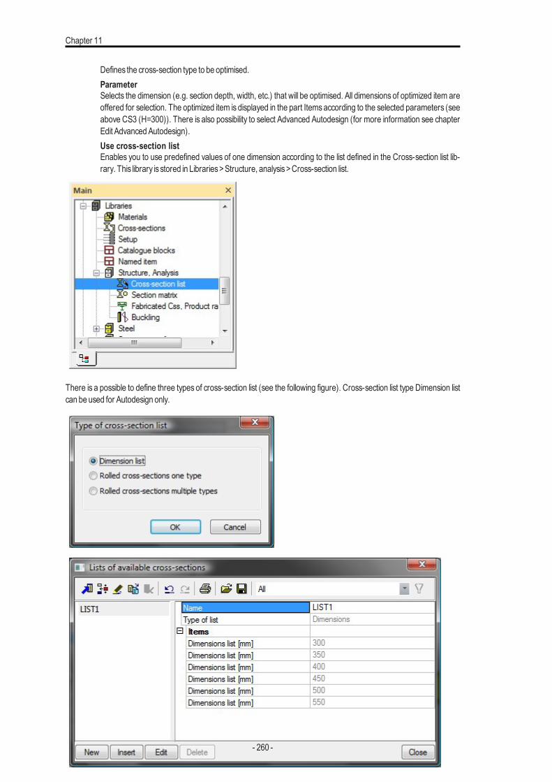
Chapter 11
Defines the cross-section type to be optimised.ParameterSelects the dimension (e.g. section depth, width, etc.) that will be optimised. All dimensions of optimized item areoffered for selection. The optimized item is displayed in the part Itemsaccording to the selected parameters (seeabove CS3 (H=300)). There is also possibility to select Advanced Autodesign (for more information see chapterEdit AdvancedAutodesign).Use cross-section listEnables you to use predefined values of one dimension according to the list defined in the Cross-section list lib-rary. This library is stored in Libraries>Structure, analysis>Cross-section list.
There is a possible to define three types of cross-section list (see the following figure). Cross-section list type Dimension listcan be used for Autodesign only.
- 260 -
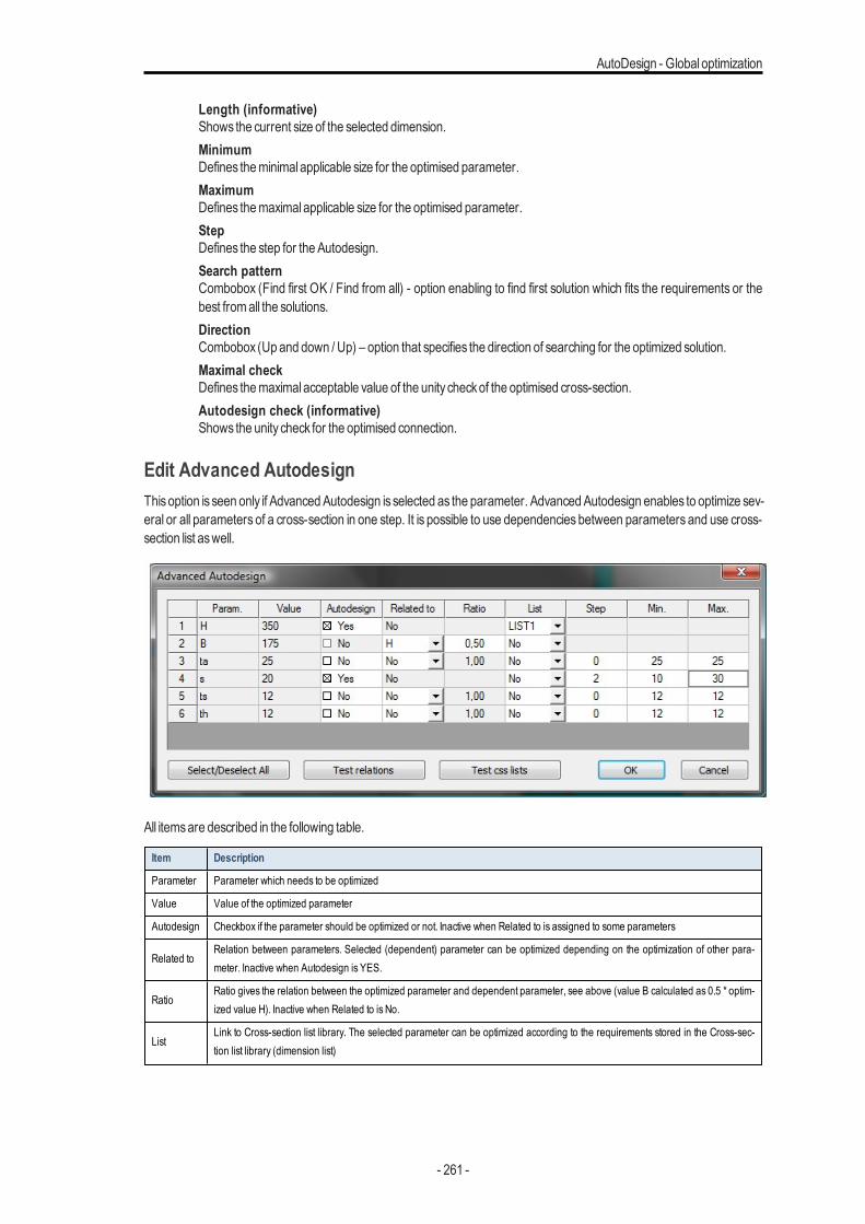
AutoDesign - Global optimization
Length (informative)Shows the current size of the selected dimension.MinimumDefines theminimal applicable size for the optimised parameter.MaximumDefines themaximal applicable size for the optimised parameter.StepDefines the step for the Autodesign.Search patternCombobox (Find first OK / Find from all) - option enabling to find first solution which fits the requirements or thebest fromall the solutions.DirectionCombobox (Up and down / Up) – option that specifies the direction of searching for the optimized solution.Maximal checkDefines themaximal acceptable value of the unity checkof the optimised cross-section.Autodesign check (informative)Shows the unity check for the optimised connection.
Edit Advanced AutodesignThisoption is seen only if AdvancedAutodesign is selected as the parameter. AdvancedAutodesign enables to optimize sev-eral or all parameters of a cross-section in one step. It is possible to use dependencies between parameters and use cross-section list aswell.
All itemsare described in the following table.
Item Description
Parameter Parameter which needs to be optimized
Value Value of the optimized parameter
Autodesign Checkbox if the parameter should be optimized or not. Inactive when Related to is assigned to some parameters
Related toRelation between parameters. Selected (dependent) parameter can be optimized depending on the optimization of other para-meter. Inactive when Autodesign is YES.
RatioRatio gives the relation between the optimized parameter and dependent parameter, see above (value B calculated as 0.5 * optim-ized value H). Inactive when Related to is No.
ListLink to Cross-section list library. The selected parameter can be optimized according to the requirements stored in the Cross-sec-tion list library (dimension list)
- 261 -
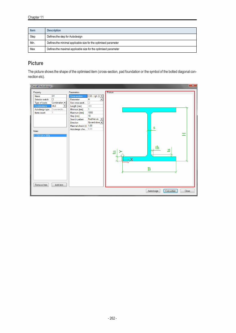
Chapter 11
Item Description
Step Defines the step for Autodesign
Min. Defines the minimal applicable size for the optimised parameter
Max Defines the maximal applicable size for the optimised parameter
PictureThe picture shows the shape of the optimised item (cross-section, pad foundation or the symbol of the bolted diagonal con-nection etc).
- 262 -
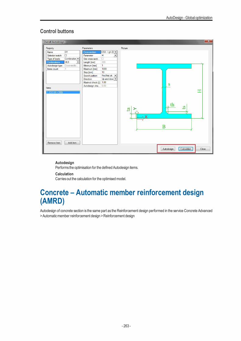
AutoDesign - Global optimization
Control buttons
AutodesignPerforms the optimisation for the definedAutodesign items.CalculationCarriesout the calculation for the optimisedmodel.
Concrete – Automatic member reinforcement design(AMRD)Autodesign of concrete section is the same part as the Reinforcement design performed in the service Concrete Advanced>Automaticmember reinforcement design >Reinforcement design
- 263 -
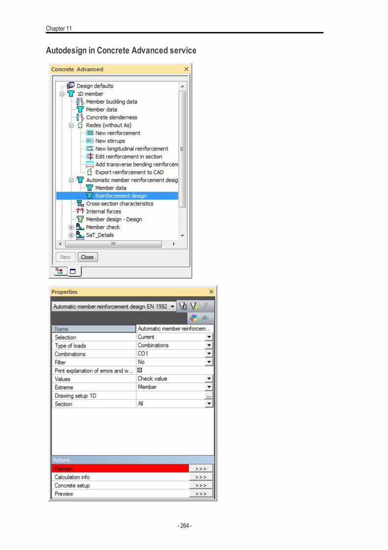
Chapter 11
Autodesign in Concrete Advanced service
- 264 -

AutoDesign - Global optimization
When the user clicks on action button Refresh then the same procedure of Autodesign is performed. For concrete cross-section the procedure is called Automatic Member Reinforcement Design (AMRD). The non-prestressed reinforcement isdesigned in selected beam. Both longitudinal reinforcement and stirrupsare designed.
Theoretical background for AMRDThe non-prestressed reinforcement in beams can be defined manually by the user or it can be calculated automatically bythe program.
The latter designs the reinforcement on the basisof parametersdefined in:
l reinforcement template,l setup dialogue of serviceConcrete Advanced,l member data related to the automaticdesign,l practical reinforcement definedmanually.
The automatic design takes into account the combination of bending moments and axial force and shear forces. It does notinclude torsion and deflections. It works within the ultimate limit state. The automatic design can be used for loads cases,ULS (not SLS) combinations and classes with ULS or ULS+SLS combinations. Concerning the parameters mentionedabove, the practical reinforcement is of the highest priority. That means, if some reinforcement has been defined, the auto-matic design uses in the first step the diameter of this practical reinforcement. There is no output to the document. The res-ults of the automatic design can be reviewed only on the screen in the graphical window and/or in the Preview window. Ofcourse, the bill of reinforcement can be inserted into the document in order to show the reinforcement that has been auto-matically designed. The automatic design uses only the layers of the reinforcement marked in the reinforcement template.The automatic design is not capable of adding a new layer in the situation when the required reinforcement cannot be putinto just one layer. Therefore, it mayhappen that the automaticdesign can fail.
The basicprocedure is the following:
l First, the parameters thatmayaffect the automaticdesign should be defined. It isnecessary to define rein-forcement template for longitudinal reinforcement, which layerscan be optimise during the automatic rein-forcement procedure,
l Specify the default parameters in
o Setup dialogue of serviceConcrete Advanced affecting and controlling the procedure for theautomaticdesign,
o member data related to the automaticdesign, if required. These data overwrites the default val-uesbymember data that are specific for a particular beam.
l During Autodesign the standard design of reinforcement for combinationN+My+Mz isperformed (max-imal bendingmomentsalongwholemember are considered for design of reinforcement). Themaximalamount of upper and lower reinforcement isdesigned.
l The designed reinforcement template isused for checks (Interaction diagram, detailing provisions). Thecalculation isevaluated based on themaximal utilisation (checkvalue) in concrete setup.When the cal-culated checkvalue is still less than the defined utilisation, then barsare deleted to achieve the optimal util-isation.
Template preparationThe template used for the Autodesign is prepared in a standard way. One difference is that the check boxAutomaticmem-ber design is switchedON.
- 265 -
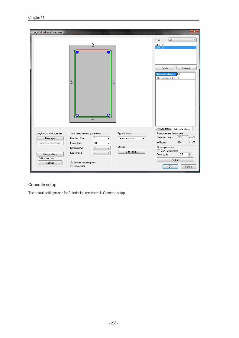
Chapter 11
Concrete setupThe default settingsused for Autodesign are stored inConcrete setup.
- 266 -

AutoDesign - Global optimization
Member data for the automatic reinforcement designThemember data used for AMRD looks like this:
GeneralMax. exploit-ation of cross-
Specifies the maximal utilisation of the cross- section in the auto-matically reinforced beam. The valuemaybe between 1 and 100%.
- 267 -

Chapter 11
section
Reinforcementtemplate
Shows the used reinforcement template. Note: This item appears inthe dialogue ONLY when the already defined member data areedited. If the member data are being assigned to a new member,this item isnot accessible.
Longitudinal reinforcement
Try to reducelength of bars
If OFF, the program uses only bars that extent over the wholelength of the beam.
If ON, some bars may be shortened if the unity check is satisfiedwithout them.
Maximal num-ber of biggerdiameters thanthe default
Defines how many different (bigger) diameters of the rein-forcement can be used for the optimisation. Let us assume that thedefault diameter specified in the Design default tab is 10 mm. If thisparameter is set to 2, the program can use diameters 10, 12 (i.e.+1 item in the manufacturing programme) and 14 (i.e. +2 item inthemanufacturing programme) for the design.
Do not use"Neighbouring"bars
Some standards recommend that "neighbouring" profiles from themanufacturing programme should not be used in one beam (inorder to avoid unintentional interchange of the profiles). Let usassume that the default diameter specified in theDesign default tabis 10 mm. Further assume that Maximal number of bigger dia-meters than the default is set to 2. If this option isON, the followingbars can be inserted into the beam: (i) either 10 mm, (ii) or 12 mm,(iii) or 14mm, (iv) or 10mmand 14mmcan be combined together.10mmand 12mmare not permitted to be combined in one beam
StirrupsMinimal stir-rups dis-tance
Specifies the minimal distance between stirrups measured from thecentre of a bar to the centre of an adjacent bar.
Stirrupsstep
Defines the step for the reduction of the distance between two adjacentstirrups. This ensures that the distance between stirrups is always a"rounded" number – e.g. 200 mm, then 250 mm, then 300 mm, etc.(and not e.g. 200, 246mm, 298mm, etc.).
Try to cre-ate sym-metricalstirrupsparts
This parameter may enforce that the stirrup parts are symmetricalalong the length of the beam.
Member(informativeonly)
Shows the nameof the beamwhere themember data are assigned to
- 268 -
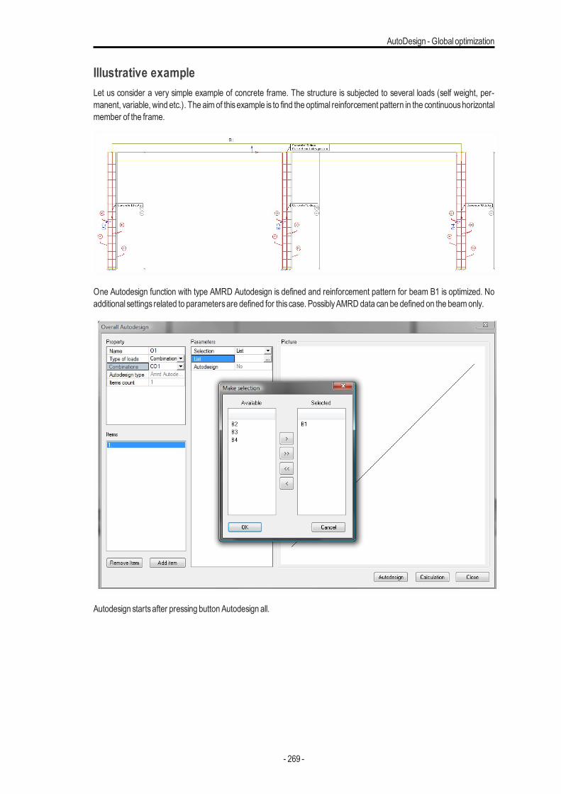
AutoDesign - Global optimization
Illustrative exampleLet us consider a very simple example of concrete frame. The structure is subjected to several loads (self weight, per-manent, variable, wind etc.). The aim of thisexample is to find the optimal reinforcement pattern in the continuoushorizontalmember of the frame.
One Autodesign function with type AMRD Autodesign is defined and reinforcement pattern for beam B1 is optimized. Noadditional settings related to parametersare defined for this case. PossiblyAMRD data can be defined on the beamonly.
Autodesign startsafter pressing button Autodesign all.
- 269 -
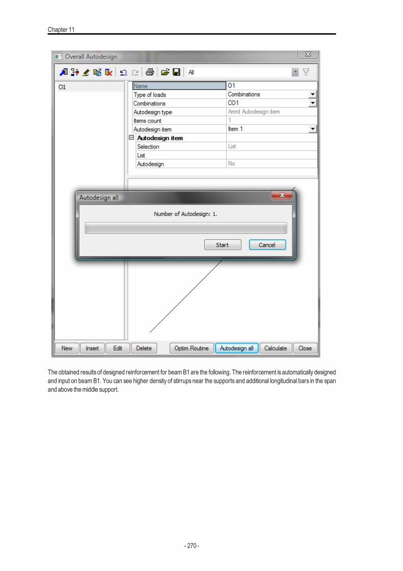
Chapter 11
The obtained results of designed reinforcement for beamB1 are the following. The reinforcement is automatically designedand input on beam B1. You can see higher density of stirrups near the supports and additional longitudinal bars in the spanand above themiddle support.
- 270 -
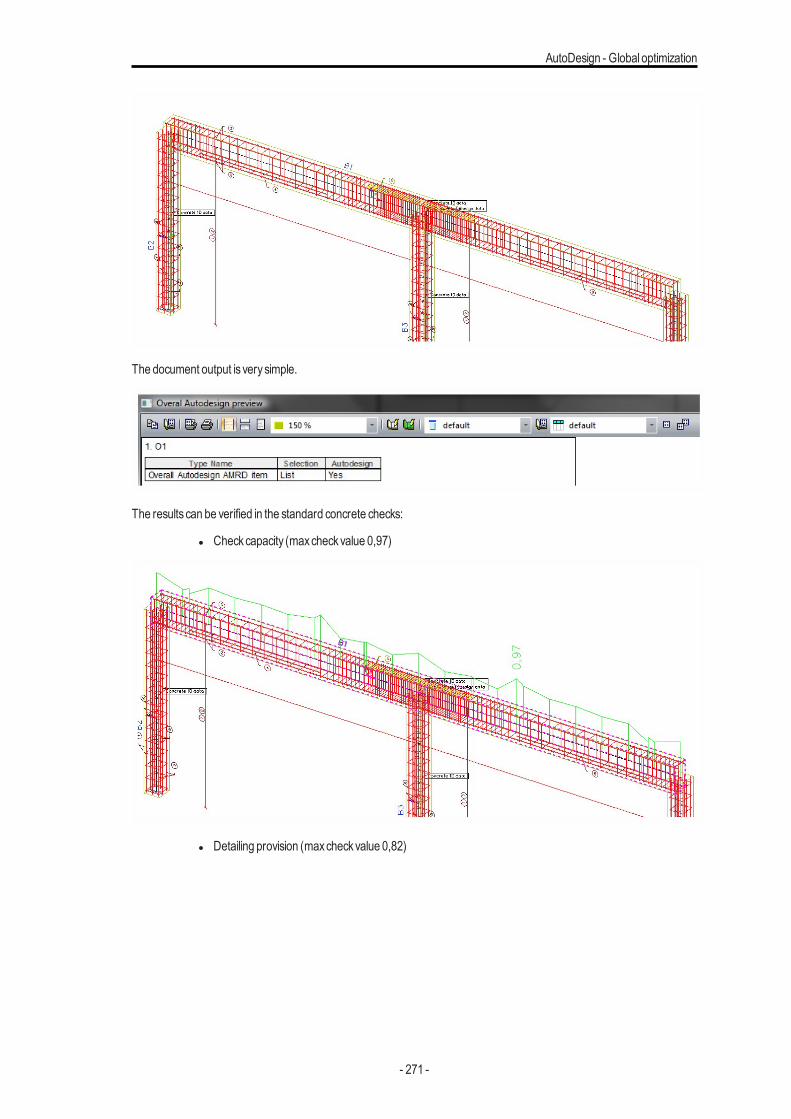
AutoDesign - Global optimization
The document output is verysimple.
The results can be verified in the standard concrete checks:
l Checkcapacity (maxcheckvalue 0,97)
l Detailing provision (maxcheckvalue 0,82)
- 271 -
Chapter 11
Steel – Cross-section AutoDesignAutodesign of cross-section steel check is the same part as the Autodesign located in the standard Steel >ULS Check>Check.
- 272 -
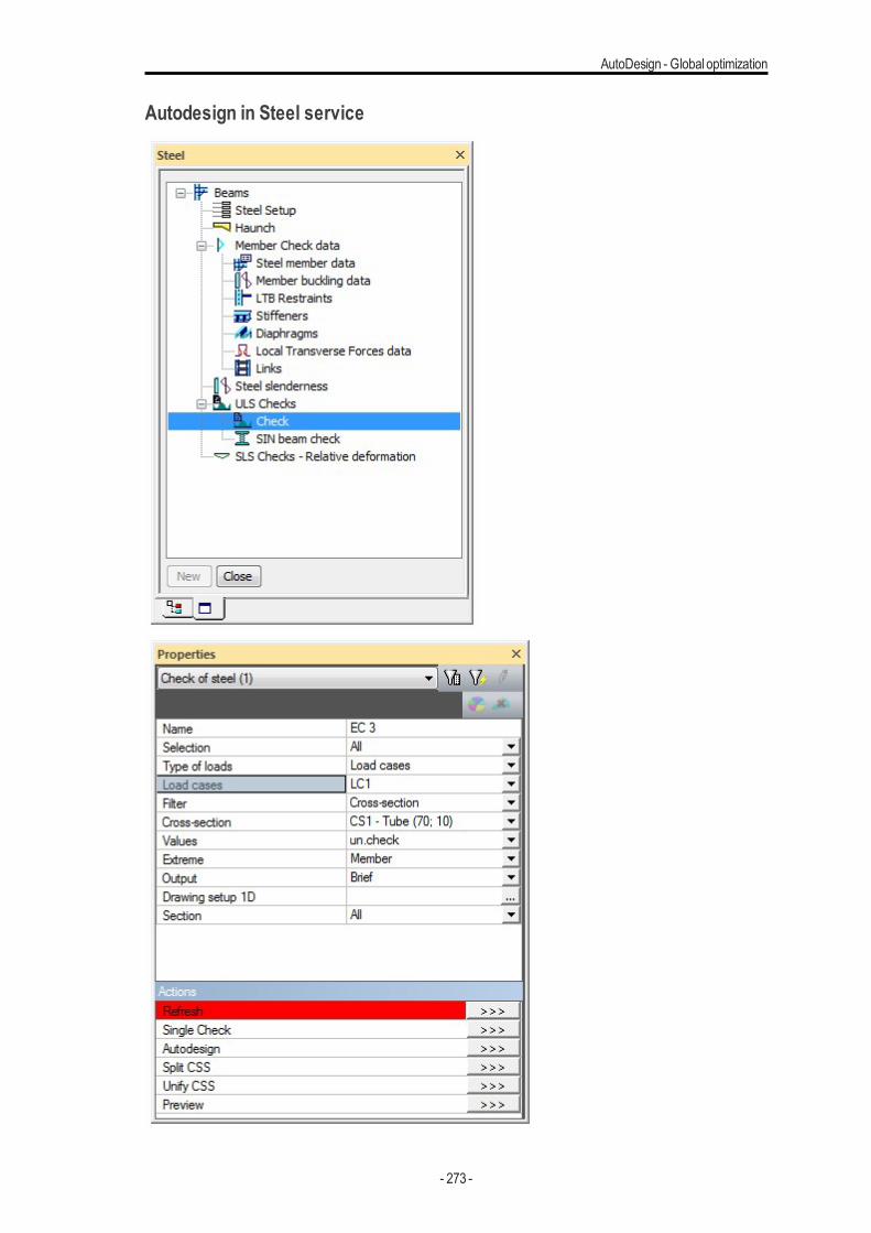
AutoDesign - Global optimization
Autodesign in Steel service
- 273 -
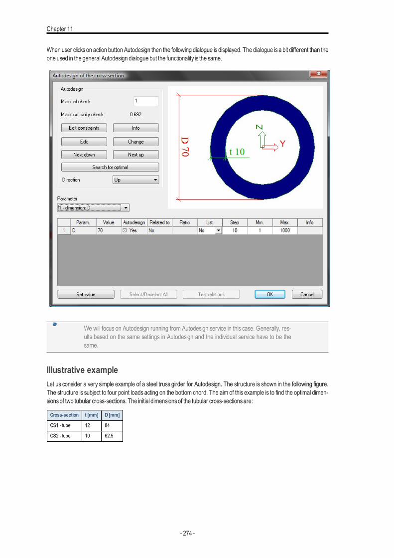
Chapter 11
When user clickson action button Autodesign then the following dialogue is displayed. The dialogue isa bit different than theone used in the generalAutodesign dialogue but the functionality is the same.
We will focus on Autodesign running from Autodesign service in this case. Generally, res-ults based on the same settings in Autodesign and the individual service have to be thesame.
Illustrative exampleLet us consider a very simple example of a steel truss girder for Autodesign. The structure is shown in the following figure.The structure is subject to four point loads acting on the bottom chord. The aim of this example is to find the optimal dimen-sionsof two tubular cross-sections. The initial dimensionsof the tubular cross-sectionsare:
Cross-section t [mm] D [mm]
CS1 - tube 12 84
CS2 - tube 10 62.5
- 274 -
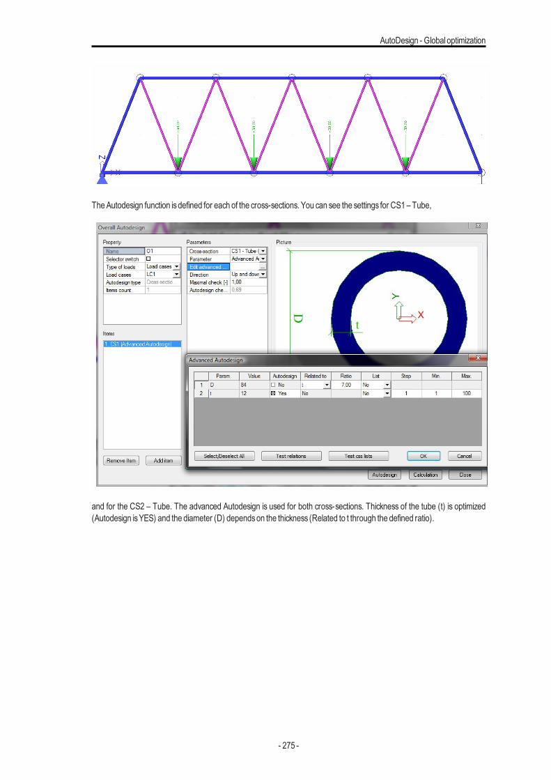
AutoDesign - Global optimization
TheAutodesign function isdefined for each of the cross-sections. You can see the settings for CS1 –Tube,
and for the CS2 – Tube. The advanced Autodesign is used for both cross-sections. Thickness of the tube (t) is optimized(Autodesign isYES) and the diameter (D) dependson the thickness (Related to t through the defined ratio).
- 275 -
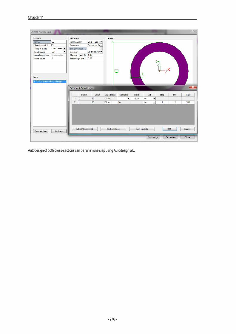
Chapter 11
Autodesign of both cross-sectionscan be run in one step usingAutodesign all..
- 276 -
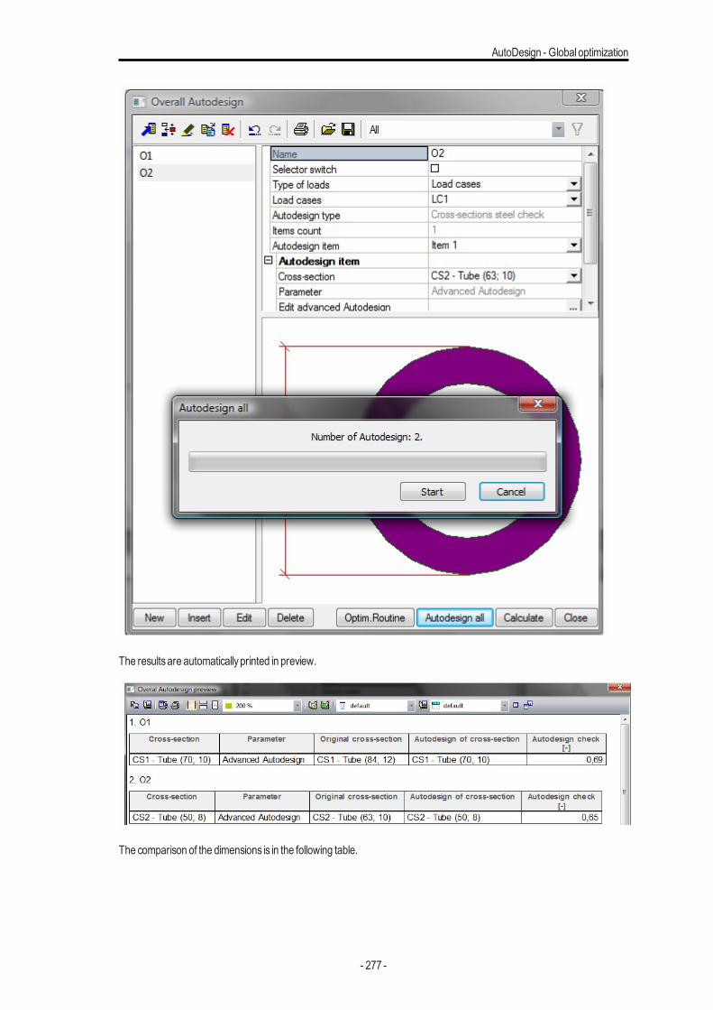
AutoDesign - Global optimization
The resultsare automaticallyprinted in preview.
The comparison of the dimensions is in the following table.
- 277 -
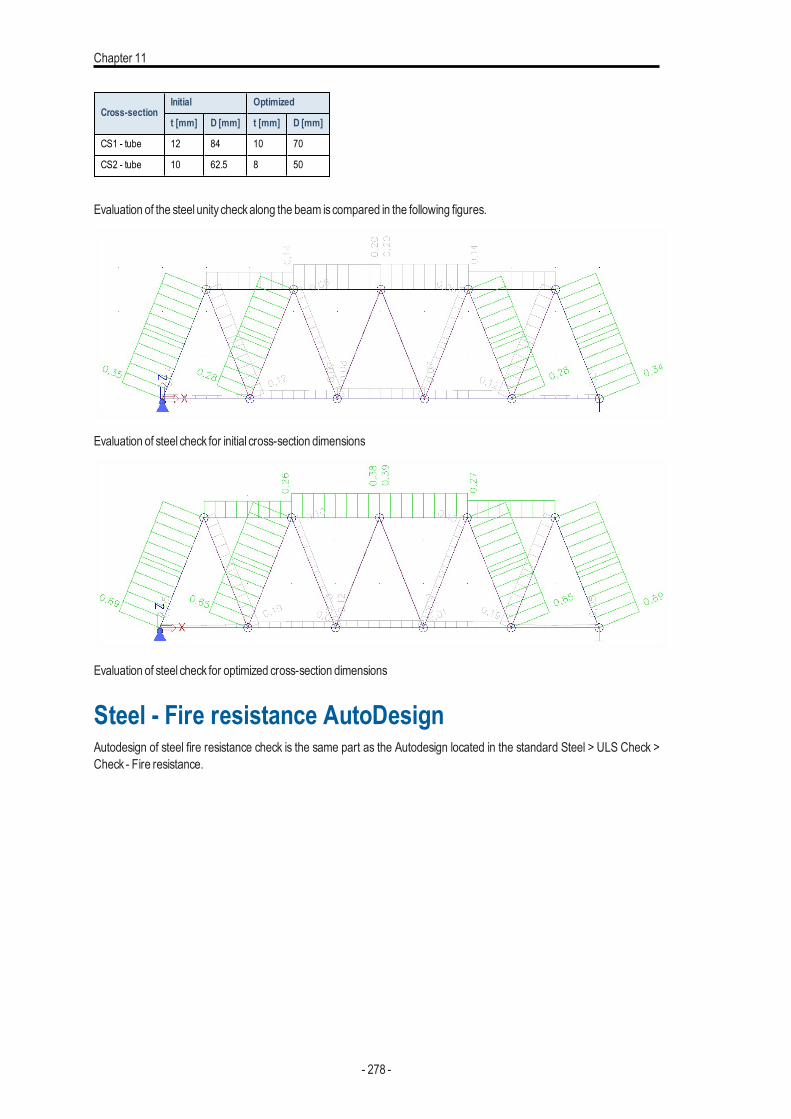
Chapter 11
Cross-sectionInitial Optimized
t [mm] D [mm] t [mm] D [mm]
CS1 - tube 12 84 10 70
CS2 - tube 10 62.5 8 50
Evaluation of the steel unity checkalong the beam iscompared in the following figures.
Evaluation of steel check for initial cross-section dimensions
Evaluation of steel check for optimized cross-section dimensions
Steel - Fire resistance AutoDesignAutodesign of steel fire resistance check is the same part as the Autodesign located in the standard Steel > ULS Check >Check - Fire resistance.
- 278 -
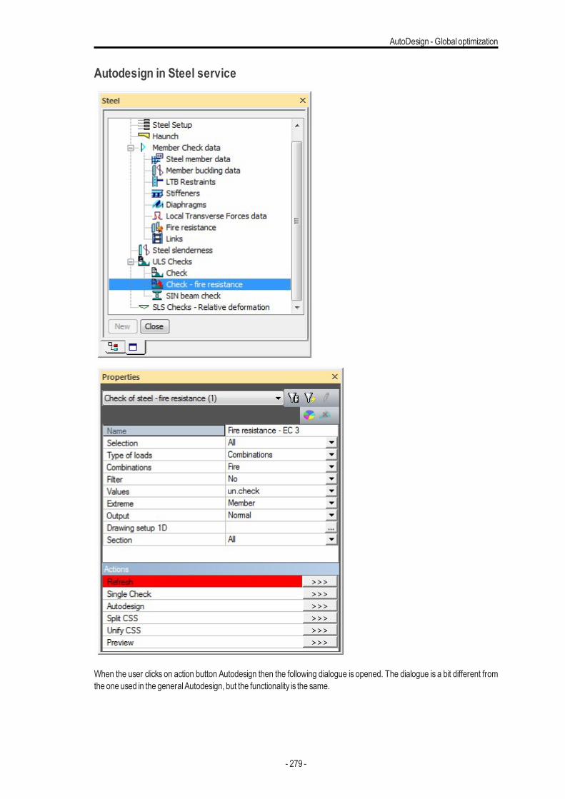
AutoDesign - Global optimization
Autodesign in Steel service
When the user clicks on action button Autodesign then the following dialogue is opened. The dialogue is a bit different fromthe one used in the generalAutodesign, but the functionality is the same.
- 279 -

Chapter 11
Illustrative exampleLet usconsider a very simple example of a steel beamwith HEB400 cross-section for Autodesign. The structure is subject tothe uniform load and to the axial force at one end. The aimof thisexample is to find the optimal height of the cross-section.
The accidental combination has to be defined. The fire resistance data are used asdefined on the following figure.
- 280 -
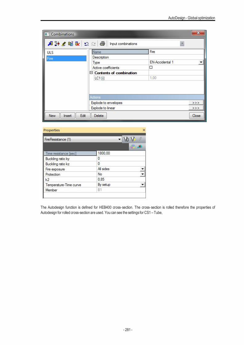
AutoDesign - Global optimization
The Autodesign function is defined for HEB400 cross- section. The cross- section is rolled therefore the properties ofAutodesign for rolled cross-section are used. You can see the settings for CS1 –Tube,
- 281 -
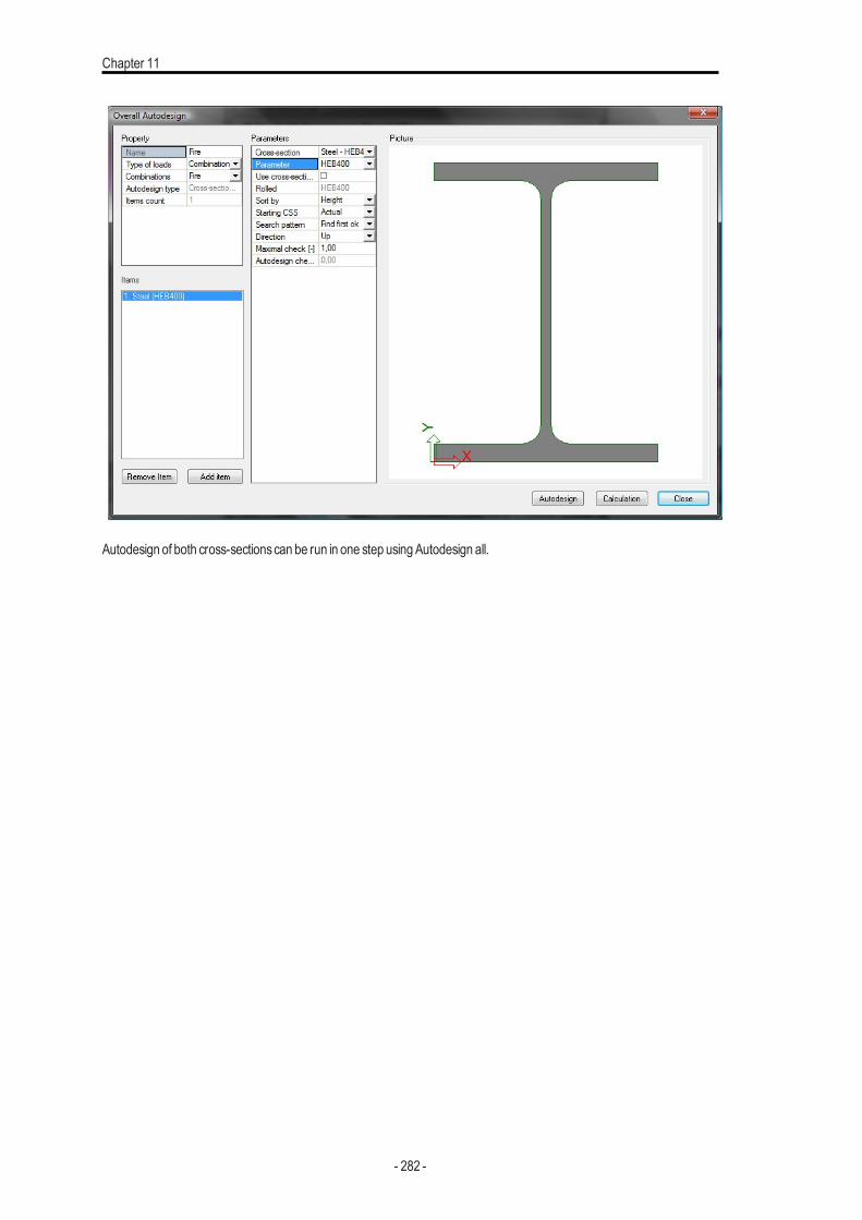
Chapter 11
Autodesign of both cross-sectionscan be run in one step usingAutodesign all.
- 282 -
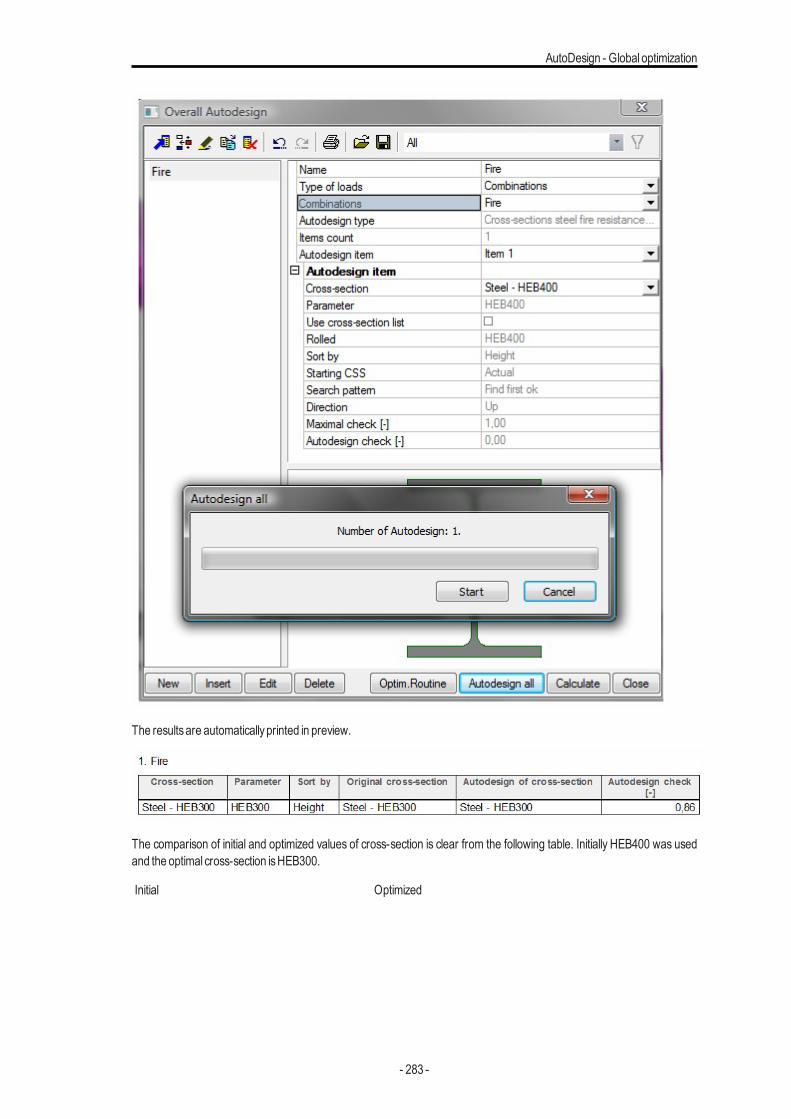
AutoDesign - Global optimization
The resultsare automaticallyprinted in preview.
The comparison of initial and optimized values of cross-section is clear from the following table. Initially HEB400 was usedand the optimal cross-section isHEB300.
Initial Optimized
- 283 -
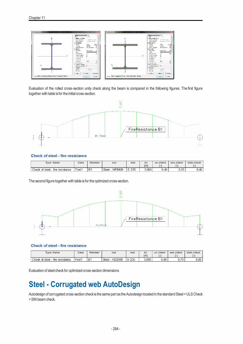
Chapter 11
Evaluation of the rolled cross-section unity check along the beam is compared in the following figures. The first figuretogether with table is for the initial cross-section.
The second figure together with table is for the optimized cross-section.
Evaluation of steel check for optimized cross-section dimensions
Steel - Corrugated web AutoDesignAutodesign of corrugated cross-section check is the same part as theAutodesign located in the standard Steel >ULSCheck>SIN beamcheck.
- 284 -
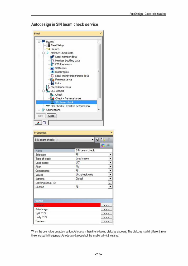
AutoDesign - Global optimization
Autodesign in SIN beam check service
When the user clicks on action button Autodesign then the following dialogue appears. The dialogue is a bit different fromthe one used in the generalAutodesign dialogue but the functionality is the same.
- 285 -
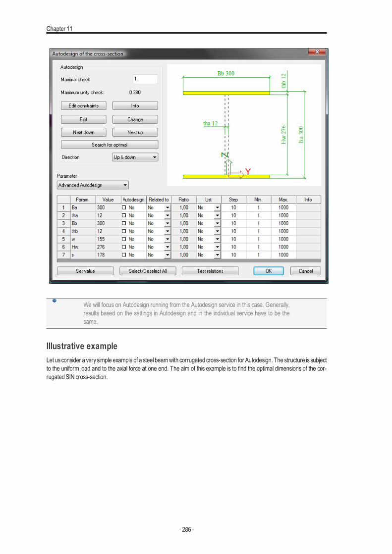
Chapter 11
We will focus on Autodesign running from the Autodesign service in this case. Generally,results based on the settings in Autodesign and in the individual service have to be thesame.
Illustrative exampleLet usconsider a verysimple example of a steel beamwith corrugated cross-section for Autodesign. The structure is subjectto the uniform load and to the axial force at one end. The aim of this example is to find the optimal dimensions of the cor-rugatedSIN cross-section.
- 286 -
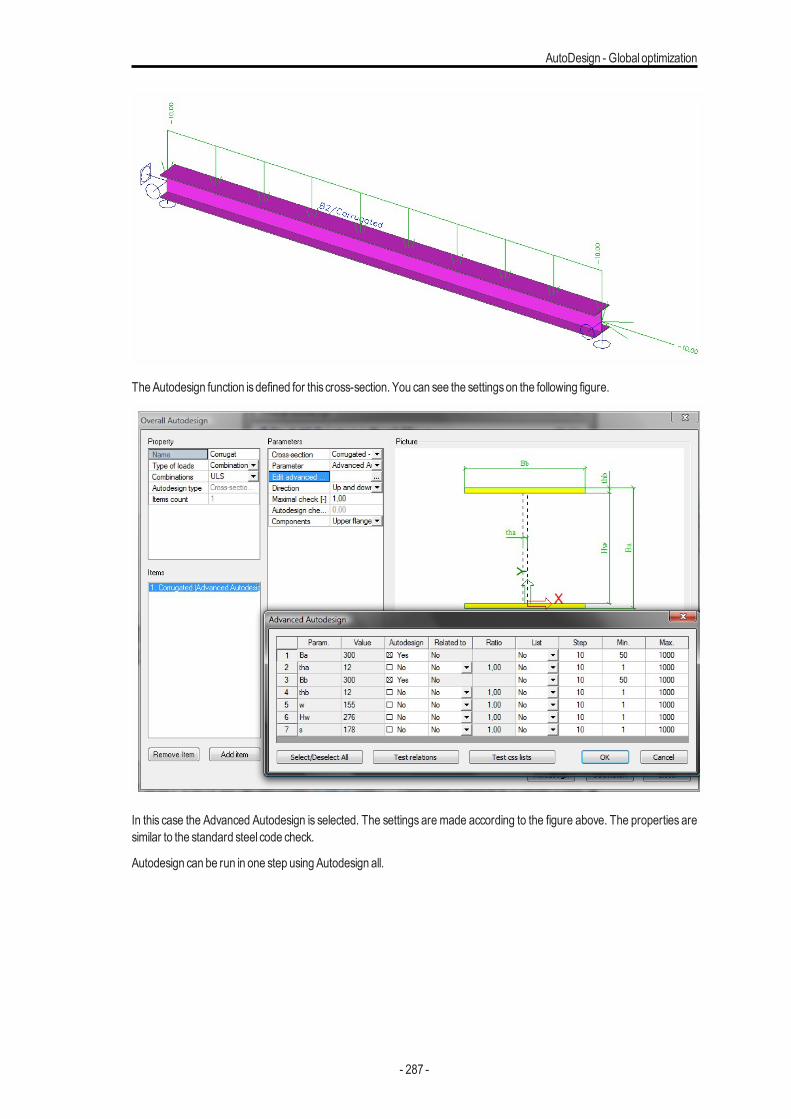
AutoDesign - Global optimization
TheAutodesign function isdefined for this cross-section. You can see the settingson the following figure.
In this case the Advanced Autodesign is selected. The settings are made according to the figure above. The properties aresimilar to the standard steel code check.
Autodesign can be run in one step usingAutodesign all.
- 287 -
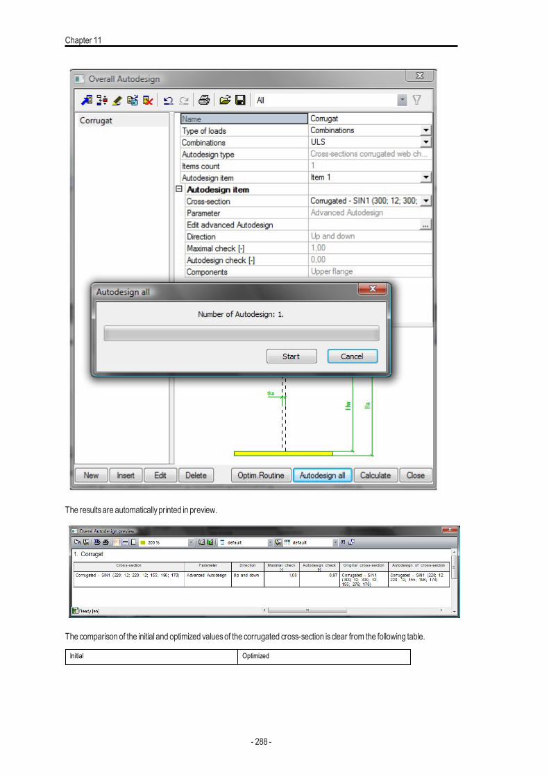
Chapter 11
The resultsare automaticallyprinted in preview.
The comparison of the initial and optimized valuesof the corrugated cross-section is clear from the following table.
Initial Optimized
- 288 -
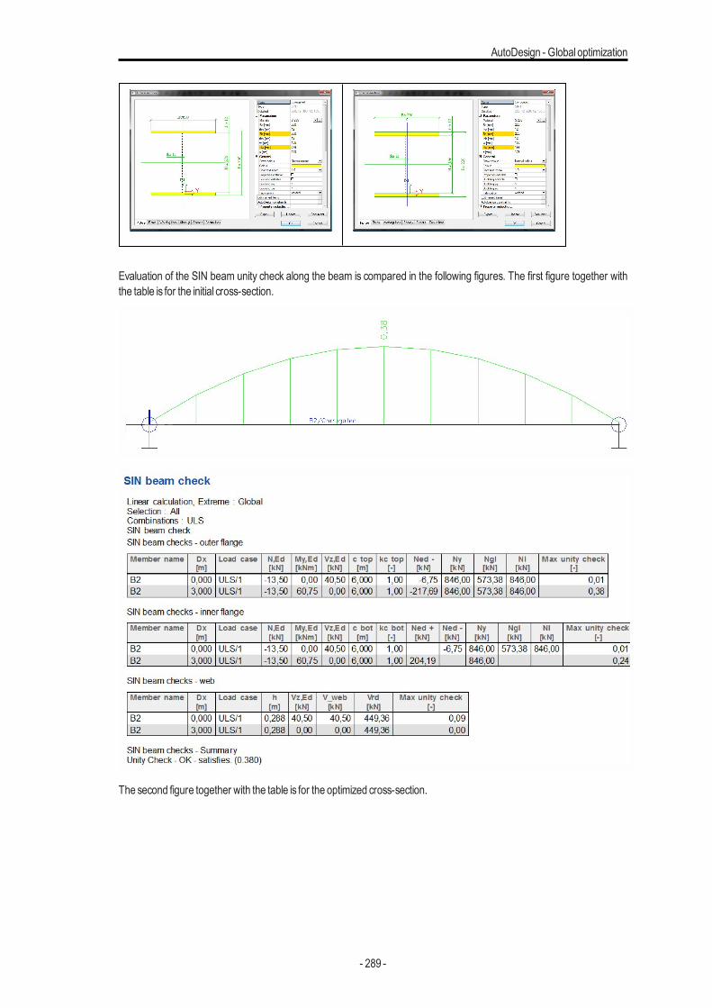
AutoDesign - Global optimization
Evaluation of the SIN beam unity check along the beam is compared in the following figures. The first figure together withthe table is for the initial cross-section.
The second figure together with the table is for the optimized cross-section.
- 289 -
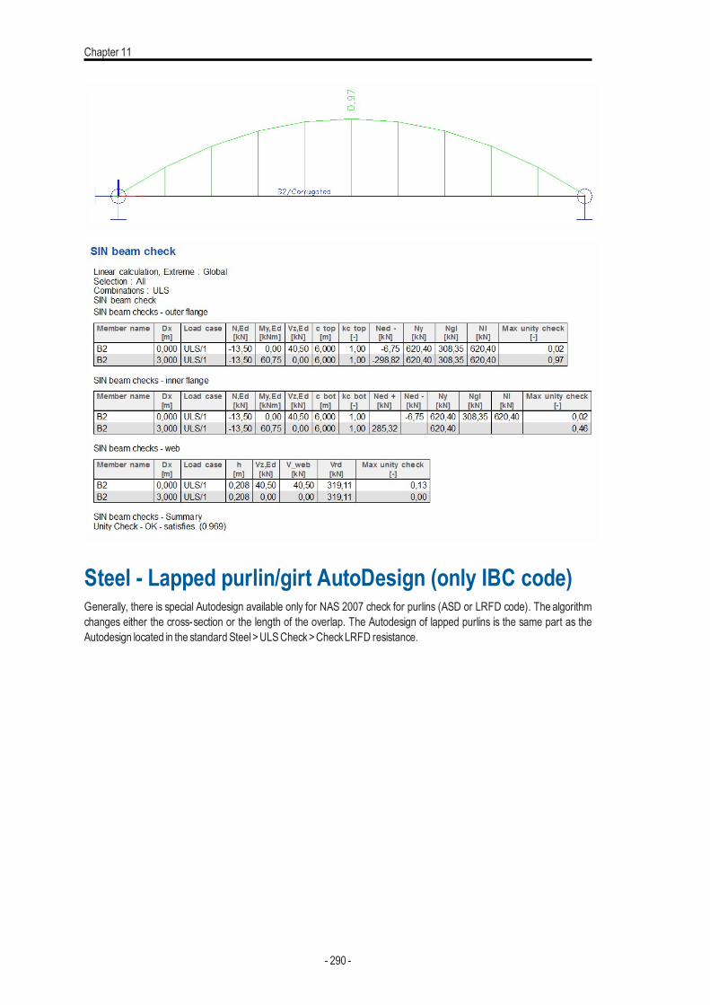
Chapter 11
Steel - Lapped purlin/girt AutoDesign (only IBC code)Generally, there is special Autodesign available only for NAS 2007 check for purlins (ASD or LRFD code). The algorithmchanges either the cross-section or the length of the overlap. The Autodesign of lapped purlins is the same part as theAutodesign located in the standard Steel >ULSCheck>CheckLRFD resistance.
- 290 -
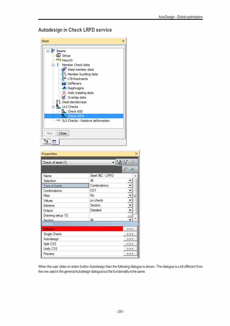
AutoDesign - Global optimization
Autodesign in Check LRFD service
When the user clicks on action button Autodesign then the following dialogue is shown. The dialogue is a bit different fromthe one used in the generalAutodesign dialogue but the functionality is the same.
- 291 -
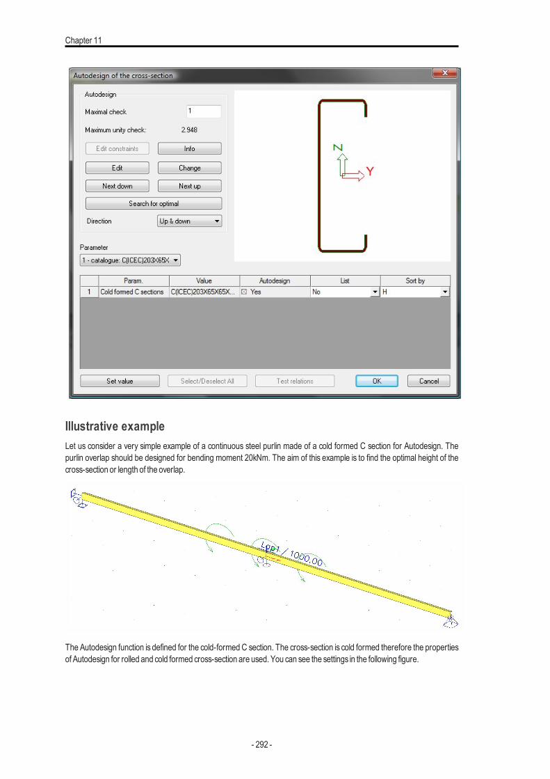
Chapter 11
Illustrative exampleLet us consider a very simple example of a continuous steel purlin made of a cold formed C section for Autodesign. Thepurlin overlap should be designed for bending moment 20kNm. The aim of this example is to find the optimal height of thecross-section or length of the overlap.
The Autodesign function is defined for the cold-formed C section. The cross-section is cold formed therefore the propertiesof Autodesign for rolled and cold formed cross-section are used. You can see the settings in the following figure.
- 292 -
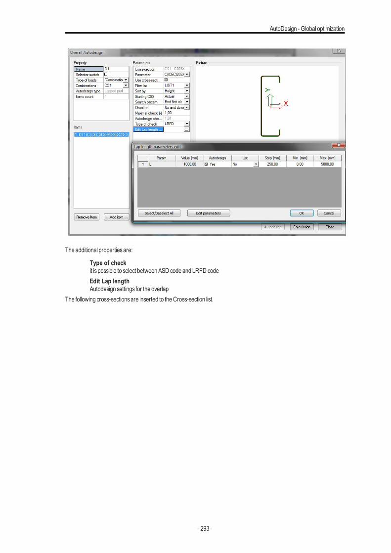
AutoDesign - Global optimization
The additional propertiesare:
Type of checkit is possible to select betweenASD code and LRFD codeEdit Lap lengthAutodesign settings for the overlap
The following cross-sectionsare inserted to theCross-section list.
- 293 -
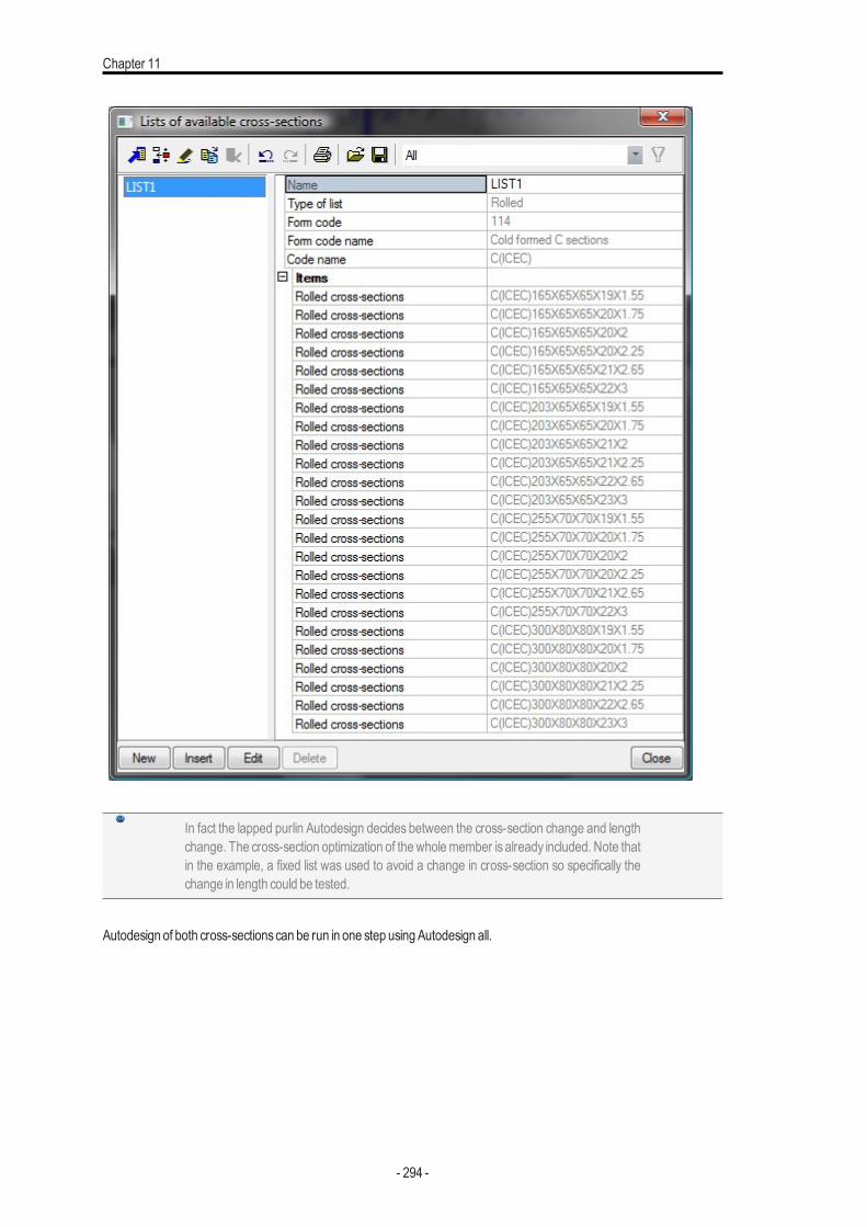
Chapter 11
In fact the lapped purlin Autodesign decides between the cross-section change and lengthchange. The cross-section optimization of thewholemember is already included. Note thatin the example, a fixed list was used to avoid a change in cross-section so specifically thechange in length could be tested.
Autodesign of both cross-sectionscan be run in one step usingAutodesign all.
- 294 -
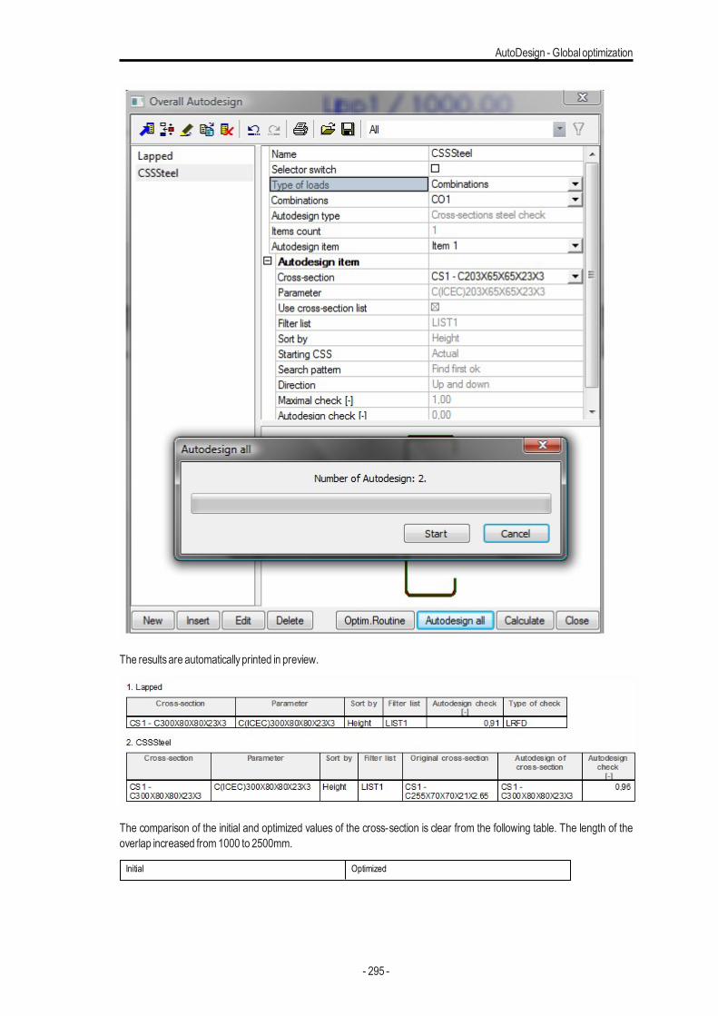
AutoDesign - Global optimization
The resultsare automaticallyprinted in preview.
The comparison of the initial and optimized values of the cross-section is clear from the following table. The length of theoverlap increased from1000 to 2500mm.
Initial Optimized
- 295 -
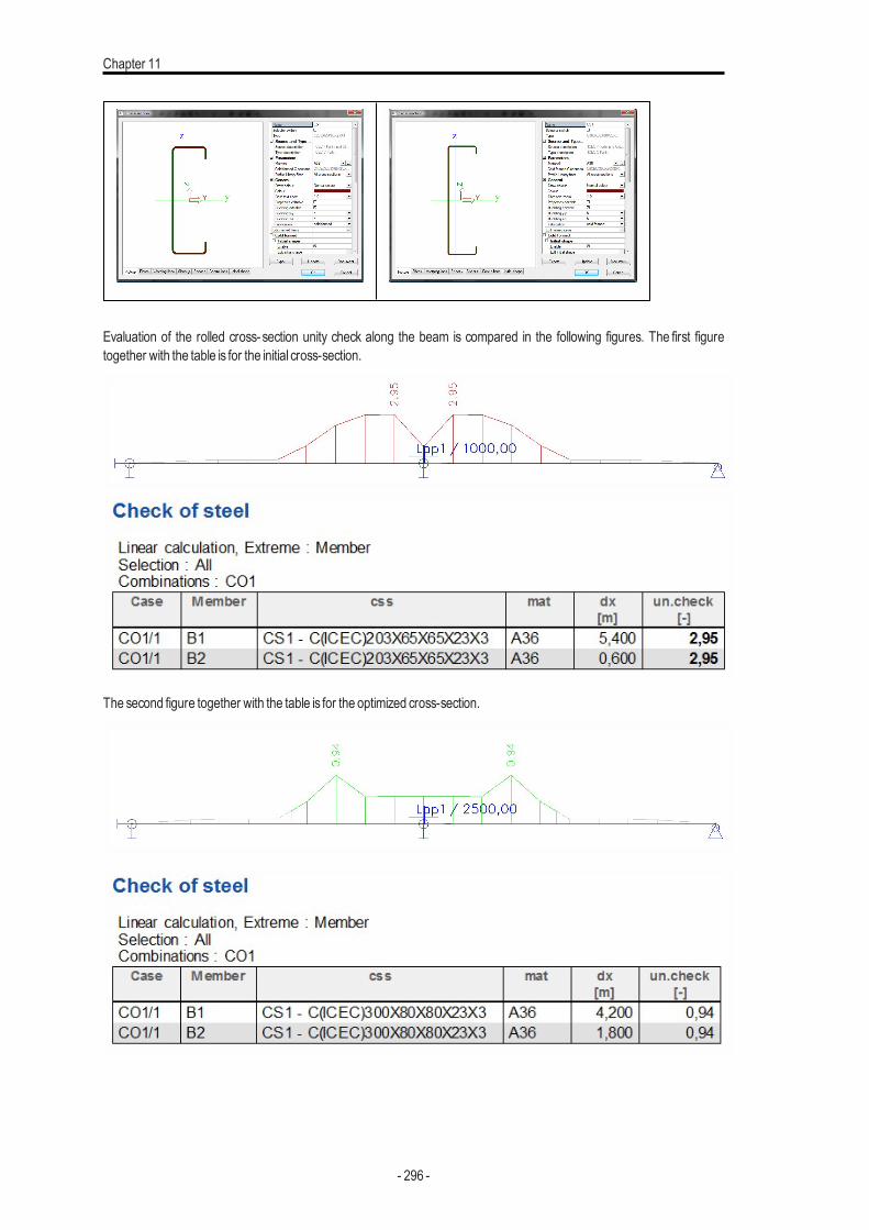
Chapter 11
Evaluation of the rolled cross-section unity check along the beam is compared in the following figures. The first figuretogether with the table is for the initial cross-section.
The second figure together with the table is for the optimized cross-section.
- 296 -

AutoDesign - Global optimization
Steel connection - Bolted diagonal AutoDesignAutodesign of bolted diagonal is the same part as the Autodesign located in the standard Steel >Connections>Bolted diag-onal.
- 297 -
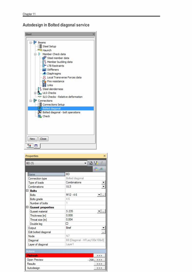
Chapter 11
Autodesign in Bolted diagonal service
- 298 -
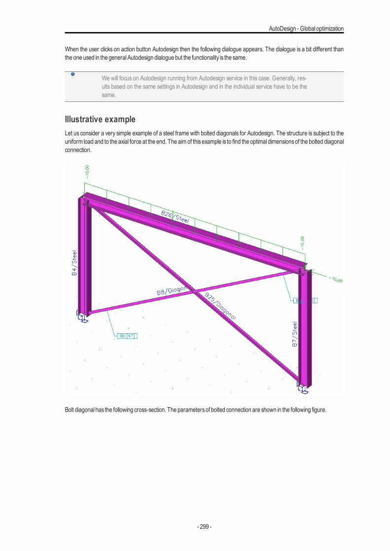
AutoDesign - Global optimization
When the user clicks on action button Autodesign then the following dialogue appears. The dialogue is a bit different thanthe one used in the generalAutodesign dialogue but the functionality is the same.
We will focus on Autodesign running from Autodesign service in this case. Generally, res-ults based on the same settings in Autodesign and in the individual service have to be thesame.
Illustrative exampleLet us consider a very simple example of a steel frame with bolted diagonals for Autodesign. The structure is subject to theuniform load and to the axial force at the end. The aim of this example is to find the optimal dimensionsof the bolted diagonalconnection.
Bolt diagonal has the following cross-section. The parametersof bolted connection are shown in the following figure.
- 299 -
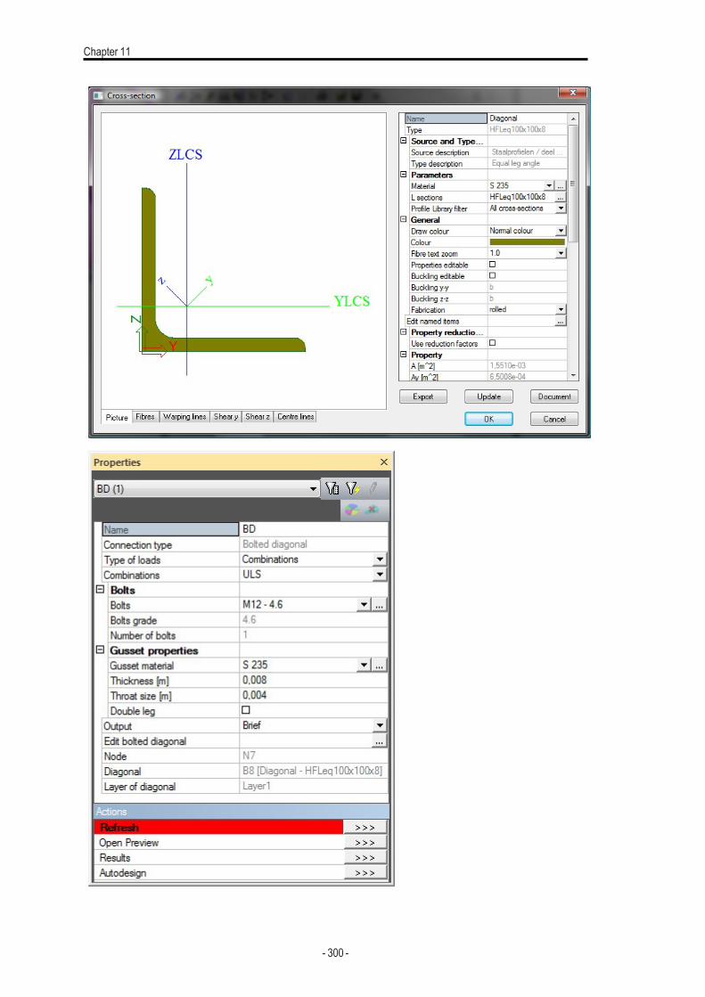
Chapter 11
- 300 -
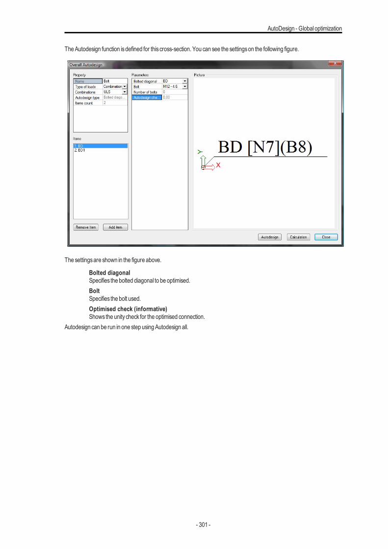
AutoDesign - Global optimization
TheAutodesign function isdefined for this cross-section. You can see the settingson the following figure.
The settingsare shown in the figure above.
Bolted diagonalSpecifies the bolted diagonal to be optimised.BoltSpecifies the bolt used.Optimised check (informative)Shows the unity check for the optimised connection.
Autodesign can be run in one step usingAutodesign all.
- 301 -
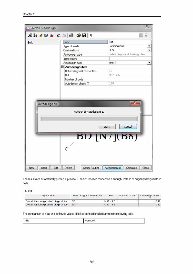
Chapter 11
The results are automatically printed in preview. One bolt for each connection is enough. Instead of originally designed fourbolts.
The comparison of initial and optimized valuesof bolted connections is clear from the following table.
Initial Optimized
- 302 -
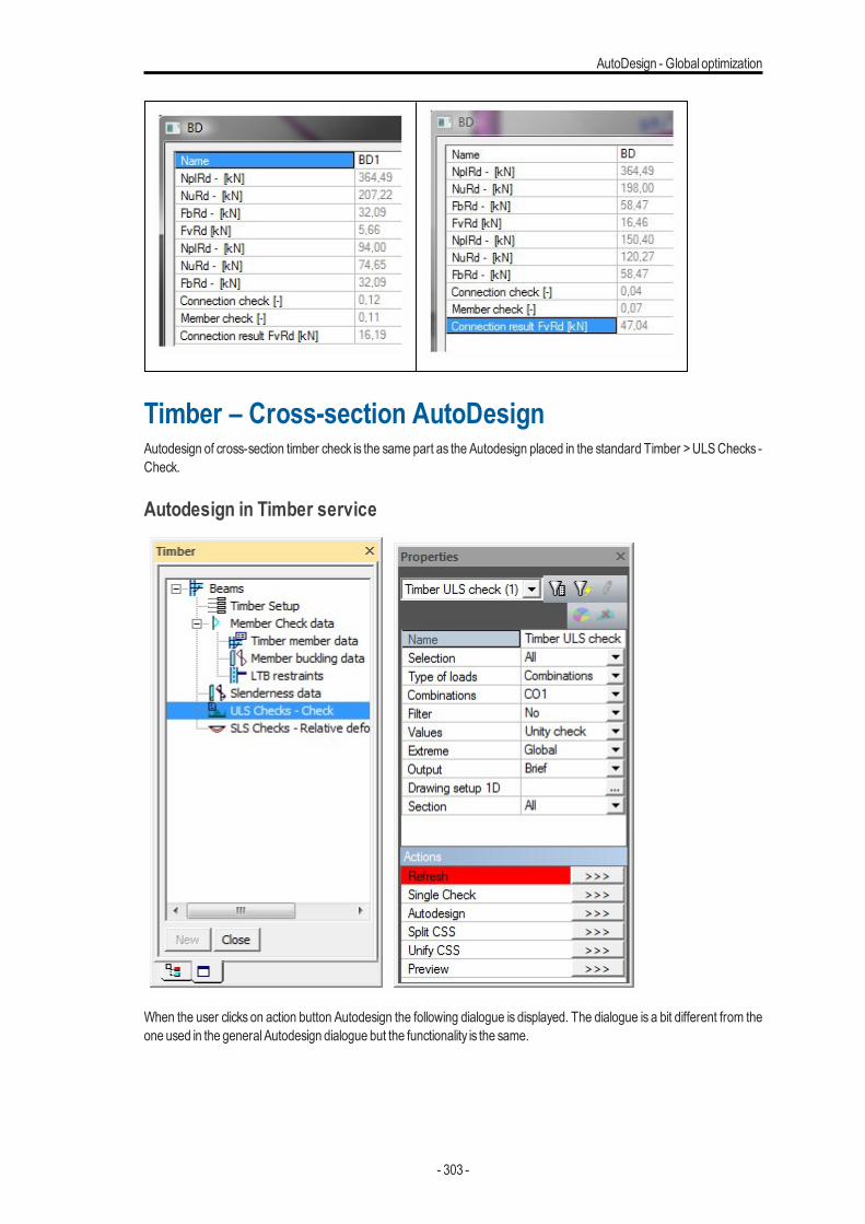
AutoDesign - Global optimization
Timber – Cross-section AutoDesignAutodesign of cross-section timber check is the same part as the Autodesign placed in the standard Timber >ULSChecks -Check.
Autodesign in Timber service
When the user clicks on action button Autodesign the following dialogue is displayed. The dialogue is a bit different from theone used in the generalAutodesign dialogue but the functionality is the same.
- 303 -
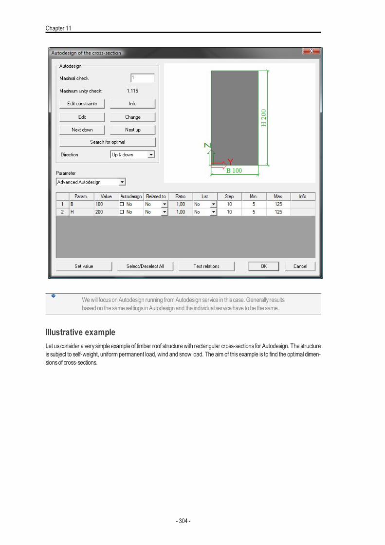
Chapter 11
Wewill focuson Autodesign running fromAutodesign service in this case. Generally resultsbased on the same settings in Autodesign and the individual service have to be the same.
Illustrative exampleLet usconsider a very simple example of timber roof structure with rectangular cross-sections for Autodesign. The structureis subject to self-weight, uniform permanent load, wind and snow load. The aim of this example is to find the optimal dimen-sionsof cross-sections.
- 304 -
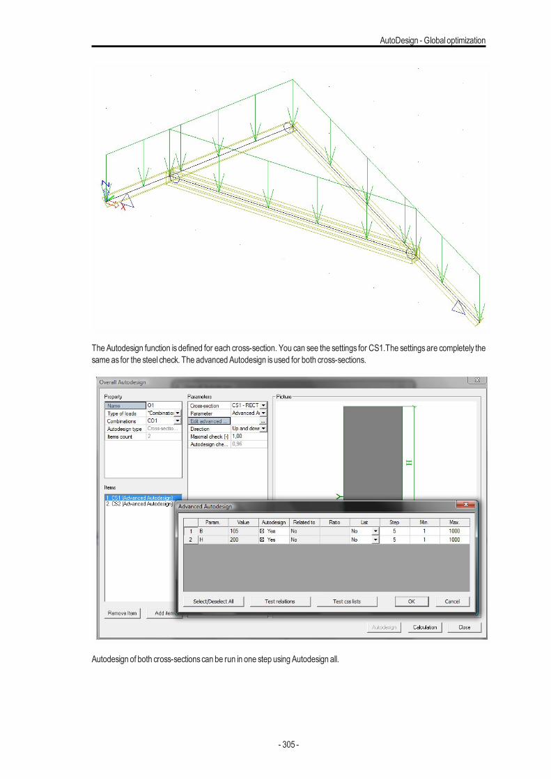
AutoDesign - Global optimization
The Autodesign function is defined for each cross-section. You can see the settings for CS1.The settingsare completely thesame as for the steel check. The advancedAutodesign isused for both cross-sections.
Autodesign of both cross-sectionscan be run in one step usingAutodesign all.
- 305 -
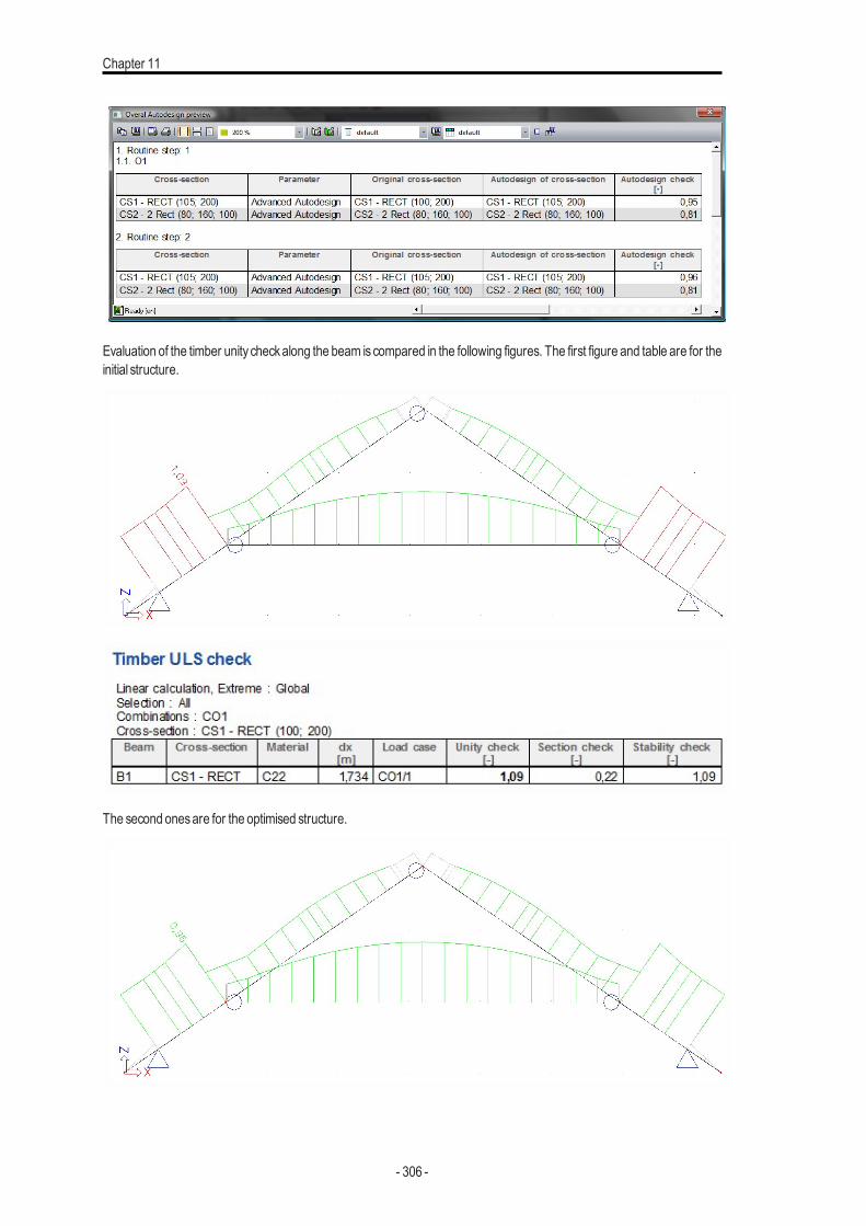
Chapter 11
Evaluation of the timber unity checkalong the beam iscompared in the following figures. The first figure and table are for theinitial structure.
The second onesare for the optimised structure.
- 306 -

AutoDesign - Global optimization
Thewidth of rafterswere optimised from100 to 105mm.
Aluminium – Cross-section AutoDesignAutodesign of cross-section steel check is the same part as theAutodesign locates in the standard Aluminium>Check.
- 307 -
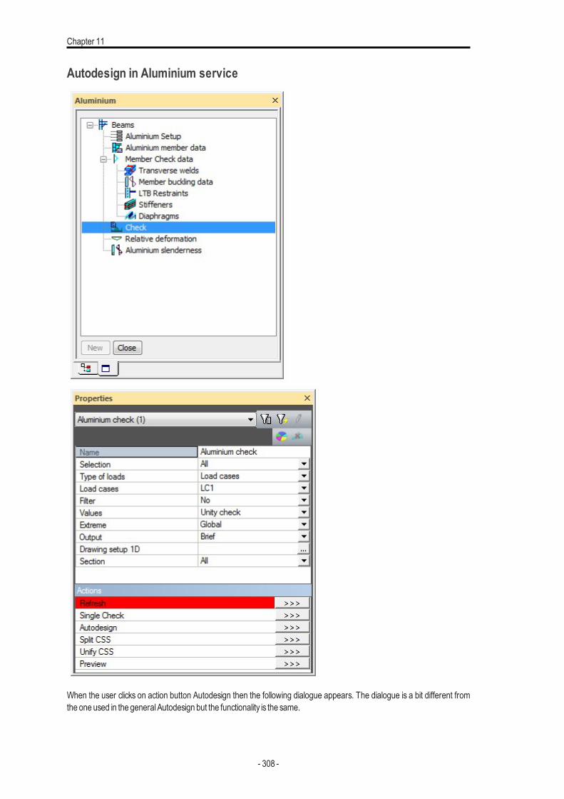
Chapter 11
Autodesign in Aluminium service
When the user clicks on action button Autodesign then the following dialogue appears. The dialogue is a bit different fromthe one used in the generalAutodesign but the functionality is the same.
- 308 -
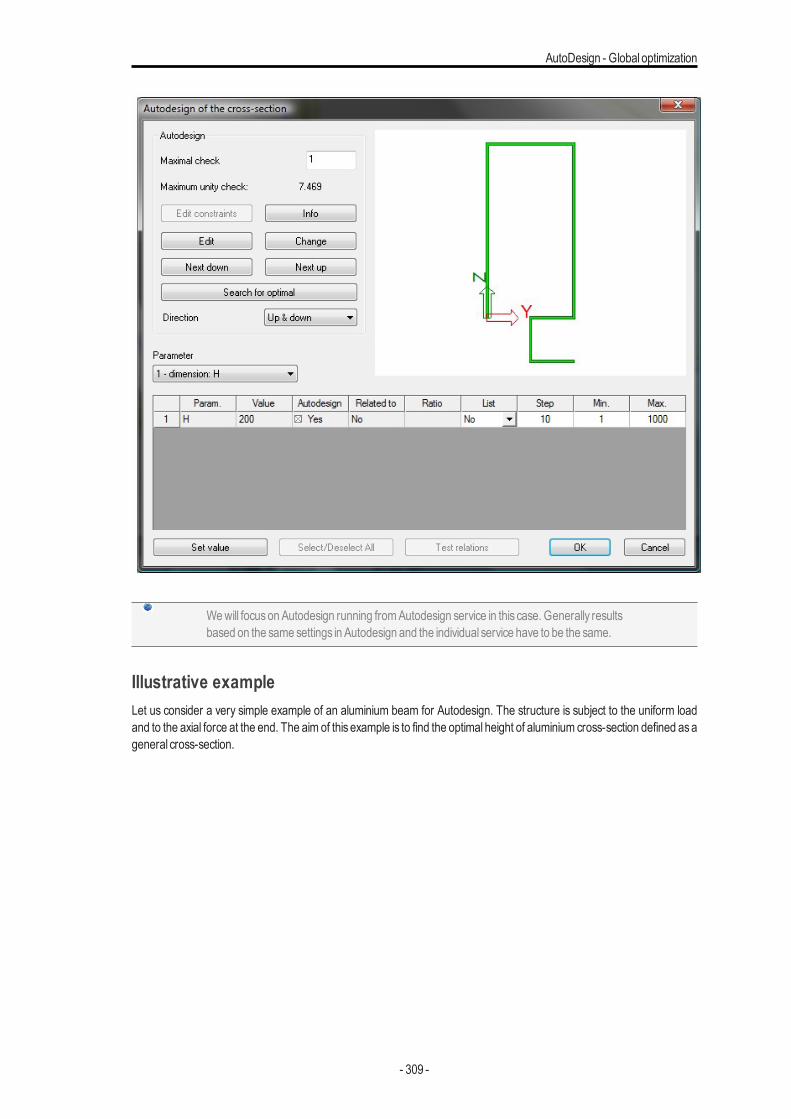
AutoDesign - Global optimization
Wewill focuson Autodesign running fromAutodesign service in this case. Generally resultsbased on the same settings in Autodesign and the individual service have to be the same.
Illustrative exampleLet us consider a very simple example of an aluminium beam for Autodesign. The structure is subject to the uniform loadand to the axial force at the end. The aim of this example is to find the optimal height of aluminium cross-section defined asageneral cross-section.
- 309 -
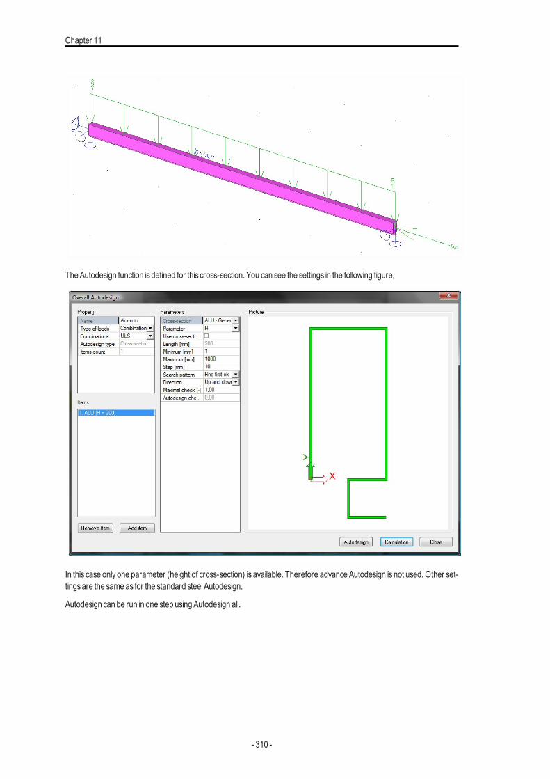
Chapter 11
TheAutodesign function isdefined for this cross-section. You can see the settings in the following figure,
In this case only one parameter (height of cross-section) is available. Therefore advance Autodesign is not used. Other set-tingsare the sameas for the standard steelAutodesign.
Autodesign can be run in one step usingAutodesign all.
- 310 -
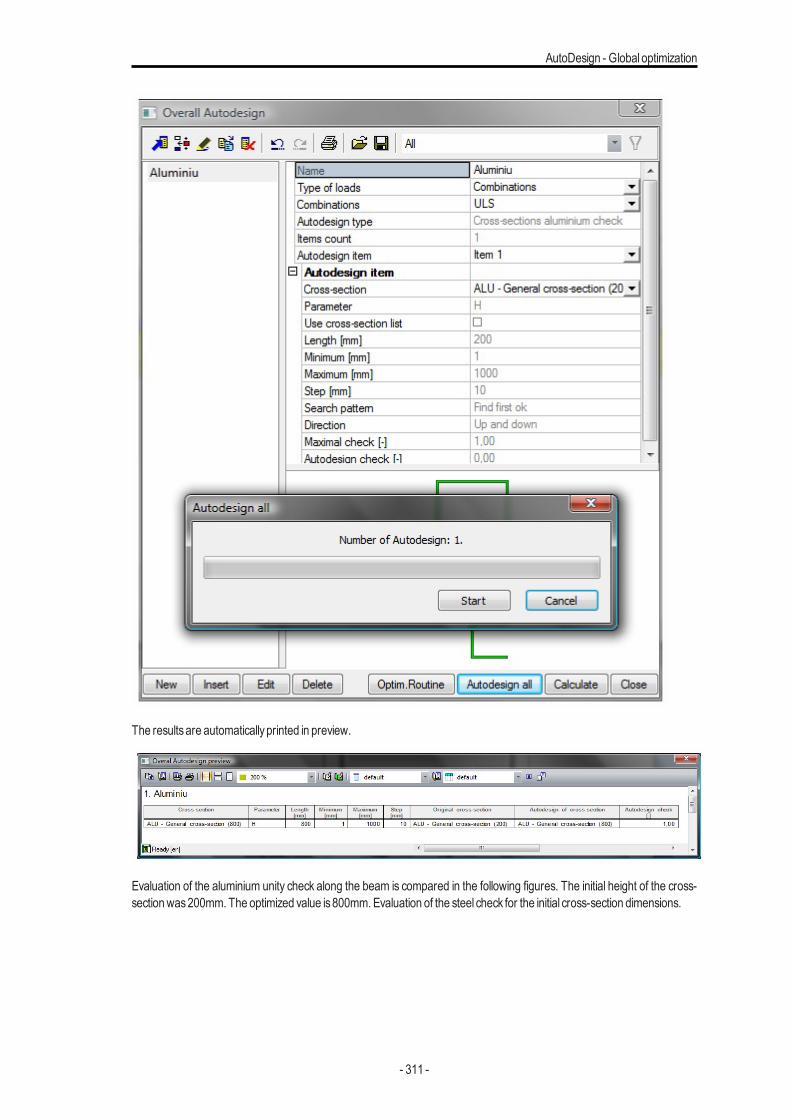
AutoDesign - Global optimization
The resultsare automaticallyprinted in preview.
Evaluation of the aluminium unity check along the beam is compared in the following figures. The initial height of the cross-sectionwas200mm. The optimized value is800mm. Evaluation of the steel check for the initial cross-section dimensions.
- 311 -
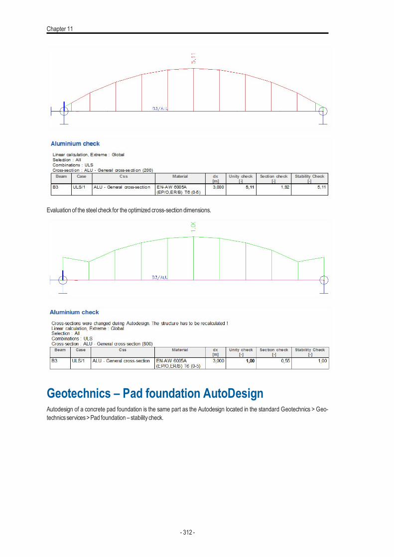
Chapter 11
Evaluation of the steel check for the optimized cross-section dimensions.
Geotechnics – Pad foundation AutoDesignAutodesign of a concrete pad foundation is the same part as the Autodesign located in the standard Geotechnics > Geo-technicsservices>Pad foundation – stability check.
- 312 -
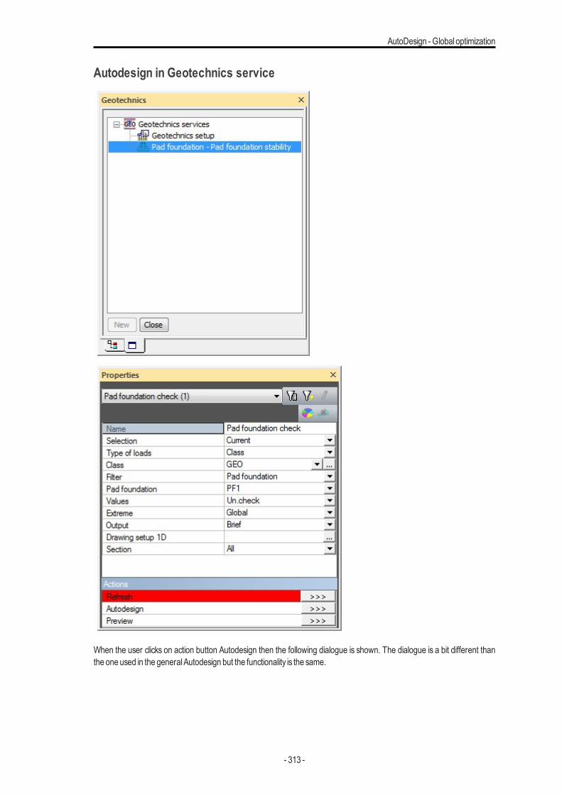
AutoDesign - Global optimization
Autodesign in Geotechnics service
When the user clicks on action button Autodesign then the following dialogue is shown. The dialogue is a bit different thanthe one used in the generalAutodesign but the functionality is the same.
- 313 -
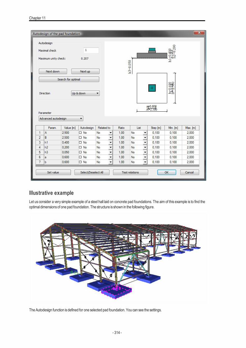
Chapter 11
Illustrative exampleLet us consider a very simple example of a steel hall laid on concrete pad foundations. The aim of this example is to find theoptimal dimensionsof one pad foundation. The structure is shown in the following figure.
TheAutodesign function isdefined for one selected pad foundation. You can see the settings.
- 314 -
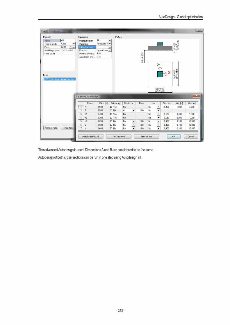
AutoDesign - Global optimization
The advancedAutodesign isused. DimensionsAandBare considered to be the same.
Autodesign of both cross-sectionscan be run in one step usingAutodesign all..
- 315 -
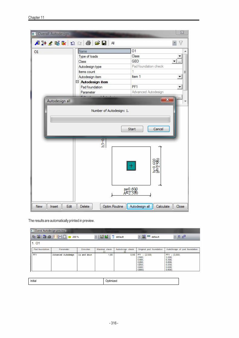
Chapter 11
The resultsare automaticallyprinted in preview.
Initial Optimized
- 316 -
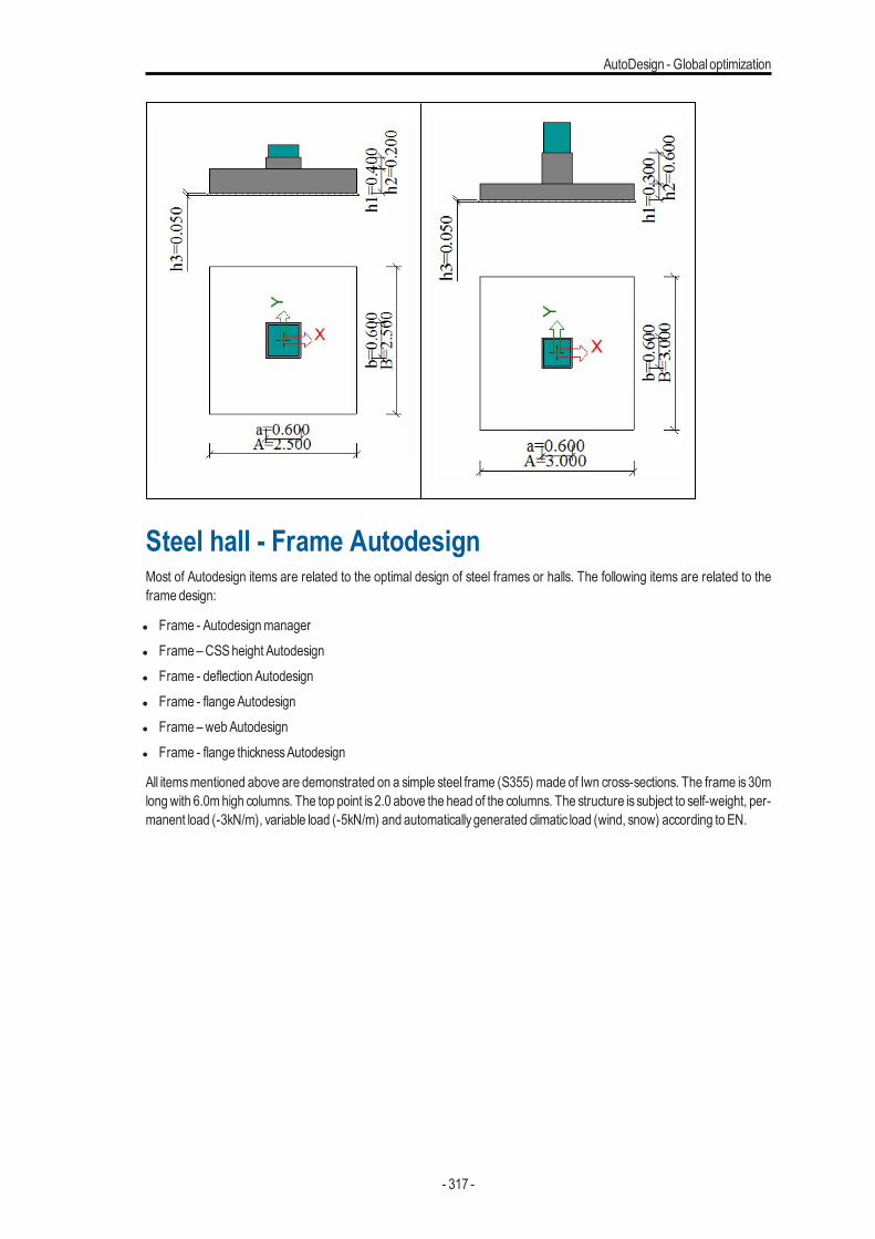
AutoDesign - Global optimization
Steel hall - Frame AutodesignMost of Autodesign items are related to the optimal design of steel frames or halls. The following items are related to theframe design:
l Frame - Autodesignmanagerl Frame –CSSheight Autodesignl Frame - deflection Autodesignl Frame - flangeAutodesignl Frame –webAutodesignl Frame - flange thicknessAutodesign
All itemsmentioned above are demonstrated on a simple steel frame (S355) made of Iwn cross-sections. The frame is 30mlongwith 6.0mhigh columns. The top point is 2.0 above the head of the columns. The structure is subject to self-weight, per-manent load (-3kN/m), variable load (-5kN/m) and automaticallygenerated climatic load (wind, snow) according to EN.
- 317 -
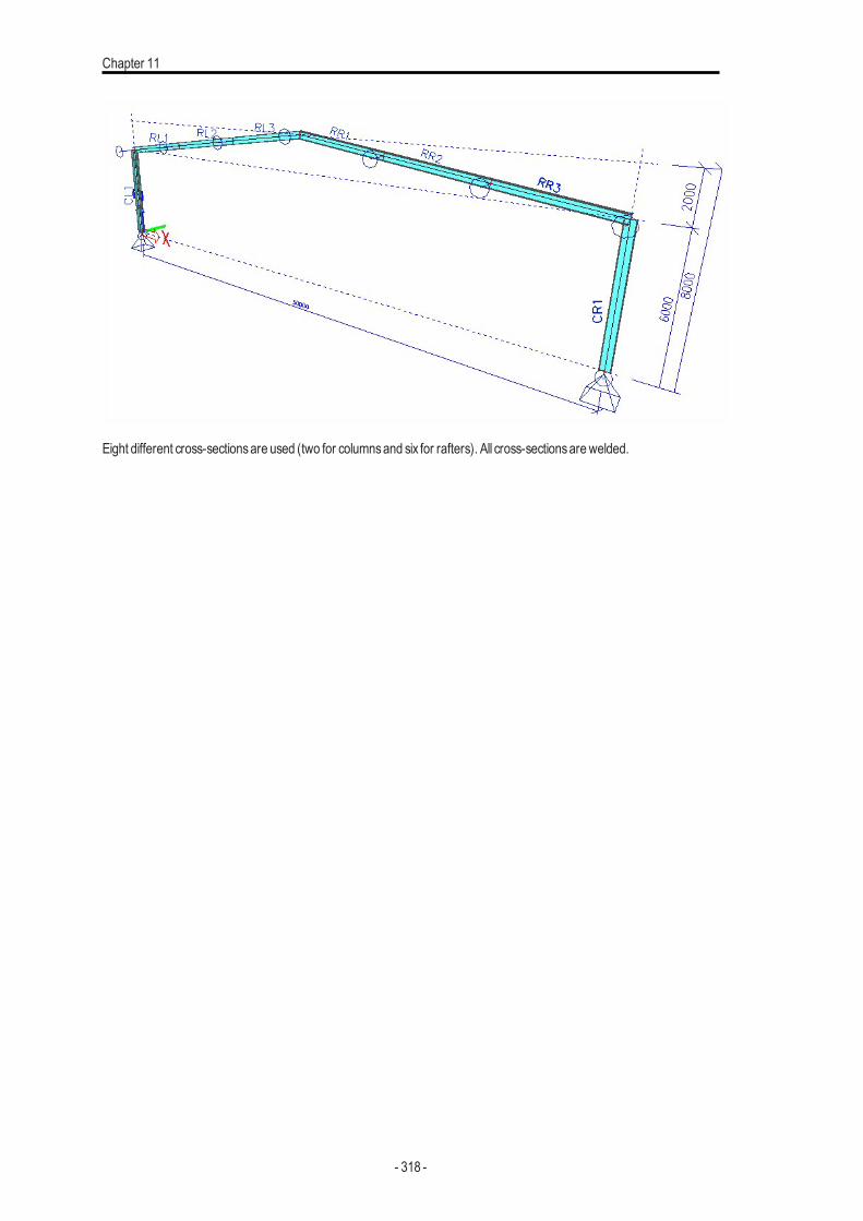
Chapter 11
Eight different cross-sectionsare used (two for columnsand six for rafters). All cross-sectionsarewelded.
- 318 -
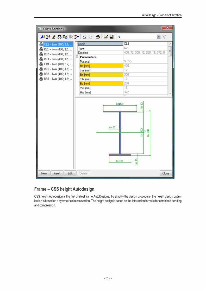
AutoDesign - Global optimization
Frame – CSS height AutodesignCSS height Autodesign is the first of steel frame AutoDesigns. To simplify the design procedure, the height design optim-ization is based on a symmetrical cross section. The height design is based on the interaction formula for combined bendingand compression.
- 319 -
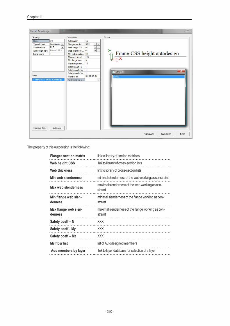
Chapter 11
The propertyof thisAutodesign is the following:
Flanges section matrix link to libraryof sectionmatrices
Web height CSS link to libraryof cross-section lists
Web thickness link to libraryof cross-section lists
Min web slenderness minimal slendernessof thewebworking asconstraint
Max web slenderness maximal slendernessof thewebworking ascon-straint
Min flange web slen-derness
minimal slendernessof the flangeworking ascon-straint
Max flange web slen-derness
maximal slendernessof the flangeworking ascon-straint
Safety coeff – N XXX
Safety coeff - My XXX
Safety coeff – Mz XXX
Member list list of Autodesignedmembers
Add members by layer link to layer database for selection of a layer
- 320 -
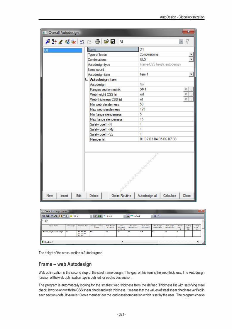
AutoDesign - Global optimization
The height of the cross-section isAutodesigned.
Frame – web AutodesignWeb optimization is the second step of the steel frame design. The goal of this item is the web thickness. The Autodesignfunction of theweb optimization type isdefined for each cross-section.
The program is automatically looking for the smallest web thickness from the defined Thickness list with satisfying steelcheck. It worksonlywith theCSSshear checkandweb thickness. It means that the valuesof steel shear checkare verified ineach section (default value is 10 on amember) for the load class/combination which is set by the user. The program checks
- 321 -

Chapter 11
theweb slenderness tomake sure that the Autodesign doesnot set a web thicknesswhich is outside the defined range. Thestarting web thickness of this Autodesign is the value after the CSS height design. It checks the value of the shear check forthis thickness.
l If the value of the check isbigger than 1 then it finds in the list the first thicknesswhich has the check lower than 1.l If the value of the check is smaller than 1 then it triesall thicknesses from the list which are smaller than the current one
and returns the thicknesswhich gives the checkclosest to 1.
The optimal (0.95), minimal (0.85) andmaximal (1.0) checkvaluesare the same as for the flange optimization. Minimal (50)and maximal (125) slenderness of web parts are different. This web optimization has different properties than the flangeoptimization:
Dimension listEnables the user to use predefined values of one dimension according to the list defined in the Cross-section listlibrary. This library is stored in Libraries>Structure, analysis>Cross-section list.
- 322 -
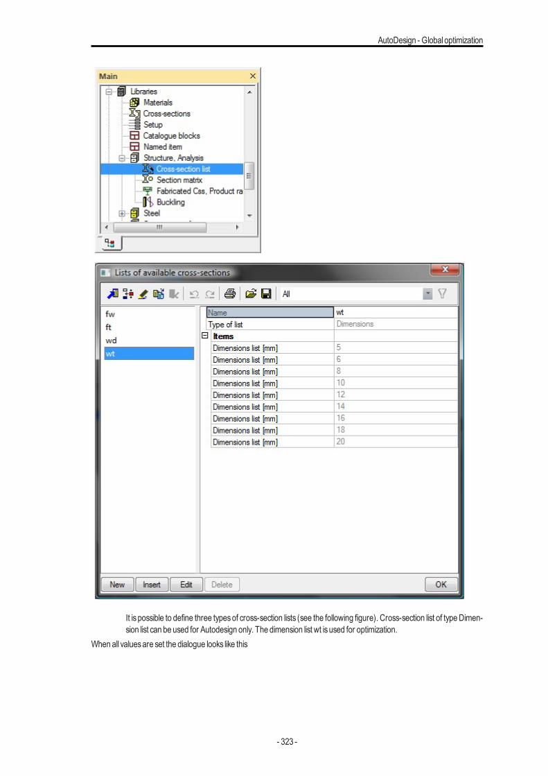
AutoDesign - Global optimization
It is possible to define three typesof cross-section lists (see the following figure). Cross-section list of type Dimen-sion list can be used for Autodesign only. The dimension list wt isused for optimization.
When all valuesare set the dialogue looks like this
- 323 -
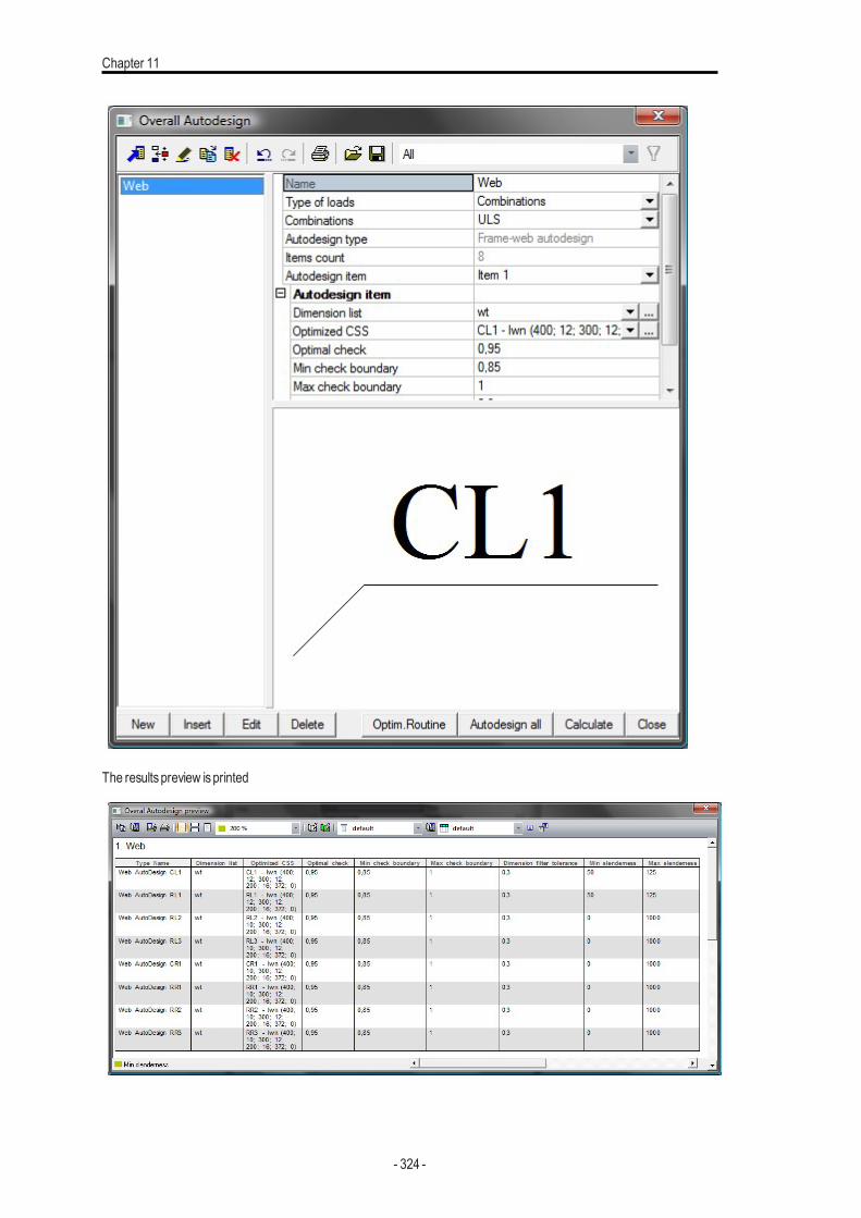
Chapter 11
The resultspreview isprinted
- 324 -
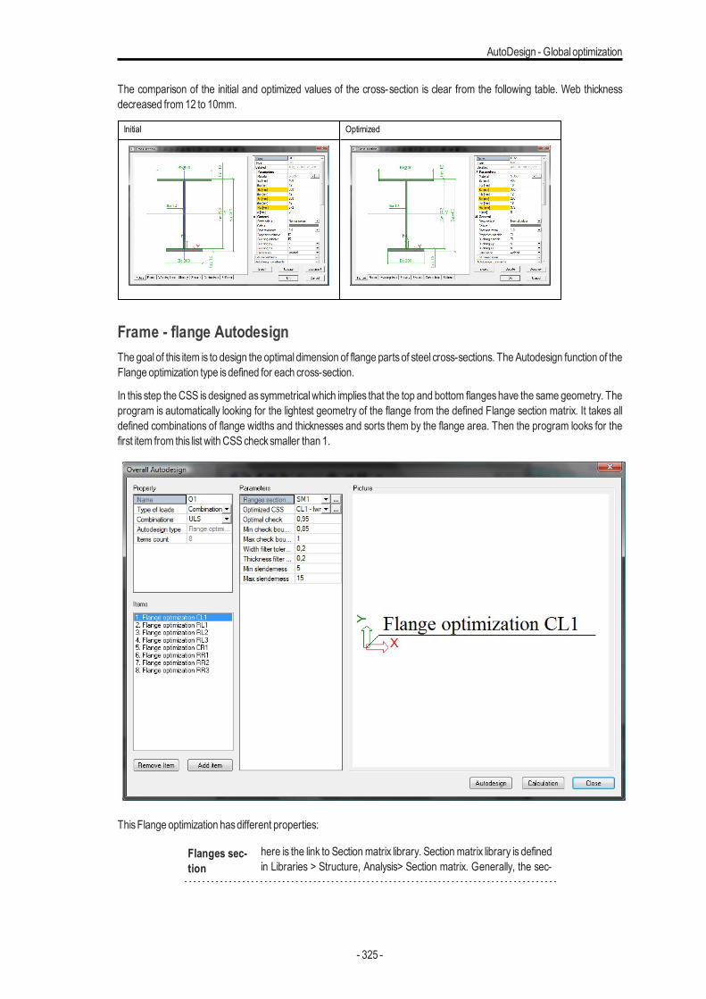
AutoDesign - Global optimization
The comparison of the initial and optimized values of the cross-section is clear from the following table. Web thicknessdecreased from12 to 10mm.
Initial Optimized
Frame - flange AutodesignThe goal of this item is to design the optimal dimension of flange partsof steel cross-sections. TheAutodesign function of theFlange optimization type isdefined for each cross-section.
In this step the CSS is designed assymmetricalwhich implies that the top and bottom flangeshave the same geometry. Theprogram is automatically looking for the lightest geometry of the flange from the defined Flange section matrix. It takes alldefined combinations of flange widths and thicknesses and sorts them by the flange area. Then the program looks for thefirst item from this list with CSSchecksmaller than 1.
ThisFlange optimization hasdifferent properties:
Flanges sec-tion
here is the link to Section matrix library. Section matrix library is definedin Libraries > Structure, Analysis> Section matrix. Generally, the sec-
- 325 -
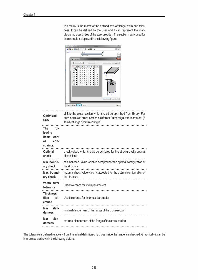
Chapter 11
tion matrix is the matrix of the defined sets of flange width and thick-ness. It can be defined by the user and it can represent the man-ufacturing possibilities of the steel provider. The section matrix used forthisexample isdisplayed in the following figure.
OptimizedCSS
Link to the cross-section which should be optimized from library. Foreach optimized cross-section a different Autodesign item is created. (8itemsof flange optimization type).
The fol-lowingitems workas con-straints.
Optimalcheck
check values which should be achieved for the structure with optimaldimensions
Min. bound-ary check
minimal check value which is accepted for the optimal configuration ofthe structure
Max. bound-ary check
maximal check value which is accepted for the optimal configuration ofthe structure
Width filtertolerance Used tolerance for width parameters
Thicknessfilter tol-erance
Used tolerance for thicknessparameter
Min slen-derness minimal slendernessof the flange of the cross-section
Max slen-derness maximal slendernessof the flange of the cross-section
The tolerance is defined relatively, from the actual definition only those inside the range are checked. Graphically it can beinterpreted asshown in the following picture.
- 326 -
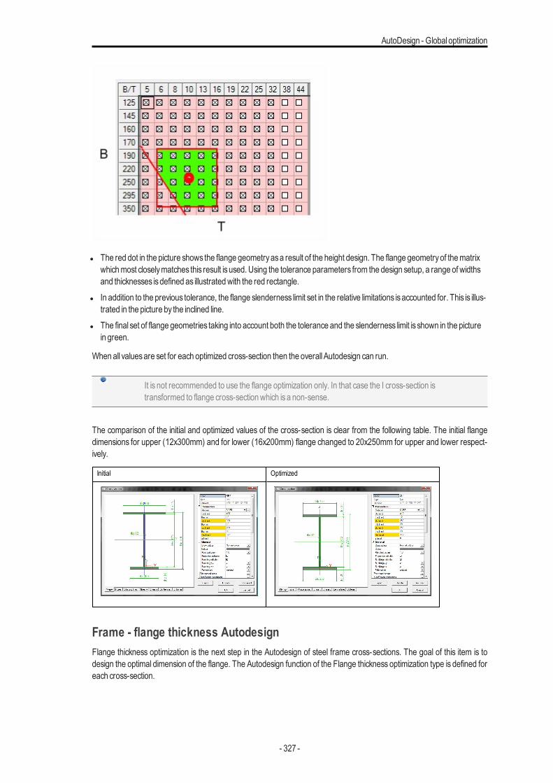
AutoDesign - Global optimization
l The red dot in the picture shows the flange geometryasa result of the height design. The flange geometryof thematrixwhichmost closelymatches this result isused. Using the tolerance parameters from the design setup, a range of widthsand thicknesses isdefined as illustratedwith the red rectangle.
l In addition to the previous tolerance, the flange slenderness limit set in the relative limitations isaccounted for. This is illus-trated in the picture by the inclined line.
l The final set of flange geometries taking into account both the tolerance and the slenderness limit is shown in the picturein green.
When all valuesare set for each optimized cross-section then the overall Autodesign can run.
It is not recommended to use the flange optimization only. In that case the I cross-section istransformed to flange cross-sectionwhich isa non-sense.
The comparison of the initial and optimized values of the cross-section is clear from the following table. The initial flangedimensions for upper (12x300mm) and for lower (16x200mm) flange changed to 20x250mm for upper and lower respect-ively.
Initial Optimized
Frame - flange thickness AutodesignFlange thickness optimization is the next step in the Autodesign of steel frame cross-sections. The goal of this item is todesign the optimal dimension of the flange. The Autodesign function of the Flange thickness optimization type is defined foreach cross-section.
- 327 -
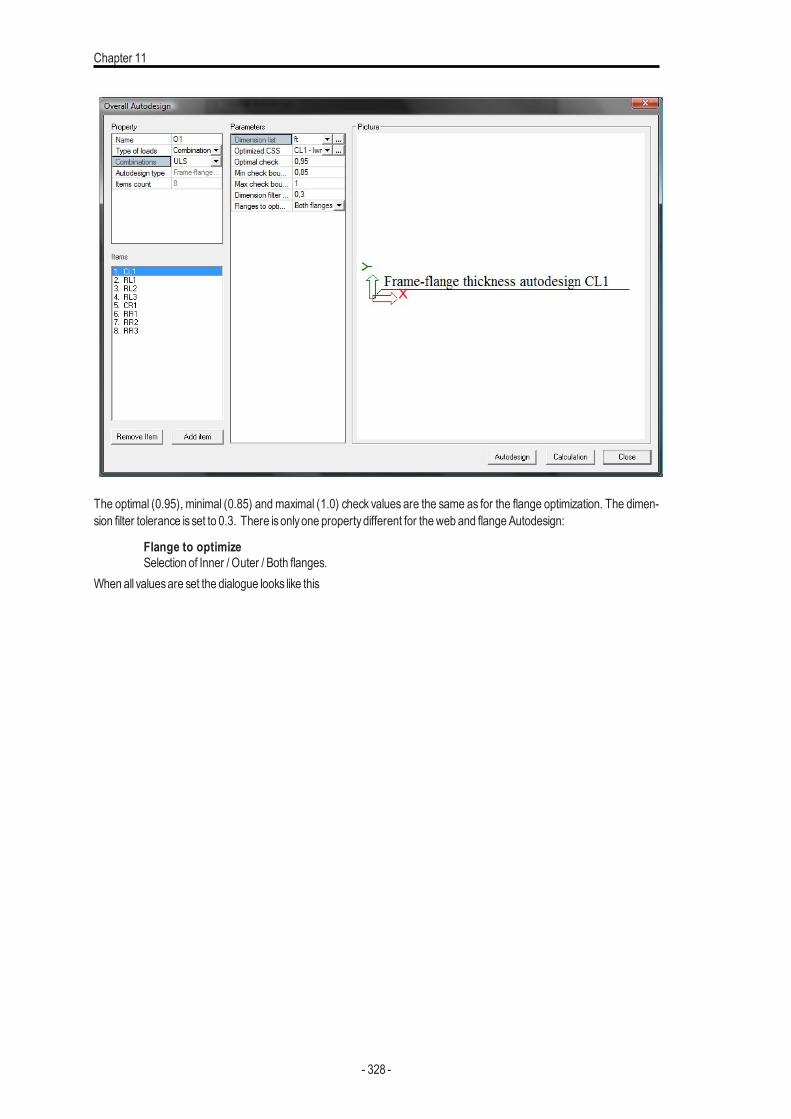
Chapter 11
The optimal (0.95), minimal (0.85) andmaximal (1.0) check values are the same as for the flange optimization. The dimen-sion filter tolerance isset to 0.3. There isonlyone propertydifferent for theweb and flangeAutodesign:
Flange to optimizeSelection of Inner / Outer / Both flanges.
When all valuesare set the dialogue looks like this
- 328 -
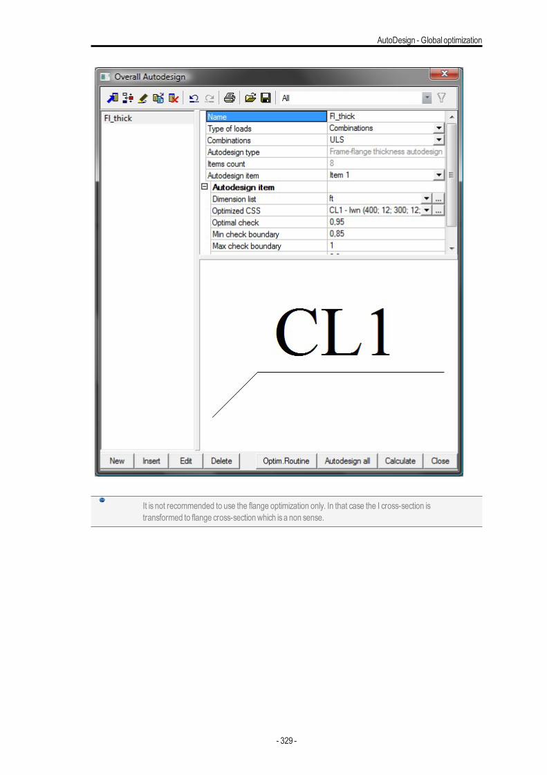
AutoDesign - Global optimization
It is not recommended to use the flange optimization only. In that case the I cross-section istransformed to flange cross-sectionwhich isa non sense.
- 329 -
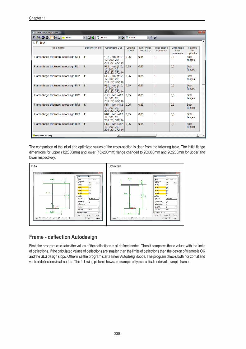
Chapter 11
The comparison of the initial and optimized values of the cross-section is clear from the following table. The initial flangedimensions for upper (12x300mm) and lower (16x200mm) flange changed to 20x300mm and 20x200mm for upper andlower respectively.
Initial Optimized
Frame - deflection AutodesignFirst, the program calculates the values of the deflections in all defined nodes. Then it compares these valueswith the limitsof deflections. If the calculated values of deflections are smaller than the limits of deflections then the design of frames isOKand the SLS design stops. Otherwise the program starts a new Autodesign loops. The program checks both horizontal andvertical deflections in all nodes. The following picture showsan example of typical critical nodesof a simple frame.
- 330 -
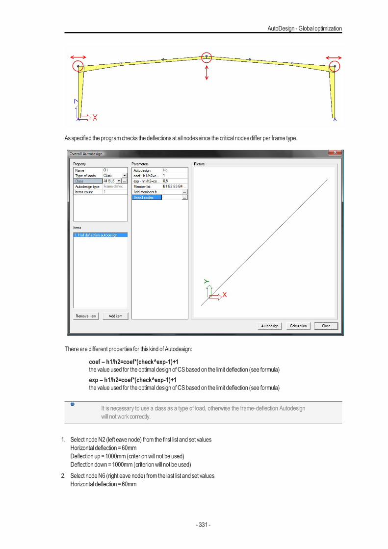
AutoDesign - Global optimization
Asspecified the programchecks the deflectionsat all nodessince the critical nodesdiffer per frame type.
There are different properties for this kind of Autodesign:
coef – h1/h2=coef*(check^exp-1)+1the value used for the optimal design of CSbased on the limit deflection (see formula)exp – h1/h2=coef*(check^exp-1)+1the value used for the optimal design of CSbased on the limit deflection (see formula)
It is necessary to use a class as a type of load, otherwise the frame-deflection Autodesignwill not workcorrectly.
1. Select nodeN2 (left eave node) from the first list and set valuesHorizontal deflection =60mmDeflection up =1000mm (criterionwill not be used)Deflection down=1000mm (criterionwill not be used)
2. Select nodeN6 (right eave node) from the last list and set valuesHorizontal deflection =60mm
- 331 -
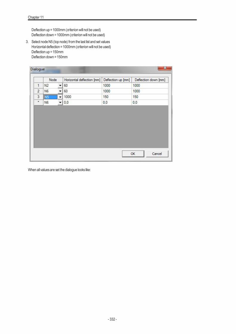
Chapter 11
Deflection up =1000mm (criterionwill not be used)Deflection down=1000mm (criterionwill not be used)
3. Select nodeN5 (top node) from the last list and set valuesHorizontal deflection =1000mm (criterionwill not be used)Deflection up =150mmDeflection down=150mm
When all valuesare set the dialogue looks like:
- 332 -
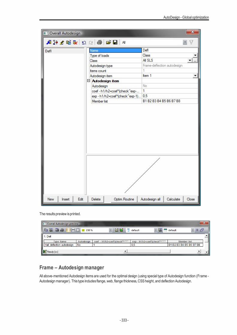
AutoDesign - Global optimization
The resultspreview isprinted.
Frame – Autodesign managerAll above-mentioned Autodesign items are used for the optimal design (using special type of Autodesign function (Frame -Autodesignmanager). This type includes flange, web, flange thickness, CSSheight, and deflection Autodesign.
- 333 -
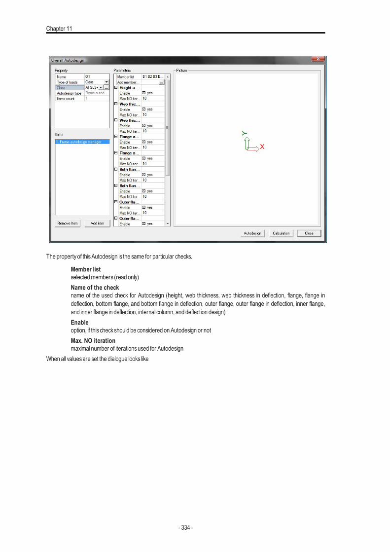
Chapter 11
The propertyof thisAutodesign is the same for particular checks.
Member listselectedmembers (read only)Name of the checkname of the used check for Autodesign (height, web thickness, web thickness in deflection, flange, flange indeflection, bottom flange, and bottom flange in deflection, outer flange, outer flange in deflection, inner flange,and inner flange in deflection, internal column, and deflection design)Enableoption, if this checkshould be considered onAutodesign or notMax. NO iterationmaximal number of iterationsused for Autodesign
When all valuesare set the dialogue looks like
- 334 -
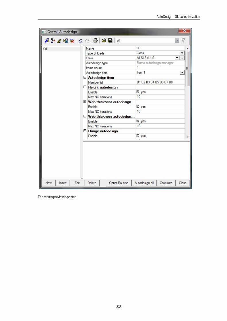
AutoDesign - Global optimization
The resultspreview isprinted
- 335 -
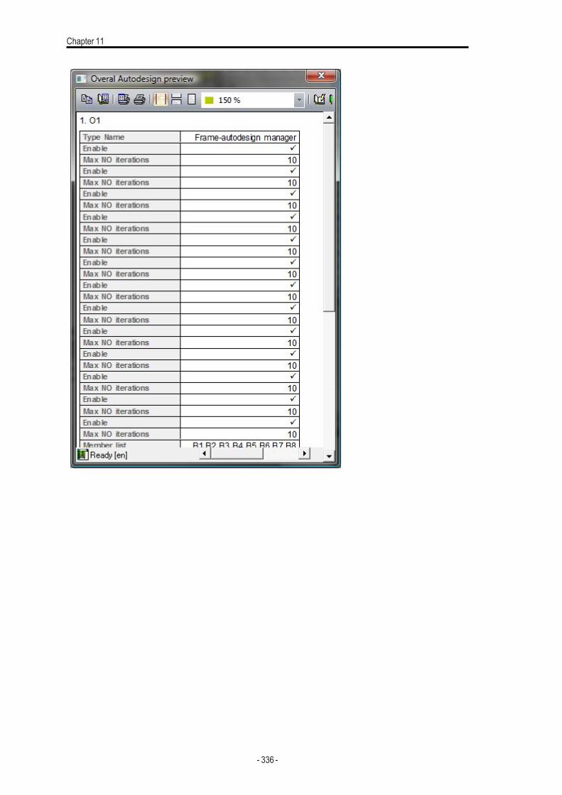
Chapter 11
- 336 -

SCIAOptimizer
SCIA Optimizer
IntroductionThe aim of this document is to introduce a brand new tool for optimization of civil engineering structures developed bySCIAand to demonstrate how it can be helpful and effective to everybodywho dealswith structural design.
About SCIA Engineer OptimizerSCIAEngineer Optimizer isan example of a new generation of software for the design of structures. It is softwarewhich cal-culates internal forces, checks the compliance to the code, and on top of that, this software is able to “find” the final optimalstructural design.
It represents a combination of the widespread structural analysis software - SCIA Engineer - and a separate optimizationengine (EOT – Engineering Optimization Tool). The two programshave been integrated together and offer a versatile andcomplete optimization solution for all typesof civil engineering structures.
- 337 -
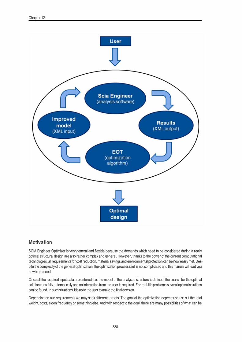
Chapter 12
MotivationSCIA Engineer Optimizer is very general and flexible because the demands which need to be considered during a reallyoptimal structural design are also rather complex and general. However, thanks to the power of the current computationaltechnologies, all requirements for cost reduction,material savingsand environmental protection can be now easilymet. Des-pite the complexity of the general optimization, the optimization process itself is not complicated and thismanualwill lead youhow to proceed.
Once all the required input data are entered, i.e. the model of the analysed structure is defined, the search for the optimalsolution runs fully automatically and no interaction from the user is required. For real-life problems several optimal solutionscan be found. In such situations, it is up to the user tomake the final decision.
Depending on our requirements we may seek different targets. The goal of the optimization depends on us: is it the totalweight, costs, eigen frequency or something else. And with respect to the goal, there are many possibilities of what can be
- 338 -
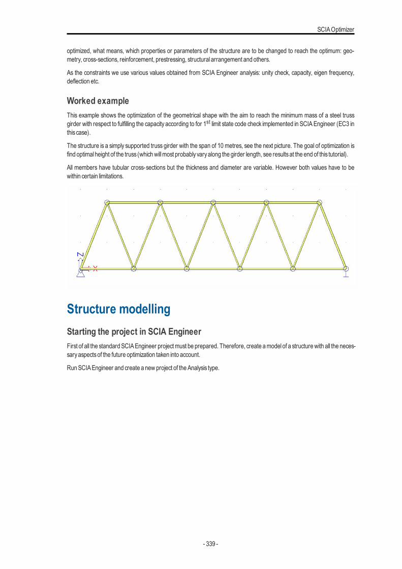
SCIAOptimizer
optimized, what means, which properties or parameters of the structure are to be changed to reach the optimum: geo-metry, cross-sections, reinforcement, prestressing, structural arrangement and others.
As the constraints we use various values obtained from SCIA Engineer analysis: unity check, capacity, eigen frequency,deflection etc.
Worked exampleThis example shows the optimization of the geometrical shape with the aim to reach the minimum mass of a steel trussgirder with respect to fulfilling the capacity according to for 1st limit state code check implemented in SCIA Engineer (EC3 inthis case).
The structure is a simply supported truss girder with the span of 10 metres, see the next picture. The goal of optimization isfind optimal height of the truss (whichwillmost probablyvaryalong the girder length, see resultsat the end of this tutorial).
All members have tubular cross-sections but the thickness and diameter are variable. However both values have to bewithin certain limitations.
Structure modellingStarting the project in SCIA EngineerFirst of all the standard SCIAEngineer projectmust be prepared. Therefore, create amodel of a structurewith all the neces-saryaspectsof the future optimization taken into account.
RunSCIAEngineer and create a new project of the Analysis type.
- 339 -
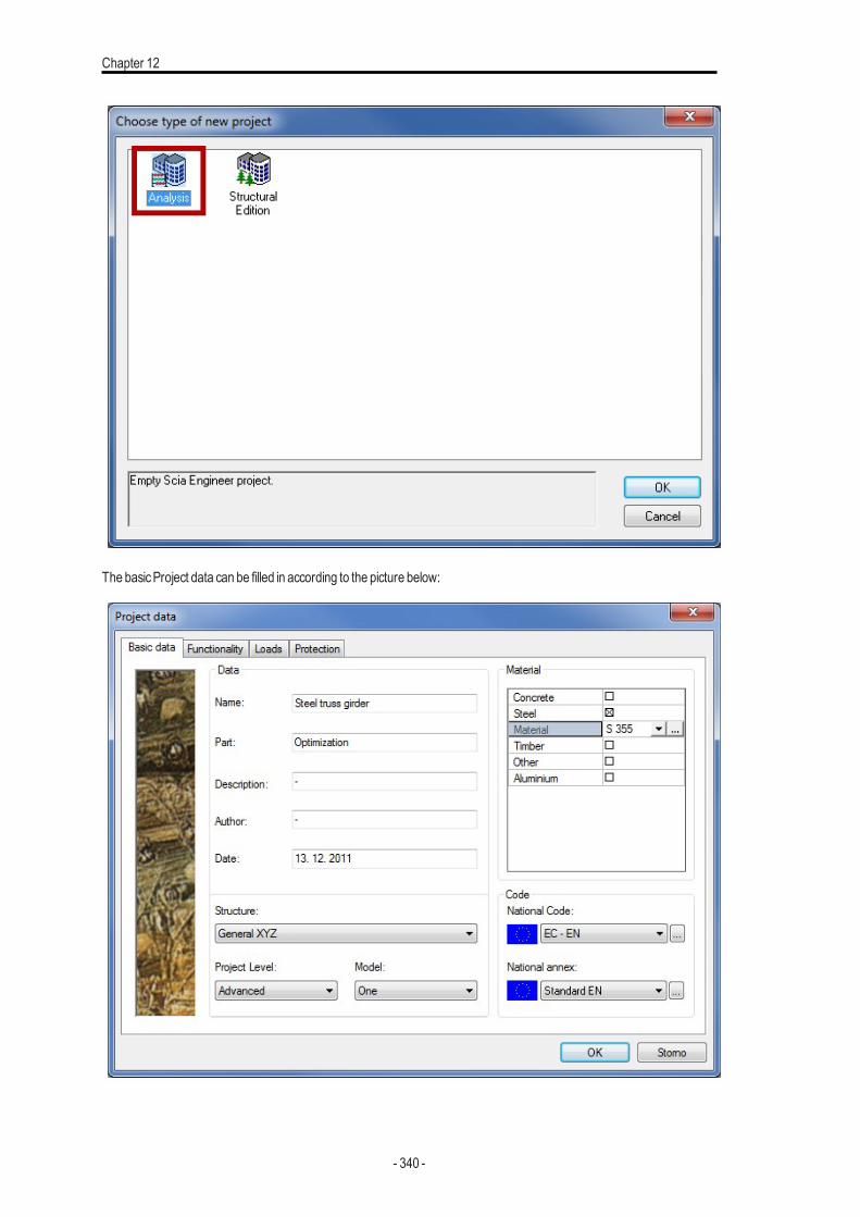
Chapter 12
The basicProject data can be filled in according to the picture below:
- 340 -
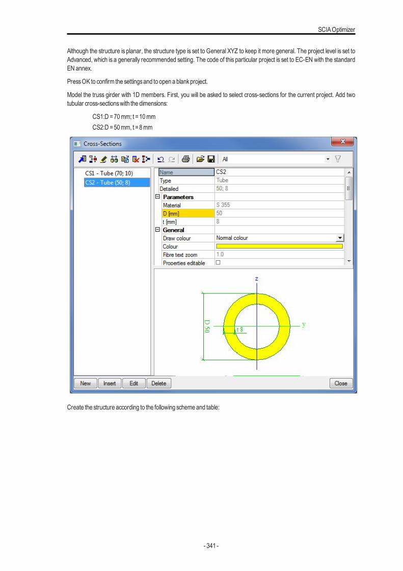
SCIAOptimizer
Although the structure is planar, the structure type is set to General XYZ to keep it more general. The project level is set toAdvanced, which is a generally recommended setting. The code of this particular project is set to EC-EN with the standardEN annex.
PressOK to confirm the settingsand to open a blankproject.
Model the truss girder with 1D members. First, you will be asked to select cross-sections for the current project. Add twotubular cross-sectionswith the dimensions:
CS1:D =70mm; t =10mmCS2:D =50mm, t =8mm
Create the structure according to the following schemeand table:
- 341 -
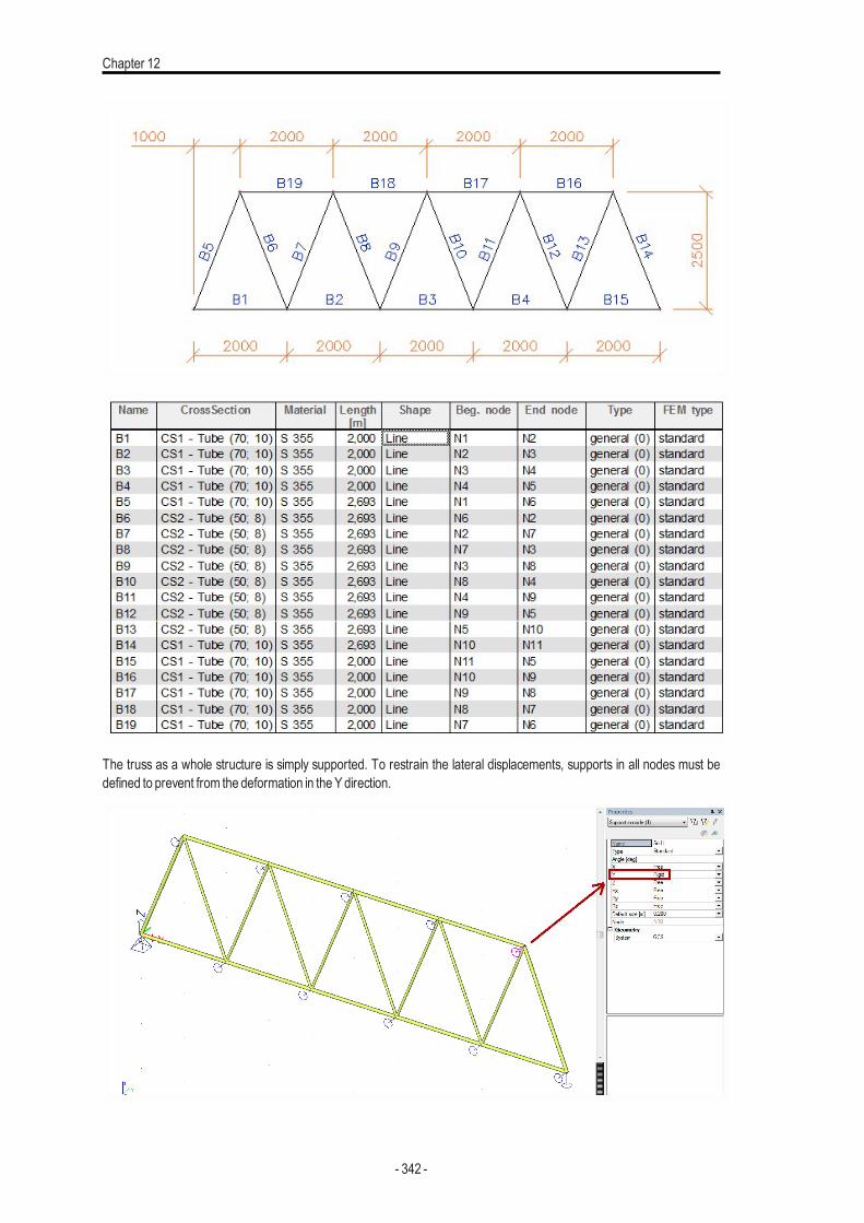
Chapter 12
The truss as a whole structure is simply supported. To restrain the lateral displacements, supports in all nodes must bedefined to prevent from the deformation in theYdirection.
- 342 -
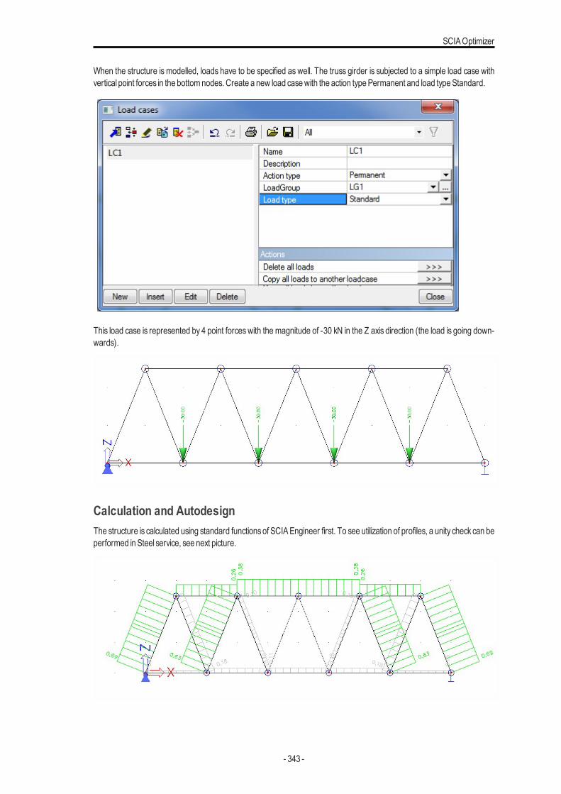
SCIAOptimizer
When the structure is modelled, loads have to be specified as well. The truss girder is subjected to a simple load case withvertical point forces in the bottomnodes. Create a new load casewith the action typePermanent and load typeStandard.
This load case is represented by 4 point forceswith the magnitude of -30 kN in the Z axis direction (the load is going down-wards).
Calculation and AutodesignThe structure is calculated using standard functionsof SCIAEngineer first. To see utilization of profiles, a unity check can beperformed in Steel service, see next picture.
- 343 -

Chapter 12
Maximal unity checkvalue 0,69 shows, profilesare too thick. In SCIAEngineer we can use veryefficient tool to design cross-sections, resulting in a good utilization of individual members under a certain load. The function is called Autodesign and itcan be found under Calculation,mesh group in theMain tree.
Autodesign can be used for variouspurposes. TheCross-section steel checkwill be used in this case. ThisAutodesign func-tion finds an optimal cross-section with respect to the unity check for all members with this cross-section. However, as thechange of a profile in a statically indeterminate structure affects the internal forces, the project has to be recalculated. Fornew internal foces, after recalculation, we can run Autodesign again. The user can do those two steps several times toreach proper cross-section design.
Autodesign is also integrated in optimization loop s of EOT. It means, during iterative search of optimal structure geometry,the program will make design of proper cross-sections. It means, in each iterative step, both geometry and cross-sectionswill be improved at the same time.
Prepare a new entry (called O1) in the Overall Autodesign library. Select both cross-sections (CS1 and CS2) in the selec-tion dialogue. It means that the itemscount will be 2.
Each cross-section has got two dimensions in their properties – thickness t and diameter D. Both dimensions can bechanged upwards and downwards in order to search for the optimum. To optimise both variables in one run, we will keep afixed ratio betweenD and t. AdvancedAutodesign isused for this.
- 344 -
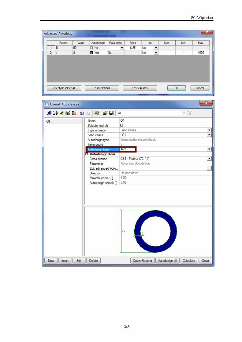
SCIAOptimizer
- 345 -
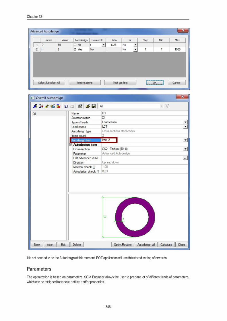
Chapter 12
It isnot needed to do theAutodesign at thismoment. EOT applicationwill use this stored setting afterwards.
ParametersThe optimization is based on parameters. SCIA Engineer allows the user to prepare lot of different kinds of parameters,which can be assigned to variousentitiesand/or properties.
- 346 -
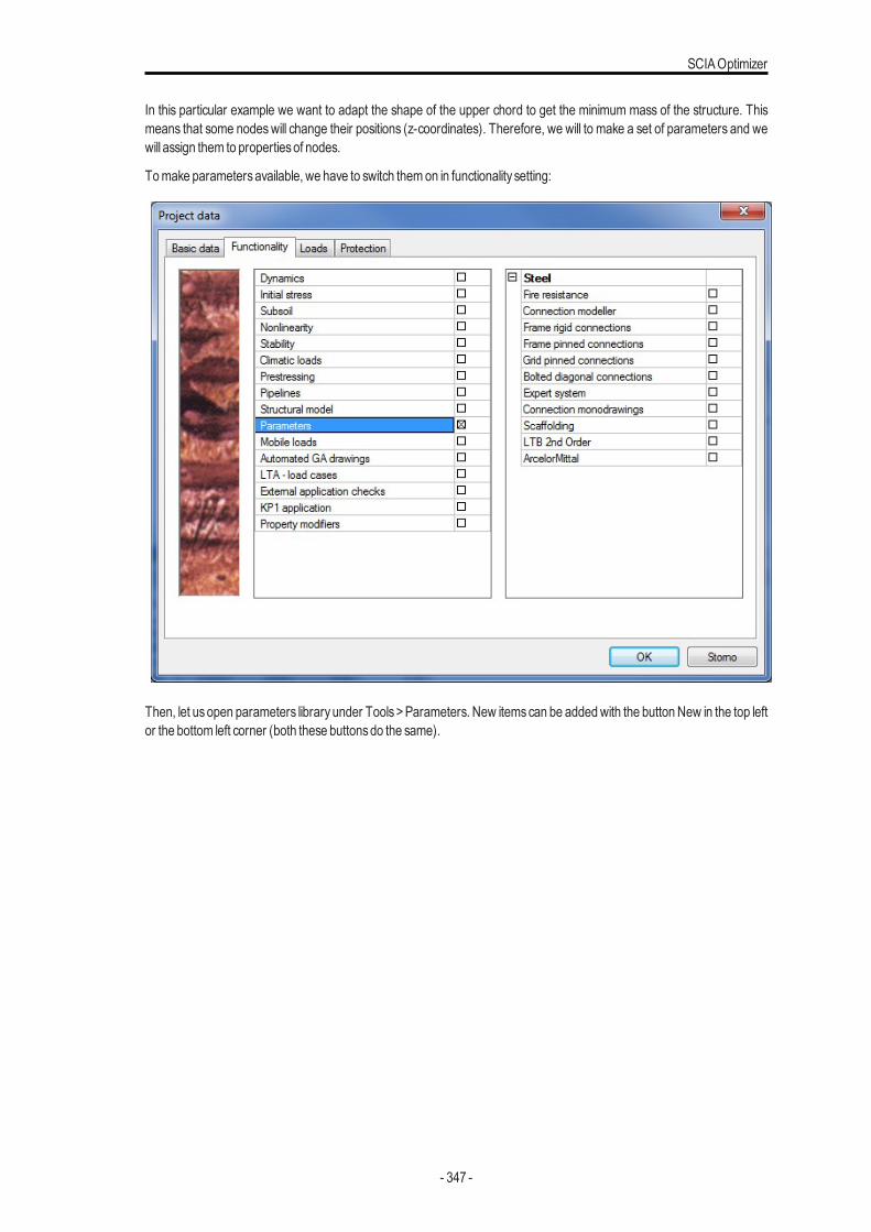
SCIAOptimizer
In this particular example we want to adapt the shape of the upper chord to get the minimum mass of the structure. Thismeans that some nodeswill change their positions (z-coordinates). Therefore, we will to make a set of parameters and wewill assign them to propertiesof nodes.
Tomake parametersavailable, we have to switch themon in functionality setting:
Then, let usopen parameters libraryunder Tools>Parameters. New itemscan be addedwith the button New in the top leftor the bottom left corner (both these buttonsdo the same).
- 347 -
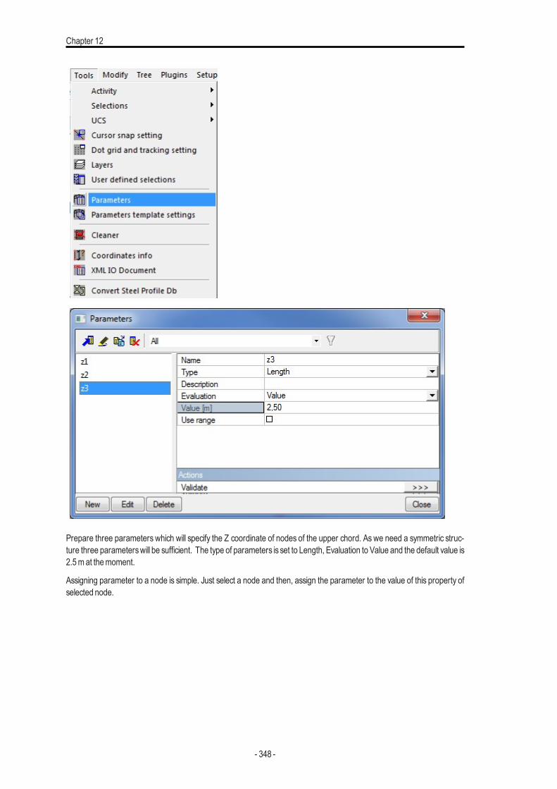
Chapter 12
Prepare three parameters which will specify the Z coordinate of nodes of the upper chord. As we need a symmetric struc-ture three parameterswill be sufficient. The type of parameters is set to Length, Evaluation to Value and the default value is2.5mat themoment.
Assigning parameter to a node is simple. Just select a node and then, assign the parameter to the value of this property ofselected node.
- 348 -
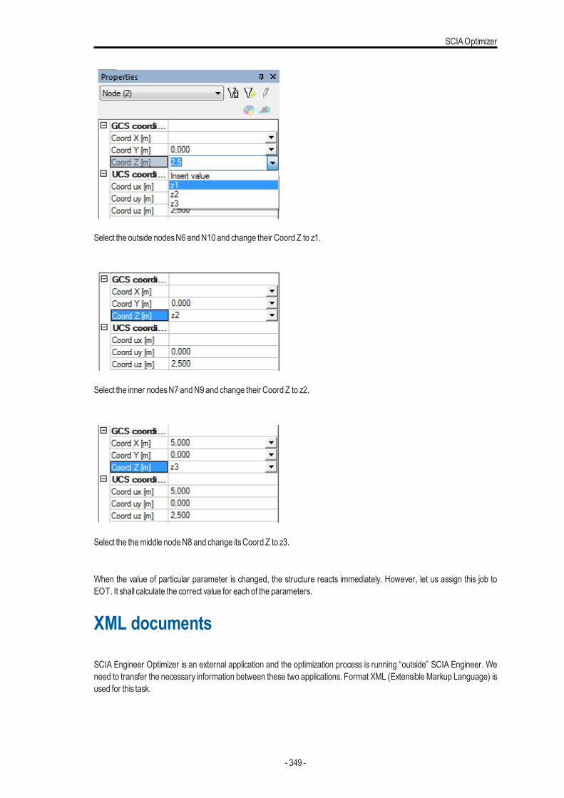
SCIAOptimizer
Select the outside nodesN6 andN10 and change their Coord Z to z1.
Select the inner nodesN7 andN9 and change their Coord Z to z2.
Select the themiddle nodeN8 and change itsCoord Z to z3.
When the value of particular parameter is changed, the structure reacts immediately. However, let us assign this job toEOT. It shall calculate the correct value for each of the parameters.
XML documents
SCIA Engineer Optimizer is an external application and the optimization process is running “outside” SCIA Engineer. Weneed to transfer the necessary information between these two applications. Format XML (Extensible Markup Language) isused for this task.
- 349 -
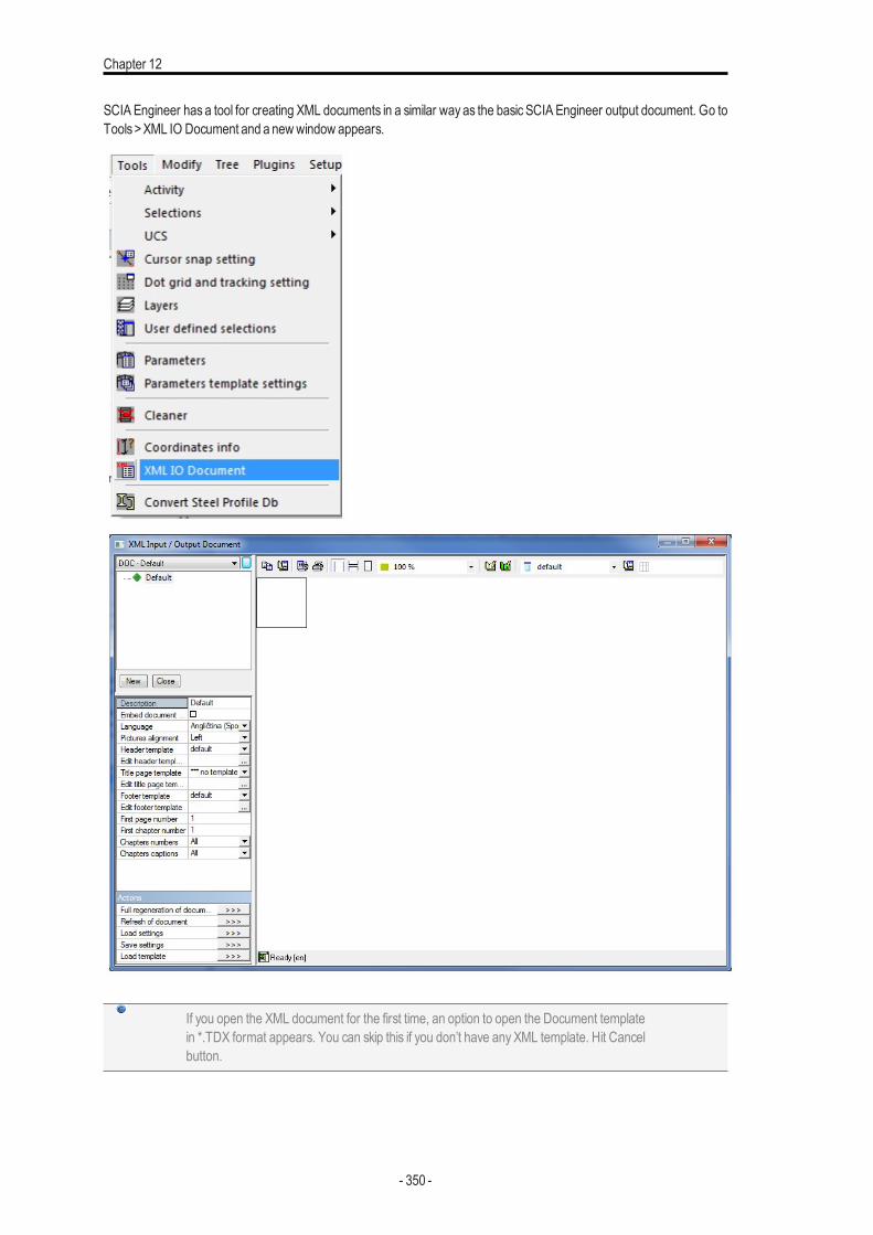
Chapter 12
SCIA Engineer has a tool for creating XML documents in a similar way as the basic SCIA Engineer output document. Go toTools>XML IO Document and a newwindow appears.
If you open the XML document for the first time, an option to open the Document templatein *.TDX format appears. You can skip this if you don’t have any XML template. Hit Cancelbutton.
- 350 -
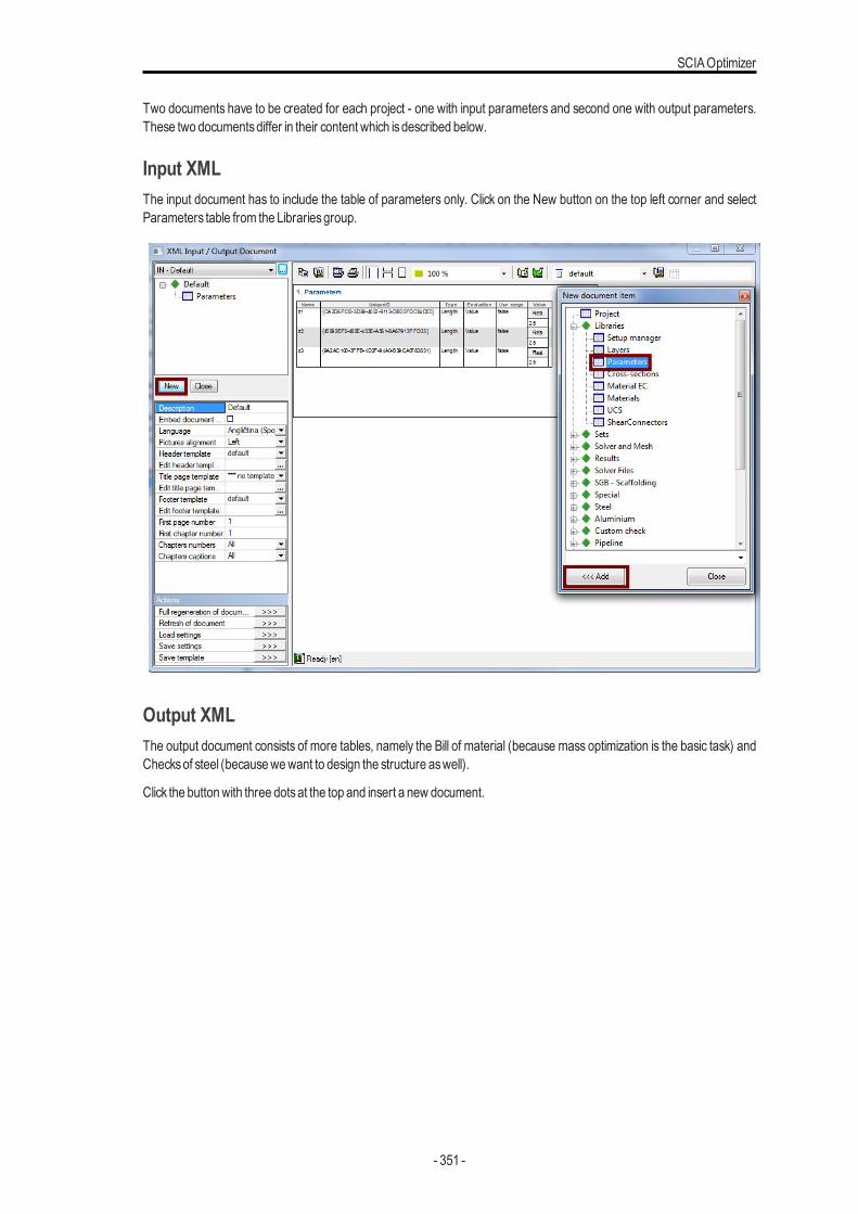
SCIAOptimizer
Two documents have to be created for each project - one with input parameters and second one with output parameters.These two documentsdiffer in their content which isdescribed below.
Input XMLThe input document has to include the table of parameters only. Click on the New button on the top left corner and selectParameters table from the Librariesgroup.
Output XMLThe output document consists of more tables, namely the Bill of material (because mass optimization is the basic task) andChecksof steel (becausewewant to design the structure aswell).
Click the buttonwith three dotsat the top and insert a new document.
- 351 -
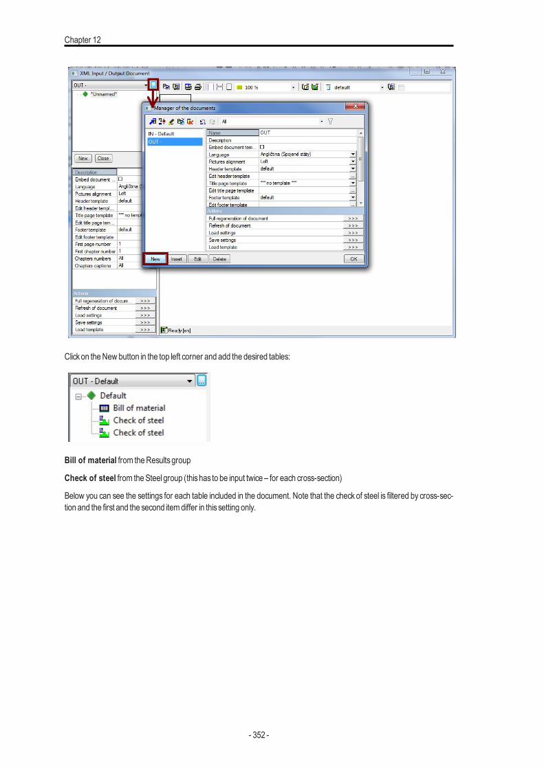
Chapter 12
Clickon theNew button in the top left corner and add the desired tables:
Bill of material from theResultsgroup
Check of steel from theSteel group (thishas to be input twice – for each cross-section)
Below you can see the settings for each table included in the document. Note that the check of steel is filtered by cross-sec-tion and the first and the second itemdiffer in this setting only.
- 352 -
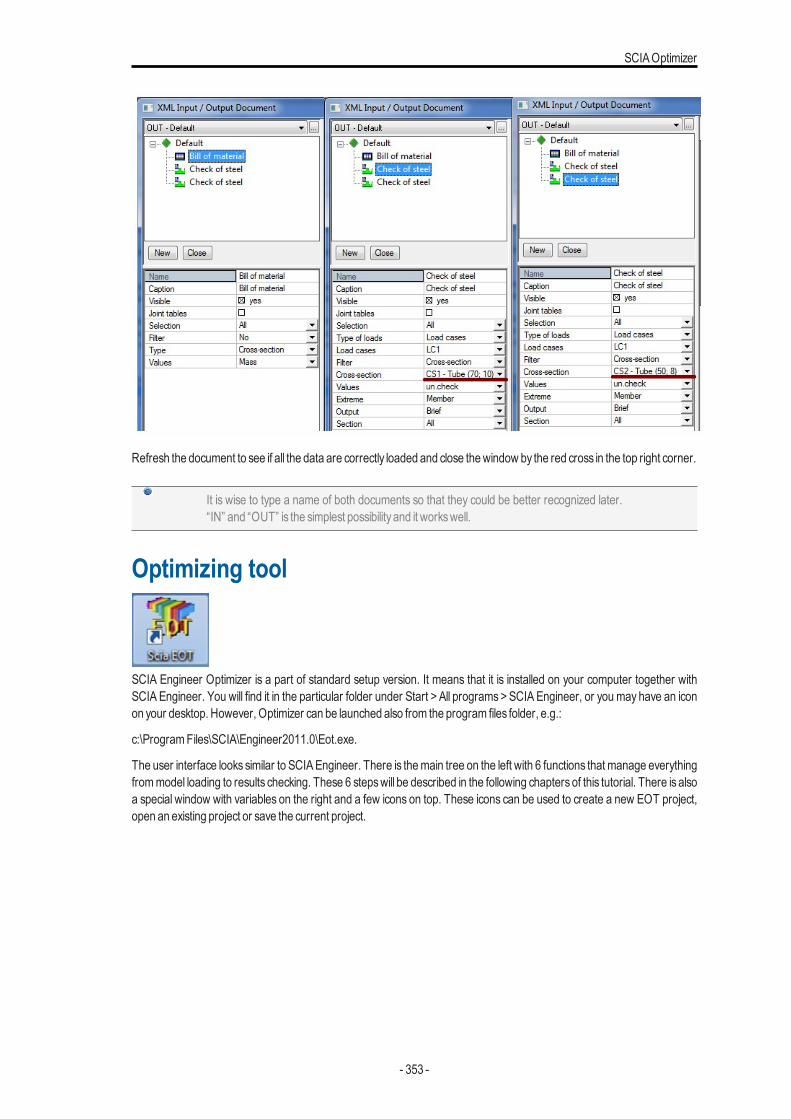
SCIAOptimizer
Refresh the document to see if all the data are correctly loaded and close thewindow by the red cross in the top right corner.
It is wise to type a name of both documents so that they could be better recognized later.“IN” and “OUT” is the simplest possibility and it workswell.
Optimizing tool
SCIA Engineer Optimizer is a part of standard setup version. It means that it is installed on your computer together withSCIA Engineer. You will find it in the particular folder under Start > All programs >SCIA Engineer, or you may have an iconon your desktop. However, Optimizer can be launched also from the program files folder, e.g.:
c:\ProgramFiles\SCIA\Engineer2011.0\Eot.exe.
The user interface looks similar to SCIAEngineer. There is themain tree on the left with 6 functions that manage everythingfrommodel loading to results checking. These 6 stepswill be described in the following chapters of this tutorial. There is alsoa special window with variables on the right and a few icons on top. These icons can be used to create a new EOT project,open an existing project or save the current project.
- 353 -
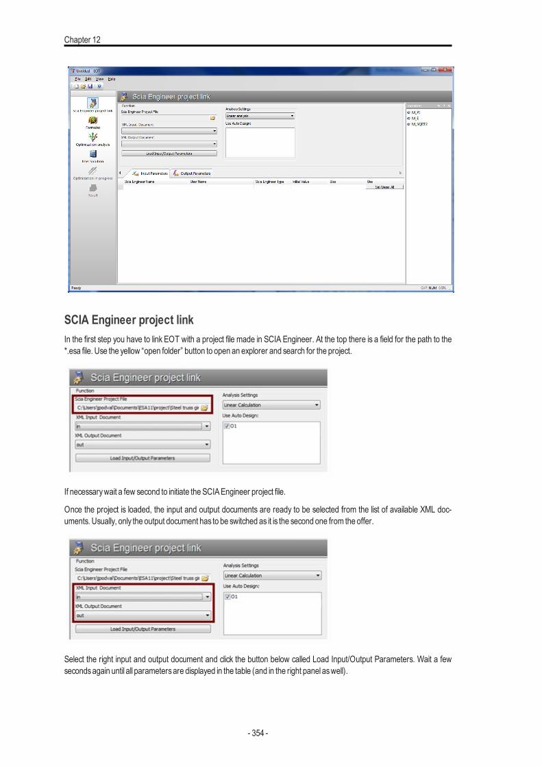
Chapter 12
SCIA Engineer project linkIn the first step you have to link EOT with a project file made in SCIA Engineer. At the top there is a field for the path to the*.esa file. Use the yellow “open folder” button to open an explorer and search for the project.
If necessarywait a few second to initiate theSCIAEngineer project file.
Once the project is loaded, the input and output documents are ready to be selected from the list of available XML doc-uments. Usually, only the output document has to be switched as it is the second one from the offer.
Select the right input and output document and click the button below called Load Input/Output Parameters. Wait a fewsecondsagain until all parametersare displayed in the table (and in the right panel aswell).
- 354 -
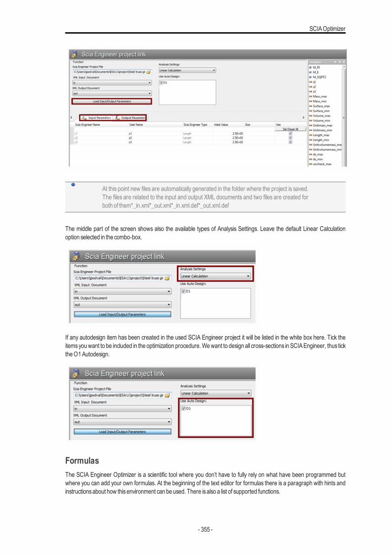
SCIAOptimizer
At this point new files are automatically generated in the folder where the project is saved.The files are related to the input and output XML documents and two files are created forboth of them*_in.xml*_out.xml*_in.xml.def*_out.xml.def
The middle part of the screen shows also the available types of Analysis Settings. Leave the default Linear Calculationoption selected in the combo-box.
If any autodesign item has been created in the used SCIA Engineer project it will be listed in the white box here. Tick theitemsyouwant to be included in the optimization procedure.Wewant to design all cross-sections in SCIAEngineer, thus ticktheO1Autodesign.
FormulasThe SCIA Engineer Optimizer is a scientific tool where you don’t have to fully rely on what have been programmed butwhere you can add your own formulas. At the beginning of the text editor for formulas there is a paragraph with hints andinstructionsabout how thisenvironment can be used. There isalso a list of supported functions.
- 355 -
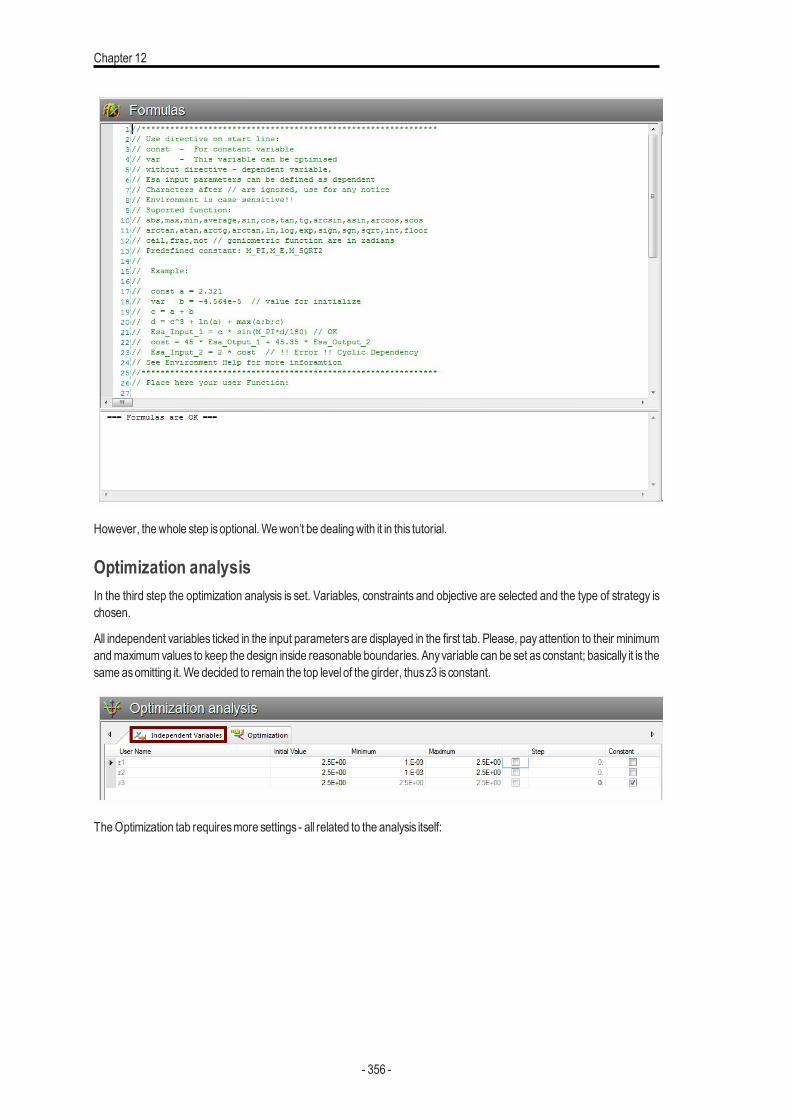
Chapter 12
However, thewhole step isoptional.Wewon’t be dealingwith it in this tutorial.
Optimization analysisIn the third step the optimization analysis is set. Variables, constraints and objective are selected and the type of strategy ischosen.
All independent variables ticked in the input parameters are displayed in the first tab. Please, pay attention to their minimumandmaximumvalues to keep the design inside reasonable boundaries. Anyvariable can be set asconstant; basically it is thesame asomitting it.We decided to remain the top level of the girder, thusz3 isconstant.
TheOptimization tab requiresmore settings - all related to the analysis itself:
- 356 -
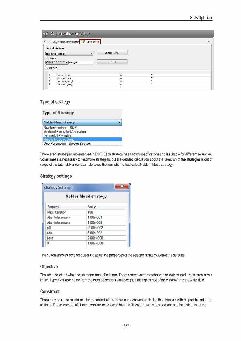
SCIAOptimizer
Type of strategy
There are 5 strategies implemented in EOT. Each strategy has its own specifications and is suitable for different examples.Sometimes it is necessary to test more strategies, but the detailed discussion about the selection of the strategies is out ofscope of this tutorial. For our example select the heuristicmethod calledNelder –Mead strategy.
Strategy settings
Thisbutton enablesadvanced users to adjust the propertiesof the selected strategy. Leave the defaults.
ObjectiveThe intention of thewhole optimization is specified here. There are two extremes that can be determined –maximumor min-imum. Type a variable name from the list of dependent variables (see the right stripe of thewindow) into thewhite field.
ConstraintThere may be some restrictions for the optimization. In our case we want to design the structure with respect to code reg-ulations. The unity checkof allmembershas to be lower than 1.0. There are two cross-sectionsand for both of them the
- 357 -
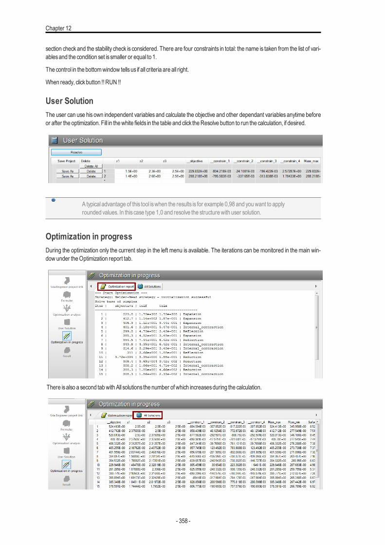
Chapter 12
section check and the stability check is considered. There are four constraints in total: the name is taken from the list of vari-ablesand the condition set is smaller or equal to 1.
The control in the bottomwindow tellsus if all criteria are all right.
When ready, clickbutton !! RUN !!
User SolutionThe user can use his own independent variables and calculate the objective and other dependant variables anytime beforeor after the optimization. Fill in thewhite fields in the table and click theResolve button to run the calculation, if desired.
A typical advantage of this tool iswhen the results is for example 0,98 and youwant to applyrounded values. In this case type 1,0 and resolve the structurewith user solution.
Optimization in progressDuring the optimization only the current step in the left menu is available. The iterations can be monitored in the main win-dow under theOptimization report tab.
There isalso a second tabwith All solutions the number of which increasesduring the calculation.
- 358 -
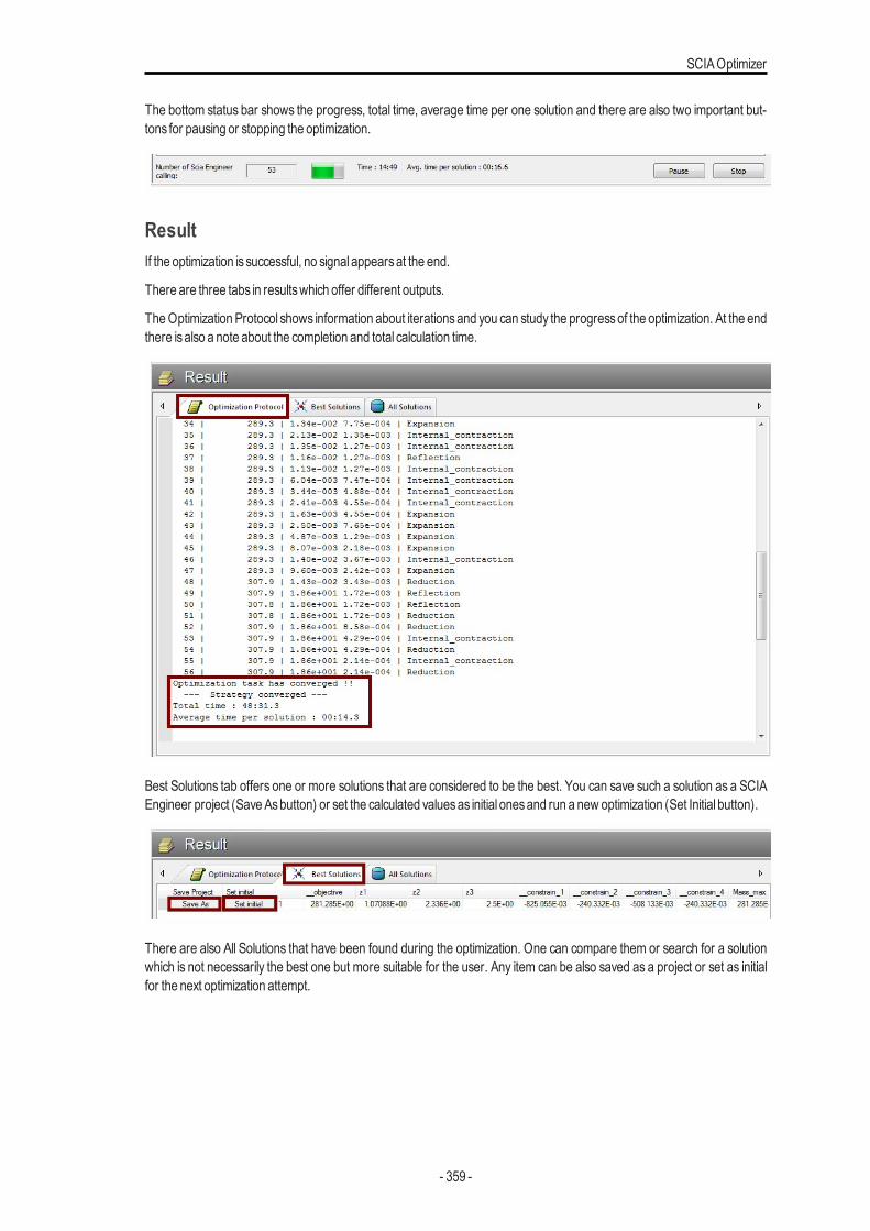
SCIAOptimizer
The bottom status bar shows the progress, total time, average time per one solution and there are also two important but-tons for pausing or stopping the optimization.
ResultIf the optimization is successful, no signal appearsat the end.
There are three tabs in resultswhich offer different outputs.
TheOptimization Protocol shows information about iterationsand you can study the progressof the optimization. At the endthere isalso a note about the completion and total calculation time.
Best Solutions tab offers one or more solutions that are considered to be the best. You can save such a solution as a SCIAEngineer project (SaveAsbutton) or set the calculated valuesas initial onesand run a new optimization (Set Initial button).
There are also All Solutions that have been found during the optimization. One can compare them or search for a solutionwhich is not necessarily the best one but more suitable for the user. Any item can be also saved as a project or set as initialfor the next optimization attempt.
- 359 -
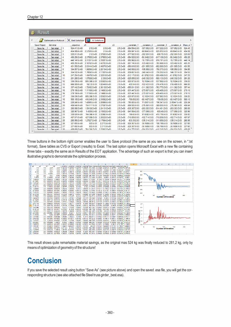
Chapter 12
Three buttons in the bottom right corner enables the user to Save protocol (the same as you see on the screen, in *.txtformat), Save tables as CVS or Export (results) to Excel. The last option opens Microsoft Excel with a new file containingthree tabs – exactly the same as in Results of the EOT application. The advantage of such an export is that you can insertillustrative graphs to demonstrate the optimization process.
This result shows quite remarkable material savings, as the original mas 524 kg was finally reduced to 281,2 kg, only bymeansof optimization of geometryof the structure!
ConclusionIf you save the selected result using button “Save As” (see picture above) and open the saved .esa file, you will get the cor-responding structure (see also attached file Steel trussgirder_best.esa).
- 360 -
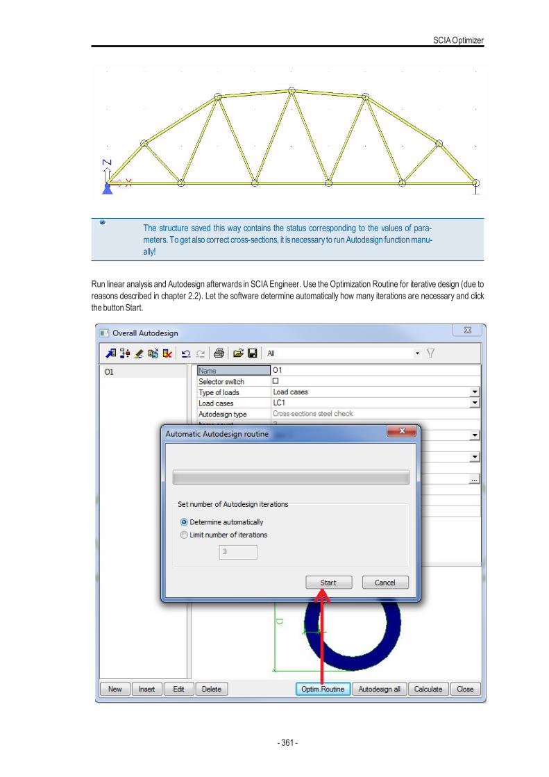
SCIAOptimizer
The structure saved this way contains the status corresponding to the values of para-meters. To get also correct cross-sections, it is necessary to runAutodesign functionmanu-ally!
Run linear analysis and Autodesign afterwards in SCIA Engineer. Use the Optimization Routine for iterative design (due toreasons described in chapter 2.2). Let the software determine automatically how many iterations are necessary and clickthe button Start.
- 361 -
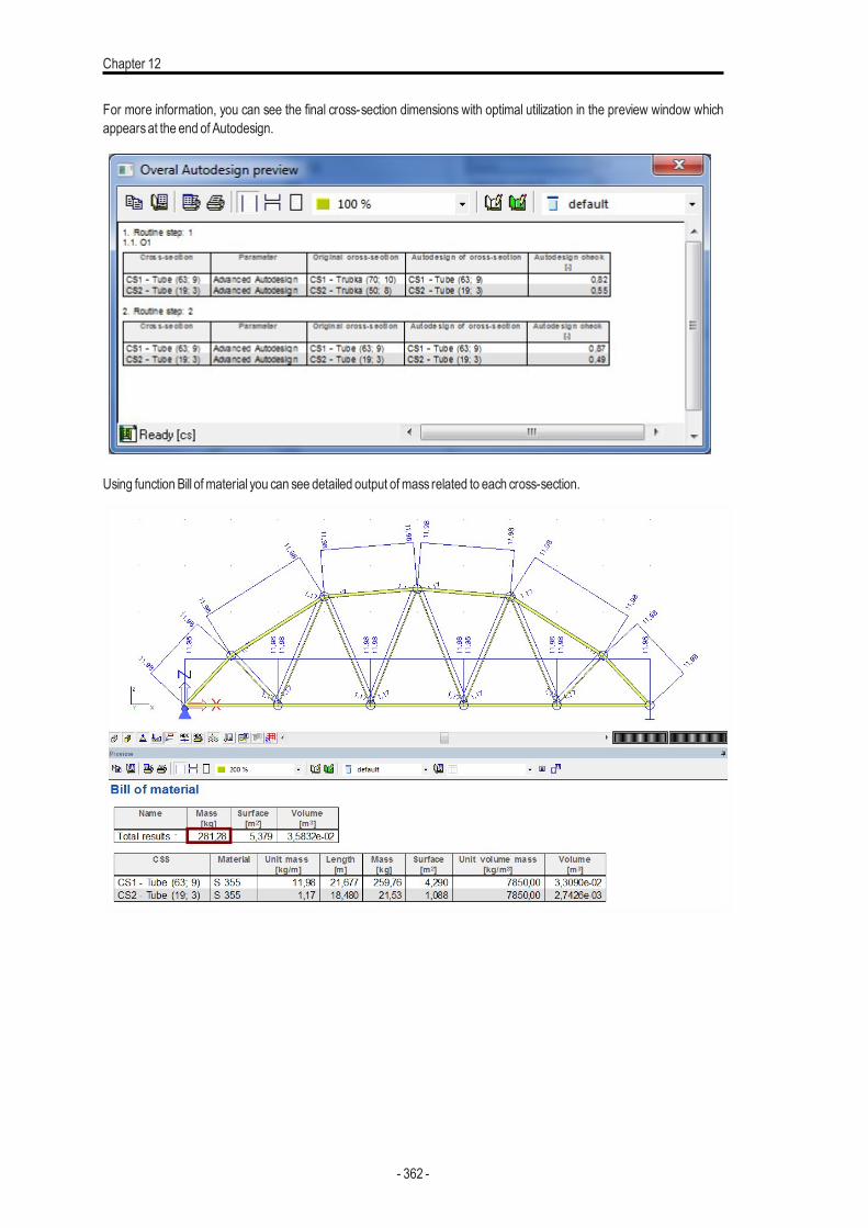
Chapter 12
For more information, you can see the final cross-section dimensions with optimal utilization in the preview window whichappearsat the end of Autodesign.
Using function Bill of material you can see detailed output ofmass related to each cross-section.
- 362 -

Steel frame design
Steel frame design
Getting startedStarting a projectBefore you can start a project, you need to start the program first.
Starting the program
1. Double-clickon theSCIAEngineer shortcut in theWindowsDesktop.
or
2. If the shortcut isnot installed, click [Start] and choosePrograms>SCIAEngineer >SCIAEngineer. If the programdoesnot find anyprotection, youwill obtain a dialogue indicating that no protectionwas found. A second dialoguewill list therestrictionsof the demo version. Click [OK] in bothwindows.
For this tutorial, youmust start a new project.
Starting a new projectFor this tutorialwe have to start a new project. If the dialogOpen appears, click [Cancel].
Clickon theNew icon in the toolbar.
Now, theProject data dialogue isopened. Here, you can enter general data about the project.
- 363 -

Chapter 13
1. In theData group, enter your preferred data. These data can bementioned on the output, e.g. in the document and onthe drawings.
2. Select FrameXYZ in theStructure field.3. ChooseModel: One.
4. Clickon the rectangular button belowNationalCode to choose the default code for the project. This codewill determine the availablematerials, combination rulesand code checks. For the project of thisTutorial, chooseEC-EN.
5. Select aNational annex. For thisexample chooseCzechCSN –ENNA.6. In theMaterial group, select Steel.
Below the itemSteel, a new itemMaterialwill appear - chooseS355 from themenu.
On the Functionality tab choose the optionsClimatic loads.
- 364 -
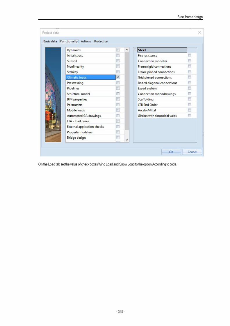
Steel frame design
On the Load tab set the value of checkboxesWind Load andSnow Load to the option According to code.
- 365 -
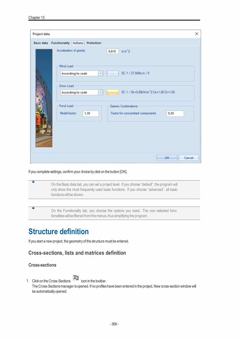
Chapter 13
If you complete settings, confirm your choice byclickon the button [OK].
On the Basic data tab, you can set a project level. If you choose “default”, the program willonly show the most frequently used basic functions. If you choose “advanced”, all basicfunctionswill be shown.
On the Functionality tab, you choose the options you need. The non- selected func-tionalitieswill be filtered from themenus, thussimplifying the program.
Structure definitionIf you start a new project, the geometryof the structuremust be entered.
Cross-sections, lists and matrices definition
Cross-sections
1. Clickon theCross-Sections icon in the toolbar.TheCross-Sectionsmanager isopened. If no profileshave been entered in the project, New cross-sectionwindowwillbe automaticallyopened.
- 366 -
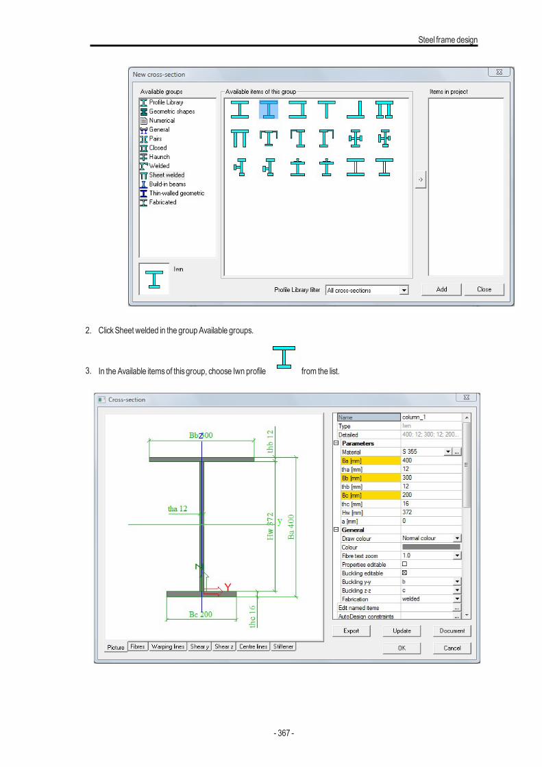
Steel frame design
2. ClickSheet welded in the groupAvailable groups.
3. In the Available itemsof thisgroup, choose Iwn profile from the list.
- 367 -
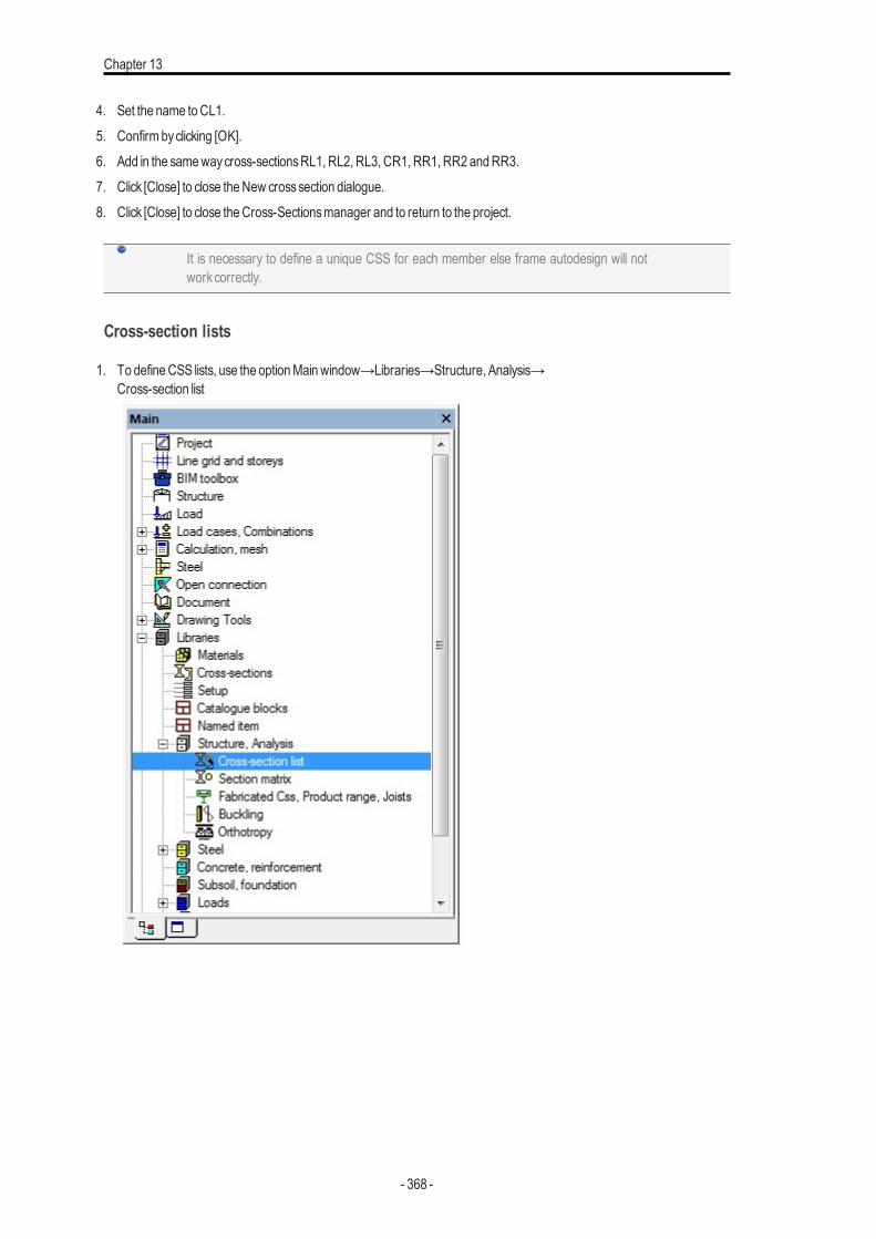
Chapter 13
4. Set the name toCL1.5. Confirm byclicking [OK].6. Add in the samewaycross-sectionsRL1, RL2, RL3, CR1, RR1, RR2 andRR3.7. Click [Close] to close theNew crosssection dialogue.8. Click [Close] to close theCross-Sectionsmanager and to return to the project.
It is necessary to define a unique CSS for each member else frame autodesign will notworkcorrectly.
Cross-section lists
1. To defineCSS lists, use the optionMainwindow→Libraries→Structure, Analysis→Cross-section list
- 368 -
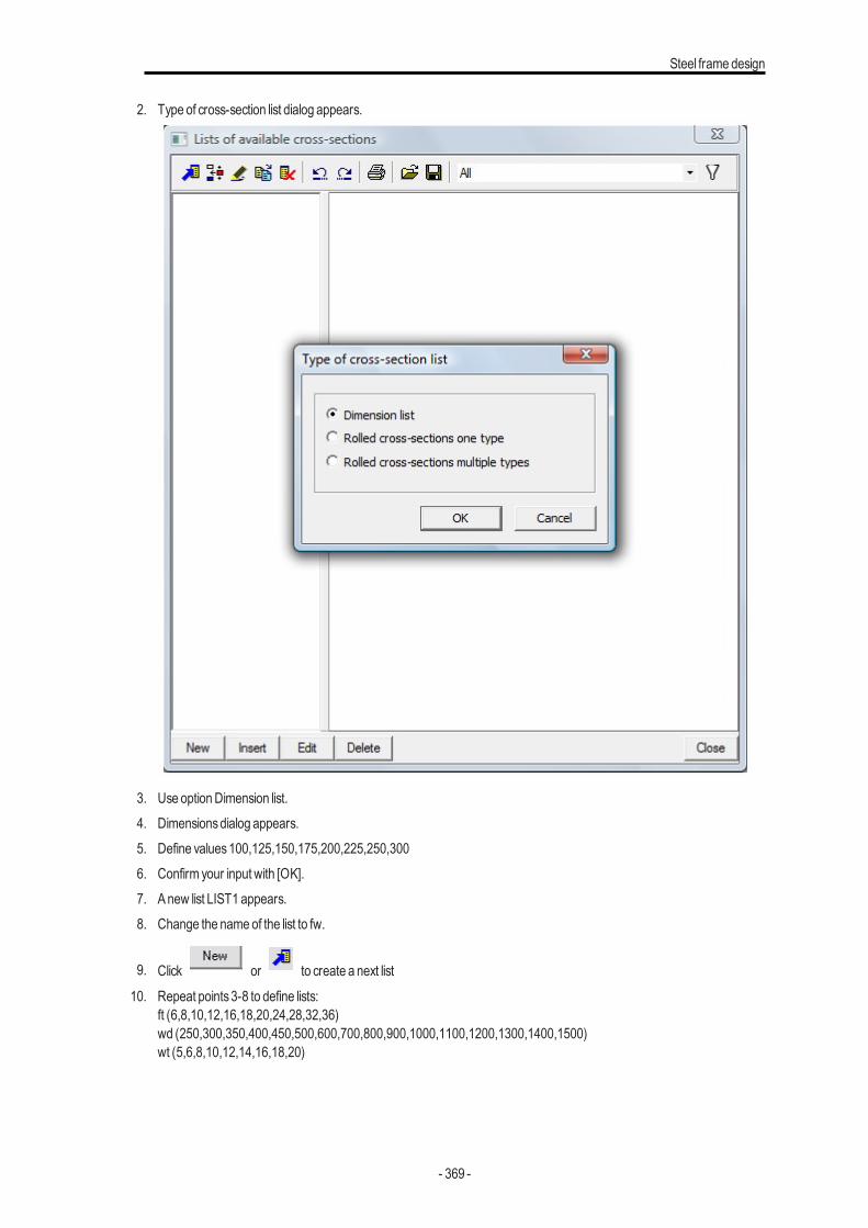
Steel frame design
2. Type of cross-section list dialog appears.
3. Use optionDimension list.4. Dimensionsdialog appears.5. Define values100,125,150,175,200,225,250,3006. Confirm your input with [OK].7. Anew list LIST1 appears.8. Change the nameof the list to fw.
9. Click or to create a next list
10. Repeat points3-8 to define lists:ft (6,8,10,12,16,18,20,24,28,32,36)wd (250,300,350,400,450,500,600,700,800,900,1000,1100,1200,1300,1400,1500)wt (5,6,8,10,12,14,16,18,20)
- 369 -
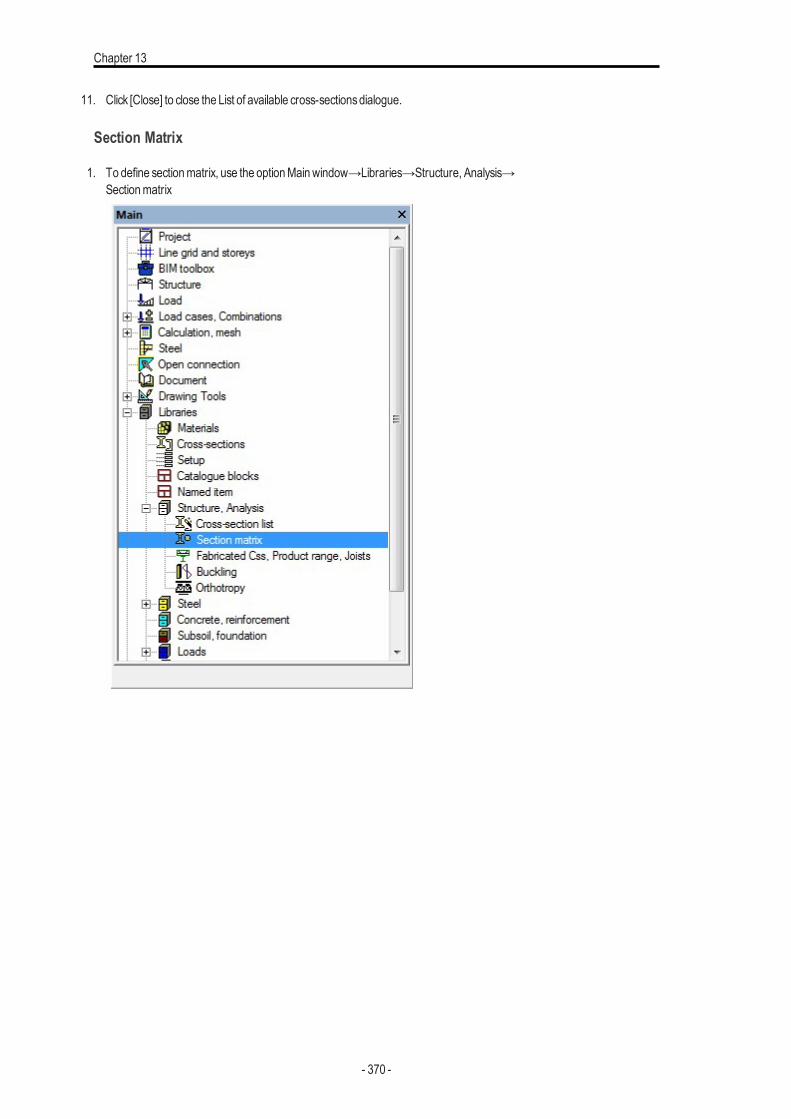
Chapter 13
11. Click [Close] to close the List of available cross-sectionsdialogue.
Section Matrix
1. To define sectionmatrix, use the optionMainwindow→Libraries→Structure, Analysis→Sectionmatrix
- 370 -
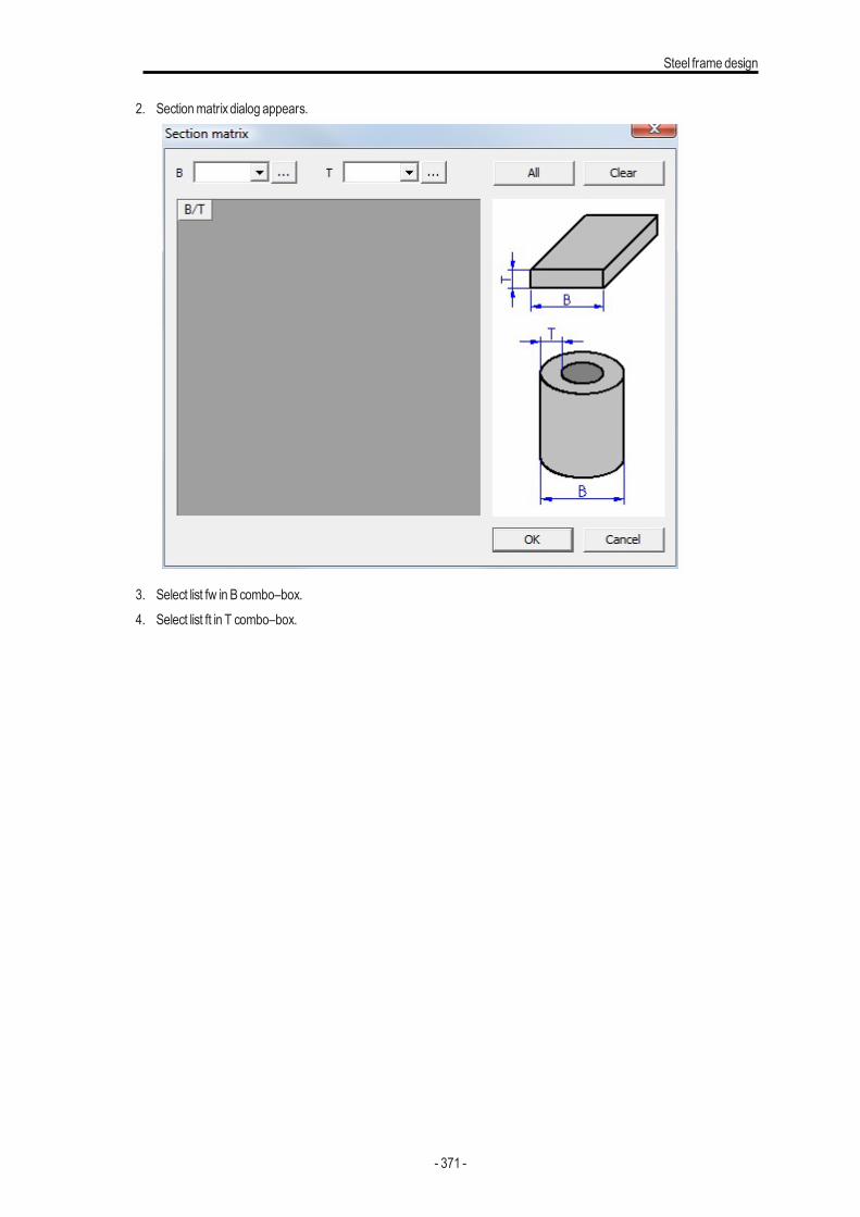
Steel frame design
2. Sectionmatrixdialog appears.
3. Select list fw in Bcombo–box.4. Select list ft in T combo–box.
- 371 -
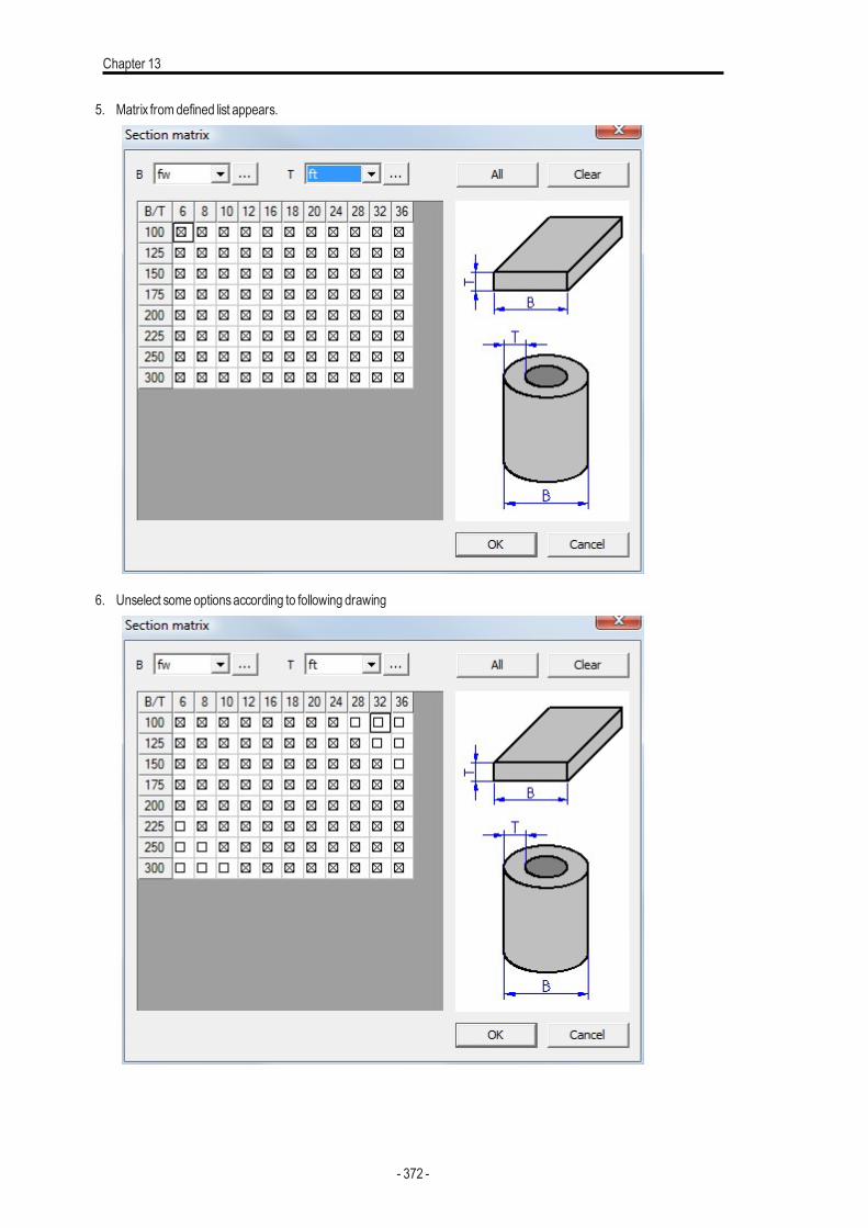
Chapter 13
5. Matrix fromdefined list appears.
6. Unselect some optionsaccording to following drawing
- 372 -
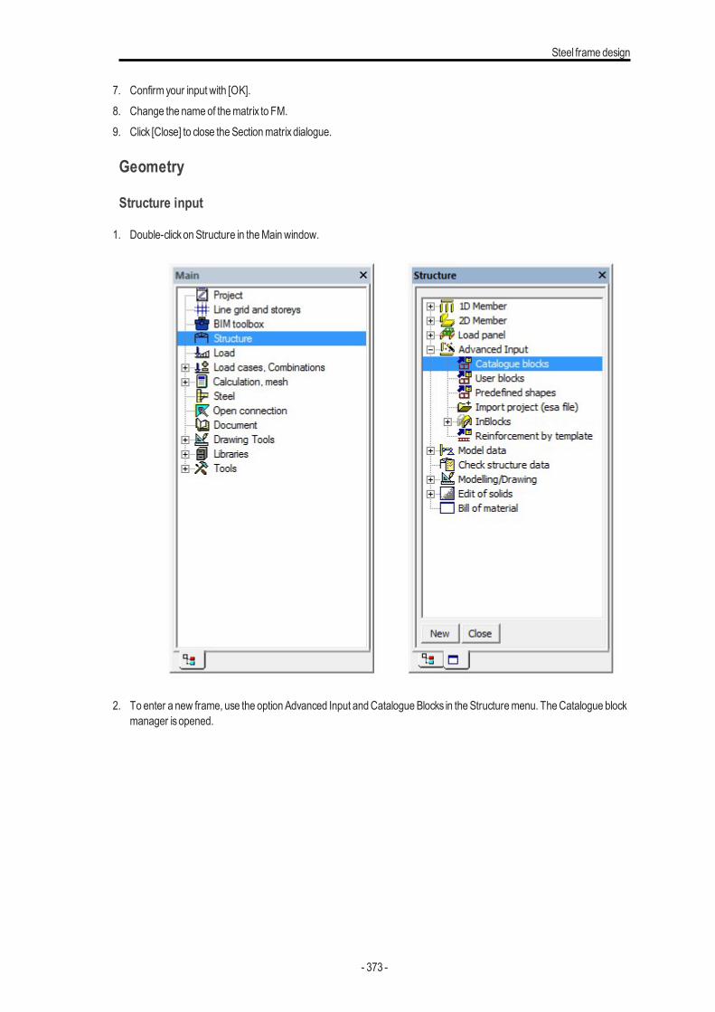
Steel frame design
7. Confirm your input with [OK].8. Change the nameof thematrix to FM.9. Click [Close] to close theSectionmatrixdialogue.
Geometry
Structure input
1. Double-clickonStructure in theMainwindow.
2. To enter a new frame, use the option Advanced Input andCatalogueBlocks in theStructuremenu. TheCatalogue blockmanager isopened.
- 373 -
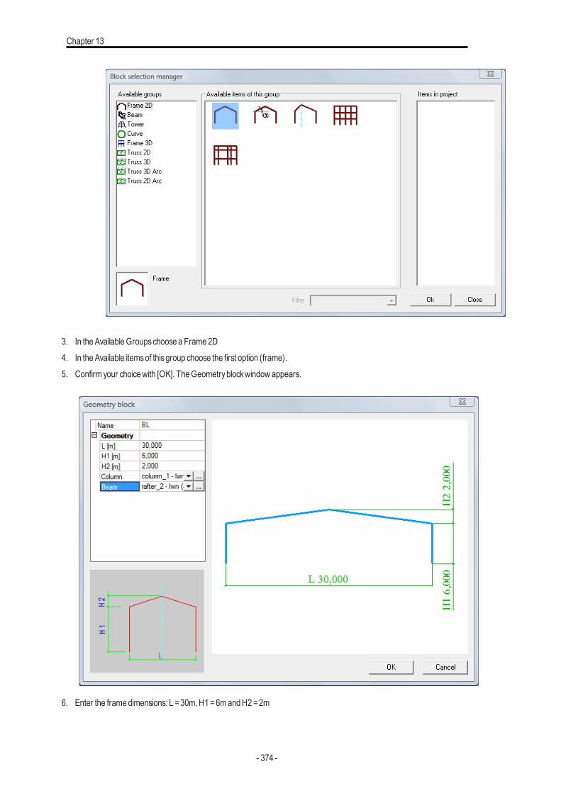
Chapter 13
3. In theAvailableGroupschoose a Frame 2D4. In theAvailable itemsof thisgroup choose the first option (frame).5. Confirm your choicewith [OK]. TheGeometryblockwindow appears.
6. Enter the frame dimensions: L =30m,H1 =6mandH2=2m
- 374 -
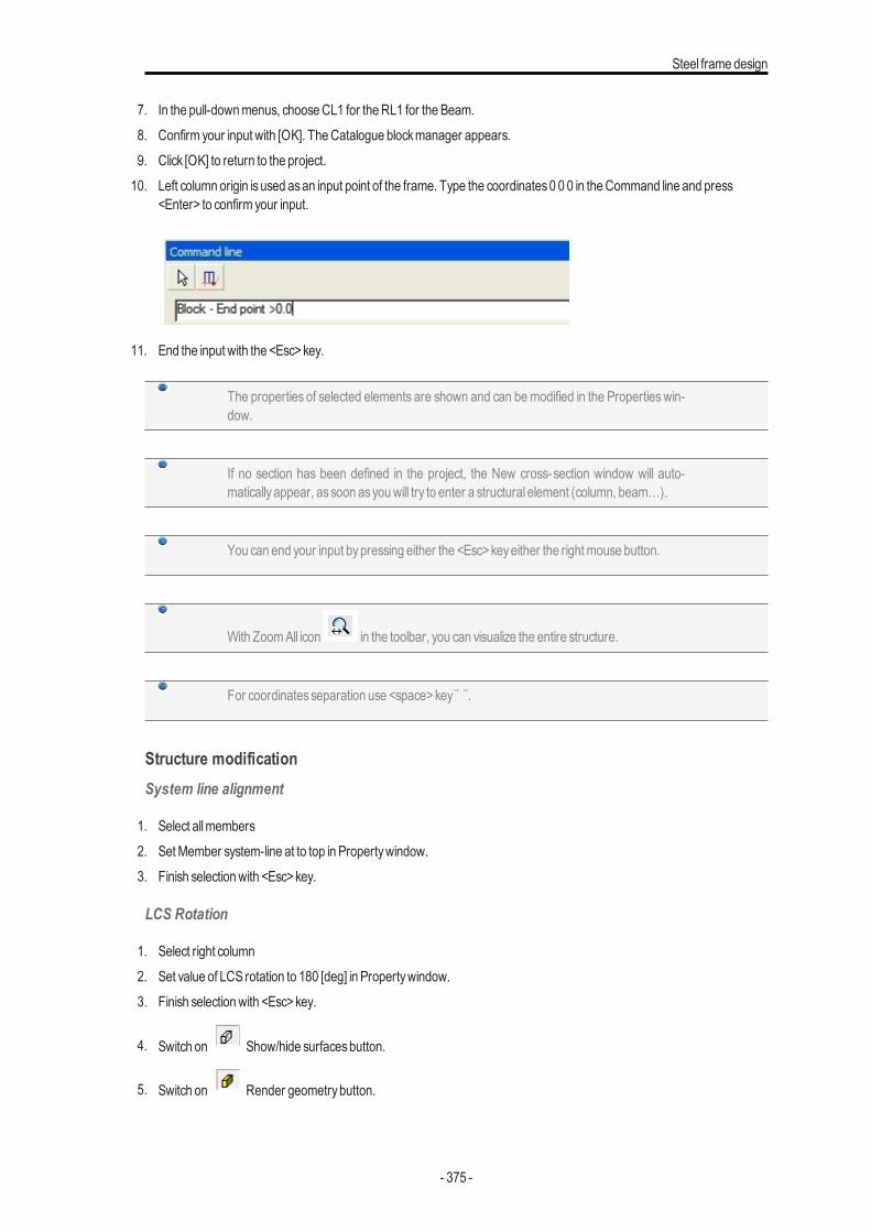
Steel frame design
7. In the pull-downmenus, chooseCL1 for theRL1 for the Beam.8. Confirm your input with [OK]. TheCatalogue blockmanager appears.9. Click [OK] to return to the project.10. Left column origin isused asan input point of the frame. Type the coordinates0 0 0 in theCommand line and press
<Enter> to confirm your input.
11. End the input with the <Esc>key.
The properties of selected elements are shown and can be modified in the Propertieswin-dow.
If no section has been defined in the project, the New cross-section window will auto-maticallyappear, assoon asyouwill try to enter a structural element (column, beam…).
You can end your input bypressing either the <Esc>keyeither the rightmouse button.
With ZoomAll icon in the toolbar, you can visualize the entire structure.
For coordinatesseparation use <space>key ¨ ¨.
Structure modificationSystem line alignment
1. Select allmembers2. SetMember system-line at to top in Propertywindow.3. Finish selectionwith <Esc>key.
LCS Rotation
1. Select right column2. Set value of LCS rotation to 180 [deg] in Propertywindow.3. Finish selectionwith <Esc>key.
4. Switch on Show/hide surfacesbutton.
5. Switch on Render geometrybutton.
- 375 -
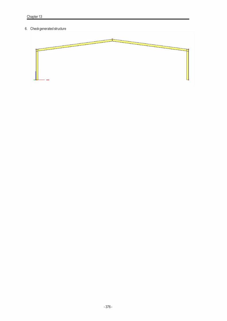
Chapter 13
6. Checkgenerated structure
- 376 -
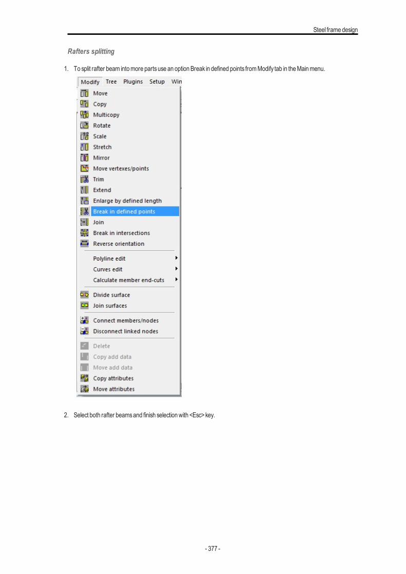
Steel frame design
Rafters splitting
1. To split rafter beam intomore partsuse an option Break in defined points fromModify tab in theMainmenu.
2. Select both rafter beamsand finish selectionwith <Esc>key.
- 377 -
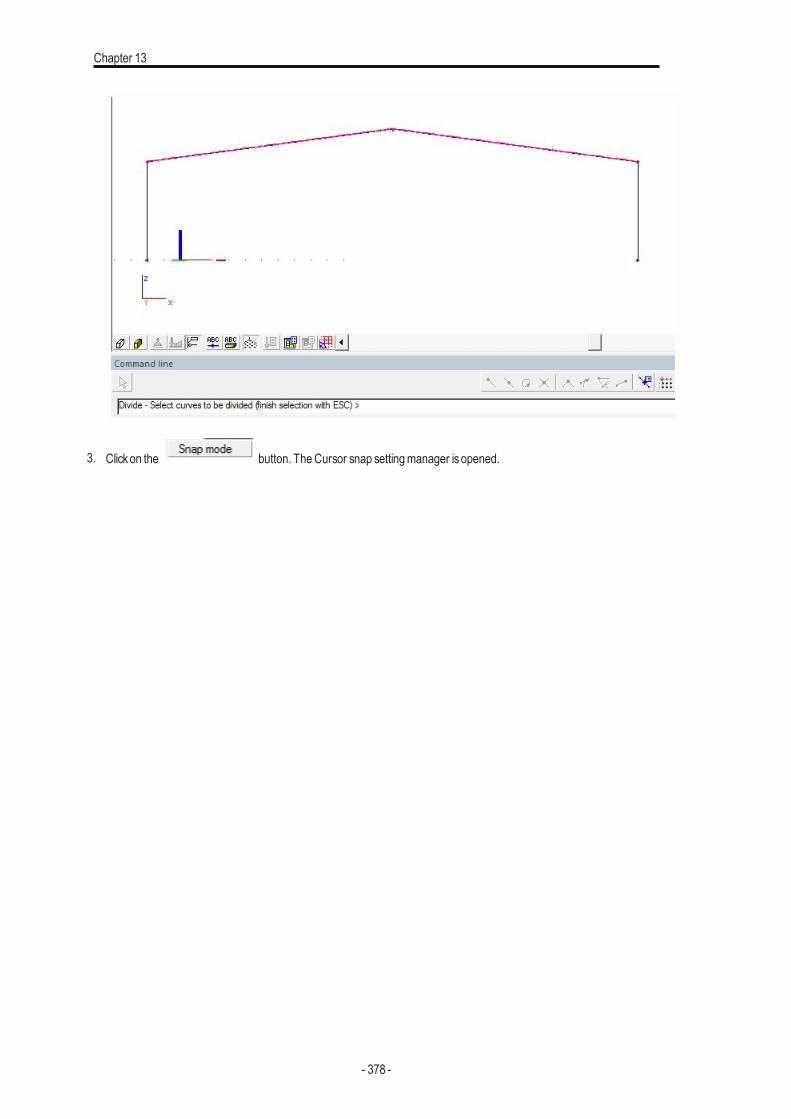
Chapter 13
3. Clickon the button. TheCursor snap settingmanager isopened.
- 378 -
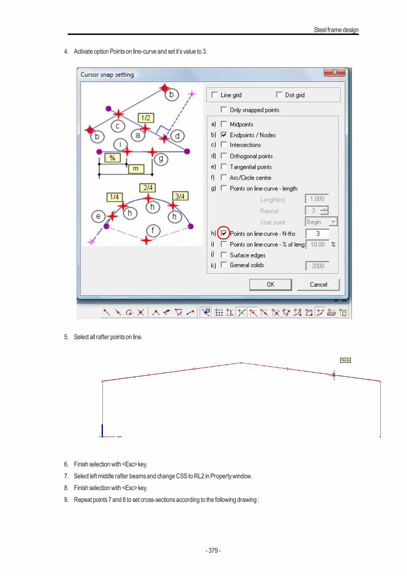
Steel frame design
4. Activate option Pointson line-curve and set it’s value to 3.
5. Select all rafter pointson line.
6. Finish selectionwith <Esc>key.7. Select left middle rafter beamsand changeCSS toRL2 in Propertywindow.8. Finish selectionwith <Esc>key.9. Repeat points7 and 8 to set cross-sectionsaccording to the following drawing :
- 379 -
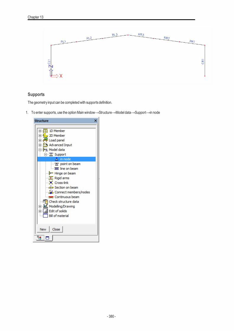
Chapter 13
SupportsThe geometry input can be completedwith supportsdefinition.
1. To enter supports, use the optionMainwindow→Structure→Model data→Support→in node
- 380 -
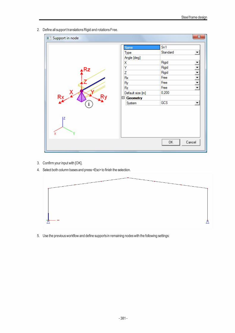
Steel frame design
2. Define all support translationsRigid and rotationsFree.
3. Confirm your input with [OK].4. Select both column basesand press<Esc> to finish the selection.
5. Use the previousworkflow and define supports in remaining nodeswith the following settings:
- 381 -
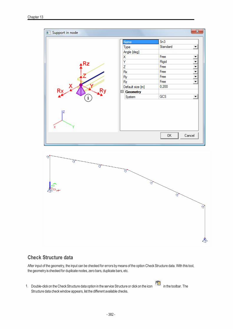
Chapter 13
Check Structure dataAfter input of the geometry, the input can be checked for errors bymeans of the option CheckStructure data. With this tool,the geometry is checked for duplicate nodes, zero bars, duplicate bars, etc.
1. Double-clickon theCheckStructure data option in the service Structure or clickon the icon in the toolbar. TheStructure data checkwindow appears, list the different available checks.
- 382 -
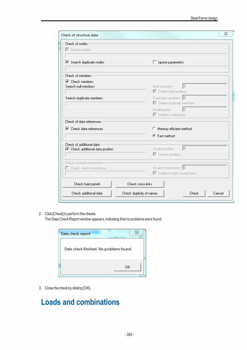
Steel frame design
2. Click [Check] to perform the checks.TheDataCheckReport window appears, indicating that no problemswere found.
3. Close the checkbyclicking [OK].
Loads and combinations
- 383 -
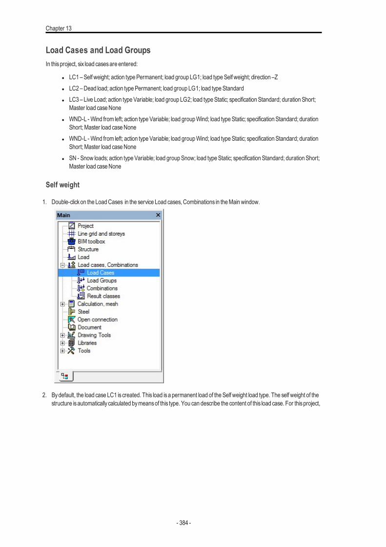
Chapter 13
Load Cases and Load GroupsIn thisproject, six load casesare entered:
l LC1 –Self weight; action typePermanent; load group LG1; load typeSelf weight; direction –Zl LC2 –Dead load; action typePermanent; load group LG1; load typeStandardl LC3 – Live Load; action typeVariable; load group LG2; load typeStatic; specification Standard; duration Short;
Master load caseNonel WND-L - Wind from left; action typeVariable; load groupWind; load typeStatic; specification Standard; duration
Short; Master load caseNonel WND-L - Wind from left; action typeVariable; load groupWind; load typeStatic; specification Standard; duration
Short; Master load caseNonel SN - Snow loads; action typeVariable; load groupSnow; load typeStatic; specification Standard; duration Short;
Master load caseNone
Self weight
1. Double-clickon the LoadCases in the service Load cases, Combinations in theMainwindow.
2. Bydefault, the load case LC1 iscreated. This load isa permanent load of the Self weight load type. The self weight of thestructure isautomatically calculated bymeansof this type. You can describe the content of this load case. For thisproject,
- 384 -
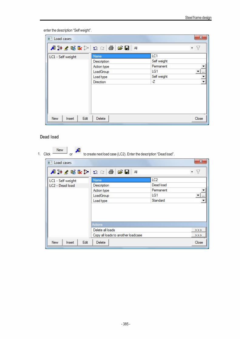
Steel frame design
enter the description “Self weight”.
Dead load
1. Click or to create next load case (LC2). Enter the description “Dead load”.
- 385 -
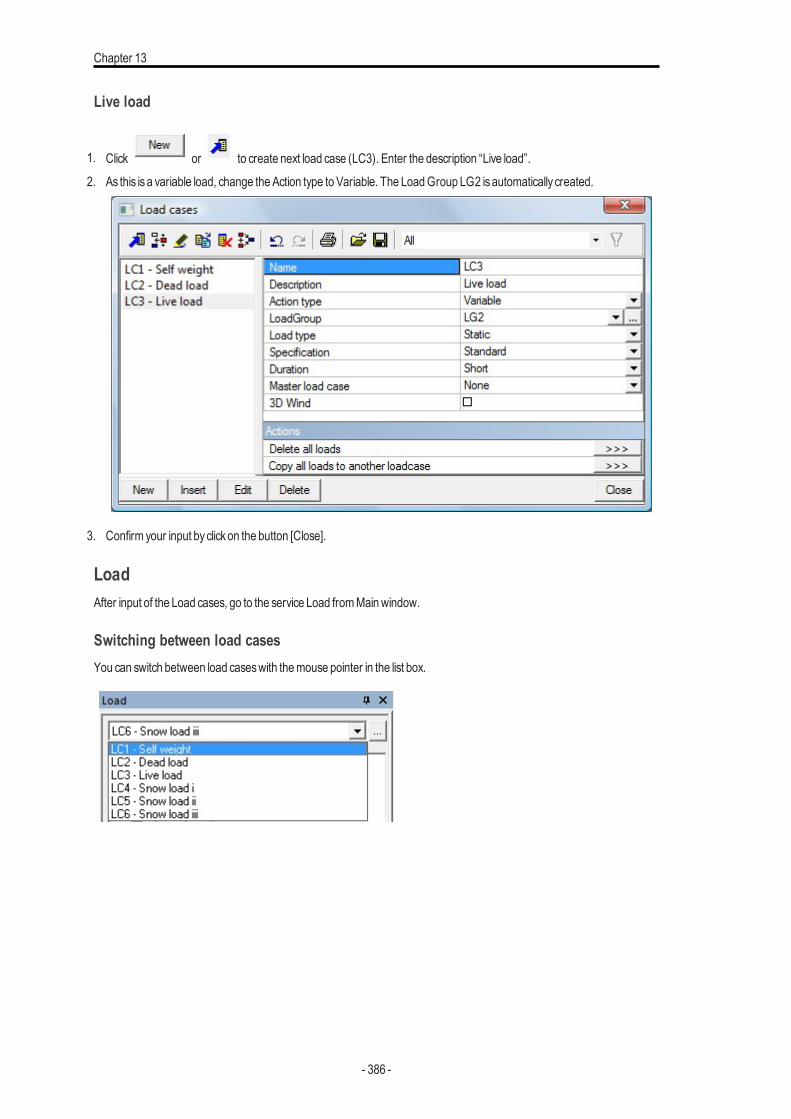
Chapter 13
Live load
1. Click or to create next load case (LC3). Enter the description “Live load”.
2. As this isa variable load, change theAction type to Variable. The LoadGroup LG2 isautomatically created.
3. Confirm your input byclickon the button [Close].
LoadAfter input of the Load cases, go to the service Load fromMainwindow.
Switching between load casesYou can switch between load caseswith themouse pointer in the list box.
- 386 -
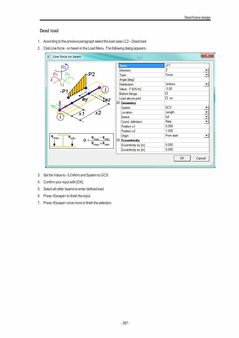
Steel frame design
Dead load
1. According to the previousparagraph select the load case LC2 –Dead load.2. ClickLine force - on beam in the LoadMenu. The following dialog appears.
3. Set the Value to -3,0 kN/mandSystem toGCS4. Confirm your input with [OK].5. Select all rafter beams to enter defined load6. Press<Escape> to finish the input.7. Press<Escape>oncemore to finish the selection.
- 387 -
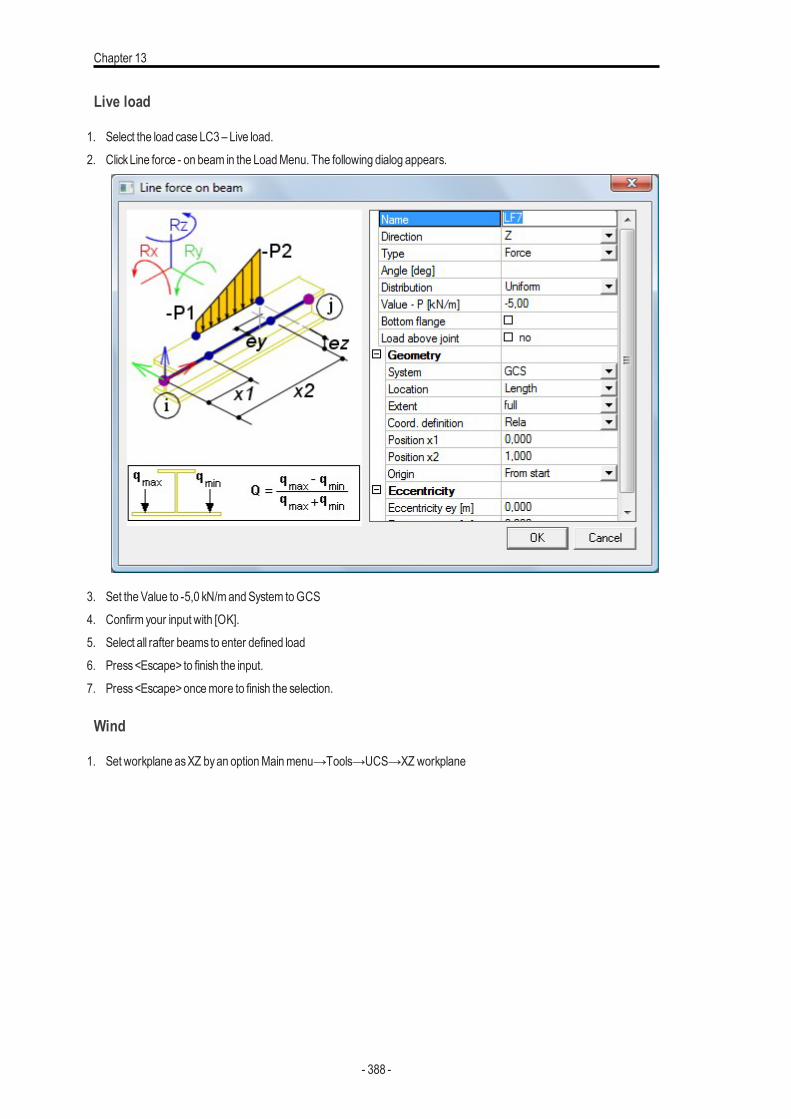
Chapter 13
Live load
1. Select the load case LC3 – Live load.2. ClickLine force - on beam in the LoadMenu. The following dialog appears.
3. Set the Value to -5,0 kN/mandSystem toGCS4. Confirm your input with [OK].5. Select all rafter beams to enter defined load6. Press<Escape> to finish the input.7. Press<Escape>oncemore to finish the selection.
Wind
1. Set workplane asXZ byan optionMainmenu→Tools→UCS→XZ workplane
- 388 -
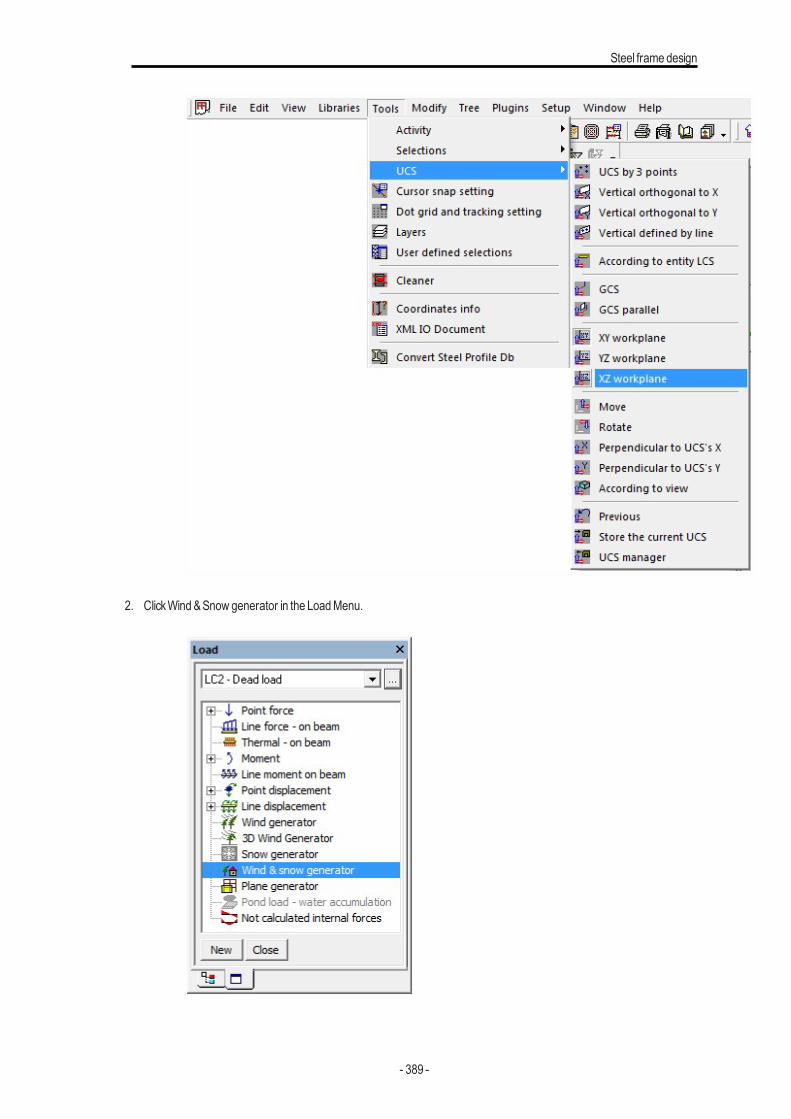
Steel frame design
2. ClickWind&Snow generator in the LoadMenu.
- 389 -
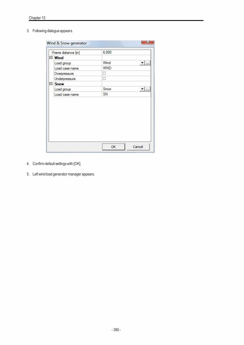
Chapter 13
3. Following dialogue appears.
4. Confirm default settingswith [OK].
5. Left wind load generator manager appears.
- 390 -
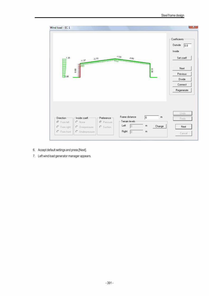
Steel frame design
6. Accept default settingsand press [Next].7. Left wind load generator manager appears.
- 391 -
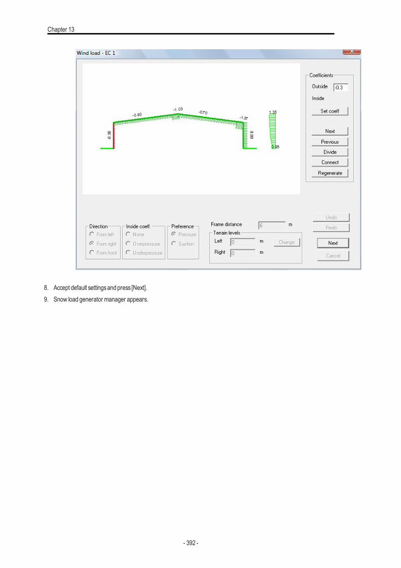
Chapter 13
8. Accept default settingsand press [Next].9. Snow load generator manager appears.
- 392 -
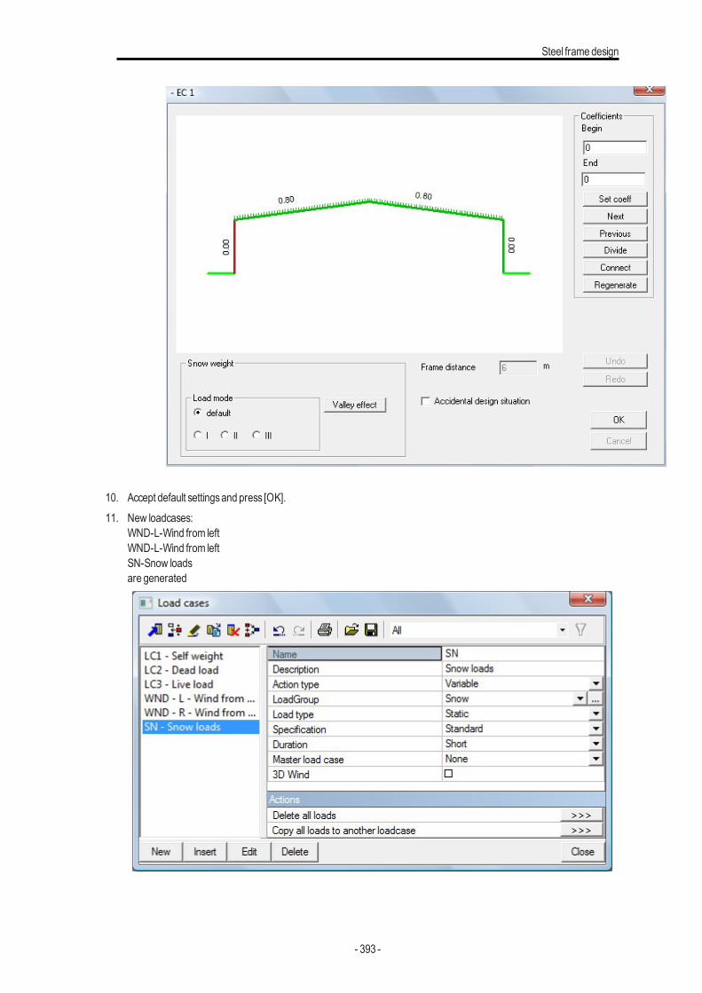
Steel frame design
10. Accept default settingsand press [OK].11. New loadcases:
WND-L-Wind from leftWND-L-Wind from leftSN-Snow loadsare generated
- 393 -
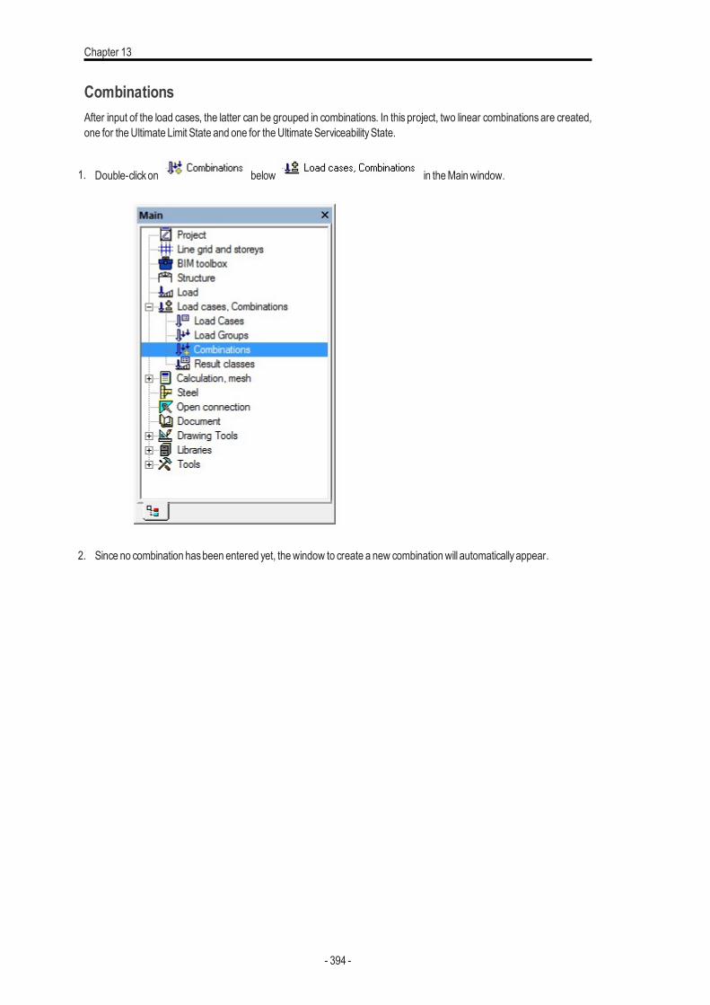
Chapter 13
CombinationsAfter input of the load cases, the latter can be grouped in combinations. In this project, two linear combinations are created,one for theUltimate Limit State and one for theUltimate ServiceabilityState.
1. Double-clickon below in theMainwindow.
2. Since no combination hasbeen entered yet, thewindow to create a new combinationwill automaticallyappear.
- 394 -
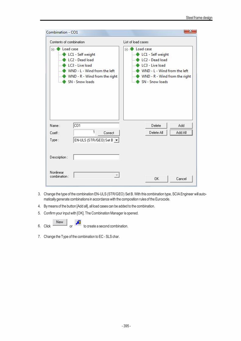
Steel frame design
3. Change the type of the combination EN-ULS (STR/GEO) Set B.With this combination type, SCIAEngineer will auto-maticallygenerate combinations in accordancewith the composition rulesof the Eurocode.
4. Bymeansof the button [Add all], all load casescan be added to the combination.5. Confirm your input with [OK]. TheCombinationManager isopened.
6. Click or to create a second combination.
7. Change the Type of the combination to EC - SLSchar.
- 395 -
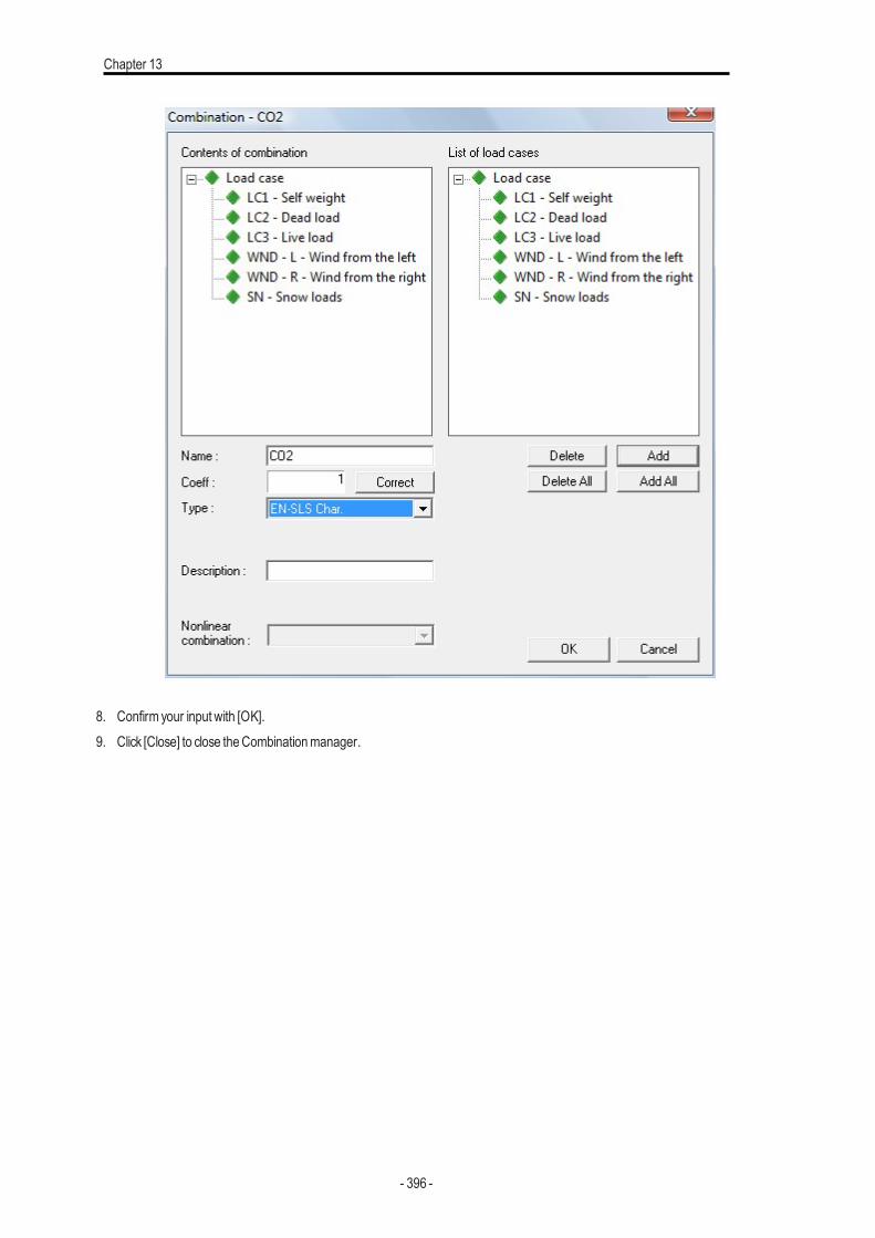
Chapter 13
8. Confirm your input with [OK].9. Click [Close] to close theCombinationmanager.
- 396 -
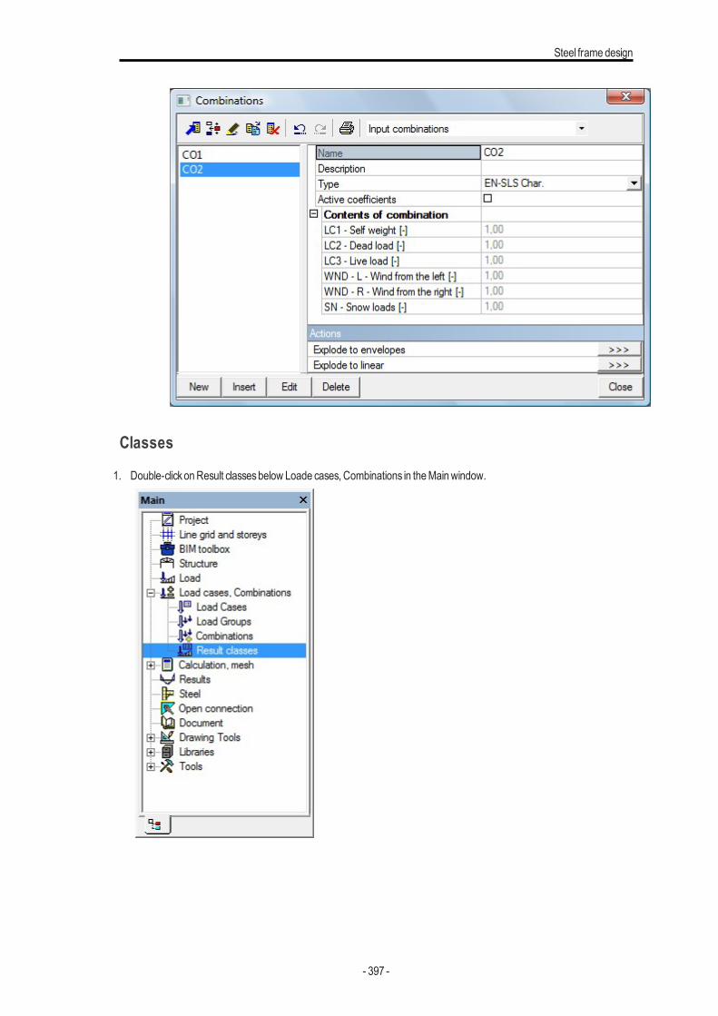
Steel frame design
Classes
1. Double-clickonResult classesbelow Loade cases, Combinations in theMainwindow.
- 397 -
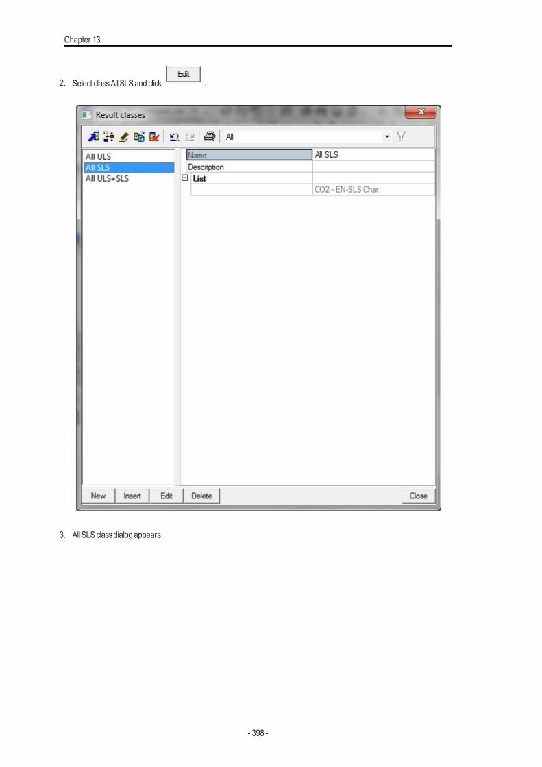
Chapter 13
2. Select classAllSLSand click .
3. AllSLSclassdialog appears
- 398 -
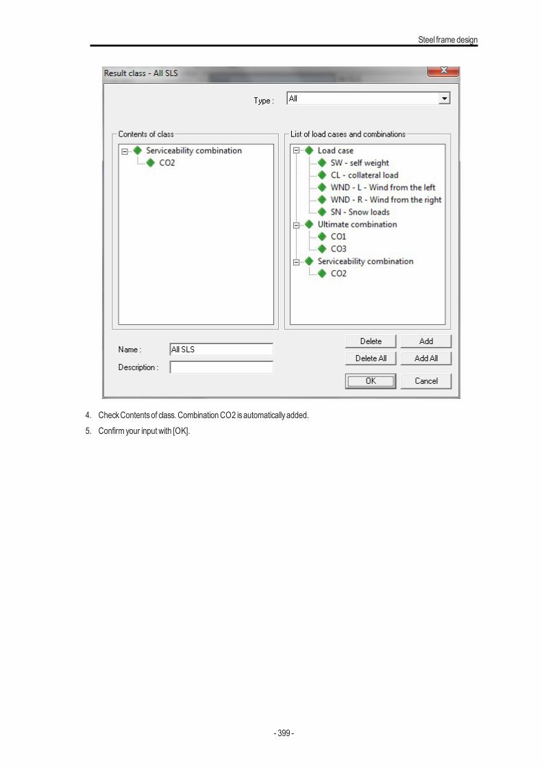
Steel frame design
4. CheckContentsof class. CombinationCO2 isautomaticallyadded.5. Confirm your input with [OK].
- 399 -
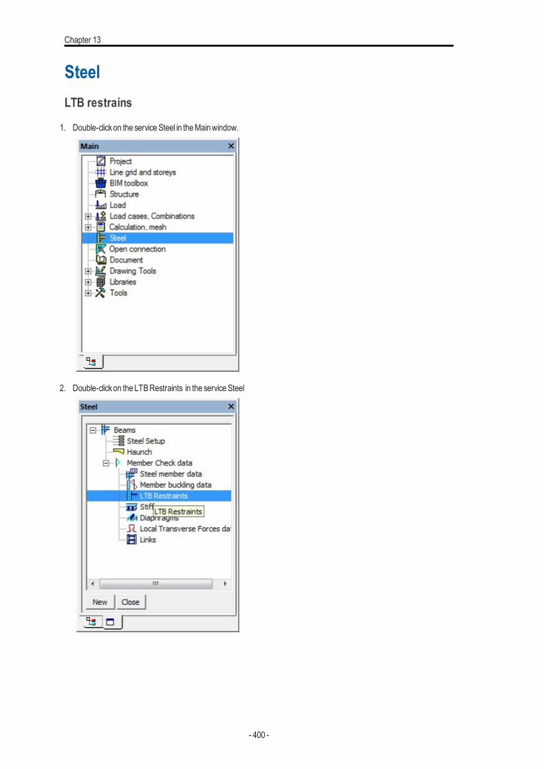
Chapter 13
SteelLTB restrains
1. Double-clickon the service Steel in theMainwindow.
2. Double-clickon the LTBRestraints in the service Steel
- 400 -
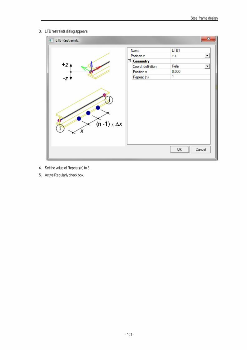
Steel frame design
3. LTB restraintsdialog appears
4. Set the value of Repeat (n) to 3.5. ActiveRegularly checkbox.
- 401 -
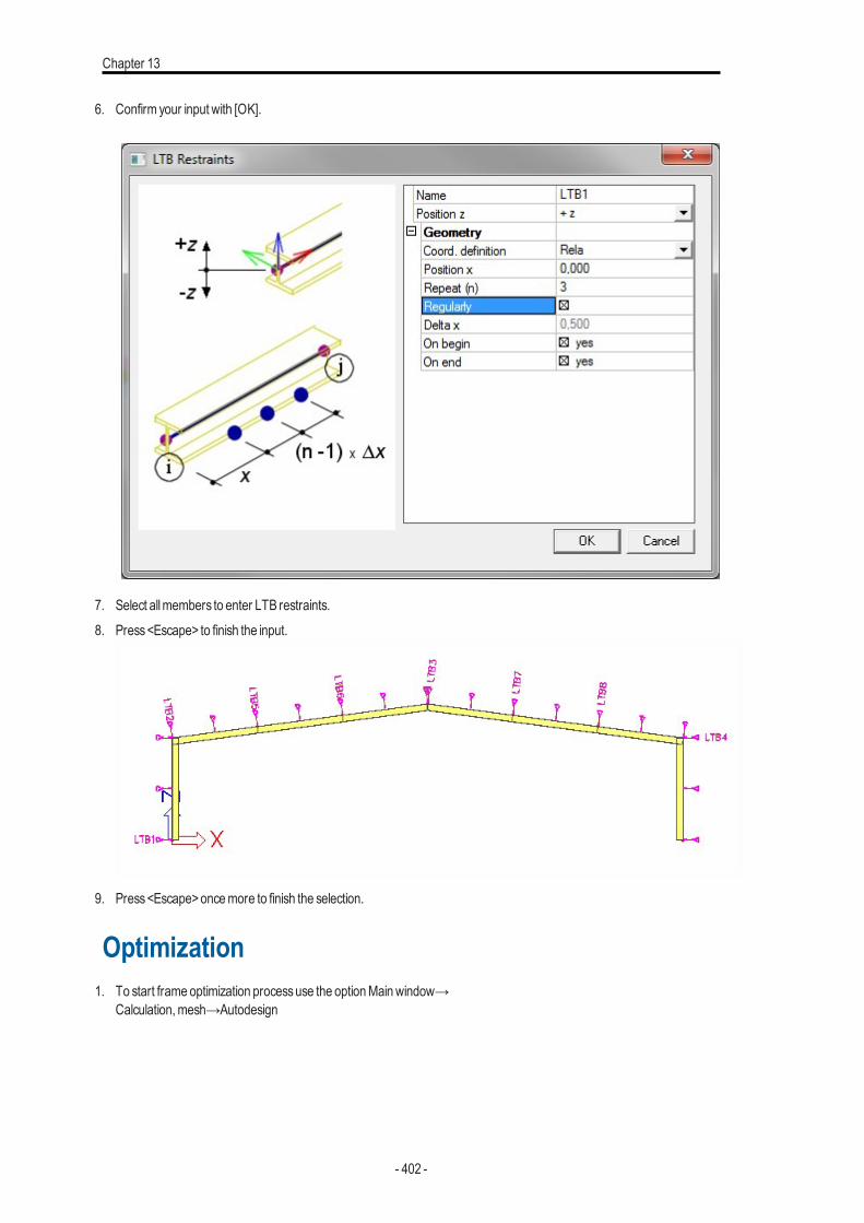
Chapter 13
6. Confirm your input with [OK].
7. Select allmembers to enter LTB restraints.8. Press<Escape> to finish the input.
9. Press<Escape>oncemore to finish the selection.
Optimization1. To start frame optimization processuse the optionMainwindow→
Calculation,mesh→Autodesign
- 402 -
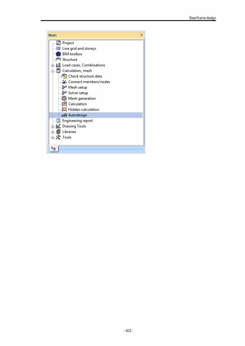
Steel frame design
- 403 -
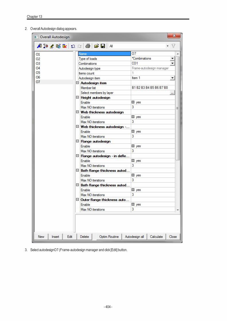
Chapter 13
2. Overall Autodesign dialog appears.
3. Select autodesignO7 (Frame-autodesignmanager and click [Edit] button.
- 404 -
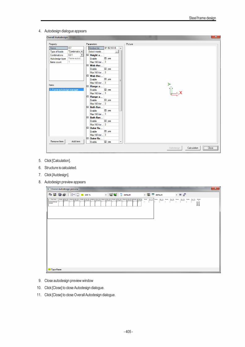
Steel frame design
4. Autodesign dialogue appears
5. Click [Calculation].6. Structure is calculated.7. Click [Autdesign].8. Autodesign preview appears
9. Close autodesign previewwindow10. Click [Close] to closeAutodesign dialogue.11. Click [Close] to closeOverall Autodesign dialogue.
- 405 -
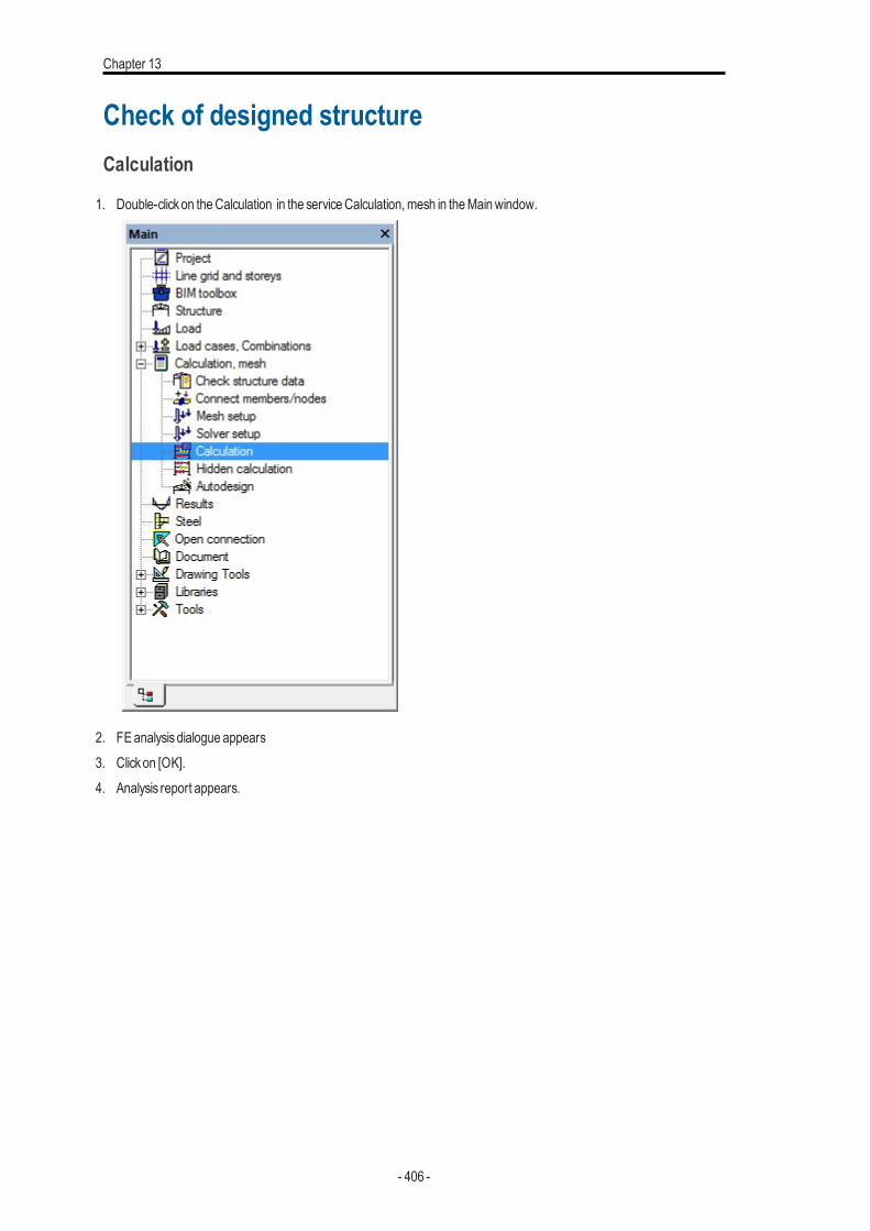
Chapter 13
Check of designed structureCalculation
1. Double-clickon theCalculation in the serviceCalculation,mesh in theMainwindow.
2. FEanalysisdialogue appears3. Clickon [OK].4. Analysis report appears.
- 406 -
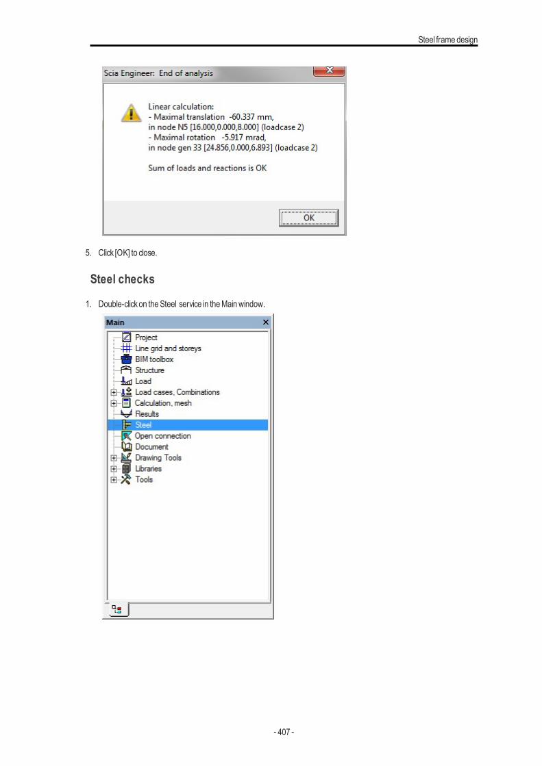
Steel frame design
5. Click [OK] to close.
Steel checks
1. Double-clickon theSteel service in theMainwindow.
- 407 -
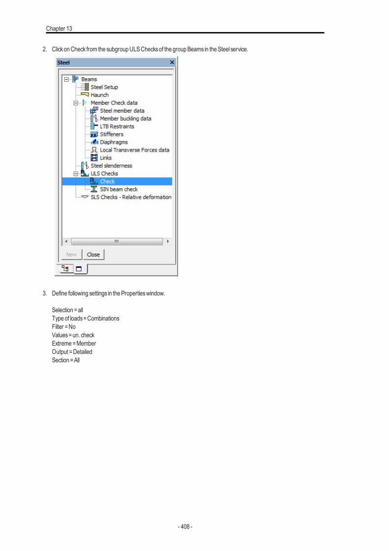
Chapter 13
2. ClickonCheck from the subgroupULSChecksof the groupBeams in theSteel service.
3. Define following settings in thePropertieswindow.
Selection =allType of loads=CombinationsFilter =NoValues=un. checkExtreme=MemberOutput =DetailedSection =All
- 408 -
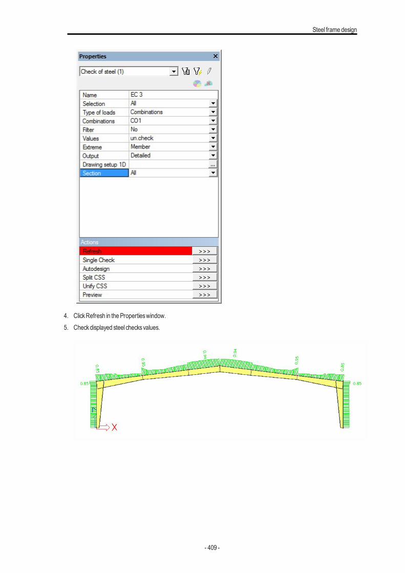
Steel frame design
4. ClickRefresh in thePropertieswindow.5. Checkdisplayed steel checksvalues.
- 409 -
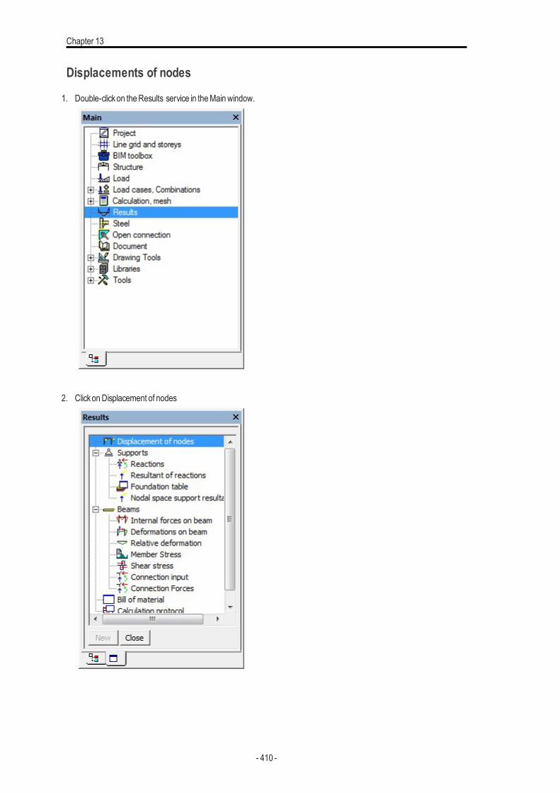
Chapter 13
Displacements of nodes
1. Double-clickon theResults service in theMainwindow.
2. ClickonDisplacement of nodes
- 410 -
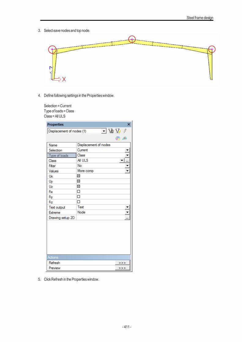
Steel frame design
3. Select eave nodesand top node.
4. Define following settings in thePropertieswindow.
Selection =CurrentType of loads=ClassClass=AllULS
5. ClickRefresh in thePropertieswindow.
- 411 -
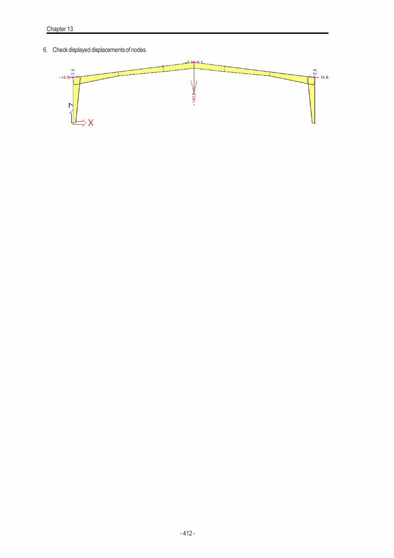
Chapter 13
6. Checkdisplayed displacementsof nodes.
- 412 -

Global optimisation
Global optimisation
IntroductionSCIAEngineer enablesyou to performan optimisation of thewhole structure or of its selected part. The optimisation can berun for steel and timber structuresor for steel or timber partsofmulti-material projects.
It is possible to optimise the value of:
l standard steel code check,
l fire resistance steel check,
l timber code check,
l bolted diagonal check.
It isalso possible to perform several of the abovementioned optimisation typesand then compare the results.
It is always the cross-section size or the bolt size that is optimised. In general, you must select which cross-section types orbolted diagonal connections used in your model are to be optimised. And it is up to you to select the cross-section types andbolted diagonal connections that are relevant to your work. It is also your responsibility to think in advance and define andassign to 1Dmembersasmanycross-section typesasnecessary for a proper design and optimisation of the project.
Note : In order to perform theAutoDesign, calculationmust be alreadyperformed.
AutoDesign managerAsstated in the introduction youmayperform several different optimisations. Youmay run theAutoDesign and compare theresults for different parts of the structure, for different optimisation types (e.g. standard and fire resistance code check).Therefore, all the defined optimisations are stored in the AutoDesignmanager . Thus you do not have to define all theAutoDesign criteria and parametersagain and again.
TheAutoDesignmanager isa standard SCIAEngineer databasemanager with usual featuresand functions.
Procedure to open the AutoDesign manager
1. Open serviceCalculation,Mesh.
2. Start (double-click) function AutoDesign.
Defining a new optimisationProcedure to define and run a new optimisation
1. Start the AutoDesignmanager.
2. Clickbutton [New] to open theOverallAutoDesign dialogue.
3. Define theAutoDesign parametersand criteria.
4. Clickbutton [AutoDesign] to run the calculation and see its result.
- 413 -

Chapter 14
5. If required, clickbutton [Calculation] to re-calculate themodel in order to reflect the resultsof the optimisation.
6. Depending onwhat you exactlyneed andwant, youmay repeat steps3 to 5 asmany timesas required.
Note: Please note, that amechanical repetition of AutoDesign andCalculation in turnsmaylead to a "never-ending" cycle. The AutoDesign may find cross-section "A" as optimal.When you perform the calculation, the internal forces are redistributed to reflect theAutoDesign results. When you run AutoDesign now, it may find cross- section "B" asoptimal. And another re-calculation once more redistributes the internal forces. And it mayhappen that the subsequent AutoDesign finds the cross-section "A" as optimal once again.And so on, and so on, and so on.
AutoDesign parameters and criteria
ItemsThe item defines the type of the optimisation and the cross-section type that should be optimised. The type of optimisation(e.g. standard and fire resistance code check) must be defined for the first item only. All the other items in one AutoDesigndefinition are of the same type. One AutoDesign item represents one cross-section type or one bolted diagonal connectionthat will be optimised.
[Add item] Adds a new optimisation item into the list.
[Remove item] Removes the existing optimisation item from the list.
PropertyName Defines the name of the optimisation (criteria).
Type of loads The AutoDesign may be performed for load cases, load case combinations, result classes, etc.
LoadSpecifies the particular load case, combination, etc. for which the selected cross-section type will beoptimised.
AutoDesigntype
(informative) Tells the type of the optimisation.
Item count (informative) Shows the number of defined AutoDesign items.
ParametersCross-section AutoDesign
Cross-section Defines the cross-section type to be optimised.
Parameter Selects the dimension (e.g. section depth, width, etc.) that will be optimised.
Length (informative) Shows the current size of the selected dimension.
Minimum Defines the minimal applicable size for the optimised parameter.
Maximum Defines the maximal applicable size for the optimised parameter.
Step Defines the step for the AutoDesign.
Maximal check Defines the maximal acceptable value of unity check of the optimised cross-section.
Optimised check (informative) Shows the unity check for the optimised connection.
Bolted diagonalAutoDesign
- 414 -

Global optimisation
Bolted diagonal Specifies the bolted diagonal to be optimised.
Bolt Specifies the bolt used.
Optimised check (informative) Shows the unity check for the optimised connection.
PictureThe picture shows the shape of the optimised cross-section or the symbol of the bolted diagonal connection.
Control buttonsAutoDesign Performs the optimisation for the defined AutoDesign items.
Calculation Carries out the calculation for the optimised model.
- 415 -


