w Original Research Paper 155

Chemometrics and Intelligent Laboratory Systems, 16 (1992) 155-167 Elsevier Science Publishers B.V., Amsterdam

Application of chemometrics to the screening of hazardous chemicals

A case study *

Maria Livia Tosato

Structure Activity Research Group, Istituto Superiore di Sanit;, Kale Regina Elena 299, Roma (Italy)

Rossano Piazza and Claudio Chiorboli

Centro di Fotochimica de1 CNR, Universitci di Ferrara, VU Borsari 46, Ferrara (Italy)

Laura Passerini and Anna Pino

Structure Activity Research Group, Istituto Superiore di Sanitri, Viile Regina Elena 299, Roma (Italy)

Gabriele Cruciani and Sergio Clementi

Chemometrics Laboratory, Dbartimento di Chimica, Universitli di Perugia, via Elce di Sotto 10, Perugia (Italy)

(Received 12 September 1991; accepted 20 February 1992)

Abstract

Tosato, M.L., Piazza, R., Chiorboli, C., Passerini, L., Pino, A., Cruciani, G. and Clementi, S., 1992. Application of chemometrics to the screening of hazardous chemicals. A case study. Chemometrics and Intelligent Laboratory Systems, 16: 155-167.

The key aspects of a priority setting process for risk assessment of chemicals are reviewed. The process is based on the assumption that chemical and biological properties can be modelled within series of closely similar compounds. It rests heavily on multivariate methodologies for the development of predictive models. Statistical design, in particular, is essential for optimizing the selection of the most informative objects and variables to be used in the calibration of the models. A case study is presented where the process is applied to all (EEC-wide) commercially available halo-methanes, -ethanes and -propanes with the objective of modelling their tropospheric reactivity and, hence, estimating their lifetimes. A training set of just nine, properly informative haloalkanes was first selected from a series of 142; their reactivity was expressed in terms of the rate constant of their reaction with

Correspondence to: Dr. M.L. Tosato, Structure Activity Research Group, Istituto Superiore di Sanita, Viale Regina Elena 299, Roma, Italy and to Dr. C. Chiorboli, Centro di Fotochimica de1 CNR, Universitl di Ferrara, Via Borsari 46, Ferrara, Italy.

* Paper presented at the 2nd Scandinavian Symposium on Chemometrics (SSCZ), Bergen, Norway, 28-31 May 1991.

0169-7439/92/$05.00 0 1992 - Elsevier Science Publishers B.V. All rights reserved

156 M.L. Tosato et al. /Chemom. Intell. Lab. Syst. 16 (1992) 15%167/0ri&al Research Paper n

the OH radical, k(OHk their st~cture was parametrized by a selected set of variables that, by using a new statistical method, were found to optimize the k(OH) model. The experimentally validated model provided &OH) estimates, and hence allowed the formulation of a persistency ranking for the non-tested compounds in the series, which also included several hydro-chlorofluoro- carbons, H-CFCs, presently considered as possible replacement chemicals for the extremely stable, environmentally incompatible ozone-depleting CFCs.

INTRODUCTION

Background: need for priorities

Under the pressure posed by emerging socio- economic issues, chemical risk assessment is a rapidly developing, multifaceted discipline. Its far from trivial goal is to achieve some understanding and provide some kind of measures of how and how much a chemical may be capable of damag- ing humans and/or the environment. This entails the collection, development, and combination - for any potentially hazardous chemical - of in- formation regarding its likely exposure levels and intrinsic capability to harm biotic and abiotic targets at risk.

Among countless and complex problems to be addressed in this area, a crucial one at the pres- ent time derives from the fact that what is cur- rently known about thousands of chemicals in use is, in most cases, just their chemical formula. Therefore, ~nsidering how high the costs of test- ing are, we need to address the non-trivial ques- tion of ‘where to start from’. In order to find appropriate answers, it is essential to define some kind of strategy for systematically filling the gaps in at least basic data, and use such data for screening chemicals and setting priorities for risk assessment studies.

A priority setting framework Present study

As a ~nt~bution in this area, a stepwise strat- egy has been formulated [l-51 which provides a general framework for a transparent, systematic, and cost-effective screening of toxic substances. The approach strives to incorporate all available information about chemicals (their structures first of all), as well as state~f-the-a~ chemometric methods for sound modelling with minimal test-

ing effort. It was suggested that, as a first step, inventories listing chemicals in use should be scrutinized in order to subdivide chemicals by classes or, more pra~atically, to sort all chemi- cals belonging to already recognized h~ardous classes (e.g., aromatic amines, halo-aliphatics, ni- tro-aromatics, etc.), or to any class of specific interest. This will provide complete series of chemicals for further processing, series by series, through the sub~quent steps 2-6. Briefly: follow- ing the parametr~ation of the structures (step 21, a training set for the series is identified by a statistical design (step 31, is then tested (step 41, and used for calibrating multivariate quantitative structure-activity relationship (QSAR) models (step 5). Finally, the predictive abili~ and the range of the models are assessed (step 6). Vali- dated models will permit us to estimate missing data for the compounds that belong within the range of the model, and to formulate ‘hazard’ rankings, thus providing the basis for identifying priorities for additional studies.

So much for the framework. Validated models will, however, also provide several other items of information, including, for example, model pa- rameters highlighting the importance of each de- scriptor with respect to the investigated end- points and some aspects of the reaction mecha- nisms.

In the following, the first case study is re- ported. This starts from scratch and goes through each of the above steps. The study addresses, and provides reasonable solutions to, problems faced in the real world. In particular, the problem de- riving from the absence, in practice, of adequate and consistent set of data for the paramet~zation of the structures is given a new, possible solution.

m M.L. Tosato et al. /Chemom. Intell. Lab. Syst. 16 (1992) 155-167/Original Research Paper 157

The objective of the study was to fo~ulate a persistency ranking for a series of volatile haloalkanes for which the persistency data are essential for hazard assessment. The series in- cludes already recognized carcinogens, mutagens, neurotoxicants, etc. It also includes chloroffuo- roalkanes, CFCs, and hydr~chloroff uoroal~nes, H-CFCs. The former, owing to their extreme stability, are considered to act as stratospheric ozone depleters and, therefore, are to be phased out of industrial production and use. The latter, owing to their lower stability, are expected to include ‘en~ro~entally compatible’ replace- ment compounds.

In view of the objective mentioned above, it was considered that the most important degrada- tion pathway for these chemicals is their gas-phase reaction with the na~rally occurring hydroxyl radical (OH * 1, the rate-determ~ing step of which is the hydrogen abstraction

C,H,X, + OH * ---!L H,O + C,H,_tX,*

(X = halogen)

followed by a rapid decay of the organic radical into degradation, down to mineralization, prod- ucts [61. The information of interest for formulat- ing a persistency ranking of haloalkanes is there- fore their reaction rate constant (k), hereinafter k(OH). Accordingly, the study focused on the const~~ion of a k(OH) model.

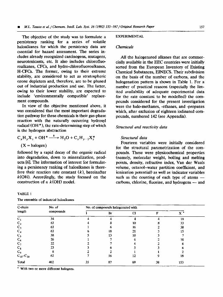
TABLE 1

The ensemble of industrial haloalkanes

Chemicals

All the halogenated alkanes that are commer- cially available in the EEC countries were initially sorted from the European Inventory of Existing Chemical Substances, EINECS. Their subdivision on the basis of the number of carbons, and the halogenation pattern is shown in Table 1. For a number of practical reasons (especially the lim- ited availabili~ of adequate e~erimental data for the rate constant to be modelled) the com- pounds considered for the present investigation were the halo-methanes, -ethanes, and -propanes which, after exclusion of eighteen iodinated com- pounds, numbered 142 (see Appendix).

Structural and reactivity data

Structural data Fourteen variables were initially considered

for the structural parametrization of the com- pounds. These were physic~hemi~l properties (namely, molecular weight, boiling and melting points, density, refractive index, Van der Waals volume, octanol-water partition coefficient, and ionization potential) as well as indicator variables such as the punting of each type of atoms - carbons, chlorine, fluorine, and hydrogens - and

C-chain No. of length compounds

Cl 34 c2 63 C3 63 c4 63 CS 38 c6 26

C, 22 c8 23

c9 8

c,o-Go 62

Total 402

No. of compounds haIogenated with

I Br cl

4 4 4 4 8 10 1 6 16 6 18 21 5 13 10 1 7 6 2 7 4 3 6 5 2 2 1 7 16 12

35 87 89

F X’

4 18 8 33 2 38 3 15 3 7 2 10 2 6 3 6 1 2 9 18

38 153

* With two or more different halogens.

1.58 M.L. Tosato et al. /Chemom. Intell. Lab. Syst. 16 (1992) 15%167/01igina1 Research Paper 8

of all the halogen atoms. This set of descriptors had, in fact, already been used in previous studies with small series of haloalkanes [7,8]. However, so many variables were not available for many of the compounds investigated in the present study. It was therefore necessary to select smaller sets of variables, yet ones which are capable of provid- ing an adequate multivariate description of the compounds. Two different approaches were taken, according to the two different purposes of the parametrization. (i) For the purpose of carry- ing out a statistical design, a subset of five vari- ables was selected on the basis of pragmatic con- siderations. These variables were: the number of carbons, fluorines, chlorines, bromines and hy- drogens. (ii) For the purpose of constructing a k(OH) model, a subset of six was selected by a newly developed statistical method (see below). It turns out that these were the same as those above, plus the total number of halogens.

A two-level ( + / - ) fractional factorial design, FFD [121, was used for selecting a training set out of 142 compounds on the basis of four PCA-de- rived design variables.

A modified PLS version was used for comput- ing the standard deviation of error of prediction, SDEP [131, and to check the model dimensional- ity with the highest predictive capacity. The method is based on the leave-N-out concept. The data set is subdivided into N groups, and N PLS are run so that each group is excluded once and used for predictions for each model dimension; using such predictions the corresponding stan- dard deviations are computed and stored. The process is repeated several times, each time fol- lowing a random permutation of the N groups. The final SDEP values (obtained by averaging the stored results), allow the identification of the PLS component with the highest predictive capacity as the one with the lowest SDEP value.

Reactivity data

Experimental values for the rate constants un- der tropospheric conditions were available for 33 compounds. A small number had been measured in our laboratory according to an agreed standard method, and have already been reported 171. The majority of the k(OH) values have been taken from a review paper [6] that lists all the values reported in the literature up to 1986. The review, in some cases, provides ‘recommended’, and in some other cases, indicates ‘non-recommended’ k(OH) data. Prior to data analysis, the rate con- stants - expressed in cm3 molecule-’ s-l - were transformed into the corresponding decimal logarithms.

A newly developed method [14] has been used for the selection of the modelling variables that optimize the predictive capacity of the model. In regard to our present application, the process (a)-(d) described below was applied to the train- ing compounds. Briefly: (a) the compounds were parametrized by the complete set of fourteen variables (see Experimental Section); (b) a num- ber of subsets of variables (including one to four- teen variables) were selected by a statistical de- sign (here FFD); (c) the SDEP analysis was car- ried out with each of these subsets; and (d) the optimal subset of variables was identified as the one providing the k(OH) model with the lowest SDEP value. (The resulting optimal subset was reported in the previous section.)

RESULTS AND DISCUSSION

STATISTICAL METHODS Selection of a training set

Principal component analysis, PCA [91, and partial least squares in latent variables, PLS [lO,ll] were the multivariate data analytic meth- ods used for deriving design variables for the statistical selection of the training set, and for constructing the k(OH) model, respectively.

Parametrization of structures As has already been mentioned, in the absence

of a rich and consistent set of descriptors for each of them, our 142 compounds were parametrized by simply counting their carbons, fluorines, chlo- rines, bromines and hydrogens. In fact, for the

N M.L. Tosato et al. /Ch-enwm. Intell. Lab. Syst. 16 (1992) 15.G167/0riginal Research Paper 1.59

identification of a representat~e training set, it was considered to be sufficient to span a few structural variables that are relevant to the prob- lem being investigated. In regard to the present application, it is well known that the atmospheric degradation of haloalkanes is strongly influenced by factors such as the carbon chain length, the number of hydrogens, and the number and type of halogens.

Design variables In order to further reduce the dimensionali~

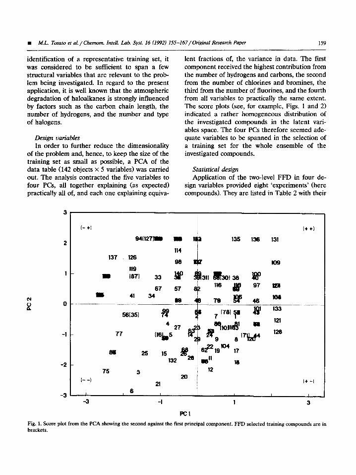
of the problem and, hence, to keep the size of the training set as small as possible, a PCA of the data table (142 objects X 5 variables) was carried out. The analysis contracted the five variables to four PCs, all together explaining (as expected) practically all of, and each one explaining equiva-

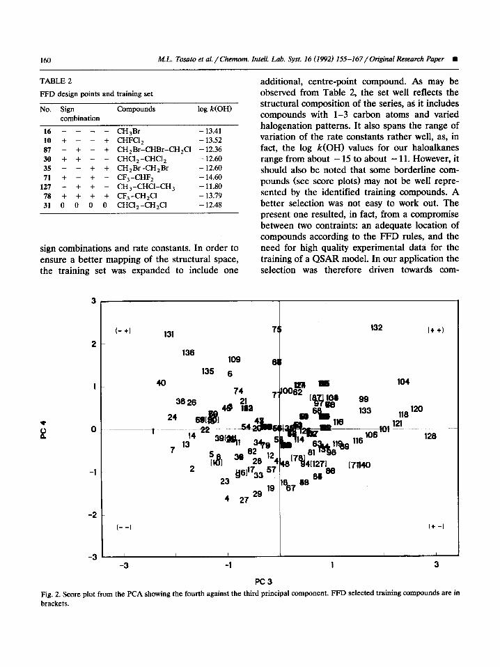
lent fractions of, the variance in data. The first component received the highest contribution from the number of hydrogens and carbons, the second from the number of chlorines and bromines, the third from the number of fluorines, and the fourth from all variables to practically the same extent. The score plots (see, for example, Figs. 1 and 2) indicated a rather homogeneous distribution of the investigated compounds in the latent vari- ables space. The four PCs therefore seemed ade- quate variables to be spanned in the selection of a training set for the whole ensemble of the investigated compounds.

Statistical design Application of the two-level FFD in four de-

sign variables provided eight ‘experiments’ (here impounds). They are listed in Table 2 with their

3

2

1

0

-1

-2

-3

Fig. 1. Score pfot from the PCA showing the second against the first principal component. FFD selected training compounds are in brackets.

160 M.L. Tosato et al. /Chemom. Intell. Lab. Syst. 16 (1992) 155-167/0riginal Research Paper W

TABLE 2

FFD design points and training set

No. Sign combination

Compounds log k(OH)

16 _ _ - - CH,Br - 13.41

10 + - - + CHFCl 2 - 13.52

81 - + - + CH,Br-CHBr-CH,CI - 12.36

30 + + - - CHCI,-CHCI, - 12.60

35 - - + + CH,Br-CH,Br - 12.60

71 + - + - CF, -CHF, - 14.60

127 - + + - CH,-CHCI-CH, - 11.80

78 + + + + CF,-CH,CI - 13.79

31 0 0 0 0 CHCl,-CH,CI - 12.48

sign combinations and rate constants. In order to ensure a better mapping of the structural space, the training set was expanded to include one

3

2

I

0

-1

-2

-3

additional, centre-point compound. As may be observed from Table 2, the set well reflects the structural composition of the series, as it includes compounds with l-3 carbon atoms and varied halogenation patterns. It also spans the range of variation of the rate constants rather well, as, in fact, the log k(OH) values for our haloalkanes range from about - 15 to about - 11. However, it should also be noted that some borderline com- pounds (see score plots) may not be well repre- sented by the identified training compounds. A better selection was not easy to work out. The present one resulted, in fact, from a compromise between two contraints: an adequate location of compounds according to the FFD rules, and the need for high quality experimental data for the training of a QSAR model. In our application the selection was therefore driven towards com-

(- +I 131 132 I+ +I

136 109

40 104

118 120

----14

121

PI - 128

-3 -1 1 3

PC3

Fig. 2. Score plot from the PCA showing the fourth against the third principal component. FFD selected training compounds are in brackets.

w M.L. Tosato et al. /Chemom. Intell. Lab. Syst. 16 (1992) 155-167/0riginal Research Paper 161

pounds for which ‘recommended’ k(OH) data were available [61.

Model development

Modelling variables By using the selection method described above,

the modelling variables that maximize the predic- tive ability of the model turned out to be just six out of the fourteen originally considered, namely: the number of each of the five atoms in the series and the sum of halogens. This was not very sur- prising as a substantial collinearity among several of the fourteen descriptors (particularly among the physicochemical properties) had in fact al- ready been noted [S].

This finding had a positive practical impact on our application. It showed, in fact, that it was

feasible to construct a k(OH) model by simply using descriptors drawn from the chemical struc- ture: i.e., a model that will be applicable to all the compounds considered, as well as to any similar one, existing or not yet synthesized. In more general terms, this finding showed that the use of several descriptors, no matter how collinear they are, does not necessarily improve the model.

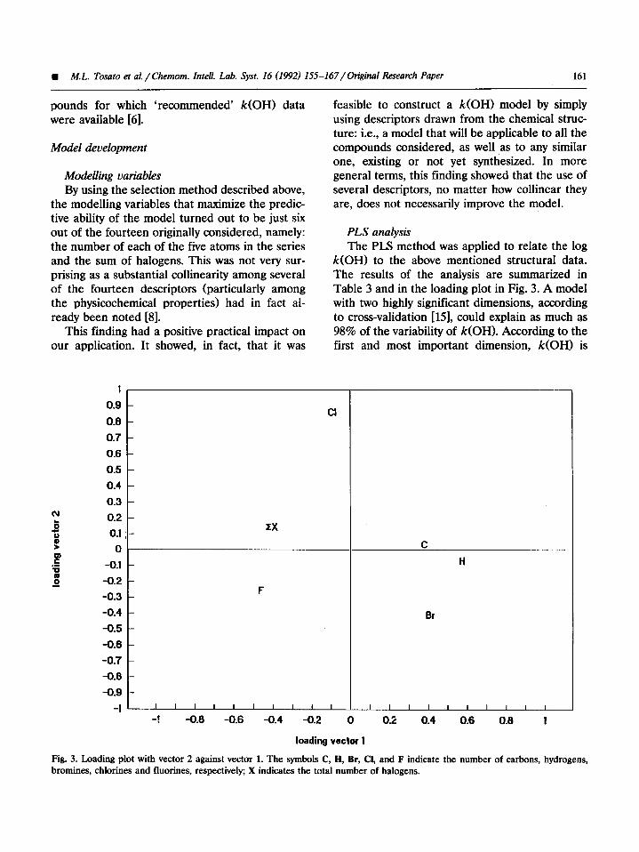
PLS analysis The PLS method was applied to relate the log

k(OH) to the above mentioned structural data. The results of the analysis are summarized in Table 3 and in the loading plot in Fig. 3. A model with two highly significant dimensions, according to cross-validation [15], could explain as much as 98% of the variability of k(OH). According to the first and most important dimension, k(OH) is

1 ,

0.9 -

0-e -

0.7 - 0.6 - 0.5 -

0.4 - 0.3 - 0.2 - 0.1 ;-

Cl

IX

C

H

Br

0

-0.1 -

-0.2 - -0.3 F -

-0.4 - -0.5 -

-0.6 - -0.7 - -0.6 -

-0.9 -

-1 I I I I I I I I, l I I I I II I, l l

4 -0.8 -0.6 -0.4 -0.2 0 0.2 0.4 0.6 0.6 1

loading vector I

Fig. 3. Loading plot with vector 2 against vector 1. The symbols C, H, Br, Cl, and F indicate the number of carbons, hydrogens, bromines, chlorines and fluorines, respectively; X indicates the total number of halogens.

162 ML. Tosato et al. /Chemom. Intell. Lab. Syst. 16 (1992) 155167/Originul Research Paper w

TABLE 3

PLS model parameters

dim Variance explained (%I

X block Y

1 23 89 2 16 9

Total 39 98

lowered by an increasing number of fluorines and number of halogens, whereas it is increased by increasing the number of carbons, hydrogens, and bromines. According to the second dimension, the number of chlorines has a positive correla- tion, whereas the number of fluorines and bromines are negatively correlated to k(OH).

The fit of the training compounds to the model was quite good, since R* and the standard devia- tion, SD, were 0.98 and 0.11, respectively. This result was promising. However, the reliability of the model had to be checked experimentally. Particular attention was, possibly, to be paid to those structural areas where a somewhat high residual standard deviation was noted for a num-

ber of compounds. These were the fully halo- genated bromo-fluoro-propanes (Nos. 104, 120, and 132, which can be seen in the score plots at the very borders of the X range of the series), pentabromoethane (No. 75) and the group of fully halogenated chloro-fluoro-propanes.

Model validation

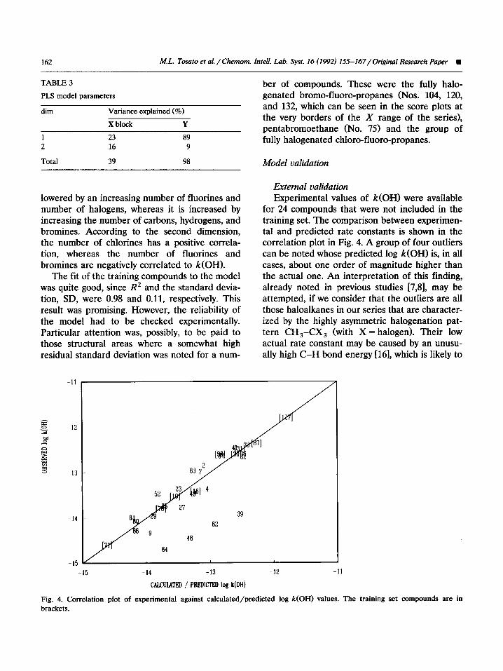
External validation Experimental values of k(OH) were available

for 24 compounds that were not included in the training set. The comparison between experimen- tal and predicted rate constants is shown in the correlation plot in Fig. 4. A group of four outliers can be noted whose predicted log k(OH) is, in all cases, about one order of magnitude higher than the actual one. An interpretation of this finding, already noted in previous studies [7,8], may be attempted, if we consider that the outliers are all those haloalkanes in our series that are character- ized by the highly asymmetric halogenation pat- tern CH,-CX, (with X = halogen). Their low actual rate constant may be caused by an unusu- ally high C-H bond energy [16], which is likely to

-12

-13 -

-14

-14 -13

CALCUIATED / PREDICI’ED log k(OH)

Fig. 4. Correlation plot of experimental against calculated/predicted log k(OH) values. The training set compounds are in brackets.

W M.L. Tosato et al. /Chemom. Intell. Lab. Syst. 16 (1992) 155-167/0tiginal Research Paper 163

reduce the frequency of their active collisions with the OH radicals. Hence, the failure to cor- rectly estimate their rate constants may depend on the absence of bond energy descriptors in the parametrization. This point needs additional in- vestigation. However, for the time being, this well-identified type of structures is outside the range of application of the model.

The predictive ability of the model was there- fore evaluated on the remaining 20 compounds for which Q* (= R* calculated on the validation set compounds) is 0.88 and the corresponding SD is 0.22. No experimental k(OH) values were available for the groups of haloalkanes with a somewhat large residual standard deviation. Their

u I 1 J I

predicted k(OH) values should therefore be re- NO. OF PLS COMPONENTS

garded with caution. A warning is also necessary Fig. 5. Variation of the SDEP parameter with the number of

in respect of the predictions for the fully halo- PLS components.

genated alkanes in general, since no experimental k(OH) was available for comparison, other than a ‘non-recommended’ one [6].

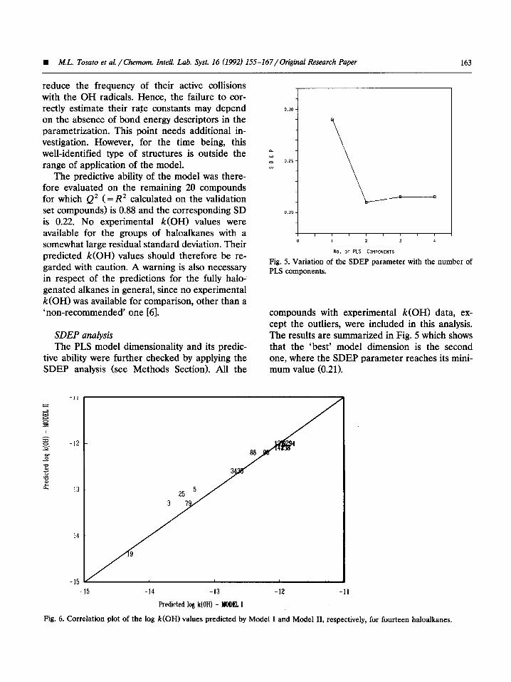
SDEP analysis The PLS model dimensionality and its predic-

tive ability were further checked by applying the SDEP analysis (see Methods Section). All the

compounds with experimental k(OH) data, ex- cept the outliers, were included in this analysis. The results are summarized in Fig. 5 which shows that the ‘best’ model dimension is the second one, where the SDEP parameter reaches its mini- mum value (0.21).

-14 -13 -12 -II

Predicted log k(OH) - YODEL 1

Fig. 6. Correlation plot of the log k(OH) values predicted by Model I and Model II, respectively, for fourteen haloalkanes.

164 ML. Tosato et al. /Chemom. Intell. Lab. Syst. 16 (1992) 155-167/0riginal Research Paper n

These findings perfectly match those previ- ously obtained in the traditional PLS analysis and in the external validation process, respectively. It is worth noting that the ‘small’ statistically de- signed training set is capable of giving results that are as good as the much larger one used for the SDEP analysis. However, examples have been reported where statistically designed training sets give a much better model than very large, non-de- signed ones [17].

Comparison of k(OH) estimates from different models

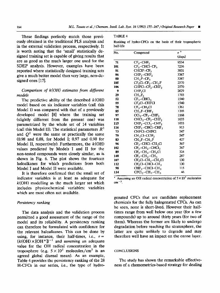
The predictive ability of the described k(OH1 model based on six indicator variables (call this Model I> was compared with that of a previously developed model [8] where the training set (slightly different from the present one) was parametrized by the whole set of 14 variables (call this Model II). The statistical parameters R2 and Q2 were the same or practically the same (0.98 and 0.88, for Model I; 0.97 and 0.90 for Model II, respectively). Furthermore, the k(OH) values predicted by Models I and II for the non-tested compounds were closely similar, as is shown in Fig. 6. The plot shows the fourteen haloalkanes for which predictions from both Model I and Model II were available.

It is therefore confirmed that the small set of indicator variables is at least as adequate for k(OH) modelling as the much larger set which includes physicochemical variables: variables which are most often not available.

Persistency ranking

The data analysis and the validation process permitted a good assessment of the range of the model and its reliability. A persistency ranking can therefore be formulated with confidence for the relevant haloalkanes. This can be done by using, for instance, their half-times, i.e., r = (k(OH) x [OH *I}- ’ and assuming an adequate value for the OH radical concentration in the troposphere (e.g. 5 x lo5 molecules/cm3 is an agreed global diurnal mean>. As an example, Table 4 provides the persistency ranking of the 28 H-CFCs in our series, i.e., the type of hydro-

TABLE 4

Ranking of hydro-CFCs on the basis of their tropospheric half-life

No. Compound l

;da ys)

71 CF, -CHF, 9534 101 CF,-CHCI-CF, 7236 81 CHCIF-CF, 3831 86 CHF, -CHF, 3387 80 CH,F-CF, 3387

105 CF,Cl-CF, -CH 2F 2570 106 CHFCI-CF, -CHF, 2570

9 CHF,CI 2029 29 C&F, 1793 52 CF,-CHCl, 1540 55 CF,Cl-CHFCl 1540 78 CF,-CH,Cl 1361 85 CH F-CHF, 2 1203 97 Ccl,-CF,-CHF, 1168

110 CHCl,-CF,-CHF, 1033 115 CHF, -CC1 -CHF, 2 1033 116 CHFz-CHCl-CHF, 913 73 CHFCl-CHFCI 547 79 CH,Cl-CClF2 547 83 CH,F-CH,F 427 96 CF,-CHCl-CH,Cl 367

102 CF,-CH,-CHCl, 367 89 CF,-CH,-CH,Cl 324

140 CF,-CH,-CH, 287 107 CF&l-CH,-CH,Cl 130 112 CF,Cl-CHCl-CH, 130 98 CHF,-CHCl-CH, 115

114 CFCI,-CH,-CH, 46

l Assuming an OH radical concentration of 5 X lo5 molecules cmm3.

genated CFCs that are candidate replacement chemicals for the fully halogenated CFCs. As can be seen, none is short-lived. However their half- times range from well below one year (for a few compounds) up to around thirty years (for two of them). Whereas the former are likely to undergo degradation before reaching the stratosphere, the latter are quite unlikely to degrade and may therefore well have an impact on the ozone layer.

CONCLUSIONS

The study has shown the remarkable effective- ness of a chemometrics-based strategy for dealing

n ML. Tosato et al. /Chemom. Intell. Lab. Syst. 16 (1992) 155-167/Original Research Paper 165

with the screening of chemicals and priority set- ting. In particular, statistical designs offer unique tools for optimizing the selection of the smallest possible number of highly informative com- pounds. Statistical designs also proved the basis for the new method described here for selecting the most informative variables, thus allowing the testing effort to be minimized while maximizing the predictive capacity of a model. Because of this, the new method provides a means for sub- stantially improving the screening strategy; it therefore deserves to become an integral part of the process.

As for the developed k(OH) model, it can certainly be improved; for example, additional investigations are necessary in order to: (i> exam- ine its validity within poorly explored structural areas; (ii> understand the reasons why the CH,CX, compounds are outliers; and (iii) distin- guish isomeric structures. However, the model seems to work well and, most important within the scope of this work, it uses simple descriptors that are drawn directly from the chemical for- mula: the kind of models that regulators seek for expediting the management of poorly tested exist- ing and new chemicals, but, as discussed, which cannot be used straight away without carefully considering the limits of application.

ACKNOWLEDGEMENTS

This study has been supported by the CNR- ENEL (National Research Council-National Agency for Electric Energy) Project “Interaction of Energy Systems with Human Health and the Environment”. The provision from HIMONT S.p.A of a grant to R.P. is also gratefully ac- knowledged.

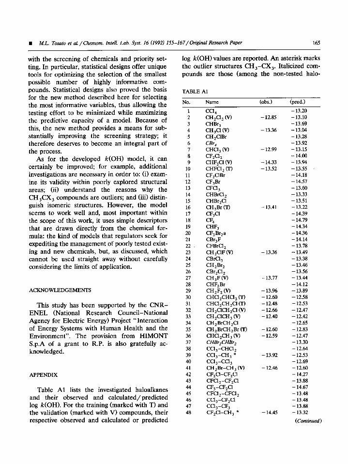
APPENDIX

Table Al lists the investigated haloalkanes and their observed and calculated/ predicted log k(OH). For the training (marked with T) and the validation (marked with V) compounds, their respective observed and calculated or predicted

log k(OH) values are reported. An asterisk marks the outlier structures CH,-CX,. Italicized com- pounds are those (among the non-tested halo-

TABLE Al

No.

1 2

3

4

5 6 7

8 9

10 11

12

13 14

15 16

17 18

19 20

21 22

23 24

25 26 27

28 29

30

31 32

33

34

35 36 37

38 39

40 41

42 43

44 45 46 47

48

Name --. cc1 4

CH ,Cl 2 6’) CHBr,

CH,CI (v) CH ,ClBr

CBr, CHCl, (VI CF,Cl z CHF,Cl Q

CHFCl 2 (T) CF,ClBr

CF,Br

CFCI 3 CHBrCl, CHBr,CI

CH,Br (T)

CF,Cl

CF4

(obs.1 (pred.)

- 12.85

- 13.36

- 12.99

- 14.33

- 13.52

- 13.41

CHF, CF,Br,a

CBr,F CFBrCl 2

CH ,ClF (V)

CBrCl,

CI%Br,

- 13.36

CBr,Cl,

CH,F (V) CHF, Br

CH,F, (V) CHCl ,CHCI 2 (T)

CHCl ,CH 2CI (T) CH ,ClCH ,Cl (V)

CH ,ClCH 3 Q

CH,BrCH,CI

CH,BrCH,Br (T) CHCI,CH, (V) CHBr,CHBr, Ccl,-CHCl,

Ccl,-CH, * ccl,-ccl,

CH,Br-CH, (V) CF,CI-CF,Cl CFCI,-CF,Cl

CF, -CF,Cl CFCI,-CFCl, Ccl, -CF,Cl CCl,-CF,

CF,CI-CH, *

- 13.77

- 13.96 - 12.60

- 12.48

- 12.66 - 12.40

- 12.60 - 12.59

- 13.92

- 12.46

- 14.4s

- 13.20 - 13.10

- 13.69

- 13.04

- 13.28 - 13.92 - 13.15

- 14.00 - 13.94

-13.55 - 14.18

- 14.57

- 13.60

- 13.33 - 13.51 - 13.22

- 14.39 - 14.79

- 14.34

- 14.36

- 14.14 - 13.78

- 13.49 - 13.38 - 13.46

- 13.56 - 13.44

- 14.12 - 13.89

- 12.58

- 12.53 - 12.47

- 12.42

- 12.65

- 12.83 - 12.47

- 13.30 - 12.64

- 12.53 - 12.69

- 12.60

- 14.27 - 13.88

- 14.67 - 13.48 - 13.48 - 13.88 - 13.32

(Continued)

166 M.L. Tosato et al. /Chemom. Intell. Lab. Syst. 16 (1992) 155-167/0riginal Research Paper n

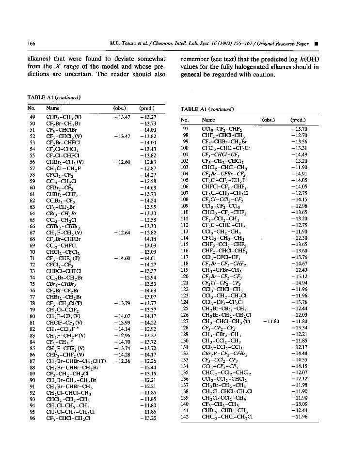
alkanes) that were found to deviate somewhat

from the X range of the model and whose pre-

dictions are uncertain. The reader should also

TABLE Al (continued)

remember (see text) that the predicted log k(OH) values for the fully halogenated alkanes should in

general be regarded with caution.

No. Name (ohs.) (pred.)

49 CHF, -CH 3 (VI 50 CF2Br-CH,Br 51 CF, -CHCIBr 52 CF,-CHCl, (V) 53 CF,Br-CHFCI 54 CF,Cl-CHCl, 55 CF,Cl-CHFCI 56 CHBr, -CH, (V) 57 CH,Cl-CH,F 58 CFCl 2 -CF, 59 Ccl,-CH,Cl 60 CFBr, -CF, 61 CHBr, -CHF, 62 CClBr, -CF, 63 CF,-CH,Br 64 CBr3 - CH, Br 65 Ccl,-CH,Cl 66 CHBr, - CHBr, 67 CH,F-CH, 0’) 68 CF,Br-CHFBr 69 Ccl,-CHFCI 70 CHCl,-CFCI, 71 CF, -CHF, CT) 72 CFCl 2 -CF, 73 CHFCI-CHFCl 74 CCl,Br-CH,Br 75 CBrJ - CHBr, 76 CF,Br-CF,Br 77 CHBr,-CH,Br 78 CF,-CH,CI CT) 79 CH,Cl-CClF, 80 CH,F-CF, (V) 81 CHCIF-CF, (V) 82 CH,-CCl,F l

83 CH,F-CH,F (V) 84 CF3-CH, * 85 CH,F-CHF* (V) 86 CHF, -CHF, (V) 87 CH2Br-CHBr-CH,Cl (T) 88 CH*Br-CHBr-CH,Br 89 CF,-CH,-CH,Cl 90 CH,Br-CH,-CH2Br 91 CH,Br-CHBr-CH3 92 CH,Cl-CHCl-CH, 93 CHCl,-CH,-CH3 94 CH,Cl-CM,-CH, 95 CH&l-CHz-CH,Cl 96 CF, -CHCl-C&Cl

- 13.47

- 13.47

- 12.60

- 12.64

- 14.60

- 13.79

- 14.07 - 13.99 - 14.14 - 12.96 - 14.70 - 13.74 - 14.28 - 12.36

- 13.27

- 13.73 - 14.00 - 13.82 - 14.00

- 13.43

- 13.82 - 12.83

- 12.87 - 14.27

- 12.58

- 14.63 - 13.73

- 14.24 - 13.95

- 13.30

- 12.58 - 13.30 - 12.82

- 14.18 - 13.03

- 13.03 - 14.61 - 14.27

- 13.37

- 12.94 - 13.53

- 14.63 - 13.07

- 13.77

- 13.37 - 14.17

- 14.22 - 12.92

- 13.27

- 13.72 - 13.72 - 14.17

- 12.26 - 12.44 - 13.15 - 12.21 - 12.21 - 11.85 - 11.85 - 11.80 - 11.85 - 13.20

TABLE Al (continued)

No.

97

Name

CC1 2 -CF, -CHF,

(ohs.) (pred.1

- 13.70 98 CHF, -CiiCl-CI-i, 99 CF3-CHBr-CH,Br

100 CFCl,-CHCl-CF,Cl 101 CF,-CHCI-CF, 102 CF,-CH,-CHCl, 103 CHCl,-CHCl-CH, 104 CF,Br-CFBr-CF, 105 CF,Cl-CF,-CH,F 106 CHFCl-CF, -CHF, 107 CF,CI-CM,-CH,Cl 108 CF,Cl-Ccl,-CF, 109 Ccl,-CF,-Ccl, 110 CHCl 2 -CF, -CHF, 111 CF,-Ccl,-CH, 112 CF,CI-CHCl-CH, 113 Ccl,-CH,-CH, 114 CFCl,-CH,-CH, 115 CHF, -Ccl, -CHF, 116 CHF, -CHCl-CHF, 117 Ccl,-CFCl-CF, 118 CF, Br - CF, - CHF, 119 CH,-CFBr-CH, 120 CF, Br - CF, - CF, 121 CF,Cl-CF,-CF, 122 Ccl,-CHCl-CH, 123 Ccl,-CH,-CH,Cl 124 Ccl,-CF,-CF,Cl 125 CH,Br-CBr,-CH, 126 CH,Br-CH,-CH,Cl 127 CH,-CHCl-CH, (T) 128 CF, - CF, - CF, 129 CH,-CBr,-CH, 130 CH,-Ccl,-CH, 131 CCl,-ccl,-ccl, 132 CBr,F-CF,-CFBr, 133 CF,-Ccl,-CF, 134 Ccl, - CF, - CF, 135 CHCl,-Ccl,-CHCl, 136 Ccl,-Ccl,-CHCl, 137 CH,Br-CH,-CH3 138 CH,Cl-CHCI-CH,Cl 139 CH,Cl-CCl,-CH, 140 CF,-CH,-CH, 141 CHBr,-CHBr-CH, 142 CHCl,-CHCl-CH,Cl

- 11.80

- 12.70 - 13.56 - 13.31

- 14.49 - 13.20

- 11.90 - 14.91

- 14.05 - 14.05

- 12.75 - 14.15

- 12.96 - 13.65

- 13.20 - 12.75

- 11.90 - 12.30

- 13.65 - 13.60 - 13.76

- 14.67 - 12.43

- 15.12 - 14.94

- 11.96 - 11.96

- 13.76 - 12.44

- 12.03

- 11.80 - 15.34

- 12.21 - 11.85

- 12.17 - 14.48

- 14.55 - 14.15 - 12.07 - 12.12 - 11.98 - 11.90 - 11.90

- 13.09 - 12.44 - 11.96

n h4.L. Tosato et al. / Chemom. Intell. Lab. Syst. 16 (1992) 155-167/0riginal Research Paper 167

REFERENCES

M.L. Tosato, D. Cesareo, S. Galassi, L. Vigano, G. Cru- ciani, S. Clementi and B. Skagerberg, Multivariate design in toxicological evaluation of chemical data, Chimica Oggi, 3 (1988) 41-45. J. Jonsson, L. Eriksson, M. Sjostrom, S. Wold and M.L. Tosato, A strategy for ranking environmentally occurring chemicals, Chemometrics and Intelligent Laboratory Sys- tems, 5 (1989) 169-186. M.L. Tosato, L. Vigano, B. Skagerberg and S. Clementi, A strategy for ranking chemical hazards: framework and application, Environmental Science and Technology, 25 (1991) 695-702. L. Eriksson, A strategy for ranking environmentally occur- ring chemicals, Thesis, Ume% University, Umei, Sweden, 1991. L. Eriksson, M. Sjostrom and S. Wold, Rational ranking of chemicals according to environmental risks, Chemometrics and Intelligent Laboratory Systems, 14 (1992) 245-252.

6 R. Atkinson, Kinetics and mechanisms of the gas-phase reaction of the hydrozyl radical with organic compounds, Chemical Reviews, 86 (1986) 69-201.

7 M.L. Tosato, C. Chiorboli, L. Eriksson and J. Jonsson, Multivariate modelling of the rate constant of the gas- phase reaction and halo-alkanes with the hydroxyl radical, Science of the Total Environment, 109/110 (1991) 307-325.

8 M.L. Tosato, C. Chiorboli, R. Piazza, L. Passerini and V. Carassiti, Estimation of the tropospheric reactivity of or- ganics with the hydrozyl radical. A QSAR model for a group of haloalkanes. Quantitative Structure - Activity Re- lations, submitted for publication.

9 S. Wold, K Esbensen and P. Geladi, Principal compo- nents analysis, Chemometric and Intelligent Laboratory Sys- tems, 2 (1987) 37-52.

10 S. Wold, A. Ruhe, H. Wold and W.J. Dunn III, The collinearity problem in linear regression. The partial least square approach to generalized inverses, SZAM Journal of Scientific Statistics and Computation, 5 (1984) 735-743.

11 A. Hoskuldsson, PLS regression methods, Journal of Chemometrics. 2 (1988) 211-228.

12

13

14

15

16

17

G.E.P. Box, W.J. Hunter and J.S. Hunter, Statistics for Experimenters, Wiley, New York, 1978. G. Cruciani, M. Baroni, D. Bonelli, S. Clementi, C. Ebert, and B. Skagerberg, Comparison of chemometric methods for QSAR, Quantitative Structure- Activity Relations, 9 (1990) 101-107. M. Baroni, G. Cruciani, G. Costantino, D. Reganelli and S. Clementi, Generating optimal linear PLS estimation, GOLPE: an advanced chemometric tool for handling 3-D QSAR programmes, Quantitative Structure- Activity Rela- tions, submitted for publication. S. Wold, Cross-validatory estimation of the number of components in factor and principal components models, Technometrics, 20 (1978) 397-405. L. Silver and R. Rudman, Polymorphism of the crystalline methylchloromethane compounds. IV: The crystal and molecular structure of methylchloroform, Journal of Chemical Physics, 37 (1972) 210-216. S. Hellberg, L. Eriksson, J. Jonsson, F. Lindgren, M. Sjiistrom, B. Skagerberg, S. Wold and P. Andrews, Mini- mum analog peptide sets (MAPS) for quantitative struc- ture-activity relationships, International Journal of Peptide and Protein Research, 37 (1991) 414-424.