Embed Size (px)
Citation preview

Distances and OtherDissimilarity Measures inChemometrics
Roberto Todeschini, Davide Ballabio and VivianaConsonniUniversity of Milano-Bicocca, Milan, Italy
1 Introduction 12 Theoretical Background 3
2.1 Notation and Symbols 32.2 Axiomatic Rules for Dissimilarity Measures 32.3 From Distance to Similarity 42.4 Weighted Distances 62.5 Data Pretreatment 6
3 Definitions of Distance and SimilarityMeasures 73.1 Distances for Real-valued Data 73.2 Distances for Ranked Data 123.3 Distances for Frequency Data 133.4 Binary Similarity Measures 133.5 Mixed-type Distances 18
4 Meta-Distances 185 Distances Between Sets 19
5.1 Hausdorff Distance 195.2 Linkage Metrics 205.3 Procrustes Analysis 205.4 Canonical Measure of Distance 21
6 Distance Measures on Graphs 227 Multivariate Comparison of Real-Valued
Distances 227.1 Comparison of Real-valued Distance
Measures in Unsupervised Analysis 247.2 Effects of Distance Measures on Similarity-
based Classification 278 Comparison of Binary Similarity Coefficients 31
Acknowledgments 33Abbreviations and Acronyms 33Related Articles 33References 33
Several similarity/diversity measures for data mining andchemometrics are presented and discussed toward thedifferent data they are applied to. After a short presentation
of the axioms for dissimilarity and similarity functions,their relationships, and the required data pretreatment,the theoretical definitions and formulas of distanceand similarity measures for real-valued, binary, ranked,frequency, and mixed-type data are provided along withthe main concepts on distances between sets and meta-distances. Simple examples of calculation are given, andextended comparisons are performed on the distancesdefined for real-valued and binary data.
1 INTRODUCTION
One can easily suppose that the concepts of similarityand dissimilarity among objects, events, situations, and soon always were basic concepts of the human reasoning,which is strongly based on the concept of analogy.
The first explicit traces of the word distance can befound in the writings by Aristoteles (384 AC – 322 AC),who, in his Metaphysics, used the word distance to mean‘It is between extremities that distance is greatest’ or‘things which have something between them, that is, acertain distance’. In addition, ‘distance’ has the sense of‘dimension’ [as in ‘space has three dimensions, length,breadth and depth’ (Aristoteles, Physics)].
Euclid, one of the most important mathematicians ofthe ancient history (323 AC – 286 AC), used the worddistance only in his third postulate of the Principia: ‘Everycircle can be described by a centre and a distance.’ Theword used in this axiom – διαστηματι – still has a verygeneral meaning.
The mathematization of the concepts of dissimilarity,diversity, distance, and their dual terms such as similarityand nearness comes back to the development of themathematics of the twentieth century.
The distance we use in everyday life is what Euclideanapplied to 2-D or 3-D spaces, but several distancemeasures exist. Every distance has its own characteristics,advantages, and drawbacks. Distances are used tomeasure the similarity among objects represented byan extended number of parameters, which is the usualsituation in analytical chemistry where objects arecharacterized by several signals, parameters, and so on.
Distance, sometimes called farness, is a numericaldescription of how far apart entities are. In data mining,entities commonly are objects or variables. The conceptof distance is a concrete way of describing what it meansfor elements of some space to be ‘close to’ or ‘far awayfrom’ each other.
The numerical value of a similarity/diversity measuredepends on three main components: (i) the description ofthe objects (i.e. the selected variables), (ii) the weightingscheme of the description elements, and (iii) the selecteddistance or similarity measure.
Encyclopedia of Analytical Chemistry, Online © 2006–2015 John Wiley & Sons, Ltd.This article is © 2015 John Wiley & Sons, Ltd.This article was published in the Encyclopedia of Analytical Chemistry in 2015 by John Wiley & Sons, Ltd.DOI: 10.1002/9780470027318.a9438

2 CHEMOMETRICS
Distances
Distance between samples Distance between sampleand reference point
Distance between variablesets
Classification methods (DA)Applicabitiy domain methodsLeverage
Canonical correlation analysisCanonical distance measuresProcrustes analysis
k-NN methods
Optimal design of experimentsCluster analysisPrincipal component analysisMultidimensional scalingMinimum spanning tree
Figure 1 Flowchart of the different applications of distance measures in data mining and modeling.
Distance and similarity measures play a fundamentalrole in chemometrics, as schematically shown in Figure 1,where the different methods are arbitrarily divided into(i) methods that calculate a distance between entitiessuch as objects or variables, (ii) methods that calculatea distance between an object and a reference point, and(iii) methods that calculate a distance between two setsof objects (or variables).
Given the data, the main problem using several ofthese methods is the choice of an appropriate distance,choice that is complicated by the huge number ofdifferent possibilities. Indeed, often, chemometric usersare not aware of the different possibilities that the useof alternative distance/similarity measures can provide inhighlighting new sources of information.
Similarity/diversity measures are the core of almost allthe methods for cluster analysis: the method k-meansassigns an object measuring its distance from each clustercentroid, which is assumed as the representative pointof the cluster; analogously, the Jarvis–Patrick method isbased on a neighbor table where for each object to beassigned, the nearest neighbors are listed; hierarchicalagglomerative methods use the distance measures, calledlinkage metrics, which are able to quantify the similaritybetween groups of objects (i.e. the clusters). Kohonenmaps (or self-organizing maps, SOM) exploit distancemeasures to assign objects to the map neurons and thento evaluate object relationships on the map projection:each object, represented by a p-dimensional vector (pis the number of variables) scaled in the range [0, 1], is
compared with each neuron of the map, whose weights arerepresented in the same scale and is assigned to the neuronfor which the Euclidean distance is minimum (winnerneuron). Then, the learning process proceeds and theinformation received in the winner neuron by the objectis spread out to the neighbors of that neuron, smoothingthe information proportionally to the topological distancefrom the winner neuron.
Principal component analysis (PCA), which is themost common approach for exploratory data analysis,generates a metric space where the distances between theobject pairs are the classical Euclidean distances. Othercommon techniques for exploratory data analysis, such asmultidimensional scaling (MDS) and minimum spanningtree (MST), are based on algorithms able to elaboratedistance (or similarity) matrices representing the internalsimilarity/diversity relationships of the objects of adata set.
In classification, one of the most well-known methodsfor nonlinear problems is the k-nearest neighbor (k-NN) method, which is based on the calculation ofsome distance measure between the target and thetraining objects to identify the first k neighbors andevaluate the class membership of the target. Anotherwell-known method is discriminant analysis (DA) thatexploits Mahalanobis distance, able to consider the wholecovariance structure of each class, to evaluate the distancebetween the object and the class centroid.
The concept of model applicability domain (AD)is increasingly gaining importance in the modeling
Encyclopedia of Analytical Chemistry, Online © 2006–2015 John Wiley & Sons, Ltd.This article is © 2015 John Wiley & Sons, Ltd.This article was published in the Encyclopedia of Analytical Chemistry in 2015 by John Wiley & Sons, Ltd.DOI: 10.1002/9780470027318.a9438

DISTANCES AND OTHER DISSIMILARITY MEASURES IN CHEMOMETRICS 3
field where the evaluation whether a given model(classification or regression model) is suitable or notto give reliable predictions for new objects is outstanding.Several methods have been proposed to date to decidewhether a new object can be considered inside the ADof a model and most of them are based on predefineddistance thresholds.
Some books, reviews, and papers(1–10) are dedicatedto present, analyze, and compare similarity/diversitymeasures.
In this article, the problem of evaluating similarityand dissimilarity relationships between objects has beenaddressed with particular attention paid to the use ofdistance and similarity measures in data mining. Thesimilarity/diversity measures commonly used in otherscientific fields, such as, for example, those based onprobability distributions and information content, werenot considered in this study. Moreover, the article wasmainly focused on similarity/diversity measures betweenobjects, although some measures, such as Pearson,Spearman, and Kendall correlation measures, are usuallyapplied to evaluate relationships between variables.
In the framework of data mining, distance and similaritymeasures are commonly distinguished on the basis of datatypes, that is, real-valued data, binary data, frequencyor ranked data, and mixed-type data. Therefore, aftera brief introduction to the theoretical background andthe data pretreatment required before the calculation ofdistances, the most common distance/similarity measuresare presented according to this general classification,which accounts for the data type. In Sections 7 and 8,some applications of the different distance and similaritymeasures to real and simulated data sets are discussedwith the aim of evaluating and comparing the differentinformation provided by each measure.
2 THEORETICAL BACKGROUND
2.1 Notation and Symbols
A chemical data set is usually constituted of a numberof objects (experiments) and a number of parameters,which have been measured on each object. Therefore,the data set is arranged in a numerical matrix (two-way array): each row represents an object of the dataset, whereas columns represent the chemical parameters.Numerical matrices are denoted as X (n ð p), where n isthe number of objects and p the number of variables. Thesingle element of the data matrix X is denoted as xij andrepresents the value of the jth variable for the ith object.Scalars are indicated by italic lower-case characters (e.g.xij) and vectors by bold lower-case characters (e.g. x).
2.2 Axiomatic Rules for Dissimilarity Measures
A function D : XðX!R, where X is a set, must satisfya certain number of properties (axioms) to be considereda distance.
Let X be a set. A function D : XðX!R is calleda distance (or dissimilarity) on X if, for all x, y2X, thefollowing three axioms hold:
Ax.1 : Dxy ½ 0 nonnegativity
Ax.2 : Dxx D 0 reflexivity
Ax.3 : Dxy D Dyx symmetry
A function D : XðX!R is called a quasi-distanceon X if, for all x, y2X, only the first two axioms hold:
Ax.1 : Dxy ½ 0 nonnegativity
Ax.2 : Dxx D 0 reflexivity
A function D : XðX!R is called a metric on X if,for all x, y, z2X, the following four axioms hold:
Ax.1 : Dxy ½ 0 nonnegativity
Ax.20 Dxy D 0 iff x D y strong reflexivity
Ax.3 : Dxy D Dyx symmetry
Ax.4 : Dxy � Dxz CDzy triangle inequality
A function D : XðX!R is called a semimetric (orpseudo-metric) on X if, for all x, y, z2X, the followingfour axioms hold:
Ax.1 : Dxy ½ 0 nonnegativity
Ax.2 : Dxx D 0 reflexivity
Ax.3 : Dxy D Dyx symmetry
Ax.4 : Dxy � Dxz CDzy triangle inequality
A function D : XðX!R is called a quasi-metric onX if, for all x, y, z2X, the following three axioms hold:
Ax.1 : Dxy ½ 0 nonnegativity
Ax.20 Dxy D 0 iff x D y strong reflexivity
Ax.4 : Dxy � Dxz CDzy triangle inequality
A function D : XðX!R is called an ultrametric onX if, for all x, y, z2X, the following four axioms hold:
Encyclopedia of Analytical Chemistry, Online © 2006–2015 John Wiley & Sons, Ltd.This article is © 2015 John Wiley & Sons, Ltd.This article was published in the Encyclopedia of Analytical Chemistry in 2015 by John Wiley & Sons, Ltd.DOI: 10.1002/9780470027318.a9438

4 CHEMOMETRICS
Dissimilarity functions
Quasi-distances
Distances
Metrics
Ultrametrics
Nonmetrics
Semimetrics
Quasi-metrics
Yes
Yes
Yes
Yes
Yes
Yes
Yes
No
No
No
Ax.1: Dxy ≥ 0Ax.2: Dxx = 0
Ax .3 :Dxy = Dyx
Ax .3 :Dxy = Dyx
Ax .4 :Dxy ≤ Dxz + Dzy
Ax .2′Dxy = 0 iff x = y
Ax .4 :Dxy ≤ Dxz + Dzy
Ax .2′Dxy = 0 iff x = y
Ax .4′ :Dxy ≤ max {Dxz, Dzy}
Figure 2 Flowchart of the relationships among the different classes of dissimilarity functions.
Ax.1 : Dxy ½ 0 nonnegativity
Ax.20 Dxy D 0 iff x D y strong reflexivity
Ax.3 : Dxy D Dyx symmetry
Ax.40 : Dxy � maxfDxz, Dzyg ultrametric inequality
The axiom 20 is a stronger condition than axiom 2 asaxiom 40 is stronger than axiom 4.
The different classes of dissimilarity functions can bedistinguished according to the axioms they satisfy, asshown in Figure 2 and Table 1. Note that all dissimilarityfunctions must fulfill at least the two basic requirementsof nonnegativity (Ax. 1) and reflexivity (Ax. 2) and arefurther distinguished into distances and quasi-distancesdepending on whether the property of symmetry (Ax. 3)is fulfilled or not. Obviously, the class of quasi-distancesis the largest one and includes all the distances. Distancescan be further distinguished into metric distances andnonmetric distances according to the property of triangleinequality (Ax. 4): if triangle inequality is not fulfilled,
then a distance is nonmetric; otherwise, it is metric ifalso the property of strong reflexivity (Ax. 20) is fulfilled.If strong reflexivity does not hold, that is, there canbe pairs of objects x 6D y for which Dxy D 0, then adistance cannot be considered properly a metric and iscalled semi-metric distance. The class of quasi-metricsincludes all the quasi-distances that fulfill the propertiesof triangle inequality (Ax. 4) and strong reflexivity (Ax. 20)and differs from the metric distances as quasi-metrics donot fulfill the property of symmetry (Ax. 3). Obviously,the class of quasi-metrics includes all the metricdistances.
2.3 From Distance to Similarity
A function S defined as S : XðX!R on X is calledsimilarity, if, for all x, y2X, the following properties hold:
Ax.1 : Sxy ½ 0 nonnegativity
Ax.2 : Sxx D 0 identity
Encyclopedia of Analytical Chemistry, Online © 2006–2015 John Wiley & Sons, Ltd.This article is © 2015 John Wiley & Sons, Ltd.This article was published in the Encyclopedia of Analytical Chemistry in 2015 by John Wiley & Sons, Ltd.DOI: 10.1002/9780470027318.a9438

DISTANCES AND OTHER DISSIMILARITY MEASURES IN CHEMOMETRICS 5
Table 1 Different classes of dissimilarity measures and their axioms
Dissimilarity function Ax. 1 Ax. 2 Ax. 20 Ax. 3 Ax. 4 Ax. 40
Quasi-distances ž žDistances ž ž žSemi-metrics or pseudo-metrics ž ž ž žQuasi-metrics ž ž ž žMetrics ž ž ž ž žUltrametrics ž ž ž ž ž ž
Ax.3 : Sxy D Syx symmetry
The most common similarity measures satisfy also acondition of closure, that is, 0�Sxy� 1. The value 1indicates the maximum similarity, whereas the value 0indicates the maximum dissimilarity. In this framework,correlation measures can be considered a special caseof similarity measures; however, correlation valuescan be negative, i.e. between [�1, C1], and in thiscase, they cannot be properly regarded as similaritymeasures owing to violation of the first axiom implyingnonnegativity.
Most of the similarity measures can be derived from thedistance measures by appropriate transform functions, thechoice of which mostly depends on whether the distancemeasure is bounded or not.
Some distances, by definition, are intrinsically boundedto the upper value of 1 and others can be bounded in thesame range by normalization on the number of variablesand/or applying some scaling procedures.
For example, given a data set constituted by n objectsand p variables, after range scaling, any distance thatranges between 0 and p can be normalized between 0and 1 simply by averaging on p. For these [0, 1] boundeddistances DN, it is possible to derive the correspondingsimilarity measures by the following equations:
S(1)xy D 1�DN
xy
S(2)xy D 1� (DN
xy)2
S(3)xy D
√1� (DN
xy)2
The obtained similarity measure is naturally bounded[0, 1], as usually required for a similarity function.
When dealing with unbounded distances, a directprocedure to transform them into similarity measures canbe obtained by specific transform functions conceivedin such a way that the similarity values result boundedbetween 0 and 1. The most known similarity transformsfor unbounded distances D are the following:
S(4)xy D
11CDxy
S(5)xy D 1� Dxy
Dmax
S(6)xy D e�Dxy
where Dmax represents the maximum distance betweenall the possible n*(n�1)/2 pairs of objects in the data set.
The similarity transform of type (4) is the simplestone, but its main drawback is that the similarity iscompressed toward zero when distances significantlylarger than all others are present. Indeed, independentlyof the adopted scaling procedure, the presence of severalvariables increases the distance value for the majorityof the distance functions. Moreover, this transform (4)should not be used for normalized distances DN, themaximum distance in this case being equal to 1, which inturn would lead to the minimum similarity of 0.5 insteadof 0. To overcome this drawback, the transform (4) shouldbe further implemented as
S(40)xy D 2 Ð (S(4)
xy � 0.5)
Transform function (6) suffers from the same draw-back, the minimum value being 0.368 (i.e. 1/e), whichis achieved while the normalized distance equals itsmaximum value of 1. In this case, the following scalingshould be adopted to have values properly ranging from0 to 1:
S(60)xy D
S(6)xy � 0.3681� 0.368
For the transform function (5), it is worthy of note thatthere will always be at least one pair of objects x and ywith similarity equal to zero, that is, the pair of objectshaving the maximum distance will have similarity equal to0 regardless of the actual value of their distance. Indeed,this similarity transform gives relative similarity values,depending on the most distant pair of objects.
As most of the similarity measures are derived fromdistance measures by appropriate transform functions,
Encyclopedia of Analytical Chemistry, Online © 2006–2015 John Wiley & Sons, Ltd.This article is © 2015 John Wiley & Sons, Ltd.This article was published in the Encyclopedia of Analytical Chemistry in 2015 by John Wiley & Sons, Ltd.DOI: 10.1002/9780470027318.a9438

6 CHEMOMETRICS
dissimilarity measures D can be derived from similaritymeasures S using any monotonically decreasing transfor-mation of S.
Examples of transformations used to obtain dissimi-larity measures from similarities are
D(1)xy D 1� Sxy
D(2)xy D
√1� Sxy
D(3)xy D
√2 Ð (1� S2
xy)
D(4)xy D arccos(Sy)
D(5)xy D � ln Sxy
where S is assumed to vary in the range [0, 1].
2.4 Weighted Distances
Weighted distances are obtained by weighting each jthvariable by a user-defined weight wj usually under theconstraint
p∑jD1
wj D 1
It can be noted that if one would like to have all thevariables with the same importance on the distance, thenall the weights would have the same value wjD 1/p.
In other cases, the weights can be user-defined andestablished by additional a priori information about thevariable.
2.5 Data Pretreatment
When dealing with data mining, a data pretreatment isoften necessary to allow a fair comparison of variablesdefined by different measurement scales, units, and so on.
The most relevant step of data pretreatment is datascaling procedures, which allow squeezing all the variablesinto a comparable scale so that distance/similaritymeasures between objects can equally exploit informationpresent in all the variables, independently of theirnumerical scale.
In general, distance measures defined for real-valueddata require that all the variables are comparable, thatis, defined in the same numerical scale. If the variablesare defined in different scales, distances between theobjects suffer from distortion effects simply because ofthe different numerical scales and not really influencedby a comparable contribution of all the variables usedto define the data. Thus, in the case of real-valued data,data pretreatment is necessary before the calculation ofdistances.
Data scaling procedures perform the transformationof each variable, separately, in a comparable numericalscale. Let n be the total number of objects of a dataset, p the number of variables, xij the value of the jthvariable for the ith object, and x0ij the correspondingscaled value. The quantities Lj, Uj, xj, and sj are theminimum, maximum, average, and standard deviation ofthe jth variable, respectively.
Thus, the most common scaling procedures are thefollowing:
Scaling to maximum x0ij DxijUj
x0ij � 1Uj D maxi(xij)
Range scaling x0ij Dxij�LjUj�Lj
0 � x0ij � 1Lj D mini(xij)Uj Dmaxi(xij)
Scaling at unitary variance x0ij Dxij
s2j
s0j D 1
Autoscaling x0ij Dxij�xj
sjx0j D 0s0j D 1
Pareto scaling x0ij Dxij�xjpsj
x0j D 0s0j D psj
Logarithmic centering x0ij D log(xij)�n∑
iD1log(xij)
n
The mean and the standard deviation of scaleddata change, for each jth variable, by the followingrelationships:
x0j D α Ð xj C β and s0j D α Ð sj
where α and β are two parameters, which can assumedifferent values on the basis of the types of scalingprocedures, as shown in Table 2.
Some scaling procedures, for instance, the meancentering, do not solve the problem of variable compara-bility.
Additional data pretreatment is usually required formore complex data such as spectra and compositionaldata, for which row scaling is preliminary applied.The column scaling procedures previously defined arestill performed after preliminary row scaling. The rowcentering is a classical scaling for spectra, whereas log-ratio transform is suggested for compositional data.
Table 2 α and β parameters of different scaling procedures
Scaling procedure α β
Mean centering 1 �xj
Scaling to maximum 1/Uj 0Range scaling 1/(Uj�Lj) �Lj/(Uj�Lj)Scaling to unitary variance 1/sj 0Autoscaling 1/sj �xj/sj
Pareto scaling 1/√
sj �xj/√
sj
Encyclopedia of Analytical Chemistry, Online © 2006–2015 John Wiley & Sons, Ltd.This article is © 2015 John Wiley & Sons, Ltd.This article was published in the Encyclopedia of Analytical Chemistry in 2015 by John Wiley & Sons, Ltd.DOI: 10.1002/9780470027318.a9438

DISTANCES AND OTHER DISSIMILARITY MEASURES IN CHEMOMETRICS 7
Example 1 Scaling versus nonscaling
This simple example aims to show the role andimportance of data scaling while dealing with the analysisof similarity/diversity relationships between objects. InTable 3, data concerning five objects described by threevariables are collected, in the original scale and afterrange-scaled treatment. Consider two objects 1 and 2. Ifthe classical Euclidean distance was calculated using thethree original variables, then the distance value of 10.05would be obtained. If the Euclidean distance betweenthe two objects was calculated considering only the firstvariable, then the distance value would be 10 and thiswould be not much different from the previous one.This means that the first variable alone contributes upto 99.5% of the value of the distance between objects1 and 2 and that the other two variables do not muchinfluence the result. If we now make the same calculationconsidering the range-scaled values instead of the originalones, the Euclidean distance between objects 1 and 2based on all the three variables becomes 0.414 and thecontribution to the distance value of the first variabledecreases to 12%. Therefore, if distances are calculatedon the raw data set in presence of variables with differentscales, variables with large variances would have thehighest weight in the distance calculation, thus hidingthe contribution of variables characterized by smallervariances.
3 DEFINITIONS OF DISTANCE ANDSIMILARITY MEASURES
Distance and similarity measures can differ dependingon the kind of data they are applied to: real-valueddata, binary data, ranked data, and frequency data. Thesedata are distinguished on the basis of the variables usedto describe objects. Variables such as signal intensity,biological activity, pressure, temperature, reaction speed,concentration, and counts are measured quantitatively onan interval or ratio scale; they are quantitative variables
Table 3 Original and range-scaled data of Example 1on data pretreatment
Original data Scaled data
Data x1 x2 x3 x1 x2 x3
1 100 2 0.2 0.714 0.333 0.4002 90 1 0.1 0.571 0.000 0.2003 120 4 0 1.000 1.000 0.0004 70 3 0.5 0.286 0.667 1.0005 50 3 0.3 0.000 0.667 0.600
and belong to the class of real-valued data. Quantitativevariables can be either continuous or discrete: in theformer case, the values that a variable can assume area set of infinite or uncountably infinite values; in thelatter case, the set of values is either finite or countablyinfinite, and the values are usually integers. Variablessuch as color, shape, and texture provide a classificationof the objects into categories describing the quality of anobject; these variables are qualitative variables and aremeasured on a nominal scale. If these variables allow anordering or ranking of the objects, then the variables aresaid measured on an ordinal scale. If a nominal variableallows just two values, e.g. yes/no, present/absent, on/off,and so on, then this is referred to as binary variable, whichis usually coded as 1/0.(11)
In the following section, distance/similarity measuresare introduced on the basis of the data types they aredefined for.
3.1 Distances for Real-valued Data
Real-valued data have all variables represented byreal values, such as concentrations, signal intensities ofspectra, and quantitative physical or chemical measures.Several dissimilarity measures were defined in literaturefor real-valued data, the most known ones beingEuclidean, Manhattan, and Mahalanobis distances.
Real-valued distances can be divided in two mainclasses based on the range they cover: unboundeddistances, which range from zero to infinite, and boundeddistances, which range from zero to a fixed finite value,that is, distances having a maximum value limited by anupper bound. The most common unbounded distancesare collected in Table 4, whereas bounded distancesin Table 5: Dxy is the general symbol to represent thedissimilarity measure between any pair of objects x and y;the symbols xj and yj indicate the values of the jth variablesfor the p-dimensional objects x and y, respectively. Thelast column of Tables 4 and 5 includes the formulas tocalculate average dissimilarity measures whose values areindependent of the number p of variables describing theobjects.
A geometrical representation of the most knownunbounded distances, that is, Euclidean (R1), Manhattan
x
Euclidean
a
b
yLagrange
Manhattan
Figure 3 Geometrical representation of Euclidean,Manhattan, and Lagrange distances.
Encyclopedia of Analytical Chemistry, Online © 2006–2015 John Wiley & Sons, Ltd.This article is © 2015 John Wiley & Sons, Ltd.This article was published in the Encyclopedia of Analytical Chemistry in 2015 by John Wiley & Sons, Ltd.DOI: 10.1002/9780470027318.a9438

8 CHEMOMETRICS
Table 4 Unbounded distances for real-valued data
Equation Distance Definition Range Average
R1 Euclidean DEUCxy D
√√√√ p∑jD1
(xj � yj)2 0 � DEUC
xy <1 DEUCxy D DEUC
xypp
R2 Manhattan or city-block DMANxy D
p∑jD1
jxj � yjj 0 � DMANxy <1 D
MANxy D DMAN
xyp
R3 Lagrange DLAGxy D maxjjxj � yjj 0 � DLAG
xy <1 DLAGxy D DLAG
xy
R4 Minkowski DMINxy D
⎡⎣ p∑
jD1
∣∣∣xj � yj
∣∣∣q⎤⎦
1/q
q > 00 � DMIN <1 D
MIN D DMIN
p1/q
R5 Bhattacharyya DBHAxy D
√√√√ p∑jD1
(√
xj �√
yj)2 x, y ½ 0
0 � DBHAxy <1 D
BHAxy D DBHA
xypp
R6 Mahalanobis DMAHxy D
√(x� y)T Ð S�1 Ð (x� y) 0 � DMAH
xy <1 DMAHxy D DMAH
xypp
R7 Locally centered Mahalanobis DLCMxy D 1
pÐ√
(x� y)T Ð S�1(y) Ð (x� y) 0 � DLCM
xy <1 DLCMxy D DLCM
xy
(R2), and Lagrange (R3) distances, is shown in Figure 3.The Euclidean distance between the points x and ycorresponds to the shortest path joining the two points(p
a2 C b2); the Manhattan distance, also called taxidistance, is the sum of the shortest paths along eachdimension (a C b); finally, the Lagrange distance, alsocalled Chebyshev distance, is the maximum path amongthe shortest paths along each dimension (a).
The Minkowski distance (R4) represents a family ofdistance measures, for which the higher the value of qis, the greater the importance given to large differencesis. Euclidean (R1), Manhattan (R2), and Lagrange (R3)distances are special cases of the Minkowski distance(R4), corresponding to different values of the exponentq of this power distance: Euclidean distance is obtainedfor q D 2, Manhattan distance for q D 1, and Lagrangedistance for q!1.
Among the dissimilarity measures defined in Table 4,Mahalanobis distance (R6) is a relative dissimilarityfunction, which measures the dissimilarity between twoobjects x and y not only on the basis of the twoconsidered objects but also accounting for the informationon the whole structure of the data set, by means ofthe data covariance matrix S. The Mahalanobis distancecan be thought of as a reliable distance measure whencorrelation between variables exists, i.e. it is able tounderweight correlated variables that give otherwiseredundant information.
Moreover, note that the Mahalanobis distance is anextended version of Euclidean distance: if the covariancematrix S is replaced by the identity matrix I, then theMahalanobis distance reduces to the Euclidean distance.
Proportional to the Mahalanobis distance DMAH isthe leverage, which is often used in the framework ofregression diagnostics and outlier detection, defined as
hic D xi Ð (XTc Xc) Ð xT
i D(DMAH
ic )2
n� 1
where Xc is the model matrix centered on the centroid cof the data and n the number of objects in the data set; hicmeasures the dissimilarity between object xi and the datacentroid, or, in other words, gives the ‘distance’ of the ithobject from the center of the model represented by thedata matrix X.
Recently, a variant of the Mahalanobis distance, calledlocally centered Mahalanobis distance (R7), has beenproposed in the literature.(12) What makes this functiondifferent from the classical Mahalanobis distance isthe way the dissimilarity between objects x and y isevaluated, as the data covariance matrix is centered inone of the two objects instead of the data centroid.Obviously, two different values are obtained dependingon whether the covariance matrix is centered in y (i.e.S(y)) or in x (i.e. S(x)) and, therefore, the property ofsymmetry (Axiom 3) is violated with the consequence thatlocally centered Mahalanobis (LCM) function cannot beproperly regarded as a distance but as a quasi-distance(i.e. DLCM
xy 6D DLCMyx ).
In order to make the LCM symmetric and thus,complying with the Axiom 3 of distances, two symmetriza-tion procedures can be applied:
DMSAxy D DLCM
xy CDLCMyx
2
Encyclopedia of Analytical Chemistry, Online © 2006–2015 John Wiley & Sons, Ltd.This article is © 2015 John Wiley & Sons, Ltd.This article was published in the Encyclopedia of Analytical Chemistry in 2015 by John Wiley & Sons, Ltd.DOI: 10.1002/9780470027318.a9438

DISTANCES AND OTHER DISSIMILARITY MEASURES IN CHEMOMETRICS 9
Table 5 Bounded distances on real-valued data. rxy is the Pearson correlation
Equation Distance Definition Range Average
R8 Canberra DCANxy D
p∑jD1
jxj � yjjjxjj C jyjj
0 � DCANxy � p D
CANxy D DCAN
xyp
R9 Clark or coefficient of divergence DCLAxy D
√√√√√ p∑jD1
⎛⎝ xj � yj∣∣∣xj
∣∣∣C jyjj
⎞⎠
2
0 � DCLAxy � p D
CLAxy D DCLA
xypp
R10 Wave-Edge DWExy D
p∑jD1
⎛⎝1�
min(
xj, yj
)max(xj, yj)
⎞⎠ 0 � DWE
xy � p DWExy D
DWExyp
R11 Lance–Williams or Bray–Curtis DLWxy D
p∑jD1
jxj � yjjp∑
jD1
(jxjj C jyjj)0 � DLW
xy � 1 DLWxy D DLW
xy
R12 Soergel DSOExy D
p∑jD1
jxj � yjjp∑
jD1
max(xj, yj)
0 � DSOExy � 1 D
SOExy D DSOE
xy
R13 Jaccard–Tanimoto distance DJTxy D
√√√√√√√√√√1�
p∑jD1
xj Ð yj
p∑jD1
x2j C
p∑jD1
y2j �
p∑jD1
xj Ð yj
0 � DJTxy � 1 D
JTxy D DJT
xy
R14 Pearson distance DPEAxy D 1� rxy 0 � DPEA
xy � 2 DPEAxy D DPEA
xy
R15 Correlation distance DCORxy D 1� rxy
20 � DCOR
xy � 1 DCORxy D DCOR
xy
R16 Cosine or angular distance DCDxy D 1�
p∑jD1
xj Ð yj
√√√√√√p∑
jD1
x2j Ð
p∑jD1
y2j
0 � DCDxy � 1 D
CDxy D DCD
xy
DMSGxy D
√DLCM
xy ðDLCMyx
the former being the arithmetic mean (MSA) of the twodissimilarity values and the latter their geometric mean(MSG). For the sake of simplicity, hereinafter, the symbolDMU
xy will be used to indicate the LCM function centeredin x in place of the symbol DLCM
xy , whereas the symbolDML
xy will replace the symbol DLCMyx to indicate the LCM
function centered in y. Note that the symbol MU refersto the elements of the upper triangular submatrix ofthe dissimilarity matrix containing LCM values betweenall the pairs of objects and the symbol ML to the
elements of the lower triangular submatrix of the samematrix.
Specific distance measures for real-valued data are alsoderived from similarity measures (Table 5). Among these,the Jaccard–Tanimoto distance (R13) is derived from thewell-known Jaccard–Tanimoto similarity coefficient SJT:
SJTxy D
p∑jD1
xj Ð yj
p∑jD1
x2j C
p∑jD1
y2j �
p∑jD1
xj Ð yj
Encyclopedia of Analytical Chemistry, Online © 2006–2015 John Wiley & Sons, Ltd.This article is © 2015 John Wiley & Sons, Ltd.This article was published in the Encyclopedia of Analytical Chemistry in 2015 by John Wiley & Sons, Ltd.DOI: 10.1002/9780470027318.a9438
10 CHEMOMETRICS
and the angular distance (R16) is derived from thesimilarity cosine coefficient SCC:
SCCxy D
p∑jD1
xj Ð yj
√√√√ p∑jD1
x2j Ð
p∑jD1
y2j
It is interesting to note that Euclidean andJaccard–Tanimoto distances are intrinsically related.Indeed, the squared Euclidean distance can be rewrittenas
(DEUCxy )2 D
p∑jD1
(xj � yj)2 D
p∑jD1
x2j C
p∑jD1
y2j � 2 Ð
p∑jD1
xj Ð yj
and the squared Jaccard–Tanimoto distance as
(DJTxy )2 D 1�
p∑jD1
xj Ð yj
p∑jD1
x2j C
p∑jD1
y2j �
p∑jD1
xj Ð yj
D
p∑jD1
x2j C
p∑jD1
y2j � 2 Ð
p∑jD1
xj Ð yj
p∑jD1
x2j C
p∑jD1
y2j �
p∑jD1
xj Ð yj
D (DEUCxy )2
p∑jD1
x2j C
p∑jD1
y2j �
p∑jD1
xj Ð yj
According to this relationship, it derives that squaredJaccard–Tanimoto distance can be viewed as a normal-ized squared Euclidean distance.
The Pearson (R14) and correlation (R15) distances,usually applied to measure variable correlation but hereapplied to pairs of objects, are derived from the Pearson’scorrelation coefficient rxy, which is the most knownbivariate correlation measure estimating the degree ofassociation between two objects x and y, defined as
rxy D
p∑jD1
(xj � x) Ð (yj � y)
√√√√ p∑jD1
(xj � x)2 Ðp∑
jD1
(yj � y)2
� 1 � rxy � C1
where x and y are the means of vectors x and y,respectively.
From the correlation coefficient, was also defined thesquared Pearson distance as
DSQPxy D 1� r2
xy
where pairs of objects with correlation equal to both �1or C1 are considered similar to each other, being theirDSQP
xy D 0.In order to obtain a suitable measure of similarity in
the range [0, 1], the Pearson distance (R14) was scaled,giving the correlation distance (R15).
DCORxy D DPEA
xy
2
It should be noted that the correlation distance, unlikethe classical distances, does not account for systematicdifferences between objects, as it measures the associationbetween the object profiles. Moreover, when objectsare described by only two variables, the correlationdistance gives always a value equal to 1 or �1, thusprojecting all the distances only in two points, and itcannot be calculated for data described by just onevariable.
A distance measure is scaling invariant if the followingrelationship is fulfilled:
D(x, y) D D(αxC β, αyC β)
where α and β are the scaling parameters. Morespecifically, a distance has the property of
1. translation invariance, i.e. invariance to translationwith respect to the origin, if D(x, y)DD(xC β, yC β)with α D 1 in the scaling invariance expression;
2. scale invariance, i.e. invariance to dilation, ifD(x, y)DD(αx, αy) with βD 0 in the scaling invarianceexpression.
Among the distances collected in Tables 4 and 5,classical Mahalanobis, LCM, Pearson, and correlationdistances are scaling invariant as both conditions(i.e. translation invariance and scale invariance) hold.Euclidean, Manhattan, Lagrange, and Minkowski areinvariant to translation, as any constant added to bothx and y vanishes when the difference between values iscalculated, whereas they are not invariant to dilation.On the contrary, most of the bounded distances ofTable 5 result to be invariant to dilation but not totranslation, as they are based on the ratio of twoquantities.
Encyclopedia of Analytical Chemistry, Online © 2006–2015 John Wiley & Sons, Ltd.This article is © 2015 John Wiley & Sons, Ltd.This article was published in the Encyclopedia of Analytical Chemistry in 2015 by John Wiley & Sons, Ltd.DOI: 10.1002/9780470027318.a9438

DISTANCES AND OTHER DISSIMILARITY MEASURES IN CHEMOMETRICS 11
00
Distances not invariant to translation
1 2 3 4 5 6 7 8 9
β values
0.5
1
1.5
2
2.5
3
3.5
4
Dis
tanc
es CAN
CLA
BHA
JT
LW
WE
Camberra (CAN)Lance–Williams (LW)Clark (CLA)Soergel (SOE)Bhattacharyya (BHA)Wave-Edge (WE)Jaccard–Tanimoto (JT)Cosine distance (CD)
Figure 4 Profiles of the different distance values between two objects obtained for increasing shift parameter values.
0
Distances not invariant to dilation
EuclideanManhattanLagrangeBhattacharyya
1 1.2 1.4 1.6 1.8 2
α values
5
10
15
20
25
30
Dis
tanc
es
Figure 5 Profiles of the different distance values between two objects obtained for increasing dilation parameter values.
Example 2 Invariance properties of distances
The invariance properties of distances have been furtherinvestigated by a simple exercise. Consider two objects xand y described by range-scaled variables in the interval[0, 1]. Then, the shift parameter β is added to all thevariable values of both x and y and varied between 0and 10 with step 1. For each different value of the shiftparameter, the distance between the two objects x andy is calculated using the different distance functions ofTables 4 and 5. This exercise can be repeated, keepingthe shift parameter β constant at value 0 and multiplyingby the dilation parameter α the variables of both objectsx and y. The dilation parameter is varied from 1 to 2with step 0.25 and, for each different value, the distancesof Tables 4 and 5 are calculated. Finally, the results of
this calculation are shown in Figures 4 and 5, whereone can easily see how much the different distancefunctions are sensitive to the shift and dilation parameters.Canberra, Lance–Williams, Clark, Soergel, Wave-Edge,Jaccard–Tanimoto, angular, and Bhattacharyya distancesare clearly not invariant to translation (Figure 4). Forthese distance functions, indeed, the origin of the axes issignificant and, therefore, if the two objects are movedaway from the origin of the axes, then the distancebetween them tends toward zero.
Euclidean, Manhattan, Lagrange, and Bhattacharyyadistances do not fulfill the property of dilation invarianceand, as can be seen in Figure 5, they tend to increasesignificantly as the value α increases: Euclidean andLagrange distances increase by a factor α and Manhattanand Bhattacharyya distances by a factor
pα.
Encyclopedia of Analytical Chemistry, Online © 2006–2015 John Wiley & Sons, Ltd.This article is © 2015 John Wiley & Sons, Ltd.This article was published in the Encyclopedia of Analytical Chemistry in 2015 by John Wiley & Sons, Ltd.DOI: 10.1002/9780470027318.a9438

12 CHEMOMETRICS
Table 6 Distance measures for ranked data
Equation Distance Definition
P1 Spearman distance DSPExy D
p∑jD1
[rxj � ryj]2
P2 Kendall distance DKENxy D
p�1∑jD1
p∑kDjC1
jδjkj if δjk < 0
P3 Mahalanobis rank distance DMRDxy D 2 Ð
p∑jD1
(rxj � ryj)2
(rxj C ryj)
P4 Bhattacharyya rank distance DBAHxy D
√√√√ p∑jD1
(√
rxj �√
ryj)2
Among the considered distances, the only distancethat does not fulfill both invariance properties isthe Bhattacharyya distance, although, with a minimalsensitivity to both the shift and dilation parameters.
3.2 Distances for Ranked Data
While dealing with ordinal data, it is implicit that data canbe ordered and a rank can be assigned to each entity; forthis kind of data, specific similarity measures are required.
The most common association measures between tworankings or permutations are the Spearman ρ coefficientand the Kendall τ coefficient. The Spearman ρ coefficientfor two ranked vectors x and y is defined as
ρxy D 1�6 Ð
p∑jD1
[rxj � ryj]2
p3 � p� 1 � ρxy � C1
where rj indicates the jth rank for the two entities xand y in the interval [1, p]. This expression of Spearmanrank correlation corresponds to the Pearson correlationcalculated on the ranks, i.e.
ρxy D
p∑jD1
[rxj � rx] Ð [ryj � ry]
√√√√ p∑jD1
[rxj � rx]2 Ðp∑
jD1
[ryj � ry]2
The Kendall τ coefficient is defined as
τxy D2 Ð
p�1∑jD1
p∑kDjC1
δjk
p Ð (p� 1)� 1 � τxy � C1
where negative δjk values indicate rank discordance of yand x, whereas positive values indicate rank concordance:
δjk D{�1 if
[(rxj � rxk
) Ð (ryj � ryk)]
< 0C1 otherwise
Distance measures derived from both Spearman rankcorrelation and Kendall coefficient along with theMahalanobis rank distance and Bhattacharyya distanceare collected in Table 6.
Example 3 Similarity/diversity measures for ranked data
In order to better explain how to calculate simi-larity/diversity measures for ranked data a simpleexample is here reported. Suppose to have two objectsx and y, each described by rankings from 1 to 4. Table 7shows the four ranks for the objects. Then, the above-mentioned similarity/diversity measures are calculated as
Spearman ρ coefficient: ρxy D 1� 6 Ð (02 C 32 C 22 C 12)
43 � 4D
�0.4Spearman ρ distance: DSPE
xy D (02 C 32 C 22 C 12) D 14Mahalanobis rank distance: DMRD
xy D 2 Ð (0C 1.80C0.67C 0.33) D 5.6Bhattacharyya distance: DBHA
xy D√(p
3�p3)2 C (p
4�p1)2 C (p
2�p4)2 C (p
1�p2)2
D 1.23
Table 7 Two objects x and y, each characterized by fourranks ranging between 1 and 4
a b c d
x 3 4 2 1y 3 1 4 2
Encyclopedia of Analytical Chemistry, Online © 2006–2015 John Wiley & Sons, Ltd.This article is © 2015 John Wiley & Sons, Ltd.This article was published in the Encyclopedia of Analytical Chemistry in 2015 by John Wiley & Sons, Ltd.DOI: 10.1002/9780470027318.a9438

DISTANCES AND OTHER DISSIMILARITY MEASURES IN CHEMOMETRICS 13
Table 8 Distance measures for frequencies
Equation Distance Definition Range
F1 Tanimoto distance DTxy D 1�
p∑jD1
min(fxj, fyj)
p∑jD1
fxjCp∑
jD1
fyj�p∑
jD1
min(fxj, fyj)
0�DTxy� 1
F2 Modified Tanimoto distance DMTxy D 1�
2Ðp∑
jD1
min(fxj, fyj)
p∑jD1
fxjCp∑
jD1
fyj
0�DMTxy� 1
Kendall τ coefficient: τxy D2 Ð (�1� 1C 1� 1� 1C 1)
4 Ð (4� 1)D
2 Ð (�2)
12D �0.33
Kendall τ distance: DKENxy D j�1j C j�1j C j�1j C j�1j D
4
3.3 Distances for Frequency Data
Frequencies are integer numbers denoting the occur-rences of repeated events, cases, and so on. The two mostknown measures of dissimilarity for frequency data arecollected in Table 8.
The two distances are derived from the Tanimoto simi-larity and the modified Tanimoto similarity, respectively,defined as
STxy D
p∑jD1
min(fxj, fyj)
p∑jD1
fxj Cp∑
jD1
fyj �p∑
jD1
min(fxj, fyj)
and
SMTxy D
2 Ðp∑
jD1
min(fxj, fyj)
p∑jD1
fxj Cp∑
jD1
fyj
where fxj is the number of occurrences of the jth event(the variable) for the object x and fyj the number ofoccurrences of the same jth event for the object y.
Example 4 Similarity/diversity measures for frequencydata
Consider the data collected in Table 7 and suppose thesedata to be frequencies instead of ranks, then the distancemeasures defined earlier for frequency occurrences arecalculated as
DTxy D 1
� 3C 1C 2C 1(3C 4C 2C 1)C (3C 1C 4C 2)� (3C 1C 2C 1)
D 1� 713D 0.46
DMTxy D 1� 2 Ð (3C 1C 2C 1)
(3C 4C 2C 1)C (3C 1C 4C 2)
D 1� 1420D 0.30
3.4 Binary Similarity Measures
Binary variables whose values are either one or zero(presence/absence, yes/no, active/nonactive, etc.) arelargely common in data mining because these variablesare able, for example, to describe the presence/absenceof a signal at a given wavelength of a spectrum andthe presence/absence of a specific functional group ormolecular fragment in a molecule, to define whether acompound is active or inactive and in general if somefeature or attribute is observed or not.
To deal with binary variables, several similaritycoefficients have been proposed in literature and they canall be described as follows. Let two objects be describedby the binary vectors x and y, each comprised p variableswith values 0/1. The common association coefficients arecalculated from the data reported in a frequency table
Encyclopedia of Analytical Chemistry, Online © 2006–2015 John Wiley & Sons, Ltd.This article is © 2015 John Wiley & Sons, Ltd.This article was published in the Encyclopedia of Analytical Chemistry in 2015 by John Wiley & Sons, Ltd.DOI: 10.1002/9780470027318.a9438

14 CHEMOMETRICS
Table 9 Frequency table of the four possible combinationsof values 0 and 1 for two binary samples x and y
y D 1 y D 0x D 1 a b a C b
x D 0 c d c C d
a C c b C d p
(Table 9), where a, b, c, and d are the frequencies of theevents (x D 1 and y D 1), (x D 1 and y D 0), (x D 0 andy D 1), and (x D 0 and y D 0), respectively, in the pairof binary vectors describing the two objects; p is the totalnumber of attributes (i.e. variables), equal to a C b C c Cd, which is the length of each binary vector.
The frequency table can be read as follows: a is thenumber of common presences of the attributes, d thenumber of ‘common absences’ in x and y, a C b thenumber of attributes present in x, and a C c the numberattributes present in y. The diagonal entries a and d hencegive information about the similarity between the twovectors, whereas the entries b and c give informationabout their dissimilarity.
Example 5 Frequency table for binary data
A simple example is presented to show how thefrequencies a, b, c, and d are calculated. Let two objectsbe represented by the vectors x and y, each described by10 binary variables (i.e. p D 10):
x : 1 1 0 1 1 0 0 0 1 1
y : 1 0 1 0 1 0 0 0 1 1
Then, a, b, c, and d take the following values:
y D 1 y D 0x D 1 a D 4 b D 2 a C b D6x D 0 c D 1 d D 3
a C c D5 p D 10
Binary coefficients are usually distinguished into (i)symmetric coefficients that use both a and d, i.e. thedouble-zero state (d) for two objects is treated in exactlythe same way as any other pair of values and should beused when the zero state is a valid basis for comparingtwo objects; (ii) asymmetric coefficients, conversely, thatignore such double-zero attributes in the similaritycalculation; and (iii) correlation-based coefficients, whichare defined in the range [�1, C1], that account for
the difference between the occurrence frequency ofconcordances (i.e. ad) and the occurrence frequency ofdiscordances (i.e. bc).
The most common binary similarity coefficients arelisted in Table 10. Most of these coefficients are naturallydefined in the range [0, 1]. For those coefficients havingranges other than [0, 1], they can be rescaled using thefollowing linear transform:
S0 D SC α
β
where S is the original similarity value, S0 the rescaledfunction in the range [0, 1], and α and β numericalparameters whose values are reported in Table 10(where, obviously, α D 0 and β D 1 indicate thatno transformation is required to obtain the desiredrange). Table 10 also collects the mathematical conditionsthat must be applied to make each binary coefficientvalid for any combination of the a, b, c, and dfrequencies.
The most common binary similarity coefficient is theJaccard–Tanimoto coefficient (B3) that emphasizes thepresence of common features a, neglecting the absenceof common features d and the simple matching (B1)accounting for both presence and absence of commonfeatures.
A weighted version of the Jaccard–Tanimoto coeffi-cient (B3) is the Tversky similarity coefficient, definedas
STVxy D
aaC γ Ð bC δ Ð c 0 � STV
xy � 1
where λ and γ are user-defined parameters. In particular,equal values of γ and δ provide a symmetrical contributionto the two dissimilarity frequencies b and c, as, forinstance, in the Jaccard–Tanimoto coefficient (B3),for which γ D δ D1, in the Gleason coefficient (B4)when γD δD 1/2, in the Sokal–Sneath coefficient (B12)when γD δD 2 and in the Jaccard coefficient (B14)when γD δD 1/3; different values of γ and δ provideasymmetrical contribution, as, for example, in theDice–Wallace, Post–Snijders coefficient (B31), for whichδ D 1 and γ D 0; this coefficient can be interpretedas the fraction of object x that is in common withobject y.
The coefficient CT5 (B43) is the normalized versionof a measure derived from a Bayesian analysis of the
Encyclopedia of Analytical Chemistry, Online © 2006–2015 John Wiley & Sons, Ltd.This article is © 2015 John Wiley & Sons, Ltd.This article was published in the Encyclopedia of Analytical Chemistry in 2015 by John Wiley & Sons, Ltd.DOI: 10.1002/9780470027318.a9438

DISTANCES AND OTHER DISSIMILARITY MEASURES IN CHEMOMETRICS 15
Tab
le10
Bin
ary
sim
ilari
tyco
effic
ient
s.In
the
colu
mn
‘Con
diti
ons’
,den
indi
cate
sth
ede
nom
inat
orof
the
func
tion
Equ
atio
nSi
mila
rity
coef
ficie
ntD
efini
tion
αβ
Con
diti
ons
B1
Soka
l–M
iche
ner,
Sim
ple
Mat
chin
gSSM xyD
aCd
p0
1N
one
B2
Rog
ers–
Tan
imot
oSR
TxyD
aCd
pCbC
c0
1N
one
B3
Jacc
ard
–T
anim
oto
SRT
xyD
aaC
bCc
01
aD
0!
sD0
B4
Gle
ason
–D
ice
–So
rens
enSG
LE
xyD
2a2aCbCc
01
aD
0!
sD0
B5
Rus
sell
–R
aoSR
RxyD
a p0
1N
one
B6
For
bes
SFO
RxyD
pa(aCb
)(aC
c)0
p/a
denD
0_aD
0!
sD0
B7
Sim
pson
SSIM
xyD
am
inf(aCb
),(aCc
)g0
1de
nD
0_aD
0!
sD0
B8
Bra
un-B
lanq
uet
SBB
xyD
am
axf(aCb
),(aCc
)g0
1aD
0!
sD0
B9
Dri
ver–
Kro
eber
–O
chia
icos
ine
SDK
xyD
ap (aCb
)(aC
c)0
1de
nD
0!
sD0
B10
Bar
oni-
Urb
ani–
Bus
erSB
U1
xyD
p adCa
p adCaCbCc
01
dD
p!
sD1
B11
Kul
czyn
ski
SKU
LxyD
1 2Ð[
aaC
bC
aaC
c
]0
1aD
0!
sD0
B12
Soka
l–Sn
eath
SSS1
xyD
aaC
2bC2
c0
1aD
0!
sD0
B13
Soka
l–Sn
eath
SSS2
xyD
2aC2
dpC
aCd
01
Non
e
B14
Jacc
ard
SJA xyD
3a3aCbCc
01
aD
0!
sD0
B15
Fai
thSF
AI
xyD
aC0.
5Ðdp
01
Non
e
B16
Mou
ntfo
rdSM
OU
xyD
2aabCa
cC2b
c0
2de
nD
0!
sDa/
p
B17
Mic
hael
SMIC
xyD
4Ð(ad�b
c)(aCd
)2C(
bCc)
2C1
2aD
p_
dD
p!
sD1
bC
cD
0!
sD1
B18
Rog
ot–
Gol
dber
gSR
GxyD
a2aCbCcC
d2dCbCc
01
aD
p_
dD
p!
sD1
B19
Haw
kins
–D
otso
nSH
DxyD
1 2Ð(
aaC
bCcC
dbC
cCd
)0
1aD
p_
dD
p!
sD1
B20
Yul
eSY
U1
xyD
ad�b
cadCb
cC1
2aD
p_
dD
p_b
cD
0!
sD1
B21
Yul
eSY
U2
xyDp ad�p
bcp adCp
bcC1
2aD
p_
dD
p_b
cD
0!
sD1
B22
Fos
sum
SFO
SxyD
pÐ(a�
0.5)
2
(aCb
)(aC
c)0
(p�0
.5)2
pde
nD
0!
sD0
B23
Den
nis
SDE
NxyD
ad�b
cp p(
aCb)
(aCc
)
p p 2p p
aD
p_
dD
p!
sD
1de
nD
0!
sD
0
B24
Col
eSC
O1
xyD
ad�b
c(aCc
)(cC
d)p�
1p
aD
p_
dD
p!
sD
1de
nD
0!
sD
0
B25
Col
eSC
O2
xyD
ad�b
c(aCb
)(bC
d)p�
1p
aD
p_
dD
p!
sD
1de
nD
0!
sD
0
Encyclopedia of Analytical Chemistry, Online © 2006–2015 John Wiley & Sons, Ltd.This article is © 2015 John Wiley & Sons, Ltd.This article was published in the Encyclopedia of Analytical Chemistry in 2015 by John Wiley & Sons, Ltd.DOI: 10.1002/9780470027318.a9438

16 CHEMOMETRICS
Tab
le10
(Con
tinue
d).
Equ
atio
nSi
mila
rity
coef
ficie
ntD
efini
tion
αβ
Con
diti
ons
B26
Dis
pers
ion
SDIS
xyD
ad�b
cp2
1/4
1/2
aD
p_
dD
p!
sD1
B27
Goo
dman
–K
rusk
alSG
KxyD
2Ðmin
(a,d
)�b�
c2Ðm
in(a
,d)C
bCc
C12
aD
p_
dD
p!
sD1
B28
Soka
l–Sn
eath
SSS3
xyD
1 4Ð[
aaC
bC
aaC
cC
dbC
dC
dcC
d
]0
1aD
p_
dD
p!
sD
1aD
0^
dD
0!
sD
0
B29
Soka
l–Sn
eath
SSS4
xyD
ap (aCb
)(aC
c)Ð
dp (bCd
)(cC
d)0
1aD
p_
dD
p!
sD
1aD
0_
dD
0!
sD
0
B30
Pea
rson
–H
eron
SPH
IxyD
ad�b
cp (aCb
)(aC
c)(cCd
)(bC
d)C1
2aD
p_
dD
p!
sD
1bD
p_
cD
p!
sD
0de
nD
0!
sD
0B
31D
ice
–W
alla
ce,P
ost–
Snijd
ers
SDI1
xyD
a(aCb
)0
1aD
0!
sD0
B32
Dic
e–
Wal
lace
,Pos
t–Sn
ijder
sSD
I2xyD
a(aCc
)0
1aD
0!
sD0
B33
Sorg
enfr
eiSSO
RxyD
a2
(aCb
)(aC
c)0
1aD
0!
sD0
B34
Coh
enSC
OE
xyD
2Ð(ad�b
c)(aCb
)(bC
d)C(
aCc)
(cCd
)C1
2aD
p_
dD
p!
sD
1de
nD
0!
sD
0
B35
Pei
rce
SPE
1xyD
ad�b
c(aCb
)(cC
d)C1
2aD
p_
dD
p!
sD
1bD
p_
cD
p!
sD
0
B36
Pei
rce
SPE
2xyD
ad�b
c(aCc
)(bC
d)C1
2aD
p_
dD
p!
sD
1bD
p_
cD
p!
sD
0
B37
Max
wel
l–P
illin
erSM
PxyD
2Ð(ad�b
c)(aCb
)(cC
d)C(
aCc)
(bCd
)C1
2aD
p_
dD
p!
sD
1de
nD
0!
sD
0
B38
Har
ris–
Lah
eySH
LxyD
aÐ(2dCbCc
)2Ð(
aCbC
c)C
dÐ(2aCbCc
)2Ð(
bCcC
d)0
paD
p_
dD
p!
sD
1de
nD
0!
sD
0B
39C
onso
nni–
Tod
esch
ini
SCT
1xyD
ln(1CaCd
)ln
(1Cp
)0
1N
one
B40
Con
sonn
i–T
odes
chin
iSC
T2
xyD
ln(1Cp
)�ln
(1CbCc
)
ln(1Cp
)0
1N
one
B41
Con
sonn
i–T
odes
chin
iSC
T3
xyD
ln(1Ca
)ln
(1Cp
)0
1N
one
B42
Con
sonn
i–T
odes
chin
iSC
T4
xyD
ln(1Ca
)ln
(1CaCbCc
)0
1N
one
B43
Con
sonn
i–T
odes
chin
iSC
T5
xyD
ln[ 1C
ad1C
bc
]ln
(1Cp
2 /4)
12
Non
e
B44
Aus
tin
–C
olw
ell
SAC
xyD
2 πÐa
rcsi
n√ (
aCd
p
)0
1N
one
Encyclopedia of Analytical Chemistry, Online © 2006–2015 John Wiley & Sons, Ltd.This article is © 2015 John Wiley & Sons, Ltd.This article was published in the Encyclopedia of Analytical Chemistry in 2015 by John Wiley & Sons, Ltd.DOI: 10.1002/9780470027318.a9438
DISTANCES AND OTHER DISSIMILARITY MEASURES IN CHEMOMETRICS 17
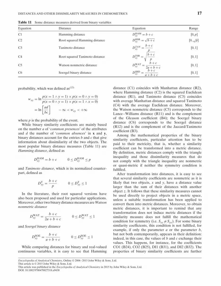
Table 11 Some distance measures derived from binary variables
Equation Distance Equation Range
C1 Hamming distance DHAMxy D bC c [0, p]
C2 Root squared Hamming distance DHSRxy D pbC c [0,
pp]
C3 Tanimoto distance DTANxy D bC c
p[0, 1]
C4 Root squared Tanimoto distance DTSRxy D
√bC c
p[0, 1]
C5 Watson nonmetric distance DWATxy D bC c
2aC bC c[0, 1]
C6 Soergel binary distance DSBDxy D bC c
aC bC c[0, 1]
probability, which was defined as(13)
wxy D lnp(x D 1 ^ y D 1)ð p(x D 0 ^ y D 0)
p(x D 0 ^ y D 1)ð p(x D 1 ^ x D 0)
D ln[
adbc
]�1 < wxy < C1
where p is the probability of the event.While binary similarity coefficients are mainly based
on the number a of ‘common presences’ of the attributesand d the number of ‘common absences’ in x and y,binary distances account for the entries b and c that giveinformation about dissimilarity of the two objects. Themost popular binary distance measures (Table 11) areHamming distance, defined as
DHAMxy D bC c 0 � DHAM
xy � p
and Tanimoto distance, which is its normalized counter-part, defined as
DTxy D
bC cp
0 � DTxy � 1
In the literature, their root squared versions havealso been proposed and used for particular applications.Moreover, other two binary distance measures are Watsonnonmetric distance
DWATxy D bC c
2aC bC c0 � DWAT
xy � 1
and Soergel binary distance
DSOExy D bC c
aC bC c0 � DSOE
xy � 1
While comparing distances for binary and real-valuedcontinuous variables, it is easy to see that Hamming
distance (C1) coincides with Manhattan distance (R2),where Hamming distance (C2) is the squared Euclideandistance (R1), and Tanimoto distance (C3) coincideswith average Manhattan distance and squared Tanimoto(C4) with the average Euclidean distance. Moreover,the Watson nonmetric distance (C5) corresponds to theLance–Williams distance (R11) and is the complementof the Gleason coefficient (B4); the Soergel binarydistance (C6) corresponds to the Soergel distance(R12) and is the complement of the Jaccard/Tanimotocoefficient (B3).
Among the mathematical properties of the binarysimilarity coefficients, particular attention has to bepaid to their metricity, that is, whether a similaritycoefficient can be transformed into a metric distance.By definition, metric distances comply with the triangleinequality and those dissimilarity measures that donot comply with the triangle inequality are nonmetricor quasi-metric if neither the symmetry condition isfulfilled.
After transformation into distances, it is easy to seethat several similarity coefficients are nonmetric as it islikely that two objects, x and y, have a distance valuelarger than the sum of their distances with anotherobject z. It follows that these similarity measures cannotbe used directly to project objects in a metric space,unless a suitable transformation has been applied toconvert them into metric distances. Moreover, to obtainmetric distances, it is important to remind that anytransformation does not induce metric distances if thesimilarity measure does not fulfill the mathematicalcondition for symmetry (i.e. Sxy 6DSyx). For some binarysimilarity coefficients, this condition is not fulfilled, forexample, if only the parameter a or the parameter b,but not both contemporarily, appears in their definition:indeed, in this case, the values of b and c exchange theirvalues. This happens, for instance, for the coefficientsCO1 (B24), CO2 (B25), DI1 (B31), and DI2 (B32). Theproperties of binary similarity coefficients are further
Encyclopedia of Analytical Chemistry, Online © 2006–2015 John Wiley & Sons, Ltd.This article is © 2015 John Wiley & Sons, Ltd.This article was published in the Encyclopedia of Analytical Chemistry in 2015 by John Wiley & Sons, Ltd.DOI: 10.1002/9780470027318.a9438
18 CHEMOMETRICS
discussed in a subsequent paragraph of this article wherea multivariate comparison of the similarity coefficients ofTable 10 on a simulated data set is carried out.
3.5 Mixed-type Distances
In real cases, the variables describing the data can be‘mixed’, i.e. can be a mixture of numeric values and counts(i.e. variables defined in interval or ratio scales), rankings(i.e. variables defined in ordinal scales), categorical,and binary attributes (i.e. variables defined in nominalscales). Therefore, mixed-type distances, referred to asthe general symbol DMT, should be used when a data setcontains variables of different types: nominal (n), binary(b), ordinal (o), and real-valued (r) variables. In thesecases, to evaluate the proximities of pairs of objects, thefollowing general equation can be used:
DMTxy D wn ÐDn
xy C wb ÐDbxy C wo ÐDo
xy C wr ÐDrxy
where Dn is the distance contribution calculated consid-ering only nominal variables, Db the distance contributioncalculated considering only binary variables, Do thedistance contribution calculated considering only ordinalvariables, and Dr the distance contribution calculatedconsidering only real-valued variables; wn, wb, wo, and wrare user-defined weights for the different types of distancecontributions.
A general similarity measure proposed to deal withmixed-type data is the Gower coefficient, which is definedas
SGOWxy D
p∑jD1
sxy,j
p∑jD1
δxy,j
where sxy,j is the similarity of objects x and y calculatedfor the jth variable and δxy,j a comparison index, it being1 when the variable j can be used to compare x and y, and0 otherwise.
For nominal variables, the similarity contribution iscalculated as
sxy,j D{
1 if x D y0 otherwise
For binary variables, the similarity contribution andvariable counter are calculated as
sxy,j D{
1 if xj D 1 ^ yj D 10 otherwise
δxy,j D{
0 if xj D 0 ^ yj D 01 otherwise
For real-valued variables, the similarity contribution iscalculated as
sxy,j D 1� jxj � yjjUj � Lj
where Uj and Lj are the upper and the lower values ofthe jth variable of the data.
Park distance is a distance measure for mixed-type datathat requires all the variables to be scaled in the range[0, 1]. To define it the following rules hold:
ž nominal variables are considered as binaryvariables;
ž binary variables are kept unchanged;ž ordinal variables taking values between [1, k] are
scaled as x0j D xj/k;ž real-valued variables are range scaled between [0, 1].
The Park distance is then calculated as averageEuclidean distance:
DPARxy D
√√√√√√√p∑
jD1
(xj � yj)2
p
It is interesting to note that Jaccard–Tanimoto distanceis defined both for binary and real-valued variables. Then,when only these two kinds of variables are present in thedata set, Jaccard–Tanimoto function is a suitable measureof proximities between objects.
4 META-DISTANCES
The concept of meta-distance introduces higher degreelevels of similarity/diversity measures. This conceptwas proposed by Buscema(10) measuring the connec-tion between two variables j and k and called, inthat specific context, atemporal target diffusion model(ATDM). The connection strength between variables wasdefined as
sjk Dn∑
iD1
⎡⎢⎢⎣xij Ð xik ð
p∑m 6Djm 6Dk
(1C ε)C (xij � xim)
(1C ε)C (xik � xim)
⎤⎥⎥⎦
where i runs over all the n objects, j and k denoted thejth/kth pair of variables, and m runs over all the p � 2variables other than j and k. The variables were rangescaled between [0, 1] and the term ε was settled equal to
Encyclopedia of Analytical Chemistry, Online © 2006–2015 John Wiley & Sons, Ltd.This article is © 2015 John Wiley & Sons, Ltd.This article was published in the Encyclopedia of Analytical Chemistry in 2015 by John Wiley & Sons, Ltd.DOI: 10.1002/9780470027318.a9438

DISTANCES AND OTHER DISSIMILARITY MEASURES IN CHEMOMETRICS 19
0.0001 to avoid singularities. The connection wjk betweentwo variables was then defined as
wjk D sjk Ð e�Djk/p
α
where Djk was any distance measure. The contributionmade by the distance was determined by the variableweighting parameter α, which was set to 0.1 in thequoted work.
In practice, ATDM weights how much each variabledepends on any other, while also considering thecontexts of the other variables. Then, we can say thatthis function weights the association of any pair ofvariables with an approximation of the highest order ofrelationship.
Analogously, the meta-distance (or its dual conceptof meta-similarity) between two objects x and y is heredefined as
DMETAxy D Dxy Ð e�αÐSMETA
xy
where, given any distance measure Dxy, called primarydistance, this is contracted by a meta-similarity factorSMETA able to catch higher degree levels of proximityaspects, which considers the similarity of the objectsx and y with all other n � 2 objects different fromx and y:
SMETAxy D 1
pÐ
p∑jD1
⎡⎢⎢⎣ 1
(n� 2)Ð
n∑z6Dxz6Dy
⎤⎥⎥⎦ 0 � SMETA
xy � 1
δj(z) D
⎧⎪⎨⎪⎩
1 ift � 1Cmin(dxz,j, dyz,j
)1Cmax(dxz,j, dyz,j)
� 1(1� ε) � t � 1
0 otherwise
where dxz,j is any dissimilarity measure between x andz, calculated considering only the jth variable, andthe threshold t is a user-defined parameter near to1. The Kronecker δj(z) measures the meta-similaritybetween two objects x and y considering their proximityrelationships with all the other n � 2 objects, that is,counting how many times the two objects x and y havesimilar distances from another object z; if the distanceswere exactly the same, then the distance ratio would beequal to 1. Note that, by definition, the largest distance isput in the denominator of the ratio to have values equalto or smaller than 1. The threshold 1 � ε allows to countalso all the cases for which there are small differencesbetween the two distances dxz,j and dyz,j.
There are several different possibilities to obtain ameta-distance, depending on the choice of the primarydistance Dxy and the dissimilarity function dxz,j usedto calculate the contraction factor of meta-similarity
SMETA. In this study, we focused on the meta-distancemeasure derived from Jaccard–Tanimoto distance DJT
as the primary distance measure and Manhattan distanceas the meta-similarity; the α parameter was arbitrarilysettled equal to 2, thus allowing a maximum reductionof 87% (e� 2D 0.135) of the primary distance whenSMETA D 1.
Mathematically, this meta-distance, called contractedJaccard–Tanimoto, is defined as
DCJTxy D DJT
xy Ð e�2ÐSMANxy 0 � DMETA
xy � 1
DJTxy D
⎛⎜⎜⎜⎜⎜⎝1�
p∑jD1
xj Ð yj
p∑jD1
x2j C
p∑jD1
y2j �
p∑jD1
xj Ð yj
⎞⎟⎟⎟⎟⎟⎠
1/2
SMANxy D 1
pÐ
p∑jD1
⎡⎢⎢⎢⎢⎢⎣
1(n� 2)
Ðn∑
i 6D xi 6D y
δj(z)
⎤⎥⎥⎥⎥⎥⎦
δj(z) D
⎧⎪⎨⎪⎩
1 if 0.95 � 1Cmin(∣∣xj � zj
∣∣ , jyj � zjj)
1Cmax(jxj � zjj, jyj � zjj)� 1
0 otherwise
The value of 0.95 was obtained with ε D 0.05 andassumed as the threshold below which the two distancesof x and y from z are considered different.
5 DISTANCES BETWEEN SETS
In the framework of the similarity/diversity evaluation,it is also important the comparison between two sets ofobjects described by the same variables (linkage metrics)or between two sets of variables describing the sameobjects (Procrustes analysis and canonical measure ofdistance). A special case is the comparison of differentmodels (regression or classification models) for the sameset of objects.
Before discussing some specific approaches to measureproximities between sets, a general distance measurebetween sets, namely the Hausdorff distance, is shortlyintroduced.
5.1 Hausdorff Distance
Let fX, Dg be a metric space, i.e. a set X equipped with ametric D. A distance measure between two nonemptysubsets A and B of a metric space fX, Dg is called
Encyclopedia of Analytical Chemistry, Online © 2006–2015 John Wiley & Sons, Ltd.This article is © 2015 John Wiley & Sons, Ltd.This article was published in the Encyclopedia of Analytical Chemistry in 2015 by John Wiley & Sons, Ltd.DOI: 10.1002/9780470027318.a9438

20 CHEMOMETRICS
Table 12 Linkage metrics used in agglomerative hierarchical clustering
Equation Linkage metric Definition
L1 Average linkage DALAB D
M∑aD1
N∑bD1
dab
MÐNL2 Single linkage DSL
AB D mina,b(dab)
L3 Complete linkage DCLAB D maxa,b(dab)
L4 Centroid linkage DCENAB D (cA � cB)2
L5 Median linkage DMEDAB D (medA �medB)2
L6 Ward linkage DWLAB D
√M ÐN
M CNÐ (cA � cB)2
Hausdorff distance, defined as
DHAUAB D maxfsup
a2A( inf
b2Bdab), sup
b2B( inf
a2Adab)g
where infb2Bdab is the distance between any point a ofA and the set B and infa2Adab the distance between anypoint b of B and the set A.
Examples of calculation of Hausdorff distances are
DHAU([1, 7], [3, 6]) D max[sup(inff2, 5g, inff4, 1g),sup(inff2, 4g, inff5, 1g)]D max[supf2, 1g, supf2, 1g] D 2
DHAU(1, [3, 6]) D max[sup(inff2, 5g), sup(inff2g, inff5g)]D max[sup(2), supf2, 5g] D 5
DHAU([1, 7], [1, 4, 5, 7]) D max[sup(inff0, 3, 4, 6g),(inff6, 3, 2, 0g), sup(inff0, 6g,inff3, 3g, inff4, 2g, inff6, 0g)]D max[sup(f0, 0g),
sup(f0, 3, 2, 0g)] D 3
Here, it must be highlighted that in general Hausdorffdistance is a semi-metric because the property ofstrong reflexivity (Axiom 20) is not fulfilled. Indeed, theHausdorff distance DHAU
AB D 0 does not imply A D B, butsimply that A�B; however, if both A and B are closedsets, then DHAU
AB D 0 implies ADB, the strong reflexivitycondition holds and the Hausdorff distance becomes ametrics.
5.2 Linkage Metrics
Linkage metrics are distances between two sets of objectsdescribed by the same variables; these kinds of distances
are typically used in cluster analysis to evaluate clusterproximities.
Let ADfa1, a2, . . . , aMg be a set of M objects andBDfb1, b2, . . . , bNg a set of N objects, each describedby the same p variables; cA D fx1, x2, . . . , xpgA andcB D fx1, x2, . . . , xpgB are the p-dimensional centroids ofthe two sets (i.e. the vectors of the average values of thep variables describing the objects, calculated consideringseparately the objects of each set); medA and medB arethe corresponding medians of the two sets.
The most common linkage metrics are collected inTable 12.
In general, linkage metrics are ultrametrics, that is, theultrametric inequality holds (Axiom 40), which states thatthe distance between two objects Dxy is smaller or equalto the maximum distance between each of the two objectand another object of the set, that is,
Ax.40 : Dxy � maxfDxz, Dzyg
The algorithms of agglomerative hierarchical clusteringexploit these linkage metrics to produce the dendrogramof a data set.
5.3 Procrustes Analysis
Procrustes analysis is a statistical method to compare twodata sets being comprised the same objects but describedwith different sets of variables. The two data sets couldbe, for instance, the sets of variables of two differentclassification or regression models obtained from thesame set of objects.
Procrustes analysis determines a linear transformation,based on translation, reflection, orthogonal rotation, andscaling, of the points in the first data set to best conformthem to the points in the second data set.(14,11) TheProcrustes goodness-of-fit criterion measures somehowthe dissimilarity between the two data sets, it being
Encyclopedia of Analytical Chemistry, Online © 2006–2015 John Wiley & Sons, Ltd.This article is © 2015 John Wiley & Sons, Ltd.This article was published in the Encyclopedia of Analytical Chemistry in 2015 by John Wiley & Sons, Ltd.DOI: 10.1002/9780470027318.a9438

DISTANCES AND OTHER DISSIMILARITY MEASURES IN CHEMOMETRICS 21
the sum of squared differences between points aftertranslation, dilation, and rotation of one data set withrespect to the other one; it is equal to 0 if two data setscoincide, whereas it is equal to 1 if data structures arecompletely dissimilar.
5.4 Canonical Measure of Distance
Canonical measure of distance (CMD) is a dissimilarityfunction proposed to compare two data sets with the sameobjects but two different sets of variables as for Procrustesanalysis.
Let A and B be the two different data sets. The simplestway to measure the distance between these two data setsdisregards the actual variable values and simply consistsin computing the number of diverse variables in the twodata sets. This function is the Hamming distance (Table 11,C1), defined for two sets A and B as
DHAMAB D bC c
where b is the number of variables in A but not in Band c the number of variables present in B but not inA. Hamming distance usually has an upward bias as itoverestimates the actual distance between two variablesets, because variable correlation is not accounted for.
The CMD(15) overcomes this drawback and is definedas
DCMDAB D pA C pB � 2 Ð
M∑jD1
√λj 0 � DCMD
AB � (pA C pB)
where pA and pB are the number of variables in set A andB, respectively, λ the eigenvalue of the symmetrical cross-correlation matrix, and M the number of nonvanishingeigenvalues.
The cross-correlation matrix contains the pairwisecorrelation coefficients between variables of the two sets;it is an unsymmetrical matrix CAB of size (pA ð pB) orCBA of size (pB ð pA). The symmetrical cross-correlationmatrix is derived by the following inner product:
QA D CAB ð CBA orQB D CBA ð CAB
where QA and QB are two different square symmetricalmatrices, one of size pAðpA and the other of size pBðpB.Although these symmetrical matrices are different, theirM nonzero eigenvalues coincide, M being the minimumrank between QA and QB.
The canonical measure of correlation was also derivedfrom the nonvanishing eigenvalues λ of the symmetrical
Table 13 Pairwise correlations between variablesx1, x2, x3, and x4
x1 x2 x3 x4
x1 1 0.979 0.061 0.475x2 0.979 1 0.194 0.593x3 0.061 0.194 1 0.240x4 0.475 0.593 0.240 1
cross-correlation matrices as the following:
ρCMCAB � CMCAB D
M∑jD1
√λj
ppA Ð pB
0 � ρCMCAB � 1
where the numerator measures the inter-set commonvariance and the denominator is its theoretical maximumvalue. This index is related to the multidimensionalcorrelational structure between two sets of variables. Ifno correlation exists between any pairs of variables fromthe two sets, then CMC D 0 and CMD index reduces tothe Hamming distance.
The CMD function fulfills the first three main axiomsfor a distance measure; however, the triangle inequalitydoes not always hold, thus CMD between sets is anonmetric distance.
Example 6 Similarity/diversity measures between sets
An example of calculation of proximity measuresbetween sets is presented. Several data sets, eachobtained by combining in different ways four variables,were generated. Table 13 shows the variable pairwisecorrelations, and CMD and CMC measures are givenin Table 14, along with the Hamming distance andProcrustes goodness-of-fit criterion.
From results of Table 14, the first consideration isthat the CMD index removes the strong degenerationof Hamming distance allowing a better distinguishing ofthe different cases. It is also apparent that conclusionsdriven from Hamming distance are quite different fromconclusions based on the CMD index. Consider, forinstance, case 2 that refers to comparison of two datasets having two common variables (x3 and x4) andthe third variable different. Hamming distance equals2 meaning that there is some difference between the twodata sets; on the contrary, the CMD index is very nearzero meaning that the two sets are actually the same.This is a consequence of the large correlation (i.e. 0.979)between variables x1 and x2. Similar considerations canbe done on all the other cases shown in Table 14.
Encyclopedia of Analytical Chemistry, Online © 2006–2015 John Wiley & Sons, Ltd.This article is © 2015 John Wiley & Sons, Ltd.This article was published in the Encyclopedia of Analytical Chemistry in 2015 by John Wiley & Sons, Ltd.DOI: 10.1002/9780470027318.a9438

22 CHEMOMETRICS
Table 14 Hamming distance DHAM, Procrustes distance DPR, CMD, and CMC indices for different variable sets; variable pairwisecorrelations are collected in Table 13
ID Set A Set B pA pB b c DHAM DPR CMD CMC
1 x1, x2, x3, x4 x1, x2, x3, x4 4 4 0 0 0 0 0 12 x1, x3, x4 x2, x3, x4 3 3 1 1 2 0.004 0.028 0.9953 x1, x2, x3, x4 x1, x3, x4 4 3 1 0 1 0.017 0.150 0.9894 x1, x2, x3, x4 x2, x3, x4 4 3 1 0 1 0.019 0.176 0.9855 x1, x2, x3, x4 x1, x2, x3 4 3 1 0 1 0.338 0.591 0.9256 x1, x2, x3 x1, x3, x4 3 3 1 1 2 0.412 0.651 0.8927 x1, x2, x3 x2, x3, x4 3 3 1 1 2 0.412 0.681 0.8878 x1, x2, x3, x4 x1, x2, x4 4 3 1 0 1 0.109 0.819 0.8929 x1, x2, x3, x4 x2, x3 4 2 2 0 2 0.377 0.927 0.89710 x1, x2, x3, x4 x1, x3 4 2 2 0 2 0.431 0.993 0.88511 x1 x1, x2, x4 1 3 0 2 2 0.491 1.045 0.85312 x1, x2, x3, x4 x1, x4 4 2 2 0 2 0.144 1.100 0.86613 x1, x2, x3, x4 x2, x4 4 2 2 0 2 0.147 1.127 0.86114 x1 x1, x2, x3 1 3 0 2 2 0.309 1.199 0.80915 x3 x4 1 1 1 1 2 0.942 1.520 0.24016 x1 x2, x3, x4 1 3 1 3 4 0.662 1.821 0.62917 x1 x1, x2, x3, x4 1 4 0 3 3 0.559 2.042 0.74018 x1, x2, x4 x3, x4 2 2 2 1 3 0.384 2.272 0.43219 x1, x2 x3, x4 2 2 2 2 4 0.740 2.291 0.42720 x3 x1, x2, x4 1 3 1 1 4 0.956 3.371 0.182
pA, pB, b, and c are the terms defined in the text.
Table 15 List of the data sets used to compare distances for real-valued data
ID Data set Objects Variables Classes
1 Iris 150 4 32 Wines 178 13 33 Perpot 100 2 24 Sulfa 50 7 25 Thiophene 24 3 36 Itaoils 572 8 97 Blood 784 4 28 Diabetes 768 8 2
6 DISTANCE MEASURES ON GRAPHS
A graph is usually denoted as G D (V, E), whereV is a set of vertices and E a set of elementsrepresenting the binary relationship between pairs ofvertices; unordered vertex pairs are called edges. Severalsystems can be represented by graphs, as, for instance,social networks, collaboration networks, communicationnetworks, bibliometric networks, and so on. In the fieldof chemistry, graphs are used to represent moleculesand specifically referred to as molecular graphs, wherevertices and edges are interpreted as atoms and chemicalbonds. A molecular graph depicts the connectivity ofatoms in a molecule irrespective of the metric parameterssuch as equilibrium interatomic distances among nuclei,bond angles, and torsion angles, representing the 3-Dmolecular geometry.
Distances between vertices and edges are mainlycalculated in terms of topological and detour distances.
The topological distance DTOPxy is the number of edges
along the shortest path between the vertices vx and vy, i.e.the length of the geodesic between vx and vy.
The detour distance �DETxy is exactly the ‘opposite’ of
the definition of the topological distance, it being thelength of the longest path between the vertices vx and vy,i.e. is the maximum number of edges that separate thetwo vertices.
It can be noted that the topological and detour distancescoincide for acyclic graphs, there being only one pathconnecting any pair of vertices, while can differ when atleast a cycle is present in the graph.
7 MULTIVARIATE COMPARISON OFREAL-VALUED DISTANCES
In order to perform a multivariate comparison amongthe real-valued distances, eight benchmark data setswere considered. The list of these data sets together
Encyclopedia of Analytical Chemistry, Online © 2006–2015 John Wiley & Sons, Ltd.This article is © 2015 John Wiley & Sons, Ltd.This article was published in the Encyclopedia of Analytical Chemistry in 2015 by John Wiley & Sons, Ltd.DOI: 10.1002/9780470027318.a9438

DISTANCES AND OTHER DISSIMILARITY MEASURES IN CHEMOMETRICS 23
with the number of objects and variables is providedin Table 15. For each data set, the partition ofobjects in different classes was used to evaluatethe effects of distance measures on similarity-basedclassification.(16–23)
The following 18 distance measures were consideredfor this analysis:
ž nine unbounded distances (Table 4), namelyEuclidean (R1), Manhattan (R2), Lagrange (R3),Bhattacharyya (R5), Mahalanobis (R6), and fourdifferent LCM distances (R7); the latter are the
unsymmetrical LCM centered in x, the unsymmetricalLCM centered in y, the symmetrical LCM based onthe arithmetic mean, and the symmetrical LCM basedon the geometric mean;
ž eight bounded distances (Table 5), namely Canberra(R8), Clark (R9), Wave-Edge (R10), Lance–Williams(R11), Soergel (R12), Jaccard–Tanimoto (R13),Correlation (R15), and Cosine (R16);
ž one meta-distance, that is, the contractedJaccard–Tanimoto distance, derived by theJaccard–Tanimoto distance as the primary distance
−0.5−0.5
0
0
0.5
−0.50
0.5
−0.4
0
0.4
−0.4
0
0.41
0.5
MAN
−0.5 0 0.5
BHA
−0.5 0 0.5
WE
−1 0 1
1
2
LAG
−0.2 0 0.2 0.4
CLA
−1 0 1
SOE
−0.2
0
0.2
−0.20
0.6
0.2
−1
0
10.4
−0.5 0 10.5
CD
−1 0 1
CJT
2−0.2 0 0.2 0.4
JT
−0.20
0.2
−0.1
0
0.1
−0.2
0
0.2
0.40.4
−0.4 0 0.4
MU
−0.2 0 0.2
ML
0.6−0.2 0 0.40.2 0.6
COR
−0.4
0
−0.5
0
0.5
−0.5
0
0.50.4
−0.5 0 10.5
MSA
−0.5 0 0.5
MAH
1−0.4 0 0.4
MSG
−1
0
−0.5
0
0.5
−2
0
21
−0.5 0 0.5 −2 0 2−1 0 1
EUC CAN LW
−1
0
1
−0.2
0
0.2
Figure 6 Projections of the 150 Iris objects by means of multidimensional scaling based on 18 distance measures. The differentcolors represent the classes.
Encyclopedia of Analytical Chemistry, Online © 2006–2015 John Wiley & Sons, Ltd.This article is © 2015 John Wiley & Sons, Ltd.This article was published in the Encyclopedia of Analytical Chemistry in 2015 by John Wiley & Sons, Ltd.DOI: 10.1002/9780470027318.a9438

24 CHEMOMETRICS
and Manhattan distance as the meta-similaritycontraction factor.
7.1 Comparison of Real-valued Distance Measures inUnsupervised Analysis
This study was undertaken with the aim of investigatinghow the different distance measures influence the mutualrelationships among the objects of a data set and,therefore, how their graphical visualization and the resultsof unsupervised analysis can change accordingly.
A visual example of how the 18 considered distancesinduce different similarity/diversity relationships amongthe objects and thus define different geometries of datais shown in Figure 6 for the Iris data set. The plots ofFigure 6 are the projections of the data into a 2-D spaceobtained by means of MDS technique, which is a suitablemultivariate method to consider the mutual relationshipsof the object distances, by reproducing the data structureencoded in the distance (similarity) matrix into a 2-Dspace.
The changes in the distribution of the three classes ofIris data set allow an easy comparison of the differenteffects of the distances on the object relationships.
At a first glance, the majority of the distances reveala separation between the blue class with respect to theothers. On the other side, this behavior is not so evidentfor the four distances derived from LCM distance (MU,ML, MSG, and MSA), which give a different overview ofthe class distribution. With the respect to the green andred classes, distances give different degree of separation;for example, these two classes overlap when CD and CORare used, while better visual separations are obtained bymeans of EUC, LAG, and CJT. Finally, each distance
gives a different perception of the presence of outliers;for example, almost all distances detect one or moreoutliers in the blue class, while CJT gives a compactclusterization of this class.
For each data set in analysis, the pairwise dissimilaritieswere then calculated between all the possible pairs ofobjects (i.e. n ž (n� 1)/2, n being the total number ofobjects of the data set) using all the considered 18 distancefunctions, one at a time. At the end of this calculation,the pairwise distances were collected into a data matrixof dimension n ž (n� 1)/2 ð 18, where the rows representthe object pairs and the columns the considered distancemeasures. PCA was then applied to this data matrix inorder to investigate the relationships among the differentdistance functions.
The loading plots of the first four PCs are reportedin Figures 7–14; the first four PCs always explain atotal variance higher than 90%. In order to makemore readable the plots, the following symbols wereadopted: white squares for the five Mahalanobis-typedistances (MAH: classical Mahalanobis, ML: LCMfunction centered in x, MU: LCM function centered inx, MSA: symmetrical LCM function-arithmetic mean,and MSG: symmetrical LCM function-geometric mean);black squares for the two correlation-based boundeddistances (COR: correlation distance) and (CD: cosinedistance); white circles for four other unboundeddistances (EUC: Euclidean, MAN: Manhattan, LAG:Lagrange, and BHA: Bhattacharyya); black circles forother six bounded distances (CAN: Canberra, LW:Lance–Williams, WE: Wave-Edge, CLA: Clark, SOE:Soergel, and JT: Jaccard–Tanimoto); asterisk for the onemeta distance (CJT: Contracted Jaccard–Tanimoto).
−0.4
−0.25
Iris Iris
−0.2 −0.15
PC1 - EV: 73.3%
−0.5 0 0.5
PC3 - EV: 3.8%(a)
−0.3
−0.2
−0.1
0
0.1
PC
2 -
EV
: 17.
2%
−0.4
(b)
−0.3
−0.2
−0.1
0
0.1
0.2
0.3
PC
4 -
EV
: 2%
MAN
MAN
EUC
EUC
LAG
LAG
MU MU
MAH ML
ML
MSA
MSA
CORBHAMAH
CJT
CDJTLW
SOE
CANCLAWECOR
BHACJTCD
JTLWSOECANCLAWE
MSG
MSG
Figure 7 PCA of the pairwise distances between the objects of Iris data set obtained by the different distance functions. (a)PC1–PC2 loading plot. (b) PC3–PC4 loading plot.
Encyclopedia of Analytical Chemistry, Online © 2006–2015 John Wiley & Sons, Ltd.This article is © 2015 John Wiley & Sons, Ltd.This article was published in the Encyclopedia of Analytical Chemistry in 2015 by John Wiley & Sons, Ltd.DOI: 10.1002/9780470027318.a9438

DISTANCES AND OTHER DISSIMILARITY MEASURES IN CHEMOMETRICS 25
−0.4
−0.50.15
Wines
0.2 0.25
PC1 - EV: 71.2%
−0.5 0 0.5
PC3 - EV: 5.3%(a) (b)
−0.3
−0.2
−0.1
0
0
0.1
0.2
PC
2 -
EV
: 15.
9%
−0.4
−0.5
−0.6
−0.3
−0.2
−0.1
0.1
0.2
0.3
PC
4 -
EV
: 3.1
%
EUC
LAG
MUMAHML
MSA
COR
MSG
Wines
MAN
EUC
LAG
MU
MAH
ML
MSA
COR
BHACJT
CDJT
LWSOE
CANCLA
WE
MSG
Figure 8 PCA of the pairwise distances between the objects of Wines data set obtained by the different distance functions. (a)PC1–PC2 loading plot. (b) PC3–PC4 loading plot.
(a)
−0.2
0
0.2
0.4
0.6
0.8
PC
2 -
EV
: 5.5
%
−0.2
−0.4
−0.6
0
0.2
0.4
0.6
PC
4 -
EV
: 3.1
%
−0.25 −0.2 −0.15
PC1 - EV: 82% (b)
−0.4 −0.2 0 0.2
PC3 - EV: 5.3%
MAN
EUC LAG
MUMU
MAH
MAH
ML
MSA
MSA
COR
COR
BHA
CJT
CD
CD
JT
JT
LWSOE
CAN
CLA
WE
MANEUCLAGMLBHACJTLWSOE
CANCLAWE
MSG
MSG
Perpot Perpot
Figure 9 PCA of the pairwise distances between the objects of Perpot data set obtained by the different distance functions. (a)PC1–PC2 loading plot. (b) PC3–PC4 loading plot.
First, it can be noted that in most of the cases,the five Mahalanobis-type distances behave differentlyfrom the other distances. In particular, this separationis apparent for the data sets Iris (Figure 7), Itaoils(Figure 12), Sulfa (Figure 10), Wines (Figure 8), andBlood (Figure 13). Moreover, the third or the fourthcomponent highlights the opposite behavior of the twoasymmetrical LCM functions MU and ML, while the twodifferent symmetrization procedures of LCM distances,i.e. by arithmetic mean (MSA) and geometric mean(MSG), are not significantly distinguishable in all thePCs for all the data sets.
Euclidean (EUC) and Manhattan (MAN) distancesare often very similar and, in several cases, not farfrom the Lagrange (LAG) distance. For the data setsBlood (Figure 13), Diabetes (Figure 14), and Thiophene(Figure 11), they are closer to the group of Mahalanobis-type distances than bounded distances. In particular,the Lagrange distance (LAG) appears to be similar toMahalanobis distance (MAH) in the data sets Diabetesand Thiophene and is, in general, the most similar to thegroup of Mahalanobis-type distances. The Bhattacharyyadistance (BHA) seems to be different from the otherunbounded distances (see, e.g. Diabetes and Blood) andis often similar to the Jaccard–Tanimoto distance (JT).
Encyclopedia of Analytical Chemistry, Online © 2006–2015 John Wiley & Sons, Ltd.This article is © 2015 John Wiley & Sons, Ltd.This article was published in the Encyclopedia of Analytical Chemistry in 2015 by John Wiley & Sons, Ltd.DOI: 10.1002/9780470027318.a9438
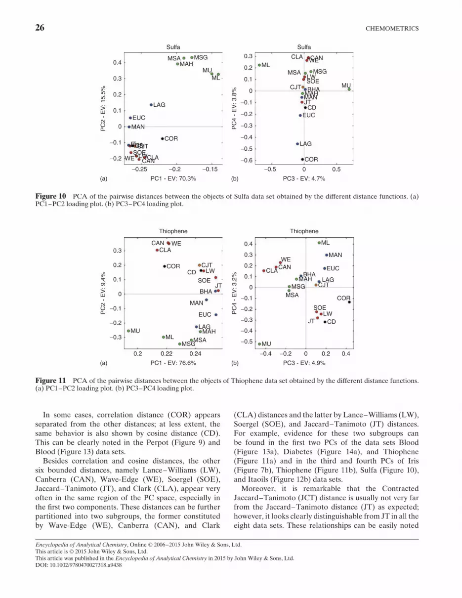
26 CHEMOMETRICS
−0.1
−0.2
0
0.1
0.2
0.3
0.4
PC
2 -
EV
: 15.
5%
(a)
−0.1
−0.3
−0.2
−0.4
−0.5
−0.6
0
0.1
0.2
0.3
PC
4 -
EV
: 3.8
%
−0.25 −0.2 −0.15
PC1 - EV: 70.3% (b)
−0.5 0 0.5
PC3 - EV: 4.7%
Sulfa Sulfa
MUMAH
MSA
COR
CDJTMAN
EUC
LAG
ML
BHACJT
LWSOE
CANCLAWE
MSGMUMAH
MSA
CORCDJT
MAN
EUC
LAG
ML
BHACJT
LWSOECANCLAWE
MSG
Figure 10 PCA of the pairwise distances between the objects of Sulfa data set obtained by the different distance functions. (a)PC1–PC2 loading plot. (b) PC3–PC4 loading plot.
−0.1
−0.2
−0.3
0
0.1
0.2
0.3
PC
2 -
EV
: 9.4
%
(a)
−0.1
−0.3
−0.2
−0.4
−0.5
0
0.1
0.2
0.3
0.4
PC
4 -
EV
: 3.2
%
0.2 0.22 0.24
PC1 - EV: 76.6% (b)
−0.4 −0.2 0 0.2 0.4
PC3 - EV: 4.9%
Thiophene Thiophene
MU
MAH
MSA COR
CDJT
MAN
EUC
LAG
ML
BHA
CJT
LWSOE
CANCLA
WE
MSG
MU MAHMSA
CORCD
JT
MAN
EUC
LAG
ML
BHA
CJTLW
SOE
CANCLA
WE
MSG
Figure 11 PCA of the pairwise distances between the objects of Thiophene data set obtained by the different distance functions.(a) PC1–PC2 loading plot. (b) PC3–PC4 loading plot.
In some cases, correlation distance (COR) appearsseparated from the other distances; at less extent, thesame behavior is also shown by cosine distance (CD).This can be clearly noted in the Perpot (Figure 9) andBlood (Figure 13) data sets.
Besides correlation and cosine distances, the othersix bounded distances, namely Lance–Williams (LW),Canberra (CAN), Wave-Edge (WE), Soergel (SOE),Jaccard–Tanimoto (JT), and Clark (CLA), appear veryoften in the same region of the PC space, especially inthe first two components. These distances can be furtherpartitioned into two subgroups, the former constitutedby Wave-Edge (WE), Canberra (CAN), and Clark
(CLA) distances and the latter by Lance–Williams (LW),Soergel (SOE), and Jaccard–Tanimoto (JT) distances.For example, evidence for these two subgroups canbe found in the first two PCs of the data sets Blood(Figure 13a), Diabetes (Figure 14a), and Thiophene(Figure 11a) and in the third and fourth PCs of Iris(Figure 7b), Thiophene (Figure 11b), Sulfa (Figure 10),and Itaoils (Figure 12b) data sets.
Moreover, it is remarkable that the ContractedJaccard–Tanimoto (JCT) distance is usually not very farfrom the Jaccard–Tanimoto distance (JT) as expected;however, it looks clearly distinguishable from JT in all theeight data sets. These relationships can be easily noted
Encyclopedia of Analytical Chemistry, Online © 2006–2015 John Wiley & Sons, Ltd.This article is © 2015 John Wiley & Sons, Ltd.This article was published in the Encyclopedia of Analytical Chemistry in 2015 by John Wiley & Sons, Ltd.DOI: 10.1002/9780470027318.a9438

DISTANCES AND OTHER DISSIMILARITY MEASURES IN CHEMOMETRICS 27
−0.1
0
0.1
0.2
0.3
0.4
0.5
PC
2 -
EV
: 13%
(a)
−0.2
−0.4
0
0.2
0.4
0.6
PC
4 -
EV
: 3.3
%
0.15 0.2 0.25
PC1 - EV: 74.4% (b)
−0.5 0 0.5
PC3 - EV: 4.9%
Itaoils Itaoils
MU
MAH
MSA
COR
CDJT
MANEUC
LAGML
BHA
CJT
LWSOE
CAN
CLA
WE
MSG
MUMAH
MSA
COR CDJTMAN
EUC
LAG
ML
BHACJTLWSOECANCLA WE
MSG
Figure 12 PCA of the pairwise distances between the objects of Itaoils data set obtained by the different distance functions. (a)PC1–PC2 loading plot. (b) PC3–PC4 loading plot.
Blood Blood
MU
MAH MSA
CORCD
JT
MANEUC
LAG
ML
BHACJT
LWSOE
CANCLAWE
MSG
MU
MAHMSA
CORCD
JT
MAN
EUC LAG
ML
BHA
CJT
LWSOECANCLAWE
MSG
−0.2
0 0
0.1
0.2
0.3
−0.3
−0.1PC
2 -
EV
: 19.
7%
−0.4
0.2
0.4
0.6
−0.6
−0.2PC
4 -
EV
: 3.9
%
(a) (b)
−0.28 −0.26 −0.24 −0.22 −0.2 −0.18
PC1 - EV: 62.9%
−0.6 −0.4 −0.2 0 0.2
PC3 - EV: 4.5%
Figure 13 PCA of the pairwise distances between the objects of Blood data set obtained by the different distance functions. (a)PC1–PC2 loading plot. (b) PC3–PC4 loading plot.
in the first two PCs for the data sets Blood (Figure 13a),Thiophene (Figure 11a), and Diabetes (Figure 14a) andin the third and fourth PCs for Thiophene (Figure 11b),Sulfa (Figure 10b), and Perpot (Figure 9b) data sets.
7.2 Effects of Distance Measures on Similarity-basedClassification
Classification methods are fundamental multivariatetechniques aimed to find mathematical models able torecognize the class membership of objects on the basisof a set of measurements. The k-NN classification rule is
conceptually quite simple: an object is classified accordingto the class memberships of the k closest objects, i.e. itis classified according to the majority of its k-NNs in thedata space. Thus, an object is classified on the basis of itssimilarity to other objects. In a computational viewpoint,all that is necessary is to calculate and analyze a distancematrix. The distance of each object from all the otherobjects is computed, and the objects are then sortedaccording to this distance. In order to quantitativelyevaluate the effects of the different geometries inducedon the data by each distance function, the k-NN analysis
Encyclopedia of Analytical Chemistry, Online © 2006–2015 John Wiley & Sons, Ltd.This article is © 2015 John Wiley & Sons, Ltd.This article was published in the Encyclopedia of Analytical Chemistry in 2015 by John Wiley & Sons, Ltd.DOI: 10.1002/9780470027318.a9438

28 CHEMOMETRICS
Diabetes Diabetes
MUMAH
MSA
COR
CDJTMAN
EUC
LAG ML
BHACJTLW
SOE
CANCLAWE
MSG
MU
MAH
MSA
COR
CD JT
MAN
EUC
LAG
ML
BHA
CJT LWSOE
CANCLA
WE
MSG
−0.2
00
0.1
0.2
0.3
0.4
−0.3
−0.1PC
2 -
EV
: 12.
3%
−0.3
0.1
0.2
0.3
0.4
−0.4
−0.1
−0.2
PC
4 -
EV
: 4.3
%
(a) (b)
−0.26 −0.24 −0.22 −0.2 −0.18
PC1 - EV: 71.9%
−0.5 0 0.5
PC3 - EV: 5%
Figure 14 PCA of the pairwise distances between the objects of Diabetes data set obtained by the different distance functions.(a) PC1–PC2 loading plot. (b) PC3–PC4 loading plot.
Table 16 Nonerror rate of the 18 distances for each data set and the average nonerror rate (NER) from k-NN classification
Distance Symbol Iris Wines Perpot Sulfa Thiophene Itaoils Blood Diabetes NER
Manhattan MAN 0.953 0.981 0.990 0.823 0.833 0.949 0.637 0.692 0.857Euclidean EUC 0.967 0.977 0.990 0.774 0.833 0.947 0.625 0.707 0.852Soergel SOE 0.953 0.967 0.980 0.788 0.792 0.947 0.637 0.708 0.847Lance–Williams LW 0.953 0.967 0.980 0.788 0.792 0.947 0.637 0.707 0.846Contracted JT CJT 0.967 0.981 0.990 0.760 0.792 0.946 0.626 0.708 0.846Jaccard–Tanimoto JT 0.960 0.972 0.980 0.724 0.792 0.947 0.628 0.718 0.840Lagrange LAG 0.967 0.955 0.970 0.774 0.792 0.943 0.609 0.697 0.838Wave-Edge WE 0.953 0.972 0.960 0.788 0.750 0.929 0.633 0.663 0.831Bhattacharyya BHA 0.953 0.977 1.000 0.683 0.792 0.932 0.637 0.673 0.831Canberra CAN 0.947 0.977 0.960 0.752 0.750 0.929 0.637 0.672 0.828Mahalanobis MAH 0.913 0.972 0.990 0.710 0.792 0.920 0.626 0.700 0.828Clark CLA 0.953 0.986 0.970 0.732 0.750 0.911 0.632 0.662 0.825LCM-symm. geom. MSG 0.920 0.917 0.980 0.718 0.792 0.913 0.635 0.684 0.820LCM-symm. arith. MSA 0.920 0.897 0.980 0.690 0.792 0.909 0.637 0.681 0.813LCM-lower mat. ML 0.933 0.888 0.940 0.766 0.708 0.869 0.633 0.645 0.798Cosine CD 0.827 0.972 0.900 0.540 0.792 0.954 0.603 0.650 0.780LCM-upper mat. MU 0.853 0.618 0.990 0.516 0.750 0.865 0.613 0.629 0.729Correlation COR 0.853 0.980 0.500 0.518 0.708 0.947 0.598 0.629 0.717
The best results for each data set are highlighted in gray.
was performed on the eight data sets (Table 15). Nosophisticated validation procedures were adopted, butonly the implicit leave-one out technique typical of thek-NN approach. Thus, a rough estimate of the potentialclassification behavior of each distance was estimated foreach data set.
The usual way of selecting k is by testing a set of kvalues (e.g. from 1 to 10); then, the k giving the lowestclassification error can be selected as the optimal one.
The nonerror rate (NER) was calculated for each dataset by mean of each of the 18 distance measures together
with the average NER (Table 16). The rank of eachdistance for each data set was calculated together withthe average rank (AR) (Table 17).
By analyzing the results reported in Tables 16 and17, it can be easily observed that the use of differentdistance measures has an effect of the classificationperformance, owing to the way each distance representsthe similarity/diversity relationships among the objects.Five distances give the best results both considering theaverage NER and the AR; these are the Manhattan(MAN), Euclidean (EUC), Soergel (SOE), Contracted
Encyclopedia of Analytical Chemistry, Online © 2006–2015 John Wiley & Sons, Ltd.This article is © 2015 John Wiley & Sons, Ltd.This article was published in the Encyclopedia of Analytical Chemistry in 2015 by John Wiley & Sons, Ltd.DOI: 10.1002/9780470027318.a9438

DISTANCES AND OTHER DISSIMILARITY MEASURES IN CHEMOMETRICS 29
Table 17 Ranks of the 18 distances for each data set and average rank (AR) from k-NN classification
Distance Symbol Iris Wines Perpot Sulfa Thiophene Itaoils Blood Diabetes AR
Manhattan MAN 7.5 1.0 1.5 3.5Euclidean EUC 1.5 14.0Contracted JT CJT
2.02.0
2.56.02.5 12.5
Soergel SOE 12.5Lance–Williams LW 12.5
3.53.5
Jaccard–Tanimoto JT
4.04.04.09.09.09.0 11.0 11.0
8.03.52.52.53.51.0
Bhattacharyya BHA
7.57.54.07.5
9.56.0 1.0 15.0 10.0 3.5 11.0
Lagrange LAG 2.0 14.0 12.5
5.58.03.03.0
5.5
2.05.08.05.05.05.0
9.0 16.0 7.0Mahalanobis MAH 15.0 4.0 12.0
7.57.57.57.57.57.57.5 13.0 12.5 6.0
3.85.25.96.36.47.37.79.29.9
Canberra CAN 11.0 14.5 13.5 11.5 3.5 12.0 10.1Wave-Edge WE
9.56.09.5 14.5
9.03.0 13.5 11.5 8.5 13.0 10.1
Clark CLA7.57.5 1.0 12.5 10.0 13.5 15.0 10.0 14.0 10.4
LCM-symm. geom. MSG 13.5 15.0 12.0 14.0 7.0 9.0 10.9LCM-symm. arith. MSA 13.5 16.0
9.09.0 14.0 16.0 3.5 10.0 11.2
Cosine CD 18.0 9.5 17.0 16.0
7.57.57.5 1.0 17.0 15.0 12.6
LCM-lower mat. ML 12.0 17.0 16.0 7.0 17.5 17.0 8.5 16.0 13.9Correlation COR 16.5 4.0 18.0 17.0 17.5 5.0 18.0 17.5 14.2LCM-upper mat. MU 16.5 18.0 4.0 18.0 13.5 18.0 15.0 17.5 15.1
The best rank(s) for each data set is highlighted in gray.
0
0.6
−0.6
0
0
0.3
0.3−0.3
−0.3 0 0.3−0.3
0
0.8
0.6
0.4
0.2
−0.6
−0.4
−0.2
0
0.2
−0.2
−0.5(a) (b)
(c) (d)
0
EUC
0.5 −0.5 0
CLA
JT CJT
0.5 11
Figure 15 Projections of the 178 Wines objects by means of multidimensional scaling based on Euclidean (EUC, Figure 15a),Clark (CLA, Figure 15b), Jaccard–Tanimoto (JT, Figure 15c), and Contracted Jaccard–Tanimoto (CJT, Figure 15d) distances. Thedifferent colors represent the classes.
Encyclopedia of Analytical Chemistry, Online © 2006–2015 John Wiley & Sons, Ltd.This article is © 2015 John Wiley & Sons, Ltd.This article was published in the Encyclopedia of Analytical Chemistry in 2015 by John Wiley & Sons, Ltd.DOI: 10.1002/9780470027318.a9438

30 CHEMOMETRICS
Table 18 Statistical parameters for 44 similarity coefficients calculated by the simulated data set
# Symbol mean std cv perc(5) perc(95)
B1 SM 0.5420 0.2869 0.5293 0.0625 0.9629B2 RT 0.4268 0.2848 0.6672 0.0323 0.9284B3 JT 0.4050 0.3112 0.7685 0.0102 0.9433B4 GLE 0.5066 0.3204 0.6325 0.0201 0.9708B5 RR 0.3329 0.2939 0.8829 0.0059 0.9014B6 FOR 0.3756 0.3234 0.8609 0.0015 0.9429B7 SIM 0.6902 0.2984 0.4323 0.0865 0.9971B8 BB 0.4427 0.3185 0.7194 0.0119 0.9569B9 DK 0.5302 0.3075 0.5800 0.0391 0.9710B10 BUB 0.5052 0.2980 0.5898 0.0375 0.9569B11 KUL 0.5665 0.2875 0.5075 0.0606 0.9712B12 SS1 0.3092 0.2880 0.9312 0.0051 0.8927B13 SS2 0.6532 0.2716 0.4158 0.1176 0.9811B14 JA 0.5658 0.3187 0.5633 0.0299 0.9804B15 FAI 0.4374 0.2655 0.6069 0.0454 0.9170B16 MOU 0.0085 0.0502 5.9205 0.0001 0.0232B17 MIC 0.5099 0.2155 0.4227 0.1096 0.8912B18 RG 0.4558 0.2411 0.5290 0.0611 0.8669B19 HD 0.3619 0.2353 0.6503 0.0328 0.8031B20 YU1 0.5349 0.3700 0.6917 0.0025 0.9978B21 YU2 0.5252 0.2837 0.5401 0.0479 0.9551B22 FOS 0.3746 0.3234 0.8635 0.0013 0.9425B23 DEN 0.3431 0.1336 0.3894 0.1270 0.5880B24 CO1 0.9921 0.0803 0.0809 0.9970 0.9999B25 CO2 0.9921 0.0802 0.0809 0.9966 0.9999B26 DIS 0.5066 0.1563 0.3085 0.2244 0.7766B27 GK 0.2961 0.2579 0.8710 0.0049 0.8076B28 SS3 0.5213 0.2161 0.4146 0.1475 0.8748B29 SS4 0.2465 0.2410 0.9778 0.0018 0.7527B30 PHI 0.5175 0.2140 0.4136 0.1379 0.8727B31 DI1 0.5473 0.3248 0.5934 0.0256 0.9868B32 DI2 0.5856 0.3390 0.5788 0.0229 0.9946B33 SOR 0.4051 0.3449 0.8516 0.0007 0.9737B34 COH 0.5378 0.1788 0.3325 0.2461 0.8673B35 PE1 0.5210 0.2308 0.4429 0.1157 0.9014B36 PE2 0.5167 0.2191 0.4240 0.1214 0.8899B37 MP 0.5164 0.2105 0.4076 0.1397 0.8708B38 HL 0.2687 0.2102 0.7824 0.0270 0.7124B39 CT1 0.8733 0.1354 0.1551 0.6022 0.9946B40 CT2 0.1628 0.1525 0.9364 0.0093 0.4715B41 CT3 0.7401 0.2208 0.2983 0.2807 0.9850B42 CT4 0.7734 0.2160 0.2793 0.3197 0.9914B43 CT5 0.5128 0.1400 0.2729 0.2857 0.7384B44 AC 0.5316 0.2174 0.4090 0.1609 0.8766
Jaccard–Tanimoto (CJT), and Lance–Williams (LW)distances.
Looking at the ranks collected in Table 17, only in fewcases the best rank (1.0) is achieved by other distancemeasures, such as Clark distance (CLA) for Wines dataset, Bhattacharyya (BHA) for Perpot data set, Cosinedistance (CD) for Itaoils data set, and Jaccard–Tanimoto(JT) for Diabetes data set.
The Contracted Jaccard–Tanimoto distance (CJT) isbetter than its parent Jaccard–Tanimoto distance (JT) in
four data sets out of eight, in one case is equal, and inthree cases is only a slightly lower.
The four Mahalanobis-type distances derived from theLCM distance (MSA, MSG, MU, and ML) appear notuseful in classification problems; on the other side, LCMdistance was proposed for different purposes, i.e. with theaim to catch outliers and analyze the AD of a model.
Correlation and cosine distance appear as much weakfor classification purposes on the studied data sets;analogous considerations can be done for Canberra
Encyclopedia of Analytical Chemistry, Online © 2006–2015 John Wiley & Sons, Ltd.This article is © 2015 John Wiley & Sons, Ltd.This article was published in the Encyclopedia of Analytical Chemistry in 2015 by John Wiley & Sons, Ltd.DOI: 10.1002/9780470027318.a9438
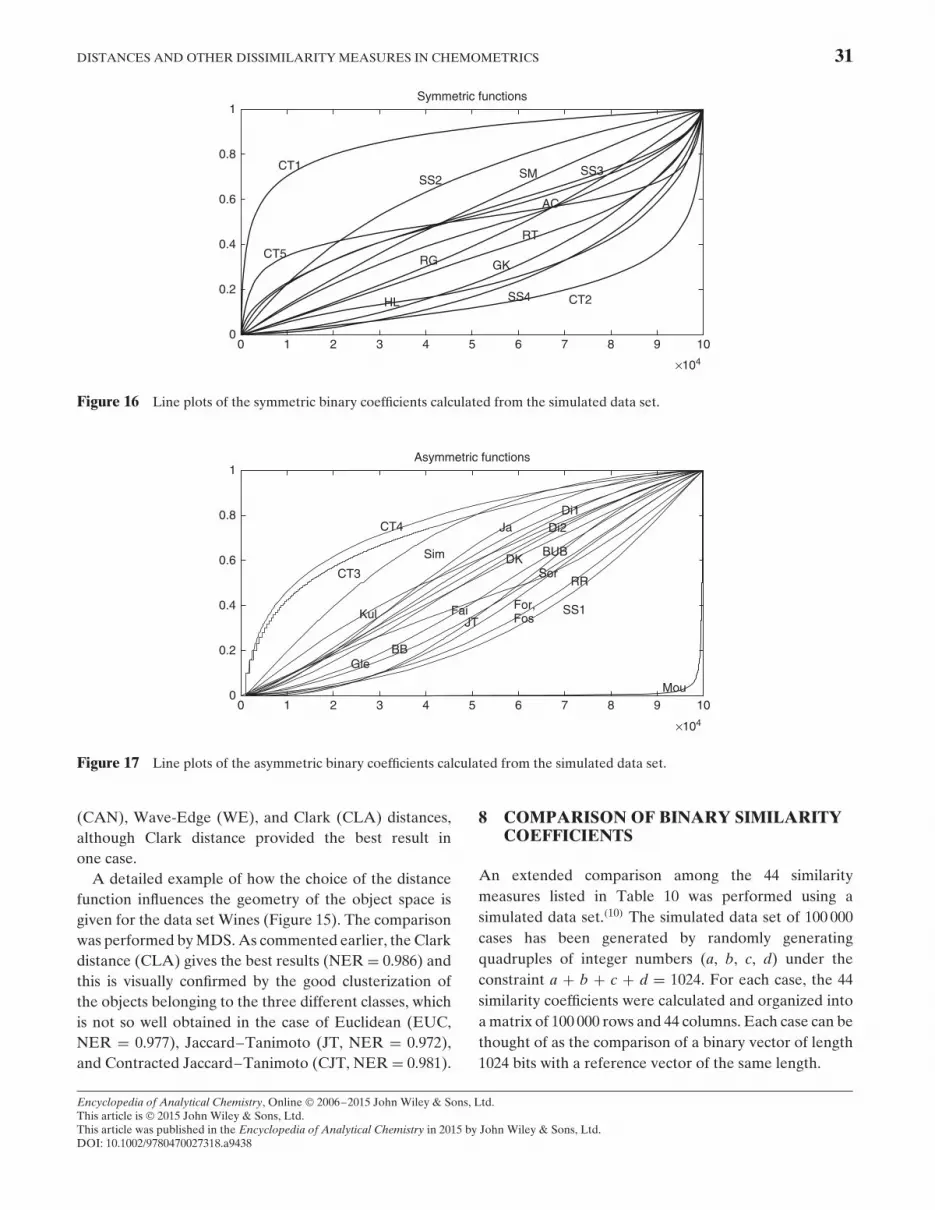
DISTANCES AND OTHER DISSIMILARITY MEASURES IN CHEMOMETRICS 31
0
0.2
0.4
0.6
0.8
1
0 1 2 3 4 5 6 7 8 9 10
×104
CT1
CT5
SS2
RG
HL
GK
RT
AC
SM SS3
SS4 CT2
Symmetric functions
Figure 16 Line plots of the symmetric binary coefficients calculated from the simulated data set.
0
0.2
0.4
0.6
0.8
1
0
Asymmetric functions
1 2 3 4 5 6 7 8 9 10
×104
CT4
CT3
Kul
Sim
GleBB
FaiJT
Ja
DKBUB
SorRR
Di2Di1
For,Fos
SS1
Mou
Figure 17 Line plots of the asymmetric binary coefficients calculated from the simulated data set.
(CAN), Wave-Edge (WE), and Clark (CLA) distances,although Clark distance provided the best result inone case.
A detailed example of how the choice of the distancefunction influences the geometry of the object space isgiven for the data set Wines (Figure 15). The comparisonwas performed by MDS. As commented earlier, the Clarkdistance (CLA) gives the best results (NER D 0.986) andthis is visually confirmed by the good clusterization ofthe objects belonging to the three different classes, whichis not so well obtained in the case of Euclidean (EUC,NER D 0.977), Jaccard–Tanimoto (JT, NER D 0.972),and Contracted Jaccard–Tanimoto (CJT, NER D 0.981).
8 COMPARISON OF BINARY SIMILARITYCOEFFICIENTS
An extended comparison among the 44 similaritymeasures listed in Table 10 was performed using asimulated data set.(10) The simulated data set of 100 000cases has been generated by randomly generatingquadruples of integer numbers (a, b, c, d) under theconstraint a C b C c C d D 1024. For each case, the 44similarity coefficients were calculated and organized intoa matrix of 100 000 rows and 44 columns. Each case can bethought of as the comparison of a binary vector of length1024 bits with a reference vector of the same length.
Encyclopedia of Analytical Chemistry, Online © 2006–2015 John Wiley & Sons, Ltd.This article is © 2015 John Wiley & Sons, Ltd.This article was published in the Encyclopedia of Analytical Chemistry in 2015 by John Wiley & Sons, Ltd.DOI: 10.1002/9780470027318.a9438

32 CHEMOMETRICS
0
0.2
0.4
0.6
0.8
1
0 1 2 3 4 5 6 7 8 9 10
×104
Co1, Co2
Coh
Yu1Yu2
Pe1, Pe2, Phi,Mic, MP
dis
Den
Correlation-based functions
Figure 18 Line plots of the correlation-based binary coefficients calculated from the simulated data set.
−1.4−2.0
SymAsymIntermCorr−1.5 −1.0 −0.5 0.0 0.5 1.0 1.5 2.0
Dim 1
−1.2
−1.0
−0.8
−0.6
−0.4
−0.2
0.0
0.2
0.4
0.6
0.8
1.0
1.2
Dim
2
Mic
Den dis
Coh
Pe2
MP PhiPe1
RG
HDSM
AC SS2
SS4GK
CT2CT1
BUB
Kul
DK JaGle
BB JTFor
FosSS1
Fai
Di1
Sor
Sim Di2
CT4CT3
RR
RT
CT5
Yu1
Yu2
SS3HL
Figure 19 Multidimensional scaling of the binary similarity coefficients. The Co1, Co2, and Mou coefficients were excluded fromanalysis as they are strong outliers (see text).
The 100 000 similarity values that had been generatedfor each coefficient were analyzed to calculate thefollowing descriptive statistics: mean, standard deviation(std), coefficient of variation (cv), and 5 and 95 percentiles[perc(5) and perc(95)]. These values are listed in Table 18.
The minimum and maximum values of all the coefficientsare 0 and 1, respectively.
Inspection of Table 18 suggests that most of thecoefficients have a mean value around 0.5 and that theyspan the similarity range in a satisfactory way. There
Encyclopedia of Analytical Chemistry, Online © 2006–2015 John Wiley & Sons, Ltd.This article is © 2015 John Wiley & Sons, Ltd.This article was published in the Encyclopedia of Analytical Chemistry in 2015 by John Wiley & Sons, Ltd.DOI: 10.1002/9780470027318.a9438

DISTANCES AND OTHER DISSIMILARITY MEASURES IN CHEMOMETRICS 33
are three very anomalous coefficients: CO1 (B24) andCO2 (B25) yield very high values and MOU (B16) yieldsvery low values. These outlier coefficients were probablyoriginally proposed to deal with short vectors, where theparameters b, c, and d may have less influence than a.Less extreme behavior is exhibited by CT1 (B39), CT4(B42), CT3 (B41), SIM (B7), SS2 (B13), DI2 (B32), andKUL (B11) (which all have mean values >0.55) andCT2 (B40), SS4 (B29), HL (B38), and GK (B27) (whichall have mean values <0.30). Turning to the standarddeviations [and excluding CO1 (B24), CO2 (B25), andMOU (B16)], the coefficients showing the maximumvariability are YU1 (B20), SOR (B33), DI2 (B32), DI1(B31), FOS (B22), FOR (B6), GLE (B4), JA (B14), BB(B8), JT (B3), and DK (B9) (all with standard deviations>0.30), whereas the minimum variability is provided byDEN (B23), CT1 (B39), CT5 (B43), CT2 (B40), DIS(B26), and COH (B34) (all with standard deviations lowerthan 0.20).
The ordered sequences of similarity values (inascending order) were plotted for each coefficient toexplore the functional shape. In order to simplify the anal-ysis and discussion that follows, the plots are presented inthree different figures: symmetric functions (Figure 16),asymmetric functions (Figure 17), and correlation-basedfunctions (Figure 18). Inspection of these figures showsthat the shapes of the functions can be approximatelycategorized as logarithmic, exponential, sigmoidal, orquasi-linear in character.
MDS was performed on the 41ð 41 matrix of thepairwise Pearson correlation coefficients calculated fromthe simulated data. This analysis omits the Mountford andCole coefficients [i.e. CO1 (B24), CO2 (B25), and MOU(B16)], as they are significant outliers (Figures 17 and 18).The final configuration of the binary similarity coefficientsin a two-dimensional MDS plot is shown in Figure 19.At a first glance, the similarity coefficients appear wellclustered according to their symmetry properties, with thesymmetric functions (green squares, on the middle-left-bottom side), the asymmetric functions (blue triangles,on the right side), and the correlation-based functions(red circles, on the left-top side) well separated fromeach other. In this respect, it is interesting to note thatBUB (B10) and FAI (B15), which are intermediate incharacter between symmetric and asymmetric functions,are appropriately located between the symmetric andasymmetric clusters. Many of the coefficients are verynear to each other in the plot, indicating close similarityrelationships, e.g. the group comprising SM (B1), RT(B2), SS2 (B13), and AC (B44), which have a rankcorrelation equal to one. In much the same way, thegroup comprising JT (B3), JA (B14), GLE (B4), SS1(B12), FOR (B6), FOS (B22), and DK (B9) has rankcorrelations larger than 0.99. Some coefficients, however,
are quite isolated in the MDS plot. This is the case for thepairs CT1 (B39) and CT2 (B40), SIM (B7) and DI2 (B32),and CT3 (B41) and CT4 (B42); RR (B5) and CT5 (B43)also seem to be quite separated from other coefficients.
ACKNOWLEDGMENTS
The Authors warmly thank Michel Marie Deza of theEcole Normal Superieure (Paris, France) for his help inmanaging mathematical properties of distances and LuisPeinador Sarabia of the University of Burgos (Spain) forhis suggestions.
ABBREVIATIONS AND ACRONYMS
SOM self-organizing mapsMDS multidimensional scalingMST minimum spanning treek-NN k-nearest neighborDA discriminant analysisAD applicability domainLCM locally centered MahalanobisATDM atemporal target diffusion modelCMD Canonical measure of distanceNER nonerror rateAR average rank
RELATED ARTICLES
Chemometrics (Volume 11)Chemometrics ž Clustering and Classification of Analyt-ical Data ž Soft Modeling of Analytical Data
Pharmaceuticals and Drugs (Volume 8)Quantitative Structure-Activity Relationships andComputational Methods in Drug Discovery
REFERENCES
1. V. Batagelj, M. Bren, ‘Comparing Resemblance Measures’,J. Classif., 12, 73–90 (1995).
2. M.M. Deza, E. Deza, Encyclopedia of Distances, Springer,Dordrecht, 2009.
3. P. Legendre, L. Legendre, Numerical Ecology, 2nd edition,Elsevier, Amsterdam, 1998.
Encyclopedia of Analytical Chemistry, Online © 2006–2015 John Wiley & Sons, Ltd.This article is © 2015 John Wiley & Sons, Ltd.This article was published in the Encyclopedia of Analytical Chemistry in 2015 by John Wiley & Sons, Ltd.DOI: 10.1002/9780470027318.a9438

34 CHEMOMETRICS
4. P.H.A. Sneath, R.R. Sokal, Numerical Taxonomy,Freeman, San Francisco, CA, 1973.
5. S.-H. Cha, ‘Comprehensive Survey on Distance/SimilarityMeasures between Probability Density Functions’, Int. J.Math. Models Methods Appl. Sci., 1, 300–307 (2007).
6. C.M. Cuadras, ‘Distancias Estadısticas (in Spanish)’,Estadistica Espanola, 30, 295–378 (1989).
7. A.G. Maldonado, J.P. Doucet, M. Petitjean, B.T. Fan,‘Molecular Similarity and Diversity in Chemoinformatics:From Theory to Applications’, Mol. Diversity, 10, 39–79(2006).
8. Y.C. Martin, J.L. Kofron, L.M. Traphagen, ‘Do StructurallySimilar Molecules Have Similar Biological Activity?’J. Med. Chem., 45, 4350–4358 (2002).
9. P. Willett, Similarity and Clustering in Chemical Informa-tion Systems, Research Studies Press, Leichworth, 1987.
10. R. Todeschini, V. Consonni, H. Xiang, J. Holliday,M. Buscema, P. Willett, ‘Similarity Coefficients forBinary Chemoinformatics Data: Overview and ExtendedComparison Using Simulated and Real Datasets’, J. Chem.Inf. Model., 52, 2884–2901 (2012).
11. W.J. Krzanowski, Principles of Multivariate Analysis,Oxford Science Publications, Oxford, 1988.
12. R. Todeschini, D. Ballabio, V. Consonni, F. Sahigara, P.Filzmoser, ‘Locally-Centred Mahalanobis Distance: A NewDistance Measure with Salient Features Towards OutlierDetection’, Anal. Chim. Acta, 787, 1–9 (2013).
13. D.E. Rumelhart, P. Smolensky, J.L. McClelland, G.E.Hinton, Schemata and Sequential Thought Processes inPDP Models, MIT Press, Cambridge, 1986.
14. J.C. Gower, ‘Generalized Procrustes Analysis’, Psychome-trika, 40, 31–51 (1975).
15. R. Todeschini, V. Consonni, A. Manganaro, D. Ballabio,A. Mauri, ‘Canonical Measure of Correlation (CMC)and Canonical Measure of Distance (CMD) betweenSets of Data. Part 1. Theory and Simple ChemometricApplications’, Anal. Chim. Acta, 648, 45–51 (2009).
16. R.A. Fisher, ‘The Use of Multiple Measurements inTaxonomic Problems’, Ann. Eugen., 7, 179–188 (1936).
17. M. Forina, C. Armanino, S. Lanteri, E. Tiscornia,‘Classification of Olive Oils from their Fatty AcidComposition’, in Food Research and Data Analysis,Applied Science Publishers, London, 189–214, 1983.
18. M. Forina, Artificial dataset by M. Forina (University ofGenoa) (2000).
19. Y. Miyashita, Y. Takahashi, C. Takayama, T. Ohkubo, K.Fumatsu, S. Sasaki, ‘Computer-Assisted Structure/TasteStudies on Sulfamates by Pattern Recognition Methods’,Anal. Chim. Acta, 184, 143–149 (1986).
20. P.P. Mager, Design Statistics in Pharmacochemistry,Research Studies Press, Letchworth, 1991.
21. M. Forina, C. Armanino, M. Castino, M. Ubigli, ‘Multi-variate Data Analysis as Discriminating Method of theOrigin of Wines’, Vitis, 25, 189–201 (1986).
22. K.A. Baggerly, J.S. Morris, S.R. Edmonson, K.R. Coombes,‘Signal in Noise: Evaluating Reported Reproducibility ofSerum Proteomic Tests for Ovarian Cancer’, J. Natl. CancerInst., 97, 307–309 (2005).
23. J.W. Smith, J.E. Everhart, W.C. Dickson, W.C. Knowler,R.S. Johannes, ‘Using the ADAP Learning Algorithm toForecast the Onset of Diabetes Mellitus’, Proc. Symp.Comput. Appl. Med. Care, 9, 261–265 (1988).
Encyclopedia of Analytical Chemistry, Online © 2006–2015 John Wiley & Sons, Ltd.This article is © 2015 John Wiley & Sons, Ltd.This article was published in the Encyclopedia of Analytical Chemistry in 2015 by John Wiley & Sons, Ltd.DOI: 10.1002/9780470027318.a9438


