Embed Size (px)
Citation preview
Appendix I:Calculations andComments on the Cases
In this appendix we furnish our calculations of statistical results for most ofthe problems requiring some calculation. We do not suggest that these are theonly “correct” solutions; there are usually a variety of analyses appropriate fora statistical question. The methods we present are designed to illustrate thetopics discussed in the text. There are also comments on some of the statisticalissues, and occasionally some supplementary technical discussion for thoseinclined to dig further. For the most part, we have left discussion of the legalissues to the reader.
Chapter 1. Descriptive Statistics
Section 1.2.1. Parking meter heist
1. Average total revenue/month for the ten months of the Brink’s contractprior to April 1980 was $1,707,000; the comparable figure for CDC thenext year was $1,800,000. The city argued that the difference of about$100,000/month was due to theft.
An alternative calculation can be made based on the questionable as-sumption that the $4,500 recovered when the employees were arrestedrepresented an average theft per collection. Since there were about 200collections in the preceding ten months, the theft in that period was200 × 4,500 = 900,000, close to the figure obtained from the time-seriesanalysis.
2-3. Brink’s argued that the difference was due to an underlying trend, point-ing to the figures in Area 1-A, where no theft occurred. Average monthly
482 Appendix I: Calculations and Comments on the Cases
revenue for Area 1-A during the last ten months of the Brink’s periodwas $7,099; its average during the CDC period was $7,328. The differ-ence of $229 is a percentage increase of 3.2%. A 3.2% increase appliedto $1,707,000 comes to $1,762,000, which leaves only $38,000/month, or$380,000 for ten months, unaccounted for. At the trial, Brink’s adduced theevidence from Area 1-A, but did not stress the comparison. Its chief defensewas that confounding factors had contributed to an overall trend that biasedthe city’s estimate. The jury found for the city and awarded $1,000,000compensatory damages and punitive damages.
Section 1.2.2. Taxing railroad property
1. The language of the statute, which refers to the assessed value of “othercommercial and industrial property in the same assessment jurisdiction,”suggests using the ratio of the aggregate assessed value to the aggregatemarket value; that would be a weighted mean. In its generic sense of “notunusual,” the word “average” is not informative on the choice between themean and the median. However, in its specific sense the “average” is themean, and “weighted average” could only be the weighted mean. The issueis made murky by the comment of the railroad spokesman, which suggeststhat the mean was not intended to be used in applying the statute.
2. Because the median minimizes the sum of absolute deviations, it might besaid to minimize discrimination with respect to the railroads.
3. Total assessment is calculated as the mean assessment rate times the num-ber of properties; use of the mean would therefore produce no change inrevenue.
4. The median is the middle measurement for all properties. Its treatment ofall properties as equal can be regarded as most equitable to the railroads.
5. The weighted mean assessment/sales ratio is a weighted harmonic meanbecause it is the reciprocal of the weighted mean of the reciprocals of the as-sessment/sales ratios in each stratum, with the weights being the proportionsthat the assessments in each stratum bear to total assessments.
Section 1.2.4. Hydroelectric fish kill
The sample arithmetic mean is equal to the sum of the observations in thesample divided by the sample size, n. From this definition, it is obvious that, ifone is given the mean of a sample, the sum of the sample observations can beretrieved by multiplying the mean by n. The sample can then be “blown up”to the population by multiplying it by the reciprocal of the proportion that thesample size bears to the whole. In short, the arithmetic mean fish kill per daytimes the number of days in the year estimates the annual fish kill. However,for the geometric mean the first step cannot be taken because the geometric
Appendix I: Calculations and Comments on the Cases 483
mean is the nth root of the product of the n observations; multiplying that by n
does not yield the sum of the sample observations. Hence, the geometric meanfish kill per day times the number of days in the year does not estimate theannual kill. Notice also that if on any day in the sample of days there were nofish killed, the geometric mean would equal zero, clearly an underestimate. Sothe geometric mean procedure is inappropriate.
Section 1.2.5. Pricey lettuce
1. The ratio of new to old lettuce prices, using the arithmetic mean indexwith constant dollar shares (RA), can be expressed algebraically as RA =∑
S0,i(Pt,i/P0,i), where S0,i is the dollar share of the ith product in thebase period; Pt,i is the price of the ith product at time t ; P0,i is the price ofthe ith product in the base period; and the summation is across productsbeing averaged. Thus the arithmetic average ratio of new to old lettuceprices is (1/2)(1/1) + (1/2)(1.5/1) = 1.25, indicating a 25% increase inprice of lettuce. The new quantities implied by this increase are 1.25 lbs oficeberg and 0.8333 lbs of romaine lettuce. (These are the quantities that keepthe expenditure shares for each kind of lettuce equal, given that the totalamount spent on lettuce increases by 25%.) Since the reduction in amountof romaine is less than the increase in quantity of iceberg, the assumptionof equal satisfaction implies that consumer satisfaction is greater per unitof romaine than of iceberg.
2. Using the geometric mean, index, the ratio of new to old prices can beexpressed as RG =
∏(Pt,i/P0,i)S0.i , where
∏indicates the product of the
relative price changes across items. The geometric average ratio of newto old lettuce prices is (1/1)1/2 × (1.5/1)1/2 = 1.225, for a 22.5% averageincrease. The new quantities implied by this increase are 1.225 lbs of icebergand 0.816 lbs of romaine lettuce. Again, consumer satisfaction is deemedgreater per unit of romaine than of iceberg, although the difference is smallerthan under the arithmetic mean computation.
3. The arithmetic mean ratio if romaine drops back from $1.5 to $1 is(1/2)(1/1) + (1/2)(1/1.5) = 0.8333, which is greater than 0.8, the recip-rocal of 1.25. The geometric mean ratio is (1/1)1/2 × (1/1.5)1/2 = 0.816,which is the reciprocal of 1.225. The geometric mean ratio would appearsuperior to the arithmetic mean ratio from this point of view because itmatches reciprocal price movements with reciprocal changes in the index.
Section 1.2.6. Super-drowsy drug
1. Baker’s expert used in effect an average percentage reduction in sleep la-tency weighted by the baseline latency. His weighted average was greaterthan the FTC simple or unweighted average because, in the data, largerpercentage reductions are associated with longer baseline latencies. If there
484 Appendix I: Calculations and Comments on the Cases
were a constant mean percentage reduction of sleep latency for all baselines,either the weighted or unweighted average would be an unbiased estimatorof it. Our choice would then depend on which was more precise.
2. If the variability of reduction percentages were the same for all baselinelatencies, the unweighted sample average (the FTC estimate) would be thepreferred estimator because it would have the smallest sampling variance.But if, as Figure 1.2.6 indicates, variability in the reduction percentagedecreases with increasing baseline latency, the more precise estimator is theweighted average (the Baker estimate), which gives greater weight to largerbaseline latencies. Regression methods (see Chapter 13) can be applied tostudy the percentage reduction as a function of baseline latency.
Able’s exclusion of data in the baseline period is clearly unacceptable, asthe week 2 latency average would appear shorter even with exactly the samevalues as in week 1. Baker’s entry criteria and non-exclusion of data aremore reasonable, defining a target population of insomniacs as those withlonger than 30 minute latencies on at least 4 out of 7 nights. Such entrycriteria ordinarily lead to some apparent reduction in sleep latency, evenwithout the sleep aid, by an effect known as the regression phenomenon(see Section 13.1 at p. 350). The total effect is a sum of drug effect, placeboeffect, and regression effect.
Section 1.3.1. Texas reapportionment
1. a. The range is 7,379. The range in percentage terms is from +5.8% to−4.1%, or 9.9 percentage points.
b. The mean absolute deviation is 1,148 (mean absolute percentagedeviation = 1.54%).
c. Using the formula
S =
{(n
n − 1
)[(1
n
∑x2
i
)−(
1
n
∑xi
)2]}1/2
,
the standard deviation of district size is 1454.92 (if the exact mean74,644.78 is used), or 1443.51 (if 74,645 is used). This formula is sensi-tive to the least significant digits in the mean. A better way to calculateS is from the mean squared deviation
S =
{(n
n − 1
)[1
n
∑(xi − x)2
]}1/2
,
which does not suffer from this instability. The sd of percentage deviationis 1.95%. We give the above formula because it is the usual one used forestimating the standard deviation from samples; in this context it could

Appendix I: Calculations and Comments on the Cases 485
well be argued that the data are the population, in which case the factorn/(n − 1) should be deleted.
d. The interquartile range is 75,191−73,740 = 1,451. In percentage termsit is 0.7 − (−1.2) = 1.9.
e. The Banzhaf measure of voting power (see Section 2.1.2, Weightedvoting) argues for the use of the square root of the population as ameasure of voting power. Transforming the data by taking square roots,the range becomes 280.97 − 267.51 = 13.46. For percentage deviationfrom the average root size of 273.2, the range is +2.84% to −2.08%, or4.92 percentage points.
2. The choice among measures depends initially on whether one is most influ-enced by the most discrepant districts or by the general level of discrepancy.The former points to the range; the latter to one of the other measures. Inany event, there would seem to be no reason to use squared differences, i.e.,the variance or standard deviation, as a measure.
Section 1.3.2. Damages for pain and suffering
1. Treating the data as the population ($ in 000’s), the variance is 913,241 −558,562 = 354,679. The standard deviation is
√354,679 = 595.55. The
mean is 747.37. Hence, the maximum award under the court’s two-standard-deviation rule would be 747.37+2 × 595.55 = 1,938.47. Probably it is morecorrect to treat the data as a sample from a larger population of “normative”awards. In that case, the variance would be estimated as 354,679 × 27
26 =368,320.5. The standard deviation would be
√368,320.5 = 606.89, and the
maximum award under the court’s rule would be 747.37 + 2 × 606.89 =1, 961.15.
2. The court’s use of a two-standard-deviation interval based on a group of“normative” cases to establish permissible variation in awards assumes thatthe pain and suffering in each case was expected to be the same, apartfrom sampling variability, assumed permissible, and was similar to thatsuffered in the Geressy case. This seems unlikely since, e.g., an award of$2,000,000 would probably have been deemed excessive if made to thecase that had received $37,000. If, as seems likely, different levels of painand suffering are involved over the range of cases, one would have to locateGeressy on that continuum, and then construct an interval for that level. Twostandard deviations calculated from the normative cases would no longerbe appropriate because that would reflect both variation at a particular leveland variation across levels, the latter being irrelevant to the reasonablenessof the award in the particular case.
These are linear regression concepts – see Section 13.3.
486 Appendix I: Calculations and Comments on the Cases
Section 1.3.3. Ancient trial of the Pyx
1. The remedy was 7,632 grains. If σ = 0.42708, then the standard deviationof the sum of n = 8,935 differences of a sovereign’s actual weight fromthe standard is σ · √
n = 40.4 gr. Thus, the deviation represented by theremedy in standard deviation units is 7,632/40.4 = 188.9 sd. The probabil-ity of finding an absolute sum of n differences greater than 188.9 standarddeviations is, by Chebyshev’s inequality, less than 1/188.92 = 2.8 × 10⁻⁵,vanishingly small.
2. The remedy grows too large because it increases by the factor of n insteadof
√n. The remedy of 3σ
√n should have amply protected the Master of
the Mint without giving him excessive leeway; in the example, it wouldhave been 3 × 0.42708 · √8935 = 121.1 gr. Whether Newton would haveappreciated the flaw in the remedy formula has been the subject of someconjecture. See Stigler, supra, in the Source.
The square root law may be inadequate if the individual coins put into thePyx were not statistically independent, e.g., because they were from thesame mint run. Such dependence tends to reduce the effective sample size.
Section 1.4.1. Dangerous eggs
1. Pearson’s correlation coefficient between mean egg consumption (EC) andmean ischemic heart disease (IHD) is 0.426.
2. The probative value of ecologic studies such as this is considered ex-tremely limited. The correlational study of national means says little aboutthe strength of correlation among individuals within the societies. The“ecologic fallacy” results from an uncritical assumption that the observedassociation applies at the individual level. In fact, it is theoretically possiblefor EC and IHD to be uncorrelated among individuals within a given soci-ety, while societal mean levels of EC and IHD co-vary with a confoundingfactor that itself varies across societies. For example, red meat consumptionin societies with high-protein diets might be such a confounding factor, i.e.,a factor correlated with both EC and IHD.
Counsel for the egg producers might argue that, in view of the ecologicfallacy, statistical comparisons should be limited to countries similar to theUnited States, at least in egg consumption. When that is done, however, thecorrelation between IHD and egg consumption virtually disappears.
3. Errors in the data would tend to reduce the correlation.
Appendix I: Calculations and Comments on the Cases 487
Section 1.4.2. Public school financing in Texas
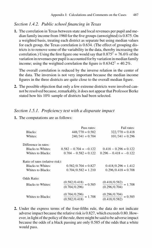
1. The correlation in Texas between state and local revenues per pupil and me-dian family income from 1960 for the five groups (unweighted) is 0.875. Ona weighted basis, treating each district as separate but using median valuesfor each group, the Texas correlation is 0.634. (The effect of grouping dis-tricts is to remove some of the variability in the data, thereby increasing thecorrelation.) Using the first figure one would say that 0.8752 = 76.6% of thevariation in revenues per pupil is accounted for by variation in median familyincome; using the weighted correlation the figure is 0.63422 = 40.2%.
The overall correlation is reduced by the inverse relation in the center ofthe data. The inversion is not very important because the median incomefigures in the three districts are quite close to the overall median figure.
2. The possible objection that only a few extreme districts were involved can-not be resolved because, remarkably, it does not appear that Professor Berkestated how his 10% sample of districts had been selected.
Section 1.5.1. Proficiency test with a disparate impact
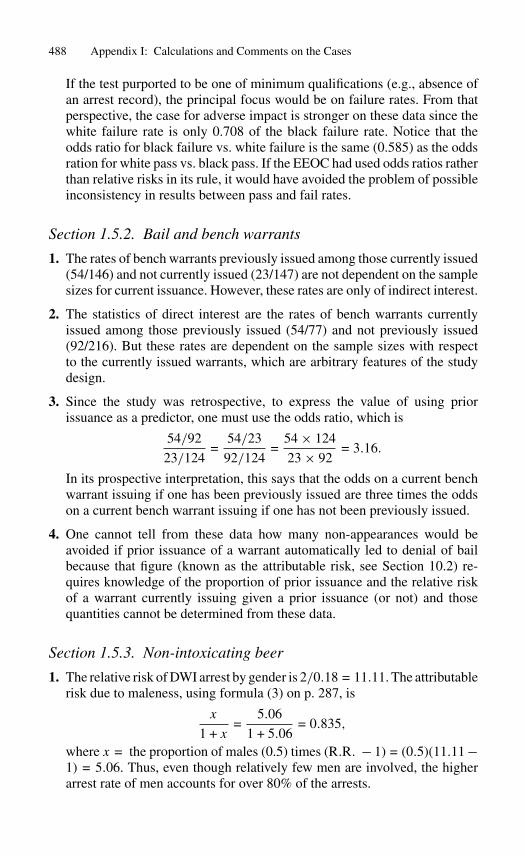
1. The computations are as follows:
Pass rates: Fail rates:Blacks: 448/770 = 0.582 322/770 = 0.418Whites: 240/341 = 0.704 101/341 = 0.296
Difference in rates:Blacks to Whites: 0.582 − 0.704 = −0.122 0.418 − 0.296 = 0.122Whites to Blacks: 0.704 − 0.582 = 0.122 0.296 − 0.418 = −0.122
Ratio of rates (relative risk):Blacks to Whites: 0.582/0.704 = 0.827 0.418/0.296 = 1.412Whites to Blacks: 0.704/0.582 = 1.210 0.296/0.418 = 0.708
Odds Ratio:
Blacks to Whites:(0.582/0.418)
(0.704/0.296)= 0.585
(0.418/0.582)
(0.296/0.704)= 1.708
Whites to Blacks:(0.704/0.296)
(0.582/0.418)= 1.708
(0.296/0.704)
(0.418/0.582)= 0.585
2. Under the express terms of the four-fifths rule, the data do not indicateadverse impact because the relative risk is 0.827, which exceeds 0.80. How-ever, in light of the policy of the rule, there might be said to be adverse impactbecause the odds of a black passing are only 0.585 of the odds that a whitewould pass.
488 Appendix I: Calculations and Comments on the Cases
If the test purported to be one of minimum qualifications (e.g., absence ofan arrest record), the principal focus would be on failure rates. From thatperspective, the case for adverse impact is stronger on these data since thewhite failure rate is only 0.708 of the black failure rate. Notice that theodds ratio for black failure vs. white failure is the same (0.585) as the oddsration for white pass vs. black pass. If the EEOC had used odds ratios ratherthan relative risks in its rule, it would have avoided the problem of possibleinconsistency in results between pass and fail rates.
Section 1.5.2. Bail and bench warrants
1. The rates of bench warrants previously issued among those currently issued(54/146) and not currently issued (23/147) are not dependent on the samplesizes for current issuance. However, these rates are only of indirect interest.
2. The statistics of direct interest are the rates of bench warrants currentlyissued among those previously issued (54/77) and not previously issued(92/216). But these rates are dependent on the sample sizes with respectto the currently issued warrants, which are arbitrary features of the studydesign.
3. Since the study was retrospective, to express the value of using priorissuance as a predictor, one must use the odds ratio, which is
54/92
23/124=
54/23
92/124=
54 × 124
23 × 92= 3.16.
In its prospective interpretation, this says that the odds on a current benchwarrant issuing if one has been previously issued are three times the oddson a current bench warrant issuing if one has not been previously issued.
4. One cannot tell from these data how many non-appearances would beavoided if prior issuance of a warrant automatically led to denial of bailbecause that figure (known as the attributable risk, see Section 10.2) re-quires knowledge of the proportion of prior issuance and the relative riskof a warrant currently issuing given a prior issuance (or not) and thosequantities cannot be determined from these data.
Section 1.5.3. Non-intoxicating beer
1. The relative risk of DWI arrest by gender is 2/0.18 = 11.11. The attributablerisk due to maleness, using formula (3) on p. 287, is
x
1 + x=
5.06
1 + 5.06= 0.835,
where x = the proportion of males (0.5) times (R.R. − 1) = (0.5)(11.11 −1) = 5.06. Thus, even though relatively few men are involved, the higherarrest rate of men accounts for over 80% of the arrests.
Appendix I: Calculations and Comments on the Cases 489
2. Justice Brennan’s statement is confusing, but appears to address an issuebeyond the large relative risk. His conclusion assumes that the low per-centage of arrests reflects the extent of the drinking and driving problemamong young people who drink 3.2% beer. In that case, the small num-bers involved would make a gender-discriminatory statute less acceptablein terms of social necessity, even in the face of the large relative risk. Adifficulty is that the data are not satisfactory for assessing the extent of theproblem. On the one hand, the number of arrests clearly underestimates theextent of the drinking and driving problem. But on the other hand, arrests forall alcoholic beverages clearly overstate the problem for 3.2% beer. Thereis no reason to think that these biases would balance out. In addition, sincethe study was made after the statute was passed, it is not clear what directbearing it has on assessing the conditions that led to and would justify itspassage.
Chapter 2. How to Count
Section 2.1.1. DNA profiling
1. There are 20 distinguishable homozygous and (20 × 19)/2 = 190 het-erozygous genotypes possible at the locus (not distinguishing betweenchromosomes of the pair). Thus, there are 210 distinguishable homozygousand heterozygous pairs of alleles at a locus.
2. With four loci, there are 2104 = 1.94 × 10⁹ possible homozygousand heterozygous genotypes at the loci (again, not distinguishing betweenchromosomes of the genotype at a locus).
Section 2.1.2. Weighted voting
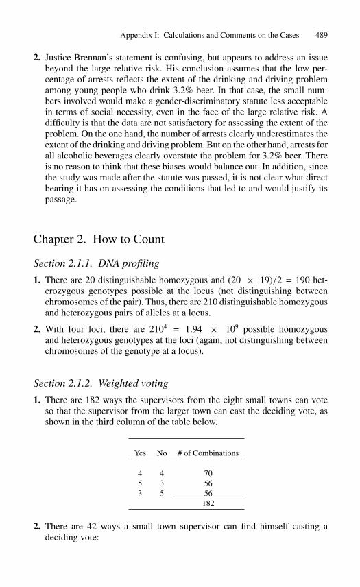
1. There are 182 ways the supervisors from the eight small towns can voteso that the supervisor from the larger town can cast the deciding vote, asshown in the third column of the table below.
Yes No # of Combinations
4 4 705 3 563 5 56
182
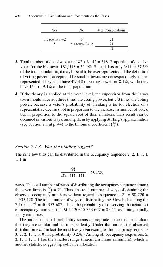
2. There are 42 ways a small town supervisor can find himself casting adeciding vote:
490 Appendix I: Calculations and Comments on the Cases
Yes No # of Combinations
big town (3)+2 5 215 big town (3)+2 21
42
3. Total number of decisive votes: 182 + 8 · 42 = 518. Proportion of decisivevotes for the big town: 182/518 = 35.1%. Since it has only 3/11 or 27.3%of the total population, it may be said to be overrepresented, if the definitionof voting power is accepted. The smaller towns are correspondingly under-represented. They each have 42/518 of voting power, or 8.1%, while theyhave 1/11 or 9.1% of the total population.
4. If the theory is applied at the voter level, the supervisor from the largertown should have not three times the voting power, but
√3 times the voting
power, because a voter’s probability of breaking a tie for election of arepresentative declines not in proportion to the increase in number of votes,but in proportion to the square root of their numbers. This result can beobtained in various ways, among them by applying Stirling’s approximation(see Section 2.1 at p. 44) to the binomial coefficient
(2N
N
).
Section 2.1.3. Was the bidding rigged?
The nine low bids can be distributed in the occupancy sequence 2, 2, 1, 1, 1,1, 1 in
9!
2!2!1!1!1!1!1!= 90,720
ways. The total number of ways of distributing the occupancy sequence amongthe seven firms is
(72
)= 21. Thus, the total number of ways of obtaining the
observed occupancy numbers without regard to sequence is 21 × 90,720 =1, 905,120. The total number of ways of distributing the 9 low bids among the7 firms is 79 = 40,353,607. Thus, the probability of observing the actual setof occupancy numbers is 1, 905,120/40,353,607 = 0.047, assuming equallylikely outcomes.
The model of equal probability seems appropriate since the firms claimthat they are similar and act independently. Under that model, the observeddistribution is not in fact the most likely. (For example, the occupancy sequence3, 2, 2, 1, 1, 0, 0 has probability 0.236.) Among all occupancy sequences, 2,2, 1, 1, 1, 1, 1 has the smallest range (maximum minus minimum), which isanother statistic suggesting collusive allocation.
Appendix I: Calculations and Comments on the Cases 491
Section 2.1.4. A cluster of leukemia
We seek the probability that, in a uniform multinomial distribution with 6 cellsand sample size 12, the largest cell frequency would be 6 or more. While acomputer algorithm is generally indispensable for calculating a quantity ofthis type, in the present case exhaustive enumeration of all cases involvinga maximum frequency of 6 or more is feasible. There are 29 such sets ofoccupancy numbers (for which multinomial probabilities must be computed).The exact answer is 0.047544. In the bid-rigging problem (Section 2.1.3), thedistribution was too uniform while in this problem it is too clumped. The pointis that either extreme is improbable under the hypothesis of equal probabilityfor all cells.
Bonferroni’s inequality may also be applied with excellent accuracy; seeSection 3.1 at p. 57.
Section 2.1.5. Measuring market concentration
1. The number of ways N customers can be divided among i firms with ai
customers of firm i is the multinomial coefficient N !/∏
ai!
2. Setting 1/ni = ai/N , we have ai = N/ni . Substituting in the multinomialcoefficient we have N !/
∏(N/ni)!
3. Using the crude form of Stirling’s approximation for the factorials, we have
NNe−N∏(N/ni)N/ni e−N/ni
.
Since∑
1/ni = 1, we have∏
e−N/ni = e−N and∏
NN/ni = NN , so thatcanceling e−N and NN from numerator and denominator and taking the N throot, we have
∏n
1/ni
i as the entropy measure of concentration.
4. In the example, the value of the entropy index is obtained as follows.The value of ni is 5 for the 20% firms, 50 for the 2% firms, and 100for the 1% firms. When there are 10 small firms, the entropy measureis 50.20×4 × 500.02×10 = 7.92 equal firms; when there are 20 small firmsthe entropy measure is 50.20×4 × 1000.01×20 = 9.10 equal firms. Thus, bythe entropy measure, the number of small firms is relevant to competition.By the Herfindahl index (HHI), when there are 10 small firms, HHI is202 × 4 + 22 × 10 = 1640, or 10,000/1640 = 6.10 equal firms; by a similarcalculation, when there are 20 small firms, HHI is 10,000/1620 = 6.17. ByHHI, the number of small firms makes little difference.
These two indices form the basis for two classical tests of the null hypothesisof uniform distribution of customers in a multinomial model. The entropymeasure gives rise to the likelihood ratio statistic (see Section 5.6), whileHHI gives rise to the Pearson chi-squared statistic (see Section 6.1).
492 Appendix I: Calculations and Comments on the Cases
Section 2.2.1. Tracing funds for constructive trusts
1. Under the reflection principle of D. Andre, to find the number of paths thatbegin at $10, touch or cross the 0 ordinate, and end at 10, we count thenumber of paths that end at −$10. This is equal to
(10040
). The total number
of paths that end at 10 is(100
50
). Hence, the probability that a path would
touch or cross 0 and end at 10 is(100
40
)/(100
50
)=
50!2
40! · 60!= 0.136.
2. The expected maximum reduction in the trust is 0.627√
100 = 6.27 dollars.
3. The probability of no $10 depletion is 1 − 0.136 = 0.864. This numberraised to the 10th power is 0.232, the probability of no $10 depletion onany of the 10 days. Therefore, the probability that a $10 depletion occursat some point during the ten day period is 1 − 0.232 = 0.768.
The fact that we apply probability theory here should not be construed as arecommendation for the rule of law that suggests the excursion into fluctuationtheory, but which otherwise seems to have little to recommend it.
Chapter 3. Elements of Probability
Section 3.1.1. Interracial couple in yellow car
1-2. The identifying factors are almost certainly not independent. However, ifprobabilities are interpreted in the conditional sense, i.e., P [e|f ] = 1/10;P [d|e and f ] = 1/3; P [c|d and e and f ] = 1/10, etc., the probability ofthe factors’ joint occurrence would be equal to the product.
3. The calculation in the court’s appendix assumes that the selection of cou-ples who might have been at the scene from the larger universe was madewith replacement. This assumption would produce a 0.41 probability ofincluding a C-couple twice in the selection in any case in which a C-couplehad been included once, even if they were the only such couple in the pop-ulation. An analysis assuming sampling without replacement would havebeen more appropriate.
4. The prosecutor assumed, in essence, that the frequency of C-couples in thepopulation was the probability of the Collinses’ innocence. It is not that,but the probability that the guilty couple would have been a C-couple if theCollinses’ were innocent. This inversion of the conditional is sometimescalled the prosecutor’s fallacy. The two probabilities would be of the samemagnitude only if the other evidence in the case implied a 50% probabilityof the Collinses’ guilt. See Sections 3.3 and 3.3.2.
Appendix I: Calculations and Comments on the Cases 493
5. The last clause of the last sentence of the court’s appendix assumes that theprobability of the Collinses’ guilt is one over the number of C-couples. Thisis called the defendant’s fallacy because it assumes that there is no otherevidence in the case except the statistics, which is generally not true andwas not true here. See the sections referred to above.
Section 3.1.2. Independence assumption in DNA profiles
1. The weighted average frequency of the homozygous genotypes consistingof allele 9 is
(130916
)2 × 9162844 + . . .+
(52508
)2 × 5082844 = 0.01537. For heterozygous
genotypes consisting of alleles 9 and 10, the weighted average calculationis [
130
916× 78
916× 2
]916
2844+ . . . +
[52
508× 43
508× 2
]508
2844= 0.02247.
2. The frequency of a homozygous genotype consisting of allele 9 using thetotal population figure is
(3502844
)2= 0.01515. For the heterozygous genotype
consisting of alleles 9 and 10, the calculation based on total populationfigures is 350
2844 × 2612844 × 2 = 0.02259.
3. In both the homozygous and heterozygous cases, the agreement with theweighted average calculation is very good, indicating that HW is justified.
4. A sufficient condition for HW in the total population is that the rates of thealleles in the subpopulations are the same (or, HW holds approximately, ifthe rates are not very different).
5. The weighted average for Canadians and non-Canadians is 0.3782 for ahomozygous genotype of allele 9. The figure based on population totals is0.25. HW doesn’t hold because the rates of allele 9 in the two subpopulationsare very different.
Section 3.1.4. Telltale hairs
1. The total number of pairs among the 861 hairs is(861
2
)= 370,230. Of these,
there were approximately 9 hairs per person or(9
2
)= 36 intra-person pairs,
yielding a total of 3.600 intra-person pairs. Of the net total of 366,630 inter-person pairs, 9 were indistinguishable, a rate of 9/366, 630 = 1/40,737;the rest of the derivation is in the Gaudette–Keeping quotation in the text.
Gaudette–Keeping assumes that the probability of one pair’s distinguisha-bility is independent of the distinguishability for other pairs. Although suchindependence is unlikely, violation of the assumption does not matter muchbecause the probability of one or more matches is less than or equal to9 · 1/40,737 (Bonferroni’s inequality), or 1/4,526—a result close to the1/4,500 figure given in the text. The substantial problems with the study
494 Appendix I: Calculations and Comments on the Cases
are its lack of blindedness and the unbelievability of the number of assertedcomparisons.
The probability reported is not the probability that the hair came fromanother individual but the probability that it would be indistinguishable ifit came from another individual.
Section 3.2.1. L’affaire Dreyfus
1. The expert computed the probability of exactly four coincidences in theparticular words in which they occurred.
2. The more relevant calculation is the probability of at least four coincidencesin any of the thirteen words. This is 0.2527, on the assumption that theoccurrence of a coincidence in one word is independent of coincidences inothers.
Section 3.2.2. Searching DNA databases
1-2. Multiplying by the size of the database is a way of applying Bonferroni’sadjustment for multiple comparisons. On the assumption that no one in thedatabase left the incriminating DNA, and that each person’s DNA had thesame probability of matching, the approximate probability of one or morematches is given by the Bonferroni adjustment. This probability would seemto be only peripherally relevant to the identification issue.
3. In the fiber-matching case, the question was whether any fibers matched; inthis case, the question is whether the DNA of a particular person matchedby coincidence, not whether any person’s DNA matched.
4. It should make no difference to the strength of the statistical evidencewhether particular evidence leads to the DNA testing, or is discovered af-terward. Because no adjustment for multiple comparisons would be madein the former case, none should be made in the latter. As for the argumentthat with a large database some matching would be likely because there aremultiple trials, if a match occurs by coincidence there is unlikely to be par-ticular evidence supporting guilt, and probably some exonerating evidence.This means that the prior probability of guilt would be no greater than 1over the size of the suspect population and the posterior probability of guiltwould be quite small.
5. Because the probative effect of a match does not depend on what occasionedthe testing, we conclude that the adjustment recommended by the committeeshould not be made. The use of Bonferroni’s adjustment may be seen as afrequentist attempt to give a result consistent with Bayesian analysis withoutthe clear-cut Bayesian formulation.
Appendix I: Calculations and Comments on the Cases 495
Section 3.3.1. Rogue bus
4. The prior odds that it was company B’s bus are 0.20/0.80 = 1/4. Thelikelihood ratio associated with the testimony that it was company B’s busis 0.70/0.30 = 7/3. The posterior odds that it was company B’s bus, giventhe prior odds and the testimony, are 1
4 × 73 = 0.583. The posterior probability
that it was company B’s bus is 0.583/(1 + 0.583) = 0.368.
Section 3.3.2. Bayesian proof of paternity
1. The expert’s calculation is wrong, but the arithmetic error is harmless. Giventhe prior odds of 1 and a genotype rate of 1%, the posterior odds are 1 ×1/0.01 = 100. This translates into a posterior probability of paternity of100/101 = 0.991. Since the expert used her own prior, which might havebeen irrelevant, it would seem that her calculation should not have beenadmitted.
The appellate court held it was improper for the expert to use a 50-50%prior, but indicated that the jurors might be given illustrative calculationsbased on a range of priors, as suggested in question 3.
Section 3.4.1. Airport screening device
The defendant will argue that among those persons who screen as “high risk,”or “+,” only the proportion
P [W |+] =P [+|W ] · P [W ]
P [+|W ] · P [W ] + P [+|W ] · P [W ]
actually carry a concealed weapon. In the example P [W ] = 0.00004,P [+|W ] = sensitivity = 0.9 and P [+|W ] = 1 − specificity = 0.0005. Thus,
P [W |+] =0.9(0.00004)
0.9(0.00004) + 0.0005(0.99996)= 0.067,
or 6.7% of “high risk” individuals carry weapons. This rate is arguably too lowfor either probable cause or reasonable suspicion.
Assuming independence of test results for any person in the repeated testsituation of the Notes, sensitivity falls to P [+|D] = P [+1|D] · P [+2|D, +1] =0.95 · 0.98 = 0.9310. Specificity increases such that P [+|D] = P [+1|D] ·P [+2|D, +1] = 0.05 · 0.02 = 0.001. Then PPV = (0.001 · 0.931)/(0.001 ·0.931+0.001·0.999) = 0.4824, which is still rather low as a basis for significantadverse action. Specificity would have to be much greater to have adequatePPV.
496 Appendix I: Calculations and Comments on the Cases
Section 3.4.2. Polygraph evidence
1. Using the Defense Department data, the PPV of the test is no greater than22/176=12.5%.
2. A statistic to compute would be either NPV or 1 − NPV. The latter is theprobability of guilt given an exonerating polygraph.
3. It seems reasonable to conclude that PPV > 1−NPV because the probabil-ity of guilt when there is an incriminating polygraph should be greater thanwhen there is an exonerating polygraph. Thus, the probability of guilt giventhe exonerating test is less than 12.5%. The test seems quite accurate whenused for exoneration even if not very persuasive when used as evidence ofguilt. Because
NPV
1 − NPV= P [not guilty|exonerating exam]/P [Guilty|exon]
=P [exon|not G]P [not G]
P [exon |G]P [G]
=specificity
1 − sensitivity× prior odds on not guilty,
the NPV will be high if the sensitivity of the test is high, or if prior probabilityof guilt is low.
4. The statistical point is that rates of error for a test that would seem acceptablysmall when the test is used as evidence in an individual case are unacceptablylarge in the screening context; the screening paradigm is more exacting thanthe individual case, not less. Because 7,616 − 176 = 7,440 persons testednegative in the Defense Department screening program, if 1 − NPV werein fact as high as 12.5%, the number of guilty but undetected personnelwould be 0.125 × 7,440 = 930. A screening test that passed so manyquestionable personnel would clearly be unacceptable. The fact that theDefense Department uses the test for screening is thus significant evidencethat it is sufficiently reliable to be admitted, at least as exonerating evidence.
Section 3.5.2. Cheating on multiple-choice tests
Under the assumption of innocent coincidence, the likelihood of 3 matchingwrong answers in dyads with 4 wrong answers is 37/10,000. Under the as-sumption of copying, the expert used 1 as the likelihood of 3 matching wronganswers out of 4. Thus, the likelihood ratio is 1
37/10,000 = 270.27. The inter-pretation is that one is 270 times more likely to observe these data under theassumption of copying than of innocent coincidence.
Appendix I: Calculations and Comments on the Cases 497
Chapter 4. Some Probability Distributions
Section 4.2.1. Discrimination in jury selection
1. The probability of no black selections at random out of 60 is (0.95)60 =0.046. This is statistically significant under the usual 5% standard (using aone-tailed test, see Section 4.4), but only marginally so.
2. The Court computed the probability of observing exactly 7 blacks. Themore relevant is the probability of observing 7 or fewer blacks.
3. From Table B, for n = 25, p = 0.25, the probability of 3 or more blacks is0.9679; the probability of 2 or fewer is 1 − 0.9679 = 0.0321.
Section 4.2.3. Small and nonunanimous juries in criminal cases
1. The probability of selecting one or more minority jurors, by the binomialmodel and Table B in Appendix II, is 0.931; two or more is 0.725; three ormore is 0.442; and four or more is 0.205. Thus, the probability that one ormore minority jurors must concur in a 12-person verdict is 0.931, and in a9–3 verdict it is 0.205.
2. Using the Kalven and Zeisel overall proportion of guilty votes on firstballots, 1828/2700 = 0.677, the binomial probability of 9 or more guiltyvotes is 0.423 and the probability of 5 unanimous guilty votes is 0.142. Aprosecutor is therefore much more likely to get at least 9 votes for convictionthan a unanimous 5, on the first ballot.
3. The Kalven and Zeisel data are inconsistent with the binomial model be-cause the expected number of cases arrayed by first ballot votes does notcorrespond with the actual number, as the following table shows:
First ballot guilty votes0 1 − 5 6 7-11 12
Observed number of cases 26 41 10 105 43Expected number of cases 0 12.7 22.7 187.5 2.09
See Section 6.1 for a formal test of goodness of fit. The data show manymore unanimous verdicts than one would expect on the basis of the model,suggesting that the greater source of variation in guilty votes is the strengthof the case, which affects all jurors, rather than variation in individual jurors.
Section 4.2.4. Cross-section requirement for federal jury lists
1. The probability of 0 or 1 blacks in a 100-person venire, with prob-ability of picking a black, p = 0.038 (the functional wheel), is(100
1
)(0.038)1(0.962)99 + (0.962)100 = 0.103. With p = 0.0634, the pro-
498 Appendix I: Calculations and Comments on the Cases
portion of blacks in a representative wheel, the probability of so few blacksis 0.011. By this probability test, the functional wheel seems unrepresen-tative. The comparable probabilities for Hispanics are 0.485 and 0.035 forthe functional and representative wheels, respectively.
2. As for absolute numbers: 6.34 − 3.8 = 2.54 blacks and 5.07 − 1.72 =3.35 Hispanics would have to be added to the average venire chosen fromthe functional wheel to make it representative. These numbers might beregarded as too small to indicate that the wheel was unrepresentative.
3. One problem with the probabilities test is that the hypothetical number ofminorities used to compare probabilities (here a maximum of 1) is fairlyarbitrary. A problem with the absolute numbers test is that, when the percent-ages are small the numbers will be small, even if the underrepresentation,in proportionate terms, is large.
Section 4.3.1. Alexander: Culling the jury list
1. The result is approximately correct. The calculations are as follows. Givenn = 400 and p = 1015/7374,
P [X ≤ 27]
= P
[z <
27.5 − 400(1015/7374)√400 · (1015/7374) · (6359/7374)
= −4.00
]< 0.00003,
from Table A1 or A2 in Appendix II.
2. The largest proportion of blacks in the qualified pool, p∗, consistent withthe data would satisfy the equation
27.5 − 400p∗√
400p∗q∗ = −1.645.
Solving for p∗ yields p∗ = 0.0926. (This is a one-sided upper 95% confi-dence limit for the proportion; see Section 5.3.) To calculate the qualificationrate ratio, note that of Q denotes qualification, B black, and W white,
P [Q|W ]
P [Q|B]=
P [W |Q]P [Q]/P [W ]
P [B|Q]P [Q]/P [B]=
P [W |Q]/P [B|Q]
P [W ]/P [B].
The odds on W vs. B among the qualified is at least 0.9074/0.0926 = 9.800,while in the initial pool the odds on being white are 6359/1015 = 6.265.The qualification rate ratio is thus at least 9.8/6.265 = 1.564, i.e., whitesqualify at a minimum of 1.5 times the rate that blacks qualify.
Appendix I: Calculations and Comments on the Cases 499
Section 4.4.1. Hiring teachers
1. Given n = 405 and p = 0.154,
P [X ≤ 15] = P
[Z <
15.5 − 405 · 0.154√405 · 0.154 · 0.846
= −6.45
]≈ 0.
given p = 0.057,
P [X ≤ 15] = P
[Z <
15.5 − 405 · 0.057√405 · 0.057 · 0.943
= −1.626
]≈ 0.052.
The exact result is 0.0456.
2. Justice Stevens’s clerk used a one-tailed test; the Castaneda two- or three-standard-deviations “rule” reflects the general social science practice ofusing two-tailed tests.
Section 4.5.1. Were the accountants negligent?
1.(983
100
) · (170
)/(1000100
)= 983·982···884
1000·999···901 = 0.164.
Because this computation is somewhat laborious, the normal approximationwould commonly be used instead.
2. If the sample were twice as large, the probability of finding none would be
P [X = 0] = P [X < 0.5]
= P
⎡⎣Z <
0.5 − 17(0.2)√200·800·17·983
10002·999
= −1.77
⎤⎦ ≈ 0.04.
3. The accountants should (and frequently do) stratify their sample, withseparate strata and heavier sampling for the large invoices.
Section 4.5.2. Challenged election
1. Let a denote the number of votes for Candidate A and b the votes forCandidate B. Let m denote the number of invalid votes. If X denotes theunknown number of invalid votes cast for A then a reversal would occurupon removal of the invalid votes if a − X ≤ b − (m − X), or X ≥(a − b + m)/2. On the facts, if 59 of the invalid votes were cast for thewinner, the election would be tied by the removal of all the invalid votes.
2. E(x) = 101 · 1422/2827 = 50.8.
500 Appendix I: Calculations and Comments on the Cases
3. Using the normal approximation for the hypergeometric, the probabilitythat X ≥ 59 is
P
⎡⎣Z ≥ 58.5 − 101 · 1422/2827√
101·2726·1422·140528272·2826
= 1.559
⎤⎦ = 0.06.
When the election is close (a ≈ b) the probability of reversal isapproximately the normal tail area above
z = (a − b − 1) ·√
1
m− 1
a + b
(1 subtracted from the plurality reflects the continuity correction).
The incumbent, who controls the election machinery, may have greateropportunity to create fraudulent, as opposed to random, errors.
Section 4.5.3. Election 2000: Who won Florida?
1. From column (7), the expected total net for Gore is −811.9. Thus Bushwould have won.
2. From column (8), the standard error of the expected total net for Gore isthe square root of 9802.2, or 99.01. The z-score is therefore −8.20, so thatwe reject the null hypothesis that Gore won Florida, with an extremelysignificant P -value.
3. Considering Miami-Dade only, the expected net for Gore among the under-vote from column (6) is 145.0, with a standard error of square root of 2271.2,or 47.66. Letting the actual net for Gore from Miami-Dade be denoted bythe random variable X, a reversal would have occurred if and only if X isgreater than or equal to 195, the plurality in favor of Bush from column (4).The probability of this event is approximately (using continuity correction)P[z > 1.0596] = 0.145.
Section 4.6.1. Heights of French conscripts
1. Chi-squared is 446.51, which on 6 to 8 degrees of freedom, has a vanishinglysmall P -value, P ≈ 0.0000. The null hypothesis that the data are normallydistributed must be rejected.
2. There are several departures from normality, of which the largest is theexcess number of men shorter than 1.570 meters. Quetelet hypothesizedthat since 1.570 meters was the cutoff for service in the army, the excessnumber of men below that height represented cheating to avoid militaryservice.
Appendix I: Calculations and Comments on the Cases 501
3. If the first two rows are combined, chi-squared drops to 66.8, which is stillhighly significant. Under either calculation, the null hypothesis that the dataare normally distributed must be rejected.
Section 4.6.2. Silver “butterfly” straddles
1. The expert has it backward: the correct statement is that, if the data werenormally distributed, there is only a 0.01 chance of observing D that largeor larger.
2. Again the expert has it backward: If the data were not normally distributeddue to positive kurtosis, the distributions would have fatter tails than thenormal and there would be greater opportunities for profit.
3. Since 4-week price changes are the sum of daily price changes, if the dailychanges were independent, the central limit theorem tells us that their sumwould tend to be normally distributed. Even if the daily changes are nega-tively autocorrelated, as they appear to be, there are central limit theoremsimplying normality of sums, so independence is not necessary for normality.
4. If daily price changes were independent, the sd of the 8-week price changeswould be
√2 times the sd of the 4-week price changes; the sd of the 4-week
price changes would be√
4 = 2 times the sd of the 1-week price changes.The data show no such increase.
5. In order to break even after commissions, the price change must be $126. Fora 2-2 contract held 4 weeks, this is approximately 126/32.68 = 3.86 sd’s.The probability of a move at least that large is, by Chebyshev’s inequality,not greater than 1/3.862 = 0.067. Thus, there is at best a small probabilityof breaking even.
6. The expert’s holding period statistic does not reflect whatever opportunitiesexist for profitable liquidation within the 4-week, etc., periods.
7. Instead of a probability model, the expert might simply have inspected thedata to determine the number of profitable points for liquidation, given theholding period. Chebyshev’s inequality indicates that at most these wouldhave been few.
Section 4.7.1. Sulphur in the air
Given a Poisson random variable with mean 1, P [X ≥ 2] = 1 − P [X =0 or 1] = 1 − [e−1 + e−1] = 0.264, as the probability of two or more dayswith excess emissions in a year. This assumes a simple Poisson with mean1. Because the mean will vary from day to day, the distribution of excessemissions will be a compound Poisson and will have a larger variance thana simple Poisson. In normal distributions, an increase in variance (with fixed
502 Appendix I: Calculations and Comments on the Cases
mean) would imply an increased probability of a tail event, such as X ≥ 2. Inthe case of the Poisson distribution, when µ is small (as it is in this case, whereµ = 1) an increase in variance would, as expected, increase the probability ofa left-tail event, such as X ≤ 1, but may decrease the probability of a right-tailevent, such as X ≥ 2. In such a case, the probability of two or more daysof excess emissions in a year would be less than calculated, not more, as onemight think by analogy to the normal distribution.
Section 4.7.2. Vaccinations
The expected number of cases of functional damage given the risk of functionaldamage that the plaintiffs accepted is µ = 300,533 × 1
310,000 = 0.969. For this
mean, the probability of 4 or more cases is 1−e−µ∑3
x=0 µx/x! = 1−e−0.969(1+0.969 + 0.9692/2! + 0.9693/3!) = 0.017. The null hypothesis that µ = 0.969can be rejected at the 0.05 level.
Section 4.7.3. Is the cult dangerous?
The expected number of deaths per 4,000 drivers over a 5 year period is 5 ·4,000 · 13.2/100,000 = 2.64, so that 10 deaths is (10 − 2.64)/
√2.64 = 4.5
standard deviations above expectation. The normal approximation cannot beused, but Chebyshev’s inequality gives us 1/4.52 = 0.049 as an upper boundon the tail area probability.
The exact tail area probability is given by
1 −9∑
i=0
e−µ(µi/i!),
which can be expressed for calculation purposes as nested quantities as follows:
1 − e−µ ·(
1 + µ(
1 +µ
2
(1 +
µ
3
(1 + · · · +
µ
8
(1 +
µ
9
)· · ·))))
.
With µ = 2.64, this gives the tail area probability as 0.000422. Note that theprobability of 10 alone is 0.0003, so that the first term dominates the sum. Cultmembers have a higher rate of death from suicide or automobile accidentsthan the general population, but the difference may be due more to the type ofperson who joined the cult than the exhortations of the leader.
Section 4.7.4. Incentive for good drivers
Consider the group of drivers with a total of n accidents in the two time periods.Any driver contributes to the sought-after sum (i.e., the number of accidentsin the second time period by those having zero accidents in the first) either (i)n accidents (if the driver has none in the first); or (ii) 0 (for those with oneor more accidents in the first period). The expected contribution to the sum is
Appendix I: Calculations and Comments on the Cases 503
n times the probability that the driver had all n accidents in the second timeperiod. Since by hypothesis an accident occurs with equal probability in thetwo time periods, the probability of all n accidents occurring in the secondperiod is (1/2)n. Thus, the expected contribution is n(1/2)n.
On the other hand, the probability that a driver will have exactly one accidentin the first period, given that he has a total of n accidents, is by the binomialformula
(n
1
)(1/2)1(1/2)n−1 = n(1/2)n. Because this is the same as the expected
contribution of the (0, n) driver, and holds for any n, we conclude that theobserved number of drivers with one accident in the first period is an unbiasedpredictor of the number of accidents drivers with no accidents in the first periodwill have in the second period.
Robbins’s expression for E(µ|X = i) furnishes a way to estimate the numberof accidents in the second period by those with zero in the first. With i = 0,estimate P [X = 1] by 1,231/7,842 and P [X = 0] by 6,305/7,842. Thenthe expected number of accidents among the 6,305 zero-accident drivers is6,305(1,231/7,842) ÷ (6,305/7,842) = 1, 231, i.e., the number of driverswith one accident in the first period.
Let m(j ) denote the number of drivers who had j accidents in the first period.Our prediction is m(1). It can be shown that a 95% prediction interval for thequantity of interest is
m(1) ± 1.96(2[m(1) + m(2)])1/2.
In the example, the prediction interval takes the value 1,231 ± 109. (Theoriginal problem did not separate those drivers with two from those with morethan two accidents; substituting 306 for m(2) provides a slightly conservativeestimate for the width of the prediction interval.) Since the actual number ofaccidents for the zero-accident group was 1,420, there is significant evidence ofdeterioration in performance. The data also support the hypothesis that driverswith one or more accidents improved in performance.
Section 4.7.5. Epidemic of cardiac arrests
1. Treat each of the n = 34 deaths as binary trial with respect to the presenceor absence of Nurse i, with parameter pi for Nurse i obtained from theproportion of evening shifts worked for that nurse. Calculate the z-scorezi = (Xi − 34pi)/(34piqi)1/2 for each nurse. Nurse 32’s zi is 4.12, Nurse60’s zi is 2.10, and the rest are all less than 1.1. The probability that amongeight z-scores the largest would equal or exceed 4.12 is P [max zi ≥ 4.12] =P [at least one zi ≥ 4.12] ≤ ∑
i P [zi ≥ 4.12] by Bonferroni’s inequality,where the sum is over i = 1, . . . , 8. Since each term is about 0.00002,P [max zi ≥ 4.12] ≤ 8 · 0.00002 = 0.00016, i.e., a z- score as large as 4.12is highly unlikely even when the worst nurse is not identified beforehand.If there had been other reasons for singling out Nurse 32, the Bonferroniinequality would be unnecessary.
504 Appendix I: Calculations and Comments on the Cases
2. The relative risk of death for shifts when Nurse 32 was on duty, op-posed to that when she was not on duty, is (27 deaths/201 shifts) ÷(7deaths/253 shifts = (0.1343 deaths / shifts )÷ (0.0277 deaths / shift ) =4.85.
Section 4.8.1. Marine transportation of liquefied natural gas
1. The exponential model is a good candidate since the risk of an accidentarguably will not increase with time.
2. The death density function for failure time is θe−θt . This is greatest in thefirst year.
3. Since the probability of survival for more than 10 years is e−10θ , the prob-ability of failure in the first ten years is 1 − e−10θ . If θ = 1/7000 the aboveexpression is approximately equal to 10/7000 = 0.0014.
4. There is no bunching of probability around the 7000 year mark. The standarddeviation of time to first accident is 7000.
Section 4.8.2. Network affiliation contracts
1. The intuitive estimate of the discrete hazard rate is p = n/S, the number ofterminations n, divided by the total number of affiliation years commenced,S. This can be shown to be the maximum likelihood estimate.
For the 1962 data, the mean life of a contract is estimated at 1767/88 = 20+
years, corresponding to a yearly discrete hazard of p = 0.05.
2. The model was ultimately found inappropriate because the risk of termi-nation declined as life continued. A Weibull model should have been usedinstead. See Section 11.1.
Section 4.8.3. Dr. Branion’s case
1. No.
2. They would be independent unless Branion had planned to call by a certaintime. In any event, the joint probability (that driving took less than 6 minutesand garroting less then 15 minutes) underestimates the probability that thesum took less than 21 (or 27) minutes, because the joint occurrence of thetwo events is only one of the many ways in which the sum of the two timescould be less than 21 (or 27) minutes.
3. If the distribution of the total driving and garroting times were skewed,there would probably be a right tail that was fatter than the left tail, i.e.,longer times would be more probable. That would help Branion’s case.The exponential distribution probably would not be appropriate to model
Appendix I: Calculations and Comments on the Cases 505
the distribution of driving and garroting times because at any intermediatepoint the elapsed time would be relevant to the time necessary to finish thework.
4. Use Chebyshev’s inequality: 27 minutes is 4.5 minutes from the mean of9 + 22.5 = 31.5 minutes. The standard deviation of the sum would be,under the assumptions, (12 + 2.52)1/2 = (7.25)1/2, so the deviation is 4.5√
7.25sd units. By Chebyshev’s inequality, such deviations occur no more than
with probability 1/(
4.5√7.25
)2= 7.25
20.25 = 0.358.
Chapter 5. Statistical Inference for Two Proportions
Section 5.1.1. Nursing examination
Using the hypergeometric distribution, we have:
P =
(9
4
)·(
26
26
)/(35
30
)= 0.000388,
a highly significant result.
Section 5.2.1. Suspected specialists
The data may be summarized as follows:
Unaccounted for Accounted for TotalFavorable 74 146 220Unfavorable 8 123 131Total 82 269 351
The formula
X2 =N · (|ad − bc| − N/2)2
m1 · m2 · n1 · n2
yields 33.24, which is highly significant. The data do not support the specialists’position.
Section 5.2.2. Reallocating commodity trades
Profitable Unprofitable TotalAccount F 607 165 772
G 98 15 113Total 705 180 885
The corrected z-score = −1.871. The one-sided P -value is about 0.03 forthese data. The data are not consistent with the broker’s defense.
506 Appendix I: Calculations and Comments on the Cases
Section 5.2.3. Police examination
The data are
Pass Fail TotalHispanics 3 23 26Others 14 50 64Total 17 73 90
z =|(3.5/26) − (13.5/64)|√
(17/90) · (73/90) · (26−1 + 64−1)= 0.84, p ≈ 0.20,
a non-significant result (one-tailed).
Section 5.2.4. Promotions at a bank
The aggregate data for Grade 4 are as follows:
B W TotalPromotions 39 34 73Non-Promotions 85 41 126Total 124 75 199
1. This model requires the hypergeometric distribution, for which the normalapproximation may be used, as follows:
P
⎡⎢⎣z ≤ 39.5 − 73(124/199)(
73·126·124·75(199)2·198
)1/2 =−5.9874
3.3030= −1.813
⎤⎥⎦ ≈ 0.035,
a result significant at the 5% level with a one-tailed test. If the balls arereturned to the urn, we have a one-sample binomial model, as follows:
P
⎡⎢⎣z ≤ 39.5 − 73(124/199)(
73·124·75(199)2
)1/2 =−5.9874
4.1405= −1.446
⎤⎥⎦ ≈ 0.074.
2. If there are two urns, we must use a two-sample binomial, as follows:
P
⎡⎢⎣z ≤ 39.5/124 − 33.5/75(
73·126(199)2
[1
124 + 175
])1/2 =−0.1281
0.0705= −1.817
⎤⎥⎦ ≈ 0.035,
a result that is in close agreement with the hypergeometric.
3. The statistical text cited by the court was referring to the fact that the t-distribution closely approximates the normal for samples of at least 30, sothat the normal distribution may be used instead. This is not of relevancehere. Despite the court’s statement, the hypergeometric is the better model.
Appendix I: Calculations and Comments on the Cases 507
First, to justify sampling with replacement, the replacement would have tobe of the same race as the promoted employee and have on average thesame probability of promotion. Neither of these conditions is likely to betrue. Second, the hypergeometric model is substantially equivalent to thetwo-sample binomial model in large samples, which would appear to be anappropriate alternative choice.
4. The expert was justified in using a one-tailed test, but not for the reasonsgiven. The point is that, in appraising the level of Type I error, only dis-crimination against blacks should be considered because the court wouldtake action only in that event.
5. There are serious objections to aggregating over years and grades. Aggre-gating over years assumes either a new employee group each year or thatdecisions not to promote in one year are independent of those in anotheryear even for the same employees. Neither of these assumptions is likely tobe true and, as a result, the effective sample size is smaller than indicatedfrom the aggregate numbers (and the significance is less). Aggregation overgrades is also risky (but perhaps less so) since the results can be misleadingif promotion rates are different in the two grades. See Section 8.1.
Section 5.3.2. Paucity of Crossets
A reasonable upper bound is provided by a one-sided 95% upper confidencelimit. Assuming a binomial model for the number of Crossets found, X ∼Bin (n, P ) where n = 129, 000, 000 with X = 0 observed, one solves theequation 0.05 = lower tail area probability = (1 − P )n. This yields Pu = 1 −0.051/n = 23×10−9. An alternative method is to use the Poisson approximationto the binomial distribution since n is large and P is small. If X ∼ Poisson withmean µ, and X = 0 is observed, the upper 95% confidence limit for µ is thesolution of the equation e−µ = 0.05, or µu = − ln 0.05 ≈ 3. The confidencelimit for P is then obtained from µu = n · Pu, or Pu = 3/129,000,000 =23 × 10−9.
Section 5.3.3. Purloined notices
1. The dispute concerns the proportion of Financial’s bond redemption noticesthat were copied by Moody’s, among the roughly 600 instances in whichcopying could not be ruled out. Consider the 600 notices as chips in anurn, some of which were copied, the others not. The existence of an erroris tantamount to withdrawing a chip at random from the urn and beingable to inspect it as to copied status. Thus, each error can be viewed asan independent binomial trial of copied status with the problem being toestimate the smallest p, the probability that a random chip would be copied,that is consistent at the given level of confidence with the number of copiedchips among those withdrawn.
508 Appendix I: Calculations and Comments on the Cases
Looking just at the 1981 data, there were 8 errors and all of them werecopied. Using a 99% one-sided confidence interval, we have P 8
L = 0.01,or PL = 0.56. Thus, the minimum proportion of copied notices, consistentwith finding 8 out of 8, is about 56%.
When not all the errors have been copied, it is necessary to solve the formulafor the cumulative binomial for p. This can be done by trial and error orby using tables of the F -distribution. Combining the two years data, therewere 18 errors, of which 15 were copied. Asserting that PL = 0.54, we have
18∑i=15
(18
i
)(0.54)i(0.46)18−i = 0.01,
which confirms the assertion.
Tables of the F -distribution can be used as follows. Given n trials, supposethat c are copied. If Fa,b;α denotes the critical value of the F -distributionwith a = 2(n−c+1) and b = 2c degrees of freedom that cuts off probabilityα in the upper tail, then
PL = b/(b + a · Fa,b;α)
is the solution to the expression for the cumulative binomial distributionwhen the upper tail is set equal to α. In our example, n = 18, c = 15, andF8,30;01 = 3.17; the above expression for PL = 0.54.
It is of some computational interest to compare this exact solution with theapproximate 99% confidence interval (±2.326 standard errors). For bothyears pooled, PL = 0.63, which is about 9 percentage points too high. Usingthe more precise approximation given by Fleiss (at p. 172), PL ≈ 0.53.
2. The lawyer for Moody’s might point out that Financial’s model assumesthat whether an error was made is independent of whether the notice wascopied. To this he might object that Moody’s was more likely to copy themore obscure notices, and those notices were more likely to involve errors.
Section 5.3.4. Commodity exchange reports
Required: to find n such that
1.96(0.05 · 0.95/n)1/2 ≤ 0.02.
Solving for n yields
n ≥ 1.962 · 0.05 · 0.95
0.022= 456.2.
Thus, a sample of 457 is required.
Appendix I: Calculations and Comments on the Cases 509
Section 5.3.5. Discharge for dishonest acts
An approximate 95% confidence interval for the proportion of blacks amongemployees discharged for dishonest acts committed outside of employmentis given by (6/18) ± 1.96 ·
√6 · 12/183 or (0.116, 0.551). The workforce
proportion of blacks is well below the lower 95% confidence limit.The small sample size is already taken into account in the standard error
formula and is not proper grounds per se for rejecting the statistical argument. Avalid objection to small sample statistics could be raised if the sample were notrandom, but of course that objection applies also to large samples. Sometimesa “small” sample means a sample of convenience, or worse, a biased sample; ifso, that is where the objection should be raised. Sometimes there is variabilityin the data not represented by sampling variability, but which is difficult tomeasure in small samples. However, it is not valid to reject a statisticallysignificant finding merely on grounds of sample size.
Section 5.3.6. Confidence interval for promotion test data
The ratio of black to white pass rates is 0.681. The approximate 95% confidencelimits for the log relative risk are at log(p1/p2)±1.96
√[q1/(n1p1)]+[q2/(n2p2)]=
−0.384 ± 0.267=(−0.652, −0.117). Exponentiating to obtain a confidenceinterval for the R.R. in original units gives
0.521 < R.R. < 0.890.
Section 5.3.7. Complications in vascular surgery
The 95% two-sided confidence interval is (0.021, 0.167).
Section 5.3.8. Torture, disappearance, and summary execution inthe Philippines
1. There can be no guarantee that the half-width of the 95% confidence intervalbased on n = 137 will not exceed plus or minus five percentage pointsbecause the width of the confidence interval depends on the results of thesample. For example, if the sample proportion were 69/137 = 0.504, theapproximate 95% confidence interval would be ±0.084, thus exceeding the5 percentage point range. A sample size of about n = 400 is required forthe guarantee. The given sample size of 137 meets the ±5% goal only if thesample proportion is ≥ 0.92 or ≤ 0.08, which would occur roughly onlyhalf the time under the expert’s assumption of P = 0.90.
2. For summary execution, a 95% confidence interval for the average awardis 128,515 ± 1.96×34,143√
50= 128,515 ± 9, 464, or (119,051, 137,979). The
argument that defendant has no cause for complaint at use of the sample
510 Appendix I: Calculations and Comments on the Cases
average award to compute the total award for the class seems reasonablebecause the sample average is just as likely to be below the populationaverage as above it, assuming the approximate normality of the distributionof the sample average based on n = 50 observations. (Notice, however, thatthis is not the same as saying that the population average is just as likelyto be above the sample average as below it, which is what the argumentassumes.) In any event, the point cannot be pressed too far because, if thesample is very small, the confidence interval would become very wide anddefendant might then justly object that the results were too indeterminate.Here the coefficient of variation for the average summary execution awardis 4,829/128,515 ≈ 3.8%, which seems acceptable.
3. Given the broad variation in individual awards, the use of an average for allplaintiffs within a class seems more questionable as a division of the totalaward for that class. It may be justified in this case by the arbitrariness of theamounts given for pain and suffering and the administrative impossibilityof processing the large number of claims.
Section 5.4.1. Death penalty for rape
In Table 5.4.1e, the black p for unauthorized entry was 0.419, and the white,0.15. Assuming these are the population values, the power of the test to detect adifference as large as 0.269 in either direction is the probability that a standardnormal variable would exceed
1.96[0.3137 · 0.6863 · (31−1 + 20−1)]1/2 − 0.269
[(0.419 · 0.581/31 + 0.15) · (0.85/20)]1/2= −0.07,
which is slightly larger than one-half. Given such a difference, there is only a50% chance that it would be found statistically significant.
The corresponding calculations for Table 5.4.1f yield probability of deathgiven unauthorized entry = 0.375; probability of death given authorized entry= 0.229. The difference is 0.146. The power to detect a difference that large in
absolute value corresponds to the probability that a standard normal variablewould exceed 0.838, which is 20%.
Dr. Wolfgang’s conclusion that the absence of significance implies anabsence of association ignores the lack of power.
Section 5.4.2. Is Bendectin a teratogen?
1. This is a one-sample binomial problem. Let X denote the number of defectsof any kind in a sample of n exposed women. To test the null hypothesisthat p = p0 = 0.03, where p denotes the true malformation rate, we rejectH0 when X > np0 + 1.645 · √
np0q0. Under the alternative hypothesisp = p1 = 0.036, the probability of rejection, i.e., power, is obtained from
P[X > np0 + 1.645 · √
np0q0
]
Appendix I: Calculations and Comments on the Cases 511
= P
[X − np1√
np1q1>
√n(p0 − p1)√
p1q1+ 1.645 ·
√p0q0√p1q1
]
∼ �
(√n · p1 − p0√
p1q1− 1.645 ·
√p0q0√p1q1
),
where � is the standard normal cdf. With n = 1000, the power isapproximately �(−0.488) = 0.31.
2. In order for power to be at least 90%, the argument of the normal cdf mustbe at least equal to the upper 10th percentile value, z0.10 = 1.282. We maysolve
√n · p1 − p0√
p1q1− 1.645 ·
√p0q0√p1q1
≥ 1.282
for n to find the requirement
n ≥(
1.282 · √p1q1 + 1.645 · √
p0q0
p1 − p0
)2
,
which in the present problem is n ≥ 7,495.
3. Now p0 = 0.001 and p1 = 0.002, which yields n ≥ 11,940. As p0 ap-proaches 0 with p1 = 2p0, the required sample size grows approximatelyas
(zα +√
2 · zβ)2
p0,
where zα is the critical value used in the test of H0 (1.645 in the example)and zβ is the upper percentile corresponding to the Type II error (1.282 inthe example).
Section 5.4.3. Automobile emissions and the Clean Air Act
1. Let n = 16, and let X denote the number of cars in the sample of n carsthat fail the emissions standard. Assume X ∼ Bin(n, P ), where P is thefleet (i.e., population) proportion that would similarly fail. Using Table Bof Appendix II for n = 16 we find that the rejection region X ≥ 2 has power0.9365 when P = 0.25, thus meeting the EPA regulation for 90% power.Under this test, Petrocoal fails.
2. The Type I error for this procedure is out of control. Using the table, ifthe fleet proportion were P = 0.10, a possibly allowable proportion, therewould still be about a 50% chance of failing the test. The EPA regulationis silent on the maximum allowable proportion P and Type I error rate forthat proportion.
3. To achieve a Type I error rate between, say 0.05 and 0.10, if the fleetproportion failing the emissions standard were P = 0.05, and meets the
512 Appendix I: Calculations and Comments on the Cases
90% power requirement at P = 0.25, we enter Table B for larger values ofn. With a sample of n = 20 cars and rejection region X ≥ 3, the test hasType I error rate 0.0755 at P = 0.05 and power 0.9087 at P = 0.25. With asample of n = 25 cars and rejection region X ≥ 4, the Type I error can belimited to 0.0341 when P = 0.05, with power 0.9038 at P = 0.25.
Section 5.5.1. Port Authority promotions
1. The pass rate for whites was 455/508 = 89.57% and for blacks was 50/64 =78.13%. The ratio of the black rate to the white rate is 78.13/89.57 =0.8723, which exceeds 80%. This is not a sufficient disparity for actionunder the four-fifths rule.
The P -value for the ratio is obtained by taking logs: ln(0.8723) = −0.1367.The s.e. of the log ratio (see p. 173) is
[1−0.8957
0.8957×508 + 1−0.78130.7813×64
]1/2= 0.0678.
Then z = (−0.1367)/0.0678 = −2.02. The ratio is statistically significantat the 5% level and meets the Supreme Court’s Castaneda standard.
2. If two more blacks had passed the test, the black pass rate would rise to52/64 = 0.8125. The ratio would be 0.9071 and ln(0.9071) = −0.0975. Thes.e. of the log ratio becomes 0.0619 and z = (−0.0975)/0.0619 = −1.58,which is not significant. The court of appeals’ conclusion as to signifi-cance is thus correct, but since calculations of significance are intended totake account of sampling error, it seems incorrect to vary the sample as ifmimicking such error and then to make another allowance for randomness.This does not mean that change-one or change-two hypotheticals are notvalid ways to appraise the depth of the disparities. As discussed in Section5.6, a better indication of the weight of evidence is the likelihood ratio,which is the maximized likelihood under the alternative hypothesis (whereP1 = 455/508 and P2 = 50/64) divided by the maximized likelihood underthe null hypothesis (where P1 = P2 = 505/574). Thus the likelihood ratio is(
455508
)455 ( 53508
)53 ( 5064
)50 ( 1464
)14
(505572
)505 ( 67572
)67 = 21.05,
which is fairly strong evidence against the null hypothesis in favor of thealternative. If two more blacks had passed the test, the likelihood ratiowould have been (
455508
)455 ( 53508
)53 ( 5264
)52 ( 1264
)12
(505572
)505 ( 65572
)65 = 5.52.
Thus the weight of evidence against the null hypothesis falls by a factor of3.8 upon alteration of the data. The altered data would still be 5.5 times morelikely under the disparate impact hypothesis than under the null hypothesis,but would be considered fairly weak evidence.
Appendix I: Calculations and Comments on the Cases 513
3. The ratio of black to white pass rates is 5/63 ÷ 70/501 = 56.80%, withln(0.5680) = −0.5656. The z-score is −1.28, which is not significant.The court of appeals’ statement (i) is technically correct, but it does notfollow that the lack of significance is irrelevant to proof of disparity whensample sizes are small. Lack of significance in a small sample, while notaffirmative evidence in favor of the null hypothesis as it would be in a largesample, implies that the sample data are consistent with either the null or thealternative hypothesis; there is not sufficient information to choose betweenthem. That is relevant when plaintiff asserts that the data are sufficient proofof disparity. The court’s more telling point is (ii): statistical significanceis irrelevant because the disparities were not caused by chance, i.e., thecourt decided not to accept the null hypothesis, but to accept the alternatehypothesis of disparate impact under which a Type II error occurred. Thisseems correct since only 42.2% of the blacks achieved a score (76) on thewritten examination sufficient to put them high enough on the list to bepromoted, while 78.1% of the whites did so. The court’s opinion is morepenetrating than most in analyzing the reason for disparities that could havebeen caused by chance.
Section 5.6.1. Purloined notices revisited
The mle for the alternative hypothesis is (0.50)15(0.50)3, and for the null hy-pothesis is (0.04)15(0.96)3. The ratio of the two is 4 × 10¹⁵. Moody’s claim isnot supported by the evidence.
Section 5.6.2. Do microwaves cause cancer?
1. The maximum likelihood estimates are p1 = 18/100 = 0.18 and p2 =5/100 = 0.05. The mle of p1/p2 is p1/p2 = 3.6 by the invariance property.
2. The maximized likelihood under H1 : p1 = p2 is
L1 = (18/100)18(82/100)82(5/100)5(95/100)95,
while under H0 : p1 = p2 the maximized likelihood is
L0 = (23/200)23(177/200)177.
The likelihood ratio is
L1/L0 = 79.66, against H0.
The data are approximately 80 times more likely under H1 than they areunder H0.
To assess the significance of a likelihood ratio this large, we calculate thelog-likelihood ratio statistic,
G2(H1 : H0) = 2 log(L1/L0) = 8.76.
514 Appendix I: Calculations and Comments on the Cases
Alternatively, by the formula at p. 195,
G2 = 2[18 log(18/11.5) + 5 log(5/11.5)
+ 82 log(82/88.5) + 95 log(95/88.5)]
= 8.76.
This exceeds the upper 1% critical value for χ 2 on 1 df.
3. Students should be wary of the multiple comparisons problem: with 155measures considered, one or more significant results at the 1% level are tobe expected, even under the null hypothesis. The case for a statistical artifactis strengthened by the fact that the rate of cancer in the cases was aboutas expected and was below expectation in the control and by the apparentabsence of any biological mechanism.
Section 5.6.3. Peremptory challenges of prospective jurors
1. Without loss of generality, we may assume that the prosecution first des-ignates its 7 strikes and the defense then designates its 11 strikes, withoutknowledge of the prosecution’s choices. Letting X and Y designate the num-ber of clear-choice jurors for the prosecution and the defense, respectively,the hypergeometric probability of one overstrike is:(
7 − X
1
)(32 − 7 − Y
11 − Y − 1
)/(32 − X − Y
11 − Y
).
2. (i) If there were all clear-choice jurors save one for the prosecution (X =6) and one for the defense (Y = 10), the probability of one overstrikewould be(
7 − 6
1
)(32 − 7 − 10
11 − 10 − 1
)/(32 − 6 − 10
11 − 10
)= 1/16 = 0.063.
(ii) If there were no clear-choice jurors, the probability of one overstrikewould be (
7
1
)(32 − 7
11 − 1
)/(32
11
)= 0.177.
(iii) If the prosecution had three clear-choice jurors and the defense had
five, the probability of one overstrike would be(7−3
1
)(32−7−511−5−1
)/(32−3−511−5
)=
0.461. This is the mle estimate. The same result follows if X = 4 andY = 5.
Appendix I: Calculations and Comments on the Cases 515
Chapter 6. Comparing Multiple Proportions
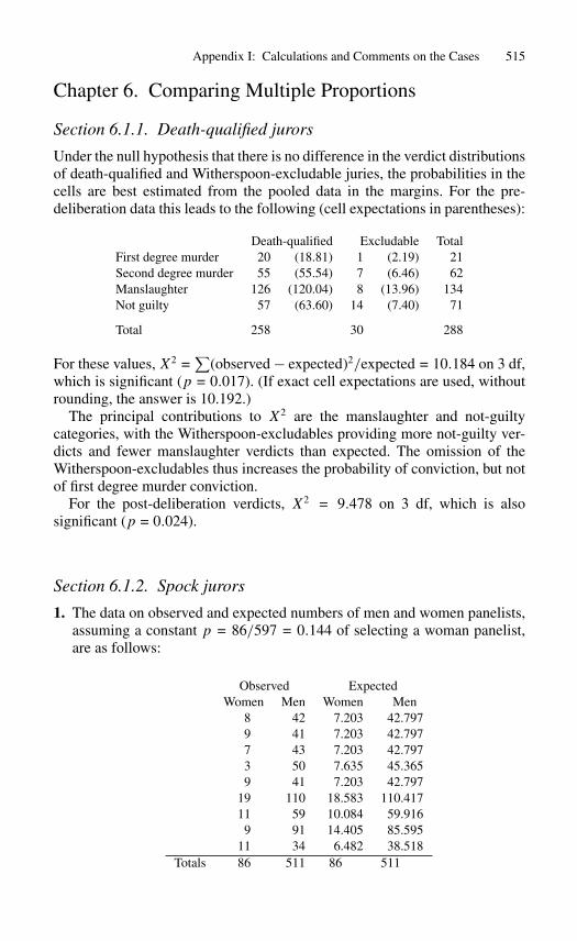
Section 6.1.1. Death-qualified jurors
Under the null hypothesis that there is no difference in the verdict distributionsof death-qualified and Witherspoon-excludable juries, the probabilities in thecells are best estimated from the pooled data in the margins. For the pre-deliberation data this leads to the following (cell expectations in parentheses):
Death-qualified Excludable TotalFirst degree murder 20 (18.81) 1 (2.19) 21Second degree murder 55 (55.54) 7 (6.46) 62Manslaughter 126 (120.04) 8 (13.96) 134Not guilty 57 (63.60) 14 (7.40) 71
Total 258 30 288
For these values, X2 =∑
(observed − expected)2/expected = 10.184 on 3 df,which is significant (p = 0.017). (If exact cell expectations are used, withoutrounding, the answer is 10.192.)
The principal contributions to X2 are the manslaughter and not-guiltycategories, with the Witherspoon-excludables providing more not-guilty ver-dicts and fewer manslaughter verdicts than expected. The omission of theWitherspoon-excludables thus increases the probability of conviction, but notof first degree murder conviction.
For the post-deliberation verdicts, X2 = 9.478 on 3 df, which is alsosignificant (p = 0.024).
Section 6.1.2. Spock jurors
1. The data on observed and expected numbers of men and women panelists,assuming a constant p = 86/597 = 0.144 of selecting a woman panelist,are as follows:
Observed ExpectedWomen Men Women Men
8 42 7.203 42.7979 41 7.203 42.7977 43 7.203 42.7973 50 7.635 45.3659 41 7.203 42.797
19 110 18.583 110.41711 59 10.084 59.916
9 91 14.405 85.59511 34 6.482 38.518
Totals 86 511 86 511
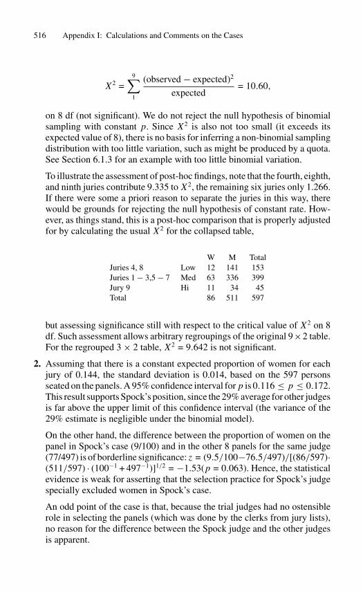
516 Appendix I: Calculations and Comments on the Cases
X2 =9∑1
(observed − expected)2
expected= 10.60,
on 8 df (not significant). We do not reject the null hypothesis of binomialsampling with constant p. Since X2 is also not too small (it exceeds itsexpected value of 8), there is no basis for inferring a non-binomial samplingdistribution with too little variation, such as might be produced by a quota.See Section 6.1.3 for an example with too little binomial variation.
To illustrate the assessment of post-hoc findings, note that the fourth, eighth,and ninth juries contribute 9.335 to X2, the remaining six juries only 1.266.If there were some a priori reason to separate the juries in this way, therewould be grounds for rejecting the null hypothesis of constant rate. How-ever, as things stand, this is a post-hoc comparison that is properly adjustedfor by calculating the usual X2 for the collapsed table,
W M TotalJuries 4, 8 Low 12 141 153Juries 1 − 3,5 − 7 Med 63 336 399Jury 9 Hi 11 34 45Total 86 511 597
but assessing significance still with respect to the critical value of X2 on 8df. Such assessment allows arbitrary regroupings of the original 9×2 table.For the regrouped 3 × 2 table, X2 = 9.642 is not significant.
2. Assuming that there is a constant expected proportion of women for eachjury of 0.144, the standard deviation is 0.014, based on the 597 personsseated on the panels. A 95% confidence interval for p is 0.116 ≤ p ≤ 0.172.This result supports Spock’s position, since the 29% average for other judgesis far above the upper limit of this confidence interval (the variance of the29% estimate is negligible under the binomial model).
On the other hand, the difference between the proportion of women on thepanel in Spock’s case (9/100) and in the other 8 panels for the same judge(77/497) is of borderline significance: z = (9.5/100−76.5/497)/[(86/597)·(511/597) · (100−1 + 497−1)]1/2 = −1.53(p = 0.063). Hence, the statisticalevidence is weak for asserting that the selection practice for Spock’s judgespecially excluded women in Spock’s case.
An odd point of the case is that, because the trial judges had no ostensiblerole in selecting the panels (which was done by the clerks from jury lists),no reason for the difference between the Spock judge and the other judgesis apparent.
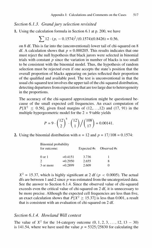
Appendix I: Calculations and Comments on the Cases 517
Section 6.1.3. Grand jury selection revisited
1. Using the calculation formula in Section 6.1 at p. 200, we have∑12 · (pi − 0.1574)2/(0.1574)(0.8426) = 0.56,
on 8 df. This is far into the (unconventional) lower tail of chi-squared on 8df. A calculation shows that p = 0.000205. This results indicates that onemust reject the null hypothesis that black jurors were selected in binomialtrials with constant p since the variation in number of blacks is too smallto be consistent with the binomial model. Thus, the hypothesis of randomselection must be rejected even if one accepts the state’s position that theoverall proportion of blacks appearing on juries reflected their proportionof the qualified and available pool. The test is unconventional in that theusual chi-squared test involves the upper tail of the chi-squared distribution,detecting departures from expectation that are too large due to heterogeneityin the proportions.
The accuracy of the chi-squared approximation might be questioned be-cause of the small expected cell frequencies. An exact computation ofP [X2 ≤ 0.56], given fixed margins of (12,. . . ,12) and (17, 91) in themultiple hypergeometric model for the 2 × 9 table yields
P = 9 ·(
12
2
)8
·(
12
1
)/(108
17
)= 0.00141.
2. Using the binomial distribution with n = 12 and p = 17/108 = 0.1574:
Binomial probabilityfor outcome: Expected #s Observed #s
0 or 1 =0.4151 3.736 12 =0.2950 2.655 83 or more =0.2899 2.609 0
X2 = 15.37, which is highly significant at 2 df (p < 0.0005). The actualdfs are between 1 and 2 since p was estimated from the uncategorized data.See the answer to Section 6.1.4. Since the observed value of chi-squaredexceeds even the critical value of chi-squared on 2 df, it is unnecessary tobe more precise. Although the expected cell frequencies are less than five,an exact calculation shows that P [X2 ≥ 15.37] is less than 0.001, a resultthat is consistent with an evaluation of chi-squared on 2 df.
Section 6.1.4. Howland Will contest
The value of X2 for the 14-category outcome (0, 1, 2, 3, . . . , 12, 13 − 30)is 141.54, where we have used the value p = 5325/25830 for calculating the
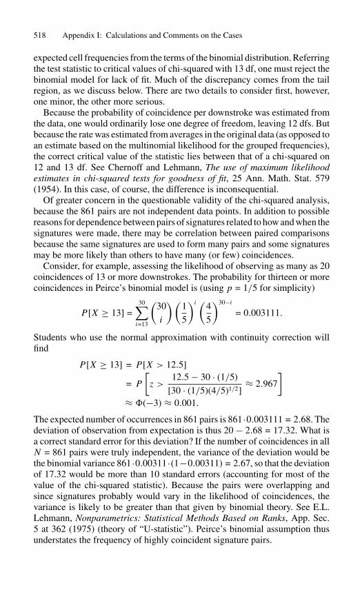
518 Appendix I: Calculations and Comments on the Cases
expected cell frequencies from the terms of the binomial distribution. Referringthe test statistic to critical values of chi-squared with 13 df, one must reject thebinomial model for lack of fit. Much of the discrepancy comes from the tailregion, as we discuss below. There are two details to consider first, however,one minor, the other more serious.
Because the probability of coincidence per downstroke was estimated fromthe data, one would ordinarily lose one degree of freedom, leaving 12 dfs. Butbecause the rate was estimated from averages in the original data (as opposed toan estimate based on the multinomial likelihood for the grouped frequencies),the correct critical value of the statistic lies between that of a chi-squared on12 and 13 df. See Chernoff and Lehmann, The use of maximum likelihoodestimates in chi-squared tests for goodness of fit, 25 Ann. Math. Stat. 579(1954). In this case, of course, the difference is inconsequential.
Of greater concern in the questionable validity of the chi-squared analysis,because the 861 pairs are not independent data points. In addition to possiblereasons for dependence between pairs of signatures related to how and when thesignatures were made, there may be correlation between paired comparisonsbecause the same signatures are used to form many pairs and some signaturesmay be more likely than others to have many (or few) coincidences.
Consider, for example, assessing the likelihood of observing as many as 20coincidences of 13 or more downstrokes. The probability for thirteen or morecoincidences in Peirce’s binomial model is (using p = 1/5 for simplicity)
P [X ≥ 13] =30∑
i=13
(30
i
)(1
5
)i (4
5
)30−i
= 0.003111.
Students who use the normal approximation with continuity correction willfind
P [X ≥ 13] = P [X > 12.5]
= P
[z >
12.5 − 30 · (1/5)
[30 · (1/5)(4/5)1/2]≈ 2.967
]≈ �(−3) ≈ 0.001.
The expected number of occurrences in 861 pairs is 861·0.003111 = 2.68. Thedeviation of observation from expectation is thus 20 − 2.68 = 17.32. What isa correct standard error for this deviation? If the number of coincidences in allN = 861 pairs were truly independent, the variance of the deviation would bethe binomial variance 861·0.00311·(1−0.00311) = 2.67, so that the deviationof 17.32 would be more than 10 standard errors (accounting for most of thevalue of the chi-squared statistic). Because the pairs were overlapping andsince signatures probably would vary in the likelihood of coincidences, thevariance is likely to be greater than that given by binomial theory. See E.L.Lehmann, Nonparametrics: Statistical Methods Based on Ranks, App. Sec.5 at 362 (1975) (theory of “U-statistic”). Peirce’s binomial assumption thusunderstates the frequency of highly coincident signature pairs.
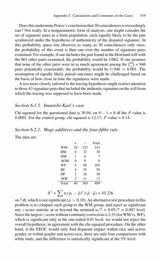
Appendix I: Calculations and Comments on the Cases 519
Does this undermine Peirce’s conclusion that 30 coincidences is exceedinglyrare? Not really. In a nonparametric form of analysis, one might consider theset of signature pairs as a finite population, each equally likely to be the pairscrutinized under the hypothesis of authenticity of the disputed signature. Inthis probability space one observes as many as 30 coincidences only once;the probability of this event is thus one over the number of signature pairsexamined. For example, if one includes the pair found in the Howland will withthe 861 other pairs examined, the probability would be 1/862. If one assumesthat none of the other pairs were in as much agreement among the
(442
)= 946
pairs potentially examinable, the probability would be 1/946 ≈ 0.001. Theassumption of equally likely paired outcomes might be challenged based onthe basis of how close in time the signatures were made.
A test more closely tailored to the tracing hypothesis might restrict attentionto those 43 signature pairs that included the authentic signature on the will fromwhich the tracing was supposed to have been made.
Section 6.1.5. Imanishi-Kari’s case
Chi-squared for the questioned data is 30.94; on 9 − 1 = 8 df the P -value is0.0001. For the control group, chi-squared is 12.17; P -value = 0.14.
Section 6.2.1. Wage additives and the four-fifths rule
The data are:+ − Total
WM 20 123 143BM 6 32 38HM 1 6 7AOM 0 8 8WF 5 98 103BF 4 55 59HF 2 36 38AOF 2 11 13Total 40 369 409
X2 =∑
ni(pi − p)2/(p · q) = 10.226
on 7 df, which is not significant (p > 0.10). An alternative test procedure in thisproblem is to compare each group to the WM group, and reject as significantany z-score statistic at or beyond the nominal α/7 = 0.05/7 = 0.007 level.Since the largest z-score without continuity correction is 2.33 (for WM vs. WF),which is significant only at the one-tailed 0.01 level, we would not reject theoverall hypothesis, in agreement with the chi-squared procedure. On the otherhand, if the EEOC would only find disparate impact within race and acrossgender, or within gender and across race, there are only four comparisons withwhite male, and the difference is statistically significant at the 5% level.
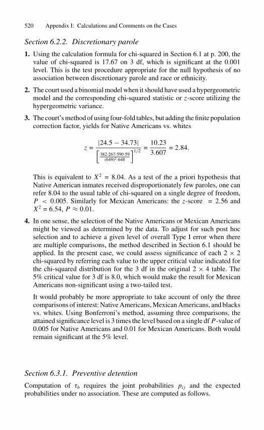
520 Appendix I: Calculations and Comments on the Cases
Section 6.2.2. Discretionary parole
1. Using the calculation formula for chi-squared in Section 6.1 at p. 200, thevalue of chi-squared is 17.67 on 3 df, which is significant at the 0.001level. This is the test procedure appropriate for the null hypothesis of noassociation between discretionary parole and race or ethnicity.
2. The court used a binomial model when it should have used a hypergeometricmodel and the corresponding chi-squared statistic or z-score utilizing thehypergeometric variance.
3. The court’s method of using four-fold tables, but adding the finite populationcorrection factor, yields for Native Americans vs. whites
z =|24.5 − 34.73|[382·267·590·59
(649)2·648
]1/2 =10.23
3.607= 2.84.
This is equivalent to X2 = 8.04. As a test of the a priori hypothesis thatNative American inmates received disproportionately few paroles, one canrefer 8.04 to the usual table of chi-squared on a single degree of freedom,P < 0.005. Similarly for Mexican Americans: the z-score = 2.56 andX2 = 6.54, P ≈ 0.01.
4. In one sense, the selection of the Native Americans or Mexican Americansmight be viewed as determined by the data. To adjust for such post hocselection and to achieve a given level of overall Type I error when thereare multiple comparisons, the method described in Section 6.1 should beapplied. In the present case, we could assess significance of each 2 × 2chi-squared by referring each value to the upper critical value indicated forthe chi-squared distribution for the 3 df in the original 2 × 4 table. The5% critical value for 3 df is 8.0, which would make the result for MexicanAmericans non-significant using a two-tailed test.
It would probably be more appropriate to take account of only the threecomparisons of interest: Native Americans, Mexican Americans, and blacksvs. whites. Using Bonferroni’s method, assuming three comparisons, theattained significance level is 3 times the level based on a single df P -value of0.005 for Native Americans and 0.01 for Mexican Americans. Both wouldremain significant at the 5% level.
Section 6.3.1. Preventive detention
Computation of τb requires the joint probabilities pij and the expectedprobabilities under no association. These are computed as follows.
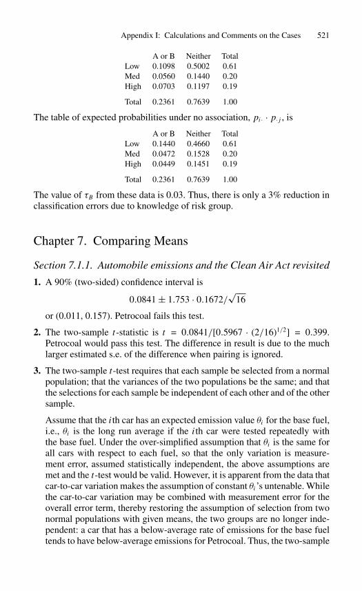
Appendix I: Calculations and Comments on the Cases 521
A or B Neither TotalLow 0.1098 0.5002 0.61Med 0.0560 0.1440 0.20High 0.0703 0.1197 0.19
Total 0.2361 0.7639 1.00
The table of expected probabilities under no association, pi· · p·j , is
A or B Neither TotalLow 0.1440 0.4660 0.61Med 0.0472 0.1528 0.20High 0.0449 0.1451 0.19
Total 0.2361 0.7639 1.00
The value of τB from these data is 0.03. Thus, there is only a 3% reduction inclassification errors due to knowledge of risk group.
Chapter 7. Comparing Means
Section 7.1.1. Automobile emissions and the Clean Air Act revisited
1. A 90% (two-sided) confidence interval is
0.0841 ± 1.753 · 0.1672/√
16
or (0.011, 0.157). Petrocoal fails this test.
2. The two-sample t-statistic is t = 0.0841/[0.5967 · (2/16)1/2] = 0.399.Petrocoal would pass this test. The difference in result is due to the muchlarger estimated s.e. of the difference when pairing is ignored.
3. The two-sample t-test requires that each sample be selected from a normalpopulation; that the variances of the two populations be the same; and thatthe selections for each sample be independent of each other and of the othersample.
Assume that the ith car has an expected emission value θi for the base fuel,i.e., θi is the long run average if the ith car were tested repeatedly withthe base fuel. Under the over-simplified assumption that θi is the same forall cars with respect to each fuel, so that the only variation is measure-ment error, assumed statistically independent, the above assumptions aremet and the t-test would be valid. However, it is apparent from the data thatcar-to-car variation makes the assumption of constant θi’s untenable. Whilethe car-to-car variation may be combined with measurement error for theoverall error term, thereby restoring the assumption of selection from twonormal populations with given means, the two groups are no longer inde-pendent: a car that has a below-average rate of emissions for the base fueltends to have below-average emissions for Petrocoal. Thus, the two-sample
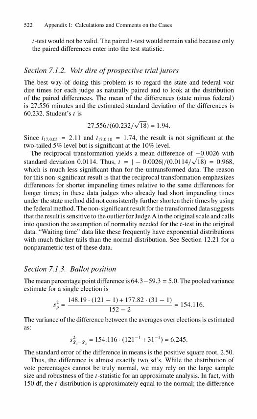
522 Appendix I: Calculations and Comments on the Cases
t-test would not be valid. The paired t-test would remain valid because onlythe paired differences enter into the test statistic.
Section 7.1.2. Voir dire of prospective trial jurors
The best way of doing this problem is to regard the state and federal voirdire times for each judge as naturally paired and to look at the distributionof the paired differences. The mean of the differences (state minus federal)is 27.556 minutes and the estimated standard deviation of the differences is60.232. Student’s t is
27.556/(60.232/√
18) = 1.94.
Since t17,0.05 = 2.11 and t17,0.10 = 1.74, the result is not significant at thetwo-tailed 5% level but is significant at the 10% level.
The reciprocal transformation yields a mean difference of −0.0026 withstandard deviation 0.0114. Thus, t = | − 0.0026|/(0.0114/
√18) = 0.968,
which is much less significant than for the untransformed data. The reasonfor this non-significant result is that the reciprocal transformation emphasizesdifferences for shorter impaneling times relative to the same differences forlonger times; in these data judges who already had short impaneling timesunder the state method did not consistently further shorten their times by usingthe federal method. The non-significant result for the transformed data suggeststhat the result is sensitive to the outlier for Judge A in the original scale and callsinto question the assumption of normality needed for the t-test in the originaldata. “Waiting time” data like these frequently have exponential distributionswith much thicker tails than the normal distribution. See Section 12.21 for anonparametric test of these data.
Section 7.1.3. Ballot position
The mean percentage point difference is 64.3−59.3 = 5.0. The pooled varianceestimate for a single election is
s2p =
148.19 · (121 − 1) + 177.82 · (31 − 1)
152 − 2= 154.116.
The variance of the difference between the averages over elections is estimatedas:
s2X1−X2
= 154.116 · (121−1 + 31−1) = 6.245.
The standard error of the difference in means is the positive square root, 2.50.Thus, the difference is almost exactly two sd’s. While the distribution of
vote percentages cannot be truly normal, we may rely on the large samplesize and robustness of the t-statistic for an approximate analysis. In fact, with150 df, the t-distribution is approximately equal to the normal; the difference
Appendix I: Calculations and Comments on the Cases 523
is statistically significant at about the two-tailed 5% level. Notice, that sinceincumbents appeared in the second position so infrequently, the assumptionthat position was determined by lot must be rejected (the observed proportionwas more than 7 sd’s from 50%). Incumbents who appeared second may havereceived a smaller proportion of the vote because they were politically lesspowerful.
Section 7.1.4. Student’s t-test and the Castaneda rule
1. The court is wrong for the binomial distribution. The t-distribution is un-necessary because there is no need to estimate the standard deviation, whichis
√npq, once p is determined under the null hypothesis.
2. The sample size of 5 illustrates the fallacy of the court’s suggestion. Themost extreme result (0 blacks) is only 2.24 sd’s from the mean of 2.5, yetthe exact binomial probability of such a result is (1/2)5 = 0.03, which issignificant at the 5% level.
3. The need for an independent estimate of the variance introduces addedvariability to the standardized test statistic.
4. If the percentage of blacks in the voting rolls were constant, a simple bi-nomial test on the aggregated data would suffice. It shows z = −2.82,p < .0025, a significant shortfall. If the percentages varied, each yearwould have to be treated separately and the methods of Section 8.1 used tocombine the evidence.
Section 7.2.1. Fiddling debt collector
1. SSw =3∑1
(39)(0.3)2 = 3 × 39 × 0.09 = 10.53
MSw = SSw/(N − 3) =10.53
120 − 3= 0.09
2. SSb =3∑1
ni(Yi − ¯Y )2
= 40(0.71 − 0.70)2 + 40(0.70 − 0.70)2 + 40(0.69 − 0.70)2 = 0.008
MSb = SSb/(k − 1) = 0.008/2 = 0.004
3. The F -statistic is F = MSb
MSw= 0.004
0.09 = 0.044 with 2 and 117 df.
4. The null hypothesis is that the samples were selected at random. The alter-native hypothesis is that the process was manipulated to create results closeto 0.70 in each sample. Given the alternative hypothesis, the lower tail of
524 Appendix I: Calculations and Comments on the Cases
the F -distribution should be used to see whether the means are too close to0.70.
5. The P -value is P [F2,117 ≤ 0.044]. We don’t need special F -tablesto evaluate this because of the relationship P [F2,117 ≤ 0.044] =P[F117,2 ≥ 1
0.044 = 22.5]
< 0.05 from Table F in Appendix II. Since theP -value is less than 0.05, we reject the null hypothesis that the sampleswere selected at random from populations with an average collection rateof 70%. However, use of the F -distribution assumes that the percentagescollected of individual invoices are normally distributed. This is unlikelysince the collection percentage only varies between 0 and 100% and maywell be U-shaped, reflecting the fact that invoices are either collected ornot. If the distribution is J -shaped, with most invoices largely collected,simulations suggest that the above calculation may be conservative, i.e., theprobability of such close adherence to 0.70 is even smaller than indicated.
Chapter 8. Combining Evidence AcrossIndependent Strata
Section 8.1.1. Hiring lawyers
Strata 1970-72 may be disregarded as non-informative. The elements of theMantel-Haenszel statistic are as follows (taking white hires as the referencecategory):
Observed whites hired (1973–82) 60Expected number 55.197Excess number whites (or shortfall for blacks) 4.8Sum of the hypergeometric variances 7.2706
The continuity corrected z-score is zc = (4.8 − 0.5)/√
7.2706 = 1.59 whichis just short of significant at the one-tailed 0.05 level. Note that if the squaredform of the Mantel-Haenszel statistic is used, the P -value corresponding tothe upper tail of the chi-squared distribution is a two-sided test because bothpositive and negative deviations in the z-score contribute to the upper tail. TheP -value should be divided by two for a one-sided test.
In the actual case, data from other positions were combined, the result wassignificant, and the magistrate accepted the Mantel-Haenszel statistic.
Fisher’s exact test is appropriate here for each year and the correspond-ing hypergeometric model is in fact the basis for the Mantel-Haenszel testthat we use. Fisher’s method of combing the evidence applies to continuousdistributions and is inappropriate here because of the small numbers and theresulting discreteness of the P -values. Pooling should be avoided because ofthe variations in outcome rate (hiring) and exposure rate (race) across years(the stratification variable).
Appendix I: Calculations and Comments on the Cases 525
Section 8.1.2. Age discrimination in employment terminations
1. In 10 out of 15 cases, the age of the terminated employee exceeded theaverage age of employees. There is a total of 89.67 years in excess ofexpectation on the hypothesis of no discrimination.
2. Following the logic of the Mantel-Haenszel test, for each termination wegenerate an expected value for age, which is the average age (or that timesthe number of terminations when there are more than 1). The differencesbetween observed and expected ages are then summed over the terminationevents. The sum is divided by the square root of the sum of the variancesof the aggregated ages at each termination in a sampling experiment with-out replacement for those at risk of termination. When only one personis terminated this variance is simply the variance of the ages of those atrisk. When more than one is terminated, it is the number of terminationstimes the variance of the ages of those at risk times the finite populationcorrection.
The result is a standard normal deviate,
z =653 − 563.4√
1276.84= 2.51,
which is significant at the one-tailed 1% level (P = 0.006).
Section 8.2.1. Bendectin revisited
1. With weights wi = 1/(s.e. log RR)2, the estimated log relative risk isθ =
∑wiθi/
∑wi = −10.025/269.75 = −0.0372. The s.e. of θ =
1/√
269.75 = 0.0609.
2. A 95% confidence interval is
−0.0372 ± (1.96)(0.0609) = (−0.157, 0.082).
3. Exponentiating, the estimated relative risk is 0.96 with confidence interval(0.85, 1.09).
4. Suppose there were a true common log relative risk underlying each ofthe studies. In order for the log confidence interval found in Answer 2 toexclude the null value of 0, we must have the estimate exceed 1.96 standarderrors. For this event to occur with 80% probability, we must have
θ − θ
s.e. θ>
1.96 s.e. θ − θ
s.e. θ.
Since the left-hand side of the above equation is approximately a standardnormal variable, the probability of rejecting the null hypothesis will exceed80% when the right-hand side is less than −0.84. This implies that θ >
526 Appendix I: Calculations and Comments on the Cases
(2.8)(0.0609) = 0.17, corresponding to an RR of approximately 1.2. Poweris sufficient to detect the relative risk posited by plaintiff’s expert. (A one-tailed test would yield even greater power.) This result indicates that the lackof significance is not due to a lack of power, but rather to the inconsistencyin direction of the study results.
5. Under the hypothesis of homogeneity, Q has a chi-squared distribution onnine df. Since the value Q = 21.46 has a tail probability of 0.011, we rejectthe hypothesis of homogeneity and conclude that the true ln(RR)’s varyfrom study to study.
6. τ 2 = 0.058; τ = 0.241. τ is the estimated standard deviation of the trueln(RR)’s in the hypothetical population. Using weights adjusted for thisfactor, the mean of the population of true ln(RR)’s is estimated as −0.136.The antilog is 0.873, with s.e. 0.1088.
Chapter 9. Sampling Issues
Section 9.1.1. Selective Service draft lotteries
2. Dichotomizing sequence numbers in those ≤ 183 or ≥ 184 yields thefollowing 2 × 12 table:
Jan Feb Mar Apr May Jun Jul Aug Sep Oct Nov Dec≥ 184 19 17 21 19 17 16 17 12 13 18 9 5 183≤ 183 12 12 10 11 14 14 14 19 17 13 21 26 183
31 29 31 30 31 30 31 31 30 31 30 31 366
The chi-squared statistic is appropriate to test for random assortment in amultiple hypergeometric model with all margins fixed. The value of X2
is 31.139 on 11 df (p ∼ 0.001). There is a significantly decreasing trendin the proportion of high-end sequence numbers from beginning to end ofyear. The later months were more likely to receive lower sequence numbersbecause the chronological sequence in which the slips were put into thebowl put them on top and the stirring was inadequate (as it usually is).
The results from the 1971 lottery are much more uniform:
Jan Feb Mar Apr May Jun Jul Aug Sep Oct Nov Dec≥ 184 9 18 16 14 15 16 14 17 19 14 14 16 182≤ 183 22 10 15 16 16 14 17 14 11 17 16 15 183
31 28 31 30 31 30 31 31 30 31 30 31 365
For these data X2 = 11.236 on 11 df (p > 0.4).
Appendix I: Calculations and Comments on the Cases 527
Section 9.1.2. Uninsured motor vehicles
1. Using Fleiss’s formula at p. 172, a 95% confidence interval is (93.7%, 98.7%).
2. The sample is not too small; the confidence interval in theory reflects theuncertainty attributable to the given sample size.
3. The true rate of uninsured vehicles is probably greater than the confi-dence interval would indicate because the missing vehicles may well havea lower insurance rate. If all the missing vehicles in the sample of size249 are assumed to be uninsured, the 95% confidence interval would be(86.3%, 93.9%).
Section 9.1.3. Mail order survey
The mail-order house argued that the respondents were “representative” of allpurchasers with respect to the resale/personal-use issue because respondentsand nonrespondents had similar distributions of order size and shipping ad-dress. In general, reference to such covariates is appropriate to justify treatinga sample as random despite nonresponse. If the sample is random, the com-pany’s position is correct. If the sample is deemed not random, there are noclear benchmarks as to the right percentage, but the Board’s position that allnonresponse should be deemed in the personal-use category would seem ex-treme. On the randomness issue, however, a chi-squared test of homogeneity inthe distribution of orders by size for respondents and nonrespondents is 22.15,on 3 df (P < 0.0001), indicating a significant departure from the homogene-ity hypothesis implicitly argued by the mail-order house. Chi-squared for theshipping address table is 2.67, on 2 df, which is not significant, a result that isconsistent with the company’s position.
Section 9.1.5. NatraTaste v. NutraSweet
1. The entry criterion was criticized by the court because respondents includedusers as well as buyers, and a user might well have not been a buyer, e.g.,those who used the product in restaurants or used it at home, but did notbuy it.
The study method was criticized because (i) the respondents were not shownthe NutraSweet box together with the other boxes, as they would be seenin a store; (ii) the question was leading; and (iii) there was no instructionagainst guessing.
2. The expert’s analysis was flawed because the control boxes did not controlfor similarities in names and colors, which were not protected elements oftrade dress. The court analyzed the reasons given by respondents for theirchoice of the NatraTaste box and found that in most cases these elementsplayed a role in respondents’ choices.
528 Appendix I: Calculations and Comments on the Cases
Section 9.1.6. Cocaine by the bag
1. Let p be the proportion of the 55 bags that contains cocaine. We seek thevalue of p for which the probability of picking three bags at random, all ofwhich contain cocaine, is 0.05 (this value is the lower end of a one-sided 95%confidence interval). This is given by p3 = 0.05; p = (0.05)1/3 = 0.368,suggesting that a minimum of about 0.368 × 55 = 20 of the 55 bags havecocaine. A one-sided interval is used because there is no p larger than thatshown by the data (p = 1).
2. Using the slightly more accurate hypergeometric distribution, the probabil-ity of finding cocaine in all 3 bags selected at random, if there were 21 bagswith cocaine, is given by(21
3
)(340
)(55
3
) =1,330
26,235∼= 0.05.
Section 9.1.7. ASCAP sampling plan
1. ASCAP’s expert’s statements:
Randomness
a. Not too bad. The reference to chance should be “knowable” to reflectthe purpose of random sampling.
b. Not “determined by statistical laws” in the sense that other days, times,etc., couldn’t be selected. The statement is correct if understood to meanthat the characteristics in repeated samples will vary in accordance withstatistical laws.
c. True, in theory.
Sampling Precision
a. False. Sampling precision is the degree to which results will vary fromsample to sample.
b. Not quite true. The less the sampling precision, the greater the averageabsolute or squared understatement or overstatement of the number of amember’s playings.
c. Under commonly assumed distributions for counts, such as the Poissonor the binomial, this statement is true in the proportional sense, but not inthe absolute sense. For a composition with many playings, the variancewill be greater in terms of number of playings, but smaller in proportionto the mean than for a piece with few playings.
d. True, and also true for a piece with many playings.
Appendix I: Calculations and Comments on the Cases 529
2. Estimates of accuracy of the samples:
In a sampling plan as complex as this, the court should require some repli-cated, split-sample technique, such as the jackknife or the bootstrap, tosupport estimates of precision. See Section 14.9.
Section 9.1.8. Current population survey
1-3.Stratified sampling is used in creating the strata composed of similar PSUs;its purpose is to reduce sampling error by creating more homogeneous sam-pling units. Cluster sampling is used in creating clusters of four neighboringhousing units for the systematic sample. This increases efficiency, but alsoincreases sampling error compared with a random sample of the same size.Ratio estimation is used in estimating the number of unemployed in eachsubgroup in the sample; its use reduces sampling error.
4. One factor is size. Sampling ratios should be greater in small PSUs than inlarge ones because it is primarily the size of the sample, not its ratio to thepopulation, that determines sampling error. Thus, PSUs in low populationstates should have higher sampling ratios.
5. Recall that CV = sd/mean. Assuming the mean to be 6%, sd =(0.06)(0.019) = 0.00114. Hence, a 95% c.i. is about 6.0 ± 0.2.
Section 9.2.1. Adjusting the Census
1. Putting aside the provision for erroneous enumerations in brackets (forwhich there is no provision in the fish example), the DSE formula is equalto the number of fish in the first sample (census) × the number of fishin the second sample (Np–the estimated population from the post-censussample) divided by the number of tagged fish in the second sample (M–theweighted-up number of matches).
2. The DSE underadjusts for black males and overadjusts for black females.This suggests that black males who are hard to catch in the census are alsohard to catch in the post-census survey. [Do you see why?] The reason forthe overadjustment of black females is unknown.
3. That adjustment should be made for this reason was argued by the plaintiffsin the first round of litigation (to compel adjustment). The Second Circuitin effect agreed, but the Supreme Court unanimously reversed. Wisconsinv. City of New York, 517 U.S. 1 (1996).
4. This remedy has been suggested by some statisticians. See the article byL.D. Brown, et al., cited at p. 281.
530 Appendix I: Calculations and Comments on the Cases
Chapter 10. Epidemiology
Section 10.2.1. Atomic weapons tests
The relative risk for males and females combined and control groups combinedin Table 10.2.1a is 4.42/2.18 = 2.03. Let p1 denote the disease rate amongthose exposed and p0 the rate among those unexposed. Among those exposed,if p0 are cases assumed to have arisen from other causes, while the remainingp1 −p0 are assumed to have been caused by the exposure, then (p1 −p0)/p1 =1−1/RR is the proportion of exposed cases caused by the exposure. Thus, theprobability that Orton’s leukemia was caused by the exposure is 1 − 1/2.03 =0.507, or slightly more likely than not. On the other hand, when the earlieryears are dropped, the relative risk falls below 2 (1.99 for Southern Utah inthe Lyon study, and 1.60 in Southern Utah and 1.33 for Northern Utah in theLand study) and the data do not indicate causation is more likely than not.In addition, the data for at least Eastern Oregon also indicate an elevated risk(1.48), suggesting that events other than fallout may have been a contributingfactor.
Section 10.3.1. Dalkon Shield
Because the study was retrospective, use the odds ratio. The odds ratios for thegroup of Dalkon Shield users vs. each group separately are as follows:
O.C. (35/15)/(127/830) = 15.2Barrier (35/15)/(60/439) = 17.1Other IUDs (35/15)/(150/322) = 5.0No Method (35/15)/(250/763) = 7.1
The data support the suggestion of a much higher risk of PID with the Shieldthan with other methods or with no method.
Since the study was conducted after extensive and negative publicity aboutthe Shield, the proportion of Shield wearers among the controls appears tobe smaller than their proportion in the general population at the time plaintiffwore the Shield. Robins estimated that 6.5% of women in the 18–44 age groupwore the Shield, while only 15/2,369 = 0.63% of the controls wore the Shield.Such a change would cause the study to overstate the risk of the Shield. It alsocould be argued that those cases still wearing the Shield at the time of the studywere more careless about their health and thus more likely to contract PID thanwomen who wore the Shield when the plaintiff did. Such a change would alsocause that study to overstate the effect of the Shield. On the other hand, itcould be argued that many of those who would contract PID from the Shieldhad already done so before the study recruitment period, thus, rate of Shielduse for those with PID was below that rate when plaintiff wore the Shield.Such a change would cause the study to understate the risk of the Shield.
Appendix I: Calculations and Comments on the Cases 531
Section 10.3.2. Radioactive “cocktails” for pregnant women
1. (i) Since the control group had 0 childhood cancer deaths, RR = ∞.
(ii) Using population data and including the liver cancer, SMR = 4/0.65 =6.15. Excluding the liver cancer, SMR = 4.62.
2. Since the exposed and control groups are about the same size, the prob-ability that a cancer death would be in the exposed group, under the nullhypothesis, is about 1/2; the probability that all four cases would be inthe exposed group is 1/24 = 1/16 = 0.0625 and the probability that all 4cases would be in either group is 2 × 0.0625 = 0.125. With three cases,the probability of all being in either group is 0.25. In neither case are thedata significant. Comparing the exposed group with the expected numberfrom general population data, we treat X, the number of childhood cancerdeaths, as a Poisson random variable with mean 0.65. Then, including theliver cancer,
P [X ≥ 4] = 1 − P [X ≤ 3]
= 1 − e−0.65{1 + 0.65 + (0.65)2/2 + (0.65)3/(3 × 2)}= 0.0044
for the upper-tail P -value. The point probability for X = 4 is 0.0039.Since the only value in the lower tail is X = 0, and the probability of thatis e−0.65 = 0.522, there is no additional P -value for the lower tail by thepoint probability method (see p. 121). The two-tailed test is thus significant.Excluding the liver cancer, the two-tailed test is still significant.
3. An approximate 95% confidence interval for the log number of cancerdeaths is ln 4 ± 1.96(1/4)1/2 = (0.4063, 2.3663). Exponentiating, we have(1.50, 10.66) as the lower and upper confidence limits, respectively, for thenumber of deaths. Dividing by 0.65 gives (2.3, 16.4) as the limits for theSMR. The size of the interval is an indication of the evidence’s weakness.If the liver cancer is excluded, the approximate interval is (0.968, 9.302),which includes 1. But an exact computation gives limits (1.258, 13.549)that are broader, shifted to the right, and as a result exclude 1.
4. Defense experts argued that the 0.65 figure was biased downward becausethe followup was for an average of 18.44 years, but childhood cancer deathsonly through age 14 were included. Plaintiffs’ experts argued in reply that toinclude later cancer deaths would introduce a biasing factor of adult cancer.One of the defense experts recalculated the expected number of deathsthrough 20 years of age and found 0.90 expected deaths in the exposedcohort. With this expectation, P [X ≥ 4] = 0.013 and P [X ≥ 3] = 0.063.
5. Plaintiff’s experts argued that the liver cancer death should be included be-cause the population figures did not exclude deaths from hereditary cancers.They also argued that the radiation “promoted” the liver cancer, causing
532 Appendix I: Calculations and Comments on the Cases
death at an earlier age. Defendant’s experts replied that the first argumentdid not justify including the liver cancer, but making an allowance for therate of hereditary cancer in computing the expected number. They rejectedthe promotion theory as speculative.
Section 10.3.3. Preconception paternal irradiation and leukemia
Given that human spermatozoa do not live more than a few days, the datafor the previous six months would seem to be the most relevant. Within thattable, to compute an odds ratio we must decide what categories to use. On thetheory that only the highest exposures have any significant effect, it would bemost reasonable to compare the ≥ 10 and 0 dosage categories and to use localcontrols as the closest to the cases. The result is:
Father’s preconception dose Leukemic children Local controls Totals(in mSv)
0 38 246 284≥ 10 4 3 7Totals 42 249 291
For this table OR = 246×43×38 = 8.63, which has an exact (one-sided) P -value of
0.0096. However, had this been one of many comparisons arrived at post hoc,it would have been necessary to apply an adjustment for multiple comparisonsin computing significance. For example, if this table were considered merelyas one of nine possible 2 × 2 subtables obtained without summing from theoriginal 3 × 3 table, the Bonferroni-adjusted P -value is 0.0096 × 9 = 0.086,which is not significant. The loss of significance that may occur when makingmultiple comparisons underscores the importance of an a priori specificationof the primary analysis.
Section 10.3.4. Swine flu vaccine and Guillain-Barre Syndrome
1. If the government’s experts were right, the decline in GBS cases amongthe vaccinated as time passed after the moratorium was due to the fact thatany risk from the vaccine declined with time and largely, if not completely,disappeared by 13 weeks; the decline was not due to underreporting of GBSamong the vaccinated, as plaintiff claimed. Since plaintiff’s use of popula-tion rates of GBS among the unvaccinated in the post-moratorium periodwas admittedly biased downward, the relative risk was biased upward. Itwould seem probable that underreporting would be greater among unvacci-nated than vaccinated persons, given the medical and media attention givento the GBS risk of the vaccine.
Appendix I: Calculations and Comments on the Cases 533
2. Denote GBS as G, vaccination as V , and illness as I . Then, using Bayes’stheorem, for vaccinated persons,
P [G | I, V ] =P [I and G | V ]
P [I | V ]=
P [I | G, V ]P [G | V ]
P [I | V ].
Because this also holds for unvaccinated persons, the ratio of the two yieldsthe relative risk equation in the text.
3. Although 33/62 may be a reasonable adjustment to reflect RR[I | G] inthe numerator of the relative risk equation in the text, a similar effect mayobtain for RR[I ] in the denominator of the equation. To the extent thatthe two effects are similar, they would cancel. This highlights a difficultywith the data: the unconditional relative risk of illness for vaccinated vs.unvaccinated people was not estimated, and the absence of such an estimatemakes problematic any adjustment for illness as a GBS risk factor.
Section 10.3.5. Silicone breast implants
1. The weighted average adjusted ln(OR) = 43.518/259.697 = 0.1676;exponentiating, OR = 1.18.
The standard error of the weighted average is 1/(sum of weights)1/2 or1/(259.697)1/2 = 0.0621. The approximate 95% confidence interval isln(OR) = 0.1676 ± 1.96(0.0621) = [0.046, 0.289]; exponentiating, thelimits are [1.05, 1.34].
2. Using Table 10.3.5b and our earlier result, 12.17 − (259.697)(0.1676)2 =4.88, which is non-significant for chi-squared on k − 1 (here 10) degreesof freedom (P = 0.899). Notice that there are two different null hypothesesfor the studies, the first being that the log odds ratios for all the studies equalzero; the second being that the studies have the same log odds ratios, butnot necessarily zero. The test for homogeneity used here is for the secondnull hypothesis.
Based on a variety of analyses, the panel concluded that there was no “con-sistent or meaningful” association between breast implants and connectivetissue disease.
Chapter 11. Survival Analysis
Section 11.1.2. Defective house sidings
Since the slope coefficient is far from unity, the exponential model must berejected in favor of the more general Weibull model. From the fitted equationlog10 H (t) = log10 θ0 + c · log10 t = −3.742 + 2.484 log10 t and θ0 = 10−3.742 =0.0001811. Then, the estimated Weibull survival function is S(t) = exp(−θ0 ·
534 Appendix I: Calculations and Comments on the Cases
t c) = exp(−0.0001811 · t2.484). The probability of a siding lasting for at leastfive years (t = 60 months) is 0.0088.
The data shown in the problem are questionable because the 9-month hazardis 0.0246, which suggests that there were initially about 40 houses (1/40 =0.025). In that case, however, the hazard should rise as the number of failuresreduces the risk set, but it essentially does not. The relative constancy of thehazard would normally suggest the exponential distribution, but in these datathe unequal spacing of failure events implies a non-exponential distributionand leads us to fit the more general Weibull distribution.
Section 11.1.3. “Lifing” deposit accounts
1. The hazard rates (one minus the proportions remaining) are decreasing withage. This suggests consideration of a Weibull distribution with c < 1.
2. A plot of the log cumulative hazard estimated by the summation of the dj/nj
method gives slope coefficient c ∼= 1/2 and intercept, ln θ0∼= −1/2, or
θ0∼= e−1/2.
3. The median based on these parameters (with 1/c rounded to 2) is{(log 2)/e−1/2}2 = 1.3. The mean is ∼= �(1 + 2)/(e−1/2)2 = 2! × e ∼= 5.4.
Section 11.2.1. Age discrimination in employment terminationsrevisited
The simplest proportional hazards model postulates that the hazard at time t
for an employee who at time t is X(t) years older than an arbitrary referenceage is θ0(t)ebX(t), where θ0(t) is the hazard at time t for the arbitrary referenceage. Using the closed form (one-step) approximation for the log-proportionalhazards constant referenced in Section 11.2 at p. 324–325, and the data ofTable 8.1.2c at p. 249, we have
β =653 − 563.4
1276.84= 0.070,
implying that each year of age increases the risk of termination by about 7%.
Section 11.2.2. Contaminated wells in Woburn
1. The risk set for Case No. 1 is all children with the same birth year who arealive and without diagnosis of leukemia in Woburn just prior to the timeCase No. 1 is diagnosed. The analysis is thus stratified by birth year, whichis more refined than a risk set consisting of all children, without regard tobirth year, who would be followed from the sames age as Case No. 1 atdiagnosis.
Appendix I: Calculations and Comments on the Cases 535
2. The expected exposure under the null hypothesis is the average cumulativeexposure for children in the risk set, for the period of residence in Woburnof the child who was diagnosed at the time of such diagnosis. For Case No.1 this was 0.31 child-years for cumulative exposure; 33% of the children inthe risk set had some exposure.
The variance is the finite population variance of these exposure scores inthe risk set at each diagnosis. For the binary exposure variable, this is theproduct of the proportions exposed and unexposed at diagnosis, which sumsto 3.493 in Table 11.2.2.
3. The excess number of cases with some exposure is 9 − 5.12 = 3.88. Forthe continuous variate the excess of 21.06 − 10.55 = 10.61 is in terms ofchild-years of exposure, which cannot be interpreted in terms of cases.
4. Using the one-step approximation given in Section 11.2 at p. 324–325, thelog-proportional hazard constant is
β =21.06 − 10.55
31.53= 0.333,
which yields an estimated relative risk of eβ = 1.40 per child-year ofcumulative exposure.
5. The Mantel-Haenszel estimate for the odds ratio on leukemia for exposedvs. unexposed children is given by
�MH =
(sum of proportion unexposed among thoseat risk at the time of each exposed death
)(sum of proportion exposed among those at
risk at the time of each unexposed death
)=
(1 − 0.33) + (1 − 0.25) + (1 − 0.36) + (1 − 0.32) + · · ·0.26 + 0.29 + 0.38 + 0.25 + · · ·
=6.21
2.33= 2.67.
6. The excess leukemia cases continued in children born after the wells wereclosed and that the cruder dichotomous measure of exposure shows a largerrelative risk than the presumably more accurate continuous exposure metric.
Section 11.3.2. Ethylene oxide
1. Using the two-stage model extrapolated from male rats, with the scalingfactor for humans given in footnote (a) of Table 11.3.2a (S = 0.129898) andthe coefficients given in footnote (b) of Table 11.3.2b (q[1] = 0.008905 andq[2] = 0.000184), the excess lifetime risk of cancer per 10,000 workers is634 for 50 ppm exposure, as follows:
Pexcess(d)=1−exp[−(0.008905)(50×0.129898)+(0.000184)(50×0.129898)2]
=0.0635,
536 Appendix I: Calculations and Comments on the Cases
or 635 in 10,000. The term q[0] does not appear because it cancels outof the expression {P (d) − P (0)}/{1 − P (0)} for P [E]. When ppm = 1 asimilar calculation indicates that the excess lifetime risk is 12. The decreaseis clearly significant under the Supreme Court’s one-in-a-thousand standardin American Petroleum Institute.
2. Although the P -value (P = 0.12) for chi-squared indicates a non-significantdeparture from the linear model, a plot of the data indicates that therelationship is nonlinear, with the curve flattening at higher doses.
3. The Weibull model, extrapolated from the female rat data, for an exposure of50 ppm, estimates Pexcess(d) = 1−exp[−0.0829× (50×0.129898)0.4830] =0.1851, or 1,851 excess cancers per 10,000. A similar calculation for anexposure of 1 ppm estimates that the excess lifetime risk is 305. The largeratios of female to male cancer rates (almost 3 to 1 at 50 ppm and over25 to 1 at 1 ppm) in the two models, not replicated in the observed data,casts some doubt on the extrapolations. (The large ratios apparently are notdue to the difference between the two-stage model used for males and theWeibull model used for females because OSHA calculated a Weibull modelfor males and got essentially the same results as the two-stage model.)
4. Chi-squared measures the fit of the model with the observed cancers at thehigher doses. A good fit with the observed data is a necessary condition,but by no means ensures that the extrapolations to low doses will be valid.
Chapter 12. Nonparametric Methods
Section 12.1.1. Supervisory examinations
1. Evaluating the binomial probability using the normal approximation withcontinuity correction, we find P [X ≤ 7|n = 32, p = 1/2] = P [X < 7.5] =P [z < (7.5 − 16)/
√32 · 1/2 · 1/2 = −3.0] ≈ 0.0013.
The shortfall of tests in which blacks and Hispanics combined passed at agreater rate than whites is thus statistically significant.
2. Black and Hispanic test-takers exceeded their 10% proportion of the eligiblepopulation (818/5, 910 = 13.8%), suggesting that they may have been lessself-selective, and perhaps less qualified as a group, than whites.
Section 12.2.1. Voir dire of prospective trial jurors revisited
1. The sum of the ranks corresponding to impaneling times longer for thefederal method than for the state method is W = 14 + 8.5 + 13 + 6 = 41.5,corresponding to Judges C, G, P, and R, where we have used the midrank8.5 for the tied differences of Judges G and O. Table H1 of Appendix II
Appendix I: Calculations and Comments on the Cases 537
with n = 18 gives P [W ≤ 41.5] just above 0.025 (or 0.05, two-tailed).Use of Table H1 ignores the zero difference (d0 = 1) for Judge J and thetwo groups of tied rankings with two tied values in each (d1 = d2 = 2).With the formulas for mean and variance adjusted for zeros and ties givenin the text, we find EW = (18 · 19 − 2)/4 = 85 and Var(W ) = [(18 ·19 · 37 − 1 · 2 · 3)/24] − (2 · 3 + 2 · 3)/48 = 527 − 0.25 = 526.75. ThenP [W ≤ 41.5] ≈ P [z ≤ (41.5 − 85)/
√526.75 = −1.90] ≈ 0.03. The
significance of the difference in impaneling times is about the same asfound in Section 7.1.2.
2. The nonparametric test used here does not assume a normal distributionand removes the influence of outliers as an issue.
Section 12.3.1. Sex discrimination in time to promotion
1. The Wilcoxon rank-sum for females is 23 + 24 = 47. In a random selectionfrom an urn containing 25 ranks, there are
(252
)= 300 ways to choose 2
ranks. Of these, only 4 selections produce a rank sum ≥ 47: these are23 + 24, 23 + 25, 24 + 25, and 22 + 25. Thus, the exact attained significancelevel is 4/300 ≈ 0.0133.
Defendant’s calculation is also combinatorial. Ignoring the ties among wait-ing times, there are 24 possible ways to interpose the waiting time of eitherwoman among the 23 times of the men, so that the 24 slots can be filled in(24
2
)+ 24 = 300 ways (the extra 24 for the event in which both waiting times
fall between two times for men or at either end). Of these,(12
2
)+ 12 = 78
result in both women’s waiting times exceeding the median time for men.The probability is 78/300 = 0.26.
2. Plaintiff’s test, by using ranks, does not depend on an assumed distribution.
3. Defendant’s test has unacceptably low power because the null hypothesiswould never be rejected.
A variation on defendant’s approach, analogous to the sign test but still lesspowerful than the Wilcoxon test, would be to calculate a hypergeometricprobability based on categorization of all 25 times as either ≤ the combinedmedian (13 such) or > median (12 such). Treating the two times for femalesas a random sample without replacement under the null hypothesis, theprobability that both exceed median is
(122
) · (130
)/(25
2
)= 0.22. Again, power
is too low.
Section 12.3.2. Selection for employment from a list
1. The rank-sum for minorities is S = 19,785. With N = 738 who passed thetest and m = 38 minorities, S has null expectation 38 · 1/2 · (738 + 1) =14,041 and variance 38 · 700 · 739/12 = 1,638,116.67. The upper tail area
538 Appendix I: Calculations and Comments on the Cases
probability is approximately
P [S ≥ 19,785] = P [S > 19,784.5]
= P
[z >
19,784.5 − 14,041√1,638,116.67
= 4.487
]≈ 4 × 10⁻⁶.
The lower scores of minorities are statistically significant.
2. The t-test would not technically be valid since the sample size for minoritiesis small and the truncation skews the distribution of scores and makes itmarkedly nonnormal.
3. Using the relation between the Mann-Whitney U-statistic and Wilcoxonrank-sum statistic, U = (38)(700) + 1
2 (38)(39) − 19,785 = 7,556. Thus,the sought-after probability is 7,556/(38 · 700) = 0.28. Under the nullhypothesis it should be 0.50.
If the minority group scores had a smaller standard deviation around theirmean than did the majority group scores, even if those means were thesame, the average rank among those passing would tend to be lower forthe majority group. For the above result to prove a lower mean score forminorities, the standard deviations for the two groups must be assumed tobe comparable. A careful analysis would therefore include a look at thepassing data for non-minorities.
Section 12.3.3. Sentencing by federal judges
1. For a single judge among 50 who sentence equally, the rank for the judgeon a single case has expectation 25.5 and variance (502 − 1)/12; for 13independent cases, the average has expectation 25.5 and variance (502 −1)/(12 · 13) = 16.02.
2. The mean squared deviation is 1,822.47/50 = 36.45. (The division is by50 rather than 49 because the mean of the ranks is known (25.5) and is notestimated from the data.) The expected value under the null hypothesis is16.02, as given in the answer to question 1. Thus, the mean squared deviationis 2.275 times larger than its expected value. This is a significant difference,as shown by X2, which is (50−1)(2.275) = 111.5, a highly significant valueby Table C. The data show significant dispersion in average rankings amongthe judges.
Section 12.4.1. Draft lottery revisited
1. Spearman’s rank correlation coefficient is −0.226 for the 1970 draft lottery,indicating a tendency for lower sequence numbers to occur toward year’s
Appendix I: Calculations and Comments on the Cases 539
end. The z-score z = −0.226√
366 − 1 = −4.3 is significantly differentfrom 0.
2. The rank correlation for the 1971 draft lottery is 0.0142, with z score = 0.27,which is not significant.
Chapter 13. Regression Models
Section 13.1.1. Head Start programs
The data were simulated with zero treatment effect. The supposed effects aredue entirely to regression to the mean.
1. Since the correlation coefficient is 1/2, the mean value of the post-test scorefor a given pre-test score regresses one-half the distance toward the grandmean of the post-test scores.
For the Experimental Group with pre-test score 55, for example, the averagepost-test score is 62.93, approximately halfway between the overall mean(60) and the five-point differential that would be naively predicted by thefive-point spread in pre-test scores above the average (55–50). For the con-trol group, the average post-test score is 70.29, roughly halfway betweenthe group average of 80 and the 15 point shortfall naively predicted on thebasis of the 15 point shortfall in pre-test scores below the average (55–70).
2. The above shows that the regression-to-the-mean effect would produce ap-proximately the difference in post-test scores for those with the same pre-testscores even if both groups (or neither) were given the same treatment. Thepoint is that, in the presence of the initial disparity in pre-test means, thepost-test means move in opposite directions, although this has nothing todo with a true “treatment effect.”
The director’s argument is similarly fallacious, also being based on theregression phenomenon, for pre-test scores regressed on post-test scores.
Students should be alerted to the serious flaw in experimental design,namely the confounding between treatment and pre-test scores, for whichregression analysis only partly adjusts. See Section 14.5.
3. Since the average difference is equal to the difference in averages, the post-test minus pre-test difference for both treatment and control groups is simply20, indicating no treatment effect.
Section 13.2.1. Western Union’s cost of equity
1. The estimated regression is cost of equity = 9.46 + 0.13× (variability ofrate) + residual. The predicted cost of equity for Western Union is 13.0%.
540 Appendix I: Calculations and Comments on the Cases
Section 13.2.2. Tariffs for North Slope oil
1. The mean value of price is $12.73/barrel; the mean value of ◦API is 34.61.The OLS regression line is
Y = 12.73 + 0.095 · (X − 34.61) = 9.442 + 0.095 · X.
2. The estimated return per ◦API is 9.5¢. In this example, the correlationcoefficient is 0.96.
3. The attorney for ERCA might question whether this relationship wouldhold for ◦API values below the range of the data on which the regressionwas computed.
Section 13.2.3. Ecological regression in vote-dilution cases
Using the two regression equations, plaintiffs made the following estimates ofthe turnout and support rates for Feliciano:
1. The average Hispanic turnout rate for Feliciano (i.e., percentage of regis-trants voting for Feliciano) was 18.4% and the average non-Hispanic turnoutrate was 7.4%.
2. 42.6% of the non-Hispanics and 37.8% of the Hispanics voted in theelection.
3. The non-Hispanic support rate for Feliciano (i.e., percentage of non-Hispanics in the district who voted for Feliciano) was 7.4/42.6 ≈ 17%; theHispanic support rate was 18.4/37.8 ≈ 49%.
4. There is significant Hispanic and non-Hispanic bloc voting.
5. The model depends on the constancy assumption, i.e., that, subject to ran-dom error, the same proportion of Hispanics in all districts votes for theHispanic candidate. This is probably not true since bloc voting is likelyto be more intense in poor, Hispanic districts than in more affluent mixeddistricts. The “neighborhood” model, which assumes that Hispanics andnon-Hispanics in all districts vote in the same proportions for the Hispaniccandidate, is at the other extreme and is also unlikely to be completely true,since ethnicity is well known to affect voting.
6. An alternative to a regression model would be exit polling, which iscommonly done to give early forecasts of election results.
Section 13.3.1. Sex discrimination in academia
The 0.8 percentage point increase in R2 is not directly related to the percentageshortfall in salaries for women relative to men. The change in R2 is more closelyrelated to the significance of the sex-coefficient when added as an explanatory
Appendix I: Calculations and Comments on the Cases 541
factor, but, like the t-statistic, that describes only the ratio of the coefficient’smagnitude relative to its standard error, not the importance of the coefficientper se.
As a special case of the formula given in Section 13.4 at p. 376, when addinga single variable to a regression model (the sex-coefficient), the F -statistic= (change in R2) ÷ (1 − R2
1)/dfe where R21 denotes the value in the larger
model (0.532) and dfe denotes the error degrees of freedom in that model. Itmay also be shown that F = t2 = β2/se(β)2 where β = the sex-coefficient.Thus, the sex-coefficient is related to the change in R2 by the formula
β2 =[se(β)]2 · dfe
1 − R21
· (change in R2).
While the change of 0.008 may be small, it must be multiplied by a potentiallyhuge factor before it can describe the salary shortfall.
Section 13.4.1. Race discrimination at Muscle Shoals
The t-statistic for the race coefficient in plaintiff’s regression is t = 1, 685.90/
643.15 = 2.62 (p = 0.0044, one-sided). For defendant’s regressions, the t-statistics are:
Schedule D : t = 1,221.56/871.82 = 1.40 (p = 0.081, one-sided)
Schedule E : t = 2,254.28/1,158.40 = 1.95 (p = 0.026, one-sided).
The standard errors are larger in defendant’s model because the samplesize for each regression is smaller. Defendant’s model is preferable because itavoids the possibly confounding effect of different schedules. Plaintiffs shouldeither have used indicator variables or separate regressions and combined theirresults to compensate for loss of power.
Fisher’s test is given by −2 · (ln 0.091 + ln 0.026) = 12.093, distributedas chi-squared on 4 df under the null hypothesis of no discrimination ineither schedule, and therefore significant at the 0.025 level. Using weightsw1 = 1/(871.82)2 and w2 = 1/(1, 158.40)2, the weighted average of the twocoefficients (w1 · 1, 221.56 + w2 · 2, 254.28)/(w1 + w2) = $1, 594.99. The s.e.is the reciprocal square root of the sum of w1 and w2, equal to 696.58, leadingto a z-score of 2.29 (p = 0.011, one-tailed).
Section 13.6.1. Pay discrimination in an agricultural extensionservice
1. The Extension Service objected that: (i) the regression did not screen outthe effects of pre-Title VII discrimination (the year 1972 was the cutofffor the governmental entity); (ii) county-to-county variations were not re-flected; and (iii) performance on the job was not reflected. The Supreme
542 Appendix I: Calculations and Comments on the Cases
Court answered these objections by pointing out that (i) pre-Act discrimi-nation could not be perpetuated; (ii) a regression need not account for allfactors and in any event studies showed that black employees were not lo-cated disproportionately in counties that contributed only a small amountto Extension Service salaries; and (iii) a regression analysis by the Exten-sion Service that included a performance variable showed an even greaterdisparity for 1975.
2. The black agents might object that the regression included job title, anexplanatory factor that might be tainted by discrimination.
3. The 394.80 coefficient for WHITE in the final model indicates that whitesreceived on average $395 more than equally qualified blacks (as measuredby the explanatory factors in the model). The coefficient is statisticallysignificant: F = 8.224; p ≈ 0.002. Because the equation is recomputedeach time a variable is entered, the fact that race was entered last does notaffect the value of the coefficient, given the selection of variables in themodel.
4. The reason for including White Chairman, White Agent, and White Asso-ciate Agent was to pinpoint the possibility of different degrees or extentof discrimination at different levels of rank. These factors were probablynot included by the stepwise regression program because the numbers weretoo small for statistical significance. If they had been included, the coeffi-cient for WHITE would have applied only to assistant agents, the referencecategory, for which no separate variable was included. The interaction coef-ficients would then give the differences between the effect of WHITE at theother levels and the effect of WHITE at the assistant level. The subject ofsuch interaction terms is an important one that is taken up in Section 14.2.
Section 13.6.2. Public school financing in the State of Washington
The inclusion of the lagged variable “Prior Test Score” radically changes theinterpretation of the regression from one of absolute prediction to one of changein language scores since 1976. While school variables may affect the absolutelevel of language scores from district to district, unless they also changed inthe four-year period, their influence would be understated by the equation.
Section 13.7.1. Projecting fuel costs
The OLS predictor of fuel costs is Y (X) = 15.545 + 2.71 · X where X =1, 2, 3, or 4 for the 1980 quarterly data. For 1981, with X = 5, 6, 7, and8, the projections are 29.10, 31.80, 34.52, and 37.22. The slope coefficient,with standard error σ /
√∑(Xi − 2.5)2 = 2.130/
√5 = 0.952 just fails to reach
significance at the two-sided 10% significance level (t = 2.845, t2;0.10 = 2.920),because of the small sample size. The 95% prediction interval for first quarter
Appendix I: Calculations and Comments on the Cases 543
1981 is 29.10 ± 4.303[1 + 14 + (5 − 2.5)2/5]1/2 = [22.3, 35.9], while that for
last quarter 1981 is 37.22 ± 4.303[1 + 14 + (8 − 2.5)2/5]1/2 = [25.6, 48.8].
Section 13.7.2. Severance pay dispute
The estimated regression mean of severance weeks at the mean value of theexplanatory factors is simply the sample mean, 15.859, with a confidenceinterval of 15.859 plus or minus 2.0 times (MSE/n)1/2 = 15.859 ± 2.0 ·9.202/
√101 = 15.859 ± 1.831, or from 14.0 to 17.7. The predicted value of
an observation at the mean is also the sample mean, although a 95% predictioninterval is this value plus or minus 2 · 9.202 · (1 + 1/101)1/2 = 18.495, or from−2.6 (i.e., 0) to 34.4.
1. At plaintiff’s values of the explanatory factors, the prediction is 24.07 =14.221+0.526·(20−12)+0.372·(45−40)+0.944·(9−5). A 95% confidenceinterval for the estimated regression mean at plaintiff’s values is 24.07 plusor minus 2.0 · 9.202 · (0.0214)1/2 = 24.07 ± 2.7, or from 21.4 to 26.8. Theprediction interval is 24.07 ± 2.0 · 9.202 · (1 + 0.0214)1/2 = 24.07 ± 18.6,or from 5.5 to 42.7.
2. At the mean value of the explanatory variables, the standard error of thedifference between actual and predicted mean severance weeks is the rootMSE times (200−1 +101−1)1/2 = 9.202 ·0.122 = 1.123. Since the differenceis 14.73 − 15.859 = −1.13, or −1 standard error, there is no significantdifference between actual and predicted mean values.
Section 13.7.3. Challenged absentee ballots
2. The slope coefficient, b, of the regression line is equal to 0.6992× 442.8424,372.3 =
0.0127. The intercept is 256.05 − (0.0127 × 30,066.7) = −125.90. ForD–R= −564, the prediction is −125.90 + 0.0127(−564) = −133.1.
A 95% prediction interval is obtained, first, by computing the standard errorof regression; second, by using the standard error of regression to computea standard error for the regression prediction at the value −564; and, third,by taking plus or minus an appropriate number of standard errors from thet-distribution for n − 2 degrees of freedom. In this case the standard error
of regression is[
20×(442.84)2×(1−0.69922)19
]1/2= 324.8. The standard error of
the prediction is 324.8[1 + 1
21 + (−564−30,066.7)2
20×24,372.32
]1/2= 344.75. The relevant
t-value is (t19,0.05 = 2.093). Finally, the 95% prediction interval is −133.1±(2.093×344.75), or approximately (−855, 588). Since the actual differencewas 1,396 − 371 = 1,025, it was well outside the 95% prediction interval.
3. A scatterplot of the data does not show them to be markedly heteroscedastic.However, because the data appear to be somewhat more widely dispersed
544 Appendix I: Calculations and Comments on the Cases
at the lower end of the machine D–R vote, where the challenged electionlies, the width of the prediction interval for that value may be somewhatunderstated.
Section 13.9.1. Western Union’s cost of equity revisited
R2 for the untransformed data is 0.922. When variability of earnings is trans-formed into logs, R2 = 0.808. The predicted value in the log scale is 14.35%,compared with 13% in the untransformed scale.
R2 is reduced in the logarithmic model because of the foreshortening inthe range of the explanatory factor. A graph of the data suggests that therelationship between cost of equity and variability of earnings is more nearlylinear when variability is transformed into logs. Hence, in terms of fit, thelogarithmic model should be preferred even though it has a smaller R2.
Section 13.9.2. Sex- and race-coefficient models for RepublicNational Bank
The district court in Vuyanich held that in plaintiffs’ regressions age was aninaccurate and biased proxy for the general work experience of women atthe bank, but not of black men. The court reached this conclusion partly onthe basis of the bank’s data, which showed that the average male was out ofthe labor force and not in school for about four months, whereas the averagefemale was out of the labor force and not in school for about 30 months. [Thecourt apparently interpreted this statement about crude averages as a strongerconditional statement, namely, that for men and women of a given age, womenwere out of the labor force more than men.] Nor did the plaintiffs compensatefor this defect by offering a regression that controlled for a job level by theuse of both Hay points or job grades and actual general work experience. Id.at 314–316.
The district court rejected the bank’s regression on the ground that therewas no variable to account for “the job the individual is performing (such aswould be done in a crude fashion through the use of Hay points).” Id. at 308.Plaintiffs might also have objected that some of the explanatory variables inthe bank’s model might have been tainted (e.g., career motivation), and thatby separating employees into two groups and computing separate regressions,the bank substantially reduced the power of the model.
Chapter 14. More Complex Regression Models
Section 14.1.1. Corrugated container price-fixing
The dominance of the lagged price as an explanatory variable in the equationmeans that the model tends to project a smooth trend from wherever the fit
Appendix I: Calculations and Comments on the Cases 545
period is ended. Franklin Fisher, the expert for the defendant in the CorrugatedContainer case, showed that stopping the fit period a little earlier led to projec-tions of collusive prices that were actually below the competitive prices in thecompetitive period. Fisher also tested the model using other data by estimatingit from the competitive period data and then using it to “backcast” competitiveprices for the collusive period, beginning in 1963. The result was that estimatedcompetitive prices in the collusive period were far above the actual collusiveprices—a perverse result indicating that the explanatory factors were not goodpredictors of price movement.
Section 14.1.3. Losses from infringing sales
The OLS regression estimate of Firm A Unit Sales on Time and SeasonalIndicator is:
Coefficient Standard Error t
Time 0.033 0.0066 4.96Seasonal Ind. 0.109 0.034 3.18Constant 1.808 0.071 25.40
R2 = 0.718, F = 19.08 on 2 and 15 df, error mean square = 0.0208.Applying the equation, the 1981 projections of Firm A Unit Sales are:
2.326, 2.359, 2.610, 2.643, 2.676, and 2.491 for a 1981 annual total of 15.105,compared with the actual total of 16.17.
Section 14.1.4. OTC market manipulation
A 95% prediction interval here is simply the regression estimate plus or minus1.96 standard errors, which is ±1.96 · 0.1055 = 0.2068.
Actual Olympic Return Regression Predictions Difference03 Jan 77 0.00000 −0.00142 0.0014204 Jan 77 0.02174 −0.00652 0.0282605 Jan 77 0.01064 −0.00493 0.0155706 Jan 77 0.00526 0.00174 0.0035207 Jan 77 0.05759 0.00103 0.05656...09 Mar 77 0.04040 −0.00442 0.0448210 Mar 77 −0.05825 0.00382 −0.0620711 Mar 77 −0.34536 0.00095 −0.3463114 Mar 77 −0.10630 0.00523 −0.11153
1. The only day on which the actual value is outside the prediction interval isMarch 11.
2. Under the model, the returns for Olympic stock increase with the DVWRreturns; because the scale of the equation increases with increasing DVWR,the errors are likely also to increase, making the model heteroscedastic.
546 Appendix I: Calculations and Comments on the Cases
Apart from a loss of efficiency in estimating the coefficients (which is notrelevant here since we assumed that the coefficients were estimated withouterror), the effect is to overstate the precision of the Olympic stock priceregression prediction when DVWR is in the high range; as a result, themodel is even less powerful in that range than it appears to be. However,since the prediction interval, as calculated, is so wide, the fact that it shouldin some contexts be even wider is of little importance.
3. The model would have serial correlation in the error term if there wereperiods extending over more than a month when special factors affected theprice of Olympic stock vis-a-vis the market; this possible defect does notseem very important. If serial correlation is suspected, the correlation ofsuccessive residuals should be tested with the Durbin–Watson statistic. Theeffect of serial correlation would be to make the estimated 95% predictioninterval appear more precise than the true interval, which, as noted, is oflittle practical importance in this context.
4. The prediction interval is so wide that the model has power to detect onlythe largest abnormal stock price movements. For example, on 07 Jan 77the actual return on Olympic stock (0.05759) was more than 5.6 percentagepoints greater than the regression estimated return (0.00103), but neverthe-less was within a 95% prediction interval for the estimate. In addition, themodel has no power to detect as abnormal any manipulation that simplymaintained Olympic prices in relation to the rest of the market.
Section 14.1.5. Fraud-on-the-market damages
1. Torkelson’s method in effect unjustifiably assumes that R2 = 1 in the re-gression model, which is far from the case. The regression method wouldseem to be more defensible. For a single backcast the difference is not large.Starting at 3.233 on April 2 (note that this is a calculated figure using theregression model; under Torkelson’s method the starting point would bedifferent), the April 1 price would be 3.233 ÷ 193.796/198.733 = 3.315,compared with 3.276 using the regression model. However, the cumulativedifference between the two methods could become large if the calculationis extended over many days.
2. Assuming the regression is estimated without error, a 95% prediction inter-val for a single backcast would be the regression estimate ±1.96 standarderrors of regression. Since the estimate for each day is built on the precedingestimate, the errors are additive in the sense that the standard error for agiven day is equal to the square root of the sum of the squared standard er-rors for the preceding estimates. Thus, a regression estimate for April 1 (theoutcome of 153 backcasts from September 1 to April 1) has a standard errorof [(0.0728)2 × 153]1/2 = 0.9005. The 95% prediction interval for April1 is therefore 3.276 ± 1.96 × 0.9005, or from 1.51 to 5.04. The errors of
Appendix I: Calculations and Comments on the Cases 547
estimating the regression coefficients would make this interval still wider.But even as it stands, if the upper limit were used, there would be no dam-ages for a purchase on that day. Note that purchasers closer to September 1would have a better chance to recover damages because the prediction inter-vals for the regression estimates on their purchase days would be narrower,although it would seem as a matter of equity that they should be treatedno differently than purchasers earlier in the class period. Finally, given theimperfection of the methods necessarily used, it would seem inappropriateto resolve uncertainties in measurement in favor of the defendant, who is,after all, a wrongdoer.
Section 14.1.6. Effects of capital gains tax reductions
The difference in the estimate of realizations elasticity between Equations 1and 2 is that, in Equation 2, the larger value of the lagged term (CTX(–1))implies that in the second year after the tax decrease the realizations woulddecline substantially (818). No significant decline is shown in Equation 1. Thereason for the difference appears to be that since Equation 1 did not includethe NYSE Composite Index, when the stock market surged in 1983, to explainthe increase in realizations that occurred as a result required two changes: (i)a large negative increase in the coefficient of CTX, since the marginal tax ratedecreased only slightly between 1982 and 1983, and (ii) a large reduction inthe lagged coefficient CTX(–1) to offset the negative effect on realizations thatwould otherwise have been caused by the substantial decrease in the marginaltax rates that occurred between 1981 and 1982.
The interpretation of the coefficient of MTR in the CBO semilogarithmicmodel (Table 14.1.6c) is that, for each percentage point decrease in rates,realizations would increase by 3.2%. According to the model, reducing ratesfrom 20% to 15% would increase realizations by 3.2×5 = 16%. However, the25% reduction in rate would more than overcome the increase in realizations,with the net result being a reduction of 13% in revenue.
Section 14.2.1. House values in the shadow of a uranium plant
The Rosen Model
1. The −6,094 coefficient means that after 1984 houses inside the five-mileradius sold on average for $6,094 less than similar houses outside the five-mile radius.
2. The objection to this figure as a measure of damage is that it does notmeasure the change in the negative premium for being inside the five-mile radius before and after the announcement. The change in the negativepremium may be expressed as [(Post-1984 In) − (Post-1984 Out)] − [(Pre-
548 Appendix I: Calculations and Comments on the Cases
1985 In) − (Pre-1985 Out)]. This equals (−6,094) − [(−1,621) − (550)] =−3,923.
3. The interpretation of this interaction coefficient is that the negative premiumfor being inside the five-mile radius increased by $3,923 between 1983 and1986.
Assuming independence of the component coefficients, the standard errorof the interaction coefficient is the square root of the sum of the componentvariances: [(
6,094
2.432
)2
+
(1,621
0.367
)2
+
(550
0.162
)2]1/2
= 6,109.
Thus,
t =−3,973
6,109= −0.65,
which is not significant. The covariances between estimated coefficients havebeen ignored.
The Gartside Model
1. The PC coefficient for each year represents the change in average housevalue over the base year, 1983, for houses in the 4–6 mile band (the basedistance category). Similarly, the RC coefficient for a particular distanceband represents the change in average house value over the base distanceband, 4–6 miles, with respect to 1983 values (the base year category). Theinteraction coefficients represent differences of the differences. For exam-ple, since there was a negative premium of $4,568 for houses at 0–1 milescompared with 4–6 miles in 1983, the coefficient for 1986/0–1 of −7,440implies that this negative premium increased by 7,440 between 1983 and1986. This would seem to be a relevant measure of damage. If the interac-tion coefficients were 0, there would be no basis for damages because thatwould imply that the negative premium on being inside the five-mile radiushad not changed after the announcement.
The cells of Table 14.2.1d can be derived by beginning with the value 62.2for 1983 values at 4–6 miles, adding the main effects to adjust for year anddistance separately, and then adding the interaction term to adjust for bothtogether.
2. One would object to Gartside’s conclusions because the interaction coef-ficients are not statistically significant either as a group (the F value forPC ∗ RC = 1.37, P ∼ 0.2) or individually (with one irrelevant excep-tion). There is also a question whether the data are normally distributed, orwhether a few high sale prices are affecting the coefficents.
Appendix I: Calculations and Comments on the Cases 549
Section 14.4.1. Urn models for Harris Bank
1. In the global log model, for which �r = 0.107, the adjusting factors fail toaccount for about 10% of the ratio of the geometric mean wage for blacks tothe geometric mean wage for whites. The figure is about 5% for the locallyweighted regression.
2. For the global urn model, z = 0.1070/{0.2171 · [309/(53 ·256)]1/2} = 3.27.For the locally weighted regression model, z = 0.0519/{0.1404 · [309/(53 ·256)]1/2} = 2.45. Both are significant.
3. Since the z-score in the locally weighted regression is smaller than in theglobal model, apparently relatively more of the mean wage disparity isexplained by the locally weighted regression, which suggests, but does notconclusively prove, that the larger z-score of the global model may be dueto model misspecification rather than discrimination.
4. Plaintiffs might have objected that the equation was biased because the pro-ductivity factors picked up part of the salary difference that was correlatedwith both race and productivity, but should have been attributed to racealone.
Section 14.5.1. Underadjustment in medical school
1. The district court assumed that the regression of productivity on proxieswas not the same for men and women, due to omitted factors on whichmen were likely to have higher values than women because they had highervalues for the included factors. This extrapolation was rejected by the courtof appeals. The district court did not deal with the effect of using reflectiveproxies on which men score higher than women.
2. The court of appeals’ statement is correct, but its argument is irrelevant toAECOM’s experts’ point, which evidently was not understood. If the modelis correct, whether or not perfect proxies would fully explain the dispar-ity in pay between men and women turns on whether the employer wasdiscriminatory. If AECOM was nondiscriminatory and the proxies wereperfect, the sex-coefficient would become nonsignificant; if AECOM wasdiscriminatory and the proxies perfect, the sex coefficient would remainsignificant. But AECOM’s experts were not addressing whether AECOMwas discriminatory, and not even whether the plaintiffs’ regressions over-stated or understated the degree of discrimination. Their point was that evenif AECOM were nondiscriminatory, a regression of salary on proxies mightnevertheless show a statistically significant sex coefficient because the prox-ies were imperfect and men scored higher on them. The statisticians passedjudgment only on the question of whether the appearance of a statisticallysignificant sex coefficient in the regression was unambiguous evidence ofdiscrimination. They concluded it was not because, on the facts in Sobel,
550 Appendix I: Calculations and Comments on the Cases
a significant sex coefficient would be produced as a statistical artifact evenfor a nondiscriminatory employer. To this observation, the court’s specu-lation about what would happen if the proxies were perfect—i.e., whetherAECOM actually discriminated—was essentially irrelevant.
3. The sex-coefficient in the regression model without the reflective proxies(except for publication rate) is −3,145, and with all the reflective proxiesis −2,204. Under the Robbins and Levin formula discussed in Section 14.5at p. 450, n.10, if underadjustment were to account for the entire sex-coefficient of −2,204, the reflective proxies would have to account forno more than about 30% of the variation in productivity after accountingfor the causal proxies:
(−3,145) · (1 − R2) = −2, 204, R2 = 0.30.
This would seem a substantial possibility because the squared partial mul-tiple correlation between salary and the proxies (including the importantreflective proxies for rank), argued to be necessary by Yeshiva and added byplaintiffs in their last round model, is (0.8173 − 0.7297) ÷ (1 − 0.7297) =0.324, or 32.4%. (See note on partial correlation in Section 13.6 at p. 385.)
Section 14.6.1. Death penalty: does it deter murder?
1. Since Ehrlich’s model is in logs, each 1% increase in the execution riskis associated with a 0.065% decrease in the murder rate. At the averagevalues, the expectation of an additional execution in year t + 1 is equalto 1/75 = 1.333% increase in executions, which the model equates to a1.333 × −0.065% = −0.0867% decrease in murders. Since the averagenumber of murders in Ehrlich’s data was 8,965, Ehrlich computed that thesaving was 0.000867 × 8, 965 = 7.770, or between 7 and 8 murders perexecution. Ehrlich’s statement that every execution saves between 7 and8 murders misrepresented the results of his model, since the effect wouldonly be achieved by increasing the average number of executions over thepreceding five years.
2. When the period after 1964 is eliminated, the apparent deterrent effectof executions disappears as the coefficients of the execution risk becomepositive (although non-significant). This casts doubt on the model, since afinding of deterrence should not depend on the particular period selected.
3. The logarithmic transformation tends to emphasize variations at the lowerrange of a variable; at such values the change in the logarithm may be largerthan the change in natural value of the variable. Because the execution riskdeclined to extremely low values in the middle and late 1960s, the logtransform emphasizes this decline. And because the murder rate soaredas the execution risk declined, this emphasis in the log model probably
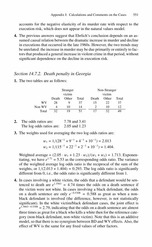
Appendix I: Calculations and Comments on the Cases 551
accounts for the negative elasticity of its murder rate with respect to theexecution risk, which does not appear in the natural values model.
4. The previous answers suggest that Ehrlich’s conclusion depends on an as-sumed causal relation between the dramatic increase in murder and declinein executions that occurred in the late 1960s. However, the two trends maybe unrelated: the increase in murder may be due primarily or entirely to fac-tors that produced a general increase in violent crime in that period, withoutsignificant dependence on the decline in execution risk.
Section 14.7.2. Death penalty in Georgia
1. The two tables are as follows:
Stranger Non-Strangervictim victim
Death Other Total Death Other TotalWV 28 9 37 15 22 37
Non WV 4 10 14 2 10 12Total 32 19 51 17 32 49
2. The odds ratios are: 7.78 and 3.41The log odds ratios are: 2.05 and 1.23
3. The weights used for averaging the two log odds ratios are:
w1 = 1/(28−1 + 9−1 + 4−1 + 10−1) = 2.013
w2 = 1/(15−1 + 22−1 + 2−1 + 10−1) = 1.404.
Weighted average = (2.05 · w1 + 1.23 · w2)/(w1 + w2) = 1.713. Exponen-tiating, we have e1.71 = 5.53 as the corresponding odds ratio. The varianceof the weighted average log odds ratio is the reciprocal of the sum of theweights, or 1/(2.013 + 1.404) = 0.293. The log odds ratio is significantlydifferent from 0, i.e., the odds ratio is significantly different from 1.
4. In cases involving a white victim, the odds that a defendant would be sen-tenced to death are e1.5563 = 4.74 times the odds on a death sentence ifthe victim were not white. In cases involving a black defendant, the oddson a death sentence are only e−0.5308 = 0.588 as great as when a non-black defendant is involved (the difference, however, is not statisticallysignificant). In the white victim/black defendant cases, the joint effect ise1.5663−0.5308 = 2.79, indicating that the odds on a death sentence are almostthree times as great for a black who kills a white then for the reference cate-gory (non-black defendant, non-white victim). Note that this is an additivemodel, so that there is no synergism between BD and WV effects. Also, theeffect of WV is the same for any fixed values of other factors.
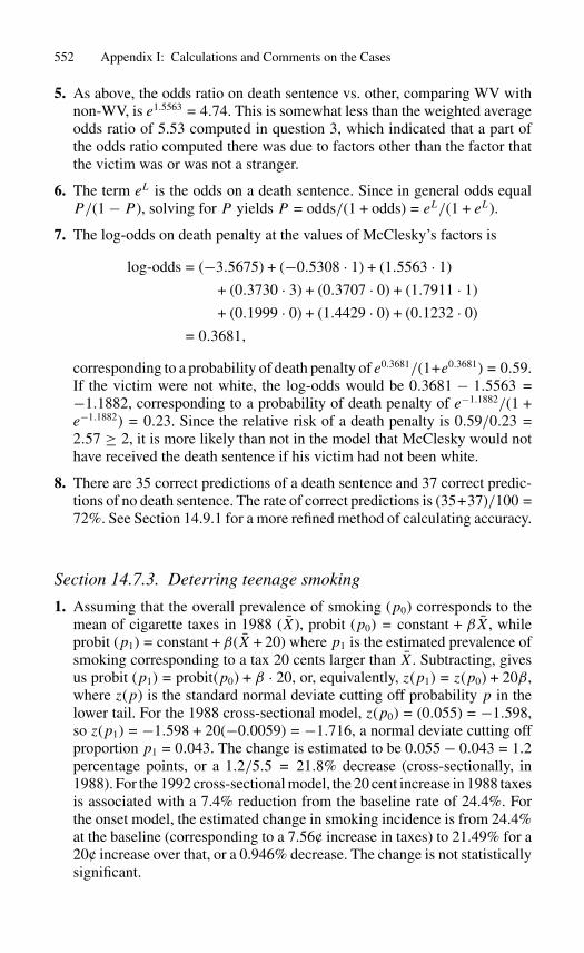
552 Appendix I: Calculations and Comments on the Cases
5. As above, the odds ratio on death sentence vs. other, comparing WV withnon-WV, is e1.5563 = 4.74. This is somewhat less than the weighted averageodds ratio of 5.53 computed in question 3, which indicated that a part ofthe odds ratio computed there was due to factors other than the factor thatthe victim was or was not a stranger.
6. The term eL is the odds on a death sentence. Since in general odds equalP/(1 − P ), solving for P yields P = odds/(1 + odds) = eL/(1 + eL).
7. The log-odds on death penalty at the values of McClesky’s factors is
log-odds = (−3.5675) + (−0.5308 · 1) + (1.5563 · 1)
+ (0.3730 · 3) + (0.3707 · 0) + (1.7911 · 1)
+ (0.1999 · 0) + (1.4429 · 0) + (0.1232 · 0)
= 0.3681,
corresponding to a probability of death penalty of e0.3681/(1+e0.3681) = 0.59.If the victim were not white, the log-odds would be 0.3681 − 1.5563 =−1.1882, corresponding to a probability of death penalty of e−1.1882/(1 +e−1.1882) = 0.23. Since the relative risk of a death penalty is 0.59/0.23 =2.57 ≥ 2, it is more likely than not in the model that McClesky would nothave received the death sentence if his victim had not been white.
8. There are 35 correct predictions of a death sentence and 37 correct predic-tions of no death sentence. The rate of correct predictions is (35+37)/100 =72%. See Section 14.9.1 for a more refined method of calculating accuracy.
Section 14.7.3. Deterring teenage smoking
1. Assuming that the overall prevalence of smoking (p0) corresponds to themean of cigarette taxes in 1988 (X), probit (p0) = constant + βX, whileprobit (p1) = constant + β(X + 20) where p1 is the estimated prevalence ofsmoking corresponding to a tax 20 cents larger than X. Subtracting, givesus probit (p1) = probit(p0) + β · 20, or, equivalently, z(p1) = z(p0) + 20β,where z(p) is the standard normal deviate cutting off probability p in thelower tail. For the 1988 cross-sectional model, z(p0) = (0.055) = −1.598,so z(p1) = −1.598 + 20(−0.0059) = −1.716, a normal deviate cutting offproportion p1 = 0.043. The change is estimated to be 0.055 − 0.043 = 1.2percentage points, or a 1.2/5.5 = 21.8% decrease (cross-sectionally, in1988). For the 1992 cross-sectional model, the 20 cent increase in 1988 taxesis associated with a 7.4% reduction from the baseline rate of 24.4%. Forthe onset model, the estimated change in smoking incidence is from 24.4%at the baseline (corresponding to a 7.56¢ increase in taxes) to 21.49% for a20¢ increase over that, or a 0.946% decrease. The change is not statisticallysignificant.
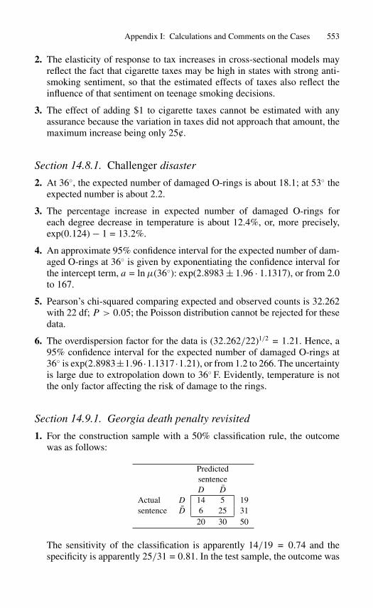
Appendix I: Calculations and Comments on the Cases 553
2. The elasticity of response to tax increases in cross-sectional models mayreflect the fact that cigarette taxes may be high in states with strong anti-smoking sentiment, so that the estimated effects of taxes also reflect theinfluence of that sentiment on teenage smoking decisions.
3. The effect of adding $1 to cigarette taxes cannot be estimated with anyassurance because the variation in taxes did not approach that amount, themaximum increase being only 25¢.
Section 14.8.1. Challenger disaster
2. At 36◦, the expected number of damaged O-rings is about 18.1; at 53◦ theexpected number is about 2.2.
3. The percentage increase in expected number of damaged O-rings foreach degree decrease in temperature is about 12.4%, or, more precisely,exp(0.124) − 1 = 13.2%.
4. An approximate 95% confidence interval for the expected number of dam-aged O-rings at 36◦ is given by exponentiating the confidence interval forthe intercept term, a = ln µ(36◦): exp(2.8983 ± 1.96 · 1.1317), or from 2.0to 167.
5. Pearson’s chi-squared comparing expected and observed counts is 32.262with 22 df; P > 0.05; the Poisson distribution cannot be rejected for thesedata.
6. The overdispersion factor for the data is (32.262/22)1/2 = 1.21. Hence, a95% confidence interval for the expected number of damaged O-rings at36◦ is exp(2.8983±1.96 ·1.1317 ·1.21), or from 1.2 to 266. The uncertaintyis large due to extropolation down to 36◦ F. Evidently, temperature is notthe only factor affecting the risk of damage to the rings.
Section 14.9.1. Georgia death penalty revisited
1. For the construction sample with a 50% classification rule, the outcomewas as follows:
PredictedsentenceD D
Actual D 14 5 19sentence D 6 25 31
20 30 50
The sensitivity of the classification is apparently 14/19 = 0.74 and thespecificity is apparently 25/31 = 0.81. In the test sample, the outcome was
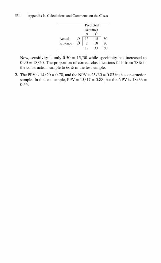
554 Appendix I: Calculations and Comments on the Cases
PredictedsentenceD D
Actual D 15 15 30sentence D 2 18 20
17 33 50
Now, sensitivity is only 0.50 = 15/30 while specificity has increased to0.90 = 18/20. The proportion of correct classifications falls from 78% inthe construction sample to 66% in the test sample.
2. The PPV is 14/20 = 0.70, and the NPV is 25/30 = 0.83 in the constructionsample. In the test sample, PPV = 15/17 = 0.88, but the NPV is 18/33 =0.55.
Appendix II:Tables
A1 The Cumulative Normal DistributionA2 Critical Values of the Standard Normal DistributionB Cumulative Terms of the Binomial DistributionC Percentage Points of the χ2 DistributionD Critical Values of the Durbin-Watson StatisticE Percentage Points of the t DistributionF Percentage Points of the F DistributionG1 Critical Values of the Kolmogorov-Smirnov One-Sample TestG2 Critical Values of the Kolmogorov-Smirnov Two-Sample TestH1 Critical Values of the Wilcoxon Signed-Ranks TestH2 Critical Values of the Wilcoxon Rank-Sum Test
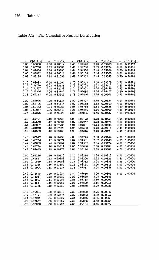
556 Table A1
Table Al: The Cumulative Normal Distribution
z P[Z < z] z P[Z < z] P[Z < z P[Z < z] z P\Z < z]0.000.020.040.060.08
0.100.120.140.160.18
0.200.220.240.260.28
0.300.320.340.360.38
0.400.420.440.460.48
0.500.520.540.560.58
0.600.620.640.660.68
0.700.720.740.760.78
0.500000.507980.515950.523920.53188
0.539830.547760.555670.563560.57142
0.579260.587060.594830.602570.61026
0.617910.625520.633070.640580.64803
0.655420.662760.670030.677240.68439
0.691460.698470.705400.712260.71904
0.725750.732370.738910.745370.75175
0.758040.764240.770350.776370.78230
0.800.820.840.860.88
0.900.920.940.960.98
1.001.021.041.061.08
1.101.121.141.161.18
1.201.221.241.261.28
1.301.321.341.361.38
1.401.421.441.461.48
1.501.521.541.561.58
0.788140.793890.799550.805110.81057
0.815940.821210.826390.831470.83646
0.841340.846140.850830.855430.85993
0.864330.868640.872860.876980.88100
0.884930.888770.892510.896170.89973
0.903200.906580.909880.913090.91621
0.919240.922200.925070.927860.93056
0.933190.935740.938220.940620.94295
1.601.621.641.661.68
1.701.721.741.761.78
1.801.821.841.861.88
1.901.921.941.961.98
2.002.022.042.062.08
2.102.122.142.162.18
2.202.222.242.262.28
2.302.322.342.362.38
0.945200.947380.949500.951540.95352
0.955430.957280.959070.960800.96246
0.964070.965620.967120.968560.96995
0.971280.972570.973810.975000.97615
0.977250.978310.979320.980300.98124
0.982140.983000.983820.984610.98837
0.986100.986790.987450.988090.98870
0.989280.989830.990360.990860.99134
2.402.422.442.462.48
2.502.522.542.562.58
2.602.622.642.662.68
2.702.722.742.762.78
2.802.822.842.862.88
2.902.922.942.962.98
3.003.053.103.153.20
3.253.303.353.403.45
0.991800.992240.992660.993050.99343
0.993790.994130.994460.994770.99506
0.995340.995600.995850.996090.99632
0.996530.99674£.996930.997110.99728
0.997440.997600.997740.997880.99801
0.998130.998250.998360.998460.99856
0.998650.998860.999030.999180.99931
0.999420.999520.999600.999660.99972
3.503.553.603.653.70
3.753.803.853.903.95
4.004.054.104.154.20
4.254.304.354.404.45
4.504.554.604.654.70
4.754.804.854.904.95
5.00
0.999770.999810.999840.999870.99989
0.999910.999930.999940.999950.99996
0.999970.999970.999980.999980.99999
0.999990.99999Q. 999990.999991.00000
1.000001.000001.000001.000001.00000
1.000001.000001.000001.000001.00000
1.00000
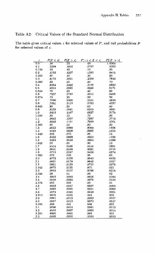
Appendix II: Tables 557
Table A2: Critical Values of the Standard Normal Distribution
The table gives critical values z for selected values of P, and tail probabilities Pfor selected values of z.
p\z P[z P\-z <Z < z] P[\Z\ > z]0.00.10.1260.20.2530.30.3850.40.50.5240.60.6740.70.80.8420.91.01.0361.11.21.2821.31.41.4401.51.61.6451.71.81.91.9602.02.12.22.2422.32.3262.42.52.5762.62.72.82.8132.93.03.0903.13.23.2913.3
.50
.5398
.55
.5793
.60
.6179
.65
.6554
.6915
.70
.7257
.75
.7580
.7881
.80
.8159
.8413
.85
.8643
.8849
.90
.9032
.9192
.925
.9332
.9452
.95
.9554
.9641
.9713
.975
.9772
.9821
.9861
.9875
.9893
.99
.9918
.9938
.995
.9953
.9965
.9974
.9975
.9981
.9987
.999
.9990
.9993
.9995
.9995
.50
.4602
.45
.4207
.40
.3821
.35
.3446
.3085
.30
.2743
.25
.2420
.2119
.20
.1841
.1587
.15
.1357
.1151
.10
.0968
.0808
.075
.0668
.0548
.05
.0446
.0359
.0287
.025
.0228
.0179
.0139
.0125
.0107
.01
.0082
.0062
.005
.0047
.0035
.0026
.0025
.0019
.0013
.001
.0010
.0007
.0005
.0005
.00
.0797
.10
.1585
.20
.2358
.30
.3108
.3829
.40
.4515
.50
.5161
.5763
.60
.6319
.6827
.70
.7287
.7699
.80
.8064
.8385
.85
.8664
.8904
.90
.9109
.9281
.9426
.95
.9545
.9643
.9722
.975
.9786
.98
.9836
.9876
.99
.9907
.9931
.9949
.995
.9963
.9973
.998
.9981
.9986
.999
.9990
1.0000.9203.90.8415.80.7642.70.6892.6171.60.5485.50.4839.4237.40.3681.3173.30.2713.2301.20.1936.1615.15.1336.1096.10.0891.0719.0574.05.0455.0357.0278.025.0214.02.0164.0124.01.0093.0069.0051.005.0037.0027.002.0019.0014.001.0010
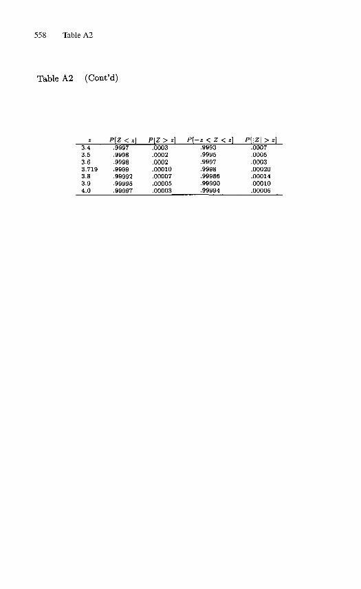
558 Table A2
Table A2 (Cont'd)
P[Z < z] P\Z > z] P[-z < Z < z] P[\Z\ > z]3.43.53.63.7193.83.94.0
.9997
.9998
.9998
.9999
.99992
.99995
.99997
.0003
.0002
.0002
.00010
.00007
.00005
.00003
.9993
.9995
.9997
.9998
.99986
.99990
.99994
.0007
.0005
.0003
.00020
.00014
.00010
.00006
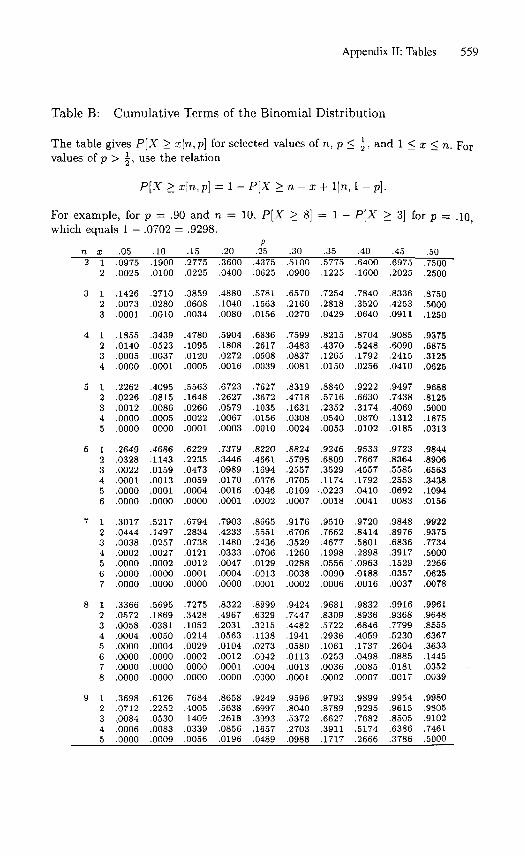
Appendix II: Tables 559
Table B: Cumulative Terms of the Binomial Distribution
The table gives P[X > x\n,p] for selected values of n, p < | , and 1 < x < n. For
values of p > | , use the relation
P[X >x\n,p] = 1 - P[X >n-x+ l|n, 1 -p ] .
For example, for p = .90 and n = 10, P[X > 8] = 1 - P[X > 3] for p = .10,which equals 1 - .0702 = .9298.
vn x .05 .10 .15 ,20 .25 .30 .35 .40 .45 .502 I !0975 T900 .2775 .3600 .4375 .5100 .5775 .6400 .6975 .7500
2 .0025 .0100 .0225 .0400 .0625 .0900 .1225 .1600 .2025 .25003 1 .1426 .2710 .3859 .4880 .5781 .6570 .7254 .7840 .8336 .8750
2 .0073 .0280 .0608 .1040 .1563 .2160 .2818 .3520 .4253 .50003 .0001 .0010 .0034 .0080 .0156 .0270 .0429 .0640 .0911 .1250
4 1 .1855 .3439 .4780 .5904 .6836 .7599 .8215 .8704 .9085 .93752 .0140 .0523 .1095 .1808 .2617 .3483 .4370 .5248 .6090 .68753 .0005 .0037 .0120 .0272 .0508 .0837 .1265 .1792 .2415 .31254 .0000 .0001 .0005 .0016 .0039 .0081 .0150 .0256 .0410 .0625
5 1 .2262 .4095 .5563 .6723 .7627 .8319 .8840 .9222 .9497 .96882 .0226 .0815 .1648 .2627 .3672 .4718 .5716 .6630 .7438 .81253 .0012 .0086 .0266 .0579 .1035 .1631 .2352 .3174 .4069 .50004 .0000 .0005 .0022 .0067 .0156 .0308 .0540 .0870 .1312 .18755 .0000 .0000 .0001 .0003 .0010 .0024 .0053 .0102 .0185 .0313
6 1 .2649 .4686 .6229 .7379 .8220 .8824 .9246 .9533 .9723 .98442 .0328 .1143 .2235 .3446 .4661 .5798 .6809 .7667 .8364 .89063 .0022 .0159 .0473 .0989 .1694 .2557 .3529 .4557 .5585 .65634 .0001 .0013 .0059 .0170 .0376 .0705 .1174 .1792 .2553 .34385 .0000 .0001 .0004 .0016 .0046 .0109 .0223 .0410 .0692 .10946 .0000 .0000 .0000 .0001 .0002 .0007 .0018 .0041 .0083 .0156
7 1 .3017 .5217 .6794 .7903 .8565 .9176 .9510 .9720 .9848 .99222 .0444 .1497 .2834 .4233 .5551 .6706 .7662 .8414 .8976 .93753 .0038 .0257 .0738 .1480 .2436 .3529 .4677 .5801 .6836 .77344 .0002 .0027 .0121 .0333 .0706 .1260 .1998 .2898 .3917 .50005 .0000 .0002 .0012 .0047 .0129 .0288 .0556 .0963 .1529 .22666 .0000 .0000 .0001 .0004 .0013 .0038 .0090 .0188 .0357 .06257 .0000 .0000 .0000 .0000 .0001 .0002 .0006 .0016 .0037 .0078
8 1 .3366 .5695 .7275 .8322 .8999 .9424 .9681 .9832 .9916 .99612 .0572 .1869 .3428 .4967 .6329 .7447 .8309 .8936 .9368 .96483 .0058 .0381 .1052 .2031 -3215 .4482 .5722 .6846 .7799 .85554 .0004 .0050 .0214 .0563 .1138 .1941 .2936 .4059 .5230 .63675 .0000 .0004 .0029 .0104 .0273 .0580 .1061 .1737 .2604 .36336 .0000 .0000 .0002 .0012 .0042 .0113 .0253 .0498 .0885 .14457 .0000 .0000 .0000 .0001 .0004 .0013 .0036 .0085 .0181 .03528 .0000 .0000 .0000 .0000 .0000 .0001 .0002 .0007 .0017 .0039
9 1 .3698 .6126 .7684 .8658 .9249 .9596 .9793 .9899 .9954 .99802 .0712 .2252 .4005 .5638 .6997 .8040 .8789 .9295 .9615 .98053 .0084 .0530 .1409 .2618 .3993 .5372 .6627 .7682 .8505 .91024 .0006 .0083 .0339 .0856 .1657 .2703 .3911 .5174 .6386 .74615 .0000 .0009 .0056 .0196 .0489 .0988 .1717 .2666 .3786 .5000
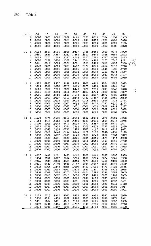
560 Table B
n
10
11
12
13
14
X
6789
12345678910
1234567891011
123456789101112
12345678910111213
12345
.05.0000.0000.0000.0000
.4013
.0861
.0115
.0010
.0001
.0000
.0000
.0000
.0000
.0000
.4312
.1019
.0152
.0016
.0001
.0000
.0000
.0000
.0000
.0000
.0000
.4596
.1184
.0196
.0022
.0002
.0000
.0000
.0000
.0000
.0000
.0000
.0000
.4867
.1354
.0245
.0031
.0003
.0000
.0000
.0000
.0000
.0000
.0000
.0000
.0000
.5123
.1530
.0301
.0042
.0004
.10.0001.0000.0000.0000
.6513
.2639
.0702
.0128
.0016
.0001
.0000
.0000
.0000
.0000
.6862
.3026
.0896
.0185
.0028
.0003
.0000
.0000
.0000
.0000
.0000
.7176
.3410
.1109
.0256
.0043
.0005
.0001
.0000
.0000
.0000
.0000
.0000
.7458
.3787
.1339
.0342
.0065
.0009
.0001
.0000
.0000
.0000
.0000
.0000
.0000
.7712
.4154
.1584
.0441
.0092
.15.0006.0000.0000.0000
.8031
.4557
.1798
.0500
.0099
.0014
.0001
.0000
.0000
.0000
.8327
.5078
.2212
.0694
.0159
.0027
.0003
.0000
.0000
.0000
.0000
.8578
.5565
.2642
.0922
.0239
.0046
.0007
.0001
.0000
.0000
.0000
.0000
.8791
.6017
.3080
.1180
.0342
.0075
.0013
.0002
.0000
.0000
.0000
.0000
.0000
.8972
.6433
.3521
.1465
.0467
.20.0031.0003.0000.0000
.8926
.6242
.3222
.1209
.0328
.0064
.0009
.0001
.0000
.0000
.9141
.6779
.3826
.1611
.0504
.0117
.0020
.0002
.0000
.0000
.0000
.9313
.7251
.4417
.2054
.0726
.0194
.0039
.0006
.0001
.0000
.0000
.0000
.9450
.7664
.4983
.2527
.0991
.0300
.0070
.0012
.0002
.0000
.0000
.0000
.0000
.9560
.8021
.5519
.3018
.1298
P.25.0100.0013.0001.0000
.9437
.7560
.4744
.2241
.0781
.0197
.0035
.0004
.0000
.0000
.9578
.8029
.5448
.2867
.1146
.0343
.0076
.0012
.0001
.0000
.0000
.9683
.8416
.6093
.3512
.1576
.0544
.0143
.0028
.0004
.0000
.0000
.0000
.9762
.8733
.6674
.4157
.2060
.0802
.0243
.0056
.0010
.0001
.0000
.0000
.0000
.9822
.8990
.7189
.4787
.2585
,30.0253.0043.0004.0000
.9718
.8507
.6172
.3504
.1503
.0473
.0106
.0016
.0001
.0000
.9802
.8870
.6873
.4304
.2103
.0782
.0216
.0043
.0006
.0000
.0000
.9862
.9150
.7472
.5075
.2763
.1178
.0386
.0095
.0017
.0002
.0000
.0000
.9903
.9363
.7975
.5794
.3457
.1654
.0624
.0182
.0040
.0007
.0001
.0000
.0000
.9932
.9525
.8392
.6448
.4158
.35.0536.0112.0014.0001
.9865
.9140
.7384
.4862
.2485
.0949
.0260
.0048
.0005
.0000
.9912
.9394
.7999
.5744
.3317
.1487
.0501
.0122
.0020
.0002
.0000
.9943
.9576
.8487
.6533
.4167
.2127
.0846
.0255
.0056
.0008
.0001
.0000
.9963
.9704
.8868
.7217
.4995
.2841
.1295
.0462
.0126
.0025
.0003
.0000
.0000
.9976
.9795
.9161
.7795
.5773
.40.0994.0250.0038.0003
.9940
.9536
.8327
.6177
.3669
.1662
.0548
.0123
.0017
.0001
.9964
.9698
.8811
.7037
.4672
.2465
.0994
.0293
.0059
.0007
.0000
.9978
.9804
.9166
.7747
.5618
.3348
.1582
.0573
.0153
.0028
.0003
.0000
.9987
.9874
.9421
.8314
.6470
.4256
.2288
.0977
.0321
.0078
.0013
.0001
.0000
.9992
.9919
.9602
.8757
.7207
.45.1658.0498.0091.0008
.9975
.9767
.9004
.7340
.4956
.2616
.1020
.0274
.0045
.0003
.9986
.9861
.9348
.8089
.6029
.3669
.1738
.0610
.0148
.0022
.0002
.9992
.9917
.9579
.8655
.6956
.4731
.2607
.1117
.0356
.0079
.0011
.0001
.9996
.9951
.9731
.9071
.7721
.5732
.3563
.1788
.0698
.0203
.0041
.0005
.0000
.9998
.9971
.9830
.9368
.8328
.50.2539.0898.0195.0020
.9990
.9893
.9453
.8281 ~
.6230- V
.3770
.1719
.0547
.0107
.0010
.9995
.9941
.9673
.8867
.7256
.5000
.2744
.1133
.0327
.0059
.0005
.9998
.9968
.9807
.9270
.8062
.6128
.3872
.1938
.0730
.0193
.0032
.0002
.9999
.9983
.9888
.9539
.8666
.7095
.5000
.2905
.1334
.0461
.0112
.0017
.0001
.9999
.9991
.9935
.9713
.9102
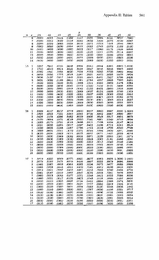
Appendix II: Tables 561
n x67891011121314
15 1234567891011121314
IS
16 12345678
910111213141516
17 1234567891011121314151617
.05.0000.0000.0000.0000.0000.0000.0000.0000.0000
.5367
.1710
.0362
.0055
.0006
.0001
.0000
.0000
.0000
.00000000.0000.0000.0000.0000
.5599
.1892
.0429
.0070
.0009
.0001
.0000
.0000
.0000
.0000
.0000
.0000
.0000
.0000
.0000
.0000
.5819
.2078
.0503
.0088
.0012
.0001
.0000
.0000
.0000
.0000
.0000
.0000
.0000
.0000
.0000
.0000
.0000
.10.0015.0002.0000.0000.0000.0000.0000.0000.0000
.7941
.4510
.1841
.0556
.0127
.0022
.0003
.0000
.0000
.0000
.0000
.0000
.0000
.0000
.0000
.8147
.4853
.2108
.0684
.0170
.0033
.0005
.0001
.0000
.0000
.0000
.0000
.0000
.0000
.0000
.0000
.8332
.5182
.2382
.0826
.0221
.0047
.0008
.0001
.0000
.0000
.0000
.0000
.0000
.0000
.0000
.0000
.0000
15.0115.0022.0003.0000.0000.0000.0000.0000.0000
.9126
.6814
.3958
.1773
.0617
.0168
.0038
.0006
.0001
.0000
.0000
.0000
.0000
.0000
.0000
.9257
.7161
.4386
.2101
.0791
.0235
.0056
.0011
.0002
.0000
.0000
.0000
.0000
.0000
.0000
.0000
.9369
.7475
.4802
.2444
.0987
.0319
.0083
.0017
.0003
.0000
.0000
.0000
.0000
.0000
.0000
.0000
.0000
.20
.0439
.0116
.0024
.0004
.0000
.0000
.0000
.0000
.0000
.9648
.8329
.6020
.3518
.1642
.0611
.0181
.0042
.0008
.0001
.0000
.0000
.0000
.0000
.0000
.9719
.8593
.6482
.4019
.2018
.0817
.0267
.0070
.0015
.0002
.0000
.0000
.0000
.0000
.0000
.0000
.9775
.8818
.6904
.4511
.2418
.1057
.0377
.0109
.0026
.0005
.0001
.0000
.0000
.0000
.0000
.0000
.0000
p.25.1117.0383.0103.0022.0003.0000.0000.0000.0000
.9866
.9198
.7639
.5387
.3135
.1484
.0566
.0173
.0042
.0008
.0001
.0000
.0000
.0000
.0000
.9900
.9365
.8029
.5950
.3698
.1897
.0796
.0271
.0075
.0016
.0003
.0000
.0000
.0000
.0000
.0000
.9925
.9499
.8363
.6470
.4261
.2347
.1071
.0402
.0124
.0031
.0006
.0001
.0000
.0000
.0000
.0000
.0000
.30.2195.0933.0315.0083.0017.0002.0000.0000.0000
.9953
.9647
.8732
.7031
.4845
.2784
.1311
.0500
.0152
.0037
.0007
.0001
.0000
.0000
.0000
.9967
.9739
.9006
.7541
.5501
.3402
.1753
.0744
.0257
.0071
.0016
.0003
.0000
.0000
.0000
.0000
.9977
.9807
.9226
.7981
.6113
.4032
.2248
.1046
.0403
.0127
.0032
.0007
.0001
.0000
.0000
.0000
.0000
.35.3595.1836.0753.0243.0060.0011.0001.0000.0000
.9984
.9858
.9383
.8273
.6481
.4357
.2452
.1132
.0422
.0124
.0028
.0005
.0001
.0000
.0000
.9990
.9902
.9549
.8661
.7108
.5100
.3119
.1594
.0671
.0229
.0062
.0013
.0002
.0000
.0000
.0000
.9993
.9933
.9673
.8972
.7652
.5803
.3812
.2128
.0994
.0383
.0120
.0030
.0006
.0001
.0000
.0000
.0000
.40.5141.3075.1501.0583.0175.0039.0006.0001.0000
.9995
.9948
.9729
.9095
.7827
.5968
.3902
.2131
.0950
.0338
.0093
.0019
.0003
.0000
.0000
.9997
.9967
.9817
.9349
.8334
.6712
.4728
.2839
.1423
.0583
.0191
.0049
.0009
.0001
.0000
.0000
.9998
.9979
.9877
.9536
.8740
.7361
.5522
.3595
.1989
.0919
.0348
.0106
.0025
.0005
.0001
.0000
.0000
.45.6627.4539.2586.1189.0426.0114.0022.0003.0000
.9999
.9983
.9893
.9576
.8796
.7392
.5478
.3465
.1818
.0769
.0255
.0063
.0011
.0001
.0000
.9999
.9990
.9934
.9719
.9147
.8024
.6340
.4371
.2559
.1241
.0486
.0149
.0035
.0006
.0001
.0000
1.0000.9994.9959.9816.9404.8529.7098.5257.3374.1834.0826.0301.0086.0019.0003.0000.0000
.50.7880.6047.3953.2120.0898.0287.0065.0009.0001
1.0000.9995,9963.9824.9408.8491.6964.5000.3036.1509.0592.0176.0037.0005.0000
1.0000.9897.9979.9894.9616.8949.7728.5982.4018.2272.1051.0384.0106.0021.0003.0000
1.0000.9999.9988.9936.9755.9283.8338.6855.5000.3145.1662.0717.0245.0064.0012.0001.0000
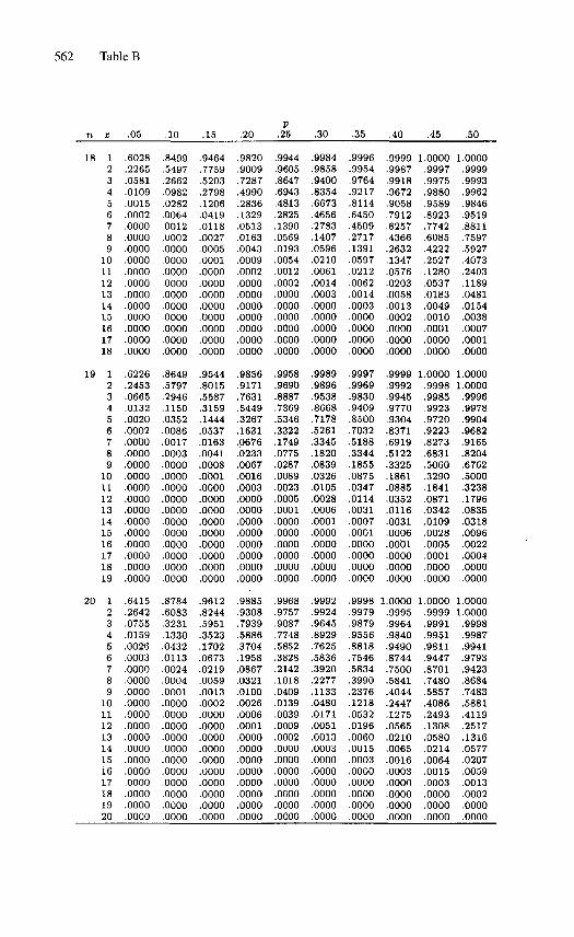
562 Table B
n x
18 123456789101112
.05
.6028
.2265
.0581
.0109
.0015
.0002
.0000
.0000
.0000
.0000
.0000
.0000
.10
.8499
.5497
.2662
.0982
.0282
.0064
.0012
.0002
.0000
.0000
.0000
.0000
.15
.9464
.7759
.5203
.2798
.1206
.0419
.0118
.0027
.0005
.0001
.0000
.0000
.20
.9820
.9009
.7287
.4990
.2836
.1329
.0513
.0163
.0043
.0009
.0002
.0000
P.25
.9944
.9605
.8647
.6943
.4813
.2825
.1390
.0569
.0193
.0054
.0012
.0002
.30
.9984
.9858
.9400
.8354
.6673
.4656
.2783
.1407
.0596
.0210
.0061
.0014
.35
.9996
.9954
.9764
.9217
.8114
.6450
.4509
.2717
.1391
.0597
.0212
.0062
.40
.9999
.9987
.9918
.9672
.9058
.7912
.62574366.2632.1347.0576.0203
.45
1.0000.9997.9975.9880.9589.8923.7742.6085.4222.2527.1280.0537
.50
1.0000.9999.9993.9962.9846.9519.8811.7597.5927.4073.2403.1189
13 .0000 .0000 .0000 .0000 .0000 .0003 .0014 .0058 .0183 .048114 .0000 .0000 .0000 .0000 .0000 .0000 .0003 .0013 .0049 .015415 .0000 .0000 .0000 .0000 .0000 .0000 .0000 .0002 .0010 .003816 .0000 .0000 .0000 .0000 .0000 .0000 .0000 .0000 .0001 .000717 .0000 .0000 .0000 .0000 .0000 .0000 .0000 .0000 .0000 .000118 .0000 .0000 .0000 .0000 .0000 .0000 .0000 .0000 .0000 .0000
19 1 .6226 .8649 .9544 .9856 .9958 .9989 .9997 .9999 1.0000 1.00002 .2453 .5797 .8015 .9171 .9690 .9896 .9969 .9992 .9998 1.00003 .0665 .2946 .5587 .7631 .8887 .9538 .9830 .9945 .9985 .999645678910111213141516171819
20 1234567891011121314151617181920
.0132
.0020
.0002
.0000
.0000
.0000
.0000
.0000
.0000
.0000
.0000
.0000
.0000
.0000
.0000
.0000
.6415
.2642
.0755
.0159
.0026
.0003
.0000
.0000
.0000
.0000
.0000
.0000
.0000
.0000
.0000
.0000
.0000
.0000
.0000
.0000
.1150
.0352
.0086
.0017
.0003
.0000
.0000
.0000
.0000
.0000
.0000
.0000
.0000
.0000
.0000
.0000
.8784
.6083
.3231
.1330
.0432
.0113
.0024
.0004
.0001
.0000
.0000
.0000
.0000
.0000
.0000
.0000
.0000
.0000
.0000
.0000
.3159
.1444
.0537
.0163
.0041
.0008
.0001
.0000
.0000
.0000
.0000
.0000
.0000
.0000
.0000
.0000
.9612
.8244
.5951
.3523
.1702
.0673
.0219
.0059
.0013
.0002
.0000
.0000
.0000
.0000
.0000
.0000
.0000
.0000
.0000
.0000
.5449
.3267
.1631
.0676
.0233
.0067
.0016
.0003
.0000
.0000
.0000
.0000
.0000
.0000
.0000
.0000
.9885
.9308
.7939
.5886
.3704
.1958
.0867
.0321
.0100
.0026
.0006
.0001
.0000
.0000
.0000
.0000
.0000
.0000
.0000
.0000
.7369
.5346
.3322
.1749
.0775
.0287
.0089
.0023
.0005
.0001
.0000
.0000
.0000
.0000
.0000
.0000
.9968
.9757
.9087
.7748
.5852
.3828
.2142
.1018
.0409
.0139
.0039
.0009
.0002
.0000
.0000
.0000
.0000
.0000
.0000
.0000
.8668
.7178
.5261
.3345
.1820
.0839
.0326
.0105
.0028
.0006
.0001
.0000
.0000
.0000
.0000
.0000
.9992
.9924
.9645
.8929
.7625
.5836
.3920
.2277
.1133
.0480
.0171
.0051
.0013
.0003
.0000
.0000
.0000
.0000
.0000
.0000
.9409
.8500
.7032
.5188
.3344
.1855
.0875
.0347
.0114
.0031
.0007
.0001
.0000
.0000
.0000
.0000
.9998
.9979
.9879
.9556
.8818
.7546
.5834
.3990
.2376
.1218
.0532
.0196
.0060
.0015
.0003
.0000
.0000
.0000
.0000
.0000
.9770
.9304
.8371
.6919
.5122
.3325
.1861
.0885
.0352
.0116
.0031
.0006
.0001
.0000
.00000000
1.0000.9995.9964.9840.9490.8744.7500.5841.4044.2447.1275.0565.0210.0065.0016.0003.0000.0000.0000.0000
.9923
.9720
.9223
.8273
.6831
.5060
.3290
.1841
.0871
.0342
.0109
.0028
.0005
.0001
.0000
.0000
1.0000.9999.9991.9951.9811.9447.8701.7480.5857.4086.2493.1308.0580.0214.0064.0015.0003.0000.0000.0000
.9978
.9904
.9682
.9165
.8204
.6762
.5000
.3238
.1796
.0835
.0318
.0096
.0022
.0004
.0000
.0000
1.00001.0000.9998.9987.9941.9793.9423.8684.7483.5881.4119.2517.1316.0577.0207.0059.0013.0002.0000.0000
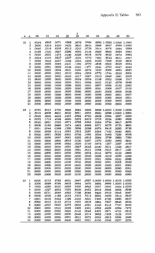
Appendix II: Tables 563
n x
21 123456789101112131415161718192021
22 12345678910111213141516171819202122
23 1234567891011121314
.05
.6594
.2830
.0849
.0189
.0032
.0004
.0000
.0000
.0000
.0000
.0000
.0000
.0000
.0000
.0000
.0000
.0000
.0000
.0000
.0000
.0000
.6765
.3018
.0948
.0222
.0040
.0006
.0001
.0000
.0000
.0000
.0000
.0000
.0000
.0000
.0000
.0000
.0000
.0000
.0000
.0000
.0000
.0000
.6926
.3206
.1052
.0258
.0049
.0008
.0001
.0000
.0000
.0000
.0000
.0000
.0000
.0000
.10
.8906
.6353
.3516
.1520
.0522
.0144
.0033
.0006
.0001
.0000
.0000
.0000
.0000
.0000
.0000
.0000
.0000
.0000
.0000
.0000
.0000
.9015
.6608
.3800
.1719
.0621
.0182
.0044
.0009
.0001
.0000
.0000
.0000
.0000
.0000
.0000
.0000
.0000
.0000
.0000
.0000
.0000
.0000
.9114
.6849
.4080
.1927
.0731
.0226
.0058
.0012
.0002
.0000
.0000
.0000
.0000
.0000
.15
.9671
.8450
.6295
.3887
.1975
.0827
.0287
.0083
.0020
.0004
.0001
.0000
.0000
.0000
.0000
.0000
.0000
.0000
.0000
.0000
.0000
.9720
.8633
.6618
.4248
.2262
.0999
.0368
.0114
.0030
.0007
.0001
.0000
.0000
.0000
.0000
.0000
.0000
.0000
.0000
.0000
.0000
.0000
.9762
.8796
.6920
.4604
.2560
.1189
.0463
.0152
.0042
.0010
.0002
.0000
.0000
.0000
.20
.9908
.9424
.8213
.6296
.4140
.2307
.1085
.0431
.0144
.0041
.0010
.0002
.0000
.0000
.0000
.0000
.0000
.0000
.0000
.0000
.0000
.9926
.9520
.8455
.6680
.4571
.2674
.1330
.0561
.0201
.0061
.0016
.0003
.0001
.0000
.0000
.0000
.0000
.0000
.0000
.0000
.0000
.0000
.9941
.9602
.8668
.7035
.4993
.3053
.1598
.0715
.0273
.0089
.0025
.0006
.0001
.0000
P.25
.9976
.9810
.9255
.8083
.6326
.4334
.2564
.1299
.0561
.0206
.0064
.0017
.0004
.0001
.0000
.0000
.0000
.0000
.0000
.0000
.0000
.9982
.9851
.9394
.8376
.6765
.4832
.3006
.1615
.0746
.0295
.0100
.0029
.0007
.0001
.0000
.0000
.0000
.0000
.0000
.0000
.0000
.0000
.9987
.9884
.9508
.8630
.7168
.5315
.3463
.1963
.0963
.0408
.0149
.0046
.0012
.0003
.30
.9994
.9944
.9729
.9144
.8016
.6373
.4495
.2770
.1477
.0676
.0264
.0087
.0024
.0006
.0001
.0000
.0000
.0000
.0000
.0000
.0000
.9996
.9959
.9793
.9319
.8355
.6866
.5058
.3287
.1865
.0916
.0387
.0140
.0043
.0011
.0002
.0000
.0000
.0000
.0000
.0000
.0000
.0000
.9997
.9970
.9843
.9462
.8644
.7312
.5601
.3819
.2291
.1201
.0546
.0214
.0072
.0021
.35
.9999
.9986
.9914
.9669
.9076
.7991
.6433
.4635
.2941
.1623
.0772
.0313
.0108
.0031
.0007
.0001
.0000
.0000
.0000
.0000
.0000
.9999
.9990
.9939
.9755
.9284
.8371
.6978
.5264
.3534
.2084
.1070
.0474
.0180
.0058
.0016
.0003
.0001
.0000
.0000
.0000
.0000
.0000
1.0000.9993.9957.9819.9449.8691.7466.5864.4140.2592.1425.0682.0283.0100
.40
1.0000.9997.9976.9890.9630.9043.7998.6505.4763.3086.1744.0849.0352.0123.0036.0008.0002.0000.0000.0000.0000
1.0000.9998.9984.9924.9734.9278.8416.7102.5460.3756.2280.1207.0551.0215.0070.0019.0004.0001.0000.0000.0000.0000
1.0000.9999.9990.9948.9810.9460.8760.7627.6116.4438.2871.1636.0813.0349
.45
1.0000.9999.9994.9969.9874.9611.9036.8029.6587.4883.3210.1841.0908.0379.0132.0037.0008.0001.0000.0000.0000
1.00001.0000.9997.9980.9917.9729.9295.8482.7236.5650.3963.2457.1328.0617.0243.0080.0021.0005.0001.0000.0000.0000
1.00001.0000.9998.9988.9945.9814.9490.8848.7797.6364.4722.3135.1836.0937
.50
1.00001.0000.9999.9993.9964.9867.9608.9054.8083.6682.5000.3318.1917.0946.0392.0133.0036.0007.0001.0000.0000
1.00001.0000.9999.9996.9978.9915.9738.9331.8569.7383.5841.4159.2617.1431.0669.0262.0085.0022.0004.0001.0000.0000
1.00001.00001.0000.9998.9987.9947.9827.9534.8950.7976.6612.5000.3388.2024
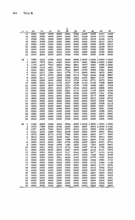
564 Table B
p
n x .05 ,10 ,15 .20 ,25 .30 .35 .40 .45 ,5015 .0000 ,0000 .0000 .0000 .0001 .0005 .0030 .0128 .0411 .105016 .0000 .0000 .0000 .0000 .0000 .0001 .0008 .0040 .0153 .046617 .0000 .0000 .0000 .0000 .0000 .0000 .0002 .0010 .0048 .017318 .0000 .0000 .0000 .0000 .0000 .0000 .0000 .0002 .0012 .005319 .0000 .0000 .0000 .0000 .0000 .0000 .0000 .0000 .0002 .001320 .0000 .0000 .0000 .0000 .0000 .0000 .0000 .0000 ^0000 .000221 .0000 .0000 .0000 .0000 .0000 .0000 .0000 .0000 .0000 .000022 .0000 .0000 .0000 .0000 .0000 .0000 .0000 .0000 .0000 .000023 .0000 .0000 .0000 .0000 .0000 0000 .0000 .0000 .0000 .0000
24 1 .7080 .9202 .9798 .9953 .9990 .9998 1.0000 1.0000 1.0000 1.00002 .3392 .7075 .8941 .9669 .9910 .9978 .9995 .9999 1.0000 1.00003 .1159 .4357 .7202 .8855 .9602 .9881 .9970 .9993 .9999 1.00004 .0298 .2143 .4951 .7361 .8850 .9576 .9867 .9965 .9992 .99995 .0060 .0851 .2866 .5401 .7534 .8889 .9578 .9866 .9964 .99926 .0010 .0277 .1394 .3441 .5778 .7712 .8956 .9600 .9873 .99677 .0001 .0075 .0572 .1889 .3926 .6114 .7894 .9040 .9636 .98878 .0000 .0017 .0199 .0892 .2338 .4353 .6425 .8081 .9137 .96809 .0000 .0003 .0059 .0362 .1213 .2750 .4743 .6721 .8270 .924210 .0000 .0001 .0015 .0126 .0547 .1528 .3134 .5109 .7009 .846311 .0000 .0000 .0003 .0038 .0213 .0742 .1833 .3498 .5461 .729412 .0000 .0000 .0001 .0010 .0072 .0314 .0942 .2130 .3849 .580613 .0000 .0000 .0000 .0002 .0021 .0115 .0423 .1143 .2420 .419414 .0000 .0000 .0000 .0000 .0005 .0036 .0164 .0535 .1341 .270615 .0000 .0000 .0000 .0000 .0001 .0010 .0055 .0217 .0648 .153716 .0000 .0000 .0000 .0000 .0000 .0002 .0016 .0075 .0269 .075817 .0000 .0000 .0000 .0000 .0000 .0000 .0004 .0022 .0095 .032018 .0000 .0000 .0000 .0000 .0000 .0000 .0001 .0005 .0028 .011319 .0000 .0000 .0000 .0000 .0000 ' .0000 .0000 .0001 .0007 .003320 .0000 .0000 .0000 .0000 .0000 .0000 .0000 .0000 .0001 .000821 .0000 .0000 .0000 .0000 .0000 .0000 .0000 .0000 .0000 .000122 .0000 .0000 .0000 .0000 .0000 .0000 .0000 .0000 .0000 .000023 .0000 .0000 .0000 .0000 .0000 .0000 .0000 .0000 .0000 .000024 .0000 .0000 .0000 .0000 .0000 .0000 .0000 .0000 .0000 .0000
25 1 .7226 .9282 .9828 .9962 .9992 .9999 1.0000 1.0000 1.0000 1.00002 .3576 .7288 .9069 .9726 .9930 .9984 .9997 .9999 1.0000 1.0000-3 .1271 .4629 .7463 .9018 .9679 .9910 .9979 .9996 .9999 1.00004 .0341 .2364 .5289 .7660 .9038 .9668 .9903 .9976 .9995 .99995 .0072 .0980 .3179 .5793 .7863 .9095 .9680 .9905 .9977 .99956 .0012 .0334 .1615 .3833 .6217 .8065 .9174 .9706 .9914 .99807 .0002 .0095 .0695 .2200 .4389 .6593 .8266 .9264 .9742 .99278 .0000 .0023 .0255 .1091 .2735 .4882 .6939 .8464 .9361 .97849 .0000 .0005 .0080 .0468 .1494 .3231 .5332 .7265 .8660 .946110 .0000 .0001 .0021 .0173 .0713 .1894 .3697 .5754 .7576 .885211 .0000 .0000 .0005 .0056 .0297 .0978 .2288 .4142 .6157 .787812 .0000 .0000 .0001 .0015 .0107 .0442 .1254 .2677 .4574 .655013 .0000 .0000 .0000 .0004 .0034 .0175 .0604 .1538 .3063 .500014 .0000 .0000 .0000 .0001 .0009 .0060 .0255 .0778 .1827 .345015 .0000 .0000 .0000 .0000 .0002 .0018 .0093 .0344 .0960 .212216 .0000 .0000 .0000 .0000 .0000 .0005 .0029 .0132 .0440 .114817 .0000 .0000 .0000 .0000 .0000 .0001 .0008 .0043 .0174 .053918 .0000 .0000 .0000 .0000 .0000 .0000 .0002 .0012 .0058 .021619 .0000 .0000 .0000 .0000 .0000 .0000 .0000 .0003 .0016 .007320 .0000 .0000 .0000 .0000 0000 .0000 .0000 .0001 .0004 .002021 .0000 .0000 .0000 .0000 .0000 .0000 .0000 .0000 .0001 .000522 .0000 .0000 .0000 .0000 .0000 .0000 .0000 .0000 .0000 .000123 .0000 .0000 .0000 .0000 .0000 .0000 .0000 .0000 .0000 .000024 .0000 .0000 .0000 .0000 .0000 .0000 .0000 .0000 .0000 .000025 .0000 .0000 .0000 .0000 .0000 .0000 .0000 .0000 .0000 .0000
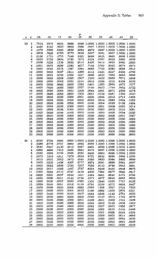
Appendix II: Tables 565
n x
30 123456789101112131415161718192021222324252627282930
35 12345678910111213141516171819202122232425262728
.05
.7854
.4465
.1878
.0608
.0156
.0033
.0006
.0001
.0000
.0000
.0000
.0000
.0000
.0000
.0000
.0000
.0000
.0000
.0000
.0000
.0000
.0000
.0000
.0000
.0000
.0000
.0000
.0000
.oooo
.0000
.8339
.5280
.2542
.0958
.0290
.0073
.0015
.0003
.0000
.0000
.0000
.ooqo
.0000
.0000
.0000
.0000
.0000
.0000
.0000
.0000
.0000
.0000
.0000
.0000
.0000
.0000
.0000
.0000
.10
.9576
.8163
.5886
.3526
.1755
.0732
.0258
.0078
.0020
.0005
.0001
.0000
.0000
.0000
.0000
.0000
.0000
.0000
.0000
.0000
.0000
.0000
.0000
.0000
.0000
.0000
.0000
.0000
.0000
.0000
.9750
.8776
.6937
.4690
.2693
.1316
.0552
.0200
.0063
.0017
.0004
.0001
.0000
.0000
.0000
.0000
.0000
.0000
.0000
.0000
.0000
.0000
.0000
.0000
.0000
.0000
.0000
.0000
.15
.9924
.9520
.8486
.6783
.4755
.2894
.1526
.0698
.0278
.0097
.0029
.0008
.0002
.0000
.0000
.0000
.0000
.0000
.0000
.0000
.0000
.0000
.0000
.0000
.0000
.0000
.0000
.0000
.0000
.0000
.9966
.9757
.9130
.7912
.6193
.4311
.2652
.1438
.0689
.0292
.0110
.0037
.0011
.0003
.0001
.0000
.0000
.0000
.0000
.0000
.0000
.0000
.0000
.0000
.0000
.0000
.0000
.0000
.20
.9988
.9895
.9558
.8773
.7448
.5725
.3930
.2392
.1287
.0611
.0256
.0095
.0031
.0009
.0002
.0001
.0000
.0000
.0000
.0000
.0000
.0000
.0000
.0000
.0000
.0000
.0000
.0000
.0000
.0000
.9996
.9960
.9810
.9395
.8565
.7279
.5672
.4007
.2550
.1457
.0747
.0344
.0142
.0053
.0018
.0005
.0001
.0000
.0000
.0000
.0000
.0000
.0000
.0000
.0000
.0000
.0000
.0000
p.25
.9998
.9980
.9894
.9626
.9021
.7974
.6519
.4857
.3264
.1966
.1057
.0507
.0216
.0082
.0027
.0008
.0002
.0001
.0000
.0000
.0000
.0000
.0000
.0000
.0000
.0000
.0000
.0000
.0000
.0000
1.0000
.9995
.9967
.9864
.9590
.9024
.8080
.6777
.5257
.3737
.2419
.1421
.0756
.0363
.0158
.0062
.0022
.0007
.0002
.0001
.0000
.0000
.0000
.0000
.0000
.0000
.0000
.0000
.30
1.0000.9997
.9979
.9907
.9698
.9234
.8405
.7186
.5685
.4112
.2696
.1593
.0845
.0401
.0169
.0064
.0021
.0006
.0002
.0000
.0000
.0000
.0000
.0000
.0000
.0000
.0000
.0000
.0000
.0000
1.0000
.9999
.9995
.9976
.9909
.9731
.9350
.8674
.7659
.6354
.4900
.3484
.2271
.1350
.0731
.0359
.0160
.0064
.0023
.0008
.0002
.0001
.0000
.0000
.0000
.0000
.0000
.0000
.35
1.00001.0000
.9997
.9981
.9925
.9767
.9414
.8762
.7753
.6425
.4922
.3452
.2198
.1263
.0652
.0301
.0124
.0045
.0014
.0004
.0001
.0000
.0000
.0000
.0000
.0000
.0000
.0000
.0000
.0000
1.0000
1.0000
.9999
.9997
.9984
.9942
.9830
.9581
.9110
.8349
.7284
.5981
.4577
.3240
.2109
.1256
.0682
.0336
.0150
.0061
.0022
.0007
.0002
.0001
.0000
.0000
.0000
.0000
111
1
.40
.0000
.0000
.0000
.9997
.9985
.9943
.9828
.9565
.9060
.8237
.7085
.5689
.4215
.2855
.1754
.0971
.0481
.0212
.0083
.0029
.0009
.0002
.0000
.0000
.0000
.0000
.0000
.0000
.0000
.0000
.0000
1.000011.0000
.0000
.9998
.9990
.9966
.9898
.9740
.9425
.8877
.8048
.6943
.5639
.4272
.2997
.1935
.1143
.0615
.0300
.0133
.0053
.0019
.0006
.0002
.0000
.0000
.0000
.45
1.00001.00001.00001.0000.9998.9989.9960.9879.9688.9306.8650.7673.6408.4975.3552.2309.1356.0714.0334.0138.0050.0016.0004.0001.0000.0000.0000.0000.0000.0000
1.00001.00001.00001.00001.0000.9999.9995.9981.9943.9848.9646.9271.8656.7767.6624.5315.3976.2751.1749.1016.0536.0255.0109.0042.0014.0004.0001.0000
.50
1.00001.00001.00001.00001.0000.9998.9993.9974.9919.9786.9506.8998.8192.7077.5722.4278.2923.1808.1002.0494.0214.0081.0026.0007.0002.0000.0000.0000.0000.0000
1.00001.00001.00001.00001.00001.0000.9999.9997.9991.9970.9917.9795.9552.9123.8447.7502.6321.5000.3679.2498.1553.0877.0448.0205.0083.0030.0009.0003
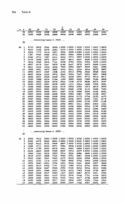
566 Table B
.05 .10 .15 .20P
.25 .30 .35 .40 .45 .5029
30.0000 .0000 .0000 .0000 .0000 .0000 .0000 .0000 .0000 .0001.0000 .0000 .0000 .0000 .0000 .0000 .0000 .0000 .0000 .0000
35. . . remaining terms = .0000 . •.
40 123456789101112131415161718192021222324252627282930313233
.8715
.6009
.3233
.1381
.0480
.0139
.0034
.0007
.0001
.0000
.0000
.0000
.0000
.0000
.0000
.0000
.0000
.0000
.0000
.0000
.0000
.0000
.0000
.0000
.0000
.0000
.0000
.0000
.0000
.0000
.0000
.0000
.0000
.9852
.9195
.7772
.5769
.3710
.2063
.0995
.0419
.0155
.0051
.0015
.0004
.0001
.0000
.0000
.0000
.0000
.0000
.0000
.0000
.0000
.0000
.0000
.0000
.0000
.0000
.0000
.0000
.0000
.0000
.0000
.0000
.0000
.9985
.9879
.9514
.8698
.7367
.5675
.3933
.2441
.1354
.0672
.0299
.0120
.0043
.0014
.0004
.0001
.0000
.0000
.0000
.0000
.0000
.0000
.0000
.0000
.0000
.0000
.0000
.0000
.0000
.0000
.0000
.0000
.0000
.9999
.9985
.9921
.9715
.9241
.8387
.7141
.5629
.4069
.2682
.1608
.0875
.0432
.0194
.0079
.0029
.0010
.0003
.0001
.0000
.0000
.0000
.0000
.0000
.0000
.0000
.0000
.0000
.0000
.0000
.0000
.0000
.0000
1.0000.9999.9990.9953.9840.9567.9038.8180.7002.5605.4161.2849.1791.1032.0544.0262.0116.0047.0017.0006.0002.0000.0000.0000.0000.0000.0000.0000.0000.0000.0000.0000.0000
1.00001.0000.9999.9994.9974.9914.9762.9447.8890.8041.6913.5594.4228.2968.1926.1151.0633.0320.0148.0063.0024.0009.0003.0001.0000.0000.0000.0000.0000.0000.0000.0000.0000
1.00001.00001.0000.9999.9997.9987.9956.9876.9697.9356.8785.7947.6857.5592.4279.3054.2022.1239.0699.0363.0173.0075.0030.0011.0004.0001.0000.0000.0000.0000.0000.0000.0000
11.0000.00001.000011.0000.0000.9999.9994.9979.9939.9844.9648.9291.8715.7888.6826.5598.4319.3115.2089.1298.0744.0392.0189.0083.0034.0012.0004.0001.0000.0000.0000.0000.0000
1.00001.00001.00001.00001.00001.0000.9999.9998.9991.9973.9926.9821.9614.9249.8674.7858.6815.5609.4349.3156.2130.1331.0767.0405.0196.0086.0034.0012.0004.0001.0000.0000.0000
1.00001.00001.00001.00001.00001.00001.00001.0000.9999.9997.9989.9968.9917.9808.9597.9231.8659.7852.6821.5627.4373.3179.2148.1341.0769.0403.0192.0083.0032.0011.0003.0001.0000
40. . . remaining terms = .0000 . . .
45 12345678910111213141516171819
.9006
.6650
.3923
.1866
.0729
.0239
.0066
.0016
.0003
.0001
.0000
.0000
.0000
.0000
.0000
.0000
.0000
.0000
.0000
.9913
.9476
.8410
.6711
.4729
.2923
.1585
.0757
.0320
.0120
.0040
.0012
.0003
.0001
.0000
.0000
.0000
.0000
.0000
.9993
.9940
.9735
.9215
.8252
.6858
.5218
.3606
.2255
.1274
.0651
.0302
.0127
.0048
.0017
.0005
.0002
.0000
.0000
1.0000.9995.9968.9871.9618.9098.8232.7025.5593.4120.2795.1741.0995.0521.0250.0110.0044.0017.0006
1.00001.0000.9997.9984.9941.9821.9554.9059.8275.7200.5911.4543.3252.2159.1327.0753.0395.0191.0085
1.00001.00001.0000.9999.9993.9974.9920.9791.9529.9066.8353.7380.6198.4912.3653.2538.1642.0986.0549
1.00001.00001.00001.0000.9999.9997.9990.9967.9909.9780.9531.9104.8453.7563.6467.5248.4017.2887.1940
111111
.0000
.0000
.0000
.0000
.0000
.0000
.9999
.9996
.9988
.9964
.9906
.9784
.9554
.9164
.8570
.7751
.6728
.5564
.4357
111
.0000
.0000
.00001.000011
1
.0000
.0000
.0000
.0000
.9999
.9996
.9987
.9964
.9910
.9799
.9591
.9238
.8698
.7944
.6985
1.00001.00001.00001.00001.00001.00001.00001.00001.00001.0000.9999.9996.9988.9967.9920.9822.9638.9324.8837
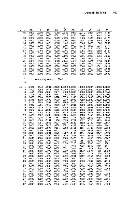
Appendix II: Tables 567
n x
2021222324252627282930313233343536
.05.0000.0000
.0000
.0000
.0000
.0000
.0000
.0000
.0000
.0000
.0000
.0000
.0000
.0000
.0000
.0000
.0000
.10.0000.0000
.0000
.0000
.0000
.0000
.0000
.0000
.0000
.0000
.0000
.0000
.0000
.0000
.0000
.0000
.0000
.15.0000.0000
.0000
.0000
.0000
.0000
.0000
.0000
.0000
.0000
.0000
.0000
.0000
.0000
.0000
.0000
.0000
.20.0002
.0001
.0000
.0000
.0000
.0000
.0000
.0000
.0000
.0000
.0000
.0000
.0000
.0000
.0000
.0000
.0000
p.25.0035.0013
.0005
.0001
.0000
.0000
.0000
.0000
.0000
.0000
.0000
.0000
.0000
.0000
.0000
.0000
.0000
.30.0283.0135
.0060
.0024
.0009
.0003
.0001
.0000
.0000
.0000
.0000
.0000
.0000
.0000
.0000
.0000
.0000
.35.1215.0708
.0382
.0191
.0089
.0038
.0015
.0005
.0002
.0001
.0000
.0000
.0000
.0000
.0000
.0000
.0000
.40.3214.2223.1436.0865.0483.0250.0120.0053.0021.0008.0003.0001.0000.0000.0000.0000.0000
.45.5869.4682.3526.2494.1650.1017.0582.0308.0150.0068.0028.0010.0004.0001.0000.0000.0000
.50.8144.7243.6170.5000.3830.2757.1856.1163.0676.0362.0178.0080.0033.0012.0004.0001.0000
45. . . remaining terms = .0000 .. .
50 1234567891Q111213141516171819-?o21222324252627282930313233343536373839
.9231
.7206
.4595
.2396
.1036
.0378
.0118
.0032
.0008
.0002
.0000
.0000
.0000
.0000
.0000
.0000
.0000
.0000
.0000
.0000
.0000
.0000
.0000
.0000
.0000
.0000
.0000
.0000
.0000
.0000
.0000
.0000
.0000
.0000
.0000
.0000
.0000
.0000
.0000
.9948
.9662
.8883
.7497
.5688
.3839
.2298
.1221
.0579
.0245
.0094
.0032
.0010
.0003
.0001
.0000
.0000
.0000
.0000
.0000
.0000
.0000
.0000
.0000
.0000
.0000
.0000
.0000
.0000
.0000
.0000
.0000
.0000
.0000
.0000
.0000
.0000
.0000
.0000
.9997
.9971
.9858
.9540
.8879
.7806
.6387
.4812
.3319
.2089
.1199
.0628
.0301
.0132
.0053
.0019
.0007
.0002
.0001
.0000
.0000
.0000
.0000
.0000
.0000
.0000
.0000
.0000
.0000
.0000
.0000
.0000
.0000
.0000
.0000
.0000
.0000
.0000
.0000
1.0000.9998.9987.9943.9815.9520.8966.8096.6927.5563.4164.2893.1861.1106.0607.0308.0144.0063.0025.0009.0003.0001.0000.0000.0000.0000.0000.0000.0000.0000.0000.0000.0000.0000.0000.0000.0000.0000.0000
1.00001.0000.9999.9995.9979.9930.9806.9547.9084.8363.7378.6184.4890.3630.2519.1631.0983.0551.0287.0139.0063.0026.0010.0004.0001.0000.0000.0000.0000.0000.0000.0000.0000.0000.0000.0000.0000.0000.0000
1.00001.00001.00001.0000.9998.9993.9975.9927.9817.9598.9211.8610.7771.6721.5532.4308.3161.2178.1406.0848.0478.0251.0123.0056.0024.0009.0003.0001.0000.0000.0000.0000.0000.0000.0000.0000.0000.0000.0000
1.00001.00001.00001.00001.0000.9999.9998.9992.9975.9933.9840.9658.9339.8837.8122.7199.6111.4940.3784.2736.1861.1187.0710.0396.0207.0100.0045.0019.0007.0003.0001.0000.0000.0000.0000.0000.0000.0000.0000
1111111
.0000
.0000
.0000
.0000
.0000
.0000
.0000
.9999
.9998
.9992
.9978
.9943
.9867
.9720
.9460
.9045
.8439
.7631
.6644
.5535
.4390
.3299
.2340
.1562
.0978
.0573
.03140160.0076.0034.0014.0005.0002.0001.0000.0000.000000000000
1.00001.00001.00001.00001.00001.00001.00001.00001.0000.9999.9998.9994.9982.9955.9896.9780.9573.9235.8727.8026.7138.6100.4981.3866.2840.1966.1279.0780.0444.0235.0fl6.0053.0022.0009.0003.0001.0000.0000.0000
1.0000.0000.0000.0000.0000.0000.0000.00001.0000.0000L.0000L.0000.9998.9995.9987.9967.9923.9836.9675T9405.8987.8389.7601.6641.5561.4439.3359.2399.1611.1013.0595.0325.0164.0077.0033.0013.0005.0002.0000
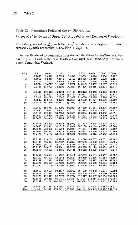
568 Table C
Table C: Percentage Points of the x2 Distribution
Values of x2 in Terms of Upper Tail Probability and Degrees of Freedom v
The table gives values xl,p such that a x2 variable with v degrees of freedomexceeds xl,P with probability p, i.e., P[x2 > xl,p] = P-
Source: Reprinted by permission from Biometrika Tables for Statisticians, Vol-ume /by E.S. Pearson and H.O. Hartley. Copyright 1954 Cambridge UniversityPress, Cambridge, England.
o.l 0.05 0.025 0.01 0.005 0,001 0.0005 0.000112345
678910
1112131415
1617181920
2122232425
2627282930
4050607080
90100
2.70554.60526.25147.77949.2364
10.644612.017013.361614.683715.9871
17.275018.549419.811921.064222.3072
23.541824.769025.989427.203628.4120
29.615130.813332.006933.196334.3816
35.563136.741237.915939.087540.2560
51.805063.167174.397085.527196.5782
107.565
118.498
3.84155.99157.81479.487711.0705
12.591614.067115.507316.919018.3070
19.675121.026122.362123.684824.9958
26.296227.587128.869330.143531.4104
32.670533.924435-172536.415137.6525
38.885240.113341.337242.556943.7729
55.758567.504879.081990.5312101.879
113.145124.342
5.02397.37789.348411.143312.8325
14.4494
16.012817.534619.022820.4831
21.920023.336724.735626.119027.4884
28.845430.191031.526432.852334.1696
35.478936.780738.075739.364140.6465
41.923243.194444.460745.722246.9792
59.341771.420283.297695.0231
106.629
118.136129.561
6.63499.210311.344913.276715.0863
16.811918.475320.090221.666023.2093
24.725026.217027.688329.141330.5779
31.999933.408734.805336.190837.5662
38.932140.289441.638442.979844.3141
45.641746.963048.278249.587950.8922
63.690776.153988.3794100.425112.329
124.116135.807
7.879410.596612.838114.860216.7496
18.547620.277721.955023.589325.1882
26.756928.299529.819431.319332.8013
34.2672
35.718537.156438.582239.9968
41.401042.795644.181345.558546.9278
48.289949.644950.993252.335653.6720
66.765979.490091.9517104.215116.321
128.299140.169
10.82813.81616.26618.46720.515
22.45824.32226.12527.87729.588
31.26432.90934.52836.12337.697
39.25240.79042.31243.82045.315
46.79748.26849.72851.17952.620
54.05255.47656.89258.302
59.703
73.40286.66199.607112.317124.839
137.208149.449
12.11615.20217.73019.99722.105
24.10326.01827.86829.66631.420
33.13734.82136.47838.10939.719
41.30842.87944.43445.97347.498
49.01150.51152.00053.47954.947
56.40757.85859.30060.73562.162
76.09589.560102.695115.578128.261
140.782153.167
15.13718.42121.10823.51325.745
27.85629.87731.82833.72035.564
37.36739.134
40.87142.57944.263
45.92547.56649.18950.79652.386
53.96255.52557.07558.61360.140
61.65763.16464.66266.15267.633
82.06295.969
109.503122.755135.783
148.627161.319
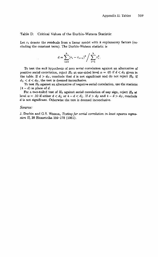
Appendix II: Tables 569
Table D: Critical Values of the Durbin-Watson Statistic
Let n denote the residuals from a linear model with k explanatory factors (ex-cluding the constant term). The Durbin-Watson statistic is
To test the null hypothesis of zero serial correlation against an alternative ofpositive serial correlation, reject Ho at one-sided level a = .05 if d < dt given inthe table. If d > du, conclude that d is not significant and do not reject Ho- Ifdi, < d < dy, the test is deemed inconclusive.
To test Ho against an alternative of negative serial correlation, use the statistic(4 — d) in place of d.
For a two-tailed test of Ho against serial correlation of any sign, reject Ho atlevel a = .10 if either d < d^ or 4 — d < di. If d > du and 4 — d > du, concluded is not significant. Otherwise the test is deemed inconclusive.
Source:J. Durbin and G.S. Watson, Testing for serial correlation in least squares regres-sion II, 38 Biometrika 159-178 (1951).
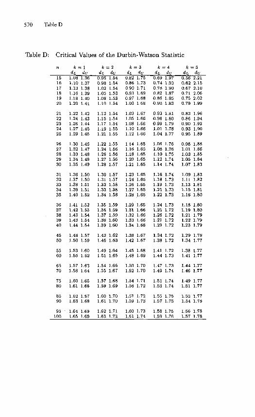
570 Table D
Table D: Critical Values of the Durbin-Watson Statistic71
151617181920
2122232425
2627282930
3132333435
3637383940
4550
5560
6570
7580
8590
95100
k -dL
1.081.101.131.161.181.20
1.221.241.261.271.29
1.301.321.331.341.35
1.361.371.381.391.40
1.411.421.431.431.44
1.481.50
1.531.55
1.571.58
1.601.61
1.621.63
1.641.65
= 1dv
1.361.371.381.391.401.41
1.421.431.441.451.45
1.461.471.481.481.49
1.501.501.511.511.52
1.521.531.541.541.54
1.571.59
1.601.62
1.631.64
1.651.66
1.671.68
1.691.69
A: =dL
0.950.981.021.051.081.10
1.131.151.171.191.21
1.221.241.261.271.28
1.301.311.321.331.34
1.351.361.371.381.39
1.431.46
1.491.51
1.541.55
1.571.59
1.601.61
1.621.63
= 2du1.541.541.541.531.531.54
1.541.541.541.551.55
1.551.561.561.561.57
1.571.571.581.581.58
1.591.591.591.601.60
1.621.63
1.641.65
1.661.67
1.681.69
1.701.70
1.711.72
fc =dL
0.820.860.900.930.971.00
1.031.051.081.101.12
1.141.161.181.201.21
1.231.241.261.271.28
1.291.311.321.331.34
1.381.42
1.451.48
1.501.52
1.541.56
1.571.59
1.601.61
= 3dv
1.751.731.711.691.681.68
1.671.661.661.661.66
1.651.651.651.651.65
1.651.651.651.651.65
1.651.661.661.661.66
1.671.67
1.681.69
1.701.70
1.711.72
1.721.73
1.731.74
fc --dL
0.690.740.780.820.860.90
0.930.960.991.011.04
1.061.081.101.121.14
1.161.181.191.211.22
1.241.251.261.271.29
1.341.38
1.411.44
1.471.49
1.511.53
1.551.57
1.581.59
= 4dv
1.971.931.901.871.851.83
1.811.801.791.781.77
1.761.761.751.741.74
1.741.731.731.731.73
1.731.721.721.721.72
1.721.72
1.721.73
1.731.74
1.741.74
1.751.75
1.751.76
k -dL
0.560.620.670.710.750.79
0.830.860.900.930.95
0.981.011.031.051.07
1.091.111.131.151.16
1.181.191.211.221.23
1.291.34
1.381.41
1.441.46
1.491.51
1.521.54
1.561.57
= 5du
2.212.152.102.062.021.99
1.961.941.921.901.89
1.881.861.851.841.83
1.831.821.811.811.80
1.801.801.791.791.79
1.781.77
1.771.77
1.771.77
1.771.77
1.771.78
1.781.78
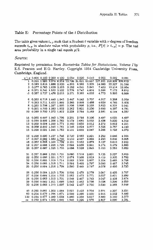
Appendix II: Tables 571
Table E: Percentage Points of the t Distribution
The table gives values tVlP such that a Student t variable with v degrees of freedomexceeds tUsV in absolute value with probability p, i.e., P[\t\ > tUtP\ = p. The tailarea probability in a single tail equals p/2.
Source:Reprinted by permission from Biometrika Tables for Statisticians, Volume I byE.S. Pearson and H.O. Hartley. Copyright 1954 Cambridge University Press,Cambridge, England.
v\p 0.800 0.500 0.200 0.100 0.050 0.020 0.010 0.005 0.002 0.0011234
\5
6789
10
1112131415
1617181920
2122232425
2627282930
4060
120oo
0.3250.2890.2770.2710.267
0.2650.2630.2620.2610.260
0.2600.2590.2590.2580.258
0.2580.2570.2570.2570.257
0.2570.2560.2560.2560.256
0.2560.2560.2560.2560.256
0.2550.2540.2540.253
l.QDO0.8160.7650.7410.727
0.7180.7110.7060.7030.700
0.6970.6950.6940.6920.691
0.6900.6890.6880.6880.687
0.6860.6860.6850.6850.684
0.6840.6840.6830.6830.683
0.6810.6790.6770.674
3.0781.8861.6381.5331.476
1.4401.4151.3971.3831.372
1.3631.3561.3501.3451.341
1.3371.3331.3301.3281.325
1.3231.3211.3191.3181.316
1.3151.3141.3131.3111.310
1.3031.2961.2891.282
6.3142.9202.3532.1322.015
1.9431.8951.8601.8331.812
1.7961.7821.7711.7611.753
1.746JVT40_T7?3T1.7291.725
1.7211.7171.7141.7111.708
1.7061.7031.7011.6991.697
1.6841.6711.6581.645
12.7064.3033.1822.7762.571
2.4472.3652.3062.2622.228
2.2012.1792.1602.1452.131
2.1202.1102.ioi2.0932.086
2.0802.0742.0692.0642.060
2.0562.0522.0482.0452.042
2.0212.0001.9801.960
31.8216.9654.5413.7473.365
3.1432.9982.8962.8212.764
2.7182.6812.6502.6242.602
2.5832.5672.5522.5392.528
2.5182.5082.5002.4922.485
2.4792.4732.4672.4622.457
2.4232.3902.3582.326
63.6579.9255.8414.6044.032
3.7073.4993.3553.2503.169
3.1063.0553.0122.9772.947
2.9212.8982.8782.8612.845
2.8312.8192.8072.7972.787
2.7792.7712.7632.7562.750
2.7042.6602.6172.576
127.32114.0897.4535.5984.773
4.3174.0293.8333.6903.581
3.4973.4283.3723.3263.286
3.2523.2233.1973.1743.153
3.1353.1193.1043.0903.078
3.0673.0573.0473.0383.030
2.9712.9152.8602.807
318.30922.32710.2147.1735.893
5.2084.7854.5014.2974.144
4.0253.9303.8523.7873.733
3.6863.6463.6103.5793.552
3.5273.5053.4853.4673.450
3.4353.4213.4083.3963.385
3.3073.2323.1603.090
636.61931.59812.9248.6106.869
5.9595.4085.0414.7814.587
4.4374.3184.2214.1404.073
4.0153.9653.9223.8833.850
3.8193.7923.7683.7453.725
3.7073.6903.6743.6593.646
3.5513.4603.3733.291
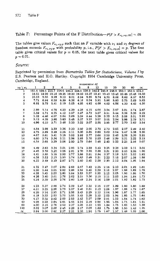
572 Table F
Table F: Percentage Points of the F Distribution—P[F > Fvi,va-,.oa] = .05
The tables give values FUIIU2-P such that an F variable with v\ and v-i degrees offreedom exceeds Fui^2.p with probability p, i.e., P[F > FvllVa-p] = p. The firsttable gives critical values for p = 0.05, the next table gives critical values forp = 0.01.
Source:Reprinted by permission from Biometrika Tables for Statisticians, Volume I byE.S. Pearson and H.O. Hartley. Copyright 1954 Cambridge University Press,Cambridge, England.
v2 \ "112345
6789
10
1112131415
1617181920
2122232425
26272829304060
120oo
1161.4
18.5110.13
7.716.61
5.995.595.325.124.96
4.844.754.674.604.54
4.494.454.414.384.35
4.324.304.284.264.24
4.234.21
" 4.204.184.174.084.003.923.84
2199.5
19.009.556.945.79
5.144.744.464.264.10
3.983.893.813.743.68
3.633.593.553.523.49
3.473.443.423.403.39
3.373.353.343.333.323.233.153.073.00
3215.7
19.169.286.595.41
4.764.354.073.863.71
3.593.493.413.343.29
3.243.203.163.133.10
3.073.053.033.012.99
2.982.962.952.932.922.842.762.682.60
4 5224.6 230.2
19.259.126.395.19
4.534.123.843.633.48
3.363.263.183.113.06
3.012.962.932.902.87
2.842.822.802.782.76
2.742.732.712.702.692.612.532.452.37
19.309.016.265.05
4.393.973.693.483.33
3.203.113.032.962.90
2.852.812.772.742.71
2.682.662.642.622.60
2.592.572.562.552.532.452.372.292.21
numerator6 8
df12 15 20 30
234.0 238.9 243.9 245.9 248.0 250.119.338.946.164.95
4.283.873.583.373.22
3.093.002.922.852.79
2.742.702.662.632.60
2.572.552.532.512.49
2.472.462.452.432.422.342.252.172.10
19.378.856.044.82
4.153.733.443.233.07
2.952.852.772.702.64
2.592.552.512.482.45
2.422.402.372.362.34
2.322.312.292.282.272.182.102.021.94
19.418.745.914.68
4.003.573.283.072.91
2.792.692.602.532.48
2.422.382.342.312.28
2.252.232.202.182.16
2.152.132.122.102.092.001.921.831.75
19.438.705.864.62
3.943.513.223.012.85
2.722.622.532.462.40
2.352.312.272.232.20
2.182.152.132.112.09
2.072.062.042.032.011.921.841.751.67
19.458.665.804.56
3.873.443.152.942.77
2.652.542.462.392.33
2.282.232.192.162.12
2.102.072.052.032.01
1.991.971.961.941.931.841.751.661.57
19.468.625.754.50
3.813.383.082.862.70
2.572.472.382.312.25
2.192.152.112.072.04
2.011.981.961.941.92
1.901.881.871.851.841.741.651.551.46
60 oo252.2 254.3
19.48 19.508.575.694.43
3.743.30 .3.01 '2.792.62
2.492.38 :2.30 '2.22 :2.16 :
2.112.062.021.981.95
1.921.891.861.841.82
1.801.791.771.751.741.641.531.431.32
3.535.631.36
J.67J.232.932.712.54
2.402.302.212.132.07
2.01L.96L.92L.88L.84
1.811.78L76L.731.71
1.69L.671.65L.64L.62L.51L.391.251.00
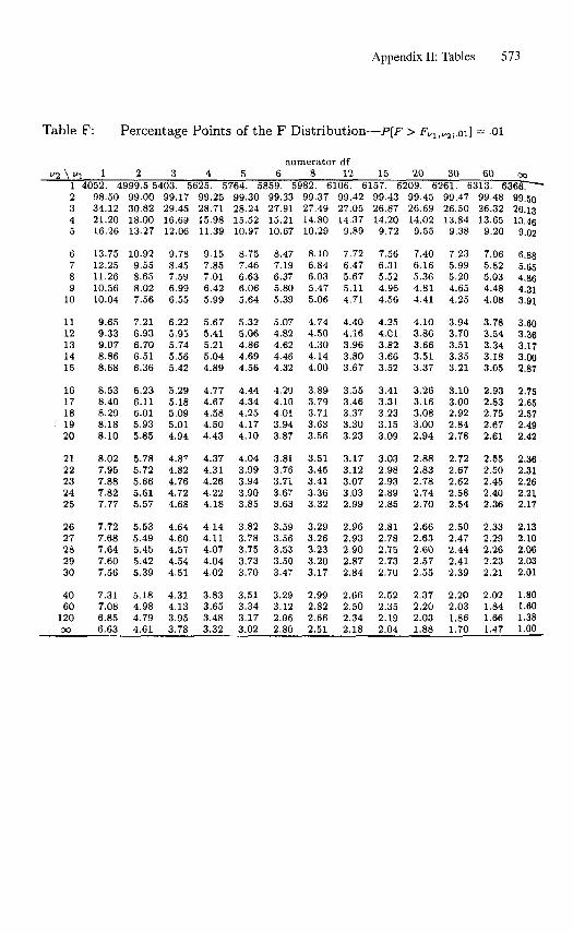
Appendix II: Tables 573
Table F: Percentage Points of the F Distribution—P[F > FuljV2X.oi] = 01
U2\v
12345
6789
10
1112131415
1617181920
2122232425
2627282930
4060
120oo
I 1 2 3 4 5numeratoi
6 8r df
12 15 20 30 60 0 04052. 4999.5 5403. 5625. 5764. 5859. 5982. 6106. 6157. 6209. 6261. 6313. 6366.—~
98.5034.1221.2016.26
13.7512.2511.2610.5610.04
9.659.339.078.868.68
8.538.408.298.188.10
8.027.957.887.827.77
7.727.687.647.607.56
7.317.086.856.63
99.0030.8218.0013.27
10.929.558.658.027.56
7.216.936.706.516.36
6.236.116.015.935.85
5.785.725.665.615.57
5.535.495.455.425.39
5.184.984.794.61
99.1729.4616.6912.06
9.788.457.596.996.55
6.225.955.745.565.42
5.295.185.095.014.94
4.874.824.764.724.68
4.644.604.574.544.51
4.314.133.953.78
99.2528.7115.9811.39
9.157.857.016.425.99
5.675.415.215.044.89
4.774.674.584.504.43
4.374.314.264.224.18
4.144.114.074.044.02
3.833.653.483.32
99.3028.2415.5210.97
8.757.466.636.065.64
5.325.064.864.694.56
4.444.344.254.174.10
4.043.993.943.903.85
3.823.783.753.733.70
3.513.343.173.02
99.3327.9115.2110.67
8.477.196.375.805.39
5.074.824.624.464.32
4.204.104.013.943.87
3.813.763.713.673.63
3.593.563.533.503.47
3.293.122.962.80
99.3727.4914.8010.29
8.106.846.035.475.06
4.744.504.304.144.00
3.893.793.713.633.56
3.513.453.413.363.32
3.293.263.233.203.17
2.992.822.662.51
99.4227.0514.379.89
7.726.475.675.114.71
4.404.163.963.803.67
3.553.463.373.303.23
3.173.123.073.032.99
2.962.932.902.872.84
2.662.502.342.18
99.4326.8714.209.72
7.566.315.524.964.56
4.254.013.823.663.52
3.413.313.233.153.09
3.032.982.932.892.85
2.812.782.752.732.70
2.522.352.192.04
99.4526.6914.029.55
7.406.165.364.814.41
4.103.863.663.513.37
3.263.163.083.002.94
2.882.832.782.742.70
2.662.632.602.572.55
2.372.202.031.88
99.4726.5013.849.38
7.235.995.204.654.25
3.943.703.513.353.21
3.103.002.922.842.78
2.722.672.622.582.54
2.502.472.442.412.39
2.202.031.861.70
99.4826.3213.659.20
7.065.825.034.484.08
3.783.543.343.183.05
2.932.832.752.672.61
2.552.502.452.402.36
2.332.292.262.232.21
2.021.841.661.47
99.5026.1313.469.02
6.885.654.864.313.91
3.603.363.173.002.87
2.752.652.572.492.42
2.362.312.262.212.17
2.132.102.062.032.01
1.801.601.381.00
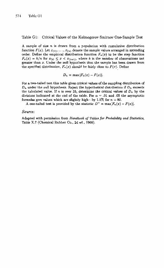
574 Table G1
Table Gl: Critical Values of the Kolmogorov-Smirnov One-Sample Test
A sample of size n is drawn from a population with cumulative distributionfunction F(x). Let X(i), . . . , X(n) denote the sample values arranged in ascendingorder. Define the empirical distribution function Fn{x) to be the step functionFn{x) = k/n for x^y < x < X(i+i), where k is the number of observations notgreater than x. Under the null hypothesis that the sample has been drawn fromthe specified distribution, Fn(x) should be fairly close to F(x). Define
Dn = max\Fn(x) - F(x)\.
For a two-tailed test this table gives critical values of the sampling distribution ofDn under the null hypothesis. Reject the hypothetical distribution if Dn exceedsthe tabulated value. If n is over 35, determine the critical values of Dn by thedivisions indicated at the end of the table. For a = .01 and .05 the asymptoticformulas give values which are slightly high—by 1.5% for n = 80.
A one-tailed test is provided by the statistic D+ = max[F»(i) — F(x)\.
Source:Adapted with permission from Handbook of Tables for Probability and Statistics,Table X.7 (Chemical Rubber Co., 2d ed., 1968).
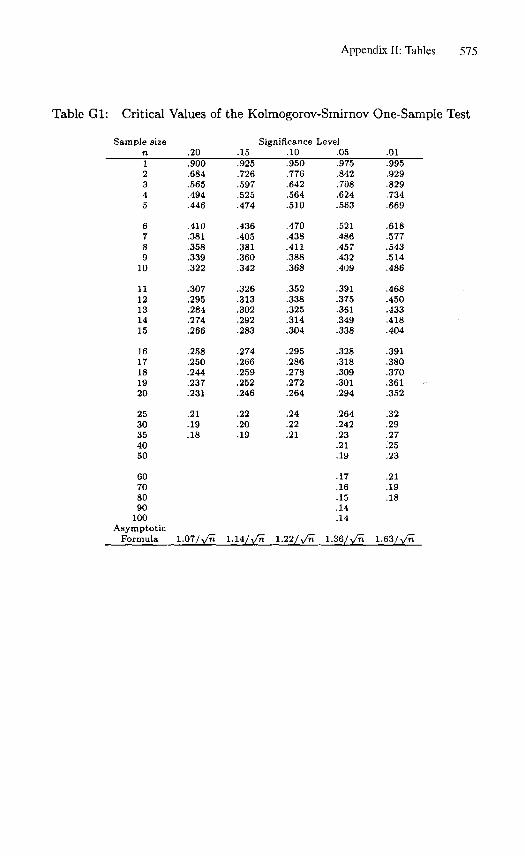
Appendix II: Tables 575
Table Gl: Critical Values of the Kolmogorov-Smirnov One-Sample Test
Sample sizen12345
6789
10
1112131415
1617181920
2530354050
60708090
100Asymptotic
Formula
.20
.900
.684
.565
.494
.446
.410
.381
.358
.339
.322
.307
.295
.284
.274
.266
.258
.250
.244
.237
.231
.21
.19
.18
1.07/Vn
.15
.925
.726
.597
.525
.474
.436
.405
.381
.360
.342
.326
.313
.302
.292
.283
.274
.266
.259
.252
.246
.22
.20
.19
1.14/v
Significance L(.10.950.776.642.564.510
.470
.438
.411
.388
.368
.352
.338
.325
.314
.304
.295
.286
.278
.272
.264
.24
.22
.21
'n 1.22/y/n
3vel.05.975.842.708.624.563
.521
.486
.457
.432
.409
.391
.375
.361
.349
.338
.328
.318
.309
.301
.294
.264
.242
.23
.21
.19
.17
.16
.15
.14
.14
1 . 3 6 / ^
.01
.995
.929
.829
.734
.669
.618
.577
.543
.514
.486
.468
.450
.433
.418
.404
.391
.380
.370
.361
.352
.32
.29
.27
.25
.23
.21
.19
.18
1.63/^/"
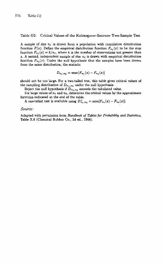
576 Table G2
Table G2: Critical Values of the Kolmogorov-Smirnov Two-Sample Test
A sample of size n\ is drawn from a population with cumulative distributionfunction F(x). Define the empirical distribution function Fni(x) to be the stepfunction Fni(x) = k/n\, where fc is the number of observations not greater thanx. A second, independent sample of size 712 is drawn with empirical distributionfunction Fn3(x). Under the null hypothesis that the samples have been drawnfrom the same distribution, the statistic
£>r.i,n2 = max|Fni(x) - Fn j(z) |
should not be too large. For a two-tailed test, this table gives critical values ofthe sampling distribution of I ) , , , , , under the null hypothesis.
Reject the null hypothesis if Dni,n2 exceeds the tabulated value.For large values of n\ and TI2, determine the critical values by the approximate
formulas indicated at the end of the table.A one-tailed test is available using Dtl<n2 — max[Fni(a:) — Fn2(x)].
Source:
Adapted with permission from Handbook of Tables for Probability and Statistics,Table X.8 (Chemical Rubber Co., 2d ed., 1968).
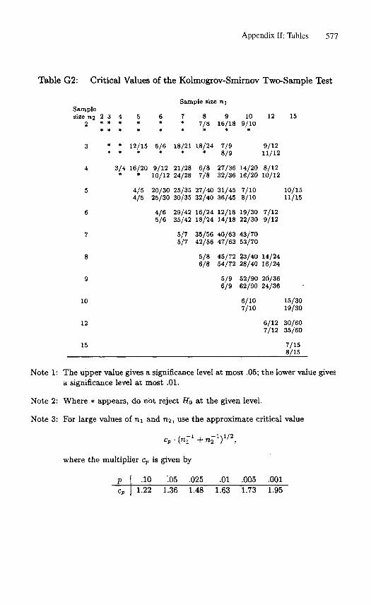
Appendix II: Tables 577
Table G2: Critical Values of the Kolmogrov-Smirnov Two-Sample Test
Samplesize «2 2 3 4
2 * * •
3 • *
4 3/4*
5
6
7
8
9
10
12
15
5
12/15
16/20*
4/54/5
6*
5/6
9/1210/12
20/3025/30
4/65/6
Sample size
7 8* 7/8
18/21
21/2824/28
25/3530/35
29/4235/42
5/75/7
18/24
6/87/8
27/4032/40
16/2418/24
35/5642/56
5/86/8
"1
916/18
7/9
8/9
27/3632/36
31/4536/45
12/1814/18
40/6347/63
45/7254/72
5/96/9
109/10
14/2016/20
7/108/10
19/3022/30
43/7053/70
23/4028/40
52/9062/90
6/107/10
12
9/12
11/12
8/1210/12
7/129/12
14/2416/24
20/3624/36
6/127/12
15
10/1511/15
15/3019/30
30/6035/60
7/158/15
Note 1: The upper value gives a significance level at most .05; the lower value givesa significance level at most .01.
Note 2: Where * appears, do not reject Ho at the given level.
Note 3: For large values of n\ and ri2, use the approximate critical value
where the multiplier cp is given by
pcp 1
.10
.22 1.0536
.0251.48
.011.63
.0051.73
.0011.95
578 Table H1
Table HI: Critical Values of the Wilcoxon Signed Ranks Test
Let di = Xi — yi denote the difference between scores in the ith of n matchedpairs of observations. Rank all the di without regard to sign, giving rank 1 tothe smallest, rank 2 to the next smallest, etc. Then affix the sign of difference dito each corresponding rank. Let W denote the smaller sum of like-signed ranks.This table gives 1%, 2%, 5%, and 10% two-sided critical values Wa for selectedvalues of n. Reject the null hypothesis of no difference between distributions ofx and y for values of W < Wa. For a one-sided test of level a/2, reject Ho onlyif W < Wa and W corresponds to a sum of ranks of proper sign.
Source:Adapted with permission from Handbook of Tables for Probability and Statistics,Table X.2 (Chemical Rubber Co., 2d ed., 1968).

Appendix II: Tables 579
Table HI: Critical Values of the Wilcoxon Signed Ranks Test
Two-sided a .10 .05 .02 .01(One-sided a) (.05) (.025) (.01) (.005)
567891011121314151617181920212223242526272829303132333435363738394041424344454647484950
12468111417212630364147546068758392101110120130141152163175188201214228242256271287303319336353371389408427446466
1246811141721253035404652596673819098107117127137148159171183195208222235250264279295311327344361379397415434
0235710131620242833384349566269778593102111120130141151162174186198211224238252267281297313329345362380398
0235710131619232832374349556168768492100109118128138149160171183195208221234248262277292307323339356373
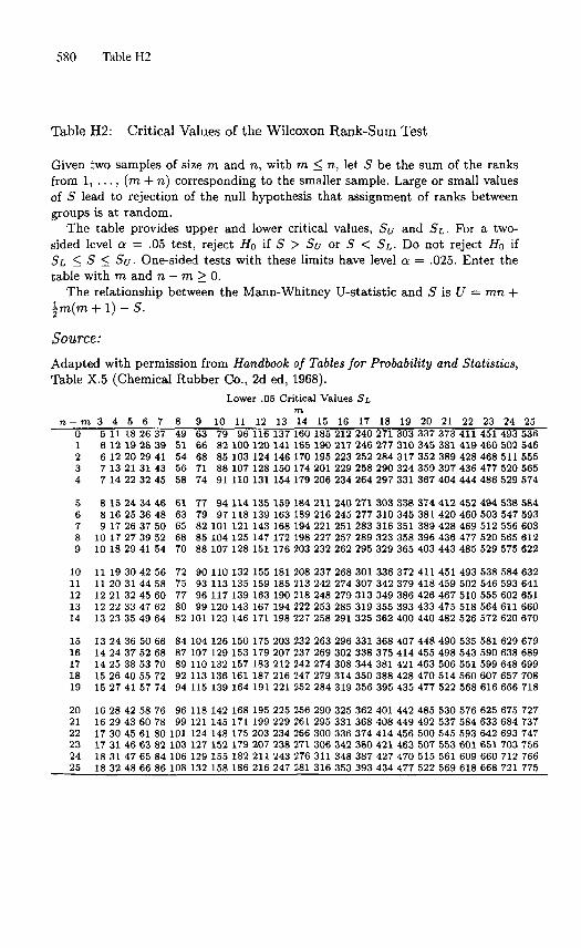
580 Table H2
Table H2: Critical Values of the Wilcoxon Rank-Sum Test
Given two samples of size m and n, with m < n, let S be the sum of the ranksfrom 1, . . . , (m + n) corresponding to the smaller sample. Large or small valuesof 5 lead to rejection of the null hypothesis that assignment of ranks betweengroups is at random.
The table provides upper and lower critical values, Su and SL- For a two-sided level a = .05 test, reject Ho if 5 > Su or S < SL- DO not reject HQ ifSL < S < SU- One-sided tests with these limits have level a = .025. Enter thetable with m and n — m > 0.
The relationship between the Mann-Whitney U-statistic and S is U — mn +
Source:Adapted with permission from Handbook of Tables for Probability and Statistics,Table X.5 (Chemical Rubber Co., 2d ed, 1968).
n - m 3 4 5 6 7 8
Lower .05 Critical Values SLm
10 11 12 13 14 15 16 17 18 19 20 21 22 23 24 25
1011121314
5 11 18 26 376 12 19 28 396 12 20 29 417 13 21 31 437 14 22 32 45
8 15 24 34 468 16 25 36 489 17 26 37 5010 17 27 39 5210 18 29 41 54
11 19 30 42 5611 20 31 44 5812 21 32 45 6012 22 33 47 6213 23 35 49 64
63 79 96 116 137 160 185 212 240 271 303 33766 82 100 120 141 165 190 217 246 277 310 34568 85 103 124 146 170 195 223 252 284 317 35271 88 107 128 150 174 201 229 258 290 324 35974 91 110 131 154 179 206 234 264 297 331 367
373 411 451 493 536381 419 460 502 546389 428 468 511 555397 436 477 520 565404 444 486 529 574
77 94 114 135 159 184 211 240 271 303 338 374 412 452 494 538 58479 97 118 139 163 189 216 245 277 310 345 381 420 460 503 547 59382 101 121 143 168 194 221 251 283 316 351 389 428 469 512 556 60385 104 125 147 172 198 227 257 289 323 358 396 436 477 520 56S 61288 107 128 151 176 203 232 262 295 329 365 403 443 485 529 575 622
72 90 110 132 155 181 208 237 268 301 336 372 411 451 493 538 584 63275 93 113 135 159 185 213 242 274 307 342 379 418 459 502 546 593 64177 96 117 139 163 190 218 248 279 313 349 386 426 467 510 555 602 65180 99 120 143 167 194 222 253 285 319 355 393 433 475 518 564 611 66082 101 123 146 171 198 227 258 291 325 362 400 440 482 526 572 620 670
15 13 24 36 50 66 84 104 126 150 175 203 232 263 296 331 368 407 448 490 535 581 629 67916 14 24 37 52 68 87 107 129 153 179 207 237 269 302 338 375 414 455 498 543 590 638 68917 14 25 38 53 70 89 110 132 157 183 212 242 274 308 344 381 421 463 506 551 599 648 69918 15 26 40 55 72 92 113 136 161 187 216 247 279 314 350 388 428 470 514 560 607 657 70819 15 27 41 57 74 94 115 139 164 191 221 252 284 319 356 395 435 477 522 568 616 666 718
20 16 28 42 58 76 96 118 142 168 195 225 256 290 325 362 401 442 485 530 576 625 675 72721 16 29 43 60 78 99 121 145 171 199 229 261 295 331 368 408 449 492 537 584 633 684 73722 17 30 45 61 80 101 124 148 175 203 234 266 300 336 374 414 456 500 545 593 642 693 74723 17 31 46 63 82 103 127 152 179 207 238 271 306 342 380 421 463 507 553 601 651 703 75624 18 31 47 65 84 106 129 155 182 211 243 276 311 348 387 427 470 515 561 609 660 712 76625 18 32 48 66 86 108 132 158 186 216 247 281 316 353 393 434 477 522 569 618 668 721 775
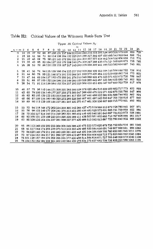
Appendix II: Tables 581
Table H2: Critical Values of the Wilcoxon Rank-Sum Test
Upper .05 Critioil Values Su
n-m 3 4 5 6 7 8 9 10 11 12 13 1-1 15 16 1? 18 "» 20 21 -2 23 24 25 _0 16 25 37 52 68 87 108 131 157 184 214 2-1 <i 280 316 355 395 4J1H 18;! 530 579 630 683 7391 18 28 41 56 73 93 114 138 164 192 223 2.r).r> 290 327 366 407 450 49!) 543 593 644 698 7542 21 32 45 61 78 98 121 145 172 200 231 2IM3OO 337 377 418 4(>2 508 556 606 659 713 7703 23 35 49 65 83 104 127 152 179 208 240271309 347 388 430 471521569 620 673 728 7854 26 38 53 70 88 110 133 159 187 217 2492811.'119 358 399 441 48(i 533 583 634 687 743 801
5 28 41 56 74 94 115 139 166 194 225 257 292 329 368 409 453 498 54<i 596 648 702 758 8166 31 44 60 78 99 121146 173 201233 266301339 379 420 464 510 559 609 662 716 773 8327 33 47 64 83 104 127 152 179 209 241274310 349 389 431476 523 571622 675 730 788 8478 35 51 68 87109 132 158 186 216 249 283 320 358 399 442 487 535 584 635 689 745 803 8639 38 54 71 91 114 138 164 193 224 257 292 329 308 410 453 499 547 597 649 703 759 817 878
10 40 57 75 96 119 144 171200 231265 300338 378 420 464 510 559 609 662 717 773 832 89311 43 60 79 100 124 149 177 207 239 273 309347 388 430 475 522 571622 675 730 788 847 90912 45 63 83 105 129 155 183 213 246 28131735(1397 441486 533 583 634 688 744 802 862 92413 48 66 87 109 134 160189 220 253 289 326 366 407 451497 545 595 647 701758 816 877 94014 50 69 90113 139 166 196 227 261297 335 375 417 461508 556 607 660 715 772 831 892 955
15 53 72 94 118 144 172 202 234 268 305 343 384 427 472 519 568 619 672 728 785 845 907 97116 55 76 98 122 149 177 208 241276 313 352 393 436 482 529 579 631685 741799 859 922 98617 58 79 102 127154 183 214 248 283 321360 402 446 492 540 591643 697 754 813 873 936 100118 60 82 105 131159 188220254290329369411456502551602655 710767826888 951101719 63 85 109 135 164 194 227 261298 337 377 420 466 513 562 613 667 723 780 840 902 966 1032
20 65 88 113 140169 200 233 268 305 345 386 430 475 523 573 625 679 735 793 854 916 981104821 68 91117144174 205 239 275 313 353 395 430 485 533 584 636 691748 807 868 931 996 106322 70 94 120 149 179 211 245 282 320 361 403 448 495 544 595 648 703 760 820 881 945 1011 107823 73 97 124 153 184 217 251 288 327 369 412 457 504 554 606 659 715 773 833 895 959 1025 109424 75 101 128 157 189 222 258 295 335 377 420460 514 564 616 671 727 785 846 909 973 1040 110925 78104 132 162 194 228 264 302 342 384 429 475 524 575 627 682 739 798 859 922 988 1055 1125
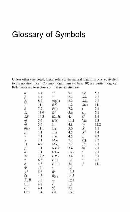
Glossary of Symbols
Unless otherwise noted, log(x) refers to the natural logarithm of x, equivalentto the notation ln(x). Common logarithms (to base 10) are written log10(x).References are to sections of first substantive use.
α 4.4 df 5.1 s.e. 5.3β 4.4 ex 2.2 SSb 7.2βi 8.2 exp(·) 2.2 SSw 7.2� 11.1 EX 1.2 S(t) 11.1δ 7.2 F (·) 7.2 t 7.1� 13.9 G2 5.6 tν,α 7.1�r 14.3 H0, H1 4.4 U 3.4 5.6 H (t) 11.1 Var 1.3 5.6 ln 4.8 W 12.2θ (t) 11.1 log 5.6 X 1.1µ 1.1 min 4.5 X2 1.4ν 7.1 max 4.5 z 4.3π 2.1 MSb 7.2
(n
a
)2.2
� 4.2 MSw 7.2 nCr 2.1ρ 1.1 NPV 3.4 ≈ 2.1σ 1.1 OLS 13.2 ! 2.1� 12.2 PPV 3.4 ∩ 3.1τ 6.3 P [·] 1.1 ∼ 4.2φ 4.3 P [·|·] 3.1
∫11.1
� 12.1 r 1.1χ2 5.6 R2 13.3� 4.5 R2
Z(X) 14.3A, B 3.3 rS 12.4Bin 4.2 s2 1.1cdf 4.1 S2
p 7.1Cov 1.4 s.d. 13.6
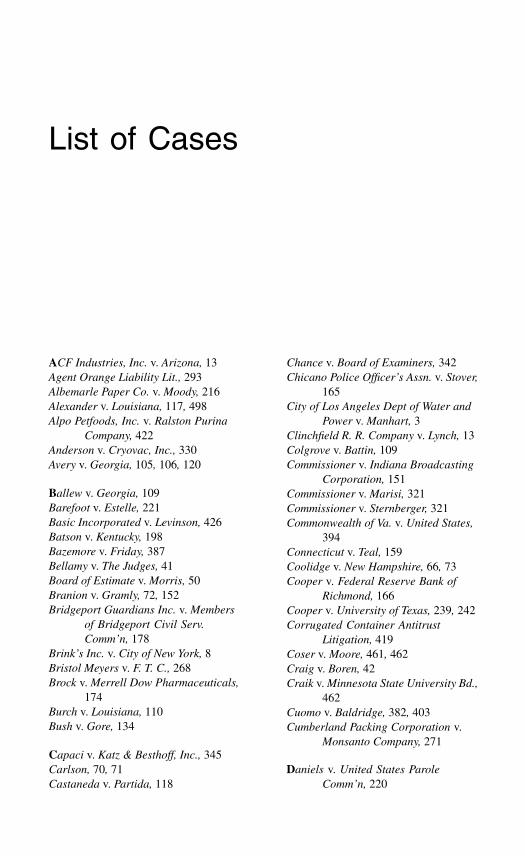
List of Cases
ACF Industries, Inc. v. Arizona, 13Agent Orange Liability Lit., 293Albemarle Paper Co. v. Moody, 216Alexander v. Louisiana, 117, 498Alpo Petfoods, Inc. v. Ralston Purina
Company, 422Anderson v. Cryovac, Inc., 330Avery v. Georgia, 105, 106, 120
Ballew v. Georgia, 109Barefoot v. Estelle, 221Basic Incorporated v. Levinson, 426Batson v. Kentucky, 198Bazemore v. Friday, 387Bellamy v. The Judges, 41Board of Estimate v. Morris, 50Branion v. Gramly, 72, 152Bridgeport Guardians Inc. v. Members
of Bridgeport Civil Serv.Comm’n, 178
Brink’s Inc. v. City of New York, 8Bristol Meyers v. F. T. C., 268Brock v. Merrell Dow Pharmaceuticals,
174Burch v. Louisiana, 110Bush v. Gore, 134
Capaci v. Katz & Besthoff, Inc., 345Carlson, 70, 71Castaneda v. Partida, 118
Chance v. Board of Examiners, 342Chicano Police Officer’s Assn. v. Stover,
165City of Los Angeles Dept of Water and
Power v. Manhart, 3Clinchfield R. R. Company v. Lynch, 13Colgrove v. Battin, 109Commissioner v. Indiana Broadcasting
Corporation, 151Commissioner v. Marisi, 321Commissioner v. Sternberger, 321Commonwealth of Va. v. United States,
394Connecticut v. Teal, 159Coolidge v. New Hampshire, 66, 73Cooper v. Federal Reserve Bank of
Richmond, 166Cooper v. University of Texas, 239, 242Corrugated Container Antitrust
Litigation, 419Coser v. Moore, 461, 462Craig v. Boren, 42Craik v. Minnesota State University Bd.,
462Cuomo v. Baldridge, 382, 403Cumberland Packing Corporation v.
Monsanto Company, 271
Daniels v. United States ParoleComm’n, 220
586 List of Cases
Daubert v. Merrell DowPharmaceuticals, 285
Davis v. City of Dallas, 36Delaware v. Prouse, 85Dendy v. Washington Hospital Ctr., 157
E. E. O. C. v. Eagle Iron Works, 268E. E. O. C. v. Federal Reserve Bank of
Richmond, 166Eastland v. Tennessee Valley Authority,
378, 379Educational Equality League v. Tate,
107
Financial Information, Inc. v. Moody’sInvestors Service, 177
Florida v. Royer, 85
Garza v. County of Los Angeles, 366Geraghty v. United States Parole
Comm’n, 220Geressy v. Digital Equipment
Corporation, 26Gregg v. Georgia, 455, 457Gore v. Harris, 134Gulf South Insulation v. U.S. Consumer
Product Safety Commission, 336
Hawkinson v. A, H. Robins Co., Inc.,298
Hazelwood School District v. UnitedStates, 122
Hilao v. Estate of Marcos, 182Hogan v. Pierce, 245Holtzman v. Power, 240Hovey v. People, 203Howland Will Case, 208Humes v. United States, 320
Iannucci v. Board of Supervisors, 49Imanishi-Kari, Thereza, 210In Re Breast Implant Litigation, 316In Re Chevron U.S.A., 182In Re Control Data Corporation
Securities Litigation, 428Industrial Union Dept., AFLCIO v.
American Petroleum Inst., 331
Inmates of The Nebraska Penal andCorrectional Complex v.Greenholtz, 215
International Bd. of Teamsters v. UnitedStates, 178
Ippolito v. Power, 127
J.E.B. v. Alabama, 198Johnson v. Louisiana, 108Johnson v. San Francisco Unified
School District, 394
Kamp v. Hernandez (Kamp v.Environmental Defense Fund),144
Kelley v. Federal Energy RegulatoryCommission, 14
Kirkpatrick v. Preisler, 23
Leigh v. Engle, 426Lockhart v. McRee, 204
Manko v. United States, 310Marks v. Stinson, 402Maxwell v. Bishop, 184, 186McCleskey v. Kemp, 469,McCleskey v. Zant, 463, 468Miller v. State, 66Mississippi Council on Human
Relations v. Mississippi, 246Morita v. Southern Cal. Permanente
Med. Group, 178Motor Vehicle Mfrs. Ass’n of U.S. v.
E.P.A., 188, 227Moultrie v. Martin, 229
National Comm’n on Egg Nutrition, 33National Treasury Employees Union v.
Von Raab, 86
Oliver v. Pacific Northwest Bell Tel.Co., 178
Page v. United States, 220Pearl v. Geriatric & Medical Centers,
Incorporated, 428Pennsylvania Association of Rural and
Small Schools v. Ridge, 396People v. Collins, 63
List of Cases 587
People v. Hill, 272People v. Kaludis, 272People v. Risley, 65Philadelphia v. Educational Equality
League, 107, 179Presseisen v. Swarthmore College, 382Puerto Rico Maritime, etc. v. Federal
Maritime Com’n, 399
Reynolds v. Sims, 23Robinson v. Mandell, 208Rosado v. Wyman, 268
San Antonio Independent SchoolDistrict v. Rodriguez, 35, 394
Seattle School District v. State ofWashington, 392
Serrano v. Priest, 34Smith v. Commissioner, 141Sobel v. Yeshiva University, 391, 442,
451Southern Pacific v. California State
Board of Equalization, 13State v. Barksdale, 206State v. Boyd, 71State v. Carlson, 69State v. Davis, 221State v. Kim, 72State v. Sneed, 175State v. Spann, 79, 80
Thornburg v. Gingles, 363Trustmark Corporation v. Commissioner
of Internal Revenue, 323
Ultramares Corp. v. Touche, 127United States Dept. of Labor v. Harris
Trust and Savings Bank, 442,447
United States v. Biaggi, 112United States v. Cruz, 220United States v. Jackman, 112United States v. Lopez, 85United States v. Massey, 70United States v. Mendenhall, 85United States v. Norcome, 220United States v. Salerno, 219United States v. Scheffer, 86United States v. Shonubi, 92United States v. Spock, 205
Vassallo v. Baxter HealthcareCorporation, 316
Vuyanich v. Republic National Bank,268, 415
Wade v. New York Tel. Co., 178Waisome v. Port Authority of New York
& New Jersey, 192Whitcomb v. Chavis, 50White v. Regester, 25Whitus v. Georgia, 105Wilkins v. University of Houston, 373Williams v. Florida, 108Williams v. State, 69, 73Witherspoon v. Illinois, 202
Zippo Manufacturing Company v.Rogers Imports, Inc., 259, 269

Bibliography
The books listed below span a broad range in subject matter and mathematicaldifficulty. Under each subject heading, we have included authoritative, standardworks that should be consulted when issues arise involving expert opinion inthat subject. The lawyer should be forewarned: many of the works—apartfrom the elementary texts—are quite technical and fully accessible only tospecialists. In reading them, guidance should be sought from an expert. We alsohave yielded to the temptation to include some specialized books of particulartopical or historical interest. Needless to say, the lists are not complete, and onsome subjects are merely introductions to a vast literature.
Elementary and Intermediate Statistical Texts
Cochran, William G., and George W. Snedecor Statistical Methods, 7th ed.,Iowa State University Press, 1980.
Fisher, Ronald A., Statistical Methods for Research Workers, Oliver & Boyd,1925 (14th ed., revised and enlarged, Hafner, 1973).
Freedman, David, Robert Pisani, and Roger Purves, Statistics, 3d ed., W.W.Norton, 1998.
Freund, John E., Modern Elementary Statistics, 7th ed., Prentice Hall, 1988.
Hodges, J.L., Jr. and Erich L. Lehmann, Basic Concepts of Probability andStatistics, 2d ed., Holden-Day, 1970.
Hoel, Paul G., Elementary Statistics, 4th ed., John Wiley, 1976.
Mendenhall, William, Introduction to Probability and Statistics, 6th ed.,Duxbury Press, 1983.
590 Bibliography
Mosteller, Frederick, Robert E.K. Rourke, and George B. Thomas, Jr.,Probability with Statistical Applications, 2d ed., Addison-Wesley, 1970.
Rice, John A., Mathematical Statistics and Data Analysis, 2d ed., DuxburyPress, 1995.
Wonnacott, Ronald J., and Thomas H. Wonnacott, Introductory Statistics, 4thed., John Wiley, 1985.
Advanced Statistical Texts
Cramer, Harald, Mathematical Methods of Statistics, Princeton UniversityPress, 1946.
Hays, William L., Statistics, 3d ed., Holt, Rhinehart & Winston, 1981.
Hoel, Paul G., Introduction to Mathematical Statistics, 5th ed., John Wiley,1984.
Hogg, Robert V. and Allen T. Craig, Introduction to Mathematical Statistics,5th ed., MacMillan, 1994.
Lehmann, Erich L., Testing Statistical Hypotheses: And Theory of PointEstimation, 2d ed., John Wiley, 1986.
Mendenhall, William, Richard L. Scheaffer, and Dennis Wackerly, Mathemat-ical Statistics with Applications, 3d ed., Duxbury Press, 1986.
Neter, John and William Wasserman, Applied Linear Statistical Models, 2ded., Richard D. Irwin, 1985.
Rao, C. Radhakrishna, Linear Statistical Inference and Its Applications, 2ded., John Wiley, 1973.
Wilks, Samuel S., Mathematical Statistics, John Wiley, 1962.
Winer, B.J., Statistical Principles in Experimental Design, 2d ed., McGraw-Hill, 1971.
Bayesian Methods
Box, George E.P., and George C. Tiao, Bayesian Inference in StatisticalAnalysis, Addison-Wesley, 1973.
DeGroot, Morris H., Optimal Statistical Decisions, McGraw-Hill, 1970.
Good, Irving J., The Estimation of Probabilities: An Essay on Modern BayesianMethods, MIT Press, 1965.
Lindley, Dennis V., Introduction to Probability and Statistics from a BayesianViewpoint, Part 1: Probability, Part 2: Inference, Cambridge UniversityPress, 1980.
Bibliography 591
Mosteller, Frederick, and David L. Wallace, Applied Bayesian and ClassicalInference: The Case of the Federalist Papers, 2d ed., Springer-Verlag, 1984.
Savage, I. Richard, Statistics = Uncertainty and Behavior, Houghton-Mifflin,1968.
Biostatistics and Epidemiology
Armitage, Peter, Sequential Medical Trials, 2d ed., Oxford University Press,1975.
Blalock, H.M., Jr., ed., Causal Models in the Social Sciences, 2d ed., Aldinede Gruyter, 1971.
Breslow, Norman E., and N.E. Day, Statistical Methods in Cancer Research,Oxford University Press, Vol. 1, Design and Analysis of Case ControlStudies, 1980, Vol. 2, The Design and Analysis of Cohort Studies, 1988.
Cox, David R., and David O. Oakes, Analysis of Survival Data, RutledgeChapman and Hall, 1984.
Fleiss, Joseph L., Statistical Methods for Rates and Proportions, 2d ed., JohnWiley, 1981.
Fleiss, Joseph L., Design and Analysis of Clinical Experiments, John Wiley,1986.
Friedman, Lawrence M., Curt D. Furberg, and David L. DeMets, Fundamentalsof Clinical Trials, 3d ed., Mosby-Year Book, 1996.
Gross, Alan J., and Virginia Clark, Survival Distributions: ReliabilityApplications in the Biomedical Sciences, John Wiley, 1975.
Kalbfleisch, John D., and Ross L. Prentice, The Statistical Analysis of FailureTime Data, John Wiley, 1980.
Kelsey, Jennifer L., Douglas Thompson, and Alfred S. Evans, Methods inObservational Epidemiology, Oxford University Press, 1986.
Lawless, Jerald F., Statistical Models and Methods for Lifetime Data, JohnWiley, 1982.
McMahon, Brian and Thomas F. Pugh, Epidemiology—Principles andMethods, Little & Brown, 1970.
Miller, Rupert G., Jr., Gail Gong, and Alvaro Munoz, Survival Analysis, JohnWiley, 1981.
Rosner, Bernard, Fundamentals of Biostatistics, 4th ed., Duxbury Press, 1995.
Rothman, Kenneth J. and Sander Greenland, Modern Epidemiology, 2d ed.,Lippincott–Raven Publishers, 1998.
592 Bibliography
Schlesselman, James J., and Paul D. Stolley, Case-Control Studies: Design,Conduct, Analysis, Oxford University Press, 1982.
Susser, Mervyn, Causal Thinking in the Health Sciences: Concepts andStrategies of Epidemiology, Oxford University Press, 1973.
Econometrics and Time Series
Anderson, Theodore W., The Statistical Analysis of Time Series, John Wiley,1971.
Box, George E.P., and Gwilym M. Jenkins, Time Series Analysis: Forecastingand Control. rev. ed., Holden-Day, 1976.
Cox, David R., and P.A.W. Lewis, The Statistical Theory of Series of Events,Rutledge Chapman and Hall, 1966.
Hannan, E.J., Time Series Analysis, Rutledge Chapman and Hall, 1967.
Johnston, J., Econometric Methods, McGraw-Hill, 1963.
Theil, Henri, Principles of Econometrics, John Wiley, 1971.
Wonnacott, Ronald J., and Thomas H. Wonnacott, Econometrics, 2d ed., JohnWiley, 1979.
Encyclopedias
Kendall, Maurice G., and William R. Buckland, A Dictionary of StatisticalTerms, 4th ed., John Wiley, 1986.
Kotz, Samuel, Norman L. Johnson, and Campbell B. Read, Encyclopedia ofStatistical Sciences, Vols. 1–9 plus Supplement, John Wiley, 1982–1989.
Kruskal, William H., and Judith M. Tanur, eds., International Encyclopedia ofStatistics, The Free Press, Vols. 1 and 2, 1978.
Exploratory Data Analysis
Mosteller, Frederick, Stephen E. Fienberg, and Robert E.K. Rourke, BeginningStatistics with Data Analysis, Addison-Wesley, 1983.
Mosteller, Frederick, and John W. Tukey, Data Analysis and Regression: ASecond Course in Statistics, Addison-Wesley, 1977.
Tukey, John W., Exploratory Data Analysis, Addison-Wesley, 1977.

Bibliography 593
Foundations and Statistical Theory
Cox, David R., and Dennis V. Hinkley, Theoretical Statistics, RutledgeChapman and Hall, 1974.
Fisher, Ronald A., Statistical Methods and Scientific Inference, Oliver & Boyd,1956 (3d ed., revised and enlarged, Hafner, 1973).
Fraser, D.A.S., The Structure of Inference, John Wiley, 1968.
Good, Irving J., Probability and the Weighing of Evidence, Hafner, 1950.
Kendall, Maurice G., and Allen Stuart, The Advanced Theory of Statistics, 4thed., Vol. I, Distribution Theory, 1977; Vol. II, Inference and Relationship,1979; Vol. III, Design and Analysis, and Time Series, Hafner, 1983.
Kolmogorov, A.N., Foundations of the Theory of Probability, 2d ed., Chelsea,1956.
Savage, Leonard Jimmie, The Foundations of Statistics, Dover, 1972.
Historical Studies
Adams, William J., The Life and Times of the Central Limit Theorem, Kaedmon,1974.
Hacking, Ian, The Emergence of Probability: A Philosophical Study of EarlyIdeas About Probability, Induction, and Statistical Inference, CambridgeUniversity Press, 1984.
Porter, Theodore M., The Rise of Statistical Thinking 1820–1900, PrincetonUniversity Press, 1986.
Stigler, Stephen M., The History of Statistics, Belknap Press of HarvardUniversity Press, 1986.
Todhunter, I., A History of the Mathematical Theory of Probability, Macmillan,1865 (reprinted, Chelsea, 1965).
Legal and Public Policy
Baldus, David, and J. Cole, Statistical Proof of Discrimination, Shepards–McGraw-Hill, 1980.
Barnes, David W. and John M. Conley, Statistical Evidence in Litigation,Methodology, Procedure, and Practice, Little, Brown, 1986.
DeGroot, Morris H., Stephen E. Fienberg, and Joseph B. Kadane, Statisticsand the Law, John Wiley, 1987.
Fairley, William B., and Frederick Mosteller, eds., Statistics and Public Policy,Addison-Wesley, 1977.
594 Bibliography
Fienberg, Stephen E., ed., The Evolving Role of Statistical Assessments asEvidence in the Courts, Springer-Verlag, 1989.
Finkelstein, Michael O., Quantitative Methods in Law: Studies in the Appli-cation of Mathematical Probability and Statistics to Legal Problems, TheFree Press, 1978.
Gastwirth, Joseph L., Statistical Reasoning in Law and Public Policy, Vol. 1,Statistical Concepts and Issues of Fairness; Vol. 2, Tort Law, Evidence, andHealth, Academic Press, 1988.
Gastwirth, Joseph L., Statistical Science in the Courtroom. Springer-VerlagNew York, 2000.
Monahan, John, and Laurens Walker, Social Science in Law: Cases andMaterials, The Foundation Press, 1985.
Reference Manual on Scientific Evidence, 2d ed. Federal Judicial Center, 2000.
Zeisel, Hans and David Kaye, Prove it with Figures: Empirical methods in lawand litigation, Springer-Verlag New York, 1997.
Multiple Regression
Belsley, D.A., E. Kuh, and Roy E. Welsch, Regression Diagnostics: IdentifyingInfluential Data and Sources of Collinearity, John Wiley, 1980.
Chatterjee, Samprit, and Bertram Price, Regression Analysis by Example, JohnWiley, 1977.
Cook, Robert and Sanford Weisberg, Residuals and Inference in Regression,Rutledge Chapman and Hall, 1982.
Draper, Norman R., and Harry Smith, Applied Regression Analysis, 2d ed.,John Wiley, 1981.
Hosmer, David W. and Stanley Lemeshow, Applied Logistic Regression, 2ded., John Wiley, 2000.
Kleinbaum, David G., Lawrence L. Kupper, and Keith E. Muller, AppliedRegression Analysis and Other Multivariable Methods, 2d ed., DuxburyPress, 1978.
Multivariate Statistics
Anderson, T.W., An Introduction to Multivariate Statistical Analysis, 2d ed.,John Wiley, 1984.
Bishop, Yvonne M.M., Stephen E. Feinberg, and Paul W. Holland, DiscreteMultivariate Analysis, MIT Press, 1974.
Bibliography 595
Bock, R. Darrell, Multivariate Statistical Methods in Behavioral Research, 2ded., Scientific Software, 1975.
Dempster, Arthur P., Elements of Continuous Multivariate Analysis, Addison-Wesley, 1969.
Morrison, Donald F., Multivariate Statistical Methods, 2d ed., McGraw-Hill,1976.
Nonparametric Methods
Gibbons, Jean D., Nonparametric Methods for Quantitative Analysis, 2d ed.,American Sciences Press, 1985.
Kendall, Maurice G., Rank Correlation Methods, 4th ed., Griffin, 1970.
Lehmann, Erich L., Nonparametrics: Statistical Methods Based on Ranks,Holden-Day, 1975.
Mosteller, Frederick, and Robert E.K. Rourke, Sturdy Statistics: Nonparamet-ric and Order Statistics, Addison-Wesley, 1973.
Probability
Bartlett, M.S., An Introduction to Stochastic Processes, 3d ed., CambridgeUniversity Press, 1981.
Breiman, Leo, Probability and Stochastic Processes: With a View TowardApplications, 2d ed., Scientific Press, 1986.
Cramer, Harald, The Elements of Probability Theory and Some of ItsApplications, 2d ed., Krieger, 1973.
Feller, William, An Introduction to Probability Theory and Its Applications,John Wiley, Vol. 1, 3d ed., 1968; Vol. 2, 2d ed., 1971.
Jeffreys, Harold, Theory of Probability, 3d ed., Oxford University Press, 1983.
Keynes, John Maynard, A Treatise on Probability, Macmillan, 1921 (reprinted,American Mathematical Society Press, 1975).
Loeve, M., Probability Theory, Vol. 1, 4th ed., 1976; Vol. 2, 1978. Springer-Verlag.
Ross, Sheldon M., Stochastic Processes, John Wiley, 1983.
Uspensky, J.V., Introduction to Mathematical Probability, McGraw-Hill, 1937.
Von Mises, Richard, Probability, Statistics and Truth, Allen & Unwin, 1928(2d ed., 1961).
596 Bibliography
Sampling
Cochran, William G., Sampling techniques, 3d ed., John Wiley, 1977.
Deming, W. Edwards, Sample Design in Business Research, John Wiley, 1960.
Deming, W. Edwards, Some Theory of Sampling, John Wiley, 1950.
Roberts, Donald M., Statistical Auditing, Amer. Inst. of Certified PublicAccountants, 1978.
Yates, Frank, Sampling Methods for Censuses and Surveys, 4th ed., OxfordUniversity Press, 1987.
Other Specialized Texts
Blalock, Hubert M., Jr., Social Statistics, 2d ed., McGraw-Hill, 1979.
Cohen, Jacob, Statistical Power Analysis, 2d ed., L. Erlbaum Assocs., 1988.
Cox, David R., Analysis of Binary Data, Rutledge Chapman and Hall, 1970.
Efron, Bradley and Rob Tibshirani, An Introduction to the Bootstrap, Chapman& Hall, 1994.
Gelman, Andrew, John B. Carlin, Hal S. Stem, and Donald Rubin, BayesianData Analysis, CRC Press, 1995.
Goodman, Leo A., and William H. Kruskal, Measures of Association for CrossClassifications, Springer-Verlag, 1979.
Johnson, Norman L. and Samuel Kotz, Distributions in Statistics, Vol. 1, Dis-crete Distributions, 1971; Vol. 2, Continuous Univariate Distributions, 1971;Vol. 3, Continuous Multivariate Distributions, 1972, John Wiley.
Li, Ching Chun, Path Analysis—A Primer, The Boxwood Press, 1975.
Miller, Rupert G., Jr., Simultaneous Statistical Inference, 2d ed., Springer-Verlag, 1981.
Scheffe, Henry, The Analysis of Variance, John Wiley, 1959.
Wald, Abraham, Sequential Analysis, Dover, 1947.
Tables
Abramowitz, Milton, and Irene A. Stegun, Handbook of Mathematical Func-tions with Formulas, Graphs, and Mathematical Tables, 10th ed., U.S. Govt.Printing Office, 1972.
Beyer, William H., ed., Handbook of Tables for Probability and Statistics, 2ded., Chemical Rubber Co. Press, 1968.
Bibliography 597
Lieberman, Gerald L., and Donald B. Owen, Tables of the HypergeometricProbability Distribution, Stanford University Press, 1961.
Institute of Mathematical Statistics, ed., Selected Tables in MathematicalStatistics, Vols. 1–6, American Mathematical Society Press, 1973.
Index
Absentee ballots, challenges to,401–402
Absolute deviation, means, 22Accident proneness, 143Accountants’ audits, sampling in, 126Actuarial tables, 320–321Adjustment, See Chapters 12–13 on
regression modelsAdministrative Procedure Act, federal,
334Adverse impact, 36, 39
examinations with, 159–163Advertising claims substantiation, 16–18Age-adjusted mortality rates, 288, 290Age discrimination, 246–249, 327Aggregated data
conditions for unbiased estimates,237–238
Agricultural extension service, 386Air quality standards, 144Airport screening devices, 84–85Alternative
hypothesis, 120models of regression analysis,
440–444Analysis of variance, 231–235, 369Andre reflection principle, 54Angina, alternative treatments for
compared, 183–184
Animalpopulations, estimates of,
276–277studies, 331, 336
ANOVA. See Analysis of varianceAnswers to problems, 481–554Antecedant factor, 37Antidiscrimination, 350, 447Antitrust, and market concentration,
52–53A posteriori, 75–77A priori, 75–77Archbishop of Canterbury, playing
poker, 76nArithmetic mean, 3Arrangements, counting of, 43–45Arrests
cardiac, 146–148, 503DWI, 42
ASCAP sampling plan, 273–274Assessments
property, 10–12risk, 331–334
Association, measures of, 28–33,36–38, 216–218
Assumptions of regression model,402–409
Atomic weapons tests, leukemia from,287–291
600 Index
Attributable risk, 284–287of bench warrant, due to prior
warrant, 40, 487of DWI arrest, due to maleness, 42,
487–488Autocorrelation, 403–404Automobile
emissions and the Clean Air Act,187–188, 226–227
random stops of, 85Autoradiograph, 48Averages, 3–7Axiomatic probability, 96
Backcasting, 427Bail, 40–41
denial of, 218–221failure, New York study of, 218–221pretrial crime, Boston study of,
219–221Ballot position, 229Bank deposit accounts, 322–323Banzhaf index of voting power, 50–51,
484Bayes, Rev. Thomas, 76
theorem, 75–81Bayesian methods, 97
paternity cases, 79–81, 494polygraph evidence, 86–88, 495screening devices, 494versus confidence intervals, 170–171
Bell-shaped relative frequency curve,113
Bellwether cases, 182Bench warrants, 40–41Bendectin, 174–175, 186–187
cohort studies of, 254–255Benzene, exposure limits, 331Berkeley graduate admissions, 237–238Bernoulli, Jakob, 103nBernoulli trials, 103nBeta coefficients in regression, 385Bias due to
ascertainment, 295case-control non-comparability, 38n,
296, 529confounding factors, 293–296ecologic fallacy, 295evasive answer, 293
recall, 294response, 293selection, 293underadjustment, 447–453
Bias in regression coefficients, 380,402, 447–453
Bidding, rigged, 51Binary variable, 104Binomial coefficient, 44Binomial distribution, 103–105
cumulative, 104F distribution used for confidence
limits, 506–507mean, 103–105misuse of Student’s t-test for, 225model and jury selection, 105–106,
205normal approximation, 115–116, 517variance, 104
effect of lack of independence indata on, 517
Binomial model of voting, 107–110Bioassay, 460Biostatistics, 36Birth defects. See BendectinBirthdays
coincidental, 45selection for draft by, 262–265
Blackstone on jury errors, 109Blind study, 282Blood
tests, for paternity, 77type evidence, 77
Bond redemption notices, extent ofcopying, 176–177
Bonferroni’s inequality, 60leukemia cluster, 60matches of hairs, 492–493multiple comparisons, 202, 211–213,
233, 235, 241nnurses at ICU deaths, 502–503
Bootstrap, 476Bradford–Hill criteria, 295–296, 304Branion, John, 151–153Breast implants, 311–316Brennan, Justice, 42Bureau of Labor Statistics, 15Bus, identifying, 77–78But-for price, 351
Index 601
Cancerbenzene, 331–334contaminated well water, 51, 327–330ethylene oxide, 336–338formaldehyde gas, 334–336atomic radiation, 287–291microwaves, 197models of, 331–334quantitative estimates of risk,
331–334Capital gains tax reductions, 428–433Capital infusions, 13Capture/recapture method, 276–277Cardiac arrests, epidemic of, 146–148Case-control study, 37–38, 292, 294,
297, 487Cash and futures prices on Chicago
Board of Trade, 398Categorical
data, 200ffresponse, 458variables, 380
Causal inference, 291–296odds ratios, 37–38, 283relative risk, 283, 290–293
Cdf. See Cumulative distributionfunction
Cell frequencies, observed andexpected, 200
Cellsballs in, 45occupancy numbers for, 45, 490
Census, sample as more accurate, 262Census, U.S.
adjustment of, 262, 277–281constitutional issues in adjustment of,
281Current Population Survey, 274–276
lawsuits attacking, 277–281Post Enumeration Survey, 278–279undercount in, 277–281
Central limit theorem, 114–115binomial tail areas, 114–115hypergeometric tail areas, 124–125Poisson tail areas, 142
Central location measures, 3–7Challenged elections, 127–134Challenger disaster, 473–475Change in R2, 376
Change-one-or-two analysis, 178–179Charitable remainders, valuation of,
320–321Cheating, on tests, 92–95, 215–216Chebyshev’s inequality, 20–21
deaths of cult members, 502price change data, 141, 501weights of coins, 485
Chewy Morsels, 420–422Chi-squared distribution
family of, 157–163, 201–202lower tail of, 206
Chi-squared testcomparing k samples, 201comparing two samples, 200equality of two proportions, 157–163goodness of fit of binomial models,
201–209, 514–518independence of data, 517–518minimum sample size for r by c
tables, 201minimum sample size for two by two
tables, 161omnibus test, 160n, 212post-hoc comparisons, adjusting for,
201–202, 514–515, 519r by c tables, 200–202two by two tables, 154–163
Chi-squared test (by application)coincidences in signature
downstrokes, 516–517discretionary parole, 520draft lottery, 265, 525grand jury selection, 205, 516homogeneity of covariates in missing
data, 526parole decisions, 214–215, 519preventive detention, 519–520verdicts of juries, 514women on juries, 514–515
Classactions, 350, 447certification issues, 399
Classification devices, 81–88, 459false positive and negative rates, 461logistic regression, 458–462positive and negative predictive
values, 81–83, 494sensitivity, 82
602 Index
Classification (continued)specificity, 82
Clean Air Act. See Automobileemissions
Cluster sampling, 257–260Coefficient of variation, 22Cohort studies, 37, 186–187, 250,
288–292Coin tossings, 99, 104
leads in, 53–55Concentration, market, 52–53Combinations, 44
hair pairs, 492leukemia in census tracts, 490market concentration, 490paths in random walks, 491voting, 488winning bids, 489
Combining the evidence, 237–255Fisher’s method, 241–243, 540independent studies, 243Mantel–Haenszel method, 237–238,
240–241, 244–245weighted average of point estimates,
243–244, 540Commerce Dep’t, U.S.
and census adjustment, 281Commodity exchanges, reports of
errors, 176–177Commodity Futures Exchange
Commission, U.S., 177Commodity trades
reallocating, 164silver butterfly straddles, 138–141
Complementary events, 58–59Compound events, 57Compound Poisson distribution,
143–144Comprehensive Crime Control Act, 218Computer simulations of random walks,
53–55, 88–89Conditional
distribution, 125–126expectation, 255n, 351, 369, 396–398probabilities, 62, 154–155, 174,
492–493probabilities and unconditional tests,
155–156, 162–163variance, 225n, 369, 396–398
Confidence intervalsapproximate, for binomial
proportions, 171–172approximate, using Fleiss’s formula,
172, 179, 507, 526approximate, using two standard
errors, 172, 508for correlation coefficient, 226defined, 166exact binomial, 166–171
F -distribution to construct, 167n,506, 507
Fleiss’s formula, 172, 526means, t-distribution for, 224–225odds ratio and log odds ratio,
173–174ratios of rates, relative risk, 172–173,
179, 508regression coefficients, 377regression means, 396–398sample size to achieve a specified
width, 179–181, 508simultaneous, 234–235small samples, 167–170, 172, 526two proportions, 172
Confidence intervals (by application)automobile emissions, 226–227, 520copied bond redemption notices,
176–177, 506–507dishonest acts outside of employment,
178–179reports of errors by commodity
exchanges, 176severance pay dispute, 399–400surname “Crosset” in a population,
175, 507uninsured motor vehicles, 266Voir dire, 228
Confounding factors, 38n, 174–175,282–283, 293
parking meter collections, 481in regression, 538. See also
Regression coefficients, biasrelative risk and, 287
Consistency of an estimator, 3–4Constructive trusts, tracing funds for,
55–56Consumer price indices, 15
Index 603
Consumer Products Safety Commission,U.S., 334
Contingency tables, See Chapter 6generally
collapsed, 201logistic regression model for,
458–462r by c
chi-squared applied to, 201–202measures of association for,
216–218regrouped, 201subtables, 201two by k, 200two by two, 154–163, 216–218
Continuity correction, one-half, 116Continuous random variable, 100–101Controlled substances, 272–273Conviction errors
jury decision models and, 108–111Copying, extent of estimated from
misprints, 176–177on multiple choice tests, 92–95,
215–216Correction for continuity, one half, 116Correlation, 28–35
coefficient for ranks, 348–349confidence interval for coefficient,
226effect on variance formulas, 20grouping of data, effect of, 486inverse relation in part of data, effect
of, 486is not necessarily causation, 295–296,
549–550ischemic heart disease and eggs,
31–33multiple, 369–371, 384–385partial and squared partial, 385restriction in range of data, effect of,
486school finance, 33–35spurious, 370–371t-test for coefficient, 226weighted and unweighted coefficient,
486Cost of equity, 361Cost-of-living indices, 15Covariance, 28
Criteria for causation, 295–296,304–305
Cross-product terms in regressionmodels, 433
Cross-validation, 475–477Crossets, paucity of, 175Cult, prosecution for endangerment,
145Cumulative distribution function,
101–102, 135–137, 318empirical, 135, 137
Cumulative hazard function, 319Cumulative normal distribution. See
Normal distributionCurrent Population Survey (CPS),
274–276
Dalkon Shield, 296–298Damages, for pain and suffering, 25–26Damages in a price-fixing case, 419–420Data
aggregated and disaggregated,237–238,
exclusion of, 483imputation for missing, 384truncated, 116
De Moivre, Abraham, 114Death
density function, 317–318Death penalty
as a deterrent, 455–458bias of jurors, 202–204discrimination based on race of
victim, 463–471for rape, 184–186
Death-qualified jurors, 202–204Debt collections, 235–236Degrees of freedom, 158, 196, 200, 368
error, 368regression, 368residual, 368total, 368
Dependent variable, in regressionmodels, 351
Deteriorated Emissions test, 187–188Diagnostic tests. See Screening devicesDifference equations, 418–419Disaggregated data, 237–238Discrete random variable, 99–100
604 Index
Discriminationcivic board, 106–107employment. See Employment
discriminationjury selection, 105–106, 107–111,
204–206, 229–231Dishonest acts, discharge for, 178–179Disjoint events, unions of, 59Disparate impact. See Adverse impactDisparity between two proportions,
36–38Distribution, defined, 99
binomial, 99–100, 103–105chi-squared, 158–159continuous, 100–101cumulative, 101–102discrete, 99exponential, 149–150, 319–320F , 232geometric, 148–149, 320hypergeometric, 100, 123–126kurtosis, 135multinomial, 105normal, 113–117Poisson, 100, 141–144skewness, 4, 134–135Student’s t , 222–226symmetrical, 4uniform, 242, 242nWeibull, 319
DNA profiling, 46–49, 66–68database searching, 74–75Hardy–Weinberg equilibrium, 67independence assumption in, 66–68linkage, 67PCR-based methods, 47–49VNTR analysis, 47
Domino effect, 268–269Dose-response curve, 331–334Double blind study, 282–283Draft lottery, 262–265
rank correlation applied to, 349Dreyfus, trial of, 73–74Drivers, incentive for, 145–146Drug laws, 272–273Drug testing, of employees, 85–86Dummy variable, 380Durbin–Watson statistic, 408
Econometrics, 454endogenous variables, 454exogenous variables, 454full information technique, 455limited information technique, 455reciprocal relationships, 454reduced form equations, 454structural equations, 454three-stage least squares, 455two-stage least squares, 455
Educational Nominating Panel,discrimination
in selection of, 106–107EEOC. See Equal Employment
Opportunity CommissionEgg consumption, and ischemic heart
disease, 31–33Election
absentee ballots, 401–402ballot position, 229challenged, 127–134disputed, 127–134Florida, 128–134voting power, 49–51
Emission standards. See Automobileemissions
Empirical cumulative distributionfunction, 135–137
Employment discrimination (byapplication)
ageemployment terminations,
246–249, 327race
department store proficiency test,39–40
examinations for police officers,164–165
hiring lawyers by State ofMississippi, 245–246
pay at Harris Bank, 446–447pay at N.C. Agricultural Ext.
Service, 386–391pay at Republic National Bank,
414–416promotions at Fed. Res. Bank,
Richmond, 165–166promotions at TVA, 377–378
Index 605
test for promotion eligibility,159–160
sexhiring and logistic regression,
461–462hiring faculty at U. of Texas,
239–240pay at Albert Einstein College of
Med., 451–453pay at Republic National Bank,
414–416pay at University of Houston,
371–373Employment discrimination, regression
modelssex-cofficient model, 371–373, 380,
440, 443two-equation model, 440–441urn model, 441–444
Endogenous variables, 453–455Entropy index of concentration, 53Environmental Protection Agency, 144Epidemic of cardiac arrests, 146–148Epidemiologic studies, power in, 183Epidemiology, 36
association vs. causation, 295–296attributable risk, 284–288biases and confounding, 293–295principles of causation, 291–296
Equal Employment OpportunityCommission, U.S., 39, 213–214
Equality of two proportions, tests of,157–163
Errorshistory of the law of, 114in classification, τB and, 216–218in screening, 81–82in hypothesis testing, Types I and II,
120–122random, 351reduction measures. See τB
sampling, 261–262standard, See standard errorsystematic and non-systematic,
261–262term (in regression models), 351,
402–409Estimators
consistent, 3
efficient, 193maximum likelihood, 193–196of mean, 3of median, 4unbiased, 3of variance, 20, 22
Ethylene oxide, 336–338Etiologic fraction, 284nEuler’s constant, 45Events, 57
complementary, 58–59compound, 57disjoint unions, 59independent, 62intersections of, 61–62simple, 57unions in general, 59–61
Evidence, relevant defined, 97Examinations with adverse impact,
159–160Exchangeability, of residuals, 442Exogenous variables, 454Expectation
conditional, 225n, 351, 369, 396–398mathematical, 6–7, 369
Explainedportion of mean wage disparity, 442and unexplained deviations, 370and unexplained variation, 368–369
Explanatory factors in regression,378–384
biased, 380–384, 402, 447–451introduced, 351extraneous, 382forms for, 380
indicator or dummy, 380interaction or cross-product, 433,
540–541lagged, 417–419, 402logarithmic, 410–413quadratic, 409–410
omitted, 380–382, 402–403selection procedures for
forward selection, 378–379Mallows’ Cp index, 379stepwise selection, 379, 386–391
tainted, 382–383Exponential distribution, 149–150,
319–320
606 Index
Exponential (continued)kurtosis, 135paint failure, 321–322
Extraneous variables, 382Extrapolation
to low doses, 331–334in regression, 397n, 419–420in time series, 7–10
F
distribution, 232to solve for binomial confidence
limits, 167nstatistic in regression models,
375–376test, in ANOVA, 232–235
Factorials, 43–44Stirling’s approximation, 44–45
Failure of paint, time to, 321–322Fair cross section requirement. See
JuriesFalse positive or negative diagnosis, in
screening devices, 81–82rate, in screening devices, 81–82, 461
Federal judges, sentencing by, 346–347Federal Reserve Bank of Richmond,
discrimination by, 165–166Federal Trade Commission, U.S., 16, 31Fibers, telltale, 69Filiation proceeding, 79–80Fisher’s
exact test, 154–156, 523method for combining the evidence,
241–243, 540rejected for small samples, 523
observed information, 194Fixed effects models, 251–252Fleiss quadratic confidence intervals,
172Fluctuation theory, 53–55Folded log (flog), 411Food and Drug Administration, U.S.,
297Forged signatures, 206–209Formaldehyde gas, cancer risk from,
334–336Forward selection for regression
models, 378Foundations of probability, 95–97
Four (4)–R Act, 10–12Four-fifths rule, 39, 213–214Fourfold tables, 154–163Fourteenth Amendment, 23Frankfurter, Justice,
rejecting a venire as improbable,105–106
Fraud on the market, damages for,426–428
French conscripts, heights of, 137–138Fuels, new. See Automobile emissionsFull information technique, 455Futures contracts, price changes in,
138–141
Galton, Sir Francis, 352–354Gartside model, 438–440Gaudette–Keeping study, 70–71Gauss, Carl Friedrich, 114Gaussian distribution. See Normal
distributionGeometric distribution, 148–149, 320Geometric mean, 5–6Goodness-of-fit statistic
chi-squared as, 201–202logistic models (G2), 196, 461regression models (R2), 369–371,
539–540Grand jury selection. See
Discrimination, jury selectionGuillain–Barre syndrome,
swine flu and, 308–311
Hair evidence, 69–71Hairs, telltale, 69–71Harmonic (reciprocal) mean, 6, 228Hazard function, 318–319
in proportional hazards model,323–324
Head Start program, 355–357Heart disease, 31, 38Heights of parents and sons, 352–355Herfindahl index of concentration,
52–53Heroin swallower, sentencing of, 89–92Heteroscedasticity, 404–405, 407Hiring lawyers, 245–246Histogram, 11, 100
Index 607
HLA. See Human Leukocyte Antigentests
Holm procedure for multiplecomparisons, 212–213
Homogeneity hypothesesof k proportions, 201of two proportions, 154–163
Homoscedasticity, 404Hospital intensive care units, deaths in,
146–147House sidings, time to failure of paint,
321–322Howland Will, 206–209Human Leukocyte Antigen (HLA) tests,
79Hydroelectric generating facility, 14Hypergeometric distribution, 100,
123–126in accountants’ audits, 126invalid votes in challenged elections,
127mean, 124non-central, 125–126normal approximation, 125origin of name, 126sampling from a finite population,
123–124test, rejected by court, 166variance, 124
Hypotheses, independence andhomogeneity, 154–155
Hypothesis testing. See Tests
Identification evidencefibers, 69, 73hair, 69–71interracial couple, 63–66the name “Crosset”, 175–176
Impartial jury, definition of, 204Income distributions, 4, 34–35, 410Independence
of events, 62–63hypothesis, 154–155in DNA profiles, 66-68
Independent samples,Student’s t-test for, 224
Independent studies, 243meta-analysis, 249–254
Indeterminacy in regression, measuresof, 367–371
Indicator (dummy) variables, 380Influential data points, 361
high leverage points, 361outliers, 361
Information, observed, 194Infringing sales, 422–423Interaction terms, 433–437Interactive regression models, 433–437
cautions for use of, 436Interquartile range, 22Interracial couple as identification
evidence, 63–66Intersections of events, 61, 64–65Intrauterine device (IUD), 296–298Invariance of odds ratio, 37Invertibility of odds ratio, 38
Jackknife, 475–477Job variables, 386Juries
binomial model of voting by,107–110
size optimization, 108–110Sixth, Seventh, and Fourteenth
Amendments, 109small and nonunanimous, 107–110
Jurorsbiased against capital punishment,
202–204Poisson’s model of, 110voir dire of, 227–228women excluded as, 204–205
Jury decision modelsconviction errors estimation, 108–110
Jury listsfair cross-section requirement,
111–112, 204Jury selection
binomial model for, 105–106, 205discrimination. See Discrimination
Justice, U.S. Dep’t of, 52–53
Kaplan–Meier estimators, 318Kolmogorov–Smirnov test, 135, 200
of normality, 135of whether two empirical distributions
have the same parent, 135
608 Index
Kurtosis, 135
Laplace, Pierre Simon de, 114Laspeyres index, 15Law of large numbers, 3n, 21–22Least squares estimation, 114, 358–361Leukemia
from drinking water, in Woburn,51–52, 327–330
from ionizing radiation, 287–291paternal irradiation and, 302–308
Leverage, from influential data points,361
Lie detector tests, 86–88Life table, 317Likelihood
function, 193partial, 324ratio, 76, 195–196
Limited information technique, 455Listwise deletion, 384Locally weighted regression, 444–446Log-likelihood
differences of, 461function, 194ratio statistic, 195–196, 461
Log-log paper, 319, 321Log odds ratio, 458–462
common, in several fourfold tables,243–245, 463–464
symmetrical distribution of, 459Log(1 + x) transformation, 410Logarithmic regression models,
410–413, 433, 455–458Logarithmic transformations, 410Logistic
distribution, 459tranformation, 459
Logit models, 458–462Low doses, extrapolation to, 331–334
Mail order survey, 266–268Mallows’ Cp index, 379Mann–Whitney U statistic, 344Mantel–Haenszel method
age discrimination, 246–249combining the evidence, 237–241,
243–245, 325–327hiring discrimination, 245–246
matched pairs, 240–241proportional hazards model, 325–327
Marcos, Ferdinand E., 179–180Market concentration, measurement of,
52–53Marriage and remarriage, probability of,
321Matched-pairs study, Mantel–Haenszel
method applied to, 240–241Maximum likelihood estimation,
193–196in logistic regression, 461in multistage models, 335in OLS regression, 360in binomial samples, 194, 360nin proportional hazards model,
324–325McNemar’s test, 241Mean, 3–6
absolute deviation, 22arithmetic, 3arithmetic vs geometric, 14comparing several, 231–235geometric, 5–6harmonic (reciprocal), 6, 228Laspeyres index, 15lettuce, prices of, 15–16and median, 4and mode, 4Paasche index, 15ntrimmed, 5weighted and unweighted, 4, 16–18
Mean square, 368regression, 368residual, 368
Mean squared contingency, 216–218Mean squared error of prediction, 397Measures of
association, 28–31, 216–218central location, 3–7correlation, 28–31dispersion, 18–22
Median, 4nonparametric test for, 339–341sensitivity to outliers, 13–14
Merger guidelines, 52–53Meta-analysis, 249–254Mexican-Americans, 118–119Microwaves and cancer, 197
Index 609
Midparent height, 352n, 352–355Missing data, 267–268, 383–384Misspecification, consequences of,
380–383, 402Mode, 4Monte Carlo methods, 88–89Mortality tables, 320–321Mortgage lending discrimination,
462–463Multi-hit model, 333–334Multi-member electoral districts, 23Multi-stage model, 331–333Multicollinearity, 374–375
tolerance, 385Multinomial
coefficient, 44distribution, 105
Multiple comparisons, 200–202and Bonferroni’s inequality, 211–213,
233, 235, 241ncollapsing contingency tables,
201–202and Holm’s procedure, 212–213with many outcome measures,
200–201of proportions, 200–202Scheffe’s method, 233–235
Multiple correlation coefficient,squared, 369–371
Multiple regression. See RegressionMultiple tests of significance. See
Multiple comparisonsMurder supply function, 455–458Musical performances, surveys by
ASCAP of, 273–274
Native-Americans, parole of, 214–215Negative predictive value, 82–83, 477Network TV affiliations, 150–151New York Stock Exchange, 404, 432Newton, Sir Isaac, 27Nitrous oxide emissions, 226–227No-fault insurance, 266Non-intoxicating beer, 42Non-linear regression models, 409,
458–462Non-response, use of covariates, 267–268Non-significant findings, power and,
182–184
Nonparametric methods, 339–349coincidences in signature pairs,
516–518Nonresponse and missing data in
samples, 267–268Nonsampling variability, 261Normal distribution, 101, 113–117
cumulative distribution function, 101,135–137
Kolmogorov-Smirnoff test for, 135kurtosis, effect of positive, 135price change data, 138–141probability graph paper, 136skewness, effect of, 134tail areas as approximation for
binomial tail areas, 115–116hypergeometric tail areas, 124–125Poisson tail areas, 142
tests of normality, 134–137Normal equations in OLS estimation,
359Normal variable. See Normal
distributionNorth Slope oil, 362–363Nuclear accident, 437–440Nuisance parameters, 156Null hypothesis, 120–122Nurse-associated clusters of deaths,
146–147
Objective probability, 95Occam’s razor, 156Occupancy problems, 45Occupational Safety and Health Act,
331Odds, 37Odds ratio (and log odds ratio), 37–38,
458–462Bendectin and birth defects, 254–255contaminated wells and leukemia,
327–330Dalkon Shield and pelvic
inflammatory disease, 296–298Mantel–Haenszel estimate of,
244-245, 535preconception paternal irradiation
and leukemia, 302–308race and mortgage lending, 462–463
610 Index
Odds (continued)race of victim and death penalty,
463–471relative risk and, 283silicone breast implants and
connective tissue disease,311–316
OLS. See Ordinary least squaresestimates
Omitted variables, 380–382, 402–403Omnibus test. See Chi-squaredOne-hit model, 333–334One-person, one-vote principle, 49–51One-tailed test, 120–122
rejected by court, 166Operating characteristics of screening
devices, 83Options exchange specialists, 163–164Ordinary least squares (OLS) estimates,
358–361OSHA rules for carcinogens, 183Outliers, 22, 361Over-optimism of regression
predictions, 475–476Over-the-counter stocks, 423–426
Paasche index, 15nPain and suffering, damages for, 25–26Paired Difference test, 187–188,
226–227Paired observations, ranks in, 342–343Paired samples, Student’s t-test, 223Pairwise deletion, 384Parameters, 1Parking meter theft, 7–10Parole
discretionary, 214–215Salient Factor Score, 220
Partial correlation, 385Partial likelihood, 324Paternal irradiation, 302–308Paternity probabilities, 76–77Path (standardized regression)
coefficients, 359Paths, behavior of, 53–55Pearson’s
chi-squared statistic, 157–162product moment correlation, 28
Peirce, Benjamin, 206–209
Peirce, Charles Sanders, 206Pelvic inflammatory disease, 297Peremptory challenges, of jurors,
197–199Permutations, 43–44Person-years, 290, 319Petrocoal, 188, 227Phi-coefficient, phi-squared, 216–217Poisson distribution, 100, 141–144
accident proneness of drivers,145–146
calculation formula for tail areas, 502compound, 143–144conditioning property of, 142deaths of cult members, 145as limit of binomial, 141mean, 142normal approximation, 142process, 142–143, 144, 333variance, 142
Polygraph tests, 86–88Pooled data. See Aggregated dataPopulation
parameter, 1. See also SamplingPopulation frequency statistics, 71–72Port Authority of New York and New
Jersey, 191Positive predictive value, 82–83Post-hoc comparisons, 201–202
Bonferroni’s method, 211–213parole, 520Scheffe’s method, 233–235wage additives, 213–214
Posteriorodds, 76probabilities, 75–77
PowerBendectin as teratogen, 186–187curves, 313death penalty for rape, 184–186, 510function, 181in hypothesis testing, 182–184independent studies, 525–526one-sample binomial, 510–511OSHA’s rule, 183sample size required, 183, 509–510silicone breast implant studies, 313of tests, 120, 122, 156z-score test and, 184
Index 611
Precision, of samples, 20, 274, 527–528Prediction intervals, 396–398Predictive values in screening devices,
82–83Prevalence of disease, 284n, 286Preventive detention, 218–221Price change data
of corrugated containers, 419geometric mean, measure of, 16–18of lettuce, 16–18nonnormal distribution of, 138–141normal distribution of, 138–141of silver butterfly straddles, 138–141of stocks, 423–428
Priorodds, 76in Polish paternity cases, 76–77probabilities, 75–77
Probabilityaxiomatic, 96density function, 101foundations of, 95–97fundamentals of calculation, 57–63objective, 95posterior, 75–77prior, 75–77subjective, 76, 96transform of random variables, 242n
Probit regression. See Regressionmodels, probit
Product efficacy claims, 16–18Product rule for probabilities,
independent events, 62Proficiency test, 39Projecting fuel costs, 399Promotions, discrimination in, 159–162,
164–166, 344–345Proportional hazards model, 323–327
leukemia and drinking water,327–330
risk of employment termination withage, 327, 524
Proportions or ratescomparing multiple, 200–221comparing two, 36–42, 284–290
Prosecutor’s fallacy, 80Prospective study, 37Proxy variables, 447–453Pseudo-random number generators, 257
Psychological profiles as screeningdevices, 85
Public opinion surveys, 261Public school finance
in Pennsylvania, 395–396in State of Washington, 392–394in Texas, 33–36
Puppy Chow, 420–422Pyx, trial of the, 26–27
Quadratic terms in regression models,409
Quantal response. See Regressionmodels, quantal
Quetelet, Adolphe, 114–115,137–138
R2
change in, when variables added,376, 540–541
as a measure of fit, 369Race coefficient. See Employment
discriminationRadioactive cocktails for pregnant
women, 299–302Radioactive fallout, 287–291Random
digit dialing, in surveys, 261digit tables, 257effects, 252–255fluctuations, 53–56number generators, pseudo, 257sampling. See Samplingstops, of automobiles, 85walks, 53–56
Random variables, 2continuous, 100–101discrete, 99–100probability transform of, 242n. See
also particular distributionsRandomization
devices, physical, 257model, 156n
Range, 22Rank correlation
applied to draft lottery, 349Rank-sum test, 343–347
eligibility list, 345–346promotion time data, 344–345
612 Index
Ranks, methods based on, 339–349in paired observations, 342–343
Rates. See Proportions or ratesRatio
of odds. See Odds ratioof rates. See Relative risk
Reapportionment, 22–25Reciprocal relationships, 454–458Reciprocal transformation
to create a linear relation 409–410to improve normality, 228
Redistricting, 22–25Reduced form equations, 454Reflection principle, 54Regression
ecological, in vote dilution cases,363–366
Poisson, 472–473Regression coefficients
bias in estimates of, due to correlationbetween errors and other factors,402–403
extraneous variables, 382omitted variables, 380–382,
402–403tainted variables, 382–383underadjustment, 447–453
confidence intervals for, 377estimation of, 358–362
maximum likelihood, 360ordinary least squares, 358–363weighted least squares, 404, 414
meaning of, 350–352significance of, 373–378
change in R2 for testing, 376Regression, computer printout for
multiple, 384–385Regression effect, 352–358
accidents, 143Head Start programs, 355–357parents’ and sons’ heights, 352–355
Regression meanbias in estimates of, 381confidence intervals for, 396–398inherent variability and uncertainty
in, 397Regression models
biased explanatory factors, 447–451bigger not always better, 470
diagnostics for, 361econometric. See Econometricserror term, assumptions
errors are independent, 403–404errors are normally distributed, 405errors have constant variance,
404–405errors have zero mean, 402–403
extrapolation, 540fitted values and residuals, 358forms for employment discrimination,
440–444single-equation, 414–416, 445two-equation, 440–441urn model, 440–444
goodness-of-fit, 369–371imperfect, admissibility of, 391indeterminacy of, 367–372
error degrees of freedom, 368error term, 367regression mean square, 368regression sum of squares, 368residual mean square, 368residual sum of squares, 367
interactive, 433–437introduction to, 350–355joint distribution view, 351–352lagged variables, 417–420linear, 351locally weighted, 444–446logarithmic, 410–416logistic or logit, 458–462misspecification, 380–383model-plus-error view, 351–352non-linear
defined, 409–410models. See Regression models,
logistic or logitprediction intervals for dependent
variable, 396–398probit, 459–460semi-logarithmic, 411, 413standard assumptions, 402–405standardized variables in, 358–360t-statistics for, 375–377, 397tainted explanatory factors, 382–383two regression lines, 354-355urn model, 441–444validation of, 405–409
Index 613
Regression models (by application)adjusting the census, 381–382capital gains realizations, 430–433corrugated cardboard container
prices, 419–420death penalty, 455–458, 463–471equity capital, cost of, 361–362, 414fuel costs, 399house values, 437–438murders, supply of, 455–458oil prices, 362–363paint failure data, 321–322salaries
Agricultural Extension Service,386–391
at banks, 414–416, 446for teachers, 371–373, 451–453TVA, 377–378
severance pay, 399–400student performance on tests,
392–396Relative frequency function, 101Relative risk, 36, 251–252, 285–287
adjusted, 287of birth defects by Bendectin,
254–255confounding factors and, 287of connective tissue disease by
silicone breast implants,311–316
of death, by duty nurse, 146–148,503–504
of DWI arrest, by gender, 42,488–489
of Guillain-Barre Syndrome by swineflu vaccine, 308–311
of leukemia, by radiation exposure,287–291, 530
log relative risk, 254–255, 525–526multiple independent studies,
249–254odds ratio and, 37–38, 283of passing a test, by race, 39–40, 157,
164, 179Replicated regressions, 476–477Representative sample, 256Resampling, 476Residuals
plots, 406–407
tests of, 408urn models, 441–444
Retrospective study, 37–38Rigged bidding, 51Risk. See Relative risk and Attributable
riskRobbins’ theorem, 143Root mean squared deviation, 18–19
Salestax, sample survey, 266–268
Salient Factor Score, 220Sample size
and Bendectin studies, 186–187for a given confidence interval, 181,
509motor vehicles insured and uninsured,
266and power, 182small, reliability of, 107, 178–179,
261, 509Sample space, 57Sample v. census, 262Sampling
biases, 261bootstrap, 89, 476coins, 26–27cluster, 257–260error, effect of, 274, 528–529frame, 256, 268guidelines for, 262inspection, 26–27legal acceptability of, 262nonresponse and missing data,
266–268, 527nonsampling variability, 261physical randomization, 257, 264,
526precision defined, 274, 528–529random, theory of, 256–262ratio estimation, 260, 275replicate, 89, 529simple random, stratified, and cluster
compared, 276, 529split-samples, 261, 529stratified, 11, 257–260systematic, 257telephone surveys, 261variability, direct assessment of, 261
614 Index
Sampling (continued)with and without replacement, 123,
260–261Sampling (by application)
adjustment of census, 277–281ASCAP musical performances,
273–274cocaine, bags of, 272–273current population survey, 274–276domino sugar trademark,
infringement of, 268–270draft lottery, birth dates for, 262–265mail order survey, 266–269, 527motor vehicles, insured and
uninsured, 266NatraTaste trade dress, infringement
of, 270–271Satterthwaite approximation, 224Scatterplots
draft lottery, 265heights of sons and midparents, 354ischemic heart disease mortality, 33of the regression mean, 398of residuals, 407sleep latency, 18voting turnout ratios, 365with same correlation coefficient, 372
Scheffe method of simultaneouscomparisons, 233–235
School finance, 33–35, 392–396Screening devices, 81–84
at airports, 84–85dichotomization in, 83–84false positive and negative rates, 82operating characteristics, 83positive and negative predictive
values in, 82–83psychological profiles as, 85sensitivity, 82specificity, 82
Securities and Exchange Commission,235, 404
Selectionbias, 293effect, 73explanatory factors in regression
analysis, 378–379Selective service lottery, 262–265
Semi-logarithmic regression models,413, 433
Sensitivity in screening devices, 82Sentencing, by federal judges, 346–347Serial correlation, 403–404, 418Severance pay dispute, 399–400Sex coefficient. See Employment
discriminationSign test, 188n, 339–341
supervisory examinations, 341Signed-rank test, 342–343Significance
legal and statistical, 188–191Significance tests. See TestsSilver butterfly straddles, 138–141Simple events, 57Simpson’s paradox, 237n–238nSimulated trials rejected, 204Simulation methods, 88–89Simultaneous tests of significance. See
Multiple comparisonsSkewed distribution, skewness, 4,
134–135, 410Smokers, national sample of, 259–260Snowfalls, distribution of, 160Spearman’s rank correlation coefficient,
348–349, 537–538Specificity in screening devices, 82Spock, Benjamin, prosecution of,
204–205jurors, 204–205
Standard assumptions of regressionmodels, 402–405
Standard deviation, 18–22Chebyshev’s inequality and, 20–22of electoral district sizes, 484–485estimated from resampling plans,
476nformulas for, 18–19, 484weights of coins, 26–27
Standard errorof the mean, 19–20of regression, 368
Standard normal distribution. SeeNormal distribution
Standardized regression coefficients(path, or beta, coefficients), 359
Standardized variables, 21
Index 615
Stepwise selection in regression, 378,379
Stirling’s approximation, 44–45, 50,53n
Stock market manipulation, 423–426Stratified sampling, 257–260Structural equations, 454–455Student’s t-
distribution, 222–223test statistic, 222–226, 375–377
automobile emissions, 226–227,511–512
ballot position for incumbents, 229and the Castaneda rule, 229–231,
523regression coefficients, 375–377voir dire methods, 227–228, 523wrongly applied to binomial trials,
523Studies
cohort, 37, 254–255, 290, 292independent, combining the evidence,
243prospective, 37retrospective, 37–38study of, meta-analysis, 249–255
Subjective probabilities, 76, 96Sulphur dioxide emissions, 144Sum of squares
between groups, 232–233regression, 368–369residual, 367, 369total, 369within groups, 232–233
Supervisory examinations, 341–342Supreme Court, Florida, 128–129Supreme Court, U.S.
charitable remainders, 320–321death penalty as a deterrent to murder,
455death penalty, discrimination on the
basis of race of victim, 463–471death-qualified jurors, 202–204discrimination in jury selection,
105–106and Castaneda rule, 118–119
election 2000, 129educational nominating panel,
106–107
hiring of teachers, 122–123pay discrimination, 391preventive detention, 219reapportionment, 22–25school finance, 33–35weighted voting, 50
Surgery, vascular, 179Surveys. See SamplingSurvival
analysis, 317–338functions, 318–320
Swan, Shanna, 186Swine flu vaccine, 308–311Symmetrical distribution, 4Systematic sampling, 257Systems of equations, 453–455
T, Student’s distribution or test. SeeStudent’s t
Tail-area probabilities, 103–104, 116,124–125
Tainted variables, 382–383τB , 217–218, 520–521Tax
avoidance, commodity straddles usedfor, 138–141
capital gains realizations, 428–433railroad property, 10–13
Teachers, discrimination in hiring,122–123
Teenage smoking, deterrence of,471–473
Telephone surveys, biases in, 261Tennessee–Vanderbilt Nutrition Project,
299Teratogen. See BendectinTests
cheating on, 92–95, 215–216conditional and unconditional,
155–156errors, Types I and II in, 120–122,
182of hypotheses, 120–122omnibus, 160none- and two-tailed, 120–122power of, 120, 122, 156n, 182–184of significance of regression
coefficients, 373–376in groups with F , 376
616 Index
Tests (continued)individually with t , 376
uniformly most powerful, 156nTexas reapportionment, 22–25Three-stage least squares, 455Threshold (tolerance) distributions,
459–460Thrift institutions, 13Time series, 403, 417–419Tolerance, 385Torture, disappearances and summary
executions, 179–182Trade dress, 270–271Transformations, 409–414
to linearize, 409–410logarithmic, 410–413quadratic, 409–410to stabilize variance, 413–414to symmetrize or normalize, 410–413
TrialBernoulli, 103nPyx, 26–27
Trimmed mean, 5Truncated data, 116Two-equation model
(for determining discrimination),440–441
Two-or-three standard deviation rule,118
Two proportionsmeasures of association (disparity),
36–38, 216–218tests of equality, 156–163
Two-stage least squares, 455Two-tailed tests, 120–122Type I and II errors, 120–122, 182, 211
Unbiasedestimator, 3proxy, 447tests, 156n
Underadjustment bias, 447–451bounds on, 450defined, 447extent of (formula for), 450in medical school, 451–453, 549–550proxies
biased and unbiased, 447causal, 449
reflective, 449Uniform distribution, 76, 135n, 242nUniformly most powerful tests, 156nUninsured motor vehicles, 266Unions of events, 59–61Ureaformaldehyde foam insulation,
334–336Urn models
for determining discrimination,441–444
for promotions, 165–166
Vaccinations, 144–145Validation of regression models,
405–409Variance
analysis of, 231–235of binomial distribution, 104ndefined, 18–19of exponential distribution, 149of geometric distribution, 148–149of hypergeometric distribution, 124inflation factor, 259measures of, 18–21of Poisson distribution, 142of sample sums and sample means,
19–20Venn diagrams, 61Vietnam War, resistance to the draft,
204Violence, statistical or clinical
predictions of, 221Voir dire, state and federal methods,
227–228Vote-dilution cases, 363–366Voter registration lists
jurors selected from, 111–112Voting
districts, 22–25power, 49–51weighted, 49–51
Wage additives, 213–214Waiting time distributions, 142,
148–149, 137–320Washington State school finances,
392–393Water, contaminated and leukemia, in
Woburn, 51, 327–330

Index 617
Weibullapplied to paint failure, 321–322distribution, 319, 333–334extrapolation, 333–334hazard function, 319
Weightedaverage. See Meanleast squares estimation, 404, 414voting, 49–51
Wilcoxonrank-sum test, 343–344signed-rank test, 342–343
Witherspoon-excludable jurors, 202–204
Woburncontaminated water and leukemia in,
51, 327–330Wolfgang, Marvin E., 184–185Women’s Health Study, 297World Health Organization, 31
Z-score test, and the normalapproximation for cumulativedistributions
binomial, 115hypergeometric, 124–125Poisson, 142