Anomalous Frictional Behavior in Collisions of Thin Disks

John CalsamigliaHelsinki Institute of Physics

Laser Physics and Quantum Optics ProjectFIN-00014 Helsingin Yliopisto, Finland

Scott W. Kennedy1

Theoretical and Applied MechanicsCornell University

Ithaca, New York 14853

Anindya ChatterjeeEngineering Science and Mechanics

Penn State UniversityUniversity Park, Pennsylvania 16802

Andy L. RuinaTheoretical and Applied Mechanics

Cornell UniversityIthaca, New York 14853

James T. JenkinsTheoretical and Applied Mechanics

Cornell UniversityIthaca, New York 14853

Submitted to Journal of Applied Mechanics, July, 1997.Review suspended and revision requested: March 15, 1998.

Revised and resubmitted: August 3, 1998

1Now at Division of Applied Sciences, Harvard University

Abstract

We report on 2D collision experiments with 9 thin Delrin disks with variable axisymmetric mass dis-tributions. The disks floated on an air table, and collided at speeds of about 0.5 to 1.0 m/s witha flat-walled stationary thick steel plate clamped to the table. The collision angle was varied. Theobserved normal restitution was roughly independent of angle, consistent with other studies. The fric-tional interaction differed from that reported for spheres and thick disks, and from predictions of moststandard rigid-body collision models. For “sliding” 2D collisions, most authors assume the ratio oftangential to normal impulse equals µ (friction coefficient). The observed impulse ratio was appreciablylower: roughly µ/2 slightly into the sliding regime, approaching µ only for nearly grazing collisions.Separate experiments were conducted to estimate µ; check its invariance with force magnitude; andcheck that the anomalies observed are not from dependence on velocity magnitude. We speculate thatthese slightly anomalous findings are related to the 2D deformation fields in thin disks, and with thedisks being only “impulse-response” rigid and not “force-response” rigid.

1 Introduction

Although the prediction of the outcome of collisions of approximately rigid bodies is of use for manypurposes, there is not much collisional data on which to base or test predictive laws. Stoianovici andHurmuzlu (1996) showed that for an apparently simple system, steel rods hitting an anvil, the collisionalinteraction is more complex than can be captured with known simple rigid body collision laws. Towardsthe end of better understanding basic issues, we set out to test collisions of an even simpler system, onefor which the collisional mass matrix is diagonal (a “central collision”) and were surprised to find thateven for this system some common rigid body collision assumptions are not applicable.

2 Sliding Collisions in 2D

We define here some sliding-related terms for 2D, frictional, single-point collisions: (1) In a slidingcollision, the tangential components of pre- and post-collision relative velocity at the contact point areboth nonzero and in the same direction. (2) In ‘single-point’ collisions, actual contact occurs over asmall region. The contact region at any instant is the region occupied by the material points (on the twobodies) that are in contact at that instant. (3) At all times during a fully sliding collision, all points inthe contact region have a nonzero relative tangential velocity in the same direction as the pre-collisionrelative tangential velocity. (4) A sliding collision that is not fully sliding is partially sliding.

In collisions of real objects it is possible that some portions of the contact region might stop orreverse their tangential velocity for part of the collision, yet resume sliding in the original direction bythe end of the collision when all transient deformations are dead. Such a collision would naturally bepartially sliding. If the frictional contact is governed by Coulomb friction, then the ratio of tangentialimpulse to normal impulse in a sliding collision will be less than µ only if the collision is partially sliding.

Our definition of partial sliding is more macroscopic than that used by some authors. For example,in Mindlin and Deresiewicz (1953), partial sliding corresponds to some portions of the contact regionsticking while others slip. In our experiments we can only distinguish between collisions where the ratioof tangential to normal impulse is roughly equal to µ (treating them as fully sliding) from collisionswhere that ratio is convincingly less than µ (treating them as partially sliding). We do not know thedetails of which parts of the contact surface are or are not sliding.

Predictions for general 3D frictional single-point collisions vary from model to model. However, forsliding collisions, if there is no inertial coupling between the normal and tangential directions1 (as forcollisions of axisymmetric disks or spheres with rigid walls), practically all authors assume the tangentialimpulse transmitted in the collision opposes the tangential velocity and is equal to µ times the normalimpulse. This is equivalent to assuming that central, sliding collisions cannot be partially sliding (thisis one main point of this paper: our data shows that they can). Some more general rigid body collisionmodels also explicitly or implicitly disallow partially sliding collisions. In Routh’s (1897) model forexample, the ‘contact point’ has a unique tangential relative velocity at all times during the collision;in 2D, if the tangential relative velocity ever becomes zero during the collision, then it must eitherstay zero or reverse direction (by Routh’s model). Thus partial sliding is explicitly disallowed in 2D.In the models of Whittaker (1944), Kane and Levinson (1985), Smith (1991), and in the treatmentof disk collisions by Brach2(1991), it is assumed that the ratio of impulses in a 2D sliding collision is

1Such collisions are sometimes called “central collisions”.2Brach’s (1991) approach, in its most general form, suggests that the impulse ratio be treated as a tangential collision

parameter that is not constant over all collisions between a given pair of bodies but that depends on initial conditions,e.g., the incidence angle. This approach is therefore neither supported nor contradicted by our data. Brach’s claims aboutplanar collisions with Coulomb friction being either fully sliding or terminated at a ‘rolling’ condition are contradicted byour data.

1

always equal to the friction coefficient (thus partial sliding is implicitly disallowed). In the treatmentof collisions of thick disks by Maw et al. (1981), based on the incremental contact analysis of Mindlinand Deresiewicz (1953), partial sliding is not disallowed a priori. The solution, however, predicts animpulse ratio of µ for all sliding collisions (and some that are ‘almost’ sliding). The same occurs for diskcollisions modeled using ad hoc localized compliances along the normal and tangential directions, as inStronge (1994a). In the new algebraic rigid body collision model presented in Chatterjee and Ruina(1998b), it is possible to predict partially sliding disk collisions for suitable choices of the tangentialrestitution parameter et. However, that model also does not capture the present data with a singlevalue of et for any one disk over the range of collision angles.

3 Description of Experiments

We now describe the disks studied and the experiments conducted (for more details, see Chatterjee,1997).

3.1 Disks

All nine disks were cut from a rod of Delrin stock3 and finished on a lathe to achieve a smooth surface.The edge of each disk was rounded to ensure ‘point’ contact (see Fig. 1). Three of the disks had holesin their centers, and four disks had smaller aluminum disks glued to their centers. The disks wereblackened and marked with two white dots: one near the edge and one at the center. The disks withholes in them had thin circular pieces of paper stuck to their lower faces to help them float on the airtable. Table 1 outlines the properties of each disk. Note that disk pairs (1,2), (4,5) and (6,7) were madevery similar (nearly identical) as a consistency check.

3.2 Procedure

The disks moved on an effectively frictionless4 air table and collided against a steel plate clamped to theair table. The plate (40.6 cm × 20.3 cm × 1.9 cm), about 130 times more massive than the most massivedisk, is treated as infinitely massive in the analysis.. Pictures of the moving disks were taken using astrobe lamp and a digital camera5. The strobe rate was held at about 8.8 Hz. This rate provided two tothree images of the disk before and after each collision on one frame. The measurement precision wasabout 0.23 mm/pixel determined by number of pixels in digital camera, lens focal length and distanceof camera from table surface (we made no checks of possible lens distortion errors). The launch speedof the disks was kept roughly consistent by using a simple rubber-band powered launcher, which alsoreleased the disks approximately without initial spin.

3.3 Kinematic Measurements

Digital pictures of each collision were downloaded from the Kodak DCS and kinematic data was retrievedusing the software NIHImage6. For each collision, we used four positions of the disk: two before andtwo after the collision. For each position, the x and y coordinates of the two marker points on the diskwere recorded. Each set of coordinates (before, and after) was used to calculate the linear and angularvelocities of the disk, before and after the collision.

3General Properties: low moisture absorption, abrasion resistance, dimensional stability and toughness, easy to machine.4Based on the constancy of velocity and angular velocity before collision, the frictional effects were not greater than

our measurement inaccuracy.5Nikon F3 with attached Kodak Professional DCS (Digital Camera System).6Available via anonymous ftp at zippy.nimh.nih.gov

2

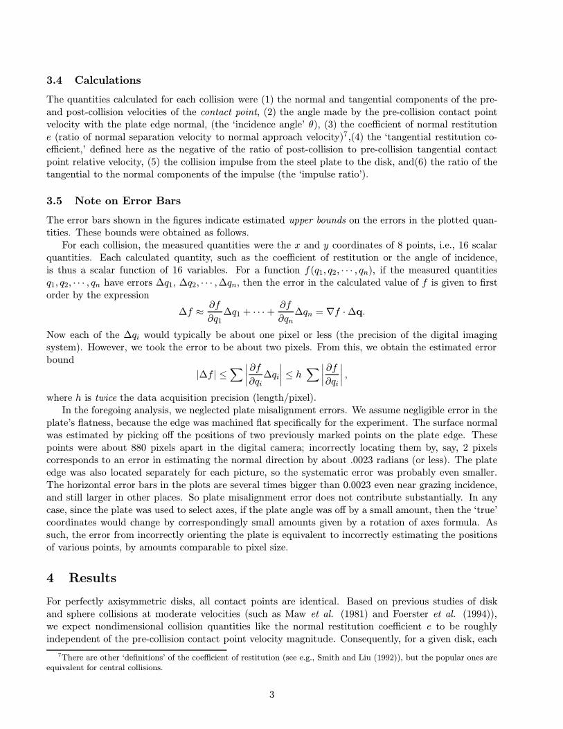
3.4 Calculations

The quantities calculated for each collision were (1) the normal and tangential components of the pre-and post-collision velocities of the contact point, (2) the angle made by the pre-collision contact pointvelocity with the plate edge normal, (the ‘incidence angle’ θ), (3) the coefficient of normal restitutione (ratio of normal separation velocity to normal approach velocity)7,(4) the ‘tangential restitution co-efficient,’ defined here as the negative of the ratio of post-collision to pre-collision tangential contactpoint relative velocity, (5) the collision impulse from the steel plate to the disk, and(6) the ratio of thetangential to the normal components of the impulse (the ‘impulse ratio’).

3.5 Note on Error Bars

The error bars shown in the figures indicate estimated upper bounds on the errors in the plotted quan-tities. These bounds were obtained as follows.

For each collision, the measured quantities were the x and y coordinates of 8 points, i.e., 16 scalarquantities. Each calculated quantity, such as the coefficient of restitution or the angle of incidence,is thus a scalar function of 16 variables. For a function f(q1, q2, · · · , qn), if the measured quantitiesq1, q2, · · · , qn have errors ∆q1, ∆q2, · · · ,∆qn, then the error in the calculated value of f is given to firstorder by the expression

∆f ≈∂f

∂q1∆q1 + · · ·+

∂f

∂qn∆qn = ∇f ·∆q.

Now each of the ∆qi would typically be about one pixel or less (the precision of the digital imagingsystem). However, we took the error to be about two pixels. From this, we obtain the estimated errorbound

|∆f | ≤∑∣∣∣∣ ∂f∂qi∆qi

∣∣∣∣ ≤ h ∑∣∣∣∣ ∂f∂qi∣∣∣∣ ,

where h is twice the data acquisition precision (length/pixel).In the foregoing analysis, we neglected plate misalignment errors. We assume negligible error in the

plate’s flatness, because the edge was machined flat specifically for the experiment. The surface normalwas estimated by picking off the positions of two previously marked points on the plate edge. Thesepoints were about 880 pixels apart in the digital camera; incorrectly locating them by, say, 2 pixelscorresponds to an error in estimating the normal direction by about .0023 radians (or less). The plateedge was also located separately for each picture, so the systematic error was probably even smaller.The horizontal error bars in the plots are several times bigger than 0.0023 even near grazing incidence,and still larger in other places. So plate misalignment error does not contribute substantially. In anycase, since the plate was used to select axes, if the plate angle was off by a small amount, then the ‘true’coordinates would change by correspondingly small amounts given by a rotation of axes formula. Assuch, the error from incorrectly orienting the plate is equivalent to incorrectly estimating the positionsof various points, by amounts comparable to pixel size.

4 Results

For perfectly axisymmetric disks, all contact points are identical. Based on previous studies of diskand sphere collisions at moderate velocities (such as Maw et al. (1981) and Foerster et al. (1994)),we expect nondimensional collision quantities like the normal restitution coefficient e to be roughlyindependent of the pre-collision contact point velocity magnitude. Consequently, for a given disk, each

7There are other ‘definitions’ of the coefficient of restitution (see e.g., Smith and Liu (1992)), but the popular ones areequivalent for central collisions.

3

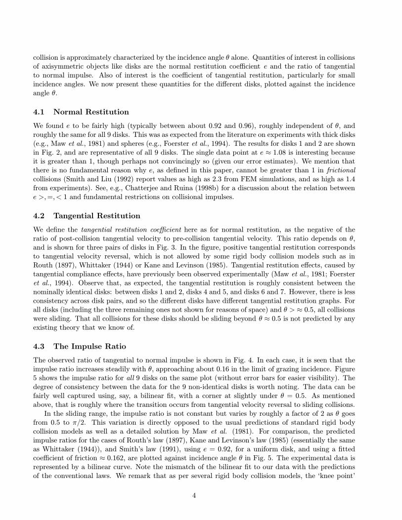
collision is approximately characterized by the incidence angle θ alone. Quantities of interest in collisionsof axisymmetric objects like disks are the normal restitution coefficient e and the ratio of tangentialto normal impulse. Also of interest is the coefficient of tangential restitution, particularly for smallincidence angles. We now present these quantities for the different disks, plotted against the incidenceangle θ.

4.1 Normal Restitution

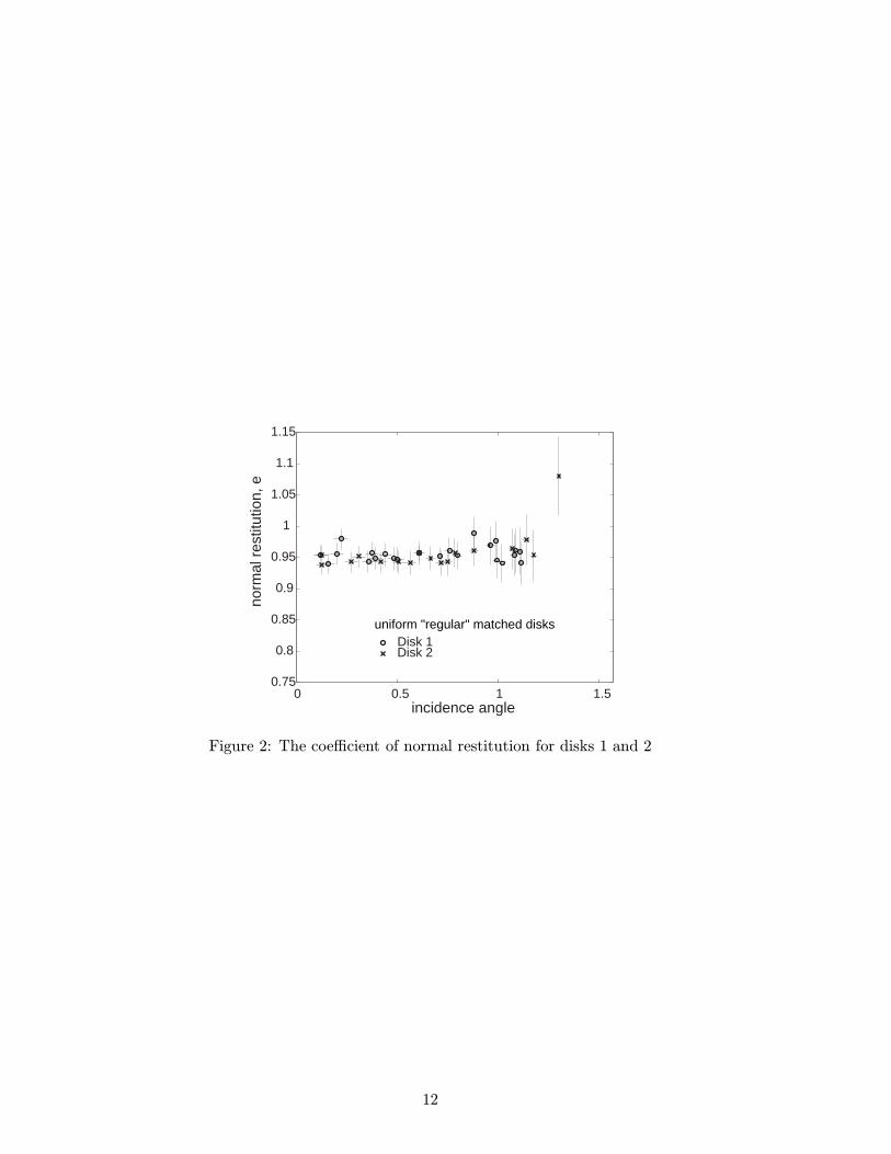
We found e to be fairly high (typically between about 0.92 and 0.96), roughly independent of θ, androughly the same for all 9 disks. This was as expected from the literature on experiments with thick disks(e.g., Maw et al., 1981) and spheres (e.g., Foerster et al., 1994). The results for disks 1 and 2 are shownin Fig. 2, and are representative of all 9 disks. The single data point at e ≈ 1.08 is interesting becauseit is greater than 1, though perhaps not convincingly so (given our error estimates). We mention thatthere is no fundamental reason why e, as defined in this paper, cannot be greater than 1 in frictionalcollisions (Smith and Liu (1992) report values as high as 2.3 from FEM simulations, and as high as 1.4from experiments). See, e.g., Chatterjee and Ruina (1998b) for a discussion about the relation betweene >,=, < 1 and fundamental restrictions on collisional impulses.

4.2 Tangential Restitution

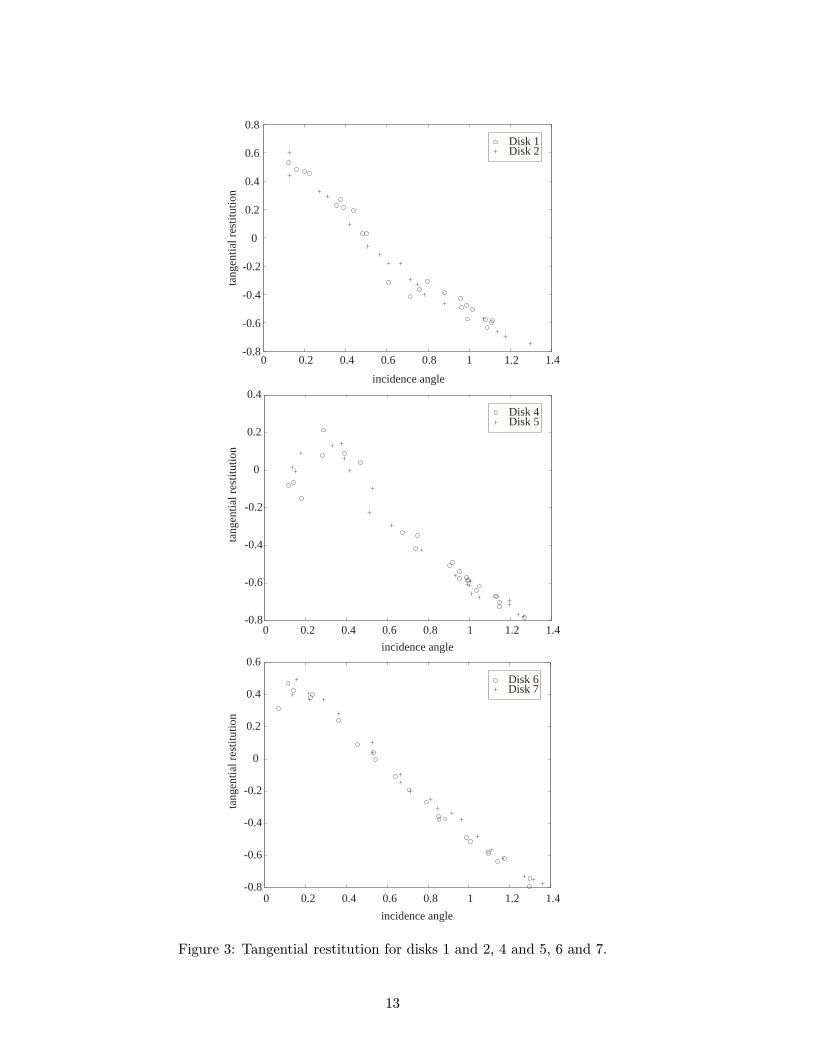
We define the tangential restitution coefficient here as for normal restitution, as the negative of theratio of post-collision tangential velocity to pre-collision tangential velocity. This ratio depends on θ,and is shown for three pairs of disks in Fig. 3. In the figure, positive tangential restitution correspondsto tangential velocity reversal, which is not allowed by some rigid body collision models such as inRouth (1897), Whittaker (1944) or Kane and Levinson (1985). Tangential restitution effects, caused bytangential compliance effects, have previously been observed experimentally (Maw et al., 1981; Foersteret al., 1994). Observe that, as expected, the tangential restitution is roughly consistent between thenominally identical disks: between disks 1 and 2, disks 4 and 5, and disks 6 and 7. However, there is lessconsistency across disk pairs, and so the different disks have different tangential restitution graphs. Forall disks (including the three remaining ones not shown for reasons of space) and θ > ≈ 0.5, all collisionswere sliding. That all collisions for these disks should be sliding beyond θ ≈ 0.5 is not predicted by anyexisting theory that we know of.

4.3 The Impulse Ratio

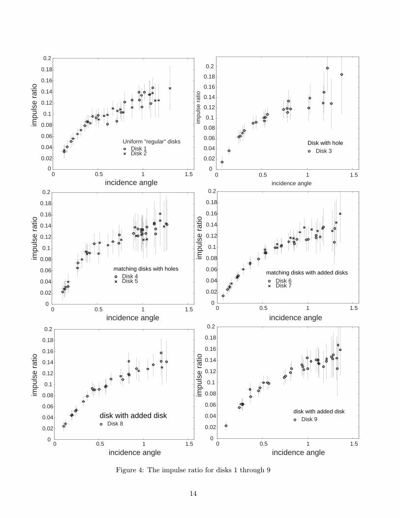
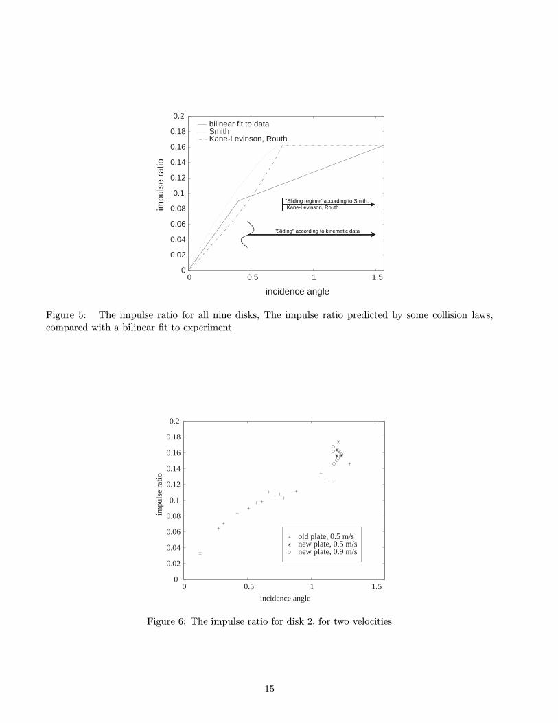
The observed ratio of tangential to normal impulse is shown in Fig. 4. In each case, it is seen that theimpulse ratio increases steadily with θ, approaching about 0.16 in the limit of grazing incidence. Figure5 shows the impulse ratio for all 9 disks on the same plot (without error bars for easier visibility). Thedegree of consistency between the data for the 9 non-identical disks is worth noting. The data can befairly well captured using, say, a bilinear fit, with a corner at slightly under θ = 0.5. As mentionedabove, that is roughly where the transition occurs from tangential velocity reversal to sliding collisions.

In the sliding range, the impulse ratio is not constant but varies by roughly a factor of 2 as θ goesfrom 0.5 to π/2. This variation is directly opposed to the usual predictions of standard rigid bodycollision models as well as a detailed solution by Maw et al. (1981). For comparison, the predictedimpulse ratios for the cases of Routh’s law (1897), Kane and Levinson’s law (1985) (essentially the sameas Whittaker (1944)), and Smith’s law (1991), using e = 0.92, for a uniform disk, and using a fittedcoefficient of friction ≈ 0.162, are plotted against incidence angle θ in Fig. 5. The experimental data isrepresented by a bilinear curve. Note the mismatch of the bilinear fit to our data with the predictionsof the conventional laws. We remark that as per several rigid body collision models, the ‘knee point’

4

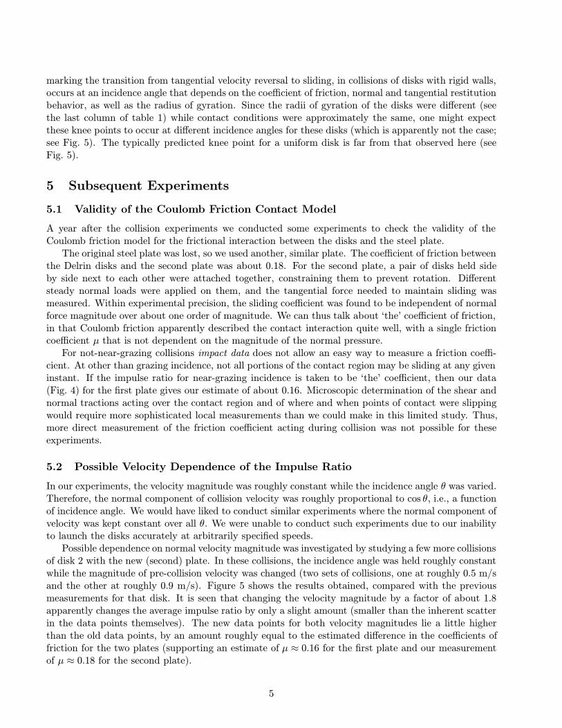
marking the transition from tangential velocity reversal to sliding, in collisions of disks with rigid walls,occurs at an incidence angle that depends on the coefficient of friction, normal and tangential restitutionbehavior, as well as the radius of gyration. Since the radii of gyration of the disks were different (seethe last column of table 1) while contact conditions were approximately the same, one might expectthese knee points to occur at different incidence angles for these disks (which is apparently not the case;see Fig. 5). The typically predicted knee point for a uniform disk is far from that observed here (seeFig. 5).

5 Subsequent Experiments

5.1 Validity of the Coulomb Friction Contact Model

A year after the collision experiments we conducted some experiments to check the validity of theCoulomb friction model for the frictional interaction between the disks and the steel plate.

The original steel plate was lost, so we used another, similar plate. The coefficient of friction betweenthe Delrin disks and the second plate was about 0.18. For the second plate, a pair of disks held sideby side next to each other were attached together, constraining them to prevent rotation. Differentsteady normal loads were applied on them, and the tangential force needed to maintain sliding wasmeasured. Within experimental precision, the sliding coefficient was found to be independent of normalforce magnitude over about one order of magnitude. We can thus talk about ‘the’ coefficient of friction,in that Coulomb friction apparently described the contact interaction quite well, with a single frictioncoefficient µ that is not dependent on the magnitude of the normal pressure.

For not-near-grazing collisions impact data does not allow an easy way to measure a friction coeffi-cient. At other than grazing incidence, not all portions of the contact region may be sliding at any giveninstant. If the impulse ratio for near-grazing incidence is taken to be ‘the’ coefficient, then our data(Fig. 4) for the first plate gives our estimate of about 0.16. Microscopic determination of the shear andnormal tractions acting over the contact region and of where and when points of contact were slippingwould require more sophisticated local measurements than we could make in this limited study. Thus,more direct measurement of the friction coefficient acting during collision was not possible for theseexperiments.

5.2 Possible Velocity Dependence of the Impulse Ratio

In our experiments, the velocity magnitude was roughly constant while the incidence angle θ was varied.Therefore, the normal component of collision velocity was roughly proportional to cos θ, i.e., a functionof incidence angle. We would have liked to conduct similar experiments where the normal component ofvelocity was kept constant over all θ. We were unable to conduct such experiments due to our inabilityto launch the disks accurately at arbitrarily specified speeds.

Possible dependence on normal velocity magnitude was investigated by studying a few more collisionsof disk 2 with the new (second) plate. In these collisions, the incidence angle was held roughly constantwhile the magnitude of pre-collision velocity was changed (two sets of collisions, one at roughly 0.5 m/sand the other at roughly 0.9 m/s). Figure 5 shows the results obtained, compared with the previousmeasurements for that disk. It is seen that changing the velocity magnitude by a factor of about 1.8apparently changes the average impulse ratio by only a slight amount (smaller than the inherent scatterin the data points themselves). The new data points for both velocity magnitudes lie a little higherthan the old data points, by an amount roughly equal to the estimated difference in the coefficients offriction for the two plates (supporting an estimate of µ ≈ 0.16 for the first plate and our measurementof µ ≈ 0.18 for the second plate).

5

Moreover, the new data points for both speeds lie below the estimated limiting value for grazingincidence (i.e., 0.18). Thus, the data points for each speed corroborate the increasing trend in theimpulse ratio seen in the first series of experiments.

We remark that the new data points for the lower speed (0.5 m/s) lie slightly higher, on average,than those for the higher speed (0.9 m/s). While not conclusive, this observation is consistent withtheory in that for disks of fixed thickness and rounded edges, as the incidence velocity magnitude ismade smaller and smaller, the localized 3D Hertz contact based solution (Maw et al., 1981; Mindlinand Deresiewicz, 1953) is expected to become accurate: for sufficiently small velocity magnitudes, theimpulse ratio graph is expected to be flat in the sliding regime.

5.3 Significance of Subsequent Experiments

The subsequent experiments described in this section roughly demonstrate two things. First, they showthat a constant µ is reasonable for the contact friction. By the discussion in Section 2, this impliesthat except in the limit of grazing incidence, the sliding collisions observed were only partially slidingcollisions and not fully sliding collisions.

Second, and somewhat less conclusively, the velocity variation experiments indicate that dependenceof the impulse ratio graph on pre-collision velocity magnitude is small. This constancy is consistentwith the usual collision modeling assumption that collisional impulses are homogeneous of degree onein the velocities (impulse is linear with velocity magnitude, for fixed values of collision “parameters”such as restitution coefficients).

6 On Rigidity in Collisions

The fundamental assumptions of rigid body collision modeling are that the time of interaction is small,displacements during the collision are small, contact forces are large, and accelerations are large; thatthe net interaction can be described by rigid body impulse-momentum relations. Further, for ‘single-point’ collisions, it is assumed that the size of the contact region is small compared to the overalldimensions of the colliding objects. These assumptions are reasonably applicable for the disks studied.However, specific rigid body collision models include extra hypotheses about the collision impulse.The particular assumptions made vary; so do the predicted results. The contradiction between ourexperimental observations and the predictions of most standard rigid body collision models should beviewed as a demonstration of the weakness of specific assumptions of these particular collision models,and not inaccuracy of the fundamental assumptions of the rigid body approach.

In a collision between any pair of real objects, contact occurs over a region (possibly small). Thevelocity distribution of material points in the contact region need not be uniform. Apparently also,the common assumption of a constant µ in the contact region is reasonable. If the relative tangentialmotion of all portions of the contact region is always in the same vectorial direction (with possiblereversals), and the net tangential impulse is less than µ times the normal impulse, then some portionsof the contact region must have stuck or reversed direction for some part of the collision, even thoughthe whole contact region might again be moving in the original direction at the end of the collision.

If contact deformations are strongly localized, as in (say) Hertzian contact of spheres or thick slicesthereof, then the whole body moves essentially like a rigid body while the contact region acts like asmall, pseudostatic interaction mechanism. Such objects, where at all instants of time including duringthe collision, the small contact region essentially behaves like a point on an ideal rigid body, are force-response rigid (see Chatterjee, 1997; or Chatterjee and Ruina, 1998a). Since any tangential (possiblyrate-dependent) compliance is of the same order as normal compliance, these objects are expected tobe slipping over the whole contact area throughout the collision for collisions that are sufficiently far

6

from normal. For such objects, in 2D sliding collisions, the tangential impulse is expected to be µ timesthe normal impulse.

In contrast, if contact deformations are not so strongly localized, so that the motions of points atsmall distances from the contact region are not effectively identical to those of a point on a rigid bodyduring the collision, but the motion of the body before and after the collision looks like that of a rigidbody, and if all displacements during the collision are very small compared to the dimensions of thebody, then the body is only impulse-response rigid (see Chatterjee (1997) or Chatterjee and Ruina(1998a)). In this case much more complex contact interactions can take place involving vibration andwave phenomena. Perhaps with such interactions the tangential relative velocity might reverse directionor stop during a collision (just as the normal component reverses direction multiple times in the dataof Stoianovici and Hurmuzlu, 1996). For such objects, in 2D sliding collisions, it might happen thatthe tangential impulse is less than µ times the normal impulse. As discussed in Chatterjee and Ruina(1998a) thin disks like in our experiments might only be well described as impulse-response rigid, whilethick disks (as in Maw et al. (1981) might be well described as force-response rigid. In particularconsider a slice of thickness H, cut from a sphere of radius R. Then the 3D Hertz-contact compliance(see Johnson, 1985) due to the rounded edges depends only on R and not on H, but the 2D compliance(or the ‘thinness’ effect of the disk) is proportional to 1/H. For a given contact force magnitude, if His made smaller, the two (3D and 2D compliances) can become comparable.

Note that the data of Foerster et al. (1994) and Maw et al. (1981) clearly showed tangentialrestitution, like our disks. Thus, our observations are not new in this regard. However, for the spheresand (presumably thick) disks studied in these works, it was found that the impulse ratio was equal tothe friction coefficient for sliding collisions, i.e., in those studies, sliding collisions were fully sliding. Incontrast, in our study of thin disks, we have found sliding collisions to be only partially sliding.

7 Conclusions

The fact that even in apparently “sliding” collisions, sliding need not persist throughout the collision,is relevant to general rigid body collision modeling. Contradiction of specific collision models, however,does not negate the basic rigid body approach to modeling collisions. We hope that our results willhelp to broaden the often restricted ideas about rigid body collisions that are promoted, in part, byseveral recent papers devoted to analyses of Routh’s incremental model or variations thereof, examplesof which include Keller (1986), Wang and Mason (1992), Stronge (1994b), Bhatt and Koechling (1995),Marghitu and Hurmuzlu (1995) and Batlle and Cardona (1997).

The details of the actual mechanical interactions in the disk collisions studied here were not resolvableat our scale of measurements. These interactions might be better understood through some combinationof experiments with micromeasurements, detailed numerical simulations, and approximate analyticalsolutions.

8 Acknowledgements

The authors thank Michel Louge for the loan of the digital camera system, the National Science Foun-dation (REU program) for summer support for (then undergraduates) Calsamiglia and Kennedy, andthe Department of Energy (Granular Flow Advanced Research Objective) for one summer’s support forChatterjee.

7

References

[1] Batlle, J. A. and Cardona, S. The jamb (self-locking) process in 3D rough collisions. ASME Journalof Applied Mechanics, 65:417–423, 1998.

[2] Bhatt, V. and Koechling, J. Three-dimensional frictional rigid-body impact. ASME Journal ofApplied Mechanics, 62:893–898, 1995.

[3] Brach, R. M. Mechanical Impact Dynamics: Rigid Body Collisions. John Wiley and Sons, NewYork, 1991.

[4] Chatterjee, A. Rigid Body Collisions: Some General Considerations, New Collision Laws, andSome Experimental Data. PhD thesis, Cornell University, 1997.

[5] Chatterjee, A. and Ruina, A. Two interpretations of rigidity in rigid body collisions. Accepted forpublication in ASME Journal of Applied Mechanics, 1998a.

[6] Chatterjee, A. and Ruina, A. A new algebraic rigid body collision law based on impulse spaceconsiderations. Accepted for ASME Journal of Applied Mechanics, 1998b.

[7] Foerster, S. F., Louge, M. Y., Chang, H., and Allia, K. Measurement of the collision properties ofsmall spheres. Physics of Fluids, 6(3):1108–1115, 1994.

[8] Johnson, K. L. Contact Mechanics. Cambridge University Press, Cambridge, 1985.

[9] Kane, T. R. and Levinson, D. A. Dynamics: Theory and Applications. McGraw-Hill, New York,1985.

[10] Keller, J. B. Impact with friction. ASME Journal of Applied Mechanics, 53:1–4, 1986.

[11] Marghitu, D. B. and Hurmuzlu, Y. Three-dimensional rigid-body collisions with multiple contactpoints. ASME Journal of Applied Mechanics, 62:725–732, 1995.

[12] Maw, N., Barber, J. R., and Fawcett, J. N. The role of elastic tangential compliance in obliqueimpact. Journal of Lubrication Technology, 103:74–80, 1981.

[13] R. D. Mindlin and H. Deresiewicz. Elastic spheres in contact under varying oblique forces. ASMEJournal of Applied Mechanics, 20:327–344, 1953.

[14] Routh, E. J. Dynamics of a System of Rigid Bodies. Macmillan and Co., London, sixth edition,1897.

[15] Smith, C. E. Predicting rebounds using rigid-body dynamics. ASME Journal of Applied Mechanics,58:754–758, 1991.

[16] Smith, C. E. and Liu, P-. P. Coefficients of restitution. ASME Journal of Applied Mechanics,59:963–969, 1992.

[17] Stoianovici, D. and Hurmuzlu, Y. A critical study of the applicability of rigid-body collision theory.ASME Journal of Applied Mechanics, 63:307–316, 1996.

[18] Stronge, W. J. Planar impact of rough compliant bodies. International Journal of Impact Engi-neering, 15(4):435–450, 1994a.

8

[19] Stronge, W. J. Swerve during three-dimensional impact of rough bodies. ASME Journal of AppliedMechanics, 61:605–611, 1994b.

[20] Wang, T. and Mason, M. T. Two-dimensional rigid-body collisions with friction. ASME Journalof Applied Mechanics, 59:635–642, 1992.

[21] Whittaker, E. T. A Treatise on the Analytical Dynamics of Particles and Rigid Bodies. Dover,New York, fourth edition, 1944.

9

List of Tables

1 Properties of axisymmetric disks used (dimensions in mm, mass in gm, Icm in gm-cm2) 11

List of Figures

1 Axisymmetric delrin disks, with holes or added disks . . . . . . . . . . . . . . . . . . . . 112 The coefficient of normal restitution for disks 1 and 2 . . . . . . . . . . . . . . . . . . . 123 Tangential restitution for disks 1 and 2, 4 and 5, 6 and 7. . . . . . . . . . . . . . . . . . 134 The impulse ratio for disks 1 through 9 . . . . . . . . . . . . . . . . . . . . . . . . . . . 145 The impulse ratio for all nine disks, The impulse ratio predicted by some collision laws,

compared with a bilinear fit to experiment. . . . . . . . . . . . . . . . . . . . . . . . . . 156 The impulse ratio for disk 2, for two velocities . . . . . . . . . . . . . . . . . . . . . . . . 15

10

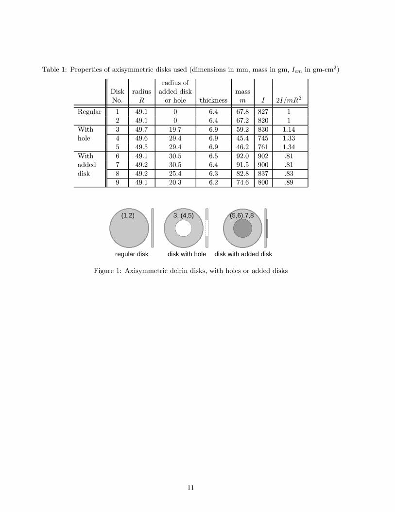
Table 1: Properties of axisymmetric disks used (dimensions in mm, mass in gm, Icm in gm-cm2)

radius ofDisk radius added disk massNo. R or hole thickness m I 2I/mR2

Regular 1 49.1 0 6.4 67.8 827 12 49.1 0 6.4 67.2 820 1

With 3 49.7 19.7 6.9 59.2 830 1.14hole 4 49.6 29.4 6.9 45.4 745 1.33

5 49.5 29.4 6.9 46.2 761 1.34

With 6 49.1 30.5 6.5 92.0 902 .81added 7 49.2 30.5 6.4 91.5 900 .81disk 8 49.2 25.4 6.3 82.8 837 .83

9 49.1 20.3 6.2 74.6 800 .89

regular disk disk with hole disk with added disk

(1,2) 3, (4,5) (5,6),7,8

Figure 1: Axisymmetric delrin disks, with holes or added disks

11

Disk 1Disk 2

0 0.5 1 1.50.75

0.8

0.85

0.9

0.95

1

1.05

1.1

1.15

incidence angle

norm

al r

estit

utio

n, e

uniform "regular" matched disks

Figure 2: The coefficient of normal restitution for disks 1 and 2

12

Disk 1Disk 2

0 0.2 0.4 0.6 0.8 1 1.2 1.4-0.8

-0.6

-0.4

-0.2

0

0.2

0.4

0.6

0.8

incidence angle

tang

entia

l res

titut

ion

Disk 4Disk 5

0 0.2 0.4 0.6 0.8 1 1.2 1.4-0.8

-0.6

-0.4

-0.2

0

0.2

0.4

incidence angle

tang

entia

l res

titut

ion

Disk 6Disk 7

0 0.2 0.4 0.6 0.8 1 1.2 1.4-0.8

-0.6

-0.4

-0.2

0

0.2

0.4

0.6

incidence angle

tang

entia

l res

titut

ion

Figure 3: Tangential restitution for disks 1 and 2, 4 and 5, 6 and 7.

13

Disk 1Uniform "regular" disks

Disk 2

0 0.5 1 1.50

0.02

0.04

0.06

0.08

0.1

0.12

0.14

0.16

0.18

0.2

incidence angle

impu

lse

ratio

Disk 3

0 0.5 1 1.50

0.02

0.04

0.06

0.08

0.1

0.12

0.14

0.16

0.18

0.2

incidence angle

impu

lse

ratio

Disk with hole

Disk 4Disk 5

0 0.5 1 1.50

0.02

0.04

0.06

0.08

0.1

0.12

0.14

0.16

0.18

0.2

incidence angle

impu

lse

ratio

matching disks with holes

Disk 6Disk 7

0 0.5 1 1.50

0.02

0.04

0.06

0.08

0.1

0.12

0.14

0.16

0.18

0.2

incidence angle

impu

lse

ratio

matching disks with added disks

Disk 8

0 0.5 1 1.50

0.02

0.04

0.06

0.08

0.1

0.12

0.14

0.16

0.18

0.2

incidence angle

impu

lse

ratio

disk with added disk Disk 9

0 0.5 1 1.50

0.02

0.04

0.06

0.08

0.1

0.12

0.14

0.16

0.18

0.2

incidence angle

impu

lse

ratio

disk with added disk

Figure 4: The impulse ratio for disks 1 through 9

14

0 0.5 1 1.50

0.02

0.04

0.06

0.08

0.1

0.12

0.14

0.16

0.18

0.2

incidence angle

impu

lse

ratio

bilinear fit to dataSmith Kane-Levinson, Routh

"Sliding regime" according to Smith, Kane-Levinson, Routh

"Sliding" according to kinematic data

Figure 5: The impulse ratio for all nine disks, The impulse ratio predicted by some collision laws,compared with a bilinear fit to experiment.

old plate, 0.5 m/snew plate, 0.5 m/snew plate, 0.9 m/s

0 0.5 1 1.50

0.02

0.04

0.06

0.08

0.1

0.12

0.14

0.16

0.18

0.2

incidence angle

impu

lse

ratio

Figure 6: The impulse ratio for disk 2, for two velocities

15