Hysteretic models for sliding bearings with varying frictional force

Hysteretic models for sliding bearings with varying frictional force

Tathagata Ray, Apostolos A. Sarlis, Andrei M. Reinhorn* and Michael C. Constantinou

Department of Civil, Structural and Environmental Engineering, University at Buffalo, SUNY, Buffalo, NY 14260, USA

SUMMARY

The friction pendulum system is a sliding seismic isolator with self-centering capabilities. Under severe earth-quakes, the movement may be excessive enough to cause the pendulum to hit the side rim of the isolator, whichis provided to restrain the sliding. The biaxial behavior of a single friction pendulum, in which the slider contactsthe restrainer, is developed using a smooth hysteretic model with nonlinear kinematic hardening. This model isextended to simulate the biaxial response of double and triple friction pendulums with multiple sliding surfaces.The model of a triple friction pendulum is based on the interaction between four sliding interfaces, which in turnis dependent upon the force and displacement conditions prevailing at these interfaces. Each of these surfacesare modeled as nonlinear biaxial springs suitable for a single friction pendulum, using the yield surface, basedon the principles of the classical theory of plasticity, and amended for varying frictional yield force, due to var-iation in vertical load and/or velocity-dependent friction coefficient. The participation of the nonlinear springs isgoverned by stick-slip conditions, dictated by equilibrium and kinematics. The model can simulate the overallforce-deformation behavior, track the displacements in individual sliding surfaces, and account for the ultimatecondition when the sliders are in contact with their restrainers. The results of this model are verified by compar-ison to theoretical calculations and to experiments. The model has been implemented in programs IDARC2Dand 3D-BASIS, and the analytical results are compared with shake table experimental results. Copyright ©2013 John Wiley & Sons, Ltd.

Received 3 July 2012; Revised 30 January 2013; Accepted 31 January 2013

KEY WORDS: seismic isolation; spherical sliding bearing; plasticity theory; hysteresis; yield surface

1. INTRODUCTION

There is an increased interest in adaptive seismic isolation systems that are able to provide structuralprotection through entirely passive means with the following attributes: (a) high damping and/orstiffness at low level forces (e.g., wind loads, loads from machines) or displacements; (b) low dampingand/or stiffness at moderate level earthquakes (Design Basis Earthquake) or at moderate displacements;and (c) high damping and/or high stiffness at severe level earthquakes (Maximum ConsideredEarthquake) or at large displacements (as discussed by Fenz and Constantinou [1], Morgan and Mahin[2]). These attributes can be obtained by using multispherical sliding bearings or friction pendulumbearings, which change the stiffness and damping properties at different levels of excitation. To date,three types of friction pendulum bearings have been developed and built: (a) a single friction pendulum(SFP) bearing that has a single sliding interface; (b) a double friction pendulum (DFP) bearing that hastwo sliding interfaces; and (c) a triple friction pendulum (TFP) bearing that has four sliding interfaces(Fenz and Constantinou [1]). In addition, systems with more sliding interfaces and even greatercomplex adaptive behavior have been proposed [3]. The isolators shown in Figure 1 are characterizedby their friction coefficient μ, radius of curvature R (or effective radius of curvature Reff), and

*Correspondence to: Andrei M. Reinhorn, Department of Civil, Structural and Environmental Engineering, University atBuffalo, SUNY, Buffalo, NY 14260, USA.†E-mail: [email protected]

Copyright © 2013 John Wiley & Sons, Ltd.

EARTHQUAKE ENGINEERING & STRUCTURAL DYNAMICSEarthquake Engng Struct. Dyn. (2013)Published online in Wiley Online Library (wileyonlinelibrary.com). DOI: 10.1002/eqe.2373

displacement capacities d of different sliding surfaces. Details of the mechanical and experimentalbehavior of these friction pendulum bearings are reported by Fenz and Constantinou [1].

In order to assess the efficacy of friction pendulum bearings, their nonlinear force-deformation behaviorneeds to be modeled so that it can be integrated into standard structural analysis software. Modelingtechniques for uniaxial and biaxial behavior of SFPs and DFPs have been discussed by Fenz andConstantinou [4], Nagarajaiah, et al. [5], Mokha, et al. [6]. Due to their inherent complexity andnonadherence to an overall force-deformation relationship to kinematic hardening principle, modelingTFPs can be achieved by the following: (i) combining existing nonlinear hysteretic elements; or (ii)developing a new hysteretic model to capture the behavior of a TFP. Fenz and Constantinou [7] andMorgan and Mahin [2] have developed a ‘series model’ by combining an existing SFP and gapelements that can be used in analysis programs like SAP2000, ABAQUS, and 3DBASIS. Although theoverall force-deformation behavior of the series model is correct, the relative displacements of theindividual sliding surfaces cannot be exactly tracked, which leads to approximations when accountingfor velocity and heating effects. Due to the use of multiple SFP elements, gap elements, and rigid linkelements, the analyses that use this model are computationally expensive. In addition, the necessity inSAP2000 to provide a finite value of mass to the link and SFP elements further complicates theconvergence of the nonlinear analysis, and requires an iterative process to achieve an optimal time-stepwith acceptable results. Sarlis, et al. [8] have developed a simpler ‘parallel model’ for the special caseof TFP (R1=R2, R2=R3, μ1=μ4, μ2=μ3), but this model cannot describe the motion of theindividual sliding interfaces. The differences in the response between this model and the experimentalresults become more significant when the velocity of sliding is small. Tsai, et al. [3] suggested that themechanics of the TFP be extended from equilibrium and compatibility considerations to n-interfaceswith an articulated slider in the middle. They considered the plasticity theory in the formulation of aforce-deformation relationship, ignoring ‘normality’ and ‘Kuhn-Tucker optimality conditions’ andwithout explicit formulation of tangent stiffness matrices at sliding interfaces. In addition, theverification of the model has yet to be completed for random excitation.

Recently, Becker and Mahin [9, 10], have developed a model for TFP that has the capacity to capturethe displacement of the individual sliding surfaces and to simulate the condition when the restrainer of asliding surface is hit. In their formulation, the governing relationships of equilibrium and compatibility areupdated after each computational step, depending upon the frictional force (obtained using plasticitytheory) and displacement states (obtained using geometric compatibility) at the sliding surfaces.

In the present paper, an alternative formulation for biaxial behavior of flat sliders and SFP is presentedusing the classical theory of plasticity with nonlinear kinematic hardening and varying strength. Using theSFP model, the behavior of TFP is formulated for the most prevalent choice of bearing geometry andfriction parameters. The proposed TFP model can carry out the following: (i) simulate the overall force-deformation behavior; (ii) track the sliding of the individual interfaces; and (iii) simulate the case whenthe restrainer is hit, similar to the previous TFP models [9, 11]. In addition to the capabilities ofprevious modeling formulations [1, 2, 5, 9, 12, 13], the proposed formulation: (i) explicitly addressesthe variation of friction force, included in the plasticity formulation, as a variation of strength, so that itcan more efficiently simulate the severe fluctuations in vertical load or the velocity-dependent friction

Figure 1. Cross sections of spherical sliding bearings.

T. RAY ET AL.

Copyright © 2013 John Wiley & Sons, Ltd. Earthquake Engng Struct. Dyn. (2013)DOI: 10.1002/eqe

coefficient; and (ii) allows transition between the elastic and plastic state as either smooth or sharp, as perthe nature of the analysis problem. Because the proposed model considers fluctuations of friction in theindividual isolators, it enables the effects of global uplift in various parts of the isolated structure to bemodeled, which produces a redistribution of vertical loads in each TFP.

The following assumptions are made in the development of the model: (i) the model only satisfies theequations of equilibrium in the translational direction, and is limited by the condition: μ2=μ3, assuggested by Fenz and Constantinou [1]. However, the model can produce results when this conditionis violated, but the accuracy needs to be assessed through a comparison to experiments or by an exacttheory, which is yet to be developed; (ii) the model does not consider conservation of momentum forindividual sliders during impact. Instead, all impacts are considered to be perfectly plastic; (iii) Theprecise motion of the individual sliders during uplift is not tracked because of the absence of a verticaldegree of freedom of the sliders; (iv) although the equilibrium of horizontal forces is considered for theTFP, the equilibrium of internal moments, which might be important at very large displacements [14],is neglected.

2. PLASTICITY-BASED MODEL FOR MULTI-AXIAL INTERACTION OF FORCES WITHVARYING STRENGTH

In the theory of plasticity using a force-strength concept (as an alternative to continuummechanics, whichuses stress instead of force), a convex yield surface, as mentioned in Simo andHughes [15] can be defined.The expression of the yield surface consists of the force variables {Fi} and the strength variables {Foj}(subscripts i and j are the indices of the respective variables). The yield surface describes the interaction(or coupling) of the force variables between themselves, and also between the strength variables. Thissurface can be formulated from the physical description of the problem, for example, in case of friction(as discussed later), or can be fitted empirically from experimental observations or computational data.Let the yield surface be defined as

ϕ Fi;Foj

� � ¼ 0 (1)

The force vector remains under or on the yield surface (ϕ(Fi, Foi) = 0), without overshooting it. Theyield surface function ϕ(Fi, Foi) denotes a boundary so that if the components of the force vector {Fi}remain inside the boundary (i.e., ϕ(Fi, Foi)< 0), the force-displacement relationship is given by theelastic stiffness matrix; otherwise, if {Fi} stays on the yield surface (i.e., ϕ(Fi, Foi) = 0), the theoryof plasticity applies.

The consistency condition in plasticity, indicating that the yield surface is stationary, implies that thedifferential of the yield surface is zero:

Δϕ ¼ 0; or ∂ϕ=∂Fif gT ΔFif g þ ∂ϕ=∂Foj

� �T ΔFoj

� � ¼ 0 (2)

The second term on the left side of Equation (2), consisting of ΔFoj, accounts for the cases when thestrength parameters vary. This condition is observed if there is a variation in the vertical load and/orchanges in the friction coefficient of the friction pendulum.

The normality condition in plasticity, which indicates that the plastic displacement (or strain) incrementΔupi� �

is normal to the plastic potential surface (Ψ (Fi, Foj) = 0), implies that the incremental plasticdisplacements are proportional to the gradient of the yield surface:

Δupi� � ¼ ∂λð Þ ∂ψ=∂Fif g (3)

Here ∂λ is the plastic multiplier. Imposing the associativity condition, indicating that the yieldsurface and the plastic potential surface are identical (i.e., Ψ ≡ϕ), Equation (3) can be rewritten as

HYSTERETIC MODEL—SLIDING BEARINGS


Δupi� � ¼ ∂λð Þ ∂ϕ=∂Fif g (4)

The total displacement increment vector {Δui} is the algebraic sum of the elastic Δuei� �

and plasticΔupi displacement increment vectors. The incremental force vector {ΔFi} is related to the incrementalelastic displacement vector through the elastic stiffness matrix [ke]:

ΔFif g ¼ ke½ � Δuei� �

; or ΔFif g ¼ ke½ � Δuif g � Δupi� ��

(5)

Using Equations (2), (4), and (5), ∂λ is obtained as

∂λ ¼ ∂ϕ=∂Fif gT ke½ � Δuif g þ ∂ϕ=∂Foj

� �T ΔFoj

� �� = ∂ϕ=∂Fif gT ke½ � ∂ϕ=∂Fif g� �

(6)

Note that ∂λ is zero when the force vector {Fi} lies under the yield surface, that is, when ϕ(Fi, Foj)< 0(or when sign (Fi

TΔFi) =�1). Otherwise, ∂λ is given by Equation (6), when {Fi} lies on the yieldsurface, that is, when ϕ(Fi, Foj) = 0 (or when sign ({Fi}

T{ΔFi}) = 1). These conditions are known asKuhn-Tucker optimality conditions. ϕ(Fi, Foj) = 0 can be normalized, generally with strengthvariables Foj, to ϕ’(Fi, Foj) = 1, such that,

ϕ Fi;Foj

� � ¼ 0⇒ϕ′ Fi;Foj

� � ¼ 1 and ϕ Fi;Foj

� �< 0⇒ϕ′ Fi;Foj

� �< 1 (7)

Using optimality conditions and Equation (7), ∂λ can be derived as

∂λ ¼ ϕ′ Fi;Foj

� �� N 1þ sign Fif gT ΔFif g� �2

!∂ϕ=∂Fif gT ke½ � Δuif g þ ∂ϕ=∂Foj

� �T ΔFoj

� �∂ϕ=∂Fif gT ke½ � ∂ϕ=∂Fif g

!(8)

Here N is an exponent (⩾2), which allows for smooth transition from the elastic region to the plasticregion. The first two terms on the right side of Equation (8) can be expressed as

H1 ¼ ϕ′ Fi;Foj

� �� Nand H2 ¼ 1þ sign Fif gT ΔFif g� ��

=2 (9)

Using Equations (4), (5), (8), and (9), the incremental force {ΔFi} can be expressed as

ΔFif g ¼ ke½ � Δuif g � H1H2∂ϕ=∂Fif gT ke½ � Δuif g þ ∂ϕ=∂Foj

� �T ΔFoj

� �∂ϕ=∂Fif gT ke½ � ∂ϕ=∂Fif g

!∂ϕ∂Fi

� ( )(10)

Note that barring the term {∂ϕ/∂Foj}T{ΔFoj} that accounts for strength variability, Equation (10) is

similar to that derived by Sivaselvan and Reinhorn [16] in kinematic terms (rate form).

3. BIAXIAL INTERACTION MODEL FOR FRICTION FORCES WITHOUTRESTORING FORCE

Consider the case of flat sliding interfaces where the restoring force is zero. It is apparent that if thefrictional stick condition can be idealized as the elastic state, and the frictional slip condition can beidealized as the plastic state, the yield function can be assumed as

T. RAY ET AL.


ϕ Fx;Fy;Fo

� �≡F2

x þ F2y � F2

0 ¼ 0 (11)

The elastic stiffness matrix [ke] can be written as

ke½ � ¼ ko I½ � (12)

Here, ko has a very large value to simulate the stick condition [5]. The force vector and the strengthcan be described as

Fif g ¼ Fx Fyf gT ; Foj

� � ¼ Fof g (13)

Functions H1 and H2 can be reformulated as

H1 ¼ffiffiffiffiffiffiffiffiffiffiffiffiffiffiffiffiffiffiffiffiffiffiffiffiffiffiffiffiF2x þ F2

x

� �=F2

o

q� �NH2 ¼ 1þ sign FxΔFx þ FyΔFy

� �� =2

(14)

Finally, using Equation (10) and some algebraic exercise, the relationship between incremental forceand displacement for sliding on a flat surface can be written as

ΔFx

ΔFy

� ¼ ko I½ � � H1H2

F2x þ F2

y

!F2x FxFy

FxFy F2y

" #( )ΔuxΔuy

� þ H1H2

FoΔFo

F2x þ F2

y

!Fx

Fy

� (15)

4. MODELING SINGLE AND DOUBLE FRICTION PENDULUM BEARINGS

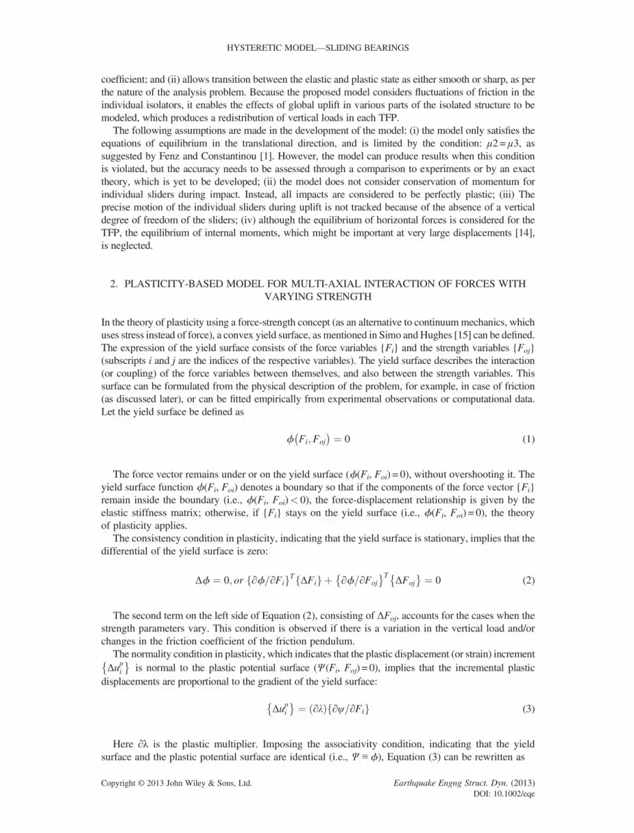
The total incremental force in the SFP bearing is considered as the algebraic sum of the incrementalhysteretic friction force as given by Equation (15) and the incremental linear elastic force originatingfrom the curvature (=1/R where R is the radius of curvature of the surface) of the SFP. Figure 2ashows the arrangement of hysteretic and nonlinear elastic springs of the SFP for the uniaxial case.For biaxial behavior, the incremental linear elastic force is given by

ΔFlex ;ΔF

ley

n oT¼ W=Rð Þ I½ � Δux;Δuy

� �T(16)

If the rim, limiting the sliding surface, is considered to have a finite (large) stiffness kres, then upon

hitting the rim (i.e., when the resultant displacement of the sliderffiffiffiffiffiffiffiffiffiffiffiffiffiffiffiu2x þ u2y

q> ro where ro is the

radius of the sliding surface), the slider will experience nonlinear force and the resultant of thisforce is given by

Fnlres ¼ kres

ffiffiffiffiffiffiffiffiffiffiffiffiffiffiffiu2x þ u2y

q� ro

� �(17)

Fnlres can be resolved in the x-y direction as



Fnlx ;F

nly

n oT¼ kres


q� ro

� �ux=


q; uy=


qn oT(18)

The total incremental force of the SFP bearing originating from the stick-slip hysteresis (Equation (15)),curvature of the sliding surface (Equation (16)), and the restrainer of the sliding surface (Equation (18), isgiven by

ΔFtotx

ΔFtoty

( )¼ kh½ � þ ke½ �f g Δux

Δuy

� þ H1H2

FoΔFo

F2x þ F2

y

!Fx

Fy

� (19)

Here, [kh] and [ke] are given by,

kh½ � ¼ ko I½ � � H1H2

F2x þ F2

y

!F2x FxFy

FxFy F2y

" #( )

ke½ � ¼ W=Rð Þ I½ � þ Uffiffiffiffiffiffiffiffiffiffiffiffiffiffiffiu2x þ u2y

q� ro

� �knl½ �

(20)

where U( ) is the heaviside step function. An expression of knl can be obtained by using partialdifferentiation of Fnl

x and Fnly with regards to ux and uy as shown herein:

knl½ � ¼ ∂Fnli

∂uj

¼ kres1� ro=

ffiffiffiffiffiffiffiffiffiffiffiffiffiffiffiu2x þ u2x

p þ u2xro= u2x þ u2x� �3=2

uxuyro= u2x þ u2x� �3=2

uxuyro= u2x þ u2x� �3=2

1� ro=ffiffiffiffiffiffiffiffiffiffiffiffiffiffiffiu2x þ u2x

p þ u2yro= u2x þ u2x� �3=2

24

35 (21)

Note that Equation (19) must be used to update the force vector of an SFP bearing for a givenincremental displacement vector, particularly when a variation of the vertical force is expected. Ifthe stiffness of the SFP is required to be found, the same equation should be formulated by adding

Figure 2. Analog spring model for spherical sliding bearings.

T. RAY ET AL.


[kh] and [ke] algebraically after updating each of the stiffness matrices using the current forces anddisplacements of the SFP.

One immediate use of Ktangent is to find the expected incremental force vector {ΔFi} for thevariable H2. In fact, Ktangent from the previous time-step must be post-multiplied by incrementaldisplacement vector {Δui}, as shown in Equation (22), in order to obtain {ΔFi}. ko and kres,required for [kh] and [knl], respectively, can be obtained in a similar manner as adopted forcalculating hysteretic stiffness kh.

ΔFx;ΔFy

� �T ¼ K tangent� �

Δux;Δuy� �T

(22)

Park, et al. [17] also proposed a hysteretic model (Park-Wen-Ang model) to describe the biaxialinteraction of forces in structural members. This model was later used by Nagarajaiah, et al. [5],Mokha, et al. [12] to model sliding on a flat surface and for an SFP. Note that in the proposedformulation, ko, the initial stiffness, is used to simulate the stick condition, and can be set either as avery large stiffness (arbitrarily proportional to the bearing stiffness), or a ratio of the friction force, andan infinitesimal ‘yield displacement, uy’ as suggested by Scheller and Constantinou [9]. ko and uy canbe related through the friction force Fo as ko=Fo/uy. It is necessary to consider two different frictioncoefficients when there is a difference in frictional properties in the direction of polish (known as thedirection of lay) and in the direction perpendicular to it. In order to incorporate different frictioncoefficients in the direction of lay and in the direction perpendicular to it (i.e., when the frictionalproperty is orthotropic) in the model using plasticity theory, the elliptic yield surface must beconsidered. The yield surface in this case is assumed as

ϕ′≡ Fx=Foxð Þ2 þ Fy=Foy

� �2 ¼ 1 (23)

It can be seen that the plasticity model updates the force vector by using incrementaldisplacements, whereby the Park-Wen-Ang [17] model updates it using instantaneous velocities.Note that the Signum functions, which describe unloading from the yield surface, are different inthese two models. The Park-Wen-Ang model uses the dot product of the current force vector withthe instantaneous velocity vector. In contrast, the plasticity model described herein uses the dotproduct of the current force vector with the incremental force vector. Note also that due to thepresence of the exponent N, the plasticity model allows for both smooth (for N= 2) and sharptransitions (for N> 5) from the elastic state to the plastic state, whereas the Park-Wen-Ang modelcan only simulate smooth transitions.

The friction coefficient (μ), which depends upon the velocity v of the slider, should be updated fordynamic analyses according to [14]:

μ ¼ μmax � μmax � μminð Þe�av (24)

Here μmax and μmin are the minimum and maximum friction coefficients of the interacting surfaces,and a is the rate parameter.

For the DFP bearing, when the lateral force F increases from zero, sliding initiates first on the surfacewith a lower friction coefficient. When F reaches the frictional force of the surface with a higher frictioncoefficient, sliding occurs on both surfaces. When any one of the sliding surfaces hits the restraining rim,the state of motion remains unchanged for the other sliding surface. During unloading at any stage, theforce-displacement relationship between the individual sliding surfaces shows pure kinematic hardeningbehavior. This behavior of the DFP is modeled through a combination of two SFPs in series (as shownin Figure 2b for the uniaxial case). The SFPs represent upper and lower sliding surfaces withcorresponding friction coefficients, displacement capacities, and radii of curvature. The biaxial behaviorof the DFP can be formulated in a similar manner.



5. MODELING TRIPLE FRICTION PENDULUM BEARING (WITH μ4⩾μ1>μ2 =μ3)

Because of the geometric and frictional characteristics of TFP bearings, it is apparent that at any instance,simultaneous sliding occurs on one single sliding surface among surfaces 1 and 2, and one single surfaceamong 3 and 4 (Fenz and Constantinou [1]). The overall stiffness of the TFP is therefore formulated as aseries combination of the stiffnesses of two participating sliding surfaces and the resultant stiffness of theTFP is split as a series combination of kupper and klower, as shown in Figure 2c. Note that this approach wasalso suggested by Tsai et al. [3] for a TFP with an articulated slider in the middle. kupper is the combinedstiffness of sliding surfaces 3 and 4 and klower is the same for sliding surfaces 1 and 2. The phenomenongoverning klower is same as that governing kupper, and thus the same modeling principles are valid forboth kupper and klower. The overall stiffness of the system is dependent on the instantaneous sliding orsticking between the surfaces. The variation and corresponding modeling of klower for uniaxial motionis described in the succeeding text.

Each of the sliding surfaces 1 and 2 is assumed to be an SFP. The most prevalent condition for the TFPis μ1>μ2. It is observed that with increase (or decrease) in lateral load F from zero, sliding starts onsurface 2 when |Fh2|=Fhy2, and klower becomes W/Reff2. Until then, klower has a large magnitude suchthat klower>>max (W/Reff1, W/Reff2), and hysteretic forces in both the SFPs remain inside theirrespective yield surfaces. With further increase (or decrease) in F when |Fh1|=Fhy1, sliding starts onsurface 1 and stops on surface 2 because both surfaces cannot slide simultaneously. At this stage, klowerbecomes W/Reff1, and hysteretic forces in both SFPs remain on their respective yield surfaces. If eithersurface 1 or 2 hits its respective rim, motion stops in that surface, and the other surface starts sliding;klower is then given by the instantaneous stiffness of the SFP corresponding to the later surface thatstarts sliding. If both sliding surfaces reach their maximum displacement capacities, klower attains a largemagnitude such that klower>>max (W/Reff1, W/Reff2).

From the aforementioned discussion, it can be deduced that for μ1>μ2, as long as |Fh1|<Fhy1, |u1|< d1and |u2|< d2, klower is given by a series combination of the stiffness of the SFP models corresponding tosurfaces 1 and 2, and when |Fh1| =Fhy1, |u1|< d1 and |u2|< d2, klower is given by the stiffnesscorresponding to surface 1 only if |u1|> d1 or |u2|> d2, klower is again given by a series combination ofthe stiffness of the SFPs corresponding to surfaces 1 and 2. Table I summarizes the different statesof Fhi and ui (i=1,2), and the corresponding combinations of stiffnesses for klower. Note that in the caseof condition 1 in Table I, surface 1 should remain stationary; however, for computational purposes, it isassumed that surface 1 will slide with a large stiffness so that its displacement will be infinitesimal andthus the stationary condition will be simulated.

The variation of kupper for μ4>μ3 is determined by similar deductions and rules. It can be shown thatthe foregoing modeling technique can depict different sliding regimes of a TFP bearing. For example,consider the most prevalent properties of TFP: μ2 =μ3<μ1<μ4, Reff2=Reff3<Reff1=Reff4,d2=d3< d1= d4, together with the conditions: (i) d1> (μ4�μ1)Reff1; (ii) d2> (μ1�μ2)Reff2; and (iii)d3> (μ4�μ3)Reff3. According to Fenz and Constantinou [1], conditions (a)–(c) ensure that the surfaceswith a higher stiffness of sliding (surface 2 and 3) re-engage after full displacement capacities arereached in surfaces with a lower stiffness of sliding (surface 1 and 4). A summary of various regimes ofthe aforementioned TFP bearing is shown in Table II. The hysteretic stiffness kh can be calculated as

Table I. The states and combinations for klower (for μ1> μ2).

Condition

Force state Displacement state Combination

(1) (2) (3)

1 |Fh1/Fhy1|< 1 (inside the yield surface) |u1/d1|< 1 and |u2/d2|< 1 klower = series combination ofstiffnesses of surface 1 and 2

2 |Fh1/Fhy1| = 1 (on the yield surface) |u1/d1|< 1 and |u2/d2|< 1 klower = stiffness of surface 13 Any |u1/d1|⩾ 1 or |u2/d2|⩾ 1 klower = series combination of

stiffnesses of surface 1 and 2

T. RAY ET AL.


Table

II.The

regimes,force,anddisplacementconditions,andstiffnessesof

upperandlower

halfof

triple

frictio

npendulum

.

Regim

eSlid

ing

Force

condition

Displacem

entcondition

Klower

Kupper

(1)

(2)

(3)

(4)

(5)

(6)

0Non

eFresi<Foii=

1-4

u resi<d i

i=1-4

([Kh1+Ke1]�

1+[K

h2+Ke2]�

1)�

1([Kh4+Ke4]�

1+[K

h3+Ke3]�

1)�

1

I2,3

Fresi=Foi,Fresj<Foji=

2,3;

j=1,4

u resi<d i

i=1–

4([Kh1+Ke1]�

1+[K

h2+Ke2]�

1)�

1([Kh4+Ke4]�

1+[K

h3+Ke3]�

1)�

1

II1,3

Fresi=Foj,Fresj<Foji=

1–3;

j=4

u resi<d i

i=1–

4[K

h1+Ke1]

([Kh4+Ke4]�

1+[K

h3+Ke3]�

1)�

1

III

1,4

Fresi=Foi,i=

1–4

u resi<d i,i=

1–4

[Kh1+Ke1]

[Kh4+Ke4]

IV2,4

Fresi=Foi,i=

1–4

u resi⩾d i,u r

esj<d j

i=1;j=

2–4

([Kh1+Ke1]�

1+[K

h2+Ke2]�

1)�

1[K

h4+Ke4]

V2,3

Fresi=Foii=

1–4

u resi⩾d i,u r

esj<d j

i=1,4;j=

2,3

([Kh1+Ke1]�

1+[K

h2+Ke2]�

1)�

1([Kh4+Ke4]�

1+[K

h3+Ke3]�

1)�

1



kh ¼ kmulð Þmax W= Re ff

� �1;W= Re ff

� �2;W= Re ff

� �3;W= Re ff

� �4

n o(25)

kmul is a multiplying factor that accounts for the fact that hysteretic stiffness is much larger than the post-elastic stiffness. Ktangent denotes the overall stiffness of the TFP bearing. All other symbols are aspreviously defined. Regime-0 is defined when the motion in the TFP is not initiated. Theoretically,there should be no sliding in regime-0; yet for computational purposes, a finite large stiffness isassumed in this regime to allow for infinitesimal sliding in all surfaces. All other regimes are defined bythe various force and displacement conditions of the surfaces of the TFP. Table II is deduced from anexpansion of Table I for kupper and klower.

The geometric compatibility demands that for a TFP bearing, the top plate, which corresponds tosliding surface 4, and the bottom plate, which corresponds to sliding surface 1, will always remainhorizontal. If Δθi is the incremental rotation due to sliding at the i-th surface, then in order to satisfythis criterion mathematically, at any instant, it is required that

Δθ1 þ Δθ2 � Δθ3 � Δθ4 ¼ 0 (26)

For small incremental displacement Δui of the i-th surface, the incremental rotation can beexpressed as

Δθi ¼ Δui= Reff

� �i (27)

It can be deduced for any incremental displacement Δu of the TFP, as shown in Table III, that underthe assumption of Equation (27), the aforementioned modeling technique can satisfy the compatibilitycondition imposed by Equation (26) for different sliding regimes.

The model can be further extended for a friction pendulum with n-surfaces in each half and anarticulated slider in the middle, under the assumptions: (i) μi>μi+1; (ii) Ri>Ri+1; and (iii) di> (μi-1�μi)Ri. Using the rules described in Table I and formulations by Tsai, et al. [3], the followingconditions can be developed for the stiffness, ktangent, of each half:

ktangent ¼ ki½ ��1 þ ki�1½ ��1 þ…þ k1½ ��1h i�1

for Fhij j⩽Foi& uij j < dij j

ktangent ¼ kiþ1½ ��1 þ ki½ ��1 þ ki�1½ ��1 þ…þ k1½ ��1h i�1

for Fhij j⩽Foi& uij j⩾ dij j(28)

Here, i is the surface with the largest friction coefficient where sliding is initiated. Fhi and Foi are thecurrent hysteretic and friction forces, respectively, and [ki] is the stiffness in surface i. Conditions (i)-(iii)ensure that sliding in the i-th surface starts before the (i� 1)-th surface hits the restrainer.

The biaxial behavior of the TFP bearing can be modeled by using the modeling principles foruniaxial behavior. The steps in the succeeding texts are followed in order to update the forces,displacements, and stiffness matrices of individual sliding surfaces and those of the TFP for a givenincremental displacement vector {Δui}:

1. Using Table I, the stiffness matrices of the upper and lower halves, [kupper] and [klower], areformulated.

2. The total incremental displacement vectors of the upper and lower halves, {Δui}upper and {Δui}lower, are calculated from the total incremental displacement vector {Δui}, [kupper], and [klower] as

Δuif gupper=lower ¼ kupper=lower� ��1

kupper=lower� ��1 þ klower=lower

� ��1h i�1

Δuif g (29)

Equation (29) arises from the fact that as the upper and lower halves are in series, they will share thesame incremental force.

T. RAY ET AL.


Table

III.Increm

entaldisplacements(Δu i)androtatio

ns(Δθ i)of

slidingsurfaces

fordifferentregimes

R��i¼

Reff

ðÞ i

�� .

Sl.No.

Variables

Regim

e

0I

IIIII

IVV

(1)

(2)

(3)

(4)

(5)

(6)

(7)

1Klower

Kh/2

W/R

2W/R

1W/R

1W/R

2W/R

2

2Kupper

Kh/2

W/R

3W/R

3W/R

4W/R

4W/R

3

3Δu lower

Δu/2

ΔuR

2/(R2+R3)

ΔuR

1/(R1+R3)

ΔuR

1/(R1+R4)

ΔuR

2/(R2+R4)

ΔuR

2/(R2+R3)

4Δu u

pper

Δu/2

ΔuR

3/(R2+R3)

ΔuR

3/(R1+R3)

ΔuR

4/(R1+R4)

ΔuR

4/(R2+R4)

ΔuR

3/(R2+R3)

5Δu 1

Δu/4≈0(asΔu≈0)

≈0(asKh>>W/R

2)

ΔuR

1/(R1+R3)

ΔuR

1/(R1+R4)

≈0(asKne>

>W/R

2)

≈0(asKne>

>W/R

2)

6Δu 2


ΔuR

2/(R2+R3)

00

ΔuR

2/(R2+R4)

ΔuR

2/(R2+R3)

7Δu 3


ΔuR

3/(R2+R3)

ΔuR

3/(R1+R3)

00

ΔuR

3/(R2+R3)

8Δu 4


≈0(asKh>>W/R

3)

≈0(asKh>>W/R

3)

ΔuR

4/(R1+R4)

ΔuR

4/(R2+R4)

≈0(asKne>

>W/R

3)

9Δθ 1

00

Δu/(R

1+R3)

Δu/(R

1+R4)

00

10Δθ 2

0Δu/(R

2+R3)

00

Δu/(R

2+R4)

Δu/(R

2+R3)

11Δθ 3

0Δu/(R

2+R3)

Δu/(R

1+R3)

00

Δu/(R

2+R3)

12Δθ 4

00

0Δu/(R

1+R4)

Δu/(R

2+R4)

0



3. The incremental displacements in the individual sliding surfaces are then calculated. For a partic-ular ‘half’ (upper or lower), if the two surfaces slide, then the two stiffness matrices of eachsurface are participating as a series combination in the overall stiffness for that ‘half’ (conditions1 and 3 in Table I). In such a case, the total incremental displacement is distributed among theindividual sliding surfaces in a similar manner as discussed in step 2. Note that due to theassumption of large hysteretic stiffness (or large nonlinear elastic stiffness when the restraineris hit), the surface, which is supposed to be stationary under conditions 1 and 3, slides byinfinitesimally small displacement in the case of a series combination and thus the geometriccompatibility conditions are not violated. In contrast, if only one of the surfaces in a ‘half’(condition 2 in Table I) is sliding and therefore contributing to the overall stiffness of that ‘half,’the total incremental displacement for that ‘half’ is attributed to that sliding surface only.

4. The force vector (both hysteretic and total) and the stiffness matrices of the sliding surfaces areupdated.

5. The force vector of the TFP bearing can be updated by calculating the overall incremental forceobtained from the overall stiffness. Alternatively, the total force vector of any of the slidingsurfaces can be attributed as the updated total force vector of the TFP.

The formulation and model of the TFP presented earlier for biaxial motion with variation in frictionalforces can also be used for analysis in the uniaxial direction. Of particular interest is the fact that theproposed model of the TFP collapses into models of a DFP, or even an SFP, if the friction coefficientsare chosen appropriately, as shown in Table IV. Note that Fenz and Constantinou [1] formulated thebehavior of a DFP and Becker [18] formulated the behavior of a SFP by modifying both the geometricand frictional properties of the TFP in their respective formulations.

Table IV. Modeling double and single friction pendulums.

Sl. No.

Model (uniaxial or biaxial motion) Friction coefficients

(1) (2)

1 DFP μ1, μ4 >>μ2, μ3μ2, μ3 are the friction coefficientsof the two sliding surfaces of the DFP

2 SFP μ1, μ4, μ3 >>μ2μ4≠μ3μ2 is the friction coefficient of the SFP

DFP, double friction pendulum; SFP, single friction pendulum.

Figure 3. Comparisons for uniaxial behavior of triple friction pendulum (Regime 1).

T. RAY ET AL.


6. VERIFICATION OF TRIPLE FRICTION PENDULUM BEARING MODEL INUNIAXIAL MOTION

6.1. Quasi-static analysis of triple friction pendulum bearing

Using the proposed model of the TFP, the aforementioned five regimes are simulated in MATLABTM

(The Mathworks Inc., 3 Apple Hill Drive Natick, MA 01760-2098, USA), and the results are shown inFigures 3–7. The parameters of the TFP, obtained from an experiment done by Fenz and Constantinou[1], are shown in Table V. It is observed that the results from the proposed model fully agree with thetheoretical results that are obtained from the basic mechanics of the TFP for the total displacements.The results of the proposed model also show reasonable agreement with the experimental results.

6.2. Dynamic analysis with triple friction pendulum bearing

A three-story single-bay scaled model steel structure, isolated with four TFP bearings, was tested on ashake table at the University at Buffalo (Figure 8, Sarlis and Constantinou [14]). The same structure is





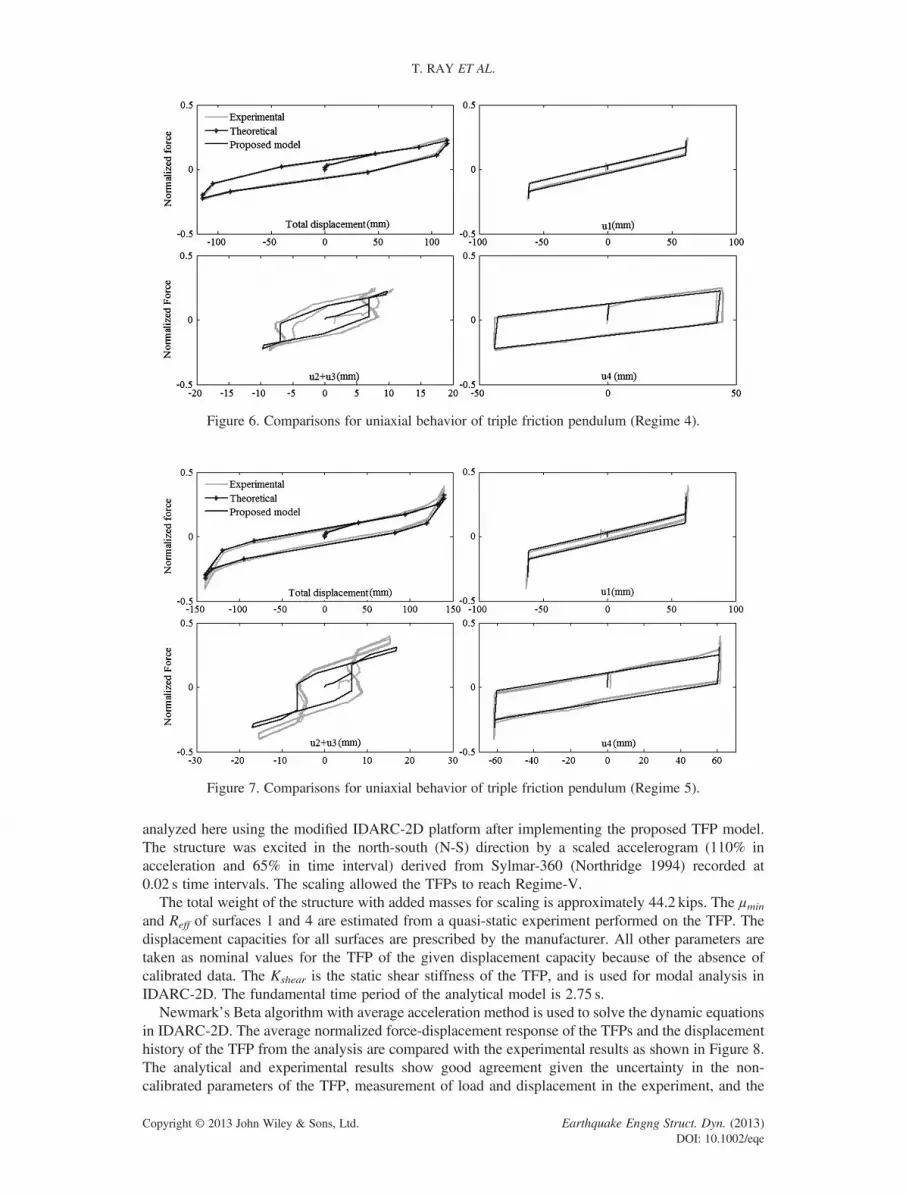
analyzed here using the modified IDARC-2D platform after implementing the proposed TFP model.The structure was excited in the north-south (N-S) direction by a scaled accelerogram (110% inacceleration and 65% in time interval) derived from Sylmar-360 (Northridge 1994) recorded at0.02 s time intervals. The scaling allowed the TFPs to reach Regime-V.

The total weight of the structure with added masses for scaling is approximately 44.2 kips. The μminand Reff of surfaces 1 and 4 are estimated from a quasi-static experiment performed on the TFP. Thedisplacement capacities for all surfaces are prescribed by the manufacturer. All other parameters aretaken as nominal values for the TFP of the given displacement capacity because of the absence ofcalibrated data. The Kshear is the static shear stiffness of the TFP, and is used for modal analysis inIDARC-2D. The fundamental time period of the analytical model is 2.75 s.

Newmark’s Beta algorithm with average acceleration method is used to solve the dynamic equationsin IDARC-2D. The average normalized force-displacement response of the TFPs and the displacementhistory of the TFP from the analysis are compared with the experimental results as shown in Figure 8.The analytical and experimental results show good agreement given the uncertainty in the non-calibrated parameters of the TFP, measurement of load and displacement in the experiment, and the



T. RAY ET AL.


approximated mass distribution in the analytical model. More importantly, the friction coefficientchanges due to the heat generated and abrasion in the interface of the sliding surfaces, whereas theproposed model assumes the friction coefficient is only dependent on the velocity.

7. VERIFICATION OF MODEL FOR BIAXIAL MOTION

7.1. Comparison for sliding on a flat surface for quasi-static displacement input

The proposed biaxial model from plasticity theory developed herein and one using the Park-Wen-Angmodel are compared for sliding of flat surface isolators using MATLAB code. 3DBASIS program can

Table V. Parameters for triple friction pendulum adapted from Fenz and Constantinou [4].

Sl. no.

Predominantslidingregime Amplitude

Frictioncoefficients

Displacementcapacities

Radii ofcurvature

Units mm. mm. mm.

(1) (2) (3) (4) (5)

1 I 1.2 μ1 = 0.03, μ4 = 0.08μ2 =μ3 = 0.02

d1 = d2 = 61.00d3 = d4 = 19.05

R1 =R4 = 435.36R2 =R3 = 53.34

2 II 25 μ1 = 0.036,μ4 = 0.08μ2 =μ3 = 0.015

3 III 75 μ1 = 0.036,μ4 = 0.14μ2 =μ3 = 0.0125

4 IV 115 μ1 = 0.03,μ4 = 0.123μ2 =μ3 = 0.0125

5 V 140 μ1 = 0.033,μ4 = 0.11μ2 =μ3 = 0.0125

Figure 8. Comparison of IDARC2D simulation with shake table test results [14].



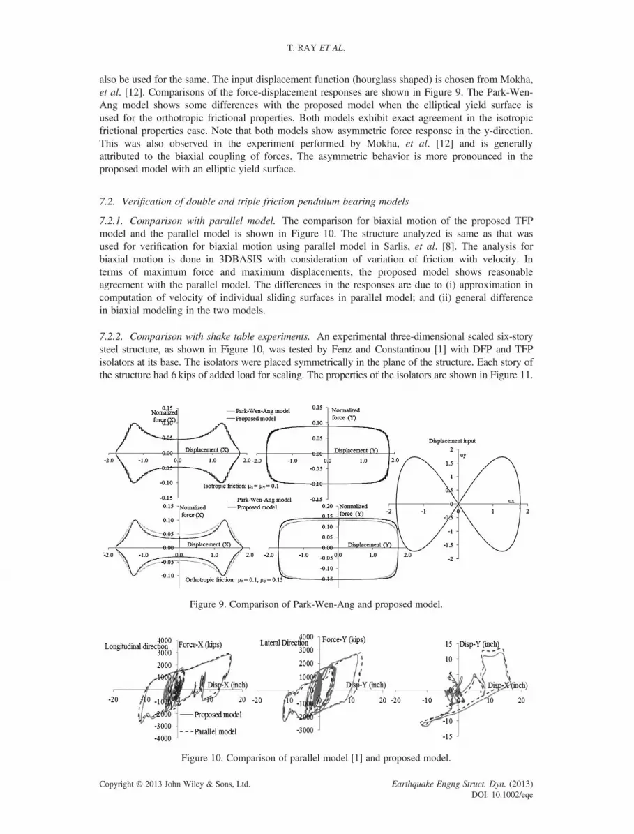
also be used for the same. The input displacement function (hourglass shaped) is chosen from Mokha,et al. [12]. Comparisons of the force-displacement responses are shown in Figure 9. The Park-Wen-Ang model shows some differences with the proposed model when the elliptical yield surface isused for the orthotropic frictional properties. Both models exhibit exact agreement in the isotropicfrictional properties case. Note that both models show asymmetric force response in the y-direction.This was also observed in the experiment performed by Mokha, et al. [12] and is generallyattributed to the biaxial coupling of forces. The asymmetric behavior is more pronounced in theproposed model with an elliptic yield surface.

7.2. Verification of double and triple friction pendulum bearing models

7.2.1. Comparison with parallel model. The comparison for biaxial motion of the proposed TFPmodel and the parallel model is shown in Figure 10. The structure analyzed is same as that wasused for verification for biaxial motion using parallel model in Sarlis, et al. [8]. The analysis forbiaxial motion is done in 3DBASIS with consideration of variation of friction with velocity. Interms of maximum force and maximum displacements, the proposed model shows reasonableagreement with the parallel model. The differences in the responses are due to (i) approximation incomputation of velocity of individual sliding surfaces in parallel model; and (ii) general differencein biaxial modeling in the two models.

7.2.2. Comparison with shake table experiments. An experimental three-dimensional scaled six-storysteel structure, as shown in Figure 10, was tested by Fenz and Constantinou [1] with DFP and TFPisolators at its base. The isolators were placed symmetrically in the plane of the structure. Each story ofthe structure had 6 kips of added load for scaling. The properties of the isolators are shown in Figure 11.

Figure 10. Comparison of parallel model [1] and proposed model.

Figure 9. Comparison of Park-Wen-Ang and proposed model.

T. RAY ET AL.


The structure with DFP bearings was excited by a tri-directional ground motion generated by theshake table simulating 200% scaled 1940 El Centro accelerograms. The structure with TFP bearingswas excited by the unscaled 1994 Newhall accelerograms (tri-directional). A proposed model ofTFP was implemented in the program 3DBASIS-ME-MB [8]. The geometric and frictionalproperties of the isolators were adopted from Fenz and Constantinou [1]. Note that the frictionalproperties were estimated from dynamic test results in Fenz and Constantinou [1]. The hystereticstiffness in the elastic range ko for the DFP and TFP isolators is calculated as

ko ¼ kmul max W=Reffi; i ¼ 1; 2 for DFPð Þ;¼ 1� 4 for TFPð Þ� �(30)

In the experiment with DFP bearings, the displacement demand exceeded the capacity, the rims of thesliding surfaces were hit, and there was significant uplift in the isolators. The radial stiffness kres offeredby the rim is calculated as kres= ko/rmul. The factor kmul is adopted as 10.0 and 2.0 in the analyses withdouble and triple friction pendulums, respectively. rmul is taken as 1.0 for both isolators. For variablevertical load, the ‘T-matrix’ and ‘A-matrix’ (refer to Tsopelas, et al. [19]) required in 3DBASIS wereformulated using SAP2000 (Computers and Structures Inc., 1646 N. California Blvd., Suite 600Walnut Creek, CA 94596, USA) analysis. The ground motions used in the analysis were thoserecorded from the shake table test. The comparison between the experimental and analytical responsesof the average longitudinal and transverse shear in the isolators normalized by average vertical load,and the displacements of the DFP isolators for the tri-directional 1940 El Centro earthquake, are shownin Figure 12. Similar comparisons for the TFP isolators for the tri-directional 1994 Newhallaccelerograms are shown in Figure 13.

From the normalized force-displacement plot in Figure 12, it can be observed that the analytical modelunder predicts the shear when the restrainer is contacted. This discrepancy can be explained by thelimitations of the proposed analytical model, which (i) ignores the effects of friction from steel onsteel when the sliders are in contact with the rim; and (ii) uses lower elastic stiffness (kres) for therestrainer. In the analytical model, the rim is assumed to be elastic with a finite radial stiffness kres,which corresponds to 10W/R. Assuming a higher value for kres (=20W/R) causes numerical problemswith Newmark’s Beta integration method in 3D-BASIS, as can be observed from Figure 12. Thereason for this numerical problem is the sharp transition from low stiffness to high stiffness duringcontact with the restrainer in biaxial motion. Fenz and Constantinou [1] have also reported thisproblem in their analytical model. A similar transition that occurs in uniaxial motion (example inSection 6.2) does not seem to create such a severe numerical issue. Alternative integration throughEuler-Lagrangian action integral or Ritz vector algorithm may alleviate the problem of sharptransition. The displacement response from the analytical calculations matched quite well with those

Figure 11. Structural layout and bearing properties.



from the experimental results, with the exception of when the rim was hit. In this scenario, the analyticalmodel predicted higher displacement due to the lower value of kres.

From the comparative responses shown in Figure 13, it can be observed that the results obtained fromthe present TFP model agree with the experimental results, given the extreme nature of the experiment. Itis worth mentioning that this particular simulation, in which significant variation of vertical load wasencountered, failed to converge with the parallel model formulated with the Park-Wen-Ang model.Discrepancies between the experimental and analytical responses may be attributed mainly to theselection of kmul=2.0 and hysteretic exponent N=2.5. Even though kmul=2.0 is a good assumption for

Figure 12. Comparisons of experimental [1] and analytical (3DBASIS) responses for double friction pendulum.

Figure 13. Comparisons of experimental [1] and analytical (3DBASIS) responses for triple friction pendulum.

T. RAY ET AL.


the outer surfaces, which have an elastic stiffness of about 16W/R, it may not be as appropriate for theinner surfaces that have 2W/R as their elastic stiffness. Although the global response, especially forlarge displacements, is not greatly affected by this smaller elastic stiffness of the inner surfaces andsmoother hysteretic transition coefficient N=2.5, they cause small undulations in the displacementresponse when all surfaces should be in a stationary condition (elastic state). Assuming higher values ofkmul=10 and N= 5 can avoid the undulations during low ground acceleration, but the maximum globaldisplacement response differs by more than 80% from the experimental results as observed fromFigure 13. This occurs again because of numerical problems that arise because of sharp transitions fromhigh stiffness to low stiffness and vice-versa. Alternative solution algorithms (as discussed earlier) and/or assigning elastic stiffness to the sliding surfaces individually may mitigate the problem of these sharptransitions. These issues need to be explored in future research.

8. CONCLUDING REMARKS

Hysteretic models for sliding bearings are developed in this study using plasticity theory. Compared topreviously developed models, the proposed models offer the following advantages: (i) handling thecase of severe variation in frictional forces; and (ii) assumption of either smooth or sharp transitionsbetween the elastic and plastic states. Modeling the uniaxial behavior of the bearings with the sharptransition (for N> 5) in Equation (10) seems to fit the observations in the experiments. However,modeling a smooth transition (N=2) for the biaxial behavior seems to better fit the observations in theexperiments. The smooth behavior is also influenced by the multi-axial interaction, as shown by thethird term on right side of Equation (8), which contributes to the incremental force in Equation (10)independently of H1. A sharp transition exponent (N> 5) may not reproduce the experimentalobservations. The proposed TFP modeling rules are extended to formulate the stiffness for a moregeneral class of spherical sliding bearings with n-surfaces in each half. The performance of the modelin quasi-static response of the bearings is verified by the experimental results and also with thealternative (more limited) hysteretic model. The proposed model shows good agreement with the shaketable tests, given the (i) limitations of the model and the adopted solution algorithm; (ii) uncertainty ofthe measurements; and (iii) estimation of the friction coefficients. The proposed model is implementedin 3DBASIS by following the steps mentioned in Section 5. Although computation of varying axialload including redistribution of the same during uplift was existing in 3DBASIS along with the parallelmodel (using Park-Wen-Ang model) of TFP, the newly implemented more versatile TFP model utilizesthe variation of axial load in plasticity formulation efficiently.

ACKNOWLEDGEMENTS

The funding for the research was provided by the National Science Foundation under Grant CMMI-NEESR:#0830391. The authors thank Dr Daniel Fenz (Research Engineer, Exxon-Mobil Corp.) for sharing theexperimental data and for providing valuable feedback.

REFERENCES

1. Fenz DM, Constantinou MC. Development, implementation and verification of dynamic analysis models for multi-spherical sliding bearings.MCEER-08-0018, University at Buffalo, SUNY, Buffalo, 2008.

2. Morgan TA, Mahin SA. Achieving reliable seismic performance enhancement using multi-stage friction pendulumisolators. Earthquake Engineering and Structural Dynamics 2010; 39(13):1443–1461.

3. Tsai CS, Lin YC, Su HC. Characterization and modeling of multiple friction pendulum isolation system with numeroussliding interfaces. Earthquake Engineering and Structural Dynamics 2010; 39(13):1463–1491.

4. Fenz DM, Constantinou MC. Spherical Sliding Isolation Bearings with Adaptive Behavior: Experimental Verification.Earthquake Engineering and Structural Dynamics 2008; 37(2):185–205.

5. Nagarajaiah S, Reinhorn AM, Constantinou MC. Nonlinear dynamic analysis of 3-D-base-isolated structures. ASCE/Journal of Structural Engineering 1991; 117(7):2035–2054.

6. Mokha A, Constantinou MC, Reinhorn AM. Experimental study and analytical prediction of earthquake response ofa sliding isolation system with spherical surface. Technical Report NCEER-90-0020, National Center for EarthquakeEngineering Research, University at Buffalo, SUNY, Buffalo, 1990.

7. Fenz DM, Constantinou MC. Modeling triple friction pendulum bearings for response-history analysis. EarthquakeSpectra 2008; 24(4):1011–1028.



8. Sarlis AA, Tsopelas PC, Constantinou MC, Reinhorn AM. Element for triple friction pendulum isolator and verificationexamples. 3D-BASIS-ME-MB:Computer Program for Non-Linear Dynamic Analysis for Sysmically Isolated Structures,University at Buffalo, SUNY, 2009.

9. Becker TC, Mahin SA. Experimental and analytical study of the bi-directional behavior of the triple friction pendulumisolator. Earthquake Engineering & Structural Dynamics 2012; 41(3):355–373.

10. Becker TC, Mahin SA. Correct treatment of rotation of sliding surfaces in a kinematic model of the triple frictionpendulum bearing. Earthquake Engineering & Structural Dynamics 2012; 42(2):311–317.

11. Fenz DM, ConstantinouMC. Sperical sliding isolation bearings with adaptive behavior: theory. Earthquake Engineeringand Structural Dynamics 2008; 37(2):163–183.

12. Mokha AS, Constantinou MC, Reinhorn AM. Verification of friction model of teflon bearings under triaxial load.Journal of Structural Engineering, ASCE 1993; 119(1):240–261.

13. Mosqueda G,Whittaker A, Fenves G. Characterization and modeling of friction pendulum bearings subjected tomultiplecomponents of excitation. Journal of Structural Engineering 2004; 130(3):433–442.

14. Sarlis AA, Constantinou MC. Model of triple friction pendulum bearing for general geometric and frictional parametersand for uplift conditions.MCEER-13-000X, Department of Civil Structural and Environmental Engineering, Universityat Buffalo, SUNY, 2013.

15. Simo JC, Hughes TJR. Computational Inelasticity. Springer-Verlag: New York, USA, 1998.16. Sivaselvan MV, Reinhorn AM. Nonlinear structural analysis towards collapse simulation: a dynamical systems

approach. MCEER-04-0005, University at Buffalo, SUNY, Buffalo, 2004.17. Park YJ, Wen YK, Ang AH-S. Random vibration of hysteretic system under Bi-directional ground motion. Earthquake

Engineering & Structural Dynamics(Chichester) 1986; 14:543–557.18. Becker TC. Advanced modeling of the performance of structures supported on triple friction pendulum bearings.

PhD, University of California, Berkeley, 2011.19. Tsopelas PC, Roussis PC, Constantinou MC, Buchanan R, Reinhorn AM. 3D-BASIS-ME-MB: computer program

for nonlinear dynamic analysis of seismically isolated structures. Technical Report MCEER-05-0009, Universityat Buffalo, State University of New York, 2005.

T. RAY ET AL.


Documents

Hysteretic models for sliding bearings with varying frictional force