Embed Size (px)
Citation preview
Accounting transparency and the cost of capital
Vincent Bignon∗
IUFM de Creteil
and
FORUM, University of Paris 10
Regis Breton†
CNRS
and
LEO, University of Orleans
This version‡: 15th March 2004
Abstract
This paper identifies a negative effect of corporate transparency, and shows
that more precise accounting standards can lead to a higher cost of capital.
We build a model of a firm raising funds through an IPO to finance a positive
NPV project. Due the presence of an informed speculator, increased disclo-
sure through accounting data can increase informational asymmetries in the
secondary market, thereby reducing market liquidity. Our uninformed traders
are rational liquidity traders that anticipate that they loose because of informed
trading. Reduction in market liquidity therefore leads to higher cost of external
capital. The ”agency cost” comes from asymmetries among investors.
JEL classification: D82, G10, M41
Keywords: financial market, cost of capital, accounting standards, trans-
parency, lemon premium.
Resume
Un effet negatif de la transparence des firmes est formalise, montrant que
des standards comptables plus precis peuvent augmenter le cout du capital. Une
firme emet des titres echangeables pour financer un projet de VAN positive.
De par la presence d’un speculateur informe, la divulgation d’information via
les annonces comptables peut augmenter les asymetries d’information dans le
marche secondaire, et reduire la liquidite. Les investisseurs non informes sont
rationnels et valorisent la liquidite des titres. La moindre liquidite du marche
induit alors un cout du financement externe plus eleve. Ce ”cout d’agence” est
explique par les asymetries entre investisseurs.
∗Address for correspondance: Universite Paris-X-Nanterre, FORUM, bat. K, 200 avenue de la
Republique, F-92001 Nanterre cedex. E-mail: [email protected]†Address for correspondance: Universite d’Orleans, Faculte de Droit, d’Economie et de Gestion,
BP 6739, rue de Blois, F-45067 Orleans cedex. E-mail: [email protected]‡We acknowledge comments by participants at seminar at the University of Paris 10. We thank
Bertrand Gobillard for pointing some mistakes in the previous manuscript. Remaining errors are
our own.
1
1 Introduction
One of the key principles underlying current evolutions in accounting regulation – e.g.
adoption of IASB standards by European Community – is the objective to provide
financial investors with more accurate and precise information about firms’ activity.
This stated objective has been reinforced by recent corporate scandals (Enron, Par-
malat), that illustrated how actual accounting practices and standards were not able
to prevent public misperception of a corporate financial position. In the view of reg-
ulation makers, more precise, ”transparent” accounting standards allow investors to
better control managers’ actions, which will “enhance the comparability and trans-
parency of financial information, thereby increasing the efficiency of the markets and
reducing the cost of capital for companies1” (EU Directive on consolidated accounts,
2002).
The line of argument sustaining this typical statement runs as follows. Well-
designed accounting standards increase the precision of information extracted from
accounting release. In turn, more precise information reduces information asymme-
tries between firms and investors, thereby contributing to lower the cost of capital
(Leuz and Verrecchia, 2000). We think this argument narrowly focuses on infor-
mational asymmetries between managers and investors, and understates important
effects on the distribution of information among investors. Intuitive as it may be,
the presumption that information disclosure reduces all informational asymmetries is
false. When investors are heterogenous – because they differ in their ability to pro-
cess accounting information, or have access to different private information – more
public information can increase informational asymmetries among market partici-
pants. This can adversely affect the liquidity of the firm’s stock and finally raise the
cost of external finance. Although we build on existing ideas in the microstructure
literature, to our knowledge the effect we stress has not appeared in the accounting
regulation debate.
Despite the widespread perception that transparency is beneficial2, the literature
has identified situations where more public information may be socially undesir-
able3. First it is well known since Hirshleifer (1971) that public information can
destroy risk-sharing opportunities. Dye (2001) applies this very general effect to dis-
cuss the desirability of information disclosure by firms. Another strand of literature
1US Security and Exchange Commission former Chairman Arthur Levitt delivered quite the same
message, see Admati and Pfleiderer (2000).2The benefits of information disclosure are well documented. See, inter alia, Diamond (1985)
and Fishman and Hagerty (1989, 1990). For a survey on the literature on disclosure, see Verrecchia
(2001). We highly recommend the discussion by Dye (2001) on the use of linear rational pricing
models in the accounting literature.3Even in settings were more information is better, more stringent disclosure legislation need not be
optimal. For instance, Dye (1985) shows that when substitutions effect with other sources of public
information (voluntary disclosure by firms) are present, this can paradoxically lower publicly available
information. Similarly, the effects on private acquisition of information are ambiguous (Bushman,
1991). We term those effects as ”indirect”, in contrast to ”direct” costs of more information.
2
points to the notion of proprietary information, the disclosure of which can benefit
the firm’s competitor, thereby lowering the firm’s position and associated cash-flow
(Dye, 1985)4. In a pure agency setting, Cremer (1995) and Prat (2003) show that
more information about the agent’s type can be detrimental to welfare through di-
minished incentives. Negative effects of corporate transparency in Almazan, Suarez
and Titman (2003) hinges on another instance of unintended disclosure to a third
party. In their model, lower public information about the firm’s type induces the
worker force to exert higher effort. Finally, Kanodia and Singh (2001) argue that
when a firm’s investment decision is influenced by how its decisions are priced in
the market, imprecision in accounting reports may be necessary to induce outside
investors to incorporate ongoing information.
We point to a distinct potential cost of transparency. The key idea is that more
public information and less private information are not synonymous. The intuition
builds on two assumptions. (i) When some investors have access to private infor-
mation, more precise accounting information can increase the informational advan-
tage of informed speculators vis-a-vis uninformed liquidity traders. As in Boot and
Thakor (2001), this occurs when the information disclosed by firm is complemen-
tary to the private information of informed traders. (ii) Informational asymmetries
among market participants hinder the liquidity of the secondary market (Glosten
and Milgrom, 1985; Gorton and Pennachi, 1990). When investors value liquidity,
this represents a cost which is ultimately borne by the firm.
More precisely, we consider a firm raising external finance for a risky project. The
capital market is populated by one potential speculator and many small investors
who value liquidity. The environment is designed such that more precise accounting
raises the speculator’s informational advantage. As an example, consider a firm
developing a product designed for one of two competing technological standards.
Some investors in the market may have private information about which standard
will finally prevail. However this information is only valuable when there is public
information about the firm’s choice of standard. When such information is disclosed
(through, e.g. accounting release), the informed trader enters the market, because
accounting information raises the value of his private information. Anticipating that
they may suffer from speculation when selling their shares for liquidity reasons, small
investors require a higher return to initially buy the firm’s shares. The firm’s cost
of capital is higher under transparency. Disclosure raises the incentives to acquire
socially harmful information. This result contrasts those in Diamond (1985) and
Boot and Thakor (2001) who study incentives to acquire socially usefull information.
Our argument can be given the following alternative interpretation. Accounting
release is raw data, that must generally be processed or combined with other sources
to yield valuable information. Hence, in real world settings, disclosure per se does not
imply more public information. Indeed, some investors may lack the ability to fully
4The idea that confidentiality has value for firms appeared in Campbell (1979). Bhattacharya
and Chiesa (1995) and Yosha (1995) use this idea to explain firm’s choice of financing source.
3
process increasingly technical financial reports, while other have a comparative ad-
vantage in this respect5. In that case, increasing the technicity of financial statement,
through a more detailed account of, e.g. firm’s derivative position can help to mit-
igate the informational asymmetry between manager and some investors (the more
sophisticated). But at the same time, this would deepen the informational asymme-
try between investors, thereby creating an opportunity for the sophisticated to make
profit at the expense of the less sophisticated as the former can used their knowledge
of the true firm position to sell their share to the less informed, before this information
is incorporated into the price. So this work is also related to some extant research
that emphasise investors’ differing sophistication (Indjejikian, 1991; Hirschleifer and
Teoh, 2004).
The rest of the paper is organised as follows. Section 2 presents the economic en-
vironment, in term of agents, information structure and trading mechanism. Section
3 solves for the equilibrium on the secondary market. Section 4 analyses the initial
public offreing stage for a given accounting structure. Effect of accounting structure
is analysed in section 5. Section 6 concludes. Computations are in the appendix.
2 Environment
This is a three-date economy. Time is indexed by t = 0, 1, 2. The situation is that
of an entrepreneur raising cash through an initial public offering (IPO) in order to
undertake an investment project.
Firm. A risk neutral entrepreneur with no cash (henceforth E) is endowed with a
project requiring a fixed investment I = 1 at t = 0. He goes to the capital market in
order to raise I through an IPO. The project yields a risky cash flow V at t = 2: it can
succeed and yield V H with probability π, or fail and yield V L = 0 with probability
1 − π. The project has positive net present value:
πV H > 1 (1)
We assume limited liability, so that E issue securities that pay R in case of success. At
the time of the IPO, the entrepreneur does not have any private information about
the project. The outcome does not depend on any (unobservable) action of the
entrepreneur. Thus there is no adverse selection nor moral hazard problem between
the firm and outside investors. Furthermore, π is common knowledge and the date 2
realisation V is publicly observed. Just after the project has started, the entrepreneur
privately observes a signal Si ∈S0, S1
on the date 2 cash flow.
5There is some support to the idea that a research on the effect of more transparent accounting
disclosure on firm’s cost of capital have to take into account the existence of various types of traders
on the financial market. The existence of various type of investors on the capital market have, e.g.,
been stressed by the FASB in July, 1995 in a report worrying about an ”information overload”
problem that at least one group of traders can experienced.
4
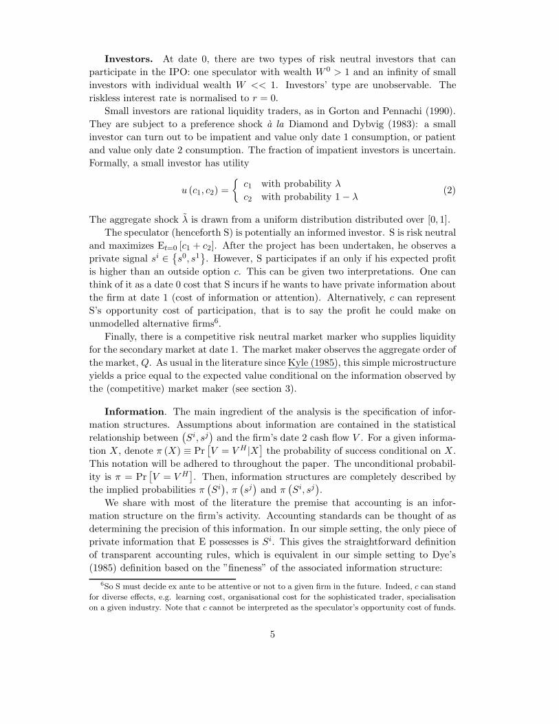
Investors. At date 0, there are two types of risk neutral investors that can
participate in the IPO: one speculator with wealth W 0 > 1 and an infinity of small
investors with individual wealth W << 1. Investors’ type are unobservable. The
riskless interest rate is normalised to r = 0.
Small investors are rational liquidity traders, as in Gorton and Pennachi (1990).
They are subject to a preference shock a la Diamond and Dybvig (1983): a small
investor can turn out to be impatient and value only date 1 consumption, or patient
and value only date 2 consumption. The fraction of impatient investors is uncertain.
Formally, a small investor has utility
u (c1, c2) =
c1 with probability λ
c2 with probability 1 − λ(2)
The aggregate shock λ is drawn from a uniform distribution distributed over [0, 1].
The speculator (henceforth S) is potentially an informed investor. S is risk neutral
and maximizes Et=0 [c1 + c2]. After the project has been undertaken, he observes a
private signal si ∈s0, s1
. However, S participates if an only if his expected profit
is higher than an outside option c. This can be given two interpretations. One can
think of it as a date 0 cost that S incurs if he wants to have private information about
the firm at date 1 (cost of information or attention). Alternatively, c can represent
S’s opportunity cost of participation, that is to say the profit he could make on
unmodelled alternative firms6.
Finally, there is a competitive risk neutral market marker who supplies liquidity
for the secondary market at date 1. The market maker observes the aggregate order of
the market, Q. As usual in the literature since Kyle (1985), this simple microstructure
yields a price equal to the expected value conditional on the information observed by
the (competitive) market maker (see section 3).
Information. The main ingredient of the analysis is the specification of infor-
mation structures. Assumptions about information are contained in the statistical
relationship between(Si, sj
)and the firm’s date 2 cash flow V . For a given informa-
tion X, denote π (X) ≡ Pr[V = V H |X
]the probability of success conditional on X.
This notation will be adhered to throughout the paper. The unconditional probabil-
ity is π = Pr[V = V H
]. Then, information structures are completely described by
the implied probabilities π(Si
), π
(sj
)and π
(Si, sj
).
We share with most of the literature the premise that accounting is an infor-
mation structure on the firm’s activity. Accounting standards can be thought of as
determining the precision of this information. In our simple setting, the only piece of
private information that E possesses is Si. This gives the straightforward definition
of transparent accounting rules, which is equivalent in our simple setting to Dye’s
(1985) definition based on the ”fineness” of the associated information structure:
6So S must decide ex ante to be attentive or not to a given firm in the future. Indeed, c can stand
for diverse effects, e.g. learning cost, organisational cost for the sophisticated trader, specialisation
on a given industry. Note that c cannot be interpreted as the speculator’s opportunity cost of funds.
5
(1
2
)S1
(α)
s1V H
(1 −α)
s0
V L
S0
( 1
2 )
V L
(1 −β)
s1
V H
(β)
s0
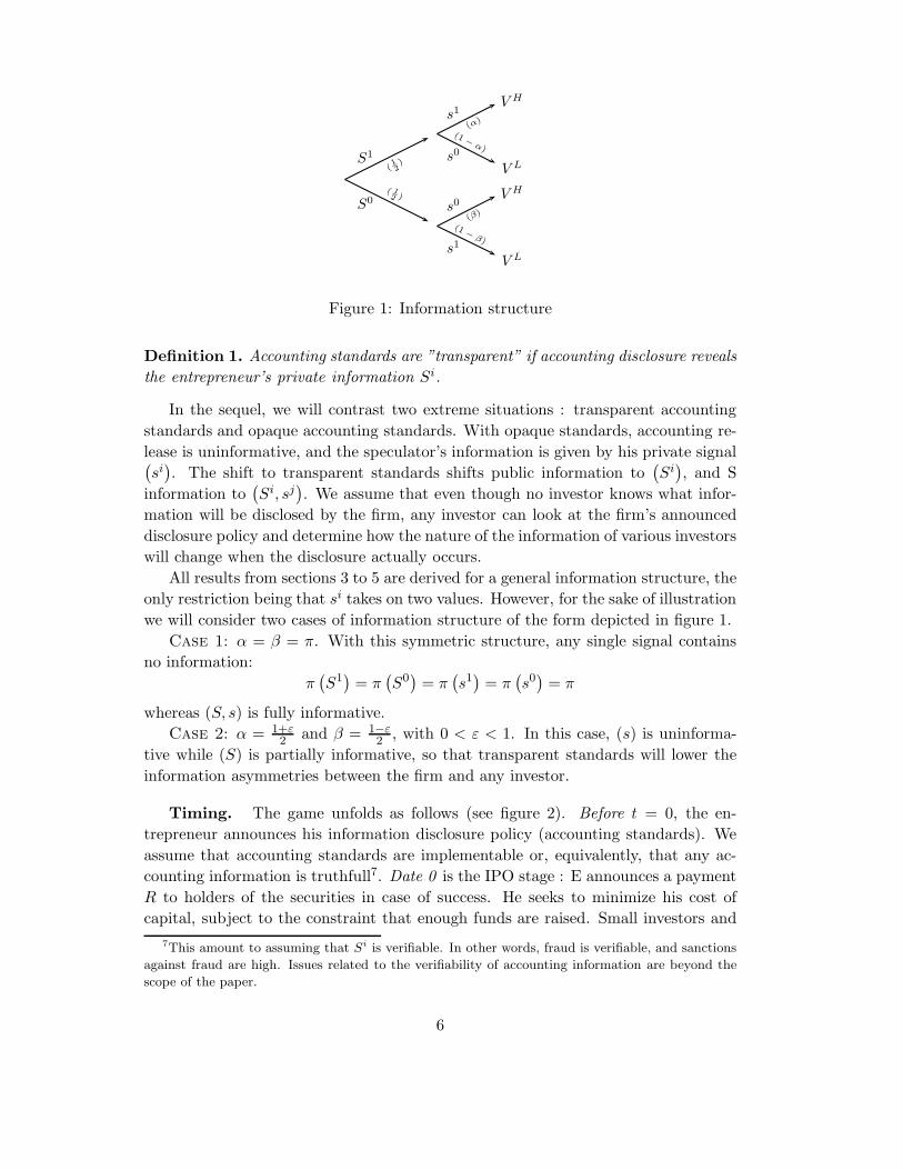
Figure 1: Information structure
Definition 1. Accounting standards are ”transparent” if accounting disclosure reveals
the entrepreneur’s private information Si.
In the sequel, we will contrast two extreme situations : transparent accounting
standards and opaque accounting standards. With opaque standards, accounting re-
lease is uninformative, and the speculator’s information is given by his private signal(si
). The shift to transparent standards shifts public information to
(Si
), and S
information to(Si, sj
). We assume that even though no investor knows what infor-
mation will be disclosed by the firm, any investor can look at the firm’s announced
disclosure policy and determine how the nature of the information of various investors
will change when the disclosure actually occurs.
All results from sections 3 to 5 are derived for a general information structure, the
only restriction being that si takes on two values. However, for the sake of illustration
we will consider two cases of information structure of the form depicted in figure 1.
Case 1: α = β = π. With this symmetric structure, any single signal contains
no information:
π(S1
)= π
(S0
)= π
(s1
)= π
(s0
)= π
whereas (S, s) is fully informative.
Case 2: α = 1+ε2 and β = 1−ε
2 , with 0 < ε < 1. In this case, (s) is uninforma-
tive while (S) is partially informative, so that transparent standards will lower the
information asymmetries between the firm and any investor.
Timing. The game unfolds as follows (see figure 2). Before t = 0, the en-
trepreneur announces his information disclosure policy (accounting standards). We
assume that accounting standards are implementable or, equivalently, that any ac-
counting information is truthfull7. Date 0 is the IPO stage : E announces a payment
R to holders of the securities in case of success. He seeks to minimize his cost of
capital, subject to the constraint that enough funds are raised. Small investors and
7This amount to assuming that Si is verifiable. In other words, fraud is verifiable, and sanctions
against fraud are high. Issues related to the verifiability of accounting information are beyond the
scope of the paper.
6
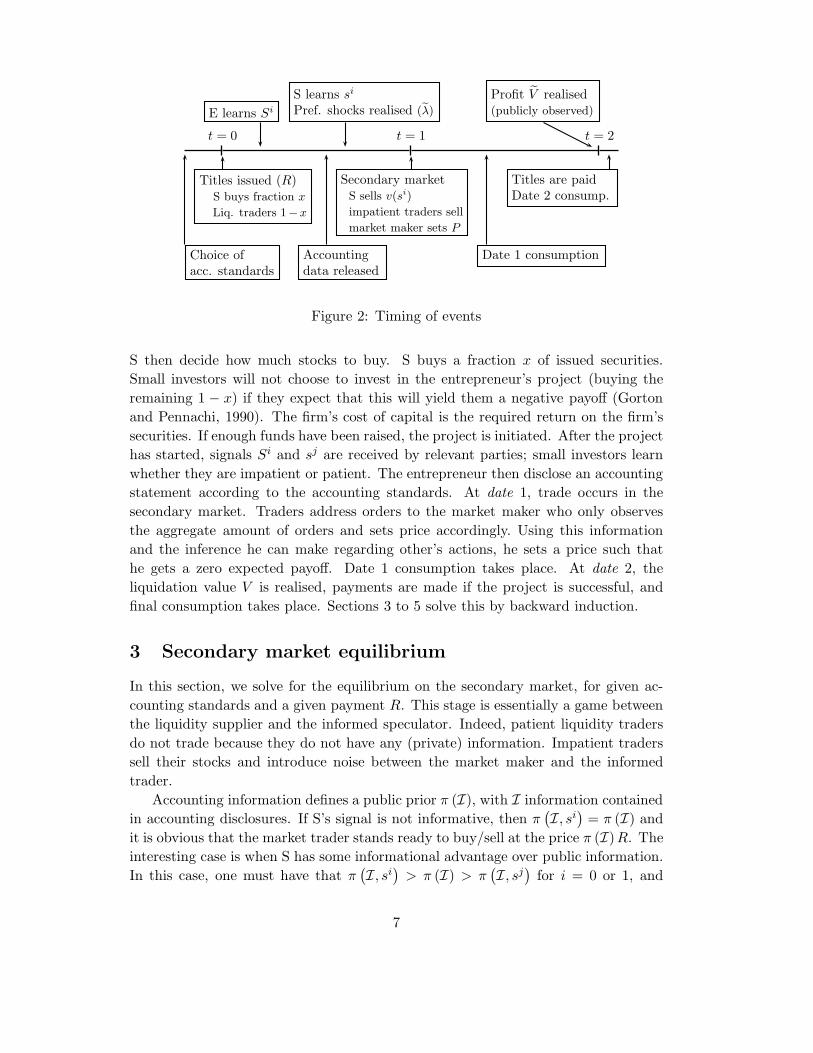
t = 0 t = 1 t = 2
E learns Si
S learns si
Pref. shocks realised (λ)
Profit V realised(publicly observed)
Choice ofacc. standards
Accountingdata released
Secondary marketS sells v(si)
impatient traders sell
market maker sets P
Titles are paidDate 2 consump.
Date 1 consumption
Titles issued (R)S buys fraction x
Liq. traders 1−x
Figure 2: Timing of events
S then decide how much stocks to buy. S buys a fraction x of issued securities.
Small investors will not choose to invest in the entrepreneur’s project (buying the
remaining 1 − x) if they expect that this will yield them a negative payoff (Gorton
and Pennachi, 1990). The firm’s cost of capital is the required return on the firm’s
securities. If enough funds have been raised, the project is initiated. After the project
has started, signals Si and sj are received by relevant parties; small investors learn
whether they are impatient or patient. The entrepreneur then disclose an accounting
statement according to the accounting standards. At date 1, trade occurs in the
secondary market. Traders address orders to the market maker who only observes
the aggregate amount of orders and sets price accordingly. Using this information
and the inference he can make regarding other’s actions, he sets a price such that
he gets a zero expected payoff. Date 1 consumption takes place. At date 2, the
liquidation value V is realised, payments are made if the project is successful, and
final consumption takes place. Sections 3 to 5 solve this by backward induction.
3 Secondary market equilibrium
In this section, we solve for the equilibrium on the secondary market, for given ac-
counting standards and a given payment R. This stage is essentially a game between
the liquidity supplier and the informed speculator. Indeed, patient liquidity traders
do not trade because they do not have any (private) information. Impatient traders
sell their stocks and introduce noise between the market maker and the informed
trader.
Accounting information defines a public prior π (I), with I information contained
in accounting disclosures. If S’s signal is not informative, then π(I, si
)= π (I) and
it is obvious that the market trader stands ready to buy/sell at the price π (I)R. The
interesting case is when S has some informational advantage over public information.
In this case, one must have that π(I, si
)> π (I) > π
(I, sj
)for i = 0 or 1, and
7
i 6= j. For the remaining of this section, we will denote si the state for which
π(I, si
)> π (I), and s−i the state for which π (I) > π
(I, s−i
).
The risk neutral market maker observes the aggregate order Q. As usual in the
literature since Kyle (1985), competitive liquidity supply yields a price equal to the
expected value conditional on the market maker information:
P (Q) = E
[R|I,Q
](3)
As a monopolist, the speculator anticipates the effect his order v has on the price
set by the market maker. As π(I, si
)> π (I), S buys the stock when his signal is si,
betting on a low realisation of λ to full the market maker. Conversely, he is willing
to sell when s = s−i; he can hide his trade when λ is high. Formally, upon observing
s, S maximises his date 2 earnings:
maxv
xπ (I)R + v · [π (I, s)− E [P (Q) |I, s]]
(4)
subject to the no short sell constraint v (s) ≤ x.
Denote by ve the anticipated speculator’s strategy. For a given realisation λ of
the aggregate liquidity shock, λ · (1 − x) stocks are sold for liquidity reasons. The
market maker sets the price equal to the expectation of the value of the firm for
claim-holders, given the aggregate selling Q = λ · (1 − x) + ve (s).
P = E
[R|I,Q
]= Pr
[V H |I,Q
]R = π (I,Q)R (5)
with
π (I, Q) = Pr[si|I, Q
]π
(I, si
)+ Pr
[s−i|I, Q
]π
(I, s−i
)(6)
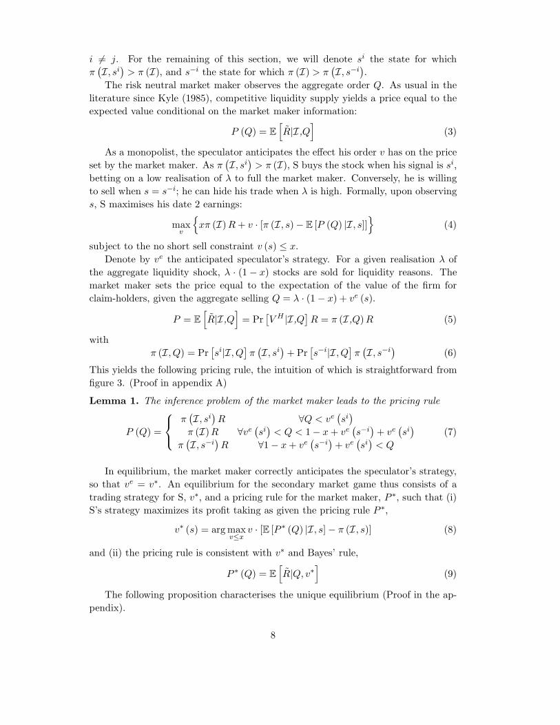
This yields the following pricing rule, the intuition of which is straightforward from
figure 3. (Proof in appendix A)
Lemma 1. The inference problem of the market maker leads to the pricing rule
P (Q) =
π(I, si
)R ∀Q < ve
(si
)
π (I)R ∀ve(si
)< Q < 1 − x + ve
(s−i
)+ ve
(si
)
π(I, s−i
)R ∀1 − x + ve
(s−i
)+ ve
(si
)< Q
(7)
In equilibrium, the market maker correctly anticipates the speculator’s strategy,
so that ve = v∗. An equilibrium for the secondary market game thus consists of a
trading strategy for S, v∗, and a pricing rule for the market maker, P ∗, such that (i)
S’s strategy maximizes its profit taking as given the pricing rule P ∗,
v∗ (s) = arg maxv≤x
v · [E [P ∗ (Q) |I, s] − π (I, s)] (8)
and (ii) the pricing rule is consistent with v∗ and Bayes’ rule,
P ∗ (Q) = E
[R|Q, v∗
](9)
The following proposition characterises the unique equilibrium (Proof in the ap-
pendix).
8

f(.)
Q
density when s = si density when s = s−i
v∗(si) 0 v∗(s−i) 1 − x + v∗(si) 1 − x + v∗(s−i)P = π(I, si)R
P = π(I, s−i)R
P = π(I)R
Figure 3: The market maker inference problem
Proposition 2. There is a unique equilibrium on the secondary market. If the spec-
ulator’s initial position x ≤ 14 , then S is constrained by his initial holding, and his
equilibrium strategy is
v∗(si
)= −
(1
2− x
)v∗
(s−i
)= x (10)
If 14 ≤ x ≤ 1, then the no-short selling contraint is not binding, and S’s equilibrium
strategy is
v∗(si
)= −
1 − x
3v∗
(s−i
)=
1 − x
3(11)
4 IPO Stage
The previous section analysed the secondary market outcome, for a given level of x.
Hence, in the first place, the speculator should be willing to contribute to a fraction
x of the investment, and uninformed liquidity traders should be ready to contribute
for the remaining fraction 1 − x, even though they know that the speculator could
participate.
4.1 Speculator position
At t = 0, the speculator decides the fraction x of total issued stocks to buy. His t = 0
expected profit (gross of the initial cost c) is
ΠS (x) = x (πR − 1) +∑
I
Pr [I]∑
s
[Pr (s|I)max
v≤xv · [π (I, s) − E [P ∗ (Q) |I, s]]
]
(12)
9
Expression (12) for the speculator’s profit can be pined down to a measure of his
informational advantage. More precisely, define
T =∑
I
Pr [I]∑
s
Pr [s|I] · |π (I, s) − π (S)| (13)
With some computations ΠS can be written as a function ΠS (x,R, T ), increasing
with R and with the informational advantage T (see appendix C).
Conditional on participating, S buys at the IPO stage the fraction x∗ (R,T ) ≡
arg max[0,1] ΠS (x,R, T ) of issued stocks. Define Π∗ (R,T ) = maxx ΠS (x,R, T ) the
associated expected profit of S if he participates. The speculator’s optimal holding
is characterised as follows:
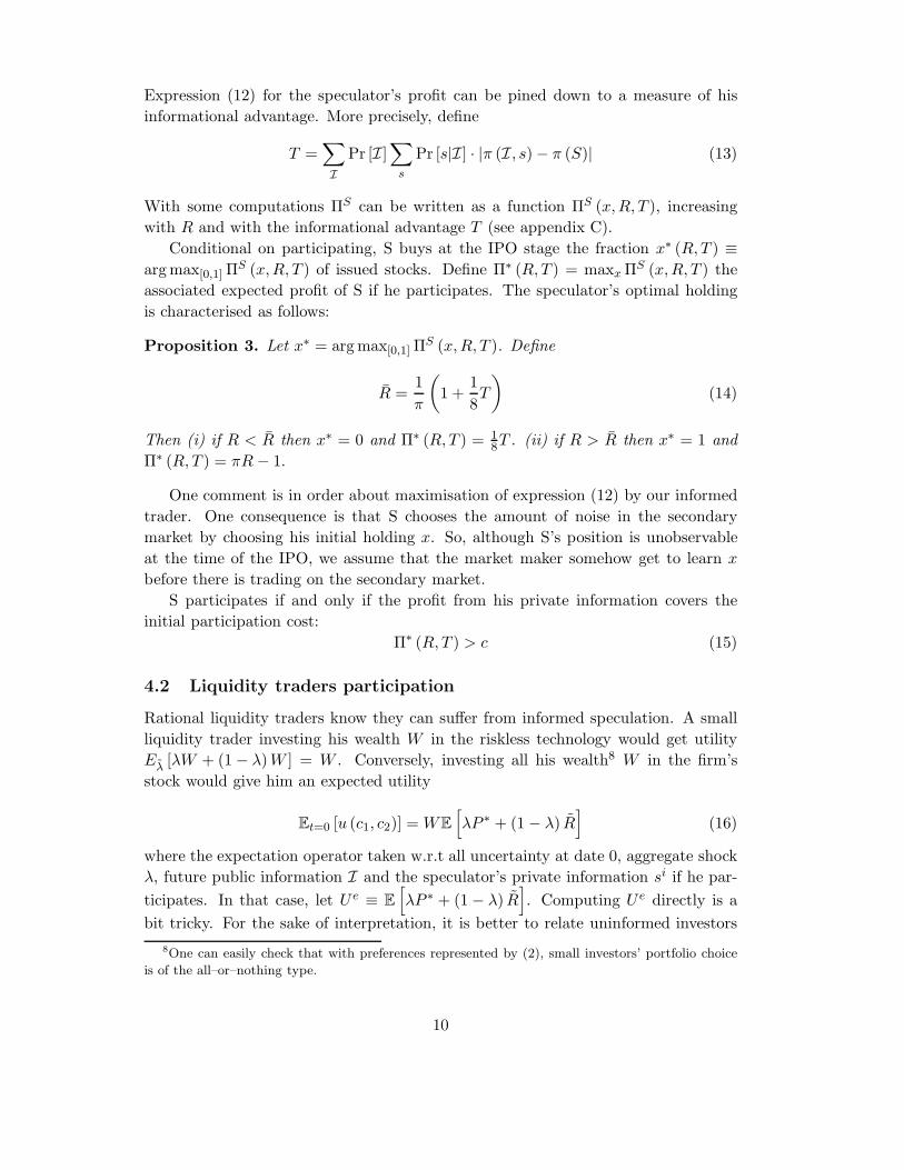
Proposition 3. Let x∗ = arg max[0,1] ΠS (x,R, T ). Define
R =1
π
(1 +
1
8T
)(14)
Then (i) if R < R then x∗ = 0 and Π∗ (R,T ) = 18T . (ii) if R > R then x∗ = 1 and
Π∗ (R,T ) = πR − 1.
One comment is in order about maximisation of expression (12) by our informed
trader. One consequence is that S chooses the amount of noise in the secondary
market by choosing his initial holding x. So, although S’s position is unobservable
at the time of the IPO, we assume that the market maker somehow get to learn x
before there is trading on the secondary market.
S participates if and only if the profit from his private information covers the
initial participation cost:
Π∗ (R,T ) > c (15)
4.2 Liquidity traders participation
Rational liquidity traders know they can suffer from informed speculation. A small
liquidity trader investing his wealth W in the riskless technology would get utility
Eλ
[λW + (1 − λ) W ] = W . Conversely, investing all his wealth8 W in the firm’s
stock would give him an expected utility
Et=0 [u (c1, c2)] = WE
[λP ∗ + (1 − λ) R
](16)
where the expectation operator taken w.r.t all uncertainty at date 0, aggregate shock
λ, future public information I and the speculator’s private information si if he par-
ticipates. In that case, let U e ≡ E
[λP ∗ + (1 − λ) R
]. Computing U e directly is a
bit tricky. For the sake of interpretation, it is better to relate uninformed investors
8One can easily check that with preferences represented by (2), small investors’ portfolio choice
is of the all–or–nothing type.
10
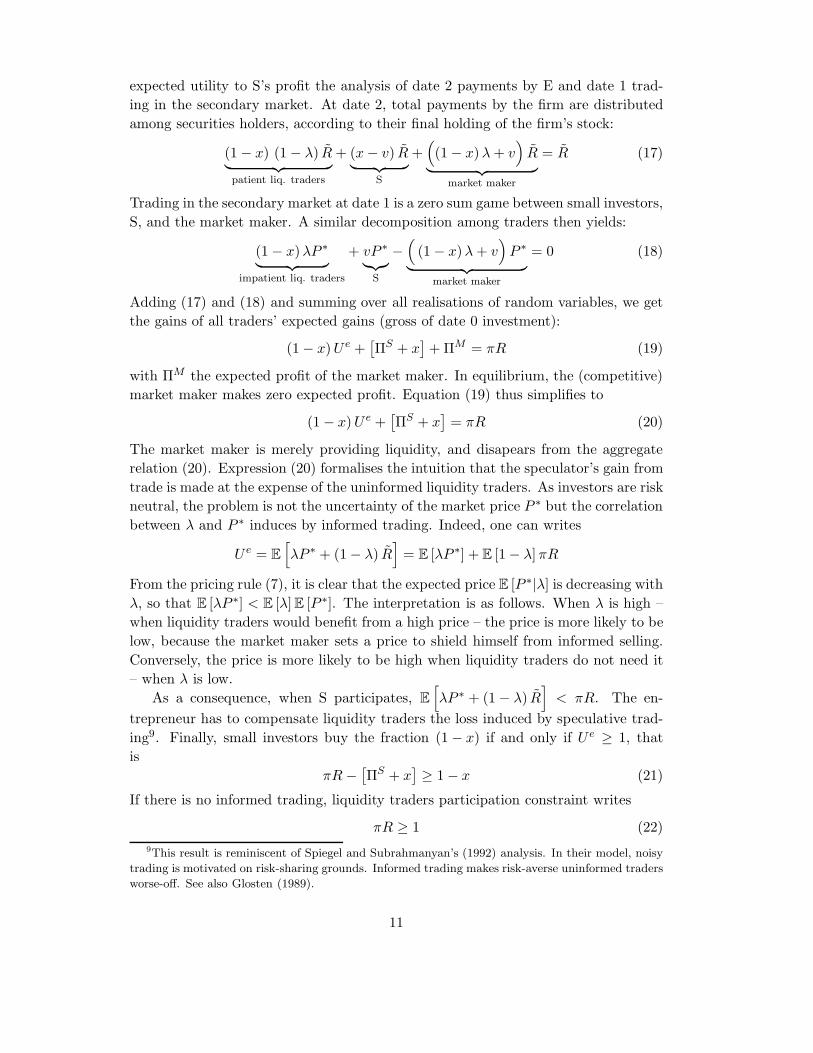
expected utility to S’s profit the analysis of date 2 payments by E and date 1 trad-
ing in the secondary market. At date 2, total payments by the firm are distributed
among securities holders, according to their final holding of the firm’s stock:
(1 − x) (1 − λ) R︸ ︷︷ ︸patient liq. traders
+ (x − v) R︸ ︷︷ ︸
S
+((1 − x) λ + v
)R
︸ ︷︷ ︸market maker
= R (17)
Trading in the secondary market at date 1 is a zero sum game between small investors,
S, and the market maker. A similar decomposition among traders then yields:
(1 − x)λP ∗
︸ ︷︷ ︸impatient liq. traders
+ vP ∗
︸︷︷︸S
−(
(1 − x)λ + v)
P ∗
︸ ︷︷ ︸market maker
= 0 (18)
Adding (17) and (18) and summing over all realisations of random variables, we get
the gains of all traders’ expected gains (gross of date 0 investment):
(1 − x) U e +[ΠS + x
]+ ΠM = πR (19)
with ΠM the expected profit of the market maker. In equilibrium, the (competitive)
market maker makes zero expected profit. Equation (19) thus simplifies to
(1 − x) U e +[ΠS + x
]= πR (20)
The market maker is merely providing liquidity, and disapears from the aggregate
relation (20). Expression (20) formalises the intuition that the speculator’s gain from
trade is made at the expense of the uninformed liquidity traders. As investors are risk
neutral, the problem is not the uncertainty of the market price P ∗ but the correlation
between λ and P ∗ induces by informed trading. Indeed, one can writes
U e = E
[λP ∗ + (1 − λ) R
]= E [λP ∗] + E [1 − λ] πR
From the pricing rule (7), it is clear that the expected price E [P ∗|λ] is decreasing with
λ, so that E [λP ∗] < E [λ] E [P ∗]. The interpretation is as follows. When λ is high –
when liquidity traders would benefit from a high price – the price is more likely to be
low, because the market maker sets a price to shield himself from informed selling.
Conversely, the price is more likely to be high when liquidity traders do not need it
– when λ is low.
As a consequence, when S participates, E
[λP ∗ + (1 − λ) R
]< πR. The en-
trepreneur has to compensate liquidity traders the loss induced by speculative trad-
ing9. Finally, small investors buy the fraction (1 − x) if and only if U e ≥ 1, that
is
πR −[ΠS + x
]≥ 1 − x (21)
If there is no informed trading, liquidity traders participation constraint writes
πR ≥ 1 (22)
9This result is reminiscent of Spiegel and Subrahmanyan’s (1992) analysis. In their model, noisy
trading is motivated on risk-sharing grounds. Informed trading makes risk-averse uninformed traders
worse-off. See also Glosten (1989).
11
4.3 The entrepreneur’s problem
For a given accounting structure, the entrepreneur’s problem is to minimise his cost
of capital, πR, subject to the constraint that enough funds are raised, I = 1. The
choice of accounting standards is analysed in the next section.
The first best payment is R∗ ≡ 1π
(alternative investments give the riskless return
r = 0). For any R < R∗, investors would not participate. Now assume that E
promises the payment R∗. This is an equilibrium if and only if the speculator does
not enter. This is the case when Π∗ (R∗, T ) < c. Using proposition 3, we get that S’s
optimal profit is ΠS (R∗, T ) = 18T which yields
1
8T < c (23)
Condition (23) is a necessary and sufficient condition to get the first best payment.
As S makes expected losses, he does not acquire his information. Anticipating that
S does not participate, liquidity traders are willing to buy the firm’s stocks at date
0, as E
[λP ∗ + (1 − λ) R
]= πR∗ ≥ 1.
When the converse of (23) holds, S enters the market. Payment R∗ is not suf-
ficient to induce liquidity traders to participate, because informed trading hinders
liquidity supply by the market maker. Liquidity traders require higher return πR in
compensation. Therefore if the investment is to be financed, one must have R > R∗
and a cost of capital higher than the first best. Formally, liquidity traders participate
if and only if
πR − (Π∗ (R,T ) + x∗ (R)) ≥ 1 − x∗ (R) (24)
Using proposition 3, it is easily checked that condition (24) does not hold for any
payment R < R ≡ R∗ + 1π
18T whereas setting R is sufficient. The main result of this
section is therefore:
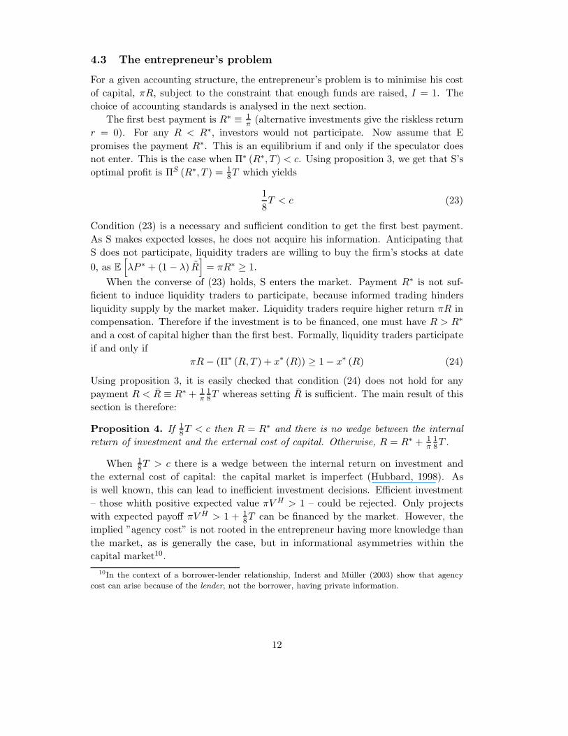
Proposition 4. If 18T < c then R = R∗ and there is no wedge between the internal
return of investment and the external cost of capital. Otherwise, R = R∗ + 1π
18T .
When 18T > c there is a wedge between the internal return on investment and
the external cost of capital: the capital market is imperfect (Hubbard, 1998). As
is well known, this can lead to inefficient investment decisions. Efficient investment
– those whith positive expected value πV H > 1 – could be rejected. Only projects
with expected payoff πV H > 1 + 18T can be financed by the market. However, the
implied ”agency cost” is not rooted in the entrepreneur having more knowledge than
the market, as is generally the case, but in informational asymmetries within the
capital market10.
10In the context of a borrower-lender relationship, Inderst and Muller (2003) show that agency
cost can arise because of the lender, not the borrower, having private information.
12
5 Choice of accounting standards
It is now straightforward to determine the consequences of accounting standards.
Proposition 4 shows how the external cost of capital can be affected by public infor-
mation through accounting disclosure. The entrepreneur will choose the accounting
standards that minimize his cost of capital. In this setting where price informative-
ness per se does not have value, this amounts to choosing the accounting standards
that minimize S’s informational advantage.
If accounting standards are opaque, accounting data do not give any public in-
formation about the realised Si. The speculator’s advantage is given by
T0 =∑
s
Pr [s] · |π (s) − π| (25)
Conversely, if E chooses a transparent accounting structure, then Si becomes
public information at the time of accounting announcement. In this case, S’s infor-
mational advantage is
T1 =∑
S
Pr [S]∑
s
Pr [s|S] · |π (S, s) − π (S)| (26)
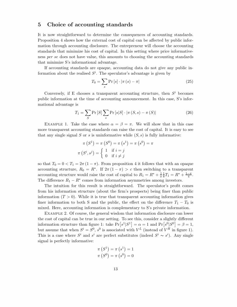
Example 1. Take the case where α = β = π. We will show that in this case
more transparent accounting standards can raise the cost of capital. It is easy to see
that any single signal S or s is uninformative while (S, s) is fully informative:
π(S1
)= π
(S0
)= π
(s1
)= π
(s0
)= π
π(Si, sj
)=
1 if i = j
0 if i 6= j
so that T0 = 0 < T1 = 2π (1 − π). From proposition 4 it follows that with an opaque
accounting structure, R0 = R∗. If 2π (1 − π) > c then switching to a transparent
accounting structure would raise the cost of capital to R1 = R∗ + 1π
18T1 = R∗ + 1−π
4 .
The difference R1 − R∗ comes from information asymmetries among investors.
The intuition for this result is straightforward. The speculator’s profit comes
from his information structure (about the firm’s prospects) being finer than public
information (T > 0). While it is true that transparent accounting information gives
finer information to both S and the public, the effect on the difference T1 − T0 is
mixed. Here, accounting information is complementary to S’s private information.
Example 2. Of course, the general wisdom that information disclosure can lower
the cost of capital can be true in our setting. To see this, consider a slightly different
information structure than figure 1: take Pr[s1|S1
]= α = 1 and Pr
[s0|S0
]= β = 1,
but assume that when Si = S0, s0 is associated with V L (instead of V H in figure 1).
This is a case where Si and si are perfect substitutes (indeed Si∼ si). Any single
signal is perfectly informative:
π(S1
)= π
(s1
)= 1
π(S0
)= π
(s0
)= 0
13
In this case, one has T0 = 12 > T1 = 0. When Si is disclosed, S’s informational
advantage vanishes to 0. Release of public information does lead to a reduction of
informational asymmetries between investors and to a reduction in the cost of capital.
That it is important to distinguish between cases where information released is
complementary or substitute to investor’s private information is emphasized by Boot
and Thakor (2001). However, they conclude that the firm should release any kind
of information. They focus on the informational content of prices and how it helps
mitigating the agency cost between E and investors. Taking into account the effect
that asymmetries of information in the market have on market liquidity can yield to
different conclusions.
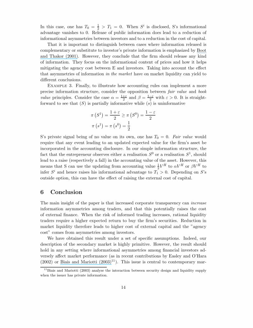
Example 3. Finally, to illustrate how accounting rules can implement a more
precise information structure, consider the opposition between fair value and book
value principles. Consider the case α = 1+ε2 and β = 1−ε
2 with ε > 0. It is straight-
forward to see that (S) is partially informative while (s) is uninformative
π(S1
)=
1 + ε
2≥ π
(S0
)=
1 − ε
2
π(s1
)= π
(s0
)=
1
2
S’s private signal being of no value on its own, one has T0 = 0. Fair value would
require that any event leading to an updated expected value for the firm’s asset be
incorporated in the accounting disclosure. In our simple information structure, the
fact that the entrepreneur observes either a realisation S0 or a realisation S1, should
lead to a raise (respectively a fall) in the accounting value of the asset. However, this
means that S can use the updating from accounting value 12V H to αV H or βV H to
infer Si and hence raises his informational advantage to T1 > 0. Depending on S’s
outside option, this can have the effect of raising the external cost of capital.
6 Conclusion
The main insight of the paper is that increased corporate transparency can increase
information asymmetries among traders, and that this potentially raises the cost
of external finance. When the risk of informed trading increases, rational liquidity
traders require a higher expected return to buy the firm’s securities. Reduction in
market liquidity therefore leads to higher cost of external capital and the ”agency
cost” comes from asymmetries among investors.
We have obtained this result under a set of specific assumptions. Indeed, our
description of the secondary market is highly primitive. However, the result should
hold in any setting where informational asymmetries among financial investors ad-
versely affect market performance (as in recent contributions by Easley and O’Hara
(2002) or Biais and Mariotti (2003)11). This issue is central to contemporary mar-
11Biais and Mariotti (2003) analyse the interaction between security design and liquidity supply
when the issuer has private information.
14
ket microstructure theory (Biais, Glosten and Spatt, 2002). However, research in
accounting have focussed mainly on the twin issue of the informational content of
market prices (see, e.g., Verrecchia (2001)) to study the effect of accounting rules on
firms’ cost of capital.
Our speculator can be interpreted as an investor making profit out of his private
information. In our setting, this information only have individual value. Arguably,
information possessed by sophisticated traders can have public value. Prices that
(partially) reveal this information can then be used to mitigate the agency problem
between managers and shareholders (Diamond and Verrecchia, 1982; Holmstrom and
Tirole, 1993). However, this is an assumption about the nature of information that
traders possess, and should not be a premise of all models. Sophisticated traders
seek information they can profit from; the nature of this information will be highly
dependent on economic environment. More research should be done to analyse en-
vironments in which agents have individual incentives to acquire socially harmful
information. We believe new insights could be gained concerning the economic con-
sequences of accounting rules. Anyhow, intuitive arguments should not be taken at
face value when evaluating the consequences of real-world changes in regulation.
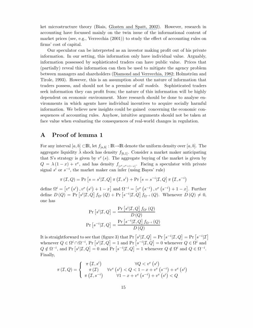
A Proof of lemma 1
For any interval [a, b] ⊂IR, let f[a,b] : IR→IR denote the uniform density over [a, b]. The
aggregate liquidity λ shock has density f[0,1]. Consider a market maker anticipating
that S’s strategy is given by ve (s). The aggregate buying of the market is given by
Q = λ (1 − x) + ve, and has density f[ve,ve+1−x]
. Facing a speculator with private
signal si or s−i, the market maker can infer (using Bayes’ rule)
π (I, Q) = Pr[s = si|I, Q
]π
(I, si
)+ Pr
[s = s−i|I, Q
]π
(I, s−i
)
define Ωi =[ve
(si
), ve
(si
)+ 1 − x
]and Ω−i =
[ve
(s−i
), ve
(s−i
)+ 1 − x
]. Further
define D (Q) = Pr[si|I, Q
]fΩi (Q) + Pr
[s−i|I, Q
]fΩ−i (Q). Whenever D (Q) 6= 0,
one has
Pr[si|I, Q
]=
Pr[si|I, Q
]fΩi (Q)
D (Q)
Pr[s−i|I, Q
]=
Pr[s−i|I, Q
]fΩ−i (Q)
D (Q)
It is straightforward to see that (figure 3) that Pr[si|I, Q
]= Pr
[s−i|I, Q
]= Pr
[s−i|I
]
whenever Q ∈ Ωi ∩Ω−i, Pr[si|I, Q
]= 1 and Pr
[s−i|I, Q
]= 0 whenever Q ∈ Ωi and
Q /∈ Ω−i, and Pr[si|I, Q
]= 0 and Pr
[s−i|I, Q
]= 1 whenever Q /∈ Ωi and Q ∈ Ω−i.
Finally,
π (I, Q) =
π(I, si
)∀Q < ve
(si
)
π (I) ∀ve(si
)< Q < 1 − x + ve
(s−i
)+ ve
(si
)
π(I, s−i
)∀1 − x + ve
(s−i
)+ ve
(si
)< Q
15

which yields the price schedule (7).
B Proof of proposition 2
Taking as given the market maker expectation ve (.) and the resulting pricing rule, S
seeks to use his private information to abuse the market maker. When his signal is
si, he trades
v(si
)= arg max
v≤xv · [E [P (Q) |I, s] − π (I, s)]
As a monopolist, S anticipates the effect his order v has on the price set by the
market maker. Formally, if he submits an order v, then the aggregate quantity is
Q = (1 − x) λ + v, and the expected price conditional on s is
E [P (Q) |I, s] = E [P ((1 − x)λ + v) |I, s]
When s = si, π(I,si
)> π (I) so S is willing to buy, and is betting for a high
realisation of λ to fool the market maker. Conditional on s = si,
P ((1 − x)λ + v) =
π
(I, si
)if (1 − x) λ + v > ve
(s−i
)
π (I) if (1 − x) λ + v > ve(s−i
)
which yields
π (I, s) − E [P (Q) |I, s] =(π
(I, si
)− π (I)
)Pr
[(1 − x)λ + v > ve
(s−i
)]
=(π
(I, si
)− π (I)
)Pr
[λ >
ve(s−i
)− v
1 − x
]
Conversely, for s = s−i, π(I,si
)> π (I) and S is willing to sell the stock and is
betting for a low aggregate liquidity shock to hide his trade. Conditional on s = s−i,
P ((1 − x) λ + v) =
π (I, sι) if (1 − x) λ + v > ve
(s−i
)
π (I) if (1 − x) λ + v > ve(s−i
)
which yields
E [P (Q) |I, s] − π (I, s) =(π (I) − π
(I, s−i
))Pr
[(1 − x)λ + v < 1 − x + ve
(si
)]
=(π (I) − π
(I, s−i
))Pr
[λ < 1 −
v − ve(si
)
1 − x
]
For the ease of notation, for the remainder of this proof we posit z = v(s−i
), ze =
ve(s−i
), −y = v
(si
)and −ye = ve
(si
). Then we seek a solution
y∗ = arg max y
(1 −
za + y
1 − x
)+ (π
(I, si
)− π (I)
)(27)
z∗ = arg maxz≤x
z
(1 −
z + ya
1 − x
)+ (π (I) − π
(I, s−i
))(28)
16

where f+ (.) = min (0, f (.)). Criteria in (27) and (28) are concave, and have one
unique, interior, unconstrained maximum for resp. y ∈ [0, 1 − x − za] and z ∈
[0, 1 − x − ya]. The F.O.C for (27) and (28) give
1 − x − za − 2y = 0∣∣∣∣
1 − x − ya − 2z = 0 and z < x
1 − x − ya − 2z < 0 and z = x
In equilibrium, one must have ya = y and za = z. If the constraint z ≤ x is not
binding, then we get
y = z =1 − x
3(29)
while if it is binding
z = x y =1
2− x (30)
The constraint is not binding when 1−x3 < x, which gives x < 1
4 .
C Proof of proposition 3
We stick with the notations of previous proof. First, define
T =∑
I
Pr [I][Pr
(s0|I
) ∣∣π(I, s0
)− π (I)
∣∣ + Pr(s1|I
) ∣∣π (I) − π(I, s1
)∣∣] (31)
noting that by Bayes’ rule
(Pr
(si|I
)+ Pr
(s−i|I
))π (I) = π (I) = Pr
(si|I
)π
(I, si
)+ Pr
(s−i|I
)π
(I, s−i
)
(32)
we get
Pr(s−i|I
) (π (I) − π
(I, s−i
))= Pr
(si|I
) (π
(I, si
)− π (I)
)(33)
so that
T = 2∑
I
Pr [I] Pr(si|I
) (π
(I, si
)− π (I)
)(34)
= 2∑
I
Pr [I] Pr(s−i|I
) (π (I)− π
(I, s−i
))(35)
As v∗(si
)and v∗
(s−i
)do not depend on public information I, the speculator’s profit
can be written as
ΠS (x) = x (πR − 1) +∑
I
Pr [I]
[Pr
(si|I
) (π
(I, si
)− π (I)
)y+
Pr(s−i|I
) (π (I) − π
(I, s−i
))z
] [1 −
z + y
1 − x
]
Using (34) and (35) this reduces to
ΠS (x) = x (πR − 1) +1
2T (y + z)
[1 −
z + y
1 − x
]
17
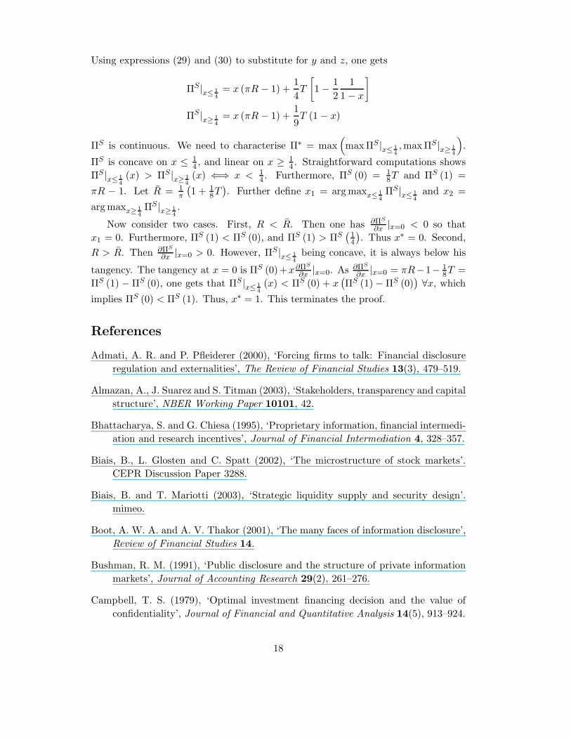
Using expressions (29) and (30) to substitute for y and z, one gets
ΠS |x≤ 14
= x (πR − 1) +1
4T
[1 −
1
2
1
1 − x
]
ΠS |x≥ 14
= x (πR − 1) +1
9T (1 − x)
ΠS is continuous. We need to characterise Π∗ = max(maxΠS |x≤ 1
4,maxΠS |x≥ 1
4
).
ΠS is concave on x ≤ 14 , and linear on x ≥ 1
4 . Straightforward computations shows
ΠS |x≤ 14(x) > ΠS |x≥ 1
4(x) ⇐⇒ x < 1
4 . Furthermore, ΠS (0) = 18T and ΠS (1) =
πR − 1. Let R = 1π
(1 + 1
8T). Further define x1 = arg maxx≤ 1
4ΠS |x≤ 1
4and x2 =
arg maxx≥ 14ΠS |x≥ 1
4.
Now consider two cases. First, R < R. Then one has ∂ΠS
∂x|x=0 < 0 so that
x1 = 0. Furthermore, ΠS (1) < ΠS (0), and ΠS (1) > ΠS(
14
). Thus x∗ = 0. Second,
R > R. Then ∂ΠS
∂x|x=0 > 0. However, ΠS |x≤ 1
4being concave, it is always below his
tangency. The tangency at x = 0 is ΠS (0)+x∂ΠS
∂x|x=0. As ∂ΠS
∂x|x=0 = πR−1− 1
8T =
ΠS (1) − ΠS (0), one gets that ΠS |x≤ 14(x) < ΠS (0) + x
(ΠS (1) − ΠS (0)
)∀x, which
implies ΠS (0) < ΠS (1). Thus, x∗ = 1. This terminates the proof.
References
Admati, A. R. and P. Pfleiderer (2000), ‘Forcing firms to talk: Financial disclosure
regulation and externalities’, The Review of Financial Studies 13(3), 479–519.
Almazan, A., J. Suarez and S. Titman (2003), ‘Stakeholders, transparency and capital
structure’, NBER Working Paper 10101, 42.
Bhattacharya, S. and G. Chiesa (1995), ‘Proprietary information, financial intermedi-
ation and research incentives’, Journal of Financial Intermediation 4, 328–357.
Biais, B., L. Glosten and C. Spatt (2002), ‘The microstructure of stock markets’.
CEPR Discussion Paper 3288.
Biais, B. and T. Mariotti (2003), ‘Strategic liquidity supply and security design’.
mimeo.
Boot, A. W. A. and A. V. Thakor (2001), ‘The many faces of information disclosure’,
Review of Financial Studies 14.
Bushman, R. M. (1991), ‘Public disclosure and the structure of private information
markets’, Journal of Accounting Research 29(2), 261–276.
Campbell, T. S. (1979), ‘Optimal investment financing decision and the value of
confidentiality’, Journal of Financial and Quantitative Analysis 14(5), 913–924.
18
Cremer, J. (1995), ‘Arm’s length relationship’, Quarterly Journal of Economics
110(2), 275–295.
Diamond, D. and R. Verrecchia (1982), ‘Optimal managerial contracts and equilib-
rium security prices’, Journal of Finance 37, 275–287.
Diamond, D. W. (1985), ‘Optimal release of information by firms’, Journal of Finance
40, 1071–1094.
Diamond, D. W. and P. Dybvig (1983), ‘Bank runs, deposit insurance, and liquidity’,
Journal of Political Economy 91(3).
Dye, R. A. (1985), ‘Strategic accounting choice and the effects of alternative financial
reporting requirements’, Journal of Accounting Research 23(2), 544–574.
Dye, R. A. (2001), ‘An evaluation of ”essays on disclosure” and the disclosure liter-
ature in accounting’, Journal of Accounting and Economics 32(1-3), 181–235.
Easley, D. and M. O’Hara (2002), ‘Information and the cost of capital’, Journal of
Finance forthcoming.
Fishman, M. J. and K. M. Hagerty (1989), ‘Disclosure decision by firms and the
competition for price efficiency’, Journal of Finance 44, 633–646.
Fishman, M. J. and K. M. Hagerty (1990), ‘The optimal amount of discretion to
allow in disclosure’, Quarterly Journal of Economics 105(2), 427–444.
Glosten, L; (1989), ‘Insider trading, liquidity, and the role of the monopolist special-
ist’, Journal of Business 92, 211–235.
Glosten, L. and P. Milgrom (1985), ‘Bid, ask, and transaction prices in a specialist
market with heterogeneously informed traders’, Journal of Financial Economics
13, 71–100.
Gorton, G. and G. Pennachi (1990), ‘Financial intermediaries and liquidity creation’,
Journal of Finance 45(1), 49–71.
Hirschleifer, D. and S. H. Teoh (2004), ‘Limited attention, information disclosure,
and financial reporting’, Journal of Accounting and Economics forthcoming.
Hirshleifer, J. (1971), ‘The private and social value of information and the reward to
inventive activity’, American Economic Review 61, 561–574.
Holmstrom, B. and J. Tirole (1993), ‘Market liquidity and performance monitoring’,
Journal of Political Economy 101, 678–709.
Hubbard, R. G. (1998), ‘Capital-market imperfections and investment’, Journal of
Economic Literature 36(1), 193–225.
19
Inderst, R. and H. M. Muller (2003), ‘Credit risk analysis and security design’. mimeo.
Indjejikian, R. J. (1991), ‘The impact of costly information interpretation on firm
disclosure decisions’, Journal of Accounting Research 29(2), 277–301.
Kanodia, C. and R. Singh (2001), ‘Optimal imprecision and ignorance’, mimeo. Carl-
son School of Management, University of Minnesota.
Kyle, A. S. (1985), ‘Continuous auctions and insider trading’, Econometrica 53, 1315–
1336.
Leuz, C. and R. E. Verrecchia (2000), ‘The economic consequences of increased dis-
closure’, Journal of Accounting Research 38, 91–124.
Prat, A. (2003), ‘The wrong kind of transparency’. STICERD Working Paper
TE/2002/439.
Spiegel, M. and A. Subrahmanyan (1992), ‘Informed speculation and hedging in a
noncompetitive securities market’, Review of Financial Studies 5, 307–329.
Verrecchia, R. E. (2001), ‘Essays on disclosure’, Journal of Accounting and Economics
32(1-3), 97–180.
Yosha, O. (1995), ‘Information disclosure costs and the choice of financing source’,
Journal of Financial Intermediation 4, 3–20.
20