Working Paper 2008 | 30 Business cycle accounting for Argentina utilizing capital utilization

Tiago Cavalcanti University of Cambridge Pedro Elosegui / George McCandless Emilio Blanco BCRA January, 2008

BBaannccoo CCeennttrraall ddee llaa RReeppúúbblliiccaa AArrggeennttiinnaa iiee || IInnvveessttiiggaacciioonneess EEccoonnóómmiiccaass January, 2008 ISSN 1850-3977 Electronic Edition Reconquista 266, C1003ABF C.A. de Buenos Aires, Argentina Phone: (5411) 4348-3719/21 Fax: (5411) 4000-1257 Email: investig@bcra.gov.ar Web Page: www.bcra.gov.ar The opinions in this work are an exclusive responsibility of his authors and do not necessarily reflect the position of the Central Bank of Argentina. The Working Papers Series from BCRA is composed by papers published with the intention of stimulating the academic debate and of receiving comments. Papers cannot be referenced without the authorization of their authors.

Business cycle accounting for Argentina utilizingcapital utilization�

Tiago V. de V. Cavalcantia Pedro Eloseguib

George McCandlessb

Emilio Blancob

University of Cambridgea

Banco Central de la República Argentinab

January 31, 2008

Abstract

We use a variation on the business cycle accounting method of Chari,Kehoe and McGrattan [3] to study the business cycle in Argentina from1972 to 2006. We use capital utilization as a household decision variableto be able to better extract the wedge that functions as a tax on capital.Applying the model to Argentina, we �nd that all four wedges are impor-tant in explaining the evolution of output over this period (although netexports is the least important). The major political subperiods can becharaterized by the relative importance of each wedge. We compare theresults of this technique to the standard narrative. JEL classi�cations:E22, E32, N16

1 Introduction

Using a prototype growth model, Chari, Kehoe and McGrattan [3] (henceforth,CKM) propose an accounting procedure for guiding researchers in developingand analyzing quantitative models of economic �uctuations. This procedure usesreal data together with the equilibrium conditions of a prototype growth modelto measure four wedges that are explained by the variables of the model. Thesewedges can be viewed as �distortions�from a perfectly competitive economy andrepresent the set of policies and institutions which a¤ect productivity and factorsinput1 . The authors show that a large class of economic models, including

�The opinions expressed here are those of the authors and should not be taken to representthose of the Banco Central de la República Argentina. Sabastian Katz and Carlos Zarazagaprovided helpful comments.

1These are wedges in the sense that they measure how di¤erent the economy is from aclosed, non-stochastic, perfectly competitive economy.

1

those with various additional features (e.g., �nancial frictions, nominal rigidities,entrepreneur decisions, and monetary shocks) are equivalent to a prototypegrowth model with time-varying wedges. Institutions, public policies, �scal,monetary, income and labor policies a¤ect the four wedges and therefore a¤ectthe allocations of capital and labor, net exports and productivity in the economy.In their standard model for business cycle accounting, CKM use four wedges

that are explained by four variables of the model. The period t value for three ofthe wedges, government expenditures and net exports, total factor productivity,and an implicit labor tax, are found using the model and period t data. Thefourth wedge, an implicit capital tax, is found using the intertemporal relationsof the model and its aggregate e¤ects on output are found as a residual of thee¤ects of the other three wedges. For the US data used by CKM, the capitalwedge is found to be quite small. It is not clear if this is a characteristic of theUS data they are using or a result of their calculation technique.Making use of capital utilization data provides an alternative way of �nding

the capital wedge. Capital utilization information can be used directly in theproduction function (since it is utilized capital that creates production) and inthe household budget constraint (since it is utilized capital that earns rents).In addition, it is quite natural to think of depreciation as being a function ofcapital utilization, since the more that capital is utilized in a period, the morelikely it is to wear out and need replacement parts or maintaince. Given thesecharacteristics of capital utilization, it becomes a household choice variable,households choose how much capital to send to the market each period, andadds an additional �rst order condition to the model. One can use this extra�rst order condition to extract, using period t data, a period t capital wedge.CKM do provide an alternative speci�cation in which they use variable cap-

ital utilization to adjust the capital stock. What they do not do, and whatwe do here, is make capital utilization a choice variable for the households, getthe additional �rst order condition and use this extra equation to extract thecapital tax and construct the capital wedge. Once the wedges are constructedit is possible to assess what fraction of output �uctuation can be attributed toeach wedge separately and in combination.In this paper, we apply a model with endogenous capital utilization to the

Argentine economy2 from 1972 to the end of 2006. The accounting procedureallows us to analyze the Argentine economy during a time period subject toseveral structural breaks and where these can be associated with di¤erent eco-nomic regimes. The wedge decomposition helps to explain several features thatcharacterize each of the di¤erent economic regimes. Emphasis is given to theevolution of labor and capital wedge as well as factor productivity. In thismodel, total factor productivity is based on labor and utilized capital.It should be noted that many of the nominal and real frictions that are often

added to standard RBC models can be captured with one of our four wedges.

2Methods similar to those of the basic CKM method have been applied to both the modernJapanese economy and the prewar economy by Hayashi and Prescott [8] and [9] and to theFrench economy by Prescott [13]. Cole and Ohanan [4] have applied the basic model to theU.S. and U.K. and Cavalcanti [2] to Portugal.

2

CKM make much of this in their paper. Determining which wedges are mostimportant for explaining the Argentine business cycle is a �rst step towardsdetermining which frictions are most important in generating a productive RBCmodel of Argentina, especially if these models are to be used for forecasting orfor analyzing monetary policy and monetary transmission channels.

2 The model with capital utilization

We assume that capital depreciation, �t, is a function of capital utilization, �t.Let depreciation in period t be given by

�t = � exp (a (�t � �))

where � is the average depreciation rate, a measures how strongly depreciationresponds to capital utilization, and � is the average utilization. This formulationproduces the average depreciation rate whenever utilitization is average andmakes depreciation an increasing function of utilization. With this additionequation, we write the CKM model as

U = Et

1Xi=0

�iu (ct+i; ht+i)

subject to

ct + kt+1 ��1� � exp (a (�t � �))

�kt =

�1� �ht

�wtht +

�1� �kt

�rt�tkt + Tt

and a production function of the perfectly competitive �rms of

Yt = At (�tKt)� � tHt

�1��:

Expected utility for a representative household is a function of a constant dis-count factor, �, and an in-period sub-utility function that depends on the house-hold�s consumption, ct, and on the labor it supplies, ht. The household accu-mulates capital, kt, and pays lump sum taxes, Tt. In the household budgetconstraint, the variables �ht and �kt are the implicit taxes being imposed bypolicies that are not oberved on labor and capital, respectively. Output of theone good is competitive and depends on the level of technology (total factorproductivity), At, the aggregate capital being used, �tKt, and the aggregagesupply, Ht, adjusted by the growth in labor augmenting technology, t. The�rst order conditions for the �rms (and the factor markets) are

wt = (1� �) tAt (�tKt)� � tHt

���and

rt = �At (�tKt)��1 �

tHt

�1��:

Note that the rental rate calculated here, rt, is that paid on utilized capitaland not on total capital, and this is taken into account in the household budgetconstraint.

3

The �rst order conditions for the households (who, in period t, choose ct,ht, kt+1, and �t) are

uh (ct; ht)

uc (ct; ht)= �

�1� �ht

�wt�

1� �kt�rt = a� exp (a (�t � �))

uc (ct; ht) = �Etuc (ct+1; ht+1)��1� � exp

�a��t+1 � �

�����1� �kt+1

�rt+1�t+1

�Three period t shocks (or wedges, are they are called in the literature), �ht ,

�kt , and At, can be found in terms of period t observations on the data from the�rst two of these �rst order condition and the production function as

uh (Ct;Ht)

uc (Ct;Ht)= �

�1� �ht

�(1� �) tAt (�tKt)

� � tHt

���; (1)

a� exp (a (�t � �)) =�1� �kt

��At (�tKt)

��1 � tHt

�1��; (2)

and

At =Yt

(�tKt)�( tHt)

1�� : (3)

In addition, A resource constraint that must hold is

Ct +Kt+1 +Gt = Yt +�1� � exp (a (�t � �))

�Kt:

Notice that with the extra choice variable of capital utilization, it is possibleto extract all four of the time t shocks using just time t data on Ct, Ht, Kt, Gt,and �t. Gt come directly from the data on government expenditures and netexports. At is calculated given output, the production function and the dataon the capital stock, capital utilization and labor (along with labor productivitygrowth). The wedges, �ht and �

kt , are then calculated from the two remaining

�rst order conditions.In the actual implementation, we take K0 as given and use the data on gross

investment, It; and capital utilization to calculate the sequence of capital stockfrom

Kt+1 =�1� � exp (a (�t � �))

�Kt + It:

Note that the capital stock path depends crucially on the parameter a of thedepreciation function.The sub-utility function3 used for implementation is

u (Ct;Ht) = logCt + log(H �Ht)

3The subutility function used in Kydland and Zarazaga [11] is�c�t

�h� ht

�1���1��1� �

;

which give exactly the same marginal conditions when = 1���:

4

souh (Ct;Ht)

uc (Ct;Ht)= � Ct

H �Ht

:

With this Cobb-Douglas type utility function, we �nd the four wedges.To �nd the impact of each of the wedges independently, we �x the values of

three of wedges at their average value, use the time series for the capital stockthat we found above, and use a nonlinear system solver in Matlab to �nd thevalues of Ct, Ht, �t, and Yt as the zeros for the system

0 = � Ct

H �Ht

+�1� �ht

�(1� �) tAt (�tKt)

� � tHt

���0 = a� exp (a (�t � �))�

�1� �kt

��At (�tKt)

��1 � tHt

�1��0 = At �

Yt

(�tKt)�( tHt)

1��

0 = Yt +�1� � exp (a (�t � �))

�Kt � Ct �Kt+1 �Gt:

In addition, we calculate the time path for output that comes from using thetotal factor productivity wedge and the capital tax wedge together, keeping theother two wedges at their average value.

3 The data and the wedges

The data are quarterly and run from 1972:1 to 2006:4, a relatively long periodof time for studies of Argentina. The data for the four macroeconomic variablesare quarterly, expressed in per capita terms in prices of 1993, and are shownin Figure 1 and those for utilization and labor (calculated from hours workedper capita) are given in Figure 2. The period has been characterized as oneof economic and political turbulence in Baer, Elosegui and Gallo [1]. The �rstdecade, from 1972 until 1982, has been characterized as a series of so called"stop and go" policies and the "plata dulce" period, with a seriously overvaluedexchange rate, that ended in a debt crisis. The lost decade of the 80s canbe characterized by systemic growing in�ation and a �nal hyperin�ation periodmixed with a number of failed attempts to introduce stabilization programs.The problem of in�ation was only dominated in 1991, with the introductionof the "Convertibility Plan", a currency board system that characterized thedecade until its collapse at the end of 2001. Since 2003, the economy has beenrecovering from that crisis. The data encompass a number of policy regimes,substantial variation over business cycles and a virtually �at long run trend.The construction of the wedges should be able to help us to analyze each of theseperiods and the impact of their policies on capital, labor and productivity.We use series on the real, per capita value of output, consumption (in this

case, the combined private and public consumption), net exports, investment,

5

1970 1975 1980 1985 1990 1995 2000 2005 2010

0

500

1000

1500

2000

date

Y

C

X­M

I

Figure 1: Deseasonalized macro data: Y , C, X �M , and I

1970 1975 1980 1985 1990 1995 2000 2005 20100.2

0.3

0.4

0.5

0.6

0.7

0.8

0.9

date

u

H

Figure 2: Data for utilization and labor

6

1970 1975 1980 1985 1990 1995 2000 2005 20100.013

0.0135

0.014

0.0145

0.015

0.0155

0.016

0.0165

0.017depreciation

Figure 3: Depreciation

normalized hours worked, and an index for capital utilization4 . The pre-1993data do not come with private and public consumption separated, so we assumethat government consumption enters the utility function mixed together withprivate consumption. Since government consumption is not available for thewhole period, the variable Gt in the above equations only contains net exports.The series for the capital stock is constructed using

Kt+1 = Yt +�1� � exp (a (�t � �))

�Kt � Ct �Gt;

using a value of 21490 for the 1980:1 value of the per capita capital stock,calculating backwards to 1972:1 and forward to 2006:4. In the calculations weused � = :57, � = :06174=4, t = 1, � = 0:6878, = :75, and a = 1. Thedepreciation series that comes from the function (in quarterly terms) is shownin Figure 3. The time series for capital (measured in quarterly, per capita, inprices of 1993 terms) that we get from these calculations is shown in Figure 4.For the years where the two studies overlap, our time path for the capital stockis generally similar to the one in Kydland and Zarazaga [10].Using this data, we �nd At using equation 3, �ht , using equation 1, and �

kt

from equation 2. The net export wedge, Gt, comes directly from the data andare per capita, measured in prices of 1993. The wedges that result from thesecalculations are shown in Figure 5. The labor and capital wedges are measuredas the fraction of income from each source paid as implicit taxes.

4The index on capital utilizaton comes from FIEL (Fundación de Investigaciones Económi-cas Latinoamericanas). The other data comes from INDEC (Argentina�s Instituto Nacionalde Estadística y Censos) except that output is de�ned from the national income accountingidentity, Y = C + I +G+ netX. Real variables are in terms of 1993 prices and were linkedto earlier real series by averaging over overlapping dates.

7

1970 1975 1980 1985 1990 1995 2000 2005 20101.6

1.7

1.8

1.9

2

2.1

2.2

2.3x 10 4

Figure 4: Calculated capital stock

1970 1980 1990 2000 2010­100

­50

0

50

100

150XM

1970 1980 1990 2000 2010

10

11

12

13

14A

1970 1980 1990 2000 2010

0.4

0.5

0.6

0.7

τk

1970 1980 1990 2000 20100.1

0.2

0.3

0.4

τh

Figure 5: Four wedges for Argentina

8

1970 1975 1980 1985 1990 1995 2000 2005 20101600

1800

2000Efect of XM on Y

1970 1975 1980 1985 1990 1995 2000 2005 20101000

1500

2000

Efect of A on Y

1970 1975 1980 1985 1990 1995 2000 2005 20101400

1600

1800

2000

2200Efect ofτ k on Y

1970 1975 1980 1985 1990 1995 2000 2005 20101400

1600

1800

2000Efect ofτ h on Y

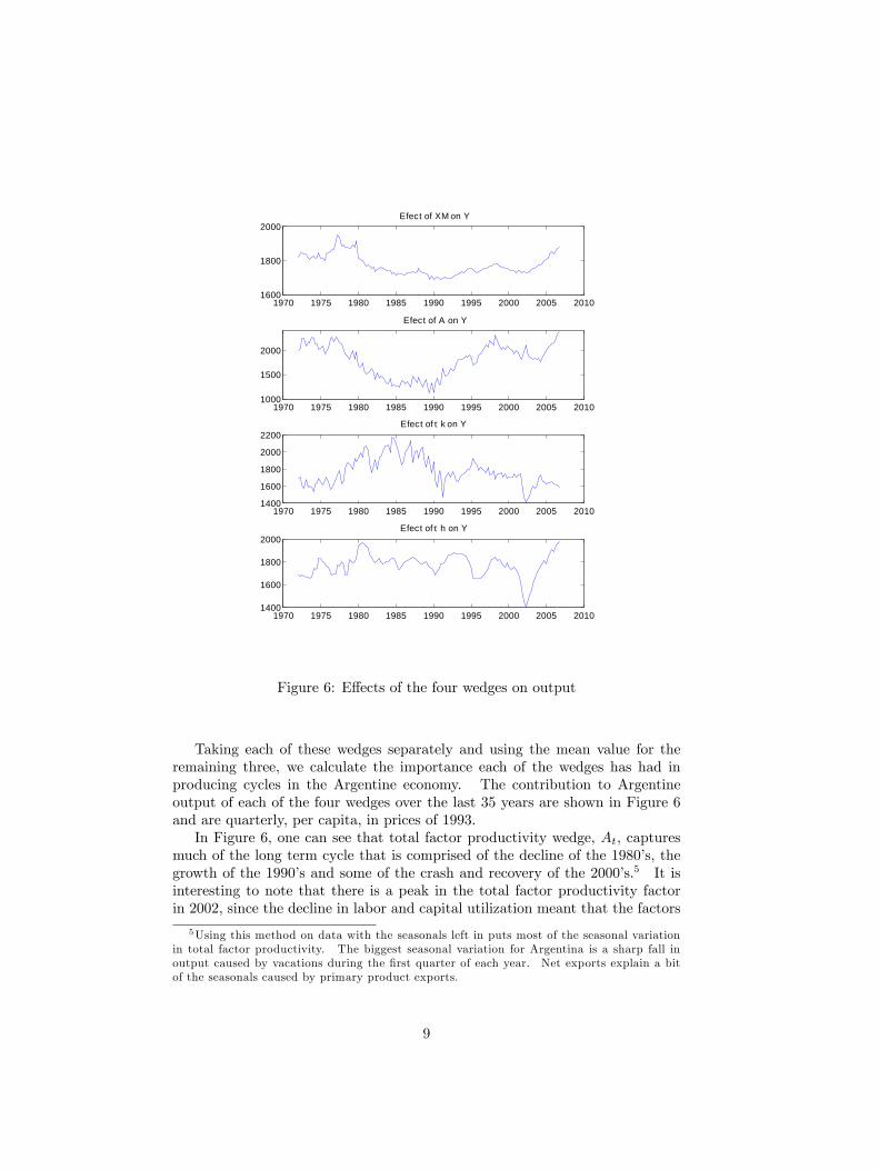
Figure 6: E¤ects of the four wedges on output

Taking each of these wedges separately and using the mean value for theremaining three, we calculate the importance each of the wedges has had inproducing cycles in the Argentine economy. The contribution to Argentineoutput of each of the four wedges over the last 35 years are shown in Figure 6and are quarterly, per capita, in prices of 1993.In Figure 6, one can see that total factor productivity wedge, At, captures

much of the long term cycle that is comprised of the decline of the 1980�s, thegrowth of the 1990�s and some of the crash and recovery of the 2000�s.5 It isinteresting to note that there is a peak in the total factor productivity factorin 2002, since the decline in labor and capital utilization meant that the factors

5Using this method on data with the seasonals left in puts most of the seasonal variationin total factor productivity. The biggest seasonal variation for Argentina is a sharp fall inoutput caused by vacations during the �rst quarter of each year. Net exports explain a bitof the seasonals caused by primary product exports.

9

still being used were highly productive. Total factor productivity "explains" adeeper cycle than is seen in the data and is mostly compensated by the e¤ectsof the capital tax.The part of the business cycle explained by net exports is quite small, al-

though it does capture a slow decline until around 1993 and a gradual rise there-after. The relatively small contribution that net exports makes in explainingthe cycles is at odds with claims that real international shocks are importantfor explaining the Argentine business cycle.The bottom two graphs in Figure 6 show the e¤ects of �kt and �

ht . Neither

of these explains much of the long term cycle and the part of output that isexplained by the capital wedge is negatively correlated with that cycle for mostof the period. The capital wedge captures a number of important events inArgentine economic history. Capital clearly su¤ered from the hyperin�ationsof 1989 and 1991 as well as the in�ation leading up to the Austral Plan in1985 and the debt crisis of 1981-2. Interestingly, capital did not seem to su¤erduring the Tequila crisis around 1995, where most of the changes seem to bere�ected through the labor wedge. Capital also su¤ered from the 2002 crisisbut recovered to a level similar to that before the crisis. This last suggests thatthe output growth in the last few years of the period under study does not seemto have come from policies that bene�t capital. The labor wedge indicates thatthe part of output explained by labor had a long slow decline during the 1980�s,although it was much less sensitive to business cycles than capital, su¤ered inthe hyperin�ations at the beginning of the 1990�s, recovered a bit after thatonly to be heavily hit by the Tequila crisis of 1995. This is consistent withthe big jump in unemployment observed in Argentina in the mid-1990�s. The2001 � 2 crisis initially had as big an impact on labor as it did on capital butthe output e¤ects of the labor wedge continue to show improvement up to thelast observations available.Figure 7 shows how well the combined e¤ects of the total factor productivity

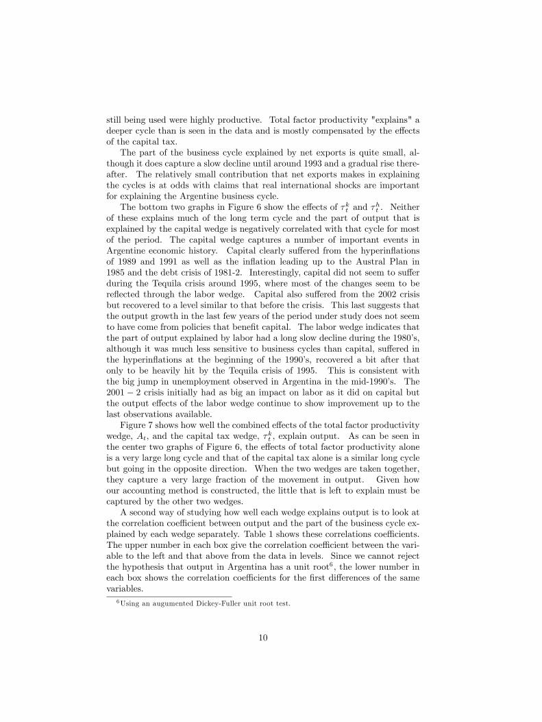
wedge, At, and the capital tax wedge, �kt , explain output. As can be seen inthe center two graphs of Figure 6, the e¤ects of total factor productivity aloneis a very large long cycle and that of the capital tax alone is a similar long cyclebut going in the opposite direction. When the two wedges are taken together,they capture a very large fraction of the movement in output. Given howour accounting method is constructed, the little that is left to explain must becaptured by the other two wedges.A second way of studying how well each wedge explains output is to look at

the correlation coe¢ cient between output and the part of the business cycle ex-plained by each wedge separately. Table 1 shows these correlations coe¢ cients.The upper number in each box give the correlation coe¢ cient between the vari-able to the left and that above from the data in levels. Since we cannot rejectthe hypothesis that output in Argentina has a unit root6 , the lower number ineach box shows the correlation coe¢ cients for the �rst di¤erences of the samevariables.

6Using an augumented Dickey-Fuller unit root test.

10

1970 1975 1980 1985 1990 1995 2000 2005 20101200

1300

1400

1500

1600

1700

1800

1900

2000

2100

2200Y

date

Y

Y explained by A and τ k wedges combined

Figure 7: The combined e¤ects of the total factor productivity wedge and thecapital tax wedge

Y YXM YA Y�k Y�h

Y1:00001:0000

0:61110:5288

0:79710:5641

�0:2439�0:0946

0:32820:4616

YXM0:61110:5288

1:00001:0000

0:66630:4685

�0:2582�0:0796

0:09410:0138

YA0:79710:5641

0:66630:4685

1:00001:0000

�0:7052�0:7729

�0:1702�0:0483

Y�k�0:2439�0:0946

�0:2582�0:0796

�0:7052�0:7729

1:00001:0000

0:40880:0794

Y�h0:32820:4616

0:09410:0138

�0:1702�0:0483

0:40880:0794

1:00001:0000

Table 1: Correlations of output and the part explained by each wedge

11

One of the most interesting features of Table 1 is the correlation betweenthe part of output explained by total factor productivity and that explained bythe capital tax. This is strongly negative, whether measured in levels or in�rst di¤erences. As we showed above, these two wedges combined explain alarge fraction of the movement in output. The path of output that results fromthe combined e¤ects of the total factor productivity wedge and the capital taxwedge has a 90:17% correlation with the output data when measured in levelsand a 81:04% correlation when measured in �rst di¤erences. This result in thetable suggests that in Argentina, whenever there is an increase in total factorproductivity, it is met with increase in policies that operate as a tax on capital7 .Looking at the wedges themselves in Figure 5, the tax on capital moves verymuch like total factor productivity except during the hyperin�ations of 1989and 1991 when the tax on capital rises without a compensating rise in totalfactor productivity and in the Tequila crisis of 1995 when the tax on capitalfalls dramatically with only a small decline in total factor productivity.The e¤ects of each of the wedges on C, �, and H are shown in Figure 8. As

one might expect, given the importance of output in determining consumption,the e¤ect of each wedge on explaining consumption is very similar to its e¤ect onexplaining output. The e¤ect of net exports, the unlabeled line in each graph, issmall in all cases, although it is a bit more important, and seasonal, in explaininglabor movements. In explaining capital utilization, it is not surprising that thecapital wedge captures some important movements, especially the drop in 2002.Technology, A, captures long trends in the capital utilization as well as someseasonals. The labor tax wedge does not explain much of utilization, althoughit does reinforce the decline in the 2002 crisis.Most of the movement in employment is explained by the labor tax wedge.

The net export wedge provides a bit of a seasonal and a bit of long term move-ment, however, this is small. The impact of the technology (A) wedge and thecapital wedge on labor are very similar, so much so that they cannot be verywell separated in the graphs.

4 More detailed historical analysis of the growthaccounting exercise for Argentina

Major crises have occurred with certain regularity in the period under consider-ation. A serious in�ation in 1975-6 was followed by a military coup (a potentialregime change8). A period of an overvalued peso (known as the Tablita) wasfollowed by a foreign exchange crisis. The return to democracy witnessed highand rising in�ation that in 1985 was met with the Austral plan. The transi-tion from the 1980s to the 1990s su¤ered two hyperin�ations. A banking crisisin 1995 resulted in the closing or consolidation of much of the banking system.

7An alternative hypothesis is that whenever policies go against capital, �rms respond byincreasing total factor productivity.

8Zablotsky [14] looks at military coups in Argentina as regime changes with democraticperiods raising taxes on land and military regimes lowering them.

12

1970 1975 1980 1985 1990 1995 2000 2005 20101000

1500

2000C

1970 1975 1980 1985 1990 1995 2000 2005 20100.4

0.6

0.8

1

u

1970 1975 1980 1985 1990 1995 2000 2005 2010

0.3

0.35

0.4H

A

A

A

τ k

τ k

τ k

τ h

Figure 8: E¤ect of each wedge separately on C, �, and H

13

The recession that began in late 1998 became a full blown banking and exchangecrisis in 2002. Each of these crisis events can be noted in Figure 6, with greateror lesser short term impact on output. What is of interest is how these crisisdi¤ered and what our wedges can tell us about how they were di¤erent.The return of Peron to power in 1973 is marked by a sharp decline in the

labor tax and a relatively small decline in total factor productivity as seen inFigure 5. The labor tax returns to its original level with the military coup of1976 and stays high for most of the time the military is in government (it fallsat the end of the period as the military is leaving government). There is asteady fall in the capital tax over the military period that is accompanied by asecular decline in total factor productivity. The overvalued peso of the Tablitapermitted capital accumulation and is observed in the positive e¤ect of netexports on output in the period just prior to 1980. This capital accumulationis also indicated in the increase in output from the capital tax but does notshow up in total factor productivity.The low level of the tax on labor continues throughout all of the Alfonsin

presidency. During the �rst part of this period, total factor productivity con-tinues to fall and then stays low for the second half of the 1980�s (the so called"lost decade"). The tax on capital rises for most of this period, although withsubstantial variation. The e¤ects of net exports on output are relatively con-stant over the Alfonsin period. The hyperin�ation of 1989 generates rises in netexports (as imports fall) and increases in the capital tax, but has little e¤ectson the labor tax or on total factor productivity.The hyperin�ation in 1991, at the beginning of the Menem period, was

somewhat di¤erent from that of 1989. The e¤ects of both the capital andlabor wedge on output are negative and the tax on capital was particularlyhigh. It is also one of the peaks of the net export wedge. The beginning ofthe convertibility period9 is marked by a fall in the tax on labor (and a increasein output from the labor wedge) and a secular rise in total factor productivity.The Tequila crisis of 1995 hit labor hard but had almost no e¤ect on the otherwedges. This is consistent with the large increases in unemployment thataccompanied and followed that crisis.The general trend of the recession of 1999 to 2002 and the recuperation after

is captured in the net export wedge. The crisis of 2002 hits both the labor andcapital wedges hard, with sharp increases in the wedges and sharp declines inthe part of the business cycle explained by these wedges. These two e¤ects areso sharp that total factor productivity actually rises during this crisis. Therecovery during the Kirchner years comes from a large reduction in the tax onlabor, an increase in total factor productivity, and a decline in net exports. Thetax on capital increases to a level similar to the Peron period at the beginningof the sample (the mid-1970�s). In Figure 6, the e¤ect of both the labor wedgeand factor productivity are the highest over the sample and the e¤ect of netexports is close to the maximum. The e¤ect of the capital wedge is a smalldecline after the initial recuperation from the 2002 crisis. These results are

9See Baer, Elosegui and Gallo [1] for a detailed explanation of the convertibility plan.

14

consistent with the perception that the Kirchner government looks to bene�tworkers with policies that tend to increase wages, promote labor formalizationand increase labor union powers while imposing increased tax pressures on theowners of capital and land. In a model as simple as this one, what we call thecapital stock is comprised of physical capital and land.

5 On the importance of the capital stock path

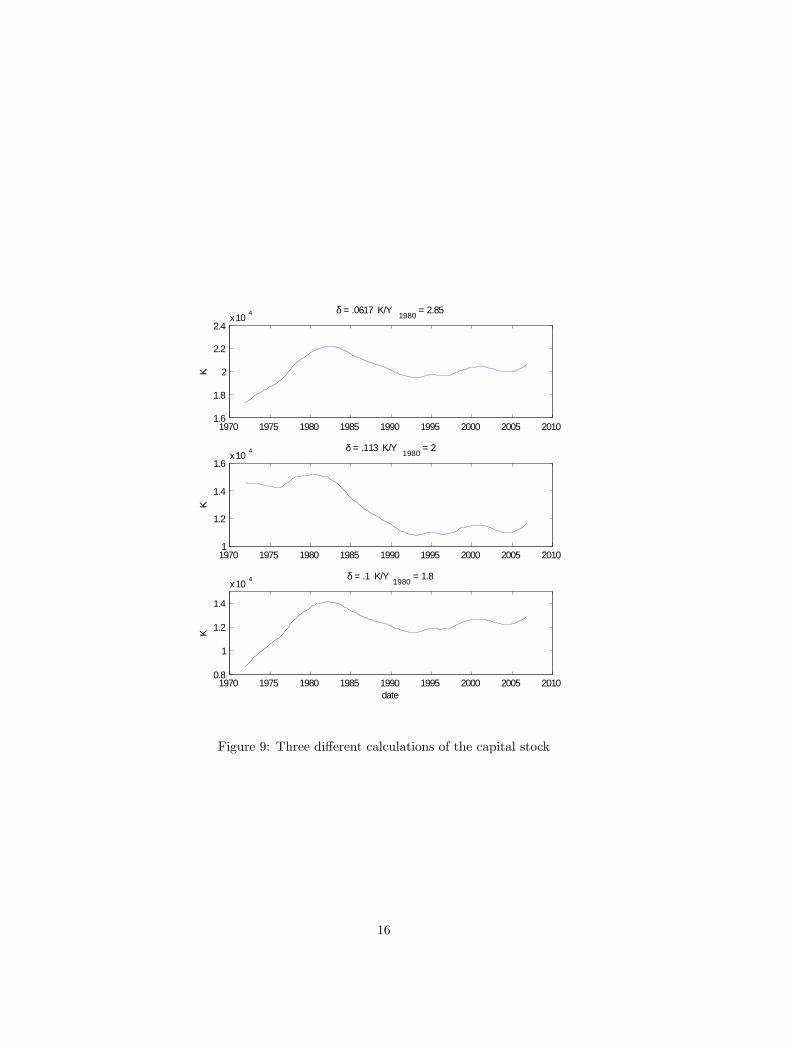
The calculation of the time path for capital is one of the more di¢ cult aspectsof this analysis. The capital path is important in determining two of thewedges, that of total factor productivity and the capital tax, and is importantin determining the time path of output that comes from each of the wedges.Data on the capital stock is not good and capital stock series are created fromthe investment series, an estimate for some initial capital stock, the averagedepreciation rate, and the function of the capital utilization rate.The time path for capital that comes from the investment series is sensitive

to the choice of an average depreciation rate and to the initial capital stock,although the importance of the initial capital stock diminishes with time. Figure9 shows the calculated time paths for capital for three values of � and ofK=Y1980.The top-most graph uses a depreciation rate of 6.17% per year and a capitalstock for 1980 of 2:85 times output. This series for capital is consistent with aliterature that gives estimates of the capital stock for Argentina that are highby international standards and where this capital stock is attributed to a mixof protectionism and government regulations that make labor expensive anddi¢ cult to change. In a regulatory environment in which labor dismissal costsgo up with length of service and can become quite large, optimizing �rms tendto keep their labor force small and use relatively high quantities of capital. Thesecond and third graphs use depreciation rates and output capital ratios morein keeping with world averages. The second graph uses the values from Kydlandand Zarazaga [10]. What is very di¤erent in this graph is the �rst decade ofthe period: there is much less growth in the capital stock during the 1970s.The third shows how a slightly lower depreciation rate and initial capital stockresult in a time path not much di¤erent from the �rst, although at a loweroutput-capital ratio.The set of wedges that come from using the �rst capital series are shown in

Figure 10, those from the second capital series in Figure 11, and those from thethird capital series in Figure 12. Notice that the capital stock has no e¤ecton the wedges related to net exports and the labor tax. The only e¤ects areon the total factor productivity (A), and the tax on capital. For the �rst andthird capital series, the changes are very minor. The relative fall in total factorproductivity during the period from 1970 through 1990 is somewhat large withthe third capital stock and the rise in TFP in the 1990�s is somewhat smaller.The capital tax series is very similar for these two as well.For the second capital series (the one that is closest to that of Kydland

and Zarazaga [10]), the fall in TFP during the �rst 20 years is smaller and the

15

1970 1975 1980 1985 1990 1995 2000 2005 20101.6

1.8

2

2.2

2.4x 10 4

K

δ = .0617  K/Y 1980 = 2.85

1970 1975 1980 1985 1990 1995 2000 2005 20101

1.2

1.4

1.6x 10 4

K

δ = .113  K/Y 1980 = 2

1970 1975 1980 1985 1990 1995 2000 2005 20100.8

1

1.2

1.4

x 10 4 δ = .1  K/Y 1980 = 1.8

date

K

Figure 9: Three di¤erent calculations of the capital stock

16

1970 1980 1990 2000 2010­100

­50

0

50

100

150XM

1970 1980 1990 2000 20109

10

11

12

13

14A

1970 1980 1990 2000 20100.1

0.2

0.3

0.4

τh

1970 1980 1990 2000 2010

0.4

0.5

0.6

0.7

τk

Figure 10: Wedges when � = :0617 and K=Y1980 = 2:85

growth during the 1990�s is substantially larger than those that result from theother two capital stock series. The capital tax associated with this capital stockseries implies a small drop in the tax in the 1980�s and a more secular upwardtrend thereafter (with similar variations, however).

All three of the capital stock series shown here produce what Kydland andZarazaga [11] refer to as Argentina�s capital shallowing. They note that therewas relatively little recovery in the capital stock in the boom of the 1990s afterthe long period of capital stock rundown that was the 1980�s. Their modelpredicts a capital stock at least 20% higher than the observed one. The outputboom of the 1990s seems to have been more motivated by increases in totalfactor productivity and by early declines in the capital tax than by capitalaccumulation. There was substantial new startup activity in the �rst half ofthe 1990s, concentrated mostly in service and commercial sectors, and manyof the older import substituting manufacturing plants were closed (see Escudé,et al [7]). Since the service and commercial sectors tend to be less capitalintensive than manufacturing, this shift in production away from manufacturingmay explain at least part of the capital shallowing observed.

17

1970 1980 1990 2000 2010­100

­50

0

50

100

150XM

1970 1980 1990 2000 201012

14

16

18A

1970 1980 1990 2000 20100.1

0.2

0.3

0.4

τh

1970 1980 1990 2000 20100.2

0.4

0.6

τk

Figure 11: Wedges when � = :113 and K=Y1980 = 2

1970 1980 1990 2000 2010­100

­50

0

50

100

150XM

1970 1980 1990 2000 201012

14

16

18

20A

1970 1980 1990 2000 2010

0.4

0.5

0.6

0.7

τk

1970 1980 1990 2000 20100.1

0.2

0.3

0.4

τh

Figure 12: Wedges when � = :1 and K=Y1980 = 1:8

18

6 Conclusions

The growth accounting technology provides another window through which wecan decompose the economic history of a country. The narrative of economichistory frequently points out that particular policies were favorable to one oranother factor or that much of the evolution of the period was based on Solowresiduals or total factor productivity10 . The growth accounting technique al-lows us to decompose the business cycle and growth of Argentina into a netexport component, a total factor productivity component, and components thatfunctions as taxes on labor and on capital.This paper makes two contributions to the literature. First, we provide a

method for extracting the wedge that functions as a capital tax by adding tothe model capital utilization as a household decision variable and then applyingthe data on capital utilization to the wedge extraction process. With thismethod, the wedge for the tax on capital makes a substantial contribution in theexplaining the business cycle of Argentina (while the earlier method resulted invery little explanatory power for the capital wedge for the United States). Thisresult may come from the method or may come from the greater importance thatthe capital wedge has in Argentina. Notable is the large negative correlationbetween total factor productivity wedge and the capital tax wedge. Further,cross-country studies on the importance of taxes on capital over the businesscycle and its relationship to growth is suggested. The second contribution isapplying this method to Argentina and comparing the results of the growthaccounting technique to the narrative history.

References

[1] Baer, W., P. Elosegui and A. Gallo, (2002): "The Achievements and Fail-ures of Argentina´s Neo-liberal Economic Policies". Oxford DevelopmentStudies. Volume 30, Number 1, February.

[2] Cavalcanti, T., (2007): "Business Cycle and Level Accounting: The Caseof Portugal," Portuguese Economic Journal, 6(1), 6:4764.

[3] Chari, V. V., Patrick J. Kehoe and E. McGrattan (2007): "Business CycleAccounting," Econometrica, 75(3), 781-836.

[4] Cole, H., and L. Ohanain, (2002): "The U.S. and U.K. Great Depressionsthrough the Lens of Neoclassical Growth Theory," American EconomicReview, 92(2), 28-32.

[5] de Pablo, Juan Carlos (2005): La Economía Argentina en la Segunda Mitaddel Siglo XX, Volumes I and II, La Ley, Buenos Aires.

[6] Elias, V., (1992): Sources of Growth: A Study of Seven Latin AmericanEconomies, ICS Press, San Francisco.

10A particularly �ne work on total factor productivity in Latin America is by Elias [6].

19

[7] Escudé, G., T. Burdisso, M. Catena, L. D�Amato, G. McCandless, and T.Murphy (2001): "Las MIPyMES y el mercado de crédito en Argentina,"Working paper, Banco Central de la República Argentina.

[8] Hayashi, F., and E. Prescott (2002): "The 1990s in Japan: A Lost Decade,"Review of Economic Dynamics, 5, 206-235.

[9] Hayashi, F., and E. Prescott (2006): "The Depressing E¤ect of AgriculturalInstitutions on the Pre-war Japanese Economy," Working Paper, Universityof Tokyo.

[10] Kydland, F., and C. E. J. M. Zarazaga (2002): "Argentina�s Lost Decade,"Review of Economic Dynamics, 5(1), 152-165.

[11] Kydland, F., and C. E. J. M. Zarazaga (2002): "Argentinas�s Recovery andExcess Capital Shallowing of the 1990�2," Estudios de Economia, 29(1),June, pp.35-45.

[12] Neumeyer, P., and F. Perri (2005): "Business Cycles in EmergingEconomies: The Role of Interest Rates," Journal of Monetary Economics,52(2), 345-380.

[13] Prescott, E., (2002): "Prosperity and Depression," Amercan Economic Re-view, 92(2), 1-15.

[14] Zablotsky, E., (1992): "A Public Choice Approach to Military Coupsd�Etat," CEMA Working Papers: Serie Documentos de Trabajo. 85, Uni-versidad del CEMA

20