Embed Size (px)
Citation preview
Abstractions for Hybrid Systems ∗
Ashish Tiwari ([email protected])SRI International,333 Ravenswood Ave,Menlo Park, CA, U.S.A
Abstract. We present a procedure for constructing sound finite-state discrete ab-stractions of hybrid systems. This procedure uses ideas from predicate abstraction toabstract the discrete dynamics and qualitative reasoning to abstract the continuousdynamics of the hybrid system. It relies on the ability to decide satisfiability ofquantifier-free formulas in some theory rich enough to encode the hybrid system. Wecharacterize the sets of predicates that can be used to create high quality abstrac-tions and we present new approaches to discover such useful sets of predicates. Undercertain assumptions, the abstraction procedure can be applied compositionally toabstract a hybrid system described as a composition of two hybrid automata. Weshow that the constructed abstractions are always sound, but are relatively completeonly under certain assumptions.
Keywords: Hybrid systems, predicate abstraction, qualitative simulation
1. Introduction
Hybrid systems describe a wide class of systems that exhibit bothdiscrete and continuous behaviors. The most natural examples of hy-brid systems are obtained when a digital system is embedded in ananalog environment. Several such systems operate in safety-critical do-mains, for example, inside automobiles, aircrafts, and chemical plants.Developing effective analysis techniques for hybrid systems will expe-dite the design process of embedded software while maintaining safetyguarantees.
Hybrid automata [2, 35] provide a formalism for modeling hybridsystems by combining the discrete transition system formalism withcontinuous dynamical systems. The development of tools for analysisof hybrid automata is not an easy task. It has been shown that checkingreachability for very simple class of hybrid systems is undecidable [24].Several decidable classes have been identified, see [5] for a survey, butvery often these classes are too weak to represent hybrid system modelsthat arise in practical applications.
∗ This research was supported in part by the National Science Foundation undergrants CCR-0311348 and CCR-0326540, NASA Langley Research Center contractNAS1-00108 to Rannoch Corporation, and the DARPA BioSpice contract DE-AC03-765F00098 to Lawrence Berkeley Laboratory. Some of the results described in thispaper also appear in [50, 49, 51].
c© 2005 Kluwer Academic Publishers. Printed in the Netherlands.
final.tex; 28/09/2005; 14:18; p.1
Abstraction is a technique to reduce the complexity of a systemdesign, while preserving some of its relevant behavior, so that the sim-plified system is more accessible to analysis tools and is still sufficientto establish certain safety properties. A powerful abstraction technique,called predicate abstraction [16], has been successfully used for analyz-ing discrete transition systems. In Section 3 of this paper, we present anabstraction methodology for hybrid systems. The abstraction mappingis defined in terms of a finite set of predicates over the continuousvariables. The discrete transitions of the hybrid systems are abstractedusing the standard predicate abstraction approach. The continuous be-havior is, however, abstracted using qualitative reasoning [44, 30, 45].In Section 2 the formal definition of a discrete abstraction of a hybridsystem is given using a simulation relation between the hybrid sys-tem and a certain discretization of the hybrid system. The abstractionalgorithm is proved correct in Section 3.
It is well known that the quality of the abstract system dependscrucially on the choice of the abstraction predicates. The same is true inour case. We present a characterization for what constitutes a “good”set of predicates. Thereafter, we describe a collection of methods inSection 4 for discovering and generating such predicates by closelyanalyzing the continuous dynamics of the hybrid system. When thedynamics is linear (X = AX), the eigenstructure of the matrix Aplays a crucial role in defining these predicates (Section 4.2). Whenthe dynamics is nonlinear, things are not so structured and we have tosearch for these predicates (Section 4.3).
The process of construction of the abstract system requires logicalreasoning in some appropriate theory of the reals. The theory shouldbe rich enough to express the hybrid system being abstracted. In ourdescription of the procedure, we will leave the choice of theory open.But a canonical example is the first-order theory of real closed fields(over the signature 〈+,−, ∗, >,=〉), which is known to be decidable [47]and to admit some practical algorithms [11, 32, 29, 26]. The theoremproving issues and challenges are discussed in Section 6.
If a hybrid system is described as a composition of two hybridautomata, then, under certain conditions, we can abstract it by inde-pendently abstracting the two hybrid automata using our abstractionalgorithm and composing the abstract transition systems. We preciselydefine the conditions and prove the correctness of the compositionalabstraction algorithm in Section 7. The qualitative approach for ab-stracting continuous dynamics may appear weak, but if the set ofpredicates is saturated under the Lie derivative computation (as de-scribed in Section 4.1), then we can prove that the abstraction producedby our method is relatively complete (Section 8).
2
2. Hybrid Systems
A discrete state transition system DS is a tuple (Y, Init , t), where Y is afinite set of variables interpreted over some (countable or uncountable)domains, Y denotes the set of all valuations of Y over the respectivedomains, Init ⊆ Y is a set of initial states, and t ⊆ Y × Y is a setof transitions. The set Y is the state-space of DS . A run of DS is anymapping σ : N 7→ Y satisfying
(a) initial condition: σ(0) ∈ Init , and
(b) discrete evolution: for all i ∈ N, (σ(i), σ(i+ 1)) ∈ t.
The set of all runs of DS is denoted by [[DS ]].Since our interest is in formal verification of hybrid system models,
we formally define autonomous, or input-free, hybrid automata.
DEFINITION 1. An autonomous hybrid automaton HS is a tuple (Q,X,-Init , Inv , t, f), where Q is a finite set of variables interpreted over finitedomains, Q denotes the finite set of all valuations of the variablesQ over the respective finite domains, X is a finite set of variablesinterpreted over the reals R, X = RX is the set of all valuations ofthe variables X, Init ⊆ Q×X is a set of initial states, Inv : Q 7→ 2X
assigns to each discrete state q ∈ Q an invariant set, t ⊂ Q×X×Q×Xis a set of (guarded) discrete transitions, f : Q 7→ (X 7→ TX) is a map-ping from the discrete states to vector fields that specify the continuousflow in that discrete state.
The set Q × X is the state-space of the hybrid automaton. Thevariables in Q are said to be discrete whereas X are called continuous.We refer to (q,x) ∈ Q ×X as the state of the hybrid automaton HS .We assume that f satisfies the standard assumptions for existence anduniqueness of solutions to ordinary differential equations. For example,f could be specified using polynomials over X.
Example 1. Consider a thermostat that controls the heating of aroom. Assume that the thermostat turns the heater on when the tem-perature is between 68 and 70 and it turns the heater off when thetemperature is between 80 and 82. Suppose the continuous dynamicsin the on and off modes is specified by the equations x = −x + 100and x = −x respectively. If we assume that the heater is initially offand the room temperature is between 70 and 80, the hybrid automatonis given by HS = (Q,X, Init , Inv , t, f), where Q = {q1} is the set ofdiscrete variables, Q = {on, off } is the set of discrete states (thus,q1 ∈ {on, off }), X = {x1} is the set of continuous variables, X = R
3
is the set of continuous states, Init = {(off , x) : 70 < x < 80} is theinitial condition, Inv = {(on, x) : x < 82} ∪ {(off , x) : x > 68} is theinvariant set, t = {(on, x, off , x) : x ≥ 80} ∪ {(off , x, on, x) : x ≤ 70} isthe set of discrete transitions, and f(on) = −x+ 100 and f(off ) = −xspecifies the continuous flows.
Let S be a (finite) set and α : Q×X 7→ S be a function that mapsthe uncountable state-space of HS onto S. The set S can be seen asthe set of observed states of the hybrid system HS . In the context ofa given mapping α, the semantics of the hybrid automaton HS can bespecified by associating a discrete transition system HSα with it.
DEFINITION 2. Given a hybrid automaton HS = (Q,X, Init , Inv , t, f)and a mapping α : Q ×X 7→ S, the discrete transition system corre-sponding to HS is the system HSα = (Q ∪ X, Init ,tα) with the samestate-space and initial states, and the following transitions:
(a) discrete transitions: ((q,x), (q′,x′)) ∈ tα if (q,x,q′,x′) ∈ t,and
(b) continuous transitions: ((q,x), (q,x′)) ∈ tα if there exists a δ >0 and a continuous function F : [0, δ] 7→ X such that for all τ ∈(0, δ), F (τ) = f(q)(F (τ)), F (τ) ∈ Inv(q), and α((q, F (τ))) is aconstant function on either the domain [0, δ) or the domain (0, δ],that is, either α((q, F (τ))) = α((q, F (0))) for all τ ∈ [0, δ), orα((q, F (τ))) = α((q, F (δ))) for all τ ∈ (0, δ].
The set [[HS]] of runs of the hybrid automaton HS with respect to themapping α is now defined simply as [[HSα]]. Intuitively speaking, thediscrete transition system HSα captures all the different “observed”behaviors of the hybrid system HS .
Note that we have assumed that there are no inputs. When takinga discrete transition, both the discrete variables and the continuousvariables can change. In other words, the discrete transitions couldcontain update functions for continuous variables.
The semantics of a hybrid system have been defined alternativelyas a collection of runs, where each run is a mapping from a dense timeinterval to the state-space, or as an infinite-state discrete transitionsystem where only the discrete transitions are observable [1, 24, 20].The semantics we use here captures the behavior of the hybrid systemduring the discrete as well as the continuous evolutions. This is thereason for the extra side condition in Definition 2 (b).
A hybrid automaton consisting of only one mode (that is,Q = ∅) andno discrete transitions (that is, t = ∅) is called a continuous dynamical
4
system. It can be represented by the tuple (X, Init , Inv , f), or simplyby (X, Init , f) if the invariant is the whole space X.
Example 2. [Hybrid Automata] The Delta and Notch proteins areinvolved in the process of cell differentiation through lateral inhibition.A simple model of a cell with these two proteins can be describedby a hybrid system containing two state variables X = {xd, xn} thatstore values of the concentrations of these two proteins in the cell [14].The transcription of these two proteins could independently be ei-ther “on” or “off”, so the cell can be in four modes. Thus, there aretwo discrete variables, Q = {qd, qn} that take values over the domain{off , on}. The rules of the lateral inhibition mechanism assert thatNotch inhibits the production of Delta in the same cell, whereas Deltapromotes Notch production in the adjacent cell. Let xu be a parameterrepresenting Delta concentration in the environment. Hence, we haveHS = (Q,X, Init , Inv , t, f), where the continuous flow f is specified by
f({qd = off , qn = off }) = [−λdxdi,−λnxni]f({qd = on, qn = off }) = [∆d − λdxdi,−λnxni]f({qd = off , qn = on}) = [−λdxdi,∆n − λnxni]f({qd = on, qn = on}) = [∆d − λdxdi,∆n − λnxni]
and the discrete transitions t—twelve in all, one from each of the fourmodes to each other mode—are obtained using the rules that qn = offwhenever xu < hn, qn = on whenever xu ≥ hn, qd = off wheneverxn > hd, and qd = on whenever xn ≤ hd. Here xu, λd, λn,∆d,∆n, hn, hdare parameters that take values in R.
We are now ready to define what we mean by a discrete (finite-state)abstraction of a hybrid system.
DEFINITION 3. Let HS = (Q,X, Init , Inv , t, f) be a hybrid automataand DS = (Q′, Init ′, t′) be a discrete transitions system. We say DS isan abstraction for HS if there exists a mapping α : Q×X 7→ Q′ suchthat
(a) if (q,x) ∈ Init, then α(q,x) ∈ Init ′, and
(b) if ((q,x), (q′,x′)) ∈ tα is a transition in the discrete transitionsystem HSα corresponding to HS with respect to α, then thereexists a transition (α(q,x), α(q′,x′)) ∈ t′ in DS.
In other words, the abstraction DS of a hybrid automaton HS isa discrete transition system that simulates the discrete system HSα
5
associated with HS , where α defines the corresponding simulation re-lation [33]. Consequently, if a ACTL∗ formula is true in the model DS ,then it is also true in HSα [18].
We consider the problem of constructing discrete transition systemabstractions for continuous dynamical systems and hybrid systems inthe sense of Definition 3.
2.1. Representation
We represent a set of states of a hybrid automaton by a formula in asuitable logical theory Th. For specifying hybrid systems, the theory ofreals is pertinent. A signature is a set of function and constant symbolsΣF , and predicate symbols ΣP . For example, {+,−, ·, , exp, log, sin}are function symbols and {=, >,≥} are examples of predicate symbols.The theory of real-closed fields, R, for example, works over the signature{Q,+,−, ·,=, >,≥}, where Q is the set of rational constants. The setT (X) of terms over the variables X (and some signature) is definedin the usual way. For example, in the theory R, the set of terms overa set X of variables corresponds to the set of polynomials Q[X]. Theset ATM (X) of atomic formulas is obtained by applying a predicatesymbol to terms from T (X). If the signature contains the minus symboland =, >,<,≥,≤ are the only predicate symbols, then atomic formulasover reals can always be written as p ∼ 0, where ∼∈ {=, >,≥} andp ∈ T (X). The set WFF (X) of well formed formulas (over X) isdefined as the smallest set containing ATM (X) and closed under theboolean operations (conjunction ∧, disjunction ∨, and negation ¬) andquantification (existential ∃ and universal ∀). We denote formulas inWFF (X) by greek symbols φ, ψ, possibly with subscripts and use p todenote terms in the set T (X).
Let Th be some theory interpreted over the reals. We use the no-tation Th |= φ(X) to denote the fact that the (first-order) formulaφ is true, in the theory of reals, for all valuations for X, that is,Th |= ∀X : φ(X). Recall that we use x ∈ RX to denote a valuation,or a point. Thus, the notation Th |= φ(x) denotes that φ evaluates totrue under the given valuation x. We say a term p occurs in a formulaφ if there is an atomic formula p ∼ 0 in φ.
Let X be a finite set of real valued variables. A formula φ(X) inWFF (X) represents a set {x ∈ X : Th |= φ(x)} of states, which isdenoted by [[φ]]. For example, the formula x1 > 0 ∧ x2 > 0 representsthe first quadrant in the 2-dimensional x1-x2 plane. If Q is a finite setof discrete variables, then we will assume that the set Q of discretemodes is finite, and hence we can use any explicit representation forsubsets of Q.
6
Consider a hybrid automaton HS = (Q,X, Init , Inv , t, f). The setsQ and X can be specified by explicitly enumerating them. The setsInit and Inv are represented using formulas from WFF (X), one foreach discrete mode. We assume that Inv∗ : Q 7→ WFF (X) representsthe invariant. The set t of discrete transitions are specified by giving thesource mode q, the target mode q′, the guard condition φ(X) (whichshould evaluate to true for the transition to be enabled), and a set ofassignments X := F (X), where F (X) is a vector of terms over X. Thisis written as
q, φ(X) −→ q′, X := F (X)
The set f is specified by enumerating all differential equations x = p,one for each variable x ∈ X and each mode in Q.
2.1.1. Inside-out representationSwitched hybrid systems are special kinds of hybrid systems which donot involve any updates to the continuous variables during a discretetransition. In practice, the explicit representation of a switched hy-brid automaton, as described above, may not be sufficiently succinct.Alternatively, the continuous dynamics (the f component) can be spec-ified just once using additional parameters. The discrete transitions(the t component) are then specified using conditional assignments tothese parameters, thus modifying the dynamics in the different dis-crete modes. This style of specification avoids any explicit enumerationof modes. Any switched system can be represented in this way byintroducing sufficiently many parameters. Our hybrid abstraction al-gorithm can use the succinct representation to optimize the process ofabstracting the given switched hybrid system.
Example 3. Consider the hybrid system HS from Example 2. Thehybrid automaton HS can be specified succinctly using an inside-outrepresentation by giving the continuous dynamics as:
xd = Dd − λdxdxn = Dn − λnxn
and specifying the discrete transitions by the following conditionalassignments to the newly introduced parameters Dd and Dn:
Dd = if (xn > hd) then 0 else ∆d
Dn = if (xu < hn) then 0 else ∆n
These four equations completely specify the dynamics of HS .
7
3. Abstracting Hybrid Systems
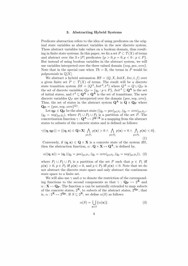
Predicate abstraction refers to the idea of using predicates on the orig-inal state variables as abstract variables in the new discrete system.These abstract variables take values on a boolean domain, thus result-ing in finite state systems. In this paper, we fix a set P ⊂ T (X) of termsand abstract over the 3 ∗ |P | predicates {p > 0, p = 0, p < 0 : p ∈ P}.But instead of using boolean variables in the abstract system, we willuse variables interpreted over the three valued domain {neg , pos, zero}.Note that in the special case when Th = R, the terms in P would bepolynomials in Q[X].
We abstract a hybrid automaton HS = (Q,X, InitX , Inv , t, f) overa given finite set P ⊂ T (X) of terms. The result will be a discretestate transition system DS = (QA, InitA, tA) where QA = Q ∪ QP isthe set of discrete variables, QP = {qp : p ∈ P}, InitA ⊆ QA is the setof initial states, and tA ⊆ QA ×QA is the set of transitions. The newdiscrete variables QP are interpreted over the domain {pos,neg , zero}.Thus, the set of states in the abstract system QA is Q × QP whereQP = {pos,neg , zero}QP .
Let qP ∈ QP be the abstract state ((qp = pos)p∈P1 , (qp = zero)p∈P2 ,-(qp = neg)p∈P3), where P1 ∪ P2 ∪ P3 is a partition of the set P . Theconcretization function γ : QA 7→ 2Q×X is a mapping from the abstractstates to subsets of the concrete states and is defined as follows:
γ((q,qP)) = {(q,x) ∈ Q×X|∧p∈P1
p(x) > 0 ∧∧p∈P2
p(x) = 0 ∧∧p∈P3
p(x) < 0}.
(1)Conversely, if (q,x) ∈ Q × X is a concrete state of the system HS ,
then the abstraction function, α : Q×X 7→ QA, is defined by,
α((q,x)) = (q, ((qp = pos)p∈P1 , (qp = zero)p∈P2 , (qp = neg)p∈P3)), (2)
where P1 ∪ P2 ∪ P3 is a partition of the set P such that p ∈ P1 iffp(x) > 0, p ∈ P2 iff p(x) = 0, and p ∈ P3 iff p(x) < 0. Note that we donot abstract the discrete state space and only abstract the continuousstate space to a finite set.
We will also use γ and α to denote the restriction of the correspond-ing functions to the second components so that γ : QP 7→ 2X andα : X 7→ QP. The function α can be naturally extended to map subsetsof the concrete states, 2X, to subsets of the abstract states, 2QP , thatis, α : 2X 7→ 2QP . If S ⊆ 2X, we define α(S) as follows:
α(S) =⋃x∈S{α(x)}. (3)
8
The context will disambiguate these usages of the abstraction andconcretization functions.
3.1. The Abstract Initial States.
Since we use formulas in WFF (X) (over some theory Th) to representelements of 2X, we will be interested in the variants, α∗ : WFF (X) 7→2QP and γ∗ : QP 7→ WFF (X), of the abstraction and concretiza-tion functions, α : 2X 7→ 2QP and γ : QP 7→ 2X. If qP is abstractstate ((qp = pos)p∈P1 , (qp = zero)p∈P2 , (qp = neg)p∈P3), then γ∗(qP) isdefined as
γ∗(qP) =∧p∈P1
p(x) > 0 ∧∧p∈P2
p(x) = 0 ∧∧p∈P3
p(x) < 0 (4)
We define α∗ using Th-satisfiability.
α∗(φ(X)) = {qP ∈ QP : Th |= ∃X : γ∗(qP) ∧ φ(X)}. (5)
If the initial states Init of the hybrid system HS is⋃i{(qi,x) : x ∈
[[φi]]}, where each formula φi ∈WFF (X) represents the initial states ina given discrete mode qi ∈ Q, then the initial states InitA are obtainedas
⋃i{(qi,qP) : qP ∈ α∗(φi)}.
LEMMA 1. If φ(X) is a formula representing a set in 2X, then α([[φ]]) ⊆α∗(φ). In particular, if HS = (Q,X, Init , Inv , t, f) is a hybrid systemwith initial states Init =
⋃i{(qi,x) : x ∈ [[φi]]} and DS, InitA, and α
are as defined as above, then, α(Init) ⊆ InitA.Proof. Let x ∈ [[φ]]. We show that α(x) ∈ α∗(φ). It follows from the
definition of the γ∗ and α functions that the formula γ∗(α(x)) evaluatesto true on the point x. By assumption, the same is true for the formulaφ. Hence, α(x) ∈ α∗(φ). Applying this result to each mode of the hybridsystem, the second part of the claim is immediately proved.
3.2. The Abstract Transition Relation.
The transitions tA of the abstract system DS = (QA, InitA, tA) areobtained by abstracting the discrete transitions and the continuousflow of the concrete hybrid system HS separately.
9
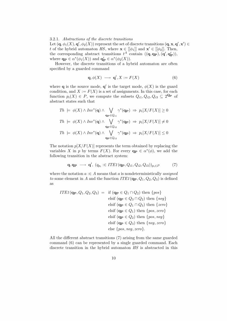
3.2.1. Abstractions of the discrete transitionsLet (q, φ1(X),q′, φ2(X)) represent the set of discrete transitions (q,x,q′,x′) ∈t of the hybrid automaton HS , where x ∈ [[φ1]] and x′ ∈ [[φ2]]. Then,the corresponding abstract transitions tA contain ((q,qP), (q′,q′P)),where qP ∈ α∗(φ1(X)) and q′P ∈ α∗(φ2(X)).
However, the discrete transitions of a hybrid automaton are oftenspecified by a guarded command
q, φ(X) −→ q′, X := F (X) (6)
where q is the source mode, q′ is the target mode, φ(X) is the guardcondition, and X := F (X) is a set of assignments. In this case, for eachfunction pi(X) ∈ P , we compute the subsets Qi1, Qi2, Qi3 ⊆ 2QP ofabstract states such that
Th |= φ(X) ∧ Inv∗(q) ∧∨
qP∈Qi1
γ∗(qP) ⇒ pi[X/F (X)] ≥ 0
Th |= φ(X) ∧ Inv∗(q) ∧∨
qP∈Qi2
γ∗(qP) ⇒ pi[X/F (X)] 6= 0
Th |= φ(X) ∧ Inv∗(q) ∧∨
qP∈Qi3
γ∗(qP) ⇒ pi[X/F (X)] ≤ 0
The notation p[X/F (X)] represents the term obtained by replacing thevariables X in p by terms F (X). For every qP ∈ α∗(φ), we add thefollowing transition in the abstract system:
q,qP −→ q′, (qpi :∈ ITE1 (qP, Qi1, Qi2, Qi3))pi∈P (7)
where the notation a :∈ Ameans that a is nondeterministically assignedto some element in A and the function ITE1 (qP, Q1, Q2, Q3) is definedas
ITE1 (qP, Q1, Q2, Q3) = if (qP ∈ Q1 ∩Q2) then {pos}elsif (qP ∈ Q3 ∩Q2) then {neg}elsif (qP ∈ Q1 ∩Q3) then {zero}elsif (qP ∈ Q1) then {pos, zero}elsif (qP ∈ Q2) then {pos,neg}elsif (qP ∈ Q3) then {neg , zero}else {pos,neg , zero}.
All the different abstract transitions (7) arising from the same guardedcommand (6) can be represented by a single guarded command. Eachdiscrete transition in the hybrid automaton HS is abstracted in this
10
way. This completes the abstraction of discrete transitions with up-dates. Note that if pi(X) does not contain any of the variables that areupdated by the assignments, then the value of qpi can be left unchanged(and we need not compute the sets Qi1, Qi2, and Qi3 in this case).
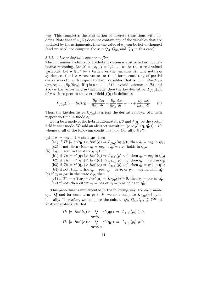
3.2.2. Abstracting the continuous flowThe continuous evolution of the hybrid system is abstracted using qual-itative reasoning. Let X = {xi : i = 1, 2, . . . , n} be the n real valuedvariables. Let p ∈ P be a term over the variables X. The notation~dp denotes the 1 × n row vector, or the 1-form, consisting of partialderivatives of p with respect to the n variables, that is, ~dp = [∂p/∂x1,-∂p/∂x2, . . . , ∂p/∂xn]. If q is a mode of the hybrid automaton HS andf(q) is the vector field in that mode, then the Lie derivative, Lf(q)(p),of p with respect to the vector field f(q) is defined as
Lf(q)(p) = ~dpf(q) =∂p
∂x1
dx1
dt+
∂p
∂x2
dx2
dt+ · · ·+ ∂p
∂xn
dxndt
(8)
Thus, the Lie derivative Lf(q)(p) is just the derivative dp/dt of p withrespect to time in mode q.
Let q be a mode of the hybrid automaton HS and f(q) be the vectorfield in that mode. We add an abstract transition ((q,qP), (q,q′P)) ∈ tAwhenever all of the following conditions hold (for all p ∈ P ):
(a) if qp = neg in the state qP, then(a1) if Th |= γ∗(qP) ∧ Inv∗(q)⇒ Lf(q)(p) ≤ 0, then qp = neg in q′P;(a2) if not, then either qp = neg or qp = zero holds in q′P.
(b) if qp = zero in the state qP, then(b1) if Th |= γ∗(qP) ∧ Inv∗(q)⇒ Lf(q)(p) < 0, then qp = neg in q′P;(b2) if Th |= γ∗(qP) ∧ Inv∗(q)⇒ Lf(q)(p) = 0, then qp = zero in q′P;(b3) if Th |= γ∗(qP) ∧ Inv∗(q)⇒ Lf(q)(p) > 0, then qp = pos in q′P;(b4) if not, then either qp = pos, qp = zero, or qp = neg holds in q′P;
(c) if qp = pos in the state qP, then(c1) if Th |= γ∗(qP) ∧ Inv∗(q)⇒ Lf(q)(p) ≥ 0, then qp = pos in q′P;(c2) if not, then either qp = pos or qp = zero holds in q′P.
This procedure is implemented in the following way. For each modeq ∈ Q and for each term pi ∈ P , we first compute Lf(q)(pi) sym-bolically. Thereafter, we compute the subsets Qi1, Qi2, Qi3 ⊆ 2QP ofabstract states such that
Th |= Inv∗(q) ∧∨
qP∈Qi1
γ∗(qP) ⇒ Lf(q)(pi) ≥ 0,
Th |= Inv∗(q) ∧∨
qP∈Qi2
γ∗(qP) ⇒ Lf(q)(pi) 6= 0,
11
Th |= Inv∗(q) ∧∨
qP∈Qi3
γ∗(qP) ⇒ Lf(q)(pi) ≤ 0.
Subsequently, for each qP ∈ α(Inv(q)), we generate the followingdiscrete abstract transition
q, qP −→ q, (qpi :∈ ITE2 (qP, qpi , Qi1, Qi2, Qi3))pi∈P
where the mode q is left unchanged, but the abstract variables qpi areassigned a value from the set returned by the function ITE2 (qP, qpi ,-Qi1, Qi2, Qi3), which is defined as follows:
ITE2 (qP, qp, Q1, Q2, Q3) = if qp = posif qP ∈ Q1 then {pos} else {pos, zero}elsif qp = negif qP ∈ Q3 then {neg} else {neg , zero}elseif (qP ∈ Q1 ∩Q2) then {pos}elsif (qP ∈ Q3 ∩Q2) then {neg}elsif (qP ∈ Q1 ∩Q3) then {zero}else {pos,neg , zero}
We repeat the process for each mode and compute the abstract tran-sitions arising from the continuous dynamics of each mode separately.This completes the phase of adding transitions to the abstract system.
Note that we can handle cases where the set Q of discrete states inHS is infinite as long as the number of distinct “modes” (which caneach be specified as a formula over Q) are finite.
THEOREM 1. Let HS = (Q,X, Init , Inv , t, f) be a hybrid automatonand P ⊂ T (X) be a finite set of terms over the set X of real variables.If DS = (QA = Q ∪ QP , InitA, tA) is the discrete transition systemconstructed by the above method, then DS is an abstraction for HS.
Proof. If (q,x) ∈ Q×X is a concrete state of the hybrid system HS ,then the abstraction mapping α is defined by Equation 2. Lemma 1establishes condition (a) of Definition 3. In order to establish condi-tion (b), let ((q,x), (q′,x′)) ∈ tα be a transition in the discrete systemHSα corresponding to HS with respect to the mapping α. There are twocases based on whether this is a discrete (Definition 2 (a)) or continuous(Definition 2 (b)) transition.
Continuous transition. In this case q′ = q. Let F be as in Defi-nition 2 (b). Without loss of generality, assume that α(q, F (τ)) is aconstant function on [0, δ). We claim that (α(q,x), α(q,x′)) ∈ tA. Let
α(x) = ((qp = pos)p∈P1 , (qp = zero)p∈P2 , (qp = neg)p∈P3).
12
There are two subcases.(1) α(x) = α(x′): Consider p ∈ P2. We note that p(F (τ)) = 0 for allτ ∈ [0, δ]. It follows that Lf(q)(p) = 0 at all points F (τ), in particularLf(q)(p) = 0 at F (0) = x. At point x, the formula γ∗(α(x)) evaluatesto true, the formula Inv∗(q) is true, and the formula Lf(q)(p) = 0 istrue. Therefore, it is not possible to prove the theorems in cases (b1)or (b3). Hence, we would apply either case (b2) or (b4) and in boththese cases we have the choice of maintaining qp = zero. Finally, forp ∈ P1 ∪ P3, all cases in (a) and (c) allow for the possibility of keepingthe sign of qp unchanged.(2) α(x) 6= α(x′): If for some p ∈ P1, p(F (δ)) = 0, then for someτ ∈ (0, δ), Lf(q)(p) < 0 at the point F (τ) ∈ Rn. Let x′′ be thisintermediate point F (τ). Now, at this point, γ∗(α(x)) evaluates to true(since, by assumption, α(x) = α(x′′)) and Inv∗(q) also evaluates to true(since again, by assumption, the invariant is true at all intermediatepoints), but Lf(q)(p) ≥ 0 evaluates to false. Consequently, case (c1)cannot be applicable and we have to use case (c2), which shows that qpcan be chosen to be zero. Using similar arguments for all other casesfor p ∈ P2 and p ∈ P3, we conclude that there will be a transition(α(q,x), α(q,x′)) ∈ tA.
Discrete transition. If ((q,x), (q′,x′)) ∈ tα is a discrete transition(from Definition 2 (b)), then by definition (q,x,q′,x′) ∈ t. Assumethat this transition is captured in HS by the guarded assignment,q, φ(X) −→ q′, X := F (X). Therefore, the formula φ evaluates totrue at the point x. It follows from Lemma 1 that α(x) is in α∗(φ).Finally, we note that for p ∈ P , the value of p after the updates willbe identical to the value of p[X/F (X)] before the transition. It nowfollows from the way the discrete transition is abstracted that there isa transition (q, α(x),q′, α(x′)) ∈ tA. This completes the proof.
Example 4. We abstract the thermostat model from Example 1 usingthe terms P = {x, x−68, x−70, x−80, x−82, x−100}, labeled p1, . . . , p6.The abstract discrete transition system is defined over seven variables,{q1, qp1 , . . . , qp6}. The dynamics are given as:
q1 = on, qp4 = pos −→ q1 := offq1 = off , qp3 = neg −→ q1 := onq1 = on, qp5 = neg −→ (qpi :∈ VN (qp1 , . . . , qp6 , i, 6))i=1,...,6
q1 = off , qp2 = pos −→ (qpi :∈ VN (qp1 , . . . , qp6 , i, 1))i=1,...,6
where the function VN (a1, a2, a3, a4, a5, a6, i, j) = ITE2 ((a1, . . . , a6),-ai, {qP ∈ QP : qpj 6= pos}, {qP ∈ QP : qpj 6= zero}, {qP ∈ QP :qpj 6= neg}). Note that the first two transitions above are abstractions
13
of the discrete transitions, while the latter two are abstractions ofthe continuous dynamics. We have simplified the formulas here. Forexample, x > 80 should be abstracted to qp4 = pos ∧ qp3 = pos · · ·,but we have just included qp4 = pos above. We also note that certainabstract states are infeasible, for example, qp4 = pos ∧ qp3 = zero. InSection 5, we will add information to the abstract system to guaranteethat the abstract trajectories remain inside the feasible region and theinvariant set.
4. Choosing the Abstraction Mapping
The quality of the abstraction computed by our method depends cru-cially on the terms P over which the abstraction is computed. In thissection, we discuss the approaches to identify (compute) P . It is clearthat the terms that occur in the statement of the property we wish toverify are ideal candidates to include in P . For example, if we wish toverify that x1 > x2 always, then we should add the term x1 − x2 to P .Similarly, the terms that occur in the guards of discrete transitions areadded to P . The set P thus constructed is the seed set. We will addmore elements to P using the techniques described below.
4.1. Higher-order Lie Derivatives
Consider a set P0 = {p1, p2, . . . , pk} of k terms over variables X. Letψ ∈ WFF (X) be a formula containing free variables from X. Definethe extended monoid of the set P0 (relative to ψ) as the minimal setEMonψ(P0) such that (i) P0 ⊂ EMonψ(P0), (ii) r ∈ EMonψ(P0) if r iszero, positive or negative definite relative to ψ (that is, Th |= ψ ⇒ r =0, or Th |= ψ ⇒ r > 0, or Th |= ψ ⇒ r < 0), (iii) p1p2 ∈ EMonψ(P0)whenever p1, p2 ∈ EMonψ(P0). In other words, the set EMonψ(P0) isthe monoid over P0 and all relatively positive and negative definitefunctions. An important property of the set EMonψ(P0) is that if thesigns (positive, negative, or zero) of all the terms in P0 are known,then the sign of any term in EMonψ(P0) can be uniquely determined(assuming ψ holds).
We add new functions to the set P by saturating the existing termsin P under the Lie derivative computation (with respect to vector fieldin a particular mode). Let q be a mode of the hybrid system HS andf(q) be the corresponding vector field. The rule for adding new terms toP is the following: If p ∈ P is a term, then we add the term Lf(q)(p) toP unless Lf(q)(p) ∈ EMonInv∗(q)(P ). Thus, the process of constructingnew terms to add to P involves computing the Lie derivative Lf(q)(p)
14
and testing if Lf(q)(p) ∈ EMonInv∗(q)(P ). Since the latter test couldbe expensive, we sometimes replace it by the following weaker tests
Th |= Inv∗(q)⇒ Lf(q)(p) ∼ 0 ∼ ∈ {>,=, <}Th |= Inv∗(q)⇒ Lf(q)(p) = cp′
for some constant c ∈ R and p′ ∈ P . If either of these proof obliga-tions can be proved, then clearly Lf(q)(p) ∈ EMonInv∗(q)(P ) and henceLf(q)(p) is not added to P .
The functions added to P by the saturation process are useful whenqualitatively abstracting the continuous dynamics of HS , as outlinedin the previous section.
Note that for general vector fields f(q) the saturation process mightnot terminate. But there are special cases where this process is guaran-teed to terminate. For example, suppose a mode q has linear dynamicsgiven by a nilpotent matrix A, that is, f(q)(X) = AX such thatAk = 0. Let p ∈ P be a polynomial with degree d. Then the (d ∗ k)-thLie derivative of p with respect to f(q) will be identically zero. As asecond example, consider a mode q that has linear dynamics given bya matrix A, which satisfies the equation An = rAm for some constantr ∈ R and n,m ∈ N. If p ∈ P is a linear polynomial, then the saturationprocess can be shown to terminate. In particular, if p = ~aTX is a linearpolynomial, then the n-th Lie derivative of p will r times the m-th Liederivative. Since the n-th derivative of p is a constant multiple of them-th derivative of p, it does not get added to the set P of polynomialsin the saturation process.
We remark here that the termination of the saturation process isdetermined by both the initial set P of seed terms and the vector fields f(in all the different modes). However, the termination of the saturationphase is not necessary for creating an abstraction. We can stop at anypoint in the saturation process and compute the abstraction using theset P computed upto that point. A larger set P yields a finer abstractionas it results in a larger state space in the resulting abstract system.
Example 5. Consider the hybrid automaton HS from Examples 2and 3. The guards of the discrete transitions give two terms P ={xn − hd, xu − hn}. Let us assume that all symbolic parameters, suchas hd, hn, λd, are constrained to be positive constants by the invari-ant. Note that the parameters are unchanging, that is, for example,xu = 0 in all modes. Consequently, the Lie derivative of xu − hn isidentically zero in all four modes. Hence, nothing is added to the setP . Next, we compute the Lie derivative of xn − hd in the four modes.We get two distinct values, −λnxn and ∆n − λnxn. These get addedto P . Next, we compute the Lie derivative of −λnxn with respect to
15
the four distinct vector fields. We get two different terms again, butthese are just −λn times the old terms. Hence, nothing new is addedto P . Similarly, when we compute the Lie derivative of ∆n − λnxn,we get the same answers and do nothing. After saturation, finallyP = {xn − hd, xu − hn,−λnxn,∆n − λnxn}.
4.1.1. Heuristic for identifying important termsWe say that a set P0 of (polynomial) functions is closed under Liederivative computation with respect to f(q) and relative to Inv∗(q)if for every function pi ∈ P0, the Lie derivative of pi w.r.t f(q) isin EMonInv∗(q)(P0). Clearly, if P0 is a set which satisfies the aboveproperty, then inclusion of P0 into P incurs no further additions to Pdue to saturation. Hence, an important heuristic for identifying newterms for inclusion into P is the following:
A set P0 of terms is good if, for each mode q of the hybrid system,the set P0 is closed under Lie derivative computation with respectto f(q) and relative to Inv∗(q).
In Sections 4.2 and 4.3, we will be guided by this basic heuristic ruleto compute important sets P0 and include them in P . Note that evenif a set P0 may not satisfy the above condition for every mode, it couldstill be useful if P0 satisfies the condition for some modes.
4.2. Linear Dynamics
Useful linear functions can be computed for inclusion in P if there aremodes with linear dynamics. Let q be a mode of the hybrid systemHS with vector field given as f(q)(X) = AX, where A ∈ Qn×n. If λis a real eigenvalue of A and ~c = [c1, . . . , cn]T is an eigenvector of AT
corresponding to λ, then we add the linear function p = ~cTX to the setP .
The reason why this particular p is a useful term to use for ab-straction becomes clear when we compute the Lie derivative of p withrespect to f(q),
Lf(q)(p) = ~cT X = ~cTAX = (AT~c)TX = (λ~c)TX = λp.
This shows that the set {p} is closed under Lie derivative computationin mode q. In this specific case, Lf(q)(p) vanishes on the surface p = 0and hence flows will not cross this surface. If the system starts onone side of this surface, it will continue to remain in that half space.This information is preserved in the abstraction if p is included in theset P . Hence, p = 0 can potentially be a barrier certificates [39]. We
16
also remark here that the linear forms p can be used to approximatereachability sets explicitly [49, 53, 54].
Each distinct real eigenvalue of A can be used to generate a suitablelinear function p for inclusion in the set P of abstraction terms. Ifthe eigenvalue is rational, then the computation and representation ofthe corresponding eigenvector is straightforward. If not, then we usepolynomials to represent the coefficients of p.
Example 6. Consider a part of the leader control developed in [15]and also discussed in [42] for collision avoidance in automated cruisecontrol in automobiles. The control is applied during safety-critical sit-uations when the inter-vehicle distance is small, or the relative velocitybetween vehicles is large. Let gap, vf , v, and a respectively representthe gap between the two cars, the velocity of the leading car, and thevelocity and acceleration of the rear car. We are given,
v = a, a = −3a− 3(v − vf ) + (gap − (v + 10)), ˙gap = vf − v.
Formally, this describes a linear dynamical system withX = {v, vf , a, gap}.Assuming the variable vf is a parameter (unchanging symbolic con-stant), the dynamics can be written as X = AX +B, where
A =
0 0 1 00 0 0 0−4 3 −3 1−1 1 0 0
B =
00−100
By a change of variables, rgap ← gap − 10, we get X = AX, whereX = [v, vf , a, rgap]T . We leave the set Init of initial states and theinvariant sets unspecified. For a given set of possible initial states, theproblem is to verify that the rear car would never collide with the carin front, that is, always gap > 0, or rgap > −10.
Now, the characteristic polynomial for A, λ(λ3 + 3λ2 + 4λ+ 1), hasexactly two real zeros. The nonzero real eigenvalue, denoted by λ, liesbetween −1/3 and −1/4. Now, if ~c = [c1, c2, c3, c4]T is an eigenvectorof AT corresponding to λ, then AT~c = λ~c. We assume, without loss ofgenerality, that c4 = 1, and hence we get an eigenvector [c1, c2, c3, 1]T
where c1, c2 and c3 satisfy the equations c3 = λ, c1 = λ2 +3λ, and c2 =−c1− 1. Therefore, the linear term corresponding to this eigenvector isp = c1v−(c1 +1)vf +c3a+rgap. We add this term to the set P . In fact,for certain initial states, the surface p = 0 acts as a barrier betweenthe initial states and the unsafe region and suffices to prove the safetyproblem (under certain assumptions on the invariant set). We refer theinterested reader to [49] for further analysis of this example.
17
4.2.1. Complex eigenvaluesLet y2 +ay+ b be a factor of the characteristic polynomial of A, wherea, b ∈ R and a 6= 0, 4b > a2. Let W denote the null space of thetransformation (AT )2 + aAT + bI, that is,
W = {~c ∈ Rn : ((AT )2 + aAT + bI)~c = 0}.
Since AT ∈ Qn×n, a ∈ R, and b ∈ R, it follows that W is nonempty.Let ~c ∈ Rn be a nonzero vector in W . Consider the linear function
p = ~cTX over the state variables corresponding to this vector. Let pdenote Lf(q)(p) and p denote Lf(q)(p). We have the following relationbetween p, p, and p.
p+ ap+ bp = ¨~cTX + a ˙~cTX + b~cTX = ~cTA2X + a~cTAX + b~cTX= ~cT (A2 + aA+ bI)X = (((AT )2 + aAT + bI)~c)TX = 0
We add p and p to the set P . Note that we can infer the sign of p fromthat of p and p in many cases.
4.2.2. Computability issuesIf eigenvalues are rational, then computation of the left eigenvectorwould just involve simple arithmetic manipulation over rationals. How-ever, if we have to deal with real numbers and the left eigenvectors arecomposed of real numbers, then we require the ability to representand reason with algebraic numbers. This requires theorem provingcapability for a theory of reals defined over {+,−, ∗,=}.
4.3. Nonlinear Dynamics
We present some heuristic approaches to find useful terms for inclusionin the set P when the dynamics in a given mode are nonlinear.
4.3.1. Linear barriersWe first discover important linear functions for inclusion into P . LetX = f(q) specify the dynamics in mode q. Separate the nonlinearcomponent from the linear component and rewrite the above equationas
X = AX +BY
where Y is the vector of non-linear functions of the state variables X,see also Example 7. Here A is an n× n matrix, B is an n×m matrix,X is a n×1 vector, and Y is a m×1 vector. Let ~c be a real eigenvectorof AT which is also in the kernel of BT (that is, the linear subspace ofzeros of BT ), that is,
AT~c = λ~c BT~c = ~0,
18
where the components of ~c are reals. The transpose ~cT of the vector ~cis a 1-form. Consider the linear function p = ~cTX.
Lf(q)(p) = ~cT X = ~cT (AX +BY ) = (AT~c)TX + (BT~c)TY= (λ~c)TX +~0 = λp.
This shows that the set {p} is closed under Lie derivative computationand hence, it is useful to include p in the set P . We note here that thematrix A and B are unique upto permutations of their rows. It is easyto see that any of these choices for B will result in the same outcome.
Example 7. If x1 and x2 represent concentrations of two proteins thatcan bind together to form a dimer, then the law of mass action givesthe following differential equations governing the dynamics of x1 andx2:
x1 = ∆1 − λx1 − kx1x2
x2 = ∆2 − λx2 − kx1x2
If we introduce a new variable x3 to homogenize the above (intuitivelyx3 is always 1), we get A = [−λ, 0,∆1; 0,−λ,∆2; 0, 0, 0] is a (3 × 3)-matrix, X = [x1;x2;x3] is a column vector, B = [−k;−k; 0] is a (3 ×1)-matrix, and Y = [x1x2] is a vector with only one element. The aboveequations can be written as X = AX + BY . If we use the methodoutlined above and replace x3 by 1, we get the linear function p =−λx1 + λx2 + ∆1 −∆2. We immediately observe that Lf (p) = −λp.
4.3.2. Nonlinear invariantsAssume that the dynamics in the mode q are given by X = f(q), wheref(q) ∈ Q[X]n is a polynomial vector field. A syzygy of the vector fieldf(q) is a 1-form ~hT such that ~hT f(q) = 0. A 1-form ~hT is exact ifthere exists a smooth function (polynomial, in our case) p such that~hT = ~dp. Suppose there is a syzygy ~qT of the vector field f(q) which isalso exact. In other words, there is a polynomial p such that
∂p/∂x1 = q1, ∂p/∂x2 = q2, . . . , ∂p/∂xn = qn andq1 ∗ (dx1/dt) + q2 ∗ (dx2/dt) + · · ·+ qn ∗ (dxn/dt) = 0.
Under these assumptions, it is easy to note that the Lie derivative of pwith respect to the vector field f(q) vanishes, that is, dp/dt = ~dpX =~dpf(q) = 0. The set {p} is closed under Lie derivative computation. Infact, in this case the value of the expression p(x1, x2, . . . , xn) remainsinvariant through the time evolution of the nonlinear system and it isfruitful to include p in the set P .
19
Example 8. Consider the nonlinear dynamical system:
x1 = x1x2 x2 = −x1
It is the case that 1x1x2 +x2(−x1) = 0 and hence (1, x2) is a syzygy ofthe polynomials x1x2,−x1. A solution for p that satisfies both ∂p/∂x1 =1 and ∂p/∂x2 = x2, is V = x1 + x2
2/2. It is easily observed that p = 0and hence p is an invariant of the above dynamical system.
4.3.3. Nonlinear barriersAssume again that the dynamics in the mode q are given by X = f(q),where f(q) ∈ Q[X]n is a polynomial vector field. Suppose that thereexists a polynomial r such that r = ~qT f(q), the 1-form ~qT is exact (thatis, dp = ~qT for some p ∈ Q[X]), and r is nonnegative or nonpositivedefinite relative to Inv∗(q)∧ p ∼ 0, where ∼ ∈ {>,<}. In other words,we have
r = ~qT f(q), ~qT = dp,Th |= Inv∗(q) ∧ p ∼ 0⇒ r ∼′ 0, ∼′∈ {≥,≤}.
In this case, we can add p to the set P , since Lf(q)(p) = r and wecan infer the sign of r given the sign of p. Note that r is in the idealgenerated by the polynomials in f(q).
4.3.4. Computability issuesThe computation of nonlinear invariants and barriers, as describedabove, requires the ability to (a) compute a syzygy basis for a finite setof polynomials, (b) check for exactness of a given 1-form, and integratean exact 1-form, (c) enumerate elements in the ideal generated by afinite set polynomials, and (d) test a polynomial for being relativelynonnegative or nonpositive definite. Questions pertaining to ideal mem-bership can be solved using Grobner basis computation and syzygybasis can also be computed using standard algorithms from compu-tational algebraic geometry. Exactness of a 1-form ~hT can be testedby checking if ∂hi/∂xj = ∂hj/∂xi, for all i, j [52]. Exact polynomial1-forms can be integrated symbolically. The test for nonnegative ornonpositive definiteness requires theorem proving capability.
Unlike the case of linear dynamics, the discovery of invariants andbarriers for nonlinear dynamics involves a search. We have to enumeratesyzygies or ideal members, and test if they satisfy the other constraints.It is left for future work to determine if the sets of nonlinear invariantsand barriers are (algorithmically) computable.
20
Example 9. Consider the nonlinear system
x1 = x1 − x2 + x1x2 x2 = −x2 − x22.
The nonnegative definite polynomial x22 is in the ideal generated by
x1 − x2 + x1x2 and −x2 − x22 and we correspondingly have x2
2 =−x2(x1 − x2 + x1x2) − x1(−x2 − x2
2). The 1-form [−x2,−x1] is ex-act since ∂(−x2)/∂x2 = ∂(−x1)/∂x1 = −1. Symbolically integratingthis 1-form, we get the polynomial −x1x2. In all, we conclude thatd/dt(−x1x2) = x2
2. Since x22 ≥ 0 is always true, we can infer that the
value of −x1x2 is nondecreasing.
4.4. Barrier Certificates
Consider a continuous dynamical system with dynamics given by X =f(X) and initial states Init . Suppose that we are also given an unsaferegion Xu. A function p such that (a) Lf(q)(p) ≤ 0 whenever p = 0,(b) p(x) > 0 whenever x ∈ Xu, and (c) p(x) ≤ 0 whenever x ∈ Init , iscalled a barrier certificate [39, 40]. An existence of a barrier certificatedemonstrates that the unsafe region is not reachable from the initialstates. Several of the functions proposed by us to be included in the setP satisfy conditions similar to condition (a). For example, the linearfunctions defined by the left eigenvectors for linear dynamics satisfycondition (a). Similarly, some of the functions proposed above for non-linear dynamics also satisfy condition (a). These functions can becomebarrier certificates if the initial and the unsafe regions additionallysatisfy conditions (b) and (c). Techniques based on convex optimizationhave been proposed for the computation of barrier certificates [40]. Anyfunctions computed in this way can also be added to the set P .
Barrier certificates are good choices for inclusion into the set P sincethey satisfy our general characterization of the set of good predicates.Alternatively, our general characterization can be seen as a general-ization of the notion of barrier certificates to sets of functions, whichif used together, can yield useful reachability information about thehybrid system.
Example 10. The Volterra predator-prey model [52] is given by
x1 = −x1 + x1x2 x2 = x2 − x1x2
where x1 indicates the number of predators and x2 indicates the numberof prey. It is an easy exercise to note that the set of four polyno-mials P0 = {x1, x2, (x2 − 1), (x1 − 1)} is closed under Lie derivativecomputation. The qualitative abstraction of this model over the four
21
polynomials in P0 shows the possible oscillatory behavior of the system.Another choice of a closed set is {x1 + x2, x2− x1, x1 + x2− 2x1x2, 1−2x1x2} and this can be used to refine the above abstraction.
5. Refining the Abstraction and Other Optimizations
The process of abstracting the continuous evolution of the hybrid sys-tem HS is done using qualitative rules in our approach as outlinedabove. As a consequence of this, the abstract transitions are obtainedas updates to the abstract variables, each one independent of the other,as in cartesian abstraction [7]. This means that the concretization ofa new abstract state reached by taking an abstract transition couldbe infeasible. Furthermore, certain abstract states can also be deletedbecause they are explicitly disallowed by the given invariant set Inv ofthe concrete system.
More specifically, any transition to the abstract state (q,qP) can bedeleted if
Th 6|= ∃X : γ∗(qP) ∧ Inv∗(q)(X).
Note that this process also removes infeasible abstract states, that is,states (q,qP) such that Th 6|= ∃X : γ∗(qP). If the infeasible abstractstates were not removed, then we could have cases where we (spuri-ously) reach a feasible abstract state via an infeasible abstract state.Thus, removing the infeasible abstract states improves the quality ofabstraction by eliminating such spurious trajectories.
This refinement step is implemented by first computing the setFeas = {qP ∈ QP : Th |= ∃X : γ∗(qP)} during the process ofconstructing the abstraction. We modify each abstract transition byadding an extra condition to check if the destination state is feasibleand satisfies the invariant of the destination mode. For example, if theoriginal abstract transition was
q, ψ1(QP ) −→ q′, QP := FQ(QP )
then we replace it by the new abstract transition
q, ψ1(QP ) −→ q′, QP := FQ(QP ), QP ∈ Feas ∩ α(Inv(q′))
where QP refer to the new values of these variables in the newly addedcondition. The transition is allowed only if the additional conditionholds.
22
5.1. Reducing the size of the abstract state space
The size of the abstract state space, O(|Q|×3|P |), grows exponentiallywith the number of terms in the set P . This size can be reduced if notall modes are abstracted using the same set P of terms. We can choosea different subset of terms for different modes of the hybrid system.
Let Pq be a set of terms indexed by the modes q ∈ Q. Whenabstracting a concrete predicate φ(X) in mode q, we will only usethe terms in Pq, so that Equation 5 is replaced by,
α∗Pq(φ(X)) = {q′ ∈ QPq : Th |= ∃X : γ∗(q′) ∧ φ(X)}. (9)
The initial states can be abstracted using this modified equation now.A discrete transition q, φ(X) −→ q′, X := F (X) is now abstracted
by the following transitions, defined for each qP ∈ α∗Pq(φ(X)),
q, qP −→ q′, (qp := ITE1 (qP, Qp1, Qp2, Qp3))p∈Pq′
where Qp1, Qp2, Qp3 are now subsets of 2QPq . The only change in theabstraction of the continuous evolution is that in mode q ∈ Q we onlymake changes to the abstract variables qp, where p ∈ Pq. The size ofthe state space of the resulting abstract system is now O(Πq∈Q|Pq|).
The process for obtaining terms to include in P , as outlined in Sec-tion 4, works on discrete modes individually. If the term p is generatedwhen working in mode q, then p is added to Pq. For example, inthe saturation process that computes higher-order Lie derivatives, ifp′ = Lf(q)(p) for p ∈ Pq, then p′ is added to Pq and it is not added toany of the other sets Pq′ , q′ 6= q.
6. Computability and Theorem Proving Obligations
We have described the abstraction procedure assuming that we havea procedure to handle the theorem proving obligations that are gener-ated. In fact, we have left the choice of the theory Th open until now.In this section, we will briefly discuss the issues related to automatingthe theorem proving support required for constructing abstractions ofhybrid systems as described in this paper.
We recapitulate the requirements on the theorem proving capabilityrequired over the theory Th. We need the ability to decide satisfiabilityof quantifier-free formulas (that is, implicitly existentially quantifiedformulas) over Th. First, this is required to abstract initial states andguards of discrete transitions, as given by Equation 5. Second, the proofobligations arising in the process of abstracting the updates on discrete
23
transitions and abstracting the continuous dynamics are of the formTh |= ψ ⇒ p ∼ 0, where ∼∈ {≥, 6=,≤}. These are equivalent to testingTh |= ∃X : (ψ ∧ p ∼′ 0), where ∼′ is respectively in {<,=, >}.Finally, we note that we need to decide satisfiability of quantifier-freeformulas to eliminate the infeasible states from the abstract system.The signature of Th is required to contain the symbols {−, >,=} andany other symbol required either to specify the input hybrid system orto express the Lie derivative of terms in Th with respect to the systemdynamics.
The time complexity of the basic abstraction procedure of Section 3,ignoring the phase of generating the set P , is O(|Q||P |3|P |TTh(N) +|Q|23|P |TTh(N)), where |S| denotes the cardinality of the set S, TTh isthe time-complexity of the satisfiability procedure for theory Th, andNis the size of the input hybrid system HS . The first term results from thephase of abstracting the continuous dynamics (Section 3.2.2) and thesecond term is contributed by the discrete transitions (Section 3.2.1).In our implementation, we attempt to overcome the two most expensivefactors, 3|P | and TTh , in the complexity.
In the process of constructing an abstraction, we do not explic-itly enumerate the 3|P | states in QP. In the case of abstracting theinitial states, we do a depth-first enumeration of these exponentiallymany states and cache witnesses of disproofs to avoid repeated theoremproving effort. In the case of abstracting the dynamics, we use severalheuristics, such as slicing, to select a small subset P1 ⊆ P , and enumer-ate only over the 3P1 states. These approximations do not compromisethe soundness of the abstraction, though they can potentially affect itsquality.
Special classes of hybrid systems, such as timed automata, can bespecified using the signature {Q,+,−, >,=}, which excludes the multi-plication operator. The theory of reals over this signature, often calledthe theory of linear arithmetic over reals, satisfies all our constraints inthis case and it can be used for abstracting such systems. Satisfiabilityof a conjunction of atomic formulas is efficiently decidable for thistheory.
If the theory Th is the theory of reals defined over the signature{Q,+,−, ∗, >,=}, then we can use polynomial expressions to specifythe dynamics of the hybrid system. This theory is called the theory ofthe real closed fields and it can be used to abstract such polynomialsystems. This theory is known to be decidable [47, 11]. In particular,the satisfiability problem is decidable. However, the decision procedureis computationally expensive.
One can also use richer signatures by including the trigonometricfunctions or the exponential function in the signature. The theory
24
of reals over such richer signatures loses some of its nice decidabilityresults.
The abstraction procedures uses theorem proving in a “failure-tolerant”mode, that is, the correctness of the procedure is preserved even whenthe theorem prover ceases to be complete as long as it is sound. Bysoundness, we mean that whenever the prover says a formula is unsat-isfiable, then it really should be unsatisfiable. Completeness requiresthat if the prover says satisfiable, then the formula should indeed besatisfiable. The proof of Theorem 1 only requires that the theoremprover be sound. The incompleteness in the theorem prover will onlyresult in a coarser abstract system. Thus, we can use efficient, sound,but incomplete, procedures to test satisfiability of quantifier-free for-mulas in the theory Th for constructing abstractions. This is especiallyuseful if it is computationally expensive, or impossible, to obtain soundand complete decision procedures.
7. Compositional Abstraction
Let HS 1 = (Q1 ∪ Qin1 , X1 ∪ X in
1 , Init1, Inv1, t1, f1) and HS 2 = (Q2 ∪Qin
2 , X2 ∪X in2 , Init2, Inv2, t2, f2) be a pair of hybrid automata, where,
for i = 1, 2, Qini is a finite set of input discrete variables, X in
i is a finiteset of input real variables, Init i ⊆ Qi×Xi, Inv i : Qi×Qin
i 7→ 2(Xi×Xini ),
ti : Qi ×Qini ×Xi ×Xin
i ×Qi ×Xi, and fi : Qi ×Qini 7→ (Xi ×Xin
i 7→TXi). Let σ1 : (Qin
1 ∪ X in1 ) 7→ (Q2 ∪ X2) and σ2 : (Qin
2 ∪ X in2 ) 7→
(Q1 ∪X1) be two renaming functions that map the input variables toother state variables1. The result of composing HS 1 and HS 2 (withrespect to σ1 and σ2) is the hybrid automaton HS = HS 1 × HS 2 =(Q,X, Init , Inv , t, f), where Q = Q1∪Q2 is the set of discrete variablesso that the discrete modes of HS is given by Q = Q1 ×Q2 and X =X1 ∪ X2 is the set of real variables and the continuous state-space ofHS is X = X1 × X2. If (q1,qin
1 ,x1,xin1 ,q1
′,x1′) ∈ t1 in HS 1, then
(q1,q2,x1,x2,q1′,q2,x1
′,x2) ∈ t in HS if qin1 matches q2 on the
variables made identical by σ1 and xin1 matches x2 on the variables
made identical by σ1. Similarly, a discrete transition in t2 induces adiscrete transition in HS . Note that the hybrid automaton HS canmake a discrete transition exactly when one of its components canmake a discrete transition. If X1 = f1(q1)(X1, X
in1 ) is the continuous
flow equation in the discrete mode q1 of the automaton HS 1, and X2 =f2(q2)(X2, X
in2 ) is the continuous flow equation in the discrete mode q2
1 For simplicity, we assume here that the composed hybrid automaton HS isautonomous, that is, it has no inputs and all inputs of HS1 and HS2 are closed bysuitably renaming them to other state variables.
25
of the automaton HS 2, then in the discrete state (q1,q2) of HS , thereis a continuous flow given by the equations X1 = f1(q1)(X1, σ1(X in
1 ))and X2 = f2(q2)(X2, σ2(X in
2 )). Note that the time evolutions of thecomponent hybrid automata happen simultaneously.
Example 11. The Delta-Notch lateral inhibition model in Example 2shows interesting behavior when there is more than one cell. A model oftwo such cells is obtained as a composition of two hybrid automata, onefor each cell. For i = 1, 2, the hybrid automaton HS i = (Qi ∪Qin
i , Xi ∪X ini , Init i, Inv i, ti, fi) is obtained from the automaton HS described in
Example 2 by (a) appending index i in the subscript of names of allvariables, (b) setting Qin
i = ∅, and (c) setting X in1 = {xu1} and X in
2 ={xu2}. Define the renaming functions σ1 and σ2 so that σ1(xu1) = xd2and σ2(xu2) = xd1. The two-cell Delta-Notch lateral signaling model isnow obtained by composing HS 1 and HS 2 with respect to σ1 and σ2.
7.1. Abstraction
Let HS 1 = (Q1 ∪ Qin1 , X1 ∪ X in
1 , Init1, Inv1, t1, f1) and HS 2 = (Q2 ∪Qin
2 , X2∪X in2 , Init2, Inv2, t2, f2) be a pair of hybrid automata. We wish
to compositionally abstract the hybrid automaton HS = HS 1 × HS 2
obtained by composing HS 1 and HS 2 under given renaming functionsσ1, σ2. However, this is only possible under some strong assumptionson the level of interaction between HS 1 and HS 2.
Assume that for i = 1, 2, it is the case that the hybrid automatonHS i = (Qi ∪Qin
i , Xi ∪X ini , Init i, Inv i, ti, fi) satisfies the following two
conditions:
(A1) The vector field fi(q) does not depend on the input variables X ini .
(A2) There is no term containing variables from both Xi and X ini that
occurs in the guard of discrete transitions and invariants.
As a consequence of Condition (A2), we can assume that all atomicformulas in a guard or invariant in HS i are of the form p ∼ 0, wherep ∈ T (Xi) or p ∈ T (X in
i ). If either of these two conditions is violatedby either HS 1 or HS 2, then the compositional abstraction algorithmfails. This algorithm is described as follows:
1. For i = 1, 2 let
P ini := {p ∈ T (X in
i ) : p ∼ 0 occurs in HS i}Pi := {p ∈ T (Xi) : p ∼ 0 occurs in HS i}
26
2. Let P1 := P1 ∪ P in2 and P2 := P2 ∪ P in
1 . Obtain the final sets Piof terms, over Xi, using saturation and other methods, for use inabstracting HS i.
3. Abstract HS i using the terms in Pi to get a discrete transitionsystem DS i under the assumption that the input variables are un-changed during both continuous evolutions and discrete transitions.Note that DS i = (Qi∪Qin
i ∪QPi ∪QP ini, InitAi , t
Ai ), where QP in
iand
Qini are input variables.
4. Construct DS = (Q1 ∪ Q2 ∪ QP1 ∪ QP2 , InitA1 × InitA2 , tA), where
tA contains (a) all transitions of tA1 and tA2 that correspond toabstractions of discrete transitions of either HS 1 or HS 2, and (b)the cross-product of all the transitions that are abstractions of thecontinuous dynamics. Return DS .
Note that Assumption (A1) guarantees that the continuous evolu-tions of HS 1 and HS 2 are completely independent of each other. Hence,to track the evolution of a pure term p over Xi along a flow, we onlyneed to consider the continuous dynamics of HS i. However, the discretetransitions of HS 1 (HS 2) depend on variables that are set by HS 2 (HS 1)via the terms p in guards and reset functions. Hence, HS 2 (HS 1) needsto “track” such terms and this is the reason for Step 2 above.
THEOREM 2. Let HS i = (Qi ∪Qini , Xi ∪X in
i , Init i, Inv i, ti, fi) be twohybrid automata and ρ1 : Qin
1 ∪X in1 7→ Q2 ∪X2 and ρ2 : Qin
2 ∪X in2 7→
Q1 ∪X1 be two renamings and HS be the result of composing HS 1 andHS 2 with respect to the two renamings. Let P1, P2, and DS = (QA =Q1∪Q2∪QP1∪QP2 , InitA, tA) be as computed by the procedure outlinedabove. Then, DS is an abstraction of HS.
Proof. If ((q1,q2), (x1,x2)) ∈ Q1×Q2×X1×X2 is a concrete stateof the hybrid system HS , then the abstraction mapping α is
α(((q1,q2), (x1,x2))) = ((q1,q2), (αP1(x1), αP2(x2)))
where αPi are defined by Equation 2. Since InitAi is a correct abstractionof Init i, it follows that InitA1 × InitA2 is a correct abstraction of Init1×Init2.
Suppose that (((q1,q2), (x1,x2)), ((q′1,q′2), (x′1,x
′2))) ∈ tα is a tran-
sition in the discrete system HSα corresponding to HS with respect tothe abstraction mapping α. Let this transition be a result of contin-uous evolution (Definition 2 (b)). Since the continuous dynamics ofHS 1 (HS 2) are independent of the state variables of HS 2 (HS 1), weknow that there is a transition (qi, α(xi),qi, α(x′i)) ∈ tAi and hence, bydefinition of DS , there is the required transition in DS .
27
Next suppose that (((q1,q2), (x1,x2)), ((q′1,q′2), (x′1,x
′2))) ∈ tα is
due to a discrete transition (Definition 2 (a)) taken by, say, HS 1. Now,the guard and the updates of this discrete transition of HS 1 may dependon state variables of HS 2. But the state variables of HS 2 do not changein this transition, and hence q′2 = q2 and x′2 = x2. By correctness of theabstraction on HS 1, it follows that ((q1, α(x1)), (q′1, α(x′1))) ∈ tA1 . Bydefinition of DS , it follows that ((q1,q2, α(x1), α(x2)), (q′1,q2, α(x′1),-α(x2))) ∈ tA. This completes the proof.
Example 12. Consider the hybrid automaton HS obtained by com-posing HS 1 and HS 2 from Example 11. In Step 1 of the procedure, wecompute P in
1 = {xd2 − hn} and P1 = {xn1 − hd}. Similarly we get thevalues of P in
2 and P2. Now, in Step 2, P1 is set to {xn1 − hd, xd1 − hn}and after saturation (also see Example 5), we get Pi = {xni, xni −hd, xni−∆n/λn, xdi, xdi−hn, xdi−∆d/λd}. Note that we have sanitizedthese saturated sets by multiplying them with appropriate positive ornegative values. Label the elements of Pi as pi1, . . . , pi6, in that order.In Step 3, we compute the abstractions DS 1 and DS 2. DS 1 has sixstate variables, qp1i , i = 1, . . . , 6 and one input variable qp25 .
(qp1i :∈ if (p25 = neg) then VN (qp11 , . . . , qp16 , 1i, 11)else VN (qp11 , . . . , qp16 , 1i, 13))i=1,2,3
(qp1i :∈ if (p12 = pos) then VN (qp11 , . . . , qp16 , 1i, 14)else VN (qp11 , . . . , qp16 , 1i, 16))i=4,5,6
Similarly, DS 2 has six local variables and one input variable qp15 andit can be represented as above. Finally, the abstract system DS isobtained by putting DS 1 and DS 2 together as in Step (4).
8. Relative Completeness
Our approach for abstracting hybrid systems uses a combination ofpredicate abstraction and qualitative reasoning techniques. The quali-tative approach for abstracting continuous dynamics appears to be veryweak. But there are indications that this approach is not far fetched,and it can give good abstractions even when applied to purely con-tinuous dynamical systems. Tabuada [46] has recently shown that thesign abstraction based on qualitative reasoning gives a system whichis bisimilar to the original system in certain cases. In the followingtheorem, we establish a relative completeness result for our qualitativeapproach.
28
Consider a simple system with one state variable, x = −x, under-going exponential decay. Let x = 1 initially. Clearly, the set of allreachable states of the system is exactly x > 0 ∧ x ≤ 1. Thus, theterms x and x − 1 are sufficient to precisely describe the reach set ofthis example. If we abstract this system using P = {x, x − 1} andcompute the reachable set on the abstract system and concretize it, weget x ≥ 0 ∧ x − 1 ≤ 0 as the reach set, which is the closure of the setdescribed by 0 < x ≤ 1. The following theorem formally states thisobservation for general continuous dynamical systems.
We make standard assumptions on the vector field so as to guaranteethe existence of solutions to the differential equations. We also assumethat we use a sound and complete theorem prover to discharge theproof obligations in constructing the abstraction for purposes of thefollowing theorem.
THEOREM 3. Let CS = (X, Init , f) be a continuous dynamical sys-tem. Let φ(X) be a quantifier-free formula in the theory Th that repre-sents the set of all reachable states of CS, that is, [[φ]] = Reach(CS).Let P0 = {p ∈ T (X) : p ∼ 0 occurs in φ} and assume that the sat-uration process of P0 under higher-order Lie derivative computationterminates in the set P . Let DS = (QP , InitA, tA) be the abstractionof CS with respect to the set P . If ψ is the reachable set of DS, then[[φ]] ⊆ γ(ψ) ⊆ [[φ]]c, where [[φ]]c denotes the closure of [[φ]].
Proof. By correctness of the abstraction procedure, it follows that[[φ]] ⊆ γ(ψ). We next show that γ(ψ) ⊆ [[φ]]c,
For q ∈ QP, we will call the set γ(q), whenever it is nonempty,a region. We note that [[φ]] is just a finite union of such regions.Consequently, if any point in a region is reachable, then all pointsin that region are necessarily reachable. If q = ((qp = pos)p∈P1 , (qp =zero)p∈P2 , (qp = neg)p∈P3), then we specify the region γ(q) by the triple(P1, P2, P3). We observe that the region (P1, P2, P3) is on the boundaryof the region (P ′
1, P′2, P
′3), if P1 ⊆ P ′
1, P3 ⊆ P ′3, and P ′
2 ⊂ P2. This factis used in the proof below.
Since Init ⊆ [[φ]], and all predicates in φ are included in the setof abstraction predicates, it follows that all the regions contained inγ(InitA) are also contained in [[φ]], and hence γ(InitA) ⊆ [[φ]]. Now,if γ(ψ) 6⊆ [[φ]]c, then there are two abstract feasible states q and q′
(and two corresponding regions (P1, P2, P3) and (P ′1, P
′2, P
′3)), such that
(q,q′) ∈ tA, and the region γ(q′) is not, while the region γ(q) is,contained in the closure [[φ]]c of the reachable set [[φ]].
First consider the case when γ(q) ⊆ [[φ]], that is, all points in theregion γ(q) are reachable in CS. Let x ∈ γ(q) be any point in thisregion. Since we have assumed the existence of a solution of the differ-
29
ential equation on Rn, we have that starting from point x the systemreaches a new point x′′ in a suitably small time step such that for allp ∈ P1, p(x′′) > 0; for all p ∈ P3, p(x′′) < 0; and for all p ∈ P2, p(x′′)is either positive, negative, or zero, depending on the sign of Lf (p)at point x. In other words, if x′′ belongs to the region (P ′′
1 , P′′2 , P
′′3 ),
then P ′′1 = P1 ∪ P+
2 , P ′′2 = P2 − P+
2 − P−2 , and P ′′
3 = P3 ∪ P−2 , where
P+2 = {p ∈ P2 : Lf (p)(x) > 0} and P−
2 = {p ∈ P2 : Lf (p)(x) < 0}.Since x′′ is reachable, the full region (P ′′
1 , P′′2 , P
′′3 ) is contained in [[φ]]
and is reachable. Using the qualitative abstraction rules (a)–(c) of Sec-tion 3.2.2 and the fact that for all p ∈ P , the sign of Lf (p) can beuniquely inferred in a given region (thanks to the closure of P underLie derivative computation), we conclude that P ′′
2 ⊆ P ′2, P
′1 ⊆ P ′′
1 ,and P ′
3 ⊆ P ′′3 . If P ′′
2 = P ′2, then P ′′
1 = P ′1 and P ′′
3 = P ′3, and the new
reachable region (P ′′1 , P
′′2 , P
′′3 ) is identically equal to the region γ(q′)
thus showing that γ(q′) ⊆ [[φ]], a contradiction. If P ′′2 ⊂ P ′
2, then usingthe above observation we infer that the region γ(q′) is on the boundaryof the region (P ′′
1 , P′′2 , P
′′3 ). This shows that γ(q′) ⊆ [[φ]]c, leading to a
contradiction again.Next consider the case when γ(q) is part of [[φ]]c− [[φ]], that is, the
set γ(q) is on the boundary of the set of reachable states of CS. Asin the previous case, we start with a point x ∈ γ(q), and construct anew point x′′ reachable from x in a small time step such that γ(q′) ⊆γ(α(x′′))c. But now, since x is not a reachable state, x′′ need not bereachable. However, by assumption, there are reachable points in theneighborhood of x. We pick a point x0 sufficiently close to x so that x0
reaches a point x′′0 that is sufficiently close to x′′. Since x ∈ γ(α(x0))c,it follows that x′′ ∈ γ(α(x′′0))c. Combining this fact with the fact thatγ(q′) ⊆ γ(α(x′′))c, we get γ(q′) ⊆ γ(α(x′′0))c. But the point x′′ and allpoints in γ(α(x′′)) are reachable, and this shows that γ(q′) ⊆ [[φ]]c,which contradicts our assumption. This completes the proof.
The above theorem cannot be easily generalized to hybrid systems.Even if all the assumptions made in Theorem 3 were true within eachmode, the abstract system could reach boundaries that are unreachablein the concrete system. If there are discrete transitions from theseboundary points, then the abstract system would take the correspond-ing abstract transitions and reach parts of state space unreachable inthe concrete. For example, in the exponential decay example discussedabove, suppose that there is a discrete transition on the condition thatx = 0, which takes the system into a new mode q′. The new mode q′
is unreachable in the concrete system, but it would be reachable in theabstract system.
30
9. Related Work
Qualitative reasoning has been used by researchers in Artificial In-telligence for modeling and analyzing physical systems in the face ofincomplete knowledge of the system dynamics [44]. The idea is to in-terpret a continuous variable, say x, over an abstract domain of the form{(−∞, c0), c0, (c0, c1), c1, (c1, c2), c2, . . . , cn, (cn,∞)}, where c0, . . . , cn ∈R are constants. Model construction involves keeping track of the signof the derivative of x. In [44], the authors give a method for provingtemporal properties about systems specified (incompletely) using qual-itative differential equations. In [30] and [45], the authors assume a(more) completely specified input model (using differential equations,for example) and construct an abstraction either incrementally [30] ordirectly [45]. We extend the ideas of qualitative reasoning for analyzinghybrid models by using arbitrary functions over the state variables,and not just state variables, for defining the qualitative state space.The methods to seek the right functions by analyzing the differentialequations systematically is also novel in our approach. An importantrealization is that a set of functions closed under Lie derivative compu-tation is important for achieving effective abstractions of the originalhybrid system. We also use powerful theorem proving support in creat-ing the abstraction. As a result, the abstractions we obtain have moreinformation and are more useful from an analysis point of view.
There has been a lot of work on constructing abstractions for hybridsystems. These works can be categorized based on the semantics of thehybrid system considered, the class of formulas preserved, the classof hybrid systems considered, the class of abstract systems generated,and whether the abstractions are conservative or accurate. Accurateabstractions, or bisimulations, lead to decidability results [5]. In [36],the interest is in abstracting certain restricted classes of linear hybridsystems into another simpler class of hybrid systems called timed au-tomata. The paper [25, 23] translates nonlinear hybrid systems intolinear hybrid automata, whereas timed automata approximations ofthe original nonlinear system are considered in [21]. These approachescan be viewed as abstracting a hybrid system by another hybrid system.
Approaches based on predicate abstraction have also been proposedfor timed systems [34] and more recently for hybrid systems [4]. Fi-nite approximations of the system are also constructed in [9]. In bothapproaches, the continuous dynamics are abstracted using differentialequation solvers. Similar approaches, but applied directly to overap-proximating reach sets (rather than constructing an abstraction), havebeen investigated in [27, 23]. There is also some recent work on refining
31
abstractions based on the spurious counter-examples produced [34, 3,10].
One can naturally associate an infinite state transition system, withuncountably many states, with a continuous dynamical system or ahybrid system. However, different abstractions attempt to preservedifferent behaviors of this infinite transition system. In [24], certaindiscrete transitions of the hybrid system are marked observables, andthe abstraction attempts to preserve the observable behavior. In othercases [19], the discrete states in a run of the system are observed andthe abstraction attempts to preserve this sequence of discrete states.In [8], the constructed abstraction captures all the discrete transitionmade by the system. Therefore, one semantic step in [8] correspondsto a continuous flow followed by exactly one discrete step. In our work,the overall behavior of the hybrid system is abstracted with respect toa finite set of polynomials and the original discrete states. In partic-ular, the behavior inside a continuous evolution is captured too. Ourapproach guarantees that the abstractions are sound. A price we payfor this is that our method for computing the abstract transitions ismore approximate (and consequently much simpler computationally)than some of these other methods. The work [43] is in the discrete-timeframework and assumes that the dynamics are specified by a solvedfunction, rather than differential equations, that also satisfies certainconditions on the existence of inverse.
A related thread of work consists of the use of abstract interpre-tation techniques, like widening, to accelerate reachability (or fixedpoint) computation [22, 12]. In these works, abstract systems are notgenerated as we do here, but the widening operation can be interpretedas “working” on the abstraction.
Our work is also closely related to the work on over-approximatingreach sets for special kinds of systems. Exact reachability sets can becomputed for linear vector fields where the matrix A is diagonalizablewith all rational or all purely imaginary eigenvalues [28]. The linearfunctions constructed from left eigenvectors for use in the abstractionprocess capture partial reachability information. Thus, our techniquescan handle linear systems with mixed (reals and imaginary) eigenvalues,unlike results by Lafferriere et. al. [5, 28], but we only get approximatereachable sets. For more recent work on approximating reachable setsusing information from the eigenstructure of the A matrix, see [53].
Some of the good functions p we generate for purposes of abstractingthe original system are just “energy” or Lyapunov functions. Such func-tions have been used to get analytical descriptions of trajectories andprovide arguments for stability or periodicity. However, the problemof generating these functions and issues about computability have not
32
been addressed. Moreover, such functions have not been used for defin-ing abstraction mapping and getting over approximations of the reachsets. These features distinguish this work from the well establishedtheory of nonlinear systems.
The sum of squares based method provides an alternative approachto discharging the theorem proving obligations generated by our ap-proach [41, 38, 37]. In our implementation, we use a sound, and in-complete, decision procedure for satisfiability of conjunction of atomicformulas in the theory of real closed fields [48].
10. Conclusion
We have presented a procedure for constructing sound abstractions forhybrid systems. The procedure selects a finite set P of terms over sometheory and the abstraction mapping interprets these terms over thethree values sign domain, {pos, zero,neg}. The discrete transitions areabstracted using the standard predicate abstraction approach, while thecontinuous dynamics are abstracted using qualitative reasoning. Bothrely on the ability to decide satisfiability of quantifier-free formulas overthe theory of reals, defined over a suitable choice of signature.
The abstraction procedure can be applied compositionally, undercertain assumptions, to abstract a hybrid system composed of twohybrid automata that interact through a well-defined set of input andoutput state variables. We also show that our abstraction procedure issound and relatively complete.
The quality of the generated abstraction depends crucially on thechoice P of terms used. We have identified an important property,viz. closure under Lie derivative computation, which appears to becritical for providing good abstraction mappings. We have outlinedsome approaches for computing good abstraction predicates.
AcknowledgmentsThe author would like to thank the reviewers for helpful comments andpointing out an error in a proof in an earlier version.
References
1. R. Alur, C. Courcoubetis, N. Halbwachs, T. A. Henzinger, P.-H. Ho, X. Nicollin,A. Olivero, J. Sifakis, and S. Yovine. The algorithmic analysis of hybridsystems. Theoretical Computer Science, 138(3):3–34, 1995.
2. R. Alur, C. Courcoubetis, T. A. Henzinger, and P.-H. Ho. Hybrid automata:An algorithmic approach to the specification and verification of hybrid systems.In Grossman et al. [17], pages 209–229.
33
3. R. Alur, T. Dang, and F. Ivancic. Counter-example guided predicateabstraction of hybrid systems. In Garavel and Hatcliff [13], pages 208–223.
4. R. Alur, T. Dang, and F. Ivancic. Progress on reachability analysis of hybridsystems using predicate abstraction. In Maler and Pnueli [31].
5. R. Alur, T. Henzinger, G. Lafferriere, and G. J. Pappas. Discrete abstractionsof hybrid systems. Proceedings of the IEEE, 88(2):971–984, July 2000.
6. R. Alur and G. J. Pappas, editors. Hybrid Systems: Computation andControl, 7th International Workshop, HSCC 2004, Philadelphia, PA, March25-27, 2004, Proceedings, volume 2993 of Lecture Notes in Computer Science.Springer, 2004.
7. T. Ball, A. Podelski, and S. K. Rajamani. Boolean and cartesian abstractionfor model checking C programs. In Proc. of the 7th Intl. Conf. on Tools andAlgorithms for the Construction and Analysis of Systems, TACAS 2001, LNCS,pages 268–283, 2001.
8. A. Chutinan and B. H. Krogh. Verification of polyhedral-invariant hybridautomata using polygonal flow pipe approximations. In F. W. Vaandrager andJ. H. van Schuppen, editors, HSCC, volume 1569 of Lecture Notes in ComputerScience, pages 76–90. Springer, 1999.
9. A. Chutinan and B. H. Krogh. Verification of infinite-state dynamic systemsusing approximate quotient transition systems. IEEE Trans. on AutomaticControl, 46(9):1401–1410, 2001.
10. E. M. Clarke, A. Fehnker, Z. Han, B. H. Krogh, O. Stursberg, and M. Theobald.Verification of hybrid systems based on counterexample-guided abstractionrefinement. In Garavel and Hatcliff [13], pages 192–207.
11. G. E. Collins. Quantifier elimination for the elementary theory of real closedfields by cylindrical algebraic decomposition. In Proc. 2nd GI Conf. AutomataTheory and Formal Languages, volume 33 of LNCS, pages 134–183. Springer,1975.
12. T. Dang and O. Maler. Reachability analysis via face lifting. In T. A. Henzingerand S. Sastry, editors, HSCC, volume 1386 of LNCS, pages 96–109. Springer,1998.
13. H. Garavel and J. Hatcliff, editors. 9th Intl. Conf. on Tools and Algorithmsfor the Construction and Analysis of Systems, TACAS 2003, volume 2619 ofLNCS. Springer, 2003.
14. R. Ghosh and C. J. Tomlin. Lateral inhibition through delta-notch signaling:A piecewise affine hybrid model. In Hybrid Systems: Computation and Control,HSCC 2001, volume 2034 of LNCS, pages 232–246, 2001.
15. D. Godbole and J. Lygeros. Longitudinal control of the lead car of a platoon.IEEE Transactions on Vehicular Technology, 43(4):1125–35, 1994.
16. S. Graf and H. Saıdi. Construction of abstract state graphs with PVS. InO. Grumberg, editor, Proc. 9th Conference on Computer-Aided Verification(CAV’97), volume 1254, pages 72–83. Springer Verlag, 1997.
17. R. L. Grossman, A. Nerode, A. P. Ravn, and H. Rischel, editors. HybridSystems, volume 736 of LNCS. Springer, 1993.
18. O. Grumberg and D. E. Long. Model checking and modular verification. ACMTransactions on Programming Languages and Systems, 16(3):843–871, 1994.
19. M. R. Henzinger, T. A. Henzinger, and P. W. Kopke. Computing simulationson finite and infinite graphs. In Proc. 36th Annual IEEE Symp. on Foundationsof Computer Science FOCS, pages 453–462, 1995.
34
20. T. A. Henzinger. Hybrid automata with finite bisimulations. In Proc. 22ndIntl. Colloquium on Automata, Languages, and Programming, ICALP 1995,volume 944 of LNCS, pages 324–335. Springer-Verlag, 1995.
21. T. A. Henzinger and P.-H. Ho. Algorithmic analysis of nonlinear hybrid sys-tems. In P. Wolper, editor, Computer Aided Verification, Proc. of the 7th Intl.Conf., CAV ’95, volume 939 of LNCS, pages 225–238. Springer, 1995.
22. T. A. Henzinger and P.-H. Ho. A note on abstract interpretation strategies forhybrid automata. In P. Antsaklis, W. Kohn, A. Nerode, and S. Sastry (eds.),editors, Hybrid Systems II, volume 999 of LNCS, pages 252–264, Berlin, 1995.Springer-Verlag.
23. T. A. Henzinger, P.-H. Ho, and H. Wong-Toi. Algorithmic analysis of nonlinearhybrid systems. IEEE Transactions on Automatic Control, 43:540–554, 1998.
24. T. A. Henzinger, P. W. Kopke, A. Puri, and P. Varaiya. What’s decidable abouthybrid automata? Journal of Computer and System Sciences, 57:94–124, 1998.
25. T. A. Henzinger and H. Wong-Toi. Linear phase-portrait approximations fornonlinear systems. In R. Alur, T. Henzinger, and E. D. Sontag (eds.), edi-tors, Hybrid Systems III, volume 1066 of LNCS, pages 377–388, Berlin, 1996.Springer-Verlag.
26. H. Hong. An improvement of the projection operator in cylindrical algebraicdecomposition. In Proc. ISAAC 90, pages 261–264, 1990.
27. B. H. Krogh and O. Stursberg. On efficient representation and computation ofreachable sets for hybrid systems. In Maler and Pnueli [31].
28. G. Lafferriere, G. J. Pappas, and S. Yovine. Symbolic reachability computationsfor families of linear vector fields. J. Symbolic Computation, 32(3):231–253,2001.
29. D. Lazard. An improved projection for cylindrical algebraic decomposition.Technical Report, Informatique, Universite Paris IV, F-75252 Paris Cedex 05,France, 1990.
30. T. Loeser, Y. Iwasaki, and R. Fikes. Safety verification proofs for physi-cal systems. In Proc. of the 12th Intl. Workshop on Qualitative Reasoning,pages 88–95. AAAI Press, 1998. Also published as a Knowledge Systems Lab,Stanford University, technical report KSL-98-14.
31. O. Maler and A. Pnueli, editors. Hybrid Systems: Computation and Control, 6thInternational Workshop, HSCC 2003 Prague, Czech Republic, April 3-5, 2003,Proceedings, volume 2623 of Lecture Notes in Computer Science. Springer, 2003.
32. S. McCallum. An improved projection operator for cylindrical algebraic de-composition of three dimensional space. J. Symbolic Computation, 5:141–161,1988.
33. R. Milner. An algebraic definition of simulation between programs. In Proc.2nd IJCAI, pages 481–489, 1971.
34. M. Oliver Moller, Harald Rueß, and Maria Sorea. Predicate abstraction fordense real-time systems. Electronic Notes in Theoretical Computer Science,65(6), 2002. http://www.elsevier.com/locate/entcs/volume65.html.
35. X. Nicollin, A. Olivero, J. Sifakis, and S. Yovine. An approach to the descriptionand analysis of hybrid systems. In Grossman et al. [17], pages 149–178.
36. A. Olivero, J. Sifakis, and S. Yovine. Using abstractions for the verification oflinear hybrid systems. In Proc. of the 6th Computer-Aided Verification, CAV,volume 818 of LNCS, pages 81–94, 1994.
37. P. A. Parrilo. Structured semidefinite programs and semialgebraic geometricmethods in robustness and optimization. PhD thesis, California Institute ofTechnology, Pasadena, 2000.
35
38. P. A. Parrilo and B. Sturmfels. Minimizing polynomial functions. In Algo-rithmic and quantitative real algebraic geometry, volume 60 of DIMACS seriesin discrete mathematics and theoretical computer science, pages 83–99, 2003.http://www/arxiv.org/abs/math.OC/0103170.
39. S. Prajna. Barrier certificates for nonlinear model validation. In Proc. IEEEConference on Decision and Control, 2003.
40. S. Prajna and A. Jadbabaie. Safety verification of hybrid systems using barriercertificates. In Alur and Pappas [6], pages 477–492.
41. S. Prajna, A. Papachristodoulou, and P. A. Parrilo. SOSTOOLS: Sum ofSquare Optimization Toolbox for MATLAB, 2002. http://www.cds.caltech.edu/sostools.
42. A. Puri and P. Varaiya. Driving safely in smart cars. In Proc. of the 1995American Control Conference, 1995.
43. J. Raisch and S. O’Young. A totally ordered set of discrete abstractions fora given hybrid or continuous system. In Hybrid Systems IV, volume 1273 ofLNCS, pages 342–360. Springer-Verlag, 1997.
44. B. Shults and B. J. Kuipers. Proving properties of continuous systems:Qualitative simulation and temporal logic. AI Journal, 92:91–129, 1997.
45. O. Sokolsky and H. S. Hong. Qualitative modeling of hybrid systems. In Proc.of the Montreal Workshop, 2001. Available from http://www.cis.upenn.edu/
~rtg/rtg_papers.htm.46. P. Tabuada. Flatness and finite bisimulations in continuous time: The single
input case, 2004. Submitted for publication.47. A. Tarski. A Decision Method for Elementary Algebra and Geometry.
University of California Press, 1948. Second edition.48. A. Tiwari. Abstraction based theorem proving: An example from the theory
of reals. In Proc. CADE-19 Workshop on Pragmatics of Decision Proceduresin Automated Deduction, PDPAR 2003, pages 40–52. INRIA, Nancy, 2003.
49. A. Tiwari. Approximate reachability for linear systems. In Maler and Pnueli[31], pages 514–525.
50. A. Tiwari and G. Khanna. Series of abstractions for hybrid automata. InC. Tomlin and M. R. Greenstreet, editors, HSCC, volume 2289 of LNCS, pages465–478. Springer, 2002.
51. A. Tiwari and G. Khanna. Nonlinear systems: Approximating reach sets. InAlur and Pappas [6], pages 600–614.
52. M. Vidyasagar. Nonlinear Systems Analysis. Prentice Hall, 1993.53. H. Yazarel and G. J. Pappas. Geometric programming relaxations for linear
system reachability. In Proc. 2004 American Control Conference, 2004.54. H. Yazarel, S. Prajna, and G. J. Pappas. S.O.S. for safety. In Proc. 43rd IEEE
Conference on Decision and Control, 2004. To appear.
36