STABILITY CRITERIA FOR SWITCHED AND HYBRID SYSTEMS

– DRAFT –

June 3, 2005

ROBERT SHORTEN, FABIAN WIRTH, OLIVER MASON, KAI WULFF ∗ AND

CHRISTOPHER KING †

Abstract. The study of the stability properties of switched and hybrid systems gives rise toa number of interesting and challenging mathematical problems. The objective of this paper is tooutline some of these problems, to review progress made in solving these problems in a number ofdiverse communities , and to review some problems that remain open. An important contributionof our work is to bring together material from several areas of research and to present results in aunified manner. We begin our review by relating the stability problem for switched linear systemsand a class of linear differential inclusions. Closely related to the concept of stability are the notionsof exponential growth rates and converse Lyapunov theorems, both of which are discussed in detail.In particular, results on common quadratic Lyapunov functions and piecewise linear Lyapunov func-tions are presented, as they represent constructive methods for proving stability, and also representproblems in which significant progress has been made. We also comment on the inherent difficultyof determining stability of switched systems in general which is exemplified by NP-hardness and un-decidability results. We then proceed by considering the stability of switched systems in which thereare constraints on the switching rules; be it through dwell time requirements or state dependentswitching laws. Also in this case the theory of Lyapunov functions and the existence of conversetheorems is reviewed. We briefly comment on the classical Lure’ problem and on the theory of sta-bility radii, both of which encapture many of the features of switched systems and are rich sourcesof practical results on the topic. Finally, both as an application, and an introduction to stochasticpositive switched systems, a switched linear model of TCP dynamics is derived and several resultspresented.

Key words. hybrid systems, switched systems, stability, growth rates, converse Lyapunovtheorem, common quadratic Lyapunov functions, dwell time, Lure’ problem, stability radii, TCP.

AMS subject classifications. 93-01, 93D09, 93D30, 34D08, 34D10, 37B25, 37C75

1. Motivation. The past decade has witnessed an enormous interest in systemswhose behaviour can be described mathematically using a mixture of logic basedswitching and difference/differential equations. This interest has been primarily mo-tivated by the realisation that many man-made systems, and some physical systems,may be modelled using such a framework. Examples of such systems include theMultiple-Models , Switching and Tuning paradigm from adaptive control [118], Hy-brid Control Systems [66], and a plethora of techniques that arise in Event DrivenSystems. Due to the ubiquitous nature of these systems, there is a growing demand inindustry for methods to model, analyse, and to understand systems with logic-basedand continuous components. Typically, the approach adopted is to describe andanalyse these systems is to employ theories that have been developed for differentialequations whose parameters vary in time. Differential equations whose parametersare time-varying have been the subject of intense study in several communities forthe best part of the last century. While major advances in this topic have been madein the Mathematics, Control Engineering, and more recently, the Computer Sciencecommunities, many important questions that relate to their behaviour still remainunanswered, even for linear systems. Perhaps the most important of these relate to

∗The Hamilton Institute, NUI Maynooth, Ireland†Department of Mathematics, Northeastern University

1

the stability of such systems. The objective of this paper is to review the theory ofstability for linear systems whose parameters vary abruptly with time and to outlinesome of the most pressing questions that remain outstanding.

The study of differential equations whose parameters vary discontinuously hasbeen the subject of study in the Mathematics community for the past 100 years.While research on this topic has progressed at a steady pace, the past decade inparticular has witnessed a developing interest in this topic in several other fields ofresearch. The multi-disciplinary research field of Hybrid Systems that has emerged asa result of this interest lies at the boundaries of computer science, control engineeringand applied mathematics.

A Hybrid System is a dynamical system that is described using a mixture ofcontinuous/discrete dynamics and logic based switching. The classical view of suchsystems is that they evolve according to mode dependent continuous/discrete dynam-ics, and experience transitions between modes that are triggered by ‘events’. Thefollowing examples show that this feature occurs in diverse areas of application.

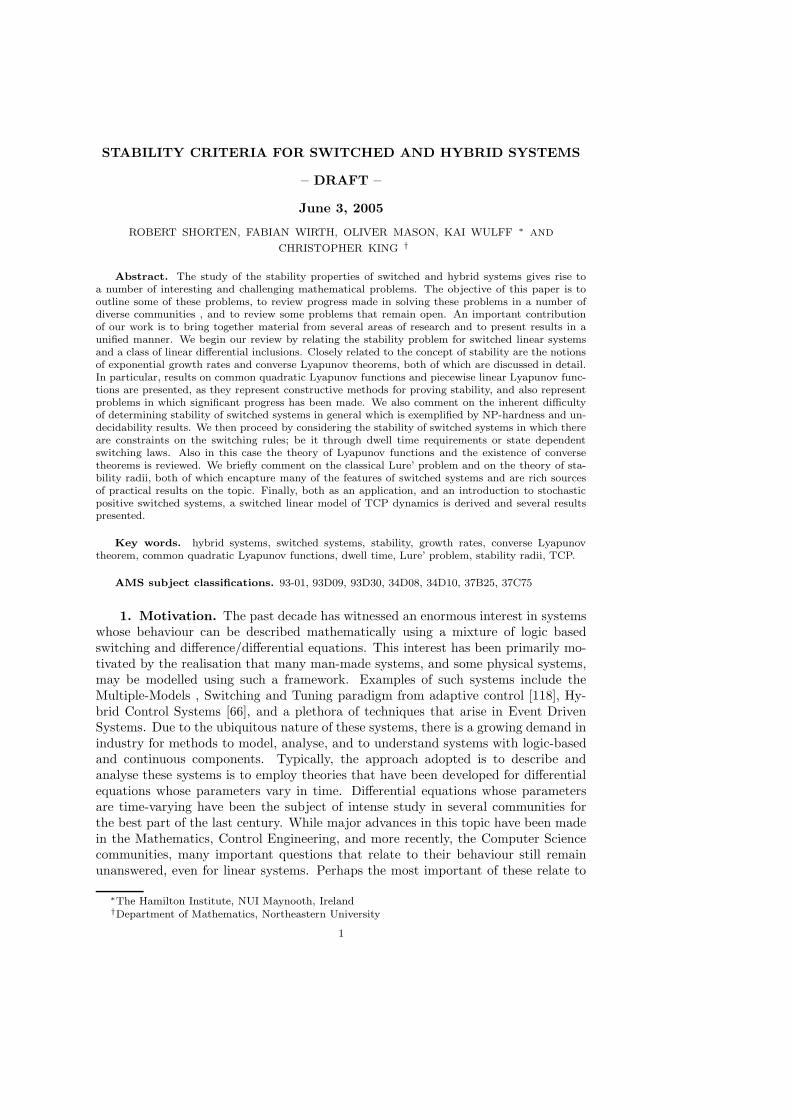
Example 1.1. [76] Automobile with a manual gearbox : The motion ofan car that travels along a fixed path can be characterised by two continuous states:velocity v and position s. The system has two inputs: the throttle angle (u) and theengaged gear (g). It is evident that the manner in which the velocity of the car respondsto the throttle input depends on the engaged gear. The dynamics of the automobilecan be therefore be thought of as being hybrid in nature: in each mode (engaged gear)the dynamics evolve in a continuous manner according to some differential equation.Transitions between modes are abrupt and are triggered by driver interventions in theform of gear changes.

) , ( =

=

1 v u f v

v s

) , ( =

=

2 v u f v

v s

) , ( =

=

3 v u f v

v s

) , ( =

=

4 v u f v

v s

2 > 1 : g 3 > 2 : g 4 > 3 : g

2 < 1 : g 4 < 3 : g 4 < 3 : g

1st gear 2nd gear 3rd gear 4th gear

Fig. 1.1: A hybrid model of a car with a manual gearbox [76].

Example 1.2. [65] Network congestion control : The Transmission ControlProtocol (TCP) is the protocol of choice for end-to-end packet delivery in the internet.TCP is an acknowledgement based protocol. Packets are sent from sources to destina-tions and destinations inform sources of packets that have been successfully received.This information is then used by the i’th source to control the number of unacknowl-edged packets (belonging to source i) in the network at any one time (wi). This basicmechanism provides TCP sources operating in congestion avoidance mode [97] witha method for inferring available network bandwidth and for controlling congestion inthe network. Upon receipt of a successful acknowledgement, the variable wi is updatedaccording to the rule: wi ← wi + a where a is some positive number and a new packetis inserted into the network. This is TCP’s self clocking mechanism. If wi exceeds

2

an integer threshold, then another packet is inserted into the network to increase thenumber of unacknowledged packets by one. TCP deduces from the detection of lostpackets that the network is congested and responds by reducing the number of unac-knowledged packets in the network according to: wi ← βwi where β is some numberbetween zero and 1.

a w w i i

+ = i i

w w =

Missing packet detected

Packet successfully acknowledged

Fig. 1.2: A hybrid model of TCP operation in congestion avoidance mode.

Example 1.3. Biology : Genetic regulatory networks [9, 43, 42] consist of afamily of interacting genes, each of which produces a specific protein through a processknown as gene expression. These proteins can then influence the rates at which thegenes in the network are expressed. In fact, the rate of expression of a given genetypically depends on the concentration of a regulatory protein in a switch-like manner,with the rate changing abruptly if the protein’s concentration crosses some thresholdvalue. If we consider a network of N genes and denote the concentration of thecorresponding proteins by x1, . . . , xN , then the threshold values for the proteins in thenetwork naturally define a partition of the state space into a number of regulatorysub-regions. Within each sub-region the network evolves continuously according toa system of differential equations. However, the system dynamics change abruptlywhenever the concentration of some protein crosses a threshold, giving rise to switchedor hybrid dynamics. Note that in this case, the switching rule is state-dependent with amode-switch triggered by the crossing of some threshold value for a regulatory protein.

Concentration of regulatory protein crosses a threshold

PSfrag replacements x = γ1 − f1(x) x = γ2 − f2(x)

Concentration of regulatory protein crosses a threshold

Fig. 1.3: Hybrid dynamics in genetic regulatory networks

3

It should be clear from the above examples that Hybrid Systems provide a con-venient method for modelling a wide variety of complex dynamical systems. Unfor-tunately, while the modelling paradigm itself is quite straightforward, the analysis ofeven relatively simple hybrid dynamical systems remains a highly non-trivial task.The basic difficulty in their analysis is that even simple hybrid systems may exhibitextremely complicated non-linear behaviour. A simple intuitive example that illus-trates one type of behaviour that emerges as a result of switching is the ‘Car in thedesert’ example from [155]. In this example the driver of a car in the desert is giventhe task of returning to the oasis, as depicted in Figure 1.4. If the driver followseither trajectory ‘a’ or ‘b’ then the car will arrive safely at the oasis. However, if thecar continually switches between these ‘stable’ trajectories, then instead of movingtowards the oasis, the car will follow trajectory ‘c’ away from the oasis.1

Fig. 1.4: ‘The car in the desert’

The above discussion should hopefully indicate that while switched and hybridsystems provide an attractive paradigm for modelling a variety of practical situations,the analysis of such systems is far from straightforward. In fact, the study of switchedsystems has raised a number of challenging mathematical problems, that remain to alarge extent, unanswered. Many of these problems are related to stability issues thatarise in Hybrid dynamical systems and give rise to a number of basic questions, someof which we now list.

(i) Arbitrary switching: Is it possible to determine verifiable conditions ona family of constituent systems that guarantee the stability of the associatedswitched system under arbitrary switching laws? Much of the work on thisproblem has been focussed on the question of common Lyapunov functionexistence.

(ii) Dwell time: If we switch between a family of individually stable systemssufficiently slowly then the overall system will be stable also [94, 117]. Thisraises the question of determining how fast we may switch while still guaran-teeing stability. In other words what is the minimum length of time that mustelapse between successive switches to ensure that the system remains stable?This problem is usually referred to as the dwell time problem.

(iii) Stabilisation: While switching can introduce instability when switching be-tween stable systems, on the other hand, it is sometimes possible to stabilize

1Even though it is beyond the scope of the work presented in this paper, it is worth mentioningthat more complex behaviour may also be found in systems of dimension three or greater; see theexcellent paper by Chase et al. [37] for a discussion of chaotic behaviour arising as a result ofswitching between several three stable LTI systems.

4

a family of individually unstable systems by switching between them appropri-ately. Based on this observation, several authors have worked on the problemof determining such stabilizing switching laws [52, 173].

(iv) Chaos: Even though it is beyond the scope of the present paper, Chase, Ser-rano and Ramadge presented an example in [37] to illustrate how chaoticbehaviour car arise when switching between low dimensional linear vectorfields. This raises the question as to whether it is possible to determine ifa switched system can exhibit chaotic behaviour for a given set of constituentvector fields?

(v) Complexity: Other problems that have been considered include questionsrelating to the complexity and decidability of determining the stability ofswitched systems [24, 22], and the precise nature of the connection betweenstability under arbitrary switching and stability under periodic switching rules(periodic stability) [21, 178, 90, 39, 60].

In view of the above basic questions, the objective of this article is to reviewthe major progress that has been made on a number of these and related questions,over the past number of years. As part of this process we will attempt to outline themajor outstanding issues that have yet to be resolved in the study of switched linearsystems.

2. Definitions and mathematical preliminaries. Throughout this paper ourprimary concern shall be with the stability properties of the switched linear system

ΣS : x(t) = A(t)x(t) A(t) ∈ A = A1, . . . , Am, (2.1)

where A is a set of matrices in Rn×n, and t→ A(t) is a piecewise constant2 mapping

from the non-negative real numbers, R+, into A. For each such mapping, there isa corresponding piecewise constant function σ from R+ into 1, . . . , m such thatA(t) = Aσ(t) for all t ≥ 0. This mapping σ is known as the switching signal , andthe points of discontinuity, t1, t2, . . ., of A(t) (or σ(t)) are known as the switchinginstances. We denote the set of switching signals by S. A function x : R+ → Rn iscalled a solution of (2.1) if it is absolutely continuous and if there is a switching signalσ such that

x(t) = Aσ(t)x(t) ,

for all t except at the switching instances of σ. By convention we only consider rightcontinuous switching signals. This does not affect the set of solutions, as going overto left continuous switching signals only changes the differential equation on a set ofmeasure zero.

For 1 ≤ i ≤ m, the ith constituent system of of the switched linear system (2.1)is the linear time-invariant (LTI) system

ΣAi: x = Aix. (2.2)

We can think of the system (2.1) as being constructed by switching between theconstituent LTI systems ΣA1

, . . . , ΣAm, with mode switches occurring at the switching

2We recall that by definition piecewise constant maps only have with only finitely many discon-tinuities in any bounded time-interval.

5

instances, and the precise nature of the switching pattern being determined by theswitching signal.

For a given switching signal σ ∈ S, the switched linear system ΣS evolves in thesame way as an LTI system between any two successive switching instances. Thus foreach switching signal σ, and initial condition x(0), there exists a unique continuous,piecewise differentiable solution x(t) which is given by

x(t) = [eA(tk)(t−tk)eA(tk−1)(tk−tk−1) . . . eA(t1)(t2−t1)eA(0)(t1)]x(0),

where t1, t2, . . . , is the sequence of switching instances and tk is the largest switchinginstance smaller than t.

It should be noted that the stability theory of switched linear systems has closelinks with the corresponding theory for linear differential inclusions (LDIs) [5, 164].The linear differential inclusion related to the set A = A1, . . . , Am is denoted by

x(t) ∈ Ax(t) | A ∈ A . (2.3)

A solution of this inclusion is an absolutely continuous function x satisfying x(t) ∈Ax(t) | A ∈ A almost everywhere. By an application of Filippov’s theorem this isequivalent to saying that there exists a measurable map A : R+ → A such that

x(t) = A(t)x(t) , almost everywhere ,

see [53] for details. So studying the differential inclusion (2.3) amounts to extendingthe set of switching signals to the class of measurable functions. If we are studying thesystem for arbitrary switching sequences, the effect of this is often negligible. In fact,if we consider the convex hull of A, denoted by convA and the convexified differentialinclusion

x(t) ∈ Ax(t) | A ∈ convA , (2.4)

then the solution sets of the three systems we have now defined are closely related.To make this statement precise, we denote by Rswitch

t (x) the set of points that can bereached from an initial condition x at time t by solutions of (2.1), i.e.

Rswitcht (x) := y ∈ R

n×n | ∃ switching signal σ such that y = x(t; x, σ) .

Similarly, we introduce the notation Rldit (x),Rconv ldi

t (x) for reachable sets of (2.3)and (2.4), respectively, then we have for all t ≥ 0, x ∈ Rn that

Rswitcht (x) ⊂ Rldi

t (x) ⊂ Rconv ldit (x) = clRswitch

t (x) , (2.5)

see e.g. [5, 53]. For an in-depth investigation of the structure of the signal setand its interplay with the dynamics of (2.3), we refer to [38]. We also note thatsystems equivalent to (2.3) are often studied under the name of linear parameter-varying systems. We will make brief reference of the relation between this literatureand switched systems where appropriate in the sequel.

2.1. Discrete-time systems. Thus far we have only considered switched linearsystems in continuous-time. However, as in the example of TCP congestion controldiscussed in the last section, it is also of interest to study discrete-time switched linearsystems. In discrete-time, a switched linear system is a system of the form

ΣS : x(k + 1) = A(k)x(k) A(k) ∈ A = A1, . . . , Am, (2.6)

6

where as before A is a set of matrices in Rn×n and k → A(k) is a mapping fromthe non-negative integers into A. The notions of switching signal, switching instancesand constituent systems are defined analogously to the continuous-time case. Theexistence of solutions to (2.6) is straightforward. In the discrete time case, the analysisof (2.6) is equivalent to that of the discrete linear inclusion

x(t + 1) ∈ Ax(t) | A ∈ A . (2.7)

On the other hand the solution set is significantly enlarged when going over to theconvexified inclusion

x(t + 1) ∈ Ax(t) | A ∈ convA . (2.8)

It is of interest to note, that the exponential stability of (2.6), (2.7) and (2.8) isequivalent nonetheless, as we shall discuss in the sequel.

2.2. Exponential Growth Rates. One of the basic properties of switched lin-ear systems is that a growth rate may be defined as in the case of linear time-invariantsystems. The definition proceeds similarly in continuous and discrete time. There areseveral approaches to defining the exponential growth rate, all of which turn out to beequivalent. A trajectory based definition considers Lyapunov exponents of individualtrajectories, which are defined by

λ(x0, σ) := lim supt→∞

1

tlog ‖x(t; x0, σ)‖ .

The exponential growth rate of the switched system is then defined by the maximalLyapunov exponent

κ(A) := maxλ(x0, σ) | x0 6= 0, σ ∈ S .

A different point of view is to consider the evolution operators corresponding to thesystem equations (2.1), resp. (2.6). In continuous time these are defined as thesolution of

Φσ(t, s) = Aσ(t)Φσ(t, s) , Φσ(s, s) = I .

Similarly, in discrete time we have for t ≥ s

Φ(t + 1, s) = Aσ(t)Φσ(t, s) , Φσ(s, s) = I .

The growth of the system can then also be measured by considering the maximalgrowth of the norms or the spectral radii of the operators Φ(t, 0) as t→∞. Ultimately,these definitions coincide. More precisely, it is known that

κ(A) = lim supt→∞

1

tlog max

σ∈Sr(Φσ(t, 0)) = lim sup

t→∞

1

tlog max

σ∈S‖Φσ(t, 0)‖ . (2.9)

The previous equality has been obtained by two different avenues. In discrete-time this was first shown by Berger and Wang [14] and alternative ways of proving theresult have been presented by Elsner [49] and Shih, Wu and Pang [147]. On the otherhand the result has also been implicit in the Russian literature. Namely, Pyatnitskiiand Rapoport [139] show that if system (2.1) has an unbounded trajectory, then thereexists a periodic switching signal σj ∈ S of period T such that r(Φσj

(T, 0)) = 1, i.e. if

7

we can find a periodic switching signal for which the system is marginally stable. Thisimplies in particular, that absolute stability is equivalent to

κ := lim supt→∞

1

tlog max

σ∈Sr(Φσ(t, 0)) < 0 .

On the other hand Barabanov [11] shows that absolute stability is equivalent to

κ := lim supt→∞

1

tlog max

σ∈S‖Φσ(t, 0)‖ .

as both κ, κ are additive with respect to spectral shifts, i.e. κ(A − αI) = κ(A) − α,for all α ∈ R, they have to satisfy κ = κ.

In the area of discrete-time systems the growth rate of discrete inclusions is oftendefined as ρ(A) := eκ(A). This quantity has become notorious under the name of jointspectral radius or generalized spectral radius.

There are numerous approaches to the computation of growth rates, either intheir guise as maximal Lyapunov exponents or as joint spectral radii. We cannotcover these methods here but refer the reader to the various methods presented in[56, 101, 12, 57].

3. Stability for switched linear systems. As with general linear and non-linear systems, numerous different concepts of stability have been defined for switchedlinear systems, including uniform stability, uniform attractivity, uniform asymptoticstability and uniform exponential stability. We now recall the definitions of uniformstability and uniform exponential stability.

Definition 3.1. The origin is a uniformly stable equilibrium point of ΣS if givenany ε > 0, there is some δ > 0 such that ‖x(0)‖ < δ implies ‖x(t)‖ < ε for t ≥ 0 forall solutions x(t) of the system.

Definition 3.2. The origin is a uniformly exponentially stable equilibrium ofΣS if there exist real constants M ≥ 1, β > 0 such that

‖x(t)‖ ≤Me−βt‖x(0)‖, (3.1)

for t ≥ 0, for all solutions x(t) of ΣS.

Uniform exponential stability is often called absolute stability especially in theRussian literature. It is known that the related concepts of attractivity and asymptoticstability together are equivalent to exponential stability for switched linear systems[41, 11, 40].

In a slight abuse of notation we shall often speak of the stability or exponentialstability of the system ΣS itself. One of the major topics discussed here is the problemof establishing when the system (2.1) is exponentially stable for arbitrary switchingsignals. In this case, Definition 3.2 requires the existence of constants M ≥ 1, β >0 such that (3.1) is satisfied for every piecewise continuous switching signal σ(t).When considering the question of exponential stability under arbitrary switching, itis necessary to assume that the matrices A1, . . . , Am in the set A are all Hurwitz (allof their eigenvalues lie in the open left half of the complex plane), thus ensuring thateach of the constituent LTI systems is exponentially stable.

8

In certain situations, it is not necessary to guarantee stability for every possibleswitching signal and a number of authors have considered questions related to thestability of switched linear systems under restricted switching regimes. One importantexample of this kind is state-dependent switching, where the rule that determines whena switch in system dynamics occurs is determined by the value of the state-vector x.The example of a genetic regulatory network discussed in the previous section wasof this type. Other results on stability for restricted switching signals consider thequestion of determining restricted classes of switching signals for which a switchedlinear system is guaranteed to be stable.

In all of the above definitions, we are concerned with the stability properties of theinternal system (2.1). In practice however, it is often necessary to consider systemswith inputs and outputs of the form

x = A(t)x + B(t)u (3.2)

y = C(t)x.

In this context the notion of bounded-input bounded-output (BIBO) stability arises.Formally, the input-output system (3.2) is uniformly BIBO stable if there exists apositive constant η such that for any essentially bounded input signal u, the zero-state response y satisfies

supt≥t0

‖y(t)‖ ≤ η supt≥t0

‖u(t).‖

Essentially, if a system is BIBO stable, this means that an input signal cannot beamplified by a factor greater than some finite constant η in passing through the system.While we shall not consider BIBO stability explicitly here, it should be noted thatif the system (2.1) is uniformly exponentially stable, then the corresponding input-output system (3.2) is BIBO stable provided the matrices B(t), C(t) are uniformlybounded in time, [111], which is the case when they switch between a finite family ofmatrices.

4. Arbitrary switching. The arbitrary switching problem is concerned withobtaining verifiable conditions on the matrices in A that guarantee the exponentialstability of the switched system (2.1) for any switching signal. This problem has beenthe subject of interest from the research community in recent years and a number ofgeneral approaches to it have been investigated. Many of these rely on the construc-tion of common quadratic and non-quadratic Lyapunov functions for the constituentsystems of (2.1). In this context, it has been established that the existence of acommon Lyapunov function is necessary and sufficient for the exponential stabilityof a switched linear system. In particular, a number of authors have derived con-verse theorems that prove the existence of common Lyapunov functions under theassumption of exponential stability. We begin by describing some of these theoremsand then proceed by reviewing results on the common Lyapunov function existenceproblem for switched linear systems. Many of the mature results in this area concernthe existence of common quadratic Lyapunov functions (CQLFs) and this part of ourreview reflects this fact. Nevertheless, some results are also presented concerning theexistence of common non-quadratic Lyapunov functions.

4.1. Converse theorems. Lyapunov theory played a key role in the stabilityanalysis of both linear and non-linear systems for much of the last century [100, 133,119, 80]. The key idea of this approach is that the stability of a dynamical system can

9

be established through demonstrating the existence of a positive definite, norm-like,function that decreases along all trajectories of the system as time evolves. Much ofthe recent research on the stability of switched linear systems has been directed to-wards applying similar ideas to the class of systems (2.1); relating the stability of suchsystems to the existence of positive definite functions, V (x), on R

n such that V (x(t))is a decreasing function of t for all solutions x(t) of (2.1). Before discussing resultsthat have been derived for specific forms of Lyapunov functions, we first present anumber of more general facts about Lyapunov theory as it relates to the stability ofswitched linear systems.

First of all, note that if a positive definite function V (x(t)) decreases along alltrajectories of the system (2.1) for arbitrary switching signals, then this certainlymust be true for constant switching signals. Hence, any such function V (x) wouldhave to be a common Lyapunov function for each of the constituent LTI systems of(2.1). It is well established [115, 94, 40] that if a common Lyapunov function existsfor the constituent systems of a switched linear system, then the system is uniformlyexponentially stable for arbitrary switching signals. We shall now discuss the work ofa variety of authors who have considered the problem of deriving converse theoremsto establish the necessity of common Lyapunov function existence for uniform expo-nential stability under arbitrary switching.

In [115] Molchanov and Pyatnitskiy established that the uniform exponential sta-bility of the system (2.1) under arbitrary switching is equivalent to the existence ofa common Lyapunov function V (x) for its constituent LTI systems. Formally theyderived the following result.

Theorem 4.1. The system (2.1) is uniformly exponentially stable for arbitraryswitching signals if and only if there exists a strictly convex, positive definite functionV (x), homogeneous of degree 2, of the form

V (x) = xTL(x)x where L(x) ∈ Rn×n and

L(x)T = L(x) = L(cx) for all non-zero c ∈ R, x ∈ Rn,

such that

maxy∈Ax

∂V (x)

∂y≤ −γ‖x‖2

for some γ > 0, where Ax = A1x, . . . , Amx and

∂V (x)

∂y= inf

t>0

V (x + ty)− V (x)

t

is the usual directional derivative of the convex function V (x) [143].

A number of points about the results presented in [115] are worth noting.

(i) The converse theorem in [115] was derived for linear differential inclusions.However, combining (2.5) with the original results of [115] shows that commonLyapunov function existence is also necessary for the uniform exponentialstability of the switched linear system (2.1) under arbitrary switching.

10

(ii) The common Lyapunov function whose existence is established in [115] isstrictly convex and homogeneous of degree two, but not necessarily continu-ously differentiable.

(iii) Furthermore, Molchanov and Pyatnitskiy have shown that if a switched linearsystem is uniformly exponentially stable under arbitrary switching, then itsconstituent LTI systems will have both a piecewise quadratic and piecewiselinear common Lyapunov function.

A closely related result was later derived by Dayawansa and Martin in [40], whereit was established that the uniform exponential stability of the switched linear system(2.1) is equivalent to the existence of a continuously differentiable common Lyapunovfunction for its constituent LTI systems. This has already been noted by Brockett in[34]. Moreover, it was also shown that while this Lyapunov function can be chosen tobe C1 and homogeneous of degree two, it cannot always be chosen to be a quadraticform.

Thus, it is not in general necessary for the stability of (2.1) that there exists acommon quadratic Lyapunov function for its constituent systems.

In the context of converse Lyapunov theorems, the work of Brayton and Tong,described in [31], is also worthy of mention. These authors established that theexistence of a common Lyapunov function for the constituent systems of a discrete-time switched linear system is equivalent to the uniform stability of the system underarbitrary switching. Independently, Barabanov [10] showed that for an exponentiallystable linear discrete inclusion there is always a norm that is a Lyapunov function.In particular, this implies by the convexity of norms, that if the set A generates anexponentially stable discrete linear inclusion, then so does convA.

More recently, building on the work of Lin, Sontag and Wang in [95] on non-linearsystems subject to disturbances, Mancilla-Aguilar and Garcia have derived converseLyapunov theorems for non-linear switched systems [102], as well as some relatedresults for input to state stability, a notion that we do not discuss here [103]. Finally,we note the recent result of Mason that shows that while a common Lyapunov functionalways exists for systems that are exponentially stable under arbitrary switching, itslevel curves may in fact be arbitrarily complex [108]. Thus searching for such afunction using numerical techniques is not easy.

4.2. The CQLF existence problem. Quadratic Lyapunov functions play acentral role in the study of linear time-invariant systems. Their existence is wellunderstood in this context and consequently, studying the existence of such functionsis a natural starting point in the study of switched linear systems. At the heart ofthe CQLF existence problem is the desire to find useful criteria to determine whethera given collection of Hurwitz matrices A1, . . . , Am has a CQLF. The main purposeof this Section is to survey the known results in this area, and indicate the differentlines of attack that have been used. Despite the considerable work done so far, thereare still some open questions that remain to be resolved.

4.2.1. Definitions. Recall that V (x) = xT Px is a quadratic Lyapunov function(QLF) for the LTI system ΣA : x = Ax if (i) P is symmetric and positive definite,and (ii) PA+AT P is negative definite. Now suppose that A1, . . . , Am is a collectionof n × n Hurwitz matrices, with associated stable LTI systems ΣA1

, . . . , ΣAm. Then

the function V (x) = xT Px is a common quadratic Lyapunov function (CQLF) forthese systems if V (x) is a QLF for each individual system. Given a set of matricesA1, . . . , Am, the CQLF existence problem is to determine whether such a matrix Pexists. A secondary question is to construct a CQLF when one is known to exist. It

11

is a standard fact that an LTI system ΣA has a QLF if and only if the matrix A isHurwitz. This property is also equivalent to the exponential stability of the systemΣA, so for a single LTI system there is no gap between the existence of a QLF andexponential stability. Therefore a simple spectral condition determines completelythe stability of the LTI system ΣA.

For a collection of Hurwitz matrices the situation is more complicated in severalrespects. Firstly, in general, CQLF existence is only a sufficient condition for theexponential stability of a switched linear system under arbitrary switching. Secondly,no correspondingly simple condition is known which can determine the existence of aCQLF for a family of LTI systems, although progress has been made in some specialcases. The rest of this section will describe a variety of approaches which have beenused to attack this problem, and outline some of the open problems.

In many cases it is useful to analyse the mapping P 7→ PA + AT P as a linearfunction on the space of matrices. To set up the notation, let Sn×n denote the linearvector space of real symmetric n×n matrices. A matrix P ∈ Sn×n is positive definite(written P > 0) if xT Px > 0 for all x 6= 0 ∈ Rn, and P is positive semidefinite(P ≥ 0) if xT Px ≥ 0 for all x ∈ Rn. Similarly P is negative definite if −P > 0, orP < 0, and P is negative semidefinite if −P ≥ 0, or P ≤ 0. Finally recall that P ispositive definite if and only if Tr PQ > 0 for all positive definite Q, where Tr is theusual matrix trace.

The Lyapunov map defined by the real n× n matrix A is

LA : Sn×n → Sn×n, LA(H) = HA + AT H (4.1)

The following properties of LA are well-known, [73]. (i) If A has eigenvalues λi withassociated eigenvectors vi, then LA has eigenvalues λi + λj, with eigenvectorsviv

Tj + vjv

Ti , for all i ≤ j. It follows immediately that LA is invertible whenever A

is Hurwitz, since in this case λi + λj cannot be zero. (ii) A is Hurwitz if and only ifthere exists P > 0 such that LA(P ) < 0. Note that in this case xT Px is a QLF forthe system ΣA.

Now define PA to be the collection of all positive definite matrices which provideQLF’s for the system ΣA, that is

PA = P > 0 : LA(P ) < 0 (4.2)

Clearly PA is an open convex cone in Sn×n. The above results concerning the Lya-punov map show that PA is nonempty if and only if A is Hurwitz. In this language,the CQLF existence problem for a collection of matrices A1, . . . , Ak is the problemof determining whether the intersection of the cones PA1

∩ · · · ∩ PAkis non-empty.

There are some straightforward observations that can be made at this point.Firstly, for A ∈ Rn×n, the cones PA and PA−1 are identical. Thus, there exists aCQLF for the systems ΣA1

, . . . , ΣAmif and only if there is a CQLF for the systems

ΣAε11

, . . . , ΣAεmm

where εi = ±1 for i = 1, . . . , m. Secondly, CQLF existence is invariant

under a change of coordinates. That is, if R ∈ Rn×n is non-singular, then

PR−1AR = RT PA R ≡ RT PR : P ∈ PA (4.3)

Therefore CQLF existence for the family of systems ΣA1, . . . , ΣAm

is equivalent toCQLF existence for the transformed family ΣR−1A1R, . . . , ΣR−1AmR.

12

4.2.2. Dual formulation. The QLF and CQLF existence problems have dualformulations which will play an important role in some of our later discussions. Toset up the notation, define LA to be the adjoint of the Lyapunov map with respectto the standard inner product 〈X, Y 〉 = TrXT Y on Sn×n, that is

〈X,LA(Y )〉 = 〈LA(X), Y 〉 (4.4)

for all X, Y ∈ Sn×n. It follows that

LA : Sn×n → Sn×n, LA(H) = AH + HAT = LAT (H) (4.5)

We will use the following formulation of duality, which can be found for examplein [81]: given a collection of Hurwitz matrices A1, . . . , Ak, there exists a CQLF ifand only if there do not exist positive semidefinite matrices X1, . . . , Xk (not all zero)

satisfying∑k

i=1 LAi(Xi) = 0. That is,

∃ P > 0 such that LAi(P ) < 0 for all i = 1, . . . , k

⇐⇒ 6 ∃ X1, . . . , Xk ≥ 0 (not all zero) such that

k∑

i=1

LAi(Xi) = 0 (4.6)

4.3. Numerical approaches to the CQLF problem. While we shall concen-trate here on theoretical results obtained on the CQLF existence problem, it shouldbe noted that numerical methods are also available for testing for CQLF existence.Recent advances in computational technology along with the development of efficientnumerical algorithms for solving problems in the field of convex optimization have re-sulted in the widespread use of linear matrix inequality (LMI) techniques throughoutsystems theory. For details on the various applications of LMI methods in systemsand control consult [28, 48, 55]. In this section, we focus on one specific aspect ofthis development; the use of LMI methods to test for the existence of a CQLF for anumber of stable LTI systems.

The conditions for V (x) = xT Px to be a CQLF for the asymptotically stable LTIsystems ΣAi

, i ∈ 1, . . . , m define a system of linear matrix inequalities (LMIs) inP , namely

P = P T > 0, (ATi P + PAi) < 0 for i ∈ 1, . . . , m (4.7)

The system of LMIs (4.7) is said to be feasible if a solution P exists; otherwise theLMIs (4.7) are infeasible. Thus, determining whether or not the LTI systems ΣAi

,i ∈ 1, . . . , m possess a CQLF amounts to checking the feasibility of a system ofLMIs. LMIs are built on convex optimization algorithms developed over the past twodecades which are capable of solving this type of problem with considerably morespeed than was possible using previous techniques. Conversely, it is also possible toverify that no CQLF exists for the LTI systems ΣAi

via the use of LMI techniques.More specifically [28], there is no CQLF for the LTI systems ΣAi

if there exist matricesRi = RT

i , i ∈ 1, . . . , m satisfying

Ri > 0, Σmi=1(A

Ti Ri + RiAi) > 0 (4.8)

While LMIs provide an effective way of verifying that a CQLF exists for a familyof LTI systems, there are also a number of drawbacks to the method which should bementioned.

13

(i) Firstly, situations have arisen where known analytic results can be used toshow that a CQLF definitely exists (or does not exist), but the (commonlyused) LMI toolbox for MATLAB fails to give a definitive answer to the ex-istence question. For instance, it is well known that any set of systems ΣAi

where the system matrices Ai are all upper triangular and Hurwitz must pos-sess a CQLF (see section 4.1 on triangular systems). However it is possibleto construct a set of two 2 × 2 Hurwitz triangular matrices where the LMItoolbox will be unable to find a CQLF. For more detailed examples of thistype, consult [107].

(ii) Secondly, because of the numerical nature of the approach, it provides littleinsight into why a CQLF may or may not exist for a set of LTI systems, anddoes not add to our understanding of the precise relationship between CQLFexistence and the dynamics of switched linear systems. A particular problemthat arises in this context, and for which numerical approaches are unsuitable,is that of determining specific classes of systems for which CQLF existenceis equivalent to exponential stability under arbitrary switching. Such systemclasses do exist and we shall mention some later in this section.

(iii) The question of weak CQLF existence, where the strict inequalities in thesystem (4.7) are replaced with non-strict inequalities, is not amenable tosolution by LMI methods. Here a more theoretical approach is required.

4.4. Special structures of matrices that guarantee existence of a CQLF.

Some special cases are known where the structure of the matrices A1, . . . , Am byitself guarantees the existence of a CQLF for the associated LTI systems, provided ofcourse that the matrices are Hurwitz. We now review these cases.

4.4.1. Matrices with Lyapunov function xT x. The condition that a systemΣA have the Lyapunov function xT x is

LA(I) = AT + A < 0 (4.9)

where I is the n×n identity matrix. If A1, . . . , Am is a collection of matrices whichall satisfy the condition (4.9), then xT x must be a QLF for every individual system,and hence must be a CQLF for the collection. The condition (4.9) is satisfied in thefollowing cases:

(i) A is symmetric and Hurwitz,(ii) A is normal (i.e. AAT = AT A) and Hurwitz,(iii) if a matrix S is skew-symmetric, (i.e. if ST = −S) then if A satisfies (4.9),

then so does A + S.

4.4.2. Triangular and related systems. If the Hurwitz matrices Ai are allin upper triangular form, then it was shown by Shorten and Narendra [155], andindependently by Mori, Mori and Kuroe in [116], that the collection of systems ΣAi

always has a CQLF, and furthermore that the matrix P which defines the CQLF canbe chosen to be diagonal. This result extends to the case where there is a non-singularmatrix R for which the matrices R−1AiR are all upper triangular, by the remarksin Section 4.2.1.

One interesting application of this result arises when the matrices A1, . . . , Am allcommute with each other. In this case there is a unitary matrix U such that U ∗AiU

14

is in upper triangular form for each i = 1, . . . , m [73], and it then follows that thesystems ΣA1

, . . . , ΣAmhave a CQLF [118]. This result has an interesting extension

to a class of systems with non-commuting matrices [60]. To explain this class, letg = A1, . . . , AmLA denote the Lie algebra generated by the matrices A1, . . . , Am,that is the collection of all matrices of the form Ai, [Ai, Aj ], [Ai, [Aj , Ak]], . . . andso on. If g is solvable, then it follows from a well-known theorem of Lie [64] thatthe matrices A1, . . . , Am can be put into upper triangular form by a nonsingulartransformation. Recall that a Lie algebra is said to be solvable if g

k = 0 for somefinite k, where the sequence of Lie algebras g

0, g1, g2, . . . are defined recursively byg

k+1 = [gk, gk], and g0 = g. The basic example of a solvable Lie algebra is the Lie

algebra generated by a set of upper triangular matrices, where it can be seen that thenonzero entries of g

k retreat further from the main diagonal at each step.

Using this result, and the Shorten-Narendra result about upper triangular matri-ces, it follows that if g = A1, . . . , AmLA is solvable, then the systems ΣA1

, . . . , ΣAm

have a CQLF. The most general result along these lines is the following theorem dueto Agrachev and Liberzon [2]. The theorem describes the type of Lie algebra whichcan be generated by a collection of Hurwitz matrices that share a CQLF. Their resultalso shows that if g is not of this type, then it could be generated by a collection ofmatrices whose LTI systems are individually stable, but for which the correspond-ing switching system can be made unstable with some switching sequence. So thetheorem describes the most general conclusions about the CQLF existence questionwhich can be reached using only the Lie algebra structure generated by the collectionA1, . . . , Am.

Theorem 4.2. [2] Let A1, . . . , Am be Hurwitz matrices, and g = I, A1, . . . , AmLA

where I is the identity matrix. Let g = r⊕ s be the Levi decomposition, where r is theradical, and suppose that s is a compact Lie algebra. Then the systems ΣA1

, . . . , ΣAm

have a CQLF. Furthermore, if s is not compact, then there is a set of Hurwitz matriceswhich generate g, such that the corresponding switched linear system is not uniformlyexponentially stable.

Given the body of literature that has been dedicated to, and continues to bededicated to, triangular system, a few further comments are in order.

(i) In essence, triangular switching systems obey the same stability laws as LTIsystems; namely the exponential stability of the system is equivalent to thecondition that the eigenvalues of A(t) lie in the open left-half of the complexplane for all t. This is not surprising; systems of this form can be representedas cascades comprised of first order sub-systems or very benign second ordersub-systems. Each such sub-system has the quadratic Lyapunov function,V (x) = xT x, and is thus exponentially stable. The exponential stability ofthe overall systems follows.

(ii) It is important to appreciate that the property of a family of matrices beingsimultaneously triangularisable is not robust, and that this requirement isonly satisfied by a very limited class of systems.

(iii) From a practical viewpoint, the requirement of simultaneous triangularisabil-ity imposes unrealistic conditions on the matrices in the set A. It is thereforeof interest to extend the results derived by [116] with a view to relaxing thisrequirement. In this context several authors have recently published newconditions for exponential stability of the switching system. Typically, the

15

approach adopted is to bound the maximum allowable perturbations of thematrix parameters from a nominal (triangularisable) set of matrices, therebyguaranteeing the existence of a CQLF; see [116]. An alternative approach ispresented in [160, 161]; rather than assuming maximum allowable perturba-tions from nominal matrix parameters, it is explicitly assumed that no singlenon-singular transformation T exists that simultaneously triangularises allof the matrices in A. Instead, the authors assume that a collection of non-singular matrices Tij exists, such that for each pair of matrices Ai, Aj inA, the pair of matrices TijAiT

−1ij , TijAjT

−1ij are upper triangular.

(iv) Several papers in the area of switching systems are related to the simultaneoustriangularisation of a set of matrices. For example, matrices that commuteare simultaneously triangularisable. Hence, the commuting vector field resultof Narendra and Balakrishnan [118] is a special case of the above discussion[152]3.

(v) To apply the above results, it is necessary to be able to determine if a non-singular T exists such that for all Ai in a set of matrices A, TAiT

−1 is uppertriangular. McCoy’s theorem provides useful insights in this context; see [89,155], as does the work relating Lie algebras and simultaneous triangularisationby Liberzon et al. [93].

4.5. Necessary and sufficient conditions for special classes. One long-standing goal in the field of switched systems has been to find simple algebraic con-ditions for existence of a CQLF which can be checked explicitly just from knowledgeof the matrices A1, . . . , Am. In the discrete-time case it is known by the work ofKozyakin [86], that exponential stability is not a property that can be described byfinitely many algebraic constraints in the set of pairs of 2×2 matrices. In this sectionwe describe several cases where such conditions are known.

4.5.1. Two second order systems. For a pair of second order systems thereis a complete solution to the CQLF existence problem. We quote the following resultfrom [157].

Theorem 4.3. Let A1 and A2 be 2 × 2 Hurwitz matrices. Then the two LTIsystems ΣA1

and ΣA2have a CQLF if and only if the matrix products A1A2 and

A1A−12 have no negative real eigenvalues.

Theorem 4.3 provides an extremely simple and elegant solution to the CQLFproblem for the case of two matrices in R2×2. It is known that CQLF existenceis a conservative criterion for the stability of second order systems; however, thesimplicity of Theorem 4.3 demonstrates the usefulness of using CQLF methods toanalyse stability, and it provides insights into the precise relationship between CQLFexistence and stability. In particular, using this result, it can be shown that if a CQLFfails to exist for a pair of LTI systems ΣA1

, ΣA2, with A1, A2 ∈ R2×2 Hurwitz, then

at least one of the related switched linear systems

x = A(t)x A(t) ∈ A1, A2 (4.10)

x = A(t)x A(t) ∈ A1, A−12 (4.11)

fails to be exponentially stable for arbitrary switching signals. Moreover, Theorem4.3 has been used in [61, 105] to show that for second order positive switched linear

3It is worth noting that it has been shown by Shim et. al. [148] that a quadratic Lyapunovfunction exists for commuting vector fields even if the vector fields are themselves non-linear

16

systems 4 with two stable constituent systems, CQLF existence is in fact equivalentto exponential stability under arbitrary switching.

No simple spectral condition is known when there are more than two matricesin R2×2, although the following result provides some useful information in this case[157]. Suppose that ΣAi

are stable LTI systems in the plane. If any subset of three ofthese systems has a CQLF, then there is a CQLF for the whole family. This can beviewed as a consequence of Helly’s theorem from convex analysis [143] in combinationwith the discussion of intersection of the cones PAj

in Section 4.2.1.

4.5.2. Two systems with a rank one difference. Suppose that A ∈ Rn×n

is Hurwitz, and b, c ∈ Rn. If the pair (A, b) is completely controllable, then thereis again a simple spectral condition which is equivalent to CQLF existence for thesystems ΣA, ΣA−bcT . This condition was originally derived as a frequency domaincondition using the SISO Circle Criterion [119], however it was later realised [158]that the condition has the following natural and elegant formulation as a conditionsimilar to Theorem 4.3. This result was then generalised to the case of a pair ofHurwitz matrices whose difference is rank 1 in [153].

Theorem 4.4. Let A1 and A2 be Hurwitz matrices in Rn×n, where the difference

A1 −A2 has rank one. Then the two LTI systems ΣA1and ΣA2

have a CQLF if andonly if the matrix product A1A2 has no negative real eigenvalues.

Theorem 4.4 provides a simple spectral condition for CQLF existence for a pair ofexponentially stable LTI systems whose system matrices differ by a rank one matrix.Further, it follows from this result that for a switched linear system

x = A(t)x A(t) ∈ A1, A2, (4.12)

where A1, A2 ∈ Rn×n are Hurwitz and rank(A2 − A−11 ) = 1, CQLF existence is

equivalent to exponential stability under arbitrary switching signals.

4.6. Sufficiency. In addition to the results discussed above, several authorshave developed tests for CQLF existence which provide sufficient conditions. In somecases these tests allow explicit computations, and therefore can be useful in practicalapplications.

4.6.1. Lyapunov operator conditions. In a series of papers [124, 122, 123,125], Ooba and Funahashi derived conditions involving the Lyapunov operators LA

defined in (4.1). The key idea in their work is the observation that ΣA1and ΣA2

havea CQLF if and only if there is some positive definite Q such that LA1

L−1A2

(Q) is alsopositive definite. This leads to their following result [122]. Recall that for an operator

L on the space of symmetric matrices Sn×n, L denotes the adjoint of L with respectto the usual inner product on Sn×n.

Theorem 4.5. Let A1 and A2 be n× n Hurwitz matrices, and suppose that

LA2−A1LA2−A1

− (LA1LA1

+ LA2LA2

) < 0 (4.13)

Then ΣA1and ΣA2

have a CQLF.

A second similar, but independent condition is presented in [123] involving theLyapunov operators of the commutators of the matrices A1 and A2. In one of their

4A positive dynamical system is one where non-negative initial conditions imply that the statevector remains in the non-negative orthant for all time.

17

other papers [124], Ooba and Funahashi derive sufficient conditions which involveminimal eigenvalues computed using the Lyapunov operators. Given a collection ofHurwitz matrices A1, . . . , Am in Rn×n, define

µij = λmin

(LAiL−1

Aj(I))

, i, j = 1, . . . , m (4.14)

where I is the n× n identity matrix, and where λmin is the smallest eigenvalue, anddefine the m×m matrix

M = (µij)i,j=1,...,m. (4.15)

Then we have the following result.

Theorem 4.6. Suppose that the matrix M defined in (4.15) is semipositive,meaning that there is a vector x ∈ Rn with xi ≥ 0 for all i, such that (Mx)i > 0 forall i. Then the systems ΣAi

, 1 ≤ i ≤ m, have a CQLF.

4.7. Necessary and sufficient conditions for the general case. In thissection we review a new approach to deriving necessary and sufficient conditions forexistence of a CQLF, based on the duality condition (4.6). This relation states thatΣA1

, . . . , ΣAmdo NOT have a CQLF if and only if there are positive semidefinite

matrices X1, . . . , Xm (not all zero) which satisfy the equation

m∑

i=1

AiXi + XiATi = 0 (4.16)

The main idea is to rewrite (4.16) in the following form.

Theorem 4.7. Suppose that equation (4.16) holds, and let d = rk(X1+· · ·+Xm).Then there are positive semidefinite d× d matrices Y1, . . . , Ym, with rk(Yi) = rk(Xi)for all i, and a skew-symmetric d× d matrix S such that

det( m∑

i=1

Ai ⊗ Yi + I ⊗ S)

= 0 (4.17)

where I is the n × n identity matrix. Conversely, if (4.17) holds for some positivesemidefinite matrices Yi and skew symmetric matrix S, then the equation (4.16)holds, with Xi positive semidefinite and not all zero, and rk(Xi) ≤ rk(Yi) for all i.

The key to deriving (4.17) is to select a basis v1, . . . , vd for the range of X1 + · · ·+XM , and express the matrices Xi with respect to this basis as

Xi =

d∑

p,q=1

(Yi)pqvpvTq (4.18)

The d× d matrix Yi is also positive semidefinite, and has the same rank as Xi.

Using (4.17), four necessary and sufficient conditions were derived for non-existenceof a CQLF for a pair of 3× 3 Hurwitz matrices [85]. Three of the conditions can beexpressed as singularity conditions for some convex combinations of Ai and A−1

i . Forexample one of the conditions says that some convex combination of A1, A2 and(xA1 + (1 − x)A2)

−1 is singular for some 0 ≤ x ≤ 1. Testing this condition involvessearching over a three-parameter space, so it is quite infeasible. The main importanceof the conditions lies in the possibility that they can lead to new insights into theCQLF problem.

18

4.8. Stability radii. Associated to the existence of Lyapunov functions or com-mon quadratic Lyapunov functions is the property that exponential stability is a ro-bust property of switched systems, that is, small perturbations of the systems datadoes not destroy stability. One is often interested in quantifying this robustness andthis is the aim in the study of stability radii.

We assume we are given a nominal asymptotically stable system, which we takefor the sake of simplicity to be time-invariant. It is thus of the form

x = A0x . (4.19)

Due to imprecise modelling it may be expected that the system of interest does nothave the same dynamics as the nominal system, but can be interpreted as a particularsystem in the class

x(t) =

(A0 +

m∑

k=1

δk(t)Ak

)x(t) (4.20)

Here the matrices Ak, k = 1, . . . , m are prescribed, modelling the expected perturba-tions of the systems, while δ(t) = (δ1(t), . . . , δm(t) is an unknown, essentially boundedperturbation. The question is how large this perturbation may be without destroyingstability. To measure this size we prescribe a norm ‖ · ‖ in Rm, and denote by ‖ · ‖∞the corresponding norm on bounded functions δ : R+ → Rm.

The stability radius in a switched systems sense is then given by

rLy(A, (Ai)) = inf‖δ‖∞ | (4.20) is not exponentially stable for δ . (4.21)

Stability radii of this type are discussed in [38, 68]. In particular, the interested readerwill find an in depth discussion of related literature in these references. In particular,the calculation of stability radii has been studied in [175] in the discrete time caseand in [58] in continuous time. Of course, this is again a difficult problem, as alreadythe determination of the growth rate is NP-hard. We note that if the set

A0 +

m∑

k=1

δkAk | ‖δ‖ ≤ 1

,

is a polytope, then we are in the case of the switched system (2.1) again, as by (2.5)the exponential stability of the inclusion (2.3) and (2.1) are equivalent.

We note that in the theory of stability radii there is an elegant interpretation ofthe CQLF problem. This applies to the special case, that perturbations are measuredin the spectral norm ‖ · ‖2 and the perturbation structure is determined by structurematrices B ∈ Rn×l, C ∈ Rq×n. We are thus considering perturbed systems of theform

x(t) = (A + B∆(t)C) x(t) (4.22)

where ∆(t) ∈ Rl×q is an unknown perturbation. In this case three different stabilityradii may be defined corresponding to real constant, real time-varying, and complexconstant perturbations may be defined. They are given by

rR(A, B, C) := inf ‖∆0‖2 | ∆0 ∈ Rl×q : (4.22) is not exp. stable for ∆(t) ≡ ∆0 ,

rLy(A, B, C) := inf ‖∆‖∞ | ∆ : R→ Rl×q : (4.22) is not exp. stable for ∆ ,

rC(A, B, C) := inf ‖∆0‖2 | ∆0 ∈ Cl×q : (4.22) is not exp. stable for ∆(t) ≡ ∆0 .

19

The relation between these stability radii is

rR(A, B, C) ≤ rLy(A, B, C) ≤ rC(A, B, C) . (4.23)

In particular, we haveTheorem 4.8. Let A ∈ Rn×n be Hurwitz and B ∈ Rn×l, C ∈ Rq×n. The

following statements are equivalent:(i) ρ < rC(A, B, C),(ii) there exists a CQLF for the set of matrices

A + B∆C | ‖∆‖2 ≤ ρ .

In view of (4.23) it is of course interesting to find conditions that guaranteerR(A, B, C) = rC(A, B, C), because in this case the intrinsically difficult problem ofcalculating the stability radius of switched systems reduces to the calculation of thecomplex stability radius. For the latter problem there exist quadratically convergentalgorithms if stability radii are constructed with respect to the spectral norm. Oneinteresting case where this can be done concerns the area of positive systems. In fact,for this system class the problem turns out to be particularly simple.

A matrix B ∈ Rn×m is called nonnegative, if all its entries are nonnegative num-bers. We denote this property by B ≥ 0. Recall, that a matrix A ∈ Rn×n is calledMetzler, if all offdiagonal entries are nonnegative numbers. Metzler matrices are pre-cisely the matrices for which eAt ≥ 0 for all t ≥ 0. For this system class the followingresult has been shown in [54] for the more general case of positive systems in infinitedimensions.

Theorem 4.9. Let A ∈ Rn×n be Metzler and Hurwitz. Assume B ∈ R

n×l, C ∈Rq×n are nonnegative. Then

rR(A, B, C) = rLy(A, B, C) = rC(A, B, C) = ‖CA−1B‖−12 .

The previous result shows that determining the stability radius or stability mar-gin of switched systems is quite easy for positive systems subjected to a particularperturbation structure.

4.9. Decidability and computability issues. At this point some readers maywonder whether Lyapunov theory is not overkill for analysing switched linear systems.After all, explicit solutions to any given differential equation of this form can be con-structed by piecing together solutions of the constituent linear time-invariant systems,and the stability properties of such solutions can be determined, for any given switch-ing sequence, can be easily deduced. We shall see that this comment is naive and thatdetermining the properties of all such solutions is a computational impossibility.

In the discrete-time case, the computational complexity and decidability of prob-lems regarding stability properties of linear inclusions have been actively investi-gated. The problem can be described as follows. Consider a finite set of matricesA = A1, . . . , Am ⊂ Rn×n and the associated switched system

x(t + 1) = A(t)x(t) , A(t) ∈ A , t ∈ N . (4.24)

One might be tempted to ask for a good algorithmic procedure for deciding, whetherthe set M defines an exponentially stable or stable system.

20

An easy answer would be possible, if the question can be decided by check-ing a finite number of algebraic inequalities, as one does in the Schur-Cohn testfor single matrices. To formulate the problem we consider m-tuples of matricesM = (A1, . . . , Am) ∈ (Rn×n)m and we denote by Σ(A1, . . . , Am) the system (4.24)corresponding to the set A of distinct matrices in M .

Definition 4.10. A set Y is called semi-algebraic in Rp, if it can be representedas a finite union of sets, that are each described by a finite number of polynomialequalities and inequalities.

The first negative result is thenTheorem 4.11 (Kozyakin, [86]). Given n, m ≥ 2, the sets

(A1, . . . , Am) ∈ (Rn×n)m | Σ(A1, . . . , Am) is exponentially stable. ,

(A1, . . . , Am) ∈ (Rn×n)m | Σ(A1, . . . , Am) is stable. .

are not semialgebraic.In fact, the proof of Kozyakin even shows that both sets are not subanalytic, a

notion of real analytic geometry, that we cannot discuss here, see [87]. Summarizing,this shows, that there is no simple description of the set of stable systems in algebraicor even analytic terms, which suggests that the problem of deciding whether a givensystem is stable is a computationally difficult one, in general.

To investigate the problem further, recall that a computational problem is calledof class P , if there exists an algorithm on a Turing machine that solves the problemin a time that depends in a polynomial manner on the amount of information neededto describe a particular instance of the problem. A problem is in class NP if a nonde-terministic Turing machine can solve the problem in polynomial time. In particular,any problem in P is in NP . A problem is termed NP -hard, if by its solution anyother problem in the class NP can be solved, so that it is at least as hard as anyother NP problem. It is one of the fundamental open questions, whether P = NP ,but assuming this is not the case, this means that for any NP hard problem there isno algorithm that computes the answer to this question in a time that is a polynomialfunction of the size of the data.

Theorem 4.12 (Tsitsiklis, Blondel, [167]). Unless P = NP , there is no algo-rithm, that approximates the joint spectral radius ρ in polynomial time for all finitesets of matrices A1, . . . , Am, n, m ≥ 2.

Definition 4.13. A problem is called (algorithmically) undecidable, if there isno algorithm, that takes any set of data from a prescribed set and terminates after afinite number of computations and gives an answer.

A more fundamental question is whether checking exponential stability is algo-rithmically decidable. Here, a problem is called (algorithmically) undecidable, if thereis no algorithm, that takes any set of data from a prescribed set and terminates aftera finite number of computations and gives an answer. As we have seen exponentialstability is equivalent to ρ(M) < 1 and stability implies ρ(M) ≤ 1. The followingtheorem states that determining the maximum spectral of a switched linear system isalgorithmically undecidable.

21

Theorem 4.14 (Blondel, Tsitsiklis, [23]). The problem, whether ρ(M) ≤ 1is algorithmically undecidable, even when restricted to sets M containing only 2 ele-ments. Furthermore, the problem of determining, whetherM is stable, is undecidable.

It is an open question, if it is algorithmically decidable whether a discrete linearinclusion is exponentially stable, that is, if ρ(M) < 1, see [19].

4.10. Periodic systems and switched systems. One class of switching sys-tem for which easily verifiable conditions for stability are known is the class of periodicswitched linear systems. For this system class, necessary and sufficient conditions areavailable from Floquet theory [113, 145]; the growth rate of these systems is deter-mined by the spectral radius of the evolution operator evaluated at the period (andsuitably normalized). Since any general system may be thought of as a periodic sys-tem whose period is infinite, and notwithstanding decidability issues that we havejust discussed, it is natural to question the precise relationship between switchedlinear systems with arbitrary switching sequences and those with periodic switchingsequences. In view of the equality (2.9) we already know that periodic switchingsignals can have growth rate arbitrarily close to the uniform exponential growth rateof the system. However, this does not answer the question, whether it is possible torealize the growth rate with one particular periodic switching signal.

Consider the system x = A(t)x, A(t) ∈ A1, ...., Am. Suppose now that theswitching system is exponentially stable for all periodic switching signals σ. Doesthis imply that the system is exponentially stable for arbitrary switching signals?

This question has been studied by many authors; see, for example, [139] andBlondel et al. [20] and the references therein. In principle, if it were true, it wouldprovide a method for testing the exponential stability of any given switching system.

When considering this problem an interesting difference occurs between the dis-crete time and the continuous time case. In discrete time, this question is equivalentto the finiteness conjecture that was introduced by Lagarias and Wang [90]. Theconjecture has been disproved by Bousch and Mairesse [27], so in discrete time theanswer to the above question is no. Blondel, Theys and Vladimirov have presentedan alternative analysis of this example [20]. In particular, in the latter paper theexistence of a switching system is shown where all periodic switching signals resultsin transition matrices with spectral radius strictly less than one, whereas the jointspectral radius ρ = exp(κ) = 1. Hence, it would appear that periodic stability doesnot generally imply absolute stability of switched linear systems. We note that thecounter example relies crucially upon the switched system operating at the boundaryof stability; namely, the system is characterised by a limiting generalised spectral ra-dius of 1.

While the counter example is certainly interesting, it merely states that switchingsystems that are marginally stable (neither divergent nor convergent), need not becharacterised by periodic motions at the boundary of stability. However, by introduc-ing a robustness margin, namely by insisting that r(Φσ(T, 0)) < 1− ε, for a suitableε > 0, and for all periodic switching signals σ, we can conclude that robust periodicstability does indeed imply asymptotic stability.The following sufficient condition for stability is due to Gurvits [60, Theorem 2.3] (indiscrete time), see also [178] for the continuous time version. Note that the result is

22

an improvement on (2.9).Theorem 4.15. The switched linear system (2.1) is absolutely stable if and only

if there exists an ε > 0 such that r(Φσ(T, 0)) < 1−ε for all periodic switching signalsσ.

In other words, if the switched system is periodically stable with any finite robust-ness margin ε, then it is also asymptotically stable for arbitrary switching signals. Wepoint out that this result is true in discrete as well as in continuous time. Thus if theswitched system is periodically stable with some finite robustness margin ε, then it isexponentially stable for arbitrary switching signals. In principle, the above theoremgives a practical method for testing the stability of any given switching system.

For continuous time systems the situation is a bit different than in discrete time, inthat there are positive results available at least for systems of dimension two or three.This problem has been studied by Pyatnitskii and Rapoport [137, 138] as well as byBarabanov [13]. In particular, for second order systems of the form x = A(t)x, A(t) ∈A1, A2, where rank(A1−A2) = 1, stability may be tested by considering all periodicswitches with two switches per period (worst case switching). Similar results havebeen obtained for third order systems, as well as for higher oder systems, that leavea proper cone invariant [140]. Whether similar statements concerning worst caseswitching signals hold for general higher dimensional systems is an open question.

4.10.1. Describing functions for switched systems. A simple argumentthat identifies the existence (or non-existence) of unstable periodic switching se-quences is given in [135, 152]. Here, the authors consider systems of the form

x = A(t)x, A(t) ∈ A, A + bcT ,

= (A + σ(t)bcT )x, σ(t) ∈ 0, 1, (4.25)

where A, A + bcT are n× n companion matrices, b, c ∈ Rn×1, and where the switch-ing signal σ(t) is assumed to be periodic. Introducing the output y and settingxT = [y, y, ..., y(n)], then systems of this form can be conveniently represented inthe frequency domain. The key to the analysis in [135, 152] revolves around findingconditions under which a sinusoid, at a particular critical frequency ωc, undergoesan amplitude magnification of unity, and an effective net phase shift of 2π as it tra-verses the feedback loop in Figure 4.1 (i.e. by assuming the that the systems desta-bilises via a sinusoidal limit cycle). Clearly, the existence of such an output signal,yc(t) = A sin(ωct+θ), constitutes the existence of a marginally stable (unstable) limitcycle as a result of switching. If σ(t) is assumed to be periodic with period Tσ , then

σ(t) =

∞∑

−∞

knejnωσt,

where the ki are the Fourier coefficients of σ(t) and ωσ = 2πTσ

. Then, by applying theprinciple of harmonic balance, the condition for the existence of yc(t) is that,

Yc(jω) = G(jω)

+∞∑

−∞

knYc(j(ω + nωσ)). (4.26)

Clearly, finding conditions under which (4.26) is satisfied is not simple. However, byassuming the typical low-pass characteristic of G(jω) enables us to neglect the effect

23

) ( jw G

) ( t h

) ( t u ) ( t y

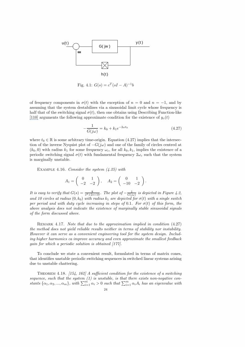
Fig. 4.1: G(s) = cT (sI −A)−1b

of frequency components in σ(t) with the exception of n = 0 and n = −1, and byassuming that the system destabilises via a sinusoidal limit cycle whose frequency ishalf that of the switching signal σ(t), then one obtains using Describing Function-like[110] arguments the following approximate condition for the existence of yc(t)

−1

G(jω)= k0 + k1e

−2ωt0 (4.27)

where t0 ∈ R is some arbitrary time-origin. Equation (4.27) implies that the intersec-tion of the inverse Nyquist plot of −G(jω) and one of the family of circles centred at(k0, 0) with radius k1 for some frequency ωc, for all k0, k1, implies the existence of aperiodic switching signal σ(t) with fundamental frequency 2ωc such that the systemis marginally unstable.

Example 4.16. Consider the system (4.25) with

A1 =

(0 1−2 −2

), A2 =

(0 1−10 −2

).

It is easy to verify that G(s) = 8s2+2s+10 . The plot of − 1

G(jω) is depicted in Figure 4.2,

and 10 circles at radius (0, k0) with radius k1 are depicted for σ(t) with a single switchper period and with duty cycle increasing in steps of 0.1. For σ(t) of this form, theabove analysis does not indicate the existence of marginally stable sinusoidal signalsof the form discussed above.

Remark 4.17. Note that due to the approximation implied in condition (4.27)the method does not yield reliable results neither in terms of stability nor instability.However it can serve as a convenient engineering tool for the system design. Includ-ing higher harmonics ca improve accuracy and even approximate the smallest feedbackgain for which a periodic solution is obtained [177].

To conclude we state a convenient result, formulated in terms of matrix cones,that identifies unstable periodic switching sequences in switched linear systems arisingdue to unstable chattering.

Theorem 4.18. [154, 162] A sufficient condition for the existence of a switchingsequence, such that the system (1) is unstable, is that there exists non-negative con-stants α1, α2, ..., αm, with

∑mi=1 αi > 0 such that

∑mi=1 αiAi has an eigenvalue with

24

−1 −0.8 −0.6 −0.4 −0.2 0 0.2 0.4 0.6 0.8 1−1

−0.8

−0.6

−0.4

−0.2

0

0.2

0.4

0.6

0.8

1

Real(jω)

Imag

(jω)

−1/G(jω) Family of circles

Fig. 4.2: Example

a positive real part.

Remark 4.19. We note that similar results, albeit in another context, are ob-tained in [173, 52]. In these papers the authors consider the quadratic stabilisation ofswitched linear systems. In [173] it is shown that a switched linear system is quadrat-ically stabilisable if

∑mi=1 αiAi is Hurwitz for some α1, ..., αm; in [52] it is shown

that this condition is both necessary and sufficient for the quadratic stabilisation ofswitched linear systems where switching takes place between two LTI systems. In bothcases the authors use arguments from Lyapunov theory to obtain their results. Whileit may be possible to use the Lyapunov-based arguments in [173, 52] to obtain the pre-vious result, it is shown in [162] that this result follows immediately from the nature ofthe solution to (2.1) using only arguments from Floquet theory. A direct consequenceof this result is the existence of a periodically destabilising switching sequence; this isentirely consistent with the more general, but also more abstract results presented in[139].

Remark 4.20. The conditions of Theorem 4.18 guarantee the existence of a peri-odic switching sequence such that the system (2.1) is unstable. More specifically, givena positive sum that has an eigenvalue with a positive real part for some non-negativeconstants α1, ..., αm, an unstable switching sequence for (2.1) is constructed as fol-lows: (a) scale the positive constants αi such that

∑mi=1 αi = 1; (b) let the matrix

Ai describe the dynamics of (2.1) for αiT seconds. Then, for sufficiently small T ,the periodic switching sequence so defined results in an unbounded solution to (2.1)irrespective of initial condition x0.Theorem 4.18 has a number of interesting consequences for the switched system (2.1):

(i) It is well known that a necessary condition for the existence of a commonquadratic Lyapunov function (CQLF), V (x) = xT Px, P = P T > 0, for theLTI systems ΣAi

, i ∈ 1, ..., m, with V (x) < 0, is that∑m

i=1 αiAi is Hurwitzfor all αi ≥ 0, with

∑mi=1 αi > 0. Hence the condition that this sum has no

eigenvalues with positive real part is necessary for the existence of a CQLF.

25

It follows from Theorem 4.18 that this condition is a much stronger necessarycondition; namely, it is also necessary for the the existence of any type ofcommon Lyapunov function for the systems ΣAi

.

(ii) Often design laws based upon the existence of a CQLF place unnecessarilyconservative restrictions on the switching system. However that this is notnecessarily true for second order systems. It follows from Theorem 4.3 thatone of the following positive sums is singular (and hence non-Hurwitz) forsome α0 ∈ [0, 1] if a CQLF does not exist for ΣA1

and ΣA2. 5

α0A1 + (1− α0)A2,

α0A1 + (1− α0)A−12 ,

Hence, as we mentioned above in Section 4, from Theorem 4.18, the non-existence of a CQLF for (2.1) implies that an unstable, or a marginally un-stable6 switching sequence exists for at least one of the dual switching systems

x = A(t)x, A(t) ∈ A1, A2, (4.28)

x = A(t)x, A(t) ∈ A1, A−12 . (4.29)

Although this observation is not true for m > 2 matrices [156], it is somewhatsurprising since it implies a strong connection between the stability problemfor (2.1), and the CQLF existence problem for the constituent systems ΣAi

,namely:

given two stable second order LTI systems for which a CQLFdoes not exist, it follows that an unstable, or marginallyunstable, switching sequence exists for one of the associatedswitching systems (4.28) and (4.29).

4.11. Common piecewise linear Lyapunov functions. Most of the availableresults for the arbitrary switching problem are related to the existence of commonquadratic Lyapunov functions. However it is not difficult to construct a switchedlinear system that is asymptotically stable for arbitrary switching sequences wherethe constituent systems do not have a common quadratic Lyapunov function (see forexample [40]). A rapidly maturing area of research is concerned with determiningconditions for the existence of non-quadratic Lyapunov functions.

It follows from the converse theorem of Molchanov and Pyatnitski that a commonpiecewise quadratic, or a common piecewise linear Lyapunov function always existsprovided that the underlying switched linear system is asymptotically stable for arbi-trary switching. Motivated by this result, a number of authors have sought to developverifiable conditions for the existence of piecewise linear Lyapunov functions (PLLF)of the form

V (x) = max1≤i≤N

wTi x (4.30)

5The stated implication can be obtained as follows. Suppose that A1A2 (respectively A1A−1

2)

has a negative real eigenvalue, −λ. Then det[λI + A1A2] = 0. Since A2 is Hurwitz, this implies thatdet[λA

−1

2+ A1] = 0; hence, the matrix λA

−1

2+ A1 is singular.

6By marginally unstable we mean a switching sequence for which there is a solution that doesnot converge to 0.

26

where wi ∈ Rn, i = 1, . . . , N and the linear functions wTi x are called generators of the

piecewise linear Lyapunov function. The function (4.30) is induced by a polyhedralset of the form

P =x ∈ R

n : wTi x ≤ c, i = 1, . . . , N, c ∈ R

+

.

Such functions can be shown to be proper and locally Lipschitz [121] and decomposethe state-space into a number of convex cones with disjoint interior. The polyhedralset P is called positively invariant with respect to the trajectories of a dynamicalsystem if for all x(0) ∈ P the solution of x(t) ∈ P for t > 0. A complete surveyof properties of positively invariant sets and their usage for a series of problems incontrol theory can be found in [17].

If the polyhedron P is bounded and centrally symmetric, then it describes apolytope and the Lyapunov function V (x) can be expressed as

V (x) = ||Wx||∞ = max1≤i≤N

|wix| (4.31)

where W ∈ RN×n, N ≥ n has full rank n. Functions of the form (4.31) are radiallyunbounded, have a unique minimum, and the onesided derivative exists [115].

The existence of piecewise linear Lyapunov functions has been considered in anumber of papers for establishing the stability of nonlinear time-varying systems andnumerical techniques for the calculation of such functions have been developed. Theexistence question for piecewise linear Lyapunov functions can be traced back to thesixties to a series of papers by Rosenbrock [144] and Weissenberger [171] on Lur’etype systems. However, despite several decades of research, powerful algebraic toolsfor the existence of piecewise linear Lyapunov functions remain scarce. Althoughthe class of PLFs appears powerful in theory, the computational requirements nec-essary to establish their existence represents a serious bottleneck in practice. Themain reason is that a complex representation (with a large number of parameters)is usually required for a solution to be found rendering the techniques applicable tolow-dimensional problems only.Indeed few theoretical tools exist to support the development of numerical or analyt-ical tests for checking the existence of such functions. One notable exception is thefollowing results that was obtained in [114, 115]:

Theorem 4.21. The function V (x) = ||Wx||∞ is a common piecewise linearLyapunov function for the switched system (2.1) if and only if there exist Qi ∈ RN×N ,i = 1, . . . , m such that

q(i)kk +

N∑

l=1

l6=k

|q(i)lk | < 0 (4.32)

and

WAi −QiW = 0 (4.33)

for i = 1, . . . , m. Here, q(i)jk denotes the (j, k) entry in the matrix Qi.

27

A generalisation of this result for norm-based Lyapunov functions of the formV (x) = ||Wx||p can be found in [83, 96].

A particular problem for the lack of results in this area is that it appears to bedifficult to specify a-priori the number N of generators that are necessary for theconstruction of a common Lyapunov function (4.30) for a given switched system. Wenote that recently some progress on this question has been made in the context of LTIsystems [26, 25]. In this work, the authors relate the number of faces of the PLLF(4.31) to the location of the spectrum of the system matrix A. The results in thesepapers may serve as a starting point for the derivation of conditions for the existenceof a common PLLF for a set of LTI systems. We can deduce the non-existence of thecommon piecewise linear Lyapunov function with N generators if the spectrum of theconvex sum of the system matrices does not satisfy the conditions on the spectrum ofLTI systems.

In [179] the existence of a PLLF with four faces (N = 4) is considered for second-order switched systems with two subsystems.

Theorem 4.22. Given the switched linear system (2.1) with A1, A2 ∈ R2×2 andσ(Ai) ∈ R−, i = 1, 2 where σ

(αA1 + (1 − α)A2

)/∈ R for some α ∈ (0, 1) then there

exits a common piecewise linear Lyapunov function (4.31) with N = 4 if and only ifthe real part of the spectrum of

σ(αA1 + (1− α)A2

),

is always greater than its imaginary part for all α ∈ [0, 1].

Finally we note that a number of attempts have been made to develop numericaltechniques for the construction of such Lyapunov functions. In [31] and [32] Braytonand Tong develop an algorithm for difference inclusions which calculates a seriesof balanced polytopes converging to the level set of a common PLLF after a finitenumber of steps. Barabanov [12] proposed another technique for checking asymptoticstability of a linear differential inclusion. An algorithm is constructed which calculatesthe Lyapunov exponent and a common PLLF in a finite number of steps. This ideahas been developed initially for difference inclusions and requires a sufficiently densediscretisation and progressive refinements. Again convex hull computations increasethe computational load significantly, rendering the techniques applicable to planarsystems, as evidenced by the examples in [31], [32], [12].

In a series of publications, Polanski has described an algorithm to construct acommon piecewise linear Lyapunov function (4.31) with a given number of generatorsfor the LTI systems ΣA1

, . . . , ΣAm[130, 131, 132]. Here the algebraic stability condi-

tion (4.33) and a scaling idea are used to formulate the search for PLLFs as a linearprogram. Similar numerical difficulties with high complexity arise and the techniqueis applicable to planar systems. In [132] an improved formulation using polytopevertices and scaling makes the technique applicable to three-dimensional problems.Thus there are cases, even in three dimensions, in which instability cannot be inferredeven when a solution cannot be found. Furthermore, the question of the number Ngenerators required remains unsolved.

This problem is partially avoided in the ray-gridding method developed by Yfoulisand his co-authors in [184, 186, 187]. The approach is based on uniform partitions ofthe state-space in terms of ray directions which allow refinable families of polytopes of

28

adjustable complexity. The technique provides two important advantages. Firstly, theoptimisation problem can be solved much more efficiently such that a complete treat-ment of the three-dimensional case is feasible; and secondly, by applying a refinementtechnique there is no prior knowledge about the numbers of generators required.

5. Restricted Switching. In earlier sections we dealt with the problem ofdetermining conditions on the set of matrices A1, ..., Am such that the resultingswitched system

x = A(t)x, A(t) ∈ A1, ..., Am, (5.1)

is exponentially stable for all switching sequences. While it is true that this problemhas received most of the recent attention in the switching systems literature, a numberof other stability problems stand out as being worthy of attention. Among these, theproblem of determining the stability of (5.1) in the case where the switching actionis constrained in some manner is a problem that arises in a number of importantapplications [94, 165].

Example 5.1. An example of how constrained switching can arise in practi-cal situations is given in [169], where the problem of designing a controller to deliverprescribed handling behaviour for a four-wheel steering vehicle is considered. The con-troller described in [169] operates by manipulating the front and rear steering anglesof the vehicle to achieve the desired behaviour. Due to physical considerations, thesteering angle of the rear tyres is subject to a tight constraint, and when the maximalallowed steering angle is reached, a change of control action is required leading to anabrupt switch in the overall system dynamics.

Roughly speaking, research on systems in which switching is constrained hasproceeded along two distinct lines of enquiry. The first of these involves the study ofsystems in which constraints on the switching action are induced by the evolution ofthe state vector x, as in the example above. The second body of research is concernedwith systems in which one seeks to impose constraints on the rate at which switchingtakes place between the constituent subsystems so as to ensure the stability of theoverall system. It should be noted that the classical Lur’e system studied by Popov[120] may be viewed as an example of the former system class, whereas classicalFloquet theory developed for the study of periodic systems may be viewed as anexample of the latter [113].

One further important problem that arises in the context of this discussion is thefollowing; namely, given a set of non-Hurwitz matrices, determine whether or not itis possible to develop a state dependent switching law such that the system (5.1) isglobally uniformly asymptotically stable [92]. We shall briefly discuss this problemlater in the paper. The interested reader is referred to [92] and the references thereinfor a discussion of some of the approaches that have been employed in the study ofthis and the other problems concerned with constrained switching.

5.1. Constraints on the rate of switching. If all of the matrices in theswitching set A1, ..., Am are Hurwitz, then it is possible to ensure the stability ofthe associated switched system by switching sufficiently slowly between the asymp-totically stable constituent LTI systems. This means that instability arises in (5.1) asa result of rapid switching between these vector fields. Given this basic fact, a naturaland obvious method to ensure the stability of (5.1) is to somehow constrain the rate

29

Constrained switching

Constraints on switching rate

State induced constraints

Constraint given

Constraint is a design parameter

Fig. 5.1: Types of constraints on switching laws that arise in practical applications

at which switching takes place.

The basic idea of constraining the switching rate has appeared in many studies ontime varying systems over the past number of decades [59, 191, 74]. One of the bestknown and most informative of these studies was given by Charles Desoer in 1969 inhis study of slowly varying systems [46]. The basic problem considered by Desoer wasto find conditions on the switching rate that would ensure the stability of an unforcedsystem of the form x = A(t)x, where A(t) is a matrix valued continuous functionsuch that supt≥0 ‖ A(t) ‖< ∞, and A(t) is Hurwitz for all fixed t (here ‖ . ‖ canbe any norm on Rn×n.) Using an argument based on quadratic Lyapunov functions,Desoer demonstrated that there exists some constant K > 0 such that the solutionx(t) satisfies ‖ x(t, t0) ‖< meλ(t − t0) ‖ x(t0) ‖ for some m > 0 and λ < 0 providedsup ‖ A(t) ‖= K. There are two key points to emphasize here; firstly, the stability ofthe time-varying system can be ensured by suitably constraining the rate of variationof A(t), and secondly the constraint on A(t) is determined by a Lyapunov functionassociated with the system.

Recently, similar ideas been exploited in the Hybrid and Switched Systems com-munity [94, 45, 91, 112, 182]. However, when dealing with switched linear systems,one may approach the problem of constraining the rate at which switching takes placein at least two ways. The first, an indirect method, is close to the method suggestedby Desoer; one constrains switching indirectly by ensuring negative definiteness ofthe derivative of a certain Lyapunov function. An alternative to this approach is touse knowledge of the form of the solutions to (5.1) to ensure stability. While thelatter approach is difficult for general time-varying linear systems, the explicit formof the solution to (5.1), makes such an approach possible in the case of switched linearsystems and gives rise to the following basic problem in the study of switched linearsystems.

Given the system (5.1), let στ (t) denote any switching signal with the propertythat tk+1− tk > τ for all k > 0. Let S[τ ] denote the class of all such signals. Onemay then pose the following question: Find the minimum τ for which (5.1)isuniformly exponentially stable for all στ ∈ S[τ ].

30

The above problem, often referred to in the literature as the Dwell-time Prob-lem, poses a fundamental question in the study of switched systems. However, rathersurprisingly, very little progress has been made on this and related problems, and tothe best of our knowledge few papers have appeared in the recent literature that dealwith this topic; the most notable of those to have appeared are [45, 91, 112, 182]. Forconvenience we report here on the work developed by Hespanha and his coauthorsin [67] as this appears at the present time to be the most complete treatment of theDwell-time problem to have appeared .

Definition 5.2 (Dwell-time). [67] Given a positive constant τD then S[τD ] ⊂ Sdenotes the set of all switching signals σ(t) ∈ S where the intervals between consecutivediscontinuities are no shorter than τD. The constant τD is called (fixed) dwell-time.

For switched linear systems all of whose subsystems, ΣAi, are Hurwitz stable,

Morse [117] established the (unsurprising) fact that the switching system (2.1) isasymptotically stable provided the dwell-time τD is chosen to be sufficiently large.This result was extended by Hespanha in [67], where the notion of average dwell-timeτD was introduced. This concept allows some switching intervals to be of length lessthan τD provided that, in a sense to be made precise below, the average dwell-timeis at least τD .

Formally, for a switching signal σ, and real numbers t1, t2 with t2 > t1 > 0, letNσ(t1, t2) denote the number of discontinuities of σ in the interval (t1, t2). Then givena positive real number τD > 0 and a positive integer N0 > 0, define S[τD , N0] to bethe set of switching signals σ ∈ S such that

Nσ(t1, t2) ≤ N0 +t2 − t1

τD

(5.2)

for all t2 > t1 > 0. The parameter N0 is referred to as the chatter bound and τD isknown as the average dwell-time. Note that for τD > 0, S[τD ] ⊂ S[τD , 1]. Using theseconcepts, Hespanha and Morse derived the following sufficient condition for stabilityin [67].

Theorem 5.3. Consider the switching system (2.1) and suppose that Ai ∈ Ais Hurwitz for 1 ≤ i ≤ m. Further, let λ0 > 0 be such that Ai + λ0I is Hurwitzfor 1 ≤ i ≤ m. Then, for any chosen λ ∈ [0, λ0), there is a finite constant τ∗

D

such that (2.1) is exponentially stable, with decay rate λ, for all switching signalsσ(t) ∈ S[τD , N0] for τD ≥ τ∗

D and any chatter bound N0 > 0.

In other words, the system is stable if we switch on average more slowly thanthe rate corresponding to τ∗

D . This lower bound on the average dwell-time can becalculated by first selecting: λ0 > 0 such that Ai+λ0I is Hurwitz for all i ∈ 1, . . . , m.We then calculate a quadratic Lyapunov function, Vi(x) = xT Pix, for each subsystemby solving the Lyapunov equations

Pi(Ai + λ0I) + (Ai + λ0I)T Pi = −I

for i = 1, . . . , m and calculate

µ = sup1≤i,j≤m

ρmax[Pi]

ρmin[Pj ].

31

Finally, one chooses a stability margin λ for the switched system and obtain theaverage dwell-time by

τ∗D =

log µ

2(λ0 − λ)

Note that the results on average dwell-time in [67] were derived for a compact(not necessarily finite) set of Hurwitz matrices A and that a version of Theorem 5.3was also derived for certain classes of switched nonlinear systems. A number of au-thors have further extended this work and derived analogous results for other classesof switched nonlinear systems [127, 44]. Further developments have also included thework of Zhai et al. [189] in which the authors modify this result so that the lowestaverage dwell-time τ∗

D ensures that the switched system achieves a chosen L2 gain,while several other authors have extended the results to allow for switching betweenstable and unstable subsystems, e.g. [190], [183].

Remark 5.4. The principal difficulty associated with the dwell-time problem isto obtain a tight lower bound on τD. It is quite remarkable that a non-conservativeestimate of τD, even for simple classes of switching systems, has to-date eluded theresearch community.

5.2. Converse Lyapunov Theorems for systems with dwell time. In thepresent context, it is important to note that converse theorems for the existence ofLyapunov functions also exist for switched systems with a restriction on the dwell time.Before we discuss these results, we note that in general it is unreasonable to expectone Lyapunov function as a function of the state to suffice for capturing stability.Consider again a set of matrices A = A1, . . . , Am and assume we are given a dwelltime restriction τD . If there exists a Lyapunov function V such that t → V (x(t))is strictly decreasing for all nonzero solutions of the switched system (5.1), then thisimplies that the system (2.1) with arbitrary switching is also exponentially stable. Ingeneral, there is of course a distinction between stability under arbitrary switchingand switching with a dwell time restriction.

A converse theorem for the case of dwell times is presented in [176, Cor. 6.5]. Inthe following statement we tacitly use the same symbol v for a norm defined on Rn

and the induced matrix norm on Rn×n.

Theorem 5.5. The system (5.1) with fixed dwell time τD is exponentially stable,if and only if there are norms v1, . . . , vm on Rn and a constant β > 0 such that

(i) for all i = 1, . . . , m it holds that

vi(eAit) ≤ e−βt , for all t ≥ 0 ,

(ii) for all i, j = 1, . . . , m it holds that

vj(eAjtx) ≤ e−βtvi(x) , for all x ∈ R

n, t ≥ τD .

Additionally, if the set of matrices A is irreducible7 then the norms in the previoustheorem may be chosen, such that β is equal to the exponential growth rate of (5.1)

7A set of matrices is called irreducible, if only the trivial subspaces 0 and Rn are invariantunder all matrices in the set.

32

with fixed dwell time τD. In this manner the result is an extension of the results ofMolchanov and Pyatnitski, and Barabanov on the existence of nonquadratic Lyapunovfunctions in the case of arbitrary switchings.

5.2.1. Indirectly induced constraints: Multiple Lyapunov functions and

slowly varying systems. An important paper in the recent evolution of stabilitytheory of switched systems was published in 1994 by Michael Branicky. Branickymade the observation, as Desoer had done in the 1960’s, that Lyapunov functionscould be used to derive laws to constrain the rate of switching in such a way as toguarantee stability. However, as was suggested by our converse theorem for dwell timesystems, rather than using a single Lyapunov function to achieve this as Desoer haddone, Branicky suggested the use of multiple Lyapunov functions (one for each modeof the system), to guarantee exponential stability.

Branicky’s basic idea was to define a Lyapunov function for each mode i of thesystem Σ. One then uses these functions to construct a stabilising switchingsignal σ(t) by only allowing the system to switch into mode i if the value of thecorresponding Lyapunov function Vi(x) is less than it was when the system lastleft mode i.

It is important to note that the use of multiple Lyapunov functions to select astable switching sequence for switched systems had been suggested by a number ofauthors prior to Branicky’s original paper in 1994; in particular Peleties & DeCarlo[126] deserve credit for promoting the original idea for switched linear systems. How-ever, Branicky’s paper, which extended the basic idea to the nonlinear case, has had agreat impact on the community and in the following discussion we adopt the notationand arguments given in the original papers [30].

Branicky considers a general autonomous switched non-linear system

x(t) = f(x, t) f(x, t) ∈ f1(x), . . . , fm(x) t ≥ 0, (5.3)

where each mode, fi, is assumed to be globally Lipschitz continuous and exponentiallystable; and where the switching strategy is chosen in such a way that there are finiteswitches in finite time. While there are several similar versions of Branicky’s result,we quote the following from [29] which can be stated with a minimum of mathematicalformalism.

Theorem 5.6. Suppose that we have a finite number of Lyapunov functions Vi(x)associated with the continuous-time vector fields x = fi(x). Let Sk = i0, i1, . . . , ik, . . .denote the switching sequence of the system, and Tk = t0, t1, . . . , tk, . . . denote thesequence of corresponding switching instances for the system. If, for each instant tj

when we switch into mode i, with corresponding Lyapunov function Vi, we have that

Vi(x(tj)) ≤ Vi(x(tk)) (5.4)

where tk < tj and tk is the last time that we switched out of mode i, then the systemis stable in the sense of Lyapunov.

Theorem 5.6 gives a simple rule for the construction of a stable slowly varyingswitching system. It states that when the system enters mode i, the value of theLyapunov function associated with this mode must be less than the value it attained

33

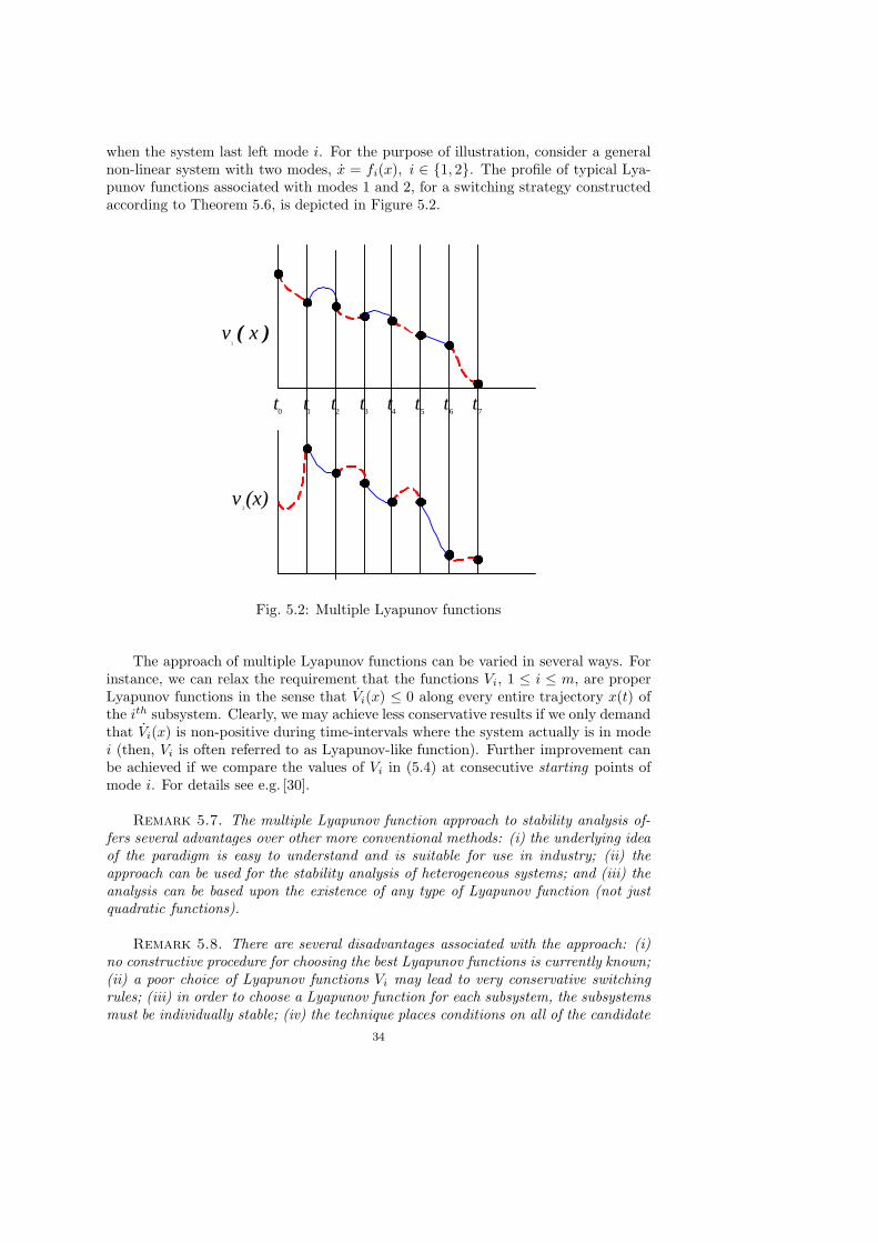
when the system last left mode i. For the purpose of illustration, consider a generalnon-linear system with two modes, x = fi(x), i ∈ 1, 2. The profile of typical Lya-punov functions associated with modes 1 and 2, for a switching strategy constructedaccording to Theorem 5.6, is depicted in Figure 5.2.

) ( x v 1

0 t

1 t

2 t

3 t

4 t

5 t

6 t

7 t

(x) v 2

Fig. 5.2: Multiple Lyapunov functions

The approach of multiple Lyapunov functions can be varied in several ways. Forinstance, we can relax the requirement that the functions Vi, 1 ≤ i ≤ m, are properLyapunov functions in the sense that Vi(x) ≤ 0 along every entire trajectory x(t) ofthe ith subsystem. Clearly, we may achieve less conservative results if we only demandthat Vi(x) is non-positive during time-intervals where the system actually is in modei (then, Vi is often referred to as Lyapunov-like function). Further improvement canbe achieved if we compare the values of Vi in (5.4) at consecutive starting points ofmode i. For details see e.g. [30].

Remark 5.7. The multiple Lyapunov function approach to stability analysis of-fers several advantages over other more conventional methods: (i) the underlying ideaof the paradigm is easy to understand and is suitable for use in industry; (ii) theapproach can be used for the stability analysis of heterogeneous systems; and (iii) theanalysis can be based upon the existence of any type of Lyapunov function (not justquadratic functions).

Remark 5.8. There are several disadvantages associated with the approach: (i)no constructive procedure for choosing the best Lyapunov functions is currently known;(ii) a poor choice of Lyapunov functions Vi may lead to very conservative switchingrules; (iii) in order to choose a Lyapunov function for each subsystem, the subsystemsmust be individually stable; (iv) the technique places conditions on all of the candidate

34

Lyapunov functions (a condition that is clearly not necessary for exponential stabilityof the switched system).

Remark 5.9. A number of interesting research questions in the multiple Lya-punov function framework remain unanswered. In our context, namely for switchedlinear systems, the most important of these pertains to developing a constructivemethod of choosing the candidate Lyapunov functions that minimise the dwell-timefor each mode.

5.3. State dependent switching and stability. In the previous subsection,we considered a variety of results concerned with switched systems for which the rateof switching is constrained in some way. An alternative type of constraint that arisesin the study of switched systems is where the switching action is constrained by thestate vector of the system. As we shall see in the next section, Internet congestioncontrol is an example of one such system. If the rule for switching between theconstituent systems of a switched system is determined by the state vector of thesystem, we say that the switching is state dependent. Loosely speaking, the stabilityproblems associated with this type of switching regime can be divided into two classes.In the first of these, the state space is partitioned by a number of hyper-surfaces thatdetermine the mode switches in the system dynamics, and the problem is to analysethe stability of the time-varying system defined in this way. On the other hand, inthe second class of problem we are concerned with finding state-dependent rules forswitching between a family of unstable systems that result in stability. Thus, in theformer case, a partition of state space is specified and the problem is to determinethe stability of the piecewise linear system defined by that partition, while in thelatter case the aim is to find stabilizing state-dependent rules for switching betweenindividually unstable systems.

5.4. Switched systems and state-dependent constraints. We shall nowconsider switched systems that are constrained in the sense that a mode switch oc-curs in the systems dynamics when its state vector crosses certain threshold surfacesin state space. We first turn our attention to the class of piecewise linear systems.

Piecewise linear systems:A piecewise linear system is a dynamical system of the form

x = Aix for x ∈ Ωi (5.5)

where Ω1, . . . , Ωm are closed sets with pairwise disjoint interiors such that ∪iΩi = Rn,

and A1, . . . , Am are in Rn×n. For such systems, requiring the existence of a commonLyapunov function for the LTI systems ΣA1

, . . . , ΣAmcan be an unduly restrictive

criterion for stability. For instance, in order for the quadratic form V (x) = xT Px todefine a CQLF for ΣA1

, . . . , ΣAm, for each i ∈ 1, . . . , m, V (x) must decrease along

all trajectories of ΣAieverywhere in the state space. However, it is clear that this

may well lead to unnecessarily conservative stability conditions as it fails to take intoaccount that the system ΣAi

is only active within the region Ωi. The so-called S-procedure [28, 77] seeks to exploit this fact in order to obtain less restrictive stabilityconditions for systems of the form (5.5).

The S-procedure:The basic idea behind using the S-procedure to analyse the stability of systems of

35

the form (5.5) is the following. First of all, determine symmetric matrices S1, . . . , Sm

such that xT Six ≥ 0 for x in Ωi and then search for a positive definite P = P T > 0satisfying the conditions

ATi P + PAi + Si < 0 for 1 ≤ i ≤ m. (5.6)

If P satisfies (5.6) then it follows that, for each i ∈ 1, . . . , m, xT (ATi P + PAi)x < 0

for x ∈ Ωi. Thus, the positive definite function, V (x) = xT Px, decreases along alltrajectories of the system (5.5), thereby establishing exponential stability. However,note that for some choices of the matrix Si, the expression xT (AT

i P + PAi)x may benon-negative for x outside of Ωi. For this reason, the conditions given by (5.6) maybe less demanding than those imposed by requiring CQLF existence.

Piecewise quadratic Lyapunov functions:Extending the ideas of the S-Procedure, a number of authors have studied piecewisequadratic Lyapunov functions [77, 129, 128, 63] in order to find less conservativestability criteria for piecewise linear systems. Here, rather than looking for a sin-gle quadratic Lyapunov function, V (x) = xT Px, for the system (5.5), the idea is tosearch for a family of such functions satisfying certain local conditions, and then topiece these together appropriately to form a Lyapunov function for the overall system.

For convenience, and to illustrate the main ideas behind the use of piecewisequadratic Lyapunov functions, we shall focus mainly on the results of [77]. In thispaper, under the assumption that the regions Ωi are polyhedral, a numerical procedureis described for searching for a piecewise quadratic Lyapunov function of the form 8

V (x) = xT Pix for x ∈ Ωi, (5.7)

where Pi = P Ti ∈ Rn×n for i = 1, 2, . . . , m. Extending the basic idea of the S-

procedure, the authors of [77] relax the conditions for stability given by CQLF exis-tence in a number of ways.

(i) The use of different quadratic forms for the different operating regions Ωi canlead to greater flexibility in the definition of the Lyapunov function V .

(ii) The matrices Pi are not required to be globally positive definite. In fact, byapplying the S-procedure, the inequality xT Pix > 0 is only required to holdwhen x ∈ Ωi for 1 ≤ i ≤ m.

(iii) Similarly, the condition xT (ATi Pi + PiAi)x < 0 is only required to hold for

x ∈ Ωi.

A few specific points relating to the results described in [77] are worth noting.

(i) The matrices Pi are parameterized so as to ensure that the piecewise quadraticfunction V (x) is continuous.

8The function takes a slightly different form in regions Ωi that do not contain the origin. Fordetails consult [77]

36

(ii) The conditions for (5.7) to define a piecewise quadratic Lyapunov functionfor the system (5.5) are expressed in the form of linear matrix inequalities(LMIs). Hence, modern convex optimization algorithms can be used to searchfor piecewise quadratic Lyapunov functions.

(iii) It is possible to use a partition other than that dictated by the system dy-namics to define the piecewise quadratic function. Thus, if an initial searchis unsuccessful, it may be possible to find a piecewise quadratic Lyapunovfunction defined with respect to an alternative, possibly finer, partition ofthe state space. However, the problem of selecting an initial partition, and ofdevising automatic methods of successively refining the partition to system-atically search for piecewise quadratic Lyapunov functions is in general farfrom straightforward.

The results of [77] were actually derived for piecewise affine systems where thedynamics within each region Ωi take the form x = Aix+ai. The ideas and techniquesof this paper were developed and extended in the subsequent papers [78, 142] andsimilar LMI conditions for the stability of piecewise linear systems based on piecewisequadratic Lyapunov functions have been presented in [63]. In this context, the workof [51] on applying piecewise quadratic methods to the problem of controller designfor uncertain piecewise affine systems should also be noted.

The paper [185] describes closely related work on the stability of the class of or-thogonal piecewise linear systems. For such systems, the hyper-planes that partitionthe state space, R

n take the general form xi = ci,j for i = 1, . . . n, j = 1, . . . ni, anddivide the state space into a family of hyper-rectangles. The conditions for stabilityderived in [185] are based on the existence of piecewise linear Lyapunov functions asopposed to piecewise quadratic Lyapunov functions.

Switching rules specified by switching surfaces:Similar ideas to those used to analyse piecewise linear systems have also been usedto study more general state dependent switching rules. Typically, these rules aredefined by specifying a set of surfaces Sij , 1 ≤ i, j ≤ m, in the state space suchthat the system switches from mode i to mode j if the ith subsystem is currentlyactive and the state vector crosses the surface Sij [129, 77, 173]. For instance, in[77] piecewise quadratic Lyapunov functions are employed to obtain LMI-based sta-bility conditions for such systems under the assumption that the switching surfacesare given by hyper-planes. The Lyapunov function used to derive the conditions inthis paper is not required to be continuous provided that the value of the functiondecreases whenever the system switches from one mode to another. Similar resultsbased on piecewise quadratic Lyapunov functions have also been presented in [129].The results of this last paper are based on a Lyapunov function that need not becontinuous and, moreover, is not required to decrease at each switching instant. Infact, all that is needed for stability is that the values of the function are bounded bysome continuous function of its initial value. The conditions in [129] are again formu-lated as LMIs, and can also be applied to systems with non-linear constituent systems.

Piecewise linear systems and the Popov criterion:The classical Popov criterion for the absolute stability of non-linear systems [133, 168]

37

can also be used in the analysis of certain piecewise linear systems. An example il-lustrating this is described in [77], where the stability of a two-dimensional piecewiselinear system is established using the Popov criterion. For the system considered inthis example, the Popov criterion ensures the existence of a Lyapunov function ofLur’e Postnikov form, meaning that it is the sum of an integral of a non-linear func-tion and a quadratic form. For the system considered in [77], this function actuallyreduces to a piecewise quadratic Lyapunov function of the form considered above. Itshould be noted that the connection between Lyapunov functions of Lur’e Postnikovform and piecewise quadratic Lyapunov functions was earlier pointed out by Weis-senberger in [171], and that the idea of using piecewise quadratic Lyapunov functionsfor stability analysis had been suggested by Power and Tsoi in [134].

Positive switched linear systems:The classes of switched system considered above are constrained in the sense that thesystem dynamics must undergo a mode switch when the state vector crosses some sur-face in state space. The nature of these systems has led naturally to the considerationof both piecewise quadratic and piecewise linear Lyapunov functions in their stabilityanalysis. A different type of constraint arises in the study of positive switched linearsystems, where any trajectory starting from non-negative initial conditions must re-main within the non-negative orthant for all subsequent times [50, 98]. In view of theconsiderable restriction that this imposes on the possible trajectories of a positive sys-tem, it is natural to consider so-called co-positive Lyapunov functions when analysingthe stability of such systems [18]. These functions are only required to satisfy therequirements of a traditional Lyapunov function within the non-negative orthant andmay lead to less conservative stability conditions for positive switched linear systemsthan can be obtained using traditional Lyapunov functions. Some initial results oncommon copositive Lyapunov function existence can be found in [61, 108, 106]

5.5. Stabilizing switching rules. The results discussed in the last subsectionwere concerned with establishing the stability of systems subject to some specifiedstate dependent switching rule. Another problem of interest in this context is that ofdetermining stabilizing switching rules for systems with unstable constituent systems.

In [173], the following problem was addressed. Given two LTI systems ΣA1, ΣA2

where both A1 and A2 have some eigenvalues in the right half plane, determine ifthere exists some rule for switching between these systems that results in stability. Ithas been established, [173], that if some convex combination of the matrices A1 andA2 is Hurwitz, then such a stabilizing switching rule does indeed exist. Formally, thisamounts to testing for the existence of some α with 0 < α < 1 such that the matrix

A(α) = αA1 + (1− α)A2

is Hurwitz. Moreover, the authors of [173] describe how to construct a state-dependentstabilizing switching rule when such a stable convex combination exists.

The basic idea behind this construction is the following. As the matrix A(α) isHurwitz, there exists some positive definite matrix P = P T > 0 such that

A(α)T P + PA(α) < 0. (5.8)

It follows that the two cones Ω1, Ω2 defined by

Ωi = x ∈ Rn : xT (AT

i P + PAi)x < 0 (5.9)

38

cover the space (meaning that Ω1 ∪Ω2 = Rn). Using this fact, it is possible to definetwo switching surfaces close to the boundaries of these cones such that the associatedswitching rule asymptotically stabilizes the overall system. In fact, the quadraticfunction, V (x) = xT Px, where P is a solution of (5.8), is a Lyapunov function for thesystem defined by this switching rule. For this reason, we say that the switching ruledefined in the above manner quadratically stabilizes the system.

The switching rule described in the previous paragraph is constructed so as toensure that only a finite number of switches occur in any finite time interval. Twoother switching rules for stabilizing the system are also described in [173], but bothof these allow for the possibility of infinitely many switches occurring in a finite timeinterval and for practical reasons this may be undesirable.

The result that a stabilizing switching rule exists if some convex combination ofthe matrices A1 and A2 is Hurwitz extends to the case of an arbitrary finite familyof matrices. Formally, given a family of unstable LTI systems ΣA1

, . . . , ΣAm, there is

some rule for switching between them that results in quadratic stability if there arenon-negative real numbers α1, . . . , αm with α1 + · · · + αm = 1 such that the matrixα1A1 + · · ·+αmAm is Hurwitz. In general this condition is not known to be necessaryfor the existence of such a quadratically stabilizing switching rule. However, for thecase of switching between two unstable systems, the existence of a Hurwitz convexcombination of the system matrices is known to be equivalent to the existence of aquadratically stabilizing switching rule [52].

The work of [173] has been extended in the paper [172] where conditions for theexistence of stabilizing switching rules were derived using piecewise quadratic Lya-punov functions as opposed to quadratic Lyapunov functions. Note also the relatedwork on piecewise quadratic Lyapunov functions described in [180], and the recentpaper [8] where it is shown that, under an additional assumption, there exists a sta-bilizing rule for switching between a pair of unstable LTI systems ΣA1

, ΣA2, provided

that there is some convex combination of the system matrices A1, A2 with the prop-erty that all of its eigenvalues have non-positive real parts and any eigenvalues on theimaginary axis are simple.

6. The Lure’ problem. The study of stability reached a peak in the 1960’sand early 1970’s in the engineering community. During this period a vast numberof researchers studied the Lure’ problem. Consequently, it is impossible to write areview on this topic without mentioning this work even briefly.

The SISO version of the Lure’ problem is depicted in Figure 6.1 (although ourcomments are equally valid for MIMO versions of the Lure’ problem).

39

du x c y

bu Ax x T + =

+ =

) , ( t y k

0

y u

PSfrag replacements

re

Fig. 6.1: Graphical depiction of the Lure’ system. For the present discussion weconsider SISO systems: A is a stable n×n matrix, b, c are appropriately dimensionedvectors, and d is a scalar.

As can be seen the Lure’ system is composed of a feedback connection of a stableLTI system and a non-linear and possibly time-varying gain that is constrained to liein some interval, say k(y, t) ∈ [0, 1].

Remark 6.1. Note that the Lure’ system reduces to an example of a classicalswitched system when k(y, t) ∈ 0, 1. Evidently, tools developed for the study of Lure’systems can therefore be applied to the analysis of special classes of switched systems.Three problems were widely studied in the context of the Lure’ system.

(i) When is the equilibrium solution of the Lure’ system globally uniformly ex-ponentially stable for arbitrary time-varying gains k(t).

(ii) Can one impose constraints on k(y, t) such that the equilibrium solution ofthe Lure’ system is globally uniformly exponentially stable?

(iii) Can one impose conditions on the rate of change of k(y, t) so that the equilib-rium solution of the Lure’ system is globally uniformly exponentially stable?

Problems (i), (ii) and (iii) are clearly analogs of the Arbitrary switching, Restrictedswitching and the Dwell-time problems respectively. Their study has led to manyclassical stability criteria: the Kalman-Yacubovich-Popov-Meyer lemma; the CircleCriterion; the off-axis Circle criterion; the Passivity theorem; and the Popov Criterion[1]. The main tool used in developing these results was the Lure’-Postnikov Lyapunovfunction. That is, one sought conditions on A, b, c, d, k(y, t) to ensure that a Lyapunovfunction of the form:

V (x) = xT Px + λ

∫ y

0

k(δ, t)dδ (6.1)

where λ ∈ R+ and where P = P T > 0. Note that V (x) is rarely quadratic. Duemainly to the remarkable results of Popov, and later of Kalman and Meyer, it wasfound that the existence of a function V (x) for the Lure’ system could be deduced bytesting whether or not

1 + Re(H(jω)G(jω)) > 0, ∀ ω ∈ R (6.2)

40

where G(jω) = d + cT (jωI − A)−1b and H(jω) is some rational function of ω thatis referred to as a multiplier. Recently, a number of results have been obtained thatrelate results derived in the context of the Lure’ problem to more general results de-rived in the context of switched linear systems. In particular, the following result hasproved to be a useful bridge between these areas.

Theorem 6.2. Let G(jω) = N(jω)D(jω) be a proper real rational transfer function and

K ∈ R+. Let A, b, c, d be a realisation of G(jω) so that G(jω) = cT (jωI−A)−1b+d.

Assume that A and(A− 1

K+dbcT)

are Hurwitz. Then, a necessary and sufficient

condition for

K + Re G(jω) > 0, ∀ ω ∈ R ∪ ∞, (6.3)

is that the matrix-product A(A− bcT

K+d

)has no negative real eigenvalues.

Theorem 6.2 has a number of implications for classical frequency domain stabilitycriteria.

(i) The Kalman-Yacubovich-Popov (KYP) Lemma : The single-input single-output(SISO) version of the Kalman-Yacubovich-Popov lemma [80] is expressed inthe form of a strictly positive real (SPR) condition: namely, A and A− 1

γbcT

are Hurwitz and

γ + RecT (jωIn −A)−1b

> 0 ∀ ω ∈ R,

for some γ ∈ R+. Hence it follows from Theorem 6.2 that a time-domainversion of the SPR condition for SISO systems is that the matrices A and(A− 1

γbcT)

are Hurwitz and A(A − 1γbcT ) does not have any negative real

eigenvalues.

(ii) The Circle Criterion [158]: The SISO version of the Circle Criterion is deriveddirectly from the SISO KYP lemma. Here, conditions are derived for theexistence of a Lyapunov function V (x) = xT Px, P = P T ∈ Rn×n for thenon-linear Lur’e type system. In this case a necessary and sufficient conditionfor the existence of a quadratic Lyapunov function V (x) is that [119] A andA− bcT are Hurwitz and that

1 + RecT (jωIn −A)−1b

> 0 ∀ ω ∈ R.

It follows from Theorem 6.2 that a time-domain version of the Circle Crite-rion with 0 ≤ k(y, t) ≤ 1 is that matrices A and A − bcT are Hurwitz andthat matrix A(A− bcT ) does not have any negative real eigenvalues.

(iii) The Popov Criterion : The SISO Popov criterion [163] considers the stabilityof the Lure’ system where the nonlinearity k is non-linear but time-invariant.A sufficient condition for the absolute stability of this system is that A andA− 1

γbcT are Hurwitz and there exists a strictly positive α ∈ R such that

1

k+ Re

(1 + jαω)cT (jωIn −A)−1b

> 0 ∀ ω ∈ R.

41

It follows from Theorem 6.2 that a time-domain version of the Popov criterionis that A and A − 1

γbcT are Hurwitz and there exists a positive α ∈ R such

that matrix A(A− 1d+ 1

k

bc) does not have any negative real eigenvalues where

A, b, c, d is a realisation of (1 + αs)cT (sIn −A)−1b.Remark 6.3. The most interesting observation arising from this theorem is that

all stability problems have been reduced to a CQLF existence problem. For example,the Popov criterion, which searches for the existence of a non-quadratic Lyapunovfunction for the original non-linear system, has been reduced to a CQLF existenceproblem for x = Ax, and x = (A − 1

d+ 1

k

bc)x. This appears to be an unexplored (and

perhaps important) observation.

7. Passivity. Apart from the Circle Criterion, one of the big successes of thisperiod, was the derivation of the Passivity theorem [168]. The Passivity Theorem givesa sufficient condition for stability of the following time-varying, nonlinear system:

x(t) = Ax(t) + Bu(t),

y(t) = Cx(t) + Du(t),

u(t) = −Φ(t, y(t)) (7.1)

where x ∈ Rn, u, y, z ∈ R

m, m < n, Φ : R × Rm → R

m, and A, B, C, D are matriceswith the appropriate dimensions. These equations describe the dynamics of a controlsystem where x(t) is the state variable, y(t) is the output variable and u(t) is thefeedback. The dynamics of x(t) is separated into a linear part Ax and a nonlinearpart Bu, and it is assumed that the matrix A is Hurwitz so that the linear part isstable. The question of finding conditions on the nonlinearity Φ which are sufficientto guarantee stability of the system is known as the Lur’e problem. The PassivityTheorem provides the following solution: the system (7.1) is gobally exponentiallystable if Φ(t, 0) = 0, yT Φ(t, y) ≥ 0 for all t ∈ R, all y ∈ Rm, and if H(jω) + H∗(jω)is positive definite for every real ω, where the transfer matrix H(s) is defined by

H(s) = C(sI −A)−1B + D, s ∈ C. (7.2)

When these conditions are satisfied the Kalman-Yacubovitch Lemma guarantees theexistence of a quadratic Lyapunov function xT Px for the system (7.1) [168].

This problem is relevant to the study of switching systems because in many casesthe dynamics of a switching system has the following form:

x(t) = Ax(t) − z(t, x(t)) (7.3)

where x ∈ Rn, A ∈ Rn×n is Hurwitz and z : R × Rn → Rn is a time-varying,nonlinear vector field. The Lur’e system (7.1) can be rewritten in the form (7.3)with z = Φ(t, y(t)), where y(t) depends on the state x(t) through the implicit relationy(t) = Cx(t)−DΦ(t, y(t)). Thus (7.3) is more general than the Lur’e system, becausez is allowed to depend on x in an arbitrary way.

One example of such a system arises in state-dependent switching where Rn ispartitioned into disjoint sets Ωi, and the dynamics switches between different linearsystems as the state crosses from one region to another. So the dynamics is given by

x(t) = A(x) x(t), A(x) = Ai ∀ x ∈ Ωi (7.4)

This system can be presented in the form (7.3) by defining z(t, x) = (A − A(x))x(t)for some Hurwitz matrix A.

42

The Passivity Theorem provides a method to analyse the stability of systemsof the form (7.3). The crucial ingredient is the existence of a quadratic Lyapunovfunction xT Px for the system. Instead of using the Kalman-Yacubovitch Lemma toprovide the matrix P , one can instead postulate the existence of such a function anduse it to derive conditions which must be satisfied by the nonlinearity Φ. This idealeads to the following result [84].

Theorem 7.1. Let A1, . . . , Am be a collection of real matrices such that theconvex combination A =

∑mi=1 αiAi is Hurwitz for some α1, . . . αm satisfying αi ≥ 0,∑

αi = 1. Choose P = P T > 0 such that AT P + PA < 0 and define Ki = x :xT P (A−Ai)x ≥ 0. Then

m⋃

i=1

Ki = Rn.

For i = 1, . . . , m let Ωi ⊂ Ki such that the Ωi are disjoint and their union is Rn.Then the system (7.4) is globally exponentially stable.

The result is proved by choosing z(t, x) = (A−A(x))x(t) in (7.4) where A(x) = Ai

for all x ∈ Ωi. Then the definition of Ki implies that xT Pz(t, x) ≥ 0 for all x ∈ Rn,and this is sufficient to guarantee that xT Px is a Lyapunov function for (7.4).

The results of Theorem 7.1 can be used to design stable switching systems ofthe form (7.4). In particular, given a collection of real matrices A1, . . . , Am forwhich some convex combination is Hurwitz, one would like to determine all matricesP = P T > 0 which satisfy AT P + PA < 0, as these would describe possible stablestate-dependent switching rules for this collection. In general it is difficult to find acompact parametrisation of these matrices. However the procedure simplifies whenthe matrices Ai have the special form Ai = A− BDT

i , where A is Hurwitz and B issome fixed matrix. In this case, if there is a matrix C such that H(jω) + H∗(jω) ispositive definite for all real ω, where now H(s) = CT (sI − A)−1B, then the conesare Ki are given as x : xT CDT

i x ≥ 0. Therefore the search for matrices P can bereplaced by a simpler search for matrices C that satisfy this positivity condition. Inthe case m = 1 where B, C are vectors in Rn, the set of all possible vectors C canbe described in the following compact and useful way [84]: a vector C satisfies thepositivity condition above if and only if CT AB < 0 and CT (A2 + ω2)−1AB < 0 forall ω ∈ R. This allows a constructive procedure to find the vectors [84].

8. Case study: Internet congestion control. To conclude our paper wepresent an example of a class of switched system that is currently finding applicationin many different areas of computer science and engineering. It has already been dis-cussed that switched systems in which the states remain positive are ubiquitous [106].A subclass of such systems that is currently arising in many current applications isthe class of discrete time switched positive system models in which the matrices inthe switching set are not only positive, but also Markov (stochastic). Such modelscan readily be found in the study of communication networks [151, 75]; in the studyof concensus algorithms [75]; and in other applications from computer science suchas Google [33]. This system class is particularly interesting since it involved switch-ing between subsystems that are themselves marginally stable. We focus here on thestudy of TCP based communication networks as it illustrates some of the interestingfeatures of such systems.

43

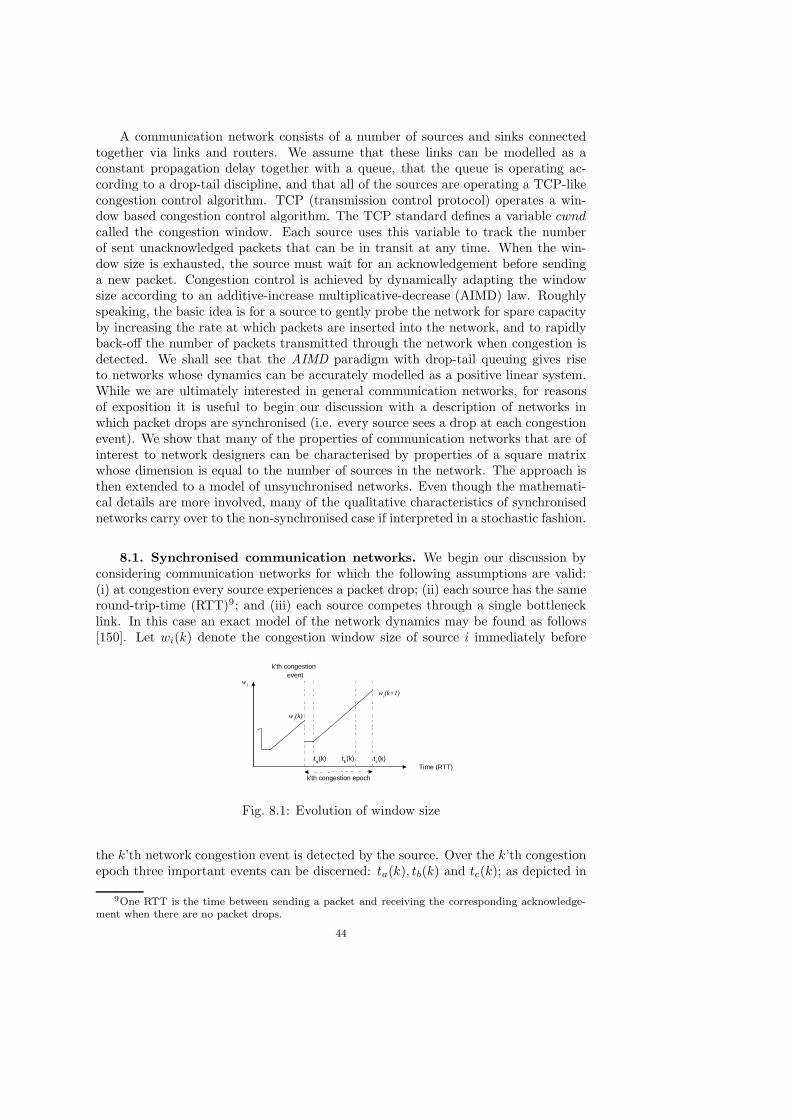
A communication network consists of a number of sources and sinks connectedtogether via links and routers. We assume that these links can be modelled as aconstant propagation delay together with a queue, that the queue is operating ac-cording to a drop-tail discipline, and that all of the sources are operating a TCP-likecongestion control algorithm. TCP (transmission control protocol) operates a win-dow based congestion control algorithm. The TCP standard defines a variable cwndcalled the congestion window. Each source uses this variable to track the numberof sent unacknowledged packets that can be in transit at any time. When the win-dow size is exhausted, the source must wait for an acknowledgement before sendinga new packet. Congestion control is achieved by dynamically adapting the windowsize according to an additive-increase multiplicative-decrease (AIMD) law. Roughlyspeaking, the basic idea is for a source to gently probe the network for spare capacityby increasing the rate at which packets are inserted into the network, and to rapidlyback-off the number of packets transmitted through the network when congestion isdetected. We shall see that the AIMD paradigm with drop-tail queuing gives riseto networks whose dynamics can be accurately modelled as a positive linear system.While we are ultimately interested in general communication networks, for reasonsof exposition it is useful to begin our discussion with a description of networks inwhich packet drops are synchronised (i.e. every source sees a drop at each congestionevent). We show that many of the properties of communication networks that are ofinterest to network designers can be characterised by properties of a square matrixwhose dimension is equal to the number of sources in the network. The approach isthen extended to a model of unsynchronised networks. Even though the mathemati-cal details are more involved, many of the qualitative characteristics of synchronisednetworks carry over to the non-synchronised case if interpreted in a stochastic fashion.

8.1. Synchronised communication networks. We begin our discussion byconsidering communication networks for which the following assumptions are valid:(i) at congestion every source experiences a packet drop; (ii) each source has the sameround-trip-time (RTT)9; and (iii) each source competes through a single bottlenecklink. In this case an exact model of the network dynamics may be found as follows[150]. Let wi(k) denote the congestion window size of source i immediately before

Time (RTT)

w i

w i (k)

w i (k+1)

k'th congestion epoch

k'th congestion event

t a (k) t c (k) t b (k)

Fig. 8.1: Evolution of window size

the k’th network congestion event is detected by the source. Over the k’th congestionepoch three important events can be discerned: ta(k), tb(k) and tc(k); as depicted in

9One RTT is the time between sending a packet and receiving the corresponding acknowledge-ment when there are no packet drops.

44

Figure 8.1. The time ta(k) denotes the instant at which the number of unacknowl-edged packets in flight equals βiwi(k); tb(k) is the time at which the bottleneck queueis full; and tc(k) is the time at which packet drop is detected by the sources, wheretime is measured in units of RTT10. It follows from the definition of the AIMD al-gorithm that the window evolution is completely defined over all time instants byknowledge of the wi(k) and the event times ta(k), tb(k) and tc(k) of each congestionepoch. We therefore only need to investigate the behaviour of these quantities.

We assume that each source is informed of congestion one RTT after the queueat the bottleneck link becomes full; that is tc(k)− tb(k) = 1. Also,

wi(k) ≥ 0,

n∑

i=1

wi(k) = P +

n∑

i=1

αi, ∀k > 0, (8.1)

where P is the maximum number of packets which can be in transit in the network atany time; P is usually equal to qmax +BTd where qmax is the maximum queue lengthof the congested link, B is the service rate of the congested link in packets per secondand Td is the round-trip time when the queue is empty. At the (k + 1)’th congestionevent

wi(k + 1) = βiwi(k) + αi[tc(k)− ta(k)]. (8.2)

and

tc(k)− ta(k) =1∑n

i=1 αi

[P −

n∑

i=1

βiwi(k)] + 1. (8.3)

Hence, it follows that

wi(k + 1) = βiwi(k) +αi∑n

j=1 αj

[

n∑

i=1

(1− βi)wi(k)] (8.4)

and that the dynamics of an entire network of such sources is given by

W (k + 1) = AW (k), (8.5)

where W T (k) = [w1(k), · · · , wn(k)], and

A =

β1 0 · · · 00 β2 0 0... 0

. . . 00 0 · · · βn

+

1∑nj=1 αj

α1

α2

· · ·αn

[

1− β1 1− β2 · · · 1− βn

].(8.6)

The matrix A is a positive matrix (all the entries are positive real numbers) andit follows that the synchronised network (8.5) is a positive linear system [15]. Manyresults are known for positive matrices and we exploit some of these to characterisethe properties of synchronised communication networks. In particular, from the view-point of designing communication networks the following properties are important:

10Note that measuring time in units of RTT results in a linear rate of increase for each of thecongestion window variables between congestion events.

45

(i) network fairness; (ii) network convergence and responsiveness; and (iii) networkthroughput. While there are many interpretations of network fairness, in this pa-per we concentrate on window fairness. Roughly speaking, window or pipe fairnessrefers to a steady state situation where n sources operating AIMD algorithms havean equal number of packets P/n in flight at each congestion event; convergence refersto the existence of a unique fixed point to which the network dynamics converge;responsiveness refers to the rate at which the network converges to the fixed point;and throughput efficiency refers to the objective that the network operates at closeto the bottleneck-link capacity. It is shown in [149, 16] that these properties can bededuced from the network matrix A.

Theorem 8.1. [150, 16] Let A be defined as in Equation (8.6). Then A is acolumn stochastic matrix with Perron eigenvector xT

p = [ α1

1−β1

, ..., αn

1−βn] and whose

eigenvalues are real and positive. Further, the network converges to a unique station-ary point Wss = Θxp, where Θ is a positive constant such that the constraint (8.1) issatisfied; limk→∞ W (k) = Wss; and the rate of convergence of the network to Wss isbounded by the second largest eigenvalue of A.

Comment: Networks of synchronised sources and drop-tail queues have alreadybeen the subject of several studies [72, 7, 35, 4, 66]. The novelty of our approachis that we use facts from the theory of positive matrices to analyse not only thenetwork steady-state behaviour but also the network dynamics, directly relating thequalitative properties of synchronised networks to source and network parameters.

8.2. Models of unsynchronised network. The preceding discussion illus-trates the relationship between important network properties and the eigensystemof a positive matrix. Unfortunately, the assumptions under which these results arederived, namely of source synchronisation and uniform RTT, are quite restrictive (al-though they may, for example, be valid in many long-distance networks [181] and areuseful in the consideration of networks with multiple bottleneck links). It is thereforeof great interest to extend our approach to more general network conditions. As wewill see the model that we obtain shares many structural and qualitative propertiesof the synchronized model described above. To distinguish variables, we will fromnow on denote the nominal parameters of the sources used in the previous section byαs

i , βsi , i = 1, . . . , n. Here the index s may remind the reader that these parameters

describe the synchronized case, as well as that these are the parameters that are cho-sen by each source.

Consider the general case of a number of sources competing for shared bandwidthin a generic dumbbell topology (where sources may have different round-trip timesand drops need not be synchronised). The evolution of the cwnd of a typical sourceas a function of time, over the k′th congestion epoch, is depicted in Figure 8.2. Asbefore a number of important events may be discerned, where we now measure timein seconds, rather than units of RTT . Denote by tai(k) the time at which the numberof packets in flight belonging to source i is equal to βs

i wi(k); tq(k) is the time at whichthe bottleneck queue begins to fill; tb(k) is the time at which the bottleneck queueis full; and tci(k) is the time at which the i’th source is informed of congestion. Inthis case the evolution of the i’th congestion window variable does not evolve linearlywith time after tq seconds due to the effect of the bottleneck queue filling and theresulting variation in RTT; namely, the RTT of the i’th source increases according

46

k'th congestion epoch ( T(k) )

t ai (k) t

ci (k) t

b (k)

w i (k)

Time [secs]

Cwnd (window evolution) w j (k)

w j (k+1)

t q (k)

w i (k+1)

Fig. 8.2: Evolution of window size over a congestion epoch. T (k) is the length of thecongestion epoch in seconds.

to RTTi(t) = Tdi+ q(t)/B after tq , where Tdi

is the RTT of source i when the bot-tleneck queue is empty and 0 ≤ q(t) ≤ qmax denotes the number of packets in thequeue. Note also that we do not assume that every source experiences a drop whencongestion occurs. For example, a situation is depicted in Figure 8.2 where the i’thsource experiences congestion at the end of the epoch whereas the j’th source does not.

Given these general features it is clear that the modelling task is more involvedthan in the synchronised case. Nonetheless, it is possible to relate wi(k) and wi(k+1)using a similar approach to the synchronised case by accounting for the effect of non-uniform RTT’s and unsynchronised packet drops as follows.

(i) Unsynchronised source drops : Consider again the situation depicted inFigure 8.2. Here, the i’th source experiences congestion at the end of the epochwhereas the j’th source does not. This corresponds to the i’th source reducing itscongestion window by the factor βs

i after the k + 1’th congestion event, and the j’thsource not adjusting its window size at the congestion event. We therefore allow theback-off factor of the i’th source to take one of two values at the k’th congestion event.

βi(k) ∈ βsi , 1 , (8.7)

corresponding to whether the source experiences a packet loss or not.

(ii) Non-uniform RTT : Due to the variation in round trip time, the conges-tion window of a flow does not evolve linearly with time over a congestion epoch.Nevertheless, we may relate wi(k) and wi(k + 1) linearly by defining an average rateαi(k) depending on the k’th congestion epoch:

αi(k) :=wi(k + 1)− βi(k)w(k)

T (k), (8.8)

where T (k) is the duration of the k’th epoch measured in seconds. Equivalently wehave

wi(k + 1) = βi(k)wi(k) + αi(k)T (k) . (8.9)

In the case when qmax << BTdi, i = 1, . . . , n, the average αi are (almost) independent

47

of k and given by αi(k) ≈ αsi /Tdi

for all k ∈ N, i = 1, . . . , n. The situation when

αi ≈αs

i

Tdi

, i = 1, . . . , n (8.10)

is of considerable practical importance and such networks are the principal concern ofthis paper. This corresponds to the case of a network whose bottleneck buffer is smallcompared with the delay-bandwidth product for all sources utilising the congestedlink. Such conditions prevail on a variety of networks; for example networks with largedelay-bandwidth products, and networks where large jitter and/or latency cannot betolerated. In view of (8.7) and (8.9) a convenient representation of the networkdynamics is obtained as follows. At congestion the bottleneck link is operating at itscapacity B, i.e.,

n∑

i=1

wi(k)− αi

RTTi,max

= B, (8.11)

where RTTi,max is the RTT experienced by the i’th flow when the bottleneck queueis full. Note, that RTTi,max is independent of k. Setting γi := (RTTi,max)−1 we havethat

n∑

i=1

γiwi(k) = B +

n∑

i=1

γiαi . (8.12)

By interpreting (8.12) at k +1 and inserting (8.9) for wi(k +1) it follows further-more that

n∑

i=1

γiβi(k)wi(k) + γiαiT (k) = B +

n∑

i=1

γiαi . (8.13)

Using (8.12) again it follows that

T (k) =1∑n

i=1 γiαi

(n∑

i=1

γi(1− βi(k))wi(k)

). (8.14)

Inserting this expression into (8.9) we finally obtain

wi(k + 1) = βi(k)wi(k) (8.15)

+αi∑n

j=1 γjαj

n∑

j=1

γj(1− βj(k))wj(k)

and the dynamics of the entire network of sources at the k-th congestion event aredescribed by

W (k + 1) = A(k)W (k), A(k) ∈ A1, ..., Am. (8.16)

where

A(k) =

β1(k) 0 · · · 00 β2(k) 0 0... 0

. . . 00 0 · · · βn(k)

+ 1

P

nj=1

γjαj

α1

α2

· · ·αn

[γ1(1−β1(k)), . . . , γn(1−

48

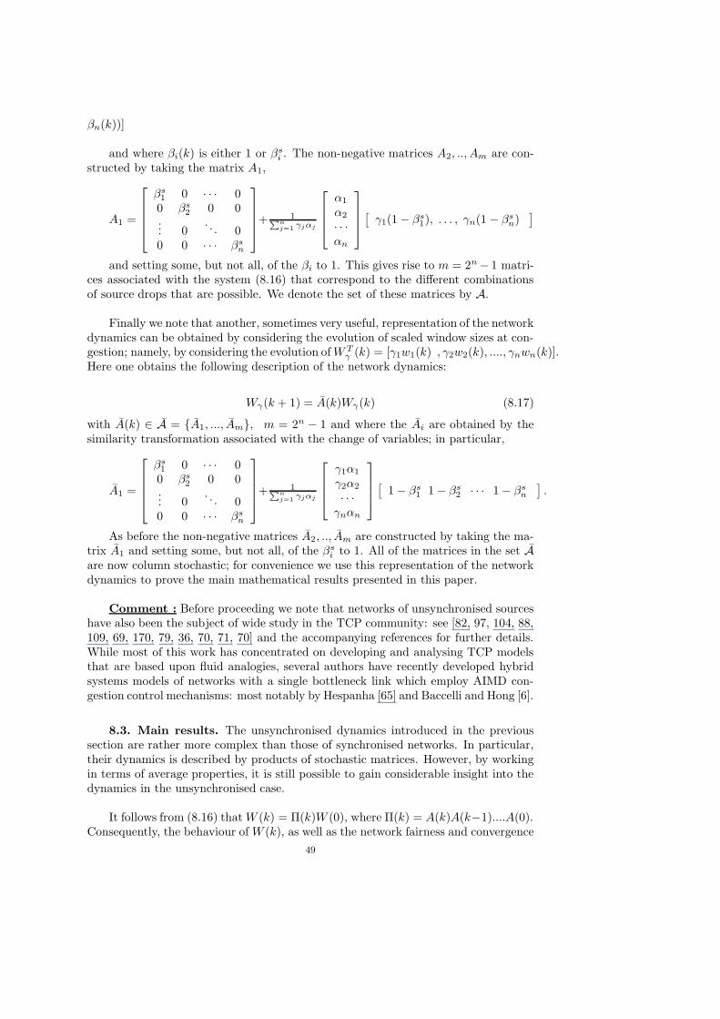
βn(k))]

and where βi(k) is either 1 or βsi . The non-negative matrices A2, .., Am are con-

structed by taking the matrix A1,

A1 =

βs1 0 · · · 00 βs

2 0 0... 0

. . . 00 0 · · · βs

n

+ 1

P

nj=1

γjαj

α1

α2

· · ·αn

[

γ1(1− βs1), . . . , γn(1− βs

n)]

and setting some, but not all, of the βi to 1. This gives rise to m = 2n− 1 matri-ces associated with the system (8.16) that correspond to the different combinationsof source drops that are possible. We denote the set of these matrices by A.

Finally we note that another, sometimes very useful, representation of the networkdynamics can be obtained by considering the evolution of scaled window sizes at con-gestion; namely, by considering the evolution of W T

γ (k) = [γ1w1(k) , γ2w2(k), ...., γnwn(k)].Here one obtains the following description of the network dynamics:

Wγ(k + 1) = A(k)Wγ(k) (8.17)

with A(k) ∈ A = A1, ..., Am, m = 2n − 1 and where the Ai are obtained by thesimilarity transformation associated with the change of variables; in particular,

A1 =

βs1 0 · · · 00 βs

2 0 0... 0

. . . 00 0 · · · βs

n

+ 1

P

nj=1

γjαj

γ1α1

γ2α2

· · ·γnαn

[

1− βs1 1− βs

2 · · · 1− βsn

].

As before the non-negative matrices A2, .., Am are constructed by taking the ma-trix A1 and setting some, but not all, of the βs

i to 1. All of the matrices in the set Aare now column stochastic; for convenience we use this representation of the networkdynamics to prove the main mathematical results presented in this paper.

Comment : Before proceeding we note that networks of unsynchronised sourceshave also been the subject of wide study in the TCP community: see [82, 97, 104, 88,109, 69, 170, 79, 36, 70, 71, 70] and the accompanying references for further details.While most of this work has concentrated on developing and analysing TCP modelsthat are based upon fluid analogies, several authors have recently developed hybridsystems models of networks with a single bottleneck link which employ AIMD con-gestion control mechanisms: most notably by Hespanha [65] and Baccelli and Hong [6].

8.3. Main results. The unsynchronised dynamics introduced in the previoussection are rather more complex than those of synchronised networks. In particular,their dynamics is described by products of stochastic matrices. However, by workingin terms of average properties, it is still possible to gain considerable insight into thedynamics in the unsynchronised case.

It follows from (8.16) that W (k) = Π(k)W (0), where Π(k) = A(k)A(k−1)....A(0).Consequently, the behaviour of W (k), as well as the network fairness and convergence

49

properties, are governed by the properties of the matrix product Π(k). The objectiveof this section is to analyse the average behaviour of Π(k) with a view to making con-crete statements about these network properties. To facilitate analytical tractabilitywe will make two mild simplifying assumptions.

Assumption 8.2. The probability that A(k) = Ai in (8.16) is independent of kand equals ρi.

In other words Assumption 8.2 says that the probability that the network dy-namics are described by W (k + 1) = A(k)W (k), A(k) = Ai over the k’th congestionepoch is ρi and that the random variables A(k), k ∈ N are independent and identicallydistributed (i.i.d.).

Given the probabilities ρi for i ∈ 1, ..., 2n − 1, one may then define the proba-bility Λj that source j experiences a backoff at the k’th congestion event as follows:

Λj =∑

ρi ,

where the summation is taken over those i which correspond to a matrix in which thej’th source sees a drop. Or to put it another way, the summation is over those indicesi for which the matrix Ai is defined with a value of βj 6= 1.

Assumption 8.3. We assume that Λj > 0 for all j ∈ 1, ..., n.

Simply stated, Assumption 8.3 states that almost surely all flows must see a dropat some time (provided that they persist for a long enough time).

Comment: A consequence of the above assumptions is that the probability thatsource j experiences a drop at the k’th congestion event is not independent of theother sources. For example, if the first n−1 sources do not see a drop then this impliesthat source n must see a drop (in accordance with the usual notion of a congestionevent, we require at least one flow to see a drop at each congestion event). Hence, theevents cannot be independent.

Under the foregoing assumptions we have the following key result.

Theorem 8.4. Consider the stochastic system defined in the above preamble. LetΠ(k) be the random matrix product arising from the evolution of the first k steps ofthis system:

Π(k) = A(k)A(k − 1)....A(0).

Then, the expectation of Π(k) is given by

E(Π(k)) = (

m∑

i=1

ρiAi)k; (8.18)

and the asymptotic behaviour of E(Π(k)) satisfies

limk→∞

E(Π(k)) = xpyTp , (8.19)

50

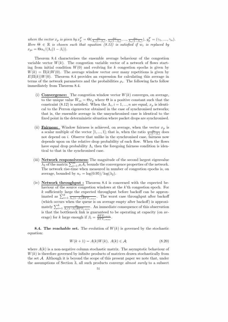
where the vector xp is given by xTp = Θ( α1

Λ1(1−β1), α2

Λ2(1−β2), ..., αn

Λn(1−βn) ), yTp = (γ1, ...., γn).

Here Θ ∈ R is chosen such that equation (8.12) is satisfied if wi is replaced byxpi = Θαi/(Λi(1− βi)).

Theorem 8.4 characterises the ensemble average behaviour of the congestionvariable vector W (k). The congestion variable vector of a network of flows start-ing from initial condition W (0) and evolving for k congestion epochs is given byW (k) = Π(k)W (0). The average window vector over many repetitions is given byE(Π(k))W (0). Theorem 8.4 provides an expression for calculating this average interms of the network parameters and the probabilities ρi. The following facts followimmediately from Theorem 8.4.

(i) Convergence: The congestion window vector W (k) converges, on average,

to the unique value Wss = Θxp where Θ is a positive constant such that theconstraint (8.12) is satisfied. When the Λi, i = 1, ..., n are equal, xp is identi-cal to the Perron eigenvector obtained in the case of synchronised networks;that is, the ensemble average in the unsynchronised case is identical to thefixed point in the deterministic situation where packet drops are synchronised.

(ii) Fairness: Window fairness is achieved, on average, when the vector xp isa scalar multiple of the vector [1, ..., 1]; that is, when the ratio αi

Λi(1−βi)does

not depend on i. Observe that unlike in the synchronised case, fairness nowdepends upon on the relative drop probability of each flow. When the flowshave equal drop probability Λi then the foregoing fairness condition is iden-tical to that in the synchronised case.

(iii) Network responsiveness: The magnitude of the second largest eigenvalueλ2 of the matrix

∑mi=1 ρiAi bounds the convergence properties of the network.

The network rise-time when measured in number of congestion epochs is, onaverage, bounded by nr = log(0.95)/ log(λ2).

(iv) Network throughput : Theorem 8.4 is concerned with the expected be-haviour of the source congestion windows at the k’th congestion epoch. Fork sufficiently large the expected throughput before backoff can be approx-imated as

∑ki=1

αi

Λi(1−βi)RTTi,max. The worst case throughput after backoff

(which occurs when the queue is on average empty after backoff) is approxi-

mately∑k

i=1αi

Λi(1−βi)RTTi,min. An immediate consequence of this observation

is that the bottleneck link is guaranteed to be operating at capacity (on av-

erage) for k large enough if βi =RTTi,min

RTTi,max.

8.4. The reachable set. The evolution of W (k) is governed by the stochasticequation:

W (k + 1) = A(k)W (k), A(k) ∈ A; (8.20)

where A(k) is a non-negative column stochastic matrix. The asymptotic behaviour ofW (k) is therefore governed by infinite products of matrices drawn stochastically fromthe set A. Although it is beyond the scope of this present paper we note that, underthe assumptions of Section 3, all such products converge almost surely to a subsect

51

of the rank-1 idempotent non-negative column stochastic matrices [151]. The imageof these matrices, projected onto the simplex

∑ni=1 γiwi(k) = B, defines the set of

reachable states for the asymptotic process. It is known that such sets can be verycomplicated; even Fractal (see Chapter 11 in [62]). For infinite products associatedwith AIMD networks this appears to be the case; an example of such an image setprojected onto the simplex

∑ni=1 γiwi(k) = B is depicted in Figure 8.4.

00.5

11.5

22.5

3

0

1

2

3

0

0.5

1

1.5

2

2.5

3

Fig. 8.3: Approximation of asymptotic image set for network of three flows. αi =1, βi = 0.25 for all i.

9. Some open problems and future directions. In this section, we shallbriefly review and summarise some of the open questions arising from the results andissues discussed throughout the paper. Broadly speaking, the major open problemsin the stability theory of switched linear systems can be divided into three categories,corresponding to the first three problems discussed at the end of Section 1; namely,the problem of stability under arbitrary switching, the dwell-time problem, and theproblem of determining stabilising switching signals.

(i) In the context of stability under arbitrary switching, Theorem 4.3 and The-orem 4.4 provide simple conditions for CQLF existence that are related tothe dynamics of switched linear systems via Theorem 4.18. While Theorem4.7 gives necessary and sufficient conditions for a general family of stable LTIsystems to have a CQLF, the conditions described by this result are extremelycomplicated and difficult to check, even for the case of a pair of third ordersystems. Hence, an open problem of some interest is to determine systemclasses, such as the class of second order systems or pairs of systems withsystem matrices differing by a rank one matrix, for which simple conditionsfor CQLF existence can be given. In this context, the work reported in [153]should be noted. In this paper, it was shown that the system classes coveredby Theorem 4.3 and Theorem 4.4 can be treated within a common frameworkprovided by the main result of [159]. This may provide some insights as tohow to obtain further system classes for which similarly simple conditions forCQLF existence can be derived.

(ii) A closely related problem to that described above is that of determiningclasses of switched linear systems for which CQLF existence is equivalent

52

to exponential stability under arbitrary switching. Two examples of suchsystem classes have been described in Section 4 above, and for such systems,the problem of determining stability under arbitrary switching is simplifiedconsiderably.

(iii) Theorem 4.22 gives a simple spectral condition for the existence of a commonpiecewise linear Lyapunov function (PLLF) for a pair of stable second orderLTI systems, and to date there are very few results of this kind available inthe literature. This gives rise to the question of whether or not it is possibleto extend this result to higher dimensional systems.

(iv) For the class of positive switched linear systems, as mentioned in Section 5,it is natural to consider co-positive Lyapunov functions. In particular, giventhat the trajectories of positive systems are constrained to remain within thenon-negative orthant, such Lyapunov functions may lead to less conservativestability criteria than those obtained through requiring CQLF existence. Thisraises the problem of determining verifiable conditions for common co-positiveLyapunov function existence for families of positive LTI systems.

(v) Apart from the above problems on stability for arbitrary switching signals, theimportant issue of determining non-conservative estimates of the dwell-timefor constrained switching regimes is still unresolved.

(vi) On the question of determining stabilising switching signals for unstable con-stituent systems, the work of Feron, Peleties, de Carlo and others discussedin Section 5 provides sufficient conditions for quadratic stabilisation laws.Also, it is known that for the case of two constituent systems, the condi-tions discussed above are both necessary and sufficient for the existence of aquadratically stabilising switching rule. To the best of the authors’ knowl-edge, necessary and sufficient conditions for the existence of a general (notnecessarily quadratic) stabilising switching law are not known. Some resultsrelated to this topic were previously mentioned in Section 5, where appropri-ate references were also given.

Acknowledgements. This work was partially supported by the European Unionfunded research training network Multi-Agent Control, HPRN-CT-1999-0010711 andby the Enterprise Ireland grant SC/2000/084/Y.

REFERENCES

[1] J. K. Aggarwal and M. Vidyasagar, eds., Nonlinear Systems - Stability Analyis, Dowden,Hutchinson and Ross Inc., 1977.

[2] A. A. Agrachev and D. Liberzon, Lie-algebraic stability criteria for switched systems,SIAM Journal of Control and Optimization, 40 (2001), pp. 253–269.

[3] M. A. Aizerman, On a problem relating to the ’global’ stability of dynamic systems, Usp.Matem. Nauk., 4 (1949), pp. 187–188.

[4] E. Altman, T. Jimenez, and R. Nunez-Queija, Analysis of two competing TCP/IP connec-tions, Perform. Evaluation, 49 (2002), pp. 43–55.

[5] J.-P. Aubin and A. Cellina, Differential Inclusions: Set-Valued Maps and Viability Theory,Springer-Verlag, Berlin, 1984.

[6] F. Baccelli and D. Hong, AIMD, Fairness and Fractal Scaling of TCP traffic, in Proceed-ings of IEEE INFOCOM, New York, NY, USA, June 2002, pp. 229–238.

[7] , Interaction of TCP flows as billiards, in Proceedings of IEEE INFOCOM, San Fran-cisco, CA, USA, March/April 2003, pp. 895–905.

11This work is the sole responsibility of the authors and does not reflect the European Union’sopinion. The EU is not responsible for any use of data appearing in this publication.

53

[8] A. Bacciotti, Stabilization by means of state space depending switching rules, Systems andControl Letters, 53 (2004), pp. 195–201.

[9] P. Baldi and G. Hatfield, DNA microarrays and gene expression, Cambridge UniversityPress, 2002.

[10] N. E. Barabanov, Lyapunov indicator of discrete inclusions I, Avtomatika i Telemekhanika(translation), (1988), pp. 40–46.

[11] , An absolute characteristic exponent of a class of linear nonstationary systems ofdifferential equations, Siberian Math. J., 29 (1989), pp. 521–530.

[12] , A method for calculating the Lyapunov exponent of a differential inclusion, Automa-tion and Remote Control, 50 (1989), pp. 475–479.

[13] , On the Aızerman problem for third-order time-dependent systems, Differential Equa-tions, 29 (1993), pp. 1439–1448.

[14] M. A. Berger and Y. Wang, Bounded semigroups of matrices, Linear Algebra and itsApplications, 166 (1992), pp. 21–27.

[15] A. Berman and R. Plemmons, Nonnegative matrices in the mathematical sciences, SIAM,1979.

[16] A. Berman, R. Shorten, and D. Leith, Positive matrices associated with synchronisedcommunication networks, Linear Algebra and its Applications, 393 (2004), pp. 47–55.

[17] F. Blanchini, Set invariance in control, Automatica, 35 (1999), pp. 1747–1767.[18] V. D. Blondel, E. D. Sontag, M. Vidyasagar, and J. C. Willems, Open Problems in

Mathematical Systems and Control Theory, Springer, 1998.[19] V. D. Blondel, J. Theys, and J. Tsitsiklis, Unsolved problems in Mathematical Systems

& Control Theory, Princeton Uiversity Press, Princeton, NJ, 2004, ch. When is a pair ofmatrices stable ?, pp. 304–308.

[20] V. D. Blondel, J. Theys, and A. A. Vladimirov, Switched systems that are periodicallystable may be unstable, in Fifteenth International Symposium on Mathematical Theoryof Networks and Systems, University of Notre Dame, IN, 2002.

[21] , An elementary counterexample to the finiteness conjecture, SIAM Journal of MatrixAnalysis and Applications, 24 (2003), pp. 963–970.

[22] V. D. Blondel and J. N. Tsitsiklis, Complexity of stability and controllability of elementaryhybrid systems, Automatica, 35 (1999), pp. 479–489.

[23] , The boundedness of all products of a pair of matrices is undecidable, Systems ControlLett., 41 (2000), pp. 135–140.

[24] , A survey of computational complexity results in systems and control, Automatica, 36(2000), pp. 479–489.

[25] O. N. Bobyleva, Piecewise-linear Lyapunov functions for linear stationary systems, Au-tomation and Remote Control, 63 (2002), pp. 540–549.

[26] O. N. Bobyleva and E. S. Pyatnitskii, Piecewise-linear Lyapunov functions and localizationof spectra of stable matrices, Automation and Remote Control, 62 (2001), pp. 1417–1427.

[27] T. Bousch and J. Mairesse, Asymptotic height optimization for topical IFS, Tetris heapsand the finiteness conjecture, Journal of the AMS, 15 (2002), pp. 77–111.

[28] S. Boyd, L. El Ghaoui, E. Feron, and V. Balakrishnan, Linear Matrix Inequalities inSystem and Control Theory, SIAM, Philadelphia, 1994.

[29] M. S. Branicky, Stability of switched and hybrid systems, Tech. Report LIDS-P-2214, Lab-oratory for Information and Decision Science, MIT, 1993.

[30] , Multiple Lyapunov functions and other analysis tools for switched and hybrid systems,IEEE Trans. on Automatic Control, 43 (1998), pp. 475–482.

[31] R. Brayton and C. Tong, Stability of dynamical systems: A constructive approach, IEEETransactions on Circuits and Systems, 26 (1979), pp. 224–234.

[32] , Constructive stability and asymptotic stability of dynamical systems: A constructiveapproach, IEEE Transactions on Circuits and Systems, 27 (1980), pp. 1121–1131.

[33] S. Brin and L. Page, The anatomy of a large-scale hypertextual Web search engine, Com-puter Networks and ISDN Systems, 30 (1998), pp. 107–117.

[34] R. W. Brockett, Optimization theory and the converse of the Circle Criterion, in Proceed-ings of National Electronic Conference, 1965, pp. 697–701.

[35] P. Brown, Resource sharing of TCP connections with different round trip times, in Proceed-ings of IEEE INFOCOM, Tel Aviv, Israel, March 2000.

[36] Y. Chait, C. V. Hollot, V. Misra, H. Han, and Y. Halevi, Dynamic analysis of congestedTCP networks, in Proceedings of American Control Conference, 1999.

[37] C. Chase, J. Serrano, and P. Ramadge, Periodicity and chaos from switched flow systems:contrasting examples of discretely controlled continuous systems, IEEE Transactions onAutomatic Control, 38 (1993), pp. 70–83.

54

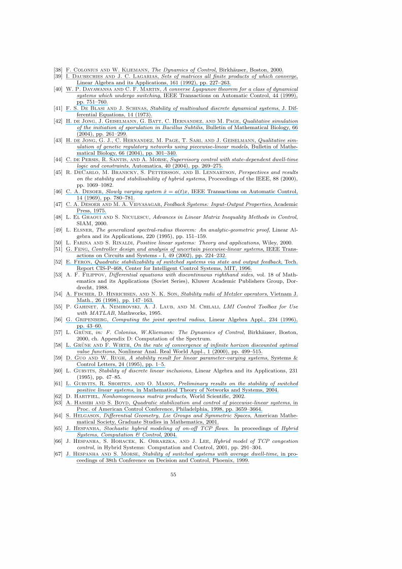
[38] F. Colonius and W. Kliemann, The Dynamics of Control, Birkhauser, Boston, 2000.[39] I. Daubechies and J. C. Lagarias, Sets of matrices all finite products of which converge,

Linear Algebra and its Applications, 161 (1992), pp. 227–263.[40] W. P. Dayawansa and C. F. Martin, A converse Lyapunov theorem for a class of dynamical

systems which undergo switching, IEEE Transactions on Automatic Control, 44 (1999),pp. 751–760.

[41] F. S. De Blasi and J. Schinas, Stability of multivalued discrete dynamical systems, J. Dif-ferential Equations, 14 (1973).

[42] H. de Jong, J. Geiselmann, G. Batt, C. Hernandez, and M. Page, Qualitative simulationof the initiation of sporulation in Bacillus Subtilis, Bulletin of Mathematical Biology, 66(2004), pp. 261–299.

[43] H. de Jong, G. J., C. Hernandez, M. Page, T. Sari, and J. Geiselmann, Qualitative sim-ulation of genetic regulatory networks using piecewise-linear models, Bulletin of Mathe-matical Biology, 66 (2004), pp. 301–340.

[44] C. de Persis, R. Santis, and A. Morse, Supervisory control with state-dependent dwell-timelogic and constraints, Automatica, 40 (2004), pp. 269–275.

[45] R. DeCarlo, M. Branicky, S. Pettersson, and B. Lennartson, Perspectives and resultson the stability and stabilisability of hybrid systems, Proceedings of the IEEE, 88 (2000),pp. 1069–1082.

[46] C. A. Desoer, Slowly varying system x = a(t)x, IEEE Transactions on Automatic Control,14 (1969), pp. 780–781.

[47] C. A. Desoer and M. A. Vidyasagar, Feedback Systems: Input-Output Properties, AcademicPress, 1975.

[48] L. El Ghaoui and S. Niculescu, Advances in Linear Matrix Inequality Methods in Control,SIAM, 2000.

[49] L. Elsner, The generalized spectral-radius theorem: An analytic-geometric proof, Linear Al-gebra and its Applications, 220 (1995), pp. 151–159.

[50] L. Farina and S. Rinaldi, Positive linear systems: Theory and applications, Wiley, 2000.[51] G. Feng, Controller design and analysis of uncertain piecewise-linear systems, IEEE Trans-

actions on Circuits and Systems - I, 49 (2002), pp. 224–232.[52] E. Feron, Quadratic stabilizability of switched systems via state and output feedback, Tech.

Report CIS-P-468, Center for Intelligent Control Systems, MIT, 1996.[53] A. F. Filippov, Differential equations with discontinuous righthand sides, vol. 18 of Math-

ematics and its Applications (Soviet Series), Kluwer Academic Publishers Group, Dor-drecht, 1988.

[54] A. Fischer, D. Hinrichsen, and N. K. Son, Stability radii of Metzler operators, Vietnam J.Math., 26 (1998), pp. 147–163.

[55] P. Gahinet, A. Nemirovski, A. J. Laub, and M. Chilali, LMI Control Toolbox for Usewith MATLAB, Mathworks, 1995.

[56] G. Gripenberg, Computing the joint spectral radius, Linear Algebra Appl., 234 (1996),pp. 43–60.

[57] L. Grune, in: F. Colonius, W.Kliemann: The Dynamics of Control, Birkhauser, Boston,2000, ch. Appendix D: Computation of the Spectrum.

[58] L. Grune and F. Wirth, On the rate of convergence of infinite horizon discounted optimalvalue functions, Nonlinear Anal. Real World Appl., 1 (2000), pp. 499–515.

[59] D. Guo and W. Rugh, A stability result for linear parameter-varying systems, Systems &Control Letters, 24 (1995), pp. 1–5.

[60] L. Gurvits, Stability of discrete linear inclusions, Linear Algebra and its Applications, 231(1995), pp. 47–85.

[61] L. Gurvits, R. Shorten, and O. Mason, Preliminary results on the stability of switchedpositive linear systems, in Mathematical Theory of Networks and Systems, 2004.

[62] D. Hartfiel, Nonhomogeneous matrix products, World Scientific, 2002.[63] A. Hassibi and S. Boyd, Quadratic stabilization and control of piecewise-linear systems, in

Proc. of American Control Conference, Philadelphia, 1998, pp. 3659–3664.[64] S. Helgason, Differential Geometry, Lie Groups and Symmetric Spaces, American Mathe-

matical Society, Graduate Studies in Mathematics, 2001.[65] J. Hespanha, Stochastic hybrid modeling of on-off TCP flows. In proceedings of Hybrid

Systems, Computation & Control, 2004.[66] J. Hespanha, S. Hohacek, K. Obrarzka, and J. Lee, Hybrid model of TCP congestion

control, in Hybrid Systems: Computation and Control, 2001, pp. 291–304.[67] J. Hespanha and S. Morse, Stability of switched systems with average dwell-time, in pro-

ceedings of 38th Conference on Decision and Control, Phoenix, 1999.

55

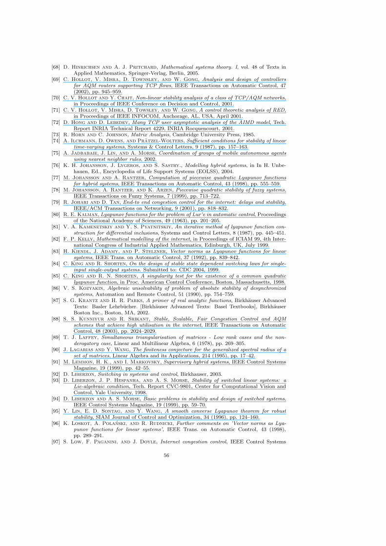
[68] D. Hinrichsen and A. J. Pritchard, Mathematical systems theory. I, vol. 48 of Texts inApplied Mathematics, Springer-Verlag, Berlin, 2005.

[69] C. Hollot, V. Misra, D. Townsley, and W. Gong, Analysis and design of controllersfor AQM routers supporting TCP flows, IEEE Transactions on Automatic Control, 47(2002), pp. 945–959.

[70] C. V. Hollot and Y. Chait, Non-linear stability analysis of a class of TCP/AQM networks,in Proceedings of IEEE Conference on Decision and Control, 2001.

[71] C. V. Hollot, V. Misra, D. Towsley, and W. Gong, A control theoretic analysis of RED,in Proceedings of IEEE INFOCOM, Anchorage, AL, USA, April 2001.

[72] D. Hong and D. Lebedev, Many TCP user asymptotic analysis of the AIMD model, Tech.Report INRIA Technical Report 4229, INRIA Rocquencourt, 2001.

[73] R. Horn and C. Johnson, Matrix Analysis, Cambridge University Press, 1985.[74] A. Ilchmann, D. Owens, and Pratzel-Wolters, Sufficient conditions for stability of linear

time-varying systems, Systems & Control Letters, 9 (1987), pp. 157–163.[75] A. Jadbabaie, J. Lin, and A. Morse, Coordination of groups of mobile autonomous agents

using nearest neighbor rules, 2002.[76] K. H. Johansson, J. Lygeros, and S. Sastry., Modelling hybrid systems, in In H. Unbe-

hauen, Ed., Encyclopedia of Life Support Systems (EOLSS), 2004.[77] M. Johansson and A. Rantzer, Computation of piecewise quadratic Lyapunov functions

for hybrid systems, IEEE Transactions on Automatic Control, 43 (1998), pp. 555–559.[78] M. Johansson, A. Rantzer, and K. Arzen, Piecewise quadratic stability of fuzzy systems,

IEEE Transactions on Fuzzy Systems, 7 (1999), pp. 713–722.[79] R. Johari and D. Tan, End-to end congestion control for the internet: delays and stability,

IEEE/ACM Transactions on Networking, 9 (2001), pp. 818–832.[80] R. E. Kalman, Lyapunov functions for the problem of Lur’e in automatic control, Proceedings

of the National Academy of Sciences, 49 (1963), pp. 201–205.[81] V. A. Kamenetskiy and Y. S. Pyatnitskiy, An iterative method of lyapunov function con-

struction for differential inclusions, Systems and Control Letters, 8 (1987), pp. 445–451.[82] F. P. Kelly, Mathematical modelling of the internet, in Proceedings of ICIAM 99, 4th Inter-

national Congress of Industrial Applied Mathematics, Edinburgh, UK, July 1999.[83] H. Kiendl, J. Adamy, and P. Stelzner, Vector norms as Lyapunov functions for linear

systems, IEEE Trans. on Automatic Control, 37 (1992), pp. 839–842.[84] C. King and R. Shorten, On the design of stable state dependent switching laws for single-

input single-output systems. Submitted to: CDC 2004, 1999.[85] C. King and R. N. Shorten, A singularity test for the existence of a common quadratic

lyapunov function, in Proc. American Control Conference, Boston, Massachusetts, 1998.[86] V. S. Kozyakin, Algebraic unsolvability of problem of absolute stability of desynchronized

systems, Automation and Remote Control, 51 (1990), pp. 754–759.[87] S. G. Krantz and H. R. Parks, A primer of real analytic functions, Birkhauser Advanced

Texts: Basler Lehrbucher. [Birkhauser Advanced Texts: Basel Textbooks], BirkhauserBoston Inc., Boston, MA, 2002.

[88] S. S. Kunniyur and R. Srikant, Stable, Scalable, Fair Congestion Control and AQMschemes that achieve high utilisation in the internet, IEEE Transactions on AutomaticControl, 48 (2003), pp. 2024–2029.

[89] T. J. Laffey, Simultaneous triangularisation of matrices - Low rank cases and the non-derogatory case, Linear and Multilinear Algebra, 6 (1978), pp. 269–305.

[90] J. Lagarias and Y. Wang, The finiteness conjecture for the generalized spectral radius of aset of matrices, Linear Algebra and its Applications, 214 (1995), pp. 17–42.

[91] M. Lemmon, H. K., and I. Markovsky, Supervisory hybrid systems, IEEE Control SystemsMagazine, 19 (1999), pp. 42–55.

[92] D. Liberzon, Switching in systems and control, Birkhauser, 2003.[93] D. Liberzon, J. P. Hespanha, and A. S. Morse, Stability of switched linear systems: a

Lie-algebraic condition, Tech. Report CVC-9801, Center for Computational Vision andControl, Yale University, 1998.

[94] D. Liberzon and A. S. Morse, Basic problems in stability and design of switched systems,IEEE Control Systems Magazine, 19 (1999), pp. 59–70.

[95] Y. Lin, E. D. Sontag, and Y. Wang, A smooth converse Lyapunov theorem for robuststability, SIAM Journal of Control and Optimization, 34 (1996), pp. 124–160.

[96] K. Loskot, A. Polanski, and R. Rudnicki, Further comments on ’Vector norms as Lya-punov functions for linear systems’, IEEE Trans. on Automatic Control, 43 (1998),pp. 289–291.

[97] S. Low, F. Paganini, and J. Doyle, Internet congestion control, IEEE Control Systems

56

Magazine, 32 (2002), pp. 28–43.[98] D. G. Luenberger, Introduction to Dynamic Systems, John Wiley & Sons, New York, 1979.[99] A. I. Lur’e and V. N. Postnikov, On the theory of stability of control systems, Prikl. Mat.

i Mehk., 3 (1944).[100] A. M. Lyapunov, The general problem of the stability of motion (English translations), Taylor

and Francis, 1892.[101] M. Maesumi, An efficient lower bound for the generalized spectral radius of a set of matrices,

Linear Algebra and its Applications, 240 (1996), pp. 1–7.[102] J. L. Mancilla-Aguilar and R. A. Garcia, A converse Lyapunov theorem for nonlinear

switched systems, Systems and Control Letters, 41 (2000), pp. 67–71.[103] , On converse Lyapunov theorems for ISS and iISS switched nonlinear systems, Systems

and Control Letters, 42 (2001), pp. 47–53.[104] S. Mascolo, Congestion control in high speed communication networks using the Smith prin-

ciple, Automatica, 35 (1999), pp. 1921,1935.[105] O. Mason and R. Shorten, Some results on the stability of positive switched linear systems,

in IEEE Conference on Decision and Control, Bahamas, 2004.[106] O. Mason and R. N. Shorten, The geometry of convex cones associated with the lyapunov

inequality and common lyapunov functions, Electronic Journal of Linear Algebra, (2005).accepted.

[107] O. Mason, R. N. Shorten, and D. Leith, Evaluation of piecewise quadratic methods appliedto the wind-turbine benchmark example, Tech. Report NUIM-SS-2001-11, Signals andSystems Group, NUI Maynooth, 2001.

[108] P. Mason, U. Boscain, and Y. Chitour, On the minimal degree of a common lyapunovfunction for planar switched systems, in Proc. Conference on Decision and Control, Ba-hamas, 2004, pp. 2786 – 2791.

[109] L. Massoulie, Stability of distributed congestion control with heterogeneous feedback delays,IEEE Transactions on Automatic Control, 47 (2002), pp. 895–902.

[110] A. I. Mees and A. R. Bergen, Describing functions revisited, IEEE Transactions on Auto-matic Control, 20 (1975), pp. 473–478.

[111] G. Michaletzky and L. Gerencser, BIBO stability of linear switching systems, IEEE Trans.Automat. Control, 47 (2002), pp. 1895–1898.

[112] A. Michel, Recent trends in the stability analysis of hybrid dynamical systems, IEEE Trans-actions on Circuits and Systems, 45 (1998), pp. 120–133.

[113] R. Mohler, Nonlinear Systems: Dynamics and Control, Prentice Hall, 1991.[114] A. P. Molchanov and E. S. Pyatnitskii, Lyapunov functions that specify necessary and

sufficient conditions of absolute stability of nonlinear nonstationary control systems III,Automation and Remote Control, 47 (1986), pp. 620–630.

[115] A. P. Molchanov and E. S. Pyatnitskii, Criteria of asymptotic stability of differential anddifference inclusions encountered in control theory, Systems & Control Letters, 13 (1989),pp. 59–64.

[116] Y. Mori, T. Mori, and Y. Kuroe, A solution to the common Lyapunov function problem forcontinuous time systems, in Proc. 36th Conference on Decision and Control, San Diego,December 1997, pp. 3530–3531.

[117] A. S. Morse, Supervisory control of families of linear set-point controllers - part 1: Exactmatching, IEEE Transactions on Automatic Control, 41 (1996), pp. 1413–1431.

[118] K. S. Narendra and J. Balakrishnan, A common Lyapunov function for stable LTI systemswith commuting A-matrices, IEEE Trans. on Automatic Control, 39 (1994), pp. 2469–2471.

[119] K. S. Narendra and R. M. Goldwyn, A geometrical criterion for the stability of certainnon-linear non-autonomous systems, IEEE Transactions on Circuit Theory, 11 (1964),pp. 406–407.

[120] K. S. Narendra and J. H. Taylor, Frequency Domain Criteria for Absolute Stability, Aca-demic Press, 1973.

[121] Y. Ohta, H. Imanishi, L. Gong, and H. Haneda, Computer generated Lyapunov functionsfor a class of nonlinear systems, IEEE Trans. on Circuits and Systems, 40 (1993), pp. 343–354.

[122] T. Ooba and Y. Funahashi, On a common quadratic Lyapunov function for widely distantsystems, IEEE Transactions on Automatic Control, 42 (1997), pp. 1697–1699.

[123] , Stability robustness for linear state space models - a Lyapunov mapping approach,Systems & Control Letters, 29 (1997), pp. 191–196.

[124] , Two conditions concerning common quadratic Lyapunov functions for linear systems,IEEE Transactions on Automatic Control, 42 (1997), pp. 719–721.

57

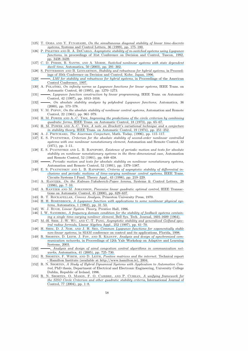
[125] T. Ooba and Y. Funahashi, On the simultaneous diagonal stability of linear time-discretesystems, Systems and Control Letters, 36 (1999), pp. 175–180.

[126] P. Peleties and R. A. DeCarlo, Asymptotic stability of m-switched systems using Lyapunovfunctions, in proceedings of 31st Conference on Decision and Control, Tuscon, 1992,pp. 3438–3439.

[127] C. D. Persis, R. Santis, and A. Morse, Switched nonlinear systems with state dependentdwell time, Automatica, 50 (2003), pp. 291–302.

[128] S. Pettersson and B. Lennartson, Stability and robustness for hybrid systems, in Proceed-ings of 35th Conference on Decision and Control, Kobe, Japan, 1996.

[129] , LMI for stability and robustness for hybrid systems, in Proceedings of the AmericanControl Conference, 1997.

[130] A. Polanski, On infinity norms as Lyapunov functions for linear systems, IEEE Trans. onAutomatic Control, 40 (1995), pp. 1270–1273.

[131] , Lyapunov function construction by linear programming, IEEE Trans. on AutomaticControl, 42 (1997), pp. 1013–1016.

[132] , On absolute stability analysis by polyhedral Lyapunov functions, Automatica, 36(2000), pp. 573–578.

[133] V. M. Popov, On the absolute stability of nonlinear control systems, Automation and RemoteControl, 22 (1961), pp. 961–979.

[134] H. M. Power and A.-C. Tsoi, Improving the predictions of the circle criterion by combiningquadratic forms, IEEE Trans. on Automatic Control, 18 (1973), pp. 65–67.

[135] H. M. Power and A.-C. Tsoi, A note on Brockett’s variational technique and a conjecturein stability theory, IEEE Trans. on Automatic Control, 19 (1974), pp. 251–252.

[136] A. J. Pritchard, The Aizerman Conjecture, Math. Today, (1996), pp. 115–117.[137] E. S. Pyatnitskii, Criterion for the absolute stability of second-order nonlinear controlled

systems with one nonlinear nonstationary element, Automation and Remote Control, 32(1971), pp. 1–11.

[138] E. S. Pyatnitskii and L. B. Rapoport, Existence of periodic motion and tests for absolutestability on nonlinear nonstationary systems in the three-dimensional case, Automationand Remote Control, 52 (1991), pp. 648–658.

[139] , Periodic motion and tests for absolute stability on nonlinear nonstationary systems,Automation and Remote Control, 52 (1991), pp. 1379–1387.

[140] E. S. Pyatnitskiy and L. B. Rapoport, Criteria of asymptotic stability of differential in-clusions and periodic motions of time-varying nonlinear control systems, IEEE Trans.Circuits Systems I Fund. Theory Appl., 43 (1996), pp. 219–229.

[141] A. Rantzer, On the Kalman-Yakubovich-Popov lemma, Systems & Control Letters, 28(1996), pp. 7–10.

[142] A. Rantzer and M. Johansson, Piecewise linear quadratic optimal control, IEEE Transac-tions on Automatic Control, 45 (2000), pp. 629–637.

[143] R. T. Rockafellar, Convex Analysis, Princeton University Press, 1970.[144] H. H. Rosenbrock, A Lyapunov function with applications to some nonlinear physical sys-

tems, Automatica, 1 (1962), pp. 31–53.[145] W. J. Rugh, Linear System Theory, Prentice Hall, 1996.[146] I. W. Sandberg, A frequency domain condition for the stability of feedback systems contain-

ing a single time-varying nonliner element, Bell Sys. Tech. Journal, 1601-1609 (1964).[147] M.-H. Shih, J.-W. Wu, and C.-T. Pang, Asymptotic stability and generalized Gelfand spec-

tral radius formula, Linear Algebra Appl., 252 (1997), pp. 61–70.[148] H. Shim, D. J. Noh, and J. H. Seo, Common Lyapunov functions for exponentially stable

non-linear systems, in SIAM conference on control and its applications, Florida, 1998.[149] R. Shorten, D. Leith, J. Foy, and R. Kilduff, Analysis and design of synchronised com-

munication networks, in Proceedings of 12th Yale Workshop on Adaptive and LearningSystems, 2003.

[150] , Analysis and design of aimd congestion control algorithms in communication net-works, Automatica, 41 (2005), pp. 725–730.

[151] R. Shorten, F. Wirth, and D. Leith, Positive matrices and the internet. Technical report- Hamilton Institute (available at http://www.hamilton.ie), 2004.

[152] R. N. Shorten, A Study of Hybrid Dynamical Systems with Application to Automotive Con-trol, PhD thesis, Department of Electrical and Electronic Engineering, University CollegeDublin, Republic of Ireland, 1996.

[153] R. N. Shorten, O. Mason, F. O. Cairbre, and P. Curran, A unifying framework forthe SISO Circle Criterion and other quadratic stability criteria, International Journal ofControl, 77 (2004), pp. 1–8.

58

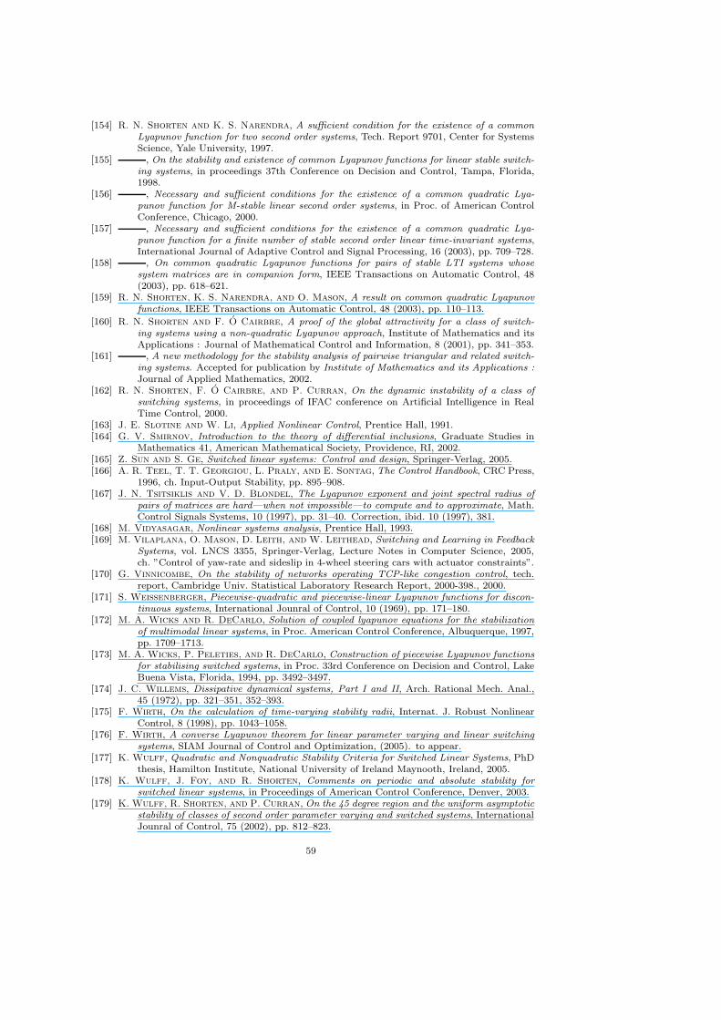
[154] R. N. Shorten and K. S. Narendra, A sufficient condition for the existence of a commonLyapunov function for two second order systems, Tech. Report 9701, Center for SystemsScience, Yale University, 1997.

[155] , On the stability and existence of common Lyapunov functions for linear stable switch-ing systems, in proceedings 37th Conference on Decision and Control, Tampa, Florida,1998.

[156] , Necessary and sufficient conditions for the existence of a common quadratic Lya-punov function for M-stable linear second order systems, in Proc. of American ControlConference, Chicago, 2000.

[157] , Necessary and sufficient conditions for the existence of a common quadratic Lya-punov function for a finite number of stable second order linear time-invariant systems,International Journal of Adaptive Control and Signal Processing, 16 (2003), pp. 709–728.

[158] , On common quadratic Lyapunov functions for pairs of stable LTI systems whosesystem matrices are in companion form, IEEE Transactions on Automatic Control, 48(2003), pp. 618–621.

[159] R. N. Shorten, K. S. Narendra, and O. Mason, A result on common quadratic Lyapunovfunctions, IEEE Transactions on Automatic Control, 48 (2003), pp. 110–113.

[160] R. N. Shorten and F. O Cairbre, A proof of the global attractivity for a class of switch-ing systems using a non-quadratic Lyapunov approach, Institute of Mathematics and itsApplications : Journal of Mathematical Control and Information, 8 (2001), pp. 341–353.

[161] , A new methodology for the stability analysis of pairwise triangular and related switch-ing systems. Accepted for publication by Institute of Mathematics and its Applications :Journal of Applied Mathematics, 2002.

[162] R. N. Shorten, F. O Cairbre, and P. Curran, On the dynamic instability of a class ofswitching systems, in proceedings of IFAC conference on Artificial Intelligence in RealTime Control, 2000.

[163] J. E. Slotine and W. Li, Applied Nonlinear Control, Prentice Hall, 1991.[164] G. V. Smirnov, Introduction to the theory of differential inclusions, Graduate Studies in

Mathematics 41, American Mathematical Society, Providence, RI, 2002.[165] Z. Sun and S. Ge, Switched linear systems: Control and design, Springer-Verlag, 2005.[166] A. R. Teel, T. T. Georgiou, L. Praly, and E. Sontag, The Control Handbook, CRC Press,

1996, ch. Input-Output Stability, pp. 895–908.[167] J. N. Tsitsiklis and V. D. Blondel, The Lyapunov exponent and joint spectral radius of

pairs of matrices are hard—when not impossible—to compute and to approximate, Math.Control Signals Systems, 10 (1997), pp. 31–40. Correction, ibid. 10 (1997), 381.

[168] M. Vidyasagar, Nonlinear systems analysis, Prentice Hall, 1993.[169] M. Vilaplana, O. Mason, D. Leith, and W. Leithead, Switching and Learning in Feedback

Systems, vol. LNCS 3355, Springer-Verlag, Lecture Notes in Computer Science, 2005,ch. ”Control of yaw-rate and sideslip in 4-wheel steering cars with actuator constraints”.

[170] G. Vinnicombe, On the stability of networks operating TCP-like congestion control, tech.report, Cambridge Univ. Statistical Laboratory Research Report, 2000-398., 2000.

[171] S. Weissenberger, Piecewise-quadratic and piecewise-linear Lyapunov functions for discon-tinuous systems, International Jounral of Control, 10 (1969), pp. 171–180.

[172] M. A. Wicks and R. DeCarlo, Solution of coupled lyapunov equations for the stabilizationof multimodal linear systems, in Proc. American Control Conference, Albuquerque, 1997,pp. 1709–1713.

[173] M. A. Wicks, P. Peleties, and R. DeCarlo, Construction of piecewise Lyapunov functionsfor stabilising switched systems, in Proc. 33rd Conference on Decision and Control, LakeBuena Vista, Florida, 1994, pp. 3492–3497.

[174] J. C. Willems, Dissipative dynamical systems, Part I and II, Arch. Rational Mech. Anal.,45 (1972), pp. 321–351, 352–393.

[175] F. Wirth, On the calculation of time-varying stability radii, Internat. J. Robust NonlinearControl, 8 (1998), pp. 1043–1058.

[176] F. Wirth, A converse Lyapunov theorem for linear parameter varying and linear switchingsystems, SIAM Journal of Control and Optimization, (2005). to appear.

[177] K. Wulff, Quadratic and Nonquadratic Stability Criteria for Switched Linear Systems, PhDthesis, Hamilton Institute, National University of Ireland Maynooth, Ireland, 2005.

[178] K. Wulff, J. Foy, and R. Shorten, Comments on periodic and absolute stability forswitched linear systems, in Proceedings of American Control Conference, Denver, 2003.

[179] K. Wulff, R. Shorten, and P. Curran, On the 45 degree region and the uniform asymptoticstability of classes of second order parameter varying and switched systems, InternationalJounral of Control, 75 (2002), pp. 812–823.

59

[180] L. Xie, S. Shishkin, and M. Fu, Piecewise Lyapunov functions for robust stability of lineartime-varying systems, Systems & Control Letters, 37 (1997), pp. 165–171.

[181] L. Xu, K. Harfoush, and I. Rhee, Binary increase congestion control for fast long-distancenetworks. Proceedings of IEEE INFOCOM, 2004.

[182] H. Ye, A. N. Michel, and L. Hou, Stability theory for hybrid dynamical systems, IEEETransactions on Automatic Control, 43 (1998), pp. 461–474.

[183] R. K. Yedavalli, Ultimate boundedness control of linear switched systems using controlleddwell time approach, in Proc. of 40th Conf. on Decision and Control, Orlando, Florida,2001.

[184] C. Yfoulis, Stabilizing of Nonlinear Systems: the piecewise linear approach, Research StudiesPress Limited, Hertfordshire, England, 2001.

[185] C. Yfoulis, A. Muir, N. Pettit, and P. Wellstead, Stabilization of orthogonal piece-wise linear systems using piecewise linear Lyapunov-like functions, in proceedings 37thConference on Decision and Control, Tampa, Florida, 1998.

[186] C. Yfoulis, A. Muir, and P. Wellstead, A new approach for estimating controllable andrecoverable regions for systems with state and control constraints, International Journalof Robust and Nonlinear Control, 12 (2002), pp. 561–589.

[187] C. Yfoulis and R. Shorten, A numerical technique for the stability analysis of linearswitched systems, International Jounral of Control, 77 (2004), pp. 1019–1039.

[188] G. Zames, On the input-output stability of nonlinear time-varying feedback systems: Part Iand II, IEEE Trans. on Automatic Control, 11 (1966), pp. 228–238, 465–477.

[189] G. Zhai, B. Ho, K. Yasuda, and A. N. Michel, L2 gain analysis of switched systems withaverage dwell time, Transactions of the Society of Instrument and Control Engineers, 36(2000), pp. 937 – 942.

[190] , Piecewise Lyapunov functions for switched systems with average dwell time, AsianJournal of Control, 2 (2000), pp. 192–197.

[191] J. Zheng, General lemmas for stability analysis of linear continuous-time systems with slowlytime-varying parameters, International Journal of Control, 58 (1993), pp. 1437–1444.

60