Embed Size (px)
Citation preview

6.1 SESSION A SUBMITTALS
Session A, Submittal No. 1
Daniel J. McCleese Jet Propulsion Laboratory/California Institute of Technology
91

<.0. 1\)
MARS GLOBAL NETWORK MISSION WORKSHOP
SCIENCE AND EXPLORATION
SCIENCE OBJECTIVES
{From a presentation by Squyres and Carr)
{Meteorology, Volatiles, Climatology, Chemistry, Mineralogy, Imaging, Seismology, Aeronomy)
ROLE ORBITER
Aeronomy
Lower atmosphere, Climatology
Other (Imaging)
DJMcC 2/6/90-1

~PL MARS GLOBAL NETWORK MISSION WORKSHOP
SCIENCE AND EXPLORATION
IMPLEMENTATION APPROACH
Number of Sites
Placement and Site Selection
Relationship to other missions (e.g., Sample Return)
Targeting
Landers or Penetrators
Balloons
DJMcC 2/6/90-2
Session A, Submittal No. 2
Francis M. Sturms Jef Propulsion Laboratory/California Institute of Technology
: ':' .
95
<.0 0')
..JPL
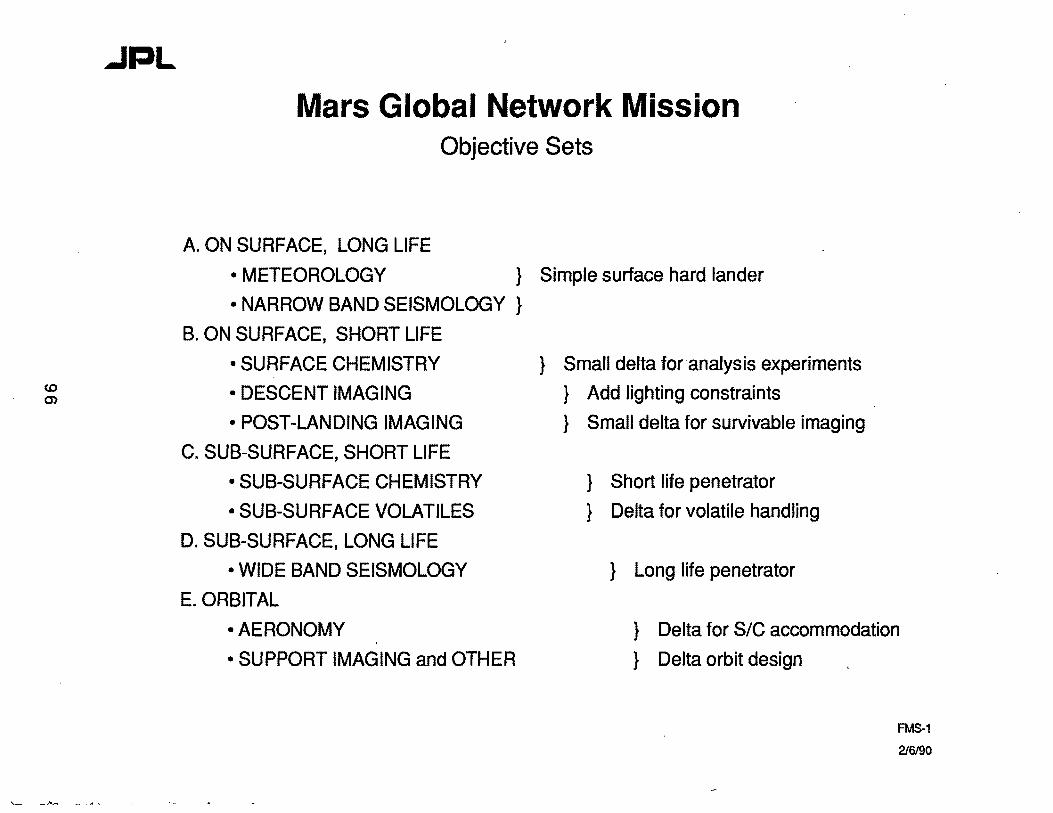
Mars Global Network Mission Objective Sets
A. ON SURFACE, LONG LIFE
• METEOROLOGY } Simple surface hard lander
• NARROW BAND SEISMOLOGY }
B. ON SURFACE, SHORT LIFE
• SURFACE CHEMISTRY
• DESCENT IMAGING
• POST-LANDING IMAGING
C. SUB-SURFACE, SHORT LIFE
• SUB-SURFACE CHEMISTRY
• SUB-SURFACE VOLATILES
D. SUB-SURFACE, LONG LIFE
• WIDE BAND SEISMOLOGY
E. ORBITAL
} Small delta foranalysis experiments
} Add lighting constraints
} Small delta for survivable imaging
} Short life penetrator
} Delta for volatile handling
} Long life penetrator
•AERONOMY
• SUPPORT IMAGING and OTHER
} Delta for SIC accommodation
} Delta orbit design
FM5-1
2/6/90
..JPL
----------
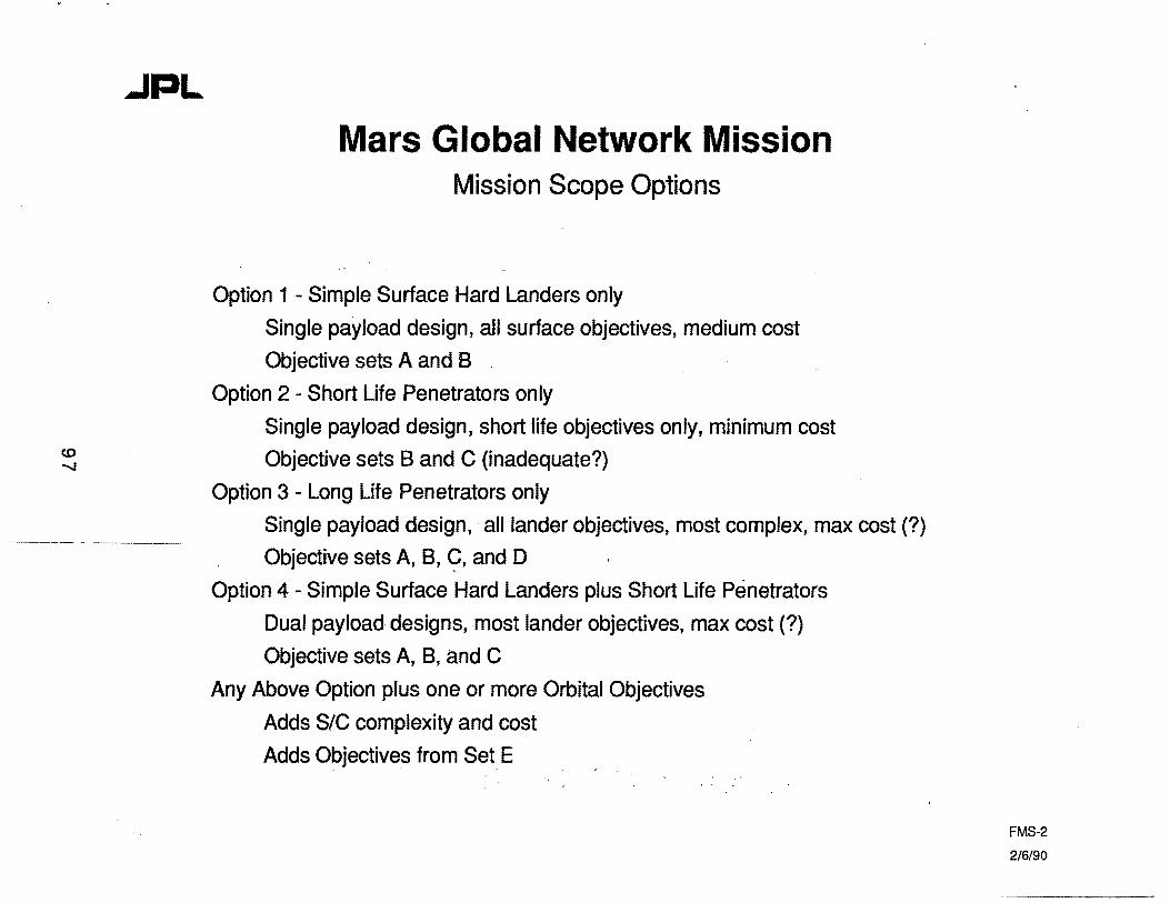
Mars Global Network Mission Mission Scope Options
Option 1 - Simple Surface Hard Landers only
Single payload design, all surface objectives, medium cost
Objective sets A and B
Option 2 - Short Life Penetrators only
Single payload design, short life objectives only, minimum cost
Objective sets Band C (inadequate?)
Option 3 - Long Life Penetrators only
Single payload design, all lander objectives, most complex, max cost (?)
Objective sets A, B, 9, and D
Option 4 - Simple Surface Hard Landers plus Short Life Penetrators
Dual payload designs, most lander objectives, max cost (?)
Objective sets A, B, and C
Any Above Option plus one or more Orbital Objectives
Adds SIC complexity and cost
Adds Objectives from Set E . . .
FMS-2
2/6/90
<0' CD
..JPL
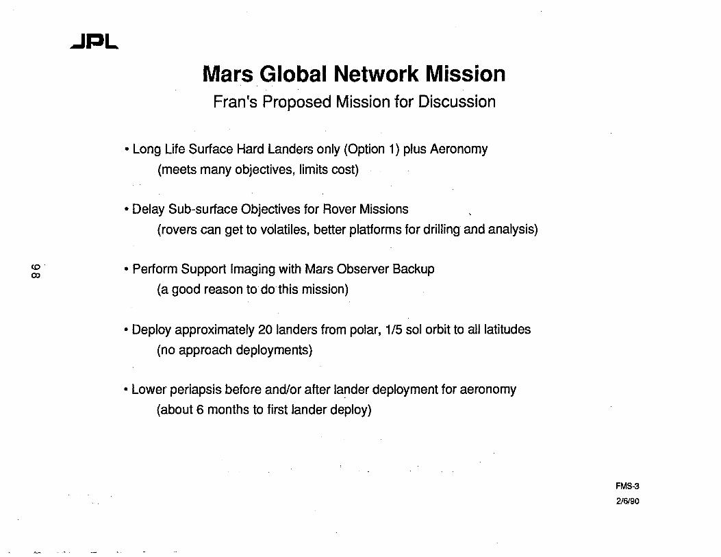
Mars Global Network Mission Fran's Proposed Mission for Discussion
• Long Life Surface Hard Landers only (Option 1) plus Aeronomy
(meets many objectives, limits cost) .
• Delay Sub-surface Objectives for Rover Missions
(rovers can get to volatiles, better platforms for drilling and analysis)
• Perform Support Imaging with Mars Observer Backup
(a good reason to do this mission)
• Deploy approximately 20 landers from polar, 1/5 sol orbit to all latitudes
(no approach deployments)
• Lower periapsis before and/or after la!lder deployment for aeronomy
(about 6 months to first lander deploy)
FMS-3
2/6/90
Session A, Submittal No. 3
David Morrison Ames Research Center
I
99 I
.:- .
....... 0 0
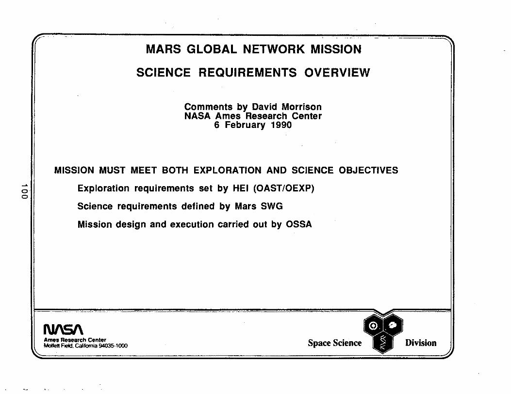
MARS GLOBAL NETWORK MISSION
SCIENCE REQUIREMENTS OVERVIEW
Comments by David Morrison NASA Ames Research Center
6 February 1990
MISSION MUST MEET BOTH EXPLORATION AND SCIENCE OBJECTIVES
Exploration requirements set by HEI (OAST/OEXP)
Science requirements defined by Mars SWG
Mission design and execution carried out by OSSA
1\U\51\ Ames Research Center Molten Field. California 94035-1000 Space Science Division
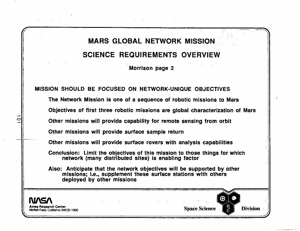
MARS GLOBAL NETWORK MISSION·
SCIENCE REQUIREMENTS OVERVIEW
Morrison page 2
MISSION SHOULD BE FOCUSED ON NETWORK-UNIQUE OBJECTIVES
The Network Mission is one of a sequence of robotic missions to Mars
Objectives of first three robotic missions are global characterization of Mars
Other missions will provide capability for remote sensing from orbit
Other missions will provide surface sample return
Other mi-ssions will provide surface rovers with analysis capabilities
Conclusion: Limit the objectives of this mission to those things for which network (many distributed sites)' is enabling factor
Also: Anticipate that the network objectives will be supported by other missions; i.e., supplement these surface stations with others deployed by other missions
N/\51\ Ames Research Center Moffen Field. California 94035-1000 Space Sf;:ience Division
0 1\)
/
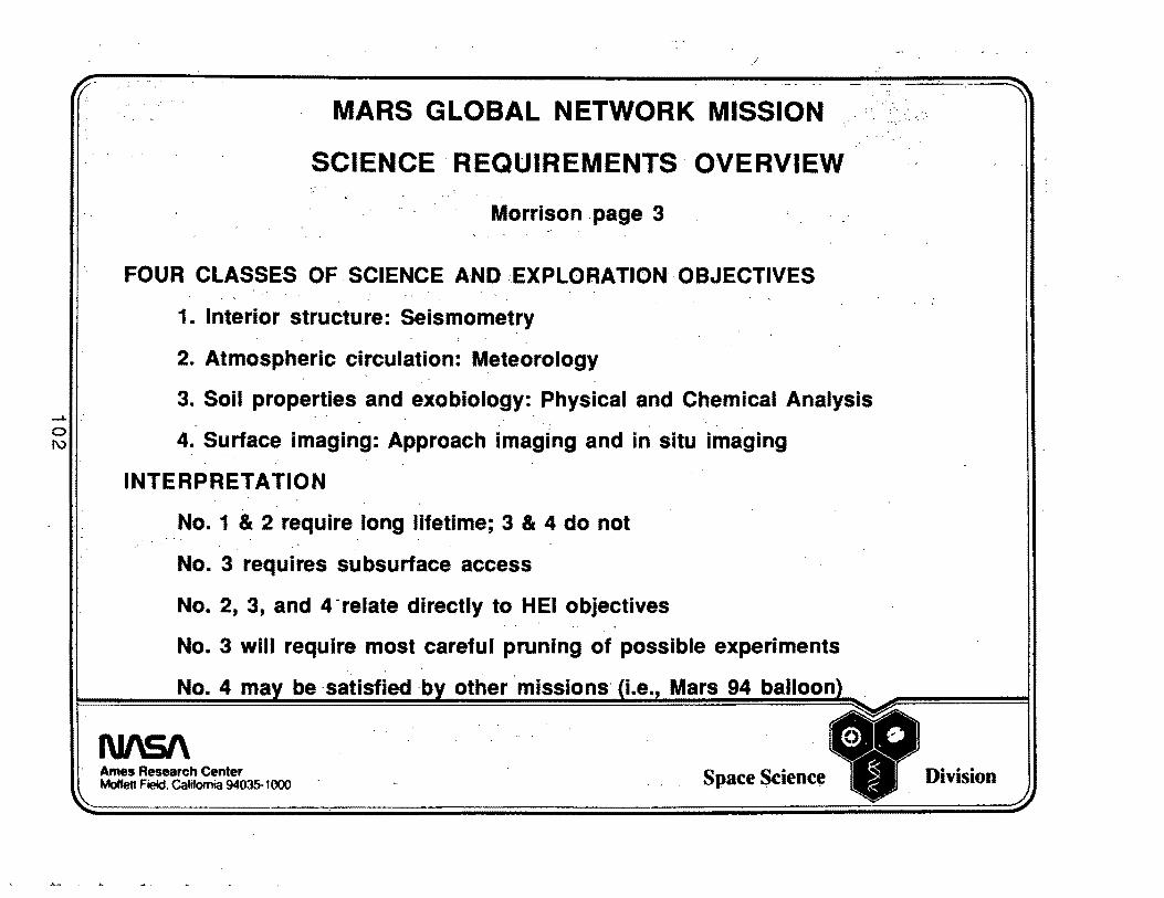
MARS GLOBAL NETWORK MISSION
SCIENCE ·REQUIREMENTS OVERVIEW
Morrison . page 3
FOUR CLASSES OF SCIENCE AND EXPLORATION OBJECTIVES
1. Interior structure: Seismometry
2. Atmospheric circulation: Meteorology
3. Soil properties and exobiology: Physical and Chemical Analysis
4. Surface imaging: Approach imaging and in situ imaging
INTERPRETATION
No. 1 & 2 require long lifetime; 3 & 4 do not
No. 3 requires subsurface access
No. 2, 3, and 4 -relate directly to HEI objectives
No. 3 will require most careful pruning of possible experiments
No. 4 m be ·satisfied· other ·missions .e. Mars 94 balloo
N/\51\ Ames Research Center Moflen Field. California 94035-1000 Space Scienc~ Division
Session A, Submittal No. 4
Michael H. Carr U.S. Geological Survey
103
~ ~~ 0~ ~0
~(;;) ~~ ~c. V(J4.
R ~ ~~v~~ ~~~~ ~' v.,O "~ &~ v.,G
~'t- ~ !QCj ~(j !QCj ~(j o"-~ ~«) $~ ~ ~0 G Cj'<~ Cj'<~ 0«)
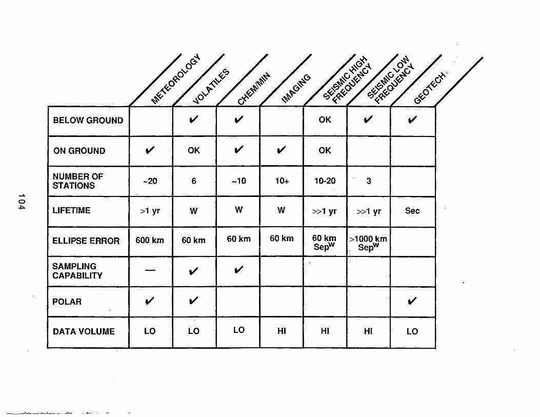
BELOW GROUND v v OK v v
ON GROUND v OK v v OK
NUMBER OF ---20 6 -10 10+ 10-20 3 STATIONS
LIFETIME >1 yr w w w >>1 yr >>1 yr Sec
ELLIPSE ERROR 600km 60km 60km 60km 60km >1000 km Sepw SepW
SAMPLING -
- v v CAPABILITY .
POLAR v v v '
DATA VOLUME LO LO LO HI HI HI LO
....1.
0 01
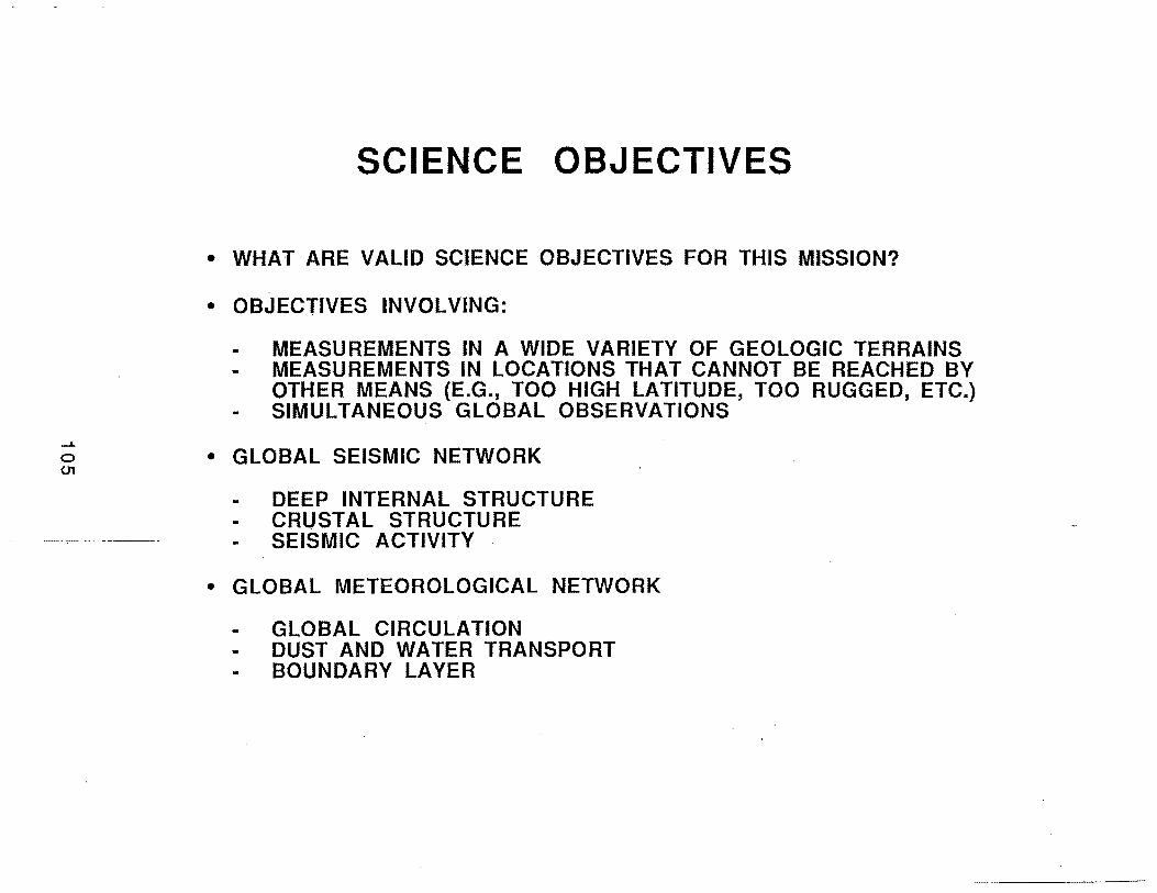
SCIENCE OBJECTIVES
• WHAT ARE VALID SCIENCE OBJECTIVES FOR THIS MISSION?
• OBJECTIVES INVOLVING:
MEASUREMENTS IN A WIDE VARIETY OF GEOLOGIC TERRAINS MEASUREMENTS IN LOCATIONS THAT CANNOT BE REACHED BY OTHER MEANS (E.G., TOO HIGH LATITUDE, TOO RUGGED, ETC.) SIMULTANEOUS GLOBAL OBSERVATIONS
• GLOBAL SEISMIC NETWORK
DEEP INTERNAL STRUCTURE CRUSTAL STRUCTURE SEISMIC ACTIVITY
• GLOBAL METEOROLOGICAL NETWORK
GLOBAL CIRCULATION DUST AND WATER TRANSPORT BOUNDARY LAYER
.......... "' 0. ()')
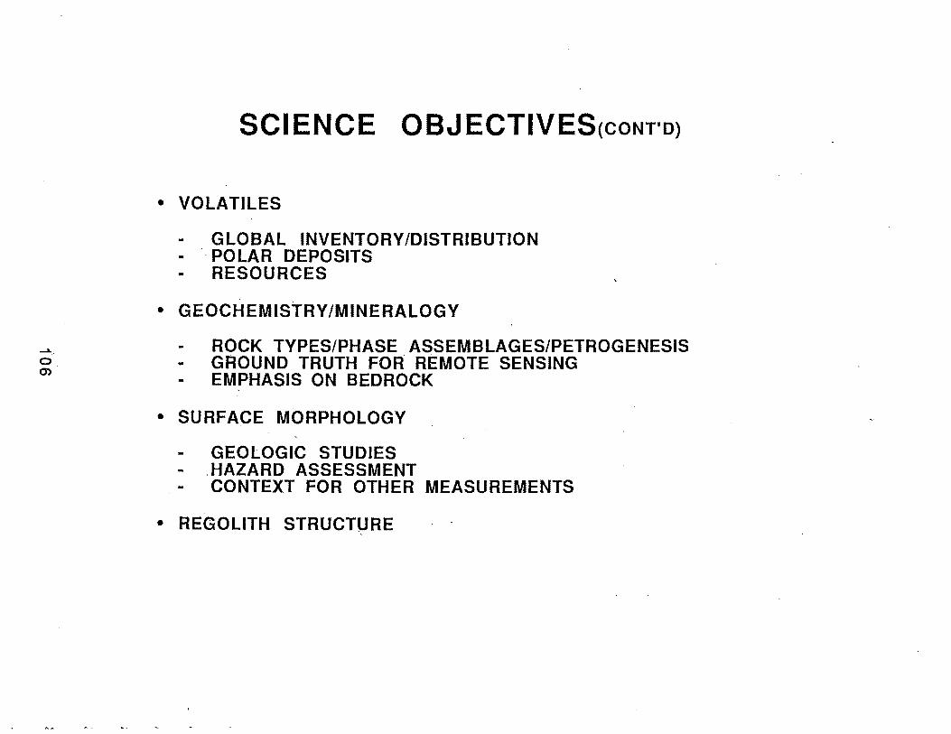
SCIENCE OBJECTIVES(coNT'D>
• VOLATILES
GLOBAL INVENTORY/DISTRIBUTION . ·POLAR DEPOSITS
RESOURCES
• GEOCHEMISTRY/MINERALOGY
ROCK TYPES/PHASE ASSEMBLAGES/PETROGENESIS GROUND TRUTH FOR REMOTE SENSING EMPHASIS ON BEDROCK
• SURFACE MORPHOLOGY
GEOLOGIC STUDIES .HAZARD ASSESSMENT CONTEXT FOR OTHER MEASUREMENTS
• REGOLITH STRUCT~RE
Session A, Subm itt a I No. 5
Bruce Murray California Institute of Technology
James D. Burke Jet Propulsion Laboratory/California Institute of Technology
107

....... 0 CD
BALLOONS FOR ENHANCED SCIENTIFIC
RETURN FROM MARS HARD LANDERS
by
Bruce Murray, Caltech, and James D. Burke, JPL
Assisted by:
Bruce Betts, James Consolver, Laszlo Keszthelyi, and Tom Svitek, Caltech; Robert Mostert, JPL;
Tom Heinsheimer, Titan Systems
February 6, 1990
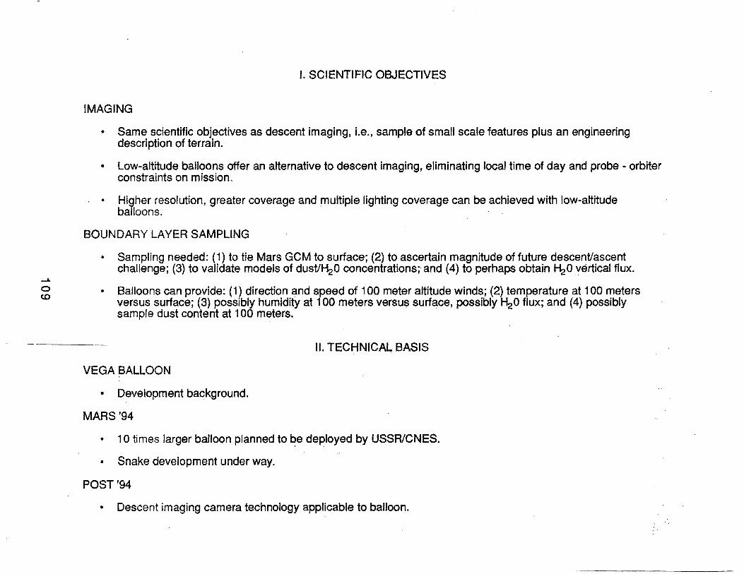
I. SCIENTIFIC OBJECTIVES
IMAGING
• Same scientific objectives as descent imaging, i.e., sample of small scale features plus an engineering description of terrain.
• Low-altitude balloons offer an alternative to descent imaging, eliminating local time of day and probe- orbiter constraints on mission.
. • Higher resolution, greater coverage and multiple lighting coverage can be achieved with low-altitude balloons.
BOUNDARY LAYER SAMPLING
• Sampling needed: (1) to tie Mars GCM to surface; (2) to ascertain magnitude of future descent' ascent challenge; (3) to validate models of dust'~O concentrations;· and (4) to perhaps obtain i-1:20 vertical flux.
• Balloons can provide: (1) direction and speed of 100 meter altitude winds; (2) temperature at 100 meters versus surface; (3) possibly humidity at 1 00 meters verSU$ surface, possibly H20 flux; and (4) possibly sample dust content at 1 00 meters.
II. TECHNICAL BASIS
VEGA BALLOON
• Development background.
MARS '94
• 10 times larger balloon planned to ~e deployed by USSRICNES.
• Snake development under way.
POST'94
• Descent imaging camera technology applicable to balloon.

JPL TETHERED BALLOON CONCEPT
---........ -
I . -1 QQ .. m ALTITUDE
I / \~ CAMERA AND 1
\ METEOROLOGY !~1H~~:g~g~ 11 ',, SENSORS
SENSORS . · ~ / ~.METEOROLOGY ~L~ SENSORS
t
v
11 0
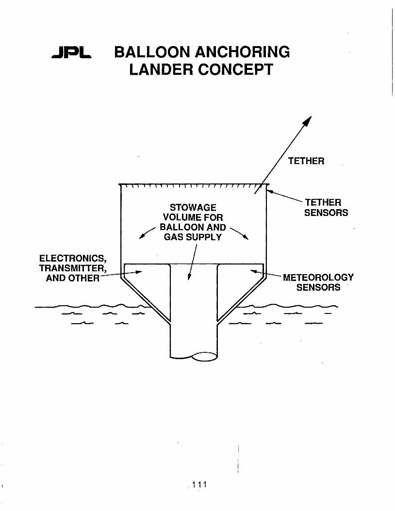
JPL BALLOON ANCHORING LANDER CONCEPT
STOWAGE VOLUME FOR
/ BALLOON AND '-.... F GAS SUPPL V ""'
1 1 1
-
TETHER
TETHER SENSORS
METEOROLOGY SENSORS .
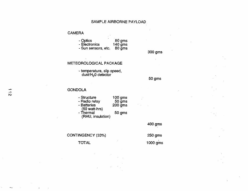
SAMPLE AIRBORNE PAYLOAD
CAMERA
-Optics· . - Electronics -Sun sensors, etc.
80gms 140 gms 80gms
METEOROLOGICAL PACKAGE
- temperature, slip speed, dust/H20 detector
GONDOLA
-Structure - Radio relay -Batteries
(50 watt-hrs) -Thermal
(RHU, insulation)
CONTINGENCY (33%)
TOTAL
100 gms 50gms
200 gms
SO.gms
300 gms
50gms
400gms
250 gms l
1000 gms

JPL CONCEPT FOR HARD LANDER WITH BALLOON AND SNAKE
• LANDER INSTRUMENTS • METEOROLOGY SENSORS • SURFACE CHEMISTRY
• BALLOON INSTRUMENTS - CAMERA AND METEOROLOGY SENSORS
• SNAKE INSTRUMENTS -DYNAMICS ... SURFACE
CHARACTER
LANDER
-·- ---~-·
/ ' / '
/ ', / '
/ ' / '
•
•
•
•
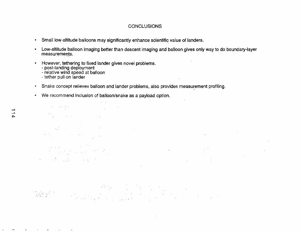
CONCLUSIONS
Small low-altitude balloons may significantly enhance scientifi~ value of landers .
Low-altitude balloon imaging better than descent imaging and balloon gives only way to do boundary-layer measuremef:lts.
However, tethering to fixed lander gives novel problems . - post-landing deployment - relative wind speed at balloon - tether pull on lander
Snake concept relieves balloon and lander problems, also provides measurement profiling. \
We recommend inclusion of balloon/snake as a payload option .

Session A, Submittal No. 6
David Morrison Ames Research Center
115
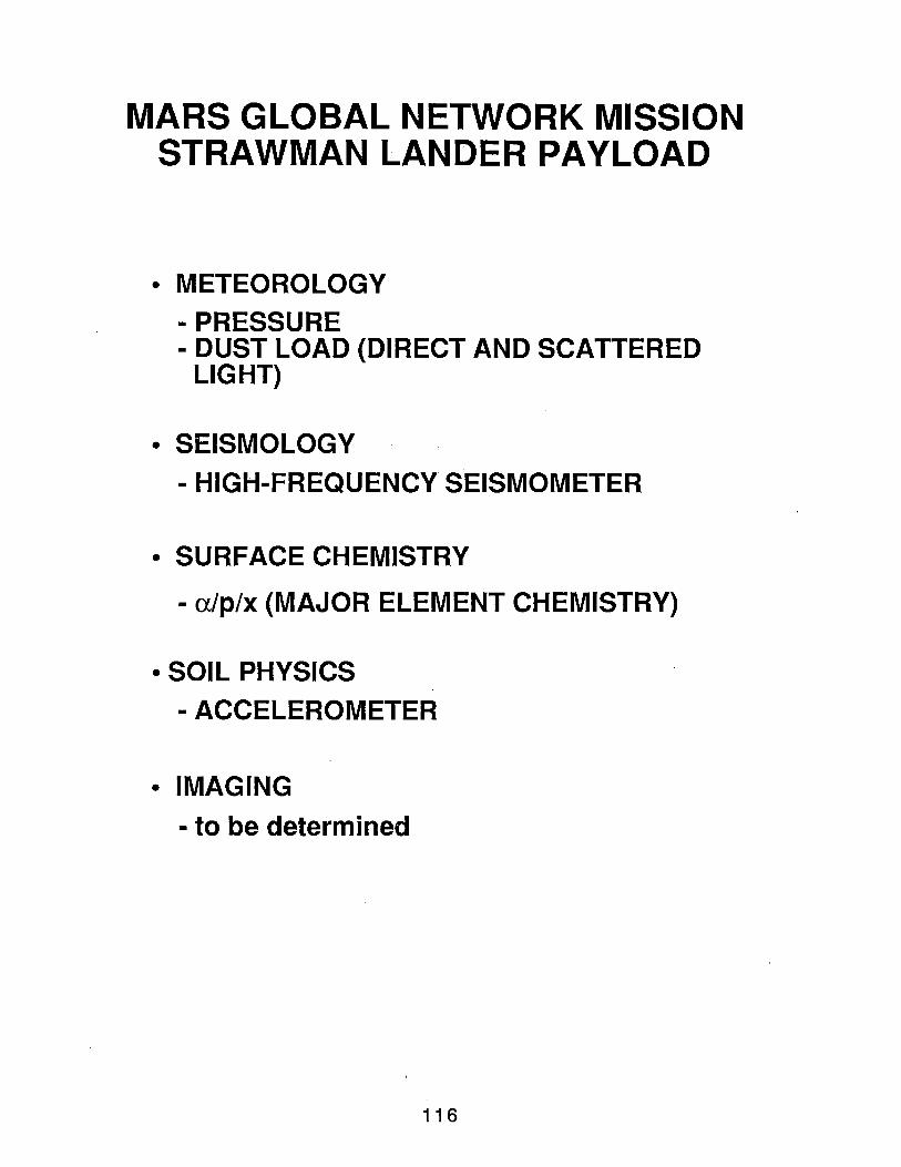
MARS GLOBAL NETWORK MISSION STRAWMAN LANDER PAYLOAD
• METEOROLOGY
-PRESSURE -DUST LOAD (DIRECT AND SCATTERED
LIGHT)
• SEISMOLOGY
- HIGH-FREQUENCY SEISMOMETER
• SURFACE CHEMISTRY
- a/p/x (MAJOR ELEMENT CHEMISTRY)
• SOIL PHYSICS
- ACCELEROMETER
• IMAGING
- to be determined
116
Session A, Submittal No. 7
Steven W. Squyers Cornell University
117
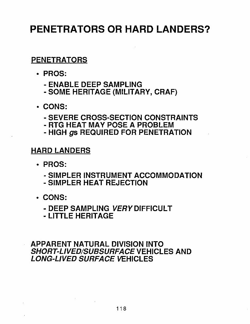
PENETRATORS OR HARD LANDERS?
PENETRATORS
• PROS:
- ENABLE DEEP SAMPLING -SOME HERITAGE (MILITARY, CRAF)
• CONS:
- SEVERE CROSS-SECTION CONSTRAINTS - RTG HEAT MAY POSE A PROBLEM -HIGH gs REQUIRED FOR PENETRATION
HARD LANDERS
• PROS:
-SIMPLER INSTRUMENT ACCOMMODATION -SIMPLER HEAT REJECTION
• CONS:
- DEEP SAMPLING VERY DIFFICULT -LITTLE HERITAGE
APPARENT NATURAL DIVISION INTO SHORT-LIVED/SUBSURFACE VEHICLES AND LONG-LIVED SURFACE VEHICLES
118
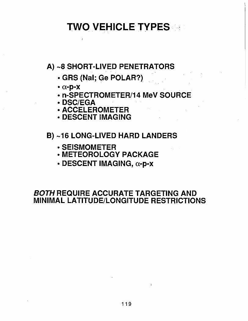
TWO V'EHICLE· TVPE·S :: ,; .· ' . .. . - .
A) -8 SHORT-LIVED PENETRATORS
• GRS .(Nal; Ge POLAR?) • a-p-x • n-SPECTROMETER/14 MeV SOURCE • DSC/EGA . • ACCELEROMETER • DESCENT IMAGING
B) -16 LONG-LIVED HARD LANDERS
• SEISMOMETER •METEOROLOGY PACKAGE • DESCENT IMAGING, a-p-x
BOTH REQUIRE ACCURATE TARGETING AND MINIMAL LATITUDE/LONGITUDE RESTRICTIONS
119

THREE KEY QUESTIONS
(1) TO WHAT EXTENT DOES SURFACE EMPLACEMENT DEGRADE SEISMIC SCIENCE?
(2) TO WHAT EXTENT DOES SURFACE EMPLACEMENTDEGRADE ... GEOCHEMISTRY/VOLATILES SCIENCE?
(3) HOW MANY STATIONS ARE R~ALL Y . REQUIRED FOR METEOROLOGY AND
SEISMOLOGY?
120

Session A, Submittal No. 8
William B. Banerdt Jet Propulsion Laboratory/California Institute of Technology
.121

-L
1\) 1\)
PAYLOAD FOR A MARS GLOBAL NETWORK MISSION
Ground Rules for "Pre-Strawman" Selection
ORBITER
Payload Capacity:
Orbit:
LANDER
Payload Capacity:
Type of Lander:
·Number:
Lifetime:
Mass Power Telemetry Rate
Circular or Elliptical? High or Low Periapsis?
Mass Power (Peak, Sustained) Telemetry Rate (Data Storage)
Hard or Soft Lander, Penetrator?
Few (-6) or Many (-20)?
Short (days) or Long (years)?
?
? ?
? ?
? ? ?
?
?
?
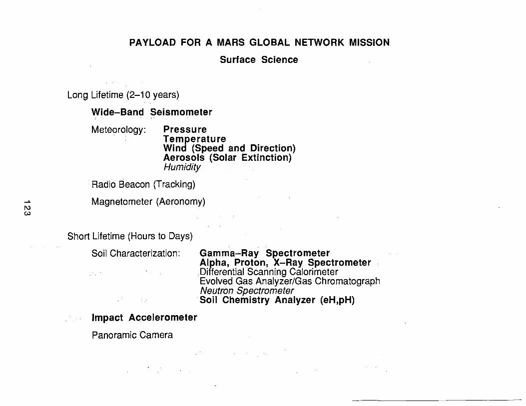
PAYLOAD FOR A MARS GLOBAL NETWORK MISSION
Long Lifetime (2-1 0 years)
Wide-Band Seismometer
Meteorology: Pressure
Surface Science
Temperature Wind (Speed and Direction) Aerosols (Solar Extinction) Humidity
· Radio Beacon (Tracking)
Magnetometer (Aeronomy)
Short Lifetime (Hours to Days)
Soil Characterization: Gamma~Ray Spectrometer Alpha, Proton, X..-Ray Spectrometer .Differential Scanning Calorimeter ·Evolved Gas Analyzer/Gas Chromatograph Neutron Spectrometer Soil Chemistry Analyzer (eH,pH)
Impact Accelerometer
Panoramic Camera
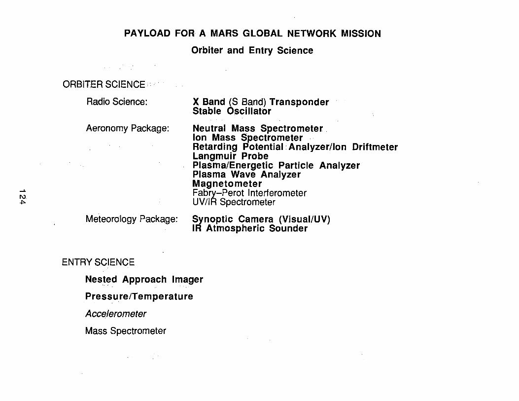
PAYLOAD FOR· A MARS GLOBAL NETWORK MISSION
Orbiter and Entry Science
ORBITER SCIENCE:~ · · ·
Radio Science:
Aeronomy Package:
Meteorology Package:
ENTRY SCIENCE
X Band (S Band) Transponder Stable Oscillator
Neutral Mass Spectrometer . lon Mass Spectrometer Retarding Potential• Analyzer/len Driftmeter Langmuir Probe Plasma/Energetic Particle Analyzer Plasma Wave Analyzer Magnetometer Fabry-Perot Interferometer UV/IR Spectrometer
Synoptic Camera (Visuai/UV) IR Atmospheric Sounder
Nes.ted Approach Imager
Pressure/Temperature
Acc~lerometer
Mass Spectrometer
PAYLOAD FOR A MARS GLOBAL NETWORK MISSION
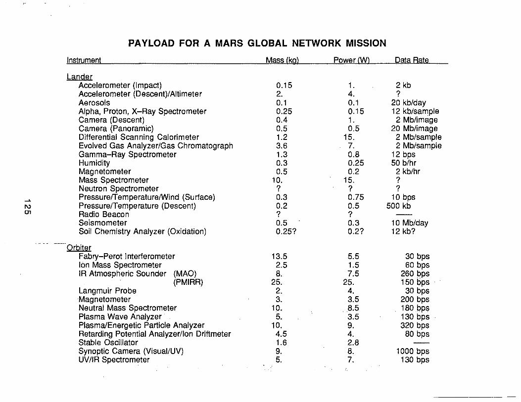
Instrument Mass (kg) Power (W) Data Rate
Lander Accelerometer (Impact) 0.15 1. 2 kb Accelerometer (Descent)/Aitimeter 2. 4. ? Aerosols 0.1 0.1 20 kb/day Alpha, Proton, X-Ray Spectrometer 0.25 0.15 12 kb/sample Camera (Descent) 0.4 1. 2Mb/image Camera (Panoramic) 0.5 0.5 20Mb/image Differential Scanning Calorimeter 1.2 15. 2Mb/sample Evolved Gas Analyzer/Gas Chromatograph 3.6 7. 2Mb/sample Gamma-Ray Spectrometer 1.3 0.8 12 bps Humidity 0.3 0.25 50 b/hr Magnetometer 0.5 0.2 2 kb/hr Mass Spectrometer 10. 15. ? Neutron Spectrometer ? ? ?
....... Pressure/Temperature/Wind {Surface) 0.3 0.75 10 bps 1\) Pressure/Temperature (Descent) 0.2 0.5 500 kb 01 Radio Beacon ? ?
Seismometer 0.5 0.3 10Mb/day Soil Chemistry Analyzer {Oxidation) 0.25? 0.2? 12 kb?
-- ---
Orbiter Fabry-Perot Interferometer 13.5 5.5 30 bps lon Mass Spectrometer 2.5 1.5 60 bps IR Atmospheric Sounder (MAO} 8. 7.5 260 pps
{PMIRR} 25. 25. 150 bps · · Langmuir Probe 2. 4. 30 bps Magnetometer 3. 3.5 200 bps Neutral Mass, Spectrometer 10. .. 8.5 180 IJps Plasma Wave Analyzer · 5. 3.5 130 bps Plasma/Energetic Particle Analyzer 10. 9. 320 bps Retarding Potential Analyzer/len Driftmeter 4.5 4. 80 bps Stable Oscillator 1.6 2.8 Synoptic Camera (Visuai/UV) 9. B. 1000 bps UV/IR Spectrometer 5. 7. 130 bps
PAYLOAD FOR A MARS GLOBAL NETWORK MISSION
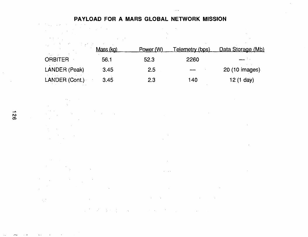
Mass (kg) Power(W) Telemetry (bps) Data Storagf3 (Mb)
ORBITER 56.1 52.3 2260 ..
LANDER (Peak) 3.45 2.5 20 (1 0 images)
LANDER: (Cont.)· 3.45 2.3 140 12 (1- day)
Session A, Submittal No. 9
Janet Luhmann University of California at Los Angeles
127
Vu-graph Captions
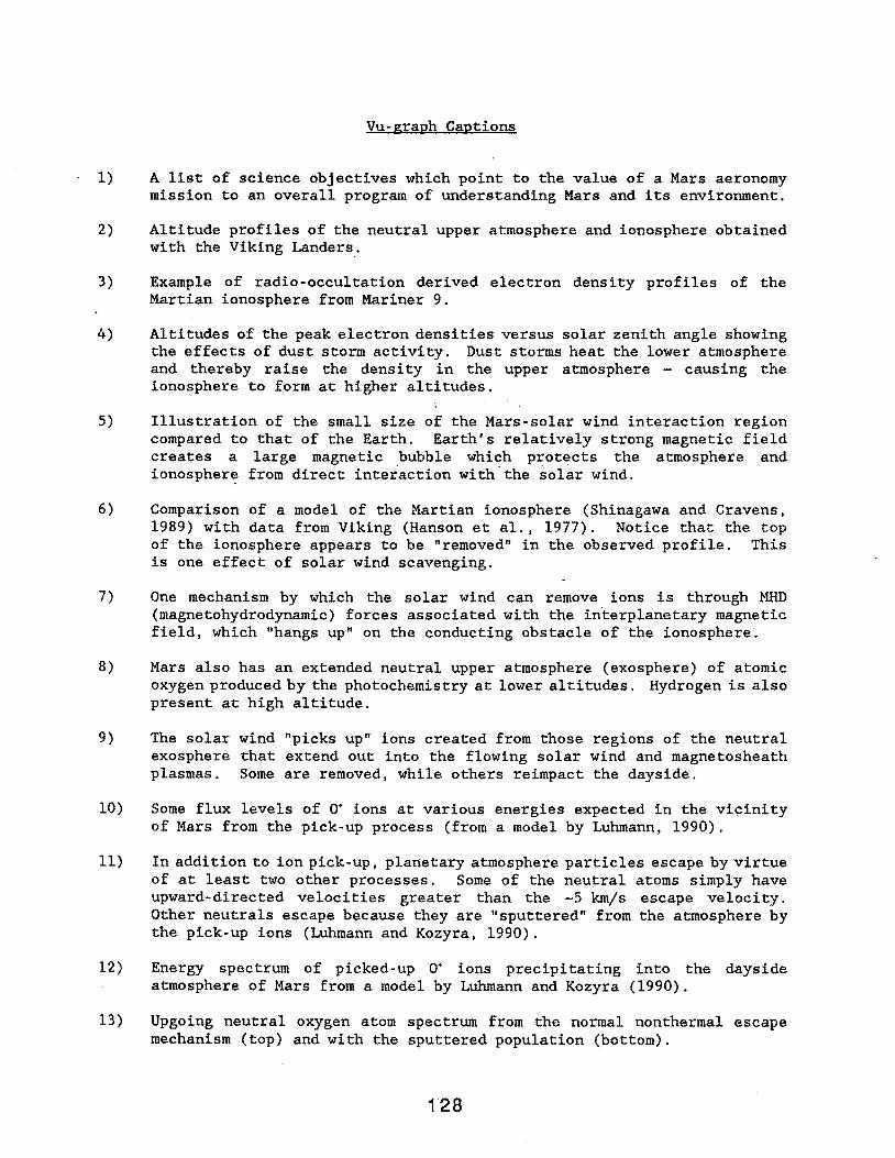
1) A list of science objectives which point to the value of a Mars aeronomy mission to an overall program of understanding Mars and its environment.
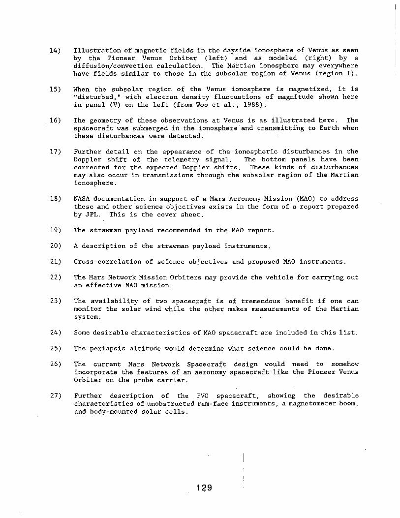
2) Altitude profiles of the neutral upper atmosphere and ionosphere obtained with the Viking Landers_.
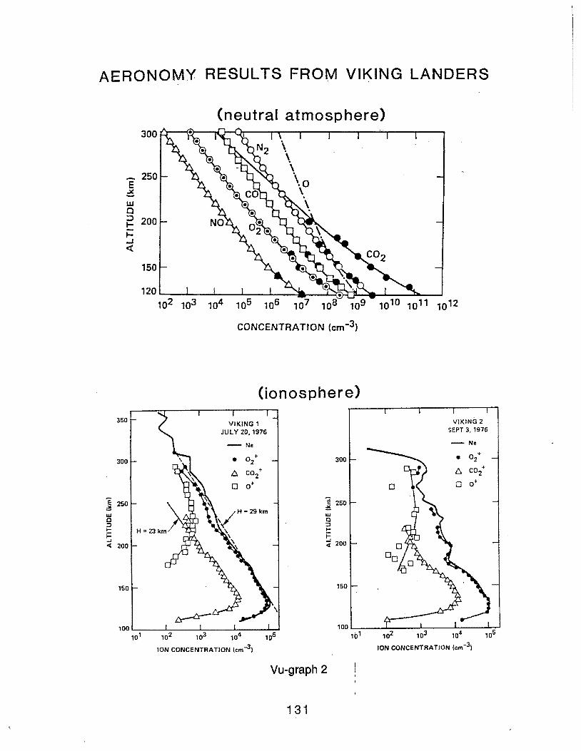
3) Example of radio-occultation derived electron density profiles of the Martian ionosphere from Mariner 9.
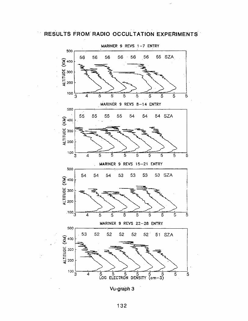
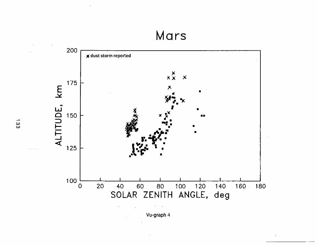
4) Altitudes of the peak electron densities versus solar zenith angle showing the effects of dust storm activity. Dust storms heat the lower atmosphere and thereby raise the density in the upper atmosphere - causing the ionosphere to form at higher altitudes.
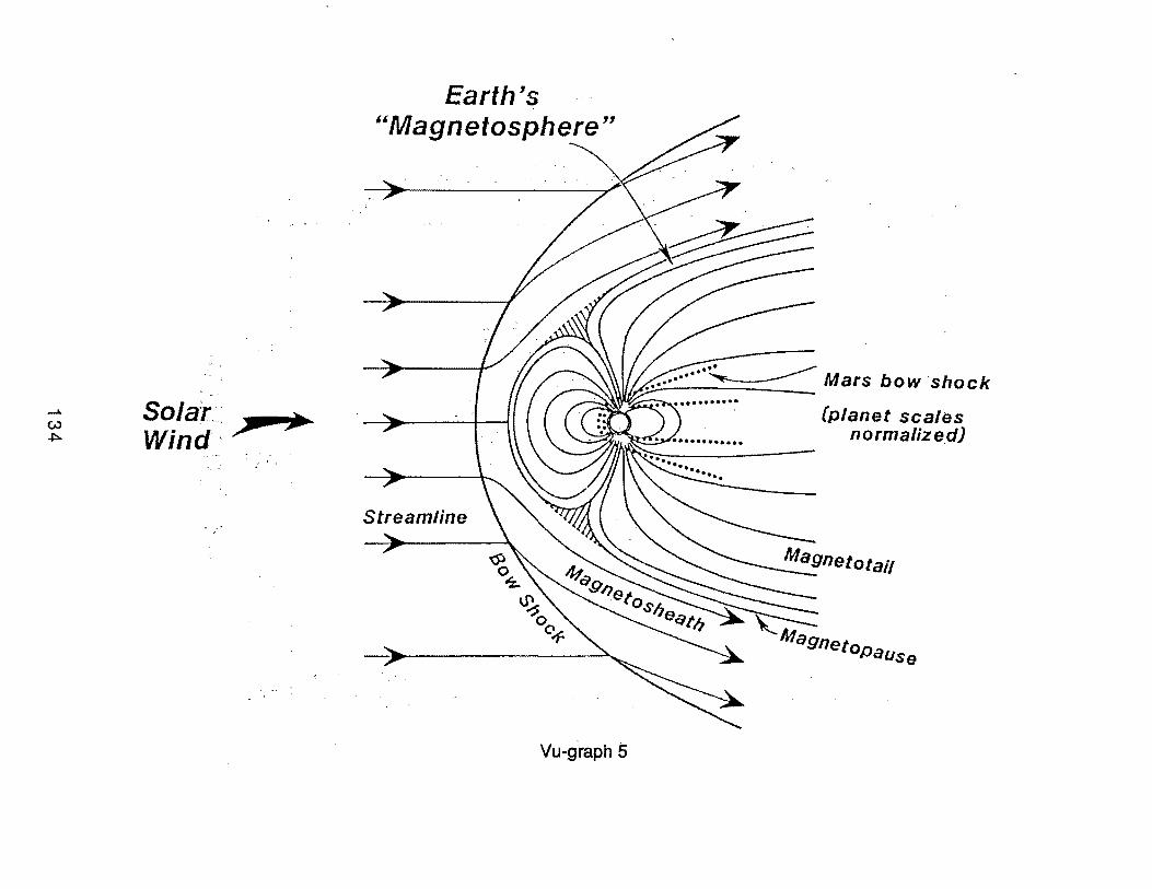
5) Illustration of the small size of the Mars-solar wind interaction region compared to that of the Earth. Earth's relatively strong magnetic field creates a large magnetic bubble which protects the atmosphere and ionospher~ from direct interaction with.the solar wind.
6) Comparison of a model of the Martian ionosphere (Shinagawa and Cravens, 1989) with data from Viking (Hanson et al., 1977). Notice that the top of the ionosphere appears to be "removed" in the observed profile. This is one effect of solar wind scavenging.
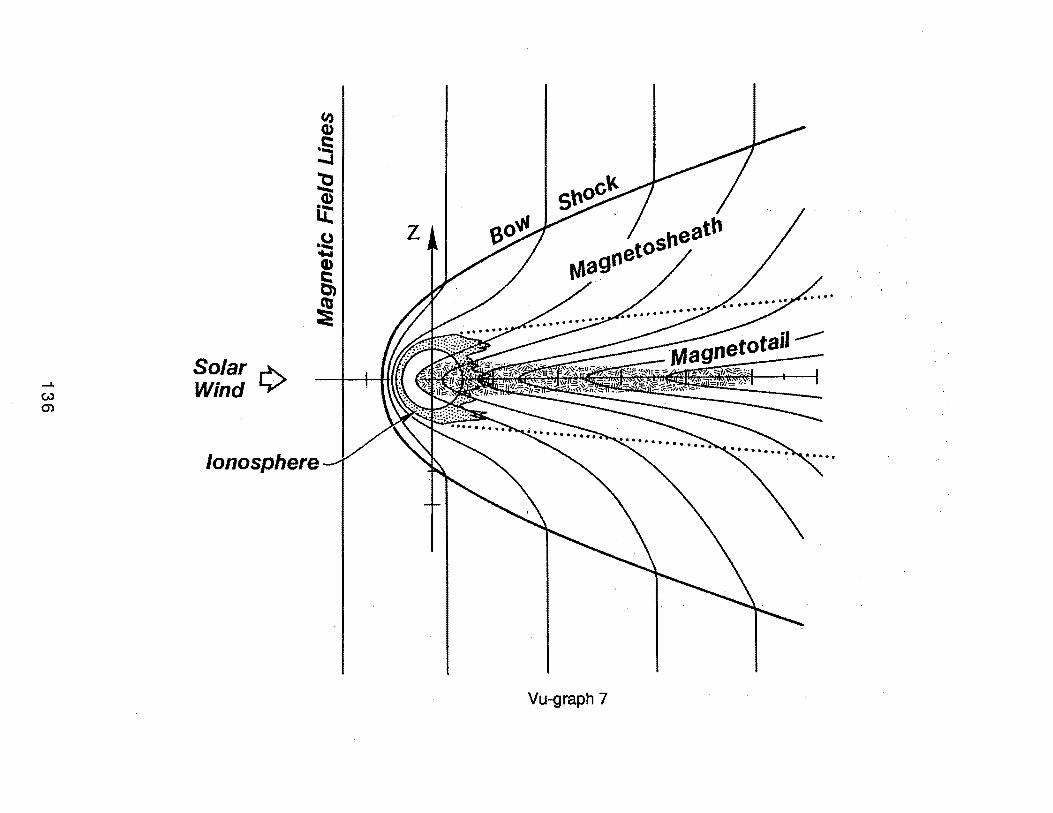
7) One mechanism by which the solar wind can remove ions is through MHD (magnetohydrodynamic) forces associated with the interplanetary magnetic field, which "hangs up" on the conducting obstacle of the ionosphere.
8) Mars also has an extended neutral upper atmosphere (exosphere) of atomic oxygen produced by the photochemistry at lower altitudes. Hydrogen is also present at high altitude.
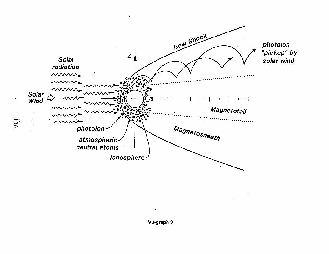
9) The solar wind "picks up" ions created from those regions of the neutral exosphere that extend out into the flowing solar wind and magnetosheath plasmas. Some are removed, while others reimpact the dayside.
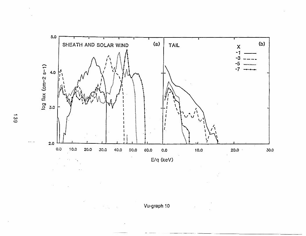
10) Some flux levels of o• ions at various energies expected in the vicinity of Mars from the pick-up process (from a model by Luhmann, 1990).
11) In addition to ion pick-up, planetary atmosphere particles escape by virtue of at least two other processes. Some of the neutral atoms simply have upward-directed velocities greater than the -5 km/s escape velocity. Other neutrals escape because they are "sputtered" from the atmosphere by the pick-up ions (Luhmann and Kozyra, 1990).
12) Energy spectrum of picked-up o• ions precipitating into the dayside atmosphere of Mars from a model by Luhmann and Kozyra (1990).
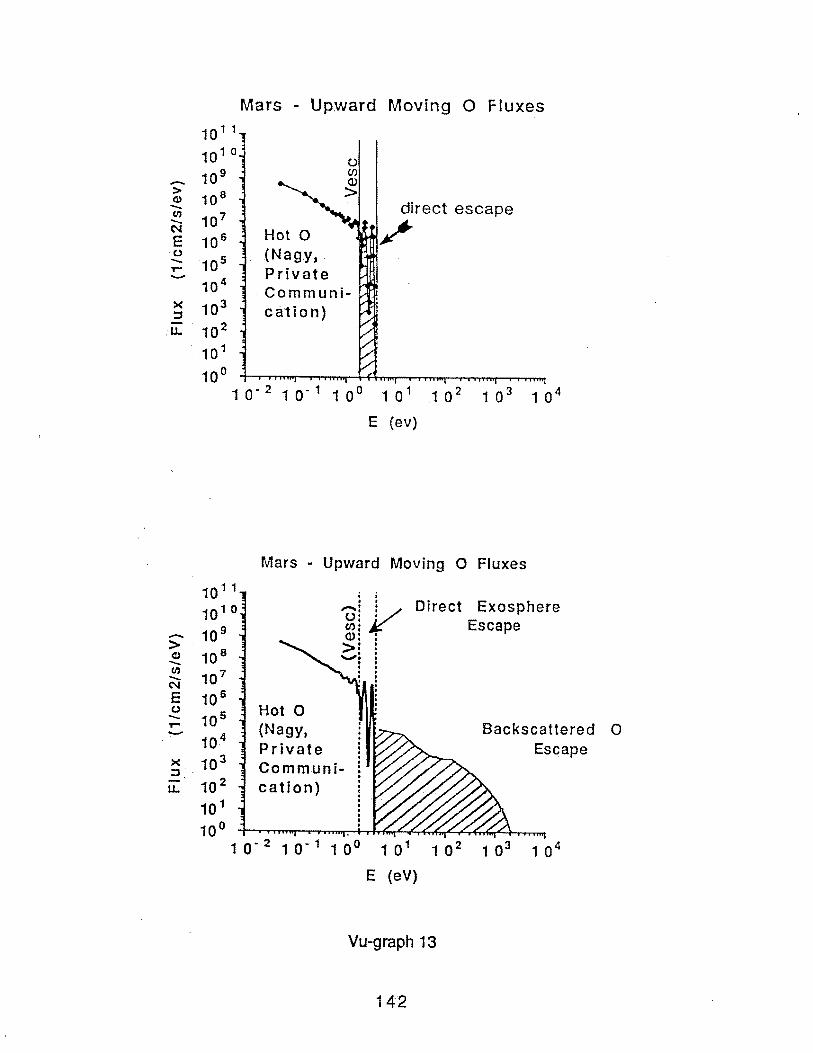
13) Upgoing neutral oxygen atom spectrum from the normal nonthermal escape mechanism (top) and with the sputtered population (bottom).
128
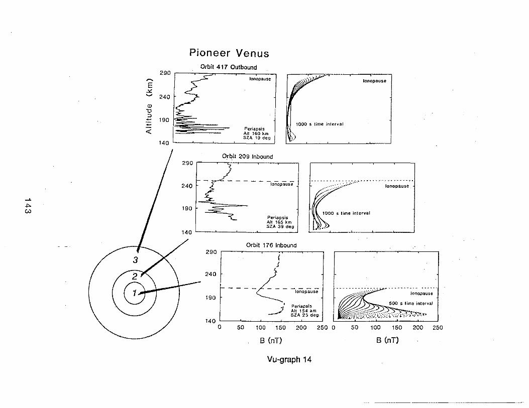
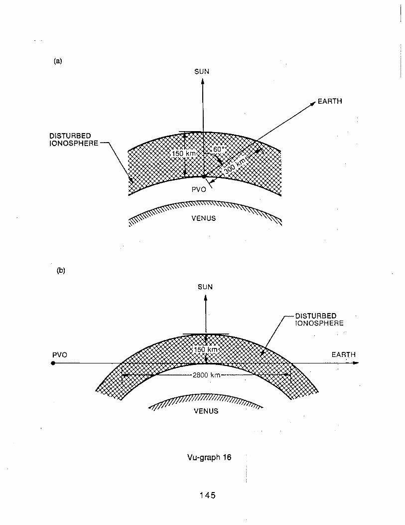
14) Illustration of magnetic fields in the daysi~e ionosphere of Venus as seen by the Pioneer Venus Orbiter (left) and as modeled (right) by a diffusion/convection calculation. The Martian ionosphere may everywhere have fields similar to those in the subsolar region of Venus (region I).
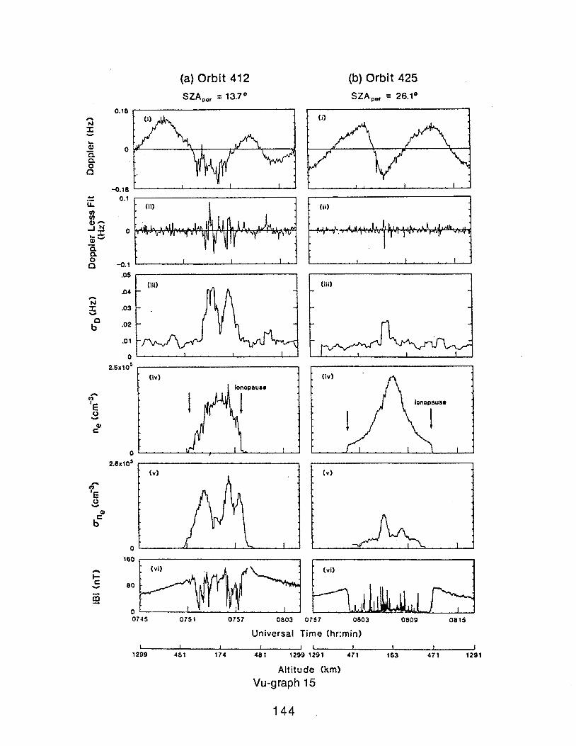
15) When the subsolar region of the Venus ionosphere is magnetized, it is "disturbed," with electron density fluctuations of magnitude shown here in panel (V) on the left (from Woo et al., 1988).
16) The geometry of these observations at Venus is as illustrated here. The spacecra.ft was submerged in the ionosphere· and transmitting to Earth when these disturbances were detected.
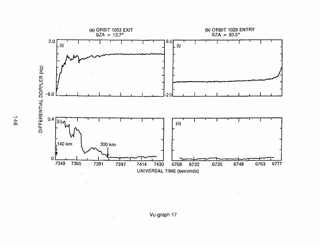
17) Further detail on the appearance of the ionospheric disturbances in the Doppler shift of the telemetry signal. The bottom panels have been corrected for the expected Doppler shifts. These kinds of disturbances may also occur in transmissions through the subsolar region of the Martian ionosphere.
18) NASA documentation in support of a Mars Aeronomy Mission (MAO) to address these and other science objectives exists in the form of a report prepared by JPL. This is the cover sheet.
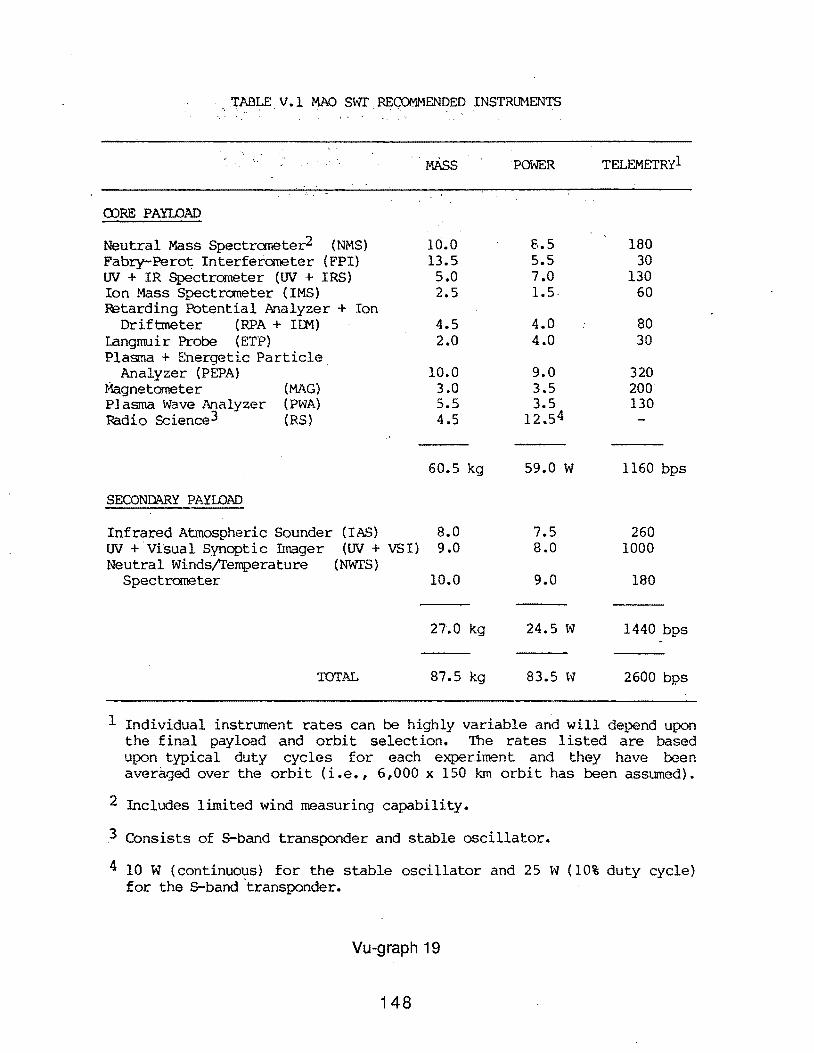
19) The strawman payload recommended in the MAO report.
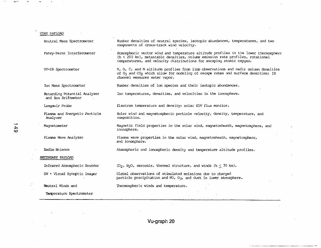
20) A description of the strawman payload instruments.
21) Cross-correlation of science objectives and proposed MAO instruments.
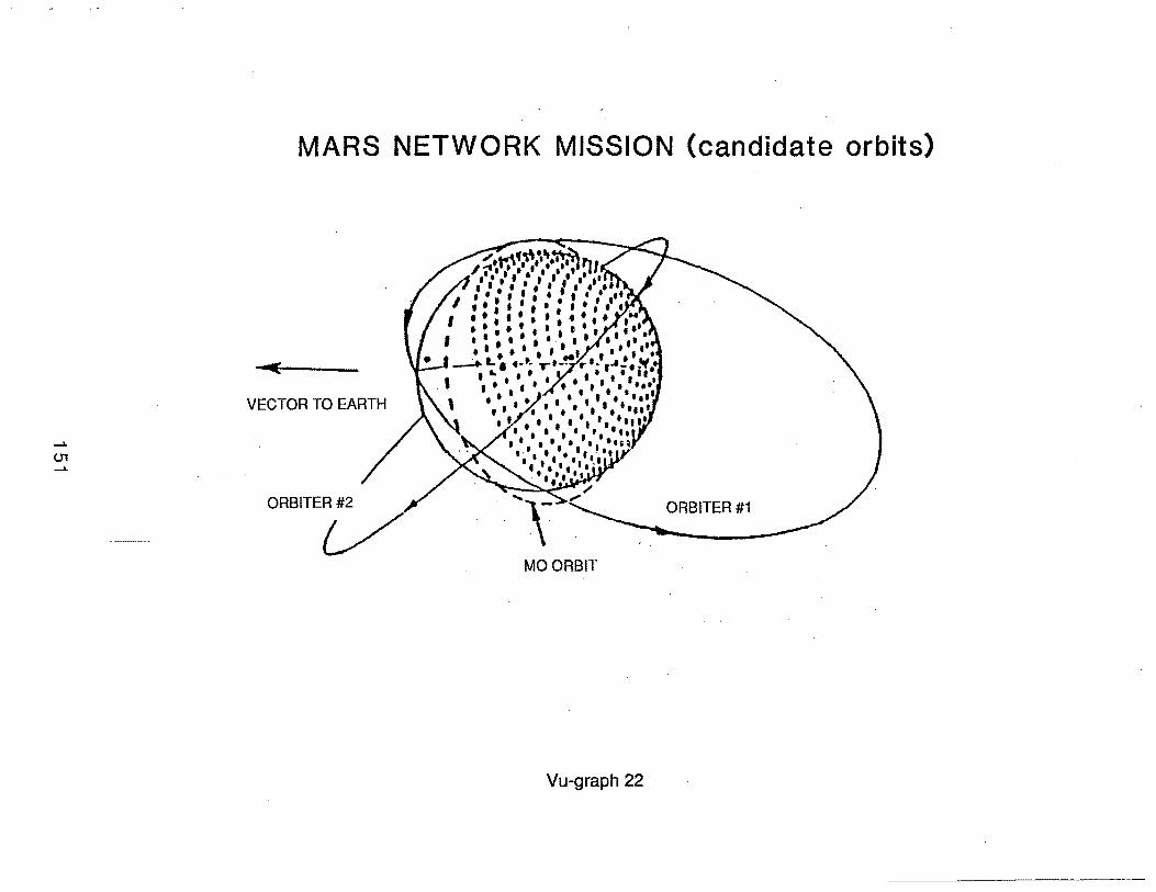
22) The Mars Network Mission Orbiters may provide the vehicle for carrying out an effective MAO mission.
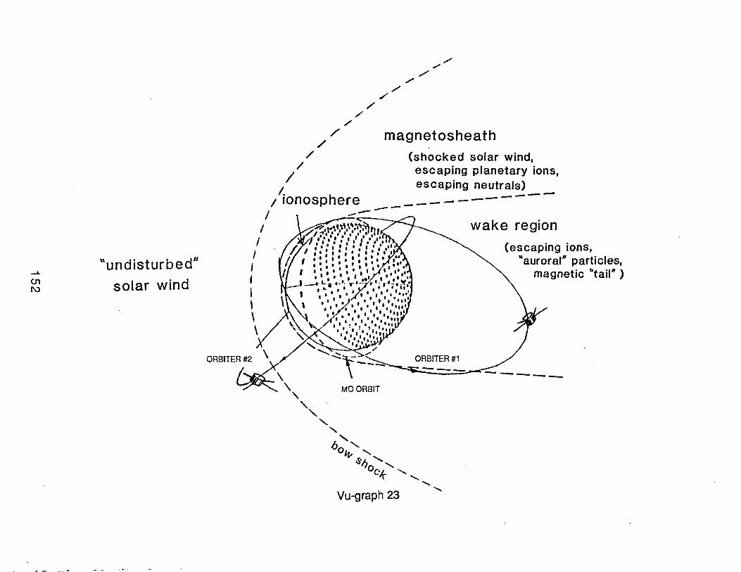
23) The availability of two spacecraft is of tremendous benefit if one can monitor the solar wind while the other makes measurements of the Martian system.
24) Some desirable characteristics of MAO spacecraft are included in this list.
25) The periapsis altitude would determine what science could be done.
26) The current Mars Network Spacecraft design would need to somehow incorporate the features of an aeronomy spacecraft like the Pioneer Venus Orbiter on the probe carrier.
27) Further description of the PVO spacecraft, showing the desirable characteristics of unobstructed ram-face instruments, a magnetometer boom, and body-mounted solar cells.
129

Mars Aeronomy Mission Science Objectives
Upper Atmosphere:
properties and variability (e.g., response to dust storms,. seasons, solar activity, solar wind conditions)
~ loss processes/ evolution
Ionosphere:
. Source of Nightside Ionosphere (e.g., auroral activity?)
temporal and spatial variability/disturbances (e.g., response to dust storms, seasons, solar activity, solar wind conditions)
Magnetic Field:
nature/ origin
variability
effects on energetic particle (radiation) environment
Solar Wind Interaction:
. . · significance of planetary magnetic fields
comparisons with Venus and Earth
Vu-graph 1
130
AERONOMY RESULTS FROM VIKING LANDERS
E
= w a ~ 200
w 0 :::l ... i= .....
-1-...J <!
< 200
150
(neutral atmosphere)
CONCENTAA TJON (cm-3)
ION CONCENTRATION (em-3)
(ionosphere)
300
e 2so ::! w 0 :::l ... i= ~ 200
150
Vu~graph 2
131
VIKING 2 SEPT 3, 1976
- Ne
• 02+
/j, C02 +
0 o•
ION CONCENTRATION (em-3)
RESULTS FROM' RADIO O'CCULT AT ION EXPERIMENTS .
MARINER 9 REVS 1 -7 ENTRY 500
- 56 56 56 56 56 56 55 SZA ::IE 400 ~ -~300 ::::J I-
!S 200 -<
100 3 4 5
.. MARINER 9 REVS 8-14 ENTRY
500
- ss· 55 55 55 54 54 54 SZA ::IE 400 ~ -~ 300 ::::J I-
5 200 <
100 3 4 5
MARINER 9 REVS 15-21 ENTRY 500
- 54 54 54 53 53 53 53 SZA ::IE 400 ~ -~ 300 ::::J I-
5 200 <·
.1003 4 5 5
MARINER 9 REVS 22-28 ENTRY 500
- 53 52 52 52 52 52 51 SZA :::::!: 400 ~ -~ 300 ::::J I-
5 200 <
100 3 4 5
Vu-graph 3
132
.. w
Mars 200 ~--------------------------------------~
)I( dust storm reported
175 -
)£ x.x X J(
II
~- -x '· I
•
• Cl 150 ~ ::>
~ )( ._._.
• • ... ••
. I--I_. <(
125 -
r.:.fi::" l ........ • .,. !'II • • .. ·~ .
• •
100 ~--~'----~'--~'~--~~----~'--~'----~·----~'~ 0 20 40 60 80 1 00 1 20 1 40 1 60 180
SOLAR ZENITH ANGLE, deg
Vu-graph 4
Solar Wind.:? :-.
Earth's "Magnetosphere"
Streamline
Vu-g.raph 5
·!.~ ~ ..•.••.••• ~ Mars bow shock
'\:..Ma
(planet scales normalized)
9netopa Use

8 3oo ..:..:: -UJ Q ::J !:: !:i 200 <C
100 0 10
400
-E 300 ~ -UJ c :::::) .,_ -~ 200 <1:
101
MARS IONOSPHERE
102 103 104
MODEL CASE 1
105
DENSITY (cm-3)
VIKING 1 (Hanson et al. data)
106
100 ,___._.........lo.l.l.l.l-.1"-'--~i.L-~u...&.ll.JL.I..-~u.I.UJIJ.-~~
1 0 1 1 o3 · 1 o4
DENSITY (cm-3)
From Shinagawa (.1989)
Vu-graph 6
135
... C02l-- 02+ -o- 0+
Ne
w 0')
Solar Wind ¢>
Ionosphere
Vu-graph 7

~
E ~
"'"' Q) -c ::J +"" +:. <(
2500
2000
1500
1000
---500
\ \
\ \
\ \
---
\ \
\ \
\ \
\ \
Mars' Exosphere
(adapted from Breus, 1986)
\ \
\ Cold H \
\ \
\ \
- - - ...: \ Cotd o . -, ____ _ \
\ 100L_ __________ _L ______ ~--~~~~----~-~5 2 3 4
Vu-graph 8 I . '
137
....... _.
(..) (X)
Solar Wind
Solar radiation ~
Vu-graph 9
. . . . ..... ............ . . . . .
Magneto tail
photoion "pickup" by solar wind
-,_ I en 4.0
C\1 I E 0 -0)
0 3.0
SHEATH AND SOLAR WIND (a) TAIL
0.0 1 o.o 20.0 30.0 40.0 50.0 60.0 0.0
E/q (keV)
Vu-graph 10
10.0
X -1 -3 -----5 -7
20.0
(b)
30.0
---~-~------~~------------~------

Nonthermal Escape- Venus and Mars
Superthermal escaping neutrals from hot exospheres
Neutral backscatter from impacting pickup ions
Vu-graph 11
. Pickup ions accelerated in solar wind
(not to scale)
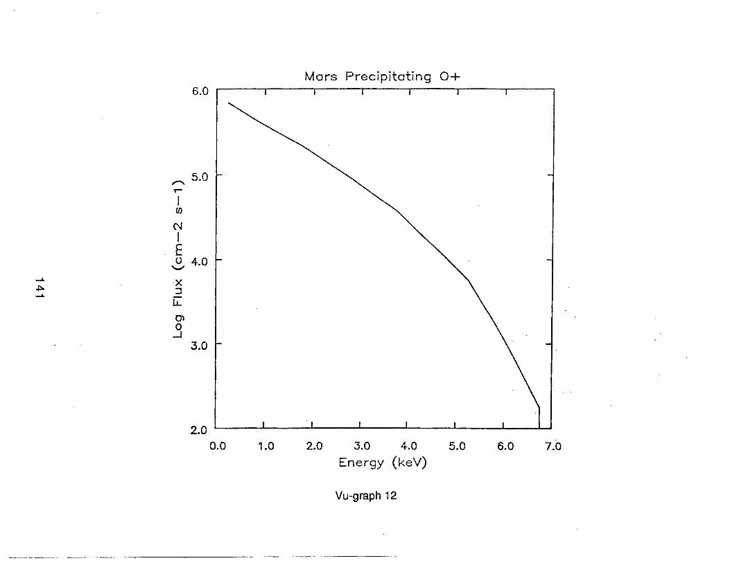
Mars Precipitating 0+
,..... 5.0 ,..... I en
N I E 0 4.0 .......,;
-""' X ,J:o. :I -""'
I.J...
Q)
0 ..J
3.0
0.0 1.0 2.0 3.0 4.0 5.0 6.0 7.0 Energy (keV)
Vu-graph 12
----------------------~·---·
>< :::J -1.1..
-> (t) .._ Cl) .._
C\1
s (.) .._
,..... ->< :::J
1.1..
101 1 1010
10 9
10 8
10 7
10 6
10 5
104
10 3
10 2
10 1
10°
Mars - Upward Moving 0 Fluxes
(..)
en Q.)
> direct escape
Hot 0 (Nagy,. Private Communication)
/
10" 1 10° 10 1 10 2
E {ev}
Mars - Upward Moving 0
. . -=y Direct o: . en: Q.). • . . >= • . -: . . . . . . . . . ! . . . .
Hot 0 :
(Nagy, Private Communi-cation)
Fluxes
Exosphere Escape
Backscattered Escape
1 0- 2 1 a· 1 1 0° 1 0 1 1 o2 1 0 3 1 0 4
E (eV)
Vu-graph 13
142
0
290 -E X. - 240 Q)
"'0 :::l ..... 190 .....
<(
140
Pioneer Venus Orbit 417 Outbound
290
240
190
140
lonopause
1000 s time interval Periapsis All 160 km SZA 19 deg
Orbit 209 Inbound
Periapsis All 165 km SZA 39 deg
Orbit 176 Inbound
1----
0 50
{ J
)
-~- -,, ... , ... 1
Periapsis J All 154 km SZA 25 deg.
100 150 200 250 0
B (nT)
Vu-graph 14
lonopause
lonopause
50 100 150 200 250
B (nT)
,.. N ::r: ... Q) a. c. 0 0
-u: !I) !I)
Ill""" ...JN ._::r: Q)-
a. c. 0 0
,.. N
(a) Orbit 412 (b) Orbit 425
(i)
-0.18 !...-----'-----_._ ___ __.__. 0.1 ,..-----------------,
(ii)
-0.1 L..-----'------1-~----l.......__,
.05 .------------------. (iii)
.04
::r: .03 .....
,.. (')
'e (.) .....
,.. (')
'e (.) .....
0 1....-------'-------_._ ___ __.~ 2.6lt105 .....-------------~
(iv) (iv)
0 ~-----~-,--~~---~~ 2Jht105 r--------------.,
(v) (v)
0751 0757 0603 075 7 0603
Universal Time (hr:min)
1299 481 174 481 1299 1291
Altitude Ckm)
Vu-graph 15
144
471
lonopsus•
1
0809
163
0815
(a)
DISTURBED IONOSPHERE
(b)
PVC
SUN
EARTH
VENUS
SUN
EARTH
VENUS
Vu-graph 16
145
-N I -a: w _J
a.. a.. g -6.0 _J <(
t= z w
-L a: 0.4 .t:>- w (J) u..
u.. b
0
(i i)
7349 7365
(a) ORBIT 1053 EXIT SZA = 13.7°
7381 7397
-2.0
. I (ii)
1-
'-
- . I
7414 7430 6708 6722
UNIVERSAL TIME (seconds)
Vu-graph 17
(b) ORBIT 1028 ENTRY SZA::: 83.5°
I I I
- _I
6735 6749
I •
--
-
•
6763 6777
NASA Technical Memorandum 89202
Mars Aeronomy Observer: Report of the Science Working Team
October 1, 1986
Nl\5/\ National Aeronautics and Space Administration
Jet Propulsion Laboratory California Institute of Technology Pasadena, California
Vu-graph 18
147
TABJ;..E. V .1 MAO swr RECOMMENDED INSTRUHENTS
CORE PAYLOAD
Neutral Mass Spectraneter2 (NMS) Fabry-Perot Interferaneter (FPI) UV + IR Spectrometer (UV + IRS) Ion Mass Spectrometer (IMS) Retarding Potential Analyzer + Ion
Driftmeter (RPA + II:J.t) Langrnu i r Probe ( ETP) Plasma + Energetic Particle
Analyzer (PEPA) r1agnetometer Plasma Wave Analyzer Radio Science3
SECONDARY PAYLOAD
(MAG) (PWA) (RS)
Infrared Atmospheric Sounder UV + Visual Synoptic Imager Neutral Winds/Temperature
Spectraneter
(IAS) (UV + VSI)
(NWTS)
TOTAL
10.0 13.5
5.0 2.5
4.5 2.0
10.0 3.0 5.5 4.5
60.5 kg
8.0 9.0
10.0
27.0 kg
87.5 kg
POWER
t?..5 5.5 7.0 1.5
4.0 4.0
9.0 3.5 3.5
12.54
59.0 w
7.5 8.0
9.0
24.5 w
83.5 \v
TELEMETRY!
180 30
130 60
80 30
320 200 130
1160 bps
260 1000
180
1440 bps
2600 bps
1 Individual instrument rates can be highly variable and will depend upon the final payload and orbit selection. The rates listed are based upon typical duty cycles for each experiment and they have been averaged over the orbit (i.e., 6,000 x 150 km orbit has been assumed).
2 Includes limited wind measuring capability.
3 Consists of 5-band transponder and stable oscillator.
4 10 W (continuous) for the stable oscillator and 25 w (10% duty cycle) for the 5-band ·transponder.
Vu-graph 19
148
. CDRE PAYLOAD
Neutral Mass Spectrometer
Fabry-Perot Interferometer
UV+IR Spectrometer
Ion Mass Spectrometer
Retarding Potential Analyzer and Ion Driftmeter
Langnu ir Probe
Plasma and Energetic Particle Analyzer
Magnetometer
Plasma Wave Analyzer
Radie· Science
. SE<XJNJlA.RY PAYLOAD
Infrared Atmospheric Sounder
UV + Visual Synoptic Imager
Neutral Winds and
Temperature Spectrometer
Number densities of neutral species, isotopic abundances, temperatures, and two components of cross-track wind velocity.
Atmospheric vector wind and temperature altitude profiles in the lower thermosphere (h < 200 km), metastable densities, .volume emission rate profiles, rotational temperatures, and velocity distributions for escaping atomic oxygen.
H, O, C; and N altitude profiles from limb observations and nadir column densities of D) and C02 which allow for modeling of escape rates and surface densities; IR channel measures water vap:::>r.
Number densities of ion species and their isotopic abundances.
Ion temperatures, densities, and velocities in the ionosphere.
Electron temperature and density; sola~ EUV flux monitor.
Solar wind and magnetospheric particle velocity, density, temperature, and carpos it ion. · ·
Magnetic field properties in the solar wind, magnetosheath, magnetosphere, and ionosphere.
Plasma wave properties in the solar wind, magnetosheath, magnetosphere, and ionosphere.
Atmospheric and ionospheric density and temperature altitude profiles.
002, H20, aerosols, thermal structure, and winds (h ~ 70 km).
Global observations of stimulated emissions due to charged particle precipitation and NO, 03, and dust in lower atmosphere.
Thermospheric winds and temperature.
Vu-graph 20
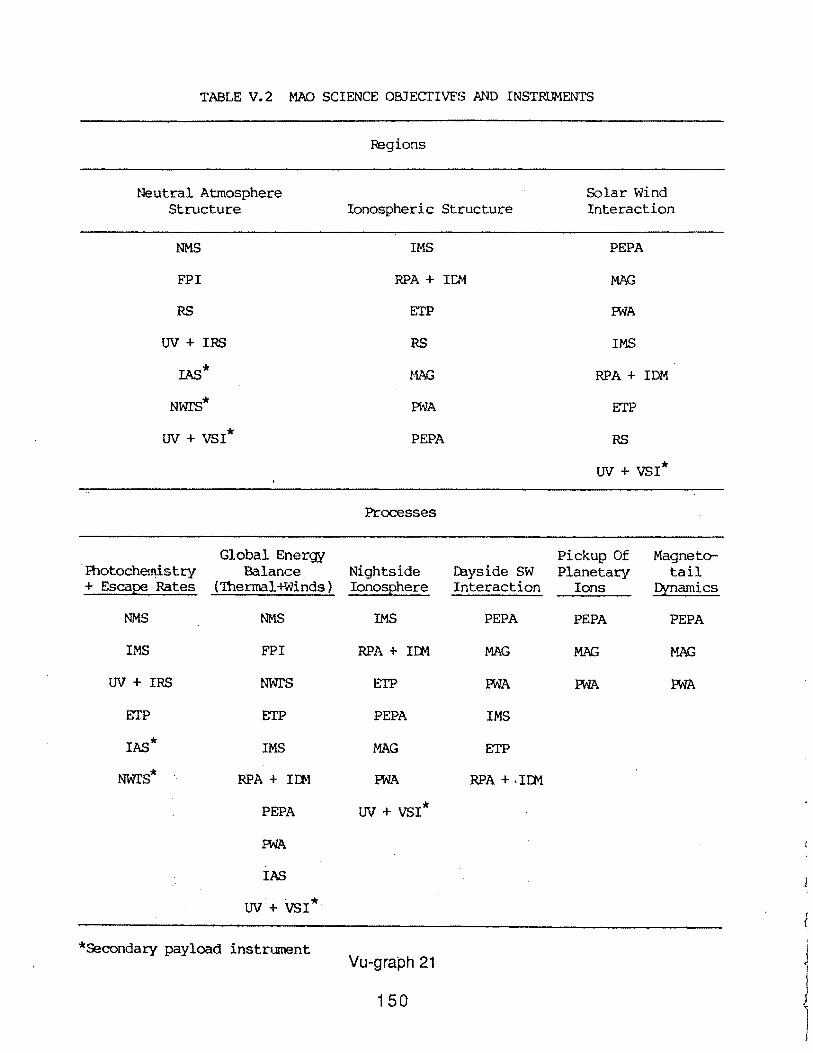
TABLE V. 2 MAO SCIENCE OBJECTIVFS AND INSTRUMENTS
Neutral Atmosphere Structure
NMS
FPI
RS
UV + IRS
!AS*
Nwrs*
uv + vsi*
Global Energy ·Ihotochemistry Balance + Escape Rates (Thermal +Winds)
NMS NMS
IMS FPI
UV + IRS NwrS
ETP ETP
IAS* IMS
Nwrs* RPA + Ir:t-1
PEPA
Pi'JA
IAS
uv + vsr*
*Secondary payload instrument
Regions
Ionospheric Structure
IMS
RPA + IC:1
ETP
RS
~1AG
Pi \lA
PEPA
Processes
Nights ide J:l::iyside SW Ionosphere Interaction
IMS PEPA
RPA+ Ir:M MAG
ETP PWA
PEPA IMS
MAG ETP
Pi'JA RPA +,JIM
uv + vsr*
Vu-graph 21
i50
Solar Wind Interaction
PEPA
MAG
Pi\! A
IMS
RPA + IDM
ETP
RS
uv + vsi*
Pickup Of Magneto-Planetary tail
Ions Q!namics
PEPA PEPA
MAG MAG
Pi'JA rnA
1
j
l J
l
MARS NETWORK MISSION (candidate orbits)
VECTOR TO EARTH
C.J1 -L
ORBITER#1 ORBITER#2
(/ MOORBIT
Vu-graph 22
(]1 1\.)
"undisturbed"
solar wind
I I I
' I \ \
'
1
/ I
/
/ /
/ /
/
/ /
/
,.-" /
magnetosheath (shocked solar wind, escaping planetary ions, escaping neutrals) I.
11onosphere -----------1 .....,.- --- ---- --
Vu-graph 23
wake region
(escaping ions, "auroraln particles,
magnetic "tailn )
-

Orbit:
Mars Aeronomy Mission
Desirable Characteristics:
elliptical (variable periapsis from <200 km (-110-150 km?), apoapsis -1-5 ~)
polar (or high inclination)
rate of periapsis motion -1 hour LT per week to sample all local times
spacecraft position in orbits can be controlled (phased)
Duration:
to cover as much of a Martian year as possible (for seasonal coverage)
Spacecraft:
Instruments identical on both spacecraft
onboard propulsion
body mounted solar cells (for low drag)
option to spin or despin (use momentum wheel)
extendable boom for magnetic, electric field experiments
Vu-graph 24
153
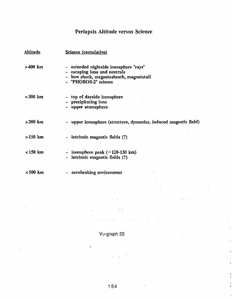
Periapsis Altitude versus Science
Altitude ·Science (cumulative)
>400 km - extended nightside ionosphere "rays" - escaping ions and neutrals - bow shock, magnetosheath, magnetotail - "PHOBOS-2" science
>300 km - top of dayside ionosphere - precipitating ions - upper atmosphere
>200 km - upper ionosphere (structure, dynamics, induced magnetic field)
>150 km - intrinsic magnetic fields (?)
<150 km - ionosphere peak ( -120-130 km) - intrinsic magnetic fields (?)
<100 km - aerobraking environment
Vu-graph 25
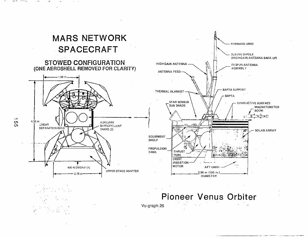
MARS NETWORK SPACECRAFT
STOWED CONFIGURATION (ONE AEROSHELL REMOVED FOR CLARITY)
UPPER STAGE ADAPTER
THERMAL BLANKET
EQUIPMENT SHELF
PROPULSION TANK
FORWARD OMNI
SLEEVE DIPOLE (HIGH-GAIN ANTENNA BACK-UP)
DESPUN ANTENNA ASSEMBLY
BAPTA SUPPORT
SOLAR ARRAY
t------=2.54 m (100 in.) ____ ___,_, DIAMETER
Pioneer Venus Orbiter Vu-graph 26

(J1 (j)
PIONEER VENUS
ORBITER netomoter
Radar mapper·
The Orbi~er. spacecraft carries 12 scientific instruments. They will measure charactenst1cs of the upper atmosphere of Venus in situ and characteristics of its cloud~ remotely. A radar mapper to study the surface of Venus is also onboard. The f1elds and particles· experiments operate both en route and while in orbit around '-:enus. The actual communication signals will be used to make radio propag?t10n measurements once the spacecraft is in Venus orbit. An X-band transm1tter was added to tho basic S-band link for this propagation research.
SCIENTIFIC INSTRUMENTS
Instrument/ Principal Investigator
ORBITER
I on mass spectrometer H Taylor, GSFC
· Neutral mass spectrometer H Niemann, GSFC
Electron temperature probe L Brace, GSFC
Magnetometer C Russell, UCLA
Plasma analyzer J Wolle, ARC
Electric field detector F Scarf. TRW
Gamma-ray burst detector W Evans. LASL
Retarding potential analyzer W Knudsen, LMSC
Objective
Measure composition of ionosphere and charged particle concentrations
Measure composition of upper atmosphere and neutral particle concentrations
Measure electron temperature and density profiles of ionosphere
Study intorplanetary magnetic fields and Venus' magnetic field from lower ionosphere to solar wind
Investigate interaction of solar wind with ionosphere
Map solar wind bow_ shock; d"etermine interaction of solar wind and ionosphore
Measure gamma-ray emanations from outer space; correlate with sensors in other locations for pinpointing of sources
Investigate physics and ion chemistry of ionosphere
Ultraviolet spectrometer Determine energy balance of thermosphere; ionization rates. A Stewart, U of Colorado (OUVS) and 0, CO, and C02 composition
Cloud photopolarimeter J Hansen, GISS (OCPP)
Infrared radiometer F Taylor, JPL (OIR)
SIX-band RF occultation RF Science Team
Radar mapper Radar Mapper Team
Determine polarimetry of planet on global scale; pictorial mapping
lnvcstigat·e thermal structure of lower atmosphere and vertical distribution of particulate matter
Derive temperature and pressure in lower atmosphere (to-35 km); map electron profiles; determine neutral atmosphere density distribution and vertical cloud structure
Determine topography and electrical properties of surface
HUGHES
Vu-graph 27
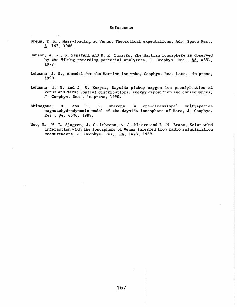
References
Breus, T. K., Mass-loading at Venus: Theoretical expectations, Adv. Space Res., ~. 167, 1986.
Hanson, W. B., S. Sanatani and D. R. Zucarro, The Martian ionosphere as observed by the Viking retarding potential analyzers, J. Geophys. Res., ~. 4351, 1977.
Luhmann, J. G., A model for the Martian ion wake, Geophys. Res. Lett., in press, 1990.
Luhmann, J. G. and J. U. Kozyra, Dayside pickup oxygen ion precipitation at Venus and Mars: Spatial distributions, energy deposition and consequences, J. Geophys. Res., in press, 1990.
Shinagawa, H. and T. E. Cravens, A one-dimensional multispecies magnetohydrodynamic model of the dayside ionosphere of Mars, J. Geophys. Res., 94, 6506, 1989.
Woo, R., W. L. Sjogren, J. G. Luhmann, A. J. Kliore and L. H. Brace, Solar wind interaction with the ionosphere of Venus inferred from radio scintillation measurements, J. Geophys. Res., 94, 1473, 1989.
157
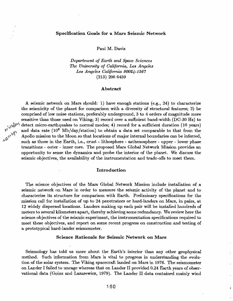
Specification Goals for a Mars Seismic Network
Paul M. Davis
Department of Earth and Space Sciences The University of California, Los Angeles
Los Angeles California 90024-1567 (213) 206 6459
Abstract
A seismic network on Mars sqould: 1) have enough stations (e.g., 24) to characterize the seismicity of the planet for comparison with a diversity of structural features; 2) be comprised of low noise stations, preferably underground, 3 to 4 orders of magnitude more sensitive than those used on Viking; 3) recordover a sufficient band-width (DC-30 Hz) to
")(.\"<~\~detect micro-earthquakes to normal modes; 4) record for a sufficient duration (10 years) \0 · (' and data rate (108 Mb/day/station) to obtain a data set comparable to that from the .fo \) Apollo mission to the Moon so that locations of major internal boundaries can be inferred,
,v\ such as those in the Earth, i.e., crust- lithosphere- asthenosphere- upper- lower phase transitions - outer - inner core. The proposed Mars Global Network Mission provides an opportunity to sense the dynamics and probe the interior of the planet. We discuss the seismic objectives, the availability of the instrumentation and trade-offs to meet them.
Introduction
The science objectives of the Mars Global Network Mission include installation of a seismic network on Mars in order to measure the seismic activity of the planet and to characterize its structure for comparison with Earth. Preliminary specifications for the mission call for installation of up to 24 penetrators or hard-landers on Mars, in pairs, at 12 widely dispersed locations. Landers making up each pair will be installed hundreds of meters to several kilometers apart, thereby achieving some redundancy. We review ~ere the science objectives of the seismic experiment, the instrumentation specifications required to meet these objectives, and report on some recent progress on construction and testing of a prototypical hard-lander seismometer.
Science Rationale for Seismic Network on Mars
Seismology has told us more about the Earth's interior than any other geophysical method. Such information from Mars is vital to progress in understanding the evolution of the solar system. The Viking spacecraft landed on Mars in 1976. The seismometer on Lander I failed to uncage whereas that on Lander II provided 0.24 Earth years of observational data (Goins and Lazarewicz, 1979). The Lander II data contained mainly wind
noise and possibly one marsquake but even that is dou~tful. The . seismic part of this mission was of secondary importance to the search for life· experiments. We are not yet sure that marsquakes exist. ' · ·
Apart from the uncaging problem on Viking I, wind !noise on Viking II was extreme because the instrument was located high up on the Lander near antennae, which vibrated or rocked the structure in response to the wind forces. Also, because only one instnunent operated on Mars, it was almost impossible to tell if a given event was a wind burst. or a. marsquake. The seismometer was less sensitive than the Lunar (Apollo) instruments due to size, weight and power constraints. However the experiment did place bounds on noise levels. It has been estimated that a network of "seismometers more sensitive than the Viking instrument by at least a factor of 103
" ••. " emplaced by penetrators or deployed as small packages can operate on the planet without being affected by typical Martian winds" (Anderson et al., 1977).
Science Goals of Mars Seismic Network
Scientific questions that a seismic network on Mars can . address depend on whether the instruments are short period (10 seconds to 10Hz) long period (DC to 10 seconds) or broad-band (DC to 30Hz) and whether they are 1-component or 3-component. Ideally they should be 3-component, broad-band, but this places severe constraints on installation, and volume and weight of the instrument package, but has the return that the science goals will be met faster than if the performance is restricted. Table 1 lists the seismic science goals separated into. those achievable with short period instruments and long period instruments.
Short Period Seismometers
1. Are there marsquakes?
2. How do their locations compare to structural features such as rift zones, volcanoes, and uplift zones?
3. How does the attenuation of seismic waves compare with Earth and the Moon where an order of magnitude difference was observed?
4. Are there major internal boundaries in Mars similar to those within Earth and the Moon, i.e., crust-lithosphere-asthenosphere-upper-lower phase transitions-outer-hmer core?
5. Is there sub-surface structure that yields information on the Martian hemispheric dichotomy (e.g. 1=1 convection)? ;
I 6. What are the dynamics of impacts on Mars from meteorites?
I
i
1 61
7. What are the focal mechanisms of marsqua.kes and how do they relate to inferred stress fields, e.g., from isostatic imbalance?
Long Period Seismometers
8. Do large impact events or marsqua.kes generate measurable normal modes which can be used to estimate velocity and density distribution?
9. Can we detect surface wave dispersion?
10. What is the Love number of the Planet?
11. Can we detect annual or Chandler wobble generated by internal changes of the moment of inertia?
Table 1 Scientific Questions for Mars Seismic Array
Science Goals of Mars Seismic Network
If we knew Mars as well as we know the internal structure of the Earth from seismology, not only would would we be exploring a new planet, we would also be adding fundamentally to our understanding of the evolution of the Solar System including the fo"rmation and composition of both Mars and Earth. Solar Nebular theories of the compositions of the planets predict that the volatile content, oxidation state and silicate iron ratios increase with distance from the Sun. The distribution of elements within a planet is determined by the temperatures during formation. For Mars we know only the mean density and moment of inertia (and there is still considerable debate on this, Kaula et al., 1989, Bills, 1989). Further progress is hampered because models satisfying these constraints allow trade-off between mantle and core densities, and core size. Direct determination of the size of the core and density profiles, by seismic means, would constrain the overall composition of the planet. Models of the thermal evolution of Mars (Schubert ,et al., 1989) since formation differ as to whether the core is solid or molten. An important factor in this regard is the amount of Sulphur in the core, which if it is the 15% as inferred from the SNC meteorites, results in a completely molten core, but if muchless, can result in a solid core. Attenuation of S-waves would tell us about the fluidity of the core.
We assume that Earth's core is mainly iron but with a substantial amount of lighter element, or elements, based on estimates of uncompressed density, shock wave data, and consistency with meteorite (type I carbonaceous) compositions. There are nonetheless uncertainties associated with this view. Are the finite strain theories used for decompression of the density truly applicable? What is the light element, or elements? Are the meteorites a relevant geochemical reference frame? Comparison of Earth with another planet will allow us to test the hypotheses used on Earth.
162
Installation of Mars Seismic Network
. Various methods to install seismometers on Mars include implantation by penetrator, deployment on the surface from a rover, or by hard, rough or soft-landers. The g loads on the instrumentation range from thousands of g for a penetrator and hard lander, hundreds of g for a rough lcmder and tens of g for a soft lander.
Penetrators
Penetrators offer an attractive way to implant a seismometer because the seismometer is firmly coupled to the planet, and is unlikely to experience the wind generated rocking motions that were thought to have generated noise on the Viking instrument (Anderson et al., 1977). Penetratortechnology is well advanced. Approximately 18,000 penetrators were dropped in Southeast Asia and radioed information on troop movements from seismic and microphone sensors which was detected by planes at 20,000 feet. The idea of a penetrator mission to Mars dates back to reports by JPL (Briggs ·et al., 1975) and Sandia (Lumpkin et al.,1974). Other studies made in the mid seventies include those by Westphal et al., · 1976, Blanchard et al., 1976, and Greely and Bunch, 1976.
Burial of the seismometer beneath the surface by a penetrator will reduce wind noise .. Also remoteness from a lander will eliminate internally generated spacecraft noise, both electrical and mechanical, as well as wind generated vibrations of the superstructure. Burial will also keep the seismometer thermally insulated from diurnal and other surface temperature changes. This is critical for long period seismometers which, if installed at the surface, record strong signals generated by thermoelastic strains, both in the· surrounding rock and in· the instrument itself. At short periods, thermoelastic changes are buffered by the thermal inertia of the instrument.
Presently we expend much effort digging pits to install sensors 1.5 m into the ground in our field installations on Earth. For short period recording, it suffices to cover the pits. For intermediate period recording, the pits are filled with insulation. However, first class seismic observatories are usually located in vaults deep underground such as mine shafts, tunnels, or in bore-holes. A penetrator installation on Mars is a practical compromise.
Surface Versus Penetrator lQstallation
A surface installation, though attractive because of its simplicity, compromises the qual~ ity of the seismic data obtainable. Ground coupling can not be assured. Proximity to wind and temperature changes would probably limit the instrumentation to short period only. However surface installations worked on the Moon, though they did not have to deal with winds. There are, however, advantages to designing two1 types of landers, a surface one for the seismic package and a sub-surface penetrator for short-lived (1 month) experiments such as soil properties, mass spectrometry etc. It would/remove the need for a small RTG, since the short term experiment in the penetrator could run on lithium batteries. It also
I
163
' i
removes the possibility of contamination of the chemical analyses by radioactive products from the RTG. A softer surface lander for the seismometer would reduce the shock tolerance requirements for the RTG and seismometer system. This may be critical for the RTG since, because of its extreme temperature (1000°C) the thermocouples can not be b<mded; it may not survive .shocks greater than a few h~ndred g.
Although it should be tested, it is probable that a large proportion of seismic short period information on Mars could come from instruments installed on the surface. The trade-off in simplifying the installation would be the loss of long period signals. Also, the low end of the short period band would be noisier than that at depth. We ran a series of tests in the alluvium in the caldera at Long Valley, California, in which a short period sensor was buried and the background noise measured as a function of depth irt a wind of ab~ut (4.0 m/s) 8 knots. In the frequency band tested, 5 Hz ..: 30Hz, there was no perceptible difference in background noise. Such tests need to be performed over the full frequency. range and for different wind and surface conditions, before effects of burial 'Can be quantified. Shedding wind vortices from obstacles can generate noise in the seismic band dependent on wind speed and obstacle shape.
Viking mission data showed that mean seismic amplitude increased as the wind velocity squared (Anderson et al., 1977) for winds ranging from 3 m/s to about 10 m/s. Optimal design of a surface installation will require the instrument package to be of a streamlined shape . It will need to have the capability to attach to the surface securely. It will also need to be kept isothermal (gradients less than 10-5°C/m) and at constant pressure (to within 10 mbar). ·
Table 1 shows the science objectives (1-7) that could be .achieved with a short period seismometer installed at the surface. We could measure the seismicity, .the travel times, fault plane solutions, invert travel times for radial structure, in~luding. detection of the Martian core. We would miss out on (8 - 11), in particular, surface waves and normal modes, which' would be regarded by most seismologists as :an extremely high price to .pay.
Normal modes ·Will give an independent check on the radial struct~re determined from travel time analysis of body waves. One large marsquake which generated a wide spectrum of normal modes would. allow inversion for internal radial structure; that would take years using short period travel-time data alone. Measurement of lateral variation in the excited modes, at multiple stations, Call be used for determination of global heterogeneity. Surface waves measured at multiple stations provides a method to measure upper mantle lateral heterogeneity, which will be particularly interesting beneath the Tharsis plateau region .
. ·Detection of latera:J. heter<?geneity means all stations should be broad-band·. We conclude that too much scie~ce is lost if the seismic installations are restriCted to' (surface) short period installations, All instruments should be br()ad-band, installed either in perietrators at d~pth ,or, if on the ~urface, they should ha~e good coupling, prefe~ably to bedrbck, and be insulated from. temperature. and pressure fluctuations. . ·
164
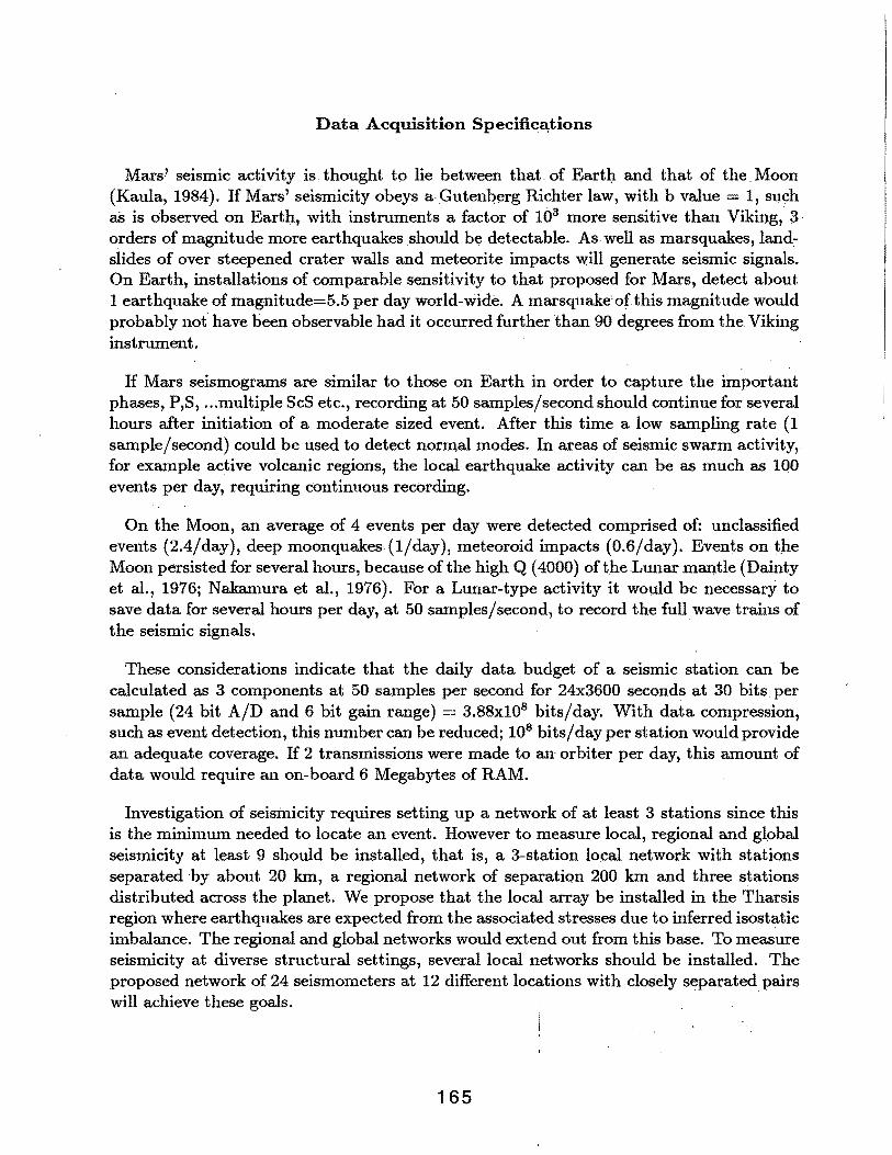
Data Acquisition Specifica,tions
Mars' seismic activity is thought to lie between that. of Eartl;t and that of the Moon (Kaula, 1984). If Mars' seismicity obeys a Gutenberg Richter law, with b value = 1, such a5 is observed on Earth, with instruments a factor of 103 more s.ensitive than Vikil}g, 3 · orders of magnitude more earthquakes should be detectable. As well as marsquakes, land:slides of over steepened crater walls and meteorite impacts will generate seismic signals. On Earth, installations of comparable sensitivity to that proposed for Mars, detect about 1 earthquake of magnitude=5.5 per day world'" wide. A marsquake'ofthis magnitude would probably not have been observable had it occurred further than 90 degrees from the Vikh1g instrument.
If Mars seismograms are similar to those on Earth in order to capture the important phases, P,S, ... multiple ScS etc., recording at 50 samples/second should continue for several hours after initiation of a moderate sized event. After this time a low sampling rate (1 sample/second) could be used to detect normal modes. In areas of seismic swarm activity, for example active volcanic regions, the local earthquake activity can be as much as 100 events per day, requiring continuous reoording.
On the Moon, an average of 4 events per day were detected comprised of: unclassified events (2.4/day), deep moonquakes (1/day), meteoroid impacts (0.6/day). Events on the Moon persisted for several hours, because of the high Q ( 4000) of the Lunar malltle (Dainty et al., 1976; Nakamura et al., ·1976). For a Lunar-type activity it wollld be necessary to save data for several hours per day, at 50 samples/second, to record the full wave trains of the seismic signals.
These considerations indicate that the daily data budget of a seismic station can be calculated as 3 components at 50 samples per second for 24x3600 seconds at 30 bits per sample (24 bit A/D and 6 bit gain range) = 3.88x108 bits/day. With data compression, such as event detection, this number can be reduced; 108 bits/ day per station would provide an adequate coverage. If 2 transmissions were made to an orbiter per day, this amount of data would require au on-board 6 Megabytes of RAM.
Investigation of seismicity requires setting up a network of at least 3 stations since this is the minimum needed to locate an event. However to measure local, regional and glc:>bal seismicity at least 9 should be installed, that is, a 3-station lo.cal network with stations separated by about 20 km, a regional network of separation 200 km and three stations distributed across the planet. We propose that the local array be installed in the Tharsis region where earthquakes are expected from the associated stresses due to h1ferred isostatic imbalance. The regional and global networks would extend out from this base. To measure seismicity at diverse structural settings, several local networks should be installed. The proposed network of 24 seismometers at 12 different locations with closely separated pairs
. .
will achieve these goals.
165
Seismometer Specifications
There is currently no seismometer available that would withstand the shock associated with penetration. Either presently available ones, with the desired sensitivity, will have to be modified, or a new design implemented. The seismometer design should be predicated on considerations of ruggedness and simplicity. Leaf spring seismometers such as the Ranger (Kinemetrics, Pasadena, California) have the required ruggedness.
In 1962 Lehner et al.,(1962) report {2000') drop tests from a helicopter of the Ranger seismometer which was clamped with all moving parts immersed in fluid (150 cc of n-heptane). Decelerations were in the range 3000-7000 g. After cushioning the various components, the final design survived a series of 7 drops with no degradation of performance.
Coil spring designs such as the Mark products (Houston, Texas) L4C or the HS10 (Geospace, Texas), are also rugged but have .less tolerance to non-verticality. The response of a damped inertial seismometer depends on the mass, the spring constant .and the damping factor. The low frequency response of a velocity transducer is critically d~-· pendent on the value of the resonant frequency. Since the response to ground displacement falls off as about 1/(frequency squared) the useful bandwidth is about a decade above and below resonance. With high signal to noise ratio and wide dynamic range, the useful bandwidth can be extended to 3 decades, e.g., 0.01 Hz to 10 Hz, for seismometers of resonant frequency 0.5 Hz. However a typical range for an L4C, as used in the USGS network in Southern California, is 0.1 to 10Hz.
One way to extend the dynamic range and linearity of an inertial seismometer is to use force-balance feedback in the form of either a magnetic or electrostatic restoring force proportiomil to the ground acceleration. The former consumes power whereas the latter, while consuming negligible power, provides a weak force a:nd is typically used on long period instruments (such as the La:Coste gravimeters of the IDA array). Alternatively addition of a displacement transducer, sensitive to sub angstrom displacements, can provide a low frequency channel output with flat response to ground acceleration with a minimal power requirement.
The final position of the penetrator may be ·well off vertical. The seismometer must either work at ··any angle or have a levelling mechanism. Seismometers with the mass suspended from coil springs have little clearance and so' jam if they are not close to vertical. For' example, the L4C jains at 17° off vertical. The mass of the Ranger seismometer is attach~d to leaf springs at either end so that when it is tilted the transverse shear strength of the flat springs prevents lateral movement- which would otherwise cause it to jain against the casing. In fact it can be converted to a horizontal seismometer merely by rezeroing the mass to the position of-greatest sensitivity. The commercially available Ranger from Kinemetrics has a diameter of 11.1 em excluding casing. This is too large to be directly transferred into a penetrator (diameter 9 em). A seismic sensor is required that has the versatility and ruggedness of the Ranger but is small enough to fit in a penetrator and has a broad-band transducer.
166
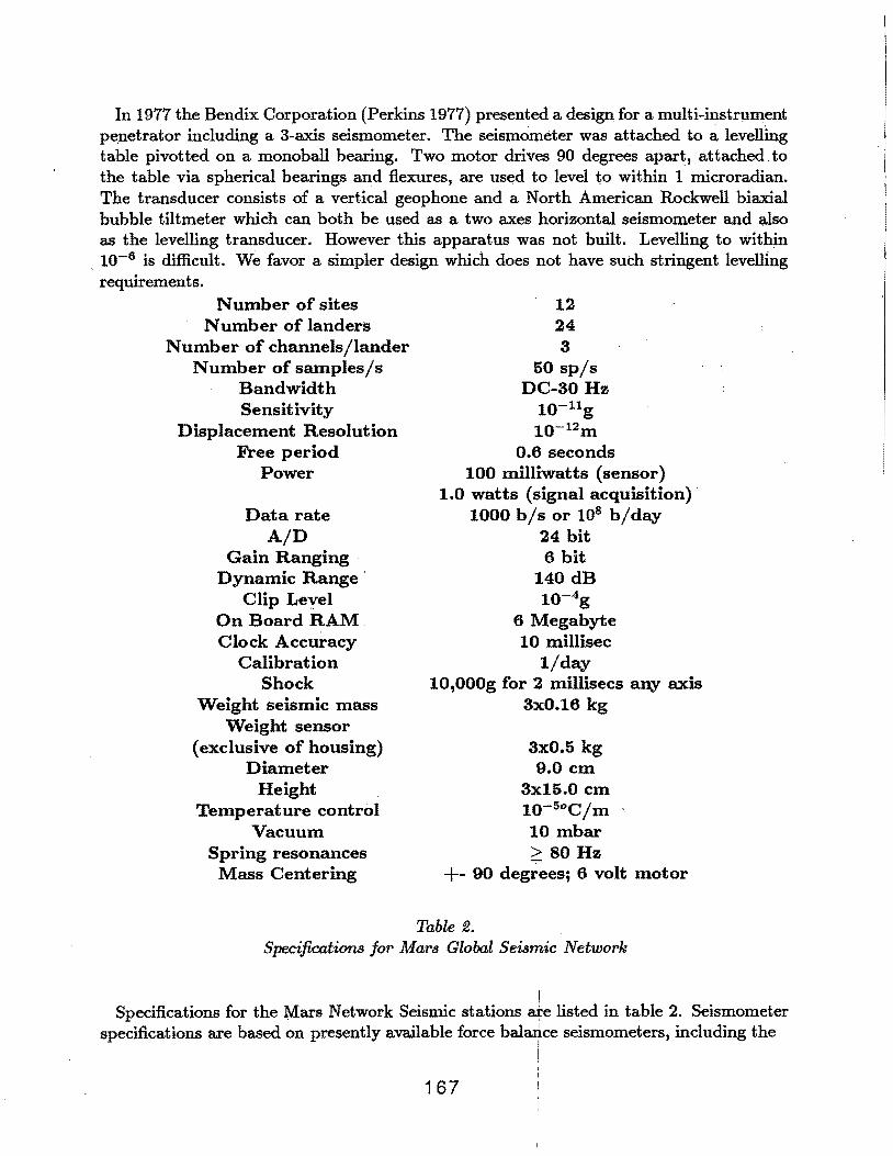
In 1977 the Bendix Corporation (Perkins 1977) presented a design for a multi-instrument pe~etrator including a 3-axis seismometer. The seismometer was attached to a levelling table pivot ted on a monoball bearing. Two motor drives 90 degrees apart, attached. to the table via spherical bearings and flexures,. are used to level to within 1 microradian. The transducer consists of a vertical geophone and a North American Rockwell biaxial bubble tiltmeter which can both be used as a two axes horizontal seismometer and also as the levelling transducer. However this apparatus was not built. Levelling to within
, to-6 is difficult. We favor a simpler design which does not have such stringent levelling requirements.
Number of sites Number of landers
Number of channels/lander Number of samples/ s
Bandwidth Sensitivity
Displacement Resolution Free period
Power
Data rate A/D
Gain Ranging · Dynamic Range ·
Clip Leyel On Board RAM . Clock Accuracy
Calibration Shock
Weight seismic mass Weight sensor
(exclusive of housing) Diameter
Height Temperature control
Vacuum Spring resonances
Mass Centering
12 24 8
50 sp/s DC-80 Hz
10-11g to-12m
0.6 seconds 100 milliwatts (sensor)
1.0 watts (signal acquisition)· 1000 b/s or 108 bjday
24 bit 6 bit
140 dB 10-4g
6 Megabyte 10 millisec
1/day lO,OOOg for 2 millisecs any axis
8x0.16 kg
8x0.5 kg 9.0 em
8x15.0 em 10-5°C/m , 10 mbar
80Hz +- 90 degrees; 6 volt motor
Table 2. Specifications for Mars Global Seismic Network
Specifications for the Mars Network Seismic stations ~e listed in table 2. Seismometer specifications are based on presently available force balar\.ce seismometers, including the
I 167

Guralp ( Guralp Systems, Reading, England) seismometer and the Strekeisen seismometer (Wielandt and Strekeisen, 1982) which have the sensitivity required but, owing to the. Bendix hinges that support the boom, they do not have the required ruggedness. Specification. of the digital acquisition system is based on systems currently in use by ffiiS · (Incorporated Research Institutions for Seismology) for the permanent and por~able networks.
Brassboard Prototypical Penetrator Seismometer
One of the most popular modern broad-band seismometers is the recently developed Guralp force-balance feedback seismometer, the mechanical part of which resembles, in many ways, a leaf spring micro-gravimeter designed by R.V. Jones (Jones and Richards, 1973). The difference is that the Guralp employs Bendix hinges to pivot the boom with a leaf spring supplying a'restoring torque whereas in the R.V. Jones design, the leaf springs also perfori:n the function of the hinge. The Bendix hinges are too weak to withstand the high deceleration impacts.
Figure 1 Leaf spring seismometer designed to be shock tolerant.
168

We have constructed a leaf spring seismometer based on the R.V. Jones design. This design has an advantage that it works 13° off-vertical without post-implantation adjustment and fitted with an adjustable re-zeroing mechanism would work in any orientation. Therefore a three component set could be installed in a penetrator for which the default would be no post impact adjustment, if the penetrator ends up close to vertical, and minimal rezeroing adjustment if it ends up well off vertical. Even then, if the rezeroing system fails, some data would be achieved, albeit at reduced sensitivity. Basically the ruggedness of leaf springs is achieved by employing 2 parallel Beryllium Copper springs on which the mass is
. suspended. A photograph and schematic of our sensor is shown in figure 1. Although it is more rugged than the Guralp seismometer, the trade-off is that it is about 1/3 as sensitive.
The position of the mass is detected by capacitance micrometry. Eventually a magnetcoil assembly will be used to provide force feedback as in the Guralp seismometer. By adjusting the filters for the force feedback output a wide dynamic range can be achieved.
Implementation of a Laboratory Impact Tester
In order to test the prototype, we assembled a laboratory impact simulator (Kewitsch, 1989). This has enabled us to conduct impact tests in the laboratory at UCLA to eliminate obvious design flaws before going to the more extensive testing at Sandia National Laboratories, Albuquerque, or from helicopter drops. Validyne Engineering (Chatsworth, California) donated a drop tower to the project. We added 8 bungee cords stretched over a
. pulley system, allowing 100% stretch of the cords to accelerate the drop, to give an effective drop of 40 feet (figures 2 and 3). An accelerometer/charge amplifier system measures the deceleration; the output is recorded on a signal analyzer (see figures 2,3,4). The system was calibrated at Environmental Associates, Chatsworth.
169

IMPACT DEVICE
I I , i
I
I I I i i
I I
I
I I
~....-..,I
I
I i ' I
=
rl....-
F~am ~ap ~a ba~~am: 8,6,4 bungee ca~ds
STATUS! PAUSED
~~~~~T!~ft~£(gRg>===============i==================9 ueee-t G
2598 G
.ll:IZY
. . . . . . o•••••••ouo•ohU~U••••••••••••H•••••••Oh,;,,;ou~ . . ' . . . . . . . . . •••••••••h•••••••••oooHoo•O•o•••••••••••••n••••• . . . . . . . . . . .. . . OU .... 000000000U0oOoooo~ooonHH0000000h0 .. 0000 . . . . .
' . . . . . . . . . ................................................... . . . . ' . . ..
•••u••••••ouoooOooooOHOoOOOO+OOo+•••o••uoOo• •O
' . ' . '''"''''''''''''*'''dooo•••••onoohoooooooooooo"o
. . . . . . ···:···················:···· ..... :·~------. . . . .. .......................................... . . . .. . . .
o ,,::.ooooooo:ooooooooo~ouoouoo:•oooUoO . . .
. . . . >000000o0U.o0o0UH0000000000~······0U000 . . . .
STATUS! PAUSED . RANGEl 18 dJV t6ioe~BtUT~I~ruE~<~~>L_ ______________ ~--------~------~
G . : : • : • ·····························"·············· .. ······· .......................................... . . . . . . . . .
OO>••••••••••••••••••••••••oooooooooooooouoooooooooo '''''"""""""'''''''''"'''""'"H~U~<••••••• . . . . .
........ : ......... : ......... : ...... : .. : ....... !.: ........ : ......... : ......... : ......... : ....... . . . . . .
$~==~ ,L_e,...•""s • .:...,...,. _.;_ __ ..;_ __ .,.:...,_...:......J.....:... __ _:...,....._s:i:T:::o:::p::-, -ia'"".~s~.~., )(I 211 .. 86 "'S•o y, 12.24 kG
16008 G
RA~IjEI 18 dJY STATUS! PAUSED
. . . ................................ u ............................................................. .
. . . . . . ......... u ......................................................................... , ••• - .. ~···· . . .
. . . . '• ''"''''*'''''''"''"''''"'*'*0>0oo0o0o>oooou+OU oO++OOooOOo••••••oo••••••o+> 0 0oOO.-,.,,.,,,., . .
:r r c·r:J_i\LJ.;;,,r ........................................................................................
s;::~,L-!,_o""S•.;..c __ _;. __ _:.. __ __; ____ ;_J __ ;..__;;_ __ .:,ST;:;O:::P-:-t -,i!,-•~S~o~o X& 118.8:1 u:S•c Yr 1.271 leG
Figure 2,3 Schematic of Bungee assisted drop tower for Lab testing seismometer and examples of deceleration pulses.
170
1
l
Addition oF weight to drop table to simulate Future seismometer
Signal analyzer
Release mechanism
Drop table and bungee cards at point oF impact
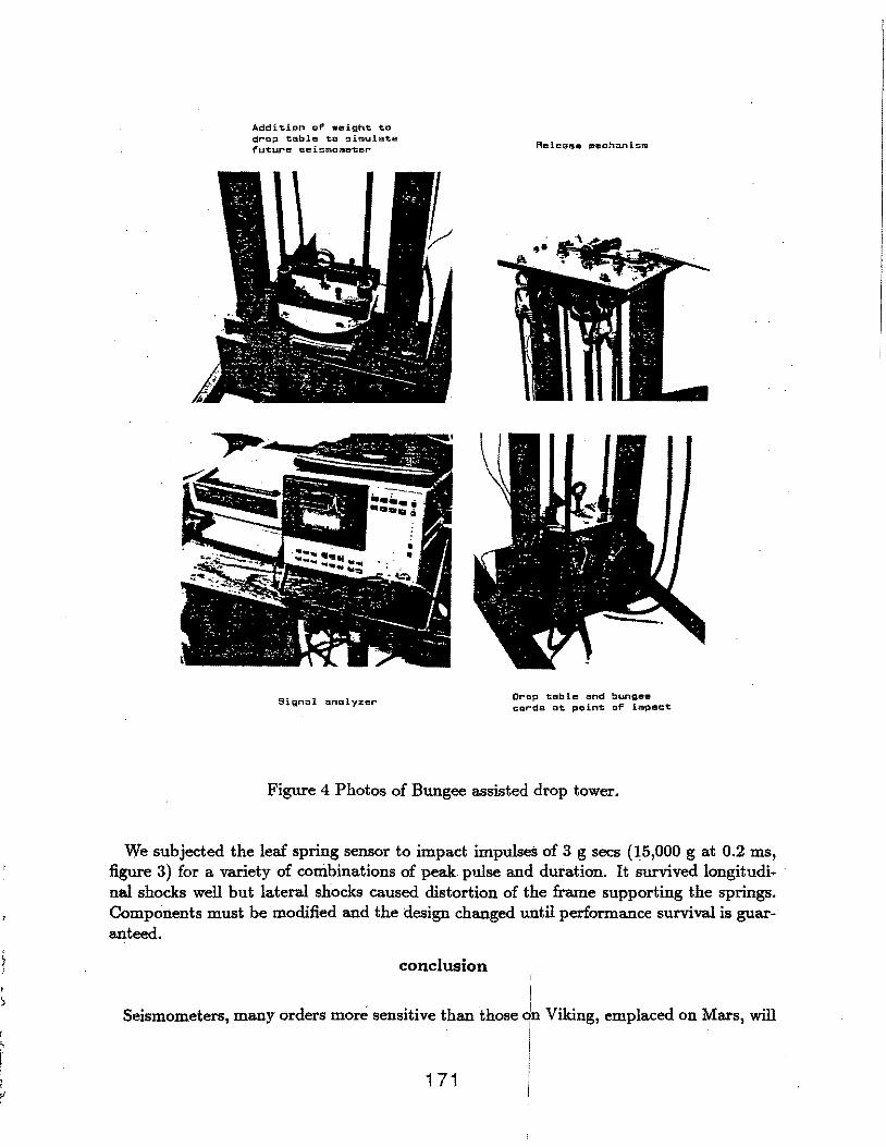
Figure 4 Photos of Bungee assisted drop tower.
We subjected the leaf spring sensor to impact impulses of 3 g sees ns,ooo g at 0.2 ms, figure 3) for a variety of combinations of peak pulse and duration. It survived longitudi ... nal shocks well but lateral shocks caused distortion of the frame supporting the springs. Components must be modified and the design changed until performance survival is guaranteed.
conclusion I
Seismometers, many orders more sensitive than those j~ Viking, emplaced on Mars, will
171 I

detect marsquakes, meteorite impacts and, possibly, landslides. To identify the locations of events, and to correlate phases, at least 4 stations are required, 3 for location and a fourth for redundancy. To exami~e diverse geological sites, several different regions should be instrumented; A total of 12 sites with 2 stations per site would achieve these goals.
Emplacement by penetrator, with detachable forebody, achieves good coupling, isolation from surface temperature and wind pressure effects; but the high g loads risk the seismometer and probably rules out \).sing an RTG.
Emplacement by hard~lander on the surface, could achieve fair coupling, if postemplacement mechanisms are eiQ.ployed (such as driving in a spike or drilling). It will need special provi~ion for isolation from temperature and wind pressure effects, which if only partially successful, will result in a short period narrow band station only. High g loads can be minimized, to less than several hundred g's, if a rough-lander is used.
Leaf spring, force-balance feedback, seismometers have the wide band-width, dynamic range, shock tolerance and sen~itivity to be used in penetrators or surface landers. They are light but consume more power than narrow-band magnet-coil velocity transducers. We have tested a brass-board suspension. design, which approaches the necessary ruggedness, but has about 1/3 the sensitivity ofa state-of-the-art instrument.
Acknowledgements This work was supported by grant CS-04-89 from California Space Isntitute.
References
Anderson, D.L., W.F. Miller, G.V. Latham, Y. Nakamura, M.N. Toksoz, A.M. Dainty, F.K. Duennebier, A.R. Lazarwicz, R.L. Kovach and T.C.D. Knight, Seismology on Mars, J. Geophys. Res., 82, 4524-4546, 1977.
Bills, B.G., Comment on ' More about the moment of inertia of Mars, Geophys. Res. Letters, 16, 11, 1337-1338, 1989.
Blanchard, M.B., V.R. Oberbeck, T.E. Bunch, R.T. Reynolds, T.N. Canning and R.W. Jackson, FY 1976 Progress report on a feasibility study evaluating the use of surface penetrators for planetary exploration, NASA Tech. Memorandum, NASA TM X-73,181.
Briggs, G.S. and others. Mars Polar Orbiter Penetrator Study Report, Jet Propulsion Laboratory, Report 760-129B, 1975.
Dainty, A.M., M.N. Toksoz, and S. Stein, Seismic investigation of the lunar interior, Proc. Lunar. Sci. Conf., 7th, 3057-3075, 1976.
172

Goins, N.R., and A. Lazarewicz, Martian Seismicity, Geophys. Res. Letters, 6, 368-370, 1979.
Greeley, R., and T.E. Bunch, Basalt models for the Mars penetrator mission: Geology of the Amboy lava field, California, NASA Technical memorandum, NAS TM- 73,125, 1976.
Jones, R.V. and J.C.S. Richards, The design and some applications of sensitive capacitance micrometers, J. Phys. E., (J. Sci. Instr.) 6, 589-600, 1973.
Kaula, W.M., The Interiors of the Terrestrial Planets: Their Structure and Evolution, UCLA Rubey Colloquium Volume, edited by Margaret Kivelson, 1984.
Kaula, W.M., N.H. Sleep, R.J. Phillips, More about the moment of inertia of Mars, Geophys. Res. Letters, 16, 11, 1333-1336, 1989.
Kewitsch, A. S., Impact tester to simulate the deceleration of a seismic penetrator implanting on Mars, Proc. lnst. of Envir. Sci., 129-133, 1989.
Lehner, F.E., E.O. Witt, W.F. Miller and R.D. Gurney, A seismometer for Ranger Lunar landing, NASA contract NASW 81, Seismol. Lab. Caltech Final Report, 1962.
Lumpkin, C.K.,( editor), Mars Penetrator: Subsurface Science Mission, Sandia Laboratories Report, SAND-74-0130, 1974.
Manning, L.A.,(editor), Mars Surface Penetrator- System Description NASA Technical Memorandum NASA TM-73,243, 1977.
Nakamura, Y., F. Duennebier, G.V. Latham, and J. Dorman, Structure of the lunar mantle, J. Geophys. Res., 81, 4818-4824, 1976.
Perkins, D., Mars penetrator instrument interface study, Final Report BSR 4307 for NAS 29649 Bendix Corp. Ann Arbor, Michigan, 1977.
Pierce, D.R., D.J. Dearborn and P.M. Davis, A Portable Cartridge Digital Seismograph., Bull. Seism. Soc. Amer., 75, 1, 323-329, 1985.
Schubert, G., S.C. Solomon, D.L. Turcotte, M.J. Drake, and N.H. Sleep, Origin and thermal evolution of Mars, (Submitted 1989 ).
Weilandt, E., and G. Streckeisen, The leaf-spring seismometer: Design and performance, Bull Seism. Soc. Amer., 72, 2349-2367, 1982.
Westphal, J.A., D. Currie, J. Fruchter, J. Head, C. Helsley, C. Lister, J. Niehoff, J. Tillman, Final Report and Recommendations of the Ad Hoc Surface Penetrator Science Committee, NASA, 1976.
173

6.2 SESSION 8 SUBMITTALS
Session B, Submittal N,o. 1
Phil Knocke Jet Propulsion Laboratory/California Institute of Technology
177
...... '
-.....~· co
A POLAR ORBIT FOR THE
MARS GLOBAL NETWORK MISSION
PHIL KNOCKE
JPL
A POLAR ORBIT FOR THE MARS GLOBAL NE'IWORK MISSION
Philip Knocke Jet Propulsion Laboratory
Presented to the Mars Global Network Mission Workshop Jet Propulsion Laboratory, Pasadena Ca.
February 6-7, 1990
INTRODUCTION
The. purpose. of the Global Network Mission {GNM) is to deploy simple landers . on the Martian surface in late 1998. The objective is to create a globally distributed network of ground stations which will collect environmental data, perhaps for as long as several years, The GNM presents unique mission design challenges, which are addressed by the following essay.
The GNM mission concept calls for two carrier spacecraft, ~ach equipped with a number of simple Iande~. Some of the landers may be deployed from approach, either to reduce carrier mass prior to orbit insertion, or to reach latitudes not available from the carrier orbit. The remaining landers are deployed from orbit.
One configuration for the Global Network Mission was proposed in a report from the Exploration Precursors Task Team to the Office of Space Science and Appiications.l This formed the basis of a previous orbit design for the GNM.2 The following analysis uses this mission scenario as a point of reference, but results from the current study are. generally applicable to a wide range of GNM mission variants.
FACTORS INFLUENCING MISSION DESIGN
The need to·minimize the orbit insertion tl.V of the carrier implies that the carrier orbit be as elliptical as possible, and have a low periapse altitude. Elliptical orbits also
I ,
179
2
lead to lower de-orbit A V' s than circular orbits.
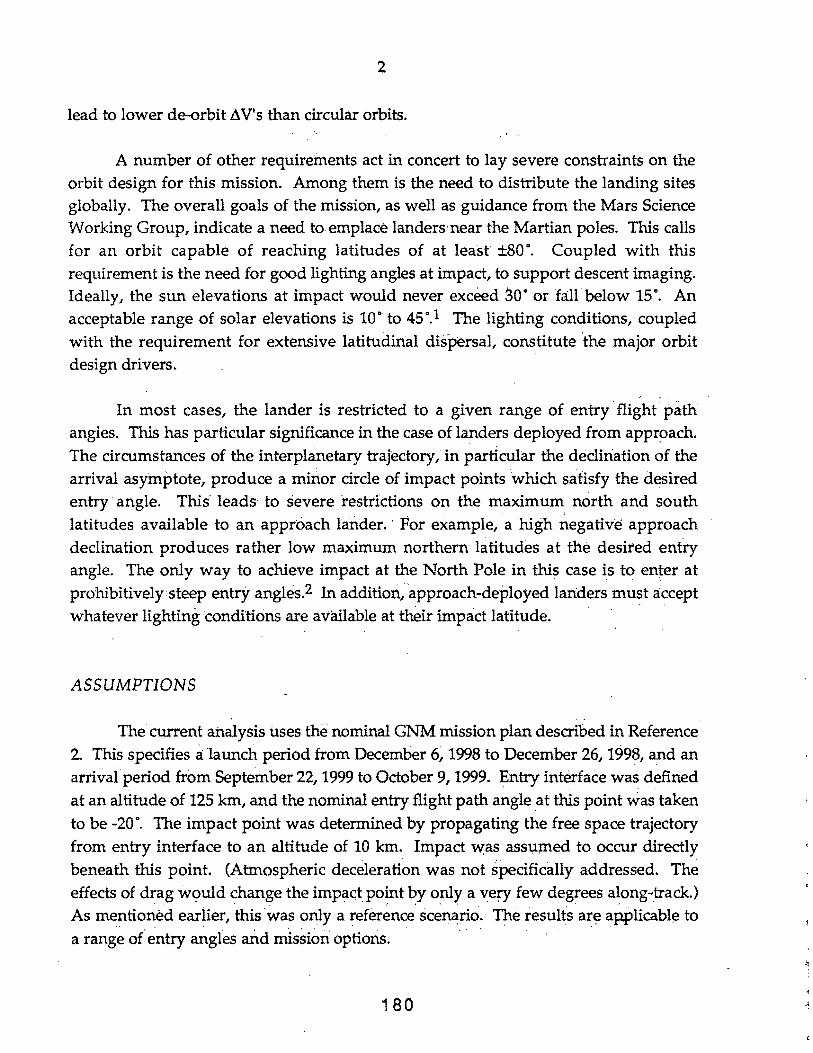
A number of other requirements act in concert to lay severe constraints on the orbit design for this mission. Among them is the need to distribute the landing sites globally. The overall goals of the mission, as well as guidance from the Mars Science Working Group, indicate a need to emplace landers near the Martian poles. This calls for an orbit capable of reaching latitudes of at least' ±so·. Coupled with this requirement is the need for good lighting angles at impact, to support descent imaging. Ideally, the sun elevations at impact would never exceed 30° or fall below 15·. An acceptable range of solar elevations is 10° to 45°.1 The lighting conditions, coupled with the requirement for extensive latitudinal dispersal, constitute 'the major orbit design drivers.
In most cases, the lander is restricted to a given range of entry· flight' path angles. This has particular significance in the case of landers deployed from appr~ach.
. .. '
The circumstances of the interplanetary trajectory,in particular the declination of the arrival asymptote, produce a minor circle of impact points which satisfy the desired entry· angle. This· leads to severe restrictions· on the maximum north and south latitudes available to an approach hinder.· For example, a high negative approach declination produces rather low maximum northern latitudes at the desired entry angle. The only way to achieve impact at the North Pole in this case is to enter at prohibitively steep entry ang1E~s.2 In addition, approach-deployed landers must a:·ccept whatever lighting conditions are available at ~ir impact latitude. · .. .
ASSUMPTIONS
The current analysis uses the nominal GNM mission plan described in Reference 2. This specifies a: launch period from December 6~ 1998 to December 26, 1998, and an arrival period from September 22, 1999 to October 9, 1999. Entry interface was defined at an altitude of 125 km, and the nominal entry flight path angle at this point was taken to be -20·. The impact point was determined by propagating the free space trajectory from entry interface to an altitude of 10 km. Impact w:as assl,lmed to occur directly beneath this point. (Atmospheric deceleration was not specifically addressed. The effects of drag W()uld change the impact point by only a very few degrees aJ.ong-track.) As mentioned earlier, this was only a reference scenario. TI:le results ar~ applicabl~ to a range of entry angles and mission options. . . . .
180
3
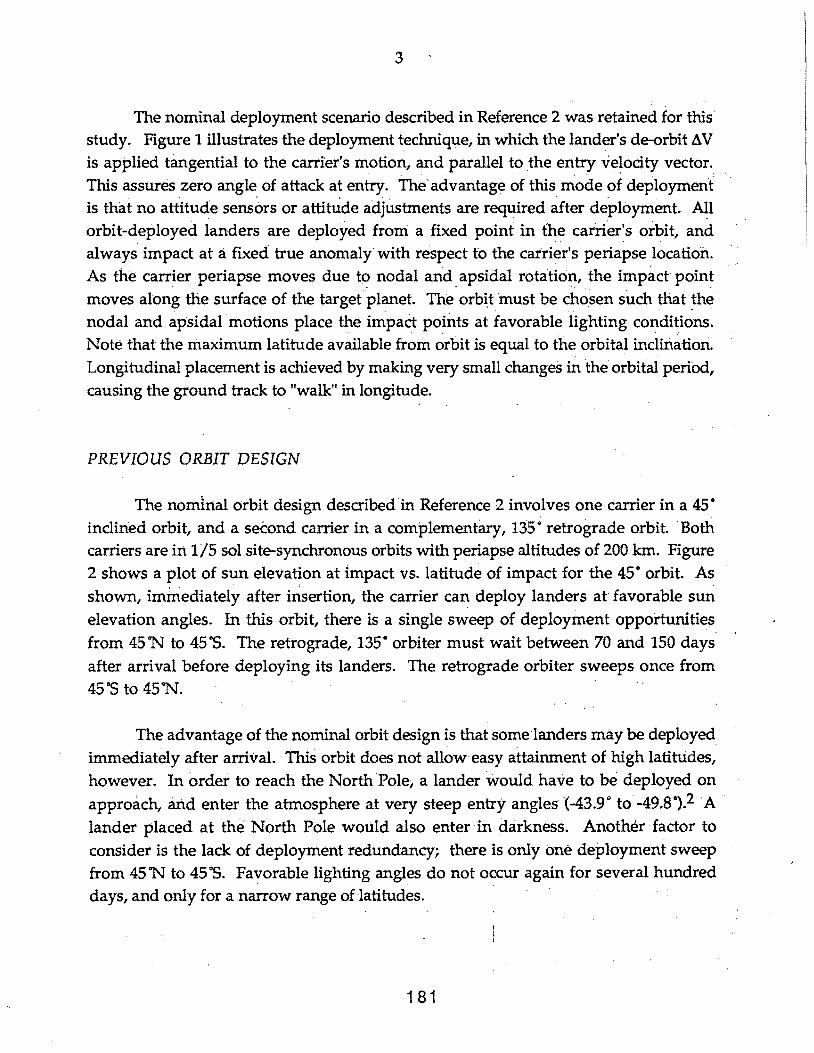
The nominal deployment scenario described in Reference 2 was retained for this study. Figure 1 illustrates the deployment technique, in which the land~r's de-orbit llV
is applied tangential to the carrier's motion, and parallel to the entry velocity vector. This assures zero angle of attack at entry. The' advantage of this mode of deployment is that no attitude sensors· or attitude adjustments are req~red ~fter deployment. All orbit-deployed landers are deployed from: a fixed point in the carrier's orbit, and always impact at a fixed true anomaly' with respect to the carrier's periapse location. As the carrier periapse moves due to nodal and_ apsidal rotatio~, the impact point moves along the surface of the target planet. The orbit-must be chosen such that the· nodal and apsidal motions place the impact points at favorable lighting conditions. Note that the maximum latitude available from orbit is equal to the orbital inclin~tion. Longitudinal placement is achieved by making very small changes in the orbital period~ causing the ground track to "walk" in longitude.
PREVIOUS ORBIT DESIGN
The nominal orbit design described-in Reference 2 involves one carrier in a 45°
inclined orbit, and a second carrier in a complementary, 135~ retrograde orbit. Both carriers are irt 1/5 sol site-synchronous orbits with periapse altitudes of 200 km. Figure 2 shows a plot of sun elevation at impact vs. latitude of impact for the 45° orbit. As shown, immediately after insertion, the carrier can deploy landers. at favorable sun elevation angles. In this orbit, there is a single sweep of deployment opportunities from 45'N to 45"5. The retrograde, 135° orbiter must wait between 70 and 150 days after arrival before deploying its landers. The retrograde orbiter sweeps once from 45 "S to 45'N.
The advantage of the nominal orbit design is that some·landers may be deployed immediately after arrival. This orbit does· not allow easy attainment of high latitudes, however. In order to reach the North Polei a lander would have to be deployed on approach, and enter the atmosphere at very steep entry angles '(-43.9° to -49.8°).2 A · lander placed at the North Pole would also enter· in darkness. Another ·factor to consider is the lack of deployment redundancy; there is only one deployment sweep from 45 'N to 45 "S. Favorable lighting angles do not occur again for several hundred days, and only for a narrow range of latitudes.
181
4
POLAR ORBIT . . .
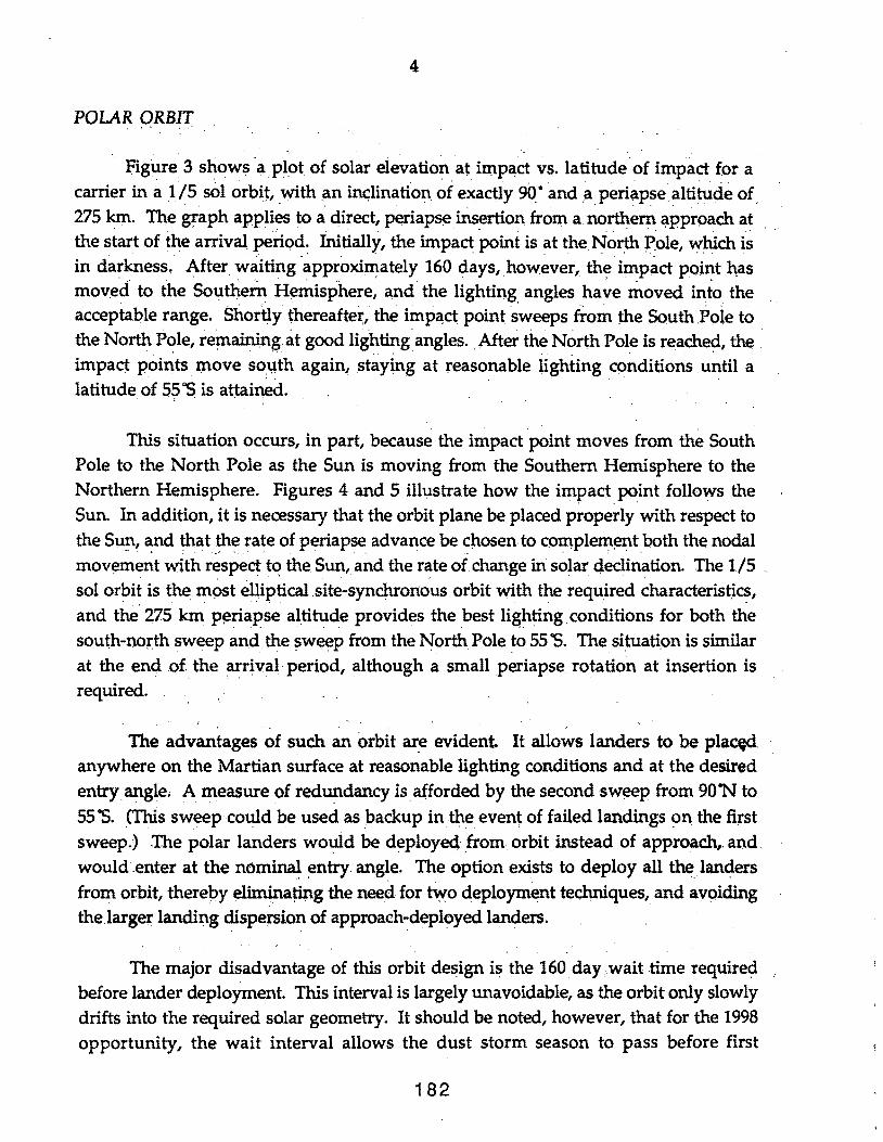
Fig11re 3 shows a plot of solar eievation at impa.ct ~s. latitude-of impact for a carrier in a _1/5 sol orbit, _with an iru;linatio~ of exactly 90_. and ,a_periapse._altitude of. _ 275 km. The ~aph applies to a direct, periapse insertion from a northe~ approach at the start of the arrival period: Initially, the impact point is at the North ]?,ole, which is in da~kness~ After waiting approxi~ately 160 days,how~ver, th~impact point has mov,ed to the Southern H~misphere,_ and. the lighting_ angles have moved into the accepta}:)le range. Shortly thereafter, the impa.ct point sweeps from the South .Poie to the North P<?le, remaining at good lighting. angles._. After the North Pole is reached, the . impact points move soqth again, staying at reasonable lighting conditions until a latitude of 5?"S is attained. ·
This situation occurs, in part, because the impact point moves from the South Pole to the North Pole as the Sun is moving from the Southern Hemisphere to the Northern Hemisphere. Figures 4 and 5 il11,1strate how the impact point follows the . ' . .
Sun. In addition, it is necessary that the orbit plane be placed properly with respect to the SU!l, ~nd that_t.ne rate of periapse. advance be cnosento compleme~tboth the nodal movement with respect tq the Sun, and the rate of change in solar. Q.eclination. The l/5
. . . . . . ~ . . sol or~it is the. most elliptical site-synchronous orbit with the required characteristics, and the. 275 km p~riapse altitude provides the best lighting conditions for both the south-no;rth sweep and the sweep from the North Pole to 55'S. The situation is similar at the end of the flfrival· period, although a small periapse rotation at insertion is required.
The advantages of such an orbit ar~ evident. It allows landers to be plac~d. anywhere on the Martian surface at reasonable lighting conditions and at the desired entry angle. A measure of redundancy is. a(forded by the second sweep from 90"N to 55'S. (This sw~p could be used as _packup in _the_ even~ of failed landings on the first sweep.) The polar landers wo':Jld be deployeq _from orbit instead of approach,. and would enter at the n()xninaJ.. entry angle. The option exists to deploy all the_ landers from orbit, there])y el.i.Inipating the need for ~o deployment techniques, and avqiding the .larger landing dispersion of approach-deployed landers.
The major disadvantage of this orbit de~ign is the 160 day .wait time required before lander deployment. This interval is largely unavoidable, as the orbit only slowly drifts into the required solar geometry. It should be noted, however, that for the 1998
opportunity, the wait interval allows the dust storm season to pass before first
182
5
deployment. The time could be used for other purposes as well, such as aeronomy measurements. The carrier could be placed in an orbit with a lower periapse, and then elevated to the 275 km altitude for a small investment in llV.
CONCLUSIONS
A 1/5 sol, polar orbit with a periapse altitude of 275 km offers the best circumstances for orbital deployment of the Global Network Mission landers. It allows easy polar access at nominal entry angles, and global dispersal of landing sites at lighting angles suitable for descent imaging. The polar orbit allows the option of deploying all the landers from orbit. A wait interval of 160 days after arrival is required before deployment can commence.
183
6
REFERENCES
1. Atkins, K., and Muirhead, B., "Mission Concept and Development for Mars Global Network Mission", Sept. 15, 1989, report from the Exploration Precursors Task Team (JPL) to the Office of Space Science and Applications ..
2. Knocke, P., "Glo[lal Network Mission Analysis", .NASA Jet Propuls.ion · Laboratory Interoffice Memora.Il.dum 312/89.2-1581, December 15, 1989.
< ,; ' • ' ' ' • ~ • ' • ' • •
184
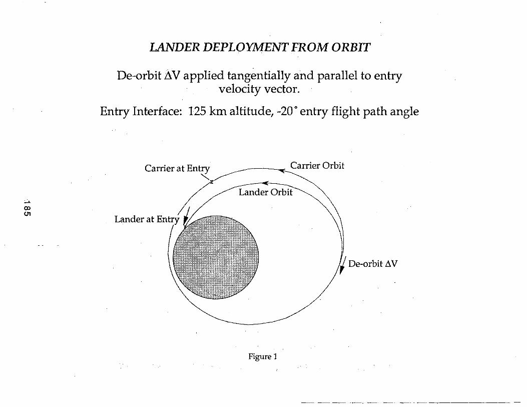
LANDER DEPLOYMENT FROM ORBIT
De-orbit AV applied tangentially and parallel to entry velocity vector.
Entry Interface: 125 km altitude, -20 ° entry flight path angle
Lander at
De-orbit ~V
Figure 1
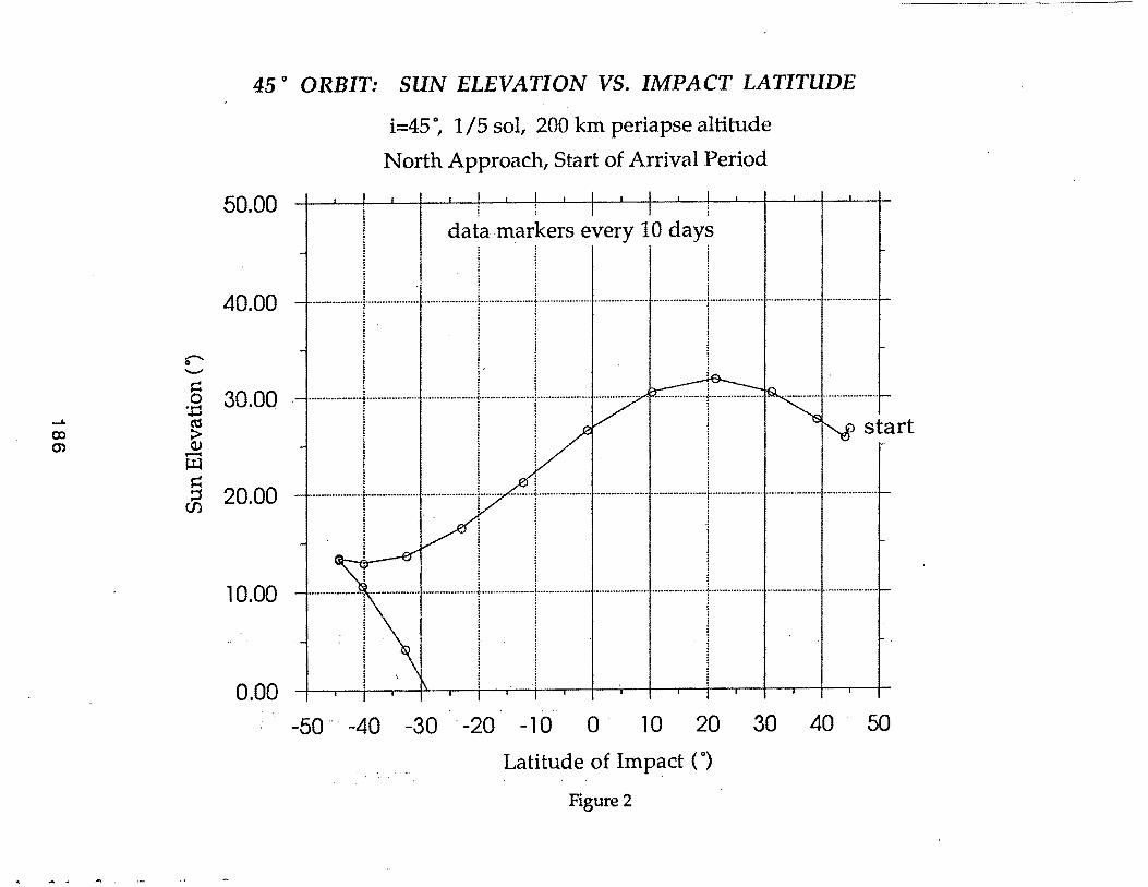
45 o ORBIT: SUN ELEVATION VS. IMPACT LATITUDE
50.00
40.00
.§ 30.00· +t\S
~ s:: ~ 20.00
10.00
0.00
i=45 °' 1/5 sol, 200 km periapse altitude
North Approach, Start of Arrival Period
i i i
data markers every 10 days
start
-50 . -40 -30 ' -20 -1 0 0 10 20 30 40 50
Latitude of Impact ( 0
)
Figure 2
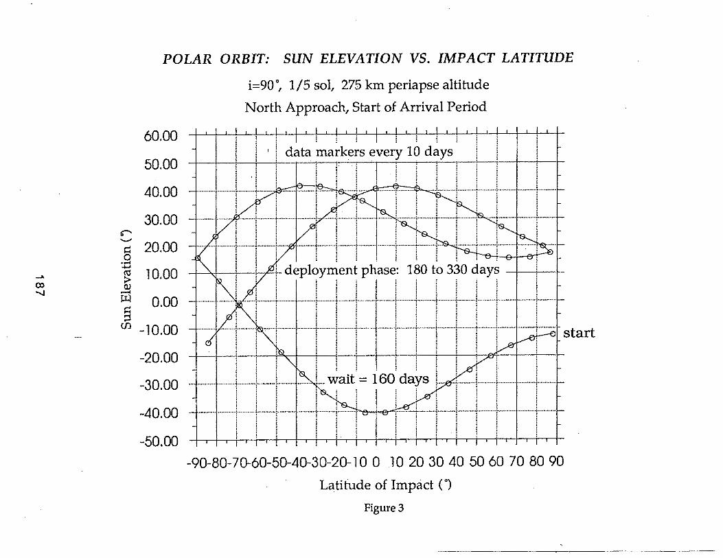
POLAR ORBIT: SUN ELEVATION VS. IMPACT LATITUDE
i=90o, 1/5 sol, 275 km periapse altitude
r
60.00
50.00
40.00
30.00
-~ 20.00 0
•.-4 ...... '
~ 10.00 QJ ........
~ 0.00 ;:::1
CJ) -10.00
-20.00
-30.00
-40.00
-50.00
North Approach, Start of Arrival Period
I ' I data ~a~ke~s eve~ 1b d~ys . .
': !
~~8~7~6~5~4~3~2~100 102030405060708090
Latitude of Impact ( 0 )
Figure3
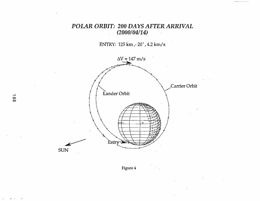
POLAR ORBIT: 200 DAYS AFTER ARRIVAL (2000/04114)
ENTRY: 125 km ,- 20°,4.2 km/s
/J.V = 147 m/s
/Carrier Orbit
~ SUN
Figure 4

POLAR ORBIT: 300DAYSAFTERARRIVAL (2000/07/25)
ENTRY: 125 km ,- 20°,4.2 km/s
SUN
\
~!!..V = 147 m/s
Figure 5
Session B, Submittal No. 2
Arden Albee California Institute of Technology
Jim Burke and Robert Mostert .:Jet Propulsion Laboratory/California Institute of Technology · ·
1 91

......... <.0
"'
MARS GLOBAL NETWORK SURFACE LANDERS
SYSTEMS DESIGN OPTIONS
ARDEN ALBEE
CAL TECH
JIM BURKE ROBERT MOSTERT
JPL
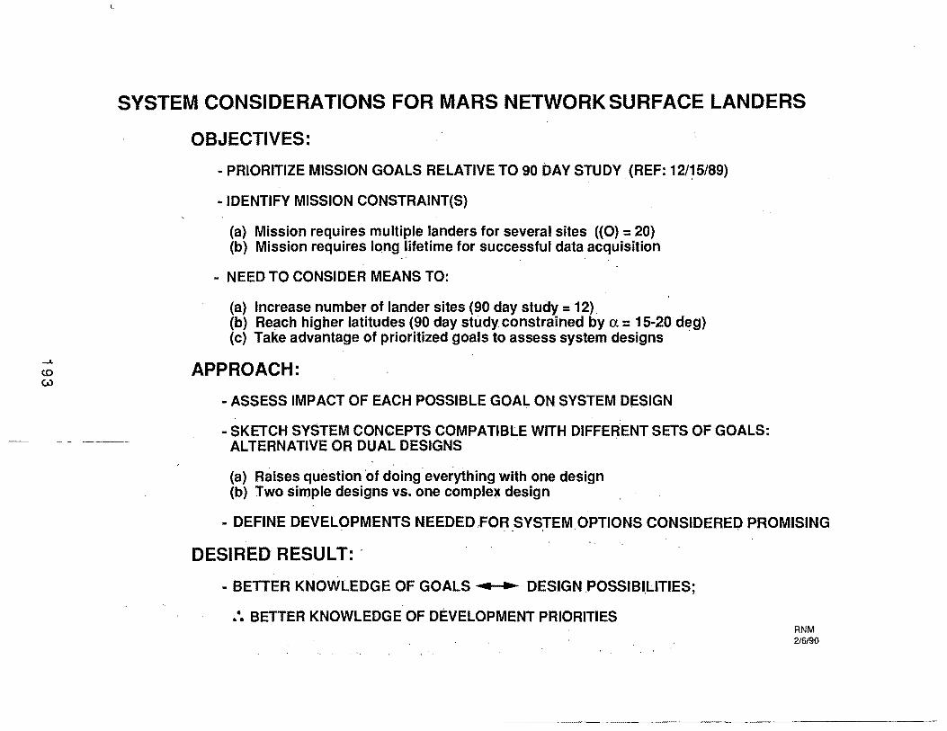
(.0
w
...
SYSTEM CONSIDERATIONS FOR MARS NETWORKSURFACE LANDERS
OBJECTIVES:
·PRIORITIZE MISSION GOALS RELATIVE TO 90 DAY STUDY. (REF: 12/15/89)
• IDENTIFY MISSION CONSTRAINT(S)
(a) Mission requires multiple landers for several sites ((0) = 20) (b) Mission require~ long lifetime for successful data acquisition
• NEED TO CONSIDER MEANS TO:
(a) Increase number of lander sites (90 day study= 12) (b) Reach higher latitudes (90 day study constrained by a= 15-20 deg) (c) Take advantage of prioritized goals to assess system designs
APPROACH:
·ASSESS IMPACT OF EACH POSSIBLE GOAL ON SYSTEM DESIGN
·SKETCH SYSTEM CONCEPTS COMPATIBLE WITH DIFFERENT SETS OF GOALS: ALTERNATIVE OR DUAL DESIGNS .
(a) Raises question ·of doing· everything with one design (b) Two simple designs vs. one complex design
• DEFINE DEVELOPMENTS NEEDED .FOR SYSTEM OPTIONS CONSIDERED PROMISING . ' ., . " . "
DESIRED RESULT: ·
• BETTER KNOWLEDGE OF GOALS ... • DESIGN POSSIBI.LITIES;
.. •• BETTER KNOWLEDGE OF DEVELOPMENT PRIORITIES RNM 2/6/90
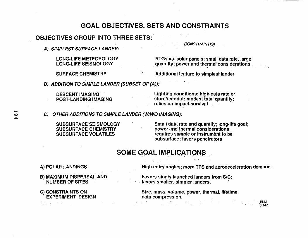
GOAL OBJECTIVES, SETS AND CONSTRAINTS
OBJECTIVES GROUP INTO THREE SETS:.
A) SIMPLEST SURFACE LANDER:
LONG-LIFE METEOROLOGY LONG-LIFE SEISMOLOGY
SURFACE CHEMISTRY
• yONSTRAINTtSJ .
RTGs vs. solar panels; small data rate, large quantity; power .and thermal considerations ,
. Additional feature to simplest lander
B) ADDITION TO SIMPLE LANDER (SUBSET OF (A)):
DESCENT IMAGING POST-LANDING IMAGING
Lighting conditions; high data rate or store/readout; modest total quantity; relies on imp.actsurvival.
w C) OTHER ADDITIONS TO SIMPLE LANDER (WIWO IMAGING): ~
SUBSURFACE SEISMOLOGY SUBSURFACE CHEMISTRY SUBSURFACE VOLATILES
Small data rateand quantity; long-life goal; power and therinal considerations; requires sample or instrument to'be ·subsurface; favors penetrators
SOME GOAL IMPLICATIONS ...
A) POLAR LANDINGS
B) MAXIMUM DISPERSAL AND NUMBER OF SITES
C) CONSTRAINTS ON EXPERIMENT DESIGN
High entry angles; more TPS and aerodeceleration demand.
Favors singly launched landers from S/C; . favors·smaller, simpler landers.
Size, mass, volume, power, thermal, lifetime, data compression.
.RNM '2/6/90
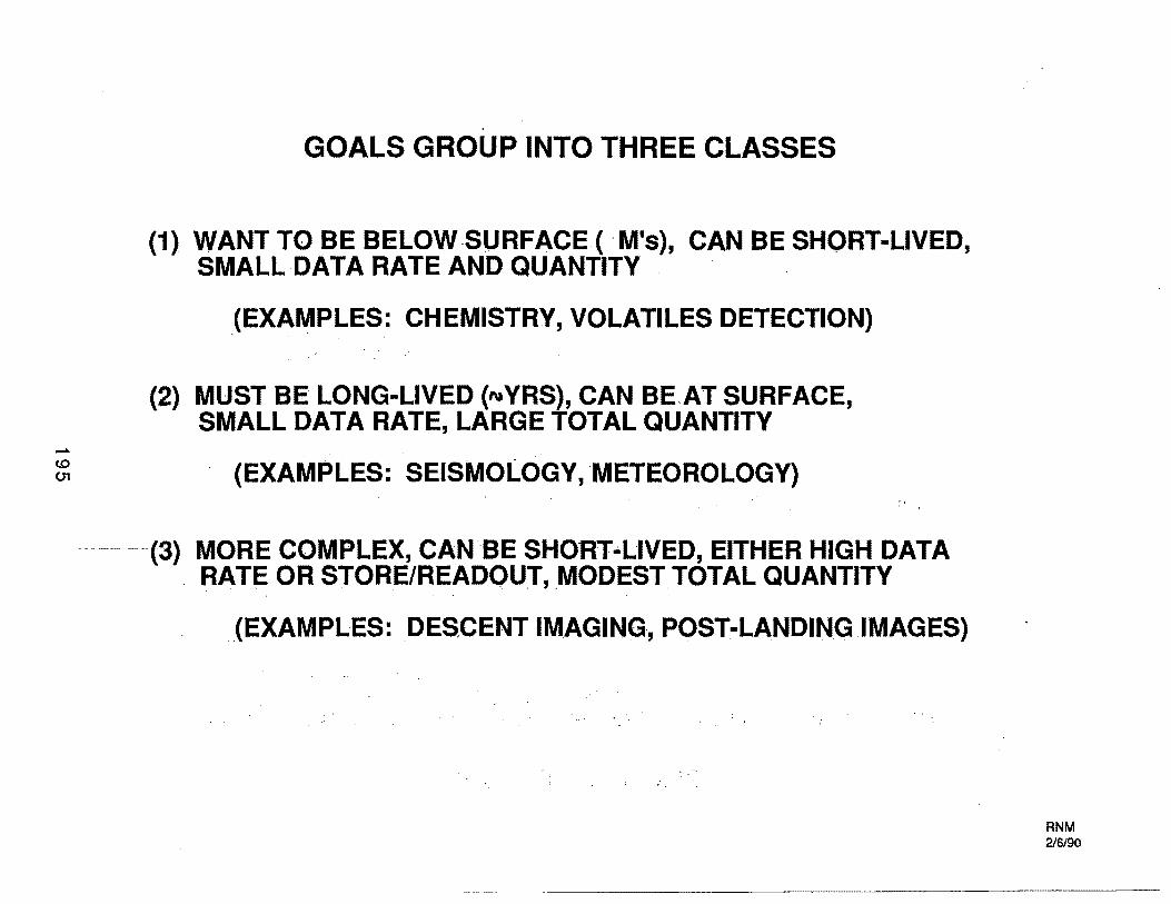
.......
GOALS GROUP INTO THREE CLASSES
(1) WANT TO BE BELOW.SURFACE ( ·M's), CAN BE SHORT-LIVED, SMALL DATA RATE AND QUANTITY .
(EXAMPLES: CHEMISTRY, VOLATILES DETECTION)
(2) MUST BE LONG-LIVED (naYRS), CAN BE.AT SURFACE, SMALL DATA RATE, LARGE TOTAL QUANTITY
~ (EXAMPLES: SEISMOLOGY, METEOROLOGY)
(3) MORE COMPLEX, CAN BE SHORT•LIVED, EITHER HIGH DATA . RATE OR STORE/READOUT, MODEST TOTAL QUANTITY
(EXAMPLES: DES.CENT IMAGING-, POST-LANDING IMAGES)
RNM 2/6/90
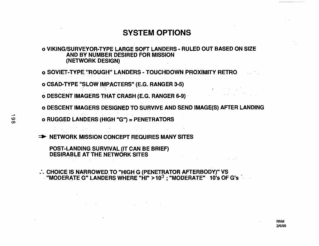
SYSTEM OPTIONS
o VIKING/SURVEYOR-TYPE LARGE SOFT LANDERS· RULED OUT BASED ON SIZE AND BY NUMBER DESIRED FOR MISSION (NETWORK DESIGN)
o SOVIET-TYPE.':'ROUGH'' LANDERS- TOUCHDOWN PROXIMITY RETRO
o CSAD-TYPE "SLOW IM,PACTERS" (E.G. RANGER 3-5)
o DESCENT IMAGERS THAT CRASH (E.G. RANGER 6-9)
o DESCENT IMAGERS DESIGNED TO SURVIVE AND SEND IMAGE(S) AFTER LANDING . .- . . .
~. 0 RUGGED LANDERS' (HIGH "G") =· PENETRATORS
~ NETWORK MISSION CONCEPT REQUIRES MANY SITES
POST-LANDING SURVIVAL (IT CAN BE BRIEF) DESIRABLE AT THE NETWORK SITES
,' ·.
:. CHOICE, IS NARROWED TO "HIGH G (PENETRATOR AFTERBODY)" VS "MODERATE G" LANDERS WHERE "HI" >103 ·"MODERATE" 10's OF G's . . . . . . '
RNM 216/90

PROS AND CONS OF ALTERNATIVE LANDER TECHNIQUES
o BUS DEFLECTION
o LANDER DEFLECTION
o NARROW ENTRY ANGl-E TOLERANCE
o WIDE ANGLE TOLERANCE
o STACKED ON AEROSHELL
o TPS FOR EACH LANDER
o LIFTING ENTRY
o PARACHUTES
--- --- o -BALLUTES
o AUTOGYROS
o AEROSHELLI(L/D) SHAPES
o IMPACT LIMITER
o ROUGH OR HARD LANDERS
o PENETRATORS
o TERMINAL ROCKETS
PROS . CONS
GOOD TARGETING;. QUARANTINE SIMPLIFIES LANDERS; USES EXISTING BUS SUBSYSTEMS
QUARANTINE; SIMPLIFIES SEQ. LANDERS MAY NOT ALL BE THE SAME
SIMPLIFIES TPS DESIGN MAY NOT REACH POLES
EXPANDS REACHABLE LATITUDES MORE TPS, AERODECEL.
SIMPLIFIES LANDERS
MORE SITES REACHABLE
MORE DISPERSION
SIMPLE
MORE ANGLE TOLERANCE
MAY ALLOW GOOD IMAGING
COMBINES FUNCTIONS
WELL TESTED
SIMPLEST
PACKING
WELL USED
DISPERSAL IN PAIRS, SETS COMPLICATES LANDERS
LARGER ERR. ELLIPSES
MAY LIMIT ANGLE TOL.
DIFFICULT
NEEDS R & D
MAY AFFECT PACKING
WITHSTANDS 100'S G's
SOME MAY FAIL
LONG-LIFE POWER, THERMAL RNM
216190
ADDS MASS TO SYSTEM
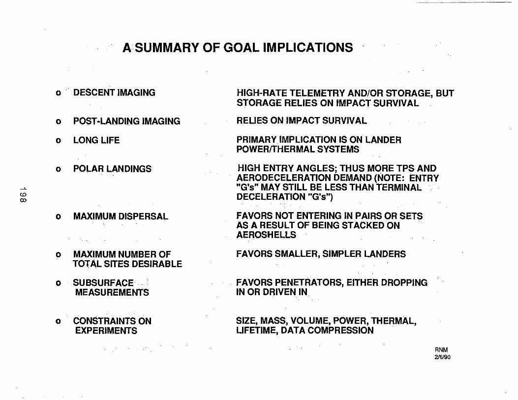
-L
<.0 co
ASUMMARY OF GOAL IMPLICATIONS · .. ·
o . DESCENT IMAGING
o POST •lANDING IMAGING
o · LONG LIFE
o POLAR LANDINGS
o MAXIMUM DISPERSAl
o MAXIMUM NUMBER OF TOtAL SITES DESIRABLE
o · SUBSURFACE ... MEASUREMENTS
o . CONSTRAlNTS ON EXPERIMENTS
HIGH-RATE TELEMETRY AND/OR STORAGE, BUT STORAGE RELIES ON IMPACT SURV:IVAl
RELIES ON IMPACT SURVIVAL
PRIMARY IMPLICATION IS ON lANDER POWER/tHERMAl SYSTEMS
HIGH ENTRY ANGLES; THUS MORE TPS·AND AERODECELERATION DEMAND (NOTE: ENTRY "G's" MAY STill BE lESS THAN TERMINAL DECELERATION "G's")
FAVORS NOT ENTERING IN PAIRS OR SETS AS A RESULT OF BEING STACKED ON . AEROSHEllS
FAVORS SMAllER, SIMPLER lANDERS
. FAVORS P·ENETRATORS, EITHER DROPPING IN OR DRIVEN IN.
SIZE, MASS, VOLUME, POWER, THERMAl, liFETIME, DATA COMPRESSION .
RNM 2/6190
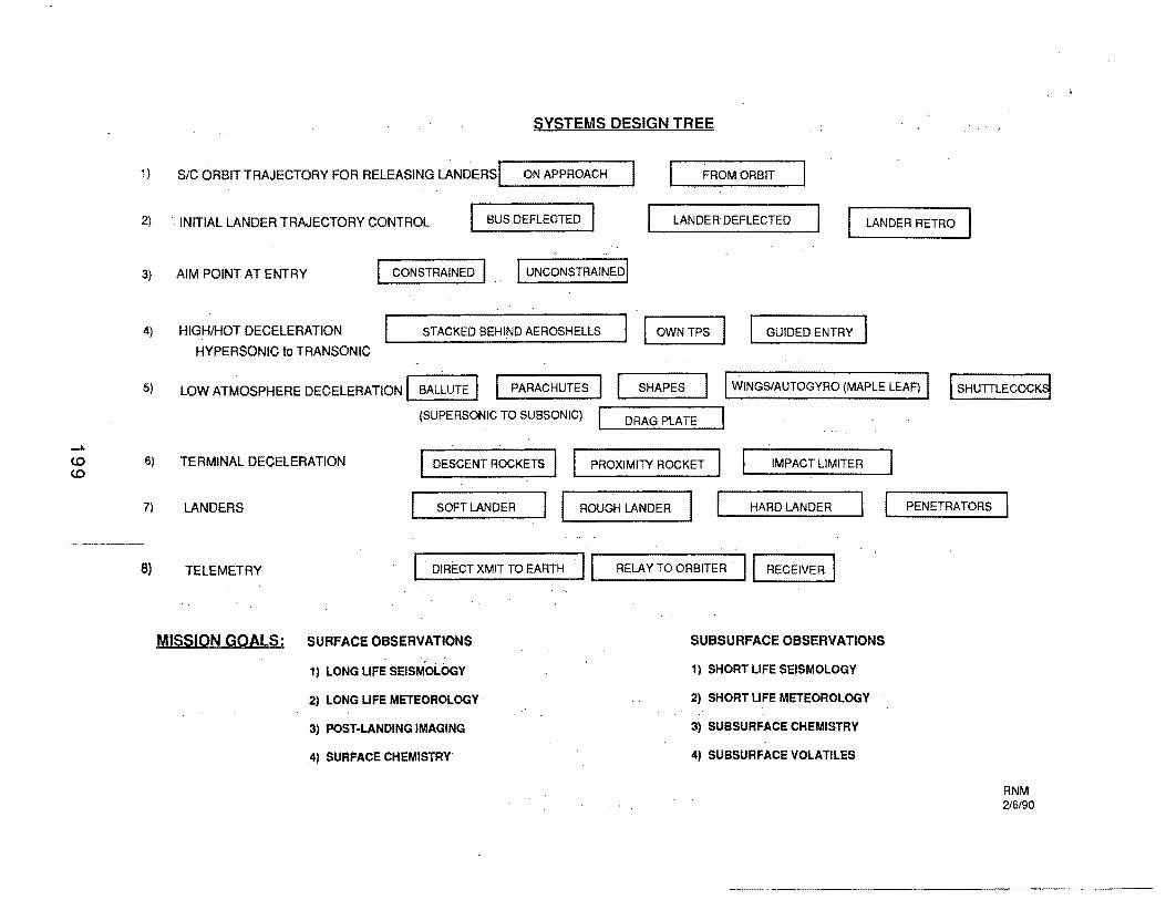
<.0 <.0
. SYSTEMS DESIGN TREE
1) SIC ORBIT TRAJECTORY FOR RELEASING LANDERS I ON APPROACH FROM ORBIT
2) ·. INITIAL LANDER TRAJECTORY CONTROL I BUS DEFLECTED I LANDER DEFLECTED LANDER RETRO
3) AIM POINT AT ENTRY I CONSTRAINED I I UNCONSTRAINED!
STACKED BEHIND AEROSHELLS I I OWN TPS GUIDED ENTRY
6) TERMINAL DECELERATION DESCENT ROCKET$ I I PROXIMITY ROCKET
L.-_s_o_F_T_LA_N_D-:-E_R_....~I I ROUGH LANDER
IMPACT LIMITER
7) LANDERS HARD LANDER
8) TELEMETRY . DIRECT XMIT TO EARTH .,, RELAY TO ORBITER . II RECEIVER I
MISSION GOALS; SURFACE OBSERVATIONS SUBSURFACE OBSERVATIONS . :· ·.- ....
1) LONG LIFE SEISMOLOGY 1) SHORT LIFE SEISMOLOGY
2) LONG LIFE METEOROLOGY · 2) SHORT LIFE METEOROLOGY
3) POST-LANDING IMAGING 3) SUBSURFACE CHEMISTRY
4) SURFACE CHEMISTRY. 4) SUBSURFACE VOLATILES
PENETRATORS
RNM 216/90
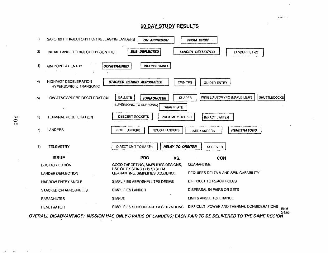
"' 0 0
90 DAY STUDY RESULTS
1) S/C ORBIT TRAJECTORY FOR RELEASING LANDERS I ON APPROACH FROM ORBrr I 2) INITIAL LANDER TRAJECTORY CONTROL . I BUS DEFLECTED I LANDER DER.EcrED I LANDER RETRO
3) AIM POINT AT ENTRY I CONSTRAINED I I UNCONSTRAINED I
STACKED BEHIND AEROBHEU.S I I OWN TPS I I GUIDED ENTRY I 4) HIGH/HOT DECELERATION HYPERSONIC to TRANSONIC
s) LOW ATMOSPHERE DECELERATION l BALLUTE I I PARACHUTES I SHAPES llwtNGStAUTOGYRO (MAPLE LEAF) llsHUTILECOCKsj
(SUPERSONIC TO SUBSONIC)-;:' =~.:::=::::;-,-.....1
6) TERMINAL DECELERATION
7) LANDERS
8) TELEMETRY
ISSUE
BUS DEFLECTION
LANDER DEFLECTION
NARROW ENTRY ANGLE
.STACKED ON AEROSHELLS
PARACHUTES
. . DRAG PLATE .
DESCENT ROCKETS I I PROXIMITY ROCKET I I IMPACT LIMITER
SOFT LANDERS I I ROUGH LANDERS II HARD LANDERS I PENETRATORB
DIRECT XMIT TO EARTH II RELAY 1t) ORBI1CR II RECEIVER I PRO vs. CON
GOOD TARGETING, SIMPLIFIES DESIGNS, QUARANTINE USE OF EXISTING BUS SYSTEM QUARANTINE, SIMPLIFIES SEQUENCE REQUIRES DELTA V AND SPIN CAPABILITY
SIMPLIFIES AEROSHELL TPS DESIGN DIFFICULT TO REACH POLES
SIMPLIFIES LANDER DISPERSAL IN PAIRS OR SETS
SIMPLE LIMITS ANGLE TOLERANCE
PENETRATOR SIMPLIFIES SUBSURFACE OBSERVATIONS DIFFICULT; POWER AND THERMAL CONSIDERATIONS RNM
2/6/90 OVERALL DISADVANTAGE: MISSION HAS ONLY 6 PAIRS OF LANDERS; EACH PAIR TO BE DELIVERED TO THE SAME REGION
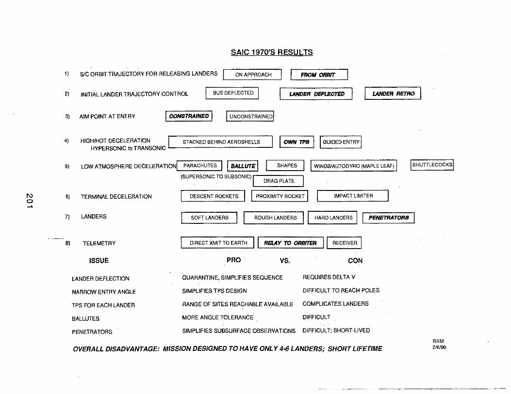
I\) 0 .......
SAIC 1970'S RESULTS
1) SIC ORBIT TRAJECTORY FOR RELEASING LANDERS. I ON APPROACH I I FROM ORBn' I 2) INITIAL LANDER TRAJECTORY CONTROL I BUS DEFLECTED I I LANDER DEFLECTED I LANDER RETRO
3) AIM POINT AT ENTRY I CONSTRAINED I I UNCONSTRAINED!
4) HIGH/HOT DECELERATION I HYPERSONIC to TRANSONIC L... --------------l
STACKED BEHIND AEROSHELLS I OWN TP8 I I GUIDED ENTRY I
5) LOW ATMOSPHERE DECELERATION! PARACHUTES I I BALLUTE I SHAPES I WINGS/AUTOGYRO (MAPLE LEAF) I (SUPE. RSONIC TO SUB. SONIC) I
. DRAG PLATE
:::=::.======:.... I PROXIMITY ROCKET I 6) TERMINAL DECELERATION DESCENT ROCKETS IMPACT LIMITER
7) LANDERS SOFT LANDERS I I ROUGH LANDERS II HARD LANDERS I I PENETRATORS
8) TELEMETRY DIRECT XMIT TO EARTH II ReLAY TO ORBTTER II RECEIVER I ISSUE PRO vs. CON
LANDER DEFLECTION QUARANTINE, SIMPLIFIES SEQUENCE REQUIRES DELTA V
NARROW ENTRY ANGLE SIMPLIFIES TPS DESIGN DIFFICULT TO REACH POLES
TPS FOR EACH LANDER RANGE OF SITES REACHABLE AVAILABLE COMPLICATES LANDERS
BALL UTES MORE ANGLE TOLERANCE DIFFICULT
PENETRATORS SIMPLIFIES SUBSURFACE OBSERVATIONS DIFFICULT: SHORT-LIVED
OVERALL DISADVANTAGE: MISSION DESIGNED TO HAVE ONLY 4·6 LANDERS; SHORT LIFETIME
!sHUTTLECOCKS'
RNM 2/6/90
~~·······-----------------------

1\) ..
0 I\).
AMES 1977 RESULTS -
1) SIC ORBIT TRAJECTORY FOR RELEASING LANDERS .____ON_AP._P._RO_" _!A~_H___.I "I FROM ORBIT . I
2) INITIAL LANDER TRAJECTORY CONTROL jsus.D~I I LANDER DEFLECTED .11 L.. _LA_N_D_ER_R_E_T_Ro___.
3) AIM POINT AT ENTRY I CONSTRAINED I . " I UNCONSTRAINED'
4) HIGH/HOT DECELERATION I HYPERSONIC to TRANSONIC
STACKED BEHIND AEROSHELLS I I OWN TPS 1-1 GUIDED ENTRY!
5) LOW ATMOSPHERE DECELERATION I BALLUTE I I PARACHUTES I I SHAPES I I WINGSIAUTOGYRO (MAPLE LEAF) I I SHUTILECOCKSI
6) TERMINAL DECELERATION
7)
8)
LANDERS
TELEMETRY
ISSUE
LANDER DEFLECTION
· NARROW ENTRY ANGLE
DRAG PLATE
PENETRATORS
(SUPERSONIC TO SUBSONIC) . I DRAG PLATE
DESCENT ROCKETS ·IIPROXIMITY ROCKE1 I IMPACT LIMITER
SOFT LANDERS I" I ROUGH LANDERS I I HARD LANDERS PENETRATORS
I· DIRECT X MIT TO EARTH II RSAY TO ORBI'7l:R II RECEIVER I PRO vs. CON
QUARANTINE, SIMPLIFIES SEQUENCE
. SIMPLIFIES TPS pESIGN
RETRO FROM SPACECRAFT; REQUIRES OWN TPS
DIFFICULT TO REACH POLES
ALLOWS ONE LANDER PER PLATE DIFFICULT
SIMPLIFIES SUBSURFACE OBSERVATIONS DIFFic"ULT; POWER AND THERMAL CONSIDERATIONS
OVERALL DISADVANTAGE: MISSION DESIGNED TO HAVE ONLY 3 LANDERS; DIFFICULT TO ESTABLISH A TRUE GLOBAL NETWORK RNM
216/90
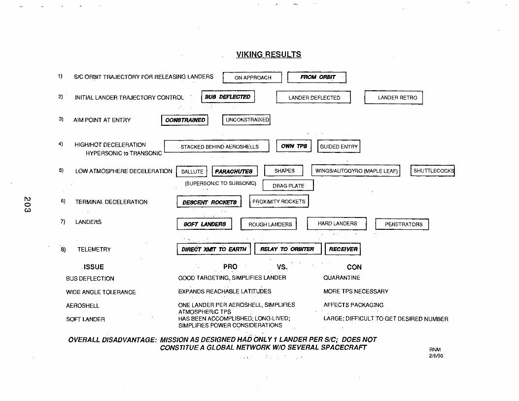
1\) 0 c.u
VIKING RESULTS
1) S/C ORBIT TRAJECTORY FOR RELEASING LANDERS L--_o_N_A_P_P_R_oA_c_H _ _.I I FROM ORBI!
2) INITIAL LANDER TRAJECTORY CONTROL . I BUS DEFLECTED I I LANDER DEFLECTED LANDER RETRO
3) AIM POINT AT ENTRY I CONSTRAINED I I UNCONSTRAINED'
4) HIGH/HOT DECELERATION I HYPERSONIC to TRANSONIC
STACKED BEHIND AEROSHELLS I I OWN TP8 I I GUIDED ENTRY I
5) LOW ATMOSPHERE DECELERATION I BALLUTE II PARACHirrcS I I SHAPES I WINGS/AUTOGYRO (MAPLE LEAF) I I SHUTILECOCK9
6) TERMINAL DECELERATION
7) LANDERS
8) TELEMETRY
ISSUE
BUS DEFLECTION
WIDE ANGLE TOLERANCE
AEROSHELL
(SUPERS?NIC TO SUBSONIC) I DRAG PLATE
DESCENT ROCKETS I I PJ:lOXIMITY ROCKETS I SOFT LANDERS I I ROUGH LANDERS I HARD LANDERS PENETRATORS
1 DIRECT XMrT ro iwml·11 REl.AY ro 'ORBITER II RECEIVER 1
PRO vs. GOOD TARGETING, SIMPLIFIES LANDER
EXPANDS REACHABLE LATITUDES
ONE LANDER PER AEROSHELL, SIMPLIFIES ATMOSPHERIC TPS .
CON
QUARANTINE
MORE TPS NECESSARY
AFFECTS PACI:(AGING
SOFT LANDER HAS BEEN AQCOMPL,JSHED; LONG-LIVED; SIMPLIFIES POWER CONSIDERATIONS
LARGE; DIFFICULT TO GET DESIRED NUMBER
OVERALL DISADVANTAGE: 'MISSION AS DESIGNED HAD ONLY 1 LANDER PER SIC; DOES NOT CONSTITUE A GLOBAL NETWORK W/0 SEVERAL SPACECRAFT RNM
2/6/90
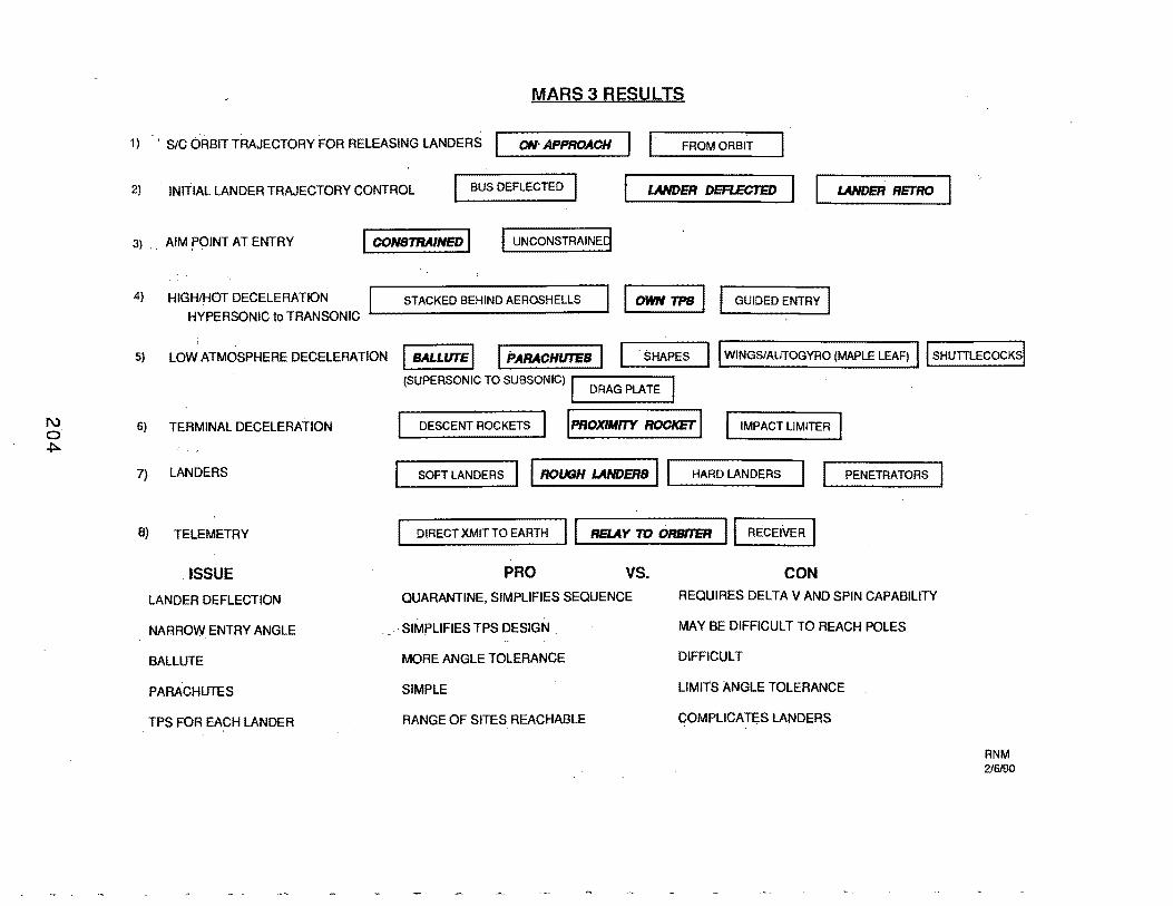
MARS3 RESULTS
1) . \ SIC ORBIT TRAJECTORY FOR RELEASING LANDERS ~..-_ON_· _AP_PRa __ IA_CH _ _Jl 1· FROM ORBIT
2) INITiAL LANDER TRAJECTORY CONTROL I BUS DEFLECTED I I LANDER DEFLECTED II.__ _LAN_'DER_RETRO_ .........
3) . AIM flOINT AT ENTRY I CONSTRAINED I I UNCONSTRAINE~
STACKED BEHIND AEROSHELLS I I OWN 1PS I I GUIDED ENTRY I 4) HIGH/HOT DECELERATION
HYPERSONIC to TRANSONIC
5) LOW ATMOSPHERE DECELERATION I BALLUTEI I PARACHUTES I I ·SHAPES II WINGSIAUTOGYRo (MAPLE LEAF) II SHUTTLEcocKs!
6) TERMINAL DECELERATION
7} LANDERS
8) TELEMETRY
.ISSUE
LANDER DEFLECTION
. NARROW ENTRY ANGLE
BALL UTE
PARACHUTES
TPS FOR EACH LANDER
(SUPERSONIC TO SUBSONIC) I I . DRAG PLATE .
DESCENT ROCKETS I I PROXIMITY ROCKET I IMPACT LIMITER I soFT LANDERS I I ROUGH LANDERS II HARD LANDERs I .... 1 _P_EN_E_T_RA_T_o_Rs-...J
DIRECT XMIT To EARTH II RELAY ro ORBITER II RECEIVER I PRO vs.
QUARANTINE, SIMPLIFIES SEQUENCE
. ·SIMPLIFIES TPS DESIGN .
MORE ANGLE TOLERANCE
SIMPLE
RANGE OF SITES REACHABLE
CON
REQUIRES DELTA V AND SPIN CAPABILITY
MAY BE DIFFICULT TO REACH POLES
DIFFICULT
LIMITS ANGLE TOLERANCE
COMPLICATES LANDERS
RNM 2/6190
Session B, Submittal No. 3 · ..
Alan L. Friedlander Science Applications International Corporation
205
1\)
0 (J')
....... -.... ..... ____ lo, ""' -- - -
A GLOBAL VIEW OF LANDER-TO-ORBITER COMMUNICATIONS ACCESSIBILITY
FOR A MARS GLOBAL NETWORK MISSION
ALAN FRIEDLANDER SAIC
A Global View of Lander-to-Orbiter Communications Accessibility for a Mars Global Network Mission
Alan Friedlander Sci~nce Applications International Corporation
Presented to Mars Global Network Mission Workshop Jet Propulsion Laboratory, February 6-7, 1990
Given the mission obj~tive to deploy a number of small landers to the surface of Mars at various· latitude/longitude locations, it is of interest to obtain a global perspective of the communications link geometry between the landers and a data relay orbiter. Specifically, the question to be answered is what is the total time interval over one martian day ( 1 sol) that a lander at any given latitude and longitude can communicate data to the orbiter. Results should be obtained for more than one elevation angle constraint (lander antenna design issue), and also for several time points into the mission since the orbiter's perlapsis location moves under the influence of Mars oblateness perturbation. This paper presents such information in terms of global contour maps of available communications time per sol summed over all orbiter passes on that day. Global data of this type· complements more detailed local site data such as communications range and elevation vs time per pass.
The reference mission launched in 1998 arrives at Mars in late September 1999 and the orbiteds placed into a polar orbit (90 deg inclination) with periapsis altitude of 275 km, apoapsis altitude Of 6903 km, and orbit period of 1/5 sol. Periapsis latitude is initially at. 27 deg N and moves southward at the rate of about 1 deg/sol. Landing sites for orbit deployment are displaced about 56 deg from the orbiter's periapsis, thus starting near the north pole and moving southward. If the landers have desce~t imaging capability with a requirement for low sun elevation angles between 15 deg and- 30 deg, then the first deployment from orbit must be delayed until sol# 180 after arrival. Thereafter, all landing site latitudes are accessible with good values ·of sun angle. Pole-topole coverage is accomplished in about 6 months.
Communications time contour maps are included here for sol #'s 180, 232, 318, 361, and 404 corresponding to orbiter periapsis latitudes of 35 S, 90S, equatorial, 45 N, and 90 N. For each of these days, there is a map for both a 15 deg and 45 deg minimum elevation constraint on the· lander-to-orbiter line of sight. The jagged appearance of the contour lines is due to computational resolution in interpolating between a finite number of latitude/longitude grid points. Although the . contpurs should really be smooth, the general information content is represented by the lower resolution maps shown here. An example of the tabulated, fmite-grid data points is also given.
Communication with all sites is possible at the 15 deg elevation constraint, at times only for several minutes per sol but more generally for a much longer time up to 14; hours per sol. Significantly less time is available with a 45 deg elevation constraint, and at certain times in the mission some localized regions of the planet are inaccessible. Still, one may conclude that the reference orbit selection will support a more than adequate communications link through tlie mission timeline with landers emplaced at any desired location on Mars. ·
207
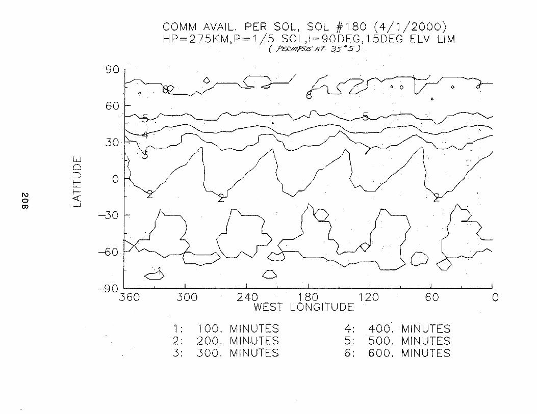
w 0
1\) t-0 <( (X) _j
90
60
30.
0
-30
--60
COMM AVAIL. PER SOL, SOL #180 (4/1 /2000) HP=275KM,P= 1/5 SOL,I=90DEG, 15DEG ELV LIM
( ,PE.£/I'l,PS/S /1 T- ~5_ "'5)
~~v/l~
0 -90~ .. ~--~--~--~--~--~--~--~--~--~--~~
360 300 240 1 80 120 60 0 WEST LONGITUDE
1: 1 00. MINUTES 2: 200. MINUTES 3: 300. MINUTES
4: 400. MINUTES 5: 500. MINUTES 6: 600. MINUTES
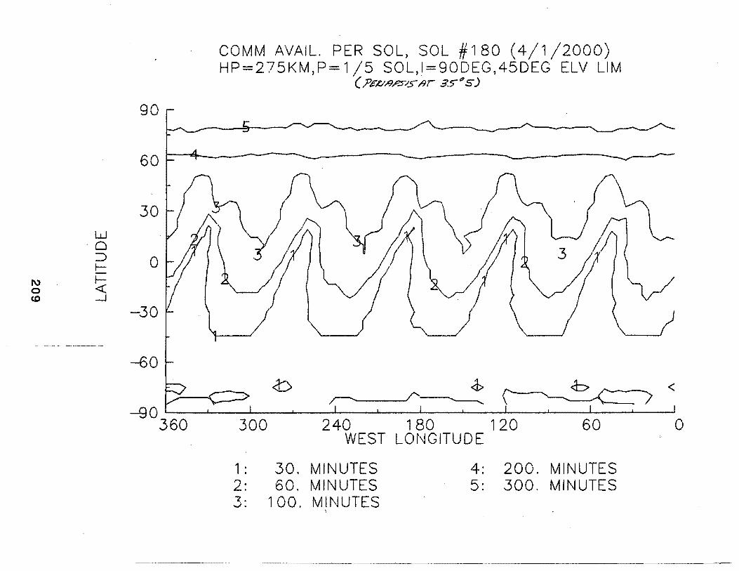
1\)
0 co
w ·o
::) II<( _,..J
90
60
30
0
-30
-60
COMM AVAIL. PER SOL, SOL #180 (4/1 /2000) HP=275KM,P= 1/5 SOL,I=90DEG,45DEG ELV LIM
(?&JY;&;P.Y/.5"/JT 35(11S)
<1> r------/'----.
-eo~~--~--~--~--~--~--~--~--~--~--~~ 360 300 240 180 120 60 0
WEST LOt'-JGITUDE
1: 30. MINUTES 2: 60. MINUTES 3: 1 00. MINUTES
4: 200. MINUTES 5: 300. MINUTES
-·······---········----------------~------
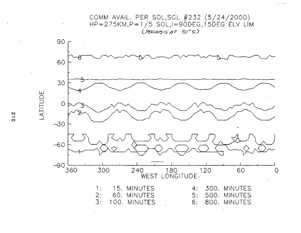
90
60
30 w 0 :::> 0 I-
1\) I-<(
-L _J 0
-30
-60
-90 360
COMM AVAIL. PER SOL,SOL #232 (5/24/2000) H P = 2 7 5 K ~vl, P = 1 /5 S 0 L, i = 9 0 DE G , 1 5 DE G E LV L1 M
(?E,.c;/9/-5/S /1 T 9o C1 s)
300 240 180 120 60 WEST LONGITUDE,
1 : 15. MINUTES 4: 300. MINUTES 2: 60. MINUTES 5: 500. MINUTES 3: 100. MINUTES 6: 800. MINUTES
0

w 0 ::> ~
1\) 1---L <( --L _j
90
30
0
-30
COMM AVAIL. PER SOL,SOL #232 (5/24/2000) HP=275KM,P= 1 /5 SOL,i=90DEG,45DEG ELV LIM
I
(?£Jl/FJPS'IS .t9T 9t:' 0 S)
-90~~--~--~--~--~--~--~--~--~--~--~~
360 300 240 180 120 60 0 . WEST LONGITUDE
1: 5. MINUTES 2: 1 5. MINUTES 3: 30. MINUTES·
4: 1 00. MINUTES 5: 300. MINUTES 6: 500. MINUTES
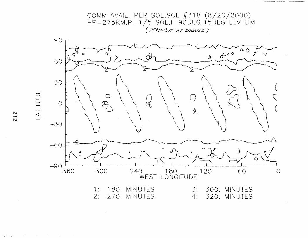
w 0 :::J f-
1\) ~ ...A
1\) _j.
COMM AVAIL. PER SOL,SOL #318 (8/20/2000) HP=275KM,P. 1/5 SOL,I=90DEG, 15DEG ELV LIM
( }JE.R..//1?5/S /9 T EuU/JriJ£)
90
&?~ oo
4 60
30
\ ~\ (
~ \ 0 0 \: 0 ~ \ (
~.
-30 ~ -60
-90~~~~--~--~--~--~--~--~--~--~--~--~
360 300 240 180 120 60 0 WEST LONGITUDE
1: 180. MINUTES 2: 270. MINUTES
3: 300. MINUTES 4: 320. MINUTES
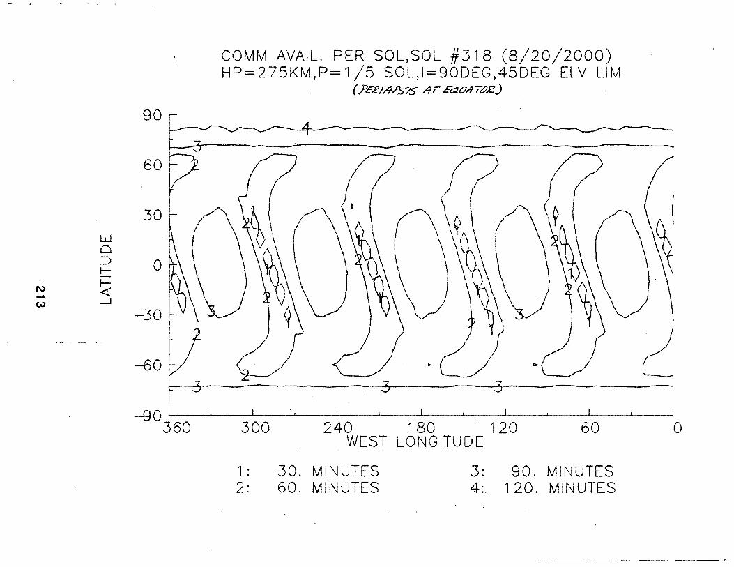
w 0 ::> I-
I\) I-_.. <{ U)
_j
90
60
30
0
-30
---{)0
COMM AVAIL. PER SOL,SOL #318 (8/20/2000) HP=275KM,P= 1/5 SOL,I=90DEG,45DEG ELV LIM
( PE£1/?/5/S .ItT Eao.IJ ,-z;z)
1: 30. MINUTES 2: 60. MINUTES
3: 90. MINUTES 4: 120. MINUTES
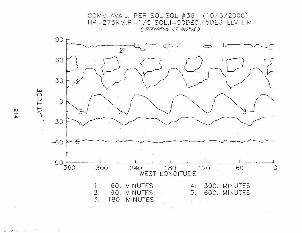
w 0 ::> I-I<( _j.
90
60
0
-30
COMM AVAIL. PER SOL,SOL #361 (10/3/2000) HP=275KM,P= 1/5 SOL,I=90DEG,45DEG ELV LIM
( ,P£;£//9?SIS 8T /f5°p/)
-9.0 ~,---'----"'-----l..----L..--....1..--...l---....L..---'----L---.i.---....____. 360 300 240 180 120 60 0
WEST LONGITUDE
1: 60. MINUTES 2: 90. MINUTES 3: 180. MINUTES
4: 300. MINUTES 5: 600. MINUTES
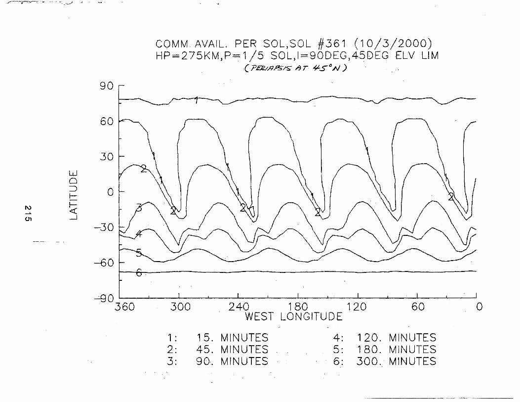
1\) -" 01
w 0 :) II-<( _J
90
60
30
0
-30
-60
~0 360
COMM AVAIL. PER SOL,SOL #361 (10/3/2000) HP=275KM,P . 1/5 SOL,I=90DEG,45DEG ELV LIM
( Pa;/9P5/s;; 1'3 T 4'-S 0 N)
300 240 180 120 . 60 WEST LONGITUDE
1 : 1 5. MINUTES 4: 120. MINUTES 2: 45. MINUTES 5: 180. MINUTES 3: 90·~ MINUTES 6: 300. MINUTES
0
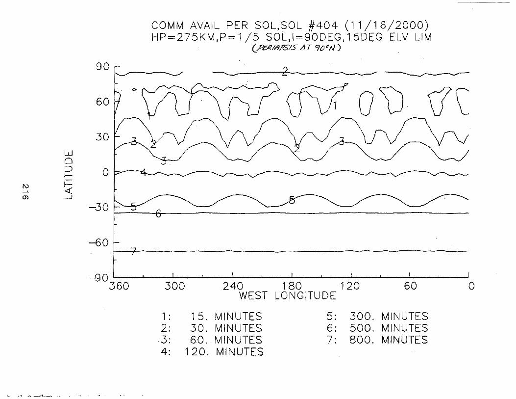
w 0 ~ I-
I\) 1-__.. <( 0') __J
90
60
30
0
-30
-60
COMM AVAIL PER SOL, SOL #404 ( 11 /16/2000) HP=275KM,P= 1/5 SOL,1=90DEG, 15DEG ELV LIM
~119;:6/S AT 90(}N)
ou vc
-eo~~--~--~--~--~--~--~--~--~~~--~~
360 300 240 180 120 60 0 WEST LONGITUDE
1: 15. MINUTES 2: 30. MINUTES ·3: 6.0 .. MINUTES 4: 120. MINUTES
5: 300. MINUTES 6: 500. MINUTES 7: 800. MINUTES
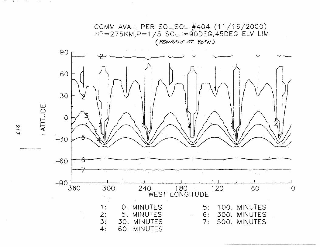
90
60
30 w 0 ::) 0 1-
1\) ~ ..... ...... _..J
-30
~0
-90 360
COMM AVAIL PER SOL, SOL #404 ( 11/1 6/2000) HP=275KM,P= 1/5. SOL,1=90DEG,45DEG ELV LIM
( .PeJl.l/l;f?..>/.5' ;::;r 'lot) AI)
300 240 180 120 60 WEST LONGITUDE
1 : 0. MINUTES 5: 100. MINUTES 2: 5·. MINUTES 6: 300. MINUTES 3: 30. MINUTES 7: 500. MINUTES 4: 60. MINUTES
0
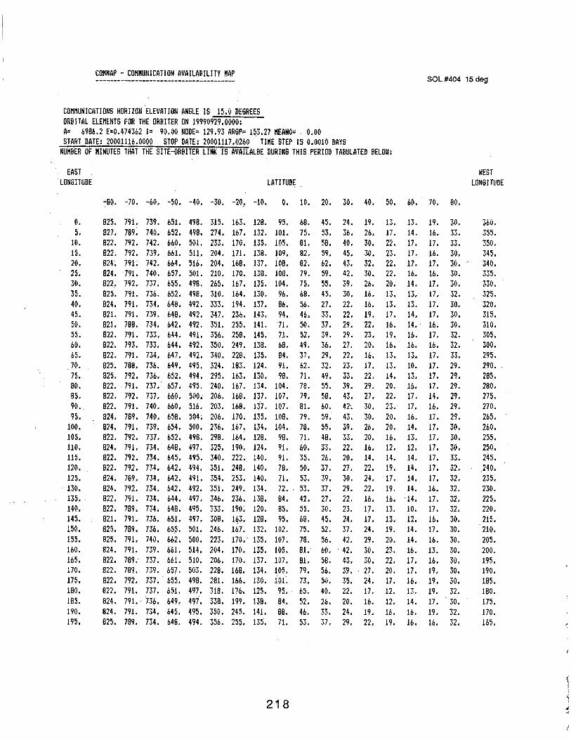
COKHAP - COHHUNICATION AVAILABILITY HAP
COMMUNICATIONS HORIZON ELEVATION ANSLE IS 15.0 DEGREES ORBITAL ELEMENTS FOR THE ORBITER ON 19990929.0000: A= 6996.2 E=0.474362 I= 90.00 NODE= 129.93 ARSP= 153.27 HEANO= . 0.00 START DATE: 20001116.0000 STOP DATE: 20001117.0260 TIHE STEP IS 0.0010 DAYS
NUMBER OF MINUTES THAT THE SITE-ORBITER LINK IS AYAILALBE DURING THIS PERIOD TABULATED BELOW:
EAST 'LONSITUDE LATITUDE .
SOL#404 15 deg
WEST LON61TUDE
-so. -7o. -6o. -so. -40. -3o. -20. -10. o. 10. 20. 30. 40. so. 60. · 10. so.
o. 5.
10. 15. 20. 25. 30. 35. 40. 45. 50. 55. 60. 65. 70. 75. BO.
.85. 90. 95.
100. 105. 110. 115. 120. m.
. 130. m .. 140. 145. 150. 155. 160. 165. 170. 175. 180. 185. 190. 195.
825. 791. 739. 651. 499. 315. 163. 128. 95. 68. 827. 789. 740. 652. 499. 274. 167. 132. 101. 75. a22. 792. m. 660. so1. 233. 110. m. 105. 81. 922. 792. 739. 661. 511. 204. 171. 139. 109. 82. 824. 791; 742. 6b4. 516. 204. 168. 137. 108. 82. 824. 791. 740. 657. 501. 210. 170. 138. 109. 79. 922. 792. 737. m. 498. m. 167. m. 104. 75. 825. 791. 736. 652. 498. 310. 164. 130. 96. 68. 824. 791. 734. 648. 492. 333. 194. 137. 86. 56. 821. 791. 739. b48. 492. 347. 236. 143. 94. 46. 821. 788. 734. 642. 492. 351. 255. 141. 71. 50. 822. 791. 733. 644. 491. 356. 258. 145. 71. 52. a22. m. 733. 644. 492. 350. 249. 13B. 6B. 49. 822. 791. 734. 647. 492. 340. 22a. m. 84. 37. 825. 788. 736. 649. 495. 324. 183. 124. 91. 62. 825. 792. 730. 652. 494. 295. 163. 130. 98. 71. s22. m. m.· 657. m. 24o. 167. m. 104. 78. 822. 792. 737. 660. 500; 206. 168. 137. 107 •. 79 • 822. 791. 740. 660, 516. 203. 168. 137. 107. 81. 824. 789 •. 740. 658. 504; 206. 170. 135. lOB. 79. 824. 191. 739. 654. 500. 236. 167. 134. 104. 78. 822. 792. 737. 652. 498. 298. 164. 128. 98. 71. 824. 791. 734. 648. m. m. m. 124. 91. 60. a22. 792. 734. m. 495. 340. 222. 140. 91. 35. 822. 792. 134. 642. 494. 351. 248. 140. 78. 50. 824. 789. 734. 642. 491. 354. 253. 140. 71. 53. 824. 792. 734. 642. m. m. 249. 134. 72 •. 53 • 822. 791. 734. b44. 497. 346. 236. 138. 84. 42. 822. 789. 134. 648. 495. 333. 190; 120. 85. 55. 821. 791. 736. 651. 497. 308. 1q3. 128. 95. 68. 825. 789. 736. 655. 501. 246. 167. 132. 102. 75. 825. 791. 740. 662. 500. 223. 170. 135. 107. 78. 824. 791. 739. 66L 514. 204. 110. m. 105. 81. 822. 789. 737. 661. 510. 206. 170. 137. 107. 81. a22. 789. m. 657. 503. 228. t6B. 134. tos. 79. 822. 792. m. · m. 498. 2a1. 166. 1so. itn: n. 822. 791. 737. 651. 497. 318. 176. 125. 95. 65. 824. 791 •. fJ6. 649. 497. 338. 199. 138. 84. 52. 824. 791. 734. 645. 495. 350. 245. 141. BB. 46. 825. 789. 734. 648. 494. 356. 255. 135. 71. 53.
218
45. 53. 58. 59. 62. 59. 55. 45. 27. 33. 37. 39. 36. 29.
24. 36. 40.
19. 26. 30.
45. 30. 32. 43.
42. 39. 30. 22. 22. 29. 29. 27. 22. 23.
30. 26. 16. 16. 19. 22. 23. 20. lb. 17. 22. 29.
13. 17. 22. 23.
22. 20. 13. 13. 17.
13. 14. 17. 17. 17. 16. 14. 13. 13. 14.
16. 14. 19. 16. 16. . 16. 13. 13. 14. 20.
13.
49. 33. 55. . 39. 58. 43. 27 •. 22.
10. 13. 16. 17. 17. 16. 14. 13. 12. 14. 14.
42'. 43. 39. 33. 22. 20. 27.
30. 30. 26. 20. 16. 14. 22.
60. 59. 55. 48. 33. 26. 37. 39. 37. 27.
30. 24. 29. 22. 22.
30. 23. 45. 24. 52. 37. 56. 42. 60 •. 42. 58. 43. 56. 39. 50. 35. 40. 22. 26. 20. 33. 24. 37. 29.
16. p. 17. 24. 29. 30. 30.
. 27. 24. 17. lb. 19. 22.
23. 20. 20. 16. 12. 14. 19. 17. 14. 19. 14. 16. . 14.
10. 12. 14. 14. 16. 17. 17 • 16. 13. 14. 16. 16.
13. 13. 19. 20. 23. 22. 20. 17. 12. 12. 16. 19.
19. 30. 16. 33. 17. 33. 16. 30. 17. 30. 16. 30. 11. 30. 17. 32. 17. 30. 17. 30. 16. 30. 17. 32. 16. 32. 17. 33. 17. 29. 17. 29. 17. 29. 14. 29. 16. 29. 17. 29. 17. 30. 17. 30. 17. 3(1. 17. 33. 17. 32. 17. 32. 16. 32. 17. 32. 17. 32. 16. 30. 17. 30. 16. 30. 13. 30. 16. 30. 19. 30, 19. 30. 19. 32. 17. 30. 19. 32. 16. 32.
360. m. 350. 345. 340. 335. 330. 325. 320. 315. 310. 305. 300. 295. 290 •. 285. 280. 275. 270. 265. 260. 255. 250. 245. 240. 235; 230. 225. 220. 215.
. 210. 205. 200. 195. 190. 185. 180. 175. 170. m.
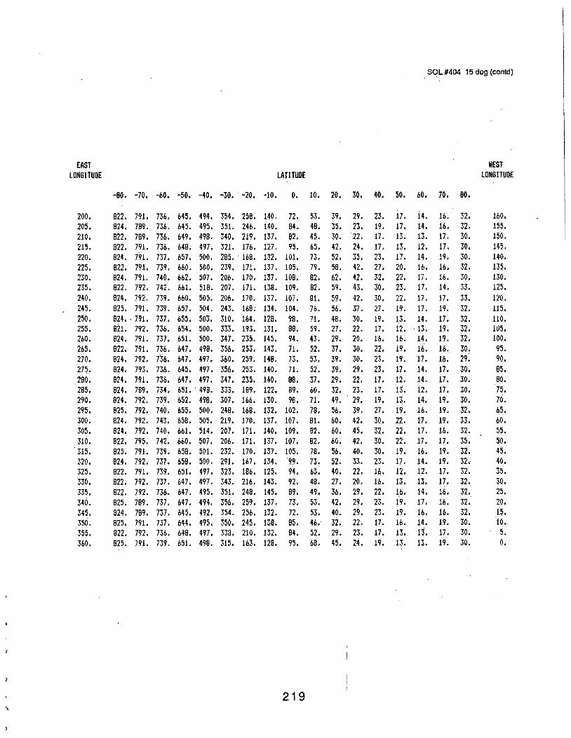
SQL #404 15 deg (contd)
EAST WEST lDNSITUDE lATITUDE lONSITUDE
-80. -70. -60. -50. -40. -30. -20. -10. o. 10. 20. 30. 40. 50. 60. 70. 80.
200. 822. 791. 736. 645. 494. 354. 258. 140. 72. 53. 39. 29. 23. 17. 14. 16. 32. 160. 205. 824. 789. 736. 645. 495. m. 246. 140. 84. 48. 35. 23. 19. 17. 14. 16. 32. 155. 210. 822. 789. 736. 649. 498. 340. 219. 137. 82. 45. 30. '22. 17. 13. 13. 17. 30. 150. 215. 822. 791. 736. 648. 497. 321. 176. 127. 95. 65. 42. 24. 17. 13. 12. 17. 30. m. 220. 824. 791. 737. 657. 500. 285. ' 168. 132. 101. 73. 52. 35. 23. 17. 14. 19. 30. 140. 225. 822. 791. 739. 660. 500. 239. 171. 137. 105. 79. 58. 42. 27. 20. 16. 16. 32. 135. 230. 824. 791. 740. 662. 507. 206. 170. 137. 108. 82. 62. 42. 32. 22. 17. 16. 30. 130. 235. 822. 792. 742. 661. 518. 207. 171. 138. 109. 82. 59. 43. 30. 23. 17. 14. 33. 125. 240. 824. m. 739. 660. 505. 206. 170. 137. 107. 81. 59. 42. 30. 22. 11. 17. '?~
'-".;)• 120. 245. 825. 791. 739. 657. 504. 243. 168; 134. 104. 76. 56. 37. 27. 19. 17. 19. 32. 115. 250. 824. ' 791. 737. 65~. 503. 310. 164. 128. 98. 71. 48. 30. 19, 13. 14. 17. 32. 110. 255. Bit. 792. 736. 654. 500. 333. 193. 131. 88. 59, 27. 22. 17. 12. '13. 19. 32. 105. 260. 824. 791. 737. 651. 500. 347. 235. 145. 94. 43. 29. 20. 16. 16. 14. 19. 32. 100. 265. 822. 791. 736. 647. 498. 356. 253. 143. 71. 52. 37. 30. 22. 19. 16. 16. 30. 95. 270. 824. 792. 736. 647. 497. 360. 259. 148. 73. 53. 39. 30. 23. 19. 17. 16. 29. 90. 2n. 824. 793. 736. 645. 497. 356. 253. 140. 71. 52. 39. 29. 23. 17. 14. 17. 30. 85. 280. 824. 791. 736. 647. 497. 347. 235. 140. 88. 37. 29. 22. 17. 12. 14, 17. 30. 80. 285. 824. 789. 734. 651. 498. 333. 189. 122. 89. 60. 32. 23. 17. 13. 12. 17. 30. 75. 290. 824. 792. 739. 652. 498. 307. 166. 130. 98. 71. 49. 29. 19. 13. 14. 19. 30. 70. 295. 825. 792. 740. 655. 500. 248. 168. 132. 102. 78. 56. 39. 27. 19. 16. 19. 32. 65. 300. 824. 792. 743. 658. 505. 219. 170. 137. 107. 81. 60. 42 •. 30. 22. 17. 19. 33. 60. 305. 824. 792. 740. 661. 514. 207. 171. 140. 109. 82. 60. 45, 32. 22. p, 16. 32. 55. 310. 822. 795. 742. 660. 507. 206. 171. 137. 107. 82. 60. 42. 30. 22. 17. 17. 35. 50. 315. 825. 791. 739. 658. 501. 232. 170. 137. 105. 78. 56. 40. 30. 19. 16. 19. 32. 45. 320. 824. 792. 737. 658. 500. 291. 167. 134. 9,9. 73. 52. 33. 23. 17. 14. 19. 32. 40. 325. 822. 791. 739. 651. 497. 323. 186. 125. 94. 63. 40. 22. 16. 12. 12. 17. 32. 35. 330. 822. 792. 737. 647. 497. 343. 216. m:; 92. 48. 27. 20. 16. 13. 13. 17. 32. 30. 335. 822. 792. 736. 647. 495. 351. 248. 145. 89. 49. 36. 29. 22. 1.6. 14. 16. 32. 25. 340. 825. 789. 737. 647. 494. 356. 259. 137. 73. 53. 42. 2~. 23. 19. 17. 16. 32. 20. 345. 824. 789. 737. 645. 492. m. 256. 132. 72. . 53. 40. 29 • 23. 19. 16. 16. 32. 15. 350. 825. 791. 737. 64.4. 495. 350. 245. 138. 85. 46.· 32. 22. 17. 16. 14. 19. 30. 10. 355. 822. 792. 736. 648. 497. 338. 210. 132. 84. 52. 29. 23. 17. 13. 13. 17. 30. 5. 360. 825. 791. 739. 651. 498. 315. 163. 128. 95. 68. 45. 24. 19. 13. 13. 19. 30. o.
219
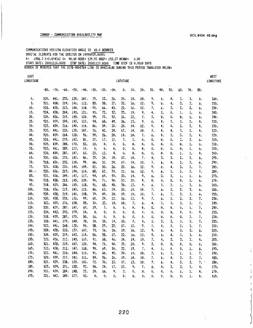
COIIMAP - COI!I!UNICATION AVAILABiliTY IIAP
COtii!UNICI\TIONS liORJZON ELEVATION ANGLE IS 45.0 DEGREES ORBITAL ELEMENTS FOR THE ORBITER ON 19990929.0000: A= b986.2 E=0.4743b2 I= 90.00 NODE= 129.93 ARSP= 153.27 MEANO= 0.00 START DATE: 20001116.0000 STOP DATE: 20001117.0260 TII!E STEP IS 0.0010 DAYS
NUMBER OF MINUTES THAT THE SITE-ORBITER LINK IS AVAilALBE DURING THIS PERIOD TABULATED BELOW:
EAST LONSITUDE LATITUDE
SOL #404 45 deg
WEST LONGITUDE
-8o. -10. -6o. -so. -40. -30. -20. -10. o. 10. 20. 30. 40. so. 6o. 10. 80.
o. 5.
10. 15. 20. 25. 30. 35. 40. 45. 50. 55. 60. b5. 70. 75. 80.-85. 90. 9.5.
100. 105. 110. 115. 120. m. 130. 135. 140. 145. 150. 155. 160. 165. 170. 175. 180. 185. 190. 195.
520. 441. 233. 134. 107. 521. 438. 219. 141. 112. 521. 438. 213. 144. 118. 524. 438. 204. 145. 121. 520. 436. 215. 145. 120. 521. 439. 209. 143. 117. 523. 439. 216. 140. 114. 520. 441. 220. m. 101. 520. 439. 264; 128. 96. 521. 441. 279. 143. 81. 520. 439. 288. 170. 53. 523. 441. 289. 177. 19. 520. 439. 287. 147. 63. 520. 436. m. 147. B6. s1a. 436. m. m. 99. 521. 438. 220. 140. 109. 520. 436. 215. 144. 114. 521. 436. 209. 147. 117. 518. 438. 215. f45. 120. 518. 435. 206. 145. 118. 518. 436. 213. 143. 115. 520. 438. 219. 140. 108. 520. 438. 255. m. 99. 523. 439. 276. 138. 85. 520. 439. 28j, 147. 65. 520. 442. 292. 179. 14. 519 •. 439. 287. 170. 50. 520. 441. 279. 148. 78. m. 441. 268. 130. 94. 520. 438. 223. 137. 107. 520. 439. 219. 143. 114. m. 436. 213. 145. 111. 521. 438. 215. 147. 120. 523. 438. 212. 147. 118. 523. 441. 210. 144. 115. ~20. 439. 217. 141. 111. 521. m. 238. m. 102. 523. 439. 271. 129, 92. 521. 439. 284. 148. 73. 521. 442. 289. 177. 42.
75. 33. 85. 58. 92. 66. 95 •. · 72.
95. 73. 94. 68. 86. 59. 76. 42. 59. 26. 27. 17. 10. 0. o. o.
23. 12. 35. 24. 66. 32. 81. 50. 88. 62. 94. 69. 94. 71. 91. 6.8. 86. 63. 79. 49. 65. 29. 30. 22. 19. 7.
o. (1,
20. 29. 36.
26. 20. 27. 22. 45. 22. 52. 33. 52. 36. 49. 26. 30. 20. 24. 17. 20. 14. 12. 7. . o. 0. o. o. 4. o.
19. 13. 24. 17. 26. 20. 39. 22. 50. 3(1. 50. 33. 48. 30. 39. 20. 24. 19. 22. 16. 14. 10. o. o. (l,
o. o. o.
10. 17.
14. 16. 16. 19. 22. 13. 14. 14. 10. 3. o . o. o.
10. 14. 16. 16. 14. 20.
14. 14. 13. 7; o. 6. o. 7.
12. 14. 22. 26. 19. 16.
o. 16. 30. 58. 75. 86. 91. 94. 94. 91. 84. 72. 50. 24.
58. 27. 22. 16. 14.
o.
68. 46. 24. 71. 69. 66. 56. 30. 24. 16. o.
50. . 35.
50. 32. 20. 45.
26. 23, 17. 9. o.
19. 17. 13.
o.
220
20. 19. 14. 14. 13. 9. o. o.
10. 12. 12. 9. 7. 9.
12. 10. 7. o. o. o. o. 7.
10. 12. 12. 9. 9. 9.
10. 10. 9. 6. o. 0. o. 4. 9.
12. 12. 10 •. 9. .., ,,
10. 10. 10. 1. o. o.
9. 9. 7. 4. 3. 6. 9. 7. 6. o. o. o. o. 4. 7. 9. 9. 6. o. 6. 7. 7. 7. 4. o. 0. o. L 7. 9. 9. 7. 3. 4. 7. 7. 7. 6. 0.
0.
6. 6. 6. 3, 0. 4. 4. 4. 4. o. o. o. o. 3. 6. 6. 6. 3. o.
6. 6. 6. 3. o. 0. (l,
3. 4, 6. 6. 4. o. 1. 6. 6. 6. 4. 0. o.
4. 4. 3. o. o.
4. 4. 3. o. o. o. o. 3. 4. 4.
3. o. 3. 3. T
"' 3. 3. o. o. o. 3. 3.
3.
1. 0. 3. 3. 3.
3. o. o. 1. 3. 3. 3. ,),
1. 0. 1. 3. 3. 3. 3. o. o. o. 3. 3.
4. . 3.
4. 3. 3. 3. o. 0. o. o. 3. 1. 4. 3. 4. 3. 3. 3. o. 1. 0. o.
3. 3. T . .. 1. 1. 3. 3. 3. 3. 3. 1. L 1. 3. 3. 3. 3. 1. 1. 3. 3. ~
"' 3. 3. 1. o.
b. 6. 6. 6. 6. 4. 4. 4. 4.
. 6. b. 6. 4. 6 .• b. 7. 7. 6. 6. 6. 6. 6. 7. }. 7. 9, 7.
3. 7. 3. 7. 3. . ~. 3. 6. 3. 4 •. 0. 6. 1. b. 1. 7. 3. 7. 3. 7. ' 3. 4. L 4. 1. 4.
360. m. 350. 345. 340. 335. 330. 325. 320. :m, 310. 30~.
300. 295. 290. 285. 280. 275. 270. 2b5. 260. 255. 250. 245. 240. m. 230. 225. 220. 215. 210. 205. 200. 195. 190. 185. 180. 175. 170. 165.
1 l
J
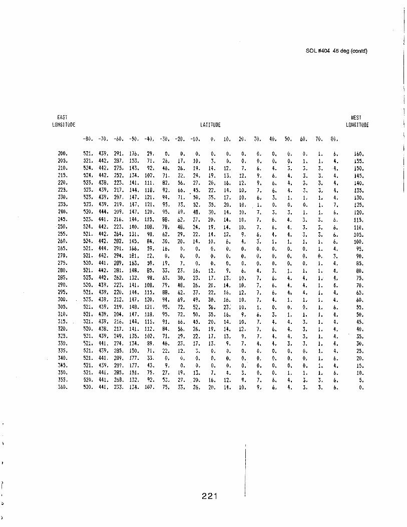
EiiST LONGITUDE
200. 205. 210. 215. 220. 225. 230. 235. 240. 245. 250. 255. 260. 265. 270. 275. 280. 285. 290. 295. 300. 305. 310. 315. 320. 325. 330. 335. 340. 345. 350. 355. 360.
LATITUDE
SOL #404 45 deg (contd)
WEST LDN61TUDE
-so. -70. -6o. -5(1, -40. -30. -20. -10. o. 10. 20. 30. 40. so. 60. 7v. eo.
521. 439. 291. 176. 29. 521. 442. 287. 153. 71. 524. 442. 275. 143. 92. 524. 442. 252. 134. 102. m. 438. m. 141. 111. 523. 439. 217. 144. 118. 523. 439. 207. 147. 121. 523. 439. 219. 147. 121. 52(1. 444. 209. 147. 110. 523, 441. 216. 144. 115. m. 442. m. 140. 1o8. 521. 442. 264. 131. 98. 524. 442. 282. 145. 84. 521. 444. 291. 166. 59. m. 442. 294. 181. 12. 520. 441. 289. 1b3. 59. m. 442. 2a1. 14B. as. 523. 442. 2b2. 132. 98. 520. 439. 223. 141. lOB. 521. 439. 220. 144. 115. m. m. 212. 147. 120. 521. 439. 219. 148. 121. 521. 439. 204. 147. 118. 521. 439. 216. 144. m. 520. 438. 217. 141. 112. s21. m. 249. 135. 102. 521. 441. 274. 134. 89. 521. 439. 285. ·150. 71. 521. 441. 289. 177. 33. 521. 439. 289. 177. 43. 521. 441. 285. 151. 75. 520. 441. 269. 132. 92. 520. 441. 233. 134. 107.
o. 26. 4b. 71. 82. 92. 94. 95. 95. 88. 78. 62. 30. 16. o.
19 •. 33. b3. 79. sa. 94. 95. 95. 91. 84. 71. 46. ')') ..... o. 9.
27. 53., 75.
o. 17. 2b. ~2.
56. 66. 71. 73. 69.
48. 29. 20. o. o. 7.
23. 30. 48. 62. b9. 72. 72. 66. 56. 29. 23. 12. o.
o. 10. 19. 24. 27. 45. 50. 52. 48. 37. 24. 22. 14. o. o. 0.
16. 23. 26. 37. 49. 52. 50. 45. 2b. 22. 17. 3. 0. 0. 0.
19. 13. 27. . 20.
2b.
o. 3.
14. 19. 20. 22. 35. 35. 30. 20. 19. 14. 10. o. o. o.
12. 17. 20. 22. 30. 36. 35. 20. 19. 17. 13. o . o. 0. 7.
lb. 20.
221
0. o.
12. 13. 16. 14. 17. 20. 14. 14. 14. 12. 6. (1,
o. o. 9.
13. 14. 16. 1b. 23; 16. 14. 14. 13. 9. o. 0. o. 4.
12. 14.
o. o. 7.
12. 12. 10. 10. 10. 10. 10. 10. 9. 4. o. o. o. b.
10. 10. 12. 10. 10. 9.
10. 12. 9. 7. o. o. 0. 3. 9.
10.
o. 0. b. 9. 9. 7. 6. 1. 7. 7. 7. b. 3·. o. o. o. 4. 7. 7. 7. 7. 1. b. 7. 7. 7. 4. 0. 0. o. o. 7. 9.
o. o. 4. 6. 6. 6. 3. o. 3. b. 6. 4. 1. 0. o. o. 3. 6. 6. b. 4. o. 3. 4. 6. 4. 4. 0. 0. o. o. 6. 6.
o. 9· 3. 4. 4. 4. 1. o. 3. 4. 4. 4. 1. o. 0. 0. ~. 4. 4. 4. 1. o. 1. 4. 4. 4. 3. o. 0. 0. 1. 4. 4.
o. 1. 3. 3.
.., "· 1. 0. 1. 3. 3.
1. 0. o. o. 1. 4. 4. 4. 1. 0. 1. 3. 3. 3. 3. o. o. o. 1. 3. 3.
1. 1. 3. 3. 3. 3 • 1. 1. 1. 3. 3. 3. 1. 1. o. 1. 1. 1. 1. 1. 1. 1. 1. 1. 1. 1. 1. 1. 1. 1. 1. 3. 3.
b. 4. 4. 4. 4. 4. 4. 7. b. 6. b. b. b. 4. ,),
4. 4. 4. 4. 4. 4. b. 4. 4. 4. 4. 4. 4. 6. 4. 6. 6. b.
lbO. m. 150. 145. 140. 135. 130. 125. 120. 115. 110. 105. 100. 95. 90. B5. 80. 75. 70. b5. bO. 55. 50. 45. 40. 35. 30. 25. 20. 15. 10. 5. o.

Session B, Submittal No. 4
Alan L. Friedlander ·,
Science Applications International Corporation
223

MARS NETWORK LANDER (FREE-FLYER CONCEPT)
ALAN FRIEDLANDER. SAIC
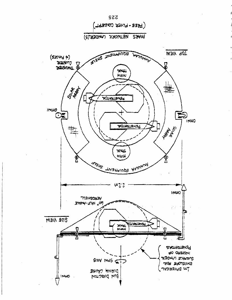
92:2:
~.J.~ lQk"7.:f .. ss~)
lS)~Qf'Wi '::t2JOM.LBN S'lWVJ
M!l" !CiiS
. M31" dOl
1~0
~~ -;10 ~S'r-11
~Cl"Vl ~~ns '11C>.:I iid01~1\Na
1V->la9HdS WT
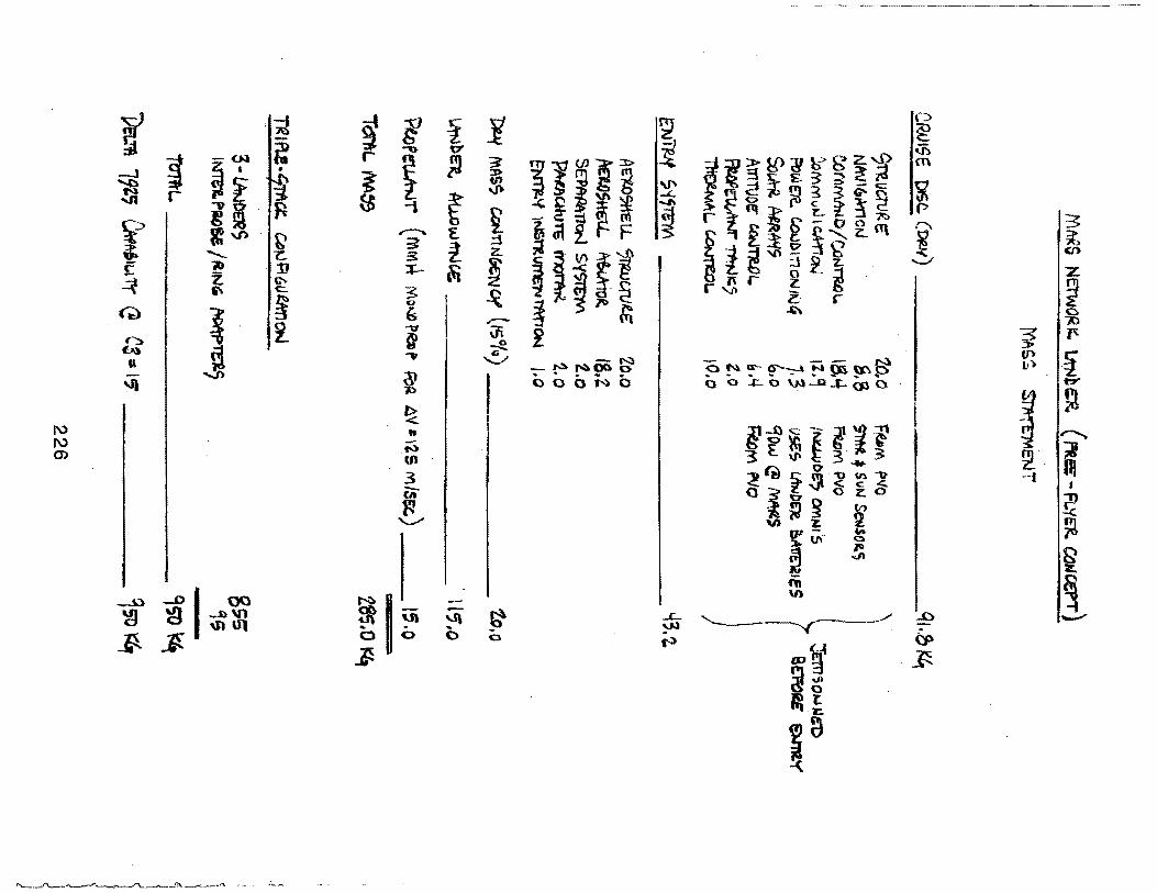
r ·?j ~ i ~ y_ ~ C>
~ ;: ""b '0" ~ ij:;.
~ j~ r
~ ;:1 3' lf(J)!~ 1f?JH'8fi>ff~~ m -J
~ ~ ~ ~
~ "'!J"'j "' ~~E3::._c: s: r ll s f -4:.. ~0 F!'o!3G'~ ; ....... ~ fql ~~~ ("
~ §01!~~ ~ r s-oaSl::> ......... 3 ~-> c'\1)· .....--.. 'E. I £ .:u r';- ,_ "' ! 5t b' 3' l. ;:j
i: z. l~"':i£_~ C/) .....__ -z: 3
~ ~iff{ E 11) ·:D X-- &\I z ~ t. c-. r n r ~ ~ · i " c::. 3 ~ '..1"1 -
~ 0
~ ~ til z.: r
C.;) ¥ ~ ..(/\ c. r-- jl()
~ -u \1i £ 3 1'-a A' ~ .>
j ...... ~/ If) ¥ -~ o~G-CS'---''NOS~~ II"> " -~~OC.o
~ .. .. . . . . - .. - .... ., """ ... "' .,..
'\II OOONO (l 0 ..(:'__ 0 \Ill .._Q -f-. 03 0 '
~ ~ ~ ~~~--lii ~· 1\) .. .............
1\) .~ 3E~£3 3 ;11 0') tn
:!4)~5~;! ~·
111 3 --· I - OIO' ozo ?! (I)
~ ~~ (/} .:.c '\........"' ,., z ~ ~ 171 -- {Ia
:.,.U\ 0
~ ~ ~ 5 «;; & ~~~
V) ._..t.;) _.,I ~ -t ~ ~ ....b'\ll '-1\ ~ _c_ ..0 --""'" 0 ~
~ ~ 0 0 0 ~ t:P
:G. w1X ·~
~~ ~1
1~ .:.(_
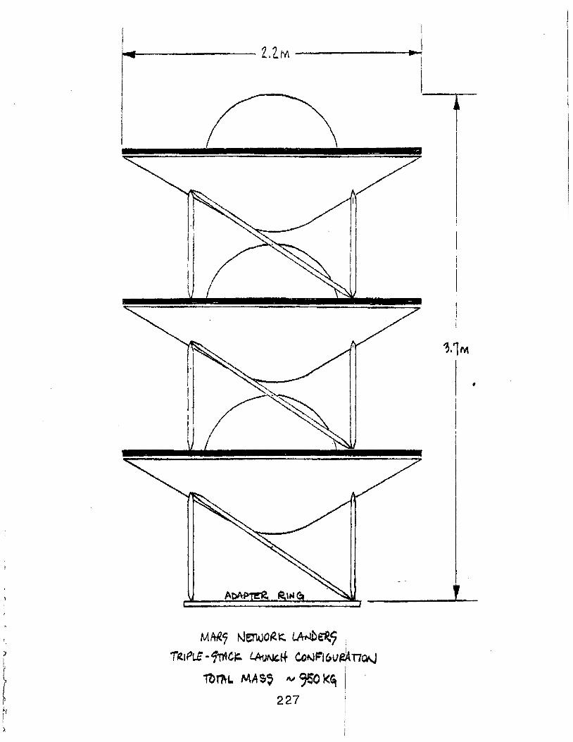
I 11011111 ... 1-----~- 2.2.M _____ .,....!
I
M ttli.7 1\lerwo~ ~ wb~7 · 1
r~au't.E ·7ntCI=- l.AuNC.t.f CotJF16V~17""-.J
1bt7H. MAS' IV %0 K~ I 227
II
,,
Session B, Submittal No. 5
Alan L. Friedlander Science Applications International Corporation
229
1\) (JJ
0
ANALYSIS OF SUCCESS PROBABILITY/COST TRADES
FOR SMALL LANDERS IN A MARS NETWORK
ALAN FRIEDLANDER SAIC
=·= =-=-~== ==---......... ...... ~== ~....-...... , Science Applications
International Corporation ~'l Emp/Ovee-O .. vnen ·~:Jmr.dnv
With addendum of new results
December 6, 1989
MEMO TO:
FROM:
SUBJECT:
Roger Bourke, EIS Team
Alan Friedlander, SAIC
Analysis of Success Probability/Cost Trades for Small Landers in a Mars Network
The premise to be tested in this analysis is whether cost economies may accrue by deiivering more
landers designed to lower reliability of operation (compared to fewer landers of higher reliability)
to obtain a desired probability of achieving a given number of lander successes. Generally, the
application in mind is a network of penetrators. although the analysis may apply as wen to other
small lander concepts or even to simple rovers. In previous MRSR studies. the approach taken to
raise the probability of a successful mission (e.g. a rover or sample return objective) was to invoke
a dual launch policy utilizing idenJical tlight systems. With this approach we found that a
substantial improvement in achieving at least one total mission success was gained for realistic
values of system element reliability, albeit at the expense of higher program cost and more complex
operations. However. in the case of a large number of small landers whose recurring cost of
production might be small compared to the development cost. a single spacecraft carrier may be
sufficient to deliver these landers to Mars within acceptable limitations of spacecraft injected mass
:md launch vehicle performance capability. It seems reasonable to at least explore the question of
potential economies if such landers were purposely designed to lower values of reliability. Wh:u is
specifically meant by lower reliability in this context is that. while fewer lander emplacements will
succeed. those that do succeed will-accomplish the desired mission objectives. The underlying
assumption here is a certain degree of independence of lander syste~ failure modes such that
objective-specific elements (science instruments and data communiCations) are highly reliable
while delivery-specific elements (e.g. deorbit propulsion and aeroshell) are less reliable and
developed at lower cost with attendant higher risk. This analysis leaves open the import~mt
question as to whether such an approach is at .all realistic in terms of engineering design. but
focuses instead on the first question of p~tential cost advantage.
The method of analysis is based on a probabilistic mOdel of lander success and a related
probabilistic model of project cost including the lander. spacecraft ~arrier, and integration. but not
launch or operations costs. Quantitativ~ results are obtained in a normalized and parametric
fashion. Sensitivity to the assumed model parameters is also examined.
1575 Woodfield Road. Suite 350. Schaunwuri/.1 illinots 60173 ·3121 330-2500 . _, , ' \1' · ·, '·llll~ll·..\lr•:"li''i'u'•1P~".It11r•Jrol.","~'w ·-'""'' s->.c O"••es ->a'""""'""'" J''""'· ' ···"·''''' >.'"'·"•IS ~·"'"" ~ n"ISc<<"' '·" '"''"' '·; ""'''f' ........ 0
... - ·•'" , .... "' • •· ' •••
' 231
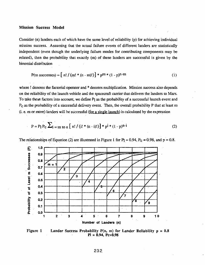
Mission ·Success Model
Consider (n) landers each of which have the same level of reliability (p) for achieving individual
mission success. Assuming that the actual failure events of different landers are statistically
independent (even though the underlying failure modes for contributing components may be
related), then the probability that exactly (m) of these landers are successful is given by the
binomial distribution
P(m successes)= [ n! I (m! * .(n- m)!)] * pm * (1- p)n-m (1)
where ! denotes the factorial operator and * denotes multiplication. Mission success also depends
on the reliability of the launch vehicle and the spacecraft carrier that delivers the landers to Mars.
To take these factors into account, we define PI as the probability of a successful launch event and
Pc as the probability of a successful delivery event Then, the overall probability P that at least m
(i.e. m or more) landerS will be successful (for a sin~le launch) is calculated by the expression
< •' i • ·, . ' •
P = PtPc Li =m ton [ n! /(i! * (n- i)!)] *pi* (1- p)n-i (2)
The relationships of Equation (2) are illustrated in Figure 1 for pt = 0.94, Pc = 0.98, and p = 0.8.
ii'. -
.... Ill
"' CD ..... ti 0 ~ :a "' .a 0 ... 0,.
1.0
0.9
0.8
0.7
0.6
0.5
Q.4
0.3
0.2
0.1
0.0
Figure 1
1
' . . ' ' .
/ ~ / --- ~ ~ --- ..-----/
~=.1 / I v / / // /
/2 / I v / / /3 I ·I v / /
114 /_ I L / I ol Is / / ./
v /7 / / 8 V9
2 3 4 5 6 7 8 9 10
Number of Landers (n)
Lander Success Probability P(n, m) for Lander Reliability p = 0.8 PI = 0.94, Pc=0.98
232.
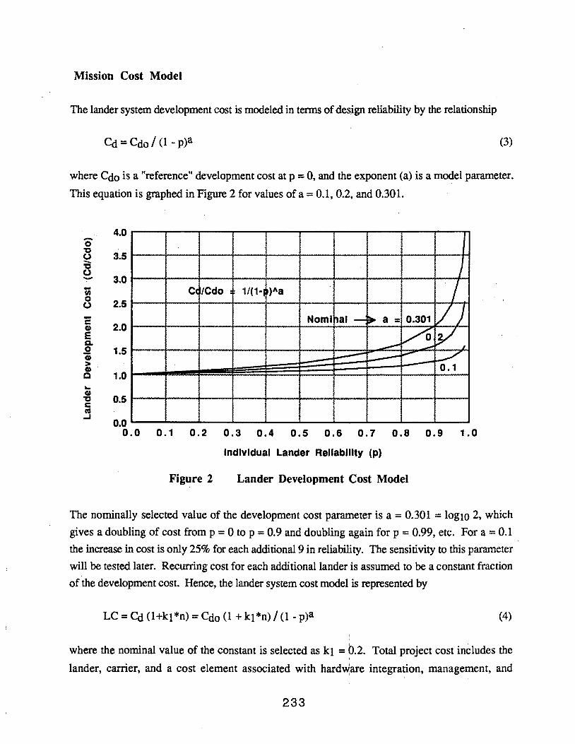
Mission Cost Model
The lander system development cost is modeled in terms of design reliability by the relationship
(3)
where Cdo is a "reference" development cost at p = 0, and the exponent (a) is a model parameter.
This equation is graphed in Figure 2 for values of a= 0.1, 0.2, and 0.301.
0 B -'0 CJ --en 0 CJ
E Cl)
e c. 0 «» > Cl) Q .. Cl) '0 c C'(l ..J
4.0
3.5
I Cc /Cdo : 1/(1· )"a I
Nom I ~al-~a= 0.301 /) __.. /o y'~ --~ __.. _...
.-/ -
3.0
2.5
2.0
1.5
0.1 1.0
0.5
0.0 0.0 0.1 0.2 0.3 0.4 0.5 0.6 0.7 0.8 0.9 1.0
Individual Lander Reliability (p)
Figure 2 Lander Development Cost Model
The nominally selected value of the development cost parameter is a= 0.301 = log10 2, which
gives a doubling of cost from p = 0 to p = 0.9 and doubling again for p = 0.99, etc. For a = 0.1
the increase in cost is only 25% for each additional9 in reliability. The sensitivity to this parameter
will be tested later. Recurring cost for each additional lander is assumed to be a constant fraction
of the development cost. Hence, the lander system cost model is represented by
LC = Cd (1+k1 *n) = Cdo (1 + k1 *n) I (1- p)a (4)
'
where the nominal value of the constant is selected as k1 = p.2. Total project cost includes the
lander, carrier, and a cost element associated with hard~are integration, management, and
233
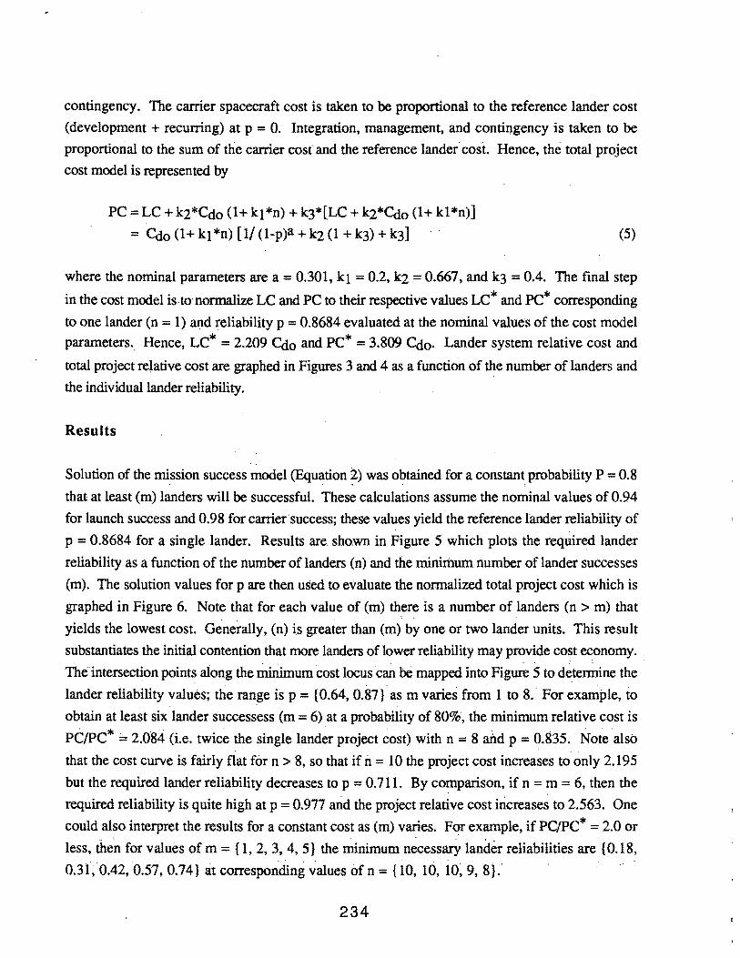
contingency. The carrier spacecraft cost is taken to be proportional to the reference lander cost
(development+ recurring) at p = 0. Integration, management, and contingency is taken to be
proportional to the sum of the carrier cost and the reference lander cost. Hence, the total project
cost model is represented by
PC= LC + k2*Cdo (1+ k1 *n) + k3*[LC + k2*Cdo (1+ k1 *n)]
= Cdo(l+k1*n) [1/(1-p)a+k2(1 +k3)+k3] (5)
where the nominal parameters are a= 0.301, k1 = 0.2, k2 = 0.667, and k3 = 0.4. The final step
in the cost model is to normalize LC and PC to their respective values LC* and PC* corresponding
to one lander (n = 1) and reliability p = 0.8684 evaluated at the nominal values of the cost model
parameters. Hence, LC* = 2.209 Cdo and PC*= 3.809 Cdo· Lander system relative cost and
total project relative cost are graphed in Figures 3 and 4 as a function of the number of landers and
the individual lander reliability.
Results
Solution of the mission success model (Equation ~) was obtained for a constant probability P = 0.8
that at least (m) landers will be successful. These calculations assume the nominal values of 0.94
for launch success and 0.98 for carrier success; these values yield the reference lander reliability of . .
p = 0.8684 for a single lander. Results are. shown in Figure 5 which plots the required lander
reliability as a function of the number of landers (n) and the minir:tmm number of lander successes
(m). The solution values for p are then used to evaluate the normalized total project cost which is
graphed in Figure 6. Note that for each value of (m) there is a number of landers (n > m) that
yields the lowest cost. Generally, (n) is greater than (m) by one or two lander units. This result
substantiates the initial contention that more landers of lower reliability may provide cost economy.
The intersection points aiong the minimum cost locus can oe mapped into Figure S to deteniune the
lander reliability values; the range is p = { 0.64, O.S7} as m varies from 1 to 8. For example, to
obtain at least six lander successess (m = 6) at a probability of 80%, the minimum relative cost is
PC/PC*= 2.084 (i.e. twice the single lander project cost) with n = 8 and p = o.S35. Note also
that the cost curve is fairly flat for n > 8, so that if n = 10 the project cost increases to. only 2.195
but the required lander reliability decreases to p = 0. 711. By comparison, if n = m = 6, then the . .
required reliability is quite high at p = 0.977 arid the project relative cost increases to 2.563. One
could also interpret the results for a constant cost as (m) varies. For example, if PC/PC* = 2.0 or
less, then for values of m = { 1' 2, 3, 4, 5 r the nrlnimum necessary lander reliabilities are { 0.18,
0.31, 0.42, 0.57, 0.74} at correspon'ding values of n = { 10, 10, 10, 9, 8}.'
234
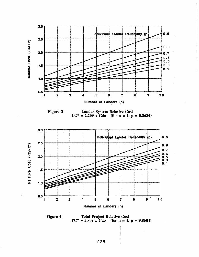
3.0
0.9
- 2.5 .. 0 ...J 0.8 -0 ...J - 2.0 0.7 .. 0.6 en 0 0.5 0 CD 1.5 0.3 > 0.1 :: C'G 1» a: 1.0.
0.5~--_.----~--~~--_.----~----~--_.----~--~
1 2 3 4 5 6 7 9 1 0
Number of Landers (n)
Figure 3 Lander System Relative Cost LC* = 2.209 x Cdo. (for n = 1, p = 0.8684)
3.0
0.9
- 2.5 0.8 ..
0 D. 0.7 -0 0.6 D. 2.0 0.5 -.. 0.3 en 0.1 0 0 CD 1.5 ~ -C'G 1» a: 1.0
0.5 .__ __ --~.. ____ ...~.-__ --....J...__-i-___ .~......_--~. ____ -~... __ ...._ _ __,
1 2 4 5 6 7 8 9 1 0
Number of Landers (n)
Figure 4 Total Project Relative Cost PC* = 3.8., x Cdo (for n ;: 1, p = 0.8684)
235
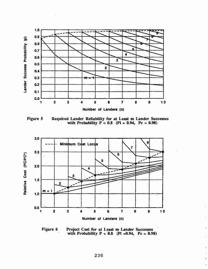
-a. ->-
.:!::: -.D C'IS .D 0 ... D. Cl) Cl) CD () () :J en ... CD , c C'IS ...I
1.0
0.9
0.8
0.7
0.6
0.5
0.4
0.3
... ro----- ,---~--~ ~ ~ ~ :-:;:.:: ~ ...
"" " ......
" "' -~ ~-.......,.. ... -
1\. ......... ~
" ' " " ~ - -~ ..... ~
'\ ' ""' ~ -~ ' ' .......... ~
"" '""" 3-.... ~ --.. ----..............
~-.... --......... -------2 ~
-............ ~
-~ -.. -. ----
0.2 -0.1
0.0 1 2 3 4 5 6 7 8 9 10
Number of Landers (n)
FigureS Required Lander Reliability for al Least m Lander Successes with Probability P = 0.8 (PI = 0.94, Pc = 0.98)
-.. 0 a.. ..._ 0 D. --Cl)
0 0
CD l! -C'IS 'i a:
3.0
2.5
2.0
1.5
1.0
0.5 1
--- · Mini 11um Cc st LOCl s ~ ~ ---"' '
...... -- ... ...
~ ...... -...... ~ ...
K ' ... ~ - _.-:
..,_. ....... :.....---::: ---~ ... ..--.:::::::; ...... '- -;....-
r-!_ ...... b;::::::= ~ ............. ...... -:::::::--
...... ~ m = 1 ...... -2 3 4 5 6 7 8 9 10
. . .
Number of Landers (n)
Figure 6 .. Project Cos'f for at Least m Lander Successes with Probability P = 0.8 (PI =0.94, Pc = 0.98)
236
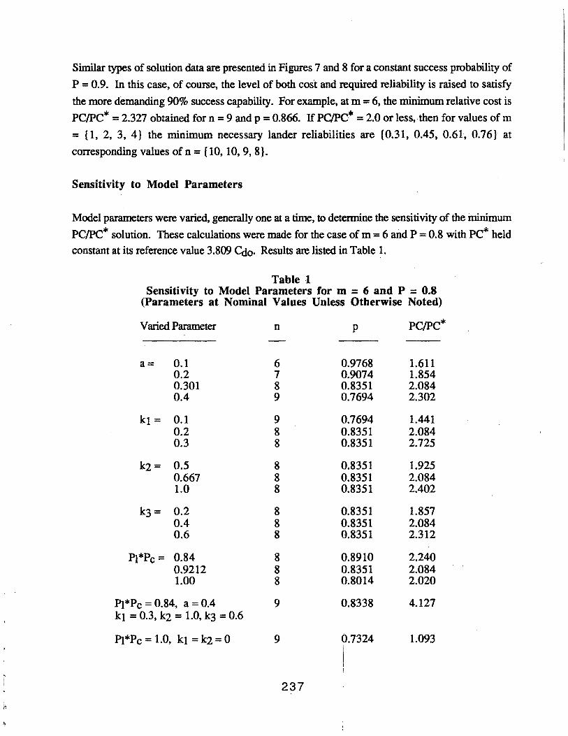
~
Similar types of solution data are presented in Figures 7 and 8 for a constant success probability of
P = 0.9. In this case, of course, the level of both cost and required reliability is raised to satisfy
the more demanding 90% success capability. For example, at m = 6, the minimum r~lative cost is
PC/PC* = 2.327 obtained for n = 9 and p = 0.866. If PC/PC~ = 2.0 or less,. then for values of m
= {1, 2, 3, 4} the minimum necessary lander reliabilities are {0.31, 0.45, 0.61, 0.76} at
corresponding values of n = { 10, 10, 9, 8}.
Sensitivity to Model Parameters
Model parameters were varied, generally one at a time, to determine the sensitivity of the minimum
PC/PC* solution. These calculations were made for the case of m = 6 and P = 0.8 with PC* held
constant at its reference value 3.809 Cdo· Results are listed in Table 1.
Table 1 Sensitivity to Model Parameters for m = 6 and P = 0.8
(Parameters at Nominal Values Unless Otherwise Noted)
Varied Parameter n p PC/PC*
a= 0.1 6 0.9768 1.611 0.2 7 0.9074 1.854 0.301 8 0.8351 2.084 0.4 9 0.7694 2.302
k1 = 0.1 9 0.7694 1.441 0.2 8 0.8351 2.084 0.3 8 0.8351 2.725
k2= 0.5 8 0.8351 1.925 0.667 8 0.8351 2.084 1.0 8 0.8351 2.402
k3 = 0.2 8 0.8351 1.857 0.4 8 0.8351 2.084 0.6 8 0.8351 2.312
P}*Pc = 0.84 8 0.8910 2.240 0.9212 8 0.8351 2.084 1.00 8 0.8014 2.020
P}*Pc = 0.84, a = 0.4 9 0.8338 4.127 kt = 0.3, k2 = 1.0, k3 = 0.6
Pl*Pc = 1.0, k1 = k2 = 0 9 0.7324 1.093
I t I
237

a: -
... C» '0 c as ....
-* 0 a. -0 a. --en 0 0 C» ~ -as 'i a::
1.0
0.9
0.8
0.7
0.6
0.5
0.4
0.3
0.2.
0.1
0.0
K--~ ~ ~ r:::-~ :----.:: :---~ " ' ~ """"""" ~ ~
-.......... -, ~-...... ~ ." ~ ~
............. ~ ----........
""" -............. ~
3 .............. ............... ..........._
~ 2 j--.......... ..........._
.......... ...._ ........... r---- ----m = 1 ~ -~
---
1 2 3 4 5 6 7 8 9 1 0
Number of Landers (n)
Figure 7 ·Required Lander Reliability for at Least m Lander Successes with Probability P = 0.9 (PI = 0.94, Pc = 0.98)
5.0
4.5
4.0
3.5
3.0
2.5
2.0
1.5
1.0
0.5 1
--- ~· Mini tnum C )St Loc ~s \8
' \7 \
\.6 \ \ f\.5 '\ \ \
r-......
"4 '\ \ ................
'( ~ ' -..__ """,. ... -- ~ -~ ·"- _ ...... -... -~· -- .. .- ....... '
2 3 4 5 6 7 8 9
Number of Landers (n)
Figure 8 Project Cost for at Least m Lander Successes with Probability = 0.9 (PI = 0.94, Pc = 0.98)
238
..........
1 0
J l '

Comparison of One and Two Launch Scenarios
Results presented so far have been for a single launch of (n) laiuiers. Additional calculations were
made for two launches, but this required modification of the mission success and cost models. To
calculate the probability P for at least (m) lander successes with two launches, it is necessary to use
Equation (1) as the basic model for lander success, multiply each term by the product Pt*Pc except
for them= 0 term which is adjusted to [(1- PI*Pc) + PI*Pc * Pm=o], and then obtain the various
combinations for exactly (m) successess with two launches .. The probability for at least (m) lander
successes can then be calculated by summation of terms as in Equation (2). The project cost model
for two launches is taken as a modification of Equation (5)
PC(2) = Cdo { (1+ k1 *n) [1/ (1- p)a + k3] + 2*k2 (1 + k3)*(1+ k1 *n/2) } (6)
where (n) is the total number of landers for two launches.
Employing the nominal values of model parameters, the first comparison case examined is n = 4
and a constant probability P = 0.8 that at least (m) landers will be successful: The single launch
carries 4 landers while the dual launch system carries 2 landers each. Results for this case are
listed in Table 2.
Table 2 Comparison of One and Two Launches for n = 4 and P = 0.8
At Least m Successes
1
2
3
4
One Launch (n=4)
p .
0.3977
0.6447
0.8336
0.9653
PC/PC*
1.180
1.275
1.441
1.929
Iwo Launches (n = 2+2)
p
0.3675
0.7747
0.8951
0.9854
PC/PC*
1.417
1.615
1.806
2.561
Although the relative cost for two launches is always higher, if the criterion of comparison is the
minimum value of lander reliability (p), then the results indicate that two launches is better only for
the condition m = 1. If more than 2 lander successes is desired, a higher reliability is required
because of the influence of possible launch and carrier failures.
239
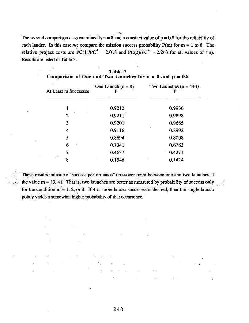
The second comparison case examined is n = 8 and a constant value of p = 0.8 for the reliability of
each lander. In this case we compare the mission success probability P(m) form= 1 to 8. The
relative project costs are PC(l)/PC* = 2.018 and PC(2)/PC* = 2.263 for all valuesof (m).
Results are listed in Table 3.
Table 3 Comparison of One and Two Launches for n = 8 and p = 0.8
One Launch (ri = 8) At Least m Successes P
1 0.9212 '
2 0.9211
3 0.9201
4 . 0.9116
5 0.8694
6 0.7341
7 0.4637
8 0.1546
Two Launches (n = 4+4) p
0.9936
0.9898
0.9665
0.8992
0.8008
0.6763
0.4271
0.1424
·· · · l.'hese results indicate a "success performance" crossover point between one and two launches at •• ' • • ",•'1
. . the value m = { 3, 4}. ·'That is, two launches are better as measured by probability of success only . ·.
for the con~tion ~ = 1, 2, or 3. If 4 or more lander successes is desired, then the single launch
policy yields a somewhat higher probability of that occurrence.
240

Addendum to December 6, 1989, Memorandum
I did some more sensitivity studies relative to the cost model assumption. The results
still confirm the conjecture (generally) that more landers at lower reliability yield lower
project cost.
Basic Cost Model No.1
(as per memos)
Basic Cost Model No.2
(modified "Bourke")
. 1 C/Cd = a
0 (1 - p)
Ftesults for m =6 and P(m ~ 6) =0.8
MinimumCost Solution
Cost Model a n p PC/Cd
No.1 0.100 6 0.9768 6.136
0.301 8 0.8351 7.938
0.500 9 0.7693 9.561
1.000 13 0.5767 10.334
No.2 0.100 6 0.9768 6.130
0.301 8 0.8351 7.703
0.500 10 0.7113 8.710
1.000 15 0.5110 9.513
Note: The greater the sensitivity (a), the more landers (n) desired.
241
0
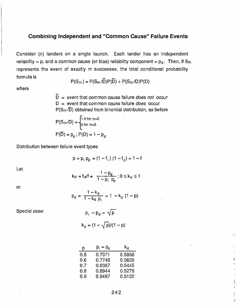
Combining Independent and "Common Cause" Failure Events
Consider (n) landers on a single launch. Each lander has an independent
reliability = Pi and a common cause (or bias) reliability component = Pd. Then, if Sm
represents the event of exactly m successes, the total conditional probability
formula is
where
- -P(Sm) = P(Sm /D)P(D) + P(Sm /D)P(D)
-D = event that common cause failure does not occur D = event that common cause failure does occur P(Sm/0) obtained from binomial distribution, as before
P(S /D) = j1.o for m=O m "t> for m>O
P(D) = pd ; P(D) = 1 - pd
Distribution between failure event types
Let
or
Special case:
1- kd Pd = 1 k = 1 - kd (1 - p)
- d Pi
P; = Pd = {P
kd = (1 - -{P)/(1 - p)
p 0.5 0.6 0.7 0.8 0.9
0.7071 0.7746 0.8367 0.8944 0.9487
0.5858 0.5635 0.5445 0.5279 0.5132
242
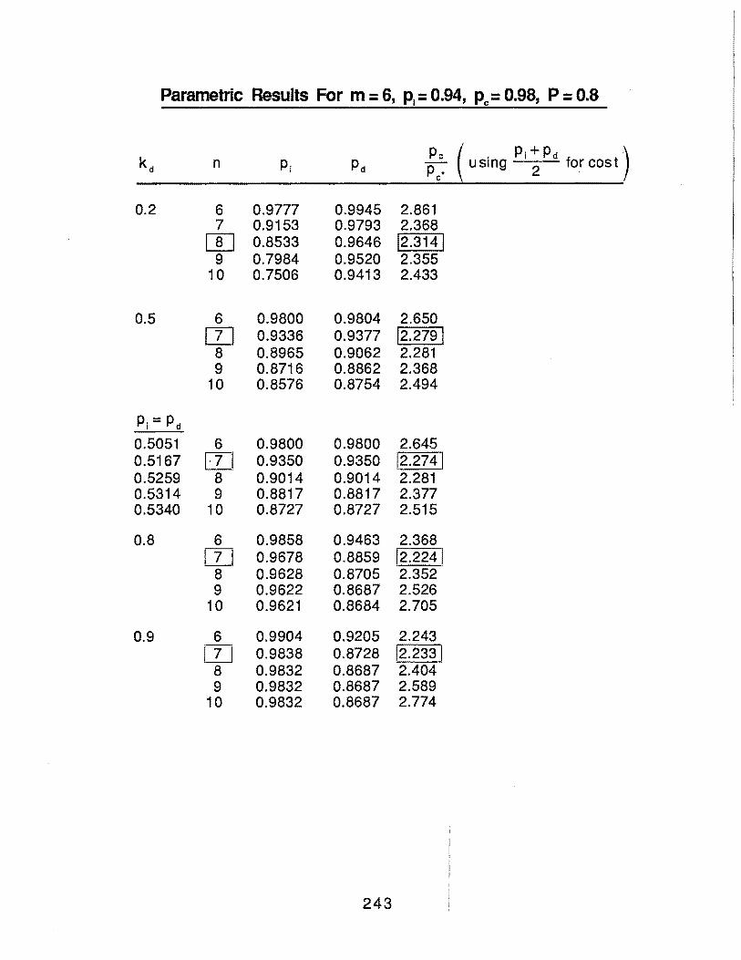
Parametric Results For m = 6, P,= 0.94, Pc= 0.98, P = 0.8
kd n pi pd p, ( . p, + p, ) Pc· usmg 2 forcost
0.2 6 0.9777 0.9945 2.861 7 0.9153 0.9793 2.368
[]] 0.8533 0.9646 12.3141 9 0.7984 0.9520 2.355
10 0.7506 0.9413 2.433
0.5 0.9800 0.9804 2.650 0.9336 0.9377 12.2791 0.8965 0.9062 2.281 0.8716 0.8862 2.368 0.8576 0.8754 2.494
pi= pd
0.5051 6 0.9800 0.9800 2.645 0.5167 [l] 0.9350 0.9350 12.2741 0.5259 8 0.9014 0.9014 2.281 0.5314 9 0.8817 0.8817 2.377 0.5340 10 0.8727 0.8727 2.515
0.8 6 0.9858 0.9463 2.368 []] 0.9678 0.8859 12.2241
8 0.9628 0.8705 2.352 9 0.9622 0.8687 2.526
10 0.9621 0.8684 2.705
0.9 6 0.9904 0.9205 2.243 l_lj 0.9838 0.8728 12.2331
8 0.9832 0.8687 2.404 9 0.9832 0.8687 2.589
10 0.9832 0.8687 2.774
243
Session B, Submittal No. 6
Manuel I. Cruz TRW
245
'·
EARTH PENETRATION CONCEPTS
AND
MARS PENETRATOR ENTRY TRADES
MANNY CRUZ TRW
Earth Penetration Concepts
lAULE I
EARTH PENETRATOR RE-ENTRY TO IMPACT CONCEPTS
Control Ballistic Star: inq Conditions Impact Conditions
Concept Mec11anlsrn Coefficient v Gamma h v Gamma 1 a· Impact Error Comments
Ckn/m2) (mpsl (deqree) (km) (mps) (degree) (meters/driver)
·Two Stage Drag modulation 10 5 [J 5 15000 180 to 250 90 30 300 to 900 90 -300/driven by Very good terminal
Ballistic Entry and staging low allitude winds velocity and !light
and High Altitude from low B to 59 rnps rath control; large
Drag Modulation high B CEP considerations
Two Stage Staging lrorn low 10 5 85 15000 180 to 250 90 30 300 to 900 90 -GOO to 900/high Very good terminal
Oallistic t:::ntry lJ to high !J altitude density velocity and flight variation 5 20 UD path control; large low allilude winds CEP considerations 59 mps
Two Stage Staging from 730 5 !J s: 15000 300 to 900 50 18 450 to 900 50 -300 to 600/high Plagued by lateral
Ballistic Entry moderate B to altitude density load carrying capa-
high B variation 5 20 UD bility of impact low altitude winds system medium s: 9 rnps strength rock
Ballistic Entry None 2500 N/A N/A N/A 215 60 -300 Plagued by rebound
Moderate B and/or ricochet
Ballistic Entry None 9800 5 [3 $ 15000 N/A N/A N/A 2100 to 3400 30 Driven by delivery Exceeds load
High 8 system carrying capability of impact system
Maneuvering Lilt Modulation 4900 s: B s: 15000 N/A N/A N/A 300 to 900 90 Driven by delivery Very good velocity Re-Entry system and flight path c;on-Pilcll!Bank trol throughout
impact error exceeds reql!irements
1\)
.J::>. c.o
PENETRATION PREDICTION
D = 0.0031 (S) (N) ~W/A (V-100), V >200FT/SEC
D = PENETRATION DEPTH CFT> S = SOIL CONSTANT N = NOSE PERFORMANCE COEFFICIENT W = WEIGHT (LB) A = CROSS-SECTIONAL AREA <FT2) V = VELOCITY AT IMPACT CFT/SEC)
1\) (J1
0
WEIGHT: 860 LBS ROLL Ml: 14.5K LB-IN2 PITCH Ml: 315K LB-IN2
STAO
STAO
WEIGHT: 850 LBS (MAX) ROLL Ml: 14.0K LB-IN2 PITCH Ml: 265K LB-IN2
;··~ ..................................................................................... : : .
1 13.27
. . l .................... ···1····· ................. ············· .. J
l 25.1 31.7 12.9 DIA 63.8 87.1
'1··············· .. ·················--······· .. ··-·----· ... . . : :
! 13.5
:-----:---r--------......1 _j_ Ll················ ·1···· ........................... .! m.o I .25.8 36.2 13.1 DlA 69.2
1\)
01 --"
2000~----~---T----------------~--~
! j 1800 ......... !··· ····--1··· ..... .
: : ; i
1600 ....... l ......... ; ......... . : i ! i : i 1400 ....... T ......... 1 ......... . : : ! :
1200- ........ j .......... J ........ .. I I
! 1 1000- ........ ; ........... i ........ . I • i I ! ! I i i i ! ! ! i I ! : I I I I
800- .......... j .......... l........ . . ....... ·.1···· ....... 1.!' ............ ; ........... :.; .......... -!-........ . ! i I I I I I : i : ; i : i !
800 - .......... , ........... 1 .......... f ....... ·; .......... l ........... , ........... r .......... -t" ........ . ! ! !' i . ! ! !
400 ........... ! ........... J .......... i ........... , ........... , ........... i ........... ~.. . : i l ! i l i i i
. l i l i i i ! i 200- .......... , ...........
1 ..........
1 ........... , ........... , ........... , ........... t ........... ~ ........ ..
! . i . I I ! ! : '.
o~ .. ~~, .. ~,~~~~~~~~~~~.~~~ o 10 20 30 40 60 eo 70 80
IMPACT ANGLE {degs)
Baseline Design - Target Type 3 (Soil) -2.0 Degrees Angle of Attack
90
-U)
0. --(; u ~ > w a: 3 ~
2000
1800-
1600-
1400- ..... ; ... ••: 1.: ::.: : : 1 :: :::::1 ::.::r : 1::: 1 : .:.
1200 .... ·: .... I.. . ... l ...... i : ... + .... , . L .... . 1000 ~ ! .... •·': ......... : ...... .
800 I l 0000 Ooo~··· 00 OH~
eoo
400
200 :.:::r ·; :::1: ::.:r::: ..r : ... :·r:::.:: r.: ~ L ...... j ....... i ! i ! . i i i i ! i i i
0~--~--.-~~~~~~~~~~~
0 10 20 30 o4o 6o· eo 10 80 so IMPACT ANGLE {degs)
860 lb Design Excursion 1 - Target Type 3 (SOU) -2.0 Degrees Angle of Attack

c:;; g
(; u
~ 1\) > 01 w 1\) a:
3 ~
2000~------------------~--~----~
~ : : .... ~ .. 1800-
: :·
1600
1400-
1200-
1000
200. ········1··.-········i .......... f .......... .j. .......... i .......... j ........... t .......... f .. "":·
O·~~~.~~.~~T~~.~~~~~.~~~.~~~ o 10 20 30 40 &o · oo 70 eo eo
IMPACT ANGLE (degs)
Baseline Design - 'J'arget 1'ype 4 (SoiVRock) -2.0 Degrees Angle of Attack
-en 0. --£; u
~ > w a: 3 ~
2000
1800
1600
1400
1200
1000-
BOO
eoo
400
200
10 20 30 40 6Q eo 70 ao eo IMPACT ANGLE (degs)
860 lb Design J~xcurslon 1 -1'arget 1'ype 4 (SoiVRock) -2.0 Degrees Angle of Attack

1\)
01 w
LATERAL DISPLACEMENT VS ANGLE OF ATTACK FOR 4 PENETRATOR CONFIGURATIONS (MEDIA - SAND)
-(/) w I 0 z
50 ,---------
40 -
1- 30 -z w ~ w 0 <( _j
D... (/)
0 20-_j <( a: w ~ _j
10
·----------------------,
---. I .2
COI,IFIG COI,IIIG CON FIG COI,JF\G
J. 3 ·. -1
-n- cor,JFIG. 1 -o- cot,JFIG. 2 --i>- COI,JFIG. 3 ~ CONFIG.4
\' L/D e.G. (FT/S[C) ( :t LENGTH) ---· ---
2000 C" ,, 40 1000 ·~ L\0 v
1000 5 50 1000 10 50
--
0~----~---~~---~---~------~--~---~--~
0 2 4 6 D
ANGLE OF ATTACK (DEGREES)

I\')
01 ~
PENETRATION VS. ANGLE OF ATTACK FOR 4 PENETRATOR CONFIGURATIONS (MEDIA- SAND)
120~--------------------------------------------~
1oo- \
-a- CONFIG. 1 --4-- CONFIG. 2 ---<>-- CONFIG. 3 --<>-- CONFIG. 4
........ tn IJJ :t: u z 30 -::r: ..... D.. LlJ 0 60-z c -..... < 0::
~ 40 z IJJ D..
20
o~--~~~~--~--~--~--~--~--~--~--~--~ 0 2 4 6 0 10 12
ANGLE OF ATT ACI< (DEGI1EES)

1\) (]1 (]1
Mars Penetrator Entry Trades
~~~-

1'\) 01 0'>
~ ~ ~ u <( a: 1-0 z ::J 0 a: (!J
450.00
400.00
350.00
300.00
250.00
200.00-
150.00
100.00
50.00
-60.00 -50.00 -40.00 -30.00 -20.00 -10.00
I ENTRY FLIGHT PATH ANGLE (DEG) I
e MIA = 10 KG/M .. 2 A MIA = 20 KG/M"*2
r-
0 0.30 -
-w -U) 0.25
-L ~ - ~ ~ "'-0 0.20
~ w - f\r--A w I:J. A a..
U) 0.15 0: -P--El --tJ ..... -0--1 o-a-· -1 0-El <(
0.10 ......
....J <( z - - -·~ 0.05 - ""' -..:7 - - "" 0: w -._
0.00 I I I I ...__ I I I I I I I
-60.00 -50.00 -40.00 -3 0.00 -20.00 -10.00
I ENTRY FLIGHT PATH ANGLE (DEG) I
e M/A = 2 KG/M**2. B M/A = 10 KG/M .. 2 A M/A == 20 KG/M ... 2

1\)
01 CD
--(!'} w 0 -w ....J (!'} z <(
:c .... <( 0... .... :c (!'} ::i Lt..
:E a: w ....
-
-55.00 -A-~. - A ~k" ~
-60.00 -~ ~
-65.00
~ -70.00 --;
~ -75.00
-80.00 8 -fl. 8-[ ~·-·8-r:t. - .... -85.00 - a.;;;(_ I; ~-EJ -
- ,.., ,.., ....... ,.., ,.., -90.00 I I I I I I I I .I I I I
-60.00 -50.00 -40.00 -30.00 -20.00 -10.00
I ENTRY FLIGHT PATH ANGLE (DEG) l
e· M/A = 2 KG/M**2 8- M/A = 10 KG/M**2 A M/A = 20 KG/M**2
I'\)
c.n tO
IMJ~~~ Jm@~r~rru
®~IMJ[pJ!L~ !ru~lllUJ !ruiM
AEROBRAKE DESIGN
Session B, Submittal No. 7
Richard P. Reinert Ball Space Systems Division
261
1\) Q') 1\)
CRAF PENETRATOR-LANDER
FOR MARS
PREPARED FOR MGNM WORKSHOP AT JPL
02/06/90 W. Boynton
University of Arizona
R. Reinert Ball Space Systems Division

y iL
1\)
m w
. Space Systems Division
BRIEFING OUTLINE
PRELIMINARY MISSION REQUIREMENTS
POLAR PENETRATOR DERIVED FROM CRAF CONFIGURATION
PV FUNCTIONAL SHOWS CENTRAL ROLE OF C&DH
SCIENCE OBJECTIVES SIMILAR TO CRAF
BASIC INSTRUMENT COMPLEMENT IS IDENTICAL EXCEPT FOR GRS
POLAR PENETRATOR MASS PROPERTIES MATCH BASELINE
POLAR PENETRATOR CONFIGURATION COMPATIBLE WITH BASELINE AEROSHELL
POLAR PENETRATORS OCCUPY ONE AEROSHELL
MPP AEROSHELL/PENETRATOR SYSTEM
PENETRATOR EXTRACTION FORM AEROSHELL
PENETRATOR DEPLOYMENT
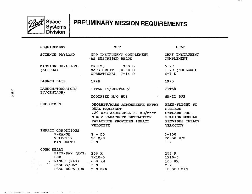
Space Systems Division
PRELIMINARY MISSION REQUIREMENTS
REQUIREMENT
SCIENCE PAYLOAD
MISSION DURATION: (APPROX)
LAUNCH DATE
LAUNCH/TRANSPORT IV/CENTAUR/
DEPLOYMENT
IMPACT CONDITIONS S-RANGE VELOCITY MIN DEPTH
COMM RELAY BITS/DAY (AVG)
.·BER RANGE (MAX) PASSES/DAY PASS DURATION
MPP
MPP INSTRUMENT COMPLEMENT ·AS DESCRIBED BELOW
CRUISE MARS ORBIT OPERATIONAL
1998
330 D 30-60 D
7-14 D
TITAN IV/CENTAUR/
MODIFIED M/0 BUS
DEORBIT/MARS ATMOSPHERE ENTRY DUAL MANIFEST 120 DEG AEROSHELL 30 K~/M**2 M = 2 PARACHUTE EXTRACTION PARACHUTE PROVIDES IMPACT VELOCITY
3 - 50 50 M/S 1M
256 K 1X10⁻⁵ 600 KM
. 2 M
5 M MIN
CRAF
CRAF INSTRUMENT COMPLEMENT
6 YR 1 YR (NUCLEUS) 6-7 D
1995
TITAN
MM/II BUS
FREE-FLIGHT TO NUCLEUS ONBOARD PROPULSION MODULE PROVIDES IMPACT VELOCITY
3-200 20-50 M/S 1 M
256 K 1X10⁻⁵ 100 KM 2 M 10 SEC MIN
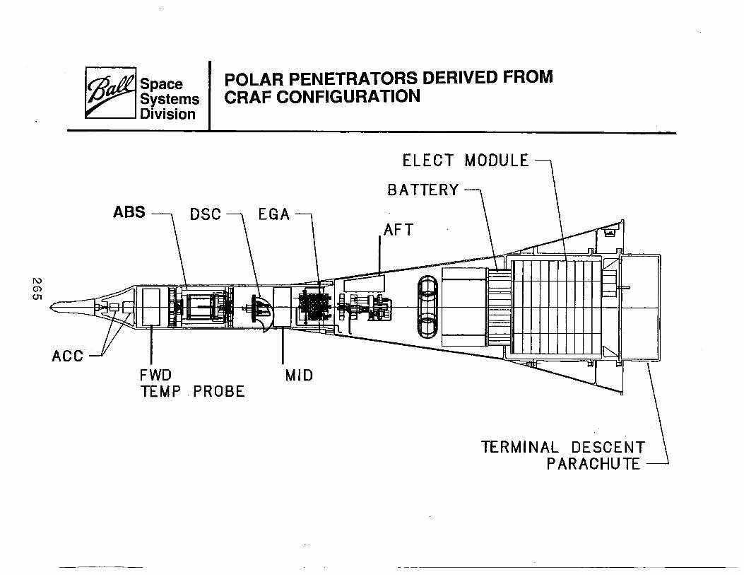
Space POLAR PENETRATORS DERIVED FROM Systems CRAF CONFIGURATION
_ Division
ABS EGA
FWD MID TEMP . PROBE
ELECT MODULE
BATTERY
AFT
TERMINAL DESCENT PARACHUTE
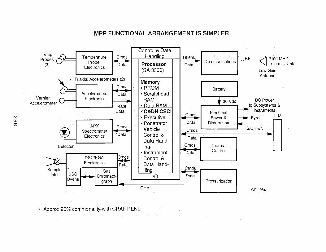
1\) 0") 0")
MPP FUNCTIONAL ARRANGEMENT IS SIMPLER
Te Pro bes
(
mp 6k= 3)
Temperature _Emd~ Probe - ..
Electronics Data
~Triaxial Accelerometers (2)
Cmds - ... Accelerometer Data er Verni
Accelero meter
~ ~ Detector
[::®:: Sample
Inlet DSC Ovens
Electronics ' ~ .. Hi-rate
·.Data
APX _Emd~. Spectrometer -:: ...
Electronics ·Data
DSC/EGA CIJ:l~S Electronics .....
Data
Gas .. ~ Chromate-.. -graph -..
Control & Data Handlina
Processor (SA 3300)
Memory •PROM • Scratchpad
RAM ·Data RAM • C&DH CSCI
· • Executive . ~ Penetrator
Vehicle Control & D.ata Handl-ing
• Instrument Control & Data Hand-ling
1/0
GHe
• Approx 90% commonality wi~h CRAF PENL
Telem._ . Communications Data
Battery
f 30 Vdc
Electrical _Cmd.§ Power & .. ..
Data Distribution
.- Cmds
Data
Cmds Thermal - ~
""Data"" Control
Cmds ·
-- --Data Pressurization
RF 2100 M Telem.
Low Gain Antenna
DC Power
... to Subsystems & - Instruments
----... Pyro IFD r--.. - SIC Pwr. -.
-
CPL.084
HZ Uplink
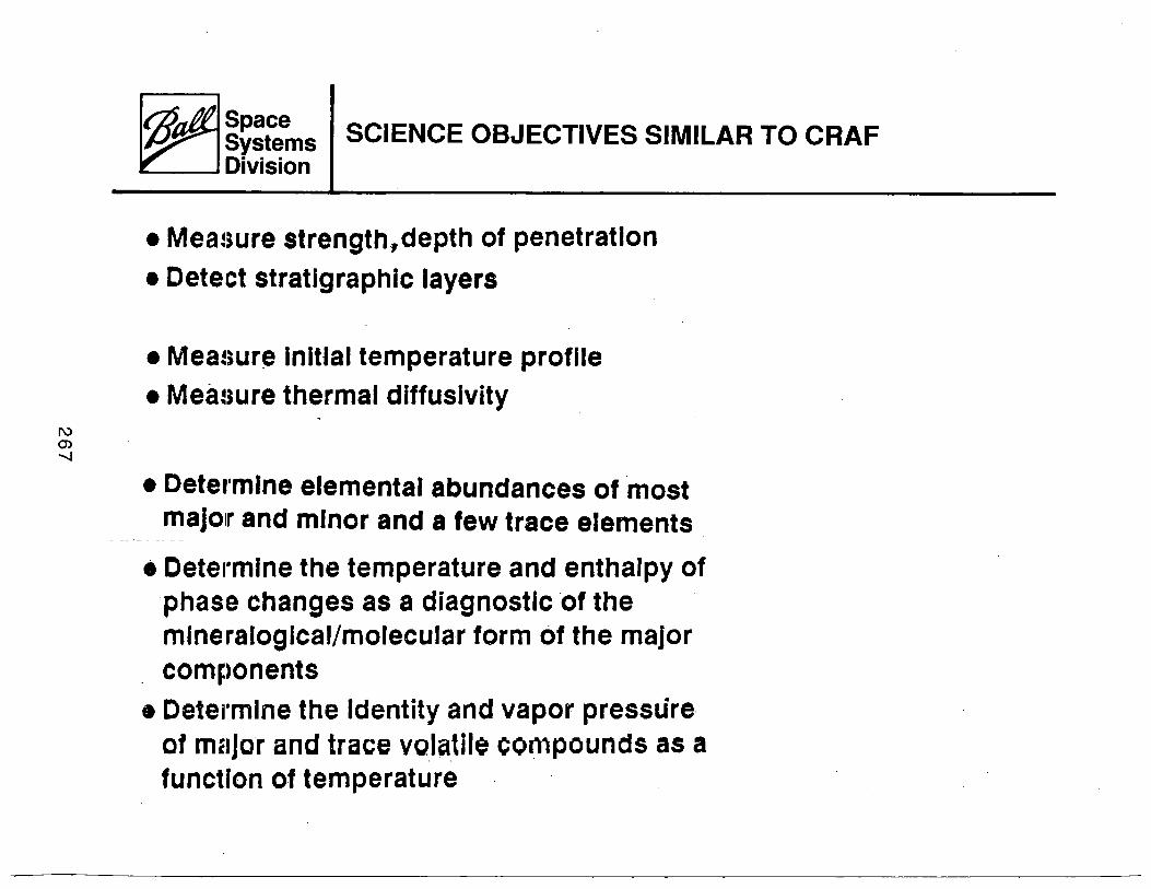
~ ~e!fee.ns SCIENCE OBJECTIVES SIMILAR TO CRAF ~Division
• Mea~~ure strength, depth of penetration
• Detect stratigraphic layers
• Mea!~ur~ Initial temperature profile
• Mea!sure thermal diffuslvity
• Deter·mrne elemental abundances of most majo1r and minor and a few trace elements
• Dete1·mrne the temperature and enthalpy of phase changes as a diagnostic of the mineralogical/molecular form of the major components
• Oete1·m1ne the Identity and vapor pressure of m~tjor and trace volaUie compounds as a function of temperature
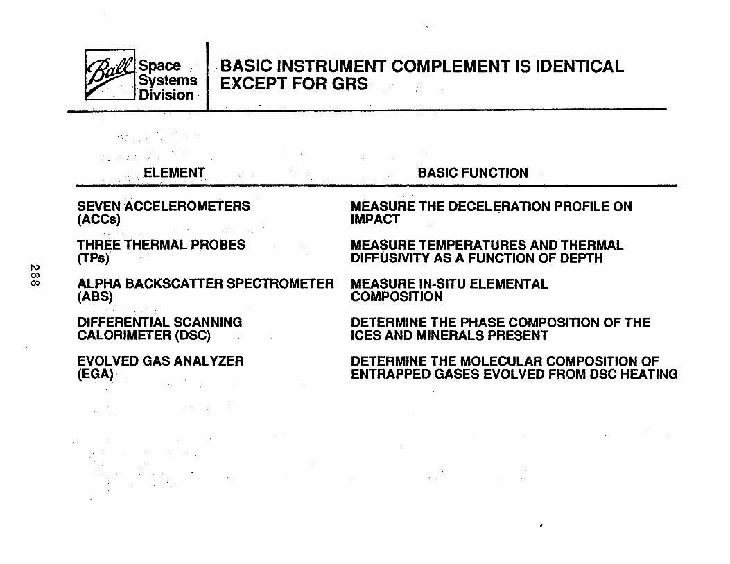
~~e::ms ~Division· BASIC INSTRUMENT COMPLEMENT IS IDENTICAL EXCEPT FOR GRS
.. ELEMENT
SEVEN ACCELEROMETERS . (ACCs)
THREE.THERMAL PROBES. (TPs) ·
BASIC FUNCTION
MEASURE THE DECELE;RATION PROFILE ON IMPACT
MEASURE TEMPERATURES AND THERMAL DIFFUSIVITY AS A FUNCTION OF DEPTH
ALPHA BACKSCATTER SPECTROMETER MEASURE IN-SITU ELEMENTAL (ABS) COMPOSITION
DIFFERENTIAL SCANNING CALORIMETER (DSC)
EVOLVED GAS ANALYZER (EGA)·.
DETERMINE THE PHASE COMPOSITION OF THE ICES AND MINERALS PRESENT
DETERMINE THE MOLECULAR COMPOSITION OF ENTRAPPED GASES EVOLVED FROM DSC HEATING
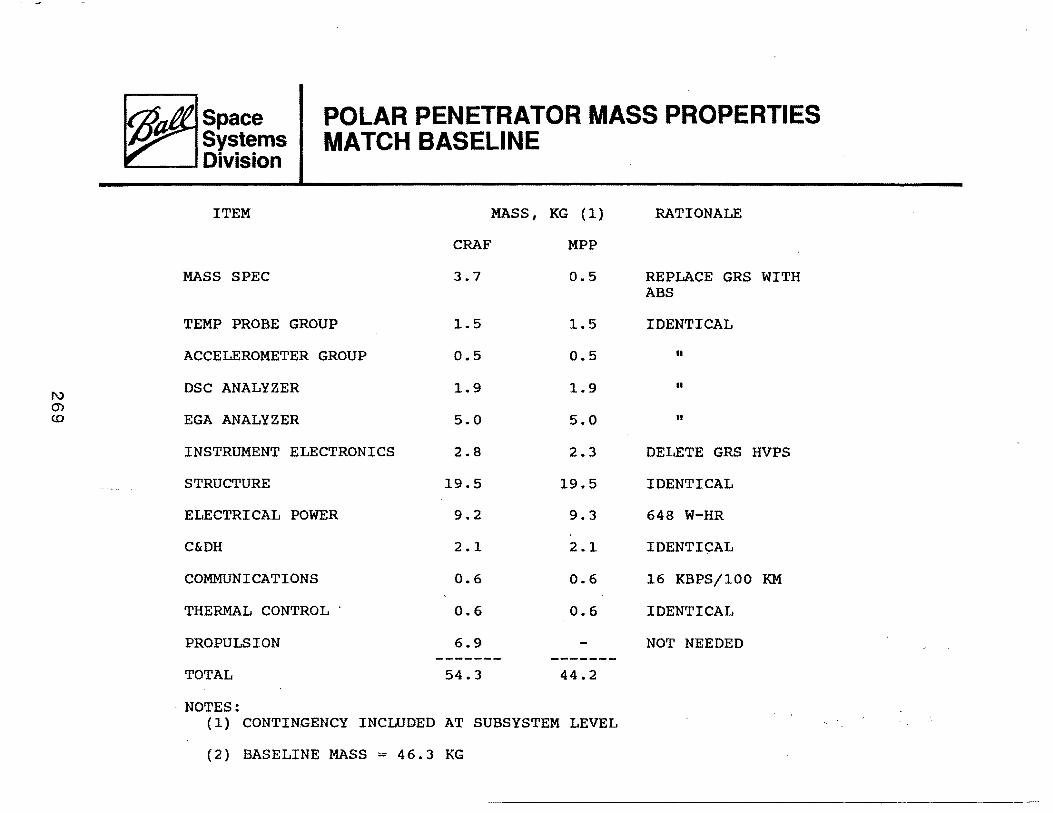
I\) 0')
co
Space Systems Division
POLAR PENETRATOR MASS PROPERTIES MATCH BASELINE
ITEM MASS, KG (1) RATIONALE
CRAF MPP
MASS SPEC 3.7 0.5 REPLACE GRS WITH ABS
TEMP PROBE GROUP 1.5 1.5 IDENTICAL
ACCELEROMETER GROUP 0.5 0.5 II
DSC ANALYZER 1.9 1.9 II
EGA ANALYZER 5.0 5.0 II
INSTRUMENT ELECTRONICS 2.8 2.3 DELETE GRS HVPS
STRUCTURE 19.5 19.5 IDENTICAL
ELECTRICAL POWER 9.2 9.3 648 W-HR
C&DH 2.1 2.1 IDENTICAL
COMMUNICATIONS 0.6 0.6 16 KBPS/100 KM
THERMAL CONTROL . 0.6 0.6 IDENTICAL
PROPULSION 6.9 NOT NEEDED ------- -------
TOTAL 54.3 44.2
· NOTES: (1) CONTIN.GENCY INCLUDED AT SUBSYSTEM LEVEL
(2) BASELINE MASS = 46.3 KG
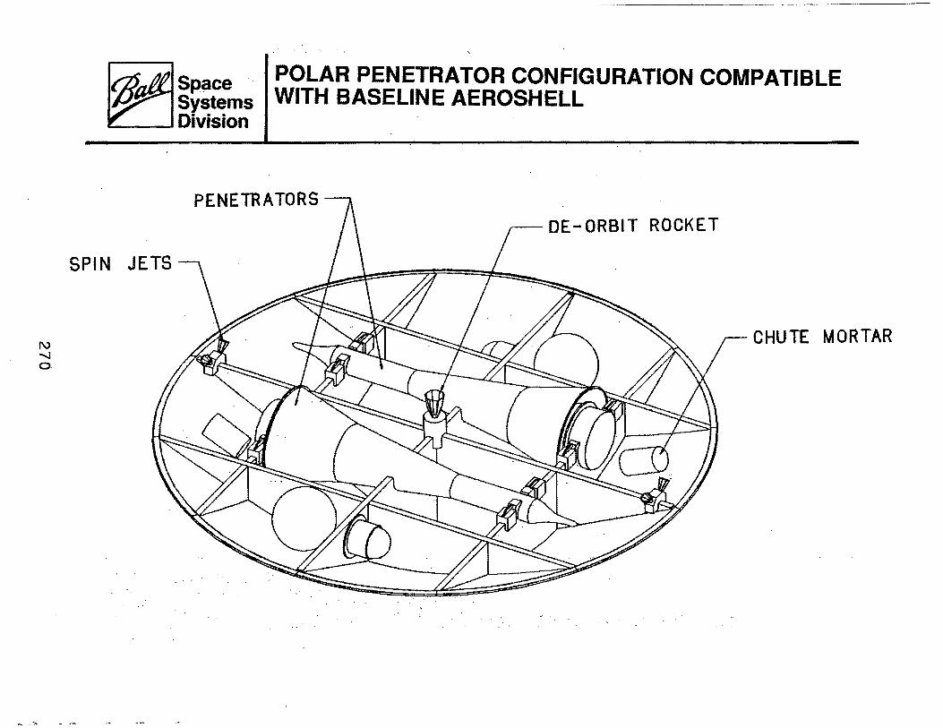
Space POLAR PENETRATOR CONFIGURATION COMPATIBLE Systems WITH BASELINE AEROSHELL Division
PENETRATORS
CHUTE MORTAR
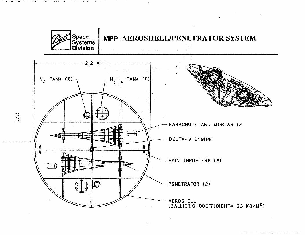
Space MPP AEROSI-IELL/PENETRATOR SYSTEM System~ Division .
~--------- 2. 2 u__c_-------~
(2)
PARACHUTE AND MORTAR (2)
. SPIN THRUSTERS (2)
PENETRATOR (2)
--- AEROSHELL (BALLISTIC COEFFICIENT= 30 KG/M 2 )
/
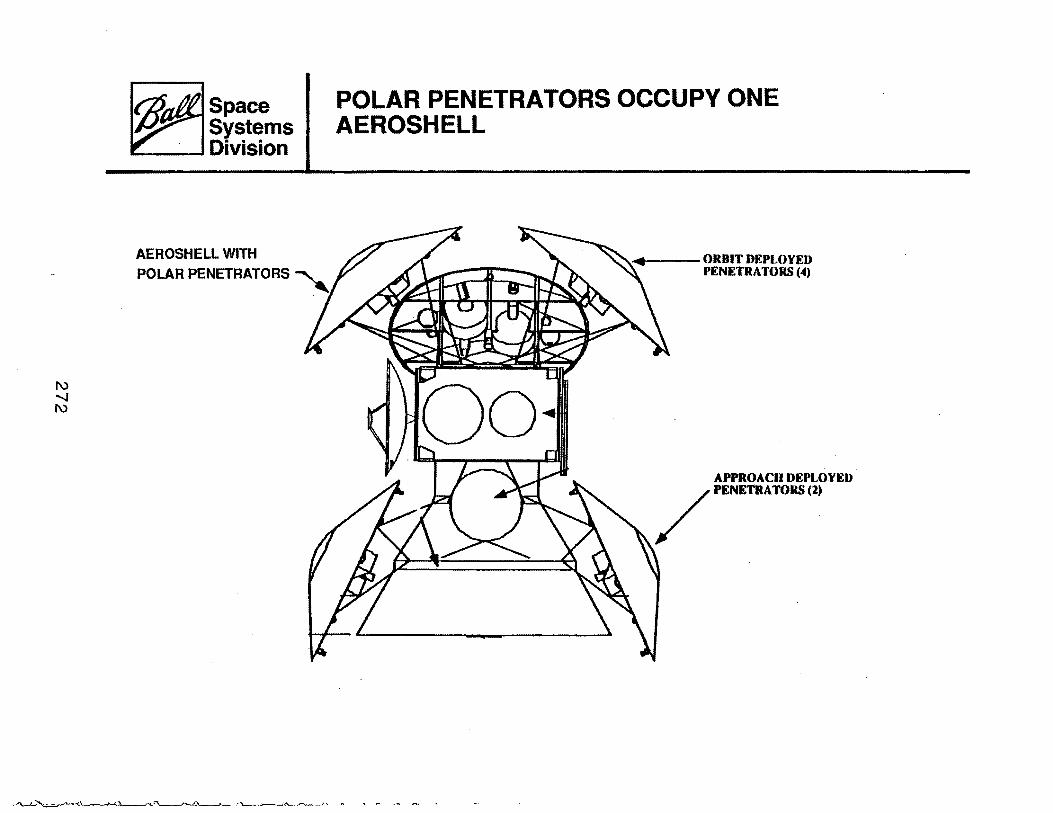
1\)
" 1\)
Space Systems Division
AEROSHELL WITH
POLAR PENETRATORS "
POLAR PENETRATORS OCCUPY ONE AEROSHELL
,.,.. __ ORBIT DEPLOYED PENETRATORS (4)
APPROACII DEPLOYED
/ I'ENE111ATORS (2)
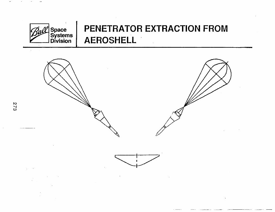
Spac~ ·Systems Division
PENETRATOR EXTRACTION FROM AEROSHELL .

Space Systems Division
PENETRATOR DEPLOYMENT
IMPACT
• ANGLE OF ATTACK- WIND EFFECT • ANGLE OF INCIDENCE- SURFACE UNDULATIONS
, • 'SURFACE HARDNESS- PENETRABILITY INDEX
COMMUN.ICATIONS
• ACCESSIBILITY TIME • BIT RATE, LINK BUDGET
SUPERSONIC PARACHUTE DEPLOYMENT
SURFACE IMPACT V = 60-100 m/sec
OPEN-CONCERN ACCEPTABLE UP TO 30° 3 -2.00
. ASSUME. 2. TO 4 MINUTES PEA PASS 12.5 Kblt/sec
Session B, Submittal No. 8
Joe D. Gamble Johnson Space Center
275

MARS GLOBAL NETWORK MISSION WORKSHOP
ENTRY SYSTEM DESIGN CONSIDERATIONS
J. Gamble - NASA/Johnson Space Center
Introduction
This section addresses some of the design issues concerned with the specific workshop question, "What is the best entry system - fixed or deployed aeroshells; parachutes or direct impact?" To address these questions some information about the entry conditions in the Mars environment is required. Results from the 90 day human exploration initiative study were used as a reference point. The MRSR pre-phase A study results were also considered. Finally some parametric data was generated to specifically address the GNM entry design question. ·
Reference Mission
The 90 day study considered two flight systems each consisting of an orbiter/carrier vehicle with six aeroshells as shown in Figure 1. Each aeroshell contains two penetrator landers as shown in Figure 2 that use parachutes to extract them from the aeroshell just prior to landing. The rigid aeroshells are deployed from the carrier vehicle and spin stabilized at 60 rpm. Small propulsion systems provide the delta V required for the desired atmospheric entry conditions. The aeroshells do not have an active guidance and control system.
The aeroshell design incorporates a rigid conical aeroshell with a spherical nose cap. The aeroshell diameter is 2.2 m and has an entry mass of approximately 110 kg, yielding a ballistic coefficient of 30 kg/m2. The aeroshell uses an ablative heat shield.
Two of the six aeroshells are deployed 2-10 days prior to Mars arrival in order to land at polar sites. The other four aeroshells are deployed after capture into a 1/5 Sol Mars qrbit.
~ Approach Deployed Aeroshells
One of the primary concerns in the MRSR study was the ability to achieve the proper entry conditions during the Mars approach. The entry corridor is bounded by the skip out and maximum allowable g load boundaries as shown in figure 3. Figure 4 shows the entry corridor limits versus L/D for an entry velocity o·f 6 km/ sec. The total corridor width is summarized in figure 5 and shows that the corridor is nearly independent of the ballistic coefficient. The ballistic
276

coefficient determines whether the vehicle flies higher or lower in the atmosphere during the early portion of the entry. While the MRSR was concerned with aerocapture during the approach phase, the results are also applicable to the entry case. The estimated corridor width for ballistic vehicles are shown on figure 5. For a maximum entry load of 5 g's, the total corridor width is less than one degree. The corridor width increases to 3 and 5.5 for ~0 and 15 g limits respectively. The MRSR study concluded that a minimum corridor width of approximately 3 degrees was required in order to accommodate navigation and atmosphere uncertainties. In order to achieve this accuracy, optical navigation was baselined for the study and trajectory corrections were considered within a few hours of entry.
GNM aeroshells deployed several days prior to entry and not having an active guidance and control system will almost certainly require much larger entry corridors than are necessary for the MRSR. It is very possible that a minimum corridor width of at least 5-10 degrees will be required. Figure 6 shows some preliminary results for the aeroshell defined by the 90 day study at an entry velocity of 6 km/sec at 125 km altitude. The figure indicates that g loads in excess of 20 g's will be required to provide a corridor width of 10 degrees. Figure 7 shows that for a 10 degree corridor width, downrange dispersions of +/- 2-5 degrees will occur for nominal entry angles of 15-20 degrees. These results were obtained from three degree-of-freedom simulations entering in a polar plane.
One proposal for decreasing the landing footprint dispersions is to enter at a much steeper entry angle. The results of entering at -35 and -45 degrees are shown as a function of ballistic coefficients in figure 8. The downrange dispersion for 10 degrees change in entry angle is less than one degree although it does increase as the ballistic coefficient increases. One of the primary problems with the steep entry angle is the large load factors that result. Figure 9 shows the maximum g loads (Earth g's) resulting from entry at -35 and -45 degrees. Load factors on the order of 40 - 60 g's result from these steep angles.
Deployable Aeroshell Considerations
Use of deployable aeroshell configurations will in general preclude the use of ablator heat shields and the ballistic coefficient will have to be small enough to limit the· aeroheating during entry. To achieve a ballistic coefficient of 10 kg/m2 using the 90 day study mass of 110 kg would require an aeroshell diameter of approxima~ely 3.8 m while a diameter of 8.5 m would be required to ach~eve a ballistic coefficient of 2 kg/m2. It would appear t~at use of deployed aeroshells of this size would have signifi~ant problems operating at 40-60 g's during entry. For this reason it is
I
277

questionable whether use of deployable aeroshells for entry during Mars approach is a viable concept.
Mars Orbit Deployed Aeroshells
The lower entry velocity for aeroshells deployed from Mars orbit present much less of a problem than for those deployed during approach. Figure 10 shows that entry corridors of 15 degrees are possible at less than 10 g maximum load. Because the navigation is much better defined for the orbit deployed aeroshell than for the approach deployed case1 the entry angle dispersions will be much less. Figure 11 indicates that for entry angle dispersions of +/- 1 degree, the dispersion in the_ downrange landing site will be well within +/- 1 degree. Aerodynamic heating for tne orbit entry cases will also be much lower than for the approach deployed aeroshells. It would appear that these advantages definitely outweigh the delta V penalty associated with capturing the aeroshells into Mars orbit.
Parachut~ Considerations
One of the primary concerns with use of parachutes for the final surface delivery of the instrument packages is whether acceptable deployment conditions can be achieved during the aeroshell entry. The Viking program used supersonic deployed parachutes which were required because of the uncertainty in the Mars atmosphere. In general deployment of parachutes up to around Mach 2 (approximately 500 m/sec at Mars) is considered well within the state of the art. Figure 12 shows the aeroshell velocity at 5 and 10 km altitude as a function of entry angle for the 30 kg/m2 configuration with an entry velocity of 3.6 km/sec at 125 km altitude. The aeroshell is seen to be subsonic at both altitudes for the range of entry angles shown. Figure 13 shows_the variation of the aeroshell velocity at 10 km altitude for various dispersions in the atmosphere. The low density cool COSPAR atmosphere results in barely supersonic conditions for the 30 kg/m2 configuration and even a severe 50% decrease in atmospheric density only produces a Mach 2 case. Therefore use of parachutes for landing of the payload should not present any significant deployment problems.
The bibliography lists several references with some applications to_· the Mars entry problem. A number of these also have extensive bibliographies.
278
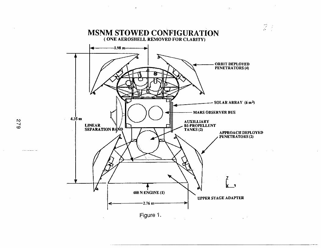
4.35 m
'
MSNM STOWED CONFIGURATION ( ONE AEROSIIELL REMOVED FOR CLARITY)
400 N ENGINE (1)
...,.._ __ ORBIT DEPLOYED PENETRATORS (4)
AUXILLIARY 81-PROPELLENT TANKS (2)
APPROACII DEPLOYED / PENETRATORS (1)
UPPER STAGE ADAPTER ~'-------2.76 m-----;11'1
Figure I.
... /

1\)
CX> 0
MSNM AEROSHELL/PENETRATOR SYSTEM
...___------2.2 m------~
N1 TANK (2)
AEROSIIELL
PARACHUTE AND MORTAR (2)
SPIN THRUSTERS. (2)
PENETRATOR (2)
(!iAi.LISTIC COEFICIENT = 30 kg/m 1 )
Figure·2.
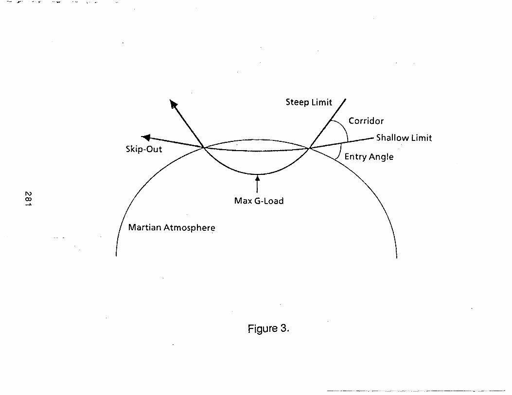
Steep Limit
Shallow Limit Skip-Out
Max G-Load
Martian Atmospher~
Figure 3.
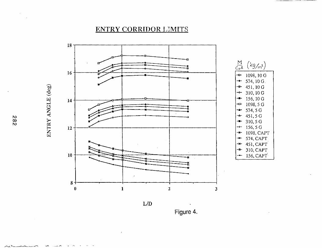
ENTRY CORRIDOR LIMITS
18~------------.-------------.-------------.
16 -e- 1098, 10 G -+- 574, 10 G
~
bll <U
-o- 451,100 "'0 '-"
-o- 310, lOG w 14. ~ c., z
... 156, 10 G -0- 1098,5 G ..... 574,5 G
1\') ~ -6- 451,5 G co > 1\') ~
t-< 12
... 310,5 G -+- 156,5 G
z w -ill- 1098, CAPT
-w- 574, CAPT -M- 451, CAPT -&- 310, CAPT
---- 156, CAPT
g+-----~--~--+-----~------+-----~------4
0 1 2 3
L/D Figure 4.
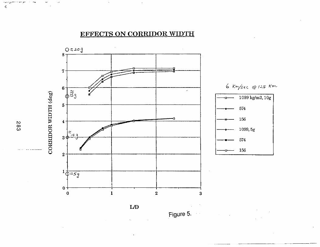
EFFECTS ON CORRIDOR WIDTH
6 '9J
<l,) "0
7
f ·~ ~
""' ·~ ·' ......, ~DI53 -e-- 1099 kg!m2, 1 Og
._.,
~ 5
574 Cl
1\) e: 4 ..... 156
(X) ~ w 0 8 3
~ -- ~-··------ 0
Q 2
/ ~
~
...... / 0 g
"/ 1099,5g
• 574
-a-- 156
1 ():::;s3
i I 0
0 1 2 3
UD Figure 5.

M A X I
M N u co M ..p..
G
L 0 A D
G LOAD VS ENTRY ANGLE M/CDA=30 KG/M2 6 km/sec ENTRY VELOCITY
30
25
20
15
10
5
0 0 5
/ /
/ i J v i
. I
'
/ Q;. ._,
~ '
1/ ! ! I
10 15 20 25 30
ENTRY ANGLE AT 125 KM
Figure 6.
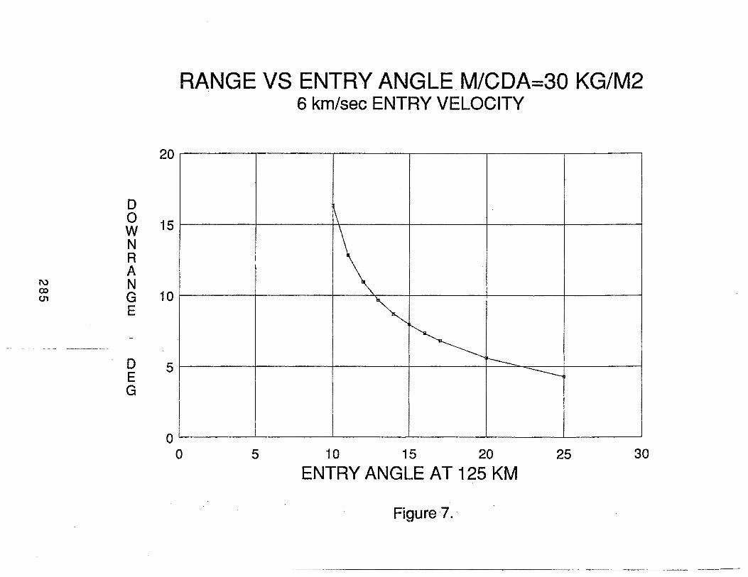
RANGE VS ENTRY ANGLE M/CDA=30 KG/M2 6 km/sec ENTRY VELOCITY
20
D 0 15 w N R A
1\) N ~ G 10
E
D 5 E G
0 0 5
\
~ ~ !--- ----_,
10 15 20 25 30
ENTRY ANGLE AT 125 KM
Figure 7. ·
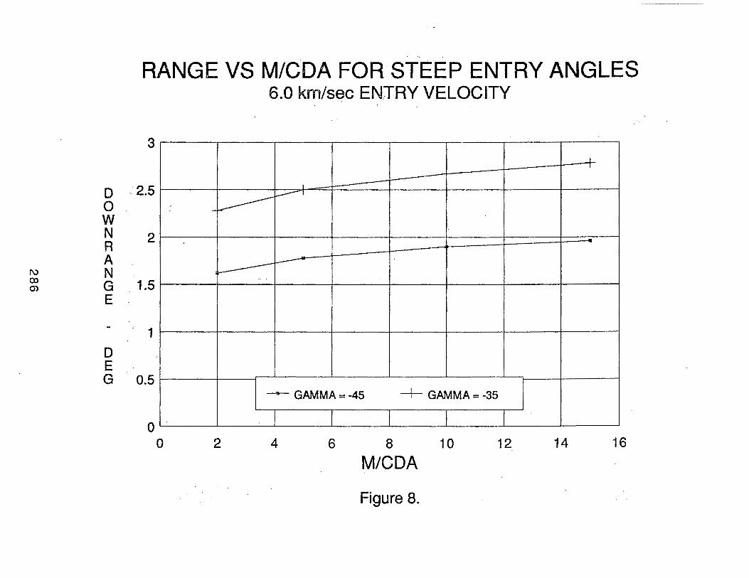
D 0 w N R A
1\) N 00 G 0'>
E
D E G
. ·.
RANGE VS M/CDA FOR STEEP ENTRY ANGLES 6.0 km/s~c ENTRY VELOCITY
3
.. · 2.5
2
1.5
1
0.5
0 0
J_ I
I
--------~· ...
.-------~
- GAMMA=-45 --+- GAMMA = -35
2 4 6 8 10 12 14 16
M/CDA
Figure 8.
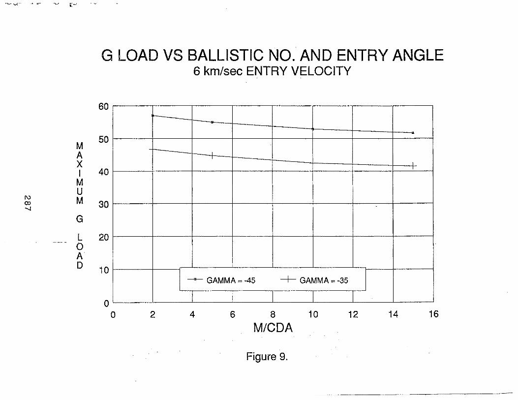
M A X I M u
1\) M Q:)
"'-.J
G
L 0 A D
G LOAD VS BALLISTIC NO. AND ENTRY ANGLE 6 km/sec ENTRY VELOCITY
60
50
40
30
20
10
0 0
,__
--
2
I I
I I
-
- GAMMA=-45 -1- GAMMA = -35
4 6 8 10 12 14 16
M/CDA
Figure 9.
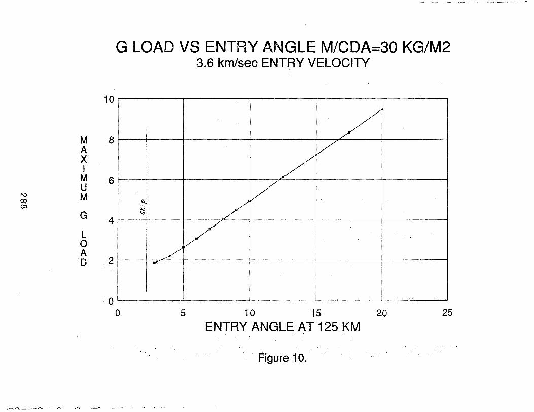
M A X I M u
1\.) M CD. CD
G
L 0 A D
G LOAD VS ENTRY ANGLE M/CDA=30 KG/M2 3.6 km/sec ENTRY VELOCITY
10
8
6
4
.2
·0 0
I I
l
I
' i i !
-~ ~! '-li
'
l!l!il'
J
/ /
v
/ / '
/ /
5 10 15 20 25
ENTRY ANGLE AT 125 KM ~ . ' .· '
.. . ~.. .. '. .
· Figure 10. '·

RANGE VS ENTRY ANGLE M/CDA=30 KG/M2 3.6 km/sec ENTRY VELOCITY
35
D 30
0 w 25 N R A 20 N G E 15
D 10 .E
G 5
0 0
\ \ \ ~ ~ ~
1----- ------
5 10 15 20 25
ENTRY ANGLE AT 125 KM
Figure 11.
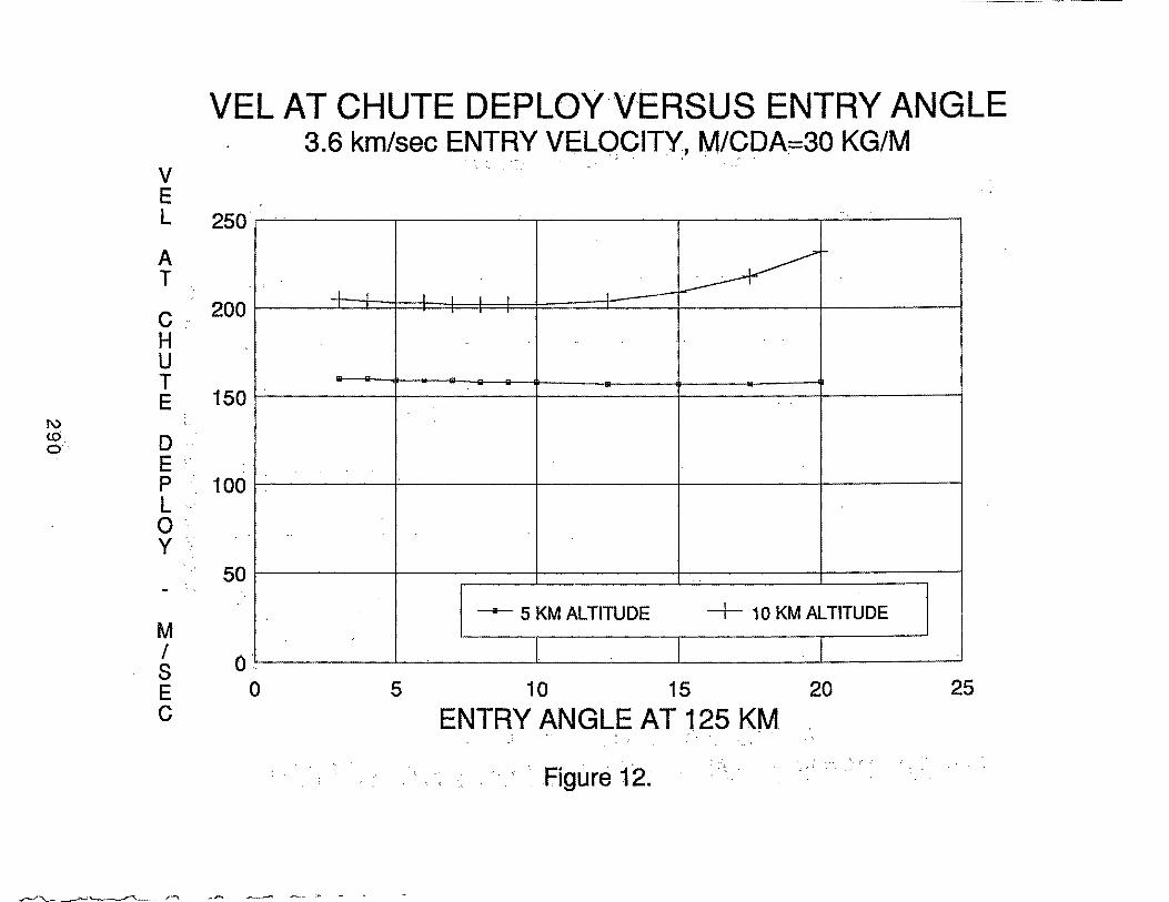
1\)
<.0 .. C)
v E L
A T
c H u T E
D E p L 0 y
M I s E c
..
..
·.
....
'
VEL AT CHUTE DEPLOY·V-ERSUS ENTRY ANGLE 3.6 km/sec ENTRY VEL9C?IT'(, M,/CDA~30 KG/M
250
200
150
100
50
.. 0 0
J. I
....
..
~ 1-
I I I I I -.
- 5 KM ALTITUDE -t- 10 KM ALTITUDE
5 10 15 20 25
ENTRY ANGLE AT 125 KM -: ... . ·. . .
. , Figure 12.
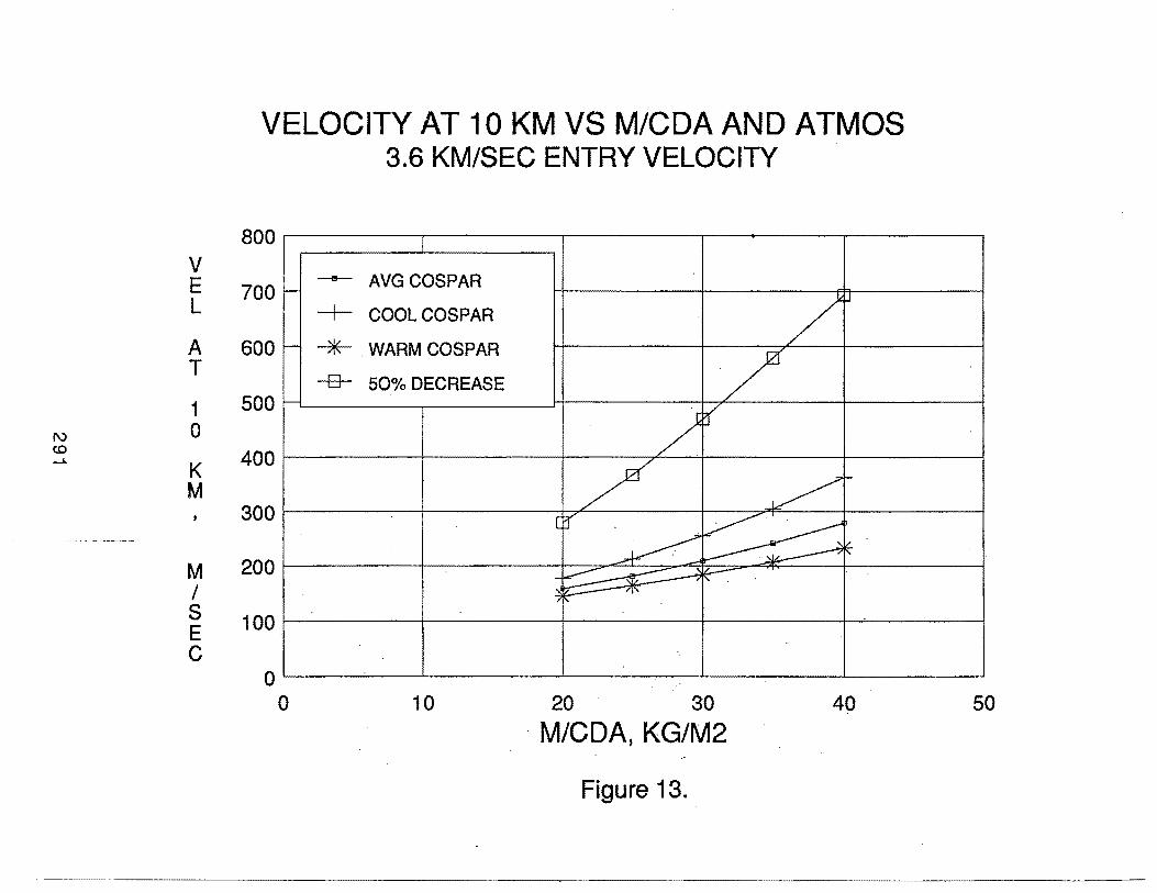
v E L
A T
1 1\) 0 tO _...
K M
M I s E c
VELOCITY AT 10 KM VS M/CDA AND ATMOS 3.6 KM/SEC ENTRY VELOCITY
800
700 1-
600 1-
500 1-
400
300
200
100
0 0
- AVGCOSPAR
COOLCOSPAR
--*- . WARM COSPAR
-B- 50% DECREASE
10
/J /
/ f
/ ~ -
[:(
~ ~ ~ ~ -~~ ~. -?~ 'I' "' .
20 30 40 · M/CDA, KG/M2
Figure 13.
50
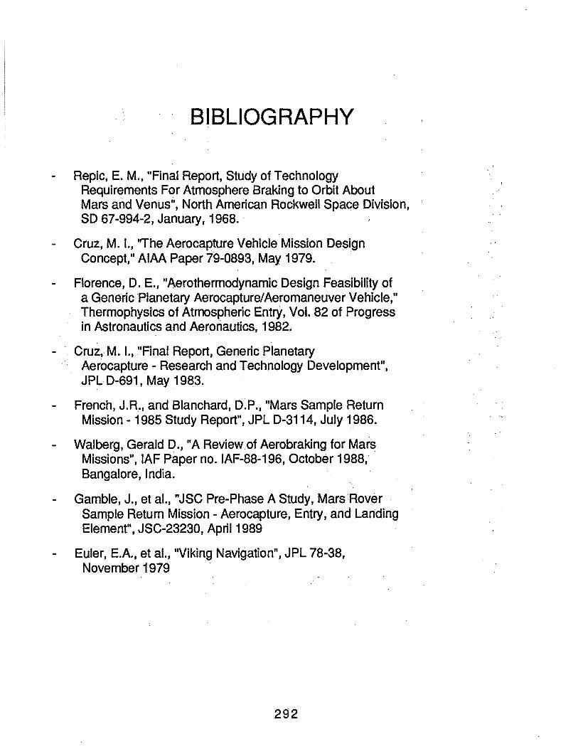
BIBLIOGRAPHY
Repic, E. M., "Final Report, Study of Technology Requirements For Atmosphere Braking to Orbit About Mars and Venus'', North American Rockwell Space Division, SD 67-994-2, January, 1968. ·
Cruz, M. 1., "The Aerocapture Vehicle Mission Design Concept, .. AIM Paper 79-0893, May 1979~ ·
Florence, D. E., "Aerothermodynamic Design Feasibility of a Generic Planetary Aerocapture/Aeromaneuver Vehicle," Thermophysics of Atmospheric Entry, Vol. 82 of Progress in Astronautics and Aeronautics, 1982.
Cruz, M. 1., "Final Report, Generic Planetary Aerocapture- Research and Technology Development", JPL D.-691 I May 1983 ..
French, J.R., and Blanchard, D.P., "Mars Sample Return Mission- 1985 Study Report", JPL D-3114, July 1986.
Walberg, Gerald D., "A Review of Aerobraking for Mars Missions" I IAF Paper no. IAF-88-196, October 1988,· Bangalore, India.
Gamble, J., et al., "JSC Pre-Phase A Study, Mars Rover · Sample Return Mission - Aerocapture, Entry, and Landing Element", JSC-23230, April 1989
Euler, E.A., et al., "Viking Navigation", JPL 78-381 November 1979
292

Session B, Subm itt a I No. 9
Byron L Swenson Science Applications International Corporation
..
293
tvtARS GLOBAL NETWORK MISSION
ENTRY AND TERMINAL DESCENT SYSTEM DESIGN CONSIDERATIONS & ISSUES
PRESENTATION TO THE MARS GLOBAL NETWORK MISSION WORKSHOP
FEBRUARY 6-7~ 1990
BY
BYRON L SWENSON
51\ftt,
LANDER ENTRY SVSTEM,DESIGN
REQUIREMENTS
• TO PROVIDE STABLE & CONTROllED ATMOSPHERIC DECELERATION FROM HYPERBOLIC OR ORBITAL ENTRIES
• TO PROVIDE PROTECTION FROM AEROTHERM_ODYNAMIC HEATING
• TO DECELERATE lANDER TO TERMINAl DESCENT SYSTEM DEPLOYMENT CONDITIONS
DESIGN CONSIDERATIONS & ISSUES
• ENTRY CONDITIONS- SPEED, FliGHT-PATH ANGLE, ANGLE OF ATTACK
• MARTIAN ATMOSPHERE- lOW DENSITY, VARIATIONS, SITE ELEVATIONS
• FREE-SPACE & ATMOSPHERIC DYNAMICS
- • REQUIRED DELIVERY ACCURACIES
• BAlliSTIC OR liFTING TRAJECTORIES
• AERODYNAMIC & AEROTHERMODYNAMIC DATA BASE
• lOW BALLISTIC COEFFICIENT- TERMINAl SYSTEM DEPLOYMENT
• SPACECRAFT INTERFACE- TARGETING, SEPARATION, ENVELOPE
• AEROSHEll JETTISON
CONFI(2URATIONS ·
• 'BAlliSTIC
ENTRY SYSTEM OPTIONS
BlUNTED CONES- VIKING; PV~ GAlllEO; DISCOVERER
• liFTING SYMMETRICAl (C.G~ OFFSET)- BICONICS NON-SYMMETRIC- RAKED CONES (AFE); HALF-CONES (tvt-1)
~· AEROSHEll DESIGN 0)
• RIGID
SKINISTRINGE:R; ABlATOR
• DEPlOYABlE INFLATABlE BAllUTES- FABRIC; RERADIATOR 0~ ABlATOR. COllAPSABlE- FABRIC/RIB & STRUT; RERADI.ATOR OR ABLATOR
· FOL:DABlE- RIGID HINGED PANELS; RERADIATOR qR ABlATOR
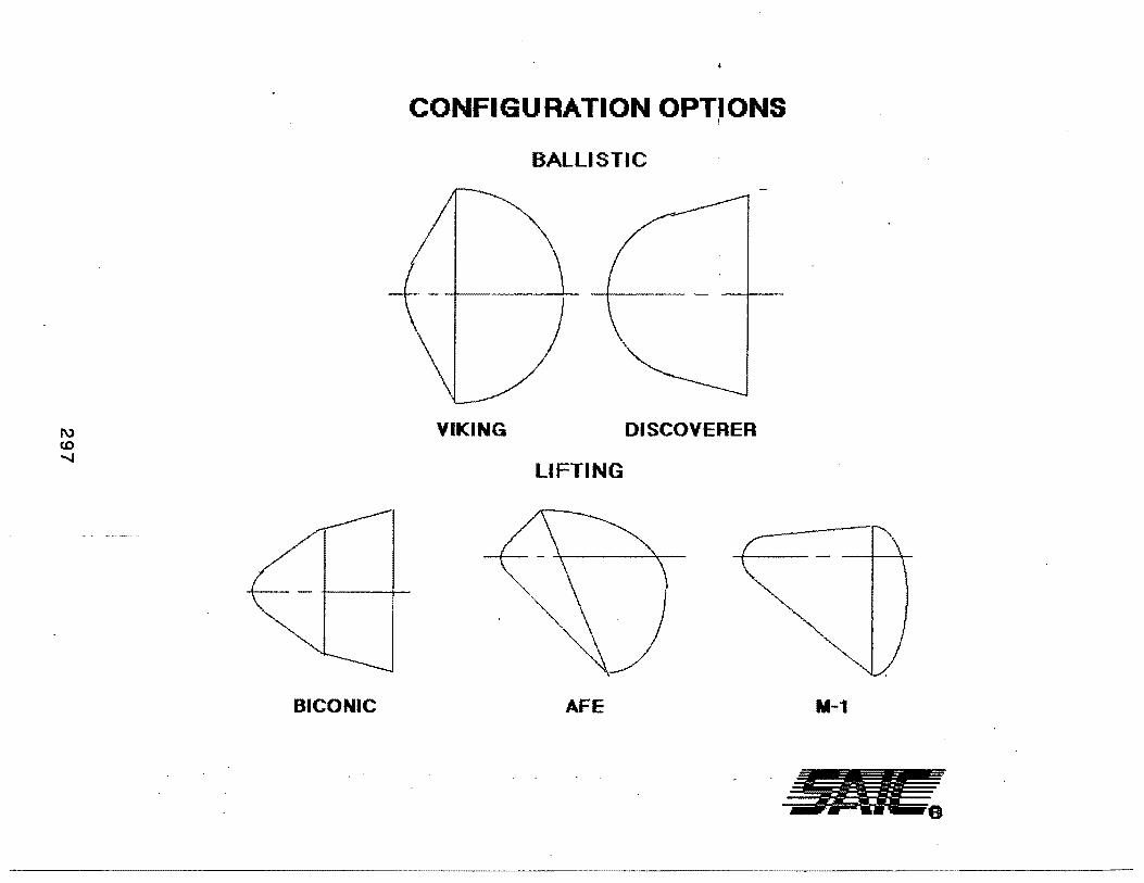
CONFIGURATION OPTIONS !
BALLISTIC
\
VIKING DISCOVERER
LIFTING
BICONIC AFE M-1
6

MARS PENETRATOR - EXTENDIBLE STRUT DECELERATOR
REFERENCE DRAWING SK 050978 (SHEET 2)
-~ DUAL LOCK PIN PLUNGERS
r RIB DEAD-CENTER I I POSITION
EXTENDABLE STRUT
DECELERATOR DEPLOYMENT INITIATOR SPRING
E~~==:=:=::::::=:=::=:=E=:~::~~~~~~~~~~~~~;;;~~~~m coMPRESSION
STA 0
Mars Penetrator - Extendible Strut Decelerator
CL
VEHICLE
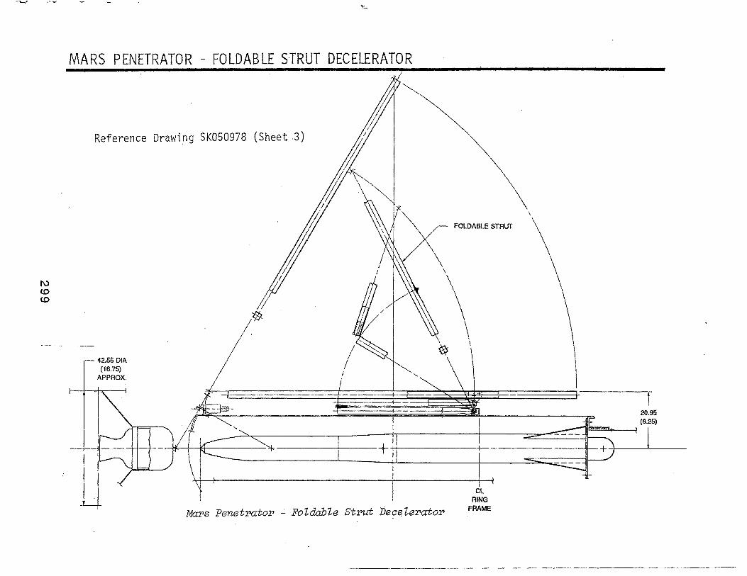
MARS PENETRATOR - FOLDABLE STRUT DECELERATOR
Reference Drawing SK050978 (Sheet .3)
- 42.55 DIA (16.75)
APPROX.
~ FotDABLESTRUT
\
~~~---------~--------4-----~~'-----------+-1
Mars Penetrator ~ FoZdabZe Strut Decelerator
CL RING
FRAME
\ \
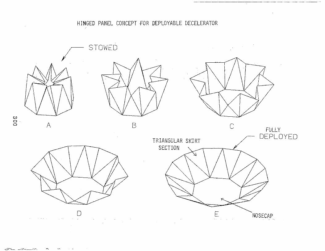
w 0· 0 A
HINGED PANEL CONCEPT FOR DEPLOYABLE DECELERATOR •'
r STOWED
B
TRIANGULAR SKIRT SECTION
0 E
c FuLLY DEPLOY 0

AEROSHELL JETTISON OPTIONS
• PULL OUT OF THE REAR. - REQUIRES lARGE PARACHUTE SYSTEM
• FALL-THRU THE NOSE - CONSTRAINS lANDER SHAPE - NOSE CAP JETTISON
• SEPARATE IN PIECES - HAZARDOUS - REQUIRES EXTENSIVE PYROTECHNICS AND VERY
ACCURATE TIMING
• RETAIN TO LANDING
- lANDING SYSTEM DESIGN IMPACT
w 0 1\)
TERMINAL DESCENT SYSTEM DESIGN.
REQUIREMENTS
• TO PROVIDE A STABLE & CONTROLLED PLATFORM FOR DESCENT IMAGERY
• ' ·,,. ' .-: .
TO PROVIDE STABLE & CONTROLLED SURFACE APPROACH CONDITIONS FOR LANDING
DESIGN CONSIDERATION'S &_ ISSU,ES . ' .
• DEPLOYMENT CONDITIONS
• TECHNOLOGY BASE
• DESCENT TIME~ RATE~·& ST ABili·TY FOR IMAGERY : . . .
• WINDS ALOFT & SHEARS
• ELEVATION DIFFERENCES OF SITES
• REQUIRED LANDING CONDITIONS ..
- VERTICAL & HORIZONTAL VELOCITY - STABILITY&DYNAMICS
• SURFACE WINDS & SHEARS
Session B, Submittal No. 10
Arden Albee California Institute of Technology
303

COMPARISON OF ALTERNATIVE LANDER STRATEGIES
ARDEN ALBEE
CAL TECH
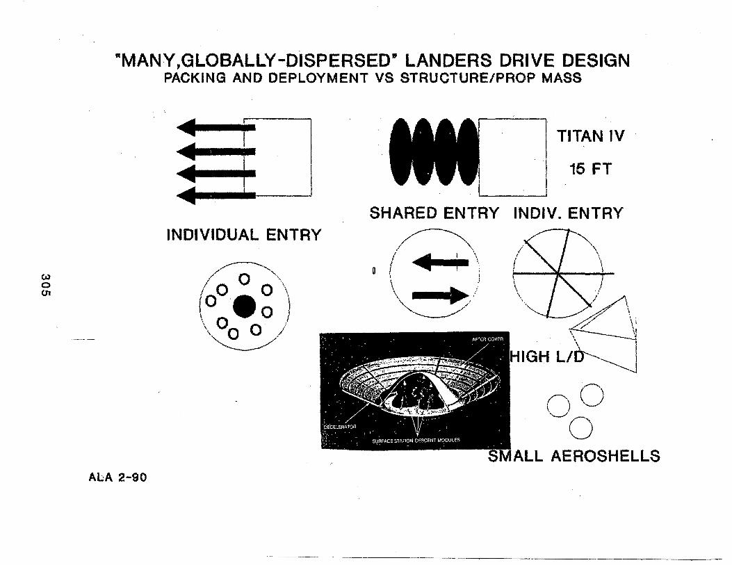
CAl 0 01
•MANY,GLOBALLY-DISPERSED" LANDERS DRIVE DESIGN PACKING AND DEPLOYMENT VS STRUCTURE/PROP MASS
i INDIVIDUAL ENTRY
ALA 2-90
TITAN IV ·
15FT
SHARED ENTRY INDIV. ENTRY
~,,
f/ IIIII I \
D - I ; I I I I
\ ~ .. '/ "'~/
·---._
r-, (_) \, )
~0
ALL AEROSHELLS
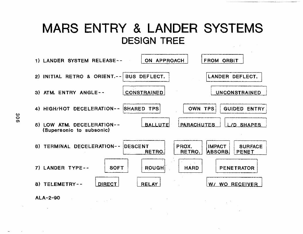
MARS ENTRY & LANDER SYSTEMS DESIGN TREE
1) LANDER SYSTEM RELEASE-- I ON APPROACH I I FROM ORBIT I
2) INITIAL RETRO & ORIENT.- -l BUS DEFLECT. I LANDER DEFLECT.
3) ATM. ENTRY ANGLE-- I CO~STRAINED I I UNCONSTRAINED ::I
4) HIGH/HOT DECELERATION-- !sHARl=D TPsl owN IPS jJ GUIDED ENTRY I
5) LOW ATM. DECELERATION-- I BALLUTEI I PARACHUTES II LIP SHAPES j (Supersonic to subsonic)
6) TERMINAL DECELERATION-- !DESCENT PROX. IMPACT SURFACE ' RETRO. RETRO. BSORB PENET
7) LANDER TYPE-- [;;] ~· I HARD I I I PENETRATOR
8) TELEMETRY-- I DIRE~T I RELAY I I W/ wo RECEIVER
ALA-2-90

MARS ENTRY & LANDER SYSTEMS DESIGN T·R·EE
1) LANDER SYSTEM RELEASE-- I ON APP~OACH I I FROM ORBIT VK M,A,VB
2) INITIAL RETRO & ORIENT.--! BUS DEFLECT. A, VB
3) ATM. ENTRY- ANGLE-- I CONSTRAINED I M,VK,A
4) HIGH/HOT DECELERATION-- !sHARED TPSI
5) LOW ATM. DECELERATION-(Supersonic to subsonic) I BALLuTel
M,A
l LANDER DEFLECT. M,.VK
, I UNCONSTRAINED VB
I OWN TPS I I GUIDED. ENTRY I ·M, VK, VB, A .
I PABACH UTES l I L/D _·SHAPES M, VK, VB
- - -ar-tEBMINAL DECELERATION-- DESCENT PROX. IMPACT SURFACE
7) LANDER TYPE--
8) TELEMETRY--
~----~R~E~T~R~O~. RETRO. BSORB PENET VK M VB A
c;;J G;J VB
I PENETRATOR I A
I DIRECT I I BELAY I M,VK,VB,A
I W/ wo RECEIVER' I, VK/M,A, VB
Key: M = Mars 3; VK = Viking; VB = Venera B; A = Ames n
,, ---~~--------------------------------
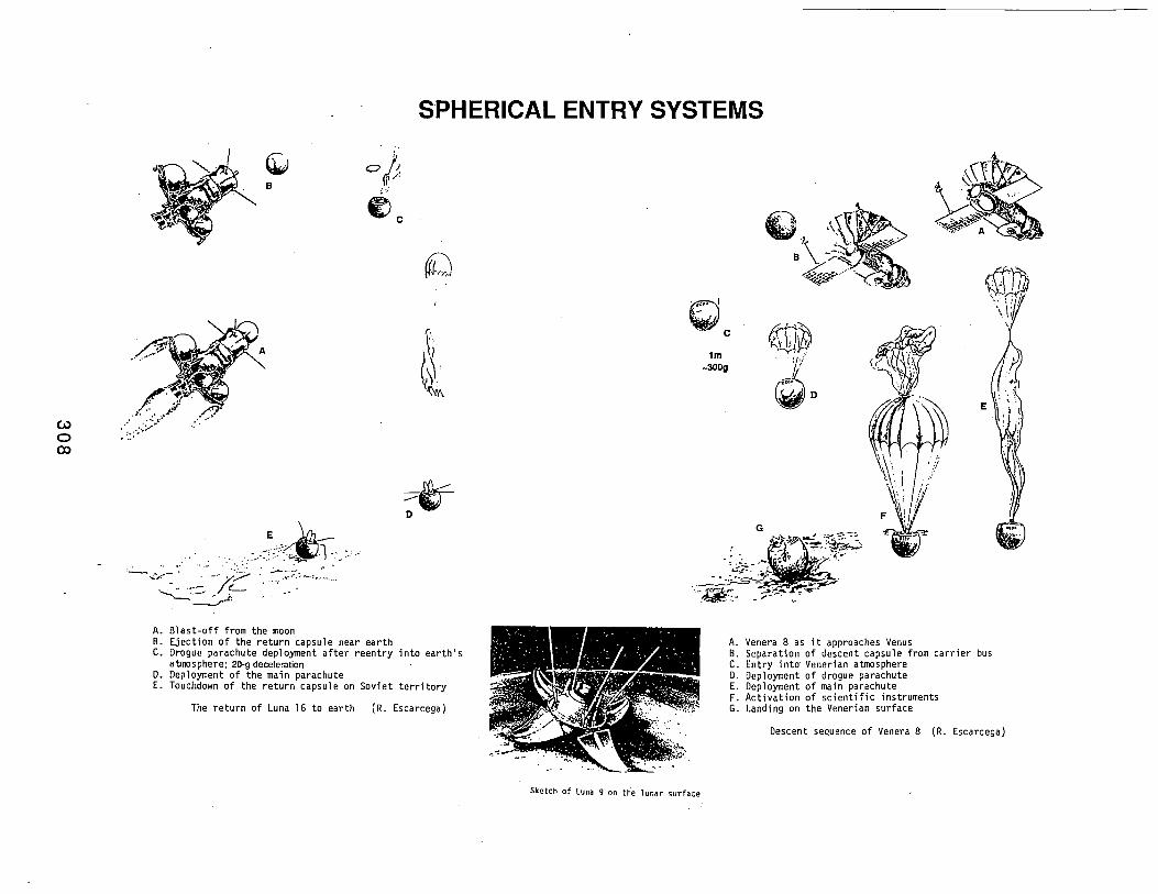
w 0 (X)
SPHERICAL ENTRY SYSTEMS
o/;: 11; B
.-0
-----_, .. · ........ : ..
A. Blast-off from the moon B. Ejection of the return capsule near earth C. Drogue parachute deployment after reentry into earth's
atmosphere; 20-g deceleration D. Deployment of the main parachute E. Touchdown of the return capsule on Soviet territory
The return of Luna 16 to earth (R. Escarcega)
~jjg \.:· : ith ',,
\\: 0 -- c
Sketch of luna 9 on th-e lunar surface
1m -300g
E
A. Venera 8 as it approaches Venus B. Separation of descent capsule from carrier bus C. Entry into· Venerian atmosphere D. Deployment of drogue parachute E. Deployment of main parachute F. Activation of scientific instruments G. Landing on the Venerian surface
Descent sequence of Venera 8 (R. Escarcega)
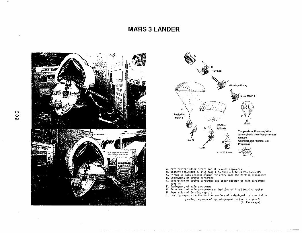
w 0 c.o
MARS 3 LANDER
Vj- 21>.7 m/s
Temperature, Pressure, Wind Atmospheric Mass Spectrometer camera Chemical and Physical Soli Properties .~
I ~}t:;~l -· ~·-.,··~ •i~iv~~
A. Mars orbiter after separation of descent apparatus B. Descent apparatus pulling away from Mars orbiter-41/2hrbeforeMOI C. Firing of main descent engine for entry into the Martian. atmosphere D. Deployment of drogue parachute E. Separation of drogue parachute and upper portion of main parachute
housing F. Deployment of main parachute . G. Detachment of main parachute and ignition of final braking rocket H. Separation of landing capsule !. Landing capsule on the l~artian surface with deployed instrumentation
Landing sequence of second-generation Mars spacecraft (R. Escarcega)
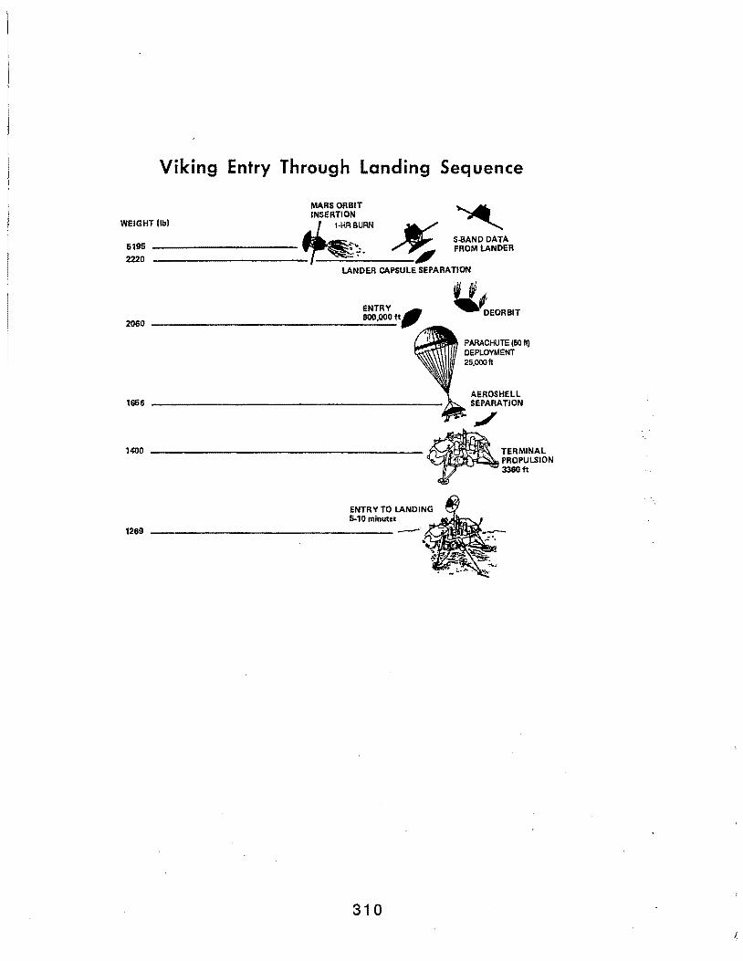
Viking Entry Through Landing Sequence
WEIGHT (lbl
MARSORBIT ~
INSERTION - "" 1-HR BURN ...., S.SAND DATA
5195 ---------- ~~- ~ FROMLANDER
2220 ----------- ""' LANDER CAPSULE SEPARATION
1~6 -------------------------------
ENTRY TO LANDING 5-10 minutes
1269 --------------------- -·
310
~· ~EORBIT
PARACHUTE (50 11) DEPLOYMENT 25,00011
AEROSHELL SEPARATION
./ TERMINAL PROPULSION 3360ft
I
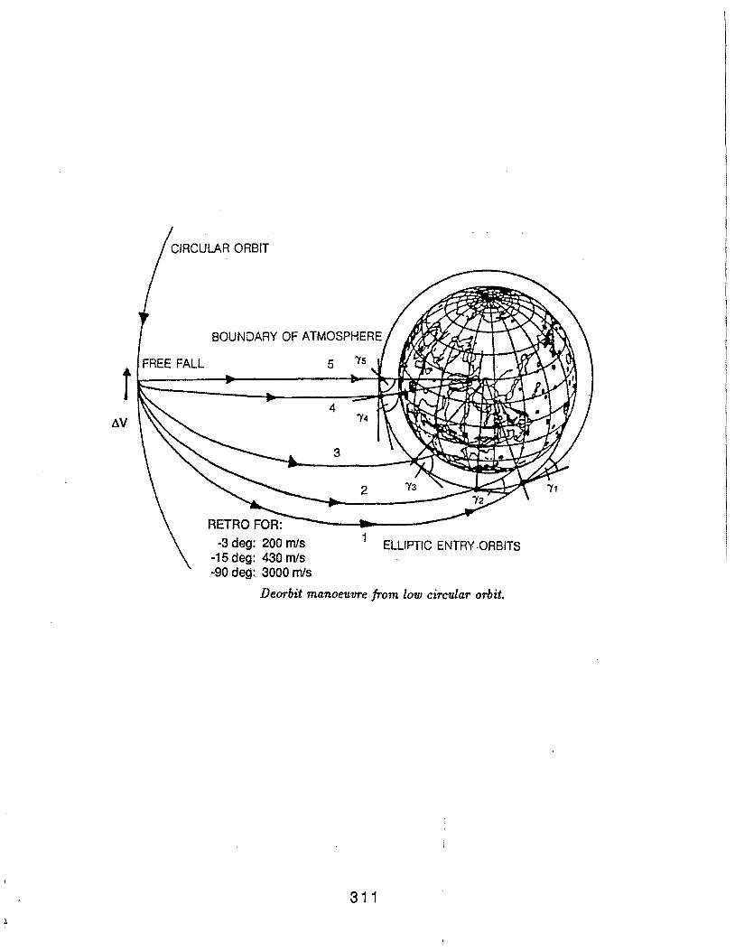
CIRCULAR ORBIT
BOUNDARY OF ATMOSPHERE
5
tN
-3 deg: 200 m/S ELLIPTIC ENTRY .ORBITS -15 deg: 430 m/s -90 deg: 3000 m/s
Deorbit manoeuvre from low circular orbit.
311
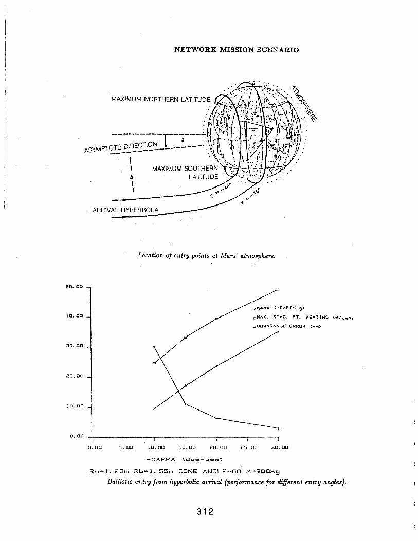
NETWORK MISSION SCENARIO
A
\ ARRIVAL HYPERBOLA
Location of entry points at Mars' atmosphere.
sa.oa
40.00 cHAX. STAG. PT. HEATING (W/c~2l
30.00
2a.oo
1 a. oa
a. oo s.oo 10.00 15.ao 20.00 25.00 30.00
0
Rn=l.2Sm Rb=l. SSm CONE ANGLE=BO M=300ks
Ballistic entry from hyperbolic arrival (performance for different entry angles).
312
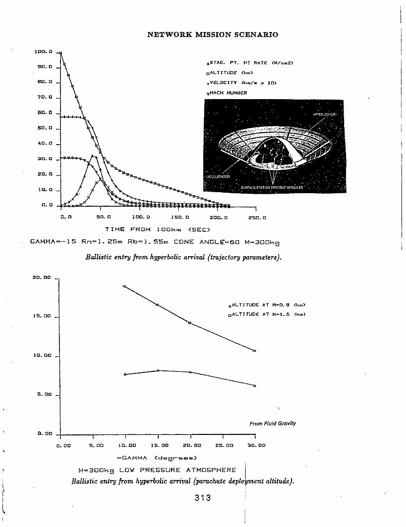
l
l
NETWORK MISSION SCENARIO
1 co. 0
90.0 ASTAC. PT. HT RATE CW/cmZ>
cALTlTUOE Ckm>
80.0 +VELOCITY Ckm/c ~ 10>
70.0 vHACH NUMBER
60.0
so.o
40.0
:ao.o
zo.o
10. []
0. 0
o.c so.o 100.0 lSO. 0 zoo.o 250.0
TIME FROM lOOkm <SEC)
GAMMA--15 Rn=l.25m Rb=l.SSm CONE ANGLE~60 M=300ks
Ballistic entry from hyperbolic arrival (trajectory parameters).
20.00
15.00
1 o. 00
s.oo
D. 00
o.oo s.ob 10.00 15. 00 20.00
4ALTITUOE AT M•O.B Ckm)
0 ALTJTUOE AT H-1.5 Ckm)
From Fluid Gravity
25.00 :ao.oo
-GAMMA (dQgrags) i
M=3ooks Low PREssuRE ATMosPHERE /
Ballistic entry from hyperbolic arrival (parachute deployment altitude).
313
Session B, Submittal No. 11
Lester L. Sackett The Charles Stark Draper Laboratory
315
\
GLOBAL NETWORK MISSION WORKSHOP
Achievable Accuracies for Targeting Landing Sites ·
Les Sackett (617 /258-2289) The Charles Stark Draper La~oratory
Cambridge, Massachusetts 02139
Workshop held at the Jet Propulsion Laboratory February 6-7, 1990
Data provided by John Higgins (617/2582433) Ken Spratlin (617/258-2441)
Global Netw9rk Workshop ,
Primary Question:
What are the desired and achievable accuracies for targeting the landing sites?
Subsidiary Questions:
What are the navigation (knowledge) uncenainties at the time of aeroshell firings?
What are the landing (guidance) dispersions of the penetrators?
What contribute.s to the errors in knowledge and targeting accuracy?
How can the errors be reduced?
For the approach targeted aeroshells, what are the errors as a function of the deployment
time?
Does onboard nav help and how much?
What is the dispersion due to passage of the aeroshell through the atmosphere?
Due to the time on the parachute?
Due to the error introduced by the small rocket firing?
Does Viking experience help in estimating the targeting accuracies?
What is the effect on the trajectory of the despin from 60 to 15 rpm following the targeting
firing?
What is the effect of changing the assumptions or parameter values (e.g., flight path angle.
ballistic coefficient, etc.)?
317
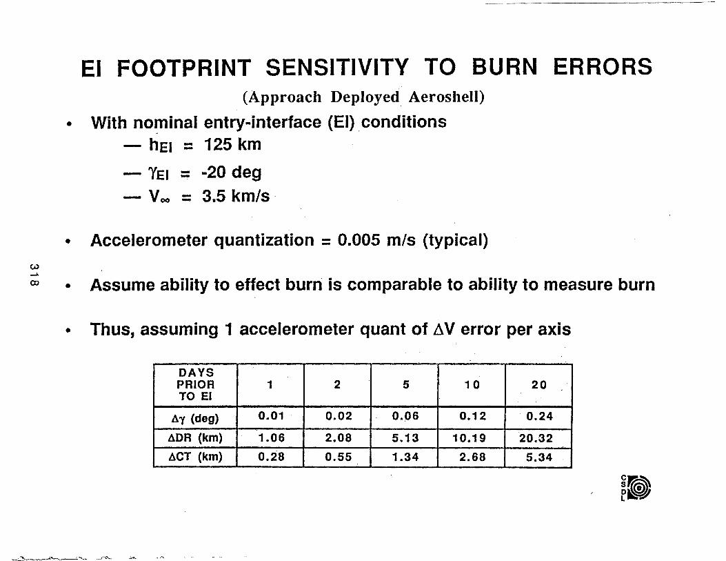
El FOOTPRINT SENSITIVITY TO BURN ERRORS (Approach Deployed_ Aeroshell)
• With nominal entry-interface (EI) .conditions - hEI = 125 km
- 'YEI = ·20 deg - Voo = 3.5 km/s ·
• Accelerometer quantization = 0.005 m/s (typical)
• Assume ability to effect burn is comparable to ability to measure burn
• Thus, assuming 1 accelerometer quant of AV error per axis
DAYS PRIOR 1 2 5 10 20 TO El
li:y (deg) 0.01 . 0.02 0.()6 0.12 0.24
~DR (km) 1.06 2.08 5.13 10.19 20.32
~CT (km) 0.28 0.55 1.34 2.68 5.34
MARS PENETRATOR VEHICLE
ENTRY DISPERSION ANALYSIS
John P. Higgins (617)-258-2433 c s
f
ASSUMPTIONS • PRE -DEORBIT TRAJECTORY
• SEMI-MAJOR AXIS = 6986 KM
• ECCENTRICITY = 0.485097
• ENTRY INTERFACE CONDITIONS
• ALTITUDE = 125K KM
• VELOCITY = 4.2 KM/S (DEORBIT PENETRATOR)
• VELOCITY = 6.0 KMIS (DEPLOYED PENETRATOR)
• GAMMA . ~ -15·/ -20 D"EGREES .
• BALLISTIC ENTRY (ZERO LIFT)
• PENETRATOR BALUSTIC coEFFICIENT = 3·o KG 1 sa METERs
• PARACHUTE BALLISTIC COEFFICIENT = 3 KG I SQ METERS
• DEPLOYED AT 10 KM ALTITUDE
• ATMOSPHERE MODEL - MARS NORTHERN MEAN
• GRAVITY MODEL - CONIC
ENTRY DISPERSION SOURCES
• · LIFT-TO-DRAG RATIO
• ATMOSPHERIC VARIATIONS .
• ENTRY INTERFACE FLIGHT PATH ANGLE
• DUE TO GN&C DEORBIT BURN PERFORMANCE (PRIMARILY NAVIGATION ERRORS)
• DOWNRANGE DISPERSION PRIMARILY DUE TO ENTRY PENETRATION POINT VARIATION
c.u 1\) 1\)
MARS ENTRY DISPERSION ANALYSIS DEORBIT PENETRATOR- El GAMMA= -20 deg
RANGE (KM) 360~----------------------------------~
67 = +0.2 deg
lll/D = +0.1
llp =-50%
llp = +100% llL/D = -0.1 .
300T-----------------------~----------~
67 = ...:.o.2 deg
280~.------~------------~--~----------J
...... ·
c.u .I\)
c.u
.MARS ENTRY DISPERSION ANALYSIS DEORBIT PENETRATOR- El GAMMA= -15 deg
RANGE (KM) 500~--------------------------------~
fl-y = +0.2 deg 480+-------~~----------------------~
flL/D = +0.1
fl-y = -0.2 deg 400~~------------------------~·----~
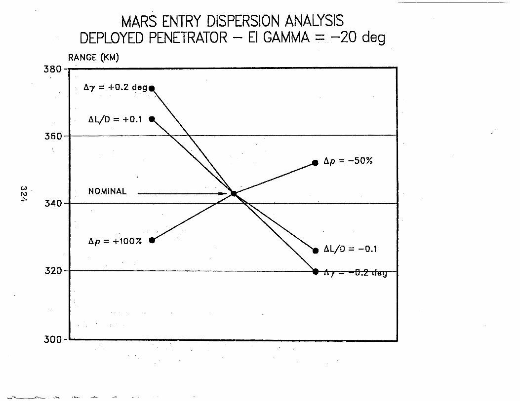
c..> 1\) .f:>.
MARS ENTRY DISPERSION ANALYSIS DEPLOYED PENETRATOR- El GAMMA= -20 deg
RANGE (KM) 380~--------------------------------~
.. fl7 = +0.2 deg ' . •'
lll/D = +0.1
360
llp =-50%
NOMINAL 340
..
llp = +100% AL/D = -0.1
300-.._ ________________ ---J
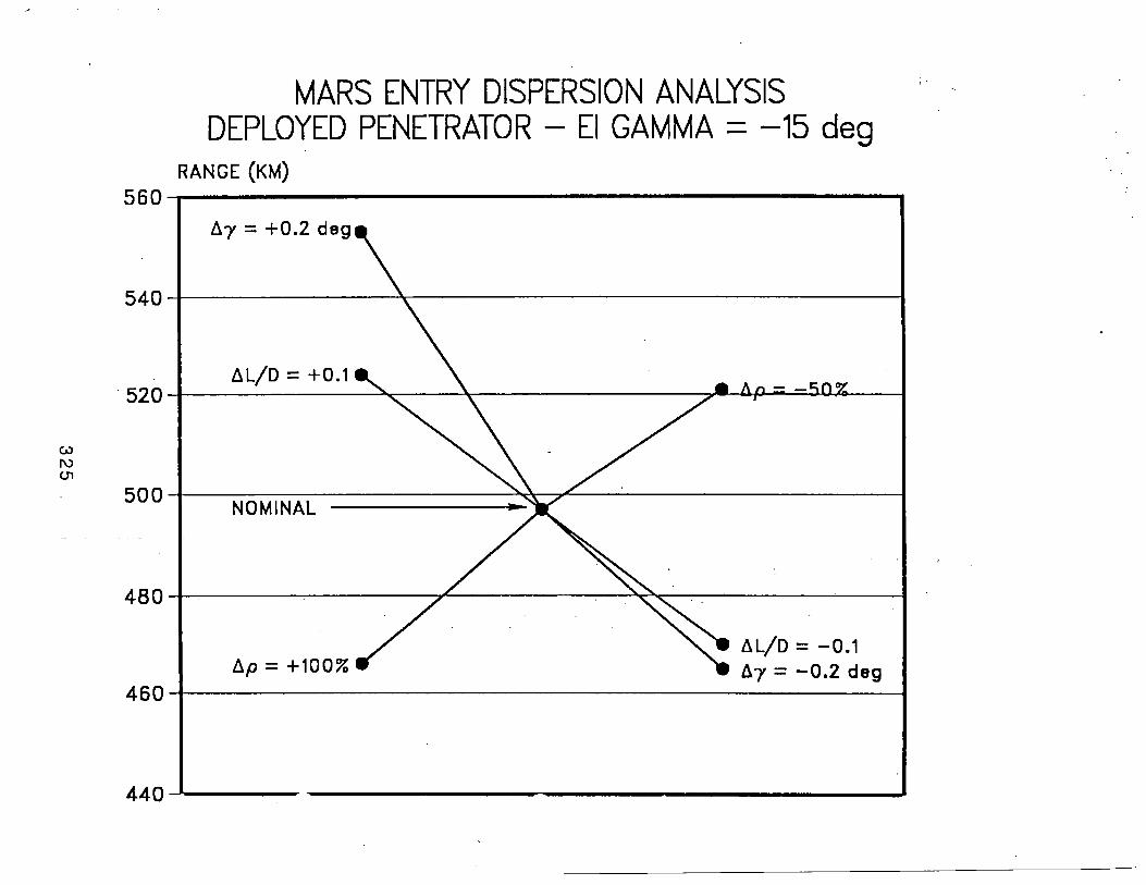
MARS ENTRY DISPERSION ANALYSIS DEPLOYED PENETRATOR- El GAMMA= -15 deg
RANGE (KM) 560~----------------------------------~
{).7 = +0.2 deg
540+---------~~----------------------~
{).p;::::; +100% {). L/D = - 0 . 1 {).7 = -0.2 deg
460+-----------------------------------~
440 _._ _____________________ __.
Following is a list of memos produced at the Draper Laboratory on guidance, navigation, and.control for the Mars Rover Sample Return Mission. Some of these may be relevant to the Global Network Mission studies.
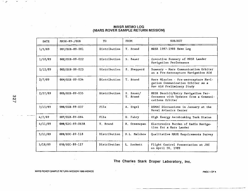
MRSR MEMO LOG (MARS ROVER SAMPLE RETURN MISSION)
DATE MRSR-89-/EGB TO FROM SUBJECT
1/3/89 001/EGB-89-001 Distribution T. Brand MRSR 1987-1988 Memo Log
l/18/89 002/EGB-89-022 Distribution s. Bauer Executive Summary of MRSR Lander Navigation Performance
1/12/89 003/EGB-89-023 Distribution s. Shepperd Summary. - Mars Communication Orbiter as a Pre-Aerocapture Navigation Aid
2/7/89 004/EGB-89-034 Distribution T. Brand Mars Mission - Pre-aerocapture Navi-gation Communication Orbiter as a Nav Aid Preliminary Study
2/27/89 005/EGB-89-035 Distribution s. Bauer/ MRSR Deorbit/Entry Navigation Per-T. Brand formance with Updates from a Communi-
cations Orbiter
3/15/89 006/EGB-89-037 File A. Engel DSMAC Discussions ih January at the Naval Avionics Center
4/7/89 007/EGB-89-084 File D. Fuhry High Energy Aerobraking Task Status
4/11/89 008/EJC- 89 -065R T. Brnnd R. Greenspan Electronics Burden of Radio Naviga-tion for a Mars Lander
5/ll/89 009/EGC- 89-118 Distribution H.L. Malchow Qualitative MRSR Requirements Survey
5/18/89 010/EGC-89-127 Distribution L. Sackett Flight Control Presentation at JSC on April 20, 1989
The Charles Stark Draper Laboratory, Inc.
MARS ROVER SAMPLE RETURN MISSION 1989 MEMOS PAGE 1 OF4
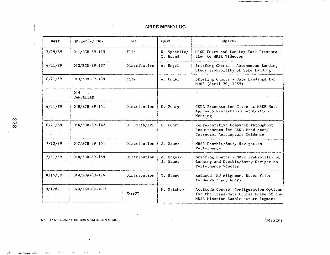
MRSR MEMO LOG
DATE MRSR-89-/EGB- TO FROM SUBJECT
5/19/89 011/EGB-89-115 File K. Spratlin/ MRSR Entry and Landing Task Presents.-T. Brand tion to MRSR Videocon
6/21/89 012/EGB -89-13 7 Distribution A. Engel Briefing Charts - Autonomous Landing Study Probability of Safe Landing
6/21/89 013/EGB-89-139 File A. Engel Briefing Charts - Safe Landings for MRSR (Apiil 20, 1989)
014 -yAN<:;ELLED
6/21/89 015/EGB-89-141 Distrlbution D. Fuhry CSDL Presentation Given at MRSR Mars Approach Naviga~ion Coordination Meeting
6/21/89 016/EGB-89-142 D. Smi.th/JPL D. Fuhry Representative Computer Throughput Requirements for CSDL Predictor/ Corrector Aerocapture Guidance
7/12/89 017/EGB- 89-151 Distrlbution s. Bauer MRSR Deorbit/Entry Navigation Performance
7/31/89 018/EGB-89-169 Distrlbution A. Engel/ Brie.fing Charts - MRSR Probability of s. Bauer Landing and Deorbit/Entry Navigation
Performance Studies
8/14/89 019/EGB~ 89-174 Distribution T. Brand Reduced IMU Alignment Error Prior to Deorbit and Entry
9/1/89 020/EcJC-89-.,_,, H. Malchow Attitude Control Configuration Options r:>·~r. for the Trans Mars Cruise Phase of the
MRSR Misssion Sample Return Segment
MARS ROVER SAMPLE RETURN MISSION 1989 MEMOS PAGE 2 OF 4
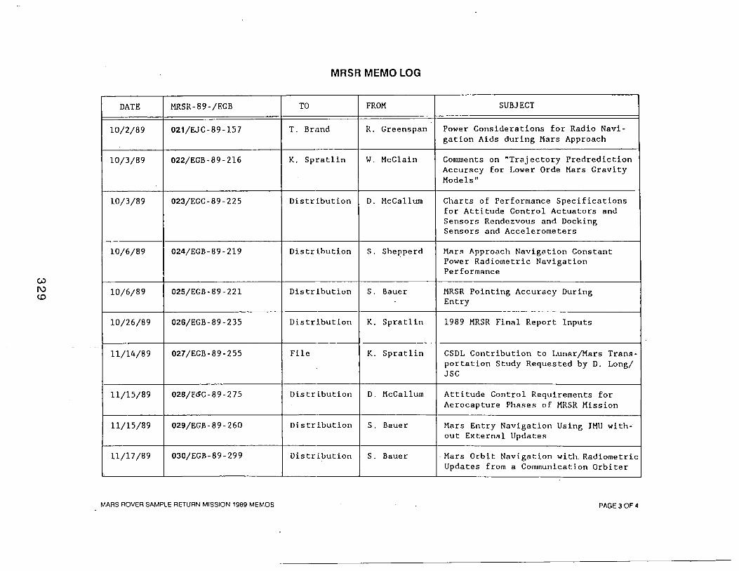
c.u 1\)
<.0
DATE MRSR-89-/EGB
10/2/89 021/EJC- 89-15 7
10/3/89 022/EGB-89-216
10/3/89 023/EGC-89-225
10/6/89 024/EGB-89-219
10/6/89 025/EGB-89-221
10/26/89 026/EGB-89-235
--
11/14/89 027/EGB-89-255
11/15/89 028/E<5C-89-275
11/15/89 029/EGB-89-260
11/17/89 030/EGB-89-299
MARS ROVER SAMPLE RETURN MISSION 1989 MEMOS
MRSR MEMO LOG
TO FROM
T. Brand R. Greenspan
K. Spratlin w. McClain
Distribution D. McCallum
Distribution S. She!Jperd
Distribution s. Bauer
Distribution K. Spratlin
File K. Spratlin
Distrlbution D. McCallum
Distrlbution s. Bauer
Distribution s. Bauer
SUBJECT
Power Considerations for Radio Navi-gation Aids during Mars Approach
Comments on "Trajectory Predrediction Accuracy for Lower Orde Mars Gravity Models"
Charts of Performance Specifications for Attitude Control Actuators and Sensors Rendezvous and Docking Sensors and Accelerometers
Mars Approach Navigation Constant Power Radiometric Navigation Performance
MRSR Pointing Accuracy During Entry
1989 MRSR Final Report Inputs
CSDL Contribution to Lunar/Mars Trans-portation Study Requested by D. Long/ JSC
Attitude Control Requirements for Aerocapture Phases of MRSR Mission
Mars Entry Navigation Using IMU with-out External Updates
·Mars Orbit Navigation with_ Radiometric Updates from a Communication Orbiter
PAGE 3 OF 4
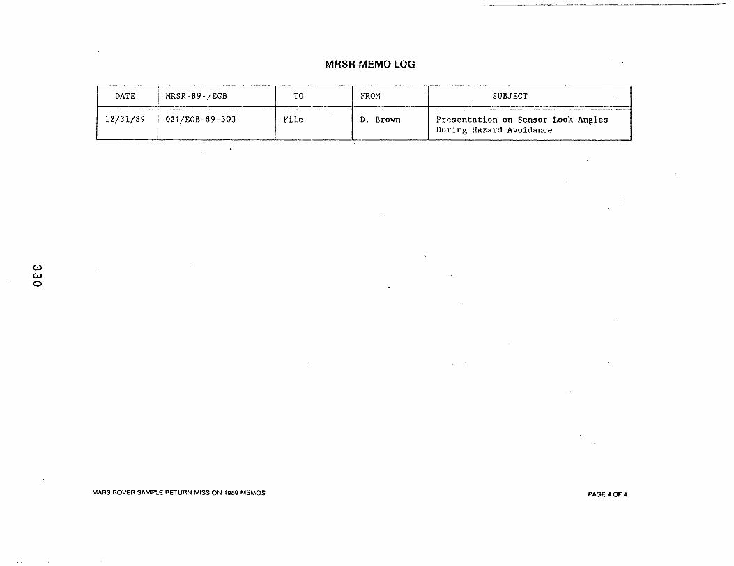
w w 0
DATE MRSR-89-/EGB
12/31/89 031/EGB-89-303
MARS ROVER SAMPLE RETURN MISSION 1989 MEMOS
TO
File
MRSR MEMO LOG
FROM SUBJECT
D. Brown Presentation on Sensor Look Angles During Hazard Avoidance
PAGE 4 OF 4
Session B, Submittal No. 12
Bruce A. Crandall Hughes Aircraft Company
331

LAUNCH VEHICLE ALTERNATIVE STRATEGIES
BRUCE CRANDALL
HUGHES AIRCRAFT CO.
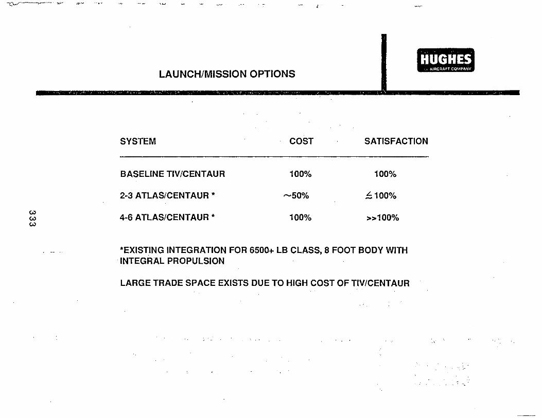
. .. ~ . . . .
HUGHES LAUNCH/MISSION OPTIONS
, AIRCRAFT COMPANY
SYSTEM COST SATISFACTION
BASELINE TIV/CENTAUR 100o/o 100%
2*3 ATLAS/CENTAUR * -50% ~100%
4-6 ATLAS/CENTAUR * 100% >>100%
*EXISTING INTEGRATION FOR 6500+ LB CLASS, 8 FOOT BODY WITH ·INTEGRAL PROPULSION
LARGE TRADE SPACE EXISTS DUE TO HIGH COST OF TIV/CENTAUR
··. :,..
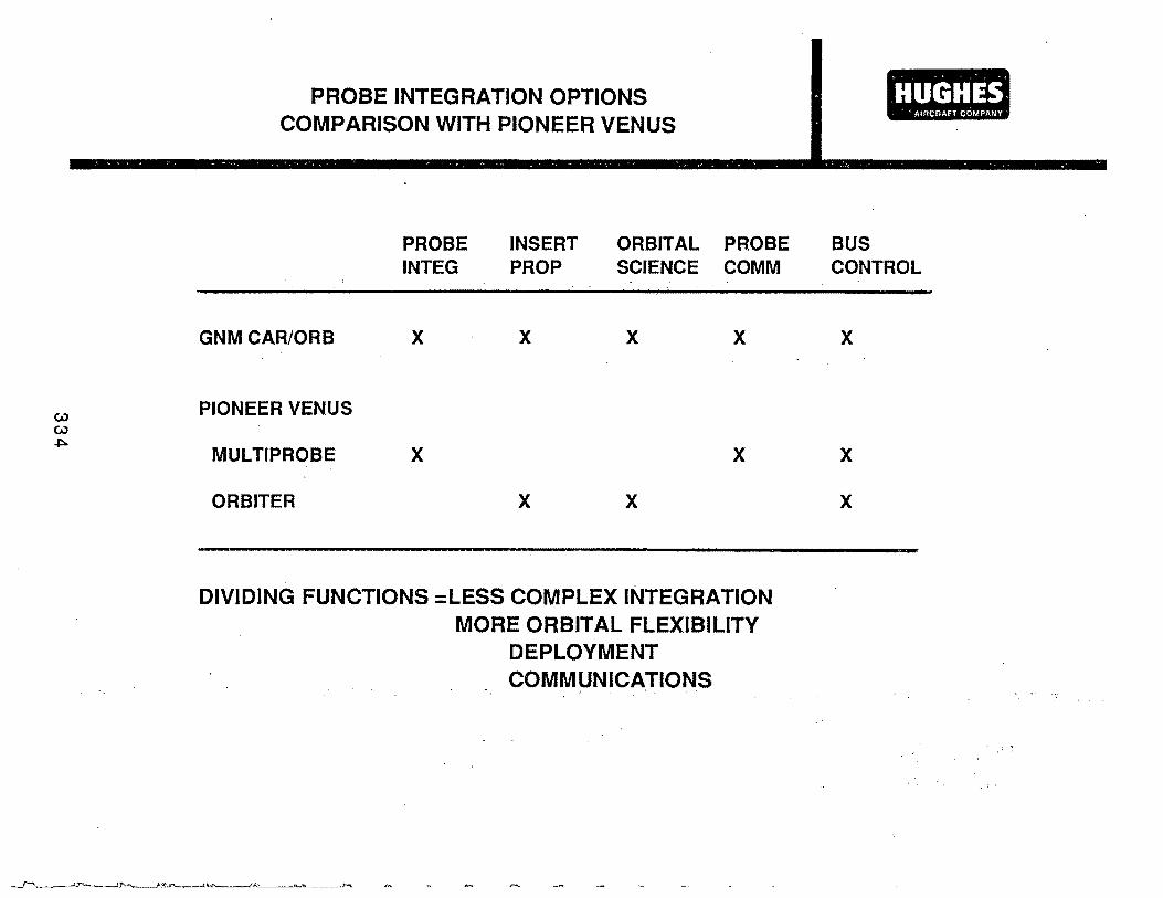
PROBE INTEGRATION OPTIONS COMPARISON WITH PIONEER VENUS
PROBE INSERT ORBITAL PROBE BUS
.H.UGH.ES. . AIRCRAFT COMPAI\IY
INTEG PROP SCIENCE COMM CONTROL
GNM CAR/ORB X X X X
PIONEER VENUS
MULTIPROBE X X
ORBITER X X
DIVIDING FUNCTIONS :LESS COMPLEX INTEGRATION MORE ORBITAL FLEXIBILITY
DEPLOYMENT COMMUNICATIONS
X
X
X
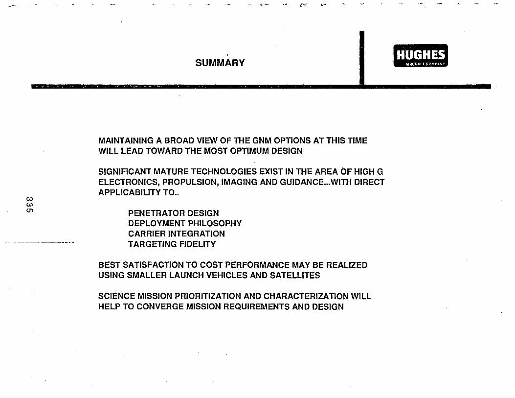
SUMMARY
MAINTAINING A BROAD VIEW OF THE GNM OPTIONS AT THIS TIME WILL LEAD TOWARD THE MOST OPTIMUM DESIGN
SIGNIFICANT MATURE TECHNOLOGIES EXIST IN THE AREA OF HIGH G ELECTRONICS, PROPULSION, IMAGING AND GUIDANCE ..• WITH DIRECT APPLICABILITY TO ..
PENETRATOR DESIGN DEPLOYMENT PHILOSOPHY CARRIER INTEGRATION TARGETING FIDELITY
BEST SATISFACTION TO COST PERFORMANCE MAY BE REALIZED USING SMALLER LAUNCH VEHICLES AND SATELLITES
SCIENCE MISSION PRIORITIZATION AND CHARACTERIZATION WILL HELP TO CONVERGE MISSION REQUIREMENTS AND DESIGN
' . HUGHES
AIRCRAFT COMPANY

·-~
~-
,··
·,;
~ .· ;
-~:-
.··:\
;•
' ' '
' . - ' ~
-,.
... -.. ,.,
_;
-~
--~
~' '.
Session B, Submittal No. 13
Carlos S. Moreno Jet Propulsion Laboratory/California Institute of Technology
337
HARD LANDER CONCEPTUAL DESIGN
CARLOS MORENO
JPL
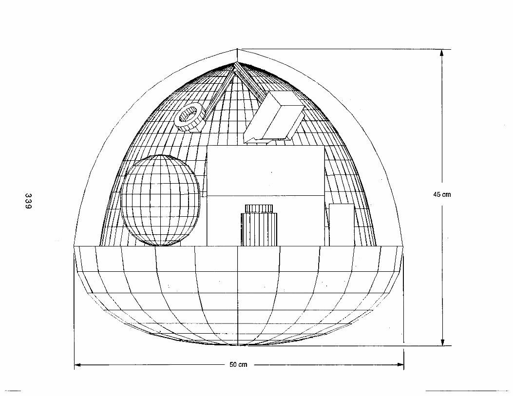
45cm
lliiiilllll
50 em
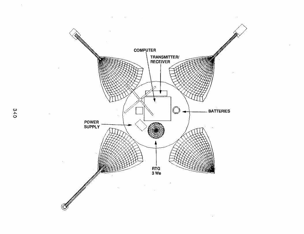
RTG 3We
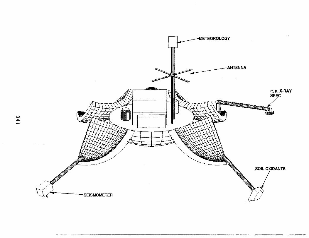
METEOROLOGY
a, p, X-RAY
SEISMOMETER
-- -~-------------------------------------------

An automated biological laboratory was developed by Philco Aeronutronic Company to study the possibility of a hard-landing entry probe to make simple assays of the Martian environment. One of several studies for Voyager · in the mid-1960s, it grouped science instruments that could be programmed for numerous experiments. None of the projects was flown, but they provided understanding of extraterrestrial biology detectors.
. , • ... " ,.. .. . _ ..
Session B, Submittal No. 14
John Garvey McDonnell Douglas
345
DELTA LAUNCH VEHICLE STRATEGIES
JOHN GARVEY
MDAC
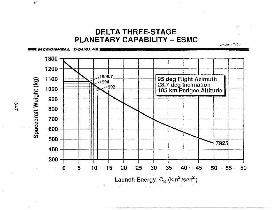
(A)
..J::>.. ""-J
Ill.
DELTA THREE-STAGE PLANETARY CAPABILITY- ESMC
VJX098.1 T1 CV
!!!!! MCDONNELL DOUGLAS !!!!!!!!!!!!!!!!!!!!!!!!!!!!!!!!!!!!!!!!!!!!!!!!!!!!!!!!!!!!!!!!!!!!!!!!!!!!!!!!!!!!!!!!!!!!!!!!!!!!!!!!!!!!!!!!!!!!!!!!!!!!!!!!!!!!!!!!!!!!!!!!!!!!
1300
1200
- 1100 C> ~ ..........
1000 ..... .c:. C>
900 ·-CD :: 800 ..... .... ca ... 700 (.) CD (.)
600 ca c. en 500
' ~ ' ..... 1996/7 95 deg Flight Azimuth , ...... 1994
" .,..1992 28.7 deg Inclination , . 185 km Perigee Altitude
' " ~ ........_
"' ~ " ~ ~ ..
............... 7925 400
300 0 5 1 0 15 . 20 25 30 35 40 . . 45 50 55 . 60
Launch Energy, C3 (km2 /sec2)

MSP SPACECRAFT BASED ON PIONEER-VEN·US BUS
VJX144 T2CA
!!!!!! MCDONNELL D 0 U G LAS !!!!!!!!!!!!!!!!!!!!!!!!!!!!!!!!!!!!!!!!!!!!!!!!!!!!!!!!!!!!!!!!!!!!!!!!!!!!!!!!!!!!!!!!!!!!!!!!!!!!!!!!!!!!!!!!!!!!!!!!!!!!!!!!!!!!!!!!!!!!!!!!!!!!!!!!!!!!!!!!!!!!!J!\!!!! Sleeve ------ Widebeam Omni Antenna 'Qipdle · ..._~~--- UHF Antenna (New)
Antenna ------.
Penetrator Assembly (TOW)~
Secondary Structure
(New) ----ii--1'1-
, _____ S-Band High-Gain
Antenna
-~,...,.....::---- BAPTA '">---- BAPTA
Support
Solar Panel Cylinder
, ___ Equipment Shell
With Penetrator Cutouts
n Orbit Insertion M.?tor
/'S{j""?--~ Aft Thermal L.. '-.:_) ...l. · Barrier (lntelsat IV
~ -y) Telesat) ..___
Session B, Submittal No. 15
Stephen Bailey Johnson Space Center
349
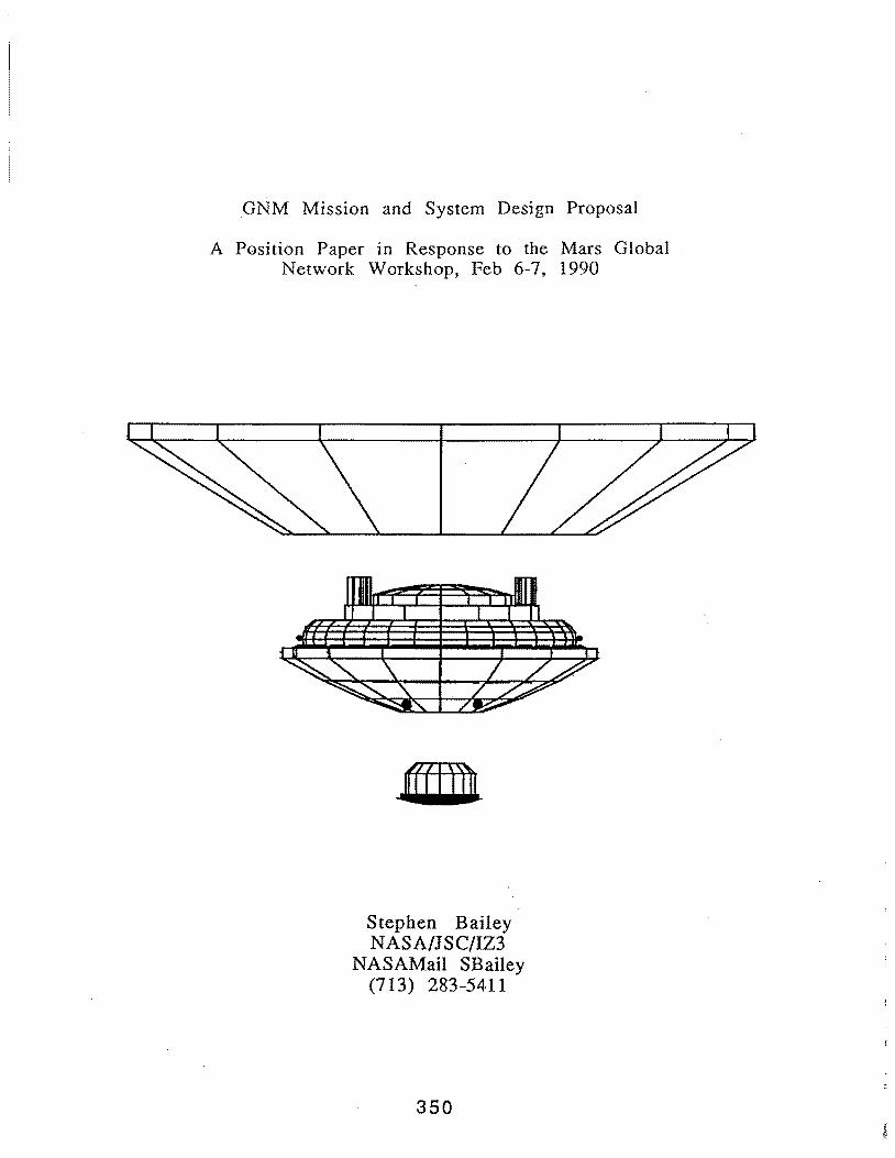
GNM Mission and System Design Proposal
A Position Paper in Response to the Mars Global Network Workshop, Feb 6-7, 1990
Stephen Bailey NASA/JSC/IZ3
NASAMail SBailey (713) 283-5411
350
A GNM Mission and System Design Proposal
A Position Paper in Response to the Session B of the Mars Global Network Workshop, Feb 6-7, 1990
Introduction
After having attended the Mars Global Network Mission (GNM) Workshop, and upon some reflection, I have put together a mission and system design option for the GNM which I believe is complementary to the 2001 Sample Return Mission (SRM). In this paper I take an advocacy position for the proposed mission; it is not intended to be an objective review, although both pros and cons are presented in summary. This work represents my own opinions and judgements, and is not an SRM policy statement, nor is it supported by any systematic analysis. These ideas are an expansion and elaboration of the design proposed by AI Friedlander of SAIC in the Session B discussion of the GNM workshop.
In arriving at the proposed design I used the following criteria, in order of priority, for evaluation:
1) Maximize Science Value 2) Keep Costs Low 3) Maximize Heritage (both from previous missions and heritage to be
provided to future exploration missions, particularly the SRM) 4) Design to fly in the earliest possible opportunity 5) Make it ''Innovative"
The Elements of the proposed mission are:
I) Aeroshelled Landers 2) Communication Orbiter(s)
Mission Scenario
The mission consists of launches from earth in the '96, '98, and '01 opportunities on 'Delta-class launch vehicles ( -1000 Kg injected to Mars in 8 to lO ft diameter shroud). The trans Mars boost stage injects a stack of small independent, aeroshelled spacecraft. The stack separates from the boost stage and each rigid (as opposed to deployable) aeroshell. flies to Mars on its own, performing midcourse maneuvers as necessary. On-board GN&C systems provide precision pointing (via torque wheels) and bum execution. Each spacecraft flies a unique trajectory which is targeted to achieve approach atmospheric interface at the desired latitude and lighting conditions; arrival . times may vary by a month or more. A direct entry is performed, there is no propulsive orbit capture. The aeroshelled rough-landers are targeted to achieve a desired attitude and entry flight path angle, and then follow a passive· ballistic trajectory until terminal descent. Based on sensed acceleration (integrated to deduce altitude), the aft ,aeroshell skirt is jettisoned, a short time later a supersonic parachute is deploye~. The ballistic coefficient
GNM Mission and System Design Proposal Feb 16, 1990
351
of the parachute is sized to achieve terminal velocity at about 8 Km. However the parachute is not deployed until a few Km above the surface to minimize wind-induced drift. This relatively short period on the parachute is possible because of the low ballistic coefficient of the aeroshell, and allows surface sites up to 6 Km above the mean surface level to be visited. The nose cap (weighted by the no longer required torque wheel assembly) is jettisoned and descent imaging begins, a laser altimeter also measures true altitude. (Depending on what altitude descent imaging is first required, the nose cap may be jettisoned prior to the aeroshell skirt jettison.) Based on range and range rate to the surface, the parachute is jettisoned and the lander uses descent engines to achieve touchdown velocity. (Note: if the ballistic coefficient of the aeroshell is sufficiently low, a parachute is not required, the ballistic terminal velocity provided by the aeroshell would be low enough that a propulsive descent could be performed directly). A contact sensor shuts down the motors to avoid cratering, and the lander rough-lands at less than 5 m/sec. The remaining aeroshell and a deployable bladder attenuate landing loads and minimize the possibility of tip over. Science instruments are deployed and activated, and the network is established.
See the appendix of figures which illustrate the mission and spacecraft designs.
Shared Communications Infrastructure
In this scenario, th.e communications relay orbiter(s) are provided as infrastructure for both the GNM and the SRM. In the reference GNM and SRM scenarios, each mission provides its own communications system. These systems are a part of the carriers which are captured into deployment and (in the case of the SRM) retrieval orbits; these orbits are not the preferred ones from a communications standpoint, and may in fact be far from optimum. Because of the successive nature of these missions, commonality between the communications system requirements should be explored. Because of the stated commitment to planetary exploration, consideration should include the use of this system to backup or augment future, higher capability Mars communications systems.
Deployment from the Trans Mars Boost Stage Contrasted to the Reference GNM Mission Scenario
Another key feature of this design · proposal is the lack of a centralized carrier vehicle which propulsively captures into Mars orbit and performs deployment of landers from thai· orbit.' In the proposed approach, the aeroshells are separated for the boost structure via a simple sequencer. They then become independent spacecraft, each targeted and track_ed on a unique trajectory.
In contrast, the reference GNM mission designs involve a combination of deployment from orbit and deployment on approach.
Although an orbit design exists which satisfies lighting conditions· over a wide range of latitudes,. including polar (re. "A Polar Orbit Mission for the Mars Global Network Mission", Philip Knocke, JPL), it comes at some expense. The 1/5 sol polar orbit requires a higher capture Delta-V than a more elliptic orbit.
GNM Mission and System Design Proposal Feb 16, 1990
352
A 160 day wait (for the 1998 launch opportunity) is also required to achieve the correct orbital conditions before entry vehicle deployment may begin. The opportunity available then sweeps from the south pole to the north over a 180 day period - thus to get full latitude coverage and emplace the full network would take almost a year from the time of arrival at Mars. ·
The carrier deployment strategies discussed in the workshop considered the deployment of aeroshells with no active GN&C system. In this scenario, the · carrier would provide pre-deployment pointing and would deploy the aeroshell in such a way that tip off rates were negligible; the aeroshell would then simply execute a fixed delta-V bum. This "point-and-shoot" strategy for aeroshell deployment on approach variety has the virtue of simplicity, but at the expense of landing accuracy (especially for low entry flight path angles). Of course this accuracy can be improved by putting a GN&C system on the aeroshell. Also execution accuracy for approach can be improved· by a combination of steep entry flight path angle and simply delaying approach deployment until the last "minute" (2 days outs, 1 day out, hours ... ?). Waiting however, incurs .a Delta-V penalty. ·
The design choice of putting an on-board GN&C system then leads . one to the scenario proposed here. That is to deploy aeroshells on approach, but that deployment may begin immediately after the Trans Mars Injection (TMI) bum. In this way the aeroshells are independently guided to entry interface from post TMI separation from the boost stage. Since the aeroshells all perfonn direct entry they are all of the same design (ie. there are no disparities between having to design both orbital deployed and approach deployed aeroshells).
GNM Mission and System Design Proposal Feb 16, 1990
353
The Development of a Spacecraft Bus
Whether or not an· existing bus such as the Mars Observer bus can be used, there is significant development, integration, testing and certification to go through prior to launch. A closer look is warranted to compare the costs of developing a large central bus with separate aeroshells as contrasted to developing a simple aeroshell deployment mechanism and many small, independent spacecraft. The development of many sm.aller and simpler appears to have great potential to lower the overall costs of the GNM mission, and may help moderate costs for the following sample return mission by providing valuable infrastucture and heritage for the SRM program.
This leverage would be provided by the design of a single small aeroshelled lander which could have broader application than the currently proposed penetrator concept. Once a kick stage has provided the necessary trans-Mars Delta-V, only attitude maintenance and periodic midcourse corrections up to the point of entry interface are required for the proposed spacecraft. The GN&C heritage to solving this problem is vast, and an off-the-shelf solution requiring little more than integration is possible, given the current trend towards miniature sa~ellites. A spacecraft required to do orbital insertion and orbital deployment is in my opinion an unnecessary complication. Each aeroshell would simply maintain course and attitude until entry interface, and from there follow a passive ballistic trajectory (no aeromaneuvering) up to terminal descent.
Mission Strategy
There is a possibility that a vigorous, aggressive development schedule could produce a '96 launch. This is possible because of the strong heritage that exists from previous and current engineering and development efforts. In any case, the science objectives and program enhancing opportunities available from this proposal argue for launch in multiple opportunities. For instance, if the scheduled launch dates were in successive years (say '96, '98, and '01), a unique strategy for mission reliability exists. If a first attempt at an attractive site fails, PLAN on trying again later instead of sacrificing global placement for a strategy of sending two landers to every site in order to achieve redundancy. Or, if every thing works on the first try and the network is satisfactorily established - stop, you're finished, no extra launch or set of launches is required.
GNM Mission and System Design Proposal Feb 16, 1990
354
The Advantage of Small.er Independent Spacecraft
The idea of simple independent carriers has a number of other advantages:
l) It allows smaller, simpler launch vehicles like the Delta or Atlas to be used (while still allowing the launch of a GREATER number of landers from a Titan IV than currently planned), whiCh translates both into costs savings for the agency and much greater launch flexibility.
· 2) The mission is adaptable at modest cost. The global network can be sustained, added to, or evolved incrementally as questions arise, objectives evolve, and instrumentation improves.
3) The payload bay is reconfigurable (more so as compared to a penetrator fore/aft body design). The science equipment bay on the proposed lander is reconfigurable to accommodate 20 Kg of science instruments specific to latitudes or science objectives.
4) The design is reusable and provides heritage to the SRM. There may be tremendous design leverage to be found in the SRM if the sites selected for the SRM can be visited by simple landers (either carried piggy back and deployed on approach or launched separately), that provide exact terrain knowledge at the site and establish navigation aids that lead the lander to a landing area verified to be safe per lander design. Using GNM heritage, this could be done at a fraction of the cost of a comparable imaging orbiter mission. The Human Exploration Vehicles could use these "throwaway" landers in a similar fashion, and to conduct specific surface experiments related to site selection.
5) The design may be suitable for micro-rover ("Ant") deployment.
6) The aeroshells may be placed with relatively high accuracy by employing radiometric approach navigation via the communications orbiter(s). This would provide a flight demonstration for this navigation technique for the SRM while enhancing the GNM. · A high factor of safety for the GNM is retained since earth based navigation would probably be the primary method.
7) Engineering heritage for future possible mtsstons. A modified aeroshell bus (without the aeroshell skirt) could be used as a flying testbed for various LID configurations by modifying the aft aeroshell skirt. The testbed could be used to evaluate various GN&C algorithms and would as a bonus extend our operational understanding of the variabilities of the Martian atmosphere. This kind of testbed may the the most cost effective method of getting operational aerocapture experience at Mars. The aeroshell bus will also fit inside very small launchers such as the Orbital Sciences Pegasus or Taurus, or the General Dynamics Atlas-E. A deployable aeroshell skirt could be developed (which could have a much lower achievable ballistic coefficient), with a modified bus used in flight test and operations. This has the additional advantage of sending. a large number of probes through the martian atmosphere thus building the engineering knowledge database of Mars atmospheric flight prior to launch of a Human exploration mission.
GNM Mission and System Design Proposal Feb 16, 1990
355

Technology
I believe this proposal can be accomplished with minimal technology risk. This may not qualify it as "technologically innovative", but I see no need to invent technology where it obstructs timely, cost effective execution of the miSSIOn. The possibility of pressing for a '96 launch should be investigated. However, for serious consideration of a '96 launch, funding for · concept studies needs to be provided now.
For the mission proposed here, the program risk that I believe exists for early launch of high G designs is mitigated. This is a simple mission, with a single simple spacecraft to design (excluding the comm orbiter which has even greater heritage working for it). I am sure that no show stoppers exist for penetrators, but there seem to be significant development costs and schedule risks associated with them. The fact is that none of the instruments, with rare exception, have been developed and tested for the very high G environments, and I am not aware that INTEGRATION of this number and variety of high G instruments has ever before been attempted (CRAF penetrator is the nearest data point that I am aware of, but the G loads there are considerably lower than those considered for the Mars penetrators, especially the aft body G loads). The combination of designing for the intense thermal flux, radiation, and G load environments, have probably not been predominate considerations for the majority of past high G development programs.
In this proposal, the strategy was to provide a relatively generous 20 Kg science payload capability with an ample 10 watt constant power supply augmented with rechargeable batteries. Several types of science payloads can be envisioned, each tailored of objectives which vary with latitude and the required number of a particular experiment type. As far as satisfying the requirements ·which lead to penetrator designs (subsurface sampling, placement of seismic geophones) a number of proposals emerged in the · Session B workshop for satisfying these requirements. For instance a flexible, cable driven drill for acquiring subsurface regolith samples to a depth of up to 3 meters should be quite possible to incorporate into one such payldad type. Geophones may be placed away from the lander on teathers to reduce· the chance of interference, or they may be driven into the surface with a pyrotechnic device. I believe that the consensus at the meeting was clearly that engineering solutjons could be found to satisfy science objectives, whether the surface device was a soft, rough, or hard lander. For the proposed rough lander design, risk and cost· are mitigated by the using current expertise in developing, integrating, and testing moderate G instruments (lO's of G's instead of lOO's or 1000's). .
GNM Mission and System Design Proposal Feb 16, 1990
356'
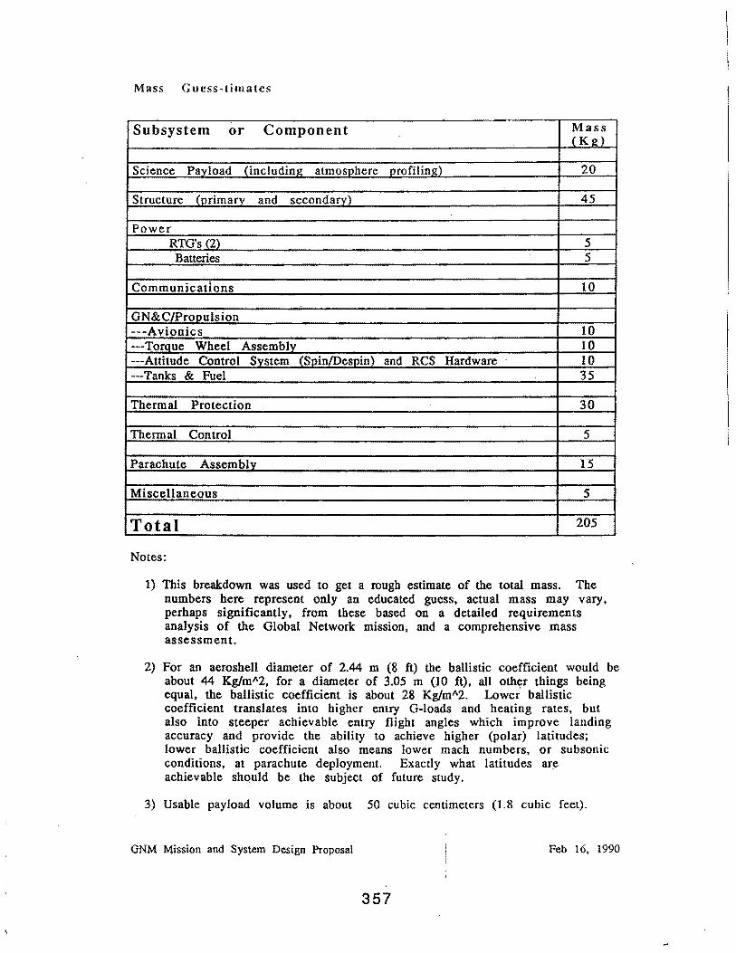
Mass Guess-timates
Subsystem or Component Mass ( K~)
Science Payload (including atmosphere profiling) 20
Structure (primary and secondary) 45
Power RTG's (2) 5 Batteries 5
Communications 10
GN&C/Prooulsion ---Avionics 10 ---Toraue Wheel Assembly 10 ---Attitude Control Svstem (Spin/Despin) and RCS Hardware 10 ---Tanks & Fuel 35
Thermal Protection 30
Thermal Control 5
Parachute Assembly 15
Miscellaneous 5
Total 205
Notes:
1) This breakdown was used to get a rough estimate of the total mass. The numbers here represent only an educated guess, actual mass may vary, perhaps significantly, from these based on a detailed requirements analysis of the Global Network mission, and a comprehensive mass assessment.
2) For an aeroshell diameter of 2.44 m (8 ft) the ballistic coefficient would be about 44 Kg/m-'2, for a diameter of 3.05 m (.10 ft), all other things being equal, the ballistic coefficient is about 28 Kg/m"2. Lower ballistic coefficient translates into higher entry G-loads and heating rates, but also into steeper achievable entry flight angles which improve landing accuracy and provide the ability to achieve higher (polar) latitudes; lower ballistic coefficient also means lower mach numbers, or subsonic conditions, at parachute deployment. Exactly what latitudes are achievable shQuld be the subject of future study.
3) Usable payload volume is about 50 cubic centimeters (1.8 cubic feet).
GNM Mission and System Design Proposal Feb 16, 1990
357
Challenges ...
This proposed design is certainly not without technical and programmatic challenge. I encourage others to critique this proposal, bot some difficulties ·I can see with the design are:
l) Navigating a fleet of vehicles to Mars simultaneously. · This may saturate an already oversubscribed DSN. An integrated DSN upgrade or an alternate communications and navigation approach. or system may have to be pursued.
2) A systematic injected mass study may show that some of my estimates are significantly in error. For instance, a stellar sensor such as the Ball CS-203 is required to provide inertial attitude reference, but even the CS-203 at 5.5 Kg, 6 watts, and 9 arcsec accuracy is not as small or precise as desired; a lightweight, low power Canopus tracker is assumed to be available. A total target weight of less than 200 Kg is attractive, I believe that lower weight (and thus lower ballistic coefficient, higher
·achievable latitudes, and higher landing accuracy) is attainable given the current trend towards micro-spacecraft. In . any case, using off the shelf miniaturized components and technology is key to the success of the proposed design approach. (Is this technologically innovative?)
3) Science objectives best accomplished from orbit will require another . orbiter (Son of Mars Observer?), or perhaps science payloads could be piggy backed on the (separate) communications orbiter.
4) Establishing a shared communications infrastructure may be a challenge. The communications and operations requirements of · the
. missions need to be analysed together to determine what the best . approach is to solving both problems. The placement of GNM landers at the poles, for instance implies . the need for highly inclined relay orbits, while a sample return operation may best be satisfied with an aerosynchronous relay orbit.
5) Achieving the desired (steep) entry flight path angles from approach :velocity may be problematic. Heating rates and total heat load are of special concern. The proposed approach would rely heavily on the heritage of Shuttle, AFE, and the High Energy Aerobrake work currently underway for Thermal protection materials, heat resistant substructure, and insulation materials and techniques.
6) Mission planning to achieve the desired distribution of landers at preselected longitudes and latitudes at the· ,proper lighting conditions for descent· imaging may be constrained by orbital mechanics and the launch dates, . combined with the achievable· entry . flight path angles
. (function of ballistic· coefficient, G loads, heating - requires further analysis). It may be necessary to relax the lighting condition requirement for descent imaging for some of the sites. ·
7) Achieving ·a '96 launch date would require an immedia.te commitment to GNM concept studies, and an innovative approach to contracting, developing, managing, and administering the program.
GNM Mission and Sys~em Design Proposal Feb 16, 1990
358 !
J '
Conclusions
An approach such as the one proposed by AI Friedlander, which I have elaborated on here, has great promise in terms of reduction of cost and risk, increased flexibility, heritage and commonality, and I believe can reap substantial political dividends as welL However, a system engineering and cost estimation effort is needed to ascertain what the payoff of such a proposal might be. For a serious investigation of the possibility of a '96 launch of any description, it is imperative that funding of these important concept studies be swiftly provided.
While there is much refinement and analysis needed for this proposal, it has attributes which I hope will. receive serious attention. My hope is that this and other proposals can generate the kind of discussions which will lead to a well balanced Robotic Exploration Program and Human Exploration Initiative.
I ask the readers of this proposal who have become hardened by the decade long neglect of planetary exploration to try to suspend doubt in a sustained exploration program. Consider the GNM in a broader context of planetary exploration that has a new commitment behind it. If there is significant gold to be found in getting science value and the taxpayers money's worth in this program, it is in looking beyond the event horizon of the next mission.
I believe the GNM work shop was very productive and I look forward to future discussion of this and other promising mission and system design options for the Robotic Exploration Program.
GNM Mission and System Design Proposal Feb 16, 1990
359
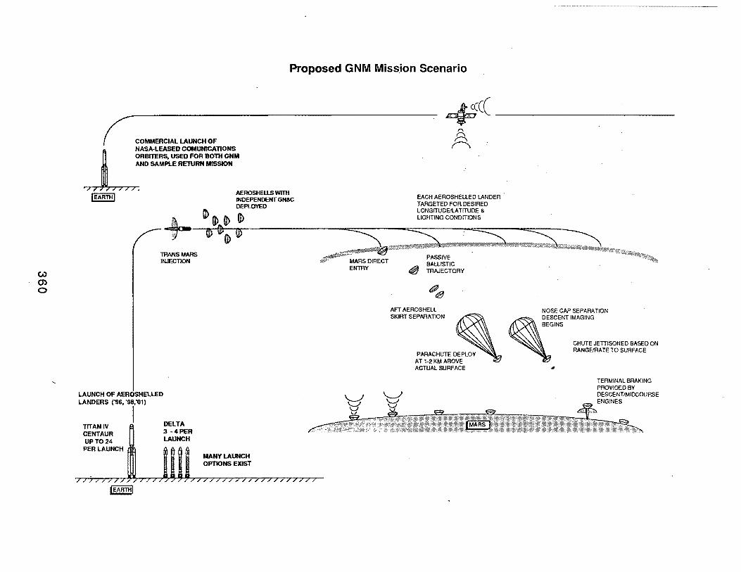
w 0)
0
fC~LM*mOF AND SAMPLE REllJRN MISSION LNASA-LEASED COMUNICATIONS ORBITERS, USED FOR Bont GNM
Proposed GNM Miss.ion Scenario
~c(
AEROSHEllS WITH I EARTH I INDEPENDENT GN&C EACH AEROSHELLED LANDER . DEPLOYED TARGETED FOR DESIRED lb LONGITUDE/LATITUDE &
~--~·~~~~~-· ~0~----------------~~--------~~l-IG-H-TI-NG_c_o_N_D_IT_~~NS=--------=~-------
TRANS MARS 11\UECTION
LAUNCH OF AEROSHELLED LANDERS ('96, '98,'01)
TITAN IV CENTAUR UPT024 PER LAUNCH
I
///////
I EARTH I
DELTA 3 -4PER LAUNCH
MANY LAUNCH OPTIONS EXIST
MARS DIRECT ENTRY
AFT AEROSHELL
SKIRT SEPARATION ~
PARACHUTE DEPLOY AT 1-2 KM ABOVE ACTUAL SURFACE
NOSE CAP SEPARATION DESCENT IMAGING
GINS
CHUTE JETTISON EO BASED ON RANGE/RATE TO SURFACE
TERMINAL BRAKING PROVIDED BY DESCENT!MIOCOURSE ENGINES

Terminal Descent Options
Parachute Deployment
Skirt Jettison
Chute Deployment
Nose Cap Jettison Followed by Propulsive Descent
Np Parachute· Aerobrake Only
Nose Cap Jettison Begin High Altitude Descent lma~ing
Skirt Jettison
Powered Descent
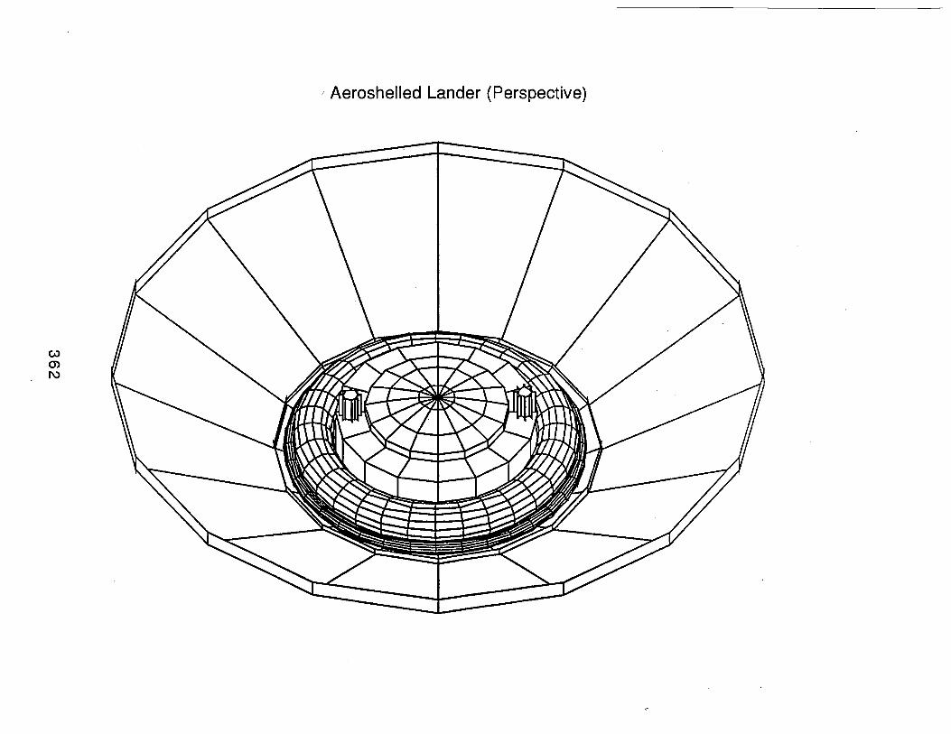
w (j) 1\)
,. Aeroshelled Lander (Perspective)

Simple Aeroshelled Lander Concept
Parachute Canister
Descent and Midcourse Correction Thrusters (6)
Cold gas thrusters for spin up/ CMG desaturation
Helium Pressurant
Reaction Wheel Assembly
-- Ablative Nose Cap

Lander Operational Configuration
Meterology and ground imaging boom
· . Air bladder to attenuate landing
loads and minimize possibility of tipover
Science equipment bay

Possible Delta Launch Configuration 3-4 Aeroshells per launch
Solid Rocket TMI Boost Stage
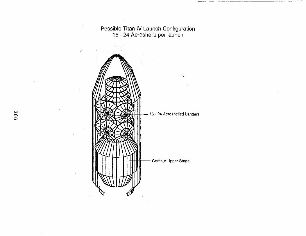
Possible Titan IV Launch Configuration 15 - 24 Aeroshells per launch

6.3 SESSION C SUBMITTALS

Session C, Submittal No. 1
C. Wayne Young Sandia National Laboratories
369
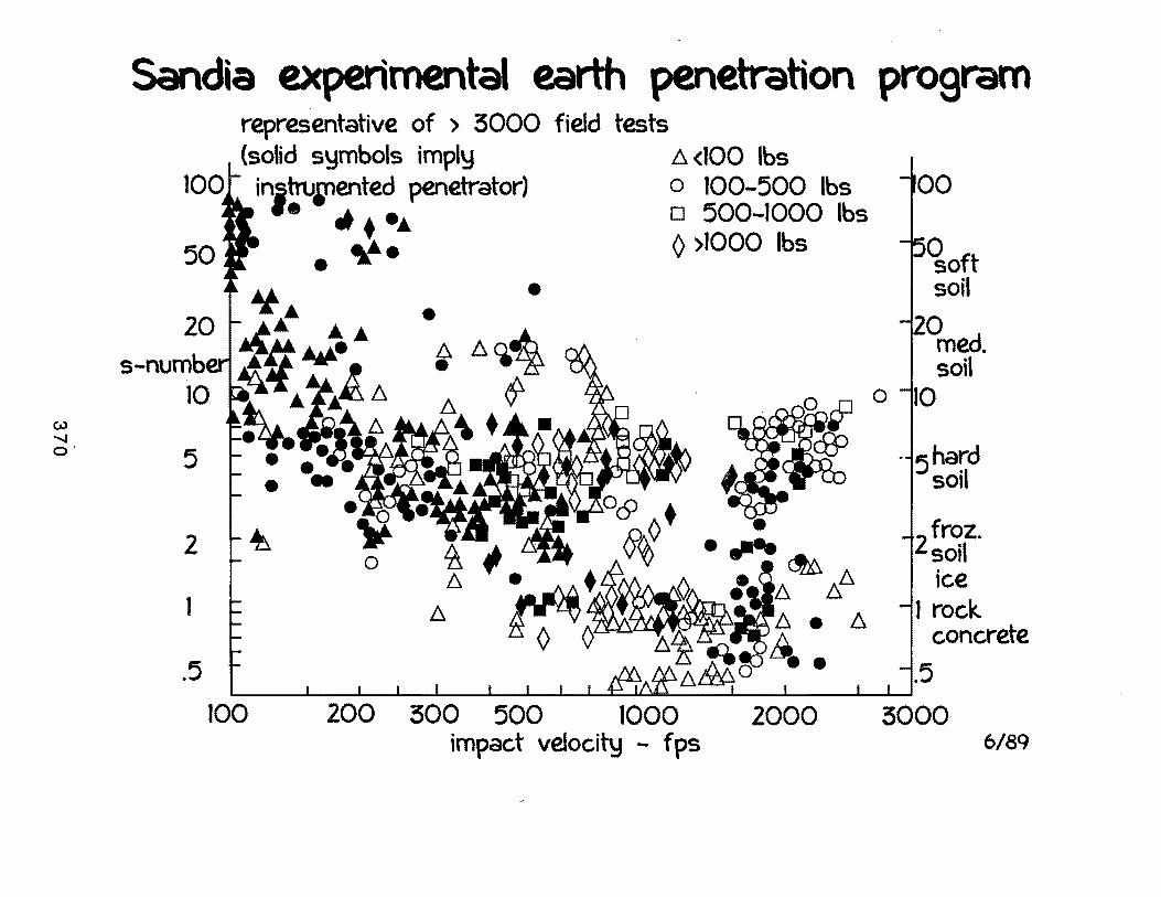
c.u -....! o·
Sandia e><penmental earth penetration program representative of > 5000 field tests (solid symbols imply ~ <100 lbs in;tru~ented penetrator) o 100-500 lbs
• ,; + • .._ o 500-1000 lbs ~· • 0 >1000 lbs • • •
5
2
1
.5
100 200 500 500 1000 2000 impact velocity - fps
ice 1 rock.
concrete
5000 6/89

.JPL JPL EXPLORATION PRECURSORS TASK TEAM MARS SURFACE NETWORK MISSION
PENETRATION DEPTH
6 E 60 E u
LOOS.E .. ... SAND z z
·0 0 -- .... 7 t- cc cc 4 a: 40 ANTENNA PLANE a: t-1- w w z z w w a. D.
Ul >- \ >--...,J FROZEN c 20 _... c 2 SILT 0 0 m HI·STRENGTH m a: . ROCK w w a: .... 0
HI-STRENGTH ROCK u. U.-- cc 0 0
60 80. 100 60 80 100
IMPACT VELOCITY, m/sec IMPACT VELOCITY, m/sec
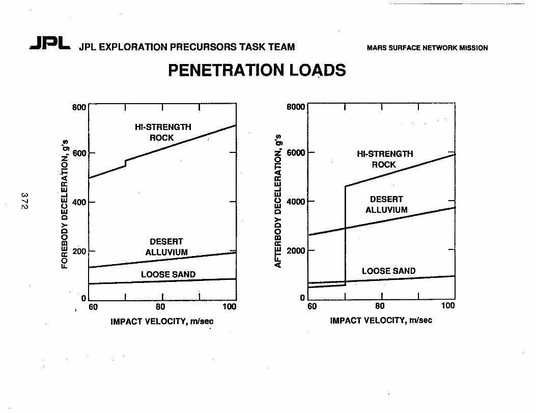
.JPL JPL EXPLORATION PRECURSORS TASK TEAM MARS SURFACE NETWORK MISSION
PENETRATION LOADS
800 8000
HI-STRENGTH ROCK 0
0 ·a ·~ 600 z 6000 HI-STRENGTH z 0
ROCK 0 -- ~ ...... <C a: a: w w _.
w _. w ........ w 400 fd 4000 1\) 0
w Q Q >-> Q Q 0 0 DESERT m m a: w 200 ALLUVIUM t 2000 a: 0 u. <C
LOOSE SAND LOOSE SAND
0 0 I 60 80 100 60 80 100
IMPACT VELOCITY, m/sec IMPACT VELOCITY, m/sec .
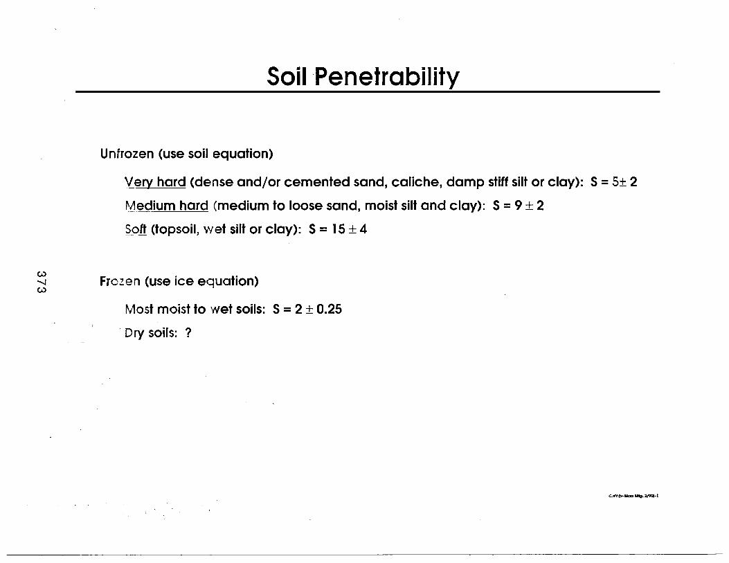
Soil-Penetrability
Unfrozen (use soil equation)
Very hard (dense and/or cemented sand, caliche, damp stiff silt or clay): S = 5± 2
Medium hard (medium to loose sand, moist silt and clay): S = 9 + 2
Soft (topsoil, wet silt or clay): S = 15 ± 4
w -....J Frozen (use ice equation) w
Most moist to wet soils: S = 2 ± 0.25
Dry soils: ?

Anal}'fical Methods Recommended
Axial Loading
• Sandia empirical equations
• Wavecodes are available, but perhaps not the most appropriate method
Lateral Plus Axial Loading
• SAMPLL - engineering tool
• Hydrocodes (PRONTO, DYNA, HULL, etc.) - more limited use, but necessary for
coupled calculation with structural response
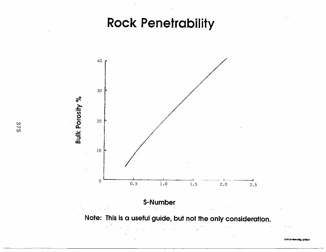
Rock Penetrability
40
30
~ 0
>-. :!:: Cl)
0 - 20 ' 0 0..
I / ~ ! - I ::l al
10 I f
0 0.5
1--·--·-···----i.. . -·-·-····· ... -· ...... L ..... ______ -----~, 1.0 1.5 2.0 2.5
S-Number
Note: This is a useful guide, but not the only consideration.
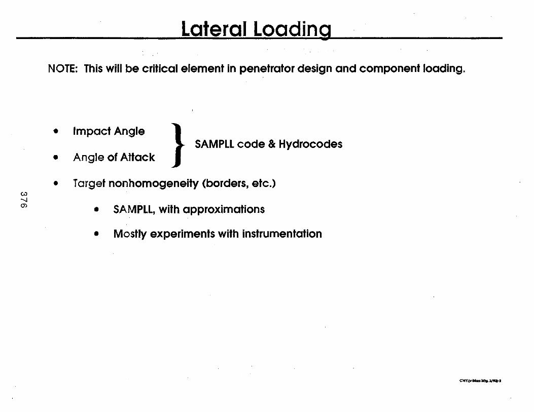
Lateral Loading
NOTE: This will be critical element in penetrator design and component loading.
• Impact Angle SAMPLL code & Hydrocodes
• Angle of Attack
• Target nonhomogeneity (borders, etc.)
• SAMPLL, with approximations
• Mostly experiments with instrumentation
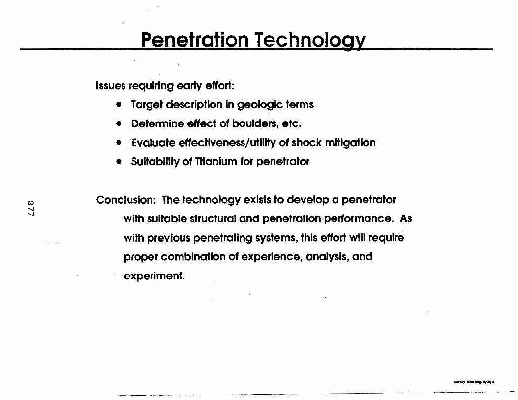
Penetration Technolog}'
Issues requiring early effort:
• Target description in geologic terms
• Determine effect of boulders, etc.
• Evaluate effectiveness/utility of shock mitigation
• Suitability of Titanium for penetrator
Conclusion: The technology exists to develop a penetrator
with suitable structural and penetration performance. As
with previous penetrating systems, this effort will require
proper combination of experience, analysis, and
experiment.
(
r '
Session C, Submittal No. 2
David E. Ryerson Sandia National Laboratories
379
sandia National Laboratories Telemetry Department
High Shock Penetrator Instrumentation Program
D. E. Ryerson Division 5144
February 2, 1990
Sandia National Laboratories Telemetry Department has been building high shock instrumentation systems for penetration studies for over twenty years. The instrumentation systems are digital stored data acquisition systems used to gather data during the penetration event and then recovered for data readout. The systems are powered by batteries, which are presently Eagle Picher LTC-7PST thionyl chloride batteries.
The shock loads that these systems are designed for are:
20,000 g for 8,000 g for 3,000 g for 1,000 g for
1 millisecond 10 milliseconds 20 milliseconds 50 milliseconds
Sandia has been fielding an average of sixty instrumented penetrator tests per year for the last five years. Attached is a plot of a sample penetrator test acceleration record.
To make our electronics survive high shock, we constrain all of the components very tightly in the penetrator package. We use selected components and encapsulate the~ in hard potting per the attached "Rules for Building High-g Electronics." Our temperature environment is typically between 0 and 50 degrees Celsius, so we can use components that would not survive standard military temperature ranges.
We normally try not to use shock attenuation to protect the electronic components. An analysis of shock attenuation is given on an attached page. It shows that to get shock attenuation, one must let electronics move a much larger distance than the penetrator housing, which is impossible.
We have used material to remove high frequency components of a shock pulse to protect such devices as accelerometers which can be broken by high-amplitude high-frequency inputs. The disadvantage of this shock material is that it may distort the accelerometer response and in certain cases, actually amplify certain frequencies of the shock pulse. In our work, we stay away from shock attenuators if at all possible.
380
I
~ !
c
J l (
J
l i
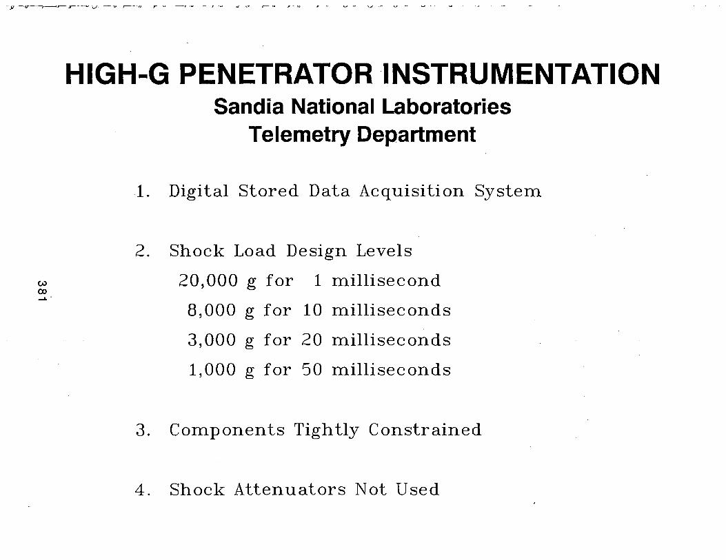
HIGH-G PENETRATOR INSTRUMENTATION Sandia National Laboratories
Telemetry Department
1. Digital Stored Data Acquisition System
2. Shock Load Design Levels
w 20,000 g for 1 millisecond (X) __..-
8,000 g for 10 milliseconds
3,000 g for 20 milliseconds
1,000 g for 50 milliseconds
3. Components Tightly Constrained
4. Shock Attenuators Not Used

Sample Penetrator Test Axial Acceleration
Analog LPF: 4800 Hz Digital LPF: none
Test Date 07-13-88 SSP-88
6000~--------~--------~------~~------~~------~~--------
4-000
. . 2000 .................... ~··:0·····~······· ...... ; ................. . . . . . . . . . . . . . . . . . . . . . . . . . . . .
0 1-----.......1':)1'11'1'7.':
. . . . -2000 · ................... : .. , ................. ; .................... ) ....................................... ; ................ .
-4-000 .• •••• 0 0 ..... ,. ......... ·:· ..... 0 •• 0 0 ............. 0 ! ............ ,. ........ ~ w: .................... "' ••• 0 •••••••••••••• . . . . . . . . . . . . . . . . . . . . . . . . . . . . . -6000
. . ....................... :-···················~····················:·····················: ....... . . ........ '• .................... . . . . . . . . . . . . . . . . . . . . . . . . . . . . . . . . . . . . . . -8000
. . . ••• 0 ••• ~ ....... ,. ••• •;- ..................... ! ...................... : . .. . . . . . . . . . .. .. .. . . . . . . . • . . • ............... ! ................. ', . . . . . . . . . . . . . . . . . . . . . . . . . . . . . . . . . . . . .
-10000 . . .
••••••• 0 ........................... ,. ........ ,. ••• "' ........... ".......... •• • .. • • • .. • • • • • .. • • • .. • • • • • • • ...................................... .
-12000 . .
• ~ o o • o o o • o o • o o • • • o •:- o a • # a a o o a • • o 10 • "'o • o o ~ • o o o * o o"., o o •" o" •, o • ": o ;; o o o • o , • • • o., • o o,. o a •: • o o • • o" • • o •" o o • • o ".o o • • • o • o • o • • o o • o o o
o I o o . . . . . . . . . . . . . . . . . . . " . . . . . . . . . . . . . . . . . . -14000~-----------~--------~---------~------~~------~~-------_J
-40 -30 -20 -10 0 10 20
02-02-110 Time (ms) 382
SNLA 5144.
J 1 •
I 1 1 J J
1
! I ~
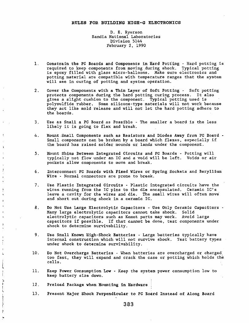
l
~ 1
l I
f r k
RULES FOR BUILDING HIGH-G ELECTRONICS
D. E. Ryerson Sandia National Laboratories
Division 5144 February 2, 1990
1. Constrain the PC Boards and Components in Hard Potting - Hard potting is required to keep components from moving during shock. Typical potting is epoxy filled with glass micro-balloons. Make sure electronics and potting material are compatible with temperature ranges that the system will see in curing of potting and system operation.
2. Cover the Components with a Thin Layer of Soft Potting - Soft potting protects components during the hard potting curing process. It also gives a slight cushion to the component. Typical potting used is polysulfide rubber. Some silicone-type materials will not work because they act like mold release and will not let the hard potting adhere to the boards.
3. Use as Small a PC Board as Possible - The smaller a board is the less likely it is going ·to flex and break.
4. Mount .small Components such as Resistors and Diodes Away from PC Board -Small components can be broken by a board which flexes, especially if the board has raised solder mounds or lands under the component.
5. Mount Shims Between Integrated Circuits and PC Boards - Potting will typically not flow under an IC and a void will be left. Voids or air pockets allow components to move and break.
6. Interconnect PC Boards with Fixed Wires or Spring Sockets and Beryllium Wire - Normal connectors are prone to break.
7. Use Plastic Integrated Circuits - Plastic integrated circuits have the wires running from the IC pins to the die encapsulated. Ceramic IC's leave a cavity for the wires and die. The small wires will often move and short out during shock in a ceramic IC.
8. Do Not Use Large Electrolytic Capacitors - Use Only Ceramic Capacitors -Many large electrolytic capacitors cannot take shock. Solid electrolytic capacitors such as Kemet parts may work. Avoid large capacitors if possible. If that cannot be done, test components under shock to determine survivability.
9. Use Small Known High-Shock Batteries - Large batteries typically have internal construction which will not survive shock. Test battery types under shock to determine survivability.
10. Do Not Overcharge Batteries - When batteries are overcharged or charged too fast, they will expand and crack the case or potting which holds the cells.
11. Keep Power Consumption Low - Keep the system power consumption low to keep battery size down.
12.
13.
Preload Package when Mounting in Hardware
Present Major .Shock Perpendicular to PC Board Instead of Along Board
383

UJ (X) .,&::=..··
RULES FOR BUILDING HIGH-G ELECTRONICS
1.
2.
3.
4.
5.
6.
7.
8.
9.
10.
11.
12.
13.
. Sandia National Laboratories Telemetry Department
Constrain PC Boards and Components in_ Hard Potting
Cover· Components with a Thin Layer of Soft Potting
Use Small PC Boards
Mount Discrete Components ·Away from PC Board
Mount Shims between IC ·and PC Board ..
Minimize Connector Use
Use Plastic ICs
Don't Use. Large Electrolytic Capacitors
Use Small Batteries
Don't Overcharge ·Batteries
Keep Power Consumption Low
Preload Package· in Mounting Hardware
Shock PC Boards Perpendicularly
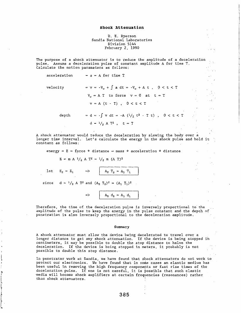
l
Shock Attenuation
D. E. Ryerson Sandia National Laboratories
Division 5144 February 2, 1990
The purpose of a shock attenuator is to reduce the amplitude of a deceleration pulse. Assume a deceleration pulse of constant amplitude A for timeT. Calculate the motion parameters as follows:
acceleration = a A for time T
velocity = v = -V0 + f a dt = -V0 + A t , 0 < t < T
V0
= A T to force v 0 at t = T
v A (t - T) , 0 < t < T
depth d = -f v dt -A (lj2 tZ - T t) , 0 < t < T
d - lfz A T2 t = T
A shock attenuator would reduce the deceleration by slowing the body over a longer time interval. Let's calculate the energy in the shock pulse and hold it constant as follows:
energy = E = f~rce * distance = mass * acceleration * distance
E = m A lj2 A TZ = lj2 m (A T)2
let =>
since
Therefore, the time of the deceleration pulse is inversely proportional to the amplitude of the pulse to keep the energy in the pulse constant and the depth of penetration is also inversely proportional to the deceleration amplitude.
Summary
A shock attenuator must allow the device being longer distance to get any shock attenuation. centimeters, it may be possible to double the deceleration. If the device is being stopped possible to double this stop distance.
decelerated to travel over a If the device is being stopped in
stop distance to halve the in meters, it probably is not
In penetrator work at Sandia, we have found that shock attenuators do not work to protect our electronics. We have found that in some cases an elastic medium has been useful in removing the high frequency components or fast rise times of the deceleration pulse. If one is not careful, it is possible that such elastic ·media will become shock amplifiers at certain freq~encies (resonances) rather than shock attenuators.
385
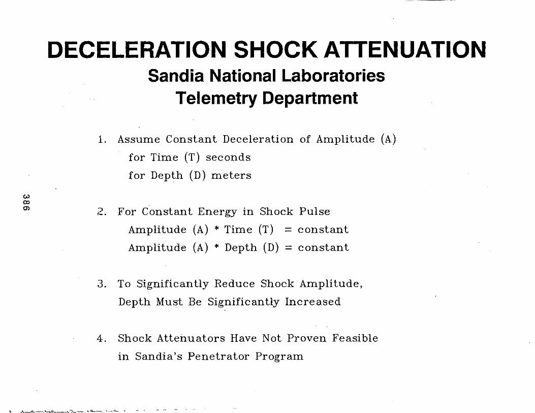
DECELERATION SHOCK ATTENUATION Sandia National Laboratories
Telemetry Department
1. Assume Constant Deceleration of Amplitude (A)
for Time (T) seconds
for Depth (D) meters
2. For Constant Energy in Shock Pulse
Amplitude (A) * Time (T) = constant
Amplitude (A) * Depth (D) = constant
3. To Significantly Reduce Shock Amplitude,
Depth Must Be Significantly Increased
4. Shock Atte:huators Have Not Proven Feasible
in Sandia's Penetrator Program
)
David E. Ryerson
Supervisor of Telemetry Technology Development .Division 5144 at Sandia National Laboratories, Albuquerque, New Mexico.
BS in Electrical Engineering, Iowa State University, 1965. MS in Electrical Engineering, University of New Mexico, 1967.
Worked at Sandia from 1965 to the present in telemetry, data acquisition, and control systems. Designed real-time aircraft computer-controlled systems for target tracking and rocket-launch computer systems for Sandia's Kauai test range. Developed long-life (1 to 3 years) ocean-floor seismic systems and underwater acoustic telemetry for data 'recovery. Presently directing the designing and fielding of ultra-high shock (up to 20,000 times gravity) penetrator data acquisitions systems, rocket and reentry vehicle instrumentation, and specialized data acquisition systems.
387
Session C, Submittal No. 3
Tomas A. Komarek Jet Propulsion Laboratory/California Institute of Technology
389
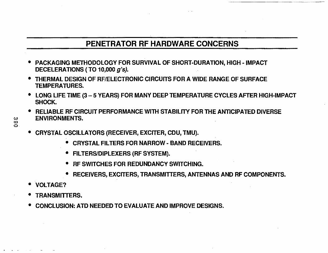
PENETRATOR RF HARDWARE CONCERNS
• PACKAGING METHODOLOGY FOR SURVIVAL OF SHORT-DURATION, HIGH -IMPACT DECELERATIONS ( TO 10,000 g's).
• THERMAL DESIGN OF RF/ELECTRONIC CIRCUITS FOR A WIDE RANGE OF SURFACE TEMPERATURES.
• LONG LIFE TIME (3- 5 YEARS) FOR MANY DEEP TEMPERATURE CYCLES AFTER HIGH-IMPACT SHOCK.
• RELIABLE RF CIRCUIT PERFORMANCE WITH STABILITY FOR THE ANTICIPATED DIVERSE w ENVIRONMENTS. CD 0
• CRYSTAL OSCILLATORS (RECEIVER, EXCITER, CDU, TMU).
• CRYSTAL FILTERS FOR NARROW- BAND RECEIVERS.
• FIL TERS/DIPLEXERS (RF SYSTEM).
• RF SWITCHES FOR REDUNDANCY SWITCHING.
• RECEIVERS, EXCITERS, TRANSMITTERS, ANTENNAS AND RF COMPONENTS.
• VOLTAGE?
• TRANSMITTERS.
• CONCLUSION: ATD NEEDED TO EVALUATE AND IMPROVE DESIGNS.
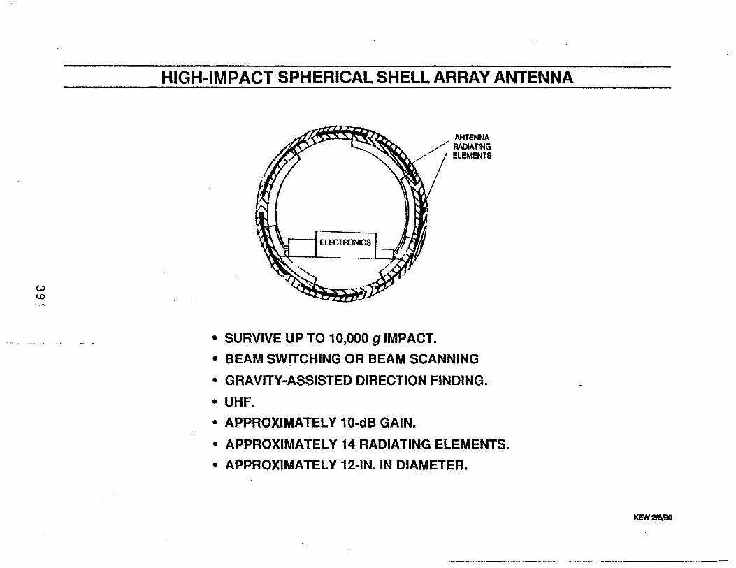
HIGH-IMPACT SPHERICAL SHELL ARRAY ANTENNA
• SURVIVE UP TO 10,000 g IMPACT.
ANTENNA RADIATING ELEMENTS
• BEAM SWITCHING OR BEAM SCANNING
• GRAVITY-ASSISTED DIRECTION FINDING.
• UHF.
• APPROXIMATElY 10-dB GAIN.
• APPROXIMATElY 14 RADIATING ElEMENTS.
• APPROXIMATElY 12-IN.IN DIAMETER.

Session C, Submittal No .. 4
Farley Palmer Hughes Aircraft Company
393

c.u lO ..p.;.·
Session C - Subsystem Technology Focal Questions
HUGHES
) What technology will help achieve 10 year lifetimes?
AIRCRAFT COMPANY
) What technology.will help survival of high-g landings?
3) Are RTGs a workable power subsystem (size, location on the lander)?
--- ·-
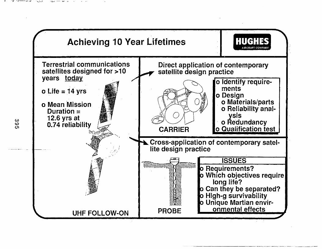
VJ <.0 CJ1
Achieving 10 Year Lifetimes HUGHES AIRCRAFT COMPANY
Terrestrial communications satellites designed for > 10 years today
o Life= 14 yrs
o Mean ·Mission Duration= 12.6 yrs at 0.74 reliability
: /
UHF FOLLOW-ON
Direct application of contemporary satellite design practice
------~...--------. o Identify require-ments
o D~sign . o Materials/parts
o Reliability analysis
· o Redundancy o Qualification test
Cross-application of contemporary satellite design practice
ISSUES -~ ~ ___ R_e_q_u_i..;;..,re..;;..,m ..... e ..... n ..... t-s?-. ----11
PROBE
Which objectives require long life?
Can they be separated? High-g survivability Unique Martian envir-
onmental effects·
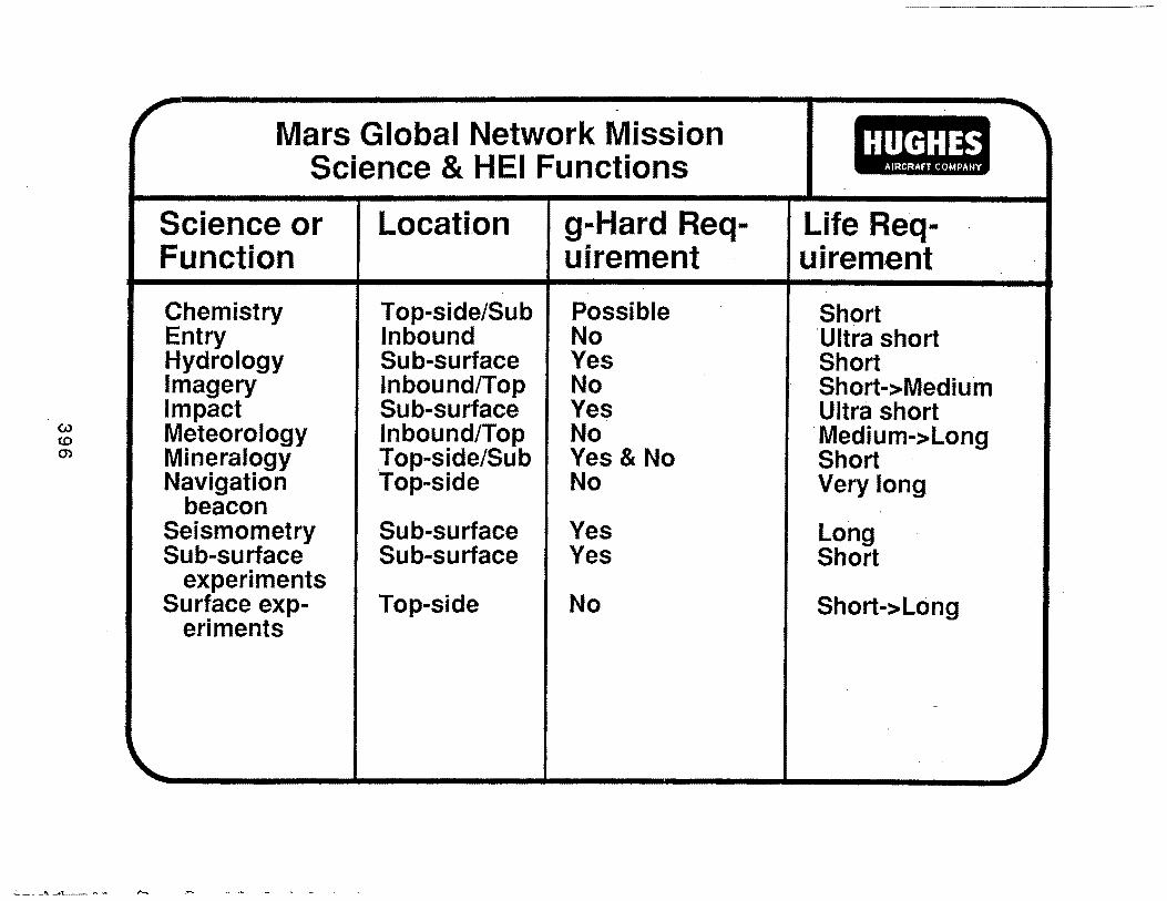
w (0 Q')
Mars Global Network Mission Science & HEI Functions
Science or Function
Chemistry Entry Hydrology Imagery Impact Meteorology Mineralogy Navigation
beacon Seismometry Sub-surface
experiments Surface exp
eriments
Location
Top-side/Sub Inbound Sub-surface Inbound/Top Sub-surface Inbound/Top Top-side/Sub Top-side
Sub-surface Sub-surface
Top-side
g-Hard Requirement
Possible No Yes No Yes No Yes & No No
Yes Yes
No
HUGHES AIRCRAFT COMPANY
Life Requirement
Short ·ultra short Short Short-> Medium Ultra short · Medium->Long Short · Very long
Long Short
Short->Long
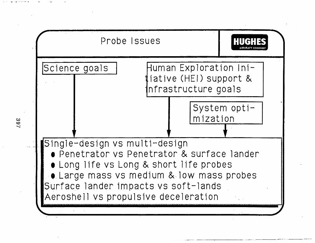
: ,, -·~ ., ·- .. ...... .....
Probe Issues HUGHES
Science goals
AIRCRAFT COMPANY
uman Exploration lnii at ive (HE I) support & nfrastructure goals
System opt imization
SJngle-design vs multi-design • Penetrator vs Penetrator & surface 1 ander • Long 1 i fe vs Long & short 1 i fe probes
. • Large mass vs medium &. low mass probes Surface lander impacts vs soft-lands Aeroshell vs propulsive deceleration
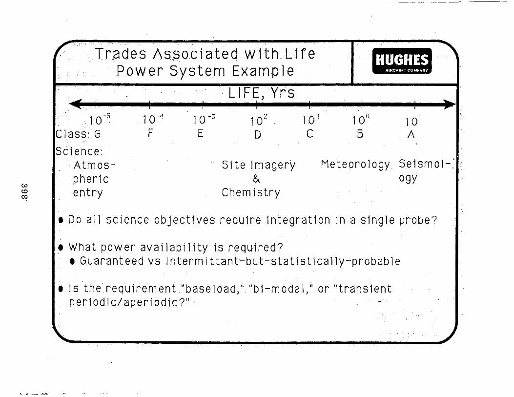
Trad,es Asso,ciated .with L.ife :Power System Example
.··· '4!. I
Science: ·. Atmos-pheric entry
. 1 o-4
F 1 0-3
E
· .. Ll FE, Yrs I
5 i t e I m age ry &
Chemistry
L 1 ()] c
HUGHES AIRCRAFT COMPANY
Meteorology Seismol-" .•.. ogy
• Do all science objectives require integration in a single probe?
• What power availability is required? 1 G u a rant e e d v s I n term i t tan t-but-stat i s t i c a 11 y-pro b a b 1 e
I Is the requirement "base load} ... "bi-modal}'i or "transient periodic/aperiodic?"·

w <0 <0
~Jr.::%1'~'~r.::n:: • .,!>ll!~~u:r.lf.ll!!'lt~=r.""''1:l"~·-r'"':...r.m1.t::r.i!=l!e:r:rn:..~"r,."""'ex;,.. •• Tn:'lr."'~
(Candidate Povvet~ Systern 1-\pproa- u ches I
• - .• • • ~~JIT:nt'C!!r.l"t!~=" ... -=~~~·~[~-,,_-~
Class TtEe Availabi litv Burst Power! Exam le ---A 1 I Bi-m 0 ~ H:Jli:Jl_,...o:IIIGIH!tu="te~'d''mc:rn~~nr.-=d~ '"''·o~;;;~j;;';j'*'·~k;.r;;,~;fij-T.rii~i7; a ry' battery
'Nith or wHhout I e RTG + 2ary batte-
A2 B1-modul
Bl Bose load
B2 Bcselood
Cl Tronsient
C2 Tnmsicnt
lnterrnittant but stnt-1 sU co 11 y prcba[ll e
G uera ntecd
I ntenni ttunt but ~>tnt-i st i call y probn!J l e
GuurantHed
seconr.iory storage 1 · ry or flywheel
Oversized primary wHh or without seconfJaql ntor~ge
N/A
N/A
1 Solar panel or wind-generator+ 2ory battery or nuwheel
• Primary battery 1 -RT6
1 Solar panel 1• Wind generator
l Possible !>econdary 1 • Primary battery
1 e RTG + 2ory batt-1 ery or flywheel
nturage
lntermittant but s'tn~~- Possible s:eccndnq; ! 1 5o1Hr panel or wi-istlcally, prohabh: Gton~ge ! nd generator+
u~~ -~M·"_, __ = .. ~ --~~=--·=~~J~~ 7
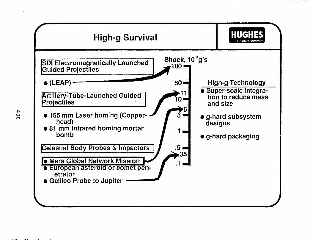
~ 0 0
High-g Survival
SDI Electromagnetically Launched Guided Projectiles
e (LEAP)
rtillery-Tube-Launched Guided rojectiles
• 155 mm Laser homing (Copperhead)
• 81 mm Infrared homing mortar bomb
ICelestial Body Probes & Impactors I
. ·--·--------~
HUGHES AIRCRAFT COMPANY
High-g Technology • Super-scale integra
tion to reduce mass and size
• g-hard subsystem designs
• g-hard packaging
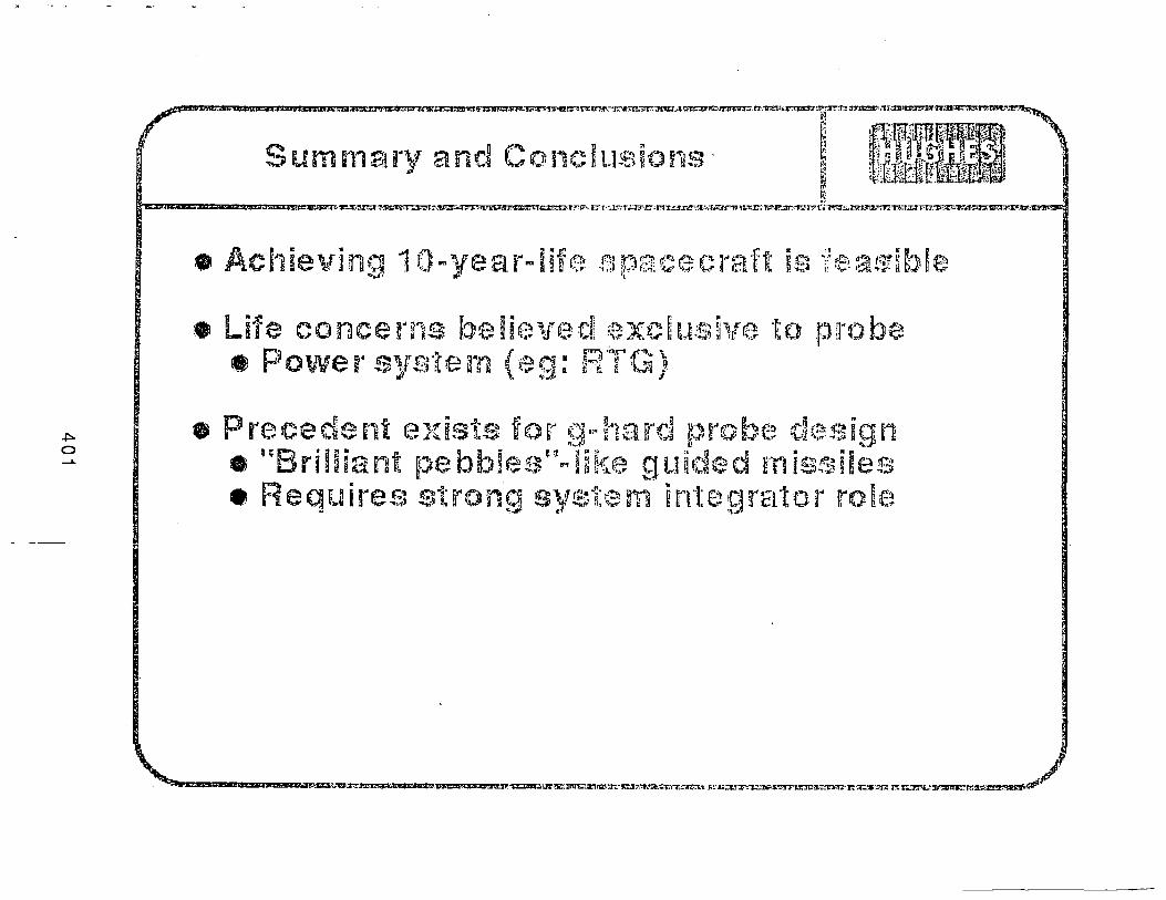
Session C, Submittal No. 5
Michael Shirbacheh Jet Propulsion Laboratory/California Institute of Technology
(Information provided by Wayne M. Brittain, Teledyne Energy Systems)
403
SPECIAL APPLICATIOOS Lat-~ RTG
DEVELOPMENT PR(X;RAM SOMMARY
January 1990
· "'"TELEDYNE ENERGY SYSTEMS 404
· A. Background
- 1 -
SP~IAL APPLICATIOOS LOO-J?OmR RTG
DEVELOPMENT PRc:x;RAM Sl.JttMARY
The Special Applications RTG Development Program was initiated at Teledyne
Energy Systems (TES) in September 1983 under OOE Contract DE-AC01-83NE32115.
The development effort was performed under this contract through September 1988.
After this time the program was continued as the Two-Watt Special Applications
RTG Program (OOE Contract DE-AC01-88NE32142) with the objective of fueling a
prototype RTG unit. Present activities at TES include fabrication, assembly and
test of the electrically-heated prototype RTG which will be delivered to
EG&G/Mound in June 1990 for fueling in December 1990.
Development of a sealed, 3-layer fuel capsule for use in the Two-Watt RTG
is being performed for OOE in a joint effort by TES, EG&G/Mound and LANL. The
capsule design is based on an upsizing of the Milliwatt RTG and Navy One-Half
Watt RTG terrestrial 3-layer capsule technology.
B. Introduction
The primary objectives of the Special Applications RTG Development Program
are to:
(1) develop a low-power (2 to SW) relatively high voltage (5 to 12V)
thermoelectric module using proven PbTe/TAGS thermoelectric
materials. This materials technology has been applied to both NASA
SNAP-19 space RTGs (Pioneer 10 and 11 Jupiter Fly-by spacecraft and
Viking 1 and 2 Mars Landers), and terrestrial RTGs delivered to OOE
405
- 2 -
for subsea·. applications.· Demonstrated thermoelectric module
technology for low-power terrestrial RTGs at the initiation of the
development program was limited to bismuth telluride with a typical
RTG system efficiency of 3.5 to 4.0%. The goal for the development
program was to increase this efficiency by 50%.
(2) develop a sealed heat source intended for terrestrial applications to
·contain the helium gas generated by the Pu-238 fuel decay. Available
RTG heat source technologies for the anticipated thermal inventory
requirement were all vented designs which result in increased
parasitic heat losses with operating time due to the introduction of
helium into the thermal insulation. The goal was to contain· this
helium within the capsule.
(3) design, fabricate, assemble, fuel and test a prototype terrestrial
RTG system to demonstrate the developed technology. The selected
terrestrial RTG design would consider pcitential near-term
applications of low-power RTGs.
Although the hardware development for the Special Applications RTG has been
oriented towards terrestrial applications, the thermoelectric module technology
is ·generic and may ·be adapted to both space and terrestrial missions which
require a low-power RTG power source. The radioisotopic heat source for space
applications can be selected from available, qualified space hardware (such as
the GPHS technology) or possibly be specifically designed and qualified for the
mission requirements.
406
- 3 -
c. . 'lbermoelectric Module Technology Description
The Special Applications thermoelectric module has evolved during the
development program from using a couple with an all-PbTe N-leg and TAGS P-leg to
one with Bi2Te3 cold segments on both the N and P-legs.
segments were added to the latest generation of thermoelectric modules to
enhance the· thermoelectric conversion efficiency for terrestrial applications
where the RTG would be exposed directly to the cold subsea environment. These
cold segments would not be beneficial for space applications and would not be
included in the thermoelectric couple design.
1. Viewgraph l
Vi ewgraph 1 shows Special Applications PbTe/TAGS mini couples which
exemplify a configuration which could be considered for space application. The
couple design is basically a miniaturization of the proven SNAP-19 space RTG
thermoelectric technology. The couple has iron hot and cold shoes and copper
pins to provide for electrically interconnecting the couples within a module.
The Special Applications module uses a printed circuit board at the cold side to
complete the interconnects between the couples.
individual legs are 0.102 in. sq. by 0.625 lg.
2. Viewgrapll 2
For the couple shown the
Viewgraph 2 shows the typical internal construction of a Special
Applications RTG. The configuration shown is that for the subsea prototype RTG
407

- 4-
now being fabricated at TES. The 30-pound weight shown is almost all in the
BeCu pressure housing, with less than 5 pounds attributable to the RTG internal
components (thermoelectric module, heat sour~e, heat distribution cup,.thermal
insulation and preload springs) . For a space RTG configuration, particularly
for a penetrator mission with high shock loading, the internal configuration
would p~obably vary somewhat from that shown to satisfy mission vibration/shock
requirements. For example, the heat sourc~ could have a support system
independent. of the thermoelectric module to minimize dynamic loads on the
module.
3. Viewgraph 3
Viewgraph 3 shows a typical Special Applications thermoelectric module
containing 68 couples. The module is approximat~ly 3 inches in diameter by 0.8
inch thick.. The cold side printed circuit board provides the basic structure
for the module. Powdered Min-K thermal insulation is vacuum~impregnated between
the couples to minimize heat loss. A thermoelectric module similar to that
shown has been successfully tested to a lOOg axial, SOg lateral (both applied
simultaneously) shock loading to simulate impact deployment of an RTG.
4. Viewgraph 4 . .
Viewgraph 4 shows the typical performance for the subsea RTG design shown
on Viewgraph 2. The BOL in-water power output is approximately SW .with a system.
efficiency approaching 7%. Note that the hot junction temperatur~ of the
408
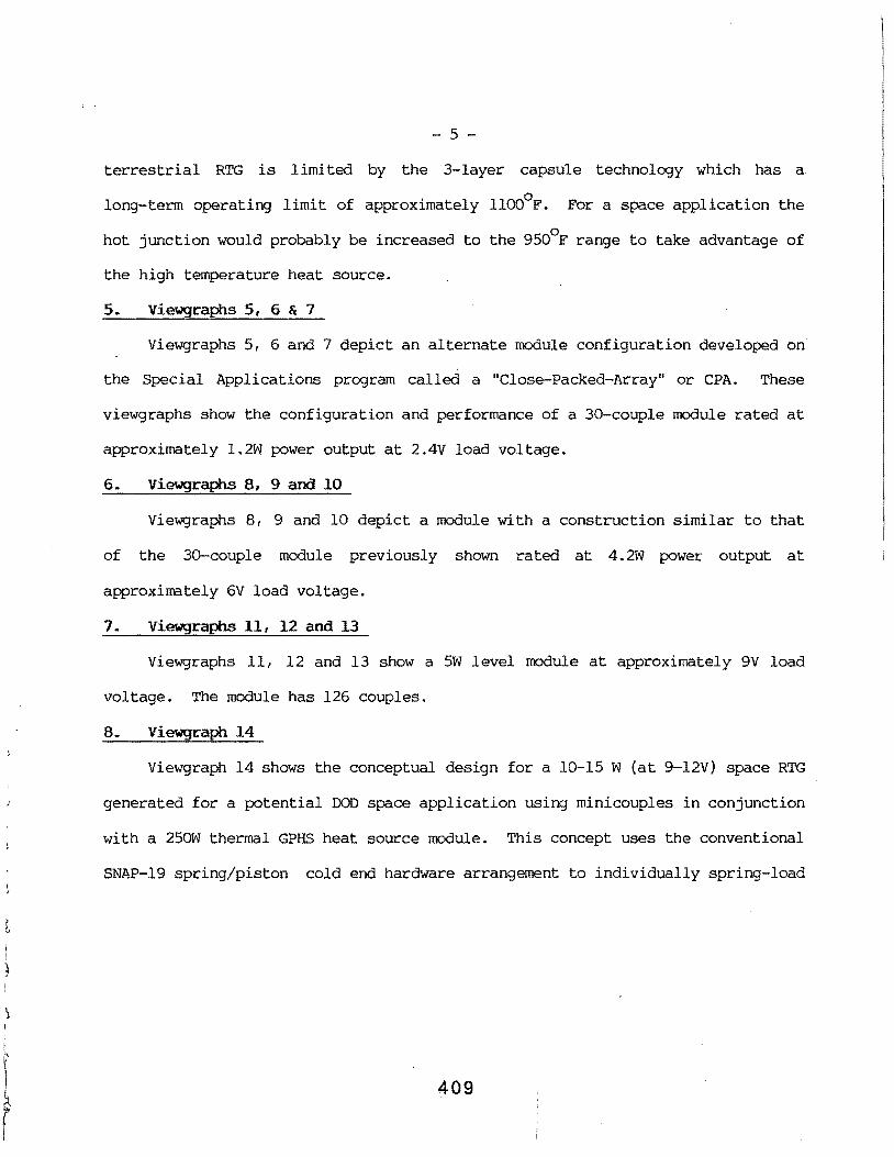
I ~
i
t r
- 5 -
terrestrial RTG is limited by the 3-layer capsule technolo::~y which has a
long-term operating limit of approximately ll00°F. For a space application the
0 hot junction would probably be increased to the 950 F range to take advantage of
the high temperature heat source.
5. Viewgraphs 5, 6 & 7
Viewgraphs 5, 6 and 7 depict an alternate module configuration developed on
the Special Applications program called a "Close-Packed-Array" or CPA. These
viewgraphs show the configuration and performance of a 30-couple module rated at
approximately 1.2W power output at 2.4V load voltage.
6. Viewgraphs 8, 9 and 10
Viewgraphs 8, 9 and 10 depict a module with a construction similar to that
of the 30-couple module previously shown rated at 4.2W power output at
approximately 6V load voltage.
7. Viewgraphs 11, 12 and 13
Viewgraphs 11, 12 and 13 show a 5W level module at approximately 9V load
voltage. The module has 126 couples.
8. Viewgraph 14
Viewgraph 14 shows the conceptual design for a lQ-15 W (at 9-12V) space RTG
generated for a potential DOD space application using minicouples in conjunction
with a 250W thermal GPHS heat source module. This concept uses the conventional
SNAP-19 spring/piston cold end hardware arrangement to individually spring-load
409
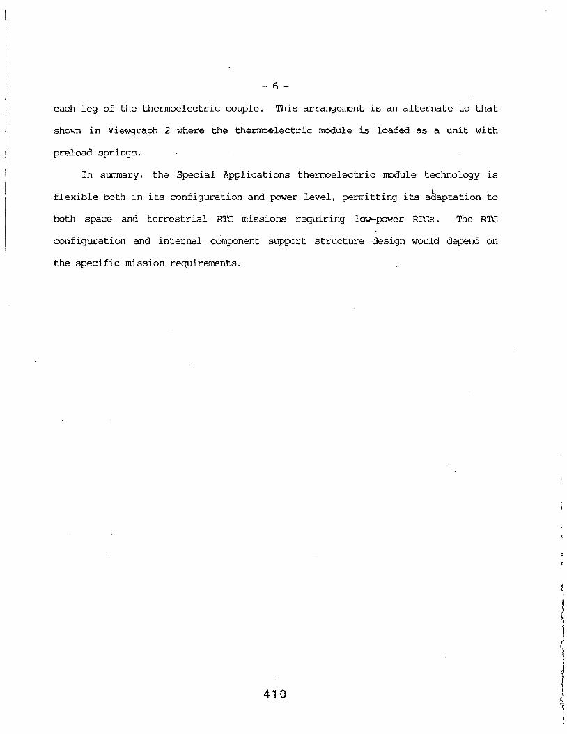
- 6 -
each leg of the thermoelectric couple. This arrangement is an alternate to that
shown in Viewgraph 2 where the thermoelectric module is loaded as a unit with
preload springs.
In summary, the Special Applications thermoelectric module technology is
flexible both in its configuration and power level, permitting its aaaptation to
both space and terrestrial RTG missions requiring low-power RTGs. The RTG
configuration and internal component support structure design would depend on
the specific mission requirements.
410
i
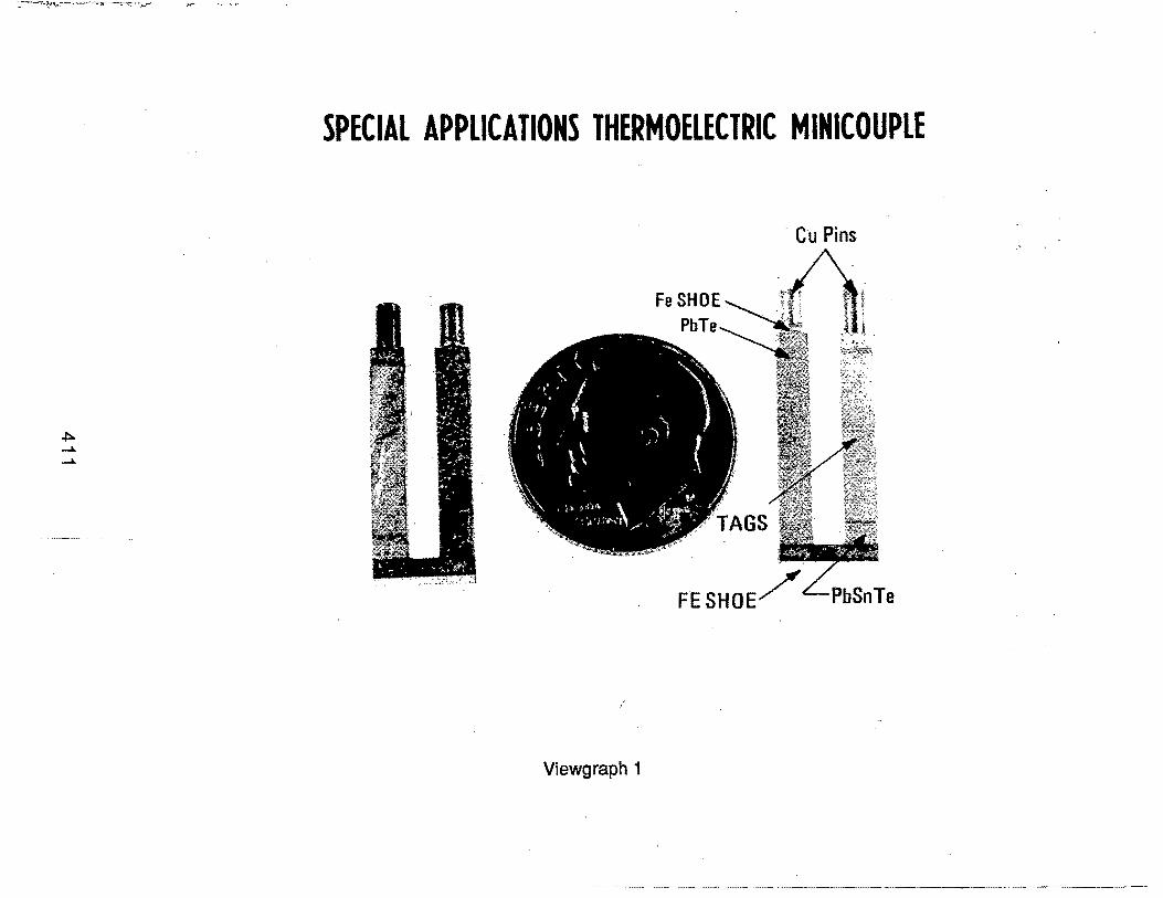
SPECIAL APPLICATIONS THERMOELECTRIC MINICOUPLE
Cu Pins
Viewgraph 1
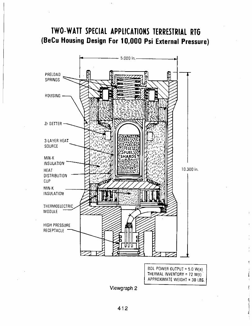
TWO-WATT SPECIAL APPLICATIONS TERRESTRIAL RTG (BeCu Housing Design For 10,000 Psi External Pressure)
PRELOAD SPRINGS
HOUSING
Zr GETTER
3-LAYER HEAT SOURCE
MIN-K INSULATION
HEAT DISTRIBUTION CUP
MIN-K INSULATION
14------ 5.000 in.-----~
Viewgraph 2
412
10.300 in.
BOL POWER OUTPUT= 5.0 W(e) THERMAL INVENTORY = 72 W(t) . APPROXIMATE WEIGHT= 30 LBS.
!
:
l

SPECIAL APPLICATIONS MODULE (HOT SIDE VIEW)
Viewgraph 3
413

TWO-WATT SPECIAL APPLICATIONS RIG PERfORMANCE PREDJCTION SUMMARY
WoRsT-CAsE IN-AIR IN-WATER IN-WATER (8£X..) CBOU 00 YRS.)
PowER OuTPUT CW(E)) 3.95 4.92 3.37 (2.6 ~ .99 TO 0.999 REL.)
FUEL INVENTORY (W(T)) 70.8 70.8 65.4
T/E EFFICIENCY (%) 7.74 9.36 6.89 THERMAL EFFICIENCY (%) 73.2 75.1 74.8 SYSTEM EFFICIENCY (%) 5.58 6.94 5.15
HoT JUNCTION TEMPERATURE (°F) 814 676 641 COLD JUNCTION TEMPERATURE (°F) 214 50 50 AMBIENT TEMPERATURE (°F) 113 40 40
NOTES: (1) T/E ELEMENT DIMENSIONS: 0.450 IN. LG. X 0.103 IN. SQ. (2) NUMBER T/E COUPLES: 68 (3) RTG FILL GAS: 100% XENON
Viewgraph 4
414
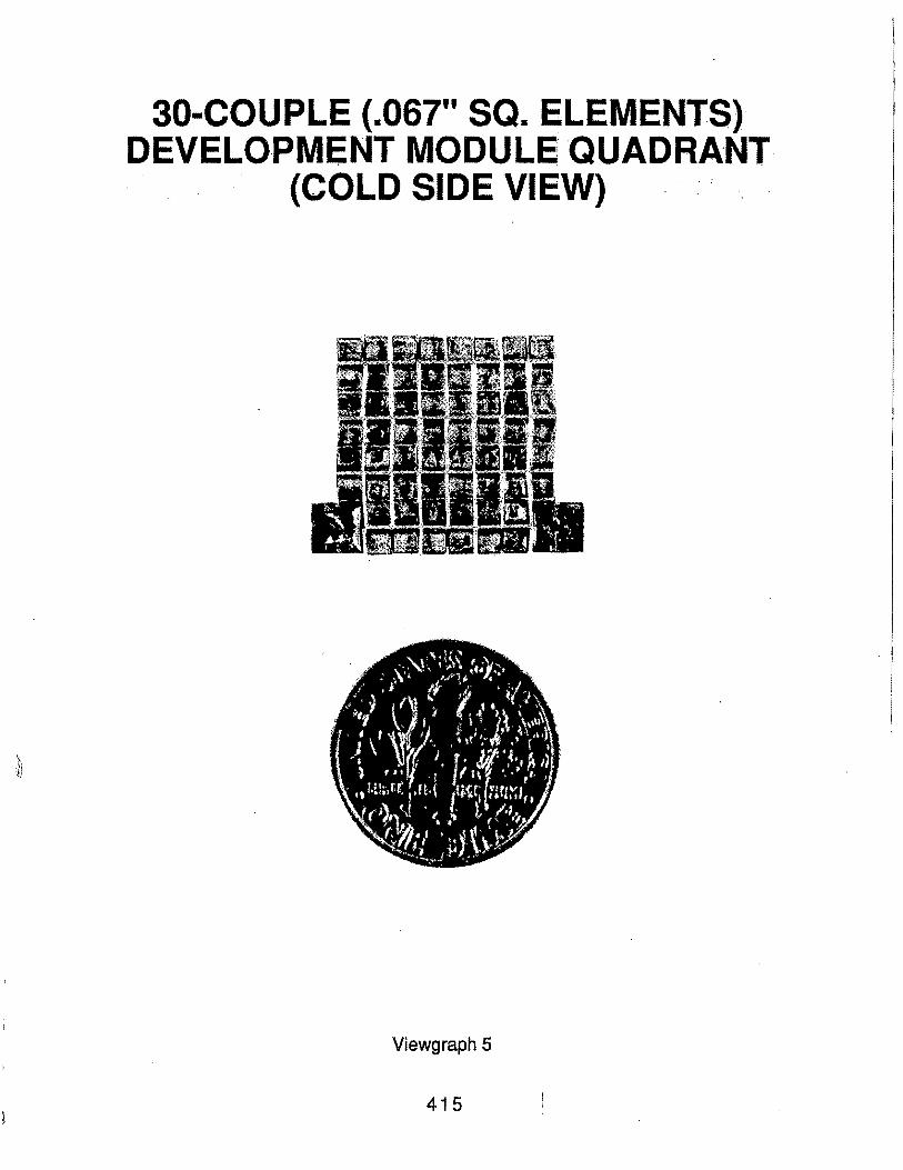
30-COUPLE (.067" SQ. ELEMENTS) DEVELOPMENT MODULE QUADRANT
(COLD SIDE VIEW)
Viewgraph 5
415
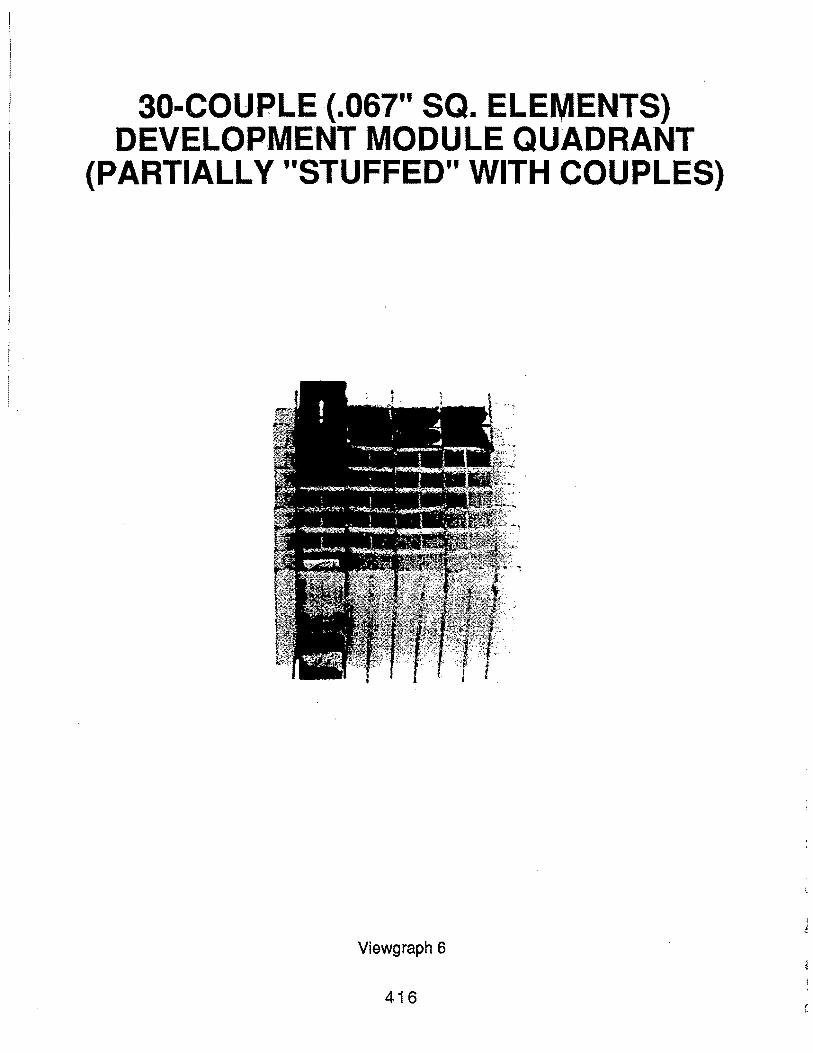
30-COUPLE (.067" SQ. ELEI\IIENTS) DEVELOPMENT MODULE QUADRANT
(PARTIALLY "STUFFED" WITH COUPLES)
Viewgraph 6
416
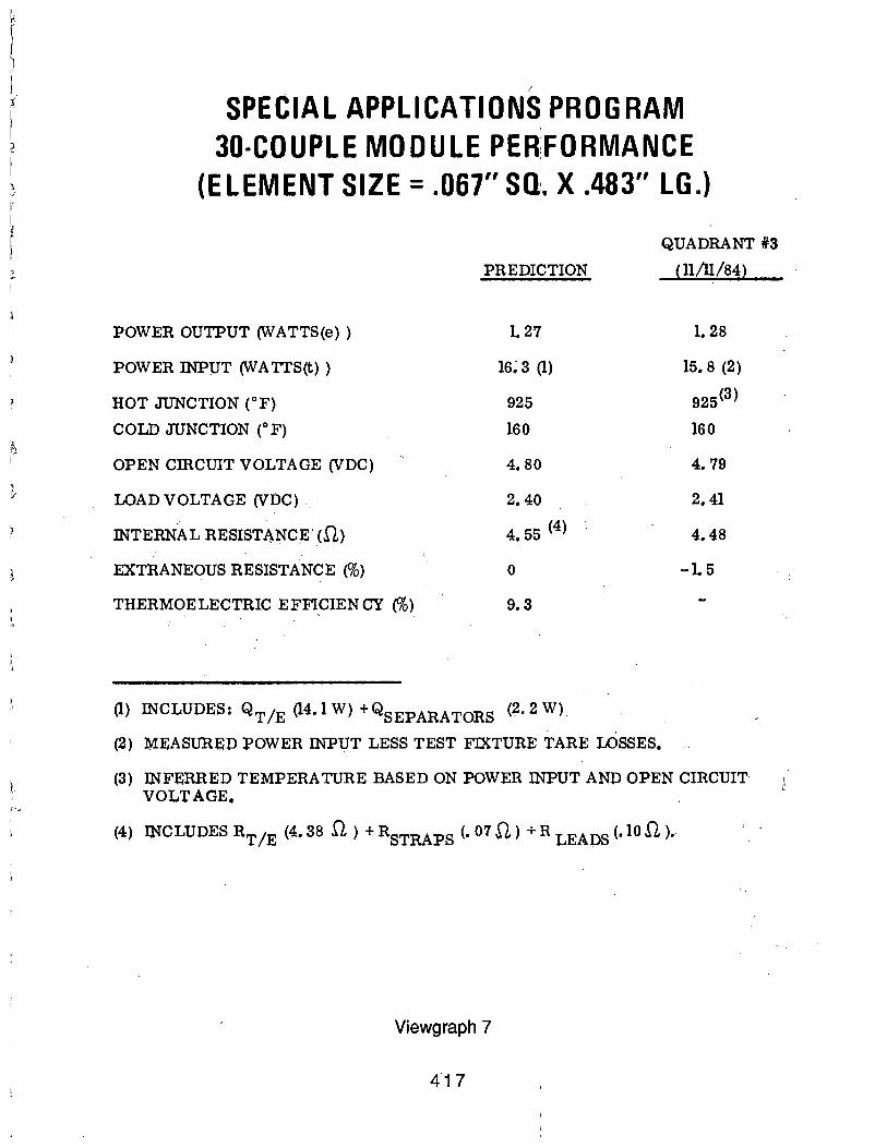
~ I
~ I
' ,. :/
f
SPECIAL APPLICATIONS PROGRAM 3D-COUPLE MODULE PER:FORMANCE
(ELEMENT SIZE= .067" SO~. X .483" LG.)
PREDICTION
POWER OUTPUT (WATTS(e)) L27
POWER INPU'T (WATTS(t)) 16~ 3 (1)
HOT JUNCTION (°F) 925
COLD JUNCTION (° F) 160
OPEN CffiCUIT VOLTAGE (VDC) 4.80
LOAD VOLTAGE (VDC) .. 2.40
INTERNAL RESISTANCE" (.0.) 4. 55 (4)
EXTRANEOUS RESISTANCE(%) 0
THERMOELECTRIC EFFICIENCY (%) 9. 3
(1) INCLUDES: QT/E (14• 1 W) +QSEPARATORS <2• 2 W)
(2) MEASURED POWER INPUT LESS TEST FIXTURE TARE LOSSES.
QUADRANT 13
(11/11/84)
1. 28
15. 8 (2)
925(3 )
160
4.79
2. 41
4.48
-L5
(3) INFERRED TEMPERATURE BASED ON POWER INPUT AND OPEN CIRCUIT VOLTAGE.
(4) INCLUDES RT /E (4. 38 fL ) + RSTRAPS (. 07 D,) + R LEADS (.10 fl. ).
Viewgraph 7
417

SPECIAL-APPLICATIONS TECHNOLOGY PARTIALLY ASSEMBLED MODULE ASSEMBLY
Viewgraph 8

c.o
SPECIAL APPLICATIONS PROGRAM 76-COUPLE DEVELOPMENT MODULE
HOTS IDE
SYNTH~NE_j . SEPARATOR (.Ol51N. THK. l
CERAMABOND FILLER (NOT SHOWN)
1:
1.410
L-----~----- ·--------
~.570 ~
Viewgraph 9
Cu WIRE S-HOE (.030 IN. DIA. l
CQD Sl DE
NO. ACTIVE COUPLES= 76 NO. POWER LEAD ASSYS. = 2
. ELEMENT LENGTH= .483·1N. ELEMENT SECT! 00 = . 077 IN. SQ. ELEMENT MATERIAL
N LEGS= TE1006 P LEGS= TAGS 85
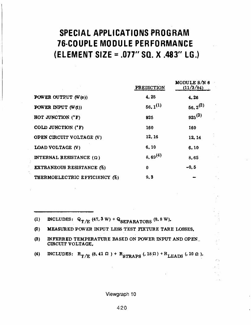
SPECIAL APPLICATIONS PROGRAM 76-COUPLE MODULE PERFORMANCE
(ELEMENT SIZE= .077" SO. X .483" LG.)
.MODULE SIN 6 PREDICTION ,11/S/84}
POWEll OUTP.UT (W (e)) 4.25 4.26
POWEll INPUT (W(t)) 56.1(1) 56. 2<2>
HOT JUNCTION (•F) 925 925(3)
COLD JU~CTION (•F) 160 160
OPEN CmCUIT VOLTAGE (V) 12.16 12.14
LOAD VOLTAGE (V) 6.10 6.10
lNTERNAL RESISTANCE ( 0 ) 8. 69<4> 8.65
. . EXTRANEOUS RESISTANCE (%) 0 -0.5
THERMOELECTRIC EFFICIENCY(%) 9. 3
(1) JNCLUDES: Q'i' IE (47. 3 W) + QSEPARA TORS (8. 8 W).
(2) MEASURED POWER INPUT LESS TEST FIXTURE TARE LOSSES.
(3) lNFERRED TEMPERATUR.E BASED ON POWER INPUT AND OPEN~ ClllCUIT VOLTAGE.
(4) INCLUDES: RT/E (8. 41 0 ) + llBTRAPS (.18.0) + RLEADS {.10 0 ).
Viewgraph 1 o
420
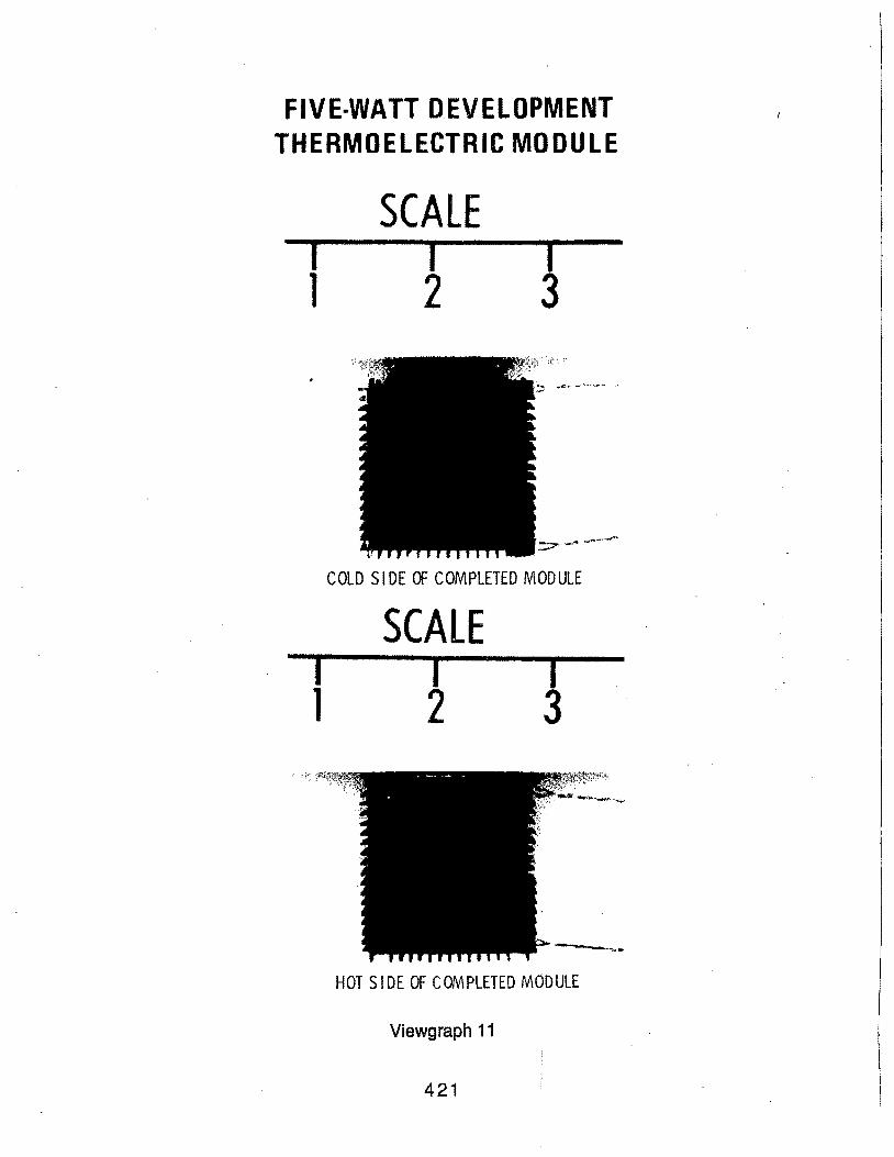
FIVE-WATT DEVELOPMENT THERMOELECTRIC MODULE
I l
I 1
SCALE I 2
COLD SIDE OF COMPLETED MODULE
SCAlE I 2
HOTS I DE OF COMPLETED MODULE
Viewgraph 11
421

k2J.oo5 I t
.564
k71 .oo5 I I
THERMOELECTRIC MODULE ARRANGEMENT
Viewgraph 12
CCl.D HOT SIDE SIDE
No. ACTIVE COUPLES = 126. No. INACTIVE COUPLES = 2 ELEMENT LENGTH = • 500 IN.
• ELEMENT SECT tON = • 063 IN. SQ. ELEMENT MATERIAL
N LEGS = TE1004 P LEGS= TAGS
SEPARATOR THt CKNESS = • 015 IN.
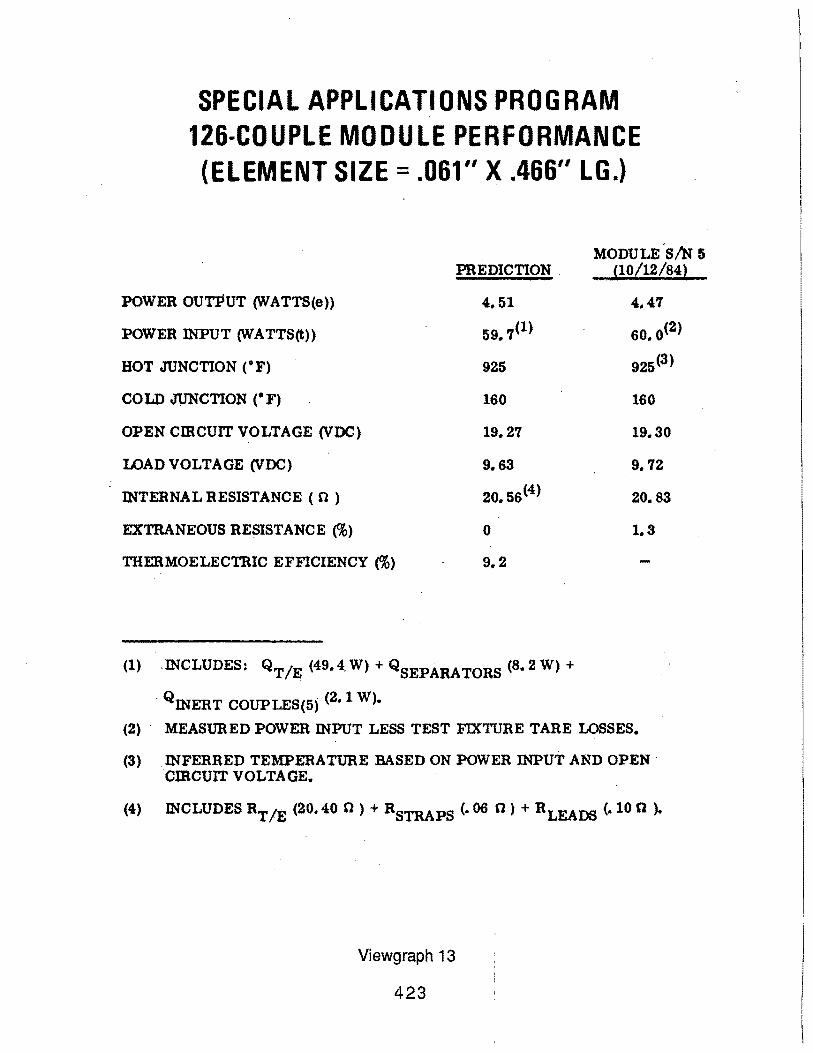
SPECIAL APPLICATIONS PROGRAM 126-COUPLE MODULE PERFORMANCE (ELEMENT SIZE= .061" X .466" LG.)
PREDICTION
POWER OUTPUT (WATTS(e)) 4.51
POWER INPUT (W A TTS(t)) 59. 7(l)
HOT JUNCTION (°F) 925
COLD JUNCTION (°F) 160
OPEN CIRCUIT VOLTAGE (VDC) 19.27
WAD VOLTAGE (VDC) 9.63
INTERNAL RESISTANCE ( 0) 20. 56(4)
EXTRANEOUS RESISTANCE (%) 0
THERMOELECTRIC EFFICIENCY (%) 9.2
(1) .INCLUDES: QT/E (49.4. W) + QSEPARATORS (8. 2 W) +
QINERT COUPLES(5) (2• 1 W).
MODULE ·s/N 5 {10/12/841
4.47
60. o<2>
925(3)
160
19.30
9. 72
20.83
1.3
(2) · MEASURED POWER INPUT LESS TEST FIXTURE TARE LOSSES.
(3) . INFERRED TEMPERATURE BASED ON POWER INPUT AND OPEN · CIRCUIT VOLTAGE.
(4) INCLUDES RT /E (20. 40 0 ) + RSTRAPS (. 06 0 ) + RLEAI>S (. 10 0 ).
Viewgraph 13
423
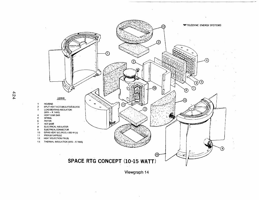
·--···---------------------------
"""TELEDYNE ENERGY SYSTEMS
~ 1\J ~ ~
I-OUSrG 2 SPLIT HEAT ACCUMULATOR BLOCK 3 LOAD BEARING INSULATION
(MIN - K 1400) 4 HEAT SINK BAR 5 SPRlNG 6 PISTON 7 HOTSHJE 9 ELECTRICAL INSULATOR 9 aECTRICAL~ECToR 10 GPHS HEAT SOURCE (-250 W (I)) 11 IRIDIUM CAPSULE 12 HEAT REJECTION FIN (6)
13 THERMAL INS\JLA TION (MIN-K 1800)
SPACE RTG CONCEPT (10-15 WATT)
Viewgraph 14

RADIOISOTOPE HEAT SOURCE
Fuel Pellet (Pu02)
Clad (lr)
· Impact Shell {FWPF*)
Insulator (CBCF* *)
Aeroshell (FWPF*)
*Fine-WvrRe Pierced Fabric) **Carbon-Bonded Carbon Fibers
426
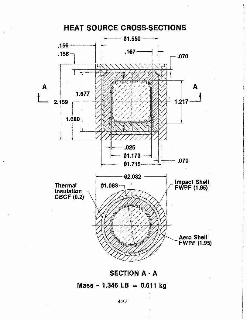
A
L
HEAT SOURCE CROSS-SECTIONS ,_____ 01.550 ---'----1
1.677 2.159 ........---\---
1.080
.167-----'~ .070
A
1.217_j
~- .070
Thermal Insulation CBCF (0.2)
1------ (&2.032 ----l
SECTION A· A
Mass - 1.346 LB = 0.611 kg
427
Impact Shell. FWPF (1.95) ·
Aero Shell FWPF (1.95)

EXPLODED VIEW OF MUL TICOUPLE (2.6 Watt, 3.5 Volt)
HEAT COLLECTOR (Graphite)
HOT SHOES (SiMo)
THERMOELECTRIC LEGS (SiGe/GaP)
COLD SHOES (Tungsten)
PAD (Graphite)
COLD STUD (Tungsten)
LEAD WIRES
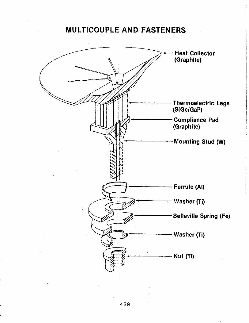
MULTICOUPLE AND FASTENERS
-Heat Collector (Graphite)
-----Thermoelectric Legs (SiGe/GaP)
-----Compliance Pad (Graphite)
------Mounting Stud (W)
-----Ferrule (AI)
----Washer (Ti)
-----Belleville Spring (Fe)
"i''l-+--.l>" -----Washer (Ti)
I
~------Nut (Ti)
~ I
429
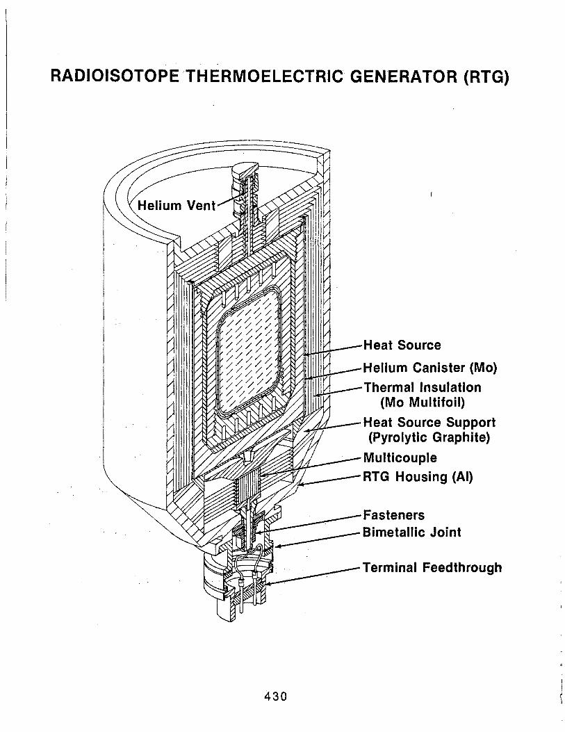
RADIOISOTOPE THERMOELECTRIC GEN'ERATOR (RTG)
430
Heat Source
Helium Canister (Mo)
Thermal Insulation (Mo Multifoil)
Heat Source Support (Pyrolytic Graphite)
Multicouple RTG Housing (AI)
Fasteners Bimetallic Joint
Terminal Feedthrough
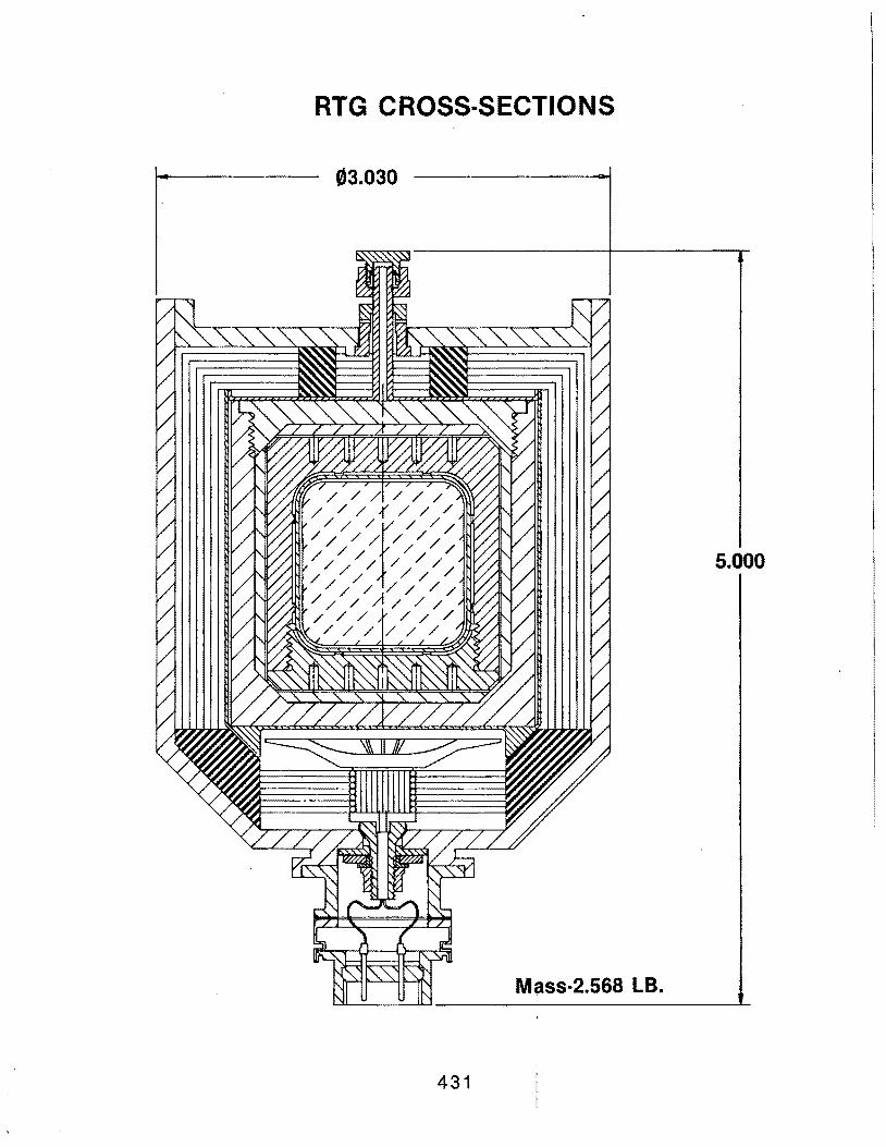
RTG CROSS-SECTIONS
03.030
5.000
Mass-2.568 LB.
431
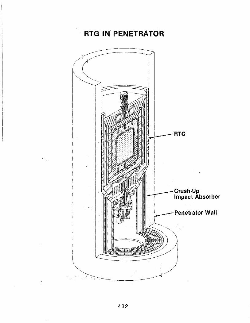
RTG IN PENETRATOR
RTG
Crush-Up Impact Absorber
Penetrator Wall
432
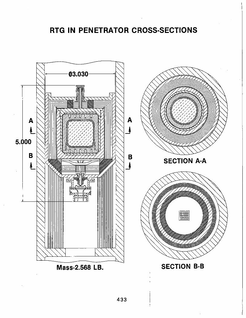
5.000
RTG IN PENETRATOR CROSS-SECTIONS
Mass-2.568 LB.
A
J
B j
433
SECTION A·A
SECTION B·B
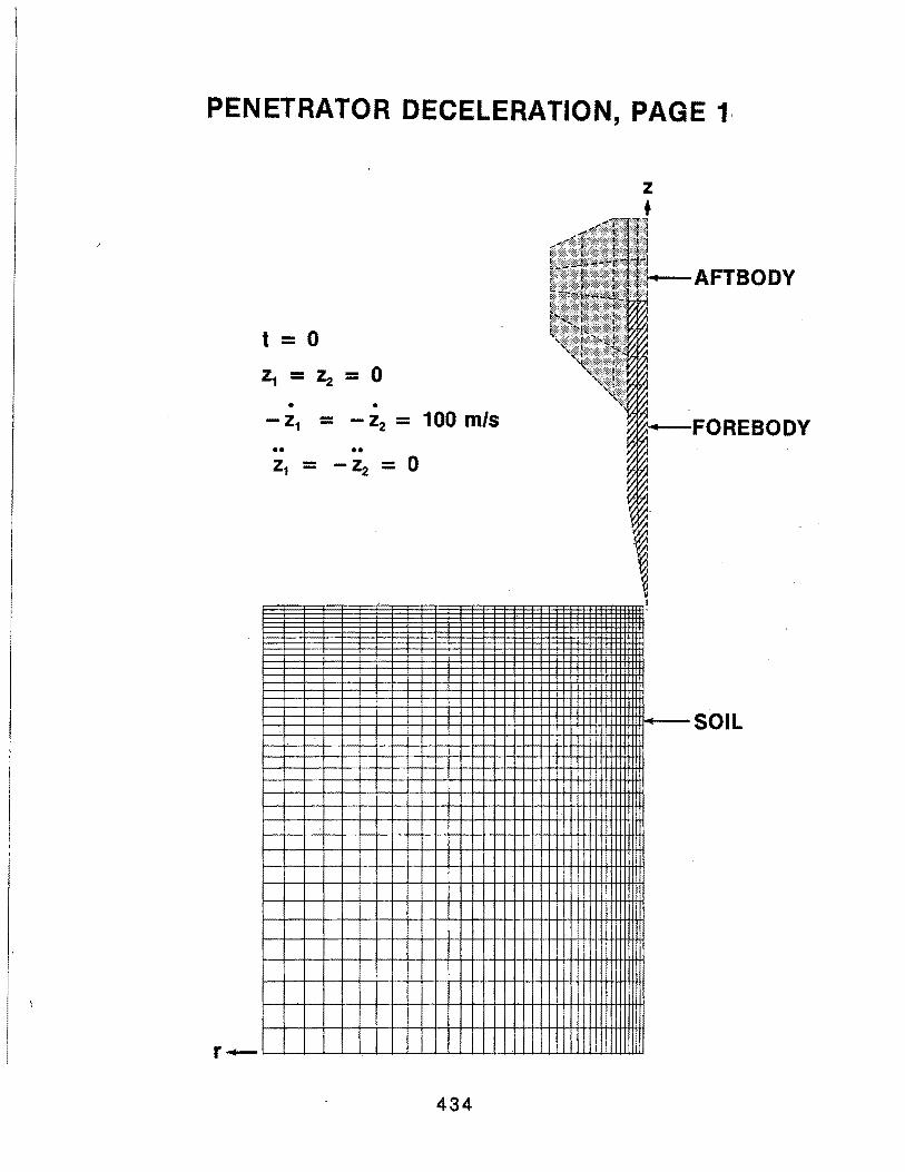
PENETRATOR DECELERATION, PAGE 1·
t = 0
• • - Z1 = - Z2 = 100 m/s
434
z f
REBODY
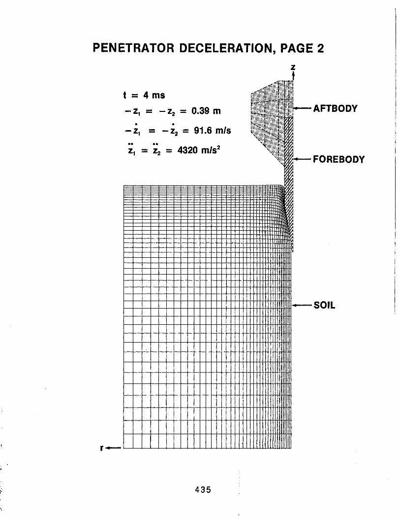
PENETRATOR DECELERATION, PAGE 2
z
t = 4 ms
-z1 = -z2 = 0.39 m AFTBODY • •
-z1 - - Z2 = 91.6 m/s -•• •• ~ z1 = z2 = 4320 m/s2 ~
~~ ~ ~ ~
~ ~
FOREBODY
v.
SOIL
435
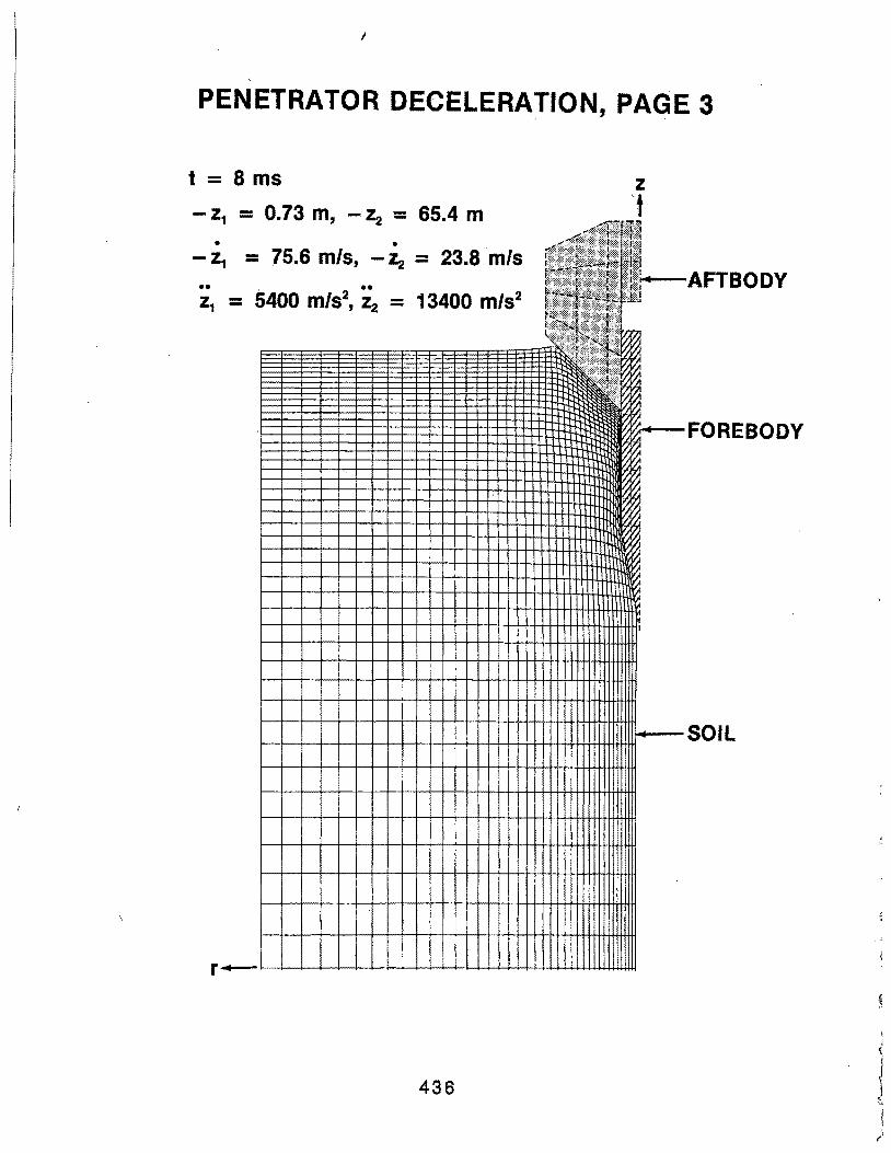
I
'
PENETRATOR DECELERATION, PAGE 3
t = 8 ms z
- z1 = 0 73 m - z - 65 4 m . ' 2 - . 't
• • -~ = 75.6 m/s, - z2 = 23.8 m/s
•• , 400 m/s2
, ~ = 13400 m/s2 AFTBODY
~ ~ ~ :m ~ ~
H FOREBODY
EfE ~ ~ ~
~
I I ttlli
SOIL
r,..._.. I
436
PENETRATOR DECELERATION, PAGE 4
t = 12 ms
- z1 = 1 005 m z - 0 697 m z • ' - 2 - . •
62.2 m/s, - z2 = 2.3 mls
AFTBODY •• ••
3100 m/s2, ~ = 4000 m/s2
~
~ ~
I FOREBODY
~ a ,,
I
SOIL
f-+--
437
PENETRATOR DECELERATION, PAGE 5
t = 16 ms z - z1 = 1.233 m, - z2 = 0.701 m
• • - z1 = 51.5 m/s, - Z2 = 1.0 m/s •• •• , AFTBODY z1 = 2700 m/s2
, z2 = 0
~FOREBODV
)
1....,_-SOIL
438

\ \ ,, ' i l
(
\
CJ Q) UJ -
DECELERATION OF AFTBOQY, VELOCITY VERSUS TIME AFTER IMPACT
80
E so >; -·-CJ 0 -Q)
> 40
20
-5 0 5 10
Time, msec
439
(.) CD Cl) -E
... >a -·-(.) 0 -CD >
. OECELERATION .. OF FOREBODY, VELOCITY VERSUS TIME AFTER IMPACT
80
60
40
0 5 10
Time, msec
440
15 . (
I
f ..
( ,!
i ·,
., '
I
u Q) en -E ~ -·-u 0 -Q)
>
60
40
DECELERATION OF FOREBODY, VELOCITY VERSUS PENiETRATION
0 0.5
Penetration, m
441
1.0