Intersecting and Trimming Parametric Meshes

on Finite�Element Shells�

Luiz Cristov�ao G� Coelhoy Marcelo Gattassy Luiz Henrique de Figueiredoz

Abstract

We present an algorithm for intersecting �nite�element meshes de�ned on parametric sur�face patches� The intersection curves are modeled precisely and both meshes are adjusted to thenewly formed borders� without unwanted reparametrizations� The algorithm is part of an inter�active shell modeling program that has been used in the design of large o�shore oil structures�To achieve good interactive response� we represent meshes with a topological data structurethat stores its entities in spatial indexing trees instead of linear lists� These trees speed up theintersection computations required to determine points of the trimming curves� moreover� whencombined with the topological information� they allow remeshing using only local queries�

keywords� surface intersection� �nite�element mesh generation� parametric representation�geometric modeling� topological data structures� constrained triangulation�

� Introduction

Surface modeling and mesh generation on surfaces are important problems in computer�aided ge�ometric design �CAGD�� specially in engineering applications that use the �nite�element methodfor analyzing shell structures� One way to build complex models is to take several simple surfacepatches and sew them together into a single surface� trimming excess parts away� If this modelingtechnique is to be e�ective� then the problem of computing the intersection between two patchesmust be solved eciently and robustly�We consider a modeling environment in which surface patches are interpolated from boundary

curves given in parametric form� Such surfaces are called Coons patches �� � The user providesdiscretizations for the boundary curves� which are then used to interpolate a mesh for the surface�We approach the surface intersection problem as a meshing problem� in the sense that we are

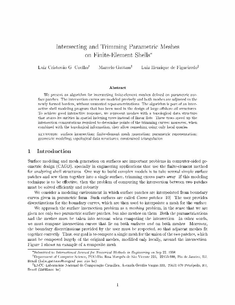
given not only two parametric surface patches� but also meshes on them� Both the parametrizationsand the meshes must be taken into account when computing the intersection� In other words�we must compute intersection curves that lie on both surfaces and on both meshes� Moreover�the boundary discretizations provided by the user must be respected� so that adjacent meshes �ttogether correctly� Thus� our goal is to compute a single mesh for the union of the two patches� whichmust be composed largely of the original meshes� modi�ed only locally� around the intersection�Figure � shows an example of a composite mesh�

�Submitted to International Journal for Numerical Methods in Engineering on Sep ��� �����yDepartment of Computer Science� PUC�Rio� Rua Marques de Sao Vicente ���� ���� ����� Rio de Janeiro� RJ�

Brazil �lula�gattass�tecgraf�puc�rio�br��zLNCC�Laborat�orio Nacional de Computa�cao Cient���ca� Avenida Get�ulio Vargas � ��������� Petr�opolis� RJ�

Brazil �lhf�lncc�br��

�

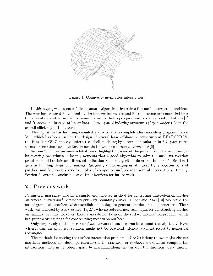
Figure �� Composite mesh after intersection�

In this paper� we present a fully automatic algorithm that solves this mesh intersection problem�The searches required for computing the intersection curves and for re�meshing are supported by atopological data structure whose main feature is that topological entities are stored in B�trees � and R��trees � � instead of linear lists� These spatial indexing structures play a major role in theoverall eciency of the algorithm�The algorithm has been implemented and is part of a complete shell modeling program� called

MG� which has been used in the design of several large o�shore oil structures at PETROBRAS�the Brazilian Oil Company� Interactive shell modeling by direct manipulation in �D space raisesseveral interesting user�interface issues that have been discussed elsewhere � �Section � reviews previous related work� highlighting some of the problems that arise in simple

intersecting procedures� The requirements that a good algorithm to solve the mesh intersectionproblem should satisfy are discussed in Section �� The algorithm described in detail in Section �aims at ful�lling these requirements� Section � shows examples of intersections between pairs ofpatches� and Section � shows examples of composite surfaces with several intersections� Finally�Section � contains conclusions and lists directions for future work�

� Previous work

Parametric mappings provide a simple and e�ective method for generating �nite�element mesheson general curved surface patches given by boundary curves� Haber and Abel �� pioneered theuse of graphical interfaces with trans�nite mappings to generate meshes in shell structures� Theirwork was followed by a few others ��� �� � who introduced new techniques for constructing mesheson trimmed patches� However� these works do not focus on the surface intersection problem� whichis a preprocessing stage for constructing meshes on surfaces�Only very rarely the intersection of two parametric surfaces can be computed analytically� Even

when it can� an analytical solution might not be practical� Hence� we must resort to numericaltechniques�The methods for solving the surface intersection problem in CAGD belong to two major classes�

marching methods and decomposition methods� Marching or continuation methods compute theintersection curve in �D object space by marching along the curve in the direction of its tangent

�

vector �� �� ��� �� � Decomposition or subdivision methods compute the trimming curves in �Dparameter space by recursively re�ning the solution at each step �� ��� �� �Previous solutions to the surface intersection problem work well in many cases� but do not

handle the mesh intersection problem as de�ned in Section �� An exception is the work of Lo �� �which motivated the present work� Lo �� proposed a simple algorithm for intersecting triangularmeshes that automatically rede�nes the meshes to adapt to the intersection curves� Lo�s solutiondoes not use the continuous parametric representation of the surfaces� and thus can be used easilyin most modeling systems� On the other hand� around regions of high curvature� the computedintersection points may not lie on the original surfaces� which may yield unacceptable results inmany shell problems�

� Algorithm requirements for mesh intersection

The well�known requirements for good solutions for the surface intersection problem in CAGD ���p� ��� must be re�ned for the mesh intersection problem� We believe that an ideal solution for themesh intersection problem should satisfy the following requirements�

Correctness� The computed intersection curves must lie on both surfaces� If the intersection curveslie only on the faces of the meshes but not on the surfaces� then the �nite�element analysis mayyield false or unacceptable results� The easiest way to guarantee correctness is to compute thetrimming curves in parametric space and then map them to object space�

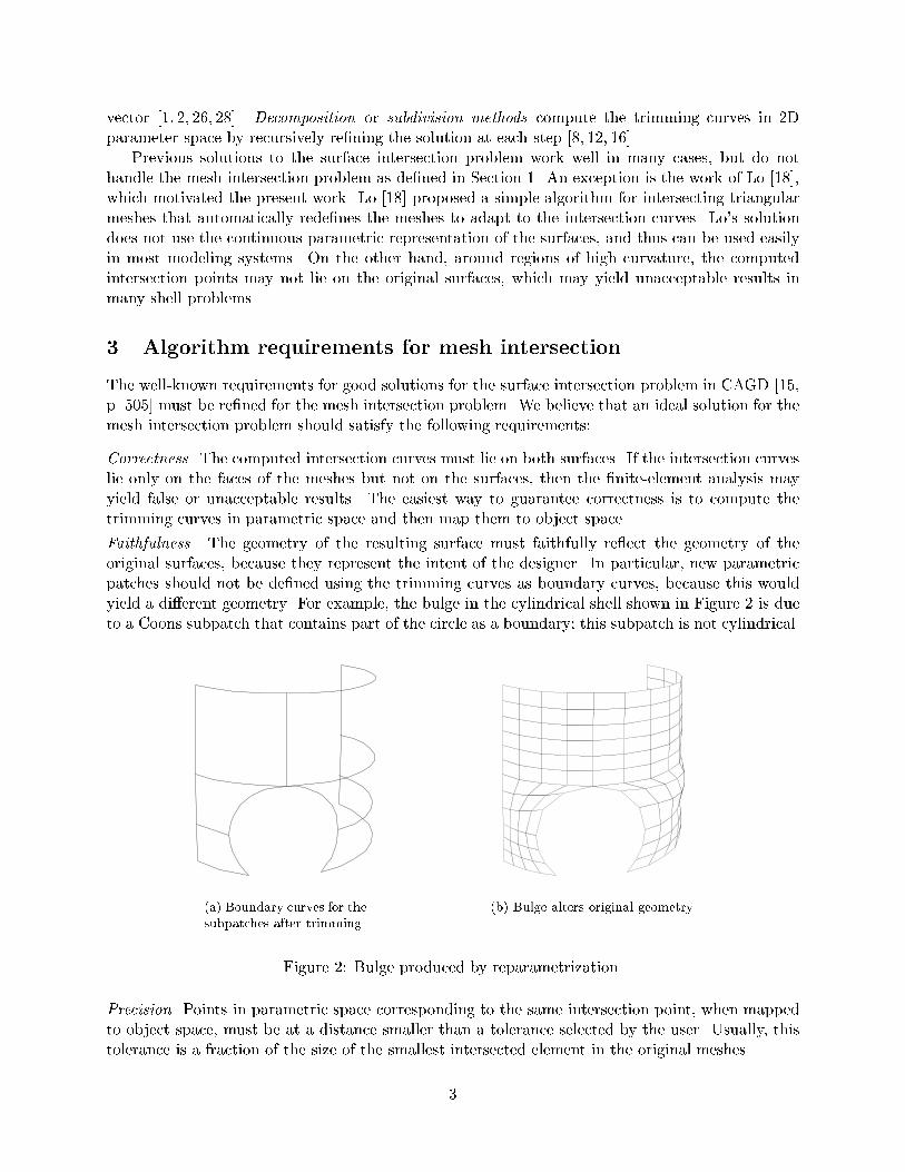
Faithfulness� The geometry of the resulting surface must faithfully re�ect the geometry of theoriginal surfaces� because they represent the intent of the designer� In particular� new parametricpatches should not be de�ned using the trimming curves as boundary curves� because this wouldyield a di�erent geometry� For example� the bulge in the cylindrical shell shown in Figure � is dueto a Coons subpatch that contains part of the circle as a boundary� this subpatch is not cylindrical�

�a� Boundary curves for thesubpatches after trimming�

�b� Bulge alters original geometry�

Figure �� Bulge produced by reparametrization�

Precision� Points in parametric space corresponding to the same intersection point� when mappedto object space� must be at a distance smaller than a tolerance selected by the user� Usually� thistolerance is a fraction of the size of the smallest intersected element in the original meshes�

�

Self control� The two meshes should be automatically rede�ned to include the intersection curvesand possibly exclude trimmed regions� The user should not be required to manually edit theresulting meshes�

Quality� The elements generated during re�meshing must have a good geometric shape and mustbe of the same average size as the elements in the original meshes� When the original mesheshave elements with very di�erent sizes� the resulting mesh may have elongated elements with sharpangular di�erences� if no corrections are made� A common technique for ensuring mesh quality isto run a post�processing smoothing step� Moreover� if smoothing is performed� then it should beautomatic� with no user intervention�

Locality� Only elements close to the intersection region should be modi�ed during re�meshing�Elements far from the intersection region should remain unaltered� Moreover� if smoothing is usedto improve mesh quality� then its e�ect should be local too�

Regions� The regions de�ned in parametric space by the trimming curves must be automaticallyidenti�ed� These regions may or may not take part in the �nal model� they can even have di�erentattributes �loads� materials� boundary conditions��

E�ciency� The time and space required for computing the intersection should be ideally linearin the number of elements around the intersection region� Algorithms that are quadratic in thetotal number of elements in the meshes are too slow for large meshes and are not appropriate forinteractive modeling�

Robustness� An arbitrary number of intersection curves may be generated� having di�erent geome�try� topology� and interpolation points� In particular� closed curves must be handled correctly� andmust yield regions with holes when trimmed�

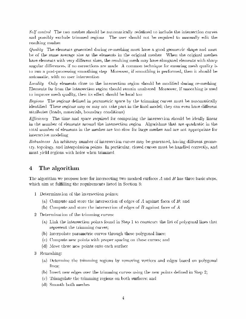
� The algorithm

The algorithm we propose here for intersecting two meshed surfaces A and B has three basic steps�which aim at ful�lling the requirements listed in Section ��

�� Determination of the intersection points�

�a� Compute and store the intersection of edges of A against faces of B� and

�b� Compute and store the intersection of edges of B against faces of A�

�� Determination of the trimming curves�

�a� Link the intersection points found in Step � to construct the list of polygonal lines thatrepresent the trimming curves�

�b� Interpolate parametric curves through these polygonal lines�

�c� Compute new points with proper spacing on these curves� and

�d� Move these new points onto each surface�

�� Remeshing�

�a� Determine the trimming regions by removing vertices and edges based on polygonallines�

�b� Insert new edges over the trimming curves using the new points de�ned in Step ��

�c� Triangulate the trimming regions on both surfaces� and

�d� Smooth both meshes�

�

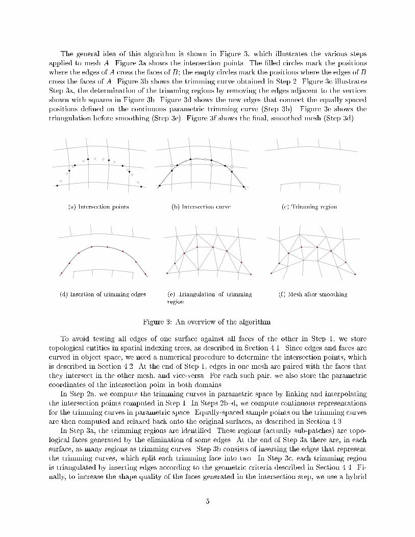
The general idea of this algorithm is shown in Figure �� which illustrates the various stepsapplied to mesh A� Figure �a shows the intersection points� The �lled circles mark the positionswhere the edges of A cross the faces of B� the empty circles mark the positions where the edges of Bcross the faces of A� Figure �b shows the trimming curve obtained in Step �� Figure �c illustratesStep �a� the determination of the trimming regions by removing the edges adjacent to the verticesshown with squares in Figure �b� Figure �d shows the new edges that connect the equally�spacedpositions de�ned on the continuous parametric trimming curve �Step �b�� Figure �e shows thetriangulation before smoothing �Step �c�� Figure �f shows the �nal� smoothed mesh �Step �d��

�a� Intersection points� �b� Intersection curve� �c� Trimming region�

�d� Insertion of trimming edges� �e� Triangulation of trimmingregion�

�f� Mesh after smoothing�

Figure �� An overview of the algorithm�

To avoid testing all edges of one surface against all faces of the other in Step �� we storetopological entities in spatial indexing trees� as described in Section ���� Since edges and faces arecurved in object space� we need a numerical procedure to determine the intersection points� whichis described in Section ���� At the end of Step �� edges in one mesh are paired with the faces thatthey intersect in the other mesh� and vice�versa� For each such pair� we also store the parametriccoordinates of the intersection point in both domains�In Step �a� we compute the trimming curves in parametric space by linking and interpolating

the intersection points computed in Step �� In Steps �b�d� we compute continuous representationsfor the trimming curves in parametric space� Equally�spaced sample points on the trimming curvesare then computed and relaxed back onto the original surfaces� as described in Section ����In Step �a� the trimming regions are identi�ed� These regions �actually sub�patches� are topo�

logical faces generated by the elimination of some edges� At the end of Step �a there are� in eachsurface� as many regions as trimming curves� Step �b consists of inserting the edges that representthe trimming curves� which split each trimming face into two� In Step �c� each trimming regionis triangulated by inserting edges according to the geometric criteria described in Section ���� Fi�nally� to increase the shape quality of the faces generated in the intersection step� we use a hybrid

�

smoothing technique that is done partially in parametric space and partially in �D� as described inSection ����

��� The data structure

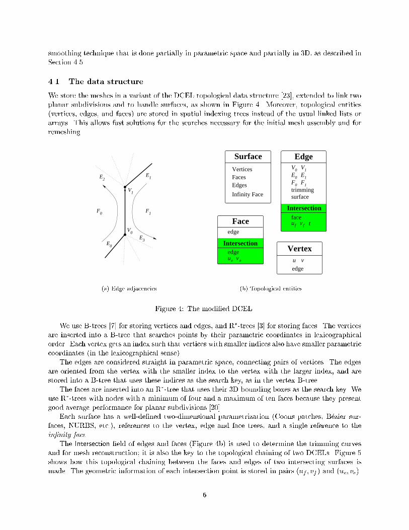
We store the meshes in a variant of the DCEL topological data structure �� � extended to link twoplanar subdivisions and to handle surfaces� as shown in Figure �� Moreover� topological entities�vertices� edges� and faces� are stored in spatial indexing trees instead of the usual linked lists orarrays� This allows fast solutions for the searches necessary for the initial mesh assembly and forremeshing�

E2E1

V1

F0 F1

E0

V0E3

�a� Edge adjacencies�

u v

edge

Vertex

Edges

Infinity Face

FacesVertices V0 V1

1E0E

1F0F

ue evedge

edge

uf v f t

surface

face

Edge

trimming

Surface

Face

Intersection

Intersection

�b� Topological entities�

Figure �� The modi�ed DCEL�

We use B�trees � for storing vertices and edges� and R��trees � for storing faces� The verticesare inserted into a B�tree that searches points by their parametric coordinates in lexicographicalorder� Each vertex gets an index such that vertices with smaller indices also have smaller parametriccoordinates �in the lexicographical sense��The edges are considered straight in parametric space� connecting pairs of vertices� The edges

are oriented from the vertex with the smaller index to the vertex with the larger index� and arestored into a B�tree that uses these indices as the search key� as in the vertex B�tree�The faces are inserted into an R��tree that uses their �D bounding boxes as the search key� We

use R��trees with nodes with a minimum of four and a maximum of ten faces because they presentgood average performance for planar subdivisions �� �Each surface has a well�de�ned two�dimensional parametrization �Coons patches� B�ezier sur�

faces� NURBS� etc��� references to the vertex� edge and face trees� and a single reference to thein�nity face�The Intersection �eld of edges and faces �Figure �b� is used to determine the trimming curves

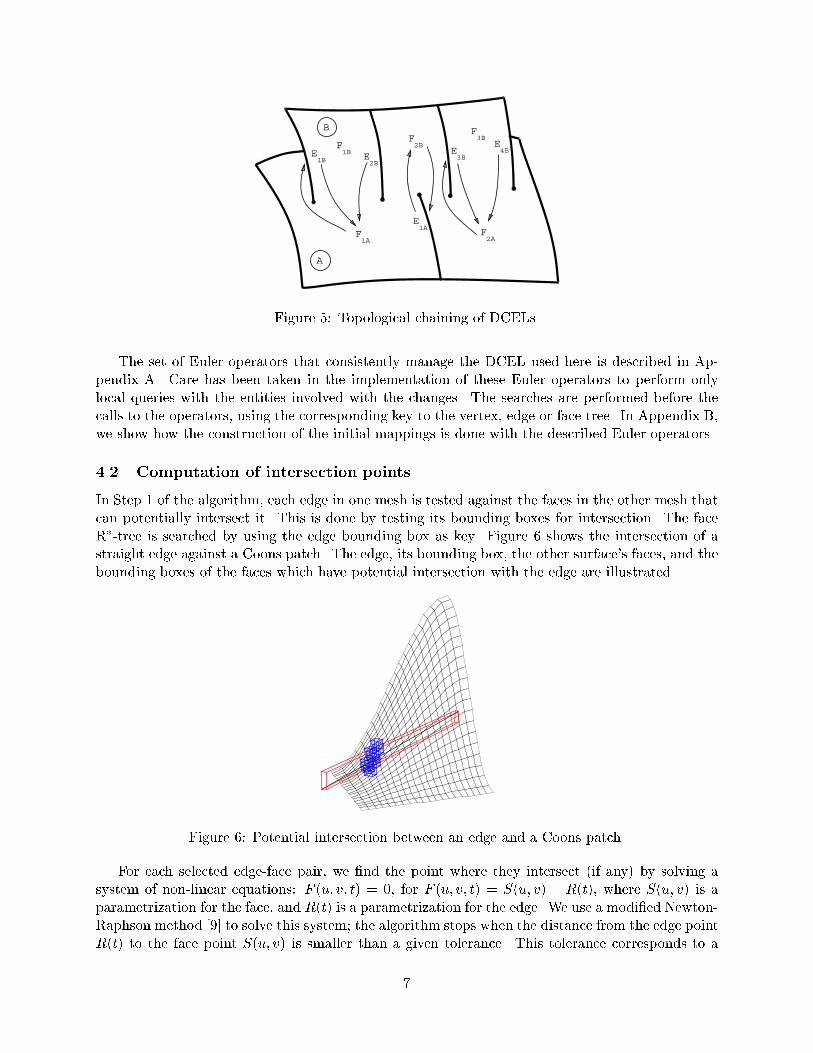
and for mesh reconstruction� it is also the key to the topological chaining of two DCELs� Figure �shows how this topological chaining between the faces and edges of two intersecting surfaces ismade� The geometric information of each intersection point is stored in pairs �uf � vf � and �ue� ve��

�

A

B

1BE

F1A

F1B

E4B

E2B

E1A

F2B

E3B

F2A

F3B

Figure �� Topological chaining of DCELs�

The set of Euler operators that consistently manage the DCEL used here is described in Ap�pendix A� Care has been taken in the implementation of these Euler operators to perform onlylocal queries with the entities involved with the changes� The searches are performed before thecalls to the operators� using the corresponding key to the vertex� edge or face tree� In Appendix B�we show how the construction of the initial mappings is done with the described Euler operators�

��� Computation of intersection points

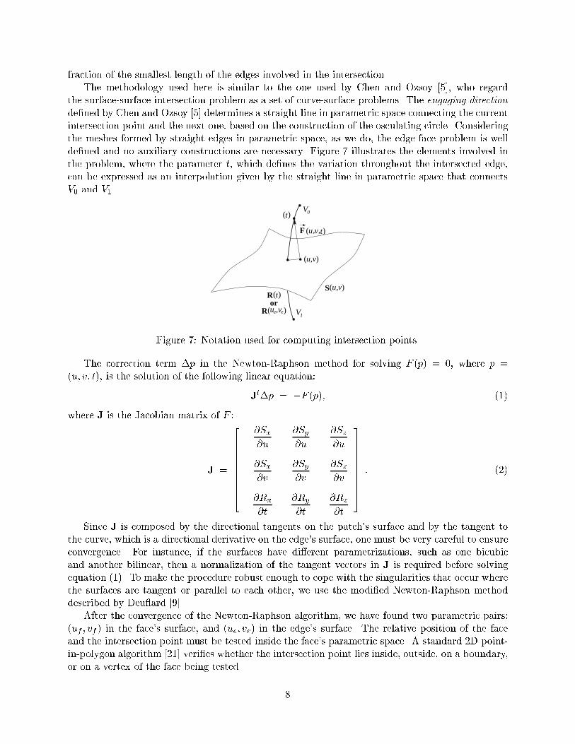
In Step � of the algorithm� each edge in one mesh is tested against the faces in the other mesh thatcan potentially intersect it� This is done by testing its bounding boxes for intersection� The faceR��tree is searched by using the edge bounding box as key� Figure � shows the intersection of astraight edge against a Coons patch� The edge� its bounding box� the other surface�s faces� and thebounding boxes of the faces which have potential intersection with the edge are illustrated�

Figure �� Potential intersection between an edge and a Coons patch�

For each selected edge�face pair� we �nd the point where they intersect �if any� by solving asystem of non�linear equations� F �u� v� t� � �� for F �u� v� t� � S�u� v� � R�t�� where S�u� v� is aparametrization for the face� and R�t� is a parametrization for the edge� We use a modi�ed Newton�Raphson method � to solve this system� the algorithm stops when the distance from the edge pointR�t� to the face point S�u� v� is smaller than a given tolerance� This tolerance corresponds to a

�

fraction of the smallest length of the edges involved in the intersection�The methodology used here is similar to the one used by Chen and Ozsoy � � who regard

the surface�surface intersection problem as a set of curve�surface problems� The engaging directionde�ned by Chen and Ozsoy � determines a straight line in parametric space connecting the currentintersection point and the next one� based on the construction of the osculating circle� Consideringthe meshes formed by straight edges in parametric space� as we do� the edge�face problem is wellde�ned and no auxiliary constructions are necessary� Figure � illustrates the elements involved inthe problem� where the parameter t� which de�nes the variation throughout the intersected edge�can be expressed as an interpolation given by the straight line in parametric space that connectsV� and V��

veue )R( ,

)R(t)(u vS ,

)(t

F (u,v t),

)(u v,

V0

V1

or

Figure �� Notation used for computing intersection points�

The correction term �p in the Newton�Raphson method for solving F �p� � �� where p ��u� v� t�� is the solution of the following linear equation�

Jt�p � �F �p�� ���

where J is the Jacobian matrix of F �

J �

�����������

�Sx

�u

�Sy

�u

�Sz

�u

�Sx

�v

�Sy

�v

�Sz

�v

��Rx

�t��Ry

�t��Rz

�t

�����������

� ���

Since J is composed by the directional tangents on the patch�s surface and by the tangent tothe curve� which is a directional derivative on the edge�s surface� one must be very careful to ensureconvergence� For instance� if the surfaces have di�erent parametrizations� such as one bicubicand another bilinear� then a normalization of the tangent vectors in J is required before solvingequation ���� To make the procedure robust enough to cope with the singularities that occur wherethe surfaces are tangent or parallel to each other� we use the modi�ed Newton�Raphson methoddescribed by Deu�ard � �After the convergence of the Newton�Raphson algorithm� we have found two parametric pairs�

�uf � vf � in the face�s surface� and �ue� ve� in the edge�s surface� The relative position of the faceand the intersection point must be tested inside the face�s parametric space� A standard �D point�in�polygon algorithm �� veri�es whether the intersection point lies inside� outside� on a boundary�or on a vertex of the face being tested�

�

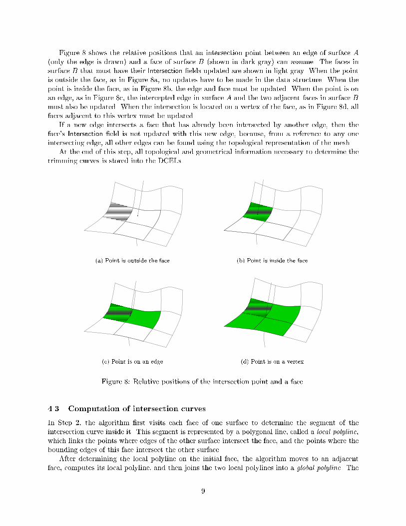
Figure � shows the relative positions that an intersection point between an edge of surface A�only the edge is drawn� and a face of surface B �shown in dark gray� can assume� The faces insurface B that must have their Intersection �elds updated are shown in light gray� When the pointis outside the face� as in Figure �a� no updates have to be made in the data structure� When thepoint is inside the face� as in Figure �b� the edge and face must be updated� When the point is onan edge� as in Figure �c� the intercepted edge in surface A and the two adjacent faces in surface Bmust also be updated� When the intersection is located on a vertex of the face� as in Figure �d� allfaces adjacent to this vertex must be updated�If a new edge intersects a face that has already been intersected by another edge� then the

face�s Intersection �eld is not updated with this new edge� because� from a reference to any oneintersecting edge� all other edges can be found using the topological representation of the mesh�At the end of this step� all topological and geometrical information necessary to determine the

trimming curves is stored into the DCELs�

���������������������������������������������������������������������������������

���������������������������������������������������������������������������������

�a� Point is outside the face�

������������������������������������������������������������������������

������������������������������������������������������������������������

�b� Point is inside the face�

���������������������������������������������������������������������������������

���������������������������������������������������������������������������������

�c� Point is on an edge�

���������������������������������������������������������������������������������

���������������������������������������������������������������������������������

�d� Point is on a vertex�

Figure �� Relative positions of the intersection point and a face�

��� Computation of intersection curves

In Step �� the algorithm �rst visits each face of one surface to determine the segment of theintersection curve inside it� This segment is represented by a polygonal line� called a local polyline�which links the points where edges of the other surface intersect the face� and the points where thebounding edges of this face intersect the other surface�After determining the local polyline on the initial face� the algorithm moves to an adjacent

face� computes its local polyline� and then joins the two local polylines into a global polyline� The

�

algorithm proceeds in this way until all adjacent faces have been visited� and a global polyline hasbeen completed�In the general case� the intersection of two patches may be formed by several disconnected

curves� In this case� Step �a �nds a global polyline for each component� after �nding the �rstglobal polyline� the algorithm searches for a new face whose Intersection is marked and that has notalready been visited� It then proceeds as before� and builds the corresponding global polyline�Step �a stops when all intersected faces in both meshes have been visited� Thus� all connected

components of the intersection are found with a single search through the intersected faces� Totake advantage of the R��tree that stores faces of surface A� the algorithm actually computes thebounding box of the intersection points found in Step � and� using spatial indexing� extracts onlythe faces that intersect this box�Local and global polylines are simply lists of points� Each point contains two references for

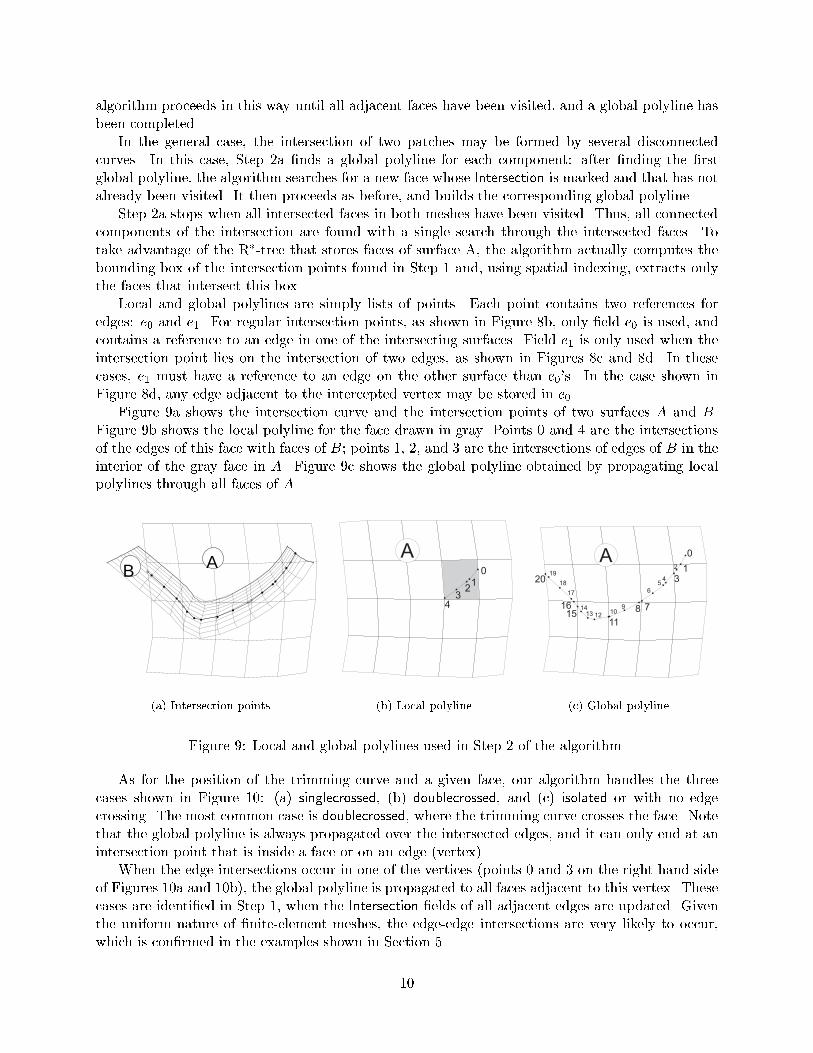
edges� e� and e�� For regular intersection points� as shown in Figure �b� only �eld e� is used� andcontains a reference to an edge in one of the intersecting surfaces� Field e� is only used when theintersection point lies on the intersection of two edges� as shown in Figures �c and �d� In thesecases� e� must have a reference to an edge on the other surface than e��s� In the case shown inFigure �d� any edge adjacent to the intercepted vertex may be stored in e��Figure �a shows the intersection curve and the intersection points of two surfaces A and B�

Figure �b shows the local polyline for the face drawn in gray� Points � and � are the intersectionsof the edges of this face with faces of B� points �� �� and � are the intersections of edges of B in theinterior of the gray face in A� Figure �c shows the global polyline obtained by propagating localpolylines through all faces of A�

AB

�a� Intersection points� �b� Local polyline� �c� Global polyline�

Figure �� Local and global polylines used in Step � of the algorithm�

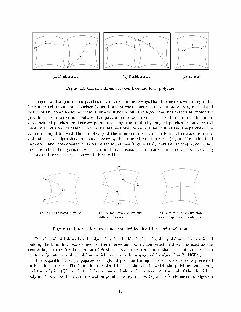
As for the position of the trimming curve and a given face� our algorithm handles the threecases shown in Figure ��� �a� singlecrossed� �b� doublecrossed� and �c� isolated or with no edgecrossing� The most common case is doublecrossed� where the trimming curve crosses the face� Notethat the global polyline is always propagated over the intersected edges� and it can only end at anintersection point that is inside a face or on an edge �vertex��When the edge intersections occur in one of the vertices �points � and � on the right�hand side

of Figures ��a and ��b�� the global polyline is propagated to all faces adjacent to this vertex� Thesecases are identi�ed in Step �� when the Intersection �elds of all adjacent edges are updated� Giventhe uniform nature of �nite�element meshes� the edge�edge intersections are very likely to occur�which is con�rmed in the examples shown in Section ��

��

0

12

1

2

0

�a� Singlecrossed�

0

1 2

3

01

2

3

�b� Doublecrossed�

12

0

�c� Isolated�

Figure ��� Classi�cations between face and local polyline�

In general� two parametric patches may intersect in more ways than the ones shown in Figure ���The intersection can be a surface �when both patches concur�� one or more curves� an isolatedpoint� or any combination of these� Our goal is not to build an algorithm that detects all geometricpossibilities of intersections between two patches� since we are concerned with remeshing� Instancesof coincident patches and isolated points resulting from mutually tangent patches are not treatedhere� We focus on the cases in which the intersections are well�de�ned curves and the patches havea mesh compatible with the complexity of the intersection curves� In terms of entities from thedata structure� edges that are crossed twice by the same intersection curve �Figure ��a�� identi�edin Step �� and faces crossed by two intersection curves �Figure ��b�� identi�ed in Step �� could notbe handled by the algorithm with the initial discretization� Both cases can be solved by increasingthe mesh discretization� as shown in Figure ��c�

1

2

0

�a� An edge crossed twice�

0

2

0

1

2

1

�b� A face crossed by twodi�erent curves�

�c� Greater discretizationsolves topological problems�

Figure ��� Intersections cases not handled by algorithm� and a solution�

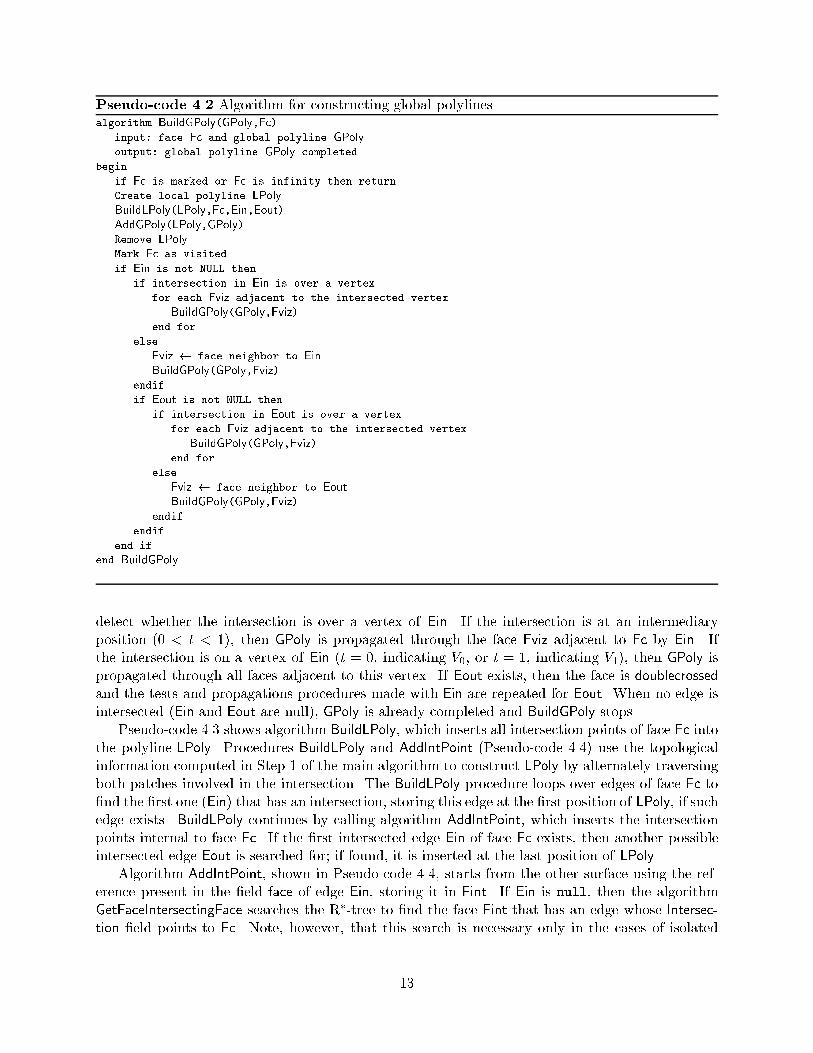
Pseudo�code ��� describes the algorithm that builds the list of global polylines� As mentionedbefore� the bounding box de�ned by the intersection points computed in Step � is used as thesearch key in the for loop in BuildGPolyList� Each intersected face that has not already beenvisited originates a global polyline� which is recursively propagated by algorithm BuildGPoly�The algorithm that propagates each global polyline through the surface�s faces is presented

in Pseudo�code ���� The input for the algorithm are the face in which the polyline starts �Fc��and the polyline �GPoly� that will be propagated along the surface� At the end of the algorithm�polyline GPoly has� for each intersection point� one �e�� or two �e� and e�� references to edges on

��

Pseudo�code ��� Algorithm for constructing the global polyline list�algorithm BuildGPolyList�S�

input� surface S

output� list of global polylines L

begin

Initialize L as empty

for each Face intersecting box containing all intersection points do

if Face has Intersection and Face is not visited then

Create new GPoly

BuildGPoly�Face�GPoly�

Add GPoly to L

end if

end for

end BuildGPolyList

the surfaces� This information is also used in the remeshing step �Step � of the main algorithm��without the need to perform searches to identify the relative position of the trimming curves andthe faces and edges on both patches�Note that recursion stops in two cases� when the face Fc is marked� that is� when it has already

been visited by the algorithm� and when Fc is the in�nity face� because polyline GPoly has thenreached the boundary of the mesh� The algorithm initially creates the local polyline LPoly� whichis a list of intersection points� like GPoly� in which all existing intersections with Fc are stored� Thealgorithm BuildLPoly creates LPoly of Fc� and returns references to the possible intersected edges�Ein and Eout� which correspond to the �rst and second intersected edges of Fc� respectively� EdgesEin and Eout are used to classify the face Fc according to the cases shown in Figure ���The intersection points in LPoly are then inserted into one of the two extremities of GPoly by

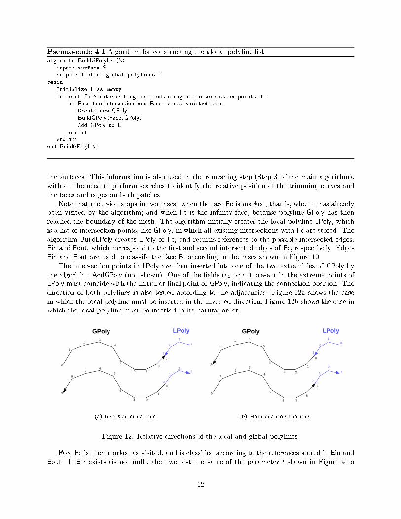
the algorithm AddGPoly �not shown�� One of the �elds �e� or e�� present in the extreme points ofLPoly must coincide with the initial or �nal point of GPoly� indicating the connection position� Thedirection of both polylines is also tested according to the adjacencies� Figure ��a shows the casein which the local polyline must be inserted in the inverted direction� Figure ��b shows the case inwhich the local polyline must be inserted in its natural order�

GPoly LPoly

0

1

23

4

5

6 7

8

9

0

1

2

3

0

1

23

0

1

23

4

5

67

8

9

�a� Inversion situations�

GPoly LPoly

0

1

23

4

5

6 7

8

9

0

1

2

3

01

2

3

0

1

23

4

5

67

8

9

�b� Maintenance situations�

Figure ��� Relative directions of the local and global polylines�

Face Fc is then marked as visited� and is classi�ed according to the references stored in Ein andEout� If Ein exists �is not null�� then we test the value of the parameter t shown in Figure � to

��

Pseudo�code ��� Algorithm for constructing global polylines�algorithm BuildGPoly�GPoly�Fc�

input� face Fc and global polyline GPoly

output� global polyline GPoly completed

begin

if Fc is marked or Fc is infinity then return

Create local polyline LPoly

BuildLPoly�LPoly�Fc�Ein�Eout�

AddGPoly�LPoly�GPoly�

Remove LPoly

Mark Fc as visited

if Ein is not NULL then

if intersection in Ein is over a vertex

for each Fviz adjacent to the intersected vertex

BuildGPoly�GPoly�Fviz�

end for

else

Fviz � face neighbor to Ein

BuildGPoly�GPoly�Fviz�

endif

if Eout is not NULL then

if intersection in Eout is over a vertex

for each Fviz adjacent to the intersected vertex

BuildGPoly�GPoly�Fviz�

end for

else

Fviz � face neighbor to Eout

BuildGPoly�GPoly�Fviz�

endif

endif

end if

end BuildGPoly

detect whether the intersection is over a vertex of Ein� If the intersection is at an intermediaryposition �� � t � ��� then GPoly is propagated through the face Fviz adjacent to Fc by Ein� Ifthe intersection is on a vertex of Ein �t � �� indicating V�� or t � �� indicating V��� then GPoly ispropagated through all faces adjacent to this vertex� If Eout exists� then the face is doublecrossedand the tests and propagations procedures made with Ein are repeated for Eout� When no edge isintersected �Ein and Eout are null�� GPoly is already completed and BuildGPoly stops�Pseudo�code ��� shows algorithm BuildLPoly� which inserts all intersection points of face Fc into

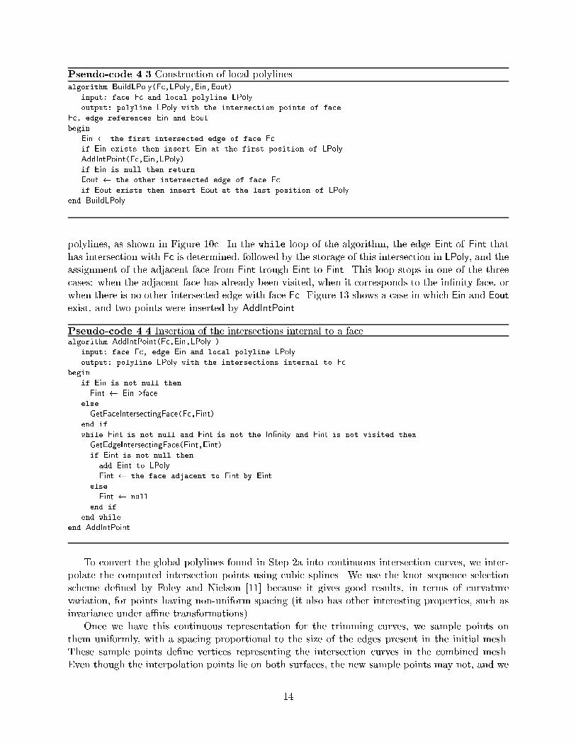
the polyline LPoly� Procedures BuildLPoly and AddIntPoint �Pseudo�code ���� use the topologicalinformation computed in Step � of the main algorithm to construct LPoly by alternately traversingboth patches involved in the intersection� The BuildLPoly procedure loops over edges of face Fc to�nd the �rst one �Ein� that has an intersection� storing this edge at the �rst position of LPoly� if suchedge exists� BuildLPoly continues by calling algorithm AddIntPoint� which inserts the intersectionpoints internal to face Fc� If the �rst intersected edge Ein of face Fc exists� then another possibleintersected edge Eout is searched for� if found� it is inserted at the last position of LPoly�Algorithm AddIntPoint� shown in Pseudo�code ���� starts from the other surface using the ref�

erence present in the �eld face of edge Ein� storing it in Fint� If Ein is null� then the algorithmGetFaceIntersectingFace searches the R��tree to �nd the face Fint that has an edge whose Intersec�tion �eld points to Fc� Note� however� that this search is necessary only in the cases of isolated

��

Pseudo�code ��� Construction of local polylines�algorithm BuildLPoly�Fc�LPoly�Ein�Eout�

input� face Fc and local polyline LPoly

output� polyline LPoly with the intersection points of face

Fc� edge references Ein and Eout

begin

Ein � the first intersected edge of face Fc

if Ein exists then insert Ein at the first position of LPoly

AddIntPoint�Fc�Ein�LPoly�

if Ein is null then return

Eout � the other intersected edge of face Fc

if Eout exists then insert Eout at the last position of LPoly

end BuildLPoly

polylines� as shown in Figure ��c� In the while loop of the algorithm� the edge Eint of Fint thathas intersection with Fc is determined� followed by the storage of this intersection in LPoly� and theassignment of the adjacent face from Fint trough Eint to Fint� This loop stops in one of the threecases� when the adjacent face has already been visited� when it corresponds to the in�nity face� orwhen there is no other intersected edge with face Fc� Figure �� shows a case in which Ein and Eoutexist� and two points were inserted by AddIntPoint�

Pseudo�code ��� Insertion of the intersections internal to a face�algorithm AddIntPoint�Fc�Ein�LPoly �

input� face Fc� edge Ein and local polyline LPoly

output� polyline LPoly with the intersections internal to Fc

begin

if Ein is not null then

Fint � Ein�face

else

GetFaceIntersectingFace�Fc�Fint�

end if

while Fint is not null and Fint is not the In�nity and Fint is not visited then

GetEdgeIntersectingFace�Fint�Eint�

if Eint is not null then

add Eint to LPoly

Fint � the face adjacent to Fint by Eint

else

Fint � null

end if

end while

end AddIntPoint

To convert the global polylines found in Step �a into continuous intersection curves� we inter�polate the computed intersection points using cubic splines� We use the knot sequence selectionscheme de�ned by Foley and Nielson �� because it gives good results� in terms of curvaturevariation� for points having non�uniform spacing �it also has other interesting properties� such asinvariance under ane transformations��Once we have this continuous representation for the trimming curves� we sample points on

them uniformly� with a spacing proportional to the size of the edges present in the initial mesh�These sample points de�ne vertices representing the intersection curves in the combined mesh�Even though the interpolation points lie on both surfaces� the new sample points may not� and we

��

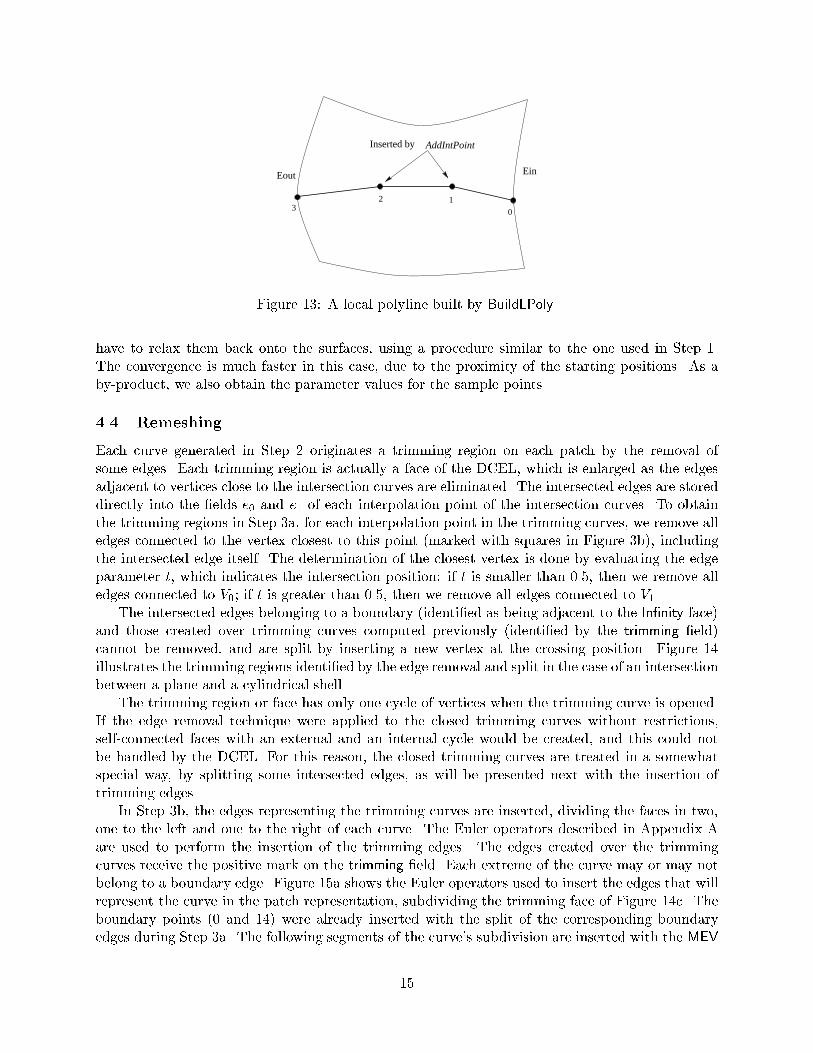
Inserted by AddIntPoint

32 1

0

EinEout

Figure ��� A local polyline built by BuildLPoly�

have to relax them back onto the surfaces� using a procedure similar to the one used in Step ��The convergence is much faster in this case� due to the proximity of the starting positions� As aby�product� we also obtain the parameter values for the sample points�

��� Remeshing

Each curve generated in Step � originates a trimming region on each patch by the removal ofsome edges� Each trimming region is actually a face of the DCEL� which is enlarged as the edgesadjacent to vertices close to the intersection curves are eliminated� The intersected edges are storeddirectly into the �elds e� and e� of each interpolation point of the intersection curves� To obtainthe trimming regions in Step �a� for each interpolation point in the trimming curves� we remove alledges connected to the vertex closest to this point �marked with squares in Figure �b�� includingthe intersected edge itself� The determination of the closest vertex is done by evaluating the edgeparameter t� which indicates the intersection position� if t is smaller than ���� then we remove alledges connected to V�� if t is greater than ���� then we remove all edges connected to V��The intersected edges belonging to a boundary �identi�ed as being adjacent to the In�nity face�

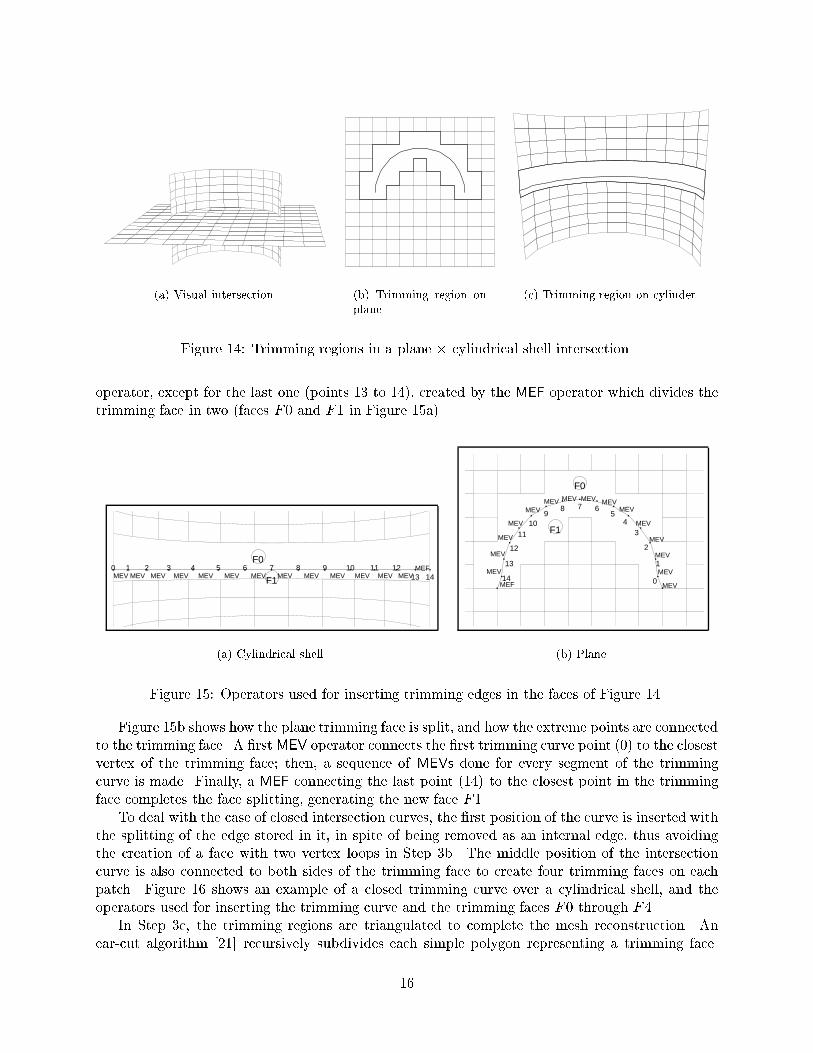
and those created over trimming curves computed previously �identi�ed by the trimming �eld�cannot be removed� and are split by inserting a new vertex at the crossing position� Figure ��illustrates the trimming regions identi�ed by the edge removal and split in the case of an intersectionbetween a plane and a cylindrical shell�The trimming region or face has only one cycle of vertices when the trimming curve is opened�

If the edge removal technique were applied to the closed trimming curves without restrictions�self�connected faces with an external and an internal cycle would be created� and this could notbe handled by the DCEL� For this reason� the closed trimming curves are treated in a somewhatspecial way� by splitting some intersected edges� as will be presented next with the insertion oftrimming edges�In Step �b� the edges representing the trimming curves are inserted� dividing the faces in two�

one to the left and one to the right of each curve� The Euler operators described in Appendix Aare used to perform the insertion of the trimming edges� The edges created over the trimmingcurves receive the positive mark on the trimming �eld� Each extreme of the curve may or may notbelong to a boundary edge� Figure ��a shows the Euler operators used to insert the edges that willrepresent the curve in the patch representation� subdividing the trimming face of Figure ��c� Theboundary points �� and ��� were already inserted with the split of the corresponding boundaryedges during Step �a� The following segments of the curve�s subdivision are inserted with the MEV

��

�a� Visual intersection� �b� Trimming region onplane�

�c� Trimming region on cylinder�

Figure ��� Trimming regions in a plane � cylindrical shell intersection�

operator� except for the last one �points �� to ���� created by the MEF operator which divides thetrimming face in two �faces F� and F� in Figure ��a��

MEV0

MEV1

MEV2

MEV3

MEV4

MEV5

MEV6

MEVF1

F07

MEV8

MEV9

MEV10

MEV11

MEV12

13MEF

14

�a� Cylindrical shell�

MEV0

MEV1

MEV2

MEV3

MEV

4

MEV

5

MEV

6MEV

7MEV

8MEV 9MEV 10

MEV 11

MEV12

13MEV

14MEVMEF

F0

F1

�b� Plane�

Figure ��� Operators used for inserting trimming edges in the faces of Figure ���

Figure ��b shows how the plane trimming face is split� and how the extreme points are connectedto the trimming face� A �rstMEV operator connects the �rst trimming curve point ��� to the closestvertex of the trimming face� then� a sequence of MEVs done for every segment of the trimmingcurve is made� Finally� a MEF connecting the last point ���� to the closest point in the trimmingface completes the face splitting� generating the new face F��To deal with the case of closed intersection curves� the �rst position of the curve is inserted with

the splitting of the edge stored in it� in spite of being removed as an internal edge� thus avoidingthe creation of a face with two vertex loops in Step �b� The middle position of the intersectioncurve is also connected to both sides of the trimming face to create four trimming faces on eachpatch� Figure �� shows an example of a closed trimming curve over a cylindrical shell� and theoperators used for inserting the trimming curve and the trimming faces F� through F��In Step �c� the trimming regions are triangulated to complete the mesh reconstruction� An

ear�cut algorithm �� recursively subdivides each simple polygon representing a trimming face�

��

MEV 0

SEMV

MEV1

MEV2

MEV

3

MEV

4

MEV

5

MEV

6

MEV

7

MEV

8

MEV

9

MEV10MEV

11MEF

F0

F1 F2F3

MEF

MEV12MEV13

MEV14

MEV15

MEV

16

MEV

17

MEV

18

MEV

19

MEV

2021MEF

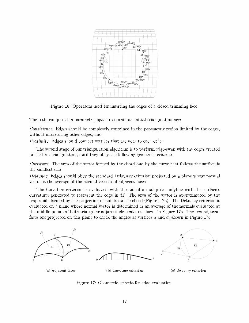
Figure ��� Operators used for inserting the edges of a closed trimming face�

The tests computed in parametric space to obtain an initial triangulation are�

Consistency� Edges should be completely contained in the parametric region limited by the edges�without intersecting other edges� and

Proximity� Edges should connect vertices that are near to each other�

The second stage of our triangulation algorithm is to perform edge�swap with the edges createdin the �rst triangulation� until they obey the following geometric criteria�

Curvature� The area of the sector formed by the chord and by the curve that follows the surface isthe smallest one�

Delaunay� Edges should obey the standard Delaunay criterion projected on a plane whose normalvector is the average of the normal vectors of adjacent faces�

The Curvature criterion is evaluated with the aid of an adaptive polyline with the surface�scurvature� generated to represent the edge in �D� The area of the sector is approximated by thetrapezoids formed by the projection of points on the chord �Figure ��b�� The Delaunay criterion isevaluated on a plane whose normal vector is determined as an average of the normals evaluated atthe middle points of both triangular adjacent elements� as shown in Figure ��a� The two adjacentfaces are projected on this plane to check the angles at vertices a and d� shown in Figure ��c�

a b

c

d

n1n2

F1 F2

�a� Adjacent faces�

b c

�b� Curvature criterion�

a

b

c

d

F1F2

�c� Delaunay criterion�

Figure ��� Geometric criteria for edge evaluation�

��

The triangulation algorithm uses these criteria in the order in which they were presented for thefollowing reasons� First� the trimming regions may present sharp curvatures� where planar criteria�like Delaunay� may not give good results� Furthermore� in �nite�element meshes over surfaceswith sharp curvatures� the best models are those whose edges obey the curvature more than theDelaunay criterion� Second� the Curvature criterion alone may not be adequate� as is the case ofplanar surfaces� And third� trimming regions in planar surfaces subdivided by edges which onlyobey the Consistency criterion may be transformed into a constrained Delaunay triangulation byan algorithm which makes edge swap �� with the Delaunay criterion�For these reasons� the basic steps of the algorithm for triangulating a trimming face are�

�� Obtain an initial triangulation by using the Consistency and Proximity criteria by recursivelysubdividing the trimming face�

�� Make edge swap on the edges created on Step � according to the Curvature criterion� Ifthe curvatures of both edges are identical� then the Delaunay criterion is used to settle theproblem�

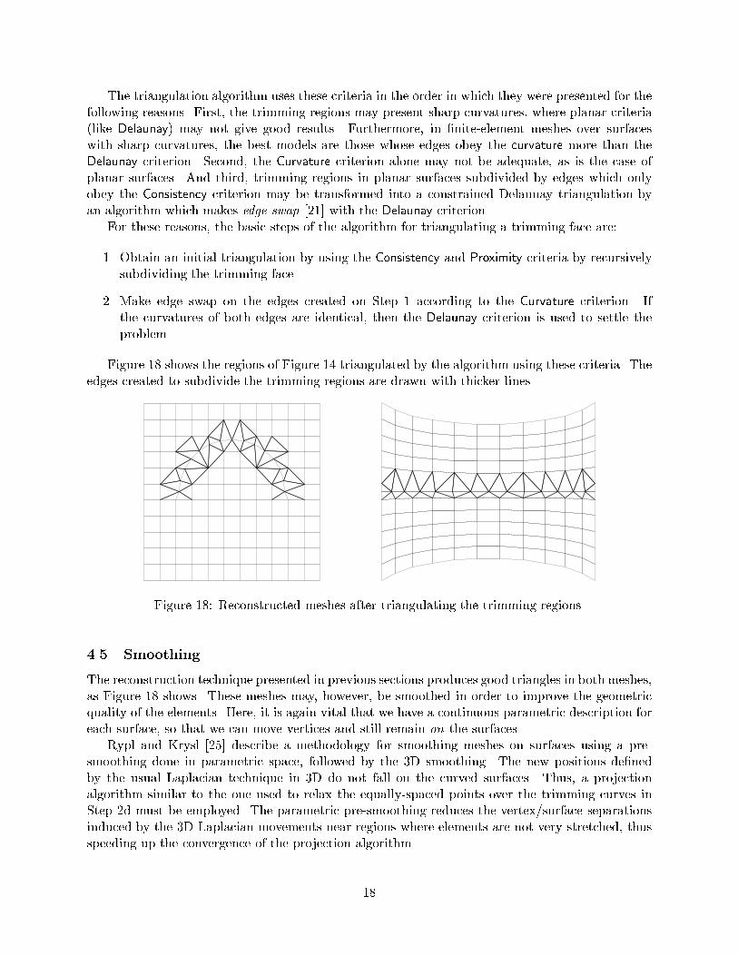
Figure �� shows the regions of Figure �� triangulated by the algorithm using these criteria� Theedges created to subdivide the trimming regions are drawn with thicker lines�

Figure ��� Reconstructed meshes after triangulating the trimming regions�

��� Smoothing

The reconstruction technique presented in previous sections produces good triangles in both meshes�as Figure �� shows� These meshes may� however� be smoothed in order to improve the geometricquality of the elements� Here� it is again vital that we have a continuous parametric description foreach surface� so that we can move vertices and still remain on the surfaces�Rypl and Krysl �� describe a methodology for smoothing meshes on surfaces using a pre�

smoothing done in parametric space� followed by the �D smoothing� The new positions de�nedby the usual Laplacian technique in �D do not fall on the curved surfaces� Thus� a projectionalgorithm similar to the one used to relax the equally�spaced points over the trimming curves inStep �d must be employed� The parametric pre�smoothing reduces the vertex�surface separationsinduced by the �D Laplacian movements near regions where elements are not very stretched� thusspeeding up the convergence of the projection algorithm�

��

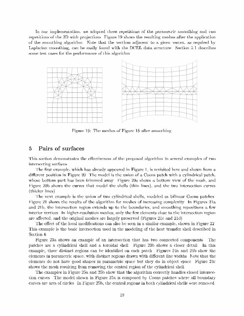
In our implementation� we adopted three repetitions of the parametric smoothing and tworepetitions of the �D with projections� Figure �� shows the resulting meshes after the applicationof the smoothing algorithm� Note that the vertices adjacent to a given vertex� as required byLaplacian smoothing� can be easily found with the DCEL data structure� Section ��� describessome test cases for the performance of this algorithm�

Figure ��� The meshes of Figure �� after smoothing�

� Pairs of surfaces

This section demonstrates the e�ectiveness of the proposed algorithm in several examples of twointersecting surfaces�The �rst example� which has already appeared in Figure �� is revisited here and shown from a

di�erent position in Figure ��� The model is the union of a Coons patch with a cylindrical patch�whose bottom part has been trimmed away� Figure ��a shows a bottom view of the mesh� andFigure ��b shows the curves that model the shells �thin lines�� and the two intersection curves�thicker lines��The next example is the union of two cylindrical shells� modeled as bilinear Coons patches�

Figure �� shows the results of the algorithm for meshes of increasing complexity� In Figures ��aand ��b� the intersection region extends up to the boundaries� and smoothing repositions a fewinterior vertices� In higher�resolution meshes� only the few elements close to the intersection regionare a�ected� and the original meshes are largely preserved �Figures ��c and ��d��The e�ect of the local modi�cations can also be seen in a similar example� shown in Figure ���

This example is the basic intersection used in the modeling of the heat transfer shell described inSection ��Figure ��a shows an example of an intersection that has two connected components� The

patches are a cylindrical shell and a toroidal shell� Figure ��b shows a closer detail� In thisexample� three distinct regions can be identi�ed on each patch� Figures ��a and ��b show theelements in parametric space� with distinct regions drawn with di�erent line widths� Note that theelements do not have good shapes in parametric space but they do in object space� Figure ��cshows the mesh resulting from removing the central region of the cylindrical shell�The examples in Figure ��a and ��b show that the algorithm correctly handles closed intersec�

tion curves� The model shown in Figure ��a is composed by Coons patches where all boundarycurves are arcs of circles� In Figure ��b� the central regions in both cylindrical shells were removed�

��

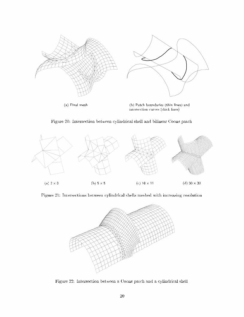
�a� Final mesh� �b� Patch boundaries �thin lines� andintersection curves �thick lines��

Figure ��� Intersection between cylindrical shell and bilinear Coons patch�

�a� �� � �b� �� �� �c� �� � ��� �d� �� ��

Figure ��� Intersections between cylindrical shells meshed with increasing resolution�

Figure ��� Intersection between a Coons patch and a cylindrical shell�

��

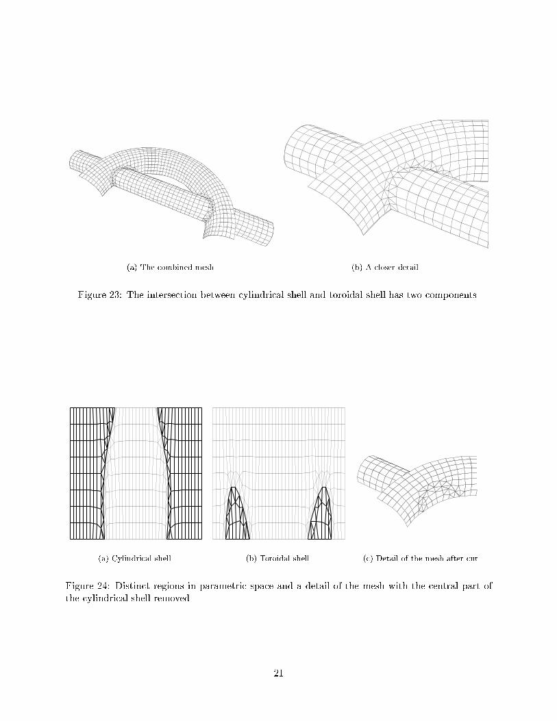
�a� The combined mesh� �b� A closer detail�

Figure ��� The intersection between cylindrical shell and toroidal shell has two components�

�a� Cylindrical shell� �b� Toroidal shell� �c� Detail of the mesh after cut�

Figure ��� Distinct regions in parametric space and a detail of the mesh with the central part ofthe cylindrical shell removed�

��

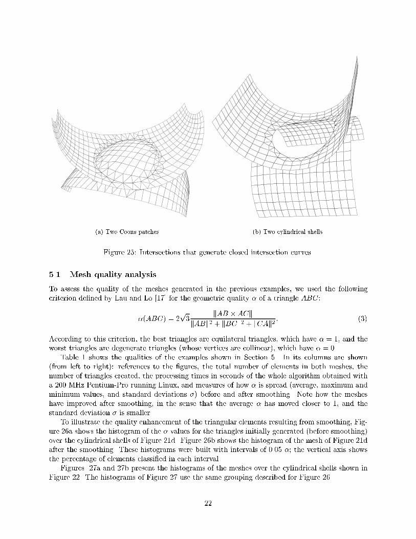
�a� Two Coons patches� �b� Two cylindrical shells�

Figure ��� Intersections that generate closed intersection curves�

��� Mesh quality analysis

To assess the quality of the meshes generated in the previous examples� we used the followingcriterion de�ned by Lau and Lo �� for the geometric quality � of a triangle ABC�

��ABC� � �p�

kAB �ACkkABk� � kBCk� � kCAk� � ���

According to this criterion� the best triangles are equilateral triangles� which have � � �� and theworst triangles are degenerate triangles �whose vertices are collinear�� which have � � ��Table � shows the qualities of the examples shown in Section �� In its columns are shown

�from left to right�� references to the �gures� the total number of elements in both meshes� thenumber of triangles created� the processing times in seconds of the whole algorithm obtained witha ��� MHz Pentium�Pro running Linux� and measures of how � is spread �average� maximum andminimum values� and standard deviations �� before and after smoothing� Note how the mesheshave improved after smoothing� in the sense that the average � has moved closer to �� and thestandard deviation � is smaller�To illustrate the quality enhancement of the triangular elements resulting from smoothing� Fig�

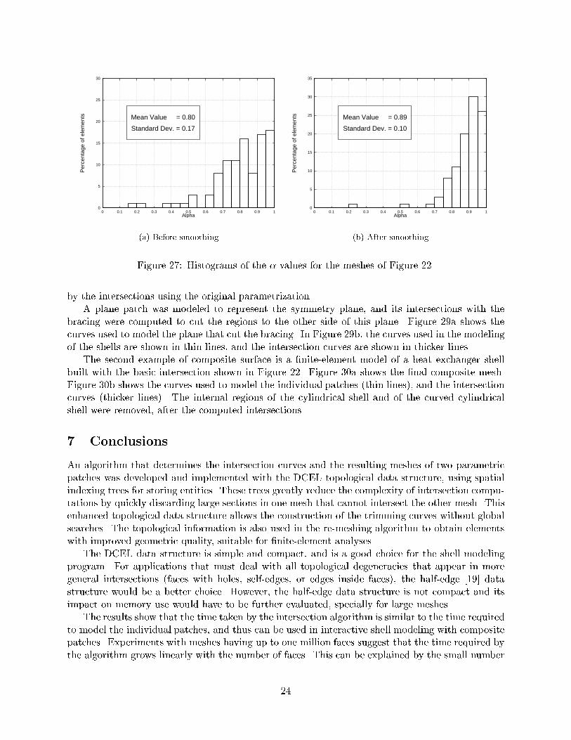
ure ��a shows the histogram of the � values for the triangles initially generated �before smoothing�over the cylindrical shells of Figure ��d� Figure ��b shows the histogram of the mesh of Figure ��dafter the smoothing� These histograms were built with intervals of ���� �� the vertical axis showsthe percentage of elements classi�ed in each interval�Figures ��a and ��b present the histograms of the meshes over the cylindrical shells shown in

Figure ��� The histograms of Figure �� use the same grouping described for Figure ���

��

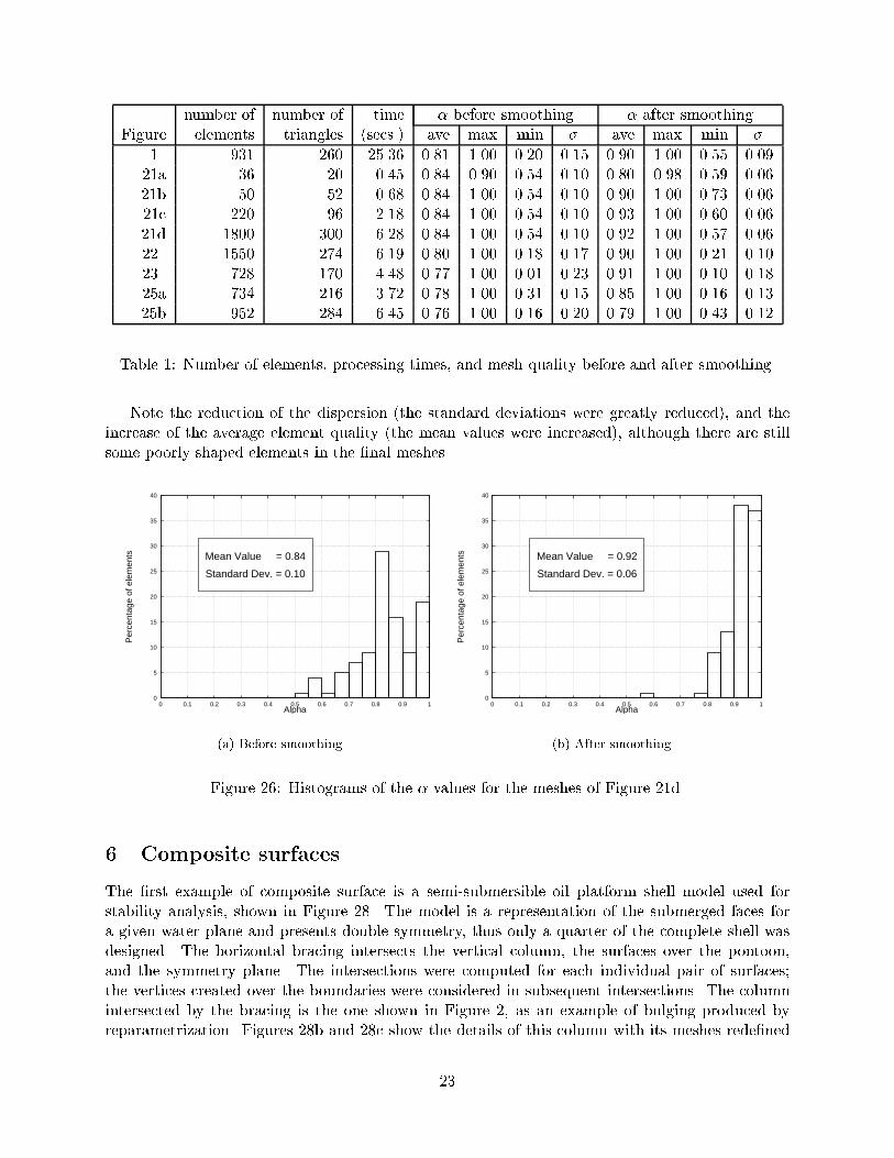
number of number of time � before smoothing � after smoothingFigure elements triangles �secs�� ave max min � ave max min �

� ��� ��� ����� ���� ���� ���� ���� ���� ���� ���� ������a �� �� ���� ���� ���� ���� ���� ���� ���� ���� ������b �� �� ���� ���� ���� ���� ���� ���� ���� ���� ������c ��� �� ���� ���� ���� ���� ���� ���� ���� ���� ������d ���� ��� ���� ���� ���� ���� ���� ���� ���� ���� ������ ���� ��� ���� ���� ���� ���� ���� ���� ���� ���� ������ ��� ��� ���� ���� ���� ���� ���� ���� ���� ���� ������a ��� ��� ���� ���� ���� ���� ���� ���� ���� ���� ������b ��� ��� ���� ���� ���� ���� ���� ���� ���� ���� ����

Table �� Number of elements� processing times� and mesh quality before and after smoothing�

Note the reduction of the dispersion �the standard deviations were greatly reduced�� and theincrease of the average element quality �the mean values were increased�� although there are stillsome poorly shaped elements in the �nal meshes�

0

5

10

15

20

25

30

35

40

0 0.1 0.2 0.3 0.4 0.5 0.6 0.7 0.8 0.9 1

Per

cent

age

of e

lem

ents

Alpha

Mean Value = 0.84

Standard Dev. = 0.10

�a� Before smoothing�

0

5

10

15

20

25

30

35

40

0 0.1 0.2 0.3 0.4 0.5 0.6 0.7 0.8 0.9 1

Per

cent

age

of e

lem

ents

Alpha

Mean Value = 0.92

Standard Dev. = 0.06

�b� After smoothing�

Figure ��� Histograms of the � values for the meshes of Figure ��d�

� Composite surfaces

The �rst example of composite surface is a semi�submersible oil platform shell model used forstability analysis� shown in Figure ��� The model is a representation of the submerged faces fora given water plane and presents double symmetry� thus only a quarter of the complete shell wasdesigned� The horizontal bracing intersects the vertical column� the surfaces over the pontoon�and the symmetry plane� The intersections were computed for each individual pair of surfaces�the vertices created over the boundaries were considered in subsequent intersections� The columnintersected by the bracing is the one shown in Figure �� as an example of bulging produced byreparametrization� Figures ��b and ��c show the details of this column with its meshes rede�ned

��

0

5

10

15

20

25

30

0 0.1 0.2 0.3 0.4 0.5 0.6 0.7 0.8 0.9 1

Per

cent

age

of e

lem

ents

Alpha

Mean Value = 0.80

Standard Dev. = 0.17

�a� Before smoothing�

0

5

10

15

20

25

30

35

0 0.1 0.2 0.3 0.4 0.5 0.6 0.7 0.8 0.9 1

Per

cent

age

of e

lem

ents

Alpha

Mean Value = 0.89

Standard Dev. = 0.10

�b� After smoothing�

Figure ��� Histograms of the � values for the meshes of Figure ���

by the intersections using the original parametrization�A plane patch was modeled to represent the symmetry plane� and its intersections with the

bracing were computed to cut the regions to the other side of this plane� Figure ��a shows thecurves used to model the plane that cut the bracing� In Figure ��b� the curves used in the modelingof the shells are shown in thin lines� and the intersection curves are shown in thicker lines�The second example of composite surface is a �nite�element model of a heat exchanger shell

built with the basic intersection shown in Figure ��� Figure ��a shows the �nal composite mesh�Figure ��b shows the curves used to model the individual patches �thin lines�� and the intersectioncurves �thicker lines�� The internal regions of the cylindrical shell and of the curved cylindricalshell were removed� after the computed intersections�

� Conclusions

An algorithm that determines the intersection curves and the resulting meshes of two parametricpatches was developed and implemented with the DCEL topological data structure� using spatialindexing trees for storing entities� These trees greatly reduce the complexity of intersection compu�tations by quickly discarding large sections in one mesh that cannot intersect the other mesh� Thisenhanced topological data structure allows the construction of the trimming curves without globalsearches� The topological information is also used in the re�meshing algorithm to obtain elementswith improved geometric quality� suitable for �nite�element analyses�The DCEL data structure is simple and compact� and is a good choice for the shell modeling

program� For applications that must deal with all topological degeneracies that appear in moregeneral intersections �faces with holes� self�edges� or edges inside faces�� the half�edge �� datastructure would be a better choice� However� the half�edge data structure is not compact and itsimpact on memory use would have to be further evaluated� specially for large meshes�The results show that the time taken by the intersection algorithm is similar to the time required

to model the individual patches� and thus can be used in interactive shell modeling with compositepatches� Experiments with meshes having up to one million faces suggest that the time required bythe algorithm grows linearly with the number of faces� This can be explained by the small number

��

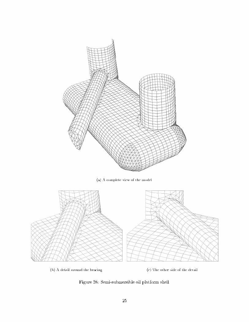
�a� A complete view of the model�

�b� A detail around the bracing� �c� The other side of the detail�

Figure ��� Semi�submersible oil platform shell�

��

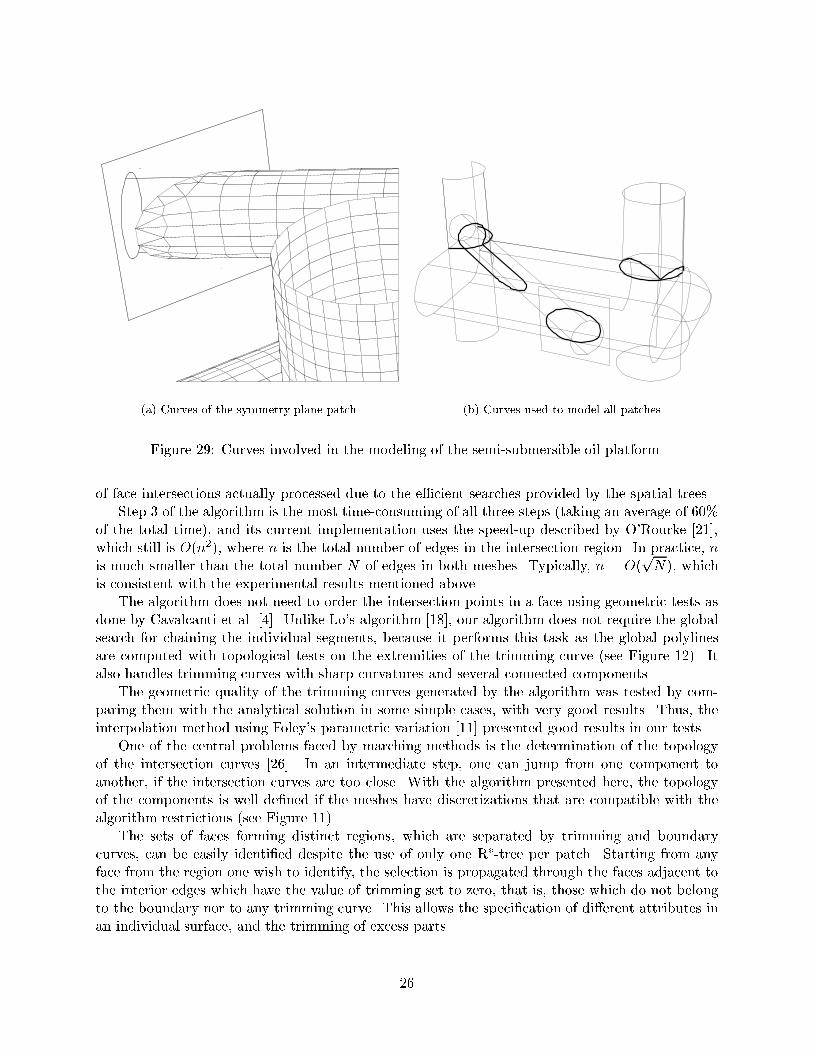
�a� Curves of the symmetry plane patch� �b� Curves used to model all patches�

Figure ��� Curves involved in the modeling of the semi�submersible oil platform�

of face intersections actually processed due to the ecient searches provided by the spatial trees�Step � of the algorithm is the most time�consuming of all three steps �taking an average of ��

of the total time�� and its current implementation uses the speed�up described by O�Rourke �� �which still is O�n��� where n is the total number of edges in the intersection region� In practice� nis much smaller than the total number N of edges in both meshes� Typically� n � O�

pN�� which

is consistent with the experimental results mentioned above�The algorithm does not need to order the intersection points in a face using geometric tests as

done by Cavalcanti et al� � � Unlike Lo�s algorithm �� � our algorithm does not require the globalsearch for chaining the individual segments� because it performs this task as the global polylinesare computed with topological tests on the extremities of the trimming curve �see Figure ���� Italso handles trimming curves with sharp curvatures and several connected components�The geometric quality of the trimming curves generated by the algorithm was tested by com�

paring them with the analytical solution in some simple cases� with very good results� Thus� theinterpolation method using Foley�s parametric variation �� presented good results in our tests�One of the central problems faced by marching methods is the determination of the topology

of the intersection curves �� � In an intermediate step� one can jump from one component toanother� if the intersection curves are too close� With the algorithm presented here� the topologyof the components is well de�ned if the meshes have discretizations that are compatible with thealgorithm restrictions �see Figure ����The sets of faces forming distinct regions� which are separated by trimming and boundary

curves� can be easily identi�ed despite the use of only one R��tree per patch� Starting from anyface from the region one wish to identify� the selection is propagated through the faces adjacent tothe interior edges which have the value of trimming set to zero� that is� those which do not belongto the boundary nor to any trimming curve� This allows the speci�cation of di�erent attributes inan individual surface� and the trimming of excess parts�

��

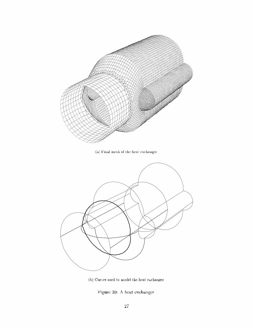
�a� Final mesh of the heat exchanger�

�b� Curves used to model the heat exchanger�

Figure ��� A heat exchanger�

��

The models shown in Figures �� and �� show that the algorithm can be used to model complexcomposite surfaces with few intersection operations� These examples also show that most elementsof the mesh kept their original aspects� and those adjacent to the intersected elements had theirvertices moved to enhance geometric quality�We are currently working on mesh uniformization� converting triangular elements into quadri�

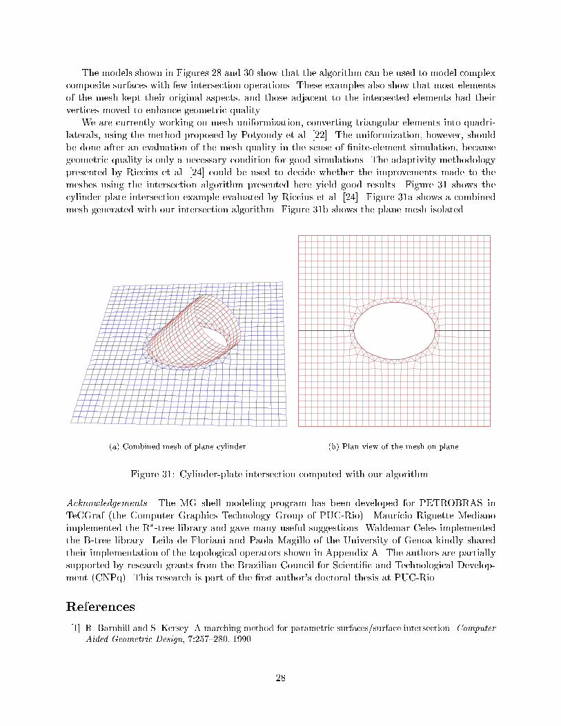
laterals� using the method proposed by Potyondy et al� �� � The uniformization� however� shouldbe done after an evaluation of the mesh quality in the sense of �nite�element simulation� becausegeometric quality is only a necessary condition for good simulations� The adaptivity methodologypresented by Riccius et al� �� could be used to decide whether the improvements made to themeshes using the intersection algorithm presented here yield good results� Figure �� shows thecylinder�plate intersection example evaluated by Riccius et al� �� � Figure ��a shows a combinedmesh generated with our intersection algorithm� Figure ��b shows the plane mesh isolated�

�a� Combined mesh of plane cylinder� �b� Plan view of the mesh on plane�

Figure ��� Cylinder�plate intersection computed with our algorithm�

Acknowledgements� The MG shell modeling program has been developed for PETROBRAS inTeCGraf �the Computer Graphics Technology Group of PUC�Rio�� Maur�!cio Riguette Medianoimplemented the R��tree library and gave many useful suggestions� Waldemar Celes implementedthe B�tree library� Leila de Floriani and Paola Magillo of the University of Genoa kindly sharedtheir implementation of the topological operators shown in Appendix A� The authors are partiallysupported by research grants from the Brazilian Council for Scienti�c and Technological Develop�ment �CNPq�� This research is part of the �rst author�s doctoral thesis at PUC�Rio�

References

� R� Barnhill and S� Kersey� A marching method for parametric surfaces�surface intersection� ComputerAided Geometric Design� ��� ����� ����

��

�� R� E� Barnhill� G� Farin� M� Jordan� and B� R� Piper� Surface�surface intersection� Computer Aided

Geometric Design� ������ �� �

�� N� Beckmann� H��P� Kriegel� R� Schneider� and B� Seeger� The R��tree� An e�cient and robust accessmethod for points and rectangles� In Proceedings of the ACM SIGMOD Conference on Management of

Data� pages �������� May ����

�� P� R� Cavalcanti� P� C� P� Carvalho� and L� F� Martha� Nonmanifold modeling� an approach based onspatial subdivision� Computer�Aided Design� ����������� �� �

�� J�J� Chen and T�M� Ozsoy� Predictor�corrector type of intersection algorithm for C� parametric surfaces�Computer�Aided Design� ����� ����� ����

�� L� C� G� Coelho and C� S� de Souza� Comunica�c�ao de problemas e solu�c�oes geom�etricas em uma interface�D� In Anais do VIII SIBGRAPI� pages �������� ����

� D� Comer� The ubiquitous B�tree� ACM Computing Surveys� ����� � ��

�� L� H� de Figueiredo� Surface intersection using a�ne arithmetic� In Proceedings of Graphics Interface ����pages �� �� ���� http���www�dgp�toronto�edu�gi�gi���proceedings�papers�deFigueiredo�

�� P� Deu�ard� A modi�ed Newton method for the solution of ill�conditioned systems of non�linear equa�tions with applications to multiple shooting� Numer� Math�� ���������� � ��

�� G� Farin� Curves and Surfaces for Computer Aided Geometric Design� Academic Press� ����

� T� A� Foley and G� M� Nielson� Knot selection for parametric spline interpolation� In L� Schumaker�editor� Mathematical Methods in CAGD� pages ������ � Academic Press� ����

�� M� Gleicher and M� Kass� An interval re�nement technique for surface intersection� In Proceedings of

Graphics Interface ���� pages �������� ����

�� R� Haber and J� F� Abel� Discrete trans�nite mappings for the description and meshing of three�dimensional surfaces using interactive computer graphics� International Journal for Numerical Methods

in Engineering� ������� ����

�� C� M� Ho�mann� Geometric and Solid Modeling � An Introduction� Morgan Kaufmann Publishers� Inc��San Mateo� California� ����

�� J� Hoschek and D� Lasser� Fundamentals of Computer Aided Geometric Design� A K Peters� ����

�� E� Houghton� E� Emnett� R� Factor� and L� Sabharwal� Implementation of a divide�and�conquer�methodfor the intersection of parametric surfaces� Computer Aided Geometric Design� �� ����� ����

� T� S� Lau and S� H� Lo� Finite element mesh generation over analytical curved surfaces� Computers Structures� ���������� ����

�� S� H� Lo� Automatic mesh generation over intersecting surfaces� International Journal for NumericalMethods in Engineering� ����������� ����

�� M� M�antyl�a� An Introduction to Solid Modeling� Computer Science Press� Rockville� Maryland� ����

��� M� R� Mediano� M� Gattass� and M� A� Casanova� HPS�tree� Um m�etodo de acesso para armazenarmapas longos com multi�resolu�c�ao geom�etrica e topol�ogica� In Anais do IX SIBGRAPI� pages ����������� http���www�visgraf�impa�br�sibgrapi���trabs�abst�a���html�

�� J� O�Rourke� Computational Geometry in C� Cambridge University Press� New York� ����

��� D� O� Potyondy� P� A� Wawrzynek� and A� R� Ingra�ea� An algorithm to generate quadrilateral or trian�gular element surface meshes in arbitrary domains with applications to crack propagation� InternationalJournal for Numerical Methods in Engineering� ����� �� �� ����

��� F� P� Preparata and M� I� Shamos� Computational Geometry � An Introduction� Springer Verlag� NewYork� ����

��

��� J� Riccius� K� Schweizer� and M� Baumann� Combination of adaptativity and mesh smoothing for the�nite element analysis of shells with intersections� International Journal for Numerical Methods in

Engineering� ���������� �� �� �

��� D� Rypl and P� Krysl� Triangulation of �D surfaces� Engineering with Computers� ��� ���� �� �

��� P� Schramm� Intersection problems of parametric surfaces in CAGD� Computing� ����������� ����

� � L� T� Souza and M� Gattass� A new scheme for mesh generation and mesh re�nement using graphtheory� Computers Structures� ���� ������ ����

��� Tz� E� Stoyanov� Marching along surface�surface intersection curves with an adaptive step length�Computer Aided Geometric Design� ���������� ����

A Topological operators

The creation and maintenance of the parametric subdivision stored by DCEL is consistently per�formed by a set of Euler operators which maintain the Euler�Poincar�e formula ��� �� �V �E�F ���� This group of constructive and destructive operators covers all updates necessary to DCEL�sstructure inside the construction and intersection algorithms� as follows�

MSVF Operator Make Surface Vertex and In�nity Face initializes the construction by building theSurface entity� generating a vertex and the in�nity face� The trees are also initialized andthe in�nity face is not inserted into the R�tree� as it is a special entity with an orientationopposite to the others� Euler�s number is kept as� �� V � � � ��

MEV Operator Make Edge and Vertex creates a new vertex and a new edge that connects thevertex to the rest of the structure�

MEBF Operator Make Edge Bound Face creates the �rst face of the representation by dividingthe in�nity face into two� inserting a new edge� This special operator is activated only onceduring the whole construction� and it is presented separately because it has totally di�erentimplementation and functionality from the traditional MEF�

MEF Operator Make Edge and Face creates an edge which connects two existing vertices� dividinga face which is passed as a parameter divided in two� It is used to create the faces followingthe face created by MEBF�

KEF Operator Kill Edge and Face �opposite to MEF� is used to remove an edge and� consequently�a face� The edges that used to point to the removed face will point to the one beside theremoved edge�

KEV Operator Kill Edge and Vertex �opposite to MEV� eliminates an edge and a vertex� which issimply connected to the rest of DCEL by this edge�

KSVF Operator Kill Surface Vertex and In�nity Face is the contrary to MSVF� being used for the�nal removal of the structure�

SEMV Operator Split Edge and Make Vertex is used to divide edges belonging to the boundary orto a trimming curve inside a patch� in Step �b of the algorithm� as presented in Section ����

��

B Initial surface mapping

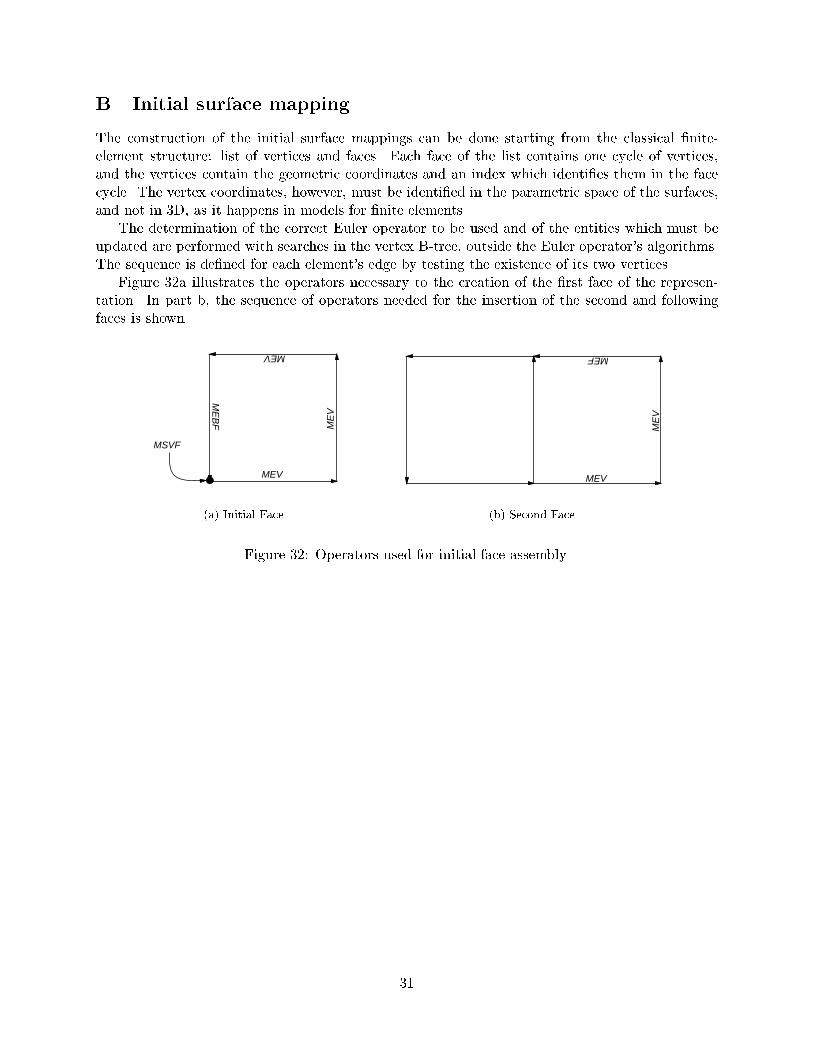
The construction of the initial surface mappings can be done starting from the classical �nite�element structure� list of vertices and faces� Each face of the list contains one cycle of vertices�and the vertices contain the geometric coordinates and an index which identi�es them in the facecycle� The vertex coordinates� however� must be identi�ed in the parametric space of the surfaces�and not in �D� as it happens in models for �nite elements�The determination of the correct Euler operator to be used and of the entities which must be

updated are performed with searches in the vertex B�tree� outside the Euler operator�s algorithms�The sequence is de�ned for each element�s edge by testing the existence of its two vertices�Figure ��a illustrates the operators necessary to the creation of the �rst face of the represen�

tation� In part b� the sequence of operators needed for the insertion of the second and followingfaces is shown�

MEV

ME

BF M

EV

MEV

MSVF

�a� Initial Face�

MEV

ME

V

MEF

�b� Second Face�

Figure ��� Operators used for initial face assembly�

��