Elsevier Editorial System(tm) for

Computational Statistics and Data Analysis

Manuscript Draft

Manuscript Number: CSDA-D-15-00296R3

Title: The joint role of trimming and constraints in robust estimation

for mixtures of Gaussian factor analyzers

Article Type: Research Paper

Section/Category: II. Statistical Methodology for Data Analysis

Keywords: Constrained estimation; Factor Analyzers Modeling; Mixture

Models; Model-Based Clustering; Robust estimation.

Corresponding Author: Dr. Francesca Greselin,

Corresponding Author's Institution: Milano-Bicocca University

First Author: Luis Angel Garcia-Escudero, Professor (with tenure)

Order of Authors: Luis Angel Garcia-Escudero, Professor (with tenure);

Alfonso Gordaliza, Full Professor; Francesca Greselin; Salvatore

Ingrassia, Full Professor; Agustin Mayo Iscar, Professor (with tenure)

Correspondence to: francesca.greselin@unimib.it

March 23, 2015

J. Cabrera, E.J. Kontoghiorghes, and J.C. Lee

Co-Editors of

Computational Statistics and Data Analysis

Dear Sirs,

Please find enclosed our manuscript entitled “The joint role of trimming and con-

straints in robust estimation for mixtures of Gaussian factor analyzers”, which

we would like to submit for publication as a research paper in Computational

Statistics and data Analysis.

Factor analysis is an effective method of summarizing the variability between a

number of correlated features, through a much smaller number of unobservable

latent factors. It originated from the consideration that, in many phenomena,

several observed variables could be explained by a few unobserved ones. The

applicability of this approach has been widened by combining local models of

Gaussian factors in the form of finite mixtures. Mixture of factor analyzers

model is well known way of modelling heterogeneous variability from hidden

population with a reduced number of parameters. In the literature, error and

factors are routinely assumed to have a Gaussian distribution: however some im-

portant applications in fields like computer vision, pattern recognition, analysis

of microarray gene expression data, or tomography suggest that more attention

should be paid to robustness, because noise in the data sets may be frequent in

all these fields of application. Some authors in the literature have considered the

use of mixtures of analyzers based on heavier tail distributions, in an attempt to

make the model less sensitive to noisy data, but the resulting estimators still fail

with very extreme outliers. It is of interest hence to provide a robust approach

for mixtures of Gaussian models, as assumed for most of the observations in the

mentioned kind of datasets, which could be safely estimated also in presence of

contaminating observations.

Hence, we introduce here a robust estimating procedure for mixture of Gaussian

factors analyzers that can resist the effect of outliers, based on trimming and

constraints. Trimming has been shown to be a simple, powerful, flexible and

computationally feasible way to provide robustness in many different statistical

frameworks, by removing a little proportion alpha of observations whose val-

ues would be the more unlikely to occur under the fitted model. Due to the

singularities in the objective function, the only use of trimming cannot pro-

vide robustness in mixture model estimation. As a side effect, singularities give

rise to spurious local maximizers, i.e. solutions without any statistical interest.

Hence we incorporate constraints for the relative variability between popula-

tions, to avoid singularities and to reduce spurious local maximizers. These

constraints can also be used to take into account prior information about the

scatter parameters. After discussing and defining the new approach, we also

provide a detailed algorithm for its implementation.

*Cover Letter

As it happens in other multivariate mixture models after the joint application of

trimming and constraints, it is expected that the proposed estimator exists and

is consistent to the corresponding population parameters. Our findings, through

Monte Carlo experiments, show that the biases and MSEs of robustly estimated

model parameters for different cases of data contamination are comparable to

results obtained from non-contaminated datasets from the mixture of Gaussians

factors model. The application to the Australian Institute of Sports data, a

famous benchmark and somehow challenging dataset, shows excellent results in

classification and an interesting factor analysis solution.

We believe our findings would appeal to a broad audience, such as the readership

of Computational Statistic and Data Analysis. As a wide-reaching journal pub-

lishing original research on Statistical Methodology, Data Analysis, along with

their Computational aspects, we hope to eventually see our findings published

in it.

We confirm that our manuscript has not been published elsewhere and it is

not under consideration by another journal. All authors have approved the

manuscript and agree to the submission to CSDA. We have read and have abided

by the statement of ethical standards for manuscripts submitted to CSDA. The

authors have no conflict of interest to declare. Please address all the correspon-

dence to francesca.greselin@unimib.it Thank you for your time and considera-

tion,

Sincerely,

Luis Angel Garcıa Escudero, Alfonso

Gordaliza, Francesca Greselin,

Salvatore Ingrassia and Agustın

Mayo-Iscar

2

Prof. Dr. Erricos John Kontoghiorghes,

Co-Editor Computational Statistics and Data Analysis

RE: Manuscript CSDA-D-15-00296R2:

“The joint role of trimming and constraints

in robust estimation for mixtures of Gaussian factor analyzers”

Dear Editor and Associate Editor,

We are indebted to you for your encouragement to revise and resubmit

our paper to Computational Statistics and Data Analysis.

We are grateful to you and the Reviewers for constructive criticism, and

for finding our work having merit. In response, we have augmented the paper

with a few notes – in blue color to facilitate their finding in the revision. We

have also made a number of small edits throughout the text, to correct the

English form.

In the following pages, we have reproduced the reviewers’ reports and

supplemented them with our detailed responses.

Best regards,

L.A. Garcıa-Escudero, A. Gordaliza, F. Greselin, S. Ingrassia and A.

Mayo-Iscar

Original submission: March 23, 2015, second referees’ report received

December 24, 2015

1

*Detailed Response to Reviewers

Authors’ responses to the reviewers

of the manuscript CSDA-D-15-00296R2

“”The joint role of trimming and constraints

in robust estimation for mixtures of Gaussian factor analyzers”

REVIEWER 1

The authors adequately addressed almost all of the issues raised, so I

think the paper can now be accepted for publication subject to one minor

comment. I congratulate the authors for an interesting paper and a very

good job.

AUTHORS: Thank you for appreciating our work.

(1) For the AIS data with p=11 attributes, the maximum number of fac-

tor (d) to satisfy (p − d)2 > p + d is 6. However, the authors report the

results for d = 1− 11 in Table 5. Is that reasonable?

Are there any identifiability problems for d > 6?

The authors claim a d = 6 MFAmodel is allowed to achieve parsimony. Look-

ing further, the number of parameters to be estimated in each component

covariance matrix is pd+p = 11 ·6+11 = 77. If we do not use factor-analytic

representation, the free number of parameters is p(p + 1)/2 = 11 · 6 = 66.

Thus, I think that the chosen (d=6) MFA model does not really achieve par-

simony. Do you agree or disagree?

I run the MFA model for fitting the AIS data (w/o standardization) with

30 different initializations, the best (fixed g=2) MFA model chosen by AIC

and BIC for both (w/o standardization) data is d=4 (smaller than yours).

Maybe, I lose some important information. I would suggest the authors

reanalyze the data to double check the correctness again.

AUTHORS: The question of uniqueness (or, following statistical terminology,

identifiability) of the factor analysis model is closely related to the estimability

2

of parameters Λg and Ψg (e.g. Browne 1982, Section 1.31). Identifiability of

the matrices Λg and Ψg amounts to the question whether these matrices can be

solved uniquely from Σg = ΛgΛ′

g+Ψg. A relevant discussion has been developed

around this issue in the literature and further references can be found in Anderson

and Rubin (1956), Anderson (1984), Shapiro (1982, 1985), Bekker and De Leeuw

(1987), and Bekker, Merckens, and Wansbeek (1994). It is easy to notice that,

in the case of d > 1, there is an infinity of choices for Λg, since the equation

Σg = ΛgΛ′

g+ Ψg is still satisfied if we replace Λg by ΛgH

′, where H is any

orthogonal matrix of order d. As d(d − 1)/2 constraints are needed for Λg to be

uniquely defined, the number of free parameters for each component covariance

matrix of the mixture of factor analyzers is finally given by

pd+ p− 1

2d(d− 1).

The following condition on p and d assures the desired parsimony (see also

McLachlan and Peel, 2000, page 241):

[(p− d)2 − (p+ d)] > 0.

Therefore, for the AIS dataset with p = 11 and d = 6 we have to estimate

pd+p− 1

2d(d−1) = 62 parameters for each component, instead of 66, for the fully

parameterized Σg. Accordingly, we have added a remark at the end of Section 2.

Hence, when we presented our results in Table 5 for d = 1−11, our aim was to

show that for d = 6 we effectively got a minimum; further, we discussed our choice

in the following way: “In practice, we could have stopped our investigation at d = 6

because in a factor analyzer, to reach parsimony, we should have (p−d)2 ≥ p+d.”

In the revised version of the paper we reduced the Table to present only useful

results.

Now, willing to answer to the second remark of the referee, about identifiability

problems for d > 6, let us consider again the factor analysis model, following

Shapiro (2007). Till now, we have discussed identifiability issues related to the

estimation of Λ, now we want to consider those related to Ψ.

By substituting ΛH for Λ, where H is an arbitrary d × d orthogonal matrix,

since the dimension of the (smooth) manifold of d × d orthogonal matrices is

d(d−1)/2 and the dimension of the space of p×p symmetric matrices is p(p+1)/2,

it is possible to show that the characteristic rank r of the factor analysis model

3

Σg = ΛgΛ′

g+Ψg is

r = minpd+ p− d(d− 1)/2, p(p + 1)/2.

Then the question of global (local) identifiability of the factor analysis model is

reduced to the global (local) identifiability of the diagonal matrixΨ (Anderson and

Rubin, 1956). We have that a necessary condition for generic local identifiability of

Ψ is that pd+p−d(d−1)/2 is less than or equal to p(p+1)/2, which is equivalent

to (p − d)(p − d+ 1)/2 ≥ p, and in turn is equivalent to d ≤ φ(p), where

φ(p) =2p + 1−√

8p+ 1

2.

The above function φ(p) corresponds to the so-called Ledermann bound (Leder-

mann, 1937). In the present case we have that d ≤ φ(p) is a necessary and sufficient

condition for local identifiability of the diagonal matrix Ψ, of the factor analysis

model, in the generic sense (Shapiro, 1985). Bekker and ten Berge (1997) showed

that d < φ(p) is a necessary and sufficient condition for global identifiability of the

diagonal matrix Ψ. For the AIS dataset, we have that φ(p) = 6.78, hence for d > 6

identifiability issues arise. We added a sentence with reference to this remark in

Section 4.2.

Finally, with reference to the fourth question of the referee, we recall that

before performing the analysis of a multivariate dataset it is common practice to

standardize variables. This previous step is due to the fact that variables could

be measured on different scales, and methods based on their covariance structure

are clearly affected. Without standardization, the variability of the features with

higher scale could override the variability of some other features, and important in-

formation could be masked. (Another option is to adopt a method for the analysis

that is based on the correlation structure.)

Table 1 shows that these general considerations are particularly required on the

AIS dataset. Notice that the variance σ2 has different order of magnitude among

the 11 features, from the maximum value of 2256.37 for σ2(Fe) to its minimum

value of 0.21 for σ2(RCC). In the last column of Table 1, after the variance, we

calculated also the coefficient of variation σ/µ, which can be used for a correct

variability comparison. Clearly, covariance is affected from scale in multivariate

data, as well. Therefore, to avoid variables having a greater impact due to different

4

min Q1 Me Q3 max µ σ2 σ/µ

RCC 3.80 4.37 4.75 5.03 5.03 4.72 0.21 0.10

WCC 3.30 5.90 6.85 8.28 8.28 7.11 3.24 0.25

Hc 35.90 40.60 43.50 45.58 45.58 43.09 13.42 0.09

Hg 11.60 13.50 14.70 15.57 15.57 14.57 1.86 0.09

Fe 8.00 41.25 65.50 97.00 97.00 76.88 2256.37 0.62

BMI 16.75 21.08 22.72 24.46 24.46 22.96 8.20 0.12

SSF 28.00 43.85 58.60 90.35 90.35 69.02 1060.50 0.47

Bfat 5.63 8.54 11.65 18.08 18.08 13.51 38.31 0.46

LBM 34.36 54.67 63.03 74.75 74.75 64.87 170.83 0.20

Ht 148.90 174.00 179.70 186.17 186.17 180.10 94.76 0.05

Wt 37.80 66.53 74.40 84.12 84.12 75.01 193.92 0.19

Table 1: Summary information for the AIS dataset

scales, as in this paper we are dealing with robust techniques, we adopt a robust

estimation of variability, given by the interquartile difference, i.e. IQR = Q3−Q1

and we divide the columns of the original data by their IQR (see Section 4.2).

(2) (p.7, line -8) based in → based on

AUTHORS: A careful review by a native English speaker has been done.

5

REVIEWER 3

Thanks for this revision (and your clear supporting notes) that seems to

have addressed many of my previous comments.

The paper is generally well-written and clear, although you do use a

few strange constructions and there is the occasional mis-used word. For

example, ”on the other side” should be ’on the other hand” and occasionally

you use ”in” when you mean ”on” e.g. p7 L-8 ”based on small samples”, L-7

”on this idea”, etc.

AUTHORS: Thank you for the appreciation and the useful suggestions. See

the changes highlighted in blue in the present version of the abstract and through-

out the paper.

6

Editor’s Comments

1. Follow all the editorial guidelines when you prepare the revised manuscript

(e.g. abstract in the third person and no statements like ’this paper’ etc.).

The paper should be formally written and check thoroughly by a native

English speaker and/or professional service.

Write the abstract in the third person without the unnecessary terms

like ”Unfortunately” and redundant terms like ”this paper”. The ”open

serious issues” is vague. You should be specific and say exactly what are the

issues. Please pay attention in the details and generally avoid superfluous

unnecessary statements.

E.g. The high prevalence of spurious solutions and the disturbing effects

of outlying observations in maximum likelihood estimation results in .... Re-

strictions for the component covariances are considered in order to avoid

spurious solutions, and trimming, to provide robustness against violations of

normality assumptions of the underlying latent factors.

AUTHORS: Thank you for the suggestions. See the changes highlighted in

blue in the present version of the abstract and throughout the paper.

2. Have the paper proof read and corrected by a native English speaker

with knowledge of the topic and/or professional service.

AUTHORS: A careful review by a native English speaker has been done.

7

REFERENCES:

Anderson, T. W. (1984) Estimating linear statistical relationships, Annals

of Statistics, 12,1–45.

Anderson, T. W. and Rubin, H. (1956) Statistical inference in factor

analysis, in Proceedings of the Third Berkeley Symposium on Mathematical

Statistics and Probability, J. Neyman, Ed., Univ. of California Press, 5,

111–150.

Bekker, P. A. and de Leeuw, J. (1987) The rank of reduced dispersion

matrices, Psychometrika, 52, 125–135.

Browne, M. W., (1982) Covariance structures, Topics in Applied Multi-

variate Analysis, D. M. Hawkins Ed., Cambridge U.P.

Bekker, P.A. and ten Berge, J.M.F. (1997) Generic global identification

in factor analysis, Linear Algebra and its Applications, 264, 255–263.

Bekker, P. A., Merckens, A., and Wansbeek, T. J. (1994) Identification

Equivalent Models and Computer Algebra, Academic.

Jennrich, R. I. (1987) Tableau algorithms for factor analysis by instru-

mental variable methods, Psychometrika, 52(3), 469-476.

Ledermann, W. (1937) On the rank of the reduced correlational matrix

in multiple-factor analysis, Psychometrika, 2(2), 85-93.

McLachlan, G. J., Peel D. (2000) Finite Mixture Models, John Wiley &

Sons, New York.

Shapiro, A. (1982) Rank-reducibility of symmetric matrix and sampling

theory of minimum trace factor analysis, Psychometrika, 47, 187–199.

Shapiro, A. (1985) Identifiability of factor analysis: some results and open

problems, Linear Algebra and its Applications, 70, 1–7.

Shapiro, A. (2007) Statistical Inference of Moment Structures, in Hand-

book of Computing and Statistics with Applications, Vol. 1, E. J. Kon-

toghiorghes Ed., Elsevier.

8

Computational Statistics & Data Analysis 00 (2016) 1–21

JournalLogo

The joint role of trimming and constraints in robust estimationfor mixtures of Gaussian factor analyzers

Luis Angel Garcıa-Escuderoa, Alfonso Gordalizaa, Francesca Greselinb,Salvatore Ingrassiac, Agustın Mayo-Iscara

aDepartment of Statistics and Operational Research and IMUVA, University of Valladolid (Spain)bDepartment of Statistics and Quantitative Methods, Milano-Bicocca University (Italy)

cDepartment of Economics and Business, University of Catania (Italy)

AbstractMixtures of Gaussian factors are powerful tools for modeling an unobserved heterogeneous population, offering - at the same time- dimension reduction and model-based clustering. The high prevalence of spurious solutions and the disturbing effects of outlyingobservations in maximum likelihood estimation may cause biased or misleading inferences. Restrictions for the component covari-ances are considered in order to avoid spurious solutions, and trimming is also adopted, to provide robustness against violations ofnormality assumptions of the underlying latent factors. A detailed AECM algorithm for this new approach is presented. Simulationresults and an application to the AIS dataset show the aim and effectiveness of the proposed methodology.

c© 2015 Published by Elsevier Ltd.

Keywords: Constrained estimation, Factor Analyzers Modeling, Mixture Models, Model-Based Clustering,, Robust estimation.

1. Introduction and motivation

Factor analysis is an effective method of summarizing the variability between a number of correlated features,through a much smaller number of unobservable, hence named latent, factors. It originated from the considerationthat, in many phenomena, several observed variables could be explained by a few unobserved ones. Under thisapproach, each single variable (among the p observed ones) is assumed to be a linear combination of d underlyingcommon factors with an accompanying error term to account for that part of the variability which is unique to it (notin common with other variables). Ideally, d should be substantially smaller than p, to achieve parsimony.

Clearly, the effectiveness of this method is limited by its global linearity, as happens for principal componentsanalysis. Hence, Ghahramani and Hilton (1997), Tipping and Bishop (1999) and McLachlan and Peel (2000a) solidlywidened the applicability of these approaches by combining local models of Gaussian factors in the form of finitemixtures. The idea is to employ latent variables to perform dimensional reduction in each component, thus providinga statistical method which concurrently performs clustering and, within each cluster, local dimensionality reduction.

In the literature, error and factors are routinely assumed to have a Gaussian distribution because of their mathemat-ical and computational tractability: however, statistical methods which ignore departure from normality may cause

Email addresses: lagarcia@eio.uva.es (Luis Angel Garcıa-Escudero), alfonsog@eio.uva.es (Alfonso Gordaliza),francesca.greselin@unimib.it (Francesca Greselin), s.ingrassia@unict.it (Salvatore Ingrassia), agustin@med.uva.es (Agustın Mayo-Iscar)

1

*ManuscriptClick here to view linked References

/ Computational Statistics & Data Analysis 00 (2016) 1–21 2

biased or misleading inference. Moreover, it is well known that maximum likelihood estimation for mixtures oftenleads to ill-posed problems because of the unboundedness of the objective function to be maximized, which favors theappearance of non-interesting local maximizers and degenerate or spurious solutions.

The lack of robustness in mixture fitting arises whenever the sample contains a certain proportion of data that doesnot follow the underlying population model. Spurious solutions can even appear when ML estimation is applied toartificial data drawn from a given finite mixture model, i.e. without adding any kind of contamination. Hence, morerobust estimation is needed. Many contributions in this sense can be found in the literature: from the Mclust modelwith a noise component in Fraley and Raftery (1998), mixtures of t-distributions in McLachlan and Peel (2000),the trimmed likelihood mixture fitting method in Neykov et al. (2007), the trimmed ML estimation of contaminatedmixtures in Gallegos and Ritter (2009), and the robust improper ML estimator introduced in Coretto and Hennig(2011), among many others. Some important applications such fields as computer vision, pattern recognition, analysisof microarray gene expression data, or tomography suggest that more attention should be paid to robustness, becausenoise in the data sets may be frequent in all these fields of application.

Different types of constraints have been traditionally applied in Gaussian mixtures of factor analyzers, for instance,some authors propose taking a common (diagonal) error matrix (as for the Mixtures of Common Factor Analyzers,denoted by MCFA, in Baek et al., 2010) or imposing an isotropic error matrix (Bishop and Tipping, 1998). Thisstrategy has proven to be effective in many cases, at the expenses of stronger distributional restrictions on the data. Toavoid singularities and spurious solutions, under milder conditions, Greselin and Ingrassia (2015) recently proposedmaximizing the likelihood by constraining the eigenvalues of the covariance matrices, following previous work ofIngrassia (2004) and going back to Hathaway (1985). Furthermore, mixtures of t-analyzers have been considered (seeMcLachlan and Bean, 2005; Lin et al., 2014, and references therein) in an attempt to make the model less sensitive tooutliers, but they, too, are not robust against very extreme outliers (Hennig, 2004).

The purpose of the present work is to introduce an estimating procedure for the mixture of Gaussian factorsanalyzers that can resist the effect of outliers and avoid spurious local maximizers. The proposed constraints can alsobe used to take into account prior information about the scatter parameters.

Trimming has been shown to be a simple, powerful, flexible and computationally feasible way to provide ro-bustness in many different statistical frameworks. The basic idea behind trimming here is the removal of a smallproportion α of observations whose values would be the most unlikely to occur if the fitted model were true. In thisway, trimming avoids into a small fraction of outlying observations exerting a harmful effect on the estimation. In-corporating constraints into the mixture fitting estimation method moves the mathematical problem to a well-posedsetting and hence minimizes the risk of incurring spurious solutions. Moreover, a correct statement of the problemallows the desired statistical properties for the estimators to be obtained, such as the existence and consistency results,as in Garcıa-Escudero et al. (2008).

The rest of the paper has been organized as follows. In Section 2, the notation is introduced and the main ideasabout Gaussian Mixtures of Factor Analyzers (hereafter denoted by MFA) are summarized. Then, in Section 3 thetrimmed likelihood for MFA is presented, and fairly extensive notes are provided concerning the EM algorithm, withincorporated trimming and constrained estimation. In Section 4, the performance of the new procedure is discussed,on the grounds of some numerical results obtained from simulated and real data. In particular, the bias and MSEof robustly estimated model parameters for different cases of data contamination, are compared using Monte Carloexperiments. The application to the Australian Institute of Sports dataset shows how classification and factor analysiscan be developed using the new model. Section 5 contains concluding notes and provides ideas for further research.

2. Gaussian Mixtures of Factor Analyzers

The density of the p-dimensional random variable X of interest is modeled as a mixture of G multivariate normaldensities in some unknown proportions π1, . . . πG, whenever each data point is taken to be a realization of the followingdensity function,

f (x; θ) =G∑

g=1

πgφp(x;µg,Σg) (1)

where φp(x;µ,Σ) denotes the p-variate normal density function with mean vector µ and covariance matrix Σ. Herethe vector θ = θGM(p,G) of unknown parameters consists of the (G−1) mixing proportions πg, the Gp elements of the

2

/ Computational Statistics & Data Analysis 00 (2016) 1–21 3

component means µg, and the 12Gp(p+1) distinct elements of the component-covariance matrices Σg. MFA postulates

a finite mixture of linear sub-models for the distribution of the full observation vector X, given the (unobservable)factors U. That is, MFA provides local dimensionality reduction by assuming that the distribution of the observationXi can be given as

Xi = µg + ΛgUig + eig with probability πg (g = 1, . . . ,G) for i = 1, . . . , n, (2)

where Λg is a p × d matrix of factor loadings, the factors U1g, . . . ,Ung are N(0, Id) distributed independently of theerrors eig. The latter are independentlyN(0,Ψg) distributed, and Ψg is a p × p diagonal matrix (g = 1, . . . ,G). Thediagonality of Ψg is one of the key assumptions of factor analysis: the observed variables are independent given thefactors. Note that the factor variables Uig model correlations between the elements of Xi, while the errors eig accountfor independent noise for Xi. We suppose that d < p, which means that d unobservable factors are jointly explainingthe p observable features of the statistical units. Under these assumptions, the mixture of factor analyzers model isgiven by (1), where the g-th component-covariance matrix Σg has the form

Σg = ΛgΛ′g +Ψg (g = 1, . . . ,G). (3)

The parameter vector θ = θMFA(p, d,G) now consists of the elements of the component means µg, the Λg, and theΨg,along with the mixing proportions πg (g = 1, . . . ,G − 1), on putting πG = 1 −∑G−1

i=1 πg.Note that, in the case of d > 1, there is an infinity of choices for Λg, since model (2) is still satisfied if we replace

Λg by ΛgH′, where H is any orthogonal matrix of order d. As d(d − 1)/2 constraints are needed for Λg to be uniquelydefined, the number of free parameters for each component of the mixture is given by

pd + p − 12

d(d − 1).

The following condition on p and d assures the desired parsimony:

[(p − d)2 − (p + d)] > 0.

3. Robust Mixtures of Factor Analyzers

In this section the trimmed (Gaussian) mixtures of factor analyzers model (trimmed MFA) is presented and afeasible algorithm for its implementation is provided.

3.1. Problem statement

Let x = x1, x2, . . . , xn be a given data set in Rp. With the theoretical underlying model described in Section 3

in mind, a mixture of Gaussian factor components can be robustly fitted to this dataset x by maximizing a trimmedmixture log-likelihood (see Neykov et al. 2007, Gallegos and Ritter 2009 and Garcıa-Escudero et al. 2014) defined as:

Ltrim =

n∑i=1

ζ(xi) log

G∑

g=1

φp(xi; µg,Σg)πg

(4)

where ζ(·) is a 0-1 trimming indicator function that tells us whether observation xi is trimmed off: ζ(xi)=0, or not:ζ(xi)=1 and Σg = ΛgΛ

′g + Ψg as in (3). A fixed fraction α of observations can be unassigned by setting

∑ni=1 ζ(xi) =

[n(1 − α)] and, hence, the parameter α denotes the trimming level.Moreover, to avoid the unboundedness of Ltrim, constrained maximization of (4) is introduced. In more detail,

with reference to the diagonal elements ψgkk=1,...,p of the noise matrices Ψg for g = 1, . . . ,G, it is required that

ψg1k ≤ cnoise ψg2h for every 1 ≤ k h ≤ p and 1 ≤ g1 g2 ≤ G (5)

3

/ Computational Statistics & Data Analysis 00 (2016) 1–21 4

The constant cnoise is finite and such that cnoise ≥ 1, to avoid the |Σg| → 0 case. This constraint can be seen as anadaptation to MFA of those introduced in Ingrassia and Rocci (2007), Garcıa-Escudero et al. (2008), and is similar tothe mild restrictions implemented for MFA in Greselin and Ingrassia (2015). They all go back to the seminal paper ofHathaway (1985). We will look for the maximization of Ltrim on Ψg under the given constraints: this setting leads toa well-defined maximization problem, and at the same time allows singularities to be discarded and the occurrence ofspurious solutions to be reduced.

Our methodology also includes the possibility of controlling the relative variability of the norms of the p dimen-sional column vectors of the matrices Λg (for g = 1, . . . ,G). If ηk gk=1,...,d denote the set of these norms, a second setof constraints applies on their values

ηk g1 ≤ cload ηh g2 for every 1 ≤ k h ≤ d and 1 ≤ g1 g2 ≤ G. (6)

In fact, these types of constraints are not needed to avoid singularities in the target function, but they could beuseful to achieve more sensible solutions.

Hereafter, Θc will denote the constrained parameter space for θ = πg, µg,Ψg,Λg; g = 1, . . . ,G under the require-ments (5) and (6).

3.2. AlgorithmThe maximization of Ltrim in (4) for θ ∈ Θc is not an easy task, obviously. We will give a feasible algorithm

obtained by combining the Alternating Expectation-Conditional Maximization algorithm (AECM) for MFA with that(with trimming and constraints) introduced in Garcıa-Escudero et al. (2014) (see, also, Fritz et al., 2013).

As usual in the EM framework, each observation xi is associated with an unobserved state zi = (zi1, . . . , ziG)′ fori = 1, . . . , n where zig is one or zero, depending on whether xi does or does not belong to the g-th component. Thecomponent label vectors z1, . . . , zn are taken to be the realized values of the random vectors Z1, . . . ,Zn, where, forindependent feature data, it is appropriate to assume that they are (unconditionally) multinomially distributed. i.e.Z1, . . . ,Zn ∼i.i.d. MultG(1; π1, ..., πG). The AECM is an extension of the EM, suggested by the factor structure ofthe model, which uses different specifications of missing data at each stage. The idea is to partition the vector ofparameters θ = (θ1, θ2) in such a way that Ltrim is easy to be maximized for θ1, given θ2 and viceversa, replacingthe M-step by a number of computationally simpler conditional maximization (CM) steps. In more detail, in the firstcycle we set θ1 = πg, µg; g = 1, . . . ,G and the missing data are the unobserved group labels z = (z1, . . . , zn)′; whilein the second cycle we set θ2 = Λg,Ψg; g = 1, . . . ,G and the missing data are the group labels z and the unobservedlatent factors u = (u11, . . . , unG)′. Hence, the application of the AECM algorithm consists of two cycles, and thereis one E-step and one CM-step, alternatively considering θ1 and θ2 in each cycle. A trimming step, to evaluate thetrimming function, precedes each cycle. The trimming function has the role of discarding the α100% of observationswith the lowest contribution to the likelihood. Before describing the algorithm, we remark that the unobserved grouplabels Z are considered missing data in both cycles. Therefore, during the l-th iteration, z(l+1/2)

ig and z(l+1)ig denote the

conditional expectations at the first and second cycle, respectively.The algorithm has to be run multiple times on the same dataset, with different starting values, to prevent the

attainment of a local, rather than global, maximum log-likelihood. In each run it executes the following steps:

1 Initialization:Each iteration begins by selecting initial values for θ(0) where θ(0) = (π(0)

g , µ(0)g ,Λ(0)

g ,Ψ(0)g ; g = 1, . . . ,G). Inspired

from results obtained in a series of extensive test experiments about initialization strategies (see Maitra, 2009),and aiming to allow the algorithm to visit the entire parameter space, p+1 units are randomly selected (withoutreplacement) for group g from the observed data x. In this way a subsample xg is obtained that may be arrangedin a (p + 1) × p matrix, and its sample mean will be the initial µ(0)

g . Additionally, based on these p + 1 obser-vations, a new ad hoc approach for providing an initialization procedure for Ψ(0)

g and Λ(0)g has been developed,

to deal with the possible existence of gross outlying observations among the subsamples, which could inflatedisproportionately some of their eigenvalues. The rationale under the proposed procedure is, as usual, to fill inrandomly the missing information in the complete model through random subsamples and, then, to estimate theother parameters. The missing information here are the factors uig for i = 1, . . . , n and g = 1, . . . ,G, which,under the assumptions for the model, are realizations from independentlyN(0, Id) distributed Uig random vari-ables. We may consider model (2) in group g as a regression of Xi with intercept µg, regression coefficients

4

/ Computational Statistics & Data Analysis 00 (2016) 1–21 5

given by Λg, where the explanatory variables are the latent factors Uig, and with regression errors eig. Hence,we draw p+1 random independent observations from the d-variate standard Gaussian to fill a (p+1)×d matrixug. Then we set Λ(0)

g = ((ug)′ug)−1(ug)′xgc, where xg

c is obtained by centering the columns of the xg matrix. Toprovide a restricted random generation of Ψg, the (p + 1) × p matrix εg = xg

c − Λ(0)g ug is computed, and the

diagonal elements of Ψ(0)g are set equal to the variances of the p columns of the εg matrix. After repeating this

for g = 1, . . . ,G, if the obtained matrices Λ(0)g and Ψ(0)

g do not satisfy the required constraints (5) and (6), thenthe constrained maximizations described in step 2.4 must be applied. Finally, weights π(0)

1 , ..., π(0)G in the interval

(0, 1) and summing up to 1 are randomly chosen.

2 Trimmed AECM steps:The following steps 2.1–2.6. are alternatively executed until a maximum number of iterations, MaxIter, isreached. The implementation of trimming is related to the “concentration” steps applied in high-breakdownrobust methods (Rousseeuw and Van Driessen, 1999). Trimming is performed before each E-step, while con-straints are enforced during the second cycle CM step.

2.1 First cycle. Trimming: Evaluate the n quantities

D(xi; θ(l)) =G∑

g=1

φp(xi; µg,ΛgΛ′g +Ψg)πg for i = 1, . . . , n

and sort them to obtain their α quantile denoted by D([nα]). Notice that D(xi; θ(l)) is the contribution givenfrom xi to the overall likelihood. Now consider the set of indices I ⊂ 1, 2, ..., n defined as

I =i : D(xi; θ(l)) ≥ D([nα])

.

Then set the trimming function as ζ(xi) = 1 for i ∈ I, and ζ(xi) = 0 otherwise. To update the parameters,only the observations with indices in I will be taken into account. In other words, the proportion α ofobservations with the smallest D(xi; θ(l)) values are tentatively discarded.

2.2 First cycle. E-step:Here θ1 = πg, µg; g = 1, . . . ,G and the missing data are the unobserved group labels z = (z1, . . . , zn)′.The E-step on the first cycle on the (l + 1)-th iteration requires the calculation of

Q1

(θ1; θ(l)

)= Eθ(l)

[ n∑i=1

ζ(xi)G∑

g=1

Zig

(log πg + logφp

(xi;µ(l)

g ,Σ(l)g

)) ∣∣∣ x],

which is the expected trimmed complete-data log-likelihood, given the data x and using the current esti-mate θ(l) for θ, where Σ(l)

g = Λ(l)g[Λ(l)

g]′+Ψ

(l)g . In practice, it is necessary to calculate Eθ(l) [Zig| x] = z(l+1/2)

ig ,where the latter are the “posterior probabilities” often considered in standard EM algorithms and whichare evaluated as follows. Let us define

Dg(x; θ(l)) = φp

(x;µ(l)

g ,Σ(l)g

)π(l)

g

then, set

z(l+1/2)ig =

Dg(xi; θ(l))D(xi; θ(l))

.

5

/ Computational Statistics & Data Analysis 00 (2016) 1–21 6

2.3 First cycle. CM-step: This first CM step requires the maximization of Q1(θ1; θ(l)) over θ1, with θ2 heldfixed at θ(l)

2 . We get θ(l+1)1 by updating πg and µg as follows

π(l+1)g =

∑ni=1 z(l+1/2)

ig ζ(xi)

[n(1 − α)]

and

µ(l+1)g =

∑ni=1 z(l+1/2)

ig ζ(xi)xi

n(l+1/2)g

where n(l+1/2)g =

∑ni=1 z(l+1/2)

ig ζ(xi), for g = 1, . . . ,G.

According to notation in McLachlan and Peel (2000b), we set θ(l+1/2) =(θ(l+1)

1 , θ(l)2

).

2.4 Second cycle. Trimming: Re-evaluate the n quantities D(xi; θ(l)) and, as done in step [2.1], update thetrimming function ζ(xi).

2.5 Second cycle. E- step:Here θ2 = (Λg,Ψg), g = 1, . . . ,G has to be considered, where the missing data are the unobserved grouplabels Z and the latent factors U.The E-step on the second cycle on the l-th iteration requires the calculation of the conditional expectationof the trimmed complete-data log-likelihood, given the observed data x and using the current estimateθ(l+1/2) for θ, i.e.

Q2

(θ2; θ(l+1/2)

)= Eθ(l+1/2)

[ n∑i=1

ζ(xi)G∑

g=1

Zig

(log π(l+1)

g + logφp(xi;µ(l+1)

g − Λ(l)g Uig,Ψ

(l)g)+ logφd

(Uig; 0, Id

)) ∣∣∣ x].

In addition to updating the posterior probabilitiesEθ(l+1/2) [Zig|x] = z(l+1)ig (and consequently n(l+1)

g =∑n

i=1 z(l+1)ig ζ(xi),

for g = 1, . . . ,G, as previously done), this leads to an evaluation of the following conditional expectations:Eθ(l+1/2) [ZigUig|x] and Eθ(l+1/2) [ZigUigU′ig|x]. Recalling that the conditional distribution of Uig, given xi, is

Uig|xi ∼ N(γg(xi − µg), Iq − γgΛg

)

for i = 1, . . . , n and g = 1, . . . ,G with

γg = Λ′g(ΛgΛ

′g +Ψg)−1,

we obtain

Eθ(l+1/2) [ZigUig|xi] = z(l+1)ig γ(l)

g

(xi − µ(l+1)

g

)

Eθ(l+1/2) [ZigUigU′ig|xi] = z(l+1)ig

[γ(l)

g

(xi − µ(l+1)

g

) (xi − µ(l+1)

g

)′γ(l)

g′+ Iq − γ(l)

g Λ(l)g

]

where we set

γ(l)g = Λ

(l)g′ (Λ(l)

g Λ(l)g′+Ψ(l)

g

)−1.

6

/ Computational Statistics & Data Analysis 00 (2016) 1–21 7

2.6 Second cycle. CM-step for constrained estimation of Λg and Ψg :Here our aim is to maximize Q2

(θ2; θ(l)

)over θ, with θ1 held fixed at θ(l+1)

1 . After some matrix algebra,this yields the updated ML-estimates

Λg = S(l+1)g γ(l)

g′[γ(l)

g S(l+1)g γ(l)

g′+ Iq − γ(l)

g Λ(l)g ]−1

Ψg = diagS(l+1)

g − Λ(l+1)g γ(l)

g S(l+1)g

where S(l+1)g denotes the sample scatter matrix in group g, for g = 1, . . . ,G

S(l+1)g = (1/n(l+1)

g )n∑

i=1

z(l+1)ig ζ(xi)

(xi − µ(l+1)

g

) (xi − µ(l+1)

g

)′.

During the iterations, due to the updates, it may happen that the Λg matrices do not belong to the con-strained parameter space Θc. In the case where that the additional constraints (6) have to be imposed, andthe norms of the column vectors of the matrices Λg do not satisfy them, Λ(l+1)

g ∈ Θc can be obtained asfollows. After defining the diagonal matrix Eg = diag(ηg1, ηg2, ..., ηgd), the truncated norms are then givenas

[ηgk]m = min(cload · m, max(ηgk,m)

), for k = 1, . . . , d and g = 1, . . . ,G,

with m being some threshold value. The loading matrices are finally updated as Λ(l+1)g = ΛgE−1

g E∗g with

E∗g = diag([ηg1]mopt , [ηg2]mopt , ..., [ηgd]mopt

)

and mopt minimizing the real valued function

fload(m) =G∑

g=1

π(l+1)g

d∑k=1

(log([ηgk]m

)+

ηgk

[ηgk]m

). (7)

It may be mentioned here, in passing, that Proposition 3.2 in Fritz et al. (2013) shows that mopt can beobtained by evaluating 2dG + 1 times the real valued function fload(m) in (7).Given the Λ(l+1)

g , the matrices

Ψg = diagS(l+1)

g − Λ(l+1)g γ(l)

g S(l+1)g

= diag

(ψg1, ..., ψgp

)

can be obtained, and may not necessarily satisfy the required constraint (5). In this case, we set

[ψgk]m = min(cnoise · m, max(ψgk,m)

), for k = 1, . . . , p; g = 1, . . . ,G,

and fix the optimal threshold value mopt by minimizing the following real valued function

fnoise(m) →G∑

g=1

π(l+1)g

p∑k=1

(log([ψgk]m

)+

ψgk

[ψgk]m

). (8)

As before, in Fritz et al. (2013), it is shown that mopt can be obtained in a straightforward way by evaluating2pG + 1 times fnoise(m) in (8). Thus,Ψ(l+1)

g is finally updated as

Ψ(l+1)g = diag

([ψg1]mopt , ..., [ψgp]mopt

). (9)

It is worth remarking that the given constrained estimation provides, at each step, the parameters Ψg andΛg that maximize the likelihood in the constrained parameter space Θc.

7

/ Computational Statistics & Data Analysis 00 (2016) 1–21 8

3 Evaluate target function: After applying the trimmed and constrained EM steps, and setting ζ(xi) = 0 if i ∈ Iand ζ(xi) = 1 if i I, the associated value of the target function (4) is evaluated. If convergence has not beenachieved before reaching the maximum number of iterations, MaxIter, the results are discarded.

The set of parameters yielding the highest value of the target function (among the multiple runs) and the associatedtrimmed indicator function ζ(·) are returned as the final output of the algorithm. In the framework of model-basedclustering, each unit is assigned to one group, based on the maximum a posteriori probability. Notice, in passing, thata high number of initializations is not needed, and nor is a high value for MaxIter, as will be seen in Section 4.

In relation with the initialization strategy, the obtained initial values for the parameters in each population arebased on small subsamples, aiming at ideally covering, in many trials, the full parameter space. Our proposal is basedon the following idea: a small subsample has to be drawn for each group and then the information extracted from thesubsample is completed with random data generated under the model assumptions. The expected consequence of thisexploration of the parameter space is that spurious solutions, even singularities, can arise when running EM iterations,and the constraints on the scatters play the role of protecting against these undesired solutions. By considering manyrandom initializations, we are confident that the best point, in terms of the likelihood, can be approached inside therestricted parameter space. The number of random initializations should increase with the number of groups G, thedimension p and in the case of very different group sizes.

It is worth remarking that the usual monotone convergence of the likelihood in the robust AECM algorithm holdstrue when incorporating trimming and constrained estimation forΨg. To prove this, notice firstly that, when perform-ing the trimming step, the optimal observations have been retained, i.e. the ones with the highest contributions to theobjective function. Secondly, the first cycle is the usual one in the AECM algorithm for MFA and, therefore, it sharesits optimality properties. Finally, it can be easily proved that, in the second EM cycle, the evaluation of the optimal(Λg,Ψg

)for g = 1, . . . ,G corresponds to the usual way of obtaining firstly the optimal Λg, which is not affected by

the restrictions on Ψg, and then the optimal Ψg is obtained as

arg maxG∑

g=1

ng

2log(|Ψg|) +

G∑g=1

12

trace[Ψ−1

g

(S(l+1)

g − Λ(l+1)g γ(l)

g S(l+1)g

)], (10)

and this corresponds to (9).On the other hand, when the algorithm also requires the constrained estimation of Λg, the latter is based on

a heuristic approach. We have empirical evidences about the monotonicity of this second EM cycle for the hugemajority of the steps in which we applied it, producing low decreases in the objective function in extremely rare cases.In any case, after each entire AECM cycle, an increased likelihood was always observed.

4. Numerical studies

In this section, numerical studies will be presented, based on simulated and real data, to show the performance ofthe constrained and trimmed AECM algorithm with respect to unconstrained and/or untrimmed approaches.

4.1. Artificial dataWe consider here the following mixture of G components of d-variate normal distributions. To perform each

estimation, 40 different random initializations have been considered to start the algorithm at each run, as describedin the previous section, and the best solution is retained. The needed routines have been written in R-code (R Team,2013), and are available from the authors upon request.

Mixture: G = 3, d = 6, q = 2, n = 150.

The sample has been generated with weights π = (0.3, 0.4, 0.3)′ according to the following parameters:µ1 = (0, 0, 0, 0, 0, 0)′ Ψ1 = diag(0.1, 0.1, 0.1, 0.1, 0.1, 0.1)

µ2 = (5, 5, 0, 0, 0, 0)′ Ψ2 = diag(0.4, 0.4, 0.4, 0.4, 0.4, 0.4)

µ3 = (10, 10, 0, 0, 0, 0)′ Ψ3 = diag(0.2, 0.2, 0.2, 0.2, 0.2, 0.2)

8

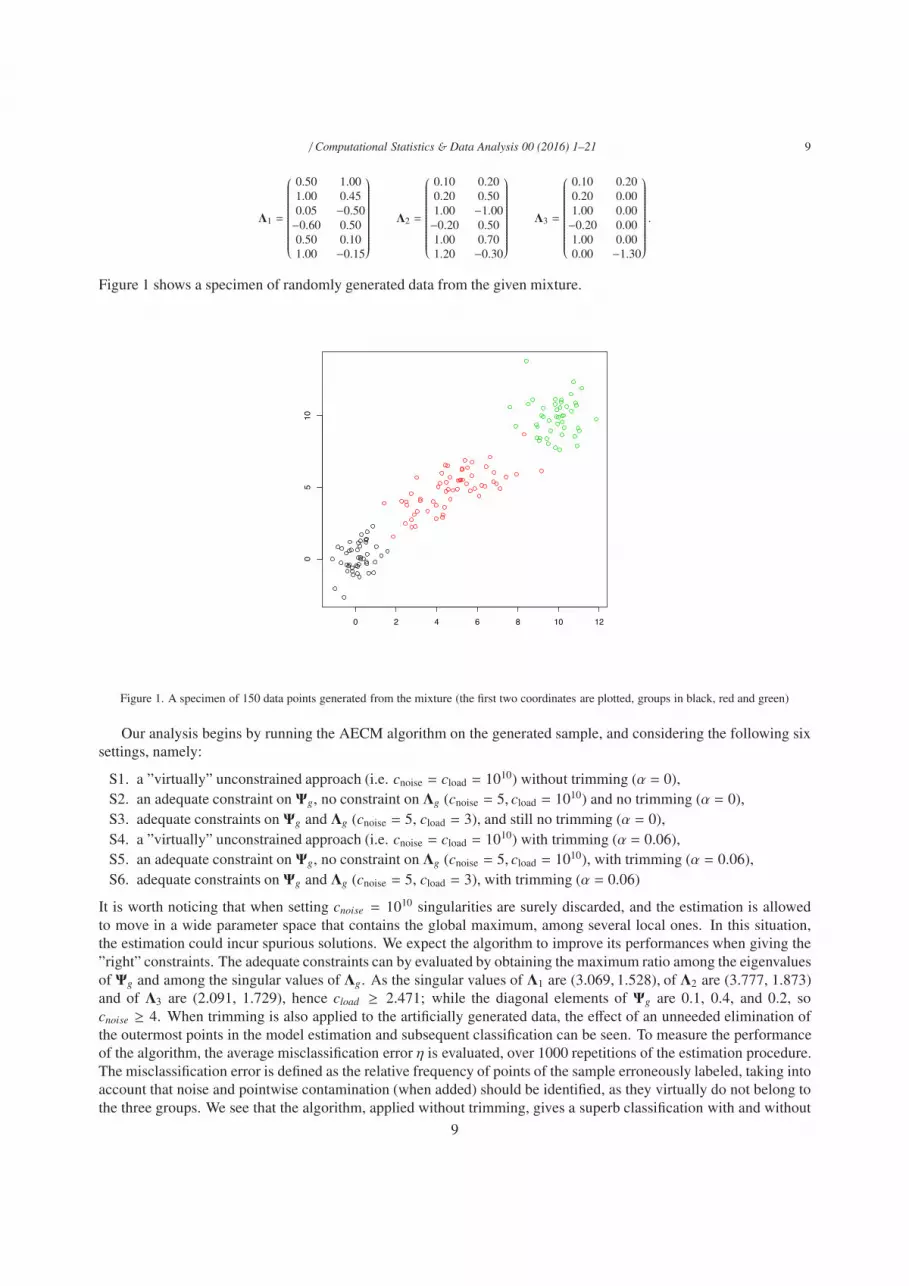
/ Computational Statistics & Data Analysis 00 (2016) 1–21 9

Λ1 =

0.50 1.001.00 0.450.05 −0.50−0.60 0.500.50 0.101.00 −0.15

Λ2 =

0.10 0.200.20 0.501.00 −1.00−0.20 0.501.00 0.701.20 −0.30

Λ3 =

0.10 0.200.20 0.001.00 0.00−0.20 0.001.00 0.000.00 −1.30

.

Figure 1 shows a specimen of randomly generated data from the given mixture.

0 2 4 6 8 10 12

05

10

Figure 1. A specimen of 150 data points generated from the mixture (the first two coordinates are plotted, groups in black, red and green)

Our analysis begins by running the AECM algorithm on the generated sample, and considering the following sixsettings, namely:

S1. a ”virtually” unconstrained approach (i.e. cnoise = cload = 1010) without trimming (α = 0),S2. an adequate constraint on Ψg, no constraint on Λg (cnoise = 5, cload = 1010) and no trimming (α = 0),S3. adequate constraints on Ψg and Λg (cnoise = 5, cload = 3), and still no trimming (α = 0),S4. a ”virtually” unconstrained approach (i.e. cnoise = cload = 1010) with trimming (α = 0.06),S5. an adequate constraint on Ψg, no constraint on Λg (cnoise = 5, cload = 1010), with trimming (α = 0.06),S6. adequate constraints on Ψg and Λg (cnoise = 5, cload = 3), with trimming (α = 0.06)

It is worth noticing that when setting cnoise = 1010 singularities are surely discarded, and the estimation is allowedto move in a wide parameter space that contains the global maximum, among several local ones. In this situation,the estimation could incur spurious solutions. We expect the algorithm to improve its performances when giving the”right” constraints. The adequate constraints can by evaluated by obtaining the maximum ratio among the eigenvaluesof Ψg and among the singular values of Λg. As the singular values of Λ1 are (3.069, 1.528), of Λ2 are (3.777, 1.873)and of Λ3 are (2.091, 1.729), hence cload ≥ 2.471; while the diagonal elements of Ψg are 0.1, 0.4, and 0.2, socnoise ≥ 4. When trimming is also applied to the artificially generated data, the effect of an unneeded elimination ofthe outermost points in the model estimation and subsequent classification can be seen. To measure the performanceof the algorithm, the average misclassification error η is evaluated, over 1000 repetitions of the estimation procedure.The misclassification error is defined as the relative frequency of points of the sample erroneously labeled, taking intoaccount that noise and pointwise contamination (when added) should be identified, as they virtually do not belong tothe three groups. We see that the algorithm, applied without trimming, gives a superb classification with and without

9

/ Computational Statistics & Data Analysis 00 (2016) 1–21 10

constraints. While adding trimming, the misclassification error, as expected, is pretty close to the trimming level, andall non-trimmed observations are perfectly classified (with the sole exception of 1 misclassified unit, that happenedonly once, when cnoise = cload = 1010, and occurred 4 times when cnoise = 5 and cload = 1010, over 1000 runs). Theresults are summarized in the first row of Table 1. Moreover, the other parameters, such as the means µg, and Ψg, Λg

for g = 1, 2, 3, are close to the values from which the data have been generated, as will be shown in Subsection 4.1.1.

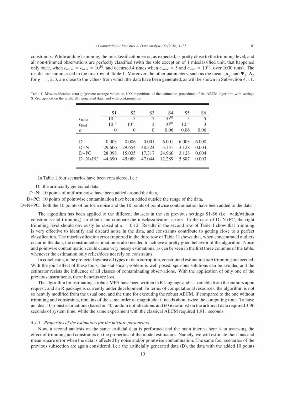
Table 1. Misclassification error η (percent average values on 1000 repetitions of the estimation procedure) of the AECM algorithm with settingsS1-S6, applied on the artificially generated data, and with contamination

S1 S2 S3 S4 S5 S6cnoise 1010 5 5 1010 5 5cload 1010 1010 3 1010 1010 3α 0 0 0 0.06 0.06 0.06

D 0.003 0.006 0.001 6.001 6.003 6.000D+N 29.606 29.654 48.324 3.131 3.128 0.004D+PC 28.098 15.035 17.317 24.966 3.128 0.004D+N+PC 44.690 45.089 47.044 12.289 5.887 0.003

In Table 1 four scenarios have been considered, i.e.:

D: the artificially generated data,D+N: 10 points of uniform noise have been added around the data,

D+PC: 10 points of pointwise contamination have been added outside the range of the data,D+N+PC: both the 10 points of uniform noise and the 10 points of pointwise contamination have been added to the data.

The algorithm has been applied to the different datasets in the six previous settings S1-S6 (i.e. with/withoutconstraints and trimming), to obtain and compare the misclassification errors. In the case of D+N+PC, the righttrimming level should obviously be raised at α = 0.12. Results in the second row of Table 1 show that trimmingis very effective to identify and discard noise in the data, and constraints contribute to getting close to a perfectclassification. The misclassification error (reported in the third row of Table 1) shows that, when concentrated outliersoccur in the data, the constrained estimation is also needed to achieve a pretty good behavior of the algorithm. Noiseand pointwise contamination could cause very messy estimations, as can be seen in the first three columns of the table,whenever the estimation only relies/does not rely on constraints.

In conclusion, to be protected against all types of data corruption, constrained estimation and trimming are needed.With the joint effect of these tools, the statistical problem is well posed, spurious solutions can be avoided and theestimator resists the influence of all classes of contaminating observations. With the application of only one of theprevious instruments, these benefits are lost.

The algorithm for estimating a robust MFA have been written in R language and is available from the authors uponrequest, and an R package is currently under development. In terms of computational resources, the algorithm is notso heavily modified from the usual one, and the time for executing the robust AECM, if compared to the one withouttrimming and constraints, remains of the same order of magnitude: it needs about twice the computing time. To havean idea, 10 robust estimations (based on 40 random initializations and 60 iterations) on the artificial data required 3.96seconds of system time, while the same experiment with the classical AECM required 1.911 seconds.

4.1.1. Properties of the estimators for the mixture parametersNow, a second analysis on the same artificial data is performed and the main interest here is in assessing the

effect of trimming and constraints on the properties of the model estimators. Namely, we will estimate their bias andmean square error when the data is affected by noise and/or pointwise contamination. The same four scenarios of theprevious subsection are again considered, i.e.: the artificially generated data (D), the data with the added 10 points

10

/ Computational Statistics & Data Analysis 00 (2016) 1–21 11

of uniform noise (D+N), the data with added 10 points of pointwise contamination (D+PC), and finally the data withboth uniform noise and the pointwise contamination (D+N+PC).

We apply the algorithm for estimating a trimmed MFA model in all the four scenarios, exploring the six settings oncnoise, cload and α that have been shown in Table 1. The benchmark of all simulations is given by the results obtained onartificial data drawn from a given MFA without outliers. In each experiment, a sample of size n = 150 has been drawn1000 times from the mixture described at the beginning of this Section, and the model parameters for the trimmedMFA have been estimated using the algorithm presented in the previous Section 3.2, by setting cnoise = cload = 1010

(a virtually unconstrained solution) or cnoise = 5, cload = 3 for a constrained one, and α = 0 for no trimming, whileα = 0.06 or α = 0.12 when adopting adequate trimming.

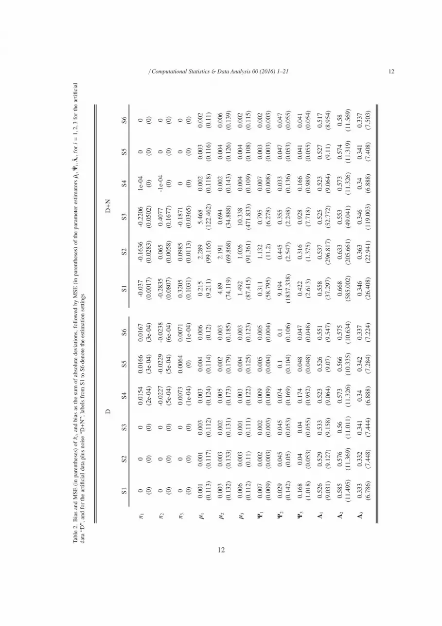
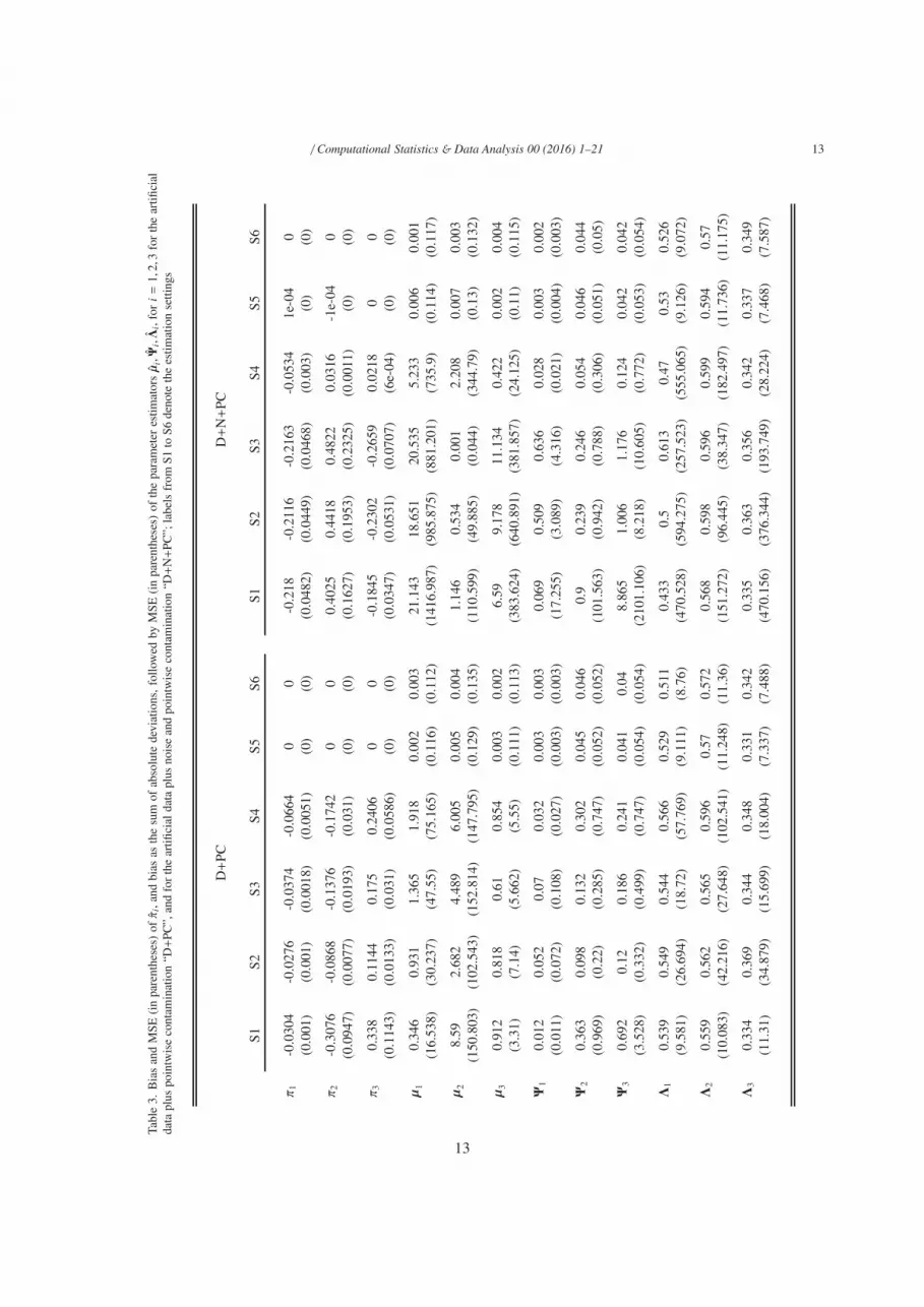
Notice that the considered estimators in each component are vectors (apart from πg which are scalar quantities,for g = 1, . . . ,G). We are interested in providing synthetic measures of their properties, such as bias and mean squareerror (MSE). As usual, let T be an estimator for the scalar parameter t, then the bias of T is given by bias(T ) = E(T )−t,i.e. it is the signed absolute deviation of the expected value E(T ) from t. Therefore, we would have 6 biases for eachcomponent of the mean µg, 6 for diag(Ψg) and 12 for Λg. On the other hand, MSE is defined as a scalar quantity,namely E(|T − t|2) = trace(Var(T ))+ bias(T )2, also for vector estimators. Hence, a synthesis of each parameter’s biasis adopted by considering the mean of their absolute values on each component. Below the bias, in Tables 2 and 3,the MSE is provided in parenthesis.

The results on bias and mean square error for the case of estimating the trimmed MFA with trimming but withoutconstraints or viceversa, show the harmful effects of distorted inference. The only exception comes from D+N, wheretrimming is pretty able to cope with the contamination. On the other hand, when reasonable constraints cnoise = 5,cload = 3 and a right trimming level are applied to deal with the added outliers, the results come back to being veryclose to the benchmark, shown in the first column of Table 2. Therefore, it has been shown that robust inferencereduces bias and mean square error, in both cases of sparse and concentrated outliers.

11

/ Computational Statistics & Data Analysis 00 (2016) 1–21 12Ta

ble

2.B

ias

and

MSE

(in

pare

nthe

ses)

ofπ

i,an

dbi

asas

the

sum

ofab

solu

tede

viat

ions

,fol

low

edby

MSE

(inpa

rent

hese

s)of

the

para

met

eres

timat

orsµ

i,Ψ

i,Λ

i,fo

ri=

1,2,

3fo

rthe

artifi

cial

data

“D”,

and

fort

hear

tifici

alda

tapl

usno

ise

“D+

N”;

labe

lsfr

omS1

toS6

deno

teth

ees

timat

ion

setti

ngs

DD+

N

S1S2

S3S4

S5S6

S1S2

S3S4

S5S6

π1

00

00.

0154

0.01

660.

0167

-0.0

37-0

.163

6-0

.220

61e

-04

00

(0)

(0)

(0)

(2e-

04)

(3e-

04)

(3e-

04)

(0.0

017)

(0.0

283)

(0.0

502)

(0)

(0)

(0)

π2

00

0-0

.022

7-0

.022

9-0

.023

8-0

.283

50.

065

0.40

77-1

e-04

00

(0)

(0)

(0)

(5e-

04)

(5e-

04)

(6e-

04)

(0.0

807)

(0.0

058)

(0.1

677)

(0)

(0)

(0)

π3

00

00.

0073

0.00

640.

0071

0.32

050.

0985

-0.1

871

00

0(0

)(0

)(0

)(1

e-04

)(0

)(1

e-04

)(0

.103

1)(0

.011

3)(0

.036

5)(0

)(0

)(0

)

µ1

0.00

10.

001

0.00

30.

003

0.00

40.

006

0.21

52.

289

5.46

80.

002

0.00

30.

002

(0.1

13)

(0.1

17)

(0.1

12)

(0.1

24)

(0.1

14)

(0.1

2)(9

.211

)(9

9.16

5)(1

22.4

62)

(0.1

18)

(0.1

16)

(0.1

1)

µ2

0.00

30.

003

0.00

20.

005

0.00

20.

003

4.89

2.19

10.

694

0.00

20.

004

0.00

6(0

.132

)(0

.133

)(0

.131

)(0

.173

)(0

.179

)(0

.185

)(7

4.11

9)(6

9.86

8)(3

4.88

8)(0

.143

)(0

.126

)(0

.139

)

µ3

0.00

60.

003

0.00

10.

003

0.00

40.

003

1.49

21.

026

10.3

380.

004

0.00

40.

002

(0.1

12)

(0.1

1)(0

.111

)(0

.122

)(0

.125

)(0

.123

)(8

7.41

5)(9

1.36

1)(4

71.8

33)

(0.1

09)

(0.1

08)

(0.1

15)

Ψ1

0.00

70.

002

0.00

20.

009

0.00

50.

005

0.31

11.

132

0.79

50.

007

0.00

30.

002

(0.0

09)

(0.0

03)

(0.0

03)

(0.0

09)

(0.0

04)

(0.0

04)

(58.

795)

(11.

2)(6

.278

)(0

.008

)(0

.003

)(0

.003

)

Ψ2

0.02

90.

045

0.04

50.

074

0.1

0.1

9.19

40.

445

0.35

50.

033

0.04

70.

047

(0.1

42)

(0.0

5)(0

.053

)(0

.169

)(0

.104

)(0

.106

)(1

837.

338)

(2.5

47)

(2.2

48)

(0.1

36)

(0.0

53)

(0.0

55)

Ψ3

0.16

80.

040.

040.

174

0.04

80.

047

0.42

20.

316

0.92

80.

166

0.04

10.

041

(1.0

18)

(0.0

53)

(0.0

55)

(0.9

52)

(0.0

48)

(0.0

48)

(2.6

13)

(1.3

75)

(7.7

18)

(0.9

89)

(0.0

55)

(0.0

54)

Λ1

0.52

60.

529

0.53

30.

523

0.52

60.

551

0.55

80.

537

0.52

50.

523

0.52

70.

517

(9.0

31)

(9.1

27)

(9.1

58)

(9.0

64)

(9.0

7)(9

.547

)(3

7.29

7)(2

96.8

17)

(52.

772)

(9.0

64)

(9.1

1)(8

.954

)

Λ2

0.58

50.

576

0.56

0.57

30.

566

0.57

50.

668

0.63

30.

553

0.57

30.

574

0.58

(11.

495)

(11.

369)

(11.

011)

(11.

326)

(10.

335)

(10.

634)

(585

.002

)(2

05.6

61)

(49.

041)

(11.

326)

(11.

319)

(11.

569)

Λ3

0.33

30.

332

0.34

10.

340.

342

0.33

70.

346

0.36

30.

346

0.34

0.34

10.

337

(6.7

86)

(7.4

48)

(7.4

44)

(6.8

88)

(7.2

84)

(7.2

24)

(26.

408)

(22.

941)

(119

.003

)(6

.888

)(7

.408

)(7

.503

)

12

/ Computational Statistics & Data Analysis 00 (2016) 1–21 13Ta

ble

3.B

ias

and

MSE

(in

pare

nthe

ses)

ofπ

i,an

dbi

asas

the

sum

ofab

solu

tede

viat

ions

,fol

low

edby

MSE

(inpa

rent

hese

s)of

the

para

met

eres

timat

orsµ

i,Ψ

i,Λ

i,fo

ri=

1,2,

3fo

rthe

artifi

cial

data

plus

poin

twis

eco

ntam

inat

ion

“D+

PC”,

and

fort

hear

tifici

alda

tapl

usno

ise

and

poin

twis

eco

ntam

inat

ion

“D+

N+

PC”;

labe

lsfr

omS1

toS6

deno

teth

ees

timat

ion

setti

ngs

D+

PCD+

N+

PC

S1S2

S3S4

S5S6

S1S2

S3S4

S5S6

π1

-0.0

304

-0.0

276

-0.0

374

-0.0

664

00

-0.2

18-0

.211

6-0

.216

3-0

.053

41e

-04

0(0

.001

)(0

.001

)(0

.001

8)(0

.005

1)(0

)(0

)(0

.048

2)(0

.044

9)(0

.046

8)(0

.003

)(0

)(0

)

π2

-0.3

076

-0.0

868

-0.1

376

-0.1

742

00

0.40

250.

4418

0.48

220.

0316

-1e-

040

(0.0

947)

(0.0

077)

(0.0

193)

(0.0

31)

(0)

(0)

(0.1

627)

(0.1

953)

(0.2

325)

(0.0

011)

(0)

(0)

π3

0.33

80.

1144

0.17

50.

2406

00

-0.1

845

-0.2

302

-0.2

659

0.02

180

0(0

.114

3)(0

.013

3)(0

.031

)(0

.058

6)(0

)(0

)(0

.034

7)(0

.053

1)(0

.070

7)(6

e-04

)(0

)(0

)

µ1

0.34

60.

931

1.36

51.

918

0.00

20.

003

21.1

4318

.651

20.5

355.

233

0.00

60.

001

(16.

538)

(30.

237)

(47.

55)

(75.

165)

(0.1

16)

(0.1

12)

(141

6.98

7)(9

85.8

75)

(881

.201

)(7

35.9

)(0

.114

)(0

.117

)

µ2

8.59

2.68

24.

489

6.00

50.

005

0.00

41.

146

0.53

40.

001

2.20

80.

007

0.00

3(1

50.8

03)

(102

.543

)(1

52.8

14)

(147

.795

)(0

.129

)(0

.135

)(1

10.5

99)

(49.

885)

(0.0

44)

(344

.79)

(0.1

3)(0

.132

)

µ3

0.91

20.

818

0.61

0.85

40.

003

0.00

26.

599.

178

11.1

340.

422

0.00

20.

004

(3.3

1)(7

.14)

(5.6

62)

(5.5

5)(0

.111

)(0

.113

)(3

83.6

24)

(640

.891

)(3

81.8

57)

(24.

125)

(0.1

1)(0

.115

)

Ψ1

0.01

20.

052

0.07

0.03

20.

003

0.00

30.

069

0.50

90.

636

0.02

80.

003

0.00

2(0

.011

)(0

.072

)(0

.108

)(0

.027

)(0

.003

)(0

.003

)(1

7.25

5)(3

.089

)(4

.316

)(0

.021

)(0

.004

)(0

.003

)

Ψ2

0.36

30.

098

0.13

20.

302

0.04

50.

046

0.9

0.23

90.

246

0.05

40.

046

0.04

4(0

.969

)(0

.22)

(0.2

85)

(0.7

47)

(0.0

52)

(0.0

52)

(101

.563

)(0

.942

)(0

.788

)(0

.306

)(0

.051

)(0

.05)

Ψ3

0.69

20.

120.

186

0.24

10.

041

0.04

8.86

51.

006

1.17

60.

124

0.04

20.

042

(3.5

28)

(0.3

32)

(0.4

99)

(0.7

47)

(0.0

54)

(0.0

54)

(210

1.10

6)(8

.218

)(1

0.60

5)(0

.772

)(0

.053

)(0

.054

)

Λ1

0.53

90.

549

0.54

40.

566

0.52

90.

511

0.43

30.

50.

613

0.47

0.53

0.52

6(9

.581

)(2

6.69

4)(1

8.72

)(5

7.76

9)(9

.111

)(8

.76)

(470

.528

)(5

94.2

75)

(257

.523

)(5

55.0

65)

(9.1

26)

(9.0

72)

Λ2

0.55

90.

562

0.56

50.

596

0.57

0.57

20.

568

0.59

80.

596

0.59

90.

594

0.57

(10.

083)

(42.

216)

(27.

648)

(102

.541

)(1

1.24

8)(1

1.36

)(1

51.2

72)

(96.

445)

(38.

347)

(182

.497

)(1

1.73

6)(1

1.17

5)

Λ3

0.33

40.

369

0.34

40.

348

0.33

10.

342

0.33

50.

363

0.35

60.

342

0.33

70.

349

(11.

31)

(34.

879)

(15.

699)

(18.

004)

(7.3

37)

(7.4

88)

(470

.156

)(3

76.3

44)

(193

.749

)(2

8.22

4)(7

.468

)(7

.587

)

13

/ Computational Statistics & Data Analysis 00 (2016) 1–21 14

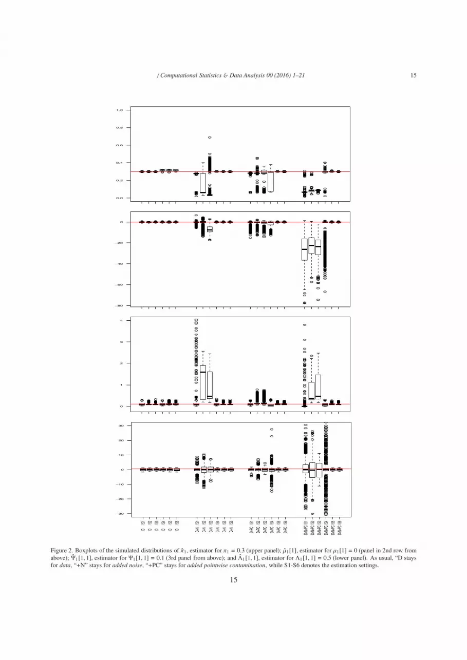
The distributions of the estimators for the model parameters can be represented by box plots, and some of themare shown in Figure 2, namely with reference to π1 (upper panel), µ1[1, 1] (second panel), Ψ1[1, 1] (third panel)and Λ1[1, 1] (bottom panel). In a direct comparison, the small efficiency reduction of the estimator when applyingtrimming and constraints on the true data (cases D / S2-S6) can be seen, the effect of using only trimming whenuniform noise has been added to data (case D+N / S4) is apparent; finally, the joint usage of trimming and constraintson Ψg is shown to be effective to protect against all types of contamination.

4.2. Real data: the AIS data set

As an illustration, we apply the proposed technique to the Australian Institute of Sports (AIS) data, which is afamous benchmark dataset in the multivariate literature, originally reported by Cook and Weisberg (1994) and sub-sequently analyzed by Azzalini and Dalla Valle (1996), among many other authors. The dataset consists of p = 11physical and hematological measurements on 202 athletes (100 females and 102 males) in different sports, and is avail-able within the R package sn (Azzalini, A., 2011). The observed variables are: red cell count (RCC), white cell count(WCC), Hematocrit (Hc), Hemoglobin (Hg), plasma ferritin concentration (Fe), body mass index, weight/height2

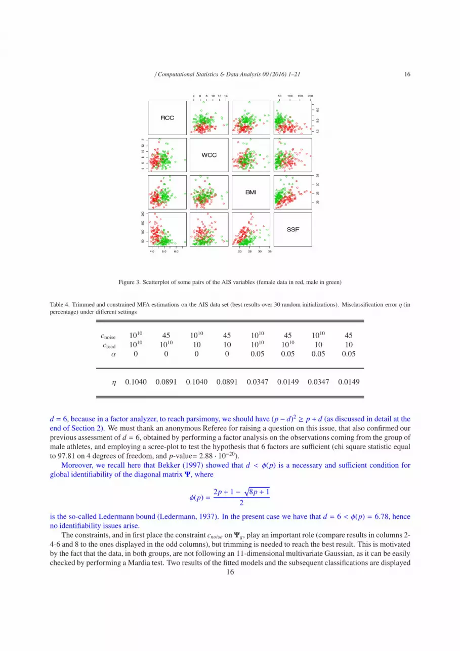
(BMI), sum of skin folds (SSF), body fat percentage (Bfat), lean body mass (LBM), height, cm (Ht), weight, kg (Wt),apart from gender and kind of sport. A partial scatterplot of the AIS dataset is given in Figure 3.

Our purpose is to provide a model for the entire dataset, and since the group labels (athletes’ gender) are providedin advance, the aim is to classify athletes by this feature.

Let us begin our analysis by fitting a mixture of multivariate Gaussian distributions, using the Mclust package inR. The routine mclustBIC, after fitting a set of normal mixture models, considering from 1 to 9 components in themixture and different patterns for the covariance matrices, selects the best EEV model (ellipsoidal scatters, with equalvolume and shape, different orientation of the component scatters) with G = 2 components, providing the highest BICvalue, i.e. BIC = −10251.6. Now, using this model to classify AIS data, 18 misclassified units are obtained, i.e., amisclassification error equal to 18/202 = 9.4%. The classification results are shown in Figure 4 (lefthanded panel).

To improve the classification, we may exploit the conjecture that a strong correlation exists between the hemato-logical and physical measurements. Therefore, a mixture of factor analyzers may be estimated, assuming the existenceof some underlying unknown factors (like nutritional status, hematological composition, overweight status indices,and so on) which jointly explain the observed measurements. Through the factors, the aim is to find a perspective ondata which disentangles the overlapping components. To avoid variables having a greater impact in the model (whichis not affine equivariant) due to different scales, before performing the estimation, the variables have been divided bytheir interquartile range. We begin by adopting the pGmm package from R, that fits mixtures of factors analyzers withpatterned covariances. Parsimonious Gaussian mixtures are obtained by constraining the loadings Λg and the errorsΨg to be equal or not among the components. We employed the routine pGmmEM, considering from 1 to 9 compo-nents, and number of underlying factors d ranging from 1 to 6, with 30 different random initialization, to provide thebest iteration (in terms of BIC) for each case. The best model is a CUU mixture model with d = 4 factors and G = 3components, with BIC = −3127.424. CUU means “Constrained” loading matricesΛg = Λ and “Unconstrained” errormatrices Ψg = ωg∆g, where ∆g are normalized diagonal matrices and ωg is a real value varying across components.Using this model to classify athletes, we got 109 misclassified units and we discarded it.

As a second attempt using pGmm, a UUU model has been estimated by setting G = 2 components, and d = 6.The acronym UUU means that the estimation of loadings Λg and errors Ψg is unconstrained. Based on 30 randomstarts, the best UUU model has BIC = −3330.306, and the consequent classification of the AIS dataset produces 72misclassified units (misclassification error=35.6%, see the right panel in Figure 4).

Finally, we want to show the performance of our trimmed and constrained estimation for MFA. All the resultsare generated by the procedure described in Section 3.2, based on 30 random initializations and returning the bestobtained solution of the parameters, in terms of the highest value of the final likelihood. We see that the best solution,with only 3 misclassified points, has been obtained by combining trimming (α = 0.05) and the constrained estimationof Ψg (cnoise = 45) and Λg (cload = 10), with d = 6.

Notice that the choice of G = 2 and d = 6 could be motivated by estimating all models within a range of values forG and d, and choosing the pair of values providing the best BIC. A trimmed version of the BIC = 2Ltrim(x; θ)−k log n∗should be considered, where we denote by k the number of free parameters in the model, and by n∗ the number of nontrimmed observations (i.e. n∗ = [n(1− α)]). Results are shown in Table 5. In practice, we stopped our investigation at

14

/ Computational Statistics & Data Analysis 00 (2016) 1–21 15

0.0

0.2

0.4

0.6

0.8

1.0

−80

−60

−40

−20

0

0

1

2

3

4

D /

S1D

/ S2

D /

S3D

/ S4

D /

S5D

/ S6

D+N

/ S1

D+N

/ S2

D+N

/ S3

D+N

/ S4

D+N

/ S5

D+N

/ S6

D+PC

/ S1

D+PC

/ S2

D+PC

/ S3

D+PC

/ S4

D+PC

/ S5

D+PC

/ S6

D+N+

PC / S

1D+

N+PC

/ S2

D+N+

PC / S

3D+

N+PC

/ S4

D+N+

PC / S

5D+

N+PC

/ S6

−30

−20

−10

0

10

20

30

Figure 2. Boxplots of the simulated distributions of π1, estimator for π1 = 0.3 (upper panel); µ1[1], estimator for µ1[1] = 0 (panel in 2nd row fromabove); Ψ1[1, 1], estimator for Ψ1[1, 1] = 0.1 (3rd panel from above); and Λ1[1, 1], estimator for Λ1[1, 1] = 0.5 (lower panel). As usual, “D staysfor data, “+N” stays for added noise, “+PC” stays for added pointwise contamination, while S1-S6 denotes the estimation settings.

15

/ Computational Statistics & Data Analysis 00 (2016) 1–21 16

RCC

4 6 8 10 12 14 50 100 150 200

4.0

5.0

6.0

46

810

1214

WCC

BMI

2025

3035

4.0 5.0 6.0

5010

015

020

0

20 25 30 35

SSF

Figure 3. Scatterplot of some pairs of the AIS variables (female data in red, male in green)

Table 4. Trimmed and constrained MFA estimations on the AIS data set (best results over 30 random initializations). Misclassification error η (inpercentage) under different settings

cnoise 1010 45 1010 45 1010 45 1010 45cload 1010 1010 10 10 1010 1010 10 10α 0 0 0 0 0.05 0.05 0.05 0.05

η 0.1040 0.0891 0.1040 0.0891 0.0347 0.0149 0.0347 0.0149

d = 6, because in a factor analyzer, to reach parsimony, we should have (p − d)2 ≥ p + d (as discussed in detail at theend of Section 2). We must thank an anonymous Referee for raising a question on this issue, that also confirmed ourprevious assessment of d = 6, obtained by performing a factor analysis on the observations coming from the group ofmale athletes, and employing a scree-plot to test the hypothesis that 6 factors are sufficient (chi square statistic equalto 97.81 on 4 degrees of freedom, and p-value= 2.88 · 10−20).

Moreover, we recall here that Bekker (1997) showed that d < φ(p) is a necessary and sufficient condition forglobal identifiability of the diagonal matrix Ψ, where

φ(p) =2p + 1 − √8p + 1

2

is the so-called Ledermann bound (Ledermann, 1937). In the present case we have that d = 6 < φ(p) = 6.78, henceno identifiability issues arise.

The constraints, and in first place the constraint cnoise onΨg, play an important role (compare results in columns 2-4-6 and 8 to the ones displayed in the odd columns), but trimming is needed to reach the best result. This is motivatedby the fact that the data, in both groups, are not following an 11-dimensional multivariate Gaussian, as it can be easilychecked by performing a Mardia test. Two results of the fitted models and the subsequent classifications are displayed

16

/ Computational Statistics & Data Analysis 00 (2016) 1–21 17

RCC

4 6 8 10 12 14 50 100 150 200

4.0

5.0

6.0

46

810

1214

WCC

BMI

2025

3035

4.0 5.0 6.0

5010

015

020

0

20 25 30 35

SSF

RCC

4 6 8 10 12 14 50 100 150 200

4.0

5.0

6.0

46

810

1214

WCC

BMI

2025

3035

4.0 5.0 6.0

5010

015

020

0

20 25 30 35

SSF

Figure 4. The classification of AIS data obtained through the best model from Mclust (left panel), and through the best UUU model from pGmm(right panel) with G = 2 and d = 6 (female data in red, male in blue, misclassified units as black circlecrosses).

Groups G 1 2 3 4 5Factors d

1 3484.32 2833.18 2744.96 2702.89 2780.272 2436.87 2311.24 2283.16 2331.43 2433.883 1938.75 1885.03 1967.93 2068.36 2261.204 1490.72 1513.43 1662.43 1818.78 2002.085 1409.03 1390.86 1559.12 1774.64 1971.566 1142.15 1099.89 1371.98 1772.44 1976.96

Table 5. trimmed BIC for different choices of the number of factors d and the number of groups G, on AIS data.

in Figure 5, by selecting the 2 variables in the scatterplot that enable us to point out the trimmed and misclassifiedunits. We have chosen to represent the best solution (left panel), with only 3 misclassified points, colored in black,and with 10 trimmed points, denoted by “X”. In the right panel, to make a comparison, we report classification resultsobtained by the non-robustly fitted model, whose details are shown in the first column of Table 4. In this second case,we were doing an almost unconstrained estimation of Ψg and Λg and we were not applying trimming, obtaining 21misclassified observations.

In the robustly estimated model, the misclassified observations are in rows 70, 121 and 153 in the AIS dataset.Two misclassified units are from male athletes, one is a female athlete. The discriminant function of the mixturecomponents for the observation in position 153 are close (D1(x; θ) = 0.0115 and D2(x; θ) = 0.0855), while for theother two observations they are neatly different.

Finally, we recall that trimmed observations have been discarded to provide robustness to the parameter estimation.After estimating the model, it thus also makes sense to classify these observations. The trimmed observations are inrows 11, 75, 93, 99, 133, 160, 163, 166, 178, 181 and, if we assign them by the Bayes rule to the component g havinggreater value of Dg(x; θ) = φp

(x;µg,ΛgΛ

′g +Ψg

)πg, we classify the first four in the female group of athletes, and the

second group of six in the male group. This means that all the trimmed observations have been assigned to their truegroup. Table 6 shows the details of the classification, and the rightmost panel in Figure 5 plots the final result of therobust model fitting.

As a last analysis on the AIS dataset, we are interested in factor interpretation. The rotated factor loading matriceshave been obtained by employing a Gradient Projection algorithm, available through the R package GPArotation(Bernaards and Jennrich, 2005; Browne, 2001). We opted for an oblimin transformation, which yielded results shown

17

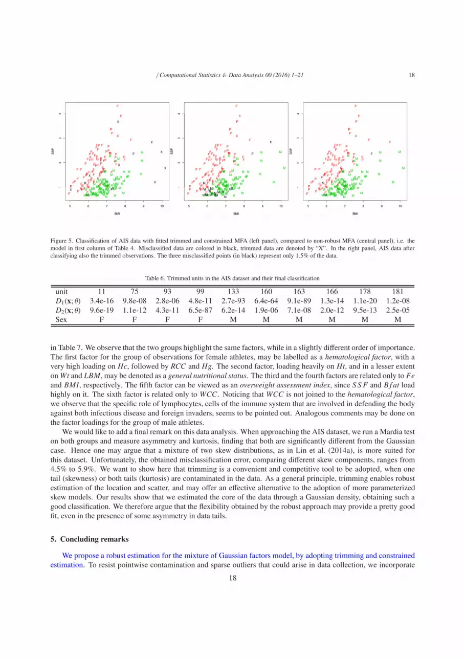
/ Computational Statistics & Data Analysis 00 (2016) 1–21 18

FF F

F

FF

F

F

F

F

X

F

F

FFF

F

F

FF

FF

FF

F

F

FF

F

F

F

F

F

F

F

F

F

F

F

F

F

F

F

F

F

F

FF

F

F

F

F

F

F

F

F

F

F

F

F

FF

FF

F

F

F

FF

F

F

F

FF

X

F

F F

F

F

F

F

F

F FF

FFF

F

F

F

X

F

F

FF

F

X

F

M MM

M

M

MM MM

M

M

MM

M

M

M

M

M

MM

M

M

M

M

MM

M

M

MM

M M

X

M

M

M

M

M

M

MM

MM

M

MM

MMM MMMM MM M

M MM

X

M

M

X

M

MX

M

MMMM

M

MM

M

M

M

X

M

MX

M

M

MM

M

M

MM

M

M

M

MM

MM

M

M

M

M

M

M

5 6 7 8 9 10

12

34

BMI

SS

F

FF F

F

FF

F

F

F

F

F

F

F

FFF

F

F

FF

FF

FF

F

F

FF

F

F

F

F

F

F

F

F

F

F

F

F

F

F

F

F

F

F

FF

F

F

F

F

F

F

F

F

F

F

F

F

FF

FF

F

F

F

FF

F

F

F

FF

F

F

F F

F

F

F

F

F

F FF

FFF

F

F

F

F

F

F

FF

F

F

F

M MM

M

M

MM MM

M

M

MM

M

M

M

M

M

MM

M

M

M

M

MM

M

M

MM

M M

M

M

M

M

M

M

M

MM

MM

M

MM

MMM MMMM MM M

M MM

M

M

M

M

M

MM

M

MMMM

M

MM

M

M

M

M

M

MM

M

M

MM

M

M

MM

M

M

M

MM

MM

M

M

M

M

M

M

5 6 7 8 9 10

12

34

BMI

SS

F

FF F

F

FF

F

F

F

F

F

F

F

FFF

F

F

FF

FF

FF

F

F

FF

F

F

F

F

F

F

F

F

F

F

F

F

F

F

F

F

F

F

FF

F

F

F

F

F

F

F

F

F

F

F

F

FF

FF

F

F

F

FF

F

F

F

FF

F

F

F F

F

F

F

F

F

F FF

FFF

F

F

F

F

F

F

FF

F

F

F

M MM

M

M

MM MM

M

M

MM

M

M

M

M

M

MM

M

M

M

M

MM

M

M

MM

M M

M

M

M

M

M

M

M

MM

MM

M

MM

MMM MMMM MM M

M MM

M

M

M

M

M

MM

M

MMMM

M

MM

M

M

M

M

M

MM

M

M

MM

M

M

MM

M

M

M

MM

MM

M

M

M

M

M

M

5 6 7 8 9 10

12

34

BMI

SS

F

Figure 5. Classification of AIS data with fitted trimmed and constrained MFA (left panel), compared to non-robust MFA (central panel), i.e. themodel in first column of Table 4. Misclassified data are colored in black, trimmed data are denoted by “X”. In the right panel, AIS data afterclassifying also the trimmed observations. The three misclassified points (in black) represent only 1.5% of the data.

Table 6. Trimmed units in the AIS dataset and their final classification

unit 11 75 93 99 133 160 163 166 178 181D1(x; θ) 3.4e-16 9.8e-08 2.8e-06 4.8e-11 2.7e-93 6.4e-64 9.1e-89 1.3e-14 1.1e-20 1.2e-08D2(x; θ) 9.6e-19 1.1e-12 4.3e-11 6.5e-87 6.2e-14 1.9e-06 7.1e-08 2.0e-12 9.5e-13 2.5e-05Sex F F F F M M M M M M

in Table 7. We observe that the two groups highlight the same factors, while in a slightly different order of importance.The first factor for the group of observations for female athletes, may be labelled as a hematological factor, with avery high loading on Hc, followed by RCC and Hg. The second factor, loading heavily on Ht, and in a lesser extenton Wt and LBM, may be denoted as a general nutritional status. The third and the fourth factors are related only to Feand BMI, respectively. The fifth factor can be viewed as an overweight assessment index, since S S F and B f at loadhighly on it. The sixth factor is related only to WCC. Noticing that WCC is not joined to the hematological factor,we observe that the specific role of lymphocytes, cells of the immune system that are involved in defending the bodyagainst both infectious disease and foreign invaders, seems to be pointed out. Analogous comments may be done onthe factor loadings for the group of male athletes.

We would like to add a final remark on this data analysis. When approaching the AIS dataset, we run a Mardia teston both groups and measure asymmetry and kurtosis, finding that both are significantly different from the Gaussiancase. Hence one may argue that a mixture of two skew distributions, as in Lin et al. (2014a), is more suited forthis dataset. Unfortunately, the obtained misclassification error, comparing different skew components, ranges from4.5% to 5.9%. We want to show here that trimming is a convenient and competitive tool to be adopted, when onetail (skewness) or both tails (kurtosis) are contaminated in the data. As a general principle, trimming enables robustestimation of the location and scatter, and may offer an effective alternative to the adoption of more parameterizedskew models. Our results show that we estimated the core of the data through a Gaussian density, obtaining such agood classification. We therefore argue that the flexibility obtained by the robust approach may provide a pretty goodfit, even in the presence of some asymmetry in data tails.

5. Concluding remarks

We propose a robust estimation for the mixture of Gaussian factors model, by adopting trimming and constrainedestimation. To resist pointwise contamination and sparse outliers that could arise in data collection, we incorporate

18

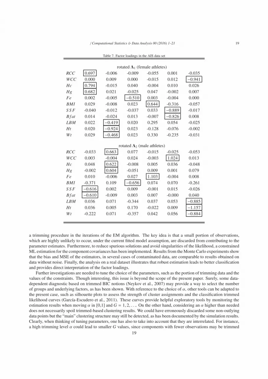
/ Computational Statistics & Data Analysis 00 (2016) 1–21 19

Table 7. Factor loadings in the AIS data set

rotated Λ1 (female athletes)RCC 0.697 -0.006 -0.009 -0.055 0.001 -0.035WCC 0.000 0.009 0.000 -0.015 0.012 −0.941Hc 0.794 -0.015 0.040 -0.004 0.010 0.026Hg 0.682 0.021 -0.025 0.047 -0.002 0.007Fe 0.002 -0.005 −0.510 0.003 -0.004 0.000BMI 0.029 -0.008 0.023 0.644 -0.316 -0.057S S F -0.040 -0.012 -0.037 0.033 −0.889 -0.017B f at 0.014 -0.024 0.013 -0.007 −0.826 0.008LBM 0.022 −0.419 0.020 0.295 0.054 -0.025Ht 0.020 −0.924 0.023 -0.128 -0.076 -0.002Wt 0.029 −0.468 0.023 0.330 -0.235 -0.031

rotated Λ2 (male athletes)RCC -0.033 0.663 0.077 -0.015 -0.025 -0.053WCC 0.003 -0.004 0.024 -0.003 1.024 0.013Hc 0.048 0.622 -0.008 0.005 0.036 -0.048Hg -0.002 0.604 -0.051 0.009 0.001 0.079Fe 0.010 -0.006 0.027 1.103 -0.004 0.008BMI -0.371 0.109 −0.656 0.074 0.070 -0.261S S F −0.616 0.002 0.009 -0.001 0.015 -0.026B f at −0.610 -0.009 0.003 0.007 -0.000 0.040LBM 0.036 0.071 -0.344 0.037 0.053 −0.885Ht 0.036 0.005 0.170 -0.022 0.009 −1.157Wt -0.222 0.071 -0.357 0.042 0.056 −0.884

a trimming procedure in the iterations of the EM algorithm. The key idea is that a small portion of observations,which are highly unlikely to occur, under the current fitted model assumption, are discarded from contributing to theparameter estimates. Furthermore, to reduce spurious solutions and avoid singularities of the likelihood, a constrainedML estimation for the component covariances has been implemented. Results from the Monte Carlo experiments showthat the bias and MSE of the estimators, in several cases of contaminated data, are comparable to results obtained ondata without noise. Finally, the analysis on a real dataset illustrates that robust estimation leads to better classificationand provides direct interpretation of the factor loadings.

Further investigations are needed to tune the choice of the parameters, such as the portion of trimming data and thevalues of the constraints. Though interesting, this issue is beyond the scope of the present paper. Surely, some data-dependent diagnostic based on trimmed BIC notions (Neykov et al., 2007) may provide a way to select the numberof groups and underlying factors, as has been shown. With reference to the choice of α, other tools can be adapted tothe present case, such as silhouette plots to assess the strength of cluster assignments and the classification trimmedlikelihood curves (Garcıa-Escudero et al., 2011). These curves provide helpful exploratory tools by monitoring theestimation results when moving α in [0,1] and G = 1, 2, . . .. On the other hand, considering an α higher than neededdoes not necessarily spoil trimmed-based clustering results. We could have erroneously discarded some non-outlyingdata points but the “main” clustering structure may still be detected, as has been documented by the simulation results.Clearly, when thinking of tuning parameters, one has also to take into account that they are interrelated. For instance,a high trimming level α could lead to smaller G values, since components with fewer observations may be trimmed

19

/ Computational Statistics & Data Analysis 00 (2016) 1–21 20

off. Moreover, larger values of the constraints could lead to higher values of G, since new components with few almostcollinear observations may arise. With respect to the choice of the specific values for the constraints, our experiencetells us that a moderate interval of values for cload and cnoise produces almost the same estimation and exactly thesame classification. Also, from an interpretative point of view, this corresponds to the fact that, generally, the user hassome intuition (or rough knowledge) about the order of magnitude of these constraints, and this partial informationcan be incorporated into the estimation. The encouraging results obtained here suggest that a deeper discussion ofthese implementation details could be developed as a future work.

As a final remark, following the suggestions for further investigation we received from an unknown referee,the proposed method can also be extended to accommodate missing values, as in Wang (2015); and much fasterconvergence to the EM-based algorithm could be improved along the lines of Zhao and Yu (2008).

Acknowledgements

The authors would like to thank two anonymous referees for many interesting and helpful comments that ledto a clearer presentation of the material. Research partially supported by the Spanish Ministerio de Economıa yCompetitividad and FEDER, grant MTM2014-56235-C2-1-P, and by Consejerıa de Educacion de la Junta de Castillay Leon, grant VA212U13, by grant FAR 2015 from the University of Milano-Bicocca and by grant FIR 2014 from theUniversity of Catania.

References

Azzalini A., R package sn: The skew-normal and skew-t distributions (version 0.4-17), URL http://azzalini. stat. unipd. it/SN, (2011).Azzalini A., Dalla Valle A., The multivariate skew-normal distribution, Biometrika, 83 (4), 715–726, (1996).Baek J., McLachlan G., Flack L., Mixtures of Factor Analyzers with Common Factor Loadings: Applications to the Clustering and Visualization

of High-Dimensional Data, IEEE Transactions on Pattern Analysis and Machine Intelligence, 32 (7), 1298 –1309, (2010).Baek J., McLachlan G., Mixtures of common t-factor analyzers for clustering high-dimensional microarray data, Bioinformatics, 27 (9), 1269–

1276, (2011).Bernaards C. A., Jennrich R. I. , Gradient projection algorithms and software for arbitrary rotation criteria in factor analysis, Educational and

Psychological Measurement, 65 (5), 676–696, (2005).Bekker P. A., ten Berge J. M. F. , Generic global identification in factor analysis, Linear Algebra and its Applications, 264, 255–263, (1997).Bickel D.R., Robust cluster analysis of microarray gene expression data with the number of clusters determined biologically, Bioinformatics, 19 (7),

818–824, (2003).Bishop C. M., Tipping M. E., A Hierarchical Latent Variable Model for Data Visualization, IEEE Transactions on Pattern analysis and Machine

Intelligence , 20, 281–293, (1998).Browne M. W., An overview of analytic rotation in exploratory factor analysis, Multivariate Behavioral Research, 36 (1), 111–150, (2001).Campbell J., Fraley C., Murtagh F., Raftery A., Linear flaw detection in woven textiles using model-based clustering, Pattern Recognition Letters,

18 (14), 1539 – 1548, (1997).Cook R. D., Weisberg S., An introduction to regression graphics, vol. 405, John Wiley & Sons, 1994.Coretto P., Hennig C., Maximum likelihood estimation of heterogeneous mixtures of Gaussian and uniform distributions, Journal of Statistical

Planning and Inference, 141 (1) 462–473, (2011) .Fokoue E., Titterington D., Mixtures of factor analysers. Bayesian estimation and inference by stochastic simulation, Machine Learning, 50 (1-2),

73–94, (2003).Fraley C., Raftery A. E., How Many Clusters? Which Clustering Method? Answers Via Model-Based Cluster Analysis, Computer Journal, 41 (8),

578–588, (1998).Fritz H., Garcıa-Escudero L., Mayo-Iscar A., A fast algorithm for robust constrained clustering, Computational Statistics & Data Analysis, (61),

124–136, (2013).Gallegos M., Ritter G., Trimmed ML estimation of contaminated mixtures, Sankhya (Ser. A), (71), 164–220, (2009).Garcıa-Escudero L. A., Gordaliza A., Matran C., Mayo-Iscar A., A General Trimming Approach to Robust Cluster Analysis, The Annals of

Statistics, 36 (3) 1324–1345 (2008).Garcıa-Escudero L. A., Gordaliza A., Matran C., Mayo-Iscar A., Exploring the Number of Groups in Robust Model-Based Clustering, Statistics

and Computing, 21 (4), 585–599, (2011).Garcıa-Escudero L., Gordaliza A., Mayo-Iscar A., A constrained robust proposal for mixture modeling avoiding spurious solutions, Advances in

Data Analysis and Classification, 8 (1), 27–43, (2014).Ghahramani Z., Hilton G., The EM algorithm for mixture of factor analyzers, Techical Report CRG-TR-96-1, (1997).Greselin F., Ingrassia S., Maximum likelihood estimation in constrained parameter spaces for mixtures of factor analyzers, Statistics and Comput-

ing, 25, 215–226, (2015).Hathaway R., A constrained formulation of maximum-likelihood estimation for normal mixture distributions, The Annals of Statistics, 13 (2),

795–800, (1985).Hennig C., Breakdown points for maximum likelihood-estimators of location-scale mixtures, Annals of Statistics, 32, 1313–1340, (2004).

20

/ Computational Statistics & Data Analysis 00 (2016) 1–21 21

Ingrassia S., A likelihood-based constrained algorithm for multivariate normal mixture models, Statistical Methods & Applications, 13, 151–166,(2004).

Ingrassia S., Rocci R., Constrained monotone EM algorithms for finite mixture of multivariate Gaussians, Computational Statistics &Data Analysis,51, 5339–5351, (2007).

Ledermann, W., On the rank of the reduced correlational matrix in multiple-factor analysis, Psychometrika, 2 (2), 85-93, (1937).Lin T.-I., Ho H. J., Lee C. R., Flexible mixture modelling using the multivariate skew-t-normal distribution, Statistics and Computing, 24 (4),

531-546, (2014).Lin T.-I., McNicholas P. D., Ho H. J., Capturing patterns via parsimonious t mixture models, Statistics & Probability Letters, 88, 80–87, (2014).Maitra R., Clustering Massive Datasets With Application in Software Metrics and Tomography, Technometrics, 43 (3), 336–346, (2001).Maitra R., Initializing partition-optimization algorithms, IEEE/ACM Transactions on Computational Biology and Bioinformatics 6 (1) 144–157,

(2009).McLachlan G. J., Bean R. W., Maximum likelihood estimation of mixtures of t factor analyzers, Technical Report, University of Queensland,

(2005).McLachlan G., Peel D., Robust mixture modelling using the t distribution, Statistics and Computing, 10 (4) 335–344, (2000).McLachlan G., Peel D., Mixtures of factor analyzers, in: Proceedings of the Seventeenth International Conference on Machine Learning, P. Langley

(Ed.)., San Francisco: Morgan Kaufmann, 599–606, (2000a).McLachlan G. J., Peel D., Finite Mixture Models, John Wiley & Sons, New York, (2000b).McNicholas P., Murphy T., Parsimonious Gaussian mixture models, Statistics and Computing, 18 (3), 285–296, (2008).Neykov N., Filzmoser P., Dimova R., Neytchev P., Robust Fitting of Mixtures Using the Trimmed Likelihood Estimator, Computational Statistics& Data Analysis, 52 (1), 299–308, (2007).

R. D. C. Team, R: A Language and Environment for Statistical Computing, R Foundation for Statistical Computing, Vienna, Austria, URLhttp://www.R-project.org, (2013).

Rousseeuw P. J., Van Driessen K., A Fast Algorithm for the Minimum Covariance Determinant Estimator, Technometrics, 41, 212–223, (1999).Steane M. A., McNicholas P. D., R. Y. Yada, Model-based classification via mixtures of multivariate t-factor analyzers, Communications in

Statistics-Simulation and Computation, 41 (4), 510–523, (2012).Stewart C. V., Robust parameter estimation in computer vision, SIAM review, 41 (3), 513–537, (1999).Tipping M. E., Bishop C. M., Mixtures of probabilistic principal component analyzers, Neural computation, 11 (2), 443–482, (1999).Wang, W. L., Mixtures of common t-factor analyzers for modeling high-dimensional data with missing values, Computational Statistics & Data

Analysis, 83, 223–235, (2015).Zhao J. H., Yu P. L. Fast ML estimation for the mixture of factor analyzers via an ECM algorithm, Neural Networks, IEEE Transactions on,

19 (11), 1956–1961, (2008).

21

0 2 4 6 8 10 12

05

10

Figure

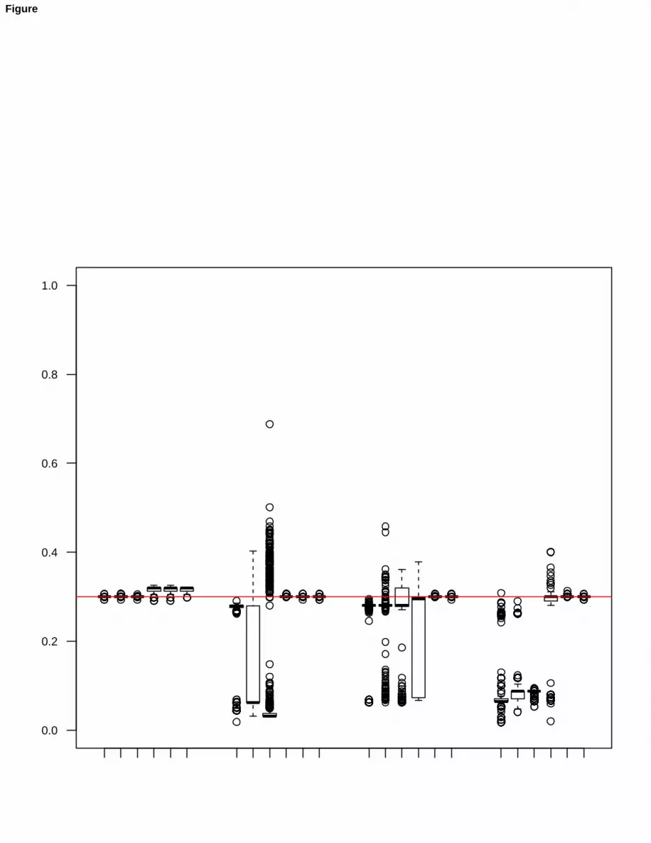
0.0

0.2

0.4

0.6

0.8

1.0

Figure

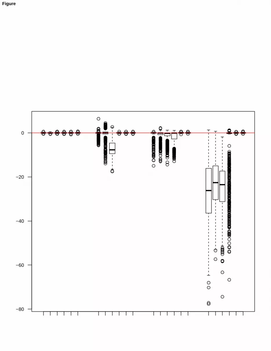
−80

−60

−40

−20

0

Figure

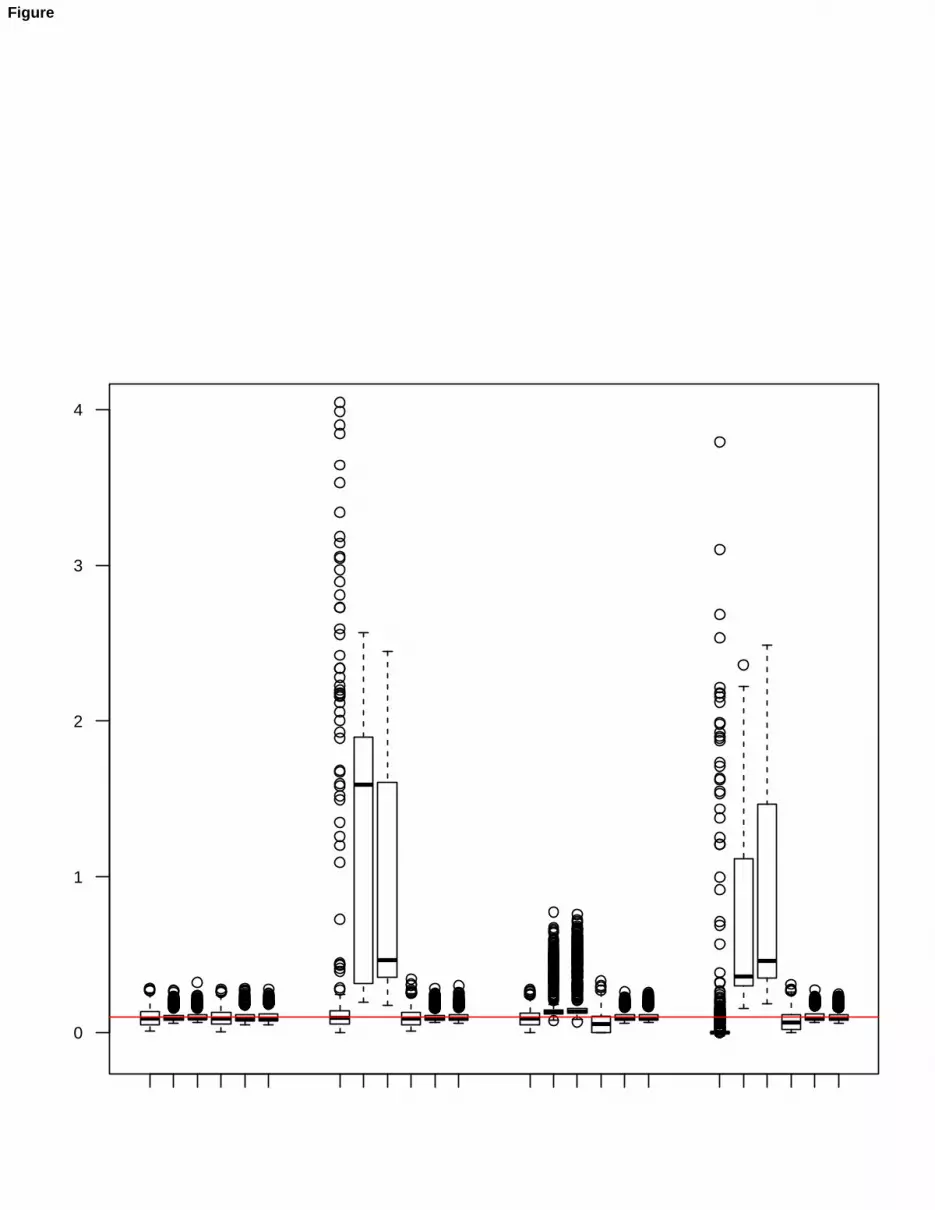
0

1

2

3

4

Figure

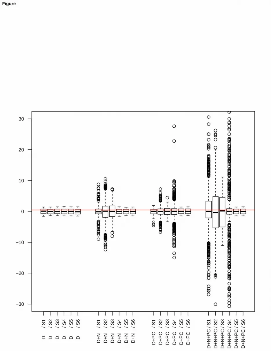
D

/ S

1D

/ S2

D

/ S

3D

/ S4

D

/ S

5D

/ S6

D+

N

/ S

1D

+N

/

S2

D+

N

/ S

3D

+N

/

S4

D+

N

/ S

5D

+N

/

S6

D+

PC

/ S

1D

+P

C

/ S2

D+

PC

/ S

3D

+P

C

/ S4

D+

PC

/ S

5D

+P

C

/ S6

D+

N+

PC

/ S

1D

+N

+P

C /

S2

D+

N+

PC

/ S

3D

+N

+P

C /

S4

D+

N+

PC

/ S

5D

+N

+P

C /

S6

−30

−20

−10

0

10

20

30

Figure

RCC

4 6 8 10 12 14 50 100 150 200

4.0

5.0

6.0

46

810

1214

WCC

BMI20

2530

35

4.0 5.0 6.0

5010

015

020

0

20 25 30 35

SSF

Figure

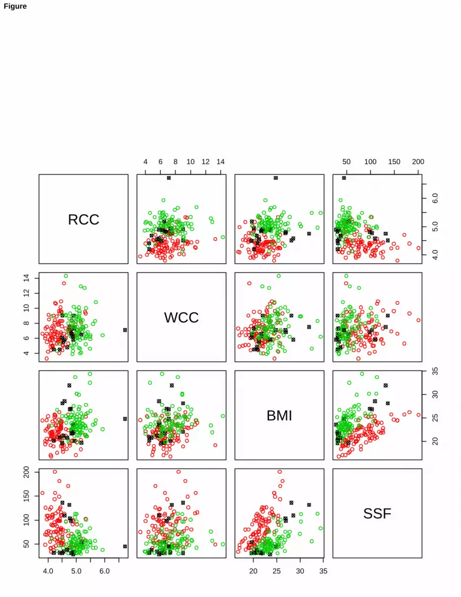
RCC

4 6 8 10 12 14 50 100 150 200

4.0

5.0

6.0

46

810

1214

WCC

BMI20

2530

35

4.0 5.0 6.0

5010

015

020

0

20 25 30 35

SSF

Figure

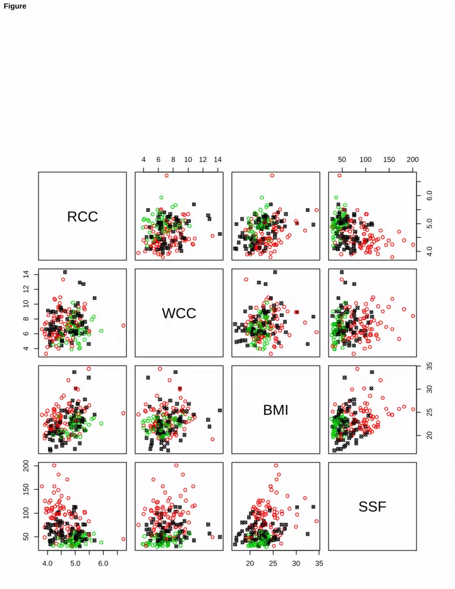
RCC

4 6 8 10 12 14 50 100 150 200

4.0

5.0

6.0

46

810

1214

WCC

BMI20

2530

35

4.0 5.0 6.0

5010

015

020

0

20 25 30 35

SSF

Figure

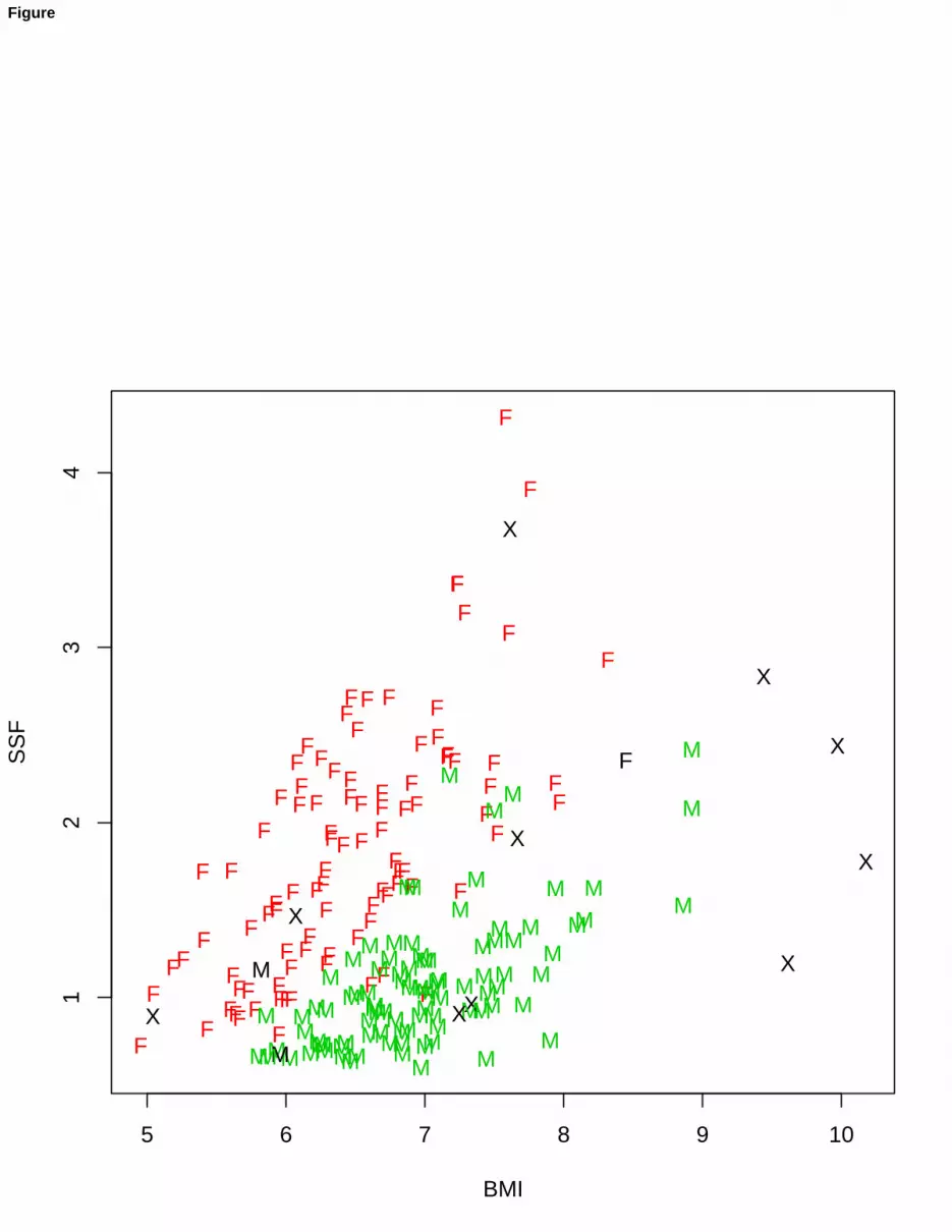
FF F

F

FF

F

F

F

F

X

F

F

FFF

F

F

FF

FF

FF

F

F

FF

F

F

F

F

F

F

F

F

F

F

F

F

F

F

F

F

F

F

FF

F

F

F

F

F

F

F

F

F

F

F

F

FF

FF

F

F

F

FF

F

F

F

FF

X

F

F F

F

F

F

F

F

F FF

FFF

F

F

F

X

F

F

FF

F

X

F

M MM

M

M

MM MM

M

M

MM

M

M

M

M

M

MM

M

M

M

M

MM

M

M

MM

M M

X

M

M

M

M

M

M

MM

MM

M

MM

MMM MMMM MM M

M MM

X

M

M

X

M

MX

M

MMMM

M

MM

M

M

M

X

M

MX

M

M

MM

M

M

MM

M

M

M

MM

MM

M

M

M

M

M

M

5 6 7 8 9 10

12

34

BMI

SS

FFigure

FF F

F

FF

F

F

F

F

F

F

F

FFF

F

F

FF

FF

FF

F

F

FF

F

F

F

F

F

F

F

F

F

F

F

F

F

F

F

F

F

F

FF

F

F

F

F

F

F

F

F

F

F

F

F

FF

FF

F

F

F

FF

F

F

F

FF

F

F

F F

F

F

F

F

F

F FF

FFF

F

F

F

F

F

F

FF

F

F

F

M MM

M

M

MM MM

M

M

MM

M

M

M

M

M

MM

M

M

M

M

MM

M

M

MM

M M

M

M

M

M

M

M

M

MM

MM

M

MM

MMM MMMM MM M

M MM

M

M

M

M

M

MM

M

MMMM

M

MM

M

M

M

M

M

MM

M

M

MM

M

M

MM

M

M

M

MM

MM

M

M

M

M

M

M

5 6 7 8 9 10

12

34

BMI

SS

FFigure

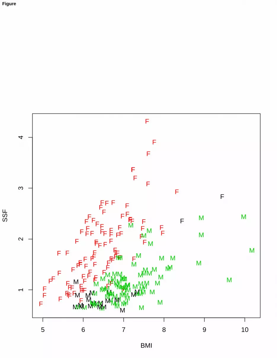
FF F

F

FF

F

F

F

F

F

F

F

FFF

F

F

FF

FF

FF

F

F

FF

F

F

F

F

F

F

F

F

F

F

F

F

F

F

F

F

F

F

FF

F

F

F

F

F

F

F

F

F

F

F

F

FF

FF

F

F

F

FF

F

F

F

FF

F

F

F F

F

F

F

F

F

F FF

FFF

F

F

F

F

F

F

FF

F

F

F

M MM

M

M

MM MM

M

M

MM

M

M

M

M

M

MM

M

M

M

M

MM

M

M

MM

M M

M

M

M

M

M

M

M

MM

MM

M

MM

MMM MMMM MM M

M MM

M

M

M

M

M

MM

M

MMMM

M

MM

M

M

M

M

M

MM

M

M

MM

M

M

MM

M

M

M

MM

MM

M

M

M

M

M

M

5 6 7 8 9 10

12

34

BMI

SS

FFigure