Embed Size (px)
Citation preview

Hermes2D
C++ library for rapid development of adaptive
hp-FEM / hp-DG solvers
Lukas Korous
Johannesburg, 12th Oct 2016

Hermes2d Overview
What it is?
- C++ multi-platform (Win, Linux, MacOS) library for rapid prototyping of FEM & DG solvers
- “When you want to solve a non-trivial PDE in 2d with the least possible effort. And you know some C/C++.”
- “When you want to test drive something small (a preconditioner, error estimate, FE space), and you don’t want to write all the rest for it. And you know some OOP in C++.”
How can I try it out?
- https://github.com/hpfem/hermes
- On Linux- Download, get dependencies via package managers, configure, build
- On Windows- Download, get dependencies from https://github.com/l-korous/hermes-windows, configure, build
What technologies are used in Hermes2d?
- (Modern) C++, (well) documented, and exception-safe
- OpenMP for parallelization of the most CPU-intensive tasks
- Real-time OpenGL visualization
- External linear solvers (UMFPACK, PARALUTION, MUMPS, Trilinos)
- Usual exchange formats (XML, BSON, VTK, ExodusII, MatrixMarket, Matlab)
Hermes2D – Lukas Korous

Hermes2d Overview > Features
What can it do?
- Stationary / Time-dependent / Harmonic equations
- Number of manual, and automatic mesh refinement (AMR) / Spatial adaptivity options
- Granular AMR setup based on customizable error estimate calculations
- Nonlinear equation handling using Newton’s and Picard’s method
- Fully automatic & configurable Newton’s method with damping coefficient control, jacobian reuse control, arbitrary stopping criteria control
- Time-adaptivity, Space-time adaptivity using embedded Runge-Kutta methods
- Time-error space distribution, arbitrary calculations of any error estimate pluggable into AMR, and time-step controllers
- Weak & Strong coupled problems
- No matter what the coupling is, when you can write the weak formulation of your problem on paper, you can do that in Hermes2d as well.
What it cannot do (does not do)
- Problem specific optimizations, caching, shortcuts, etc.- But #1: In some cases, the Hermes2D API provides methods that can be used for some optimizations.
- But #2: Due to the use of OOP, users of the library are welcome to sub-class Hermes2d core classes and implement the missing functionality.
Hermes2D – Lukas Korous

Hermes2d Structures > Introduction
As a user, I have a problem:
Hermes2D – Lukas Korous
Domain Geometry
Weak Formulation
Essential Boundary Conditions & Initial
Conditions
Problem Knowledge
Desired Output
Domain needs to be meshed usually via a specific tool (GMSH, Cubit, etc.).
Since triangulation is very crucial part of the FE method, even though Graphical User Interface software (e.g. Agros2D) is generally able to accept the geometry (and it triangulates internally), the mesh is available for inspection by the user.
Mesh

Hermes2d Structures > Introduction
As a user, I have a problem:
Hermes2D – Lukas Korous
Domain Geometry
Weak Formulation
Essential Boundary Conditions & Initial
Conditions
Problem Knowledge
Desired Output
Problem Knowledge translates to selecting suitable FE spaces / solvers & their attributes / preconditioners, manual mesh refinements in problematic areas, etc.
Desired Output translates to selecting desired post-processing tools - integral calculations, point values, graphical representation of the solution, or any function of solution(s).
Mesh

Hermes2d Structures > Mapping
As a user, I have a problem:
Hermes2D – Lukas Korous
Domain Geometry
Weak Formulation
Essential Boundary Conditions & Initial
Conditions
Problem Knowledge
Desired Output
Mesh
Mesh WeakForm
EssentialBoundaryCondition
Space- H1Space- L2Space (DG)- HcurlSpace View
FilterIntegralCalculator
ExactSolutionSolver
- LinearSolver- NewtonSolver

Hermes2d Structures > Mesh
Functionality:
Input / Output – own format (plain text, XML), Cubit, GMSH (through Agros2D)
Graphical representation – direct (OpenGL view), VTK format
Refinements – set of methods for manual mesh refinement
Data:
Element []
Vertex []
Edge []
Hermes2D – Lukas Korous
Hermes2d Structures > Space
Functionality:
Input / Output – own format (XML, BSON)
Graphical representation
– direct (OpenGL view), VTK format
– OrderView (top), BaseView (bottom)
Element order handling – Get/Set, increase, decrease, uniform settings
Essential boundary conditions handling:virtual Scalar value(double x, double y)
Data:
Mesh
Shapeset
ElementOrder []
EssentialBoundaryCondition []
Hermes2D – Lukas Korous

Hermes2d Structures > WeakForm, Solver
WeakForm Functionality:
For each Form (=integral), performs calculations:
Scalar matrix_form(int n, double *wt, Func<double> *u, Func<double> *v)
Ord matrix_form(int n, double *wt, Func<Ord> *u, Func<Ord> *v)
Scalar vector_form(int n, double *wt, Func<double> *v)
Ord vector_form(int n, double *wt, Func<Ord> *v)
- n ... Number of integration points
- wt ... Integration weights
- u ... Basis function values(, derivatives) at integration points
- v ... Test function values(, derivatives) at integration points
WeakForm Data:
Form []
Hermes2D – Lukas Korous
Solver Subtypes:LinearSolverNewtonSolverPicardSolver
Solver Functionality:Damping factor handling- in case of Newton’s methodAlgebraic solver selection
Solver Data:SpaceWeakForm

Examples > Magnetostatics
In this example, we solve the equation
𝛻 ×1
𝜇(𝛻 × u) = J, u|𝛿Ω = 0
Where
- J is the current density,
- 𝜇 is (nonlinear) permeability,
- u is the (sought) magnetic vector potential (its z-component),
- Ω is the space domain (picture on next slide).
The features illustrated on this example are
- Newton’s method for nonlinear problems,
- nonlinear term specification using a table of values, and cubic spline interpolation.
Hermes2D – Lukas Korous

Examples > Magnetostatics
Hermes2D – Lukas Korous
Domain Ω with
triangular mesh
Solution –
vector potential u

Examples > Magnetostatics
Refining the mesh according to a criterionmesh->refine_by_criterion(&refinement_criterion);
- header: int refinement_criterion(Element* e), returning whether or not to refine a particular Element.
Used to refine the mesh around the copper <> iron interface.
CubicSpline class used for nonlinearity description// Define nonlinear magnetic permeability via a cubic spline.
std::vector<double> mu_inv_pts({ 0.0, 0.5, 0.9, ... });
std::vector<double> mu_inv_val({ 1. / 1500.0, 1. / 1480.0, 1. / 1440.0, ... });
CubicSpline mu_inv_iron(mu_inv_pts, mu_inv_val, ...);
Newton’s method for a strong nonlinearity// Automatic damping ratio – if a step is unsuccessful, damping factor will be multiplied by this, if successful, it will be divided by this.
newton.set_auto_damping_ratio(1.5);
// Initial damping factor – we can start with a small one, automation will increase it if possible.
newton.set_initial_auto_damping_coeff(.1);
// The redidual norm after a step must be at most this factor times the norm from the previous step to pronounce the step ‘successful’.
// Now for very strong nonlinearities, we may even need this > 1.
newton.set_sufficient_improvement_factor(1.25);
// This is a strong nonlinearity, where we can’t afford to reuse Jacobian matrix from a step in subsequent steps.
newton.set_max_steps_with_reused_jacobian(0);
// Maximum number of iterations. Hermes will throw an exception if this number is exceeded and the tolerance is not met.
newton.set_max_allowed_iterations(100);
// The tolerance – simple in this case, but can be a combination of relative / absolute thresholds of residual norm, solution norm, solution difference norm, ...
newton.set_tolerance(1e-8, Hermes::Solvers::ResidualNormAbsolute);
Hermes2D – Lukas Korous

Examples > Advection
In this example, we solve the equation
𝛻 ⋅ (−𝑥2, 𝑥1)u = 0, u|𝛿Ω = gWhere
- u is the sought solution,
- Ω is the space domain - square (0, 1) x (0, 1),
- g is defined as follows:- g = 1, where (−𝑥2, 𝑥1) ∙ 𝑛 Ԧ𝑥 > 0,
- g = 0, where (−𝑥2, 𝑥1) ∙ 𝑛 Ԧ𝑥 ≤ 0.
The features illustrated on this example are
- Discontinuous Galerkin (DG) implementation of integrating over internal edges,
- Post-processing of results – in this case using a limiter preventing spurious oscillations that occur in DG method.
Hermes2D – Lukas Korous

Examples > Advection
Hermes2D – Lukas Korous
Domain Ω with
quadrilateral meshSolution

Examples > Advection
Integration over internal edges
- Regular forms (simplified)matrix_form(int n, double *wt, Func<double> *u, Func<double> *v)
- n ... Number of integration points
- wt ... Integration weights
- u ... Basis function values(, derivatives) at integration points
- v ... Test function values(, derivatives) at integration points
- DG forms (simplified)matrix_form(int n, double *wt, DiscontinuousFunc<double> *u, DiscontinuousFunc<double> *v)
- n, wt ... As above
- u, v ... DiscontinuousFunc<double> = { Func<double> u->central, Func<double>* u->neighbor } ... Only one is filled for each matrix_form call.
Postprocessing
- e.g. Vertex-based limiter (Kuzmin, D.: A vertex-based hierarchical slope limiter for -adaptive discontinuous Galerkin methods, JCAM, 233(12):3077-3085)
// sln_vector ... Algebraic system solution
// space ... FE space of the solution
// Instantiate the limiter
PostProcessing::VertexBasedLimiter limiter(space, sln_vector);
// Get a limited solution, already as a Hermes2D Solution object
Hermes::Hermes2D::Solution<double> limited_sln = limiter.get_solution();
Hermes2D – Lukas Korous

Examples > Advection > Automatic adaptivity (AMR)
We solve the same problem – equation & boundary conditions:
𝛻 ⋅ (−𝑥2, 𝑥1)u = 0, u|𝛿Ω = g
But this time, we start from a very coarse mesh:
And we employ AMR (h-adaptivity) to get results on the next slide.
Hermes2D – Lukas Korous

Examples > Advection > Automatic adaptivity (AMR)
Hermes2D – Lukas Korous
AMR step 1, Element count: 32 AMR step 2, Element count: 116 AMR step 3, Element count: 272
AMR step 4, Element count: 504 AMR step 5, Element count: 848

Examples > Advection > Automatic adaptivity (AMR)
How automatic hp-adaptivity in Hermes works?
- based on a reference solution approach:
1. Solution is searched for in a “fine” Space.
Hermes2D – Lukas Korous

Examples > Advection > Automatic adaptivity (AMR)
How automatic hp-adaptivity in Hermes works?
- based on a reference solution approach:
1. Solution is searched for in a “fine” Space.
2. Obtained Solution is projected to a “coarse” Space.• One level of refinement coarser mesh, and degree p-1
3. Error is calculated as the appropriate norm of the difference.• In an element-wise manner
• This is fully overridable by custom ErrorCalculator classes
Hermes2D – Lukas Korous
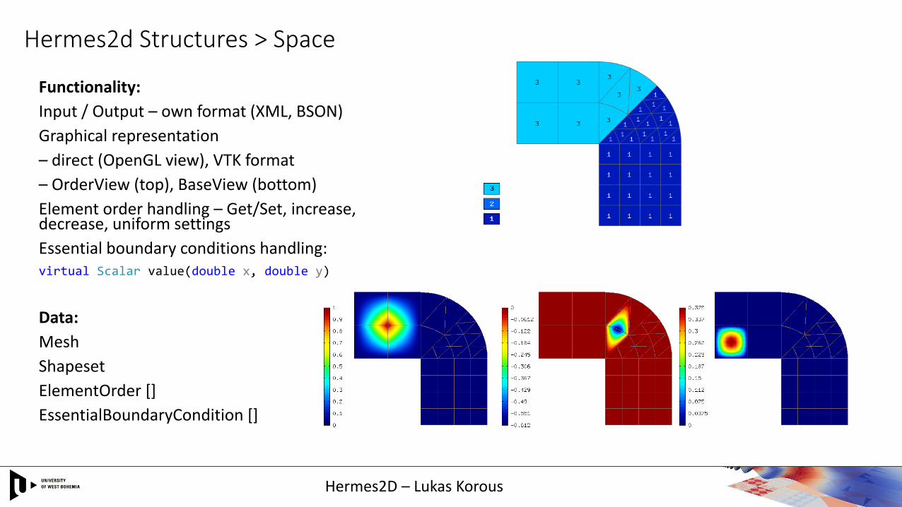
Examples > Advection > Automatic adaptivity (AMR)
How automatic hp-adaptivity in Hermes works?
- based on a reference solution approach:
1. Solution is searched for in a “fine” Space.
2. Obtained Solution is projected to a “coarse” Space.• One level of refinement coarser mesh, and degree p-1
3. Error is calculated as the appropriate norm of the difference.• In an element-wise manner
• This is fully overridable by custom ErrorCalculator classes
4. The Elements with the largest errors are selected for refinement.
5. For these Elements, the appropriate refinement is selected from candidates using local projections of the “fine” Solution.• Standard lists of the candidates for illustrations are on the right.
Hermes2D – Lukas Korous

Examples > Advection > Automatic adaptivity (AMR)
int adaptivity_step = 1; bool done = false;
do
{
// Construct globally refined reference mesh and setup reference space.
Mesh::ReferenceMeshCreator ref_mesh_creator(mesh);
MeshSharedPtr ref_mesh = ref_mesh_creator.create_ref_mesh();
Space<double>::ReferenceSpaceCreator refspace_creator(space, ref_mesh, USE_TAYLOR_SHAPESET ? 0 : 1);
SpaceSharedPtr<double> refspace = refspace_creator.create_ref_space();
// Solve the problem on the reference space.
linear_solver.set_space(refspace);
linear_solver.solve();
// Get the Hermes2D Solution object from the solution vector.
Solution<double>::vector_to_solution(linear_solver.get_sln_vector(), refspace, refsln);
// Project the reference solution to the coarse space in L2 norm for error calculation.
OGProjection<double>::project_global(space, refsln, sln, HERMES_L2_NORM);
// Calculate element errors and total error estimate.
errorCalculator.calculate_errors(sln, refsln);
double total_error_estimate = errorCalculator.get_total_error_squared() * 100;
// If error is too large, adapt the (coarse) space.
if (error_estimate > ERR_STOP)
adaptivity.adapt(&selector);
else
done = true;
// Increase the step counter.
adaptivity_step++;
} while (done == false);
Hermes2D – Lukas Korous
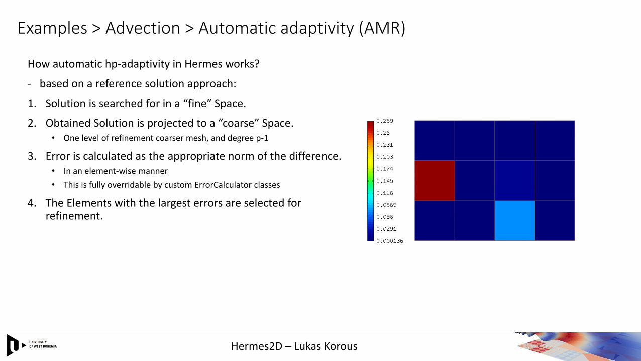
Examples > Navier-Stokes
In this example, we solve the equations𝛿𝑢
𝛿𝑡−∆𝑢
𝑅𝑒+ 𝑢 ⋅ 𝛻 𝑢 + 𝛻𝑝 = 0, u|𝛿Ω\Γ𝑜 = g
𝛻 ∙ 𝑢 = 0
Where
- Γ𝑜 is the output boundary,
- u, p is the sought solution,
- Ω is the space domain – see next slide,
- g is defined as follows:- 𝑔1 = 0 everywhere except inlet,- 𝑔2 = 0 everywhere,- 𝑔1 is a parabolic profile on the inlet.
The features illustrated on this example are
- OpenGL visualization of vector fields,
- Simple time-stepping using implicit Euler scheme.
Hermes2D – Lukas Korous

Examples > Navier-Stokes > OpenGL visualization of vector fields
Solution
- Velocity (vector field) top
- Pressure bottom
- t = 30s
Hermes2D – Lukas Korous

Examples > Navier-Stokes > OpenGL visualization of vector fields
Solution
- Velocity (vector field) top
- Pressure bottom
- t = 40s
Hermes2D – Lukas Korous

Examples > Navier-Stokes > OpenGL visualization of vector fields
Solution
- Velocity (vector field) top
- Pressure bottom
- t = 55s
Hermes2D – Lukas Korous

Examples > Navier-Stokes
Simple time-stepping using implicit Euler scheme
for (int time_step = 1; time_step <= T_FINAL / TAU; time_step++, current_time += TAU){
// Update time-dependent essential BCs.newton.set_time(current_time);
// Solve Newton.// Weak formulation implements the implicit Euler scheme, and uses previous time step solutions.newton.solve(coeff_vec);
// Get the solutions, insert as Hermes2D Solution object into the previous time step solutions.Hermes::Hermes2D::Solution<double>::vector_to_solutions(newton.get_sln_vector(), spaces, sln_prev_time);
// Visualization.vview.set_title("Velocity, time %g", current_time);vview.show(xvel_prev_time, yvel_prev_time);
pview.set_title("Pressure, time %g", current_time);pview.show(p_prev_time);
}
Hermes2D – Lukas Korous

Example > Complex
This problem describes the distribution of the vector potential in a domain comprising a wire carrying electrical current, air, and
an iron which is not under voltage. We solve the equation
−1
𝜇∆𝐴 + 𝑖𝜔𝜎𝐴 − = 0, u|Γ1 = 0, ቤ
𝛿𝑢
𝛿𝑛Γ2
= 0
Where
- Ω is the space domain - rectangle (0, 0.004) x (0, 0.003),
- Γ1 is the top and right and left edge of Ω,
- Γ2 is the bottom edge of Ω,
- A is the sought solution, 𝜔 is the given angular velocity, 𝜎 given conductivity
The features illustrated on this example are
- hp-adaptive FEM,
- Handling of complex equations in Hermes2D,
- Spatial error inspection.
Hermes2D – Lukas Korous

Example > Complex > hp-FEM step #1
Hermes2D – Lukas Korous
Solution- Reference
space
Coarse mesh Fine mesh
Spatial error inspection
Element-wise error for the coarse mesh

Example > Complex > hp-FEM step #5
Hermes2D – Lukas Korous
Solution- Reference
space
Coarse mesh Fine mesh
Spatial error inspection
Element-wise error for the coarse mesh

Example > Complex > hp-FEM step #15
Hermes2D – Lukas Korous
Solution- Reference
space
Coarse mesh Fine mesh
Spatial error inspection
Element-wise error for the coarse mesh

Example > Complex > hp-FEM step #29
Hermes2D – Lukas Korous
Solution- Reference
space
Coarse mesh Fine mesh
Spatial error inspection
Element-wise error for the coarse mesh

Example > Complex
Handling of complex equations in Hermes2D
- Very easy, all relevant Hermes2d classes have the number (real | complex) as their template argument:- For real numbers we use double - H1Space<double>(mesh, boundary_conditions)
- For complex numbers we use std::complex<double> - H1Space<std::complex<double> >(mesh, boundary_conditions)
hp-adaptive FEM
- Basic settings to control the AMR process
// Error calculation & adaptivity. We specify the norm here, and the type of errorDefaultErrorCalculator<::complex, HERMES_H1_NORM> errorCalculator(RelativeErrorToGlobalNorm);
// Stopping criterion for an adaptivity step. Influences the number of elements refined at each step.AdaptStoppingCriterionSingleElement<::complex> stoppingCriterion(0.9);
// Adaptivity processor class. Gets the error calculator and stopping criterionAdapt<::complex> adaptivity(&errorCalculator, &stoppingCriterion);
// Stopping criterion for adaptivity.const double TOTAL_ERROR_ESTIMATE_STOP = 1e-3;
Hermes2D – Lukas Korous

Examples > Wave Equation
In this example, we solve the equations
1
𝑐2𝛿2𝑢
𝛿𝑡2− ∆𝑢 = 0, u|𝛿Ω = 0, ቤ
𝛿𝑢
𝛿𝑡𝛿Ω
= 0 (1)
Where- u is the sought solution,- Ω is the space domain – see next slide,- c is the wave speed.
We transform (1) into
𝛿𝑢
𝛿𝑡= v
𝛿𝑣
𝛿𝑡= 𝑐2Δ𝑢
The features illustrated on this example are
- Using an arbitrary Runge-Kutta method for time discretization,
- Time-adaptivity using embedded Runge-Kutta methods.
Hermes2D – Lukas Korous

Example > Wave Equation
Hermes2D – Lukas Korous
u (left), v(right), t = 1e-2s

Example > Wave Equation
Hermes2D – Lukas Korous
u (left), v(right), t = 5.1e-1s

Example > Wave Equation
Hermes2D – Lukas Korous
u (left), v(right), t = 1.01s

Example > Wave Equation
Hermes2D – Lukas Korous
u (left), v(right), t = 1.51s

Example > Wave Equation
Hermes2D – Lukas Korous
u (left), v(right), t = 2.01s

Examples > Wave Equation > Runge-Kutta methods
These Runge-Kutta methods are available in Hermes2D:
Explicit methods:
Explicit_RK_1, Explicit_RK_2, Explicit_RK_3, Explicit_RK_4.
Implicit methods:
Implicit_RK_1, Implicit_Crank_Nicolson_2_2, Implicit_SIRK_2_2, Implicit_ESIRK_2_2, Implicit_SDIRK_2_2,
Implicit_Lobatto_IIIA_2_2, Implicit_Lobatto_IIIB_2_2, Implicit_Lobatto_IIIC_2_2, Implicit_Lobatto_IIIA_3_4,
Implicit_Lobatto_IIIB_3_4, Implicit_Lobatto_IIIC_3_4, Implicit_Radau_IIA_3_5, Implicit_SDIRK_5_4.
Embedded explicit methods:
Explicit_HEUN_EULER_2_12_embedded, Explicit_BOGACKI_SHAMPINE_4_23_embedded, Explicit_FEHLBERG_6_45_embedded,
Explicit_CASH_KARP_6_45_embedded, Explicit_DORMAND_PRINCE_7_45_embedded.
Embedded implicit methods:
Implicit_SDIRK_CASH_3_23_embedded, Implicit_ESDIRK_TRBDF2_3_23_embedded, Implicit_ESDIRK_TRX2_3_23_embedded,
Implicit_SDIRK_BILLINGTON_3_23_embedded, Implicit_SDIRK_CASH_5_24_embedded, Implicit_SDIRK_CASH_5_34_embedded,
Implicit_DIRK_ISMAIL_7_45_embedded.
Hermes2D – Lukas Korous

Example > Wave Equation
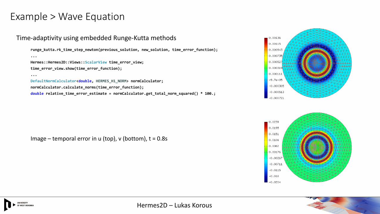
Time-adaptivity using embedded Runge-Kutta methods
runge_kutta.rk_time_step_newton(previous_solution, new_solution, time_error_function);
...
Hermes::Hermes2D::Views::ScalarView time_error_view;
time_error_view.show(time_error_function);
...
DefaultNormCalculator<double, HERMES_H1_NORM> normCalculator;
normCalculator.calculate_norms(time_error_function);
double relative_time_error_estimate = normCalculator.get_total_norm_squared() * 100.;
Image – temporal error in u (top), v (bottom), t = 0.3s
Hermes2D – Lukas Korous
Example > Wave Equation
Time-adaptivity using embedded Runge-Kutta methods
runge_kutta.rk_time_step_newton(previous_solution, new_solution, time_error_function);
...
Hermes::Hermes2D::Views::ScalarView time_error_view;
time_error_view.show(time_error_function);
...
DefaultNormCalculator<double, HERMES_H1_NORM> normCalculator;
normCalculator.calculate_norms(time_error_function);
double relative_time_error_estimate = normCalculator.get_total_norm_squared() * 100.;
Image – temporal error in u (top), v (bottom), t = 0.8s
Hermes2D – Lukas Korous

Example > Benchmark Interior Layer
We solve the equation
−∆𝑢 = f, u|𝛿Ω = ሚ𝑓
Where
- Ω is the space domain - square (0, 1) x (0, 1),
- ሚ𝑓 is the (known) exact solution,
- 𝑓 is the Laplacian of the exact solution,
- u is the sought solution
The features illustrated on this example are
- Calculating exact error,
- Anisotropic refinements usage in AMR.
Hermes2D – Lukas Korous

Example > Benchmark Interior Layer
Hermes2D – Lukas Korous
solution (left), FE space (right), adaptivity step #1

Example > Benchmark Interior Layer
Hermes2D – Lukas Korous
solution (left), FE space (right), adaptivity step #2

Example > Benchmark Interior Layer
Hermes2D – Lukas Korous
solution (left), FE space (right), adaptivity step #3

Example > Benchmark Interior Layer
Hermes2D – Lukas Korous
solution (left), FE space (right), adaptivity step #6

Example > Benchmark Interior Layer
Hermes2D – Lukas Korous
solution (left), FE space (right), adaptivity step #11

Example > Benchmark Interior Layer
Hermes2D – Lukas Korous
solution (left), FE space (right), adaptivity step #19

Example > Benchmark Interior Layer
Calculating exact error – through sub-classing existing Hermes2D class ExactSolutionScalar<double>:
class CustomExactSolution : public ExactSolutionScalar<double>{public:// Implement the actual function expression.virtual double value(double x, double y) const;
// Implement the derivatives expression.virtual void derivatives (double x, double y, double& dx, double& dy) const;
// Overwrite the expression calculating polynomial order (for integration order deduction).virtual Ord value(Ord x, Ord y) const;
};
- and then employing standard ErrorCalculator<double> class for error calculation
Anisotropic refinements usage in AMR
// Predefined list of element refinement candidates.// H2D_HP_ANISO stands for h-, and p-candidates, anisotropic in shape, and polynomial orders.const CandList CAND_LIST = H2D_HP_ANISO;// Class which for each element selected for refinement, selects the best refinement candidate.H1ProjBasedSelector<double> selector(CAND_LIST);...// As before, adapt the FE space – using the selector providedadaptivity.adapt(&selector);
Hermes2D – Lukas Korous

Example > Heat and Moisture
We solve the system of equations
𝑐𝑇𝑇𝛿𝑇
𝛿𝑡+ 𝑐𝑇𝑤
𝛿𝑤
𝛿𝑡− 𝑑𝑇𝑇∆T − 𝑑𝑇𝑤∆𝑤 = 0,
𝑐𝑤𝑇𝛿𝑇
𝛿𝑡+ 𝑐𝑤𝑤
𝛿𝑤
𝛿𝑡− 𝑑𝑤𝑇∆T −𝑑𝑤𝑤∆𝑤 = 0.
Where
- 𝑇,𝑤 is the sought solution,
- 𝑐𝑎𝑏, 𝑑𝑎𝑏are thermal capacity and thermal conductivity properties,
- (complicated) boundary conditions (Axisymmetric, Dirichlet, Newton) are prescribed.
The features illustrated on this example are
- Multimesh,
- Dynamical meshes.
Hermes2D – Lukas Korous
Example > Heat and Moisture
Hermes2D – Lukas Korous
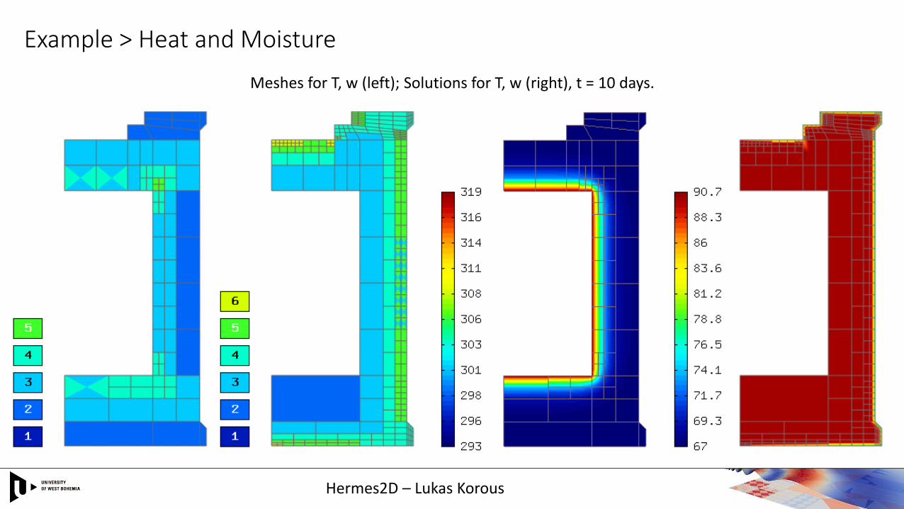
Meshes for T, w (left); Solutions for T, w (right), t = 10 days.

Example > Heat and Moisture
Hermes2D – Lukas Korous
Meshes for T, w (left); Solutions for T, w (right), t = 10 days.

Example > Heat and Moisture
Hermes2D – Lukas Korous
Meshes for T, w (left); Solutions for T, w (right), t = 10 days.

Example > Heat and Moisture
Hermes2D – Lukas Korous
Meshes for T, w (left); Solutions for T, w (right), t = 10 days.

Example > Heat and Moisture
- Multimesh & Dynamical meshes- The key functionality here is de-refining the FE space, either periodically or when some indicator indicates us to.
if (should_unrefine_in_this_step){
// Unrefine one layer of refinements on the mesh for T.T_mesh->unrefine_all_elements();// Also coarsen the polynomial order. T_space->adjust_element_order(-1);
// Do the above also for the mesh for w.w_mesh->unrefine_all_elements();w_space->adjust_element_order(-1);
// Assign DOFs after the change.
T_space->assign_dofs();
w_space->assign_dofs();}
- Note:- In the above, it is clearly seen that there are two Space, and two Mesh structures – different for each component.- This is enough input from the user to achieve multi-mesh behavior. Hermes2D takes care of the rest.
Hermes2D – Lukas Korous

Example > GAMM channel
We solve the Euler equations of compressible flow
Where
- w is the sought solution,
- 𝑅, 𝑐𝑣are constants
- (complicated) Boundary conditions (reflective, ‘do nothing’, and inlet) are prescribed.
The feature illustrated on this example are:
- Post-processing filters (calculating Mach number, pressure)
Hermes2D – Lukas Korous

Example > GAMM channel
Hermes2D – Lukas Korous
Mach number (left), Pressure (right), t = 3e-4 s.

Example > GAMM channel
Hermes2D – Lukas Korous
Mach number (left), Pressure (right), t = 0.09 s.

Example > GAMM channel
Hermes2D – Lukas Korous
Mach number (left), Pressure (right), t = 0.21 s.

Example > GAMM channel
Hermes2D – Lukas Korous
Mach number (left), Pressure (right), t = 0.36 s.

Example > GAMM channel
Post-processing filters
- Implemented by sub-classing Filter classes
class MachNumberFilter : public Hermes::Hermes2D::SimpleFilter<double>
{
// Constructors, etc.
...
// Overriden method performing the actual calculation
virtual void filter_fn(int n, const std::vector<const double*>& source_values, double* result)
{
// Calculate result for each integration point.
for (int i = 0; i < n; i++)
{
double density = source_values.at(0)[i];
double momentum_x = source_values.at(1)[i];
double momentum_y = source_values.at(2)[i];
double energy = source_values.at(3)[i];
// Expression to calculate Mach number in the integration point.
result[i] = std::sqrt((momentum_x / density) * (momentum_x / density) + (momentum_y / density) * (momentum_y / density))
/ std::sqrt(kappa * QuantityCalculator::calc_pressure(density, momentum_x, momentum_y, energy, kappa) / density);
}
}
};
Hermes2D – Lukas Korous
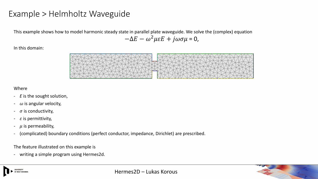
Example > Helmholtz Waveguide
This example shows how to model harmonic steady state in parallel plate waveguide. We solve the (complex) equation
−∆𝐸 − 𝜔2𝜇휀𝐸 + 𝑗𝜔𝜎𝜇 = 0,
In this domain:
Where
- E is the sought solution,
- 𝜔 is angular velocity,
- 𝜎 is conductivity,
- 휀 is permittivity,
- 𝜇 is permeability,
- (complicated) boundary conditions (perfect conductor, impedance, Dirichlet) are prescribed.
The feature illustrated on this example is
- writing a simple program using Hermes2d.
Hermes2D – Lukas Korous

Example > Helmholtz Waveguide
std::cout << "Done?";std::cin >> change_state;if (!strcmp(change_state, "y"))
break;std::cout << "Frequency change [1e9 Hz]: ";std::cin >> frequency_change;
Hermes2D – Lukas Korous

Example > Helmholtz Waveguide
std::cout << "Done?";std::cin >> change_state;if (!strcmp(change_state, "y"))
break;std::cout << "Frequency change [1e9 Hz]: ";std::cin >> frequency_change;
Hermes2D – Lukas Korous

Example > Helmholtz Waveguide
std::cout << "Done?";std::cin >> change_state;if (!strcmp(change_state, "y"))
break;std::cout << "Frequency change [1e9 Hz]: ";std::cin >> frequency_change;
Hermes2D – Lukas Korous

Example > Helmholtz Waveguide
std::cout << "Done?";std::cin >> change_state;if (!strcmp(change_state, "y"))
break;std::cout << "Frequency change [1e9 Hz]: ";std::cin >> frequency_change;
Hermes2D – Lukas Korous

Example > Helmholtz Waveguide
std::cout << "Done?";std::cin >> change_state;if (!strcmp(change_state, "y"))
break;std::cout << "Frequency change [1e9 Hz]: ";std::cin >> frequency_change;
Hermes2D – Lukas Korous

Example > Helmholtz Waveguide
Hermes2D – Lukas Korous
Thank you for your attention.
www.hpfem.org/hermes