Embed Size (px)
Citation preview

1/22
Introduction Our choice Example Problem Final slide :-)
Python + FEMIntroduction to SFE
Robert Cimrman
Department of Mechanics & New Technologies Research CentreUniversity of West BohemiaPlzen, Czech Republic
April 3, 2007, Plzen

2/22
Introduction Our choice Example Problem Final slide :-)
Outline
1 IntroductionProgramming LanguagesProgramming Techniques
2 Our choiceMixing Languages — Best of Both WorldsPythonSoftware Dependencies
3 Example ProblemContinuous FormulationWeak FormulationProblem Description File
4 Final slide :-)

3/22
Introduction Our choice Example Problem Final slide :-)
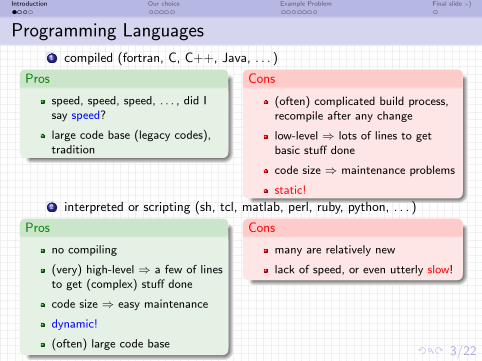
Programming Languages1 compiled (fortran, C, C++, Java, . . . )
Pros
speed, speed, speed, . . . , did Isay speed?
large code base (legacy codes),tradition
Cons
(often) complicated build process,recompile after any change
low-level ⇒ lots of lines to getbasic stuff done
code size ⇒ maintenance problemsstatic!
2 interpreted or scripting (sh, tcl, matlab, perl, ruby, python, . . . )
Pros
no compiling
(very) high-level ⇒ a few of linesto get (complex) stuff done
code size ⇒ easy maintenancedynamic!
(often) large code base
Cons
many are relatively new
lack of speed, or even utterly slow!

3/22
Introduction Our choice Example Problem Final slide :-)
Programming Languages1 compiled (fortran, C, C++, Java, . . . )
Pros
speed, speed, speed, . . . , did Isay speed?
large code base (legacy codes),tradition
Cons
(often) complicated build process,recompile after any change
low-level ⇒ lots of lines to getbasic stuff done
code size ⇒ maintenance problemsstatic!
2 interpreted or scripting (sh, tcl, matlab, perl, ruby, python, . . . )
Pros
no compiling
(very) high-level ⇒ a few of linesto get (complex) stuff done
code size ⇒ easy maintenancedynamic!
(often) large code base
Cons
many are relatively new
lack of speed, or even utterly slow!

4/22
Introduction Our choice Example Problem Final slide :-)
Example Python Code

5/22
Introduction Our choice Example Problem Final slide :-)
Example C Code
char s [ ] = ” s e l tudy , mel dudy . a s e l opravdu tudy . ” ;
i n t s t r f i n d ( char ∗ s t r , char ∗ t g t )
i n t t l e n = s t r l e n ( t g t ) ;i n t max = s t r l e n ( s t r ) − t l e n ;r e g i s t e r i n t i ;
f o r ( i = 0 ; i < max ; i ++) i f ( strncmp(& s t r [ i ] , tgt , t l e n ) == 0)
re tu rn i ;re tu rn −1;
i n t i 1 ;
i 1 = s t r f i n d ( s , ” tudy ” ) ;p r i n t f ( ”%d\n” , i 1 ) ;

6/22
Introduction Our choice Example Problem Final slide :-)
Programming Techniques
Random remarks:
spaghetti code
modular programming
OOP
design patterns (gang-of-four, GO4)
post-OOP — dynamic languages
. . . all used, but I try to move down the list! :-)

6/22
Introduction Our choice Example Problem Final slide :-)
Programming Techniques
Random remarks:
spaghetti code
modular programming
OOP
design patterns (gang-of-four, GO4)
post-OOP — dynamic languages
. . . all used, but I try to move down the list! :-)

7/22
Introduction Our choice Example Problem Final slide :-)
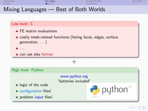
Mixing Languages — Best of Both Worlds
Low level: C
FE matrix evaluations
costly mesh-related functions (listing faces, edges, surfacegeneration, . . . )
. . .
can use also fortran
+High level: Python
www.python.org“batteries included”
logic of the code
configuration files!
problem input files!
7/22
Introduction Our choice Example Problem Final slide :-)
Mixing Languages — Best of Both Worlds
Low level: C
FE matrix evaluations
costly mesh-related functions (listing faces, edges, surfacegeneration, . . . )
. . .
can use also fortran
+High level: Python
www.python.org“batteries included”
logic of the code
configuration files!
problem input files!
8/22
Introduction Our choice Example Problem Final slide :-)
Python I
Python r©is a dynamic object-oriented programminglanguage that can be used for many kinds of softwaredevelopment. It offers strong support for integration with otherlanguages and tools, comes with extensive standard libraries,and can be learned in a few days. Many Python programmersreport substantial productivity gains and feel the languageencourages the development of higher quality, moremaintainable code.
. . .
“batteries included”

9/22
Introduction Our choice Example Problem Final slide :-)
Python II
1.1.16 Why is it called Python?At the same time he began implementing Python, Guido
van Rossum was also reading the published scripts from ”MontyPython’s Flying Circus” (a BBC comedy series from theseventies, in the unlikely case you didn’t know). It occurred tohim that he needed a name that was short, unique, and slightlymysterious, so he decided to call the language Python.
1.1.17 Do I have to like ”Monty Python’s Flying Circus”?
No, but it helps. :)
. . . General Python FAQ

10/22
Introduction Our choice Example Problem Final slide :-)
Python III
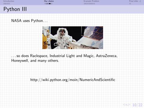
NASA uses Python. . .
. . . so does Rackspace, Industrial Light and Magic, AstraZeneca,Honeywell, and many others.
http://wiki.python.org/moin/NumericAndScientific
10/22
Introduction Our choice Example Problem Final slide :-)
Python III
NASA uses Python. . .
. . . so does Rackspace, Industrial Light and Magic, AstraZeneca,Honeywell, and many others.
http://wiki.python.org/moin/NumericAndScientific

11/22
Introduction Our choice Example Problem Final slide :-)
Software Dependencies
1 libraries & modules SciPy: free (BSD license) collection of numerical computinglibraries for Python
enables Matlab-like array/matrix manipulations and indexing UMFPACK: very fast direct solver for sparse systems
Python wrappers are part of SciPy :-) output files (results) and data files in HDF5:
general purpose library and file format for storing scientificdata, efficient storage and I/O. . . via PyTables
misc: Pyparsing, Matplotlib2 tools
SWIG: automatic generation of Python-C interface code Medit: simple mesh and data viewer ParaView: VTK-based advanced mesh and data viewer inTcl/Tk
MayaVi/MayaVi2: VTK-based advanced mesh and data viewerin Python

12/22
Introduction Our choice Example Problem Final slide :-)
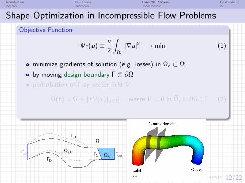
Shape Optimization in Incompressible Flow ProblemsObjective Function
ΨΓ(u) ≡ν
2
∫Ωc|∇u|2 −→ min (1)
minimize gradients of solution (e.g. losses) in Ωc ⊂ Ωby moving design boundary Γ ⊂ ∂Ω
perturbation of Γ by vector field V
Ω(t) = Ω + tV(x)x∈Ω where V = 0 in Ωc ∪ ∂Ω \ Γ (2)
Γin ΓoutΓD
ΓD
ΓC ΩC
ΩD
Ω
12/22
Introduction Our choice Example Problem Final slide :-)
Shape Optimization in Incompressible Flow ProblemsObjective Function
ΨΓ(u) ≡ν
2
∫Ωc|∇u|2 −→ min (1)
minimize gradients of solution (e.g. losses) in Ωc ⊂ Ωby moving design boundary Γ ⊂ ∂Ω
perturbation of Γ by vector field V
Ω(t) = Ω + tV(x)x∈Ω where V = 0 in Ωc ∪ ∂Ω \ Γ (2)
Γin ΓoutΓD
ΓD
ΓC ΩC
ΩD
Ω

13/22
Introduction Our choice Example Problem Final slide :-)
Appetizerflow and spline boxes, left: initial, right: final
→
connectivity of spline boxes (6 boxes in different colours)

14/22
Introduction Our choice Example Problem Final slide :-)
Continuous Formulation
laminar steady state incompressible Navier-Stokes equations
−ν∇2u + u · ∇u +∇p = 0 in Ω (3)
∇ · u = 0 in Ω (4)
boundary conditions
u = u0 on Γin
−pn + ν∂u∂n= −pn on Γout
u = 0 on Γwalls
(5)
adjoint equations for computing the adjoint solution w :
−ν∇2w +∇u · w − u · ∇w −∇r = χΩc ν∇2u in Ω∇ · w = 0 in Ω
(6)
w = 0 on Γin ∪ Γwalls and χΩc is the characteristic function of Ωc

15/22
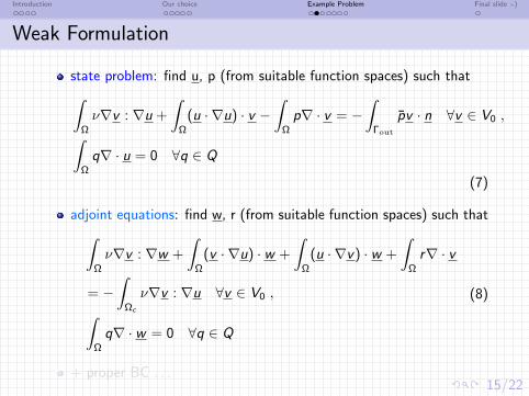
Introduction Our choice Example Problem Final slide :-)
Weak Formulation
state problem: find u, p (from suitable function spaces) such that∫Ω
ν∇v : ∇u +∫Ω(u · ∇u) · v −
∫Ωp∇ · v = −
∫Γoutpv · n ∀v ∈ V0 ,∫
Ωq∇ · u = 0 ∀q ∈ Q
(7)
adjoint equations: find w, r (from suitable function spaces) such that∫Ω
ν∇v : ∇w +∫Ω(v · ∇u) · w +
∫Ω(u · ∇v) · w +
∫Ωr∇ · v
= −∫Ωc
ν∇v : ∇u ∀v ∈ V0 ,∫Ωq∇ · w = 0 ∀q ∈ Q
(8)
+ proper BC . . .
15/22
Introduction Our choice Example Problem Final slide :-)
Weak Formulation
state problem: find u, p (from suitable function spaces) such that∫Ω
ν∇v : ∇u +∫Ω(u · ∇u) · v −
∫Ωp∇ · v = −
∫Γoutpv · n ∀v ∈ V0 ,∫
Ωq∇ · u = 0 ∀q ∈ Q
(7)
adjoint equations: find w, r (from suitable function spaces) such that∫Ω
ν∇v : ∇w +∫Ω(v · ∇u) · w +
∫Ω(u · ∇v) · w +
∫Ωr∇ · v
= −∫Ωc
ν∇v : ∇u ∀v ∈ V0 ,∫Ωq∇ · w = 0 ∀q ∈ Q
(8)
+ proper BC . . .

16/22
Introduction Our choice Example Problem Final slide :-)
Problem Description File I
a regular python file ⇒ all python machinery is accessible!requires/recognizes several keywords to define
meshregions → subdomains, boundaries, characteristic functions, . . .boundary conditions → Dirichletfields → field approximation per subdomainvariables → unknown fields, test fields, parametersequationsmaterials→ constitutive relations, e.g. newton fluid, elastic solid, . . .solver parameters → nonlinear solver, flow solver, optimizationsolver, . . .. . .

17/22
Introduction Our choice Example Problem Final slide :-)
Problem Description File IImesh
f i l eName mesh = ’ s imp l e . mesh ’
regionsr e g i o n 1000 =
’ name ’ : ’ Omega ’ ,’ s e l e c t ’ : ’ e l ement s o f group 6 ’ ,
r e g i o n 0 =
’ name ’ : ’ Wal ls ’ ,’ s e l e c t ’ : ’ nodes o f s u r f a c e −n r . Out le t ’ ,
r e g i o n 1 =
’ name ’ : ’ I n l e t ’ ,’ s e l e c t ’ : ’ nodes by c i n c ( x , y , z , 0 ) ’ ,
r e g i o n 2 =
’ name ’ : ’ Out l e t ’ ,’ s e l e c t ’ : ’ nodes by c i n c ( x , y , z , 1 ) ’ ,
r e g i o n 100 =
’ name ’ : ’ Omega C ’ , # Con t r o l domain .’ s e l e c t ’ : ’ nodes i n ( x > −25.9999e−3) & ( x < −18.990e−3) ’ ,
r e g i o n 101 =
’ name ’ : ’ Omega D ’ , # Des ign domain .’ s e l e c t ’ : ’ a l l −e r . Omega C ’ ,

18/22
Introduction Our choice Example Problem Final slide :-)
Problem Description File III
fieldsf i e l d 1 =
’ name ’ : ’ 3 v e l o c i t y ’ ,’ dim ’ : ( 3 , 1 ) ,’ f l a g s ’ : ( ’ BQP’ , ) ,’ bases ’ : ( ( ’ Omega ’ , ’ 3 4 P1B ’ ) , )
f i e l d 2 = ’ name ’ : ’ p r e s s u r e ’ ,’ dim ’ : ( 1 , 1 ) ,’ f l a g s ’ : ( ) ,’ bases ’ : ( ( ’ Omega ’ , ’ 3 4 P1 ’ ) , )
variablesv a r i a b l e s =
’ u ’ : ( ’ f i e l d ’ , ’ parameter ’ , ’ 3 v e l o c i t y ’ , ( 3 , 4 , 5 ) ) ,’ w 0 ’ : ( ’ f i e l d ’ , ’ parameter ’ , ’ 3 v e l o c i t y ’ , ( 3 , 4 , 5 ) ) ,’w ’ : ( ’ f i e l d ’ , ’ unknown ’ , ’ 3 v e l o c i t y ’ , ( 3 , 4 , 5 ) , 0 ) ,’ v ’ : ( ’ f i e l d ’ , ’ t e s t ’ , ’ 3 v e l o c i t y ’ , ( 3 , 4 , 5 ) , ’ w’ ) ,’ p ’ : ( ’ f i e l d ’ , ’ parameter ’ , ’ p r e s s u r e ’ , ( 9 , ) ) ,’ r ’ : ( ’ f i e l d ’ , ’ unknown ’ , ’ p r e s s u r e ’ , ( 9 , ) , 1 ) ,’ q ’ : ( ’ f i e l d ’ , ’ t e s t ’ , ’ p r e s s u r e ’ , ( 9 , ) , ’ r ’ ) ,’Nu ’ : ( ’ f i e l d ’ , ’ meshVe loc i t y ’ , ’ p r e s s u r e ’ , ( 9 , ) ) ,
19/22
Introduction Our choice Example Problem Final slide :-)
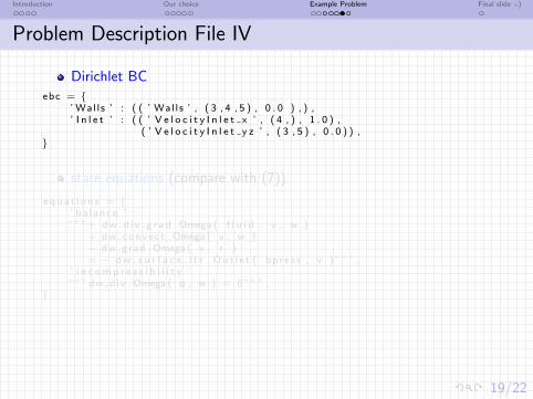
Problem Description File IV
Dirichlet BCebc =
’ Wal ls ’ : ( ( ’ Wal ls ’ , ( 3 , 4 , 5 ) , 0 . 0 ) , ) ,’ I n l e t ’ : ( ( ’ V e l o c i t y I n l e t x ’ , ( 4 , ) , 1 . 0 ) ,
( ’ V e l o c i t y I n l e t y z ’ , ( 3 , 5 ) , 0 . 0 ) ) ,
state equations (compare with (7))
e qua t i o n s = ’ ba lance ’ :”””+ dw d i v g r ad . Omega ( f l u i d , v , w )+ dw convect . Omega ( v , w )− dw grad .Omega ( v , r )= − dw s u r f a c e l t r . Ou t l e t ( bp re s s , v ) ””” ,
’ i n c om p r e s s i b i l i t y ’ :””” dw div . Omega ( q , w ) = 0””” ,

19/22
Introduction Our choice Example Problem Final slide :-)
Problem Description File IV
Dirichlet BCebc =
’ Wal ls ’ : ( ( ’ Wal ls ’ , ( 3 , 4 , 5 ) , 0 . 0 ) , ) ,’ I n l e t ’ : ( ( ’ V e l o c i t y I n l e t x ’ , ( 4 , ) , 1 . 0 ) ,
( ’ V e l o c i t y I n l e t y z ’ , ( 3 , 5 ) , 0 . 0 ) ) ,
state equations (compare with (7))
e qua t i o n s = ’ ba lance ’ :”””+ dw d i v g r ad . Omega ( f l u i d , v , w )+ dw convect . Omega ( v , w )− dw grad .Omega ( v , r )= − dw s u r f a c e l t r . Ou t l e t ( bp re s s , v ) ””” ,
’ i n c om p r e s s i b i l i t y ’ :””” dw div . Omega ( q , w ) = 0””” ,

20/22
Introduction Our choice Example Problem Final slide :-)
Problem Description File V
adjoint equations (compare with (8))e q u a t i o n s a d j o i n t =
’ ba lance ’ :”””+ dw d i v g r ad . Omega ( f l u i d , v , w )+ dw ad j convec t1 . Omega ( v , w , u )+ dw ad j convec t2 . Omega ( v , w , u )+ dw grad .Omega ( v , r )= − dw ad j d i v g r a d 2 . Omega C ( one , f l u i d , v , u ) ””” ,
’ i n c om p r e s s i b i l i t y ’ :””” dw div . Omega ( q , w ) = 0””” ,
materialsma t e r i a l 2 =
’ name ’ : ’ f l u i d ’ ,’mode ’ : ’ here ’ ,’ r e g i on ’ : ’ Omega ’ ,’ v i s c o s i t y ’ : 1 . 2 5 e−1,
ma t e r i a l 1 0 0 =
’ name ’ : ’ bp re s s ’ ,’mode ’ : ’ here ’ ,’ r e g i on ’ : ’ Omega ’ ,’ va l ’ : 0 . 0 ,
21/22
Introduction Our choice Example Problem Final slide :-)
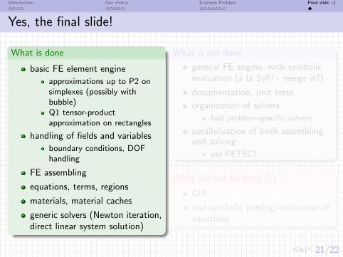
Yes, the final slide!
What is done
basic FE element engineapproximations up to P2 onsimplexes (possibly withbubble)Q1 tensor-productapproximation on rectangles
handling of fields and variablesboundary conditions, DOFhandling
FE assembling
equations, terms, regions
materials, material caches
generic solvers (Newton iteration,direct linear system solution)
What is not donegeneral FE engine, with symbolicevaluation (a la SyFi - merge it?)
documentation, unit testsorganization of solvers
fast problem-specific solvers
parallelization of both assemblingand solving
use PETSC?
What will not be done (?)
GUI
real symbolic parsing/evaluation ofequations

21/22
Introduction Our choice Example Problem Final slide :-)
Yes, the final slide!
What is done
basic FE element engineapproximations up to P2 onsimplexes (possibly withbubble)Q1 tensor-productapproximation on rectangles
handling of fields and variablesboundary conditions, DOFhandling
FE assembling
equations, terms, regions
materials, material caches
generic solvers (Newton iteration,direct linear system solution)
What is not donegeneral FE engine, with symbolicevaluation (a la SyFi - merge it?)
documentation, unit testsorganization of solvers
fast problem-specific solvers
parallelization of both assemblingand solving
use PETSC?
What will not be done (?)
GUI
real symbolic parsing/evaluation ofequations

22/22
Introduction Our choice Example Problem Final slide :-)
This is not a slide!


