University of New Orleans University of New Orleans
ScholarWorks@UNO ScholarWorks@UNO
University of New Orleans Theses and Dissertations Dissertations and Theses
12-19-2003
An Investigation and Comparison of Accepted Design An Investigation and Comparison of Accepted Design
Methodologies for the Analysis of Laterally Loaded Foundations Methodologies for the Analysis of Laterally Loaded Foundations
Chad Rachel University of New Orleans
Follow this and additional works at: https://scholarworks.uno.edu/td
Recommended Citation Recommended Citation Rachel, Chad, "An Investigation and Comparison of Accepted Design Methodologies for the Analysis of Laterally Loaded Foundations" (2003). University of New Orleans Theses and Dissertations. 55. https://scholarworks.uno.edu/td/55
This Thesis is protected by copyright and/or related rights. It has been brought to you by ScholarWorks@UNO with permission from the rights-holder(s). You are free to use this Thesis in any way that is permitted by the copyright and related rights legislation that applies to your use. For other uses you need to obtain permission from the rights-holder(s) directly, unless additional rights are indicated by a Creative Commons license in the record and/or on the work itself. This Thesis has been accepted for inclusion in University of New Orleans Theses and Dissertations by an authorized administrator of ScholarWorks@UNO. For more information, please contact [email protected].
AN INVESTIGATION AND COMPARISON OF ACCEPTED DESIGN METHODOLOGIES FOR THE ANALYSIS OF LATERALLY LOADED
FOUNDATIONS
A Thesis
Submitted to the Graduate Faculty of the University of New Orleans in partial fulfillment of the
requirements for the degree of
Master of Science in
The Department of Civil Engineering
by
Chad M. Rachel
B.S., University of New Orleans, 2000
December 2003
ii
ACKNOWLEDGEMENT
I would like to express my sincere gratitude to Dr. John B. Grieshaber for his
assistance, guidance, and instruction during my graduate studies at the University of New
Orleans. Thank you to Dr. Kenneth McManis and Dr. Mysore S. Nataraj for taking the
time to serve on my thesis committee. I would like to thank the New Orleans District of
the U.S. Army Corps of Engineers for financing my graduate education. I would like to
thank Mr. Shung Kwok Chiu, Mr. Richard Pinner, and the other senior engineers of
Structure Foundations, New Orleans District for providing me with geotechnical
knowledge and guidance. I would like to thank Ms. Sandra Brown of the New Orleans
District Library for assisting me in locating references for this thesis. I would like to
thank the geotechnical staff at Virginia Tech for the valuable geotechnical knowledge
that they provided to me. I offer thanks to my parents, who instilled good educational
values in me, which was instrumental in the pursuit of advanced studies. Finally, and
above all, I would like to thank my wife Cathy, and children Sebastian and Sydney, for
their love, support, encouragement, and sacrifice.
TABLE OF CONTENTS
ABSTRACT....................................................................................................................... iv INTRODUCTION ...............................................................................................................v I. THEORY OF BEAM ON ELASTIC FOUNDATION................................................1 II. ULTIMATE LATERAL RESISTANCE OF PILES ...................................................7 III. P-Y CURVES ............................................................................................................45 IV. DETERMINATION OF SOIL MODULUS ...........................................................108 V. COMPARISON OF THE VARIABLES OF LATERALLY LOADED FOUNDATIONS .....................................................................................................112 VI. COMPARISON BETWEEN P-Y CURVE AND THE ULTIMATE RESISTANCE APPROACH...................................................................................117 VII. CONCLUSIONS AND RECOMMENDATIONS..................................................121 VIII. BIBLIOGRAPHY...................................................................................................123 IX. APPENDIX.............................................................................................................126 X. VITA .......................................................................................................................143
iv
ABSTRACT
Single piles and pile groups are frequently subjected to high lateral forces. The
safety and functionality of many structures depends on the ability of the supporting pile
foundation to resist the resulting lateral forces. In the analysis and design of laterally
loaded piles, two criterions usually govern. First, the deflection at the working load
should not be so excessive as to impair the proper function of the supporting member.
Second, the ultimate strength of the pile should be high enough to take the load imposed
on it under the worst loading condition. Typically, pile length, pile section, soil type, and
pile restraint dictate the analysis.
This paper presents different methods, specifically Broms’ method and the p-y
method, for both the analysis and design of laterally loaded single piles. Both linear and
nonlinear analyses are considered. The measured results of several full-scale field tests
performed by Lymon Reese are compared to computed results using Broms’ method of
analysis and the p-y method of analysis. Observations are made as to the correlation
between the results and recommendations are made as to the applicability of the accepted
methods for the analysis and design of laterally loaded piles.
v
INTRODUCTION
It is well known that pile foundations are subjected to vertical loading. In addition
to being subjected to vertical loads, single piles and pile groups are often subjected to
high lateral loads. These loads may be forces of nature such as wave or wind loads, man
made loads such as mooring loads, or by lateral earth pressures. For example, structures
constructed for offshore use are subjected to static and cyclic lateral loads caused by
waves and wind. The safety and functionality of these structures depends on the ability of
the supporting pile foundation to resist the resulting lateral loads.
Pile supported retaining walls, abutments, sector gates, or lock structures
frequently resist high lateral loads. These lateral loads may be caused be lateral earth
pressures acting on a retaining structure, by differential fluid pressures acting on a sector
gate or lock structure, or by horizontal thrust loads acting on abutments of bridges.
In the analysis and design of laterally loaded piles, three criterions usually govern.
First, the deflection at the working load should not be so excessive as to impair the proper
function of the supporting member. Second, the ultimate strength of the pile should be
high enough to take the load imposed on it under the worst loading condition (Broms,
1964b). And third, the load carrying capacity of the soil should not be exceeded, allowing
the pile to rotate freely.
vi
This paper presents different methods for both the analysis and design of laterally
loaded single piles. The methods are presented in such a way as to guide the reader from
the original concepts and theories of the laterally loaded foundation, to the more state-of-
the-art approaches. Although each of the methods presented are well accepted in
literature and have been used extensively to analyze the problem of the laterally loaded
foundation, each does not provide the same information. While some methods provide
information such as ultimate soil capacity and bending moments in the pile, others
provide information such as lateral deflections and bending moments in the pile. It is well
known that the problem of the laterally loaded pile is a soil-structure interaction type
problem. Because of this, information on the lateral deflection of the pile is needed for an
adequate analysis or design.
This paper considers both linear and nonlinear analyses of single piles. Pile
groups and effects of pile spacing are beyond the scope of this paper, and will not be
considered. The measured results of several full-scale field tests performed in stiff clay
formations and sand formations are compared to computed results using Broms’ linear
approach and the nonlinear p-y criteria developed by Reese and Matlock. Only
methodologies that consider the lateral deflection of the pile are included in the
comparisons. Observations and recommendations are made as to the correlation between
the results and the applicability and limits of the methodologies.
Additionally, a computer software program known as FB-Pier, developed by the
University of Florida, is used to perform a series of sensitivity analyses. The analyses are
performed assuming various soil and pile scenarios. The effects of varying each

vii
parameter independently is studied and the observations are reported.
In addition to this thesis being written to fulfill the requirements of the Master of
Science Degree, the contents of the thesis will be used to assist the New Orleans District
of the U.S. Army Corps of Engineers. The New Orleans District is currently in a
transition period of adapting the p-y methodologies. Previously, the New Orleans District
designed for lateral loads on pile foundation by using either a conservative linear
subgrade modulus method of analysis or by using battered piles. Several of the recent
projects assigned to the New Orleans District, such as the IHNC Lock Replacement and
the Harvey Canal Sector Gate Structure require a large footprint and large diameter piles.
It is realized that the methods used in past designs will not be cost effective for this type
of project. The author’s intent is for the findings reported in this paper to be used as a
reference for future designs of laterally loaded foundations by the New Orleans District.
1
I. THEORY OF BEAM ON ELASTIC FOUNDATION
The analysis of bending of beams on an elastic foundation was developed on the
assumption that the reaction forces of the foundation are proportional at every point to the
deflection of the beam at that point, and independent of the pressure or deflection
occurring in other parts of the foundation. This assumption was first introduced by E.
Winkler in 1867 (Hetenyi, 1942). Its application to soil foundations should be regarded
only as a practical approximation. It is perhaps the simplest approximation that can be
made regarding the nature of a supporting elastic media.
However, its drawback is that the soil is not treated as a continuum, but rather as a
series of discrete resistances. The physical properties of soil are obviously of a much
more complex nature than that which could be accurately represented by such a simple
mathematical relationship as the one assumed by Winkler (Hetenyi, 1942).
Consider a straight beam supported along its entire length by an elastic medium
and subjected to vertical forces acting in the principle plane of the symmetrical cross-
section. The beam will deflect producing continuously distributed reaction forces in the
supporting media. The intensity of these reaction forces, p , at any point is proportional
to the deflection of the beam, y , at that point. Or, kyp = , where k is the proportionality
constant (Hetenyi, 1942).
2
The elasticity of the material assumed by this relationship can be characterized by
a force distributed over a unit area causing a unit deflection. The constant of the
supporting material, 0k , in units of 3inlb , is called the modulus of subgrade reaction and
thus k , in units of 2inlb , will be simply 0k multiplied by the width of the beam, b , or
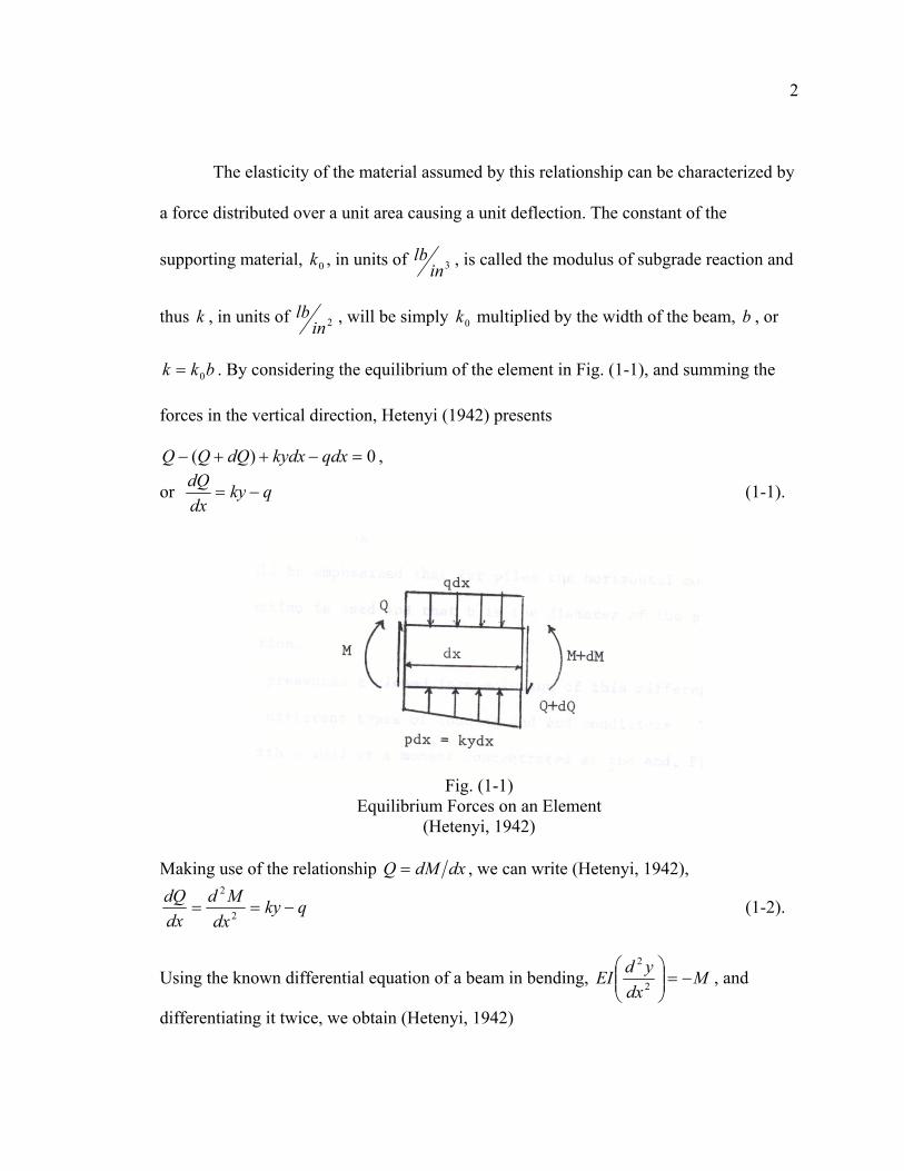
bkk 0= . By considering the equilibrium of the element in Fig. (1-1), and summing the
forces in the vertical direction, Hetenyi (1942) presents
0)( =−++− qdxkydxdQQQ ,
or qkydxdQ
−= (1-1).
Fig. (1-1)
Equilibrium Forces on an Element (Hetenyi, 1942)
Making use of the relationship dxdMQ = , we can write (Hetenyi, 1942),
qkydxMd
dxdQ
−== 2
2
(1-2).
Using the known differential equation of a beam in bending, MdxydEI −=
2
2
, and
differentiating it twice, we obtain (Hetenyi, 1942)
3
2
2
4
4
dxMd
dxydEI −= (1-3).
Substituting (1-3) into (1-2), we get (Hetenyi, 1942)
qkydxydEI +−=4
4
(1-4).
Equation (1-4) is the differential equation for the deflection curve of a beam
supported on an elastic foundation. For unloaded parts where 0=q , we get (Hetenyi,
1942)
kydxydEI −=4
4
(1-5).
If an axial force, xP , is introduced, then the differential equation will be (Hetenyi, 1942)
02
2
4
4
=++dxydPky
dxydEI x (1-6).
It should be emphasized that for piles, the horizontal modulus of subgrade
reaction is used and that b is the diameter of the pile for a circular section.
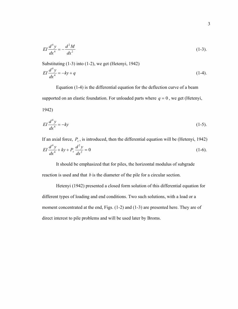
Hetenyi (1942) presented a closed form solution of this differential equation for
different types of loading and end conditions. Two such solutions, with a load or a
moment concentrated at the end, Figs. (1-2) and (1-3) are presented here. They are of
direct interest to pile problems and will be used later by Broms.
4
Fig. (1-2)
Beam with Concentrated Moment at End (Hetenyi, 1942)
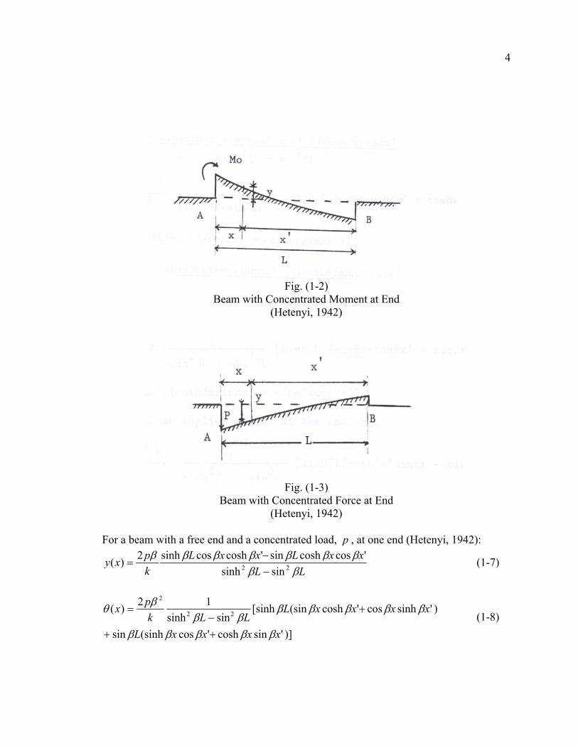
Fig. (1-3)
Beam with Concentrated Force at End (Hetenyi, 1942)
For a beam with a free end and a concentrated load, p , at one end (Hetenyi, 1942):
LLxxLxxL
kpxy
βββββββββ
22 sinsinh'coscoshsin'coshcossinh2)(
−−
= (1-7)
)]'sincosh'cos(sinhsin
)'sinhcos'cosh(sin[sinhsinsinh
12)( 22
2
xxxxL
xxxxLLLk
px
βββββ
βββββββ
βθ
++
+−
= (1-8)
5
LLxxLxxLpxM
ββββββββ
β 22 sinsinh'sinsinhsin'sinhsinsinh)(
−−
−= (1-9)
)]'cossinh'sin(coshsin
)'coshsin'sinh(cos[sinhsinsinh
1)( 22
xxxxL
xxxxLLL
pxQ
βββββ
βββββββ
−−
−−
−= (1-10).
For the case of an applied moment at the end , 0M , (Hetenyi, 1942)
)]'sincosh'cos(sinhsin
)cos'sinhsin'(cosh[sinhsinsinh
12)( 22
20
xxxxL
xxxxLLLk
Mxy
βββββ
βββββββ
β
−+
−−
= (1-11)
LL
xxLxxLkM
xββ
βββββββθ 22
30
sinsinh'coscoshsincos'coshsinh4
)(−+
= (1-12)
)]'sincosh'cos(sinhsin
)sin'coshcos'(sinh[sinhsinsinh
)( 220
xxxxL
xxxxLLL
MxM
βββββ
βββββββ
+−
+−
= (1-13)
LLxxLxxLMxQ
βββββββββ 220 sinsinh
'sinsinhsinsin'sinhsinh2)(−+
= (1-14)
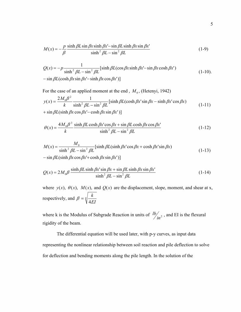
where ),(xy ),(xθ ),(xM and )(xQ are the displacement, slope, moment, and shear at x,
respectively, and 44EIk
=β
where k is the Modulus of Subgrade Reaction in units of 2in
lb , and EI is the flexural
rigidity of the beam.
The differential equation will be used later, with p-y curves, as input data
representing the nonlinear relationship between soil reaction and pile deflection to solve
for deflection and bending moments along the pile length. In the solution of the
6
differential equation, appropriate boundary conditions must be selected at the top of the
pile to insure that the equations of equilibrium and compatibility are satisfied at the
interface between the pile and the superstructure. The selection of the boundary
conditions is a simple problem in some instances, for example, where the superstructure
is simply a continuation of the pile. However, in other instances, it may be necessary to
iterate between solutions for the piles and for the superstructure in order to obtain a
correct solution. Such iterations may be required because the soil behavior is usually
nonlinear (Reese, 1974).
7
II. ULTIMATE LATERAL RESISTANCE OF PILES
The calculation of the ultimate lateral resistance and lateral deflection, at working
loads of single piles driven in cohesive and cohesionless soil, is considered here based on
simplified assumptions of ultimate soil resistance. Both free and fixed headed piles have
been considered. These methods were used by engineers before the development of p-y
curves.
The ultimate lateral resistance and working load deflections of single piles depends
on the dimensions, strength, and flexibility of the individual pile, and on the deformation
characteristics of the soil surrounding the loaded pile. The ultimate lateral resistance of a
laterally loaded pile will be governed by either the ultimate lateral resistance of the
surrounding soil or by the yield or ultimate moment resistance of the pile section. Lateral
deflections at working loads have been calculated using the concept of subgrade reaction
taking into account edge effects both at the ground surface and at the bottom of each
individual pile.
1. General Background
The simplest and direct method of estimating the ultimate lateral resistance of a pile is
to consider the statics of the problem. For a laterally loaded pile, passive and active earth
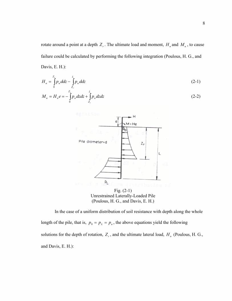
pressures will develop. Assuming a general distribution shown in Fig. (2-1), the pile will
8
rotate around a point at a depth rZ . The ultimate load and moment, uH and uM , to cause
failure could be calculated by performing the following integration (Poulous, H. G., and
Davis, E. H.):
∫∫ −=L
Zu
Z
uu
r
r
ddzpddzpH0
(2-1)
∫∫ +−==L
Zu
Z
uuu
r
r
dzdzpdzdzpeHM0
(2-2)
Fig. (2-1)
Unrestrained Laterally-Loaded Pile (Poulous, H. G., and Davis, E. H.)
In the case of a uniform distribution of soil resistance with depth along the whole
length of the pile, that is, uL ppp ==0 , the above equations yield the following
solutions for the depth of rotation, rZ , and the ultimate lateral load, uH (Poulous, H. G.,
and Davis, E. H.):
9
+= L
dpH
Zu
ur 2
1 (2-3)
−
−==
2
41
22
21
dLpM
dLpH
dLpeH
dLpM
u
u
u
u
u
u
u
u (2-4)
+−+
+=
Le
Le
dLpH
u
u 211212
(2-5)
dLpH
u
u is plotted against Le in Fig. (2-2).
For the case of a linear variation of soil resistance with depth, from 0p at the
ground surface to Lp at the pile tip, the following equations may be derived (Poulous, H.
G., and Davis, E. H.):
02
3
1264
0
0
0
0
0
0
0
023
=
−+
−
−+
−
+
+
+
pppp
pppp
Le
LZ
Le
ppp
ppp
Le
LZ
LZ
L
L
L
L
r
LL
rr
(2-6)
and
+−
+
−=
L
r
L
r
Lu
u
pp
LZ
pp
LZ
pp
dLpH 0
210
20 121 (2-7)
dLpH
u
u is plotted against Le in Fig. (2-2) for the case of 00 =p .
10
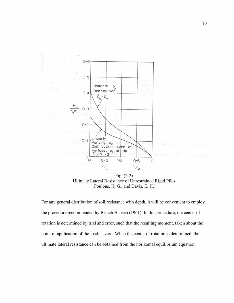
Fig. (2-2)
Ultimate Lateral Resistance of Unrestrained Rigid Piles (Poulous, H. G., and Davis, E. H.)
For any general distribution of soil resistance with depth, it will be convenient to employ
the procedure recommended by Brinch Hansen (1961). In this procedure, the center of
rotation is determined by trial and error, such that the resulting moment, taken about the
point of application of the load, is zero. When the center of rotation is determined, the
ultimate lateral resistance can be obtained from the horizontal equilibrium equation.
11
This analysis holds true for rigid piles. For non-rigid piles the lesser of either the
horizontal load causing failure in the soil along the length of the pile, or the horizontal
load causing yielding in the pile section, should be considered. The ultimate soil
resistance for a purely cohesive soil up is considered generally to increase from the
surface down to a depth of about three pile diameters and remain constant for greater
depths. The distribution is shown in Fig. (2-10). For a general case of a φ−c soil,
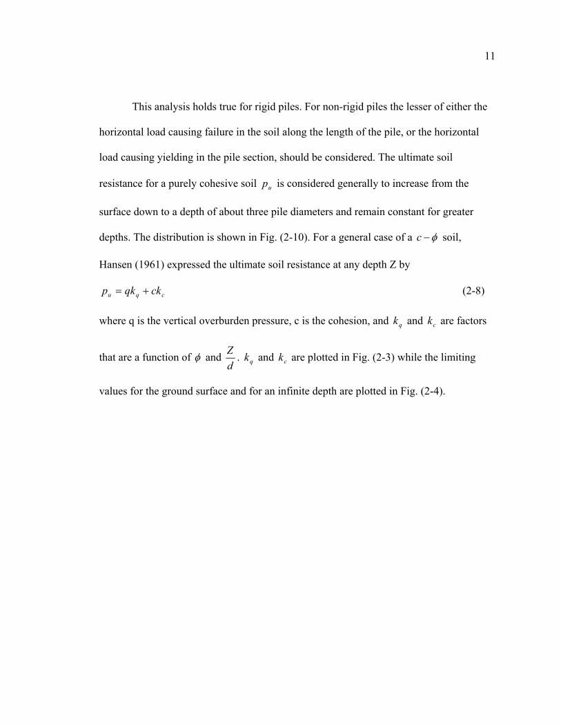
Hansen (1961) expressed the ultimate soil resistance at any depth Z by
cqu ckqkp += (2-8)
where q is the vertical overburden pressure, c is the cohesion, and qk and ck are factors
that are a function of φ and dZ . qk and ck are plotted in Fig. (2-3) while the limiting
values for the ground surface and for an infinite depth are plotted in Fig. (2-4).

12
Fig. (2-3) Lateral Resistance Factors Kq and Kc
(Brinch Hansen, 1961)
13
Fig. (2-4)
Lateral Resistance Factors at the Ground Surface (0) and at great depth ( )∞ (Brinch Hansen, 1961)
Broms (1964a & 1964b) made some simplification to the ultimate soil resistance.
He justified his simplification with several experiments he conducted and with test data.
His method and its reliability is the subject of the following sections.
2. Piles in Cohesive Soils
The load deflection relationships of laterally loaded piles driven into cohesive soils
are similar to the stress-strain relationships as obtained from consolidated-undrained
tests. At loads less than 21 to 3
1 of the ultimate lateral resistance of the pile, the deflection
14
increases approximately linear with the applied load. At higher loads, the load-deflection
relationships become non-linear and the maximum resistance is, in general, reached when
the deflection at the ground surface is approximately equal to 20% of the diameter or side
of the pile (Broms, 1964b).
The possible modes of failure of laterally loaded piles are illustrated in Figs. (2-
5), (2-6), (2-7), (2-8), and (2-9) for free-headed and restrained piles, respectively. An
unrestrained pile, which is free to rotate around its top end, is defined herein as a free-
headed pile (Broms, 1964b).
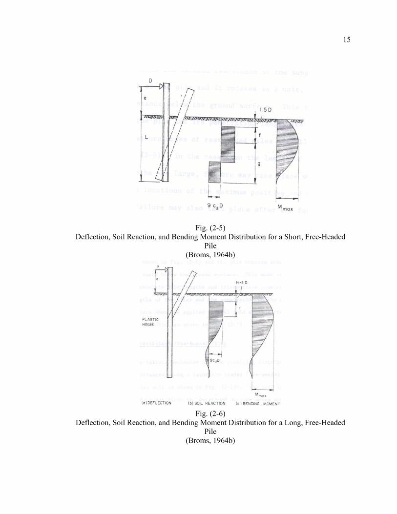
Failure of a free-headed pile, shown in Figs. (2-5) and (2-6), takes place when (a)
the maximum bending moment in the pile exceeds the moment causing yielding or failure
of the pile section (this takes place when the pile penetration is relatively large), or (b) the
resulting lateral earth pressure exceeds the lateral resistance of the supporting soil along
the full length of the pile and it rotates as a unit, around a point located at some distance
below the ground surface. This takes place when the length of the pile and its penetration
lengths are small (Broms, 1964b).
15
Fig. (2-5) Deflection, Soil Reaction, and Bending Moment Distribution for a Short, Free-Headed
Pile (Broms, 1964b)
Fig. (2-6)
Deflection, Soil Reaction, and Bending Moment Distribution for a Long, Free-Headed Pile
(Broms, 1964b)
16
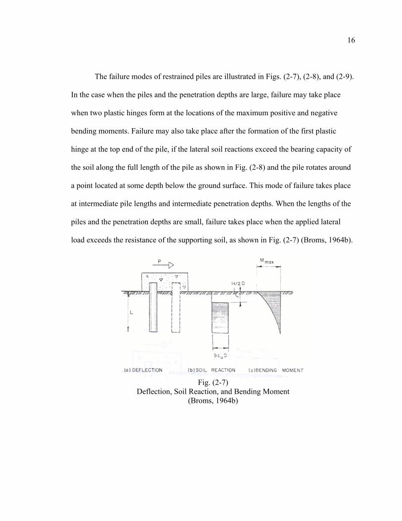
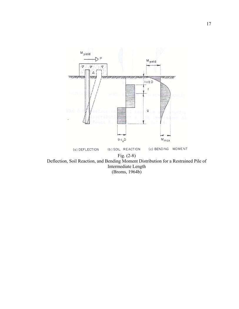
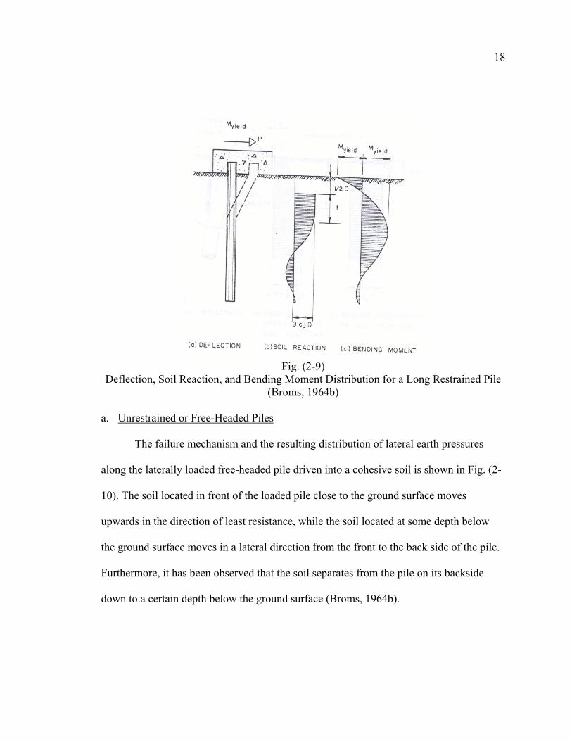
The failure modes of restrained piles are illustrated in Figs. (2-7), (2-8), and (2-9).
In the case when the piles and the penetration depths are large, failure may take place
when two plastic hinges form at the locations of the maximum positive and negative
bending moments. Failure may also take place after the formation of the first plastic
hinge at the top end of the pile, if the lateral soil reactions exceed the bearing capacity of
the soil along the full length of the pile as shown in Fig. (2-8) and the pile rotates around
a point located at some depth below the ground surface. This mode of failure takes place
at intermediate pile lengths and intermediate penetration depths. When the lengths of the
piles and the penetration depths are small, failure takes place when the applied lateral
load exceeds the resistance of the supporting soil, as shown in Fig. (2-7) (Broms, 1964b).
Fig. (2-7)
Deflection, Soil Reaction, and Bending Moment (Broms, 1964b)
17
Fig. (2-8)
Deflection, Soil Reaction, and Bending Moment Distribution for a Restrained Pile of Intermediate Length
(Broms, 1964b)
18
Fig. (2-9)
Deflection, Soil Reaction, and Bending Moment Distribution for a Long Restrained Pile (Broms, 1964b)
a. Unrestrained or Free-Headed Piles
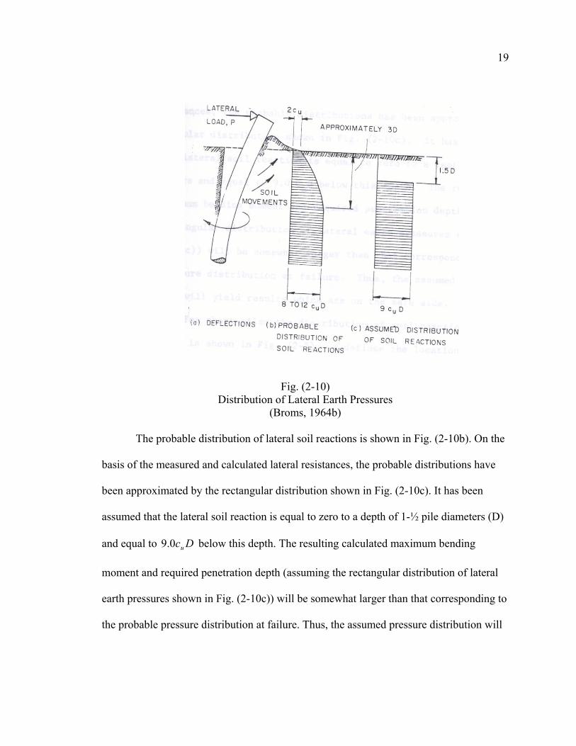
The failure mechanism and the resulting distribution of lateral earth pressures
along the laterally loaded free-headed pile driven into a cohesive soil is shown in Fig. (2-
10). The soil located in front of the loaded pile close to the ground surface moves
upwards in the direction of least resistance, while the soil located at some depth below
the ground surface moves in a lateral direction from the front to the back side of the pile.
Furthermore, it has been observed that the soil separates from the pile on its backside
down to a certain depth below the ground surface (Broms, 1964b).
19
Fig. (2-10)
Distribution of Lateral Earth Pressures (Broms, 1964b)
The probable distribution of lateral soil reactions is shown in Fig. (2-10b). On the
basis of the measured and calculated lateral resistances, the probable distributions have
been approximated by the rectangular distribution shown in Fig. (2-10c). It has been
assumed that the lateral soil reaction is equal to zero to a depth of 1-½ pile diameters (D)
and equal to Dcu0.9 below this depth. The resulting calculated maximum bending
moment and required penetration depth (assuming the rectangular distribution of lateral
earth pressures shown in Fig. (2-10c)) will be somewhat larger than that corresponding to
the probable pressure distribution at failure. Thus, the assumed pressure distribution will
20
yield results that are on the safe side (Broms, 1964b).
For short piles the distribution of soil reaction and bending moments is shown in
Fig. (2-5). The distance f defines the location of the maximum moment and since the
shear there is zero (Broms, 1964b),
DcH
fu
u
9= (2-10)
Also, taking moments about the maximum moment location (Broms, 1964b),
( )fDeHM u 5.05.1max ++= (2-11a)
also,
ucDgM 2max 25.2= (2-11b)
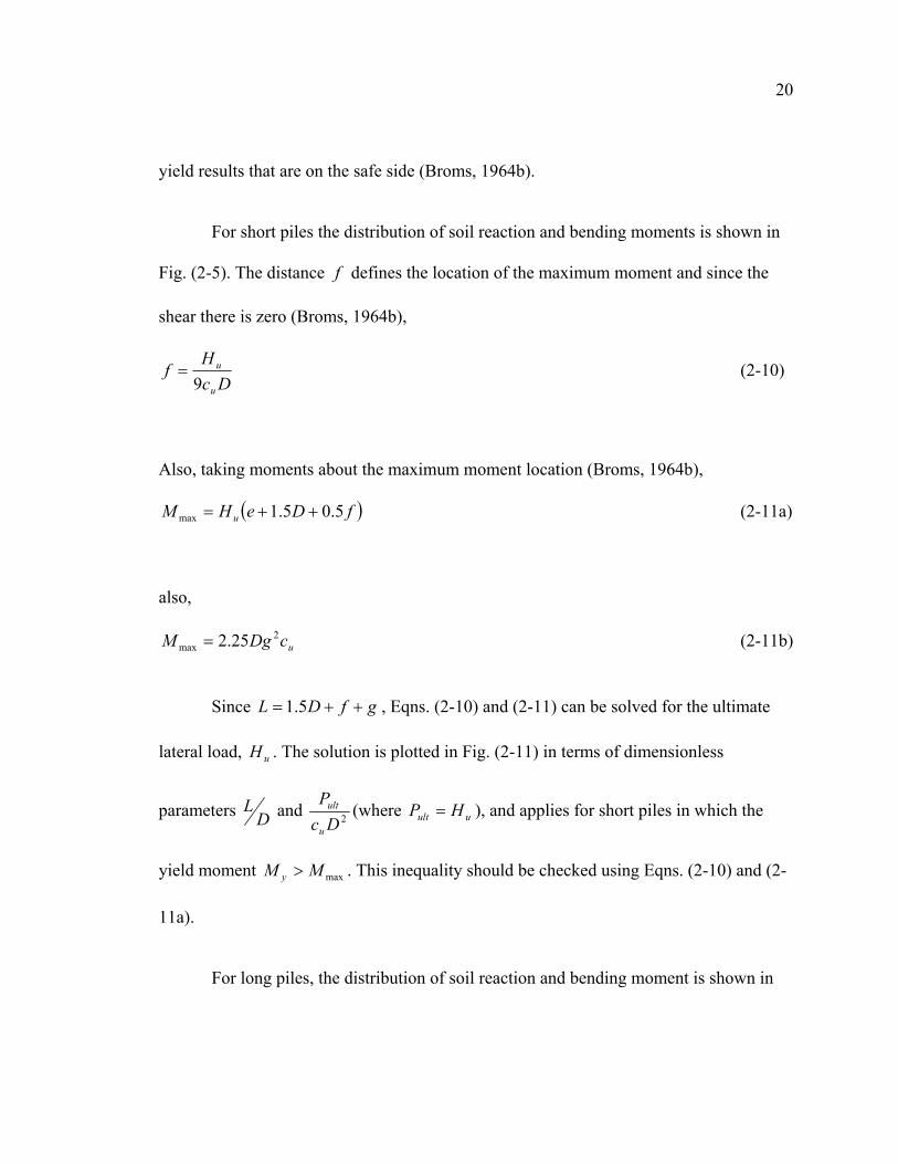
Since gfDL ++= 5.1 , Eqns. (2-10) and (2-11) can be solved for the ultimate
lateral load, uH . The solution is plotted in Fig. (2-11) in terms of dimensionless
parameters DL and 2Dc
P
u
ult (where uult HP = ), and applies for short piles in which the
yield moment maxMM y > . This inequality should be checked using Eqns. (2-10) and (2-
11a).
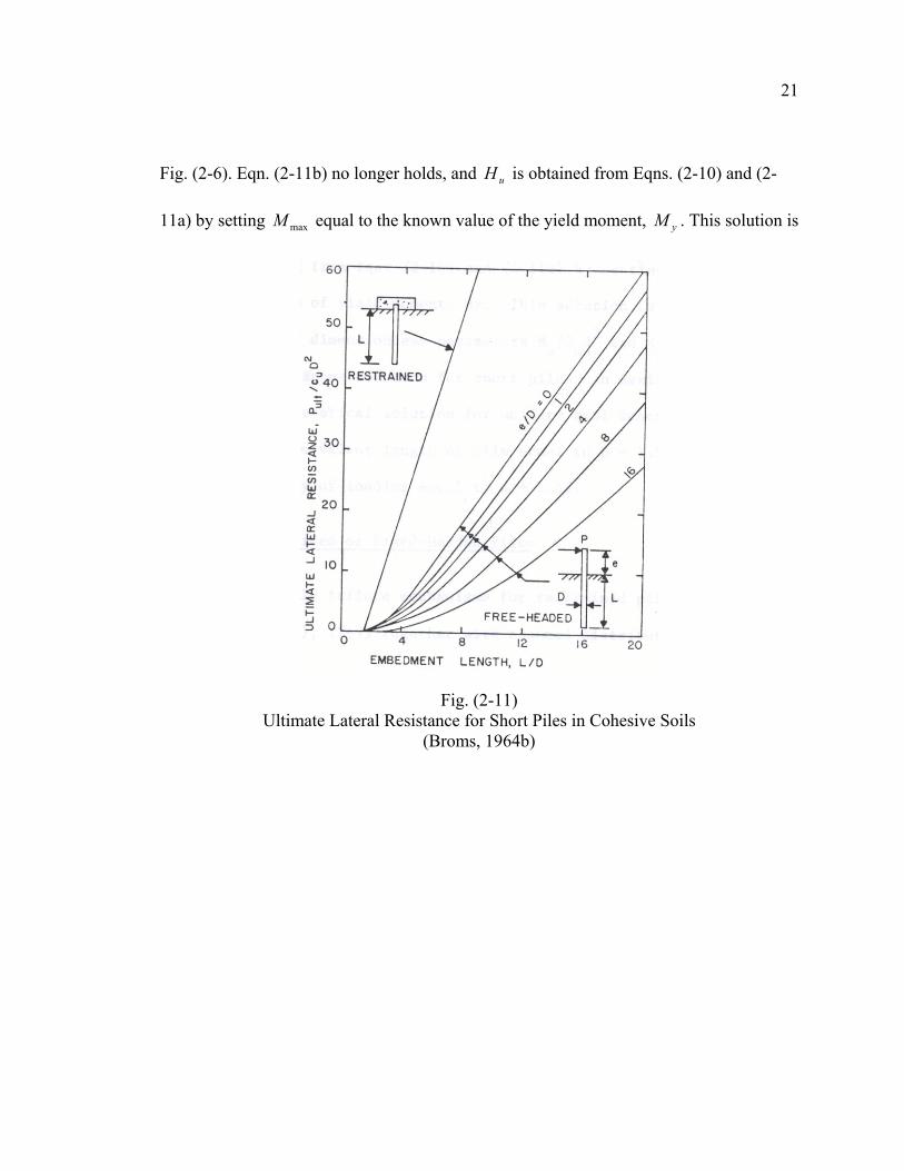
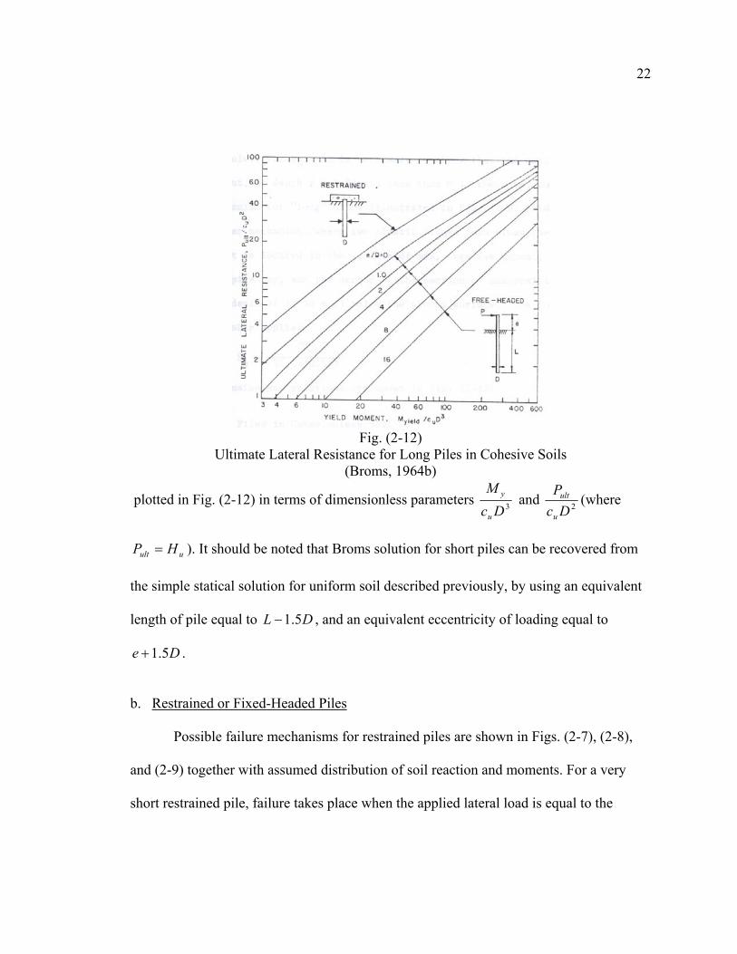
For long piles, the distribution of soil reaction and bending moment is shown in
21
Fig. (2-6). Eqn. (2-11b) no longer holds, and uH is obtained from Eqns. (2-10) and (2-
11a) by setting maxM equal to the known value of the yield moment, yM . This solution is
Fig. (2-11) Ultimate Lateral Resistance for Short Piles in Cohesive Soils
(Broms, 1964b)
22
Fig. (2-12)
Ultimate Lateral Resistance for Long Piles in Cohesive Soils (Broms, 1964b)
plotted in Fig. (2-12) in terms of dimensionless parameters 3DcM
u
y and 2DcP
u
ult (where
uult HP = ). It should be noted that Broms solution for short piles can be recovered from
the simple statical solution for uniform soil described previously, by using an equivalent
length of pile equal to DL 5.1− , and an equivalent eccentricity of loading equal to
De 5.1+ .
b. Restrained or Fixed-Headed Piles
Possible failure mechanisms for restrained piles are shown in Figs. (2-7), (2-8),
and (2-9) together with assumed distribution of soil reaction and moments. For a very
short restrained pile, failure takes place when the applied lateral load is equal to the
23
ultimate lateral resistance of the supporting soil, and the pile moves as a unit in the soil.
The following relation holds for short piles (Broms, 1964b):
( )DLDcH uu 5.19 −= (2-12)
( )DLHM u 75.05.0max += (2-13)
Solutions in dimensionless terms are shown in Fig. (2-11).
For intermediate or long piles, failure takes place when the restraining moment at
the head of the pile is equal to the ultimate moment resistance of the pile section yM , and
the pile rotates around a point located at some depth below the ground surface. Taking a
moment about the ground surface (Broms, 1964b),
( )fDDfccDgM uuy 5.05.1925.2 2 +−= (2-14)
This equation, together with the relationship gfDL ++= 5.1 , may be solved for
uH . It is necessary to check that the maximum positive moment, at depth Df 5.1+ , is
less than yM ; otherwise, the failure mechanism for long piles shown in Fig. (2-9) holds.
For the latter mechanism, where two plastic hinges form along the length of the pile, the
first is located in the section of maximum negative moment, at the bottom of the pile cap.
The second is located at the section of maximum positive moment at the depth of
Df 5.1+ below the ground surface. The following relation applies (Broms, 1964b):
( )fDM
H yu 5.05.1
2+
= (2-15).
24
Dimensionless solutions are shown in Fig. (2-12).
3. Piles in Cohesionless Soil
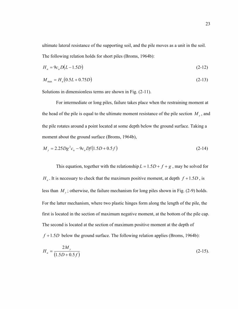
The possible modes of failure of laterally loaded piles, along with the distribution
of soil reaction, are shown in Figs. (2-13), (2-14), (2-16), (2-17), and (2-18) for free-
headed and restrained piles driven in cohesionless soils. The mode of failure of a laterally
loaded pile driven into a cohesionless soil will depend on the depth of embedment and on
the degree of end restraint.
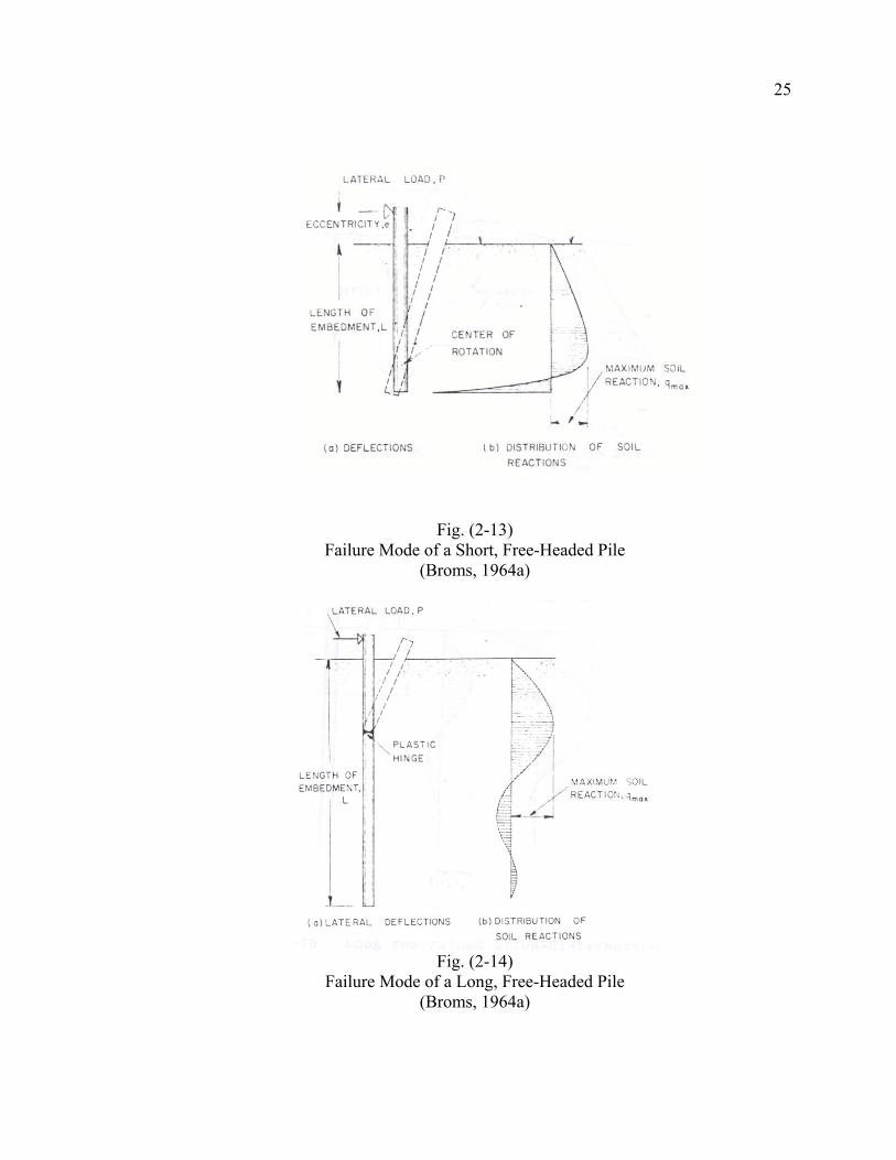
The mechanism of failure and the assumed distribution of soil reaction are shown
in Fig. (2-15). The soil located in front of the pile moves in an upward direction, whereas
the soil located at the backside of the pile moves downward and fills the void created by
the lateral deflection of the pile. However, at relatively large depths, the soil located in
front of the pile will move laterally to the backside of the pile instead of upward (Broms,
1964a).
25
Fig. (2-13)
Failure Mode of a Short, Free-Headed Pile (Broms, 1964a)
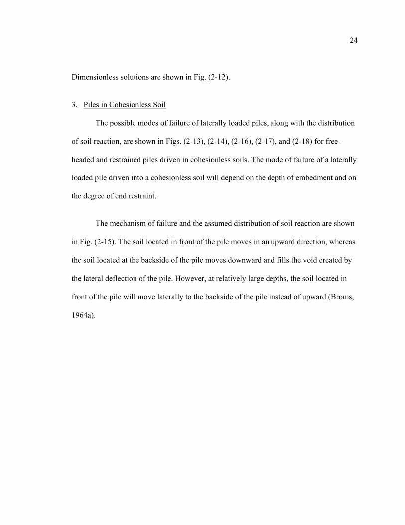
Fig. (2-14)
Failure Mode of a Long, Free-Headed Pile (Broms, 1964a)
26
Fig. (2-15) Assumed Distribution of Soil Reactions
(Broms, 1964a)
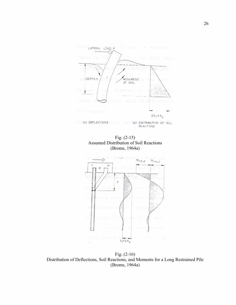
Fig. (2-16) Distribution of Deflections, Soil Reactions, and Moments for a Long Restrained Pile
(Broms, 1964a)
27
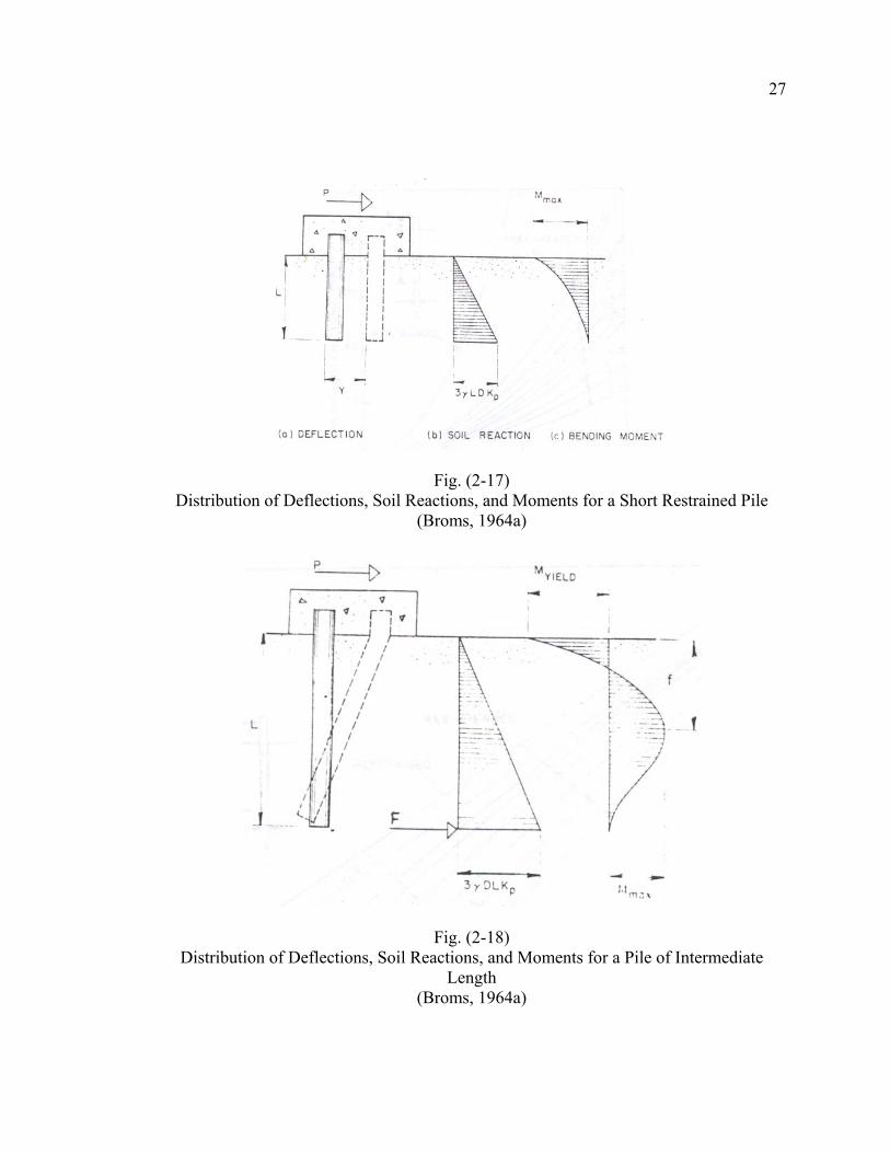
Fig. (2-17) Distribution of Deflections, Soil Reactions, and Moments for a Short Restrained Pile
(Broms, 1964a)
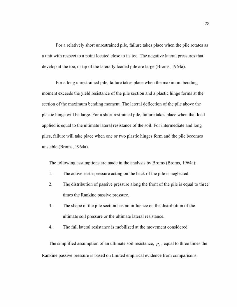
Fig. (2-18) Distribution of Deflections, Soil Reactions, and Moments for a Pile of Intermediate
Length (Broms, 1964a)
28
For a relatively short unrestrained pile, failure takes place when the pile rotates as
a unit with respect to a point located close to its toe. The negative lateral pressures that
develop at the toe, or tip of the laterally loaded pile are large (Broms, 1964a).
For a long unrestrained pile, failure takes place when the maximum bending
moment exceeds the yield resistance of the pile section and a plastic hinge forms at the
section of the maximum bending moment. The lateral deflection of the pile above the
plastic hinge will be large. For a short restrained pile, failure takes place when that load
applied is equal to the ultimate lateral resistance of the soil. For intermediate and long
piles, failure will take place when one or two plastic hinges form and the pile becomes
unstable (Broms, 1964a).
The following assumptions are made in the analysis by Broms (Broms, 1964a):
1. The active earth-pressure acting on the back of the pile is neglected.
2. The distribution of passive pressure along the front of the pile is equal to three
times the Rankine passive pressure.
3. The shape of the pile section has no influence on the distribution of the
ultimate soil pressure or the ultimate lateral resistance.
4. The full lateral resistance is mobilized at the movement considered.
The simplified assumption of an ultimate soil resistance, up , equal to three times the
Rankine passive pressure is based on limited empirical evidence from comparisons
29
between predicted and observed ultimate resistances made by Broms. These comparisons
suggest that the assumed factor of 3 may be, in some cases, conservative, as the average
ratio of predicted to measured ultimate loads is about 2/3. The distribution of soil
resistance is (Broms, 1964a):
pvu Kp '3σ= (2-16)
where
='vσ effective vertical overburden pressure
( )( )'sin1
'sin1φ
φ−
+=pK
='φ angle of internal friction (effective stress).
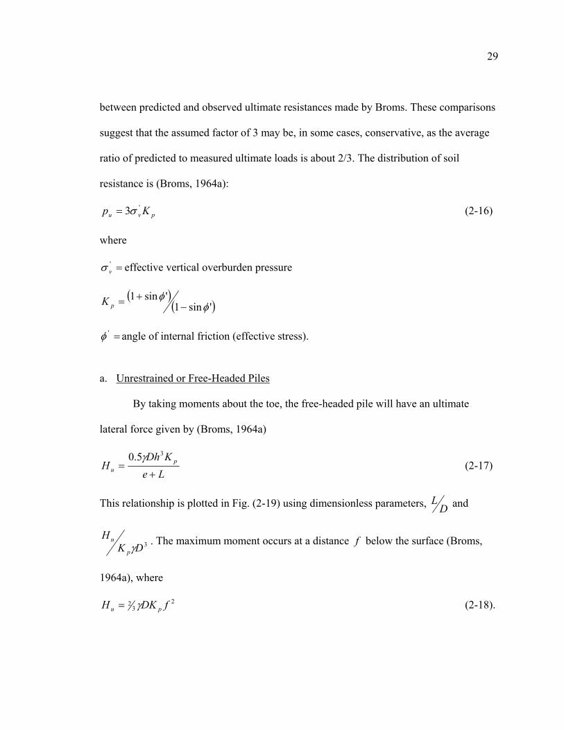
a. Unrestrained or Free-Headed Piles
By taking moments about the toe, the free-headed pile will have an ultimate
lateral force given by (Broms, 1964a)
LeKDh
H pu +
=35.0 γ
(2-17)
This relationship is plotted in Fig. (2-19) using dimensionless parameters, DL and
3DKH
p
uγ . The maximum moment occurs at a distance f below the surface (Broms,
1964a), where
23
2 fDKH pu γ= (2-18).
30
That is, γp
u
DKH
f 82.0= .
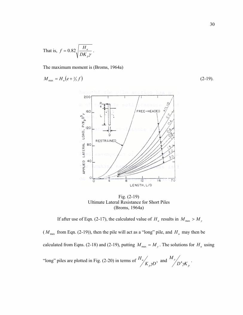
The maximum moment is (Broms, 1964a)
( )feHM u 32
max += (2-19).
Fig. (2-19) Ultimate Lateral Resistance for Short Piles
(Broms, 1964a)
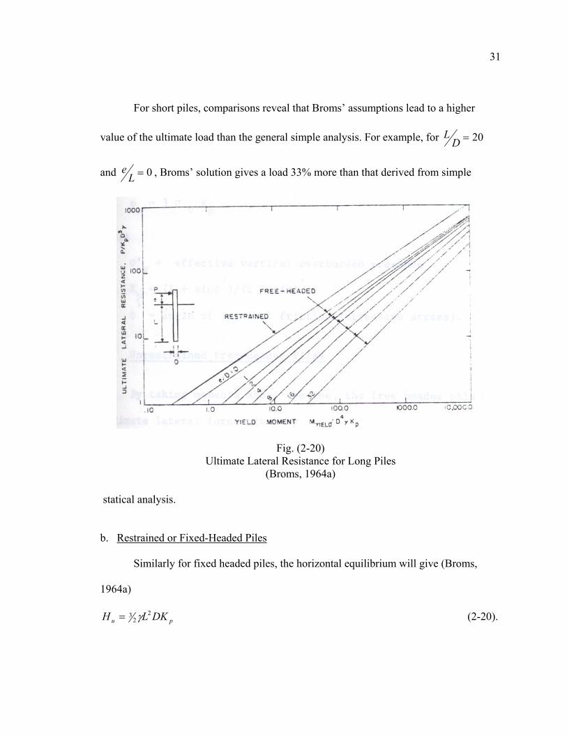
If after use of Eqn. (2-17), the calculated value of uH results in yMM >max
( maxM from Eqn. (2-19)), then the pile will act as a “long” pile, and uH may then be
calculated from Eqns. (2-18) and (2-19), putting yMM =max . The solutions for uH using
“long” piles are plotted in Fig. (2-20) in terms of 3DKH
p
uγ and
p
y
KDM
γ4 .
31
For short piles, comparisons reveal that Broms’ assumptions lead to a higher
value of the ultimate load than the general simple analysis. For example, for 20=DL
and 0=Le , Broms’ solution gives a load 33% more than that derived from simple
Fig. (2-20) Ultimate Lateral Resistance for Long Piles
(Broms, 1964a)
statical analysis.
b. Restrained or Fixed-Headed Piles
Similarly for fixed headed piles, the horizontal equilibrium will give (Broms,
1964a)
pu DKLH 22
3 γ= (2-20).
32
This solution is plotted in dimensionless form in Fig. (2-19). The maximum moment is
(Broms, 1964a)
LHM u32
max = (2-21).
If the maxM exceeds yM , then the failure mode in Fig. (2-18) is relevant. From Fig. (2-
18), for horizontal equilibrium:
( ) up HKDLF −= 22
3 γ (2-22).
Taking moments about the top of the pile, and substituting for F from Eqn. (2-22),
( ) LHKDLM upy −= 35.0 γ (2-23).
Hence, uH may be obtained.
This equation only holds if the maximum moment at depth f is less than yM ,
the distance f being calculated from Eqn. (2-18). For the situation shown in Fig. (2-16),
where the maximum moment reaches yM at two locations, it can be found that
( ) yu MfeH 232 =+ (2-24).
Dimensionless solutions from this equation are shown in Fig. (2-20).
4. Correlation with Test Results
The ultimate lateral resistances have been compared with some available test data
(Broms, 1964a and Broms, 1964b). The average measured ultimate lateral resistances
exceeded the calculated resistances by more than 50 percent for cohesionless soil.
33
However, the measured ultimate lateral resistances of piles tested by Walsenko were
found to be only 2/3 of the calculated resistances. These piles were embedded in a fine
gravel with a reported angle of internal friction of °= 45φ as measured by direct shear
tests. Frequently it is difficult to measure accurately the shearing strength of gravel by
means of direct shear tests. If a value of °= 35φ is taken as the angle of internal friction,
then the average ratio calc
testp
p is increased to 1.43, a value that compares well with the
remainder of the test data. The conclusion that can be drawn from this comparison is that
the ultimate resistance of laterally loaded piles can be estimated conservatively assuming
an ultimate lateral soil reaction equal to three times the Rankine lateral earth pressure.
Comparisons have been made by Broms between maximum bending moments
calculated from the above approach and values determined experimentally from the
available test data. For cohesionless soils, this ratio ranged between 0.54 and 1.61 with an
average value of 0.93 (Broms, 1964a). For cohesive soils, the ratio of calculated to
observed moment ranged between 0.88 and 1.19, with an average value of 1.06 (Broms,
1964b). While good agreement was obtained, it was pointed out by Broms that the
calculated maximum moment is not sensitive to small variations in the assumed soil-
resistance distribution.
5. Load-Deflection Prediction
At working loads, the deflection of a single pile or of a pile group can be
34
considered to increase approximately linearly with the applied loads. Part of the lateral
deflection is caused by the shear deformation of the soil at the time of loading and part by
consolidation and creep subsequent to loading. The deformation caused by consolidation
and creep increases with time.
It will be assumed in the following analysis, that the lateral deflections and
distribution of bending moments and shear forces can be calculated at working loads by
means of the theory of subgrade reaction. Thus, it will be assumed that the unit soil
reaction p (in inlb ) acting on a laterally loaded pile increases in proportion to the
lateral deflection y (in inches) expressed by the equation
yKp 0= (2-25)
where the coefficient 0K (in 2inlb ) is defined as the coefficient of subgrade reaction.
The numerical value of the coefficient of subgrade reaction varies with the width of the
loaded area and the load distribution, as well as with the distance from the ground surface
(Broms, 1964b).
It will be assumed that for clay, the modulus is constant with depth and that for
granular soils, the modulus increases linearly with depth. For real soils, the relationship
between soil pressure p and deflection y is non-linear with the soil pressure reaching a
limiting value when the deflection is sufficiently large. The more satisfactory approach to
deflection prediction is to perform a non-linear analysis. However, if linear theory is to be
35
used, it is necessary to choose appropriate secant values of the subgrade modulus. Reese
and Matlock argue that the adoption of a linearly increasing modulus of subgrade
reaction with depth takes some account of soil yield and nonlinearity, as values of the
secant modulus near the top of the pile are likely to be very small, but will increase with
depth because of both a higher soil strength and lower levels of deflection. Reese and
Matlock’s argument is most relevant to piles in sand and soft clay. In some cases, for
example, relatively stiff piles in over-consolidated clay at relatively low load levels, the
assumption of a constant subgrade modulus with depth may be more appropriate.
Solutions for the simple cases of constant subgrade modulus with depth, and
linearly increasing modulus with depth are described below. For horizontal load H
applied at ground level to a free-headed or unrestrained pile of length L , the following
solutions are given by Hetenyi, and shown before, for horizontal displacement y , slope
θ , moment M , and shear Q at a depth z below the surface (Hetenyi, 1964):
yHkKHy ⋅=
β2 (2-26a)
HkKH
θβθ ⋅=
22 (2-26b)
MHkHM ⋅−=β
(2-26c)
QHkHQ ⋅−= (2-26d)
where β , yHk , Hkθ , MHk , and QHk are coefficients used with horizontal loads H and
36
are described previously, and where
dKK h= (2-27)
=hK horizontal subgrade reaction (in 3inlb )
=d diameter of pile (in inches)
The corresponding expressions for moment loadings 0M applied at the ground
surface are as follows (Hetenyi, 1964):
yMkKM
y ⋅=2
02 β (2-28a)
MkKM
θβ
θ ⋅=3
04 (2-28b)
MMkMM ⋅= 0 (2-28c)
QMkMQ ⋅= β02 (2-28d)
Solutions for the case of a fixed-head or restrained pile may be obtained from the
above solutions for a free-head pile by adding to the solutions for horizontal loading H ,
the solutions for an applied moment of (Hetenyi, 1964)
( )( )
==
−=
00
20 zkzkHM
M
H
θ
θ
β (2-29)
This will be the applied moment to produce zero slope at the pile head.
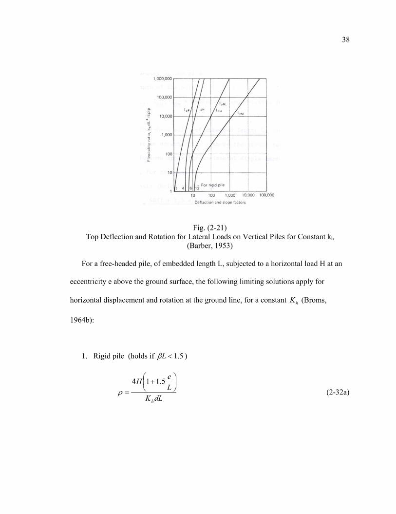
For deflections and rotations at the soil surface, plots are shown in Fig. (2-21).
37
For a free-headed or unrestrained pile, for constant hK (Barber, 1953),
deflection Mh
Hh
IdLKMI
dLKH
ρρρ ⋅
+⋅
= 2
0 (2-30a)
rotation Mh
Hh
IdLKMI
dLKH
θθθ ⋅
+⋅
= 2
0 (2-30b)
For a fixed-headed pile, which is free to translate but not to rotate (Barber, 1953),
deflection Fh
IdLKH
ρρ ⋅
= (2-31)
where
H = applied horizontal force at the ground surface
M0 = applied moment at the ground surface
d = diameter of the pile
L = length of the pile
HI ρ , MI ρ , HIθ , MIθ , and FI ρ = deflection and rotation influence factors from Fig. (2-21)
38
Fig. (2-21)
Top Deflection and Rotation for Lateral Loads on Vertical Piles for Constant kh (Barber, 1953)
For a free-headed pile, of embedded length L, subjected to a horizontal load H at an
eccentricity e above the ground surface, the following limiting solutions apply for
horizontal displacement and rotation at the ground line, for a constant hK (Broms,
1964b):
1. Rigid pile (holds if 5.1<Lβ )
dLKLeH
h
+
=5.114
ρ (2-32a)
39
2
216
dLKLeH
h
+
=θ (2-32b)
2. Infinitely long pile (holds if 5.2>Lβ )
( )dKeH
h
12 +=
ββρ (2-33a)
( )dKeH
h
ββθ 212 2 += (2-33b)
For a fixed-headed pile, the limiting solutions are (Broms, 1964b):
1. Rigid pile (holds if 5.0<Lβ )
dLKH
h
=ρ (2-34)
2. Infinitely long pile (holds if 5.1>Lβ )
dKH
h
βρ = (2-35)
For linearly varying hK with depth, Terzaghi expressed the variation as follows
(Broms, 1964a):
=dznK hh (2-36)
where
=hn coefficient of subgrade reaction at a depth of unity below the ground surface
40
(units of 3lengthforce )
=z depth below ground surface
=d pile diameter
No convenient closed form solutions are available for this case, but the following
limiting solutions apply for free-headed piles (Broms, 1964a):
1. Rigid pile ( 0.2max <z )
hnLLeH
2
33.1118
+
=ρ (2-37a)
hnLLeH
3
5.1124
+
=θ (2-37b)
2. Infinitely long pile ( 0.4max >z )
( ) ( ) ( ) ( ) 53
52
52
53
6.14.2
EIn
He
EIn
H
hh
+=ρ (2-38a)
( ) ( ) ( ) ( ) 54
51
53
52
74.16.1
EIn
He
EIn
H
hh
+=θ (2-38b)
For fixed-headed piles (Broms, 1964a):
1. Rigid pile ( 0.2max <z )
41
hnLH
2
2=ρ (2-39)
2. Infinitely long pile ( 0.4max >z )
( ) ( ) 52
53
93.0
EIn
H
h
=ρ (2-40)
For the above solutions, maxz is defined as
TLz =max (2-41)
where
51
=
hnEIT (2-42)
=EI Flexural rigidity of the pile
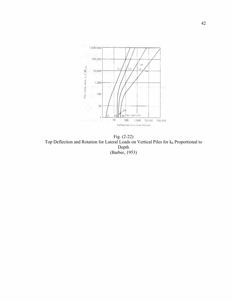
Solution for pile head deflection and slope are plotted in Fig. (2-22). The actual
slope and deflection are given by Eqns. (2-30) and (2-31), except that dKh is now
replaced by Lnh in the denominator of these equations.
42
Fig. (2-22) Top Deflection and Rotation for Lateral Loads on Vertical Piles for kh Proportional to
Depth (Barber, 1953)
43
6. Correlation with Test Data
In cohesive soils the lateral deflection at workings loads can be calculated by the
methods previously presented if the stiffness of the pile section, the pile diameter, the
penetration depth, and the average unconfined compressive strength of the soil are known
within the significant depth (Broms, 1964b).
The lateral deflections calculated from Eqns. (2-32a), (2-34), (2-33a), and (2-35) have
been compared with the test data (Broms, 1964b). The measured lateral deflections at the
ground surface varied between 0.5 to 3.0 times the calculated deflections. Broms noted
that the calculated lateral deflections for short piles are inversely proportional to the
assumed coefficient of subgrade reactions and thus to the measured average unconfined
compressive strength of the supporting soil. Thus, small variations of the measured
average unconfined compressive strength will have large effects on the calculated lateral
deflections. Broms also noted that agreement between measured and calculated lateral
deflections improves with decreasing shear strengths of the soil. The cohesive soils
reported with a high unconfined compressive strength have been preloaded by
desiccation and it is well known that the shear strength of such soils is erratic and may
vary appreciably within short distances due to the pressure of shrinkage cracks (Broms,
1964b).
Test data (Broms, 1964a) indicates that the proposed method can be used to calculate
the lateral deflection at working loads (at load levels equal to one-half to one-third the
44
ultimate lateral capacity of a pile) when the unconfined compressive strength of the soil is
less than about 1.0 tsf. However, when the unconfined compressive strength of the soil
exceeds about 1.0 tsf, it is expected that the actual deflections at the ground surface may
be considerably larger than the calculated lateral deflections due to the erratic nature of
the supporting soil (Broms, 1964a).
For cohesionless soils, the calculated lateral deflections have been compared with
some available test data on free-headed and restrained steel, reinforced concrete, and
timber piles driven or jetted into dense, medium, or loose cohesionless soils. The
calculated lateral deflections depend on the stiffness of the pile sections, the relative
density of the soil surrounding the test piles and on the degree of end restraint. The
calculated lateral deflections in almost all cases considerably exceeded the measured
lateral deflection.
However, Broms noted that only an estimate of the lateral deflection is required
for most problems and that the accuracy of the proposed methods of analysis is probably
sufficient for this purpose. Additional test data would be required to determine the
accuracy and the limitations of the proposed methods used with cohesionless soils.
45
III. P-Y CURVES
The differential equation for solving the problem of laterally loaded deep
foundations has been shown and analyzed before:
02
2
4
4
=++dxydPyE
dxydEI xs (3-1)
Approximate solutions for the equation can sometimes be obtained by the use of
non-dimensional relationships. A more favorable approach is to write the differential
equation in difference form and to obtain solutions by the use of a computer. Some of the
computer programs available for this type of analysis include L-Pile, FB-Pier, and CLM
2.02.
The numerical description of the soil modulus, sE , in this equation is
accomplished best by a set of curves that relates the soil reaction to pile deflection. If
such a set of curves can be predicted, the differential equation can be solved to yield
deflection, pile rotation, bending moment, shear, and soil reaction of any load capable of
being sustained by the deep foundation.
Most of the recent research on laterally loaded piles has been in the development
of such curves. Some of the important research was conducted to solve the problem in the
design and construction of piles in many offshore installations. In such installations,
cyclic loadings from wind and waves associated with hurricanes or otherwise play a
46
major role in the design criteria, along with the static loading.
1. Pile Deflection-Soil Reaction
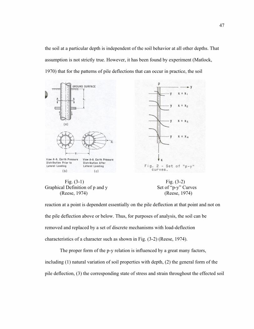
The idea of p-y curves is presented in Fig. (3-1). Fig. (3-1a) shows a section
through a pile at a depth below the ground surface. The behavior of a stratum of soil at a
depth 1x below the surface will be discussed. Fig. (3-1b) shows a possible earth pressure
distribution around the pile after installation, but before applying a lateral load to the pile.
The earth pressure distribution in Fig. (3-1b) assumes that the pile was perfectly straight
prior to driving and that there was no bending of the pile during driving. While neither of
these conditions is precisely met in practice, it is believed that in most instances the
assumption can be made without serious error.
The deflection of the pile through a distance iy , as shown in Fig. (3-1c), would
generate unbalanced soil pressures against the pile, perhaps as indicated in the figure.
Integration of the soil pressures around the pile would yield an unbalanced force ip per
unit length of the pile. The deflection of the pile could generate a soil resistance parallel
to the axis of the pile, however, it is assumed that such soil resistance would be quite
small and it can be ignored in the analysis. As shown in Fig. (3-1), the deflection of iy is
the distance the pile deflects laterally as being subjected to a lateral load. The soil
resistance ip is the force per unit length from the soil against the pile, which develops as
a result of the pile deflection.
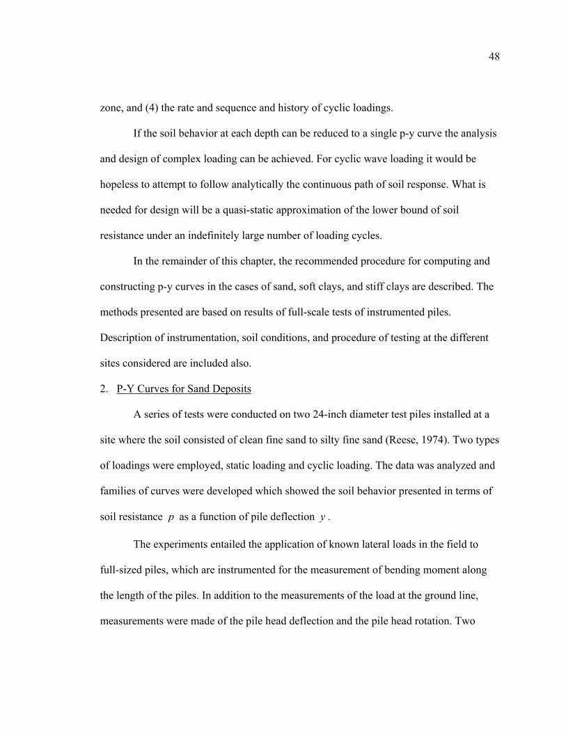
The set of curves shown in Fig. (3-2) would seem to imply that the behavior of
47
the soil at a particular depth is independent of the soil behavior at all other depths. That
assumption is not strictly true. However, it has been found by experiment (Matlock,
1970) that for the patterns of pile deflections that can occur in practice, the soil
Fig. (3-1) Fig. (3-2) Graphical Definition of p and y Set of “p-y” Curves
(Reese, 1974) (Reese, 1974)
reaction at a point is dependent essentially on the pile deflection at that point and not on
the pile deflection above or below. Thus, for purposes of analysis, the soil can be
removed and replaced by a set of discrete mechanisms with load-deflection
characteristics of a character such as shown in Fig. (3-2) (Reese, 1974).
The proper form of the p-y relation is influenced by a great many factors,
including (1) natural variation of soil properties with depth, (2) the general form of the
pile deflection, (3) the corresponding state of stress and strain throughout the effected soil
48
zone, and (4) the rate and sequence and history of cyclic loadings.
If the soil behavior at each depth can be reduced to a single p-y curve the analysis
and design of complex loading can be achieved. For cyclic wave loading it would be
hopeless to attempt to follow analytically the continuous path of soil response. What is
needed for design will be a quasi-static approximation of the lower bound of soil
resistance under an indefinitely large number of loading cycles.
In the remainder of this chapter, the recommended procedure for computing and
constructing p-y curves in the cases of sand, soft clays, and stiff clays are described. The
methods presented are based on results of full-scale tests of instrumented piles.
Description of instrumentation, soil conditions, and procedure of testing at the different
sites considered are included also.
2. P-Y Curves for Sand Deposits
A series of tests were conducted on two 24-inch diameter test piles installed at a
site where the soil consisted of clean fine sand to silty fine sand (Reese, 1974). Two types
of loadings were employed, static loading and cyclic loading. The data was analyzed and
families of curves were developed which showed the soil behavior presented in terms of
soil resistance p as a function of pile deflection y .
The experiments entailed the application of known lateral loads in the field to
full-sized piles, which are instrumented for the measurement of bending moment along
the length of the piles. In addition to the measurements of the load at the ground line,
measurements were made of the pile head deflection and the pile head rotation. Two
49
types of loading were employed, static and cyclic.
Two piles were driven open-ended at the test site on Mustang Island near Corpus
Christi, Texas. The water table was maintained above the ground surface during loading
to simulate conditions which would exist at an offshore location. For each type of
loading, a series of lateral loads were applied, beginning with a load of small magnitude.
A bending moment curve was obtained for each load; thus, the experiments resulted in a
set of bending moment curves along with the associated boundary conditions for each
type of loading.
Soil studies were made at the site involving the use of undisturbed sampling.
Laboratory studies were performed. The sand at the test site varied from clean fine sand
to silty fine sand, both having relatively high densities. The sand particles by inspection
through a microscope were found to be subangular with a large percentage of flaky
grains. The angle of internal friction φ was determined to be °39 and the value of the
submerged unit weight 'γ was found to be 66 3ftlb (Reese, 1974).
a. Elastic Modulus
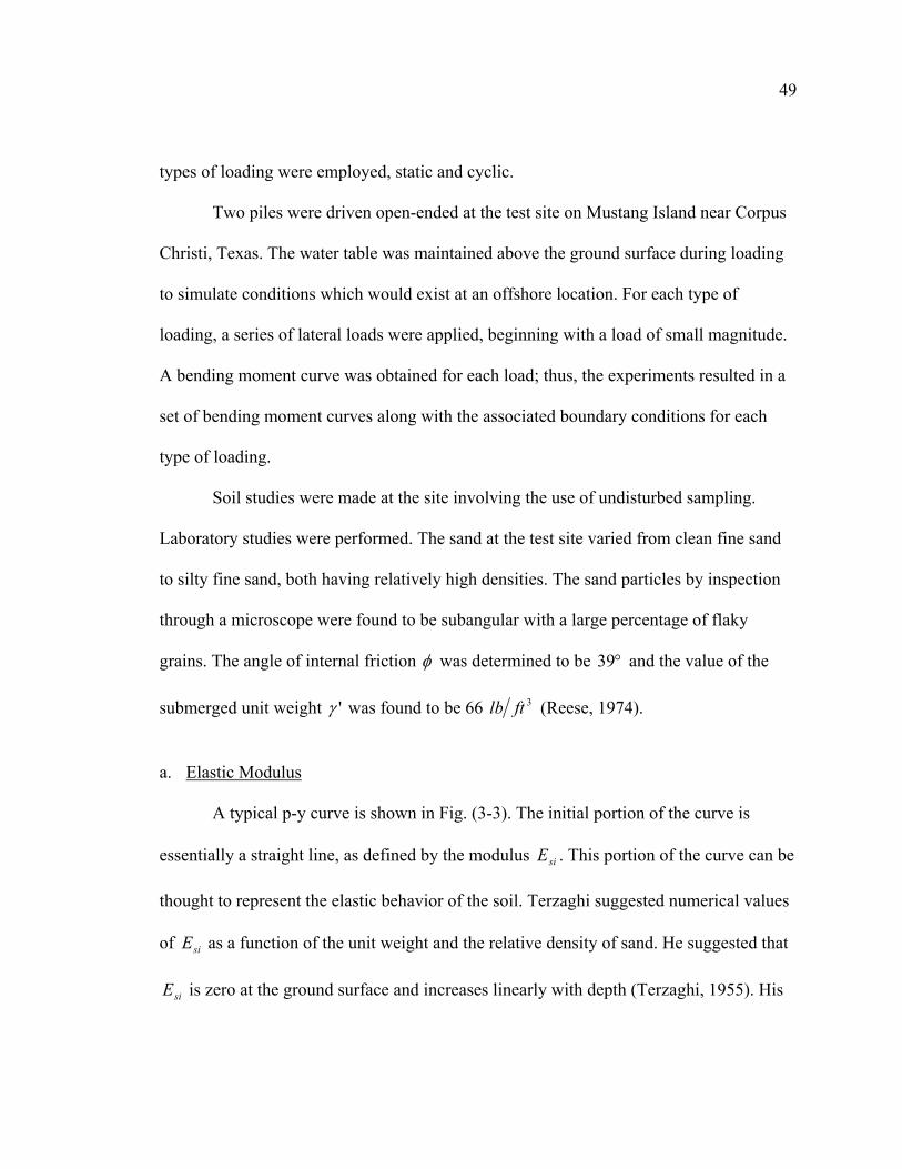
A typical p-y curve is shown in Fig. (3-3). The initial portion of the curve is
essentially a straight line, as defined by the modulus siE . This portion of the curve can be
thought to represent the elastic behavior of the soil. Terzaghi suggested numerical values
of siE as a function of the unit weight and the relative density of sand. He suggested that
siE is zero at the ground surface and increases linearly with depth (Terzaghi, 1955). His
50
suggestion was based on the fact that experiments had shown that the initial slope of a
laboratory stress-strain curve for sand is a linear function of the confining pressure.
siE is given by the following equation:
kxEsi =
where
k = a coefficient, 3inlb
x = depth below ground surface, in
Fig. (3-3) Typical “p-y” Curve
(Reese, 1974)
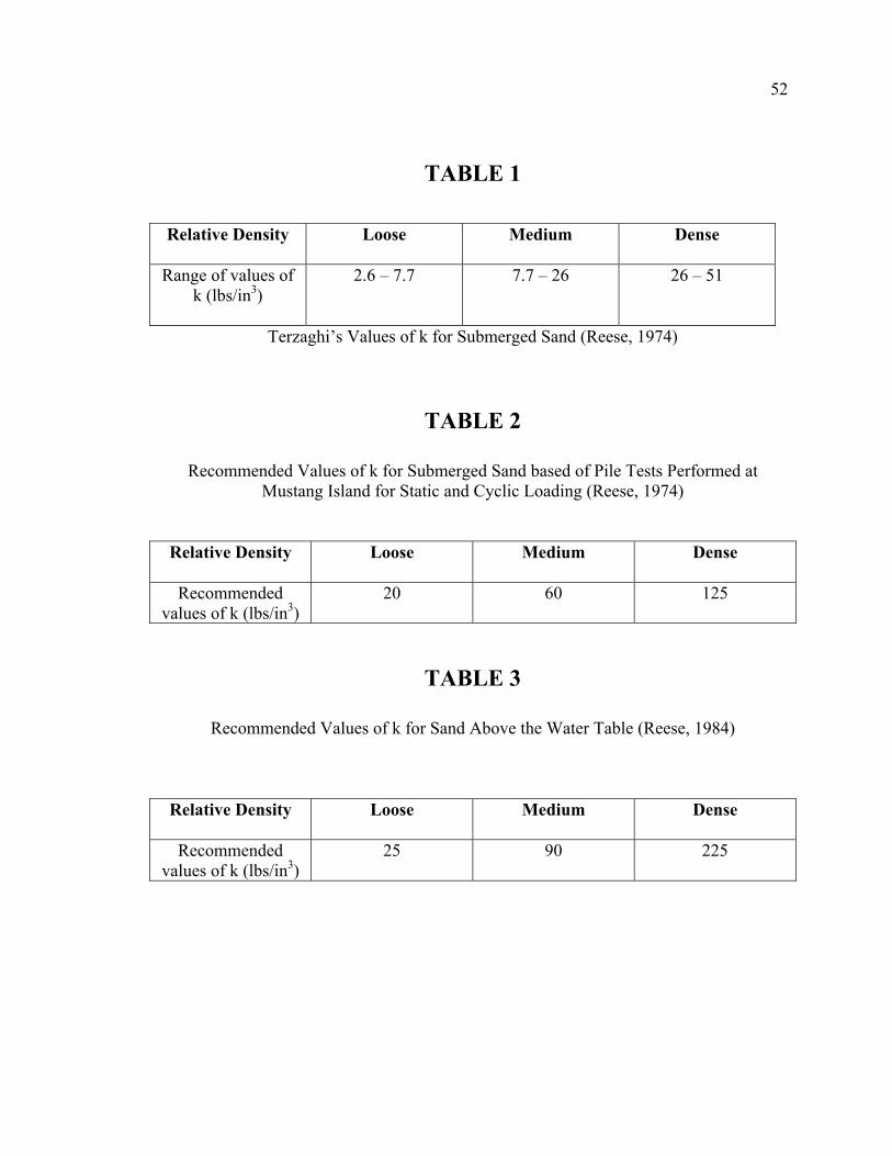
The value of k recommended by Terzaghi are shown in Table 1. The values of k
obtained from the Mustang Island test for the static case were 2.5 times the highest value
reported by Terzaghi. The values for the cyclic case were 3.9 times the highest value
51
given by Terzaghi. With regard to recommended values, it is proposed by Reese that the
values of k shown in Table 2 and 3 be used. These values of k are recommended for
static and cyclic loading (Reese, 1974 and Reese, 1984). An examination of the shape of
the p-y curves which are recommended in Fig. (3-7) shows that the initial straight-line
portions of the curves (where sE is constant with deflection) governs for only small
deflections. Therefore, the initial slope of the p-y curve influences analyses only for the
52
TABLE 1
Terzaghi’s Values of k for Submerged Sand (Reese, 1974)
TABLE 2
Recommended Values of k for Submerged Sand based of Pile Tests Performed at Mustang Island for Static and Cyclic Loading (Reese, 1974)
Relative Density Loose Medium Dense
Recommended values of k (lbs/in3)
20 60 125
TABLE 3
Recommended Values of k for Sand Above the Water Table (Reese, 1984)
Relative Density Loose Medium Dense
Recommended values of k (lbs/in3)
25 90 225
Relative Density Loose Medium Dense
Range of values of k (lbs/in3)
2.6 – 7.7 7.7 – 26 26 – 51
53
very smallest loads. In more normal cases, a secant modulus, such as the one defined by
snE shown in Fig. (3-3), controls the analyses. Because the initial portion of the p-y
curve has little influence on most analyses and because of the relatively small amount of
data on the early portions of the curves, it was thought to be undesirable to recommend
different values of k for static and for cyclic loading.
b. Soil Resistance
Referring to Fig. (3-3), it may be seen that soil resistance p attains a limiting
value defined as the ultimate soil resistance up . Soil mechanics theory can be applied to
derive equations for up for two cases, near the ground surface and at a depth.
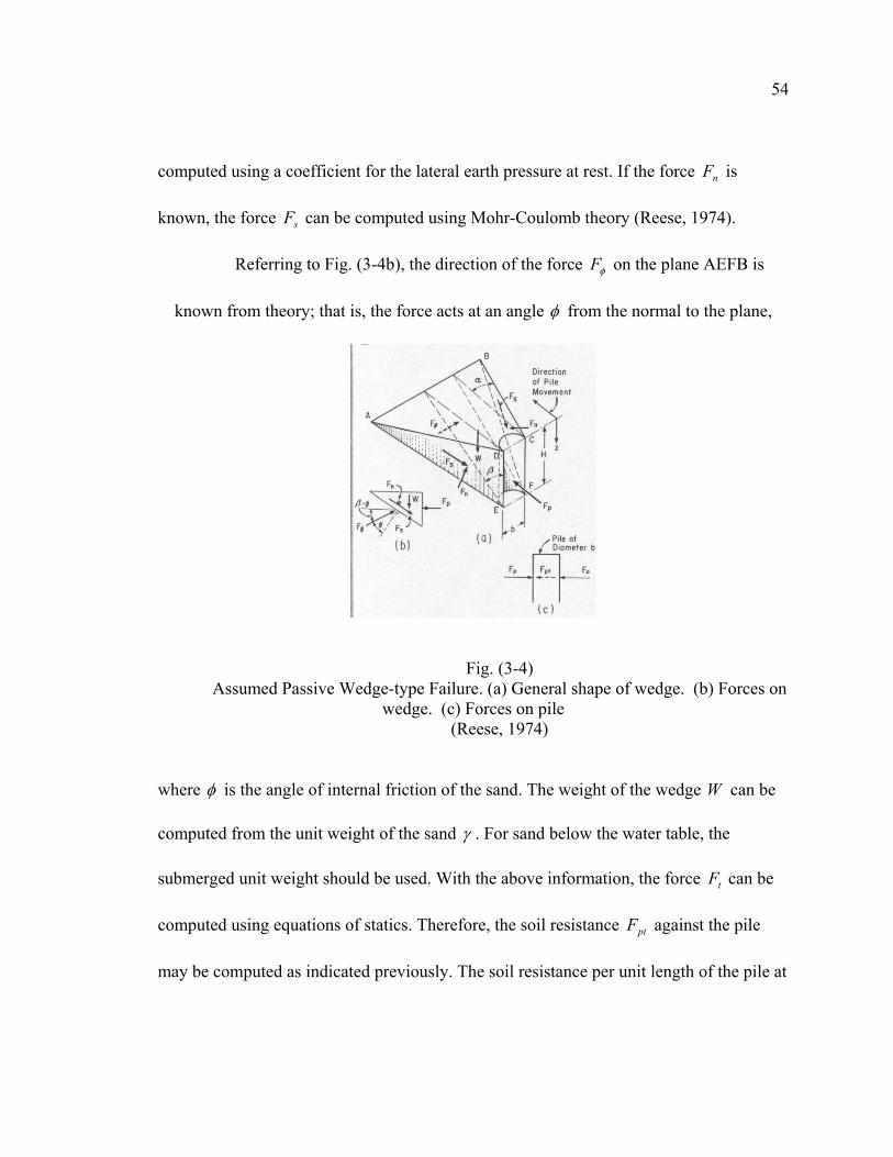
The ultimate soil resistance near the ground surface is computed using the free
body shown in Fig. (3-4). As may be seen in the figure, the total ultimate lateral
resistance ptF on the pile section is equal to the passive force pF minus the active force
aF . The force aF may be computed from the Rankine’s theory, using the minimum
coefficient of active earth pressure. The passive force pF may be computed from the
geometry of the wedge, assuming the Mohr-Coulomb failure theory to be valid for sand.
By referring to Fig. (3-4), it can be seen that the shape of the wedge is defined by the pile
diameter b , the depth of the wedge H , and by the angles α and β . It is assumed that
no frictional resistance occurs on the base of the pile; therefore, there is no tangential
forces on the surface CDEF. The normal force nF on planes ADE and BCF can be
54
computed using a coefficient for the lateral earth pressure at rest. If the force nF is
known, the force sF can be computed using Mohr-Coulomb theory (Reese, 1974).
Referring to Fig. (3-4b), the direction of the force φF on the plane AEFB is
known from theory; that is, the force acts at an angle φ from the normal to the plane,
Fig. (3-4)
Assumed Passive Wedge-type Failure. (a) General shape of wedge. (b) Forces on wedge. (c) Forces on pile
(Reese, 1974)
where φ is the angle of internal friction of the sand. The weight of the wedge W can be
computed from the unit weight of the sand γ . For sand below the water table, the
submerged unit weight should be used. With the above information, the force tF can be
computed using equations of statics. Therefore, the soil resistance ptF against the pile
may be computed as indicated previously. The soil resistance per unit length of the pile at
55
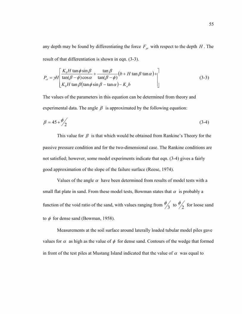
any depth may be found by differentiating the force ptF with respect to the depth H . The
result of that differentiation is shown in eqn. (3-3).
( )
( )
−−
++−
+−=
bKHK
HbHKHP
a
ct
αβφβ
αβφβ
βαφββφ
γtansintantan
tantan)tan(
tancos)tan(sintan
0
0
(3-3)
The values of the parameters in this equation can be determined from theory and
experimental data. The angle β is approximated by the following equation:
245 φβ += (3-4)
This value for β is that which would be obtained from Rankine’s Theory for the
passive pressure condition and for the two-dimensional case. The Rankine conditions are
not satisfied; however, some model experiments indicate that eqn. (3-4) gives a fairly
good approximation of the slope of the failure surface (Reese, 1974).
Values of the angle α have been determined from results of model tests with a
small flat plate in sand. From these model tests, Bowman states that α is probably a
function of the void ratio of the sand, with values ranging from 3φ to 2
φ for loose sand
to φ for dense sand (Bowman, 1958).
Measurements at the soil surface around laterally loaded tubular model piles gave
values for α as high as the value of φ for dense sand. Contours of the wedge that formed
in front of the test piles at Mustang Island indicated that the value of α was equal to
56
about 3φ for static loading and about 4
3φ for cyclic loading.
The value of the coefficient of earth pressure at rest is dependant on the void ratio
or relative density of the sand and the process by which the deposit was formed. Terzaghi
and Peck state that the value of the coefficient of earth pressure at rest is about 0.4 for
loose sand and about 0.5 for dense sand (Terzaghi, 1948). In the absence of precise
methods for determining relative density in the field, especially when soil deformations
are large, a value of 0.4 for 0K was selected in computing the ultimate soil resistance
near the ground surface. The value of α selected for this computation was 2φ . The
angle of internal friction φ was taken as °39 as indicated previously.
The coefficient aK in eqn. (3-3) is the Rankine coefficient of minimum active
earth pressure and is given by the following equation:
)245(tan 2 φ−=aK (3-5)
With regard to the use of theory for computing the ultimate lateral resistance against the
pile at a considerable depth below the ground surface, the model shown in Fig. (3-5) is
employed. In this model, the soil is assumed to flow in the horizontal direction only.
Referring to the model, Block 1 will fail by shearing along the dashed lines allowing the
soil in that block to follow the pile. Block 2 will fail along the dashed line as shown.
Block 3 will slide horizontally. Block 4 will fail as shown, and Block 5 will be in the
failure condition as the pile pushes against it. In this simplified model it is assumed that
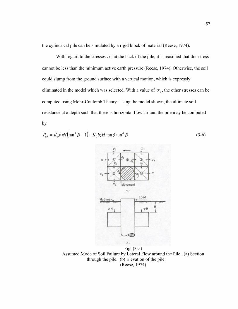
57
the cylindrical pile can be simulated by a rigid block of material (Reese, 1974).
With regard to the stresses 1σ at the back of the pile, it is reasoned that this stress
cannot be less than the minimum active earth pressure (Reese, 1974). Otherwise, the soil
could slump from the ground surface with a vertical motion, which is expressly
eliminated in the model which was selected. With a value of 1σ , the other stresses can be
computed using Mohr-Coulomb Theory. Using the model shown, the ultimate soil
resistance at a depth such that there is horizontal flow around the pile may be computed
by
( ) βφγβγ 40
8 tantan1tan HbKHbKP acd +−= (3-6)
Fig. (3-5)
Assumed Mode of Soil Failure by Lateral Flow around the Pile. (a) Section through the pile. (b) Elevation of the pile.
(Reese, 1974)
58
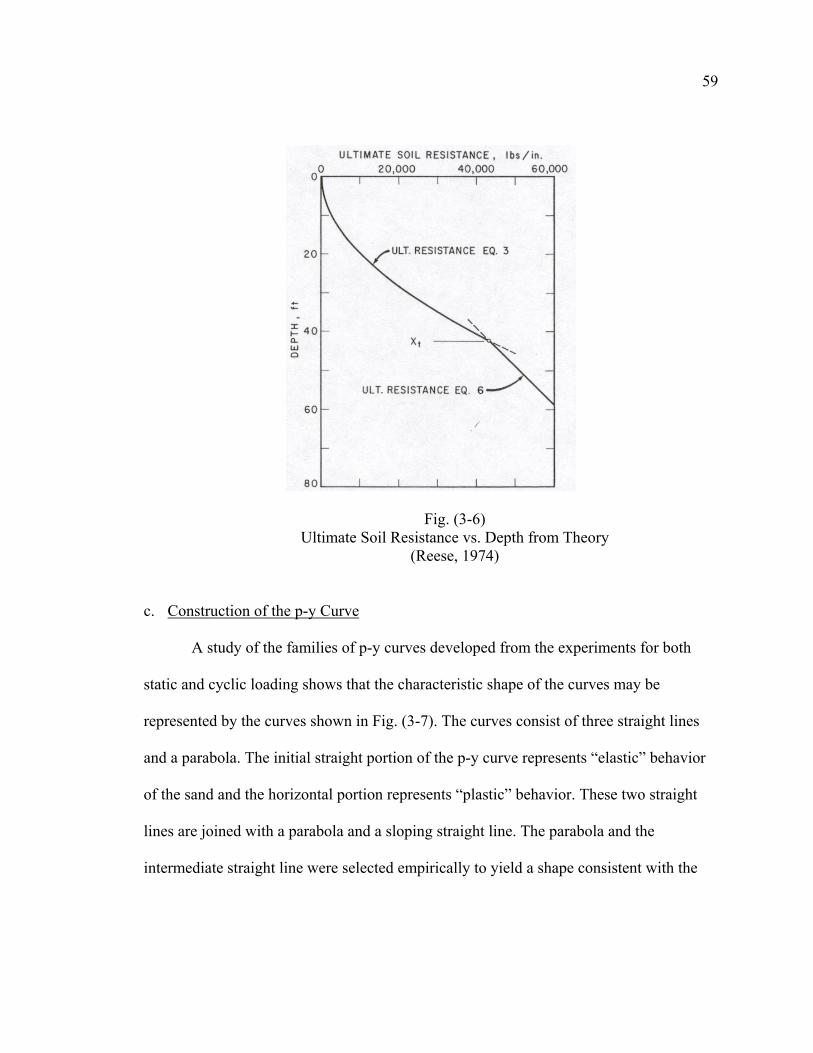
For the Mustang Island test, values of cP were computed using Eqns. (3-3) and
(3-6). These values are shown plotted in Fig. (3-6). The values of the parameters used in
making the computations are as follows (Reese, 1974):
( )
ftb
submergedftlbs
K
2245
66
4.02
39
3
0
=
+°=
=
=
=
°=
φβ
γ
φα
φ
The symbol tX shown in Fig. (3-6) defines the intersection of Eqns. (3-3) and (3-
6).
59
Fig. (3-6) Ultimate Soil Resistance vs. Depth from Theory
(Reese, 1974)
c. Construction of the p-y Curve
A study of the families of p-y curves developed from the experiments for both
static and cyclic loading shows that the characteristic shape of the curves may be
represented by the curves shown in Fig. (3-7). The curves consist of three straight lines
and a parabola. The initial straight portion of the p-y curve represents “elastic” behavior
of the sand and the horizontal portion represents “plastic” behavior. These two straight
lines are joined with a parabola and a sloping straight line. The parabola and the
intermediate straight line were selected empirically to yield a shape consistent with the
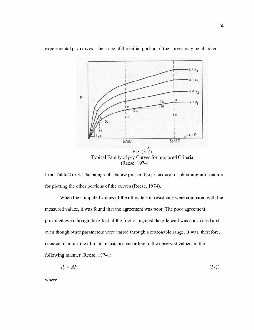
60
experimental p-y curves. The slope of the initial portion of the curves may be obtained
Fig. (3-7)
Typical Family of p-y Curves for proposed Criteria (Reese, 1974)
from Table 2 or 3. The paragraphs below present the procedure for obtaining information
for plotting the other portions of the curves (Reese, 1974).
When the computed values of the ultimate soil resistance were compared with the
measured values, it was found that the agreement was poor. The poor agreement
prevailed even though the effect of the friction against the pile wall was considered and
even though other parameters were varied through a reasonable range. It was, therefore,
decided to adjust the ultimate resistance according to the observed values, in the
following manner (Reese, 1974):
cu APP = (3-7)
where
61
=uP ultimate resistance in proposed criteria, lbs/in
=cP ultimate resistance from theory, lbs/in
=A empirical adjustment factor
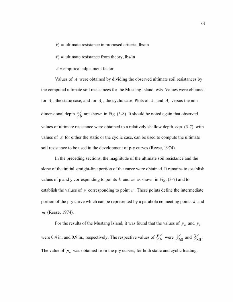
Values of A were obtained by dividing the observed ultimate soil resistances by
the computed ultimate soil resistances for the Mustang Island tests. Values were obtained
for sA , the static case, and for cA , the cyclic case. Plots of sA and cA versus the non-
dimensional depth bx are shown in Fig. (3-8). It should be noted again that observed
values of ultimate resistance were obtained to a relatively shallow depth. eqn. (3-7), with
values of A for either the static or the cyclic case, can be used to compute the ultimate
soil resistance to be used in the development of p-y curves (Reese, 1974).
In the preceding sections, the magnitude of the ultimate soil resistance and the
slope of the initial straight-line portion of the curve were obtained. It remains to establish
values of p and y corresponding to points k and m as shown in Fig. (3-7) and to
establish the values of y corresponding to point u . These points define the intermediate
portion of the p-y curve which can be represented by a parabola connecting points k and
m (Reese, 1974).
For the results of the Mustang Island, it was found that the values of my and uy
were 0.4 in. and 0.9 in., respectively. The respective values of by were 60
1 and 803 .
The value of mp was obtained from the p-y curves, for both static and cyclic loading.
62
From these values, values of the parameter B were computed as follows (Reese, 1974):
c
m
PP
B = (3-8)
Values of B for both static and cyclic cases are shown in Fig. (3-9). Thus, from the
Fig. (3-8)
Non-dimensional Coefficient, A, for Ultimate Soil Resistance vs. Depth (Reese, 1974)
63
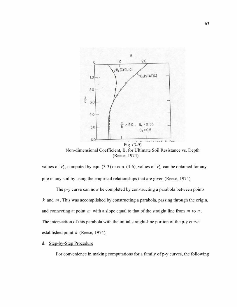
Fig. (3-9)
Non-dimensional Coefficient, B, for Ultimate Soil Resistance vs. Depth (Reese, 1974)
values of cP , computed by eqn. (3-3) or eqn. (3-6), values of mP can be obtained for any
pile in any soil by using the empirical relationships that are given (Reese, 1974).
The p-y curve can now be completed by constructing a parabola between points
k and m . This was accomplished by constructing a parabola, passing through the origin,
and connecting at point m with a slope equal to that of the straight line from m to u .
The intersection of this parabola with the initial straight-line portion of the p-y curve
established point k (Reese, 1974).
d. Step-by-Step Procedure
For convenience in making computations for a family of p-y curves, the following
64
step-by-step procedure is presented (Reese, 1984). A typical family of such curves is
shown in Fig. (3-7).
1. Obtain values for significant soil properties and pile dimensions, φ , γ ,
and b .
2. Use the following for computing soil resistance: 2φα = , 245 φβ += ,
4.00 =K , and
−= 245tan 2 φ
aK .
3. Use the following equations for computing soil resistance:
a. Ultimate resistance near ground surface.
( )
( )
−−
++−
+−=
bKHK
HbHK
HP
a
ct
αβφβ
αβφβ
βαφββφ
γtansintantan
tantan)tan(
tancos)tan(sintan
0
0
(3-9)
b. Ultimate resistance well below the ground surface.
( ) βφγβγ 40
8 tantan1tan HbKHbKP acd +−= (3-10)
4. Find the intersection, tX , of the equation for the ultimate soil resistance
near the ground surface and the ultimate soil resistance well below the
ground surface. Above this depth use eqn. (3-3), below this depth use eqn.
(3-6).
5. Select one depth at which a p-y curve is desired.
6. Establish uy at 803b . Compute up by the following equation:
65
cu APP = (3-7)
Use the appropriate values of A from Fig. (3-8), for the particular
nondimensional depth, and for either the static or cyclic case. Use the
appropriate equation for cP , eqn. (3-3) or eqn. (3-6) by referring to
computation in step 4.
7. Establish my as 60b . Compute mp by the following equation:
cm BPp = (3-8)
Use the appropriate values of B from Fig. (3-9), for the particular
nondimensional depth, and for either the static or cyclic case. Use the
appropriate equation for cP .
8. Establish the slope of the initial portion of the p-y curve by selecting the
appropriate value of k from Table 2 or 3. Use the equation,
ykxp )(=
9. Select the following parabola to be fitted between points k and m :
nCyp1
= (3-11)
10. Fit the parabola between points k and m as follows:
a. Get slope of line between points m and u by,
mu
mumu yy
ppk−−
= (3-12)
b. Obtain the exponent of the parabolic section by,
66
mmu
m
ykpn = (3-13)
c. Obtain the coefficient C as follows:
nm
m
y
pC 1= (3-14)
d. Determine point k on the curve as,
1−
=
nn
k kxCy (3-15)
where k is obtained from Table 2 or 3.
e. Compute appropriate numbers of points on the parabola by using eqn.
(3-11).
This completes the development of the p-y curve for the desired depth. Repeating
the steps above for each depth desired can develop any number of curves.
e. Limitations
The following limitations were taken from Reese, 1974:
1. The soil is assumed to be cohesionless sand. A soil that is predominately
granular but contains a sufficient amount of clay to give some cohesion would
behave entirely different than cohesionless sand.
2. The pile is assumed to have been driven so that the sand is densified rather
67
than loosened during installation. The proposed method does not apply to piles
that have been installed by jetting.
3. The pile is assumed to be essentially vertical. However, it is believed that the
method can be used to predict the behavior of batter piles if the batter is not to
severe.
3. P-Y Curves in Soft Clay
A research program was performed by Matlock to solve the problems pertinent to
the design of laterally loaded piles in soft, normally consolidated marine clay (Matlock,
1970). The program was oriented mainly for offshore structures and has included field
tests with an instrumented pile and laboratory model testing. Three types of loading were
considered: (1) short-term static loading, (2) cyclic loading, and (3) subsequent reloading
after cyclic loading. The research included extensive field-testing with an instrumented
pile, experiments with laboratory models and parallel development of analytical methods
and correlations.
The steel test pile was 12.75 inches in diameter and 35 pairs of electric resistance
strain gages were installed in the 42 foot embedded portion. The pile was calibrated to
provide extremely accurate determinations of bending moment. Gage spacing varied
from 6 inches near the top to 4 feet in the lowest section.
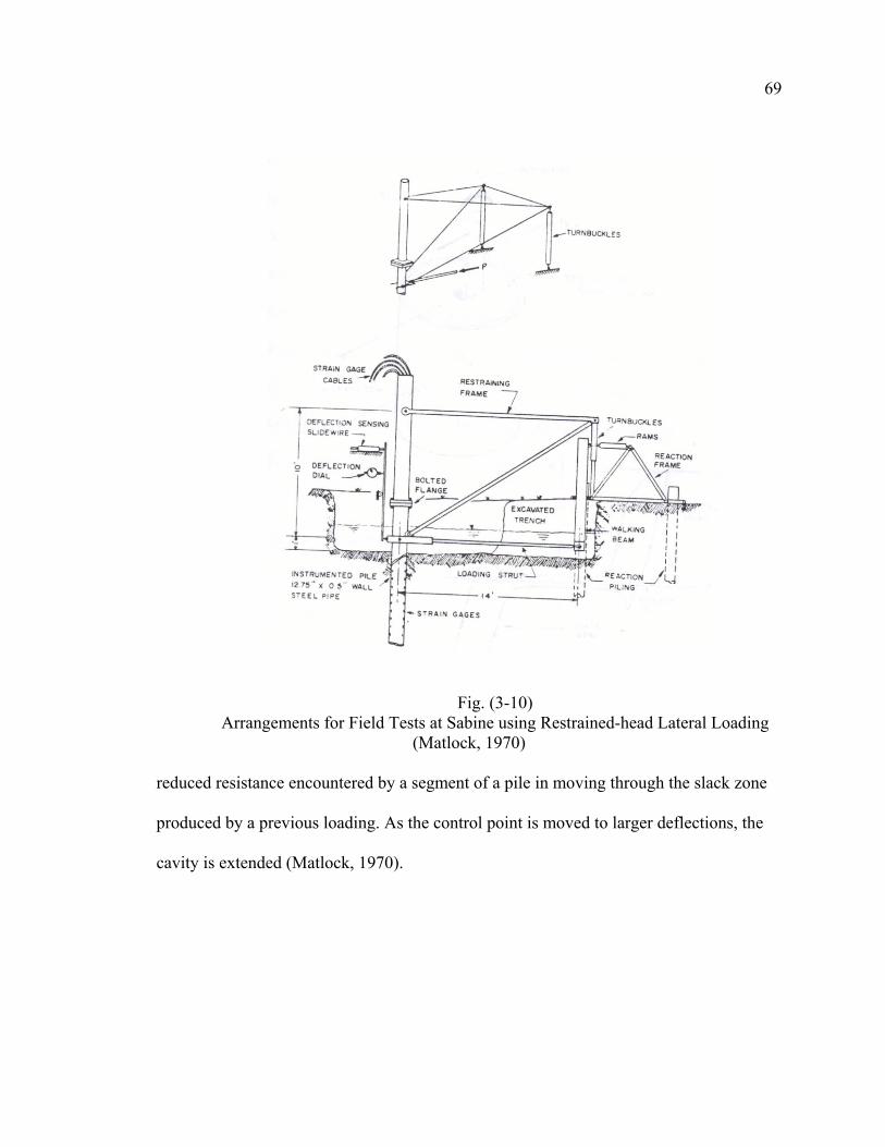
Free-headed tests were done with only lateral loads applied at the mud line. As
shown in Fig. (3-10), restrained-headed loadings utilized a framework to simulate the
effect of a jacket-type structure. The load from hydraulic rams was transmitted to the pile
68
by a walking beam and loading strut. For cyclic loadings, the peak forward and reverse
loads during cycling were automatically controlled.
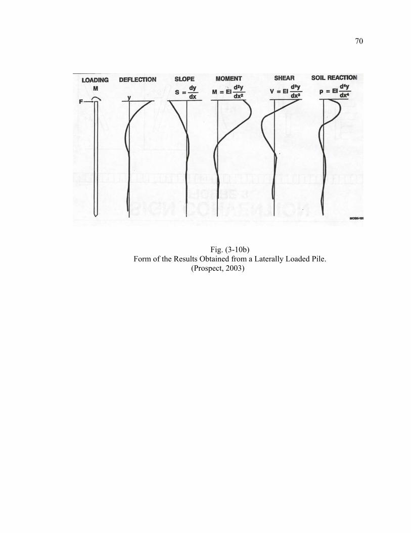
Precise determination of the bending moments during all static loadings allowed
differentiation to obtain curves of the distribution of soil reaction along the pile to a very
satisfactory degree of accuracy. Integration of the bending moment diagrams provided
the deflected shape of the pile. For illustrative purposes, see Fig. (3-10b). Loads were
increased by increments, and for any selected depth, the soil reaction p may be plotted
as a function of pile deflection y . These experimental p-y curves are the principle basis
for the development of design procedures.
The pile was driven twice and two complete series of free-headed loadings, one
static and one cyclic, were performed at Lake Austin. At a site near the mouth of the
Sabine River there were four primary series of test loadings, two static and two cyclic,
with each type tested under both free-headed and restrained-headed conditions. In
addition to these, numerous variations were tried including tests with sand, artificially
softened clay, and the use of sand and pea gravel to restore the loss in resistance of the
pile caused by previous cyclic loadings.
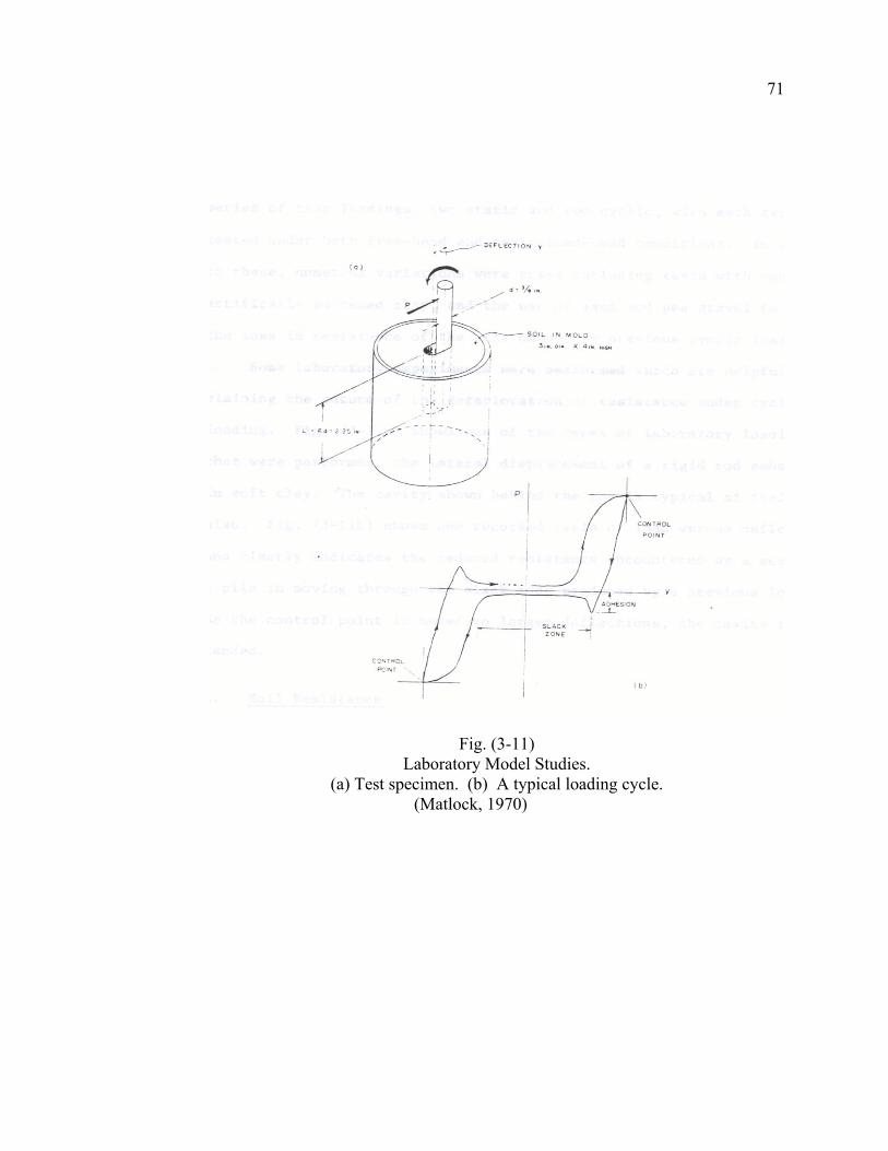
Some laboratory experiments were performed which are helpful in explaining the
nature of the deterioration of resistance under cyclic loading. Fig. (3-11a) shows one of
the types of laboratory loadings that were performed, the lateral displacement of a rigid
rod embedded in soft clay. The cavity shown behind the rod is typical of field tests also.
Fig. (3-11b) shows one recorded cycle of load versus deflection and clearly indicates the
69
Fig. (3-10)
Arrangements for Field Tests at Sabine using Restrained-head Lateral Loading (Matlock, 1970)
reduced resistance encountered by a segment of a pile in moving through the slack zone
produced by a previous loading. As the control point is moved to larger deflections, the
cavity is extended (Matlock, 1970).
70
Fig. (3-10b)
Form of the Results Obtained from a Laterally Loaded Pile. (Prospect, 2003)
71
Fig. (3-11)
Laboratory Model Studies. (a) Test specimen. (b) A typical loading cycle.
(Matlock, 1970)
72
a. Soil Resistance
In conventional soil mechanics, most problems involving load capacity of soils
are handled by consideration only of ultimate strength characteristics. In contrast, with
long piles laterally loaded, the static ultimate soil resistance is seldom achieved except
very near the surface; the allowable stresses in the pile are usually reached first, with
most of the soil still in a pre-plastic state of strain. Nevertheless, a rational and orderly
prediction of soil deformation characteristics for various loading conditions should start
with an estimate of static ultimate resistance.
In soft clay, soil is confined so that plastic flows around a pile occur only in
horizontal planes. The ultimate resistance per unit length of pile may be expressed as
cdNp pu = (3-16)
where c is the soil strength, d is the pile diameter, and pN is a non-dimensional
ultimate resistance coefficient. A consensus of the investigators appears to indicate that
for soft clay soil flowing around a cylindrical pile at a considerable depth below the
surface, the coefficient should be
9=pN (3-17)
Very near the surface, the soil in front of the pile will fail by shearing forward and
upward and the corresponding value of pN reduces to the range of 2 to 4, depending on
whether the pile segment is considered as a plate with only frontal resistance or whether
it is a square cross section with soil shear acting along the sides. For a cylindrical pile, a
73
value of 3 is believed to be appropriate. The resistance should be expected to vary from
this value at the surface to the maximum indicated by eqn. (3-17) at some depth rX ,
which is termed the depth of reduced resistance. Within the upper zone, resistance to
vertical movement is provided by the overburden pressure xσ from the soil itself and by
resistance developed by deformation within the surrounding soil mass. This resistance
increases with distance from the free soil surface. The following equation appears to
describe this variation to a satisfactory degree of approximation:
dxJ
cN xp ++=
σ3 (3-18)
The first term expresses the resistance at the surface, the second term gives the
increase with depth due to overburden pressure, and the third term may be thought of as
the geometrically related restraint that even a weightless soil around a pile would provide
against upward flow of the soil. The equation corresponds closely to one developed by
Reese who considered a failing prism or wedge of soil ahead of the pile. However,
Reese’s value of J was 2.8, which does not agree with experimental results. Therefore,
the coefficient J must be determined empirically.
Fortunately, the third term in eqn. (3-18) represents only a part of the total
ultimate resistance coefficient pN , and according to Matlock, because it contains the
depth x , it becomes relatively insignificant in the more important upper layers. From
experimental evidence, a clear distinction cannot be made between contributions of the
first and last terms in eqn. (3-18).
74
Studies based on the Sabine data indicate that a value of J equal to
approximately 0.5 is satisfactory when used in eqn. (3-18). A lower value of about 0.25
fits the Lake Austin data somewhat better, which may be a consequence of the stiffer clay
at that site.
If the soil strength and the effective unit weight γ are constant with depth, the
value of the depth at which the value of pN becomes equal to the maximum of 9 is
obtained by the simultaneous solutions of Eqns. (3-17) and (3-18):
J
cddxr+
=γ
6 (3-19)
The coefficient J and the resulting values of rx should be thought of as rational
but essentially empirical parameters by which correlations have been made between
prediction methods and the available field results. Where soil properties undergo
considerable variation with depth, it appears reasonable to consider the soil as a system of
thin layers with rx computed as a variable with depth according to the properties of each
layer (Matlock, 1970).
b. Construction of the P-Y Curve
The following section presents a summary taken from Matlock’s 1970 paper of
the recommended procedure for constructing p-y curves for the three different loading
conditions is given in Fig. (3-12). In a given problem, the appropriate form selected from
Fig. (3-12) is applied at numerous depths to produce a family of p-y curves. The basis for
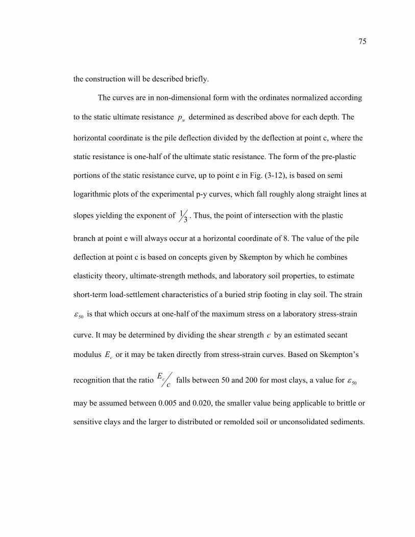
75
the construction will be described briefly.
The curves are in non-dimensional form with the ordinates normalized according
to the static ultimate resistance up determined as described above for each depth. The
horizontal coordinate is the pile deflection divided by the deflection at point c, where the
static resistance is one-half of the ultimate static resistance. The form of the pre-plastic
portions of the static resistance curve, up to point e in Fig. (3-12), is based on semi
logarithmic plots of the experimental p-y curves, which fall roughly along straight lines at
slopes yielding the exponent of 31 . Thus, the point of intersection with the plastic
branch at point e will always occur at a horizontal coordinate of 8. The value of the pile
deflection at point c is based on concepts given by Skempton by which he combines
elasticity theory, ultimate-strength methods, and laboratory soil properties, to estimate
short-term load-settlement characteristics of a buried strip footing in clay soil. The strain
50ε is that which occurs at one-half of the maximum stress on a laboratory stress-strain
curve. It may be determined by dividing the shear strength c by an estimated secant
modulus cE or it may be taken directly from stress-strain curves. Based on Skempton’s
recognition that the ratio cEc falls between 50 and 200 for most clays, a value for 50ε
may be assumed between 0.005 and 0.020, the smaller value being applicable to brittle or
sensitive clays and the larger to distributed or remolded soil or unconsolidated sediments.
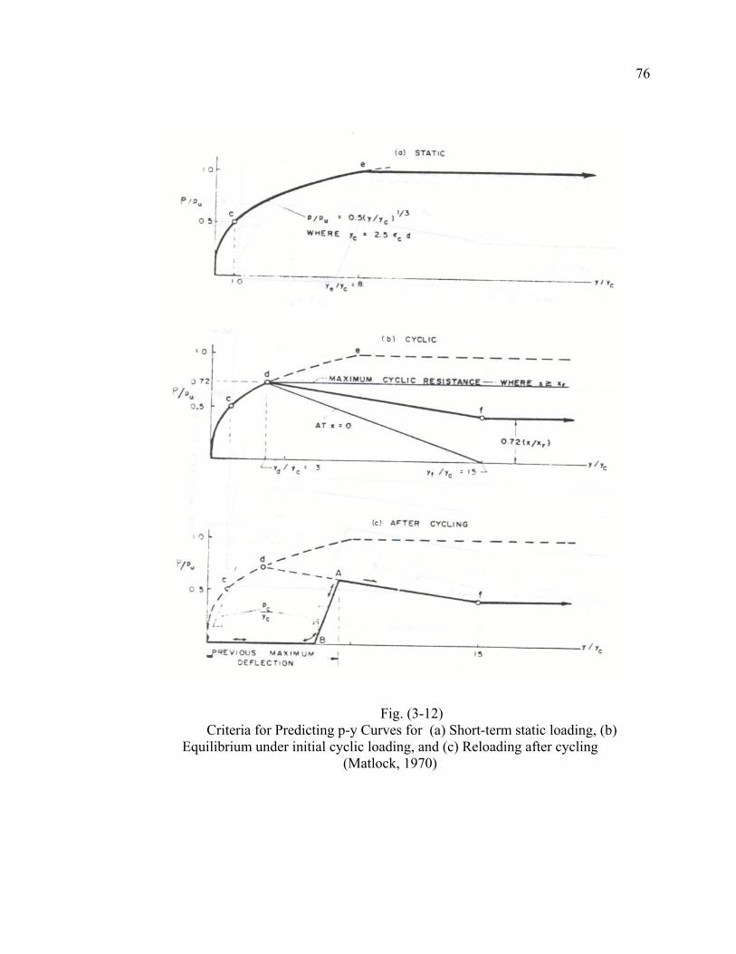
76
Fig. (3-12) Criteria for Predicting p-y Curves for (a) Short-term static loading, (b)
Equilibrium under initial cyclic loading, and (c) Reloading after cycling (Matlock, 1970)
77
An intermediate value of 0.010 is probably satisfactory for most purposes, according to
Skempton (Matlock, 1970). Using Skempton’s approach, the deflection sought is
approximately
dyc 505.2 ε= (3-20)
The modifications to the static p-y curve to express the possible deterioration due
to cycling are shown in Fig. (3-12b). According to the curve, substantial deflections are
possible, up to point d, without any deterioration in resistance as compared to the static
curve. At this point the resistance under cyclic loading has reached a maximum even at
greater depths. At shallow depths further reductions in resistance are provided which are
more severe with increasing and decreasing depth. Complete loss in resistance is assumed
to occur at the soil surface when deflections at that point reach cy15 . For deflections
greater than cy15 , the pseudo-plastic resistance is established by
ru xx
pp 72.0= (3-21)
The complete effect can be seen more readily from the family of cyclic p-y curves in Fig.
(3-26) (Matlock, 1970).
There are three aspects of the cyclic construction procedure, which are primarily
empirical, at least from a quantitative standpoint. These are (1) the position of the cyclic
deterioration threshold (point d) along the pre-plastic portion of the static p-y curve, (2)
the value of the deflection fy , and (3) the manner in which the final resistance fp is
78
adjusted with depth according to eqn. (3-21). The depth rx represents what is in reality a
rather indefinite point of transition from a condition of incomplete vertical restraint to
one where plastic flow is confined to horizontal planes. Furthermore, it is a quantity taken
from static-loading correlations. The use of rx in eqn. (3-21) is based primarily on
intuition and judgment, but is supported as being satisfactory by comparisons of
computed results versus experimental results (Matlock, 1970).
After any particular point, such as point A in fig. (3-12c), has been reached along
a p-y curve, rebound to zero resistance is assumed to occur along a line parallel to a
secant through point c. The resulting slack zone and reloading path are indicated in fig.
(3-12c). This construction is the basis for the p-y family in fig. (3-13). The deflection for
each depth must be known from a solution for the maximum loading condition in order to
establish the modified return branch for each curve (Matlock, 1970).
c. Step-by-Step Procedure
A step-by-step procedure for constructing p-y curves in soft clay is given below.
For short term, static loads:
1. Obtain the best possible estimate of the variation of shear strength and
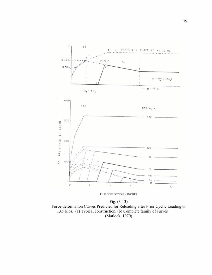
79
PILE DEFLECTION y, INCHES
Fig. (3-13) Force-deformation Curves Predicted for Reloading after Prior Cyclic Loading to
13.5 kips, (a) Typical construction, (b) Complete family of curves (Matlock, 1970)
80
effective unit weight with depth. Also obtain the value of 50ε , the strain
corresponding to one-half the maximum principle stress difference. If no
values of 50ε are available, typical values suggested by Skempton are
given in Table 4 or Table 5.
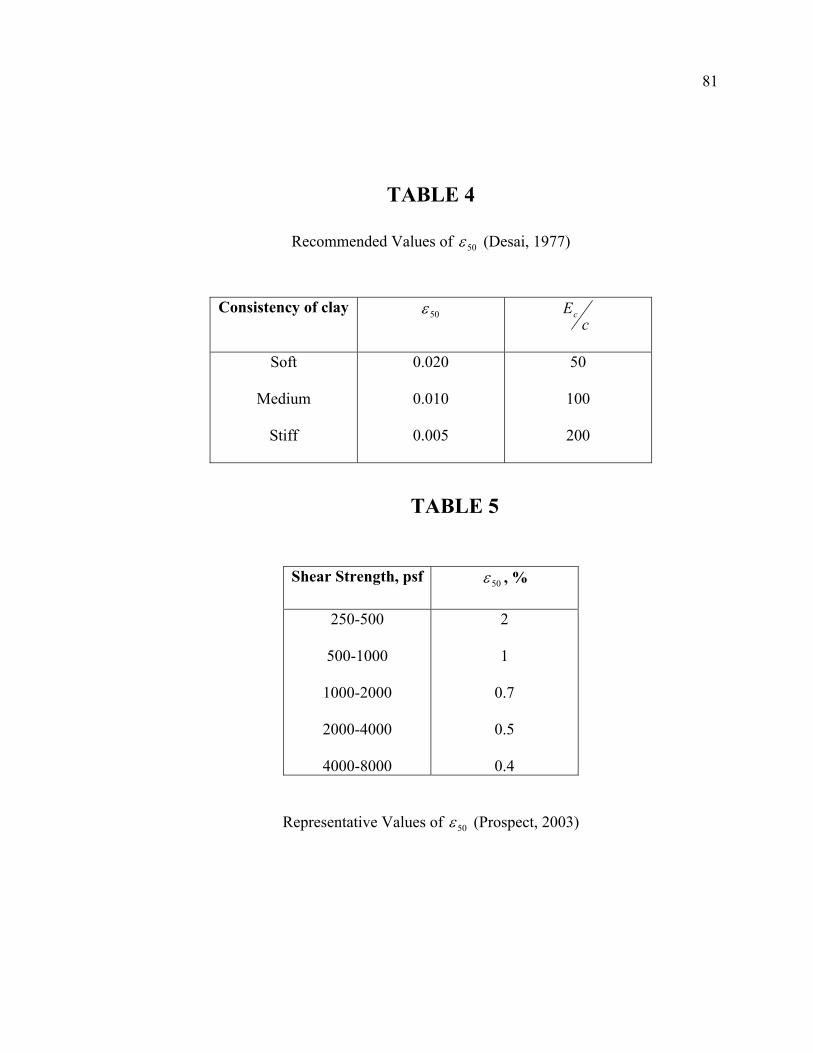
81
TABLE 4
Recommended Values of 50ε (Desai, 1977)
TABLE 5
Representative Values of 50ε (Prospect, 2003)
Consistency of clay 50ε c
Ec
Soft
Medium
Stiff
0.020
0.010
0.005
50
100
200
Shear Strength, psf 50ε , %
250-500
500-1000
1000-2000
2000-4000
4000-8000
2
1
0.7
0.5
0.4
82
2. Compute the ultimate soil resistance per unit length of shaft up , using the
smaller of the values given by:
cddxx
cpu
++= 5.03 γ (3-22)
and cdpu 9= (3-23) where =γ average effective unit weight from ground surface to p-y curve depth =x depth from ground surface to p-y curve =c shear strength at depth x =d width of pile 3. Compute the deflection 50y at one-half the ultimate soil resistance from dy 5050 5.2 ε= (3-24) 4. Points describing the p-y curve are now computed from
3
1
50
5.0
=
yy
pp
u
(3-25)
For cyclic loading:
1. Construct the p-y curve in the same manner as for short-term static loading
for values of p less than up72.0 .
2. Solve eqn. (3-22) and eqn. (3-23) simultaneously to find the depth rx
where the transition occurs. If the unit weight and shear strength are
83
constant in the upper zone, then
cd
cdxr 5.06+
=γ
(3-26)
3. If the depth to the p-y curve is greater than or equal to rx , p is equal to
up72.0 for all values of y greater than 503y .
4. If the depth to the p-y curve is less than rx , the value of p decreases from
up72.0 at 503yy = to the value given by the expression below at
5015yy = :
r
u xxpp 72.0= (3-21)
The value of p remains constant beyond 5015yy = .
d. Observations from Field Testing
Matlock developed these design criteria based on the results of the Sabine tests.
Matlock’s observations resulted in the following principle conclusions (Matlock, 1970):
1. The resistance-deflection (p-y) characteristics of the soil are highly non-
linear and inelastic.
2. Within practical ranges, the fundamental resistance-deflection
characteristics of the soil appear to be independent of the degree of pile-
head restraint.
3. A principle effect of cyclic loading appears to be the permanent physical
84
displacement of the soil away from the pile in the direction of loading. It is
not clear what contribution to this effect was provided by loss in strength
within the soil mass. Although no significant amount of mixing of water
and soil was directly evident, the cyclic shear reversals in the soil mass
may have caused some structural deterioration in the clay.
4. The permanent displacement of the soil created a slack zone in the
resistance-deflection characteristics. On reloading the pile with forces less
than previously attained maximum values, the slack-zone effect was
manifested by much greater bending moments than obtained with similar
loading during the initial cyclic series.
5. Although significant changes occurred with continued repetition of load
cycles, at any given magnitude of lateral load (except the highest) the
behavior of the pile-soil system tended to stabilize. Such equilibrium
response was usually attained to a practical degree in less than 100 cycles.
It was demonstrated at Lake Austin and confirmed at Sabine Pass that a period of
rest does not provide any restoration of soil resistance at the top of the pile. Subsequent
deposition of clay or clay slurry in the cavity is not followed by any significant gain in
strength because of the absence of sustained consolidating forces. Only by maintaining
granular material in the cavity was the resistance improved or restored (Matlock, 1970).
4. P-Y Curves in Stiff Clay
Experiments were conducted by Lymon C. Reese and aimed at developing criteria
85
for predicting the behavior of stiff clay around a deep foundation subjected to lateral
loads. Similar to the research conducted by Matlock, the basic concern was in short-term
static and cyclic loadings. The experiments involved the loading in the field of a deep
foundation that is instrumented so that bending moments can be measured along the
length of the foundation (Reese, 1975).
The deep foundation that was tested was a drilled shaft, constructed by drilling an
open hole with a diameter of 30 inches, to a depth of 42 feet below the surface. An
instrumented column and a reinforcing steel cage were placed in the hole and the hole
was then filled with a tremie-placed concrete. Using a short cylindrical form, the shaft
was extended 2 feet above the ground surface, for a total length of 44 feet (Reese, 1975).
The instrumented column was a steel pipe with a wall thickness of ¼ inches, and
an outside diameter of 10-¾ inches. The wall thickness was selected such that the flexural
stiffness of the instrumented column was about equal to the flexural stiffness of the
concrete it replaced (Reese, 1975).
To install strain gages for measuring the bending moments in the drilled shaft,
the pipe for the instrumented column was split longitudinally, and two strain gages, with
their axes parallel to the axis of the pipe, were mounted on each half of the pipe at each
gage level. At each level, four gages were connected in a bridge circuit to give the
maximum sensitivity to the bending. The strain gages were spaced at 15-inch intervals for
the top 2/3 of the shaft and at 30-inch intervals in the bottom 1/3 (Reese, 1975).
The soil profile at the site consisted of 28 feet of stiff to very stiff red clay, 2 feet
86
of interspersed silt and clay layers, and very stiff tan silty clay to a depth of 42 feet. The
water table was at a depth of 18 feet at the time of the field test (Reese, 1975).
Unconsolidated-undrained triaxial compression tests were performed on
undisturbed samples taken at the test site, with the confining pressures made equal to the
effective overburden pressure. The shear strength in the upper 20 feet, the zone of most
importance in lateral behavior, varied widely, due in part to the slickenside structure of
the sample. But, according to Reese, there was no discernable pattern of strength
variation with depth. The average undrained shear strength in the upper 20 feet was 1.1
tsf. A secant modulus intersecting the stress-strain curve at ½ the maximum principle
stress difference was used to describe the stiffness of the soil, cE . The overall pattern
shows a decreasing soil stiffness with depth (Reese, 1975).
To define the stress-strain relationship in nondimensional terms, the applied
principle stress difference was divided by the maximum principle stress difference, and
the strain was divided by the strain at ½ the maximum, 50ε . The values of ( )
( )max31
31
σσσσ
−−
and 50εε were determined for all tests. These values were plotted, and the equation of the
curve was found to be
( )
( )2
1
50max31
31 5.0
=
−−
εε
σσσσ
(3-27)
The average value of 50ε was 0.005 inin (Reese, 1975).
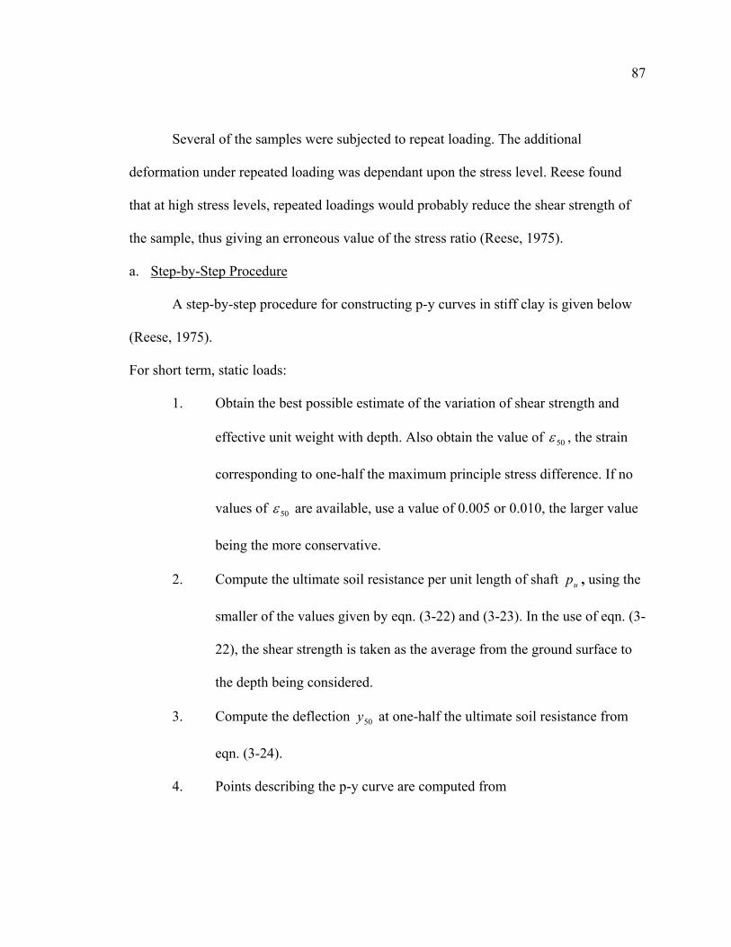
87
Several of the samples were subjected to repeat loading. The additional
deformation under repeated loading was dependant upon the stress level. Reese found
that at high stress levels, repeated loadings would probably reduce the shear strength of
the sample, thus giving an erroneous value of the stress ratio (Reese, 1975).
a. Step-by-Step Procedure
A step-by-step procedure for constructing p-y curves in stiff clay is given below
(Reese, 1975).
For short term, static loads:
1. Obtain the best possible estimate of the variation of shear strength and
effective unit weight with depth. Also obtain the value of 50ε , the strain
corresponding to one-half the maximum principle stress difference. If no
values of 50ε are available, use a value of 0.005 or 0.010, the larger value
being the more conservative.
2. Compute the ultimate soil resistance per unit length of shaft up , using the
smaller of the values given by eqn. (3-22) and (3-23). In the use of eqn. (3-
22), the shear strength is taken as the average from the ground surface to
the depth being considered.
3. Compute the deflection 50y at one-half the ultimate soil resistance from
eqn. (3-24).
4. Points describing the p-y curve are computed from
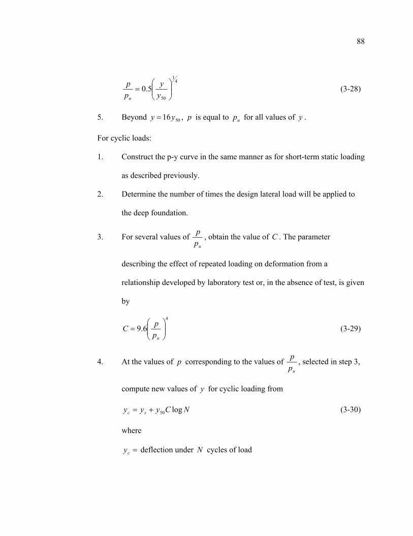
88
4
1
50
5.0
=
yy
pp
u
(3-28)
5. Beyond 5016yy = , p is equal to up for all values of y .
For cyclic loads:
1. Construct the p-y curve in the same manner as for short-term static loading
as described previously.
2. Determine the number of times the design lateral load will be applied to
the deep foundation.
3. For several values of upp , obtain the value of C . The parameter
describing the effect of repeated loading on deformation from a
relationship developed by laboratory test or, in the absence of test, is given
by
4
6.9
=
uppC (3-29)
4. At the values of p corresponding to the values of upp , selected in step 3,
compute new values of y for cyclic loading from
NCyyy sc log50+= (3-30)
where
=cy deflection under N cycles of load
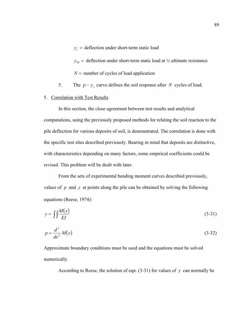
89
=sy deflection under short-term static load
=50y deflection under short-term static load at ½ ultimate resistance
=N number of cycles of load application
5. The cyp − curve defines the soil response after N cycles of load.
5. Correlation with Test Results
In this section, the close agreement between test results and analytical
computations, using the previously proposed methods for relating the soil reaction to the
pile deflection for various deposits of soil, is demonstrated. The correlation is done with
the specific test sites described previously. Bearing in mind that deposits are distinctive,
with characteristics depending on many factors, some empirical coefficients could be
revised. This problem will be dealt with later.
From the sets of experimental bending moment curves described previously,
values of p and y at points along the pile can be obtained by solving the following
equations (Reese, 1974):
( )∫ ∫=
EIxMy (3-31)
( )xMdxdp 2
2
= (3-32)
Approximate boundary conditions must be used and the equations must be solved
numerically.
According to Reese, the solution of eqn. (3-31) for values of y can normally be
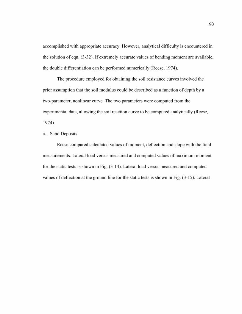
90
accomplished with appropriate accuracy. However, analytical difficulty is encountered in
the solution of eqn. (3-32). If extremely accurate values of bending moment are available,
the double differentiation can be performed numerically (Reese, 1974).
The procedure employed for obtaining the soil resistance curves involved the
prior assumption that the soil modulus could be described as a function of depth by a
two-parameter, nonlinear curve. The two parameters were computed from the
experimental data, allowing the soil reaction curve to be computed analytically (Reese,
1974).
a. Sand Deposits
Reese compared calculated values of moment, deflection and slope with the field
measurements. Lateral load versus measured and computed values of maximum moment
for the static tests is shown in Fig. (3-14). Lateral load versus measured and computed
values of deflection at the ground line for the static tests is shown in Fig. (3-15). Lateral
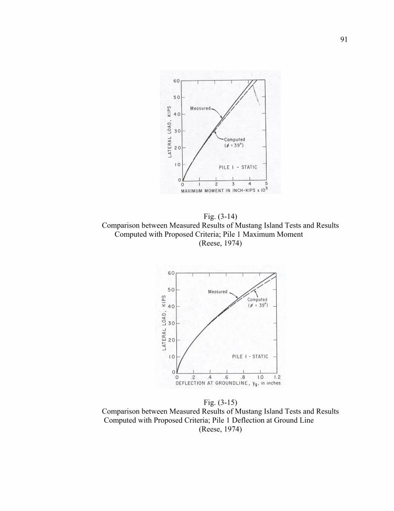
91
Fig. (3-14)
Comparison between Measured Results of Mustang Island Tests and Results Computed with Proposed Criteria; Pile 1 Maximum Moment
(Reese, 1974)
Fig. (3-15) Comparison between Measured Results of Mustang Island Tests and Results Computed with Proposed Criteria; Pile 1 Deflection at Ground Line
(Reese, 1974)
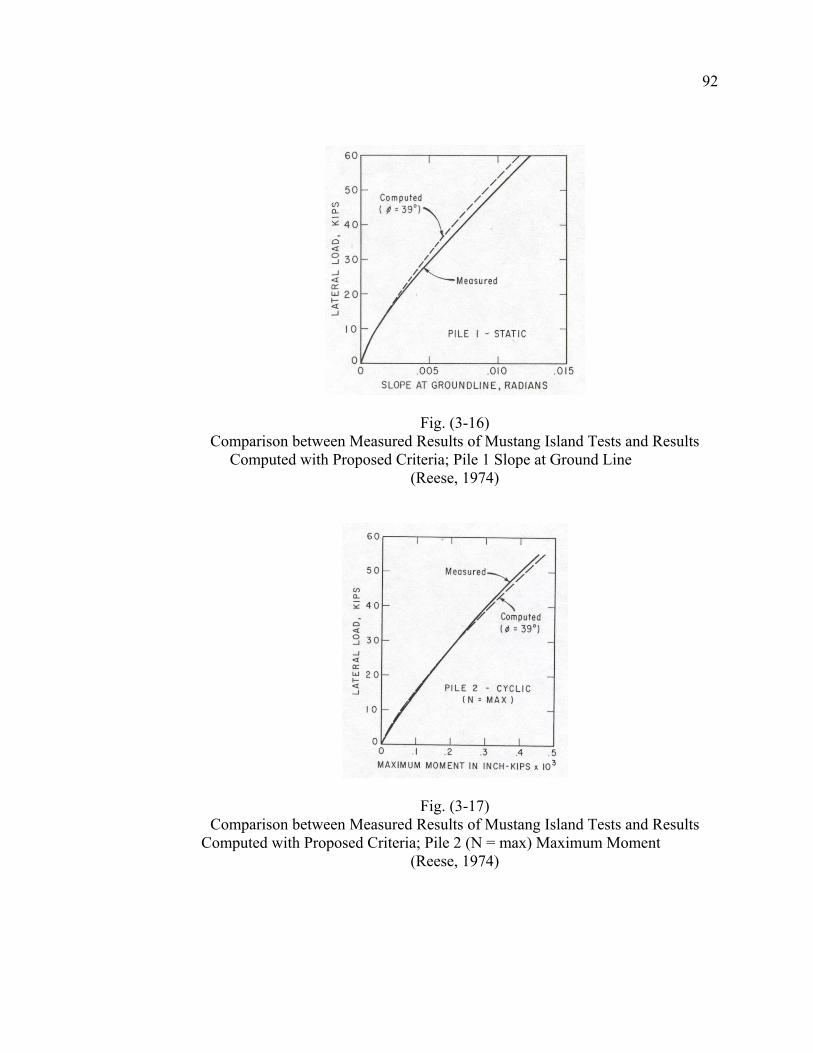
92
Fig. (3-16) Comparison between Measured Results of Mustang Island Tests and Results
Computed with Proposed Criteria; Pile 1 Slope at Ground Line (Reese, 1974)
Fig. (3-17) Comparison between Measured Results of Mustang Island Tests and Results
Computed with Proposed Criteria; Pile 2 (N = max) Maximum Moment (Reese, 1974)
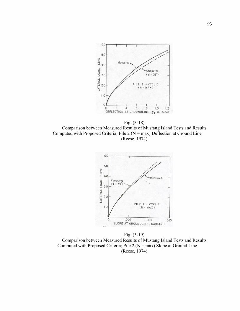
93
Fig. (3-18) Comparison between Measured Results of Mustang Island Tests and Results
Computed with Proposed Criteria; Pile 2 (N = max) Deflection at Ground Line (Reese, 1974)
Fig. (3-19) Comparison between Measured Results of Mustang Island Tests and Results
Computed with Proposed Criteria; Pile 2 (N = max) Slope at Ground Line (Reese, 1974)
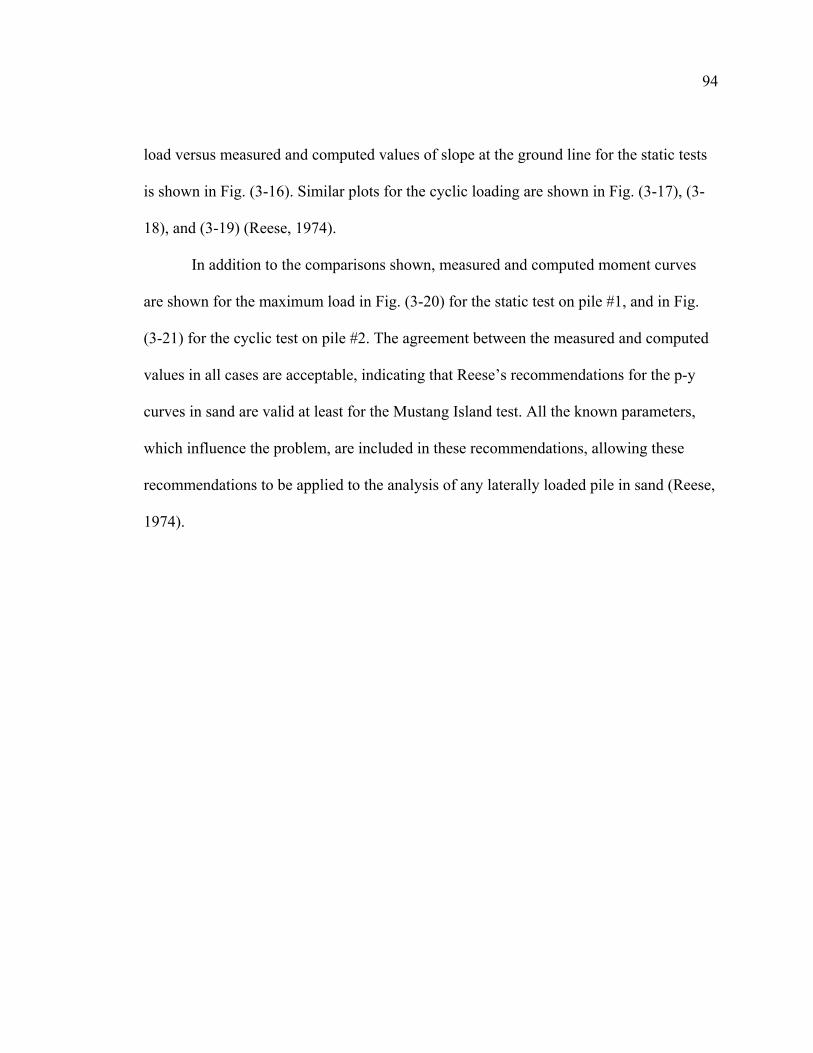
94
load versus measured and computed values of slope at the ground line for the static tests
is shown in Fig. (3-16). Similar plots for the cyclic loading are shown in Fig. (3-17), (3-
18), and (3-19) (Reese, 1974).
In addition to the comparisons shown, measured and computed moment curves
are shown for the maximum load in Fig. (3-20) for the static test on pile #1, and in Fig.
(3-21) for the cyclic test on pile #2. The agreement between the measured and computed
values in all cases are acceptable, indicating that Reese’s recommendations for the p-y
curves in sand are valid at least for the Mustang Island test. All the known parameters,
which influence the problem, are included in these recommendations, allowing these
recommendations to be applied to the analysis of any laterally loaded pile in sand (Reese,
1974).
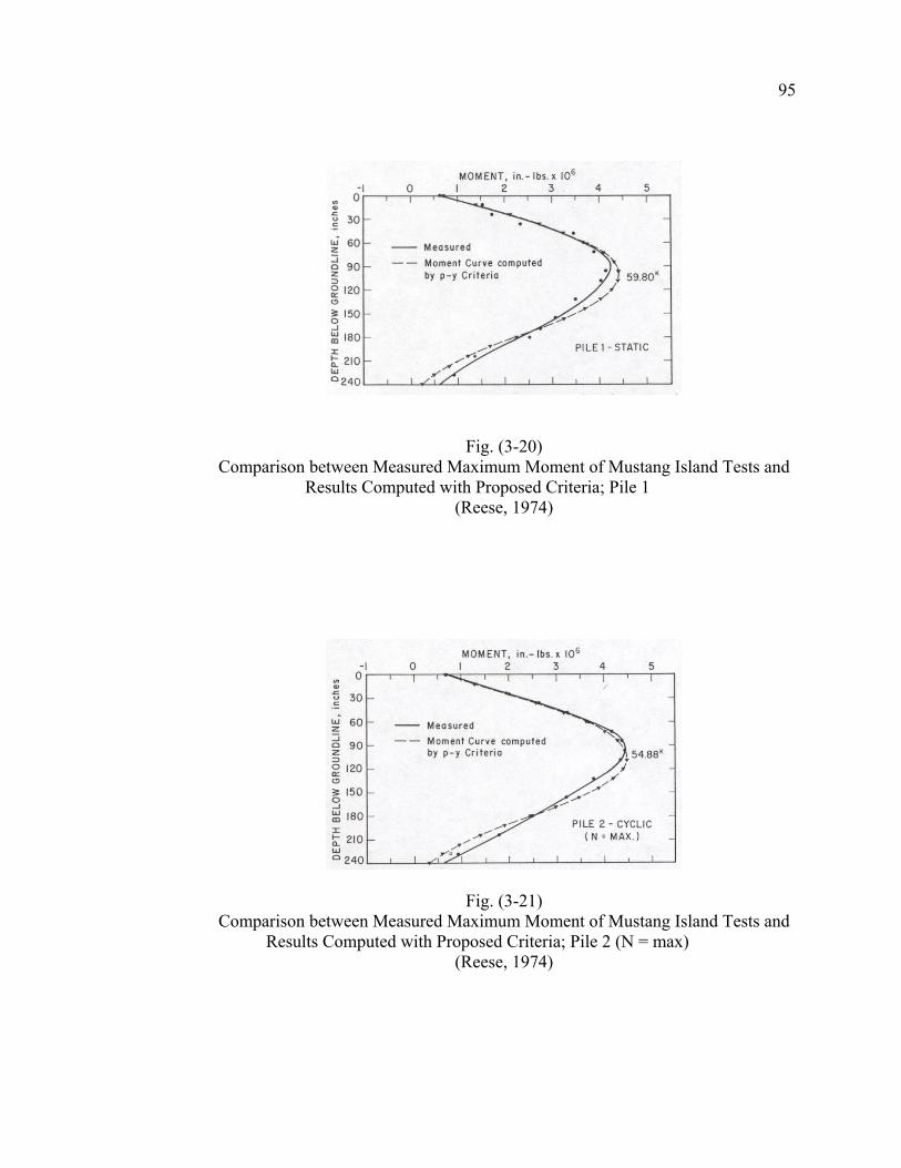
95
Fig. (3-20)
Comparison between Measured Maximum Moment of Mustang Island Tests and Results Computed with Proposed Criteria; Pile 1
(Reese, 1974)
Fig. (3-21) Comparison between Measured Maximum Moment of Mustang Island Tests and
Results Computed with Proposed Criteria; Pile 2 (N = max) (Reese, 1974)
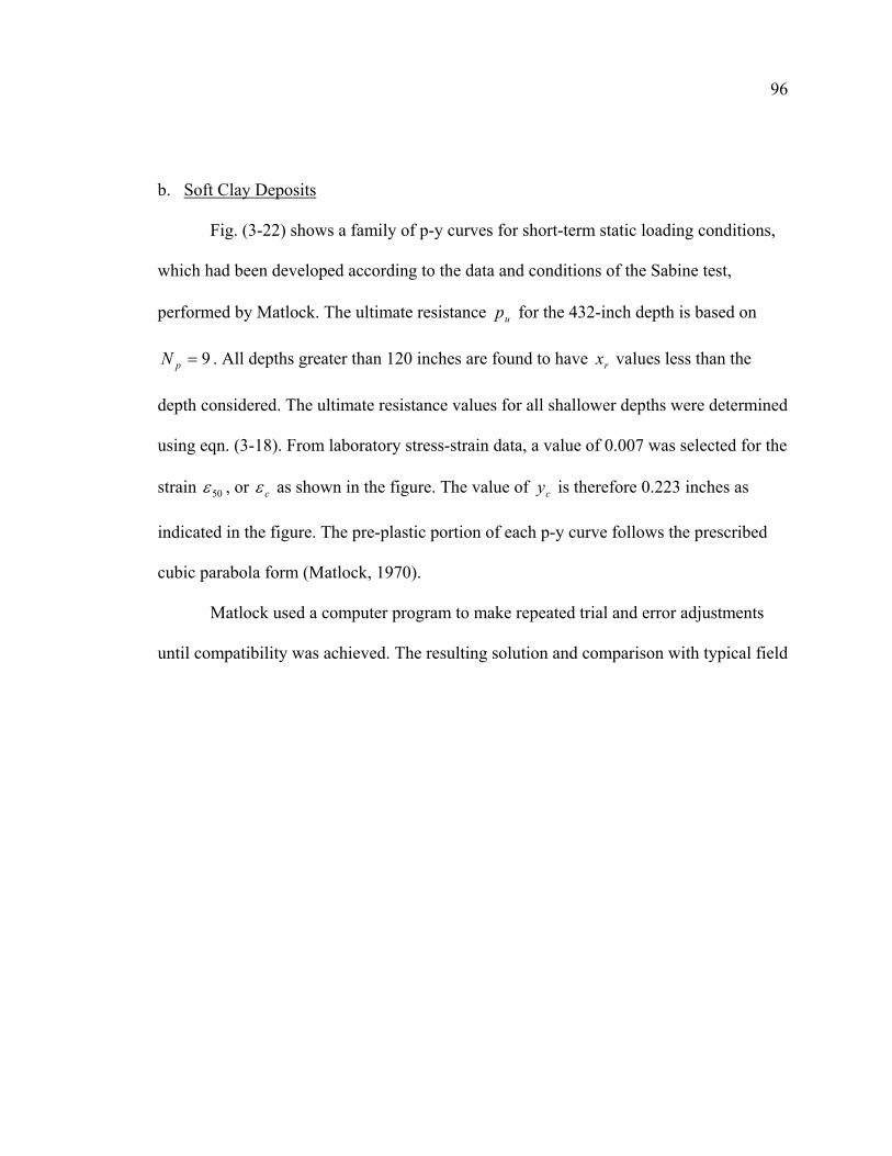
96
b. Soft Clay Deposits
Fig. (3-22) shows a family of p-y curves for short-term static loading conditions,
which had been developed according to the data and conditions of the Sabine test,
performed by Matlock. The ultimate resistance up for the 432-inch depth is based on
9=pN . All depths greater than 120 inches are found to have rx values less than the
depth considered. The ultimate resistance values for all shallower depths were determined
using eqn. (3-18). From laboratory stress-strain data, a value of 0.007 was selected for the
strain 50ε , or cε as shown in the figure. The value of cy is therefore 0.223 inches as
indicated in the figure. The pre-plastic portion of each p-y curve follows the prescribed
cubic parabola form (Matlock, 1970).
Matlock used a computer program to make repeated trial and error adjustments
until compatibility was achieved. The resulting solution and comparison with typical field
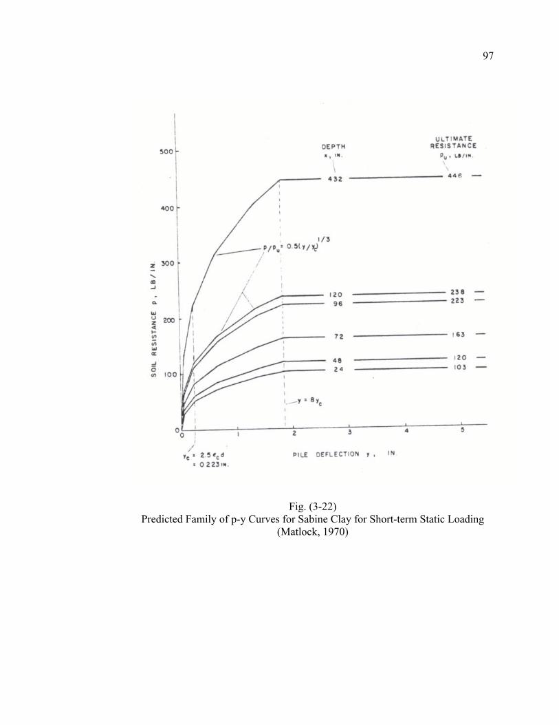
97
Fig. (3-22) Predicted Family of p-y Curves for Sabine Clay for Short-term Static Loading
(Matlock, 1970)
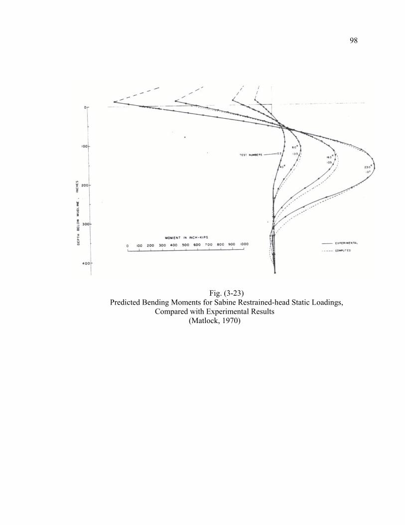
98
Fig. (3-23) Predicted Bending Moments for Sabine Restrained-head Static Loadings,
Compared with Experimental Results (Matlock, 1970)
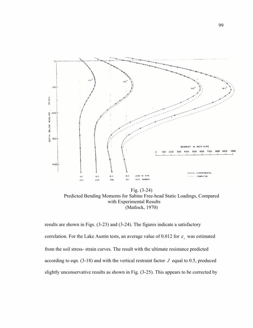
99
Fig. (3-24) Predicted Bending Moments for Sabine Free-head Static Loadings, Compared
with Experimental Results (Matlock, 1970)
results are shown in Figs. (3-23) and (3-24). The figures indicate a satisfactory
correlation. For the Lake Austin tests, an average value of 0.012 for cε was estimated
from the soil stress- strain curves. The result with the ultimate resistance predicted
according to eqn. (3-18) and with the vertical restraint factor J equal to 0.5, produced
slightly unconservative results as shown in Fig. (3-25). This appears to be corrected by
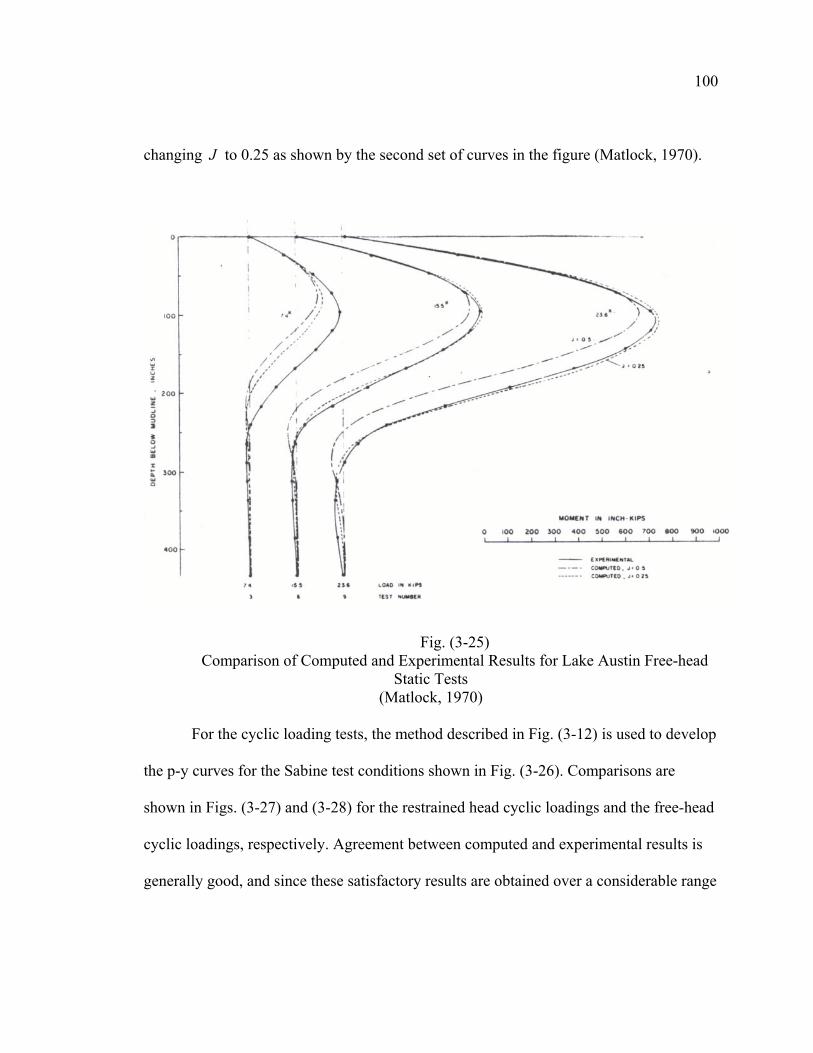
100
changing J to 0.25 as shown by the second set of curves in the figure (Matlock, 1970).
Fig. (3-25) Comparison of Computed and Experimental Results for Lake Austin Free-head
Static Tests (Matlock, 1970)
For the cyclic loading tests, the method described in Fig. (3-12) is used to develop
the p-y curves for the Sabine test conditions shown in Fig. (3-26). Comparisons are
shown in Figs. (3-27) and (3-28) for the restrained head cyclic loadings and the free-head
cyclic loadings, respectively. Agreement between computed and experimental results is
generally good, and since these satisfactory results are obtained over a considerable range
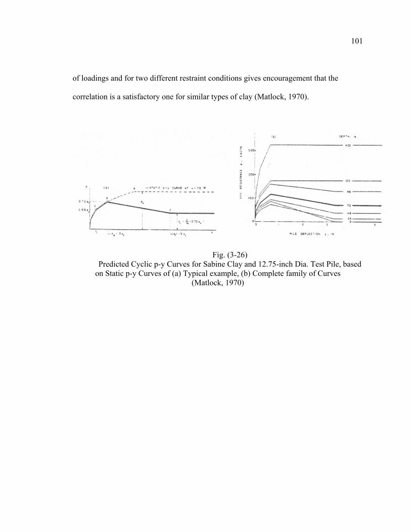
101
of loadings and for two different restraint conditions gives encouragement that the
correlation is a satisfactory one for similar types of clay (Matlock, 1970).
Fig. (3-26) Predicted Cyclic p-y Curves for Sabine Clay and 12.75-inch Dia. Test Pile, based
on Static p-y Curves of (a) Typical example, (b) Complete family of Curves (Matlock, 1970)
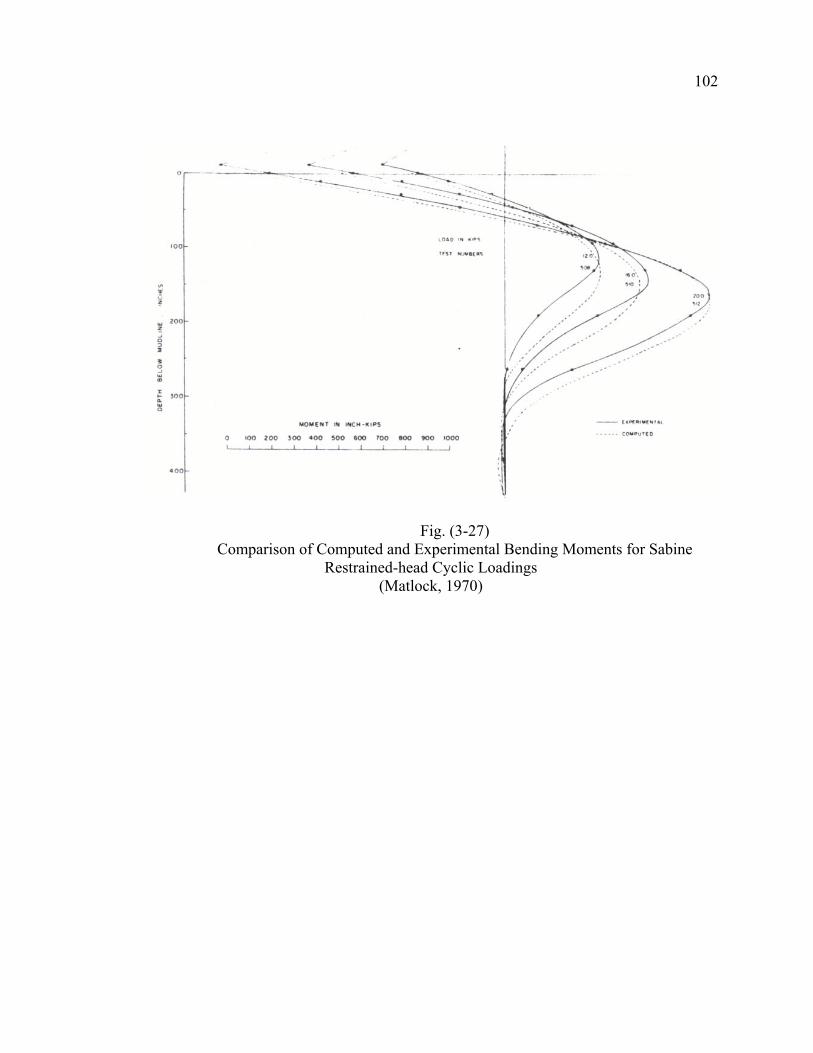
102
Fig. (3-27) Comparison of Computed and Experimental Bending Moments for Sabine
Restrained-head Cyclic Loadings (Matlock, 1970)
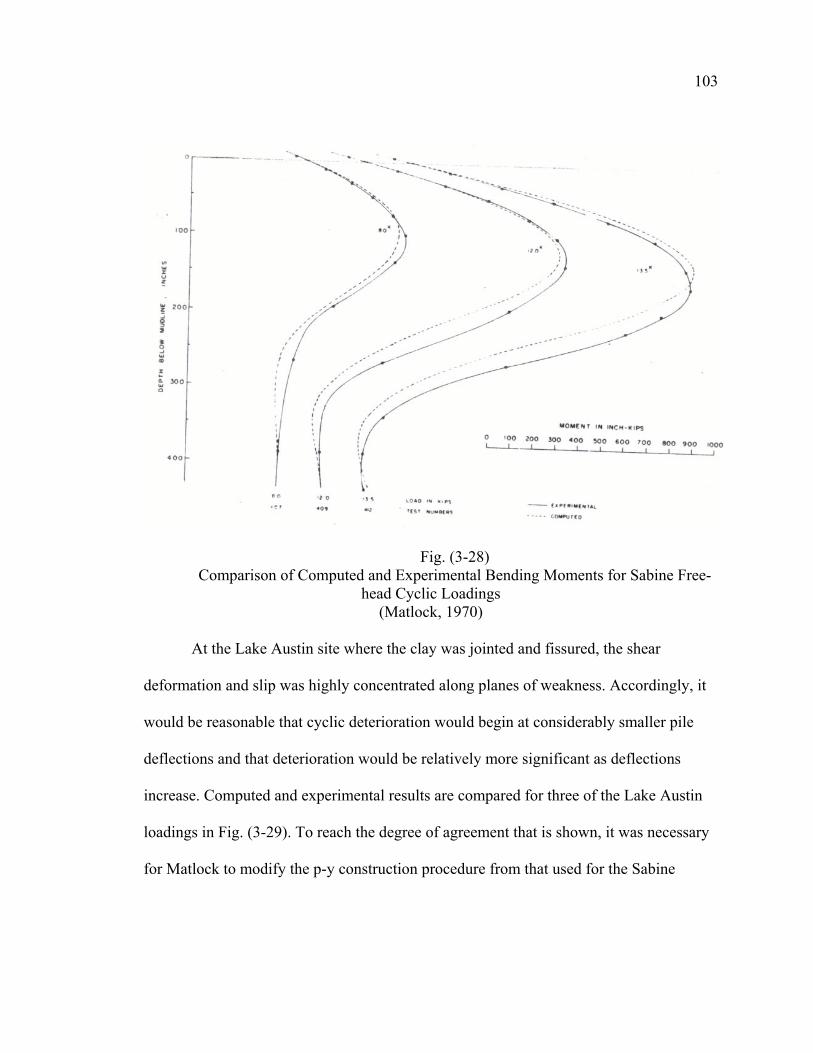
103
Fig. (3-28) Comparison of Computed and Experimental Bending Moments for Sabine Free-
head Cyclic Loadings (Matlock, 1970)
At the Lake Austin site where the clay was jointed and fissured, the shear
deformation and slip was highly concentrated along planes of weakness. Accordingly, it
would be reasonable that cyclic deterioration would begin at considerably smaller pile
deflections and that deterioration would be relatively more significant as deflections
increase. Computed and experimental results are compared for three of the Lake Austin
loadings in Fig. (3-29). To reach the degree of agreement that is shown, it was necessary
for Matlock to modify the p-y construction procedure from that used for the Sabine
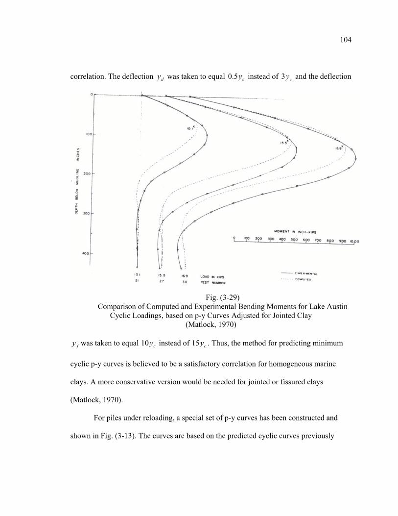
104
correlation. The deflection dy was taken to equal cy5.0 instead of cy3 and the deflection
Fig. (3-29) Comparison of Computed and Experimental Bending Moments for Lake Austin
Cyclic Loadings, based on p-y Curves Adjusted for Jointed Clay (Matlock, 1970)
fy was taken to equal cy10 instead of cy15 . Thus, the method for predicting minimum
cyclic p-y curves is believed to be a satisfactory correlation for homogeneous marine
clays. A more conservative version would be needed for jointed or fissured clays
(Matlock, 1970).
For piles under reloading, a special set of p-y curves has been constructed and
shown in Fig. (3-13). The curves are based on the predicted cyclic curves previously
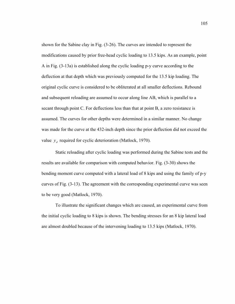
105
shown for the Sabine clay in Fig. (3-26). The curves are intended to represent the
modifications caused by prior free-head cyclic loading to 13.5 kips. As an example, point
A in Fig. (3-13a) is established along the cyclic loading p-y curve according to the
deflection at that depth which was previously computed for the 13.5 kip loading. The
original cyclic curve is considered to be obliterated at all smaller deflections. Rebound
and subsequent reloading are assumed to occur along line AB, which is parallel to a
secant through point C. For deflections less than that at point B, a zero resistance is
assumed. The curves for other depths were determined in a similar manner. No change
was made for the curve at the 432-inch depth since the prior deflection did not exceed the
value dy required for cyclic deterioration (Matlock, 1970).
Static reloading after cyclic loading was performed during the Sabine tests and the
results are available for comparison with computed behavior. Fig. (3-30) shows the
bending moment curve computed with a lateral load of 8 kips and using the family of p-y
curves of Fig. (3-13). The agreement with the corresponding experimental curve was seen
to be very good (Matlock, 1970).
To illustrate the significant changes which are caused, an experimental curve from
the initial cyclic loading to 8 kips is shown. The bending stresses for an 8 kip lateral load
are almost doubled because of the intervening loading to 13.5 kips (Matlock, 1970).
106
Fig. (3-30) Comparison Between Experimental and Computed Results for Reloading to 8
kips After Prior Cycling with a 13.5-kip Lateral Load (Matlock, 1970)
c. Stiff Clay Deposits
The proposed predictions for the p-y curve for stiff clay is based on a small
amount of experimental data; therefore, the method should be used with great care until
additional data allows the method to be validated.
Correlation between computed and measured values of deflection and moment,
for the lateral loading test of the drilled shaft mentioned previously, was good. Table 6
and Fig. (3-31) show the comparison.
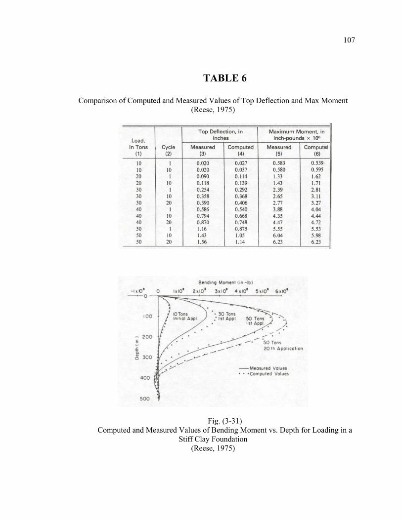
107
TABLE 6
Comparison of Computed and Measured Values of Top Deflection and Max Moment (Reese, 1975)
Fig. (3-31) Computed and Measured Values of Bending Moment vs. Depth for Loading in a
Stiff Clay Foundation (Reese, 1975)
108
IV. DETERMINATION OF SOIL MODULUS
The determination of the soil modulus with sufficient accuracy helps in reaching a
realistic result for the problem of laterally loaded piles. The soil modulus has been the
subject of many researches and many recommendations have been presented.
The determination of the soil modulus, also known as the modulus of elasticity of
the soil or modulus of subgrade (soil) reaction, is generally carried out by either direct
means or indirect means. One direct mean would consist of having a full-scale lateral
load test on a pile. This is the most direct mean but it is the most time consuming and
expensive. It would only be feasible for large-scale projects.
Other direct means would be the results of in-situ tests such as a plate-loading test
or a pressuremeter test. Recent advances have been made in the determination of the soil
modulus by using an in-situ testing instrument known as a flat dilatometer. Each of these
in-situ tests is relatively inexpensive.
Indirect means to determine the soil modulus would include empirical correlation
with other soil properties, mainly the stress-strain relationship, which is most relevant.
Terzaghi, in 1955, considered that for clays, the coefficient of subgrade reaction is
essentially the same both horizontally and vertically, and is independent of depth. He
suggested the following conservative relationship for the coefficient of subgrade reaction,
hk for laterally loaded foundations:
109
( )15.11
sh kd
k
= (4-1)
where
=1sk constant of vertical subgrade reaction for a square plate, 1 ft. wide
=d width or diameter of the load area in feet
Table 7 shows Terzaghi’s values of 1sk . Adaptation of the coefficient of subgrade
reaction to fit the soil modulus, sE , leads to
dkE hs = (4-2)
sE is by definition the ratio between the pressure at any point of the surface of contact
and the pile deflection produced by the load application at that point,
yEp s−= (4-3)
The value of sE would be constant only if the soil were a perfectly elastic material.
However, it is known that sE generally increases with depth, and at a given depth it
becomes smaller as the deflection increases.
Terzaghi also showed that for a cohesionless soil, the modulus of subgrade
reaction would increase approximately linearly with depth and decrease linearly with the
width d of the load area, as expressed in Eqn. (2-36).
Broms related hk for clays to the secant modulus 50E at half the ultimate stress in
an unconsolidated-undrained test as
110
dE
kh5067.1= (4-4)
Calculation of the modulus of subgrade reaction by these methods is only
approximate and can be used only as an estimate. However, if it is required to determine
the lateral deflection accurately, a field test should be performed.
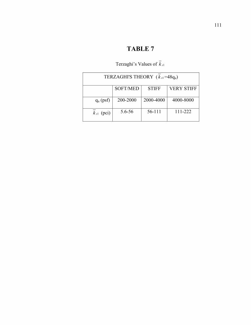
111
TABLE 7
Terzaghi’s Values of 1sk
TERZAGHI'S THEORY ( 1sk =48qu)
SOFT/MED STIFF VERY STIFF
qu (psf) 200-2000 2000-4000 4000-8000
1sk (pci) 5.6-56 56-111 111-222
112
V. COMPARISON OF THE VARIABLES OF LATERALLY LOADED FOUNDATIONS
The problem of the laterally loaded foundation involves many variables. These
variables include but are certainly not limited to the unit weight of the soil, the internal
angle of friction of the soil, the soil modulus, the diameter of the pile, the length of the
pile, and of course the load itself. Although it is well known that many of these properties
are not independent of each other, in order to study the effect of altering each variable,
the variables must be treated as independent parameters. Due to the complex nature of the
laterally loaded foundation, a computer program such as FB-Pier or L-Pile can be used to
aid in the effort.
The appendix of this thesis presents the results of several scenarios in which one
of the variables is allowed to vary, while the others remain constant. The computer
program FB-Pier is used for these analyses. The first analysis presents the alteration of
the p-y curve in sand as each parameter is varied. The next analysis presents an example
problem in which a pile is laterally loaded in a uniform sand foundation and as each
parameter is allowed to vary, the effects on the pile deflection and bending moment are
observed. Finally, an example problem is presented in which a pile is laterally loaded in a
soft clay foundation and as each parameter is allowed to vary, the effects on the pile
deflection and bending moment are observed.
From the analysis of the impacts of the variables on the p-y curve in sand, several
113
conclusions can be made. By allowing the pile diameter only to vary, it is evident that the
initial portion of the p-y curve is independent of the pile diameter. Also evident is that the
nonlinear portion of the p-y curve will have a larger soil resistance when the pile
diameter increases at a shallow depth. But at a certain greater depth, the nonlinear portion
of the p-y curve will decrease in soil resistance as pile diameter increases. Allowing the
soil modulus only to vary, it is apparent that this variable has little effect on Reese’s Sand
Model.
The next analysis compares the pile deflection and bending moment of the pile
while varying each parameter independently. The scenario included a single free-headed
pile of 0.5m diameter subjected to a lateral load at the ground surface. The pile was
driven in uniform sand with the ground water located at the ground surface. The soil
parameters, internal angle of friction, unit weight, and subgrade modulus, were each
varied independently, while the other parameters remained constant. Reese’s Sand Model
was used in this analysis.
From the analysis, it is apparent that varying the subgrade modulus alone causes
only minor, if any, changes in the pile deflection and bending moment of the pile. Also,
changing the unit weight of the sand does not appear to have a significant effect on the
results. The internal angle of friction of the sand proves to have a significant influence on
the pile deflection and the bending moment of the pile.
It is known that these soil parameters are not independent of each other.
Therefore, an analysis was made comparing the effects of a pile driven in loose sand, and
114
medium sand, and dense sand. The parameters of these materials were assumed based on
values accepted in literature. It can be seen from this analysis, and in comparison with the
previous analyses where the parameters were allowed to vary independently, that the
effects of each parameter is uncertain when considered alone, and that these parameters
are correlated with each other. It is evident that the pile deflection and the bending
moment of the pile is interdependent on each of these soil properties.
The final analysis shown in the appendix of this thesis makes use of Matlock’s
Soft Clay Below the Water Table Model. This analysis is similar in that it also compares
the pile deflection and bending moment of the pile while varying each parameter
independently. The scenario included a single free-headed pile of 12in diameter subjected
to a lateral load at the ground surface. The pile was driven in a soft clay foundation with
the ground water located at the ground surface. The soil and pile parameters, shear
strength, soil strain, pile diameter, and pile length, were each varied independently, while
the other parameters remained constant. The final comparison shows the load condition
varying, from a static load to a cyclic load.
From the analyses in which the pile properties are allowed to vary, it is evident
that the pile length had very little effect on the pile deflection and the moment
distribution. It can be seen that any part of the pile below a depth of 30ft is not
contributing to the moment capacity. In contrast, the pile diameter is shown to have a
great influence on the pile deflection and the moment distribution. It is seen that as the
diameter increases, the deflection decreases and the moment distribution increases. This
115
is attributed to an increase in pile stiffness and also an increase in the area of resisting
soil.
From the analysis allowing the shear strength to vary alone, it is evident that the
shear strength has a great influence on the deflection. As the shear strength increases,
deflection decreases. This is because as the soil gets stronger, its resistance to movement
increases. Also note that the pile has some deflection all the way down to approx. 30 ft of
the total 42 ft long pile for all shear strength values. This is because the depth of
deflection is more dependent on pile diameter than shear strength. It can also be seen that
as the shear strength increases, the maximum moment decreases and moves closer to the
surface. The moment increases as the shear strength decreases because the pile is forced
to take on more of the moment, as the soil gets weaker.
In the analysis in which the soil strain is allowed to vary independently, it is
apparent that as the ε50 value increases, the deflection increases. This is because the ε50 is
the strain at the midway point of the initial portion of the p-y curve; therefore as this
value increases, the more deflection the pile will experience for a given load. Also
evident is that as the ε50 value increases, the maximum moment, and the depth at which it
occurs, will also increase. This is because the moment arm will increase as the strain in
the soil increases because of the greater displacement in the weaker soil.
It the final comparison in which the load condition is varied, it is evident that the
deflection for the cyclic loading case is about two times that of the static loading case.
This is because of a gap produced during the cycled load. Due to the nature of Matlock’s
116
soft clay model, the clay tends to stay in a deformed shape as the pile is cycled in the
other direction. Therefore as the pile completes one cycle it will have to move through
the gap before it is pushed against the clay again, causing the pile to gradually push the
clay out of the way and allow the pile to deflect more. It is also evident that the moment
produced during the cycled load is approximately twice as much as the moment produced
during the static loading. This is because the moment arm in the cycled case is larger than
the static case due to the gap created.
117
VI. COMPARISON BETWEEN P-Y CURVES AND BROMS’ APPROACH
Many different methods of analysis have been proposed to solve the problem of a
laterally loaded pile (or drilled shaft), where the problem can be generally defined as
computing pile deflections and bending moments as a function of depth below the ground
surface. Some methods are based on the theory of subgrade reaction and on simplifying
assumptions such as assuming a variation of the subgrade modulus with depth and that
soil is linearly elastic (Broms, 1964). These assumptions reduce the difficulty in
obtaining a solution to the problem, but according to Reese (1979), errors of an unknown
magnitude are introduced into the solution. A comparison is made here between the
results presented earlier in the p-y curve chapter, where actual measured responses of
tested piles are compared to those calculated using nonlinear variations, and those
yielding from the use of Broms’ assumptions.
Reese (1974) presented the results of a series of field tests that were conducted to
develop criteria for the design of laterally loaded piles in sand. Two 24-inch diameter
piles with 3/8 inch wall thickness and of A-53 grade B seamless steel, embedded 69 feet,
were instrumented with strain gages for measuring bending moments and deflection at
Mustang Island, Texas, and a complete description of it was presented by Cox and Reese
(1974).
118
Laboratory tests were run on samples from two borings, and soil properties
determined from these tests included grain size distribution, natural densities, and
minimum and maximum densities. The soil was classified as medium dense sand in the
top 20-foot layer, to dense sand in the rest of the formations, with an angle of internal
friction, °= 39φ and a submerged unit weight of 366 ftlbs=γ . The results for the
ground line deflection are shown in Fig. (3-15) and Fig. (3-18), and compared to those
computed with the proposed criteria of the p-y curve.
Table 2 gives the recommended value hk for dense sand as 3125 inlbs . Using this
value of hk in Eqn. (2-30a), and varying H from 10 kips to 60 kips, the comparison
could be made between the p-y approach and Broms’ approach. Table 8 shows this
comparison. As can be seen from this table, Broms’ approach gives close results for the
elastic range loads. As we move to the inelastic range, errors would exceed 50%.
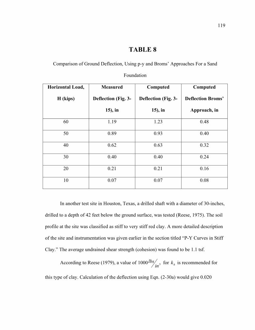
119
TABLE 8
Comparison of Ground Deflection, Using p-y and Broms’ Approaches For a Sand
Foundation
Horizontal Load,
H (kips)
Measured
Deflection (Fig. 3-
15), in
Computed
Deflection (Fig. 3-
15), in
Computed
Deflection Broms’
Approach, in
60 1.19 1.23 0.48
50 0.89 0.93 0.40
40 0.62 0.63 0.32
30 0.40 0.40 0.24
20 0.21 0.21 0.16
10 0.07 0.07 0.08
In another test site in Houston, Texas, a drilled shaft with a diameter of 30-inches,
drilled to a depth of 42 feet below the ground surface, was tested (Reese, 1975). The soil
profile at the site was classified as stiff to very stiff red clay. A more detailed description
of the site and instrumentation was given earlier in the section titled “P-Y Curves in Stiff
Clay.” The average undrained shear strength (cohesion) was found to be 1.1 tsf.
According to Reese (1979), a value of 31000 inlbs for hk is recommended for
this type of clay. Calculation of the deflection using Eqn. (2-30a) would give 0.020
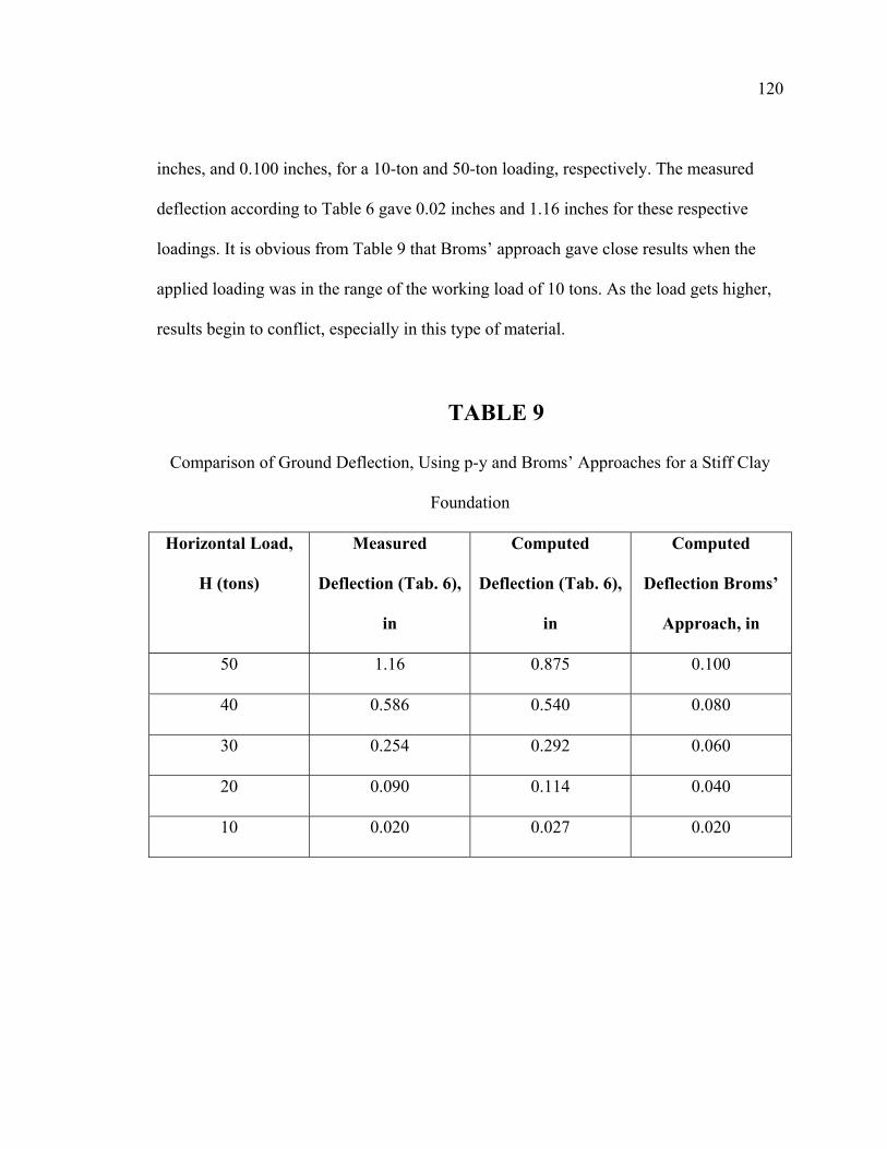
120
inches, and 0.100 inches, for a 10-ton and 50-ton loading, respectively. The measured
deflection according to Table 6 gave 0.02 inches and 1.16 inches for these respective
loadings. It is obvious from Table 9 that Broms’ approach gave close results when the
applied loading was in the range of the working load of 10 tons. As the load gets higher,
results begin to conflict, especially in this type of material.
TABLE 9
Comparison of Ground Deflection, Using p-y and Broms’ Approaches for a Stiff Clay
Foundation
Horizontal Load,
H (tons)
Measured
Deflection (Tab. 6),
in
Computed
Deflection (Tab. 6),
in
Computed
Deflection Broms’
Approach, in
50 1.16 0.875 0.100
40 0.586 0.540 0.080
30 0.254 0.292 0.060
20 0.090 0.114 0.040
10 0.020 0.027 0.020
121
VII. CONCLUSIONS AND RECOMMENDATIONS
The problem of a deep foundation subjected to a lateral loading involves the
interaction of soil and structure. The solution to the problem usually requires the use of
iterative techniques because soil response is a nonlinear function of the deflection of the
foundation.
Some approximate predictions of the ultimate lateral capacity can be reached by
logical and experienced assumptions of soil resistance and its distribution along the pile
length. In most cases, a simplified solution of the problem, sufficiently accurate for all
practical purposes, can be obtained by solving a differential equation of the fourth order.
Very often, ready-made solutions in the form of diagrams or formulas can be used
to provide sufficiently accurate answers, within the “working load” range. Material
constants appearing in these solutions can be determined from lateral load tests on actual
piles. For some soils types, there are also established means of predicting these material
constants from the laboratory or in situ measured deformation characteristics of soils.
Broms limited his method for calculating deflection to the working load range,
which is normally considered to be 1/3 to 1/2 of the computed ultimate pile capacity. In
the working load range, Broms assumed that the soil was linearly elastic. Even though
cohesive soil is not linearly elastic in the working load range, Broms’ assumption
probably leads to only minor errors. However, Broms’ method for cohesive soil is limited
122
because in many instances it is desirable to obtain the response of a pile for a full range of
loads. Also, to simplify the analysis, Broms assumed that for cohesive soils, the subgrade
modulus was constant with depth.
In sand soils the assumption of linearly varying soil modulus is useful in practice
according to Reese and Matlock (1956), but the value of sE will decrease substantially as
the lateral load is increased. This might have contributed to the discrepancy between
results when the load increased. Broms’ method of solution is easy to use, and can
produce a preliminary estimate of the ultimate collapse load or of the maximum bending
moment for a pile in cohesionless soil. If a better estimate of the pile behavior is required,
a computer program in conjunction with nonlinear soil resistance-deflection curves
should be used, such as L-Pile or FB-Pier. The method of p-y curves can be improved as
more information is gained on the behavior of full-scale piles under lateral loadings.
A valid solution to the problem of the laterally loaded deep foundation requires,
as for other boundary-value problems, the satisfaction of the conditions of equilibrium
and compatibility. It is important, however, to be able to accurately determine soil
properties and predict soil response. As more knowledge is gained concerning the
prediction of soil behavior, new knowledge can be incorporated into the analytical
procedures.
123
VIII. BIBLIOGRAPHY
1. Alizadeh, M., and Davisson, M. T., 1970, “Lateral Load Tests on Piles-Arkansas
River Project,” J. Soils Mech. Found. Div, ASCE, Vol. 96, No. SM5, pp. 1583-1604.
2. Bowles, Joseph E., Foundation Analysis and Design, McGraw-Hill Book Co.,
1968, p. 750. 3. Bowman, Elliott, R., “Investigation of the Lateral Resistance to Movement of a
Plate in Cohesionless Soil,” Unpublished Master’s Degree Thesis, Austin, The University of Texas, January 1958.
4. Brinch-Hansen, J., “The Ultimate Resistance of Rigid Piles Against Transversal
Forces,” Bulletin No. 12, Danish Geotechnical Institute, Copenhagan, Denmarck 1961, pp. 5-9
5. Broms, B. B., “Lateral Resistance of Piles in Cohesionless Soils,” J. Soils Mech.
Found. Div, ASCE, Vol. 90, No. SM3, 1964.
6. Broms, B. B., “Design of Laterally Loaded Piles,” J. Soils Mech. Found. Div, ASCE, Vol. 90, No. SM3, 1965.
7. Broms, B. B., “Lateral Resistance of Piles in Cohesive Soils,” J. Soils Mech.
Found. Div, ASCE, Vol. 90, No. SM2, 1964.
8. Cox, W. R., Reese, L. C., and Grubbs, B. R., “Field Testing of Laterally Loaded Piles in Sand,” 6th Offshore Technical Conference,” Houston, 1974.
9. Davisson, M. T., “Lateral Load Capacity of Piles,” High. Res. Rec, No. 333,
1970, pp. 104-112.
10. Desai, C. S., and Christian, J. T., Numerical Methods in Geotechnical Engineering, McGraw-Hill Book Co., 1977, p. 783.
11. Fruco and Associates, “Pile Driving and Loading Tests: Lock and Dam No. 4,
Arkansas River and Tributaries, Arkansas and Oklahoma,” U.S. Army Corps of Engineers District, Little Rock, September 1964.
124
12. Garissino, A., Jamiolkowski, M., and Pasqualini, E., “Soil Modulus for Laterally
Loaded Piles in Sands and N.C. Clays,” 6th European Conference on Soil Mechanics & Foundation Engineering, Vienna, 1976.
13. Gill, H. L., “Lateral-Plate and Rigid-Pile Tests in Beach Sand,” U.S. Naval Civil
Engineering Laboratories, Rep. No. 310, California, 1964.
14. Glesser, S. M., “Lateral Load Tests on Vertical Fixed-Head and Free-Head Piles,” Symposium on Lateral Pile Load Tests, ASTM Special Technical Publication 154, 1953, pp. 75-101.
15. Hetenyi, M., Beams on Elastic Foundation, University of Michigan Press, Ann
Arbor, Michigan, 1942.
16. Lambe, T. W., and Whitman, R. V., Soil Mechanics, John Wiley & Sons, Inc., New York, 1969, p. 553.
17. Matlock, Hudson, and Ripperger, E. A., “Procedures and Instrumentation for
Tests on a Laterally Loaded Pile,” Proceedings of the Eighth Texas Conference on Soil Mechanics and Foundation Engineering, Special Publication No. 29, Bureau of Engineering Research, The University of Texas, Austin, Texas, 1956.
18. Matlock, H., and Ripperger, E. A., “Measurement of Soil Pressure on a Laterally
Loaded Pile,” Proc. ASTM, Vol. 58, 1958, pp. 1245-1259.
19. Matlock, H., “Correlation for Design of Laterally Loaded Piles in Soft Clay,” 2nd Offshore Technology Conf., Houston, Texas, 1970.
20. Matlock, Hudson and Reese, L. C., “Generalized Solution for Laterally Loaded
Piles,” Transactions, ASCE, Vol. 127, Part 1, 1962, pp. 1220-1251.
21. McClelland, Bramlette and Focht, J. A., Jr., “Soil Modulus for Laterally Loaded Piles,” Transactions, ASCE, Vol. 123, 1958, pp. 1071-1074.
22. Meyer, B. J., and Reese, L. C., “Analysis of Single Piles Under Lateral Loading,”
Federal Highway Administration, Austin, Texas, Dec. 1979.
23. Poulous, H. G., “Behavior of Laterally Loaded Piles: I-Single Piles,” J. Soils Mech. Found. Div, ASCE, Vol. 97, No. SM5, May 1971.
125
24. Poulous, H. G., and Davis, E. H., Pile Foundation Analysis and Design, John
Wiley and Sons, Inc., New York.
25. Prospect, Soil-Structure Interaction Analysis, Course Notes, U.S. Army Engineer, Waterways Experiment Station, March 2003.
26. Reese, L. C., and Welch, Robert C., “Lateral Loading of Deep Foundation in Stiff
Clay,” J. Geotech. Eng. Div. ASCE, Vol. 101, No. 677, July 1975.
27. Reese, L. C., Cox, W. R., “Soil Behavior from Analysis of Tests of Uninstrumented Piles Under Lateral Loading,” Symposium on Performance of Deep Foundations, ASTM Special Technical Publication 444, June 1968, pp. 160-176.
28. Reese, L. C., Cox, W. R., and Koop, Francis D., “Analysis of Laterally Loaded
Piles in Sand,” 6th Offshore Technology Conf., Houston, Texas, 1974.
29. Reese, L. C., Cooley, L. A., and Radhakrishnan, N., “Laterally Loaded Piles and Computer Program COM624G,” U.S. Army Engineer, Waterways Experiment Station, April 1984.
30. Skempton, A. W., “The Bearing Capacity of Clays,” Building Research Congress,
Division 1, Part 3, London, 1951, pp. 180-189.
31. Terzaghi, Karl, “Evaluation of Coefficients of Subgrade Reaction,” Geotechnique, Vol. 5, December 1955, pp. 297-326.
32. Terzaghi, Karl, and Peck, Ralph B., Soil Mechanics in Engineering Practice, John
Wiley and Sons, Inc., New York, 1948.
33. Valsangkar, A. J., Rao Kamenswara, N. S. V., and Basudher, P. K., “Generalized Solutions of axially and Laterally Loaded Piles in Elasto-plastic Soils,” Soils and Foundations, Japanese Society of Soil Mech. And Found. Eng., Vol. 13, No. 4, Dec. 1973.
34. Yegian, M., and Wright, S. G., “Lateral Soil Resistance-Displacement
Relationship for Pile Foundations in Soft Clays,” 5th Offshore Technology Conf., Houston, Texas, 1973.
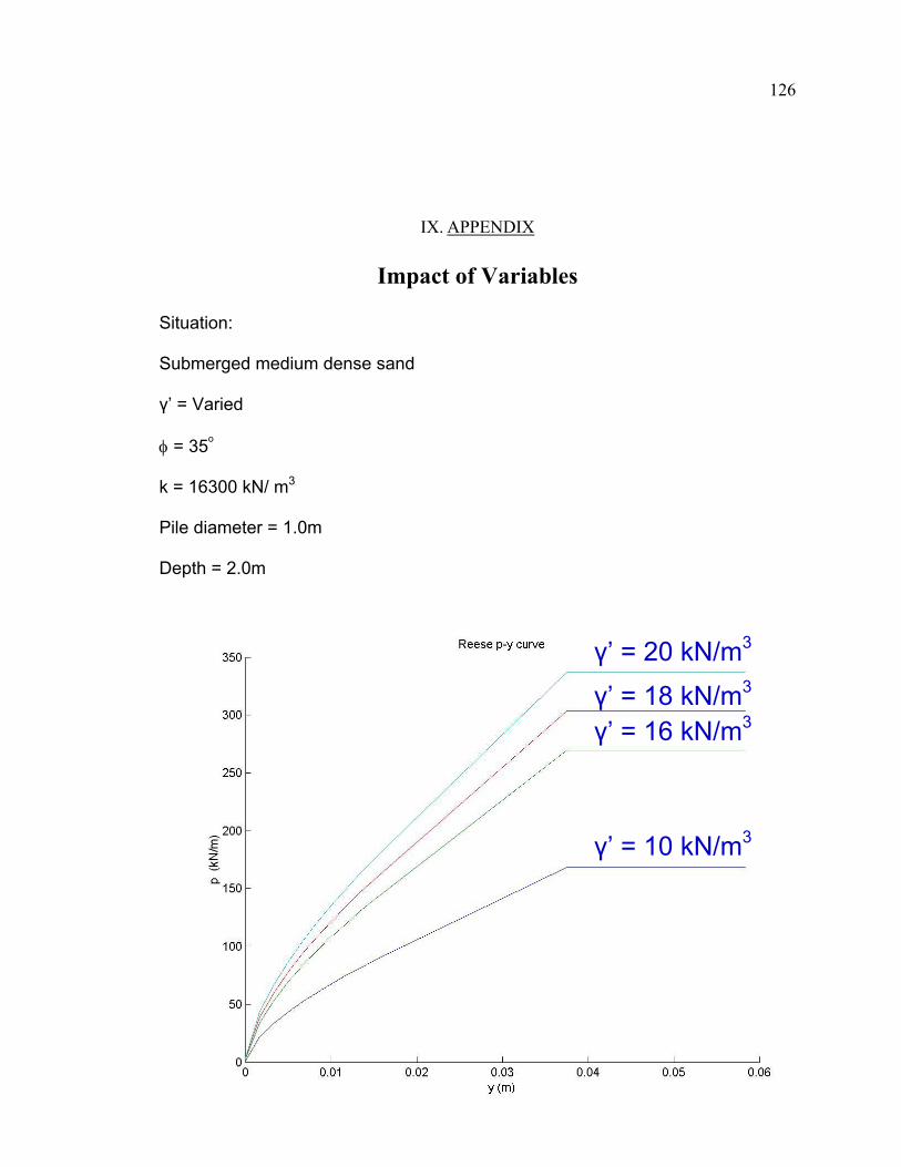
126
IX. APPENDIX
Impact of Variables Situation: Submerged medium dense sand γ’ = Varied φ = 35o
k = 16300 kN/ m3
Pile diameter = 1.0m Depth = 2.0m
γ’ = 20 kN/m3
γ’ = 18 kN/m3
γ’ = 16 kN/m3
γ’ = 10 kN/m3
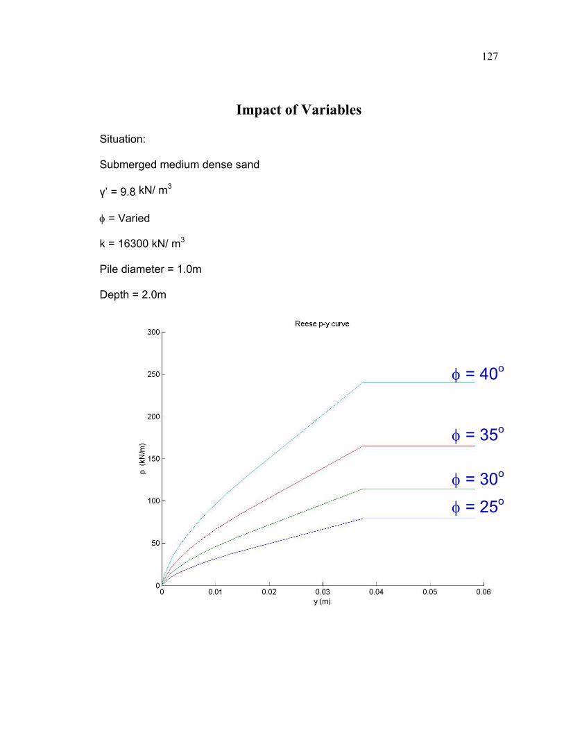
127
Impact of Variables Situation: Submerged medium dense sand γ’ = 9.8 kN/ m3 φ = Varied
k = 16300 kN/ m3
Pile diameter = 1.0m Depth = 2.0m
φ = 40o
φ = 35o
φ = 30o
φ = 25o
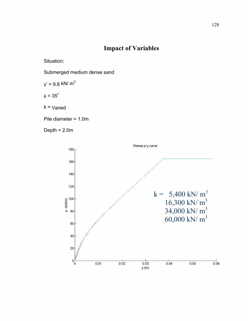
128
Impact of Variables Situation: Submerged medium dense sand γ’ = 9.8 kN/ m3 φ = 35o
k = Varied
Pile diameter = 1.0m Depth = 2.0m
k = 5,400 kN/ m3
16,300 kN/ m3
34,000 kN/ m3
60,000 kN/ m3
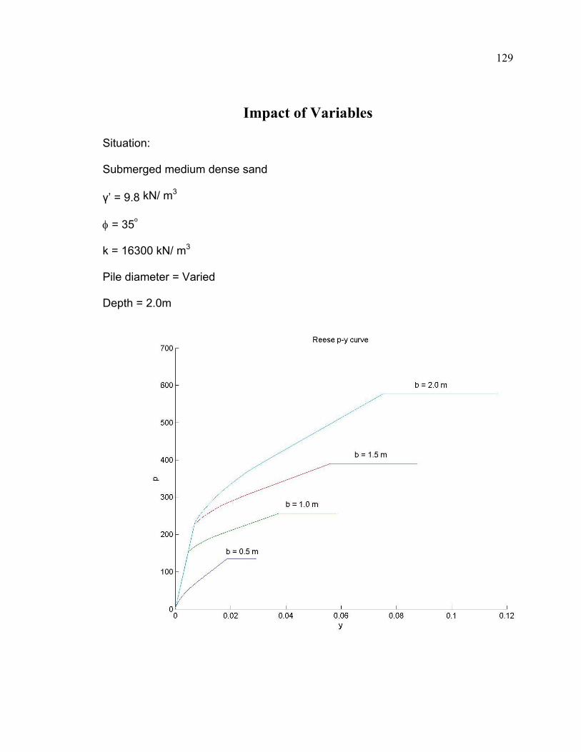
129
Impact of Variables Situation: Submerged medium dense sand γ’ = 9.8 kN/ m3 φ = 35o
k = 16300 kN/ m3
Pile diameter = Varied Depth = 2.0m
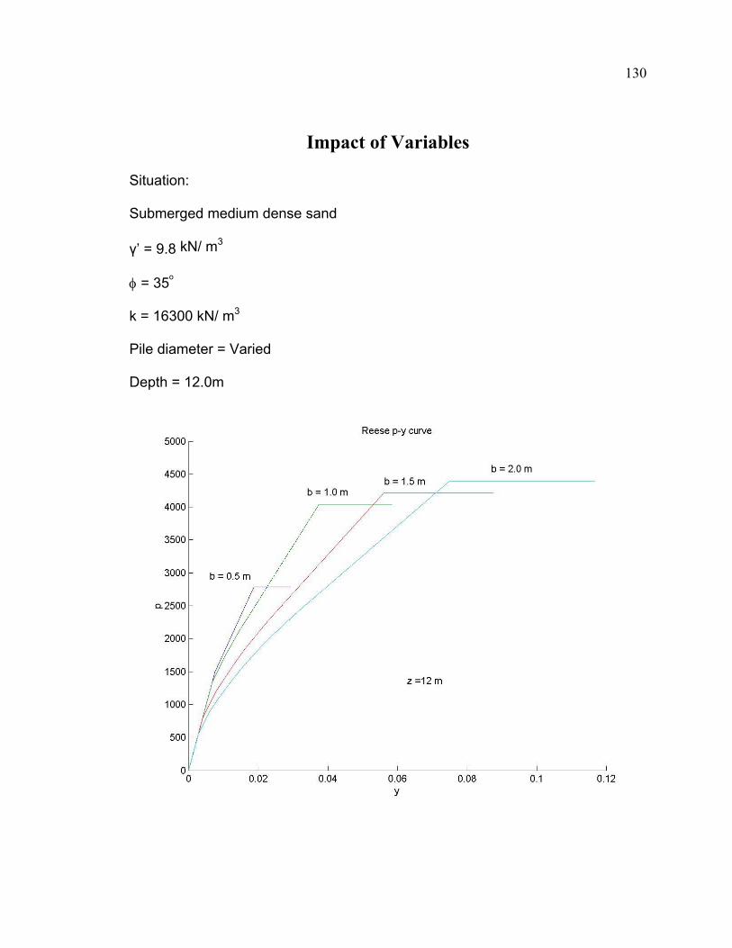
130
Impact of Variables Situation: Submerged medium dense sand γ’ = 9.8 kN/ m3 φ = 35o
k = 16300 kN/ m3
Pile diameter = Varied Depth = 12.0m
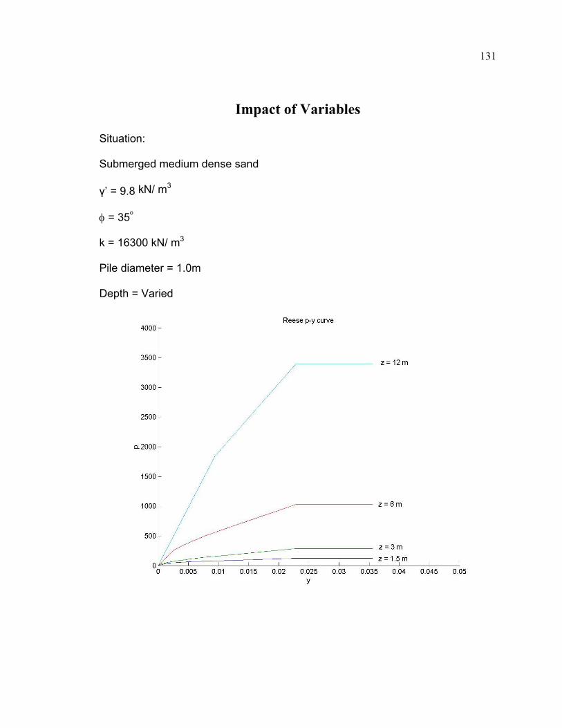
131
Impact of Variables Situation: Submerged medium dense sand γ’ = 9.8 kN/ m3 φ = 35o
k = 16300 kN/ m3
Pile diameter = 1.0m Depth = Varied
132
Example Problem in FB-Pier
Problem overview
• Single free head pile (Diameter = 0.5m) subjected a lateral load at the ground surface • Uniform sand • Water table at the ground surface
Objective To study the effects of the soil properties (internal friction angle φ, subgrade modulus k, and unit weight γ) on the behavior of Reese’s Sand Model
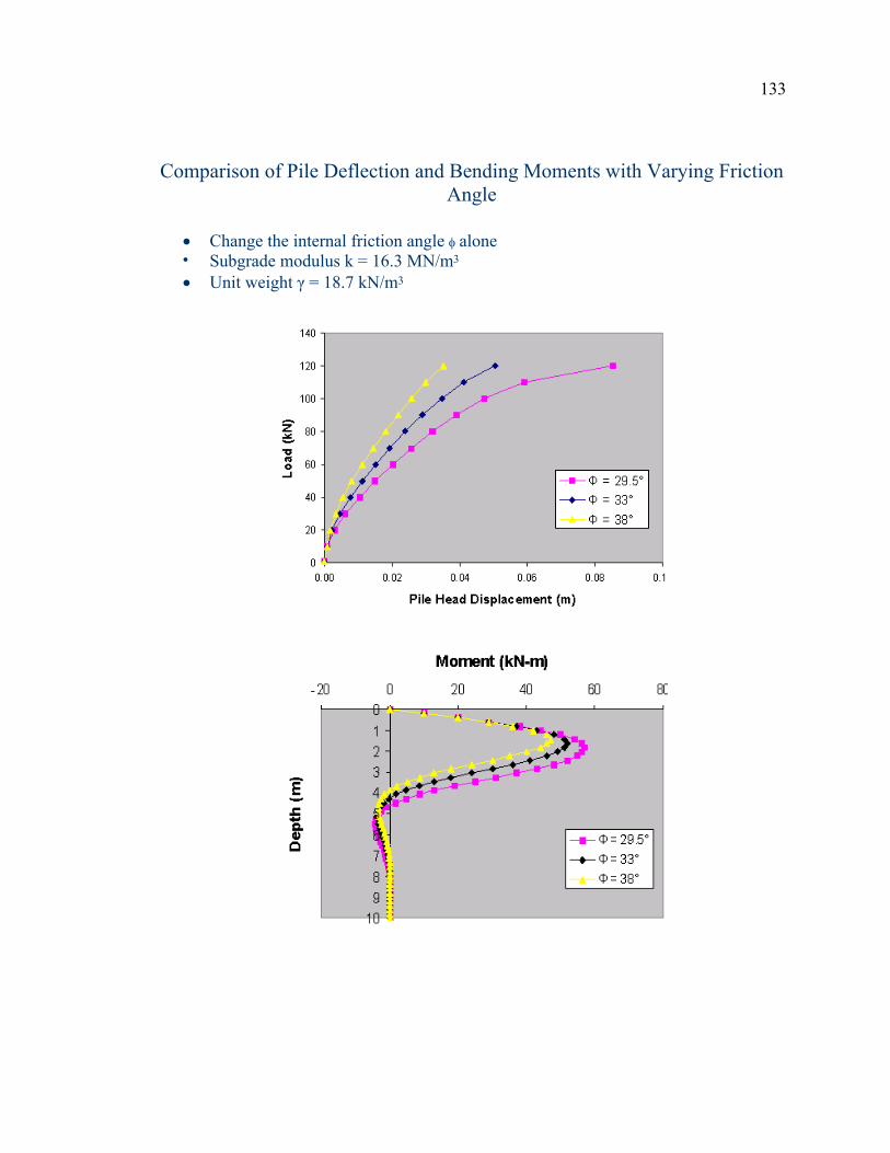
133
Comparison of Pile Deflection and Bending Moments with Varying Friction Angle
• Change the internal friction angle φ alone • Subgrade modulus k = 16.3 MN/m3
• Unit weight γ = 18.7 kN/m3
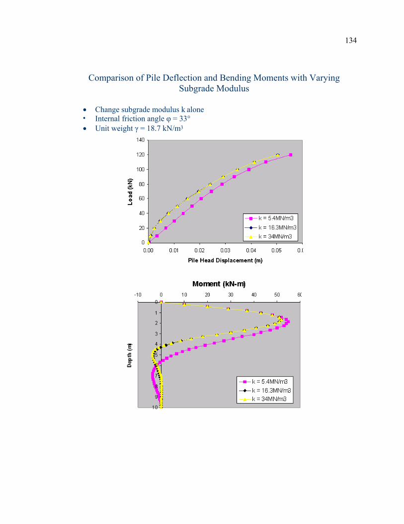
134
Comparison of Pile Deflection and Bending Moments with Varying Subgrade Modulus
• Change subgrade modulus k alone • Internal friction angle φ = 33° • Unit weight γ = 18.7 kN/m3
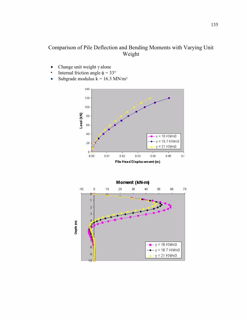
135
Comparison of Pile Deflection and Bending Moments with Varying Unit Weight
• Change unit weight γ alone • Internal friction angle φ = 33° • Subgrade modulus k = 16.3 MN/m3
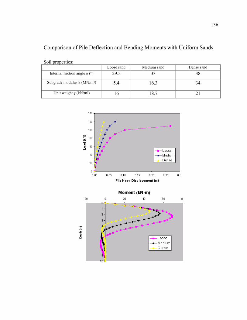
136
Comparison of Pile Deflection and Bending Moments with Uniform Sands Soil properties: Loose sand Medium sand Dense sand
Internal friction angle φ (°) 29.5 33 38
Subgrade modulus k (MN/m3)
5.4 16.3 34
Unit weight γ (kN/m3) 16 18.7 21
137
Example Problem in FB-Pier
Problem overview •Single free head pile (Diameter = 12in) subjected a lateral load at the ground surface •Soft clay foundation •Water table at the ground surface Objective To study the effects of the soil properties and pile properties (shear strength, soil strain e50, pile diameter, and pile length) on the behavior of Matlock’s Soft Clay below the Water Table Model
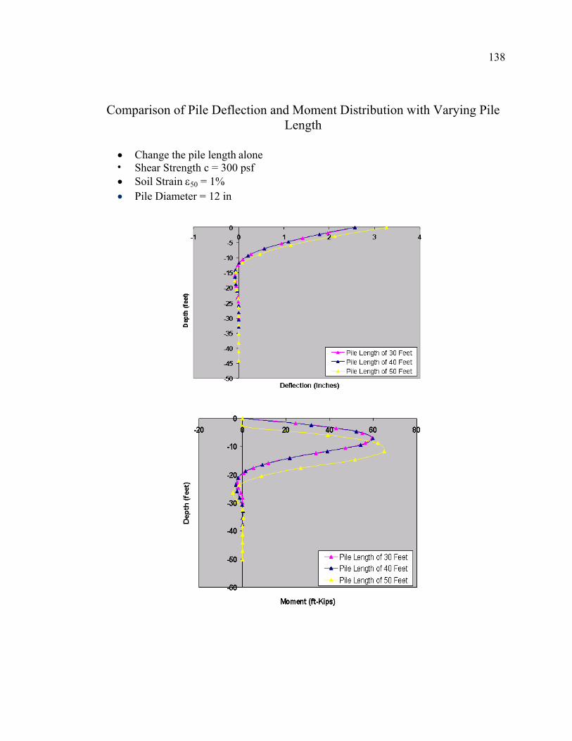
138
Comparison of Pile Deflection and Moment Distribution with Varying Pile Length
• Change the pile length alone • Shear Strength c = 300 psf • Soil Strain ε50 = 1% • Pile Diameter = 12 in
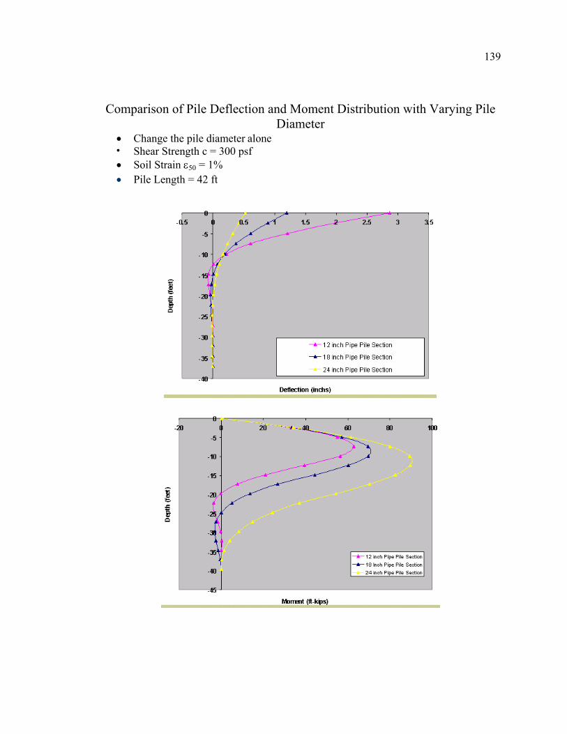
139
Comparison of Pile Deflection and Moment Distribution with Varying Pile Diameter
• Change the pile diameter alone • Shear Strength c = 300 psf • Soil Strain ε50 = 1% • Pile Length = 42 ft
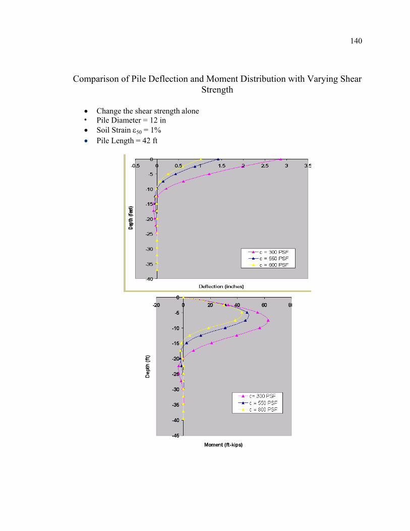
140
Comparison of Pile Deflection and Moment Distribution with Varying Shear Strength
• Change the shear strength alone • Pile Diameter = 12 in • Soil Strain ε50 = 1% • Pile Length = 42 ft
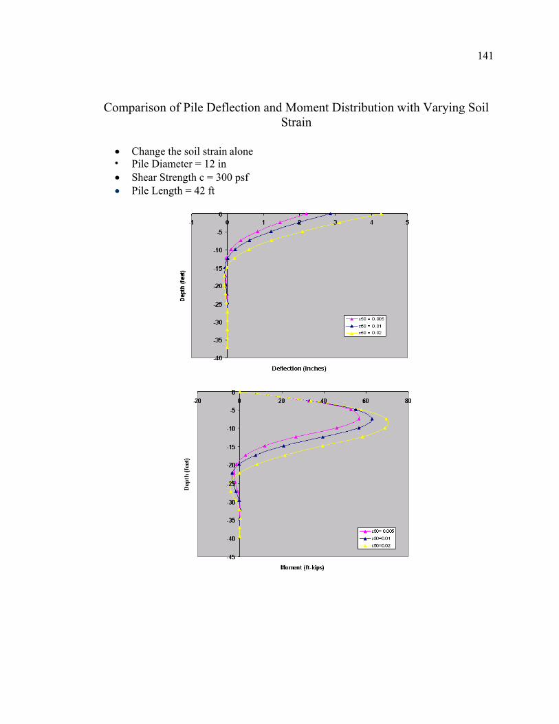
141
Comparison of Pile Deflection and Moment Distribution with Varying Soil Strain
• Change the soil strain alone • Pile Diameter = 12 in • Shear Strength c = 300 psf • Pile Length = 42 ft
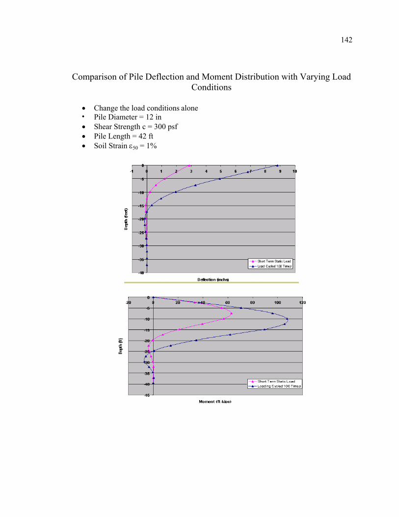
142
Comparison of Pile Deflection and Moment Distribution with Varying Load Conditions
• Change the load conditions alone • Pile Diameter = 12 in • Shear Strength c = 300 psf • Pile Length = 42 ft • Soil Strain ε50 = 1%
143
X. VITA
Chad Michael Rachel was born February 21, 1974, in Marrero, Louisiana. He
received a Bachelor of Science Degree in Civil Engineering from the University of New
Orleans in 2000. He currently works as a civil (geotechnical) engineer at the U.S. Army
Corps of Engineers in New Orleans, Louisiana.
Recommended