Embed Size (px)
Citation preview
University of New Orleans University of New Orleans
ScholarWorks@UNO ScholarWorks@UNO
University of New Orleans Theses and Dissertations Dissertations and Theses
Spring 5-22-2020
Modeling of Distributary Channels Formed by a Large Sediment Modeling of Distributary Channels Formed by a Large Sediment
Diversion in Broken Marshland Diversion in Broken Marshland
Dylan Blaskey University of New Orleans, New Orleans, [email protected]
Follow this and additional works at: https://scholarworks.uno.edu/td
Part of the Civil Engineering Commons, Environmental Indicators and Impact Assessment Commons,
Hydraulic Engineering Commons, and the Water Resource Management Commons
Recommended Citation Recommended Citation Blaskey, Dylan, "Modeling of Distributary Channels Formed by a Large Sediment Diversion in Broken Marshland" (2020). University of New Orleans Theses and Dissertations. 2728. https://scholarworks.uno.edu/td/2728
This Thesis is protected by copyright and/or related rights. It has been brought to you by ScholarWorks@UNO with permission from the rights-holder(s). You are free to use this Thesis in any way that is permitted by the copyright and related rights legislation that applies to your use. For other uses you need to obtain permission from the rights-holder(s) directly, unless additional rights are indicated by a Creative Commons license in the record and/or on the work itself. This Thesis has been accepted for inclusion in University of New Orleans Theses and Dissertations by an authorized administrator of ScholarWorks@UNO. For more information, please contact [email protected].
Modeling of Distributary Channels Formed by a Large Sediment Diversion in Broken Marshland
A Thesis
Submitted to the Graduate Faculty of the
University of New Orleans
in partial fulfillment of the
requirements for the degree of
Master of Science
in
Engineering
Civil and Environmental Engineering
by
Dylan Blaskey
B.S. University of Minnesota, 2015
May, 2020

ii
Acknowledgements
I would like to thank Dr. John Alex McCorquodale for the constant guidance as we worked
through the many difficulties that occur during a master’s program. Your continued support and
incredible patience has taught me so much about the field of engineering and the process of
researching. None of this would be possible without you.
In addition, I would like to extend my gratitude to Dr. Malay Ghose Hajra for guiding me
through the process of being a master student and always checking in with me to make sure I was
on track. I really appreciate you accommodating me when I was trying to finish my research
quickly and then working on a plan to extend my timeline as my life circumstances changed.
Finally, I would like to thank Dr. Ioannis Georgiou for asking me the tough questions when I
was developing the model and making me think critically about the results. I still remember you
telling me to fully understand my results before you start to draw conclusion. This is a lesson I
learned the hard way but it will be with me as I continue on as a researcher.
iii
Table of Contents
List of Figures ..................................................................................................................... v
List of Tables .................................................................................................................. viii
List of Acronyms .............................................................................................................. ix
Abstract ............................................................................................................................... x
Chapter 1: Introduction ....................................................................................................... 1
1.1 Introduction ................................................................................................................ 1
1.2 Caernarvon and Davis Pond....................................................................................... 4
1.3 Bohemia Spillway/Mardi Gras Pass .......................................................................... 5
1.4 West Bay .................................................................................................................... 6
1.5 Wax Lake Delta ......................................................................................................... 7
1.6 Bonnet Carré Spillway ............................................................................................... 9
1.7 Proposed Mid-Barataria Sediment Diversion .......................................................... 10
1.8 Previous Models of Barataria Basin ........................................................................ 11
1.9 Objectives of the Research....................................................................................... 12
1.10 Methodology in General ........................................................................................ 12
Chapter 2: Methods ........................................................................................................... 14
2.1 Model Selection ....................................................................................................... 14
2.2 Domain ..................................................................................................................... 14
2.3 Grid Design .............................................................................................................. 15
2.4 Bathymetry ............................................................................................................... 16
2.5 Time Frame .............................................................................................................. 17
2.6 Boundary Conditions ............................................................................................... 18
2.6.1 River and Diversion Discharge .......................................................................... 18
2.6.2 Tidal Flux ........................................................................................................... 20
2.6.3 Salinity ............................................................................................................... 21
2.6.4 Sediment ............................................................................................................ 22
2.7 Wind Forcing ........................................................................................................... 24
2.8 Initial Conditions ..................................................................................................... 25
2.9 Morphology ............................................................................................................. 26
2.10 Changing Conditions ............................................................................................. 27
Chapter 3: Calibration ....................................................................................................... 28
3.1 Calibration Overview ............................................................................................... 28
3.2 Water Depth Calibration .......................................................................................... 29
3.3 Salinity Calibration .................................................................................................. 32
3.4 Calibration Equations .............................................................................................. 36
3.4.1 Root Mean Square Error .................................................................................... 36
3.4.2 Pearson Product-Moment Correlation Coefficient ............................................ 37
3.4.3 Bias .................................................................................................................... 38
3.4.4 Critical Model Outputs ...................................................................................... 38
Chapter 4: Results ............................................................................................................. 39
4.1 Introduction .............................................................................................................. 39
4.2 Water Level .............................................................................................................. 41
4.3 Depth Averaged Velocity ........................................................................................ 50
iv
4.4 Geomorphology ....................................................................................................... 59
4.4.1 Basin Wide ......................................................................................................... 59
4.4.2 Localized Geomorphology................................................................................. 65
4.5 Sediment .................................................................................................................. 72
4.6 Salinity ..................................................................................................................... 74
Chapter 5: Discussion ....................................................................................................... 77
5.1 Introduction .............................................................................................................. 77
5.2 Development of the Distributary System ................................................................. 77
5.2.1 Diversion Mouth ................................................................................................ 77
5.2.2 Southern Path ..................................................................................................... 78
5.2.2.1 Round Lake .................................................................................................. 78
5.2.2.2 Grand Bayou ................................................................................................ 79
5.2.3 Northern Path ..................................................................................................... 80
5.2.4 Mid-Barataria Waterway Path ........................................................................... 82
5.3 Flood Levels............................................................................................................. 83
5.3.1 Water Level Filter .............................................................................................. 83
5.3.2 Receiving Basin ................................................................................................. 83
5.3.3 Barataria Waterway ........................................................................................... 85
5.3.4 Grand Bayou ...................................................................................................... 86
5.4 Velocity .................................................................................................................... 87
5.4.1 Velocity Filter .................................................................................................... 87
5.4.2 Receiving Basin ................................................................................................. 88
5.4.3 Barataria Waterway ........................................................................................... 88
5.4.4 Grand Bayou ...................................................................................................... 90
5.5 Sediment .................................................................................................................. 91
5.5.1 Receiving Basin ................................................................................................. 91
5.5.2 Barataria Waterway ........................................................................................... 92
5.5.3 Grand Bayou ...................................................................................................... 93
5.6 Salinity ..................................................................................................................... 93
5.7 Model Sensitivity ..................................................................................................... 94
5.8 Recommendations .................................................................................................... 95
Chapter 6: Conclusions ..................................................................................................... 96
References ......................................................................................................................... 97
Appendix A ..................................................................................................................... 109
Vita .................................................................................................................................. 112
v
List of Figures
Figure 2.1 Modeling domain of the Barataria Basin......................................................... 14
Figure 2.2: The grid around the sediment diversion ......................................................... 15
Figure 2.3: The final grid over the domain ....................................................................... 16
Figure 2.4: Bathymetry and monitoring station of the study domain ............................... 17
Figure 2.5: Mississippi River Discharge over the Last Decade ........................................ 18
Figure 2.6: Diversion Discharge Based on 2017 Mississippi River Hydrograph ............. 19
Figure 2.7: Diversion Discharge Based on 2018 Mississippi River Hydrograph ............. 20
Figure 2.8: Gulf of Mexico Stage Tidal Boundary Condition Normal Flow Year ........... 20
Figure 2.9: Gulf of Mexico Stage Tidal Boundary Condition High Flow Year ............... 21
Figure 2.10: Gulf of Mexico Salinity during Normal Flow Year ..................................... 21
Figure 2.11: Gulf of Mexico Salinity during High Flow Year ......................................... 22
Figure 2.12: Sediment Concentration during Simulated Normal Flow Year ................... 23
Figure 2.13: Sediment Concentration during Simulated High Flow Year ........................ 24
Figure 2.14: Wind Speed during Normal Flow Year ........................................................ 25
Figure 2.14: Wind Speed during High Flow Year ............................................................ 25
Figure 2.16: Initial Salinity Condition for the Model ....................................................... 26
Figure 3.1: Water Surface Elevation Comparison for USGS 07380335 during
Normal River Flow ........................................................................................................... 29
Figure 3.2: Water Surface Elevation Comparison for USGS 07380335 High
River Flow ........................................................................................................................ 30
Figure 3.3: Water Surface Elevation Comparison for USGS 292859090004000
during Normal River Flow ................................................................................................ 30
Figure 3.4: Water Surface Elevation Comparison for USGS 292859090004000
during High River Flow .................................................................................................... 31
Figure 3.5: Water Surface Elevation Comparison for USGS 07380251 during
Normal River Flow ........................................................................................................... 31
Figure 3.6: Water Surface Elevation Comparison for USGS 07380251 High
River Flow ........................................................................................................................ 32
Figure 3.7: Salinity Comparison for USGS 07380330 during Normal River Flow ......... 33
Figure 3.8: Salinity Comparison for USGS 07380330 during High River Flow ............. 33
Figure 3.9: Salinity Comparison for USGS 292859090004000 during Normal
River Flow ........................................................................................................................ 34
Figure 3.10: Salinity Comparison for USGS 292859090004000 during High
River Flow ........................................................................................................................ 34
Figure 3.11: Salinity Comparison for USGS 07380251 during Normal River Flow ....... 35
Figure 3.12: Salinity Comparison for USGS 07380251 during High River Flow ........... 35
Figure 4.1: Diversion Discharge for Normal River Flow Year ........................................ 39
Figure 4.2: Diversion Discharge for High River Flow Year ............................................ 39
Figure 4.3: Major Distributary Channels Established by the Diversion ........................... 40
Figure 4.4: Water bodies in Barataria Basin ..................................................................... 41
Figure 4.5: Water Level Difference at Bayou DuPont during a Normal Flow Year ........ 42
Figure 4.6: Water Level Difference at Bayou DuPont during a High Flow Year ........... 42
Figure 4.7: Water Level Difference in Round Lake during a Normal Flow Year ........... 43
vi
Figure 4.8: Water Level Difference at Round Lake during a High Flow Year ............... 44
Figure 4.9: Water Level Difference in North Barataria Waterway Lake ........................ 44
Figure 4.10: Water Level Difference in Mid-Barataria Waterway Lake ......................... 45
Figure 4.11: Water Level Difference in North Barataria Waterway Lake ...................... 45
Figure 4.12: Water Level Difference in Mid-Barataria Waterway Lake ......................... 46
Figure 4.13: Water Level Difference in South Barataria Waterway Lake ...................... 47
Figure 4.14: Water Level Difference in South Barataria Waterway Lake ...................... 47
Figure 4.15: Water Level Difference in Lake Salvador during a Normal Flow Year ..... 48
Figure 4.16: Water Level Difference in Lake Salvador during a High Flow Year ......... 48
Figure 4.17: Water Level Difference in Grand Bayou during a Normal Flow Year ....... 49
Figure 4.18: Water Level Difference in Grand Bayou during a High Flow Year ........... 50
Figure 4.19: Velocity One Day after the Diversion is Opened Normal Flow Year .......... 51
Figure 4.20: Velocity One Day after the Diversion is Opened High Flow Year .............. 51
Figure 4.21: Velocity at Peak Diversion Flow Normal Flow Year .................................. 52
Figure 4.22: Velocity at Peak Diversion Flow High Flow Year ....................................... 52
Figure 4.23: Velocity on Falling Limb Normal Flow Year .............................................. 53
Figure 4.24: Velocity on Falling Limb High Flow Year .................................................. 53
Figure 4.25: Velocity of North Barataria Waterway Normal Flow Year ......................... 54
Figure 4.26: Velocity of North Barataria Waterway High Flow Year ............................. 55
Figure 4.27: Velocity of Mid-Barataria Waterway Normal Flow Year ............................ 55
Figure 4.28: Velocity of Mid-Barataria Waterway High Flow Year ................................ 56
Figure 4.29: Velocity of South Barataria Waterway Normal Flow Year ......................... 56
Figure 4.30: Velocity of South Barataria Waterway High Flow Year ............................. 57
Figure 4.31: Velocity of Grand Bayou Normal Flow Year .............................................. 58
Figure 4.32: Velocity of Grand High Flow Year .............................................................. 58
Figure 4.33: Erosion of the marshland two days after the diversion opened during
a Normal Mississippi River flow year with velocity vectors ........................................... 59
Figure 4.34: Erosion of the marshland when the diversion reaches maximum
discharge during a normal Mississippi River flow year with velocity vectors ................ 60
Figure 4.35: Erosion of the marshland when the diversion begins to reduce in
discharge during a normal Mississippi River flow year with velocity vectors ................ 61
Figure 4.36: Erosion of the marshland when the diversion is increasing discharge
during a normal Mississippi River flow year .................................................................... 62
Figure 4.37: Erosion of the marshland when the diversion is increasing discharge
during a high Mississippi River flow year ........................................................................ 62
Figure 4.38: Erosion of the marshland when the diversion is at maximum discharge
during a normal Mississippi River flow year .................................................................... 63
Figure 4.39: Erosion of the marshland when the diversion is increasing discharge
during a high Mississippi River flow year ........................................................................ 63
Figure 4.40: Erosion of the marshland when the diversion closes during a normal
Mississippi River flow year .............................................................................................. 64
Figure 4.41: Erosion of the marshland when the diversion closes during a high
Mississippi River flow year .............................................................................................. 65
Figure 4.42: Erosion of Bayou DuPont during Normal Flow Year ................................. 66
Figure 4.43: Erosion of Bayou DuPont during High Flow Year ..................................... 66
Figure 4.44: Erosion at Grand Bayou during Normal Flow Year .................................... 67
vii
Figure 4.45: Erosion at Grand Bayou during High Flow Year ........................................ 68
Figure 4.46: Erosion at Mid-Barataria Waterway during Normal Flow Year ................. 69
Figure 4.47: Erosion at Mid-Barataria Waterway during High Flow Year ..................... 69
Figure 4.48: Erosion at South Barataria Waterway during Normal Flow Year ............... 70
Figure 4.49: Erosion at South Barataria Waterway during High Flow Year ................... 70
Figure 4.50: Erosion at North Barataria Waterway during Normal Flow Year ............... 71
Figure 4.51: Erosion at North Barataria Waterway during High Flow Year ................... 71
Figure 4.52: Clay Concentration in Grand Bayou during Normal Flow Year .................. 73
Figure 4.53: Clay Concentration in Grand Bayou during High Flow Year ...................... 73
Figure 4.54: Salinity in North Barataria Waterway during High Flow Year ................... 74
Figure 4.55: Salinity in Mid-Barataria Waterway during High Flow Year ..................... 75
Figure 4.56: Salinity in Grand Bayou during High Flow Year ........................................ 75
Figure 4.57: Salinity in Lake Washington during High Flow Year .................................. 76
Figure 4.58: Salinity in Western Barataria Bay during High Flow Year.......................... 76
Figure 5.1: The Southern Path .......................................................................................... 79
Figure 5.2: The Grand Bayou Outlet ............................................................................... 80
Figure 5.3: The Northern Path Start .................................................................................. 81
Figure 5.4: The Northern Path Turn to Bayou Rigolettes ................................................. 81
Figure 5.5: Mid-Barataria Waterway Path ........................................................................ 82
Figure 5.6: Modeled and Filtered Water Level Difference during a High Flow Year
Operated at Maximum Capacity ....................................................................................... 83
Figure 5.7: Water Level Peak in Round Lake Compared to Diversion Discharge ........... 84
Figure 5.8: Water Level Peak at Mid-Barataria Waterway Compared to Diversion
Discharge .......................................................................................................................... 86
Figure 5.9: Water Level Peak in Grand Bayou Compared to Diversion Discharge ......... 87
Figure 5.10: Modeled and Filtered Velocity Difference during a High Flow Year
Operated at Maximum Capacity ....................................................................................... 88
Figure 5.11: Velocity at Mid-Barataria Waterway Compared to Diversion Discharge ... 90
Figure 5.12: Velocity in Grand Bayou Compared to Diversion Discharge ...................... 91
viii
List of Tables
Table 2.1: Wind Observation Stations Used in Boundary Conditions ............................. 24
Table 2.2: Sediment mass fraction by layer ...................................................................... 26
Table 2.3: Settling velocity parameters based on sediment type ...................................... 27
Table 3.1: Location of USGS stations used during the calibration of the model ............. 28
Table 3.2: Results of RMSE analysis ............................................................................... 36
Table 3.3: Results of Pearson Product-Moment Correlation Coefficient analysis ........... 37
Table 3.4: Results of bias analysis .................................................................................... 38
Table 4.1: Average Silt Concentration during Peak Diversion Discharge ....................... 72
ix
List of Acronyms
BWW Barataria Waterway
CPRA Coastal Protection and Restoration Authority
ESLR Eustatic Sea Level Rise
GIWW Gulf Intracoastal Waterway
NAVD88 North American Vertical Datum 1988
NCDC National Climatic Data Center
NOAA National Oceanic and Atmospheric Administration
RM River Mile
RMSE Root Mean Square Error
RSLR Relative Sea Level Rise
SLR Sea Level Rise
TWIG The Water Institute of the Gulf
USACE United States Army Corps of Engineers
USGS United States Geological Survey
UTM Universal Transverse Mercator
x
Abstract
A 2-D DELFT3D model was developed to address the morphological response of
Barataria Bay, the sediment deposition rate in the receiving basin, and the impact on the existing
distributary channels within the broken marsh system due to the proposed Mid-Barataria
Sediment Diversion. The model had a mesh size sufficient to accurately represent the
development of the distributary channels, localized flooding, erosion, and salinity in the basin.
The model predicts that the receiving basin will experience extensive erosion during the first
year the diversion is open creating three major distributary pathways which flood much of the
basin in freshwater. Most locations experience peak flood stage when the diversion reaches its
peak capacity after which flood stage tends to decrease. The area of open water near the
diversion opening will experience higher suspended sediment concentrations than those in the
diversion due to the erosion of the receiving basin.
Keywords: Mid-Barataria Sediment Diversion, hydrodynamic modeling, distributary channel
formation, marsh flooding
1
Chapter 1: Introduction
1.1 Introduction
Deltas across the world are some of the most sensitive features on the planet due to the large
populations, vast agricultural resources, and their proximity to the sea. They rely on a constant
inflow of sediment to maintain their elevation to counteract sea level rise, storm surge and wave
attack, salt water intrusion, and human activities that erode them. Sea level rise is accelerating
and is expected to eliminate 22% of the world’s coastal wetlands by 2100 (Nicholls et al., 1999)
although this varies by region (Michener et al. 1997).
The Mississippi River Delta has a large economic, cultural, and natural value to southern
Louisiana and the United States as a whole (Batker et al., 2014). The Lower Mississippi River
corridor contains wetlands, bayous, shallow estuaries, and emerged ridges formed through delta
progradation during the late Holocene (Coleman et al., 1998) Annual floods developed natural
levees and the low marshes surrounding the main channels of the river. Lobe switching carved
new channels to the gulf, connected marshes systems to form interwoven deltaic wetlands
(Russell, 1936; Russell, 1939; Russell, 1940; Fisk 1944; Kolb and Van Lopik, 1966). The delta is
characterized as sediment supply dominated with low wave and tidal energy (Roberts, 1997)
Prior to the 20th century long term land loss was balanced with the land building driven by the
Mississippi River (Frazier, 1967; Penland et al., 1988; Paola et al. 2011). Since then, the human
impact on these areas accelerated through increasing fertilizer usage, dams and levees,
deforestation, and other land use changes (Bianchi and Allison, 2009). Whereas soil erosion rates
have been accelerating due to human activities, the amount of water and sediment penetrating
these areas has decreased (Syvitski, Kettner, Correggiari, & Nelson, 2005; Vörösmarty &
Meybeck, 2004).
Coastal Louisiana is experiencing some of the highest rates of wetlands loss on earth (Gagliano
et al., 1981; Day et al., 2000). The causes of these losses are vest including subsidence, saltwater
intrusion, sediment toxicity, artificial channel cutting leading to expansion, pond creation,
urbanization, and oil and gas withdrawal (Britsch and Kemp, 1990; Penland et al., 2005; Turner,
1997; Day et al., 2000, 2007; Reed, 2002; Morton et al., 2003, 2006; Barras, 2006). These are
continually eroding the coastline while hurricanes are periodic events in the geologic record that
account for significant wetland loss. Hurricane Katrina and Rita in 2005 destroyed a combined
562 km2 of land in South Louisiana; (Barras, 2006). Due to these numerous factors, more than
1800 square miles of land has been lost to the Gulf of Mexico since the 1930s (Couvillion et al.,
2017).
The wetlands of Louisiana are built of layers of uncompact peat and mud due to the yearly
floods. Over time, the peat at the lower depths are dewatered and compacted by the weight of the
overlaying soil (Morton et al., 2002). Vertical accretion of both mineral sediment and organic
matter must be sufficient to offset this subsidence and sea level rise for these wetlands to survive
(Mossa and Roberts, 1990; Conner et al., 1997; Simas et al., 2001; Van Wijnen and Bakker,
2001; Lane et al., 2006; Paola et al., 2011; Delaune et al., 1983; Nyman et al., 1990; Cahoon and
2
Reed, 1995). Mineral deposits come from suspended sediment particles composed mainly of clay
and silt which are trapped during high flow events. When the flow is slowed by bed friction and
above ground structures (stems, trunks, pneumatophores, burrows, etc.) the particles flocculate
and settle out (Wolanski and Gibbs, 1995; Young and Harvey, 1996). Without the addition of
sediment from the Mississippi River, these wetlands become sediment starved (Baumann et al.,
1984; Boesch et al., 1994; Penland and Ramsey, 1990) and not able to outpace relative sea level
rise (Blum and Roberts, 2009) 80% of which is subsidence (Dokka, 2006). As the sea rises, the
marshes become inundated allowing salt water to penetrate further into the back basin (DeLaune
and White 2012). This is a positive feedback loop that is accelerating wetland loss.
Climate change will bring increases in precipitation amount and intensity, rates of sea level rise,
and frequency of hurricanes inundating more of these coastal wetlands. In coastal Louisiana, sea
level rise will be a major factor in wetland survivability (Simas et al., 2001; Van Wijnen and
Bakker, 2001; Day et al., 2008). Accelerated eustatic sea level rise, which is estimated by the
IPCC to be between 40 to 120 cm by 2100 (IPPC, 2013; Horton et al, 2014), will lead to longer
inundation periods, increase erosion and saltwater intrusions affecting the proliferation of
vegetation leading to wetland loss (Day et al., 2005; Blankespoor et al., 2012). Hurricane
intensity is expected to increase due to increased sea surface temperature (Mendelsohn et al.
2012; Donnelly et al. 2015; Knutson et al. 2010). However, there are still limitations in scientific
understanding of the divers of hurricane frequency and intensity (Zwiers et al. 2013), so specific
increases are hard to predict and model. It is unknown whether coastal wetlands will be able to
survive more frequent and severe storms (Michener et al. 1997, Day et al. 2008, Knutson et al.
2010, Leonardi et al. 2016).
Many of the solutions to these problems focus on moving sediment from the Mississippi River
into the coastal marshland. However, human interventions, such as dams and bank protection,
around the river basin have reduced the sediment load of the lower Mississippi by more than
50% (Kesel, 1988; Meade and Moody, 2010; Horowitz, 2010). In the delta, long, interconnected
levee systems put in place after the great flood of 1927 to protect New Orleans and the
surrounding populations have prevented the river from overflowing its banks and replenishing
the sediment in the surrounding marshes (Baumann et al., 1984; Walker et al., 1987). This annual
flooding would also resupply the marshes with fresh water preventing saltwater intrusion
(Walker et al., 1987; Boesch et al., 1994; Day et al., 2000). Other causes of water and sediment
loss include dredging for navigational channels, removal of water for industrial and agricultural
use, and flood protection outflows like the Bonnet Carré Spillway, which has a maximum design
capacity of 250,000 cfs, and an overflow weir near Bohemia at river mile 38.6.
This study focuses on Barataria Basin which is nestled between the Mississippi and the
Atchafalaya River. The Atchafalaya River has been known as a distributary channel of the
Mississippi River since as early as the 1500s (Fisk, 1952). The river steadily increased its
volume during the first half of the 20th century and would have captured the entire discharge of
the Mississippi River if not for the Old River Control Structure. This was built in 1963 and was
updated after a high flood in 1973 damaged the structure. To this day, the structure allows 30%
of the flow of the Mississippi River to enter the Atchafalaya River, which is further supplied by
the Red River creating a flow that is fairly equal to the Mississippi River (Roberts, 1998)
3
Today, Barataria Basin loses around 1300 acres of coastal wetlands each year (Couvillion et al.,
2017) leaving Plaquemines and Lafourche Parish even more susceptible to storms. Yet, over 100
million tons of sediment pass down the Mississippi River adjacent to the Barataria Basin each
year (Allison et al., 2012). To combat this problem, the State of Louisiana has planned a
sediment diversion into the basin (CPRA, 2017). A sediment diversion is a control structure built
through the levees of the Mississippi River to allow the river water, sediment, and nutrients to
flow into the broken distributary channels remaining in the wetlands. These diversions are
anticipated reduce the rate of land loss and possibly build land, restore freshwater habitats, and
improve the overall health of the Gulf (Paola et al., 2011; Gagliano et al., 1970; Kim et al., 2009;
Gagliano et al., 1973).
A sediment diversion reintroduces sediment rich river water into the wetland by maximizing the
sediment to water ratio in the diversion (Meselhe et al., 2012) and retaining this sediment in the
receiving area by mimicking the natural effects of crevasse splay, which is an integral part in the
evolution of deltas (Snedden et al., 2007; Day et al., 2009, 2012; Kim et al., 2009; Allison and
Meselhe, 2010; Paola et al., 2011; Meselhe et al., 2012; Wang et al., 2014). Increasing the
sediment ratio particularly of sand and coarse silt is controlled by the angular orientation and
elevation at the intake of the diversion (Gaweesh and Meselhe, 2016; Yuill et al., 2016) and the
proximity to bank margin lateral or point bars. These are significant sources of bed load material
(Ramirez and Allison, 2013; Allison et al., 2014). Sediment capture in the receiving basin is a
function of concentration, grain size, and flow. Coarse sediment, such as sand, is easier to
capture in the receiving area due to its faster settling velocities and resistance to resuspension.
Sand has limited consolidation and forms a substrate allowing for initial subaerial emergence.
Once these are established with vegetation, silts become important for sustaining them through
vertical accretion (Peyronnin et al., 2017). The orientation of these sediment accretions help to
develop splay island channels by resisting local flow and shielding existing wetlands from waves
(Wellner et al., 2005; Esposito et al., 2013). Inundation of saline marshes will account for about
40% of future land loss but 10% comes from salt water intrusion (Reed et al., 2019). Both
freshwater and sediment diversion establish salinity gradients acceptable for sustaining fish
species, maintain wetlands stability, and reducing hypoxia in the Gulf of Mexico (Day et al.,
1997, 2009; LaPeyre et al., 2009; Rivera-Monroy et al., 2013; White et al., 2019).
Sediment diversions are critical to restoring the Louisiana Coastline (DeLaune et al., 2003; Lane
et al., 2006; Day et al., 2009; Allison and Meselhe, 2010; Paola et al., 2011; Meselhe et al., 2012;
Teal et al., 2012), so the CPRA is planning to build two along the Mississippi River: Mid-
Barataria and Mid-Brenton. Together these will cost over $2.2 billion to help accomplish the
ambitious goals set forward in Louisiana’s Coastal Master Plan, which aims to create 800 square
miles of land over the next 50 years (CPRA, 2012; CPRA, 2017). The Mid-Barataria Diversion
will be constructed just north of Myrtle Gove, LA at river mile 60.7 with a flow of
approximately 2100 m3/s (Meselhe et al., 2012). The location of the diversion is placed just
below a sandbar in the river to maximize sediment being transported through the diversion. The
first of its kind project has been planned for decades which has allowed plenty of time for it to be
modeled but construction is still a few years off (CPRA, 2012; CPRA, 2017; Meselhe et al.,
2012) so there is no hard data yet. While there are currently no large scale sediment diversions to
base the Mid Barataria Diversion models, there are numerous other diversions of the Mississippi
4
River that provide a scientific basis for modeling this diversion (CPRA, 2017; Peyronnin et al.,
2017).
1.2 Caernarvon and Davis Pond
Caernarvon and Davis Pond are freshwater diversions on the Mississippi River intended to
reduce salt water intrusion in the receiving basins. Caernarvon is a gated structure that allows a
maximum flow of 8000 cfs into the Brenton Estuary since it began operation in 1991 (Allison
and Meselhe, 2010). It is a box culvert with five vertical lift gates that adjust the flow based on
the Mississippi River discharge. A minimum river stage of 4 ft is needed to operate the diversion.
On average the diversion has a flow of 1200 cfs and is open 60% of the year (CPRA, 2003). The
goal of the diversion is to keep the average salinity at 15 ppt near Stone Island by operating the
diversion December through May with a minimum flow of 500 cfs and a maximum of 7500 cfs
(CPRA, 2020). Most of the flow (one half to two third) from the diversion travels east and south
to Lake Leary while the rest travels to Oak River (DNR, 1991; USACOE, 1993).
The Caernarvon Diversion was built on a historic crevasse that opened up in the early 1900s and
was active during the Great Flood of 1927. This provided the first data of what a diversion like
this would do. Deposition during this event was at least 22 mm/month, with a capture efficiency
of 55% to 75% of suspended sediment concentrations that flowed in from the river. This crevasse
deposition event shows how sediment and freshwater capture efficiencies can be enhanced
through pulsed flooding (Day et al., 2016).
The modern day diversion, however, was designed to introduce freshwater and were not
designed to maximize sediment capture, yet they have still built land. Soil accumulation is a
byproduct of this diversion and not the main goal. The Caernarvon Diversion has built 700 acres
of new land and developed a sizable subdelta in and around Big Mar Pond (Baker et al., 2011,
Lopez et al., 2014b). Sediment availability differs throughout the year. The TSS of water
entering the Brenton Sound through the diversion ranged from 40 to 252 mg/L, with the lowest
concentrations occurring in the summer and fall and the highest concentrations during the winter
and spring. This sediment reached 10-15 km into the sound (Lane, 2007). This land building
takes time. From 1992 to 2005, Caernarvon had almost no land change before and after the
diversion opening. Then Hurricane Katrina came and dramatically reduced the land cover in the
receiving basin (Turner, 2019). Vegetation coverage around Caernarvon declined by 142 km2 or
about 33% following the hurricane and the marshland near the outlets of the diversion lost more
vegetation than further away (Kearney, 2011). Some studies show that nutrient influx from the
diversion leads to more erodible soils which contributed to the large land loss after Hurricane
Katrina (Howes et al., 2010). In fact, six major hurricanes have affected Louisiana since the
opening of Caernarvon and the land has recovered from all of them but possibly not because of
the diversion. Turner (2019) found that no significant land changes between the diversion
opening and 2010 as compared to a control marsh.
Davis Pond showed similar results. Davis Pond Diversion is located at river mile 118 above
Head of Passes on the west bank of the river that has been operational since 2002. The diversion
is made up of four gated reinforced concrete 14 by 14 ft culverts with inflow and outflow
channels and a 570 cfs pumping station that has a maximum capacity of 10,670 cfs. The goal of
the project is to preserve 33,000 acres of wetlands and benefit 777,000 acres of marshes over its
5
50 year lifespan (Allison and Meselhe, 2010; Das et al., 2012). However, there was no
significant changes in land before and after the diversion was opened with a slight decrease of
land in the flow path (Turner, 2019). DeLaune et al. (2013) researched the marsh soil accretion at
12 locations around the northern Barataria Basin in both fresh and brackish marshes. He found
that soil accretion ranged from ranged from 0.59 to 1.03 cm/yr. This vast majority of this
accumulation was organic matter rather than mineral soil. This organic matter had void ratios
over 0.9. He determined that this type of soil was more fragile than a mineral based marsh soil
when subjected to saltwater intrusion and storm surge, but accretion of this material is helping to
slow down and in some areas prevent the drowning the northern Barataria Basin which is
experiencing a local subsidence of 1 cm/yr. This is consistent with the findings of Nyman et al.,
(1993) and Turner et al., (2000) that found vertical accretion is correlated with in situ organic
accumulation.
Yet a lot of sediment is making it into the receiving basin. During a period from November 2014
to April 2015, the time of highest discharge through the diversion that year, Davis Pond received
over 100,000 metric tons of sediment, 44% of which is retained within the basin. The mean flow
velocity during this time was 0.21 m/s. For the summer through fall of 2015, less flood water
flowed through the diversion. During this period, 36,000 metric tons of sediment enter the
receiving basin and 81% of that is retained due to a mean velocity of only 0.10 m/s. This shows
that while the high velocity brought and retained more sediment, the capture efficiently was cut
in half. This is likely due to increased turbulence and bed shear stress in higher velocity currents
and less capacity for deposition. The retention rate of Davis Pond is one of the highest in the
area due to the enclosed geometry of the receiving basin (Keogh et al., 2019). Much of this
sediment is building up subaqueous which would not be captured in aerial imagery used by
Turner (2019) (Day et al., 2016; Keogh et al., 2019)
Das et al (2012) studied Davis Pond and determined that this diversion has a limited effect on the
salinity of the upper and lower estuary. The upper estuary was already influenced heavily by
other freshwater sources such as the Inner Coastal Water Way, rainfall and lock exchange flows
limiting the effect of the large volume of fresh water from Davis Pond. The lower estuary’s
salinity levels are controlled by marine processes limiting the effect of the diversion. The central
estuary is heavily influenced by Davis Pond causing salinity levels to fluctuate by 10 ppt
depending on the flow.
Unlike Davis Pond, Caernarvon does not have a large source of freshwater near it but is a much
smaller estuary of 2x10⁸ m3 compared to 4.7x10⁸ m3. Lane et al. (2007) found that the diversion
was able to keep the upper estuary fresh throughout the year while spring pulses could cause the
entire estuary to become fresh for less than a month. Lane also observed that there was a two
week lag time between discharge and salinity changes in the lower estuary.
From these findings future diversions should target a moderate water discharge and flow
velocities to maximize sediment deposition and retention, while adding enough fresh water to
maintain salinity gradients without flooding the wetlands.
1.3 Bohemia Spillway/Mardi Gras Pass
6
Mardi Gras Pass is located within the Bohemia Spillway at river mile 43.7 on the east
descending bank. This pass developed during the Mississippi River flood in 2011 through an
overbank flow that developed into channelized flow over the natural levee, which eventually
breached creating a new channel. Headwater erosion across a bar stabilized by trees allowed this
pass to breach the Mississippi River completely in early 2012. This pass is now freely flowing
distributary of the Mississippi River. Mardi Gras Pass is part of the larger Bohemia Spillway
which encompasses almost a 12 mile reach of the river and has been active since the Great Flood
of 1927 (Lopez et al., 2013). Today, Mardi Gras Pass can be defined as the four channels (two
developed and two pre-existing canals) that extend 0.85 miles to the Back Levee Canal. This
pass is significant because it is extremely rare for a new distributary channel to form along the
Mississippi River due to the extensive levee system. Research on this pass that discharges
freshwater, sediment, and nutrients is used to further understanding of our large scale sediment
diversions but is still limited.
Basin wide understanding of the effects of Mardi Gras Pass is hard to determine. The pass started
at approximately 2000 cfs but grew to over 13,000 cfs in capacity in just 5 years however this is
still much smaller than the Fort Saint Phillip breach that now has a flow of about 160,000 cfs.
What is noticeable is that during the time since Mardi Gras Pass has opened, salinity levels in
Breton Sound have decreased. Mardi Gras Pass and the Bohemia spillway also deliver significant
fluvial sediment to the receiving basin with annual sediment loads around 0.3 MT per year
(Allison et al., 2012). While this loading rate was found over just a couple years, if it were
constant since the opening of the Bohemia Spillway then 62% of the annual sediment
accumulation in the receiving basin is due to this diversion. Downstream almost 20 MT per year
of sediment reaches the Breton Sound through eight additional river outlets. This sediment can
be moved higher into the basin through tides, cold fronts, and hurricanes (Smith et al., 2015).
Lopez et al. (2014) found the Bohemia Spillway has infilled some canals and prevented indirect
wetland loss due to erosion and sea level rise with the canals. The Bohemia wetlands seem to be
more resilient than the ones created by Caernarvon since land loss has been negligible around the
spillway when net negative at Caernarvon. This led him to hypothesize that diversions should
have high discharges and high sediment concentrations early in their operation followed by
lower discharges for maintenance of the created wetlands. Numerous studies have shown that
marshes that receive a constant supply of sediment are stable and growing more resilient
compared to marshes that are saltier with no river inputs (Amer et al., 2017; Smith et al., 2015).
They can accrete 1-5 cm of sediment during a seasonal flood, which offsets relative sea level rise
at current rates (Kolker, 2012; Esposito et al., 2013)
1.4 West Bay
In 1839, a crevasse opened on the extreme southern tip of the Mississippi River. During the first
century this crevasse was open, West Bay developed 297 km2 of land but then sea level rise,
storms, and reduced sediment deposition lead to land loss exceeding land gain (Wells and
Coleman, 1987). By the 1980s, West Bay returned to mainly open water (Barras et al., 2009). In
2003, a two-hundred-yard crevasse cut into the bank on the Mississippi River, at river mile 4.7
above Head of Passes, LA to mimic the natural crevasse that used to be there. It consists of an
uncontrolled conveyance channel that has a designed capacity of 50,000 cfs at 50 percent
7
duration stage of the river. The location was chosen to optimize bed material concentration in
the diverted water and the channel was built at a 120 degree angle from downstream to enhance
this sediment capture. Originally, the channel was 7.6 m deep but increased to 15.2 m with
depths in some areas exceeding 20 m by 2009. This change corresponds to an increase in the
cross-sectional area from around 800 m2 to 1600 m2. In 2009, an island was constructed in West
Bay in order to slow flow into the basin and retain more sediment. This decreased the predicted
flow velocities within the base and promoted a backwater effect that reduced sediment transport.
Local areas of sediment accumulation and erosion show that the diversion was continuing to
evolve during this time (Barras et al., 2009). By 2014, erosion around the diversion stopped
indicating that after 10 years of development the diversion finally stabilized (Yuill, 2016). Since
then the diversion of uncontrolled discharges ranged from negative flow to 70,000 cfs, averaging
around 27,000 cfs (Plitsch, 2017). During high flow this diversion fits Allison and Meselhe’s
(2010) definition of a “large” diversion.
Initially sediment deposition rates were equal or slightly greater than relative sea level rise but
the bay has an average depth of 2-4 m meaning only infilling took place of the first few years
and no large areas of new land were created (Andrus, 2007; Plitsch, 2017). Then the marsh
began to accumulate sediment at a rate of 3 cm per year which exceeded relative sea level
(Kolker et al., 2012). This has caused shoaling in the basin and splay islands have become
emergent (USACE, 2012) following the floods of 2011 (Khan et al., 2013).
Sediment for this diversion has distributed over a 13.5 km area with the maximum deposition on
the seaward side of the receiving basin. This could be due to the silt deposition downstream
instead of closest to the riverbank. However, most sediment is retained in the nearshore zone
with a capture efficiency of near 70% (Kolker et al., 2012). Allison (2017) broke this down into
different types of sediment retention over two weeks of low Mississippi River discharge. He
found that silt retention in the basin was 60% but dropped to 4% by the end of the study while
sand retention dropped from 100% to 40%.
This shear strength of this soil was found to be 0.2 Pa (Xu, 2016). Sha (2018) followed up on
Xu’s experiment and found that critical shear stress for resuspension was dependent on the time
since deposition. Two months after deposition the sediment had a critical shear stress of 0.2 Pa
but that increased to 0.45 Pa after 4 months of consolidation. They also showed that the enclosed
basin with low salinity and minimal disturbances all favor mud deposition and retention. Allison
(2017) demonstrated that tides, wind generated currents, and waves also have an effect on sand
transport within the bay.
1.5 Wax Lake Delta
The Wax Lake Delta is one of the only areas in Louisiana that is gaining land. In 1942, the Army
Corps of Engineers dredged the Wax Lake Outlet to reduce flooding in Morgan City (Latimer
and Schweitzer, 1951; Fisk, 1952). This outlet was 40 km long, 8 km wide, 3 m deep channel
that connected the Atchafalaya River to Atchafalaya Bay which is exposed to the open waters of
the Gulf of Mexico.
At first, all sands were removed in the channel allowing only clay and silt to enter Atchafalaya
Bay. As the channel filled with these sandy deposits, a long sandbar developed separating the
8
Wax Lake Outlet from the Atchafalaya River. By 1973, Grand Lake had filled with deposits
which allowed more sand to be transported through the Wax Lake Outlet (Roberts et al., 1980;
Tye and Coleman, 1989). This early sand transport built the first subaerially exposed deposits in
the Wax Lake Delta (Roberts et al., 1980).
Initial channel development began to occur around 1970 (Roberts et al. 1980). These channels
incised into the pre-delta substrate (Roberts et al., 1997; Wellner et al., 2005). Just like the West
Bay diversion, over the years the channels in the Wax Lake Delta have gotten deeper and wider.
From 1973 to 1999, the channels eroded up to 40% of modern flow depth. From 1991 to 2009,
the channels widened by 11%. This forces a downstream migration of islands. During spring
floods almost all available grains sizes are transported in suspension. Many of the current
channels beds are almost entirely made of consolidated clay covered in alluvial sands, which can
be eroded easily by sand rich water scouring the bedrock causing the particles to be entrained
(Shaw et al., 2013). Adjustments in these channel networks are important to understand the
stability of the distributary networks (Smart and Moruzzi, 1971). Changes in channel width force
the migration of channel banks and island shorelines (Johnson et al., 1985; Visser et al., 1998;
Viparelli et al., 2011). This causes the islands to migrate laterally downstream (Shaw et al.,
2013).
When the flow changes from confined within the channel system and unconfined in the islands
much of the flow is lost laterally before reaching the receiving basin (Hiatt and Passalacqua,
2017). Only 25-50% of the flow will reach the island system (Hiatt and Passalacqua, 2015). The
variation is driven by vegetation roughness within models and not river flow due to backwater
control of the subcritical flow. Vegetation on the islands increases velocities within the channels
after significant lateral flow has occurred. Areas upstream of this lateral flow vegetation
decreases velocities due to increased water levels and a higher cross-section. The gradient
between these channels and islands develops a lateral flow to occur which influences the flow
and deposition in the backwater (Hiatt and Passalacqua, 2017).
The splay islands created by this diversion has influenced the sediment retention efficiency of the
receiving basin (Roberts, 1998; Shaw and Mohrig, 2014; Shaw et al., 2016). These islands resist
local currents to shield inland waters from waves to encourage more deposition and less uptakes
(Wellner et al., 2005; Esposito et al., 2013) Travel times through these islands is three times
longer than the channels at roughly 4 days. These islands are subject to tides and wind which can
cause flow reversal that increases travel time allowing even more deposition to occur (Hiatt and
Passalacqua, 2015).
The channels reach 2-6 km beyond the sub-aerial emergent delta with bifurcations into similarly
sized bifurcation channels with an average width of 150 m. These distributary channels develop
through erosion of the foreset deposit. High river flow and high sand supply aggrade the bed
inside and outside the channel. Erosion occurs at the sandy shoals along the sidewalls of the
bifurcate channels to create a single primary channel. Low flow causes erosion at the channel
tips and the beds of the subaqueous channels leading to a lengthening of the channels towards the
bay. This process is mainly driven by tidal cycles that support sand suspension in the channels
during the ebb tide. Very little sand is supplied from upstream (Shaw and Morhig, 2014; Shaw et
al., 2016)
9
The delta has gone through multiple bifurcations until the modern delta was formed with five
main channels. This transition resulted in a 66% reduction in characteristic flow depth and a 33%
reduction in flow velocity. The channels maintain 86% of the flow from the feeder channel with
14% of the flow being lost to shallow overland flow over weakly emergent islands.
Characteristic channel depths and velocities remain fairly consistent even with channel widths
varying by a factor of two. Velocity is maintained around 0.2 m/s (Buttles et al., 2007)
Today, the delta receives around 30 Mt per year of sediment of which roughly 18% is sand (Kim
et al., 2009). The large percentage of sand allows the delta to prograde into the bay at a rate of
270 m/yr with 5 km2/yr of land built to or above mean sea level between 1980 and 2002 (Parker
and Sequeiros, 2006). Composition of this new land is made of 67% sand (Roberts et al., 1997).
The vegetation in the Wax Lake Delta has increased in area and vegetation index (NDVI) from
1984 to 2011. This accounts of major storms like Hurricanes Lili (2002), Katrina and Rita (2005)
and Ike (2008) where NDVI decreased significantly due to saltwater intrusion brought on by
storm surge but recovered quickly and show an increase over the long term trend. This shows
that the freshwater marshes within the delta are becoming more productive as the delta matures
and are resilient to coastal storm disturbance (Carle and Sasser, 2016; Couvillion et al., 2017).
In 2011, the large flood of the Mississippi River which pushes more sediment and freshwater
into the marsh but has the potential to damage plants. Carle et al. (2015) showed that there was a
net growth of 6.5 km2 of land at mean water level and 4.9 km2 at mean seal level. Almost 32% of
the area accreted during the flood and started to transition to higher-elevation species. Most of
this came in the transition from fully submerged aquatic vegetation: 55% remained unchanged
while 13% converted to lower vegetation. This is a good model for large scale pulsed river
diversions. Bevington and Twilley (2018) found that systems can change rapidly in a matter of
months due to large river floods. High levels of organic matter also correlates to high elevation
in marshes. This shows that organic matter production and accretion play into an important
positive feedback loop in wetland development.
Cold fronts can also play a role in vertical accretion of the marsh outside the sand rich delta.
When cold fronts approach the Atchafalaya Bay water levels can elevate up to 1 m reversing
discharge into the bay. This causes overbank flow into the coastal plain marshes building these
up at over 1 cm per year (Roberts et al., 2015).
1.6 Bonnet Carré Spillway
The Bonnet Carré spillway is an existing gated water diversion of the Mississippi with a capacity
of 250,000 cfs used to divert water around the city of New Orleans while the river is in flood
stage. It differs from both freshwater and sediment diversions due to its sporadic openings (river
flow must exceed 1.25 million cfs before it is opened) and it is not intended to help restore
sediment (Only the top 10-15% of the water column is skimmed into the floodway (Nittrouer et
al. 2012)) or fresh water to the receiving basin. During the flood of 2011, 10-20% of the river
was diverted into the spillway but 31-46% of the total sand load in the Mississippi River was
diverted into the spillway. Local river condition and the high flow during the flood led to high
concentrations of suspended sand load. This is important in the planning of future diversions.
10
Meselhe et al. (2016) found that reductions in stream flow caused by large diversion such as the
Bonnet Carré Spillway can result in aggradation of sand near the diversion and downstream of it.
The quantity of this aggregation depends on the capture efficiency of the diversion and the
quantity of the water captured. Invert elevation and the placement of diversions near lateral or
point bars and the curvature of the river also play into these deposits. However, silt and clay
capture are a function of the river hydrograph and not these other factors.
1.7 Proposed Mid-Barataria Sediment Diversion
The closest resemblance to what the Mid-Barataria will look like is West Bay Diversion and the
Wax Lake Outlet (Peyronnin et al., 2017). Both of these are deliver sediment and freshwater to a
receiving basin that has depths of 1 to 3 m (Kolker et al., 2012; Shaw and Mohrig, 2014). The
difference is that the Mid-Barataria sediment diversion will be located farther upstream. This
diversion will be located just north of Ironton on the west bank of the Mississippi River at river
mile 61. The diversion will have an invert elevation of -40 ft, a width of 1,600 ft, and the
conveyance channel will be 2 miles long. This will be a controlled diversion with a capacity of
75,000 cfs that will be conveyed into the broken marshland and areas of shallow open water
(CPRA, 2017). From there it will make its way to Barataria Bay which is only 2 m deep (Wilson
et al., 2008). The receiving area does not currently have defined distributary channels to convey
the amount of water that will flow through the diversion (Shaw and Mohrig, 2014). This could
cause temporary flooding of the marshland posing a risk to local communities until the flow
develops these distributary channels (Lopez et al., 2014; Lacey, 1929; Cao and Knight, 2002).
These channels could take 5 to 10 years to develop before the flow could operate at full capacity
(Lopez et al., 2014).
The vegetation in the receiving basin is already flood stressed (Snedden and Steyer, 2013;
Snedden et al., 2015) and could die due to limited adaption time once the diversion is opened this
in the short term increasing wetland loss (Snedden et al., 2015; Visser and Sandy, 2009). Fish
and wildlife species may be affected as well. These effects could be limited if the operation is
completed during the non-growing season for the first few years (Peyronnin et al., 2017).
However, the proposal has the diversion opening whenever the river reaches 17000 m3/s (CPRA,
2012). In recent years, this would have the diversion remaining open into late spring or early
summer (USGS, 2019).
Another problem that arises is the flooding at the mouth of the diversion. If it was to operate at
full capacity on Day 1, the water could surge through these broken distributaries endangering
users and scouring the point where the diversion channel meets the receiving basin (Wellner et
al., 2005; Wright, 1977). Erosion of the marsh outside of the distributary channels could occur if
velocities are greater than 20-50 cm/s but most of this material will eventually be trapped in the
downstream wetlands. A gradual operational strategy of the first 10 years should reduce this
erosion (Peyronnin et al., 2017). This will also help to build the emergent land area at the mouth
of the diversion, which help with the suspended sediment capture (CPRA, 2017).
Under future climate change scenarios, there will be a possible increase in discharge in the basin.
Tao et al. (2014) determined that an additional −100 to +450 km3/yr of water will flow through
the lower Mississippi. But this will not be evenly spread through the season. The spring floods
will see increased discharge and then late summer droughts will decrease the flow (Nakaegawa
11
et al., 2013). Climate change literature predicts an increase in both floods and droughts across the
Mississippi River watershed (Tao et al., 2014; Melillo et al., 2014) so future hydrographs are
hard to predict (Falloon and Betts, 2006). Peyronnin et al. (2017) suggests that the operation of
the sediment diversion should be adjusted to correspond with future river discharge patterns.
1.8 Previous Models of Barataria Basin
Georgiou et al. (2010) developed a multidimensional model to study the Barataria Basin’s
response to multiple diversion of the Mississippi River. This was accomplished through two
different models: A one-dimensional link-node model used for simulations over 20 years, and a
higher resolutions FVCOM model for shorter timespans. Both models predict that during high
flood years, diversions can increase water levels from 0.4 m in the upper part of the receiving
basin to 0.05 m in Barataria Bay. Locally at the diversion water levels were shown to reach more
than 1 m if flows were high enough. Both high and low flow diversion scenarios had a
significant effect of salinities in the basin. The upper Basin was converted to freshwater lakes
and ponds with salinities below 0.5 ppt. Diversions dropped the salinity in the middle of the
Basin around Little Lake about 5 ppt but with high variability. The lower part of the Basin also
drops around 10 ppt. From the model it was determined that the Basin had three distinct parts.
The first part, a region north of the GIWW, is primarily freshwater and receives mostly
freshwater runoff. The central region is very dynamic since tide, waves, and the diversions will
all act in this area and will be the first to show a response to diversions. The lower region is
dominated by the exchange with the Gulf of Mexico making it very dynamic but the diversions
have less of an impact here.
The Water Institute developed a similar model in DELFT3D to connect the Barataria Basin and
the Mississippi River through the Mid-Barataria Sediment Diversion in a single model. This is a
depth average 2D model to reduce computation time since velocity and water levels are the most
important factors in sediment transport. This model accounts for scour and the movement of
sediment which changes downstream geometry and water surface elevation. Parameters from
West Bay Sediment Diversion were used in this model. A spread of 0.1 to 1.0 Pa was used as the
critical shear stress that resulted in significant variation in sediment deposition and land building
capabilities (Meselhe et al., 2015).
The most recent Louisiana Coastal Master Plan used an Integrated Compartment Model to study
this diversion. This is a coast wide mass balance model used for a large number of 50-year
simulation. This a large scale model so resolutions of the model is small enough to collect valid
sediment transport data making projections at a 30 m by 30 m grid cell resolution of the wetland
area (Brown et al., 2017). The settling velocity of these particles were calculated using Stokes’
Law. The representative particle diameters for the sand, silt, and clay was determined using
existing calibration datasets. A critical shear stress of 0.1 Pa was used for sediment suspension
(McCorquodale et al., 2017). Data for riverine inflow was calculated using years from 1964 to
2014 at Tarbert Landing truncating at 1.25 million cfs, since the Bonnet Carré Spillway would
divert all flow above that level. Tide data came from across the region with the closest station to
the Barataria Basin at Caillou Bay. Gridded wind data was obtained from NCDC’s North
American Regional Reanalysis. This model was run over 50 years with limited analysis taking
place of the developing distributary channels during year one (Brown et al., 2017).
12
Brown et al. (2017) used an AdH model validated against surface elevation, discharge, and
salinity to study the land building capability of the diversion. This model shows that there is net
land gain in the near vicinity of the diversion outlets and net land loss farther away from them
over the project’s 50 year lifespan. This loss occurs where there is significant inundation without
substantial sediment deposition. Overall they found that there was no net land gain due to this
inundation. However, if the diversion operation was optimized there could be near net zero land
change. One limitation of this study was that their vegetation growth model only used one
variable to predict growth: inundation depth. The CPRA and Water Institute models have much
more complex vegetation models. This model found that water freshens significantly during the
diversion operation and when the diversion operation is ceased, recovery depends on prevailing
offshore conditions rather than the minimal flow they simulated traveling through the diversion.
They did note that salinity levels in Southwestern Barataria Bay were minimally affected by the
diversion operation.
On the other hand, Lezina and Barth (2019) found that the Mid-Barataria Sediment Diversion
could benefit as much as 47 square miles of land over its 50 year lifespan. This model shows that
salinity changes will occur over the lifetime of the project whether or not the diversion is built.
Their model assumes a year round 5000 cfs of water. When the river reaches 450,000 cfs at Belle
Chasse the diversion gates will open allowing 35,000 cfs of water into the bay. When the flow
reaches 1 million cfs the diversion will allow 75,000 cfs into the bay. The model showed that the
maximum water height during the diversion’s operation will be half a foot at Lafitte and about a
food at Grand Bayou. Wilkinson Canal water heights could increase by just under three feet.
1.9 Objectives of the Research
The primary objective of this study was to investigate the evolution of a distributary system
when a large sediment laden diversion is introduced into a broken marsh.
A secondary objective is to determine the impacts on flooding throughout the receiving waters of
the diversion while the distributary is developing.
1.10 Methodology in General
The following approach will be used to address the primary and secondary objectives:
a) The purposed 75,000 cfs Mid-Barataria Diversion into Barataria Basin will be used as a
test case for considering the evolution of a distributary system.
b) The flood risk at the Grand Bayou Community will be used to examine flood risk and
flood risk changes during the development of the distributary system.
c) A numerical model will be calibrated to physical observation in the Basin and applied to
study the introduction of the large diversion.
d) The impacts will be considered by comparing the ‘no diversion’ and ‘diversion’ results
for normal and high flood years on the Mississippi River.

13
14
Chapter 2: Methods
2.1 Model Selection
Delft3D-FLOW is a multi-dimensional program that calculates unsteady flow based on tidal and
hydrological/meteorological forcing over the grid. Delft3D-FLOW is designed to solve the
Navier Stokes equations for incompressible flow over a structured grid using appropriate initial
and boundary conditions (Deltares, 2011).
The program Delft3D was chosen because it includes the relevant physical process involved in
hydrodynamics and morphology of distributary development in the receiving area of a large
diversion and meets the following criteria: uses the finite volume method, available to non-
commercial researchers, free to registered users, open source code, structured curvilinear grid
system, salinity module, wind module, a robust sediment module, a large users group and
pre/post processing tools. Multiple studies of Barataria and Breton Basins, Pontchartrain Estuary,
Lower Mississippi River and the surrounding coast have used Delft3D (Sadid et al., 2018, Brown
et al., 2019; McCorquodale et al., 2017; Amini, 2014). The previous work on this domain was
also done in Delft3D so a continuation was beneficial to prevent conversion errors.
2.2 Domain
The model covers the Barataria Basin in southern Louisiana, extending from The Pen in the
north to the barrier islands on the southern end, and Bayou Lafourche to the Mississippi River
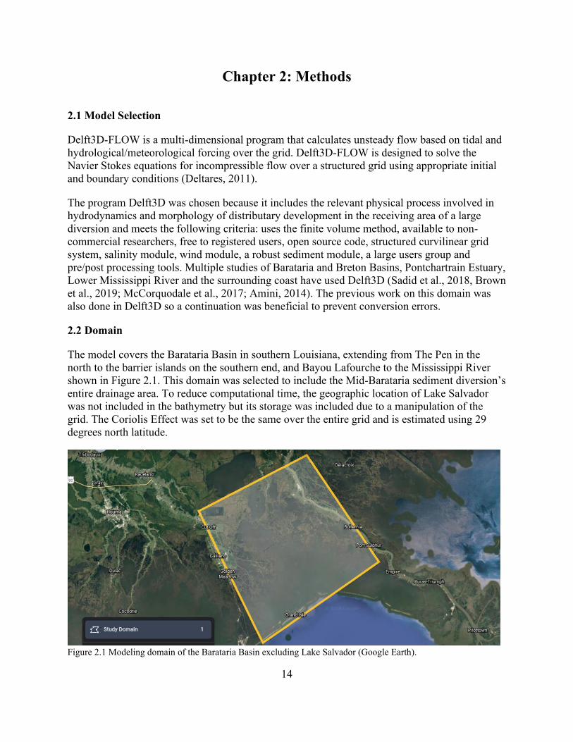
shown in Figure 2.1. This domain was selected to include the Mid-Barataria sediment diversion’s
entire drainage area. To reduce computational time, the geographic location of Lake Salvador
was not included in the bathymetry but its storage was included due to a manipulation of the
grid. The Coriolis Effect was set to be the same over the entire grid and is estimated using 29
degrees north latitude.
Figure 2.1 Modeling domain of the Barataria Basin excluding Lake Salvador (Google Earth).
15
2.3 Grid Design
Bathymetric (NOAA/CPRA) data were interpolated onto the grid in Delft3D. The horizontal
coordinates are in Universal Trans-Mercator zone 15R in meters, while the vertical coordinate
system is in North American Vertical Datum of 1988 (NAVD88) also in meters. A total of 561
longitudinal nodes and 901 lateral nodes were assigned to discretize the domain into a grid.
These nodes created 505,461 cells with a maximum size of 10000 m2 and a minimum size of 400
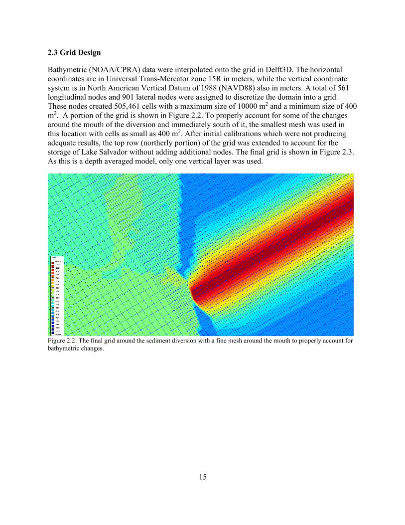
m2. A portion of the grid is shown in Figure 2.2. To properly account for some of the changes
around the mouth of the diversion and immediately south of it, the smallest mesh was used in
this location with cells as small as 400 m2. After initial calibrations which were not producing
adequate results, the top row (northerly portion) of the grid was extended to account for the
storage of Lake Salvador without adding additional nodes. The final grid is shown in Figure 2.3.
As this is a depth averaged model, only one vertical layer was used.
Figure 2.2: The final grid around the sediment diversion with a fine mesh around the mouth to properly account for
bathymetric changes.
16
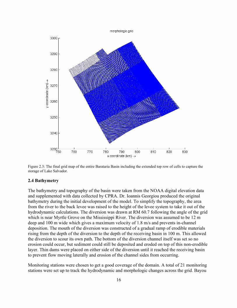
Figure 2.3: The final grid map of the entire Barataria Basin including the extended top row of cells to capture the
storage of Lake Salvador.
2.4 Bathymetry
The bathymetry and topography of the basin were taken from the NOAA digital elevation data
and supplemented with data collected by CPRA. Dr. Ioannis Georgiou produced the original
bathymetry during the initial development of the model. To simplify the topography, the area
from the river to the back levee was raised to the height of the levee system to take it out of the
hydrodynamic calculations. The diversion was drawn at RM 60.7 following the angle of the grid
which is near Myrtle Grove on the Mississippi River. The diversion was assumed to be 12 m
deep and 100 m wide which gives a maximum velocity of 1.8 m/s and prevents in-channel
deposition. The mouth of the diversion was constructed of a gradual ramp of erodible materials
rising from the depth of the diversion to the depth of the receiving basin in 100 m. This allowed
the diversion to scour its own path. The bottom of the diversion channel itself was set so no
erosion could occur, but sediment could still be deposited and eroded on top of this non-erodible
layer. Thin dams were placed on either side of the diversion until it reached the receiving basin
to prevent flow moving laterally and erosion of the channel sides from occurring.
Monitoring stations were chosen to get a good coverage of the domain. A total of 21 monitoring
stations were set up to track the hydrodynamic and morphologic changes across the grid. Bayou
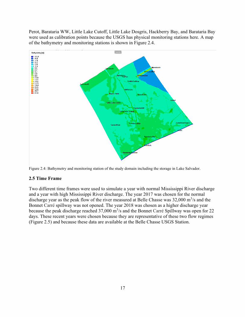
17
Perot, Barataria WW, Little Lake Cutoff, Little Lake Dosgris, Hackberry Bay, and Barataria Bay
were used as calibration points because the USGS has physical monitoring stations here. A map
of the bathymetry and monitoring stations is shown in Figure 2.4.
Figure 2.4: Bathymetry and monitoring station of the study domain including the storage in Lake Salvador.
2.5 Time Frame
Two different time frames were used to simulate a year with normal Mississippi River discharge
and a year with high Mississippi River discharge. The year 2017 was chosen for the normal
discharge year as the peak flow of the river measured at Belle Chasse was 32,000 m3/s and the
Bonnet Carré spillway was not opened. The year 2018 was chosen as a higher discharge year
because the peak discharge reached 37,000 m3/s and the Bonnet Carré Spillway was open for 22
days. These recent years were chosen because they are representative of these two flow regimes
(Figure 2.5) and because these data are available at the Belle Chasse USGS Station.
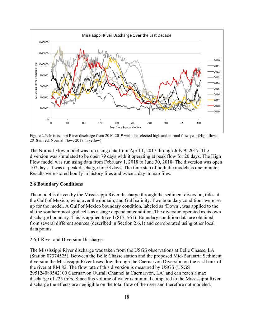
18
Figure 2.5: Mississippi River discharge from 2010-2019 with the selected high and normal flow year (High flow:
2018 in red. Normal Flow: 2017 in yellow)
The Normal Flow model was run using data from April 1, 2017 through July 9, 2017. The
diversion was simulated to be open 79 days with it operating at peak flow for 20 days. The High
Flow model was run using data from February 1, 2018 to June 30, 2018. The diversion was open
107 days. It was at peak discharge for 53 days. The time step of both the models is one minute.
Results were stored hourly in history files and twice a day in map files.
2.6 Boundary Conditions
The model is driven by the Mississippi River discharge through the sediment diversion, tides at
the Gulf of Mexico, wind over the domain, and Gulf salinity. Two boundary conditions were set
up for the model. A Gulf of Mexico boundary condition, labeled as ‘Down’, was applied to the
all the southernmost grid cells as a stage dependent condition. The diversion operated as its own
discharge boundary. This is applied to cell (817, 561). Boundary condition data are obtained
from several different sources (described in Section 2.6.1) and corroborated using other local
data points.
2.6.1 River and Diversion Discharge
The Mississippi River discharge was taken from the USGS observations at Belle Chasse, LA
(Station 07374525). Between the Belle Chasse station and the proposed Mid-Barataria Sediment
diversion the Mississippi River loses flow through the Caernarvon Diversion on the east bank of
the river at RM 82. The flow rate of this diversion is measured by USGS (USGS
295124089542100 Caernarvon Outfall Channel at Caernarvon, LA) and can reach a max
discharge of 225 m3/s. Since this volume of water is minimal compared to the Mississippi River
discharge the effects are negligible on the total flow of the river and therefore not modeled.
0
200000
400000
600000
800000
1000000
1200000
1400000
0 40 80 120 160 200 240 280 320 360
MississippiRiverDischarge(cfs)
DaysSinceStartoftheYear
MississippiRiverDischargeOvertheLastDecade
2010
2011
2012
2013
2014
2015
2016
2017
2018
2019
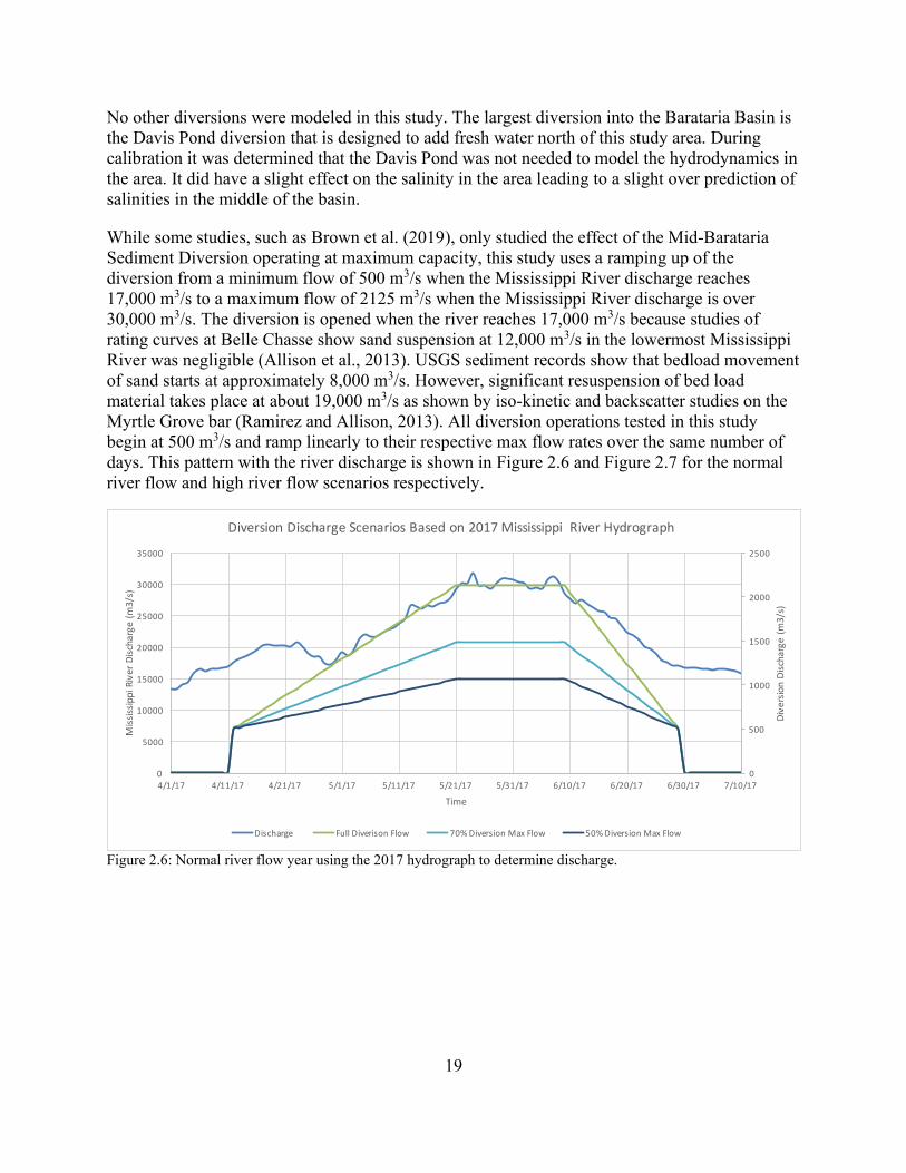
19
No other diversions were modeled in this study. The largest diversion into the Barataria Basin is
the Davis Pond diversion that is designed to add fresh water north of this study area. During
calibration it was determined that the Davis Pond was not needed to model the hydrodynamics in
the area. It did have a slight effect on the salinity in the area leading to a slight over prediction of
salinities in the middle of the basin.
While some studies, such as Brown et al. (2019), only studied the effect of the Mid-Barataria
Sediment Diversion operating at maximum capacity, this study uses a ramping up of the
diversion from a minimum flow of 500 m3/s when the Mississippi River discharge reaches
17,000 m3/s to a maximum flow of 2125 m3/s when the Mississippi River discharge is over
30,000 m3/s. The diversion is opened when the river reaches 17,000 m3/s because studies of
rating curves at Belle Chasse show sand suspension at 12,000 m3/s in the lowermost Mississippi
River was negligible (Allison et al., 2013). USGS sediment records show that bedload movement
of sand starts at approximately 8,000 m3/s. However, significant resuspension of bed load
material takes place at about 19,000 m3/s as shown by iso-kinetic and backscatter studies on the
Myrtle Grove bar (Ramirez and Allison, 2013). All diversion operations tested in this study
begin at 500 m3/s and ramp linearly to their respective max flow rates over the same number of
days. This pattern with the river discharge is shown in Figure 2.6 and Figure 2.7 for the normal
river flow and high river flow scenarios respectively.
Figure 2.6: Normal river flow year using the 2017 hydrograph to determine discharge.
0
500
1000
1500
2000
2500
0
5000
10000
15000
20000
25000
30000
35000
4/1/17 4/11/17 4/21/17 5/1/17 5/11/17 5/21/17 5/31/17 6/10/17 6/20/17 6/30/17 7/10/17DiversionDischarge(m3/s)
MississippiRiverDischarge(m3/s)
Time
DiversionDischargeScenariosBasedon2017MississippiRiverHydrograph
Discharge FullDiverisonFlow 70%DiversionMaxFlow 50%DiversionMaxFlow
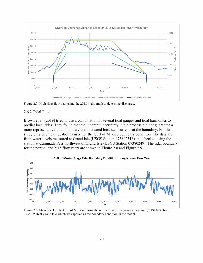
20
Figure 2.7: High river flow year using the 2018 hydrograph to determine discharge.
2.6.2 Tidal Flux
Brown et al. (2019) tried to use a combination of several tidal gauges and tidal harmonics to
predict local tides. They found that the inherent uncertainty in the process did not guarantee a
more representative tidal boundary and it created localized currents at the boundary. For this
study only one tidal location is used for the Gulf of Mexico boundary condition. The data are
from water levels measured at Grand Isle (USGS Station 073802516) and checked using the
station at Caminada Pass northwest of Grand Isle (USGS Station 07380249). The tidal boundary
for the normal and high flow years are shown in Figure 2.8 and Figure 2.9.
Figure 2.8: Stage level of the Gulf of Mexico during the normal river flow year as measure by USGS Station
073802516 at Grand Isle which was applied as the boundary condition in the model.
0
500
1000
1500
2000
2500
0
5000
10000
15000
20000
25000
30000
35000
40000
2/1/18 2/21/18 3/13/18 4/2/18 4/22/18 5/12/18 6/1/18 6/21/18
DiversionDischarge(m3/s)
MississippiRiverDischarge(m3/s)
Time
DiversionDischargeScenariosBasedon2018MississippiRiverHydrograph
RiverDischarge FullDiverisonFlow 70%DiversionMaxFlow 50%DiverionMaxFlow
-0.40
-0.20
0.00
0.20
0.40
0.60
0.80
1.00
4/1/17 4/11/17 4/21/17 5/1/17 5/11/17 5/21/17 5/31/17 6/10/17 6/20/17 6/30/17 7/10/17
GulfofM
exicoStageHeight(m)
Time
GulfofMexicoStageTidalBoundaryConditionduringNormalFlowYear
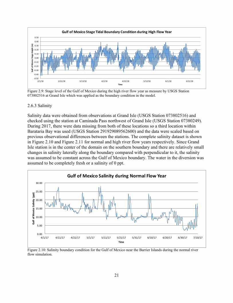
21
Figure 2.9: Stage level of the Gulf of Mexico during the high river flow year as measure by USGS Station
073802516 at Grand Isle which was applied as the boundary condition in the model.
2.6.3 Salinity
Salinity data were obtained from observations at Grand Isle (USGS Station 073802516) and
checked using the station at Caminada Pass northwest of Grand Isle (USGS Station 07380249).
During 2017, there were data missing from both of these locations so a third location within
Barataria Bay was used (USGS Station 291929089562600) and the data were scaled based on
previous observational differences between the stations. The complete salinity dataset is shown
in Figure 2.10 and Figure 2.11 for normal and high river flow years respectively. Since Grand
Isle station is in the center of the domain on the southern boundary and there are relatively small
changes in salinity laterally along the boundary compared with perpendicular to it, the salinity
was assumed to be constant across the Gulf of Mexico boundary. The water in the diversion was
assumed to be completely fresh or a salinity of 0 ppt.
Figure 2.10: Salinity boundary condition for the Gulf of Mexico near the Barrier Islands during the normal river
flow simulation.
-0.50
-0.40
-0.30
-0.20
-0.10
0.00
0.10
0.20
0.30
0.40
0.50
2/1/18 2/21/18 3/13/18 4/2/18 4/22/18 5/12/18 6/1/18 6/21/18
GulfofM
exicoStageHeight(m
)
Time
GulfofMexicoStageTidalBoundaryConditionduringHighFlowYear
0.00
5.00
10.00
15.00
20.00
25.00
30.00
4/1/17 4/11/17 4/21/17 5/1/17 5/11/17 5/21/17 5/31/17 6/10/17 6/20/17 6/30/17 7/10/17
GulfofM
exicoSalinity(ppt)
Time
GulfofMexicoSalinityduringNormalFlowYear
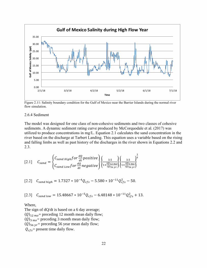
22
Figure 2.11: Salinity boundary condition for the Gulf of Mexico near the Barrier Islands during the normal river
flow simulation.
2.6.4 Sediment
The model was designed for one class of non-cohesive sediments and two classes of cohesive
sediments. A dynamic sediment rating curve produced by McCorquodale et al. (2017) was
utilized to produce concentrations in mg/L. Equation 2.1 calculates the sand concentration in the
river based on the discharge at Tarbert Landing. This equation uses a variable based on the rising
and falling limbs as well as past history of the discharges in the river shown in Equations 2.2 and
2.3.
[2.1] 𝐶𝑠𝑎𝑛𝑑 = {𝐶𝑠𝑎𝑛𝑑 𝐻𝑖𝑔ℎ𝑓𝑜𝑟
𝑑𝑄
𝑑𝑡𝑝𝑜𝑠𝑖𝑡𝑖𝑣𝑒
𝐶𝑠𝑎𝑛𝑑 𝐿𝑜𝑤𝑓𝑜𝑟𝑑𝑄
𝑑𝑡𝑛𝑒𝑔𝑎𝑡𝑖𝑣𝑒
} {3.5
1+⟨𝑄⟩12 𝑚𝑜⟨𝑄⟩56 𝑦𝑟
} {3.5
1+⟨𝑄⟩3 𝑚𝑜⟨𝑄⟩56 𝑦𝑟
}
3
4
[2.2] 𝐶𝑠𝑎𝑛𝑑 ℎ𝑖𝑔ℎ = 1.7327 ∗ 10−4𝑄𝑐𝑓𝑠 − 5.580 ∗ 10−11𝑄𝑐𝑓𝑠
2 − 50.
[2.3] 𝐶𝑠𝑎𝑛𝑑 𝑙𝑜𝑤 = 15.48667 ∗ 10−5𝑄𝑐𝑓𝑠 − 6.48148 ∗ 10−11𝑄𝑐𝑓𝑠
2 + 13.
Where,
The sign of dQ/dt is based on a 6 day average; ⟨𝑄⟩12 𝑚𝑜= preceding 12 month mean daily flow; ⟨𝑄⟩3 𝑚𝑜= preceding 3 month mean daily flow; ⟨𝑄⟩56 𝑦𝑟= preceding 56 year mean daily flow;
𝑄𝑐𝑓𝑠= present time daily flow.
0.00
5.00
10.00
15.00
20.00
25.00
30.00
35.00
2/1/18 3/3/18 4/2/18 5/2/18 6/1/18 7/1/18
GulfofM
exicoSalinity(ppt)
Time
GulfofMexicoSalinityduringHighFlowYear
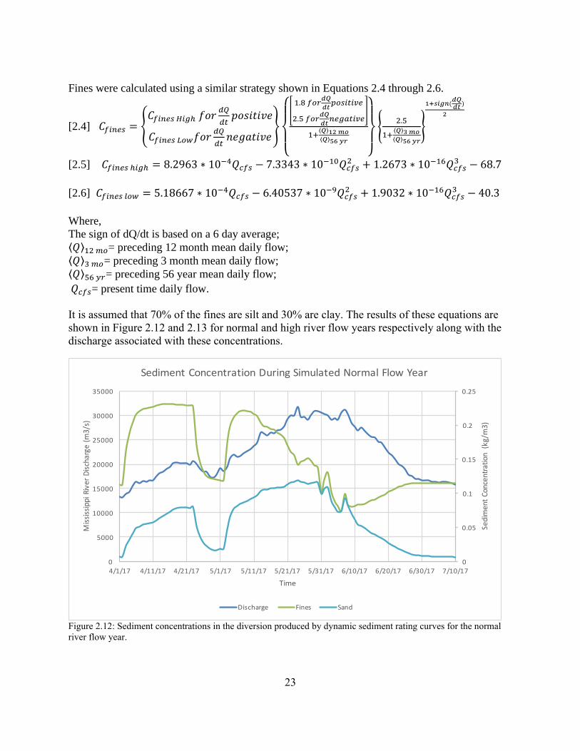
23
Fines were calculated using a similar strategy shown in Equations 2.4 through 2.6.
[2.4] 𝐶𝑓𝑖𝑛𝑒𝑠 = {𝐶𝑓𝑖𝑛𝑒𝑠 𝐻𝑖𝑔ℎ 𝑓𝑜𝑟
𝑑𝑄
𝑑𝑡𝑝𝑜𝑠𝑖𝑡𝑖𝑣𝑒
𝐶𝑓𝑖𝑛𝑒𝑠 𝐿𝑜𝑤𝑓𝑜𝑟𝑑𝑄
𝑑𝑡𝑛𝑒𝑔𝑎𝑡𝑖𝑣𝑒
}
{
[
1.8 𝑓𝑜𝑟𝑑𝑄
𝑑𝑡𝑝𝑜𝑠𝑖𝑡𝑖𝑣𝑒
2.5 𝑓𝑜𝑟𝑑𝑄
𝑑𝑡𝑛𝑒𝑔𝑎𝑡𝑖𝑣𝑒
]
1+⟨𝑄⟩12 𝑚𝑜⟨𝑄⟩56 𝑦𝑟
}
{2.5
1+⟨𝑄⟩3 𝑚𝑜⟨𝑄⟩56 𝑦𝑟
}
1+𝑠𝑖𝑔𝑛(𝑑𝑄𝑑𝑡)
2
[2.5] 𝐶𝑓𝑖𝑛𝑒𝑠 ℎ𝑖𝑔ℎ = 8.2963 ∗ 10−4𝑄𝑐𝑓𝑠 − 7.3343 ∗ 10
−10𝑄𝑐𝑓𝑠2 + 1.2673 ∗ 10−16𝑄𝑐𝑓𝑠
3 − 68.7
[2.6] 𝐶𝑓𝑖𝑛𝑒𝑠 𝑙𝑜𝑤 = 5.18667 ∗ 10−4𝑄𝑐𝑓𝑠 − 6.40537 ∗ 10
−9𝑄𝑐𝑓𝑠2 + 1.9032 ∗ 10−16𝑄𝑐𝑓𝑠
3 − 40.3
Where,
The sign of dQ/dt is based on a 6 day average; ⟨𝑄⟩12 𝑚𝑜= preceding 12 month mean daily flow;
⟨𝑄⟩3 𝑚𝑜= preceding 3 month mean daily flow; ⟨𝑄⟩56 𝑦𝑟= preceding 56 year mean daily flow;
𝑄𝑐𝑓𝑠= present time daily flow.
It is assumed that 70% of the fines are silt and 30% are clay. The results of these equations are
shown in Figure 2.12 and 2.13 for normal and high river flow years respectively along with the
discharge associated with these concentrations.
Figure 2.12: Sediment concentrations in the diversion produced by dynamic sediment rating curves for the normal
river flow year.
0
0.05
0.1
0.15
0.2
0.25
0
5000
10000
15000
20000
25000
30000
35000
4/1/17 4/11/17 4/21/17 5/1/17 5/11/17 5/21/17 5/31/17 6/10/17 6/20/17 6/30/17 7/10/17
SedimentConcentration(kg/m3)
MississippiRiverDischarge(m3/s)
Time
SedimentConcentrationDuringSimulatedNormalFlowYear
Discharge Fines Sand
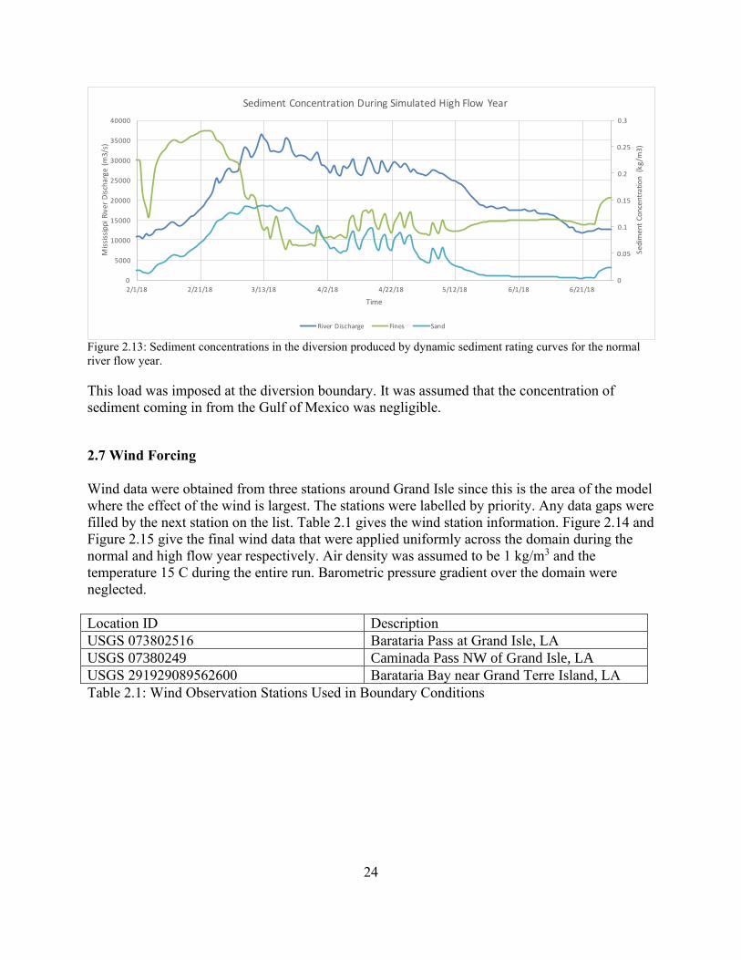
24
Figure 2.13: Sediment concentrations in the diversion produced by dynamic sediment rating curves for the normal
river flow year.
This load was imposed at the diversion boundary. It was assumed that the concentration of
sediment coming in from the Gulf of Mexico was negligible.
2.7 Wind Forcing
Wind data were obtained from three stations around Grand Isle since this is the area of the model
where the effect of the wind is largest. The stations were labelled by priority. Any data gaps were
filled by the next station on the list. Table 2.1 gives the wind station information. Figure 2.14 and
Figure 2.15 give the final wind data that were applied uniformly across the domain during the
normal and high flow year respectively. Air density was assumed to be 1 kg/m3 and the
temperature 15 C during the entire run. Barometric pressure gradient over the domain were
neglected.
Location ID Description
USGS 073802516 Barataria Pass at Grand Isle, LA
USGS 07380249 Caminada Pass NW of Grand Isle, LA
USGS 291929089562600 Barataria Bay near Grand Terre Island, LA
Table 2.1: Wind Observation Stations Used in Boundary Conditions
0
0.05
0.1
0.15
0.2
0.25
0.3
0
5000
10000
15000
20000
25000
30000
35000
40000
2/1/18 2/21/18 3/13/18 4/2/18 4/22/18 5/12/18 6/1/18 6/21/18
SedimentConcentration(kg/m3)
MississippiRiverDischarge(m3/s)
Time
SedimentConcentrationDuringSimulatedHighFlowYear
RiverDischarge Fines Sand
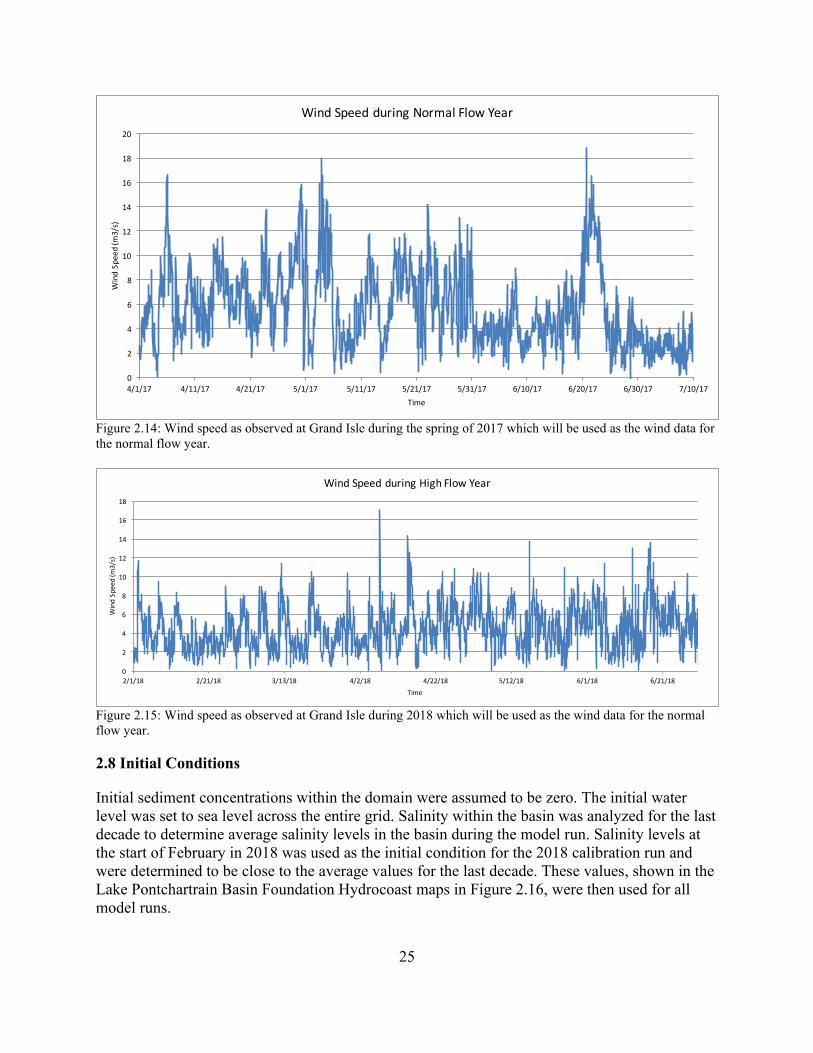
25
Figure 2.14: Wind speed as observed at Grand Isle during the spring of 2017 which will be used as the wind data for
the normal flow year.
Figure 2.15: Wind speed as observed at Grand Isle during 2018 which will be used as the wind data for the normal
flow year.
2.8 Initial Conditions
Initial sediment concentrations within the domain were assumed to be zero. The initial water
level was set to sea level across the entire grid. Salinity within the basin was analyzed for the last
decade to determine average salinity levels in the basin during the model run. Salinity levels at
the start of February in 2018 was used as the initial condition for the 2018 calibration run and
were determined to be close to the average values for the last decade. These values, shown in the
Lake Pontchartrain Basin Foundation Hydrocoast maps in Figure 2.16, were then used for all
model runs.
0
2
4
6
8
10
12
14
16
18
20
4/1/17 4/11/17 4/21/17 5/1/17 5/11/17 5/21/17 5/31/17 6/10/17 6/20/17 6/30/17 7/10/17
WindSpeed(m
3/s)
Time
WindSpeedduringNormalFlowYear
0
2
4
6
8
10
12
14
16
18
2/1/18 2/21/18 3/13/18 4/2/18 4/22/18 5/12/18 6/1/18 6/21/18
WindSpeed(m
3/s)
Time
WindSpeedduringHighFlowYear
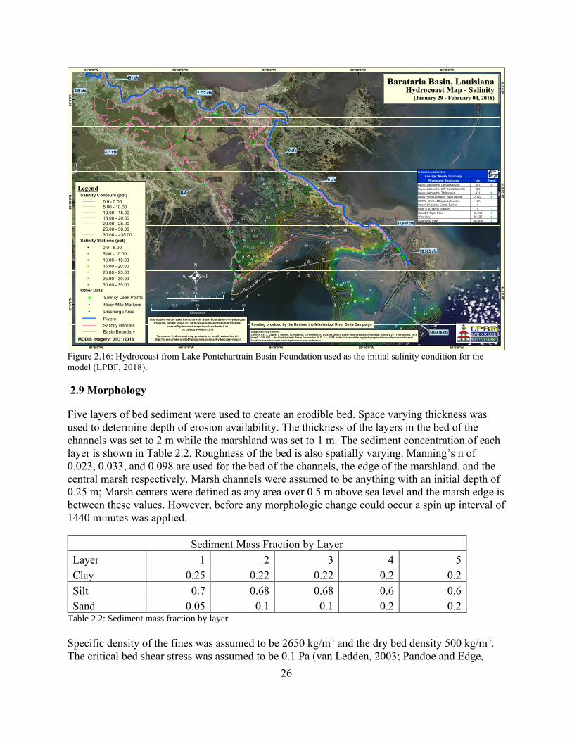
26
Figure 2.16: Hydrocoast from Lake Pontchartrain Basin Foundation used as the initial salinity condition for the
model (LPBF, 2018).
2.9 Morphology
Five layers of bed sediment were used to create an erodible bed. Space varying thickness was
used to determine depth of erosion availability. The thickness of the layers in the bed of the
channels was set to 2 m while the marshland was set to 1 m. The sediment concentration of each
layer is shown in Table 2.2. Roughness of the bed is also spatially varying. Manning’s n of
0.023, 0.033, and 0.098 are used for the bed of the channels, the edge of the marshland, and the
central marsh respectively. Marsh channels were assumed to be anything with an initial depth of
0.25 m; Marsh centers were defined as any area over 0.5 m above sea level and the marsh edge is
between these values. However, before any morphologic change could occur a spin up interval of
1440 minutes was applied.
Sediment Mass Fraction by Layer
Layer 1 2 3 4 5
Clay 0.25 0.22 0.22 0.2 0.2
Silt 0.7 0.68 0.68 0.6 0.6
Sand 0.05 0.1 0.1 0.2 0.2 Table 2.2: Sediment mass fraction by layer
Specific density of the fines was assumed to be 2650 kg/m3 and the dry bed density 500 kg/m3.
The critical bed shear stress was assumed to be 0.1 Pa (van Ledden, 2003; Pandoe and Edge,
27
2008; Deltares, 2013; Ghose Hajra et al., 2014). Sand was assumed to have a dry bed density of
1600 kg/m3 and a D50 of 183.34 mm. Settling velocity of each sediment class is laid out in Table
2.3.
Sediment Type Settling velocity
Clay 0.00275 mm/s unflocculated (Mikes and Manning, 2010; Reins, 2018)
Silt 0.71 mm/s (Maggi, 2013; Reins, 2018)
Sand Use Van Rijn 84 equations to predict settling with a reference height of 1 and
a threshold sediment thickness of 0.05m
Table 2.3: Settling velocity parameters based on sediment type
2.10 Changing Conditions
Day et al. (2012) and Blankespoor et al. (2012) find that coastal restoration and protection
projects should consider the impacts of relative sea level rise when predicting benefits. Since,
this model is only looking at the early development of the distributary channels sea level rise was
not simulated. Likewise, no large storms were modeled in the selected scenarios.
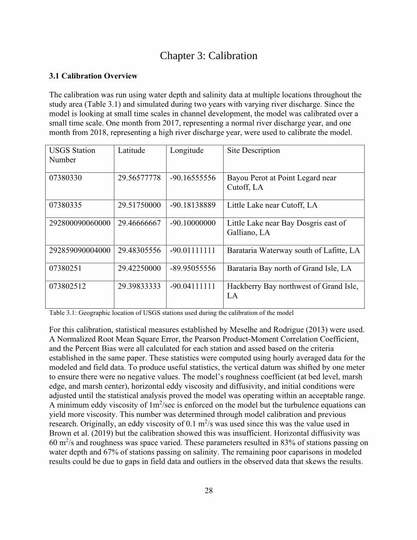
28
Chapter 3: Calibration
3.1 Calibration Overview
The calibration was run using water depth and salinity data at multiple locations throughout the
study area (Table 3.1) and simulated during two years with varying river discharge. Since the
model is looking at small time scales in channel development, the model was calibrated over a
small time scale. One month from 2017, representing a normal river discharge year, and one
month from 2018, representing a high river discharge year, were used to calibrate the model.
USGS Station
Number
Latitude Longitude Site Description
07380330 29.56577778 -90.16555556 Bayou Perot at Point Legard near
Cutoff, LA
07380335 29.51750000 -90.18138889 Little Lake near Cutoff, LA
292800090060000 29.46666667 -90.10000000 Little Lake near Bay Dosgris east of
Galliano, LA
292859090004000 29.48305556 -90.01111111 Barataria Waterway south of Lafitte, LA
07380251 29.42250000 -89.95055556 Barataria Bay north of Grand Isle, LA
073802512 29.39833333 -90.04111111
Hackberry Bay northwest of Grand Isle,
LA
Table 3.1: Geographic location of USGS stations used during the calibration of the model
For this calibration, statistical measures established by Meselhe and Rodrigue (2013) were used.
A Normalized Root Mean Square Error, the Pearson Product-Moment Correlation Coefficient,
and the Percent Bias were all calculated for each station and assed based on the criteria
established in the same paper. These statistics were computed using hourly averaged data for the
modeled and field data. To produce useful statistics, the vertical datum was shifted by one meter
to ensure there were no negative values. The model’s roughness coefficient (at bed level, marsh
edge, and marsh center), horizontal eddy viscosity and diffusivity, and initial conditions were
adjusted until the statistical analysis proved the model was operating within an acceptable range.
A minimum eddy viscosity of 1m2/sec is enforced on the model but the turbulence equations can
yield more viscosity. This number was determined through model calibration and previous
research. Originally, an eddy viscosity of 0.1 m2/s was used since this was the value used in
Brown et al. (2019) but the calibration showed this was insufficient. Horizontal diffusivity was
60 m2/s and roughness was space varied. These parameters resulted in 83% of stations passing on
water depth and 67% of stations passing on salinity. The remaining poor caparisons in modeled
results could be due to gaps in field data and outliers in the observed data that skews the results.
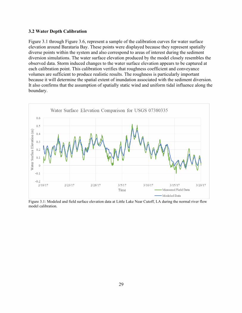
29
3.2 Water Depth Calibration
Figure 3.1 through Figure 3.6, represent a sample of the calibration curves for water surface
elevation around Barataria Bay. These points were displayed because they represent spatially
diverse points within the system and also correspond to areas of interest during the sediment
diversion simulations. The water surface elevation produced by the model closely resembles the
observed data. Storm induced changes to the water surface elevation appears to be captured at
each calibration point. This calibration verifies that roughness coefficient and conveyance
volumes are sufficient to produce realistic results. The roughness is particularly important
because it will determine the spatial extent of inundation associated with the sediment diversion.
It also confirms that the assumption of spatially static wind and uniform tidal influence along the
boundary.
Figure 3.1: Modeled and field surface elevation data at Little Lake Near Cutoff, LA during the normal river flow
model calibration.
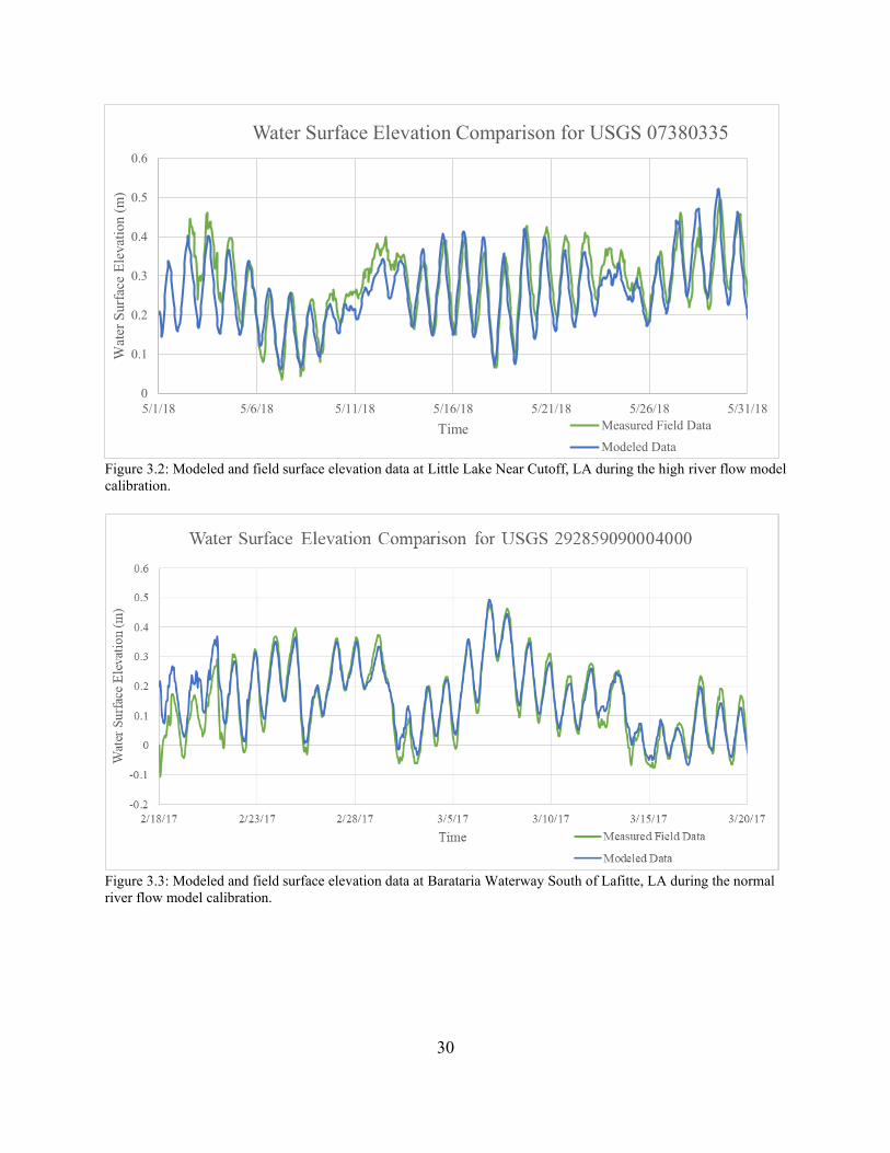
30
Figure 3.2: Modeled and field surface elevation data at Little Lake Near Cutoff, LA during the high river flow model
calibration.
Figure 3.3: Modeled and field surface elevation data at Barataria Waterway South of Lafitte, LA during the normal
river flow model calibration.
0
0.1
0.2
0.3
0.4
0.5
0.6
5/1/18 5/6/18 5/11/18 5/16/18 5/21/18 5/26/18 5/31/18
Wat
er S
urf
ace
Ele
vat
ion (
m)
Time
Water Surface Elevation Comparison for USGS 07380335
Measured Field Data
Modeled Data
31
Figure 3.4: Modeled and field surface elevation data at Barataria Waterway South of Lafitte, LA during the high
river flow model calibration.
Figure 3.5: Modeled and field surface elevation data at Barataria Bay North of Grand Isle, LA during the normal
river flow model calibration.
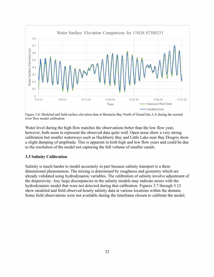
32
Figure 3.6: Modeled and field surface elevation data at Barataria Bay North of Grand Isle, LA during the normal
river flow model calibration
Water level during the high flow matches the observations better than the low flow year,
however, both seem to represent the observed data quite well. Open areas show a very strong
calibration but smaller waterways such as Hackberry Bay and Little Lake near Bay Dosgris show
a slight damping of amplitude. This is apparent in both high and low flow years and could be due
to the resolution of the model not capturing the full volume of smaller canals.
3.3 Salinity Calibration
Salinity is much harder to model accurately in part because salinity transport is a three
dimensional phenomenon. The mixing is determined by roughness and geometry which are
already validated using hydrodynamic variables. The calibration of salinity involve adjustment of
the dispersivity. Any large discrepancies in the salinity models may indicate errors with the
hydrodynamic model that were not detected during that calibration. Figures 3.7 through 3.12
show modeled and field observed hourly salinity data at various locations within the domain.
Some field observations were not available during the timeframe chosen to calibrate the model.
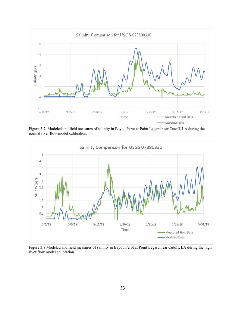
33
Figure 3.7: Modeled and field measures of salinity in Bayou Perot at Point Legard near Cutoff, LA during the
normal river flow model calibration.
Figure 3.8 Modeled and field measures of salinity in Bayou Perot at Point Legard near Cutoff, LA during the high
river flow model calibration.
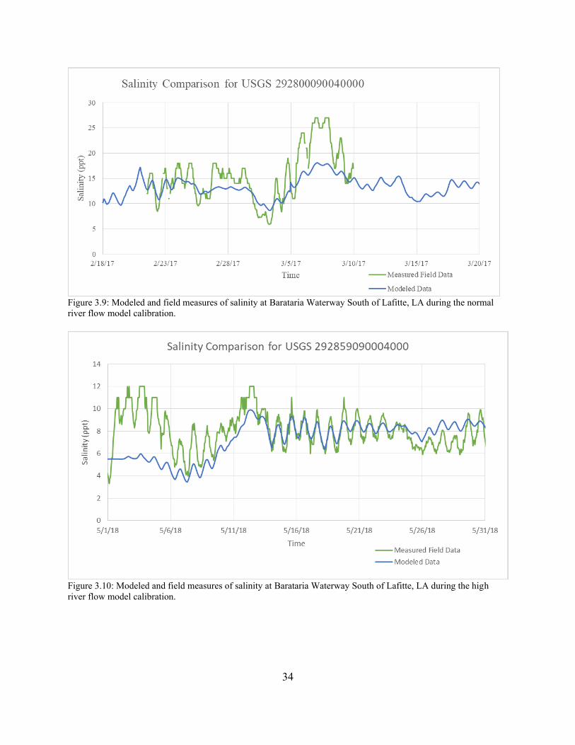
34
Figure 3.9: Modeled and field measures of salinity at Barataria Waterway South of Lafitte, LA during the normal
river flow model calibration.
Figure 3.10: Modeled and field measures of salinity at Barataria Waterway South of Lafitte, LA during the high
river flow model calibration.
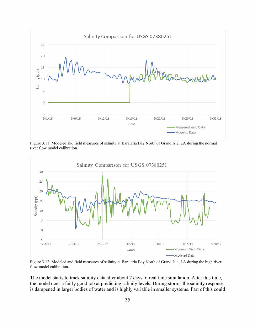
35
Figure 3.11: Modeled and field measures of salinity at Barataria Bay North of Grand Isle, LA during the normal
river flow model calibration.
Figure 3.12: Modeled and field measures of salinity at Barataria Bay North of Grand Isle, LA during the high river
flow model calibration.
The model starts to track salinity data after about 7 days of real time simulation. After this time,
the model does a fairly good job at predicting salinity levels. During storms the salinity response
is dampened in larger bodies of water and is highly variable in smaller systems. Part of this could
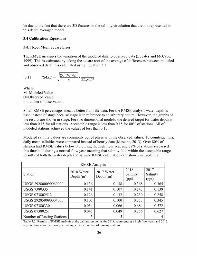
36
be due to the fact that there are 3D features in the salinity circulation that are not represented in
this depth averaged model.
3.4 Calibration Equations
3.4.1 Root Mean Square Error
The RMSE measures the variation of the modeled data to observed data (Legates and McCabe,
1999). This is estimated by taking the square root of the average of differences between modeled
and observed data. It is calculated using Equation 3.1.
[3.1] 𝑅𝑀𝑆𝐸 = √∑ (𝑀𝑖−𝑂𝑖)
2𝑛𝑖=1
𝑛∗
𝑛
∑ (𝑂𝑖)2𝑛
𝑖=1
Where,
M=Modeled Value
O=Observed Value
n=number of observations
Small RMSE percentages mean a better fit of the data. For the RMSE analysis water depth is
used instead of stage because stage is in reference to an arbitrary datum. However, the graphs of
the results are shown in stage. For two dimensional models, the desired target for water depth is
less than 0.15 for all stations. Acceptable range is less than 0.15 for 80% of stations. All of
modeled stations achieved the values of less than 0.15.
Modeled salinity values are commonly out of phase with the observed values. To counteract this,
daily mean salinities were compared instead of hourly data (Meselhe, 2013). Over 80% of
stations had RMSE values below 0.5 during the high flow year and 67% of stations surpassed
this threshold during a normal flow year meaning that salinity falls within the acceptable range.
Results of both the water depth and salinity RMSE calculations are shown in Table 3.2.
RMSE Analysis
Station 2018 Water
Depth (m)
2017 Water
Depth (m)
2018
Salinity
(ppt)
2017
Salinity
(ppt)
USGS 292800090060000 0.136 0.138 0.368 0.365
USGS 7380335 0.141 0.107 0.543 0.139
USGS 073802512 0.126 0.132 0.230 0.258
USGS 292859090004000 0.105 0.100 0.253 0.345
USGS 07380330 0.054 0.066 0.684 0.572
USGS 07380251 0.045 0.049 0.256 0.627
Number of Passing Stations 5 5 4 4
Table 3.2: Results of RMSE analysis at the calibration points for 2018, representing a high flow year, and 2017,
representing a normal flow year, along with the number of passing stations.
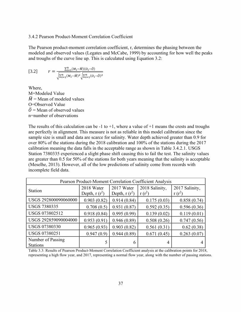
37
3.4.2 Pearson Product-Moment Correlation Coefficient
The Pearson product-moment correlation coefficient, r, determines the phasing between the
modeled and observed values (Legates and McCabe, 1999) by accounting for how well the peaks
and troughs of the curve line up. This is calculated using Equation 3.2:
[3.2] 𝑟 =∑ (𝑀𝑖−�̅�)(𝑂𝑖−�̅�)𝑛𝑖=1
√∑ (𝑀𝑖−�̅�)2𝑛
𝑖=1 √∑ (𝑂𝑖−�̅�)2𝑛
𝑖=1
Where,
M=Modeled Value
�̅� = Mean of modeled values
O=Observed Value
�̅� = Mean of observed values
n=number of observations
The results of this calculation can be -1 to +1, where a value of +1 means the crests and troughs
are perfectly in alignment. This measure is not as reliable in this model calibration since the
sample size is small and data are scarce for salinity. Water depth achieved greater than 0.9 for
over 80% of the stations during the 2018 calibration and 100% of the stations during the 2017
calibration meaning the data falls in the acceptable range as shown in Table 3.4.2.1. USGS
Station 7380335 experienced a slight phase shift causing this to fail the test. The salinity values
are greater than 0.5 for 50% of the stations for both years meaning that the salinity is acceptable
(Meselhe, 2013). However, all of the low predictions of salinity come from records with
incomplete field data.
Pearson Product-Moment Correlation Coefficient Analysis
Station 2018 Water
Depth, r (r2)
2017 Water
Depth, r (r2)
2018 Salinity,
r (r2)
2017 Salinity,
r (r2)
USGS 292800090060000 0.903 (0.82) 0.914 (0.84) 0.175 (0.03) 0.858 (0.74)
USGS 7380335 0.708 (0.5) 0.931 (0.87) 0.592 (0.35) 0.596 (0.36)
USGS 073802512 0.918 (0.84) 0.995 (0.99) 0.139 (0.02) 0.119 (0.01)
USGS 292859090004000 0.953 (0.91) 0.946 (0.89) 0.508 (0.26) 0.747 (0.56)
USGS 07380330 0.965 (0.93) 0.903 (0.82) 0.561 (0.31) 0.62 (0.38)
USGS 07380251 0.947 (0.9) 0.944 (0.89) 0.671 (0.45) 0.263 (0.07)
Number of Passing
Stations 5 6 4 4
Table 3.3: Results of Pearson Product-Moment Correlation Coefficient analysis at the calibration points for 2018,
representing a high flow year, and 2017, representing a normal flow year, along with the number of passing stations.
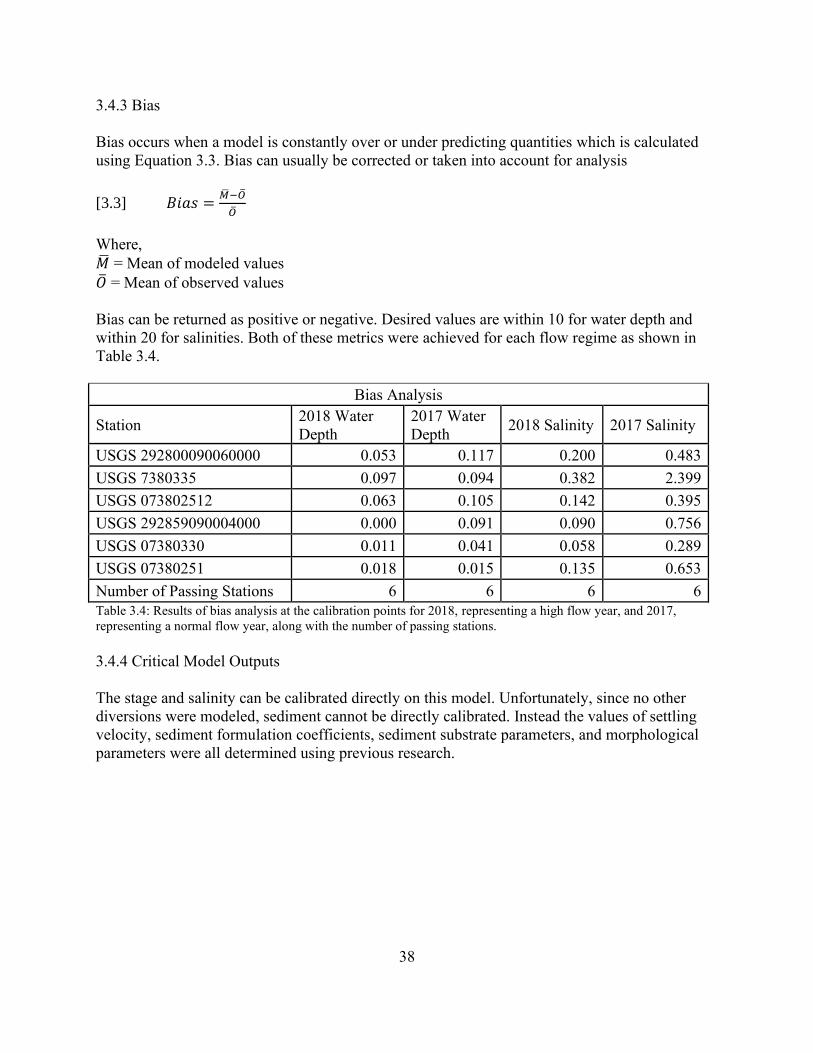
38
3.4.3 Bias
Bias occurs when a model is constantly over or under predicting quantities which is calculated
using Equation 3.3. Bias can usually be corrected or taken into account for analysis
[3.3] 𝐵𝑖𝑎𝑠 =�̅�−�̅�
�̅�
Where,
�̅� = Mean of modeled values
�̅� = Mean of observed values
Bias can be returned as positive or negative. Desired values are within 10 for water depth and
within 20 for salinities. Both of these metrics were achieved for each flow regime as shown in
Table 3.4.
Bias Analysis
Station 2018 Water
Depth
2017 Water
Depth 2018 Salinity 2017 Salinity
USGS 292800090060000 0.053 0.117 0.200 0.483
USGS 7380335 0.097 0.094 0.382 2.399
USGS 073802512 0.063 0.105 0.142 0.395
USGS 292859090004000 0.000 0.091 0.090 0.756
USGS 07380330 0.011 0.041 0.058 0.289
USGS 07380251 0.018 0.015 0.135 0.653
Number of Passing Stations 6 6 6 6
Table 3.4: Results of bias analysis at the calibration points for 2018, representing a high flow year, and 2017,
representing a normal flow year, along with the number of passing stations.
3.4.4 Critical Model Outputs
The stage and salinity can be calibrated directly on this model. Unfortunately, since no other
diversions were modeled, sediment cannot be directly calibrated. Instead the values of settling
velocity, sediment formulation coefficients, sediment substrate parameters, and morphological
parameters were all determined using previous research.
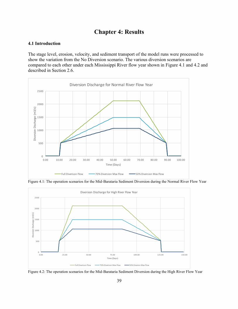
39
Chapter 4: Results
4.1 Introduction
The stage level, erosion, velocity, and sediment transport of the model runs were processed to
show the variation from the No Diversion scenario. The various diversion scenarios are
compared to each other under each Mississippi River flow year shown in Figure 4.1 and 4.2 and
described in Section 2.6.
Figure 4.1: The operation scenarios for the Mid-Barataria Sediment Diversion during the Normal River Flow Year
Figure 4.2: The operation scenarios for the Mid-Barataria Sediment Diversion during the High River Flow Year
0
500
1000
1500
2000
2500
0.00 10.00 20.00 30.00 40.00 50.00 60.00 70.00 80.00 90.00 100.00
DiversionDischarge(m3/s)
Time(Days)
DiversionDischargeforNormalRiverFlowYear
FullDiverisonFlow 70%DiversionMaxFlow 50%DiversionMaxFlow
0
500
1000
1500
2000
2500
0.00 25.00 50.00 75.00 100.00 125.00 150.00
DiversionDischarge(m3/s)
Time(Days)
DiversionDischargeforHighRiverFlowYear
FullDiverisonFlow 70%DiversionMaxFlow 50%DiverionMaxFlow
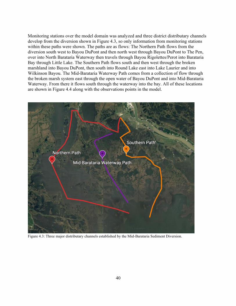
40
Monitoring stations over the model domain was analyzed and three district distributary channels
develop from the diversion shown in Figure 4.3, so only information from monitoring stations
within these paths were shown. The paths are as flows: The Northern Path flows from the
diversion south west to Bayou DuPont and then north west through Bayou DuPont to The Pen,
over into North Barataria Waterway then travels through Bayou Rigolettes/Perot into Barataria
Bay through Little Lake. The Southern Path flows south and then west through the broken
marshland into Bayou DuPont, then south into Round Lake east into Lake Laurier and into
Wilkinson Bayou. The Mid-Barataria Waterway Path comes from a collection of flow through
the broken marsh system east through the open water of Bayou DuPont and into Mid-Barataria
Waterway. From there it flows south through the waterway into the bay. All of these locations
are shown in Figure 4.4 along with the observations points in the model.
Figure 4.3: Three major distributary channels established by the Mid-Barataria Sediment Diversion.
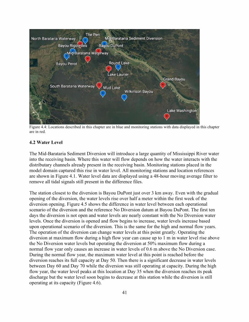
41
Figure 4.4: Locations described in this chapter are in blue and monitoring stations with data displayed in this chapter
are in red.
4.2 Water Level
The Mid-Barataria Sediment Diversion will introduce a large quantity of Mississippi River water
into the receiving basin. Where this water will flow depends on how the water interacts with the
distributary channels already present in the receiving basin. Monitoring stations placed in the
model domain captured this rise in water level. All monitoring stations and location references
are shown in Figure 4.1. Water level data are displayed using a 48-hour moving average filter to
remove all tidal signals still present in the difference files.
The station closest to the diversion is Bayou DuPont just over 3 km away. Even with the gradual
opening of the diversion, the water levels rise over half a meter within the first week of the
diversion opening. Figure 4.5 shows the difference in water level between each operational
scenario of the diversion and the reference No Diversion datum at Bayou DuPont. The first ten
days the diversion is not open and water levels are nearly constant with the No Diversion water
levels. Once the diversion is opened and flow begins to increase, water levels increase based
upon operational scenario of the diversion. This is the same for the high and normal flow years.
The operation of the diversion can change water levels at this point greatly. Operating the
diversion at maximum flow during a high flow year can cause up to 1 m in water level rise above
the No Diversion water levels but operating the diversion at 50% maximum flow during a
normal flow year only causes an increase in water levels of 0.6 m above the No Diversion case.
During the normal flow year, the maximum water level at this point is reached before the
diversion reaches its full capacity at Day 50. Then there is a significant decrease in water levels
between Day 60 and Day 70 while the diversion was still operating at capacity. During the high
flow year, the water level peaks at this location at Day 35 when the diversion reaches its peak
discharge but the water level soon begins to decrease at this station while the diversion is still
operating at its capacity (Figure 4.6).
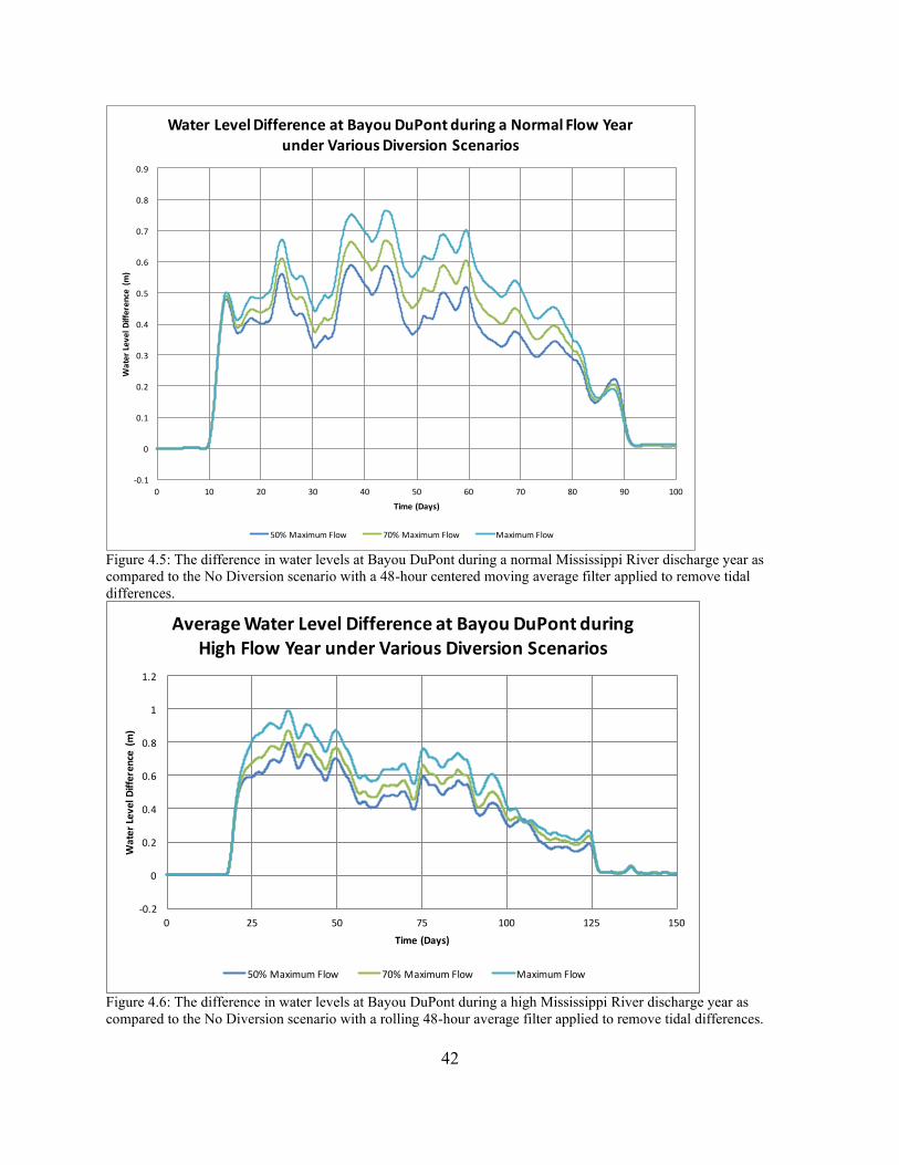
42
Figure 4.5: The difference in water levels at Bayou DuPont during a normal Mississippi River discharge year as
compared to the No Diversion scenario with a 48-hour centered moving average filter applied to remove tidal
differences.
Figure 4.6: The difference in water levels at Bayou DuPont during a high Mississippi River discharge year as
compared to the No Diversion scenario with a rolling 48-hour average filter applied to remove tidal differences.
-0.1
0
0.1
0.2
0.3
0.4
0.5
0.6
0.7
0.8
0.9
0 10 20 30 40 50 60 70 80 90 100
WaterLevelD
ifference(m
)
Time(Days)
WaterLevelDifferenceatBayouDuPontduringaNormalFlowYearunderVariousDiversionScenarios
50%MaximumFlow 70%MaximumFlow MaximumFlow
-0.2
0
0.2
0.4
0.6
0.8
1
1.2
0 25 50 75 100 125 150
WaterLevelDifference(m)
Time(Days)
AverageWaterLevelDifferenceatBayouDuPontduringHighFlowYearunderVariousDiversionScenarios
50%MaximumFlow 70%MaximumFlow MaximumFlow
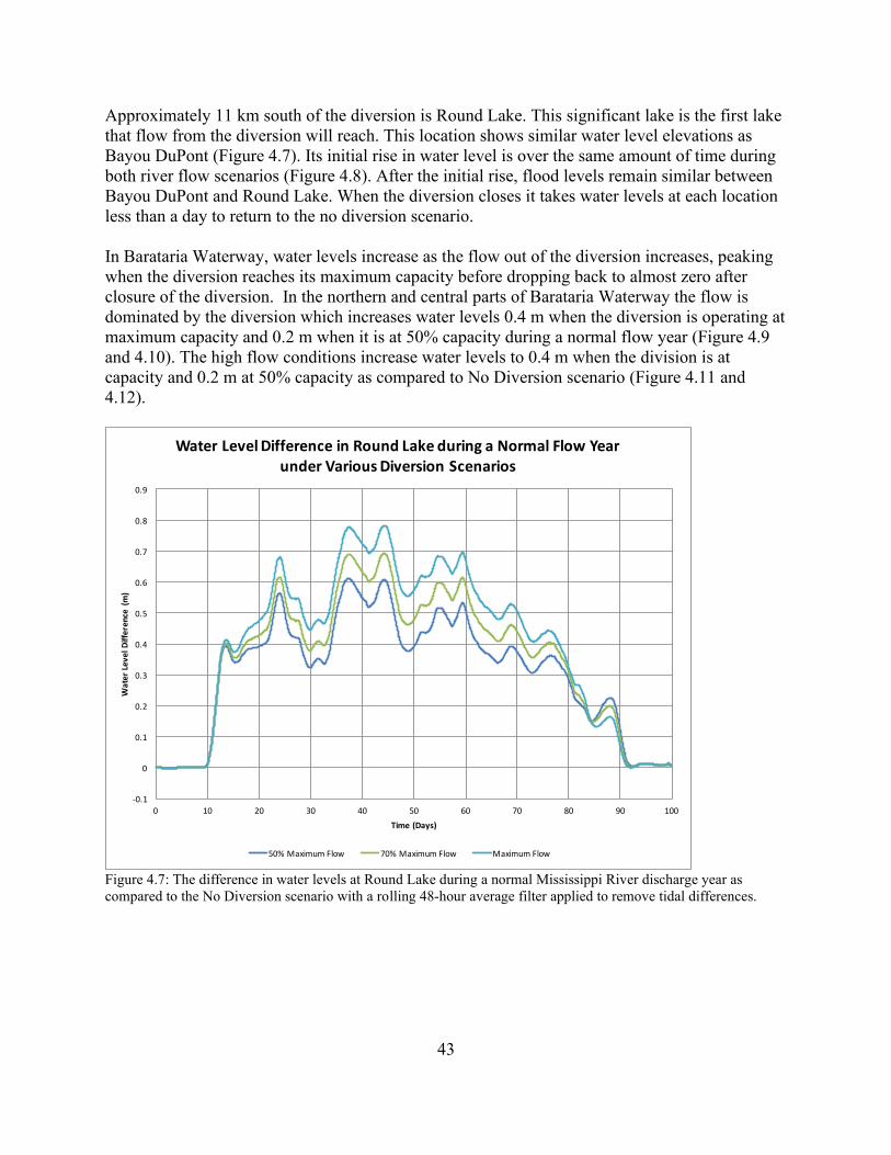
43
Approximately 11 km south of the diversion is Round Lake. This significant lake is the first lake
that flow from the diversion will reach. This location shows similar water level elevations as
Bayou DuPont (Figure 4.7). Its initial rise in water level is over the same amount of time during
both river flow scenarios (Figure 4.8). After the initial rise, flood levels remain similar between
Bayou DuPont and Round Lake. When the diversion closes it takes water levels at each location
less than a day to return to the no diversion scenario.
In Barataria Waterway, water levels increase as the flow out of the diversion increases, peaking
when the diversion reaches its maximum capacity before dropping back to almost zero after
closure of the diversion. In the northern and central parts of Barataria Waterway the flow is
dominated by the diversion which increases water levels 0.4 m when the diversion is operating at
maximum capacity and 0.2 m when it is at 50% capacity during a normal flow year (Figure 4.9
and 4.10). The high flow conditions increase water levels to 0.4 m when the division is at
capacity and 0.2 m at 50% capacity as compared to No Diversion scenario (Figure 4.11 and
4.12).
Figure 4.7: The difference in water levels at Round Lake during a normal Mississippi River discharge year as
compared to the No Diversion scenario with a rolling 48-hour average filter applied to remove tidal differences.
-0.1
0
0.1
0.2
0.3
0.4
0.5
0.6
0.7
0.8
0.9
0 10 20 30 40 50 60 70 80 90 100
WaterLevelD
ifference(m
)
Time(Days)
WaterLevelDifferenceinRoundLakeduringaNormalFlowYearunderVariousDiversionScenarios
50%MaximumFlow 70%MaximumFlow MaximumFlow
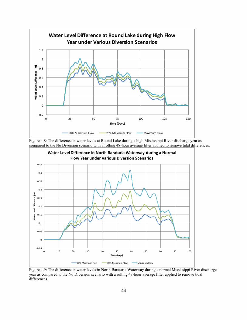
44
Figure 4.8: The difference in water levels at Round Lake during a high Mississippi River discharge year as
compared to the No Diversion scenario with a rolling 48-hour average filter applied to remove tidal differences.
Figure 4.9: The difference in water levels in North Barataria Waterway during a normal Mississippi River discharge
year as compared to the No Diversion scenario with a rolling 48-hour average filter applied to remove tidal
differences.
-0.2
0
0.2
0.4
0.6
0.8
1
1.2
0 25 50 75 100 125 150
WaterLevelDifference(m)
Time(Days)
WaterLevelDifferenceatRoundLakeduringHighFlowYearunderVariousDiversionScenarios
50%MaximumFlow 70%MaximumFlow MaximumFlow
-0.05
0
0.05
0.1
0.15
0.2
0.25
0.3
0.35
0.4
0.45
0 10 20 30 40 50 60 70 80 90 100
WaterLevelD
ifference(m
)
Time(Days)
WaterLevelDifferenceinNorthBaratariaWaterwayduringaNormalFlowYearunderVariousDiversionScenarios
50%MaximumFlow 70%MaximumFlow MaximumFlow
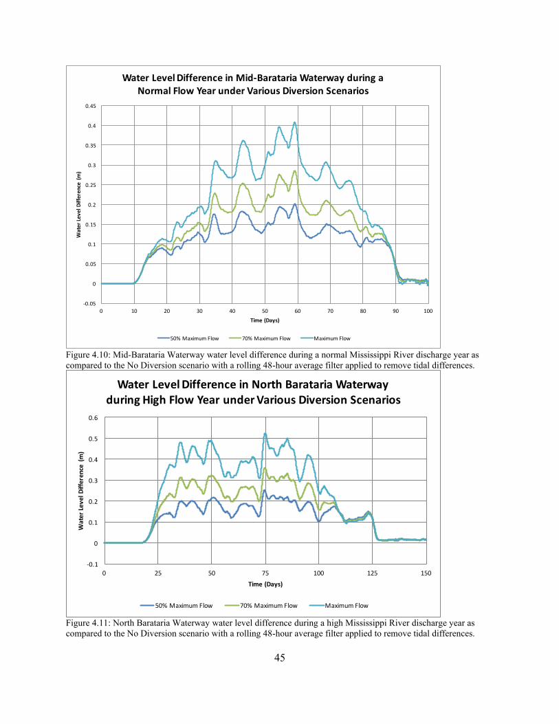
45
Figure 4.10: Mid-Barataria Waterway water level difference during a normal Mississippi River discharge year as
compared to the No Diversion scenario with a rolling 48-hour average filter applied to remove tidal differences.
Figure 4.11: North Barataria Waterway water level difference during a high Mississippi River discharge year as
compared to the No Diversion scenario with a rolling 48-hour average filter applied to remove tidal differences.
-0.05
0
0.05
0.1
0.15
0.2
0.25
0.3
0.35
0.4
0.45
0 10 20 30 40 50 60 70 80 90 100
WaterLevelD
ifference(m
)
Time(Days)
WaterLevelDifferenceinMid-BaratariaWaterwayduringaNormalFlowYearunderVariousDiversionScenarios
50%MaximumFlow 70%MaximumFlow MaximumFlow
-0.1
0
0.1
0.2
0.3
0.4
0.5
0.6
0 25 50 75 100 125 150
WaterLevelDifference(m)
Time(Days)
WaterLevelDifferenceinNorthBaratariaWaterwayduringHighFlowYearunderVariousDiversionScenarios
50%MaximumFlow 70%MaximumFlow MaximumFlow
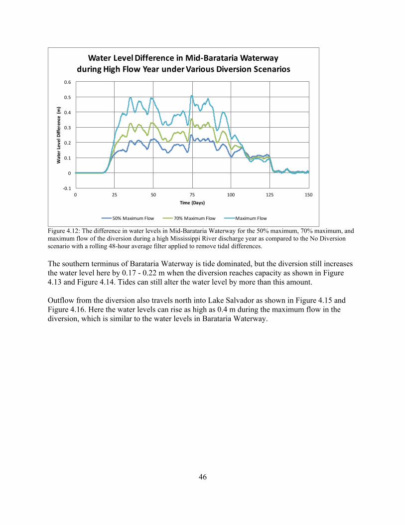
46
Figure 4.12: The difference in water levels in Mid-Barataria Waterway for the 50% maximum, 70% maximum, and
maximum flow of the diversion during a high Mississippi River discharge year as compared to the No Diversion
scenario with a rolling 48-hour average filter applied to remove tidal differences.
The southern terminus of Barataria Waterway is tide dominated, but the diversion still increases
the water level here by 0.17 - 0.22 m when the diversion reaches capacity as shown in Figure
4.13 and Figure 4.14. Tides can still alter the water level by more than this amount.
Outflow from the diversion also travels north into Lake Salvador as shown in Figure 4.15 and
Figure 4.16. Here the water levels can rise as high as 0.4 m during the maximum flow in the
diversion, which is similar to the water levels in Barataria Waterway.
-0.1
0
0.1
0.2
0.3
0.4
0.5
0.6
0 25 50 75 100 125 150
WaterLevelDifference(m)
Time(Days)
WaterLevelDifferenceinMid-BaratariaWaterwayduringHighFlowYearunderVariousDiversionScenarios
50%MaximumFlow 70%MaximumFlow MaximumFlow
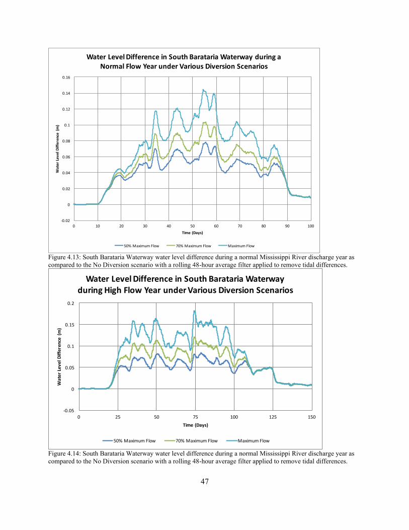
47
Figure 4.13: South Barataria Waterway water level difference during a normal Mississippi River discharge year as
compared to the No Diversion scenario with a rolling 48-hour average filter applied to remove tidal differences.
Figure 4.14: South Barataria Waterway water level difference during a normal Mississippi River discharge year as
compared to the No Diversion scenario with a rolling 48-hour average filter applied to remove tidal differences.
-0.02
0
0.02
0.04
0.06
0.08
0.1
0.12
0.14
0.16
0 10 20 30 40 50 60 70 80 90 100
WaterLevelD
ifference(m
)
Time(Days)
WaterLevelDifferenceinSouthBaratariaWaterwayduringaNormalFlowYearunderVariousDiversionScenarios
50%MaximumFlow 70%MaximumFlow MaximumFlow
-0.05
0
0.05
0.1
0.15
0.2
0 25 50 75 100 125 150
WaterLevelDifference(m)
Time(Days)
WaterLevelDifferenceinSouthBaratariaWaterwayduringHighFlowYearunderVariousDiversionScenarios
50%MaximumFlow 70%MaximumFlow MaximumFlow
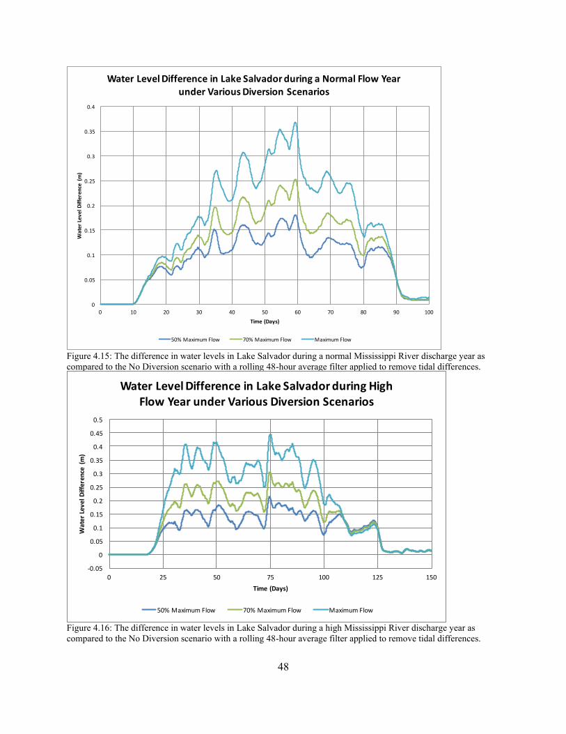
48
Figure 4.15: The difference in water levels in Lake Salvador during a normal Mississippi River discharge year as
compared to the No Diversion scenario with a rolling 48-hour average filter applied to remove tidal differences.
Figure 4.16: The difference in water levels in Lake Salvador during a high Mississippi River discharge year as
compared to the No Diversion scenario with a rolling 48-hour average filter applied to remove tidal differences.
0
0.05
0.1
0.15
0.2
0.25
0.3
0.35
0.4
0 10 20 30 40 50 60 70 80 90 100
WaterLevelD
ifference(m
)
Time(Days)
WaterLevelDifferenceinLakeSalvadorduringaNormalFlowYearunderVariousDiversionScenarios
50%MaximumFlow 70%MaximumFlow MaximumFlow
-0.05
0
0.05
0.1
0.15
0.2
0.25
0.3
0.35
0.4
0.45
0.5
0 25 50 75 100 125 150
WaterLevelDifference(m)
Time(Days)
WaterLevelDifferenceinLakeSalvadorduringHighFlowYearunderVariousDiversionScenarios
50%MaximumFlow 70%MaximumFlow MaximumFlow
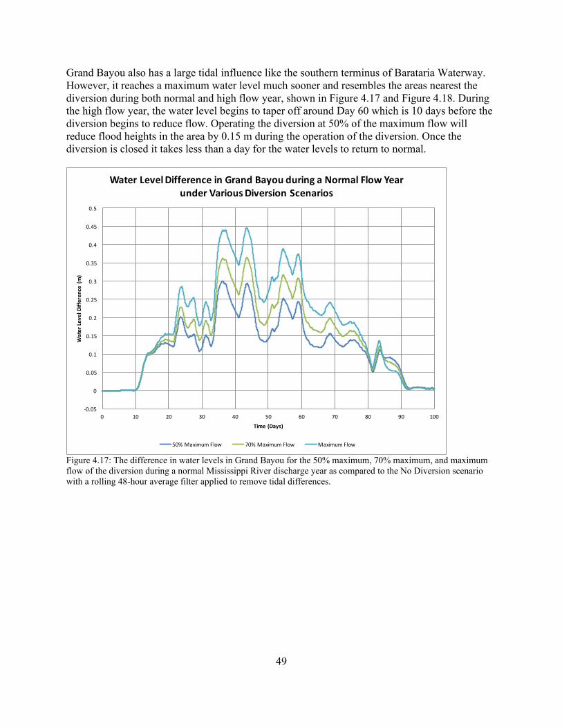
49
Grand Bayou also has a large tidal influence like the southern terminus of Barataria Waterway.
However, it reaches a maximum water level much sooner and resembles the areas nearest the
diversion during both normal and high flow year, shown in Figure 4.17 and Figure 4.18. During
the high flow year, the water level begins to taper off around Day 60 which is 10 days before the
diversion begins to reduce flow. Operating the diversion at 50% of the maximum flow will
reduce flood heights in the area by 0.15 m during the operation of the diversion. Once the
diversion is closed it takes less than a day for the water levels to return to normal.
Figure 4.17: The difference in water levels in Grand Bayou for the 50% maximum, 70% maximum, and maximum
flow of the diversion during a normal Mississippi River discharge year as compared to the No Diversion scenario
with a rolling 48-hour average filter applied to remove tidal differences.
-0.05
0
0.05
0.1
0.15
0.2
0.25
0.3
0.35
0.4
0.45
0.5
0 10 20 30 40 50 60 70 80 90 100
WaterLevelD
ifference(m
)
Time(Days)
WaterLevelDifferenceinGrandBayouduringaNormalFlowYearunderVariousDiversionScenarios
50%MaximumFlow 70%MaximumFlow MaximumFlow
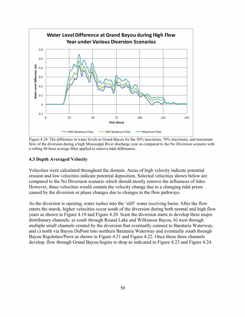
50
Figure 4.18: The difference in water levels in Grand Bayou for the 50% maximum, 70% maximum, and maximum
flow of the diversion during a high Mississippi River discharge year as compared to the No Diversion scenario with
a rolling 48-hour average filter applied to remove tidal differences.
4.3 Depth Averaged Velocity
Velocities were calculated throughout the domain. Areas of high velocity indicate potential
erosion and low velocities indicate potential deposition. Selected velocities shown below are
compared to the No Diversion scenario which should mostly remove the influences of tides.
However, these velocities would contain the velocity change due to a changing tidal prism
caused by the diversion or phase changes due to changes in the flow pathways.
As the diversion is opening, water rushes into the ‘still’ water receiving basin. After the flow
enters the marsh, higher velocities occur south of the diversion during both normal and high flow
years as shown in Figure 4.19 and Figure 4.20. Soon the diversion starts to develop three major
distributary channels: a) south through Round Lake and Wilkinson Bayou, b) west through
multiple small channels created by the diversion that eventually connect to Barataria Waterway,
and c) north via Bayou DuPont into northern Barataria Waterway and eventually south through
Bayou Rigolettes/Perot as shown in Figure 4.21 and Figure 4.22. Once these three channels
develop, flow through Grand Bayou begins to drop as indicated in Figure 4.23 and Figure 4.24.
-0.1
0
0.1
0.2
0.3
0.4
0.5
0.6
0 25 50 75 100 125 150
WaterLevelDifference(m)
Time(Days)
WaterLevelDifferenceatGrandBayouduringHighFlowYearunderVariousDiversionScenarios
50%MaximumFlow 70%MaximumFlow MaximumFlow
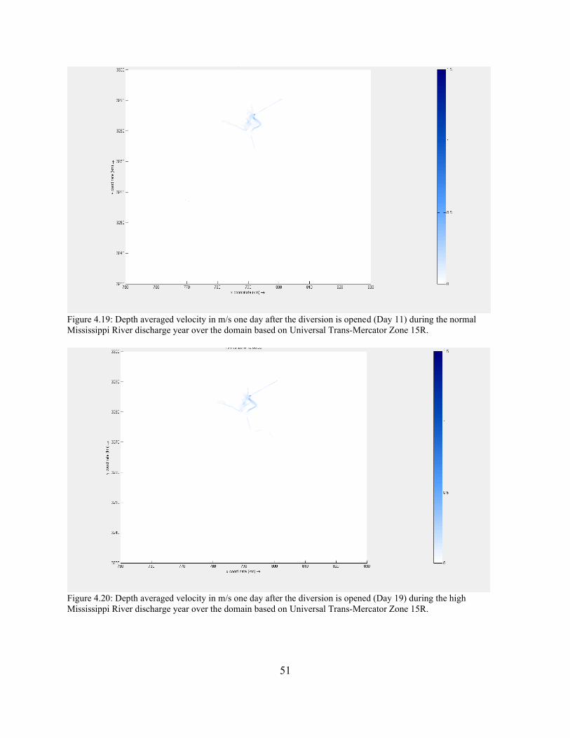
51
Figure 4.19: Depth averaged velocity in m/s one day after the diversion is opened (Day 11) during the normal
Mississippi River discharge year over the domain based on Universal Trans-Mercator Zone 15R.
Figure 4.20: Depth averaged velocity in m/s one day after the diversion is opened (Day 19) during the high
Mississippi River discharge year over the domain based on Universal Trans-Mercator Zone 15R.
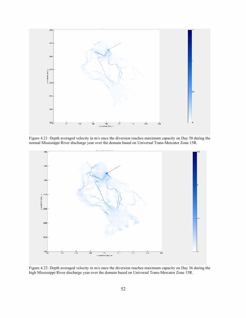
52
Figure 4.21: Depth averaged velocity in m/s once the diversion reaches maximum capacity on Day 50 during the
normal Mississippi River discharge year over the domain based on Universal Trans-Mercator Zone 15R.
Figure 4.22: Depth averaged velocity in m/s once the diversion reaches maximum capacity on Day 36 during the
high Mississippi River discharge year over the domain based on Universal Trans-Mercator Zone 15R.
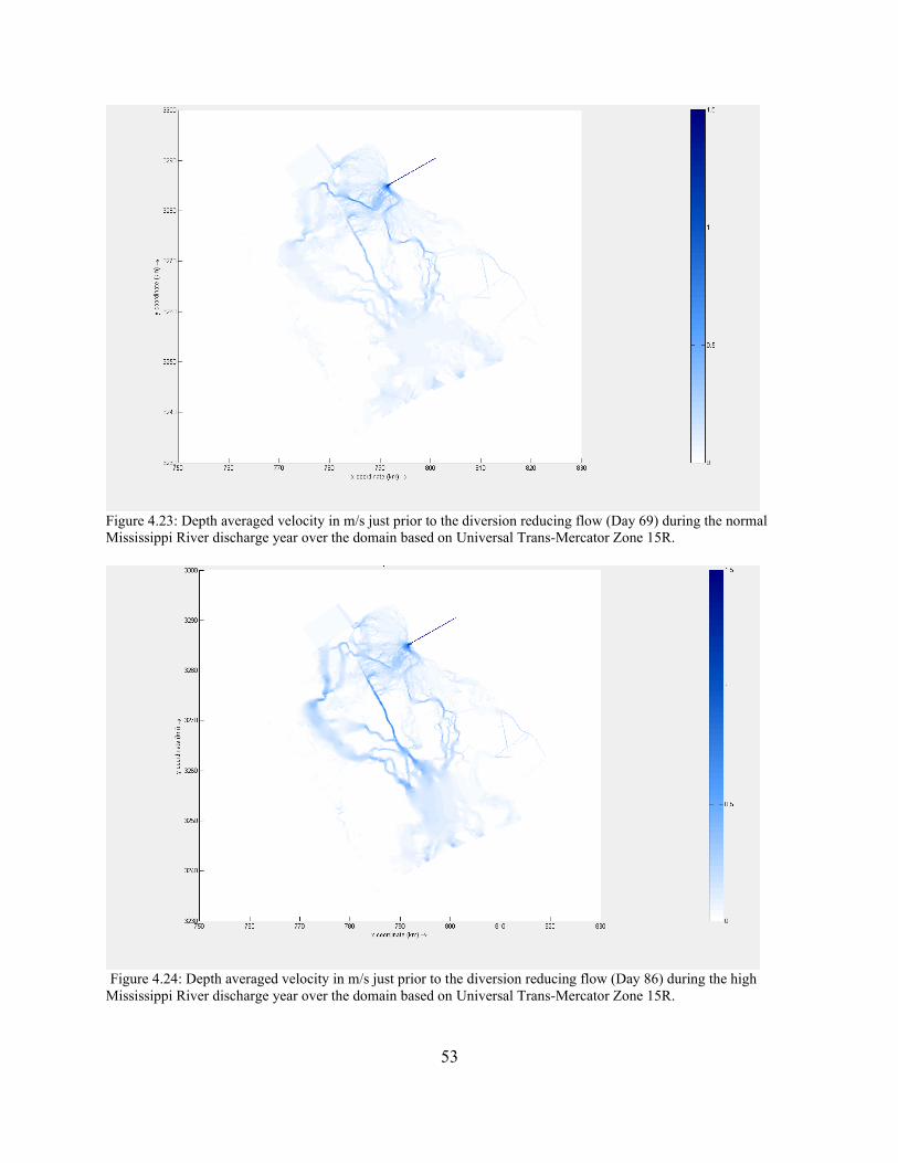
53
Figure 4.23: Depth averaged velocity in m/s just prior to the diversion reducing flow (Day 69) during the normal
Mississippi River discharge year over the domain based on Universal Trans-Mercator Zone 15R.
Figure 4.24: Depth averaged velocity in m/s just prior to the diversion reducing flow (Day 86) during the high
Mississippi River discharge year over the domain based on Universal Trans-Mercator Zone 15R.
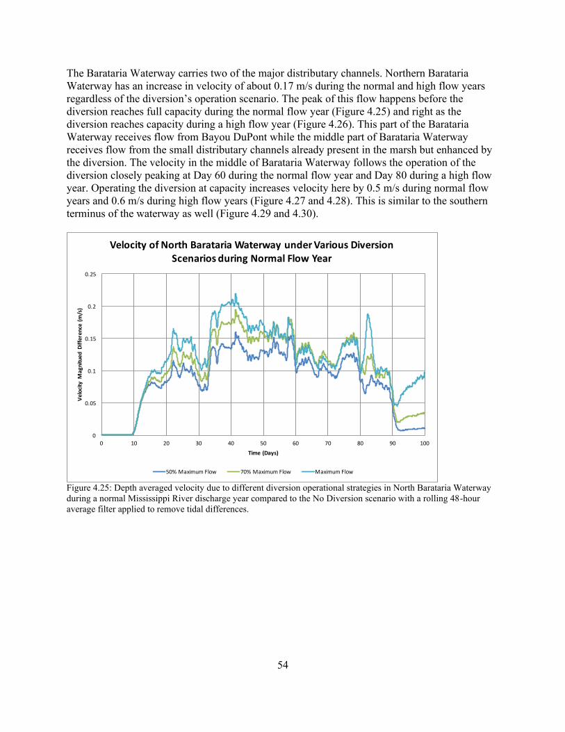
54
The Barataria Waterway carries two of the major distributary channels. Northern Barataria
Waterway has an increase in velocity of about 0.17 m/s during the normal and high flow years
regardless of the diversion’s operation scenario. The peak of this flow happens before the
diversion reaches full capacity during the normal flow year (Figure 4.25) and right as the
diversion reaches capacity during a high flow year (Figure 4.26). This part of the Barataria
Waterway receives flow from Bayou DuPont while the middle part of Barataria Waterway
receives flow from the small distributary channels already present in the marsh but enhanced by
the diversion. The velocity in the middle of Barataria Waterway follows the operation of the
diversion closely peaking at Day 60 during the normal flow year and Day 80 during a high flow
year. Operating the diversion at capacity increases velocity here by 0.5 m/s during normal flow
years and 0.6 m/s during high flow years (Figure 4.27 and 4.28). This is similar to the southern
terminus of the waterway as well (Figure 4.29 and 4.30).
Figure 4.25: Depth averaged velocity due to different diversion operational strategies in North Barataria Waterway
during a normal Mississippi River discharge year compared to the No Diversion scenario with a rolling 48-hour
average filter applied to remove tidal differences.
0
0.05
0.1
0.15
0.2
0.25
0 10 20 30 40 50 60 70 80 90 100
VelocityM
agnituedDifference(m/s)
Time(Days)
VelocityofNorthBaratariaWaterwayunderVariousDiversionScenariosduringNormalFlowYear
50%MaximumFlow 70%MaximumFlow MaximumFlow
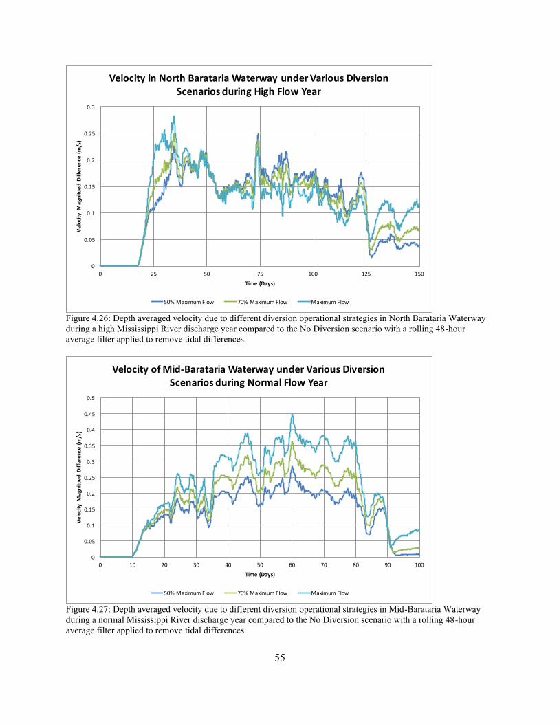
55
Figure 4.26: Depth averaged velocity due to different diversion operational strategies in North Barataria Waterway
during a high Mississippi River discharge year compared to the No Diversion scenario with a rolling 48-hour
average filter applied to remove tidal differences.
Figure 4.27: Depth averaged velocity due to different diversion operational strategies in Mid-Barataria Waterway
during a normal Mississippi River discharge year compared to the No Diversion scenario with a rolling 48-hour
average filter applied to remove tidal differences.
0
0.05
0.1
0.15
0.2
0.25
0.3
0 25 50 75 100 125 150
VelocityM
agnituedDifference(m/s)
Time(Days)
VelocityinNorthBaratariaWaterwayunderVariousDiversionScenariosduringHighFlowYear
50%MaximumFlow 70%MaximumFlow MaximumFlow
0
0.05
0.1
0.15
0.2
0.25
0.3
0.35
0.4
0.45
0.5
0 10 20 30 40 50 60 70 80 90 100
VelocityM
agnituedDifference(m/s)
Time(Days)
VelocityofMid-BaratariaWaterwayunderVariousDiversionScenariosduringNormalFlowYear
50%MaximumFlow 70%MaximumFlow MaximumFlow
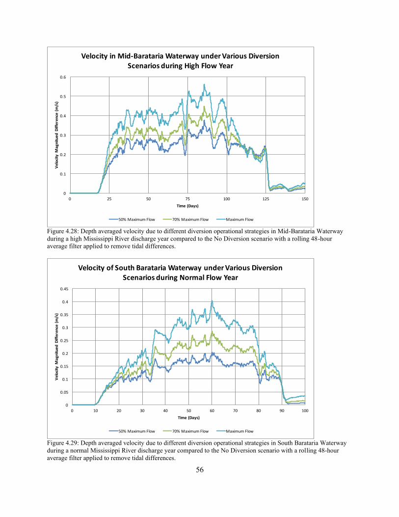
56
Figure 4.28: Depth averaged velocity due to different diversion operational strategies in Mid-Barataria Waterway
during a high Mississippi River discharge year compared to the No Diversion scenario with a rolling 48-hour
average filter applied to remove tidal differences.
Figure 4.29: Depth averaged velocity due to different diversion operational strategies in South Barataria Waterway
during a normal Mississippi River discharge year compared to the No Diversion scenario with a rolling 48-hour
average filter applied to remove tidal differences.
0
0.1
0.2
0.3
0.4
0.5
0.6
0 25 50 75 100 125 150
VelocityM
agnituedDifference(m/s)
Time(Days)
VelocityinMid-BaratariaWaterwayunderVariousDiversionScenariosduringHighFlowYear
50%MaximumFlow 70%MaximumFlow MaximumFlow
0
0.05
0.1
0.15
0.2
0.25
0.3
0.35
0.4
0.45
0 10 20 30 40 50 60 70 80 90 100
VelocityM
agnituedDifference(m/s)
Time(Days)
VelocityofSouthBaratariaWaterwayunderVariousDiversionScenariosduringNormalFlowYear
50%MaximumFlow 70%MaximumFlow MaximumFlow
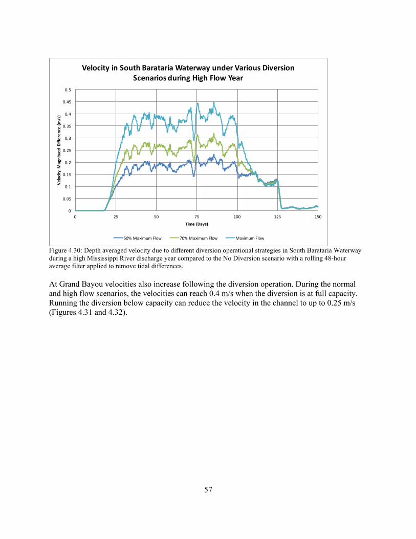
57
Figure 4.30: Depth averaged velocity due to different diversion operational strategies in South Barataria Waterway
during a high Mississippi River discharge year compared to the No Diversion scenario with a rolling 48-hour
average filter applied to remove tidal differences.
At Grand Bayou velocities also increase following the diversion operation. During the normal
and high flow scenarios, the velocities can reach 0.4 m/s when the diversion is at full capacity.
Running the diversion below capacity can reduce the velocity in the channel to up to 0.25 m/s
(Figures 4.31 and 4.32).
0
0.05
0.1
0.15
0.2
0.25
0.3
0.35
0.4
0.45
0.5
0 25 50 75 100 125 150
VelocityM
agnituedDifference(m/s)
Time(Days)
VelocityinSouthBaratariaWaterwayunderVariousDiversionScenariosduringHighFlowYear
50%MaximumFlow 70%MaximumFlow MaximumFlow
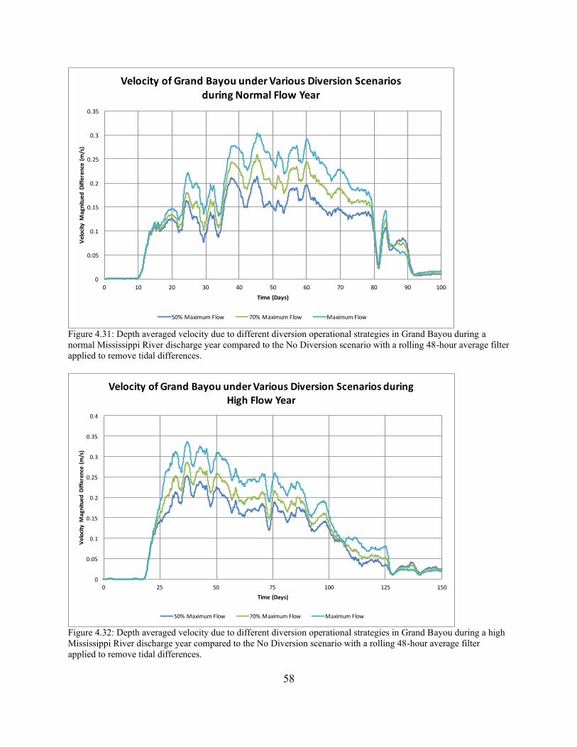
58
Figure 4.31: Depth averaged velocity due to different diversion operational strategies in Grand Bayou during a
normal Mississippi River discharge year compared to the No Diversion scenario with a rolling 48-hour average filter
applied to remove tidal differences.
Figure 4.32: Depth averaged velocity due to different diversion operational strategies in Grand Bayou during a high
Mississippi River discharge year compared to the No Diversion scenario with a rolling 48-hour average filter
applied to remove tidal differences.
0
0.05
0.1
0.15
0.2
0.25
0.3
0.35
0 10 20 30 40 50 60 70 80 90 100
VelocityM
agnituedDifference(m/s)
Time(Days)
VelocityofGrandBayouunderVariousDiversionScenariosduringNormalFlowYear
50%MaximumFlow 70%MaximumFlow MaximumFlow
0
0.05
0.1
0.15
0.2
0.25
0.3
0.35
0.4
0 25 50 75 100 125 150
VelocityM
agnituedDifference(m/s)
Time(Days)
VelocityofGrandBayouunderVariousDiversionScenariosduringHighFlowYear
50%MaximumFlow 70%MaximumFlow MaximumFlow
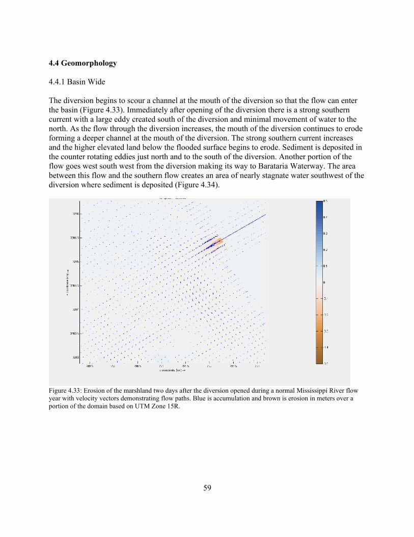
59
4.4 Geomorphology
4.4.1 Basin Wide
The diversion begins to scour a channel at the mouth of the diversion so that the flow can enter
the basin (Figure 4.33). Immediately after opening of the diversion there is a strong southern
current with a large eddy created south of the diversion and minimal movement of water to the
north. As the flow through the diversion increases, the mouth of the diversion continues to erode
forming a deeper channel at the mouth of the diversion. The strong southern current increases
and the higher elevated land below the flooded surface begins to erode. Sediment is deposited in
the counter rotating eddies just north and to the south of the diversion. Another portion of the
flow goes west south west from the diversion making its way to Barataria Waterway. The area
between this flow and the southern flow creates an area of nearly stagnate water southwest of the
diversion where sediment is deposited (Figure 4.34).
Figure 4.33: Erosion of the marshland two days after the diversion opened during a normal Mississippi River flow
year with velocity vectors demonstrating flow paths. Blue is accumulation and brown is erosion in meters over a
portion of the domain based on UTM Zone 15R.
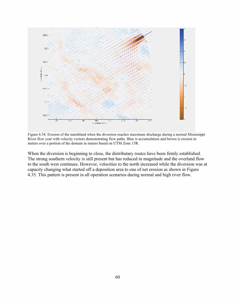
60
Figure 4.34: Erosion of the marshland when the diversion reaches maximum discharge during a normal Mississippi
River flow year with velocity vectors demonstrating flow paths. Blue is accumulation and brown is erosion in
meters over a portion of the domain in meters based on UTM Zone 15R.
When the diversion is beginning to close, the distributary routes have been firmly established.
The strong southern velocity is still present but has reduced in magnitude and the overland flow
to the south west continues. However, velocities to the north increased while the diversion was at
capacity changing what started off a deposition area to one of net erosion as shown in Figure
4.35. This pattern is present in all operation scenarios during normal and high river flow.
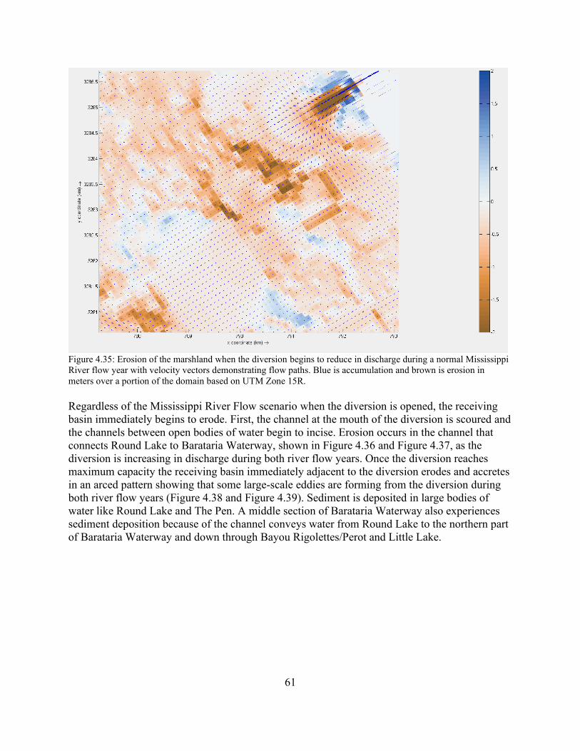
61
Figure 4.35: Erosion of the marshland when the diversion begins to reduce in discharge during a normal Mississippi
River flow year with velocity vectors demonstrating flow paths. Blue is accumulation and brown is erosion in
meters over a portion of the domain based on UTM Zone 15R.
Regardless of the Mississippi River Flow scenario when the diversion is opened, the receiving
basin immediately begins to erode. First, the channel at the mouth of the diversion is scoured and
the channels between open bodies of water begin to incise. Erosion occurs in the channel that
connects Round Lake to Barataria Waterway, shown in Figure 4.36 and Figure 4.37, as the
diversion is increasing in discharge during both river flow years. Once the diversion reaches
maximum capacity the receiving basin immediately adjacent to the diversion erodes and accretes
in an arced pattern showing that some large-scale eddies are forming from the diversion during
both river flow years (Figure 4.38 and Figure 4.39). Sediment is deposited in large bodies of
water like Round Lake and The Pen. A middle section of Barataria Waterway also experiences
sediment deposition because of the channel conveys water from Round Lake to the northern part
of Barataria Waterway and down through Bayou Rigolettes/Perot and Little Lake.
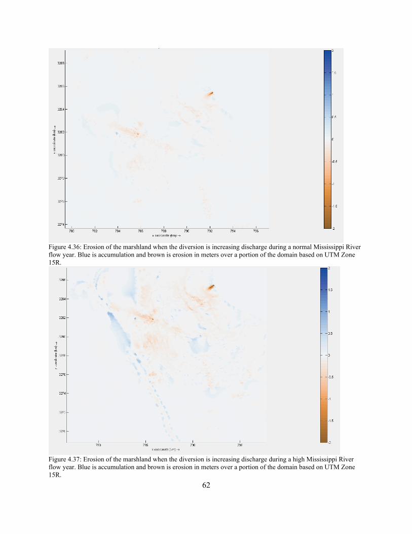
62
Figure 4.36: Erosion of the marshland when the diversion is increasing discharge during a normal Mississippi River
flow year. Blue is accumulation and brown is erosion in meters over a portion of the domain based on UTM Zone
15R.
Figure 4.37: Erosion of the marshland when the diversion is increasing discharge during a high Mississippi River
flow year. Blue is accumulation and brown is erosion in meters over a portion of the domain based on UTM Zone
15R.
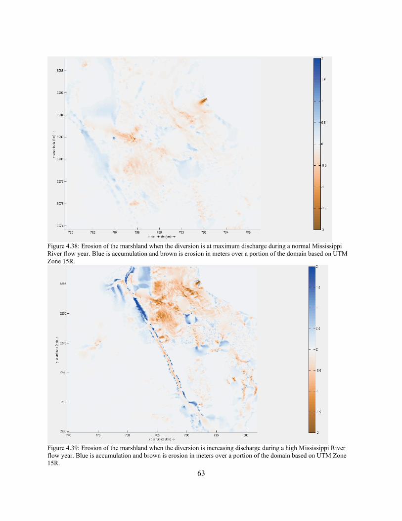
63
Figure 4.38: Erosion of the marshland when the diversion is at maximum discharge during a normal Mississippi
River flow year. Blue is accumulation and brown is erosion in meters over a portion of the domain based on UTM
Zone 15R.
Figure 4.39: Erosion of the marshland when the diversion is increasing discharge during a high Mississippi River
flow year. Blue is accumulation and brown is erosion in meters over a portion of the domain based on UTM Zone
15R.
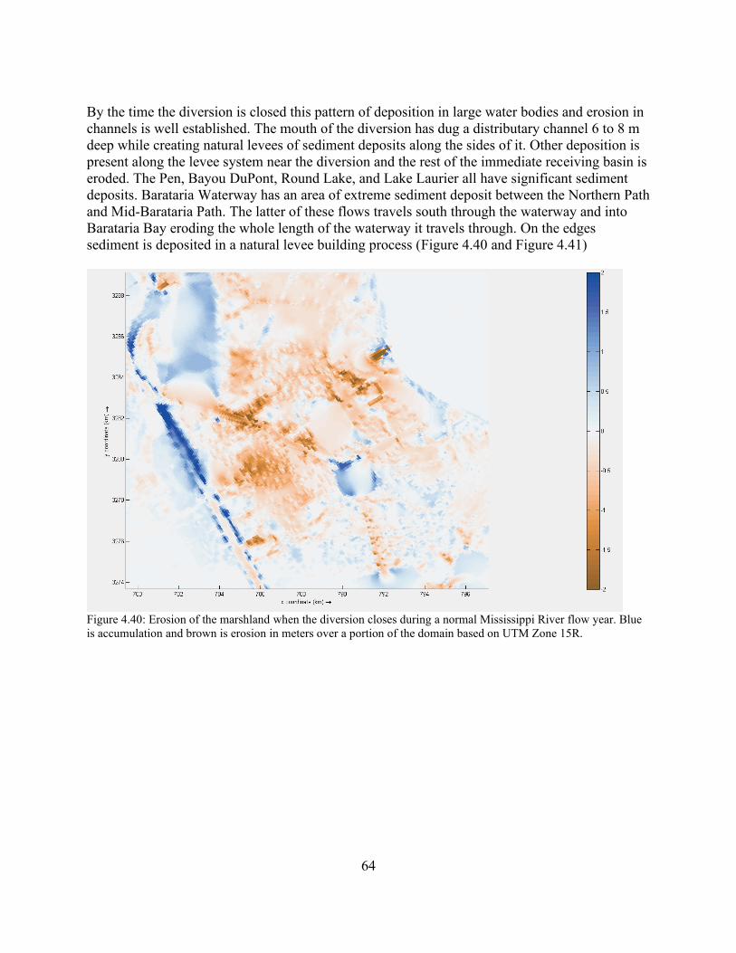
64
By the time the diversion is closed this pattern of deposition in large water bodies and erosion in
channels is well established. The mouth of the diversion has dug a distributary channel 6 to 8 m
deep while creating natural levees of sediment deposits along the sides of it. Other deposition is
present along the levee system near the diversion and the rest of the immediate receiving basin is
eroded. The Pen, Bayou DuPont, Round Lake, and Lake Laurier all have significant sediment
deposits. Barataria Waterway has an area of extreme sediment deposit between the Northern Path
and Mid-Barataria Path. The latter of these flows travels south through the waterway and into
Barataria Bay eroding the whole length of the waterway it travels through. On the edges
sediment is deposited in a natural levee building process (Figure 4.40 and Figure 4.41)
Figure 4.40: Erosion of the marshland when the diversion closes during a normal Mississippi River flow year. Blue
is accumulation and brown is erosion in meters over a portion of the domain based on UTM Zone 15R.
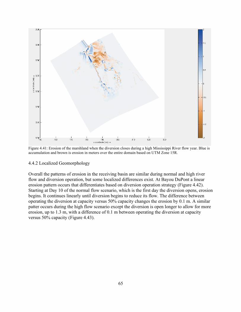
65
Figure 4.41: Erosion of the marshland when the diversion closes during a high Mississippi River flow year. Blue is
accumulation and brown is erosion in meters over the entire domain based on UTM Zone 15R.
4.4.2 Localized Geomorphology
Overall the patterns of erosion in the receiving basin are similar during normal and high river
flow and diversion operation, but some localized differences exist. At Bayou DuPont a linear
erosion pattern occurs that differentiates based on diversion operation strategy (Figure 4.42).
Starting at Day 10 of the normal flow scenario, which is the first day the diversion opens, erosion
begins. It continues linearly until diversion begins to reduce its flow. The difference between
operating the diversion at capacity versus 50% capacity changes the erosion by 0.1 m. A similar
patter occurs during the high flow scenario except the diversion is open longer to allow for more
erosion, up to 1.3 m, with a difference of 0.1 m between operating the diversion at capacity
versus 50% capacity (Figure 4.43).
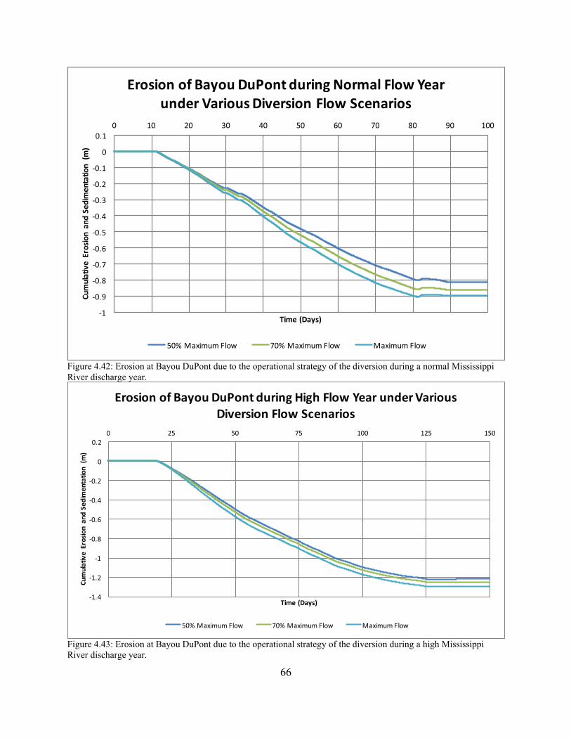
66
Figure 4.42: Erosion at Bayou DuPont due to the operational strategy of the diversion during a normal Mississippi
River discharge year.
Figure 4.43: Erosion at Bayou DuPont due to the operational strategy of the diversion during a high Mississippi
River discharge year.
-1
-0.9
-0.8
-0.7
-0.6
-0.5
-0.4
-0.3
-0.2
-0.1
0
0.10 10 20 30 40 50 60 70 80 90 100
Cum
ulativeErosionandSedimentation(m
)
Time(Days)
ErosionofBayouDuPontduringNormalFlowYearunderVariousDiversionFlowScenarios
50%MaximumFlow 70%MaximumFlow MaximumFlow
-1.4
-1.2
-1
-0.8
-0.6
-0.4
-0.2
0
0.20 25 50 75 100 125 150
Cum
ulativeErosionandSedimentation(m
)
Time(Days)
ErosionofBayouDuPontduringHighFlowYearunderVariousDiversionFlowScenarios
50%MaximumFlow 70%MaximumFlow MaximumFlow
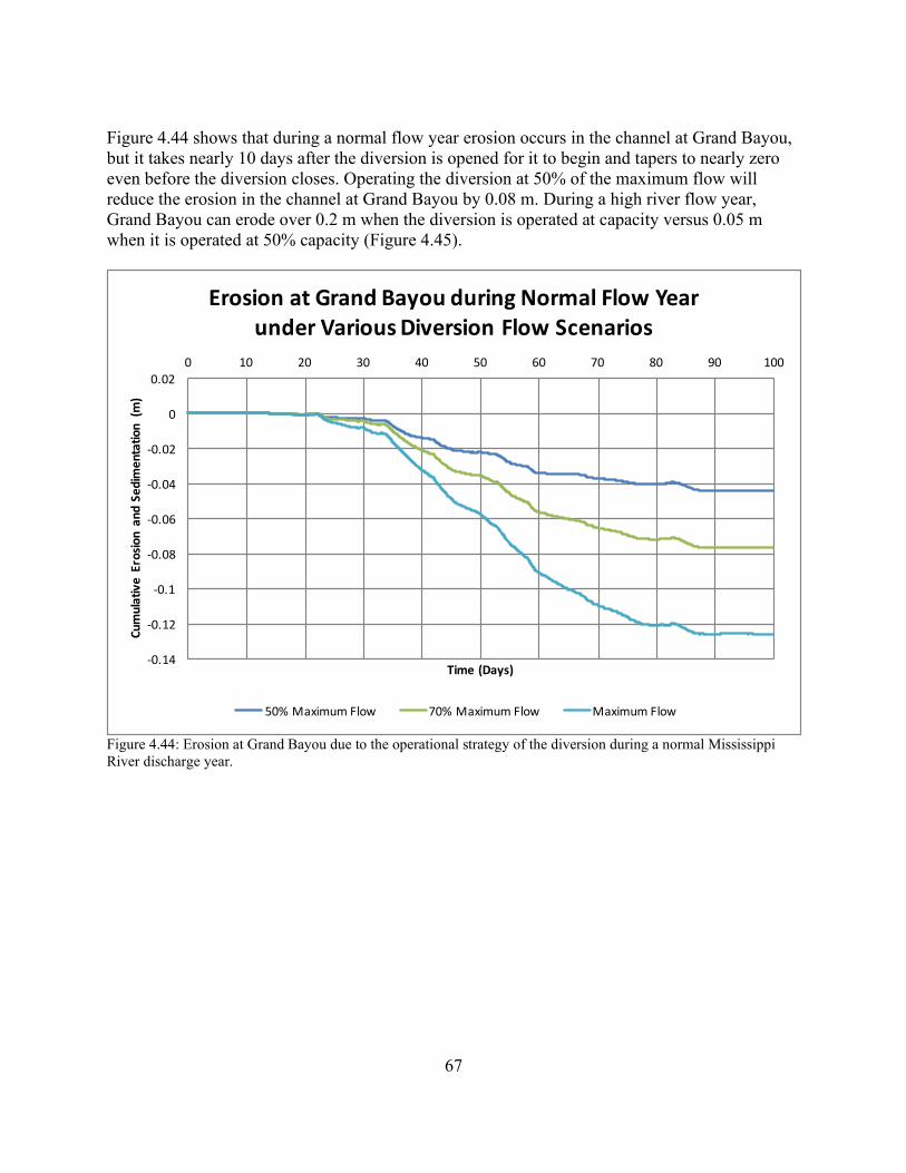
67
Figure 4.44 shows that during a normal flow year erosion occurs in the channel at Grand Bayou,
but it takes nearly 10 days after the diversion is opened for it to begin and tapers to nearly zero
even before the diversion closes. Operating the diversion at 50% of the maximum flow will
reduce the erosion in the channel at Grand Bayou by 0.08 m. During a high river flow year,
Grand Bayou can erode over 0.2 m when the diversion is operated at capacity versus 0.05 m
when it is operated at 50% capacity (Figure 4.45).
Figure 4.44: Erosion at Grand Bayou due to the operational strategy of the diversion during a normal Mississippi
River discharge year.
-0.14
-0.12
-0.1
-0.08
-0.06
-0.04
-0.02
0
0.020 10 20 30 40 50 60 70 80 90 100
Cum
ulativeErosionandSedimentation(m
)
Time(Days)
ErosionatGrandBayouduringNormalFlowYearunderVariousDiversionFlowScenarios
50%MaximumFlow 70%MaximumFlow MaximumFlow
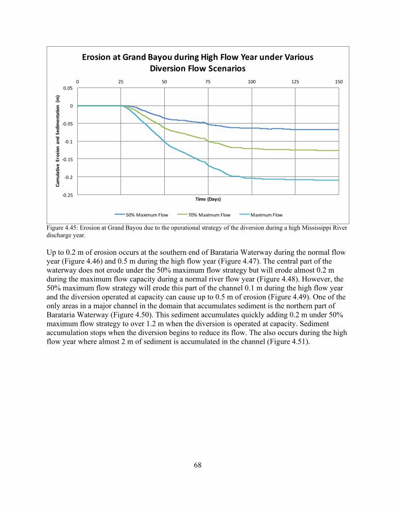
68
Figure 4.45: Erosion at Grand Bayou due to the operational strategy of the diversion during a high Mississippi River
discharge year.
Up to 0.2 m of erosion occurs at the southern end of Barataria Waterway during the normal flow
year (Figure 4.46) and 0.5 m during the high flow year (Figure 4.47). The central part of the
waterway does not erode under the 50% maximum flow strategy but will erode almost 0.2 m
during the maximum flow capacity during a normal river flow year (Figure 4.48). However, the
50% maximum flow strategy will erode this part of the channel 0.1 m during the high flow year
and the diversion operated at capacity can cause up to 0.5 m of erosion (Figure 4.49). One of the
only areas in a major channel in the domain that accumulates sediment is the northern part of
Barataria Waterway (Figure 4.50). This sediment accumulates quickly adding 0.2 m under 50%
maximum flow strategy to over 1.2 m when the diversion is operated at capacity. Sediment
accumulation stops when the diversion begins to reduce its flow. The also occurs during the high
flow year where almost 2 m of sediment is accumulated in the channel (Figure 4.51).
-0.25
-0.2
-0.15
-0.1
-0.05
0
0.050 25 50 75 100 125 150
Cum
ulativeErosionandSedimentation(m
)
Time(Days)
ErosionatGrandBayouduringHighFlowYearunderVariousDiversionFlowScenarios
50%MaximumFlow 70%MaximumFlow MaximumFlow
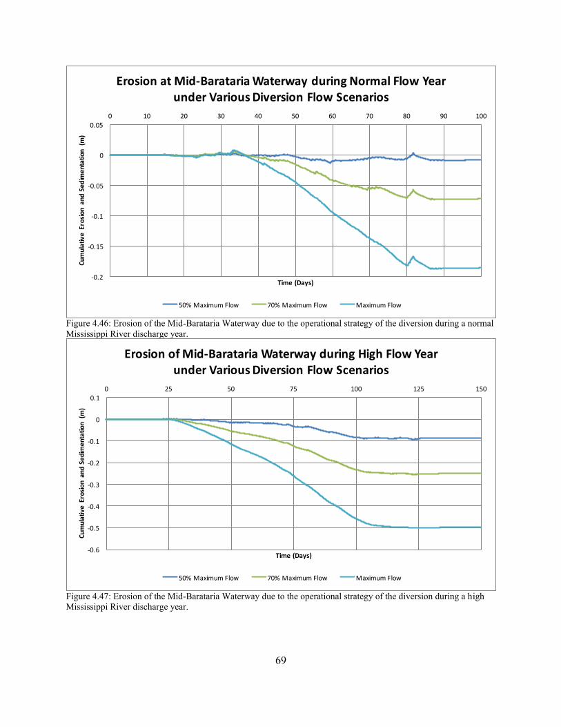
69
Figure 4.46: Erosion of the Mid-Barataria Waterway due to the operational strategy of the diversion during a normal
Mississippi River discharge year.
Figure 4.47: Erosion of the Mid-Barataria Waterway due to the operational strategy of the diversion during a high
Mississippi River discharge year.
-0.2
-0.15
-0.1
-0.05
0
0.050 10 20 30 40 50 60 70 80 90 100
Cum
ulativeErosionandSedimentation(m
)
Time(Days)
ErosionatMid-BaratariaWaterwayduringNormalFlowYearunderVariousDiversionFlowScenarios
50%MaximumFlow 70%MaximumFlow MaximumFlow
-0.6
-0.5
-0.4
-0.3
-0.2
-0.1
0
0.10 25 50 75 100 125 150
Cum
ulativeErosionandSedimentation(m
)
Time(Days)
ErosionofMid-BaratariaWaterwayduringHighFlowYearunderVariousDiversionFlowScenarios
50%MaximumFlow 70%MaximumFlow MaximumFlow
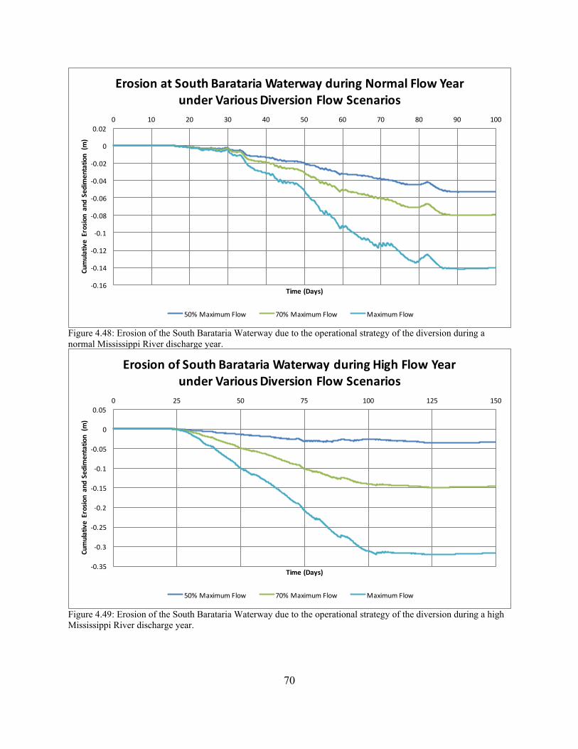
70
Figure 4.48: Erosion of the South Barataria Waterway due to the operational strategy of the diversion during a
normal Mississippi River discharge year.
Figure 4.49: Erosion of the South Barataria Waterway due to the operational strategy of the diversion during a high
Mississippi River discharge year.
-0.16
-0.14
-0.12
-0.1
-0.08
-0.06
-0.04
-0.02
0
0.020 10 20 30 40 50 60 70 80 90 100
Cum
ulativeErosionandSedimentation(m
)
Time(Days)
ErosionatSouthBaratariaWaterwayduringNormalFlowYearunderVariousDiversionFlowScenarios
50%MaximumFlow 70%MaximumFlow MaximumFlow
-0.35
-0.3
-0.25
-0.2
-0.15
-0.1
-0.05
0
0.050 25 50 75 100 125 150
Cum
ulativeErosionandSedimentation(m
)
Time(Days)
ErosionofSouthBaratariaWaterwayduringHighFlowYearunderVariousDiversionFlowScenarios
50%MaximumFlow 70%MaximumFlow MaximumFlow
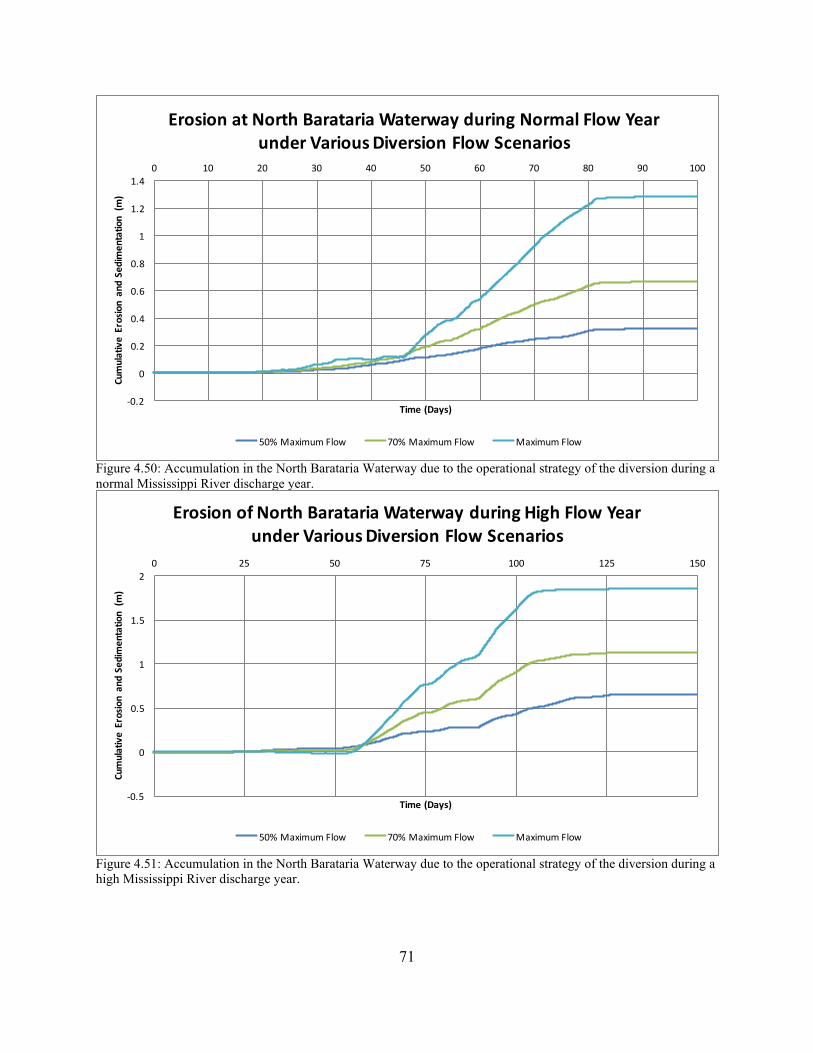
71
Figure 4.50: Accumulation in the North Barataria Waterway due to the operational strategy of the diversion during a
normal Mississippi River discharge year.
Figure 4.51: Accumulation in the North Barataria Waterway due to the operational strategy of the diversion during a
high Mississippi River discharge year.
-0.2
0
0.2
0.4
0.6
0.8
1
1.2
1.40 10 20 30 40 50 60 70 80 90 100
Cum
ulativeErosionandSedimentation(m
)
Time(Days)
ErosionatNorthBaratariaWaterwayduringNormalFlowYearunderVariousDiversionFlowScenarios
50%MaximumFlow 70%MaximumFlow MaximumFlow
-0.5
0
0.5
1
1.5
20 25 50 75 100 125 150
Cum
ulativeErosionandSedimentation(m
)
Time(Days)
ErosionofNorthBaratariaWaterwayduringHighFlowYearunderVariousDiversionFlowScenarios
50%MaximumFlow 70%MaximumFlow MaximumFlow
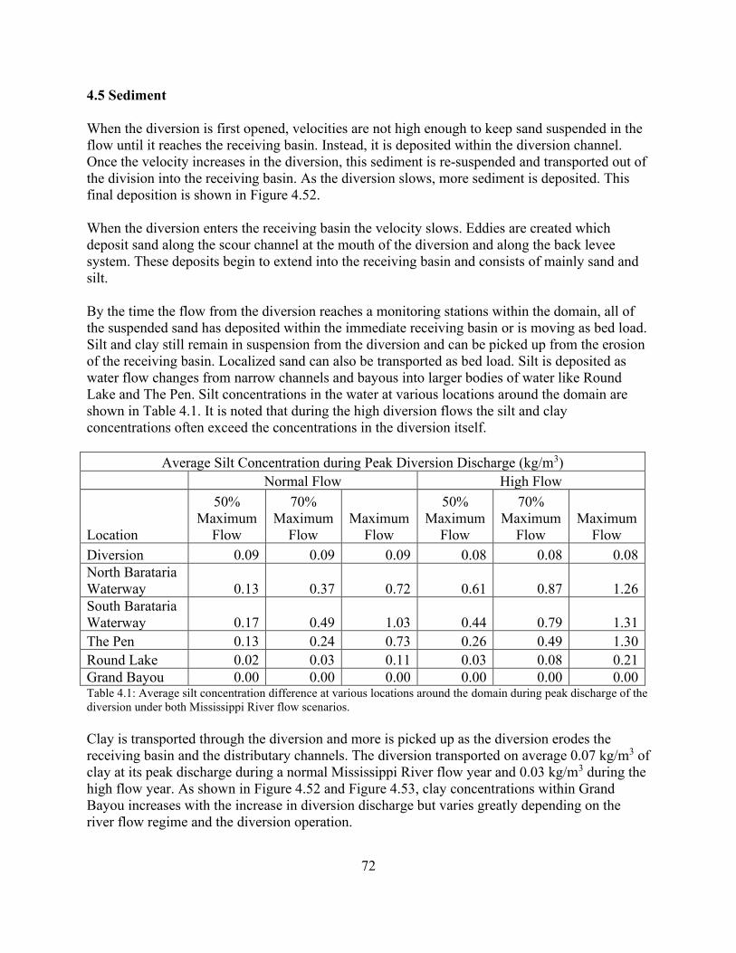
72
4.5 Sediment
When the diversion is first opened, velocities are not high enough to keep sand suspended in the
flow until it reaches the receiving basin. Instead, it is deposited within the diversion channel.
Once the velocity increases in the diversion, this sediment is re-suspended and transported out of
the division into the receiving basin. As the diversion slows, more sediment is deposited. This
final deposition is shown in Figure 4.52.
When the diversion enters the receiving basin the velocity slows. Eddies are created which
deposit sand along the scour channel at the mouth of the diversion and along the back levee
system. These deposits begin to extend into the receiving basin and consists of mainly sand and
silt.
By the time the flow from the diversion reaches a monitoring stations within the domain, all of
the suspended sand has deposited within the immediate receiving basin or is moving as bed load.
Silt and clay still remain in suspension from the diversion and can be picked up from the erosion
of the receiving basin. Localized sand can also be transported as bed load. Silt is deposited as
water flow changes from narrow channels and bayous into larger bodies of water like Round
Lake and The Pen. Silt concentrations in the water at various locations around the domain are
shown in Table 4.1. It is noted that during the high diversion flows the silt and clay
concentrations often exceed the concentrations in the diversion itself.
Average Silt Concentration during Peak Diversion Discharge (kg/m3)
Normal Flow High Flow
Location
50%
Maximum
Flow
70%
Maximum
Flow
Maximum
Flow
50%
Maximum
Flow
70%
Maximum
Flow
Maximum
Flow
Diversion 0.09 0.09 0.09 0.08 0.08 0.08
North Barataria
Waterway 0.13 0.37 0.72 0.61 0.87 1.26
South Barataria
Waterway 0.17 0.49 1.03 0.44 0.79 1.31
The Pen 0.13 0.24 0.73 0.26 0.49 1.30
Round Lake 0.02 0.03 0.11 0.03 0.08 0.21
Grand Bayou 0.00 0.00 0.00 0.00 0.00 0.00 Table 4.1: Average silt concentration difference at various locations around the domain during peak discharge of the
diversion under both Mississippi River flow scenarios.
Clay is transported through the diversion and more is picked up as the diversion erodes the
receiving basin and the distributary channels. The diversion transported on average 0.07 kg/m3 of
clay at its peak discharge during a normal Mississippi River flow year and 0.03 kg/m3 during the
high flow year. As shown in Figure 4.52 and Figure 4.53, clay concentrations within Grand
Bayou increases with the increase in diversion discharge but varies greatly depending on the
river flow regime and the diversion operation.
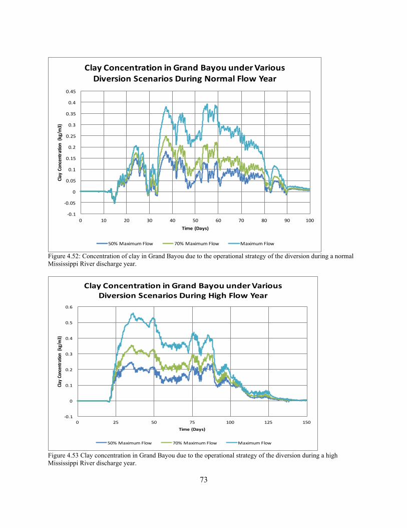
73
Figure 4.52: Concentration of clay in Grand Bayou due to the operational strategy of the diversion during a normal
Mississippi River discharge year.
Figure 4.53 Clay concentration in Grand Bayou due to the operational strategy of the diversion during a high
Mississippi River discharge year.
-0.1
-0.05
0
0.05
0.1
0.15
0.2
0.25
0.3
0.35
0.4
0.45
0 10 20 30 40 50 60 70 80 90 100
ClayConcentration(kg/m3)
Time(Days)
ClayConcentrationinGrandBayouunderVariousDiversionScenariosDuringNormalFlowYear
50%MaximumFlow 70%MaximumFlow MaximumFlow
-0.1
0
0.1
0.2
0.3
0.4
0.5
0.6
0 25 50 75 100 125 150
ClayConcentration(kg/m3)
Time(Days)
ClayConcentrationinGrandBayouunderVariousDiversionScenariosDuringHighFlowYear
50%MaximumFlow 70%MaximumFlow MaximumFlow
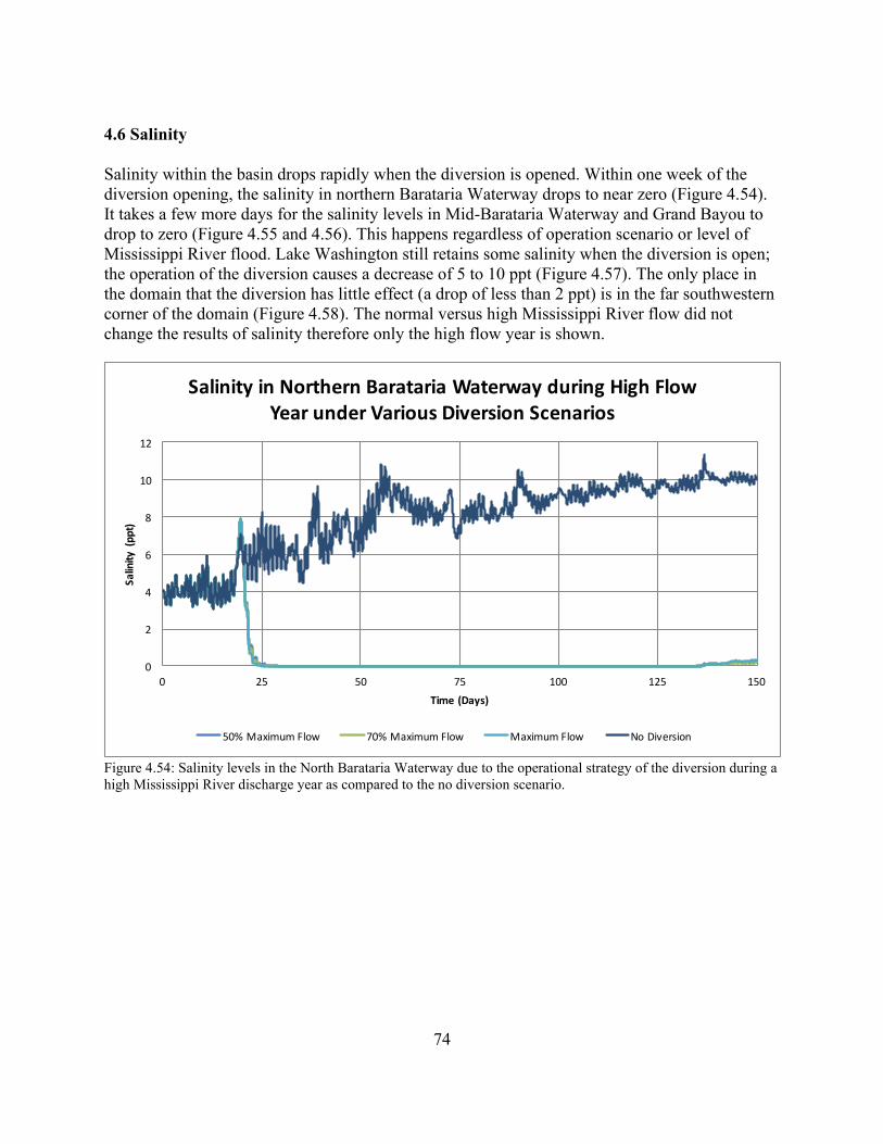
74
4.6 Salinity
Salinity within the basin drops rapidly when the diversion is opened. Within one week of the
diversion opening, the salinity in northern Barataria Waterway drops to near zero (Figure 4.54).
It takes a few more days for the salinity levels in Mid-Barataria Waterway and Grand Bayou to
drop to zero (Figure 4.55 and 4.56). This happens regardless of operation scenario or level of
Mississippi River flood. Lake Washington still retains some salinity when the diversion is open;
the operation of the diversion causes a decrease of 5 to 10 ppt (Figure 4.57). The only place in
the domain that the diversion has little effect (a drop of less than 2 ppt) is in the far southwestern
corner of the domain (Figure 4.58). The normal versus high Mississippi River flow did not
change the results of salinity therefore only the high flow year is shown.
Figure 4.54: Salinity levels in the North Barataria Waterway due to the operational strategy of the diversion during a
high Mississippi River discharge year as compared to the no diversion scenario.
0
2
4
6
8
10
12
0 25 50 75 100 125 150
Salinity(ppt)
Time(Days)
SalinityinNorthernBaratariaWaterwayduringHighFlowYearunderVariousDiversionScenarios
50%MaximumFlow 70%MaximumFlow MaximumFlow NoDiversion
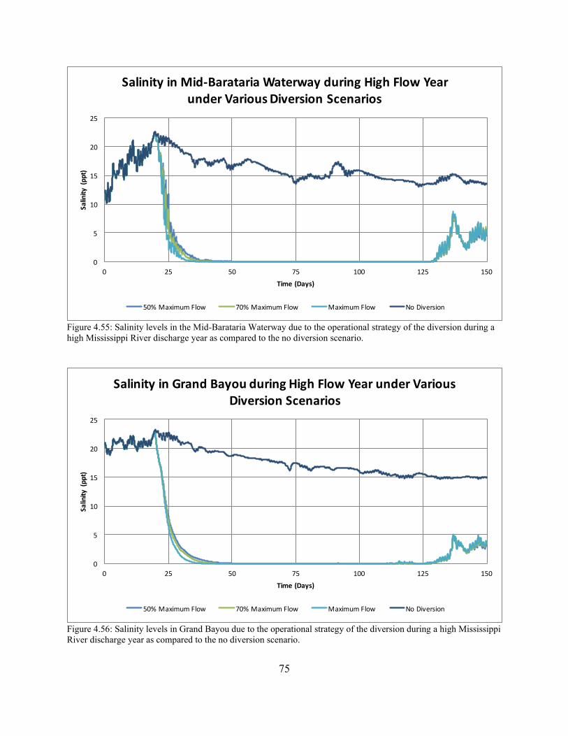
75
Figure 4.55: Salinity levels in the Mid-Barataria Waterway due to the operational strategy of the diversion during a
high Mississippi River discharge year as compared to the no diversion scenario.
Figure 4.56: Salinity levels in Grand Bayou due to the operational strategy of the diversion during a high Mississippi
River discharge year as compared to the no diversion scenario.
0
5
10
15
20
25
0 25 50 75 100 125 150
Salinity(ppt)
Time(Days)
SalinityinMid-BaratariaWaterwayduringHighFlowYearunderVariousDiversionScenarios
50%MaximumFlow 70%MaximumFlow MaximumFlow NoDiversion
0
5
10
15
20
25
0 25 50 75 100 125 150
Salinity(ppt)
Time(Days)
SalinityinGrandBayouduringHighFlowYearunderVariousDiversionScenarios
50%MaximumFlow 70%MaximumFlow MaximumFlow NoDiversion
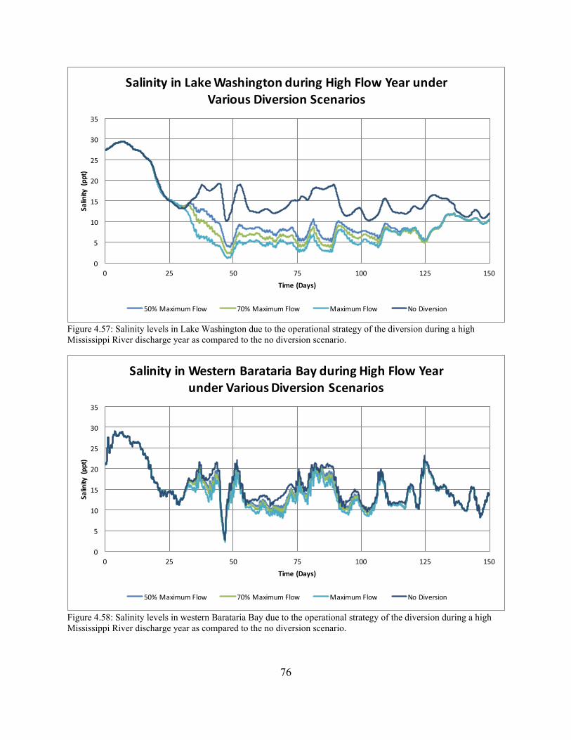
76
Figure 4.57: Salinity levels in Lake Washington due to the operational strategy of the diversion during a high
Mississippi River discharge year as compared to the no diversion scenario.
Figure 4.58: Salinity levels in western Barataria Bay due to the operational strategy of the diversion during a high
Mississippi River discharge year as compared to the no diversion scenario.
0
5
10
15
20
25
30
35
0 25 50 75 100 125 150
Salinity(ppt)
Time(Days)
SalinityinLakeWashingtonduringHighFlowYearunderVariousDiversionScenarios
50%MaximumFlow 70%MaximumFlow MaximumFlow NoDiversion
0
5
10
15
20
25
30
35
0 25 50 75 100 125 150
Salinity(ppt)
Time(Days)
SalinityinWesternBaratariaBayduringHighFlowYearunderVariousDiversionScenarios
50%MaximumFlow 70%MaximumFlow MaximumFlow NoDiversion
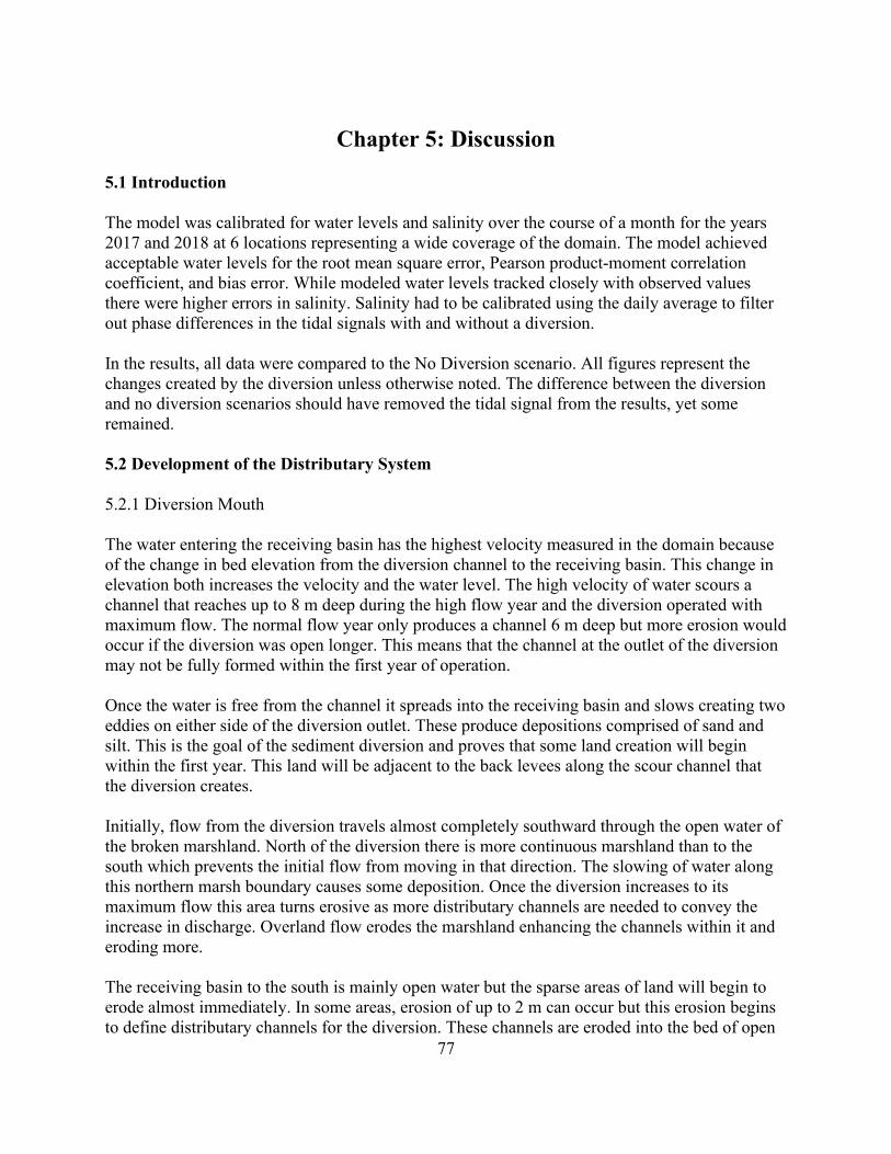
77
Chapter 5: Discussion
5.1 Introduction
The model was calibrated for water levels and salinity over the course of a month for the years
2017 and 2018 at 6 locations representing a wide coverage of the domain. The model achieved
acceptable water levels for the root mean square error, Pearson product-moment correlation
coefficient, and bias error. While modeled water levels tracked closely with observed values
there were higher errors in salinity. Salinity had to be calibrated using the daily average to filter
out phase differences in the tidal signals with and without a diversion.
In the results, all data were compared to the No Diversion scenario. All figures represent the
changes created by the diversion unless otherwise noted. The difference between the diversion
and no diversion scenarios should have removed the tidal signal from the results, yet some
remained.
5.2 Development of the Distributary System
5.2.1 Diversion Mouth
The water entering the receiving basin has the highest velocity measured in the domain because
of the change in bed elevation from the diversion channel to the receiving basin. This change in
elevation both increases the velocity and the water level. The high velocity of water scours a
channel that reaches up to 8 m deep during the high flow year and the diversion operated with
maximum flow. The normal flow year only produces a channel 6 m deep but more erosion would
occur if the diversion was open longer. This means that the channel at the outlet of the diversion
may not be fully formed within the first year of operation.
Once the water is free from the channel it spreads into the receiving basin and slows creating two
eddies on either side of the diversion outlet. These produce depositions comprised of sand and
silt. This is the goal of the sediment diversion and proves that some land creation will begin
within the first year. This land will be adjacent to the back levees along the scour channel that
the diversion creates.
Initially, flow from the diversion travels almost completely southward through the open water of
the broken marshland. North of the diversion there is more continuous marshland than to the
south which prevents the initial flow from moving in that direction. The slowing of water along
this northern marsh boundary causes some deposition. Once the diversion increases to its
maximum flow this area turns erosive as more distributary channels are needed to convey the
increase in discharge. Overland flow erodes the marshland enhancing the channels within it and
eroding more.
The receiving basin to the south is mainly open water but the sparse areas of land will begin to
erode almost immediately. In some areas, erosion of up to 2 m can occur but this erosion begins
to define distributary channels for the diversion. These channels are eroded into the bed of open
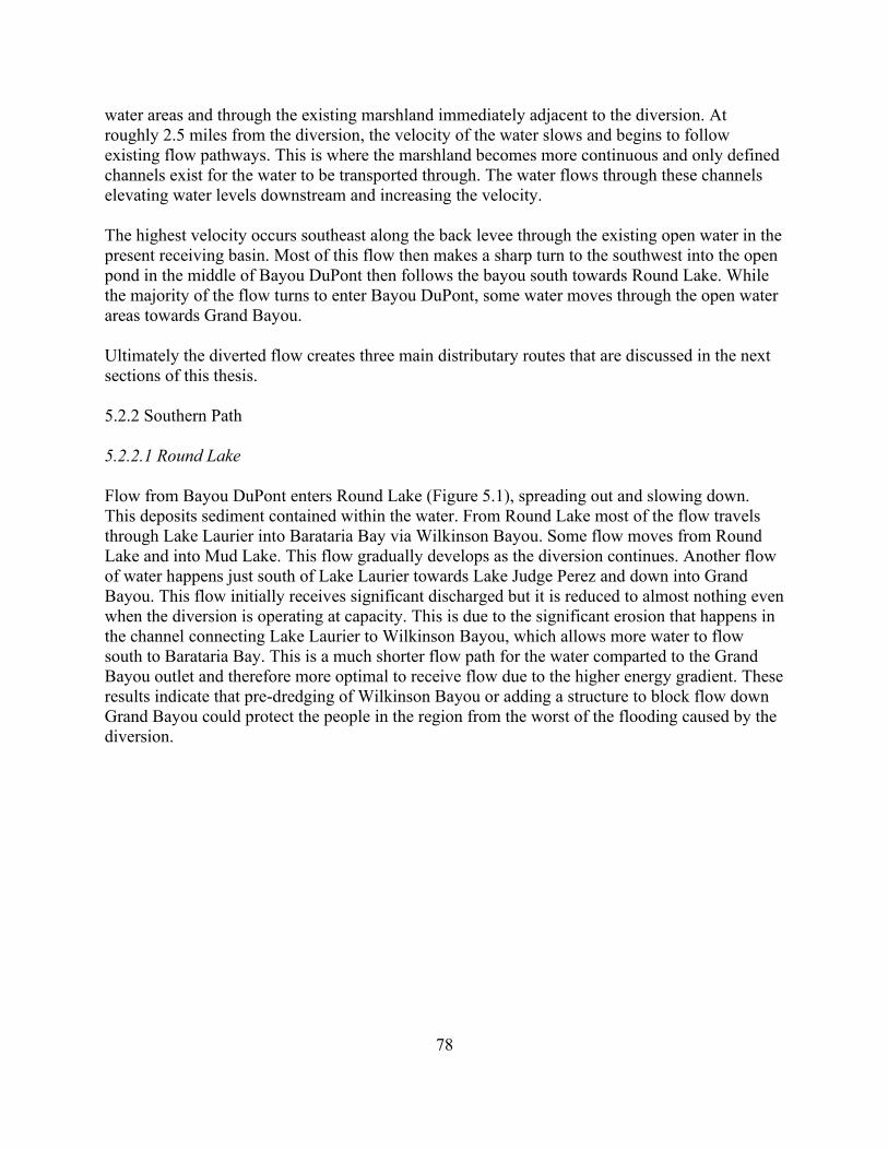
78
water areas and through the existing marshland immediately adjacent to the diversion. At
roughly 2.5 miles from the diversion, the velocity of the water slows and begins to follow
existing flow pathways. This is where the marshland becomes more continuous and only defined
channels exist for the water to be transported through. The water flows through these channels
elevating water levels downstream and increasing the velocity.
The highest velocity occurs southeast along the back levee through the existing open water in the
present receiving basin. Most of this flow then makes a sharp turn to the southwest into the open
pond in the middle of Bayou DuPont then follows the bayou south towards Round Lake. While
the majority of the flow turns to enter Bayou DuPont, some water moves through the open water
areas towards Grand Bayou.
Ultimately the diverted flow creates three main distributary routes that are discussed in the next
sections of this thesis.
5.2.2 Southern Path
5.2.2.1 Round Lake
Flow from Bayou DuPont enters Round Lake (Figure 5.1), spreading out and slowing down.
This deposits sediment contained within the water. From Round Lake most of the flow travels
through Lake Laurier into Barataria Bay via Wilkinson Bayou. Some flow moves from Round
Lake and into Mud Lake. This flow gradually develops as the diversion continues. Another flow
of water happens just south of Lake Laurier towards Lake Judge Perez and down into Grand
Bayou. This flow initially receives significant discharged but it is reduced to almost nothing even
when the diversion is operating at capacity. This is due to the significant erosion that happens in
the channel connecting Lake Laurier to Wilkinson Bayou, which allows more water to flow
south to Barataria Bay. This is a much shorter flow path for the water comparted to the Grand
Bayou outlet and therefore more optimal to receive flow due to the higher energy gradient. These
results indicate that pre-dredging of Wilkinson Bayou or adding a structure to block flow down
Grand Bayou could protect the people in the region from the worst of the flooding caused by the
diversion.
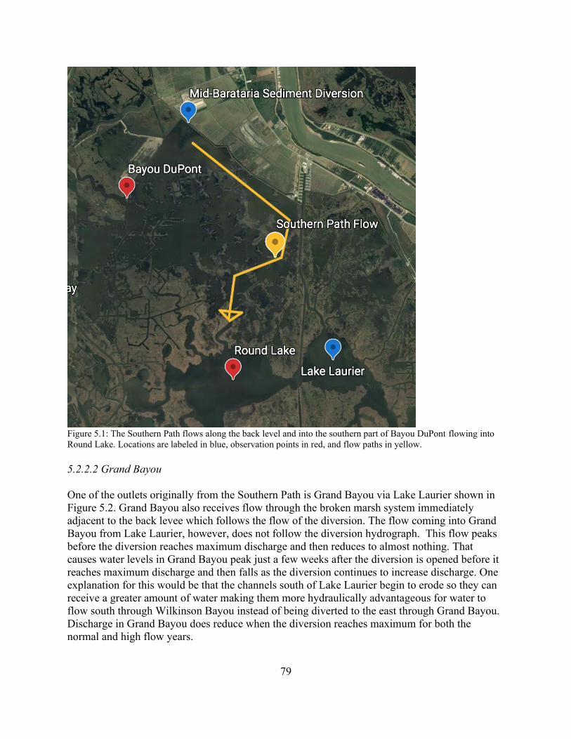
79
Figure 5.1: The Southern Path flows along the back level and into the southern part of Bayou DuPont flowing into
Round Lake. Locations are labeled in blue, observation points in red, and flow paths in yellow.
5.2.2.2 Grand Bayou
One of the outlets originally from the Southern Path is Grand Bayou via Lake Laurier shown in
Figure 5.2. Grand Bayou also receives flow through the broken marsh system immediately
adjacent to the back levee which follows the flow of the diversion. The flow coming into Grand
Bayou from Lake Laurier, however, does not follow the diversion hydrograph. This flow peaks
before the diversion reaches maximum discharge and then reduces to almost nothing. That
causes water levels in Grand Bayou peak just a few weeks after the diversion is opened before it
reaches maximum discharge and then falls as the diversion continues to increase discharge. One
explanation for this would be that the channels south of Lake Laurier begin to erode so they can
receive a greater amount of water making them more hydraulically advantageous for water to
flow south through Wilkinson Bayou instead of being diverted to the east through Grand Bayou.
Discharge in Grand Bayou does reduce when the diversion reaches maximum for both the
normal and high flow years.
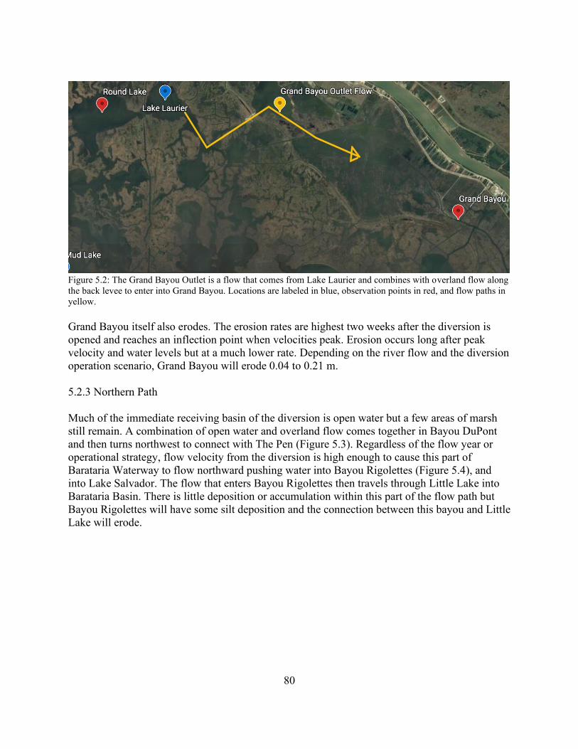
80
Figure 5.2: The Grand Bayou Outlet is a flow that comes from Lake Laurier and combines with overland flow along
the back levee to enter into Grand Bayou. Locations are labeled in blue, observation points in red, and flow paths in
yellow.
Grand Bayou itself also erodes. The erosion rates are highest two weeks after the diversion is
opened and reaches an inflection point when velocities peak. Erosion occurs long after peak
velocity and water levels but at a much lower rate. Depending on the river flow and the diversion
operation scenario, Grand Bayou will erode 0.04 to 0.21 m.
5.2.3 Northern Path
Much of the immediate receiving basin of the diversion is open water but a few areas of marsh
still remain. A combination of open water and overland flow comes together in Bayou DuPont
and then turns northwest to connect with The Pen (Figure 5.3). Regardless of the flow year or
operational strategy, flow velocity from the diversion is high enough to cause this part of
Barataria Waterway to flow northward pushing water into Bayou Rigolettes (Figure 5.4), and
into Lake Salvador. The flow that enters Bayou Rigolettes then travels through Little Lake into
Barataria Basin. There is little deposition or accumulation within this part of the flow path but
Bayou Rigolettes will have some silt deposition and the connection between this bayou and Little
Lake will erode.
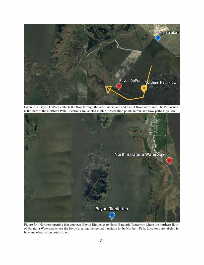
81
Figure 5.3: Bayou DuPont collects the flow through the open marshland and then it flows north into The Pen which
is the start of the Northern Path. Locations are labeled in blue, observation points in red, and flow paths in yellow.
Figure 5.4: Northern opening that connects Bayou Rigolettes to North Barataria Waterway where the northern flow
of Barataria Waterway enters the bayou creating the second transition in the Northern Path. Locations are labeled in
blue and observation points in red.
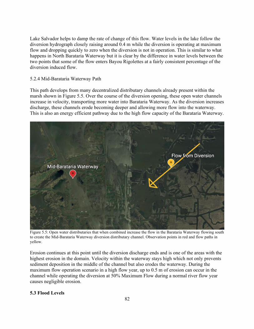
82
Lake Salvador helps to damp the rate of change of this flow. Water levels in the lake follow the
diversion hydrograph closely raising around 0.4 m while the diversion is operating at maximum
flow and dropping quickly to zero when the diversion is not in operation. This is similar to what
happens in North Barataria Waterway but it is clear by the difference in water levels between the
two points that some of the flow enters Bayou Rigolettes at a fairly consistent percentage of the
diversion induced flow.
5.2.4 Mid-Barataria Waterway Path
This path develops from many decentralized distributary channels already present within the
marsh shown in Figure 5.5. Over the course of the diversion opening, these open water channels
increase in velocity, transporting more water into Barataria Waterway. As the diversion increases
discharge, these channels erode becoming deeper and allowing more flow into the waterway.
This is also an energy efficient pathway due to the high flow capacity of the Barataria Waterway.
Figure 5.5: Open water distributaries that when combined increase the flow in the Barataria Waterway flowing south
to create the Mid-Barataria Waterway diversion distributary channel. Observation points in red and flow paths in
yellow.
Erosion continues at this point until the diversion discharge ends and is one of the areas with the
highest erosion in the domain. Velocity within the waterway stays high which not only prevents
sediment deposition in the middle of the channel but also erodes the waterway. During the
maximum flow operation scenario in a high flow year, up to 0.5 m of erosion can occur in the
channel while operating the diversion at 50% Maximum Flow during a normal river flow year
causes negligible erosion.
5.3 Flood Levels
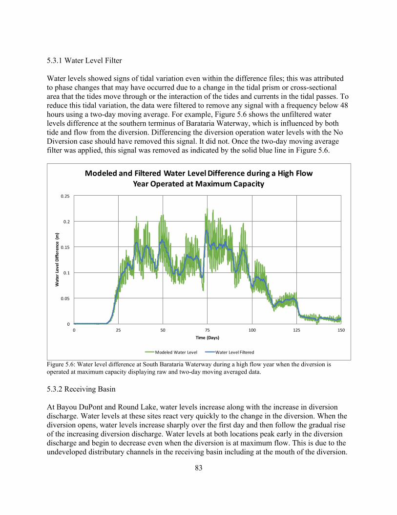
83
5.3.1 Water Level Filter
Water levels showed signs of tidal variation even within the difference files; this was attributed
to phase changes that may have occurred due to a change in the tidal prism or cross-sectional
area that the tides move through or the interaction of the tides and currents in the tidal passes. To
reduce this tidal variation, the data were filtered to remove any signal with a frequency below 48
hours using a two-day moving average. For example, Figure 5.6 shows the unfiltered water
levels difference at the southern terminus of Barataria Waterway, which is influenced by both
tide and flow from the diversion. Differencing the diversion operation water levels with the No
Diversion case should have removed this signal. It did not. Once the two-day moving average
filter was applied, this signal was removed as indicated by the solid blue line in Figure 5.6.
Figure 5.6: Water level difference at South Barataria Waterway during a high flow year when the diversion is
operated at maximum capacity displaying raw and two-day moving averaged data.
5.3.2 Receiving Basin
At Bayou DuPont and Round Lake, water levels increase along with the increase in diversion
discharge. Water levels at these sites react very quickly to the change in the diversion. When the
diversion opens, water levels increase sharply over the first day and then follow the gradual rise
of the increasing diversion discharge. Water levels at both locations peak early in the diversion
discharge and begin to decrease even when the diversion is at maximum flow. This is due to the
undeveloped distributary channels in the receiving basin including at the mouth of the diversion.
0
0.05
0.1
0.15
0.2
0.25
0 25 50 75 100 125 150
WaterLevelD
ifference(m
)
Time(Days)
ModeledandFilteredWaterLevelDifferenceduringaHighFlowYearOperatedatMaximumCapacity
ModeledWaterLevel WaterLevelFiltered
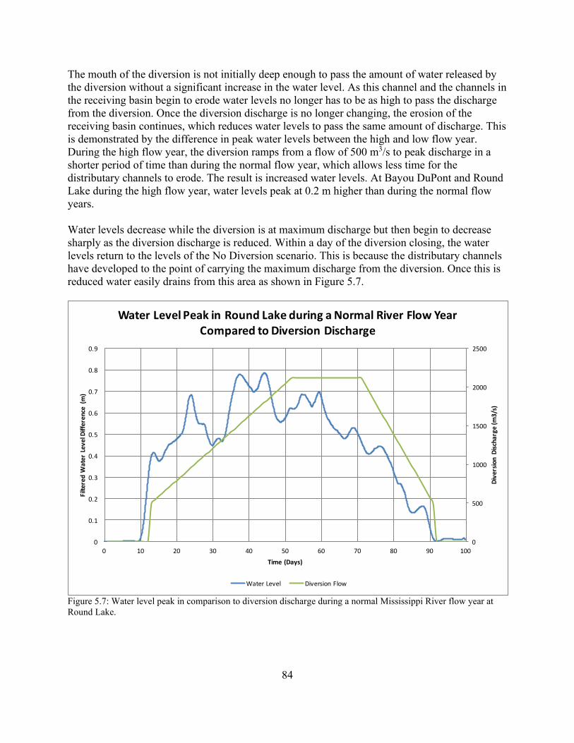
84
The mouth of the diversion is not initially deep enough to pass the amount of water released by
the diversion without a significant increase in the water level. As this channel and the channels in
the receiving basin begin to erode water levels no longer has to be as high to pass the discharge
from the diversion. Once the diversion discharge is no longer changing, the erosion of the
receiving basin continues, which reduces water levels to pass the same amount of discharge. This
is demonstrated by the difference in peak water levels between the high and low flow year.
During the high flow year, the diversion ramps from a flow of 500 m3/s to peak discharge in a
shorter period of time than during the normal flow year, which allows less time for the
distributary channels to erode. The result is increased water levels. At Bayou DuPont and Round
Lake during the high flow year, water levels peak at 0.2 m higher than during the normal flow
years.
Water levels decrease while the diversion is at maximum discharge but then begin to decrease
sharply as the diversion discharge is reduced. Within a day of the diversion closing, the water
levels return to the levels of the No Diversion scenario. This is because the distributary channels
have developed to the point of carrying the maximum discharge from the diversion. Once this is
reduced water easily drains from this area as shown in Figure 5.7.
Figure 5.7: Water level peak in comparison to diversion discharge during a normal Mississippi River flow year at
Round Lake.
0
500
1000
1500
2000
2500
0
0.1
0.2
0.3
0.4
0.5
0.6
0.7
0.8
0.9
0 10 20 30 40 50 60 70 80 90 100
DiversionDischarge(m
3/s)
FilteredW
aterLevelDifference(m)
Time(Days)
WaterLevelPeakinRoundLakeduringaNormalRiverFlowYearComparedtoDiversionDischarge
WaterLevel DiversionFlow
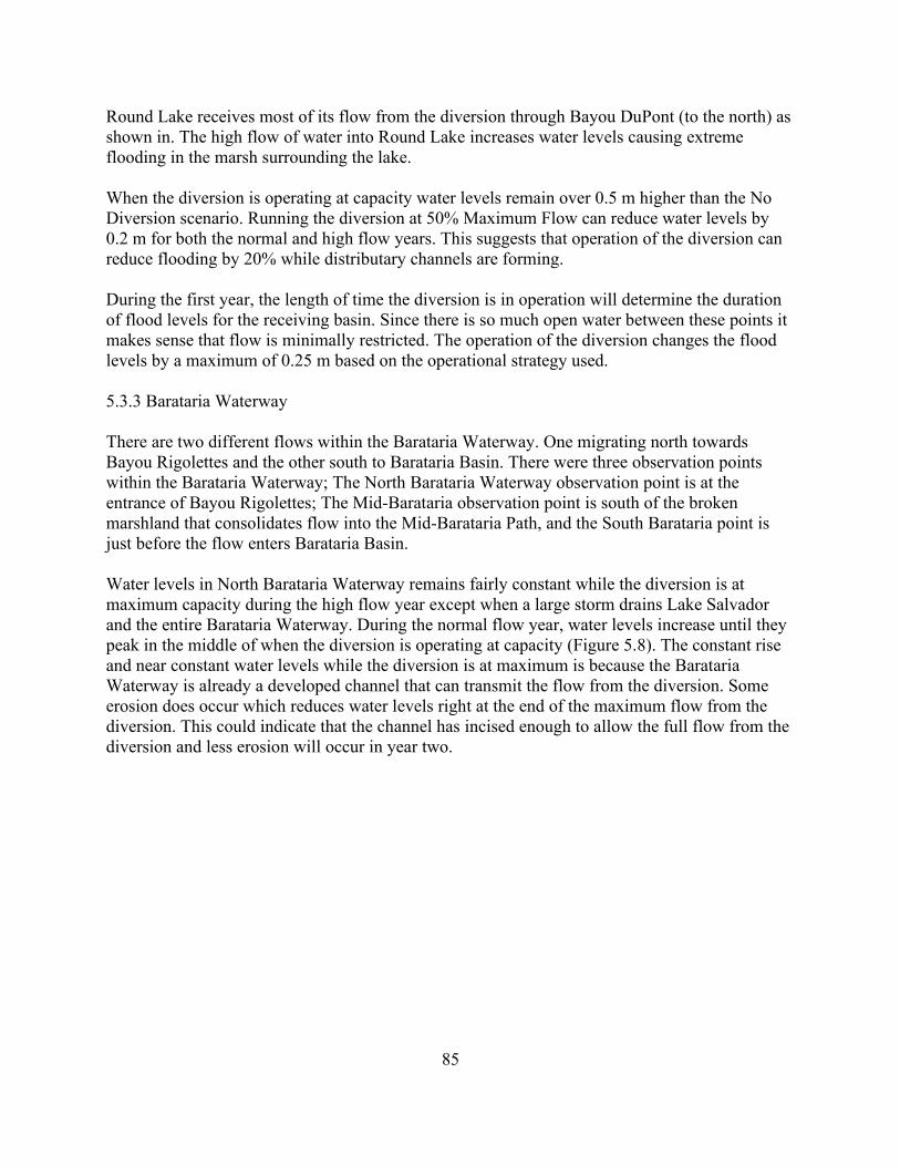
85
Round Lake receives most of its flow from the diversion through Bayou DuPont (to the north) as
shown in. The high flow of water into Round Lake increases water levels causing extreme
flooding in the marsh surrounding the lake.
When the diversion is operating at capacity water levels remain over 0.5 m higher than the No
Diversion scenario. Running the diversion at 50% Maximum Flow can reduce water levels by
0.2 m for both the normal and high flow years. This suggests that operation of the diversion can
reduce flooding by 20% while distributary channels are forming.
During the first year, the length of time the diversion is in operation will determine the duration
of flood levels for the receiving basin. Since there is so much open water between these points it
makes sense that flow is minimally restricted. The operation of the diversion changes the flood
levels by a maximum of 0.25 m based on the operational strategy used.
5.3.3 Barataria Waterway
There are two different flows within the Barataria Waterway. One migrating north towards
Bayou Rigolettes and the other south to Barataria Basin. There were three observation points
within the Barataria Waterway; The North Barataria Waterway observation point is at the
entrance of Bayou Rigolettes; The Mid-Barataria observation point is south of the broken
marshland that consolidates flow into the Mid-Barataria Path, and the South Barataria point is
just before the flow enters Barataria Basin.
Water levels in North Barataria Waterway remains fairly constant while the diversion is at
maximum capacity during the high flow year except when a large storm drains Lake Salvador
and the entire Barataria Waterway. During the normal flow year, water levels increase until they
peak in the middle of when the diversion is operating at capacity (Figure 5.8). The constant rise
and near constant water levels while the diversion is at maximum is because the Barataria
Waterway is already a developed channel that can transmit the flow from the diversion. Some
erosion does occur which reduces water levels right at the end of the maximum flow from the
diversion. This could indicate that the channel has incised enough to allow the full flow from the
diversion and less erosion will occur in year two.
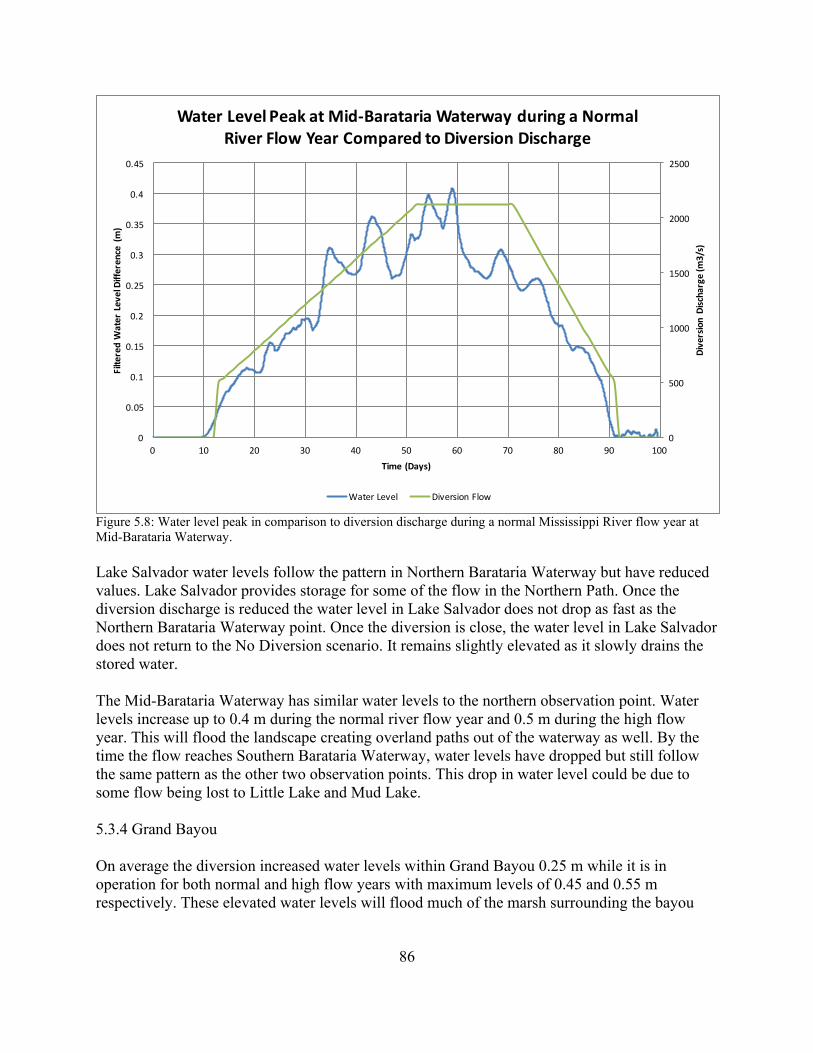
86
Figure 5.8: Water level peak in comparison to diversion discharge during a normal Mississippi River flow year at
Mid-Barataria Waterway.
Lake Salvador water levels follow the pattern in Northern Barataria Waterway but have reduced
values. Lake Salvador provides storage for some of the flow in the Northern Path. Once the
diversion discharge is reduced the water level in Lake Salvador does not drop as fast as the
Northern Barataria Waterway point. Once the diversion is close, the water level in Lake Salvador
does not return to the No Diversion scenario. It remains slightly elevated as it slowly drains the
stored water.
The Mid-Barataria Waterway has similar water levels to the northern observation point. Water
levels increase up to 0.4 m during the normal river flow year and 0.5 m during the high flow
year. This will flood the landscape creating overland paths out of the waterway as well. By the
time the flow reaches Southern Barataria Waterway, water levels have dropped but still follow
the same pattern as the other two observation points. This drop in water level could be due to
some flow being lost to Little Lake and Mud Lake.
5.3.4 Grand Bayou
On average the diversion increased water levels within Grand Bayou 0.25 m while it is in
operation for both normal and high flow years with maximum levels of 0.45 and 0.55 m
respectively. These elevated water levels will flood much of the marsh surrounding the bayou
0
500
1000
1500
2000
2500
0
0.05
0.1
0.15
0.2
0.25
0.3
0.35
0.4
0.45
0 10 20 30 40 50 60 70 80 90 100
DiversionDischarge(m
3/s)
FilteredW
aterLevelDifference(m)
Time(Days)
WaterLevelPeakatMid-BaratariaWaterwayduringaNormalRiverFlowYearComparedtoDiversionDischarge
WaterLevel DiversionFlow
87
but this water level is not static. Initially water levels in Grand Bayou increase greatly and then
reduce remaining below 0.2 m for over half the time the diversion is in operation.
During the high flow year, water levels reach 0.45 m and stay above 0.4 m for three weeks. This
is due to the flow from Lake Laurier peaking around this time. During a normal flow year, water
levels above 0.4 m occur for two weeks but happen one month after the diversion is opened as
shown in Figure 5.9. This is because the flow of the water has less time to erode the channel of
Grand Bayou. Water levels drop off here for two reasons. Grand Bayou erodes to a level that
allows for the diversion flow to pass through it with minimal increases in water level and that
discharge from Lake Laurier reduces over the course of the diversion flow. This is due to erosion
in Wilkinson Bayou that increases discharge through that path.
Figure 5.9: Water level peak in comparison to diversion discharge during a normal Mississippi River flow year at
Grand Bayou.
5.4 Velocity
5.4.1 Velocity Filter
There are low velocity regions within larger bodies of water such as Round Lake. Here the water
velocity at slack water would be close to zero regardless of whether the diversion is operating.
The velocity of the diversion and the tide would counteract during flood tide damping the results
as seen in the raw difference files and would enhance the flow during ebb tide. The tidal
0
500
1000
1500
2000
2500
0
0.05
0.1
0.15
0.2
0.25
0.3
0.35
0.4
0.45
0.5
0.00 10.00 20.00 30.00 40.00 50.00 60.00 70.00 80.00 90.00 100.00
DiversionDischarge(m
3/s)
FilteredW
aterLevelDifference(m)
Time(Days)
WaterLevelPeakinGrandBayouduringaNormalRiverFlowYearComparedtoDiversionDischarge
WaterLevel DiversionFlow
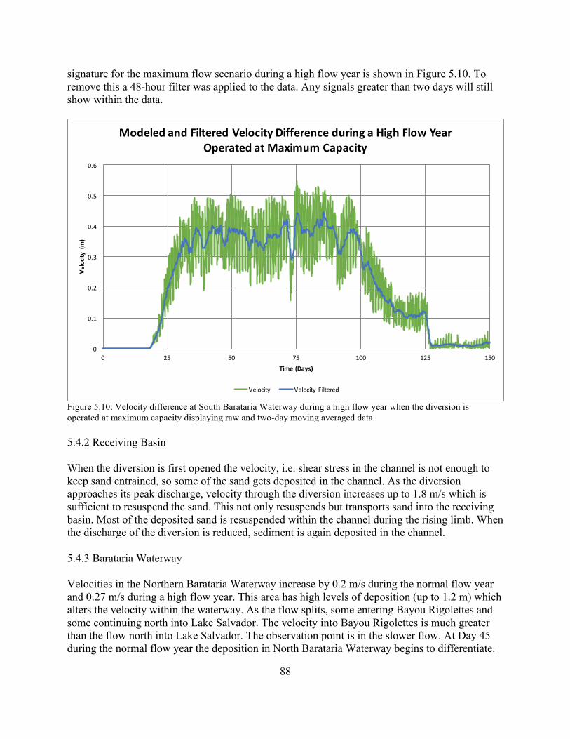
88
signature for the maximum flow scenario during a high flow year is shown in Figure 5.10. To
remove this a 48-hour filter was applied to the data. Any signals greater than two days will still
show within the data.
Figure 5.10: Velocity difference at South Barataria Waterway during a high flow year when the diversion is
operated at maximum capacity displaying raw and two-day moving averaged data.
5.4.2 Receiving Basin
When the diversion is first opened the velocity, i.e. shear stress in the channel is not enough to
keep sand entrained, so some of the sand gets deposited in the channel. As the diversion
approaches its peak discharge, velocity through the diversion increases up to 1.8 m/s which is
sufficient to resuspend the sand. This not only resuspends but transports sand into the receiving
basin. Most of the deposited sand is resuspended within the channel during the rising limb. When
the discharge of the diversion is reduced, sediment is again deposited in the channel.
5.4.3 Barataria Waterway
Velocities in the Northern Barataria Waterway increase by 0.2 m/s during the normal flow year
and 0.27 m/s during a high flow year. This area has high levels of deposition (up to 1.2 m) which
alters the velocity within the waterway. As the flow splits, some entering Bayou Rigolettes and
some continuing north into Lake Salvador. The velocity into Bayou Rigolettes is much greater
than the flow north into Lake Salvador. The observation point is in the slower flow. At Day 45
during the normal flow year the deposition in North Barataria Waterway begins to differentiate.
0
0.1
0.2
0.3
0.4
0.5
0.6
0 25 50 75 100 125 150
Velocity(m)
Time(Days)
ModeledandFilteredVelocityDifferenceduringaHighFlowYearOperatedatMaximumCapacity
Velocity VelocityFiltered
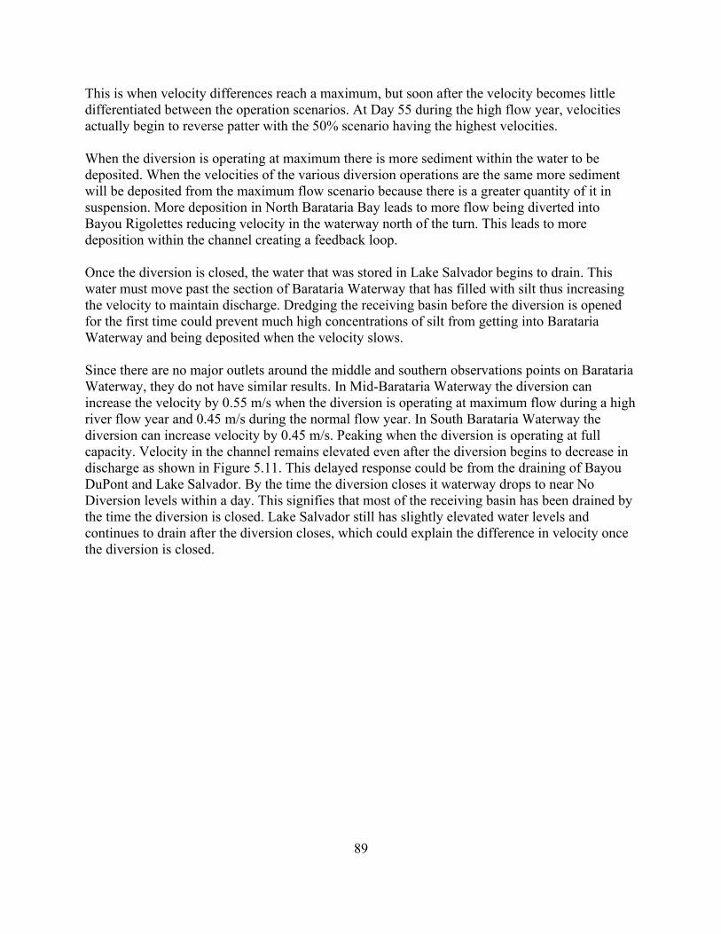
89
This is when velocity differences reach a maximum, but soon after the velocity becomes little
differentiated between the operation scenarios. At Day 55 during the high flow year, velocities
actually begin to reverse patter with the 50% scenario having the highest velocities.
When the diversion is operating at maximum there is more sediment within the water to be
deposited. When the velocities of the various diversion operations are the same more sediment
will be deposited from the maximum flow scenario because there is a greater quantity of it in
suspension. More deposition in North Barataria Bay leads to more flow being diverted into
Bayou Rigolettes reducing velocity in the waterway north of the turn. This leads to more
deposition within the channel creating a feedback loop.
Once the diversion is closed, the water that was stored in Lake Salvador begins to drain. This
water must move past the section of Barataria Waterway that has filled with silt thus increasing
the velocity to maintain discharge. Dredging the receiving basin before the diversion is opened
for the first time could prevent much high concentrations of silt from getting into Barataria
Waterway and being deposited when the velocity slows.
Since there are no major outlets around the middle and southern observations points on Barataria
Waterway, they do not have similar results. In Mid-Barataria Waterway the diversion can
increase the velocity by 0.55 m/s when the diversion is operating at maximum flow during a high
river flow year and 0.45 m/s during the normal flow year. In South Barataria Waterway the
diversion can increase velocity by 0.45 m/s. Peaking when the diversion is operating at full
capacity. Velocity in the channel remains elevated even after the diversion begins to decrease in
discharge as shown in Figure 5.11. This delayed response could be from the draining of Bayou
DuPont and Lake Salvador. By the time the diversion closes it waterway drops to near No
Diversion levels within a day. This signifies that most of the receiving basin has been drained by
the time the diversion is closed. Lake Salvador still has slightly elevated water levels and
continues to drain after the diversion closes, which could explain the difference in velocity once
the diversion is closed.
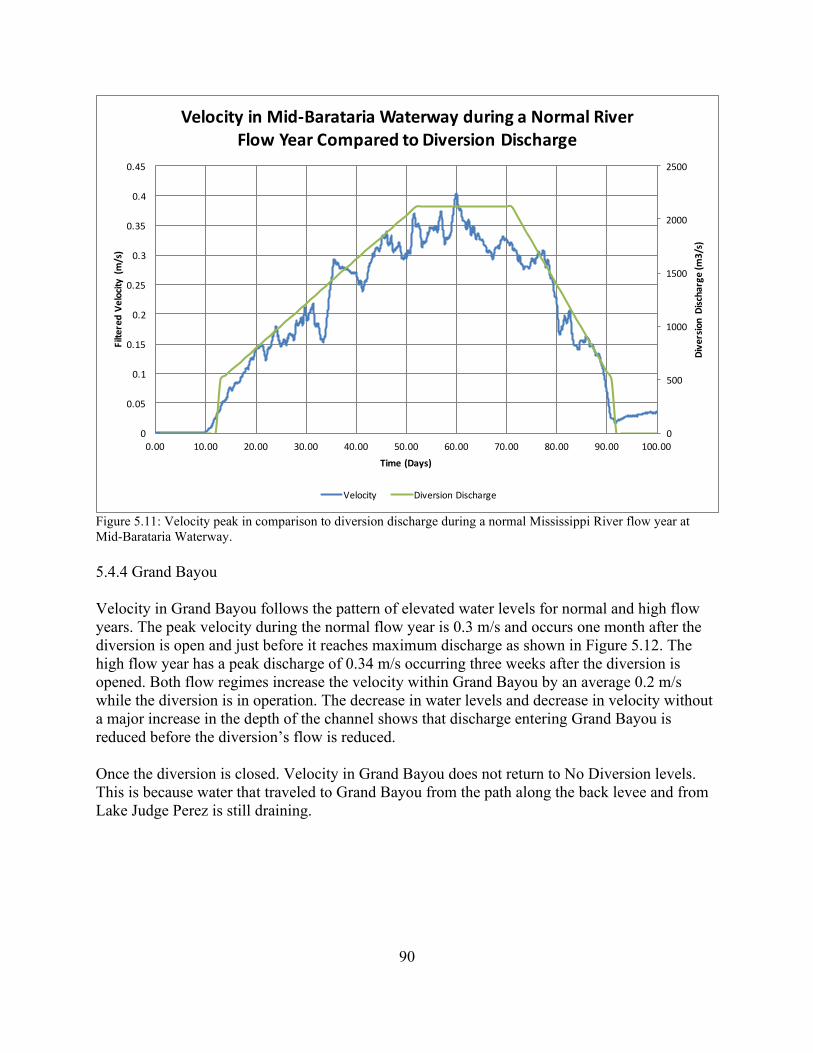
90
Figure 5.11: Velocity peak in comparison to diversion discharge during a normal Mississippi River flow year at
Mid-Barataria Waterway.
5.4.4 Grand Bayou
Velocity in Grand Bayou follows the pattern of elevated water levels for normal and high flow
years. The peak velocity during the normal flow year is 0.3 m/s and occurs one month after the
diversion is open and just before it reaches maximum discharge as shown in Figure 5.12. The
high flow year has a peak discharge of 0.34 m/s occurring three weeks after the diversion is
opened. Both flow regimes increase the velocity within Grand Bayou by an average 0.2 m/s
while the diversion is in operation. The decrease in water levels and decrease in velocity without
a major increase in the depth of the channel shows that discharge entering Grand Bayou is
reduced before the diversion’s flow is reduced.
Once the diversion is closed. Velocity in Grand Bayou does not return to No Diversion levels.
This is because water that traveled to Grand Bayou from the path along the back levee and from
Lake Judge Perez is still draining.
0
500
1000
1500
2000
2500
0
0.05
0.1
0.15
0.2
0.25
0.3
0.35
0.4
0.45
0.00 10.00 20.00 30.00 40.00 50.00 60.00 70.00 80.00 90.00 100.00
DiversionDischarge(m
3/s)
FilteredVelocity(m/s)
Time(Days)
VelocityinMid-BaratariaWaterwayduringaNormalRiverFlowYearComparedtoDiversionDischarge
Velocity DiversionDischarge
91
Figure 5.12: Velocity peak in comparison to diversion discharge during a normal Mississippi River flow year in
Grand Bayou.
5.5 Sediment
5.5.1 Receiving Basin
Sediment concentration in this water varies greatly based on diversion operational scenarios.
While higher amounts of sediment are brought into the receiving basin when the diversion is
operated at maximum flow versus 50% the concentration remains the same in the model. What
does change is the erosion of the receiving basin. The mouth of the diversion can erode up to 8 m
when the diversion is operated at maximum flow in the first year increasing the sediment in the
water.
Sand settles out of the water column quickly, depositing on the sides of the channel created at the
mouth of the diversion and along the levee system due to the eddies coming out of the diversion.
Even the sand that is picked up while scouring the channel at the mouth of the diversion is
quickly deposited. Outside of the mouth of the diversion, the velocity of water is not fast enough
to keep sand in suspension. Some sand can move as bed load, however this is very small.
Silt leaves the diversion at a concentration of just under 0.1 kg/m3. The souring at the mouth of
the diversion and continued erosion of the immediate receiving basin increases the silt
concentration. By the time the flow reaches The Pen, concentrations in the water have increased
0
500
1000
1500
2000
2500
0
0.05
0.1
0.15
0.2
0.25
0.3
0.35
0.00 10.00 20.00 30.00 40.00 50.00 60.00 70.00 80.00 90.00 100.00
DiversionDischarge(m
3/s)
FilteredVelocity(m/s)
Time(Days)
VelocityinGrandBayouduringaNormalRiverFlowYearComparedtoDiversionDischarge
Velocity DiversionDischarge
92
by up to 1.3 kg/m3. When the flow is operated at 50% maximum flow during the high flow year,
the silt concentration increases by 0.26 kg/m3. This means that much of the silt is entrained
during the initial scour at the mouth of the diversion and the continued erosion of the receiving
basin.
The initial time to peak discharge also plays a role in how much silt enters The Pen. At
maximum flow, the difference in concentration between the normal and high flow years is
almost 0.6 kg/m3. This corresponds with a 2 m increase in the depth of the channel at the mouth
of the diversion.
Round Lake has much lower concentrations of silt. When the diversion is operated at maximum
flow during a high flow year the average concentration of silt is 0.21 kg/m3 but run at 50% it is
0.03 kg/m3. This is because the cannel into Round Lake is more established that the flow
entering The Pen so less erosion occurs. Also, much of the flow entering The Pen goes through
the northern portion of Bayou DuPont with no areas of deposition. The flow into Round Lake
comes through the southern portion of Bayou DuPont which travels through an open water
section slowing velocities and depositing much of the silt before it reaches Round Lake.
Clay follows a similar pattern to silt however less is deposited. Once the flow picks up clay from
the receiving basin it stays in suspension until the flow enters Barataria Bay and beyond. This is
partially due to the fact that salinity within the basin drops to zero just days after the diversion is
open which reduces the flocculation of the clay particles in the water.
5.5.2 Barataria Waterway
Velocities entering The Pen are high enough to cause erosion along the bottom half of this area.
Some flow escapes north into the nearly still water; Velocities slow and silt is deposited. As the
flow enters Barataria Waterway velocities continue to slow and more silt is deposited. By the
time the flow reaches the observation point at North Barataria Waterway, some sediment has
been lost since The Pen but silt levels are still as high as 1.26 kg/m3 during the high flow year
which is 15 times the concentration of silt entering the through the diversion. At the turn into
Bayou Rigolettes this silt is deposited as the velocity of the water continues to slow. This can
deposit as much as 1.2 m of silt in the waterway, which would be a problem for transpiration in
the channel. This sediment will have to be dredged to allow for ships to continue through the
waterway unhindered. More research will have to be done to determine if this silt will deposit
within the waterway every year or will this deposition slow as the distributary channels become
more defined. If the latter is the case, the receiving basin could be dredged before the diversion is
opened to reduce the amount of erosion that will occur in the diversions first year.
Silt concentrations at the southern terminus of Barataria Waterway is the highest out of any
observation point during the Maximum flow but is less than at North Barataria Waterway during
reduced maximum flow scenarios. The northern and southern flow in Barataria Waterway start
with similar concentrations. As the flow travels south down the waterway silt is deposited along
the edges as the middle of the channel erodes. During the maximum flow scenarios, this channel
can erode up to 0.5 m adding more silt to the water column but when the diversion is operated at
93
50% maximum flow the waterway has minimal erosion. This explains why there is much less silt
when the diversion is operated at a reduced maximum flow.
5.5.3 Grand Bayou
Sand and silt that came through the diversion is deposited before the flow reaches Grand Bayou.
Round Lake and Lake Laurier both have large silt deposits that take most of the silt out of
suspension. Clay concentrations increased within the water range from 0.2 to 0.55 kg/m3
depending on operational strategy. During the high flow year, the diversion had a lower
concentration of clay than during the high flow year yet the concentration of silt in Grand Bayou
during the high flow year had a concentration of 0.15 kg/m3 greater than that of the normal flow
year. This is because of the erosion happening within the receiving basin during the high flow
year with its quicker time to peak discharge.
Clay has little impact on the geomorphology of Grand Bayou because the velocities within the
bayou are too high for the clay to settle out and there is limited flocculation while the salinity is
at zero. However, the increased turbidity of the water reduces the light available for
photosynthesis, which alters oxygen levels within the water. Increased turbidity can harm fish
spawning and increase pollution levels in the area so working to reduce this concentration would
be beneficial.
5.6 Salinity
The diversion causes salinity levels to drop to zero over much of the domain. The area around
Bayou DuPont, Round Lake, and Barataria Waterway become fresh just days after the diversion
is open and recovery is slow once the diversion is closed. In North Barataria Waterway, salinity
rebound is negligible but could change if the silt restricting some of the flow is dredged. Then it
would probably similar to the salinity in Mid-Barataria Waterway which shows modest recovery
after the diversion is closed. If that rate of recovery were to continue, it would take over a month
for salinity levels to return to normal.
The salinity within Grand Bayou falls to 0 ppt within the first two weeks of the diversion
opening. This prevents flocculation of sediment. The bayou remains purely fresh water until the
diversion is closed. Then it slowly begins to increase in salinity levels. This recovery is not
nearly as rapid as the decline and will take months to return to normal levels if the rate stays the
same.
Lake Washington has salinity levels as low as 5 ppt when the diversion is operated at maximum
flow. This area is far south of the diversion but is fed by Grand Bayou. When the diversion is
open it has fresh water entering from the north and salt water coming in from Bay Long to the
south. This large tidal influence is why Lake Washington retains some salinity while the
diversion is in operation. The area west of Lake Washington is the central Barataria Bay which
receives a large influx of fresh water from Barataria Waterway but gets salt water from inlets
near Grand Isle and Grand Terre Islands. For that reason, the eastern part of the bay has similar
responses to the diversion. Once the diversion closes salinity levels rebound to near No
Diversion levels however freshwater drainage from the rest of the basin could be slowing the
94
complete return to these levels. Even salinity changes of this much could affect a lot of species
that require higher salinity levels to survive.
The western part of Barataria Bay has even less direct fresh water input. The closest flow path
created by the diversion is the Northern Path that enters Barataria Bay through Little Lake which
is to the east of the Western Barataria Bay observation point. Due to mixing of the bay some of
this water coming from the northern path reduces the salinity that is present during the No
Diversion scenario but this was minimal when the diversion is at peak discharge and there is no
difference after the diversion begins to decrease discharge.
5.7 Model Sensitivity
There are multiple sources of error that could occur within the model. One source is that there
are a range of values determined by previous studies that could be used in the model. Precedence
from previous models was used to determine these values. When that was not immediately
available a best approximation was used to determine model values based on literature analysis.
In addition to value ranges between students, many are spatially variable as well. Simplifications
were made to reduce the number of spatially varying possibilities.
The critical shear stress of the bed was modeled as 0.1 Pa, which is on the lower side of critical
shears stresses tested in Barataria Basin. This value was chosen because this is the critical shear
stress of newly deposited sediment within the basin. The sediment deposited by the diversion
would likely have an initial critical shear stress less than this value but sediment that was in the
basin prior to the diversion construction would have a larger value. Studies have shown that the
critical shear stress increases to 0.2 Pa within 6 months of sediment deposition in the basin.
Vegetation also increases the critical shear stress of soil yet no vegetation was modeled in this
study. A higher average critical shear stress in the marsh areas of the basin would lead to reduced
marsh erosion and increased incising of the open water pathways.
Critical shear stress is not the only value that determines erosion in the model. The velocity and,
in turn, the shear stress of the flow is determined based on the Manning’s roughness. Three
different Manning’s roughness were used in the model increasing from the center of the channel,
to the marsh edge and center. The higher roughness in the middle of the marsh was used to
approximate the roughness due to vegetation that reduces the velocity and shear stress caused by
the flow. This roughness dampens erosion in the basin. These values were determining through
literature and the model calibration. However, any under estimate in these values would also lead
to an over prediction of erosion.
The sediment composition of the bed determines how easy it is eroded. There were five layers of
the bed each chosen to be 2 m deep. The sand percentage ranged from 5 – 20% through the
layers from top to bottom. This was chosen based on literature values. These layers were
assumed to be constant throughout the domain and were only differentiated between the marsh
(elevation 0 m and above) and the channels (elevation below 0 m) in layer thickness. In reality,
sediment fractions in the basin would vary. However, this would cost computational time so the
simplification was made. More sand in these layers would make the bed harder to erode reducing
the erosion determined by the model. The critical shear for sand is based on the Shields Curve.
95
The final parameter that determines erosion and deposition is settling velocity. For sand, the
settling velocity was determined using the van Rijn equations based on an average sediment
diameter determined from literature. For silt and clay, both the settling velocity and average
particle size were determined from literature. Any under estimation in settling velocity would
increase the net erosion values especially in the immediate receiving basin since slow settling
velocities would cause particles to remain in suspension longer moving away from the diversion.
5.8 Recommendations
The results show that dredging a channel at the mouth of the diversion is needed to reduce
increased turbidity in the water and silt deposition in Round Lake, The Pen, and Barataria
Waterway. Dredging of the three major distributary pathways within the receiving basin could
further reduce erosion and prevent high concentrations of sediment in the water. This would also
result in a more control evolution of the distributary system and would help reduce the maximum
flood levels. The depth and duration of marsh flooding may also be reduced by pre-dredging the
main distributary channels.
Grand Bayou could be protected through the addition of a flood diverting structure or pre-
dredging of Wilkinson Bayou. This bayou eventually erodes enough to receive the majority of
the flow from the Southern Path but it takes time of this channel to develop. Pre-dredging this
path would immediately reduce the flood waters in Grand Bayou protecting the native
populations along its banks.
A combination of pre-dredged channels, slowly ramping the diversion up to peak discharge, and
operating the diversion at reduced flow in the initial years could prevent flooding within the
basin while still developing the distributary pathway needed to move the full diversion flow.
Also, timing of the diversion opening is critical. If the diversion is only operated off of the
Mississippi River hydrograph, the diversion could cause much of the basin to be completely
fresh water late into June when the peak discharge is late for example in the modeled normal
river flow scenario. Some years the maximum sediment building capacity will need to be
balanced against the salinity needs of oyster and other fisheries that cannot handle the fresh
water during warm water periods in the spring and summer months.
96
Chapter 6: Conclusions
The Barataria Basin model was successfully developed, calibrated, and applied to simulate tides,
diversion flow, wind forcing, sediment, and salinity. As the diversion enters the receiving basin
the mouth of the diversion is scoured creating a deep channel with sediment depositing on either
side in a natural levee building process. However, the majority of the immediate receiving basin
experiences erosion with large amounts of silt and clay being resuspended with a consequent
increase in the sediment concentration in the water.
Three major pathways were created by the diversion out of the immediate receiving basin. The
southern path through Round Lake that initially pushes flow through Grand Bayou until
Wilkinson Bayou erodes enough to take a large portion of the flow. The Mid-Barataria
Waterway path that enters Barataria Waterway through the broken mashes west of Bayou
DuPont. Finally, the Northern Path that moves water north through Barataria Waterway into
Bayou Rigolettes. These pathways distribute fresh water that reduces salinity levels to near zero
and floods the marshes around them. When the velocity slows in large bodies of water like The
Pen and Round Lake silt deposits are built. This also occurs in the area of nearly stagnate water
between the northern and southern flow of water in Barataria Waterway. Pre-dredging of the
receiving basin will reduce the amount of silt resuspension and subsequent deposition and reduce
the turbidity of the water. If Wilkinson Bayou is dredged before the diversion is operated, Grand
Bayou could be spared the worst of the flooding.
The operation of the diversion will determine the impact that the diversion has on the landscape.
The diversion should have a slow ramp up to peak discharge to allow channel development. The
length of time that the diversion is open is directly proportional to the length of time water levels
are elevated, so even if pre-dredging is utilized, peak discharge should be shortened during the
first year to reduce the duration of major flooding while channels are developing to their full
capacity. Finally, timing of the diversion opening cannot be solely based on the Mississippi
River hydrograph. The model showed that during the simulated normal flow year much of the
basin would be fresh water into June possibly damaging the oyster harvest for the year.
More research needs to be done to test the effectiveness of some of the recommendations in
Chapter 5. The model could be run again using the final bathymetry generated during this one
season scenario to see if the channels have fully developed during the first year or if more
erosion should be expected in year two and possibly beyond. The model could also be used to
text how much pre-dredging of the channels before the diversion is opened would needed to
achieve the optimum benefits such as reducing excessive erosion, high silt concentrations and
subsequent deposition in Barataria Waterway. Further model work could be done to determine
the best way to operate the diversion in subsequent years to maximize land building and
minimize erosion while reducing other impacts on the receiving basin.
97
References
Allison, M. A., Demas, C., Ebersole, B., Kleiss, B., Little, C., Meselhe, E., Powell, J., Pratt, T.,
& Vosburg, B. (2012). A Water and Sediment Budget for the Lower Mississippi–Atchafalaya
River in Flood Years 2008–2010: Implications for Sediment Discharge to the Oceans and
Coastal Restoration in Louisiana. Journal of Hydrology, 432–433, 84–97.
Allison, M. A., Ramirez, M. T., & Meselhe, E. A. (2014). Diversion of Mississippi River water
downstream of New Orleans, Louisiana, USA to maximize sediment capture and ameliorate
coastal land loss. Water resources management, 28(12), 4113-4126.
Allison, M. A., & Meselhe, E. A. (2010). The use of large water and sediment diversions in the
lower Mississippi River (Louisiana) for coastal restoration. Journal of Hydrology, 387(3-4), 346-
360.
Amer, R., Kolker, A. S., & Muscietta, A. (2017). Propensity for erosion and deposition in a
deltaic wetland complex: Implications for river management and coastal restoration. Remote
Sensing of Environment, 199, 39-50.
Amini, Sina (2014) Hydrodynamics and Salinity of Pontchartrain Estuary during Hurricanes,
Master of Science Thesis, Civil and Environmental Engineering, University of New Orleans,
New Orleans, LA.
Adrus, T. M., & Bentley, S. J. (2007). Sediment flux and fate in the Mississippi River Diversion
at West Bay: Observation study. Coastal Sediments, 07, 722-735.
Barras, J., Beville, S., Britsch, D., Hartley, S., Hawes, S., Johnston, J., Kemp, P., Kinler, Q.,
Martucci, A., Porthouse, J., Reed, D., Roy, K., Sapkota, S., & Suhayda, J. (2003). Historical and
projected coastal Louisiana land changes: 1978-2050. USGS Open File Report 03-334, 39.
Barras, J. A. (2006). Land area change in coastal Louisiana after the 2005 hurricanes—a series of
three maps. U.S. Geological Survey Open-File Report 06-1274.
Barras, J. A., Padgett, W. C., & Sanders, C. B. (2009). Aerial and Bathymetric Spatial Change
Analysis of the West Bay Sediment Diversion Receiving Area, Louisiana for US Army Engineer
District, New Orleans (MVN) Report. US Army Eng. Res. Dev. Cent., Environ. Lab, Baton
Rouge, La.
Barras, J. A. (2010). Hurricane-induced failure of low salinity wetlands. Proceedings of the
National Academy of Sciences, 107(32), 14014 LP-14019.
Batker D., Mack S., Sklar F., Nuttle W., Kelly M., Freeman A. (2014) The Importance of
Mississippi Delta Restoration on the Local and National Economies. In: Day J., Kemp G.,
Freeman A., Muth D. (eds) Perspectives on the Restoration of the Mississippi Delta. Estuaries of
the World. Springer, Dordrecht
98
Baker, A., Henkel, T., Lopez, J. & Boyd, E. (2011). A Project of the Lake Pontchartrain Basin
Foundation and the Coalition to Restore Coastal Louisiana. Lake Pontchartrain Basin
Foundation.
Bauman, R. H., Day, J. W., & Miller, C. A. (1984). Mississippi Deltaic Wetland Survival:
Sedimentation Versus Coastal Submergence. Science, 224(4653), 1093 LP-1095.
Bevington, A. E., & Twilley, R. R. (2018). Island edge morphodynamics along a
chronosequence in a prograding deltaic floodplain wetland. Journal of Coastal Research, 34(4),
806-817.
Bianchi, T. S., & Allison, M. A. (2009). Large-river delta-front estuaries as natural “recorders”
of global environmental change. Proceedings of the National Academy of Sciences, 106(20),
8085-8092
Blankespoor, B., Dasgupta, S., & Laplante, B. (2012). Sea-level rise and coastal wetlands. Policy
Research Working Paper (WPS6277), World Bank.
Blum, M. D., & Roberts, H. H. (2009). Drowning of the Mississippi Delta due to insufficient
sediment supply and global sea-level rise. Nature Geoscience, 2, 488.
Boesch, D., Josselyn, M., Mehta, A., Morris, J., Nuttle, W., Simenstad, C., & Swift, D. (1994).
Scientific Assessment of Coastal Wetland Loss, Restoration and Management in Louisiana.
Journal of Coastal Research, I-103.
Britsch, L. D., & Kemp III, E. B. (1990). Land loss rates: Mississippi River deltaic plain (No.
WES/TR/GL-90-2). Army Engineer Waterways Experiment Station, Vicksburg, MS.
Brown, S., Couvillion, B., Conzelmann, C., de Mutsert, K., Fischbach, J., Hunnicutt, C.,
McKelvy, M., Quibodeaux, P., Roberts, H., Rodrigue, M., Schindler, J., Suir, K., Thomson, G.,
Visser, J., & White, E. (2017). 2017 Coastal Master Plan: Appendix C: Modeling Chapter 3 -
Modeling Components and Overview. Version Final. (p. 72). Baton Rouge, Louisiana: Coastal
Protection and Restoration Authority
Brown, G., McAlpin, J., Pevey, K., Loung, P., Price, C., & Kleiss, B. (2019). Mississippi River
Hydrodynamic and Delta Management Study: Delta Management Modeling. US Army Corps of
Engineers Coastal and Hydraulics Laboratory. TR-19-2.
Buttles, J., Mohrig, D., Nittrouer, J., McElroy, B., Baitis, E., Allison, M., & Kim, W. (2007).
Partitioning of water discharge by distributary channels in the prograding, Wax Lake Delta,
coastal Louisiana, USA. AGU.
Cahoon, D. R., & Reed, D. J. (1995). Relationships among marsh surface topography,
hydroperiod, and soil accretion in a deteriorating Louisiana salt marsh. Journal of Coastal
Research, 357-369.
99
Cao, S., & Knight, D.W. (2002) Review of regime theory of alluvial channels. Journal of
Hydrodynamics, 3, 1–3.
Carle, M. V., Sasser, C. E., & Roberts, H. H. (2015). Accretion and vegetation community
change in the Wax Lake Delta following the historic 2011 Mississippi River flood. Journal of
Coastal Research, 31(3), 569-587.
Carle, M. V., & Sasser, C. E. (2016). Productivity and resilience: long-term trends and storm-
driven fluctuations in the plant community of the accreting Wax Lake Delta. Estuaries and
coasts, 39(2), 406-422.
Coastal Protection and Restoration Authority of Louisiana. (2012). Louisiana’s Coastal Master
Plan for a Sustainable Coast; Coastal Protection and Restoration Authority of Louisiana: Baton
Rouge, LA, USA.
Coastal Protection and Restoration Authority of Louisiana. (2017) Louisiana’s Coastal Master
Plan for a Sustainable Coast; Coastal Protection and Restoration Authority of Louisiana: Baton
Rouge, LA, USA.
Coleman, J.M., Roberts, H., & Stone, G. (1998) Mississippi River Delta: an Overview. Journal
of Coastal Research, 14(3), 698-716.
Conner, W., Nuttle, W. K., Brinson, M. M., Cahoon, D., Callaway, J. C., Christian, R. R., &
Lynch, C. (1997). Conserving Coastal Wetlands Despite Sea Level Rise. Eos, Transactions,
American Geophysical Union.
Couvillion, B. R., Beck, H., Schoolmaster, D., & Fischer, M. (2017). Land area change in
coastal Louisiana (1932 to 2016) (No. 3381). US Geological Survey.
Das, A., Justic, D., Inoue, M., Hoda, A., Huang, H., & Park, D. (2012). Impacts of Mississippi
River diversions on salinity gradients in a deltaic Louisiana estuary: Ecological and management
implications. Estuarine, Coastal and Shelf Science, 111, 17-26.
Day Jr, J. W., Martin, J. F., Cardoch, L., & Templet, P. H. (1997). System functioning as a basis
for sustainable management of deltaic ecosystems. Coastal Management, 25(2), 115-153.
Day, J. W., Britsch, L. D., Hawes, S. R., Shaffer, G. P., Reed, D. J., & Cahoon, D. (2000).
Pattern and process of land loss in the Mississippi Delta: a spatial and temporal analysis of
wetland habitat change. Estuaries, 23(4), 425-438.
Day Jr, J. W., Barras, J., Clairain, E., Johnston, J., Justic, D., Kemp, G. P., & Templet, P. (2005).
Implications of global climatic change and energy cost and availability for the restoration of the
Mississippi delta. Ecological Engineering, 24(4), 253-265.
Day, J. W., Boesch, D. F., Clairain, E. J., Kemp, G. P., Laska, S. B., Mitsch, W. J., & Whigham,
D. F. (2007). Restoration of the Mississippi Delta: Lessons from Hurricanes Katrina and Rita.
Science, 315(5819), 1679-1684.
100
Day, J. W., Christian, R. R., Boesch, D. M., Yáñez-Arancibia, A., Morris, J., Twilley, R. R., &
Schaffner, L. (2008). Consequences of climate change on the ecogeomorphology of coastal
wetlands. Estuaries and Coasts, 31(3), 477-491.
Day, J. W., Cable, J. E., Cowan Jr, J. H., DeLaune, R., De Mutsert, K., Fry, B., & Rick, J.
(2009). The impacts of pulsed reintroduction of river water on a Mississippi Delta coastal basin.
Journal of Coastal Research, 225-243.
Day, J.W., Christian, R.R., & Boesch, D.M. (2012). Consequences of Climate Change on the
Ecogeomorphology of Coastal Wetlands. Climatic Change, 110, 297.
Day, J., Lane, R., Moerschbaecher, M., DeLaune, R., Mendelssohn, I., Baustian, J., & Twilley,
R. (2013). Vegetation and soil dynamics of a Louisiana estuary receiving pulsed Mississippi
River water following Hurricane Katrina. Estuaries and coasts, 36(4), 665-682.
Day, J. W., Cable, J. E., Lane, R. R., & Kemp, G. P. (2016). Sediment deposition at the
Caernarvon crevasse during the great Mississippi flood of 1927: implications for coastal
restoration. Water, 8(2), 38.
DeLaune, R. D., Baumann, R. H., & Gosselink, J. G. (1983). Relationships among vertical
accretion, coastal submergence, and erosion in a Louisiana Gulf Coast marsh. Journal of
Sedimentary Research, 53(1), 147-157.
DeLaune, R. D., Jugsujinda, A., Peterson, G. W., & Patrick Jr, W. H. (2003). Impact of
Mississippi River freshwater reintroduction on enhancing marsh accretionary processes in a
Louisiana estuary. Estuarine, Coastal and Shelf Science, 58(3), 653-662.
DeLaune, R. D., & White, J. R. (2012). Will coastal wetlands continue to sequester carbon in
response to an increase in global sea level?: a case study of the rapidly subsiding Mississippi
river deltaic plain. Climatic Change, 110(1-2), 297-314.
DeLaune, R. D., Kongchum, M., White, J. R., & Jugsujinda, A. (2013). Freshwater diversions as
an ecosystem management tool for maintaining soil organic matter accretion in coastal marshes.
Catena, 107, 139-144.
Deltares. (2013) Ch. 11: Sediment transport and morphology. In: Delft3D-FLOW – Simulation
of multi-dimensional hydrodynamic flows and transport phenomena, including sediments – User
Manual – Hydro-Morphodynamics, version 3.15.30059.
Dokka, R. K. (2006). Modern-day tectonic subsidence in coastal Louisiana. Geology, 34(4),
281–284.
Donnelly, J. P., Hawkes, A. D., Lane, P., MacDonald, D., Shuman, B. N., Toomey, M. R., &
Woodruff, J. D. (2015). Climate forcing of unprecedented intense‐hurricane activity in the last
2000 years. Earth's Future, 3(2), 49-65.
101
Esposito, C. R., Georgiou, I. Y., & Kolker, A. S. (2013). Hydrodynamic and geomorphic
controls on mouth bar evolution. Geophysical Research Letters, 40(8), 1540-1545.
Falloon, P. D., & Betts, R. A. (2006). The impact of climate change on global river flow in
HadGEM1 simulations. Atmospheric Science Letters, 7(3), 62-68.
Fisk, H. N. (1944). Geological investigations of the alluvial valley of the lower Mississippi
River: US Army Corps of Engineers. Mississippi River Commission, Vicksburg, Mississippi.
Fisk, H. N. (1952). Geological investigation of the Atchafalaya Basin and the problem of
Mississippi River diversion, Vol. 1. US Corps of Engineers Waterways Experiment Station,
Vicksburg, Mississippi.
Gagliano, S.M., Culley, P., Earle, D.W., Jr., King, P., Latiolas, C., Light, P., & Rowland, A.
(1973). Environmental Atlas and Multiuse Management Plan for South Central Louisiana.
Louisiana State University: Baton Rouge, LA, USA,
Gagliano, S. M., Kwon, H. J., & Van Beek, J. L. (1970). Deterioration and restoration of coastal
wetlands. Coastal Engineering, 1767-1781.
Gagliano, S. M., Meyer-Arendt, K. J., & Wicker, K. M. (1981). Land loss in the Mississippi
River deltaic plain. Gulf Coast Association of Geological Societies Transactions, 31, 295-300.
Gaweesh, A., & Meselhe, E. (2016). Evaluation of sediment diversion design attributes and their
impact on the capture efficiency. Journal of Hydraulic Engineering, 142(5)
Georgiou, I.Y, McCorquodale, J.A., Neupani, J., Howes, N., Hughes, Z., FitzGerald, D.M.,
Schindler, J.K. (2010) Modeling the Hydrodynamics of diversion into Barataria Basin, Final
report submitted to the Lake Pontchartrain Basin Foundation, Pontchartrain Institute for
Environmental Sciences, University of New Orleans, New Orleans, LA, 102 pp.
Ghose Hajra, M., McCorquodale, A., Mattson, G., Jerolleman, D., and Filostrat, J. (2014).
“Effects of salinity and particle concentration on sediment hydrodynamics and critical bed-shear-
stress for erosion of fine grained sediments used in wetland restoration projects,” Proceedings,
Sediment Dynamics from the Summit to the Sea, ICCE/IAHS International Symposium,
December 11-14, 2014, New Orleans, LA
Hiatt, M., & Passalacqua, P. (2015). Hydrological connectivity in river deltas: The first‐order
importance of channel‐island exchange. Water Resources Research, 51(4), 2264-2282.
Hiatt, M., & Passalacqua, P. (2017). What controls the transition from confined to unconfined
flow? Analysis of hydraulics in a coastal river delta (Doctoral dissertation, American Society of
Civil Engineers).
Horowitz, A. J. (2010). A quarter century of declining suspended sediment fluxes in the
Mississippi River and the effect of the 1993 flood. Hydrological Processes: An International
Journal, 24(1), 13-34.
102
Horton, B. P., Rahmstorf, S., Engelhart, S. E., & Kemp, A. C. (2014). Expert assessment of sea-
level rise by AD 2100 and AD 2300. Quaternary Science Reviews, 84, 1-6.
Howes, N. C., FitzGerald, D. M., Hughes, Z. J., Georgiou, I. Y., Kulp, M. A., Miner, M. D., ... &
Barras, J. A. (2010). Hurricane-induced failure of low salinity wetlands. Proceedings of the
National Academy of Sciences, 107(32), 14014-14019.
Kearney, M. S., Riter, J. A., & Turner, R. E. (2011). Freshwater river diversions for marsh
restoration in Louisiana: Twenty‐six years of changing vegetative cover and marsh area.
Geophysical Research Letters, 38(16).
Keogh, M. E., Kolker, A. S., Snedden, G. A., & Renfro, A. A. (2019). Hydrodynamic controls on
sediment retention in an emerging diversion-fed delta. Geomorphology, 332, 100-111.
Kesel, R. H. (1988). The decline in the suspended load of the lower Mississippi River and its
influence on adjacent wetlands. Environmental Geology and Water Sciences, 11(3), 271-281.
Khan, N. S., Horton, B. P., McKee, K. L., Jerolmack, D., Falcini, F., Enache, M. D., & Vane, C.
H. (2013). Tracking sedimentation from the historic AD 2011 Mississippi River flood in the
deltaic wetlands of Louisiana, USA. Geology, 41(4), 391-394.
Kim, W., Mohrig, D., Twilley, R., Paola, C., & Parker, G. (2009). Is it feasible to build new land
in the Mississippi River Delta?. Eos, Transactions American Geophysical Union, 90(42), 373-
374.
Knutson, T. R., McBride, J. L., Chan, J., Emanuel, K., Holland, G., Landsea, C., & Sugi, M.
(2010). Tropical cyclones and climate change. Nature geoscience, 3(3), 157-163.
Kolb, C. R., & Van Lopik, J. R. (1966). Depositional environments of the Mississippi River
deltaic plain—southeastern Louisiana. Deltas in Their Geologic Framework, 17-61.
Kolker, A. S., Miner, M. D., & Weathers, H. D. (2012). Depositional dynamics in a river
diversion receiving basin: The case of the West Bay Mississippi River Diversion. Estuarine,
Coastal and Shelf Science, 106, 1-12.
Lake Pontchartrain Basin Foundation. (2018). Hydrocoast Map – Salinity. Saveourlake.org.
Lane, R. R., Day, J. W., & Day, J. N. (2006). Wetland surface elevation, vertical accretion, and
subsidence at three Louisiana estuaries receiving diverted Mississippi River water. Wetlands,
26(4), 1130-1142.
Lane, R. R., Day Jr, J. W., Marx, B. D., Reyes, E., Hyfield, E., & Day, J. N. (2007). The effects
of riverine discharge on temperature, salinity, suspended sediment and chlorophyll a in a
Mississippi delta estuary measured using a flow-through system. Estuarine, Coastal and Shelf
Science, 74(1-2), 145-154.
103
Lacey, G. (1930). Stable Channels in Alluvium Minutes of the Proceedings of the Institution of
Civil Engineers (Vol. 229, No. 1930, pp. 259-292). Thomas Telford-ICE Virtual Library.
Legates, D.R., & McCabe, G.J., Jr. (1999). Evaluating the use of “goodness-of-fit” measures in
hydrologic and hydroclimatic model validation. Water Resources Research, 35(1), 233-241
Leonardi, N., Defne, Z., Ganju, N. K., & Fagherazzi, S. (2016). Salt marsh erosion rates and
boundary features in a shallow Bay. Journal of Geophysical Research: Earth Surface, 121(10),
1861-1875.
Lezina, B., & Barth, B. (2019, December). Mid-Barataria Sediment Diversion Modeling Data.
Coastal Protection and Restoration Authority Board Meeting. Baton Rouge, LA.
Lopez, J.; Henkel, T.; Moshogianis, A.; Baker, A.; Boyd, E.; Hillman, E.; Batker, D. (2014a)
Evolution of Mardi Grad Pass within the Bohemia Spillway of the Mississippi Delta in Southeast
Louisiana: March 2012 through December 2013; Lake Pontchartrain Basin Foundation: New
Orleans, LA, USA.
Lopez, J. & Henkel, T. & Moshogianis, A. & Baker, A. & Boyd, E. & Hillmann, Eva & Connor,
P. & Baker, D.B.. (2014b). Examination of deltaic processes of Mississippi River outlets-
Caernarvon Delta and Bohemia Spillway in Southeast Louisiana. Gulf Coast Assoc. Geol. Sci.
Trans, 64, 707-708.
Louisiana Coastal Wetlands Conservation and Restoration Task Force and the Wetlands
Conservation and Restoration Authority (LCWCRTF). (1998). Coast 2050: Toward a
Sustainable Coastal Louisiana; Louisiana Department of Natural Resources: Baton Rouge, LA,
USA.
McCorquodale, A., Couvillion, B., Dortch, Freeman, A., M., Meselhe, E., Reed, D., Roth, B.,
Shelden, J., Snedden, G., Wang, H., & White, E. (2017). 2017 Coastal Master Plan: Attachment
C3-1: Sediment Distribution. Version Final. (pp. 1-56). Baton Rouge, Louisiana: Coastal
Protection and Restoration Authority.
Meade, R. H., & Moody, J. A. (2010). Causes for the decline of suspended‐sediment discharge in
the Mississippi River system, 1940–2007. Hydrological Processes: An International Journal,
24(1), 35-49.
Melillo, J.M.; Richmond, T.C.; Yohe, G.W. (2014). Climate Change Impacts in the United
States: The Third National Climate Assessment. U.S. Glob. Chang. Res. Program, 841
Mendelsohn, R., Emanuel, K., Chonabayashi, S., & Bakkensen, L. (2012). The impact of climate
change on global tropical cyclone damage. Nature Climate Change, 2, 205.
Meselhe, E. A., Georgiou, I., Allison, M. A., & McCorquodale, J. A. (2012). Numerical
modeling of hydrodynamics and sediment transport in lower Mississippi at a proposed delta
building diversion. Journal of Hydrology, 472, 340-354.
104
Meselhe E. A., & Rodrigue, M.D. (2013). Models Performance Assessment Metrics and
Uncertainty Analysis. Final Report. Prepared for the Louisiana Coastal Protection and
Restoration Authority.
Meselhe, E.A., Baustian, M.M., Allison, M.A. (2015). Basin-wide model development for the
Louisiana Coastal Area Mississippi River hydrodynamic and delta management study. The
Water Institute of the Gulf, Baton Rouge, Louisiana.
Meselhe, E. A., Sadid, K. M., & Allison, M. A. (2016). Riverside morphological response to
pulsed sediment diversions. Geomorphology, 270, 184-202.
Michener, W. K., Blood, E. R., Bildstein, K. L., Brinson, M. M. & Gardner, L. R. (1997),
Climate Change, Hurricanes and Tropical Storms, and Rising Sea Level in Coastal Wetlands.
Ecological Applications, 7, 770-801.
Mikeš, D., and Manning, A. (2010). Assessment of Flocculation Kinetics of Cohesive Sediments
from the Seine and Gironde Estuaries, France, through Laboratory and Field Studies. Journal of
Waterway, Port, Coastal and Ocean Engineering, 136(6), 306-318.
Morton, R. A., Buster, N. A., & Krohn, M. D. (2002). Subsidence controls on historical
subsidence rates and associated wetland loss in southcentral Louisiana, Gulf Coast Association of
Geological Societies Transactions, 52, 767-778
Morton, R., & Asbury H. Sallenger Jr. (2003). Morphological Impacts of Extreme Storms on
Sandy Beaches and Barriers. Journal of Coastal Research, 19(3), 560-573.
Morton, R. A., Bernier, J. C., & Barras, J. A. (2006). Evidence of regional subsidence and
associated interior wetland loss induced by hydrocarbon production, Gulf Coast region, USA.
Environmental Geology, 50(2), 261.
Mossa, J., & Roberts, H. H. (1990). Synergism of riverine and winter storm-related sediment
transport processes in Louisiana's coastal wetlands. Transactions of the Gulf Coast Association
of Geological Societies, 40, 635-642.
Nakaegawa, T., Kitoh, A., & Hosaka, M. (2013). Discharge of major global rivers in the late 21st
century climate projected with the high horizontal resolution MRI‐AGCMs. Hydrological
Processes, 27(23), 3301-3318.
Nicholls, R. J., Hoozemans, F. M., & Marchand, M. (1999). Increasing flood risk and wetland
losses due to global sea-level rise: regional and global analyses. Global Environmental Change,
9, S69-S87.
Nittrouer, J. A., Best, J. L., Brantley, C., Cash, R. W., Czapiga, M., Kumar, P., & Parker, G.
(2012). Mitigating land loss in coastal Louisiana by controlled diversion of Mississippi River
sand. Nature Geoscience, 5(8), 534-537.
105
Nyman, J. A., DeLaune, R. D., & Patrick Jr, W. H. (1990). Wetland soil formation in the rapidly
subsiding Mississippi River deltaic plain: Mineral and organic matter relationships. Estuarine,
Coastal and Shelf Science, 31(1), 57-69.
Nyman, J., DeLaune, R., Roberts, H., & Patrick, W. (1993). Relationship between vegetation and
soil formation in a rapidly submerging coastal marsh. Marine Ecology Progress Series, 96(3),
269-279.
Pandoe, W. W., and Edge, B. L. (2008). Case Study for a Cohesive Sediment Transport Model
for Matagorda Bay, Texas, with Coupled ADCIRC 2D-Transport and SWAN Wave Models.
Journal of Hydraulic Engineering, 134(3), 303-314.
Paola, C., Twilley, R. R., Edmonds, D. A., Kim, W., Mohrig, D., Parker, G., & Voller, V. R.
(2011). Natural processes in delta restoration: Application to the Mississippi Delta. Annual
review of marine science, 3, 67-91.
Parker, G., & Sequeiros, O. (2006). Large scale river morphodynamics: Application to the
Mississippi Delta. In River Flow 2006: Proceedings of the International Conference on Fluvial
Hydraulics (pp. 3-11). London: Taylor and Francis.
Penland, S., Boyd, R., & Suter, J. R. (1988). Transgressive depositional systems of the
Mississippi Delta plain; a model for barrier shoreline and shelf sand development. Journal of
Sedimentary Research, 58(6), 932-949.
Penland, S., Connor, P., Beall, A., Fearnley, S., & Williams, S. (2005). Changes in Louisiana's
Shoreline: 1855–2002. Journal of Coastal Research, 7-39.
Penland, S., & Ramsey, K. E. (1990). Relative sea-level rise in Louisiana and the Gulf of
Mexico: 1908-1988. Journal of Coastal Research, 323-342.
Peyronnin, N., Caffey, R., Cowan, J., Justic, D., Kolker, A., Laska, S., & Visser, J. (2017).
Optimizing sediment diversion operations: working group recommendations for integrating
complex ecological and social landscape interactions. Water, 9(6), 368.
Plitsch, E. (2017). 2016 Operations, Maintenance, and Monitoring Report for West Bay
Sediment Diversion (MR-03), Coastal Protection and Restoration Authority of Louisiana, New
Orleans, Louisiana.
Ramirez, M. T., & Allison, M. A. (2013). Suspension of bed material over sand bars in the
Lower Mississippi River and its implications for Mississippi delta environmental restoration.
Journal of Geophysical Research: Earth Surface, 118(2), 1085-1104.
Reed, D. J. (2002). Sea-level rise and coastal marsh sustainability: geological and ecological
factors in the Mississippi delta plain. Geomorphology, 48(1-3), 233-243.
Rivera-Monroy, V. H., Branoff, B., Meselhe, E., McCorquodale, A., Dortch, M., Steyer, G. D.,
& Wang, H. (2013). Landscape-level estimation of nitrogen removal in coastal Louisiana
106
wetlands: Potential sinks under different restoration scenarios. Journal of Coastal Research,
67(sp1), 75-87.
Roberts, H. H., Adams, R. D., & Cunningham, R. H. W. (1980). Evolution of sand-dominant
subaerial phase, Atchafalaya Delta, Louisiana. AAPG Bulletin, 64(2), 264-279.
Roberts, H. H. (1997). Dynamic changes of the Holocene Mississippi River delta plain: the delta
cycle. Journal of Coastal Research, 605-627.
Roberts, H. H. (1998). Delta switching: early responses to the Atchafalaya River diversion.
Journal of Coastal Research, 14(3).
Russell, R. J. (1936). Physiography of lower Mississippi River delta. Louisiana Geological
Survey
Russell, R. J. (1939). Louisiana stream patterns. AAPG Bulletin, 23(8), 1199-1227.
Russell, R. J. (1940). Quaternary history of Louisiana. Bulletin of the Geological Society of
America, 51(8), 1199-1233.
Sadid, K., Messina, F., Jung, H., Yuill, B., & Meselhe, E. (2018). TO51: Basinwide Model
Version 3 - Basinwide Model for Mid-Breton Sediment Diversion Modeling. Baton Rouge, LA:
The Water Institute of the Gulf. Funded by the Coastal Protection and Restoration Authority
under Task Orders 51.
Sha, X., Xu, K., Bentley, S. J., & Robichaux, P. A. (2018). Characterization and modeling of
sediment settling, consolidation, and suspension to optimize coastal Louisiana restoration.
Estuarine, Coastal and Shelf Science, 203, 137-147.
Shaw, J. B., Mohrig, D., & Whitman, S. K. (2013). The morphology and evolution of channels
on the Wax Lake Delta, Louisiana, USA. Journal of Geophysical Research: Earth Surface,
118(3), 1562-1584.
Shaw, J. B., & Mohrig, D. (2014). The importance of erosion in distributary channel network
growth, Wax Lake Delta, Louisiana, USA. Geology, 42(1), 31-34.
Shaw, J. B., Mohrig, D., & Wagner, R. W. (2016). Flow patterns and morphology of a
prograding river delta. Journal of Geophysical Research: Earth Surface, 121(2), 372-391.
Simas, T., Nunes, J. P., & Ferreira, J. G. (2001). Effects of global climate change on coastal salt
marshes. Ecological Modelling, 139(1), 1-15.
Smith, J. E., Bentley, S. J., Snedden, G. A., & White, C. (2015). What role do hurricanes play in
sediment delivery to subsiding river deltas?. Scientific reports, 5(1), 1-8.
Snedden, G. A., Cable, J. E., Swarzenski, C., & Swenson, E. (2007). Sediment discharge into a
subsiding Louisiana deltaic estuary through a Mississippi River diversion. Estuarine, Coastal
and Shelf Science, 71(1-2), 181-193.
107
Snedden, G. A., & Steyer, G. D. (2013). Predictive occurrence models for coastal wetland plant
communities: Delineating hydrologic response surfaces with multinomial logistic regression.
Estuarine, Coastal and Shelf Science, 118, 11-23.
Syvitski, J. P., Kettner, A. J., Correggiari, A., & Nelson, B. W. (2005). Distributary channels and
their impact on sediment dispersal. Marine Geology, 222, 75-94.
Tao, B., Tian, H., Ren, W., Yang, J., Yang, Q., He, R., & Lohrenz, S. (2014). Increasing
Mississippi river discharge throughout the 21st century influenced by changes in climate, land
use, and atmospheric CO2. Geophysical Research Letters, 41(14), 4978-4986.
Teal, J. M., Best, R., Caffrey, J., Hopkinson, C. S., McKee, K. L., Morris, J. T., & Orem, B.
(2012). Mississippi River freshwater diversions in Southern Louisiana: effects on wetland
vegetation, soils, and elevation. Final report to the state of Louisiana and the US army corps of
engineers through the Louisiana coastal area science & technology program.
Ian L. Turner, Bruce P. Coates, & R. Ian Acworth. (1997). Tides, Waves and the Super-elevation
of Groundwater at the Coast. Journal of Coastal Research, 13(1), 46-60.
Turner, R. E. (1997). Wetland loss in the northern Gulf of Mexico: multiple working hypotheses.
Estuaries, 20(1), 1-13.
Turner, R. E., Swenson, E. M., & Milan, C. S. (2002). Organic and inorganic contributions to
vertical accretion in salt marsh sediments. Concepts and controversies in tidal marsh ecology
583-595.
Turner, R. E., Layne, M., Mo, Y., & Swenson, E. M. (2019). Net land gain or loss for two
Mississippi River diversions: Caernarvon and Davis Pond. Restoration Ecology, 27(6), 1231-
1240.
Van Wijnen, H. J., & Bakker, J. P. (2001). Long-term surface elevation change in salt marshes: a
prediction of marsh response to future sea-level rise. Estuarine, Coastal and Shelf Science, 52(3),
381-390.
Viparelli, E., Shaw, J., Bevington, A., Meselhe, E., Holm, G. O., Mohrig, D., & Parker, G.
(2011). Inundation model as an aid for predicting ecological succession on newly-created deltaic
land associated with Mississippi River diversions: Application to the Wax Lake delta. World
Environmental and Water Resources Congress 2011: Bearing Knowledge for Sustainability.
2340-2349.
Visser, J. M. (1989). The impact of vertebrate herbivores on primary production of Sagittaria
marshes in the Wax Lake Delta, Atchafalaya Bay, Louisiana. LSU Historical Dissertations and
Theses. 4816.
Visser, J. M., & Sandy, E. R. (2009). The effects of flooding on four common Louisiana marsh
plants. Gulf of Mexico Science, 27(1), 3.
108
Vörösmarty, C. J., & Meybeck, M. (2004). Responses of continental aquatic systems at the
global scale: new paradigms, new methods. Vegetation, water, humans and the climate, 375-413.
Walker, H. J., Coleman, J. M., Roberts, H. H., & Tye, R. S. (1987). Wetland loss in Louisiana.
Geografiska Annaler: Series A, Physical Geography, 69(1), 189-200.
Wang, H., Steyer, G. D., Couvillion, B. R., Rybczyk, J. M., Beck, H. J., Sleavin, W. J., &
Rivera-Monroy, V. H. (2014). Forecasting landscape effects of Mississippi River diversions on
elevation and accretion in Louisiana deltaic wetlands under future environmental uncertainty
scenarios. Estuarine, Coastal and Shelf Science, 138, 57-68.
Wellner, R., Beaubouef, R., Van Wagoner, J., Roberts, H., & Sun, T. (2005). Jet-plume
depositional bodies—the primary building blocks of Wax Lake Delta. Gulf Coast Assoc. Geol.
Soc. Trans., 55, 867–909.
Wells, J. T., & Coleman, J. M. (1987). Wetland loss and the subdelta life cycle. Estuarine,
Coastal and Shelf Science, 25(1), 111-125.
Wilson, C. A., & Allison, M. A. (2008). An equilibrium profile model for retreating marsh
shorelines in southeast Louisiana. Estuarine, Coastal and Shelf Science, 80(4), 483-494.
Wolanski, E., & Gibbs, R. J. (1995). Flocculation of suspended sediment in the Fly River
estuary, Papua New Guinea. Journal of Coastal Research, 754-762.
Wright, L. D. (1977). Sediment transport and deposition at river mouths: a synthesis. Geological
Society of America Bulletin, 88(6), 857-868.
Xu, K., Bentley, S. J., Robichaux, P., Sha, X., & Yang, H. (2016). Implications of texture and
erodibility for sediment retention in receiving basins of coastal Louisiana diversions. Water,
8(1), 26.
Young, B. M., & Harvey, E. L. (1996). A spatial analysis of the relationship between mangrove
(Avicennia marinavar. australasica) physiognomy and sediment accretion in the Hauraki Plains,
New Zealand. Estuarine, Coastal and Shelf Science, 42(2), 231-246.
Yuill, B. T., Khadka, A. K., Pereira, J., Allison, M. A., & Meselhe, E. A. (2016).
Morphodynamics of the erosional phase of crevasse-splay evolution and implications for river
sediment diversion function. Geomorphology, 259, 12-29.
Zwiers F.W. et al. (2013) Climate Extremes: Challenges in Estimating and Understanding
Recent Changes in the Frequency and Intensity of Extreme Climate and Weather Events. In:
Asrar G., Hurrell J. (eds) Climate Science for Serving Society. Springer, Dordrecht
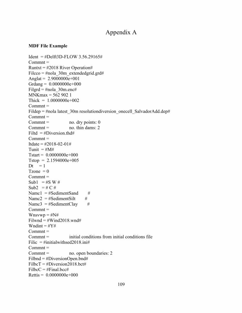
109
Appendix A
MDF File Example
Ident = #Delft3D-FLOW 3.56.29165#
Commnt =
Runtxt = #2018 River Operation#
Filcco = #nola_30m_extendedgrid.grd#
Anglat = 2.9000000e+001
Grdang = 0.0000000e+000
Filgrd = #nola_30m.enc#
MNKmax = 562 902 1
Thick = 1.0000000e+002
Commnt =
Fildep = #nola latest_30m resolutiondiversion_onecell_SalvadorAdd.dep#
Commnt =
Commnt = no. dry points: 0
Commnt = no. thin dams: 2
Filtd = #Diversion.thd#
Commnt =
Itdate = #2018-02-01#
Tunit = #M#
Tstart = 0.0000000e+000
Tstop = 2.1594000e+005
Dt = 1
Tzone = 0
Commnt =
Sub1 = #S W #
Sub2 = # C #
Namc1 = #SedimentSand #
Namc2 = #SedimentSilt #
Namc3 = #SedimentClay #
Commnt =
Wnsvwp = #N#
Filwnd = #Wind2018.wnd#
Wndint = #Y#
Commnt =
Commnt = initial conditions from initial conditions file
Filic = #initialwithsed2018.ini#
Commnt =
Commnt = no. open boundaries: 2
Filbnd = #DiversionOpen.bnd#
FilbcT = #Diversion2018.bct#
FilbcC = #Final.bcc#
Rettis = 0.0000000e+000
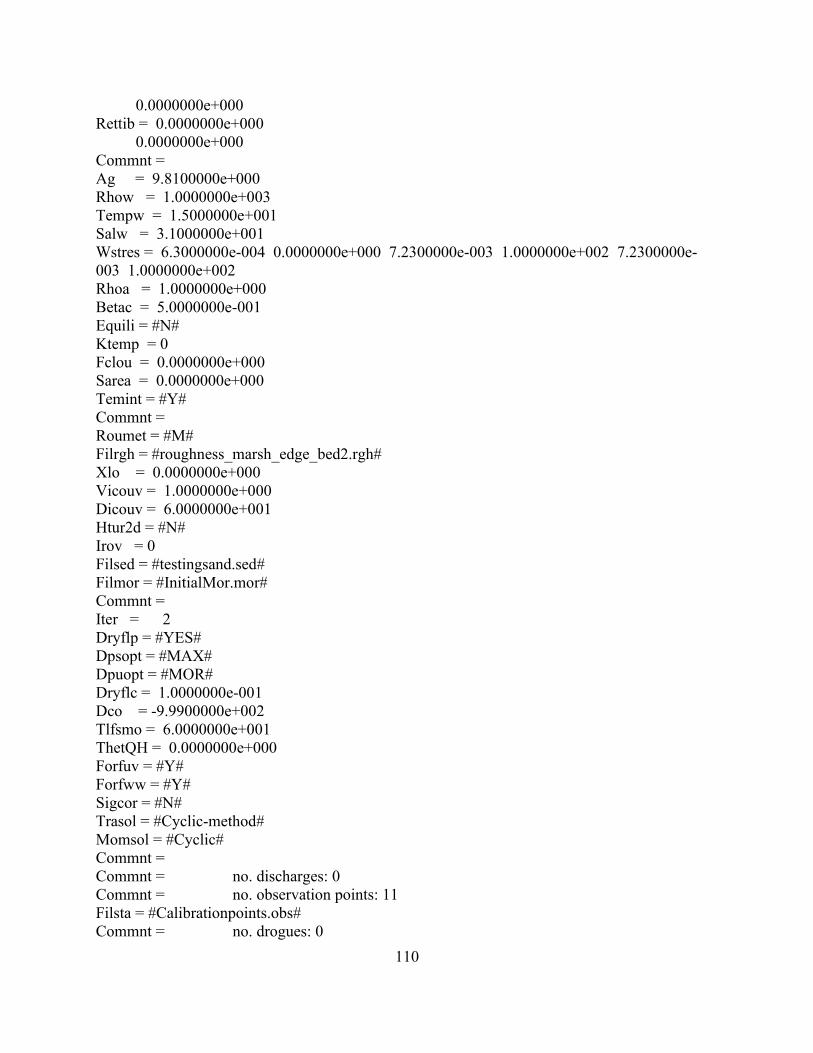
110
0.0000000e+000
Rettib = 0.0000000e+000
0.0000000e+000
Commnt =
Ag = 9.8100000e+000
Rhow = 1.0000000e+003
Tempw = 1.5000000e+001
Salw = 3.1000000e+001
Wstres = 6.3000000e-004 0.0000000e+000 7.2300000e-003 1.0000000e+002 7.2300000e-
003 1.0000000e+002
Rhoa = 1.0000000e+000
Betac = 5.0000000e-001
Equili = #N#
Ktemp = 0
Fclou = 0.0000000e+000
Sarea = 0.0000000e+000
Temint = #Y#
Commnt =
Roumet = #M#
Filrgh = #roughness_marsh_edge_bed2.rgh#
Xlo = 0.0000000e+000
Vicouv = 1.0000000e+000
Dicouv = 6.0000000e+001
Htur2d = #N#
Irov = 0
Filsed = #testingsand.sed#
Filmor = #InitialMor.mor#
Commnt =
Iter = 2
Dryflp = #YES#
Dpsopt = #MAX#
Dpuopt = #MOR#
Dryflc = 1.0000000e-001
Dco = -9.9900000e+002
Tlfsmo = 6.0000000e+001
ThetQH = 0.0000000e+000
Forfuv = #Y#
Forfww = #Y#
Sigcor = #N#
Trasol = #Cyclic-method#
Momsol = #Cyclic#
Commnt =
Commnt = no. discharges: 0
Commnt = no. observation points: 11
Filsta = #Calibrationpoints.obs#
Commnt = no. drogues: 0
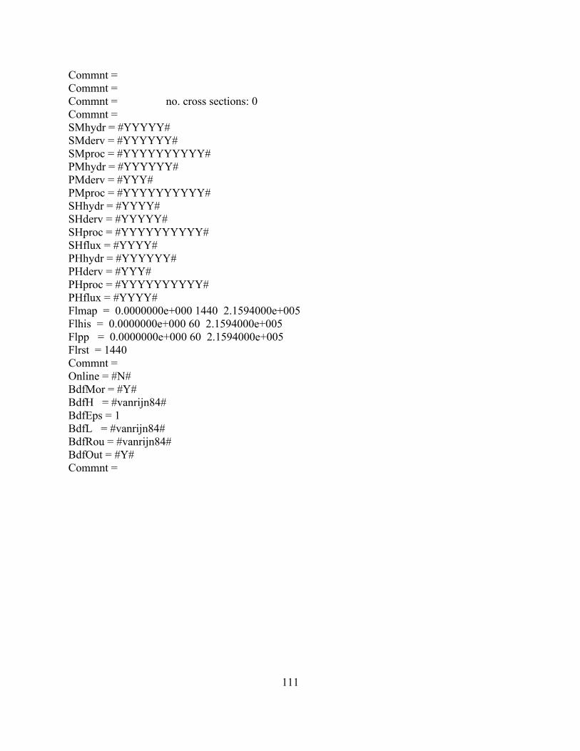
111
Commnt =
Commnt =
Commnt = no. cross sections: 0
Commnt =
SMhydr = #YYYYY#
SMderv = #YYYYYY#
SMproc = #YYYYYYYYYY#
PMhydr = #YYYYYY#
PMderv = #YYY#
PMproc = #YYYYYYYYYY#
SHhydr = #YYYY#
SHderv = #YYYYY#
SHproc = #YYYYYYYYYY#
SHflux = #YYYY#
PHhydr = #YYYYYY#
PHderv = #YYY#
PHproc = #YYYYYYYYYY#
PHflux = #YYYY#
Flmap = 0.0000000e+000 1440 2.1594000e+005
Flhis = 0.0000000e+000 60 2.1594000e+005
Flpp = 0.0000000e+000 60 2.1594000e+005
Flrst = 1440
Commnt =
Online = #N#
BdfMor = #Y#
BdfH = #vanrijn84#
BdfEps = 1
BdfL = #vanrijn84#
BdfRou = #vanrijn84#
BdfOut = #Y#
Commnt =
112
Vita
Dylan Blaskey was born and raised in Madison, Wisconsin. He obtained his Bachelor’s degree in
Bioproducts and Biosystems Engineering from the University of Minnesota in 2015. He joined
the University of New Orleans Civil and Environmental Engineering department to study
solutions to the coastal land loss issues of southern Louisiana.