Worst-case large-deviation asymptotics with application to ... · Worst-case large-deviation asymptotics with application to queueing ... received in revised form 19 October 2005;

Stochastic Processes and their Applications 116 (2006) 724–756www.elsevier.com/locate/spa

Worst-case large-deviation asymptotics with applicationto queueing and information theoryI

Charuhas Pandita, Sean Meynb,∗

a Morgan Stanley and Co., 1585 Broadway, New York, NY 10019, United Statesb Coordinated Science Laboratory, Department of Electrical and Computer Engineering, University of Illinois,

1308 W. Main Street, Urbana, IL 61801, United States

Received 28 September 2004; received in revised form 19 October 2005; accepted 11 November 2005Available online 12 December 2005

Abstract

An i.i.d. process X is considered on a compact metric space X. Its marginal distribution π is unknown,but is assumed to lie in a moment class of the form,

P = π : 〈π, fi 〉 = ci , i = 1, . . . , n,

where fi are real-valued, continuous functions on X, and ci are constants. The following conclusionsare obtained:

(i) For any probability distribution µ on X, Sanov’s rate-function for the empirical distributions of X isequal to the Kullback–Leibler divergence D(µ ‖ π). The worst-case rate-function is identified as

L(µ) := infπ∈P

D(µ ‖ π) = supλ∈R( f,c)

〈µ, log(λT f )〉,

where f = (1, f1, . . . , fn)T , and R( f, c) ⊂ Rn+1 is a compact, convex set.(ii) A stochastic approximation algorithm for computing L is introduced based on samples of the process

X.(iii) A solution to the worst-case one-dimensional large-deviation problem is obtained through properties

of extremal distributions, generalizing Markov’s canonical distributions.

I This paper is based upon work supported by the National Science Foundation under Award Nos. ECS 02 17836 andITR 00-85929. Any opinions, findings, and conclusions or recommendations expressed in this publication are those ofthe authors and do not necessarily reflect the views of the National Science Foundation.

∗ Corresponding author. Tel.: +1 217 244 1782; fax: +1 217 244 1653.E-mail addresses: [email protected] (C. Pandit), [email protected] (S. Meyn).URL: http://decision.csl.uiuc.edu:80/∼meyn (S. Meyn).

0304-4149/$ - see front matter c© 2005 Elsevier B.V. All rights reserved.doi:10.1016/j.spa.2005.11.003

http://www.elsevier.com/locate/spa

mailto:[email protected]

mailto:[email protected]

http://decision.csl.uiuc.edu:80/~meyn







http://dx.doi.org/10.1016/j.spa.2005.11.003

C. Pandit, S. Meyn / Stochastic Processes and their Applications 116 (2006) 724–756 725

(iv) Applications to robust hypothesis testing and to the theory of buffer overflows in queues are alsodeveloped.

c© 2005 Elsevier B.V. All rights reserved.

MSC: 60F10; 94A17; 62F15; 37M05; 68M20

Keywords: Large deviations; Entropy; Bayesian inference; Simulation; Queueing

1. Introduction and background

Consider an i.i.d. sequence X on a compact metric space X. It is assumed that its marginaldistribution π is not known exactly, but belongs to the moment class P defined as follows: A finiteset of real-valued continuous functions fi : i = 1, . . . , n and real constants ci : i = 1, . . . , n

are given, and

P := π ∈ M1 : 〈π, fi 〉 = ci , i = 1, . . . , n, (1)

whereM1 is the space of probability distributions on X, and the notation 〈π, fi 〉 is used to denotethe mean of the function fi according to the distribution π .

The motivation for consideration of moment classes comes primarily from the simpleobservation that the most common approach to partial statistical modeling is through moments,typically mean and correlation. Moment classes have been considered in applications tofinance [41]; admission control [10,5,32]; queueing theory [20,19,12]; and other applications.

For a moment class of this form, and a given function g ∈ C(X), the map π → 〈π, g〉 definesa continuous linear functional onM1. Consequently, the following maximization may be viewedas a linear program,

maxπ∈P

〈π, g〉. (2)

The value of this (infinite-dimensional) linear program provides a bound on the mean of g thatis uniform over π ∈ P. A.A. Markov, a student of Chebyshev, considered a special case of thelinear programs (2) in which the functions fi are polynomials. A comprehensive survey byM.G. Kreın in 1959 describes many of Markov’s original results [26]. Since then, these ideashave been developed in various directions [1,13,44,29,21,8,38,34,36,3,42].

The present paper concerns various large-deviation bounds that are uniform across a momentclass. One set of results concerns relaxations of Chernoff’s bound: For a given function h ∈

C(X), and any r ≥ 〈π, h〉,

PSN ≥ r ≤ exp(−N Iπ,h(r)), N ≥ 1, (3)

where SN = N−1∑Nj=1 h(X j ) : N ≥ 1, and Iπ,h is the usual one-dimensional large-deviation

rate-function under the distribution π . Denoting the log moment-generating function as,

Mπ,h(θ) := log 〈π, exp(θh)〉, θ ∈ R, (4)

the rate-function is equal to the convex dual,

Iπ,h(r) = supθ∈R

θr − Mπ,h(θ), r ∈ R. (5)

Theorem 1.5 and related results in Section 3 contain expressions for the minimum of the ratefunction Iπ,h(r) over the moment class P. To put these results in context we present some knownresults in the special case of polynomial constraint functions.

726 C. Pandit, S. Meyn / Stochastic Processes and their Applications 116 (2006) 724–756

1.1. Markov’s canonical distributions

Suppose that X = [0, 1], h(x) ≡ x , and that the constraint functions fi are of the form,

fi (x) = x i , x ∈ X = [0, 1], i = 1, . . . , n. (6)

A direct approach is to introduce the worst-case moment-generating function, which for eachθ ∈ R is a special case of (2), defined as

mh(θ) := maxπ∈P

〈π, exp(θh)〉, θ ∈ R. (7)

The solution of this linear program gives a uniform lower bound on the rate-function (5). Undermild conditions on the vector c used in (1), it is shown in [26] that there is a single probabilitydistribution π∗

∈ P that optimizes (7) simultaneously for every θ ∈ R+. The probabilitydistribution π∗ is known as a Markov canonical distribution.

Theorem 1.1 (Markov’s Canonical Distributions). Suppose that h is the identity function on[0, 1]; the functions fi are given in (6) for some n ≥ 1; and that the vector (c1, . . . , cn)T liesin the interior of the set of feasible moment vectors,

∆ := x ∈ Rn: xi = 〈π, fi 〉, i = 1, . . . , n, for some π ∈ M1. (8)

Then,

(i) There exists a probability distribution π∗∈ P, depending only on the moment constraints

ci , that optimizes the linear program (7) for each θ ≥ 0.(ii) The probability distribution π∗ is a discrete distribution with exactly dn/2e + 1 points of

support. Moreover, if n is even, then the end-point 1 lies in the support of π∗. If n is odd,then the end-points 0, 1 each lie in the support of π∗.

It can be shown that finding the distribution π∗ is equivalent to solving an nth degreepolynomial. Consequently, analytical formulae for π∗ are available for n ≤ 4. Consider thefollowing two special cases:

(i) A single mean-constraint. When n = 1, the canonical distribution is supported on 0 and 1,with π∗(0) = 1 − π∗(1) = c1.

(ii) First and second moment constraints. The canonical distribution π∗ is again binary whenn = 2, and can be expressed

π∗= p0δx0 + (1 − p0)δ1, (9)

where x0 =c1−c21−c1

, and p0 =(1−c1)

2

1+c2−2c1.

The case n = 1 was considered by Hoeffding [13], and the case n = 2 was considered byBennett [1] to obtain celebrated probability inequalities for sums of bounded random variables.The following Generalized Bennett’s Theorem follows directly from Theorem 1.1 and Chernoff’sbound (3).

Theorem 1.2 (Generalized Bennett’s Theorem). Suppose that the assumptions of Theorem 1.1hold. Consider the worst-case, one-dimensional rate-function defined by,

I (r) := infIπ (r) : π ∈ P, r ∈ R, (10)


where the rate-function Iπ is defined in (5) with h(x) ≡ x. Then, the Markov canonicaldistribution π∗ achieves the point-wise minimum:

Iπ∗(r) = I (r), r ≥ c1. (11)

Consequently, the universal Chernoff bound holds,

PSN ≥ r ≤ exp(−N Iπ∗(r)), π ∈ P, N ≥ 1, r ≥ c1.

1.2. Main results

How can Theorems 1.1 and 1.2 be extended to allow general constraint functions, or a generalcompact state space? Theorem 1.4 provides generalizations in both directions, and also gives atransparent bound on the empirical distribution of large-deviation asymptotics.

We first recall some well-known definitions and results [7]. For two distributions µ, π ∈ M1,the relative entropy, or Kullback–Leibler divergence is defined as,

D(µ ‖ π) =

⟨π,

dµ

dπlog

dµ

dπ

⟩if µ ≺ π,

∞ otherwise.

The domain of definition of D is usually restricted to the space of probability distributions M1,but for the convex analytic methods to be applied in this paper, we extend the definition of D inthe obvious way to include the spaceM of all finite positive measures on X.

We let S denote the set of signed measures on X with finite mass, so that |µ| ∈ M for µ ∈ S.We assume that S is endowed with the weak*-topology, defined to be the smallest topology onS that contains the system of neighborhoods

µ ∈ S : |µ(g) − s| < ε, for real-valued g ∈ C(X), s ∈ R, ε > 0. (12)

The associated Borel σ -field induced by the weak*-topology onM1 is denoted F .The sequence of empirical distributions is defined by,

L N :=1N

N−1∑j=0

δX j , N ≥ 1. (13)

We then have the well-known limit theorem [37,7].

Theorem 1.3 (Sanov’s Theorem for Empirical Measures). Suppose that X is i.i.d. with marginaldistribution π on the compact state space X. The sequence of empirical measures L N satisfiesan LDP in the space (M1,F) equipped with the weak*-topology, with the good, convex rate-function

I (µ) := D(µ ‖ π), µ ∈ M1. (14)

Consequently, for any E ∈ F ,

− infµ∈Eo

I (µ) ≤ lim infN→∞

N−1 log L N (E)

≤ lim supN→∞

N−1 log L N (E) ≤ − infµ∈E

I (µ),

where Eo and E denote the interior and the closure of E in the weak*-topology, respectively.


On considering the special case E = µ ∈ M1 : 〈µ, h〉 ≥ r for r ∈ R, Theorem 1.3 impliesthe following representation of the one-dimensional rate-function,

Iπ,h(r) = infD(µ ‖ π) : µ ∈ M1 s.t. 〈µ, h〉 ≥ r. (15)

Eq. (15) is known as the contraction principle.In view of Theorem 1.3 and the representation (15), we are led to seek lower bounds on the

rate-function I defined in (14).We are now in a position to state the main result of this paper. Theorem 1.4 provides an

expression for the worst-case rate-function L:M1 → R defined as,

L(µ) := infπ∈P

D(µ ‖ π). (16)

For an arbitrary probability distribution π ∈ M1 and for β ∈ R+, the divergence setsQβ(π),Q+

β (π) are defined as

Qβ(π) := µ ∈ M1 : D(µ ‖ π) < β,

Q+

β (π) := µ ∈ M1 : D(µ ‖ π) ≤ β.(17)

Divergence sets are convex subsets of M1 since D(· ‖ π) is a convex function. The abovedefinition is extended to include divergence sets of the moment class P:

Qβ(P) =

⋃π∈P

Qβ(π) and Q+

β (P) =

⋃π∈P

Q+

β (π). (18)

We have L(µ) < β if and only if µ ∈ Qβ(P).The following assumptions on these constraint functions and constants are imposed

throughout the paper:

(A1) The functions 1, f1, . . . , fn , are continuous on X, and the vector (c1, . . . , cn)T lies inthe interior of the set of feasible moment vectors, defined as

∆ := x ∈ Rn: xi = 〈π, fi 〉, i = 1, . . . , n, for some π ∈ M1. (19)

A version of Theorem 1.4 appears as Proposition 2.2.1 in the dissertation [31]. A proof isincluded in the Appendix A.

Let f1, . . . , fn be the continuous functions and ci , . . . , cn the constants used in thedefinition (1). We let f : X → Rn+1 denote the vector of functions (1, f1, . . . , fn)T , and writec := (1, c1, . . . , cn)T

∈ Rn+1.

Theorem 1.4 (Worst-Case Sanov Bound). The following hold under Assumption (A1):

(i) The function L may be expressed,

L(µ) = supλ∈R( f )

〈µ, log λT f 〉 + 1 − λT c, (20)

where

R( f ) := λ ∈ Rn+1: λT f (x) ≥ 0 for all x ∈ X. (21)


(ii) The infimum in (16) and the supremum in (20) are achieved by a pair π∗∈ P, λ∗

∈ R( f ),satisfying

dµ

dπ∗= λ∗T f.

Consequently, λ∗T c = 1.(iii) The function L is convex; it is continuous in the weak*-topology; and it is uniformly

bounded:

supµ∈M1

L(µ) < ∞.

(iv) For β > 0, the sets Qβ(P),Q+

β (P) defined in (18) are convex. These sets also enjoy the

following properties in the weak*-topology: The set Q+

β (P) is compact, the set Qβ(P) is

open, and the closure of Qβ(P) is equal to Q+

β (P).

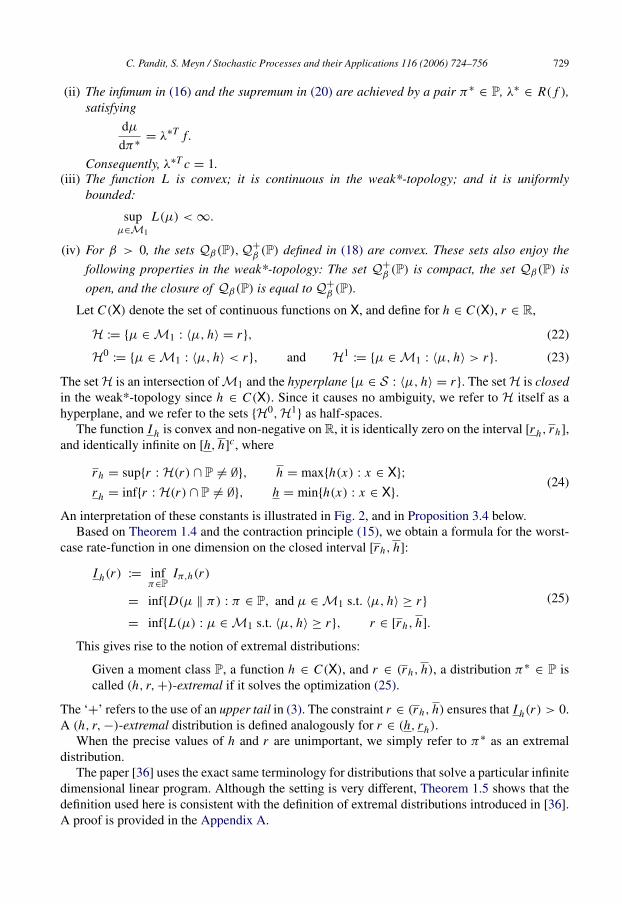
Let C(X) denote the set of continuous functions on X, and define for h ∈ C(X), r ∈ R,

H := µ ∈ M1 : 〈µ, h〉 = r, (22)

H0:= µ ∈ M1 : 〈µ, h〉 < r, and H1

:= µ ∈ M1 : 〈µ, h〉 > r. (23)

The setH is an intersection ofM1 and the hyperplane µ ∈ S : 〈µ, h〉 = r. The setH is closedin the weak*-topology since h ∈ C(X). Since it causes no ambiguity, we refer to H itself as ahyperplane, and we refer to the sets H0,H1

as half-spaces.The function I h is convex and non-negative on R, it is identically zero on the interval [rh, rh],

and identically infinite on [h, h]c, where

rh = supr : H(r) ∩ P 6= ∅, h = maxh(x) : x ∈ X;

rh = infr : H(r) ∩ P 6= ∅, h = minh(x) : x ∈ X.(24)

An interpretation of these constants is illustrated in Fig. 2, and in Proposition 3.4 below.Based on Theorem 1.4 and the contraction principle (15), we obtain a formula for the worst-

case rate-function in one dimension on the closed interval [rh, h]:

I h(r) := infπ∈P

Iπ,h(r)

= infD(µ ‖ π) : π ∈ P, and µ ∈ M1 s.t. 〈µ, h〉 ≥ r

= infL(µ) : µ ∈ M1 s.t. 〈µ, h〉 ≥ r, r ∈ [rh, h].

(25)

This gives rise to the notion of extremal distributions:

Given a moment class P, a function h ∈ C(X), and r ∈ (rh, h), a distribution π∗∈ P is

called (h, r, +)-extremal if it solves the optimization (25).

The ‘+’ refers to the use of an upper tail in (3). The constraint r ∈ (rh, h) ensures that I h(r) > 0.A (h, r, −)-extremal distribution is defined analogously for r ∈ (h, rh).

When the precise values of h and r are unimportant, we simply refer to π∗ as an extremaldistribution.

The paper [36] uses the exact same terminology for distributions that solve a particular infinitedimensional linear program. Although the setting is very different, Theorem 1.5 shows that thedefinition used here is consistent with the definition of extremal distributions introduced in [36].A proof is provided in the Appendix A.


Fig. 1. Geometric interpretation of extremal distributions. The dark region insideQ+

β∗ (P) is the divergence setQ+

β∗ (π∗).

Fig. 2. Plot of a typical worst-case one-dimensional rate-function, and worst-case log moment-generating function.

Theorem 1.5 (Saddle-Point Property). For any r ∈ (rh, h), there exists π∗∈ P and θ∗ < ∞

such that

I h(r) = Iπ∗,h(r) = [θ∗r − Mπ∗,h(θ∗)] = minπ∈P

maxθ≥0

[θr − Mπ,h(θ)]

= maxθ≥0

minπ∈P

[θr − Mπ,h(θ)] = [θ∗r − Mh(θ∗)],

where Mh := log(mh) is the worst-case log moment-generating function.

A geometric interpretation of the extremal property is provided by convexity of the divergencesets: The minimization (25) can be expressed,

I h(r) = infπ∈P

infµ∈H∪H1

D(µ ‖ π), r ∈ (rh, h). (26)

Which is equivalently expressed,

I h(r) = supβ : Q+

β (P) ∩H = ∅, r ∈ (rh, h). (27)

This follows from the geometry illustrated in Fig. 1.The set H forms a supporting hyperplane for Q+

β∗(P), passing through distributions µ∗

in the intersection Q+

β∗(P) ∩ H. Theorem 1.4 asserts that there exists π∗∈ P such that

D(µ∗‖ π∗) = β∗. The pair of probability distributions µ∗, π∗

solve (26), and π∗ is anextremal distribution.

The remainder of the paper is organized as follows. The next section develops two generalapplications to queueing theory and information theory. Section 3.1 contains a development oftheory related to the geometry illustrated in Fig. 1. In particular, the geometry of divergence setsis explored, and extremal distributions are characterized. Conclusions are contained in Section 4,along with a description of possible future directions and applications for this research.

Proofs of the major results are contained in the Appendix A.


2. Applications

We illustrate the application of the Generalized Bennett’s Lemma Theorem 1.2 and theworst-case Sanov bound Theorem 1.4 in two general settings. In Section 2.1 we considerbounds on error exponents arising in the analysis of buffer overflows in queues. Section 2.2contains application to robust hypothesis testing based on Theorem 1.4. Further discussion on thehypothesis testing problem is included in Section 3.3.1, and [33,31] contains a more completedevelopment in a completely general setting.

2.1. Buffer overflows in queues

The reflected random walk is a basic model in queueing theory. In the most commonapplication, Wt is interpreted as the total workload in the queue at time k, and evolves accordingto

Wt+1 = [Wt + X t+1]+, W0 ∈ R+,

where X is an i.i.d. sequence. For example, X i might represent the duration of the i th telephonecall to a call center, minus the time elapsed since the previous call. The marginal distributionof X may be complex. To obtain a simpler model, one can estimate the first few moments ofthe marginal distribution, and then compute the worst case marginal that maximizes some costcriterion subject to these moment constraints.

For example, if just two moments are estimated, and if one maximizes 〈π, f 〉 over all π

subject to these moment constraints with f (x) = eθx for some θ > 0, then we have seen that π∗

is a binary by Bennett’s Lemma. The following is a simple but useful extension:

Proposition 2.1. Each of the following expectations,

E[X p], E[eϑ X

], E[X peϑ X],

is maximized simultaneously for each ϑ > 0, p ∈ Z+, by a fixed binary distribution in each ofthe following two situations:

(i) If the first moment c1 =∫

x π(dx) is specified, then each of these expectations is maximizedover all probability distributions on [−x−, x+

] with mean c1 by

π∗= p∗ δ−x− + (1 − p∗) δx+ , (28)

where p∗= (x+

− c1)/(x++ x−).

(ii) If two moments are specified, ci =∫

x i π(dx), i = 1, 2, then the optimizer is,

π∗= p∗ δx0 + (1 − p∗) δx+ , (29)

where x0 = [x+− c1]

−1(c1x+− c2) and p∗

= [x+2+ c2 − 2c1x+

]−1(x+

− c1)2.

The significance of Proposition 2.1 is that a very simple model can be constructed that capturesworst-case behavior.

Assume that the marginal distribution π of X is supported on an interval [−x−, x+] with

x− and x+ each strictly positive. The mean is assumed negative E[X i ] = −d < 0, andPX i > 0 > 0. This ensures that W is positive recurrent, and its unique invariant measurehas non-trivial support.

Under general conditions, the steady state mean of W is determined by only the firstand second moments of X (see for example the version of the Pollaczek–Khintchine formula


[30, Prop. 1.1]). However, two distributions with common first and second moments may havevery different higher-order statistics, and hence exhibit very different behavior during a rare eventsuch as a buffer overflow.

We consider the worst case behavior of the stationary version of the random walk on thetwo-sided time interval Z. Denoting the stationary process W∗, consider the tail exponent,

IW = − limb→∞

b−1 log(PW ∗

0 ≥ b).

The log moment generating function for π , denoted Λ, satisfies Λ′(0) = −d and Λ(θ) → ∞ asθ → ∞. Consequently, there is a unique second zero θ0 > 0. It is known that IW = θ0, and thatthe derivative d+

= Λ′(θ0) is the most likely slope of W∗ prior to ‘overflow’ [9].

Proposition 2.2. The exponent IW is minimized, and the slope d+= Λ′(θ0) is maximized, over

all marginals π on [−x−, x+] with given first moment −d, by the values obtained when the

marginal distribution of X is supported on the two points −x−, x+. In particular, for any

increment distribution supported on this interval with the given mean −d we have,

limb→∞

−b−1 log(PW ∗

0 ≥ b) ≤ −θ•

0 ,

where θ•

0 denotes the positive zero of the worst-case log moment generating function

Λ•(θ) = log

((x+

+ d)e−x−θ+ (x−

− d)ex+θ

x−+ x+

), θ ∈ R.

Proof. Applying Proposition 2.1, we see that the binary distribution maximizes Λ(θ) for θ > 0,and hence the location of the second zero θ0 is minimized over all π ∈ P. Moreover, we have

Λ′(θ0) = E[Xeϑ0 X],

which is also maximized for the same reasons.

We close with a numerical example of the following parametrized form. Fix d ∈ (0, 1), and letκ ≥ 1 denote the parameter. We choose x−

= 1 and x+= κ , so that the worst-case distribution

π∗ is determined by pκ = π∗−1 = (1 + κ)−1(d + κ) to satisfy the mean constraint.

The moment generating function and its derivative are expressed,

λ(ϑ) = pκe−ϑ+ (1 − pκ)eκϑ , λ′(ϑ) = −pκe−ϑ

+ (1 − pκ)κeκϑ , ϑ ∈ R.

Through a second-order Taylor series approximation we obtain,

1 = λ(ϑ0) ≥ pκ(1 − ϑ0) + (1 − pκ)(1 + κϑ0 +12(κϑ0)

2),

which after substituting the definition of pκ and rearranging terms gives,

lim supκ→∞

κϑ0(κ) ≤ 2d

1 − d.

Based on this bound, we obtain through a first-order Taylor series approximation,

pκ(1 − ϑ0) + (1 − pκ)eκϑ0 = 1 + O(κ−2),

which then implies the limit,

limκ→∞

κϑ0(κ) = B0,


Fig. 3. Log moment generating function for three binary distributions supported on −1, κ with κ = 5, 15, 50, andcommon mean E[X t ] = −d.

where B0 ∈ (0, 2(1 − d)−1d] solves the fixed point equation eB0 = 1 + (1 − d)−1 B0.As expected, the value of ϑ0 vanishes as κ → ∞. However, the slope d+

= Λ′(θ0) = λ′(ϑ0)

is bounded, and converges to the finite limit,

d+(∞) := limκ→∞

d+(κ) = −1 + (1 − d)eB0 .

From the fixed point equation and the bound B0 ≤ 2(1 − d)−1d this gives,

d+(∞) = −1 + (1 − d)[1 + (1 − d)−1 B0] = −d + B0 ≤

(1 + d

1 − d

)d.

A numerical experiment was conducted with d = 1/19.1 A plot of Λ = log(λ) is shown in Fig. 3for κ = 5, 15, 50. We have Λ′(0) = −d for each κ , and d+

= Λ′(θ0) is approximately equal tod in each of the three plots.

In conclusion, although the error exponent ϑ0 is highly sensitive to the parameter κ , the mostlikely behavior during a rare event is relatively insensitive.

2.2. Robust hypothesis testing

The most compelling applications of the results developed in this paper concern hypothesistesting, and related topics in information theory.

Consider the following classical hypothesis testing problem. A set of i.i.d. measurementsX1, . . . , X N is observed, and one must decide if the observations are generated by one of twogiven marginal distributions π0 or π1, representing the two ‘hypotheses’ H0 and H1. To avoidtechnicalities we shall assume that the state space X is finite.

For a given N ≥ 1, suppose that a decision test φN is constructed based on the finite setof measurements X1, . . . , X N , with φN (X1, . . . , X N ) = 1 interpreted as the declaration thathypothesis H1 is true. The performance of a given test sequence is reflected in the error exponents

1 When κ = 1, this corresponds to a sampled M/M/1 queue with load ρ = 0.9.


for the type-II and type-I error probabilities, defined respectively by,

Iφ := − lim infN→∞

1N

log Pπ1φN = 0, Jφ := − lim infN→∞

1N

log Pπ0φN = 1,

where Pπ0 , Pπ1 denote the distributions of X under H0 and H1 respectively.A test is optimal with respect to the (asymptotic) Neyman–Pearson N–P criterion if it

maximizes the type-II exponent subject to a constraint on the type-I exponent. Thus, for a givenconstant η > 0,

supφ

Iφ subject to Jφ ≥ η. (30)

The value of the optimization (30) can be expressed as the convex program,

β∗(π0, π1) = infD(µ‖π1) : D(µ‖π0) ≤ η, (31)

and the solution to (31) leads to the well-known log-likelihood ratio test [14,35].However, there are many other solutions to (30), and hence many optimal tests. It is shown

in [45] that one may restrict to tests of the following form without loss of generality: for a closedset A ⊆ M1,

φN = IΓN ∈ Ac. (32)

There is a universal test of this form that is also optimal, and does not require knowledge ofhypothesis H1: One takes A = Q+

η (π0), or equivalently,

φ∗

N = 0 ⇐⇒ D(ΓN ‖π0) ≤ η. (33)

This test is minimal over all tests based on the empirical distributions ΓN . That is, for any testof the form (32) for a closed set A ⊂ M1, if the Neyman–Pearson criterion is satisfied thenQ+

η (π0) ⊂ A.In most applications, the statistics under either hypothesis are not completely known a priori.

In this case, it may be reasonable to assume that for each i , the measure πi belongs to a givenuncertainty class. A standard approach to designing decision rules in this setting is the min–max“robust” approach, where the goal is to minimize the worst-case performance over the uncertaintyclasses. Robust detection has been the subject of numerous papers in this setting since the seminalwork of Huber and Strassen [18]. A survey of robust hypothesis testing research may be foundin [43].

Consider the following robust hypothesis testing problem in which Hi refers to the hypothesisthat the marginal distribution belongs to the moment class Pi , i = 0, 1. A robust N–P hypothesistesting problem is formulated in which the worst-case type-II exponent is maximized overπ1 ∈ P1, subject to a uniform constraint on the type-I exponent over all π0 ∈ P0:

supφ

infπ1∈P1

I π1φ subject to inf

π0∈P0

Jπ0φ ≥ η. (34)

A test is called optimal if it solves this optimization problem.We first describe the analog of (33). Let L0(µ) := infπ∈P0 D(µ‖π) denote the minimal

relative entropy under H0. An optimal test can be defined by choosing as an acceptance regionfor H0 the sublevel set Q+

η (P0),

φ∗uN = 0 ⇐⇒ L0(ΓN ) ≤ η. (35)


Proposition 2.3. Suppose that P0 satisfies Assumption (A1). Then the test (35) is optimal.Moreover, it is universal in that it maximizes I π1

φ over all test sequences, regardless of themarginal distribution π1.

Proof. The fact that this test achieves the constraint η on the worst-case missed detectionexponent follows directly from the fact that Q+

η (P0) = µ : L0(µ) ≤ η contains Q+η (π0)

for any π0 ∈ P0.Conversely, as remarked above, for any π0 ∈ P0 the acceptance region Q+

η (π0) is minimalover all closed subsets of M1 that give rise to a feasible test. Hence any optimal acceptanceregion for the min–max problem must contain the union

⋃π0∈P0

Q+η (π0), which is precisely

Q+η (P0).

When H1 is specified via moment constraints then it is possible to construct a simpler optimaltest. Although the test itself is not a log-likelihood test, it has a geometric interpretation that isentirely analogous to that given in Hoeffding’s result [14]. The value β∗ in an optimal test can beexpressed,

β∗= infβ : Q+

η (P0) ∩Q+

β (P1) 6= ∅. (36)

Moreover, the infimum is achieved by some µ∗∈ Q+

η (P0)∩Q+

β∗(P1), along with least favorabledistributions π∗

0 ∈ P0, π∗

1 ∈ P1, satisfying

D(µ∗‖π∗

0 ) = η, D(µ∗‖π∗

1 ) = β∗.

The distribution µ∗ has the form µ∗(x) = `0(x)π∗

0 (x), where the function `0 is a linearcombination of the constraint functions fi used to define P0. The function log `0 defines aseparating hyperplane between the convex sets Q+

η (P0) and Q+

β∗(P1), as illustrated in Fig. 4.Note that log `0 is defined everywhere, yet the likelihood ratio dµ∗/dπ∗

0 may be defined onlyon a small subset of X.

Proposition 2.4. Suppose that P0 and P1 each satisfy Assumption (A1). Letting f denote thevector function and c the constant vector that determine P0, there exists λ ∈ R( f, c) such thatwith `0 = λT f , the following test is optimal

φ∗

N = 0 ⇐⇒ N−1N−1∑t=0

log(`0(X t )) ≤ η. (37)

Proof. We appeal to the convex geometry illustrated in Fig. 4. Since Q+η (P0) and Q+

β∗(P1)

are compact sets it follows from their construction that there exists µ∗∈ Q+

η (P0) ∩ Q+

β∗(P1).Moreover, by convexity there exists some function h: X → R defining a separating hyperplanebetween the sets Q+

η (P0) and Q+

β∗(P1), satisfying

Qη(P0) ⊂ µ ∈ M1 : 〈µ, h〉 < η, Qβ∗(P1) ⊂ µ ∈ M1 : 〈µ, h〉 > η.

Theorem 3.2 then implies that there exists λ ∈ R( f, c) such that the function log(λT f ) alsodefines a separating hyperplane,

Qη(P0) ⊂ H0∗ := µ ∈ M1 : 〈µ, h〉 < η, Qβ∗(P1) ⊂ H1

∗ := µ ∈ M1 : 〈µ, h〉 > η.

Moreover log(λT f ) ≥ h everywhere (with equality a.e. µ∗.) This is the vector λ used in (37).


Fig. 4. The two-moment worst-case hypothesis testing problem. The uncertainty classes Pi , i = 0, 1 are determined bya finite number of linear constraints, and the thickened regionsQη(P0),Qβ∗ (P1) are each convex. The linear thresholdtest is interpreted as a separating hyperplane between these two convex sets.

This test is more ‘liberal’ then the universal test (35), in the sense that it accepts H0 morefrequently, so that the test is feasible. In fact, the worst-case false alarm error exponent isprecisely η since µ∗

∈ ∂H0 and D(µ∗‖π∗

0 ) = η.Since D(µ∗

‖π∗

1 ) = β∗ it follows that the value of (34) can be no greater than this β∗.Conversely, considering the convex geometry shown in Fig. 4 we conclude that for any π1 ∈ P1,µ ∈ H0

∗, we have D(µ‖π1) ≥ L1(µ) ≥ L1(µ∗) = β∗. Sanov’s Theorem then implies that this

test achieves this upper bound,

infπ1∈P1

I π1φ = inf

π1∈P1,µ∈H0∗

D(µ‖π1) = β∗.

In the remainder of this section these tests are illustrated using a simple example.

Variance discrimination

Consider the special case in which the two hypotheses are defined by first and second momentconstraints. It is assumed that X = [−1, 1], and the first moments are assumed to be zero, giving

P0 =

π ∈ M1 : 〈π, f1〉 = 0, 〈π, f2〉 ≤ σ 2

0

P1 =

π ∈ M1 : 〈π, f1〉 = 0, 〈π, f2〉 ≥ σ 2

1

(38)

where fk(x) ≡ xk for k = 1, 2, and 0 < σ 20 < σ 2

1 < 1 are known bounds on the respectivevariances.

Note that we have relaxed the assumption that the state space is finite. Also, note that we areconsidering inequality constraints in this problem. However, we will find the solution is identicalto what is obtained using equality constraints.

The solution to the robust hypothesis testing problem is illustrated in Fig. 4. The optimalexponent β∗ is given by the supremum in (36), and there exists µ∗ solving (36) in the sense thatL0(µ

∗) = η and L1(µ∗) = β∗. Three tests are considered here:

(i) The universal test that does not depend upon P1 is expressed,

φ∗uN = 0 ⇐⇒ N−1

N−1∑t=0

log(1 + λ1 X t + λ2(X2t − σ 2

0 )) ≤ η, (39)

for every pair λ1, λ2 such that the quadratic function q0(x) := 1 + λ1x + λ2(x2− σ 2

0 ) isnon-negative on [−1, 1]. Note that q0 = λT f with λ = (λ0, λ1, λ2)

T∈ R( f, c), where we

have eliminated λ0 using the linear constraint λT c = λ0 + λ2σ20 = 1.


(ii) When P1 is specified by (38) then one can restrict to a single quadratic in an optimal test,

φ∗

N = 0 ⇐⇒ N−1N−1∑t=0

log(1 + λ2(X2t − σ 2

0 )) ≤ η. (40)

We show in Proposition 2.5 that, letting σ 2• ∈ (σ 2

0 , σ 21 ) denote the variance of µ∗,

λ2 =1

σ 20

σ 2• − σ 2

0

1 − σ 20

. (41)

(iii) The naive test is defined based on the sample-path second moment,

φN = 0 ⇐⇒ N−1N−1∑t=0

X2t ≤ τ 2, (42)

with τ 2∈ (σ 2

0 , σ 21 ) a fixed threshold.

Proposition 2.5 asserts that the test (42) is optimal for an appropriate value of τ 2 dependingon η. We note that the proof of this result is based on symmetry, and is hence extremely fragile:If for example the state space X = [−1, 1] is replaced by any non-symmetric interval, or if thezero-mean constraints are modified, then we no longer know if the naive test is optimal.

Proposition 2.5. Suppose that the two moment classes are defined by (38). Then the test (40) isoptimal when λ2 is given by (41), where the variance parameter σ 2

• is the solution to,

η = (1 − σ 2• ) log

(1 − σ 2

•

1 − σ 20

)+ σ 2

• log

(σ 2

•

σ 20

).

The naive test (42) using τ 2= σ 2

• is also optimal, and the three optimal tests satisfy,

φ∗uN = 0 H⇒ φ∗

N = 0 H⇒ φN = 0.

To prove Proposition 2.5 we first demonstrate that the optimizing distributions are symmetric.The conclusion (43) can be equivalently expressed µ∗

∈ Q+η (P0) ∩ Q+

β∗(P1) since β∗ satisfies(31).

Lemma 2.6. There exist three symmetric distributions π∗

0 , π∗

1 , µ∗ on [−1, 1] that solve therobust hypothesis testing problem:

D(µ∗‖π∗

0 ) = η, D(µ∗‖π∗

1 ) = β∗. (43)

Proof. For any distribution µ denote by µ the symmetric distribution defined by µ=

12 (µ+µ),

where µ(dx) = µ(−dx).Suppose that π∗

0 , π∗

1 , µ∗ is any triple solving the robust hypothesis testing problem. Then,

the triple π∗

0 , π∗

1 , µ∗ also forms a solution. Convexity then implies that L0(µ∗) ≤ η and

L1(µ∗) ≤ β∗, and since β∗ solves (36) these upper bounds must be achieved.

We henceforth assume that the three distributions are symmetric.Applying (37) we can construct an optimal test of the form,

φ∗

N = 0 ⇐⇒ 〈ΓN , log(q0)〉 ≤ η


where q0(x) = λ0+λ1x+λ2x2, with λ ∈ R( f, c0). Optimality is characterized by the inclusions,

Qη(P0) ⊂ H0∗, Qβ∗(P1) ⊂ H1

∗, (44)

where,

H0∗ := µ : 〈µ, log(q0)〉 < η, H1

∗ := µ : 〈µ, log(q0)〉 > η.

Lemma 2.7. The quadratic q0 is of the form, for some λ2 ∈ R,

q0(x) = 1 + λ2(x2− σ 2

0 ), x ∈ R.

Proof. Theorem 1.4 implies that µ∗ can be expressed,

dµ∗

dπ∗

0= q0, a.e. [π∗

0 ].

Symmetry of µ∗ and π∗

0 implies that λ1 = 0. Moreover, since µ∗ is a probability measure wehave 1 = µ∗(X) = π∗

0 (q0) = λ0 + λ2σ20 , giving λ0 = 1 − λ2σ

20 .

Switching the roles of η and β∗ we obtain,

Lemma 2.8. There exists a quadratic function of the form,

q1(x) = 1 + γ2(x2− σ 2

1 ), x ∈ R,

with γ2 ∈ R, such that q1 is non-negative on [−1, 1], and

Qβ∗(P1) ⊂ H0∗∗ := µ : 〈µ, log(q1)〉 < β∗

Qη(P0) ⊂ H1∗∗ := µ : 〈µ, log(q0)〉 > β∗

.

Lemma 2.9. The two probabilities π∗

0 , π∗

1 have just three points of support −1, 0, 1, and hencethe explicit form,

π∗

i =12σ 2

i (δ1 + δ−1) + (1 − σ 2i )δ0.

The support of µ∗ is identical, with

µ∗=

12σ 2

• (δ1 + δ−1) + (1 − σ 2• )δ0.

Proof. Lemma 2.8 asserts that (log(q1), β∗) defines a tangent hyperplane to Qη(P0) passing

through µ∗, which we write as

Qη(P0) ⊂ µ : 〈µ, − log(q1)〉 < −β∗.

We can thus apply Theorem 3.2 to find θ∗ > 0 satisfying,

log(q0(x)) − η ≥ θ∗(− log(q1(x)) + β∗), x ∈ [−1, 1],

with equality almost everywhere. Writing y = x2 this becomes,

log(λ0 + λ2 y) − η ≥ θ∗[− log(γ0 + γ2 y) + β∗], y ∈ [0, 1], (45)


again with equality almost everywhere. The left hand side of this inequality is a strictly concavefunction of y, and the right hand side is convex. It follows that equality can hold only at the twopoints 0, 1. That is, for some pi ∈ (0, 1),

π∗

i =12

piδ1 +12

piδ−1 + (1 − pi )δ0.

From the variance constraint we obtain pi = σ 2i .

Identical reasoning yields the desired representation for µ∗.

Proof of Proposition 2.5. To prove the proposition we establish an analog of (44),

Qη(P0) ⊂ H0:= µ : 〈µ, f2〉 < τ 2

,

Qβ∗(P1) ⊂ H1:= µ : 〈µ, f2〉 > τ 2

.(46)

This entails constructing a linear function `(y) satisfying,

log(λ0 + λ2 y) − η ≥ `(y) ≥ θ∗[− log(γ0 + γ2 y) + β∗], y ∈ [0, 1]. (47)

This is clearly possible, due to the alignment condition (45), and we necessarily have equality atthe two endpoints. In particular, `(0) = log(λ0) − η.

Writing `(x2) = A + B f2(x) we obtain,

0 = 〈µ∗, log(λ0 + λ2 f2) − η〉 = 〈µ∗, A + B f2〉 = A + Bτ 2,

giving B = −A−1τ−2, and A = `(0) = log(λ0) − η. These two equations can be combined togive `(x2) = θ•(x2

− τ 2) with θ• := τ−2(η − log(λ0)).Given this form we can rewrite (47) as follows,

log(q0(x)) − η ≥ θ•( f2(x) − τ 2) ≥ θ∗[− log(q1(x)) + β∗], x ∈ [−1, 1]. (48)

To see that this implies (46) we note that the two inequalities in (48) imply the followingcorresponding inclusions,

Qη(P0) ⊂ µ : 〈µ, log(q0) − η〉 < 0 ⊂ µ : 〈µ, θ•( f2 − τ 2)〉 < 0 = H0,

Qβ∗(P1) ⊂ µ : 〈µ, log(q1)〉 − β∗ < 0 ⊂ µ : 〈µ, θ−1∗ θ•(− f2 + τ 2)〉 < 0 = H1.

To complete the proof we now obtain the expressions for λ2 and τ 2. The formula for τ 2

follows from the relative entropy expression,

η = D(µ∗‖π∗

0 ) = 〈µ, log(dµ∗/dπ∗)〉,

and the expressions for µ∗ and π0∗ given in Lemma 2.9.

The formula for λ2 also follows from Lemma 2.9, and the expression µ∗= q0π

∗

0 :

τ 2= µ∗(−1) + µ∗(1) = q0(−1)π∗

0 (−1) + q0(1)π∗

0 (1) = q0(1)σ 20 .

Substituting the identity q0(1) = 1 + λ2(1 − σ 20 ) and solving for λ2 we obtain (41).

3. Convexity and alignment

In this section we develop some basic results required in the proof of Theorem 1.4, and variousproperties of extremal distributions. Recall that M1 denotes the space of (Borel) probabilitymeasures on the Borel σ -algebra B, endowed with the weak-topology.


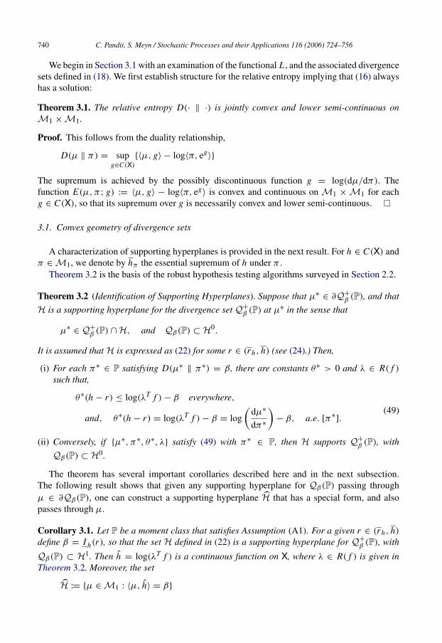
We begin in Section 3.1 with an examination of the functional L , and the associated divergencesets defined in (18). We first establish structure for the relative entropy implying that (16) alwayshas a solution:

Theorem 3.1. The relative entropy D(· ‖ ·) is jointly convex and lower semi-continuous onM1 ×M1.

Proof. This follows from the duality relationship,

D(µ ‖ π) = supg∈C(X)

〈µ, g〉 − log〈π, eg〉

The supremum is achieved by the possibly discontinuous function g = log(dµ/dπ). Thefunction E(µ, π; g) := 〈µ, g〉 − log〈π, eg

〉 is convex and continuous on M1 × M1 for eachg ∈ C(X), so that its supremum over g is necessarily convex and lower semi-continuous.

3.1. Convex geometry of divergence sets

A characterization of supporting hyperplanes is provided in the next result. For h ∈ C(X) andπ ∈ M1, we denote by hπ the essential supremum of h under π .

Theorem 3.2 is the basis of the robust hypothesis testing algorithms surveyed in Section 2.2.

Theorem 3.2 (Identification of Supporting Hyperplanes). Suppose that µ∗∈ ∂Q+

β (P), and that

H is a supporting hyperplane for the divergence set Q+

β (P) at µ∗ in the sense that

µ∗∈ Q+

β (P) ∩H, and Qβ(P) ⊂ H0.

It is assumed that H is expressed as (22) for some r ∈ (rh, h) (see (24).) Then,

(i) For each π∗∈ P satisfying D(µ∗

‖ π∗) = β, there are constants θ∗ > 0 and λ ∈ R( f )

such that,

θ∗(h − r) ≤ log(λT f ) − β everywhere,

and, θ∗(h − r) = log(λT f ) − β = log(

dµ∗

dπ∗

)− β, a.e. [π∗

].(49)

(ii) Conversely, if µ∗, π∗, θ∗, λ satisfy (49) with π∗∈ P, then H supports Q+

β (P), with

Qβ(P) ⊂ H0.

The theorem has several important corollaries described here and in the next subsection.The following result shows that given any supporting hyperplane for Qβ(P) passing throughµ ∈ ∂Qβ(P), one can construct a supporting hyperplane H that has a special form, and alsopasses through µ.

Corollary 3.1. Let P be a moment class that satisfies Assumption (A1). For a given r ∈ (rh, h)

define β = I h(r), so that the set H defined in (22) is a supporting hyperplane for Q+

β (P), with

Qβ(P) ⊂ H1. Then h = log(λT f ) is a continuous function on X, where λ ∈ R( f ) is given inTheorem 3.2. Moreover, the set

H := µ ∈ M1 : 〈µ, h〉 = β


is also a supporting hyperplane for Q+

β (P), with

Qβ(P) ⊂ H0:= µ ∈ M1 : 〈µ, h〉 < β;

H1⊂ H1

:= µ ∈ M1 : 〈µ, h〉 > β.

Proof. Since f is a vector of continuous functions, to establish continuity of h it is sufficient toprove that λT f (x) > 0 for all x ∈ X. Since H supports Q+

β (P), it must satisfy the necessary

conditions of Theorem 3.2 for some θ∗ > 0 and λ ∈ R( f ). From Theorem 3.2, we know that his bounded below by h, which is bounded. Therefore we do have λT f > 0 on X.

With θ∗:= 1, it is clear that h, µ∗, π∗, θ∗, λ satisfy the sufficient conditions of Theorem 3.2.

Thus the hyperplane H forms a supporting hyperplane for Q+

β (P) with Qβ(P) ⊂ µ ∈ M1 :

〈µ, h〉 < β. Moreover, since θ∗(h − r) ≤ h − β everywhere, we have

H1= µ ∈ M1 : 〈µ, h − r〉 > 0 ⊂ µ ∈ M1 : 〈µ, h − β〉 > 0 = H1.

We now provide illustrations of the alignment conditions (49) through numerical examples. Ineach example below the state space is taken to be the unit interval X = [0, 1]. Moment classes aredefined using the polynomials fi (x) = x i , x ∈ X, with c defined consistently with the uniformdistribution ν on [0, 1]:

ci = 〈ν, fi 〉 =

∫ 1

0fi (x) dx = 1/(i + 1)−1, 1 ≤ i ≤ n. (50)

Case I: µ Bernoulli. If µ is the symmetric Bernoulli distribution supported on 0, 1 thenD(µ‖ν) = ∞. Shown in Fig. 5 are results from numerical calculation of L for n = 1, 3, 7and 20. When n = 1 we have c = (1, 0.5)T , so that µ ∈ P, and hence L(µ) = 0. For each n ≥ 2we have µ 6∈ P and, as shown in the figure for three values of n, the worst-case divergence L(µ)

is strictly positive. Also shown in Fig. 5 is the nth order polynomial λT f in each case. FromTheorem 1.4 we know that L(µ) = D(µ ‖ π∗) for some π∗

∈ P with dµdπ∗ = λT f . It follows

that π∗ is supported on the union,

supp (π∗) ⊂ roots of λT f ∪ supp (µ) = 0, 1.

Case II: µ uniform. If µ is uniform on [0, 0.5] then D(µ‖ν) = log(2) ≈ 0.69. Shown inFig. 6 is the nth order polynomial λT f for n = 7 and n = 20 with λ ∈ R( f, c) andL(µ) = 〈µ, log(λT f )〉. In each case this function roughly approximates the density of µ withrespect to ν, which is 2I[0,0.5].

3.2. Extremal distributions

We have seen that I h can be computed in (25) by first constructing the worst-case rate-functionL:M1 → R+, and then applying the contraction principle. Here we consider the alternaterepresentation of I h obtained from the worst-case log moment generating function, leading toa proof of Theorem 1.5.

Moreover, on analysing general infinite-dimensional linear programs of the form (7) wedemonstrate that, without any loss of generality, extremal distributions can be assumed discrete,with no more than n + 2 points of support.


Fig. 5. Computation of L(µ) with µ Bernoulli.

Fig. 6. Computation of L(µ) with µ uniform on [0, 0.5].

The dual of the general linear program (2) is expressed as,

minλT c : λ ∈ Rn+1s.t. λT f ≥ g, (51)

where λT f ≥ g means λT f (x) ≥ g(x) for all x ∈ X. It is known that there is no duality gapunder Assumption (A1), i.e., the value of the primal (2) is equal to the value of the dual (51).The following result is required in an analysis of the linear program (7). A proof is containedin [22,39].

Theorem 3.3 (Lack of Duality Gap). Under Assumption (A1), for any g ∈ C(X),

max〈π, g〉 : π ∈ P = minλT c : λ ∈ Rn+1 s.t. λT f ≥ g. (52)

Any distribution π∗ and vector λ∗ optimizing the respective linear programs (2) and (51) aretogether called a dual pair. A necessary and sufficient condition for a given pair (π, λ) to form adual pair is the alignment condition,

λT f − g ≥ 0 and 〈π, λT f − g〉 = 0. (53)


Fig. 7. The worst-case log moment-generating function Mh .

In this section we focus on the specific linear program that defines mh in (7). Theorem 1.5provides the following alternate expression for the worst-case rate-function defined in (25):

I h(r) = maxθ≥0

[θr − Mh(θ)

], r ∈ (rh, h). (54)

Recall that in the setting of Theorem 1.1 we have

I h(r) = maxθ≥0

[θr − Mπ∗,h(θ)], r > c1,

with π∗ independent of r . When the assumptions of Theorem 1.1 are relaxed then this uniformoptimality no longer holds. Shown in Fig. 7 are numerical results obtained using h(x) =

2(x − 1) − x sin(2πx), x ∈ [0, 1]. The moment class P was defined using polynomials (see(6)), with n = 2 and n = 5. The worst-case log moment-generating function is plotted forθ ∈ [0, 5]. Also, for θ = θ∗

= 2.5, the distribution π∗ that maximizes (7) was computed, andthe figure shows the log moment-generating function Mπ∗,h . As required by Theorem 1.5, thefunctions Mh and Mπ∗,h coincide at θ = θ∗. However, the inequality Mh(θ) ≥ Mπ∗,h(θ) isstrict for θ ∈ (0, θ∗) and θ ∈ (θ∗, 5].

Proposition 3.4 provides justification for the correspondences illustrated in Fig. 2.

Proposition 3.4. The worst-case log moment-generating function satisfies,

(i) d+

dθMh (0) = rh , where the ‘plus’ denotes the right derivative;

(ii) The constant rh can be expressed as the solution to the linear program,

rh = maxπ∈P

〈π, h〉;

(iii) limθ→∞d+

dθMh (θ) = h.

The maximization (7) is a linear program, and is therefore achieved at the extreme points ofthe set P. These extreme points correspond to discrete measures, and thus (7) suggests (thoughit does not imply), that π∗ is a discrete measure. The following theorem establishes that withoutloss of generality, an extremal distribution can be assumed discrete.


Theorem 3.5 (Discrete Extremal Distributions). Under Assumption (A1) suppose that h iscontinuous, and that r ∈ (rh, h). Then there exists a probability distribution π

∈ P that isdiscrete, with no more than n + 2 points of support, and is also (r, h, +)-extremal.

Proof. Theorem 1.5 implies that an (r, h, +)-extremal distribution π∗∈ P is also a solution to

the infinite dimensional linear program (7) for some θ∗≥ 0, and that Iπ∗,h(r) = I (r). Since

Mπ∗,h is analytic and strictly convex on R, the maximality property (5) implies that

ddθ

Mπ∗,h (θ∗) = r.

To prove the theorem we construct a discrete probability distribution π∈ P that satisfies

Mπ,h(θ∗) = Mπ∗,h(θ∗) = Mh(θ∗), and also the consistent derivative constraint,

ddθ

Mπ,h (θ∗) = r. (55)

It will then follow that Iπ,h(r) = Iπ∗,h(r) = I (r), which is the desired conclusion.The derivative can be computed for any π ∈ M1 as follows,

ddθ

Mπ,h (θ) =〈π, heθh

〉

〈π, eθh〉, θ ∈ R.

Consequently, Eq. (55) is expressed as the equality constraint 〈π, heθ∗h〉 = r〈π, eθ∗h

〉.Consider then the linear program,

max 〈π, exp(θ∗h)〉 s.t. 〈π, fi 〉 = ci , i = 0, . . . , n

〈π, heθ∗h− reθ∗h

〉 = 0.

This is feasible since the (h, r, +)-extremal distribution π∗ is one solution. Without loss ofgenerality, we may search among extreme points of the constraint set in this linear program.Since there are n + 2 linear contraints, an extreme point may have no more than n + 2 points ofsupport.

3.3. Algorithms

From Theorem 1.4 it follows that L(µ) can be expressed as the maximum,

L(µ) = maxλ∈R( f,c)

〈µ, log λT f 〉, µ ∈ M1, (56)

where R( f, c) denotes the convex set,

R( f, c) := R( f ) ∩ λ : λT c = 1. (57)

We thus arrive at a concave program that can be solved in various different ways.Algorithmic methods for optimization over probability distributions are developed in several

recent papers. The multi-dimensional polynomial moment problem is considered in [36], and [6,16] consider algorithms for computation of mutual information.

We survey several approaches here since one may have to experiment using differenttechniques when P is complex. Throughout it is assumed that X is a compact subset of Euclideanspace.


3.3.1. Nonlinear programming

Interior point methods. The first-order condition for an interior optimizer of (56) is expressed

ξ∗:= 〈µ, h∗

− c〉 = 0, (58)

where h := (λ∗T f )−1 f . When µ has full support then the condition (58) characterizes anoptimizer. Hence (56) can be solved using standard interior-point optimization algorithms suchas the conjugate gradient algorithm (e.g. [28,2,4]).

The logarithmic barrier method introduces a ‘cost’ for approaching the boundary of R( f, c).One version can be expressed as the concave program,

sup(1 − ε)〈µ, log λT f 〉 + ε〈ν, log λT f 〉 : λ ∈ R( f, c), (59)

where ν is any fixed distribution with full support, and ε ∈ (0, 1) is the barrier parameter. Thesolution of the relaxation (59) is precisely L((1 − ε)µ + εν). The relaxation can again be solvedusing standard methods.

Projected gradient methods. In the case of a boundary optimizer for the original program(56), the vector ξ∗ is not necessary zero, but rather satisfies the following inequalityconstraints:

Proposition 3.6. The vector λ∈ R( f, c) optimizes (56) if and only if the gradient ξ

:=

〈µ, f (λT

f )−1〉 − c satisfies the family of inequalities,

vT ξ≤ 0, v ∈ Tλ( f, c), (60)

where Tλ( f, c) ⊂ RN+1 denotes the set of feasible directions satisfying vT c = 0, and for somer0 > 0,

(λ+ rvT ) f (x) ≥ 0 0 ≤ r ≤ r0.

The following algorithm was successfully used to compute L(µ) in the examples illustratedin Figs. 5 and 6. For any λ ∈ R( f, c) we define Πλ to be the projection from RN+1 to Tλ( f, c).Given any λt

∈ R( f, c), an ascent direction v ∈ Tλt ( f, c) is computed satisfying vT ξ t > 0,where ξ t

:= 〈µ, ht 〉 − c with ht = (λtTf )−1 f . For example, one can take

v = Πλt ξ t, or v = Πλt Σtξ

t

where Σ−1t := 〈µ, ht hT

t 〉 is the negative of the Hessian of 〈µ, log λT f 〉, evaluated at λt .Once a vector v = vt is selected, the next vector is computed using line-maximization:

λt+1= λt

+ rtvt where,

rt = arg maxr≥0

〈µ, log((λt+ rvt )T f )〉 : λt

+ rvt∈ R( f, c). (61)

Constraint relaxation. To simplify either of the algorithms described above one can simplify thestate space. For example, the line search (61) is easily computed when X is finite. One can thenintroduce new points as the estimate of λ∗ is refined.

Suppose that Xt= x1, . . . , x t

⊂ X is a finite set, and suppose that λ∗t is the optimal solutionto (56) for the reduced state space. We have λ∗t

∈ Rn( f, c), meaning that cT λ∗t= 1, and λ∗tT

f


is non-negative on Xt . Since this amounts to a relaxation of (56) we have L(µ) ≤ Ln(µ) =

〈µ, log λ∗tTf 〉. If λ∗t

∈ R( f, c) then this inequality is achieved, so that λ∗t= λ∗. Otherwise, we

set Xt+1= Xt

∪ x t+1 with,

x t+1= arg min

x∈Xλ∗tT

f (x).

This is similar to the steepest ascent algorithm introduced in [16], which is shown to beconvergent. The same arguments can be used to show that λ∗t

→ λ∗ as t → ∞.

3.3.2. On-line algorithmsAn apparent difficulty with the Neyman–Pearson test defined in (37) is that the nonlinear

program (56) must be solved to compute L(ΓN ) as each new sample is obtained. To make thistest practical we require a recursive formula for L(ΓN ).

Based on the unconstrained first order condition (58), or the refined first order conditiondescribed in Proposition 3.6, we arrive at the Robbins–Monro, stochastic-approximationrecursion,

λt+1= λt

+ γtΠλt ht+1, n ≥ 0, (62)

where ht := (λtTf (X t ))

−1 f (X t ), and γt is a positive gain sequence satisfying standardassumptions [11].

A refinement of (62) is obtained by mimicking the constrained Newton–Raphson recursion,λt+1

= λt+γtΠλt Σ t ht where here Σ−1

t is an approximation to 〈µ, ht hTt 〉. Given the sequence

of estimates,

Σ−1t = Σ−1

t − γt (Σ−1t − ht h

Tt ),

we arrive at the following algorithm by applying the Matrix Inversion Lemma [11]:

λt+1= λt

+ γtΠλt Σt ht+1 (63a)

Σt+1 = Σt − γtΣt + Σt ht hT

t Σt

1 + hTt Σt ht

, (63b)

where again ht = (λtTf (X t ))

−1 f (X t ).To illustrate the application of these stochastic approximation algorithms, consider the

computation of L(µ) when X = [0, 1], f (x) = (1, x, . . . , xn)T , and P is consistent with theuniform distribution (see (50).) We consider two cases: in the first, the marginal distribution µ ofX was Bernoulli as in the results shown in Fig. 5. In the second µ was uniform on [0, 1]. Sevenmoment constraints were specified, so that L(µ) ≈ 1.74 with µ Bernoulli by the results shownin Fig. 5 with n = 7, while L(µ) = 0 when µ is uniform since µ ∈ P for any n. The step sizewas taken to be γt = t−1.

Fig. 8 shows results obtained when implementing (62). The two plots are (i) the runningsample path average of log(λi T

f (X i )), and (ii) 〈µ, log λtTf 〉 for t ≥ 1. In the plot shown on

the left the marginal distributions of the observations X were Bernoulli, and in the plot on theright the marginal was uniform on [0, 1]. The algorithm is slow to converge to the precise valueof L(µ), but it distinguishes the observations from P rapidly.

Similar conclusions were obtained when µ was uniform on [0, 0.5], or a mixture of a Bernoulliand a uniform distribution: The rate of convergence was slow, but the sample path average


Fig. 8. The plot shows 〈µ, log λtTf 〉 and the running sample path average of log(λiT

f (Xi )), where the sequence ofvectors λt

is obtained using the algorithm (62). In the plot shown on the left the observations Xi were Bernoulli, andin the plot on the right the observations were uniformly distributed.

of log(λi Tf (X i )) remained strictly positive, maintaining 80% of its final value after a short

transient period.The performance of the more complex algorithm (63a) and (63b) was similar. Also, as can be

expected, the convergence became slower for larger values of n since λt is (n + 1) dimensional.

4. Conclusions and future directions

We have established explicit formulae for the worst-case large deviation rate-functionsappearing in Sanov’s Theorem and Chernoff’s bound. The geometric structure of the divergenceset Q+

β (P) plays a central role in interpreting the results, and is a valuable tool in analysis.Potential directions for future research include,

(a) The structure of the worst-case, one-dimensional rate-function defined in (10) deservesfurther consideration. In particular, under what conditions outside of the polynomial caseis π∗ independent of r > 0?

(b) We have not dealt with methods for selecting the functions fi in a particular application.(c) Extensions of the results here to Markov processes may be possible by applying recent results

on exact large deviations [24,25], and on finite-n bounds [23]. It appears that the formulationof an appropriate moment class is non-trivial for Markov models.

(d) Results from [31] and this paper provided inspiration for the research described in [16,15,17]. The discrete nature of extremal distributions provided motivation for a new class ofalgorithms for the computation of efficient channel codes based on optimal discrete inputdistributions. It is likely that a worst-case approach to channel modeling based on momentclasses will lead to simple coding approaches, and easily implemented decoding algorithms.

We are convinced that the theory of extremal distributions will have significant impact inmany other areas that involve statistical modeling and prediction.

Acknowledgements

Thanks to Professors I. Kontoyiannis and O. Zeitouni for advice on the hypothesis testingliterature, and insightful comments.

Appendix A

We collect here proofs of the main results, and several complementary results. We begin witha bound on L , and a description of the domain of I h .


Lemma A.1. Let P be a moment class that satisfies Assumption (A1). Then,

(i) The functional L:M1 → R+ is uniformly bounded:

supµ∈M1

L(µ) < ∞.

(ii) The function I h is uniformly bounded on [h, h]:

supr∈[h,h]

I h(r) < ∞.

Proof. Define cµ := 〈µ, f 〉 for µ ∈ M. This satisfies the uniform bound ‖cµ‖ ≤

maxx∈X ‖ f (x)‖ for µ ∈ M.Under (A1) the vector c lies in the interior of ∆. This assumption and the uniform bound on

cµ implies that there exists ε > 0 independent of µ such that,

c − ε cµ

1 − ε∈ ∆, µ ∈ M1.

By the definition of ∆, this means that there exists π ∈ M1 such that 〈π, f 〉 =c−εcµ

1−ε. Let

π ε:= εµ + (1 − ε)π . Then π ε

∈ P, and

D(µ ‖ π ε) ≤ − log ε < ∞.

Thus L(µ) = infπ∈P D(µ ‖ π) ≤ | log ε| for all µ ∈ M1, and this establishes (i).Since h is continuous we can find x, x ∈ X such that h(x) = h and h(x) = h. Moreover,

exactly as in the construction of π ε above, we can construct π ∈ P such that,

p := πx > 0, p := πx > 0.

We then have,

Mπ,h(θ) ≥ log(pehθ+ pehθ ), θ ∈ R. (64)

Consequently, for r ∈ [h, h],

supθ≥0

[θr − Mπ,h(θ)] ≤ supθ≥0

[θ(r − h) − log(p)] ≤ | log(p)|,

supθ≤0

[θr − Mπ,h(θ)] ≤ supθ≤0

[θ(r − h) − log(p)] ≤ | log(p)|.

This shows that Iπ,h is bounded on [h, h]. Minimality of I h completes the proof.

The following result allows us to restrict ourselves to a compact domain in the maximization(20).

Lemma A.2. Suppose that Assumption (A1) holds. Then, the set R( f, c) ⊂ Rn+1 defined in (57)is convex and compact.

Proof. It is obvious that R( f, c) is closed and convex.To complete the proof we show that R( f, c) is bounded. Let ei denote the i th standard basis

vector in Rn . Since (c1, . . . , cn)T lies in the interior of the set ∆ by Assumption (A1), thereexists ε > 0 such that (c1, c2, . . . , cn)T

± ε ei: i = 1, . . . , n ⊂ ∆.


Now from the definition of R( f ) it follows that

R( f ) = λ ∈ Rn+1: λT

〈π, f 〉 ≥ 0, for each π ∈ M1

= λ ∈ Rn+1: λT (1, x) ≥ 0 for each x ∈ ∆,

where (1, x)T:= (1, x1, . . . , xn)T . Using the fact that (c1, . . . , cn)T

+ ε ei∈ ∆ we conclude

λT (1, (c1, . . . , cn)T+ ε ei ) ≥ 0,

and since λT c = 1 it then follows that 1+ελi ≥ 0. Similar reasoning gives the bound 1−ελi ≥ 0.Repeating this argument for each i = 1, . . . , n, we can infer that

λi ∈ [−ε−1, +ε−1], i = 1, . . . , n.

Since λT c = 1 and c0 = 1, the above bounds imply upper and lower bounds on λ0 as well.Hence R( f, c) is closed and bounded, hence compact, as claimed.

The following version of Cramer’s Theorem is used repeatedly below.

Theorem A.3. Suppose that X is i.i.d. with one dimensional distribution π on B. Fix h ∈ C(X),and r ∈ [〈π, h〉, hπ ) where hπ denotes the essential supremum of h. Then,

(i) The Chernoff bound is asymptotically tight:

limN→∞

1N

log

(P

[1N

N∑i=1

h(X i ) ≥ r

])= lim

N→∞

1N

log

(P

[1N

N∑i=1

h(X i ) > r

])= −Iπ,h(r).

(ii) The one-dimensional rate-function has the following representations,

Iπ,h(r) = supθ≥0

θr − Mπ,h(θ)

= infD(µ ‖ π) : µ s.t. 〈µ, h〉 ≥ r.

(iii) The infimum over µ and the supremum over θ in (ii) are uniquely achieved by some µ∗, θ∗

satisfying

dµ∗

dπ=

exp(θ∗h)

〈π, exp(θ∗h)〉, and 〈µ∗, h〉 = r.

Proof. Parts (i) and (ii) follow from Theorem 1.3 and the Contraction Principle.Part (iii) follows from [40, Theorem 1.5].

Define the functional K :M → R by,

K (π) := infD(µ ‖ π): µ ∈ H1∪H, π ∈ P. (65)

The following result is an application of Cramer’s Theorem:

Lemma A.4. For each π ∈ M we have,

K (π) = supθ≥0

[θr − Mπ,h(θ)]. (66)

Proof. This follows directly from Theorem A.3 when π ∈ M1. Moreover, since K (γ π) =

K (π) − log(γ ) for each π ∈ M, γ ≥ 0, it follows that (66) holds for all π ∈ M.


The following simple result is used in an analysis of the functional K .

Lemma A.5. For each θ ∈ R the functional Y (π) = Mπ,h(θ) is concave and Gateauxdifferentiable onM. Its derivative is represented by the function gπ,h = 〈π, eθh

〉−1eθh , so that

Y (π) ≤ Y (π0) + 〈π − π0, gπ,h〉, π, π0∈ M.

The next result from convex analysis is required in the proofs of the major results. We adoptthe following notation: X and Y denote normed linear spaces; Y∗ denotes the usual dual space ofcontinuous linear functionals on Y; K denotes a convex subset of X; Ω is a real-valued convexfunctional defined on K; and the mapping Θ : X → Y is affine.

For a proof of Proposition A.6 see [27, Problem 7, page 236], following [27, Theorem 1, page224].

Proposition A.6. Suppose that Y is finite dimensional, and that the following two conditionshold:

(a) The optimal value κ0 is finite, where

κ0 := infΩ(x): Θ(x) = 0, x ∈ K.

(b) 0 ∈ Y is an interior point of the non-empty set y ∈ Y : Θ(x) = y for some x ∈ K.

Then, there exists y∗

0 ∈ Y∗ such that

κ0 = infΩ(x) + 〈Θ(x), y∗

0 〉: x ∈ K.

Below we collect results required in the proof of Theorem 3.2.

Lemma A.7. Suppose that H is expressed as (22) for some r ∈ (rh, h), and suppose thatβ := infµ∈H L(µ) > 0. Then, there exists µ∗

∈ H, π∗∈ P, θ∗ > 0, and λ∗

∈ Rn+1 satisfying,

(i) β = L(µ∗) = K (π∗) = infπ∈P K (π),(ii) K (π∗) = supθ≥0θr − Mπ∗,h(θ) = θ∗r − Mπ∗,h(θ∗),

(iii) dµ∗

dπ∗ =exp(θ∗h)

〈π,exp(θ∗h)〉,

(iv) K (π∗) = minπ∈MK (π) + λ∗T (〈π, f 〉 − c).

Proof. Theorem 3.1 states that D(· ‖ ·) is jointly lower semi-continuous. SinceM1 is compact,it follows that an optimizing pair (µ∗, π∗) exists.

To establish (ii) we must show that the supremum over θ in (66) is attained by some θ∗≥ 0.

We prove this by contradiction: Suppose that no finite θ∗∈ R+ exists, so that

K (π∗) = limθ→∞

θr − Mπ∗,h(θ).

From the definition of K in (66) we then obtain the representation,

K (π∗) = infπ∈P

(lim

θ→∞θr − Mπ,h(θ)

).

However, on taking π ∈ P with support at h, we have as in the proof of (64) in Lemma A.1,

limθ→∞

θr − Mπ∗,h(θ) ≤ limθ→∞

θr − Mπ,h(θ) = limθ→∞

θr − (log(p) + hθ) = −∞,

where p = πx : h(x) = h. This contradiction shows that there exists θ∗ < ∞ as claimed.


Note that we must have θ∗ > 0 since K (π∗) = β > 0. Cramer’s Theorem A.3 then implies(iii).

It is straightforward to verify that the infimum in (i) meets the conditions of Proposition A.6,from which we obtain (iv).

The proof of the following result is routine calculus.

Lemma A.8. Let π0, π1, µ ∈ M, and define π%= (1 − %)π0

+ %π1 for % ∈ [0, 1]. Then,

dd%

D(µ‖π%)

∣∣∣∣%=0

= 1 −

⟨µ,

dπ1

dπ0 IA

⟩,

where A ⊂ X denotes the support of π0.

Proof of Theorem 1.4. Proof of (i): This is based on Proposition A.6 with the identification,

X = S; Y = Rn+1; K = M; Ω(π) = D(µ ‖ π); Θ(π) = 〈π, f 〉 − c.

We now verify the two required assumptions in Proposition A.6: (a) the infimum (16) that definesL must be finite, and (b) the constraint vector c must lie in the interior of the set ∆. The firstproperty is established in Lemma A.1(i), and the second is guaranteed by Assumption (A1).

Consequently, Proposition A.6 implies the following expression for the worst-case ratefunction:

L(µ) = infπ∈P

D(µ ‖ π) = maxλ∈Rn

Ψ(λ),

where Ψ(λ) := infπ∈M

D(µ ‖ π) + λT (〈π, f 〉 − c)

.

We now obtain an expression for Ψ . Consider λ ∈ R( f ) satisfying λT f > 0 a.e. [µ], anddefine the positive measure πλ through dπλ

dµ=

1λT f

Note that this may not be a probability

measure, but we will prove that πλ achieves the minimum in the definition of Ψ(λ).Define π%

:= πλ+ %(π − πλ) for a given π ∈ M, and % ∈ [0, 1]. We have,

dd%

(D(µ ‖ π%) + λT (〈π%, f 〉 − c)

)∣∣∣%=0

= 1 −

⟨µ,

dπ

dπλIA

⟩+ λT

〈π − πλ, f 〉

= 1 − 〈π, (λT f )IA〉 + 〈π, λT f 〉 − 〈µ, 1〉

= 〈π, (λT f )IAc 〉

where the first equality follows from Lemma A.8 with A equal to the support of πλ. The secondequality follows from the definition (λT f )IA =

dµ

dπλ IA. Since λT f ≥ 0 this shows that for anyπ ∈ M,

dd%

(D(µ ‖ π%) + λT (〈π%, f 〉 − c)

)∣∣∣%=0

≥ 0,

and hence πλ achieves the minimum in the expression for Ψ(λ). The formula for Ψ(λ) whenλ ∈ R( f ) follows.

To complete the proof of the duality relation we show that Ψ(λ) = −∞ in either of the twocases, λ 6∈ R( f ) or λT f 6> 0, µ-a.e. Indeed, if λ 6∈ R( f ) then λT f (x0) < 0 for some x0 ∈ Xsatisfying µx0 = 0. Let πκ

:= µ + κδx0 , where δx0 is the atom at x0. Then D(µ ‖ πκ) = 0whereas 〈πκ , λT f 〉 ↓ −∞ as κ ↑ ∞.


In the latter case, in which λT f is not strictly positive a.e. [µ], it follows that the setA := x : λT f (x) ≤ 0 has positive µ-measure. Consider the sequence of positive measuresπκ defined through dπκ

dµ= nIA. Then D(µ ‖ πκ) = − log(κ) and 〈πκ , λT f 〉 ≤ 0 so that

D(µ ‖ πκ) + 〈πκ , λT f 〉 ↓ −∞ as κ → ∞.

Proof of (ii) and (iii): We first show that the infimum in (16) and the supremum in (20) areachieved by a pair π∗

∈ P, λ∗∈ R( f ). The fact that the supremum is achieved follows directly

from Proposition A.6, and the existence of an optimizing π∗∈ P follows from Theorem 3.1.

Convexity of L follows directly from its formulation as a supremum of linear functionals inpart (i). The finiteness of L is proved in Lemma A.1(i).

To show that L:M1 → R+ is continuous, consider any convergent sequence of probabilitymeasures, µk w

−→ µ. From part (i) we know that there exist λk ⊂ R( f, c) and πk

⊂ P such

that dµk

dπk = λk T f , and L(µk) = D(µk‖ πk) for each k.

Consider any limit point of L(µk), and a subsequence ki such that L(µki ) is convergentto this limit point. Since the sets P and R( f, c) are compact (the latter from Lemma A.2),we can construct if necessary a further subsequence so that λki → λ and πk w

−→ π , forsome λ ∈ R( f, c), and π ∈ P. As in the proof of part (i), it follows that dµ

dπ= λT f and

L(µ) = D(µ ‖ π). Since f is a bounded function, we must have λki T f → λT f uniformly onX.

Consider now the functions (λki T f ) log λki T f : i ≥ 1. Since x log x is a continuousfunction on R, it follows that,

(λki T f ) log λki T f → (λT f ) log λT f, uniformly on X,

and, since π∗kiw

−→ π∗, we have

〈π∗ki , (λki T f ) log λki T f 〉 → 〈π, (λT f ) log λT f 〉.

From the identities,

L(µki ) = 〈π∗ki , (λki T f ) log(λki T f )〉 and L(µ) = 〈π, (λT f ) log(λT f 〉),

we conclude that L(µki ) → L(µ). This completes the proof of continuity, and therebyestablishes (ii).

To prove part (iii), we begin with the representation,

Qβ(P) = µ: L(µ) < β.

This set is convex and open since the functional L is convex and continuous. We have seen thatthe infimum in (16) is achieved by some π∗

∈ P, from which it follows that

Q+

β (P) = µ: L(µ) ≤ β.

Since L is convex and continuous, Q+

β (P) is convex and closed. It easily follows from these

expressions and continuity of L that Q+

β (P) is equal to the closure of Qβ(P).

Proof of Theorem 3.2. Part (i) (Necessity): We apply Lemmas A.7 and A.5 to establish thealignment condition (49): Consider any π0

∈ M such that the supremum in (66) is achievedfor some θ0

∈ R+. We apply the following bound,

β = K (π∗) ≥ θ0r − Mπ∗,h(θ0) ≥ θ0r − Mπ0,h(θ0) − 〈π∗− π0, g0〉

= K (π0) − 〈π∗− π0, g0〉,


where the first inequality follows from Lemma A.7(ii), and the second is a consequence ofLemma A.5 with g0 := gπ0,h . Consequently, for any λ ∈ R( f, c),

K (π∗) + λT (〈π∗, f 〉 − c) ≥ K (π0) + λT (〈π0, f 〉 − c)

+ 〈π∗− π0, λT ( f − c) − g0〉,

and on combining this with Lemma A.7(iv) we obtain,

〈π∗− π0, λ∗T ( f − c) − g0〉 ≤ 0.

Consider the special case π0= π∗

+ εδx for ε > 0, x ∈ X, so that the bound above becomes,

g0(x) ≤ λ∗T ( f (x) − c).

It is clear that Mπ0,h → Mπ∗,h as ε ↓ 0, uniformly for θ in compact subsets of R+. The functionMπ∗,h is strictly convex on R+, from which we conclude that θ0

→ θ∗ as ε ↓ 0. It then followsthat the function g0 = gπ0,h converges to gπ∗,h = 〈π, eθ∗h

〉−1eθ∗h uniformly on X. We conclude

that

eθ∗h(x)

〈π, eθ∗h〉≤ λ∗T ( f (x) − c), x ∈ X.

Now consider the special case π0= (1 − ε)π∗ for ε > 0. In this case θ0

= θ∗, and we canuse identical arguments to conclude that 〈π∗, λ∗T ( f − c) − g∗〉 ≤ 0. The representation (49)follows on taking logarithms.

Part (ii) (Sufficiency): From the assumption θ∗h ≤ θ∗r − β + log(λT f ) we obtain from (66),

K (π) ≥ θ∗r − Mπ,h(θ∗)

:= θ∗r − log(〈π, exp(θ∗h)〉)

≥ θ∗r − [θ∗r − β + log(〈π, λT f 〉)] = β.

Moreover, since we also have log dµ∗

dπ∗ = β + θ∗(h − r) and 〈µ∗, h〉 = r , we can conclude thatthis lower bound is achieved when π = π∗:

K (π∗) ≤ D(µ∗‖π∗) = 〈µ∗, β + θ∗(h − r)〉 = β.

It follows that for any µ ∈ H, π ∈ P,

D(µ‖π) ≥ K (π) ≥ β = K (π∗) = L(µ∗).

Consequently, Qβ(P) ⊂ H1 and Q+

β (P) ⊂ H ∪H1. Since µ∗∈ H ∩Q+

β (P), the hyperplane Hmust be a supporting hyperplane for Q+

β (P).

The two lemmas below are consequences of Theorem 3.2. The first provides a characterizationof an extremal distribution in terms of the threshold function h, the constraints fi , ci , and thevalue r ∈ R.

Lemma A.9. A necessary and sufficient condition for a distribution π∗∈ P to be (h, r, +)-

extremal for some r ∈ (rh, h) is that there exist π∗∈ H0

∩ P, µ∗∈ H, λ ∈ R( f ), and

θ∗, b0 > 0 such that

exp(θ∗h)

= b0λT f = b0

dµ∗

dπ∗, a.e. [π∗

]

≤ b0λT f everywhere.

(67)


Proof. The fact that H is a supporting hyperplane for Q+

β∗(P), together with Theorem 3.2,implies that, for some λ ∈ R( f ) and θ∗ > 0, we must have

h − r

=

1θ∗

(log λT f − β∗) =1θ∗

(log

dµ∗

dπ∗− β∗

), a.e. [π∗

]

≤1θ∗

(log λT f − β∗) everywhere.

We conclude that the relation (67) is a necessary condition for π∗ to be an extremal distribution,where b0 := exp(θ∗r − β∗).

Conversely, if π∗, µ∗ satisfy (67) along with D(µ∗‖ π∗) = β∗, then from Theorem 3.2, the

hyperplane H supports Q+

β∗(P), and therefore the pair π∗, µ∗ solves (26). Thus (67) is also a

sufficient condition for π∗ to be an extremal distribution.

Lemma A.10. Let P be a moment class that satisfies Assumption (A1). Suppose that π∗∈ P is

(h, r, +)-extremal for some r ∈ (rh, h), and let θ∗ > 0 be the constant given in Lemma A.9.Then, π∗ is also an optimizer of the infinite-dimensional linear program (7) that defines theworst-case moment-generating function, with θ = θ∗.

Proof. From (67) it follows that for any π ∈ P we have

〈π, exp(θ∗h)〉 ≤ 〈π, b0λT f 〉 = b0λ

T c,

with equality when π = π∗. Thus π∗ solves (7).

Proof of Theorem 1.5. The proof follows from Lemma A.10 and Lemma A.7(ii): From theseresults and maximality of Mh we have,

I h(r) ≥ θr − Mπ∗,h(θ) ≥ θr − Mh(θ), θ ≥ 0,

and all inequalities become equalities when θ = θ∗.

References

[1] G. Bennett, Probability inequalities for the sum of independent random variables, J. Amer. Statist. Assoc. 57 (1962)33–45.

[2] D.P. Bertsekas, Convex Analysis and Optimization, Atena Scientific, Cambridge, MA, 2003 (with Angelia Nedicand Asuman E. Ozdaglar).

[3] D. Bertsimas, J. Sethuraman, Moment problems and semidefinite optimization, in: Handbook of SemidefiniteProgramming, in: Internat. Ser. Oper. Res. Management Sci., vol. 27, Kluwer Acad. Publ., Boston, MA, 2000,pp. 469–509.

[4] S. Boyd, L. Vandenberghe, Convex Optimization, 1st ed., Cambridge University Press, New York, 2004.[5] F. Brichet, A. Simonian, Conservative Gaussian models applied to measurement-based admission control, in:

Proceedings of IWQoS, Napa, CA, May 1998, pp. 68–71.[6] M. Chiang, S. Boyd, Geometric programming duals of channel capacity and rate distortion, IEEE Trans. Inform.

Theory 50 (2) (2004) 245–258.[7] A. Dembo, O. Zeitouni, Large Deviations Techniques and Applications, 2nd ed., Springer-Verlag, New York, 1998.[8] P. Diaconis, Application of the method of moments in probability and statistics, in: Moments in Mathematics (San

Antonio, TX, 1987), in: Proc. Sympos. Appl. Math., vol. 37, Amer. Math. Soc., Providence, RI, 1987, pp. 125–142.[9] A. Ganesh, N. O’Connell, D. Wischik, Big Queues, in: Lecture Notes in Mathematics, vol. 1838, Springer-Verlag,

Berlin, 2004.[10] R. Gibbens, F. Kelly, Measurement-based connection admission control, 1997, in: International Teletraffic Congress

15, June 1997.[11] G.C. Goodwin, K.S. Sin, Adaptive Filtering Prediction and Control, Prentice Hall, Englewood Cliffs, NJ, 1984.


[12] S.G. Henderson, S.P. Meyn, V.B. Tadic, Performance evaluation and policy selection in multiclass networks,in: Learning, Optimization and Decision Making, Discrete Event Dyn. Sys. 13 (1–2) (2003) 149–189 (specialissue) (invited).

[13] W. Hoeffding, Probability inequalities for sums of bounded random variables, J. Amer. Statist. Assoc. 58 (1963)13–30.

[14] W. Hoeffding, Asymptotically optimal tests for multinomial distributions, Ann. Math. Statist. 36 (1965) 369–408.[15] J. Huang, S. Meyn, M. Medard, Error exponents for channel coding and signal constellation design, in: Nonlinear

Optimization of Communication Systems, Journal of Selected Areas in Comm. (2005) (special issue) (submittedfor publication).

[16] J. Huang, S.P. Meyn, Characterization and computation of optimal distribution for channel coding, IEEE Trans.Inform. Theory 51 (7) (2005) 1–16.

[17] J. Huang, C. Pandit, S. Meyn, M. Medard, V. Veeravalli, Entropy, inference, and channel coding. in: P. Agrawal,M. Andrews, P.J. Fleming, G. Yin, L. Zhang, (Eds.), Proceedings of the Summer Workshop on Wireless Networks,in: IMA volumes in Mathematics and its Applications, Springer-Verlag, New York, 2005 (in press).

[18] P.J. Huber, V. Strassen, Minimax tests and the Neyman–Pearson lemma for capacities, Ann. Statist. 1 (1973)251–263.

[19] M.A. Johnson, M.R. Taaffe, Matching moments to phase distributions: nonlinear programming approaches, Comm.Statist. Stochastic Models 6 (2) (1990) 259–281.

[20] M.A. Johnson, M.R. Taaffe, An investigation of phase-distribution moment-matching algorithms for use inqueueing models, Queueing Syst. Theory Appl. 8 (2) (1991) 129–147.

[21] S. Karlin, W.J. Studden, Tchebycheff systems: With applications in analysis and statistics, in: Pure and AppliedMathematics, vol. XV, Interscience Publishers John Wiley and Sons, New York, London, Sydney, 1966.

[22] J.M.B. Kemperman, The general moment problem, a geometric approach, Ann. Math. Statist. 39 (1968) 93–122.[23] I. Kontoyiannis, L.A. Lastras-Montano, S.P. Meyn, Relative entropy and exponential deviation bounds for general

Markov chains, in: Proceedings of the IEEE International Symposium on Information Theory, Adelaide, Australia,4–9 September, 2005.

[24] I. Kontoyiannis, S.P. Meyn, Spectral theory and limit theorems for geometrically ergodic Markov processes, Ann.Appl. Probab. 13 (2003) 304–362. Presented at the INFORMS Applied Probability Conference, NYC, July, 2001.

[25] I. Kontoyiannis, S.P. Meyn, Large deviations asymptotics and the spectral theory of multiplicatively regular Markovprocesses, Electron. J. Probab. 10 (3) (2005) 61–123 (electronic).

[26] M.G. Kreın, The ideas of P. L. Cebysev and A. A. Markov in the theory of limiting values of integrals and theirfuture developments, Transl. Amer. Math. Soc. 12 (1959) 1–121.

[27] D.G. Luenberger, Optimization by Vector Space Methods, John Wiley, 1969.[28] D.G. Luenberger, Linear and Nonlinear Programming, 2nd ed., Kluwer Academic Publishers, Norwell, MA, 2003.[29] A.W. Marshall, I. Olkin, Inequalities: theory of majorization and its applications, in: Mathematics in Science and

Engineering, vol. 143, Academic Press Inc. [Harcourt Brace Jovanovich Publishers], New York, 1979.[30] S.P. Meyn, Dynamic safety-stocks for asymptotic optimality in stochastic networks, Queueing Syst. Theory Appl.

50 (2005) 255–297.[31] C. Pandit, Robust statistical modeling based on moment classes with applications to admission control, large

deviations and hypothesis testing, Ph.D. Thesis, University of Illinois at Urbana Champaign, University of Illinois,Urbana, IL, USA, 2004.

[32] C. Pandit, S.P. Meyn, Robust measurement-based admission control using Markov’s theory of canonicaldistributions, in: Conference version presented at the Conference on Information Sciences and Systems, 2003,IEEE Trans. Inform. Theory (2003) (submitted for publication).

[33] C. Pandit, S.P. Meyn, V.V. Veeravalli, Asymptotic robust Neyman–Pearson hypothesis testing based on momentclasses, 2005 (in preparation).

[34] J.E. Pecaric, F. Proschan, Y.L. Tong, Convex functions, partial orderings, and statistical applications,in: Mathematics in Science and Engineering, vol. 187, Academic Press Inc., Boston, MA, 1992.

[35] H.V. Poor, An introduction to signal detection and estimation, in: Springer Texts in Electrical Engineering, 2nd ed.,Springer-Verlag, New York, 1994 (A Dowden and Culver Book).

[36] F. Popescu, D. Bertsimas, Optimal inequalities in probability theory: A convex optimization approach, INSEADworking paper TM62. http://faculty.insead.edu/popescu/ioana/myresearch.htm, 2003.

[37] I.N. Sanov, On the probability of large deviations of random magnitudes, Mat. Sb. N. S. 42 (84) (1957) 11–44.[38] M. Shaked, Y.L. Tong (Eds.), Stochastic Inequalities (Papers from the AMS-IMS-SIAM Joint Summer Research

Conference held in Seattle, Washington, July 1991), in: Institute of Mathematical Statistics Lecture Notes—Monograph Series, vol. 22, Institute of Mathematical Statistics, Hayward, CA, 1992.

http://faculty.insead.edu/popescu/ioana/myresearch.htm


[39] A. Shapiro, A. Nemirovski, Duality of linear conic problems, Optimization Online (2003) 1–27 (publishedelectronically).

[40] A. Shwartz, A. Weiss, Large deviations for performance analysis, in: Stochastic Modeling Series, Chapman andHall, London, 1995. Queues, communications, and computing, With an appendix by Robert J. Vanderbei.

[41] J.E. Smith, Generalized Chebychev inequalities: theory and applications in decision analysis, Operations Res. 43(5) (1995) 807–825.

[42] L. Vandenberghe, S. Boyd, K. Comanor, Generalized Chebyshev bounds via semidefinite programming, SIAMReview, Problems and Techniques Section, January 2004 (in press).

[43] V.V. Veeravalli, T. Basar, H.V. Poor, Minimax robust decentralized detection, IEEE Trans. Inform. Theory 40 (1)(1994) 35–40.

[44] W. Whitt, Bivariate distributions with given marginals, Ann. Statist. 4 (6) (1976) 1280–1289.[45] O. Zeitouni, M. Gutman, On universal hypotheses testing via large deviations, IEEE Trans. Inform. Theory 37 (2)

(1991) 285–290.

Documents

Worst-case large-deviation asymptotics with application to ... · Worst-case large-deviation asymptotics with application to queueing ... received in revised form 19 October 2005;