arX

iv:0

907.

2440

v2 [

gr-q

c] 1

5 Ju

l 200

9

Lorentzian spin foam amplitudes: graphical calculus and

asymptotics

John W. Barretta∗, Richard J. Dowdalla†, Winston J. Fairbairna‡,Frank Hellmanna§, Roberto Pereirab ¶

aSchool of Mathematical SciencesNottingham University

University ParkNottingham NG7 2RD

UK

bCentre de Physique TheoriqueLuminy, Case 907

13288 Marseille - Cedex 9France

Abstract

The amplitude for the 4-simplex in a spin foam model for quantum gravity is definedusing a graphical calculus for the unitary representations of the Lorentz group. The asymp-totics of this amplitude are studied in the limit when the representation parameters arelarge, for various cases of boundary data. It is shown that for boundary data correspondingto a Lorentzian simplex, the asymptotic formula has two terms, with phase plus or minusthe Lorentzian signature Regge action for the 4-simplex geometry, multiplied by an Immirziparameter. Other cases of boundary data are also considered, including a surprising contri-bution from Euclidean signature metrics.

1 Introduction

Spin foam models are discrete versions of a functional integral, usually constructed using atriangulation of the space-time manifold (‘foam’), local variables (‘spins’), and local amplitudesfor the simplexes in the triangulation. In this paper, a particular spin foam amplitude forLorentzian signature quantum gravity in constructed and studied in the asymptotic regime. Itis shown that, in suitable cases, the asymptotics can be expressed in terms of the action of Reggecalculus.

Spin foam models of quantum gravity started with the Ponzano-Regge model for quantumgravity in a three-dimensional space-time with the Euclidean signature of the metric [1]. Four-dimensional spin foam models for quantum gravity were first considered by Reisenberger andRovelli [2], inspired by loop quantum gravity.

∗john.barrett@nottingham.ac.uk†richard.dowdall@maths.nottingham.ac.uk‡winston.fairbairn@nottingham.ac.uk§frank.hellmann@maths.nottingham.ac.uk¶pereira@cpt.univ-mrs.fr

1

Current research in quantum gravity seeks to emulate the success of the Ponzano-Reggemodel by constructing four-dimensional models which are a direct generalisation of Ponzano-Regge technique. The first such model was constructed by Ooguri [3] from the perspective ofmatrix models, giving a spin foam model based on flat connections of a gauge field. Models forquantum gravity were introduced by Barrett and Crane [4], first for Euclidean metrics, then forLorentzian signature metrics [5]. Generally, the Euclidean models are easier to define becausethe representation theory of the rotation group is much simpler than the representation theoryof the Lorentz group. The compactness of the rotation group also means that the Euclideanmodels have fewer regularisation issues.

In the last couple of years a new class of spin foam models for 4d gravity have been introduced[6, 7, 8, 9], based on the quantum tetrahedron of Barbieri [10] as the boundary data. These newspin foam models can be seen as an improvement of the Barrett-Crane [4] model, and incorporatea new parameter which plays the role of the Immirzi parameter in Lagrangian approaches. Asusual, the models started in Euclidean versions, the generalisation to the Lorentz group beinggiven first in [11].

In this paper, the approach of [7] is followed to define and study the amplitude for a 4-simplexin the physical Lorentzian signature quantum gravity. The technical details differ slightly; theapproach here being based on a graphical calculus for the representations of the Lorentz group,generalising the ‘relativistic spin networks’ of [5].

It is worth explaining how the new spin foam models differ from the Barrett-Crane model.An important question with the BC model was the relation with a loop quantum gravity [12]boundary geometry, this causing some problems in the computation of the spin foam gravitonpropagator [13, 14]. This was the main motivation in the work leading to the models proposedin [6, 7]. This problem is solved in [6, 7] by first introducing the Immirzi parameter [15] γ,in parallel to its use in LQG and, in a second step, dealing with the ‘simplicity constraints’ oftetrahedron geometry in a different way. In the γ → ∞ limit, one recovers the BC model, while inthe γ → 0 limit one recovers the flipped model of [6](see [16] for a discussion on these limits). Ina certain sense, and even though the constructions are different, the situation is similar to LQG,where one is able to construct a connection (kinematical) Hilbert space only after introducingthe Immirzi parameter. This Hilbert space is generated by SU(2) spin networks, and it is oneof the main results of the work in [6, 7] that the boundary state space (on a fixed graph) is alsospanned by spin networks. An alternative boundary space construction for the BC model, basedon projected spin networks, has been proposed in [17].

A second question, put forward in [8] was related to the gluing of two neighbouring four-simplices along a tetrahedron. In the BC model, the 3d geometries seen by two adjacent four-simplices were correlated only through the four triangle areas, leaving the two further degreesof freedom of a tetrahedron geometry uncorrelated. This is somewhat similar to the geometryof a version of Regge calculus based only on areas, instead of lengths, cf. [18]. For γ < 1 thetwo constructions of [6, 7] and [8, 9] are equivalent, meaning one has both a LQG-like boundaryspace and an exact gluing of tetrahedron geometries. For γ > 1 the constructions are different– in [7] the gluing of geometries is not exact, and for [8], the boundary space is spanned byprojected spin networks – but not too different, as explained in [19].

The semiclassical analysis of the models of Euclidean signature for γ < 1 and for arbitrarytriangulations of a closed manifold has been studied in [20], where the saddle points for nondegenerate configurations are related to Regge-like geometries. The asymptotic analysis of theamplitude for a single 4-simplex was carried out in [21], including the contribution of degenerateconfigurations and also for any value of γ for the Euclidean model of [6, 7]. The results showthat the asymptotics is given in terms of the action of Regge calculus multiplied by the Immirziparameter, as expected from the Lagrangian point of view. The relation with Regge calculusin the semiclassical limit is a remarkable result and gives confidence in these new models as a

2

description of simplicial gravity. It is also a valuable tool in computing observables, e.g., thegraviton propagator [22]. In the Euclidean model there are however some puzzling additionalterms (the ‘weird terms’) in the asymptotics which have the same Regge calculus phase factorbut with the Immirzi parameter absent. A priori it seems that there should be interferencebetween these terms and the terms with the Immirzi parameter; the physical interpretation ofthis is unclear.

The results of this paper are as follows. There is a precise definition of the spin networkcalculus for the unitary representations of the Lorentz group, leading to a definition of the 4-simplex amplitude along similar lines to [11, 7], but using bilinear inner products instead ofHermitian ones. Then the stationary phase method is applied to the resulting integrals to givean asymptotic formula for the amplitude in the limit where the representation parameters areall large. The geometry of the critical points is analysed, giving a formula for the phase partof each contribution to the asymptotics in terms of the Regge action for a geometric simplexdetermined by the boundary data, following the method developed in [21]. For boundary datawhich determines a Lorentzian signature metric inside the 4-simplex, the action is the LorentzianRegge action, as one would hope. In contrast to the Euclidean case, there are no additional‘weird terms’. Instead, these reappear on their own in the case of Euclidean boundary data.Some further remarks about the asymptotic results are given in section 7.

2 Graphical calculus for the Lorentz group

Throughout this paper, SL(2,C) refers to the 6-dimensional real Lie group of 2 × 2 complexmatrices with unit determinant, and is called simply the Lorentz group. It covers the group ofproper orthochronous Lorentz transformations, SO+(3, 1), which is the component of the groupO(3, 1) connected to the identity.

2.1 Representations

The principal series of irreducible unitary representations of the Lorentz group SL(2,C) arelabelled by two parameters (k, p), with k a half-integer and p a real number [23]. The represen-tations are in a Hilbert space H(k,p), the labels (k, p) indicating the action of the group in thisspace. The hermitian inner product is denoted (ψ,χ) for vectors ψ,χ ∈ H(k,p).

Some standard facts about these representations are as follows; explicit formulae with whichone can check these results are given a little later.

• The (k, p) representation splits into the irreducible representations Vj of the SU(2) sub-group as

H(k,p) =

∞⊕

j=|k|

Vj

with j increasing in steps of 1.

• There is a unitary intertwiner of representations

A : H(k,p) → H(−k,−p)

• There is an anti-linear mapJ : H(k,p) → H(k,p)

which commutes with the group action, and is unitary in the sense that (Jψ,J χ) = (χ,ψ).It satisfies J 2 = (−1)2k.

3

PSfrag replacements

τ1 τ2

(k1,p1)

(k2,p2) (k3,p3)

(k4,p4)

Figure 1: An example of a Lorentzian spin network.

• There is an invariant bilinear form β on H(k,p) defined by

β(ψ,χ) = (Jψ,χ).

The properties of J show immediately that β(ψ,χ) = (−1)2kβ(χ,ψ), so that β is sym-metric or antisymmetric as 2k is even or odd.

Both A and J respect the decomposition into SU(2) subspaces; clearly A restricts to amultiple of the identity operator on the j-th subspace, whilst J restricts to a phase times thestandard antilinear map J on an SU(2) representation. Explicit formulae fixing these constantsare given below.

These elements are almost all one needs to start constructing a diagrammatic calculus alongthe lines of the spin network calculus for SU(2). The one remaining piece of data needed is theR-matrix

R : H(k,p) ⊗H(k′,p′) → H(k′,p′) ⊗H(k,p)

given by R = (−1)4kk′times the flip map x ⊗ y → y ⊗ x. This R-matrix reduces to the usual

one for SU(2) on the Vj subspaces.

2.2 Lorentzian diagrammatic calculus

The idea of a diagrammatic calculus is to organize calculations in tensor calculus according to adiagram drawn in the plane. The elements of the diagrammatic calculus for the Lorentz groupare as follows.

2.2.1 Lorentzian spin networks

The bilinear form β for the representation H(k,p) is represented by a line labelled with (k, p). Thecrossing diagram stands for the R-matrix. A tensor τ ∈ H(k1,p1) ⊗ . . . ⊗H(kn,pn) is representedby a vertex labelled with τ having n ‘legs’ pointing upwards, labelled with (k1, p1) to (kn, pn)from left to right. For every vertex it is required that k1 + . . . + kn is an integer.

A diagrammatic calculus is defined as follows. A diagram is a graph drawn in the plane,with every vertex having its legs pointing upwards. The graph is decorated with a representationlabel (k, p) on each edge, and a tensor τ at each vertex (in the tensor product dictated by itslegs, in the order in which they appear from left to right). The calculus consists of makingcomposite amplitudes somewhat analogous to Feynman diagrams. The amplitude for this graphis the complex number formed by contracting all of the diagrammatic elements for diagramformed from this graph. In other words, the legs of the tensors are contracted in pairs using the‘propagator’ β, and an R-matrix is inserted for every crossing in the diagram.

4

The main property of this calculus is that the amplitude is independent of the way that it isdrawn in the plane. This means it depends only on the underlying graph (that is, the topologicalstructure of vertices and edges), the ordering of the legs on each vertex, and on the labellingdata. This result is obvious if the 2k are all even numbers, for then the bilinear forms β are allsymmetric and the R-matrix factors are all just 1.

However in general the result is not entirely trivial. It can be proved by demonstratingthat the Reidemeister moves for deformations of the diagram hold. These are the familiarReidemeister moves I, II and III from knot theory, plus the move which slides a line across avertex.

PSfrag replacements⇔PSfrag replacements

⇔⇔

PSfrag replacements

⇔⇔

⇔

PSfrag replacements

⇔⇔⇔

⇔

Move I follows from the combination of the antisymmetry of β for odd 2k and the −1 from aself-crossing, while the slide of a line across the vertex follows from the fact that the sum of thek for a vertex is an integer. It is important to note that to define the amplitude correctly oneneeds to keep track of either the diagram in the plane, up to Reidemeister moves, or the graphplus the ordering of the legs for each vertex. The amplitude is not a property of the graph alone.This is the same as for the binor calculus version of the spin networks for SU(2) [24, 25]. Then-string braid diagrams give an action of the permutation group on the vertex tensors, so thevertices for different choices of ordering of the legs at a vertex can be canonically related.

2.2.2 Comparison with the compact case

The definitions given above have analogues for the representations of the compact group G =SU(2) × SU(2), or just G = SU(2). However in those cases it is usual to arrange the definitionssomewhat differently. A major difference is that in those cases one usually works with onlyintertwining operators at the vertices. This is important for the geometrical interpretation ofthe construction: if the representations stand for quantized bivectors, then the invariant tensorswith four legs stand for a quantized set of bivectors which sum to zero, as is the case for thebivectors belonging to the faces of a tetrahedron in four-dimensional Euclidean space.

In the present framework that would mean using invariant tensors in H(k1,p1) . . .H(kn,pn).However non-zero invariant tensors do not exist for the Lorentz group, due to the infinite-dimensional nature of the Hilbert spaces1.

To get around this problem, the diagrammatic calculus is constructed using vectors τ whichare not invariant. Then the action of the Lorentz group on each of these vectors is consideredby calculating the diagram evaluation using Xτ , with X ∈ SL(2,C). In the compact case onewould average over the group G at each vertex to get an invariant tensor

ι =

∫

X∈GXτ

However for the Lorentz group there is no way of normalising this integral to form an average, andusing the standard unnormalised integral would result in a vector of infinite norm. The solutionto this problem, as in [5], is to write a formal integral for the entire diagram and regulariseit by dropping one of the integrals. In fact, after performing all but one of the integrals, theamplitude is independent of the one remaining X variable.

1Using two such invariant tensors and the inner product, one could construct a non-zero invariant operatorH(k1,p1) → H(k1,p1) with finite trace, which is impossible.

5

This procedure was investigated in detail for the Lorentz group representations with k = 0in [26], where it was found that although the regularised integrals do not always converge, theones of interest for the state sum model do. Similar results are obtained in the generalisation toarbitrary k presented here [27].

The other main difference is that in the compact case it is usual to put the propagator factorin the ‘max’ diagram, writing the ‘min’ diagram as the inverse of the max (i.e., the correspondinginvariant tensor), and a vertical line as the identity operator. This can’t be done in the Lorentzgroup case, because the min diagram would not exist. Therefore it seems most natural just toassociate the propagator to the whole line, regardless of minima and maxima.

2.3 Explicit formulae

The standard representation is to takeH(k,p) to be the space of functions of two complex variablesz = (z0, z1) that are homogeneous

f(λz) = λ−1+ip+kλ−1+ip−kf(z).

The inner product on this vector space is defined using the standard invariant 2-form on C2−0

given by

Ω =i

2(z0dz1 − z1dz0) ∧ (z0dz1 − z1dz0).

For f, g ∈ H(k,p), the form fgΩ has the right homogeneity to project down to CP1. The inner

product is given by integrating this 2-form.

(f, g) =

∫

CP1f g Ω.

Alternatively, one can do the integration on a section of the bundle C2 −0 → CP1. Gelfand’s

choice is the section ζ 7→ (ζ, 1), for which the integration measure reduces to the standardmeasure on the plane, Ω = i

2dζ ∧ dζ = dx ∧ dy, with ζ = x+ iy.The element X ∈ SL(2,C) acts on a homogeneous function by

(Xf)(z) = f(XT z), (1)

which uses the transpose matrix XT . This gives the unitary representation in the principalseries.

Our standard notation for structures on C2 is as follows. The Hermitian inner product is

〈z, w〉 = z0w0 + z1w1,

the SU(2) structure map

J

(

z0z1

)

=

(

−z1z0

)

,

and the antisymmetric bilinear form is

[z, w] = z0w1 − z1w0 = 〈Jz,w〉.

The unitary isomorphism A for (k, p) 6= (0, 0) is a scalar multiple of the map defined in [23]

Af(w) = c′∫

CP1[w, z]−1−k−ip[w, z]

−1+k−ipf(z) Ω

with the constant c′ =√

k2 + p2/π.

6

There is also an anti-unitary isomorphism H(k,p) → H(−k,−p) given by complex conjugationof functions. Combining these two gives the antilinear stucture map

J f = Af.

According to [23],AAf = (−1)2kf,

mapping from H(k,p) to H(−k,−p) and back. A short calculation shows that this implies also

J 2 = (−1)2k, this time both mappings being on the same space. These relations will be verifiedagain explicitly below, using coherent states.

Using these definitions, the bilinear form is

β(ψ,χ) = c

∫

CP1×CP

1[w, z]−1−k−ip[w, z]

−1+k−ipψ(z)χ(w) Ωz Ωw. (2)

These integrals are a little tricky since each power of [z, w] does not separately exist as a functionon the whole plane; one has to combine them. Writing [w, z] = reiθ, the integrand contains

r−2−2ipe−2ikθ,

which is well-defined. It is also clear from this formula that β(ψ,χ) = (−1)2kβ(χ,ψ).

3 The spin foam amplitude

In this section, we use the presented formalism to construct 4-simplex amplitudes for spin foammodels of Lorentzian quantum gravity. We follow the Lorentzian EPRL construction [7] in thechoice of intertwining operators but keep the representation labels general and use bilinear formsinstead of Hermitian inner products for the construction. This last point suppresses ambiguitiesin the definition of the orientations of the corresponding spin networks.

3.1 Boosted SU(2) intertwiner

A four-simplex geometry has as its boundary five geometrical tetrahedra. For the construction ofthe four-simplex amplitude in this paper, it is assumed that these tetrahedra are spacelike, andso have a Euclidean geometry. The quantization of such a Euclidean geometry is the quantumtetrahedron of Barbieri [10], in which each triangle is assigned an irreducible representation ofSU(2), and the tetrahedron an intertwiner (invariant vector) in the tensor product of the fourrepresentations of its triangles

ι ∈ Vk1 ⊗ Vk2 ⊗ Vk3 ⊗ Vk4 .

The four-simplex amplitude however requires the specification of two parameters (k, p) foreach triangle, specifying an irreducible representation of the Lorentz group. Since H(k,p) isisomorphic to H(−k,−p) it is not necessary to consider both of these representations. Therefore,it is assumed that k ≥ 0.

The main assumption of this paper is that this parameter k is the same as the one specifyingthe SU(2) representation on the boundary. Then the SU(2) representation is isomorphic to thelowest member of the tower of SU(2) representations contained in H(k,p).

Hence the construction [7] uses a fixed unitary injection

I : Vk → H(k,p),

for each k and p, which commutes with SU(2). An explicit formula for this injection is definedas follows. The vector space Vk can be defined as the space of polynomials in z = (z0, z1) of

7

degree 2k, with the action of SU(2) the same formula as (1). The injection is defined by takinga polynomial φ(z) to

Iφ(z) = 〈z, z〉−1+ip−kφ(z).

A polynomial can be written explicitly as

φ(z) = φa1a2...a2kza1za2 . . . za2k .

A calculation shows that the inner product on Vk which makes I unitary is the one which satisfies

|φ|2 =π

2k + 1φa1a2...a2kφb1b2...b2kδa1b1δa2b2 . . . δakbk .

Applying I on each factor then gives an injection

Vk1 ⊗ Vk2 ⊗ Vk3 ⊗ Vk4 → H(k1,p1) ⊗H(k2,p2) ⊗H(k3,p3) ⊗H(k4,p4).

For convenience, this map will also be denoted by I.The quantum tetrahedron then gives a tensor I

(

ι)

, which is not Lorentz invariant. Actingon this by the complex conjugate2 of a Lorentz transformation X ∈ SL(2,C) then gives thevertex factor

XI(

ι)

corresponding to the tetrahedron.In the original EPRL construction, the representation labels are restricted to those such

that p = γk, where γ ∈ R is the Immirzi parameter, in order to implement the full simplicityconstraints. We will leave the labels as general as possible. Interestingly, we will see in theasymptotic analysis that only the labels for which p and k are proportional admit critical points,and so labels which do not satisfy a relation of this type are suppressed.

3.2 Definition of the amplitude

The 4-simplex amplitude is evaluated using the graph Γ of edges of the dual complex to theboundary of the 4-simplex. This graph has a vertex at the centre of each tetrahedron and anedge dual to each triangle of the 4-simplex. Since the boundary of the 4-simplex is a 3-sphere,the graph can be projected to a graph diagram in the plane, as in knot theory. All ways of doingthis are related by Reidemeister moves, and so the amplitude for the graph will be the same nomatter which projection is used.

Labelling the tetrahedra of the boundary of the simplex with the latin indices a, b = 1, ..., 5,the input data for the 4-simplex amplitude are an irreducible (kab, pab) of the Lorentz grouplabelling the triangle common to the a-th and the b-th tetrahedra, and an intertwiner ιa on thea-tetrahedron. To specify this intertwiner unambiguously, it is necessary to give an order of thefour triangles in each tetrahedron. This can be done in any convenient way.

A complex number 〈Γ〉 is defined by evaluating the diagram Γ in the plane with the edgeslabelled with the corresponding (kab, pab) and the vertices with XaI

(

ιa)

, using the given orderingfor its legs. This evaluation is a function of the five variablesXa ∈ SL(2,C). Finally the 4-simplexamplitude is defined by

f4 =

∫

SL(2,C)4〈Γ〉 dX1dX2 dX3 dX4.

The integral over the SL(2,C) variables is performed using the Haar measure and is regularisedby omitting one of the integrals, the integral over X5, exactly as in [5]. The formula for f4 is infact independent of X5, so integrating over it would certainly give an infinite answer.

2The reason why we are acting with the complex conjugate matrix X and not X is simply for the convenienceof the notation in what follows.

8

3.3 Coherent states and propagators

The boundary states used for the asymptotic analysis are those determined by coherent states ineach SU(2) representation [21]. These states have the property that a definite geometry emergesfor each tetrahedron in the semiclassical limit [28].

A coherent state [29] is determined by a spinor ξ ∈ C2. The coherent state in Vk is the tensor

product of 2k copies of ξ, and is an eigenvector of the spin operator, with maximal weight,along the axis in three-dimensional space determined by ξ. Coherent states satisfy a numberof interesting properties that will be used in the sequel. Firstly, to a coherent state ξ in C

2 isassociated a unit vector nξ in R

3, where we have introduced a bold letter notation for 3-vectors.To the coherent state Jξ is associated the antipodal vector −nξ. These coherent states aredetermined up to a phase, that turns out to play an important geometrical role, and they arenormalised, i.e., 〈ξ, ξ〉 = 1.

As a polynomial, a normalised coherent state is written

φ(z) =

√

dkπ[z, ξ]2k,

with dk = 2k + 1. This gives

Iφ(z) =√

dkπ〈z, z〉−1+ip−k[z, ξ]2k

in H(k,p).A calculation of the integral shows that for (k, p) 6= (0, 0)

JIφ(z) = (−1)2k√

dkπ

√

k2 + p2

k + ip〈z, z〉−1+ip−k[z, Jξ]2k, (3)

from which one can again verify J 2 = J2 = (−1)2k. This calculation is done as follows. We

calculate the action of A on Iφ(w) by also multiplying by 〈w, ξ〉2k

〈w, ξ〉2kAIφ(w) = c′√

dkπ

∫

CP1〈z, z〉−1+ip−k〈Jw, z〉−1−k−ip〈z, Jw〉−1+k−ip〈ξ, w〉2k〈Jz, ξ〉2k Ωz

= (−1)2kc′√

dkπ

∫

CP1〈z, z〉−1+ip−k(〈Jw, z〉〈z, Jw〉)−1−k−ip ×

× (〈ξ, w〉〈w, Jz〉〈Jz, ξ〉)2k Ωz

Where we have used J2 = (−1)2k. We can simplify the integration by setting |z| = |w| = 1, andnow take the integral over the 2-sphere S2. We also use the following identity for unit spinors

z ⊗ z† =1

2(1 + σσσ · nz). (4)

Here, σσσ = (σ1, σ2, σ3) are the Hermitian Pauli matrices with eigenvalues ±1 (see Appendix B),and the dot · is the 3d Euclidean scalar product. The symbol † is for Hermitian conjugation.This gives

〈w, ξ〉2kAIφ(w) = (−1)2kc′√

dkππ

∫

S2

tr

(

1

8(1 + σσσ · nξ)(1 + σσσ · nw)(1− σσσ · nz)

)2k

× tr

(

1

4(1 + σσσ · nz)(1 − σσσ · nw)

)−1−k−ip

d2nz.

9

This integral can now be computed directly, the result being

〈w, ξ〉2kAIφ(w) = (−1)2k√

dkπ

√

k2 + p2

k − ip|〈w, ξ〉|4k .

We cancel 〈w, ξ〉2k from both sides and use the homogeneity to evaluate the function for |w| 6= 1,since

φ(w) = φ

(

w

|w|

)

|w|−2+2p = φ

(

w

|w|

)

〈w,w〉−1−ip. (5)

Which leaves us with

AIφ(w) = (−1)2k√

dkπ

√

k2 + p2

k − ip〈w,w〉−1−ip−k〈w, ξ〉2k .

Taking the complex conjugate then gives equation 3.The action of J 2 gives

J 2Iφ(z) =k2 + p2

(k + ip)(k − ip)

√

dkπ〈z, z〉−1+ip−k[z, J2ξ]2k

= (−1)2kIφ(z) (6)

In the context of the four-simplex, the coherent state in tetrahedron a along the dual edgeleading to tetrahedron b is denoted φab(z) =

√

dkabπ−1[z, ξab]

2k. The state for the tetrahedronis then obtained by tensoring together four coherent states, one for each triangle, and thenaveraging over SU(2) to obtain the SU(2)-invariant part.

ιa =

∫

SU(2)dg

⊗

b : b6=a

gφab. (7)

Applying the formula for the amplitude to these boundary states gives

f4 = (−1)χ∫

(SL(2,C)R)5

∏

a

dXa δ(X5)∏

a<b

Pab (8)

with χ determined by the graphical calculus, and the propagator defined as

Pab = β(XaIφab, XbIφba).

In this formula, the integration over SU(2) in (7) can be ignored because is subsumed in theintegrals over the Lorentz group.

The propagator can be expressed as a double integral using (2). However, (3) removes oneof the integrals, leading to a more compact formula

Pab = cabdkab

∫

CP1〈X†

az,X†az〉−1−ipab−kab〈X†

az, ξab〉2kab〈X†b z,X

†b z〉−1+ipab−kab〈Jξba,X†

b z〉2kab Ωz

with cab =

√k2ab+p2

ab

π(kab+ipab). Note that this reduces to the formula in [5] for kab = 0.

The formula for the amplitude can be derived in different ways. One approach is via canonicalbases, in the next section. Another approach is to generalise the construction of [5] directly byreplacing the functions on the unit hyperboloid by sections of tensor powers of the spinor bundleover the unit hyperboloid. The spin network vertex now requires a tensor at each point of thehyperboloid to contract together four sections to form a scalar which can be integrated over thehyperboloid. This tensor is an SU(2) tensor, since this is the group for the spin space at eachpoint on the hyperboloid. The tensor is of course given by the SU(2) intertwiner ι.

10

3.4 Canonical bases

In this subsection we would like to establish a dictionary with the construction presented in [7].There, the canonical bases for SL(2,C) were heavily used and the language was more algebraic,in contrast to the more geometrical setting developed in this paper. The definition of the modelused here is slightly different than the one in [7].

Following [23, 30, 31], we use the canonical basis f jq (z)(k,p) for the representation space H(k,p).For the moment we keep (k, p) arbitrary, in particular, k may be negative. As homogeneousfunctions, they can be given an explicit expression using hypergeometrical functions. Howeverit will be more useful to use homogeneity to scale the argument such that it is normalized:〈z, z〉 = 1. Given a normalized spinor ξ, construct the SU(2) matrix:

g(ξ) =

(

ξ0 −ξ1ξ1 ξ0

)

. (9)

The canonical basis when restricted to normalized spinors is identified with SU(2) represen-tation matrices:

f jq (ξ)(k,p) =

√

djπDj

q k(g(ξ)). (10)

The following formula will be useful later:

Djq k(g(ξ)) =

[

(j + q)!(j − q)!

(j + k)!(j − k)!

]12 ∑

n

(

j + kn

)(

j − kj + q − n

)

×

× (ξ0)n (−ξ1

)j+q−n(ξ1)

j+k−n (ξ0)n−q−k

.

Evaluating f jq (z)(k,p) on non-normalized spinors and using homogeneity, we get the followingformula:

f jq (z)(k,p) =

√

djπ

〈z, z〉ip−1−j Djq k(g(z)), (11)

where we have extended the action g defined above to non-normalized spinors, the result of whichlies in GL(2,C). One can check that the function defined above has the correct homogeneity.

Coherent states f jξ (z)(k,p) are defined by 3:

f jξ (z)(k,p) := T

(k,p)g(ξ) f

j+j(z)

(k,p) = f j+j(g(ξ)T z)(k,p) = f j+j

(

〈z, ξ〉,[

ξ, z])(k,p)

, (12)

where the notation f j+j(z) = f j+j(z1, z2) has been used in the last step. Because A intertwinesthe representations (k, p) and (−k,−p) we have that:

Af jξ (z)(k,p) = AT (k,p)g(ξ) f

j+j(z)

(k,p) = T(−k,−p)g(ξ) Af j+j(z)

(k,p) =

= c T(−k,−p)g(ξ) f j+j(z)

(−k,−p) = c f jξ (z)(−k,−p),

where we used in the second to last step that the action of A commutes with the generators ofSL(2,C) and in special maps elements of the basis in H(k,p) to elements of the basis in H(−k,−p),up to a constant c that may depend on j and (k, p)4. We now restrict to the case j = k with kpositive. We have that

3In this section, for clarity, we use a different notation for the action of an SL(2,C) group element on homo-

geneous functions of degree (k, p): (Xf) (z) =: T(k,p)X f (z).

4Note that the normalization of A is arbitrary. This constant will be chosen to agree with the results of thelast section.

11

fkξ (z)(k,p) =

√

dkπ

〈z, z〉ip−1−k 〈z, ξ〉2k (13)

and

fkξ (z)(−k,−p) =

√

dkπ

〈z, z〉−ip−1−k Dk+k−k(g(ξ)

T z) =

√

dkπ

〈z, z〉−ip−1−k [z, ξ]2k , (14)

from which we get:

A√

dkπ

〈z, z〉ip−1−k 〈z, ξ〉2k = c

√

dkπ

〈z, z〉−ip−1−k [z, ξ]2k .

The propagator is defined as:

Pab = β(

T(kab,pab)Xa

fkabξab(z)(kab,pab), T

(kab,pab)Xb

fkabξba(z)(kab,pab)

)

= cab

∫

CP1〈X†

az, X†a z〉−ipab−1−kab 〈Jξab,X†

a z〉2k 〈X†b z, X

†b z〉ipab−1−kab 〈X†

b z, ξba〉2k Ωz.

This propagator can be related to the one defined in the last section by the change ofvariables:

Jz 7→ z , Xa 7→ J X†aJ

−1.

The Lorentzian four-simplex amplitude defining the spin foam model is now defined. Inthe second part of this paper, we study the asymptotic properties of the amplitude f4. Moreprecisely, we study the regime in which the representation labels (k, p) are large using extendedstationary phase methods [32].

4 Symmetries and critical points

Each propagator contains an internal variable, z, which is integrated over. Where it is necessaryto distinguish these variables on the different propagators, the notation zab will be used for thisvariable, for each a < b. In the following, the combinations

Zab = X†azab and Zba = X†

bzab

for each a < b occur frequently; this notation will be used as a shorthand.Using this notation, the propagator can be written as

Pab = cabdkab

∫

CP1Ωab

(〈Zba, Zba〉〈Zab, Zab〉

)ipab( 〈Zab, ξab〉〈Jξba, Zba〉〈Zab, Zab〉1/2〈Zba, Zba〉1/2

)2kab

,

where

Ωab =Ω

〈Zab, Zab〉〈Zba, Zba〉,

which is a measure on CP1. Therefore, the four-simplex amplitude can be re-expressed in a form

amenable to stationary phase as follows

f4 = (−1)χ∫

(SL(2,C))5δ(X5)

∏

a

dXa

∫

(CP1)10eS∏

a<b

cabdkab Ωab.

The action S for the stationary problem is given by

S[X, z] =∑

a<b

kab log〈Zab, ξab〉2〈Jξba, Zba〉2〈Zab, Zab〉〈Zba, Zba〉

+ ipab log〈Zba, Zba〉〈Zab, Zab〉

. (15)

The first term is complex, defined mod 2πi, and the second term purely imaginery.

12

4.1 Symmetries of the action

It is straightforward to see that the amplitude (8), and also the action (15) (modulo 2πi), admitthree types of symmetry.

• Lorentz. A global transformation Xa → Y Xa, zab → (Y †)−1zab, for Y in SL(2,C), actingon all the variables simultaneously.

• Spin lift. At each vertex a, the transformation Xa → −Xa.

• Rescaling. At each triangle a < b, the transformation zab → κzab for 0 6= κ ∈ C

Note however that the Lorentz symmetry does not affect the asymptotic problem becausethe amplitude is gauge-fixed such that X5 = 1. The spin lift symmetry then only acts at thevertices a = 1, 2, 3, 4.

4.2 Critical points

If the representation labels (kab, pab) assigned to the triangles of the 4-simplex are simultaneouslyrescaled by a constant parameter (kab, pab) → (λkab, λpab), in the regime where λ → ∞ theamplitude f4 is dominated by the critical points of the complex action S, that is, the stationarypoints of S for which ReS is a maximum. It is assumed from now on that (k, p) 6= 0.

4.2.1 Condition on the real part of the action

The real part of the action

ReS =∑

a<b

kab log|〈Zab, ξab〉|2|〈Jξba, Zba〉|2

〈Zab, Zab〉〈Zba, Zba〉,

satisfies ReS ≤ 0 and is hence a maximum where it vanishes. It vanishes if and only if, on eachtriangle ab, a < b, the following condition holds

〈Zab, ξab〉〈ξab, Zab〉〈Jξba, Zba〉〈Zba, Jξba〉〈Zab, Zab〉〈Zba, Zba〉

= 1. (16)

This equation admits solutions if the coherent states ξab and Jξba are proportional to Zab andZba respectively. Considering the fact that the coherent states are normalised, the most generalsolution to the above equation can be written

ξab =eiφab

‖ Zab ‖X†

a z, and Jξba =eiφba

‖ Zba ‖X†b z, (17)

where ‖ Zab ‖ is the norm of Zab induced by the Hermitian inner product, and φab and φba arephases. Eliminating z, and introducing the notation θab = φab − φba, we obtain the first of theequations for a critical point

(X†a)

−1 ξab =‖ Zba ‖‖ Zab ‖

eiθab(X†b )

−1J ξba, (18)

for each a < b. We now turn towards the variational problem of the action.

13

4.2.2 Stationary and critical points

We now compute the critical points of the action by evaluating the first derivative of the actionof the configurations satisfying the condition (16). The action (15) is a function of the SL(2,C)group variables X and of the spinors z. We start by considering stationarity with respect to thespinor variables.

There is a spinor zab for each triangle ab, a < b, and the variation of the action with respectto these complex variables gives two spinor equations for each triangle. For the triangle ab, thevariation with respect to the corresponding z variable leads to the following (co-)spinor equation

δzS = ipab

(

1

〈Zba, Zba〉(XbZba)

† − 1

〈Zab, Zab〉(XaZab)

†

)

+kab

(

2

〈Jξba, Zba〉(XbJξba)

† − 1

〈Zab, Zab〉(XaZab)

† − 1

〈Zba, Zba〉(XbZba)

†

)

,

while the variation with respect to z yields the spinor equation displayed below

δzS = ipab

(

1

〈Zba, Zba〉XbZba −

1

〈Zab, Zab〉XaZab

)

+kab

(

2

〈Zab, ξab〉Xaξab −

1

〈Zab, Zab〉XaZab −

1

〈Zba, Zba〉XbZba

)

.

Evaluating the above variations on the motion (17) and equating them to zero leads to thefollowing two equations

(Xa ξab)† =

‖ Zab ‖‖ Zba ‖e

−iθab(Xb J ξba)†, and Xa ξab =

‖ Zab ‖‖ Zba ‖e

iθabXb J ξba,

using the assumption that (kab, pab) 6= (0, 0). The two equations above are related by Hermitianconjugation and there is therefore only one relevant equation extracted from the stationarity ofthe spinor variables. Thus, our second critical equation is the following

Xa ξab =‖ Zab ‖‖ Zba ‖e

iθabXb J ξba. (19)

Finally, we consider stationarity with respect to the group variables. The right variation ofan arbitrary SL(2,C) element X and its Hermitian conjugate are given by

δX = X L, and δX† = L† X†, (20)

where L is an arbitrary element of the real Lie algebra sl(2,C)R.Because sl(2,C) = su(2)C, there exists a vector space isomorphism sl(2,C)R ∼= su(2)⊕isu(2).

Using this isomorphism, we can decompose L into a rotational and boost part L = αiJi + βiKi,with αi, βi in R for all i = 1, 2, 3. Throughout this paper, we will use the convention J = i

2σσσand K = 1

2σσσ for the spinor representation of the rotation and boost generators respectively. SeeAppendix B for further details on our conventions.

The variation of the action with respect to the group variable5 Xa, a = 1, ..., 4, yields

δXaS = −∑

b:b6=a

[

ipab

(〈Zab, LZab〉〈Zab, Zab〉

+〈Zab, L

† Zab〉〈Zab, Zab〉

)

+kab

(〈Zab, LZab〉〈Zab, Zab〉

+〈Zab, L

† Zab〉〈Zab, Zab〉

− 2〈Zab, L ξab〉〈Zab, ξab〉

)]

.

5The variation with respect to the variable Xa performed here corresponds to a vertex which is the source ofall its edges. The variation for a vertex which is the target of some, or all, of its edges will require varying withrespect to Xb. This proceeds similarly to the above and leads to the same stationary point equations.

14

Now, evaluating this first derivative on the points satisfying the condition on the real part ofthe action (17) and equating the result to zero leads to

∑

b:b6=a

ipab

(

〈ξab, L ξab〉+ 〈ξab, L† ξab〉)

+ kab

(

−〈ξab, L ξab〉+ 〈ξab, L† ξab〉)

= 0.

Finally, we use the fact that the spinors ξab determine SU(2) coherent states, that is,

〈ξab,J ξab〉 =i

2nab, and 〈ξab,K ξab〉 =

1

2nab, (21)

where n := nξ ∈ R3 is the unit vector corresponding to the coherent state ξ. This leads

immediately to the following two equations

∑

b:b6=a

pabnab = 0, and∑

b:b6=a

kabnab = 0,

because αi and βi are arbitrary. These two equations can only be satisfied if there is a restrictionon the representation labels. We have that pab = γakab for some arbitrary constant γa at thea-th tetrahedron. However, since the equations hold for each tetrahedron, γa = γb = γ and therepresentations are related by a global parameter pab = γkab. This provides further evidencefor the simplicity constraints given in [7] as we have shown that the action does not admitany stationary points unless this condition is satisfied. With this condition, the two equationscollapse to a single stationary point equation

∑

b:b6=a

kabnab = 0. (22)

To summarise, we have obtained three critical point equations given by expressions (18), (19)and (22). Solutions to these equations dominate the asymptotic formula for the Lorentzian4-simplex amplitude.

5 Geometrical interpretation

In this section, we show how geometrical structures emerge from the critical point equations.

5.1 Bivectors

Let Λ2(R3,1) be the space of Lorentzian bivectors. A pair of vectors N,M ∈ R3,1 determines a

simple bivector N ∧M which can be considered as the antisymmetric tensor

N ∧M = N ⊗M −M ⊗N.

The above equation fixes our conventions for the wedge product of two vectors. The norm |B|of a bivector B in Λ2(R3,1) is defined by

|B|2 = 1

2BIJBIJ ,

where I, J,K = 0, ..., 3 label the components of the antisymmetric tensor, and indices are raisedand lowered with the standard Minkowski metric η = (−,+,+,+) on R

3,1. A bivector is said tobe space-like (resp. time-like) if |B|2 > 0 (resp. |B|2 < 0). We will use the fact that the spaceΛ2(R3,1) can be identified as a vector space with the Lie algebra so(3, 1) of the Lorentz groupusing the isomorphism ς : Λ2(R3,1) → so(3, 1), B 7→ Id ⊗ η (B), with the metric regarded as a

15

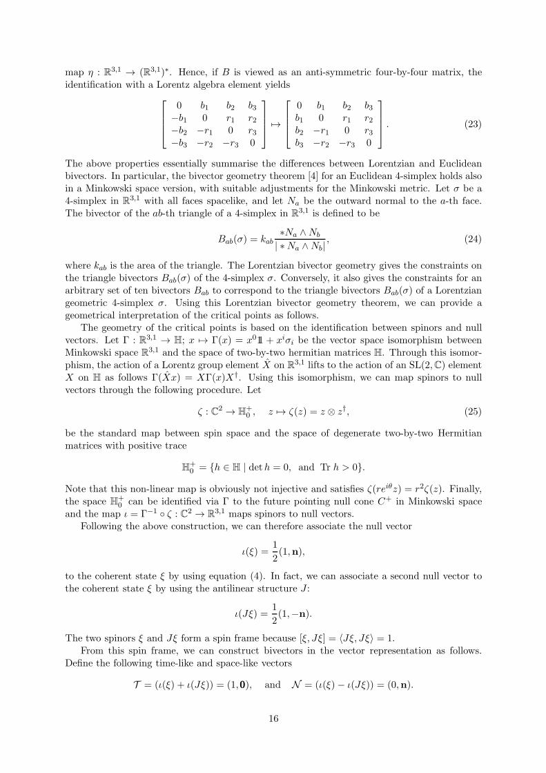
map η : R3,1 → (R3,1)∗. Hence, if B is viewed as an anti-symmetric four-by-four matrix, theidentification with a Lorentz algebra element yields

0 b1 b2 b3−b1 0 r1 r2−b2 −r1 0 r3−b3 −r2 −r3 0

7→

0 b1 b2 b3b1 0 r1 r2b2 −r1 0 r3b3 −r2 −r3 0

. (23)

The above properties essentially summarise the differences between Lorentzian and Euclideanbivectors. In particular, the bivector geometry theorem [4] for an Euclidean 4-simplex holds alsoin a Minkowski space version, with suitable adjustments for the Minkowski metric. Let σ be a4-simplex in R

3,1 with all faces spacelike, and let Na be the outward normal to the a-th face.The bivector of the ab-th triangle of a 4-simplex in R

3,1 is defined to be

Bab(σ) = kab∗Na ∧Nb

| ∗Na ∧Nb|, (24)

where kab is the area of the triangle. The Lorentzian bivector geometry gives the constraints onthe triangle bivectors Bab(σ) of the 4-simplex σ. Conversely, it also gives the constraints for anarbitrary set of ten bivectors Bab to correspond to the triangle bivectors Bab(σ) of a Lorentziangeometric 4-simplex σ. Using this Lorentzian bivector geometry theorem, we can provide ageometrical interpretation of the critical points as follows.

The geometry of the critical points is based on the identification between spinors and nullvectors. Let Γ : R3,1 → H; x 7→ Γ(x) = x011 + xiσi be the vector space isomorphism betweenMinkowski space R

3,1 and the space of two-by-two hermitian matrices H. Through this isomor-phism, the action of a Lorentz group element X on R

3,1 lifts to the action of an SL(2,C) elementX on H as follows Γ(Xx) = XΓ(x)X†. Using this isomorphism, we can map spinors to nullvectors through the following procedure. Let

ζ : C2 → H+0 , z 7→ ζ(z) = z ⊗ z†, (25)

be the standard map between spin space and the space of degenerate two-by-two Hermitianmatrices with positive trace

H+0 = h ∈ H | deth = 0, and Tr h > 0.

Note that this non-linear map is obviously not injective and satisfies ζ(reiθz) = r2ζ(z). Finally,the space H

+0 can be identified via Γ to the future pointing null cone C+ in Minkowski space

and the map ι = Γ−1 ζ : C2 → R3,1 maps spinors to null vectors.

Following the above construction, we can therefore associate the null vector

ι(ξ) =1

2(1,n),

to the coherent state ξ by using equation (4). In fact, we can associate a second null vector tothe coherent state ξ by using the antilinear structure J :

ι(Jξ) =1

2(1,−n).

The two spinors ξ and Jξ form a spin frame because [ξ, Jξ] = 〈Jξ, Jξ〉 = 1.From this spin frame, we can construct bivectors in the vector representation as follows.

Define the following time-like and space-like vectors

T = (ι(ξ) + ι(Jξ)) = (1,000), and N = (ι(ξ)− ι(Jξ)) = (0,n).

16

From these two vectors construct the space-like bivector

b = ∗T ∧ N = −2 ∗ ι(ξ) ∧ ι(Jξ), (26)

where the star ∗ is the Hodge operator acting on the space Λ2(R3,1). In the four-by-four matrixrepresentation, b is given explicitly by

b = ∗

0 n1 n2 n3

−n1 0 0 0−n2 0 0 0−n3 0 0 0

. (27)

This bivector is space-like because T ∧N is time-like and the Hodge operator is an anti-involution.It is also simple by construction and satisfies a cross-simplicity condition

T IbJKηIJ = 0.

Following this construction for every coherent state ξab consequently leads to a collection ofbivectors living in the hyperplane T ⊥, with T the reference point of the future hyperboloid H+

3 .Our critical point equations carry a richer structure. They correspond, in the geometrical

case, to conditions [4] satisfied by the bivectors Bab(σ) of a geometric 4-simplex in R3,1. Consider

the set of ten space-like bivectors constructed as follows:

Bab = kab Xa ⊗ Xa bab, (28)

where Xa is the SO(3, 1) element corresponding to ±Xa in SL(2,C). These bivectors are of normkab and satisfy the following bivector geometry conditions.

They are simple and cross-simple by construction. The cross-simplicity occurs because theylive in the hyperplane F⊥

a , with the future pointing vector Fa in H+3 being the image of the

reference vector T under the action of Xa, that is,

F IaB

JKab ηIJ = 0, with Γ(Fa) = XaX

†a.

Note that the matrix Γ(Fa) lives in the space H+1 of two-by-two Hermitian matrices with unit

determinant and positive trace, which is isomorphic to H+3 as a manifold. Furthermore, the

constructed bivectors satisfy closure∑

b:b6=a

Bab = 0,

because of the closure condition (22) satisfied by the critical points. As we have seen, thiscondition implies pab = γkab with γ constant on the whole simplex.

Another important property is to show that the constructed bivectors also satisfy an orien-tation equation

Bab = −Bba. (29)

This is shown by the following argument. Firstly, we compute the action of the J structure onSL(2,C). Writing an arbitrary SL(2,C) element X as X = exp αiJi + βiKi, with α

i, βi real, itis immediate to see that

JXJ−1 = (X†)−1. (30)

The restriction of the above equation to the unitary subgroup states that J commutes withSU(2) as expected. Using this action, one can show that the two critical point equations (18),(19) lead to the following equations in the vector representation of the Lorentz group

Xa ι(ξab) =‖ Zab ‖2‖ Zba ‖2 Xb ι(Jξba), and Xa ι(Jξab) =

‖ Zba ‖2‖ Zab ‖2

Xb ι(ξba).

17

Wedging these two vector equations leads to the bivector equation

Xa ⊗ Xa ι(ξab) ∧ ι(Jξab) = −Xb ⊗ Xb ι(ξba) ∧ ι(Jξba), (31)

which proves that the orientation condition (29).Finally, the tetrahedron condition, which states that each tetrahedron has a non-degenerate

geometry, is also fulfilled if we choose non-degenerate boundary data.Therefore, for non-degenerate boundary data, the constructed bivectors (28) satisfy all the

bivector geometry constraints [4] except possibly the four-dimensional non-degeneracy condition,which states that the bivectors span the 6-dimensional space of bivectors. However, Lemma 3of [21] which states that the bivector geometry is either fully non-degenerate or fully containedin a 3-dimensional hyperplane did not use the metric at all and so applies unaltered to our case.We shall first discuss the non-degenerate case.

5.2 Non-degenerate Lorentzian 4-simplex: reconstruction

The reconstruction theorem of [4] goes through as used in [21]. The only difference is that whencomparing the bivectors of the reconstructed 4 simplex to the bivector geometry, the Lorentzianmetric is used to evaluate areas.

We therefore again have the equivalence of solutions to (18) to geometric 4-simplices up toinversion. Inversion is the isometry of Minkowski space given by x → −x. In particular, forevery solution that is non-degenerate, there exists a parameter µ which takes the value either1 or −1, and an inversion-related pair of Lorentzian 4-simplexes σ. These are such that thebivectors (of either of the two simplexes) Bab(σ) satisfy

Bab(σ) = µBab = µkab Xa ⊗ Xa bab. (32)

A key subtlety in the geometric interpretation of our equations arises due to the fact thatSL(2,C) maps only to the connected component of SO(3, 1) and takes future pointing vectorsinto future pointing vectors. This means that the inversion map is not in SL(2,C), and so theanalysis in the following sections is somewhat different from the Euclidean case analysed in [21].

5.3 Vector geometries

If the solutions fall into the fully degenerate case this implies all Fa are pointing in the samedirection. As we have fixed X5 = 1 this means we have Fa = XaT = T , for all a. That is theXa are in the SU(2) subgroup that stabilizes T . As such the two distinct critical and stationarypoint equations leading to the bivector equation (18) reduce to the single equation:

Xa ξab = eiθabXb Jξba (33)

The solutions to these equations have been studied in [21, 33]. A solution determines a geo-metrical structure called a vector geometry. This is a set of vectors vab ∈ R

3 satisfying closure,∑

a vab = 0, and orientation, vab = −vab. In this case, vab = Xanab.In particular it was shown that for Regge like boundary data equation (33) admits solutions

exactly if the boundary is that of a Euclidean 3- or 4-dimensional 4-simplex. In the 3-dimensionalcase Xanab are the normals to the faces of the 4-simplex, in the 4-dimensional case there aretwo solutions corresponding to the self-dual and anti self-dual parts of the Euclidean bivectorgeometry.

5.4 Symmetries and classification of the solutions

An important input for the asymptotic formula is the classification of the solutions to the criticalpoints. To start with, we need to consider their symmetries.

18

5.4.1 Symmetries induced by the symmetries of the action

The symmetries of the action listed in section 4.1 map critical points to critical points, exceptthat, as mentioned in section 4.1, some of the symmetries are broken by the gauge-fixing that isused to define the non-compact integrals.

One difference to the Euclidean case of [21] is that there are only half as many discretesymmetries here as there were for the Euclidean amplitude. This means we are no longer able toinvert the normal vectors using a different choice of lift. The bivectors Bab are also left invariantby this symmetry as can be seen from equation (26).

5.4.2 Parity

An additional symmetry of the critical points that is not determined by a symmetry of the actionis the parity operation, given by the inversion of the spatial coordinates of Minkowski space.Using the SU(2) antilinear map J , one can construct a map acting on Minkowski vectors throughtheir identification with two-by-two Hermitian matrices. Most importantly, because the J mapcommutes with SU(2), it necessarily anticommutes with Hermitian matrices which implies that

JΓ(x)J−1 = x011− xiσi = Γ(Px), (34)

where P is the mapping (x0,x) 7→ (x0,−x) on R3,1. Now, we have seen that the J map has

a well defined action (30) on SL(2,C). The corresponding parity transformation P is of keyimportance since it shows that given a solution to the critical point equations (18) and (19), thetransformation

Xa → P (Xa) = JXaJ−1 ∀a,

zab → XaX†azab ∀a < b

(35)

leaves the critical point equations unchanged, because ‖ Zab ‖ / ‖ Zba ‖ is mapped to (‖ Zab ‖/ ‖ Zba ‖)−1, and is an involution. Therefore, P , together with the above transformation on zis a symmetry of the critical points. It is not a symmetry of the action, but a prescription toconstruct a solution out of a solution.

An important feature of the action of P is that it flips the orientation parameter µ to −µ.The remainder of this section shows that this is the case.

Firstly, from the definition (24) of the bivectors of a 4-simplex, it follows that

PBab(σ) = −Bab(Pσ).

This is because the the normal vectors Na transform as vectors under P , but P∗ = −P∗.Another way of saying this is that the Na are determined by the metric only but ∗ requires anorientation.

Secondly, the bivector bab has only space-space components, so is unaffected by the parityoperation. This means that in the equation (32) defining µ,

PBab(σ) = µkab P (Xa)⊗ P (Xa) bab

and henceµσ = −µPσ.

5.4.3 Classification

Using the above results we can now classify the solutions to the critical point equations for differ-ent types of boundary data. In this classification, solutions which are related by the symmetriesof the action, as described in section 4.1, are regarded as the same solution.

19

Regge-like boundary data. Given a Regge-like boundary geometry, a flat metric geometryfor the 4-simplex is specified completely up to rigid motion. In particular the metric on theinterior is uniquely fixed by knowing all the edge lengths, and this is fixed by the boundarydata. One way to see this is to note that there is a linear isomorphism between the set of squareedge lengths and set of interior metrics. Note that l2ab = vµabv

νabgµν for a 4-simplex with edge

vectors v and lengths l is indeed linear and that choosing the edge vectors as basis vectors onecan calculate their inner products using only the other edge lengths. But knowing the innerproducts and the lengths of the basis vectors is equivalent to knowing the metric. Now asthe tetrahedra are all Euclidean and non-degenerate, the metric of the four-simplex must be ofsignature (−,+,+,+) or (+,+,+,+).

The solutions can now be classified according to the boundary data.

• Lorentzian 4-simplex: If the boundary data is that of a non-degenerate Lorentzian 4-simplex, then two distinct critical points exist, related by the parity transformation P insection 5.4.2. Since the boundary data determines the metric of the 4-simplex σ, thereare only four possibilities which are unrelated by the action of SL(2,C), corresponding tothe four connected components of the group O(3, 1). These are σ, its inversion partner−σ and the parity-related Pσ and −Pσ. The solutions correspond to inversion-relatedpairs, thus it is clear that the two solutions given by (σ,−σ) and (Pσ,−Pσ) exhaust allthe possibilities.

• Euclidean 4-simplex: If the boundary data describes a Euclidean 4-simplex, then there willbe exactly two critical points, X+

a and X−a , with all matrices in SU(2). These can be

used to reconstruct a Euclidean 4-simplex σE, as in [21]. These critical points can also beused to construct the parity related 4-simplex PσE .

• 4-simplex in R3: If the boundary data corresponds to a degenerate 4-simplex in R

3 thenthere will be a single SU(2) critical point. This determines a vector geometry. A secondcritical point cannot exist or we would be able to construct a non-degenerate Euclidean4-simplex, which is not possible with this boundary data.

Furthermore it was established in [33] that no other vector geometries exist for Regge likeboundary data.

Non Regge-like boundary data. If the boundary data is not Regge-like then the remainingpossibilities are to obtain exactly one critical point in SU(2) which determines a vector geometry,or no critical points at all.

6 Asymptotic formula

In this section, we provide the asymptotic formula for the four-simplex amplitude f4. We startby defining a canonical choice of phase for the boundary coherent state. Then, we evaluate theaction on the critical points for boundary data forming a non-degenerate Lorentzian 4-simplexgeometry, and finally give the asymptotic formula.

6.1 Regge states

Call Na the outward pointing normals of the 4-simplex and Fa the future pointing normals. Itis immediate that Fa = XaT .

For boundary data that is the boundary of a Lorentzian geometric 4-simplex we define gabas a spin lift of the rotation defined by

gabnab = −nba

20

andgab∆ab = ∆ba

where ∆ab is the b face of the ta tetrahedron which has nab outward if Na = Fa and inwardotherwise.

We define the dihedral boost Dab ∈ SO+(3, 1) as the Lorentz transformation stabilising thebivector Bab(σ) and mapping Fa to Fb:

Dab Fa = Fb, and Dab ⊗ DabBab(σ) = Bab(σ).

Call νabDab, with νab = ±1, a lift of the dihedral boost to SL(2,C).Now consider the diagram:

ta

gab

Xa// τa

νab Dab

tb

Xb

// τb

Arguments similar to those in the Euclidean case show that these signs can all be set to νab = 1using the discrete symmetries. We will make this choice in what follows. It is now straightforwardto see that this diagram commutes.

As argued above, the definition of Regge-like boundary data is the same for Lorentzianboundary data. With the definition of the gluing maps gab as above the definition of the Reggeboundary state is unchanged as well. In particular, then, we have the phase convention definingthe Regge state,

gabξab = Jξba. (36)

6.2 Dihedral angles

The following definitions of the dihedral angles and the Regge action for a Lorentzian simplexis based on the discussion in [34]. For a 4-simplex in Minkowski space with all tetrahedraspace-like, the dihedral angles are all boost parameters. The a-th tetrahedron has a outward-pointing timelike normal vector Na, and the dihedral angle at the intersection of two tetrahedrais determined up to sign by

coshΘab = |Na ·Nb|,and can be viewed as a distance on the unit hyperboloid.

The sign of the dihedral angle is more delicate. One could define them all to be positive,but this would lead to additional signs in the formula for the Regge action. It is much better totake account of the nature of the triangle where the two tetrahedra meet. The tetrahedra comein two types: the outward normals are either future-pointing or past-pointing. The triangles arethen classified into two types: thin wedge, where one of the incident tetrahedra is future and theother one past, and thick wedge, where both are either future or past (see figure 2). The dihedralangle is defined to be positive for a thin wedge and negative for a thick wedge. It is worth notingthat the type of the triangle is unchanged if σ is replaced by −σ, so that the dihedral angle isan unambiguous property of the critical point.

6.3 Regge action

In this section, the action (15) at a critical point is expressed in terms of the underlying geometry.On all critical points, the real part vanishes and we are left with the imaginary part

S = i∑

a<b

pab log‖ Zba ‖2‖ Zab ‖2

+ 2kab θab. (37)

21

N

N

Na a

b

Nb

(b)(a)

Figure 2: Example of a thin wedge (a), and of a thick wedge (b).

In the case where the critical points determine a non-degenerate 4-simplex, the following dis-cussion shows that the argument of the logarithm is related to the dihedral angle Θab at the abtriangle [34].

If Fa and Fb are the future pointing normals determining the two hyperplanes intersectingalong the triangle ab, the corresponding dihedral angle Θab obeys

coshΘab = −Fa · Fb =1

2Tr (Γ(Fa)

−1Γ(Fb)). (38)

To see how this relates to the critical points, couple equations (18) and (19) and eliminate Jξab.This leads to the following eigenvalue equation

X−1a XbX

†b (X

†a)

−1 ξab =‖ Zba ‖2‖ Zab ‖2

ξab.

The matrix X−1a XbX

†b (X

†a)−1 in this equation is Hermitian, so it follows that it has eigenvalues

erab =‖ Zba ‖2‖ Zab ‖2

.

and the inverse of this, e−rab . Moreover, the eigenvectors are orthogonal. This trace is the sameas the trace in (38), and so

|Θab| = |rab|. (39)

Therefore, the parameter rab is the dihedral angle up to a sign.To solve this sign ambiguity, it will prove useful to obtain an exponentiated form of this

matrix. This is achieved by noting that since the spinors ξab are SU(2) coherent states, theysatisfy

(J.n) ξ =i

2ξ, and (K.n) ξ =

1

2ξ.

Hence, the Hermitian matrix X−1a XbX

†b (X

†a)−1 can be written as a pure boost

X−1a XbX

†b (X

†a)

−1 = e2rab K.nab = g(nab)

(

erab 00 e−rab

)

g(nab)−1, (40)

where g(nab) is a unitary matrix.Using the above expression, we can now overcome the sign ambiguity of (39), by using

the definition of the dihedral angle of a Lorentzian 4-simplex σ in terms of the parameter

22

of the dihedral boost. Explicitly, the dihedral boost around the triangle ab is obtained asthe exponential of the Hodge dual of the (normalized) bivector Bab(σ), after the identificationς : Λ2(R3,1) → so(3, 1) defined in (23):

Dab = exp(

Θab ς(∗Bab(σ)))

, (41)

where Bab = Bab/|Bab| is the normalised bivector.This formula is proved as follows. Since Bab(σ) is a simple spacelike bivector, then Dab is a

Lorentz transformation which stabilises a spacelike plane. The bivector in the exponent is

Θab ∗ Bab(σ) = −ΘabNa ∧Nb

| ∗Na ∧Nb|= |Θab|

Fa ∧ Fb

| ∗ Fa ∧ Fb|,

using the sign convention in the definition of a dihedral angle. This bivector acts in the planespanned by Fa and Fb and the boost parameter has the right magnitude. It just remains tocheck that it maps Fa to Fb, and not vice-versa. To first order in small Θ, one has

exp

(

|Θab|ς(Fa ∧ Fb)

| ∗ Fa ∧ Fb|

)

Fa ≃ Fa +|Θab|

| sinhΘab|((Fb · Fa)Fa − (Fa · Fa)Fb) ≃ Fb.

This calculation uses the convention replacing wedge products with bivectors, and the fact thatF 2 = −1.

Now, the expression (32) of the geometric bivectors in terms of the the boundary data leadsto the following equality

ς(∗Bab(σ)) = −µ Xa

0 n1ab n2ab n3abn1ab 0 0 0n2ab 0 0 0n3ab 0 0 0

X−1a = µ Xa π(nab ·K) X−1

a , (42)

where π : sl(2,C)R → End(R3,1) is the vector representation of the Lorentz algebra (see equation(59) in Appendix B).

This implies that a lift of the dihedral boost to SL(2,C) is explicitly given by

Dab = Xa eµΘabK.nab X−1

a , (43)

K being here a 2× 2 matrix. The sign choice of the lift plays no role in what follows.Next, we use that a property of the dihedral boost just established,

Γ(Dab Fa) = Γ(Fb).

This can be writtenDabXaX

†aD

†ab = XbX

†b ,

which impliesXa e

2µΘabK.nab X†a = XbX

†b .

Comparing the last equality and (40) finally gives that

e2µΘabK.nab = e2rabK.nab , (44)

which implies that µΘab = rab. This solves the sign ambiguity.

23

In this last part, we show how the action at critical point simplifies for the case of a Reggestate. The computation uses the critical point equations combined with the commuting diagramas follows

Xa ξab =‖ Zab ‖‖ Zba ‖e

iθabXb J ξba,

=‖ Zab ‖‖ Zba ‖e

iθabXb gab ξab,

=‖ Zab ‖‖ Zba ‖e

iθabXb gabX−1a Xa ξab,

=‖ Zab ‖‖ Zba ‖e

iθabDabXa ξab,

As Dab is a pure boost, that is, has eigenvalues that are strictly positive, it follows that θab = 0.Therefore the action on the critical points corresponding to a non-degenerate 4-simplex yields

the Regge action for the Lorentzian 4-simplex determined by the boundary data

S = iµγ∑

a<b

kabΘab. (45)

6.4 Asymptotic formula

We can now state the asymptotic formula for the 4-simplex amplitude. A formula is calledasymptotic if the error term is bounded by a constant times one more power of λ−1 than thatstated in the asymptotic formula.

Given a set of boundary data, then in the limit λ→ ∞ and for pab = γkab

1. If the boundary state is the Regge state of the boundary geometry of a non-degenerateLorentzian 4-simplex we obtain:

f4 ∼(

1

λ

)12[

N+ exp

(

iλγ∑

a<b

kabΘab

)

+N− exp

(

−iλγ∑

a<b

kabΘab

)]

(46)

N± are independent of λ and are given below.

2. If the boundary state is the Regge state of the boundary geometry of a non-degenerateEuclidean 4-simplex we obtain:

f4 ∼(

1

λ

)12[

N+ exp

(

iλ∑

a<b

kabΘEab

)

+N− exp

(

−iλ∑

a<b

kabΘEab

)]

(47)

ΘEab is the dihedral angle of the Euclidean 4-simplex.

3. If the boundary state is not that of the boundary of a non-degenerate 4-simplex but allowsa single vector geometry as solution, then for an appropriate phase choice the asymptoticformula is:

f4 ∼(

2π

λ

)12

N (48)

The number N is independent of λ.

24

4. For a set of boundary data that is neither a non-degenerate 4-geometry nor a vectorgeometry, the amplitude is suppressed for large λ.

f4 = o(λ−M ) ∀M (49)

In the Lorentzian case the two contributions to the asymptotics correspond to the parityrelated reconstructions of this 4 simplex geometry. Calling N± the constants for the sector withµ = ±1 respectively they are given by

N± = (−1)χ(2π)2224

√

detH±

∏

a<b

2kabcabΩab|crit

= (−1)χ236π12exp(−10i arctan γ)

√

detH±

∏

a<b

kabΩab|crit (50)

The factor (2π)22 comes from the stationary phase formula as the integral has 6× 4 dimensionscoming from the SL(2,C) integrations and 20 dimensions from the z variables. Since the formulais asymptotic, we have used dλk ∼ 2λk and cancelled the scaling from the coefficients. Theadditional factor 24 comes from the fact that both spin lifts at the critical points give the samecontribution to the action. H± is the Hessian matrix of the action 15 evaluated at the criticalpoints (+) and the parity related critical points (-), this is evaluated in appendix A. Ωab|critis the measure term evaluated at the critical points. A choice of coordinate must be made toevaluate this, however the ratio Ωab with

√

detH± is invariant of this choice of coordinates. Theconstant cab gives exp(−i arctan γ)/π.

For the Euclidean case we get contributions from the self dual and anti self dual part of thebivector geometry which combine to give the full 4-dimensional Euclidean bivector geometry.The phase part of the action for Euclidean boundary data is evaluated in [33]. N± are the sameas above but evaluated at the appropriate critical points. The dihedral angle ΘE

ab of a Euclidean4-simplex arises in the following way. For the case of Euclidean boundary data, there are twoSU(2) solutions, say X+,X−, to the critical point equations (18). For these solutions the boostparameter rab = 0 but the phase term θ± remains. The interpretation of the critical points isa non-degenerate Euclidean 4-simplex as described in [21] and the Regge phase choice impliesthat θ+ + θ− = 0 and θ+ = 1

2ΘEab. Combining this gives case 2.

The case of a single vector geometry proceeds analogously. An appropriate phase choice andthe geometry of these solutions is described in [33]. In particular it was shown that no suchvector geometries exist for Lorentzian boundary data there.

For the final case, no critical points exist and the stationary phase theorem tells us that theamplitude is suppressed.

By the classification of critical points in section 5.4.3 this concludes our asymptotic analysisof the amplitude.

7 Conclusion

In this work we have defined a graphical calculus for the unitary representations of Lorentzgroup, and used it to give a systematic definition of the 4-simplex amplitude in the case ofLorentzian quantum gravity. The asymptotic analysis of the amplitude has some surprisingfeatures. In the corresponding Euclidean quantum gravity problem analysed in [21], there wasa puzzling superposition of terms with the Regge action multiplied by the Immirzi parameterand terms with the Regge action not multiplied by the Immirzi parameter.

25

In the Lorentzian quantum gravity analysed here, these two phenomena are separated out.The terms with the Immirzi parameter occur for boundary data of a Lorentzian metric andinvolve the Lorentzian Regge action. For this case, the result is much cleaner than for theEuclidean theory, as these are the only terms for this boundary data. The terms without theImmirzi parameter occur for boundary data of a Euclidean metric and, rather surprisingly,involve the Euclidean Regge action, still in an oscillatory manner, and so are not suppressed.The physical significance of this is still unclear; the Euclidean action might be expected inrelation to a tunnelling phenomenon, but then the amplitude would be exponentially damped,not oscillatory. Another surprise is that these terms are related to the SU(2) BF theory, andnot to the Euclidean quantum gravity amplitudes. It is of course possible that in a state summodel, these terms are topological and do not contribute to the dynamics. This possibility is atopic for future work.

It is also important to mention the further case of non Regge-like boundary data. There arean extra five parameters for the boundary data in this case, so naively one might expect theseto dominate. However this depends on further analysis of the phase factor for this case, whichmay turn out to be trivial.

Another feature which deserves further anaylsis is the formula for the Hessian. For example,we do not know yet whether the parity-related terms involving the Regge action and minus theRegge action occur with equal magnitude, or if one is heavily favoured over the other. Also, ageometric formula for the Hessian along the lines of the Ponzano-Regge formula is missing.

Another result of this work is that a condition for the existence of stationary points of theaction is that pab = γkab for some constant γ. This is exactly the same restriction on therepresentation labels derived in [7], by different methods, where γ is the Immirzi parameter.

Acknowledgements

Eugenio Bianchi and Carlo Rovelli are thanked for useful discussions. WF is supported by theRoyal Commission for the Exhibition of 1851. RD and FH are funded by EPSRC doctoralgrants. RP thanks the QG research networking programme of the ESF for a visit grant.

A The Hessian

Here we calculate the Hessian matrix required in the stationary phase formula.The Hessian is defined as the matrix of second derivatives of the action where the variable X5

has been gauge fixed to the identity. We split the Hessian matrix into derivatives with respectto the Xa variables and derivatives with respect to the zab. The Hessian will then be a 44× 44matrix of the form

H =

(

HXX HXz

HzX Hzz

)

(51)

We will now describe each block of this matrix. HXX is a 24 × 24 matrix containing onlyderivatives with respect to the Xa. Note that due to the form of the action, derivatives withrespect to two different variables will be zero and it will be block diagonal

HXX =

HX1X1 0 0 00 HX2X2 0 00 0 HX3X3 00 0 0 HX4X4

(52)

26

Each HX1X1 is a 6 × 6 matrix. The variation has been performed by splitting the SL(2,C)element into a boost and a rotation generator. This gives

HXaXa =

(

HXRa XR

a HXBa XR

a

HXRa XB

a HXBa XB

a

)

(53)

With

HXR

a XRa

ij =∑

b6=a

−2kab(δij − niξabn

jξab

)

HXB

a XRa

ij = i∑

b6=a

2kab(δij − niξabn

jξab

)

HXR

a XBa

ij = i∑

b6=a

2kab(δij − niξabn

jξab

)

HXB

a XBa

ij =∑

b6=a

−4ipab(δij − niξabn

jξab

)− 2kab(δij − niξabn

jξab

)

(54)

Where i, j = 1, 2, 3 and we have used the critical and stationary point equations.Hzz is a 20× 20 matrix. The derivatives are with respect to the spinor variables zab on each

of the ten edges ab of the amplitude. To perform these derivatives we must choose a section forzab.

Next the mixed spinor and SL(2,C) derivatives. We have arranged the derivatives in theorder of the orientation a < b, ie z12, z13, z14, z15, z23, z24, z25, z34, z35, z45. The matrix HXz is a24× 20 matrix with the following non-zero entries

HXz =

HX1z12 HX1z13 HX1z14 HX1z15 0 0 0 0 0 0HX2z12 0 0 0 HX2z23 HX2z24 HX2z25 0 0 0

0 HX3z13 0 0 HX2z23 0 0 HX3z34 HX3z35 00 0 HX4z14 0 0 HX4z24 0 HX4z34 0 HX4z45

These derivatives also require a choice of section for zab.

B The Lorentz algebra

In this Appendix, we summarise the conventions used throughout this paper regarding theLorentz algebra. The Lie algebra so(3, 1) of the Lorentz group is a real, semi-simple Lie algebraof dimension six. A basis of so(3, 1) is provided by the generators (Lαβ)α<β=0,...,3. The liealgebra structure is coded in the brackets

[Lαβ, Lγδ ] = −ηαγ Lβδ + ηαδ Lβγ + ηβγ Lαδ − ηβδ Lαγ ,

where η is the standard Minkowski metric with signature −+++.It is convenient to decompose any (infinitesimal) Lorentz transformation into a purely spatial

rotation and a hyperbolic rotation, or boost. This is achieved by introducing the rotation andboost generators respectively given by

Ji =1

2ǫ jki Ljk, and Ki = Li0, i, j, k = 1, 2, 3, (55)

27

where ǫijk is the three-dimensional Levi-Cevita tensor.Using the Lie algebra structure of so(3, 1) displayed above, it is immediate to check the

following commutation relations between the rotation and boost generators

[Ji, Jj ] = −ǫ kij Jk, [Ji,Kj ] = −ǫ k

ij Kk, [Ki,Kj ] = ǫ kij Jk. (56)

The finite dimensional representations of the Lorentz algebra used in this paper are the spinorand vector representations. In the spinor representation ρ : so(3, 1) → EndC2, the rotation andboost generators are given explicitly in terms of the Hermitian Pauli matrices

σ1 =

(

0 11 0

)

, σ2 =

(

0 −ii 0

)

, σ3 =

(

1 00 −1

)

,

by the following expressions

ρ(Ji) =i

2σi, and ρ(Ki) =

1

2σi. (57)

This is immediate to check by using the property [σi, σj ] = 2iǫ kij σk of the Pauli matrices.

Throughout the text, the map ρ is kept implicit when there is no possible confusion.In fact, the above presentation gives the explicit isomorphism between the Lorentz alge-

bra so(3, 1) and the realification sl(2,C)R of the Lie algebra of the two-dimensional complexunimodular group SL(2,C) because

sl(2,C)R = (su(2)C)R ∼= su(2) ⊕ isu(2),

where the direct sum is at the level of vector spaces.Finally, we also used explicitly the vector representation π : so(3, 1) → EndR3,1 of the

Lorentz algebra in which the matrix elements of the Lαβ generators are given by

π(Lαβ)IJ = δIαηβJ − ηαJδ

Iβ , I, J = 0, ..., 3.

From the above expression, it is immediate to compute the matrix elements of the image of therotation and boost generators in the vector representation:

π(Ji)IJ = ǫ I

i J , and π(Ki)IJ = δIi η0J − ηiJδ

I0 . (58)

Therefore, an arbitrary element L in the Lorentz algebra expressed in the rotation/boost basisas follows L = r · J+ b ·K is given by the four-by-four matrix

π(L) =

0 −b1 −b2 −b3−b1 0 r3 −r2−b2 −r3 0 r1

−b3 r2 −r1 0

, (59)

in the vector representation.

References

[1] G. Ponzano and T. Regge, Spetroscopy and group theoretical methods in physics, ed. F.

Block. North Holland, 1968.

[2] M. P. Reisenberger and C. Rovelli, “*Sum over surfaces* form of loop quantum gravity,”Phys. Rev., vol. D56, pp. 3490–3508, 1997, gr-qc/9612035.

28

[3] H. Ooguri, “Topological lattice models in four-dimensions,” Mod. Phys. Lett., vol. A7,pp. 2799–2810, 1992, hep-th/9205090.

[4] J. W. Barrett and L. Crane, “Relativistic spin networks and quantum gravity,” Journal of

Mathematical Physics, vol. 39, p. 3296, 1998.

[5] J. W. Barrett and L. Crane, “A Lorentzian signature model for quantum general relativity,”Class. Quant. Grav., vol. 17, pp. 3101–3118, 2000, gr-qc/9904025.

[6] J. Engle, R. Pereira, and C. Rovelli, “Flipped spinfoam vertex and loop gravity,” Nucl.

Phys., vol. B798, pp. 251–290, 2008, 0708.1236.

[7] J. Engle, E. Livine, R. Pereira, and C. Rovelli, “LQG vertex with finite Immirzi parameter,”Nucl. Phys., vol. B799, pp. 136–149, 2008, 0711.0146.

[8] L. Freidel and K. Krasnov, “A New Spin Foam Model for 4d Gravity,” Class. Quant. Grav.,vol. 25, p. 125018, 2008, 0708.1595.

[9] E. R. Livine and S. Speziale, “Consistently Solving the Simplicity Constraints for SpinfoamQuantum Gravity,” Europhys. Lett., vol. 81, p. 50004, 2008, 0708.1915.

[10] A. Barbieri, “Quantum tetrahedra and simplicial spin networks,” Nucl. Phys., vol. B518,pp. 714–728, 1998, gr-qc/9707010.

[11] R. Pereira, “Lorentzian LQG vertex amplitude,” Class. Quant. Grav., vol. 25, p. 085013,2008, 0710.5043.

[12] C. Rovelli, Quantum Gravity. Cambridge University Press, 2004.

[13] E. Alesci and C. Rovelli, “The complete LQG propagator: I. Difficulties with the Barrett-Crane vertex,” Phys. Rev., vol. D76, p. 104012, 2007, 0708.0883.

[14] E. Alesci and C. Rovelli, “The complete LQG propagator: II. Asymptotic behavior of thevertex,” Phys. Rev., vol. D77, p. 044024, 2008, 0711.1284.

[15] G. Immirzi, “Real and complex connections for canonical gravity,” Class. Quant. Grav.,vol. 14, pp. L177–L181, 1997, gr-qc/9612030.

[16] J. Engle and R. Pereira, “Coherent states, constraint classes, and area operators in the newspin-foam models,” Class. Quant. Grav., vol. 25, p. 105010, 2008, 0710.5017.

[17] E. R. Livine, “Projected spin networks for Lorentz connection: Linking spin foams and loopgravity,” Class. Quant. Grav., vol. 19, pp. 5525–5542, 2002, gr-qc/0207084.

[18] B. Dittrich and S. Speziale, “Area-angle variables for general relativity,” New J. Phys.,vol. 10, p. 083006, 2008, 0802.0864.

[19] F. Conrady and L. Freidel, “Path integral representation of spin foam models of 4d gravity,”Class. Quant. Grav., vol. 25, p. 245010, 2008, 0806.4640.

[20] F. Conrady and L. Freidel, “On the semiclassical limit of 4d spin foam models,” Phys. Rev.,vol. D78, p. 104023, 2008, 0809.2280.

[21] J. W. Barrett, R. J. Dowdall, W. J. Fairbairn, H. Gomes, and F. Hellmann, “Asymptoticanalysis of the EPRL four-simplex amplitude,” 2009, 0902.1170.

29

[22] E. Bianchi, E. Magliaro, and C. Perini, “LQG propagator from the new spin foams,” 2009,0905.4082.

[23] I. Gelfand and N. Y. V. M.I. Graev, GENERALIZED FUNCTIONS: Vol 5, Integral geom-

etry and representation theory. Academic Press, 1966.

[24] R. Penrose, “Angular momentum: an approach to combinatorial spacetime, in ‘quantumtheory and beyond’, ed. e.t. bastin.,” 1970.

[25] J. W. Barrett and I. Naish-Guzman, “The Ponzano-Regge model,” 2008, 0803.3319.

[26] J. C. Baez and J. W. Barrett, “Integrability for relativistic spin networks,” Class. Quant.

Grav., vol. 18, pp. 4683–4700, 2001, gr-qc/0101107.

[27] J. Engle and R. Pereira, “Regularization and finiteness of the Lorentzian LQG vertices,”2008, 0805.4696.

[28] E. R. Livine and S. Speziale, “A new spinfoam vertex for quantum gravity,” Physical Review

D, vol. 76, p. 084028, 2007.

[29] A. Perelomov, Generalized coherent states and their applications. Springer-Verlag, 1986.

[30] M. A. Naimark, Linear representations of the Lorentz group. Pergamon Press, 1964.

[31] W. Ruhl, The Lorentz group and harmonic analysis. W.A. Benjamin, 1970.

[32] L. Hormander, The analysis of linear partial differential operators I. Springer-Verlag, 1983.

[33] J. W. Barrett, W. J. Fairbairn, and F. Hellmann, “Quantum gravity asymptotics from thesu(2) 15j symbol (in preparation),”

[34] J. W. Barrett and T. J. Foxon, “Semiclassical limits of simplicial quantum gravity,” Class.

Quant. Grav., vol. 11, pp. 543–556, 1994, gr-qc/9310016.

30