6.042J Chapter 9: Sums and asymptotics

“mcs-ftl” — 2010/9/8 — 0:40 — page 243 — #249

9 Sums and AsymptoticsSums and products arise regularly in the analysis of algorithms, financial applica-tions, physical problems, and probabilistic systems. For example, we have alreadyencountered the sum 1 C 2 C 4 C � � � C N when counting the number of nodesin a complete binary tree with N inputs. Although such a sum can be representedcompactly using the sigma notation

logNXiD0

2i ; (9.1)

it is a lot easier and more helpful to express the sum by its closed form value

2N � 1:

By closed form, we mean an expression that does not make use of summationor product symbols or otherwise need those handy (but sometimes troublesome)dots. . . . Expressions in closed form are usually easier to evaluate (it doesn’t getmuch simpler than 2N � 1, for example) and it is usually easier to get a feel fortheir magnitude than expressions involving large sums and products.

But how do you find a closed form for a sum or product? Well, it’s part math andpart art. And it is the subject of this chapter.

We will start the chapter with a motivating example involving annuities. Figuringout the value of the annuity will involve a large and nasty-looking sum. We will thendescribe several methods for finding closed forms for all sorts of sums, includingthe annuity sums. In some cases, a closed form for a sum may not exist and so wewill provide a general method for finding good upper and lower bounds on the sum(which are closed form, of course).

The methods we develop for sums will also work for products since you canconvert any product into a sum by taking a logarithm of the product. As an example,we will use this approach to find a good closed-form approximation to

nŠ WWD 1 � 2 � 3 � � �n:

We conclude the chapter with a discussion of asymptotic notation. Asymptoticnotation is often used to bound the error terms when there is no exact closed formexpression for a sum or product. It also provides a convenient way to express thegrowth rate or order of magnitude of a sum or product.

1

“mcs-ftl” — 2010/9/8 — 0:40 — page 244 — #250

Chapter 9 Sums and Asymptotics

9.1 The Value of an Annuity

Would you prefer a million dollars today or $50,000 a year for the rest of your life?On the one hand, instant gratification is nice. On the other hand, the total dollarsreceived at $50K per year is much larger if you live long enough.

Formally, this is a question about the value of an annuity. An annuity is a finan-cial instrument that pays out a fixed amount of money at the beginning of every yearfor some specified number of years. In particular, an n-year, m-payment annuitypays m dollars at the start of each year for n years. In some cases, n is finite, butnot always. Examples include lottery payouts, student loans, and home mortgages.There are even Wall Street people who specialize in trading annuities.1

A key question is, “What is an annuity worth?” For example, lotteries often payout jackpots over many years. Intuitively, $50,000 a year for 20 years ought to beworth less than a million dollars right now. If you had all the cash right away, youcould invest it and begin collecting interest. But what if the choice were between$50,000 a year for 20 years and a half million dollars today? Now it is not clearwhich option is better.

9.1.1 The Future Value of Money

In order to answer such questions, we need to know what a dollar paid out in thefuture is worth today. To model this, let’s assume that money can be invested at afixed annual interest rate p. We’ll assume an 8% rate2 for the rest of the discussion.

Here is why the interest rate p matters. Ten dollars invested today at interest ratep will become .1Cp/ � 10 D 10:80 dollars in a year, .1Cp/2 � 10 � 11:66 dollarsin two years, and so forth. Looked at another way, ten dollars paid out a year fromnow is only really worth 1=.1C p/ � 10 � 9:26 dollars today. The reason is that ifwe had the $9.26 today, we could invest it and would have $10.00 in a year anyway.Therefore, p determines the value of money paid out in the future.

So for an n-year,m-payment annuity, the first payment ofm dollars is truly worthm dollars. But the second payment a year later is worth only m=.1 C p/ dollars.Similarly, the third payment is worth m=.1 C p/2, and the n-th payment is worthonly m=.1 C p/n�1. The total value, V , of the annuity is equal to the sum of the

1Such trading ultimately led to the subprime mortgage disaster in 2008–2009. We’ll talk moreabout that in Section 19.5.3.

2U.S. interest rates have dropped steadily for several years, and ordinary bank deposits now earnaround 1.5%. But just a few years ago the rate was 8%; this rate makes some of our examples a littlemore dramatic. The rate has been as high as 17% in the past thirty years.

2

“mcs-ftl” — 2010/9/8 — 0:40 — page 245 — #251

9.1. The Value of an Annuity

payment values. This gives:

V D

nXiD1

m

.1C p/i�1

D m �

n�1XjD0

�1

1C p

�j(substitute j D i � 1)

D m �

n�1XjD0

xj (substitute x D 1=.1C p/): (9.2)

The goal of the preceding substitutions was to get the summation into a simplespecial form so that we can solve it with a general formula. In particular, the termsof the sum

n�1XjD0

xj D 1C x C x2 C x3 C � � � C xn�1

form a geometric series, which means that the ratio of consecutive terms is alwaysthe same and it is a positive value less than one. In this case, the ratio is always x,and 0 < x < 1 since we assumed that p > 0. It turns out that there is a niceclosed-form expression for any geometric series; namely

n�1XiD0

xi D1 � xn

1 � x: (9.3)

Equation 9.3 can be verified by induction, but, as is often the case, the proof byinduction gives no hint about how the formula was found in the first place. So we’lltake this opportunity to describe a method that you could use to figure it out foryourself. It is called the Perturbation Method.

9.1.2 The Perturbation Method

Given a sum that has a nice structure, it is often useful to “perturb” the sum so thatwe can somehow combine the sum with the perturbation to get something muchsimpler. For example, suppose

S D 1C x C x2 C � � � C xn�1:

An example of a perturbation would be

xS D x C x2 C � � � C xn:

3

“mcs-ftl” — 2010/9/8 — 0:40 — page 246 — #252


The difference between S and xS is not so great, and so if we were to subtract xSfrom S , there would be massive cancellation:

S D 1C x C x2 C x3 C � � � C xn�1

�xS D � x � x2 � x3 � � � � � xn�1 � xn:

The result of the subtraction is

S � xS D 1 � xn:

Solving for S gives the desired closed-form expression in Equation 9.3:

S D1 � xn

1 � x:

We’ll see more examples of this method when we introduce generating functionsin Chapter 12.

9.1.3 A Closed Form for the Annuity Value

Using Equation 9.3, we can derive a simple formula for V , the value of an annuitythat pays m dollars at the start of each year for n years.

V D m

�1 � xn

1 � x

�(by Equations 9.2 and 9.3) (9.4)

D m

1C p � .1=.1C p//n�1

p

!(substituting x D 1=.1C p/): (9.5)

Equation 9.5 is much easier to use than a summation with dozens of terms. Forexample, what is the real value of a winning lottery ticket that pays $50,000 peryear for 20 years? Plugging in m D $50,000, n D 20, and p D 0:08 givesV � $530,180. So because payments are deferred, the million dollar lottery isreally only worth about a half million dollars! This is a good trick for the lotteryadvertisers.

9.1.4 Infinite Geometric Series

The question we began with was whether you would prefer a million dollars todayor $50,000 a year for the rest of your life. Of course, this depends on how longyou live, so optimistically assume that the second option is to receive $50,000 ayear forever. This sounds like infinite money! But we can compute the value of anannuity with an infinite number of payments by taking the limit of our geometricsum in Equation 9.3 as n tends to infinity.

4

“mcs-ftl” — 2010/9/8 — 0:40 — page 247 — #253


Theorem 9.1.1. If jxj < 1, then

1XiD0

xi D1

1 � x:

Proof.

1XiD0

xi WWD limn!1

n�1XiD0

xi

D limn!1

1 � xn

1 � x(by Equation 9.3)

D1

1 � x:

The final line follows from that fact that limn!1 xn D 0 when jxj < 1. �

In our annuity problem, x D 1=.1C p/ < 1, so Theorem 9.1.1 applies, and weget

V D m �

1XjD0

xj (by Equation 9.2)

D m �1

1 � x(by Theorem 9.1.1)

D m �1C p

p.x D 1=.1C p//:

Plugging inm D $50,000 and p D 0:08, we see that the value V is only $675,000.Amazingly, a million dollars today is worth much more than $50,000 paid everyyear forever! Then again, if we had a million dollars today in the bank earning 8%interest, we could take out and spend $80,000 a year forever. So on second thought,this answer really isn’t so amazing.

9.1.5 Examples

Equation 9.3 and Theorem 9.1.1 are incredibly useful in computer science. In fact,we already used Equation 9.3 implicitly when we claimed in Chapter 6 than anN -input complete binary tree has

1C 2C 4C � � � CN D 2N � 1

5

“mcs-ftl” — 2010/9/8 — 0:40 — page 248 — #254


nodes. Here are some other common sums that can be put into closed form using

Equation 9.3 and Theorem 9.1.1:

1C 1=2C 1=4C � � � D

1XiD0

�1

2

�iD

1

1 � .1=2/D 2 (9.6)

0:99999 � � � D 0:9

1XiD0

�1

10

�iD 0:9

1

1 � 1=10

!D 0:9

10

9

!D 1 (9.7)

1 � 1=2C 1=4 � � � � D

1XiD0

��1

2

�iD

1

1 � .�1=2/D2

3(9.8)

1C 2C 4C � � � C 2n�1 D

n�1XiD0

2i D1 � 2n

1 � 2D 2n � 1 (9.9)

1C 3C 9C � � � C 3n�1 D

n�1XiD0

3i D1 � 3n

1 � 3D3n � 1

2(9.10)

If the terms in a geometric sum grow smaller, as in Equation 9.6, then the sum issaid to be geometrically decreasing. If the terms in a geometric sum grow progres-sively larger, as in Equations 9.9 and 9.10, then the sum is said to be geometricallyincreasing. In either case, the sum is usually approximately equal to the term in thesum with the greatest absolute value. For example, in Equations 9.6 and 9.8, thelargest term is equal to 1 and the sums are 2 and 2/3, both relatively close to 1. InEquation 9.9, the sum is about twice the largest term. In Equation 9.10, the largestterm is 3n�1 and the sum is .3n � 1/=2, which is only about a factor of 1:5 greater.You can see why this rule of thumb works by looking carefully at Equation 9.3 andTheorem 9.1.1.

9.1.6 Variations of Geometric Sums

We now know all about geometric sums—if you have one, life is easy. But inpractice one often encounters sums that cannot be transformed by simple variablesubstitutions to the form

Pxi .

A non-obvious, but useful way to obtain new summation formulas from old isby differentiating or integrating with respect to x. As an example, consider thefollowing sum:

n�1XiD1

ixi D x C 2x2 C 3x3 C � � � C .n � 1/xn�1

6

“mcs-ftl” — 2010/9/8 — 0:40 — page 249 — #255


This is not a geometric sum, since the ratio between successive terms is not fixed,and so our formula for the sum of a geometric sum cannot be directly applied. Butsuppose that we differentiate Equation 9.3:

d

dx

n�1XiD0

xi

!D

d

dx

�1 � xn

1 � x

�: (9.11)

The left-hand side of Equation 9.11 is simply

n�1XiD0

d

dx.xi / D

n�1XiD0

ixi�1:

The right-hand side of Equation 9.11 is

�nxn�1.1 � x/ � .�1/.1 � xn/

.1 � x/2D�nxn�1 C nxn C 1 � xn

.1 � x/2

D1 � nxn�1 C .n � 1/xn

.1 � x/2:

Hence, Equation 9.11 means that

n�1XiD0

ixi�1 D1 � nxn�1 C .n � 1/xn

.1 � x/2:

Often, differentiating or integrating messes up the exponent of x in every term.In this case, we now have a formula for a sum of the form

Pixi�1, but we want a

formula for the seriesPixi . The solution is simple: multiply by x. This gives:

n�1XiD1

ixi Dx � nxn C .n � 1/xnC1

.1 � x/2(9.12)

and we have the desired closed-form expression for our sum3. It’s a little compli-cated looking, but it’s easier to work with than the sum.

Notice that if jxj < 1, then this series converges to a finite value even if there areinfinitely many terms. Taking the limit of Equation 9.12 as n tends infinity givesthe following theorem:

3Since we could easily have made a mistake in the calculation, it is always a good idea to go backand validate a formula obtained this way with a proof by induction.

7

“mcs-ftl” — 2010/9/8 — 0:40 — page 250 — #256


Theorem 9.1.2. If jxj < 1, then

1XiD1

ixi Dx

.1 � x/2:

As a consequence, suppose that there is an annuity that pays im dollars at theend of each year i forever. For example, if m D $50,000, then the payouts are$50,000 and then $100,000 and then $150,000 and so on. It is hard to believe thatthe value of this annuity is finite! But we can use Theorem 9.1.2 to compute thevalue:

V D

1XiD1

im

.1C p/i

D m �1=.1C p/

.1 � 11Cp

/2

D m �1C p

p2:

The second line follows by an application of Theorem 9.1.2. The third line isobtained by multiplying the numerator and denominator by .1C p/2.

For example, if m D $50,000, and p D 0:08 as usual, then the value of theannuity is V D $8,437,500. Even though the payments increase every year, the in-crease is only additive with time; by contrast, dollars paid out in the future decreasein value exponentially with time. The geometric decrease swamps out the additiveincrease. Payments in the distant future are almost worthless, so the value of theannuity is finite.

The important thing to remember is the trick of taking the derivative (or integral)of a summation formula. Of course, this technique requires one to compute nastyderivatives correctly, but this is at least theoretically possible!

9.2 Power Sums

In Chapter 3, we verified the formula

nXiD1

i Dn.nC 1/

2: (9.13)

But the source of this formula is still a mystery. Sure, we can prove it is true usingwell ordering or induction, but where did the expression on the right come from in

8

“mcs-ftl” — 2010/9/8 — 0:40 — page 251 — #257

9.2. Power Sums

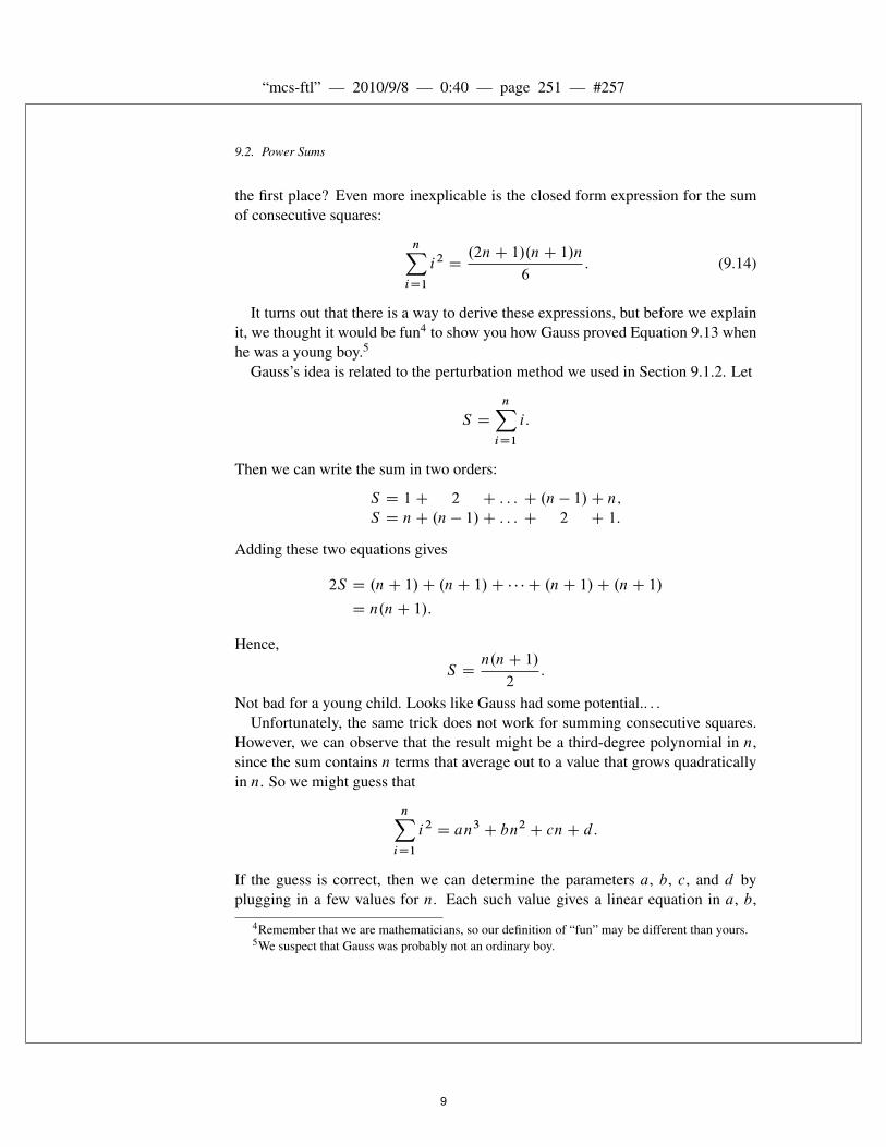
the first place? Even more inexplicable is the closed form expression for the sumof consecutive squares:

nXiD1

i2 D.2nC 1/.nC 1/n

6: (9.14)

It turns out that there is a way to derive these expressions, but before we explainit, we thought it would be fun4 to show you how Gauss proved Equation 9.13 whenhe was a young boy.5

Gauss’s idea is related to the perturbation method we used in Section 9.1.2. Let

S D

nXiD1

i:

Then we can write the sum in two orders:

S D 1 C 2 C : : : C .n � 1/C n;

S D nC .n � 1/C : : : C 2 C 1:

Adding these two equations gives

2S D .nC 1/C .nC 1/C � � � C .nC 1/C .nC 1/

D n.nC 1/:

Hence,

S Dn.nC 1/

2:

Not bad for a young child. Looks like Gauss had some potential.. . .Unfortunately, the same trick does not work for summing consecutive squares.

However, we can observe that the result might be a third-degree polynomial in n,since the sum contains n terms that average out to a value that grows quadraticallyin n. So we might guess that

nXiD1

i2 D an3 C bn2 C cnC d:

If the guess is correct, then we can determine the parameters a, b, c, and d byplugging in a few values for n. Each such value gives a linear equation in a, b,

4Remember that we are mathematicians, so our definition of “fun” may be different than yours.5We suspect that Gauss was probably not an ordinary boy.

9

“mcs-ftl” — 2010/9/8 — 0:40 — page 252 — #258


c, and d . If we plug in enough values, we may get a linear system with a uniquesolution. Applying this method to our example gives:

n D 0 implies 0 D d

n D 1 implies 1 D aC b C c C d

n D 2 implies 5 D 8aC 4b C 2c C d

n D 3 implies 14 D 27aC 9b C 3c C d:

Solving this system gives the solution a D 1=3, b D 1=2, c D 1=6, d D 0.Therefore, if our initial guess at the form of the solution was correct, then thesummation is equal to n3=3C n2=2C n=6, which matches Equation 9.14.

The point is that if the desired formula turns out to be a polynomial, then onceyou get an estimate of the degree of the polynomial, all the coefficients of thepolynomial can be found automatically.

Be careful! This method let’s you discover formulas, but it doesn’t guaranteethey are right! After obtaining a formula by this method, it’s important to go backand prove it using induction or some other method, because if the initial guess atthe solution was not of the right form, then the resulting formula will be completelywrong!6

9.3 Approximating Sums

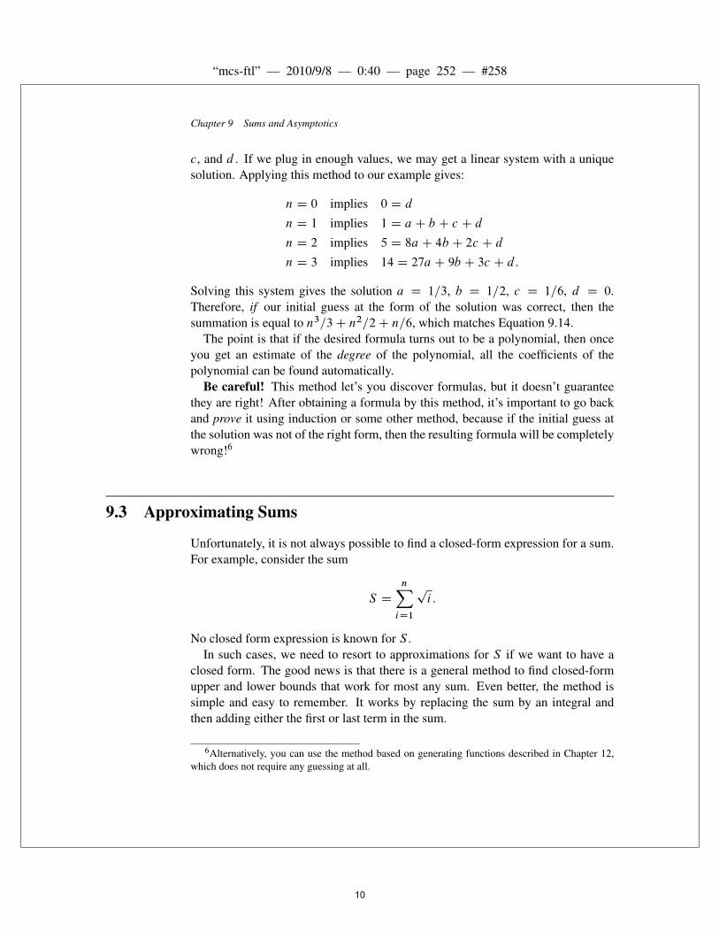
Unfortunately, it is not always possible to find a closed-form expression for a sum.For example, consider the sum

S D

nXiD1

pi :

No closed form expression is known for S .In such cases, we need to resort to approximations for S if we want to have a

closed form. The good news is that there is a general method to find closed-formupper and lower bounds that work for most any sum. Even better, the method issimple and easy to remember. It works by replacing the sum by an integral andthen adding either the first or last term in the sum.

6Alternatively, you can use the method based on generating functions described in Chapter 12,which does not require any guessing at all.

10

“mcs-ftl” — 2010/9/8 — 0:40 — page 253 — #259

9.3. Approximating Sums

Theorem 9.3.1. Let f W RC ! RC be a nondecreasing7 continuous function andlet

S D

nXiD1

f .i/

and

I D

Z n

1

f .x/ dx:

ThenI C f .1/ � S � I C f .n/:

Similarly, if f is nonincreasing, then

I C f .n/ � S � I C f .1/:

Proof. Let f W RC ! RC be a nondecreasing function. For example, f .x/ Dpx

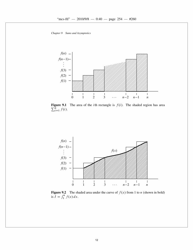
is such a function.Consider the graph shown in Figure 9.1. The value of

S D

nXiD1

f .i/

is represented by the shaded area in this figure. This is because the i th rectangle inthe figure (counting from left to right) has width 1 and height f .i/.

The value of

I D

Z n

1

f .x/ dx

is the shaded area under the curve of f .x/ from 1 to n shown in Figure 9.2.Comparing the shaded regions in Figures 9.1 and 9.2, we see that S is at least

I plus the area of the leftmost rectangle. Hence,

S � I C f .1/ (9.15)

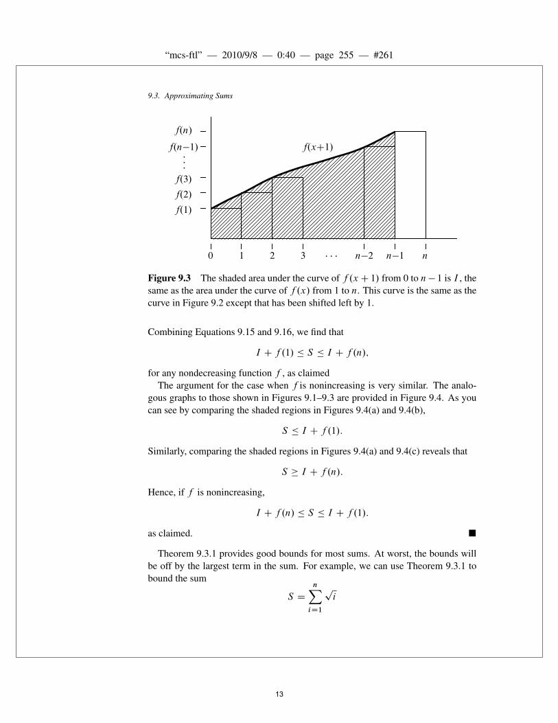
This is the lower bound for S . We next derive the upper bound.Figure 9.3 shows the curve of f .x/ from 1 to n shifted left by 1. This is the same

as the curve f .x C 1/ from 0 to n � 1 and it has the same area I .Comparing the shaded regions in Figures 9.1 and 9.3, we see that S is at most

I plus the area of the rightmost rectangle. Hence,

S � I C f .n/: (9.16)

7A function f is nondecreasing if f .x/ � f .y/ whenever x � y. It is nonincreasing if f .x/ �f .y/ whenever x � y.

11

“mcs-ftl” — 2010/9/8 — 0:40 — page 254 — #260


0 1 2 3

n�2 n�1 n

f.n/

f.n�1/

f.3/

f.2/

f.1/

Figure 9.1 The area of the i th rectangle is f .i/. The shaded region has areaPniD1 f .i/.

0 1 2 3 n�2 n�1 n

f.n/

f.x/f.n�1/

f.3/

f.2/

f.1/

Figure 9.2 The shaded area under the curve of f .x/ from 1 to n (shown in bold)is I D

R n1 f .x/ dx.

12

“mcs-ftl” — 2010/9/8 — 0:40 — page 255 — #261

9.3. Approximating Sums

0 1 2 3 n�2 n�1 n

f.n/

f.n�1/ f.xC1/

f.3/

f.2/

f.1/

Figure 9.3 The shaded area under the curve of f .xC 1/ from 0 to n� 1 is I , thesame as the area under the curve of f .x/ from 1 to n. This curve is the same as thecurve in Figure 9.2 except that has been shifted left by 1.

Combining Equations 9.15 and 9.16, we find that

I C f .1/ � S � I C f .n/;

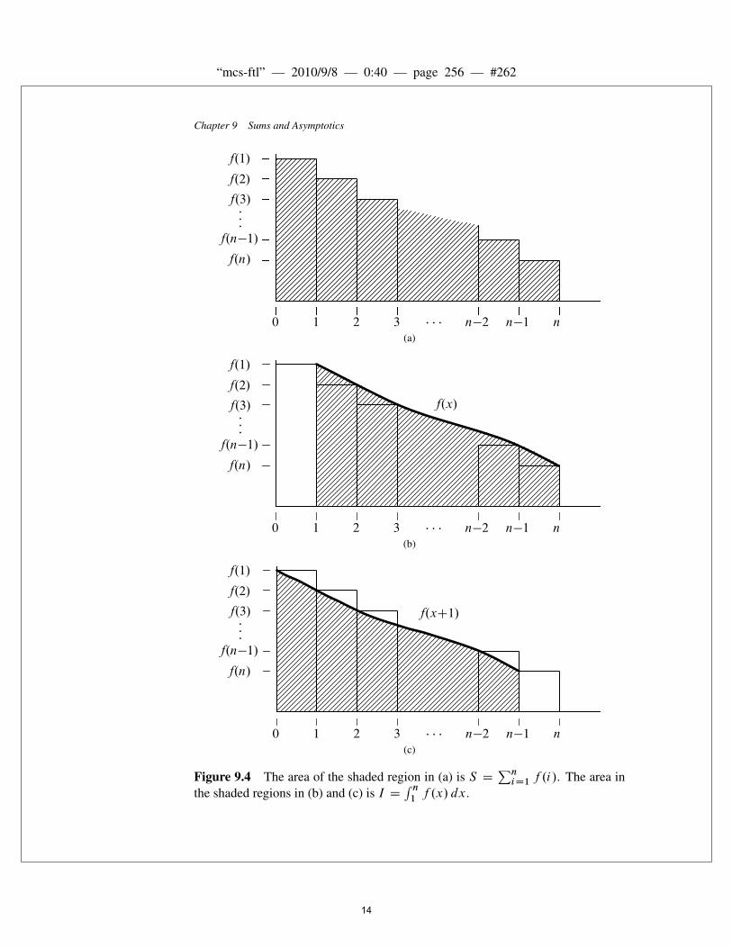
for any nondecreasing function f , as claimedThe argument for the case when f is nonincreasing is very similar. The analo-

gous graphs to those shown in Figures 9.1–9.3 are provided in Figure 9.4. As youcan see by comparing the shaded regions in Figures 9.4(a) and 9.4(b),

S � I C f .1/:

Similarly, comparing the shaded regions in Figures 9.4(a) and 9.4(c) reveals that

S � I C f .n/:

Hence, if f is nonincreasing,

I C f .n/ � S � I C f .1/:

as claimed. �

Theorem 9.3.1 provides good bounds for most sums. At worst, the bounds willbe off by the largest term in the sum. For example, we can use Theorem 9.3.1 tobound the sum

S D

nXiD1

pi

13

“mcs-ftl” — 2010/9/8 — 0:40 — page 256 — #262


0 1 2 3 n�2 n�1 n

f.n/

f.n�1/

f.3/

f.2/

f.1/

(a)

0 1 2 3 n�2 n�1 n

f.n/

f.n�1/

f.3/

f.2/

f.1/

f.x/

(b)

0 1 2 3 n�2 n�1 n

f.n/

f.n�1/

f.xC1/f.3/

f.2/

f.1/

(c)

Figure 9.4 The area of the shaded region in (a) is S DPniD1 f .i/. The area in

the shaded regions in (b) and (c) is I DR n1 f .x/ dx.

14

“mcs-ftl” — 2010/9/8 — 0:40 — page 257 — #263

9.4. Hanging Out Over the Edge

as follows.We begin by computing

I D

Z n

1

px dx

Dx3=2

3=2

ˇˇn

1

D2

3.n3=2 � 1/:

We then apply Theorem 9.3.1 to conclude that

2

3.n3=2 � 1/C 1 � S �

2

3.n3=2 � 1/C

pn

and thus that2

3n3=2 C

1

3� S �

2

3n3=2 C

pn �

2

3:

In other words, the sum is very close to 23n3=2.

We’ll be using Theorem 9.3.1 extensively going forward. At the end of thischapter, we will also introduce some notation that expresses phrases like “the sumis very close to” in a more precise mathematical manner. But first, we’ll see howTheorem 9.3.1 can be used to resolve a classic paradox in structural engineering.

9.4 Hanging Out Over the Edge

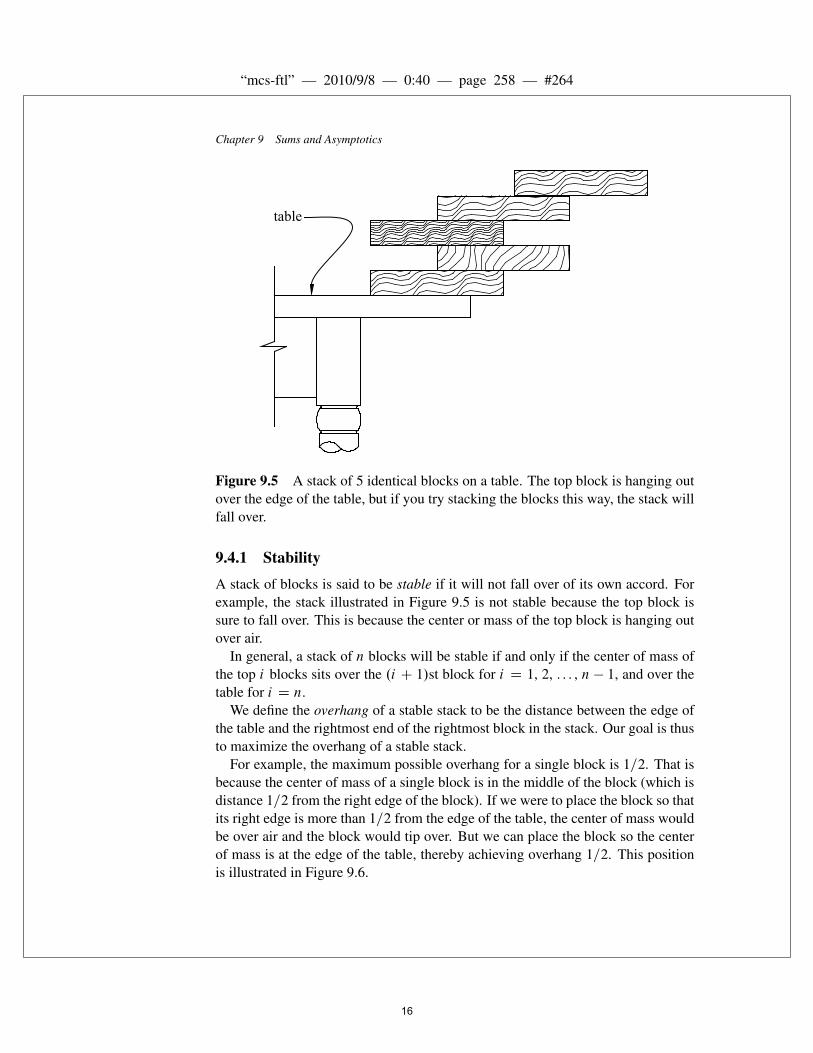
Suppose that you have n identical blocks8 and that you stack them one on top ofthe next on a table as shown in Figure 9.5. Is there some value of n for which it ispossible to arrange the stack so that one of the blocks hangs out completely overthe edge of the table without having the stack fall over? (You are not allowed to useglue or otherwise hold the stack in position.)

Most people’s first response to this question—sometimes also their second andthird responses—is “No. No block will ever get completely past the edge of thetable.” But in fact, if n is large enough, you can get the top block to stick out as faras you want: one block-length, two block-lengths, any number of block-lengths!

8We will assume that the blocks are rectangular, uniformly weighted and of length 1.

15

“mcs-ftl” — 2010/9/8 — 0:40 — page 258 — #264


table

Figure 9.5 A stack of 5 identical blocks on a table. The top block is hanging outover the edge of the table, but if you try stacking the blocks this way, the stack willfall over.

9.4.1 Stability

A stack of blocks is said to be stable if it will not fall over of its own accord. Forexample, the stack illustrated in Figure 9.5 is not stable because the top block issure to fall over. This is because the center or mass of the top block is hanging outover air.

In general, a stack of n blocks will be stable if and only if the center of mass ofthe top i blocks sits over the .i C 1/st block for i D 1, 2, . . . , n � 1, and over thetable for i D n.

We define the overhang of a stable stack to be the distance between the edge ofthe table and the rightmost end of the rightmost block in the stack. Our goal is thusto maximize the overhang of a stable stack.

For example, the maximum possible overhang for a single block is 1=2. That isbecause the center of mass of a single block is in the middle of the block (which isdistance 1=2 from the right edge of the block). If we were to place the block so thatits right edge is more than 1=2 from the edge of the table, the center of mass wouldbe over air and the block would tip over. But we can place the block so the centerof mass is at the edge of the table, thereby achieving overhang 1=2. This positionis illustrated in Figure 9.6.

16

“mcs-ftl” — 2010/9/8 — 0:40 — page 259 — #265


1=2

table

center of mass of block

Figure 9.6 One block can overhang half a block length.

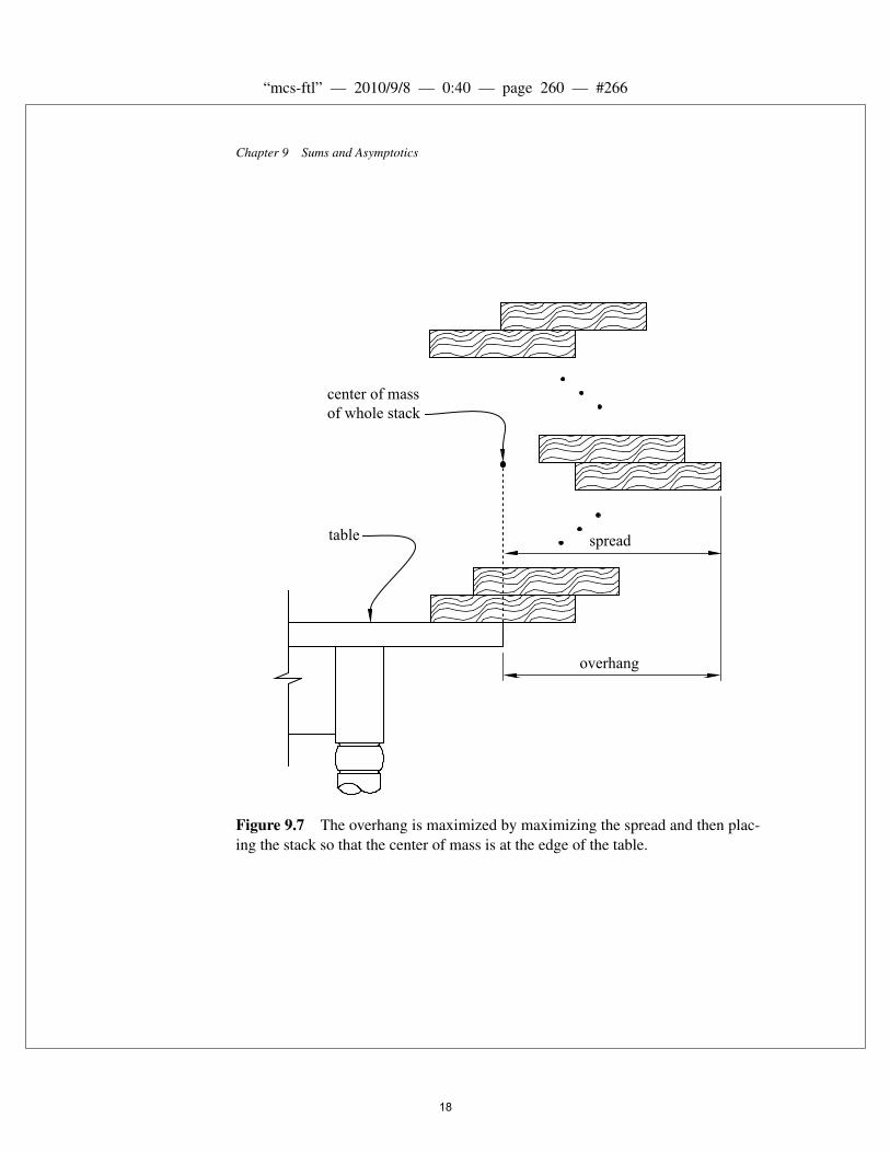
In general, the overhang of a stack of blocks is maximized by sliding the entirestack rightward until its center of mass is at the edge of the table. The overhangwill then be equal to the distance between the center of mass of the stack and therightmost edge of the rightmost block. We call this distance the spread of the stack.Note that the spread does not depend on the location of the stack on the table—itis purely a property of the blocks in the stack. Of course, as we just observed,the maximum possible overhang is equal to the maximum possible spread. Thisrelationship is illustrated in Figure 9.7.

9.4.2 A Recursive Solution

Our goal is to find a formula for the maximum possible spread Sn that is achievablewith a stable stack of n blocks.

We already know that S1 D 1=2 since the right edge of a single block withlength 1 is always distance 1=2 from its center of mass. Let’s see if we can use arecursive approach to determine Sn for all n. This means that we need to find aformula for Sn in terms of Si where i < n.

Suppose we have a stable stack S of n blocks with maximum possible spread Sn.There are two cases to consider depending on where the rightmost block is in thestack.

17

“mcs-ftl” — 2010/9/8 — 0:40 — page 260 — #266


overhang

table

center of mass of whole stack

spread

Figure 9.7 The overhang is maximized by maximizing the spread and then plac-ing the stack so that the center of mass is at the edge of the table.

18

“mcs-ftl” — 2010/9/8 — 0:40 — page 261 — #267


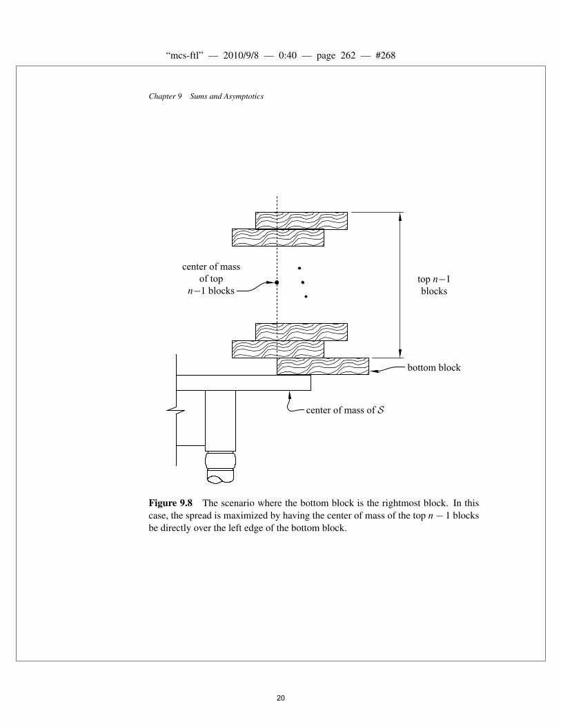
Case 1: The rightmost block in S is the bottom block. Since the center of massof the top n � 1 blocks must be over the bottom block for stability, the spread ismaximized by having the center of mass of the top n�1 blocks be directly over theleft edge of the bottom block. In this case the center of mass of S is9

.n � 1/ � 1C .1/ � 12

nD 1 �

1

2n

to the left of the right edge of the bottom block and so the spread for S is

1 �1

2n: (9.17)

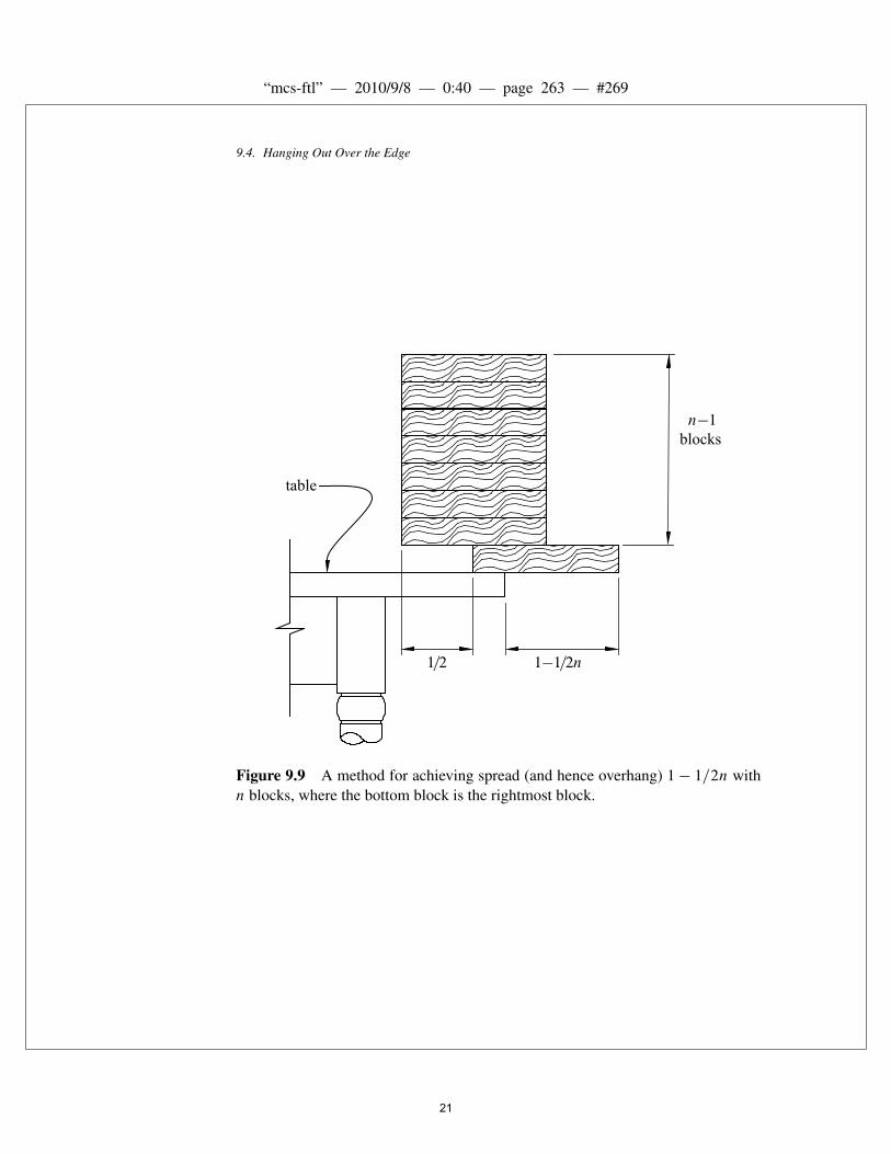
For example, see Figure 9.8.In fact, the scenario just described is easily achieved by arranging the blocks as

shown in Figure 9.9, in which case we have the spread given by Equation 9.17. Forexample, the spread is 3=4 for 2 blocks, 5=6 for 3 blocks, 7=8 for 4 blocks, etc.

Can we do any better? The best spread in Case 1 is always less than 1, whichmeans that we cannot get a block fully out over the edge of the table in this scenario.Maybe our intuition was right that we can’t do better. Before we jump to any falseconclusions, however, let’s see what happens in the other case.

Case 2: The rightmost block in S is among the top n � 1 blocks. In this case, thespread is maximized by placing the top n � 1 blocks so that their center of mass isdirectly over the right end of the bottom block. This means that the center of massfor S is at location

.n � 1/ � C C 1 ��C � 1

2

�n

D C �1

2n

where C is the location of the center of mass of the top n � 1 blocks. In otherwords, the center of mass of S is 1=2n to the left of the center of mass of the topn� 1 blocks. (The difference is due to the effect of the bottom block, whose centerof mass is 1=2 unit to the left of C .) This means that the spread of S is 1=2ngreater than the spread of the top n � 1 blocks (because we are in the case wherethe rightmost block is among the top n � 1 blocks.)

Since the rightmost block is among the top n � 1 blocks, the spread for S ismaximized by maximizing the spread for the top n�1 blocks. Hence the maximumspread for S in this case is

Sn�1 C1

2n(9.18)

9The center of mass of a stack of blocks is the average of the centers of mass of the individualblocks.

19

“mcs-ftl” — 2010/9/8 — 0:40 — page 262 — #268


top n�1

blocks

bottom block

center of mass of top

n�1 blocks

center of mass of S

Figure 9.8 The scenario where the bottom block is the rightmost block. In thiscase, the spread is maximized by having the center of mass of the top n� 1 blocksbe directly over the left edge of the bottom block.

20

“mcs-ftl” — 2010/9/8 — 0:40 — page 263 — #269


n�1

blocks

1�1=2n1=2

table

Figure 9.9 A method for achieving spread (and hence overhang) 1 � 1=2n withn blocks, where the bottom block is the rightmost block.

21

“mcs-ftl” — 2010/9/8 — 0:40 — page 264 — #270


where Sn�1 is the maximum possible spread for n� 1 blocks (using any strategy).We are now almost done. There are only two cases to consider when designing

a stack with maximum spread and we have analyzed both of them. This meansthat we can combine Equation 9.17 from Case 1 with Equation 9.18 from Case 2 toconclude that

Sn D max�1 �

1

2n; Sn�1 C

1

2n

�(9.19)

for any n > 1.Uh-oh. This looks complicated. Maybe we are not almost done after all!Equation 9.19 is an example of a recurrence. We will describe numerous tech-

niques for solving recurrences in Chapter 10, but, fortunately, Equation 9.19 issimple enough that we can solve it without waiting for all the hardware in Chap-ter 10.

One of the first things to do when you have a recurrence is to get a feel for itby computing the first few terms. This often gives clues about a way to solve therecurrence, as it will in this case.

We already know that S1 D 1=2. What about S2? From Equation 9.19, we findthat

S2 D max�1 �

1

4;1

2C1

4

�D 3=4:

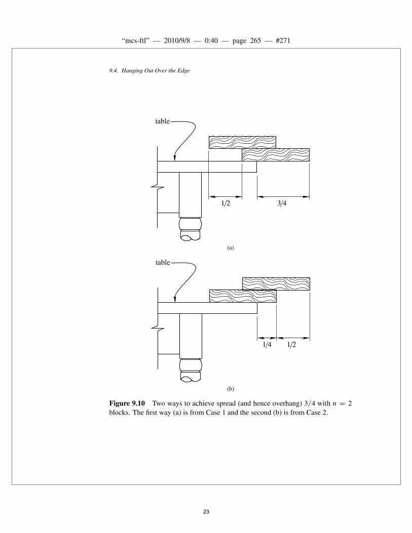
Both cases give the same spread, albeit by different approaches. For example, seeFigure 9.10.

That was easy enough. What about S3?

S3 D max�1 �

1

6;3

4C1

6

�D max

�5

6;11

12

�D11

12:

As we can see, the method provided by Case 2 is the best. Let’s check n D 4.

S4 D max�1 �

1

8;11

12C1

8

�D25

24: (9.20)

22

“mcs-ftl” — 2010/9/8 — 0:40 — page 265 — #271


1=2 3=4

table

(a)

1=21=4

table

(b)

Figure 9.10 Two ways to achieve spread (and hence overhang) 3=4 with n D 2

blocks. The first way (a) is from Case 1 and the second (b) is from Case 2.

23

“mcs-ftl” — 2010/9/8 — 0:40 — page 266 — #272


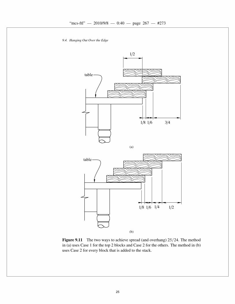
Wow! This is a breakthrough—for two reasons. First, Equation 9.20 tells us thatby using only 4 blocks, we can make a stack so that one of the blocks is hangingout completely over the edge of the table. The two ways to do this are shown inFigure 9.11.

The second reason that Equation 9.20 is important is that we now know thatS4 > 1, which means that we no longer have to worry about Case 1 for n > 4 sinceCase 1 never achieves spread greater than 1. Moreover, even for n � 4, we havenow seen that the spread achieved by Case 1 never exceeds the spread achieved byCase 2, and they can be equal only for n D 1 and n D 2. This means that

Sn D Sn�1 C1

2n(9.21)

for all n > 1 since we have shown that the best spread can always be achievedusing Case 2.

The recurrence in Equation 9.21 is much easier to solve than the one we startedwith in Equation 9.19. We can solve it by expanding the equation as follows:

Sn D Sn�1 C1

2n

D Sn�2 C1

2.n � 1/C

1

2n

D Sn�3 C1

2.n � 2/C

1

2.n � 1/C

1

2n

and so on. This suggests that

Sn D

nXiD1

1

2i; (9.22)

which is, indeed, the case.Equation 9.22 can be verified by induction. The base case when n D 1 is true

since we know that S1 D 1=2. The inductive step follows from Equation 9.21.So we now know the maximum possible spread and hence the maximum possible

overhang for any stable stack of books. Are we done? Not quite. Although weknow that S4 > 1, we still don’t know how big the sum

PniD1

12i

can get.It turns out that Sn is very close to a famous sum known as the nth Harmonic

number Hn.

9.4.3 Harmonic Numbers

Definition 9.4.1. The nth Harmonic number is

Hn WWD

nXiD1

1

i:

24

“mcs-ftl” — 2010/9/8 — 0:40 — page 267 — #273


3=41=8

1=2

1=6

table

(a)

1=4 1=21=8 1=6

table

(b)

Figure 9.11 The two ways to achieve spread (and overhang) 25=24. The methodin (a) uses Case 1 for the top 2 blocks and Case 2 for the others. The method in (b)uses Case 2 for every block that is added to the stack.

25

“mcs-ftl” — 2010/9/8 — 0:40 — page 268 — #274


So Equation 9.22 means that

Sn DHn

2: (9.23)

The first few Harmonic numbers are easy to compute. For example,

H4 D 1C1

2C1

3C1

4D25

12:

There is good news and bad news about Harmonic numbers. The bad news is thatthere is no closed-form expression known for the Harmonic numbers. The goodnews is that we can use Theorem 9.3.1 to get close upper and lower bounds onHn.In particular, since Z n

1

1

xdx D ln.x/

ˇn1D ln.n/;

Theorem 9.3.1 means that

ln.n/C1

n� Hn � ln.n/C 1: (9.24)

In other words, the nth Harmonic number is very close to ln.n/.Because the Harmonic numbers frequently arise in practice, mathematicians

have worked hard to get even better approximations for them. In fact, it is nowknown that

Hn D ln.n/C C1

2nC

1

12n2C

�.n/

120n4(9.25)

Here is a value 0:577215664 : : : called Euler’s constant, and �.n/ is between 0and 1 for all n. We will not prove this formula.

We are now finally done with our analysis of the block stacking problem. Plug-ging the value of Hn into Equation 9.23, we find that the maximum overhang forn blocks is very close to 1

2ln.n/. Since ln.n/ grows to infinity as n increases, this

means that if we are given enough blocks (in theory anyway), we can get a block tohang out arbitrarily far over the edge of the table. Of course, the number of blockswe need will grow as an exponential function of the overhang, so it will probablytake you a long time to achieve an overhang of 2 or 3, never mind an overhangof 100.

9.4.4 Asymptotic Equality

For cases like Equation 9.25 where we understand the growth of a function likeHnup to some (unimportant) error terms, we use a special notation, �, to denote theleading term of the function. For example, we say that Hn � ln.n/ to indicate thatthe leading term of Hn is ln.n/. More precisely:

26

“mcs-ftl” — 2010/9/8 — 0:40 — page 269 — #275

9.5. Double Trouble

Definition 9.4.2. For functions f; g W R! R, we say f is asymptotically equal tog, in symbols,

f .x/ � g.x/

ifflimx!1

f .x/=g.x/ D 1:

Although it is tempting to write Hn � ln.n/ C to indicate the two leadingterms, this is not really right. According to Definition 9.4.2,Hn � ln.n/C c wherec is any constant. The correct way to indicate that is the second-largest term isHn � ln.n/ � .

The reason that the � notation is useful is that often we do not care about lowerorder terms. For example, if n D 100, then we can computeH.n/ to great precisionusing only the two leading terms:

jHn � ln.n/ � j �ˇ1

200�

1

120000C

1

120 � 1004

ˇ<

1

200:

We will spend a lot more time talking about asymptotic notation at the end of thechapter. But for now, let’s get back to sums.

9.5 Double Trouble

Sometimes we have to evaluate sums of sums, otherwise known as double summa-

tions. This sounds hairy, and sometimes it is. But usually, it is straightforward—

you just evaluate the inner sum, replace it with a closed form, and then evaluate the

27

“mcs-ftl” — 2010/9/8 — 0:40 — page 270 — #276


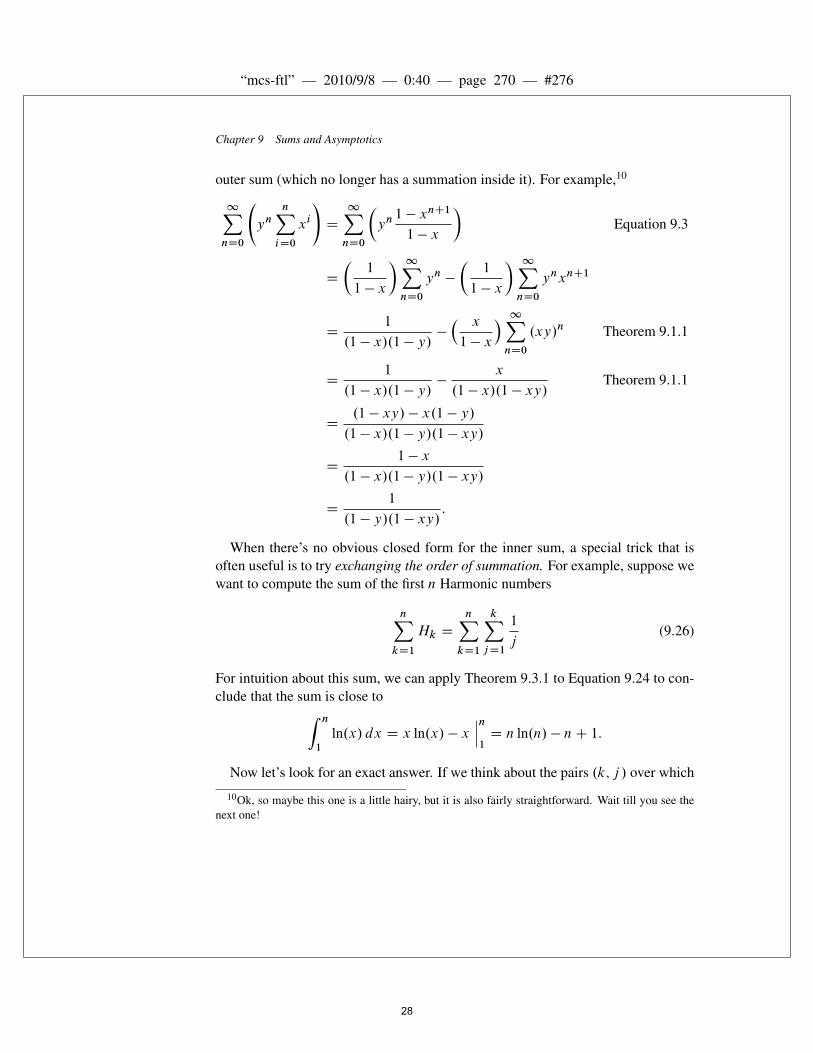
outer sum (which no longer has a summation inside it). For example,10

1XnD0

yn

nXiD0

xi

!D

1XnD0

�yn1 � xnC1

1 � x

�Equation 9.3

D

�1

1 � x

� 1XnD0

yn �

�1

1 � x

� 1XnD0

ynxnC1

D1

.1 � x/.1 � y/�

� x

1 � x

� 1XnD0

.xy/n Theorem 9.1.1

D1

.1 � x/.1 � y/�

x

.1 � x/.1 � xy/Theorem 9.1.1

D.1 � xy/ � x.1 � y/

.1 � x/.1 � y/.1 � xy/

D1 � x

.1 � x/.1 � y/.1 � xy/

D1

.1 � y/.1 � xy/:

When there’s no obvious closed form for the inner sum, a special trick that isoften useful is to try exchanging the order of summation. For example, suppose wewant to compute the sum of the first n Harmonic numbers

nXkD1

Hk D

nXkD1

kXjD1

1

j(9.26)

For intuition about this sum, we can apply Theorem 9.3.1 to Equation 9.24 to con-clude that the sum is close toZ n

1

ln.x/ dx D x ln.x/ � xˇn1D n ln.n/ � nC 1:

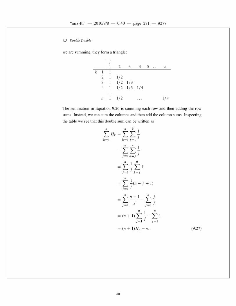
Now let’s look for an exact answer. If we think about the pairs .k; j / over which

10Ok, so maybe this one is a little hairy, but it is also fairly straightforward. Wait till you see thenext one!

28

“mcs-ftl” — 2010/9/8 — 0:40 — page 271 — #277

9.5. Double Trouble

we are summing, they form a triangle:

j

1 2 3 4 5 : : : n

k 1 1

2 1 1=2

3 1 1=2 1=3

4 1 1=2 1=3 1=4

: : :

n 1 1=2 : : : 1=n

The summation in Equation 9.26 is summing each row and then adding the row

sums. Instead, we can sum the columns and then add the column sums. Inspecting

the table we see that this double sum can be written as

nXkD1

Hk D

nXkD1

kXjD1

1

j

D

nXjD1

nXkDj

1

j

D

nXjD1

1

j

nXkDj

1

D

nXjD1

1

j.n � j C 1/

D

nXjD1

nC 1

j�

nXjD1

j

j

D .nC 1/

nXjD1

1

j�

nXjD1

1

D .nC 1/Hn � n: (9.27)

29

“mcs-ftl” — 2010/9/8 — 0:40 — page 272 — #278


9.6 Products

We’ve covered several techniques for finding closed forms for sums but no methodsfor dealing with products. Fortunately, we do not need to develop an entirely newset of tools when we encounter a product such as

nŠ WWD

nYiD1

i: (9.28)

That’s because we can convert any product into a sum by taking a logarithm. Forexample, if

P D

nYiD1

f .i/;

then

ln.P / DnXiD1

ln.f .i//:

We can then apply our summing tools to find a closed form (or approximate closedform) for ln.P / and then exponentiate at the end to undo the logarithm.

For example, let’s see how this works for the factorial function nŠ We start bytaking the logarithm:

ln.nŠ/ D ln.1 � 2 � 3 � � � .n � 1/ � n/

D ln.1/C ln.2/C ln.3/C � � � C ln.n � 1/C ln.n/

D

nXiD1

ln.i/:

Unfortunately, no closed form for this sum is known. However, we can applyTheorem 9.3.1 to find good closed-form bounds on the sum. To do this, we firstcompute Z n

1

ln.x/ dx D x ln.x/ � xˇn1

D n ln.n/ � nC 1:

Plugging into Theorem 9.3.1, this means that

n ln.n/ � nC 1 �nXiD1

ln.i/ � n ln.n/ � nC 1C ln.n/:

30

“mcs-ftl” — 2010/9/8 — 0:40 — page 273 — #279

9.6. Products

Exponentiating then gives

nn

en�1� nŠ �

nnC1

en�1: (9.29)

This means that nŠ is within a factor of n of nn=en�1.

9.6.1 Stirling’s Formula

nŠ is probably the most commonly used product in discrete mathematics, and somathematicians have put in the effort to find much better closed-form bounds on itsvalue. The most useful bounds are given in Theorem 9.6.1.

Theorem 9.6.1 (Stirling’s Formula). For all n � 1,

nŠ Dp2�n

�ne

�ne�.n/

where1

12nC 1� �.n/ �

1

12n:

Theorem 9.6.1 can be proved by induction on n, but the details are a bit painful(even for us) and so we will not go through them here.

There are several important things to notice about Stirling’s Formula. First, �.n/is always positive. This means that

nŠ >p2�n

�ne

�n(9.30)

for all n 2 NC.Second, �.n/ tends to zero as n gets large. This means that11

nŠ �p2�n

�ne

�n; (9.31)

which is rather surprising. After all, who would expect both � and e to show up ina closed-form expression that is asymptotically equal to nŠ?

Third, �.n/ is small even for small values of n. This means that Stirling’s For-mula provides good approximations for nŠ for most all values of n. For example, ifwe use

p2�n

�ne

�n11The � notation was defined in Section 9.4.4.

31

“mcs-ftl” — 2010/9/8 — 0:40 — page 274 — #280


Approximation n � 1 n � 10 n � 100 n � 1000p2�n

�ne

�n< 10% < 1% < 0.1% < 0.01%

p2�n

�ne

�ne1=12n < 1% < 0.01% < 0.0001% < 0.000001%

Table 9.1 Error bounds on common approximations for nŠ from Theorem 9.6.1.For example, if n � 100, then

p2�n

�ne

�n approximates nŠ to within 0.1%.

as the approximation for nŠ, as many people do, we are guaranteed to be within afactor of

e�.n/ � e112n

of the correct value. For n � 10, this means we will be within 1% of the correctvalue. For n � 100, the error will be less than 0.1%.

If we need an even closer approximation for nŠ, then we could use either

p2�n

�ne

�ne1=12n

orp2�n

�ne

�ne1=.12nC1/

depending on whether we want an upper bound or a lower bound, respectively. ByTheorem 9.6.1, we know that both bounds will be within a factor of

e112n� 112nC1 D e

1

144n2C12n

of the correct value. For n � 10, this means that either bound will be within 0.01%of the correct value. For n � 100, the error will be less than 0.0001%.

For quick future reference, these facts are summarized in Corollary 9.6.2 andTable 9.1.

Corollary 9.6.2. For n � 1,

nŠ < 1:09p2�n

�ne

�n:

For n � 10,nŠ < 1:009

p2�n

�ne

�n:

For n � 100,nŠ < 1:0009

p2�n

�ne

�n:

32

“mcs-ftl” — 2010/9/8 — 0:40 — page 275 — #281

9.7. Asymptotic Notation

9.7 Asymptotic Notation

Asymptotic notation is a shorthand used to give a quick measure of the behavior ofa function f .n/ as n grows large. For example, the asymptotic notation � of Defi-nition 9.4.2 is a binary relation indicating that two functions grow at the same rate.There is also a binary relation indicating that one function grows at a significantlyslower rate than another.

9.7.1 Little Oh

Definition 9.7.1. For functions f; g W R ! R, with g nonnegative, we say f isasymptotically smaller than g, in symbols,

f .x/ D o.g.x//;

ifflimx!1

f .x/=g.x/ D 0:

For example, 1000x1:9 D o.x2/, because 1000x1:9=x2 D 1000=x0:1 and sincex0:1 goes to infinity with x and 1000 is constant, we have limx!1 1000x1:9=x2 D0. This argument generalizes directly to yield

Lemma 9.7.2. xa D o.xb/ for all nonnegative constants a < b.

Using the familiar fact that log x < x for all x > 1, we can prove

Lemma 9.7.3. log x D o.x�/ for all � > 0.

Proof. Choose � > ı > 0 and let x D zı in the inequality log x < x. This implies

log z < zı=ı D o.z�/ by Lemma 9.7.2: (9.32)

�

Corollary 9.7.4. xb D o.ax/ for any a; b 2 R with a > 1.

Lemma 9.7.3 and Corollary 9.7.4 can also be proved using l’Hopital’s Rule orthe McLaurin Series for log x and ex . Proofs can be found in most calculus texts.

33

“mcs-ftl” — 2010/9/8 — 0:40 — page 276 — #282


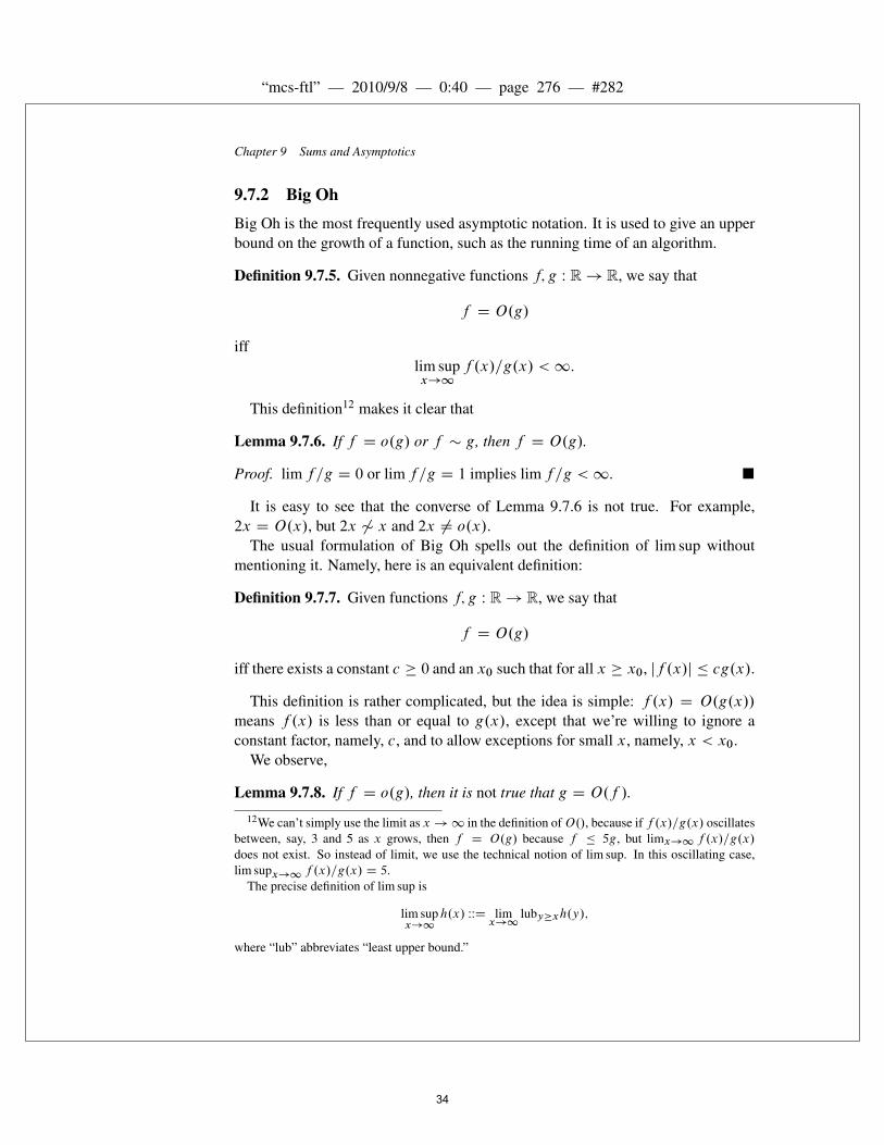
9.7.2 Big Oh

Big Oh is the most frequently used asymptotic notation. It is used to give an upperbound on the growth of a function, such as the running time of an algorithm.

Definition 9.7.5. Given nonnegative functions f; g W R! R, we say that

f D O.g/

ifflim supx!1

f .x/=g.x/ <1:

This definition12 makes it clear that

Lemma 9.7.6. If f D o.g/ or f � g, then f D O.g/.

Proof. limf=g D 0 or limf=g D 1 implies limf=g <1. �

It is easy to see that the converse of Lemma 9.7.6 is not true. For example,2x D O.x/, but 2x 6� x and 2x ¤ o.x/.

The usual formulation of Big Oh spells out the definition of lim sup withoutmentioning it. Namely, here is an equivalent definition:

Definition 9.7.7. Given functions f; g W R! R, we say that

f D O.g/

iff there exists a constant c � 0 and an x0 such that for all x � x0, jf .x/j � cg.x/.

This definition is rather complicated, but the idea is simple: f .x/ D O.g.x//

means f .x/ is less than or equal to g.x/, except that we’re willing to ignore aconstant factor, namely, c, and to allow exceptions for small x, namely, x < x0.

We observe,

Lemma 9.7.8. If f D o.g/, then it is not true that g D O.f /.

12We can’t simply use the limit as x !1 in the definition ofO./, because if f .x/=g.x/ oscillatesbetween, say, 3 and 5 as x grows, then f D O.g/ because f � 5g, but limx!1 f .x/=g.x/does not exist. So instead of limit, we use the technical notion of lim sup. In this oscillating case,lim supx!1 f .x/=g.x/ D 5.

The precise definition of lim sup is

lim supx!1

h.x/ WWD limx!1

luby�xh.y/;

where “lub” abbreviates “least upper bound.”

34

“mcs-ftl” — 2010/9/8 — 0:40 — page 277 — #283


Proof.

limx!1

g.x/

f .x/D

1

limx!1 f .x/=g.x/D1

0D1;

so g ¤ O.f /.�

Proposition 9.7.9. 100x2 D O.x2/.

Proof. Choose c D 100 and x0 D 1. Then the proposition holds, since for allx � 1,

ˇ100x2

ˇ� 100x2. �

Proposition 9.7.10. x2 C 100x C 10 D O.x2/.

Proof. .x2C100xC10/=x2 D 1C100=xC10=x2 and so its limit as x approachesinfinity is 1C0C0 D 1. So in fact, x2C100xC10 � x2, and therefore x2C100xC10 D O.x2/. Indeed, it’s conversely true that x2 D O.x2 C 100x C 10/. �

Proposition 9.7.10 generalizes to an arbitrary polynomial:

Proposition 9.7.11. akxk C ak�1xk�1 C � � � C a1x C a0 D O.xk/.

We’ll omit the routine proof.Big Oh notation is especially useful when describing the running time of an

algorithm. For example, the usual algorithm for multiplying n � n matrices usesa number of operations proportional to n3 in the worst case. This fact can beexpressed concisely by saying that the running time is O.n3/. So this asymptoticnotation allows the speed of the algorithm to be discussed without reference toconstant factors or lower-order terms that might be machine specific. It turns outthat there is another, ingenious matrix multiplication procedure that uses O.n2:55/operations. This procedure will therefore be much more efficient on large enoughmatrices. Unfortunately, theO.n2:55/-operation multiplication procedure is almostnever used in practice because it happens to be less efficient than the usual O.n3/procedure on matrices of practical size.13

9.7.3 Omega

Suppose you want to make a statement of the form “the running time of the algo-rithm is a least. . . ”. Can you say it is “at least O.n2/”? No! This statement ismeaningless since big-oh can only be used for upper bounds. For lower bounds,we use a different symbol, called “big-Omega.”

13It is even conceivable that there is anO.n2/matrix multiplication procedure, but none is known.

35

“mcs-ftl” — 2010/9/8 — 0:40 — page 278 — #284


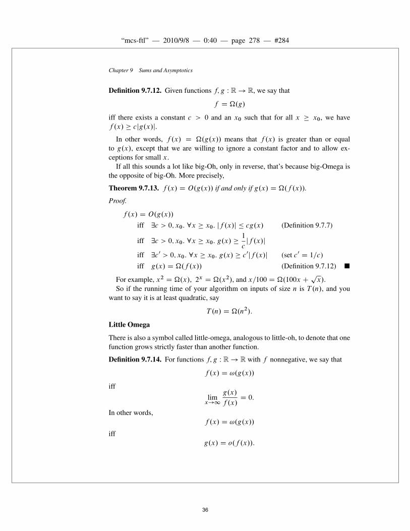
Definition 9.7.12. Given functions f; g W R! R, we say that

f D �.g/

iff there exists a constant c > 0 and an x0 such that for all x � x0, we havef .x/ � cjg.x/j.

In other words, f .x/ D �.g.x// means that f .x/ is greater than or equalto g.x/, except that we are willing to ignore a constant factor and to allow ex-ceptions for small x.

If all this sounds a lot like big-Oh, only in reverse, that’s because big-Omega isthe opposite of big-Oh. More precisely,

Theorem 9.7.13. f .x/ D O.g.x// if and only if g.x/ D �.f .x//.

Proof.

f .x/ D O.g.x//

iff 9c > 0; x0: 8x � x0: jf .x/j � cg.x/ (Definition 9.7.7)

iff 9c > 0; x0: 8x � x0: g.x/ �1

cjf .x/j

iff 9c0 > 0; x0: 8x � x0: g.x/ � c0jf .x/j (set c0 D 1=c)

iff g.x/ D �.f .x// (Definition 9.7.12) �

For example, x2 D �.x/, 2x D �.x2/, and x=100 D �.100x Cpx/.

So if the running time of your algorithm on inputs of size n is T .n/, and youwant to say it is at least quadratic, say

T .n/ D �.n2/:

Little Omega

There is also a symbol called little-omega, analogous to little-oh, to denote that onefunction grows strictly faster than another function.

Definition 9.7.14. For functions f; g W R! R with f nonnegative, we say that

f .x/ D !.g.x//

iff

limx!1

g.x/

f .x/D 0:

In other words,f .x/ D !.g.x//

iffg.x/ D o.f .x//:

36

“mcs-ftl” — 2010/9/8 — 0:40 — page 279 — #285


For example, x1:5 D !.x/ andpx D !.ln2.x//.

The little-omega symbol is not as widely used as the other asymptotic symbolswe have been discussing.

9.7.4 Theta

Sometimes we want to specify that a running time T .n/ is precisely quadratic up toconstant factors (both upper bound and lower bound). We could do this by sayingthat T .n/ D O.n2/ and T .n/ D �.n2/, but rather than say both, mathematicianshave devised yet another symbol, ‚, to do the job.

Definition 9.7.15.

f D ‚.g/ iff f D O.g/ and g D O.f /:

The statement f D ‚.g/ can be paraphrased intuitively as “f and g are equalto within a constant factor.” Indeed, by Theorem 9.7.13, we know that

f D ‚.g/ iff f D O.g/ and f D �.g/:

The Theta notation allows us to highlight growth rates and allow suppressionof distracting factors and low-order terms. For example, if the running time of analgorithm is

T .n/ D 10n3 � 20n2 C 1;

then we can more simply write

T .n/ D ‚.n3/:

In this case, we would say that T is of order n3 or that T .n/ grows cubically, whichis probably what we really want to know. Another such example is

�23x�7 C.2:7x113 C x9 � 86/4

px

� 1:083x D ‚.3x/:

Just knowing that the running time of an algorithm is‚.n3/, for example, is use-ful, because if n doubles we can predict that the running time will by and large14

increase by a factor of at most 8 for large n. In this way, Theta notation preserves in-formation about the scalability of an algorithm or system. Scalability is, of course,a big issue in the design of algorithms and systems.

14Since ‚.n3/ only implies that the running time, T .n/, is between cn3 and dn3 for constants0 < c < d , the time T .2n/ could regularly exceed T .n/ by a factor as large as 8d=c. The factor issure to be close to 8 for all large n only if T .n/ � n3.

37

“mcs-ftl” — 2010/9/8 — 0:40 — page 280 — #286


9.7.5 Pitfalls with Asymptotic Notation

There is a long list of ways to make mistakes with asymptotic notation. This sectionpresents some of the ways that Big Oh notation can lead to ruin and despair. Withminimal effort, you can cause just as much chaos with the other symbols.

The Exponential Fiasco

Sometimes relationships involving Big Oh are not so obvious. For example, onemight guess that 4x D O.2x/ since 4 is only a constant factor larger than 2. Thisreasoning is incorrect, however; 4x actually grows as the square of 2x .

Constant Confusion

Every constant is O.1/. For example, 17 D O.1/. This is true because if we letf .x/ D 17 and g.x/ D 1, then there exists a c > 0 and an x0 such that jf .x/j �cg.x/. In particular, we could choose c = 17 and x0 D 1, since j17j � 17 � 1 for allx � 1. We can construct a false theorem that exploits this fact.

False Theorem 9.7.16.nXiD1

i D O.n/

Bogus proof. Define f .n/ DPniD1 i D 1C2C3C� � �Cn. Since we have shown

that every constant i is O.1/, f .n/ D O.1/CO.1/C � � � CO.1/ D O.n/. �

Of course in realityPniD1 i D n.nC 1/=2 ¤ O.n/.

The error stems from confusion over what is meant in the statement i D O.1/.For any constant i 2 N it is true that i D O.1/. More precisely, if f is any constantfunction, then f D O.1/. But in this False Theorem, i is not constant—it rangesover a set of values 0, 1,. . . , n that depends on n.

And anyway, we should not be adding O.1/’s as though they were numbers. Wenever even defined whatO.g/means by itself; it should only be used in the context“f D O.g/” to describe a relation between functions f and g.

Lower Bound Blunder

Sometimes people incorrectly use Big Oh in the context of a lower bound. Forexample, they might say, “The running time, T .n/, is at least O.n2/,” when theyprobably mean15 “T .n/ D �.n2/.”

15This can also be correctly expressed as n2 D O.T .n//, but such notation is rare.

38

“mcs-ftl” — 2010/9/8 — 0:40 — page 281 — #287


Equality Blunder

The notation f D O.g/ is too firmly entrenched to avoid, but the use of “=”is really regrettable. For example, if f D O.g/, it seems quite reasonable towrite O.g/ D f . But doing so might tempt us to the following blunder: because2n D O.n/, we can say O.n/ D 2n. But n D O.n/, so we conclude that n DO.n/ D 2n, and therefore n D 2n. To avoid such nonsense, we will never write“O.f / D g.”

Similarly, you will often see statements like

Hn D ln.n/C CO�1

n

�or

nŠ D .1C o.1//p2�n

�ne

�n:

In such cases, the true meaning is

Hn D ln.n/C C f .n/

for some f .n/ where f .n/ D O.1=n/, and

nŠ D .1C g.n//p2�n

�ne

�nwhere g.n/ D o.1/. These transgressions are OK as long as you (and you reader)know what you mean.

39

“mcs-ftl” — 2010/9/8 — 0:40 — page 282 — #288

40

MIT OpenCourseWarehttp://ocw.mit.edu

6.042J / 18.062J Mathematics for Computer Science Fall 2010

For information about citing these materials or our Terms of Use, visit: http://ocw.mit.edu/terms.

http://ocw.mit.edu

http://ocw.mit.edu/terms

Documents

6.042J Chapter 9: Sums and asymptotics