Embed Size (px)
Citation preview

8/10/2019 Detailed Notes on Asymptotics
http://slidepdf.com/reader/full/detailed-notes-on-asymptotics 1/77
Asymptotics
Helle Bunzel
Iowa State University
September 26, 2008
Bunzel (ISU) Asymptotics September 26, 2008 1 / 77
8/10/2019 Detailed Notes on Asymptotics
http://slidepdf.com/reader/full/detailed-notes-on-asymptotics 2/77
Asymptotics: What and Why? I
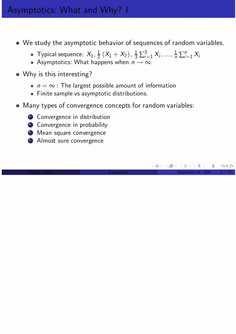
We study the asymptotic behavior of sequences of random variables.
Typical sequence: X 1, 12 (X 1 + X 2) ,
13 ∑
3i =1 X i , ....,
1n ∑
ni =1 X i
Asymptotics: What happens when n ! ∞.
Why is this interesting?
n = ∞ : The largest possible amount of informationFinite sample vs asymptotic distributions.
Many types of convergence concepts for random variables:
1 Convergence in distribution2 Convergence in probability3 Mean square convergence4 Almost sure convergence
Bunzel (ISU) Asymptotics September 26, 2008 2 / 77

8/10/2019 Detailed Notes on Asymptotics
http://slidepdf.com/reader/full/detailed-notes-on-asymptotics 3/77
Convergence in distribution I
De…nition
Let fY ng be a sequence of random variables and let fF ng be the sequenceof associated CDFs. If there exists a CDF F , such that F n (y ) ! F (y ) forall y where F is continuous, then F is called the limiting CDF of fY ng andletting Y have CDF F , we say that Y n converges in distribution to the r.v.
Y .
Also called "convergence in law"
Denoted Y nd ! Y or Y n
L! Y or Y n ) Y or Y nd ! F etc.
If Y is degenerate, we say that Y n converges in distribution to aconstant.
Often we can …nd F , but not F n .
How does this help us?
Bunzel (ISU) Asymptotics September 26, 2008 3 / 77

8/10/2019 Detailed Notes on Asymptotics
http://slidepdf.com/reader/full/detailed-notes-on-asymptotics 4/77
Convergence in distribution II
Sometimes the density is su¢cient to establish convergence indistribution:
Theorem
Let fY ng be a sequence of either co ntinuou s or non-negative, integer valued, discrete random variables, and let ff ng be the corresponding sequence of pdfs. If there exists a density function f such that f n (y ) ! f (y ) , except perhaps on a set of points A such that
P Y (A) = 0, where Y f . Then Y nd ! Y .
Bunzel (ISU) Asymptotics September 26, 2008 4 / 77

8/10/2019 Detailed Notes on Asymptotics
http://slidepdf.com/reader/full/detailed-notes-on-asymptotics 5/77
Convergence in distribution III
A consequence of convergence in distribution is that the mean andthe variance of X n converge to the mean and the variance of X .
Simplistic example: If we sample form a normal distribution, thenX n N µ,
σ 2
n
.
The limiting distribution of X is the degenerate distribution with meanµ and variance 0.
Bunzel (ISU) Asymptotics September 26, 2008 5 / 77

8/10/2019 Detailed Notes on Asymptotics
http://slidepdf.com/reader/full/detailed-notes-on-asymptotics 6/77
Convergence in distribution IExample
Let
fX n
g be a sequence of r.v.s. X n
N (0, 1)
8n.
Let fZ ng be a sequence of r.v.s where Z n =
3 + 1n
X n + 2n
n1 .
Then Z n N
2nn1 ,
3 + 1
n
2
and Z nd ! N (2, 9)
Bunzel (ISU) Asymptotics September 26, 2008 6 / 77

8/10/2019 Detailed Notes on Asymptotics
http://slidepdf.com/reader/full/detailed-notes-on-asymptotics 7/77
Convergence in probability I
De…nition
The sequence of random variables fX ng converges in probability to therandom variable X i¤
a. Scalar case: limn!∞ P (jx n x j<
ε) = 1 8ε>
0b. Matrix case: limn!∞ P (jx n [i , j ] x [i , j ]j < ε) = 1 8ε > 0, 8 i and j
The notation we use is X nP ! X or plim(X n ) = X .
For large enough n, outcomes of X can serve as approximations of outcomes of X n .
Bunzel (ISU) Asymptotics September 26, 2008 7 / 77
8/10/2019 Detailed Notes on Asymptotics
http://slidepdf.com/reader/full/detailed-notes-on-asymptotics 8/77
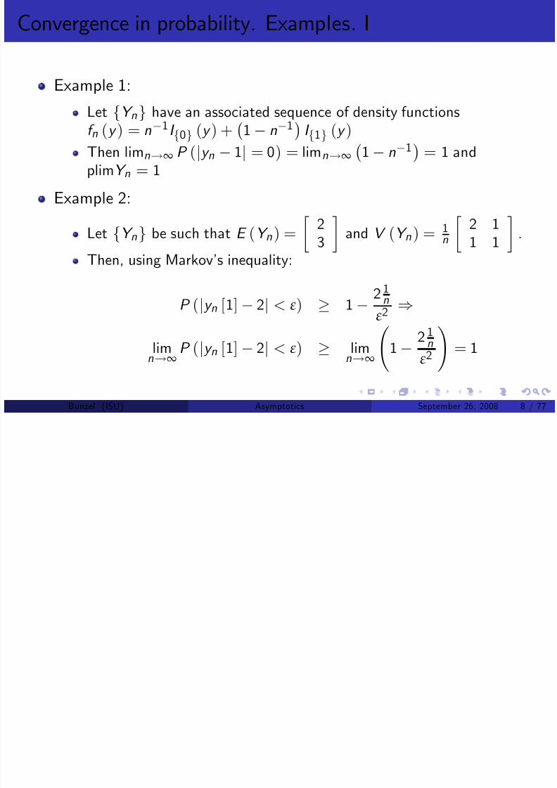
Convergence in probability. Examples. I
Example 1:
Let fY ng have an associated sequence of density functionsf n (y ) = n1I f0g (y ) +
1 n1
I f1g (y )
Then limn!∞ P (jy n 1j = 0) = limn!∞
1 n1
= 1 and
plimY n = 1
Example 2:
Let fY ng be such that E (Y n ) =
23
and V (Y n ) = 1
n
2 11 1
.
Then, using Markov’s inequality:
P (jy n [1] 2j < ε) 1 2 1n
ε2 )
limn!∞
P (jy n [1] 2j < ε) limn!∞
1 2 1
n
ε2
! = 1
Bunzel (ISU) Asymptotics September 26, 2008 8 / 77

8/10/2019 Detailed Notes on Asymptotics
http://slidepdf.com/reader/full/detailed-notes-on-asymptotics 9/77
Convergence in probability. Examples. II
and
P (jy n [2] 3j < ε) 1 1n
ε2 )
limn!∞
P (jy n [2] 3j < ε) limn!∞
1 1n
ε2
! = 1
So, Y nP !
23 .
Bunzel (ISU) Asymptotics September 26, 2008 9 / 77

8/10/2019 Detailed Notes on Asymptotics
http://slidepdf.com/reader/full/detailed-notes-on-asymptotics 10/77
Convergence in probability I
Theorem
If limn!∞E (X n ) = µ and limn!∞V (X n ) = 0 then plimX n = µ
Prove using Chebychev’s inequality.
Events or distributions. What is the di¤erence?
Many di¤erent experiments can have the same distributions.Convergence in probability talks speci…cally about the probability of speci…c events.
Bunzel (ISU) Asymptotics September 26, 2008 10 / 77

8/10/2019 Detailed Notes on Asymptotics
http://slidepdf.com/reader/full/detailed-notes-on-asymptotics 11/77
Convergence in probability II
TheoremLet X n
P ! X , and let g be a functio n which is continuous, except perhaps on a set of points with probability 0. Thenplim g (X n ) = g (plim (X n )) .
EXTREMELY useful theorem.
Consider example from before where plimY n [1] = 2.
Using the theorem we know that plim 1Y n [1]
= 12 .
But we couldn’t do the calculations from scratch since we don’t knowE
1Y n [1]
.
Bunzel (ISU) Asymptotics September 26, 2008 11 / 77

8/10/2019 Detailed Notes on Asymptotics
http://slidepdf.com/reader/full/detailed-notes-on-asymptotics 12/77
Convergence in probability, Examples I
Let fX ng be a strictly positive valued r.v. such that X nP ! 3. Then
Y n = g (X n ) = ln (X n ) +p
X nP
!ln (3) +
p 3 = 2.8307
Let fX ng : k 1 be such that X nP ! X N (0, I k ) and let
Y n = g (X n ) = X 0nX n . Then Y nP ! X 0X χ2 (k )
Bunzel (ISU) Asymptotics September 26, 2008 12 / 77

8/10/2019 Detailed Notes on Asymptotics
http://slidepdf.com/reader/full/detailed-notes-on-asymptotics 13/77
Convergence in probability IProperties
For conformable r.v.s X n , Y n and constant matrix A :
1 plim AX n = A plimX n
2 plim ∑ mi =1 X n [i ] = ∑ mi =1 plimX n [i ]3 plim ∏
mi =1 X n [i ] = ∏
mi =1 plimX n [i ]
4 plim X nY n = plimX n plimY n
5 plim X 1n Y n = (plimX n )1
plimY n
Bunzel (ISU) Asymptotics September 26, 2008 13 / 77

8/10/2019 Detailed Notes on Asymptotics
http://slidepdf.com/reader/full/detailed-notes-on-asymptotics 14/77
Convergence in probability, Examples I
Let A = 2 11 1 and let fX ng be such that plim X n =
25 . Then
plim AX n = A plim X n =
2 11 1
25
=
97
and
plim (X n [1] + X n [2]) = plim X n [1] + plim X n [2] = 2 + 5 = 7
and
plim (X n [1] X n [2]) = (plim X n [1]) (plim X n [2]) = 2 5 = 10
Bunzel (ISU) Asymptotics September 26, 2008 14 / 77

8/10/2019 Detailed Notes on Asymptotics
http://slidepdf.com/reader/full/detailed-notes-on-asymptotics 15/77
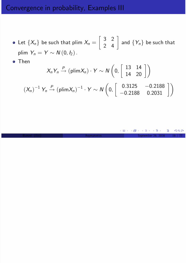
Convergence in probability, Examples II
Let fY ng be such that plim Y n =
1 22 1
and fX ng be such that
plim X n =
3 12 1
.
Then
plimX nY n = plimX n
plimY n = 3 1
2 1 1 2
2 1 = 5 7
4 5
plim (X n )1 Y n = (plimX n )1 plimY n = 3 12 1
1
1 22 1
=
1 12 3
1 22 1
=
1 14 1
Bunzel (ISU) Asymptotics September 26, 2008 15 / 77
8/10/2019 Detailed Notes on Asymptotics
http://slidepdf.com/reader/full/detailed-notes-on-asymptotics 16/77
C i b I
8/10/2019 Detailed Notes on Asymptotics
http://slidepdf.com/reader/full/detailed-notes-on-asymptotics 17/77
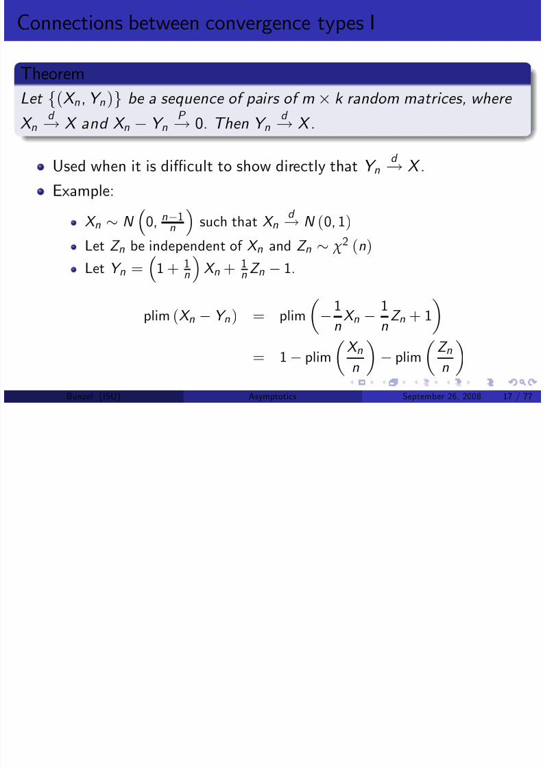
Connections between convergence types I
Theorem
Let f(X n , Y n )g be a sequence of pairs of m k random matrices, where X n
d ! X and X n Y nP ! 0. Then Y n
d ! X .
Used when it is di¢cult to show directly that Y nd ! X .
Example:
X n N
0, n1
n
such that X n
d ! N (0, 1)
Let Z n be independent of X n and Z n χ2 (n)
Let Y n = 1 + 1nX n + 1
n Z n
1.
plim (X n Y n ) = plim
1
nX n 1
nZ n + 1
= 1 plimX nn plim
Z nn
Bunzel (ISU) Asymptotics September 26, 2008 17 / 77
C i b II

8/10/2019 Detailed Notes on Asymptotics
http://slidepdf.com/reader/full/detailed-notes-on-asymptotics 18/77
Connections between convergence types II
Now, E
X nn
= 0, V
X nn
= n1
n3 ! 0 so plim
X nn
= 0
E Z nn = 1, V Z n
n = 2n
!0 so plimZ n
n = 1
This implies that plim(X n Y n ) = 0 and theref ore Y nd ! N (0, 1)
Theorem
Y nP
! Y ) Y nd
! Y
Previous theorem with X n = Y 8n.
Bunzel (ISU) Asymptotics September 26, 2008 18 / 77
C i b III

8/10/2019 Detailed Notes on Asymptotics
http://slidepdf.com/reader/full/detailed-notes-on-asymptotics 19/77
Connections between convergence types III
Theorem
Y nd
! c ) Y nP
! c
Not true unless the limit is a constant.
Proof:
Y nd
! c ) F n (y ) ) F (y ) = 1fy c g (y )P (jy n c j < ε) = F n (c + ε) F n (c ε) ! 1
Theorem
Let fX ng : k m, fY ng : l q , and fang : j p be such that X nd
! X ,Y n
P ! Y and an ! a. Let B be such that P X (B ) = 1 and let the randomvariable g (X n , Y n , an ) be de…ned by a function g that is continuous at
every point in B y a. Then g (X n , Y n , an ) d ! g (X , Y , a)
Bunzel (ISU) Asymptotics September 26, 2008 19 / 77
C ti b t t E l I
8/10/2019 Detailed Notes on Asymptotics
http://slidepdf.com/reader/full/detailed-notes-on-asymptotics 20/77
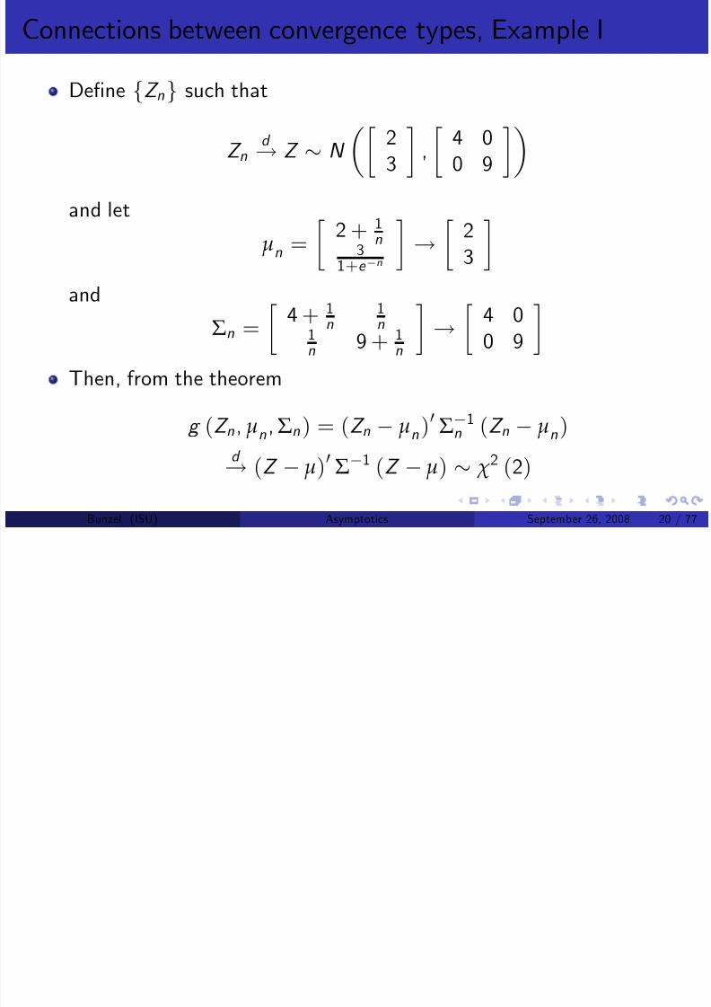
Connections between convergence types, Example I
De…ne fZ ng such that
Z nd ! Z N
23
,
4 00 9
and let
µn = 2 + 1
n
31+e n ! 2
3
and
Σn =
4 + 1
n1n
1n 9 + 1
n
!
4 00 9
Then, from the theorem
g (Z n , µn ,Σn ) = (Z n µn )0Σ1
n (Z n µn)
d ! (Z µ)0Σ1 (Z µ) χ2 (2)
Bunzel (ISU) Asymptotics September 26, 2008 20 / 77
C ti b t t I

8/10/2019 Detailed Notes on Asymptotics
http://slidepdf.com/reader/full/detailed-notes-on-asymptotics 21/77
Connections between convergence types I
Theorem
Slutsky’s Theorems: Let X nd ! X and Y n
P ! c . Then, for conformable X nand Y n
a. X n + Y n d ! X + c b. Y n X n
d ! cX
c. Y 1n X n
d ! c 1X
All special cases of previous theorem.
Bunzel (ISU) Asymptotics September 26, 2008 21 / 77
Order of magnitude in probability I

8/10/2019 Detailed Notes on Asymptotics
http://slidepdf.com/reader/full/detailed-notes-on-asymptotics 22/77
Order of magnitude in probability I
De…nition
Let fX ng be a sequence of random scalars. Thena. The sequence fX ng is said to be at most of order nk in probability,denoted by O P nk i¤ for every ε > 0 there exists a corresponding positive
constant c (ε) < ∞ such that P
nk
jX n j c (ε) 1 ε for all n.
b. The sequence fX ng is said to be of order smaller than nk in probability,
denoted by o P
nk
i¤ nk X nP ! 0.
Main use: Find out which terms are irrelevant as n increases.O P (1) : Bounded in probability.
Bunzel (ISU) Asymptotics September 26, 2008 22 / 77
Example I

8/10/2019 Detailed Notes on Asymptotics
http://slidepdf.com/reader/full/detailed-notes-on-asymptotics 23/77
Example I
Let fX ng be such that X i N (0, 1) 8i and all the X i areindependent.
Let fZ ng be de…ned as Z n = ∑ ni =1 X i .
What are the orders of X n and Z n?
Note that we can always …nd a c (ε) large enough that
P (jX n j c (ε)) = 2
Z c (ε)
0N (x ; 0, 1) dx 1 ε
So, X n = O P (1)Consider Z n :
Z n =n
∑ i =1
X i N (0, n)
Bunzel (ISU) Asymptotics September 26, 2008 23 / 77

8/10/2019 Detailed Notes on Asymptotics
http://slidepdf.com/reader/full/detailed-notes-on-asymptotics 24/77
Mean Square Convergence I
8/10/2019 Detailed Notes on Asymptotics
http://slidepdf.com/reader/full/detailed-notes-on-asymptotics 25/77
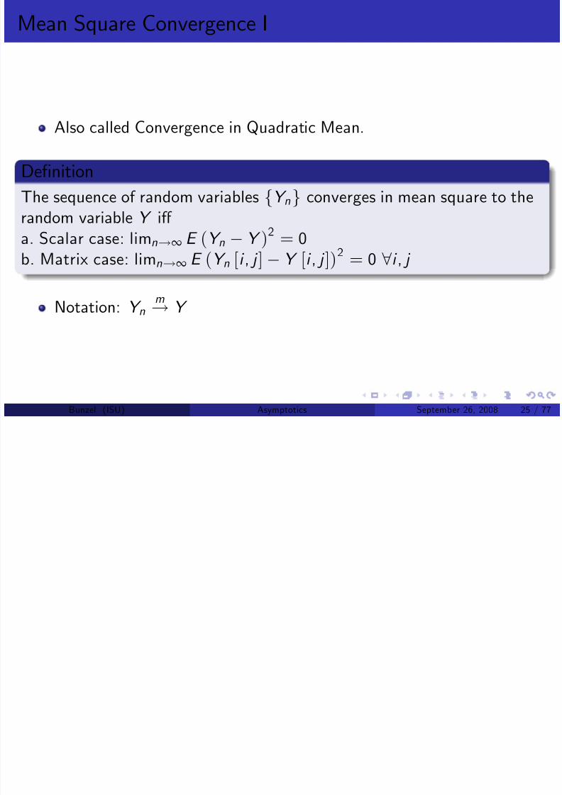
Mean Square Convergence I
Also called Convergence in Quadratic Mean.
De…nition
The sequence of random variables fY ng converges in mean square to therandom variable Y i¤ a. Scalar case: limn!∞ E (Y n Y )2 = 0b. Matrix case: limn!∞ E (Y n [i , j ] Y [i , j ])2 = 0 8i , j
Notation: Y n m! Y
Bunzel (ISU) Asymptotics September 26, 2008 25 / 77
Mean Square Convergence II

8/10/2019 Detailed Notes on Asymptotics
http://slidepdf.com/reader/full/detailed-notes-on-asymptotics 26/77
Mean Square Convergence II
Theorem
Y nm! Y i¤
a. E (Y n [i , j ]) ! E (Y [i , j ])b. V (Y n [i , j ]) ! V (Y [i , j ])b. Cov (Y n [i , j ] , Y [i , j ])
!V (Y [i , j ])
Proof, scalar case only.
Y nm! Y ) a. b. and c.
a.
jEY n EY j = jE (Y n Y )j E jY n Y j h
E jY n Y j2i 1
2 ! 0
Bunzel (ISU) Asymptotics September 26, 2008 26 / 77
Mean Square Convergence III

8/10/2019 Detailed Notes on Asymptotics
http://slidepdf.com/reader/full/detailed-notes-on-asymptotics 27/77
Mean Square Convergence III
b.V (Y n ) = E (Y n EY n )2 = E
Y 2n
(EY n )2
E
Y 2n
= E (Y n Y )2 + E
Y 2
+ 2E (Y (Y n Y ))
By Cauchy-Schwartz
jE (Y (Y n
Y ))
j hE Y 2E ((Y n
Y ))2i12
,
h
E
Y 2
E
((Y n Y ))2i 1
2 E (Y (Y n Y ))
hE Y 2 E ((Y n Y ))2
i12
and therefore
E (Y n Y )2 + E
Y 2
2h
E
Y 2
E
((Y n Y ))2i 1
2 E
Y 2n
E (Y n
Y )2 + E Y 2 + 2 hE Y 2 E ((Y n
Y ))2i
12
Bunzel (ISU) Asymptotics September 26, 2008 27 / 77
Mean Square Convergence IV

8/10/2019 Detailed Notes on Asymptotics
http://slidepdf.com/reader/full/detailed-notes-on-asymptotics 28/77
Mean Square Convergence IV
Taking limits:
E Y 2 lim
n!∞
E Y 2n E Y 2 ,
limn!∞
E
Y 2n
= E
Y 2
limn!∞
V (Y n ) = limn!∞
E
Y 2n
lim
n!∞(EY n )2 = E
Y 2
(EY )2 = V (Y )
c. We know that
E (Y n Y )2 = E
Y 2n
+ E
Y 2
2E (Y nY ) ! 0
By de…nition
Cov (Y n,
Y ) = E [(Y n EY n ) (Y EY )] = E (Y n Y ) EY n EY ,E (Y n Y ) = Cov (Y n , Y ) + EY n EY
2E (Y n Y ) = 2Cov (Y n , Y ) 2EY n EY
Bunzel (ISU) Asymptotics September 26, 2008 28 / 77
Mean Square Convergence V

8/10/2019 Detailed Notes on Asymptotics
http://slidepdf.com/reader/full/detailed-notes-on-asymptotics 29/77
Mean Square Convergence V
E (Y n Y )2 = E
Y 2n
+ E
Y 2 2Cov (Y n , Y ) 2EY n EY ! 0
Taking limits on the left side:
2E
Y 2
2 limn!∞
Cov (Y n , Y ) 2 (EY )2 = 0
limn!∞Cov (Y n,
Y ) = V (Y )
Now prove that a. b. and c. imply Y nm! Y .
E (Y n Y )2 = E Y 2n + E Y 2 2E (Y nY )
= E
Y 2n
+ E
Y 2 2Cov (Y n , Y ) 2EY nEY
! 2E
Y 2
2V (Y ) 2 (EY )2 = 0
Bunzel (ISU) Asymptotics September 26, 2008 29 / 77
Mean Square Convergence, Example I
8/10/2019 Detailed Notes on Asymptotics
http://slidepdf.com/reader/full/detailed-notes-on-asymptotics 30/77
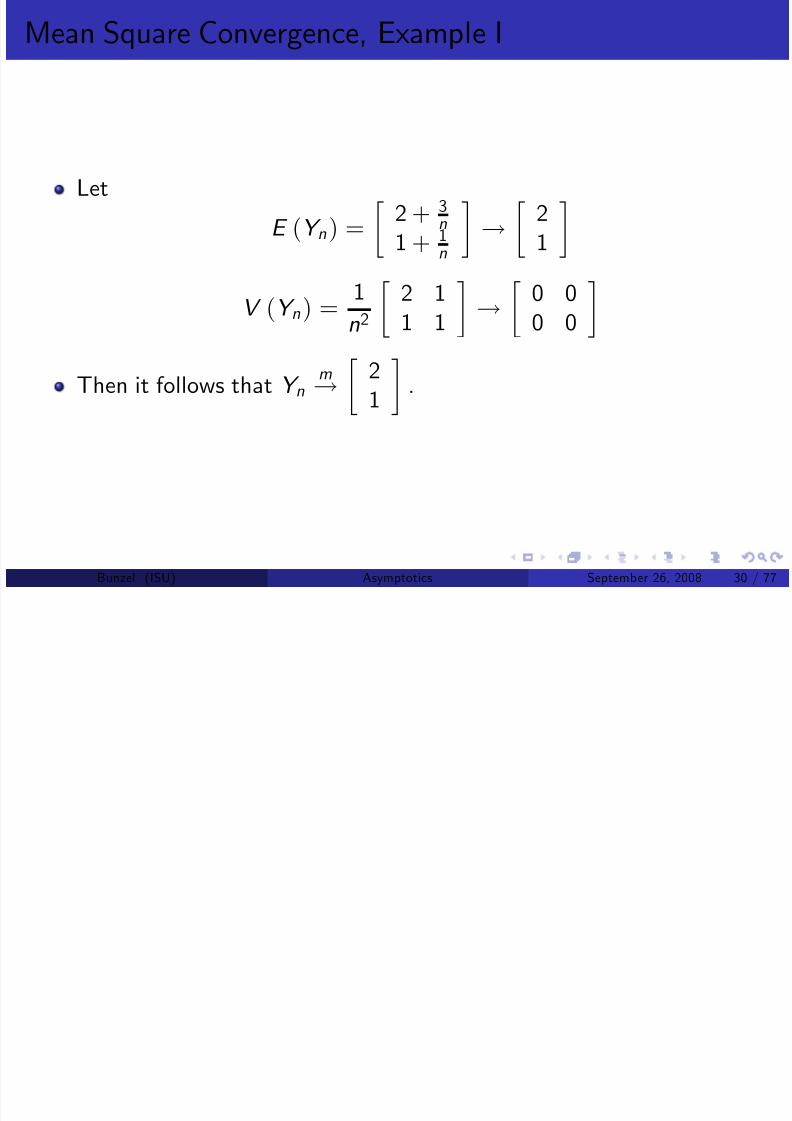
Mean Square Convergence, Example I
Let
E (Y n ) =
2 + 3
n1 + 1
n
!
21
V (Y n) = 1n2
2 11 1
!
0 00 0
Then it follows that Y nm!
21 .
Bunzel (ISU) Asymptotics September 26, 2008 30 / 77
Mean Square Convergence I

8/10/2019 Detailed Notes on Asymptotics
http://slidepdf.com/reader/full/detailed-notes-on-asymptotics 31/77
Mean Square Convergence I
Corollary
Y nm
! Y ) ρ (Y n [i , j ] , Y [i , j ]) ! 1 when V (Y [i , j ]) > 0 8i , j .
Intuition. Outcomes perfectly correlated with equal variances.
Bunzel (ISU) Asymptotics September 26, 2008 31 / 77
Mean Square Convergence II
8/10/2019 Detailed Notes on Asymptotics
http://slidepdf.com/reader/full/detailed-notes-on-asymptotics 32/77
q g
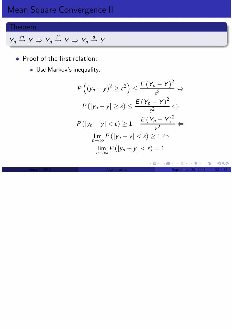
Theorem
Y n
m
! Y ) Y n
P
! Y ) Y n
d
! Y
Proof of the …rst relation:
Use Markov’s inequality:
P
(y n y )2 ε2
E (Y n Y )2
ε2 ,
P (jy n y j ε) E (Y n Y )2
ε2 ,
P (jy n y j < ε) 1 E (Y n
Y )2
ε2 ,lim
n!∞P (jy n y j < ε) 1 ,
limn!∞
P (jy n y j < ε) = 1
Bunzel (ISU) Asymptotics September 26, 2008 32 / 77
Mean Square Convergence, Example I
8/10/2019 Detailed Notes on Asymptotics
http://slidepdf.com/reader/full/detailed-notes-on-asymptotics 33/77
q g , p
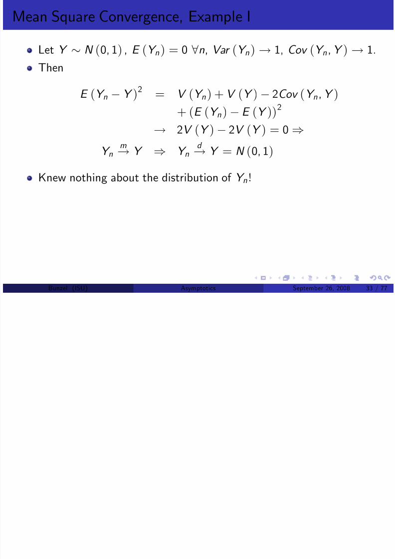
Let Y N (0, 1) , E (Y n ) = 0 8n, Var (Y n ) ! 1, Cov (Y n , Y ) ! 1.
Then
E (Y n Y )2 = V (Y n ) + V (Y ) 2Cov (Y n , Y )
+ (E (Y n ) E (Y ))2
! 2V (Y )
2V (Y ) = 0
)Y nm! Y ) Y n
d ! Y = N (0, 1)
Knew nothing about the distribution of Y n !
Bunzel (ISU) Asymptotics September 26, 2008 33 / 77
Mean Square Convergence, Example II
8/10/2019 Detailed Notes on Asymptotics
http://slidepdf.com/reader/full/detailed-notes-on-asymptotics 34/77
q g p
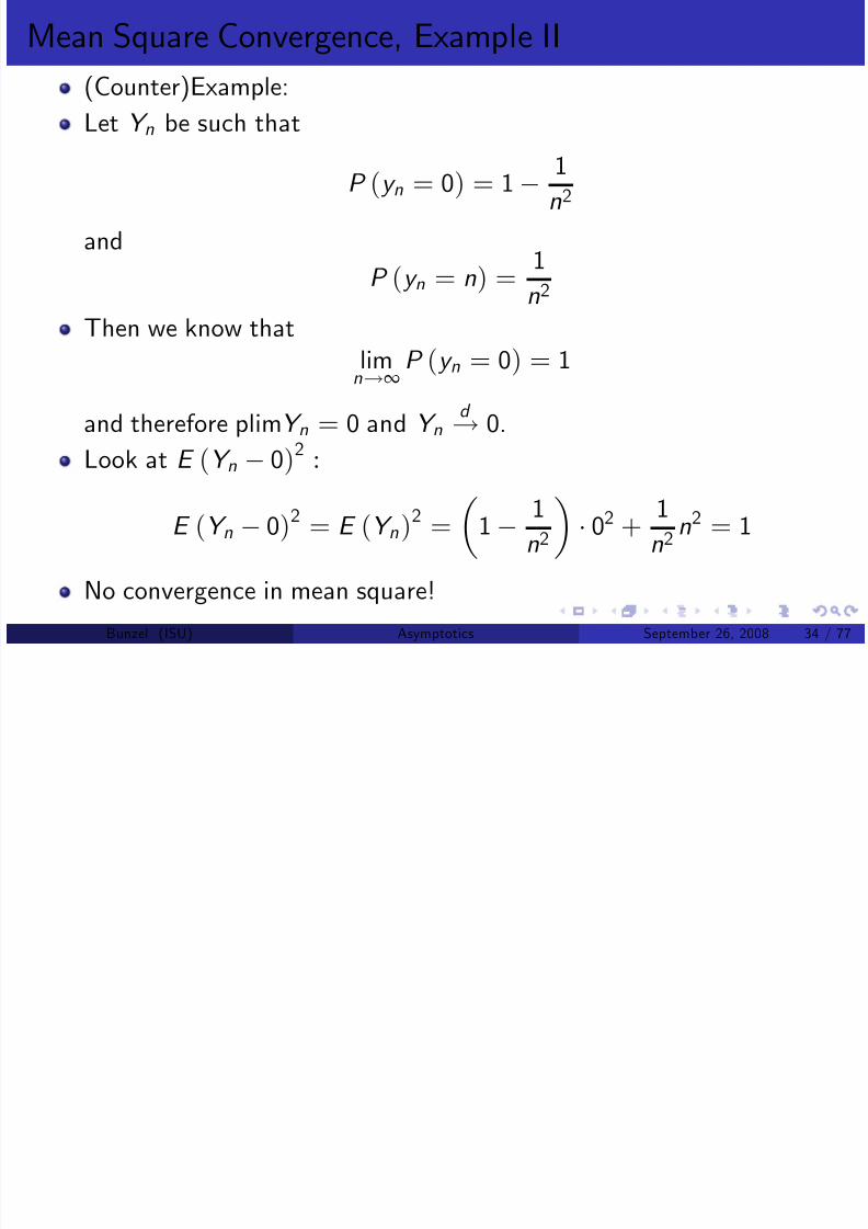
(Counter)Example:
Let Y n be such that
P (y n = 0) = 1 1n2
and
P (y n = n) = 1
n2
Then we know thatlim
n!∞P (y n = 0) = 1
and therefore plimY n = 0 and Y nd ! 0.
Look at E (Y n 0)2
:
E (Y n 0)2 = E (Y n)2 =
1 1
n2
02 +
1
n2n2 = 1
No convergence in mean square!
Bunzel (ISU) Asymptotics September 26, 2008 34 / 77
Almost sure convergence I

8/10/2019 Detailed Notes on Asymptotics
http://slidepdf.com/reader/full/detailed-notes-on-asymptotics 35/77
g
Almost sure convergence is the convergence of outcomes .
De…nition
The sequence of random variables fY ng converges almost surely to therandom variable Y i¤ a. Scalar case: P (limn
!∞ y n = y ) = 1
b. Matrix case: P (limn!∞ y n [i , j ] = y [i , j ]) = 1 8i , j
The notation is Y na.s .! Y .
Note that each sequence of random variables has MANY possible
sequences of outcomes.
Note that Y np ! c ; that limn!∞ y n exists. Why?
For limn!∞ y n = c , it must be the case that8n N (ε) , jy n c j < ε.
Bunzel (ISU) Asymptotics September 26, 2008 35 / 77
Almost sure convergence II

8/10/2019 Detailed Notes on Asymptotics
http://slidepdf.com/reader/full/detailed-notes-on-asymptotics 36/77
A.s. convergence provides this limit with probability 1.
Y n p ! c , P (jy n c j < ε) ! 1 8ε.
This corresponds to
8n N (δ) : 1 P (jy n c j < ε) < δ
or 8n N (δ) : P (jy n c j < ε) > 1 δ
So, for big n, the probability that y n is close to c is high, but not 1. ForNO …xed n is the probability 1, so it certainly isn’t for all n greaterthan N .
Thus, convergence in probability does NOT imply almost sureconvergence.
Bunzel (ISU) Asymptotics September 26, 2008 36 / 77
Almost sure convergence III

8/10/2019 Detailed Notes on Asymptotics
http://slidepdf.com/reader/full/detailed-notes-on-asymptotics 37/77
Theorem
P (limn!∞ y n = y ) = 1 ,limn!∞ P (jy i y j < ε i n) = 1, 8ε > 0.
Alternative de…nition.
Theorem
Y na.s .! Y ) Y n
P ! Y
Proof:
We know that 8ε > 0 limn!∞ P (jy i y j < ε i n) = 1
Bunzel (ISU) Asymptotics September 26, 2008 37 / 77
Almost sure convergence IV

8/10/2019 Detailed Notes on Asymptotics
http://slidepdf.com/reader/full/detailed-notes-on-asymptotics 38/77
Note that jy i y j < ε i n ) jy n y j < ε, so
P (jy i y j < ε i n) P (jy n y j < ε) )limn!∞P (jy n y j < ε) limn!∞P (jy i y j < ε i n) = 1 8ε ,
limn!∞
P (jy n y j < ε) = 1
Bunzel (ISU) Asymptotics September 26, 2008 38 / 77
Almost sure convergence, (Counter)Example I

8/10/2019 Detailed Notes on Asymptotics
http://slidepdf.com/reader/full/detailed-notes-on-asymptotics 39/77
Let fY ng be a sequence of independent random variables such that
Y n f n (y ) =
1 1
n
I f0g (y ) +
1
nI f1g (y )
Convergence in distribution:
f n (y ) ! f (y ) = I f0g (y ) )Y n
d ! 0
Convergence in probability:Since Y n converges in distribution to a constant, we know that
Y nP ! 0
Bunzel (ISU) Asymptotics September 26, 2008 39 / 77
Almost sure convergence, (Counter)Example II

8/10/2019 Detailed Notes on Asymptotics
http://slidepdf.com/reader/full/detailed-notes-on-asymptotics 40/77
Mean square convergence:
E (Y n 0)2 =
1 1n
02 +
1n 12 =
1n ! 0
Almost sure convergence:
8ε 2 (0,
1) and 8s >
n,
s integer
P (jy i j < ε, n i s )
=s
∏i =n
1 1
i
=
s
∏i =n
i 1
i
=
n 1n
n
n + 1
n + 1n + 2
...
s 2s 1
s 1
s
=
n 1
s ! 0 as s ! ∞
Bunzel (ISU) Asymptotics September 26, 2008 40 / 77
Almost sure convergence, (Counter)Example III
8/10/2019 Detailed Notes on Asymptotics
http://slidepdf.com/reader/full/detailed-notes-on-asymptotics 41/77
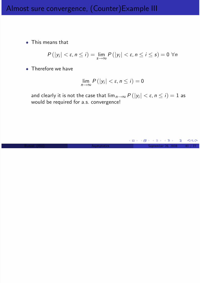
This means that
P (jy i j < ε, n i ) = lims !∞
P (jy i j < ε, n i s ) = 0 8n
Therefore we have
limn!∞
P (jy i j < ε, n i ) = 0
and clearly it is not the case that limn!∞ P (jy i j < ε, n i ) = 1 aswould be required for a.s. convergence!
Bunzel (ISU) Asymptotics September 26, 2008 41 / 77
Almost sure convergence, (Counter)Example I

8/10/2019 Detailed Notes on Asymptotics
http://slidepdf.com/reader/full/detailed-notes-on-asymptotics 42/77
Y na.s .! Y ; Y n
m! Y
Let
fY n
g be a sequence of independent random variables such that
Y n f n (y ) =
1 1
n2
I f0g (y ) +
1
n2I fng (y )
8ε
2(0, n) and
8s > n, s integer
P (jy i j < ε, n i s )
=s
∏i =n
1 1
i 2
=
s
∏i =n
i 2 1
i 2
= n2
1
n2 (n+1)2
1
(n+1)2 (n+2)2
1
(n+2)2
... (s
1)2
1
(s 1)2 s 2
1
s 2
=
(n1)(n+1)n2
n(n+2)
(n+1)2
(n+1)(n+3)
(n+2)2
...
(s 3)2s
(s 1)2
(s 1)(s +1)
s 2
= (n 1) (s + 1)
ns Bunzel (ISU) Asymptotics September 26, 2008 42 / 77
Almost sure convergence, (Counter)Example II

8/10/2019 Detailed Notes on Asymptotics
http://slidepdf.com/reader/full/detailed-notes-on-asymptotics 43/77
So
P (jy i j < ε, n i ) = (n 1)n
limn!∞
P (jy i j < ε, n i ) = 1
Which proves that Y na.s .
! Y
Now, note that E (Y n ) = 1n ! 0 but
V (Y n ) =
1 1
n2
1
n2 +
1
n2
n 1
n
2
=
1 1
n2 1
n2 +n2 + 1
n2
2
n2 ! 1
Then, Y n does not converge in mean square.
Bunzel (ISU) Asymptotics September 26, 2008 43 / 77
Overview of convergence modes I

8/10/2019 Detailed Notes on Asymptotics
http://slidepdf.com/reader/full/detailed-notes-on-asymptotics 44/77
Yn Ya.s.
Yn YP Yn Yd
Yn Ym
y = c
Bunzel (ISU) Asymptotics September 26, 2008 44 / 77
Almost sure convergence I

8/10/2019 Detailed Notes on Asymptotics
http://slidepdf.com/reader/full/detailed-notes-on-asymptotics 45/77
Theorem
Let X n
a.s .
! X and let the random variable g (X ) be de…ned by a functiong (x ) that is continuous, except perhaps on a set of points assigned
probability 0 by the distribution of X . Then g (X n ) a.s .! g (X ) .
Same as for plim
Example:
Let X na.s .!
21
. Then
g 1 (X n ) =
X n [2]
X n [1]a.s .
! 1
2
g 2 (X n ) = X n [2] X n [1] a.s .! 1
g 3 (X n ) = g 1 (X n ) g 2 (X n ) a.s .! 1
2
Bunzel (ISU) Asymptotics September 26, 2008 45 / 77
Almost sure convergence II
8/10/2019 Detailed Notes on Asymptotics
http://slidepdf.com/reader/full/detailed-notes-on-asymptotics 46/77
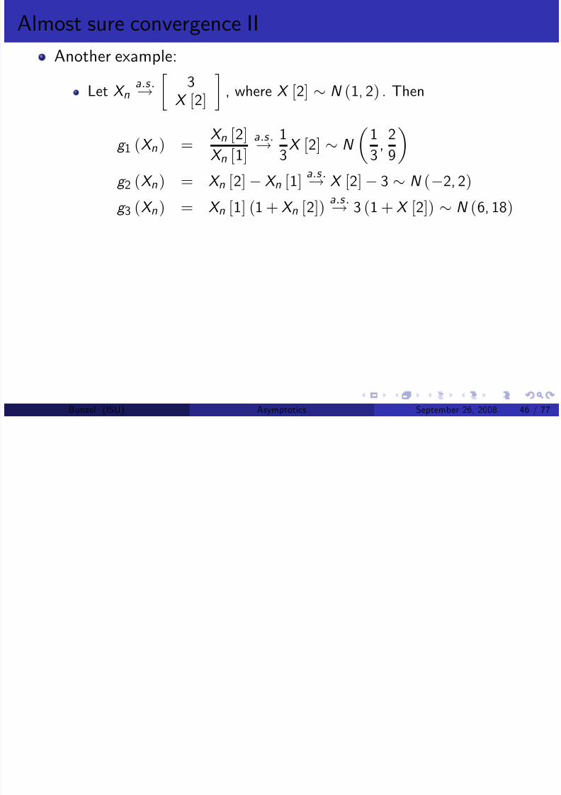
Another example:
Let X na.s .
! 3
X [2] , where X [2]
N (1, 2) . Then
g 1 (X n ) = X n [2]
X n [1]a.s .! 1
3X [2] N
1
3,
2
9
g 2 (X n ) = X n [2] X n [1] a.s .! X [2] 3 N (2, 2)
g 3 (X n ) = X n [1] (1 + X n [2]) a.
s .
! 3 (1 + X [2]) N (6, 18)
Bunzel (ISU) Asymptotics September 26, 2008 46 / 77
Almost sure convergence III
8/10/2019 Detailed Notes on Asymptotics
http://slidepdf.com/reader/full/detailed-notes-on-asymptotics 47/77
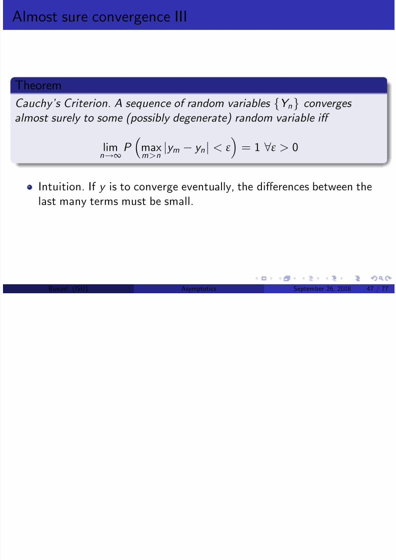
Theorem
Cauchy’s Criterion. A sequence of r andom variables fY ng converges almost surely to some (possibly degenerate) random variable i¤
limn!∞P
maxm>n jy m y n j < ε
= 1 8ε > 0
Intuition. If y is to converge eventually, the di¤erences between thelast many terms must be small.
Bunzel (ISU) Asymptotics September 26, 2008 47 / 77
Laws of Large Numbers I

8/10/2019 Detailed Notes on Asymptotics
http://slidepdf.com/reader/full/detailed-notes-on-asymptotics 48/77
Laws of large numbers give results f or the convergence of sequences
fX ng , where
X n = 1
n
n
∑ i =1
X i
If data is generated by f
X ng
,
fX n
g is the sequence of sample means.
Convergence in probability: Weak Laws of Large Numbers (WLLN)
Almost Sure Convergence: Strong Laws of Large Numbers (SLLN)
Two types of Laws of Large Numbers:
1 If E (X i ) = µ 8i , ¯
X n ! µ2 If E (X i ) = µi (not the same for all i ), X n µn ! 0, where
µn = 1n ∑
ni =1 µi
Bunzel (ISU) Asymptotics September 26, 2008 48 / 77
WLLN I

8/10/2019 Detailed Notes on Asymptotics
http://slidepdf.com/reader/full/detailed-notes-on-asymptotics 49/77
Weak Laws of Large Numbers, basic idea:Impose conditions such that the limiting distribution of Y n = 1
n ∑ ni =1 (X i µi ) is degenerate on 0.
This happens when ∑ ni =1 (X i µi ) = o P (n)
Suppose X i are iid with mean µ and variance σ 2?
BUT: Neither iid nor existence of variance is required.
Theorem
(Khinchin’s WLLN) Let fX ng be a sequenc e of iid random variables, and suppose E (X i ) = µ < ∞, 8i . Then X n
P ! µ.
Bunzel (ISU) Asymptotics September 26, 2008 49 / 77
WLLN, Examples I

8/10/2019 Detailed Notes on Asymptotics
http://slidepdf.com/reader/full/detailed-notes-on-asymptotics 50/77
Let fX ng be a sequence of random variables such thatX i p x (1 p )1x 1f0,1g (x ) 8i . Then E (X i ) = p 8i and by
Khinchin’s WLLN X nP ! p .
Let f (x ) = 2x 31[1,∞) (x ) and suppose the sequence of random
variables fX ng is iid such that X i f (x ) . Then
E (X i ) =Z ∞
∞x 2x 31[1,∞) (x ) dx =
Z ∞1
2x 2dx
= 2x 1∞1 = 2
By Khinchin’s WLLN X nP ! 2.
Bunzel (ISU) Asymptotics September 26, 2008 50 / 77
WLLN, Examples II

8/10/2019 Detailed Notes on Asymptotics
http://slidepdf.com/reader/full/detailed-notes-on-asymptotics 51/77
BUT: Note that
V (X i ) = E
X 2i 4
= Z ∞
∞x 22x 31[1,∞) (x ) dx
4
=Z ∞
12x 1dx 4
= [2 ln (x )]∞1 4 ! ∞
Bunzel (ISU) Asymptotics September 26, 2008 51 / 77
WLLN I

8/10/2019 Detailed Notes on Asymptotics
http://slidepdf.com/reader/full/detailed-notes-on-asymptotics 52/77
Theorem
(Convergence in Probability of Relat ive Fre quency) Let A be any event in
the sample space. Let an outcome N A be the number of times that anevent occurs in n independent and identical repetitions of the experiment.
Then the relative frequency of event A occurring is such that N An
P ! P (A)
The relative frequence can be used as a measure of the probability asn ! ∞.
Now relax iid assumption. Cost: Assume existence of variances.
Bunzel (ISU) Asymptotics September 26, 2008 52 / 77
WLLN II

8/10/2019 Detailed Notes on Asymptotics
http://slidepdf.com/reader/full/detailed-notes-on-asymptotics 53/77
Theorem
Let fX ng be a sequence of random variable s with …nite variances, and let fµng be the corresponding sequence of expected values. Then
limn!∞
P (jx n µn j < ε) = 1, 8ε > 0
i¤
E
" ( X n µn )
2
1 + ( X n µn )2
#! 0
Usage: Any conditions which imply that E
( X nµn )2
1+( X nµn )2
! 0 will
provide a WLLN.
Bunzel (ISU) Asymptotics September 26, 2008 53 / 77
WLLN III

8/10/2019 Detailed Notes on Asymptotics
http://slidepdf.com/reader/full/detailed-notes-on-asymptotics 54/77
Theorem
(WLLN for non-iid case) Let fX ng be a seq uence of random variables with
…nite variances, and let fµng be the corresponding sequence of expected values. If Var ( X n ) ! 0, then ( X n µn )
P ! 0.
Bunzel (ISU) Asymptotics September 26, 2008 54 / 77

8/10/2019 Detailed Notes on Asymptotics
http://slidepdf.com/reader/full/detailed-notes-on-asymptotics 55/77
WLLN, Example II
8/10/2019 Detailed Notes on Asymptotics
http://slidepdf.com/reader/full/detailed-notes-on-asymptotics 56/77
Now,
σ 2
i 28i )n
∑ i =1 σ 2
i 2n
which implies that1
n2
n
∑ i =1
σ 2i 1
n22n ! 0
and
σ ij = ρji j j )n
∑ j >i
σ ij =n
∑ j >i
ρ j i = ρi n
∑ j >i
ρ j = ρi ρ1+i ρn+1
1 ρ
= ρ ρni +1
1 ρ ! ρ
1 ρ for i ! ∞
Bunzel (ISU) Asymptotics September 26, 2008 56 / 77
WLLN, Example III
8/10/2019 Detailed Notes on Asymptotics
http://slidepdf.com/reader/full/detailed-notes-on-asymptotics 57/77
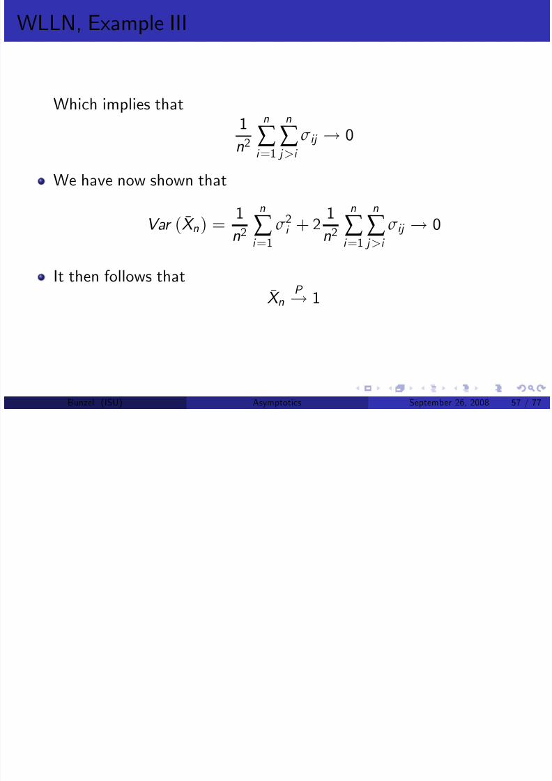
Which implies that 1
n2
n
∑ i =1
n
∑ j >i
σ ij ! 0
We have now shown that
Var ( X n ) = 1
n2
n
∑ i =1
σ 2i + 2 1
n2
n
∑ i =1
n
∑ j >i
σ ij ! 0
It then follows that¯
X nP
! 1
Bunzel (ISU) Asymptotics September 26, 2008 57 / 77

8/10/2019 Detailed Notes on Asymptotics
http://slidepdf.com/reader/full/detailed-notes-on-asymptotics 58/77
SLLN I
8/10/2019 Detailed Notes on Asymptotics
http://slidepdf.com/reader/full/detailed-notes-on-asymptotics 59/77
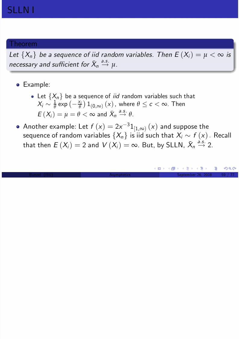
TheoremLet fX ng be a sequence of iid rand om variables. Then E (X i ) = µ < ∞ is
necessary and su¢cient for X na.s .! µ.
Example:
Let fX ng be a sequence of iid random variables such thatX i 1
θ exp x i
θ
1(0,∞) (x ) , where θ c < ∞. Then
E (X i ) = µ = θ < ∞ and X na.s .! θ.
Another example: Let f (x ) = 2x
31[1
,
∞) (x ) and suppose the
sequence of random variables fX ng is iid such that X i f (x ) . Recall
that then E (X i ) = 2 and V (X i ) = ∞. But, by SLLN, X na.s .! 2.
Bunzel (ISU) Asymptotics September 26, 2008 59 / 77
SLLN II

8/10/2019 Detailed Notes on Asymptotics
http://slidepdf.com/reader/full/detailed-notes-on-asymptotics 60/77
Theorem
(A.s. convergence of relative freque ncy) Let A be any event in the sample space. Let an outcome N A be the number of times that an event occurs inn independent and identical repetitions of the experiment. Then the
relative frequency of event A occurring is such that N
An
a.s .
! P (A)
Theorem
If ( X n µn ) a.s .! 0 and µn ! c then X n
a.s .! c
Bunzel (ISU) Asymptotics September 26, 2008 60 / 77
Central Limit Theorems I

8/10/2019 Detailed Notes on Asymptotics
http://slidepdf.com/reader/full/detailed-notes-on-asymptotics 61/77
CLT: Asymptotic distribution of sequences of random variables.
Typical CLT: Sequence of r.v.s such that
Y n = b 1n (S n an )
d ! N (0,Σ)
where
fS n
g is a sequence such that S n = ∑
ni =1 X i .
CLT provides restrictions on fX ng , fang, and fb ng such that theconvergence in distribution occurs.
Main usage: Distribution of parameter estimates and test statistics, if
Finite sample distribution is unknown, or
Finite sample distribution is hard to work with.
A good illustration:http://www.statisticalengineering.com/central_limit_theorem.htm
Bunzel (ISU) Asymptotics September 26, 2008 61 / 77
CLT, Independent Scalar r.v.s I
8/10/2019 Detailed Notes on Asymptotics
http://slidepdf.com/reader/full/detailed-notes-on-asymptotics 62/77
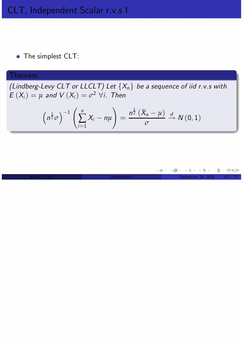
The simplest CLT:
Theorem
(Lindberg-Levy CLT or LLCLT) Let f
X ng
b e a sequence of iid r.v.s withE (X i ) = µ and V (X i ) = σ 2 8i . Then
n
12 σ
1
n
∑ i =1
X i nµ
! =
n12 ( X n µ)
σ
d ! N (0, 1)
Bunzel (ISU) Asymptotics September 26, 2008 62 / 77
CLT, Independent Scalar r.v.s II
Intuition:
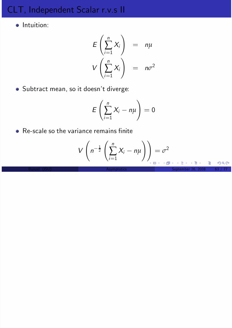
8/10/2019 Detailed Notes on Asymptotics
http://slidepdf.com/reader/full/detailed-notes-on-asymptotics 63/77
Intuition:
E n
∑ i =1 X i !
= nµ
V
n
∑ i =1
X i
! = nσ 2
Subtract mean, so it doesn’t diverge:
E
n
∑ i =1
X i nµ
! = 0
Re-scale so the variance remains …nite
V
n 1
2
n
∑ i =1
X i nµ
!! = σ 2
Bunzel (ISU) Asymptotics September 26, 2008 63 / 77
CLT, Independent Scalar r.v.s III
8/10/2019 Detailed Notes on Asymptotics
http://slidepdf.com/reader/full/detailed-notes-on-asymptotics 64/77
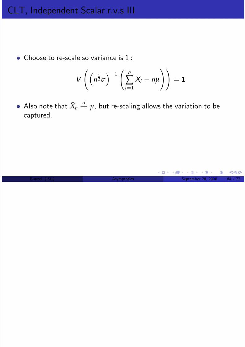
Choose to re-scale so variance is 1 :
V
n
12 σ
1
n
∑ i =1
X i nµ
!! = 1
Also note that X nd ! µ, but re-scaling allows the variation to be
captured.
Bunzel (ISU) Asymptotics September 26, 2008 64 / 77
CLT, Independent Scalar r.v.s, Example I

8/10/2019 Detailed Notes on Asymptotics
http://slidepdf.com/reader/full/detailed-notes-on-asymptotics 65/77
Let fX ng be a sequence of χ2 (1) variables. Then E (X i ) = 1 andV (X i ) = 2 and ∑
ni =1 X i χ2 (n) .
Then, by LLCLT
∑ n
i =1 X i nn
12 (2)
12
= ∑
n
i =1 X i n(2n)
12
d ! N (0, 1)
How good is the approximation? In reality we don’t know. There aresome theoretical bounds. Also we often use simulation techniques to
determine how big n should be for the approximation to work well.
Bunzel (ISU) Asymptotics September 26, 2008 65 / 77
CLT, Independent Scalar r.v.s I

8/10/2019 Detailed Notes on Asymptotics
http://slidepdf.com/reader/full/detailed-notes-on-asymptotics 66/77
A CLT where we don’t require that the variables be iid:
Bunzel (ISU) Asymptotics September 26, 2008 66 / 77
CLT, Independent Scalar r.v.s II
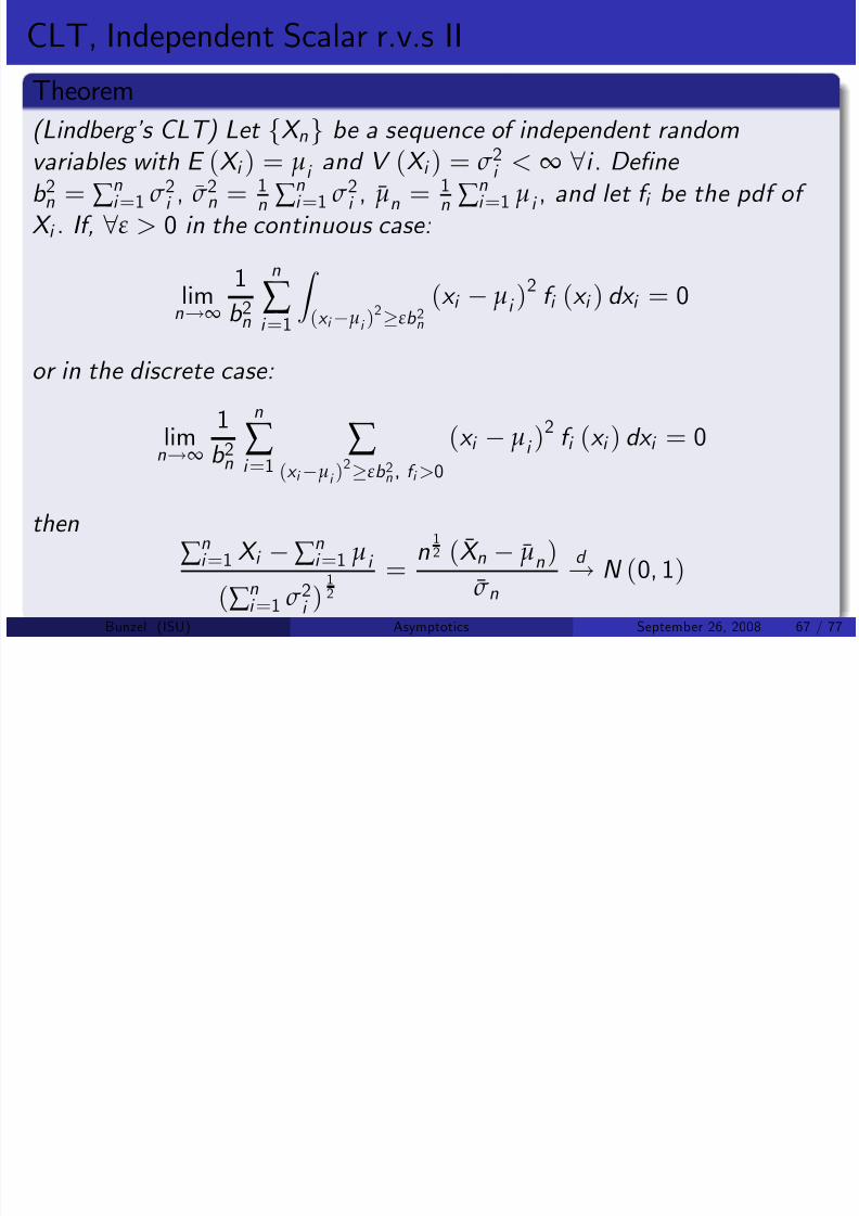
Theorem
8/10/2019 Detailed Notes on Asymptotics
http://slidepdf.com/reader/full/detailed-notes-on-asymptotics 67/77
(Lindberg’s CLT) Let fX ng be a seq uence o f independent random
variables with E (X i ) = µi and V (X i ) = σ 2
i < ∞
8i .
De…ne b 2n = ∑ ni =1 σ
2i , σ 2n = 1
n ∑ ni =1 σ
2i , µn = 1
n ∑ ni =1 µi , and let f i be the pdf of
X i . If, 8ε > 0 in the continuous case:
lim
n!∞
1
b 2n
n
∑ i =1
Z (x i µi )
2
εb 2n
(x i
µi )
2 f i (x i ) dx i = 0
or in the discrete case:
limn
!∞
1
b 2n
n
∑ i =1
∑ (x i µi )
2
εb 2n , f i >0
(x i µi )2 f i (x i ) dx i = 0
then∑
ni =1 X i ∑
ni =1 µi
(∑ ni =1 σ 2i )
12
= n
12 ( X n µn )
σ n
d ! N (0, 1)
Bunzel (ISU) Asymptotics September 26, 2008 67 / 77
CLT, Independent Scalar r.v.s I
It can be shown that the condition in the Lindberg CLT (Lindberg
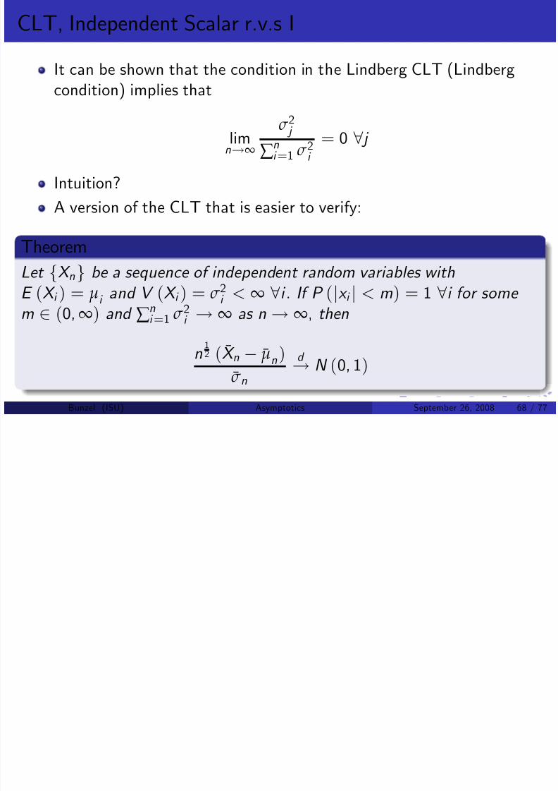
8/10/2019 Detailed Notes on Asymptotics
http://slidepdf.com/reader/full/detailed-notes-on-asymptotics 68/77
It can be shown that the condition in the Lindberg CLT (Lindbergcondition) implies that
limn!∞
σ 2 j
∑ ni =1 σ
2i
= 0 8 j
Intuition?
A version of the CLT that is easier to verify:
Theorem
Let fX ng be a sequence of independ ent random variables withE (X i ) = µi and V (X i ) = σ 2i < ∞
8i . If P (
jx i
j< m) = 1
8i for some
m 2 (0,∞) and ∑ ni =1 σ 2i ! ∞ as n ! ∞, then
n12 ( X n µn )
σ n
d ! N (0, 1)
Bunzel (ISU) Asymptotics September 26, 2008 68 / 77
CLT, Independent Scalar r.v.s, Example I

8/10/2019 Detailed Notes on Asymptotics
http://slidepdf.com/reader/full/detailed-notes-on-asymptotics 69/77
Let the sequence fY ng be de…ned by Y i = z i β + εi , where: β is a real number
z i is the i’th element in the sequence of real numbers fz ng , for which1n ∑
ni =1 z 2i > a > 0 and jz i j < d < ∞, 8i
εi is the i’th element in the sequence iid random variables
fεn
g, for
which E (εi ) = 0 and V (εi ) = σ 2 2 (0,∞) and P (jεi j m) = 1, 8i ,where m 2 (0,∞)
Find an asymptotic distribution of the least squares estimator of βde…ned by
ˆ βn = ∑
n
i =1 z i Y i ∑
ni =1 z 2i
Bunzel (ISU) Asymptotics September 26, 2008 69 / 77
CLT, Independent Scalar r.v.s, Example II
8/10/2019 Detailed Notes on Asymptotics
http://slidepdf.com/reader/full/detailed-notes-on-asymptotics 70/77
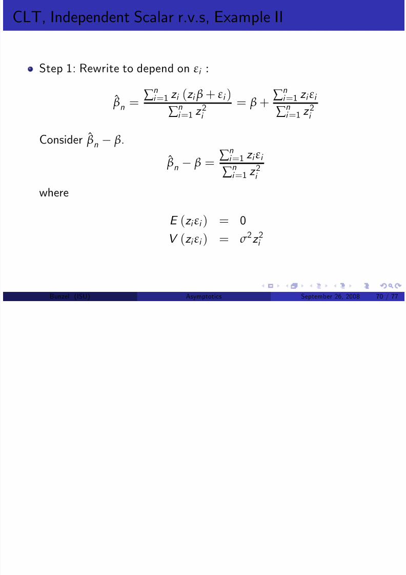
Step 1: Rewrite to depend on εi :
ˆ βn = ∑
ni =1 z i (z i β + εi )
∑ ni =1 z 2i
= β + ∑
ni =1 z i εi
∑ ni =1 z 2i
Consider ˆ βn
β.
ˆ βn β = ∑ ni =1 z i εi
∑ ni =1 z 2i
where
E (z i εi ) = 0V (z i εi ) = σ 2z 2i
Bunzel (ISU) Asymptotics September 26, 2008 70 / 77
CLT, Independent Scalar r.v.s, Example III

8/10/2019 Detailed Notes on Asymptotics
http://slidepdf.com/reader/full/detailed-notes-on-asymptotics 71/77
Is z i εi bounded?
P (jz i εi j < dm) = P (jz i j jεi j < dm) P (jεi j < m) = 1
and dm
2(0,∞) .
Now check the sum of the variances:
n
∑ i =1
V (z i εi ) = σ 2n
∑ i =1
z 2i = nσ 2
1
n
n
∑ i =1
z 2i
!
> anσ 2
! ∞
Bunzel (ISU) Asymptotics September 26, 2008 71 / 77
CLT, Independent Scalar r.v.s, Example IV
8/10/2019 Detailed Notes on Asymptotics
http://slidepdf.com/reader/full/detailed-notes-on-asymptotics 72/77
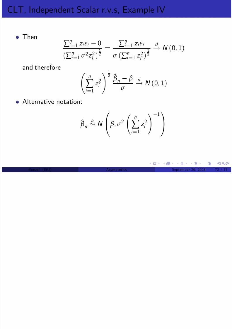
Then∑
n
i =1 z
i ε
i 0
(∑ ni =1 σ 2z 2i )
12
= ∑
n
i =1 z
i ε
i σ (∑ ni =1 z 2i )
12
d
! N (0, 1)
and therefore
n
∑ i =1
z 2
i !
12 ˆ βn β
σ
d
!N (0, 1)
Alternative notation:
ˆ βn
a
N 0@ β, σ 2 n
∑ i =1
z 2
i !
1
1A
Bunzel (ISU) Asymptotics September 26, 2008 72 / 77
Multivariate CLT I

8/10/2019 Detailed Notes on Asymptotics
http://slidepdf.com/reader/full/detailed-notes-on-asymptotics 73/77
Theorem
(Multivariate Lindberg-Levy CLT) Let fX ng be a sequence of iid randomvariables with E (X i ) = µ and Cov (X i ) = Σ 8i , where Σ is a k k
positive de…nite matrix. Then
n12
1
n
n
∑ i =1
X i µ
! d ! N (0,Σ)
Bunzel (ISU) Asymptotics September 26, 2008 73 / 77

8/10/2019 Detailed Notes on Asymptotics
http://slidepdf.com/reader/full/detailed-notes-on-asymptotics 74/77
Multivariate CLT, Example II
Then

8/10/2019 Detailed Notes on Asymptotics
http://slidepdf.com/reader/full/detailed-notes-on-asymptotics 75/77
E (X i ) = p 1
p 2
Cov (X i ) =
p 1 (1 p 1) 0
0 p 2 (1 p 2)
Also let X n = 1n ∑ ni =1
X 1i X 2i
.
Then, by the multivariate LLCLT
n12 X n
p 1
p 2 d
!N 0, p 1 (1
p 1) 0
0 p 2 (1 p 2)
Suppose we’re interested in the di¤erence in failure rates.
That is X 1i X 2i or cX i , where c = [1, 1]
Bunzel (ISU) Asymptotics September 26, 2008 75 / 77
Multivariate CLT, Example III

8/10/2019 Detailed Notes on Asymptotics
http://slidepdf.com/reader/full/detailed-notes-on-asymptotics 76/77
Then
cn12
X n
p 1p 2
= n
12
c X n c
p 1p 2
= n12 (( X 1n X 2n ) (p 1 p 2))
d ! N
0, c
p 1 (1 p 1) 00 p 2 (1 p 2)
c 0
= N (0, p 1 (1 p 1) + p 2 (1 p 2))
Note the variance is what we’d expect when we’re subtracting two
independent variables.
Bunzel (ISU) Asymptotics September 26, 2008 76 / 77
Multivariate CLT I
8/10/2019 Detailed Notes on Asymptotics
http://slidepdf.com/reader/full/detailed-notes-on-asymptotics 77/77
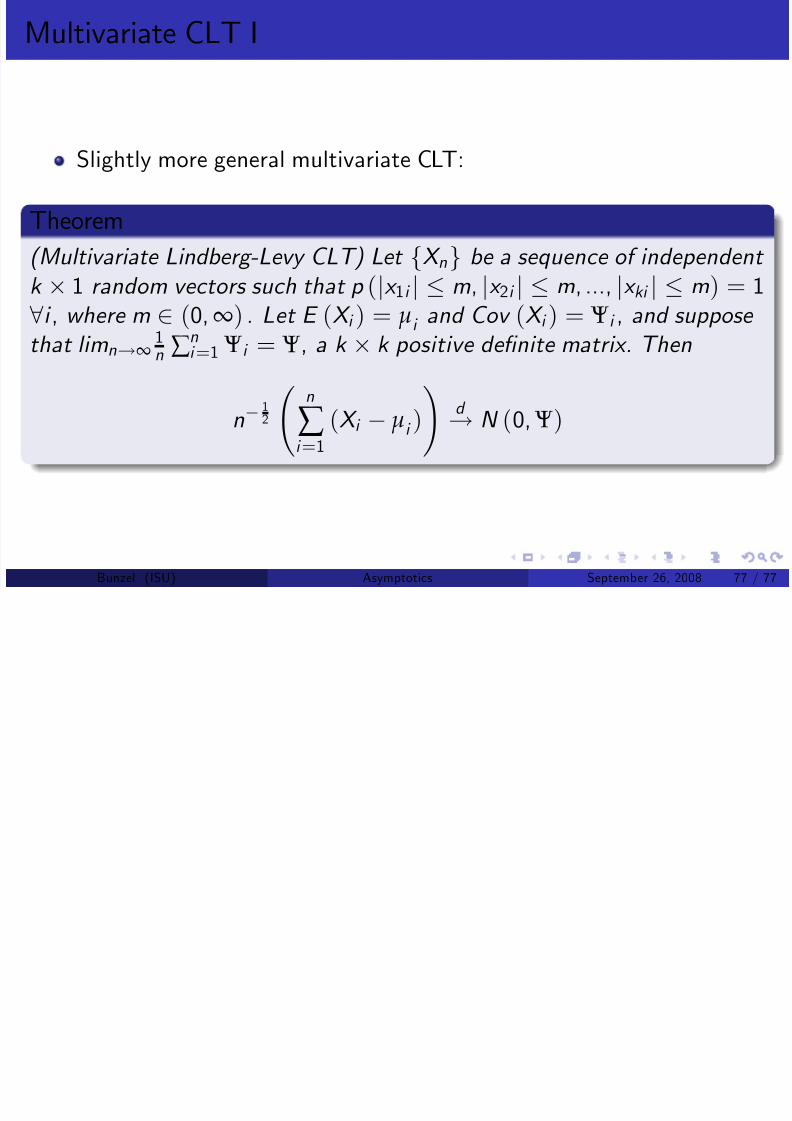
Slightly more general multivariate CLT:
Theorem
(Multivariate Lindberg-Levy CLT) Let fX ng be a sequence of independent k
1 random vectors such that p (
jx
1i j m,
jx
2i j m, ...,
jx
ki j m) = 1
8i , where m 2 (0,∞) . Let E (X i ) = µi and Cov (X i ) = Ψi , and suppose that limn!∞
1n ∑
ni =1 Ψi = Ψ, a k k positive de …nite matrix. Then
n 12
n
∑ i =1
(X i
µi )! d
!N (0, Ψ)
Bunzel (ISU) Asymptotics September 26, 2008 77 / 77