Notes for a graduate-level course inasymptotics for statisticians

David R. HunterPenn State University

June 2014

Contents

Preface 1

1 Mathematical and Statistical Preliminaries 3

1.1 Limits and Continuity . . . . . . . . . . . . . . . . . . . . . . . . . . . . . . 4

1.1.1 Limit Superior and Limit Inferior . . . . . . . . . . . . . . . . . . . . 6

1.1.2 Continuity . . . . . . . . . . . . . . . . . . . . . . . . . . . . . . . . . 8

1.2 Differentiability and Taylor’s Theorem . . . . . . . . . . . . . . . . . . . . . 13

1.3 Order Notation . . . . . . . . . . . . . . . . . . . . . . . . . . . . . . . . . . 18

1.4 Multivariate Extensions . . . . . . . . . . . . . . . . . . . . . . . . . . . . . 26

1.5 Expectation and Inequalities . . . . . . . . . . . . . . . . . . . . . . . . . . . 33

2 Weak Convergence 41

2.1 Modes of Convergence . . . . . . . . . . . . . . . . . . . . . . . . . . . . . . 41

2.1.1 Convergence in Probability . . . . . . . . . . . . . . . . . . . . . . . . 41

2.1.2 Probabilistic Order Notation . . . . . . . . . . . . . . . . . . . . . . . 43

2.1.3 Convergence in Distribution . . . . . . . . . . . . . . . . . . . . . . . 45

2.1.4 Convergence in Mean . . . . . . . . . . . . . . . . . . . . . . . . . . . 48

2.2 Consistent Estimates of the Mean . . . . . . . . . . . . . . . . . . . . . . . . 51

2.2.1 The Weak Law of Large Numbers . . . . . . . . . . . . . . . . . . . . 52

i

2.2.2 Independent but not Identically Distributed Variables . . . . . . . . . 52

2.2.3 Identically Distributed but not Independent Variables . . . . . . . . . 54

2.3 Convergence of Transformed Sequences . . . . . . . . . . . . . . . . . . . . . 58

2.3.1 Continuous Transformations: The Univariate Case . . . . . . . . . . . 58

2.3.2 Multivariate Extensions . . . . . . . . . . . . . . . . . . . . . . . . . 59

2.3.3 Slutsky’s Theorem . . . . . . . . . . . . . . . . . . . . . . . . . . . . 62

3 Strong convergence 70

3.1 Strong Consistency Defined . . . . . . . . . . . . . . . . . . . . . . . . . . . 70

3.1.1 Strong Consistency versus Consistency . . . . . . . . . . . . . . . . . 71

3.1.2 Multivariate Extensions . . . . . . . . . . . . . . . . . . . . . . . . . 73

3.2 The Strong Law of Large Numbers . . . . . . . . . . . . . . . . . . . . . . . 74

3.3 The Dominated Convergence Theorem . . . . . . . . . . . . . . . . . . . . . 79

3.3.1 Moments Do Not Always Converge . . . . . . . . . . . . . . . . . . . 79

3.3.2 Quantile Functions and the Skorohod Representation Theorem . . . . 81

4 Central Limit Theorems 88

4.1 Characteristic Functions and Normal Distributions . . . . . . . . . . . . . . 88

4.1.1 The Continuity Theorem . . . . . . . . . . . . . . . . . . . . . . . . . 89

4.1.2 Moments . . . . . . . . . . . . . . . . . . . . . . . . . . . . . . . . . . 90

4.1.3 The Multivariate Normal Distribution . . . . . . . . . . . . . . . . . 91

4.1.4 Asymptotic Normality . . . . . . . . . . . . . . . . . . . . . . . . . . 92

4.1.5 The Cramer-Wold Theorem . . . . . . . . . . . . . . . . . . . . . . . 94

4.2 The Lindeberg-Feller Central Limit Theorem . . . . . . . . . . . . . . . . . . 96

4.2.1 The Lindeberg and Lyapunov Conditions . . . . . . . . . . . . . . . . 97

4.2.2 Independent and Identically Distributed Variables . . . . . . . . . . . 98

ii

4.2.3 Triangular Arrays . . . . . . . . . . . . . . . . . . . . . . . . . . . . . 99

4.3 Stationary m-Dependent Sequences . . . . . . . . . . . . . . . . . . . . . . . 108

4.4 Univariate extensions . . . . . . . . . . . . . . . . . . . . . . . . . . . . . . . 111

4.4.1 The Berry-Esseen theorem . . . . . . . . . . . . . . . . . . . . . . . . 112

4.4.2 Edgeworth expansions . . . . . . . . . . . . . . . . . . . . . . . . . . 113

5 The Delta Method and Applications 116

5.1 Local linear approximations . . . . . . . . . . . . . . . . . . . . . . . . . . . 116

5.1.1 Asymptotic distributions of transformed sequences . . . . . . . . . . 116

5.1.2 Variance stabilizing transformations . . . . . . . . . . . . . . . . . . . 119

5.2 Sample Moments . . . . . . . . . . . . . . . . . . . . . . . . . . . . . . . . . 121

5.3 Sample Correlation . . . . . . . . . . . . . . . . . . . . . . . . . . . . . . . . 123

6 Order Statistics and Quantiles 127

6.1 Extreme Order Statistics . . . . . . . . . . . . . . . . . . . . . . . . . . . . . 127

6.2 Sample Quantiles . . . . . . . . . . . . . . . . . . . . . . . . . . . . . . . . . 134

6.2.1 Uniform Order Statistics . . . . . . . . . . . . . . . . . . . . . . . . . 134

6.2.2 Uniform Sample Quantiles . . . . . . . . . . . . . . . . . . . . . . . . 135

6.2.3 General sample quantiles . . . . . . . . . . . . . . . . . . . . . . . . . 137

7 Maximum Likelihood Estimation 140

7.1 Consistency . . . . . . . . . . . . . . . . . . . . . . . . . . . . . . . . . . . . 140

7.2 Asymptotic normality of the MLE . . . . . . . . . . . . . . . . . . . . . . . . 144

7.3 Asymptotic Efficiency and Superefficiency . . . . . . . . . . . . . . . . . . . 149

7.4 The multiparameter case . . . . . . . . . . . . . . . . . . . . . . . . . . . . . 154

7.5 Nuisance parameters . . . . . . . . . . . . . . . . . . . . . . . . . . . . . . . 159

iii

8 Hypothesis Testing 161

8.1 Wald, Rao, and Likelihood Ratio Tests . . . . . . . . . . . . . . . . . . . . . 161

8.2 Contiguity and Local Alternatives . . . . . . . . . . . . . . . . . . . . . . . . 165

8.3 The Wilcoxon Rank-Sum Test . . . . . . . . . . . . . . . . . . . . . . . . . . 175

9 Pearson’s chi-square test 180

9.1 Null hypothesis asymptotics . . . . . . . . . . . . . . . . . . . . . . . . . . . 180

9.2 Power of Pearson’s chi-square test . . . . . . . . . . . . . . . . . . . . . . . . 187

10 U-statistics 190

10.1 Statistical Functionals and V-Statistics . . . . . . . . . . . . . . . . . . . . . 190

10.2 Asymptotic Normality . . . . . . . . . . . . . . . . . . . . . . . . . . . . . . 194

10.3 Multivariate and multi-sample U-statistics . . . . . . . . . . . . . . . . . . . 201

10.4 Introduction to the Bootstrap . . . . . . . . . . . . . . . . . . . . . . . . . . 205

iv

Preface

These notes are designed to accompany STAT 553, a graduate-level course in large-sampletheory at Penn State intended for students who may not have had any exposure to measure-theoretic probability. While many excellent large-sample theory textbooks already exist,the majority (though not all) of them reflect a traditional view in graduate-level statisticseducation that students should learn measure-theoretic probability before large-sample the-ory. The philosophy of these notes is that these priorities are backwards, and that in factstatisticians have more to gain from an understanding of large-sample theory than of measuretheory. The intended audience will have had a year-long sequence in mathematical statistics,along with the usual calculus and linear algebra prerequisites that usually accompany sucha course, but no measure theory.

Many exercises require students to do some computing, based on the notion that comput-ing skills should be emphasized in all statistics courses whenever possible, provided that thecomputing enhances the understanding of the subject matter. The study of large-sample the-ory lends itself very well to computing, since frequently the theoretical large-sample resultswe prove do not give any indication of how well asymptotic approximations work for finitesamples. Thus, simulation for the purpose of checking the quality of asymptotic approxi-mations for small samples is very important in understanding the limitations of the resultsbeing learned. Of course, all computing activities will force students to choose a particularcomputing environment. Occasionally, hints are offered in the notes using R (http://www.r-project.org), though these exercises can be completed using other packages or languages,provided that they possess the necessary statistical and graphical capabilities.

Credit where credit is due: These notes originally evolved as an accompaniment to the bookElements of Large-Sample Theory by the late Erich Lehmann; the strong influence of thatgreat book, which shares the philosophy of these notes regarding the mathematical levelat which an introductory large-sample theory course should be taught, is still very muchevident here. I am fortunate to have had the chance to correspond with Professor Lehmannseveral times about his book, as my students and I provided lists of typographical errorsthat we had spotted. He was extremely gracious and I treasure the letters that he sent me,written out longhand and sent through the mail even though we were already well into the

1

era of electronic communication.

I have also drawn on many other sources for ideas or for exercises. Among these are thefantastic and concise A Course in Large Sample Theory by Thomas Ferguson, the compre-hensive and beautifully written Asymptotic Statistics by A. W. van der Vaart, and the classicprobability textbooks Probability and Measure by Patrick Billingsley and An Introduction toProbability Theory and Its Applications, Volumes 1 and 2 by William Feller. Arkady Tem-pelman at Penn State helped with some of the Strong-Law material in Chapter 3, and it wasTom Hettmansperger who originally convinced me to design this course at Penn State backin 2000 when I was a new assistant professor. My goal in doing so was to teach a coursethat I wished I had had as a graduate student, and I hope that these notes help to achievethat goal.

2

Chapter 1

Mathematical and StatisticalPreliminaries

We assume that many readers are familiar with much of the material presented in thischapter. However, we do not view this material as superfluous, and we feature it prominentlyas the first chapter of these notes for several reasons. First, some of these topics may havebeen learned long ago by readers, and a review of this chapter may remind them of knowledgethey have forgotten. Second, including these preliminary topics as a separate chapter makesthe notes more self-contained than if the topics were omitted: We do not have to referreaders to “a standard calculus textbook” or “a standard mathematical statistics textbook”whenever an advanced result relies on this preliminary material. Third, some of the topicshere are likely to be new to some readers, particularly readers who have not taken a coursein real analysis.

Fourth, and perhaps most importantly, we wish to set the stage in this chapter for a math-ematically rigorous treatment of large-sample theory. By “mathematically rigorous,” wedo not mean “difficult” or “advanced”; rather, we mean logically sound, relying on argu-ments in which assumptions and definitions are unambiguously stated and assertions mustbe provable from these assumptions and definitions. Thus, even well-prepared readers whoknow the material in this chapter often benefit from reading it and attempting the exercises,particularly if they are new to rigorous mathematics and proof-writing. We strongly cautionagainst the alluring idea of saving time by skipping this chapter when teaching a course,telling students “you can always refer to Chapter 1 when you need to”; we have learned thehard way that this is a dangerous approach that can waste more time in the long run thanit saves!

3

1.1 Limits and Continuity

Fundamental to the study of large-sample theory is the idea of the limit of a sequence. Muchof these notes will be devoted to sequences of random variables; however, we begin here byfocusing on sequences of real numbers. Technically, a sequence of real numbers is a functionfrom the natural numbers 1, 2, 3, . . . into the real numbers R; yet we always write a1, a2, . . .instead of the more traditional function notation a(1), a(2), . . ..

We begin by defining a limit of a sequence of real numbers. This is a concept that will beintuitively clear to readers familiar with calculus. For example, the fact that the sequencea1 = 1.3, a2 = 1.33, a3 = 1.333, . . . has a limit equal to 4/3 is unsurprising. Yet there aresome subtleties that arise with limits, and for this reason and also to set the stage for arigorous treatment of the topic, we provide two separate definitions. It is important toremember that even these two definitions do not cover all possible sequences; that is, notevery sequence has a well-defined limit.

Definition 1.1 A sequence of real numbers a1, a2, . . . has limit equal to the real num-ber a if for every ε > 0, there exists N such that

|an − a| < ε for all n > N .

In this case, we write an → a as n→∞ or limn→∞ an = a and we could say that“an converges to a”.

Definition 1.2 A sequence of real numbers a1, a2, . . . has limit ∞ if for every realnumber M , there exists N such that

an > M for all n > N .

In this case, we write an → ∞ as n → ∞ or limn→∞ an = ∞ and we could saythat “an diverges to∞”. Similarly, an → −∞ as n→∞ if for all M , there existsN such that an < M for all n > N .

Implicit in the language of Definition 1.1 is that N may depend on ε. Similarly, N maydepend on M (in fact, it must depend on M) in Definition 1.2.

The symbols +∞ and −∞ are not considered real numbers; otherwise, Definition 1.1 wouldbe invalid for a = ∞ and Definition 1.2 would never be valid since M could be taken tobe ∞. Throughout these notes, we will assume that symbols such as an and a denote realnumbers unless stated otherwise; if situations such as a = ±∞ are allowed, we will state thisfact explicitly.

A crucial fact regarding sequences and limits is that not every sequence has a limit, evenwhen “has a limit” includes the possibilities ±∞. (However, see Exercise 1.4, which asserts

4

that every nondecreasing sequence has a limit.) A simple example of a sequence without alimit is given in Example 1.3. A common mistake made by students is to “take the limit ofboth sides” of an equation an = bn or an inequality an ≤ bn. This is a meaningless operationunless it has been established that such limits exist. On the other hand, an operation that isvalid is to take the limit superior or limit inferior of both sides, concepts that will be definedin Section 1.1.1. One final word of warning, though: When taking the limit superior of astrict inequality, < or > must be replaced by ≤ or ≥; see the discussion following Lemma1.10.

Example 1.3 Define

an = log n; bn = 1 + (−1)n/n; cn = 1 + (−1)n/n2; dn = (−1)n.

Then an → ∞, bn → 1, and cn → 1; but the sequence d1, d2, . . . does not have alimit. (We do not always write “as n→∞” when this is clear from the context.)Let us prove one of these limit statements, say, bn → 1. By Definition 1.1, givenan arbitrary ε > 0, we must prove that there exists some N such that |bn− 1| < εwhenever n > N . Since |bn − 1| = 1/n, we may simply take N = 1/ε: With thischoice, whenever n > N , we have |bn− 1| = 1/n < 1/N = ε, which completes theproof.

We always assume that log n denotes the natural logarithm, or logarithm base e,of n. This is fairly standard in statistics, though in some other disciplines it ismore common to use log n to denote the logarithm base 10, writing lnn insteadof the natural logarithm. Since the natural logarithm and the logarithm base 10differ only by a constant ratio—namely, loge n = 2.3026 log10 n—the difference isoften not particularly important. (However, see Exercise 1.27.)

Finally, note that although limn bn = limn cn in Example 1.3, there is evidentlysomething different about the manner in which these two sequences approach thislimit. This difference will prove important when we study rates of convergencebeginning in Section 1.3.

Example 1.4 A very important example of a limit of a sequence is

limn→∞

(1 +

c

n

)n= exp(c)

for any real number c. This result is proved in Example 1.20 using l’Hopital’srule (Theorem 1.19).

Two or more sequences may be added, multiplied, or divided, and the results follow in-tuitively pleasing rules: The sum (or product) of limits equals the limit of the sums (orproducts); and as long as division by zero does not occur, the ratio of limits equals the limit

5

of the ratios. These rules are stated formally as Theorem 1.5, whose complete proof is thesubject of Exercise 1.1. To prove only the “limit of sums equals sum of limits” part of thetheorem, if we are given an → a and bn → b then we need to show that for a given ε > 0,there exists N such that for all n > N , |an + bn − (a + b)| < ε. But the triangle inequalitygives

|an + bn − (a+ b)| ≤ |an − a|+ |bn − b|, (1.1)

and furthermore we know that there must be N1 and N2 such that |an−a| < ε/2 for n > N1

and |bn− b| < ε/2 for n > N2 (since ε/2 is, after all, a positive constant and we know an → aand bn → b). Therefore, we may take N = maxN1, N2 and conclude by inequality (1.1)that for all n > N ,

|an + bn − (a+ b)| < ε

2+ε

2,

which proves that an + bn → a+ b.

Theorem 1.5 Suppose an → a and bn → b as n → ∞. Then an + bn → a + b andanbn → ab; furthermore, if b 6= 0 then an/bn → a/b.

A similar result states that continuous transformations preserve limits; see Theorem 1.16.Theorem 1.5 may be extended by replacing a and/or b by ±∞, and the results remain trueas long as they do not involve the indeterminate forms ∞−∞, ±∞× 0, or ±∞/∞.

1.1.1 Limit Superior and Limit Inferior

The limit superior and limit inferior of a sequence, unlike the limit itself, are defined for anysequence of real numbers. Before considering these important quantities, we must first definesupremum and infimum, which are generalizations of the ideas of maximum and minumum.That is, for a set of real numbers that has a minimum, or smallest element, the infimumis equal to this minimum; and similarly for the maximum and supremum. For instance,any finite set contains both a minimum and a maximum. (“Finite” is not the same as“bounded”; the former means having finitely many elements and the latter means containedin an interval neither of whose endpoints are ±∞.) However, not all sets of real numberscontain a minimum (or maximum) value. As a simple example, take the open interval (0, 1).Since neither 0 nor 1 is contained in this interval, there is no single element of this intervalthat is smaller (or larger) than all other elements. Yet clearly 0 and 1 are in some senseimportant in bounding this interval below and above. It turns out that 0 and 1 are theinfimum and supremum, respectively, of (0, 1).

An upper bound of a set S of real numbers is (as the name suggests) any value m such thats ≤ m for all s ∈ S. A least upper bound is an upper bound with the property that no smaller

6

upper bound exists; that is, m is a least upper bound if m is an upper bound such that forany ε > 0, there exists s ∈ S such that s > m − ε. A similar definition applies to greatestlower bound. A useful fact about the real numbers—a consequence of the completeness ofthe real numbers which we do not prove here—is that every set that has an upper (or lower)bound has a least upper (or greatest lower) bound.

Definition 1.6 For any set of real numbers, say S, the supremum supS is defined tobe the least upper bound of S (or +∞ if no upper bound exists). The infimuminf S is defined to be the greatest lower bound of S (or −∞ if no lower boundexists).

Example 1.7 Let S = a1, a2, a3, . . ., where an = 1/n. Then inf S, which may alsobe denoted infn an, equals 0 even though 0 6∈ S. But supn an = 1, which iscontained in S. In this example, maxS = 1 but minS is undefined.

If we denote by supk≥n ak the supremum of an, an+1, . . ., then we see that this supremum istaken over a smaller and smaller set as n increases. Therefore, supk≥n ak is a nonincreasingsequence in n, which implies that it has a limit as n → ∞ (see Exercise 1.4). Similarly,infk≥n ak is a nondecreasing sequence, which implies that it has a limit.

Definition 1.8 The limit superior of a sequence a1, a2, . . ., denoted lim supn an orsometimes limnan, is the limit of the nonincreasing sequence

supk≥1

ak, supk≥2

ak, . . . .

The limit inferior, denoted lim infn an or sometimes limnan, is the limit of thenondecreasing sequence

infk≥1

ak, infk≥2

ak, . . . .

Intuitively, the limit superior and limit inferior may be understood as follows: If we definea limit point of a sequence to be any number which is the limit of some subsequence, thenlim inf and lim sup are the smallest and largest limit points, respectively (more precisely,they are the infimum and supremum, respectively, of the set of limit points).

Example 1.9 In Example 1.3, the sequence dn = (−1)n does not have a limit. How-ever, since supk≥n dk = 1 and infk≤n dk = −1 for all n, it follows that

lim supn

dn = 1 and lim infn

dn = −1.

In this example, the set of limit points of the sequence d1, d2, . . . is simply −1, 1.

Here are some useful facts regarding limits superior and inferior:

7

Lemma 1.10 Let a1, a2, . . . and b1, b2, . . . be arbitrary sequences of real numbers.

• lim supn an and lim infn an always exist, unlike limn an.

• lim infn an ≤ lim supn an

• limn an exists if and only if lim infn an = lim supn an, in which case

limnan = lim inf

nan = lim sup

nan.

• Both lim sup and lim inf preserve nonstrict inequalities; that is, if an ≤ bnfor all n, then lim supn an ≤ lim supn bn and lim infn an ≤ lim infn bn.

• lim supn(−an) = − lim infn an.

The next-to-last claim in Lemma 1.10 is no longer true if “nonstrict inequalities” is replacedby “strict inequalities”. For instance, 1/(n+ 1) < 1/n is true for all positive n, but the limitsuperior of each side equals zero. Thus, it is not true that

lim supn

1

n+ 1< lim sup

n

1

n.

We must replace < by ≤ (or > by ≥) when taking the limit superior or limit inferior of bothsides of an inequality.

1.1.2 Continuity

Although Definitions 1.1 and 1.2 concern limits, they apply only to sequences of real numbers.Recall that a sequence is a real-valued function of the natural numbers. We shall also requirethe concept of a limit of a real-valued function of a real variable. To this end, we make thefollowing definition.

Definition 1.11 For a real-valued function f(x) defined for all points in a neighbor-hood of x0 except possibly x0 itself, we call the real number a the limit of f(x)as x goes to x0, written

limx→x0

f(x) = a,

if for each ε > 0 there is a δ > 0 such that |f(x)−a| < ε whenever 0 < |x−x0| < δ.

First, note that Definition 1.11 is sensible only if both x0 and a are finite (but see Definition1.13 for the case in which one or both of them is ±∞). Furthermore, it is very importantto remember that 0 < |x − x0| < δ may not be replaced by |x − x0| < δ: The latter would

8

imply something specific about the value of f(x0) itself, whereas the correct definition doesnot even require that this value be defined. In fact, by merely replacing 0 < |x − x0| < δby |x − x0| < δ (and insisting that f(x0) be defined), we could take Definition 1.11 to bethe definition of continuity of f(x) at the point x0 (see Definition 1.14 for an equivalentformuation).

Implicit in Definition 1.11 is the fact that a is the limiting value of f(x) no matter whetherx approaches x0 from above or below; thus, f(x) has a two-sided limit at x0. We may alsoconsider one-sided limits:

Definition 1.12 The value a is called the right-handed limit of f(x) as x goes to x0,written

limx→x0+

f(x) = a or f(x0+) = a,

if for each ε > 0 there is a δ > 0 such that |f(x)−a| < ε whenever 0 < x−x0 < δ.

The left-handed limit, limx→x0− f(x) or f(x0−), is defined analagously: f(x0−) =a if for each ε > 0 there is a δ > 0 such that |f(x)−a| < ε whenever −δ < x−x0 <0.

The preceding definitions imply that

limx→x0

f(x) = a if and only if f(x0+) = f(x0−) = a; (1.2)

in other words, the (two-sided) limit exists if and only if both one-sided limits exist and theycoincide. Before using the concept of a limit to define continuity, we conclude the discussionof limits by addressing the possibilities that f(x) has a limit as x→ ±∞ or that f(x) tendsto ±∞:

Definition 1.13 Definition 1.11 may be expanded to allow x0 or a to be infinite:

(a) We write limx→∞ f(x) = a if for every ε > 0, there exists N such that|f(x)− a| < ε for all x > N .

(b) We write limx→x0 f(x) = ∞ if for every M , there exists δ > 0 such thatf(x) > M whenever 0 < |x− x0| < δ.

(c) We write limx→∞ f(x) =∞ if for everyM , there existsN such that f(x) > Mfor all x > N .

Definitions involving −∞ are analogous, as are definitions of f(x0+) = ±∞ andf(x0−) = ±∞.

9

As mentioned above, the value of f(x0) in Definitions 1.11 and 1.12 is completely irrelevant;in fact, f(x0) might not even be defined. In the special case that f(x0) is defined and equalto a, then we say that f(x) is continuous (or right- or left-continuous) at x0, as summarizedby Definition 1.14 below. Intuitively, f(x) is continuous at x0 if it is possible to draw thegraph of f(x) through the point [x0, f(x0)] without lifting the pencil from the page.

Definition 1.14 If f(x) is a real-valued function and x0 is a real number, then

• we say f(x) is continuous at x0 if limx→x0 f(x) = f(x0);

• we say f(x) is right-continuous at x0 if limx→x0+ f(x) = f(x0);

• we say f(x) is left-continuous at x0 if limx→x0− f(x) = f(x0).

Finally, even though continuity is inherently a local property of a function (since Defini-tion 1.14 applies only to the particular point x0), we often speak globally of “a continuousfunction,” by which we mean a function that is continuous at every point in its domain.

Statement (1.2) implies that every (globally) continuous function is right-continuous. How-ever, the converse is not true, and in statistics the canonical example of a function that isright-continuous but not continuous is the cumulative distribution function for a discreterandom variable.

−0.5 0.0 0.5 1.0 1.5

0.0

0.2

0.4

0.6

0.8

1.0

t

F(t

)

Figure 1.1: The cumulative distribution function for a Bernoulli (1/2) random variable isdiscontinuous at the points t = 0 and t = 1, but it is everywhere right-continuous.

10

Example 1.15 Let X be a Bernoulli (1/2) random variable, so that the events X = 0and X = 1 each occur with probability 1/2. Then the distribution functionF (t) = P (X ≤ t) is right-continuous but it is not continuous because it has“jumps” at t = 0 and t = 1 (see Figure 1.1). Using one-sided limit notation ofDefinition 1.12, we may write

0 = F (0−) 6= F (0+) = 1/2 and 1/2 = F (1−) 6= F (1+) = 1.

Although F (t) is not (globally) continuous, it is continuous at every point in theset R \ 0, 1 that does not include the points 0 and 1.

We conclude with a simple yet important result relating continuity to the notion of thelimit of a sequence. Intuitively, this result states that continuous functions preserve limitsof sequences.

Theorem 1.16 If a is a real number such that an → a as n→∞ and the real-valuedfunction f(x) is continuous at the point a, then f(an)→ f(a).

Proof: We need to show that for any ε > 0, there exists N such that |f(an) − f(a)| < εfor all n > N . To this end, let ε > 0 be a fixed arbitrary constant. From the definition ofcontinuity, we know that there exists some δ > 0 such that |f(x) − f(a)| < ε for all x suchthat |x − a| < δ. Since we are told an → a and since δ > 0, there must by definition besome N such that |an − a| < δ for all n > N . We conclude that for all n greater than thisparticular N , |f(an)− f(a)| < ε. Since ε was arbitrary, the proof is finished.

Exercises for Section 1.1

Exercise 1.1 Assume that an → a and bn → b, where a and b are real numbers.

(a) Prove that anbn → ab

Hint: Show that |anbn− ab| ≤ |(an− a)(bn− b)|+ |a(bn− b)|+ |b(an− a)| usingthe triangle inequality.

(b) Prove that if b 6= 0, an/bn → a/b.

Exercise 1.2 For a fixed real number c, define an(c) = (1 + c/n)n. Then Equation(1.9) states that an(c) → exp(c). A different sequence with the same limit isobtained from the power series expansion of exp(c):

bn(c) =n−1∑i=0

ci

i!

11

For each of the values c ∈ −10,−1, 0.2, 1, 5, find the smallest value of n suchthat |an(c) − exp(c)|/ exp(c) < .01. Now replace an(c) by bn(c) and repeat.Comment on any general differences you observe between the two sequences.

Exercise 1.3 (a) Suppose that ak → c as k → ∞ for a sequence of real numbersa1, a2, . . .. Prove that this implies convergence in the sense of Cesaro, whichmeans that

1

n

n∑k=1

ak → c as n→∞. (1.3)

In this case, c may be real or it may be ±∞.

Hint: If c is real, consider the definition of ak → c: There exists N such that|ak − c| < ε for all k > N . Consider what happens when the sum in expression(1.3) is broken into two sums, one for k ≤ N and one for k > N . The casec = ±∞ follows a similar line of reasoning.

(b) Is the converse true? In other words, does (1.3) imply ak → c?

Exercise 1.4 Prove that if a1, a2, . . . is a nondecreasing (or nonincreasing) sequence,then limn an exists and is equal to supn an (or infn an). We allow the possibilitysupn an =∞ (or infn an = −∞) here.

Hint: For the case in which supn an is finite, use the fact that the least upperbound M of a set S is defined by the fact that s ≤ M for all s ∈ S, but for anyε > 0 there exists s ∈ S such that s > M − ε.

Exercise 1.5 Let an = sinn for n = 1, 2, . . ..

(a) What is supn an? Does maxn an exist?

(b) What is the set of limit points of a1, a2, . . .? What are lim supn an andlim infn an? (Recall that a limit point is any point that is the limit of a subse-quence ak1 , ak2 , . . ., where k1 < k2 < · · ·.)

(c) As usual in mathematics, we assume above that angles are measured inradians. How do the answers to (a) and (b) change if we use degrees instead (i.e.,an = sinn)?

Exercise 1.6 Prove Lemma 1.10.

Exercise 1.7 For x 6∈ 0, 1, 2, define

f(x) =|x3 − x|

x(x− 1)(x− 2).

12

(a) Graph f(x). Experiment with various ranges on the axes until you attain avisually pleasing and informative plot that gives a sense of the overall behaviorof the function.

(b) For each of x0 ∈ −1, 0, 1, 2, answer these questions: Is f(x) continuous atx0, and if not, could f(x0) be defined so as to make the answer yes? What arethe right- and left-hand limits of f(x) at x0? Does it have a limit at x0? Finally,what are limx→∞ f(x) and limx→−∞ f(x)?

Exercise 1.8 Define F (t) as in Example 1.15 (and as pictured in Figure 1.1). Thisfunction is not continuous, so Theorem 1.16 does not apply. That is, an → a doesnot imply that F (an)→ F (a).

(a) Give an example of a sequence an and a real number a such that an → abut lim supn F (an) 6= F (a).

(b) Change your answer to part (a) so that an → a and lim supn F (an) = F (a),but limn F (an) does not exist.

(c) Explain why it is not possible to change your answer so that an → a andlim infn F (an) = F (a), but limn F (an) does not exist.

1.2 Differentiability and Taylor’s Theorem

Differential calculus plays a fundamental role in much asymptotic theory. In this sectionwe review simple derivatives and one form of Taylor’s well-known theorem. Approximationsto functions based on Taylor’s Theorem, often called Taylor expansions, are ubiquitous inlarge-sample theory.

We assume that readers are familiar with the definition of a derivative of a real-valuedfunction f(x):

Definition 1.17 If f(x) is continuous in a neighborhood of x0 and

limx→x0

f(x)− f(x0)

x− x0(1.4)

exists, then f(x) is said to be differentiable at x0 and the limit (1.4) is called thederivative of f(x) at x0 and is denoted by f ′(x0) or f (1)(x0).

We use the standard notation for second- and higher-order derivatives. Thus, if f ′(x) isitself differentiable at x0, we express its derivative as f ′′(x0) or f (2)(x0). In general, if thekth derivative f (k)(x) is differentiable at x0, then we denote this derivative by f (k+1)(x0). We

13

also write (dk/dxk)f(x) (omitting the k when k = 1) to denote the function f (k)(x), and todenote the evaluation of this function at a specific point (say x0), we may use the followingnotation, which is equivalent to f (k)(x0):

dk

dxkf(x)

∣∣∣∣x=x0

In large-sample theory, differential calculus is most commonly applied in the construction ofTaylor expansions. There are several different versions of Taylor’s Theorem, distinguishedfrom one another by the way in which the remainder term is expressed. The first form wepresent here (Theorem 1.18), which is proved in Exercise 1.11, does not state an explicit formfor the remainder term. This gives it the advantage that it does not require that the functionhave an extra derivative. For instance, a second-order Taylor expansion requires only twoderivatives using this version of Taylor’s Theorem (and the second derivative need only existat a single point), whereas other forms of Taylor’s Theorem require the existence of a thirdderivative over an entire interval. The disadvantage of this form of Taylor’s Theorem is thatwe do not get any sense of what the remainder term is, only that it goes to zero; however,for many applications in these notes, this form of Taylor’s Theorem will suffice.

Theorem 1.18 If f(x) has d derivatives at a, then

f(x) = f(a) + (x− a)f ′(a) + · · ·+ (x− a)d

d!f (d)(a) + rd(x, a), (1.5)

where rd(x, a)/(x− a)d → 0 as x→ a.

In some cases, we will find it helpful to have an explicit form of rd(x, a). This is possibleunder stronger assumptions, namely, that f(x) has d + 1 derivatives on the closed intervalfrom x to a. In this case, we may write

rd(x, a) =

∫ x

a

(x− t)d

d!f (d+1)(t) dt (1.6)

in equation (1.5). Equation (1.6) is often called the Lagrange form of the remainder. By theMean Value Theorem of calculus, there exists x∗ somewhere in the closed interval from x toa such that

rd(x, a) =(x− a)d+1

(d+ 1)!f (d+1)(x∗). (1.7)

Expression (1.7), since it follows immediately from Equation (1.6), is also referred to as theLagrange form of the remainder.

To conclude this section, we state the well-known calculus result known as l’Hopital’s Rule.This useful Theorem provides an elegant way to prove Theorem 1.18, among other things.

14

Theorem 1.19 l’Hopital’s Rule: For a real number c, suppose that f(x) and g(x)are differentiable for all points in a neighborhood containing c except possibly citself. If limx→c f(x) = 0 and limx→c g(x) = 0, then

limx→c

f(x)

g(x)= lim

x→c

f ′(x)

g′(x), (1.8)

provided the right-hand limit exists. Similarly, if limx→c f(x) =∞ and limx→c g(x) =∞, then Equation (1.8) also holds. Finally, the theorem also applies if c = ±∞, inwhich case a “neighborhood containing c” refers to an interval (a,∞) or (−∞, a).

Example 1.20 Example 1.4 states that

limn→∞

(1 +

c

n

)n= exp(c) (1.9)

for any real number c. Let us prove this fact using l’Hopital’s Rule. Care isnecessary in this proof, since l’Hopital’s Rule applies to limits of differentiablefunctions, whereas the left side of Equation (1.9) is a function of an integer-valuedn.

Taking logarithms in Equation (1.9), we shall first establish that n log(1+c/n)→c as n→∞. Define f(x) = log(1 + cx) and g(x) = x. The strategy is to treat nas 1/x, so we will see what happens to f(x)/g(x) as x→ 0. By l’Hopital’s Rule,we obtain

limx→0

log(1 + cx)

x= lim

x→0

c/(1 + cx)

1= c.

Since this limit must be valid no matter how x approaches 0, in particular wemay conclude that if we define xn = 1/n for n = 1, 2, . . ., then

limn→∞

log(1 + cxn)

xn= lim

n→∞n log

(1 +

c

n

)= c, (1.10)

which was to be proved. Now we use the fact that the exponential functionh(t) = exp t is a continuous function, so Equation (1.9) follows from Theorem1.16 once we apply the exponential function to Equation (1.10).

Exercises for Section 1.2

Exercise 1.9 The well-known derivative of the polynomial function f(x) = xn for apositive integer n is given by nxn−1. Prove this fact directly using Definition 1.17.

15

Exercise 1.10 For f(x) continuous in a neighborhood of x0, consider

limx→x0

f(x)− f(2x0 − x)

2(x− x0). (1.11)

(a) Prove or give a counterexample: When f ′(x0) exists, limit (1.11) also existsand it is equal to f ′(x0).

(b) Prove or give a counterexample: When limit (1.11) exists, it equals f ′(x0),which also exists.

Exercise 1.11 Prove Theorem 1.18.

Hint: Let Pd(x) denote the Taylor polynomial such that

rd(x, a) = f(x)− Pd(x).

Then use l’Hopital’s rule, Theorem 1.19, d − 1 times. (You can do this becausethe existence of f (d)(a) implies that all lower-order derivatives exist on an intervalcontaining a.) You cannot use l’Hopital’s rule d times, but you won’t need to ifyou use Definition 1.17.

Exercise 1.12 Let f(t) = log t. Taking a = 1 and x = a + h, find the explicitremainder term rd(x, a) in Equation (1.5) for all values of d ∈ 2, 3 and h ∈0.1, 0.01, 0.001. Give your results in a table. How does rd(x, a) appear to varywith d? How does rd(a+ h, a) appear to vary with h?

Exercise 1.13 The idea for Exercise 1.10 is based on a numerical trick for accuratelyapproximating the derivative of a function that can be evaluated directly but forwhich no formula for the derivative is known.

(a) First, construct a “first-order” approximation to a derivative. Definition1.17 with d = 1 suggests that we may choose a small h and obtain

f ′(a) ≈ f(a+ h)− f(a)

h. (1.12)

For f(x) = log x and a = 2, calculate the approximation to f ′(a) in Equation(1.12) using h ∈ 0.5, 0.05, 0.005. How does the difference between the truevalue (which you happen to know in this case) and the approximation appear tovary as a function of h?

(b) Next, expand both f(a + h) and f(a − h) using Taylor’s theorem withd = 2. Subtract one expansion from the other and solve for f ′(a). Ignore the

16

remainder terms and you have a “second-order” approximation. (Compare thisapproximation with Exercise 1.10, substituting x0 and x−x0 for a and h.) Repeatthe computations of part (a). Now how does the error appear to vary as a functionof h?

(c) Finally, construct a “fourth-order” approximation. Perform Taylor expan-sions of f(x + 2h), f(x + h), f(x − h), and f(x − 2h) with d = 4. Ignore theremainder terms, then find constants C1 and C2 such that the second, third, andfourth derivatives all disappear and you obtain

f ′(a) ≈ C1 [f(a+ h)− f(a− h)] + C2 [f(a+ 2h)− f(a− 2h)]

h. (1.13)

Repeat the computations of parts (a) and (b) using the approximation in Equation(1.13).

Exercise 1.14 The gamma function Γ(x) is defined for positive real x as

Γ(x) =

∫ ∞0

tx−1e−t dt (1.14)

[in fact, equation (1.14) is also valid for complex x with positive real part]. Thegamma function may be viewed as a continuous version of the factorial functionin the sense that Γ(n) = (n− 1)! for all positive integers n. The gamma functionsatisfies the identity

Γ(x+ 1) = xΓ(x) (1.15)

even for noninteger positive values of x. Since Γ(x) grows very quickly as x in-creases, it is often convenient in numerical calculations to deal with the logarithmof the gamma function, which we term the log-gamma function. The digammafunction Ψ(x) is defined to be the derivative of the log-gamma function; this func-tion often arises in statistical calculations involving certain distributions that usethe gamma function.

(a) Apply the result of Exercise 1.13(b) using h = 1 to demonstrate how toobtain the approximation

Ψ(x) ≈ 1

2log [x(x− 1)] (1.16)

for x > 2.

Hint: Use Identity (1.15).

17

(b) Test Approximation (1.16) numerically for all x in the interval (2, 100) byplotting the ratio of the approximation to the true Ψ(x). What do you no-tice about the quality of the approximation? If you are using R or Splus, thendigamma(x) gives the value of Ψ(x).

Exercise 1.15 The second derivative of the log-gamma function is called the trigammafunction:

Ψ′(x) =d2

dx2log Γ(x). (1.17)

Like the digamma function, it often arises in statistical calculations; for example,see Exercise 1.35.

(a) Using the method of Exercise 1.13(c) with h = 1 [that is, expanding f(x+2h),f(x + h), f(x − h), and f(x − 2h) and then finding a linear combination thatmakes all but the second derivative of the log-gamma function disappear], showhow to derive the following approximation to Ψ′(x) for x > 2:

Ψ′(x) ≈ 1

12log

[(x

x− 1

)15(x− 2

x+ 1

)]. (1.18)

(b) Test Approximation (1.18) numerically as in Exercise 1.14(b). In R or Splus,trigamma(x) gives the value of Ψ′(x).

1.3 Order Notation

As we saw in Example 1.3, the limiting behavior of a sequence is not fully characterizedby the value of its limit alone, if the limit exists. In that example, both 1 + (−1)n/n and1 + (−1)n/n2 converge to the same limit, but they approach this limit at different rates. Inthis section we consider not only the value of the limit, but the rate at which that limit isapproached. In so doing, we present some convenient notation for comparing the limitingbehavior of different sequences.

Definition 1.21 We say that the sequence of real numbers a1, a2, . . . is asymptoticallyequivalent to the sequence b1, b2, . . ., written an ∼ bn, if (an/bn)→ 1 as n→∞.

Equivalently, an ∼ bn if and only if ∣∣∣∣an − bnan

∣∣∣∣→ 0.

18

The expression |(an − bn)/an| above is called the relative error in approximating an by bn.

The definition of asymptotic equivalence does not say that

lim anlim bn

= 1;

the above fraction might equal 0/0 or∞/∞, or the limits might not even exist! (See Exercise1.17.)

Example 1.22 A well-known asymptotic equivalence is Stirling’s formula, which states

n! ∼√

2πnn+.5 exp(−n). (1.19)

There are multiple ways to prove Stirling’s formula. We outline one proof, basedon the Poisson distribution, in Exercise 4.5.

Example 1.23 For any k > −1,

n∑i=1

ik ∼ nk+1

k + 1. (1.20)

This is proved in Exercise 1.19. But what about the case k = −1? Let us provethat

n∑i=1

1

i∼ log n. (1.21)

Proof: Since 1/x is a strictly decreasing function of x, we conclude that∫ i+1

i

1

xdx <

1

i<

∫ i

i−1

1

xdx

for i = 2, 3, 4, . . .. Summing on i (and using 1/i = 1 for i = 1) gives

1 +

∫ n+1

2

1

xdx <

n∑i=1

1

i< 1 +

∫ n

1

1

xdx.

Evaluating the integrals and dividing through by log n gives

1 + log(n+ 1)− log 2

log n<

∑ni=1

1i

log n<

1

log n+ 1.

The left and right sides of this expression have limits, both equal to 1 (do you seewhy?). A standard trick is therefore to take the limit inferior of the left inequality

19

and combine this with the limit superior of the right inequality (remember tochange < to ≤ when doing this; see the discussion following Lemma 1.10) toobtain

1 ≤ lim infn

∑ni=1

1i

log n≤ lim sup

n

∑ni=1

1i

log n≤ 1.

This implies that the limit inferior and limit superior are in fact the same, so thelimit exists and is equal to 1. This is what we wished to show.

The next notation we introduce expresses the idea that one sequence is asymptotically neg-ligible compared to another sequence.

Definition 1.24 We write an = o(bn) (“an is little-o of bn”) as n → ∞ if an/bn → 0as n→∞.

Among other advantages, the o-notation makes it possible to focus on the most importantterms of a sequence while ignoring the terms that are comparatively negligible.

Example 1.25 According to Definition 1.24, we may write

1

n− 2

n2+

4

n3=

1

n+ o

(1

n

)as n→∞.

This makes it clear at a glance how fast the sequence on the left tends to zero,since all terms other than the dominant term are lumped together as o(1/n).

Some of the exercises in this section require proving that one sequence is little-o of anothersequence. Sometimes, l’Hopital’s rule may be helpful; yet as in Example 1.20, care must beexercised because l’Hopital’s rule applies to functions of real numbers whereas a sequence isa function of the positive integers.

Example 1.26 Let us prove that log log n = o(log n). The function (log log x)/ log x,defined for x > 1, agrees with (log log n)/ log n on the positive integers; thus,since l’Hopital’s rule implies

limx→∞

log log x

log x= lim

x→∞

1x log x

1x

= limx→∞

1

log x= 0,

we conclude that (log log n)/ log n must also tend to 0 as n tends to ∞ as aninteger.

Often, however, one may simply prove an = o(bn) without resorting to l’Hopital’s rule, as inthe next example.

20

Example 1.27 Prove that

n = o

(n∑i=1

√i

). (1.22)

Proof: Letting bn/2c denote the largest integer less than or equal to n/2,

n∑i=1

√i ≥

n∑i=bn/2c

√i ≥ n

2

√⌊n2

⌋.

Since n = o(n√n), the desired result follows.

Equation (1.22) could have been proved using the result of Example 1.23, in whichEquation (1.20) with k = 1/2 implies that

n∑i=1

√i ∼ 2n3/2

3. (1.23)

However, we urge extreme caution when using asymptotic equivalences like Ex-pression (1.23). It is tempting to believe that expressions that are asymptoticallyequivalent may be substituted for one another under any circumstances, and thisis not true! In this particular example, we may write

n∑ni=1

√i

=

(3

2√n

)(2n3/2

3∑n

i=1

√i

),

and because we know that the second fraction in parentheses tends to 1 by Ex-pression (1.23) and the first fraction in parentheses tends to 0, we conclude thatthe product of the two converges to 0 and Equation (1.22) is proved.

We define one additional order notation, the capital O.

Definition 1.28 We write an = O(bn) (“an is big-o of bn”) as n → ∞ if there existM > 0 and N > 0 such that |an/bn| < M for all n > N .

In particular, an = o(bn) implies an = O(bn). In a vague sense, o and O relate to sequencesas < and ≤ relate to real numbers. However, this analogy is not perfect: For example, notethat it is not always true that either an = O(bn) or bn = O(an).

Although the notation above is very precisely defined, unfortunately this is not the case withthe language used to describe the notation. In particular, “an is of order bn” is ambiguous;it may mean simply that an = O(bn), or it may mean something more precise: Some authorsdefine an bn or an = Θ(bn) to mean that |an| remains bounded between m|bn| and M |bn|

21

for large enough n for some constants 0 < m < M . Although the language can be imprecise,it is usually clear from context what the speaker’s intent is.

This latter case, where an = O(bn) but an 6= o(bn), is one in which the ratio |an/bn| remainsbounded and also bounded away from zero: There exist positive constants m and M , andan integer N , such that

m <

∣∣∣∣anbn∣∣∣∣ < M for all n > N . (1.24)

Some books introduce a special symbol for (1.24), such as an bn or an = Θ(bn).

Do not forget that the use of o, O, or ∼ always implies that there is some sort of limit beingtaken. Often, an expression involves n, in which case we usually assume n tends to ∞ evenif this is not stated; however, sometimes things are not so clear, so it helps to be explicit:

Example 1.29 According to Definition 1.24, a sequence that is o(1) tends to zero.Therefore, Equation (1.5) of Taylor’s Theorem may be rewritten

f(x) = f(a) + (x− a)f ′(a) + · · ·+ (x− a)d

d!

f (d)(a) + o(1)

as x→ a.

It is important to write “as x→ a” in this case.

It is often tempting, when faced with an equation such as an = o(bn), to attempt to apply afunction f(x) to each side and claim that f(an) = o[f(bn)]. Unfortunately, however, this isnot true in general and it is not hard to find a counterexample [see Exercise 1.18(d)]. Thereare certain circumstances in which it is possible to claim that f(an) = o[f(bn)], and one suchcircumstance is particularly helpful. It involves a convex function f(x), defined as follows:

Definition 1.30 We say that a function f(x) is convex if for all x, y and any α ∈ [0, 1],we have

f [αx+ (1− α)y] ≤ αf(x) + (1− α)f(y). (1.25)

If f(x) is everywhere differentiable and f ′′(x) > 0 for all x, then f(x) is convex (this isproven in Exercise 1.24). For instance, the function f(x) = exp(x) is convex because itssecond derivative is always positive.

We now see a general case in which it may be shown that f(an) = o[f(bn)].

Theorem 1.31 Suppose that a1, a2, . . . and b1, b2, . . . are sequences of real numberssuch that an →∞, bn →∞, and an = o(bn); and f(x) is a convex function suchthat f(x)→∞ as x→∞. Then f(an) = o[f(bn)].

22

The proof of Theorem 1.31 is the subject of Exercise 1.25.

There are certain rates of growth toward∞ that are so common that they have names, suchas logarithmic, polynomial, and exponential growth. If α, β, and γ are arbitrary positiveconstants, then the sequences (log n)α, nβ, and (1+γ)n exhibit logarithmic, polynomial, andexponential growth, respectively. Furthermore, we always have

(log n)α = o(nβ) and nβ = o([1 + γ]n). (1.26)

Thus, in the sense of Definition 1.24, logarithmic growth is always slower than polynomialgrowth and polynomial growth is always slower than exponential growth.

To prove Statement (1.26), first note that log log n = o(log n), as shown in Example 1.26.Therefore, α log log n = o(β log n) for arbitrary positive constants α and β. Since exp(x) isa convex function, Theorem 1.31 gives

(log n)α = o(nβ). (1.27)

As a special case of Equation (1.27), we obtain log n = o(n), which immediately givesβ log n = o[n log(1 +γ)] for arbitrary positive constants β and γ. Exponentiating once againand using Theorem 1.31 yields

nβ = o[(1 + γ)n].

Exercises for Section 1.3

Exercise 1.16 Prove that an ∼ bn if and only if |(an − bn)/an| → 0.

Exercise 1.17 For each of the following statements, prove the statement or providea counterexample that disproves it.

(a) If an ∼ bn, then limn an/ limn bn = 1.

(b) If limn an/ limn bn is well-defined and equal to 1, then an ∼ bn.

(c) If neither limn an nor limn bn exists, then an ∼ bn is impossible.

Exercise 1.18 Suppose that an ∼ bn and cn ∼ dn.

(a) Prove that ancn ∼ bndn.

(b) Show by counterexample that it is not generally true that an + cn ∼ bn +dn.

(c) Prove that |an|+ |cn| ∼ |bn|+ |dn|.

(d) Show by counterexample that it is not generally true that f(an) ∼ f(bn) fora continuous function f(x).

23

Exercise 1.19 Prove the asymptotic relationship in Example 1.23.

Hint: One way to proceed is to prove that the sum lies between two simple-to-evaluate integrals that are themselves asymptotically equivalent. Consult theproof of Expression (1.21) as a model.

Exercise 1.20 According to the result of Exercise 1.16, the limit (1.21) implies thatthe relative difference between

∑ni=1(1/i) and log n goes to zero. But this does

not imply that the difference itself goes to zero (in general, the difference maynot even have any limit at all). In this particular case, the difference converges toa constant called Euler’s constant that is sometimes used to define the complex-valued gamma function.

Evaluate∑n

i=1(1/i)−log n for various large values of n (say, n ∈ 100, 1000, 10000)to approximate the Euler constant.

Exercise 1.21 Let X1, . . . , Xn be a simple random sample from an exponential dis-tribution with density f(x) = θ exp(−θx) and consider the estimator δn(X) =∑n

i=1Xi/(n+2) of g(θ) = 1/θ. Show that for some constants c1 and c2 dependingon θ,

bias of δn ∼ c1 (variance of δn) ∼ c2n

as n→∞. The bias of δn equals its expectation minus (1/θ).

Exercise 1.22 LetX1, . . . , Xn be independent with identical density functions f(x) =θxθ−1I0 < x < 1.

(a) Let δn be the posterior mean of θ, assuming a standard exponential prior forθ (i.e., p(θ) = e−θIθ > 0). Compute δn.

Hints: The posterior distribution of θ is gamma. If Y is a gamma randomvariable, then f(y) ∝ yα−1e−yβ and the mean of Y is α/β. To determine α andβ for the posterior distribution of θ, simply multiply the prior density times thelikelihood function to get an expression equal to the posterior density up to anormalizing constant that is irrelevant in determining α and β.

(b) For each n ∈ 10, 50, 100, 500, simulate 1000 different samples of size n fromthe given distribution with θ = 2. Use these to calculate the value of δn 1000times for each n. Make a table in which you report, for each n, your estimateof the bias (the sample mean of δn − 2) and the variance (the sample varianceof δn). Try to estimate the asymptotic order of the bias and the variance ofthis estimator by finding “nice” positive exponents a and b such that na|biasn|

24

and nbvariancen are roughly constant. (“Nice” here may be interpreted to meanintegers or half-integers.)

Hints: To generate a sample from the given distribution, use the fact that ifU1, U2, . . . is a sample from a uniform (0, 1) density and the continuous distribu-tion function F (x) may be inverted explicitly, then letting Xi = F−1(Ui) resultsin X1, X2, . . . being a simple random sample from F (x). When using Splus or R, asample from uniform (0, 1) of size, say, 50 may be obtained by typing runif(50).

Calculating δn involves taking the sum of logarithms. Mathematically, this isthe same as the logarithm of the product. However, mathematically equivalentexpressions are not necessarily computationally equivalent! For a large sample,multiplying all the values could result in overflow or underflow, so the logarithmof the product won’t always work. Adding the logarithms is safer even thoughit requires more computation due to the fact that many logarithms are requiredinstead of just one.

Exercise 1.23 Let X1, X2, . . . be defined as in Exercise 1.22.

(a) Derive a formula for the maximum likelihood estimator of θ for a sample ofsize n. Call it θn.

(b) Follow the directions for Exercise 1.22(b) using θn instead of δn.

Exercise 1.24 Prove that if f(x) is everywhere twice differentiable and f ′′(x) ≥ 0 forall x, then f(x) is convex.

Hint: Expand both αf(x) and (1 − α)f(y) using Taylor’s theorem 1.18 withd = 1, then add. Use the mean value theorem version of the Lagrange remainder(1.7).

Exercise 1.25 Prove Theorem 1.31.

Hint: Let c be an arbitrary constant for which f(c) is defined. Then in inequality(1.25), take x = bn, y = c, and α = (an − c)/(bn − c). Be sure your proof uses allof the hypotheses of the theorem; as Exercise 1.26 shows, all of the hypothesesare necessary.

Exercise 1.26 Create counterexamples to the result in Theorem 1.31 if the hypothe-ses of the theorem are weakened as follows:

(a) Find an, bn, and convex f(x) with limx→∞ f(x) = ∞ such that an = o(bn)but f(an) 6= o[f(bn)].

(b) Find an, bn, and convex f(x) such that an → ∞, bn → ∞, and an = o(bn)

25

but f(an) 6= o[f(bn)].

(c) Find an, bn, and f(x) with limx→∞ f(x) = ∞ such that an → ∞, bn → ∞,and an = o(bn) but f(an) 6= o[f(bn)].

Exercise 1.27 Recall that log n always denotes the natural logarithm of n. Assumingthat log n means log10 n will change some of the answers in this exercise!

(a) The following 5 sequences have the property that each tends to∞ as n→∞,and for any pair of sequences, one is little-o of the other. List them in order ofrate of increase from slowest to fastest. In other words, give an ordering such thatfirst sequence = o(second sequence), second sequence = o(third sequence), etc.

n√

log n!∑n

i=13√i 2logn (log n)log logn

Prove the 4 order relationships that result from your list.

Hint: Here and in part (b), using a computer to evaluate some of the sequencesfor large values of n can be helpful in suggesting the correct ordering. However,note that this procedure does not constitute a proof!

(b) Follow the directions of part (a) for the following 13 sequences.

log(n!) n2 nn 3n

log(log n) n log n 23 logn nn/2

n! 22n nlogn (log n)n

Proving the 12 order relationships is challenging but not quite as tedious as itsounds; some of the proofs will be very short.

1.4 Multivariate Extensions

We now consider vectors in Rk, k > 1. We denote vectors by bold face and their componentsby regular type with subscripts; thus, a is equivalent to (a1, . . . , ak). For sequences ofvectors, we use bold face with subscripts, as in a1, a2, . . .. This notation has a drawback:Since subscripts denote both component numbers and sequence numbers, it is awkward todenote specific components of specific elements in the sequence. When necessary, we willdenote the jth component of the ith vector by aij. In other words, ai = (ai1, . . . , aik)

> fori = 1, 2, . . .. We follow the convention that vectors are to be considered as columns insteadof rows unless stated otherwise, and the transpose of a matrix or vector is denoted by asuperscripted >.

26

The extension to the multivariate case from the univariate case is often so trivial that it isreasonable to ask why we consider the cases separately at all. There are two main reasons.The first is pedagogical: We feel that any disadvantage due to repeated or overlappingmaterial is outweighed by the fact that concepts are often intuitively easier to grasp in Rthan in Rk. Furthermore, generalizing from R to Rk is often instructive in and of itself, as inthe case of the multivariate concept of differentiability. The second reason is mathematical:Some one-dimensional results, like Taylor’s Theorem 1.18 for d > 2, need not (or cannot, insome cases) be extended to multiple dimensions in these notes. In later chapters in thesenotes, we will treat univariate and multivariate topics together sometimes and separatelysometimes, and we will maintain the bold-face notation for vectors throughout.

To define a limit of a sequence of vectors, we must first define a norm on Rk. We areinterested primarily in whether the norm of a vector goes to zero, a concept for which anynorm will suffice, so we may as well take the Euclidean norm:

‖a‖ def=

√√√√ k∑i=1

a2i =√

a>a.

We may now write down the analogue of Definition 1.1.

Definition 1.32 The sequence a1, a2, . . . is said to have limit c ∈ Rk, written an → cas n→∞ or limn→∞ an = c, if ‖an − c‖ → 0 as n→∞. That is, an → c meansthat for any ε > 0 there exists N such that ‖an − c‖ < ε for all n > N .

It is sometimes possible to define multivariate concepts by using the univariate definition oneach of the components of the vector. For instance, the following lemma gives an alternativeway to define an → c:

Lemma 1.33 an → c if and only if anj → cj for all 1 ≤ j ≤ k.

Proof: Since

‖an − c‖ =√

(an1 − c1)2 + · · ·+ (ank − ck)2,

the “if” part follows from repeated use of Theorem 1.5 (which says that the limit of a sum isthe sum of the limits and the limit of a product is the product of the limits) and Theorem 1.16(which says that continuous functions preserve limits). The “only if” part follows because|anj − cj| ≤ ‖an − c‖ for each j.

There is no multivariate analogue of Definition 1.2; it is nonsensical to write an → ∞.However, since ‖an‖ is a real number, writing ‖an‖ → ∞ is permissible. If we writelim‖x‖→∞ f(x) = c for a real-valued function f(x), then it must be true that f(x) tendsto the same limit c no matter what path x takes as ‖x‖ → ∞.

27

Suppose that the function f(x) maps vectors in some open subset U of Rk to vectors in R`,a property denoted by f : U → R`. In order to define continuity, we first extend Definition1.11 to the multivariate case:

Definition 1.34 For a function f : U → R`, where U is open in Rk, we writelimx→a f(x) = c for some a ∈ U and c ∈ R` if for every ε > 0 there exists aδ > 0 such that ‖f(x)− c‖ < ε whenever x ∈ U and 0 < ‖x− a‖ < δ.

In Definition 1.34, ‖f(x)− c‖ refers to the norm on R`, while ‖x− a‖ refers to the norm onRk.

Definition 1.35 A function f : U → R` is continuous at a ∈ U ⊂ Rk if limx→a f(x) =f(a).

Since there is no harm in letting k = 1 or ` = 1 or both, Definitions 1.34 and 1.35 includeDefinitions 1.11 and 1.14(a), respectively, as special cases.

The extension of differentiation from the univariate to the multivariate setting is not quite asstraightforward as the extension of continuity. Part of the difficulty lies merely in notation,but we will also rely on a qualitatively different definition of the derivative in the multivariatesetting. Recall that in the univariate case, Taylor’s Theorem 1.18 implies that the derivativef ′(x) of a function f(x) satisfies

f(x+ h)− f(x)− hf ′(x)

h→ 0 as h→ 0. (1.28)

It turns out that Equation (1.28) could have been taken as the definition of the derivativef ′(x). To do so would have required just a bit of extra work to prove that Equation (1.28)uniquely defines f ′(x), but this is precisely how we shall now extend differentiation to themultivariate case:

Definition 1.36 Suppose that f : U → R`, where U ⊂ Rk is open. For a point a ∈ U ,suppose there exists an ` × k matrix Jf (a), depending on a but not on h, suchthat

limh→0

f(a + h)− f(a)− Jf (a)h

‖h‖= 0. (1.29)

Then Jf (a) is unique and we call Jf (a) the Jacobian matrix of f(x) at a. We saythat f(x) is differentiable at the point a, and Jf (x) may be called the derivativeof f(x).

The assertion in Definition 1.36 that Jf (a) is unique may be proved as follows: Suppose that

J(1)f (a) and J

(2)f (a) are two versions of the Jacobian matrix. Then Equation (1.29) implies

28

that

limh→0

(J(1)f (a)− J (2)

f (a))

h

‖h‖= 0;

but h/‖h‖ is an arbitrary unit vector, which means that(J(1)f (a)− J (2)

f (a))

must be the

zero matrix, proving the assertion.

Although Definition 1.36, sometimes called the Frechet derivative, is straightforward andquite common throughout the calculus literature, there is unfortunately not a universallyaccepted notation for multivariate derivatives. Various authors use notation such as f ′(x),f(x), Df(x), or ∇f(x) to denote the Jacobian matrix or its transpose, depending on thesituation. In these notes, we adopt perhaps the most widespread of these notations, letting∇f(x) denote the transpose of the Jacobian matrix Jf (x). We often refer to ∇f as thegradient of f .

When the Jacobian matrix exists, it is equal to the matrix of partial derivatives, which aredefined as follows:

Definition 1.37 Let g(x) be a real-valued function defined on a neighborhood of ain Rk. For 1 ≤ i ≤ k, let ei denote the ith standard basis vector in Rk, consistingof a one in the ith component and zeros elsewhere. We define the ith partialderivative of g(x) at a to be

∂g(x)

∂xi

∣∣∣∣x=a

def= lim

h→0

g(a + hei)− g(a)

h,

if this limit exists.

Now we are ready to state that the Jacobian matrix is the matrix of partial derivatives.

Theorem 1.38 Suppose f(x) is differentiable at a in the sense of Definition 1.36.Define the gradient matrix ∇f(a) to be the transpose of the Jacobian matrixJf (a). Then

∇f(a) =

∂f1(x)∂x1

· · · ∂f`(x)∂x1

......

∂f1(x)∂xk

· · · ∂f`(x)∂xk

∣∣∣∣∣∣∣x=a.

(1.30)

The converse of Theorem 1.38 is not true, in the sense that the existence of partial derivativesof a function does not guarantee the differentiability of that function (see Exercise 1.31).

When f maps k-vectors to `-vectors, ∇f(x) is a k × ` matrix, a fact that is important tomemorize; it is often very helpful to remember the dimensions of the gradient matrix when

29

trying to recall the form of various multivariate results. To try to simplify the admittedlyconfusing notational situation resulting from the introduction of both a Jacobian matrixand a gradient, we will use only the gradient notation ∇f(x), defined in Equation (1.30),throughout these notes.

By Definition 1.36, the gradient matrix satisfies the first-order Taylor formula

f(x) = f(a) +∇f(a)>(x− a) + r(x, a), (1.31)

where r(x, a)/‖x− a‖ → 0 as x→ a.

Now that we have generalized Taylor’s Theorem 1.18 for the linear case d = 1, it is worthwhileto ask whether a similar generalization is necessary for larger d. The answer is no, except forone particular case: We will require a second-order Taylor expansion (that is, d = 2) whenf(x) is real-valued but its argument x is a vector. To this end, suppose that U ⊂ Rk is openand that f(x) maps U into R. Then according to Equation (1.30), ∇f(x) is a k×1 vector ofpartial derivatives, which means that ∇f(x) maps k-vectors to k-vectors. If we differentiateonce more and evaluate the result at a, denoting the result by ∇2f(a), then Equation (1.30)with ∂/∂xif(x) substituted for fi(x) gives

∇2f(a) =

∂2f(x)

∂x21· · · ∂2f(x)

∂x1∂xk...

...∂2f(x)∂xk∂x1

· · · ∂2f(x)

∂x2k

∣∣∣∣∣∣∣∣x=a.

(1.32)

Definition 1.39 The k × k matrix on the right hand side of Equation (1.32), whenit exists, is called the Hessian matrix of the function f(x) at a.

Twice differentiability guarantees the existence (by two applications of Theorem 1.38) andsymmetry (by Theorem 1.40 below) of the Hessian matrix. The Hessian may exist for afunction that is not twice differentiable, as seen in Exercise 1.33, but this mathematicalcuriosity will not concern us elsewhere in these notes.

We state the final theorem of this section, which extends second-order Taylor expansions toa particular multivariate case, without proof, but the interested reader may consult Magnusand Neudecker (1999) for an encyclopedic treatment of this and many other topics involvingdifferentiation.

Theorem 1.40 Suppose that the real-valued function f(x) is twice differentiable atsome point a ∈ Rk. Then ∇2f(a) is a symmetric matrix, and

f(x) = f(a) +∇f(a)>(x− a) +1

2(x− a)>∇2f(a)(x− a) + r2(x, a),

where r2(x, a)/‖x− a‖2 → 0 as x→ a.

30

Exercises for Section 1.4

Exercise 1.28 (a) Suppose that f(x) is continuous at 0. Prove that f(tei) is con-tinuous as a function of t at t = 0 for each i, where ei is the ith standard basisvector.

(b) Prove that the converse of (a) is not true by inventing a function f(x) thatis not continuous at 0 but such that f(tei) is continuous as a function of t att = 0 for each i.

Exercise 1.29 Suppose that anj → cj as n → ∞ for j = 1, . . . , k. Prove that iff : Rk → R is continuous at the point c, then f(an) → f(c). This proves everypart of Exercise 1.1. (The hard work of an exercise like 1.1(b) is in showing thatmultiplication is continuous).

Exercise 1.30 Prove Theorem 1.38.

Hint: Starting with Equation (1.29), take x = a + tei and let t → 0, where eiis defined in Definition 1.37.

Exercise 1.31 Prove that the converse of Theorem 1.38 is not true by finding afunction that is not differentiable at some point but whose partial derivatives atthat point all exist.

Exercise 1.32 Suppose that X1, . . . , Xn comprises a sample of independent and iden-tically distributed normal random variables with density

f(xi;µ, σ2) =

exp− 12σ2 (xi − µ)2√

2πσ2.

Let `(µ, σ2) denote the loglikelihood function; i.e., `(µ, σ2) is the logarithm of thejoint density

∏i f(Xi;µ, σ

2), viewed as a function of the parameters µ and σ2.

The score vector is defined to be the gradient of the loglikelihood. Find the scorevector for this example.

Hint: The score vector is a vector with two components and it is a function ofX1, . . . , Xn, µ, and σ2. Setting the score vector equal to zero and solving for µand σ2 gives the well-known maximum likelihood estimators of µ and σ2, namelyX and 1

n

∑i(Xi −X)2.

Exercise 1.33 Define

f(x, y) =

0 if x = y = 0;x3y−xy3x2+y2

otherwise.

31

Use Theorem 1.40 to demonstrate that f(x, y) is not twice differentiable at (0, 0)by showing that ∇2f(0, 0), which does exist, is not symmetric.

Exercise 1.34 (a) Find the Hessian matrix of the loglikelihood function defined inExercise 1.32.

(b) Suppose that n = 10 and that we observe this sample:

2.946 0.975 1.333 4.484 1.711

2.627 -0.628 2.476 2.599 2.143

Evaluate the Hessian matrix at the maximum likelihood estimator (µ, σ2). (Aformula for the MLE is given in the hint to Exercise 1.32).

(c) As we shall see in Chapter 7, the negative inverse of the Hessian matrix is areasonable large-sample estimator of the covariance matrix of the MLE (thoughwith only n = 10, it is not clear how good this estimator would be in thisexample!). Invert your answer from part (b), then put a negative sign in frontand use the answer to give approximate standard errors (the square roots of thediagonal entries) for µ and σ2.

Exercise 1.35 Suppose X1, . . . , Xn is a sample of independent and identically dis-tributed random variables from a Beta(α, β) distribution, for which the densityfunction is

f(x;α, β) =Γ(α + β)

Γ(α)Γ(β)xα−1(1− x)β−1 for 0 < x < 1,

where α and β are assumed to be positive parameters.

(a) Calculate the score vector (the gradient of the loglikelihood) and the Hes-sian of the loglikelihood. Recall the definitions of the digamma and trigammafunctions in Exercises (1.14) and (1.15).

Exercise 1.36 The gamma distribution with shape parameter α > 0 and rate pa-rameter β > 0 has density function

f(x;α, β) =βα

Γ(α)xα−1e−βx for x > 0.

(a) Calculate the score vector for an independent and identically distributedgamma(α, β) sample of size n.

(b) Using the approximation to the digamma function Ψ(x) given in Equation(1.16), find a closed-form approximation to the maximum likelihood estimator

32

(obtained by setting the score vector equal to zero and solving for α and β).Simulate 1000 samples of size n = 50 from gamma(5, 1) and calculate this ap-proximation for each. Give histograms of these estimators. Can you characterizetheir performance?

The approximation of Ψ(x) in Equation (1.16) can be extremely poor for x < 2,so the method above is not a reliable general-purpose estimation procedure.

1.5 Expectation and Inequalities

While random variables have made only occasional appearances in these notes before now,they will be featured prominently from now on. We do not wish to make the definition of arandom variable rigorous here—to do so requires measure theory—but we assume that thereader is familiar with the basic idea: A random variable is a function from a sample spaceΩ into R. (We often refer to “random vectors” rather than “random variables” if the rangespace is Rk rather than R.)

For any random variable X, we denote the expected value of X, if this value exists, byE X. We assume that the reader is already familiar with expected values for commonly-encountered random variables, so we do not attempt here to define the expectation operatorE rigorously. In particular, we avoid writing explicit formulas for E X (e.g., sums if X isdiscrete or integrals if X is continuous) except when necessary. Much of the theory in thesenotes may be developed using only the E X notation; exceptions include cases in whichwe wish to evaluate particular expectations and cases in which we must deal with densityfunctions (such as the topic of maximum likelihood estimation). For students who have notbeen exposed to any sort of a rigorous treatment of random variables and expectation, wehope that the many applications of this theory presented here will pique your curiosity andencourage you to delve further into the technical details of random variables, expectations,and conditional expectations. Nearly any advanced probability textbook will develop thesedetails. For a quick, introductory-level exposure to these intricacies, we recommend the firstchapter of Lange (2003).

Not all random variables have expectations, even if we allow the possibilities E X = ±∞:Let X+ = maxX, 0 and X− = max−X, 0 denote the positive and negative parts of X,so that X = X+−X−. Now both E X+ and E X− are always well-defined if we allow∞ asa possibility, but if both X+ and X− have infinite expectation, then there is no sensible wayto define E X. It is easy to find examples of random variables X for which E X is undefined.Perhaps the best-known example is a Cauchy random variable (whose density function isgiven in Exercise 7.3), but we may construct other examples by taking any two independentnonnegative random variables Y1 and Y2 with infinite expectation—e.g., let Yi take the value

33

2n with probability 2−n for all positive integers n—and simply defining X = Y1 − Y2.

The expectation operator has several often-used properties, listed here as axioms becausewe will not derive them from first principles. We assume below that X and Y are definedon the same sample space Ω and E X and E Y are well-defined.

1. Linearity: For any real numbers a and b, E (aX + bY ) = aE (X) + bE (Y ) (and ifaE (X) + bE (Y ) is undefined, then so is E (aX + bY )).

2. Monotonicity: If X(ω) ≤ Y (ω) for all ω ∈ Ω, then E X ≤ E Y .

3. Conditioning: If E (X|Y ) denotes the conditional expectation of X given Y (which,as a function of Y , is itself a random variable), then E X = E E (X|Y ).

As a special case of the conditioning property, note that if X and Y are independent, thenE (X|Y ) = E X, which gives the well-known identity

E XY = E E (XY |Y ) = E Y E (X|Y ) = E Y E X = E X E Y,

where we have used the fact that E (XY |Y ) = Y E (X|Y ), which is always true becauseconditioning on Y is like holding it constant.

The variance and covariance operators are defined as usual, namely,

Cov (X, Y )def= E XY − (E X)(E Y )

and Var (X)def= Cov (X,X). The linearity property above extends to random vectors: For

scalars a and b we have E (aX + bY) = aE (X) + bE (Y), and for matrices P and Q withdimensions such that PX + QY is well-defined, E (PX + QY) = P E (X) + QE (Y). Thecovariance between two random vectors is

Cov (X,Y)def= E XY> − (E X)(E Y)>,

and the variance matrix of a random vector (sometimes referred to as the covariance matrix)

is Var (X)def= Cov (X,X). Among other things, these properties imply that

Var (PX) = P Var (X)P> (1.33)

for any constant matrix P with as many columns as X has rows.

Example 1.41 As a first application of the monotonicity of the expectation operator,we derive a useful inequality called Chebyshev’s inequality. For any positiveconstants a and r and any random variable X, observe that

|X|r ≥ |X|rI|X| ≥ a ≥ arI|X| ≥ a,

34

where throughout these notes, I· denotes the indicator function

Iexpression def=

1 if expression is true0 if expression is not true.

(1.34)

Since E I|X| ≥ a = P (|X| ≥ a), the monotonicity of the expectation operatorimplies

P (|X| ≥ a) ≤ E |X|r

ar. (1.35)

Inequality (1.35) is sometimes called Markov’s inequality. In the special case thatX = Y − E Y and r = 2, we obtain Chebyshev’s inequality: For any a > 0 andany random Y ,

P (|Y − E Y | ≥ a) ≤ Var Y

a2. (1.36)

Example 1.42 We now derive another inequality, Jensen’s, that takes advantage oflinearity as well as monotonicity. Jensen’s inequality states that

f (E X) ≤ E f(X) (1.37)

for any convex function f(x) and any random variable X. Definition 1.30 tellsprecisely what a convex function is, but the intuition is simple: Any line segmentconnecting two points on the graph of a convex function must never go below thegraph (valley-shaped graphs are convex; hill-shaped graphs are not). To proveinequality 1.37, we require another property of any convex function, called thesupporting hyperplane property. This property, whose proof is the subject ofExercise 1.38, essentially guarantees that for any point on the graph of a convexfunction, it is possible to construct a hyperplane through that point that putsthe entire graph on one side of that hyperplane.

In the context of inequality (1.37), the supporting hyperplane property guaranteesthat there exists a line g(x) = ax + b through the point [E X, f(E X)] suchthat g(x) ≤ f(x) for all x (see Figure 1.2). By monotonicity, we know thatE g(X) ≤ E f(X). We now invoke the linearity of the expectation operator toconclude that

E g(X) = g(E X) = f(E X),

which proves inequality (1.37).

Exercises for Section 1.5

35

f(x)g(x)

E X

g(E X) = f(E X)

Figure 1.2: The solid curve is a convex function f(x) and the dotted line is a supportinghyperplane g(x), tangent at x = E X. This figure shows how to prove Jensen’s inequality.

Exercise 1.37 Show by example that equality can hold in inequality 1.36.

Exercise 1.38 Let f(x) be a convex function on some interval, and let x0 be anypoint on the interior of that interval.

(a) Prove that

limx→x0+

f(x)− f(x0)

x− x0(1.38)

exists and is finite; that is, a one-sided derivative exists at x0.

Hint: Using Definition 1.30, show that the fraction in expression (1.38) is non-increasing and bounded below as x decreases to x0.

(b) Prove that there exists a linear function g(x) = ax+b such that g(x0) = f(x0)and g(x) ≤ f(x) for all x in the interval. This fact is the supporting hyperplaneproperty in the case of a convex function taking a real argument.

Hint: Let f ′(x0+) denote the one-sided derivative of part (a). Consider the linef(x0) + f ′(x0+)(x− x0).

Exercise 1.39 Prove Holder’s inequality: For random variables X and Y and positivep and q such that p+ q = 1,

E |XY | ≤(E |X|1/p

)p (E |Y |1/q

)q. (1.39)

36

(If p = q = 1/2, inequality (1.39) is also called the Cauchy-Schwartz inequality.)

Hint: Use the convexity of exp(x) to prove that |abXY | ≤ p|aX|1/p + q|bY |1/qwhenever aX 6= 0 and bY 6= 0 (the same inequality is also true if aX = 0 orbY = 0). Take expectations, then find values for the scalars a and b that give thedesired result when the right side of inequality (1.39) is nonzero.

Exercise 1.40 Use Holder’s Inequality (1.39) to prove that if α > 1, then

(E |X|)α ≤ E |X|α.

Hint: Take Y to be a constant in Inequality (1.39).

Exercise 1.41 Kolmogorov’s inequality is a strengthening of Chebyshev’s inequalityfor a sum of independent random variables: IfX1, . . . , Xn are independent randomvariables, define

Sk =k∑i=1

(Xi − E Xi)

to be the centered kth partial sum for 1 ≤ k ≤ n. Then for a > 0, Kolmogorov’sinequality states that

P

(max1≤k≤n

|Sk| ≥ a

)≤ Var Sn

a2. (1.40)

(a) Let Ak denote the event that |Si| ≥ a for the first time when i = k; that is,that |Sk| ≥ a and |Sj| < a for all j < k. Prove that

a2P

(max1≤k≤n

|Sk| ≥ a

)≤

n∑i=1

E[IAkS2

k

].

Hint: Argue that

n∑i=1

E IAi = P

(max1≤k≤n

|Sk| ≥ a

)and E [IAkS2

k ] ≥ a2 E IAk.

(b) Prove that

E S2n ≥

n∑k=1

E[IAkS2

k + 2Sk(Sn − Sk)].

37

Hint: Use the fact that the Ak are nonoverlapping, which implies that 1 ≥I(A1) + · · ·+ I(An). Also use S2

n = S2k + 2Sk(Sn − Sk) + (Sn − Sk)2.

(c) Using parts (a) and (b), prove inequality (1.40).

Hint: By independence,

E [IAkSk(Sn − Sk)] = E [IAkSk] E (Sn − Sk).

What is E (Sn − Sk)?

Exercise 1.42 Try a simple numerical example to check how much sharper Kol-mogorov’s inequality (1.40) is than Chebyshev’s inequality (1.36).

(a) Take n = 8 and assume that X1, . . . , Xn are independent normal randomvariables with E Xi = 0 and Var Xi = 9 − i. Take a = 12. Calculate the exactvalues on both sides of Chebyshev’s inequality (1.36).

(b) Simulate 104 realizations of the situation described in part (a). For each,record the maximum value attained by |Sk| for k = 1, . . . , 8. Approximate theprobability on the left hand side of Kolmogorov’s inequality (1.40). Describewhat you find when you compare parts (a) and (b). How does a histogram of themaxima found in part (b) compare with the distribution of |Sn|?

Exercise 1.43 The complex plane C consists of all points x+ iy, where x and y arereal numbers and i =

√−1. The elegant result known as Euler’s formula relates

the points on the unit circle to the complex exponential function:

expit = cos t+ i sin t for all t ∈ R. (1.41)

Because eit is on the unit circle for all real-valued t, the norm (also known asthe modulus) of eit, denoted |eit|, equals 1. This fact leads to the followinggeneralization of the triangle inequality: For any real-valued function g(x) andany real number t,∣∣∣∣∫ t

0

g(x)eix dx

∣∣∣∣ ≤ ∣∣∣∣∫ t

0

∣∣g(x)eix∣∣ dx∣∣∣∣ =

∣∣∣∣∫ t

0

|g(x)| dx∣∣∣∣ . (1.42)

The inequalities below in parts (a) through (d) involving expit will be usedin Chapter 4. Assume t is a real number, then use Equations (1.6) and (1.41),together with Inequality (1.42), to prove them. [Since we only claim Equation(1.6) to be valid for real-valued functions of real variables, it is necessary hereto use Euler’s formula to separate eit into its real and imaginary parts, namelycos t and sin t, then Taylor-expand them separately before reassembling the partsusing Euler’s formula again.]

38

(a) In Equation (1.6), use a = 0 and d = 0 on both cos t and sin t to show thatfor any t ∈ R,

| expit − 1| ≤ |t|.

(b) Proceed as above but with d = 1 to show that

| expit − 1− it| ≤ t2/2.

(c) Proceed as above but with d = 2 to show that∣∣∣∣expit − 1− it+1

2t2∣∣∣∣ ≤ |t|3/6.

(d) Proceed as above but using d = 1 for sin t, then d = 2 together withintegration by parts for cos t, to show that∣∣∣∣expit − 1− it+

1

2t2∣∣∣∣ ≤ t2.

Exercise 1.44 Refer to Exercise 1.43. Graph the functions∣∣expit − 1− it+ 1

2t2∣∣,

|t|3/6, and t2 for t in the interval [−10, 10]. Graph the three curves on the sameset of axes, using different plotting styles so they are distinguishable from oneanother. As a check, verify that the inequalities in Exercises 1.43(c) and (d)appear to be satisfied.

Hint: The modulus |z| of a complex number z = x+ iy equals√x2 + y2. Refer

to Equation (1.41) to deal with the expression expit.

Exercise 1.45 For any nonnegative random variable Y with finite expectation, provethat

∞∑i=1

P (Y ≥ i) ≤ E Y. (1.43)

Hint: First, prove that equality holds if Y is supported on the nonnegativeintegers. Then note for a general Y that E bY c ≤ E Y , where bxc denotes thegreatest integer less than or equal to x.

Though we will not do so here, it is possible to prove a statement stronger thaninequality (1.43) for nonnegative random variables, namely,∫ ∞

0

P (Y ≥ t) dt = E Y.

39

(This equation remains true if E Y = ∞.) To sketch a proof, note that if wecan prove

∫E f(Y, t) dt = E

∫f(Y, t) dt, the result follows immediately by taking

f(Y, t) = IY ≥ t.

40

Chapter 2

Weak Convergence

Chapter 1 discussed limits of sequences of constants, either scalar-valued or vector-valued.Chapters 2 and 3 extend this notion by defining what it means for a sequence of randomvariables to have a limit. As it turns out, there is more than one sensible way to do this.

Chapters 2 and 4 (and, to a lesser extent, Chapter 3) lay the theoretical groundwork fornearly all of the statistical topics that will follow. While the material in Chapter 2 isessential, readers may wish to skip Chapter 3 on a first reading. As is common throughoutthe book, some of the proofs here have been relegated to the exercises.

2.1 Modes of Convergence

Whereas the limit of a sequence of real numbers is unequivocally expressed by Definition1.32, in the case of random variables there are several ways to define the convergence of asequence. This section discusses three such definitions, or modes, of convergence; Section 3.1presents a fourth. Because it is often easier to understand these concepts in the univariatecase than the multivariate case, we only consider univariate random vectors here, deferringthe analogous multivariate topics to Section 2.3.

2.1.1 Convergence in Probability

What does it mean for the sequence X1, X2, . . . of random variables to converge to, say,the random variable X? Under what circumstances should one write Xn → X? We beginby considering a definition of convergence that requires that Xn and X be defined on thesame sample space. For this form of convergence, called convergence in probability, the

41

absolute difference |Xn − X|, itself a random variable, should be arbitrarily close to zerowith probability arbitrarily close to one. More precisely, we make the following definition.

Definition 2.1 Let Xnn≥1 and X be defined on the same probability space. We

say that Xn converges in probability to X, written XnP→X, if for any ε > 0,

P (|Xn −X| < ε)→ 1 as n→∞. (2.1)

It is very common that the X in Definition 2.1 is a constant, say X ≡ c. In such cases, we

simply write XnP→ c. When we replace X by c in Definition 2.1, we do not need to concern

ourselves with the question of whether X is defined on the same sample space as Xn becauseany constant may be defined as a random variable on any sample space. In the most commonstatistical usage of convergence to a constant c, we take c to be some parameter θ and Xn

to be an estimator of θ:

Definition 2.2 If XnP→ θ, Xn is said to be consistent (or weakly consistent) for θ.

As the name suggests, weak consistency is weaker than (i.e., implied by) a condition called“strong consistency,” which will be defined in Chapter 3. “Consistency,” used without theword “strong” or “weak,” generally refers to weak consistency. Throughout this book, weshall refer repeatedly to (weakly) consistent estimators, whereas strong consistency plays acomparatively small role.

Example 2.3 Suppose that X1, X2, . . . are independent and identically distributed(i.i.d.) uniform (0, θ) random variables, where θ is an unknown positive constant.For n ≥ 1, let X(n) be defined as the largest value among X1 through Xn: That

is, X(n)def= max1≤i≤nXi. Then we may show that X(n) is a consistent estimator

of θ as follows:

By Definition 2.1, we wish to show that for an arbitrary ε > 0, P (|X(n) − θ| <ε) → 1 as n → ∞. In this particular case, we can evalulate P (|X(n) − θ| < ε)directly by noting that X(n) cannot possibly be larger than θ, so that

P (|X(n) − θ| < ε) = P (X(n) > θ − ε) = 1− P (X(n) ≤ θ − ε).

The maximum X(n) is less than some constant if and only if each of the randomvariables X1, . . . , Xn is less than that constant. Therefore, since the Xi are i.i.d.,

P (X(n) ≤ θ − ε) = [P (X1 ≤ θ − ε)]n =

[1− (ε/θ)]n if 0 < ε < θ0 if ε ≥ θ.

Since 1 − (ε/θ) is strictly less than 1, we conclude that no matter what positivevalue ε takes, P (Xn ≤ θ − ε)→ 0 as desired.

42

2.1.2 Probabilistic Order Notation

There are probabilistic analogues of the o and O notations of Section 1.3 that apply torandom variable sequences instead of real number sequences.

Definition 2.4 We write Xn = oP (Yn) if Xn/YnP→ 0.

In particular, oP (1) is shorthand notation for a sequence of random variables that convergesto zero in probability, as illustrated in Equation (2.2) below.

Definition 2.5 We write Xn = OP (Yn) if for every ε > 0, there exist M and N suchthat

P

(∣∣∣∣Xn

Yn

∣∣∣∣ < M

)> 1− ε for all n > N .

As a special case of Definition 2.5, we refer to any OP (1) sequence as a bounded in probabilitysequence:

Definition 2.6 We say that X1, X2, . . . is bounded in probability if Xn = OP (1), i.e.,if for every ε > 0, there exist M and N such that P (|Xn| < M) > 1−ε for n > N .

Definition 2.6 is primarily useful because of the properties of bounded in probability se-quences established in Exercise 2.2.

Example 2.7 In Example 2.3, we showed that if X1, X2, . . . are independent andidentically distributed uniform (0, θ) random variables, then

max1≤i≤n

XiP→ θ as n→∞.

Equivalently, we may say that

max1≤i≤n

Xi = θ + oP (1) as n→∞. (2.2)

It is also technically correct to write

max1≤i≤n

Xi = θ +OP (1) as n→∞, (2.3)

though Statement (2.3) is less informative than Statement (2.2). On the otherhand, we will see in Example 6.1 that Statement (2.3) may be sharpened considerably—and made more informative than Statement (2.2)—by writing

max1≤i≤n

Xi = θ +OP

(1

n

)as n→∞.

43

Using the oP notation defined above, it is possible to rewrite Taylor’s theorem 1.18 in aform involving random variables. This theorem will prove to be useful in later chapters; forinstance, it is used to prove the result known as the delta method in Section 5.1.1.

Theorem 2.8 Suppose that XnP→ θ0 for a sequence of random variables X1, X2, . . .

and a constant θ0. Furthermore, suppose that f(x) has d derivatives at the pointθ0. Then there is a random variable Yn such that

f(Xn) = f(θ0) + (Xn − θ0)f ′(θ0) + · · ·+ (Xn − θ0)d

d!

f (d)(θ0) + Yn

(2.4)

and Yn = oP (1) as n→∞.

The proof of Theorem 2.8 is a useful example of an “epsilon-delta” proof (named for the εand δ in Definition 1.11).

Proof: Let

Yn =

d!

(Xn−θ0)d

[f(Xn)− f(θ0)− (Xn − θ0)f ′(θ0)− · · · − (Xn−θ0)d−1

(d−1)!

]− f (d)(θ0) if Xn 6= θ0

0 if Xn = θ0.

Then Equation (2.4) is trivially satisfied. We will show that Yn = oP (1), which means YnP→ 0,

by demonstrating that for an arbitrary ε > 0, there exists N such that P (|Yn| < ε) > 1− εfor all n > N . By Taylor’s Theorem 1.18, there exists some δ > 0 such that |Xn − θ0| < δimplies |Yn| < ε (that is, the event ω : |Xn(ω) − θ0| < δ is contained in the event ω :

|Yn(ω)| < ε). Furthermore, because XnP→ θ0, we know that there exists some N such that

P (|Xn − θ0| < δ) > 1 − ε for all n > N . Putting these facts together, we conclude that forall n > N ,

P (|Yn| < ε) ≥ P (|Xn − θ0| < δ) > 1− ε,

which proves the result.

In later chapters, we will generally write simply

f(Xn) = f(θ0) + (Xn − θ0)f ′(θ0) + · · ·+ (Xn − θ0)d

d!

f (d)(θ0) + oP (1)

as n→∞ (2.5)

when referring to the result of Theorem 2.8. A technical quibble with Expression (2.5) isthat it suggests that any random variable Yn satisfying (2.4) must also be oP (1). This is notquite true: Since Yn may be defined arbitrarily in the event that Xn = θ0 and still satisfy(2.4), if

P (Xn = θ0) > c for all n

for some positive constant c, then Yn 6= oP (1) may still satisfy (2.4). However, as long asone remembers what Theorem 2.8 says, there is little danger in using Expression (2.5).

44

2.1.3 Convergence in Distribution

As the name suggests, convergence in distribution (also known as convergence in law) hasto do with convergence of the distribution functions (or “laws”) of random variables. Givena random variable X, the distribution function of X is the function

F (x) = P (X ≤ x). (2.6)

Any distribution function F (x) is nondecreasing and right-continuous, and it has limitslimx→−∞ F (x) = 0 and limx→∞ F (x) = 1. Conversely, any function F (x) with these proper-ties is a distribution function for some random variable.

It is not enough to define convergence in distribution as simple pointwise convergence of asequence of distribution functions; there are technical reasons that such a simplistic definitionfails to capture any useful concept of convergence of random variables. These reasons areillustrated by the following two examples.

Example 2.9 Let Xn be normally distributed with mean 0 and variance n. Thenthe distribution function of Xn is Fn(x) = Φ(x/

√n), where Φ(z) denotes the

standard normal distribution function. Because Φ(0) = 1/2, we see that for anyfixed x, Fn(x)→ 1/2 as n→∞. But the function that is constant at 1/2 is nota distribution function. This example shows that not all convergent sequences ofdistribution functions have limits that are distribution functions.

Example 2.10 By any sensible definition of convergence, 1/n should converge to 0as n → ∞. But consider the distribution functions Fn(x) = Ix ≥ 1/n andF (x) = Ix ≥ 0 corresponding to the constant random variables 1/n and 0. Wedo not have pointwise convergence of Fn(x) to F (x), since Fn(0) = 0 for all n butF (0) = 1. However, Fn(x) → F (x) is true for all x 6= 0. Not coincidentally, thepoint x = 0 where convergence of Fn(x) to F (x) fails is the only point at whichthe function F (x) is not continuous.

To write a sensible definition of convergence in distribution, Example 2.9 demonstrates thatwe should require that the limit of distribution functions be a distribution function itself,say F (x), while Example 2.10 suggests that we should exclude points where F (x) is notcontinuous. We therefore arrive at the following definition:

Definition 2.11 Suppose that X has distribution function F (x) and that Xn hasdistribution function Fn(x) for each n. Then we say Xn converges in distribution

to X, written Xnd→X, if Fn(x) → F (x) as n → ∞ for all x at which F (x) is

continuous. Convergence in distribution is sometimes called convergence in law

and written XnL→ X.

45

The notation of Definition 2.11 may be stretched a bit; sometimes the expressions on either

side of thed→ symbol may be distribution functions or other notations indicating certain

distributions, rather than actual random variables as in the definition. The meaning isalways clear even if the notation is not consistent.

However, one common mistake should be avoided at all costs: Ifd→ (or

P→ or any other “limitarrow”) indicates that n→∞, then n must never appear on the right side of the arrow. SeeExpression (2.8) in Example 2.12 for an example of how this rule is sometimes violated.

Example 2.12 The Central Limit Theorem for i.i.d. sequences: Let X1, . . . , Xn beindependent and identically distributed (i.i.d.) with mean µ and finite varianceσ2. Then by a result that will be covered in Chapter 4 (but which is perhapsalready known to the reader),

√n

(1

n

n∑i=1

Xi − µ

)d→N(0, σ2), (2.7)

where N(0, σ2) denotes a normal distribution with mean 0 and variance σ2.[N(0, σ2) is not actually a random variable; this is an example of “stretching

thed→ notation” referred to above.]

Because Equation 2.7 may be interpreted as saying that the sample mean Xn

has approximately a N(µ, σ2/n) distribution, it may seem tempting to “rewrite”Equation (2.7) as

1

n

n∑i=1

Xid→N

(µ,σ2

n

). (2.8)

Resist the temptation to do this! As pointed out above, n should never appearon the right side of a limit arrow (as long as that limit arrow expresses the ideathat n is tending to ∞).

By the result of Exercise 2.2, the limit statement (2.7) implies that the left sideof that statement is OP (1). We may therefore write (after dividing through by√n and adding µ)

1

n

n∑i=1

Xi = µ+OP

(1√n

)as n→∞. (2.9)

Unlike Expression (2.8), Equation (2.9) is perfectly legal; and although it is lessspecific than Expression (2.7), it expresses at a glance the

√n-rate of convergence

of the sample mean to µ.

46

Unlike XnP→X, the expression Xn

d→X does not require Xn −X to be a random variable;

in fact, Xnd→X is possible even if Xn and X are not defined on the same sample space.

Even if Xn and X do have a joint distribution, it is easy to construct an example in which

Xnd→X but Xn does not converge to X in probability: Take Z1 and Z2 to be independent

and identically distributed standard normal random variables, then let Xn = Z1 for all n

and X = Z2. Since Xn and X have exactly the same distribution by construction, Xnd→X

in this case. However, since Xn −X is a N(0, 2) random variable for all n, we do not have

XnP→X.

We conclude that Xnd→X cannot possibly imply Xn

P→X (but see Theorem 2.14 for a specialcase in which it does). However, the implication in the other direction is always true:

Theorem 2.13 If XnP→X, then Xn

d→X.

Proof: Let Fn(x) and F (x) denote the distribution functions of Xn and X, respectively.

Assume that XnP→X. We need to show that Fn(t)→ F (t), where t is any point of continuity

of F (x).

Choose any ε > 0. Whenever Xn ≤ t, it must be true that either X ≤ t+ ε or |Xn−X| > ε.This implies that

Fn(t) ≤ F (t+ ε) + P (|Xn −X| > ε).

Similarly, whenever X ≤ t− ε, either Xn ≤ t or |Xn −X| > ε, implying

F (t− ε) ≤ Fn(t) + P (|Xn −X| > ε).

We conclude that for arbitrary n and ε > 0,

F (t− ε)− P (|Xn −X| > ε) ≤ Fn(t) ≤ F (t+ ε) + P (|Xn −X| > ε). (2.10)

Taking both the lim infn and the lim supn of the above inequalities, we conclude [since

XnP→X implies P (|Xn −X| > ε)→ 0] that

F (t− ε) ≤ lim infn

Fn(t) ≤ lim supn

Fn(t) ≤ F (t+ ε)

for all ε. Since t is a continuity point of F (x), letting ε→ 0 implies

F (t) = lim infn

Fn(t) = lim supn

Fn(t),

so we conclude Fn(t)→ F (t) and the theorem is proved.

We remarked earlier that Xnd→X could not possibly imply Xn

P→X because the latterexpression requires that Xn and X be defined on the same sample space for every n. However,a constant c may be considered to be a random variable defined on any sample space; thus,

it is reasonable to ask whether Xnd→ c implies Xn

P→ c. The answer is yes:

47

Theorem 2.14 Xnd→ c if and only if Xn

P→ c.

Proof: We only need to prove that Xnd→ c implies Xn

P→ c, since the other direction is aspecial case of Theorem 2.13. If F (x) is the distribution function Ix ≥ c of the constantrandom variable c, then c + ε and c − ε are points of continuity of F (x) for any ε > 0.

Therefore, Xnd→ c implies that Fn(c − ε) → F (c − ε) = 0 and Fn(c + ε) → F (c + ε) = 1 as

n→∞. We conclude that

P (−ε < Xn − c ≤ ε) = Fn(c+ ε)− Fn(c− ε)→ 1,

which means XnP→ c.

When we speak of convergence of random variables to a constant in this book, most com-monly we refer to convergence in probability, which (according to Theorem 2.14) is equivalentto convergence in distribution. On the other hand, when we speak of convergence to a ran-dom variable, we nearly always refer to convergence in distribution. Therefore, in a sense,Theorem 2.14 makes convergence in distribution the most important form of convergence inthis book. This type of convergence is often called “weak convergence”.

2.1.4 Convergence in Mean

The third and final mode of convergence in this chapter is useful primarily because it issometimes easy to verify and thus gives a quick way to prove convergence in probability, asTheorem 2.17 below implies.

Definition 2.15 Let a be a positive constant. We say that Xn converges in ath meanto X, written Xn

a→X, if

E |Xn −X|a → 0 as n→∞. (2.11)

Two specific cases of Definition 2.15 deserve special mention. When a = 1, we normally omitmention of the a and simply refer to the condition E |Xn−X| → 0 as convergence in mean.Convergence in mean is not equivalent to E Xn → E X: For one thing, E Xn → E X ispossible without any regard to the joint distribution of Xn and X, whereas E |Xn−X| → 0clearly requires that Xn −X be a well-defined random variable.

Even more important than a = 1 is the special case a = 2:

Definition 2.16 We say that Xn converges in quadratic mean to X, written Xnqm→X,

if

E |Xn −X|2 → 0 as n→∞.

48

Convergence in quadratic mean is important for two reasons. First, it is often quite easyto check; in Exercise 2.6, you are asked to prove that Xn

qm→ c if and only if E Xn → cand Var Xn → 0 for some constant c. Second, quadratic mean convergence (indeed, athmean convergence for any a > 0) is stronger than convergence in probability, which meansthat weak consistency of an estimator may be established by checking that it converges inquadratic mean. This latter property is a corollary of the following result:

Theorem 2.17 (a) For a constant c, Xnqm→ c if and only if E Xn → c and Var Xn → 0.

(b) For fixed a > 0, Xna→X implies Xn

P→X.

Proof: Part (a) is the subject of Exercise 2.6. Part (b) relies on Markov’s inequality (1.35),which states that

P (|Xn −X| ≥ ε) ≤ 1

εaE |Xn −X|a (2.12)

for an arbitrary fixed ε > 0. If Xna→X, then by definition the right hand side of inequality

(2.12) goes to zero as n→∞, so the left side also goes to zero and we conclude that XnP→X

by definition.

Example 2.18 Any unbiased estimator is consistent if its variance goes to zero. Thisfact follows directly from Theorem 2.17(a) and (b). As an example, consider asequence of independent and identically distributed random variables X1, X2, . . .with mean µ and finite variance σ2. The sample mean

Xn =1

n

n∑i=1

Xi

has mean µ and variance σ2/n. Therefore, Xn is unbiased and its variance goes

to zero, so we conclude that it is consistent; i.e., XnP→µ. This fact is the Weak

Law of Large Numbers (see Theorem 2.19) for the case of random variables withfinite variance.

Exercises for Section 2.1

Exercise 2.1 For each of the three cases below, prove that XnP→ 1:

(a) Xn = 1 + nYn, where Yn is a Bernoulli random variable with mean 1/n.

(b) Xn = Yn/ log n, where Yn is a Poisson random variable with mean∑n

i=1(1/i).

(c) Xn = 1n

∑ni=1 Y

2i , where the Yi are independent standard normal random

variables.

49

Exercise 2.2 This exercise deals with bounded in probability sequences; see Defini-tion 2.6.

(a) Prove that if Xnd→X for some random variable X, then Xn is bounded in

probability.

Hint: You may use the fact that any interval of real numbers must contain apoint of continuity of F (x). Also, recall that F (x)→ 1 as x→∞.

(b) Prove that if Xn is bounded in probability and YnP→ 0, then XnYn

P→ 0.

Hint: For fixed ε > 0, argue that there must be M and N such that P (|Xn| <M) > 1 − ε/2 and P (|Yn| < ε/M) > 1 − ε/2 for all n > N . What is then thesmallest possible value of P (|Xn| < M and |Yn| < ε/M)? Use this result to prove

XnYnP→ 0.

Exercise 2.3 The Poisson approximation to the binomial:

(a) Suppose that Xn is a binomial random variable with n trials, where theprobability of success on each trial is λ/n. Let X be a Poisson random variable

with the same mean as Xn, namely λ. Prove that Xnd→X.

Hint: Argue that it suffices to show that P (Xn = k) → P (X = k) for allnonnegative integers k. Then use Stirling’s formula (1.19).

(b) Part (a) can be useful in approximating binomial probabilities in cases wherethe number of trials is large but the success probability is small: Simply considera Poisson random variable with the same mean as the binomial variable. Assumethat Xn is a binomial random variable with parameters n and 2/n. Create a ploton which you plot P (X10 = k) for k = 0, . . . , 10. On the same set of axes, plotthe same probabilities for X20, X50, and the Poisson variable we’ll denote by X∞.Try looking at the same plot but with the probabilities transformed using thelogit (log-odds) transformation logit(t) = log(t) − log(1 − t). Which plot makesit easier to characterize the trend you observe?

Exercise 2.4 Suppose that X1, . . . , Xn are independent and identically distributedUniform(0, 1) random variables. For a real number t, let

Gn(t) =n∑i=1

IXi ≤ t.

(a) What is the distribution of Gn(t) if 0 < t < 1?

(b) Suppose c > 0. Find the distribution of a random variable X such that

50

Gn(c/n)d→X. Justify your answer.

(c) How does your answer to part (b) change if X1, . . . , Xn are from a stan-dard exponential distribution instead of a uniform distribution? The standardexponential distribution function is F (t) = 1− e−t.

Exercise 2.5 For each of the three examples in Exercise 2.1, does Xnqm→ 1? Justify

your answers.

Exercise 2.6 Prove Theorem 2.17(a).

Exercise 2.7 The converse of Theorem 2.17(b) is not true. Construct a counterex-

ample in which XnP→ 0 but E Xn = 1 for all n (by Theorem 2.17, if E Xn = 1,

then Xn cannot converge in quadratic mean to 0).

Hint: The mean of a random variable may be strongly influenced by a largevalue that occurs with small probability (and if this probability goes to zero,then the mean can be influenced in this way without destroying convergence inprobability).

Exercise 2.8 Prove or disprove this statement: If there exists M such that P (|Xn| <M) = 1 for all n, then Xn

P→ c implies Xnqm→ c.

Exercise 2.9 (a) Prove that if 0 < a < b, then convergence in bth mean is stronger

than convergence in ath mean; i.e., Xnb→ X implies Xn

a→X.

Hint: Use Exercise 1.40 with α = b/a.

(b) Prove by counterexample that the conclusion of part (a) is not true in generalif 0 < b < a.

2.2 Consistent Estimates of the Mean

For a sequence of random vectors X1, X2, . . ., we denote the nth sample mean by

Xndef=

1

n

n∑i=1

Xi.

We begin with a formal statement of the weak law of large numbers for an independentand identically distributed sequence. Later, we discuss some cases in which the sequence ofrandom vectors is not independent and identically distributed.

51

2.2.1 The Weak Law of Large Numbers

Theorem 2.19 Weak Law of Large Numbers (univariate version): Suppose thatX1, X2, . . . are independent and identically distributed and have finite mean µ.

Then XnP→µ.

The proof of Theorem 2.19 in its full generality is beyond the scope of this chapter, though itmay be proved using the tools in Section 4.1. However, by tightening the assumptions a bit,a proof can be made simple. For example, if the Xi are assumed to have finite variance (nota terribly restrictive assumption), the weak law may be proved in a single line: Chebyshev’sinequality (1.36) implies that

P(|Xn − µ| ≥ ε

)≤ Var Xn

ε2=

Var X1

nε2→ 0,

so XnP→µ follows by definition. (This is an alternative proof of the same result in Example

2.18.)

Example 2.20 If X ∼ binomial(n, p), then X/nP→ p. Although we could prove this

fact directly using the definition of convergence in probability, it follows imme-diately from the Weak Law of Large Numbers due to the fact that X/n is thesample mean of n independent and identically distributed Bernoulli random vari-ables, each with mean p.

Example 2.21 Suppose that X1, X2, . . . are independent and identically distributedwith mean µ and finite variance σ2. Then the estimator

σ2n =

1

n

n∑i=1

(Xi − µ)2

is consistent for σ2 because of the Weak Law of Large Numbers: The (Xi − µ)2

are independent and identically distributed and they have mean σ2.

Ordinarily, of course, we do not know µ, so we replace µ by Xn (and often replace1n

by 1n−1) to obtain the sample variance. We need a bit more theory to establish

the consistency of the sample variance, but we will revisit this topic later.

2.2.2 Independent but not Identically Distributed Variables

Let us now generalize the conditions of the previous section: Suppose that X1, X2, . . . areindependent but not necessarily identically distributed but have at least the same mean, so

52

that E Xi = µ and Var Xi = σ2i . When is Xn consistent for µ? Since Xn is unbiased, the

result of Example 2.18 tells us that we may conclude that Xn is consistent as long as the

variance of Xn tends to 0 as n → ∞. (However, XnP→µ does not imply Var Xn → 0; see

Exercise 2.10.) Since

Var Xn =1

n2

n∑i=1

σ2i , (2.13)

we conclude that XnP→µ if

∑ni=1 σ

2i = o(n2).

What about alternatives to the sample mean? Suppose we restrict attention to weightedmean estimators of the form

µn =

∑ni=1 ciXi∑ni=1 ci

for some sequence of positive constants c1, c2, . . .. The µn estimator above is unbiased, so weconsider whether its variance tends to zero. By independence, we may write

Var µn =

∑ni=1 c

2iσ

2i

(∑n

i=1 ci)2 .

How may we obtain the smallest possible variance for µn? To find the answer, we may setγi = ci/

∑ni=1 ci and finding partial derivatives of Var µn with respect to γ1, . . . , γn−1 (after

making the substitution γn = 1− γ1 − · · · − γn−1). Setting these partial derivatives equal tozero gives the equations

γiσ2i = γnσ

2n for 1 ≤ i ≤ n− 1.

After checking to ensure that the solution is indeed a minimizer of the variance, we con-clude that Var µn is minimized when each ci is proportional to 1/σ2

i . Thus, the variance isminimized by

δn =

∑ni=1Xi/σ

2i∑n

j=1 1/σ2j

, (2.14)

which attains the variance

Var δn =1∑n

j=1 1/σ2j

. (2.15)

An interesting fact about nVar Xn and nVar δn is that they are, respectively, the arithmeticand harmonic means of σ2

1, . . . , σ2n. In other words, our conclusion that Var δn ≤ Var Xn,

53

with equality only when the σ2i are all equal, is simply a restatement of a well-known math-

ematical inequality relating the harmonic and arithmetic means! See Exercise 2.11 for aparticularly compelling demonstration of the discrepancy between these two means.

Suppose for a sequence of independent random variables that instead of estimating theirmean µ, we wish to estimate their conditional mean, given a covariate. This is exactly thecase in regression:

Example 2.22 In the case of simple linear regression, let

Yi = β0 + β1zi + εi,

where we assume the zi are known covariates and the εi are independent andidentically distributed with mean 0 and finite variance σ2. (This implies that theYi are independent but not identically distributed.) If we define

w(n)i =

zi − zn∑nj=1(zj − zn)2

and v(n)i =

1

n− znw(n)

i ,

then the least squares estimators of β0 and β1 are

β0n =n∑i=1

v(n)i Yi and β1n =

n∑i=1

w(n)i Yi, (2.16)

respectively. One may prove, as in Exercise 2.14(a), that β0n and β1n are unbiasedestimators of β0 and β1, so Example 2.18 tells us that they are consistent as longas their variances tend to zero as n → ∞. It is therefore possible to show, as inExercise 2.14(b), that β0n is consistent if

z2n∑nj=1(zj − zn)2

→ 0 (2.17)

and β1n is consistent if

1∑nj=1(zj − zn)2

→ 0. (2.18)

2.2.3 Identically Distributed but not Independent Variables

Suppose that X1, X2, . . . have the same mean, say µ, but that they are not necessarilyindependent. Since the unbiasedness of Xn does not rely on independence, we still haveE Xn = µ, so Xn is consistent if its variance tends to zero. A direct calculation gives

Var Xn =1

n2

n∑i=1

n∑j=1

Cov (Xi, Xj). (2.19)

54

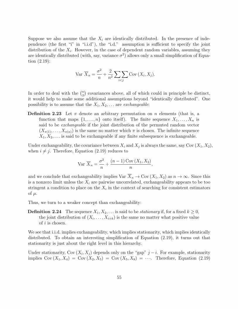
Suppose we also assume that the Xi are identically distributed. In the presence of inde-pendence (the first “i” in “i.i.d”), the “i.d.” assumption is sufficient to specify the jointdistribution of the Xi. However, in the case of dependent random variables, assuming theyare identically distributed (with, say, variance σ2) allows only a small simplification of Equa-tion (2.19):

Var Xn =σ2

n+

2

n2

∑∑i<j

Cov (Xi, Xj).

In order to deal with the(n2

)covariances above, all of which could in principle be distinct,

it would help to make some additional assumptions beyond “identically distributed”. Onepossibility is to assume that the X1, X2, . . . are exchangeable:

Definition 2.23 Let π denote an arbitrary permutation on n elements (that is, afunction that maps 1, . . . , n onto itself). The finite sequence X1, . . . , Xn issaid to be exchangeable if the joint distribution of the permuted random vector(Xπ(1), . . . , Xπ(n)) is the same no matter which π is chosen. The infinite sequenceX1, X2, . . . is said to be exchangeable if any finite subsequence is exchangeable.

Under exchangeability, the covariance betweenXi andXj is always the same, say Cov (X1, X2),when i 6= j. Therefore, Equation (2.19) reduces to

Var Xn =σ2

n+

(n− 1) Cov (X1, X2)

n,

and we conclude that exchangeability implies Var Xn → Cov (X1, X2) as n→∞. Since thisis a nonzero limit unless the Xi are pairwise uncorrelated, exchangeability appears to be toostringent a condition to place on the Xi in the context of searching for consistent estimatorsof µ.

Thus, we turn to a weaker concept than exchangeability:

Definition 2.24 The sequence X1, X2, . . . is said to be stationary if, for a fixed k ≥ 0,the joint distribution of (Xi, . . . , Xi+k) is the same no matter what positive valueof i is chosen.

We see that i.i.d. implies exchangeability, which implies stationarity, which implies identicallydistributed. To obtain an interesting simplification of Equation (2.19), it turns out thatstationarity is just about the right level in this hierarchy.

Under stationarity, Cov (Xi, Xj) depends only on the “gap” j − i. For example, stationarityimplies Cov (X1, X4) = Cov (X2, X5) = Cov (X5, X8) = · · ·. Therefore, Equation (2.19)

55

becomes

Var Xn =σ2

n+

2

n2

n−1∑k=1

(n− k) Cov (X1, X1+k). (2.20)

Lemma 2.25 Expression (2.20) tends to 0 as n→∞ if σ2 <∞ and Cov (X1, X1+k)→0 as k →∞.

Proof: It is immediate that σ2/n → 0 if σ2 < ∞. Assuming that Cov (X1, X1+k) → 0,select ε > 0 and note that if N is chosen so that |Cov (X1, X1+k)| < ε/2 for all k > N , wehave∣∣∣∣∣ 2

n2

n−1∑k=1

(n− k) Cov (X1, X1+k)

∣∣∣∣∣ ≤ 2

n

N∑k=1

|Cov (X1, X1+k)|+2

n

n−1∑k=N+1

|Cov (X1, X1+k)| .

The second term on the right is strictly less than ε/2, and the first term is a constant dividedby n, which may be made smaller than ε/2 by choosing n large enough. (This lemma is alsoa corollary of the result stated in Exercise 1.3.)

Because of Lemma 2.25, it is sensible to impose conditions guaranteeing that Cov (X1, X1+k)tends to zero as k →∞. For instance, we might consider sequences for which Cov (X1, X1+k)is exactly equal to zero for all k larger than some cutoff value, say m. This is the idea ofm-dependence:

Definition 2.26 For a fixed nonnegative integer m, the sequence X1, X2, . . . is calledm-dependent if the random vectors (X1, . . . , Xi) and (Xj, Xj+1, . . .) are indepen-dent whenever j − i > m.

Any stationary m-dependent sequence trivially satisfies Cov (X1, X1+k) → 0 as k → ∞,so by Lemma 2.25, Xn is consistent for any stationary m-dependent sequence with finitevariance. As a special case of m-dependence, any independent sequence is 0-dependent.

Exercises for Section 2.2

Exercise 2.10 The goal of this Exercise is to construct an example of an independent

sequence X1, X2, . . . with E Xi = µ such that XnP→µ but Var Xn does not

converge to 0. There are numerous ways we could proceed, but let us supposethat for some positive constants ci and pi, Xi = ciYi(2Zi − 1), where Yi and Ziare independent Bernoulli random variables with E Yi = pi and E Zi = 1/2.

(a) Verify that E Xi = 0 and find Var Xn.

56

(b) Show that XnP→ 0 if

1

n

n∑i=1

cipi → 0. (2.21)

Hint: Use the triangle inequality to show that if Condition (2.21) is true, thenXn converges in mean to 0 (see Definition 2.15).

(c) Now specify ci and pi so that Var Xn does not converge to 0 but Condition(2.21) holds. Remember that pi must be less than or equal to 1 because it is themean of a Bernoulli random variable.

Exercise 2.11 Suppose thatX1, X2, . . . are independent with mean zero and Var Xi =(i + 1) log(i + 1). Let δn be the minimum variance linear estimator defined inEquation (2.14) and let Xn denote the sample mean. Find the relative efficiencyof δn with respect to Xn (defined as Var Xn/Var δn) for n = 10k, k = 1, . . . , 6.What seems to be happening? Find, with proof, the limits of Var Xn and Var δnas n→∞ to try to verify your conjecture.

Exercise 2.12 Suppose X1, X2, . . . are independent and identically distributed withmean µ and finite variance σ2. Let Yi = X i = (

∑ij=1Xj)/i.

(a) Prove that Y n = (∑n

i=1 Yi)/n is a consistent estimator of µ.

(b) Compute the relative efficiency eY n,Xnof Y n toXn, defined as Var (Xn)/Var (Y n),

for n ∈ 5, 10, 20, 50, 100,∞ and report the results in a table. For n = ∞, givethe limit (with proof) of the efficiency.

Exercise 2.13 Let Y1, Y2, . . . be independent and identically distributed with meanµ and variance σ2 <∞. Let

X1 = Y1, X2 =Y2 + Y3

2, X3 =

Y4 + Y5 + Y63

, etc.

Define δn as in Equation (2.14).

(a) Show that δn and Xn are both consistent estimators of µ.

(b) Calculate the relative efficiency eXn,δnofXn to δn, defined as Var (δn)/Var (Xn),

for n = 5, 10, 20, 50, 100, and ∞ and report the results in a table. For n = ∞,give the limit (with proof) of the efficiency.

(c) Using Example 1.23, give a simple expression asymptotically equivalentto eXn,δn

. Report its values in your table for comparison. How good is theapproximation for small n?

57

Exercise 2.14 Consider the case of simple linear regression in Example 2.22.

(a) Prove that the least squares regression estimators defined in equation (2.16)are unbiased. In other words, show that E β0n = β0 and E β1n = β1.

Hint: Prove and use the facts that∑n

i=1w(n)i = 0 and

∑ni=1w

(n)i zi = 1.

(b) Prove consistency of β0n and β1n under conditions (2.17) and (2.18), respec-tively.

2.3 Convergence of Transformed Sequences

Many statistical estimators of interest may be written as functions of simpler statistics whoseconvergence properties are known. Therefore, results that describe the behavior of trans-formed sequences have central importance for the study of statistical large-sample theory.We begin with some results about continuous transformations of univariate random variablesequences. Yet the important result near the end of this section, called Slutsky’s theorem,is intrinsically multivariate in nature. For this reason, after presenting a few results on con-tinuous transformations, we will extend these and other univariate concepts from earlier inthis chapter to the k-dimensional setting for k > 1.

2.3.1 Continuous Transformations: The Univariate Case

Just as they do for sequences of real numbers, continuous functions preserve convergenceof sequences of random variables. We state this result formally for both convergence inprobability and convergence in distribution.

Theorem 2.27 Suppose that f(x) is a continuous function.

(a) If XnP→X, then f(Xn)

P→ f(X).

(b) If Xnd→X, then f(Xn)

d→ f(X).

Theorem 2.27 is the random-variable analogue of Theorem 1.16, which is proved using astraightforward ε-δ argument. It is therefore surprising that proving Theorem 2.27 is quitedifficult. Indeed, each of its two statements relies on an additional theorem for its proof.For statement (a), this additional theorem (Theorem 3.10) involves almost sure convergence,a mode of convergence not defined until Chapter 3. Statement (b) about convergence indistribution, on the other hand, follows from a powerful characterization of convergence indistribution (its proof is the subject of Exercises 2.15 and 2.16).

58

Theorem 2.28 Xnd→X if and only if E g(Xn) → E g(X) for all bounded and con-

tinuous real-valued functions g(x).

The forward half of Theorem 2.28, the fact that Xnd→X implies E g(Xn)→ E g(X) if g(x)

is bounded and continuous, is called the Helly-Bray theorem. Taken as a whole, the theoremestablishes a condition equivalent to convergence in distribution, and in fact this condition is

sometimes used as the definition of Xnd→X. It is very important to remember that Theorem

2.28 does not say that Xnd→X implies E Xn → E X (because the function g(t) = t, while

certainly continuous, is not bounded). In fact, the special conditions under which Xnd→X

implies E Xn → E X are the subject of Section 3.3.

Using Theorem 2.28, Theorem 2.27(b) follows quickly.

Proof of Theorem 2.27(b) Let g(x) be any bounded and continuous function. ByTheorem 2.28, it suffices to show that E g[f(Xn)] → E g[f(X)]. Since f(x) is continuous,the composition x 7→ g[f(x)] is bounded and continuous. Therefore, another use of Theorem2.28 proves that E g[f(Xn)]→ E g[f(X)] as desired.

2.3.2 Multivariate Extensions

We now extend our notions of random-vector convergence to the multivariate case. Severalearlier results from this chapter, such as the weak law of large numbers and the resultson continuous functions, generalize immediately to this case. Note the use of bold typeto signify random vectors: Whereas Xn and X denote univariate random variables, thepossibly-multidimensional analogues are Xn and X.

A k-dimensional random vector is a function X(ω), usually abbreviated X, that maps aprobability space Ω into k-dimensional Euclidean space Rk. As we remarked in Section1.5, it is not possible to develop a coherent theory if we consider all possible functionsX(ω) to be random vectors; therefore, strictly speaking we must restrict attention only tomeasurable functions X(ω). Yet a reasonable treatment of measurability is beyond the scopeof this book, and instead of delving into technicalities we rest assured that basically everyinteresting function X(ω) is a legitimate random variable. (Indeed, it is a fairly challengingmathematical exercise to construct a nonmeasurable function.)

The multivariate definitions of convergence in probability and convergence in ath meanare both based on the sequence ‖Xn − X‖, which is a univariate sequence, so they arestraightforward and require no additional development:

Definition 2.29 Xn converges in probability to X (written XnP→X) if for any ε > 0,

P (‖Xn −X‖ < ε)→ 1 as n→∞.

59

Definition 2.30 For a > 0, Xn converges in ath mean to X (written Xna→X) if

E ‖Xn −X‖a → 0 as n→∞.

Convergence in quadratic mean, written Xnqm→X, is the special case of Definition 2.30 when

a = 2. Since ‖c‖2 = c>c, Xn converges in quadratic mean to X if

E[(Xn −X)>(Xn −X)

]→ 0 as n→∞. (2.22)

Because Definitions 2.29 and 2.30 rely only on the univariate random variables ‖Xn −X‖,Theorem 2.17 immediately implies that (a) Xn

qm→ c if and only if E ‖Xn − c‖ → 0 and

Var ‖Xn − c‖ → 0; and (b) if Xna→X, then Xn

P→X. However, fact (a) is less useful thanin the univariate setting; consider the comments following the proof of Theorem 2.31 below.

As an immediate application of the above results, we may extend the weak law of largenumbers to the multivariate case. For a sequence X1,X2, . . ., define the nth sample meanto be

Xndef=

1

n

n∑i=1

Xi.

Theorem 2.31 The Weak Law of Large Numbers: Suppose that X1,X2, . . . are in-

dependent and identically distributed and have finite mean µ. Then XnP→µ.

Partial Proof: We do not prove this theorem in full generality until Section 4.1. However,in the special (and very common) case in which the k × k covariance matrix Σ = Var X1

has only finite entries,

E (Xn − µ)>(Xn − µ) =1

n2E

[n∑i=1

(Xi − µ)

]> [ n∑i=1

(Xi − µ)

]

=1

n2

n∑i=1

E (Xi − µ)>(Xi − µ) =1

nTr(Σ)→ 0

as n→∞. Therefore, Xnqm→µ by definition, which implies that Xn

P→µ.

It is instructive to compare the proof outlined in the univariate Example 2.18 to the multi-variate proof above because the former method may not be adapted to the latter situation.It is still true that any unbiased estimator whose covariance matrix converges to the zeromatrix is consistent [by Equation (2.22) with X replaced by E Xn], but an argument for thiscannot easily be based on Theorem 2.17(a): The fact that an estimator like Xn is unbiasedfor µ does not immediately imply that E

∥∥Xn − µ∥∥ = 0.

60

To extend convergence in distribution to random vectors, we need the multivariate analogueof Equation (2.6), the distribution function. To this end, let

F (x)def= P (X ≤ x),

where X is a random vector in Rd and X ≤ x means that Xi ≤ xi for all 1 ≤ i ≤ d.

Definition 2.32 Xn converges in distribution to X (written Xnd→X) if for any point

c at which F (x) is continuous,

Fn(c)→ F (c) as n→∞.

There is one subtle way in which the multivariate situation is not quite the same as theunivariate situation for distribution functions. In the univariate case, it is very easy tocharacterize the points of continuity of F (x): The distribution function of the univariaterandom variable X is continuous at x if and only if P (X = x) = 0. However, this simplecharacterization no longer holds true for random vectors; a point x may be a point ofdiscontinuity yet still satisfy P (X = x) = 0. The task in Exercise 2.18 is to produce anexample of this phenomenon.

We may now extend Theorems 2.13, 2.14, and 2.27 to the multivariate case. The proofsof these results do not differ substantially from their univariate counterparts; all necessarymodifications are straightforward. For instance, in the proofs of Theorems 2.13 and 2.14,the scalar ε should be replaced by the vector ε = ε1, each of whose entries equals ε; withthis change, modified statements such as “whenever Xn ≤ t, it must be true that eitherX ≤ t + ε or ‖Xn −X‖ > ε” remain true.

Theorem 2.33 XnP→X implies Xn

d→X. Furthermore, if c is a constant, then

XnP→ c if and only if Xn

d→ c.

Theorem 2.34 Suppose that f : S → R` is a continuous function defined on somesubset S ⊂ Rk, Xn is a k-component random vector, and P (X ∈ S) = 1.

(a) If XnP→X, then f(Xn)

P→ f(X).

(b) If Xnd→X, then f(Xn)

d→ f(X).

The proof of Theorem 2.34 is basically the same as in the univariate case. For proving part(b), we use the multivariate version of Theorem 2.28:

Theorem 2.35 Xnd→X if and only if E g(Xn) → E g(X) for all bounded and con-

tinuous real-valued functions g : Rk → R.

61

Proving Theorem 2.35 involves a few complications related to the use of multivariate distri-bution functions, but the essential idea is the same as in the univariate case (the univariateproof is the subject of Exercises 2.15 and 2.16).

2.3.3 Slutsky’s Theorem

As we have seen in the preceding few pages, many univariate definitions and results concern-ing convergence of sequences of random vectors are basically the same as in the univariatecase. Here, however, we consider a result that has no one-dimensional analogue.

At issue is the question of when we may “stack” random variables to make random vectorswhile preserving convergence. It is here that we encounter perhaps the biggest surprise ofthis section: Convergence in distribution is not preserved by “stacking”.

To understand what we mean by “stacking” preserving convergence, consider the case ofconvergence in probability. By definition, it is straightforward to show that

XnP→X and Yn

P→Y together imply that

(Xn

Yn

)P→(X

Y

). (2.23)

Thus, two convergent-in-probability sequences Xn and Yn may be stacked, one on top of theother, to make a vector, and this vector must still converge in probability to the vector ofstacked limits.

Example 2.36 Statement (2.23) gives a way to show that the multivariate WeakLaw of Large Numbers (Theorem 2.31) follows immediately from the univariateversion (Theorem 2.19).

Example 2.37 If X1, X2, . . . are independent and identically distributed with mean µand positive variance σ2, we often take as an estimator of σ2 the so-called samplevariance

s2n =1

n− 1

n∑i=1

(Xi −Xn

)2.

We may use Statement (2.23) and Theorem 2.34(a), together with the univariateWeak Law of Large Numbers (Theorem 2.19), to prove that s2n is a consistentestimator of σ2.

To accomplish this, we first rewrite s2n as

s2n =n

n− 1

[1

n

n∑i=1

(Xi − µ)2 − (Xn − µ)2

].

62

The WLLN tells us that Xn − µP→ 0, from which we deduce that (Xn − µ)2

P→ 0by Theorem 2.27(a). Since E (Xi − µ)2 = σ2, the Weak Law also tells us that

(1/n)∑

i(Xi − µ)2P→σ2. Combining these two facts by “stacking” as in (2.23)

yields ( 1n

∑ni=1(Xi − µ)2

(Xn − µ)2

)P→(σ2

0

).

We now apply the continuous function f(a, b) = a− b to both sides of the aboveresult, as allowed by Theorem 2.34(a), to conclude that

1

n

n∑i=1

(Xi − µ)2 − (Xn − µ)2P→σ2 − 0. (2.24)

Finally, we may perform a similar stacking operation using Equation (2.24) to-

gether with the fact that n/(n−1)P→ 1, whereupon multiplication yields the final

conclusion that s2nP→σ2.

If it seems as though we spent too much time in the above proof worrying about“obvious” steps such as stacking followed by addition or multiplication, we did so

in order to make a point: When we replaceP→ by

d→, the “obvious” is no longercorrect.

The converse of (2.23) is true by Theorem 2.27 because the function f(x, y) = x is a con-tinuous function from R2 to R. By induction, we can therefore stack or unstack arbitrarilymany random variables or vectors without distrurbing convergence in probability. Combin-ing this fact with Theorem 2.27 yields a useful result; see Exercise 2.22. By Definition 2.30,

Statement 2.23 remains true if we replaceP→ by

a→ throughout the statement for some a > 0.

However, Statement 2.23 is not true ifP→ is replaced by

d→. Consider the following simplecounterexample.

Example 2.38 Take Xn and Yn to be independent standard normal random variablesfor all n. These distributions do not depend on n at all, and it is correct to write

Xnd→Z and Yn

d→Z, where Z ∼ N(0, 1). But it is certainly not true that(Xn

Yn

)d→(Z

Z

), (2.25)

since the distribution on the left is bivariate normal with correlation 0, while thedistribution on the right is the (degenerate) bivariate normal with correlation 1.

63

Expression (2.25) is untrue precisely because the marginal distributions do not in generaluniquely determine the joint distribution. However, there are certain special cases in whichthe marginals do determine the joint distribution. For instance, if random variables areindependent, then their marginal distributions uniquely determine their joint distribution.Indeed, we can say that if Xn → X and Yn → Y , where Xn is independent of Yn and X is

independent of Y , then statement (2.23) remains true whenP→ is replaced by

d→ (see Exercise2.23). As a special case, the constant c, when viewed as a random variable, is automatically

independent of any other random variable. Since Ynd→ c is equivalent to Yn

P→ c by Theorem2.14, it must be true that

Xnd→X and Yn

P→ c implies that

(Xn

Yn

)d→(X

c

)(2.26)

if Xn is independent of Yn for every n. The content of a powerful theorem called Slutsky’sTheorem is that statement (2.26) remains true even if the Xn and Yn are not independent.Although the preceding discussion involves stacking only random (univariate) variables, wepresent Slutsky’s theorem in a more general version involving random vectors.

Theorem 2.39 Slutsky’s Theorem: For random vectors Xn, Yn, and X and a con-

stant c, if Xnd→X and Yn

P→ c as n→∞, then(Xn

Yn

)d→(

X

c

).

A proof of Theorem 2.39 is outlined in Exercise 2.24.

Putting several of the preceding results together yields the following corollary.

Corollary 2.40 If X is a k-vector such that Xnd→X, and Ynj

P→ cj for 1 ≤ j ≤ m,then

f

(Xn

Yn

)d→ f

(X

c

)for any continuous function f : S ⊂ Rk+m → R`.

It is very common practice in statistics to use Corollary 2.40 to obtain a result, then statethat the result follows “by Slutsky’s Theorem”. In fact, there is not a unanimously heldview in the statistical literature about what precisely “Slutsky’s Theorem” refers to; someconsider the Corollary itself, or particular cases of the Corollary, to be Slutsky’s Theorem.These minor differences are unimportant; the common feature of all references to “Slutsky’sTheorem” is some combination of one sequence that converges in distribution with one ormore sequences that converge in probability to constants.

64

Example 2.41 Asymptotic normality of the t-statistic: Let X1, . . . , Xn be indepen-dent and identically distributed with mean µ and finite positive variance σ2. By

Example 2.12,√n(Xn − µ)

d→N(0, σ2). Suppose that σ2n is any consistent esti-

mator of σ2; that is, σ2nP→σ2. (For instance, we might take σ2

n to be the usualunbiased sample variance estimator s2n of Example 2.37, whose asymptotic prop-erties will be studied later.) If Z denotes a standard normal random variable,Theorem 2.39 implies (√

n(Xn − µ)

σ2n

)d→(σZ

σ2

). (2.27)

Therefore, since f(a, b) = a/b is a continuous function for b > 0 (and σ2 isassumed positive),

√n(Xn − µ)√

σ2n

d→Z. (2.28)

It is common practice to skip step (2.27), attributing equation (2.28) directly to“Slutsky’s Theorem”.

Exercises for Section 2.3

Exercise 2.15 Here we prove half (the “only if” part) of Theorem 2.28: If Xnd→X

and g(x) is a bounded, continuous function on R, then E g(Xn)→ E g(X). (Thishalf of Theorem 2.28 is sometimes called the univariate Helly-Bray Theorem.)

Let Fn(x) and F (x) denote the distribution functions of Xn and X, as usual. Forε > 0, take b < c to be constant real numbers such that F (b) < ε and F (c) > 1−ε.First, we note that since g(x) is continuous, it must be uniformly continuous on[b, c]: That is, for any ε > 0 there exists δ > 0 such that |g(x)−g(y)| < ε whenever|x − y| < δ. This fact, along with the boundedness of g(x), ensures that thereexists a finite set of real numbers b = t0 < t1 < · · · < tm = c such that:

• Each ti is a continuity point of F (x).

• F (t0) < ε and F (tm) > 1− ε.• For 1 ≤ i ≤ m, |g(x)− g(ti)| < ε for all x ∈ [ti−1, ti].

(a) As in Figure 2.1, define

h(x) =g(ti) if ti−1 < x ≤ ti for some 1 ≤ i ≤ m.0 otherwise.

65

−− M

M

t0 == b t1 t2 t3 t4 t5 t6 == c

Figure 2.1: The solid curve is the function g(x), assumed to be bounded by −M and M forall x, and the horizontal segments are the function h(x). The points t0, . . . , t6 are chosen sothat |g(x)− h(x)| is always less than ε. The ti are continuity points of F (x), and both F (t0)and 1− F (t6) are less than ε.

Prove that there exists N such that |E h(Xn)− E h(X)| < ε for all n > N .

Hint: Use the fact that for any random variable Y ,

E h(Y ) =m∑i=1

g(ti)P (ti−1 < Y ≤ ti).

Also, please note that we may not write E h(Xn)− E h(X) as E [h(Xn)− h(X)]because it is not necessarily the case that Xn and X are defined on the samesample space.

(b) Prove that E g(Xn)→ E g(X).

Hint: Use the fact that

|E g(Xn)− E g(X)| ≤ |E g(Xn)− E h(Xn)|+ |E h(Xn)− E h(X)|+|E h(X)− E g(X)|.

Exercise 2.16 Prove the other half (the “if” part) of Theorem 2.28, which statesthat if E g(Xn)→ E g(X) for all bounded, continuous functions g : R→ R, then

Xnd→X.

66

(a) Let t be any continuity point of F (x). Let ε > 0 be arbitrary. Show thatthere exists δ > 0 such that F (t− δ) > F (t)− ε and F (t+ δ) < F (t) + ε.

(b) Show how to define continuous functions g1 : R → [0, 1] and g2 : R → [0, 1]such that for all x ≤ t, g1(x) = g2(x − δ) = 1 and for all x > t, g1(x + δ) =g2(x) = 0. Use these functions to bound the difference between Fn(t) and F (t)in such a way that this difference must tend to 0.

Exercise 2.17 To illustrate a situation that can arise in the multivariate settingthat cannot arise in the univariate setting, construct an example of a sequence(Xn, Yn), a joint distribution (X, Y ), and a connected subset S ∈ R2 such that

(i) (Xn, Yn)d→(X, Y );

(ii) every point of R2 is a continuity point of the distribution function of (X, Y );

(iii) P [(Xn, Yn) ∈ S] does not converge to P [(X, Y ) ∈ S].

Hint: Condition (ii) may be satisfied even if the distribution of (X, Y ) is con-centrated on a line.

Exercise 2.18 If X is a univariate random variable with distribution function F (x),then F (x) is continuous at c if and only if P (X = c) = 0. Prove by counterex-ample that this is not true if variables X and c are replaced by vectors X andc.

Exercise 2.19 Suppose that (X, Y ) is a bivariate normal vector such that both X andY are marginally standard normal and Corr (X, Y ) = ρ. Construct a computerprogram that simulates the distribution function Fρ(x, y) of the joint distributionof X and Y . For a given (x, y), the program should generate at least 50,000random realizations from the distribution of (X, Y ), then report the proportionfor which (X, Y ) ≤ (x, y). (If you wish, you can also report a confidence intervalfor the true value.) Use your function to approximate F.5(1, 1), F.25(−1,−1), andF.75(0, 0). As a check of your program, you can try it on F0(x, y), whose truevalues are not hard to calculate directly for an arbitrary x and y assuming yoursoftware has the ability to evaluate the standard normal distribution function.

Hint: To generate a bivariate normal random vector (X, Y ) with covariance

matrix

(1 ρρ 1

), start with independent standard normal U and V , then take

X = U and Y = ρU +√

1− ρ2V .

Exercise 2.20 Adapt the method of proof in Exercise 2.15 to the multivariate case,

proving half of Theorem 2.35: If Xnd→X, then E g(Xn) → E g(X) for any

67

bounded, continuous g : Rk → R.

Hint: Instead of intervals (ai−1, ai] as in Exercise 2.15, use small regions x :ai,j−1 < xi ≤ ai,j for all i of Rk. Make sure these regions are chosen so that theirboundaries contain only continuity points of F (x).

Exercise 2.21 Construct a counterexample to show that Slutsky’s Theorem 2.39 may

not be strengthened by changing YnP→ c to Yn

P→Y .

Exercise 2.22 (a) Prove that if f : Rk → R` is continuous and XnjP→Xj for all

1 ≤ j ≤ k, then f(Xn)P→ f(X).

(b) Taking f(a, b) = a + b for simplicity, construct an example demonstrating

that part (a) is not true ifP→ is replaced by

d→.

Exercise 2.23 Prove that if Xn is independent of Yn for all n and X is independentof Y , then

Xnd→X and Yn

d→Y implies that

(Xn

Yn

)d→(X

Y

).

Hint: Be careful to deal with points of discontinuity: If Xn and Yn are indepen-dent, what characterizes a point of discontinuity of the joint distribution?

Exercise 2.24 Prove Slutsky’s Theorem, Theorem 2.39, using the following approach:

(a) Prove the following lemma:

Lemma 2.42 Let Vn and Wn be k-dimensional random vectors on thesame sample space.

If Vnd→V and Wn

P→0, then Vn + Wnd→V.

Hint: For ε > 0, let ε denote the k-vector all of whose entries are ε. Takea ∈ Rk to be a continuity point of FV(v). Now argue that a, since it is a pointof continuity, must be contained in a neighborhood consisting only of points ofcontinuity; therefore, ε may be taken small enough so that a − ε and a + ε arealso points of continuity. Prove that

P (Vn ≤ a− ε)− P (‖Wn‖ ≥ ε) ≤ P (Vn + Wn ≤ a)

≤ P (Vn ≤ a + ε) + P (‖Wn‖ ≥ ε).

Next, take lim supn and lim infn. Finally, let ε→ 0.

68

(b) Show how to prove Theorem 2.39 using Lemma 2.42.

Hint: Consider the random vectors

Vn =

(Xn

c

)and Wn =

(0

Yn − c

).

69

Chapter 3

Strong convergence

There are multiple ways to define the convergence of a sequence of random variables. Chapter2 introduced convergence in probability, convergence in distribution, and convergence inquadratic mean. We now consider a fourth mode of convergence, almost sure convergenceor convergence with probability one. We will see that almost sure convergence implies bothconvergence in probability and convergence in distribution, which is why we sometimes usethe term “strong” for almost sure convergence and “weak” for the other two.

The terms “weak” and “strong” do not indicate anything about their importance; indeed,the “weak” modes of convergence are used much more frequently in asymptotic statisticsthan the strong mode. Because weak convergence dominates the remainder of this bookbeginning with Chapter 4, a reader may safely skip much of the material in the currentchapter if time is limited; however, the quantile function and the Dominated ConvergenceTheorem of Section 3.3 are used elsewhere, and at least these topics should be reviewedbefore moving on. Due to the technical nature of the material of this chapter, the exercisesare almost exclusively devoted to proofs.

3.1 Strong Consistency Defined

A random variable like Xn or X is a function on a sample space, say Ω. Suppose that wefix a particular element of that space, say ω0, so we obtain the real numbers Xn(ω0) andX(ω0). If Xn(ω0)→ X(ω0) as n→∞ in the sense of Definition 1.1, then ω0 is contained inthe event

S = ω ∈ Ω : Xn(ω)→ X(ω). (3.1)

70

If the probability of S—that is, E IXn → X—equals 1, then we say that Xn convergesalmost surely to X:

Definition 3.1 Suppose X and X1, X2, . . . are random variables defined on the samesample space Ω (and as usual P denotes the associated probability measure). If

P (ω ∈ Ω : Xn(ω)→ X(ω)) = 1,

then Xn is said to converge almost surely (or with probability one) to X, denotedXn

a.s.→X or Xn→X a.s. or Xn→X w.p. 1.

In other words, convergence with probability one means exactly what it sounds like: Theprobability that Xn converges to X equals one. Later, in Theorem 3.3, we will formulatean equivalent definition of almost sure convergence that makes it much easier to see whyit is such a strong form of convergence of random variables. Yet the intuitive simplicity ofDefinition 3.1 makes it the standard definition.

As in the case of convergence in probability, we may replace the limiting random variableX by any constant c, in which case we write Xn

a.s.→ c. In the most common statistical usageof convergence to a constant, the random variable Xn is some estimator of a particularparameter, say θ:

Definition 3.2 If Xna.s.→ θ, Xn is said to be strongly consistent for θ.

As the names suggest, strong consistency implies consistency (also known as weak consis-tency), a fact we now explore in more depth.

3.1.1 Strong Consistency versus Consistency

As before, suppose that X and X1, X2, . . . are random variables defined on the same samplespace, Ω. For given n and ε > 0, define the events

An = ω ∈ Ω : |Xk(ω)−X(ω)| < ε for all k ≥ n (3.2)

and

Bn = ω ∈ Ω : |Xn(ω)−X(ω)| < ε. (3.3)

First, note that An must be contained in Bn and that both An and Bn imply that Xn is closeto X as long as ε is small. Therefore, both P (An)→ 1 and P (Bn)→ 1 seem like reasonableways to define the convergence of Xn to X. Indeed, as we have already seen in Definition2.1, convergence in probability means precisely that P (Bn)→ 1 for any ε > 0.

Yet what about the sets An? One fact is immediate: Since An ⊂ Bn, we must haveP (An) ≤ P (Bn). Therefore, P (An) → 1 implies P (Bn) → 1. In other words, if we were to

71

take P (An) → 1 for all ε > 0 to be the definition of a new form of convergence of randomsequences, then this form of convergence would be stronger than (i.e., it would imply) con-vergence in probability. By now, the reader may already have guessed that this new form ofconvergence is actually equivalent to almost sure convergence:

Theorem 3.3 With An defined as in Equation (3.2), P (An)→ 1 for any ε > 0 if andonly if Xn

a.s.→X.

Proving Theorem 3.3 is the subject of Exercise 3.1. The following corollary now follows fromthe preceding discussion:

Corollary 3.4 If Xna.s.→X, then Xn

P→X.

The converse of Corollary 3.4 is not true, as the following example illustrates.

...and so on

0 1

J1

J2

J3

J4

J5

J6

J7

J8

J9

J10

J11

J12

J13

J14

J15

J16

J17

J18

J19

J20

J21

J22

J23

J24

J25

Figure 3.1: Example 3.5, in which P (Jn) → 0 as n → ∞, which means that IJnP→ 0.

However, the intervals Jn repeatedly cover the entire interval (0, 1], so the subset of (0, 1] onwhich IJn converges to 0 is empty!

Example 3.5 Take Ω to be the half-open interval (0, 1], and for any interval J ⊂ Ω,say J = (a, b], take P (J) = b − a to be the length of that interval. Define asequence of intervals J1, J2, . . . as follows (see Figure 3.1):

J1 = (0, 1]

J2 through J4 = (0, 13] , ( 1

3, 23] , ( 2

3,1]

72

J5 through J9 = (0, 15] , ( 1

5, 25] , ( 2

5, 35] , ( 3

5, 45] , ( 4

5,1]

...

Jm2+1 through J(m+1)2 =

(0,

1

2m+ 1

], . . . ,

(2m

2m+ 1, 1

]...

Note in particular that P (Jn) = 1/(2m + 1), where m = b√n− 1c is the largest

integer not greater than√n− 1. Now, define Xn = IJn and take 0 < ε < 1.

Then P (|Xn − 0| < ε) is the same as 1 − P (Jn). Since P (Jn) → 0, we conclude

XnP→ 0 by definition.

However, it is not true that Xna.s.→ 0. Since every ω ∈ Ω is contained in infinitely

many Jn, the set An defined in Equation (3.2) is empty for all n. Alternatively,consider the set S = ω : Xn(ω) → 0. For any ω, Xn(ω) has no limit becauseXn(ω) = 1 and Xn(ω) = 0 both occur for infinitely many n. Thus S is empty.This is not convergence with probability one; it is convergence with probabilityzero!

3.1.2 Multivariate Extensions

We may extend Definition 3.1 to the multivariate case in a completely straightforward way:

Definition 3.6 Xn is said to converge almost surely (or with probability one) to X(Xn

a.s.→X) if

P (Xn → X as n→∞) = 1.

Alternatively, since the proof of Theorem 3.3 applies to random vectors as wellas random variables, we say Xn

a.s.→X if for any ε > 0,

P (‖Xk −X‖ < ε for all k ≥ n)→ 1 as n→∞. (3.4)

We saw in Theorems 2.27 and 2.34 that continuous functions preserve both convergence inprobability and convergence in distribution. Yet these facts were quite difficult to prove.Fortunately, the analogous result for almost sure convergence follows immediately from theresults of Chapter 1. Similarly, unlike with convergence in distribution, there is no problem“stacking” random sequences into vectors while preserving almost sure convergence. Thefollowing theorem is really just a corollary of earlier results (specifically, Theorem 1.16 andLemma 1.33).

73

Theorem 3.7 (a) Suppose that f : S → R` is a continuous function defined on somesubset S ⊂ Rk, Xn is a k-component random vector, and the range of X and ofeach Xn is contained in S with probability 1. If Xn

a.s.→X, then f(Xn)a.s.→ f(X).

(b) Xna.s.→X if and only if Xnj

a.s.→Xj for all j.

We conclude this section with a simple diagram summarizing the implications among themodes of convergence defined so far. In the diagram, a double arrow like⇒ means “implies”.Note that the picture changes slightly when convergence is to a constant c rather than arandom vector X.

Xnqm→X⇓

Xna.s.→X ⇒ Xn

P→X ⇒ Xnd→X

Xnqm→ c⇓

Xna.s.→ c ⇒ Xn

P→ c ⇔ Xnd→ c

Exercises for Section 3.1Exercise 3.1 Let S be the set defined in equation (3.1), so Xn

a.s.→X is equivalent toP (S) = 1 by definition.

(a) Let An be defined as in Equation (3.2). Prove that

ω0 ∈ ∪∞n=1An for all ε > 0

if and only if ω0 ∈ S.

Hint: Use Definition 1.1.

(b) Prove Theorem 3.3.

Hint: Note that the sets An are increasing in n, so that by the lower continuityof any probability measure (which you may assume without proof), limn P (An)exists and is equal to P (∪∞n=1An).

Exercise 3.2 The diagram at the end of this section suggests that neither Xna.s.→X

nor Xnqm→X implies the other. Construct two counterexamples, one to show that

Xna.s.→X does not imply Xn

qm→X and the other to show that Xnqm→X does not

imply Xna.s.→X.

3.2 The Strong Law of Large Numbers

Some of the results in this section are presented for univariate random variables and some arepresented for random vectors. Take note of the use of bold print to denote vectors. Nearly

74

all of the technical proofs are posed as exercises (with hints, of course).

Theorem 3.8 Strong Law of Large Numbers: Suppose that X1,X2, . . . are indepen-dent and identically distributed and have finite mean µ. Then Xn

a.s.→µ.

It is possible to use fairly simple arguments to prove a version of the Strong Law under morerestrictive assumptions than those given above. See Exercise 3.4 for details of a proof of theunivariate Strong Law under the additional assumption that E X4

n <∞. To aid the proof ofthe Strong Law, with or without such an additional assumption, we first establish a usefullemma.

Lemma 3.9 If∑∞

k=1 P (‖Xk −X‖ > ε) <∞ for any ε > 0, then Xna.s.→X.

Proof: The proof relies on the countable subadditivity of any probability measure, an axiomstating that for any sequence C1, C2, . . . of events,

P

(∞⋃k=1

Ck

)≤

∞∑k=1

P (Ck). (3.5)

To prove the lemma using (3.4), we must demonstrate that P (‖Xk −X‖ ≤ ε for all k ≥ n)→1 as n→∞, which (taking complements) is equivalent to P (‖Xk −X‖ > ε for some k ≥ n)→0. Letting Ck denote the event that ‖Xk −X‖ > ε, countable subadditivity implies

P (Ck for some k ≥ n) = P

(∞⋃k=n

Ck

)≤

∞∑k=n

P (Ck) ,

and the right hand side tends to 0 as n→∞ because it is the tail of a convergent series.

Lemma 3.9 is nearly the same as a famous result called the First Borel-Cantelli Lemma,or sometimes simply the Borel-Cantelli Lemma; see Exercise 3.3. Lemma 3.9 is extremelyuseful for establishing almost sure convergence of sequences. As an illustration of the type ofresult this lemma helps to prove, consider the following theorem (see Exercise 3.8 for hintson how to prove it).

Theorem 3.10 XnP→X if and only if each subsequence Xn1 ,Xn2 , . . . contains a fur-

ther subsequence that converges almost surely to X.

Using Theorem 3.10, it is now—finally—possible to prove that continuous transformationspreserve convergence in probability. This fact was stated in Theorem 2.27(a) (for the uni-variate case) and Theorem 2.34(a) (for the multivariate case). It suffices to complete theproof for the multivariate case.

Proof of Theorem 2.34(a): If XnP→X and f(x) is continuous, it suffices to prove

that each subsequence f(Xn1), f(Xn2), . . . contains a further subsequence that converges

75

almost surely to f(X). But we know that Xn1 ,Xn2 , . . . must contain a further subsequence,say Xni(1) ,Xni(2) , . . ., such that Xni(j)

a.s.→X and therefore f(Xni(j))a.s.→ f(X) as j → ∞ by

Theorem 3.7(a). This proves the theorem!

To conclude this section, we provide a proof of the Strong Law (Theorem 3.8). The approachwe give here is based on a powerful theorem of Kolmogorov:

Theorem 3.11 Kolmogorov’s Strong Law of Large Numbers: Suppose thatX1, X2, . . .are independent with mean µ and

∞∑i=1

Var Xi

i2<∞.

Then Xna.s.→ µ.

Note that there is no reason the Xi in Theorem 3.11 must have the same means: If E Xi = µi,then the conclusion of the theorem becomes (1/n)

∑i(Xi − µi)

a.s.→ 0. Theorem 3.11 may beproved using Kolmogorov’s inequality from Exercise 1.41; this proof is the focus of Exercise3.7.

The key to completing the Strong Law of Large Numbers for an independent and identicallydistributed sequence using Theorem 3.11 is to introduce truncated versions of X1, X2, . . . asin the following lemmas, which are proved in Exercises 3.5 and 3.6.

Lemma 3.12 Suppose that X1, X2, . . . are independent and identically distributedand have finite mean µ. Define X∗i = XiI|Xi| ≤ i. Then

∞∑i=1

Var X∗ii2

<∞. (3.6)

Lemma 3.13 Under the assumptions of Lemma 3.12, let X∗n = (1/n)

∑ni=1X

∗i . Then

Xn −X∗na.s.→ 0.

Finally, it is possible to put the preceding results together to prove the Strong Law of LargeNumbers:

Proof of Theorem 3.8: Let X1, X2, . . . be independent and identically distributed withfinite mean µ, and let X∗i = XiI|Xi| ≤ i. Then Lemma 3.12 and Theorem 3.11 togetherimply that X

∗na.s.→ µ. From Lemma 3.13, we obtain Xn − X

∗na.s.→ 0. Adding these two limit

statements (which is legal because of Theorem 3.7), we obtain

Xn = X∗n + (Xn −X

∗n)

a.s.→ µ,

which establishes the Strong Law for the univariate case. Since “stacking” sequences presentsno problems for almost sure convergence [Theorem 3.7(b)], the multivariate version followsimmediately.

76

Exercises for Section 3.2

Exercise 3.3 Let B1, B2, . . . denote a sequence of events. Let Bn i.o., which standsfor Bn infinitely often, denote the set

Bn i.o.def= ω ∈ Ω : for every n, there exists k ≥ n such that ω ∈ Bk.

Prove the First Borel-Cantelli Lemma, which states that if∑∞

n=1 P (Bn) < ∞,then P (Bn i.o.) = 0.

Hint: Argue that

Bn i.o. =∞⋂n=1

∞⋃k=n

Bk,

then adapt the proof of Lemma 3.9.

Exercise 3.4 Use the steps below to prove a version of the Strong Law of LargeNumbers for the special case in which the random variables X1, X2, . . . have afinite fourth moment, E X4

1 <∞.

(a) Assume without loss of generality that E X1 = 0. Expand E (X1+ . . .+Xn)4

and then count the nonzero terms.

Hint: The only nonzero terms are of the form E X4i or (E X2

i )2.

(b) Use Markov’s inequality (1.35) with r = 4 to put an upper bound on

P(∣∣Xn

∣∣ > ε)

involving E (X1 + . . .+Xn)4.

(c) Combine parts (a) and (b) with Lemma 3.9 to show that Xna.s.→ 0.

Hint: Use the fact that∑∞

n=1 n−2 <∞.

Exercise 3.5 Lemmas 3.12 and 3.13 make two assertions about the random vari-ables X∗i = XiI|Xi| ≤ i, where X1, X2, . . . are independent and identicallydistributed with finite mean µ.

(a) Prove that for an arbitrary real number c,

c2∞∑i=1

1

i2I|c| ≤ i ≤ 1 + |c|.

Hint: Bound the sum on the left hand side by an easy-to-evaluate integral.

77

(b) Prove Lemma 3.12, which states that

∞∑i=1

Var X∗ii2

<∞.

Hint: Use the fact that

Var X∗i ≤ E (X∗i )2 = E X21I|X1| ≤ i

together with part (a) and the fact that E |X1| <∞.

Exercise 3.6 Assume the conditions of Exercise 3.5.

(a) Prove that Xn −X∗na.s.→ 0.

Hint: Note that Xn and X∗n do not have bars here. Use Exercise 1.45 togetherwith Lemma 3.9.

(b) Prove Lemma 3.13, which states that

Xn −X∗na.s.→ 0.

Hint: Use Exercise 1.3.

Exercise 3.7 Prove Theorem 3.11. Use the following steps:

(a) For k = 1, 2, . . ., define

Yk = max2k−1≤n<2k

|Xn − µ|.

Use the Kolmogorov inequality from Exercise 1.41 to show that

P (Yk ≥ ε) ≤ 4∑2k

i=1 Var Xi

4kε2.

(b) Use Lemma 3.9 to show that Yka.s.→ 0, then argue that this proves Xn

a.s.→ µ.

Hint: Letting dlog2 ie denote the smallest integer greater than or equal to log2 i(the base-2 logarithm of i), verify and use the fact that

∞∑k=dlog2 ie

1

4k≤ 4

3i2.

78

Exercise 3.8 Prove Theorem 3.10:

(a) To simplify notation, let Y1 = Xn1 ,Y2 = Xn2 , . . . denote an arbitrarysubseqence of X1,X2, . . ..

Prove the “only if” part of Theorem 3.10, which states that if XnP→X, then there

exists a subsequence Ym1 ,Ym2 , . . . such that Ymja.s.→X as j →∞.

Hint: Show that there exist m1,m2, . . . such that

P (‖Ymj −X‖ > ε) <1

2j,

then use Lemma 3.9.

(b) Now prove the “if” part of the theorem by arguing that if Xn does notconverge in probability to X, there exists a subsequence Y1 = Xn1 ,Y2 = Xn2 , . . .and ε > 0 such that

P (‖Yk −X‖ > ε) > ε

for all k. Then use Corollary 3.4 to argue that Y1,Y2, . . . does not have asubsequence that converges almost surely.

3.3 The Dominated Convergence Theorem

In this section, the key question is this: When does Xnd→X imply E Xn → E X? The

answer to this question impacts numerous results in statistical large-sample theory. Yetbecause the question involves only convergence in distribution, it may seem odd that it isbeing asked here, in the chapter on almost sure convergence. We will see that one of the

most useful conditions under which E Xn → E X follows from Xnd→X, the Dominated

Convergence Theorem, is proved using almost sure convergence.

3.3.1 Moments Do Not Always Converge

It is easy to construct cases in which Xnd→X does not imply E Xn → E X, and perhaps

the easiest way to construct such examples is to recall that if X is a constant, thend→X and

P→X are equivalent: For XnP→ c means only that Xn is close to c with probability approaching

one. What happens to Xn when it is not close to c can have an arbitrarily extreme influence

on the mean of Xn. In other words, XnP→ c certainly does not imply that E Xn → c, as the

next two examples show.

79

Example 3.14 Suppose that U is a standard uniform random variable. Define

Xn = nI U < 1/n =

n with probability 1/n0 with probability 1− 1/n.

(3.7)

We see immediately that XnP→ 0 as n→∞, but the mean of Xn, which is 1 for

all n, is certainly not converging to zero!. Furthermore, we may generalize thisexample by defining

Xn = cnI U < pn =

cn with probability pn0 with probability 1− pn.

In this case, a sufficient condition for XnP→ 0 is pn → 0. But the mean E Xn =

cnpn may be specified arbitrarily by an appropriate choice of cn, no matter whatnonzero value pn takes.

Example 3.15 Let Xn be a contaminated standard normal distribution with mixturedistribution function

Fn(x) =

(1− 1

n

)Φ(x) +

1

nGn(x), (3.8)

where Φ(x) denotes the standard normal distribution function. No matter how

the distribution functions Gn are defined, Xnd→Φ. However, letting µn denote

the mean of Gn, E Xn = µn/n may be set arbitrarily by an appropriate choice ofGn.

Consider Example 3.14, specifically Equation (3.7), once again. Note that each Xn in thatexample can take only two values, 0 or n. In particular, each Xn is bounded, as is anyrandom variable with finite support. Yet taken as a sequence, the Xn are not uniformlybounded—that is, there is no single constant that bounds all of the Xn simultaneously.

On the other hand, suppose that a sequence X1, X2, . . . does have some uniform bound, say,M such that |Xn| ≤M for all n. Then define the following function:

g(t) =

M if t > Mt if |t| ≤M−M if t < −M .

Note that g(t) is bounded and continuous. Therefore, Xnd→X implies that E g(Xn) →

E g(X) by the Helly-Bray Theorem (see Theorem 2.28). Because of the uniform bound onthe Xn, we know that g(Xn) is always equal to Xn. We conclude that E Xn → E g(X), andfurthermore it is not difficult to show that |X| must be bounded by M with probability 1, soE g(X) = E X. We may summarize this argument by the following Corollary of Theorem2.28:

80

Corollary 3.16 If X1, X2, . . . are uniformly bounded (i.e., there exists M such that

|Xn| < M for all n) and Xnd→X, then E Xn → E X.

Corollary 3.16 gives a vague sense of the type of condition—a uniform bound on the Xn—

sufficient to ensure that Xnd→X implies E Xn → E X. However, the corollary is not very

broadly applicable, since many common random variables are not bounded. In Example3.15, for instance, the Xn could not possibly have a uniform bound (no matter how the Gn

are defined) because the standard normal component of each random vector is supportedon all of R and is therefore not bounded. It is thus desirable to generalize the idea ofa “uniform bound” of a sequence. There are multiple ways to do this, but probably thebest-known generalization is the Dominated Convergence Theorem introduced later in thissection. To prove this important theorem, we must first introduce quantile functions andanother theorem called the Skorohod Representation Theorem.

3.3.2 Quantile Functions and the Skorohod Representation The-orem

Roughly speaking, the q quantile of a variable X, for some q ∈ (0, 1), is a value ξq suchthat P (X ≤ ξq) = q. Therefore, if F (x) denotes the distribution function of X, we ought todefine ξq = F−1(q). However, not all distribution functions F (x) have well-defined inversefunctions F−1(q). To understand why not, consider Example 3.17.

Example 3.17 Suppose that U ∼ Uniform(0, 1) and V ∼ Binomial(2, 0.5) are inde-pendent random variables. Let X = V/4 +UV 2/8. The properties of X are mosteasily understood by noticing that X is either a constant 0, uniform on (1/4, 3/8),or uniform on (1/2, 1), conditional on V = 0, V = 1, or V = 2, respectively. Thedistribution function of X, F (x), is shown in Figure 3.2.

There are two problems that can arise when trying to define F−1(q) for an ar-bitrary q ∈ (0, 1) and an arbitrary distribution function F (x), and the currentexample suffers from both: First, in the range q ∈ (0, 1/4), there is no x for whichF (x) equals q because F (x) jumps from 0 to 1/4 at x = 0. Second, for q = 1/4or q = 3/4, there is not a unique x for which F (x) equals q because F (x) is flat(constant) at 1/4 and again at 3/4 for whole intervals of x values.

From Example 3.17, we see that a meaningful general inverse of a distribution function mustdeal both with “jumps” and “flat spots”. The following definition does this.

Definition 3.18 If F (x) is a distribution function, then we define the quantile func-

81

0.0 0.5 1.0

0.0

0.5

1.0

Figure 3.2: The solid line is a distribution function F (x) that does not have a uniquelydefined inverse F−1(q) for all q ∈ (0, 1). However, the dotted quantile function F−(q) ofDefinition 3.18 is well-defined. Note that F−(q) is the reflection of F (x) over the line q = x,so “jumps” in F (x) correspond to “flat spots” in F−(q) and vice versa.

tion F− : (0, 1)→ R by

F−(q)def= infx ∈ R : q ≤ F (x). (3.9)

With the quantile function thus defined, we may prove a useful lemma:

Lemma 3.19 q ≤ F (x) if and only if F−(q) ≤ x.

Proof: Using the facts that F−(·) is nondecreasing and F−[F (x)] ≤ x by definition,

q ≤ F (x) implies F−(q) ≤ F−[F (x)] ≤ x,

which proves the “only if” statement. Conversely, assume that F−(q) ≤ x. Since F (·) isnondecreasing, we may apply it to both sides of the inequality to obtain

F [F−(q)] ≤ F (x).

Thus, q ≤ F (x) follows if we can prove that q ≤ F [F−(q)]. To this end, consider theset x ∈ R : q ≤ F (x) in Equation (3.9). Because any distribution function is right-continuous, this set always contains its infimum, which is F−(q) by definition. This provesthat q ≤ F [F−(q)].

82

Corollary 3.20 If X is a random variable with distribution function F (x) and U isa uniform(0, 1) random variable, then X and F−(U) have the same distribution.

Proof: For any x ∈ R, Lemma 3.19 implies that

P [F−(U) ≤ x] = P [U ≤ F (x)] = F (x).

Assume now that X1, X2, . . . is a sequence of random variables converging in distribution toX, and let Fn(x) and F (x) denote the distribution functions of Xn and X, respectively. Wewill show how to construct a new sequence Y1, Y2, . . . such that Yn

a.s.→ Y and Yn ∼ Fn(·) andY ∼ F (·).

Take Ω = (0, 1) to be a sample space and adopt the probability measure that assigns to eachinterval subset (a, b) ⊂ Ω its length (b− a). [There is a unique probability measure on (0, 1)with this property, a fact we do not prove here.] Then for every ω ∈ Ω, define

Yn(ω)def= F−n (ω) and Y (ω)

def= F−(ω). (3.10)

Note that the random variable defined by U(ω) = ω is a uniform(0, 1) random variable,so Corollary 3.20 demonstrates that Yn ∼ Fn(·) and Y ∼ F (·). It remains to prove thatYn

a.s.→ Y , but once this is proven we will have established the following theorem:

Theorem 3.21 Skorohod Representation Theorem: Assume F, F1, F2, . . . are distri-

bution functions and Fnd→F . Then there exist random variables Y, Y1, Y2, . . .

such that

1. P (Yn ≤ t) = Fn(t) for all n and P (Y ≤ t) = F (t);

2. Yna.s.→ Y .

A completion of the proof of Theorem 3.21 is the subject of Exercise 3.10.

Having thus established the Skorohod Represenation Theorem, we now introduce the Dom-inated Convergence Theorem.

Theorem 3.22 Dominated Convergence Theorem: If for a nonnegative random vari-

able Z, |Xn| ≤ Z for all n and E Z <∞, then Xnd→X implies that E Xn → E X.

Proof: Use the Skorohod Representation Theorem to construct a sequence Yn converging to

Y almost surely such that Ynd=Xn for all n and Y

d=X. Furthermore, construct a nonnegative

random variable Z∗ on the same sample space satisfying Z∗d=Z and |Yn| ≤ Z∗; this is

possible by defining Z∗ = supn |Yn| + W , where W is constructed to have the distribution

83

of Z − supn |Xn| using the idea of expression (3.10). In other words, we now have Yna.s.→ Y ,

|Yn| ≤ Z∗, and E Z∗ <∞. Since E Xn = E Yn for all n and E X = E Y , it suffices to provenow that E Yn → E Y .

Fatou’s Lemma (see Exercise 3.11) states that

E lim infn|Yn| ≤ lim inf

nE |Yn|. (3.11)

A second application of Fatou’s Lemma to the nonnegative random variables Z∗−|Yn| implies

E Z∗ − E lim supn|Yn| ≤ E Z∗ − lim sup

nE |Yn|.

Because E Z∗ <∞, subtracting E Z∗ preserves the inequality, so we obtain

lim supn

E |Yn| ≤ E lim supn|Yn|. (3.12)

Together, inequalities (3.11) and (3.12) imply

E lim infn|Yn| ≤ lim inf

nE |Yn| ≤ lim sup

nE |Yn| ≤ E lim sup

n|Yn|.

Since Yna.s.→ Y , both lim infn |Yn| and lim supn |Yn| are equal to |Y | with probability one, so

we conclude that lim E |Yn| exists and is equal to E |Y |.

The Dominated Convergence Theorem essentially tells us when it is possible to interchangethe operations of limit and expectation, that is, when the limit of the expectations (of theXn) equals the expectation of their limit.

Exercises for Section 3.3

Exercise 3.9 Prove that any nondecreasing function must have countably many pointsof discontinuity. (This fact is used in proving the Skorohod Representation The-orem.)

Hint: Use the fact that the set of rational numbers is a countably infinite setand that any real interval must contain a rational number.

Exercise 3.10 To complete the proof of Theorem 3.21, it only remains to show thatYn

a.s.→ Y , where Yn and Y are defined as in Equation (3.10).

(a) Let δ > 0 and ω ∈ (0, 1) be arbitrary. Show that there exists N1 such that

Y (ω)− δ < Yn(ω) (3.13)

84

for all n > N1.

Hint: There exists a point of continuity of F (x), say x0, such that

Y (ω)− δ < x0 < Y (ω).

Use the fact that Fn(x0) → F (x0) together with Lemma 3.19 to show how thisfact leads to the desired conclusion.

(b) Take δ and ω as in part (a) and let ε > 0 be arbitrary. Show that thereexists N2 such that

Yn(ω) < Y (ω + ε) + δ (3.14)

for all n > N2.

Hint: There exists a point of continuity of F (x), say x1, such that

Y (ω + ε) < x1 < Y (ω + ε) + δ.

Use the fact that Fn(x1) → F (x1) together with Lemma 3.19 to show how thisfact leads to the desired conclusion.

(c) Suppose that ω ∈ (0, 1) is a continuity point of F (x). Prove that Yn(ω) →Y (ω).

Hint: Take lim infn in Inequality (3.13) and lim supn in Inequality (3.14). Putthese inequalities together, then let δ → 0. Finally, let ε→ 0.

(d) Use Exercise 3.9 to prove that Yna.s.→ Y .

Hint: Use countable subadditivity, Inequality (3.5), to show that the set ofdiscontinuity points of F (x) has probability zero.

Exercise 3.11 Prove Fatou’s lemma:

E lim infn|Xn| ≤ lim inf

nE |Xn|. (3.15)

Hint: Argue that E |Xn| ≥ E infk≥n |Xk|, then take the limit inferior of eachside. Use (without proof) the monotone convergence property of the expectationoperator: If

0 ≤ X1(ω) ≤ X2(ω) ≤ · · · and Xn(ω)→ X(ω) for all ω ∈ Ω,

then E Xn → E X.

85

Exercise 3.12 If Ynd→Y , a sufficient condition for E Yn → E Y is the uniform

integrability of the Yn.

Definition 3.23 The sequence Y1, Y2, . . . of random variables is said tobe uniformly integrable if

supnE (|Yn| I|Yn| ≥ α)→ 0 as α→∞.

Use the following steps to prove that if Ynd→Y and the Yn are uniformly inte-

grable, then E Yn → E Y .

(a) Prove that if A1, A2, . . . and B1, B2, . . . are both uniformly integrable se-quences defined on the same probability space, then A1 + B1, A2 + B2, . . . is auniformly integrable sequence.

Hint: First prove that

|a+ b|I|a+ b| ≥ α ≤ 2|a|I|a| ≥ α/2+ 2|b|I|b| ≥ α/2.

(b) Define Zn and Z such that Zn has the same distribution as Yn, Z has thesame distribution as Y , and Zn

a.s.→Z. (We know that such random variables existbecause of the Skorohod Representation Theorem.) Show that if Xn = |Zn − Z|,then X1, X2, . . . is a uniformly integrable sequence.

Hint: Use Fatou’s Lemma (Exercise 3.11) to show that E |Z| < ∞, i.e., Z isintegrable. Then use part (a).

(c) By part (b), the desired result now follows from the following result, whichyou are asked to prove: If X1, X2, . . . is a uniformly integrable sequence withXn

a.s.→ 0, then E Xn → 0.

Hint: Use the Dominated Convergence Theorem 3.22 and the fact that

E Xn = E XnI|Xn| ≥ α+ E XnI|Xn| < α.

Exercise 3.13 Prove that if there exists ε > 0 such that supn E |Yn|1+ε < ∞, thenY1, Y2, . . . is a uniformly integrable sequence.

Hint: First prove that

|Yn| I|Yn| ≥ α ≤ 1

αε|Yn|1+ε.

Exercise 3.14 Prove that if there exists a random variable Z such that E |Z| = µ <∞ and P (|Yn| ≥ t) ≤ P (|Z| ≥ t) for all n and for all t > 0, then Y1, Y2, . . . is a

86

uniformly integrable sequence. You may use the fact (without proof) that for anonnegative X,

E (X) =

∫ ∞0

P (X ≥ t) dt.

Hints: Consider the random variables |Yn|I|Yn| ≥ t and |Z|I|Z| ≥ t. Inaddition, use the fact that

E |Z| =∞∑i=1

E (|Z|Ii− 1 ≤ |Z| < i)

to argue that E (|Z|I|Z| < α)→ E |Z| as α→∞.

87

Chapter 4

Central Limit Theorems

The main result of this chapter, in Section 4.2, is the Lindeberg-Feller Central Limit Theo-rem, from which we obtain the result most commonly known as “The Central Limit Theorem”as a corollary. As in Chapter 3, we mix univariate and multivariate results here. As a generalsummary, much of Section 4.1 is multivariate and most of the remainder of the chapter isunivariate. The interplay between univariate and multivariate results is exemplified by theCentral Limit Theorem itself, Theorem 4.9, which is stated for the multivariate case butwhose proof is a simple combination of the analagous univariate result with Theorem 4.12,the Cramer-Wold theorem.

Before we discuss central limit theorems, we include one section of background material forthe sake of completeness. Section 4.1 introduces the powerful Continuity Theorem, Theorem4.3, which is the basis for proofs of various important results including the Lindeberg-FellerTheorem. This section also defines multivariate normal distributions.

4.1 Characteristic Functions and Normal Distributions

While it may seem odd to group two such different-sounding topics into the same section,there are actually many points of overlap between characteristic function theory and themultivariate normal distribution. Characteristic functions are essential for proving the Cen-tral Limit Theorems of this chapter, which are fundamentally statements about normaldistributions. Furthermore, the simplest way to define normal distributions is by using theircharacteristic functions. The standard univariate method of defining a normal distributionby writing its density does not work here (at least not in a simple way), since not all normaldistributions have densities in the usual sense. We even provide a proof of an importantresult—that characteristic functions determine their distributions uniquely—that uses nor-

88

mal distributions in an essential way. Thus, the study of characteristic functions and thestudy of normal distributions are so closely related in statistical large-sample theory that itis perfectly natural for us to introduce them together.

4.1.1 The Continuity Theorem

Definition 4.1 For a random vector X, we define the characteristic function φX :Rk → C by

φX(t) = E exp(it>X) = E cos(t>X) + i E sin(t>X),

where i2 = −1 and C denotes the complex numbers.

The characteristic function, which is defined on all of Rk for any X (unlike the momentgenerating function, which requires finite moments), has some basic properties. For instance,φX(t) is always a continuous function with φX(0) = 1 and |φX(t)| ≤ 1. Also, inspection ofDefinition 4.1 reveals that for any constant vector a and scalar b,

φX+a(t) = exp(it>a)φX(t) and φbX(t) = φX(bt). (4.1)

Also, if X and Y are independent,

φX+Y(t) = φX(t)φY(t). (4.2)

One of the main reasons that characteristic functions are so useful is the fact that theyuniquely determine the distributions from which they are derived. This fact is so importantthat we state it as a theorem:

Theorem 4.2 The random vectors X1 and X2 have the same distribution if and onlyif φX1(t) = φX2(t) for all t.

Now suppose that Xnd→X, which implies t>Xn

d→ t>X. Since both sinx and cosx arebounded continuous functions, Theorem 2.28 implies that φXn(t) → φX(t). The converse,which is much harder to prove, is also true:

Theorem 4.3 Continuity Theorem: Xnd→X if and only if φXn(t)→ φX(t) for all t.

Here is a partial proof that φXn(t) → φX(t) implies Xnd→X. First, we note that the

distribution functions Fn must contain a convergent subsequence, say Fnk → G as k → ∞,where G : R → [0, 1] must be a nondecreasing function but G is not necessarily a truedistribution function (and, of course, convergence is guaranteed only at continuity points ofG). It is possible to define the characteristic function of G—though we will not prove this

89

assertion—and it must follow that φFnk (t) → φG(t). But this implies that φG(t) = φX(t)because it was assumed that φXn(t)→ φX(t). By Theorem 4.2, G must be the distributionfunction of X. Therefore, every convergent subsequence of Xn converges to X, which givesthe result.

Theorem 4.3 is an extremely useful tool for proving facts about convergence in distribution.Foremost among these will be the Lindeberg-Feller Theorem in Section 4.2, but other resultsfollow as well. For example, a quick proof of the Cramer-Wold Theorem, Theorem 4.12, ispossible (see Exercise 4.3).

4.1.2 Moments

One of the facts that allows us to prove results about distributions using results aboutcharacteristic functions is the relationship between the moments of a distribution and thederivatives of a characteristic function. We emphasize here that all random variables havewell-defined characteristic functions, even if they do not have any moments. What we willsee is that existence of moments is related to differentiability of the characteristic function.

We derive ∂φX(t)/∂tj directly by considering the limit, if it exists, of

φX(t + hej)− φX(t)

h= E

[expit>X

(expihXj − 1

h

)]as h→ 0, where ej denotes the jth unit vector with 1 in the jth component and 0 elsewhere.Note that ∣∣∣∣expit>X

(expihXj − 1

h

)∣∣∣∣ =

∣∣∣∣∫ Xj

0

expiht dt∣∣∣∣ ≤ |Xj|,

so if E |Xj| <∞ then the dominated convergence theorem, Theorem 3.22, implies that

∂

∂tjφX(t) = E lim

h→0

[expit>X

(expihXj − 1

h

)]= iE

[Xj expit>X

].

We conclude that

Lemma 4.4 If E ‖X‖ <∞, then ∇φX(0) = iE X.

A similar argument gives

Lemma 4.5 If E X>X <∞, then ∇2φX(0) = −E XX>.

It is possible to relate higher-order moments of X to higher-order derivatives of φX(t) usingthe same logic, but for our purposes, only Lemmas 4.4 and 4.5 are needed.

90

4.1.3 The Multivariate Normal Distribution

It is easy to define a univariate normal distribution. If µ and σ2 are the mean and vari-ance, respectively, then if σ2 > 0 the corresponding normal distribution is by definition thedistribution whose density is the well-known function

f(x) =1√

2πσ2exp

− 1

2σ2(x− µ)2

.

If σ2 = 0, on the other hand, we simply take the corresponding normal distribution to be theconstant µ. However, it is not quite so easy to define a multivariate normal distribution. Thisis due to the fact that not all nonconstant multivariate normal distributions have densitieson Rk in the usual sense. It turns out to be much simpler to define multivariate normaldistributions using their characteristic functions:

Definition 4.6 Let Σ be any symmetric, nonnegative definite, k×k matrix and let µbe any vector in Rk. Then the normal distribution with mean µ and covariancematrix Σ is defined to be the distribution with characteristic function

φX(t) = exp

(it>µ− t>Σt

2

). (4.3)

Definition 4.6 has a couple of small flaws. First, because it does not stipulate k 6= 1, it offers adefinition of univariate normality that might compete with the already-established definition.However, Exercise 4.1(a) verifies that the two definitions coincide. Second, Definition 4.6asserts without proof that equation (4.3) actually defines a legitimate characteristic function.How do we know that a distribution with this characteristic function really exists for allpossible Σ and µ? There are at least two ways to mend this flaw. One way is to establishsufficient conditions for a particular function to be a legitimate characteristic function, thenprove that the function in Equation (4.3) satisfies them. This is possible, but it would takeus too far from the aim of this section, which is to establish just enough background toaid the study of statistical large-sample theory. Another method is to construct a randomvariable whose characteristic function coincides with equation (4.3); yet to do this requiresthat we delve into some linear algebra. Since this linear algebra will prove useful later, thisis the approach we now take.

Before constructing a multivariate normal random vector in full generality, we first considerthe case in which Σ is diagonal, say Σ = D = diag(d1, . . . , dk). The stipulation in Definition4.6 that Σ be nonnegative definite means in this special case that di ≥ 0 for all i. Nowtake X1, . . . , Xk to be independent, univariate normal random variables with zero meansand Var Xi = di. We assert without proof—the assertion will be proven later—that X =(X1, . . . , Xk) is then a multivariate normal random vector, according to Definition 4.6, withmean 0 and covariance matrix D.

91

To define a multivariate normal random vector with a general (non-diagonal) covariancematrix Σ, we make use of the fact that any symmetric matrix may be diagonalized by anorthogonal matrix. We first define orthogonal, then state the diagonalizability result as alemma that will not be proven here.

Definition 4.7 A square matrix Q is orthogonal if Q−1 exists and is equal to Q>.

Lemma 4.8 If A is a symmetric k×k matrix, then there exists an orthogonal matrixQ such that QAQ> is diagonal.

Note that the diagonal elements of the matrix QAQ> in the matrix above must be theeigenvalues of A. This follows since if λ is a diagonal element of QAQ>, then it is aneigenvalue of QAQ>. Hence, there exists a vector x such that QAQ>x = λx, which impliesthat A(Q>x) = λ(Q>x) and so λ is an eigenvalue of A.

Taking Σ and µ as in Definition 4.6, Lemma 4.8 implies that there exists an orgthogonalmatrix Q such that QΣQ> is diagonal. Since we know that every diagonal entry in QΣQ>

is nonnegative, we may define Y = (Y1, . . . , Yk), where Y1, . . . , Yk are independent normalrandom vectors with mean zero and Var Yi equal to the ith diagonal entry of QΣQ>. Thenthe random vector

X = µ +Q>Y (4.4)

has the characteristic function in equation (4.3), a fact whose proof is the subject of Exercise4.1. Thus, Equation (4.3) of Definition 4.6 always gives the characteristic function of anactual distribution. We denote this multivariate normal distribution by Nk(µ,Σ), or simplyN(µ, σ2) if k = 1.

To conclude this section, we point out that in case Σ is invertible, then Nk(µ,Σ) has adensity in the usual sense on Rk:

f(x) =1√

2kπk|Σ|exp

−1

2(x− µ)>Σ−1(x− µ)

, (4.5)

where |Σ| denotes the determinant of Σ. However, this density will be of little value in thelarge-sample topics to follow.

4.1.4 Asymptotic Normality

Now that Nk(µ,Σ) is defined, we may use it to state one of the most useful theorems in all ofstatistical large-sample theory, the Central Limit Theorem for independent and identicallydistributed (iid) sequences of random vectors. We defer the proof of this theorem to the nextsection, where we establish a much more general result called the Lindeberg-Feller CentralLimit Theorem.

92

Theorem 4.9 Central Limit Theorem for independent and identically distributed mul-tivariate sequences: If X1,X2, . . . are independent and identically distributedwith mean µ ∈ Rk and covariance Σ, where Σ has finite entries, then

√n(Xn − µ)

d→Nk(0,Σ).

Although we refer to several different theorems in this chapter as central limit theorems ofone sort or another, we also employ the standard statistical usage in which the phrase “TheCentral Limit Theorem,” with no modifier, refers to Theorem 4.9 or its univariate analogue.

Before exhibiting some examples that apply Theorem 4.9, we discuss what is generally meantby the phrase “asymptotic distribution”. Suppose we are given a sequence X1, X2, . . . ofrandom variables and asked to determine the asymptotic distribution of this sequence. This

might mean to find X such that Xnd→X. However, depending on the context, this might

not be the case; for example, if Xnd→ c for a constant c, then we mean something else by

“asymptotic distribution”.

In general, the “asymptotic distribution of Xn” means a nonconstant random variable X,

along with real-number sequences an and bn, such that an(Xn − bn)d→X. In this case,

the distribution of X might be referred to as the asymptotic or limiting distribution of eitherXn or of an(Xn − bn), depending on the context.

Example 4.10 Suppose that Xn is the sum of n independent Bernoulli(p) random

variables, so that Xn ∼ binomial(n, p). Even though we know that Xn/nP→ p

by the weak law of large numbers, this is not generally what we mean by theasymptotic distribution of Xn/n. Instead, the asymptotic distribution of Xn/nis expressed by

√n

(Xn

n− p)

d→N0, p(1− p),

which follows from the Central Limit Theorem because a Bernoulli(p) randomvariable has mean p and variance p(1− p).

Example 4.11 Asymptotic distribution of sample variance: Suppose that X1, X2, . . .are independent and identically distributed with E (Xi) = µ, Var (Xi) = σ2, andVar (Xi − µ)2 = τ 2 <∞. Define

S2n =

1

n

n∑i=1

(Xi −Xn)2. (4.6)

We wish to determine the asymptotic distribution of S2n.

93

Since the distribution of Xi − Xn does not change if we replace each Xi byXi − µ, we may assume without loss of generality that µ = 0. By the CentralLimit Theorem, we know that

√n

(1

n

n∑i=1

X2i − σ2

)d→N(0, τ 2).

Furthermore, the Central Limit Theorem and the Weak Law imply√n(Xn)

d→N(0, σ2)

and XnP→ 0, respectively, so Slutsky’s theorem implies

√n(X

2

n

)P→ 0. Therefore,

since

√n(S2

n − σ2) =√n

(1

n

n∑i=1

X2i − σ2

)+√n(X

2

n

),

Slutsky’s theorem implies that√n (S2

n − σ2)d→N(0, τ 2), which is the desired re-

sult.

Note that the definition of S2n in Equation 4.6 is not the usual unbiased sample

variance, which uses the denominator n− 1 instead of n. However, since

√n

(n

n− 1S2n − σ2

)=√n(S2

n − σ2) +

√n

n− 1S2n

and√n/(n − 1) → 0, we see that the simpler choice of n does not change the

asymptotic distribution at all.

4.1.5 The Cramer-Wold Theorem

Suppose that X1,X2, . . . is a sequence of random k-vectors. By Theorem 2.34, we seeimmediately that

Xnd→X implies a>Xn

d→ a>X for any a ∈ Rk. (4.7)

This is because multiplication by a constant vector aT is a continuous transformation fromRk to R. It is not clear, however, whether the converse of statement (4.7) is true. Such aconverse would be useful because it would give a means for proving multivariate convergencein distribution using only univariate methods. As the counterexample in Example 2.38 shows,multivariate convergence in distribution does not follow from the mere fact that each of thecomponents converges in distribution. Yet the converse of statement (4.7) is much strongerthan the statement that each component converges in distribution; could it be true thatrequiring all linear combinations to converge in distribution is strong enough to guaranteemultivariate convergence? The answer is yes:

94

Theorem 4.12 Cramer-Wold Theorem: Xnd→X if and only if a>Xn

d→ a>X for alla ∈ Rk.

Using the machinery of characteristic functions, to be presented in Section 4.1, the proof ofthe Cramer-Wold Theorem is immediate; see Exercise 4.3. This theorem in turn providesa straightforward method for proving cerain multivariate theorems using univariate results.For instance, once we establish the univariate Central Limit Theorem (Theorem 4.19), wewill show how to use the Cramer-Wold Theorem to prove the multivariate CLT, Theorem 4.9.

Exercises for Section 4.1

Exercise 4.1 (a) Prove that if Y ∼ N(0, σ2) with σ2 > 0, then φY (t) = exp(−1

2t2σ2

).

Argue that this demonstrates that Definition 4.6 is valid in the case k = 1.

Hint: Verify and solve the differential equation φ′Y (t) = −tσ2φY (t). Use inte-gration by parts.

(b) Using part (a), prove that if X is defined as in Equation (4.4), then φX(t) =exp

(it>µ− 1

2t>Σt

).

Exercise 4.2 We will prove Theorem 4.2, which states that chacteristic functionsuniquely determine their distributions.

(a) First, prove the Parseval relation for random X and Y:

E[exp(−ia>Y)φX(Y)

]= E φY(X− a).

Hint: Use conditioning to evaluate E expi(X− a)>Y.

(b) Suppose that Y = (Y1, . . . , Yk), where Y1, . . . , Yk are independent and iden-tically distributed normal random variables with mean 0 and variance σ2. Thatis, Y has density

fY(y) = (√

2πσ2)−k exp(−y>y/2σ2).

Show that X + Y has density

fX+Y(s) = E fY(s−X).

(c) Use the result of Exercise 4.1 along with part (b) to show that

fX+Y(s) = (√

2πσ2)−k E φY

(X

σ2− s

σ2

).

95

Argue that this fact proves φX(t) uniquely determines the distribution of X.

Hint: Use parts (a) and (b) to show that the distribution of X + Y depends on

X only through φX. Then note that X + Yd→X as σ2 → 0.

Exercise 4.3 Use the Continuity Theorem to prove the Cramer-Wold Theorem, The-orem 4.12.

Hint: a>Xnd→ a>X implies that φa>Xn

(1)→ φa>X(1).

Exercise 4.4 Suppose X ∼ Nk(µ,Σ), where Σ is invertible. Prove that

(X− µ)>Σ−1(X− µ) ∼ χ2k.

Hint: If Q diagonalizes Σ, say QΣQ> = Λ, let Λ1/2 be the diagonal, nonnegativematrix satisfying Λ1/2Λ1/2 = Λ and consider Y>Y, where Y = (Λ1/2)−1Q(X−µ).

Exercise 4.5 Let X1, X2, . . . be independent Poisson random variables with meanλ = 1. Define Yn =

√n(Xn − 1).

(a) Find E (Y +n ), where Y +

n = YnIYn > 0.

(b) Find, with proof, the limit of E (Y +n ) and prove Stirling’s formula

n! ∼√

2π nn+1/2e−n.

Hint: Use the result of Exericse 3.12.

Exercise 4.6 Use the Continuity Theorem to prove Theorem 2.19, the univariateWeak Law of Large Numbers.

Hint: Use a Taylor expansion (1.5) with d = 2 for both the real and imaginaryparts of the characteristic function of Xn.

Exercise 4.7 Use the Cramer-Wold Theorem along with the univariate Central LimitTheorem (from Example 2.12) to prove Theorem 4.9.

4.2 The Lindeberg-Feller Central Limit Theorem

The Lindeberg-Feller Central Limit Theorem states in part that sums of independent randomvariables, properly standardized, converge in distribution to standard normal as long as acertain condition, called the Lindeberg Condition, is satisfied. Since these random variablesdo not have to be identically distributed, this result generalizes the Central Limit Theoremfor independent and identically distributed sequences.

96

4.2.1 The Lindeberg and Lyapunov Conditions

Suppose that X1, X2, . . . are independent random variables such that E Xn = µn andVar Xn = σ2

n <∞. Define

Yn = Xn − µn,Tn =

∑ni=1 Yi,

s2n = Var Tn =∑n

i=1 σ2i .

Instead of defining Yn to be the centered version of Xn, we could have simply taken µn to bezero without loss of generality. However, when these results are used in practice, it is easyto forget the centering step, so we prefer to make it explicit here.

Note that Tn/sn has mean zero and variance 1. We wish to give sufficient conditions that

ensure Tn/snd→N(0, 1). We give here two separate conditions, one called the Lindeberg con-

dition and the other called the Lyapunov condition. The Lindeberg Condition for sequencesstates that

for every ε > 0,1

s2n

n∑i=1

E(Y 2i I |Yi| ≥ εsn

)→ 0 as n→∞; (4.8)

the Lyapunov Condition for sequences states that

there exists δ > 0 such that1

s2+δn

n∑i=1

E(|Yi|2+δ

)→ 0 as n→∞. (4.9)

We shall see later (in Theorem 4.16, the Lindeberg-Feller Theorem) that Condition (4.8)implies Tn/sn → N(0, 1). For now, we show only that Condition (4.9)—the LyapunovCondition—is stronger than Condition (4.8). Thus, the Lyapunov Condition also impliesTn/sn → N(0, 1):

Theorem 4.13 The Lyapunov Condition (4.9) implies the Lindeberg Condition (4.8).

Proof: Assume that the Lyapunov Condition is satisfied and fix ε > 0. Since |Yi| ≥ εsnimplies |Yi/εsn|δ ≥ 1, we obtain

1

s2n

n∑i=1

E(Y 2i I |Yi| ≥ εsn

)≤ 1

εδs2+δn

n∑i=1

E(|Yi|2+δI |Yi| ≥ εsn

)≤ 1

εδs2+δn

n∑i=1

E(|Yi|2+δ

).

Since the right hand side tends to 0, the Lindeberg Condition is satisfied.

97

Example 4.14 Suppose that we perform a series of independent Bernoulli trials withpossibly different success probabilities. Under what conditions will the proportionof successes, properly standardized, tend to a normal distribution?

Let Xn ∼ Bernoulli(pn), so that Yn = Xn − pn and σ2n = pn(1− pn). As we shall

see later (Theorem 4.16), either the Lindeberg Condition (4.8) or the Lyapunov

Condition (4.9) will imply that∑n

i=1 Yi/snd→N(0, 1).

Let us check the Lyapunov Condition for, say, δ = 1. First, verify that

E |Yn|3 = pn(1− pn)3 + (1− pn)p3n = σ2n[(1− pn)2 + p2n] ≤ σ2

n.

Using this upper bound on E |Yn|3, we obtain∑n

i=1 E |Yi|3 ≤ s2n. Therefore, theLyapunov condition is satisfied whenever s2n/s

3n → 0, which implies sn →∞. We

conclude that the proportion of successes tends to a normal distribution whenever

s2n =n∑i=1

pn(1− pn)→∞,

which will be true as long as pn(1− pn) does not tend to 0 too fast.

4.2.2 Independent and Identically Distributed Variables

We now set the stage for proving a central limit theorem for independent and identicallydistributed random variables by showing that the Lindeberg Condition is satisfied by sucha sequence as long as the common variance is finite.

Example 4.15 Suppose that X1, X2, . . . are independent and identically distributedwith E (Xi) = µ and Var (Xi) = σ2 <∞. The case σ2 = 0 is uninteresting, so weassume σ2 > 0.

Let Yi = Xi − µ and s2n = Var∑n

i=1 Yi = nσ2. Fix ε > 0. The LindebergCondition states that

1

nσ2

n∑i=1

E(Y 2i I|Yi| ≥ εσ

√n)→ 0 as n→∞. (4.10)

Since the Yi are identically distributed, the left hand side of expression (4.10)simplifies to

1

σ2E(Y 21 I|Y1| ≥ εσ

√n). (4.11)

98

To simplify notation, let Zn denote the random variable Y 21 I|Y1| ≥ εσ

√n.

Thus, we wish to prove that E Zn → 0. Note that Zn is nonzero if and only if|Y1| ≥ εσ

√n. Since this event has probability tending to zero as n → ∞, we

conclude that ZnP→ 0 by the definition of convergence in probability. We can also

see that |Zn| ≤ Y 21 , and we know that E Y 2

1 < ∞. Therefore, we may apply theDominated Convergence Theorem, Theorem 3.22, to conclude that E Zn → 0.This demonstrates that the Lindeberg Condition is satisfied.

The preceding argument, involving the Dominated Convergence Theorem, is quite commonin proofs that the Lindeberg Condition is satisfied. Any beginning student is well-advisedto study this argument carefully.

Note that the assumptions of Example 4.15 are not strong enough to ensure that the Lya-punov Condition (4.9) is satisfied. This is because there are some random variables thathave finite variances but no finite 2 + δ moment for any δ > 0. Construction of such anexample is the subject of Exercise 4.10. However, such examples are admittedly somewhatpathological, and if one is willing to assume that X1, X2, . . . are independent and identicallydistributed with E |X1|2+δ = γ <∞ for some δ > 0, then the Lyapunov Condition is mucheasier to check than the Lindeberg Condition. Indeed, because sn = σ

√n, the Lyapunov

Condition reduces to

nγ

(nσ2)1+δ/2=

γ

nδ/2σ2+δ→ 0,

which follows immediately.

4.2.3 Triangular Arrays

It is sometimes the case that X1, . . . , Xn are independent random variables—possibly evenidentically distributed—but their distributions depend on n. Take the simple case of thebinomial(n, pn) distribution as an example, where the probability pn of success on any trialchanges as n increases. What can we say about the asymptotic distribution in such acase? It seems that what we need is some way of dealing with a sequence of sequences, say,Xn1, . . . , Xnn for n ≥ 1. This is exactly the idea of a triangular array of random variables.

Generalizing the concept of “sequence of independent random variables,” a triangular arrayor random variables may be visualized as follows:

X11 ← independentX21 X22 ← independentX31 X32 X33 ← independent

...

99

Thus, we assume that for each n, Xn1, . . . , Xnn are independent. Carrying over the notationfrom before, we assume E Xni = µni and Var Xni = σ2

ni <∞. Let

Yni = Xni − µni,Tn =

∑ni=1 Yni,

s2n = Var Tn =∑n

i=1 σ2ni.

As before, Tn/sn has mean 0 and variance 1; our goal is to give conditions under which

Tnsn

d→N(0, 1). (4.12)

Such conditions are given in the Lindeberg-Feller Central Limit Theorem. The key to thistheorem is the Lindeberg condition for triangular arrays:

For every ε > 0,1

s2n

n∑i=1

E(Y 2niI |Yni| ≥ εsn

)→ 0 as n→∞. (4.13)

Before stating the Lindeberg-Feller theorem, we need a technical condition that says essen-tially that the contribution of each Xni to s2n should be negligible:

1

s2nmaxi≤n

σ2ni → 0 as n→∞. (4.14)

Now that Conditions (4.12), (4.13), and (4.14) have been written, the main result may bestated in a single line:

Theorem 4.16 Lindeberg-Feller Central Limit Theorem: Condition (4.13) holds ifand only if Conditions (4.12) and (4.14) hold.

A proof of the Lindeberg-Feller Theorem is the subject of Exercises 4.8 and 4.9. In mostpractical applications of this theorem, the Lindeberg Condition (4.13) is used to establishasymptotic normality (4.12); the remainder of the theorem’s content is less useful.

Example 4.17 As an extension of Example 4.14, suppose Xn ∼ binomial(n, pn). Thecalculations here are not substantially different from those in Example 4.14, sowe use the Lindeberg Condition here for the purpose of illustration. We claimthat

Xn − npn√npn(1− pn)

d→N(0, 1) (4.15)

whenever npn(1 − pn) → ∞ as n → ∞. In order to use Theorem 4.16 to provethis result, let Yn1, . . . , Ynn be independent and identically distributed with

P (Yni = 1− pn) = 1− P (Yni = −pn) = pn.

100

Then with Xn = npn +∑n

i=1 Yni, we obtain Xn ∼ binomial(n, pn) as specified.Furthermore, E Yni = 0 and Var Yni = pn(1 − pn), so the Lindeberg conditionsays that for any ε > 0,

1

npn(1− pn)

n∑i=1

E(Y 2niI|Yni| ≥ ε

√npn(1− pn)

)→ 0. (4.16)

Since |Yni| ≤ 1, the left hand side of expression (4.16) will be identically zerowhenever ε

√npn(1− pn) > 1. Thus, a sufficient condition for (4.15) to hold is

that npn(1 − pn) → ∞. One may show that this is also a necessary condition(this is Exercise 4.11).

Note that any independent sequence X1, X2, . . . may be considered a triangular array bysimply taking Xn1 = X1 for all n ≥ 1, Xn2 = X2 for all n ≥ 2, and so on. Therefore,Theorem 4.16 applies equally to the Lindeberg Condition (4.8) for sequences. Furthermore,the proof of Theorem 4.13 is unchanged if the sequence Yi is replaced by the array Yni.Therefore, we obtain an alternative means for checking asymptotic normality:

Corollary 4.18 Asymptotic normality (4.12) follows if the triangular array abovesatisfies the Lyapunov Condition for triangular arrays:

there exists δ > 0 such that1

s2+δn

n∑i=1

E(|Yni|2+δ

)→ 0 as n→∞. (4.17)

Combining Theorem 4.16 with Example 4.15, in which the Lindeberg condition is verified fora sequence of independent and identically distributed variables with finite positive variance,gives the result commonly referred to simply as “The Central Limit Theorem”:

Theorem 4.19 Univariate Central Limit Theorem for iid sequences: Suppose thatX1, X2, . . . are independent and identically distributed with E (Xi) = µ andVar (Xi) = σ2 <∞. Then

√n(Xn − µ

) d→N(0, σ2). (4.18)

The case σ2 = 0 is not covered by Example 4.15, but in this case limit (4.18) holds auto-matically.

We conclude this section by generalizing Theorem 4.19 to the multivariate case, Theorem4.9. The proof is straightforward using theorem 4.19 along with the Cramer-Wold theorem,theorem 4.12. Recall that the Cramer-Wold theorem allows us to establish multivariateconvergence in distribution by proving univariate convergence in distribution for arbitrarylinear combinations of the vector components.

101

Proof of Theorem 4.9: Let X ∼ Nk(0,Σ) and take any vector a ∈ Rk. We wish to showthat

a>[√n(Xn − µ

)] d→ a>X.

But this follows immediately from the univariate Central Limit Theorem, since a>(X1 −µ), a>(X2 − µ), . . . are independent and identically distributed with mean 0 and variancea>Σa.

We will see many, many applications of the univariate and multivariate Central Limit The-orems in the chapters that follow.

Exercises for Section 4.2

Exercise 4.8 Prove that (4.13) implies both (4.12) and (4.14) (the “forward half” ofthe Lindeberg-Feller Theorem). Use the following steps:

(a) Prove that for any complex numbers a1, . . . , an and b1, . . . , bn with |ai| ≤ 1and |bi| ≤ 1,

|a1 · · · an − b1 · · · bn| ≤n∑i=1

|ai − bi| . (4.19)

Hint: First prove the identity when n = 2, which is the key step. Then usemathematical induction.

(b) Prove that∣∣∣∣φYni ( t

sn

)−(

1− t2σ2ni

2s2n

)∣∣∣∣ ≤ ε|t|3σ2ni

s2n+t2

s2nE(Y 2niI|Yni| ≥ εsn

). (4.20)

Hint: Use the results of Exercise 1.43, parts (c) and (d), to argue that for anyY ,∣∣∣∣exp

itY

sn

−(

1 +itY

sn− t2Y 2

2s2n

)∣∣∣∣ ≤ ∣∣∣∣tYsn∣∣∣∣3 I ∣∣∣∣ Ysn

∣∣∣∣ < ε

+

(tY

sn

)2

I|Y | ≥ εsn.

(c) Prove that (4.13) implies (4.14).

Hint: For any i, show that

σ2ni

s2n< ε2 +

E (Y 2niI|Yni| ≥ εsn)

s2n.

102

(d) Use parts (a) and (b) to prove that, for n large enough so that t2 maxi σ2ni/s

2n ≤

1,∣∣∣∣∣n∏i=1

φYni

(t

sn

)−

n∏i=1

(1− t2σ2

ni

2s2n

)∣∣∣∣∣ ≤ ε|t|3 +t2

s2n

n∑i=1

E(Y 2niI |Yni| ≥ εsn

).

(e) Use part (a) to prove that∣∣∣∣∣n∏i=1

(1− t2σ2

ni

2s2n

)−

n∏i=1

exp

(−t

2σ2ni

2s2n

)∣∣∣∣∣ ≤ t4

4s4n

n∑i=1

σ4ni ≤

t4

4s2nmax1≤i≤n

σ2ni.

Hint: Prove that for x ≤ 0, |1 + x− exp(x)| ≤ x2.

(f) Now put it all together. Show that∣∣∣∣∣n∏i=1

φYni

(t

sn

)−

n∏i=1

exp

(−t

2σ2ni

2s2n

)∣∣∣∣∣→ 0,

proving (4.12).

Exercise 4.9 In this problem, we prove the converse of Exercise 4.8, which is thepart of the Lindeberg-Feller Theorem due to Feller: Under the assumptions ofthe Exercise 4.8, the variance condition (4.14) and the asymptotic normality(4.12) together imply the Lindeberg condition (4.13).

(a) Define

αni = φYni (t/sn)− 1.

Prove that

max1≤i≤n

|αni| ≤ 2 max1≤i≤n

P (|Yni| ≥ εsn) + 2ε|t|

and thus

max1≤i≤n

|αni| → 0 as n→∞.

Hint: Use the result of Exercise 1.43(a) to show that | expit−1| ≤ 2 min1, |t|for t ∈ R. Then use Chebyshev’s inequality along with condition (4.14).

103

(b) Use part (a) to prove that

n∑i=1

|αni|2 → 0

as n→∞.

Hint: Use the result of Exercise 1.43(b) to show that |αni| ≤ t2σ2ni/s

2n. Then

write |αni|2 ≤ |αni|maxi |αni|.

(c) Prove that for n large enough so that maxi |αni| ≤ 1/2,∣∣∣∣∣n∏i=1

exp(αni)−n∏i=1

(1 + αni)

∣∣∣∣∣ ≤n∑i=1

|αni|2.

Hint: Use the fact that |exp(z − 1)| = exp(Re z − 1) ≤ 1 for |z| ≤ 1 to arguethat Inequality (4.19) applies. Also use the fact that | exp(z) − 1 − z| ≤ |z|2 for|z| ≤ 1/2.

(d) From part (c) and condition (4.12), conclude that

n∑i=1

Re (αni)→ −1

2t2.

(e) Show that

0 ≤n∑i=1

E

(cos

tYnisn− 1 +

t2Y 2ni

2s2n

)→ 0.

(f) For arbitrary ε > 0, choose t large enough so that t2/2 > 2/ε2. Show that(t2

2− 2

ε2

)1

s2n

n∑i=1

E(Y 2niI|Yni| ≥ εsn

)≤

n∑i=1

E

(cos

tYnisn− 1 +

t2Y 2ni

2s2n

),

which completes the proof.

Hint: Bound the expression in part (e) below by using the fact that −1 is alower bound for cosx. Also note that |Yni| ≥ εsn implies −2 ≥ −2Y 2

ni/(ε2s2n).

104

Exercise 4.10 Give an example of an independent and identically distributed se-quence to which the Central Limit Theorem 4.19 applies but for which the Lya-punov condition is not satisfied.

Exercise 4.11 In Example 4.17, we show that npn(1 − pn) → ∞ is a sufficient con-dition for (4.15) to hold. Prove that it is also a necessary condition. You mayassume that pn(1− pn) is always nonzero.

Hint: Use the Lindeberg-Feller Theorem.

Exercise 4.12 (a) Suppose that X1, X2, . . . are independent and identically dis-tributed with E Xi = µ and 0 < Var Xi = σ2 <∞. Let an1, . . . , ann be constantssatisfying

maxi≤n a2ni∑n

j=1 a2nj

→ 0 as n→∞.

Let Tn =∑n

i=1 aniXi, and prove that (Tn − E Tn)/√

Var Tnd→N(0, 1).

(b) Reconsider Example 2.22, the simple linear regression case in which

β0n =n∑i=1

v(n)i Yi and β1n =

n∑i=1

w(n)i Yi,

where

w(n)i =

zi − zn∑nj=1(zj − zn)2

and v(n)i =

1

n− znw(n)

i

for constants z1, z2, . . .. Using part (a), state and prove sufficient conditionson the constants zi that ensure the asymptotic normality of

√n(β0n − β0) and√

n(β1n − β1). You may assume the results of Example 2.22, where it was shownthat E β0n = β0 and E β1n = β1.

Exercise 4.13 Give an example (with proof) of a sequence of independent randomvariables Z1, Z2, . . . with E (Zi) = 0, Var (Zi) = 1 such that

√n(Zn) does not

converge in distribution to N(0, 1).

Exercise 4.14 Let (a1, . . . , an) be a random permutation of the integers 1, . . . , n. Ifaj < ai for some i < j, then the pair (i, j) is said to form an inversion. Let Xn

be the total number of inversions:

Xn =n∑j=2

j−1∑i=1

Iaj < ai.

105

For example, if n = 3 and we consider the permutation (3, 1, 2), there are 2inversions since 1 = a2 < a1 = 3 and 2 = a3 < a1 = 3. This problem asks you tofind the asymptotic distribution of Xn.

(a) Define Y1 = 0 and for j > 1, let

Yj =

j−1∑i=1

Iaj < ai

be the number of ai greater than aj to the left of aj. Then the Yj are independent(you don’t have to show this; you may wish to think about why, though). FindE (Yj) and Var Yj.

(b) Use Xn = Y1 + Y2 + · · ·+ Yn to prove that

3

2

√n

(4Xn

n2− 1

)d→N(0, 1).

(c) For n = 10, evaluate the distribution of inversions as follows. First, simulate1000 permutations on 1, 2, . . . , 10 and for each permutation, count the numberof inversions. Plot a histogram of these 1000 numbers. Use the results of thesimulation to estimate P (X10 ≤ 24). Second, estimate P (X10 ≤ 24) using anormal approximation. Can you find the exact integer c such that 10!P (X10 ≤24) = c?

Exercise 4.15 Suppose that X1, X2, X3 is a sample of size 3 from a beta (2, 1) dis-tribution.

(a) Find P (X1 +X2 +X3 ≤ 1) exactly.

(b) Find P (X1 +X2 +X3 ≤ 1) using a normal approximation derived from thecentral limit theorem.

(c) Let Z = IX1 +X2 +X3 ≤ 1. Approximate E Z = P (X1 +X2 +X3 ≤ 1)by Z =

∑1000i=1 Zi/1000, where Zi = IXi1 + Xi2 + Xi3 ≤ 1 and the Xij are

independent beta (2, 1) random variables. In addition to Z, report Var Z foryour sample. (To think about: What is the theoretical value of Var Z?)

(d) Approximate P (X1 + X2 + X3 ≤ 32) using the normal approximation and

the simulation approach. (Don’t compute the exact value, which is more difficultto than in part (a); do you see why?)

Exercise 4.16 Lindeberg and Lyapunov impose sufficient conditions on moments sothat asymptotic normality occurs. However, these conditions are not necessary;

106

it is possible to have asymptotic normality even if there are no moments at all.Let Xn assume the values +1 and −1 with probability (1− 2−n)/2 each and thevalue 2k with probability 2−k for k > n.

(a) Show that E (Xjn) =∞ for all positive integers j and n.

(b) Show that√n(Xn

) d→N(0, 1).

Exercise 4.17 Assume that elements (“coupons”) are drawn from a population ofsize n, randomly and with replacement, until the number of distinct elementsthat have been sampled is rn, where 1 ≤ rn ≤ n. Let Sn be the drawing on whichthis first happens. Suppose that rn/n→ ρ, where 0 < ρ < 1.

(a) Suppose k − 1 distinct coupons have thus far entered the sample. Let Xnk

be the waiting time until the next distinct one appears, so that

Sn =rn∑k=1

Xnk.

Find the expectation and variance of Xnk.

(b) Let mn = E (Sn) and τ 2n = Var (Sn). Show that

Sn −mn

τn

d→N(0, 1).

Tip: One approach is to apply Lyapunov’s condition with δ = 2. This involvesdemonstrating an asymptotic expression for τ 2n and a bound on E [Xnk − E(Xnk)]

4.There are several ways to go about this.

Exercise 4.18 Suppose that X1, X2, . . . are independent binomial(2, p) random vari-ables. Define Yi = IXi = 0.

(a) Find a such that the joint asymptotic distribution of

√n

[(Xn

Y n

)− a

]is nontrivial, and find this joint asymptotic distribution.

(b) Using the Cramer-Wold Theorem, Theorem 4.12, find the asymptotic dis-tribution of

√n(Xn + Y n − 1− p2).

107

4.3 Stationary m-Dependent Sequences

Here we consider sequences that are identically distributed but not independent. In fact, wemake a stronger assumption than identically distributed; namely, we assume that X1, X2, . . .is a stationary sequence. (Stationary is defined in Definition 2.24.) Denote E Xi by µ andlet σ2 = Var Xi.

We seek sufficient conditions for the asymptotic normality of√n(Xn − µ). The variance of

Xn for a stationary sequence is given by Equation (2.20). Letting γk = Cov (X1, X1+k), weconclude that

Var√

n(Xn − µ)

= σ2 +2

n

n−1∑k=1

(n− k)γk. (4.21)

Suppose that

2

n

n−1∑k=1

(n− k)γk → γ (4.22)

as n→∞. Then based on Equation (4.21), it seems reasonable to ask whether

√n(Xn − µ)

d→N(0, σ2 + γ).

The answer, in many cases, is yes. This section explores one such case.

Recall from Definition 2.26 that X1, X2, . . . is m-dependent for some m ≥ 0 if the vector(X1, . . . , Xi) is independent of (Xi+j, Xi+j+1, . . .) whenever j > m. Therefore, for an m-dependent sequence we have γk = 0 for all k > m, so limit (4.22) becomes

2

n

n−1∑k=1

(n− k)γk → 2m∑k=1

γk.

For a stationary m-dependent sequence, the following theorem asserts the asymptotic nor-mality of Xn as long as the Xi are bounded:

Theorem 4.20 If for some m ≥ 0, X1, X2, . . . is a stationary m-dependent sequenceof bounded random variables with E Xi = µ and Var Xi = σ2, then

√n(Xn − µ)

d→N

(0, σ2 + 2

m∑k=1

Cov [X1, X1+k]

).

108

The assumption in Theorem 4.20 that theXi are bounded is not necessary, as long as σ2 <∞.However, the proof of the theorem is quite tricky without the boundedness assumption, andthe theorem is strong enough for our purposes as it stands. See, for instance, Ferguson (1996)for a complete proof. The theorem may be proved using the following strategy: For someinteger kn, define random variables V1, V2, . . . and W1,W2, . . . as follows:

V1 = X1 + · · ·+Xkn , W1 = Xkn+1 + · · ·+Xkn+m,V2 = Xkn+m+1 + · · ·+X2kn+m, W2 = X2kn+m+1 + · · ·+X2kn+2m,

...

(4.23)

In other words, each Vi is the sum of kn of the Xi and each Wi is the sum of m of the Xi.Because the sequence of Xi is m-dependent, we conclude that the Vi are independent. Forthis reason, we may apply the Lindeberg-Feller theorem to the Vi. If kn is defined carefully,then the contribution of the Wi may be shown to be negligible. This strategy is implementedin Exercise 4.19, where a proof of Theorem 4.20 is outlined.

Example 4.21 Runs of successes: Suppose X1, X2, . . . are independent Bernoulli(p)variables. Let Tn denote the number of runs of successes in X1, . . . , Xn, wherea run of successes is defined as a sequence of consecutive Xi, all of which equal1, that is both preceded and followed by zeros (unless the run begins with X1 orends with Xn). What is the asymptotic distribution of Tn?

We note that

Tn =n∑i=1

Irun starts at ith position

= X1 +n∑i=2

Xi(1−Xi−1),

since a run starts at the ith position for i > 1 if and only if Xi = 1 and Xi−1 = 0.

Letting Yi = Xi+1(1 − Xi), we see immediately that Y1, Y2, . . . is a stationary1-dependent sequence with E Yi = p(1− p), so that by Theorem 4.20,

√nY n −

p(1− p) d→N(0, τ 2), where

τ 2 = Var Y1 + 2 Cov (Y1, Y2)

= E Y 21 − (E Y1)

2 + 2 E Y1Y2 − 2(E Y1)2

= E Y1 − 3(E Y1)2 = p(1− p)− 3p2(1− p)2.

Since

Tn − np(1− p)√n

=√nY n − p(1− p)+

X1 − Yn√n

,

109

we conclude that

Tn − np(1− p)√n

d→N(0, τ 2).

Exercises for Section 4.3

Exercise 4.19 We wish to prove theorem 4.20. Suppose X1, X2, . . . is a station-ary m-dependent sequence of bounded random variables such that Var Xi =σ2. Without loss of generality, assume E Xi = 0. We wish to prove that√n(Xn)

d→N(0, τ 2), where

τ 2 = σ2 + 2m∑k=1

Cov (X1, X1+k).

For all n, define kn = bn1/4c and `n = bn/(kn +m)c and tn = `n(kn +m). DefineV1, . . . , V`n and W1, . . . ,W`n as in Equation (4.23). Then

√n(Xn) =

1√n

`n∑i=1

Vi +1√n

`n∑i=1

Wi +1√n

n∑i=tn+1

Xi.

(a) Prove that

1√n

n∑i=tn+1

XiP→ 0. (4.24)

Hint: Bound the left hand side of expression (4.24) using Markov’s inequality(1.35) with r = 1. What is the greatest possible number of summands?

(b) Prove that

1√n

`n∑i=1

WiP→ 0.

Hint: For kn > m, the Wi are independent and identically distributed with dis-tributions that do not depend on n. Use the central limit theorem on (1/

√`n)∑`n

i=1Wi.

110

(c) Prove that

1√n

`n∑i=1

Vid→ N(0, τ 2),

then use Slutsky’s theorem to prove theorem 4.20.

Hint: Use the Lindeberg-Feller theorem.

Exercise 4.20 Suppose X0, X1, . . . is an independent sequence of Bernoulli trials withsuccess probability p. Suppose Xi is the indicator of your team’s success on rallyi in a volleyball game. Your team scores a point each time it has a success thatfollows another success. Let Sn =

∑ni=1Xi−1Xi denote the number of points your

team scores by time n.

(a) Find the asymptotic distribution of Sn.

(b) Simulate a sequence X0, X1, . . . , X1000 as above and calculate S1000 for p = .4.Repeat this process 100 times, then graph the empirical distribution of S1000 ob-tained from simulation on the same axes as the theoretical asymptotic distributionfrom (a). Comment on your results.

Exercise 4.21 Let X0, X1, . . . be independent and identically distributed randomvariables from a continuous distribution F (x). Define Yi = IXi < Xi−1 and Xi < Xi+1.Thus, Yi is the indicator that Xi is a relative minimum. Let Sn =

∑ni=1 Yi.

(a) Find the asymptotic distribution of Sn.

(b) Let n = 5000. For a sample X0, . . . , X5001 of size 5002 from the uniform (0, 1)random number generator in R, compute an approximate two-sided p-value basedon the observed value of Sn and the answer to part (a). The null hypothesis isthat the sequence of “random” numbers generated is independent and identicallydistributed. (Naturally, the “random” numbers are not random at all, but aregenerated by a deterministic formula that is supposed to mimic randomness.)

4.4 Univariate extensions

This section discusses two different extensions of Theorem 4.19, the univariate Central LimitTheorem. As in the statement of that theorem, we assume here that X1, X2, . . . are inde-pendent and identically distributed with E (Xi) = µ and Var (Xi) = σ2.

111

4.4.1 The Berry-Esseen theorem

Let us define Yi = (Xi−µ)/σ and Sn =√nY n. Furthermore, let Gn(s) denote the cumulative

distribution function of Sn, i.e., Gn(s) = P (Sn ≤ s). Then the Central Limit Theorem tellsus that for any real number s, Gn(s)→ Φ(s) as n→∞, where as usual we let Φ denote thecumulative distribution function of the standard normal distribution. Since Φ(s) is boundedand continuous, we know that this convergence is uniform, which is to say that

sups∈R|Gn(s)− Φ(s)| → 0 as n→∞.

Of course, this limit result says nothing about how close the left and right sides must befor any fixed (finite) n. However, theorems discovered independently by Andrew Berry andCarl-Gustav Esseen in the early 1940s do just this (each of these mathematicians actuallyproved a result that is slightly more general than the one that typically bears their names).The so-called Berry-Esseen Theorem is as follows:

Theorem 4.22 There exists a constant c such that if Y1, Y2, . . . are independent andidentically distributed random variables with mean 0 and variance 1, then

sups∈R|Gn(s)− Φ(s)| ≤ cE |Y 3

1 |√n

for all n, where Gn(s) is the cumulative distribution function of√nY n.

Notice that the inequality is vacuously true whenever E |Y 31 | is infinite. In terms of the

original sequence X1, X2, . . . , the theorem is therefore sometimes stated by saying that whenλ = E |X3

1 | <∞,

sups∈R|Gn(s)− Φ(s)| ≤ cλ

σ3√n.

We will not give a proof of Theorem 4.22 here, though the interested reader might wish toconsult papers by Ho and Chen (1978, Annals of Probability, pp. 231–249) and Stein (1972,Proceedings of the Sixth Berkeley Symposium on Mathematical Statistics and Probability,Volume 2, pp. 583–602). The former authors give a proof of Theorem 4.22 based on theStein paper that gives the value c = 6.5. However, they do not prove that 6.5 is thesmallest possible value of c, and in fact an interesting aspect of the Berry-Esseen Theoremis that the smallest possible value is not known. Currently, one author (Irina Shevtsova,arXiv:1111.6554v1) has shown that the inequality is valid for c = 0.4748. Furthermore,Esseen himself proved that c cannot be less than 0.4097. For the sake of simplicity, we mayexploit the known results by taking c = 1/2 to state with certainty that

sups∈R|Gn(s)− Φ(s)| ≤ E |Y 3

1 |2√n.

112

4.4.2 Edgeworth expansions

As in the previous section, Let us define Yi = (Xi−µ)/σ and Sn =√nY n. Furthermore, let

γ = E Y 3i and τ = E Y 4

i

and suppose that τ <∞. The Central Limit Theorem says that for every real y,

P (Sn ≤ y) = Φ(y) + o(1) as n→∞.

But we would like a better approximation to P (Sn ≤ y) than Φ(y), and we begin by con-structing the characteristic function of Sn:

ψSn(t) = E exp

(it/√n)

n∑i=1

Yi

=[ψY (t/

√n)]n, (4.25)

where ψY (t) = E expitY is the characteristic function of Yi.

Before proceeding with an examination of Equation (4.25), we first establish four preliminaryfacts:

1. Sharpening a well-known limit: We already know that (1 + a/n)n → ea. But howgood is this approximation? The binomial theorem shows (after quite a bit of algebra)that for a fixed nonnegative integer k,(

1 +a

n

)n−k= ea

(1− a(a+ 2k)

2n

)+ o

(1

n

)(4.26)

as n→∞.

2. Hermite polynomials: If φ(x) denotes the standard normal density function, thenwe define the Hermite polynomials Hk(x) by the equation

(−1)kdk

dxkφ(x) = Hk(x)φ(x). (4.27)

Thus, by simply differentiating φ(x) repeatedly, we may verify that H1(x) = x, H2(x) =x2−1, H3(x) = x3−3x, and so on. By differentiating Equation (4.27) itself, we obtainthe recursive formula

d

dx[Hk(x)φ(x)] = −Hk+1(x)φ(x). (4.28)

113

3. An inversion formula for characteristic functions: Suppose Z ∼ G(z) and ψZ(t)denotes the characteristic function of Z. If

∫∞−∞ |ψZ(t)| dt <∞, then g(z) = G′(z) exists

and

g(z) =1

2π

∫ ∞−∞e−itzψZ(t) dt. (4.29)

We won’t prove Equation (4.29) here, but a proof can be found in most books ontheoretical probability.

4. An identity involving φ(x): For any positive integer k,

1

2π

∫ ∞−∞e−itxe−t

2/2(it)k dt =(−1)k

2π

dk

dxk

∫ ∞−∞e−itxe−t

2/2 dt

= (−1)kdk

dxkφ(x) (4.30)

= Hk(x)φ(x), (4.31)

where (4.30) follows from (4.29) since e−t2/2 is the characteristic function for a standard

normal distribution, and (4.31) follows from (4.27).

Returning to Equation (4.25), we next use a Taylor expansion of expitY/√n: As n→∞,

ψY

(t√n

)= E

1 +

itY√n

+(it)2Y 2

2n+

(it)3Y 3

6n√n

+(it)4Y 4

24n2

+ o

(1

n2

)=

(1− t2

2n

)+

(it)3γ

6n√n

+(it4)τ

24n2+ o

(1

n2

).

If we raise this tetranomial to the nth power, most terms are o(1/n):[ψY

(t√n

)]n=

[(1− t2

2n

)n+

(1− t2

2n

)n−1((it)3γ

6√n

+(it)4τ

24n

)+

(1− t2

2n

)n−2(n− 1)(it)6γ2

72n2

]+ o

(1

n

). (4.32)

By Equations (4.26) and (4.32), we conclude that

ψSn(t) = e−t2/2

[1− t4

8n+

(it)3γ

6√n

+(it)4τ

24n+

(it)6γ2

72n

]+ o

(1

n

)= e−t

2/2

[1 +

(it)3γ

6√n

+(it)4(τ − 3)

24n+

(it)6γ2

72n

]+ o

(1

n

). (4.33)

114

If we apply these three approximations to equation (4.32), we obtain[ψX

(t√n

)]n= e−t

2/2

[1− t4

8n+

(it)3γ

6√n

+(it)4τ

24n+

(it)6γ2

72n

]+ o

(1

n

)= e−t

2/2

[1 +

(it)3γ

6√n

+(it)4(τ − 3)

24n+

(it)6γ2

72n

]+ o

(1

n

).

Putting (4.33) together with (4.29), we obtain the following density function as an approxi-mation to the distribution of Sn:

g(y) =1

2π

(∫ ∞−∞e−itye−t

2/2 dt+γ

6√n

∫ ∞−∞e−itye−t

2/2(it)3 dt

+τ − 3

24n

∫ ∞−∞e−itxe−t

2/2(it)4 dt+γ2

72n

∫ ∞−∞e−itye−t

2/2(it)6 dt

). (4.34)

Next, combine (4.34) with (4.31) to yield

g(y) = φ(y)

(1 +

γH3(y)

6√n

+(τ − 3)H4(y)

24n+γ2H6(y)

72n

). (4.35)

By (4.28), the antiderivative of g(y) equals

G(y) = Φ(y)− φ(y)

(γH2(y)

6√n

+(τ − 3)H3(y)

24n+γ2H5(y)

72n

)= Φ(y)− φ(y)

(γ(y2 − 1)

6√n

+(τ − 3)(y3 − 3y)

24n+γ2(y5 − 10y3 + 15y)

72n

).

The expression above is called the second-order Edgeworth expansion. By carrying out theexpansion in (4.33) to more terms, we may obtain higher-order Edgeworth expansions. Onthe other hand, the first-order Edgeworth expansion is

G(y) = Φ(y)− φ(y)

(γ(y2 − 1)

6√n

). (4.36)

(see Exercise 4.23). Thus, if the distribution of Y is symmetric, we obtain γ = 0 andtherefore in this case, the usual (zero-order) central limit theorem approximation given byΦ(y) is already first-order accurate.

Incidentally, the second-order Edgeworth expansion explains why the standard definition ofkurtosis of a distribution with mean 0 and variance 1 is the unusual-looking τ − 3.

Exercises for Section 4.4Exercise 4.22 Verify Equation (4.26).

Exercise 4.23 Verify that Equation (4.36) is the first-order Edgeworth approxima-tion to the distribution function of Sn.

115

Chapter 5

The Delta Method and Applications

5.1 Local linear approximations

Suppose that a particular random sequence converges in distribution to a particular con-stant. The idea of using a first-order (linear) Taylor expansion of a known function, in theneighborhood of that constant limit, is a very useful technique known as the delta method.This chapter introduces the method, named for the ∆ in g(x + ∆x) ≈ g(x) + ∆xg′(x), anddiscusses some of its applications.

5.1.1 Asymptotic distributions of transformed sequences

In the simplest form of the Central Limit Theorem, Theorem 4.19, we consider a sequenceX1, X2, . . . of independent and identically distributed (univariate) random variables withfinite variance σ2. In this case, the Central Limit Theorem states that

√n(Xn − µ)

d→σZ, (5.1)

where µ = E X1 and Z is a standard normal random variable.

In this chapter, we wish to consider the asymptotic distribution of some function of Xn. Inthe simplest case, the answer depends on results already known: Consider a linear functiong(t) = at+b for some known constants a and b. Since E Xn = µ, clearly E g(Xn) = aµ+b =g(µ) by the linearity of the expectation operator. Therefore, it is reasonable to ask whether√n[g(Xn)− g(µ)] tends to some distribution as n→∞. But the linearity of g(t) allows one

to write√n[g(Xn)− g(µ)

]= a√n(Xn − µ

).

116

We conclude by Theorem 2.27 that

√n[g(Xn)− g(µ)

] d→ aσZ.

Of course, the distribution on the right hand side above is N(0, a2σ2).

None of the preceding development is especially deep; one might even say that it is obviousthat a linear transformation of the random variable Xn alters its asymptotic distributionby a constant multiple. Yet what if the function g(t) is nonlinear? It is in this nonlinearcase that a strong understanding of the argument above, as simple as it may be, pays realdividends. For if Xn is consistent for µ (say), then we know that, roughly speaking, Xn

will be very close to µ for large n. Therefore, the only meaningful aspect of the behavior ofg(t) is its behavior in a small neighborhood of µ. And in a small neighborhood of µ, g(µ)may be considered to be roughly a linear function if we use a first-order Taylor expansion.In particular, we may approximate

g(t) ≈ g(µ) + g′(µ)(t− µ)

for t in a small neighborhood of µ. We see that g′(µ) is the multiple of t, and so the logic ofthe linear case above suggests

√ng(Xn)− g(µ)

d→ g′(µ)σZ. (5.2)

Indeed, expression (5.2) is a special case of the powerful theorem known as the delta method,which we now state and prove:

Theorem 5.1 Delta method: If g′(a) exists and nb(Xn − a)d→X for b > 0, then

nb g(Xn)− g(a) d→ g′(a)X.

Proof: By Slutsky’s Theorem, Xn−aP→ 0 becauseXn−a = n−bnb(Xn−a) and n−b(X)

d→ 0(X) =0. Therefore, we may apply Theorem 2.8, which is Taylor’s theorem as it applies to randomvariables. Taking d = 1 in Equation (2.5) gives

nb g(Xn)− g(a) = nb(Xn − a) g′(a) + oP (1)

as n→∞. Therefore, Slutsky’s theorem together with the fact that nb(Xn− a)d→X proves

Theorem 5.1.

Expression (5.2) may be reexpressed as a corollary of Theorem 5.1:

Corollary 5.2 The often-used special case of Theorem 5.1 in which X is normally

distributed states that if g′(µ) exists and√n(Xn − µ)

d→N(0, σ2), then

√ng(Xn)− g(µ)

d→N

0, σ2g′(µ)2.

117

Ultimately, we will extend Theorem 5.1 in two directions: Theorem 5.5 deals with the specialcase in which g′(a) = 0, and Theorem 5.6 is the multivariate version of the delta method. Butwe first apply the delta method to a couple of simple examples that illustrate a principle thatwe discussed in Section 4.1.4: When we speak of the “asymptotic distribution” of a sequenceof random variables, we generally refer to a nontrivial (i.e., nonconstant) distribution. Forexample, in the case of an independent and identically distributed sequence X1, X2, . . . ofrandom variables with finite variance, the phrase “asymptotic distribution of Xn” generallyrefers to the fact that

√n(Xn − E X1

) d→N(0,Var X1),

not the fact that XnP→E X1.

Example 5.3 Asymptotic distribution of X2

n Suppose X1, X2, . . . are independentand identically distributed with mean µ and finite variance σ2. Then by thecentral limit theorem,

√n(Xn − µ)

d→N(0, σ2).

Therefore, the delta method gives

√n(X

2

n − µ2)d→N(0, 4µ2σ2). (5.3)

However, this is not necessarily the end of the story. If µ = 0, then the normal

limit in (5.3) is degenerate—that is, expression (5.3) merely states that√n(X

2

n)converges in probability to the constant 0. This is not what we mean by theasymptotic distribution! Thus, we must treat the case µ = 0 separately, noting

in that case that√nXn

d→N(0, σ2) by the central limit theorem, which impliesthat

nX2

nd→σ2χ2

1.

Example 5.4 Estimating binomial variance: Suppose Xn ∼ binomial(n, p). BecauseXn/n is the maximum likelihood estimator for p, the maximum likelihood esti-mator for p(1−p) is δn = Xn(n−Xn)/n2. The central limit theorem tells us that√n(Xn/n− p)

d→N0, p(1− p), so the delta method gives

√n δn − p(1− p)

d→N

0, p(1− p)(1− 2p)2.

Note that in the case p = 1/2, this does not give the asymptotic distribution ofδn. Exercise 5.1 gives a hint about how to find the asymptotic distribution of δnin this case.

118

We have seen in the preceding examples that if g′(a) = 0, then the delta method givessomething other than the asymptotic distribution we seek. However, by using more termsin the Taylor expansion, we obtain the following generalization of Theorem 5.1:

Theorem 5.5 If g(t) has r derivatives at the point a and g′(a) = g′′(a) = · · · =

g(r−1)(a) = 0, then nb(Xn − a)d→X for b > 0 implies that

nrb g(Xn)− g(a) d→ 1

r!g(r)(a)Xr.

It is straightforward using the multivariate notion of differentiability discussed in Definition1.36 to prove the following theorem:

Theorem 5.6 Multivariate delta method: If g : Rk → R` has a derivative ∇g(a) ata ∈ Rk and

nb (Xn − a)d→Y

for some k-vector Y and some sequence X1,X2, . . . of k-vectors, where b > 0,then

nb g (Xn)− g (a) d→ [∇g(a)]>Y.

The proof of Theorem 5.6 involves a simple application of the multivariate Taylor expansionof Equation (1.31).

5.1.2 Variance stabilizing transformations

Often, if E (Xi) = µ is the parameter of interest, the central limit theorem gives

√n(Xn − µ)

d→N0, σ2(µ).

In other words, the variance of the limiting distribution is a function of µ. This is a problemif we wish to do inference for µ, because ideally the limiting distribution should not dependon the unknown µ. The delta method gives a possible solution: Since

√ng(Xn)− g(µ)

d→N

0, σ2(µ)g′(µ)2,

we may search for a transformation g(x) such that g′(µ)σ(µ) is a constant. Such a transfor-mation is called a variance stabilizing transformation.

119

Example 5.7 Suppose that X1, X2, . . . are independent normal random variableswith mean 0 and variance σ2. Let us define τ 2 = Var X2

i , which for the normaldistribution may be seen to be 2σ4. (To verify this, try showing that E X4

i = 3σ4

by differentiating the normal characteristic function four times and evaluating atzero.) Thus, Example 4.11 shows that

√n

(1

n

n∑i=1

X2i − σ2

)d→N(0, 2σ4).

To do inference for σ2 when we believe that our data are truly independent andidentically normally distributed, it would be helpful if the limiting distributiondid not depend on the unknown σ2. Therefore, it is sensible in light of Corollary5.2 to search for a function g(t) such that 2[g′(σ2)]2σ4 is not a function of σ2. Inother words, we want g′(t) to be proportional to

√t−2 = |t|−1. Clearly g(t) = log t

is such a function. Therefore, we call the logarithm function a variance-stabilizingfunction in this example, and Corollary 5.2 shows that

√n

log

(1

n

n∑i=1

X2i

)− log

(σ2) d→N(0, 2).

Exercises for Section 5.1

Exercise 5.1 Let δn be defined as in Example 5.4. Find the asymptotic distributionof δn in the case p = 1/2. That is, find real-valued sequences an and bn and a

nontrivial random variable X such that an(δn − bn)d→X.

Hint: Let Yn = Xn − (n/2). Apply the central limit theorem to Yn, thentransform both sides of the resulting limit statement so that a statement involvingδn results.

Exercise 5.2 Prove Theorem 5.5.

Exercise 5.3 Suppose Xn ∼ binomial(n, p), where 0 < p < 1.

(a) Find the asymptotic distribution of g(Xn/n)−g(p), where g(x) = minx, 1−x.

(b) Show that h(x) = sin−1(√x) is a variance-stabilizing transformation for

Xn/n. This is called the arcsine transformation of a sample proportion.

Hint: (d/du) sin−1(u) = 1/√

1− u2.

120

Exercise 5.4 Let X1, X2, . . . be independent from N(µ, σ2) where µ 6= 0. Let

S2n =

1

n

n∑i=1

(Xi −Xn)2.

Find the asymptotic distribution of the coefficient of variation Sn/Xn.

Exercise 5.5 Let Xn ∼ binomial(n, p), where p ∈ (0, 1) is unknown. Obtain confi-dence intervals for p in two different ways:

(a) Since√n(Xn/n−p)

d→N [0, p(1−p)], the variance of the limiting distribution

depends only on p. Use the fact that Xn/nP→ p to find a consistent estimator of

the variance and use it to derive a 95% confidence interval for p.

(b) Use the result of problem 5.3(b) to derive a 95% confidence interval for p.

(c) Evaluate the two confidence intervals in parts (a) and (b) numerically forall combinations of n ∈ 10, 100, 1000 and p ∈ .1, .3, .5 as follows: For 1000realizations of X ∼ bin(n, p), construct both 95% confidence intervals and keeptrack of how many times (out of 1000) that the confidence intervals contain p.Report the observed proportion of successes for each (n, p) combination. Doesyour study reveal any differences in the performance of these two competingmethods?

5.2 Sample Moments

The weak law of large numbers tells us that If X1, X2, . . . are independent and identicallydistributed with E |X1|k <∞, then

1

n

n∑i=1

XkiP→E Xk

1 .

That is, sample moments are (weakly) consistent. For example, the sample variance, whichwe define as

s2n =1

n

n∑i=1

(Xi −Xn)2 =1

n

n∑i=1

X2i − (Xn)2, (5.4)

is consistent for Var Xi = E X2i − (E Xi)

2.

121

However, consistency is not the end of the story. The central limit theorem and the deltamethod will prove very useful in deriving asymptotic distribution results about sample mo-ments. We consider two very important examples involving the sample variance of Equation(5.4).

Example 5.8 Distribution of sample T statistic: Suppose X1, X2, . . . are indepen-dent and identically distributed with E (Xi) = µ and Var (Xi) = σ2 <∞. Defines2n as in Equation (5.4), and let

Tn =

√n(Xn − µ)

sn.

Letting

An =

√n(Xn − µ)

σ

and Bn = σ/sn, we obtain Tn = AnBn. Therefore, since And→N(0, 1) by the

central limit theorem and BnP→ 1 by the weak law of large numbers, Slutsky’s

theorem implies that Tnd→N(0, 1). In other words, T statistics are asymptotically

normal under the null hypothesis.

Example 5.9 Let X1, X2, . . . be independent and identically distributed with meanµ, variance σ2, third central moment E (Xi − µ)3 = γ, and Var (Xi − µ)2 =τ 2 < ∞. Define S2

n as in Equation (4.6). We have shown earlier that√n(S2

n −σ2)

d→N(0, τ 2). The same fact may be proven using Theorem 4.9 as follows.

First, let Yi = Xi − µ and Zi = Y 2i . We may use the multivariate central limit

theorem to find the joint asymptotic distribution of Y n and Zn, namely

√n

(Y n

Zn

)−(

0

σ2

)d→N2

0,

(σ2 γγ τ 2

).

Note that the above result uses the fact that Cov (Y1, Z1) = γ.

We may write S2n = Zn − (Y n)2. Therefore, define the function g(a, b) = b − a2

and observe that this gives ∇g(a, b) = (−2a, 1)>. To use the delta method, weshould evaluate

∇g(0, σ2)>(σ2 γγ τ 2

)∇g(0, σ2) = ( 0 1 )

(σ2 γγ τ 2

)(0

1

)= τ 2

We conclude that

√n

g

(Y n

Zn

)− g(

0

σ2

)=√n(S2

n − σ2)d→N(0, τ 2)

as we found earlier (using a different argument) in Example 4.11.

122

Exercises for Section 5.2

Exercise 5.6 Suppose that X1, X2, . . . are independent and identically distributedNormal (0, σ2) random variables.

(a) Based on the result of Example 5.7, Give an approximate test at α = .05 forH0 : σ2 = σ2

0 vs. Ha : σ2 6= σ20.

(b) For n = 25, estimate the true level of the test in part (a) for σ20 = 1 by

simulating 5000 samples of size n = 25 from the null distribution. Report theproportion of cases in which you reject the null hypothesis according to your test(ideally, this proportion will be about .05).

5.3 Sample Correlation

Suppose that (X1, Y1), (X2, Y2), . . . are independent and identically distributed vectors withE X4

i < ∞ and E Y 4i < ∞. For the sake of simplicity, we will assume without loss of

generality that E Xi = E Yi = 0 (alternatively, we could base all of the following derivationson the centered versions of the random variables).

We wish to find the asymptotic distribution of the sample correlation coefficient, r. If we letmx

my

mxx

myy

mxy

=1

n

∑n

i=1Xi∑ni=1 Yi∑ni=1X

2i∑n

i=1 Y2i∑n

i=1XiYi

(5.5)

and

s2x = mxx −m2x, s

2y = myy −m2

y, and sxy = mxy −mxmy, (5.6)

then r = sxy/(sxsy). According to the central limit theorem,

√n

mx

my

mxx

myy

mxy

−

00σ2x

σ2y

σxy

d→N5

00000

,

Cov (X1, X1) · · · Cov (X1, X1Y1)Cov (Y1, X1) · · · Cov (Y1, X1Y1)

.... . .

...Cov (X1Y1, X1) · · · Cov (X1Y1, X1Y1)

.(5.7)

Let Σ denote the covariance matrix in expression (5.7). Define a function g : R5 → R3 suchthat g applied to the vector of moments in Equation (5.5) yields the vector (s2x, s

2y, sxy) as

123

defined in expression (5.6). Then

∇g

abcde

=

−2a 0 −b

0 −2b −a1 0 00 1 00 0 1

.

Therefore, if we let

Σ∗ =

∇g

00σ2x

σ2y

σxy

>

Σ

∇g

00σ2x

σ2y

σxy

=

Cov (X21 , X

21 ) Cov (X2

1 , Y21 ) Cov (X2

1 , X1Y1)Cov (Y 2

1 , X21 ) Cov (Y 2

1 , Y21 ) Cov (Y 2

1 , X1Y1)Cov (X1Y1, X

21 ) Cov (X1Y1, Y

21 ) Cov (X1Y1, X1Y1)

,

then by the delta method,

√n

s2x

s2ysxy

− σ2

x

σ2y

σxy

d→N3(0,Σ∗). (5.8)

As an aside, note that expression (5.8) gives the same marginal asymptotic distribution for√n(s2x − σ2

x) as was derived using a different approach in Example 4.11, since Cov (X21 , X

21 )

is the same as τ 2 in that example.

Next, define the function h(a, b, c) = c/√ab, so that we have h(s2x, s

2y, sxy) = r. Then

[∇h(a, b, c)]> =1

2

(−c√a3b

,−c√ab3

,2√ab

),

so that

[∇h(σ2x, σ

2y, σxy)]

> =

(−σxy2σ3

xσy,−σxy2σxσ3

y

,1

σxσy

)=

(−ρ2σ2

x

,−ρ2σ2

y

,1

σxσy

). (5.9)

Therefore, if A denotes the 1 × 3 matrix in Equation (5.9), using the delta method onceagain yields

√n(r − ρ)

d→N(0, AΣ∗A>).

To recap, we have used the basic tools of the multivariate central limit theorem and themultivariate delta method to obtain a univariate result. This derivation of univariate factsvia multivariate techniques is common practice in statistical large-sample theory.

124

Example 5.10 Consider the special case of bivariate normal (Xi, Yi). In this case,we may derive

Σ∗ =

2σ4x 2ρ2σ2

xσ2y 2ρσ3

xσy2ρ2σ2

xσ2y 2σ4

y 2ρσxσ3y

2ρσ3xσy 2ρσxσ

3y (1 + ρ2)σ2

xσ2y

. (5.10)

In this case, AΣ∗A> = (1− ρ2)2, which implies that

√n(r − ρ)

d→N0, (1− ρ2)2. (5.11)

In the normal case, we may derive a variance-stabilizing transformation. Accord-ing to Equation (5.11), we should find a function f(x) satisfying f ′(x) = (1−x2)−1.Since

1

1− x2=

1

2(1− x)+

1

2(1 + x),

we integrate to obtain

f(x) =1

2log

1 + x

1− x.

This is called Fisher’s transformation; we conclude that

√n

(1

2log

1 + r

1− r− 1

2log

1 + ρ

1− ρ

)d→N(0, 1).

Exercises for Section 5.3

Exercise 5.7 Verify expressions (5.10) and (5.11).

Exercise 5.8 Assume (X1, Y1), . . . , (Xn, Yn) are independent and identically distributedfrom some bivariate normal distribution. Let ρ denote the population correlationcoefficient and r the sample correlation coefficient.

(a) Describe a test of H0 : ρ = 0 against H1 : ρ 6= 0 based on the fact that

√n[f(r)− f(ρ)]

d→ N(0, 1),

where f(x) is Fisher’s transformation f(x) = (1/2) log[(1 + x)/(1 − x)]. Useα = .05.

(b) Based on 5000 repetitions each, estimate the actual level for this test in thecase when E (Xi) = E (Yi) = 0, Var (Xi) = Var (Yi) = 1, and n ∈ 3, 5, 10, 20.

125

Exercise 5.9 Suppose that X and Y are jointly distributed such that X and Yare Bernoulli (1/2) random variables with P (XY = 1) = θ for θ ∈ (0, 1/2).Let (X1, Y1), (X2, Y2), . . . be independent and identically distributed with (Xi, Yi)distributed as (X, Y ).

(a) Find the asymptotic distribution of√n[(Xn, Y n)− (1/2, 1/2)

].

(b) If rn is the sample correlation coefficient for a sample of size n, find theasymptotic distribution of

√n(rn − ρ).

(c) Find a variance stabilizing transformation for rn.

(d) Based on your answer to part (c), construct a 95% confidence interval for θ.

(e) For each combination of n ∈ 5, 20 and θ ∈ .05, .25, .45, estimate the truecoverage probability of the confidence interval in part (d) by simulating 5000samples and the corresponding confidence intervals. One problem you will faceis that in some samples, the sample correlation coefficient is undefined becausewith positive probability each of the Xi or Yi will be the same. In such cases,consider the confidence interval to be undefined and the true parameter thereforenot contained therein.

Hint: To generate a sample of (X, Y ), first simulate the X’s from their marginaldistribution, then simulate the Y ’s according to the conditional distribution ofY given X. To obtain this conditional distribution, find P (Y = 1 | X = 1) andP (Y = 1 | X = 0).

126

Chapter 6

Order Statistics and Quantiles

Consider an “ordering” function on n real numbers, a vector-valued function fn that mapsRn → Rn so that if we let y = fn(x), then the values y1, . . . , yn are simply a permutationof the values x1, . . . , xn such that y1 ≤ · · · ≤ yn. In this chapter, we consider the orderstatistics, which are the result of applying this ordering function to a simple random sampleX1, . . . , Xn.

We introduce a specialized notation for these random variables, which we call the orderstatistics. Given a finite sample X1, . . . , Xn, define the values X(1), . . . , X(n) to be a permu-tation of X1, . . . , Xn such that X(1) ≤ X(2) ≤ · · · ≤ X(n). We call X(i) the ith order statisticof the sample.

Even though the notation X(i) does not explicitly use the sample size n, the distribution ofX(i) depends essentially on n. For this reason, some textbooks use slightly more complicatednotation such as

X(1:n), X(2;n), . . . , X(n;n)

for the order statistics of a sample. We choose to use the simpler notation here, though it isimportant to remember that we will always understand the sample size to be n.

6.1 Extreme Order Statistics

The asymptotic distributions of order statistics at the extremes of a sample may be derivedwithout any specialized knowledge other than the limit formula(

1 +c

n

)n→ ec as n→∞ (6.1)

127

and its generalization (1 +

cnbn

)bn→ ec if cn → c and bn →∞ (6.2)

(see Example 1.20). Recall that by “asymptotic distribution of X(1),” we mean sequences an

and bn, along with a nondegenerate random variable X, such that an(X(1) − bn)d→X. This

section consists mostly of a series of illustrative examples.

Example 6.1 Suppose X1, . . . , Xn are independent and identically distributed uni-form(0,1) random variables. What is the asymptotic distribution of X(n)?

Since X(n) ≤ t if and only if X1 ≤ t, X2 ≤ t, . . . , and Xn ≤ t, by independencewe have

P (X(n) ≤ t) =

0 if t ≤ 0tn if 0 < t < 11 if t ≥ 1.

(6.3)

From Equation (6.3), it is apparent that X(n)P→ 1, though this limit statement

does not fully reveal the asymptotic distribution of X(n). We desire sequencesan and bn such that an(X(n) − bn) has a nondegenerate limiting distribution.Evidently, we should expect bn = 1, a fact we shall rederive below.

Computing the distribution function of an(X(n) − bn) directly, we find

F (u) = Pan(X(n) − bn) ≤ u = P

X(n) ≤

u

an+ bn

as long as an > 0. Therefore, we see that

F (u) =

(u

an+ bn

)nfor 0 <

u

an+ bn < 1. (6.4)

We would like this expression to tend to a limit involving only u as n → ∞.Keeping expression 6.2 in mind, we take bn = 1 and an = n so that F (u) =(1 + u/n)n, which tends to eu.

However, we are not quite finished, since we have not determined which valuesof u make the above limit valid. Equation 6.4 required that 0 < bn + (u/an) < 1,which in this case becomes −1 < u/n < 0. This means u may be any negativereal number, since for any u < 0, −1 < u/n < 0 for all n > |u|. We concludethat if the random variable U has distribution function

F (u) =

exp(u) if u ≤ 01 if u > 0,

128

then n(X(n)−1)d→U . Since−U is simply a standard exponential random variable,

we may also write

n(1−X(n))d→Exponential(1).

Example 6.2 Suppose X1, X2, . . . are independent and identically distributed expo-nential random variables with mean 1. What is the asymptotic distribution ofX(n)?

As in Equation 6.3, if u/an + bn > 0 then

Pan(X(n) − bn) ≤ u

= P

(X(n) ≤

u

an+ bn

)=

1− exp

(−bn −

u

an

)n.

Taking bn = log n and an = 1, the rightmost expression above simplifies to1− e−u

n

n,

which has limit exp(−e−u). The condition u/an + bn > 0 becomes u+ log n > 0,which is true for all u ∈ R as long as n > exp(−u). Therefore, we conclude that

X(n) − log nd→U , where

P (U ≤ u)def= exp− exp(−u) for all u. (6.5)

The distribution of U in Equation 6.5 is known as the extreme value distributionor the Gumbel distribution.

In Examples 6.1 and 6.2, we derived the asymptotic distribution of a maximum from a simplerandom sample. We did this using only the definition of convergence in distribution withoutrelying on any results other than expression 6.2. In a similar way, we may derive the jointasymptotic distribution of multiple order statistics, as in the following example.

Example 6.3 Range of uniform sample: Let X1, . . . , Xn be a simple random samplefrom Uniform(0, 1). Let Rn = X(n) −X(1) denote the range of the sample. Whatis the asymptotic distribution of Rn?

To answer this question, we begin by finding the joint asymptotic distribution of(X(n), X(1)), as follows. For sequences an and bn, as yet unspecified, consider

P (anX(1) > x and bn(1−X(n)) > y) = P (X(1) > x/an and X(n) < 1− y/bn)

= P (x/an < X(1) < · · · < X(n) < 1− y/bn),

129

where we have assumed that an and bn are positive. Since the probability aboveis simply the probability that the entire sample is to be found in the interval(x/an, 1− y/bn), we conclude that as long as

0 <x

an< 1− y

bn< 1, (6.6)

we have

P (anX(1) > x and bn(1−X(n)) > y) =

(1− y

bn− x

an

)n.

Expression (6.1) suggests that we set an = bn = n, resulting in

P (nX(1) > x and n(1−X(n)) > y) =(

1− y

n− x

n

)n.

Expression 6.6 becomes

0 <x

n< 1− y

n< 1,

which is satisfied for large enough n if and only if x and y are both positive. Weconclude that for x > 0, y > 0,

P (nX(1) > x and n(1−X(n)) > y)→ e−xe−y.

Since this is the joint distribution of independent standard exponential randomvariables, say, Y1 and Y2, we conclude that(

nX(1)

n(1−X(n))

)d→(Y1Y2

).

Therefore, applying the continuous function f(a, b) = a+ b to both sides gives

n(1−X(n) +X(1)) = n(1−Rn)d→Y1 + Y2 ∼ Gamma(2, 1).

Let us consider a different example in which the asymptotic joint distribution does notinvolve independent random variables.

Example 6.4 As in Example 6.3, let X1, . . . , Xn be independent and identically dis-tributed from uniform(0, 1). What is the joint asymptotic distribution of X(n−1)and X(n)?

Proceeding as in Example 6.3, we obtain

P

[(n(1−X(n−1))

n(1−X(n))

)>

(x

y

)]= P

(X(n−1) < 1− x

nand X(n) < 1− y

n

). (6.7)

130

We consider two separate cases: If 0 < x < y, then the right hand side of (6.7)is simply P (X(n) < 1− y/n), which converges to e−y as in Example 6.1. On theother hand, if 0 < y < x, then

P(X(n−1) < 1− x

nand X(n) < 1− y

n

)= P

(X(n) < 1− x

n

)+P

(X(n−1) < 1− x

n< X(n) < 1− y

n

)=

(1− x

n

)n+ n

(1− x

n

)n−1 (xn− y

n

)→ e−x(1 + x− y).

The second equality above arises because X(n−1) < a < X(n) < b if and only ifexactly n−1 of the Xi are less than a and exactly one is between a and b. We nowknow the joint asymptotic distribution of n(1 − X(n−1)) and n(1 − X(n−1)); butcan we describe this joint distribution in a simple way? Suppose that Y1 and Y2are independent standard exponential variables. Consider the joint distributionof Y1 and Y1 + Y2: If 0 < x < y, then

P (Y1 + Y2 > x and Y1 > y) = P (Y1 > y) = e−y.

On the other hand, if 0 < y < x, then

P (Y1 + Y2 > x and Y1 > y) = P (Y1 > maxy, x− Y2) = E e−maxy,x−Y2

= e−yP (y > x− Y2) +

∫ x−y

0

et−xe−t dt

= e−x(1 + x− y).

Therefore, we conclude that(n(1−X(n−1))

n(1−X(n))

)d→(Y1 + Y2Y1

).

Notice that marginally, we have shown that n(1−X(n−1))d→ Gamma(2, 1).

Recall that if F is a continuous, invertible distribution function and U is a standard uniformrandom variable, then F−1(U) ∼ F . The proof is immediate, since PF−1(U) ≤ t =PU ≤ F (t) = F (t). We may use this fact in conjunction with the result of Example 6.4as in the following example.

Example 6.5 SupposeX1, . . . , Xn are independent standard exponential random vari-ables. What is the joint asymptotic distribution of (X(n−1), X(n))?

131

The distribution function of a standard exponential distribution is F (t) = 1−e−t,whose inverse is F−1(u) = − log(1− u). Therefore,(

− log(1− U(n−1))

− log(1− U(n))

)d=

(X(n−1)

X(n)

),

whered= means “has the same distribution”. Thus,(− log

[n(1− U(n−1))

]− log

[n(1− U(n))

] ) d=

(X(n−1) − log n

X(n) − log n

).

We conclude by the result of Example 6.4 that(X(n−1) − log n

X(n) − log n

)d→(− log(Y1 + Y2)

− log Y1

),

where Y1 and Y2 are independent standard exponential variables.

Exercises for Section 6.1

Exercise 6.1 For a given n, let X1, . . . , Xn be independent and identically distributedwith distribution function

P (Xi ≤ t) =t3 + θ3

2θ3for t ∈ [−θ, θ].

Let X(1) denote the first order statistic from the sample of size n; that is, X(1) isthe smallest of the Xi.

(a) Prove that −X(1) is consistent for θ.

(b) Prove that

n(θ +X(1))d→ Y,

where Y is a random variable with an exponential distribution. Find E (Y ) interms of θ.

(c) For a fixed α, define

δα,n = −(

1 +α

n

)X(1).

Find, with proof, α∗ such that

n (θ − δα∗,n)d→ Y − E (Y ),

132

where Y is the same random variable as in part (b).

(d) Compare the two consistent θ-estimators δα∗,n and −X(1) empirically asfollows. For n ∈ 102, 103, 104, take θ = 1 and simulate 1000 samples of sizen from the distribution of Xi. From these 1000 samples, estimate the bias andmean squared error of each estimator. Which of the two appears better? Do yourempirical results agree with the theoretical results in parts (c) and (d)?

Exercise 6.2 Let X1, X2, . . . be independent uniform (0, θ) random variables. LetX(n) = maxX1, . . . , Xn and consider the three estimators

δ0n = X(n) δ1n =n

n− 1X(n) δ2n =

(n

n− 1

)2

X(n).

(a) Prove that each estimator is consistent for θ.

(b) Perform an empirical comparison of these three estimators for n = 102, 103, 104.Use θ = 1 and simulate 1000 samples of size n from uniform (0, 1). From these1000 samples, estimate the bias and mean squared error of each estimator. Whichone of the three appears to be best?

(c) Find the asymptotic distribution of n(θ − δin) for i = 0, 1, 2. Based on yourresults, which of the three appears to be the best estimator and why? (For thelatter question, don’t attempt to make a rigorous mathematical argument; simplygive an educated guess.)

Exercise 6.3 Find, with proof, the asymptotic distribution of X(n) if X1, . . . , Xn areindependent and identically distributed with each of the following distributions.(That is, find an, bn, and a nondegenerate random variable X such that an(X(n)−bn)

d→X.)

(a) Beta(3, 1) with distribution function F (x) = x2 for x ∈ (0, 1).

(b) Standard logistic with distribution function F (x) = ex/(1 + ex).

Exercise 6.4 Let X1, . . . , Xn be independent uniform(0, 1) random variables. Findthe joint asymptotic distribution of

[nX(2), n(1−X(n−1))

].

Hint: To find a probability such as P (a < X(2) < X(n) < b), consider thetrinomial distribution with parameters [n; (a, b − a, 1 − b)] and note that theprobability in question is the same as the probability that the numbers in thefirst and third categories are each ≤ 1.

Exercise 6.5 Let X1, . . . , Xn be a simple random sample from the distribution func-tion F (x) = [1− (1/x)]Ix > 1.

133

(a) Find the joint asymptotic distribution of (X(n−1)/n,X(n)/n).

Hint: Proceed as in Example 6.5.

(b) Find the asymptotic distribution of X(n−1)/X(n).

Exercise 6.6 If X1, . . . , Xn are independent and identically distributed uniform(0, 1)

variables, prove that X(1)/X(2)d→ uniform(0, 1).

Exercise 6.7 Let X1, . . . , Xn be a simple random sample from a logistic distributionwith distribution function F (t) = et/θ/(1 + et/θ) for all t.

(a) Find the asymptotic distribution of X(n) −X(n−1).

Hint: Use the fact that logU(n) and logU(n−1) both converge in probability tozero.

(b) Based on part (a), construct an approximate 95% confidence interval forθ. Use the fact that the .025 and .975 quantiles of the standard exponentialdistribution are 0.0253 and 3.6889, respectively.

(c) Simulate 1000 samples of size n = 40 with θ = 2. How many confidenceintervals contain θ?

6.2 Sample Quantiles

To derive the distribution of sample quantiles, we begin by obtaining the exact distributionof the order statistics of a random sample from a uniform distribution. To facilitate thisderivation, we begin with a quick review of changing variables. Suppose X has density fX(x)and Y = g(X), where g : Rk → Rk is differentiable and has a well-defined inverse, which wedenote by h : Rk → Rk. (In particular, we have X = h[Y].) The density for Y is

fY(y) = |Det[∇h(y)]| fX[h(y)], (6.8)

where |Det[∇h(y)]| is the absolute value of the determinant of the k × k matrix ∇h(y).

6.2.1 Uniform Order Statistics

We now show that the order statistics of a uniform distribution may be obtained using ratiosof gamma random variables. Suppose X1, . . . , Xn+1 are independent standard exponential,

134

or Gamma(1, 1), random variables. For j = 1, . . . , n, define

Yj =

∑ji=1Xi∑n+1i=1 Xi

. (6.9)

We will show that the joint distribution of (Y1, . . . , Yn) is the same as the joint distribution ofthe order statistics (U(1), . . . , U(n)) of a simple random sample from uniform(0, 1) by demon-strating that their joint density function is the same as that of the uniform order statistics,namely n!I0 < u(1) < . . . < u(n) < 1.

We derive the joint density of (Y1, . . . , Yn) as follows. As an intermediate step, define Zj =∑ji=1Xi for j = 1, . . . , n+ 1. Then

Xi =

Zi if i = 1Zi − Zi−1 if i > 1,

which means that the gradient of the transformation from Z to X is upper triangular withones on the diagonal, a matrix whose determinant is one. This implies that the density forZ is

fZ(z) = exp−zn+1I0 < z1 < z2 < · · · < zn+1.

Next, if we define Yn+1 = Zn+1, then we may express Z in terms of Y as

Zi =

Yn+1Yi if i < n+ 1Yn+1 if i = n+ 1.

(6.10)

The gradient of the transformation in Equation (6.10) is lower triangular, with yn+1 alongthe diagonal except for a 1 in the lower right corner. The determinant of this matrix is ynn+1,so the density of Y is

fY(y) = ynn+1 exp−yn+1Iyn+1 > 0I0 < y1 < · · · < yn < 1. (6.11)

Equation (6.11) reveals several things: First, (Y1, . . . , Yn) is independent of Yn+1 and themarginal distribution of Yn+1 is Gamma(n + 1, 1). More important for our purposes, themarginal joint density of (Y1, . . . , Yn) is proportional to I0 < y1 < · · · < yn < 1, which isexactly what we needed to prove. We conclude that the vector Y defined in Equation (6.9)has the same distribution as the vector of order statistics of a simple random sample fromuniform(0, 1).

6.2.2 Uniform Sample Quantiles

Using the result of Section 6.2.1, we may derive the joint asymptotic distribution of a set ofsample quantiles for a uniform simple random sample.

135

Suppose we are interested in the p1 and p2 quantiles, where 0 < p1 < p2 < 1. The followingargument may be generalized to obtain the joint asymptotic distribution of any finite numberof quantiles. If U1, . . . , Un are independent uniform(0, 1) random variables, then the p1 andp2 sample quantiles may be taken to be the anth and bnth order statistics, respectively, where

andef= b.5+np1c and bn

def= b.5+np2c (b.5+xc is simply x rounded to the nearest integer).

Next, let

Andef=

1

n

an∑i=1

Xi, Bndef=

1

n

bn∑i=an+1

Xi, and Cndef=

1

n

n+1∑i=bn+1

Xi.

We proved in Section 6.2.1 that (U(an), U(bn)) has the same distribution as

g(An, Bn, Cn)def=

(An

An +Bn + Cn,

An +Bn

An +Bn + Cn

). (6.12)

The asymptotic distribution of g(An, Bn, Cn) may be determined using the delta method ifwe can determine the joint asymptotic distribution of (An, Bn, Cn).

A bit of algebra reveals that

√n (An − p1) =

√ann

√an

(nAnan− np1

an

)=

√ann

√an

(nAnan− 1

)+an − np1√

n.

By the central limit theorem,√an(nAn/an − 1)

d→N(0, 1) because the Xi have mean 1 andvariance 1. Furthermore, an/n → p1 and the rightmost term above goes to 0, so Slutsky’stheorem gives

√n (An − p1)

d→N(0, p1).

Similar arguments apply to Bn and to Cn. Because An and Bn and Cn are independent ofone another, we may stack them as in Exercise 2.23 to obtain

√n

An

Bn

Cn

− p1

p2 − p11− p2

d→N3

0

00

,

p1 0 00 p2 − p1 00 0 1− p2

by Slutsky’s theorem. For g : R3 → R2 defined in Equation (6.12), we obtain

∇g(a, b, c) =1

(a+ b+ c)2

b+ c c−a c−a −a− b

.

136

Therefore,

[∇g(p1, p2 − p1, 1− p2)]> =

(1− p1 −p1 −p11− p2 1− p2 −p2

),

so the delta method gives

√n

(U(an)

U(bn)

)−(p1p2

)d→N2

(00

),

(p1(1− p1) p1(1− p2)p1(1− p2) p2(1− p2)

). (6.13)

The method used above to derive the joint distribution (6.13) of two sample quantiles maybe extended to any number of quantiles; doing so yields the following theorem:

Theorem 6.6 Suppose that for given constants p1, . . . , pk with 0 < p1 < · · · < pk < 1,we define sequences a1n, . . . , akn such that for all 1 ≤ i ≤ k,

√n(ainn− pi

)→ 0.

Then if U1, . . . , Un is a sample from Uniform(0,1),

√n

U(a1n)

...U(akn)

− p1

...pk

d→Nk

0

...0

,

p1(1− p1) · · · p1(1− pk)...

...p1(1− pk) · · · pk(1− pk)

.

Note that for i < j, both the (i, j) and (j, i) entries in the covariance matrix above equalpi(1− pj) and pj(1− pi) never occurs in the matrix.

6.2.3 General sample quantiles

Let F (x) be the distribution function for a random variable X. The quantile function F−(u)of Definition 3.18 is nondecreasing on (0, 1) and it has the property that F−(U) has the samedistribution as X for U ∼ uniform(0, 1). This property follows from Lemma 3.19, since

P [F−(U) ≤ x] = P [U ≤ F (x)] = F (x)

for all x. Since F−(u) is nondecreasing, it preserves ordering; thus, if X1, . . . , Xn is a randomsample from F (x), then

(X(1), . . . , X(n))d=[F−(U(1)), . . . , F

−(U(n))].

(The symbold= means “has the same distribution as”.)

137

Now, suppose that at some point ξ, the derivative F ′(ξ) exists and is positive. Then F (x)must be continuous and strictly increasing in a neighborhood of ξ. This implies that in thisneighborhood, F (x) has a well-defined inverse, which must be differentiable at the point

pdef= F (ξ). If F−1(u) denotes the inverse that exists in a neighborhood of p, then

dF−1(p)

dp=

1

F ′(ξ). (6.14)

Equation (6.14) may be derived by differentiating the equation F [F−1(p)] = p. Note alsothat whenever the inverse F−1(u) exists, it must coincide with the quantile function F−(u).Thus, the condition that F ′(ξ) exists and is positive is a sufficient condition to imply thatF−(u) is differentiable at p. This differentiability is important: If we wish to transform theuniform order statistics U(ain) of Theorem 6.6 into order statistics X(ain) using the quantilefunction F−(u), the delta method requires the differentiability of F−(u) at each of the pointsp1, . . . , pk.

The delta method, along with Equation (6.14), yields the following corollary of Theorem 6.6:

Theorem 6.7 LetX1, . . . , Xn be a simple random sample from a distribution functionF (x) such that F (x) is differentiable at each of the points ξ1 < · · · < ξk andF ′(ξi) > 0 for all i. Denote F (ξi) by pi. Then under the assumptions of Theorem6.6,

√n

X(a1n)

...X(akn)

− ξ1

...ξk

d→Nk

0

...0

,

p1(1−p1)F ′(ξ1)2

· · · p1(1−pk)F ′(ξ1)F ′(ξk)

......

p1(1−pk)F ′(ξ1)F ′(ξk)

· · · pk(1−pk)F ′(ξk)2

.

Exercises for Section 6.2

Exercise 6.8 Let X1, . . . , Xn be independent uniform(0, 2θ) random variables.

(a) Let M = (X(1) +X(n))/2. Find the asymptotic distribution of n(M − θ).

(b) Compare the asymptotic performance of the three estimators M , Xn, andthe sample median Xn by considering their relative efficiencies.

(c) For n ∈ 101, 1001, 10001, generate 500 samples of size n, taking θ = 1.Keep track of M , Xn, and Xn for each sample. Construct a 3× 3 table in whichyou report the sample variance of each estimator for each value of n. Do yoursimulation results agree with your theoretical results in part (b)?

138

Exercise 6.9 Let X1 be Uniform(0, 2π) and let X2 be standard exponential, indepen-dent of X1. Find the joint distribution of (Y1, Y2) = (

√2X2 cosX1,

√2X2 sinX1).

Note: Since− logU has a standard exponential distribution if U ∼ uniform(0, 1),this problem may be used to simulate normal random variables using simulateduniform random variables.

Exercise 6.10 Suppose X1, . . . , Xn is a simple random sample from a distributionthat is symmetric about θ, which is to say that P (Xi ≤ x) = F (x − θ), whereF (x) is the distribution function for a distribution that is symmetric about zero.We wish to estimate θ by (Qp +Q1−p)/2, where Qp and Q1−p are the p and 1− psample quantiles, respectively. Find the smallest possible asymptotic variance forthe estimator and the p for which it is achieved for each of the following forms ofF (x):

(a) Standard Cauchy

(b) Standard normal

(c) Standard double exponential

Hint: For at least one of the three parts of this question, you will have to solvefor a minimizer numerically.

Exercise 6.11 When we use a boxplot to assess the symmetry of a distribution, oneof the main things we do is visually compare the lengths of Q3−Q2 and Q2−Q1,where Qi denotes the ith sample quartile.

(a) Given a random sample of size n from N(0, 1), find the asymptotic distribu-tion of (Q3 −Q2)− (Q2 −Q1).

(b) Repeat part (a) if the sample comes from a standard logistic distribution.

(c) Using 1000 simulations from each distribution, use graphs to assess theaccuracy of each of the asymptotic approximations above for n = 5 and n = 13.(For a sample of size 4k + 1, define Qi to be the (ik + 1)th order statistic.) Foreach value of n and each distribution, plot the empirical distribution functionagainst the theoretical limiting distribution function.

Exercise 6.12 Let X1, . . . , Xn be a random sample from Uniform(0, 2θ). Find theasymptotic distributions of the median, the midquartile range, and 2

3Q3, where

Q3 denotes the third quartile and the midquartile range is the mean of the 1stand 3rd quartiles. Compare these three estimates of θ based on their asymptoticvariances.

139

Chapter 7

Maximum Likelihood Estimation

7.1 Consistency

If X is a random variable (or vector) with density or mass function fθ(x) that depends ona parameter θ, then the function fθ(X) viewed as a function of θ is called the likelihoodfunction of θ. We often denote this function by L(θ). Note that L(θ) = fθ(X) is implicitlya function of X, but we suppress this fact in the notation. Since repeated references tothe “density or mass function” would be awkward, we will use the term “density” to referto fθ(x) throughout this chapter, even if the distribution function of X is not continuous.(Allowing noncontinuous distributions to have density functions may be made technicallyrigorous; however, this is a measure theoretic topic beyond the scope of this book.)

Let the set of possible values of θ be the set Ω. If L(θ) has a maximizer in Ω, say θ, then θis called a maximum likelihood estimator or MLE. Since the logarithm function is a strictly

increasing function, any maximizer of L(θ) also maximizes `(θ)def= logL(θ). It is often much

easier to maximize `(θ), called the loglikelihood function, than L(θ).

Example 7.1 Suppose Ω = (0,∞) and X ∼ binomial(n, e−θ). Then

`(θ) = log

(n

X

)−Xθ + (n−X) log(1− e−θ),

so

`′(θ) = −X +X − n1− eθ

.

Thus, setting `′(θ) = 0 yields θ = − log(X/n). It isn’t hard to verify that`′′(θ) < 0, so that − log(X/n) is in fact a maximizer of `(θ).

140

As the preceding example demonstrates, it is not always the case that a MLE exists—for ifX = 0 or X = n, then − log(X/n) is not contained in Ω. This is just one of the technicaldetails that we will consider. Ultimately, we will show that the maximum likelihood estimatoris, in many cases, asymptotically normal. However, this is not always the case; in fact, it isnot even necessarily true that the MLE is consistent, as shown in Problem 7.1.

We begin the discussion of the consistency of the MLE by defining the so-called Kullback-Leibler divergence.

Definition 7.2 If fθ0(x) and fθ1(x) are two densities, the Kullback-Leibler divergencefrom fθ0 to fθ1 equals

K(fθ0 , fθ1) = E θ0 logfθ0(X)

fθ1(X).

If Pθ0(fθ0(X) > 0 and fθ1(X) = 0) > 0, then K(fθ0 , fθ1) is defined to be ∞.

The Kullback-Leibler divergence is sometimes called the Kullback-Leibler information num-ber or the relative entropy of fθ1 with respect to fθ0 . Although it is nonnegative, and takesthe value zero if and only if fθ1(x) = fθ0(x) except possibly for a set of x values having mea-sure zero, The K-L divergence is not a true distance because K(fθ0 , fθ1) is not necessarilythe same as K(fθ1 , fθ0).

We may show that the Kullback-Leibler information must be nonnegative by noting that

E θ0

fθ1(X)

fθ0(X)= E θ1 Ifθ0(X) > 0 ≤ 1.

Therefore, by Jensen’s inequality (1.37) and the strict convexity of the function − log x,

K(fθ0 , fθ1) = E θ0 − logfθ1(X)

fθ0(X)≥ − log E θ0

fθ1(X)

fθ0(X)≥ 0, (7.1)

with equality if and only if Pθ0 fθ0(X) = fθ1(X) = 1. Inequality (7.1) is sometimes calledthe Shannon-Kolmogorov information inequality.

In the (admittedly somewhat bizarre) case in which the parameter space Ω contains onlyfinitely many points, the Shannon-Kolmogorov information inequality may be used to provethe consistency of the maximum likelihood estimator. For the proof of the following theorem,note that if X1, . . . , Xn are independent and identically distributed with density fθ0(x), thenthe loglikelihood is `(θ) =

∑ni=1 log fθ0(xi).

Theorem 7.3 Suppose Ω contains finitely many elements and that X1, . . . , Xn areindependent and identically distributed with density fθ0(x). Furthermore, sup-pose that the model parameter is identifiable, which is to say that different valuesof θ lead to different distributions. Then if θn denotes the maximum likelihood

estimator, θnP→ θ0.

141

Proof: The Weak Law of Large Numbers (Theorem 2.19) implies that

1

n

n∑i=1

logfθ(Xi)

fθ0(Xi)

P→E θ0 logfθ(Xi)

fθ0(Xi)= −K(fθ0 , fθ) (7.2)

for all θ ∈ Ω. The value of −K(fθ0 , fθ) is strictly negative for θ 6= θ0 by the identifiability ofθ. Therefore, since θ = θn is the maximizer of the left hand side of Equation (7.2),

P (θn 6= θ0) = P

(maxθ 6=θ0

1

n

n∑i=1

logfθ(Xi)

fθ0(Xi)> 0

)≤∑θ 6=θ0

P

(1

n

n∑i=1

logfθ(Xi)

fθ0(Xi)> 0

)→ 0.

This implies that θnP→ θ0.

The result of Theorem 7.3 may be extended in several ways; however, it is unfortunately nottrue in general that a maximum likelihood estimator is consistent, as demonstrated by theexample of Problem 7.1.

If we return to the simple Example 7.1, we found that the MLE was found by solving theequation

`′(θ) = 0. (7.3)

Equation (7.3) is called the likelihood equation, and naturally a root of the likelihood equa-tion is a good candidate for a maximum likelihood estimator. However, there may be noroot and there may be more than one. It turns out the probability that at least one rootexists goes to 1 as n→∞. Consider Example 7.1, in which no MLE exists whenever X = 0or X = n. In that case, both P (X = 0) = (1 − e−θ)n and P (X = n) = e−nθ go to zero asn → ∞. In the case of multiple roots, one of these roots is typically consistent for θ0, asstated in the following theorem.

Theorem 7.4 Suppose that X1, . . . , Xn are independent and identically distributedwith density fθ0(x) for θ0 in an open interval Ω ⊂ R, where the parameter is iden-tifiable (i.e., different values of θ ∈ Ω give different distributions). Furthermore,suppose that the loglikelihood function `(θ) is differentiable and that the supportx : fθ(x) > 0 does not depend on θ. Then with probability approaching 1 as

n→∞, there exists θn = θn(X1, . . . , Xn) such that `′(θn) = 0 and θnP→ θ0.

Stated succinctly, Theorem 7.4 says that under certain regularity conditions, there is aconsistent root of the likelihood equation. It is important to note that there is no guaranteethat this consistent root is the MLE. However, if the likelihood equation only has a singleroot, we can be more precise:

142

Corollary 7.5 Under the conditions of Theorem 7.4, if for every n there is a uniqueroot of the likelihood equation, and this root is a local maximum, then this rootis the MLE and the MLE is consistent.

Proof: The only thing that needs to be proved is the assertion that the unique root isthe MLE. Denote the unique root by θn and suppose there is some other point θ such that`(θ) ≥ `(θn). Then there must be a local minimum between θn and θ, which contradicts theassertion that θn is the unique root of the likelihood equation.

Exercises for Section 7.1

Exercise 7.1 In this problem, we explore an example in which the MLE is not con-sistent. Suppose that for θ ∈ (0, 1), X is a continuous random variable withdensity

fθ(x) = θg(x) +1− θδ(θ)

h

(x− θδ(θ)

), (7.4)

where δ(θ) > 0 for all θ, g(x) = I−1 < x < 1/2, and

h(x) =3(1− x2)

4I−1 < x < 1.

(a) What condition on δ(θ) ensures that x : fθ(x) > 0 does not depend on θ?

(b) With δ(θ) = exp−(1 − θ)−4, let θ = .2. Take samples of sizes n ∈50, 250, 500 from fθ(x). In each case, graph the loglikelihood function and findthe MLE. Also, try to identify the consistent root of the likelihood equation ineach case.

Hints: To generate a sample from fθ(x), note that fθ(x) is a mixture density,which means you can start by generating a standard uniform random variable.If it’s less than θ, generate a uniform variable on (−1, 1). Otherwise, generate avariable with density 3(δ2−x2)/4δ3 on (−δ, δ) and then add θ. You should be ableto do this by inverting the distribution function or by using appropriately scaledand translated beta(2, 2) variables. If you use the inverse distribution functionmethod, verify that

H−1(u) = 2 cos

4π

3+

1

3cos−1(1− 2u)

.

Be very careful when graphing the loglikelihood and finding the MLE. In partic-ular, make sure you evaluate the loglikelihood analytically at each of the sample

143

points in (0, 1) and incorporate these analytical calculations into your code; ifyou fail to do this, you’ll miss the point of the problem and you’ll get the MLEincorrect. This is because the correct loglikelhood graph will have tall, extremelynarrow spikes.

Exercise 7.2 In the situation of Exercise 7.1, prove that the MLE is inconsistent.

Exercise 7.3 Suppose that X1, . . . , Xn are independent and identically distributedwith density fθ(x), where θ ∈ (0,∞). For each of the following forms of fθ(x),prove that the likelihood equation has a unique solution and that this solutionmaximizes the likelihood function.

(a) Weibull: For some constant a > 0,

fθ(x) = aθaxa−1 exp−(θx)aIx > 0

(b) Cauchy:

fθ(x) =θ

π

1

x2 + θ2

(c)

fθ(x) =3θ2√

3

2π(x3 + θ3)Ix > 0

Exercise 7.4 Find the MLE and its asymptotic distribution given a random sampleof size n from fθ(x) = (1− θ)θx, x = 0, 1, 2, . . ., θ ∈ (0, 1).

Hint: For the asymptotic distribution, use the central limit theorem.

7.2 Asymptotic normality of the MLE

As seen in the preceding section, the MLE is not necessarily even consistent, let aloneasymptotically normal, so the title of this section is slightly misleading—however, “Asymp-totic normality of the consistent root of the likelihood equation” is a bit too long! It will benecessary to review a few facts regarding Fisher information before we proceed.

Definition 7.6 Fisher information: For a density (or mass) function fθ(x), theFisher information function is given by

I(θ) = E θ

d

dθlog fθ(X)

2

. (7.5)

144

If η = g(θ) for some invertible and differentiable function g(·), then since

d

dη=dθ

dη

d

dθ=

1

g′(θ)

d

dθ

by the chain rule, we conclude that

I(η) =I(θ)

g′(θ)2. (7.6)

Loosely speaking, I(θ) is the amount of information about θ contained in a single observationfrom the density fθ(x). However, this interpretation doesn’t always make sense—for example,it is possible to have I(θ) = 0 for a very informative observation. See Exercise 7.6.

Although we do not dwell on this fact in this course because it has measure-theoretic un-derpinnings, expectation may be viewed as integration (even when, say, the distribution isdiscrete and the “density” is actually a mass function). Suppose that fθ(x) is twice differ-entiable with respect to θ and that the operations of differentiation and integration may beinterchanged in the following sense:

d

dθ

∫fθ(x) dx =

∫d

dθfθ(x) dx (7.7)

and

d2

dθ2

∫fθ(x) dx =

∫d2

dθ2fθ(x) dx. (7.8)

(It is awkward to express the above ideas using our usual E θ operator!) Since∫fθ(x) dx = 1,

the left-hand sides of Equations (7.7) and (7.8) are both zero and this fact leads to twoadditional expressions for I(θ). From Equation (7.7) follows

I(θ) = Var θ

d

dθlog fθ(X)

, (7.9)

and Equation (7.8) implies

I(θ) = −E θ

d2

dθ2log fθ(X)

; (7.10)

see Exercise 7.5. In many cases, Equation (7.10) is the easiest form of the information towork with.

Equations (7.9) and (7.10) make clear a helpful property of the information, namely thatfor independent random variables, the information about θ contained in the joint sample is

145

simply the sum of the individual information components. In particular, if we have a simplerandom sample of size n from fθ(x), then the information about θ equals nI(θ).

The reason that we need the Fisher information is that we will show that under certainassumptions (often called “regularity conditions”),

√n(θn − θ0)

d→N

0,

1

I(θ0)

, (7.11)

where θn is the consistent root of the likelihood equation guaranteed to exist by Theorem7.4.

Example 7.7 Suppose that X1, . . . , Xn are independent Poisson(θ0) random vari-ables. Then the likelihood equation has a unique root, namely θn = Xn, and we

know that by the central limit theorem√n(θn−θ0)

d→N(0, θ0). Furthermore, theFisher information for a single observation in this case is

−E θ

d2

dθ2log fθ(X)

= E θ

X

θ2=

1

θ.

Thus, in this example, Equation (7.11) holds.

Rather than stating all of the regularity conditions necessary to prove Equation (7.11), wework backwards, figuring out the conditions as we go through the steps of the proof. Thefirst step is to expand `′(θn) in a Taylor series around θ0. Let us introduce the notation `i(θ)to denote the contribution to the loglikelihood from the ith observation; that is, `i(θ) =log fθ(Xi). Thus, we obtain

`(θ) =n∑i=1

`i(θ).

For the Taylor expansion of `′(θn), let ei(θn, θ0) denote the remainder for a first-order expan-sion of `′i(θn). That is, we define ei(θn, θ0) so that

`′i(θn) = `′i(θ0) + (θn − θ0)`′′i (θ0) + ei(θn, θ0).

Summing over i, we obtain

`′(θn) = `′(θ0) + (θn − θ0) [`′′(θ0) + En] , (7.12)

where En =∑n

i=1 ei(θn, θ0)/(θn − θ0), or, in the event θn = θ0, En = 0. (Remember, θn andEn are random variables.)

146

Rewriting Equation (7.12) gives

√n(θn − θ0) =

√n`′(θn)− `′(θ0)`′′(θ0) + En

=

1√n`′(θ0)− `′(θn)− 1n`′′(θ0)− 1

nEn

. (7.13)

Let’s consider the pieces of Equation (7.13) individually. If Equation (7.7) holds and I(θ0) <∞, then

1√n`′(θ0) =

√n

(1

n

n∑i=1

d

dθlog fθ0(Xi)

)d→N0, I(θ0)

by the central limit theorem and Equation (7.9). If Equation (7.8) holds, then

− 1

n`′′(θ0) = − 1

n

n∑i=1

d2

dθ2log fθ0(Xi)

P→ I(θ0)

by the weak law of large numbers and Equation (7.10). And we relied on the conditions ofTheorem 7.4 to guarantee the existence of θn such that `′(θn) = 0 with probability approach-ing one and θn → θ0 (do you see where we used the latter fact?).

Finally, we need a condition that ensures that 1nEn

P→ 0. One way this is often done is asfollows: If we assume that the third derivative `′′′i (θ) exists and is uniformly bounded in aneighborhood of θ0, say by the constant K0, we may write the Taylor theorem remainderei(θn, θ0) in the form of equation (1.7) to obtain

1

nEn =

1

n

n∑i=1

ei(θn, θ0)

θn − θ0=θn − θ0

2n

n∑i=1

`′′′i (θ∗in),

where each θ∗in is between θn and θ0. Therefore, since θnP→ θ0, we know that with probability

approaching 1 as n→∞,∣∣∣∣ 1nEn∣∣∣∣ ≤ θn − θ0

2n

n∑i=1

K0 =K0

2(θn − θ0),

which means that 1nEn

P→ 0.

In conclusion, if all of our assumptions hold, then the numerator of (7.13) converges indistribution to N0, I(θ0) by Slutsky’s theorem. Furthermore, the denominator in (7.13)converges to I(θ0), so a second use of Slutsky’s theorem gives the following theorem.

Theorem 7.8 Suppose that the conditions of Theorem 7.4 are satisfied, and let θndenote a consistent root of the likelihood equation. Assume also that Equations

147

(7.7) and (7.8) hold and that 0 < I(θ0) <∞. Finally, assume that `i(θ) has threederivatives in some neighborhood of θ0 and that `′′′i (θ) is uniformly bounded inthis neighborhood. Then

√n(θn − θ0)

d→N

0,

1

I(θ0)

.

Sometimes, it is not possible to find an exact zero of `′(θ). One way to get a numericalapproximation to a zero of `′(θ) is to use Newton’s method, in which we start at a point θ0and then set

θ1 = θ0 −`′(θ0)

`′′(θ0). (7.14)

Ordinarily, after finding θ1 we would set θ0 equal to θ1 and apply Equation (7.14) iteratively.

However, we may show that by using a single step of Newton’s method, starting from a√n-

consistent estimator of θ0, we may obtain an estimator with the same asymptotic distributionas θn. A

√n-consistent estimator is an estimator of θ0, say θn, with the property that√

n(θn−θ0) is bounded in probability. For the full definition of bounded in probability, referto Exercise 2.2, but a sufficient condition is that

√n(θn − θ0) converges in distribution to

any random variable.

The proof of the following theorem is left as an exercise:

Theorem 7.9 Suppose that θn is any√n-consistent estimator of θ0. Then under the

conditions of Theorem 7.8, if we set

δn = θn −`′(θn)

`′′(θn), (7.15)

then

√n(δn − θ0)

d→N

(0,

1

I(θ0)

).

Exercises for Section 7.2

Exercise 7.5 Show how assumptions (7.7) and (7.8) establish Equations (7.9) and (7.10),respectively.

Exercise 7.6 Suppose that X is a normal random variable with mean θ3 and knownvariance σ2. Calculate I(θ), then argue that the Fisher information can be zeroin a case in which there is information about θ in the observed value of X.

148

Exercise 7.7 (a) Show that under the conditions of Theorem 7.8, then if θn is aconsistent root of the likelihood equation, Pθ0(θn is a local maximum)→ 1.

(b) Using the result of part (a), show that for any two sequences θ1n and θ2n ofconsistent roots of the likelihood equation, Pθ0(θ1n = θ2n)→ 1.

Exercise 7.8 Prove Theorem 7.9.

Hint: Start with√n(δn − θ0) =

√n(δn − θn) +

√n(θn − θ0), then expand `′(θn)

in a Taylor series about θ0 and substitute the result into Equation (7.15). Aftersimplifying, use the result of Exercise 2.2 along with arguments similar to thoseleading up to Theorem 7.8.

Exercise 7.9 Suppose that the following is a random sample from a logistic densitywith distribution function Fθ(x) = (1+expθ−x)−1 (I’ll cheat and tell you thatI used θ = 2.)

1.0944 6.4723 3.1180 3.8318 4.1262

1.2853 1.0439 1.7472 4.9483 1.7001

1.0422 0.1690 3.6111 0.9970 2.9438

(a) Evaluate the unique root of the likelihood equation numerically. Then, takingthe sample median as our known

√n-consistent estimator θn of θ, evaluate the

estimator δn in Equation (7.15) numerically.

(b) Find the asymptotic distributions of√n(θn − 2) and

√n(δn − 2). Then,

simulate 200 samples of size n = 15 from the logistic distribution with θ = 2.Find the sample variances of the resulting sample medians and δn-estimators.How well does the asymptotic theory match reality?

7.3 Asymptotic Efficiency and Superefficiency

In Theorem 7.8, we showed that a consistent root θn of the likelihood equation satisfies

√n(θn − θ0)

d→N

(0,

1

I(θ0)

).

In Theorem 7.9, we stated that if θn is a√n-consistent estimator of θ0 and δn = θn −

`′(θn)/`′′(θn), then

√n(δn − θ0)

d→N

(0,

1

I(θ0)

). (7.16)

149

Note the similarity in the last two asymptotic limit statements. There seems to be somethingspecial about the limiting variance 1/I(θ0), and in fact this is true.

Much like the Cramer-Rao lower bound states that (under some regularity conditions) anunbiased estimator of θ0 cannot have a variance smaller than 1/I(θ0), the following result istrue:

Theorem 7.10 Suppose that the conditions of theorem 7.8 are satisfied and that δnis an estimator satisfying

√n(δn − θ0)

d→N0, v(θ0)

for all θ0, where v(θ) is continuous. Then v(θ) ≥ 1/I(θ) for all θ.

In other words, 1/I(θ) is, in the sense of Theorem 7.10, the smallest possible asymptoticvariance for an estimator. For this reason, we refer to any estimator δn satisfying (7.16) forall θ0 an efficient estimator.

One condition in Theorem 7.10 that may be a bit puzzling is the condition that v(θ) becontinuous. If this condition is dropped, then a well-known counterexample, due to Hodges,exists:

Example 7.11 Suppose that δn is an efficient estimator of θ0. Then if we define

δ∗n =

0 if n(δn)4 < 1;δn otherwise,

it is possible to show (see Exercise 7.10) that δ∗n is superefficient in the sense that

√n(δ∗n − θ0)

d→N

(0,

1

I(θ0)

)for all θ0 6= 0 but

√n(δ∗n − θ0)

d→ 0 if θ0 = 0. In other words, when the true valueof the parameter θ0 is 0, then δ∗n does much better than an efficient estimator;yet when θ0 6= 0, δ∗n does just as well.

Just as the invariance property of maximum likelihood estimation states that the MLE ofa function of θ equals the same function applied to the MLE of θ, a function of an efficientestimator is itself efficient:

Theorem 7.12 If δn is efficient for θ0, and if g(θ) is a differentiable and invertiblefunction with g′(θ0) 6= 0, g(δn) is efficient for g(θ0).

The proof of the above theorem follows immediately from the delta method, since the Fisherinformation for g(θ) is I(θ)/g′(θ)2 by Equation (7.6). In fact, if one simply remembers

150

the content of Theorem 7.12, then it is not necessary to memorize Equation (7.6), for it isalways possible to rederive this equation quickly using the delta method!

We have already noted that (under suitable regularity conditions) if θn is a√n-consistent

estimator of θ0 and

δn = θn −`′(θn)

`′′(θn), (7.17)

then δn is an efficient estimator of θ0. Alternatively, we may set

δ∗n = θn +`′(θn)

nI(θn)(7.18)

and δ∗n is also an efficient estimator of θ0. Problem 7.8 asked you to prove the formerfact regarding δn; the latter fact regarding δ∗n is proved in nearly the same way because

− 1n`′′(θn)

P→ I(θ0). In Equation (7.17), as already remarked earlier, δn results from a sin-gle step of Newton’s method; in Equation (7.18), δ∗n results from a similar method calledFisher scoring. As is clear from comparing Equations (7.17) and (7.18), scoring differs fromNewton’s method in that the Fisher information is used in place of the negative secondderivative of the loglikelihood function. In some examples, scoring and Newton’s methodare equivalent.

A note on terminology: The derivative of `(θ) is sometimes called the score function.Furthermore, nI(θ) and −`′′(θ) are sometimes referred to as the expected informationand the observed information, respectively.

Example 7.13 Suppose X1, . . . , Xn are independent from a Cauchy location familywith density

fθ(x) =1

π1 + (x− θ)2.

Then

`′(θ) =n∑i=1

2(xi − θ)1 + (xi − θ)2

,

so the likelihood equation is very difficult to solve. However, an efficient estimatormay still be created by starting with some

√n-consistent estimator θn, say the

sample median, and using either Equation (7.17) or Equation (7.18). In the lattercase, we obtain the simple estimator

δ∗n = θn +2

n`′(θn), (7.19)

verification of which is the subject of Problem 7.11.

151

For the remainder of this section, we turn our attention to Bayes estimators, which giveyet another source of efficient estimators. A Bayes estimator is the expected value of theposterior distribution, which of course depends on the prior chosen. Although we do notprove this fact here (see Ferguson §21 for details), any Bayes estimator is efficient under somevery general conditions. The conditions are essentially those of Theorem 7.8 along with thestipulation that the prior density is positive everywhere on Ω. (Note that if the prior densityis not positive on Ω, the Bayes estimator may not even be consistent.)

Example 7.14 Consider the binomial distribution with beta prior, sayX ∼ binomial(n, p)and p ∼ beta(a, b). Then the posterior density of p is proportional to the prod-uct of the likelihood and the prior, which (ignoring multiplicative constants notinvolving p) equals

pa−1(1− p)b−1 × pX(1− p)n−X .

Therefore, the posterior distribution of p is beta(a + X, b + n − X). The Bayesestimator is the expectation of this distribution, which equals (a+X)/(a+b+n).If we let γn denote the Bayes estimator here, then

√n(γn − p) =

√n

(X

n− p)

+√n

(γn −

X

n

).

We may see that the rightmost term converges to zero in probability by writing

√n

(γn −

X

n

)=

√n

a+ b+ n

(a− (a+ b)

X

n

),

since a− (a + b)X/nP→ a− (a + b)p by the weak law of large numbers. In other

words, the Bayes estimator in this example has the same limiting distribution asthe MLE, X/n. It is possible to verify that the MLE is efficient in this case.

The central question when constructing a Bayes estimator is how to choose the prior distri-bution. We consider one class of prior distributions, called Jeffreys priors. (A commongrammatical mistake is to write “Jeffrey’s priors,” but this is incorrect because they arenamed for Harold Jeffreys and the letter s is not possessive. Analogously, Bayes estimatorsare named for Thomas Bayes.)

For a Bayes estimator θn of θ0, we have

√n(θn − θ0)

d→N

(0,

1

I(θ0)

).

Since the limiting variance of θn depends on I(θ0), if I(θ) is not a constant, then some valuesof θ may be estimated more precisely than others. In analogy with the idea of variance-stabilizing transformations seen in Section 5.1.2, we might consider a reparameterization

152

η = g(θ) such that g′(θ)2/I(θ) is a constant. More precisely, if g′(θ) = c√I(θ), then

√ng(θn)− η0

d→N(0, c2).

So as not to influence the estimation of η, we choose as the Jeffreys prior a uniform prior onη. Therefore, the Jeffreys prior density on θ is proportional to g′(θ), which is proportionalto√I(θ). Note that this may lead to an improper prior.

Example 7.15 In the case of Example 7.14, we may verify that for a Bernoulli(p)observation,

I(p) = −Ed2

dp2X log p+ (1−X) log(1− p)

= E

(X

p2+

1−X(1− p)2

)=

1

p(1− p).

Thus, the Jeffreys prior on p in this case has a density proportional to p−1/2(1−p)−1/2. In other words, the prior is beta(1

2, 12). Therefore, the Bayes estimator

corresponding to the Jeffreys prior is

γn =X + 1

2

n+ 1.

Exercises for Section 7.3

Exercise 7.10 Verify the claim made in Example 7.11.

Exercise 7.11 If fθ(x) forms a location family, so that fθ(x) = f(x − θ) for somedensity f(x), then the Fisher information I(θ) is a constant (you may assumethis fact without proof).

(a) Verify that for the Cauchy location family,

fθ(x) =1

π1 + (x− θ)2,

we have I(θ) = 12.

(b) For 500 samples of size n = 51 from a standard Cauchy distribution, calculatethe sample median θn and the efficient estimator δ∗n of Equation (7.19). Comparethe variances of θn and δ∗n with their theoretical asymptotic limits.

153

Exercise 7.12 (a) Derive the Jeffreys prior on θ for a random sample from Poisson(θ).Is this prior proper or improper?

(b) What is the Bayes estimator of θ for the Jeffreys prior? Verify directly thatthis estimator is efficient.

Exercise 7.13 (a) Derive the Jeffreys prior on σ2 for a random sample fromN(0, σ2).Is this prior proper or improper?

(b) What is the Bayes estimator of σ2 for the Jeffreys prior? Verify directly thatthis estimator is efficient.

7.4 The multiparameter case

Suppose now that the parameter is the vector θ = (θ1, . . . , θk). If X ∼ fθ(x), then I(θ), theinformation matrix, is the k × k matrix

I(θ) = E θ

hθ(X)h>θ (X)

,

where hθ(x) = ∇θ[log fθ(x)]. This is a rare instance in which it’s probably clearer to usecomponent-wise notation than vector notation:

Definition 7.16 Given a k-dimensional parameter vector θ and a density functionfθ(x), the Fisher information matrix I(θ) is the k×k matrix whose (i, j) elementequals

Iij(θ) = E θ

∂

∂θilog fθ(X)

∂

∂θjlog fθ(X)

,

as long as the above quantity is defined for all (i, j).

Note that the one-dimensional Definition 7.6 is a special case of Definition 7.16.

Example 7.17 Let θ = (µ, σ2) and suppose X ∼ N(µ, σ2). Then

log fθ(x) = −1

2log σ2 − (x− µ)2

2σ2− log

√2π,

so

∂

∂µlog fθ(x) =

x− µσ2

and∂

∂σ2log fθ(x) =

1

2σ2

((x− µ)2

σ2− 1

).

154

Thus, the entries in the information matrix are as follows:

I11(θ) = E θ

((X − µ)2

σ4

)=

1

σ2,

I21(θ) = I12(θ) = E θ

((X − µ)3

2σ6− X − µ

2σ4

)= 0,

I22(θ) = E θ

(1

4σ2− (X − µ)2

2σ6+

(X − µ)4

4σ8

)=

1

4σ4− σ2

2σ6+

3σ4

4σ8=

1

2σ4.

As in the one-dimensional case, Definition 7.16 is often not the easiest form of I(θ) to workwith. This fact is illustrated by Example 7.17, in which the calculation of the informationmatrix requires the evaluation of a fourth moment as well as a lot of algebra. However, inanalogy with Equations (7.7) and (7.8), if

0 =∂

∂θiE θ

fθ(X)

fθ(X)= E θ

∂∂θifθ(X)

fθ(X)and 0 =

∂2

∂θi∂θjE θ

fθ(X)

fθ(X)= E θ

∂2

∂θi∂θjfθ(X)

fθ(X)(7.20)

for all i and j, then the following alternative forms of I(θ) are valid:

Iij(θ) = Cov θ

(∂

∂θilog fθ(X),

∂

∂θjlog fθ(X)

)(7.21)

= −E θ

(∂2

∂θi∂θjlog fθ(X)

). (7.22)

Example 7.18 In the normal case of Example 7.17, the information matrix is perhapsa bit easier to compute using Equation (7.22), since we obtain

∂2

∂µ2log fθ(x) = − 1

σ2,

∂2

∂µ∂σ2log fθ(x) = −x− µ

σ4,

and

∂2

∂(σ2)2log fθ(x) =

1

2σ4− (x− µ)2

σ6.

Taking expectations gives

I(θ) =

(1σ2 00 1

2σ4

)as before but without requiring any fourth moments.

155

By Equation (7.21), the Fisher information matrix is nonnegative definite, just as the Fisherinformation is nonnegative in the one-parameter case. A further fact the generalizes intothe multiparameter case is the additivity of information: If X and Y are independent,then IX(θ) + IY (θ) = I(X,Y )(θ). Finally, suppose that η = g(θ) is a reparameterization,where g(θ) is invertible and differentiable. Then if J is the Jacobian matrix of the inversetransformation (i.e., Jij = ∂θi/∂ηj), then the information about η is

I(η) = J>I(θ)J.

As we’ll see later, almost all of the same efficiency results that applied to the one-parametercase apply to the multiparameter case as well. In particular, we will see that an efficientestimator θ is one that satisfies

√n(θ − θ0)

d→Nk0, I(θ0)−1.

Note that the formula for the information under a reparameterization implies that if η is anefficient estimator for η0 and the matrix J is invertible, then g−1(η) is an efficient estimatorfor θ0 = g−1(η0), since

√ng−1(η)− g−1(η0) d→Nk0, J(J>I(θ0)J)−1J>,

and the covariance matrix above equals I(θ0)−1.

As in the one-parameter case, the likelihood equation is obtained by setting the derivative of`(θ) equal to zero. In the multiparameter case, though, the gradient ∇`(θ) is a 1×k vector,so the likelihood equation becomes ∇`(θ) = 0. Since there are really k univariate equationsimplied by this likelihood equation, it is common to refer to the likelihood equations (plural),which are

∂

∂θi`(θ) = 0 for i = 1, . . . , k.

In the multiparameter case, we have essentially the same theorems as in the one-parametercase.

Theorem 7.19 Suppose that X1, . . . , Xn are independent and identically distributedrandom variables (or vectors) with density fθ0(x) for θ0 in an open subset Ω of Rk,where distinct values of θ0 yield distinct distributions for X1 (i.e., the parameteris identifiable). Furthermore, suppose that the support set x : fθ(x) > 0 doesnot depend on θ. Then with probability approaching 1 as n→∞, there exists θ

such that ∇`(θ) = 0 and θP→θ0.

As in the one-parameter case, we shall refer to the θ guaranteed by Theorem 7.19 as aconsistent root of the likelihood equations. Unlike Theorem 7.4, however, Corollary 7.5 does

156

not generalize to the multiparameter case because it is possible that θ is the unique solutionof the likelihood equations and a local maximum but not the MLE. The best we can say isthe following:

Corollary 7.20 Under the conditions of Theorem 7.19, if there is a unique root ofthe likelihood equations, then this root is consistent for θ0.

The asymptotic normality of a consistent root of the likelihood equation holds in the multi-parameter case just as in the single-parameter case:

Theorem 7.21 Suppose that the conditions of Theorem 7.19 are satisfied and that θdenotes a consistent root of the likelihood equations. Assume also that Equation(7.20) is satisfied for all i and j and that I(θ0) is positive definite with finiteentries. Finally, assume that ∂3 log fθ(x)/∂θi∂θj∂θk exists and is bounded in aneighborhood of θ0 for all i, j, k. Then

√n(θ − θ0)

d→Nk0, I−1(θ0).

As in the one-parameter case, there is some terminology associated with the derivatives ofthe loglikelihood function. The gradient vector∇`(θ) is called the score vector. The negativesecond derivative −∇2`(θ) is called the observed information, and nI(θ) is sometimes calledthe expected information. And the second derivative of a real-valued function of a k-vector,such as the loglikelihood function `(θ), is called the Hessian matrix.

Newton’s method (often called the Newton-Raphson method in the multivariate case) andscoring work just as they do in the one-parameter case. Starting from the point θn, one stepof Newton-Raphson gives

δn = θn −∇2`(θn)

−1∇`(θn) (7.23)

and one step of scoring gives

δ∗n = θn +1

nI−1(θn)∇`(θn). (7.24)

Theorem 7.22 Under the assumptions of Theorem 7.21, if θn is a√n-consistent esti-

mator of θ0, then the one-step Newton-Raphson estimator δn defined in Equation(7.23) satisfies

√n(δn − θ0)

d→Nk0, I−1(θ0)

and the one-step scoring estimator δ∗n defined in Equation (7.24) satisfies

√n(δ∗n − θ0)

d→Nk0, I−1(θ0).

157

As in the one-parameter case, we define an efficient estimator θn as one that satisfies√n(θn − θ0)

d→Nk0, I−1(θ0).

This definition is justified by the fact that if δn is any estimator satisfying√n(δn − θ)

d→Nk0,Σ(θ),

where I−1(θ) and Σ(θ) are continuous, then Σ(θ)− I−1(θ) is nonnegative definite for all θ.This is analagous to saying that σ2(θ)− I−1(θ) is nonnegative in the univariate case, whichis to say that I−1(θ) is the smallest possible variance.

Finally, we note that Bayes estimators are efficient, just as in the one-parameter case. Thismeans that the same three types of estimators that are efficient in the one-parameter case—the consistent root of the likelihood equation, the one-step scoring and Newton-Raphsonestimators, and Bayes estimators—are also efficient in the multiparameter case.

Exercises for Section 7.4

Exercise 7.14 Let X ∼ multinomial(1,p), where p is a k-vector for k > 2. Letp∗ = (p1, . . . , pk−1). Find I(p∗).

Exercise 7.15 Suppose that θ ∈ R×R+ (that is, θ1 ∈ R and θ2 ∈ (0,∞)) and

fθ(x) =1

θ2f

(x− θ1θ2

)for some continuous, differentiable density f(x) that is symmetric about the ori-gin. Find I(θ).

Exercise 7.16 Prove Theorem 7.21.

Hint: Use Theorem 1.40.

Exercise 7.17 Prove Theorem 7.22.

Hint: Use Theorem 1.40.

Exercise 7.18 The multivariate generalization of a beta distribution is a Dirichletdistribution, which is the natural prior distribution for a multinomial likelihood.If p is a random (k+1)-vector constrained so that pi > 0 for all i and

∑k+1i=1 pi = 1,

then (p1, . . . , pk) has a Dirichlet distribution with parameters a1 > 0, . . . , ak+1 > 0if its density is proportional to

pa1−11 · · · pak−1k (1− p1 − · · · − pk)ak+1−1I

minipi > 0

I

k∑i=1

pi < 1

.

158

Prove that ifG1, . . . , Gk+1 are independent random variables withGi ∼ gamma(ai, 1),then

1

G1 + · · ·+Gk+1

(G1, . . . , Gk)

has a Dirichlet distribution with parameters a1, . . . , ak+1.

7.5 Nuisance parameters

This section is the one intrinsically multivariate section in this chapter; it does not have ananalogue in the one-parameter setting. Here we consider how efficiency of an estimator isaffected by the presence of nuisance parameters.

Suppose θ is the parameter vector but θ1 is the only parameter of interest, so that θ2, . . . , θkare nuisance parameters. We are interested in how the asymptotic precision with which wemay estimate θ1 is influenced by the presence of the nuisance parameters. In other words, ifθ is efficient for θ, then how does θ1 as an estimator of θ1 compare to an efficient estimatorof θ1, say θ∗, under the assumption that all of the nuisance parameters are known?

Assume I(θ) is positive definite. Let σij denote the (i, j) entry of I(θ) and let γij denotethe (i, j) entry of I−1(θ). If all of the nuisance parameters are known, then I(θ1) = σ11,which means that the asymptotic variance of

√n(θ∗− θ1) is 1/σ11. On the other hand, if the

nuisance parameters are not known then the asymptotic variance of√n(θ − θ) is I−1(θ),

which means that the marginal asymptotic variance of√n(θ1 − θ1) is γ11. Of interest here

is the comparison between γ11 and 1/σ11.

The following theorem may be interpreted to mean that the presence of nuisance parametersalways increases the variance of an efficient estimator.

Theorem 7.23 γ11 ≥ 1/σ11, with equality if and only if γ12 = · · · = γ1k = 0.

Proof: Partition I(θ) as follows:

I(θ) =

(σ11 ρ>

ρ Σ

),

where ρ and Σ are (k − 1) × 1 and (k − 1) × (k − 1), respectively. Let τ = σ11 − ρ>Σ−1ρ.We may verify that if τ > 0, then

I−1(θ) =1

τ

(1 −ρ>Σ−1

−Σ−1ρ Σ−1ρρ>Σ−1 + τΣ−1

).

159

This proves the result, because the positive definiteness of I(θ) implies that Σ−1 is positivedefinite, which means that

γ11 =1

σ11 − ρ>Σ−1ρ≥ 1

σ11,

with equality if and only if ρ = 0. Thus, it remains only to show that τ > 0. But this isimmediate from the positive definiteness of I(θ), since if we set

v =

(1

−ρ>Σ−1

),

then τ = v>I(θ)v.

The above result shows that it is important to take nuisance parameters into account inestimation. However, it is not necessary to estimate the entire parameter vector all at once,since (θ1, . . . , θk) is efficient for θ if and only if each of the θi is efficient for θi in the presenceof the other nuisance parameters (see problem 7.19).

Exercises for Section 7.5

Exercise 7.19 Letting γij denote the (i, j) entry of I−1(θ), we say that θi is efficientfor θi in the presence of the nuisance parameters θ1, . . . , θi−1, θi+1, . . . , θk if theasymptotic variance of

√n(θi − θi) is γii.

Prove that (θ1, . . . , θk) is efficient for θ if and only if for all i, the estimator θi isefficient for θi in the presence of nuisance parameters θ1, . . . , θi−1, θi+1, . . . , θk.

160

Chapter 8

Hypothesis Testing

8.1 Wald, Rao, and Likelihood Ratio Tests

Suppose we wish to test H0 : θ = θ0 against H1 : θ 6= θ0. The likelihood-based results ofChapter 7 give rise to several possible tests.

To this end, let `(θ) denote the loglikelihood and θn the consistent root of the likelihoodequation. Intuitively, the farther θ0 is from θn, the stronger the evidence against the nullhypothesis. But how far is “far enough”? Note that if θ0 is close to θn, then `(θ0) shouldalso be close to `(θn) and `′(θ0) should be close to `′(θn) = 0.

• If we base a test upon the value of (θn − θ0), we obtain a Wald test.

• If we base a test upon the value of `(θn)− `(θ0), we obtain a likelihood ratio test.

• If we base a test upon the value of `′(θ0), we obtain a (Rao) score test.

Recall that in order to prove Theorem 7.8, we argued that under certain regularity conditions,the following facts are true under H0:

√n(θn − θ0)

d→ N

(0,

1

I(θ0)

); (8.1)

1√n`′(θ0)

d→ N0, I(θ0); (8.2)

− 1

n`′′(θ0)

P→ I(θ0). (8.3)

161

Equation (8.2) is proved using the central limit theorem; Equation (8.3) is proved usingthe weak law of large numbers; and Equation (8.1) is the result of a Taylor expansiontogether with Equations (8.2) and (8.3). The three equations above will help us to justifythe definitions of Wald, score, and likelihood ratio tests to follow.

Equation (8.1) suggests that if we define

Wn =√nI(θ0)(θn − θ0), (8.4)

then Wn, called a Wald statistic, should converge in distribution to standard normal underH0. Note that this fact remains true if we define

Wn =√nI(θn − θ0), (8.5)

where I is consistent for θ0; for example, I could be I(θn).

Definition 8.1 A Wald test is any test that rejects H0 : θ = θ0 in favor of H1 : θ 6= θ0when |Wn| ≥ uα/2 for Wn defined as in Equation (8.4) or Equation (8.5). As usual,uα/2 denotes the 1− α

2quantile of the standard normal distribution.

Equation (8.2) suggests that if we define

Rn =1√nI(θ0)

`′(θ0), (8.6)

then Rn, called a Rao score statistic or simply a score statistic, converges in distribution tostandard normal under H0. We could also replace I(θ0) by a consistent estimator I as inEquation (8.5), but usually this is not done: One of the main benefits of the score statisticis that it is not necessary to compute θn, and using I(θn) instead of I(θ0) would defeat thispurpose.

Definition 8.2 A score test, sometimes called a Rao score test, is any test thatrejects H0 : θ = θ0 in favor of H1 : θ 6= θ0 when |Rn| ≥ uα/2 for Rn defined as inEquation (8.6).

The third type of test, the likelihood ratio test, requires a bit of development. It is a testbased on the statistic

∆n = `(θn)− `(θ0). (8.7)

If we Taylor expand `′(θn) = 0 around the point θ0, we obtain

`′(θ0) = −(θn − θ0)

`′′(θ0) +

θn − θ02

`′′′(θ∗)

. (8.8)

162

We now use a second Taylor expansion, this time of `(θn), to obtain

∆n = (θn − θ0)`′(θ0) +1

2(θn − θ0)2

[`′′(θ0) +

θn − θ03

`′′′(θ∗∗)

]. (8.9)

If we now substitute Equation (8.8) into Equation (8.9), we obtain

∆n = n(θn − θ0)2− 1

n`′′(θ0) +

1

2n`′′(θ0) + (θn − θ0)OP (1)

, (8.10)

where the OP (1) term consists of the sum of −`′′′(θ∗)/(2n) and `′′′(θ∗∗)/(6n), which isbounded in probability under the third-derivative assumption of Theorem 7.8.

By Equations (8.1) and (8.3) and Slutsky’s theorem, this implies that 2∆nd→χ2

1 under thenull hypothesis. Noting that the 1 − α quantile of a χ2

1 distribution is u2α/2, we make thefollowing definition.

Definition 8.3 A likelihood ratio test is any test that rejects H0 : θ = θ0 in favorof H1 : θ 6= θ0 when 2∆n ≥ u2α/2 or, equivalently, when

√2∆n ≥ uα/2.

Since it may be shown that√

2∆n−|Wn|P→ 0 and Wn−Rn

P→ 0, the three tests defined above— Wald tests, score tests, and likelihood ratio tests — are asymptotically equivalent in thesense that under H0, they reach the same decision with probability approaching 1 as n→∞.However, they may be quite different for a fixed sample size n, and furthermore they havesome relative advantages and disadvantages with respect to one another. For example,

• It is straightforward to create one-sided Wald and score tests (i.e., tests of H0 : θ = θ0against H1 : θ > θ0 or H1 : θ < θ0), but this is more difficult with a likelihood ratiotest.

• The score test does not require θn whereas the other two tests do.

• The Wald test is most easily interpretable and yields immediate confidence intervals.

• The score test and likelihood ratio test are invariant under reparameterization, whereasthe Wald test is not.

Example 8.4 Suppose thatX1, . . . , Xn are independent with density fθ(x) = θe−xθIx >0. Then `(θ) = n(log θ − θXn), which yields

`′(θ) = n

(1

θ−Xn

)and `′′(θ) = − n

θ2.

163

From the form of `′′(θ), we see that I(θ) = θ−2, and setting `′(θ) = 0 yieldsθn = 1/Xn. From these facts, we obtain as the Wald, score, and likelihood ratiostatistics

Wn =

√n

θ0

(1

Xn

− θ0),

Rn = θ0√n

(1

θ0−Xn

)= Wnθ0Xn, and

∆n = nXnθ0 − 1− log(θ0Xn)

.

Thus, we reject H0 : θ = θ0 in favor of H1 : θ 6= θ0 whenever |Wn| ≥ uα/2,|Rn| ≥ uα/2, or

√2∆n ≥ uα/2, depending on which test we’re using.

Generalizing the three tests to the multiparameter setting is straightforward. Suppose wewish to test H0 : θ = θ0 against H1 : θ 6= θ0, where θ ∈ Rk. Then

Wndef= n(θ − θ0)>I(θ0)(θ − θ0)

d→ χ2k, (8.11)

Rndef=

1

n∇`(θ0)>I−1(θ0)∇`(θ0)

d→ χ2k, and (8.12)

∆ndef= `(θ)− `(θ0)

d→ 1

2χ2k. (8.13)

Therefore, if ckα denotes the 1−α quantile of the χ2k distribution, then the multivariate Wald

test, score test, and likelihood ratio test reject H0 when Wn ≥ ckα, Rn ≥ ckα, and 2∆n ≥ ckα,respectively. As in the one-parameter case, the Wald test may also be defined with I(θ0)replaced by a consistent estimator I.

Exercises for Section 8.1

Exercise 8.1 Let X1, . . . , Xn be a simple random sample from a Pareto distributionwith density

f(x) = θcθx−(θ+1)Ix > c

for a known constant c > 0 and parameter θ > 0. Derive the Wald, Rao, andlikelihood ratio tests of θ = θ0 against a two-sided alternative.

Exercise 8.2 Suppose that X is multinomial(n,p), where p ∈ Rk. In order to satisfythe regularity condition that the parameter space be an open set, define θ =(p1, . . . , pk−1). Suppose that we wish to test H0 : θ = θ0 against H1 : θ 6= θ0.

(a) Prove that the Wald and score tests are the same as the usual Pearson chi-square test.

(b) Derive the likelihood ratio statistic 2∆n.

164

8.2 Contiguity and Local Alternatives

Suppose that we wish to test the hypotheses

H0 : θ = θ0 and H1 : θ > θ0. (8.14)

The test is to be based on a statistic Tn, where as always n denotes the sample size, and weshall decide to

reject H0 in (8.14) if Tn ≥ Cn (8.15)

for some constant Cn. The test in question may be one of the three types of tests introducedin Section 8.1, or it may be an entirely different test. We may define some basic asymptoticconcepts regarding tests of this type.

Definition 8.5 If Pθ0(Tn ≥ Cn) → α for test (8.15), then test (8.15) is said to haveasymptotic level α.

Definition 8.6 If two different tests of the same hypotheses reach the same conclusionwith probability approaching 1 under the null hypothesis as n → ∞, the testsare said to be asymptotically equivalent.

The power of test (8.15) under the alternative θ is defined to be

βn(θ) = Pθ(Tn ≥ Cn).

We expect that the power should approach 1.

Definition 8.7 A test (or, more precisely, a sequence of tests) is said to be consistentagainst the alternative θ if βn(θ)→ 1.

Note that in some contexts, β is used to denote the type II error probability, which isactually one minus the power. We admit that the inconsistent usage of β in the literature isconfusing, but we hope that bringing attention to this inconsistency will help to allay muchof this confusion. Here, β will always refer to power.

Unfortunately, the concepts we have defined so far are of limited usefulness. If we wish tocompare two different tests of the same hypotheses, then if the tests are both sensible theyshould be asymptotically equivalent and consistent. Thus, consistency is nice but it doesn’ttell us much; asymptotic equivalence is nice but it doesn’t allow us to compare tests.

We make things more interesting by considering, instead of a fixed alternative θ, a sequenceof alternatives θ1, θ2, . . .. Let us make some assumptions about the asymptotic distribution

165

of the test statistic Tn in (8.15). First, define µ(θ) and τ 2(θ)/n to be the mean and variance,respectively, of Tn when θ is the true value of the parameter. In other words, let

µ(θ) = E θ(Tn) and τ 2(θ) = nVar θ(Tn).

We assume that if the null hypothesis is true, which means θ is fixed and equal to θ0, then

√nTn − µ(θ0)√

τ 2(θ0)

d→N(0, 1) (8.16)

as n→∞. Furthermore, we assume that if the alternatives are true, which means that thedistribution of Tn is determined by θ = θn for each n, then

√nTn − µ(θn)√

τ 2(θn)

d→N(0, 1) (8.17)

as n→∞. The limit in (8.17) is trickier than the one in (8.16) because it assumes that theunderlying parameter is changing along with n. Consider Example 8.8.

Example 8.8 Suppose we have a sequence of independently and identically distributedrandom variables X1, X2, . . . with common distribution Fθ. In a one-sample t-test, the test statistic Tn may be taken to be the sample mean Xn. In this case,the limit in (8.16) follows immediately from the central limit theorem. Yet toverify (8.17), it is necessary to consider a triangular array of random variables:

X11 ∼ Fθ1X21, X22 ∼ Fθ2

X31, X32, X33 ∼ Fθ3. . .

We may often check that the Lyapunov or Lindeberg condition is satisfied, thenuse the results of Section 4.2 to establish (8.17). In fact, the existence of, say,a finite third absolute central moment, γ(θ) = E θ |X1 − E X1|3, is generallysufficient because

1

(√nτ 2(θn))3

n∑i=1

E |Xni − E Xni|3 =γ(θn)√nτ 3(θn)

and the Lyapunov condition holds as long as γ(θn)/τ 3(θn) tends to some finitelimit. We generally assume that θn → θ0, so as long as γ(θ) and τ(θ) are contin-uous, γ(θn)/τ 3(θn) tends to γ(θ0)/τ

3(θ0).

166

If (8.16) and (8.17) are true, we may calculate the power of the test against the sequenceof alternatives θ1, θ2, . . . in a straightforward way using normal distribution calculations. Asmentioned in Example 8.8, we typically assume that this sequence converges to θ0. Sucha sequence is often referred to as a contiguous sequence of alternatives, since “contiguous”means “next to”; the idea of contiguity is that we choose not a single alternative hypothesisbut a sequence of alternatives next to the null hypothesis.

First, we should determine a value for Cn so that test (8.15) has asymptotic level α. Defineuα to be the 1− α quantile of the standard normal distribution. By limit (8.16),

Pθ0

Tn − µ(θ0) ≥

τ(θ0)uα√n

→ α;

therefore, we define a new test, namely

reject H0 in (8.14) if Tn ≥ µ(θ0) +τ(θ0)uα√

n(8.18)

and conclude that test (8.18) has asymptotic level α as desired.

We now calculate the power of test (8.18) against the alternative θn:

βn(θn) = Pθn

Tn ≥ µ(θ0) +

τ(θ0)uα√n

= Pθn

√nTn − µ(θn)

τ(θn)· τ(θn)

τ(θ0)+

√n(θn − θ0)τ(θ0)

· µ(θn)− µ(θ0)

θn − θ0≥ uα

.(8.19)

Thus, βn(θn) tends to an interesting limit (i.e., a limit between α and 1) if τ(θn) → τ(θ0);√n(θn − θ0) tends to a nonzero, finite limit; and µ(θ) is differentiable at θ0. This fact is

summarized in the following theorem:

Theorem 8.9 Let θn > θ0 for all n. Suppose that limits (8.17) and (8.16) hold, τ(θ)is continuous at θ0, µ(θ) is differentiable at θ0, and

√n(θn − θ0) → ∆ for some

finite ∆ > 0. If µ′(θ0) or τ(θ0) depends on n, then suppose that µ′(θ0)/τ(θ0)tends to a nonzero, finite limit. Then if βn(θn) denotes the power of test (8.18)against the alternative θn,

βn(θn)→ limn→∞

Φ

(∆µ′(θ0)

τ(θ0)− uα

).

The proof of Theorem 8.9 merely uses Equation (8.19) and Slutsky’s theorem, since thehypotheses of the theorem imply that τ(θn)/τ(θ0)→ 1 and µ(θn)−µ(θ0)/(θn−θ0)→ µ′(θ0).

167

Example 8.10 Let X ∼ Binomial(n, pn), where pn = p0 + ∆/√n and Tn = X/n. To

test H0 : p = p0 against H1 : p > p0, note that√n(Tn − p0)√p0(1− p0)

d→N(0, 1)

underH0. Thus, test (8.18) says to rejectH0 whenever Tn ≥ p0+uα√p0(1− p0)/n.

This test has asymptotic level α. Since τ(p) =√p(1− p) is continuous and

µ(p) = p is differentiable, Theorem 8.9 applies in this case as long as we canverify the limit (8.17).

Let Xn1, . . . , Xnn be independent Bernoulli(pn) random variables. Then if Xn1−pn, . . . , Xnn − pn can be shown to satisfy the Lyapunov condition, we have

√n(Tn − pn)

τ(pn)

d→N(0, 1)

and so Theorem 8.9 applies. The Lyapunov condition follows since |Xni−pn| ≤ 1implies

1

Var (nTn)2n∑i=1

E |Xni − pn|4 ≤n

npn(1− pn)2→ 0.

Thus, we conclude by Theorem 8.9 that

βn(pn)→ Φ

(∆√

p0(1− p0)− uα

).

To apply this result, suppose that we wish to test whether a coin is fair by flippingit 100 times. We reject H0 : p = 1/2 in favor of H1 : p > 1/2 if the number ofsuccesses divided by 100 is at least as large as 1/2 +u.05/20, or 0.582. The powerof this test against the alternative p = 0.6 is approximately

Φ

(√100(0.6− 0.5)√

0.52− 1.645

)= Φ(2− 1.645) = 0.639.

Compare this asymptotic approximation with the exact power: The probabilityof at least 59 successes out of 100 for a binomial(100, 0.6) random variable is0.623.

Starting from Equation (8.19) and using the fact that√nTn − µ(θn)

τ(θn)· τ(θn)

τ(θ0)

168

is approximately distributed as standard normal, we may obtain the following approximationto the power for a fixed sample size n and a fixed alternative θ as follows:

βn(θ) ≈ Φ

(√nµ(θ)− µ(θ0)

τ(θ0)− uα

). (8.20)

Note that in the case of Example 8.10, the approximation of Equation (8.20) is the same asthe approximation obtained from Theorem 8.9 by setting ∆ =

√n(p− p0).

There is an alternative formulation that yields a slightly different approximation. Startingfrom

βn(θ) = Pθ

√nTn − µ(θ)

τ(θ)≥ uα

τ(θ0)

τ(θ)−√nµ(θ)− µ(θ0)

τ(θ)

,

we obtain

βn(θ) ≈ Φ

(√nµ(θ)− µ(θ0)

τ(θ)− uα

τ(θ0)

τ(θ)

). (8.21)

Applying approximation (8.21) to the binomial case of Example 8.10, we obtain 0.641 insteadof 0.639 for the approximate power.

We may invert approximations (8.20) and (8.21) to obtain approximate sample sizes requiredto achieve desired power β against alternative θ. From (8.20) we obtain

√n ≈ (uα − uβ)τ(θ0)

µ(θ)− µ(θ0)(8.22)

and from (8.21) we obtain

√n ≈ uατ(θ0)− uβτ(θ)

µ(θ)− µ(θ0). (8.23)

We may compare tests by considering the relative sample sizes necessary to achieve the samepower at the same level against the same alternative.

Definition 8.11 Given tests 1 and 2 of the same hypotheses with asymptotic level αand a sequence of alternatives θk, suppose that

β(1)mk

(θk)→ β and β(2)nk

(θk)→ β

as k →∞ for some sequences mk and nk of sample sizes. Then the asymp-totic relative efficiency (ARE) of test 1 with respect to test 2 is

e1,2 = limk→∞

nkmk

,

assuming this limit exists.

169

In Examples 8.12 and 8.13, we consider two different tests for the same hypotheses. Then,in Example 8.15, we compute their asymptotic relative efficiency.

Example 8.12 Suppose we have paired data (X1, Y1), . . . , (Xn, Yn). Let Zi = Yi−Xi

for all i. Assume that the Zi are independent and identically distributed withdistribution function P (Zi ≤ z) = F (z− θ) for some θ, where f(z) = F ′(z) existsand is symmetric about 0. Let W1, . . . ,Wn be a permutation of Z1, . . . , Zn suchthat |W1| ≤ |W2| ≤ · · · ≤ |Wn|.

We wish to test H0 : θ = 0 against H1 : θ > 0. First, consider the Wilcoxonsigned rank test. Define

Rn =n∑i=1

iIWi > 0.

Then under H0, the IWi > 0 variables are independent Bernoulli(1/2) randomvariables. Thus,

E Rn =n∑i=1

i

2=n(n+ 1)

4and Var Rn =

n∑i=1

i2

4=n(n+ 1)(2n+ 1)

24.

Furthermore, one may prove that

Rn − E Rn√Var Rn

d→N(0, 1)

under H0 by verifying, say, the Lindeberg condition. Thus, a test with asymptoticlevel α rejects H0 when

Rn ≥n(n+ 1)

4+uατ(0)√

n,

where τ(0) = n√

(n+ 1)(2n+ 1)/24. Furthermore, it is possible to prove that

√n[Rn − µ(θn)]√

τ 2(θn)

d→N(0, 1),

where µ(θn) and τ 2(θn) are the mean and n times the variance of Rn under thealternatives θn = ∆/

√n, though we will not prove this fact here (it is not as

simple as checking a Lindeberg condition because under θn > 0, the IWi > 0variables are not quite independent). This means that it is possible to applyTheorem 8.9.

170

Now we must find E Rn under the alternative θn = ∆/√n. First, we note that

since |Wi| ≤ |Wj| for i ≤ j, Wi + Wj > 0 if and only if Wj > 0. Therefore,∑ji=1 IWi +Wj > 0 = jIWj > 0 and so we may rewrite Rn in the form

Rn =n∑j=1

j∑i=1

IWi +Wj > 0 =n∑j=1

j∑i=1

IZi + Zj > 0.

Therefore, we obtain

µ(θn) =n∑j=1

j∑i=1

Pθn(Zi + Zj > 0) = nPθn(Z1 > 0) +

(n

2

)Pθn(Z1 + Z2 > 0).

Since Pθn(Z1 > 0) = Pθn(Z1 − θn > −θn) = 1− F (−θn) and

Pθn(Z1 + Z2 > 0) = Pθn (Z1 − θn) + (Z2 − θn) > −2θn= E Pθn Z1 − θn > −2θn − (Z2 − θn) | Z2

=

∫ ∞−∞1− F (−2θn − z)f(z) dz,

we conclude that

µ′(θ) = nf(θ) +

(n

2

)∫ ∞−∞

2f(−2θ − z)f(z) dz.

Thus, because f(−z) = f(z) by assumption,

µ′(0) = nf(0) + n(n− 1)

∫ ∞−∞f 2(z) dz.

Letting

K =

∫ ∞−∞f 2(z) dz,

we obtain

limn→∞

µ′(0)

τ(0)= lim

n→∞

√24f(0) + (n− 1)K√

(n+ 1)(2n+ 1)= K

√12.

Therefore, Theorem 8.9 shows that

βn(θn)→ Φ(∆K√

12− uα). (8.24)

171

Example 8.13 As in Example 8.12, suppose we have paired data (X1, Y1), . . . , (Xn, Yn)and Zi = Yi − Xi for all i. The Zi are independent and identically distributedwith distribution function P (Zi ≤ z) = F (z − θ) for some θ, where f(z) = F ′(z)exists and is symmetric about 0. Suppose that the variance of Zi is σ2.

Since the t-test (unknown variance) and z-test (known variance) have the sameasymptotic properties, let’s consider the z-test for simplicity. Then τ(θ) = σ forall θ. The relevant statistic is merely Zn, and the central limit theorem implies√nZn/σ

d→N(0, 1) under the null hypothesis. Therefore, the z-test in this caserejects H0 : θ = 0 in favor of H1 : θ > 0 whenever Zn > uασ/

√n. A check of the

Lindeberg condition on the triangular array given by Z1 under θ1; Z1, Z2 underθ2; Z1, Z2, Z3 under θ3; and so on shows that

√n(Zn − θn)

σ

d→N(0, 1)

under the alternatives θn = ∆/√n. Therefore, by Theorem 8.9, we obtain

βn(θn)→ Φ(∆/σ − uα) (8.25)

since µ′(θ) = 1 for all θ.

Before finding the asymptotic relative efficiency (ARE) of the Wilcoxon signed rank test andthe t-test, we prove a lemma that enables this calculation.

Suppose that for two tests, called test 1 and test 2, we use sample sizes m and n, respectively.We want m and n to tend to infinity together, an idea we make explicit by setting m = mk

and n = nk for k = 1, 2, . . .. Suppose that we wish to apply both tests to the same sequenceof alternative hypotheses θ1, θ2, . . .. As usual, we make the assumption that (θk − θ0) timesthe square root of the sample size tends to a finite, nonzero limit as k → ∞. Thus, weassume

√mk(θk − θ0)→ ∆1 and

√nk(θk − θ0)→ ∆2.

Then if Theorem 8.9 may be applied to both tests, define c1 = limµ′1(θ0)/τ1(θ0) and c2 =limµ′2(θ0)/τ2(θ0). The theorem says that

βmk(θk)→ Φ ∆1c1 − uα and βnk(θk)→ Φ ∆2c2 − uα . (8.26)

To find the ARE, then, Definition 8.11 specifies that we assume that the two limits in (8.26)are the same, which implies ∆1c1 = ∆2c2, or

nkmk

→ c21c22.

Thus, the ARE of test 1 with respect to test 2 equals (c1/c2)2. This result is summed up in

the following lemma, which defines a new term, efficacy.

172

Lemma 8.14 For a test to which Theorem 8.9 applies, define the efficacy of the testto be

c = limn→∞

µ′(θ0)/τ(θ0). (8.27)

Suppose that Theorem 8.9 applies to each of two tests, called test 1 and test 2.Then the ARE of test 1 with respect to test 2 equals (c1/c2)

2.

Example 8.15 Using the results of Examples 8.12 and 8.13, we conclude that theefficacies of the Wilcoxon signed rank test and the t-test are

√12

∫ ∞−∞f 2(z) dz and

1

σ,

respectively. Thus, Lemma 8.14 implies that the ARE of the signed rank test tothe t-test equals

12σ2

(∫ ∞−∞f 2(z) dz

)2

.

In the case of normally distributed data, we may verify without too much difficultythat the integral above equals (2σ

√π)−1, so the ARE is 3/π ≈ 0.9549. Notice how

close this is to one, suggesting that for normal data, we lose very little efficiencyby using a signed rank test instead of a t-test. In fact, it may be shown that thisasymptotic relative efficiency has a lower bound of 0.864. However, there is noupper bound on the ARE in this case, which means that examples exist for whichthe t-test is arbitrarily inefficient compared to the signed rank test.

Exercises for Section 8.2

Exercise 8.3 For the hypotheses considered in Examples 8.12 and 8.13, the sign test

is based on the statistic N+ = #i : Zi > 0. Since 2√n(N+/n − 1

2)d→N(0, 1)

under the null hypothesis, the sign test (with continuity correction) rejects H0

when

N+ −1

2≥ uα

√n

2+n

2.

(a) Find the efficacy of the sign test. Make sure to indicate how you go aboutverifying Equation (8.17).

(b) Find the ARE of the sign test with respect to the signed rank test and thet-test. Evaluate each of these for the case of normal data.

173

Exercise 8.4 Suppose X1, . . . , Xn are a simple random sample from a uniform (0, 2θ)distribution. We wish to test H0 : θ = θ0 against H1 : θ > θ0 at α = .05.

Define Q1 and Q3 to be the first and third quartiles of the sample. Consider testA, which rejects when

Q3 −Q1 − θ0 ≥ An,

and test B, which rejects when

X − θ0 ≥ Bn.

Based on the asymptotic distribution of X and the joint asymptotic distributionof (Q1, Q3), find the values of An and Bn that correspond with the test in (8.18).Then find the asymptotic relative efficiency of test A relative to test B.

Exercise 8.5 Let Pθ be a family of probability distributions indexed by a real param-eter θ. If X ∼ Pθ, define µ(θ) = E (X) and σ2(θ) = Var (X). Now let θ1, θ2, . . .be a sequence of parameter values such that θn → θ0 as n → ∞. Suppose thatE θn |X|2+δ < M for all n for some positive δ and M . Also suppose that for each n,Xn1, . . . , Xnn are independent with distribution Pθn and define Xn =

∑ni=1Xni/n.

Prove that if σ2(θ0) <∞ and σ2(θ) is continuous at the point θ0, then

√n[Xn − µ(θn)]

d→ N(0, σ2(θ0))

as n→∞.

Hint:

|a+ b|2+δ ≤ 22+δ(|a|2+δ + |b|2+δ

).

Exercise 8.6 Suppose X1, X2, . . . are independent exponential random variables withmean θ. Consider the test of H0 : θ = 1 vs H1 : θ > 1 in which we reject H0 when

Xn ≥ 1 +uα√n,

where α = .05.

(a) Derive an asymptotic approximation to the power of the test for a fixedsample size n and alternative θ. Tell where you use the result of Problem 8.5.

(b) Because the sum of independent exponential random variables is a gammarandom variable, it is possible to compute the power exactly in this case. Createa table in which you compare the exact power of the test against the alternativeθ = 1.2 to the asymptotic approximation in part (a) for n ∈ 5, 10, 15, 20.

174

Exercise 8.7 Let X1, . . . , Xn be independent from Poisson (λ). Create a table inwhich you list the exact power along with approximations (8.20) and (8.21) forthe test that rejects H0 : λ = 1 in favor of H1 : λ > 1 when

√n(Xn − λ0)√

λ0≥ uα,

where n = 20 and α = .05, against each of the alternatives 1.1, 1.5, and 2.

Exercise 8.8 Let X1, ..., Xn be an independent sample from an exponential distribu-tion with mean λ, and Y1, ..., Yn be an independent sample from an exponentialdistribution with mean µ. Assume that Xi and Yi are independent. We are in-terested in testing the hypothesis H0 : λ = µ versus H1 : λ > µ. Consider thestatistic

Tn = 2n∑i=1

(Ii − 1/2)/√n,

where Ii is the indicator variable Ii = I(Xi > Yi).

(a) Derive the asymptotic distribution of Tn under the null hypothesis.

(b) Use the Lindeberg Theorem to show that, under the local alternative hy-pothesis (λn, µn) = (λ+ n−1/2δ, λ), where δ > 0,∑n

i=1(Ii − ρn)√nρn(1− ρn)

L−→ N(0, 1), where ρn =λn

λn + µn=

λ+ n−1/2δ

2λ+ n−1/2δ.

(c) Using the conclusion of part (b), derive the asymptotic distribution of Tnunder the local alternative specified in (b).

Exercise 8.9 Suppose X1, . . . , Xm is a simple random sample and Y1, . . . , Yn is an-other simple random sample independent of the Xi, with P (Xi ≤ t) = t2 fort ∈ [0, 1] and P (Yi ≤ t) = (t − θ)2 for t ∈ [θ, θ + 1]. Assume m/(m + n) → ρ asm,n→∞ and 0 < θ < 1.

Find the asymptotic distribution of√m+ n[g(Y −X)− g(θ)].

8.3 The Wilcoxon Rank-Sum Test

Suppose that X1, . . . , Xm and Y1, . . . , Yn are two independent simple random samples, with

P (Xi ≤ t) = P (Yj ≤ t+ θ) = F (t) (8.28)

175

for some continuous distribution function F (t) with f(t) = F ′(t). Thus, the distribution ofthe Yj is shifted by θ from the distribution of the Xi. We wish to test H0 : θ = 0 againstH1 : θ > 0.

To do the asymptotics here, we will assume that n and m are actually both elements ofseparate sequences of sample sizes, indexed by a third variable, say k. Thus, m = mk andn = nk both go to∞ as k →∞, and we suppress the subscript k on m and n for convenienceof notation. Suppose that we combine the Xi and Yj into a single sample of size m + n.Define the Wilcoxon rank-sum statistic to be

Sk =n∑j=1

Rank of Yj among combined sample.

Letting Y(1), . . . , Y(n) denote the order statistics for the sample of Yj as usual, we may rewriteSk in the following way:

Sk =n∑j=1

Rank of Y(j) among combined sample

=n∑j=1

(j + #i : Xi < Y(j)

)=

n(n+ 1)

2+

n∑j=1

m∑i=1

IXi < Y(j)

=n(n+ 1)

2+

n∑j=1

m∑i=1

IXi < Yj. (8.29)

Let N = m+ n, and suppose that m/N → ρ as k →∞ for some constant ρ ∈ (0, 1). First,we will establish the asymptotic behavior of Sk under the null hypothesis. Define

µ(θ) = E θ Sk and τ(θ) =√N Var Sk.

To evaluate µ(θ0) and τ(θ0), where θ0 = 0, let Zi =∑n

j=1 IXi < Yj. Then the Zi areidentically distributed but not independent, and we have E θ0 Zi = n/2 and

Var θ0 Zi =n

4+ n(n− 1) Cov θ0 (IXi < Y1, IXi < Y2)

=n

4+n(n− 1)

3− n(n− 1)

4

=n(n+ 2)

12.

176

Furthermore,

E θ0 ZiZj =n∑r=1

n∑s=1

Pθ0(Xi < Yr and Xj < Ys) =n(n− 1)

4+ nPθ0(Xi < Y1 and Xj < Y1),

which implies

Cov θ0(Zi, Zj) =n(n− 1)

4+n

3− n2

4=

n

12.

Therefore,

µ(θ0) =n(n+ 1)

2+mn

2=n(N + 1)

2

and

τ 2(θ0) = NmVar Z1 +Nm(m− 1) Cov (Z1, Z2)

= [Nmn(n+ 2) +Nm(m− 1)n] /12

= [Nmn(N + 1)] /12.

Let θ1, θ2, . . . be a sequence of alternatives such that√N(θk − θ0)→ ∆ for a positive, finite

constant ∆. It is possible to show that

√NSk − µ(θ0)

τ(θ0)

d→N(0, 1) (8.30)

under H0 (see Exercise 8.10) and

√NSk − µ(θk)

τ(θk)

d→N(0, 1) (8.31)

under the alternatives θk. As in the case of the signed-rank test of the previous section, wewill not prove the asymptotic normality under the sequence of alternatives here because itis not a direct consequence of any of the results we have seen thus far. Yet it may be provenusing the Hoeffding projection idea described in Chapter 10, by which Sk may be expressedas a sum of independent random variables plus an asymptotically negligible term.

By expression (8.30), the test based on Sk with asymptotic level α rejects H0 : θ = 0 in favorof Ha : θ > 0 whenever Sk ≥ µ(θ0) + uατ(θ0)/

√N , or

Sk ≥n(N + 1)

2+ uα

√mn(N + 1)

12.

177

The Wilcoxon rank-sum test is sometimes referred to as the Mann-Whitney test. Thisalternative name helps to distinguish this test from the similarly named Wilcoxon signedrank test.

To find the limiting power of the rank-sum test, we may use Theorem 8.9 to conclude that

βk(θk)→ limk→∞

Φ

(∆µ′(θ0)

τ(θ0)− uα

). (8.32)

According to expression (8.32), we must evaluate µ′(θ0). To this end, note that

Pθ(X1 < Y1) = E θ Pθ(X1 < Y1 | Y1)= E θ F (Y1)

=

∫ ∞−∞F (y)f(y − θ) dy

=

∫ ∞−∞F (y + θ)f(y) dy.

Therefore,

d

dθPθ(X1 < Y1) =

∫ ∞−∞f(y + θ)f(y) dy.

This gives

µ′(0) = mn

∫ ∞−∞f 2(y) dy.

Thus, the efficacy of the Wilcoxon rank-sum test is

limk→∞

µ′(θ0)

τ(θ0)= lim

k→∞

mn√

12∫∞−∞f

2(y) dy√mnN(N + 1)

=√

12ρ(1− ρ)

∫ ∞−∞f 2(y) dy.

The asymptotic power of the test follows immediately from (8.32).

Exercises for Section 8.3

Exercise 8.10 Prove expression (8.30) under the null hypothesis H0 : θ = 0.

Hint: Verify either the Lindeberg condition or the Lyapunov condition.

178

Exercise 8.11 Suppose Var Xi = Var Yi = σ2 <∞ and we wish to test the hypothe-ses H0 : θ = 0 vs. H1 : θ > 0 using the two-sample Z-statistic

Y −X

σ√

1m

+ 1n

.

Note that this Z-statistic is s/σ times the usual T-statistic, where s is the pooledsample standard deviation, so the asymptotic properties of the T-statistic are thesame as those of the Z-statistic.

(a) Find the efficacy of the Z test. Justify your use of Theorem 8.9.

(b) Find the ARE of the Z test with respect to the rank-sum test for normallydistributed data.

(c) Find the ARE of the Z test with respect to the rank-sum test if the datacome from a double exponential distribution with f(t) = 1

2λe−|t/λ|.

(d) Prove by example that the ARE of the Z-test with respect to the rank-sumtest can be arbitrarily close to zero.

179

Chapter 9

Pearson’s chi-square test

9.1 Null hypothesis asymptotics

Let X1,X2, · · · be independent from a multinomial(1,p) distribution, where p is a k-vectorwith nonnegative entries that sum to one. That is,

P (Xij = 1) = 1− P (Xij = 0) = pj for all 1 ≤ j ≤ k (9.1)

and each Xi consists of exactly k−1 zeros and a single one, where the one is in the componentof the “success” category at trial i. Note that the multinomial distribution is a generalizationof the binomial distribution to the case in which there are k categories of outcome insteadof only 2.

The purpose of this section is to derive the asymptotic distribution of the Pearson chi-squarestatistic

χ2 =k∑j=1

(nj − npj)2

npj, (9.2)

where nj is the random variable nXj, the number of successes in the jth category for trials1, . . . , n. In a real application, the true value of p is not known, but instead we assumethat p = p0 for some null value p0. We will show that χ2 converges in distribution to thechi-square distribution on k − 1 degrees of freedom, which yields to the familiar chi-squaretest of goodness of fit for a multinomial distribution.

Equation (9.1) implies that Var Xij = pj(1− pj). Furthermore, Cov (Xij, Xi`) = E XijXi`−

180

pjp` = −pjp` for j 6= `. Therefore, the random vector Xi has covariance matrix

Σ =

p1(1− p1) −p1p2 · · · −p1pk−p1p2 p2(1− p2) · · · −p2pk

.... . .

...−p1pk −p2pk · · · pk(1− pk)

. (9.3)

Since E Xi = p, the central limit theorem implies

√n(Xn − p

) d→Nk(0,Σ). (9.4)

Note that the sum of the jth column of Σ is pj − pj(p1 + · · ·+ pk) = 0, which is to say thatthe sum of the rows of Σ is the zero vector, so Σ is not invertible.

We now present two distinct derivations of this asymptotic distribution of the χ2 statisticin equation (9.2), because each derivation is instructive. One derivation avoids dealing withthe singular matrix Σ, whereas the other does not.

In the first approach, define for each i Yi = (Xi1, . . . , Xi,k−1). That is, let Yi be the k − 1-vector consisting of the first k − 1 components of Xi. Then the covariance matrix of Yi isthe upper-left (k − 1) × (k − 1) submatrix of Σ, which we denote by Σ∗. Similarly, let p∗

denote the vector (p1, . . . , pk−1).

One may verify that Σ∗ is invertible and that

(Σ∗)−1 =

1p1

+ 1pk

1pk

· · · 1pk

1pk

1p2

+ 1pk· · · 1

pk...

. . ....

1pk

1pk

· · · 1pk−1

+ 1pk

. (9.5)

Furthermore, the χ2 statistic of equation (9.2) by be rewritten as

χ2 = n(Y − p∗)>(Σ∗)−1(Y − p∗). (9.6)

The facts in Equations (9.5) and (9.6) are checked in Problem 9.2. If we now define

Zn =√n(Σ∗)−1/2(Y − p∗),

then the central limit theorem implies Znd→Nk−1(0, I). By definition, the χ2

k−1 distributionis the distribution of the sum of the squares of k − 1 independent standard normal randomvariables. Therefore,

χ2 = (Zn)>Znd→χ2

k−1, (9.7)

181

which is the result that leads to the familiar chi-square test.

In a second approach to deriving the limiting distribution (9.7), we use some properties ofprojection matrices.

Definition 9.1 A symmetric matrix P is called a projection matrix if it is idempotent;that is, if P 2 = P .

The following lemmas, to be proven in Problem 9.3, give some basic facts about projectionmatrices.

Lemma 9.2 Suppose P is a projection matrix. Then every eigenvalue of P equals 0or 1. Suppose that r denotes the number of eigenvalues of P equal to 1. Then ifZ ∼ Nk(0, P ), Z>Z ∼ χ2

r.

Lemma 9.3 The trace of a square matrix M , Tr (M), is equal to the sum of itsdiagonal entries. For matrices A and B whose sizes allow them to be multipliedin either order, Tr (AB) = Tr (BA).

Recall (Lemma 4.8) that if a square matrix M is symmetric, then there exists an orthogonalmatrix Q such that QMQ> is a diagonal matrix whose entries consist of the eigenvalues ofM . By Lemma 9.3, Tr (QMQ>) = Tr (Q>QM) = Tr (M), which proves yet another lemma:

Lemma 9.4 If M is symmetric, then Tr (M) equals the sum of the eigenvalues of M .

Define Γ = diag (p), and let Σ be defined as in Equation (9.3). Equation (9.4) implies

√nΓ−1/2(X− p)

d→Nk(0,Γ−1/2ΣΓ−1/2).

Since Σ may be written in the form Γ− pp>,

Γ−1/2ΣΓ−1/2 = I − Γ−1/2pp>Γ−1/2 = I −√p√

p> (9.8)

has trace k − 1; furthermore,

(I −√p√

p>)(I −√p√

p>) = I − 2√

p√

p> +√

p√

p>√

p√

p> = I −√p√

p>

because√

p>√

p = 1, so the covariance matrix (9.8) is a projection matrix.

Define An =√nΓ−1/2(X− p). Then we may check (in problem 9.3) that

χ2 = (An)>An. (9.9)

Therefore, since the covariance matrix (9.8) is a projection with trace k− 1, Lemma 9.4 and

Lemma 9.2 prove that χ2 d→χ2k−1 as desired.

182

Exercises for Section 9.1

Exercise 9.1 Hotelling’s T 2. Suppose X(1),X(2), . . . are independent and identicallydistributed from some k-dimensional distribution with mean µ and finite nonsin-gular covariance matrix Σ. Let Sn denote the sample covariance matrix

Sn =1

n− 1

n∑j=1

(X(j) −X)(X(j) −X)>.

To test H0 : µ = µ0 against H1 : µ 6= µ0, define the statistic

T 2 = (V(n))>S−1n (V(n)),

where V(n) =√n(X− µ0). This is called Hotelling’s T 2 statistic.

[Notes: This is a generalization of the square of a unidimensional t-statistic. If thesample is multivariate normal, then [(n− k)/(nk− k)]T 2 is distributed as Fk,n−k.A Pearson chi square statistic may be shown to be a special case of Hotelling’sT 2. ]

(a) You may assume that S−1nP→Σ−1, which follows from the Weak Law of Large

Numbers since P (Sn is nonsingular)→ 1. Prove that under the null hypothesis,

T 2 d→χ2k.

(b) An approximate 1 − α confidence set for µ based on the result in part (a)may be formed by plotting the elliptical set

µ : n(X− µ)>S−1n (X− µ) = cα,

where cα is defined by the equation tP (χ2k > cα) = α. For a random sample of

size 100 from N2(0,Σ), where

Σ =

(1 3/5

3/5 1

),

produce a scatterplot of the sample and plot 90% and 99% confidence sets on thisscatterplot.

Hints: In part (b), to produce a random vector with the N2(0,Σ) distribution,take a N2(0, I) random vector and left-multiply by a matrix A such that AA> =Σ. It is not hard to find such an A (it may be taken to be lower triangular). Oneway to graph the ellipse is to find a matrix B such that B>S−1n B = I. Then notethat

µ : n(X− µ)>S−1n (X− µ) = cα = X−Bν : ν>ν = cα/n,

183

so it remains only to find points ν, closely spaced, such that ν>ν equals a con-stant. To find a matrix B such as the one specified, note that the matrix ofeigenvectors of Sn, properly normalized, gives an orthogonal matrix that diago-nalizes.

Exercise 9.2 Verify Equations (9.5) and (9.6).

Exercise 9.3 Prove Lemma 9.2 and Lemma 9.3, then verify Equation (9.9).

Exercise 9.4 Pearson’s chi-square for a 2-way table: Product multinomial model.If A and B are categorical variables with 2 and k levels, respectively, and wecollect random samples of size m and n from levels 1 and 2 of A, then classifyeach individual according to its level of the variable B, the results of this studymay be summarized in a 2 × k table. The standard test of the independence ofvariables A and B is the Pearson chi-square test, which may be written as∑

all cells in table

(Oj − Ej)2

Ej,

where Oj is the observed count in cell j and Ej is the estimate of the expectedcount under the null hypothesis. Equivalently, we may set up the problem asfollows: If X and Y are independent Multinomial(m,p) and Multinomial (n,p)random vectors, respectively, then the Pearson chi-square statistic is

W2 =k∑j=1

(Xj −mZj/N)2

mZj/N+

(Yj − nZj/N)2

nZj/N

,

where Z = X + Y and N = n + m. (Note: I used W2 to denote the chi-squarestatistic to avoid using yet another variable that looks like an X.)

Prove that if N →∞ in such a way that n/N → α ∈ (0, 1), then

W2 d→ χ2k−1.

Exercise 9.5 Pearson’s chi-square for a 2-way table: Multinomial model. Now con-sider the case in which (X,Y) is a single multinomial (N,q) random 2k-vector.Xi will still denote the (1, i) entry in a 2 × k table, and Yi will still denote the(2, i) entry.

(a) In this case, q is a 2k-vector. Let α = q1/(q1 + qk+1) and define p to be thek-vector such that (q1, . . . , qk) = αp. Prove that under the usual null hypothesisthat variable A is independent of variable B (i.e., the row variable and the columnvariable are independent), q = (αp, (1− α)p) and p1 + · · ·+ pk = 1.

184

(b) As in Problem 9.4, let Z = X + Y. Assume the null hypothesis is true andsuppose that for some reason α is known. The Pearson chi-square statistic maybe written as

W2 =k∑j=1

(Xj − αZj)2

αZj+

(Yj − (1− α)Zj)2

(1− α)Zj

. (9.10)

Find the joint asymptotic distribution of√Nα(1− α)

(X1

Nα− Y1N(1− α)

, . . . ,Xk

Nα− Ykn(1− α)

)and use this result to prove that W2 d→χ2

k.

Exercise 9.6 In Problem 9.5(b), it was assumed that α was known. However, in mostproblems this assumption is unrealistic. Therefore, we replace all occurrences ofα in Equation (9.10) by α =

∑ki=1Xi/N . This results in a different asymptotic

distribution for the W2 statistic. Suppose we are given the following multinomialprobabilities for a 2× 2 table with independent row and column variables:

P (X1 = 1) = .1 P (X2 = 1) = .15 .25P (Y1 = 1) = .3 P (Y2 = 1) = .45 .75

.4 .6 1

Note that α = .25 in the above table. Let N = 50 and simulate 1000 multinomialrandom vectors with the above probabilities. For each, calculate the value ofW2 using both the known value α = .25 and the value α estimated from thedata. Plot the empirical distribution function of each of these two sets of 1000values. Compare with the theoretical distribution functions for the χ2

1 and χ22

distributions.

Hint: To generate a multinomial random variable with expectation vectormatching the table above, because of the independence inherent in the table youcan generate two independent Bernoulli random variables with respective successprobabilities equal to the margins: That is, let P (A = 2) = 1 − P (A = 1) = .6and P (B = 2) = 1 − P (B = 1) = .75, then classify the multinomial observationinto the correct cell based on the random values of A and B.

Exercise 9.7 The following example comes from genetics. There is a particular char-acteristic of human blood (the so-called MN blood group) that has three types:M, MN, and N. Under idealized circumstances known as Hardy-Weinberg equi-librium, these three types occur in the population with probabilities p1 = π2

M ,

185

p2 = 2πMπN , and p3 = π2N , respectively, where πM is the frequency of the M

allele in the population and πN = 1− πM is the frequency of the N allele.

We observe data X1, . . . ,Xn, where Xi has one of three possible values: (1, 0, 0)T ,(0, 1, 0)T , or (0, 0, 1)T , depending on whether the ith individual has the M, MN,or N blood type. Denote the total number of individuals of each of the threetypes by n1, n2, and n3; in other words, nj = nXj for each j.

If the value of πM were known, then the results of this section would show thatthe Pearson χ2 statistic converges in distribution to a chi-square distribution on2 degrees of freedom. However, of course we usually don’t know πM . Instead,we estimate it using the maximum likelihood estimator πM = (2n1 + n2)/2n.By the invariance principle of maximum likelihood estimation, this gives p =(π2

M , 2πM πN , π2N)T as the maximum likelihood estimator of p.

(a) Define Bn =√n(X − p). Use the delta method to derive the asymptotic

distribution of Γ−1/2Bn, where Γ = diag(p1, p2, p3).

(b) Define Γ to be the diagonal matrix with entries p1, p2, p3 along its diagonal.Derive the asymptotic distribution of Γ−1/2Bn.

(c) Derive the asymptotic distribution of the Pearson chi-square statistic

χ2 =3∑j=1

(nj − npj)2

npj. (9.11)

Exercise 9.8 Take πM = .75 and n = 100 in the situation described in Problem 9.7.Simulate 500 realizations of the data.

(a) Compute

3∑j=1

(nj − npj)2

npj

for each of your 500 datasets. Compare the empirical distribution function ofthese statistics with both the χ2

1 and χ22 distribution functions. Comment on

what you observe.

(b) Compute the χ2 statistic of Equation (9.11) for each of your 500 datasets.Compare the empirical distribution function of these statistics with both the χ2

1

and χ22 distribution functions. Comment on what you observe.

186

9.2 Power of Pearson’s chi-square test

Suppose the k-vector X is distributed as multinomial (n,p), and we wish to test the nullhypothesis H0 : p = p0 against the alternative H1 : p 6= p0 using the Pearson chi-squaretest. We are given a sequence of specific alternatives p(n) satisfying

√n(p(n) − p) → δ for

some constant matrix δ. Note that this means∑k

i=1 δi = 0, a fact that will be used later.Our task is to derive the limit of the power of the sequence of tests under the sequence ofalternatives p(n).

The notion of a noncentral chi-square distribution will be important in this development, sowe first give a definition.

Definition 9.5 If A1, . . . , An are independent random variables with Ai ∼ N(µi, 1),then the distribution of A2

1 +A22 + · · ·+A2

n is noncentral chi-square with n degreesof freedom and noncentrality parameter φ = µ2

1 + · · · + µ2n. (In particular, the

distribution depends on the µi only through φ.) We denote this distributionχ2n(φ). Equivalently, we can say that if A ∼ Nn(µ, I), then A>A ∼ χ2

n(φ) whereφ = µ>µ.

In some references, the noncentrality parameter is defined to be equal to µ>µ/2. The formof the actual parameter is not important, though it is of course necessary to know in aparticular context which parameterization is used.

Actually, Definition (9.5) is not a valid definition unless we may prove that the distributionof A>A depends on µ only through φ = µ>µ. We prove this as follows. First, note thatif φ = 0 then there is nothing to prove. Otherwise, define µ∗ = µ/

√φ. Next, find an

orthogonal matrix Q whose first row is (µ∗)>. (It is always possible to do this, though we donot explain the details here. One method is the process of Gram-Schmidt orthogonalization).Then QA ∼ Nk(Qµ, I). Since Qµ is a vector with first element

√φ and remaining elements

0, QA has a distribution that depends on µ only through φ. But A>A = (QA)>(QA),proving that the distribution of A>A depends on the µi only through φ.

We will derive the power of the chi-square test by adapting the projection matrix techniqueof Section 9.1. First, we prove a lemma that generalizes Lemma 9.2.

Lemma 9.6 Suppose Z ∼ Nk(µ, P ), where P is a projection matrix of rank r ≤ kand Pµ = µ. Then Z>Z ∼ χ2

r(µ>µ).

Proof: Since P is a covariance matrix, it is symmetric, which means that there exists anorthogonal matrix Q with QPQ−1 = diag (λ), where λ is the vector of eigenvalues of P .Since P is a projection matrix, all of its eigenvalues are 0 or 1. Since P has rank r, exactlyr of the eigenvalues are 1. Without loss of generality, assume that the first r entries of λ are1 and the last k − r are 0. The random vector QZ is Nn(Qµ, diag (λ)), which implies that

187

Z>Z = (QZ)>(QZ) is by definition distributed as χ2r(φ) + ϕ, where

φ =r∑i=1

(Qµ)2i and ϕ =k∑

i=r+1

(Qµ)2i .

Note, however, that

Qµ = QPµ = QPQ>Qµ = diag (λ)Qµ. (9.12)

Since entries r + 1 through k of λ are zero, the corresponding entries of Qµ must be zerobecause of Equation (9.12). This implies two things: First, ϕ = 0; and second,

φ =r∑i=1

(Qµ)2i =k∑i=1

(Qµ)2i = (Qµ)>(Qµ) = µ>µ.

Thus, Z>Z ∼ χ2r(µ

>µ), which proves the result.

Define Γ = diag (p0). Let Σ = Γ − p0(p0)> be the usual multinomial covariance matrix

under the null hypothesis; i.e.,√n(X(n)/n − p0)

d→Nk(0,Σ) if X(n) ∼ multinomial(n,p0).Consider X(n) to have instead a multinomial (n,p(n)) distribution. Under the assumptionmade earlier that

√n(p(n) − p0)→ δ, it may be shown that

√n(X(n)/n− p(n))

d→ Nk(0,Σ). (9.13)

We claim that the limit (9.13) implies that the chi square statistic n(X(n)/n−p0)>Γ−1(X(n)/n−p0) converges in distribution to χ2

k−1(δ>Γ−1δ), a fact that we now prove.

First, recall that we have already shown that Γ−1/2ΣΓ−1/2 is a projection matrix of rankk − 1. Define V(n) =

√n(X(n)/n− p0). Then

V(n) =√n(X(n)/n− p(n)) +

√n(p(n) − p0).

The first term on the right hand side converges in distribution to Nk(0,Σ) and the second

term converges to δ. Therefore, Slutsky’s theorem implies that V(n) d→Nk(δ,Σ), which gives

Γ−1/2V(n) d→Nk(Γ−1/2δ,Γ−1/2ΣΓ−1/2).

Thus, if we can show that (Γ−1/2ΣΓ−1/2)(Γ−1/2δ) = (Γ−1/2δ), then the result we wish toprove follows from Lemma 9.6. But

Γ−1/2ΣΓ−1δ = Γ−1/2[Γ− p0(p0)>]Γ−1δ = Γ−1/2[δ − p0(1)>δ] = Γ−1/2δ

since 1>δ =∑k

i=1 δi = 0. Thus, we conclude that the chi-square statistic converges indistribution to χ2

k−1(δ>Γ−1δ) under the sequence of alternatives p(1),p(2), . . ..

188

Example 9.7 For a particular trinomial experiment with n = 200, suppose the nullhypothesis is H0 : p = p0 = (1

4, 12, 14). (This hypothesis might arise in the

context of a genetics experiment.) We may calculate the approximate power ofthe Pearson chi-square test at level α = 0.01 against the alternative p = (1

3, 13, 13).

First, set δ =√n(p − p0) =

√200( 1

12,−1

6, 112

). Under the alternative p, the chisquare statistic is approximately noncentral χ2

2 with noncentrality parameter

δ> diag (p0)−1δ = 200

(4

144+

2

36+

4

144

)=

200

9.

Since the test rejects H0 whenever the statistic is larger than the .99 quantile ofχ22, namely 9.210, the power is approximated by Pχ2

2(2009

) > 9.210 = 0.965.These values were found using R as follows:

> qchisq(.99,2)

[1] 9.21034

> 1-pchisq(.Last.value, 2, ncp=200/9)

[1] 0.965006

Exercises for Section 9.2

Exercise 9.9 Suppose we have a tetranomial experiment and wish to test the hypoth-esisH0 : p = (1/4, 1/4, 1/4, 1/4) against the alternativeH1 : p 6= (1/4, 1/4, 1/4, 1/4)at the .05 level.

(a) Approximate the power of the test against the specific alternative (1/10, 2/10, 3/10, 4/10)for a sample of size n = 200.

(b) Give the approximate sample size necessary to give power of 80% againstthe alternative in part (a).

Exercise 9.10 In Exercise 9.1, let µ(n) be alternatives such that√n(µ(n)−µ0)→

δ. You may assume that under µ(n),√n(X− µ(n))

d→ Nk(0,Σ).

Find (with proof) the limit of the power against the alternatives µ(n) of thetest that rejects H0 : µ = µ0 when T 2 ≥ cα, where P (χ2

k > cα) = α.

189

Chapter 10

U-statistics

When one is willing to assume the existence of a simple random sample X1, . . . , Xn, U-statistics generalize common notions of unbiased estimation such as the sample mean andthe unbiased sample variance (in fact, the “U” in “U-statistics” stands for “unbiased”). Eventhough U-statistics may be considered a bit of a special topic, their study in a large-sampletheory course has side benefits that make them valuable pedagogically. The theory of U-statistics nicely demonstrates the application of some of the large-sample topics presentedthus far. Furthermore, the study of U-statistics enables a theoretical discussion of statisticalfunctionals, which gives insight into the common modern practice of bootstrapping.

10.1 Statistical Functionals and V-Statistics

Let S be a set of cumulative distribution functions and let T denote a mapping from S intothe real numbers R. Then T is called a statistical functional. If, say, we are given a simplerandom sample from a distribution with unknown distribution function F , we may wantto learn the value of θ = T (F ) for a (known) functional T . In this way, we may think ofthe value of a statistical functional as a parameter we wish to estimate. Some particularinstances of statistical functionals are as follows:

• If T (F ) = F (c) for some constant c, then T is a statistical functional mapping each Fto PF (Y ≤ c).

• If T (F ) = F−1(p) for some constant p, where F−1(p) is defined in Equation (3.18),then T maps F to its pth quantile.

• If T (F ) = E F (Y ) or T (F ) = Var F (Y ), then T maps F to its mean µ or its variance σ2,

190

respectively.

Suppose X1, . . . , Xn is an independent and identically distributed sequence — in other words,a simple random sample — with distribution function F (x). We define the empirical dis-tribution function Fn to be the distribution function for a discrete uniform distribution onX1, . . . , Xn. In other words,

Fn(x) =1

n#i : Xi ≤ x =

1

n

n∑i=1

IXi ≤ x.

Since Fn(x) is a legitimate distribution function, a reasonable estimator of T (F ) is the so-called plug-in estimator T (Fn). For example, if T (F ) = E F (Y ), then the plug-in estimatorgiven a simple random sample X1, X2, . . . from F is

T (Fn) = E Fn(Y ) =

1

n

n∑i=1

Xi = Xn. (10.1)

In Equation (10.1), Y is a random variable whose distribution is the same as the empiricaldistribution of the data, which means that the true population mean of Y equals the samplemean of X1, . . . , Xn. This equation illustrates how we distinguish between the notationaluse of X and Y in this chapter: We use X and Xi whenever we must refer specifically tothe data X1, . . . , Xn; but we use Y and Yi whenever we refer generally to a functional andno specific reference to the data is made.

As we will see later, a plug-in estimator, such as Xn above, is also known as a V-statistic or aV-estimator when the functional T (F ) is of a particular type called an expectation functional.

Suppose that for some real-valued function φ(y), we define T (F ) = E F φ(Y ). In this case,we find

TαF1 + (1− α)F2 = αE F1 φ(Y ) + (1− α) E F2 φ(Y ) = αT (F1) + (1− α)T (F2).

For this reason, such a functional is sometimes called a linear functional; see Definition 10.1.

To generalize this idea, we consider a real-valued function taking more than one real argu-ment, say φ(y1, . . . , ya) for some a > 1, and define

T (F ) = E F φ(Y1, . . . , Ya), (10.2)

which we take to mean the expectation of φ(Y1, . . . , Ya) where Y1, . . . , Ya is a simple ran-dom sample from the distribution function F . Letting π denote some permutation map-ping 1, . . . , a onto itself, the fact that the Yi are independent and identically distributed

191

means that the joint distribution of (Y1, . . . , Ya) is the same as the joint distribution of(Yπ(1), . . . , Yπ(a)). Therefore,

E F φ(Y1, . . . , Ya) = E F φ(Yπ(1), . . . , Yπ(a)).

Since there are a! such permutations, consider the function

φ∗(y1, . . . , ya)def=

1

a!

∑all π

φ(yπ(1), . . . , yπ(a)).

Since E F φ(Y1, . . . , Ya) = E F φ∗(Y1, . . . , Ya) and φ∗ is symmetric in its arguments, we see

that in Equation (10.2) we may assume without loss of generality that φ is symmetric inits arguments. In other words, φ(y1, . . . , ya) = φ(yπ(1), . . . , yπ(a)) for any permutation π ofthe integers 1 through a. A function defined as in Equation (10.2) is called an expectationfunctional, as summarized in the following definition:

Definition 10.1 For some integer a ≥ 1, let φ:Ra → R be a function symmet-ric in its a arguments. The expectation of φ(Y1, . . . , Ya) under the assumptionthat Y1, . . . , Ya are independent and identically distributed from some distri-bution F will be denoted by E F φ(Y1, . . . , Ya). Then the functional T (F ) =E F φ(Y1, . . . , Ya) is called an expectation functional. If a = 1, then T is alsocalled a linear functional.

Expectation functionals are important in this chapter because they are precisely the func-tionals that give rise to V-statistics and U-statistics. The function φ(y1, . . . , ya) in Definition10.1 is used so frequently that we give it a special name:

Definition 10.2 Let T (F ) = E F φ(Y1, . . . , Ya) be an expectation functional, whereφ:Ra → R is a function that is symmetric in its arguments. Then φ is called thekernel function associated with T (F ).

Suppose T (F ) is an expectation functional defined according to Equation (10.2). If we havea simple random sample of size n from F , then as noted earlier, a natural way to estimateT (F ) is by the use of the plug-in estimator T (Fn). This estimator is called a V-estimator or aV-statistic. It is possible to write down a V-statistic explicitly: Since Fn assigns probability1n

to each Xi, we have

Vn = T (Fn) = E Fnφ(Y1, . . . , Ya) =

1

na

n∑i1=1

· · ·n∑

ia=1

φ(Xi1 , . . . , Xia). (10.3)

In the case a = 1, Equation (10.3) becomes

Vn =1

n

n∑i=1

φ(Xi). (10.4)

192

It is clear in Equation (10.4) that E Vn = T (F ), which we denote by θ. Furthermore, ifσ2 = Var F φ(Y ) <∞, then the central limit theorem implies that

√n(Vn − θ)

d→N(0, σ2).

For a > 1, however, the sum in Equation (10.3) contains some terms in which i1, . . . , iaare not all distinct. The expectation of such terms is not necessarily equal to θ = T (F )because in Definition 10.1, θ requires a independent random variables from F . Thus, Vn isnot necessarily unbiased for a > 1.

Example 10.3 Let a = 2 and φ(y1, y2) = |y1 − y2|. It may be shown (Problem 10.2)that the functional T (F ) = E F |Y1 − Y2| is not linear in F . Furthermore, since|Yi1 − Yi2| is identically zero whenever i1 = i2, it may also be shown that theV-estimator of T (F ) is biased:

E Vn =1

n2

∑∑i 6=j

EF |Yi − Yj| =n− 1

nT (F )

because there are exactly n(n− 1) pairs (i, j) for which i 6= j.

Since the bias in Vn is due to the duplication among the subscripts i1, . . . , ia, one way tocorrect this bias is to restrict the summation in Equation (10.3) to sets of subscripts i1, . . . , iathat contain no duplication. For example, we might sum instead over all possible subscriptssatisfying i1 < · · · < ia. The result is the U-statistic, which is the topic of Section 10.2.

Exercises for Section 10.1

Exercise 10.1 Let X1, . . . , Xn be a simple random sample from F . For a fixed t forwhich 0 < F (t) < 1, find the asymptotic distribution of Fn(t).

Exercise 10.2 Let T (F ) = E F |Y1 − Y2|. Show that T (F ) is not a linear functionalby exhibiting distributions F1 and F2 and a constant α ∈ (0, 1) such that

TαF1 + (1− α)F2 6= αT (F1) + (1− α)T (F2).

Exercise 10.3 Let X1, . . . , Xn be a random sample from a distribution F with finitethird absolute moment.

(a) For a = 2, find φ(y1, y2) such that E F φ(Y1, Y2) = Var F Y . Your φ functionshould be symmetric in its arguments.

Hint: The fact that θ = E Y 21 − E Y1Y2 leads immediately to a non-symmetric

φ function. Symmetrize it.

193

(b) For a = 3, find φ(y1, y2, y3) such that E F φ(Y1, Y2, Y3) = E F (Y − E F Y )3.As in part (a), φ should be symmetric in its arguments.

10.2 Asymptotic Normality

Recall that X1, . . . , Xn are independent and identically distributed random variables. Be-cause the V-statistic

Vn =1

na

n∑i1=1

· · ·n∑

ia=1

φ(Xi1 , . . . , Xia)

is in general a biased estimator of the expectation functional T (F ) = E F φ(Y1, . . . , Ya) dueto the presence of summands in which there are duplicated indices on the Xik , one way toproduce an unbiased estimator is to sum only over those (i1, . . . , ia) in which no duplicatesoccur. Because φ is assumed to be symmetric in its arguments, we may without loss ofgenerality restrict attention to the cases in which 1 ≤ i1 < · · · < ia ≤ n. Doing this, weobtain the U-statistic Un:

Definition 10.4 Let a be a positive integer and let φ(y1, . . . , ya) be the kernel functionassociated with an expectation functional T (F ) (see Definitions 10.1 and 10.2).Then the U-statistic corresponding to this functional equals

Un =1(na

) ∑ · · ·∑

1≤i1<···<ia≤n

φ(Xi1 , . . . , Xia), (10.5)

where X1, . . . , Xn is a simple random sample of size n ≥ a.

The “U” in “U-statistic” stands for unbiased (the “V” in “V-statistic” stands for von Mises,who was one of the originators of this theory in the late 1940’s). The unbiasedness of Unfollows since it is the average of

(na

)terms, each with expectation T (F ) = E F φ(Y1, . . . , Ya).

Example 10.5 Consider a random sample X1, . . . , Xn from F , and let

Rn =n∑j=1

jIWj > 0

be the Wilcoxon signed rank statistic, where W1, . . . ,Wn are simply X1, . . . , Xn

reordered in increasing absolute value. We showed in Example 8.12 that

Rn =n∑i=1

i∑j=1

IXi +Xj > 0.

194

Letting φ(a, b) = Ia + b > 0, we see that φ is symmetric in its arguments andthus it is a legitimate kernel function for an expectation functional. We find that

1(n2

)Rn = Un +1(n2

) n∑i=1

IXi > 0 = Un +OP ( 1n) ,

where Un is the U-statistic corresponding to the expectation functional T (F ) =PF (Y1 + Y2 > 0). Therefore, some asymptotic properties of the signed rank testthat we have already derived elsewhere can also be obtained using the theory ofU-statistics.

In the special case a = 1, the V-statistic and the U-statistic coincide. In this case, we havealready seen that both Un and Vn are asymptotically normal by the central limit theorem.However, for a > 1, the two statistics do not coincide in general. Furthermore, we may nolonger use the central limit theorem to obtain asymptotic normality because the summandsare not independent (each Xi appears in more than one summand).

To prove the asymptotic normality of U-statistics, we shall use a method sometimes known asthe H-projection method after its inventor, Wassily Hoeffding. If φ(y1, . . . , ya) is the kernelfunction of an expectation functional T (F ) = E F φ(Y1, . . . , Ya), suppose X1, . . . , Xn is asimple random sample from the distribution F . Let θ = T (F ) and let Un be the U-statisticdefined in Equation (10.5). For 1 ≤ k ≤ a, suppose that the values of Y1, . . . , Yk are heldconstant, say, Y1 = y1, . . . , Yk = yk. This may be viewed as projecting the random vector(Y1, . . . , Ya) onto the (a− k)-dimensional subspace in Ra given by (y1, . . . , yk, ck+1, . . . , ca) :(ck+1, . . . , ca) ∈ Ra−k. If we take the conditional expectation, the result will be a functionof y1, . . . , yk, which we will denote by φk. To summarize, for k = 1, . . . , a we shall define

φk(y1, . . . , yk) = E F φ(y1, . . . , yk, Yk+1, . . . , Ya). (10.6)

Equivalently, we may use conditional expectation notation to write

φk(Y1, . . . , Yk) = E F φ(Y1, . . . , Ya) | Y1, . . . , Yk . (10.7)

From Equation (10.7), we see that E F φk(Y1, . . . , Yk) = E F φ(Y1, . . . , Ya) = θ for all k.

The variances of the φk functions will be useful in what follows. Therefore, we introducenew notation, letting

σ2k = Var F φk(Y1, . . . , Yk). (10.8)

The importance of the σ2k values, particularly σ2

1, is seen in the following theorem, whichgives a closed-form expression for the variance of a U-statistic:

195

Theorem 10.6 The variance of a U-statistic is

Var F Un =1(na

) a∑k=1

(a

k

)(n− aa− k

)σ2k.

If σ21, . . . , σ

2a are all finite, then

Var F Un =a2σ2

1

n+O

(1

n2

).

Theorem 10.6 is proved in Exercise 10.4. This theorem shows that the variance of√nUn tends

to a2σ21, and indeed we may well wonder whether it is true that

√n(Un−θ) is asymptotically

normal with this limiting variance. It is the goal of Hoeffding’s H-projection method to proveexactly that fact.

We shall derive the asymptotic normality of Un in a sequence of steps. The basic idea willbe to show that Un − θ has the same limiting distribution as the sum

Un =n∑j=1

E F (Un − θ | Xj) (10.9)

of projections. The asymptotic distribution of Un follows from the central limit theorembecause Un is the sum of independent and identically distributed random variables.

Lemma 10.7 For all 1 ≤ j ≤ n,

E F (Un − θ | Xj) =a

nφ1(Xj)− θ .

Proof: Expanding Un using the definition (10.5) gives

E F (Un − θ | Xj) =1(na

) ∑ · · ·∑

1≤i1<···<ia≤n

E F φ(Xi1 , . . . , Xia)− θ | Xj ,

where from equation (10.7) we see that

E F φ(Xi1 , . . . , Xia)− θ | Xj =φ1(Xj)− θ if j ∈ i1, . . . , ia0 otherwise.

The number of ways to choose i1, . . . , ia so that j is among them is(n−1a−1

), so we obtain

E F (Un − θ | Xj) =

(n−1a−1

)(na

) φ1(Xj)− θ =a

nφ1(Xj)− θ .

196

Lemma 10.8 If σ21 <∞ and Un is defined as in Equation (10.9), then

√nUn

d→N(0, a2σ21).

Proof: Lemma 10.8 follows immediately from Lemma 10.7 and the central limit theoremsince aφ1(Xj) has mean aθ and variance a2σ2

1.

Now that we know the asymptotic distribution of Un, it remains to show that Un − θ andUn have the same asymptotic behavior.

Lemma 10.9

E F

Un(Un − θ)

= E F U

2n.

Proof: By Equation (10.9) and Lemma 10.7, E F U2n = a2σ2

1/n. Furthermore,

E F

Un(Un − θ)

=

a

n

n∑j=1

E F (φ1(Xj)− θ)(Un − θ)

=a

n

n∑j=1

E F E F (φ1(Xj)− θ)(Un − θ) | Xj

=a2

n2

n∑j=1

E F φ1(Xj)− θ2

=a2σ2

1

n,

where the third equality above follows from Lemma 10.7.

Lemma 10.10 If σ2k <∞ for k = 1, . . . , a, then

√n(Un − θ − Un

)P→ 0.

Proof: Since convergence in quadratic mean implies convergence in probability (Theorem2.17), it suffices to show that

E F

√n(Un − θ − Un)

2

→ 0.

By Lemma 10.9, nE F

(Un − θ − Un

)2= n

(Var F Un − E F U

2n

). But nVar F Un = a2σ2

1 +

O(1/n) by Theorem 10.6, and nE F U2n = a2σ2

1, proving the result.

Finally, since√n(Un − θ) =

√nUn +

√n(Un − θ − Un), Lemmas 10.8 and 10.10 along with

Slutsky’s theorem result in the theorem we originally set out to prove:

197

Theorem 10.11 If σ2k <∞ for k = 1, . . . , a, then

√n(Un − θ)

d→N(0, a2σ21). (10.10)

Example 10.12 Consider the expectation functional defined by the kernel functionφ(y1, y2) = (y1 − y2)2/2. We obtain

T (F ) = E F φ(Y1, Y2) = E F (Y 21 + Y 2

2 − 2Y1Y2)/2 = EFY2 − (E F Y )2 = Var F Y.

Given a simple random sample X1, . . . , Xn from F , let us derive the asymptoticdistribution of the associated U-statistic. First, we obtain

Un =1(n2

)∑∑1≤i<j≤n

φ(Xi, Xj) =1

n(n− 1)

n∑i=1

n∑j=1

φ(Xi, Xj),

where we have used the fact that φ(Xi, Xj) = 0 in this example whenever i = jin order to allow both i and j to range from 1 to n. Continuing, we obtain

Un =1

n(n− 1)

n∑i=1

n∑j=1

(X2i +X2

j − 2XiXj)2/2

=1

2(n− 1)

n∑i=1

X2i +

1

2(n− 1)

n∑j=1

X2j −

1

n(n− 1)

n∑i=1

n∑j=1

XiXj.

By observing that X2

n =∑

i

∑j XiXj/n

2, we may now conclude that

Un =1

n− 1

[n∑i=1

X2i − nX

2

n

]=

1

n− 1

n∑i=1

(Xi −Xn)2,

which is the usual unbiased sample variance.

We have already derived the asymptotic distribution of the sample variance —twice! — in Examples 4.11 and 5.9, though we used a biased version of the samplevariance in each of those examples. Now, we may obtain the same result a thirdtime using the theory of U-statistics we just developed. Since a = 2 here, weknow that

√n(Un − σ2)

d→N(0, 4σ21).

It remains to find σ21. To this end, we must define φ1(y). Letting µ = E F Y and

σ2 = Var F Y , we obtain

φ1(y) = E F φ(y, Y2) = E F (y2 − 2yY2 + Y 22 )/2 = (y2 − 2µy + σ2 + µ2)/2.

198

Therefore (since adding the constant σ2 does not change the variance),

σ21 = Var F φ1(Y ) =

1

4Var F (Y 2 − 2µY + µ2) =

1

4Var F (Y − µ)2.

We conclude that√n(Un − σ2)

d→N [0,Var F (Y − µ)2].

This confirms the results obtained in Examples 4.11 and 5.9.

Exercises for Section 10.2Exercise 10.4 Prove Theorem 10.6, as follows:

(a) Prove that for 1 ≤ k ≤ a,

E F φ(Y1, . . . , Ya)φ(Y1, . . . , Yk, Ya+1, . . . , Ya+(a−k)) = σ2k + θ2

and thus Cov Fφ(Y1, . . . , Ya), φ(Y1, . . . , Yk, Ya+1, . . . , Ya+(a−k)) = σ2k.

Hint: Use conditioning! In this case, it makes sense to condition on Y1, . . . , Ykbecause conditional on those random variables, the expression above is the prod-uct of independent realizations of φk.

(b) Show that

Var F

(n

a

)Un =(

n

a

) a∑k=1

(a

k

)(n− aa− k

)Cov Fφ(X1, . . . , Xa), φ(X1, . . . , Xk, Xa+1, . . . , Xa+(a−k))

and then use part (a) to prove the first equation of theorem 10.6.

(c) Verify the second equation of theorem 10.6.

Exercise 10.5 Suppose a kernel function φ(y1, . . . , ya) satifies E F |φ(Yi1 , . . . , Yia)| <∞ for any (not necessarily distinct) i1, . . . , ia. Prove that if Un and Vn are thecorresponding U- and V-statistics for a simple random sample X1, . . . , Xn, then√n(Vn − Un)

P→ 0 so that Vn has the same asymptotic distribution as Un.

Hint: Verify and use the equation

Vn − Un =

Vn − 1

na

∑· · ·∑

all ij distinct

φ(Xi1 , . . . , Xia)

+

[1

na− 1

a!(na

)]∑ · · ·∑

all ij distinct

φ(Xi1 , . . . , Xia).

199

Exercise 10.6 For the kernel function of Example 10.3, φ(a, b) = |a − b|, the corre-sponding U-statistic is called Gini’s mean difference and it is denoted Gn. For arandom sample from uniform(0, τ), find the asymptotic distribution of Gn.

Exercise 10.7 Let φ(y1, y2, y3) have the property

φ(a+ by1, a+ by2, a+ by3) = φ(y1, y2, y3)sgn(b) for all a, b. (10.11)

Let θ = E φ(Y1, Y2, Y3). The function sgn(b) is defined as the sign of b, whichmay be expressed as Ib > 0 − Ib < 0.

(a) We define the distribution F to be symmetric if for Y ∼ F , there exists someµ (the center of symmetry) such that Y −µ and µ−Y have the same distribution.Prove that if F is symmetric then θ = 0.

(b) Let y and y denote the mean and median of y1, y2, y3. Let φ(y1, y2, y3) =sgn(y − y). Show that this function satisfies criterion (10.11), then find theasymptotic distribution for the corresponding U-statistic if F is the standarduniform distribution.

Exercise 10.8 If the arguments of the kernel function φ(y1, . . . , ya) of a U-statisticare vectors instead of scalars, note that Theorem 10.11 still applies with nomodification. With this in mind, consider for y, z ∈ R2 the kernel φ(y, z) =I(y1 − z1)(y2 − z2) > 0.

(a) Given a simple random sample X1, . . . ,Xn, if Un denotes the U-statisticcorresponding to the kernel above, the statistic 2Un − 1 is called Kendall’s taustatistic. Suppose the marginal distributions of Xi1 and Xi2 are both continuous,with Xi1 and Xi2 independent. Find the asymptotic distribution of

√n(Un − θ)

for an appropriate value of θ.

(b) To test the null hypothesis that a sample W1, . . . ,Wn is independent andidentically distributed against the alternative hypothesis that the Wi are stochas-tically increasing in i, suppose we reject the null hypothesis if the number of pairs(Wi,Wj) with Wi < Wj and i < j is greater than cn. This test is called Mann’stest against trend. Based on your answer to part (a), find cn so that the test hasasymptotic level .05.

(c) Estimate the true level of the test in part (b) for a simple random sampleof size n from a standard normal distribution for each n ∈ 5, 15, 75. Use 5000samples in each case.

Exercise 10.9 Suppose thatX1, . . . , Xn is a simple random sample from a uniform(0, α)distribution. For some fixed a, let Un be the U-statistic associated with the kernel

200

function

φ(y1, . . . , ya) = maxy1, . . . , ya.

Find the asymptotic distribution of Un.

10.3 Multivariate and multi-sample U-statistics

In this section, we generalize the idea of U-statistics in two different directions. First, weconsider single U-statistics for situations in which there is more than one sample. Next, weconsider the joint asymptotic distribution of two (single-sample) U-statistics.

We begin by generalizing the idea of U-statistics to the case in which we have more thanone random sample. Suppose that Xi1, . . . , Xini is a simple random sample from Fi for all1 ≤ i ≤ s. In other words, we have s random samples, each potentially from a differentdistribution, and ni is the size of the ith sample. We may define a statistical functional

θ = E φ (Y11, . . . , Y1a1 ;Y21, . . . , Y2a2 ; · · · ;Ys1, . . . , Ysas) . (10.12)

Notice that the kernel φ in Equation (10.12) has a1 + a2 + · · ·+ as arguments; furthermore,we assume that the first a1 of them may be permuted without changing the value of φ, thenext a2 of them may be permuted without changing the value of φ, etc. In other words, thereare s distinct blocks of arguments of φ, and φ is symmetric in its arguments within eachof these blocks. Finally, notice that in Equation (10.12), we have dropped the subscriptedF on the expectation operator used in the previous section, when we wrote E F — this isbecause there are now s different distributions, F1 through Fs, and writing E F1,...,Fs wouldmake a bad notational situation even worse!

Letting N = n1 + · · ·+ ns denote the total sample size, the U-statistic corresponding to theexpectation functional (10.12) is

UN =1(n1

a1

) · · · 1(nsas

) ∑· · ·∑

1≤i1<···<ia1≤n1···

1≤r1<···<ras≤ns

φ(X1i1 , . . . , X1ia1

; · · · ;Xsr1 , . . . , Xsras

). (10.13)

As we did in the case of single-sample U-statistics, define for 0 ≤ k1 ≤ ai, . . . , 0 ≤ ks ≤ as

φk1···ks(Y11, . . . , Y1k1 ; · · · ;Ys1, . . . , Ysks) =

E φ(Y11, . . . , Y1a1 ; · · · ;Ys1, . . . , Ysas) | Y11, . . . , Y1k1 , · · · , Ys1, . . . , Ysks (10.14)

and

σ2k1···ks = Var φk1···ks(Y11, . . . , Y1k1 ; · · · ;Ys1, . . . , Ysks). (10.15)

201

By an argument similar to the one used in the proof of Theorem 10.6, but much more tediousnotationally, we can show that

σ2k1···ks = Cov φ(Y11, . . . , Y1a1 ; · · · ;Ys1, . . . , Ysas),φ(Y11, . . . , Y1k1 , Y1,a1+1, . . . ; · · · ;Ys1, . . . , Xsks , Ys,as+1, . . .) . (10.16)

Notice that some of the ki may equal 0. This was not true in the single-sample case, sinceφ0 would have merely been the constant θ, so σ2

0 would have been 0.

In the special case when s = 2, Equations (10.14), (10.15) and (10.16) become

φjk(Y1, . . . , Yj;Z1, . . . , Zk) = E φ(Y1, . . . , Ya1 ;Z1, . . . , Za2) | Y1, . . . , Yj, Z1, . . . , Zk ,σ2jk = Var φjk(Y1, . . . , Yj;Z1 . . . , Zk),

and

σ2jk = Cov φ(Y1, . . . , Ya1 ;Z1, . . . , Za2),

φ(Y1, . . . , Yj, Ya1+1, . . . , Ya1+(a1−j);Z1, . . . , Zk, Za2+1, . . . , Za2+(a2−k)),

respectively, for 0 ≤ j ≤ a1 and 0 ≤ k ≤ a2.

Although we will not derive it here as we did for the single-sample case, there is an analagousasymptotic normality result for multisample U-statistics, as follows.

Theorem 10.13 Suppose that for i = 1, . . . , s, Xi1, . . . , Xini is a random samplefrom the distribution Fi and that these s samples are independent of each other.Suppose further that there exist constants ρ1, . . . , ρs in the interval (0, 1) suchthat ni/N → ρi for all i and that σ2

a1···as <∞. Then

√N(UN − θ)

d→N(0, σ2),

where

σ2 =a21ρ1σ210···00 + · · ·+ a2s

ρsσ200···01.

Although the notation required for the multisample U-statistic theory is nightmarish, lifebecomes considerably simpler in the case s = 2 and a1 = a2 = 1, in which case we obtain

UN =1

n1n2

n1∑i=1

n2∑j=1

φ(X1i;X2j).

202

Equivalently, we may assume that X1, . . . , Xm are a simple random sample from F andY1, . . . , Yn are a simple random sample from G, which gives

UN =1

mn

m∑i=1

n∑j=1

φ(Xi;Yj). (10.17)

In the case of the U-statistic of Equation (10.17), Theorem 10.13 states that

√N(UN − θ)

d→N

(0,σ210

ρ+

σ201

1− ρ

),

where ρ = limm/N , σ210 = Cov φ(X1;Y1), φ(X1;Y2), and σ2

01 = Cov φ(X1;Y1), φ(X2;Y1).

Example 10.14 For independent random samples X1, . . . Xm from F and Y1, . . . , Ynfrom G, consider the Wilcoxon rank-sum statistic W , defined to be the sum ofthe ranks of the Yi among the combined sample. We may show that

W =1

2n(n+ 1) +

m∑i=1

n∑j=1

IXi < Yj.

Therefore, if we let φ(a; b) = Ia < b, then the corresponding two-sample U-statistic UN is related to W by W = 1

2n(n+ 1) +mnUN . Therefore, we may use

Theorem 10.13 to obtain the asymptotic normality of UN , and therefore of W .However, we make no assumption here that F and G are merely shifted versionsof one another. Thus, we may now obtain in principle the asymptotic distributionof the rank-sum statistic for any two distributions F and G that we wish, so longas they have finite second moments.

The other direction in which we will generalize the development of U-statistics is consid-eration of the joint distribution of two single-sample U-statistics. Suppose that there aretwo kernel functions, φ(y1, . . . , ya) and ϕ(y1, . . . , yb), and we define the two correspondingU-statistics

U (1)n =

1(na

) ∑ · · ·∑

1≤i1<···<ia≤n

φ(Xi1 , . . . , Xia)

and

U (2)n =

1(nb

) ∑ · · ·∑

1≤j1<···<jb≤n

ϕ(Xj1 , . . . , Xjb)

for a single random sample X1, . . . , Xn from F . Define θ1 = E U(1)n and θ2 = E U

(2)n .

Furthermore, define γjk to be the covariance between φj(Y1, . . . , Yj) and ϕk(Y1, . . . , Yk), whereφj and ϕk are defined as in Equation (10.7). Letting ` = minj, k, it may be proved that

γjk = Covφ(Y1, . . . , Ya), ϕ(Y1, . . . , Y`, Ya+1, . . . , Ya+(b−`))

. (10.18)

203

Note in particular that γjk depends only on the value of minj, k.

The following theorem, stated without proof, gives the joint asymptotic distribution of U(1)n

and U(2)n .

Theorem 10.15 Suppose X1, . . . , Xn is a random sample from F and that φ : Ra →R and ϕ : Rb → R are two kernel functions satisfying Var φ(Y1, . . . , Ya) <∞ andVar ϕ(Y1, . . . , Yb) <∞. Define τ 21 = Var φ1(Y1) and τ 22 = Var ϕ1(Y1), and let γjkbe defined as in Equation (10.18). Then

√n

(U

(1)n

U(2)n

)−(θ1θ2

)d→N

(0

0

),

(a2τ 21 abγ11abγ11 b2τ 22

).

Exercises for Section 10.3

Exercise 10.10 Suppose X1, . . . , Xm and Y1, . . . , Yn are independent random samplesfrom distributions Unif(0, θ) and Unif(µ, µ+ θ), respectively. Assume m/N → ρas m,n→∞ and 0 < µ < θ.

(a) Find the asymptotic distribution of the U-statistic of Equation (10.17), whereφ(x; y) = Ix < y. In so doing, find a function g(x) such that E (UN) = g(µ).

(b) Find the asymptotic distribution of g(Y −X).

(c) Find the range of values of µ for which the Wilcoxon estimate of g(µ) isasymptotically more efficient than g(Y −X). (The asymptotic relative efficiencyin this case is the ratio of asymptotic variances.)

Exercise 10.11 Solve each part of Problem 10.10, but this time under the assump-tions that the independent random samples X1, . . . , Xm and Y1, . . . , Yn satisfyP (X1 ≤ t) = P (Y1 − θ ≤ t) = t2 for t ∈ [0, 1] and 0 < θ < 1. As in Problem10.10, assume m/N → ρ ∈ (0, 1).

Exercise 10.12 Suppose X1, . . . , Xm and Y1, . . . , Yn are independent random samplesfrom distributions N(0, 1) and N(µ, 1), respectively. Assume m/(m + n) → 1/2as m,n → ∞. Let UN be the U-statistic of Equation (10.17), where φ(x; y) =Ix < y. Suppose that θ(µ) and σ2(µ) are such that

√N [UN − θ(µ)]

d→N [0, σ2(µ)].

Calculate θ(µ) and σ2(µ) for µ ∈ .2, .5, 1, 1.5, 2.

204

Hint: This problem requires a bit of numerical integration. There are a coupleof ways you might do this. A symbolic mathematics program like Mathematicaor Maple will do it. There is a function called integrate in R and Splus andone called quad in MATLAB for integrating a function. If you cannot get any ofthese to work for you, let me know.

Exercise 10.13 Suppose X1, X2, . . . are independent and identically distributed withfinite variance. Define

S2n =

1

n− 1

n∑i=1

(xi − x)2

and let Gn be Gini’s mean difference, the U-statistic defined in Problem 10.6.Note that S2

n is also a U-statistic, corresponding to the kernel function φ(x1, x2) =(x1 − x2)2/2.

(a) If Xi are distributed as Unif(0, θ), give the joint asymptotic distribution ofGn and Sn by first finding the joint asymptotic distribution of the U-statisticsGn and S2

n. Note that the covariance matrix need not be positive definite; in thisproblem, the covariance matrix is singular.

(b) The singular asymptotic covariance matrix in this problem implies that asn→∞, the joint distribution of Gn and Sn becomes concentrated on a line. Doesthis appear to be the case? For 1000 samples of size n from Uniform(0, 1), plotscatterplots of Gn against Sn. Take n ∈ 5, 25, 100.

10.4 Introduction to the Bootstrap

This section does not use very much large-sample theory aside from the weak law of largenumbers, and it is not directly related to the study of U-statistics. However, we includeit here because of its natural relationship with the concepts of statistical functionals andplug-in estimators seen in Section 10.1, and also because it is an increasingly popular andoften misunderstood method in statistical estimation.

Consider a statistical functional Tn(F ) that depends on n. For instance, Tn(F ) may be someproperty, such as bias or variance, of an estimator θn of θ = θ(F ) based on a random sampleof size n from some distribution F .

As an example, let θ(F ) = F−1(12

)be the median of F . Take θn to be the mth order statistic

from a random sample of size n = 2m− 1 from F .

Consider the bias TBn (F ) = E F θn − θ(F ) and the variance T Vn (F ) = E F θ2n − (E F θn)2.

205

Theoretical properties of TBn and T Vn are very difficult to obtain. Even asymptotics aren’t

very helpful, since√n(θn − θ)

d→N0, 1/(4f 2(θ)) tells us only that the bias goes to zeroand the limiting variance may be very hard to estimate because it involves the unknownquantity f(θ), which is hard to estimate.

Consider the plug-in estimators TBn (Fn) and T Vn (Fn). (Recall that Fn denotes the empiricaldistribution function, which puts a mass of 1

non each of the n sample points.) In our median

example,

TBn (Fn) = E Fnθ∗n − θn

and

T Vn (Fn) = E Fn(θ∗n)2 − (E Fn

θ∗n)2,

where θ∗n is the sample median from a random sample X∗1 , . . . , X∗n from Fn.

To see how difficult it is to calculate TBn (Fn) and T Vn (Fn), consider the simplest nontrivialcase, n = 3: Conditional on the order statistics (X(1), X(2), X(3)), there are 27 equally likely

possibilities for the value of (X∗1 , X∗2 , X

∗3 ), the sample of size 3 from Fn, namely

(X(1), X(1), X(1)), (X(1), X(1), X(2)), . . . , (X(3), X(3), X(3)).

Of these 27 possibilities, exactly 1 + 6 = 7 have the value X(1) occurring 2 or 3 times.Therefore, we obtain

P (θ∗n = X(1)) =7

27, P (θ∗n = X(2)) =

13

27, and P (θ∗n = X(3)) =

7

27.

This implies that

E Fnθ∗n =

1

27(7X(1) + 13X(2) + 7X(3)) and E Fn

(θ∗n)2 =1

27(7X2

(1) + 13X2(2) + 7X2

(3)).

Therefore, since θn = X(2), we obtain

TBn (Fn) =1

27(7X(1) − 14X(2) + 7X(3))

and

T Vn (Fn) =14

729(10X2

(1) + 13X2(2) + 10X2

(3) − 13X(1)X(2) − 13X(2)X(3) − 7X(1)X(3)).

To obtain the sampling distribution of these estimators, of course, we would have to considerthe joint distribution of (X(1), X(2), X(3)). Naturally, the calculations become even moredifficult as n increases.

206

Alternatively, we could use resampling in order to approximate TBn (Fn) and T Vn (Fn). This isthe bootstrapping idea, and it works like this: For some large number B, simulate B randomsamples from Fn, namely

X∗11, . . . , X∗1n,...

X∗B1, . . . , X∗Bn,

and approximate a quantity like E Fnθ∗n by the sample mean

1

B

B∑i=1

θ∗in,

where θ∗in is the sample median of the ith bootstrap sample X∗i1, . . . , X∗in. Notice that the

weak law of large numbers asserts that

1

B

B∑i=1

θ∗inP→E Fn

θ∗n.

To recap, then, we wish to estimate some parameter Tn(F ) for an unknown distribution Fbased on a random sample from F . We estimate Tn(F ) by Tn(Fn), but it is not easy toevaluate Tn(Fn) so we approximate Tn(Fn) by resampling B times from Fn and obtain abootstrap estimator T ∗B,n. Thus, there are two relevant issues:

1. How good is the approximation of Tn(Fn) by T ∗B,n? (Note that Tn(Fn) is NOT anunknown parameter; it is “known” but hard to evaluate.)

2. How precise is the estimation of Tn(F ) by Tn(Fn)?

Question 1 is usually addressed using an asymptotic argument using the weak law or thecentral limit theorem and letting B →∞. For example, if we have an expectation functionalTn(F ) = E F h(X1, . . . , Xn), then

T ∗B,n =1

B

B∑i=1

h(X∗i1, . . . , X∗in)

P→ Tn(Fn)

as B →∞.

Question 2, on the other hand, is often tricky; asymptotic results involve letting n→∞ andare handled case-by-case. We will not discuss these asymptotics here. On a related note,

207

however, there is an argument in Lehmann’s book (on pages 432–433) about why a plug-inestimator may be better than an asymptotic estimator. That is, if it is possible to showTn(F )→ T as n→∞, then as an estimator of Tn(F ), Tn(Fn) may be preferable to T .

We conclude this section by considering the so-called parametric bootstrap. If we assume thatthe unknown distribution function F comes from a family of distribution functions indexedby a parameter µ, then Tn(F ) is really Tn(Fµ). Then, instead of the plug-in estimator Tn(Fn),we might consider the estimator Tn(Fµ), where µ is an estimator of µ.

Everything proceeds as in the nonparametric version of bootstrapping. Since it may not beeasy to evaulate Tn(Fµ) explicitly, we first find µ and then take B random samples of sizen, X∗11, . . . , X

∗1n through X∗B1, . . . , X

∗Bn, from Fµ. These samples are used to approximate

Tn(Fµ).

Example 10.16 Suppose X1, . . . , Xn is a random sample from Poisson(µ). Take µ =X. Suppose Tn(Fµ) = Var Fµ µ. In this case, we happen to know that Tn(Fµ) =µ/n, but let’s ignore this knowledge and apply a parametric bootstrap. For somelarge B, say 500, generate B samples from Poisson(µ) and use the sample varianceof µ∗ as an approximation to Tn(Fµ). In R, with µ = 1 and n = 20 we obtain

x <- rpois(20,1) # Generate the sample from F

muhat <- mean(x)

muhat

[1] 0.85

muhatstar <- rep(0,500) # Allocate the vector for muhatstar

for(i in 1:500) muhatstar[i] <- mean(rpois(20,muhat))

var(muhatstar)

[1] 0.04139177

Note that the estimate 0.041 is close to the known true value 0.05. This exampleis simplistic because we already know that Tn(F ) = µ/n, which makes µ/n a morenatural estimator. However, it is not always so simple to obtain a closed-formexpression for Tn(F ).

Incidentally, we could also use a nonparametric bootstrap approach in this exam-ple:

for (i in 1:500) muhatstar2[i] <- mean(sample(x,replace=T))

var(muhatstar2)

[1] 0.0418454

Of course, 0.042 is an approximation to Tn(Fn) rather than Tn(Fµ). Furthermore,

we can obtain a result arbitrarily close to Tn(Fn) by increasing the value of B:

208

muhatstar2_rep(0,100000)

for (i in 1:100000) muhatstar2[i] <- mean(sample(x,replace=T))

var(muhatstar2)

[1] 0.04136046

In fact, it is in principle possible to obtain an approximate variance for ourestimates of Tn(Fn) and Tn(Fµ), and, using the central limit theorem, constructapproximate confidence intervals for these quantities. This would allow us tospecify the quantities to any desired level of accuracy.

Exercises for Section 10.4

Exercise 10.14 (a) Devise a nonparametric bootstrap scheme for setting confidenceintervals for β in the linear regression model Yi = α + βxi + εi. There is morethan one possible answer.

(b) Using B = 1000, implement your scheme on the following dataset to obtain a95% confidence interval. Compare your answer with the standard 95% confidenceinterval.

Y 21 16 20 34 33 43 47x 460 498 512 559 614 675 719

(In the dataset, Y is the number of manatee deaths due to collisions with power-boats in Florida and x is the number of powerboat registrations in thousands foreven years from 1978-1990.)

Exercise 10.15 Consider the following dataset that lists the latitude and mean Au-gust temperature in degrees Fahrenheit for 7 US cities. The residuals are listedfor use in part (b).

City Latitude Temperature Residual

Miami 26 83 -5.696Phoenix 33 92 10.116Memphis 35 81 1.062Baltimore 39 76 -0.046Pittsburgh 40 71 -4.073

Boston 42 72 -1.127Portland, OR 46 69 -0.235

Minitab gives the following output for a simple linear regression:

209

Predictor Coef SE Coef T P

Constant 113.99 13.01 8.76 0.000

latitude -0.9730 0.3443 -2.83 0.037

S = 5.546 R-Sq = 61.5% R-Sq(adj) = 53.8%

Note that this gives an asymptotic estimate of the variance of the slope parameteras .34432 = .1185.

In (a) through (c) below, use the described method to simulate B = 500 boot-strap samples (x∗b1, y

∗b1), . . . , (x

∗b7, y

∗b7) for 1 ≤ b ≤ B. For each b, refit the model

to obtain β∗b . Report the sample variance of β∗1 , . . . , β∗B and compare with the

asymptotic estimate of .1185.

(a) Parametric bootstrap. Take x∗bi = xi for all b and i. Let y∗bi = β0+β1xi+εi,

where εi ∼ N(0, σ2). Obtain β0, β1, and σ2 from the above output.

(b) Nonparametric bootstrap I. Take x∗bi = xi for all b and i. Let y∗bi =

β0 + β1xi + r∗bi, where r∗b1, . . . , r∗b7 is an iid sample from the empirical distribution

of the residuals from the original model (you may want to refit the original modelto find these residuals).

(c) Nonparametric bootstrap II. Let (x∗b1, y∗b1), . . . , (x

∗b7, y

∗b7) be an iid sample

from the empirical distribution of (x1, y1), . . . , (x7, y7).

Note: In R or Splus, you can obtain the slope coefficient of the linear regressionof the vector y on the vector x using lm(y~x)$coef[2].

Exercise 10.16 The same resampling idea that is exploited in the bootstrap can beused to approximate the value of difficult integrals by a technique sometimescalled Monte Carlo integration. Suppose we wish to compute

θ = 2

∫ 1

0

e−x2

cos3(x) dx.

(a) Use numerical integration (e.g., the integrate function in R and Splus) toverify that θ = 1.070516.

(b) Define g(t) = 2e−t2

cos3(t). Let U1, . . . , Un be an iid uniform(0,1) sample.Let

θ1 =1

n

n∑i=1

g(Ui).

Prove that θ1P→ θ.

210

(c) Define h(t) = 2− 2t. Prove that if we take Vi = 1−√Ui for each i, then Vi

is a random variable with density h(t). Prove that with

θ2 =1

n

n∑i=1

g(Vi)

h(Vi),

we have θ2P→ θ.

(d) For n = 1000, simulate θ1 and θ2. Give estimates of the variance for eachestimator by reporting σ2/n for each, where σ2 is the sample variance of the g(Ui)or the g(Vi)/h(Vi) as the case may be.

(e) Plot, on the same set of axes, g(t), h(t), and the standard uniform densityfor t ∈ [0, 1]. From this plot, explain why the variance of θ2 is smaller than thevariance of θ1. [Incidentally, the technique of drawing random variables from adensity h whose shape is close to the function g of interest is a variance-reductiontechnique known as importance sampling.]

Note: This was sort of a silly example, since numerical methods yield an ex-act value for θ. However, with certain high-dimensional integrals, the “curse ofdimensionality” makes exact numerical methods extremely time-consuming com-putationally; thus, Monte Carlo integration does have a practical use in suchcases.

211