Working Paper No. 402

A Post-Keynesian Stock-Flow Consistent Macroeconomic Growth Model:Preliminary Results

by

Claudio H. Dos Santos,The Levy Economics Institute

andGennaro Zezza,

University of Cassino, Italy, and The Levy Economics Institute*

February 2004

* We are indebted to Wynne Godley, Marc Lavoie, and Philip Arestis for helpful comments on an earlierdraft. A shorter version of this paper is being published in Lavoie (forthcoming). We gratefully

acknowledge research support from The Levy Economics Institute.

The Levy Economics Institute Working Paper Collection presents research in progress byLevy Institute scholars and conference participants. The purpose of the series is to

disseminate ideas to and elicit comments from academics and professionals.

The Levy Economics Institute of Bard College, founded in 1986, is a nonprofit,nonpartisan, independently funded research organization devoted to public service.Through scholarship and economic research it generates viable, effective public policyresponses to important economic problems that profoundly affect the quality of life inthe United States and abroad.

The Levy Economics InstituteP.O. Box 5000

Annandale-on-Hudson, NY 12504-5000http://www.levy.org

Copyright © The Levy Economics Institute 2004 All rights reserved.

2

INTRODUCTION

The Post Keynesian literature on growth is both old and rich. It’s fair to say, however, that

most Post-Keynesian growth models—in particular the ones associated with the founding

Post-Keynesians authors such as Joan Robinson, Nicholas Kaldor and Michal Kalecki—are

“deficient in terms of their discussion of monetary aspects” (Davidson, 1972, p. 127). On the

other hand, most Post Keynesian growth stories that do incorporate monetary factors—such,

for example, the ones in Davidson (1972) or Minsky (1975, 1982, 1986)— “rely solely on a

narrative method which puts a strain on the reader’s imagination and makes disagreements

difficult to resolve” (Godley, 1999, p. 394). Last, but not least, most models presented in the

extensive literature that has tried to formalize Minskyan views (such as, for example, Delli

Gatti et. al., 1994 and the papers in Semmler (1989) and Fazzari and Papadimitriou (1992)),

though certainly illuminating, are somewhat stylized and not always logically consistent

(Dos Santos, forthcoming).

In a path-breaking paper,1 Lavoie & Godley (2001-2002, L&G from now on)

presented a model in which banks were assumed—in the best broad Post-Keynesian tradition

(of, say, Davidson, 1972, Minsky, 1975 and the “Circuitist” school)—to create money to

finance firms production decisions. Moreover, investment (and, therefore, growth) was

assumed to depend crucially on “financial variables,” specifically the debt to capital ratio of

the firms and Tobin’s “q.” Finally, and equally important, Lavoie and Godley phrased their

model as a “closure” of a fully stock-flow consistent accounting framework, one in which all

flows come from somewhere and go somewhere and financial balances and capital

gains/losses add to their respective stocks of wealth/debt.

The present paper aims to build on Lavoie and Godley’s previous analysis by

extending their model to account also for the existence of a government sector (including a

central bank) and inflation. In particular, the extensions we propose are unavoidable if one

wants to use the model to address—even if in a preliminary way—practical concerns about

policy-making. From the Post-Keynesian perspective proposed here, mainstream views

about these issues are not satisfactory, for once one assumes that the economy’s long run

(dynamic) equilibrium is pre-determined by real factors, all the government and the central

bank can possibly do is facilitate the convergence of the economy to (but not actually affect)

this equilibrium. The model to be presented here, on the other hand, assumes that the

1 Several contributions have recently appeared, based on L&G seminal work, as was apparent in the threesessions on “Studies in Stock-Flow Consistent Macro-Modelling” at the Eastern Economic Association 2003Conference. See among others Taylor and Rada (2003); Taylor (2004, ch.8); and Zezza (2003).

1

3

Keynesian Principle of Effective Demand is valid even in the long run—conceived as a path-

dependent and uncertain “sequence of short runs”—therefore allowing monetary factors to

play a crucial role in the long run dynamic path of the economy.

In what follows, we present the formal structure of the L&G model, extended to

incorporate the government and a central bank, laying down the accounting in section 1, and

presenting our behavioral hypothesis in section 2. We proceed to explore the characteristics

of the model under the assumption of exogenous inflation in section 3, and study the impact

of fiscal and monetary policy in section 4. We then show, in section 5, some preliminary

results of model behavior when inflation and the distribution of income are endogenized.

Section 6 summarizes and concludes.

1 – THE ACCOUNTING STRUCTURE OF THE MODEL

The bulk of macroeconomic research assumes the form (or is done with the help) of

mathematical models and/or literary descriptions that fail to take systematically into

consideration the logical (“economy-wide”) constraints one knows for sure to exist in any

economy considered “as a whole.” The basic insight of the stock-flow consistent (SFC)

macroeconomic models—associated with the names of Wynne Godley and James

Tobin2—is that these constraints introduce considerable structure to an otherwise virtually

intractable macroeconomic reality.

SFC practitioners, therefore, base their models on detailed accounting frameworks that

consistently integrate financial flows of funds with a full set of balance sheets. These

frameworks not only provide a concise (and yet careful) description of the model, but also a

consistency check mechanism to its theoretical hypotheses (since they ensure that every

assumed flow comes from somewhere and goes somewhere and savings and capital gains

add to stocks of wealth and/or debt). Besides that, and maybe more important, they allow

one to identify with precision the logical inter-relations between the transactions among the

sectors, both in a given period (or Post-Keynesian “short run”) and between periods. It is

recognized, of course, that accounting frameworks are “skeletons” (Taylor, 2004, p. 1), that

only “come to life as (...) economic model(s)” (Backus et.al., 1980, p. 262) when behavioral

assumptions are added to it. But it is precisely the alleged completeness and consistency of

their “skeletons” that lead SFC authors to believe their models are closer than others to the 2 Some of the classical texts in this tradition are Backus et.al. (1980), Tobin (1982), Godley and Cripps (1983)and Godley (1999). They all build on “flow of funds” ideas originally developed by Morris Copeland (see, e.g.,Copeland, 1952).

2

4

goal of providing macroeconomists with logical equivalents of (fully coherent) “artificial

economies.”3

As pointed out by L&G, SFC models are particularly adequate to Post-Keynesian

theorizing, for they emphasize long held Post-Keynesian (and Marxian4) views (especially

the importance of production, financial circulation among sectors and the interdependence of

balance sheets) and allow for all kinds of combinations of Post-Keynesian hypotheses about

these things. They also seem particularly useful for Post-Keynesian prospective analyses of

(fundamentally uncertain) long run configurations, for the one thing one knows for sure

about a “sequence of short periods” is that stock-flow relations hold irrespective of

expectation shifts.5

Table 1. Social Accounting Matrix

Prod. Households Firms BanksCentral

Bank

Govern-ment

CapitalAccount

Total

Production +IG +C +G +I +X

Households +W +FD+iM+Fb

+iBh +Yh

Firms +FT +FT

Banks +iL +iBb +Yb

Central Bank +iA +iBc +Yc

Government +IT +DT +TF +Fc +Yg

Capital Account +Sh +FU 0 0 +Sg +SAV

TOTAL +X +Yh +FT +Yb +Yc +Yg +I

3 It’s recognized that most existing macroeconomic models are based (explicitly or not) on some kind of(social) accounting framework, but emphasis is put on the fact that these frameworks almost invariably focusonly on flows or deal with stocks and flows inconsistently. As a consequence, these models fail to take intoconsideration (and even to identify) all “system-wide” implications of their hypotheses. While it’s true that formany applications this (often neglected) bias may not be relevant, SFC authors argue that this has to be provedrather than simply asserted. As put by Tobin (1982, p. 188), “a model whose solution generates flows butcompletely ignores their consequences may be suspected of missing phenomena important even in a relativelyshort-run, and therefore of giving incomplete or even misleading analyses (…).”4 The emphasis on production is particularly clear in Marx’s analysis of the “Circuit of Capital” (Foley, 1986a,ch.5). As put by De Carvalho (1992, p. 44), “it is (…) meaningful that it is in [this] (…) context (…) thatKeynes made the only friendly reference to Marx’s view that one can discover in the whole of his CollectedWritings (Collected Writings of John Maynard Keynes, XXIX, p. 81). Here Keynes acknowledge the ‘pregnantobservation’ by Marx that the attitude of business is of ‘parting with money for commodity (or effort) to obtainmore money’.”5 We are not oblivious, of course, to the fact that the model presented here has constant parameters andessentially pre-determined average long-run configurations. In this sense, it is not meant to describe events intrue historical time. We hope, however, that many will agree that a lot can be learned from the kinds of“laboratory experiments” this model allows one to perform. We note also that—as stressed long ago by Harrod(1948), Godley and Cripps (1983), and many others—real stock-flow ratios cannot and do not explode inhistorical time. Of course, one can only study these ratios rigorously in the context of SFC models.

3

4

We expand the L&G model for a closed economy with no inflation and no public

sector, by taking into account the existence of a government and a central bank. Table 1

summarizes our assumptions about the monetary flows among all sectors in the economy,6

while a complete list of model equations is given in the appendix.

Table 1 is organized so that monetary outflows from sectors are recorded in columns,

while rows summarize receipts. Accounting consistency requires that the total for each row

equals the total for the corresponding column, and therefore from table 1 we can derive a

system of 7 accounting identities, one of which is a linear combination of the others.

Flow accounting in the model is relatively straightforward for the readers familiar with

L&G model, but it is useful to recall the assumptions adopted for each sector.

Production, Sales And Effective Demand

Production is assumed to match final sales, and therefore there are no inventories.7 Final

sales are given by the row total (or the column total) in table 1, net of intermediate goods IG.

Therefore we have8

S ≡X – IG ≡ C + I + G (1

where C and I stand for final sales of consumption and investment goods to the private

sector, while G stands for final sales of consumption goods to the government.

The first column of table 1, by its turn, shows the income counterparts of the

expenditures in the first row:

S ≡ W + FT + IT (2

where FT stands for profits gross of interest payments and direct taxes9, IT for indirect taxes

and W for the wage bill of firms.

6 Table 1 could alternatively be presented using the layout adopted, for example, in Godley (1999), and L&G where: (i) all payments from one sector to the others are recorded in a single row, so that all row totals equal to zero; and (ii) additional flow of funds rows for all sectors ensure that all column totals sum to zero, so that all income received from each sector is either spent or allocated to a change in financial assets. We prefer to adopt the current layout, which follows the methodology adopted by Stone (1966), and Taylor (1983; 2004) among others, since we find it simpler for expanding the degree of complexity while keeping consistency. 7 So as to allow us to avoid complications related to inventory cycles. This is somewhat at odds with some Godley-type models (e.g., Godley and Cripps, 1983, ch.6 or Godley, 1999) in which unexpected inventory accumulation is the main reason why firms need to borrow from banks. Since we are adopting a different view on the need for bank credit, however, we believe we can postpone the analysis of inventories to a future development of our model. 8 A complete listing of the model, together with a glossary, is given in the appendix. 9 The word “profits” is used here as a synonym of “the excess of proceeds over running costs of a business” (Robinson, 1956, p.13) or, in other words, as a synonym of Marshallian “quasi-rents.” Many other definitions of profits exist, of course, but we don’t want to discuss them here.

5

Households

Households’ receipts are listed in the second row of table 1. Subtracting direct taxes on

wages from it, one gets households’ disposable income Y:

Y ≡Yh - DT ≡ W + FD + iM + FB + iBh – DT (3

namely, households receive wages (W); interest payments on bank deposits (iM) and treasury

bills (iBh); profits distributed from firms (FD) and banks (FB); and pay direct taxes (DT) on

wages. Household savings, by their turn, are given (from the second column in table 1) by:

Sh ≡ Yh - DT – C ≡ Y – C (4

Firms

Firms pay direct taxes (TF) on their gross profits, interest on loans obtained from

banks (iL), and distribute part of its gross profits (FD) to households. From the third column

in table 1 above we have that firms’ retained profits FU are given by:

FU ≡ FT – (FD + iL + TF) (5

Government

The government raises funds from three different taxes: on production (IT), on wages

(DT) and on profits (TF). We have also assumed that: (i) the government finances its deficit

issuing Treasury bills; (ii) the market for government bills doesn’t necessarily equilibrate, so

the central bank might have to intervene buying and selling T-bills; and (iii) any profits

realized by the central bank (Fc) are immediately transferred to the government, so that the

central bank does not accumulate net assets. We therefore have, from the equivalence

between government column and the corresponding row in table 1:

Sg ≡ IT + DT + TF + Fc – (G + iBh + iBb + iBc) (6

where iBh, iBb, iBc are, respectively, the interest paid on government bills hold by

households, banks and the central bank, and Sg stands for the government current savings (or

the negative of its current deficit).

Also, from the fifth row and column of table 1 above is clear that the central bank’s

“profits” are given by:

Fc ≡ iA + iBc (7

or, in words, given by the interest payments it receives from the advancements it gives to

banks and the government bills it holds.

6

Banks

We follow Godley (1999) and assume that private banks distribute any difference from

receipts and payments to the households sector, so that they do not accumulate wealth:

FB ≡ Yb- (iM + iA) ≡ iL + iBb - (iM + iA) (8

in words, banks’ income (Yb) consists of the interest income they receive on loans to firms

(iL) and treasury bills (iBb). Subtracting the interest banks pay on households’ deposits (iM)

and central bank advancements (iA) from Yb, one gets banks’ profits (Fb).

Balance Sheets, Interest Payments and Budget Constraints

The flow behavior discussed above depends crucially on the aggregate stocks of wealth and

debt of each of the macroeconomic sectors in the model, that appear in table 2 below. In

particular, we’ll assume here that the interest payments/income each sector is due in any

given period will be given by the relevant interest rate of the previous period times the value

of the relevant stock in the end of the previous period/beginning of the current period.

Formally, we have:

iAt = rct-1·At-1 = interest paid by banks on central bank advances (9

iMt = rmt-1··Mt-1 = interest paid by banks on the households’ money deposits (10

iBt = rbt-1··Bt-1 = rbt-1··(Bht-1+ Bbt-1 + Bct-1) = interest paid by gov. on its T. bills (11

iLt = rlt-1··Lt-1 = interest paid by firms on bank loans (12

A careful account of the stocks allows us also to investigate the aggregate budget

constraints of the sectors. Table 3 breaks down the saving and investment column in table 1

to show ex-post sources and uses of funds of the macroeconomic sectors in our artificial

economy.

Table 2. Balance sheets

Households Firms Banks Central Bank Government Total

High powered money +Hh +Hb -H 0 Central Bank advances -A +A 0 Bank deposits +M -M 0 Loans -L +L 0 Bills +Bh +Bb +Bc -B 0 Capital +K +K Equities +E pe -E pe 0 Total (net worth) + V + Vf 0 0 -B +K

7

Table 3 below ensures two things. First, each dollar spent by any sector has necessarily

to come up from somewhere. It can either be earned during the period, or borrowed from

some other sector, or taken from previous wealth―so that, as pointed out by Moudud

(1999), the columns of table 3 above can be interpreted as the budget constraints of their

respective sectors provided its components are viewed as ex-ante, expected variables.

Second, it demonstrates how stocks (that will constrain the flow behavior in the next period)

are modified by current flows.

Indeed, the net worth of the sectors in Table 2 is related to the capital account flows in

table 3 by the accounting identity:

NWt = NWt-1 + St + CGt

or, in words, the net worth of a sector is increased by its current savings during the period,

plus capital gains CG arising from changes in the market value of its assets during the

period10. In particular:

Vt = Vt-1 + Sht + ∆pet·Et-1 (13

Bt = Bt-1 - Sgt (14

Vft = Vft-1 + Fut - ∆pet·Et-1 (15

Table 3. Sources and uses of funds11

Changes in Households Firms Banks Central Bank Government Total

Cash +∆Hh + ∆Hb - ∆H 0 Central Bank advances - ∆A + ∆A 0 Bank deposits + ∆M - ∆M 0 Loans - ∆L + ∆L 0 Treasury Bills + ∆Bh + ∆Bb + ∆Bc - ∆B 0 Capital +I +I Equities + ∆E·pe - ∆E·pe 0 Total Sh Fu 0 0 Sg SAV

Inflation Accounting Issues

All the accounts presented so far are phrased in nominal terms. We are assuming a single

price deflator p for all the variables, so all stocks and flows in tables 1 and 2 above have

10 We assume that treasury bills last exactly one period, so that the only nominal capital gain in this model is obtainable from fluctuations in the market value of equities. 11 The ∆ operator signifies a discrete change, so for example, ∆E = Et – Et-1

8

straightforward “real” counterparts given by their nominal value divided by p. We will add a

k to the variable name to denote its deflated value. For example:

Sk =S/p = C/p + I/p + G/p =Ck + Ik + Gk

Things are somewhat different, however, with capital gains and losses. The purchasing

power on the stock of equities will be increased by real capital gains arising from

fluctuations in its market value, and decreased by changes in the price level, while the real

value of all other assets will decline with inflation. Accordingly, the value of the households’

real stock of wealth changes according to

Vkt = Vkt-1 + Ykt – Ckt + ∆pet·Et-1/pt - ∆pt·Vkt-1/pt (16

A final point to make is that the real interest received ex-post on any asset can never be

known ex-ante. Indeed, while the best one can know in time t is the nominal interest rate and

general price level in t, the interest on loans made in t will only be received in t+1.

2- BEHAVIORAL HYPOTHESES

We believe our model to be consistent with the Post-Keynesian and circuitist literature12

(see, e.g., Fontana (2000); Lavoie (2001; forthcoming)). It’s common in this literature to

start with a simple model (of an economy without government and central bank) in which

firms make an initial and synchronized decision, to produce (consumption and investment)

goods which require an amount of finance equal to L0 to pay for wages. Banks are supposed

to grant this credit to firms, allowing them to transfer the money to the bank deposits of

workers, so that the value of these deposits in the beginning of the period is exactly equal to

the value of bank loans to firms (in the simple case in which their previous stock of money

deposits was zero). Households then spend their money buying goods produced by firms

(during the period), so their deposits decrease along with the outstanding debt of firms,

which use the money to reimburse at least part of the initial loans (as well as pay their

interest charges). At the end of the period, the amount of savings held in deposits by

households will be exactly equal to the value of debt of firms.

12 Lavoie (2001), (forthcoming). Graziani (2003) however stresses an important difference between the post-keynesian, or kaldorian, approach and the circuitist approach, with the former assuming that banks passively finance investment decisions taken by firms, while the latter is assuming that banks operate a selection on which investment projects will be financed.

9

Things are not dissimilar, though somewhat more complex, in the model we propose

here. One first difference is that we do not assume a “pure credit” economy (as, for example,

Lavoie (2001) and Graziani (1996)). In the real world a demand for cash may arise because

credit money is not universally accepted as a means of payment. We have thus introduced a

demand for cash from households, proportional to payments on consumption.

The introduction of a government treasury and a central bank also complicates the

initial scheme in several ways. First, government expenditures (that can be financed by

central bank purchases of Treasury bills), increases the amount of circulating cash of the

economy. Second, we have assumed that the banking sector is required by the central bank

to hold a given amount of cash as reserves (Hb).

As much as in the circuitist literature, bank deposits come into existence because of

loans granted to firms by banks, and transferred to households. As households and the

government spend their money on goods, and households make financial investments in

equities, the firms are able to pay back part of their debt with the banking sector, allowing it

to reduce its debt with the central bank (given by the total amount of cash required in their

initial transactions). In the end of the period the amount of loans private banks demand is

exactly given by the demand for cash which is not already satisfied by that supplied by the

central bank’s financing of the government debt. As bank checks are usually accepted as

means of payment, banks only need to borrow from the central bank to satisfy the

economy’s additional demand for cash.

These are the ideas we aimed to formalize with the behavioral hypotheses below.

Households Behavior

Households’ play three key roles in this model. First, their consumption expenditures are a

crucial part of aggregate demand. Second, their financial decisions are crucial determinants

of financial markets’ behavior. Third, their nominal wage demands affect prices and,

therefore, inflation. We’ll discuss the first two roles played by households here, leaving

inflation issues to the end of this section.

It’s usual in Godley-type models to assume that real consumption is based on expected

real disposable income and the opening stock of real wealth,13 with an additional effect

coming from expected real capital gains:

ett

ett CGkaVkaYkaCk ⋅+⋅+⋅= − 3121 (19

13 In L&G the stock of wealth does not enter the consumption function. However, the specification we adopt here is similar to the one used, for instance, in Godley (1999).

10

Expectations on any variable x at time t+1, denoted xet+1, are assumed to depend on the

current value for x, plus an error correction mechanism14. So we have that expectations on

any (stationary) variable Zt+1 at time t, denoted by etZ 1+ , are given by

)(1 tett

et ZZZZ −⋅+=+ θ

Households’ demand for financial assets are based on the Tobinesque approach.

Specifically:

Bh/VNe = λ00 + λ01·rrm + λ02·rre + λ03·rrb + λ04·Ye/Ve (20

pe*Ed/VNe = λ10 + λ11·rrm + λ12·rre + λ13·rrb + λ14·Ye/Ve (21

Md/VNe = λ20 + λ21·rrm + λ22·rre + λ23·rrb + λ24·Ye/Ve (22

where rrm, rre, rrb are, respectively, the expected real interest rate on deposits, equities and

treasury bills; Ye/Ve the expected income to wealth ratio and VNe is the value of expected

wealth net of cash holdings. The λ parameters obey the standard constraints for asset

demand functions.15 Formally:

λ00 + λ10 + λ20 = 1

λ01 + λ11 + λ21 = 0

λ02 + λ12 + λ22 = 0

λ03 + λ13 + λ23 = 0

λ04 + λ14 + λ24 = 0

and the symmetry constraints

λ01 = λ23

λ02 = λ13

λ11 = λ22

Equations (20)-(22) are not reported in the model listed in the appendix, since they are

substituted by the appropriate reduced form obtained from the equilibrium condition in the

assets markets, making it explicit how the price of equities clears demand and supply of such

asset, and demand for bank deposits is a residual item which may differ from the notional

demand for deposits when expectations on income and wealth do not match realized values.

Household demand for cash is given by a fixed percentage of their nominal

consumption:

14 More details on the properties of our expectation mechanism can be found in the appendix. 15 See L&G (2001-2002).

11

Hhd = ν1·C (23

The desired demand for bank deposits is given by equation (22). However, asset

demand functions (20)-(22) are based on the expected wealth to income ratio, which may

differ from the realized value: there is the need for one of the assets to function as a buffer,

and household deposits are therefore determined as a residual:

M = V – Hh - pe·E – Bh (24

Firms’ Behavior

Firms in this model fix prices and decide how much to invest and how to finance their

investment. We’ll discuss these last two decisions here, letting price determination issues to

the end of this section.

We keep L&G investment equation, which may be viewed as a very general post-

keynesian specification encompassing different, possibly alternative hypothesis, thereby

allowing the model to be used to compare the growth path of our artificial economy under

different assumptions about investment.

Growth in the real stock of capital is assumed to be stimulated by retained profits, a

rise in Tobin’s q and in the utilization rate, while an increase in firms’ cost of borrowing has

a negative impact on investment. Formally:

0 1 2 3 41 1 1 1 11

tt t t t t

t

Ik rfc rrl lev q uKk

γ γ λ γ γ− − − − −−

= + ⋅ − ⋅ ⋅ + ⋅ + ⋅ (25

where Kk is the real stock of capital; Ik is real investment; rfc is the ratio of retained profits

FU to the opening stock of capital (K); lev is a measure of leverage, defined as the ratio

between the stock of loans (L) and the stock of capital and rrl the real interest rate on

loans16; q is Tobin’s q, defined as the ratio of equities (pe·E) to the stock of capital;17 and u is

a measure of the degree of capacity utilization (i.e., real final sales, Sk, divided by a measure

of the normal output of the economy, modeled as a fixed proportion, ξ, of Kk).

All effects are assumed to operate with a lag of one period, “on the assumption that

investment goods must be ordered and that they take time to be produced and installed …”.18

L&G’s investment equation (25) has some important points of departure from other

post-keynesian theories of growth which focus on the relationship between investment and 16 Although our investment equation is identical to the one adopted in L&G, in their model there was no inflation, and therefore no need for distinction between real and nominal interest rates. 17 In L&G Tobin’s q is defined as the ratio of both the stock of equities and loans to the stock of capital. Our formulation can be seen as a reparameterization of their equation, although this issue should deserve a more detailed analysis should the model be developed to represent firms and banks financial behavior in more detail. 18 L&G (2001-2002), page 286.

12

the degree of capacity utilization u, assuming away or denying effects from changes in

interest rates.19 However, a general layout is to be preferred since it can be used to test

hypothesis about alternative theories, both at the theoretical and empirical level.

Our emphasis in the interest rate as a determinant of aggregate investment is closer to

Post Keynesian models based on the chapter XVII of the General Theory (like Davidson,

1972)―though the causal mechanisms assumed here are somewhat different. A rise in

interest rates in this model directly increases the firms’ cost of borrowing from banks, with

an impact proportional to their existing stock of loans; and higher interest payments will

reduce retained profits and therefore the firms’ ability to finance investment internally.

Firms are assumed to distribute their profits (along the period) according to a simple

rule of thumb: distributed profits are a fixed proportion σ of profits net of taxes and interest

paid on loans20:

FD = σ·(FT - iL - TF) (26

Undistributed profits are thus given as a residual by

FU = (1-σ)·*(FT - iL - TF) (27

The supply of new equities, by its turn, is assumed to be a fixed (exogenous) share x of

investment decisions which cannot be financed by retained profits:

)( FUIxpeE s −⋅=⋅∆ (28

Finally, firms are assumed to ask for loans to cover any investment decisions not

funded either by retained profits or by issuing new equities. The demand for loans, therefore,

is not directly linked to the cost of borrowing but, given that investment decisions are

negatively related to interest payments on loans, an increase in interest rate on bank loans

will lower the demand for credit by reducing investment.

)( 11 −− −⋅−−+= tttttdt EEpeFUILL (29

Government’s Behavior

Real government expenditure on goods and services (Gk) is assumed to increase at the

expected rate of growth of the economy, i.e.

)1(1

.ettt YkGkGk +⋅= − (30

19 See, among others, Dutt (forthcoming) and Taylor (1991, ch.3). 20 Our modeling of distributed profits is rather rudimentary: however, simulations of the model show that distributed profits tend to converge to a stable ratio to the value of equities, and therefore our simple rule of thumb yields reasonable results.

13

This assumption ensures that the size of government expenditure relative to total

expenditure stabilize on a steady growth path. It can easily be modified to analyze the impact

of changes in fiscal policy on the economy’s growth trajectory.

The government finances any deficit issuing bills, so that the supply of bills in the

economy is identical to the stock of government debt. In other words, it is given by the pre-

existing stock of debt plus its current deficit (-Sg):21

ttst SgBB −= −1 (31

Finally, the real interest rate on bills is exogenous,22 while the nominal interest rate is

determined from expected inflation

1)1)(1(.

1 −++= +ettt prrbrb (32

Private Banks and the Central Bank

In the spirit of L&G, we assume that banks satisfy any demand for credit at a given interest

rate.

Private banks are therefore assumed to lend credit money to firms “in the beginning of

the period” and receive part of this money back within the period. None of this can, of

course, be explicitly modeled in our quasi-static accounting framework in which each

variable can assume only one value in each period23. We can, however, assume that: banks

(i) fix a rate of interest rl applying a mark-up on the central bank discount rate ra; and (ii)

provide whatever loans are demanded by firms at this rate. Or, formally:

Ls = Ld = L (33

rl = ra·(1+µl) (34

where the L above is the end-of period stock of firms’ loans (i.e., the one after firms re-

pay the relevant part of their initial “production” loans).

Analogously, banks are also assumed to fix the nominal interest on household deposits

at a rate rd, applying a spread on the interest rate on loans and accept whatever deposits

households want to make at this rate, so that:

Ms = Md = M (35

21 Given our assumptions about growth in government consumption, government debt will always stabilize as a ratio to output on any steady growth path. 22 Our treatment of interest rate determination is still rudimentary: in the current version of the model we assure that the structure of real interest rates reflects the relative risk of each asset, so that the government has to set the real interest rate on its treasury bills in order to obtain a spread on other assets which reflects their relative risk and liquidity, for given expectations on inflation. 23 Foley (1986) presents a promising way to model these issues.

14

rm = rl· (1 - µm) (36

In the current version of our model the exogenous spreads are such that rm < ra < rl

(so to allow the banks to have positive profits on loans).

Banks are also required by the central bank to hold a fixed share of deposits as reserves

Hb = ν2·M (37

that added to the households’ demand for cash (Hhd) is equal to the economy’s demand for

cash:

Hd = Hhd + Hb (38

Cash is supplied to the economy by the central bank through two channels: purchases

of treasury bills, and advances to banks. Namely

Hs = As + Bc (39

where purchases of treasury bills from the central bank are such to clear the bill’s market

Bc = B – Bh – Bb (40

We assume no credit ration from the central bank, so that any demand for advances is

satisfied

As = Ad = A (41

To determine all our stocks of assets in the model, we still need to introduce some

hypothesis on banks’ demand for treasury bills and central bank advances. Note that, from

our assumption that banks transfer all of their profits to households, we have that banks

assets must equal their liabilities (see table 2 above):

Hb + Bb + L = A + M (42

There are several possible closures to the model, each requiring an additional

hypothesis on how banks set their demand for central bank advances or treasury bills. We

will assume here that banks do not demand treasury bills, so that the central bank acquires

any amount of bills which is not demanded by households. Demand for central bank

advances will be set from banks to balance their capital account.24

We are aware that this treatment of banks behavior is still not satisfactory, since banks’

prices and portfolio behavior cannot be treated independently of profitability

considerations.25

24 See the appendix for further elaboration on different hypothesis about banks behavior. 25 These issues have already been modeled in Godley and Lavoie (forthcoming) in a steady state model.

15

Be that as it may, in the current model, the Central bank will influence interest rates on

loans and deposits by setting the discount rate. As long as banks are able to supply loans in

the form of credit money, however, there is no possible direct control from the central bank

on the total amount of money (cash plus deposits) in the economy.

Inflation, Wages and Productivity

We start assuming that firms pre-tax total profits (FT) are determined by a mark-up ρ

on wages, so that:

FT = ρ·W (43

In the L&G model, the mark-up ρ was exogenously given. In the context of their

model such hypothesis was not crucial since inflation was assumed away. Inflation does play

a crucial role in our own model, however, and therefore changes in the mark-up will deserve

a more careful analysis.

Assuming that indirect taxes are determined by a constant share τ of sales we get from

equation (2)

WS ⋅−+

=τρ

11 (2a

Remembering our relation between sales at constant and current prices S = Sk·p, we

have

WpSk ⋅−+

=⋅τρ

11 (44

Following L&G, we assume that employment is determined by sales, given

productivity:

N = Sk/π (45

and wages W can be decomposed into a unit wage w times employment:

W = w·N (46

to obtain, using (45) and (46) into (44)

πτρ wp ⋅

−+

=11 (44a

and since productivity and unit wages are fixed in the L&G model, so is the price level.

Turning now our attention to inflation dynamics, we begin by assuming that

productivity growth fluctuates randomly around a fixed average. Namely

16

tt εππ +=_.

; εt ~ i.i.d.(0,σ2) (47

Our view about inflation will be driven by the idea that wage and mark-up settings

depend on a conflict on the distribution of income between wages and profits,26 where

conditions in the labor market―as measured by the unemployment rate―influence the

increase in wages, profits and inflation, for a given increase in productivity. In particular,

unit wages are assumed to be set on the basis of the expected real wage, where both firms

and workers share the same view about productivity increases:

... ett

ett pw πχ ⋅+= (48

where χ ≥ 0 depends on the relative strength of workers.

We can derive our equation for price inflation from equation (44a) for the price level,

assuming that the indirect tax rate τ stays constant and setting ρ' = 1 + ρ:

tttt wp....

πρ −+≈ ' (56

We assume that when firms are relatively strong (χ is lower than one) they rise their

mark-up instead of dropping prices fully by the decrease in unit labor costs. Conversely, the

mark-up is reduced when workers are relatively strong (χ is greater than one) increasing the

share of wages on income. Namely:

tttt w....

πχϖπϖρ ⋅−⋅=−⋅= )1()(' ; 0 < ω < 1 (49

In steady growth, when expectations are realized, we have therefore that

ttp..

πχω ⋅−⋅−≈ )1()1( (50

When χ = 1 real wages rise in line with productivity, the mark-up is unchanged

keeping the same distribution of income between profits and wages, and there is no inflation.

When workers are relatively strong, a value of χ over 1 will generate both inflation and a

change in the distribution of income towards wages, while prices will drop, and the

distribution of income change towards profits, when χ is smaller than one.

In our model, therefore, any policy aimed at reducing inflation should be targeted to

reducing the value of χ, for given levels of productivity growth. Natural candidates for the

ultimate determinants of inflation in these models are a low level of the unemployment rate,

26 In the spirit of Rowthorn (1977).

17

and/or a value of sales above its normal level. Before we turn to modelling the relationships

among these variables properly, it is interesting to study the behavior of the model when

inflation is still exogenous.

In the following two sections we will therefore assume that the mark up is fixed, and

that there is no inflation (ω = 0 ; χ = 1) and proceed to study how our artificial economy

responds to different shocks.

3 – MODEL PERFORMANCE

The full model laid down in the previous section is highly non-linear, and therefore its

analytical solution would hardly be informative. We refer to the appendix for a formal

treatment of a simplified version of the model, but we believe it is more useful to analyze

model properties by virtue of dynamic simulations, obtaining a base solution for given

values of the exogenous variables and initial values for all stocks. We found that the model

quickly converged to a steady growth path, characterized by stable stock-flow ratios, over a

wide range of possible and plausible values for the key parameters.

The “Normal” and the “Puzzling” Regimes

In the L&G model, it was important to distinguish between what they call a “normal” and a

“puzzling” regime, characterized respectively by a higher (lower) parameter in the

investment equation for Tobin’s q and a lower (higher) value for the parameter related to the

rate of capacity utilization. In the “normal” regime the paradox of savings was respected, i.e.

an increase in the propensity to consume leads to a higher growth path, both in the short and

the long run. The contrary happened in the “puzzling” regime.

To verify this result in our extension of L&G model, we have increased the propensity

to consume out of income adopting a “normal” regime. Our results are summarized in Charts

1a-1c where, as usual, variables are drawn as differences or ratios to their values in a

baseline solution.

The increase of consumption spurred by a lower propensity to save determines an

immediate increase in the rate of capacity utilization u. This stimulates investment, with a

lag, generating faster growth in the stock of capital which tends to stabilize u. Meanwhile,

the increase in sales generates an increase in the cash flow ratio, with an additional positive

effect on investment.

18

Turning to the financial side, the decrease in savings out of income reduces

households’ demand for all assets. In the market for equities, this is reflected in a drop in

their market value, which generates negative capital gains on the existing stock of equities

held by households. Capital gains have an adverse effect on consumption, and therefore its

growth rate will start to decrease with respect to its initial response.

The drop in the price of equities will also lower the value of Tobin’s q, with a negative

impact on investment which, however, is not high enough to counterbalance the positive

effects arising from the increase in u and retained profits.

Demand for treasury bills will fall in line with the fall in savings, while deposits will

initially rise, as ratios to total wealth, since the shock will determine deviations in expected

wealth from realized wealth.

As the economy adjusts to a higher growth path, firms will increase their issues of new

equities, with a negative effect on their prices. Simultaneously, faster growth in income will

generate an increase in households’ asset demands, so that demand for equities will rise. The

combined effects will eventually stabilize the price of equities to a new steady level, where

the price of equities is lower than in the baseline, but the quantity of equities held by

households has increased more than the fall in their prices, so that the share of equities on

households’ wealth turns out to be higher.

Households’ demand for cash rises considerably with the increase in consumption, and

this explains why deposits end up being lower, as a share of households’ wealth, than in our

baseline.

Charts 1a-1c have been obtained in the “normal” L&G regime, with investment

reacting more to changes in the utilization rate than to changes to Tobin’s q. The paradox of

savings, however, holds in both “regimes” in our model, provided that the elasticity of

investment to q is not too high. When the reaction of investment to changes in u is low,

growth in the stock of capital will be much lower than growth in consumption, and this will

generate a larger increase in u, which compensates for its lower elasticity.

Shocks to wages

We have next assumed an exogenous shock to wage inflation of 1% in one year. The shock

will have an immediate effect on price inflation, and be propagated by expectations. By the

end of the simulation period, inflation will still be higher than in the baseline, by 20% of the

initial shock. Our results are summarized in charts 2a-2c.

19

Higher wages are immediately transferred to higher prices, and therefore there is no

positive effect either on real income or on consumption. Instead, the rise in inflation

generates negative capital gains on the real stock of wealth, with a sensible, though

temporary, adverse effect on consumption growth rate.

The unexpected increase in inflation also generates temporary variations in real and

nominal interest rates. The real interest rate on loans, which affects investment decisions

through the real cost of borrowing to firms, increases temporarily, generating a drop in the

growth rate of investment. The burden of interest payments on loans rises in nominal terms,

generating a fall in retained profits as a share of capital, which again depress investment.

The fall in the demand for equities, generated by the lower value of real wealth, is

accompanied by a faster decrease in the supply of equities, generated by lower investment,

so that the price of equities rises. We note in passing that in any simulation of the model

which generates inflation, the rate of growth in the price of equities converges to inflation,

when both are measured as deviations from the baseline. This feature is a necessary

condition for asset demands to stabilize to new levels, as shares of households’ wealth.

In a somewhat surprising way, demand for new loans from firms drop, because

investment decisions drop more than profits. As a consequence, the financial value of the

firms, as measured by our definition of q, drops, again reducing investment. The result is not

due to any direct relation between loans demanded and the interest rate on loans.

Following the shock, inflation takes a long time to go back to its initial level, since

nominal wages keep rising with expected inflation. Meanwhile, the combined negative

effects on investment are stronger than those operating on consumption, and the utilization

rate will start rising.

The economy stabilize on a lower growth path―even though the steady-growth effect

is quite small―with higher unemployment and a higher utilization rate.

Shocks To Labor Productivity

Growth in labor productivity, be it exogenous or endogenous, plays a key role in any

mainstream growth model, while its effects are more dubious in post-keynesian models. “If

we assume that technological change results in an exogenously given rate of growth of labor

productivity … [the rate of growth] and [the degree of capacity utilization] will be

unaffected by technological change both in the short or long runs.”27 If this is the case, any

increase in productivity per worker will only reduce the rate of growth in employment,

27 Dutt (forthcoming), p. 144.

20

increasing the unemployment rate. However, other models assume that a higher rate of

technological change will stimulate investment “as firms need to invest in order to make use

of new technology embodied in new machines, to use new processes and to produce new

products.”28 Finally, in some post-keynesian models positive shocks to productivity may

affect the distribution of income between profits and wages.

Given our assumptions about investment, productivity changes have no effect in the

long run dynamics of our “artificial economy.” In the short run, a positive temporary shock

to productivity generates a temporary negative shock to inflation, but no changes on wages,

since the latter depend on expectations on both future inflation and future productivity

growth, and the positive error made in forecasting inflation cancels out with the negative

error made in forecasting productivity.

In the long run the economy will be on the same growth path as in the baseline, but

now employment will be reduced, and the unemployment rate higher.

Changes in the distribution of income

We next investigate the effects of changes in the distribution of income between wages and

profits, by allowing an exogenous increase in the mark-up ρ while holding prices constant.

It so happens that, when the distribution of income is shifted towards profits,

investment is stimulated by the rise in retained profits over sales which also generate a

decrease in firms’ demand for loans. However, the fall in real wages determine a consistent

drop in real consumption, which more than offset the rise in investment. As investment

grows faster than total sales, the utilization rate decreases relative to the baseline, slowing

down capital accumulation.

Over a sensible range of parameters, the economy will reach a lower growth path. On

this respect, our model belongs to the category of wage-led growth models,29 where

investment generates profits, while any attempt to increase profits by changing the

distribution of income will be detrimental both to firms and to the economy as a whole.

Model behavior switches to profit-led growth only if we assume the “puzzling” regime

where reaction of investment to u is rather low, and we increase substantially the impact of

retained profits on investment. However, given the negative impact of the initial fall in

28 Dutt (forthcoming), ibidem 29 See Bhaduri and Marglin (1990) for an analysis of post-keynesian models which are wage-led or profit-led.

21

wages on consumption, and since consumption is usually a much larger share of total sales,

the possibility of switching our model to operate under a profit-led regime is dubious.30

4 - MONETARY AND FISCAL POLICY

We now turn to study the effects on our artificial economy of changes in policy instruments.

The Central Bank in our model has direct control over the interest rate on its advances to

banks, and on the reserve ratio, while the government can operate on its expenditure or on

the various tax rates.

Fiscal policy

Under the assumption of a fixed mark-up and no inflation, increases in real government

expenditures move the economy on a higher growth path, generating both a rise in the

utilization rate and a drop in unemployment. The impact on growth is substantial, so that the

increase in government receipts is more than sufficient to balance the increase in government

payments (due to higher expenditure and to an increase in payments on the stock of bills,

which rise initially to finance the increase in expenditure): in the long run government deficit

turns out to be lower, as a ratio to output, than in the baseline.

A permanent increase in the tax rate on wages slows down growth, with a fall in u and

higher unemployment, while an increase in the indirect tax rate has the additional effect of

increasing the price level, with a further adverse effect on growth.

Fiscal policy in this model is therefore very effective in achieving a desired growth

path.

Changes To The Interest Rate On Central Bank Advances

The rise in central bank discount rate will increase proportionately the rate on loans and the

rate on deposits. Households will therefore modify the composition of their wealth towards

bank deposits, and demand for equities will fall generating a decrease in the price of equities.

An additional negative effect on the demand for equities comes from the fall in distributed

profits, which drives down the expected real return on equities.

The drop in the price of equities in turn will have two effects: it generates negative

capital gains, proportional to the existing stock of equities, which will determine a drop in

30 With our given choice of parameters, investment converges to 1% of sales in steady growth, while consumption converges to 62%, with government expenditure getting the remaining 37%.

22

real consumption. And, since the price level is fixed in this experiment, the real value of the

stock of wealth will also fall, with an additional and stronger negative impact on

consumption.

The rise in interest rates generates also a positive effect on households’ income, since

interest payments on deposits increase. However, bank profits decrease by the same reason,

since the increase in interest payments on deposits and central bank advances is higher than

the increase in interest receipts on loans: since bank profits are transferred to households,

part of the increase in income from interest payments is balanced by the decrease in income

from reduced bank profits. The overall short-run effect of the shock to interest rates on

consumption is thus negative.

Investment respond with a lag to the rise in interest rates. Interest payments on loans

increase, and this reduces retained profits, generating a direct and an indirect negative effect

on investment. The drop in the price of equities lowers q substantially, with a further

negative effect, and since sales drop faster than investment, the capacity rate decreases. In

the short run, therefore, a rise in central bank interest rate generates adverse effects on all

determinants of investment.

All short-run effects on consumption and investment will have a certain degree of

persistence, due the slow revision to expectations on income and wealth.

Once households reach a new equilibrium in their asset allocation, the price of equities

will stop falling, eliminating the capital gains effect on consumption and on q. This will

reduce the drop in the growth rates of consumption and investment, with a stronger effect on

the former. Eventually, investment growth rate become lower than sales growth, and this

generates a rise in the utilization rate which partially counters the permanent negative effect

on investment growth of a lower q.

As sales growth converges to investment growth, our virtual economy stabilize on a

lower growth path, characterized by a higher capacity rate, a lower q, and a higher leverage.

The composition of households’ portfolio also stabilize with a higher share of deposits on

wealth, balanced by a reduction in the share of treasury bills and equities.

The stock of money, as measured by cash held by households plus deposits increases,

contrary to what might be expected in mainstream models, since the drop in the demand for

cash generated by lower growth in consumption is not large enough to offset the increase in

deposits generated by the change in relative asset returns.

23

Changes To All Interest Rates

Since our treatment of interest rates is still rudimentary, the assumption which is implicit in

the previous experiment, namely that all interest rates rise with the exception of the interest

rate on treasury bills, may not look plausible. We have thus analyzed the effects on the

economy of an increase in the interest rate on treasury bills.

This immediately generates a rise in households’ income, proportional to the existing

stock of bills in the economy, with a strong impact on consumption.

The rise in the expected rate of return on bills modifies asset demands towards bills

and away from equities and deposits, with a small negative effect on the price of equities.

Consumption starts to grow faster than the stock of capital, generating a rise in profits

and in u which stimulate investment.

The increase in households’ wealth now increases the demand for all assets―including

equities, while the increase in retained profits reduces the supply of new equities, so that the

price of equities starts to rise, generating a rise in q which gives a further stimulus to

investment. Any subsequent adjustment to the relative rate of returns on assets now works

through changes in the expected return on equities, while the increase in the supply of

bills―generated by the larger government deficit given by higher interest payments, is

compensated ultimately by the increase in bills purchased by the central bank.

In the long-run, therefore, the economy will find itself on a higher growth path, where

the share of bills in households’ wealth has actually fallen, since the rise in the rate of return

on equities more than compensates the initial increase in the return on bills.

If we shock the interest rate on bills together with the interest rate on central bank

advances, so that the entire structure of real interest rates shifts upwards, we find that―for

our choice of parameters―while in the short run the adverse effect of interest rates on

investment prevails, moving the economy on a lower growth path, the income effect

generated by higher interest payments to households is stronger in the long run, a result not

so unexpected in Keynesian models where interest rates play a minor role in investment

decisions.

Summing up, if lower inflation can be obtained through slower growth and higher

unemployment, this model predicts that by setting a target real interest rate, monetary policy

will be less effective than fiscal policy to achieve its objective, at least in the long run.

24

Changes To The Banks Reserve Ratio

The second tool available to monetary authorities is the bank reserve ratio. A rise in the

reserve requirement forces banks to increase their holdings of cash, obtainable by a rise in

central bank advances. For stable interest rates, this generates a fall in banks profits and an

equivalent increase in central banks receipts, where the former affect negatively households

income, and the latter reducing government deficit. There will therefore be a fall in

consumption, and a fall in the amount of bills issued by the government.

The drop in consumption will generate a fall in the utilization rate and in profits, which

affect investment adversely: the economy will find itself on a slower growth path, even

though the steady-growth reaction of output growth to the shock is very small.

On the financial side, the drop in the supply of new bills is faster than the drop in

household demand, so that households find themselves with a higher share of bills on

wealth. The decrease in households income drives down demand for all assets, and this

generates a fall in the price of equities which gives and additional negative shock to

consumption. As the price of equities fall, households switch slowly to a higher demand for

bills and bank deposits, and in the final steady growth solution the stock of household

deposits over wealth has increased, relative to the baseline.

The stock of money, as measured by households’ cash plus deposits, rises as a ratio to

output, since the increase in deposits due to the increase in their return relative to equities

more than compensates the fall in cash holdings due to lower consumption.

Alternative Closures

In section 2 above we noted that our model could have at least three possible closures for

bank’s behavior, each implying that money was endogenous to the system. All the

simulations described so far have been obtained under the simplest hypothesis that private

banks were not purchasing treasury bills. We verified that all our results were similar under

alternative closures. Let us replicate our last exercise under the assumption that banks

demand treasury bills following a liquidity ratio, so that

Bbt = γbb·Lt

Following an increase in the banks’ reserve ratio, the adjustment process and the final

changes to the economy growth path will be very similar to what has just been described,

with the only difference that part of the adjustment on the treasury bills market will also

work through changes in private banks’ holdings of bills.

25

If we assume instead that banks demand for central bank advances is in a fixed ratio to

loans, and banks demand treasury bills to balance their capital account e.g.

At = γa·Lt

Bbt = Mt + At – Lt - Hbt

we obtain results which are similar in pattern, but of different magnitude. In this case, an

increase in the reserve ratio reduces banks demand for treasury bills, and increases the

central bank purchases of bills by the same amount. Again, bank profits will fall because of

reduced interest payments on bills, while central bank receipts increase by the same amount,

starting the same process described for the other closures. The difference in magnitude is

given from the fact that in the first two closures the drop in banks’ profits was due to an

increase in interest payments on central bank advances, while in the last closure profits fall

because of smaller receipts on treasury bills, and we assumed the interest rate on bills to be

higher than that on central bank advances.

As stated above, we are aware that our treatment of banks behavior is too

rudimentary,31 but we believe that more sophisticated assumptions on how banks manage

their asset portfolio would not change the qualitative result about the endogeneity of money.

5 – MAKING INFLATION ENDOGENOUS: FIRST RESULTS

The Post-Keynesian models we refer to usually assume that inflation increases either from

conflicts over the real wage and the distribution of income, as outlined previously, or when

the economy is running over its normal capacity.

We believe the last hypothesis should require a more complex model, linking the level

of capacity utilization to some more sophisticated measure of normal costs of production.

We do not wish to address this issue in this paper, and we therefore simply assume that when

sales growth increases over capital accumulation, generating a rise of u over a “normal”

level, productivity growth will slow down. We modify our equation (47) accordingly to

tt uu ειππ +−⋅−= )( 0

_. (47’

where u0 is a “normal” rate of capacity utilization.

31 An obvious shortcoming of our two last closures is that, since the interest rate on central bank advances is lower than the interest rate on treasury bills, banks may demand an infinite amount of central bank credit to purchase treasury bills.

26

According to our results for shocks to wages and productivity, this mechanism will

stabilize the economy in the short run, with little impact in the long run, since any shock to

output which increases the rate of capacity utilization will now lower productivity growth,

with a transitory effect on inflation and a permanent effect on the unemployment rate.

We next assume that the relative strength of workers, which affects wage inflation in

our equation (48), depends non-linearly on the unemployment rate:

2/100 )/( ururtt −= χχ (51

where ur is the unemployment rate; and ur0 its “normal” level such that when ur = ur0

nominal wages rise with productivity (χ = 1) and the distribution of income between wages

and profits is unchanged.

Finally, we assume that the unemployment rate evolves through a simple version of

Okun’s law, namely:

)(1

_.YkYkurur ttt −⋅−= − ϑ (52

where _

Yk is the “normal” rate of growth in the economy.

Given these assumptions, the steady-growth properties of the model change

substantially. In all our previous simulations, changes in unemployment or in the utilization

rate would not feed back to inflation or the distribution of income, and in our baseline the

economy converged rather quickly to its stable growth path, with stock/flow ratios

converging to stable values.

With our new assumptions, for instance, any positive shock to consumption which gets

the economy to a growth rate above “normal” will make unemployment fall and the

utilization rate rise. This puts in motion a chain of reactions which affect the economy in

different directions:

a) the drop in unemployment increases inflation and the share of wages on sales: the first

effect will slow down growth, while the latter effect speeds up growth;

b) the rise in the utilization rate speeds up investment, but slows down productivity and

inflation;

The model therefore exhibits a clear cycle around its “normal” growth rate, and small

changes to the key parameters may imply instability.

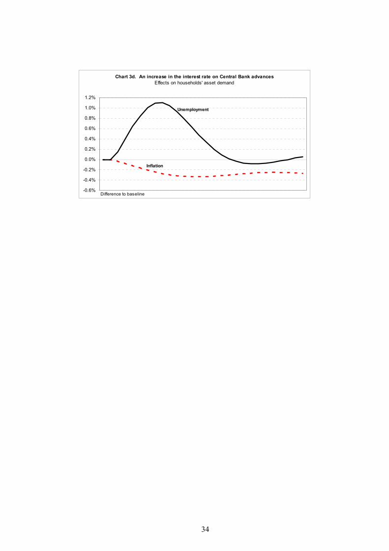
Our first policy experiments, summarized in charts 3a-3d, show that a rise in interest

rate on central bank advances does no longer have a permanent effect on the growth path of

the economy, but it does reduce inflation through a temporary increase in the unemployment

27

rate over its normal level. Our results, however, are not robust enough yet to changes in the

different parameters of the model, and will require further analysis.

6 – FINAL REMARKS

We have presented an extended version of the Lavoie & Godley (2001-2002) post-keynesian

growth model, which incorporates the government sector and a central bank. The extensions

required substantial changes to the treatment of both financial decisions on the part of

households, banks and the government and to incorporate inflation accounting. In modelling

private banks and central bank behavior we tried to adhere to other contributions by the same

authors (Lavoie & Godley (forthcoming)) developed in steady state models, even though we

limited our analysis to the case of a non-independent central bank which accommodates any

borrowing requirement from the government.

Our extension allowed us to analyze the robustness of L&G findings in a more general

context: some of their major results, such as the validity of the paradox of savings, and the

endogeneity of money, were proved to hold under a larger set of possible model parameters.

We next turned to analyze the efficacy of fiscal and monetary policy in our growth

model, under the hypothesis of exogenous inflation. As expected from a post-keynesian

approach, fiscal policy is more efficient in controlling the growth path of the economy, while

changes to interest rates controlled by monetary authorities may give conflicting results,

since the adverse effect on investment of a rise in real interest rates is countered by the

income effect obtained through higher interest payments which increase households’ income

and expenditure.

Finally, we showed that under simple assumptions about wage and mark-up settings,

our growth model will exhibit cycles around its steady-growth path.

We believe our model to be a good starting point for future research, which will

certainly require a more sophisticated treatment of banks behavior, and a more careful

integration with the post-keynesian literature on inflation.

28

REFERENCES Backus, D., Brainard, W., Smith, G. and Tobin, J. 1980. “A Model of the U.S. Financial and

Non-Financial Economic Behavior.” Journal of Money, Credit and Banking. May. Bhaduri, A., and Marglin, S. 1990. “Unemployment and the Real Wage: the Economic Basis

of Contesting Political Ideologies.” Cambridge Journal of Economics 14. Copeland, M. 1952. A Study of the Money Flows in the United States. National Bureau of

Economic Research. Davidson, P. 1972. Money and the Real World. Halsted Press. De Carvalho, F. 1992. Mr. Keynes and the Post-Keynesians: Principles of Macroeconomics

for a Monetary Production Economy. Edward Elgar. Delli Gatti, D., M. Gallegati and H. Minsky. 1994. “Financial Institutions, Economic Policy

and the Dynamic Behavior of the Economy.” Working Paper No. 126. Annandale-on-Hudson, N.Y.: The Levy Economics Institute.

Dos Santos, C.H. 2003. Three Essays on Stock-Flow Consistent Macroeconomic Modeling.

Unpublished Ph.D. thesis. New York: New School for Social Research. Dos Santos, C.H. Forthcoming. “A Stock-Flow Consistent General Framework for Formal

Minskyan Analyses of Closed Economies.” Working Paper Series. Annandale-on-Hudson, N.Y.: The Levy Economics Institute.

Dutt, A. K. Forthcoming. “New Growth Theory, Effective Demand, and Post-Keynesian

Dynamics.” In Salvadori N. ed., Old and New Growth Theory: An Assessment. Edward Elgar.

Fazzari, S. and D. Papadimitriou. 1992. Financial Conditions and Macroeconomic

Performance: Essays in Honour of Hyman P. Minsky. Armonk, N.Y.: ME Sharpe. Foley, D. 1986. Understanding Capital. Harvard University Press. Fontana, G. 2000. “Post Keynesians and Circuitists on Money and Uncertainty: An Attempt

on Generality.” Journal of Post Keynesian Economics 23 (1): Fall. Godley, W. 1999. “Money and Credit in a Keynesian Model of Income Determination.”

Cambridge Journal of Economics 23 (4): July. Godley, W. and Cripps, F. 1983. Macroeconomics. Oxford University Press.

29

Godley, W. and Lavoie, M. Forthcoming. Monetary Economics: An Integrated Approach to Credit, Money, Income, Production and Wealth. Mimeo.

Graziani, A. 1996. “Money as Purchasing Power and Money as a Stock of Wealth in

Keynesian Economic Thought.” In Delepace, G. and Nell, E. eds., Money in Motion: The Post Keynesian and Circulation Approaches. St. Martin’s Press.

Graziani, A. 2003. The Monetary Theory of Production. Cambridge University Press. Harrod, R. 1948. Towards a dynamic economics. Macmillan. Keynes, J. M. 1971. Collected Writings of John Maynard Keynes. St. Martins Press. Lavoie, M. 1992. Foundations of Post-Keynesian Economic Analysis. Edward Elgar. Lavoie, M. 2001. “Endogenous Money in a Coherent Stock-Flow Framework.” Working

Paper no. 325. Annandale-on-Hudson, N.Y.: The Levy Economics Institute. Lavoie, M. Forthcoming. “Circuit and Coherent Stock-Flow Accounting.” In Arena R., and

Salvadori N. eds. Money, Credit and the Role of the State. Ashgate, Aldershot. Lavoie, M. and Godley, W. 2001-2002. “Kaleckian Growth Models in a Stock and Flow

Monetary Framework: A Kaldorian View.” Journal of Post Keynesian Economics. Winter.

Minsky, H. 1975. John Maynard Keynes. New York: Columbia University Press. Minsky, H. 1982. Can it Happen Again? Armonk, N.Y.: ME Sharpe. Minsky, H. 1986. Stabilizing an Unstable Economy. Yale University Press. Moudud, J. 1999. “Finance in a Classical and Harrodian Cyclical Growth Model.” Working

Paper No. 290. Annandale-on-Hudson, N.Y.: The Levy Economics Institute. Robinson, J. 1956. The Accumulation of Capital. London: Macmillan. Rowthorn, R. 1977. “Conflict, Inflation and Money.” Cambridge Journal of Economics 1. Semmler, W. ed. 1989. Financial Dynamics and the Business Cycles: New Perspectives.

Armonk, N.Y.: ME Sharpe. Stone, R. 1966. “The Social Accounts from a Consumer Point of View.” Review of Income

and Wealth 12 (1).

30

Taylor, L. 1983. Structuralist Macroeconomics. Basic Books. Taylor, L. 1991. Income Distribution, Inflation and Growth: Lectures on Structuralist

Macroeconomic Theory. MIT Press. Taylor, L. 2004. Reconstructing Macroeconomics: Structuralist Proposals and Critiques of

the Mainstream. Harvard University Press. Taylor, L. and Rada, C. 2003. “Debt Equity Cycles in the Twentieth Century.” Center for

Economic Policy Analysis Working Paper 2003-1. New York: New School University.

Tobin, J. 1982. “Money and the Macroeconomic Process.” Journal of Money, Credit and

Banking. May. Zezza, G. 2003. “Dynamic Properties of Stock-Flow Models with Stable Stock-Flow

Norms.” Presented at the Eastern Economic Association 2003 Conference. New York.

Zezza, G. and C.H. Dos Santos. Forthcoming. “The role of Monetary Policy in Post-

Keynesian Stock-Flow Consistent Macroeconomic Growth Models: Preliminary Results.” In M. Lavoie and M. Seccareccia, Central banking in the modern world: Alternative perspectives. Edward Elgar, Aldershot.

31

CHARTS

Chart 1a. Shock to the propensity to saveEffects on growth rates

0%

1%

2%

3%

4%

5%

6%

7%

Consumption

Sales

Stock of capital

Difference to baseline

Chart 1b. Shock to the propensity to saveEffects on the determinants of investment

0.75

0.80

0.85

0.90

0.95

1.00

1.05

1.10

1.15

1.20

Capacity utilization

Interest burden

Tobin's q

Ratios to baseline

Cash flow ratio

Chart 1c. Shock to the propensity to saveEffects on households' asset demand

0.90

0.92

0.94

0.96

0.98

1.00

1.02

1.04

1.06

Equities

Deposits

Treasury bills

Ratios to baseline

32

Chart 2a. Shock to unit wagesEffects on growth rates

-0.6%

-0.5%

-0.4%

-0.3%

-0.2%

-0.1%

0.0%

Consumption

Sales

Stock of capital

Difference to baseline

Chart 2b. Shock to unit wagesEffects on the determinants of investment

0.94

0.96

0.98

1.00

1.02

1.04

1.06

1.08

Capacity utilization

Interest burden

Tobin's q

Ratios to baseline

Cash flow ratio

Chart 2c. Shock to unit wagesEffects on households' asset demand

0.99

1.00

1.00

1.01

1.01

1.02

Equities

Deposits

Treasury bills

Ratios to baseline

33

Chart 3a. An increase in the interest rate on Central Bank advancesEffects on growth rates

-1.0%

-0.8%

-0.6%

-0.4%

-0.2%

0.0%

0.2%

0.4%

0.6%

Consumption

Sales Stock of capital

Difference to baseline

Chart 3b. An increase in the interest rate on Central Bank advancesEffects on the determinants of investment

0.90

0.95

1.00

1.05

1.10

1.15

1.20

1.25

Capacity utilization

Interest burden

Tobin's q

Ratios to baseline

Cash flow ratio

Chart 3c. An increase in the interest rate on Central Bank advancesEffects on households' asset demand

0.98

0.99

0.99

1.00

1.00

1.01

1.01

1.02

1.02

Equities

Deposits

Treasury bills

Ratios to baseline

34

Chart 3d. An increase in the interest rate on Central Bank advancesEffects on households' asset demand

-0.6%

-0.4%

-0.2%

0.0%

0.2%

0.4%

0.6%

0.8%

1.0%

1.2%

Inflation

Unemployment

Difference to baseline

35

APPENDIX

1. The complete model; 2. Money endogeneity under different closures; 3. Properties of model expectation mechanism; 4. Formal properties of a reduced form of the full model.

1. The full model Vt = Vt-1 + Yt – Ct + CGt Households’ wealth (A.01 Vkt = Vt/pt Real households’ wealth (A.02 Skt = Ckt + Ikt + Gk Real sales (A.03 St = Skt·pt Sales (A.04 Ct = Ckt·pt Consumption (A.05 It = Ikt·pt Investment (A.06 Gt = Gkt·pt Government expenditure (A.07 FTt = ρt·Wt Total profits (A.08 Yt = Wt + FDt + rmt-1·Mt-1 + FBt + rbt-1·Bht-1 - DTt Households’ disposable income (A.09 Ykt = Yt/pt Real disposable income (A.10 Sht = Yt – Ct Household savings (A.11 FBt = rlt-1·Lt-1 +rbt-1·*Bbt-1 -(rmt-1·Mt-1 + rct-1·At-1) Bank profits (A.12 FCt = rct-1·*At-1 + rbt-1·Bct-1 Central bank profits (A.13 GDt = (Gt + rbt-1·Bht-1 + rbt-1·Bbt-1 + rbt-1·Bct-1) - (ITt + DTt + TFt + Fct) Government deficit (A.14 Ikt = Kkt - Kkt-1 Real investment (A.15 Kkt = (1 + grt)·Kkt-1 Real stock of capital (A.16 Kt = Kkt·pt Stock of capital (A.17 rfct = FUt/Kt-1 Rate of cash flow (A.18 levt = Lt/Kt Leverage (A.19 qt = pet·Et/Kt Tobin’s q (A.20 ut = Skt/Sfct Capacity utilization rate (A.21 Sfct = η·*Kkt-1 Normal capacity sales (A.22 gryt = Skt/Skt-1 - 1 Growth rate of sales (A.23

1

1

−

−−=

t

tt

ppp

p.

Inflation (A.24

CGt = (pet - pet-1)·Et-1 Capital gains on equities (A.25

)1(1 ttt

.πππ +⋅= − Productivity (A.26

)1(1 ttt www.

+⋅= − Unit wages (A.27

t

ttt

wp

πτρ

⋅−

+=

11

Price level (A.28

36

Wt = wt·Nt Wages (A.29

ett

ett pw

...πχ ⋅+= Wage inflation (A.30

ttt uu ειππ +−⋅−= )( 0

_. Productivity growth (A.31

)(' ttt w...

−⋅= πϖρ Change in mark-up (A.32

Nt = Skt/πt Employment (A.33 ITt = τi·St Indirect taxes (A.34 DTt = τd·Wt Direct taxes (A.35 TFt = τf·FTt Taxes on profits (A.36 FDt = (1 - φ)·(FTt - rlt-1·Lt-1 - TFt) Distributed profits (A.37 FUt = FTt – rlt-1·Lt-1 - FDt - TFt Undistributed profits (A.38

)1

( 13121 −− ⋅+

−⋅+⋅+⋅= tet

ete

ttett Vk

p

pCGkaVkaYkaCk .

. Real consumption (A.39

grt = γ0 + γ1·rfct-1 – γ2·rrlt-1·levt-1 + γ3·qt-1 + γ4·ut-1 Growth in the stock of capital (A.40 )1(1

ettt gryGkGk +⋅= − Real government expenditure (A.41

)(_

1 grygryurur ttt −⋅−= − ξ ; 0 ≤ ur ≤1 Unemployment rate (A.42

)( 1101 −−− −⋅+= tett

et grygrygrygry θ Expected sales growth (A.43

)( 1111 −−− −⋅+= tett

et pppp

...θ Expected inflation (A.44

)( 1121 −−− −⋅−= tett

et

... .ππθππ Expected growth in productivity (A.45

)( 1131 −−− −⋅+= tett

et pepepepe

... .θ Expected change in pe (A.46

)1(1ett

et gryYkYk +⋅= − Expected real income (A.47

)1()1(1et

ett

et pgryYY

.+⋅+⋅= − Expected income (A.48

)()1( 11 −− ⋅⋅+= ttet

et EpepeCG

. Expected capital gains (A.49

1

11

1

1

−

−− ⋅⋅

+

+=

t

tt

et

ete

t pEpe

p

peCGk .

. Expected real capital gains (A.50

ett

ett

et CGCYVV +−+= −1 Expected households’ wealth (A.51

_

0 ururtt −= χχ Wage share in productivity growth (A.52

Bt = Bt-1 + GDt Government budget constraint (A.53

37

)()( 1413121110 te

ttbe

te

tttmt HhVrrVYrrerrBh −⋅⋅+⋅−⋅−⋅−= λλλλλ

Households’ demand for bonds (A.54

10403020100 /)]()()[( −−⋅−−⋅⋅−⋅−⋅+⋅−= tttte

ttbe

te

tttmt EFUIxHhVrrVYrrerrpe λλλλλ

Price of equities (A.55 Et = Et-1 + x·(It – FUt)/pet Number of equities (A.56 Mt = Vt – Hht – Bht - Et·pet Households’ bank deposits (A.57 Hht = υ1·Ct Households’ demand for cash (A.58 Hbt = υ2·Mt Reserve requirement (A.59 Lt = Lt-1 + It – FUt - pet·(Et - Et-1) Stock of loans to firms (A.60 At = Lt + Hbt - Mt Bank loans from Central Bank (A.61 Bct = Bt – Bht (- Bbt) C. Bank stock of treasury bills (A.62 rlt = rct + µ1 Interest rate on loans (A.63 rmt = rct - µ2 Interest rate on deposits (A.64

1)1()1( 1 −+⋅+= +

. ettbtb prrr Interest rate on treasury bills (A.65

1)1()1( 1 −+⋅+= +

. ettctc prrr Interest rate on Central B. advances(A.66

11 −− ⋅+

=tt

ett

t EpeCGFD

re Return on equities (A.67

)(41 tett

et rererere −⋅+=+ θ Expected return on equities (A.68

. et

tmtm

p

rrr

11

11

++

+=+ Real interest rate on deposits (A.69

. et

tltl

p

rrr

11

11

++

+=+ Real interest rate on loans (A.70

. et

et

tp

rerre

11

11

++

+=+ Real expected return on equities (A.71

38

2. Money endogeneity under different closures From the balance sheet in table 3 we get the following 7 identities: H = Hh + Hb (A2.1 B = Bh + Bb + Bc (A2.2 V +Vf – B = K (A2.3 V = Hh + M + Bh + E (A2.4 Vf = K – L – E (A2.5 Hb + L + Bb = M + A (A2.6 H = A + Bc (A2.7

one of which is linearly dependent from the others, and will need to be dropped. Given our behavioral assumptions, which determine B; Bh; Hh; Hb; E; K; L; we know that Vf will be given by (A2.5), so that V is given by

V = K + B – Vf = K + B – K + L + E = B + L + E (A2.3b Households’ wealth contains the stock of loans to firms, since we assume that banks

transfer any profits to households. Deposits M will thus be given by M = V – (Hh + Bh + E) = B + L + E – Hh – Bh – E = L – Hh + (B – Bh) (A2.4b We are now left with 3 equations in 3 unknowns: A; Bb and Bc: Bc = B - Bh - Bb (A2.2b Bc = Hh + Hb - A (using A2.1) (A2.7b Hb + L + Bb = M + A (A2.6b Since one of the equations is linearly dependent from the others, it must be dropped,

and some additional assumption is required to determine a solution. We drop equation (A2.7b) assuring that demand for cash is equal to supply, and study three possible closures:

Closure 1. Central bank advances are a fixed ratio of loans A = ϕ1·L we drop equation (A2.7b) from the model obtaining the values for Bb and Bc Bb = M + A – Hb - L (A2.6’ Bc = B - Bh - Bb (A2.2’ Closure 2. Bank demand bills on the basis of a liquidity ratio: Bb = ϕ2·L we drop equation (A2.6b) from the model obtaining the values for A and Bc A = Hb + L + Bb - M (A2.6’’ Bc = B - Bh - Bb (A2.2’’ Closure 3. Bank do not demand bills: Bb = 0 we drop equation (A2.6b) from the model obtaining the values for A and Bc A = Hb + L - M (A2.6’’’ Bc = B - Bh (A2.2’’’ In all our closures, demand for cash will turn out to equal supply by accounting

consistency.

39

3. Properties of the model expectation mechanism We study our equation for the expectations on productivity growth: other equations

will have the same properties. Starting from equation (A.45)

)(1 tett

et

... .ππθππ −⋅−=+

Using the lag operator L (such as that Lxt = xt-1) we obtain, for θ < 1,

( ) ( ) ( ) ∑∑∞

=

−

∞

=+ ⋅⋅−=⋅⋅−=⋅

⋅−−

=0

10

1 111

1i

iti

it

it

et L

L....

πθθπθθπθ

θπ

Notice that, if the variable to be forecasted is stationary, its expected value will always be correct on average. To prove it, let us productivity grows at a rate given by

tt εππ +=_.

; where εt ~ iid(0, σ2t)

so that its expected value is

( )___

πεπεππ =+=

+=

ttt EEE.

Using our result, the expected value of productivity growth will be given by

( ) ( ) ∑∑∞

=−

∞

=

−+ +⋅⋅−=⋅⋅−=0

_

01 )(11

iit

i

iit

iet επθθπθθπ

..

( ) ( ) ∑∑∞

=−

∞

=+ ⋅⋅−+⋅⋅−=

00

_

1 11i

iti

i

iet εθθθπθπ.

( ) ∑∞

=−+ ⋅⋅−+=

0

_

1 1i

itie

t εθθππ.

The expected value will therefore be

( ) ( ) ( ) ( )_

0

_

0

_

0

_

1 111)( πεθθπεθθπεθθππ =⋅⋅−+=

⋅⋅−+=

⋅⋅−+= ∑∑∑

∞

=−

∞

=−

∞

=−+

iit

i

iit

i

iit

iet EEEE.

Note also that while a simpler mechanism such as

tet

..ππ =+1

will have the same expected value, it does not allow to analyze the effects of changes in the speed of adjustment in expectations. For given set of parameter values, our model may exhibit oscillatory (stable) patterns as the speed of adjustment in expectations increases.

Finally, we can derive the mean lag in the response of expectations to changes in the actual variable of interest. Recalling that the mean lag in the response of a variable y to changes in a variable x from yt = P(L)xt is given by m.l. = P’(1), ie by the first derivative of the polynomial P evaluated at L=1, we have

ttet L

LL

...π

θθπ

θθπ ⋅

⋅−⋅−

=⋅⋅−

−= −

1)1(

11

1

θ−=

11..lm

so that higher values of θ will shorten the responses of expectations to actual values. We chose a mean lag of two periods for the simulation discussed in the text.

40

4. Formal properties of a reduced form of the model To derive a more tractable form of the full model we assume: (1) exogenous inflation;

(2) a stable mark-up; (3) expectation are always realized; (4) the tax rate on profits is zero; (5) the interest rate on central bank advances is zero; (6) government expenditure is exogenous. The “real” part of the model thus reduces to 6 equations in Ck, Kk, Lk, Sk, Vk, Yk:

Skt =Ckt + Gkt + Kkt - Kkt-1 (A4.1

13

21 )(1

−⋅

−⋅⋅+

++⋅= tttet

t

tt Vkpvshepp

aaYkaCk

... (A4.2

ttttet

t

t YkaVkpvshepp

aaVk ⋅−+⋅

−⋅⋅+

−+−= − )1()(

1

11 11

32

... (A4.3

2.

1

211121

4110

1)

11()1( −

−

−−−−− ⋅

+⋅−⋅⋅−⋅+

+−

+⋅+= t

t

tttttt Lk

p

rlLkrrlSkKkKk γγ

ηγ

ρτφργγ

113 −− ⋅⋅+ tt Vkvsheγ (A4.4

11.1

11

1

1−−

− ⋅+−

+⋅+

−= tt

t

tt SkLk

p

rlLk

ρτφρ (A4.5

1.1

1.1

11])1(1[

11

−−

−− ⋅⋅

++⋅

+

⋅+⋅−−+⋅

+−

= t

t

tt

t

ttdt Vkvshb

p

rbLk

p

rlSkYk

φτρφ

ρτ (A4.6

Here the new variables vshe, vshb represent the share of equities and bonds on wealth, respectively, which are assumed to depend only on relative returns on a steady growth path, where the income to wealth ratio should be stable, and Lk is the real stock of loans.

We have derived a reduced form of the model partly to show why we prefer to use dynamic simulations rather than algebra, since even in its simplest form our model turns out to be highly non-linear, and reduced form parameters are therefore hardly informative, and moreover inspection of equations (A4.1)-(A4.6) clearly show that by simplifying the model some of its crucial characteristics get modified.

Finally, we note that in the simplified version, for a given set of parameters and initial values, growth is conditional on government expenditure and that part of investment which is exogenously determined (γ0). In the full model assumptions on these two crucial variables will have to be consistent to avoid government share on output growing without limit, or approaching zero.